WORKING PAPER SERIES

NO. 55

PREDICTING SUCCESSFUL AND UNSUCCESSFUL TRANSITIONSFROM SCHOOL TO WORK USING SEQUENCE METHODS

DUNCAN McVICAR and MICHAEL ANYADIKE-DANES

NORTHERN IRELAND

ECONOMIC RESEARCH CENTRE

Predicting Successful and Unsuccessful Transitions

from School to Work Using Sequence Methods

August 2000

Duncan McVicar and Michael Anyadike-Danes

Northern Ireland Economic Research Centre46-48 University Road, Belfast BT7 1NJ, United Kingdom

Tel: 44 (0)28 9026 1800Fax: 44 (0)28 9043 9435

Email: d.mcvicar@qub.ac.ukEmail: m.anyadike-danes@qub.ac.uk

We are grateful to the Training and Employment Agency for supporting the collectionof the original survey data which this paper is based. The research is part of NIERC’sHuman Resources and Economic Development research programme supported by theDepartment of Enterprise, Trade and Investment, and the Department of Finance andPersonnel. All views are those of the authors.

Abstract

Policy makers recognise the importance of early identification of young people that

are likely to end up jobless on entry to the adult labour market. This paper uses

sequencing techniques to characterise 712 young people’s transitions from school to

work into ‘types’, with jobless types interpreted as unsuccessful transitions. A logit

model is estimated for transition type using a collection of static individual, family

and school characteristics. This allows us to identify which young people are most

likely to experience unsuccessful transitions into the adult labour market. Policy

makers might use such information to target social and educational policy more

effectively to promote social inclusion.

Young people with the following characteristics at age 16 (in order of importance) are

more likely to experience an unsuccessful transition into the adult labour market:

! Poor qualifications;

! Coming from a disadvantaged area of Northern Ireland;

! Having an unemployed father;

! Coming from a single parent family;

! Being female, and

! Being Catholic.

1

1. Introduction

Policy makers have long recognised the importance of ‘catching problems early’ if

they are to be effectively dealt with in the most efficient way. This belief, that

‘prevention’ is better than ‘cure’, now pervades much of social policy in the US and

the UK. In particular, governments now believe that if they can catch the future long-

term jobless early enough with targeted interventions then they may be able to prevent

a slide into social exclusion. In this paper we identify a typology of transitions from

school to work, one of which is essentially a transition into long-term joblessness, and

show how young people’s background characteristics influence their chances of

experiencing a particular type of transition. Such findings might potentially be used

by policy makers to help target early interventions more effectively.

Our data consist of a vector of static background characteristics and a time series

sequence of 72 monthly labour market activities for each of 712 individuals in a

cohort survey. The sequences follow each young person from the month they are first

eligible to leave compulsory education (July 1993) for a further six years. Our

problem is how best to use this data to identify ‘at risk’ young people at age 16 and to

characterise their post-school career trajectories. One possibility is to construct a

dynamic stochastic model (e.g. a Markov model) where activity in one month is some

function of activity in the previous month coupled with the static characteristic

variables.1 The approach adopted here takes a different route, where the raw

sequences are analysed using optimal matching and cluster analysis to enable

classification into a simple typology of transition patterns.

Our motivation for the adoption of these methods is threefold. First we feel there is

worth in introducing these sequence methods to an audience that may not routinely

come across them in the economics literature, despite their role in other scientific

disciplines. Second, these sequence methods are ideally suited to the problem of

reducing the dimensionality of our large database down to manageable and readily

interpretable dimensions. Third, our data are ideally suited to these sequence methods

1 This approach is adopted in a companion paper with the same data set and for similar purposes (seeAnyadike-Danes and McVicar, 2000b).

2

and provide an application which goes further, in terms of successfully estimating a

regression model with sequence ‘types’ on the left hand side, than has previously been

possible.

The dependent variable in our regression analysis is transition ‘type’ – a fivefold

categorisation of economic and educational activity over the six years immediately

following completion of compulsory education (i.e. from age 16 to age 22). This is

discussed in Section 5. The classification of transition types is based on a cluster

analysis of the data and is discussed in Section 4. The cluster analysis in turn is based

on a distance matrix computed using optimal matching techniques (developed in

genetics to compare complex protein sequences). This is discussed in Section 3.

Finally, Section 6 discusses the sensitivity of the results to changes in assumptions at

the various stages, and Section 7 concludes. The following section introduces the data

used in our application.

2. The Data and the Context

Our data are taken from the 1999 sweep of the Status Zero Survey (see McVicar et

al., 2000). The survey was first carried out, by means of face-to-face interviews, in

June 1995 with a sample of 980 young people from Northern Ireland that had

completed compulsory education two years previously.2 For each sample member

monthly activity (e.g. at school, at further education college (FE), in training,

employment or jobless) was collected for the intervening two years along with a

considerable amount of background information on qualifications levels, parental

employment status etc. In the June 1999 follow-up sweep, this background data and

monthly activity information was updated to cover the first six years following

completion of compulsory education, or the years from age 16-22 (and higher

education (HE) was added as an activity category to reflect this older age group). The

sample size was 712 in this most recent sweep and the panel is fully balanced.

Appropriate weights adjust for response bias.

2 There are around 24,000 young people in this cohort in total.

3

School is compulsory in Northern Ireland until age 16 at which time (at the end of the

academic year) young people are faced with a number of choices.

! Around a half of the 1993 cohort stayed on at school either for one year (to retake

previously failed examinations or one-year vocational courses) or for two years (to

take an academic qualification (A-Level) with a small proportion taking a vocational

qualification (GNVQ)). Some young people, by combining one-year and two-year

courses, or by repeating a year, stayed on for three years. School generally leads on to

higher education (HE) or employment directly.

! Around 20% of the cohort entered FE at 16, taking a similar mix of courses

although more weighted towards the vocational end of the spectrum. This is also a

stepping stone to HE but many FE graduates enter employment directly.

! A further 20% of the cohort entered government sponsored training schemes often

based with an employer and involving work experience plus study towards a

vocational qualification. This tends to lead to employment directly.

! The remaining 10% of the cohort entered employment directly at 16 or

joblessness.

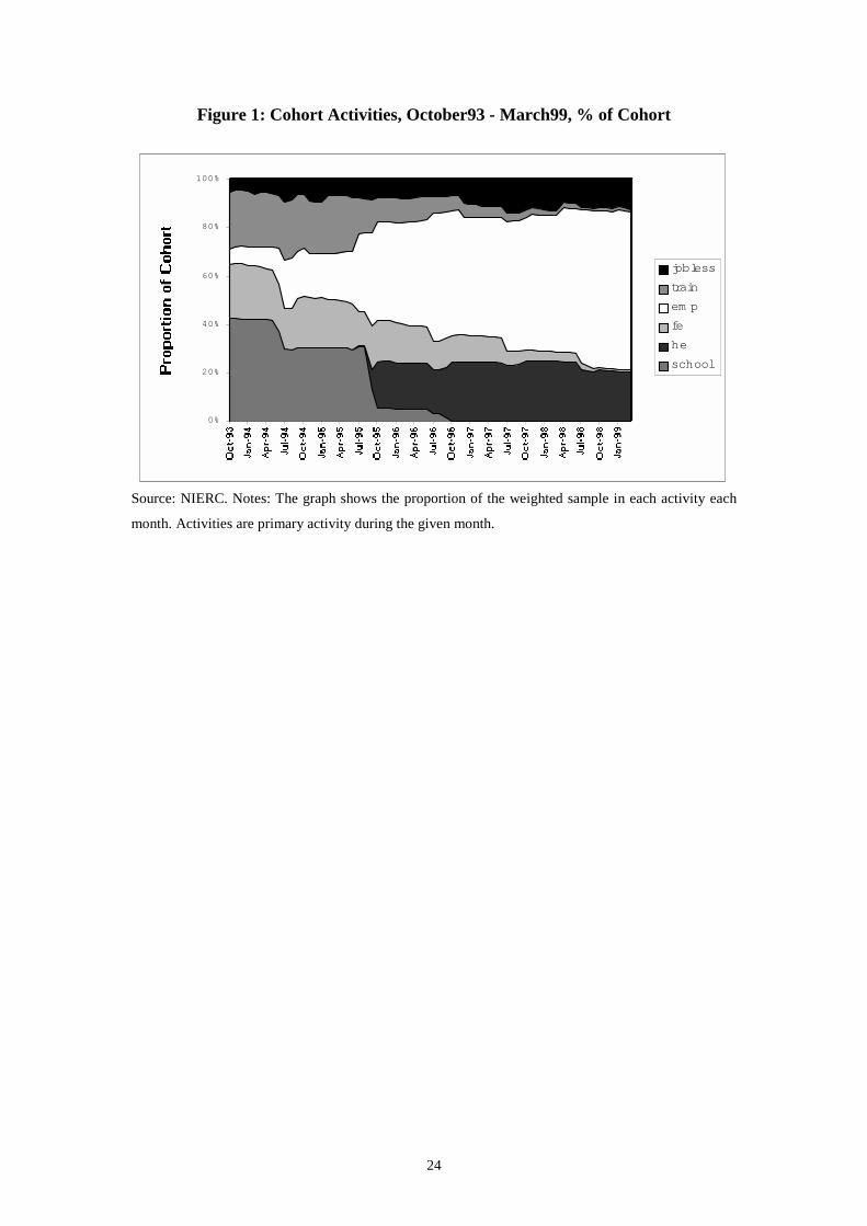
Figure 1 shows the pattern of the cohort’s economic activities from the October

following completion of compulsory education (age 16) to age 22. Most young people

are in some form of full time education or training for the first two years. Most end up

in employment by age 22, although many are still in HE and a significant proportion

are jobless. There are three discrete jumps in the proportions engaged in the various

activities, corresponding with the summers of 12, 24 and 36 months after completing

5th Form. Firstly, at age 17, there is a discrete fall in numbers attending school and a

corresponding rise in numbers in employment. This is repeated at age 18,

accompanied by a fall in numbers in training and a proportion entering HE. Finally, at

19, school numbers drop to zero, FE and training display a significant discrete fall and

HE, employment and joblessness display discrete rises (the latter slightly delayed).

For the remainder of the sample period, numbers in FE, HE and training fall, whilst

joblessness and employment rise.

4

In order to create a typology of youth transitions, we need a method of comparing the

similarities between the 712 sequences of 72 monthly activity variables that lie behind

the aggregate proportions shown in Figure 1. In the following section we argue that

optimal matching analysis provides a suitable method for this purpose.

3. Optimal Matching (OM)

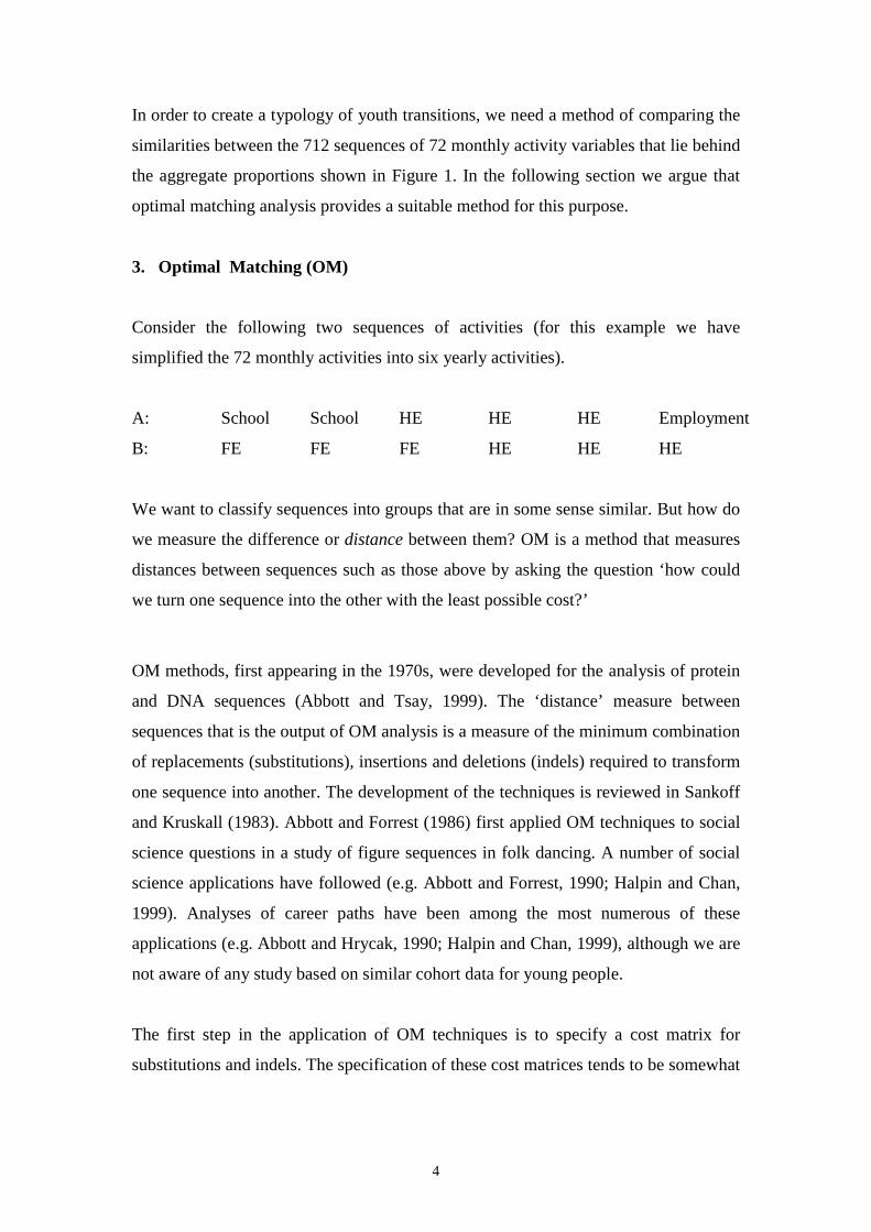
Consider the following two sequences of activities (for this example we have

simplified the 72 monthly activities into six yearly activities).

A: School School HE HE HE Employment

B: FE FE FE HE HE HE

We want to classify sequences into groups that are in some sense similar. But how do

we measure the difference or distance between them? OM is a method that measures

distances between sequences such as those above by asking the question ‘how could

we turn one sequence into the other with the least possible cost?’

OM methods, first appearing in the 1970s, were developed for the analysis of protein

and DNA sequences (Abbott and Tsay, 1999). The ‘distance’ measure between

sequences that is the output of OM analysis is a measure of the minimum combination

of replacements (substitutions), insertions and deletions (indels) required to transform

one sequence into another. The development of the techniques is reviewed in Sankoff

and Kruskall (1983). Abbott and Forrest (1986) first applied OM techniques to social

science questions in a study of figure sequences in folk dancing. A number of social

science applications have followed (e.g. Abbott and Forrest, 1990; Halpin and Chan,

1999). Analyses of career paths have been among the most numerous of these

applications (e.g. Abbott and Hrycak, 1990; Halpin and Chan, 1999), although we are

not aware of any study based on similar cohort data for young people.

The first step in the application of OM techniques is to specify a cost matrix for

substitutions and indels. The specification of these cost matrices tends to be somewhat

5

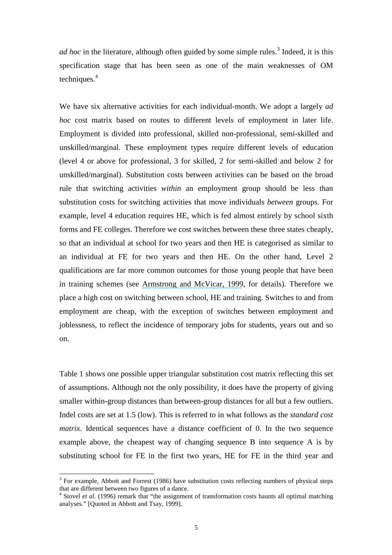
ad hoc in the literature, although often guided by some simple rules.3 Indeed, it is this

specification stage that has been seen as one of the main weaknesses of OM

techniques.4

We have six alternative activities for each individual-month. We adopt a largely ad

hoc cost matrix based on routes to different levels of employment in later life.

Employment is divided into professional, skilled non-professional, semi-skilled and

unskilled/marginal. These employment types require different levels of education

(level 4 or above for professional, 3 for skilled, 2 for semi-skilled and below 2 for

unskilled/marginal). Substitution costs between activities can be based on the broad

rule that switching activities within an employment group should be less than

substitution costs for switching activities that move individuals between groups. For

example, level 4 education requires HE, which is fed almost entirely by school sixth

forms and FE colleges. Therefore we cost switches between these three states cheaply,

so that an individual at school for two years and then HE is categorised as similar to

an individual at FE for two years and then HE. On the other hand, Level 2

qualifications are far more common outcomes for those young people that have been

in training schemes (see Armstrong and McVicar, 1999, for details). Therefore we

place a high cost on switching between school, HE and training. Switches to and from

employment are cheap, with the exception of switches between employment and

joblessness, to reflect the incidence of temporary jobs for students, years out and so

on.

Table 1 shows one possible upper triangular substitution cost matrix reflecting this set

of assumptions. Although not the only possibility, it does have the property of giving

smaller within-group distances than between-group distances for all but a few outliers.

Indel costs are set at 1.5 (low). This is referred to in what follows as the standard cost

matrix. Identical sequences have a distance coefficient of 0. In the two sequence

example above, the cheapest way of changing sequence B into sequence A is by

substituting school for FE in the first two years, HE for FE in the third year and

3 For example, Abbott and Forrest (1986) have substitution costs reflecting numbers of physical stepsthat are different between two figures of a dance.4 Stovel et al. (1996) remark that “the assignment of transformation costs haunts all optimal matchinganalyses.” [Quoted in Abbott and Tsay, 1999].

6

employment for HE in the last year. From Table 1 the total cost of this substitution is

4. This is then standardised so that the most distant sequences have a distance

coefficient of 1. Since the maximum inter-sequence distance would be displayed by

six years of joblessness compared to three years of school and then three years HE, a

total substitution cost or indel cost of 18, the normalised distance coefficient between

sequences A and B above would be 4/18 = 0.22.

Section 6 discusses the sensitivity of our results to adoption of alternative cost

matrices – the standard cost matrix but with high indel costs (indel = 4) and a unit cost

matrix where all substitutions cost 1 (and indel = 4).5 The various cost matrices are

input to the OPTIMIZE program which then runs the OM analysis (for details of this

software see www.svc.uchicago.edu/users/Abbot/optfdoc.htm). The output is a

21 *712*712 matrix of standardised (and minimised) distances between each sequence.

This distance matrix then forms the input to a cluster analysis as discussed in the

following section.

We could carry out cluster analysis of the sequence data directly – without going

through the OM stage – using some other form of inter-sequence distance. In an

earlier paper (Anyadike-Danes and McVicar, 2000a) we do this with a distance

measure based on correlation of six binary state variables for each month (e.g. FE = 1

if individual i in month m is in FE and 0 otherwise). There are several advantages to

the OM based method however. Firstly, the cluster analysis based on the OM is

computationally simpler. More importantly, the cluster analysis performed on the data

directly cannot account for two sequences that may be very similar but not perfectly

temporally aligned. Consider two career sequences, with ‘E’ representing a year in

employment and ‘U’ a year in unemployment: EUEUEU and UEUEUE. Cluster

analysis applied to the data directly will treat these two sequences as maximally

different. The OM analysis, however, by indel of a single term, will treat these

sequences as quite similar. Another attraction of the OM based cluster analysis is its

versatility, in that assumptions (e.g. of the substitution costs between different

5 This unit cost matrix is adopted in previous applications where there is no clear reason for specifyingcosts otherwise (e.g. Dijkstra and Taris, 1995). In our two sequence example above the unit cost matrixwould also yield a cost of 4 of turning B into A, but the normalisation factor (the maximum distance)would be 6, giving a normalised distance of .67 (4/6).

7

activities) can be easily altered at the input stage in a way that cluster analysis alone

does not allow.

4. Cluster Analysis

Cluster analysis is used to create homogeneous groups of cases (or in our example,

sequences) from large samples. Cases are grouped according to some distance

measure between them. This allows complex information to be synthesised into a

small number of clusters with similar patterns, or in our case similar career

trajectories. In other words it offers a method for creating a simple typology of the

transition from school to work, without necessarily discarding any of the information

contained within the data and without imposing any stochastic restrictions ex ante.

Hannan and Doyle (2000) provide a recent application of cluster analysis to career

trajectory data of young Irish people in transition from school to work. They reduce

the monthly categorical data for each individual to six-monthly figures that measure

the proportions of the six-month period that the individual spends in each of the

different activities. This has the effect of turning categorical variables (e.g.

1=education, 2=employment etc.) into pseudo-continuous variables (e.g. number of

months in education in last six months) for which more standard distance measures

can be computed and clusters identified.6

Cluster analysis has a number of well-known weaknesses (for a recent discussion see

Morgan and Roy, 1995). First, different variants of cluster analysis (e.g. hierarchical

cluster analysis or k-means cluster analysis) can lead to different solutions. Second, it

is not clear how to identify the appropriate number of clusters either ex ante or ex

post. The researcher can therefore apply a great deal of influence on her results from

the way she specifies the problem. The best available practical defence is to subject

the results of a particular cluster analysis to a battery of sensitivity analyses, applying

different cluster methods, using different sub-samples of the data or pre-specifying

6 Notice that this method seems to discard what might be useful information from the data set. Forexample, their method does not discriminate between three separate monthly spells of unemploymentand a contiguous three-month spell of unemployment.

8

different numbers of clusters, for example. Section 6 presents and discusses such a

sensitivity analysis exercise for our cluster analysis based on the OM solution with the

standard cost matrix.

A further criticism, particularly of cluster analysis of sequences, is that results have

not generally been applied to further explanatory analysis with much success. Where

researchers have tried to use cluster solutions as dependent or independent variables

in further analysis (e.g. regression analysis) they have usually been frustrated (Abbott

and Tsay, 1999). However, our application is one where cluster analysis of sequences

is shown to be amenable to this sort of further analysis – in the form of a regression

model with the cluster solution as the dependent variable. This is discussed in more

detail in Section 5.

In our standard approach, we set the number of clusters to be five.7 We then use the

OM output (distance matrix), based on the standard cost matrix, as the input to a

hierarchical cluster analysis carried out in SPSS. The cluster method here was the

"between-groups linkage", one of the class of "average linkage" methods, using as a

distance measure the "squared Euclidean distance" (see Alenderfer and Blashfield,

1984, and Section 6 of this paper for a discussion of alternatives). The analysis is

carried out on the full sample of 712 individuals over the full sample period of 72

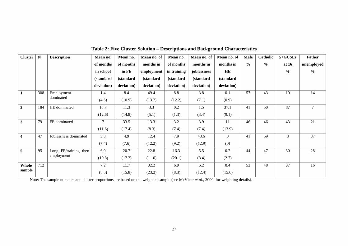
months. Table 2 presents descriptions of the five clusters along with some information

on the characteristics of their members.

Cluster 1, the largest cluster, is dominated by employment. The mean (standard

deviation) number of months in employment within this cluster is 49.4 (13.7)

compared to an overall sample mean (standard deviation) of 32.2 (23.2). HE

dominates Cluster 2. Cluster 3 is less distinct, but dominated by FE.

Cluster 4 is of most interest given the policy context of the research – it is the cluster

dominated by joblessness. The average (standard deviation) amount of joblessness

experienced within this cluster is 43.6 (12.9) months compared to the sample average

7 Our reasons for this are discussed in Section 6.

9

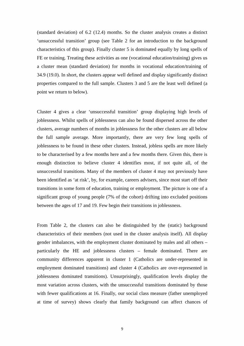
(standard deviation) of 6.2 (12.4) months. So the cluster analysis creates a distinct

‘unsuccessful transition’ group (see Table 2 for an introduction to the background

characteristics of this group). Finally cluster 5 is dominated equally by long spells of

FE or training. Treating these activities as one (vocational education/training) gives us

a cluster mean (standard deviation) for months in vocational education/training of

34.9 (19.0). In short, the clusters appear well defined and display significantly distinct

properties compared to the full sample. Clusters 3 and 5 are the least well defined (a

point we return to below).

Cluster 4 gives a clear ‘unsuccessful transition’ group displaying high levels of

joblessness. Whilst spells of joblessness can also be found dispersed across the other

clusters, average numbers of months in joblessness for the other clusters are all below

the full sample average. More importantly, there are very few long spells of

joblessness to be found in these other clusters. Instead, jobless spells are more likely

to be characterised by a few months here and a few months there. Given this, there is

enough distinction to believe cluster 4 identifies most, if not quite all, of the

unsuccessful transitions. Many of the members of cluster 4 may not previously have

been identified as ‘at risk’, by, for example, careers advisers, since most start off their

transitions in some form of education, training or employment. The picture is one of a

significant group of young people (7% of the cohort) drifting into excluded positions

between the ages of 17 and 19. Few begin their transitions in joblessness.

From Table 2, the clusters can also be distinguished by the (static) background

characteristics of their members (not used in the cluster analysis itself). All display

gender imbalances, with the employment cluster dominated by males and all others –

particularly the HE and joblessness clusters – female dominated. There are

community differences apparent in cluster 1 (Catholics are under-represented in

employment dominated transitions) and cluster 4 (Catholics are over-represented in

joblessness dominated transitions). Unsurprisingly, qualification levels display the

most variation across clusters, with the unsuccessful transitions dominated by those

with fewer qualifications at 16. Finally, our social class measure (father unemployed

at time of survey) shows clearly that family background can affect chances of

10

successful transitions (particularly into HE) and unsuccessful transitions into

joblessness.

It is apparent that OM-based cluster analysis can sort the sample into distinct groups,

or ‘types’ of transition. Further, the type of transition that young people experience

appears to be related to their background characteristics. But people that drift into

social exclusion or long term joblessness are often characterised by several correlated

disadvantages – multiple disadvantages in the sociology literature – and if we wish to

disentangle these effects we need to go back to econometric analysis. In the following

section we discuss a logit model where transition type is the dependent variable and a

list of background characteristics are the independent variables. In this way we hope

to quantify what are the most important individual and background (observable)

characteristics that can help cause a young person to experience a successful or

unsuccessful transition.

5. A Logit Model of Transition Type

Abbott and Deviney (1992) attempted unsuccessfully to use the output of OM-based

cluster analysis (sequence type) as a dependent variable in a regression analysis. Their

results were either negligible or counterintuitive (Abbott and Tsay, 1999). However,

Abbott and Tsay (1999) identify several examples of sequence types being used with

varying degrees of success as independent variables (see, e.g. Poole and Holmes,

1995; Carpenter, 1996 and Han and Moen, 1998). Han and Moen, for example, found

‘career pathway type’ to have strong effects on the timing of retirement.

Our clusters appear distinct and appear to be related in many cases to the background

characteristics of the cluster members. There is a fairly well established set of causal

factors in the economics and sociology literatures that can help explain much of the

movement into long-term joblessness among young people (see McVicar et al., 2000,

for a review). Many of these commonly used explanatory factors are present in our

data set. In these two respects, our data seemed to suggest that these sequence types

might be sensibly treated as dependent variables in a regression equation to be

explained by a set of background characteristics. The discussion that follows is based

on the five-cluster solution, in turn based on the standard cost matrix. Section 6

11

discusses the sensitivity of the logit results to assumptions on substitution costs, indel

costs and number of clusters.

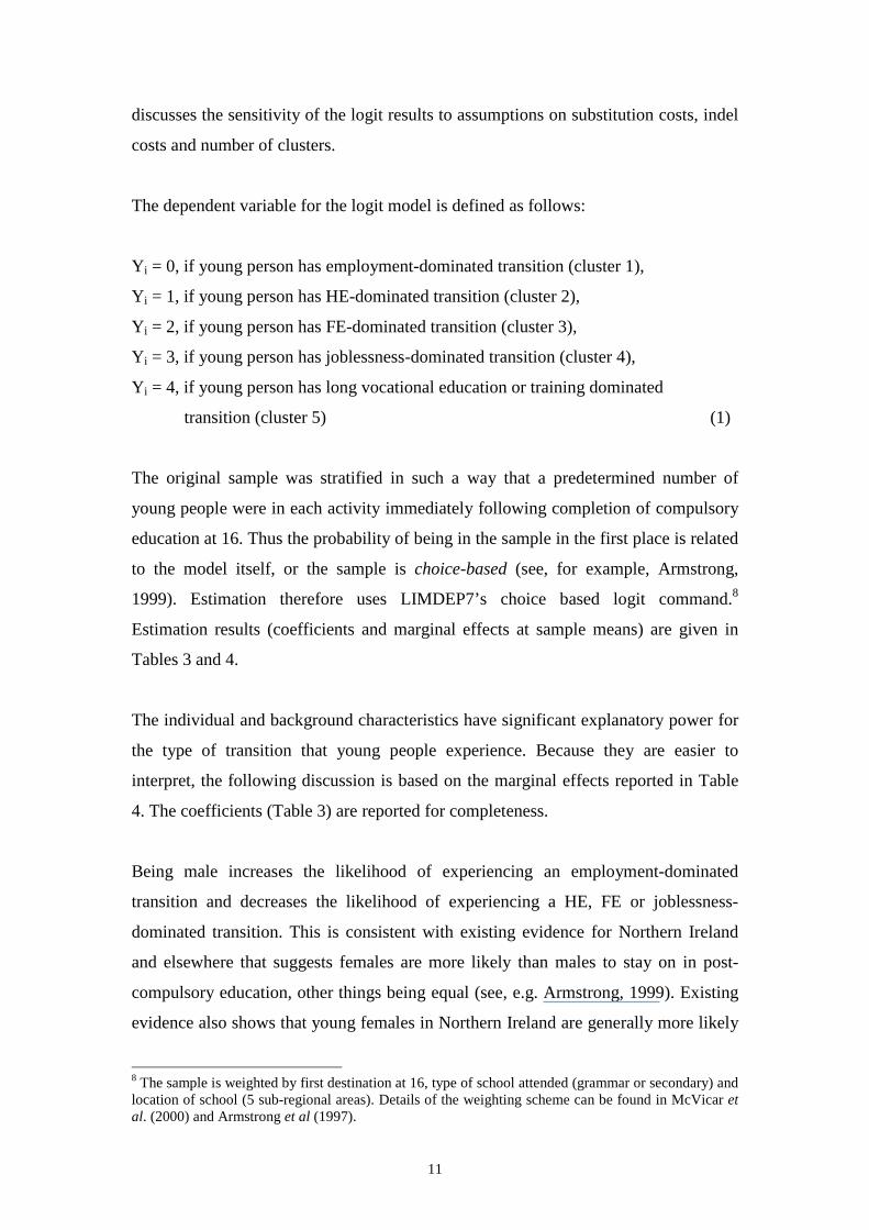
The dependent variable for the logit model is defined as follows:

Yi = 0, if young person has employment-dominated transition (cluster 1),

Yi = 1, if young person has HE-dominated transition (cluster 2),

Yi = 2, if young person has FE-dominated transition (cluster 3),

Yi = 3, if young person has joblessness-dominated transition (cluster 4),

Yi = 4, if young person has long vocational education or training dominated

transition (cluster 5) (1)

The original sample was stratified in such a way that a predetermined number of

young people were in each activity immediately following completion of compulsory

education at 16. Thus the probability of being in the sample in the first place is related

to the model itself, or the sample is choice-based (see, for example, Armstrong,

1999). Estimation therefore uses LIMDEP7’s choice based logit command.8

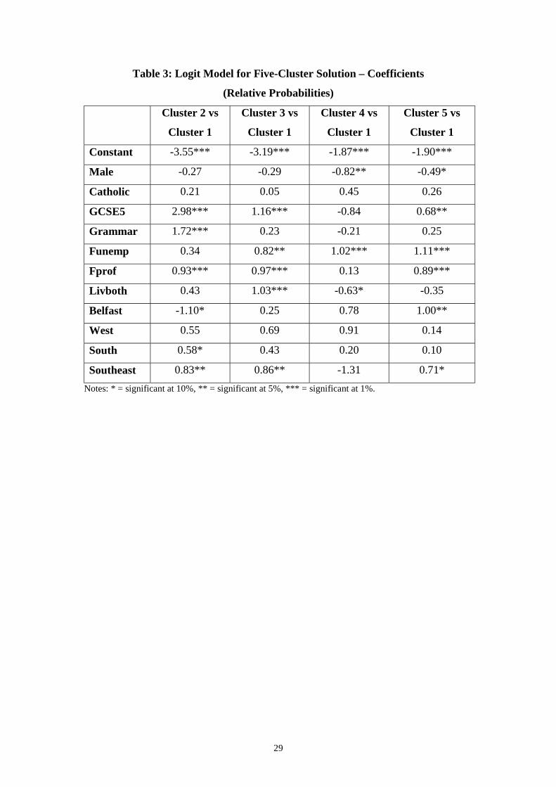
Estimation results (coefficients and marginal effects at sample means) are given in

Tables 3 and 4.

The individual and background characteristics have significant explanatory power for

the type of transition that young people experience. Because they are easier to

interpret, the following discussion is based on the marginal effects reported in Table

4. The coefficients (Table 3) are reported for completeness.

Being male increases the likelihood of experiencing an employment-dominated

transition and decreases the likelihood of experiencing a HE, FE or joblessness-

dominated transition. This is consistent with existing evidence for Northern Ireland

and elsewhere that suggests females are more likely than males to stay on in post-

compulsory education, other things being equal (see, e.g. Armstrong, 1999). Existing

evidence also shows that young females in Northern Ireland are generally more likely

8 The sample is weighted by first destination at 16, type of school attended (grammar or secondary) andlocation of school (5 sub-regional areas). Details of the weighting scheme can be found in McVicar etal. (2000) and Armstrong et al (1997).

12

to be jobless than young males (see, e.g. McVicar et al., 2000) – usually the result of

staying home to look after children. Although not officially unemployed, many of

these young women are at risk of increasing social exclusion. Hammer (1997) argues

that in many cases, previous spells of unemployment or joblessness drive young

women to ‘retreat to the home’ rather than persist with job search.

Of particular interest in Northern Ireland is the differences in employment

experiences between the Catholic and Protestant communities, where the rate of

unemployment for Catholic males is consistently higher than the rate for Protestant

males. Catholics have also been found to be more likely to stay on in post-compulsory

education and training rather than enter the labour market directly at 16 (Armstrong et

al., 1997). McVicar et al. (2000) finds that this is reflected in lower numbers of

jobless among Catholics for the first two years of transition than among Protestants.

At 18+ however, joblessness among Catholics, particularly jobless spells of long

duration, increases to higher levels than among Protestants. This is reflected in the

marginal effects of the Catholic dummy variable presented in Table 4. Other things

being equal, Catholics are significantly more likely to experience an unsuccessful

(joblessness-dominated) transition than Protestants. As we would expect, they are less

likely to experience an employment-dominated transition and more likely to

experience a HE-dominated transition.

The GCSE5 variable is a binary dummy for having five or more GCSEs at grades A-

C at the end of compulsory education. These examinations are generally taken at 16

and 5 grades at A-C is the traditional cut-off point for progression onto further

academic education (A-Levels) and then on into HE. We would expect this to have

significant effects on transition paths and this is indeed the case. There are strong

positive effects on the likelihood of a HE or FE dominated transition and strong

negative effects on the likelihood of an employment or joblessness dominated

transition. This variable is not only acting as a qualifications variable, but is likely to

be capturing part of the effect of the (unobserved) raw ability of the young people –

and we would expect the more ‘able’ young people to be less likely to experience an

unsuccessful transition. The grammar school variable may also be acting in this way

since almost all of those young people that attended grammar schools at 11-16 had

13

previously passed an 11+ examination. Again, the direction of the marginal effects

support this interpretation – young people that have attended grammar schools are

more likely to experience HE-dominated transitions and less likely to experience

employment or joblessness dominated transitions.

There are three family background variables included in the model. Firstly, a dummy

for having an unemployed father (at the time of sweep 2 of the survey). Secondly, a

dummy for having a father whose current or most recent job was professional,

managerial or related and thirdly a dummy for whether the young person lived with

both parents at the age of 18 (at the time of sweep 1 of the survey). These all have

effects that are intuitive and supported by existing studies (see, e.g. McVicar et al.,

2000). Young people with unemployed fathers are more likely to experience

unsuccessful joblessness-dominated transitions and less likely to experience

employment-dominated transitions. They are also more likely to experience

transitions characterised by prolonged periods in FE or training. Young people with

professional fathers are more likely to experience HE or FE dominated transitions and

less likely to move directly into employment at 16 or at 18 and less likely to

experience joblessness-dominated transitions. Young people that live with single

parents are more likely to experience joblessness-dominated transitions or

employment-dominated transitions and less likely to stay in education. They are more

likely, however, to experience a prolonged spell of vocational education or training

than young people living with both parents.

Finally, there are four sub-regional dummies (corresponding to Education and Library

Board areas (ELBs)). Existing evidence suggests Belfast and the West of Northern

Ireland are disadvantaged in terms of availability of jobs in local labour markets and

in terms of social need more generally (see, e.g. Robson et al., 1994). The omitted

area here is the Northeast of Northern Ireland, characterised by the lowest

unemployment rates in the region. Therefore marginal effects are expressed relative to

the transition patterns of young people from the Northeast. Consistent with existing

evidence (e.g. McVicar et al., 2000), young people from the West and from Belfast

are more likely than their counterparts in the Northeast to experience unsuccessful

transitions. Those in the West are also less likely to experience an employment-

dominated transition – likely to be reflecting the lack of job opportunities. Instead,

14

young people from the West tend towards FE or HE, as do those from the South and

Southeast of the region.9

The identification of the five separate states for the dependent variable can be tested

by Cramer-Ridder tests of pooling outcomes (see Cramer and Ridder, 1991).10 In this

case we carry out three separate tests for the aggregation of clusters 1 and 5, clusters 2

and 3 and clusters 3 and 5. Recall that cluster 1 is the employment-dominated cluster

and that cluster 5 is the ‘long vocational education/training followed by short

employment’ cluster. Cluster 2 is the HE-dominated cluster and cluster 3 the FE-

dominated cluster (but containing some members that go on to HE). Of all the

clusters, 3 and 5 appear to be the least well determined, as discussed in the previous

section. In each case the aggregation of these states is not supported by the tests so we

retain the five-state disaggregated dependent variable as shown in (1). The test

statistics are 30.0, 45.2 and 9.7 respectively and are distributed chi-square with 12

degrees of freedom (the number of parameter restrictions in the model) giving a 5%

critical value of 5.23. The null hypothesis is the pooling of states. In other words, the

clusters identified by the cluster analysis are supported as being distinct ‘types’ for the

purposes of the logit model.

In the introduction to this paper we set out to ‘predict’ which young people were more

likely to experience unsuccessful transitions, dominated by joblessness, and which

were likely to experience successful transitions, not dominated by joblessness. The

logit model suggests young people with the following characteristics, in order of

magnitude of the marginal effects, have higher chances of unsuccessful transitions:

! Young people with poor qualifications at 16,

! Young people from the West of Northern Ireland or from Belfast and not from the

Southeast or Northeast of Northern Ireland,

9 The tendency for those from Belfast to reject the HE route may be a result of imbalance in the surveythat is not fully accounted for by the weighting regime because of missing careers service records forgrammar school pupils from the Belfast area. These records were used to derive the original sample forsweep 1 of the Status Zero Survey. The weighted sample does not fully compensate for these missingrecords because of small sample sizes in individual cells in the weighting matrix. In some cases thesehave been merged with adjoining cells to avoid over-large weights on a few individuals.10 The Cramer-Ridder test is a likelihood-ratio test comparing the log-likelihoods of the model whensome states of the dependent variable are aggregated and when they are left disaggregated.

15

! Young people with unemployed fathers,

! Young people not living with both parents at 18,

! Females,

! Catholics,

! Young people whose fathers are not in the professional, managerial or related

employment category.

Abbott and Tsay (1999) remark that ‘the proof of the classificatory pudding is in the

explanatory eating’. In as much as this is the case, the results of the logit model of

transition types described here – which are generally significant, intuitive and

consistent with existing applied econometric research – support our OM and cluster

analysis-based typology of the transition from school to work. How much we can

claim for these results depends to a large extent on how fragile or robust they are to

making alternative assumptions at each stage. This is discussed in the next section.

6. Sensitivity Analysis

Sensitivity to Assumptions on Substitution and Indel Costs in the OM Analysis

The five-cluster solutions based on the OM analysis using the standard cost matrix but

with high indel costs and using the unit cost matrix are similar, but not identical, to

the five-cluster solution outlined in Section 4 for the standard cost matrix with low

indel costs. The clusters that are identified are very similar in nature (e.g. a large

employment-dominated cluster, a smaller joblessness-dominated cluster etc.) to those

outlined in Section 4, but cluster size and membership is not identical. In particular,

using the unit cost matrix gives a larger – but slightly less distinct – joblessness

cluster. It has 101 members, with average joblessness of 27.6 months and standard

deviation of 19.4 months compared to an average of 43.4 and a standard deviation of

13.0 based on the standard cost matrix. This reduction in the distinction of the

joblessness cluster is a result of the lower substitution costs between joblessness and

other activities.

16

The main difference between the standard cost matrix using the high indel cost

compared to the low indel cost is the reduced size of cluster 5. Most of the members

of cluster 5 from the low indel cost analysis are now located in cluster 3. Given that

the clusters 3 and 5 appear to be the least distinct, the fact that their memberships are

the most sensitive to changes in assumptions is not surprising. All else, however,

appears robust.

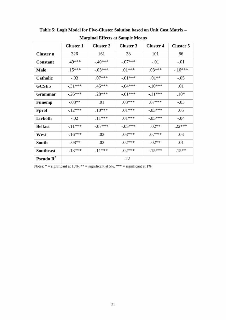
Table 5 reports the marginal effects of the logit model based on the unit cost matrix

five-cluster solution. Overall the results are similar to those based on the standard cost

matrix. For example, all the marginal effects for clusters 1 and 2 for both models

share the same signs. The marginal effects for cluster 4 also share the same signs with

the exception of the male dummy, which displays a positive effect in the unit cost

matrix model. The ‘loosening’ of this cluster – which is characterised by more spells

of employment interspersed with spells of joblessness – is the likely explanation for

this. There are some differences between the models in the marginal effects for

clusters 3 and 5 that result from switching members.

Sensitivity to Specification of the Number of Clusters

In the analysis above we have set the number of clusters at five. Our reasons for this

stem from the trade-off between the number of values the dependent variable can take

in the logit model (not too many), the size of each cluster (not too small) and the level

of distinction of each cluster (not too few clusters).11 But what happens if we specify

three clusters, or ten?

Figure 2 shows each stage of the evolution of clusters from the two-cluster solution to

the ten-cluster solution (using hierarchical cluster analysis). It is the HE-dominated

cluster (cluster 2 in our five-cluster solution) that is the first to break off. This remains

intact up to ten clusters. The next to break off (at the three-cluster solution) is the long

vocational education and training group (cluster 5 in our five-cluster solution). This

also remains intact until the ten-cluster solution where a small group with experience

of long-ish spells of joblessness splits off. At the four-cluster solution, the FE group

11 The more values the dependent variable can take the more the number of parameters to estimate inthe model proliferates.

17

(cluster 3 in our five-cluster solution) separates. This group splits again at the six-

cluster solution into those that go on to HE from FE and those that do not. That this

group is the most sensitive to our choice of five clusters is perhaps not surprising

given its relative lack of distinction. The joblessness cluster first breaks off from the

main cluster at the five-cluster solution but remains together until the eight-cluster

solution where a very small sub-group that stayed on at school before joblessness

splits off.

Evidently, we need to specify at least five clusters in order to identify what we have

labelled the ‘unsuccessful’ transitions. However, Cramer-Ridder tests rule out pooling

the joblessness and employment categories in the logit model so we would be unwise

to reduce the number of clusters below five.12 Increasing the disaggregation

(increasing the number of clusters) has little effect on this joblessness cluster.

So, we cannot estimate a logit model with less than the five clusters or we will lose

the unsuccessful transition cluster. But what of estimating a model with more than the

five clusters? The problem here is that adding clusters leads to a proliferation of the

parameters the model has to estimate, so we are reluctant to go much above six

clusters. However, the logit model for the six-cluster case (where the FE cluster has

split into two groups) gives very similar results to those presented in Tables 3 and 4

for the five-cluster case. The coefficients and marginal effects change very little for

the joblessness cluster and for the other clusters. The most change is unsurprisingly

seen in the estimates for cluster 3. However, even these estimates appear broadly

robust, probably since the group that breaks off from cluster 3 is small. Of course, it

would have been very helpful had a Cramer-Ridder test suggested pooling the newly

split FE clusters to give us the five-cluster logit model – unfortunately it does not.

Sensitivity to Particular Cluster Analysis Techniques

Different clustering techniques can sometimes lead to different outcomes. So far all

our cluster analysis has been based on “between-groups linkage” hierarchical

clustering. Other hierarchical methods give similar patterns of results with one or two

12 The Cramer-Ridder test for pooling clusters 1 and 4 in the five-cluster logit model gives a teststatistic of 56.4 with critical value 5.23 so the null hypothesis of pooling states is rejected.

18

exceptions.13 Here we give details of the clustering exercise based on the standard

cost matrix using k-means clustering. Once again we set the number of clusters equal

to five.

The k-means technique also gives broadly similar clusters to the hierarchical

technique – in particular the joblessness and HE-dominated clusters are very similar.

In this case, the joblessness cluster has a mean number of months in joblessness of

42.5 and a standard deviation of 12.4. However, the employment-dominated cluster

from our earlier analysis is here spread over two roughly equal sized clusters. One is

characterised by two or three years of education or training and then employment. The

other is characterised by less than two years education or training and then

employment (including those that enter employment directly). Clusters 3 and 5 from

the earlier analysis are here pooled into a larger cluster characterised by at least four

years of education or training, mostly followed by one or two years employment.

Since both hierarchical and k-means methods identify a very similar and clear

joblessness cluster, along with broadly similar other clusters, our results would appear

robust to choice of particular method. As we would expect, the logit model shows

very similar marginal effects for the joblessness cluster based on k-means as those

presented in Table 4.

Robustness across Samples

All analysis has so far been based on the full sample available from the Status Zero

Survey. There is no other similar data (e.g. data for another cohort) with which we can

test the robustness of our results across samples. However, we can sub-divide our

current sample and re-run the analysis to check for sensitivity. The sample is split in

half randomly and the OM and cluster analysis, specifying five clusters, is repeated.

13 The analysis was repeated using the six other methods available within SPSS: within-groupslinkage; nearest neighbour; furthest neighbour; centroid clustering; median clustering; and Ward'smethod (see Alenderfer and Blashfield, 1984, for a description of these methods). For four out of thesix methods the five cluster solution had broadly similar characteristics to that in our standard case. Ineach of them there were clear employment, unemployment and HE clusters, although the boundariesbetween our standard case clusters 3 and 5 (the FE and FE/Training clusters) varied somewhat. Justtwo methods produced very different results: nearest neighbour and farthest neighbour. Single linkagemethods such as these two are known though to be prone to producing anomalous results (here indeedthe nearest neighbour method put all but a handful of cases in the same cluster).

19

The clusters identified in each half-sample are broadly similar to those identified in

the full sample. Both half-samples display HE-dominated clusters of roughly equal

size. Both display joblessness-dominated clusters, also of roughly equal size. In one

case, the employment-dominated cluster is split in two (longer and shorter initial

spells in education or training) leaving a single FE-dominated cluster. In the other

case, there is a single employment-dominated cluster and two FE/training dominated

clusters. The jobless cluster in the first half-sample has mean months of joblessness of

46.6 with standard deviation 11.6. The second half-sample joblessness cluster has

mean months of joblessness 46.2 with standard deviation 8.9. In other words, the

joblessness cluster for each half-sample displays almost identical characteristics to the

full-sample joblessness cluster. The logit model is estimated for each half sample.

Given the similarity in the cluster solutions, the logit solutions are unsurprisingly also

similar.14

7. Concluding Remarks

This paper shows how sequence techniques can be used to create a typology of

transitions from school to work – in particular distinguishing unsuccessful transitions

dominated by joblessness from broadly successful transitions dominated by

employment or extended education. This typology is then used here as the basis of a

logit model where young people’s transition types can be ‘predicted’ from their

background characteristics. The results of this exercise are intuitive, consistent with

existing evidence based on more standard stochastic approaches and generally robust

to a large number of specification changes.

The paper adds value to the existing literature in two main respects. Firstly, on the

technical side, we successfully use the output of cluster analysis of sequences, itself

based on OM analysis, as the dependent variable in a regression equation for

transition type. Previous attempts at using cluster analyses of sequences in this way

before have met with little success. Our intuition for why we might have made more

progress on this front is that our data – and our problem – are ideally suited to such an

exercise.

14 More details and results from the sensitivity analyses discussed in Section 6 are available from theauthors on request.

20

Secondly, the typology of unsuccessful transitions and the results showing how young

people’s transition types depend on their individual and family background

characteristics can contribute to an ‘early warning system’ for policy makers

concerned with reducing the drift of significant numbers of young people into long-

term joblessness and social exclusion. We are not quite at the stage where we can put

background characteristics in one end and get an exact prediction of transition

patterns out at the other end – but we can identify young people that are more at risk

of experiencing unsuccessful transitions. Further research may reduce the uncertainty.

21

References

Abbott, A. and Deviney, S. (1992). ‘The welfare state as transnational event.’ SocialScience History, 16, pp 245-74.

Abbott, A. and Forrest, J. (1986). ‘Optimal matching methods for historical data.’Journal of Interdisciplinary History, 16, pp 473-96.

Abbott, A. and Forrest, J. (1990). ‘The optimal matching method for anthropologicaldata.’ Journal of Quantitative Anthropology, 2, pp 151-70.

Abbott, A. and Hrycak, A. (1990). ‘Measuring resemblance in social sequences.’American Journal of Sociology, 96, pp 144-85.

Abbott, A. and Tsay, A. (1999). ‘Sequence analysis and optimal matching methods insociology: review and prospect.’ Mimeo, University of Chicago.

Aldenderfer, M. S. and Blashfield, R. K. (1984). Cluster Analysis. Sage Publications,London.

Anyadike-Danes, M. and McVicar, D. (2000a). ‘Characterising the transition fromschool to work in Northern Ireland: alternative data analytic strategies.’ Paperpresented to the Conference on Applied Statistics in Ireland, Rosslare, CountyWexford, 17th-19th May, 2000.

Anyadike-Danes, M. and McVicar, D. (2000b). ‘Markov models and the transitionfrom school to work’ Mimeo, Northern Ireland Economic Research Centre, Belfast,UK.

Armstrong, D. (1999). ‘School performance and staying-on: A micro analysis forNorthern Ireland.’ Manchester School, 67, 2, pp 203-230.

Armstrong, D. and McVicar, D. (1999). ‘Value added in further education andvocational training in Northern Ireland.’ Applied Economics, forthcoming.

Armstrong, D., Istance, D., Loudon, R., McCready, S., Rees, G. and Wilson, D.(1997). Status 0: A socio-economic study of young people on the margin. Training andEmployment Agency, Belfast.

Carpenter, D. (1996). Corporate identity and administrative capacity in executivedepartments. Unpublished PhD dissertation, University of Chicago.

Cramer, J. S. and Ridder, G. (1991). ‘Pooling states in the multinomial logit model,’Journal of Econometrics, 47, pp 267-72.

Dijkstra, W. and Taris, T. (1995). Measuring the agreement between sequences.Sociological Methods and Research, 24, pp 214-231.

22

Halpin, B. and Chan, T-W. (1998). Class careers as sequences. European SociologicalReview, 14, 2, pp 111-30.

Hammer, T. (1997). History dependence in youth unemployment. EuropeanSociological Review, 13, 1, pp 17-33.

Han, S-K., and Moen, P (1998). ‘Clocking out.’ Mimeo, Cornell University.

Hannan, D.F. and Doyle, A. (2000), ‘Changing school-to-work transitions: threecohorts 1982-1987; 1986-1992; 1992-1998.’ Mimeo, ESRI Dublin, Paper for ESRISeminar, 17 February 2000.

McVicar, D., Loudon, R., McCready, S., Armstrong, D. and Rees, G. (2000). Youngpeople and social exclusion in Northern Ireland: Status 0 four years on. Training andEmployment Agency, Belfast.

Morgan, B. J. T. and Ray, A. P. G. (1995). ‘Non-uniqueness and inversions in clusteranalysis.’ Applied Statistics, 44, pp 117-34.

Poole, M. S. and Holmes, M. E. (1995). ‘Decision development in computer assistedgroup decision-making.’ Human Communication Research, 22, pp 90-127.

Robson, B., Bradford, M. and Deas, I. (1994). ‘Relative deprivation in NorthernIreland.’ Occasional Paper 28, Policy, Planning and Research Unit, Department ofFinance and Personnel, Belfast.

Sankoff, D. and Kruskal, J.B. eds (1983). Time warps, string edits andmacromolecules. Reading MA: Addison Wesley.

Stovel, K. Savage, M. and Bearman, P. (1996). ‘Ascription into achievement.’American Journal of Sociology, 102, pp 358-99.

23

Figures and Tables

24

Figure 1: Cohort Activities, October93 - March99, % of Cohort

Source: NIERC. Notes: The graph shows the proportion of the weighted sample in each activity each

month. Activities are primary activity during the given month.

0%

20%

40%

60%

80%

100%

jobless

train

em p

fe

he

school

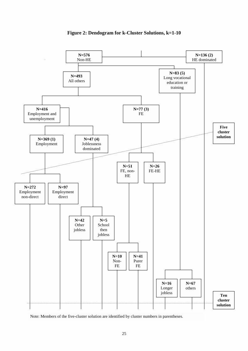
Figure 2: Dendogram for k-Cluster Solutions, k=1-10

H d

N=All o

N=416Employment andunemployment

NO

jo

N=97Employment

direct

N=272Employment

non-direct

N=369 (1)Employment

Note: Members of the five-

N=576Non-HE

25

493thers

N=83 (5)Long vocational

education ortraining

N=6othe

N=41Purer

FE

N=10Non-FE

N=26FE-HE

N=47 (4)Joblessnessdominated

N=51FE, non-

HE

N=5School

thenjobless

=42therbless

N=77 (3)FE

cluster solution are identified by cluster numbers in parentheses.

N=136 (2)E dominate

7rs

Fivecluster

solution

Ten

N=16Longerjobless

clustersolution

26

Table 1: Substitution Costs for the Standard Cost Matrix

School FE Training Employment Joblessness

1 1 2 1 3 HE

1 2 1 3 School

2 1 2 FE

1 1 Training

2 Employment

Joblessness

27

Table 2: Five Cluster Solution – Descriptions and Background CharacteristicsCluster N Description Mean no.

of months

in school

(standard

deviation)

Mean no.

of months

in FE

(standard

deviation)

Mean no. of

months in

employment

(standard

deviation)

Mean no.

of months

in training

(standard

deviation)

Mean no. of

months in

joblessness

(standard

deviation)

Mean no. of

months in

HE

(standard

deviation)

Male

%

Catholic

%

5+GCSEs

at 16

%

Father

unemployed

%

1 308 Employmentdominated

1.4

(4.5)

8.4

(10.9)

49.4

(13.7)

8.8

(12.2)

3.8

(7.1)

0.1

(0.9)

57 43 19 14

2 184 HE dominated 18.7

(12.6)

11.3

(14.8)

3.3

(5.1)

0.2

(1.3)

1.5

(3.4)

37.1

(9.1)

41 50 87 7

3 79 FE dominated 7

(11.6)

33.5

(17.4)

13.3

(8.3)

3.2

(7.4)

3.9

(7.4)

11

(13.9)

46 46 43 21

4 47 Joblessness dominated 3.3

(7.4)

4.9

(7.6)

12.4

(12.2)

7.9

(9.2)

43.6

(12.9)

0

(0)

41 59 8 37

5 95 Long FE/training thenemployment

6.0

(10.8)

20.7

(17.2)

22.8

(11.0)

16.3

(20.1)

5.5

(8.4)

0.7

(2.7)

44 47 30 28

Wholesample

712 7.2

(8.5)

11.7

(15.8)

32.2

(23.2)

6.9

(8.3)

6.2

(12.4)

8.4

(15.6)

52 48 37 16

Note: The sample numbers and cluster proportions are based on the weighted sample (see McVicar et al., 2000, for weighting details).

29

Table 3: Logit Model for Five-Cluster Solution – Coefficients

(Relative Probabilities)

Cluster 2 vs

Cluster 1

Cluster 3 vs

Cluster 1

Cluster 4 vs

Cluster 1

Cluster 5 vs

Cluster 1

Constant -3.55*** -3.19*** -1.87*** -1.90***

Male -0.27 -0.29 -0.82** -0.49*

Catholic 0.21 0.05 0.45 0.26

GCSE5 2.98*** 1.16*** -0.84 0.68**

Grammar 1.72*** 0.23 -0.21 0.25

Funemp 0.34 0.82** 1.02*** 1.11***

Fprof 0.93*** 0.97*** 0.13 0.89***

Livboth 0.43 1.03*** -0.63* -0.35

Belfast -1.10* 0.25 0.78 1.00**

West 0.55 0.69 0.91 0.14

South 0.58* 0.43 0.20 0.10

Southeast 0.83** 0.86** -1.31 0.71*Notes: * = significant at 10%, ** = significant at 5%, *** = significant at 1%.

30

Table4: Logit Model for Five-Cluster Solution – Marginal Effects at

Sample Means

Cluster 1 Cluster 2 Cluster 3 Cluster 4 Cluster 5

Constant .69*** -.33*** -.25*** -.02*** -.09

Male .10*** -.01* -.01** -.03*** -.05

Catholic -.05*** .02** -.01 .01*** .03

GCSE5 -.35*** .34*** .07*** -.06*** .01

Grammar -.16*** .21*** -.01 -.02*** -.01

Funemp -.19*** -.01 .06*** .03*** .12**

Fprof -.22*** .08*** .08*** -.01*** .08*

Livboth -.06*** .05*** .13*** -.03*** -.08**

Belfast -.03 -.17*** .03*** .03*** .15**

West -.12*** .05*** .06*** .03*** -.02

South -.09*** .06*** .04*** .01 -.01

Southeast -.15*** .08*** .08*** -.07*** .07

Pseudo R2 .22Notes: * = significant at 10%, ** = significant at 5%, *** = significant at 1%.

31

Table 5: Logit Model for Five-Cluster Solution based on Unit Cost Matrix –

Marginal Effects at Sample Means

Cluster 1 Cluster 2 Cluster 3 Cluster 4 Cluster 5

Cluster n 326 161 38 101 86

Constant .49*** -.40*** -.07*** -.01 -.01

Male .15*** -.03*** .01*** .03*** -.16***

Catholic -.03 .07*** -.01*** .01** -.05

GCSE5 -.31*** .45*** -.04*** -.10*** .01

Grammar -.26*** .28*** -.01*** -.11*** .10*

Funemp -.08** .01 .03*** .07*** -.03

Fprof -.12*** .10*** .01*** -.03*** .05

Livboth -.02 .11*** .01*** -.05*** -.04

Belfast -.11*** -.07*** -.05*** .02** .22***

West -.16*** .03 .03*** .07*** .03

South -.08** .03 .02*** .02** .01

Southeast -.13*** .11*** .02*** -.15*** .15**

Pseudo R2 .22Notes: * = significant at 10%, ** = significant at 5%, *** = significant at 1%.