eScholarship provides open access, scholarly publishingservices to the University of California and delivers a dynamicresearch platform to scholars worldwide.

Previously Published WorksUCLA

A University of California author or department has made this article openly available. Thanks tothe Academic Senate’s Open Access Policy, a great many UC-authored scholarly publicationswill now be freely available on this site.Let us know how this access is important for you. We want to hear your story!http://escholarship.org/reader_feedback.html

Peer Reviewed

Title:Predicted macroinvertebrate response to water diversion from a montane stream using two-dimensional hydrodynamic models and zero flow approximation

Author:Holmquist, Jeffrey GWaddle, Terry J

Publication Date:May 1, 2013

Series:UCLA Previously Published Works

Publication Info:Ecological Indicators

Permalink:http://escholarship.org/uc/item/97d660jq

DOI:http://dx.doi.org/10.1016/j.ecolind.2012.03.005

Keywords:macroinvertebrate, two-dimensional hydrodynamic model, montane stream assemblage, flow,Yosemite National Park, Sierra Nevada Mountains

Abstract:We used two-dimensional hydrodynamic models for the assessment of water diversion effectson benthic macroinvertebrates and associated habitat in a montane stream in Yosemite NationalPark, Sierra Nevada Mountains, CA, USA. We sampled the macroinvertebrate assemblage viaSurber sampling, recorded detailed measurements of bed topography and flow, and coupled a two-dimensional hydrodynamic model with macroinvertebrate indicators to assess habitat across arange of low flows in 2010 and representative past years. We also made zero flow approximationsto assess response of fauna to extreme conditions. The fauna of this montane reach had a higherpercentage of Ephemeroptera, Plecoptera, and Trichoptera (%EPT) than might be expected given

eScholarship provides open access, scholarly publishingservices to the University of California and delivers a dynamicresearch platform to scholars worldwide.

the relatively low faunal diversity of the study reach. The modeled responses of wetted area andarea-weighted macroinvertebrate metrics to decreasing discharge indicated precipitous declinesin metrics as flows approached zero. Changes in area-weighted metrics closely approximatedpatterns observed for wetted area, i.e., area-weighted invertebrate metrics contributed relativelylittle additional information above that yielded by wetted area alone. Loss of habitat area in thismontane stream appears to be a greater threat than reductions in velocity and depth or changes insubstrate, and the modeled patterns observed across years support this conclusion. Our modelssuggest that step function losses of wetted area may begin when discharge in the Merced fallsto 0.02 m3/s; proportionally reducing diversions when this threshold is reached will likely reduceimpacts in low flow years.

Copyright Information:All rights reserved unless otherwise indicated. Contact the author or original publisher for anynecessary permissions. eScholarship is not the copyright owner for deposited works. Learn moreat http://www.escholarship.org/help_copyright.html#reuse

1

2013. Ecological Indicators 28: 115-124 1

http://www.sciencedirect.com/science/article/pii/S1470160X12000945 2

3

Predicted macroinvertebrate response to water diversion from a montane stream 4

using two-dimensional hydrodynamic models and zero flow approximation 5

Jeffrey G. Holmquista* and Terry J. Waddleb 6

aUniversity of California San Diego, White Mountain Research Station, 3000 E. Line 7

Street, Bishop, California 93514, U.S.A. 8

Current: University of California Los Angeles, Institute of the Environment and 9

Sustainability, White Mountain Research Center, 3000 East Line Street, Bishop, 10

California 93514, U.S.A. 11

12

bUnited States Geological Survey, Fort Collins Science Center, 2150 Centre Avenue, 13

Building C, Fort Collins, CO 80526, U.S.A. waddlet@usgs.gov 14

*corresponding author: jholmquist@ucla.edu 15

Abbreviations: BMI, benthic macroinvertebrates; CA, California; DEM, digital elevation 16

model; EPT, Ephemeroptera, Plecoptera, and Trichoptera; E(S), expected number of 17

species; LIDAR, light detection and ranging; NPS, United States National Park Service; 18

PIE, probability of interspecific encounter; RMS, root mean square error; S, slope; SE, 19

standard error; TIN, triangulated irregular network; 2D, two-dimensional; USGS, United 20

States Geological Service; WSL, water surface level.21

2

ABSTRACT 1

We used two-dimensional hydrodynamic models for the assessment of water 2

diversion effects on benthic macroinvertebrates and associated habitat in a montane 3

stream in Yosemite National Park, Sierra Nevada Mountains, CA, USA. We sampled 4

the macroinvertebrate assemblage via Surber sampling, recorded detailed 5

measurements of bed topography and flow, and coupled a two-dimensional 6

hydrodynamic model with macroinvertebrate indicators to assess habitat across a range 7

of low flows in 2010 and representative past years. We also made zero flow 8

approximations to assess response of fauna to extreme conditions. The fauna of this 9

montane reach had a higher percentage of Ephemeroptera, Plecoptera, and Trichoptera 10

(%EPT) than might be expected given the relatively low faunal diversity of the study 11

reach. The modeled responses of wetted area and area-weighted macroinvertebrate 12

metrics to decreasing discharge indicated precipitous declines in metrics as flows 13

approached zero. Changes in area-weighted metrics closely approximated patterns 14

observed for wetted area, i.e., area-weighted invertebrate metrics contributed relatively 15

little additional information above that yielded by wetted area alone. Loss of habitat 16

area in this montane stream appears to be a greater threat than reductions in velocity 17

and depth or changes in substrate, and the modeled patterns observed across years 18

support this conclusion. Our models suggest that step function losses of wetted area 19

may begin when discharge in the Merced falls to 0.02 m3/s; proportionally reducing 20

diversions when this threshold is reached will likely reduce impacts in low flow years. 21

2

3

Keywords: macroinvertebrate; two-dimensional hydrodynamic model; montane stream 1

assemblage; flow; Yosemite National Park; Sierra Nevada Mountains 2

3

1. Introduction 4

River and stream regulation can cause diverse changes to organisms and their 5

physical environment (Magilligan and Nislow, 2005; Carlisle et al., 2011). Direct effects 6

of dams and water diversion can include alteration of flow periodicity, substrate 7

composition, sedimentation, temperature, and channel morphology, reductions in 8

velocity, depth, wetted area, and dissolved oxygen, elimination of migratory taxa, and 9

increases in conductivity (e.g., Holmquist et al., 1998; Bowen et al., 2003; Suren et al., 10

2003; Greathouse et al., 2006a; b; Dewson et al., 2007a). Such changes can in turn 11

lead to a plethora of indirect effects such as a) disruption of successional processes, 12

benthic and riparian assemblage structure, invertebrate drift, and island and bar 13

maintenance, b) loss of habitat complexity, faunal richness, and floodplain connectivity, 14

and c) proliferation of invasives and algae (Holmquist et al., 1998; Dewson et al., 2007a; 15

b; Finn et al., 2009; Tonkin et al., 2009). 16

Effects of regulation are often assessed via instream flow models that couple 17

hydraulic models to habitat suitability models based on faunal indicator responses to 18

physical predictors, typically velocity, depth, and substrate particle sizes (Gore and 19

Judy, 1981; Gore et al., 2001; Stewart et al., 2005). Models based on site-specific 20

physical and biological assessments are most valuable (Gore et al., 2001). Such efforts 21

generally emphasize fishes (e.g., Stewart et al., 2005; Mingelbier, 2008; Waddle, 2010). 22

Benthic macroinvertebrate (BMI) responses are often different from those of fishes due 23

3

4

to narrower habitat requirements, and BMI-habitat relationships can be more 1

predictable, in part due to lower motility (Statzner et al., 1988; Gore et al., 1998; Gore et 2

al., 2001). Measures of richness, diversity, percentage of Ephemeroptera, Plecoptera, 3

and Trichoptera (%EPT), and selected population abundances are typically used as 4

response metrics in various combinations for evaluation of effects of flow reduction on 5

BMI (Gore et al., 2001; McKay and King, 2006; Suren and Jowett, 2006; Dewson et al., 6

2007b); high values of these metrics are generally indicative of good stream condition 7

(Barbour et al., 1992). 8

Two-dimensional hydrodynamic models are increasingly being used for 9

evaluation of flow and habitat requirements of fauna (Reiser et al., 1989; Stewart et al., 10

2005; Waddle, 2010), but, as with instream modeling in general, such modeling efforts 11

have typically focused on fishes (e.g., Stewart et al., 2005; Mingelbier, 2008). We 12

recently tested application of two-dimensional hydrodynamic models to a BMI 13

assemblage and associated habitat in a subalpine stream in Yosemite National Park, 14

Sierra Nevada Mountains, CA, USA (Dana Fork of the Tuolumne River; Waddle and 15

Holmquist, in press). Modeling of water diversion effects on this subalpine BMI 16

assemblage indicated likely reductions in macroinvertebrate diversity and abundance as 17

a function of both loss of total wetted area and microhabitat degradation. Reductions in 18

wetted area, however, explained most of the overall modeled effects of diversion. 19

In the present study, we examine the extent to which our initial two-dimensional 20

modeling results from the subalpine stream generalize to the BMI assemblage of a 21

lower elevation, montane stream, in the same Yosemite National Park ecosystem, that 22

is also partially diverted for water consumption. Our montane study stream, the South 23

4

5

Fork of the Merced River, is, like the subalpine Dana Fork, a fourth order stream with 1

high water quality (Clow et al., 2011) and with similar alluvial features and wetted area. 2

The montane stream, however, differs from the previously studied subalpine stream in a 3

number of ways in addition to the lower elevation (1215 versus 2630 m), and there is 4

more associated development in the form of a large 104-room hotel, campgrounds, 5

private residences, a golf course, and extensive Park infrastructure. There is year-6

round water diversion from the montane Merced stream, versus seasonal withdrawal 7

from the subalpine stream. Minimum annual discharge, although frequently less than 8

0.1 m3/s, is higher than that of the subalpine stream, but maximum demand for diverted 9

water similarly coincides with seasonally low flows, and the potential for increasing 10

water diversion is a concern for Park managers. The lower, montane stream has only 11

intermittent winter snow cover, and recession to base flow levels after spring snowmelt 12

runoff occurs about a month earlier than in the subalpine stream. Most precipitation at 13

the elevation of the Merced study reach falls in the form of rain, not snow, and there is 14

higher upland vegetation diversity. Our primary question was: Do our hydrological and 15

biological modeling approaches indicate that diversion is likely to affect the BMI 16

assemblage of this montane stream primarily via reduction of wetted area, as was the 17

case in the subalpine stream? 18

19

2. Methods 20

We assessed habitat suitability for BMI using standard velocity, depth, and 21

substrate predictors (Gore and Judy, 1981; Gore et al., 2001) for our modeling efforts. 22

Other correlated factors, such as temperature and dissolved oxygen, will vary with flow, 23

5

6

but are unlikely to exert equivalent influence (Gore and Judy, 1981). Dissolved oxygen 1

levels (~10 mg/l; spot measurements; Stillwater Sciences, unpublished report) and 2

temperature ( x = 18.3 oC, SE = 0.044, National Park Service Solinst datalogger at the 3

study site) during the late summer and fall low-flow period should not be stressful to 4

most stream fauna at this relatively low montane site (but see 4). Field, laboratory, and 5

analytical methods were similar to those used in our study of the subalpine Dana Fork 6

(Waddle and Holmquist, in press). 7

2.1. Study site 8

The study reach of the South Fork of the Merced River is located near Wawona, 9

CA, USA (37º 32’ 20” N, 119º 39’ 02” W). We selected a 191 m study segment 10

downstream of the water diversion, near the National Park Service (NPS) maintenance 11

facilities and fire station at Wawona, California (Fig. 1). Low flows occur from August 12

through October. The stream channel is incised 5 – 7 m into the floodplain and consists 13

of alluvium overlying bedrock and, on the left bank in the upstream one-third of the 14

study site, colluvial talus. Bedrock outcrops are exposed at numerous locations in the 15

channel walls and portions of the channel flow over exposed bedrock. 16

In order to place the study site in geomorphic context, we obtained 1 m resolution 17

LIDAR (Light Detection And Ranging) data for the Wawona area from the NPS (Jim 18

Roche, unpublished data) and constructed a hypsometric profile for the 4 km of the 19

South Fork Merced that bracketed the site. We calculated average gradient for each 1 20

m change in elevation. The proportions of the stream at a given gradient (slope, S) 21

were: S < 0.01, 52.6%; 0.01 < S < 0.03, 38.1%; S > 0.03, 9.3%. The average gradient in 22

our study site was 0.003, i.e., in the most common, lower gradient category. The site, 23

6

7

however, had sections representing the range of gradient of the overall stream: 86.4%, 1

12.1%, and 1.5%, respectively, in the above categories. Our one-cm resolution 2

elevation scale within the site refines the gradient values, but the overall pattern of 3

larger portions of low gradient, pool conditions, separated by shorter steep sections, 4

persists. 5

The surrounding habitat includes ponderosa pine Pinus ponderosa, incense-6

cedar Calocedrus decurrens, California black oak Quercus kelloggii (Sawyer et al., 7

2009), and white fir Abies concolor forest and montane wet meadow, which supports a 8

diverse and abundant arthropod assemblage that includes adult forms of stream fauna 9

(Holmquist et al., 2011). Some fishes are present, including rainbow trout 10

Oncorhynchus mykiss, brown trout Salmo trutta, and Sacramento sucker Catostomus 11

occidentalis. 12

2.2. Field Data Collection and Processing, Macroinvertebrates 13

Benthic macroinvertebrate samples were collected at 100 random sites within the 14

study area (Fig. 2) over six days of relatively low flow interspersed through August and 15

September 2010. We used a standard Surber sampler (Surber, 1937; Hauer and Resh, 16

2007); depth, substrate, and velocity data were collected at each sample location. We 17

measured water depth at four equidistant points within each Surber quadrat. We used a 18

modified Wentworth scale to record the dominant grain size class in the quadrat as a 19

number ranging from silt (2) to bedrock (9; see also Degraaf and Bain, 1986; Mykrä et 20

al., 2008), thus producing a continuous variable representing a class along a continuum 21

(Sokal and Rohlf, 1995). The spectrum of particle categories was well represented 22

among the samples; all categories, from silt to bedrock, were present ( x = 6.98, SE = 23

7

8

0.14), and each particle category except silt dominated three or more samples. We 1

used an acoustic Doppler current meter on a wading rod, with a SonTek FlowTracker® 2

computer, to measure velocity at 0.6 depth at each Surber location. Two sample 3

locations were rejected because the depth was too great for Surber sampling (> 70 cm), 4

and these two sites were replaced with two randomly chosen sampling locations. We 5

sorted samples completely, rather than subsampling, and we identified organisms to as 6

low a taxonomic level as possible, most frequently to the genus/morphospecies level. 7

See Waddle and Holmquist (in press) for further details on BMI sampling and 8

processing. 9

2.3. Field Data Collection and Processing, Physical Data 10

Topographic and discharge related data were collected using methods described 11

in Waddle and Holmquist (in press). We established a survey control benchmark in an 12

open area near the National Park Service (NPS) maintenance facilities approximately 13

100 m north of the study site. Temporary total station baseline points were located in 14

open, dry portions of the stream channel using survey grade (1 cm precision) GPS 15

equipment. Areas along the left bank (south side) of the channel were subject to greater 16

GPS signal interference than the right bank and were measured with a 3-second total 17

station. We surveyed 2992 points in the channel and used them to construct a 18

topographic map of the study site using a triangulated irregular network (TIN) algorithm. 19

Each observed location was coded as to topographic feature (top of bank, toe of 20

bank, thalweg, bar, etc.), and substrate category. Thiessen polygons were constructed 21

among the surveyed points to develop a map of substrate for the entire study site. 22

8

9

Boulders and bedrock outcrops were surveyed by ascending circumnavigation to 1

obtain the minimum number of points required to define their shapes. Generalized ovoid 2

shapes were generated for the large boulders. The generated shapes were 3

incorporated into the site bathymetry as described in Waddle and Holmquist (in press). 4

Inflow boundary conditions were obtained with the flow meter near the location of 5

a stage recorder operated by the NPS at the best, though not ideal, discharge 6

measurement cross section in the study site. A discharge of 0.094 m3/s measured on 7

September 11, 2009 was somewhat higher than the 0.085 m3/s recorded at a gage 8

downstream of the study site (see 2.5). A longitudinal survey of the water surface profile 9

was obtained using a total station at the same time as the discharge measurement. The 10

observed water surface elevations were used to calibrate the two-dimensional model. 11

The NPS provided stage-discharge relations for the upstream and downstream 12

boundary of the study site derived from data collected during 2009 (J. Erxleben, 13

unpublished data). 14

2.4. Survey Quality Control 15

We established a temporary reference benchmark as a survey control point on a 16

right bank bar near the downstream end of the study site. At the beginning and end of 17

every field day, each GPS rover measured that point and compared the measurement 18

with the known position to ensure loop closure for each instrument. Total station 19

measurements were conducted as short distance side shots and relied on the GPS 20

baselines for closure. 21

9

10

2.5. Hydrodynamic Modeling 1

The surveyed topographic locations were assembled into a digital elevation 2

model (DEM) of the study site using a TIN algorithm. We reviewed and corrected the 3

TIN using breaklines to enforce appropriate topographic contours. We compared the 4

final DEM with photographs to ensure agreement with topography. To describe bed 5

roughness, we created a spatially distributed roughness map corresponding to the 6

median diameter of the observed substrate size classes at the surveyed locations. 7

The River2D model (Ghanem et al., 1996; Steffler and Blackburn, 2002) was 8

used to perform all hydraulic simulations (see Waddle and Holmquist, in press). The 9

model estimates the location of the water’s edge by interpolation from the three points 10

of each triangular element spanning the point of zero depth using a simplified 11

groundwater component to produce sub-surface water elevations. This approach is 12

advantageous, because the model approximates hyporheic flow, a potentially significant 13

flow component in this study. 14

We developed an irregular computational mesh containing 17,418 nodes using a 15

process of iterative refinement of wet areas. An initial coarse mesh was used to 16

simulate the calibration discharge. Areas of significant topographic change such as 17

steep banks and boulders were refined by adding a new node at the centroid of the 18

mesh elements spanning that feature. Intermediate simulation results were inspected 19

for irregularities such as excessive velocity or unusual flow direction, and additional 20

mesh refinements were added in those areas to reduce discretization error and promote 21

model convergence. Anomalous velocity patterns were dampened by increasing eddy 22

viscosity globally. The model was re-run with the refined mesh until the average node 23

10

11

density in wetted areas was approximately 7 nodes per square meter. The area per wet 1

node ranged from 0.002 m2 to 3 m2 with the smallest elements occurring in a narrow, 2

necked-down section and the largest elements occurring in a large pool where there 3

were few topographic or substrate changes. 4

The model was initially calibrated for a discharge of 0.094 m3/s using the 5

measured discharge and water surface profile data described previously in this section. 6

To obtain calibration we globally adjusted roughness height, groundwater transmissivity, 7

and eddy viscosity in an attempt to match the predicted water surface profile to 8

observed conditions. The initial attempt using default parameters produced a predicted 9

water surface profile that was substantially lower (mean error of -0.0365 m) than 10

observed. We decreased groundwater transmissivity, and increased roughness heights 11

in an attempt to raise the predicted water surface elevation. Successive changes in 12

these parameters improved the calibration error but resulted in a mean error of -0.008 m 13

at the measured discharge. As bed transmissivity was decreased, we encountered 14

excessive velocities and numerical stability problems in the narrow section. Small 15

increases in eddy viscosity were found to dampen extreme velocity variation and yield a 16

stable solution. 17

Even with substantial adjustments to roughness and transmissivity, the model 18

was underpredicting the water surface upstream of the outflow boundary for all 19

combinations of the calibration parameters. We concluded the reason for this 20

discrepancy was likely due to our inability to measure the entire discharge; that is, flow 21

through extensive boulder and large cobble talus on the left bank of the channel was not 22

accessible to the velocity meter. Based on field observations, we concluded the 23

11

12

discharge may be undersampled by as much as 10 - 25%. Calibrating the model using 1

an assumed discharge of 0.105 m3/s produced a more satisfactory match to observed 2

water surface elevation measurements. 3

Once calibrated to water surface elevation, we compared simulated and 4

observed velocities at the discharge measurement transect. The simulated velocity 5

pattern was similar to the observed, but sharp localized variations were smoothed. Such 6

minor variations are a common characteristic of two-dimensional models, and we 7

concluded that the calibration was adequate and proceeded to production runs for 8

habitat simulation. 9

The calibrated model was run for discharges of 0.014, 0.028, 0.042, 0.057, 10

0.071, 0.085, 0.096, 0.117, 0.142, 0.212, and 0.283 m3/s (see Waddle and Holmquist, in 11

press). This range of flow spanned the August-September conditions obtained from the 12

13 years of records we used for hydrograph derivation (see 2.7) To ensure coverage of 13

the full range of flow considered in the analysis it was necessary to describe a condition 14

of zero discharge. The hydrodynamic model becomes unstable when attempting to 15

simulate zero flow, so we approximated a zero discharge condition by identifying the 16

pool areas and estimating the zero flow pool water surface elevation as the minimum 17

elevation at the hydraulic control for each pool, assuming zero velocity in all pool areas, 18

and assuming that all riffle areas would be dry if there was no discharge. We calculated 19

BMI indices (see 2.6) for the nodes in the computational mesh that were wet given this 20

approximation. 21

12

13

2.6. Macroinvertebrate Habitat Modeling 1

We examined BMI indicator response to varying velocity, depth, and substrate 2

category. We assessed diversity using expected number of species, i.e., rarefaction 3

(E(S2); Hurlbert, 1971; Magurran, 2004). We also examined %EPT, i.e., the percent of 4

total fauna composed of Ephemeroptera (mayflies), Plecoptera (stoneflies), and 5

Trichoptera (caddisflies). Lastly, we used number of Plecoptera/m2 as an indicator that 6

would scale linearly with area, because this order was the most "intolerant" (sensu 7

Hilsenhoff, 1987; Barbour et al., 1992; i.e., sensitive to degraded conditions) across all 8

constituent taxa. We corrected metrics not meeting parametric assumptions (Lilliefors, 9

Fmax and Cochran's tests; Lilliefors, 1967; Kirk, 1995) with log transformations: log (y + 10

1) for velocity and log y for substrate class. We modeled relationships of BMI metrics to 11

physical predictors using ternary quadratic exponential polynomials with cross-product 12

terms (Gore and Judy, 1981; Jowett and Richardson, 1990; Jowett et al., 1991; Collier, 13

1993; Gore et al., 2001). This approach has been advocated, because these models 14

minimize variance, better represent habitat selection, and offer more accurate predictors 15

than techniques such as incremental curve fitting (Gore and Judy, 1981; Morin et al., 16

1986; Gore et al., 2001). We provide p-values, R2, and adjusted R2 for the models. 17

Both R2 and adjusted R2 are of value; the latter reduces R2 to compensate for the 18

tendency for R2 to increase with additional predictor terms. 19

We calculated these BMI indicators for each wetted computational node point at 20

each simulated discharge and multiplied each nodal index value by the area of the 21

Thiessen polygon surrounding a given node and summed these products over the 22

domain of the study site to obtain an area-weighted habitat value for each index. 23

13

14

2.7. Hydrograph Derivation 1

A U.S. Geological Survey (USGS) gage (#11267300; 2

http://waterdata.usgs.gov/nwis) located downstream of the California Highway 41 bridge 3

at Wawona was operated from Oct. 1, 1958 to September 30, 1968. The Merced 4

Irrigation District has operated a gage at the same location since October 5, 2007 5

(provisional record: http://cdec.water.ca.gov/cgi-progs/staMeta?station_id=SMW), and 6

we obtained daily flow values for the 2008 – 2010 water years from Sierra 7

Hydrographics Inc. (Dan Garrigue, pers. comm.). These records correspond to the 8

current level of infrastructure development in the Wawona area and thus approximate 9

current effects of water management practices on this portion of the stream. 10

We evaluated 13 years of observed discharges by combining the water year 11

1958 – 1968 and 2008 - 2010 records to get the maximum range of recently observed 12

conditions. We extracted the August and September flow events and arrayed those 13

events in order of the two-month total flow volume. The analysis was focused on August 14

and September, because this specific low flow period was of management interest, and 15

BMI samples were accordingly obtained during these months. Using the ordered data, 16

we selected the lowest (1960), median (1968), and next to highest flow (2009) years for 17

analysis of daily average flow, as those years were representative of the range of 18

events occurring at Wawona and were within the 0.014 to 0.283 m3/s range of flow that 19

we believed could be simulated using the calibration data obtained in the field. Thus, we 20

excluded the highest recorded flow period from the analysis. During high flow periods, 21

however, diversion has the least impact, so we concluded that the chosen flow range 22

adequately addressed habitat effects of water diversion practices. 23

14

15

2.8. Evaluation of Macroinvertebrate Habitat Over Time 1

In order to evaluate modeled BMI responses for the selected lowest, median, and 2

next -to-highest flow years noted in 2.7, we calculated E(S), %EPT, and Plecoptera 3

abundance for the period of August 1 – September 30 for each of the years by 4

interpolating an index value from each BMI metric to discharge relationship for each 5

daily flow value during that period. The resulting time series of biological metrics were 6

evaluated for the existing seasonal streamflow pattern. We then reduced the flow time 7

series by a hypothetical 0.014 m3/s (in effect doubling the maximum diversion currently 8

practiced) in order to model an increase in upstream water withdrawal and recalculated 9

the BMI indices as described. One limitation of our study was that these modeling 10

efforts were necessarily based upon sampling done in a single year, due to NPS 11

funding and schedule constraints. Although we do not have multi-year BMI data from 12

the Merced, we do have such data from the nearby Tuolumne River at an almost 13

identical elevation (Holmquist and Schmidt-Gengenbach, unpublished report). 14

Tuolumne BMI demonstrate less inter-annual than seasonal variation in diversity 15

metrics, %EPT, and Plecoptera abundance, providing some reassurance that extreme 16

annual fluctuations among Merced assemblages are not probable. The limited 17

sampling in the Merced should nevertheless be kept in mind when considering our 18

results (see also Mykrä et al., 2008). 19

3. Results 20

3.1. Assemblage Characterization 21

The 100 samples yielded 1,388 individuals representing nine orders and 30 22

families (Table 1). Diptera and Ephemeroptera were the most abundant orders. There 23

15

16

were about six taxa per sample, and probability of interspecific encounter was 0.651 1

(SE = 0.026; Table 1). There was 43.8% dominance (SE = 2.4); common families 2

included chironomid midges ( x = 53.7/m2, SE = 8.5), baetid ( x = 18.5, SE = 3.1), 3

leptophlebiid ( x = 17.8, SE = 3.4), and heptageniid ( x = 15.6, SE = 2.5) mayflies, and 4

elmid riffle beetles ( x = 10.3, SE = 1.9). 5

6

3.2. Nonlinear Regressions and Univariate Trends 7

The nonlinear regressions of all modeled faunal metrics on velocity, depth, and 8

substrate were highly significant (Table 2). Substrate had the lowest p-values among 9

individual coefficients. Response of E(S), %EPT, and Plecoptera abundance to the 10

individual physical predictors was variable, although there was a weak trend of lower 11

E(S) and %EPT values with decreased velocity (Fig. 3). Higher values for E(S) and 12

%EPT tended to be observed at intermediate depths, and there was another weak trend 13

of higher E(S) and Plecoptera abundance at intermediate substrate sizes (Fig. 3). 14

3.3. Hydrodynamic Model Calibration and Production Run Results 15

As noted in 2.5, the best calibration was obtained using an assumed discharge of 16

0.105 m3/s (Table 3). Observed and simulated water surface profiles were well aligned 17

(Fig. 4). We obtained a mean water surface prediction error of 0.0011 m and a root 18

mean square error of 0.0133 m. This error scatter reflects the challenges of surveying 19

the site and modeling a step-pool stream. Comparison of simulated and observed 20

velocities at the discharge transect revealed a smoothed transverse velocity profile and 21

produced a mean error of 0.009 m/s and RMS of 0.03 m/s, thus supporting our reliance 22

on the model to approximate velocity over the simulation domain. 23

16

17

Once calibrated, the River2D model was run for the previously described range of 1

discharges. The simulations showed decreasing wetted area with decreasing discharge 2

(Figs. 5, 6). The field data represent an approximate sampling of the true bed condition. 3

Because individual cobbles and pebbles were not explicitly mapped, the sampled 4

topography represented general bar shapes while explicitly incorporating the shapes of 5

boulders and bedrock outcrops. Connectivity of marginal patches was strongly 6

influenced by discharge (Fig. 5). Our zero flow approximations resulted in a substantial 7

and abrupt drop in wetted area due to drying of the riffles and runs. 8

3.4. Modeled faunal response to diversion 9

Area-weighted metrics decreased with decreasing discharge almost in parallel 10

(Fig. 6) with wetted area, and losses accelerated as zero flow was approached (Fig. 6). 11

Response of area-weighted metrics differed little from that of wetted area alone. We 12

calculated daily time series for BMI variables (Fig. 7) for late July through early October 13

of three representative years by interpolating from the BMI index versus discharge 14

relationships (Fig 6). We interpolated BMI for discharges below 0.014 m3/s from 15

habitat to discharge relationships that were extended using the zero flow approximation 16

to produce continuous habitat time series for the three selected years. The resulting 17

time series (Fig. 7) reflect the greater slope of the BMI versus discharge relations as 18

zero flow was approached, but only on 6 days of the lowest flow year (1960). Thus our 19

estimate of zero flow conditions did not strongly influence this analysis. All area 20

weighted metrics tracked wetted area closely across years. When these time series 21

were reduced by 0.014 m3/s, as a hypothetical means of evaluating further water 22

diversion, a representative and frequently evaluated (Gore et al., 2001) weighted metric 23

17

18

(%EPT) showed relatively minor losses (Fig. 8), despite the fact that during the lowest 1

flow periods this hypothetical flow reduction would deplete the stream by more than 2

60% of the daily mean discharge, thus reducing flow to approximately 0.008 m3/s. 3

Under this reduction scenario, %EPT generally paralleled patterns observed for the 4

unmanipulated actual flows, but did demonstrate the greatest absolute losses (Fig. 8) 5

during the weeks and year with the lowest flows (Fig. 7), and proportional losses were 6

greater still during the lowest flow events (Fig. 8). 7

4. Discussion 8

Given the overall match of predicted water surface profile to observed conditions, 9

we concluded that the hydrodynamic model calibration was satisfactory for the range of 10

discharges that we simulated. We were initially concerned about increasing the 11

calibration discharge to a value greater than the gage reading. A bedrock sill, however, 12

forced all water to the surface at the location of our discharge measurement, whereas 13

the gage is located in a broad alluvial valley, where, at this low discharge, a fraction of 14

the total down-valley flow may lie below the bed. From the consistency of the calibrated 15

water surface profile across both riffle and pool channel types we concluded that the our 16

calibration at the estimated discharge was a better approximation of the flow than the 17

discharge measurement made on September 11, 2009. 18

We employed a wide range of extrapolation from the measured conditions, and 19

the precision of the hydraulic predictions likely decreases toward both ends of the 20

range. However, an advantage of two-dimensional models is simulation of momentum 21

effects describing the forces of flow around objects and over the bed of the channel. 22

Waddle (2010) demonstrated that 2D model predictions in turbulent field conditions are 23

18

19

sufficiently accurate that it is difficult to discern if discrepancies between measured and 1

modeled velocities are due to measurement or model error. Thus we rely on the 2D 2

representation of flow to provide velocity and depth values over the study site. Though 3

errors in extrapolation certainly occur and cannot be quantified without additional data, 4

we believe the predicted trends in BMI response and relative BMI magnitudes are 5

accurate. 6

The fauna of this montane reach had a higher percentage of Ephemeroptera, 7

Plecoptera, and Trichoptera (%EPT) than might be expected given the relatively low 8

faunal diversity of the study reach. Ephemeroptera abundances were low, but made up 9

a large proportion of the total abundance. Although shallow pool habitat was extensive, 10

low flow specialists were lacking among the Ephemeroptera in the montane stream, yet 11

many generalists were present, and Ephemeroptera abundance had a negative 12

relationship to velocity (p = 0.037). The most common trichopteran in our samples, 13

Lepidostoma, occurs in low flow habitats (Wiggins, 1996), and the same is true for many 14

of the other common Trichoptera. Similarly, odonate nymphs (dragon- and damselflies) 15

and veliid water striders (Hemiptera) were present in these relatively quiescent waters. 16

Despite the relatively low gradient and large amount of pool habitat in this reach, 17

Diptera were less abundant than expected, possibly because of a comparatively low silt 18

component ( x = 0.79%, frequency= 0.19), although this order was still the most 19

abundant by a small margin. Diptera made up 80% of an abundant subalpine 20

assemblage (Waddle and Holmquist, in press), versus only 38% of the montane Merced 21

assemblage, and the great reduction in dipteran numbers at our montane site likely 22

explains much of the overall lower abundance and higher %EPT. 23

19

20

Diversity, expected number of species, and %EPT often decrease in response to 1

lower discharge and velocity (Cazaubon and Giudicelli, 1999; McIntosh et al., 2002; 2

Dewson et al., 2007a;b). Gore et al. (2001) showed highest BMI diversity at 3

intermediate velocities of 30-60 cm/s, depending on stream gradient (see also Suren 4

and Jowett, 2006). Our E(S) was generally consistent with these patterns. Similarly, 5

Gore et al. (2001) found EPT suitability to peak at 10-30 cm/s, and our %EPT results 6

showed a similar pattern, although the upper end of the velocity range was largely 7

absent as a result of our emphasis on water diversion and the preponderance of 8

shallow pool habitat in this section of the Merced. Much higher flows might begin to 9

reduce E(S) and %EPT, because velocities greater than ~80 cm/s generally decrease 10

habitat suitability (Gore et al., 2001). We similarly found highest %EPT and Plecoptera 11

abundances at intermediate velocities in our subalpine study (Waddle and Holmquist, in 12

press), although this trend was mediated by depth and substrate characteristics. We 13

found some tendency for highest E(S) and %EPT at ~30 cm depth in the Merced; Gore 14

et al. reported similar results for diversity, but their EPT suitability peaked at 50+ cm. 15

These results were in contrast to those that we obtained in the previously studied 16

subalpine stream, in which metrics had lower values at intermediate depths. All three 17

studies (present, Gore et al., 2001; Waddle and Holmquist, in press) were generally 18

consistent in terms of maximum habitat provision in approximately cobble-sized 19

substrata, though this trend was lacking for %EPT in the present study. 20

Responses of wetted area and area-weighted BMI metrics to decreasing 21

discharge were strong and similar for both the montane Merced and subalpine Dana 22

Fork (Waddle and Holmquist, in press), despite the many inter-stream differences as a 23

20

21

function of habitat, assemblage structure, and response of metrics to predictors. 1

Overall direct loss of wetted area in the montane stream appears to be a greater threat 2

than indirect effects on microhabitat as a function of discharge reductions, and the 3

patterns observed across years bolster this contention. Thus, our earlier results from a 4

subalpine environment do appear to generalize well to a very different stream (see also 5

Englund and Malmqvist, 1996). 6

Although there was clearly a strong modeled relationship between wetted area 7

and the BMI assemblage, reliance on modeled wetted area alone may underestimate 8

impacts, as individual habitat parameters (e.g., velocity and depth), can be important 9

influences, and ecosystem processes, such as nutrient enrichment, can rival wetted 10

area in importance in some environments (Jowett, 1997; Suren et al., 2003). Losses of 11

wetted area, however, are unlikely to be entirely in the form of mortality, which may be 12

mitigated by movement into the hyporheic zone (Williams and Hynes, 1976; Boulton et 13

al., 1998), acquisition of waterless refugia (Lake, 2000), horizontal movement (Gore, 14

1977; Lake, 2000; but see McIntosh, 2002), and ultimate rapid recovery of populations 15

(Williams and Hynes, 1976; Lake, 2000; Dewson et al., 2007a). Further, low flow 16

impacts may occur slowly (Armitage and Petts, 1992; Suren and Jowett, 2006), and it 17

may be that effects are relatively reversible if extreme low flows are not maintained for 18

an extended period. 19

The available historical data, used in concert with our modeling efforts, suggest 20

that these streams are resilient environments that to date have probably not been 21

heavily impacted by diversion. Responses to very low or zero discharge, however, for 22

both wetted area and BMI, are probably more abrupt than modeled. Although potential 23

21

22

mortality is likely mitigated by the factors outlined above (see also Suren and Jowett, 1

2006), many of these mechanisms would fail to provide compensation during extreme 2

flow reductions, which would cause disproportionate losses to sedentary taxa (Canton 3

et al., 1984) and filterers (Dewson et al., 2007b). Persistent, very low flows (such as 4

during a severe drought) would cause pools to drain, possibly reducing the wetted 5

hyporheic zone; because invertebrates recolonize habitat more slowly than fishes, 6

recovery of BMI assemblages is slow, particularly for taxa without volant stages (Gore 7

and Milner, 1990; Gore et al., 2001). With extreme discharge reductions, losses of 8

habitat quality would begin to become more important. Temperature, although not 9

always a major factor during normal seasonal low discharge, particularly in smaller 10

streams with a large groundwater component and/or at higher elevations and latitudes 11

(Mosely, 1983; Rader and Belish, 1999; Dewson et al., 2007a), would likely be a source 12

of mortality if flow were to approach zero (discussion in Suren et al., 2003). Dissolved 13

oxygen might similarly begin to play a larger role in low-flow conditions (Hicks et al., 14

1991). Sedimentation often increases in response to flow reductions (Dewson et al., 15

2007a; b) resulting in negative effects at a variety of scales (Jones et al., in press). In 16

addition, increases in nutrient enrichment in this relatively developed reach would be 17

likely to exacerbate diversion impacts (Suren et al., 2003; see also Armitage and Petts, 18

1992). 19

The greatest impact of a given amount of water diversion thus likely occurs at 20

seasonal low flow. The three selected years cover the range of summer low flow events 21

occurring at this location in the Merced River; seven of the thirteen years available for 22

analysis had discharges below 0.1 m3/s for at least 30 days, and in most years the 23

22

23

lowest daily flows were ~0.05 m3/s. The lowest daily flows were reached in 1960 and 1

1961 when the recession reached minima of 0.02 and 0.03 m3/s, respectively. Such 2

extreme low flows may become more frequent as a response to a combination of 3

increasing Park visitation, resulting in increased withdrawals, and lower late season 4

discharge as a function of the changing climate (Yarnell et al., 2010). Proportionally 5

reducing diversion will likely decrease impacts from extreme low flow events during 6

years in which discharge in this stream falls to 0.02 m3/s, as our models suggest that 7

step function losses to BMI may begin at these very low levels of flow. 8

9

Acknowledgements 10

We thank Jim Roche, Yosemite National Park, for his fine support throughout this 11

project. Physical data collection was ably assisted and facilitated by Chris Holmquist-12

Johnson and Leanne Hanson of the USGS Fort Collins Science Center and Jennifer 13

Erxleben of the NPS. We had excellent ecological field and lab assistance from Jutta 14

Schmidt-Gengenbach (taxonomy; University of California San Diego, White Mountain 15

Research Station) and Marie French (sample sorting). The paper was improved by 16

discussion with Peggy Moore and Heather McKenny and by draft manuscript review by 17

Brandy Logan, Jim Roche, Mike Yochim, Bob Zuelig, and two anonymous reviewers, as 18

well as the editorial attention of Felix Müller. This work was supported by IA 19

#F8813090088 to the Fort Collins Science Center, USGS and NPS #J8C07100012 to 20

UCSD-WMRS and was built upon recent work funded by NPS #J8R07090011. The 21

WMRS portion of this work was also supported by the Californian Cooperative 22

Ecosystems Studies Unit with the help of Angela Evenden. 23

23

24

1

Role of the funding source 2

The funding agency (US National Park Service) had no role in the study design, 3

analysis and interpretation of data, the decision to submit the work for publication, or 4

writing of the paper. We acquired baseline hydrological data from the NPS as 5

described in Section 2, and an NPS technician assisted the team with low-level physical 6

data collection duties under the supervision of the second author. Two NPS staff 7

members offered a small number of minor comments on an earlier draft of the 8

manuscript. The NPS did not attempt to guide the study in any manner whatsoever. 9

10

11

12

24

25

References 1

Armitage, P.D., Petts, G.E., 1992. Biotic score and prediction to assess the effects of 2

water abstractions on river macroinvertebrates for conservation purposes. Aquatic 3

Conservation: Marine and Freshwater Ecosystems 2, 1-17. 4

Barbour, M.T., Plafkin, J.L., Bradley, B.P., Graves, C.G., Wisseman, R.W., 1992. 5

Evaluation of EPA's rapid bioassessment benthic metrics: metric redundancy and 6

variability among reference stream sites. Environmental Toxicology and Chemistry 7

11, 437-449. 8

Boulton, A.J., Findlay, S., Marmonier, P., Stanley, E.H., Valett, H.M., 1998. The 9

functional significance of the hyporheic zone in streams and rivers. Annual Review 10

of Ecology and Systematics 29, 59-81. 11

Bowen, Z.H., Bovee, K.D., Waddle, T.J., 2003. Effects of flow regulation on shallow-12

water habitat dynamics and floodplain connectivity. Transactions of the American 13

Fisheries Society 132, 809-823. 14

Canton, S.P., Cline, L.D, Short, R.A., Ward, J.A., 1984. The macroinvertebrates and fish 15

of a Colorado stream during a period of fluctuating discharge. Freshwater Biology 16

14, 311-316. 17

Carlisle, D.M., Wolock, D.M., Meador, M.R., 2011. Alteration of streamflow magnitudes 18

and potential ecological consequences: a multiregional assessment. Frontiers in 19

Ecology and the Environment 9, 264-270. 20

21

25

26

Cazaubon, A., Giudicelli, J., 1999. Impact of the residual flow on the physical 1

characteristics and benthic community (algae, invertebrates) of a regulated 2

Mediterranean river: the Durance, France. Regulated Rivers: Research & 3

Management 15, 441-461. 4

Clow, D.W., Peavler, R.S., Roche, J., Panorska, A.K., Thomas, J.M., Smith, S., 2011. 5

Assessing possible visitor-use impacts on water quality in Yosemite National Park. 6

Environmental Monitoring and Assessment 183: 197–215. 7

Collier, K.J., 1993. Flow preferences of larval Chironomidae (Diptera) in Tongariro 8

River, New Zealand. New Zealand Journal of Marine and Freshwater Research 27, 9

219-226. 10

Degraaf, D.A., and Bain, L.H., 1986. Habitat use by and preferences of juvenile Atlantic 11

salmon in two Newfoundland rivers. Transactions of the American Fisheries 12

Society 115, 671-681. 13

Dewson, Z.S., James, A.B.W., Death, R.G., 2007a. A review of the consequences of 14

decreased flow for instream habitat and macroinvertebrates. Journal of the North 15

American Benthological Society 26, 401-415. 16

Dewson, Z.S., James, A.B.W., Death, R.G., 2007b. Invertebrate community responses 17

to experimentally reduced discharge in small streams of different water quality. 18

Journal of the North American Benthological Society 26, 754-766. 19

Englund, G., Malmqvist, B., 1996. Effects of flow regulation, habitat area and isolation 20

on the macroinvertebrate fauna of rapids in north Swedish rivers. Regulated Rivers: 21

Research & Management 12, 433-445. 22

26

27

Finn, M.A., Boulton, A.J., Chessman, B.C., 2009. Ecological responses to artificial 1

drought in two Australian rivers with differing water extraction. Fundamental and 2

Applied Limnology: Archiv für Hydrobiologie 175, 231-248. 3

Ghanem, A., Steffler, P., Hicks, F., Katopodis, C., 1996. Two-dimensional simulation of 4

physical habitat conditions in flowing streams. Regulated Rivers: Research & 5

Management 12, 185–200. 6

Gore, J.A., 1977. Reservoir manipulations and benthic macroinvertebrates in a prairie 7

river. Hydrobiologia 55, 113-123. 8

Gore, J.A., Crawford, D.J., Addison, D.S., 1998. An analysis of artificial riffles and 9

enhancement of benthic community diversity by physical habitat simulation 10

(PHABSIM) and direct observation. Regulated Rivers: Research & Management 14, 11

69-77. 12

Gore, J.A., Judy, R.D., Jr., 1981. Predictive models of benthic macroinvertebrate 13

density for use in instream flow studies and regulated flow management. Canadian 14

Journal of Fisheries and Aquatic Sciences 38, 1363-1370. 15

Gore, J.A., Layzer, J.B., Mead, J., 2001. Macroinvertebrate instream flow studies after 16

20 years: a role in stream management and restoration. Regulated Rivers: Research 17

& Management 17, 527-542. 18

Gore, J.A., Milner, A.M., 1990. Island biogeographical theory: can it be used to predict 19

lotic recovery rates? Environmental Management 14, 737-753. 20

Greathouse, E.A., Pringle, C.M., Holmquist, J.G., 2006a. Conservation and 21

management of migratory fauna: dams in tropical streams of Puerto Rico. Aquatic 22

Conservation: Marine and Freshwater Ecosystems 16, 695-712. 23

27

28

Greathouse, E.A., Pringle, C.M., McDowell, W.H., Holmquist, J.G., 2006b. Indirect 1

upstream effects of dams: consequences of migratory consumer extirpation in 2

Puerto Rico. Ecological Applications 16, 339-352. 3

Hauer, F.R., Resh, V.H., 2007. Macroinvertebrates, in: Hauer, F.R., Lamberti, G.A. 4

(Eds.), Methods in Stream Ecology, second ed. Academic Press, San Diego, pp. 5

435-463. 6

Hicks, B.J., Beschta, R.L., Harr, R.D., 1991. Long-term changes in streamflow following 7

logging in western Oregon and associated fisheries implications. Water Resources 8

Bulletin 27, 217-226. 9

Hilsenhoff, W., 1987. An improved biotic index of organic stream pollution. The Great 10

Lakes Entomologist 20, 31-39. 11

Holmquist, J.G., Jones, J.R., Schmidt-Gengenbach, J., Pierotti, L.F., Love, J.P., 2011. 12

Terrestrial and aquatic macroinvertebrate assemblages as a function of wetland type 13

across a mountain landscape. Arctic, Antarctic, and Alpine Research 43, 568-584. 14

Holmquist, J.G., Schmidt-Gengenbach, J.M., Yoshioka, B.B., 1998. High dams and 15

marine-freshwater linkages: effects on native and introduced fauna in the Caribbean. 16

Conservation Biology 12, 621-630. 17

Hurlbert, S.H., 1971. The nonconcept of species diversity: a critique and alternative 18

parameters. Ecology 52, 577-586. 19

Jones, J.I., Murphy, J.F., Collins, A.L., Sear, D.A., Naden, P.S., Armitage, P.D., In 20

press. The impact of fine sediment on macro-invertebrates. River Research and 21

Applications. DOI: 10.1002/rra.1516. 22

28

29

Jowett, I.G., 1997. Instream flow methods: a comparison of approaches. Regulated 1

Rivers: Research & Management 13, 115-127. 2

Jowett, I.G., Richardson, J., 1990. Microhabitat preferences of benthic invertebrates in a 3

New Zealand river and the development of in-stream flow-habitat models for 4

Deleatidium spp. New Zealand Journal of Marine and Freshwater Research 24, 19-5

30. 6

Jowett, I.G., Richardson, J., Biggs, B.J.F., Hickey, C.W., Quinn, J.M., 1991. 7

Microhabitat preferences of benthic invertebrates and the development of 8

generalised Deleatidium spp. habitat suitability curves, applied to four New Zealand 9

rivers. New Zealand Journal of Marine and Freshwater Research 25, 187-199. 10

Kirk, R.E., 1995. Experimental Design: Procedures for the Behavioral Sciences, third 11

ed. Brooks/Cole Publishing, Pacific Grove. 12

Lake, P.S., 2000. Disturbance, patchiness, and diversity in streams. Journal of the 13

North American Benthological Society 19, 573-592. 14

Lilliefors, H.W., 1967. On the Kolmogorov-Smirnov test for normality with mean and 15

variance unknown. Journal of the American Statistical Association 64, 399-402. 16

Magilligan, F.J., Nislow, K.H., 2005. Changes in hydrologic regime by dams. 17

Geomorphology 71, 61-78. 18

Magurran, A.E., 2004. Measuring Biological Diversity. Blackwell Publishing, Malden. 19

McIntosh, M.D., Benbow, M.E., Burky, A.J., 2002. Effects of stream diversion on riffle 20

macroinvertebrate communities in a Maui, Hawaii, stream. River Research and 21

Applications 18, 569-581. 22

29

30

McKay, S.F., King, A.J., 2006. Potential ecological effects of water extraction in small, 1

unregulated streams. River Research and Applications 22, 1023-1037. 2

Mingelbier, M., Brodeur, P., Morin, J., 2008. Spatially explicit model predicting the 3

spawning habitat and early stage mortality of Northern pike (Esox lucius) in a large 4

system: the St. Lawrence River between 1960 and 2000. Hydrobiologia 601, 55-69. 5

Morin, A., Harper, P.P., Peters, R.H., 1986. Microhabitat-preference curves of blackfly 6

larvae (Diptera, Simuliidae) – a comparison of three estimation methods. Canadian 7

Journal of Fisheries and Aquatic Sciences 43, 1235-1241. 8

Mosley, M.P., 1983. Variability of water temperatures in the braided Ashley and Rakaia 9

Rivers. New Zealand Journal of Marine and Freshwater Research 17, 331-342. 10

Mykrä, H., Heino, J., Muotka, T., 2008. Concordance of stream macroinvertebrate 11

assemblage classifications: How general are patterns from single-year surveys? 12

Biological Conservation 141, 1218-1223. 13

Rader, R.B., Belish, T.A., 1999. Influence of mild to severe flow alterations on 14

invertebrates in three mountain streams. Regulated Rivers: Research & 15

Management 15, 353-363. 16

Reiser, D.W., Wesche, T.A., Estes, C., 1989. Status of instream flow legislation and 17

practices in North America. Fisheries 14, 22-29. 18

Sawyer, J.O., Keeler-Wolf, T., Evens, J.M., 2010. A Manual of California Vegetation, 19

second ed. California Native Plant Society Press, Sacramento. 20

Sokal, R.R., Rohlf, F.J., 1995. Biometry, third ed. Freeman and Co., New York. 21

30

31

Statzner, B., Gore, J.A., Resh, V.H., 1988. Hydraulic stream ecology: observed patterns 1

and potential applications. Journal of the North American Benthological Society 7, 2

307-360. 3

Steffler, P., Blackburn, J., 2002. River2D: Two–dimensional Depth Averaged Model of 4

River Hydrodynamics and Fish Habitat. Introduction to Depth Averaged Modeling 5

and Users Manual. University of Alberta, Edmonton. 6

Stewart, G., Anderson, R., Wohl, E., 2005. Two-dimensional modeling of habitat 7

suitability as a function of discharge on two Colorado rivers. River Research and 8

Applications 21, 1061-1074. 9

Surber, E.W., 1937. Rainbow trout and bottom fauna production in one mile of stream. 10

Transactions of the American Fisheries Society 66, 193-202. 11

Suren, A.M., Biggs, B.J.F., Duncan, M.J., Bergey, L., 2003. Benthic community 12

dynamics during summer low-flows in two rivers of contrasting enrichment 2. 13

Invertebrates. New Zealand Journal of Marine and Freshwater Research 37, 71-83. 14

Suren, A.M., Jowett, I.G., 2006. Effects of floods versus low flows on invertebrates in a 15

New Zealand gravel-bed river. Freshwater Biology 51, 2207-2227. 16

Tonkin, J.D., Death, R.G., Joy, M.K., 2009. Invertebrate drift patterns in a regulated 17

river: dams, periphyton biomass or longitudinal patterns? River Research and 18

Applications 25, 1219-1231. 19

Waddle, T.J., 2010. Field evaluation of a two-dimensional hydrodynamic model near 20

boulders for habitat calculation. River Research and Applications 26, 730-741. 21

22

31

32

Waddle, T.J., Holmquist, J.G. In press. Macroinvertebrate response to flow changes in a 1

subalpine stream: predictions from two-dimensional hydrodynamic models. River 2

Research and Applications. DOI: 10.1002/rra.1607. 3

Wiggins, G.B., 1996. Larvae of the North American Caddisfly Genera (Trichoptera), 4

second ed. University of Toronto Press, Toronto. 5

Williams, D.D., Hynes, H.B.N., 1976. The recolonization mechanisms of stream 6

benthos. Oikos 27, 265-272. 7

Yarnell, S.M., Viers, J.H., Mount, J.F., 2010. Ecology and management of the spring 8

snowmelt recession. BioScience 60, 114-127. 9

10

32

33

Figure captions 1

Fig. 1. Location of Wawona study site on the South Fork of the Merced River. Dashed 2

arrow indicates flow direction. 3

Fig. 2. Study reach and locations of macroinvertebrate samples (dots). Blue line = 4

simulated water’s edge at 0.086 m3/s flow; contour intervals = 0.5 m. 5

Fig. 3. Scatterplots for E(S), %EPT, and Plecoptera abundance/m2 at sampled sites as 6

a function of velocity (cm/s), water depth (cm), and dominant grain size class, ranging 7

from silt (2) to bedrock (9). 8

Fig. 4. Observed and calibrated water surface level (WSL) profile assuming discharge 9

(0.105 m3/s) was 12% higher than recorded. 10

Fig. 5. Depth (m) and wetted area for three simulated discharges. Boundary of modeled 11

area shown in red. 12

Fig. 6. Comparison of wetted area and area-weighted macroinvertebrate indices as a 13

function of discharge. 14

Fig. 7. Response of area-weighted macroinvertebrate indices to high, median, and low 15

flow years by date. Late season storms occurred in both the high and low flow years. 16

Fig. 8. Comparison of %EPT by date under observed and reduced flow scenarios. The 17

two minima for reduced flows in 1960 are in part an artifact of the zero flow 18

approximation. 19

20

33

N

Wawona Hotel

Wawona District Circle

S. Fk. Merced R.

Fig. 1

Location of Study Site

Stream gage

Fire Station

Diversion Structure Located Upstream

Figure 1

34

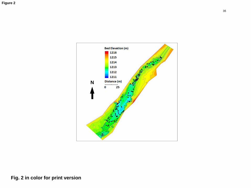
Fig. 2 in color for print version

N

Figure 2

35

E(S

) %

EP

T

Ple

co

pte

ra/m

2

Velocity (cm/s) Depth (cm) Substrate Code

Fig. 3

Figure 3

36

1211.6

1212.0

1212.4

1212.8

1213.2

1213.6

0 50 100 150 200

Longitudinal Distance (m)

Ele

vati

on

(m

)

Thalweg Simulated WSL Observed WSL

Fig. 4

Figure 4

37

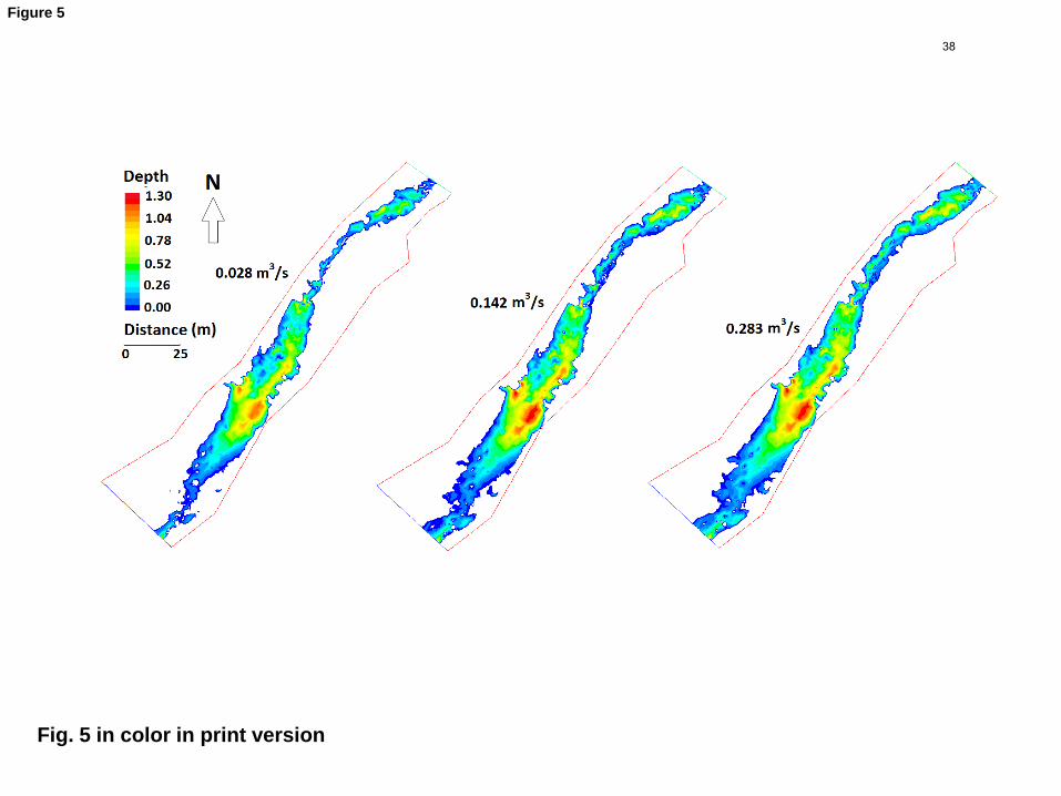
Fig. 5 in color in print version

Figure 5

38

Fig. 6

0

1000

2000

3000

0.0 0.1 0.2 0.3

We

t A

rea

(m

2)

Discharge (m3/s)

0

500

1000

1500

2000

0.0 0.1 0.2 0.3

We

igh

ted

%E

PT

0

10

20

30

40

50

0.0 0.1 0.2 0.3

We

igh

ted

E(S

) Discharge (m3/s)

0

5000

10000

15000

20000

0.0 0.1 0.2 0.3

Nu

mb

er

of

Ple

co

pte

ra

Figure 6

39

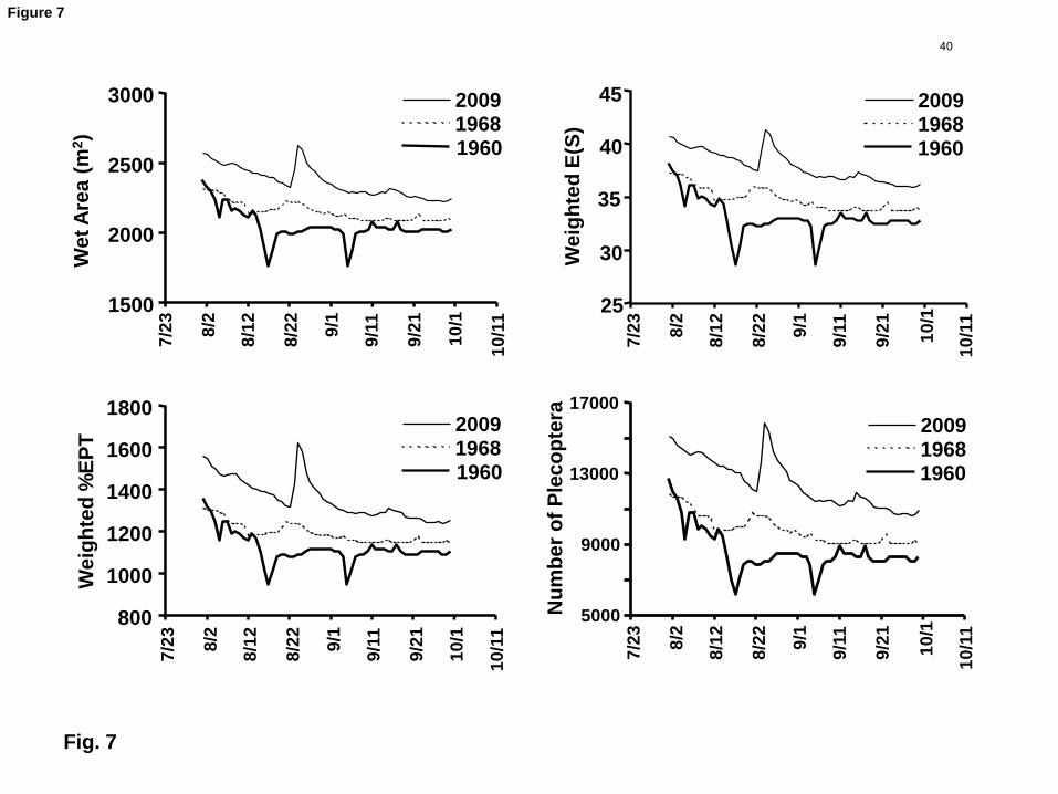
Fig. 7

We

t A

rea

(m

2)

1960 1968 2009

7/2

3

8/2

8/1

2

8/2

2

9/1

9/1

1

9/2

1

10

/1

10

/11 1500

2000

2500

3000

800

1000

1200

1400

1600

1800

We

igh

ted

%E

PT

7/2

3

8/2

8/1

2

8/2

2

9/1

9/1

1

9/2

1

10

/1

10

/11

1960 1968 2009

25

30

35

40

45

We

igh

ted

E(S

)

7/2

3

8/2

8/1

2

8/2

2

9/1

9/1

1

9/2

1

10

/1

10

/11

1960 1968 2009

5000

9000

13000

17000

Nu

mb

er

of

Ple

co

pte

ra

7/2

3

8/2

8/1

2

8/2

2

9/1

9/1

1

9/2

1

10

/1

10

/11

1960 1968 2009

Figure 7

40

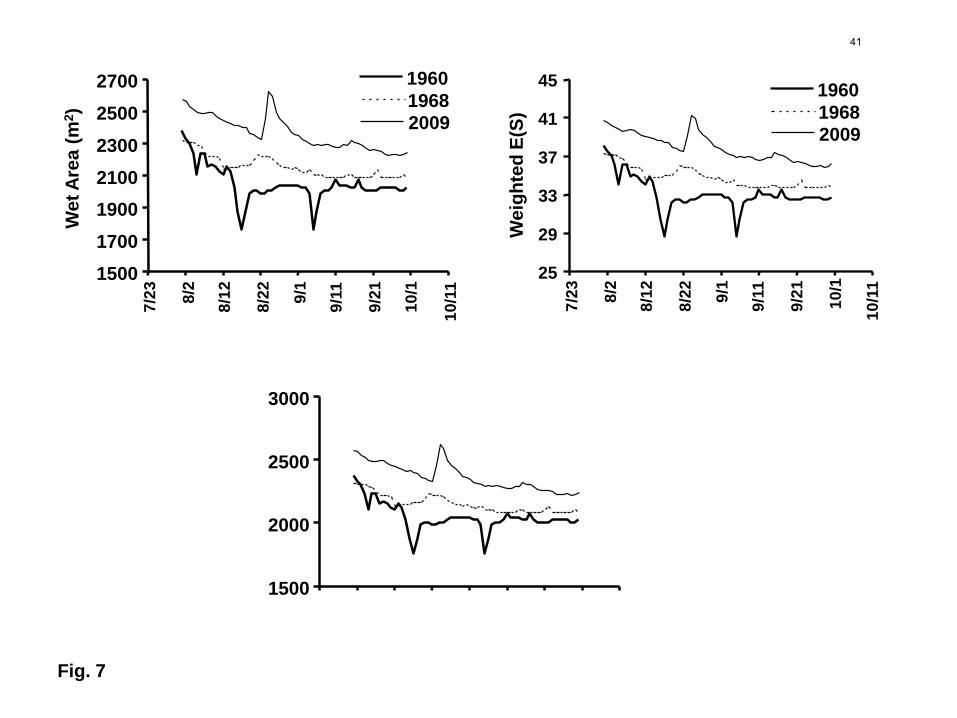
Fig. 7

1500

1700

1900

2100

2300

2500

2700 W

et A

rea

(m

2)

1960 1968 2009 7

/23

8/2

8/1

2

8/2

2

9/1

9/1

1

9/2

1

10

/1

10

/11 25

29

33

37

41

45

We

igh

ted

E(S

)

7/2

3

8/2

8/1

2

8/2

2

9/1

9/1

1

9/2

1

10

/1

10

/11

1960 1968 2009

1500

2000

2500

3000

41

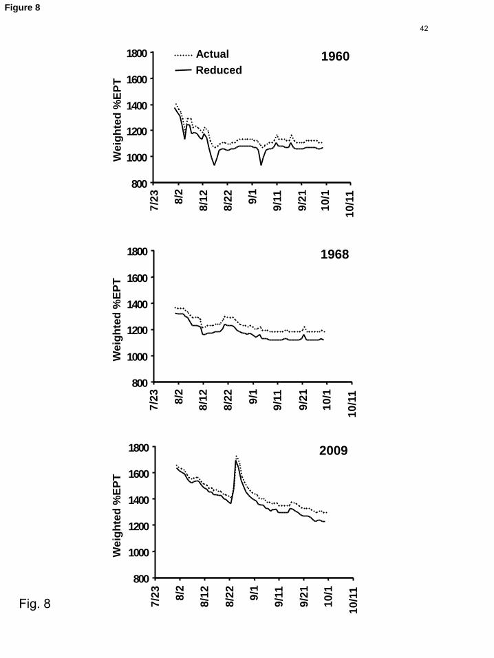
Fig. 8

8 0 0

1 0 0 0

1 2 0 0

1 4 0 0

1 6 0 0

1 8 0 0

7/2

3

8/2

8/1

2

8/2

2

9/1

9/1

1

9/2

1

10

/1

10

/11

We

igh

ted

%E

PT

Actual

Reduced 1960

8 0 0

1 0 0 0

1 2 0 0

1 4 0 0

1 6 0 0

1 8 0 0

7/2

3

8/2

8/1

2

8/2

2

9/1

9/1

1

9/2

1

10

/1

10

/11

We

igh

ted

%E

PT

1968

8 0 0

1 0 0 0

1 2 0 0

1 4 0 0

1 6 0 0

1 8 0 0

7/2

3

8/2

8/1

2

8/2

2

9/1

9/1

1

9/2

1

10

/1

10

/11

We

igh

ted

%E

PT

2009

Figure 8

42

Table 1. Mean and standard error for macroinvertebrate assemblage metrics used in 1

instream flow assessment as well as additional assemblage metrics and order 2

abundances. Probability of interspecific encounter (PIE) is a measure of evenness 3

(Hurlbert, 1971). %Dominance = abundance of the most common taxon in a 4

sample/total sample abundance. Note that richness measures do not scale linearly with 5

area, so values cannot be converted to per square meter values. See 2.6 for further 6

metric information. 7

8

9

10

11

12

13

14

15

16

17

18

19

20

21

22

23

24

25

26

27

28

29

30

31

32

33

34

35

36

37

38

39

40

41

42

43

Mean SE

Total individuals/m2 149 16

Species richness/0.09m2 5.97 0.41

E(S) 1.69 0.045

Family richness/0.09m2 4.40 0.27

PIE 0.651 0.026

% Dominance 43.8 2.4

% EPT 58.9 2.6

Ephemeroptera/m2 55.3 6.4

Plecoptera/m2 5.70 1.3

Odonata/m2 0.430 0.21

Hemiptera/m2 0.323 0.24

Coleoptera/m2 11.2 2.0

Neuroptera/m2 0.323 0.18

Trichoptera/m2 19.6 3.3

Diptera/m2 56.7 8.6

Acari/m2 0.108 0.11

Tables

43

1

Table 2. Coefficients from nonlinear regressions of E(S), %EPT, and Plecoptera abundance on velocity, depth, and 2

substrate using ternary quadratic exponential polynomials with cross-product terms: 3

Y = exp (-((a1V)+(a2D)+(a3S)+(a4V2)+(a5D

2)+(a6S2)+(a7VD)+(a8VS)+(a9DS))), where ai = coefficient, V = velocity, D = 4

Depth, S = substrate category. R2, Adjusted R2, and p-values for the models appear in the columns to the right. 5

Coefficients with p < 0.05 are indicated in bold, those with p < 0.01 in bold and italic, and those with p < 0.001 are 6

underlined, bold, and italicized. See 2.6 for transformations. 7

8

a1V a2D a3S a4V2 a5D

2 a6S

2 a7V*D a8V*S a9D*S R

2 Adjusted R

2 P

E(S) 2.3 0.045 -3.1 -0.53 0.00097 3.0 0.033 -2.6 -0.078 0.94 0.14 <0.0001

%EPT -4.9 -0.11 -6.1 3.5 -0.00056 1.7 -0.13 5.0 0.14 0.86 0.079 <0.0001

#Plecoptera/m2 -63 2.5 -14 45 0.065 13 -3.2 70 -3.0 0.45 0.35 <0.0001

9

10

11

12

13

44

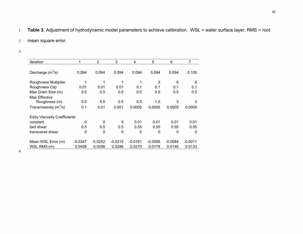
Table 3. Adjustment of hydrodynamic model parameters to achieve calibration. WSL = water surface layer; RMS = root 1

mean square error. 2

3

Iteration 1 2 3 4 5 6 7

Discharge (m3/s) 0.094 0.094 0.094 0.094 0.094 0.094 0.105 Roughness Multiplier 1 1 1 1 3 6 6 Roughness Clip 0.01 0.01 0.01 0.1 0.1 0.1 0.1 Max Grain Size (m) 0.5 0.5 0.5 0.5 0.5 0.5 0.5 Max Effective

Roughness (m) 0.5 0.5 0.5 0.5 1.5 3 3

Transmissivity (m2/s) 0.1 0.01 0.001 0.0005 0.0005 0.0005 0.0005 Eddy Viscosity Coefficients constant 0 0 0 0.01 0.01 0.01 0.01 bed shear 0.5 0.5 0.5 0.55 0.55 0.55 0.55 transverse shear 0 0 0 0 0 0 0 Mean WSL Error (m) -0.0347 -0.0252 -0.0215 -0.0161 -0.0095 -0.0084 -0.0011 WSL RMS (m) 0.0408 0.0296 0.0286 0.0270 0.0178 0.0146 0.0133

4

45