Predictability of carbon emissions from biomass burning in Indonesia from 1997 to 2006

Predictability of carbon emissions from biomass burning in Indonesia

from 1997 to 2006

Robert D. Field1 and Samuel S. P. Shen2

Received 20 January 2008; revised 26 June 2008; accepted 12 August 2008; published 5 December 2008.

[1] Drought and sea surface temperature were examined as the causes of severe biomassburning C emissions in Indonesia for 1997–2006, obtained from the Global FireEmissions Database. Eighteen predictor variables were considered under log linear andpiecewise regression models. The predictor variables considered were precipitation totalsof up to 6 months, output from two soil moisture models, and sea surface temperature(SST) indicators reflecting El Nino and Indian Ocean Dipole strength. Nonparametricbootstrap techniques were used to estimate confidence intervals for predictability andthresholds below which severe C emissions are likely. Across equatorial Southeast Asia,the best predictor was 3-month total precipitation, which explained 79% of variance in Cemissions. When considered individually, and with the incorporation of satelliteprecipitation estimates, predictability for southern Sumatra and southern Kalimantanimproved to 97% and 92%, respectively, using 4-month total precipitation. There is a highrisk of severe burning when 4-month precipitation falls below thresholds of 350 mm insouthern Sumatra and 650 mm in southern Kalimantan and when 6-month precipitation fallsbelow 900 mm in Papua. In general, simple precipitation totals outperformed morecomplicated soil moisture models and SST-based indices. Physically, seasonal precipitationcontrols fire emissions through its regulation of groundwater level and, hence, the amount ofpeat available for drying. Seasonal precipitation, in turn, is strongly influenced by SSTpatterns in the tropical Pacific and Indian oceans. The most severe drought and fire eventsappear equally influenced by Indian Ocean Dipole events and El Nino events.

Citation: Field, R. D., and S. S. P. Shen (2008), Predictability of carbon emissions from biomass burning in Indonesia from 1997 to

2006, J. Geophys. Res., 113, G04024, doi:10.1029/2008JG000694.

1. Introduction

[2] The interannual growth of CO2 and other greenhousegases is not steady but occurs irregularly over timescales of2–5 years, with biomass burning proposed as the mainsource of this interannual growth [Langenfelds et al., 2002].Zeng et al. [2005] estimated that biomass burning representsroughly 20% of the mean interannual carbon flux anomaly,mainly through the increase in tropical fires in response todrought conditions. Indonesian biomass burning in 1997was estimated to constitute 15–40% of the mean annualglobal C emissions from fossil fuel burning [Page et al.,2002]. Podgorny et al. [2003] quantified the climaticimpacts of the 1997 event, estimating that aerosol emissionsfrom the fires resulted in at least a 50% increase inatmospheric solar heating within the first three verticalkilometers and at least a 15% reduction in seasonal meansolar radiation incident at the surface of the equatorialIndian Ocean. The serious health impacts of transboundary

haze generated by Indonesian fires have also been docu-mented [Sastry, 2002; Kunii et al., 2002].[3] With industrial logging and agriculture as the under-

lying causes [Dennis et al., 2005; Langner et al., 2007],the trigger for severe fire and haze episodes in Indonesia isdrought. There is significant interannual variability in dryseason rainfall over Indonesia, due to changes in oceanand atmospheric circulation in the tropical Pacific andIndian oceans. In the Pacific, the anomalously high seasurface temperatures (SST) appear in the east, weakeningthe Walker circulation and resulting in a reduced poolingof warm water and convection in the western Pacific[Gutman et al., 2000; Hendon, 2003]. Over Indonesia,this results in a pronounced decrease in rainfall duringthe dry seasons, as convection shifts eastward into thecentral Pacific. Similar impacts also result from SSTanomalies in the Indian Ocean, where precipitation shiftsnorthwestward away from western Indonesia [Saji et al.,1999]. During these periods, burning escapes control,igniting vast deposits of peat soils, whose water holdingcapacity has been reduced because of extensive draining[Page et al., 2002; Usup et al., 2004]. The provinces ofRiau, Jambi, and South Sumatra on the island ofSumatra and West, Central, South and East Kalimantanare the main fire prone regions of Indonesia [Heil andGoldammer, 2001].

JOURNAL OF GEOPHYSICAL RESEARCH, VOL. 113, G04024, doi:10.1029/2008JG000694, 2008

1Department of Physics, University of Toronto, Toronto, Ontario,Canada.

2Department of Mathematics and Statistics, San Diego State University,San Diego, California, USA.

Copyright 2008 by the American Geophysical Union.0148-0227/08/2008JG000694

G04024 1 of 17

[4] Because of the large amounts of smoke produced, thehaze signature of the fires is seen clearly in different proxymeasurements, which have also been used to understandunderlying causes of the fires. Field et al. [2004] showedthat reductions in visible range at airports in Sumatra andKalimantan during 1994–1998 could be explained byanomalously low values of a drought code used for firedanger monitoring in boreal and temperate forests. Over alonger period from 1973 to 2003, Wang et al. [2004]showed that reductions in visible range over Sumatra werein phase with warm ENSO periods in 1982/1983, 1987/1988, 1991/1992, 1994/1995, 1997/1998 and 2002/2003, asindicated by the Nino3.4 SST index.[5] Kita et al. [2000] and Thompson et al. [2001] also

showed qualitatively that enhancements of the Total OzoneMapping Spectrometer Aerosol Index (TOMS AI) overIndonesia have occurred during the El Nino episodes of1982/1983, 1987/1988 and 1991/1992 and 1997/1998, alsousing SSTs as an explanatory variable. Severe burning wasalso observed more recently in 2006 [Lohman et al., 2007],and elevated CO and O3 measurements from the Tropo-spheric Emission Spectrometer (TES) and Measurements ofPollution in the Troposphere (MOPITT) instruments wereattributed to Indonesian fires, and ultimately to El Nino-induced drought [Logan et al., 2008]. These atmosphericindicators provide useful longer-term characterizations ofsmoke but are complicated by several factors. Visible rangedata is a useful surface indicator, but is somewhat subjectivein that it records maximum distance seen by a humanobserver. The TOMS sensor and AI retrieval algorithmhave limited detection ability in the lower troposphere[Herman et al., 1997], resulting in underdetection problemsand a lag between the onset of severe haze and its detection.It is also difficult to attribute observed atmospheric haze to aspecific origin, due to transport and mixing of smoke fromdifferent sources.[6] Satellite-detected hot spots are the best available fire

indicator for many regions of the world [Duncan et al.,2003] and provide a means for quantifying the underlyingcauses of fire, especially in regions such as Indonesia whichlack systematic aerial estimates of burned area. Over Indo-nesia, Sudiana et al. [2003] assessed the relationshipbetween AVHRR hot spot occurrence from 1981 to 1993,showing qualitatively that fire episodes occurred underdryer conditions, as reflected by a fire danger index cali-brated for North American conditions.[7] van der Werf et al. [2008] examined the relationship

between climate and fire over the entire tropics andsubtropics using TRMM fire counts. Using an index offire potential based on dry season length and total dryseason precipitation, they showed that fire in some regionsof Indonesia was correlated with high fire potential, andthat high fire count years were associated with anomalous-ly low dry season rainfall. Other studies using satellite-detected hot spots in Indonesia have shown that fireoccurrence is related to land use [Stolle and Lambin,2003] and occurs under dryer conditions associated withEl Nino conditions [Dymond et al., 2005; Fuller andMurphy, 2006].[8] The goal of this study was to better understand

climatic factors contributing to biomass burning emissionsin Indonesia. Specifically, we tried to identify, from among

a broad pool, climate variables which explain the highestproportion of variance in direct C emissions from biomassburning over Indonesia, as estimated from the Global FireEmissions Database of van der Werf et al. [2006], for 1997to 2006. Particular attention was devoted to interregionalvariability of emissions and predictability, and the degree towhich drought thresholds could be identified for improvedinterpretation of seasonal rainfall forecasts. Formal quanti-tative estimates of proportion of variance in fire occurrenceexplained by climate predictor variables have been limitedto Field et al. [2004] and Fuller and Murphy [2006]. Giventhe potential application of such predictor variables inseasonal prediction or in climate change outlooks, detailedassessments of the uncertainty of predictions were alsomade.

2. Data and Methods

2.1. The Global Fire Emissions Database

[9] Estimates of biomass burning emissions over Indo-nesia were obtained from the Global Fire Emissions Data-base (GFED) [van der Werf et al., 2006], which is currentlythe best available source of global fire emissions data. Thedata is available on a 1� by 1� grid for the period 1997–2006 at monthly temporal resolution. Fire occurrence andarea burned are determined from cross-calibrated ATSR,TRMM, and MODIS hot spot counts. Emissions estimatesare based on fuel load predictions from a global vegetationmodel, a soils map for subsurface fuels, and emissionsfactors specific to different combustion products. OverIndonesia, an important distinction is also made betweenorganic soils and nonburning mineral soils. Following Pageet al. [2002] and van der Werf et al. [2006], we used directcarbon (C) emissions as our emissions indicator.[10] Previous case studies have shown that the seasonality

of fire emissions can vary considerably across Indonesia.The 1998 fires in East Kalimantan during February to April1998, for example, were decoupled from the 1997 July–November burning across the rest of Kalimantan [Heil andGoldammer, 2001; Siegert and Hoffmann, 2000] and oc-curred under localized drought conditions not seen in otherparts of Kalimantan [Field et al., 2004]. To identify Indo-nesia’s main seasonal burning regions, a spatial principalcomponent analysis was performed to identify regions ofcoherent seasonal burning, similar to the approach ofGedalof et al. [2005]. Each region was then analyzedindividually to identify possible climatic drivers.

2.2. Climatic Indices

[11] We considered a broad range of variables in trying topredict severe biomass burning. Following Fuller andMurphy [2006], we used the sea level-pressure-based South-ern Oscillation Index and sea surface temperature-basedNino3.4 index as indicators of El Nino strength. In addition,we considered the Multivariate ENSO Index (MEI) [Wolterand Timlin, 1993] and the recently developed Dipole ModeIndex (DMI) of Saji et al. [1999]. The MEI is a hybrid indexincorporating the SLP behavior of the SOI and the SSTbehavior of the Nino3.4. The DMI measures the strength ofthe Indian Ocean Dipole events, whereby anomalies appear-ing in the basin are related to anomalously low precipitationin Indonesia.

G04024 FIELD AND SHEN: DROUGHT AND BIOMASS BURNING IN INDONESIA

2 of 17

G04024

[12] To examine the direct relationship between droughtand fire in Indonesia, we considered two different precip-itation data sets and two soil moisture models, all of whichhave global coverage and monthly temporal resolution. TheNCEP Precipitation over Land (PRECL) data set [Chen etal., 2002] was the simplest data set considered, consisting ofrain gauge only measurements interpolated onto a 2.5� �2.5� grid. The Global Precipitation Climatology Project(GPCP) data set [Adler et al., 2003] uses gauge data, butalso incorporates infrared and microwave satellite retrievals.The incorporation of satellite data was warranted for inclu-sion in this analysis given the sparse rain gauge coverageover much of Indonesia. To distinguish between singlemonths with anomalously low precipitation and persistentseasonal drought, precipitation totals for up to 6 monthsprior were considered as individual drought indices.[13] Given the significant contribution of peat burning to

emissions, we also examined output from two soil moisturemodels as predictor variables. The National Centre forEnvironmental Prediction Global Soil Moisture (SOILM)data set of Fan and van den Dool [2004] is based on asimple single bucket moisture model. Although the data areavailable globally, model parameters are based on fieldstudies in the U.S. Great Plains, and currently with noparameter variation across soil or land cover types. Asinput, the model uses the monthly precipitation data fromPRECL, and surface air temperature data from the NCEP-NCAR reanalysis [Kalnay et al., 1996]. Data are distributedat a 0.5 by 0.5 spatial resolution, but have an effectiveresolution of 2.5� � 2.5� corresponding to that of thePRECL data set.[14] The Palmer Drought Severity Index (PDSI) comput-

ed globally by Dai et al. [2004] was also considered. Likethe SOILM model, the PDSI was designed mainly foragricultural applications in the U.S., to measure the cumu-lative departure in moisture supply and loss at the surface,but has been applied in numerous other applications, includ-ing historical forest fire and climate analyses [Westerlinget al., 2002; Hessl et al., 2004]. It is an anomaly basedindex, in that local climatological means of rainfall areincluded as moisture parameters, and is cumulative, withthe current month’s PDSI a function of the currentmonth’s weather and last month’s PDSI.[15] The PDSI uses a two-layer soil model, and unlike the

SOILM model, does distinguish between the water holdingcapacity of different soil types. PDSI values are on astandardized scale, with a minimum of �10 correspondingto severe moisture deficit and a maximum of +10 cor-responding to a moisture surplus. The technical details ofthe PDSI are described by Ntale and Gan [2003]. Unlike theSOILM model, the PDSI has undergone some validationagainst field data outside of the U.S., showing strong corre-lation with measured soil moisture in southern China andstreamflow in Brazil and the Congo, particularly comparedwith raw rainfall measurements [Dai et al., 2004].[16] In total, 18 predictor variables were considered,

including the 1- to 6-month back totals for each of theprecipitation indices.

2.3. Threshold Estimation

[17] Although there is a regular wet and dry season cycledriven by the Asian-Australian monsoon, it is only during

anomalously dry years that fires are a serious problem. Fieldet al. [2004] showed this to be the case over the period from1994 to 1999, when there were severe haze events duringthe dry seasons of the 1994 and 1997 El Nino years, but anear absence of haze events during the other non El Ninoyears. Their analysis showed that the absence of haze duringnon El Nino years corresponded to a moisture thresholdabove which conditions are too wet to support extensivebiomass burning and haze.[18] Presumably, this threshold corresponds to a moisture

threshold in vegetation and organic soil, which is supportedby experimental data. Frandsen [1997] found this to be thecase in a series of experimental burns for different organicsoils across North America, showing that the probability ofignition increases below a moisture content of 120% for themajority of soil types, and with a higher threshold for soiltypes with a higher inorganic content. In Indonesia, deGroot et al. [2005] showed that dead ‘‘alang-alang’’ grass,a key surface fuel type leading to subsurface fires, had amoisture content ignition threshold of 27.8%. Moisturecontent in Indonesian peatlands will begin to decrease whenthe groundwater level falls below the surface and the peat isexposed to unsaturated air.[19] Piecewise regression was used to estimate the rela-

tionship between drought and emissions in such a way as toexplicitly include an estimate of drought threshold. Themodel consists of two linear segments, constrained to beequal at an unknown change point which is interpreted asthe threshold value in this context. Using the formulation ofToms and Lesperance [2003], the model is given by

f xð Þ ¼ b0 þ b1x; x � ab0 þ b1xþ b2 x� að Þ; x > a

�ð1Þ

where a is the change point to be estimated, b1 is the slopeof the line below the change point and b1 + b2 is the slopeof the second line, x is a given predictor variable, and f (x) isthe emissions. This formulation constrains continuitybetween the two model sections at a, which provides aless ambiguous threshold estimate than the curvature-basedapproach of Field et al. [2004]. The model was estimatedthrough straightforward use of nonlinear fitting routines.For a comparison to Fuller and Murphy [2006], basic log-transformed relationships were also considered for eachvariable and analysis region, which implicitly models thedrought-emissions relationship in a nonlinear fashion.Drought-emissions relationships were examined individu-ally for each subregion region identified through theprincipal component analysis, rather than the analysis ofField et al. [2004] or Dymond et al. [2005], who aggregateddata across all of Sumatra and Kalimantan, and Fuller andMurphy [2006], who focused on the entire Indonesianarchipelago.[20] Ultimately, we wished to identify the moisture index

which best predicted serious emissions episodes, and whichseparated severe drought from normal conditions. Theperformance of different models and predictor variableswas evaluated using the coefficient of determination (R2).To estimate a confidence interval for R2 and thresholdstatistics, we used a fully nonparametric bootstrappingapproach [Efron and Tibshirani, 1993]. Using this method,the random samples of pairs (xi, yi) are drawn with replace-


3 of 17

G04024

ment from the original sample, rather than resampling theresiduals, which is more sensitive to the underlying distri-bution of error terms. The change point function (1) was fitto each random sample, yielding a distribution of R2 and aestimates for each model. 95% confidence intervals for theestimates were obtained from the 2.5th and 97.5th percen-tiles of the bootstrapped distributions. For each moistureindex and region, a total of 1000 resamples were drawn.

3. Results

3.1. Emissions Characteristics

[21] Figure 1 shows the mean annual C emissions acrossall of Indonesia, during the 1997–2006 period, calculatedfrom the GFED data set [van der Werf et al., 2006]. The

spatial principal component analysis yielded five mainregions where C emissions tended to covary (Figure 2)within the entire Indonesian region (EQSA, for equatorialSoutheast Asia): central Sumatra (CSUM), southern Sumatra(SSUM), southern Kalimantan (SKAL), eastern Kalimantan(EKAL) and Papua (PAP). Figure 2a shows the spatialloadings of the first EOF, which is a dominant mode ofburning during the southeast monsoon dry season, andcoincides with the primary precipitation zone of Aldrianand Susanto [2003]. Figure 2b shows the second EOF, whichmainly reflects the early 1998 burning in EKAL. Figure 2bshows the third EOF, which is dominated by early seasonburning in 2002, 2005, and 2006 in CSUM. The first threeEOFs explain 59%, 12%, and 10% of the variability in Cemissions, respectively.

Figure 1. Mean annual C emissions (Tg), 1997–2006, and the five burning regions considered withinthe EQSA domain. Regional names do not correspond to province names.

Figure 2. (a) First, (b) second, and (c) third EOF patterns of C emissions.


4 of 17

G04024

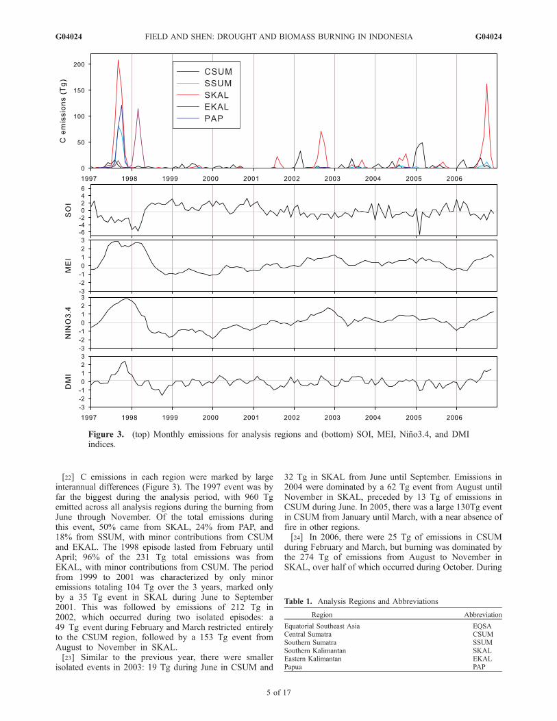
[22] C emissions in each region were marked by largeinterannual differences (Figure 3). The 1997 event was byfar the biggest during the analysis period, with 960 Tgemitted across all analysis regions during the burning fromJune through November. Of the total emissions duringthis event, 50% came from SKAL, 24% from PAP, and18% from SSUM, with minor contributions from CSUMand EKAL. The 1998 episode lasted from February untilApril; 96% of the 231 Tg total emissions was fromEKAL, with minor contributions from CSUM. The periodfrom 1999 to 2001 was characterized by only minoremissions totaling 104 Tg over the 3 years, marked onlyby a 35 Tg event in SKAL during June to September2001. This was followed by emissions of 212 Tg in2002, which occurred during two isolated episodes: a49 Tg event during February and March restricted entirelyto the CSUM region, followed by a 153 Tg event fromAugust to November in SKAL.[23] Similar to the previous year, there were smaller

isolated events in 2003: 19 Tg during June in CSUM and

32 Tg in SKAL from June until September. Emissions in2004 were dominated by a 62 Tg event from August untilNovember in SKAL, preceded by 13 Tg of emissions inCSUM during June. In 2005, there was a large 130Tg eventin CSUM from January until March, with a near absence offire in other regions.[24] In 2006, there were 25 Tg of emissions in CSUM

during February and March, but burning was dominated bythe 274 Tg of emissions from August to November inSKAL, over half of which occurred during October. During

Figure 3. (top) Monthly emissions for analysis regions and (bottom) SOI, MEI, Nino3.4, and DMIindices.

Table 1. Analysis Regions and Abbreviations

Region Abbreviation

Equatorial Southeast Asia EQSACentral Sumatra CSUMSouthern Sumatra SSUMSouthern Kalimantan SKALEastern Kalimantan EKALPapua PAP


5 of 17

G04024

this period, there was also 36 Tg of emissions from CSUMand 21 Tg of emissions from SSUM. These combinedevents led to 2006 being the second-largest emissions year,after 1997.[25] Over the analysis period, the SKAL region was the

biggest source of emissions, constituting 39% of emissionsin EQSA during 1997 to 2006, and driving the anoma-lously high emissions during 1997, 2002, and 2006. TheCSUM region represented the 17% of the emissions,which often occurred during the first 3 months of a year,decoupled from the emissions in other regions, such asSKAL, where burning occurred only in June–November.The remainder of the total emissions was split evenlyacross SSUM (8%), EKAL (12%), and PAP (11%), whichoccurred primarily as single large pulses in 1997 and1998, with only minor contributions at other times. Thesefive areas together represented 82% of emissions withinthe EQSA regions.

3.2. Prediction Across All of Indonesia

[26] Table 1 shows that across the entire EQSA regionand among the 18 predictor variables, the MEI under thepiecewise model was the best climate-based predictor, withR2 = 0.43, but the performance of the DMI was comparablewith R2 = 0.40, hence SST variability is a better predictorthan SLP variability. Indeed, the SST indices are morerobust climate indicators, being spatially integrated over abroad region, compared to the SOI which is based on theSLP variations at two individual sites. Although a strongquantitative relationship appears not to exist, a generalcorrespondence between emissions and SST variability isapparent from Figure 3. The large 1997 and 1998 eventsoccurred under exceptionally strong El Nino conditions, asindicated by the Nino3.4 and MEI and also with an IndianOcean Dipole event indicated by the DMI. From thesecond half of 1998 until 2001, neutral or La Ninaconditions persisted, during which severe fire occurrencewas absent. The elevated emissions in 2002 and 2006appeared to occur under El Nino conditions, as indicatedby the MEI. The 2006 event also occurred under positiveDMI conditions.[27] Improvements in predictability were obtained by

considering drought conditions across EQSA, rather thanthe ENSO or DMI indices. The best results were obtainedwith the piecewise linear model, under which thePRECL3 was identified as the best predictor with R2 =0.79. Figure 4 shows the time series of EQSA Cemissions and PRECL3, with the estimated threshold of413 mm also plotted. The PRECL2, GPCP and GPCP2indices yielded comparable levels of predictability, butwith slightly wider confidence intervals. The significantburning events in the dry seasons of 1997, 2002, and2006 all occurred below threshold values, with a veryfine separation between these years and the only moder-ately dry years of 2001 and 2004. The significant EKALburning in 1998 occurred under EQSA-wide PRECL3conditions well above the estimated threshold range,owing to the highly localized nature of the drought inEKAL.

Figure 4. EQSA monthly C emissions and PRECL3. The solid horizontal line is the threshold estimate,and the dashed lines are 95% confidence intervals.

Table 2. Regression Summary Statistics for EQSA Regiona

Log Linear R2 Piecewise R2 Piecewise a

SOI 0.27 (0.15, 0.40) 0.22 (0.11, 0.41) �0.7 (�1.9, 0.7)MEI 0.32 (0.19, 0.45) 0.43 (0.20, 0.86) �20 (�2.7, �0.5)NINO34 0.28 (0.14, 0.41) 0.33 (0.15, 0.72) �1.2 (�2.9, 0.2)DMI 0.09 (0.01, 0.23) 0.40 (0.12, 0.78) �0.3 (�1.1, �0.1)

GPCP 0.52 (0.37, 0.65) 0.78 (0.31, 0.92) 109 (92, 128)GPCP2 0.47 (0.32, 0.60) 0.81 (0.27, 0.94) 203 (169, 207)GPCP3 0.41 (0.27, 0.53) 0.54 (0.26, 0.86) 437 (295, 527)GPCP4 0.31 (0.18, 0.45) 0.39 (0.21, 0.82) 626 (481, 794)GPCP5 0.27 (0.14, 0.41) 0.37 (0.15, 0.76) 734 (480, 978)GPCP6 0.24 (0.12, 0.38) 0.35 (0.17, 0.69) 916 (631, 1027)PRECL 0.50 (0.36, 0.63) 0.49 (0.25, 0.84) 142 (103, 168)PRECL2 0.42 (0.28, 0.55) 0.81 (0.23, 0.94) 257 (244, 265)PRECL3 0.35 (0.21, 0.50) 0.79 (0.34, 0.90) 413 (379, 456)PRECL4 0.25 (0.12, 0.39) 0.20 (0.10, 0.30) NAPRECL5 0.19 (0.08, 0.32) 0.49 (0.14, 0.85) 784 (609, 883)PRECL6 0.15 (0.05, 0.27) 0.37 (0.12, 0.77) 980 (786, 1099)SOILM 0.32 (0.19, 0.46) 0.60 (0.22, 0.88) 343 (307, 364)PDSI 0.31 (0.18, 0.46) 0.28 (0.15, 0.52) �2 (�2, �1)

aR2 values for log linear fit, R2 values for piecewise fit, thresholdestimate a for piecewise fit. Values in parentheses indicate bootstrap-derived 95% confidence intervals. NA, not available.


6 of 17

G04024

3.3. Subregional Prediction

[28] The results for the subregional analyses are listed inTables 2–7. In CSUM, none of the climate indices showedany well-constrained predictive power under either of thelog linear or piecewise models (Table 3). The bestperforming drought predictor was GPCP2 under a loglinear model, with R2 = 0.39. The precipitation predictorswere similar to the EQSA region in that predictabilitydecreased as the precipitation back totaling periods in-creased beyond 2 months, suggesting a shorter droughtmemory with respect to biomass burning emissions. ForCSUM, the best piecewise predictor was GPCP2 with anR2 of 0.22, and so the piecewise model offered noimprovement over the log linear model, nor did the PDSIor SOILM indices. The GPCP2 and C emissions for

CSUM are shown in Figure 5 along with the estimatedthreshold range. Although the piecewise model providedless predictability over CSUM than the EQSA region, the3 most significant emissions episodes in 1997, early 2002,and early 2005 did occur under GPCP2 conditions belowthe lower estimated confidence limit of 317 mm, sug-gesting some correspondence, albeit more complicated,between precipitation and C emissions.[29] In contrast to CSUM, the predictability for the

SSUM region improved compared to the whole EQSAregion (Table 4). The best log linear predictors were theGPCP2 and GPCP3 variables, and again, the predictabil-ity for both rainfall-based totals decreased with a longerback totaling period. The fitted piecewise models hadhigher R2 values, but as in the case for EQSA, were less

Table 3. Regression Summary Statistics for CSUM Regiona


SOI 0.04 (0.00, 0.14) 0.23 (0.00, 0.62) �5.7 (�5.8, �5.6)MEI 0.02 (0.00, 0.09) 0.02 (0.00, 0.07) �0.7 (�3.2, 2.6)NINO34 0.00 (0.00, 0.04) 0.04 (0.01, 0.08) �0.3 (�0.6, 0.7)DMI 0.01 (0.00, 0.05) 0.06 (0.00, 0.57) 0.5 (�0.2, 3.1)

GPCP 0.35 (0.23, 0.48) 0.19 (0.10, 0.41) 221 (136, 286)GPCP2 0.39 (0.23, 0.53) 0.22 (0.10, 0.45) 431 (317, 567)GPCP3 0.29 (0.16, 0.43) 0.11 (0.03, 0.26) 782 (535, 1076)GPCP4 0.17 (0.06, 0.30) 0.03 (0.00, 0.09) 772 (288, 2385)GPCP5 0.09 (0.02, 0.20) 0.01 (0.00, 0.05) 1085 (708, 2307)GPCP6 0.06 (0.01, 0.15) 0.02 (0.00, 0.06) 1300 (1047, 1879)PRECL 0.27 (0.15, 0.42) 0.07 (0.02, 0.19) 122 (�144, 487)PRECL2 0.20 (0.09, 0.34) 0.06 (0.01,0.14) 371 (117, 927)PRECL3 0.12 (0.04, 0.23) 0.03 (0.01, 0.08) 687 (591, 1044)PRECL4 0.04 (0.00, 0.14) 0.00 (0.00, 0.03) NAPRECL5 0.01 (0.00, 0.07) 0.01 (0.00, 0.07) 1150 (719, 1848)PRECL6 0.00 (0.00, 0.03) 0.00 (0.00, 0.03) NASOILM 0.01 (0.00, 0.06) 0.01 (0.00, 0.04) NAPDSI 0.06 (0.01, 0.13) 0.07 (0.03, 0.13) �3 (�5, �2)


Table 4. Regression Summary Statistics for SSUM Regiona


SOI 0.14 (0.05, 0.27) 0.07 (0.02, 0.23) �0.2 (�2.1, 3.3)MEI 0.24 (0.09, 0.41) 0.31 (0.08, 0.97) �1.2 (�2.7, �0.3)NINO34 0.24 (0.08, 0.40) 0.35 (0.09, 0.96) �1.5 (�2.8, �1)DMI 0.21 (0.06, 0.39) 0.50 (0.17, 0.99) �0.6 (�1.5, �0.2)

GPCP 0.47 (0.30, 0.61) 0.84 (0.09, 0.99) 62 (36, 73)GPCP2 0.64 (0.46, 0.76) 0.93 (0.17, 0.99) 121 (108, 168)GPCP3 0.65 (0.46, 0.77) 0.94 (0.31, 1.00) 223 (179, 290)GPCP4 0.59 (0.43, 0.72) 0.97 (0.64, 1.00) 317 (290, 361)GPCP5 0.52 (0.36, 0.66) 0.83 (0.21, 0.99) 468 (358, 564)GPCP6 0.46 (0.30, 0.60) 0.58 (0.16, 0.99) 734 (392, 858)PRECL 0.47 (0.33, 0.60) 0.97 (0.12, 1.00) 22 (22, 25)PRECL2 0.59 (0.41, 0.72) 0.94 (0.19, 0.99) 75 (64, 101)PRECL3 0.57 (0.39, 0.71) 0.92 (0.35, 1.00) 170 (118, 267)PRECL4 0.51 (0.34, 0.64) 0.95 (0.61, 1.00) 240 (187, 363)PRECL5 0.42 (0.26, 0.57) 0.73 (0.33, 0.99) 466 (251, 578)PRECL6 0.34 (0.18, 0.49) 0.41 (0.11, 0.98) 774 (458, 983)SOILM 0.61 (0.43, 0.74) 0.92 (0.22, 1.00) 440 (401, 486)PDSI 0.15 (0.04, 0.30) 0.09 (0.02, 0.19) 4 (4, 4)

aR2 values for log linear fit, R2 values for piecewise fit, thresholdestimate a for piecewise fit. Values in parentheses indicate bootstrap-derived 95% confidence intervals.

Table 5. Regression Summary Statistics for SKAL Regiona


SOI 0.08 (0.01, 0.19) 0.10 (0.05, 0.18) �3.1 (�3.4, �2.6)MEI 0.16 (0.05, 0.30) 0.18 (0.04, 0.67) �0.1 (�2.7, 2)NINO34 0.19 (0.08, 0.33) 0.23 (0.06, 0.55) �0.3 (�1.8, 1.4)DMI 0.16 (0.04, 0.31) 0.44 (0.20, 0.76) �0.2 (�0.8, 0.1)

GPCP 0.38 (0.23, 0.53) 0.20 (0.11, 0.31) 603 (603, 603)GPCP2 0.58 (0.43, 0.70) 0.63 (0.36, 0.92) 306 (160, 356)GPCP3 0.70 (0.57, 0.80) 0.88 (0.75, 0.97) 411 (275, 465)GPCP4 0.67 (0.55, 0.77) 0.92 (0.74, 0.98) 595 (472, 656)GPCP5 0.56 (0.41, 0.68) 0.69 (0.44, 0.91) 882 (688, 1121)GPCP6 0.42 (0.27, 0.55) 0.47 (0.25, 0.78) 1281 (978,1573)PRECL 0.52 (0.40, 0.63) 0.40 (0.25, 0.63) 119 (66, 162)PRECL2 0.66 (0.55, 0.74) 0.61 (0.42, 0.92) 186 (69, 282)PRECL3 0.67 (0.56, 0.77) 0.71 (0.50, 0.92) 275 (219, 365)PRECL4 0.59 (0.46, 0.70) 0.69 (0.49, 0.90) 427 (278, 502)PRECL5 0.49 (0.35, 0.61) 0.27 (0.17, 0.37) NAPRECL6 0.38 (0.25, 0.52) 0.23 (0.13, 0.34) NASOILM 0.69 (0.57, 0.77) 0.70 (0.50, 0.91) 488 (418, 519)PDSI 0.14 (0.04, 0.26) 0.10 (0.03, 0.19) �4 (�18, 12)


Table 6. Regression Summary Statistics for EKAL Regiona


SOI 0.24 (0.08, 0.43) 0.35 (0.08, 0.99) �2.1 (�3.3, �0.4)MEI 0.40 (0.20, 0.55) 0.46 (0.23, 1.00) �2.2 (�2.7, �1.6)NINO34 0.27 (0.12, 0.41) 0.08 (0.02, 0.22) 7.7 (7.7, 7.7)DMI 0.10 (0.02, 0.26) 0.01 (0.00, 0.18) �0.5 (�3.7, 2.3)

GPCP 0.43 (0.28, 0.56) 0.34 (0.03, 0.96) 84 (21, 106)GPCP2 0.60 (0.47, 0.71) 0.58 (0.12, 1.00) 171 (81, 293)GPCP3 0.61 (0.48, 0.71) 0.46 (0.08, 1.00) 298 (193, 573)GPCP4 0.55 (0.42, 0.66) 0.22 (0.07, 0.85) 637 (375, 826)GPCP5 0.47 (0.30, 0.60) 0.20 (0.08, 0.72) 833 (597, 1010)GPCP6 0.41 (0.24, 0.56) 0.28 (0.12, 0.87) 956 (728, 1085)PRECL 0.29 (0.15, 0.43) 0.02 (0.00, 0.10) NAPRECL2 0.37 (0.23, 0.52) 0.02 (0.01, 0.30) 252 (�23, 906)PRECL3 0.35 (0.22, 0.51) 0.02 (0.00, 0.14) 467 (NA)PRECL4 0.31 (0.19, 0.47) 0.02 (0.00, 0.11) 721 (NA)PRECL5 0.28 (0.16, 0.44) 0.01 (0.00, 0.14) 1487 (905, 1911)PRECL6 0.28 (0.15, 0.42) 0.03 (0.01, 0.10) NASOILM 0.55 (0.40,0.67) 0.27 (0.06, 0.91) 519 (428, 575)PDSI 0.32 (0.11, 0.54) 0.52 (0.07, 1.00) �5 (�6, �3)



7 of 17

G04024

well constrained than under the simpler log linear model.The exception was for the GPCP4 predictor, which had ahigh and well-constrained R2 of 0.97. The thresholdestimate for this predictor was 317 mm, above whichsevere burning was largely absent (Figure 6). In SSUM,the SOILM performed substantially better than the PDSIfor both the log linear and piecewise models, whereas inCSUM and EQSA the results were poor for both soilmoisture models.[30] The biggest gains in predictability for a subregional

analysis were for the SKAL region (Table 5), the largestregion in terms of area and total emissions. The best overallpredictor was GPCP4, which had a well-constrained R2 of0.92 under the piecewise model. The GPCP3 performedcomparably, with an R2 of 0.88. The fitted model in thiscase performs well in capturing the 208 Tg of emissionsin September 1997, the single largest emissions month

across all regions (Figure 7). The estimated GPCP4threshold of 595 mm does an excellent job in distinguish-ing severe haze months, and the magnitude of this indexcorresponds to that of the emissions for the 1997, 2002,and 2006 periods. Over SKAL, the precipitation-basedvariables performed significantly better than any of theENSO-based indices, the best of which was the DMI withan R2 of 0.44. Like in SSUM, the SOILM model out-performed the PDSI, showing potential usefulness on alimited regional basis.[31] For reference, Figure 8 shows the fitted piecewise

and log linear models for GPCP4, showing the advantage ofthe former’s threshold-based approach. Under the log linearmodel, the gradual increase in C emissions with decreasingprecipitation gives no impression of a distinction betweensevere and nonsevere burning periods. Converesly, thisdistinction is explicit under the piecewise model below aGPCP4 threshold of 595 mm. The linear segment abovethe threshold more appropriately captures the lack ofvariability in C emissions above the threshold, whereasthis variability is inflated under the log linear model,leading to its weaker fit.[32] In EKAL, the GPCP2 and GPCP3 under a log

linear model were the best predictors, with R2 = 0.60and R2 = 0.61, respectively (Table 6). Values under thepiecewise model were lower and had higher uncertainty,with a maximum R2 of 0.58 for the GPCP2 index and acorresponding threshold estimate of 171 mm. The thresh-old estimate does, however, distinguish between the burn-ing and nonburning periods (Figure 9), although notbetween magnitudes of the 1997 burning and the muchlarger 1998 burning. In PAP, the GPCP5 index was thebest log linear predictor with an R2 of 0.35, but generallylow compared to other regions (Table 7). The GPCP6under the piecewise model had a somewhat constrainedR2 of 0.91 corresponding to a threshold of 803 mm(Figure 10). The piecewise estimates for EKAL andPAP were unique in that, whereas the PRECL R2 esti-mates were all near 0, the best GPCP estimates indicatedsome level of predictability under the piecewise model,

Figure 5. CSUM monthly C emissions and GPCP2. The solid horizontal line is the threshold estimate,and the dashed lines are 95% confidence intervals.

Table 7. Regression Summary Statistics for PAP Regiona


SOI 0.05 (0.00, 0.19) 0.06 (0.02, 0.15) 64.4 (64.4, 64.4)MEI 0.22 (0.05, 0.40) 0.35 (0.10, 1.00) �1.2 (�2.7, �0.7)NINO34 0.21 (0.05, 0.39) 0.34 (0.13, 1.00) �1.5 (�2.8, �0.8)DMI 0.22 (0.05, 0.41) 0.47 (0.04, 1.00) �0.9 (�1.5, �0.1)

GPCP 0.11 (0.01, 0.26) 0.52 (0.02, 1.00) 55 (29, 83)GPCP2 0.18 (0.05, 0.35) 0.91 (0.05, 1.00) 122 (103, 156)GPCP3 0.29 (0.13, 0.46) 0.93 (0.12, 1.00) 285 (254, 337)GPCP4 0.32 (0.17, 0.50) 0.96 (0.13, 1.00) 322 (279, 333)GPCP5 0.35 (0.18, 0.54) 0.99 (0.12, 1.00) 531 (503, 536)GPCP6 0.32 (0.14, 0.52) 0.91 (0.39, 1.00) 803 (564, 905)PRECL 0.15 (0.04, 0.29) 0.03 (0.01, 0.08) NAPRECL2 0.20 (0.08, 0.34) 0.04 (0.01, 0.11) NAPRECL3 0.25 (0.12, 0.40) 0.04 (0.02, 0.22) NAPRECL4 0.26 (0.13, 0.42) 0.04 (0.02, 0.10) NAPRECL5 0.25 (0.11, 0.42) 0.04 (0.02, 0.10) NAPRECL6 0.22 (0.08, 0.39) 0.04 (0.01, 0.10) NASOILM 0.24 (0.11, 0.39) 0.04 (0.01, 0.09) NAPDSI 0.06 (0.01, 0.15) 0.01 (0.00, 0.03) �51 (�99, 55)



8 of 17

G04024

albeit with considerable uncertainty. This can likely beexplained by the scarcity of ground-based stations in bothregions in the PRECL data set, and hence, the improve-ment yielded by the incorporation of satellite data, similarto the SKAL region.

4. Discussion

4.1. Summary of Drought-Fire Predictability

[33] The rainfall-based indices performed significantlybetter across all regions than the SST-based predictors,and in some cases could explain a large proportion of thevariance in C emissions. Across the entire EQSA analysisdomain, the gauge-based PRECL and hybrid gauge-satelliteGPCP indices had comparable performance. The stationdensity across this large area appears sufficient to warrantuse of a gauge-based index only, although there was nodisadvantage in the inclusion of satellite-based data. In thecase of both the PRECL and GPCP, the predictability of Cusing a spatial precipitation average over such a large area

was surprisingly good, given the heterogeneity in precip-itation seasonality between regions, the inclusion ofregions largely absent of fire such as Sulawesi and Java,and in the case of the GPCP, the inclusion of nonlandregions.[34] In SSUM, the incorporation of satellite data provided

only small advantages over the PRECL indices, perhapsreflecting a more even station distribution or greater proxim-ity of stations to burning regions. For the SKAL subregion,the incorporation of satellite data into the GPCP yieldedsignificant improvements in C emissions predictability. Thiswas also the case in EKAL and PAP under the log linearmodels where the GPCP R2 values were consistently higherthan for the PRECL indices.[35] In none of the regions did the SOILM model perform

better than the rainfall indices, and the PDSI consistentlyhad no power in predicting C emissions. The PDSI per-formed poorly due to the fact that it is an anomaly basedindex, reflecting departures from normal precipitationlevels. Fuel moisture, conversely, is controlled by absolute

Figure 7. SKAL monthly C emissions and GPCP4. The solid horizontal line is the threshold estimate,and the dashed lines are 95% confidence intervals.

Figure 6. SSUM monthly C emissions and GPCP4. The solid horizontal line is the threshold estimate,and the dashed lines are 95% confidence intervals.


9 of 17

G04024

precipitation amounts. In Indonesia, even during a wetseason with anomalously low precipitation, there is stillsufficient precipitation to saturate peat soils, an effectwhich is not captured by the PDSI. To confirm this, werepeated all regressions using PRECL and GPCP monthlytotal anomalies, and found that their performance wasuniformly poorer than the regressions for the absoluteprecipitation totals.[36] Fire occurrence in CSUM, and to some extent

EKAL, proved more difficult to predict, which was similarto the results of van der Werf et al. [2008]. In their study,cell-by-cell correlations were computed between TRMMhot spot occurrence and a seasonal fire danger index for1998 to 2006. Strong positive correlations were observedbetween hot spot counts and fire danger in the SSUM andSKAL regions, but were absent or weakly negative inCSUM and EKAL. We note that both the CSUM andEKAL fall outside of Indonesia’s primary rainfall region,as defined by Aldrian and Susanto [2003], who showed thatboth regions experience two shorter dry seasons, due to thetwice annual absence of the ITCZ. This is seen most clearlyin the GPCP2 signal for CSUM (Figure 5), which exhibits a

second mode of higher frequency variability not seen inother regions. In EKAL (Figure 9), the early 1998 droughtwas unique compared to other regions where normal north-west monsoon precipitation was present, confirming theresults of Field et al. [2004].[37] In contrast, a more pronounced single dry season

occurs across SSUM and SKAL when the IntertropicalConvergence Zone (ITCZ) is positioned to the north. Thelack of fire predictability over CSUM could partly beexplained by the lack of a single persistent dry season tomore narrowly restrict agricultural burning activities.Other nonclimatic factors such as differences in peatdrainage are also potential explanations which requirefurther investigation.[38] Overall, in wanting to identify a single common

index, we suggest that the GPCP4 is appropriate for SSUMand SKAL, where predictability was robust. In the case ofSSUM, a 4-month rainfall total of less than 350 mm wouldindicate the potential for serious haze, as would a 4-monthprecipitation total of less than 650 mm in SKAL. In PAP,serious haze occurred only in 1997 and was associated witha rainfall threshold of 900 mm.

Figure 9. EKAL monthly C emissions and GPCP2. The solid horizontal line is the threshold estimate,and the dashed lines are 95% confidence intervals.

Figure 8. (left) Log linear and (right) piecewise fits for SKAL with GPCP4 predictor.


10 of 17

G04024

[39] The predictability of fire obtained in this analysis isstronger than previous studies of Indonesia and comparableregions. Over all of Indonesia, the predictability of Cemissions from the SOI and Nino3.4 was limited, consistentwith the results of Fuller and Murphy [2006]. During their

analysis period of July 1996 to December 2001, the R2 ofthe log linear relationship was R2 = 0.46 for both the SOIand Nino3.4 for predicting C emissions, nearly identical totheir R2 for counts of ATSR hot spot and the SOI (R2 =0.46) and Nino3.4 (R2 = 0.49). This is unsurprising given

Figure 11. (top) Groundwater levels near Palangka Raya, central Kalimantan from Usup et al. [2004]with GFED C emissions from SKAL. (bottom) GPCP4 totals over SKAL.

Figure 10. PAP monthly C emissions and GPCP6. The solid horizontal line is the threshold estimate,and the dashed lines are 95% confidence intervals.


11 of 17

G04024

that GFED data is based in large part on ATSR fire counts.During the 1997–2006 period considered in our study,however, the SOI and Nino3.4 had R2 values of 0.27 and0.28, respectively, both with considerable uncertainty. TheFuller and Murphy result was applicable, as suggested bythem, only to the strong 1997/1998 El Nino cycle andsubsequent few years.[40] For peatlands in western Canada, Turetsky et al.

[2004] showed that large fires occurred under warmer anddrier conditions, but that a series of climatic indices under amultivariate statistical model could only explain 9% of thevariation in fire size. For their more intensive study regionin central Alberta, a maximum of 40% of the variability infire size could be explained by climatic factors. Dolling etal. [2005] showed that over the Hawaiian islands, themaximum predictability across all islands using theKeetch-Byram Drought Index was 18% for both burnedarea and for total number of fires. We propose that thestronger predictability in Indonesia is due to fire beingstrictly human caused. In temperate regions, fire manage-ment agencies are heavily invested in fire prevention andsuppression programs, which under drought conditions willhelp to limit the number and size of fires. Furthermore, alarge proportion of ignitions are caused by lightning, whichoccurs irregularly and not necessarily in drought regions. InIndonesia, by contrast, burning is relied upon as a landclearing tool and will likely occur whenever conditions aresufficiently dry.

4.2. Precipitation Controls on Peat Fuel Availability

[41] Previous studies have shown that the majority ofemissions in Indonesia result from peat burning, and notfrom surface fuel burning [Levine, 1999; Page et al., 2002].While the fuel moisture of dead alang-alang grass andagricultural residues will be influenced by precipitation,fires in these fuel types are important mainly in providingan ignition source for fires which spread below into peat.[42] Physically, the seasonal precipitation considered here

controls water table depth, which controls the amount ofpeat able to dry, and hence the fuel available for combus-tion. There are no comprehensive field observations ofwater table depth across Indonesia, but some field datahave been collected. Usup et al. [2004] monitored watertable depth from 1993 to September 2002 for a peat swampin Central Kalimantan within our SKAL domain. Figure 11shows the monthly groundwater level (GWL) at their studysite, GFED C emissions for SKAL, and GPCP4 total for the1993–2002 period and the 1997 drought. On average overthe 1993–2002 period, groundwater levels reached anannual minimum of 35 cm below the surface in September,slowly recovering to surface levels during the remainder ofthe year. The situation in 1997 was much different. Begin-ning in June, groundwater levels began to depart fromclimatological levels, but were only 10 cm below normallevels for June and July. This difference widened in August,with groundwater level of 53 cm, twice the normal depth, atwhich time the severe burning started. Groundwater levelscontinued to decrease through September (70 cm), reachinga minimum in October of 85 cm, compared to a climato-logical average of 28 cm. September and October were alsowhen C emissions were most severe. Groundwater levelsbegan to slowly recover in November, reaching a depth of

30 cm in December, at which point burning had stopped.Postfire measurements in the same region made by Page etal. [2002] showed a mean depth of burn of 50 cm during1997, presumably the depth to which sufficient drying hadoccurred to sustain peat combustion.[43] The difference between climatological and 1997

groundwater levels is very well captured by the GPCP4totals over SKAL. On average, the GPCP4 begins todecrease in May, and reaches a minimum of 677 mm inSeptember, increasing through the remainder of the year to1144 mm in December. In 1997, the GPCP4 July total of885 mm was only slightly lower than its climatologicalnormal, but dropped sharply to 502 mm in August, wellbelow the estimated threshold of 595 mm. This decreasecontinued into September, during which only 33 mm ofprecipitation occurred, and remained low through Octoberat 265 mm, slowly recovering through November, andcrossing above the threshold in December with the delayedarrival of the northwest monsoon. We note that the 1997groundwater levels are nearly perfectly correlated with theGPCP4 (R2 = 0.93), much greater than with the singlemonth GPCP (R2 = 0.51), providing physical evidence ofhow the variation in back totaled precipitation reflects thecumulative nature of water table depth on the landscape.[44] The estimated threshold is also relevant for severe

burning during the 1994 haze episode. The water table at asite in central Kalimantan near that of Usup et al. [2004]reached a minimum depth of roughly 75 cm in October andNovember of 1994 [Jauhiainen et al., 2005] correspondingto a 4-month GPCP October total of 239 mm over SKAL.Although this predates the GFED data, severe fires wereknown to occur during this period, generating regional hazeacross western Indonesia, Singapore and Peninsular Malay-sia [Nichol, 1997; Yonemura et al., 2002; Field et al., 2004].[45] In Sumatra, where GPCP4 was the best predictor, the

lower threshold of 317 mm indicates a less sensitive fireenvironment, with severe fire events occurring only duringmore severe droughts than in SKAL. It is not immediatelyclear why this would be the case, although perhaps thepeatlands have undergone less drainage, which seems lesslikely than there simply being less agricultural activity andconsequent burning during the past decade in SSUMcompared to SKAL.[46] The PAP region also appears to have a less sensitive

fire environment than SKAL, with the longer-term GPCP6being the best predictor of C emissions, rather than theGPCP4. PAP’s only severe fire event occurred in 1997,although climatologically low GPCP6 values also occurredduring the dry seasons of 2002 and 2004. The simplestexplanation is that PAP has undergone less forest degrada-tion, and so is less subject to severe fires.

4.3. Spatial Drought Patterns and Underlying SeaSurface Temperature Controls

[47] Although the SST-based predictors did not perform aswell as the precipitation-based indicators, they did offer somelevel of predictability of C emissions which varied meridio-nally across Indonesia. Under the piecewise model, there isan apparent decrease from west to east in the influence ofIndian Ocean SSTs and an increase in that of Pacific SSTs onC emissions. Over SSUM the DMI explained 50% of thevariance in C emissions, compared to 35% explained by the


12 of 17

G04024

Nino3.4. Over SKAL, 44% of variance in C emissions isexplained by the DMI, compared to 23% by the Nino3.4. InEKAL, which is in a separate rainfall zone as defined byAldrian and Susanto [2003], theMEI explained 46% of the Cemissions variability, compared to only 1% explained by theDMI. PAP was similar, where the DMI was not well con-strained, but the Nino3.4 had a somewhat well-constrainedpredictability at 34%.[48] Any SST control on C emissions occurs via the

former’s control on atmospheric circulation and precipita-tion over Indonesia. Detailed investigations on these pre-cipitation controls have been made by others [Saji et al.,1999; Hendon, 2003; Juneng and Tangang, 2005] and were

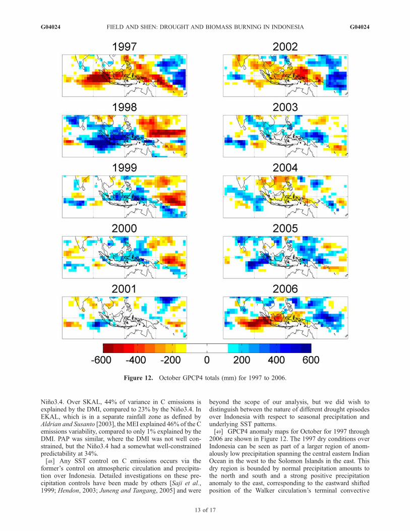
beyond the scope of our analysis, but we did wish todistinguish between the nature of different drought episodesover Indonesia with respect to seasonal precipitation andunderlying SST patterns.[49] GPCP4 anomaly maps for October for 1997 through

2006 are shown in Figure 12. The 1997 dry conditions overIndonesia can be seen as part of a larger region of anom-alously low precipitation spanning the central eastern IndianOcean in the west to the Solomon Islands in the east. Thisdry region is bounded by normal precipitation amounts tothe north and south and a strong positive precipitationanomaly to the east, corresponding to the eastward shiftedposition of the Walker circulation’s terminal convective

Figure 12. October GPCP4 totals (mm) for 1997 to 2006.


13 of 17

G04024

branch. The 1997 event illustrates the sharp distinctionbetween normal and anomalously low regions of precipita-tion: the pronounced drought conditions seen over Sumatraand Kalimantan were absent over the Java Sea, the island ofJava, southern Sulawesi and the Lesser Sunda Islandsstretching to East Timor.[50] In 1998, conditions over Indonesia had reversed,

with a wet precipitation anomaly over Indonesia of roughlythe same absolute magnitude as the dry anomaly in 1997.Weaker positive precipitation anomalies persisted over theregion in 1999 and 2000, with near-neutral conditions in2001. During the moderate El Nino conditions of 2002,there was a moderate dry anomaly over Indonesia whichwas most pronounced to the north of Papua, and appearingonly weakly over Sumatra and Kalimantan. The less severeburning during 2002 was therefore due to relocation of thedrought center, rather than by the actual absence of severedrought.[51] Wet-neutral conditions occurred in 2003 and dry-

neutral conditions in 2004, the weaker anomaly cor-responding to relatively weak El Nino conditions, but alsoto the positioning of the main drought center over the South

China Sea rather than western Indonesia. 2005 saw wet-neutral conditions over central Indonesia, bounded by strongwet regions to the east and west. The pronounced dryanomaly of 2006 was closer in nature to that of 1997 butlimited in extent to Kalimantan, Sumatra and the IndianOcean between 75E and 100E and 0 to 15S. There istherefore considerable spatial variability of drought over inIndonesia, which further explains why subregional predic-tion of fire occurrence performed better than that across theentire EQSA region.[52] The stronger precipitation anomalies in 1997 and

2006 over SSUM and SKAL appear driven by the com-bined effects of SST anomalies in the Pacific and IndianOcean basins. Figure 13 shows global mean SST anomaliesbetween 1997 and 2006 for October, when the greatest dryGPCP4 anomalies would occur. The large 1997 El Ninoevent is seen clearly, with the strongest eastern Pacific warmSST anomaly seen during our analysis period. Similaranomalies but of weaker magnitude were also seen during2002 and to a lesser extent in 2006.[53] Common to both 1997 and 2006, but only weakly

present in 2002 and absent during all other years, is a

Figure 13. October SST anomalies (�C) over the Indian and tropical Pacific oceans from 1997 to 2006[Reynolds et al., 2002].


14 of 17

G04024

negative SST anomaly in the Indian Ocean off of the coastsof western Sumatra and the southern coast of Java, coupledwith above average SSTs in the western Indian Ocean,reflected by the elevated DMI values. Saji et al. [1999]proposed that this pattern induces anomalously low precip-itation in western Indonesia via the following mechanism.The cooler than normal SSTs weaken the southeasterlytrades in the southeastern Indian Ocean, shifting equatorialconvergence to the northwest of its normal position in theIndian Ocean. As a result, the equatorial westerlies in theIndian Ocean weaken, suppressing heat supply to andconvergence over western Indonesia, and ultimately, con-tributing to reduced precipitation. This was consistent withHendon’s [2003] analysis, which showed that precipitationover all of Indonesia was negatively correlated with SSTs inthe southeastern Indian Ocean.[54] This could explain why none of Indian or Pacific

Ocean based indices were individually able to explainbeyond 50% of C emissions variability; each of thedroughts occurred for different reasons. The severity andlarge spatial extent of the 1997 drought resulted fromweaker atmospheric flow from both the east from the PacificOcean and from the southwest from the Indian Ocean,resulting in weaker convergence over all of Indonesia.The 2002 drought, which was most severe in easternIndonesia, was the result of reduced flux from the PacificOcean, whereas the 2006 drought, most pronounced overwestern Indonesia, was the result of reduced flux from theIndian Ocean. The enhanced biomass burning in 2006 overIndonesia therefore seems less attributable to the moderateEl Nino, and more to the concurrent IOD event. Similarly,the significant drought and fire in 1994 [Nichol, 1997;Fujiwara et al., 1999; Yonemura et al., 2002; Field et al.,2004] occurred under El Nino conditions weaker than in2002, but under strongly positive DMI conditions [Saji etal., 1999]. Overall, the Indian Ocean SSTs appear to have acomparable, if not greater, effect on west Indonesiandrought than Pacific Ocean SSTs.

4.4. Future Drought Conditions

[55] In the absence of peatland restoration and manage-ment, any future rainfall decrease in Indonesia’s peatlandregions caused by climate change would increase firedanger and result in increased C emissions. The most acuterisks are posed by an increase in the frequency at which theseasonal precipitation thresholds estimated here, and hencepeat moisture levels, are crossed. This could be caused byan increase in higher frequency of El Nino or Indian OceanDipole events, or a decrease in normal condition dry seasonprecipitation toward below threshold values.[56] Climate change projections of precipitation over

Indonesia remain inconclusive, but allow for the possibilityof a decrease in certain regions. The IPCC AR4 projectionsof precipitation changes over Indonesia showed little agree-ment between models in the sign of any change, but thiswas an examination only DJF and JJA precipitation, where-as the most critical changes in Indonesia involve a pro-longed dry season through the SON period. Li et al. [2007]considered rainfall over western Indonesia during the morerelevant JAS period under the IPCC SRES A1B anthropo-genic emissions scenario. Rainfall was seen to decrease for7 of the 11 models considered, particularly south of the

equator, which they translated into an increase in water tabledepth and increased evaporative fraction (ratio of latent heatflux to net evaporation). Such a change in mean state ofIndonesia’s peatland hydrology would increase the suscep-tibility to deep peat fires and further C emissions.[57] As shown in Figure 12, the 1997 and 2006 droughts

were most pronounced over the Indian Ocean to the west ofSumatra and not over the Indonesian islands. We wouldargue that any persistent eastward shift in this droughtcenter, which seems most closely related to IOD events,represents the greatest possible increase in Indonesian firedanger.

5. Summary and Conclusions

[58] We have shown that a large portion of the emissionsfrom biomass burning in Indonesia are controlled bydrought, which is best characterized by simple rainfall totalsas opposed to more complicated soil moisture models orSST indices. It should come as no surprise that firesusceptibility in Indonesia is better explained by regionalprecipitation than by SST or pressure-based climate indices.This analysis has helped to quantify the extent to which thisis the case, and will hopefully lead to better operational firemanagement planning to reduce future emissions episodes.Indeed, the effectiveness of SST indices in predicting fireoccurrence is limited by the strength of their control onregional precipitation, which in turn is the physical under-lying trigger for the burning through its control of ground-water levels in Indonesia’s peatlands.[59] None of the SST-based indices considered here can

individually explain drought occurrence over Indonesia,which can vary spatially and result from anomalies in eitheror both of the Pacific or Indian Ocean basins. Cautionshould therefore be exercised when attributing Indonesianfire and drought events to a single cause such as El Nino.Other historical studies [Kita et al., 2000;Wang et al., 2004]attributing fire episodes strictly to El Nino conditionsappear to have oversimplified controlling factors on fireoccurrence; it would be worthwhile revisiting these anal-yses to determine the relative contributions of SST vari-ability in the Pacific and Indian oceans to drought and fireover Indonesia.[60] Significant improvements were gained in predicting

fire occurrence by considering rainfall within a specificregion, compared to precipitation across all of Indonesia.Precipitation and drought are too spatially variable overIndonesia to be meaningfully quantified by a single droughtindicator. For southern Sumatra and southern Kalimantan,region-specific analysis allowed for the estimation of pre-cipitation thresholds suitable for distinguishing betweenperiods of low and high fire danger. A piecewise regressionmodel provided a means of estimating this threshold objec-tively, and nonparametric bootstrapping was useful inproviding confidence limits for predictability and thresholdestimates. The piecewise model also allowed us to avoid thevariance-inflating properties of a log linear model and theunclear physical interpretation of log-transformed C emis-sions. Precipitation estimates derived from remote sensingproducts appear to have an advantage over strictly gauge-based products in characterizing the threshold-driven nature


15 of 17

G04024

of the fire response to drought, particularly in southernKalimantan.[61] The daily drought indices considered by Sudiana et

al. [2003], Field et al. [2004], and Dymond et al. [2005] areappropriate, with local calibration, for operational firedanger monitoring. The monthly precipitation totals con-sidered here can complement those indices, and providemore readily interpretable guidelines against which tointerpret seasonal rainfall outlooks provided from statisticalor ensembles of numerical weather prediction model inte-grations, such as those described by van Oldenborgh et al.[2005]. Such thresholds can also serve as benchmarkagainst which to assess possible future reductions in rainfallduring the dry season over Sumatra and Kalimantan under achanging climate.[62] This analysis was based on 10 years worth of data,

with only a few periods of severe biomass burning. As inthe work by Fuller and Murphy [2006] and van der Werf etal. [2008], this made the robustness of our estimatesdifficult to assess, and resulted in wide confidence intervalsfor most R2 values under the piecewise model. Every effortshould be made to extend the fire occurrence record back intime, perhaps by incorporating AVHRR data, followingSudiana et al. [2003]. In the future, we hope to extend thistype of analysis to the 1970s using observations of visiblerange at airports, which were used as a haze indicator byWang et al. [2004] over Sumatra from 1973 to 2003. Thestart of this period coincided with that of Indonesia’s officialtransmigration policies and increased development in thefire prone areas of Sumatra and Kalimantan [Fearnside,1997], and could help to separate the influence of naturalinterannual rainfall variability from anthropogenic landcover disturbance, and to further constrain estimates ofpredictability and drought thresholds. Further to this, thethreshold-driven nature of severe burning needs to beconsidered in the context of possible positive feedbacksbetween deforestation, precipitation and fire [Siegert et al.,2001; Cochrane, 2003; Hoffmann et al., 2003], and betweenblack carbon emissions, increases in atmospheric stabilityand reduced precipitation [Koren et al., 2004; Liu, 2005].

[63] Acknowledgments. We thank Christine Lee, Ray Nassar, andtwo anonymous reviewers for valuable comments and Guido van der Werf,Mingyue Chen, and Yun Fan for assistance with the data sets. R.D.F. wassupported by a grant from the Southeast Asia Regional Committee forSTART and a graduate scholarship from the Natural Sciences and Engi-neering Research Council of Canada.

ReferencesAdler, R. F., et al. (2003), The Version-2 Global Precipitation Clima-tology Project (GPCP) monthly precipitation analysis (1979–Present),J. Hydrometeorol., 4(6), 1147–1167, doi:10.1175/1525-7541(2003)004<1147:TVGPCP>2.0.CO;2.

Aldrian, E., and R. D. Susanto (2003), Identification of three dominantrainfall regions within Indonesia and their relationship to sea surfacetemperature, Int. J. Climatol., 23(12), 1435–1452, doi:10.1002/joc.950.

Chen, M. Y., P. P. Xie, J. E. Janowiak, and P. A. Arkin (2002), Global landprecipitation: A 50-yr monthly analysis based on gauge observations,J. Hydrometeorol., 3(3), 249–266, doi:10.1175/1525-7541(2002)003<0249:GLPAYM>2.0.CO;2.

Cochrane, M. A. (2003), Fire science for rainforests, Nature, 421(6926),913–919, doi:10.1038/nature01437.

Dai, A., K. E. Trenberth, and T. Qian (2004), A global data set of PalmerDrought Severity Index for 1870–2002: Relationship with soil moistureand effects of surface warming, J. Hydrometeorol., 5, 1117–1130,doi:10.1175/JHM-386.1.

de Groot, W. J., Wardati, and Y. H. Wang (2005), Calibrating the fine fuelmoisture code for grass ignition potential in Sumatra, Indonesia, Int. J.Wildland Fire, 14(2), 161–168, doi:10.1071/WF04054.

Dennis, R. A., et al. (2005), Tomich, fire, people and pixels: Linking socialscience and remote sensing to understand underlying causes and impactsof fires in Indonesia, Human Ecol., 33(4), 465 –504, doi:10.1007/s10745-005-5156-z.

Dolling, K., P. S. Chu, and F. Fujioka (2005), A climatological study of theKeetch/Byram Drought Index and fire activity in the Hawaiian islands,Agric. For. Meteorol., 133(1 – 4), 17 – 27, doi:10.1016/j.agrformet.2005.07.016.

Duncan, B. N., R. V. Martin, A. C. Staudt, R. Yevich, and J. A. Logan(2003), Inter-annual and seasonal variability of biomass burning emis-sions constrained by satellite observations, J. Geophys. Res., 108(D2),4100, doi:10.1029/2002JD002378.

Dymond, C. C., R. D. Field, O. Roswintiarti, and Guswanto (2005), Usingsatellite fire detection to calibrate components of the Fire Weather Indexsystem in Malaysia and Indonesia, Environmental Management, 35(4),426–440, doi:10.1007/s00267-003-0241-9.

Efron, B., and R. J. Tibshirani (1993), An Introduction to the Bootstrap, 436pp., Chapman and Hall, Boca Raton, Fla.

Fan, Y., and H. van den Dool (2004), Climate Prediction Center globalmonthly soil moisture data set at 0.5� resolution for 1948 to present,J. Geophys. Res., 109, D10102, doi:10.1029/2003JD004345.

Fearnside, P. M. (1997), Transmigration in Indonesia: Lessons from itsenvironmental and social impacts, Environ. Manage. N. Y., 21(4),553–570, doi:10.1007/s002679900049.

Field, R. D., Y. Wang, O. Roswintiarti, and Guswanto (2004), A drought-based predictor of recent haze events in western Indonesia, Atmos.Environ., 38(13), 1869–1878, doi:10.1016/j.atmosenv.2004.01.011.

Frandsen, W. H. (1997), Ignition probability of organic soils, Can. J. For.Res., 27(9), 1471–1477, doi:10.1139/cjfr-27-9-1471.

Fujiwara, M., K. Kita, S. Kawakami, T. Ogawa, N. Komala, S. Saraspriya,and A. Suripto (1999), Tropospheric ozone enhancements during theIndonesian forest fire events in 1994 and in 1997 as revealed byground-based observations, Geophys. Res. Lett., 26(16), 2417–2420,doi:10.1029/1999GL900117.

Fuller, D. O., and K. Murphy (2006), The ENSO-fire dynamic in insularSoutheast Asia, Clim. Change, 74(4), 435–455, doi:10.1007/s10584-006-0432-5.

Gedalof, Z., D. L. Peterson, and N. J. Mantua (2005), Atmospheric,climatic and ecological controls on extreme wildfire years in thenorthwestern United States, Ecol. Appl., 15(1), 154–174, doi:10.1890/03-5116.

Gutman, G., I. Csiszar, and P. Romanov (2000), Using NOAA/AVHRRproducts to monitor El Nino impacts: Focus on Indonesia in 1997–98,Bull. Am. Meteorol. Soc., 81(6), 1189 – 1205, doi:10.1175/1520-0477(2000)081<1189:UNPTME>2.3.CO;2.

Heil, A., and J. G. Goldammer (2001), Smoke-haze pollution: A review ofthe 1997 episode in Southeast Asia, Reg. Environ. Change, 2, 24–37,doi:10.1007/s101130100021.

Hendon, H. H. (2003), Indonesian rainfall variability: Impacts of ENSO andlocal air-sea interaction, J. Clim., 16(11), 1775–1790, doi:10.1175/1520-0442(2003)016<1775:IRVIOE>2.0.CO;2.

Herman, J. R., P. K. Bhartia, O. Torres, C. Hsu, C. Seftor, and E. Celarier(1997), Global distribution of UV-absorbing aerosols from Nimbus 7/TOMS data, J. Geophys. Res., 102(D14), 16,911–16,922, doi:10.1029/96JD03680.

Hessl, A. E., D. McKenzie, and R. Schellhaas (2004), Drought and PacificDecadal Oscillation linked to fire occurrence in the inland Pacific North-west, Ecol. Appl., 14(2), 425–442, doi:10.1890/03-5019.

Hoffmann, W. A., W. Schroeder, and R. B. Jackson (2003), Regional feed-backs among fire, climate, and tropical deforestation, J. Geophys. Res.,108(D23), 4721, doi:10.1029/2003JD003494.

Jauhiainen, J., H. Takahashi, J. E. P. Heikkinen, P. J. Martikainen, and H.Vasander (2005), Carbon fluxes from a tropical peat swamp forest floor,Global Change Biol., 11(10), 1788–1797, doi:10.1111/j.1365-2486.2005.001031.x.

Juneng, L., and F. T. Tangang (2005), Evolution of ENSO-related rainfallanomalies in Southeast Asia region and its relationship with atmosphere-ocean variations in Indo-Pacific sector, Clim. Dyn., 25(4), 337–350,doi:10.1007/s00382-005-0031-6.

Kalnay, E., et al. (1996), The NCEP/NCAR 40-Year Reanalysis Project,Bull. Am. Meteorol. Soc., 77(3), 437 – 471, doi:10.1175/1520-0477(1996)077<0437:TNYRP>2.0.CO;2.

Kita, K., M. Fujiwara, and S. Kawakami (2000), Total ozone increaseassociated with forest fires over the Indonesian region and its relation tothe El Nino–Southern Oscillation, Atmos. Environ., 34(17), 2681–2690,doi:10.1016/S1352-2310(99)00522-1.


16 of 17

G04024

Koren, I., Y. J. Kaufman, L. A. Remer, and J. V. Martins (2004), Measure-ment of the effect of Amazon smoke on inhibition of cloud formation,Science, 303(5662), 1342–1345, doi:10.1126/science.1089424.

Kunii, O., S. Kanagawa, I. Yajima, Y. Hisamatsu, S. Yamamura, T. Amagai,and I. T. S. Ismail (2002), The 1997 haze disaster in Indonesia: Its airquality and health effects, Arch. Environ. Health, 57(1), 16–22.

Langenfelds, R. L., R. J. Francey, B. C. Pak, L. P. Steele, J. Lloyd, C. M.Trudinger, and C. E. Allison (2002), Interannual growth rate variations ofatmospheric CO2 and its d13C, H2, CH4, and CO between 1992 and 1999linked to biomass burning, Global Biogeochem. Cycles, 16(3), 1048,doi:10.1029/2001GB001466.

Langner, A., J. Miettinen, and F. Siegert (2007), Land cover change2002–2005 in Borneo and the role of fire derived from MODISimagery, Global Change Biol., 13, 2329–2340, doi:10.1111/j.1365-2486.2007.01442.x.

Levine, J. S. (1999), The 1997 fires in Kalimantan and Sumatra, Indonesia:Gaseous and particulate emissions, Geophys. Res. Lett., 26(7), 815–818,doi:10.1029/1999GL900067.

Li, W., R. E. Dickinson, R. Fu, G.-Y. Niu, Z.-L. Yang, and J. G. Canadell(2007), Future precipitation changes and their implications for tropicalpeatlands, Geophys. Res. Lett., 34, L01403, doi:10.1029/2006GL028364.

Liu, Y. Q. (2005), Atmospheric response and feedback to radiative forcingfrom biomass burning in tropical South America, Agric. For. Meteorol.,133(1–4), 40–53, doi:10.1016/j.agrformet.2005.03.011.

Logan, J. A., I. Megretskaia, R. Nassar, L. T. Murray, L. Zhang, K. W.Bowman, H. M. Worden, and M. Luo (2008), Effects of the 2006 El Ninoon tropospheric composition as revealed by data from the TroposphericEmission Spectrometer (TES), Geophys. Res. Lett., 35, L03816,doi:10.1029/2007GL031698.

Lohman, D. J., D. Bickford, and N. S. Sodhi (2007), The burning issue,Science, 316(5823), 376, doi:10.1126/science.1140278.

Nichol, J. (1997), Bioclimatic impacts of the 1994 smoke haze event inSoutheast Asia, Atmos. Environ., 31(8), 1209–1219, doi:10.1016/S1352-2310(96)00260-9.

Ntale, H. K., and T. Y. Gan (2003), Drought indices and their application toEast Africa, Int. J. Climatol., 23(11), 1335–1357, doi:10.1002/joc.931.

Page, S. E., F. Siegert, J. O. Rieley, H. D. V. Boehm, A. Jaya, and S. Limin(2002), The amount of carbon released from peat and forest firesin Indonesia during 1997, Nature, 420(6911), 61–65, doi:10.1038/nature01131.

Podgorny, I. A., F. Li, and V. Ramanathan (2003), Large aerosol radiativeforcing due to the 1997 Indonesian forest fire, Geophys. Res. Lett., 30(1),1028, doi:10.1029/2002GL015979.

Reynolds, R. W., N. A. Rayner, T. M. Smith, D. C. Stokes, and W. Q.Wang (2002), An improved in-situ and satellite SST analysis for climate,J. Clim., 15(13), 1609 – 1625, doi:10.1175/1520-0442(2002)015<1609:AIISAS>2.0.CO;2.

Saji, N. H., B. N. Goswami, P. N. Vinayachandran, and T. Yamagata(1999), A dipole mode in the tropical Indian Ocean, Nature,401(6751), 360–363.

Sastry, N. (2002), Forest fires, air pollution, and mortality in SoutheastAsia, Demography, 39(1), 1–23, doi:10.1353/dem.2002.0009.

Siegert, F., and A. A. Hoffmann (2000), The 1998 forest fires in EastKalimantan (Indonesia): A quantitative evaluation using high resolution,multitemporal ERS-2 SAR images and NOAA-AVHRR hotspot data,Remote Sens. Environ., 72(1), 64 – 77, doi:10.1016/S0034-4257(99)00092-9.

Siegert, F., G. Ruecker, A. Hinrichs, and A. A. Hoffmann (2001), Increaseddamage from fires in logged forests during droughts caused by El Nino,Nature, 414(6862), 437–440, doi:10.1038/35106547.

Stolle, F., and E. F. Lambin (2003), Interprovincial and inter-annual differ-ences in the causes of land-use fires in Sumatra, Indonesia, Environ.Conserv., 30(4), 375–387, doi:10.1017/S0376892903000390.

Sudiana, D., H. Kuze, N. Takeuchiu, and R. E. Burgan (2003), Assessingforest fire potential in Kalimantan Island, Indonesia, using satellite andsurface weather data, Int. J. Wildland Fire, 12(2), 175–184, doi:10.1071/WF02035.

Thompson, A. M., J. C. Witte, R. D. Hudson, H. Guo, J. R. Herman, andM. Fujiwara (2001), Tropical tropospheric ozone and biomass burning,Science, 291(5511), 2128–2132, doi:10.1126/science.291.5511.2128.

Toms, J. D., and M. L. Lesperance (2003), Piecewise regression: A tool foridentifying ecological thresholds, Ecology, 84(8), 2034 – 2041,doi:10.1890/02-0472.

Turetsky, M. R., B. D. Amiro, E. Bosch, and J. S. Bhatti (2004), Historicalburn area in western Canadian peatlands and its relationship to fire weatherindices, Global Biogeochem. Cycles, 18, GB4014, doi:10.1029/2004GB002222.

Usup, A., Y. Hashimoto, H. Takahashi, and H. Hayasaka (2004), Combus-tion and thermal characteristics of peat fire in tropical peatland in centralKalimantan, Indonesia, Tropics, 14(1), 1–19, doi:10.3759/tropics.14.1.

van der Werf, G. R., J. T. Randerson, L. Giglio, G. J. Collatz, P. S.Kasibhatla, and A. F. Arellano (2006), Inter-annual variability in globalbiomass burning emissions from 1997 to 2004, Atmos. Chem. Phys., 6,3423–3441.

van der Werf, G. R., J. T. Randerson, L. Giglio, N. Gobron, and A. J.Dolman (2008), Climate controls on the variability of fires in the tropicsand subtropics, Global Biogeochem. Cycles, 22, GB3028, doi:10.1029/2007GB003122.

van Oldenborgh, G. J., M. A. Balmaseda, L. Ferranti, T. N. Stockdale, andD. L. T. Anderson (2005), Did the ECMWF seasonal forecast modeloutperform statistical ENSO forecast models over the last 15 years?,J. Clim., 18(16), 3240–3249, doi:10.1175/JCLI3420.1.

Wang, Y., R. D. Field, and O. Roswintiarti (2004), Trends in atmospherichaze induced by peat fires in Sumatra Island, Indonesia and El Ninophenomenon from 1973 to 2003, Geophys. Res. Lett., 31, L04103,doi:10.1029/2003GL018853.

Westerling, A. L., A. Gershunov, D. R. Cayan, and T. P. Barnett (2002),Long lead statistical forecasts of area burned in western US Wildfires byecosystem province, Int. J. Wildland Fire, 11(4), 257–266, doi:10.1071/WF02009.

Wolter, K., and M. S. Timlin (1993), Monitoring ENSO in COADS with aseasonally adjusted principal component index, Rep. NOAA/N MC/CAC,NSSL, Oklahoma Clim. Surv., CIMMS and the Sch. of Meteorol., Univ.of Okla., Norman.

Yonemura, S., H. Tsuruta, S. Kawashima, S. Sudo, L. C. Peng, L. S. Fook,Z. Johar, and M. Hayashi (2002), Tropospheric ozone climatology overPeninsular Malaysia from 1992 to 1999, J. Geophys. Res., 107(D15),4229, doi:10.1029/2001JD000993.

Zeng, N., A. Mariotti, and P. Wetzel (2005), Terrestrial mechanisms ofinterannual CO2 variability, Global Biogeochem. Cycles, 19, GB1016,doi:10.1029/2004GB002273.

��R. D. Field, Department of Physics, University of Toronto, 60 St. George

Street, Toronto, ON M5S 1A7, Canada. ([email protected])S. S. P. Shen, Department of Mathematics and Statistics, San Diego State

University, San Diego, CA 92182, USA.


17 of 17

G04024

Predictability of carbon emissions from biomass burning in Indonesia from 1997 to 2006

Documents

Transcript of Predictability of carbon emissions from biomass burning in Indonesia from 1997 to 2006