Practical Recommendations for Evaluation and Mitigation of ...

Practical Recommendations for Evaluation and Mitigation of Soil

Liquefaction in Arkansas

Principal Investigator and Graduate Student:

Dr. Brady R. Cox

Shawn C. Griffiths

Project Number: MBTC 3017

Date: February 2010

ACKNOWLEDGEMENT This material is based upon work supported by the U.S. Department of Transportation under Grant Award Number DTRT07-G-0021. The work was conducted through the Mack-Blackwell Rural Transportation Center at the University of Arkansas. DISCLAIMER The contents of this report reflect the views of the authors, who are responsible for the facts and the accuracy of the information presented herein. This document is disseminated under the sponsorship of the Department of Transportation, University Transportation Centers Program, in the interest of information exchange. The U.S. Government assumes no liability for the contents or use thereof.

II

Table of Contents

Chapter 1 ....................................................................................................................... - 1 -

Introduction ................................................................................................................. - 1 -

1.1 Motivation for Research .................................................................................... - 1 -

1.2 Problem Statement............................................................................................. - 2 -

1.3 Analysis of Site Specific Data ........................................................................... - 3 -

1.4 Thesis Overview ................................................................................................ - 4 -

Chapter 2 ....................................................................................................................... - 5 -

Review of Relevant Literature .................................................................................... - 5 -

2.1 New Madrid Seismic Zone (NMSZ) ................................................................. - 5 -

2.2 Simplified Procedure for Evaluating Liquefaction Triggering ......................... - 6 -

2.3 The Cyclic Stress Ratio (CSR) .......................................................................... - 9 -

2.3.1 Stress Reduction Coefficient, rd .................................................................. - 9 -

2.4 The Cyclic Resistance Ratio (CRR) ................................................................ - 15 -

2.4.1 Standardized Overburden Blow Count Correction Factor (CN) ............... - 21 -

2.4.2 Overburden Correction Factor (Kσ) ......................................................... - 25 -

2.4.3 Magnitude Scaling Factor (MSF) ............................................................. - 30 -

2.5 Fine-Grain Screening Criteria ......................................................................... - 32 -

2.6 Summary.......................................................................................................... - 35 -

III

Chapter 3 ..................................................................................................................... - 37 -

Liquefaction Triggering Workbook User’s Guide .................................................... - 37 -

3.1 Introduction ..................................................................................................... - 37 -

3.2 Workbook Overview ....................................................................................... - 38 -

3.3 Youd et al. (2001) Workbook .......................................................................... - 40 -

3.3.1 Input Data ................................................................................................. - 41 -

3.3.1.1 Design Peak Ground Acceleration and Moment Magnitude ............. - 43 -

3.3.1.2 Boring Elevation versus Grade Elevation .......................................... - 47 -

3.3.1.3 Sampler Type and Borehole Diameter Correction Factors ................ - 48 -

3.3.1.4 Depth-dependent Input Data .............................................................. - 49 -

3.3.2 Calculations and Calculation Tables Worksheets ..................................... - 51 -

3.3.2.1 Depth-dependent Calculations ........................................................... - 53 -

3.3.2.2 Calculation Tables .............................................................................. - 61 -

3.3.3 Output and References Worksheets .......................................................... - 62 -

3.4 Cetin et al. (2004) Workbook .......................................................................... - 64 -

3.4.1 Input Data Worksheet ............................................................................... - 66 -

3.4.2 Calculation and Calculation Tables .......................................................... - 66 -


3.4.3 Output and References Worksheets .......................................................... - 71 -

3.5 Idriss and Boulanger (2008) ............................................................................ - 72 -

IV

3.5.1 Input Data Worksheet ............................................................................... - 73 -

3.5.2 Calculations and Calculation Table Worksheets ...................................... - 73 -


3.5.3 SPT Su Correlation Worksheet ................................................................. - 77 -

3.5.4 Output and Reference Worksheets ........................................................... - 79 -

3.6 Conclusions ..................................................................................................... - 79 -

Chapter 4 ..................................................................................................................... - 81 -

Site-Specific Comparisons ........................................................................................ - 81 -

4.1 Introduction ..................................................................................................... - 81 -

4.2 Site-Specific Comparisons .............................................................................. - 81 -

4.2.1 Site No. 1 .................................................................................................. - 83 -

4.2.2 Site No. 2 .................................................................................................. - 92 -

4.2.3 Site No. 3 ................................................................................................ - 100 -

4.3 Conclusions ................................................................................................... - 109 -

Chapter 5 ................................................................................................................... - 112 -

Residual Strength of Liquefied Soils ...................................................................... - 112 -

5.1 Introduction ................................................................................................... - 112 -

5.2 Review of Past Sr Correlations ...................................................................... - 112 -

5.2.1 Seed and Harder (1990) .......................................................................... - 113 -

5.2.2 Olsen and Stark (2002) ........................................................................... - 115 -

V

5.2.3 Idriss and Boulanger (2008) ................................................................... - 117 -

5.3 Comparison of Direct Strength and Strength Ratio Relationships ................ - 119 -

5.4 Site-Specific Comparison of direct Strength and Strength Ratio

Relationships ........................................................................................... - 122 -

5.5 Conclusions and Recommendations .............................................................. - 124 -

Chapter 6 ................................................................................................................... - 126 -

Potential Liquefaction Mitigation Techniques ........................................................ - 126 -

6.1 Introduction ................................................................................................... - 126 -

6.2 Soil Liquefaction Mitigation Techniques ...................................................... - 126 -

6.2.1 Vibratory Methods .................................................................................. - 127 -

6.2.1.1 Sand Compaction Piles ..................................................................... - 128 -

6.2.1.2 Stone Columns ................................................................................. - 128 -

6.2.1.3 Vibro-Concrete Columns ................................................................. - 130 -

6.2.2 Deep Dynamic Compaction .................................................................... - 130 -

6.2.3 Compaction Grouting ............................................................................. - 132 -

6.2.4 Permeation Grouting ............................................................................... - 132 -

6.2.5 Jet Grouting ............................................................................................. - 134 -

6.2.6 Deep Soil Mixing .................................................................................... - 135 -

6.2.7 Deep Blasting .......................................................................................... - 137 -

6.2.8 Earthquake Drains ................................................................................... - 138 -

VI

6.2.9 Dewatering Techniques .......................................................................... - 138 -

6.2.10 Removal and Replacement ................................................................... - 139 -

6.3 Cost Comparison ........................................................................................... - 140 -

6.4 Summary and Conclusions ............................................................................ - 142 -

Chapter 7 ................................................................................................................... - 143 -

Conclusions and Recommendations ........................................................................ - 143 -

7.1 Conclusions ................................................................................................... - 143 -

7.1.1 SPT-based Liquefaction Triggering Procedures .................................... - 144 -

7.1.2 Residual Shear Strength .......................................................................... - 146 -

7.1.3 Ground Improvement Techniques .......................................................... - 147 -

7.2 Future Work ................................................................................................... - 148 -

VII

List of Tables

Table 2.1. Susceptibility of fine-grained soil to liquefaction triggering after Bray and

Sancio (2006) .............................................................................................. - 34 -

Table 3.1. Site Class definitions reproduced from AASHTO 2009 ............................. - 44 -

Table 4.1. Comparison of blow count correction factors for Site No. 2, at a depth of 8 m

(25 ft) .......................................................................................................... - 97 -

Table 4.2. Comparison of blow count correction factors for Site No. 3 at a depth of 20 m

(65 ft) ........................................................................................................ - 104 -

Table 5.1. Values of Δ(N1)60-Sr recommended by Seed (1987) .................................. - 115 -

Table 5.2. Sr estimates obtained from direct Sr and Sr/σ’v relationships using

hypothetical blow counts and effective confining stresses ....................... - 122 -

Table 5.3. Site-specific information used to estimate Sr ............................................ - 123 -

Table 5.4. Sr estimates obtained from direct Sr and Sr/σ’v relationships using site-

specific information. ................................................................................. - 123 -

Table 6.1. Liquefaction mitigation techniques discussed in this report ...................... - 127 -

Table 6.2. Cost estimates of liquefaction mitigation techniques (after Hayward Baker Inc.

2003) ......................................................................................................... - 141 -

VIII

List of Figures

Figure 1.1. Map of the locations of the soil borings provided from AHTD (map generated

with Google maps). ....................................................................................... - 4 -

Figure 2.1. SPT CRR curves for magnitude 7.5 earthquake (modified from Seed et al

1985, obtained from Youd et al. 2001). ........................................................ - 7 -

Figure 2.2. Stress reduction coefficient (rd) as proposed by Seed and Idriss (1971). ... - 11 -

Figure 2.3. The rd relationship adopted by Youd et al. (2001) with approximate average

values from Equation 2.3. ........................................................................... - 11 -

Figure 2.4. Comparison of three stress reduction coefficient (rd) relationships as a

function of depth and approximate vertical effective stress. ...................... - 14 -

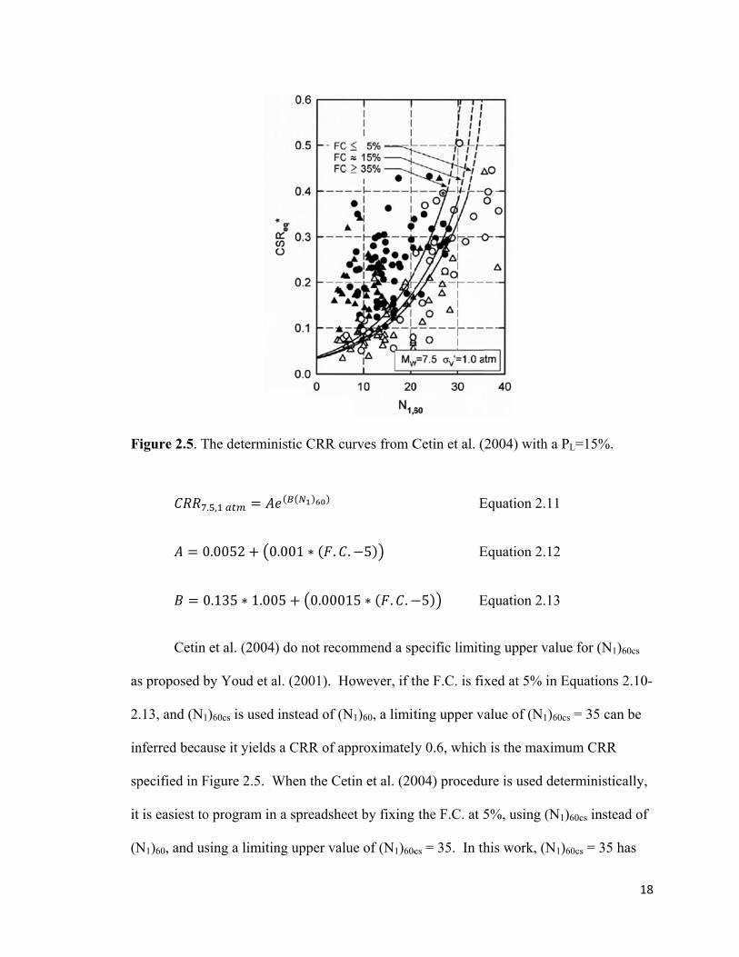
Figure 2.5. The deterministic CRR curves from Cetin et al. (2004) with a PL=15%. .. - 18 -

Figure 2.6. The CRR relationship proposed by Idriss and Boulanger (2008). ............. - 20 -

Figure 2.7. Comparison of the three CRR7.5,1 atm curves for clean sand. ...................... - 20 -

Figure 2.8. Comparison of three CN correlations as a function of vertical effective stress

and approximate depth. ............................................................................... - 24 -

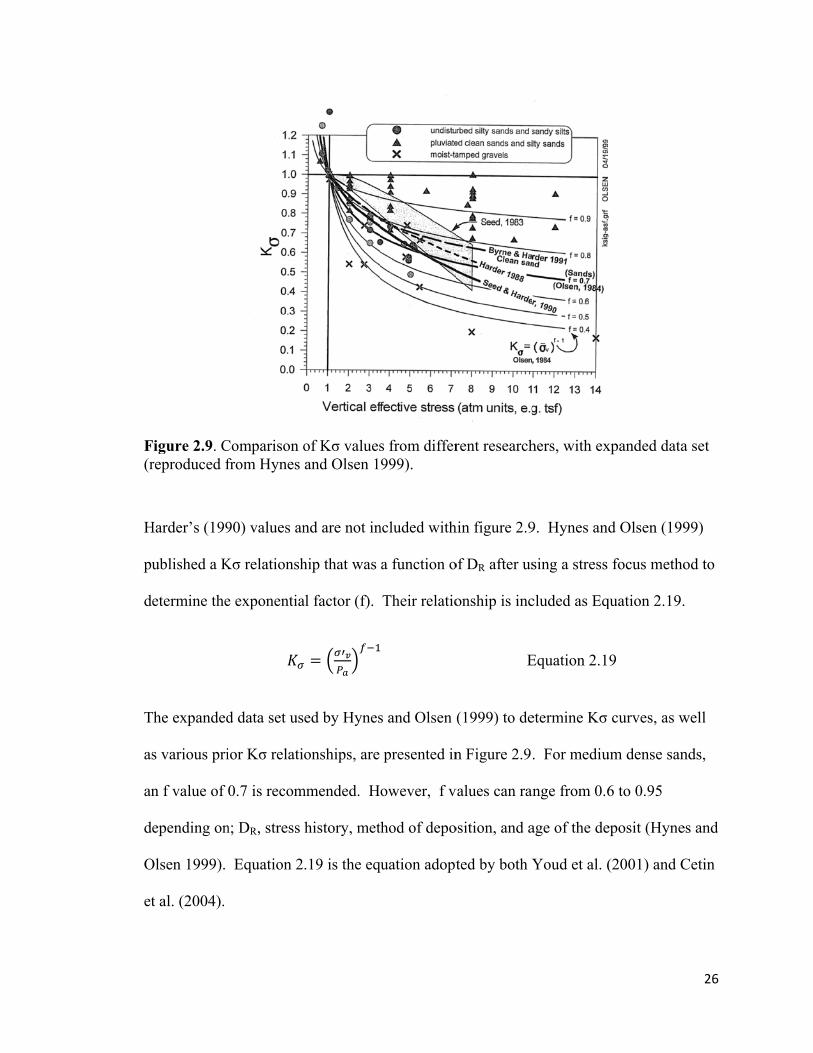
Figure 2.9. Comparison of Kσ values from different researchers, with expanded data set

(reproduced from Hynes and Olsen 1999). ................................................. - 26 -

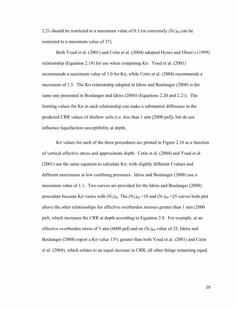
Figure 2.10. Comparison of all three Kσ correction factors as a function of vertical

effective stress and approximate depth. ...................................................... - 29 -

IX

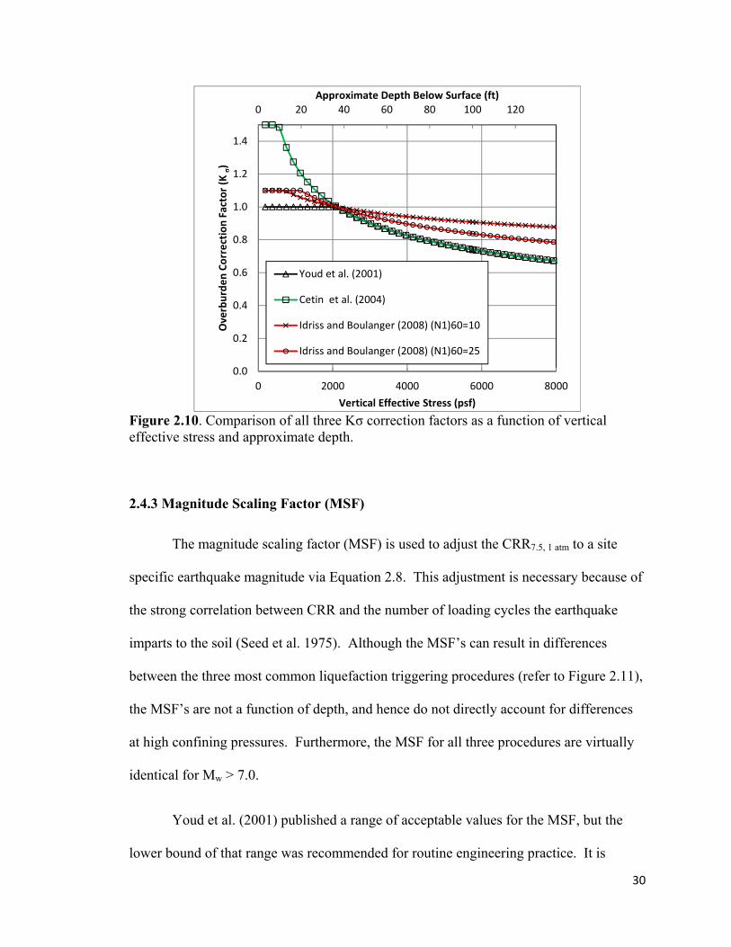
Figure 2.11. Magnitude scaling factors (MSF) of the three most commonly used

procedures. .................................................................................................. - 31 -

Figure 2.12. Graphical representation of fine-grained liquefaction susceptibility criteria

(reproduced from Bray and Sancio 2006) ................................................... - 34 -

Figure 3.1. Individual worksheet tabs within the liquefaction triggering workbooks. . - 39 -

Figure 3.2. Excel Options menu with guidance for enabling iterative calculations. .... - 40 -

Figure 3.3. Input Data worksheet with job identification information and site specific

input options................................................................................................ - 42 -

Figure 3.4. Seismic Design Parameters Version 2.10 from the USGS, included with

AASHTO (2009). ........................................................................................ - 46 -

Figure 3.5. 2008 Interactive Deaggregation (Beta) website, available from the

USGS. ......................................................................................................... - 46 -

Figure 3.6. Headings for columns A-J in the Input Data worksheet. ............................ - 50 -

Figure 3.7. Calculations worksheet, job identification and site classification. ............. - 52 -

Figure 3.8. Headings for columns K-R in the Calculations worksheet. ....................... - 54 -

Figure 3.9. Headings for columns S-Z in the Calculations worksheet. ........................ - 56 -

Figure 3.10. Headings for columns AA-AF in the Calculations worksheet. ................ - 58 -

Figure 3.11. Headings for columns AG-AL in the Calculations worksheet. ................ - 59 -

X

Figure 3.12. Output Boring El. liquefaction triggering summary information and column

headings. ..................................................................................................... - 63 -

Figure 3.13. F.S. plot included within the Output Graphs workbook. .......................... - 64 -

Figure 3.14. Clean sand base curve included within Output Graphs worksheet. ......... - 64 -

Figure 3.15. Fine grained screening criteria plot included within the Output Graphs

worksheet. ................................................................................................... -65 -

Figure 3.16. Headings for columns AB-AG in the Calculations worksheet. ................ - 68 -

Figure 3.17. Headings in columns AR and AS in the Calculations worksheet. ........... - 71 -

Figure 3.18. Plot of the clean sand corrected curve included in the Output Graphs

worksheet. ................................................................................................... - 72 -

Figure 3.19. SPT blow count, Su correlations plot in the SPT Su Correlations

worksheet. ................................................................................................... - 78 -

Figure 3.20. Clean sand curve recommended by Idriss and Boulanger (2008) shown with

data generated in the Calculations worksheet. ............................................ - 80 -

Figure 4.1. Locations of the soil borings that have been chosen for site specific

comparisons (image from Google Earth, © 2010 Google). ........................ - 82 -

Figure 4.2. Comparison of the factor of safety against liquefaction triggering at Site No.1

for all three simplified procedures. ............................................................. - 84 -

XI

Figure 4.3. Comparison of the rd values at Site No. 1 for all three simplified

procedures. .................................................................................................. - 84 -

Figure 4.4. Comparison of the CRRM=7.5, 1 atm values at Site No. 1 for all three simplified

procedures. .................................................................................................. - 86 -

Figure 4.5.Comparison of the CN values at Site No. 1 for all three simplified

procedures. .................................................................................................. - 87 -

Figure 4.6. Comparison of the (N1)60cs values at Site No. 1 for all three simplified

procedures. .................................................................................................. - 88 -


procedures. .................................................................................................. - 90 -

Figure 4.8. Comparison of the Kσ values at Site No. 1 for all three simplified

procedures. .................................................................................................. - 90 -

Figure 4.9. Comparison of the factor of safety against liquefaction triggering at Site No.2

for all three simplified procedures. ............................................................. - 93 -

Figure 4.10. Comparison of rd at Site No.2 for all three simplified procedures. .......... - 94 -


procedures. .................................................................................................. - 95 -

Figure 4.12. Comparison of the CN values at Site No. 2 for all three simplified

procedures. .................................................................................................. - 95 -

XII


procedures. .................................................................................................. - 97 -


procedures. .................................................................................................. - 98 -


procedures. ................................................................................................ - 100 -

Figure 4.16. Comparison of the factor of safety against liquefaction triggering at Site

No.3 for all three simplified procedures. .................................................. - 102 -

Figure 4.17. Comparison of the rd values at Site No. 3 for all three simplified

procedures. ................................................................................................ - 102 -

Figure 4.18. Comparison of the CSRM=7.5, 1 atm values at Site No. 3 for all three simplified

procedures. ................................................................................................ - 103 -

Figure 4.19. Comparison of the CN values at Site No. 3 for all three simplified

procedures. ................................................................................................ - 104 -


procedures. ................................................................................................ - 104 -


procedures. ................................................................................................ - 106 -


procedures. ............................................................................................... - 4.22 -

XIII

Figure 5.1. Relationship between Sr and (N1)60cs-Sr proposed by Seed and Harder

(1990). ....................................................................................................... - 114 -

Figure 5.2. Residual shear strength ratio (Sr/σ’v) correlation proposed by Olsen and Stark

(2002). ....................................................................................................... - 116 -

Figure 5.3. Relationship between Sr and (N1)60cs-Sr proposed by Idriss and Boulanger

(2008) ........................................................................................................ - 118 -

Figure 5.4. Residual shear strength ratio (Sr/σ’v) correlation proposed by Idriss and

Boulanger (2008). ..................................................................................... - 118 -

Figure 5.5. Comparison of Sr as a function of (N1)60cs-Sr ............................................ - 120 -

Figure 5.6. Sr/σ’v correlations as a function of (N1)60cs-Sr or (N1)60. .......................... - 120 -

Figure 6.1. Illustration of the Sand Compaction Pile construction process (Hayward

Baker Inc. 2010b)...................................................................................... - 129 -

Figure 6.2. Illustration of the Stone Column construction process (Hayward Baker Inc.

2010b). ...................................................................................................... - 129 -

Figure 6.3. Illustration of Vibro-Concrete Column construction process. (Hayward Baker

Inc. 2010b). ............................................................................................... - 131 -

Figure 6.4. Illustration of Deep Dynamic Compaction (Hayward Baker Inc. 2010b).- 131 -

Figure 6.5. Illustration of compaction grouting technique (Hayward Baker Inc.

2010b). ...................................................................................................... - 133 -

XIV

Figure 6.6. Common Permeation Grouting applications (Hayward Baker Inc.

2003). ........................................................................................................ - 134 -

Figure 6.7. Illustration of Jet Grouting construction process using triple fluid system

(Hayward Baker Inc. 2010b). .................................................................... - 135 -

Figure 6.8. Illustration of Deep Soil Mixing construction process (Hayward Baker, Inc.

2010b). ...................................................................................................... - 136 -

Figure 6.9. Patterns for Deep Soil Mixing (Porbaha et al. 1999). .............................. - 137 -

Figure 6.10. Illustration of Earthquake Drain installation using a vibrating mandrel (HB

Wick Drains 2009). ................................................................................... - 139 -

1

Chapter 1

Introduction

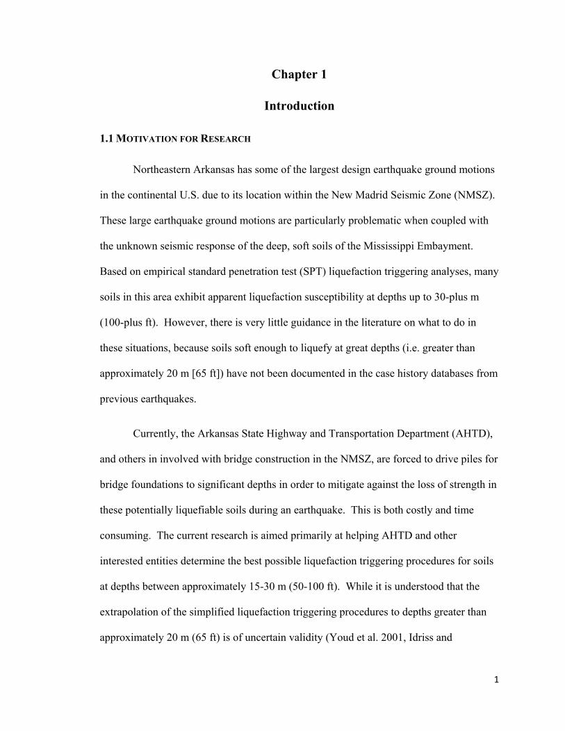
1.1 MOTIVATION FOR RESEARCH

Northeastern Arkansas has some of the largest design earthquake ground motions

in the continental U.S. due to its location within the New Madrid Seismic Zone (NMSZ).

These large earthquake ground motions are particularly problematic when coupled with

the unknown seismic response of the deep, soft soils of the Mississippi Embayment.

Based on empirical standard penetration test (SPT) liquefaction triggering analyses, many

soils in this area exhibit apparent liquefaction susceptibility at depths up to 30-plus m

(100-plus ft). However, there is very little guidance in the literature on what to do in

these situations, because soils soft enough to liquefy at great depths (i.e. greater than

approximately 20 m [65 ft]) have not been documented in the case history databases from

previous earthquakes.

Currently, the Arkansas State Highway and Transportation Department (AHTD),

and others in involved with bridge construction in the NMSZ, are forced to drive piles for

bridge foundations to significant depths in order to mitigate against the loss of strength in

these potentially liquefiable soils during an earthquake. This is both costly and time

consuming. The current research is aimed primarily at helping AHTD and other

interested entities determine the best possible liquefaction triggering procedures for soils

at depths between approximately 15-30 m (50-100 ft). While it is understood that the

extrapolation of the simplified liquefaction triggering procedures to depths greater than

approximately 20 m (65 ft) is of uncertain validity (Youd et al. 2001, Idriss and

2

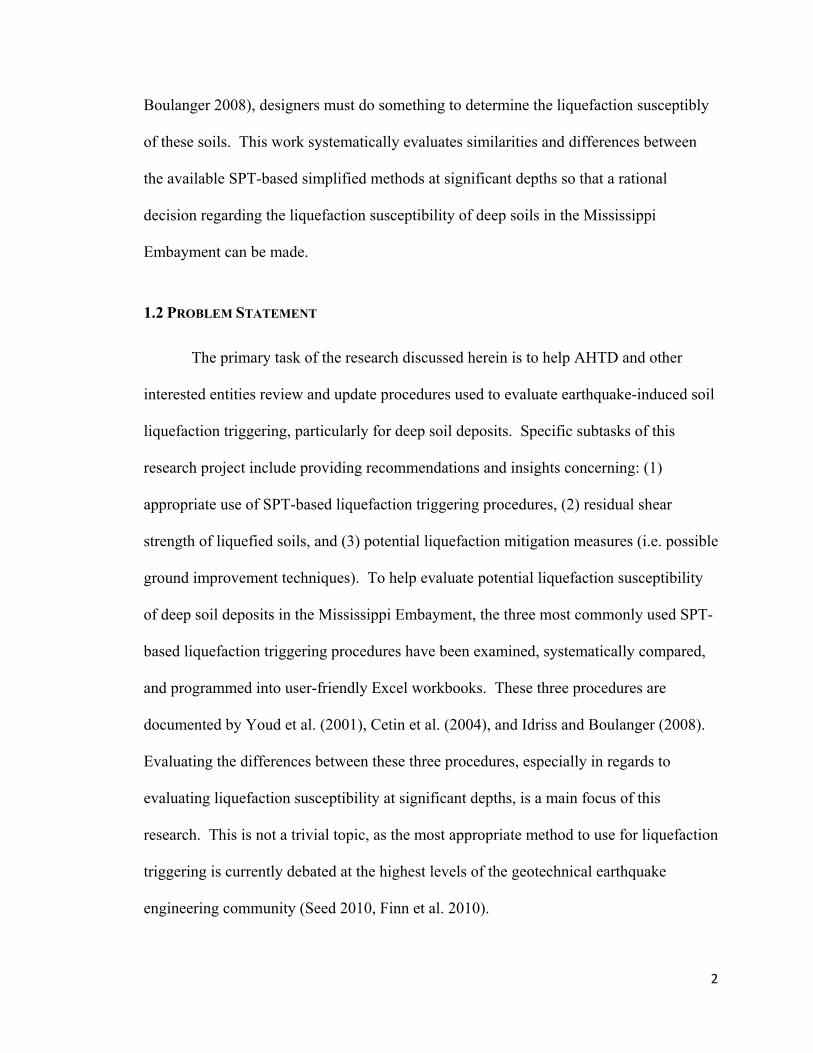
Boulanger 2008), designers must do something to determine the liquefaction susceptibly

of these soils. This work systematically evaluates similarities and differences between

the available SPT-based simplified methods at significant depths so that a rational

decision regarding the liquefaction susceptibility of deep soils in the Mississippi

Embayment can be made.

1.2 PROBLEM STATEMENT

The primary task of the research discussed herein is to help AHTD and other

interested entities review and update procedures used to evaluate earthquake-induced soil

liquefaction triggering, particularly for deep soil deposits. Specific subtasks of this

research project include providing recommendations and insights concerning: (1)

appropriate use of SPT-based liquefaction triggering procedures, (2) residual shear

strength of liquefied soils, and (3) potential liquefaction mitigation measures (i.e. possible

ground improvement techniques). To help evaluate potential liquefaction susceptibility

of deep soil deposits in the Mississippi Embayment, the three most commonly used SPT-

based liquefaction triggering procedures have been examined, systematically compared,

and programmed into user-friendly Excel workbooks. These three procedures are

documented by Youd et al. (2001), Cetin et al. (2004), and Idriss and Boulanger (2008).

Evaluating the differences between these three procedures, especially in regards to

evaluating liquefaction susceptibility at significant depths, is a main focus of this

research. This is not a trivial topic, as the most appropriate method to use for liquefaction

triggering is currently debated at the highest levels of the geotechnical earthquake

engineering community (Seed 2010, Finn et al. 2010).

3

1.3 ANALYSIS OF SITE SPECIFIC DATA

AHTD has provided a total of 19 boring logs from eight different bridge sites in

eastern Arkansas to use in trial liquefaction triggering analyses. The locations of these

bridge sites are shown relative to one another in Figure 1.1 and are grouped by AHTD

Job No. These borings have been analyzed for soil liquefaction potential using all three

of the newly-developed liquefaction triggering workbooks documented herein. Four of

the eight bridge sites are part of AHTD Job No. 001992 and contain a total of eight

boring logs. This job is located along U.S. highway 63 between Marked Tree and

Gilmore, Arkansas. Design peak ground accelerations (PGA) for these bridges are very

high, ranging from 0.82-1.03g. Nine of the boring logs come from three other bridge

sites classified as Job No.’s 110514, 110527, and 110524. These bridges are all near

Edmondson Arkansas, and have design PGA values of approximately 0.48g. The

remaining two boring logs are from Job No. 020417 near Lagrue, Arkansas. This bridge

has a design PGA value of 0.24g, the lowest of all sites considered. It will be noted that

only one example boring from each of these three groups is discussed in detail herein

(refer to Chapter 4). These example boring logs are discussed in great depth and were

chosen to illustrate similarities and differences between liquefaction triggering

procedures for typical conditions in eastern Arkansas. Although each of the subsurface

profiles differ slightly from one another, the soil is generally clay (CL, CH) from the

surface to a depth of 6-10 m (20-30 ft), underlain by sand (SW, SM) to depths between

30-36 m (100-120 ft).

Fg

1

in

re

tr

qu

C

in

ar

pr

st

C

th

Figure 1.1. Menerated wit

.4 THESIS O

This t

nformation a

elevant litera

riggering pro

uestions that

Chapter 4 sum

n eastern Ark

re compared

rocedures. C

trength of liq

Chapter 6 pre

he overall co

Map of the loth Google m

OVERVIEW

thesis is com

and an introd

ature, which

ocedures. Ch

t may arise w

mmarizes the

kansas. The

d in-depth to

Chapter 5 in

quefied soil,

esents potent

onclusions an

ocations of thmaps).

mposed of 7 c

duction to thi

includes per

hapter 3 is a

while implem

e liquefactio

e results obta

determine w

cludes a rev

and recomm

tial liquefact

nd recomme

he soil borin

chapters. Ch

is project. C

rtinent inform

a user’s guide

menting the

on triggering

ained from e

what factors

iew of curre

mendations f

tion mitigati

ndations fro

ngs provided

hapter 1 incl

Chapter 2 en

rmation rega

e which shou

liquefaction

g results from

ach of the th

most influen

ent literature

for estimatin

on technique

om this work

d from AHTD

ludes some g

ncompasses a

arding soil liq

uld serve to

n triggering w

m three differ

hree SPT-bas

nce the diffe

concerning

ng residual sh

es, and Chap

k.

D (map

general

a review of

quefaction

clarify any

workbooks.

rent bridge s

sed procedur

erences betw

residual she

hear strength

pter 7 presen

4

sites

res

ween

ear

h.

nts

5

Chapter 2

Review of Relevant Literature

2.1 NEW MADRID SEISMIC ZONE (NMSZ)

Fuller (1912) coupled personal journals and geologic evidence to describe the

events of the earthquakes that occurred within the NMSZ in the year 1811-1812. A brief

account of these events is provided below.

On the night of December 16 in the year 1811 around 2:00 A.M. an earthquake

shook the small town of New Madrid, Missouri on the banks of the Mississippi River.

This initial shock was followed by two others before morning. Although the main shocks

subsided for a time, tremors frequented the area until January 23, 1812 when another

shock equal to the first was felt. This second shock was followed by two weeks of quiet,

then, on February 7, 1812 the largest and final shock hit the area. This event was so

powerful that it caused minor structural damage as far away as St. Louis, Missouri and

Cincinnati, Ohio (Tuttle et al. 2002) people nearly 1000 miles away reported ground

shaking (Fuller 1912).

This nearly three month period of tremors and earthquakes was not recorded by

any instrumentation. As such, journal accounts and recent mapping of the geologic

features left by the earthquake events have been used to infer earthquake magnitude,

recurrence interval, and ultimately seismic ground motion hazard maps like those found

in the International Building Code (IBC 2009) and the American Association of State

Highway and Transportation Officials Seismic Bridge Design Guidelines (AASHTO

2009). Recent geodetic measurements estimate the three earthquake moment magnitudes

6

(Mw) of the 1811-1812 events to be around Mw 7-8 (Tuttle et al. 2002). Furthermore,

geologic evidence indicates that the NMSZ has produced at least three large earthquake

events in the past 1000 years, suggesting a return period of around 500 yrs +/- 300 yrs

(Tuttle et al. 2002). These earthquake events have produced large sand blows up to 10 m

(30 ft) wide and hundreds of meters long that range from 0.15 to 1.5 m (0.5 to 5 ft) thick.

Because prior liquefaction is a good indication of a soils susceptibility to liquefaction

during subsequent earthquakes (Idriss and Boulanger 2008), it is expected that the sandy

soils in the Mississippi Embayment are still susceptible to liquefaction. However, the

maximum depth to which the liquefaction occurred in the 1811-1812 earthquakes is

unknown, and current research on deep liquefaction is still evolving.

2.2 SIMPLIFIED PROCEDURE FOR EVALUATING LIQUEFACTION TRIGGERING

The ‘simplified procedure’ for evaluating soil liquefaction triggering was so

named because of a simplified approach to computing the stress induced on the soil from

earthquake forces (Seed and Idriss 1971). This dynamic stress imparted by the

earthquake is termed the cyclic stress ratio (CSR). Conversely, the dynamic stress the

soil can withstand before liquefying is often termed the cyclic resistance ratio (CRR).

The CRR of the in-situ soil is primarily based on empirical correlations to the Standard

Penetration Test (SPT), Cone Penetration Test (CPT) or shear wave velocity (Vs)

measurements (Youd et al. 2001). These empirical correlations have been developed

from case history data-bases of liquefied and non-liquefied soils documented in previous

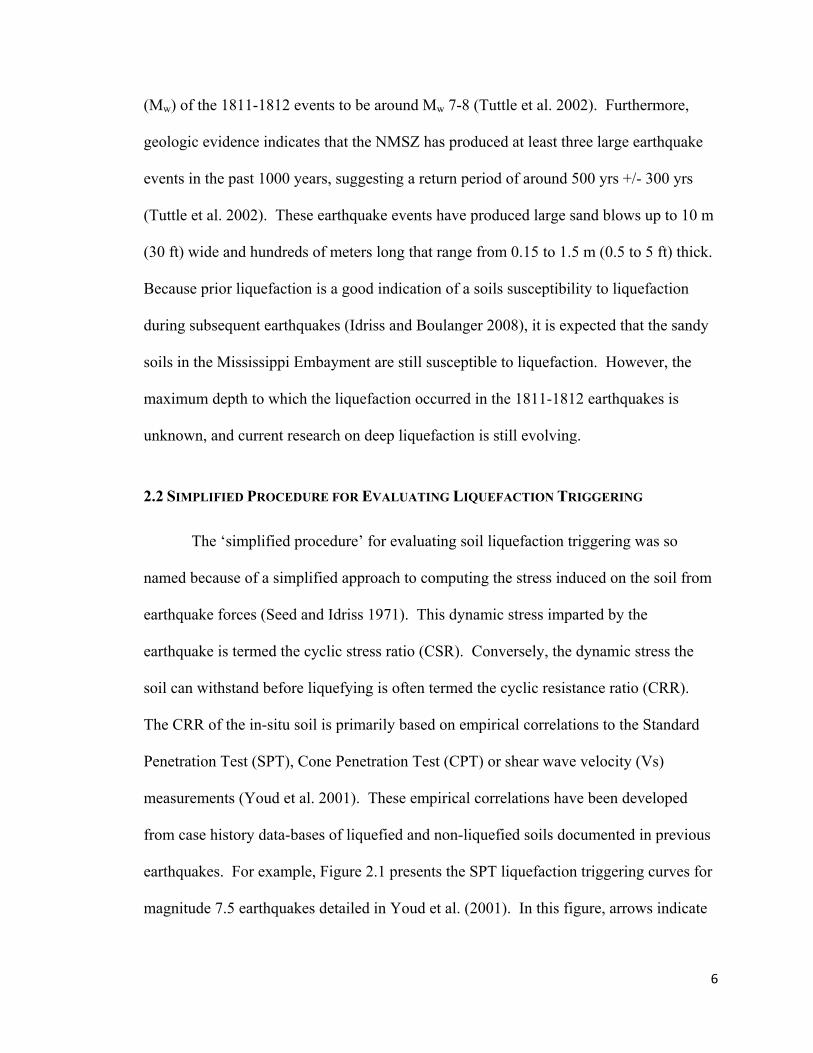
earthquakes. For example, Figure 2.1 presents the SPT liquefaction triggering curves for

magnitude 7.5 earthquakes detailed in Youd et al. (2001). In this figure, arrows indicate

F1

h

co

b

ac

fi

o

co

d

Figure 2.1. S985, obtaine

ow the chart

ount [(N1)60]

e more resis

ccordingly th

ines content

f 35%. The

ontents of 5%

etermined, th

SPT CRR cured from You

t would be u

] of approxim

tant to lique

he CRR curv

increases, w

CRR values

%, 15%, and

he CSR indu

rves for magud et al. 2001

used to determ

mately 20. S

faction trigg

ves for fines

with the maxi

s for (N1)60 =

d 35%, respe

uced by the e

gnitude 7.5 e1).

mine the CR

Sands with h

gering than c

s contents gr

imum permi

= 20 are appr

ectively. On

earthquake c

earthquake (m

RR of the soi

higher fines c

clean sands (

reater than 5%

issible shift o

roximately 0

nce the CRR

can be comp

modified fro

il from a cor

contents hav

(Seed et al. 1

% shift up an

occurring fo

0.22, 0.30, an

of the soil h

puted as outli

om Seed et a

rrected blow

ve been show

1985),

nd to the lef

or a fines con

nd 0.41 for f

has been

ined in Secti

7

al

wn to

ft as

ntent

fines

ion

8

2.3, both of these factors are necessary to determine if the soil is potentially susceptible to

liquefaction.

To compute the factor of safety (F.S.) against liquefaction triggering, the stress

the soil can withstand without liquefying (i.e. the CRR) is divided by the stress induced

by the earthquake (i.e. the CSR), according to Equation 2.1.

. . Equation 2.1

Hypothetically, a F.S. less than 1.0 suggests that the soil is susceptible to initiation of

liquefaction, whereas a F.S. greater than 1.0 suggests that the soil is not susceptible to

liquefaction. However, in reality, it is well understood that this boundary is not a distinct

line and that engineering judgment needs to be applied to evaluate the liquefaction

susceptibility of soils with a F.S. near unity. Furthermore, there are several possible

procedures that may be employed for each in-situ test method (i.e. SPT, CPT, Vs) and the

F.S. obtained from each of the procedures are not equivalent for the same input data.

Therefore, caution must be exercised when establishing a F.S. and it is advisable to check

the results from more than one procedure.

The following sections examine the primary reasons for variations in the F.S.

predicted by different liquefaction triggering procedures. The discussion is focused on

SPT-based procedures, as these are the oldest and most commonly used, and the only

procedures currently employed by the Arkansas State Highway and Transportation

Department (AHTD), whom this research is aimed at helping. Specifically, the three

most commonly used SPT-based procedures of Youd et al. (2001), Cetin et al. (2004),

and Idriss and Boulanger (2008) are discussed in detail.

9

2.3 THE CYCLIC STRESS RATIO (CSR)

The simplified procedure was developed by Seed and Idriss (1971) as an easy

approach to estimate earthquake-induced stresses without the need for a site response

analysis, and has been the primary method used to determine the CSR for the past 40

years. The simplified CSR is calculated as follows:

CSR 0.65 r Equation 2.2

where amax is the peak horizontal ground surface acceleration modified for site specific

soil conditions, g is the acceleration due to gravity, σv is the total overburden stress, σ’v is

the initial effective overburden stress, and rd is a stress reduction coefficient which takes

into account the flexibility of the soil column. All simplified liquefaction evaluation

procedures use this common equation to determine the CSR. However, the various

procedures often use different relationships to determine the coefficient rd. As such,

differences in the CSR calculations between various simplified methods are primarily a

direct result of the uncertainty in determining rd.

2.3.1 Stress Reduction Coefficient, rd

The basis of the simplified CSR equation is Newton’s second law of motion (i.e.

force is equal to mass times acceleration), which assumes rigid body motion. In reality,

the soil column is not a rigid body and behaves in a very non-linear fashion, therefore

Seed and Idriss (1971) introduced rd to account for the fact that the soil column is a

deformable body. This relationship was only presented graphically in 1971 (refer to

10

Figure 2.2) and was plotted as a range of possible values that increased with depth (i.e.

notice the hatched area suggesting the variability and uncertainty of rd with depth).

Subsequently, many researchers have attempted to quantify rd in various manners

(i.e. Ishihara 1977, Iwasaki et al. 1978, Imai et al. 1981, Golesorkhi, 1989, Idriss 1999

and Seed et al. 2001). They have found that rd is a complex parameter that depends on a

combination of factors including site stiffness, input motion frequency content, absolute

depth, relative layer thicknesses, earthquake magnitude and other criteria. Because of

this complexity, consensus on the best approach to quantify rd in a simplified manner has

not been reached. Therefore, each procedure recommends a different rd correlation.

Regardless of which rd correlation is “most correct”, rd curves cannot be “mixed and

matched”; each correlation should only be used within its recommended procedure (Idriss

and Boulanger 2008, Seed 2010).

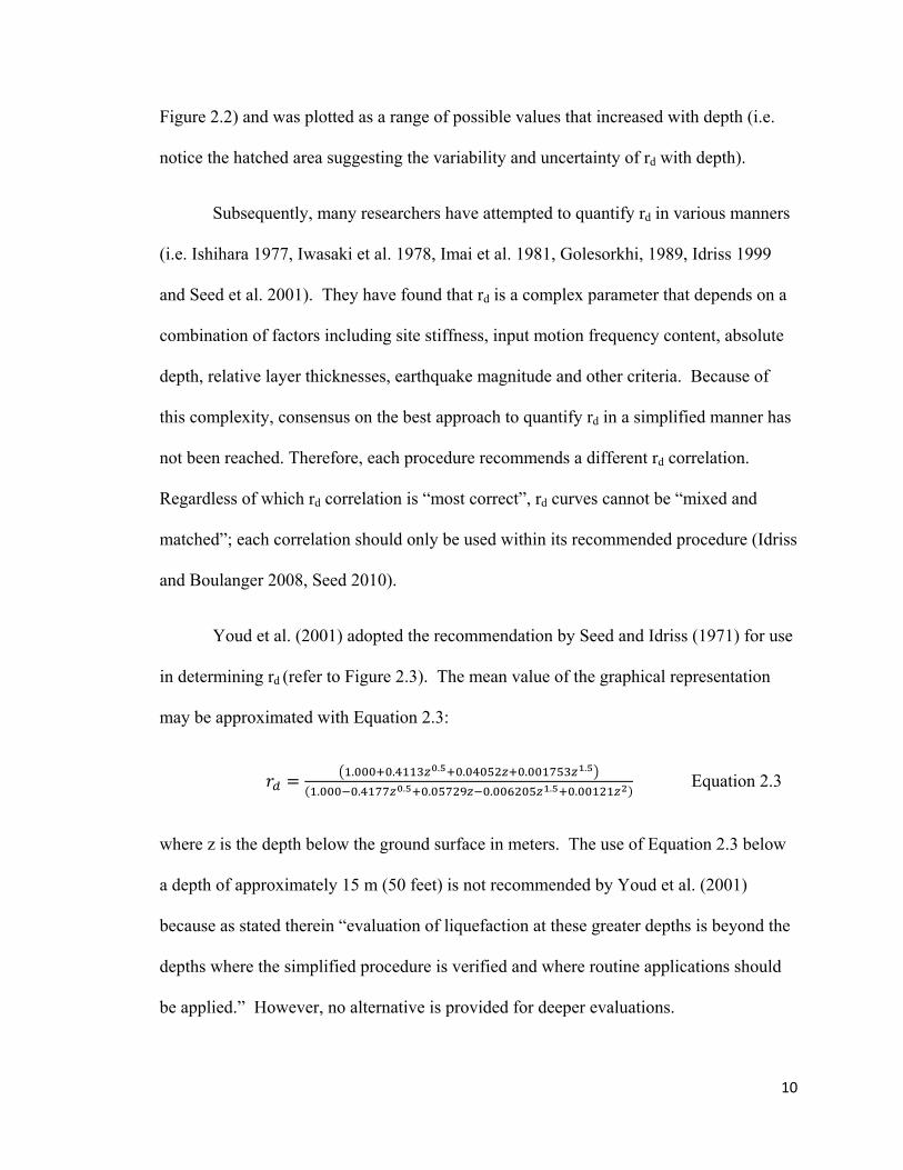
Youd et al. (2001) adopted the recommendation by Seed and Idriss (1971) for use

in determining rd (refer to Figure 2.3). The mean value of the graphical representation

may be approximated with Equation 2.3:

. . . . . .

. . . . . . . Equation 2.3

where z is the depth below the ground surface in meters. The use of Equation 2.3 below

a depth of approximately 15 m (50 feet) is not recommended by Youd et al. (2001)

because as stated therein “evaluation of liquefaction at these greater depths is beyond the

depths where the simplified procedure is verified and where routine applications should

be applied.” However, no alternative is provided for deeper evaluations.

F

Fv

Figure 2.2. S

Figure 2.3. Talues from E

Stress reducti

The rd relatioEquation 2.3

ion coefficie

nship adopte.

ent (rd) as pro

ed by Youd

oposed by S

et al. (2001)

Seed and Idri

) with appro

iss (1971).

ximate avera

11

age

12

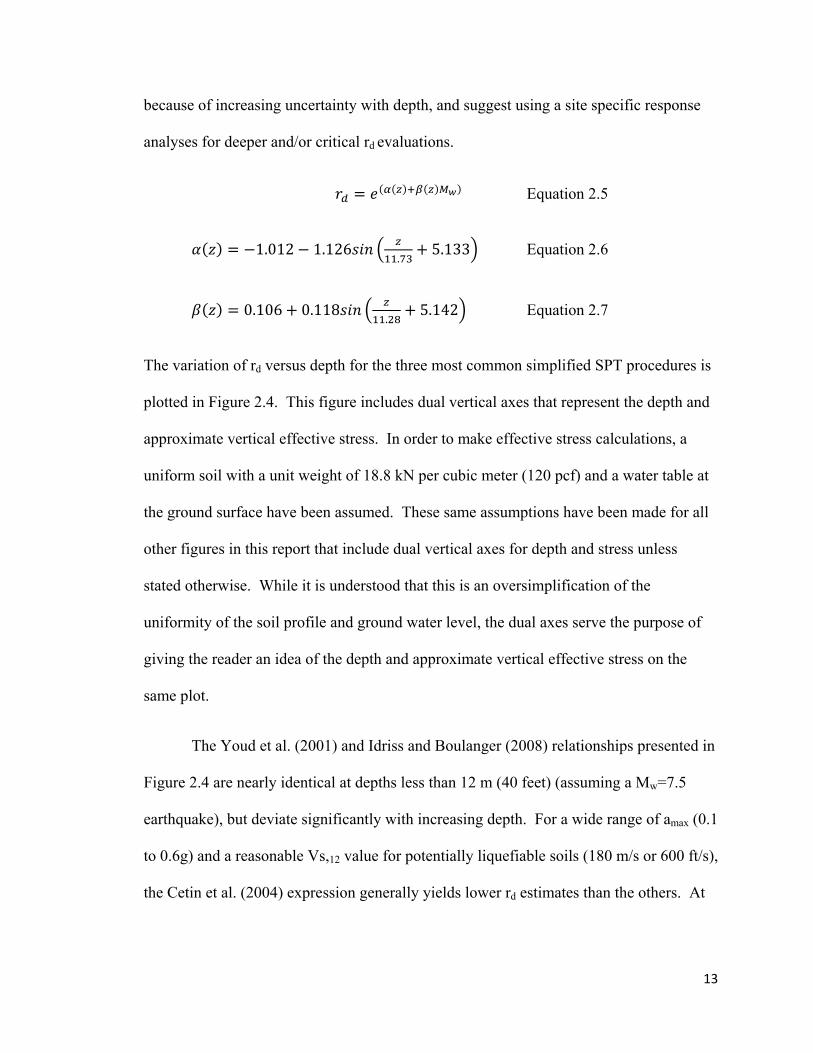
Cetin et al. (2004) investigated rd using a total of 2,153 site response analyses

performed with the program SHAKE91. These response analyses were separated into

bins according to the input parameters of moment magnitude (Mw), amax, and average site

stiffness over the top 12 m (40 feet) of soil, evaluated via shear wave velocity (Vs,12).

Mean estimates of rd with standard deviations were fit using a Bayesian regression

approach. The rd expression fit by Cetin et al. (2004) is provided in Equation 2.4 (the

standard deviation term has not been included here for brevity). It is a function of four

variables (z, Mw, amax, and Vs,12) and must be used with appropriate units (i.e. z in

meters and Vs,12 in meters per second). This equation is only applicable to depths of less

than 20 m (65 feet). A slightly modified equation found in Cetin et al. (2004) can be used

for depths greater than 20 m (65 feet). Rather than recommending a depth where this

equation is no longer valid the standard deviation term (not shown here) quantifies the

uncertainty, which increases with depth to around 12 m (40 feet) and then remains nearly

constant for all depths.

, , , V ,

. . ∗ . ∗ . ∗ ,

. . ∗ . . ∗ , .

. . ∗ . ∗ . ∗ ,

. . ∗ . . ∗ , .

Equation 2.4

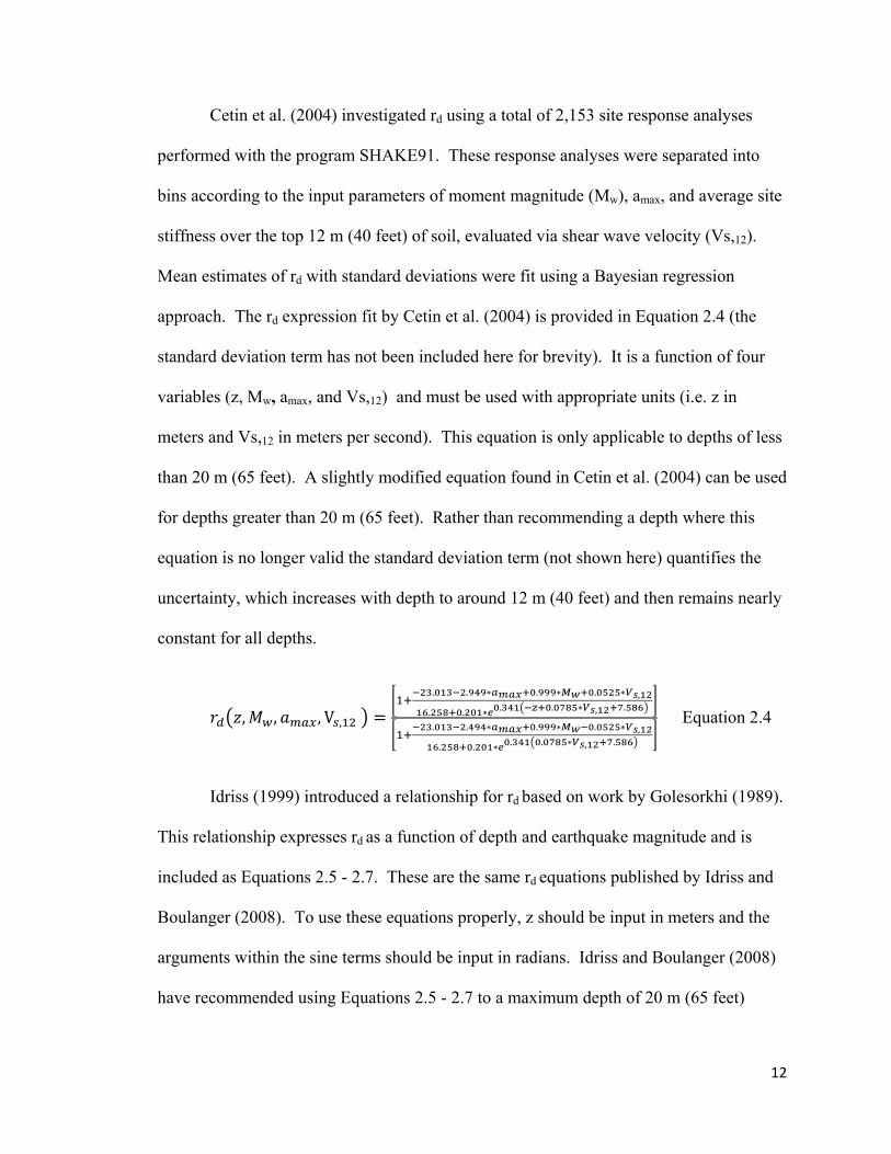
Idriss (1999) introduced a relationship for rd based on work by Golesorkhi (1989).

This relationship expresses rd as a function of depth and earthquake magnitude and is

included as Equations 2.5 - 2.7. These are the same rd equations published by Idriss and

Boulanger (2008). To use these equations properly, z should be input in meters and the

arguments within the sine terms should be input in radians. Idriss and Boulanger (2008)

have recommended using Equations 2.5 - 2.7 to a maximum depth of 20 m (65 feet)

13

because of increasing uncertainty with depth, and suggest using a site specific response

analyses for deeper and/or critical rd evaluations.

Equation 2.5

1.012 1.126.

5.133 Equation 2.6

0.106 0.118.

5.142 Equation 2.7

The variation of rd versus depth for the three most common simplified SPT procedures is

plotted in Figure 2.4. This figure includes dual vertical axes that represent the depth and

approximate vertical effective stress. In order to make effective stress calculations, a

uniform soil with a unit weight of 18.8 kN per cubic meter (120 pcf) and a water table at

the ground surface have been assumed. These same assumptions have been made for all

other figures in this report that include dual vertical axes for depth and stress unless

stated otherwise. While it is understood that this is an oversimplification of the

uniformity of the soil profile and ground water level, the dual axes serve the purpose of

giving the reader an idea of the depth and approximate vertical effective stress on the

same plot.

The Youd et al. (2001) and Idriss and Boulanger (2008) relationships presented in

Figure 2.4 are nearly identical at depths less than 12 m (40 feet) (assuming a Mw=7.5

earthquake), but deviate significantly with increasing depth. For a wide range of amax (0.1

to 0.6g) and a reasonable Vs,12 value for potentially liquefiable soils (180 m/s or 600 ft/s),

the Cetin et al. (2004) expression generally yields lower rd estimates than the others. At

14

Figure 2.4. Comparison of three stress reduction coefficient (rd) relationships as a function of depth and approximate vertical effective stress.

depths greater than 15 m (50 feet), all of the procedures vary significantly from one

another, reflecting the increased uncertainty in rd estimates at depth. The rd values near

15 m (50 feet) vary by approximately 39%, at 24 m (80 feet) they vary by approximately

32%, and at 30 m (100 feet) they vary by approximately 28%. These variations in rd lead

to equal variations in CSR, all other things being equal. According to Equation 2.1,

lower CSR estimates should yield higher F.S. values against liquefaction (i.e. based on

CSR alone, one would expect the F.S. of Youd et al. [2001] and Cetin et al. [2004] to be

greater than the F.S. of Idriss and Boulanger [2008]). However, this cannot be assumed

because the CRR also varies significantly between procedures.

0

1000

2000

3000

4000

5000

0

10

20

30

40

50

60

70

80

90

100

0.00 0.20 0.40 0.60 0.80 1.00

Approximate Vertical Effective Stress (psf)

Dep

th Below Surface (ft)

Stress Reduction Coefficient (rd)

Youd et al. (2001)

Cetin et al (2004) M=7.5,a=0.1, Vs40'=600 fpsCetin et al (2004) M=7.5,a=0.6, Vs40'=600 fpsIdriss and Boulanger(2008) M=7.5

15

2.4 THE CYCLIC RESISTANCE RATIO (CRR)

The CRR is the dynamic stress the soil can withstand before liquefying. SPT-

based liquefaction triggering procedures use blow count (N) as the basis of computing

CRR (refer to Figure 2.1). The SPT-based CRR relationships for Youd et al. (2001),

Cetin et al. (2004) and Idriss and Boulanger (2008) are presented below. In order to

compare these relationships in a meaningful manner, the CRR equations for each

procedure will be presented below as CRR7.5, 1 atm (i.e. the cyclic resistance ratio of the

soil adjusted to 1 atmosphere of effective overburden pressure for a Mw=7.5 earthquake).

This is necessary because the various relationships use different factors to account for

earthquake magnitude and overburden stresses. It is common for CRR relationships to be

normalized for this base case, and then site specific adjustments are made via magnitude

scaling factors (MSF) and overburden correction factors (Kσ) to account for the

earthquake magnitude under consideration and the overburden stresses at the depth of

interest. The site adjusted CRR is obtained from CRR7.5, 1 atm according to equation 2.8:

, . , Equation 2.8

where all variables are defined above. The MSF and Kσ relationships recommended in

each procedure will be compared after a discussion of the CRR7.5, 1 atm equations.

Youd et al. (2001) slightly modified the CRR curve of Seed et al. (1985). This

modification simply bounds the CRR clean sand curve at N-values less than 5 and is

included as a dashed line in Figure 2.1. The equation used to approximate the modified

curve is the presented as Equation 2.9:

16

. , ∗ Equation 2.9

where again CRR7.5,1 atm is the cyclic resistance ratio of the soil adjusted to 1.0

atmosphere of effective overburden pressure for a Mw=7.5 earthquake, and (N1)60cs is the

overburden and energy corrected blow count adjusted to a clean sand (cs) equivalent.

This equation should not be applied at corrected blow counts greater than 30 because as

Youd et al. (2001) states, “For (N1)60cs ≥ 30, clean granular soils are too dense to liquefy

and are classed non-liquefiable.”

Cetin et al. (2004) developed a probabilistic approach to evaluate soil liquefaction

triggering. Their probabilistic CRR relationship is presented in Equation 2.10:

. ,

∗ . ∗ . . . ∗ . ∗ . ∗ . . . . ∗

.

Equation 2.10

where once again CRR7.5,1 atm is the cyclic resistance ratio of the soil adjusted to 1.0

atmosphere of effective overburden pressure for a Mw=7.5 earthquake, (N1)60 is the

overburden and energy corrected blow count, F.C. is the fines content of the soil, Mw is

the earthquake magnitude under consideration (Mw = 7.5 for CRR7.5,1 atm), σ’v is the initial

effective overburden stress (σ’v = 1 atm for CRR7.5,1 atm), Pa is atmospheric pressure, ϕ-1

is the inverse of the cumulative normal distribution, and PL is the probability of

liquefaction. In order to use this relationship deterministically rather than

probabilistically, Cetin et al. (2004) recommends using Mw = 7.5, σ’v = 1 atm (2116 psf),

17

and PL = 15%, as indicated within Figure 2.5. When Cetin et al. (2004) developed the

probabilistic curves they were compared with the CRR curve developed by Seed et al.

(1985). An effort was made to determine a PL that would yield the two curves congruent,

unfortunately the methods differed so greatly that a range of possible probabilities from

10 - 40% was found acceptable. Cetin et al. (2004) chose a PL = 15% based on the range

above and: “Seed’s intent that the recommended (1985) boundary should represent

approximately a 10 - 15% probability of liquefaction” (Seed 2010).

Equation 2.10 is only valid for CRR’s less than 0.4. At higher CRR’s, the dashed

line portion of Figure 2.5 was sketched by hand and reflects what Cetin et al. (2004)

believe to be the best possible deterministic boundary given limited data. As no equation

exists to determine the CRR for values greater than 0.4, the deterministic procedure

presented in Cetin et al. (2004) is difficult to automate. Therefore, the author has taken

the liberty of fitting an equation to the dashed line portion of the curves shown in Figure

2.5. Equations 2.11 – 2.13 are shown below and are applicable to CRR values between

0.4-0.6. These equations are dependent on (N1)60 and fines content (F.C.), which are the

same dependent variables within Equation 2.10 once the proper constants (i.e. Mw = 7.5,

’v = 1 atm, and PL = 15%) are employed. At CRR values less than 0.4 Equation 2.10

should be used, while at CRR values greater than or equal to 0.4 Equations 2.11 – 2.13

should be employed. Note that the original deterministic CRR curves of Cetin et al.

(2004) only extend to a value of 0.6 (refer to Figure 2.5). While Equations 2.11 – 2.13

may be employed to extend these curves to CRR values greater than 0.6, these

extrapolations are of uncertain validity and are not recommended.

F

as

2

in

sp

it

(N

Figure 2.5. T

0

0

Cetin

s proposed b

.13, and (N1

nferred becau

pecified in F

t is easiest to

N1)60, and us

The determin

. ,

0.0052 0

0.135 ∗ 1.00

et al. (2004)

by Youd et a

)60cs is used

use it yields

Figure 2.5. W

o program in

sing a limitin

nistic CRR cu

.001 ∗ .

05 0.000

) do not reco

al. (2001). H

instead of (N

a CRR of ap

When the Ce

a spreadshe

ng upper val

urves from C

. 5

15 ∗ . .

ommend a sp

However, if t

N1)60, a limit

pproximately

etin et al. (20

eet by fixing

ue of (N1)60c

Cetin et al. (

E

E

5 E

pecific limiti

the F.C. is fix

ting upper v

y 0.6, which

004) procedu

the F.C. at 5

cs = 35. In th

(2004) with a

Equation 2.1

Equation 2.1

Equation 2.1

ing upper va

xed at 5% in

alue of (N1)6

h is the maxi

ure is used d

5%, using (N

his work, (N

a PL=15%.

1

2

3

alue for (N1)

n Equations

60cs = 35 can

imum CRR

deterministic

N1)60cs instea

N1)60cs = 35 h

18

60cs

2.10-

n be

ally,

ad of

has

19

been interpreted as the upper-bound cutoff between liquefiable and non-liquefiable soils

for the Cetin et al. (2004) procedure.

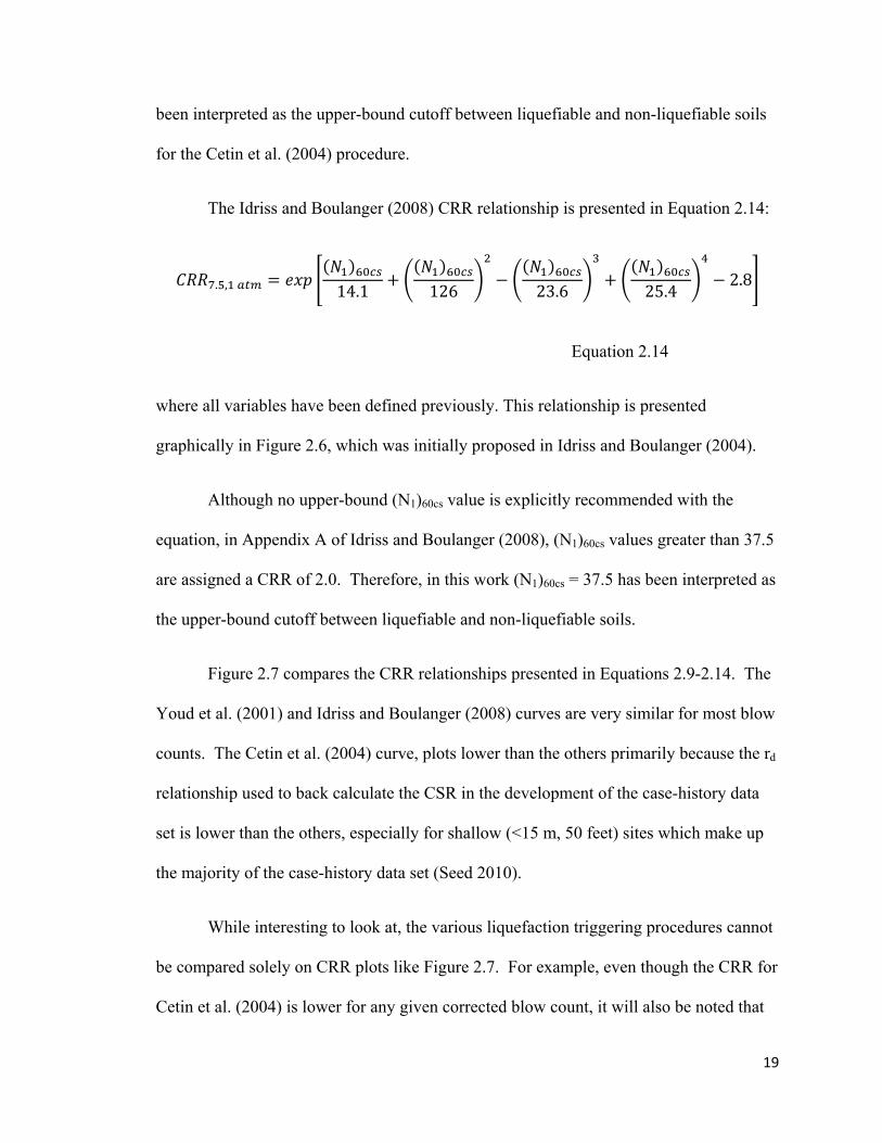
The Idriss and Boulanger (2008) CRR relationship is presented in Equation 2.14:

. , 14.1 126 23.6 25.42.8

Equation 2.14

where all variables have been defined previously. This relationship is presented

graphically in Figure 2.6, which was initially proposed in Idriss and Boulanger (2004).

Although no upper-bound (N1)60cs value is explicitly recommended with the

equation, in Appendix A of Idriss and Boulanger (2008), (N1)60cs values greater than 37.5

are assigned a CRR of 2.0. Therefore, in this work (N1)60cs = 37.5 has been interpreted as

the upper-bound cutoff between liquefiable and non-liquefiable soils.

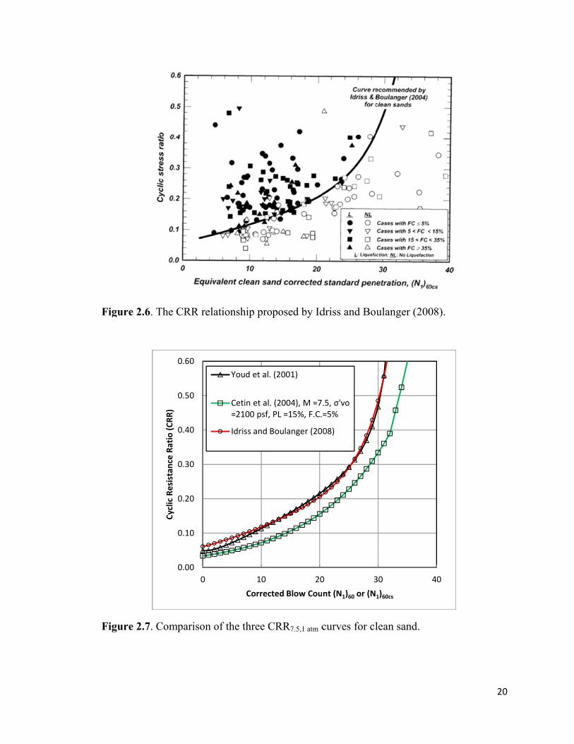
Figure 2.7 compares the CRR relationships presented in Equations 2.9-2.14. The

Youd et al. (2001) and Idriss and Boulanger (2008) curves are very similar for most blow

counts. The Cetin et al. (2004) curve, plots lower than the others primarily because the rd

relationship used to back calculate the CSR in the development of the case-history data

set is lower than the others, especially for shallow (<15 m, 50 feet) sites which make up

the majority of the case-history data set (Seed 2010).

While interesting to look at, the various liquefaction triggering procedures cannot

be compared solely on CRR plots like Figure 2.7. For example, even though the CRR for

Cetin et al. (2004) is lower for any given corrected blow count, it will also be noted that

F

F

Figure 2.6. T

Figure 2.7. C

The CRR rela

Comparison o

0.00

0.10

0.20

0.30

0.40

0.50

0.60

0

Cyclic Resistan

ce Ratio (CRR)

ationship pro

of the three C

10

Correc

Youd et al

Cetin et al=2100 psf,

Idriss and

oposed by Id

CRR7.5,1 atm c

20

cted Blow Cou

. (2001)

l. (2004), M =7, PL =15%, F.C.

Boulanger (20

driss and Bo

curves for cl

0 3

nt (N1)60 or (N

.5, σ'vo =5%

08)

ulanger (200

lean sand.

30

1)60cs

08).

40

20

21

their procedure generally yields a lower CSR (refer to Section 2.3, Figure 2.4).

Furthermore, while the Youd et al. (2001) and Idriss and Boulanger (2008) CRR

relationships appear to be very similar, one would not necessarily obtain the same CRR

value for a given raw blow count (N value) because the factors used to correct N to

(N1)60cs can vary significantly between relationships. Specifically, the overburden blow

count correction factor (CN) used in each relationship appears to be most variable.

2.4.1 Standardized Overburden Blow Count Correction Factor (CN)

Before computation of the CRR, the raw N values are generally

corrected/adjusted using five corrections. These five corrections include: (1) overburden

blow count correction (CN), (2) energy correction (CE), (3) drill rod length correction

(CR), (4) borehole diameter correction (CB), and (5) sampler liner correction (CS). These

corrections are applied as shown in Equation 2.15:

∗ ∗ ∗ ∗ ∗ Equation 2.15

where (N1)60 is the energy and overburden/stress corrected blow count. In liquefaction

analyses, it is also common to adjust the corrected blow count further using the F.C. of

the soil to obtain the clean sand (cs) equivalent corrected blow count, (N1)60cs. Among all

these corrections, only CN contributes significantly to major variations in corrected blow

count as a function of depth. As such, the remainder of this section is focused on the

various CN relationships.

The need to normalize the results of the standard penetration resistance for

overburden effects was well documented by Gibbs and Holtz (1957). In their study, a

22

large barrel type container was made and sand was compacted inside at a constant

relative density (DR) with varying overburden pressures being applied to the top of the

container. A standard split spoon sampler was driven into the sand layer, with the test

repeated for a range of DR and overburden pressures. This resulted in a correlation

between overburden pressure and blow count for a given DR. Many CN correlations have

been presented since that time (Teng 1962, Peck et. al 1974, Seed 1979, Liao and

Whitman 1985, Kayen et. al 1992). Most of the correlations are similar to one another

for relatively low overburden pressures. Differences in peak values and slope are noted

by Liao and Whitman (1986).

Youd et al. (2001) recommend using either the CN correlation proposed by Liao

and Whitman (1986) or Kayen et al. (1992). The Youd et al. (2001) worksheet

accompanying this report utilizes the correlation proposed by Kayen et al. (1992) over

Liao and Whitman (1986) because, as stated by Youd et al. (2001) “in these writers’

opinion, [Kayen et al. (1992)] provides a better fit to the original curve specified by Seed

and Idriss (1982)”. This correlation is presented below as Equation 2.16:

.

. Equation 2.16

where all variables have been defined previously. This equation limits the maximum CN

value to 1.7.

Cetin et al. (2004) adopted Liao and Whitman’s (1986) correlation with the

caveat that CN should not exceed a maximum value of 1.6. This correlation is presented

below as Equation 2.17:

23

.

Equation 2.17

Gibbs and Holtz (1957) noted the difficulty in separating the effects of confining

pressure and DR. They found that CN is not solely a function of overburden pressure, but

relies also on DR and soil type. Marcuson and Bieganousky (1977a,b) conducted

research similar to Gibbs and Holtz (1957) and also noted the influence DR had on CN.

Seed (1979) plotted CN as two different curves depending on the DR of the sand. His

correlations were the first to directly combine DR and effective overburden stress.

Boulanger (2003) used data from Marcuson and Bieganousky (1977a,b) along with a

weighted least squares nonlinear regression that modeled both density and overburden

stress. His correlation takes a form similar to Liao and Whitman (1986), with the advent

of the exponent being a function of relative density. Boulanger and Idriss (2004) have

modified the equation one step further by substituting a correlation that relates (N1)60 to

DR. The CN equation recommended by Idriss and Boulanger (2008) is presented as

Equation 2.18:

. . Equation 2.18

The authors recommend maximum values of CN = 1.7 and (N1)60 = 46 in this equation.

The Idriss and Boulanger (2008) workbook accompanying this report requires that

iterative calculations option be allowed. This is because the calculation of (N1)60 is

dependent on CN which is again dependent on (N1)60.

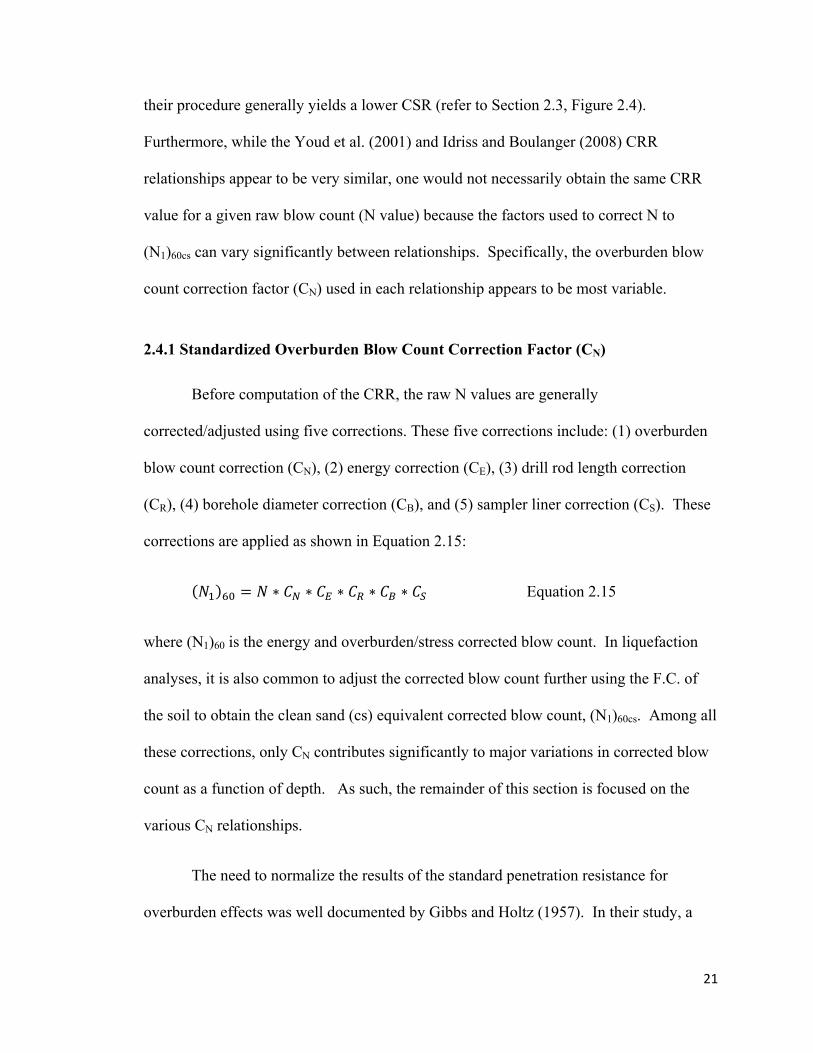
All three of the CN correlations (Equations 2.16-2.18) are compared in Figure 2.8.

In order to show the effect different (N1)60 values can have on the correlation of Idriss

24

Figure 2.8. Comparison of three CN correlations as a function of vertical effective stress and approximate depth.

and Boulanger (2008), two different curves with (N1)60 = 25 and (N1)60 = 40 have been

included, as indicated on the graph. In general, for effective overburden stresses greater

than 1 atm, the Youd et al. (2001) procedure yields the lowest CN values, while the Idriss

and Boulanger (2008) procedure yields the highest CN values. Meaning, all other things

being equal, the Idriss and Boulanger (2008) procedure will yield the highest (N1)60

values for soils at depth. The maximum CN differences between the procedures, assuming

a (N1)60 = 25 for Idriss and Boulanger (2008), are 12%, 20%, and 40% at 0.47 atm (1000

psf), 2.36 atm (5000 psf) and 3.78 atm (8000 psf), respectively.

0

20

40

60

80

100

120

0

1000

2000

3000

4000

5000

6000

7000

8000

0.00 0.50 1.00 1.50

Approximate Dep

th Below Surface (ft)

Vertical Effective Stress (psf)

Standard Overburden Blow count Correction Factor (CN)

Youd et al. (2001)

Cetin et al. (2004)

Idriss andBoulanger (2008)(N1)60=25Idriss andBoulanger (2008)(N1)60=40

25

2.4.2 Overburden Correction Factor (Kσ)

The overburden correction factor (Kσ) is currently the factor used to extrapolate

liquefaction triggering relationships to high overburden pressures. Because this research

is aimed primarily at determining liquefaction susceptibility at depth, Kσ has received a

rigorous review herein. The influence of overburden or effective stress on resistance of

saturated sands to liquefaction initiation has been noted by many (Maslov 1957, Florin

and Ivanov 1961, Seed and Lee 1966). The Kσ factor was first introduced by Seed

(1983) as a variable used to account for the decrease in the CSR required to cause a pore

pressure ratio of 100% as overburden stresses increase. The Seed (1983) correlation was

developed from cyclic simple shear and cyclic triaxial tests at different overburden

stresses. This first attempt to quantify Kσ was published graphically and consisted of a

range of possibilities. Vaid et al. (1985) subjected sands to very high confining

pressures, up to 24 atm (50,000 psf), and found that the density of the sand was

interrelated to the overburden pressure, which made it difficult to separate the two

variables. Vaid et al. (1985) also found that the cyclic resistance ratio of the sand

decreased with increasing overburden pressure, which is consistent with other studies.

Seed and Harder (1990) proposed a new Kσ relationship based on Harder’s

(1988) Ph.D. thesis. Although both studies used the same data set, Seed and Harder’s

(1990) relationship lies slightly below Harder’s (1988) relationship, as detailed in Figure

2.9. Pillai and Byrne (1994) researched Kσ as part of the seismic assessment of Duncan

Dam in British Columbia. Their study combined frozen sampling techniques and cyclic

laboratory tests with field SPT tests to determine Kσ. Their results lie above Seed and

F(r

H

pu

d

T

as

an

d

O

et

Figure 2.9. Creproduced f

Harder’s (199

ublished a K

etermine the

The expanded

s various pri

n f value of

epending on

Olsen 1999).

t al. (2004).

Comparison ofrom Hynes

90) values an

Kσ relationsh

e exponentia

d data set us

ior Kσ relatio

0.7 is recom

n; DR, stress

Equation 2

of Kσ valuesand Olsen 1

nd are not in

hip that was

al factor (f).

ed by Hynes

onships, are

mmended. H

history, met

.19 is the eq

s from differ999).

ncluded with

a function o

Their relatio

s and Olsen

presented in

owever, f v

thod of depo

quation adopt

rent research

hin figure 2.9

of DR after us

onship is inc

E

(1999) to de

n Figure 2.9

values can ran

osition, and a

ted by both Y

hers, with ex

9. Hynes and

sing a stress

cluded as Eq

Equation 2.1

etermine Kσ

. For mediu

ange from 0.6

age of the de

Youd et al. (

xpanded data

d Olsen (199

focus metho

quation 2.19.

9

curves, as w

um dense san

6 to 0.95

eposit (Hyne

(2001) and C

26

a set

99)

od to

well

nds,

es and

Cetin

27

Because the f value within Equation 2.19 is dependent on the DR of the soil,

Youd et al. (2001) recommend an f value between 0.6 - 0.8 for DR between 80-40%.

Cetin et al (2004) recommend an f value between 0.6 - 0.8 as a function of (N1)60cs

varying from 5 to 40 blows per foot, this is probably a misprint because all other trends

show that the f value increases with decreasing DR (i.e. it should have been written that f

varies from 0.6 – 0.8 as (N1)60cs varies from 40 to 5 blows per foot). In the Youd et al.

(2001) workbook, the determination of f is a two-step process; the DR is correlated to

(N1)60 and then f is correlated to DR. While in the Cetin et al. (2004) workbook, the f

value is linearly interpolated between 0.6 – 0.8 from 40 to 5 blows per foot respectively.

Work to determine the effects of overburden stress on liquefaction susceptibility

continued at the U.S. Army Engineering Research and Development Center (ERDC)

located in Vicksburg, Mississippi. Steedman et al. (2000) completed centrifuge tests with

fine Nevada sand in homogeneous and dense-over-loose configurations. Their tests

revealed that at high confining pressures, above 3 atm (6000 psf), a rise in pore pressure

may soften and degrade the soil under earthquake conditions, but may not generate 100%

excess pore water pressure necessary for “true liquefaction”. The study concluded that

liquefaction of deep soils may not be the hazard it is assumed to be (Steedman et al.

2000). However, Sharp and Steedman (2000) continued research with the centrifuge and

found that 100% excess pore water pressure, or liquefaction, can occur at high confining

stresses in the range of 3-12 atm (6,300-25,000 psf), contradicting the findings published

earlier in the year by Steedman et al. (2000).

Gonzalez et al. (2002) conducted centrifuge tests at Rensselaer Polytechnic

Institute (RPI) modeling homogenous and dense-over-loose configurations of deep soil

28

deposits. One model simulated a 38 m (125 feet) deposit of a saturated, uniform, loose

(Dr = 55%) sand. This model subjected the soil to a maximum initial effective

overburden stress of about 3.8 atm (8,000 psf) at the bottom of the soil deposit.

Liquefaction was observed throughout its entire depth, including 100% excess pore water

pressure. The input motion was 0.2 g with a frequency of 1.5 Hz. The entire column of

soil was liquefied in less than 20 seconds (around 24 cycles of shaking). This study also

collected and reported shear stress along with shear strain, which helped confirm the

acceleration and pore pressure data as well as the propagation of the liquefaction front

and its association with shear strength degradation. This study is confirmation that 100%

excess pore pressures can develop within deep sandy deposits.

Boulanger (2003) used a relative state parameter index derived from the relative

dilatancy index to correlate Kσ to the DR of sand. Boulanger and Idriss (2004) presented

a substitution for relative density based on blow count, similar to the CN correction

presented earlier. This relationship relies on the correlation of relative density to blow

count, which as Marcuson and Bieganousky (1977a,b) state is dependent on many factors

and can vary by as much as +/- 15%. These new Kσ relationships are included as

Equations 2.20 and 2.21:

1 Equation 2.20

. . Equation 2.21

Even with uncertainty in the correlation, these equations may be an improvement to the

current Kσ relationships based on the interrelation of relative density and overburden

pressure. Equation 2.20 should be restricted to a maximum value of 1.1, and Equation

29

2.21 should be restricted to a maximum value of 0.3 (or conversely (N1)60 can be

restricted to a maximum value of 37).

Both Youd et al. (2001) and Cetin et al. (2004) adopted Hynes and Olsen’s (1999)

relationship (Equation 2.19) for use when computing Kσ. Youd et al. (2001)

recommends a maximum value of 1.0 for Kσ, while Cetin et al. (2004) recommends a

maximum of 1.5. The Kσ relationship adopted in Idriss and Boulanger (2008) is the

same one presented in Boulanger and Idriss (2004) (Equations 2.20 and 2.21). The

limiting values for Kσ in each relationship can make a substantial difference in the

predicted CRR values of shallow soils (i.e. less than 1 atm [2000 psf]), but do not

influence liquefaction susceptibility at depth.

Kσ values for each of the three procedures are plotted in Figure 2.10 as a function

of vertical effective stress and approximate depth. Cetin et al. (2004) and Youd et al.

(2001) use the same equation to calculate Kσ, with slightly different f values and

different maximums at low confining pressures. Idriss and Boulanger (2008) use a

maximum value of 1.1. Two curves are provided for the Idriss and Boulanger (2008)

procedure because Kσ varies with (N1)60. The (N1)60 =10 and (N1)60 =25 curves both plot

above the other relationships for effective overburden stresses greater than 1 atm (2000

psf), which increases the CRR at depth according to Equation 2.8. For example, at an

effective overburden stress of 3 atm (6000 psf) and an (N1)60 value of 25, Idriss and

Boulanger (2008) report a Kσ value 13% greater than both Youd et al. (2001) and Cetin

et al. (2004), which relates to an equal increase in CRR, all other things remaining equal.

30

Figure 2.10. Comparison of all three Kσ correction factors as a function of vertical effective stress and approximate depth.

2.4.3 Magnitude Scaling Factor (MSF)

The magnitude scaling factor (MSF) is used to adjust the CRR7.5, 1 atm to a site

specific earthquake magnitude via Equation 2.8. This adjustment is necessary because of

the strong correlation between CRR and the number of loading cycles the earthquake

imparts to the soil (Seed et al. 1975). Although the MSF’s can result in differences

between the three most common liquefaction triggering procedures (refer to Figure 2.11),

the MSF’s are not a function of depth, and hence do not directly account for differences

at high confining pressures. Furthermore, the MSF for all three procedures are virtually

identical for Mw > 7.0.

Youd et al. (2001) published a range of acceptable values for the MSF, but the

lower bound of that range was recommended for routine engineering practice. It is

0 20 40 60 80 100 120

0.0

0.2

0.4

0.6

0.8

1.0

1.2

1.4

0 2000 4000 6000 8000

Approximate Depth Below Surface (ft)

Overburden Correction Factor (K σ)

Vertical Effective Stress (psf)

Youd et al. (2001)

Cetin et al. (2004)

Idriss and Boulanger (2008) (N1)60=10

Idriss and Boulanger (2008) (N1)60=25

31

Figure 2.11. Magnitude scaling factors (MSF) of the three most commonly used procedures.

included as Equation 2.22. Cetin et al. (2004) presented the MSF graphically. In order to

more easily use this relationship, their curve was digitized and a regression analysis was

used to fit the data with an exponential equation, which is included as Equation 2.23.

Idriss and Boulanger (2008) recommend an equation proposed by Idriss (1999), which is

provided below as Equation 2.24. Equations 2.22-2.24 are plotted in Figure 2.11.

.

. Equation 2.22

89.861 . Equation 2.23

6.9 0.058 Equation 2.24

0.0

0.5

1.0

1.5

2.0

2.5

3.0

4.5 5.5 6.5 7.5 8.5

Magnitude Scaling Factor (M

SF)

Earthquake Moment Magnitude (M)

Youd et al. (2001)

Cetin et al. (2004)

Idriss and Boulanger(2008)

32

The lower-bound MSF proposed by Youd et al. (2001) plots above the MSF

relationships of both Cetin et al. (2004) and Idriss and Boulanger (2008). At an

earthquake Mw of 6.0, differences between the largest and smallest MSF’s are almost

20%. In order to distinguish between depth dependent variables (i.e. rd, CN, Kσ), a Mw of

7.5 can be utilized to eliminate any differences the MSF would induce. The mean

earthquake magnitude used in code-based design for most sites in NE Arkansas (obtained

from deaggregation) is so close to Mw = 7.5 that the impact of various MSF’s is

irrelevant.

2.5 FINE-GRAIN SCREENING CRITERIA

The evaluation of liquefaction triggering susceptibility of fine-grained soils is

inseparably connected to both the percentage, and plasticity of the fines within the soil.

Empirical procedures for screening fine-grained soils for liquefaction susceptibility were

first developed following the Chinese earthquakes of Haicheng and Tangshan, in 1975

and 1976, respectively. Chinese researchers observed the liquefaction of silty sands and

slightly silty sands in these earthquakes. Seed and Idriss (1982) documented these

findings and the fine-grained screening criteria became known as the Chinese criteria

(Andrews and Martin 2000, Cox 2001). These criteria applied three screens to evaluate

fine-grained soils susceptibility to liquefaction triggering. If a soil had: (1) a clay

content (% finer than 0.005 mm) less than 15%, (2) a liquid limit (LL) less than 35, or (3)

an in-situ water content (wc) greater than 90% of the LL, it was considered susceptible to

liquefaction. Andrews and Martin (2000) used the case histories from earlier studies

along with some newer histories to transpose the Chinese criteria to U.S. conventions

(Seed et al. 2003).

33

Following the 1999 Adapazari earthquake, the Chinese criteria were found to be

inadequate, and were strongly advised to be abandoned in practice (Seed et al. 2003, Bray

and Sancio 2006). The main problem being, that the percentage of clay size particles was

much less important than the plasticity of the fines within the soil (Bray et al. 2001).

Seed et al. (2003) recommended an interim assessment of liquefaction susceptibility of

fine-grained soils based on research in progress. These criteria were based on the

plasticity index (PI), LL and in-situ wc. They categorized fine-grained soils susceptibility

into three zones; (1) a zone susceptible to classic cyclic liquefaction, (2) a transition zone,

and (3) a zone where the fine-grained soils are not susceptible to classic liquefaction, but

may still be vulnerable to cyclic degradation.

Bray and Sancio (2006) relied on the wc, the LL, and PI to determine fine-grained

soil liquefaction susceptibility. In this approach, the soil can be classified as: (1)

susceptible, (2) moderately susceptible, or (3) not susceptible. To more easily represent

the criteria presented by Bray and Sancio (2006), Table 2.1 is included along with Figure

2.12. The table and figure break the soil into groups depending on PI and wc/LL ratio. If

the PI if less than 12 and the wc/LL is greater than 0.85, the soil is susceptible to classic

cyclic liquefaction. If the PI is between 12 and 18 and the wc/LL is greater than 0.8, the

soil is moderately susceptible, and if the either the PI is greater than 18 or the wc/LL is

less than 0.8, the soil is not susceptible to classic cyclic liquefaction, but may still be

susceptible to strain softening and degradation of strength during earthquake loading.

Idriss and Boulanger (2008) didn’t classify the fine-grained soils as susceptible or

not, but instead developed equations that can be used to determine the F.S. for fine-

grained soils. First, the soil is classified as behaving more sand-like or clay-like

TS

F(r

d

li

ac

C

h

Table 2.1. Suancio (2006

Figure 2.12. reproduced f

epending on

ike” behavio

ccording to b

Clay-like beh

as been desi

usceptibility )

Graphical refrom Bray an

n the PI; if th

or is expected

blow count,

havior is anal

ignated as “c

S

M

S

S

of fine-grain

epresentationnd Sancio 20

he PI ≥ 7 “cla

d. Sand-like

and is synon

lyzed accord

cyclic soften

usceptible

Moderatly

usceptibleNot

usceptible

ned soil to li

n of fine-gra006)

ay-like” beh

e behavior is

nymous with

ding to the u

ning”. Althou

PI < 12

12 < PI < 18

PI > 18

iquefaction t

ained liquefa

havior is exp

s analyzed in

h classic def

undrained she

ugh previou

wc/ LL >

8 wc/ LL >

wc/ LL <

triggering af

action suscep

ected, if the

n the traditio

fined “cyclic

ear strength

us researcher

> 0.85

> 0.80

<0.80

fter Bray and

ptibility crite

PI < 7 “sand

nal manner

c liquefaction

of the soil a

rs have notic

34

d

eria

d-

n”.

and

ced

35

the potential for clayey soil to degrade during earthquake loading (Seed et al. 2003, Bray

and Sancio 2006), this F.S. computation for cyclic softening is the first attempt to

quantify a clayey soils “liquefaction” susceptibility using simplified procedures.

The fine-grained screening criteria of Bray and Sancio (2006) has been

incorporated into the workbooks of Youd et al. (2001) and Cetin et al. (2004). While, the

“clay-like or “sand-like” procedures are incorporated in the Idriss and Boulanger (2008)

workbook.

2.6 SUMMARY

Regarding evaluation of liquefaction triggering at depth (> 15 m [50 ft] or

approximately 1.5 atm) via simplified procedures, the three variables most responsible

for differences between the Youd et al. (2001), Cetin et al. (2004), and Idriss and

Boulanger (2008) procedures are rd, CN, and K. In terms of earthquake loading, the

various rd relationships tend to produce CSR’s which are lowest for Cetin et al. (2004)

and highest for Idriss and Boulanger (2008). It is common for these rd relationships to

vary by 30% or more at depths greater than 15 m (50 ft), yielding equal variations in the

CSR estimates. In terms of soil resistance at depth, the various CN relationships tend to

yield (N1)60 values that are lowest for Youd et al. (2001) and highest for Idriss and

Boulanger (2008). It is common for these CN relationships to vary by 20% or more at

depths greater than about 20 m (65 ft), yielding equal variations in the (N1)60 values

obtained from the same raw blow count. General trends concerning Kσ are dependent

on stress levels; at vertical effective stresses larger than 1 atm (2116 psf) the Youd et al.

(2001) and Cetin et al. (2004) procedures are identical and yield the lowest CRR values.

36

The Idriss and Boulanger (2008) procedure produces Kσ values that are a least 10%

greater than the others at effective confining stresses greater than 2 atm (4232 psf).

Therefore, while the Idriss and Boulanger (2008) procedure will yield the highest CSR at

depth, it will also tend to yield the highest CRR at depth.

Although these comparisons are important and help discern key differences in

current liquefaction triggering procedures, it is important to realize the limitations of

comparisons made in this broad manner. The figures depicting direct comparison

between rd, CN, and Kσ, pose two main problems when used to infer overall differences

between the F.S. predicted by each of the procedures: (1) relative differences on these

plots may not transfer directly into the final F.S. because of how the various components

within each procedure work together, and (2) the assumption of constant parameters with

depth (such as (N1)60, F.C., etc..) used to make these plots are not consistent with site

specific information. In order to overcome these obstacles, actual site specific

liquefaction evaluations should be completed using each of the procedures and then

comparisons between site specific rd, CN, Kσ, (N1)60, and other variables can be used to

directly infer differences between the F.S. predicted by the three procedures. Site

specific liquefaction triggering evaluations have been completed as part of this project

and are included in Chapter 4.

37

Chapter 3

Liquefaction Triggering Workbook User’s Guide

3.1 INTRODUCTION

Each of the three most commonly used SPT-based liquefaction triggering

procedures (Youd et al. 2001, Cetin et al. 2004, and Idriss and Boulanger 2008) have

been programmed into Microsoft Excel workbooks. The purpose of this chapter is to

provide guidance for using these workbooks to perform a liquefaction susceptibility

evaluation. The internal formulas within each workbook will not be discussed in detail,

but some concepts regarding certain calculations warrant special attention and will be

discussed herein. This user’s guide is not all encompassing, and should be used to

supplement the comments in the worksheet cells. The information will be most clear if

read while viewing the worksheet under consideration.

Each of the workbooks are designed to work in English units. If Metric units are

provided on the boring log, the user will have to convert them to English units before

they are entered into the workbook. Likewise, if the user desires an output in Metric

units the English units within the worksheet will have to be converted to Metric units.

Some of the data within the workbooks are programmed in Metric units. This is done,

only to remain consistent with the formulations in a particular procedure, and not as an

invitation to enter Metric units into the workbooks.

38

3.2 WORKBOOK OVERVIEW

The workbooks are available in the 1997-2003 Microsoft Excel file format (i.e.

[*.xls]), but where built using Microsoft Excel 2010 (i.e. [*.xlsx]), so directions

expressed herein may not be exactly the same for versions other than 2010. The basic

formats of the three workbooks are as similar as possible to facilitate data entry and

information exchange from one workbook to another. After a brief section outlining

some of the workbook similarities, a detailed section concerning the Youd et al. (2001)

workbook will be discussed. Following the Youd et al. (2001) discussion, the Cetin et al.

(2004) and Idriss and Boulanger (2008) workbooks will be discussed in detail. Some of

the calculations in each workbook are identical, as such, the discussions for the Cetin et

al. (2004) and Idriss and Boulanger (2008) workbooks will only focus on the portions

that differ from the Youd et al. (2001) workbook. Before beginning the individual

workbook sections, it is prudent to discuss the general appearance and common

characteristics of the workbooks.

Each SPT-based liquefaction triggering workbook (i.e. individual Excel file)

includes tabs near the bottom of the screen which allow the user to see different

worksheets within the workbooks. A screenshot of the tabs is included as Figure 3.1.

The tabs are labeled: Input Data, Calculations, Calculation Tables, Output Boring El.,

Output Grade El., Output Graphs, and References. The Idriss and Boulanger (2008)

workbook contains one additional tab which is discussed in Section 3.5.

The Input Data tab is the only worksheet that requires input information from the

user. The Calculation and Calculation Tables tabs are for the worksheets which are used

to perform all the necessary calculations. The Output Boring El., Output Grade El., and

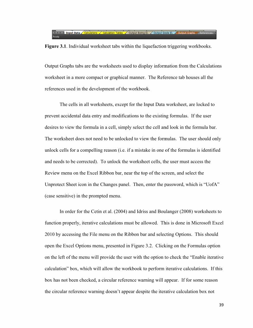
F

O

w

re

pr

d

T

un

an

R

U

(c

fu

2

op

on

ca

b

th

Figure 3.1. In

Output Graph

worksheet in

eferences use

The ce

revent accid

esires to view

The workshee

nlock cells f

nd needs to b

Review menu

Unprotect Sh

case sensitiv

In ord

unction prop

010 by acce

pen the Exce

n the left of

alculation” b

ox has not b

he circular re

ndividual wo

hs tabs are th

a more com

ed in the dev

ells in all wo

dental data en

w the formu

et does not n

for a compel

be corrected

u on the Exc

eet icon in th

ve) in the pro

der for the Ce

perly, iterativ

ssing the Fil

el Options m

the menu w

box, which w

been checked

eference war

orksheet tabs

he worksheet

mpact or grap

velopment o

orksheets, ex

ntry and mod

ula in a cell,

need to be un

lling reason (

d). To unlock

el Ribbon ba

he Changes

ompted menu

etin et al. (20

ve calculatio

le menu on t

menu, presen

ill provide th

will allow th

d, a circular r

rning doesn’

s within the

ts used to di

phical manne

f the workbo

xcept for the

difications to

simply selec

nlocked to vi

(i.e. if a mist

k the worksh

ar, near the t

panel. Then

u.

004) and Idr

ons must be a

the Ribbon b

nted in Figur

he user with

e workbook

reference wa

’t appear des

liquefaction

isplay inform

er. The Refe

ook.

e Input Data

o the existin

ct the cell an

iew the form

take in one o

heet cells, th

top of the sc

n, enter the p

riss and Bou

allowed. Th

bar and selec

re 3.2. Click

h the option t

k to perform

arning will a

spite the itera

n triggering w

mation from

erence tab ho

worksheet, a

ng formulas.

nd look in the

mulas. The u

of the formu

he user must

reen, and se

password, wh

ulanger (2008

his is done in

cting Option

king on the F

to check the

iterative calc

appear. If fo

ative calcula

workbooks.

the Calculat

ouses all the

are locked to

If the user

e formula ba

user should o

ulas is identif

access the

lect the

hich is “Uof

8) workshee

n Microsoft E

s. This shou

Formulas opt

“Enable iter

culations. If

or some reaso

ation box no

39

tions

o

ar.

only

fied

fA”

ets to

Excel

uld

tion

rative

f this

on

t

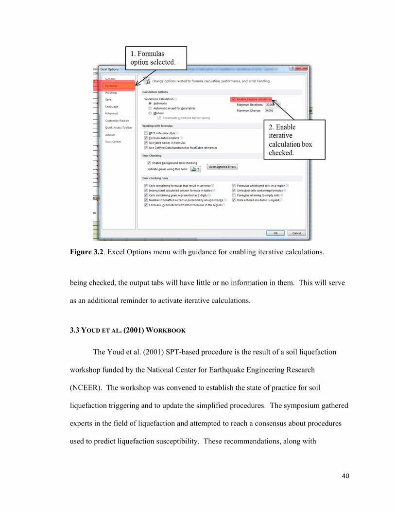
F

b

as

3

w

(N

li

ex

u

Figure 3.2. E

eing checked

s an addition

.3 YOUD ET

The Y

workshop fun

NCEER). T

iquefaction t

xperts in the

sed to predic

Excel Option

d, the output

nal reminder

AL. (2001) W

Youd et al. (2

nded by the N

he workshop

riggering an

e field of liqu

ct liquefactio

ns menu with

t tabs will ha

r to activate i

WORKBOOK

2001) SPT-b

National Cen

p was conve

nd to update

uefaction and

on susceptib

h guidance fo

ave little or n

iterative calc

K

based proced

nter for Eart

ened to estab

the simplifie

d attempted

bility. These

or enabling i

no informati

culations.

dure is the re

thquake Eng

blish the state

ed procedure

to reach a co

e recommend

iterative calc

ion in them.

esult of a soil

gineering Res

e of practice

es. The sym

onsensus ab

dations, alon

culations.

This will se

l liquefaction

search

e for soil

mposium gath

out procedu

ng with

40

erve

n

hered

ures

41

engineering practicality and a proven track record, have made the Youd et al. (2001)

procedure well accepted within the engineering community.

Many of the individual cells in the worksheets contain comments, as indicated by

a red triangle in the upper right-hand corner of the cell. These comments explain, clarify,

or expound on the function and use of the worksheet cells. This user’s guide will not

specifically address each comment, but will present what information should be entered

into each of the cells, starting with the Input Data worksheet. This guide has been written

to accompany the worksheets and it may be beneficial to have a copy of the worksheets

readily accessible while reading.

3.3.1 Input Data

Most of the Input Data necessary for the soil liquefaction triggering evaluation

should be available from the boring logs obtained during the site investigation and

subsequent laboratory testing. Note that only the cells highlighted in a light green

color should be input. All other cells should not be altered. The first group of input

cells, rows 5-15, at the top of the Input Data worksheet (refer to Figure 3.3), primarily

contain job identification information such as: job number, job name, job location

(latitude and longitude), date of boring, drilling equipment, type of drilling, hammer

energy, etc. Most of these cells are for documentation purposes only. However, the

hammer energy correction factor is critical, as it is used to correct the measured SPT

blow count (N) to the standardized N60 value (refer to Section 2.4.1). The hammer

energy correction factor (CE) is equal to the measured hammer energy ratio (in percent)

divided by the standard energy ratio of 60%. If hammer energy has not been measured

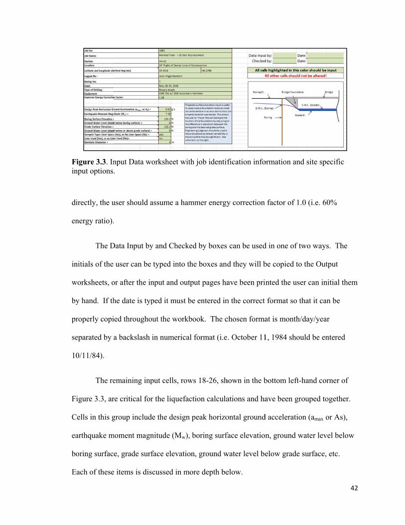
Fin

d

en

in

w

by

pr

se

1

F

C

ea

b

E

Figure 3.3. Innput options

irectly, the u

nergy ratio).

The D

nitials of the

worksheets, o

y hand. If th

roperly copi

eparated by

0/11/84).

The re

igure 3.3, ar

Cells in this g

arthquake m

oring surfac

Each of these

nput Data w.

user should a

.

Data Input by

user can be

or after the in

he date is typ

ied througho

a backslash

emaining inp

re critical for

group includ

moment magn

e, grade surf

e items is dis

orksheet wit

assume a ham

y and Checke

typed into th

nput and out

ped it must b

out the workb

in numerica

put cells, row

r the liquefac

de the design

nitude (Mw),

face elevatio

scussed in m

th job identif

mmer energy

ed by boxes

he boxes and

tput pages ha

be entered in

book. The c

al format (i.e

ws 18-26, sh

ction calcula

n peak horizo

, boring surf

on, ground w

more depth be

fication info

y correction

can be used

d they will b

ave been pri

n the correct

chosen forma

. October 11

hown in the b

ations and ha

ontal ground

face elevation

water level be

elow.

ormation and

factor of 1.0

d in one of tw

be copied to

inted the use

format so th

at is month/d

1, 1984 shou

bottom left-h

ave been gro

d acceleration

n, ground w

elow grade s

d site specific

0 (i.e. 60%

wo ways. Th

the Output

er can initial

hat it can be

day/year

uld be entere

hand corner

ouped togeth

n (amax or As

water level be

surface, etc.

42

c

he

them

d

of

her.

s),

elow

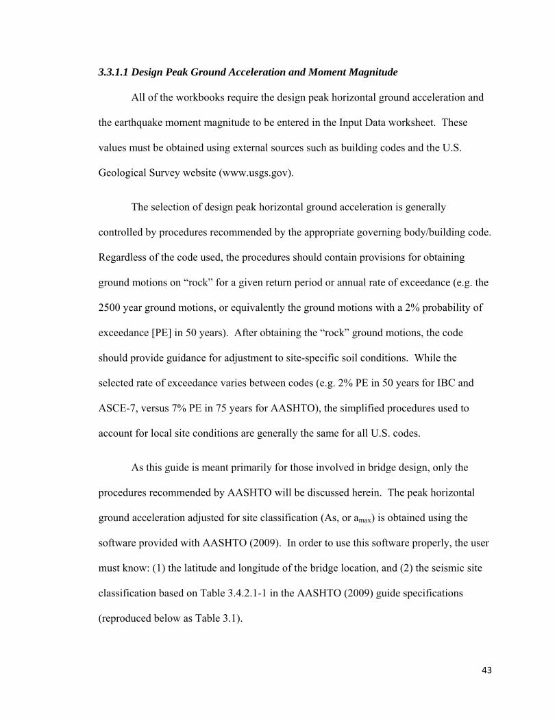
43

3.3.1.1 Design Peak Ground Acceleration and Moment Magnitude

All of the workbooks require the design peak horizontal ground acceleration and

the earthquake moment magnitude to be entered in the Input Data worksheet. These

values must be obtained using external sources such as building codes and the U.S.

Geological Survey website (www.usgs.gov).

The selection of design peak horizontal ground acceleration is generally

controlled by procedures recommended by the appropriate governing body/building code.

Regardless of the code used, the procedures should contain provisions for obtaining

ground motions on “rock” for a given return period or annual rate of exceedance (e.g. the

2500 year ground motions, or equivalently the ground motions with a 2% probability of

exceedance [PE] in 50 years). After obtaining the “rock” ground motions, the code

should provide guidance for adjustment to site-specific soil conditions. While the

selected rate of exceedance varies between codes (e.g. 2% PE in 50 years for IBC and

ASCE-7, versus 7% PE in 75 years for AASHTO), the simplified procedures used to

account for local site conditions are generally the same for all U.S. codes.

As this guide is meant primarily for those involved in bridge design, only the

procedures recommended by AASHTO will be discussed herein. The peak horizontal

ground acceleration adjusted for site classification (As, or amax) is obtained using the

software provided with AASHTO (2009). In order to use this software properly, the user

must know: (1) the latitude and longitude of the bridge location, and (2) the seismic site

classification based on Table 3.4.2.1-1 in the AASHTO (2009) guide specifications

(reproduced below as Table 3.1).

T

cl

th

C

h

ca

w

In

co

te

w

fr

gr

Table 3.1. Sit

The w

lassification

he boring log

Class E or F u

as been ente

alculated and

worksheets. T

n order for th

omplete to a

erminated at

within the wo

Once

rom the USG

round motio

te Class defi

worksheets h

for Site Cla

g. However

using the cri

ered into the

d displayed

The classific

he workbook

at least 95 fee

depths less

orksheet and

the seismic

GS probabili

ons with a 7%

initions repro

ave the abili

asses C, D an

, the user mu

iteria specifie

Input Data w

in the Calcu

cation is in a

k to determin

et below the

than 95 feet

d the user wil

site classific

stic ground m

% PE in 75 y

oduced from

ity to automa

nd E using th

ust explicitly

ed in Table 3

worksheet, th

ulations, Outp

a large yellow

ne the site cl

e boring surf

, no classific

ll have to cla

cation has be

motion haza

years be used

m AASHTO

atically dete

he raw SPT b

y check to se

3.1. After th

the seismic s

put Boring E

w box near t

lassification

face elevation

cation can be

assify the sit

een determin

ard maps. A

d. These gro

2009

ermine the se

blow count (

ee if the site

he boring log

site classifica

El., and Outp

the top of ea

, the boring

n. If the bor

e determined

te by other m

ned, As/amax

AASHTO req

ound motion

eismic site

(N) values fr

classifies as

g informatio

ation will be

put Grade El

ach workshee

must be

ring is

d automatica

means.

can be obtai

quires that

ns have been

44

from

s Site

on

e

l.

et.

ally

ined

n

45

programmed into the CD titled “Seismic Design Parameters Version 2.10” by the USGS

(2008), which is provided with AASHTO (2009). This CD allows the user to specify the

latitude and longitude coordinates, calculate PGA for a rock site (Site Class B). Then

adjust the rock PGA to an equivalent site-adjusted design value (As or amax) using site

amplification factors based on the site classification. The user may perform these steps

by either clicking on the “Calculate As, SDs, and SD1” button, or the “Design Spectrum”

button (refer to Figure 3.4). However, the author recommends using the “Design

Spectrum” button because a bug exists in the “Calculate As, SDs, and SD1” calculations,

wherein incorrect values of As can be obtained. The bug appears to be caused by using

the site amplification factor for short-period spectral acceleration (Fa) instead of the site

amplification factor for PGA (Fpga). However, this bug does not exist when using the

“Design Spectrum” button directly to obtain As. When using the “Design Spectrum”

option, the design peak ground acceleration (As, or amax) is the spectral acceleration (Sa)

at a period of 0.0 sec (refer to Figure 3.4). As a check, the user should always ensure that

this value has been properly adjusted for local soil conditions (i.e. site classification)

using the proper site amplification factors.

The proper design earthquake magnitude (Mw) can be found using the 2008

Interactive Deaggregation software available on the web from the USGS. The site can be

accessed directly using <http://eqint.cr.usgs.gov/deaggint/2008/index.php>, or by logging

onto <www.usgs.gov> and entering “deaggregation” into the search bar. Regardless, the

link titled 2008 Interactive Deaggregation (Beta) needs to be used. The website offers

instructions about how to use the deaggregation software. The deaggregation calculation

box is presented in Figure 3.5. The return period that should be used, for deaggregation

FA

F

Figure 3.4. SAASHTO (20

Figure 3.5. 2

Seismic Desi009).

008 Interact

gn Paramete

tive Deaggre

ers Version 2

egation (Beta

2.10 from th

a) website, a

he USGS, inc

available from

cluded with

m the USGS

46

S.

47

according to AASHTO (2009), is 5% in 50 years. Peak Ground Acceleration (PGA)

should be selected from the spectral acceleration dropdown box. The average shear

wave velocity over the top 30 m (100 ft) (Vs30) may be left as the default value of 760

m/s (i.e. a rock site classification) if site specific data is not available. The “Compute”

icon will calculate the magnitude deaggregation. Both the mean and modal magnitudes

are calculated in this analysis, and in many cases for the NMSZ the two magnitudes are

nearly the same. In the author’s opinion, the mean magnitude is the closest match to the

deaggregation magnitude selection techniques discussed in Finn and Wightman (2010)

and should be used within the workbooks provided. The user can read the mean

magnitude from one of the three output file options (TXT, PDF, GIF).

3.3.1.2 Boring Elevation versus Grade Elevation

This worksheet includes the option for entering two reference elevations. One

reference elevation is for the actual boring performed (i.e. the Boring Surface Elevation).

The other reference elevation (i.e. the Grade Surface Elevation) is included so that

liquefaction potential can be evaluated at a nearby location that couldn’t feasibly be

drilled. Both of these reference elevations require a separate Ground Water Level to be

entered into the corresponding labeled cells. The worksheet will allow the user to enter

water levels above or below the reference elevations. Note that the elevations of the

water table are not input, but rather a depth/distance below or above the respective

reference surface is input. Water levels above the grade and boring elevations should be

input as a negative number (i.e. if the boring was completed through 5 feet of water enter

the value -5). Figure 3.3 includes a schematic found in the worksheet to help the user

48

remember which elevation to assign each cell. The schematic depicts a situation where

the boring was completed behind the abutment of the bridge (Boring Surface Elevation)

instead of the river bottom (Grade Surface Elevation) near the future location of the

bridge foundation.

Boring surface elevations should be included within the boring logs, while the

grade surface elevations may require information from topographic maps, bathymetry, or

other sources. When calculating the liquefaction potential at the grade elevation, the

boring log data is simply ignored from the boring surface elevation down to the grade

surface elevation. Furthermore, the stresses are re-calculated based on the new grade

surface elevation and water table locations. Engineering judgment should be employed

when using the Grade Surface Elevation due to lateral variability within the soil profile.

Meaning, care should be taken when assuming the soil profile behind an abutment is

representative of the soil profile at an intermediate pier.

3.3.1.3 Sampler Type and Borehole Diameter Correction Factors

To incorporate sampler correction factors, yes or no answers must be entered into

two cells: (1) the Sampler Type cell identifies if the sampler has room for liners or not

[enter Yes or No], and (2) the Liner Used cell indicates if the sampler was used with or

without liners [enter Yes or No]. It is common for AHTD to use samplers which have

liner space and not use the liners. Therefore, as shown in Figure 3.3, Yes should be

entered into the Sampler Type input cell, while No should be entered into the Liner Used

input cell. The Borehole Diameter input cell is used to account for the borehole

correction factor, which only applies to boreholes larger than 115 mm (4.5 in). The

diameter of the borehole should be specified on the boring logs.

49

3.3.1.4 Depth-dependent Input Data

The remaining input information is all depth dependent. The headings for

columns A through J are shown in Figure 3.6. The first two columns, Sample Number

and Elevation at Sample Location, are composed of values that have been calculated

directly in the worksheet. No values should be directly input by the user into these

columns, they simply contain information that should aid the user in tracking individual

sample locations (depths) throughout the workbook. To better explain the remaining data

input columns, each of the individual column headings are discussed below in separate

paragraphs.

Depth to Sample Location (ft) – This is the depth at which each SPT sample was

obtained relative to the boring surface elevation. Typically, the interval between SPT

sample locations is a constant number such as 1 m or 1.5 m (3 ft or 5 ft). This

information is available on the boring log.

USCS Classification – The user must input the Unified Soil Classification

System (USCS) designation for each depth. This information should be provided on

the boring log if sufficient laboratory tests (i.e. grain size analysis and Atterberg Limits)

have been performed on the split-spoon samples. For dual classifications, the user should

enter both symbols separated with a dash and no spaces (i.e. SW-SP). If the USCS

designation is not provided, the user will have to assign a USCS designation for each

sample using the general soil descriptions included on the boring log. As stated within

the cell comment in the worksheet, the user can assume CL for clays, ML for silts, SP for

sands and GP for gravels if no additional information is provided. A USCS designation

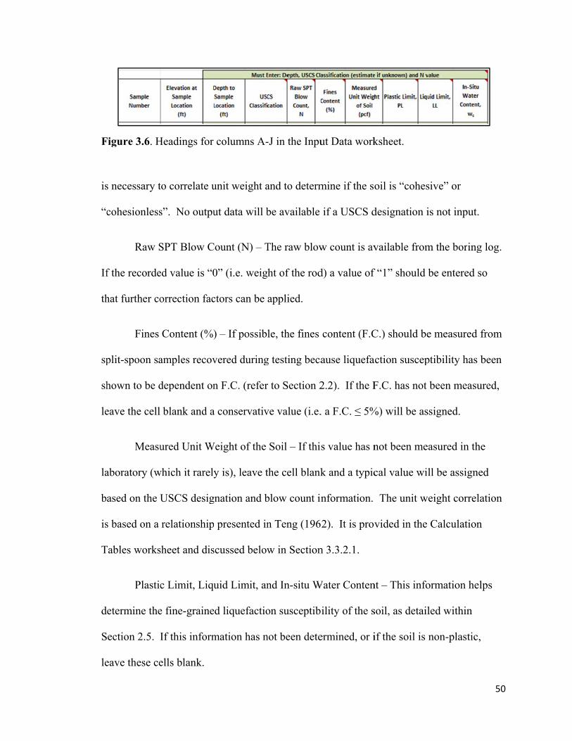
F

is

“c

If

th

sp

sh

le

la

b

is

T

d

S

le

Figure 3.6. H

s necessary t

cohesionless

Raw S

f the recorde

hat further co

Fines

plit-spoon sa

hown to be d

eave the cell

Measu

aboratory (w

ased on the U

s based on a

Tables works

Plastic

etermine the

ection 2.5. I

eave these ce

Headings for

to correlate u

s”. No outpu

SPT Blow C

ed value is “0

orrection fac

Content (%)

amples recov

dependent on

blank and a

ured Unit W

which it rarely

USCS desig

relationship

sheet and dis

c Limit, Liqu

e fine-graine

If this inform

ells blank.

columns A-

unit weight a

ut data will b

Count (N) – T

0” (i.e. weig

ctors can be

) – If possibl

vered during

n F.C. (refer

a conservativ

Weight of the

y is), leave t

gnation and b

presented in

scussed below

uid Limit, an

ed liquefactio

mation has n

-J in the Inpu

and to determ

be available

The raw blow

ht of the rod

applied.

le, the fines

g testing beca

r to Section 2

ve value (i.e.

Soil – If this

the cell blank

blow count in

n Teng (196

w in Section

nd In-situ W

on susceptib

not been dete

ut Data work

mine if the so

if a USCS d

w count is av

d) a value of

content (F.C

ause liquefa

2.2). If the F

. a F.C. ≤ 5%

s value has n

k and a typic

nformation.

2). It is prov

n 3.3.2.1.

Water Conten

ility of the s

ermined, or i

ksheet.

oil is “cohes

designation i

vailable from

f “1” should

C.) should be

action suscep

F.C. has not

%) will be as

not been me

cal value wil

The unit w

vided in the

nt – This info

soil, as detail

if the soil is

sive” or

is not input.

m the boring

be entered s

e measured f

ptibility has b

been measu

ssigned.

asured in the

ll be assigne

eight correla

Calculation

ormation hel

led within

non-plastic,

50

g log.

o

from

been

ured,

e

ed

ation

n

lps

51

3.3.2 Calculations and Calculation Tables Worksheets

The Calculation and Calculation Tables worksheets are the backbone of the entire

workbook. Data is transferred into these worksheets from the Input Data worksheet, and

data is copied out of these worksheets into the various output worksheets. These

worksheets should not be altered unless a mistake is found in the calculations. If the user

is comfortable with the liquefaction calculations, these worksheets will not need to be

viewed during routine liquefaction evaluations. In order for the user to have a sense of

how these worksheets compute and use information, a review of each of the columns will

be presented. Additionally, many of the column headings in the workbooks include cell

comments, which provide clarification concerning the column’s function.

When the Calculations worksheet is first viewed, the user will notice that most of

the information entered into the Input Data worksheet has been copied over to this

worksheet (refer to Figure 3.7). However, the user must not try to re-enter or change data

in the Calculations worksheet. The cells have been locked to prevent this mistake. As

shown in the lower left-hand corner of Figure 3.7, many of the standard blow count

correction factors that are not depth-dependent (i.e. hammer energy, borehole diameter,

sampler liner) are calculated directly below the Input Data in rows 26-33. The magnitude

scaling factor is also calculated in this block of cells. The specific equations and tables

from the Youd et al. (2001) paper that were used to obtain these factors are referenced in

the cells so the user can easily follow the worksheet development.

It will be noted that row 33 was originally reserved for the sloping ground

correction factor (K). However, this function was removed from the spreadsheet

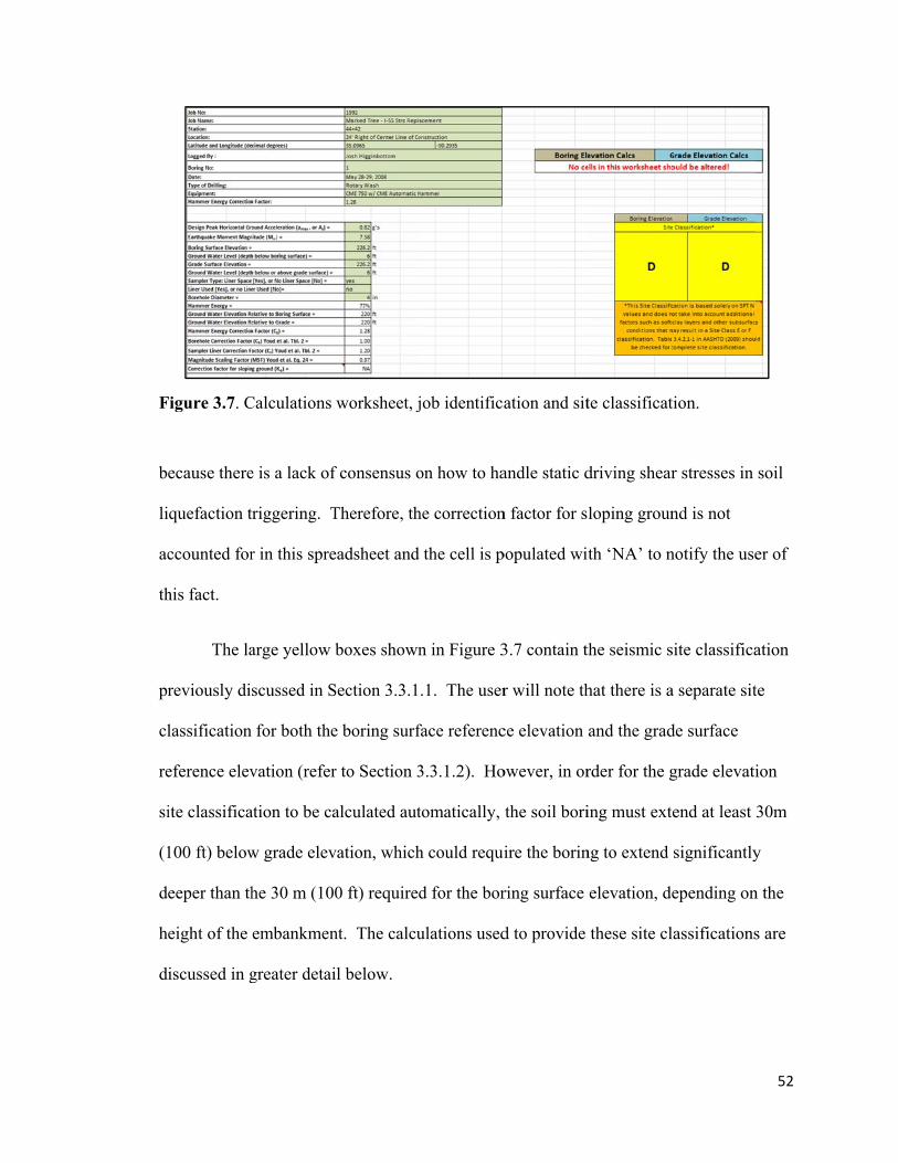
F

b

li

ac

th

pr

cl

re

si

(1

d

h

d

Figure 3.7. C

ecause there

iquefaction t

ccounted for

his fact.

The la

reviously di

lassification

eference elev

ite classifica

100 ft) below

eeper than th

eight of the

iscussed in g

Calculations

e is a lack of

riggering. T

r in this spre

arge yellow b

scussed in S

for both the

vation (refer

ation to be ca

w grade elev

he 30 m (100

embankmen

greater detai

worksheet, j

f consensus o

Therefore, th

eadsheet and

boxes shown

Section 3.3.1

e boring surf

r to Section 3

alculated aut

vation, which

0 ft) required

nt. The calcu

l below.

job identifica

on how to ha

he correction

the cell is p

n in Figure 3

.1. The user

face referenc

3.3.1.2). Ho

tomatically,

h could requi

d for the bor

ulations used

ation and sit

andle static d

n factor for s

populated wit

3.7 contain th

r will note th

ce elevation

owever, in or

the soil bori

ire the borin

ring surface

d to provide

te classificat

driving shear

loping groun

th ‘NA’ to n

the seismic s

hat there is a

and the grad

rder for the g

ing must ext

ng to extend

elevation, de

these site cl

tion.

r stresses in

nd is not

notify the use

site classifica

a separate sit

de surface

grade elevati

end at least

significantly

epending on

lassifications

52

soil

er of

ation

te

ion

30m

y

n the

s are

53

3.3.2.1 Depth-dependent Calculations

The remaining calculations are all depth dependent and are associated with a

given SPT sample location. When viewing the Calculations worksheet, the user will note

that many more columns are populated than in the Input Data worksheet (i.e. from

column K through column AL). The Calculations worksheet is also split vertically, with

rows 35-65 being dedicated to calculations relative to the boring surface elevation, and

rows 67-97 being dedicated to calculations relative to the grade surface elevation (refer to

Section 3.3.1.2).

For clarity, each of the column headings in the Calculations worksheet will be

discussed below in the same order as they are presented within the worksheet. Each

column heading will be followed by information regarding the function of the column.

Once again, the user is reminded that additional useful comments may be provided in the

cells within the worksheet. These comments are indicated by red triangles in the upper

right-hand corner of the cell. Furthermore, whenever possible, the specific equations

from the Youd et al. (2001) paper that were used to program the calculations are

referenced in the column headings so the user can easily follow the worksheet

development. To avoid repetition, the column headings copied directly from the Input

Data worksheet will not be discussed again. Also, a few of the calculation column

headings have been grouped together for discussion purposes. The calculations

performed in columns K-R are discussed below. For reference, these column headings

are presented in Figure 3.8.

General Soil Type – This column uses a lookup function based on the USCS soil

classification to determine general “cohesive” or “cohesionless” soil behavior. A table

F

ti

d

b

w

re

w

li

w

la

la

st

in

n

Figure 3.8. H

itled General

etermination

Plastic

ased on the P

worksheet. If

eturn a “cohe

wc/LL

were provided

iquefaction s

will simply re

aboratory tes

Thick

ayer thicknes

tresses withi

di /Ni

ndividual and

ecessary for

Headings for

l Soil Classif

n and can be

city Index –

Plastic Limi

f the necessa

esive” or “co

L – This colu

d in the Inpu

susceptibility

eturn a gener

sts have not b

kness – This

sses are nece

in the soil pr

and Cumul

d cumulative

r seismic site

columns K-

fication base

found in the

This column

it (PL) and L

ary index tes

ohesionless”

umn divides

ut Data work

y of fine-gra

ral “cohesive

been perform

column dete

essary in ord

rofile.

ative di /Ni –

e values of l

e classificatio

-R in the Cal

ed on USCS

e Calculation

n determines

Liquid Limit

sts have not b

” designation

the water co

ksheet. This

ained soils, a

e” or “cohes

med.

ermines the t

der to determ

– These two

ayer thickne

on via SPT b

lculations w

has been us

n Tables wo

s the Plastici

(LL) entere

been perform

n based on th

ontent (wc) b

ratio is help

as described

sionless” des

thickness of

mine seismic

columns are

ess divided b

blow count.

worksheet.

sed to make

orksheet.

ity Index (PI

ed in the Inpu

med, the colu

he General S

by the LL if t

ful in determ

in Section 2

signation if t

f the layer in

site classific

e used to cal

by blow coun

The Method

this

I) of the soil

ut Data

umn will sim

Soil Type.

these values

mining the

.5. This col

the needed

question. T

cation, and t

lculate the

nt that are

d B procedu

54

l

mply

s

umn

The

the

ures

55

outlined on pages 3-43 thru 3-46 of Section 3.4.2 in AASHTO (2009) were used. These

procedures are identical to the SPT seismic site classification procedures found in IBC

(2009). The actual site classification is obtained from these calculations using a lookup

command relative to a table titled Site Classification Based on SPT N Values in the Top

100 ft found in the Calculation Tables worksheet. The resulting site classification is

displayed in the large yellow boxes at the top of the worksheet, as discussed above. The

user is reminded of the discussion on appropriate site classification found in Section

3.3.1.1 of this chapter.

Drill Rod Length and Rod Length Correction Factor (CR) – The Drill Rod Length

column calculates the total length of the drill rod by assuming that the rod sticks up above

the ground surface 1.5 m (5 feet). The Drill Rod Length Correction Factor column uses

the drill rod length to look up CR from the Drill Rod Length Correction Factor table in the

Calculation Tables worksheet. The CR values in the Grade Elevation Calculation Table

are copied directly from the Boring Elevation Calculation Table, and not calculated

independent of the actual data collected at the boring elevation.

The calculations performed in columns S-Z are discussed below. For reference

purposes, these column headings are presented in Figure 3.9.

N60 Only Corrected for Energy – This column is used to determine the blow count

corrected to 60% hammer efficiency. This column is only used to correlate unit weight

of the soil and is not used for successive liquefaction triggering calculations.

Total Unit Weight of the Soil – A lookup formula in this column uses a table

titled N Value – Unit Weight Correlation found in the Calculation Tables workbook to

F

d

T

en

it

ef

w

en

co

gr

an

th

as

m

co

Figure 3.9. H

etermine app

The correlatio

nergy (N60).

t was assume

fficient. The

worksheet to

ntered in the

orrelation.

In-Situ

roup using th

nd effective

he total unit

ssumption is

maintained.

Stress

orrection fac

Headings for

proximate so

on is based u

This correla

ed herein tha

erefore, for t

correlate un

e Input Data

u Stresses –

he elevation

stresses with

weight of th

s reasonable

s Correction

ctor is calcul

columns S-Z

oil unit weig

upon the gen

ation was ori

at most hamm

the purpose

nit weight ins

worksheet (

The in-situ

n data, unit w

hin the soil c

he soil layer b

so long as s

Factor (CN)

lated based o

Z in the Calc

ght using the

neral soil typ

iginally pub

mers in use a

of estimating

stead of N. I

(refer to Sect

stress calcul

weight and th

column. Th

between sam

small samplin

– Here, the

on the effect

culations wo

relationship

pe and the bl

lished using

at that time w

g unit weigh

If the unit w

tion 3.3.1.4)

lations are ca

hickness to c

e total stress

mple interval

ng intervals

standardized

tive stresses

orksheet.

p presented i

low count co

g N instead o

were approx

ht, N60 is use

weight has be

) it will overr

alculated in

compute the

s computatio

ls is constan

(≈ 1.5 m [5f

d overburden

in the soil co

in Teng (196

orrected for

of N60. How

ximately 60%

ed within the

een measured

ride this

a four-colum

total, pore w

on assumes t

nt. This

ft]) are

n blow coun

olumn. The

56

62).

wever,

%

e

d and

mn

water,

that

nt

e

57

relationship proposed by Kayen et al. (1992), and detailed in Youd et al. (2001), has been

used. Additional details on stress correction are provided in Section 2.4.1.

(N1)60 – All of the blow count correction factors (CN, CR, CB, CE, CS) are

multiplied by the raw blow count (N) to determine the corrected blow count [(N1)60]. The

(N1)60 values are always rounded down to the nearest whole number.

The calculations performed in columns AA-AF are discussed below. For

reference purposes, these column headings are presented in Figure 3.10.

Alpha (α) – Alpha is calculated based on the fines content information provided in

the Input Data worksheet and the formulas detailed in Youd et al. (2001). If fines content

has not been input, alpha is conservatively assumed equal to zero.

Beta (β) – Beta is calculated based on the fines content information provided in

the Input Data worksheet and the formulas detailed in Youd et al. (2001). If fines content

has not been input, beta is conservatively assumed equal to one.

(N1)60cs – This column utilizes alpha and beta to calculate an equivalent clean

sand blow count [(N1)60cs]. This clean sand equivalent blow count is used to calculate the

CRR of the soil.

Stress Reduction Coefficient (rd) – This column uses a lookup function to

determine rd. The stress reduction coefficient is actually calculated in the Calculation

Tables worksheet within the Stress Reduction Coefficient table. The comment in this

column heading is from the rd figure contained in Youd et al. (2001), and reminds the

user that the simplified procedure is not verified with case history data for depths greater

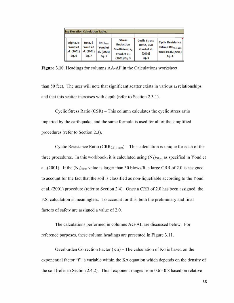
F

th

an

im

pr

th

al

to

et

F

fa

re

ex

th

Figure 3.10.

han 50 feet.

nd that this s

Cyclic

mparted by t

rocedures (r

Cyclic

hree procedu

l. (2001). If

o account for

t al. (2001) p

.S. calculatio

actors of safe

The ca

eference pur

Overb

xponential fa

he soil (refer

Headings fo

The user wi

scatter increa

c Stress Rati

the earthquak

refer to Secti

c Resistance

ures. In this

f the (N1)60cs

r the fact tha

procedure (re

on is meanin

fety are assig

alculations p

rposes, these

burden Corre

factor “f”, a v

r to Section 2

or columns A

ill note that s

ases with de

io (CSR) – T

ke, and the s

ion 2.3).

e Ratio (CRR

workbook, i

value is larg

at the soil is

efer to Secti

ngless. To a

gned a value

performed in

column hea

ection Factor

variable with

2.4.2). This

AA-AF in the

significant s

epth (refer to

This column

same formul

R7.5, 1 atm) – T

it is calculate

ger than 30 b

classified as

on 2.4). On

account for th

of 2.0.

n columns A

adings are pr

r (Kσ) – The

hin the Kσ e

f exponent r

e Calculation

catter exists

o Section 2.3

calculates th

la is used for

This calculati

ed using (N1

blows/ft, a la

s non-liquefi

nce a CRR of

his, both the

AG-AL are di

resented in F

e calculation

equation whi

ranges from

ns workshee

in various r

3.1).

he cyclic stre

r all of the si

ion is unique

1)60cs, as spec

arge CRR of

iable accordi

f 2.0 has bee

e preliminary

iscussed belo

Figure 3.11.

n of Kσ is ba

ich depends

0.6 - 0.8 ba

et.

rd relationshi

ess ratio

implified

e for each of

cified in You

f 2.0 is assign

ing to the Yo

en assigned,

y and final

ow. For

ased on the

on the densi

ased on relati

58

ips

f the

ud et

ned

oud

the

ity of

ive

F

d

d

B

th

m

b

d

co

(2

f

le

or

ar

th

fa

as

M

Figure 3.11.

ensity, as di

etermined fr

Boulanger (20

he Kσ evalua

maximum and

lows/foot, re

ensity of 80%

ounts betwee

2008) equati

value of 0.8

ess than or eq

r equal to 80

re linearly in

his correlatio

actor for Kσ

Prelim

ssessment of

MSF and Kσ

Headings fo

scussed in Y

rom the corre

008). The m

ation, accord

d minimum

espectively.

%, and blow

en 30 and 7

ion directly.

is assigned

qual to 7), an

0% (i.e. blow

nterpolated a

on is include

Equation.

minary Facto

f the factor o

factors are b

or columns A

Youd et al. (2

ected blow c

maximum an

ding to Youd

relative den

Accordingl

w counts belo

are correlate

Once relativ

to relative d

nd an f value

w counts grea

according to

ed in the Calc

or of Safety (

of safety aga

both applied

AG-AL in th

2001). There

count, (N1)60

nd minimum

d et al. (2001

sities correla

y, blow coun

ow 7 are assi

ed to relative

ve densities

densities less

e of 0.6 is as

ater than or

the relative

culation Tab

(F.S.) – This

ainst soil liqu

d to the F.S. i

e Calculatio

efore, the re

0, using Equa

relative den

1), are 80 an

ate to (N1)60

nts above 30

igned a relat

e density usi

are correlate

s than or equ

ssigned to re

equal to 30)

density of th

bles workshe

s column con

uefaction trig

in this colum

ons workshee

lative densit

ation No. 37

nsities that ar

nd 40%, resp

values of ab

0 are assigne

tive density o

ing the Idriss

ed, f can be

ual to 40% (i

elative densit

). Intermedia

he soil. The

eet titled Exp

ntains a preli

ggering at ea

mn. This F.S

et.

ty has been

7 from Idriss

re applicable

ectively. Th

bout 30 and

ed a relative

of 40%. Blo

s and Boulan

determined.

i.e. blow cou

ties greater t

ate values of

e table contai

ponential “f”

iminary

ach depth. T

S. is prelimin

59

s and

e to

hese

7

ow

nger

An

unts

than

f f

ining

”

The

nary

60

because it only considers if the soil is soft enough to liquefy, based upon SPT blow count,

and does not consider the type of soil. Cohesive soils must be further evaluated

according to the fine-grained screening criteria of Bray and Sancio (2006) to determine

the final F.S. Soil layers with a CRR of 2.0 are automatically assigned a preliminary F.S.

of 2.0. Soil layers above the water table are classified as “Unsat”, and can be assumed

non-liquefiable.

Bray and Sancio (2006) PI and wc/LL Criteria – These criteria can only be

evaluated if the proper laboratory tests have been completed. If no laboratory testing has

been performed, these columns will simply display either a “cohesive” or “cohesionless”

soil designation. It will then be up to the user to decide if the cohesive soils are

potentially liquefiable or not. If the proper laboratory tests have been completed, the

calculations performed in each column will be used to designate the soil as susceptible

(Sus), moderately susceptible (Mod Sus), or not susceptible (Not Sus) to liquefaction,

according to the Bray and Sancio (2006) criteria outlined in Section 2.5. In order for the

soil to classified as susceptible both the PI and wc/LL criteria must be met (i.e if either

the PI or wc/LL criteria classify the soil as Not Sus then the soil is not susceptible.

Final F.S. – The final factor of safety uses the preliminary factor of safety and the

fine-grained screening criteria to determine a final “factor of safety” against soil

liquefaction triggering. Possible designations in the final F.S. column include: (1) a

numerical F.S. between 0.00 - 2.00, (2) “2.00” (assigned to any soil with a preliminary

F.S. ≥ 2.00 based on high penetration resistance), (3) “Unsat” (assigned for soils above

the water table), (4) “Not Sus” (designates that the fine-grained soils were screened and

determined not susceptible in previous columns), or (5) “Cohesive” (designates that the

61

fine-grained soils have not had the proper screening tests performed and the preliminary

factor of safety is less than 1.0). Soils designated as “Cohesive” require the user to apply

engineering judgment to determine liquefaction susceptibility.

Liquefaction Occurrence Check – This column provides an easy way to visualize

the final factor of safety. Here, any numerical factor of safety greater than 1.0 is

designated “Unlikely” (meaning liquefaction is unlikely) and any factor of safety less

than 1.0 is designated “Likely” (meaning liquefaction is likely). Keep in mind that

designations of “Unlikely” or “Likely” do not relive the user of the responsibility to

exercise engineering judgment for factors of safety near unity. The designation of

“Cohesive” is carried forward for silts and clays if the preliminary F.S. is less than 1.0

and no laboratory tests have been performed to rule out liquefaction susceptibility via the

fine-grained screening criteria. For soil layers above the water table, the designation of

“Unsat” is carried forward from the final F.S. The engineer must ensure that fluctuating,

or worst-case, water levels are taken into account when the ground water level is

specified in the Input Data worksheet.

3.3.2.2 Calculation Tables

The Calculation Tables worksheet contains seven tables that are utilized within

the Calculations worksheet through lookup functions. These seven tables include: (1) N

Value - Unit Weight Correlation (Teng 1962), (2) Drill Rod Length Correction Factor,

(3) Borehole Diameter Correction Factor, (4) Stress Reduction Coefficient, (5) General

Soil Classification based on USCS, (6) Site Classification based on SPT N Value in the

top 100 ft, and (7) Exponential “f” factor for the K Equation. These tables make the

formulas in the Calculations worksheet easier to program and review. They also provide

62

the user with a visual frame of reference for how the correction factors vary as a function

of depth, blow count, etc.

3.3.3 Output and References Worksheets

This section details each of the three output worksheets. Two of these

worksheets, Boring El. and Grade El., appear nearly identical, but represent output

information relative to two different reference elevations. The Output Graphs worksheet

provides the user with graphs to aid in visualizing the analyzed data. The References

worksheet is provided so the user can locate additional details on the procedures used to

develop the workbooks if necessary.

The Output Boring El. worksheet contains data combined from the Input Data and

Calculations worksheet. This worksheet is meant to provide the user with a more

compact, printable table that contains the most important information from the

liquefaction triggering analysis relative to the boring surface elevation(refer to Figure

3.12). No data is input in this worksheet and no additional calculations are performed, it

is simply a re-organization of the input and calculations. The Output Grade El.

worksheet is identical in appearance to the Output Boring El. Worksheet. However, it

provides the user with a more compact, printable table that contains the most important

information from the liquefaction triggering analysis relative to the grade surface

elevation

The Output Graphs worksheet is designed to help the user visually decipher the

liquefaction triggering information in a quick and efficient manner. Within this

worksheet, three graphs for the boring elevation and three graphs for the grade elevation

.

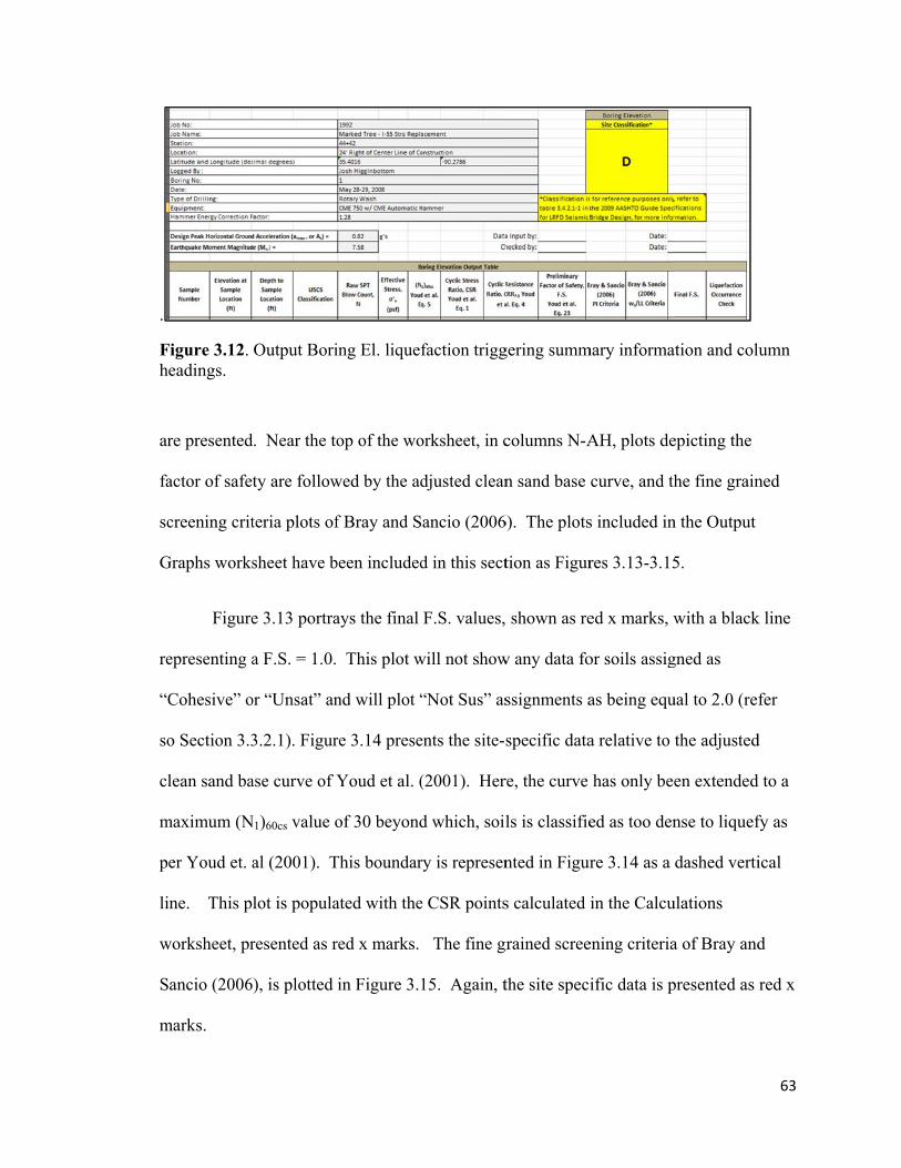
Fh

ar

fa

sc

G

re

“C

so

cl

m

p

li

w

S

m

Figure 3.12. eadings.

re presented

actor of safet

creening crit

Graphs works

Figure

epresenting a

Cohesive” o

o Section 3.3

lean sand ba

maximum (N

er Youd et. a

ine. This p

worksheet, pr

ancio (2006

marks.

Output Bori

. Near the to

ty are follow

teria plots of

sheet have b

e 3.13 portra

a F.S. = 1.0.

or “Unsat” an

3.2.1). Figur

ase curve of Y

N1)60cs value o

al (2001). T

lot is popula

resented as r

), is plotted

ing El. liquef

op of the wo

wed by the ad

f Bray and S

been included

ays the final

This plot w

nd will plot “

re 3.14 prese

Youd et al. (

of 30 beyond

This boundar

ated with the

red x marks.

in Figure 3.1

faction trigg

orksheet, in c

djusted clean

ancio (2006

d in this sect

F.S. values,

will not show

“Not Sus” as

ents the site-s

(2001). Her

d which, soil

ry is represen

e CSR points

The fine g

15. Again, t

gering summ

columns N-A

n sand base

6). The plots

tion as Figur

shown as re

w any data fo

ssignments a

specific data

re, the curve

ls is classifie

nted in Figur

s calculated

grained scree

the site speci

mary informa

AH, plots de

curve, and th

s included in

res 3.13-3.15

ed x marks, w

or soils assig

as being equ

a relative to

has only bee

ed as too den

re 3.14 as a

in the Calcu

ening criteria

ific data is p

ation and col

epicting the

he fine grain

n the Output

5.

with a black

gned as

ual to 2.0 (ref

the adjusted

en extended

nse to liquef

dashed verti

ulations

a of Bray and

presented as

63

umn

ned

k line

fer

d

d to a

fy as

ical

d

red x

F

F

Figure 3.13.

Figure 3.14.

F.S. plot inc

Clean sand b

cluded within

base curve in

n the Output

ncluded with

t Graphs wo

hin Output G

rkbook.

Graphs workksheet.

64

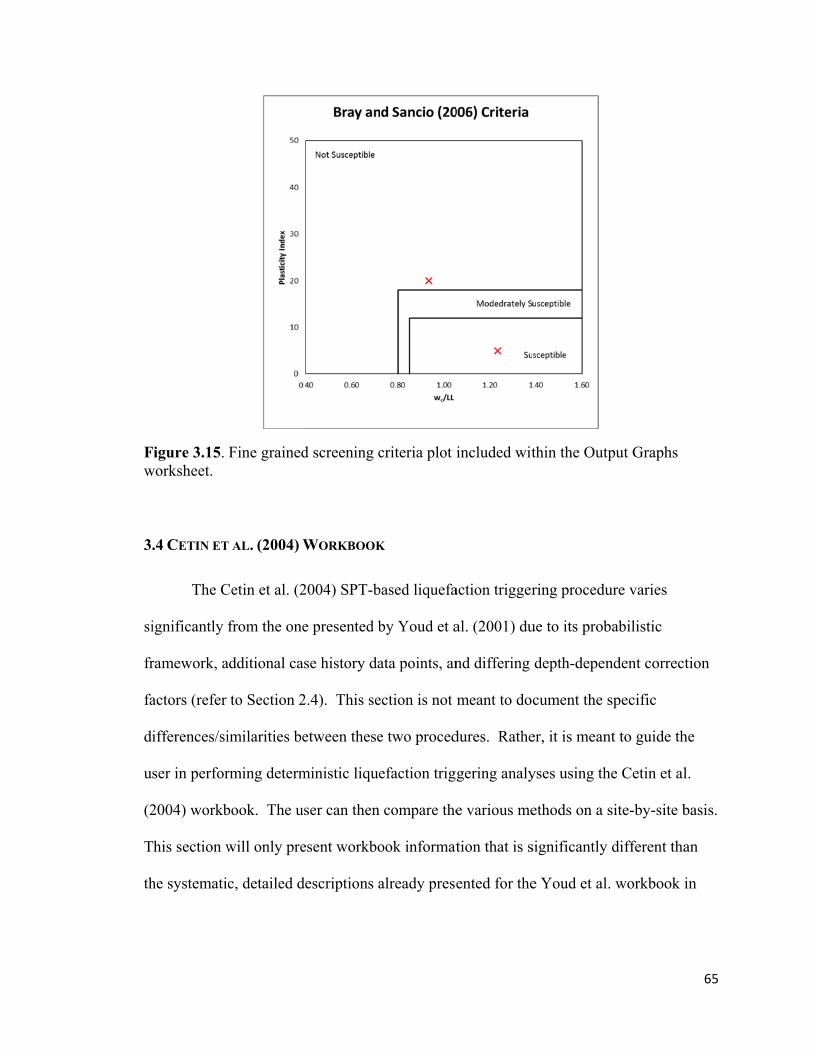
Fw

3

si

fr

fa

d

u

(2

T

th

Figure 3.15. worksheet.

.4 CETIN ET

The C

ignificantly f

ramework, a

actors (refer

ifferences/si

ser in perfor

2004) workb

This section w

he systematic

Fine grained

T AL. (2004) W

Cetin et al. (2

from the one

additional ca

to Section 2

imilarities be

rming determ

book. The u

will only pre

c, detailed d

d screening c

WORKBOOK

2004) SPT-b

e presented b

se history da

2.4). This se

etween these

ministic lique

ser can then

esent workbo

descriptions a

criteria plot i

K

based liquefa

by Youd et a

ata points, an

ection is not

e two proced

efaction trigg

compare the

ook informat

already prese

included wit

action trigger

al. (2001) du

nd differing

meant to do

dures. Rathe

gering analy

e various me

tion that is s

ented for the

thin the Outp

ring procedu

ue to its prob

depth-depen

cument the s

er, it is mean

yses using th

ethods on a s

significantly

e Youd et al

put Graphs

ure varies

babilistic

ndent correc

specific

nt to guide th

he Cetin et al

site-by-site b

different tha

. workbook i

65

tion

he

l.

basis.

an

in

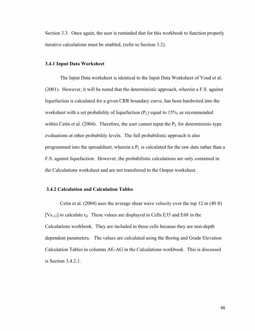
66

Section 3.3. Once again, the user is reminded that for this workbook to function properly

iterative calculations must be enabled, (refer to Section 3.2).

3.4.1 Input Data Worksheet

The Input Data worksheet is identical to the Input Data Worksheet of Youd et al.

(2001). However, it will be noted that the deterministic approach, wherein a F.S. against

liquefaction is calculated for a given CRR boundary curve, has been hardwired into the

worksheet with a set probability of liquefaction (PL) equal to 15%, as recommended

within Cetin et al. (2004). Therefore, the user cannot input the PL for deterministic-type

evaluations at other probability levels. The full probabilistic approach is also

programmed into the spreadsheet, wherein a PL is calculated for the raw data rather than a

F.S. against liquefaction. However, the probabilistic calculations are only contained in

the Calculations worksheet and are not transferred to the Output worksheet.

3.4.2 Calculation and Calculation Tables

Cetin et al. (2004) uses the average shear wave velocity over the top 12 m (40 ft)

[Vs,12] to calculate rd. These values are displayed in Cells E35 and E68 in the

Calculations workbook. They are included in these cells because they are non-depth

dependent parameters. The values are calculated using the Boring and Grade Elevation

Calculation Tables in columns AE-AG in the Calculations workbook. This is discussed

is Section 3.4.2.1.

67


Only the calculations that are different from those presented in Section 3.3.2.1 for

the Youd et al. (2001) workbook will be discussed below.

Drill Rod Length Correction Factor (CR) – The drill rod length correction factor is

obtained using Figure 7 from Cetin et al. (2004). This graphical relationship has been

digitized and is included in the Calculation Tables worksheet under the title of Drill Rod

Length Correction Factor. A lookup function is used to pull the appropriate CR from this

table based on the length of the drill rod.

Sampler Liner Correction Factor (CS) – If the sampler has been used with liners or

doesn’t have room for liners, as indicated on the Input Data worksheet (refer to section

3.3.1.3), then this value will be 1.0 at all depths. Conversely, if the sampler has room for

liners but is used without them then this correction is depth dependent, and becomes part

of the circular reference as a function of (N1)60.

Stress Correction Factor (CN) – Here, the standardized overburden blow count

correction factor is calculated based on the effective stresses in the soil column. The

relationship proposed by Liao and Whitman (1986), with a maximum permissible CN of

1.6 is employed as detailed in Section 2.4.1.

Columns headings AB-AG are all new within this worksheet and are presented in

Figure 3.16.

Fines Content for Use in the Worksheet (%) – This column assigns a fines content

between 5% and 35%. If the actual fines content is lower or higher than these values it is

set equal to 5% or 35%, respectively.

F

b

to

b

v

w

A

d

d

av

V

u

S

m

di

Figure 3.16.

Corre

ased on the p

(N1)60

o determine t

low count is

ariation from

with CRR cur

Although the

one to be mo

evelopment.

Shear

verage shear

Velocity, corr

sing a relatio

hear Wave V

meters for thi

i/VSi Shear W

. Headings f

ction for Fin

percentage o

0cs – The corr

the clean san

s used, direct

m the proced

rves modifie

procedure i

ore consisten

.

Wave Velo

r wave veloc

relates blow

onship devel

Velocity eac

is calculation

Wave Veloci

for columns A

nes (CFINES) –

of fines in th

rected blow

nd corrected

tly in the wo

dure recomm

ed for fines c

s slightly dif

nt with the o

city – This g

city over the

count to she

loped by An

ch Layer, div

n) by the she

ity, compute

AB-AG in th

– This colum

he previous c

count (N1)60

d blow count

orkbook, to c

mended in Ce

contents of 5

fferent, the c

other procedu

group of thre

top 12 m (4

ear wave vel

ndrus and Sto

vides the sam

ear wave vel

es the cumul

he Calculati

mn calculate

column.

0 is combine

t, (N1)60cs. T

compute the

etin et al. (20

5, 15 and 35%

calculated CR

ures and to s

ee columns i

40 ft). The fi

locity (in un

okoe (2000)

mple thickne

locity. The

ative di/VSi a

ons workshe

es the fines c

ed with the C

The clean san

CRR. This

004) where,

% to determ

RR is the sa

simplify the

is used to de

first column,

nits of meters

. The next c

ess (which is

third colum

as a function

eet.

content corre

CFINES correc

nd corrected

is a slight

(N1)60 is use

mine the CRR

ame. This w

workbook

termine the

Shear Wave

s per second

column, di/V

converted to

mn, Cumulativ

n of depth.

68

ection

ction

ed

R.

as

e

d)

VSi

o

ve

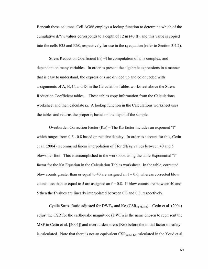
69

Beneath these columns, Cell AG66 employs a lookup function to determine which of the

cumulative di/VSi values corresponds to a depth of 12 m (40 ft), and this value is copied

into the cells E35 and E68, respectively for use in the rd equation (refer to Section 3.4.2).

Stress Reduction Coefficient (rd) –The computation of rd is complex, and

dependent on many variables. In order to present the algebraic expressions in a manner

that is easy to understand, the expressions are divided up and color coded with

assignments of A, B, C, and D, in the Calculation Tables worksheet above the Stress

Reduction Coefficient tables. These tables copy information from the Calculations

worksheet and then calculate rd. A lookup function in the Calculations worksheet uses

the tables and returns the proper rd based on the depth of the sample.

Overburden Correction Factor (Kσ) – The Kσ factor includes an exponent "f"

which ranges from 0.6 - 0.8 based on relative density. In order to account for this, Cetin

et al. (2004) recommend linear interpolation of f for (N1)60 values between 40 and 5

blows per foot. This is accomplished in the workbook using the table Exponential “f”

factor for the Kσ Equation in the Calculation Tables worksheet. In the table, corrected

blow counts greater than or equal to 40 are assigned an f = 0.6, whereas corrected blow

counts less than or equal to 5 are assigned an f = 0.8. If blow counts are between 40 and

5 then the f values are linearly interpolated between 0.6 and 0.8, respectively.

Cyclic Stress Ratio adjusted for DWFM and Kσ (CSReq M, Kσ) – Cetin et al. (2004)

adjust the CSR for the earthquake magnitude (DWFM is the name chosen to represent the

MSF in Cetin et al. [2004]) and overburden stress (Kσ) before the initial factor of safety

is calculated. Note that there is not an equivalent CSReq M, Kσ calculated in the Youd et al.

70

(2001) procedure because the MSF and Kσ factors are applied directly to the factor of

safety.

Cyclic Resistance Ratio (CRR) – The CRR in this column is calculated using a

combination of Equation 20 from Cetin et al. (2004) and Equations 2.11-2.13 in Section

2.4. However, the following variables have been fixed: (1) Mw = 7.5, (2) ’v = 1 atm, (3)

F.C. = 5%, and (4) PL = 15%. Fixing these factors essentially yields the clean sand curve

(i.e. FC < 5%) in Figure 14b of Cetin et al. (2004). The fines content is accounted for by

using (N1)60cs in the above mentioned equations instead of (N1)60. This was done in order

to be able to set a limiting upper-bound (N1)60cs in a similar manner to Youd et al. (2001)

and Idriss and Boulanger (2008) (refer to Section 2.4). Therefore, if the (N1)60cs value is

larger than 35, a large CRR of 2.0 is assigned to account for the fact that the soil is

essentially considered non-liquefiable.

Probabilistic Evaluation – The column headings for the probabilistic evaluation

performed in columns AR and AS are presented in Figure 3.17. These calculations are

included in the worksheet for completeness, but none of the probabilistic information is

transferred to the output worksheets (refer to Section 3.4.1). The initial PL is the

probability without taking into account the soil type, whereas the final PL uses the fine-

grained screening criteria and the initial PL in a similar manner to that described for the

preliminary and final F.S. in the Youd et al. (2001) workbook.

The changes to the Calculation Tables worksheet include; an updated CR table and

chart, a DWFM/MSF table and chart, Stress reduction coefficient tables and equations

F

p

d

3

(2

fo

si

o

M

C

ar

an

S

b

Figure 3.17.

lus the table

iscussed pre

.4.3 Output

Both o

2004) as they

or each samp

imilar to Fig

f 0.6. This i

Madrid Seism

CRR/CSR we

round a CSR

nd the area t

ection 2.4. T

etween lique

Headings in

titled Expon

eviously.

t and Refere

of the Boring

y are for Yo

ple elevation

gure 14b in C

is necessary

mic Zone tran

ere a maxim

R=0.4. This

that has been

The vertical

efiable and n

n columns AR

nential “f” fa

ences Work

g and Grade

ud et al. (20

n, similar to Y

Cetin et al. (2

because the

nsmit to larg

mum of 0.6. N

represents th

n programme

dashed line

non-liquefiab

R and AS in

factor for Kσ

ksheets

e elevation w

01). The Ou

Youd et al. (

2004), but w

relatively la

ger CSR valu

Notice the br

he line Cetin

ed by the aut

in Figure 3.

ble material

n the Calcula

σ Equation. A

worksheets ar

utput Graph

(2001). The

with a maxim

arge design g

ues than wou

reak in natur

n et al. (2004

thor accordi

.18, represen

(refer to Sec

ations worksh

All of which

re the same

worksheet i

e CRR plot (

mum CRR/CS

ground moti

uld be visibl

ral slope of t

4) have draw

ing to Equati

nts the interp

ction 2.4).

heet.

h have been

for Cetin et

includes grap

Figure 3.18)

SR of 1.0 in

ons in the N

le if the

the CRR cur

wn in by han

ions 2.11-2.

preted cutoff

71

al.

phs

) is

stead

New

rve

nd,

14 in

f

Fw

3

th

an

C

eq

on

en

cl

th

Figure 3.18. worksheet.

.5 IDRISS AN

Like

han the Youd

nd Boulange

Correlations t

quations for

ne for the cl

nables the en

lays and silts

hat the iterat

Plot of the c

ND BOULANG

Section 3.3,

d et al. (2001

er (2008) wo

that is discus

many of the

ay-like crite

ngineer to qu

s separate fr

ive calculati

clean sand co

GER (2008)

only portion

1) workbook

orkbook cont

ssed further

e factors asso

eria and one f

uantify the li

om tradition

ions box is c

orrected curv

ns of this wo

k will be disc

tains an entir

in Section 3

ociated with

for the sand-

iquefaction s

nal sandy soi

checked (refe

ve included

orkbook that

cussed herei

re extra wor

3.5.3. Also, t

h the liquefac

-like criteria

susceptibilit

ils. Before u

er to Section

in the Outpu

t are signific

in. For exam

rksheet titled

this procedu

ction triggeri

a (refer to Se

ty (cyclic mo

using this wo

n 3.2).

ut Graphs

cantly differe

mple, the Idr

d SPT Su

ure includes

ing evaluatio

ection 2.5). T

obility) of pl

orkbook, ens

72

ent

iss

two

on:

This

lastic

sure

73

3.5.1 Input Data Worksheet

Column J in the Input Data worksheet has been changed from in-situ water

content to undrained shear strength of the soil (Su). This change is subtle and the user

must be careful not to paste the in-situ water content data into this column from previous

(i.e. Youd et al. [2001], and Cetin et al. [2004]) liquefaction evaluation workbooks. The

undrained shear strength (Su) is only applicable to cohesive soils, and should only be

entered if the proper laboratory tests have been performed to accurately determine Su. If

the proper laboratory tests have not been performed, this column should be left blank and

a Su will be estimated based on a correlation with SPT blow count (refer to Section

3.5.3).

3.5.2 Calculations and Calculation Table Worksheets

The user will note that two magnitude scaling factors are calculated in the Idriss

and Boulanger (2008) Calculations worksheet instead of just one, like in the Youd et al.

(2001) and Cetin et al. (2004) workbooks. Two magnitude scaling factors are necessary

because the relationship between the CSR and the number of loading cycles to failure is

flatter for clays than sands (Idriss and Boulanger 2008). The Calculation Tables

worksheet provides six tables, five of which have been previously discussed. The only

table not mentioned is the Stress Reduction Coefficient, which will be discussed in

Section 3.5.2.1.


The remaining calculations are all depth dependent and are associated with a

given SPT sample location. Once again, the Calculations worksheet is populated with

74

more columns than the Input Data worksheet (i.e. from column K through column AO).

Only the columns that are different from the Youd et al. (2001) workbook will be

discussed further.

Clay-like or Sand-like Behavior – This column categorizes the soil as Clay-like or

Sand-like depending on the USCS classification and the PI of the soil (refer to Section

2.5). The Clay-like or Sand-like designation determines if the soil will be analyzed

according to liquefaction (i.e. sand-like) criteria or the newly developed cyclic softening

(i.e. clay-like) criteria. If the proper index tests have not been performed to determine the

soil PI, this column will simply designate any clay or silt as Cohesive. These Cohesive

soils will be evaluated for liquefaction susceptibility by assuming cyclic softening

behavior, but will not be given the designation of Clay-like since the PI was not directly

measured.

Sampler Liner Correction Factor (CS) –This correction factor is depth dependent

and is a part of a circular reference as a function of (N1)60.

N60 – This column differs from the N60 Only Corrected for Energy column, which

is used to correlate unit weight. It calculates the blow count corrected for all variables

except CN, and is the blow count used to correlate Su. This correlation excludes CN

because the SPT blow count – Su correlations employed herein were developed without

CN.

Estimated Undrained Shear Strength of the Soil (Su) – This column estimates the

undrained shear strength for cohesive or clay-like soils based on N60. The correlation of

Kulhawy and Mayne (1990) is employed in the workbook and is presented below as

75

Equation 3.1. It has also been graphed and is included in the worksheet SPT Su

Correlations along with several other SPT-Su correlations. Kulhawy and Mayne (1990)

state “Correlations have been attempted for estimating Su from SPT N values, even

though it is known that these correlations are weak”. Despite this warning, the

correlations between SPT blow count and Su are often times the only way of estimating

Su and must be employed in order to determine a factor of safety for the liquefaction

susceptibility of clays and silts. Measured undrained shear strength data entered in the

Input Data worksheet will override this correlation.

∗ 0.6 ∗ Equation 3.1

Stress Correction Factor (CN) –The equation used to calculate CN is a function of

(N1)60 and is the second circular reference in the Calculations worksheet of Idriss and

Boulanger (2008).

Δ(N1)60 – This column calculates Δ(N1)60, which is the change in blow count

according to the percentage of fines. This is added to (N1)60 to determine (N1)60cs.

Stress Reduction Coefficient (rd) – Similar to Youd et al. (2001) this column uses

a lookup function to determine rd from a table in the Calculation Tables worksheet,

except here, the rd table is populated by employing Equations 2.5-2.7 (refer to Section

2.3.1). The maximum recommended depth for which this rd correlation should be used,

due to the increasing uncertainty with increasing depth, is 20 m (65 ft). Idriss and

Boulanger (2008) state “Liquefaction evaluations at greater depths often involve special

conditions for which more detailed analyses can be justified”. Despite this

recommendation, this workbook employs the rd relationship to a depth of 36 m (120 ft).

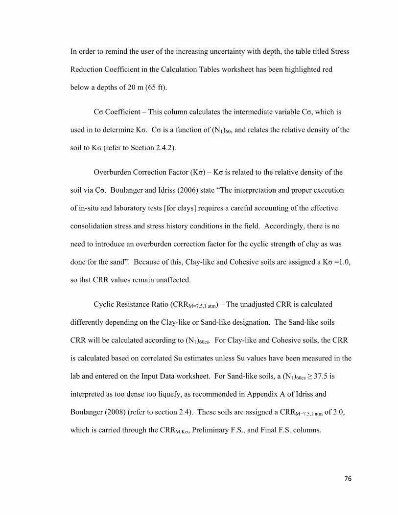
76

In order to remind the user of the increasing uncertainty with depth, the table titled Stress

Reduction Coefficient in the Calculation Tables worksheet has been highlighted red

below a depths of 20 m (65 ft).

Cσ Coefficient – This column calculates the intermediate variable Cσ, which is

used in to determine Kσ. Cσ is a function of (N1)60, and relates the relative density of the

soil to Kσ (refer to Section 2.4.2).

Overburden Correction Factor (Kσ) – Kσ is related to the relative density of the

soil via Cσ. Boulanger and Idriss (2006) state “The interpretation and proper execution

of in-situ and laboratory tests [for clays] requires a careful accounting of the effective

consolidation stress and stress history conditions in the field. Accordingly, there is no

need to introduce an overburden correction factor for the cyclic strength of clay as was

done for the sand”. Because of this, Clay-like and Cohesive soils are assigned a Kσ =1.0,

so that CRR values remain unaffected.

Cyclic Resistance Ratio (CRRM=7.5,1 atm) – The unadjusted CRR is calculated

differently depending on the Clay-like or Sand-like designation. The Sand-like soils

CRR will be calculated according to (N1)60cs. For Clay-like and Cohesive soils, the CRR

is calculated based on correlated Su estimates unless Su values have been measured in the

lab and entered on the Input Data worksheet. For Sand-like soils, a (N1)60cs ≥ 37.5 is

interpreted as too dense too liquefy, as recommended in Appendix A of Idriss and

Boulanger (2008) (refer to section 2.4). These soils are assigned a CRRM=7.5,1 atm of 2.0,

which is carried through the CRRM,Kσ, Preliminary F.S., and Final F.S. columns.

77

Cyclic Resistance Ratio adjusted for MSF and Kσ (CRRM,Kσ) – The CRRM,Kσ is

also adjusted differently according to the Sand-like or Clay-like designations. This is

accomplished by employing different MSF and Kσ values, as discussed in this Section,

and in Section 3.5.2.

Clay-like or Sand-like Behavior – This column is repeated here to remind the user of the

soil type, and help determine the final factor of safety classification. If the soil is

Cohesive and has not had the proper laboratory index tests performed, then this column

will return the designation of Cohesive rather than Clay-like.

Final F.S. – Here, there are four possible designations, they include; (1) a

numerical F.S. between 0.00 - 2.00, (2) “2.00” (assigned to any soil with a preliminary

F.S. ≥ 2.00 based on high penetration resistance), (3) “Unsat” (assignment for soils above

the water table), or (4) “Cohesive” (designates that the fine-grained soils have not had the

proper laboratory tests performed and the preliminary factor of safety is less than 1.0).

Soils designated as “Cohesive” require the user to apply engineering judgment to

determine liquefaction susceptibility.

3.5.3 SPT Su Correlation Worksheet

This worksheet includes four different SPT-Su correlations. A plot in the

worksheet is presented below as Figure 3.19. It presents four correlations between SPT

blow count and Su. The uncertainty in this correlation is evident based on the large

differences of the various relationships. The red line indicates the correlation used by

some AHTD personnel (Personal Communication, Steven Peyton, August, 2010). It is

the same correlation as Kulhawy and Mayne (1990), and is the correlation employed to

F

es

(1

av

st

co

ad

6

sh

u

co

Figure 3.19.

stimate Su in

1990) used N

vailable to th

tudy N60 has

ommon use

djusted to an

0%) for use

hear strength

sed to estim

orrelation cu

SPT blow co

n the Calcula

N instead of

hem at the ti

s been used b

have hamme

n efficiency t

in older corr

h, N60 is used

ate Su, but in

urrently emp

ount, Su cor

ations works

N60 in their

ime did not i

because man

er efficiencie

that was mo

relations. Th

d herein. Ot

n the author

ployed.

rrelations plo

sheet (refer t

original corr

indicate a sta

ny of the auto

es greater th

re common

herefore, for

ther correlati

’s opinion, p

ot in the SPT

to Section 3.

relation beca

andard energ

omatic hamm

han 80%. The

in older ham

r the purpose

ions are pres

provide no b

T Su Correla

.5.2.1). Kul

ause much o

gy level. Ho

mers which

ese raw N va

mmers (i.e. a

e of estimati

sented in the

better approx

ations worksh

hawy and M

of the data

owever, in th

are now in

alues must b

approximatel

ing undraine

e figure coul

ximation than

78

heet.

Mayne

his

be

ly

ed

ld be

n the

79

3.5.4 Output and Reference Worksheets

The Output Boring El., and Output Grade El. worksheets are the same as in the

Youd et al. (2001) workbook. The Output Graphs worksheet includes a F.S. plot but

does not include the plot for fine grained screening criteria proposed by Bray and Sancio

(2006). A plot representing the clean sand CRR curve recommended by Idriss and

Boulanger (2008) is included in the Output Graphs worksheet and is included here as

Figure 3.20. The red x’s denote the calculated CSR values and the vertical dashed line

represents the interpreted cutoff between liquefiable and non-liquefiable material (refer to

Section 2.4).

3.6 CONCLUSIONS

The three most commonly used SPT-based liquefaction triggering procedures

(Youd et al. 2001, Cetin et al. 2004, and Idriss and Boulanger 2008) have been

programmed into Microsoft Excel workbooks. This chapter has reviewed the workbooks,

and has provided direction about how to complete an SPT-based liquefaction

susceptibility evaluation using the workbooks. This chapter is meant to supplement the

workbooks and the comments therein.

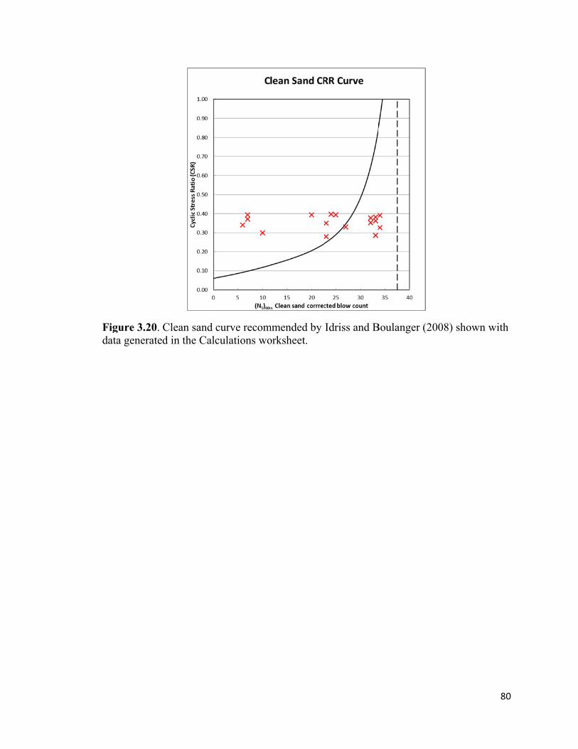
Fd

Figure 3.20. ata generate

Clean sand cd in the Calc

curve recomculations wo

mmended by orksheet.

Idriss and B

Boulanger (20008) shown

80

with

81

Chapter 4

Site-Specific Comparisons

4.1 INTRODUCTION

Many complicated and inter-related variables are calculated for each of the three

SPT-based liquefaction triggering procedures (i.e. Youd et al. [2001], Cetin et al. [2004],

and Idriss and Boulanger [2008]). General differences between some of these variables

have been discussed in Chapter 2 for simplified conditions. However, the interaction

between many of these variables is complex, and it can be difficult to determine how

fluctuations in a single variable impact the final F.S. against liquefaction triggering. In

order to determine how these variables interact to yield differences in the F.S. predictions

for the three SPT-based liquefaction triggering procedures, site-specific comparisons

have been made for a number of SPT borings at actual bridge sites in eastern Arkansas.

The boring logs from these sites were provided by AHTD (refer to Section 1.3).

4.2 SITE-SPECIFIC COMPARISONS

This section will present site-specific comparisons of the SPT-liquefaction

triggering procedures for three different bridge sites in eastern Arkansas (refer to Figure

4.1). The discussion of each site will begin by comparing the F.S. for each of the three

procedures as a function of depth/vertical effective stress. In order to clarify any

potential confusion, the “final” F.S. discussed in Section 3.3.2.1 is the only one used for

comparison in this chapter, and will simply be denoted herein as the F.S. Note that a F.S.

= 2.0 is assigned based on high penetration resistance or a designation of “Not Sus”.

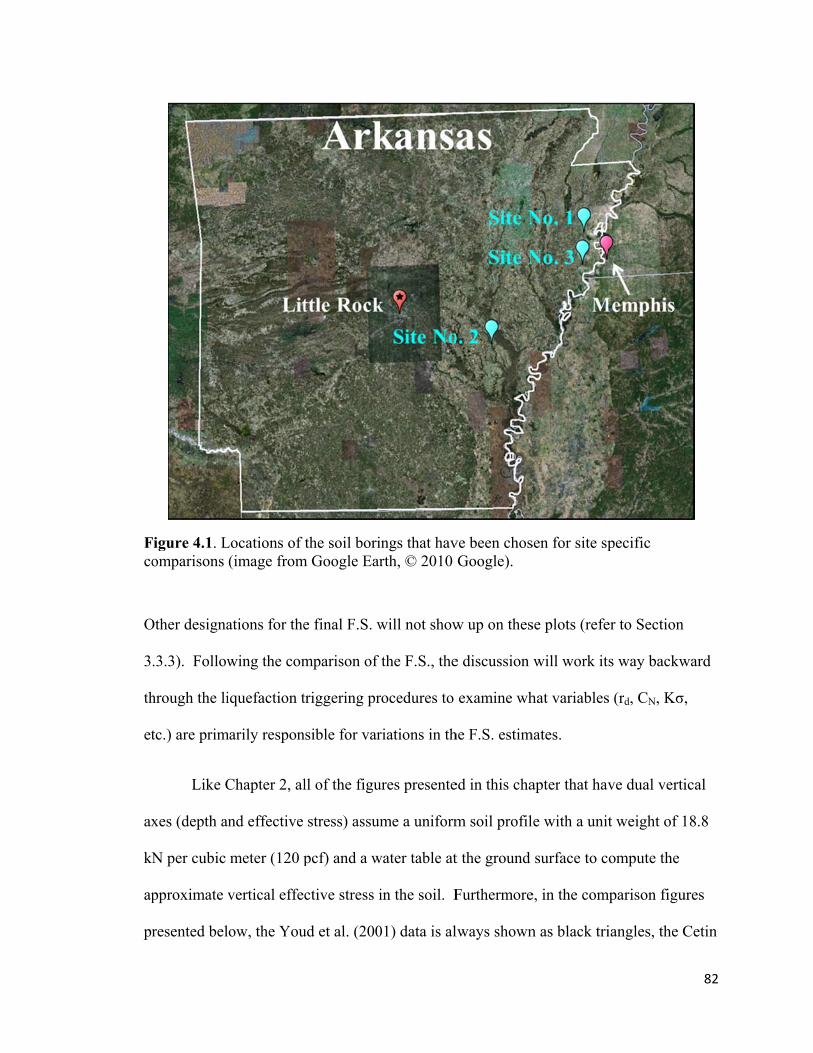
Fco

O

3

th

et

ax

kN

ap

pr

Figure 4.1. Lomparisons

Other designa

.3.3). Follow

hrough the li

tc.) are prim

Like C

xes (depth an

N per cubic

pproximate v

resented bel

Locations of (image from

ations for the

wing the com

iquefaction t

marily respon

Chapter 2, al

nd effective

meter (120 p

vertical effe

ow, the You

the soil borim Google Ear

e final F.S. w

mparison of

triggering pr

nsible for var

ll of the figu

stress) assum

pcf) and a w

ctive stress i

ud et al. (200

ings that havrth, © 2010

will not show

the F.S., the

rocedures to

riations in th

ures presente

me a uniform

water table at

in the soil. F

01) data is al

ve been chosGoogle).

w up on thes

e discussion

examine wh

he F.S. estim

ed in this cha

m soil profil

t the ground

Furthermore

lways shown

sen for site sp

se plots (refe

will work it

hat variables

mates.

apter that hav

le with a unit

surface to c

e, in the com

n as black tri

pecific

er to Section

s way backw

s (rd, CN, Kσ

ve dual verti

t weight of 1

ompute the

mparison figu

iangles, the C

82

ward

,

ical

18.8

ures

Cetin

83

et al. (2004) data is shown as green squares, and the Idriss and Boulanger (2008) data is

shown as red circles.

4.2.1 Site No. 1

Site No. 1 is located near Gilmore, Arkansas. The soil conditions are classified as

Site Class D based on the measured SPT blow counts. The site-adjusted design peak

horizontal ground acceleration (amax) with a 7% probability of exceedance in 75 years for

this site is 0.82 g and the estimated moment magnitude (MW) is 7.58 (refer to Section

3.3.1.1). The soil is mostly clay from the surface to a depth of 6 m (20 ft), beneath the

clay a sandy layer is present to the depth of 33 m (110 ft) followed by a stiff clay to 37 m

(120 ft).

The F.S. values for each of the three procedures (refer to Figure 4.2) agree very

well for all depths down to 24 m (80 ft). However, at depths greater than 24 m (80 ft) the

F.S. values begin to separate from one another, with the F.S. from the Idriss and

Boulanger (2008) procedure being consistently greater than the others. Despite this, the

only depths where the three procedures actually yield a different prediction for

liquefaction triggering are at 24 m (80 ft) and from 29-32 m(95-105 ft), where the Idriss

and Boulanger (2008) procedure produces a F.S. > 1.0 and the other two procedures do

not. In order to understand the driving cause for this variation in F.S. at depth, some of

the depth dependent variables(rd, CN, Kσ, ect.) are examined below.

Figure 4.3 presents the variable rd for each of the three procedures. The

relationship of Idriss and Boulanger (2008) consistently yields the highest rd values and

Ffo

F

Figure 4.2.Coor all three s

Figure 4.3.Co

omparison oimplified pr

omparison o

of the factor ocedures.

of the rd valu

of safety aga

ues at Site No

ainst liquefa

o. 1 for all th

action trigger

hree simplifi

ring at Site N

fied procedur

84

No.1

res.

85

the Cetin et al. (2004) procedure produces the lowest values. At least two interesting

things are noted by examining Figure 4.3 relative to Figure 4.2: (1) despite significant

differences in rd values over virtually the entire depth range (most significantly around

15m [50 ft], where the rd values vary by 45%), the F.S. values are nearly identical for all

procedures down to a depth of 24 m (80 ft), and (2) lower rd values directly result in

lower CSR values(refer to Figure 4.4) according to Equation 2.2, thereby leading one to

assume higher F.S. estimates would be obtained from those procedures with the lowest

CSR values according to Equation 2.1; this trend is not observed.

Figure 4.4 presents the unadjusted CSR (CSRM=7.5, 1 atm) for each of the three

procedures. Notice the extremely high CSRM=7.5, 1 atm values, all of which exceed 0.4 and

many of which exceed 0.6. This is a concern because the liquefaction case history data

points used in the development of these procedures nearly all have CSR values less than

0.4 (refer to Figures 2.1, 2.5, and 2.6); the applicability of simplified procedures for CSR

values greater than 0.5 is of uncertain validity. Obviously, due to the direct relationship

between rd and CSR, the same trends discussed relative to Figure 4.3 are apparent in

Figure 4.4 (i.e. very significant differences between procedures ranging up to 45% at a

depth of 15 m [50 ft]). However, as noted above, these differences do not necessarily

result in significant variations in the F.S. estimates at equivalent depths.

Additionally, contrary to expectations, the procedure with the highest CSR values

(Idriss and Boulanger 2008) also yields the highest F.S. below 24 m (80 ft). It will be

noted that one reason higher rd and CSR values do not translate directly into lower F.S.

estimates (and vice-versa) is that the CRR boundary curves for each method were

developed using the rd relationships recommended in their respective procedure.

Fpr

T

u

v

at

Id

in

F

a

or

in

Figure 4.4. Crocedures.

Therefore, the

s that rd estim

Figure

alues agree q

tm [1000-40

driss and Bo

nterestingly m

igure 4.2). O

depth of 33

rder to unde

nspected.

Comparison o

e CSR value

mates should

e 4.5 present

quite well ov

000 psf]). Ho

ulanger (200

mirroring th

One importa

.5 m (110 ft)

rstand what

of the CRRM

es and CRR c

d not be mix

ts the variab

ver the depth

owever, at d

08) range fro

he deviation i

ant point that

), which is c

drives these

M=7.5, 1 atm val

curves are d

xed across pr

le CN for eac

h range of 5-

depths greate

om 25-60%h

in the F.S. v

t will be not

ontrary to th

e differences

lues at Site N

directly linke

rocedures (S

ch of the thr

-21 m (15-70

er than 23 m

higher than t

values below

ted is the clo

he general tre

s/similarities

No. 1 for all

ed to one ano

Seed 2010).

ree procedur

0 ft) (approx

m (75 ft), the

the other pro

w this same d

ose agreemen

end observe

s the SPT blo

three simpli

other, remind

res. The CN

ximately 0.47

CN values of

ocedures,

depth (refer t

nt in CN valu

d at depth. I

ow count mu

86

ified

ding

7-1.9

f

to

ues at

In

ust be

F

(N

ob

ea

T

li

3

an

pr

m

A

d

Figure 4.5.Co

CN, al

N1)60cs value

btain the una

ach of the th

The three das

iquefiable m

0 for Youd e

nd Boulange

rocedures ag

m (30 ft), wh

At depths gre

ifferences be

omparison o

long with the

es (according

adjusted CR

hree procedu

shed vertical

aterial for th

et al. (2001),

er (2008). A

gree quite we

ere the corre

eater than 21

etween (N1)6

of the CN val

e other blow

g to Equation

RR (CRRM=7.

ures. The raw

lines repres

he each of th

, (N1)60cs = 3

At depths less

ell, with the

ected blow c

m (70 ft), e

60cs values fo

lues at Site N

w count corre

n 2.15) used

5,1atm). Figu

w N values a

sent the boun

he SPT proce

35 for Cetin

s than 21 m

largest diffe

counts are all

xcluding the

or each of th

No. 1 for all

ection factors

d in the determ

ure 4.6 prese

are also prov

ndaries betw

edures (refer

et al. (2004)

(70 ft), the (

ference of 13

l greater than

e (N1)60csvalu

he procedure

three simpli

s, directly in

rministic SPT

ents the (N1)

vided for refe

ween liquefia

r to Section 2

), and (N1)60c

(N1)60cs value

3% occurring

n 40 and too

ue at 34 m (

s begin to in

ified procedu

nfluences the

T-procedure

60cs values fo

ference purpo

able and non-

2.4): (N1)60cs

cs = 37 for Id

es for each o

g at a depth o

o stiff to liqu

110 ft), the

ncrease, with

87

ures.

e

s to

or

oses.

-

s =

driss

of the

of 9

uefy.

h the

Fpr

sm

Y

B

F

B

co

p

th

ar

H

b

h

Figure 4.6.Corocedures.

mallest diffe

Youd et al. (2

Boulanger (20

urthermore,

Boulanger (20

onsistently c

articularly im

han about 23

re in closer a

However, wh

ecome signi

igher F.S. es

omparison o

erence betwe

2001) proced

008) procedu

at depths gr

008) procedu

corrected bel

mportant to n

3,the CN and

agreement w

hen the N val

ficantly larg

stimates. It a

of the (N1)60c

een procedur

dure always

ure yields th

reater than 2

ure have bee

low the raw

note that wh

(N1)60cs valu

with the other

lue at depth

ger than the o

appears that t

cs values at S

res being 34%

yields the lo

he highest, di

4 m (80 ft),

en corrected

N values for

hen the depth

ues for the Id

r procedures

is greater th

others, result

the procedur

Site No. 1 fo

% at 26 m (8

owest (N1)60c

directly follow

the (N1)60cs v

d above the ra

r the other tw

h is significa

driss and Bo

s (refer to Fi

han about 23

ting in highe

res would yi

r all three si

85 ft). At th

cs values, wh

wing the CN

values for th

aw N values

wo procedur

ant and the N

oulanger (20

gures 4.5 an

their CN and

er CRR valu

ield much m

mplified

hese depths, t

hile the Idris

N trends.

he Idriss and

s, while they

res. It is

N value is les

08) procedu

nd 4.6).

d (N1)60csval

ues and, henc

more similar

88

the

s and

d

y are

ss

ure

ues

ce,

89

results if the Idriss and Boulanger (2008) equation for CN was not dependent on blow

count (specifically, iterative with (N1)60). This comment should not be misconstrued to

mean that the Idriss and Boulanger (2008) equation for CN is not valid. It simply means

that CN appears to have a very strong influence on the agreement/disagreement of the

techniques at depth.

Figure 4.7 presents the unadjusted Cyclic Resistance Ratio (CRRM=7.5,1atm) for

each of the three procedures. The CRRM=7.5,1atm relationship, like CN, mirrors the

deviations in the F.S. estimates, with the Idriss and Boulanger (2008) procedure yielding

the highest values. It will be noted that CRRM=7.5,1atm still needs to be adjusted

(multiplied) by the MSF and Kσ factors to obtain the adjusted CRR (CRRM, Kσ). Because

the design magnitude from the NMSZ, in eastern Arkansas is close to 7.5, and all of the

procedures have very similar MSF for Mw > 7.0 (refer to Section 2.4.3), the MSF are not

responsible for any of the variations in F.S. However, the various Kσ relationships do

have an impact.

Figure 4.8 presents the Kσ values for each of the three procedures. At depths

between 11-21 m (35-70 ft), the Kσ values of Idriss and Boulanger (2008) are higher than

the other procedures. For example, at a depth of 15 m (50 ft) the Kσ values differ by

10%, while the F.S. values are within 6% of one another(refer to Figure 4.2). This

indicates that while noticeable differences exist in the Kσ relationships, they do not have

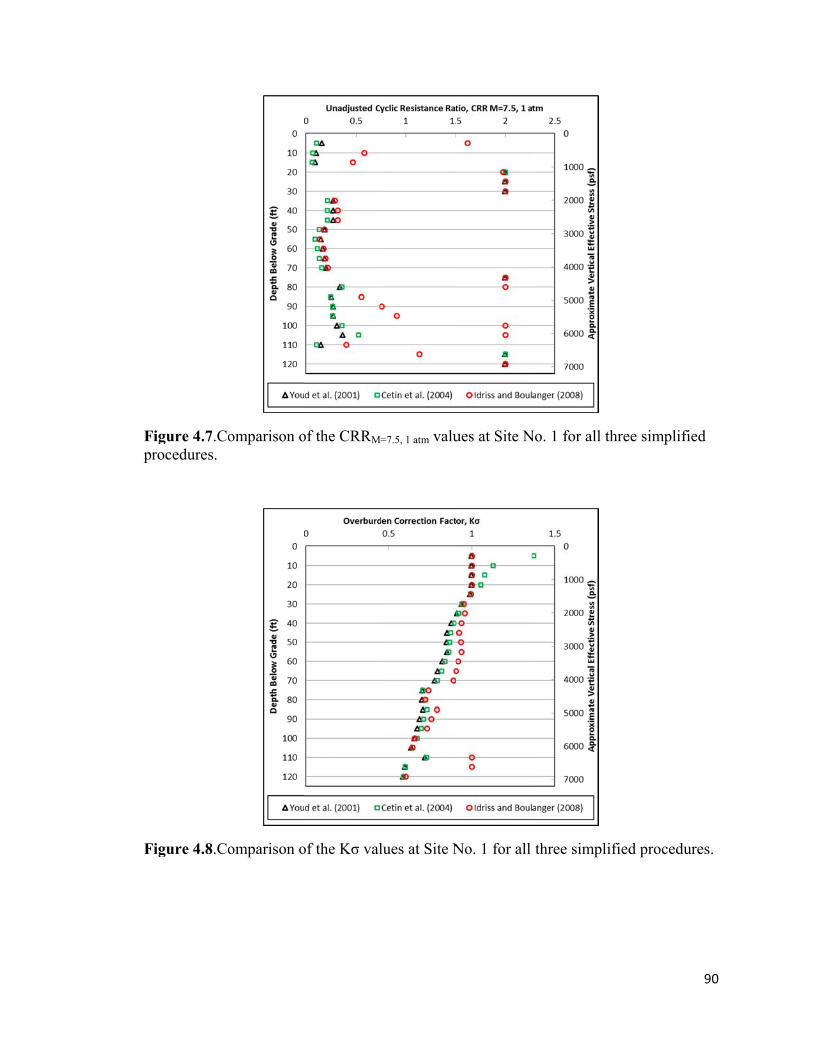
Fpr

F

Figure 4.7.Corocedures.

Figure 4.8.Co

omparison o

omparison o

of the CRRM

of the Kσ val

M=7.5, 1 atm valu

lues at Site N

ues at Site N

No. 1 for all

No. 1 for all t

three simpli

three simplif

ified procedu

90

fied

ures.

91

a very significant impact on the variations in F.S. at depth. While not a main focus of

this research, it will be noted that the shallow Kσ values can vary significantly between

procedures based on the choice of a limiting upper value (refer to Section 2.4.2).

Additionally, it will be noted that the Idriss and Boulanger (2008) Kσ values are equal to

1.0 at depths of 33.5 and 35 m (110 and 115 ft) because these are “clay-like” soils (refer

to Section 3.5.2.1).

In summary, the F.S. values for each of the three procedures at Site No. 1 (refer to

Figure 4.2) agree very well for all depths down to 24 m (80 ft). However, at depths

greater than 24 m (80 ft) the F.S. values begin to disperse from one another, with the F.S.

from the Idriss and Boulanger (2008) procedure being consistently greater than the

others. Despite this, the only depths where the three procedures actually yield a different

prediction for liquefaction triggering are at 24 m (80 ft) and from 29-32 m (95-105 ft),

where the Idriss and Boulanger (2008) procedure produces a F.S. > 1.0 and the other two

procedures do not. It appears that variations in the overburden blow count correction

factor (CN) are primarily responsible for the differences in the F.S. estimates at these

depths. At depths above 24 m (80 ft) the CN values are generally within 7% of one

another, while at greater depths the CN values of Idriss and Boulanger are generally 25-

50% greater. These differences primarily occur for N values greater than about 23 and

are driven by the Idriss and Boulanger (2008) equation for CN, which is an iterative

function of (N1)60. Kσ also plays a role in the variation of F.S. at depth, but its impact is

less significant than that of CN. For example, Kσ values vary by as much as 14% at

depths between 11-21 m (35-70 ft). However, there are very minimal differences in the

F.S. at these depths. At depths greater than 24 m (80 ft), the Kσ values of Idriss and

92

Boulanger (2008) are generally less than 12% different, but can contribute to significant

differences in F.S. when combined with the higher CN values over this depth range. In

general, when the deterministic liquefaction triggering procedures do not all agree about

the potential for liquefaction triggering (i.e. F.S. < 1.0), the author recommends going

with the prediction supported by two out of the three procedures.

4.2.2 Site No. 2

Site No. 2 is located near LaGrue, Arkansas. The soil conditions are classified as

Site Class D based on the measured SPT blow counts. The site-adjusted design peak

horizontal ground acceleration (amax) with a 7% probability of exceedance in 75 years for

this site is 0.34 g and the estimated Mw is 7.46 (refer to Section 3.3.1.1). The soil is

mostly clayey-silt (CL-ML) from the surface to a depth of 5 m (15 ft), beneath the

clayey-silt a silty-sand (SM) layer is present to the depth of 24 m (80 ft) followed by a

another silty-sand layer with fewer fines (SW-SM) to 30 m (100 ft).

The F.S. values for each of the three procedures are included as Figure 4.9.

Liquefaction is consistently predicted to occur in three isolated layers between the depths

of 6-7.5, 23-24, and 29-30 m (20-25, 75-80, and 95-100 ft). Although numerical

differences in the F.S. values are calculated for each procedure, the only depths were

liquefaction triggering evaluations disagree are at 20 and 27 m (65 and 90 ft). At depths

were liquefaction is predicted, the Cetin et al. (2004) procedure yields the lowest F.S.,

while the Youd et al. (2001) procedure yields the highest F.S., except at a depth of 29 m

(95 ft). This trend is different from the F.S. values presented for Site No. 1. (refer to

Figure 4.2), where the Idriss and Boulanger (2008) F.S. values were consistently the

Ffo

h

d

gr

h

al

(2

w

E

2

Figure 4.9.Coor all three s

ighest. Exam

etermine the

Figure

reater than 1

ighest rd valu

l. (2004) yie

2001) proced

with depth, bu

Even though

6% at a dept

omparison oimplified pr

mination of

e cause of th

e 4.10 presen

12 m (40 ft) t

ues, while at

elds the lowe

dure yields t

ut generally

the rd values

th of 30 m (1

of the factor ocedures.

the depth de

e variation in

nts the varia

the relations

t depths betw

est rd values.

the lowest rd

are in the ra

s of Youd et

100 ft), the F

of safety aga

ependent var

n F.S. value

able rd for eac

ship of Idriss

ween 6-18 m

At depths g

values. The

ange of 25%

al. (2001) a

F.S. values a

ainst liquefa

riables (rd, C

s.

ch of the thr

s and Boulan

m (20-60 ft) t

greater than

e maximum

at depths gr

and Idriss and

at this depth

action trigger

CN, Kσ, ect.),

ree procedur

nger (2008) y

the relations

20 m (65 ft)

differences

reater than 1

d Boulanger

are nearly id

ring at Site N

, will help

res. At depth

yields the

ship of Cetin

) the Youd e

in rd are var

5 m (50 ft).

r (2008) diff

dentical.

93

No.2

hs

n et

t al.

riable

fer by

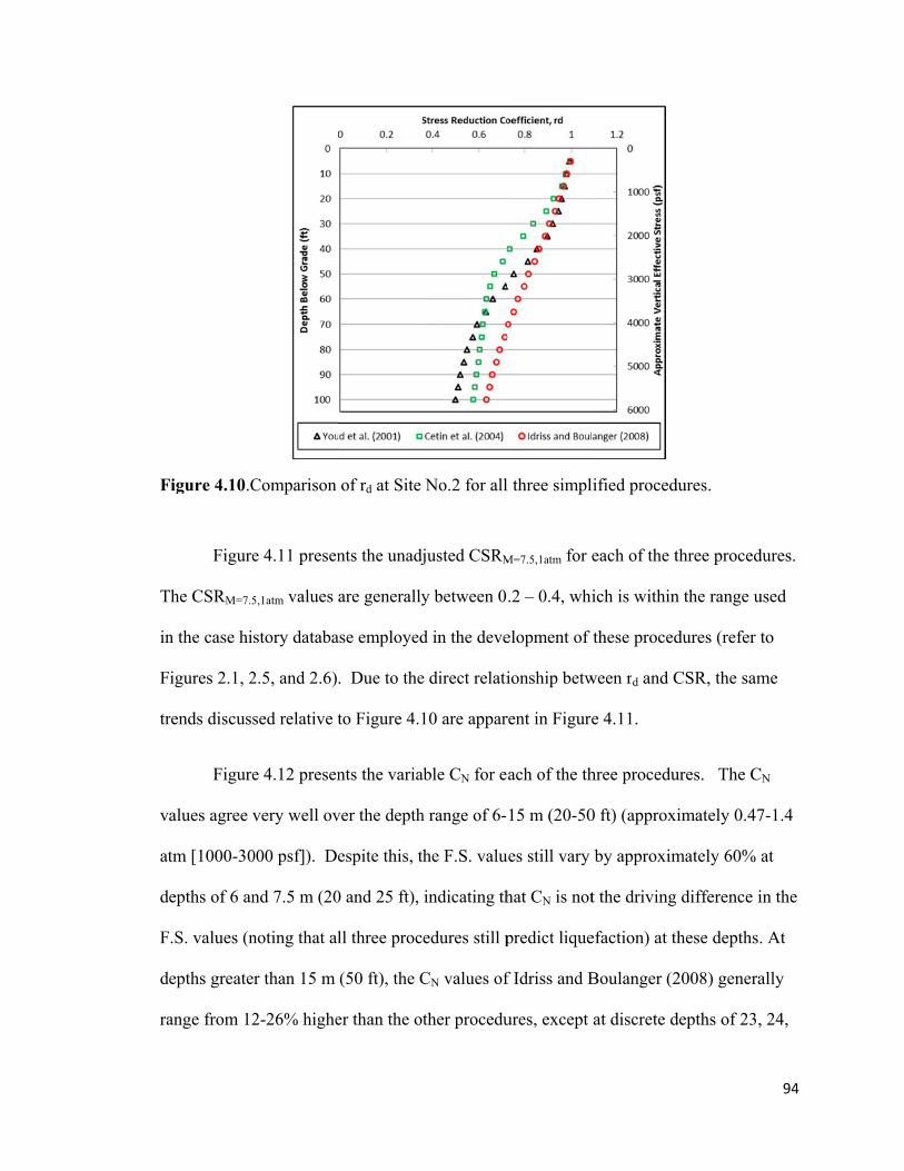
F

T

in

F

tr

v

at

d

F

d

ra

Figure 4.10.C

Figure

The CSRM=7.5

n the case hi

igures 2.1, 2

rends discuss

Figure

alues agree v

tm [1000-30

epths of 6 an

.S. values (n

epths greate

ange from 12

Comparison

e 4.11 presen

5,1atm values

story databa

2.5, and 2.6)

sed relative t

e 4.12 presen

very well ov

000 psf]). De

nd 7.5 m (20

noting that al

r than 15 m

2-26% highe

of rd at Site

nts the unadj

are generally

ase employed

. Due to the

to Figure 4.1

nts the varia

ver the depth

espite this, th

0 and 25 ft),

ll three proc

(50 ft), the C

er than the ot

No.2 for all

justed CSRM

y between 0

d in the deve

e direct relati

10 are appar

able CN for e

h range of 6-

he F.S. valu

indicating th

edures still p

CN values of

ther procedu

l three simpl

M=7.5,1atm for e

.2 – 0.4, whi

elopment of

ionship betw

rent in Figure

ach of the th

15 m (20-50

ues still vary

hat CN is not

predict lique

f Idriss and B

ures, except

lified proced

each of the t

ich is within

these proced

ween rd and C

e 4.11.

hree procedu

0 ft) (approx

by approxim

t the driving

efaction) at th

Boulanger (2

at discrete d

dures.

three proced

n the range u

dures (refer t

CSR, the sam

ures. The C

imately 0.47

mately 60%

difference i

hese depths.

2008) genera

depths of 23,

94

dures.

used

to

me

CN

7-1.4

at

in the

. At

ally

, 24,

Fpr

Fpr

Figure 4.11. rocedures.


Comparison

Comparison

n of the CRR

n of the CN v

RM=7.5, 1 atm va

values at Site

alues at Site

e No. 2 for a

No. 2 for al

all three simp

l three simpl

plified

95

lified

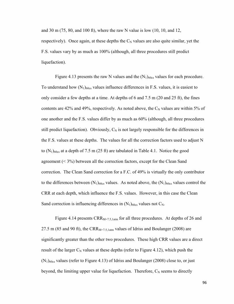
96

and 30 m (75, 80, and 100 ft), where the raw N value is low (10, 10, and 12,

respectively). Once again, at these depths the CN values are also quite similar, yet the

F.S. values vary by as much as 100% (although, all three procedures still predict

liquefaction).

Figure 4.13 presents the raw N values and the (N1)60cs values for each procedure.

To understand how (N1)60cs values influence differences in F.S. values, it is easiest to

only consider a few depths at a time. At depths of 6 and 7.5 m (20 and 25 ft), the fines

contents are 42% and 49%, respectively. As noted above, the CN values are within 5% of

one another and the F.S. values differ by as much as 60% (although, all three procedures

still predict liquefaction). Obviously, CN is not largely responsible for the differences in

the F.S. values at these depths. The values for all the correction factors used to adjust N

to (N1)60cs at a depth of 7.5 m (25 ft) are tabulated in Table 4.1. Notice the good

agreement (< 3%) between all the correction factors, except for the Clean Sand

correction. The Clean Sand correction for a F.C. of 49% is virtually the only contributor

to the differences between (N1)60cs values. As noted above, the (N1)60cs values control the

CRR at each depth, which influence the F.S. values. However, in this case the Clean

Sand correction is influencing differences in (N1)60cs values not CN.

Figure 4.14 presents CRRM=7.5,1atm for all three procedures. At depths of 26 and

27.5 m (85 and 90 ft), the CRRM=7.5,1atm values of Idriss and Boulanger (2008) are

significantly greater than the other two procedures. These high CRR values are a direct

result of the larger CN values at these depths (refer to Figure 4.12), which push the

(N1)60cs values (refer to Figure 4.13) of Idriss and Boulanger (2008) close to, or just

beyond, the limiting upper value for liquefaction. Therefore, CN seems to directly

Fpr

T(2

Figure 4.13.Crocedures.

Table 4.1. Co25 ft)

Youd et al.

Cetin e(2004

Idriss Boulanger

1. Calculate49% (refer t

Comparison

omparison o

Rawvalu

. (2001) 10

et al. 4)

10

and r (2008)

10

d using the recommto Section 2.4.1).

of the (N1)6

f blow coun

w N ue

CE C

0 1.29 0

0 1.29 0

0 1.29 0

mendations from e

0cs values at

nt correction

CR CB C

0.95 1.00 1.

0.95 1.00 1.

0.95 1.00 1.

each procedures, a

Site No. 2 f

factors for S

CS CN (N

20 1.13

16 1.16

20 1.15

as the change from

for all three s

Site No. 2, at

N1)60Clean S

Correc

16 +8

16 +3

16 +5

m (N1)60 to (N1)60cs,

simplified

t a depth of

Sand

ction1 (N1)60cs

8 24

3 19

5 21

based on a F.C. o

97

8 m

s

of

User

Stamp

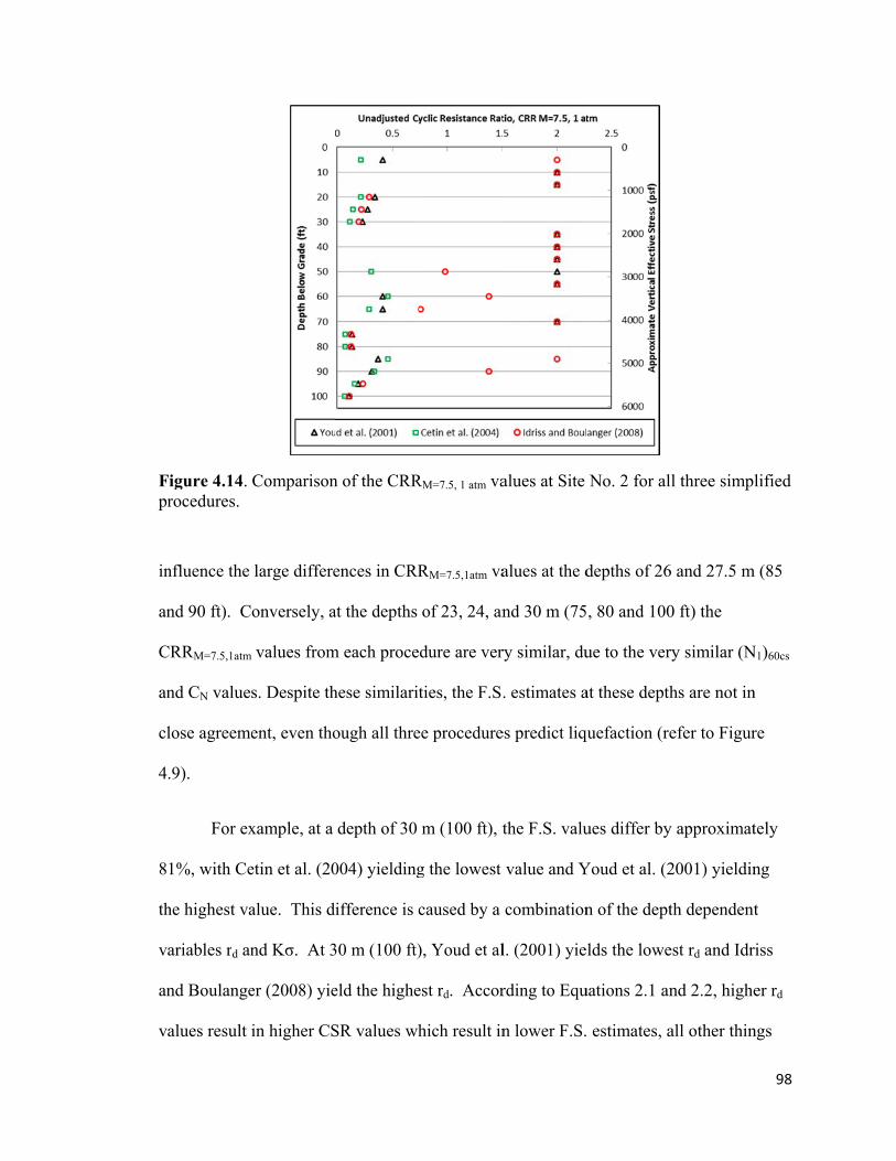
Fpr

in

an

C

an

cl

4

8

th

v

an

v


nfluence the

nd 90 ft). C

CRRM=7.5,1atm

nd CN value

lose agreeme

.9).

For ex

1%, with Ce

he highest va

ariables rd an

nd Boulange

alues result

Comparison

large differe

onversely, a

values from

s. Despite th

ent, even tho

xample, at a

etin et al. (20

alue. This d

nd Kσ. At 3

er (2008) yie

in higher CS

n of the CRR

ences in CRR

at the depths

m each proce

hese similarit

ough all thre

depth of 30

004) yielding

ifference is c

30 m (100 ft)

eld the highe

SR values wh

RM=7.5, 1 atm va

RM=7.5,1atm va

of 23, 24, an

dure are ver

ties, the F.S.

ee procedure

m (100 ft), t

g the lowest

caused by a

), Youd et al

est rd. Accor

hich result in

alues at Site

alues at the d

nd 30 m (75

ry similar, du

. estimates a

es predict liq

the F.S. valu

value and Y

combination

l. (2001) yie

rding to Equ

n lower F.S.

No. 2 for al

depths of 26

, 80 and 100

ue to the ver

at these depth

quefaction (re

ues differ by

Youd et al. (2

n of the dept

lds the lowe

uations 2.1 an

estimates, a

l three simpl

6 and 27.5 m

0 ft) the

ry similar (N

hs are not in

efer to Figur

y approximat

2001) yieldin

th dependent

est rd and Idr

nd 2.2, highe

all other thin

98

lified

m (85

N1)60cs

n

re

tely

ng

t

riss

er rd

ngs

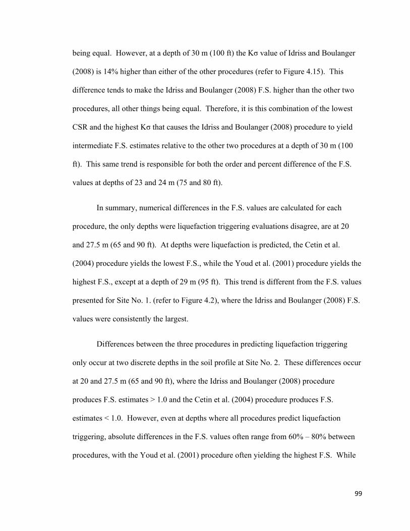
99

being equal. However, at a depth of 30 m (100 ft) the Kσ value of Idriss and Boulanger

(2008) is 14% higher than either of the other procedures (refer to Figure 4.15). This

difference tends to make the Idriss and Boulanger (2008) F.S. higher than the other two

procedures, all other things being equal. Therefore, it is this combination of the lowest

CSR and the highest Kσ that causes the Idriss and Boulanger (2008) procedure to yield

intermediate F.S. estimates relative to the other two procedures at a depth of 30 m (100

ft). This same trend is responsible for both the order and percent difference of the F.S.

values at depths of 23 and 24 m (75 and 80 ft).

In summary, numerical differences in the F.S. values are calculated for each

procedure, the only depths were liquefaction triggering evaluations disagree, are at 20

and 27.5 m (65 and 90 ft). At depths were liquefaction is predicted, the Cetin et al.

(2004) procedure yields the lowest F.S., while the Youd et al. (2001) procedure yields the

highest F.S., except at a depth of 29 m (95 ft). This trend is different from the F.S. values

presented for Site No. 1. (refer to Figure 4.2), where the Idriss and Boulanger (2008) F.S.

values were consistently the largest.

Differences between the three procedures in predicting liquefaction triggering

only occur at two discrete depths in the soil profile at Site No. 2. These differences occur

at 20 and 27.5 m (65 and 90 ft), where the Idriss and Boulanger (2008) procedure

produces F.S. estimates > 1.0 and the Cetin et al. (2004) procedure produces F.S.

estimates < 1.0. However, even at depths where all procedures predict liquefaction

triggering, absolute differences in the F.S. values often range from 60% – 80% between

procedures, with the Youd et al. (2001) procedure often yielding the highest F.S. While

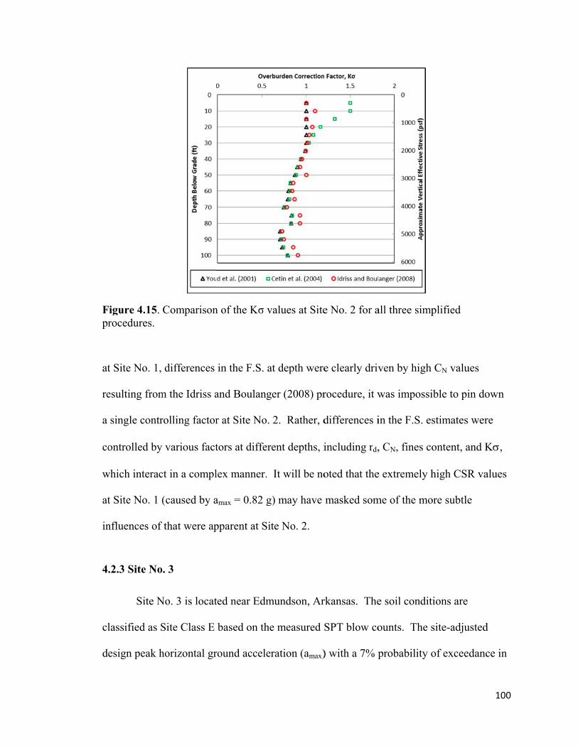
Fpr

at

re

a

co

w

at

in

4

cl

d


t Site No. 1,

esulting from

single contr

ontrolled by

which interac

t Site No. 1 (

nfluences of

.2.3 Site No

Site N

lassified as S

esign peak h

Comparison

differences

m the Idriss a

rolling factor

various fact

ct in a compl

(caused by a

that were ap

. 3

No. 3 is locat

Site Class E

horizontal gr

n of the Kσ v

in the F.S. a

and Boulang

r at Site No.

tors at differ

lex manner.

amax = 0.82 g

pparent at Si

ted near Edm

based on the

round accele

values at Site

at depth were

ger (2008) pr

2. Rather, d

rent depths, i

It will be no

g) may have

ite No. 2.

mundson, Ar

e measured S

eration (amax)

e No. 2 for a

e clearly driv

rocedure, it w

differences i

including rd,

oted that the

masked som

rkansas. The

SPT blow co

) with a 7% p

all three simp

ven by high

was impossi

in the F.S. es

, CN, fines co

e extremely h

me of the mo

e soil conditi

ounts. The s

probability o

plified

CN values

ible to pin do

stimates wer

ontent, and K

high CSR va

ore subtle

ions are

site-adjusted

of exceedanc

100

own

re

K,

alues

d

ce in

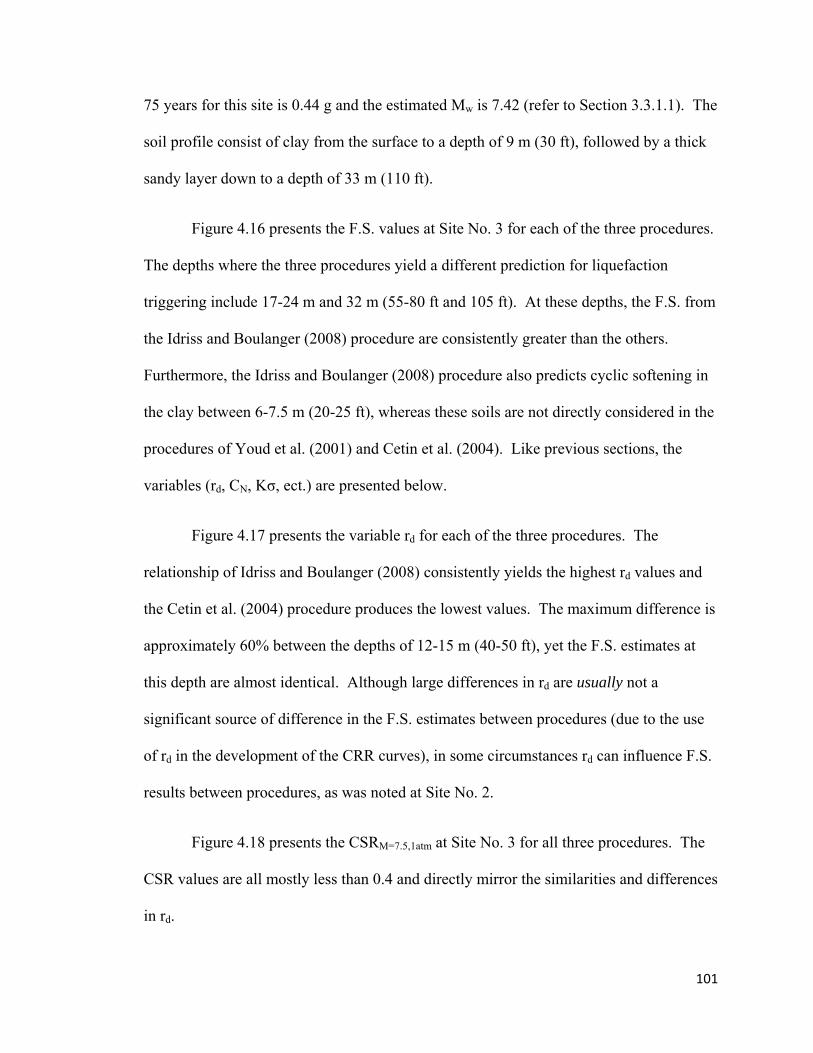
101

75 years for this site is 0.44 g and the estimated Mw is 7.42 (refer to Section 3.3.1.1). The

soil profile consist of clay from the surface to a depth of 9 m (30 ft), followed by a thick

sandy layer down to a depth of 33 m (110 ft).

Figure 4.16 presents the F.S. values at Site No. 3 for each of the three procedures.

The depths where the three procedures yield a different prediction for liquefaction

triggering include 17-24 m and 32 m (55-80 ft and 105 ft). At these depths, the F.S. from

the Idriss and Boulanger (2008) procedure are consistently greater than the others.

Furthermore, the Idriss and Boulanger (2008) procedure also predicts cyclic softening in

the clay between 6-7.5 m (20-25 ft), whereas these soils are not directly considered in the

procedures of Youd et al. (2001) and Cetin et al. (2004). Like previous sections, the

variables (rd, CN, Kσ, ect.) are presented below.

Figure 4.17 presents the variable rd for each of the three procedures. The

relationship of Idriss and Boulanger (2008) consistently yields the highest rd values and

the Cetin et al. (2004) procedure produces the lowest values. The maximum difference is

approximately 60% between the depths of 12-15 m (40-50 ft), yet the F.S. estimates at

this depth are almost identical. Although large differences in rd are usually not a

significant source of difference in the F.S. estimates between procedures (due to the use

of rd in the development of the CRR curves), in some circumstances rd can influence F.S.

results between procedures, as was noted at Site No. 2.

Figure 4.18 presents the CSRM=7.5,1atm at Site No. 3 for all three procedures. The

CSR values are all mostly less than 0.4 and directly mirror the similarities and differences

in rd.

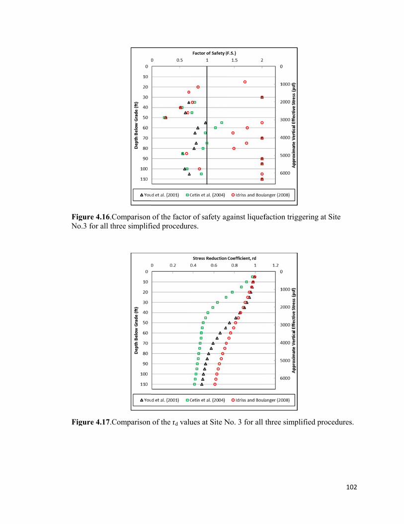
FN

F

Figure 4.16.CNo.3 for all th

Figure 4.17.C

Comparison hree simplifi

Comparison

of the factoried procedur

of the rd val

r of safety agres.

lues at Site N

gainst liquef

No. 3 for all

faction trigg

three simpli

ering at Site

ified procedu

102

e

ures.

Fpr

v

1

Id

in

F

v

w

b

C


Figure

alues agree q

.4atm [1000

driss and Bo

nterestingly m

igure 4.16).

In gen

alues betwee

which of thes

low count co

Clean Sand c

Comparison

e 4.19 presen

quite well ov

-3000 psf]).

ulanger (200

mirroring th

neral, CN is t

en procedure

se variables i

orrection fac

orrection are

n of the CSR

nts the varia

ver the depth

However, a

08) range fro

he deviation i

typically resp

es, but CS al

is most influ

ctors at a dep

e identical fo

RM=7.5, 1 atm va

able CN for e

h range of 6-

at depths gre

om 10-30% h

in the F.S. v

ponsible for

so contribute

uential for Si

pth of 20 m (

or each of th

alues at Site

ach of the th

-15 m (20-50

eater than 17

higher than

values below

most of the

es in some c

ite No. 3, Ta

(65 ft). In th

he three proc

No. 3 for all

hree procedu

0 ft) (approx

7 m (55 ft) th

the other pro

w this same d

difference i

cases. In ord

able 4.2 prese

his table, the

cedures. The

l three simpl

ures. The C

ximately 0.47

he CN values

ocedures,

depth (refer t

in the (N1)60c

der to observ

ents all of th

e CR, CB, CE,

e CS values a

103

lified

CN

7-

s of

to

cs

ve

he

, and

are

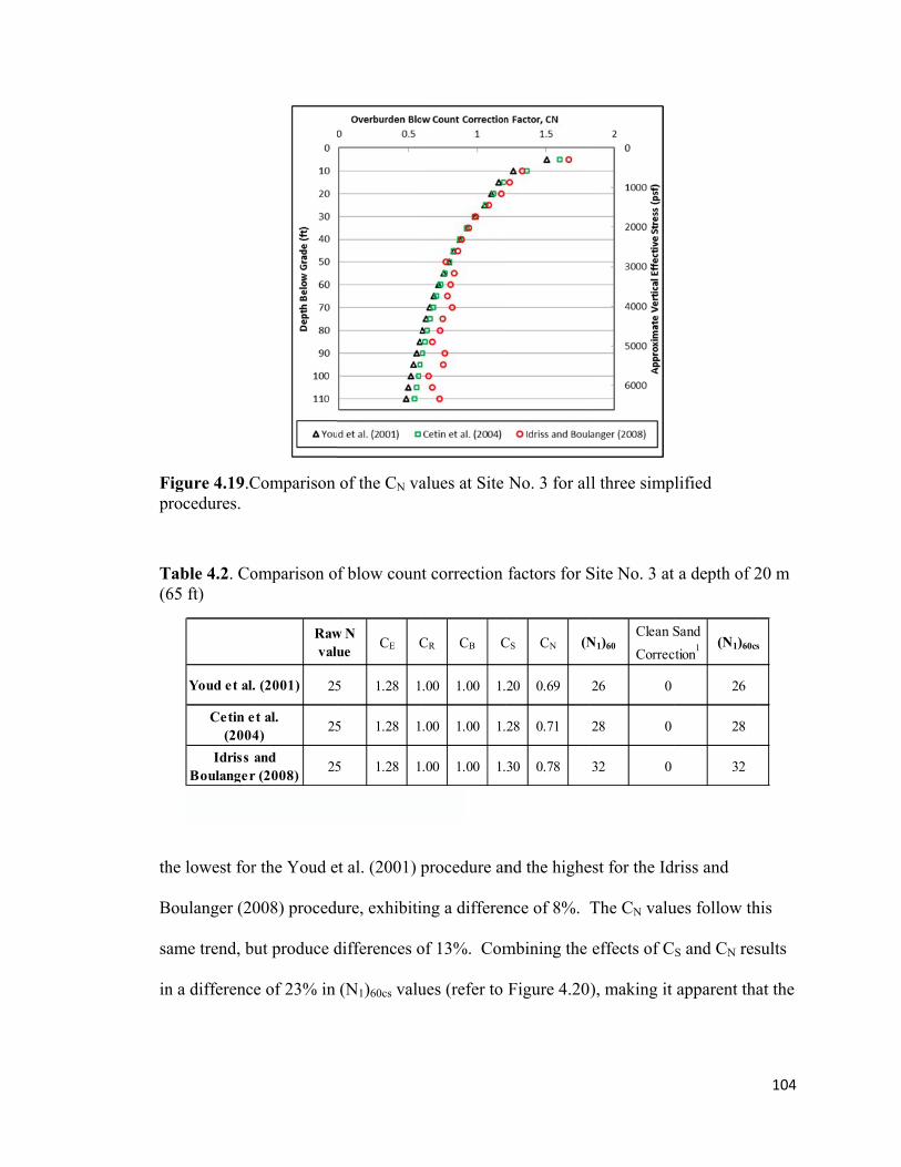
Fpr

T(6

th

B

sa

in


Table 4.2. Co65 ft)

he lowest for

Boulanger (20

ame trend, b

n a differenc

Youd et al.

Cetin e(2004

Idriss Boulanger

1. No F.C. da

Comparison

omparison o

r the Youd e

008) procedu

but produce d

e of 23% in

Rawvalu

. (2001) 25

et al. 4)

25

and r (2008)

25

ata available for th

of the CN va

f blow coun

et al. (2001) p

ure, exhibiti

differences o

(N1)60cs valu

w N ue

CE C

5 1.28 1

5 1.28 1

5 1.28 1

is sample depth.

alues at Site

nt correction

procedure an

ing a differen

of 13%. Com

ues (refer to

CR CB C

.00 1.00 1.

.00 1.00 1.

.00 1.00 1.

No. 3 for al

factors for S

nd the highe

nce of 8%. T

mbining the

Figure 4.20

CS CN (N

20 0.69

28 0.71

30 0.78

ll three simp

Site No. 3 at

est for the Idr

The CN valu

effects of C

), making it

N1)60Clean S

Correc

26 0

28 0

32 0

lified

a depth of 2

riss and

ues follow th

S and CN res

apparent tha

Sand

ction1 (N1)60cs

26

28

32

104

20 m

his

sults

at the

s

User

Stamp

Fpr

d

d

(6

N

d

(r

ar

ot

m

o


ifferences in

ifferences of

65 ft), simila

Notice that at

ifferences in

refer to Figu

Figure

re significan

ther two pro

minor differe

f the correct

Comparison

n (N1)60cs val

f CS and CN.

ar trends for

t a depth of 2

n (N1)60cs val

ure 4.19).

e 4.21 presen

nt differences

ocedures betw

nces in the (

ted blow cou

of the (N1)6

lues at a dept

. Although T

depths great

26 m (85 ft)

lues because

nts the CRR

s between th

ween the dep

(N1)60cs value

unts to the ste

0cs values at

th of 20 m (6

Table 4.2 on

ter than 17 m

the raw N v

e differences

RM=7.5,1atm val

he Idriss and

pths of 17 an

es at these sa

eep part (i.e

Site No. 3 f

65 ft) are a d

nly presents d

m (55 ft) are

value is 22, re

in CN value

lues for each

d Boulanger (

nd 24 m (55

ame depths.

. the limiting

for all three s

direct result

data for the

observed in

esulting in m

es are minim

h of the proce

(2008) CRR

and 85 ft), d

This is due

g upper-boun

simplified

of the comb

depth of 20

n Figure 4.20

minimal

mal at this dep

edures. The

R values and

despite relati

e to the proxi

nd) of the C

105

bined

m

0.

pth

ere

the

ively

imity

RR

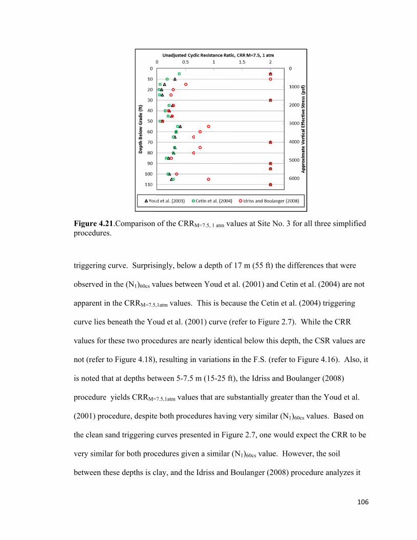
Fpr

tr

ob

ap

cu

v

n

is

pr

(2

th

v

b


riggering cur

bserved in th

pparent in th

urve lies ben

alues for the

ot (refer to F

s noted that a

rocedure yi

2001) proced

he clean sand

ery similar f

etween these

Comparison

rve. Surpris

he (N1)60cs v

he CRRM=7.5,

neath the Yo

ese two proc

Figure 4.18),

at depths bet

elds CRRM=

dure, despite

d triggering

for both proc

e depths is c

of the CRRM

ingly, below

alues betwee

,1atm values.

oud et al. (20

edures are n

, resulting in

tween 5-7.5

=7.5,1atm value

e both proced

curves prese

cedures give

clay, and the

M=7.5, 1 atm va

w a depth of

en Youd et a

This is beca

001) curve (r

nearly identic

n variations i

m (15-25 ft)

s that are sub

dures having

ented in Figu

n a similar (

Idriss and B

alues at Site N

17 m (55 ft)

al. (2001) an

ause the Ceti

refer to Figur

cal below thi

in the F.S. (r

), the Idriss a

ubstantially g

g very simila

ure 2.7, one

(N1)60cs value

Boulanger (2

No. 3 for all

the differen

nd Cetin et al

in et al. (200

ure 2.7). Wh

is depth, the

refer to Figu

and Boulang

greater than t

ar (N1)60cs va

would expec

e. However

2008) proced

l three simpl

nces that wer

l. (2004) are

04) triggerin

hile the CRR

e CSR values

ure 4.16). Al

ger (2008)

the Youd et

alues. Based

ct the CRR t

r, the soil

dure analyzes

106

ified

re

e not

g

R

s are

lso, it

al.

d on

to be

s it

107

based on the cylic softening potential of the soil (i.e. clay-like criteria), not the standard

liquefaction potential (i.e. sand-like criteria). This is also why the Idriss and Boulanger

(2008) procedure yields a F.S. at these depths (refer to Figure 4.16), while the other two

procedures do not.

Figure 4.22 presents the Kσ values for each of the procedures. As discussed

above, the differences in Kσ at shallow depths (i.e. the significantly larger Kσ values for

the Cetin et al. (2004) procedure) are generally not a concern for these studies because

most of the liquefaction potential occurs at depths greater than 6 m (20 ft). At all other

depths the Kσ values generally agree within about 5%, except at the discrete depths of 26

and 30 m (85 and 100 ft), where the Kσ values of Idriss and Boulanger (2008) are 15%

higher than the other procedures, which directly increases the F.S. by this same

percentage. This deviation in Kσ is typically evident when the raw N values are low,

because the Kσ values for each of the procedures are dependent on the relative density of

the soil (refer to Section 2.4.2) via the “f” factor. As relative densities (and N values)

decrease, the Kσ values at effective stresses higher than 1 atm (2116 psf) tend to increase.

However, the Kσ values of Idriss and Boulanger (2008) increase by larger amounts than

other two procedures, especially at low N values and high effective stresses. This effect

is often masked by the opposite trend in CN, which increases with increased relative

densities (and N values).

In summary, the F.S. values for each of the three procedures at Site No. 3 (refer to

Figure 4.16) disagree the most at depths between 17-24 m (55-80 ft). Over this same

depth range there is often disagreement between procedures about the potential for

liquefaction triggering, with the Idriss and Boulanger (2008) procedure predicting no

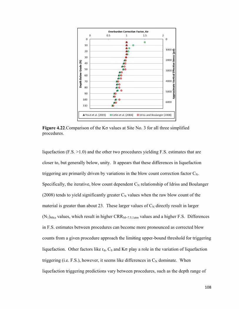
Fpr

li

cl

tr

S

(2

m

(N

in

co

li

tr

li


iquefaction (

loser to, but

riggering are

pecifically, t

2008) tends t

material is gr

N1)60cs value

n F.S. estima

ounts from a

iquefaction.

riggering (i.e

iquefaction t

Comparison

(F.S. >1.0) an

generally be

e primarily d

the iterative

to yield sign

eater than ab

es, which res

ates between

a given proce

Other factor

e. F.S.), how

riggering pr

of the Kσ va

nd the other

elow, unity.

driven by var

, blow count

nificantly gre

bout 23. The

ult in higher

n procedures

edure approa

rs like rd, CS

wever, it seem

edictions va

alues at Site

two procedu

It appears t

riations in th

t dependent

eater CN valu

ese larger va

r CRRM=7.5,1a

can become

ach the limit

S and K pla

ms like differ

ary between p

e No. 3 for al

ures yielding

that these dif

he blow coun

CN relations

ues when the

alues of CN d

atm values an

e more prono

ting upper-b

ay a role in th

rences in CN

procedures,

ll three simp

g F.S. estima

fferences in

nt correction

ship of Idriss

e raw blow c

directly resu

nd a higher F

ounced as co

bound thresh

he variation

N dominate.

such as the d

plified

ates that are

liquefaction

n factor CN.

s and Boulan

count of the

ult in larger

F.S. Differen

orrected blow

old for trigg

of liquefact

When

depth range

108

n

nger

nces

w

gering

tion

of

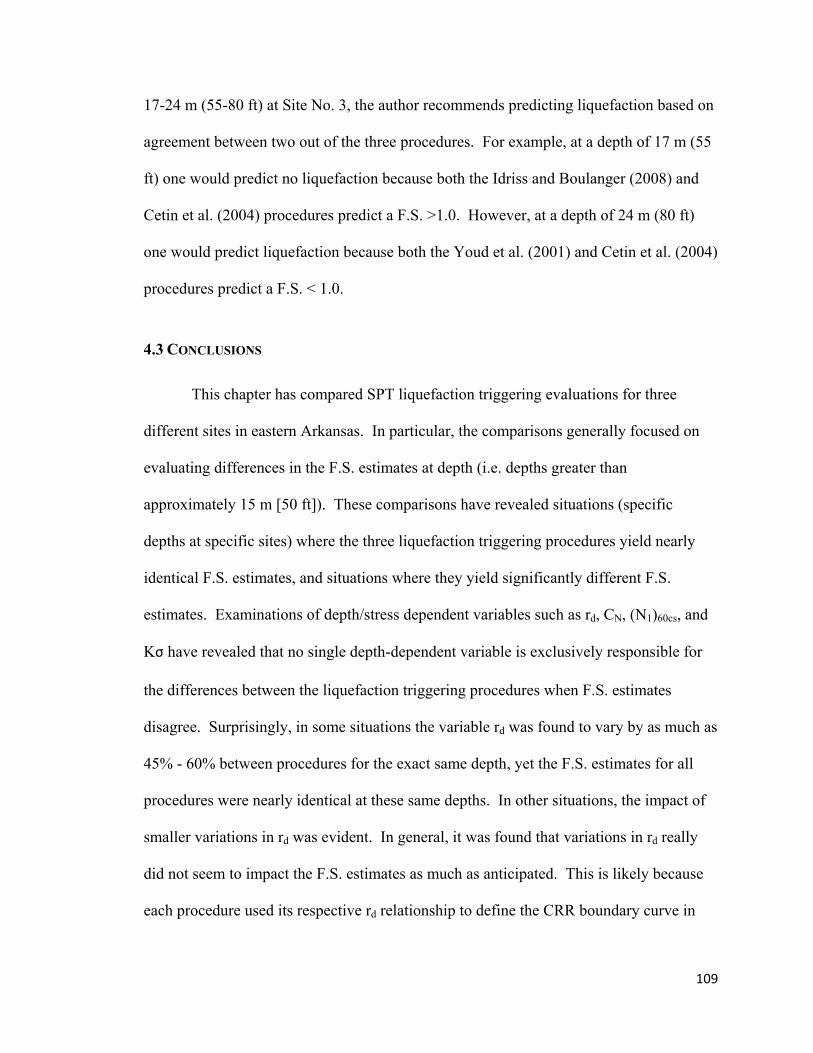
109

17-24 m (55-80 ft) at Site No. 3, the author recommends predicting liquefaction based on

agreement between two out of the three procedures. For example, at a depth of 17 m (55

ft) one would predict no liquefaction because both the Idriss and Boulanger (2008) and

Cetin et al. (2004) procedures predict a F.S. >1.0. However, at a depth of 24 m (80 ft)

one would predict liquefaction because both the Youd et al. (2001) and Cetin et al. (2004)

procedures predict a F.S. < 1.0.

4.3 CONCLUSIONS

This chapter has compared SPT liquefaction triggering evaluations for three

different sites in eastern Arkansas. In particular, the comparisons generally focused on

evaluating differences in the F.S. estimates at depth (i.e. depths greater than

approximately 15 m [50 ft]). These comparisons have revealed situations (specific

depths at specific sites) where the three liquefaction triggering procedures yield nearly

identical F.S. estimates, and situations where they yield significantly different F.S.

estimates. Examinations of depth/stress dependent variables such as rd, CN, (N1)60cs, and

Kσ have revealed that no single depth-dependent variable is exclusively responsible for

the differences between the liquefaction triggering procedures when F.S. estimates

disagree. Surprisingly, in some situations the variable rd was found to vary by as much as

45% - 60% between procedures for the exact same depth, yet the F.S. estimates for all

procedures were nearly identical at these same depths. In other situations, the impact of

smaller variations in rd was evident. In general, it was found that variations in rd really

did not seem to impact the F.S. estimates as much as anticipated. This is likely because

each procedure used its respective rd relationship to define the CRR boundary curve in

110

the back analyses of the case history database; thereby influencing both the CSR and

CRR in forward analyses.

In general, it can be stated that the Idriss and Boulanger (2008) procedure

typically yields the highest F.S. estimates at depth. While this is somewhat driven by

higher K values at depth (generally ranging from 5% - 15% greater than the other two

procedures), it seems to primarily be a result of significantly higher CN values at depth

(generally ranging from 15% - 60% greater than the other two procedures for higher blow

count material). Specifically, the iterative, blow count dependent CN relationship of

Idriss and Boulanger (2008) tends to yield significantly greater CN values when the raw

blow count of the material is greater than about 23. These larger values of CN directly

result in larger (N1)60cs values, which result in higher CRRM=7.5,1atm values and higher F.S.

estimates. Furthermore, as this difference is most pronounced at higher blow counts, and

the CRR relationship is very steep and nonlinear, somewhat subtle differences in (N1)60cs

values can result in very significant differences in CRRM=7.5,1atm values.

Overall, for the sites analyzed herein, which have fairly high to very high peak

ground accelerations, the three procedures agreed in predicting or not predicting

liquefaction at many depths. This lends confidence to these types of deterministic

triggering analyses where a “yes” or “no” answer is required. For situations where the

three procedures do not agree on liquefaction triggering, the author recommends using

the prediction agreed upon by two out of the three procedures. This seems logical given

the debate that is ongoing regarding which procedure is “best”. The liquefaction

triggering workbooks that have been developed in this work enable easy data transfer

111

between workbooks and facilitate quick and simple comparisons between all three

procedures.

112

Chapter 5

Residual Strength of Liquefied Soils

5.1 INTRODUCTION

In order to better assess the post-liquefaction performance of piles, AHTD has

expressed interest in developing guidelines for assessing residual shear strengths (Sr) for

liquefied soils. Although many correlations for Sr have been proposed over the past 20 -

25 years, some are used more frequently than others. Furthermore, even given a single

correlation, the assessment of Sr often falls back to engineering judgment as the design

engineer must choose between an upper-bound, lower-bound, or intermediate value. The

correlations to estimate Sr that are presented in this chapter have been developed

primarily for slope stability applications, not for post-liquefaction performance of piles.

But, since no guidance is available for assigning Sr for post-liquefaction pile capacity,

these correlations offer the only available alternative. In order to understand the available

Sr correlations and their development, a brief review is provided below.

5.2 REVIEW OF PAST SR CORRELATIONS

Many researchers have used laboratory and/or field data to determine the residual

shear strength of liquefied soils (Poulos et al. 1985, Seed 1987, Seed and Harder 1990,

Stark and Mesri 1992, Olsen and Stark 2002, Idriss and Boulanger 2008). Poulos et al.

(1985) developed a procedure using laboratory tests and steady state soil mechanics

theory to determine Sr. This procedure assumed that the void ratio remained constant

during the earthquake and flow slide. However, due to water/void redistribution during

liquefaction (refer to Section 5.2.3), this assumption was argued to be invalid (Seed 1987,

113

Pilecki 1988). Furthermore, various sample preparation methods were found to influence

the slope of the steady state line (Dennis 1988), causing the validity of results obtained

from reconstituted specimens to be questioned relative to their true in-situ behavior. As a

result of these findings, researchers began to focus on developing empirical Sr estimates

based on back analyses of slope failure case histories from previous earthquakes.

5.2.1 Seed and Harder (1990)

Seed (1987) analyzed 12 liquefaction-induced slope failure case histories to back-

calculate a relationship between SPT blow count and Sr. These results were later

adjusted by Seed and Harder (1990) to account for kinetic movement of the failure mass.

The Seed and Harder (1990) relationship, presented in Figure 5.1, has been used

extensively to determine Sr (Seed 2010). This Sr correlation includes an upper- and

lower-bound and allows the engineer to use some judgment when determining Sr.

However, Seed and Harder (1990) recommend using the lower bound relationship to

remain conservative. The raw data in this correlation also includes error bars, which

represent the difficulty in back-calculating shear strength and assigning a representative

SPT blow-count (Olsen and Stark 2002).

In Figure 5.1, (N1)60-cs is used to denote the corrected clean sand SPT blow count

along the horizontal axis. This is an unfortunate designation because it is not the same as

the corrected clean sand blow count used within liquefaction triggering evaluations (i.e.

(N1)60cs, as discussed in Chapter 2). The fines content correction factor used to determine

(N1)60-cs for obtaining Sr is different than the fines content correction used to determine

F

(N

d

an

co

(N

tr

th

(1

E

Figure 5.1. R

N1)60cs within

istinguish be

nd Boulange

orrected blow

N1)60cs desig

riggering eva

Table

he original fa

1990) and Id

Equation 5.1.

Relationship

n the liquefa

etween these

er (2008) has

w count adju

nates the cor

aluation.

5.1 presents

actors propo

driss and Bou

between Sr

action trigger

e two correct

s been adopt

usted for fine

rrected blow

s the Sr fines

osed by Seed

ulanger (200

and (N1)60cs-

ring relation

ted blow cou

ted within th

es content an

w count that i

s content cor

d (1987), and

08). These f

-Sr proposed

nships. In or

unts, the nom

his report: (N

nd used for e

is to be emp

rrection fact

d have been a

factors shoul

by Seed and

rder to more

menclature u

N1)60cs-Sr will

evaluation o

ployed for th

tors [Δ(N1)60

adopted by S

ld be used ac

d Harder (19

clearly

used by Idris

l designate th

of Sr, while

e liquefactio

0-Sr]. These a

Seed and Ha

ccording to

114

990).

ss

he

on

are

arder

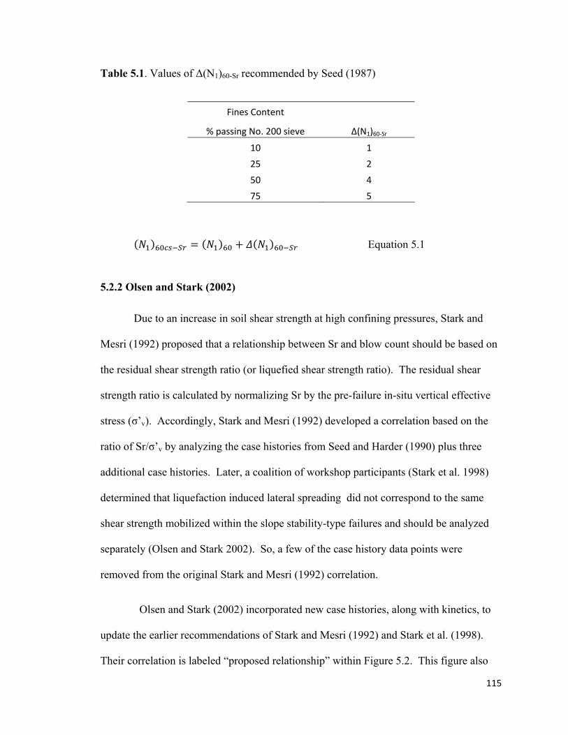
115

Table 5.1. Values of Δ(N1)60-Sr recommended by Seed (1987)

Fines Content

% passing No. 200 sieve Δ(N1)60‐Sr

10 1

25 2

50 4

75 5

Equation 5.1

5.2.2 Olsen and Stark (2002)

Due to an increase in soil shear strength at high confining pressures, Stark and

Mesri (1992) proposed that a relationship between Sr and blow count should be based on

the residual shear strength ratio (or liquefied shear strength ratio). The residual shear

strength ratio is calculated by normalizing Sr by the pre-failure in-situ vertical effective

stress (σ’v). Accordingly, Stark and Mesri (1992) developed a correlation based on the

ratio of Sr/σ’v by analyzing the case histories from Seed and Harder (1990) plus three

additional case histories. Later, a coalition of workshop participants (Stark et al. 1998)

determined that liquefaction induced lateral spreading did not correspond to the same

shear strength mobilized within the slope stability-type failures and should be analyzed

separately (Olsen and Stark 2002). So, a few of the case history data points were

removed from the original Stark and Mesri (1992) correlation.

Olsen and Stark (2002) incorporated new case histories, along with kinetics, to

update the earlier recommendations of Stark and Mesri (1992) and Stark et al. (1998).

Their correlation is labeled “proposed relationship” within Figure 5.2. This figure also

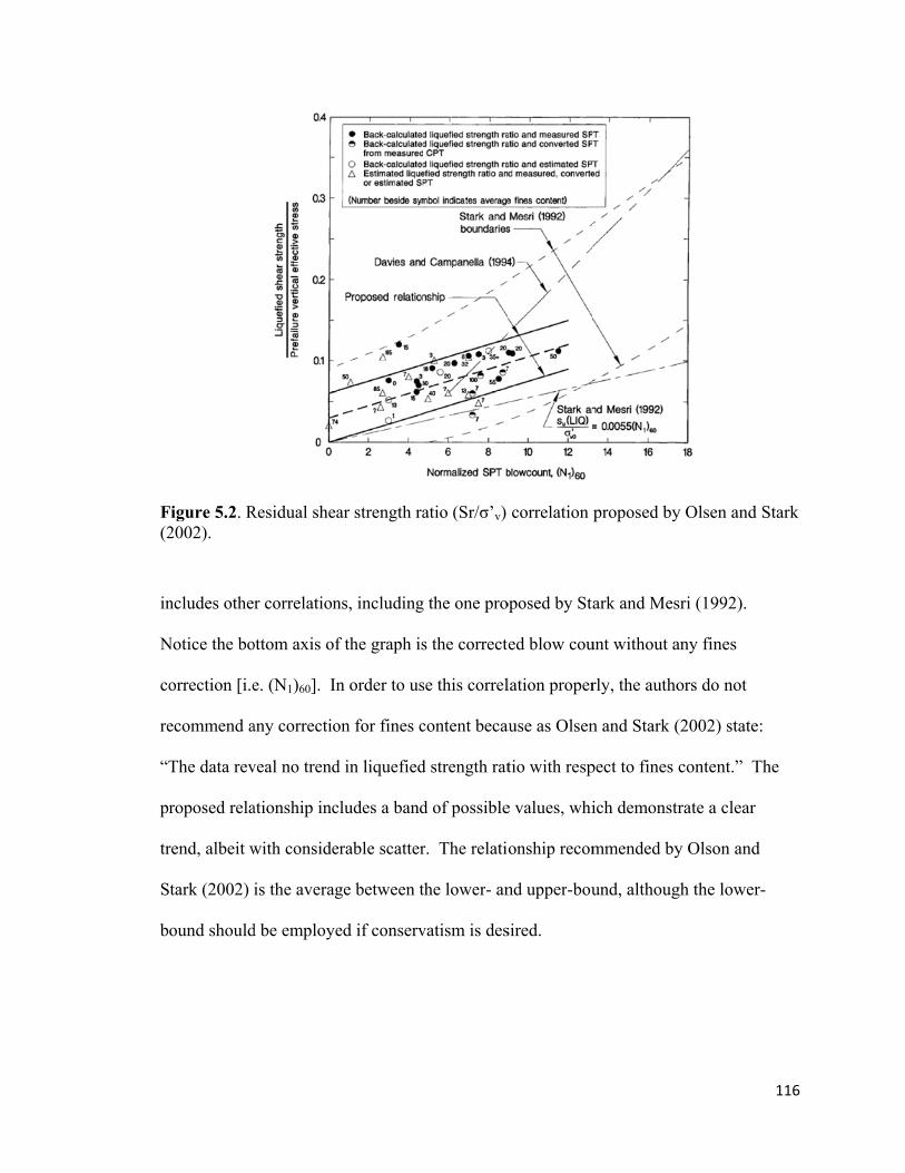
F(2

in

N

co

re

“T

pr

tr

S

b

Figure 5.2. R2002).

ncludes othe

Notice the bo

orrection [i.e

ecommend a

The data rev

roposed rela

rend, albeit w

tark (2002)

ound should

Residual shea

r correlation

ottom axis of

e. (N1)60]. In

any correctio

veal no trend

ationship inc

with conside

is the averag

d be employe

ar strength ra

ns, including

f the graph is

n order to us

on for fines c

d in liquefied

cludes a band

erable scatter

ge between t

ed if conserv

atio (Sr/σ’v)

g the one pro

s the correct

se this correl

content becau

d strength rat

d of possible

r. The relati

the lower- an

vatism is des

correlation

oposed by Sta

ed blow cou

lation proper

ause as Olsen

tio with resp

e values, whi

onship recom

nd upper-bou

sired.

proposed by

ark and Mes

unt without a

rly, the autho

n and Stark (

pect to fines

ich demonst

mmended by

und, althoug

y Olsen and

sri (1992).

any fines

ors do not

(2002) state:

content.” T

trate a clear

y Olson and

gh the lower-

116

Stark

:

The

-

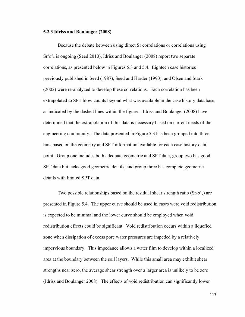
117

5.2.3 Idriss and Boulanger (2008)

Because the debate between using direct Sr correlations or correlations using

Sr/σ’v is ongoing (Seed 2010), Idriss and Boulanger (2008) report two separate

correlations, as presented below in Figures 5.3 and 5.4. Eighteen case histories

previously published in Seed (1987), Seed and Harder (1990), and Olsen and Stark

(2002) were re-analyzed to develop these correlations. Each correlation has been

extrapolated to SPT blow counts beyond what was available in the case history data base,

as indicated by the dashed lines within the figures. Idriss and Boulanger (2008) have

determined that the extrapolation of this data is necessary based on current needs of the

engineering community. The data presented in Figure 5.3 has been grouped into three

bins based on the geometry and SPT information available for each case history data

point. Group one includes both adequate geometric and SPT data, group two has good

SPT data but lacks good geometric details, and group three has complete geometric

details with limited SPT data.

Two possible relationships based on the residual shear strength ratio (Sr/σ’v) are

presented in Figure 5.4. The upper curve should be used in cases were void redistribution

is expected to be minimal and the lower curve should be employed when void

redistribution effects could be significant. Void redistribution occurs within a liquefied

zone when dissipation of excess pore water pressures are impeded by a relatively

impervious boundary. This impedance allows a water film to develop within a localized

area at the boundary between the soil layers. While this small area may exhibit shear

strengths near zero, the average shear strength over a larger area is unlikely to be zero

(Idriss and Boulanger 2008). The effects of void redistribution can significantly lower

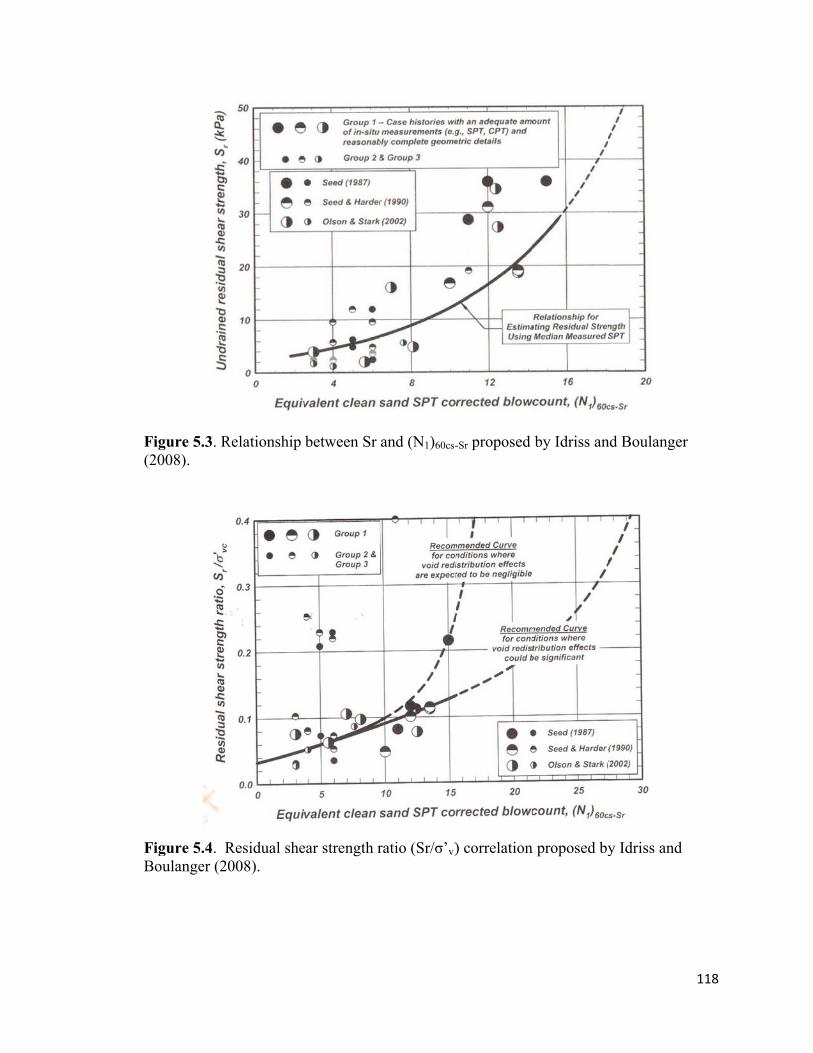
F(2

FB

Figure 5.3. R2008).

Figure 5.4. RBoulanger (20

Relationship

Residual she008).

between Sr

ear strength r

and (N1)60cs-

ratio (Sr/σ’v)

-Sr proposed

) correlation

by Idriss an

n proposed by

nd Boulanger

y Idriss and

118

r

119

the residual shear strength in localized areas, and using this relationship will result in a

more conservative assessment of Sr/σ’v. In eastern Arkansas, most of the liquefiable

sandy soil deposits are overlain by a thick clay layer, which will most likely impede the

flow of excess pore water pressure and result in significant void redistribution near the

layer interface. However, the potentially liquefiable soil layer is often quite thick, and

one would not expect significant void redistribution within the liquefiable layer.

5.3 COMPARISON OF DIRECT STRENGTH AND STRENGTH RATIO RELATIONSHIPS

In order to more easily compare direct Sr correlations, the relationships proposed

by Seed and Harder (1990) and Idriss and Boulanger (2008) have been digitized and are

presented together in Figure 5.5. The correlation of Idriss and Boulanger (2008) is near

the middle of the range proposed by Seed and Harder (1990), except at blow counts

larger than 15, were Idriss and Boulanger (2008) have extrapolated their correlation to

account for a lack of case history data. Not surprisingly, these correlations yield similar

results because the same case history data were used in their development.

In a similar manner, the Sr/σ’v correlations of Stark and Mesri (1992), Olsen and

Stark (2002), and Idriss and Boulanger (2008) are compared in Figure 5.6. The Idriss

and Boulanger (2008) relationships are very near the average Sr/σ’v relationship proposed

by Olsen and Stark (2002), except at blow counts above 12, where the relationships have

been extrapolated.

The direct Sr and Sr/σ’v relationships have been compared graphically in Figures

5.5 and 5.6. However, it is impossible to compare these two approaches outright without

applying the relationships using specific blow counts and effective confining stresses. A

F

F

Figure 5.5. C

Figure 5.6. S

1

Undrained

Shear Strength, Sr (psf)

Comparison o

Sr/σ’v correla

0

200

400

600

800

1000

0

of Sr as a fun

ations as a fu

5

Equivalent

Idriss and Bo

Seed and Har

nction of (N

unction of (N

10

t Clean Sand Bl

ulanger (2008)

rder (1990)

N1)60cs-Sr.

N1)60cs-Sr or (N

ow Count (N1)

N1)60.

15

60cs‐Sr

20

120

121

simple table (refer to Table 5.2) has been prepared to hypothetically compare the various

Sr estimates one would obtain from typical values of blow count and effective stress

using the direct Sr and Sr/σ’v relationships presented above. Corrected blow counts

ranging from 5-15 and effective stresses ranging from 0.54-2.72 atm (1152-5760 psf)

were used. Therefore, the Sr estimates provided in Table 5.2 are representative of values

one might obtain from the various relationships when applied to soft soils approximately

6-30 m (20-100 ft) below the surface.

At a depth of 6 m (20 ft) and a corrected blow count of 5, the relationships yield

Sr estimates ranging from 0-5.3 kPa (0-112 psf), with the direct Sr relationship of Idriss

and Boulanger (2008) yielding the highest estimate. At a depth of 12 m (40 ft) and a

corrected blow count of 10, the relationships yield Sr estimates ranging from 2.6-11.5

kPa (55-241 psf). Interestingly, for these parameters, all of the Sr estimates are within

15% of one another, except for the estimate obtained from the relationship of Seed and

Harder (1990), which is a lower-bound prediction. At a depth of 21 m (70 ft) and a

corrected blow count of 10, the relationships yield Sr estimates ranging from 2.6-20.2

kPa (55-423 psf), with the Sr/σ’v relationship of Olsen and Stark (2002) yielding the

highest estimate. The blow count was purposely fixed at 10 for both of these depths (i.e.

12 and 21 m [20 and 70 ft]) to demonstrate the difference between the direct Sr and Sr/σ’v

relationships. The reader will notice that the Sr estimates increase with increasing

depth/effective confining pressure when using the Sr/σ’v relationships even if the blow

count remains constant. Therefore, at significant depths/confining stresses the Sr/σ’v

relationships will always yield higher Sr estimates for a given blow count.

Thy

y

o

d

sm

pr

ap

5R

v

a

es

an

th

Table 5.2. Srypothetical b

At a d

ield Sr estim

f Idriss and B

irect Sr relat

maller than t

redicting if v

pproximately

.4 SITE-SPE

RELATIONSH

Unlik

alues using a

compilation

stimated Sr v

nd 15), the r

his is a fairly

1. Stresses c2. Lower-bo3. Average r

r estimates obblow counts

depth of 30 m

mates ranging

Boulanger (2

tionships. H

the “insignif

void redistrib

y 12 (refer to

CIFIC COMP

HIPS

e previous c

actual data f

n of informat

values. At a

relationships

y large sprea

alculated assumingund relationship

relationship

btained fromand effectiv

m (100 ft) an

g from 18.1-

2008) yield

However, the

ficant redistr

bution is lik

o Figures 5.4

PARISON OF

comparisons

from a soil b

tion needed

a depth of 9 m

s yield estima

ad (75%), the

g a uniform soil pr

m direct Sr anve confining

nd a correcte

-59.7 kPa (37

significantly

e “significan

ribution” esti

ely for soils

4 and 5.6).

DIRECT STR

in this chapt

oring compl

to estimate S

m (30 ft) and

ates between

e three lowes

rofile (refer to sect

nd Sr/σ’v rel stresses.

ed blow coun

79-1248 psf)

y higher estim

nt redistribut

imate, demo

with correct

RENGTH AND

ter, this sect

leted in Nort

Sr, while Ta

d raw blow c

n 17.2-31.4 k

st Sr values

tion 2.3.1)

lationships u

nt of 15, the

f). The Sr/σ’

mates of Sr t

tion” Sr estim

onstrating the

ted blow cou

D STRENGTH

tion presents

theast Arkan

able 5.4 prov

count of 11

kPa (379-66

differ by les

using

relationship

’v relationshi

than either o

mate is much

e importance

unts greater

H RATIO

s estimated S

nsas. Table 5

vides the

(corrected to

65 psf). Alth

ss than 10%.

122

ps

ips

of the

h

e of

than

Sr

5.3 is

o 14

hough

User

Stamp

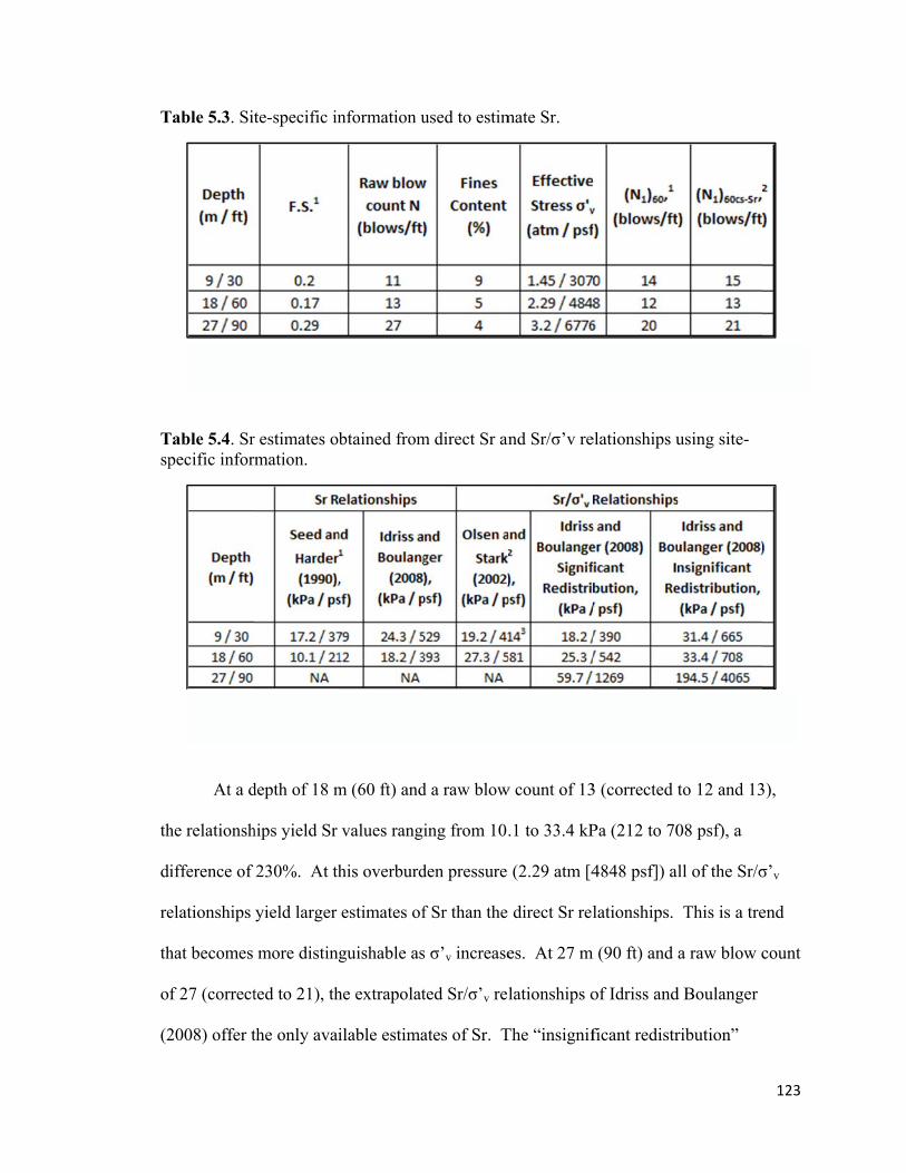
T

Tsp

th

d

re

th

o

(2

Table 5.3. Sit

Table 5.4. Srpecific infor

At a d

he relationsh

ifference of

elationships

hat becomes

f 27 (correct

2008) offer t

1. Determin2. Determin

1. Lower-bo2. Average r3. Extrapola

te-specific in

r estimates obrmation.

depth of 18 m

hips yield Sr

230%. At th

yield larger

more disting

ted to 21), th

the only avai

ned using workbooned using the recom

ound relationship. relationship. ated beyond maxim

nformation u

btained from

m (60 ft) and

values rangi

his overburd

estimates of

guishable as

he extrapolat

ilable estima

ok of Youd et al. (2mmendations of Se

mum SPT of 12 (re

used to estim

m direct Sr an

d a raw blow

ing from 10.

den pressure

f Sr than the

s σ’v increase

ted Sr/σ’v rel

ates of Sr. T

2001) accompanyieed (1987) (refer t

efer to Figure 5.2).

mate Sr.

nd Sr/σ’v re

w count of 13

.1 to 33.4 kP

(2.29 atm [4

direct Sr rel

es. At 27 m

lationships o

The “insignif

ing this report. to Section 5.2.1).

.

elationships u

3 (corrected t

Pa (212 to 70

4848 psf]) al

lationships.

m (90 ft) and

of Idriss and

ficant redistr

using site-

to 12 and 13

08 psf), a

ll of the Sr/σ

This is a tre

a raw blow c

d Boulanger

ribution”

123

3),

σ’v

end

count

User

Stamp

User

Stamp

124

relationship must be limited to a maximum Sr/σ’v value, which Idriss and Boulanger

(2008) recommend as the tangent of the soils internal angle of friction (assumed to be 0.6

in this table). Even with the maximum permissible Sr/σ’v employed, the “insignificant

redistribution” relationship yields a Sr of 194.5 kPa (4065 psf), which is 220% higher

than the “significant redistribution” Sr of 59.7 kPa (1269 psf). This large spread in Sr

demonstrates again, the importance of predicting if void redistribution is likely for soils

with corrected blow counts greater than approximately 12.

Site-specific information such as; corrected blow count, fines content, and depth

of the sample (effective stress), influence the Sr estimates these relationships provide.

This makes it challenging to determine which relationship will provide the most, or least,

conservative estimate for a given set of data. However, as effective stresses increase the

Sr estimates from Sr/σ’v relationships are usually higher than the direct Sr relationships.

At very shallow depths (low effective stresses), the blow count governs the estimated Sr

values, and any of the correlations could provide the lowest, or highest estimate of Sr.

The author recommends comparing results from at least three relationships in order to

assign an estimated Sr with some level of confidence.

5.5 CONCLUSIONS AND RECOMMENDATIONS

The available correlations for estimating Sr are based on back-analyses of

liquefaction-induced slope failure case histories. The use of these correlations in post-

liquefaction performance of piles, while not entirely accurate, provides the only available

alternative for calculating the residual shear strength of liquefied soils using SPT data.

Other correlations based on soil sampling and laboratory testing, have been shown to be

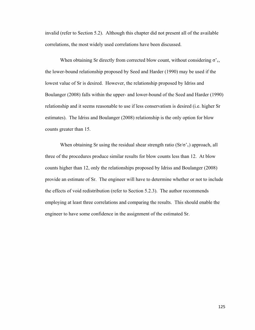
125

invalid (refer to Section 5.2). Although this chapter did not present all of the available

correlations, the most widely used correlations have been discussed.

When obtaining Sr directly from corrected blow count, without considering σ’v,

the lower-bound relationship proposed by Seed and Harder (1990) may be used if the

lowest value of Sr is desired. However, the relationship proposed by Idriss and

Boulanger (2008) falls within the upper- and lower-bound of the Seed and Harder (1990)

relationship and it seems reasonable to use if less conservatism is desired (i.e. higher Sr

estimates). The Idriss and Boulanger (2008) relationship is the only option for blow

counts greater than 15.

When obtaining Sr using the residual shear strength ratio (Sr/σ’v) approach, all

three of the procedures produce similar results for blow counts less than 12. At blow

counts higher than 12, only the relationships proposed by Idriss and Boulanger (2008)

provide an estimate of Sr. The engineer will have to determine whether or not to include

the effects of void redistribution (refer to Section 5.2.3). The author recommends

employing at least three correlations and comparing the results. This should enable the

engineer to have some confidence in the assignment of the estimated Sr.

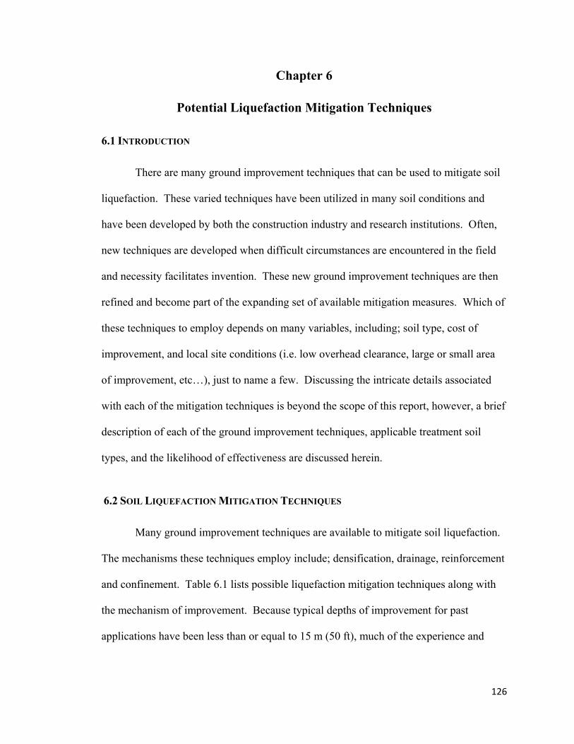
126

Chapter 6

Potential Liquefaction Mitigation Techniques

6.1 INTRODUCTION

There are many ground improvement techniques that can be used to mitigate soil

liquefaction. These varied techniques have been utilized in many soil conditions and

have been developed by both the construction industry and research institutions. Often,

new techniques are developed when difficult circumstances are encountered in the field

and necessity facilitates invention. These new ground improvement techniques are then

refined and become part of the expanding set of available mitigation measures. Which of

these techniques to employ depends on many variables, including; soil type, cost of

improvement, and local site conditions (i.e. low overhead clearance, large or small area

of improvement, etc…), just to name a few. Discussing the intricate details associated

with each of the mitigation techniques is beyond the scope of this report, however, a brief

description of each of the ground improvement techniques, applicable treatment soil

types, and the likelihood of effectiveness are discussed herein.

6.2 SOIL LIQUEFACTION MITIGATION TECHNIQUES

Many ground improvement techniques are available to mitigate soil liquefaction.

The mechanisms these techniques employ include; densification, drainage, reinforcement

and confinement. Table 6.1 lists possible liquefaction mitigation techniques along with

the mechanism of improvement. Because typical depths of improvement for past

applications have been less than or equal to 15 m (50 ft), much of the experience and

T

d

n

b

m

se

6

1

in

th

pr

co

b

la

Table 6.1. Li

esign guidan

eeded in cer

e kept in min

mitigation tec

ections.

.2.1 Vibrato

Vibrat

948 (Schaef

nclude; Sand

hese method

robe is vibra

oncrete) is in

etween the p

aterally into

iquefaction m

nce are limit

rtain areas of

nd while rea

chniques inc

ory Method

tory method

fer 1997). Th

d Compactio

ds employs so

ated to the m

ntroduced in

probe and th

the soil, thu

mitigation te

ted to these d

f the New M

ading this ch

cluded in this

ds

ds have been

he three type

n Piles, Ston

omewhat sim

maximum dep

nto the soil e

e soil. As th

s densifying

echniques dis

depths. Also

Madrid Seism

hapter and an

s table will b

used to succ

es of vibrato

ne Columns

milar equipm

pth of impro

ither through

he probe is ra

g it.

scussed in th

o, the large d

mic Zone (NM

ny available

be discussed

cessfully den

ory methods

and Vibro-C

ment and con

ovement. Th

h a tube in th

aised and low

his report

depths of imp

MSZ) (>15 m

literature. E

d in more det

nsify soil in

discussed in

Concrete Co

nstruction tec

hen, material

he probe or t

wered the m

provement

m, [50 ft]) sh

Each of the

tail in subseq

the U.S. sin

n this chapte

lumns. Each

chniques. A

l (sand, grav

the annulus

material is for

127

hould

quent

nce

er

h of

A

vel or

rced

128

6.2.1.1 Sand Compaction Piles

Sand Compaction Piles, or Vibro-Compaction, is common between depths of 3 to

15 m (10 to 50 ft), although soil depths up to 36 m (120 ft) have been successfully

densified (Schaefer 1997). This soil improvement technique uses clean sand as a backfill

material or, the site may be lowered an amount equal to the densification of the in-situ

soil. Figure 6.1 illustrates the Sand Compaction Pile construction process and finished

product. Sand Compaction Piles can be completed with or without water jets (i.e. wet or

dry method). The use of water jets aid penetration and reduce inter-granular forces,

thereby encouraging compaction (Dobson and Slocombe 1982). Wet or dry, this type of

treatment is best suited for clean granular soils. One drawback is that improvement must

be continued throughout the entire depth of insertion, even if only a deep isolated layer is

susceptible to liquefaction, which could result in a large cost increase. The degree of

densification that Sand Compaction Piles are capable of is highly dependent on; vibrator

type and size, penetration spacing, soil type, and compaction procedures (Hayden and

Baez 1994).

6.2.1.2 Stone Columns

Stone Columns are similar to Sand Compaction Piles, but use crushed gravel for

the backfill material. Figure 6.2 illustrates the stone column construction process and

finished product, which is a stone column that is tightly interlocked with the surrounding

soil (Munfakh et al. 1987). The gravel densifies the soil adjacent to the stone column and

provides a path to relieve the potential buildup of excess pore water pressures. This

technique is especially effective in clean sands, but can be used in soils with high fines

content if drainage is provided (Mitchell et al. 1998). Like Sand Compaction Piles,

FB

F2

Figure 6.1. IlBaker Inc. 20

Figure 6.2. Il010b).

llustration of010b).

llustration of

f the Sand C

f the Stone C

Compaction P

Column cons

Pile construc

struction pro

ction process

ocess (Hayw

s (Hayward

ward Baker In

129

nc.

130

improvement must be continued throughout the entire depth of insertion, even if only a

deep isolated layer is susceptible to liquefaction. The cost and effectiveness of stone

columns depend on the availability of clean gravel and the spacing and diameter of the

columns.

6.2.1.3 Vibro-Concrete Columns

Vibro-Concrete Columns were developed by the Keller Company and have been

used substantially in Europe since 1976 (Hayden and Baez 1994). Figure 6.3 illustrates

the Vibro-Concrete Column construction process and final product. Instead of sand or

gravel, concrete is pumped to the vibrator tip. Initially, at depth, the vibrator moves up

and down forcing the concrete into the surrounding soil to form a mushroom. After the

initial mushroom is formed, the vibrator is withdrawn as concrete is pumped into the void

space producing a concrete column. Vibro-Concrete Columns transfers loads from the

surface to deeper more competent strata and densify looser layers.

6.2.2 Deep Dynamic Compaction

Dynamic Compaction is a method of densifying the soil by repeatedly dropping a

heavy weight (9,000-27,000 kg [20,000-60,000 lbs]) from heights of 15-40 m (50-120 ft).

The energy imparted into the soil rearranges and densifies the particles, as portrayed in

Figure 6.4. This method has been shown to improve cohesionless soils to a maximum

depth of 10 m (30 ft) under ideal conditions when using a 1 m (3 ft) thick “working mat”

of dry granular soil on the surface (Hayden and Baez 1994). Notice that this method is

unlikely to improve the density of the soil at the depths greater than 10 m (30 ft).

Furthermore, typical soil conditions in northeast Arkansas include a thick clay layer at the

FIn

F

Figure 6.3. Ilnc. 2010b).

Figure 6.4. Il

llustration of

llustration of

f Vibro-Con

f Deep Dyna

ncrete Colum

amic Compa

mn constructi

action (Hayw

ion process.

ward Baker I

(Hayward B

Inc. 2010b).

131

Baker

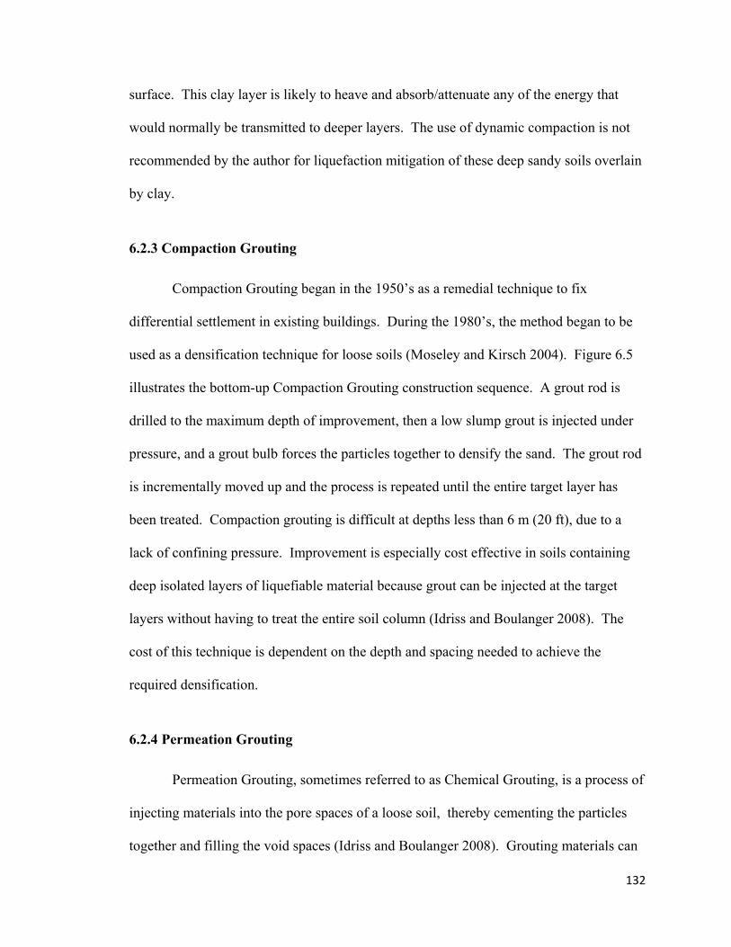
132

surface. This clay layer is likely to heave and absorb/attenuate any of the energy that

would normally be transmitted to deeper layers. The use of dynamic compaction is not

recommended by the author for liquefaction mitigation of these deep sandy soils overlain

by clay.

6.2.3 Compaction Grouting

Compaction Grouting began in the 1950’s as a remedial technique to fix

differential settlement in existing buildings. During the 1980’s, the method began to be

used as a densification technique for loose soils (Moseley and Kirsch 2004). Figure 6.5

illustrates the bottom-up Compaction Grouting construction sequence. A grout rod is

drilled to the maximum depth of improvement, then a low slump grout is injected under

pressure, and a grout bulb forces the particles together to densify the sand. The grout rod

is incrementally moved up and the process is repeated until the entire target layer has

been treated. Compaction grouting is difficult at depths less than 6 m (20 ft), due to a

lack of confining pressure. Improvement is especially cost effective in soils containing

deep isolated layers of liquefiable material because grout can be injected at the target

layers without having to treat the entire soil column (Idriss and Boulanger 2008). The

cost of this technique is dependent on the depth and spacing needed to achieve the

required densification.

6.2.4 Permeation Grouting

Permeation Grouting, sometimes referred to as Chemical Grouting, is a process of

injecting materials into the pore spaces of a loose soil, thereby cementing the particles

together and filling the void spaces (Idriss and Boulanger 2008). Grouting materials can

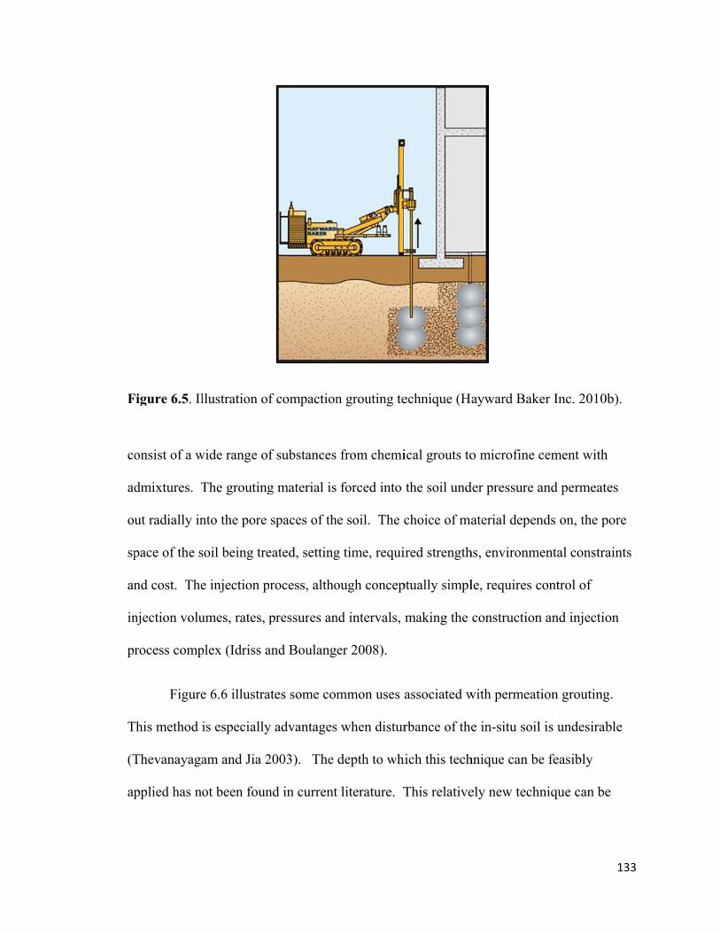
F

co

ad

ou

sp

an

in

pr

T

(T

ap

Figure 6.5. Il

onsist of a w

dmixtures. T

ut radially in

pace of the s

nd cost. The

njection volu

rocess comp

Figure

This method

Thevanayaga

pplied has n

llustration of

wide range of

The grouting

nto the pore

soil being tre

e injection p

umes, rates, p

plex (Idriss a

e 6.6 illustra

is especially

am and Jia 2

ot been foun

f compaction

f substances

g material is

spaces of th

eated, setting

rocess, altho

pressures an

and Boulang

ates some com

y advantages

2003). The

nd in current

n grouting te

from chemi

forced into

he soil. The c

g time, requi

ough concep

nd intervals,

er 2008).

mmon uses

s when distur

depth to wh

t literature. T

echnique (Ha

ical grouts to

the soil und

choice of ma

ired strength

ptually simpl

making the

associated w

rbance of the

hich this tech

This relative

ayward Bak

o microfine c

der pressure a

aterial depen

hs, environm

le, requires c

construction

with permeat

e in-situ soil

hnique can be

ely new tech

ker Inc. 2010

cement with

and permeat

nds on, the p

mental constra

control of

n and injectio

tion grouting

l is undesirab

e feasibly

hnique can be

133

0b).

h

tes

pore

aints

on

g.

ble

e

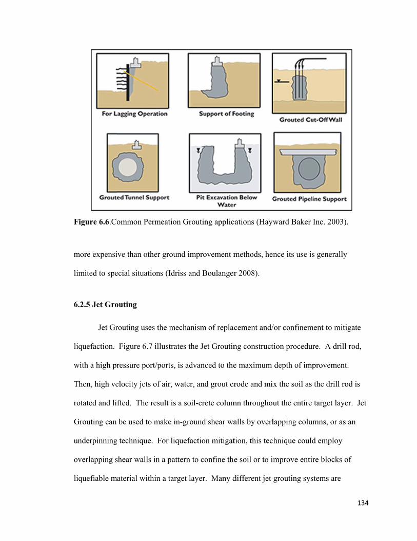
F

m

li

6

li

w

T

ro

G

un

ov

li

Figure 6.6.Co

more expensi

imited to spe

.2.5 Jet Gro

Jet Gr

iquefaction.

with a high pr

Then, high ve

otated and li

Grouting can

nderpinning

verlapping s

iquefiable m

ommon Perm

ive than othe

ecial situatio

outing

routing uses

Figure 6.7 i

ressure port/

elocity jets o

fted. The re

be used to m

g technique.

shear walls in

aterial withi

meation Gro

er ground im

ns (Idriss an

the mechani

illustrates the

/ports, is adv

of air, water,

esult is a soil

make in-grou

For liquefac

n a pattern to

in a target lay

outing applic

mprovement m

nd Boulanger

ism of replac

e Jet Groutin

vanced to the

and grout er

l-crete colum

und shear wa

ction mitigat

o confine the

yer. Many d

cations (Hayw

methods, hen

r 2008).

cement and/

ng construct

e maximum

rode and mix

mn throughou

alls by overl

tion, this tec

e soil or to im

different jet

ward Baker

nce its use is

/or confinem

tion procedu

depth of imp

x the soil as

ut the entire

lapping colu

hnique could

mprove enti

grouting sys

Inc. 2003).

s generally

ment to mitig

ure. A drill r

provement.

the drill rod

target layer

umns, or as a

d employ

ire blocks of

stems are

134

gate

rod,

d is

r. Jet

an

f

F(H

av

tr

A

C

li

6

to

au

a

fi

Figure 6.7. IlHayward Ba

vailable for

riple fluid sy

Although eac

Compaction G

iquefiable m

.2.6 Deep So

Deep

o the target d

ugers are be

soil-crete co

igure 6.8. Th

llustration ofaker Inc. 201

site-specific

ystems, as we

ch of these ar

Grouting, Je

aterial locate

oil Mixing

soil mixing

depth, follow

ing rotated a

olumn or row

he columns

f Jet Groutin0b).

c soil and pro

ell as SuperJ

rrangements

t Grouting is

ed at depth.

consists of a

wed by ceme

and lifted. T

w of column

can be arran

ng constructi

oject requirem

Jet and X-Jet

s is different,

s particularly

an auger, or

ent being pum

This causes th

ns (Idriss and

nged into ma

ion process u

ments, these

t grouting ar

, the final pr

y advantage

row of overl

mped near th

he cement an

d Boulanger

any different

using triple f

e include; sin

rrangements

roduct is very

s for a finite

lapping auge

he tip of the

and the soil to

2008), as ill

t patterns, as

fluid system

ngle, double

s (Burke 200

y similar. L

e layer of

ers, being ro

augers whil

o mix, produ

lustrated in

s illustrated i

135

m

e and

04).

Like

otated

e the

ucing

in

F2

fi

co

li

re

it

un

d

d

d

Figure 6.8. Il010b).

igure 6.9. O

onfiguration

iquefaction i

educing exce

t does liquefy

nimproved g

epths of ove

oes require l

epth must be

llustration of

Often, the pat

ns called latti

n three ways

ess pore wat

fy, and (3) it

ground (Idris

er 30 m (100

large overhe

e treated.

f Deep Soil M

tterns are int

ice (Porbaha

s; (1) it redu

ter pressure b

restricts the

ss and Boula

ft) and can

ead clearance

Mixing cons

erlocked geo

a et al. 1999)

uces the earth

buildup, (2)

migration o

anger 2008).

be used with

e, and the en

struction pro

ometric (i.e.

). The lattice

hquake induc

it restrains t

of excess por

. Deep soil m

h fine graine

ntire column

ocess (Hayw

square or he

e configurat

ces shear sta

the soil from

re water pres

mixing is ap

ed material.

of soil down

ward Baker, I

exagonal)

tion mitigate

ains, thereby

m deformatio

ssure from

pplicable for

The drill rig

n to the targ

136

Inc.

es soil

y

n if

g

et

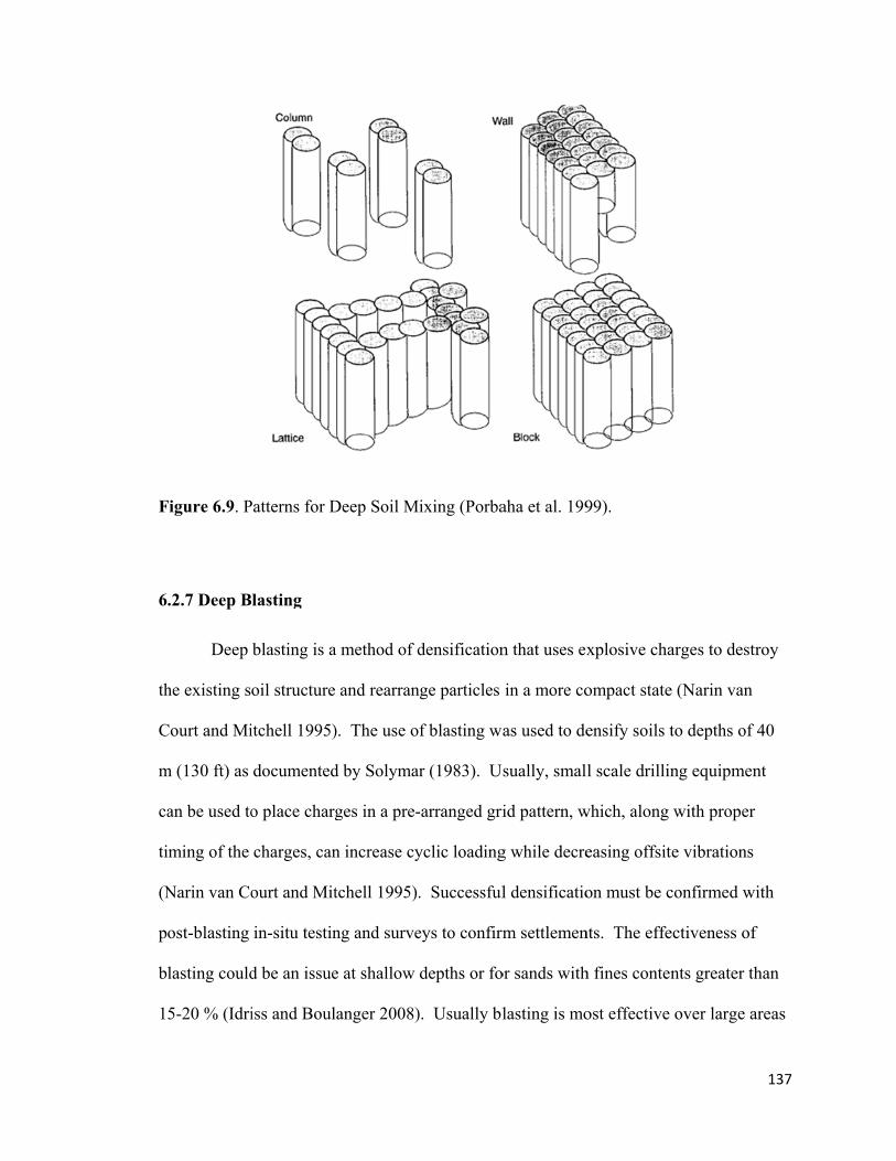
F

6

th

C

m

ca

ti

(N

p

b

1

Figure 6.9. P

.2.7 Deep B

Deep

he existing s

Court and Mi

m (130 ft) as

an be used to

iming of the

Narin van Co

ost-blasting

lasting could

5-20 % (Idri

Patterns for D

lasting

blasting is a

oil structure

itchell 1995)

documented

o place charg

charges, can

ourt and Mit

in-situ testin

d be an issue

iss and Boul

Deep Soil M

a method of d

and rearran

). The use o

d by Solymar

ges in a pre-

n increase cy

tchell 1995).

ng and surve

e at shallow

langer 2008)

ixing (Porba

densification

nge particles

f blasting wa

r (1983). Us

-arranged gri

yclic loading

. Successful

eys to confirm

depths or fo

). Usually bl

aha et al. 199

n that uses ex

in a more co

as used to de

sually, smal

id pattern, w

g while decre

l densificatio

m settlemen

or sands with

lasting is mo

99).

xplosive cha

ompact state

ensify soils t

l scale drillin

which, along

easing offsit

on must be c

nts. The effe

h fines conten

ost effective

arges to dest

e (Narin van

to depths of

ng equipmen

with proper

te vibrations

confirmed w

ectiveness of

nts greater th

over large a

137

troy

40

nt

r

with

f

han

areas

138

and can often be coupled with a testing program to ensure proper spacing, depth, and

weight of charges. Obtaining permits for blasting, off-site vibration requirements and

quantifying the area of improvement are some of the considerations when determining if

this is the best technique for liquefaction mitigation.

6.2.8 Earthquake Drains

Earthquake Drains have been used to provide drainage of excess pore water

pressures and reduce total settlements in liquefied soil layers (Chang et al. 2004).

Earthquake Drains consist of, 75-150 mm (3-6 inch) diameter corrugated pipe with open

slots, covered with filter fabric. The open slots allow excess pore water to flow into the

pipe while the filter fabric keeps fines from entering and clogging the slots. The drains

can be installed using casing and conventional drilling techniques, or a modified

vibrating mandrel (Chang et al. 2004). Figure 6.10 illustrates the mandrel type

installation technique. Earthquake Drains can be installed to depths of 25 m (85 ft)

(Hayward Baker Inc. 2010a), and are best suited for free-draining soils.

6.2.9 Dewatering Techniques

Dewatering is a possible liquefaction mitigation technique because the absence of

water makes the buildup of excess pore water pressure impossible. The use of this

technique is typically limited to short-term applications because of the high cost and

maintenance associated with continual pumping and the deterioration of pumping

efficiency over time. Dewatering, along with a cut-off wall, was used as an interim soil

liquefaction mitigation technique by the Bureau of Reclamation on the downstream slope

of Bradbury Dam. The wells pumped for 18 months while permanent solutions could be

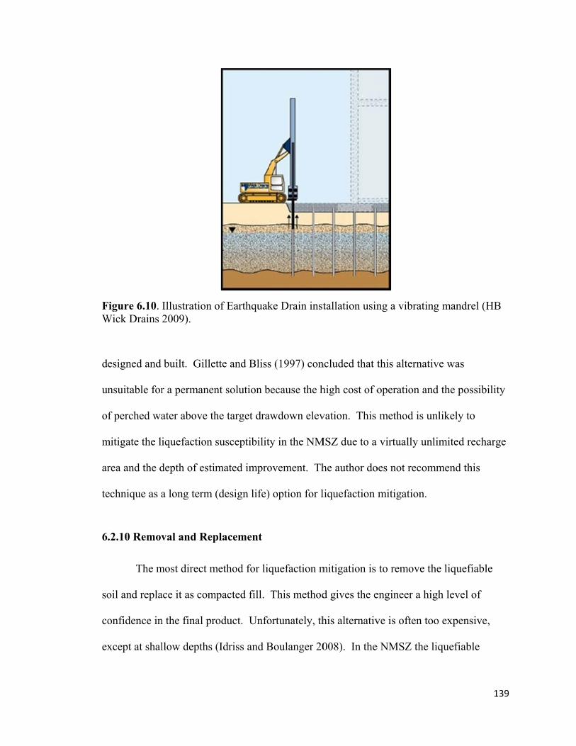
FW

d

un

o

m

ar

te

6

so

co

ex

Figure 6.10. Wick Drains

esigned and

nsuitable for

f perched wa

mitigate the l

rea and the d

echnique as a

.2.10 Remov

The m

oil and repla

onfidence in

xcept at shal

Illustration o2009).

built. Gille

r a permanen

ater above th

iquefaction

depth of estim

a long term (

val and Rep

most direct m

ace it as com

n the final pr

llow depths

of Earthquak

tte and Bliss

nt solution b

he target dra

susceptibilit

mated impro

(design life)

placement

method for liq

mpacted fill.

oduct. Unfo

(Idriss and B

ke Drain inst

s (1997) con

because the h

awdown elev

ty in the NM

ovement. Th

) option for l

quefaction m

This method

ortunately, th

Boulanger 20

tallation usin

ncluded that t

high cost of o

vation. This

MSZ due to a

he author do

liquefaction

mitigation is

d gives the e

his alternativ

008). In the

ng a vibratin

this alternati

operation an

method is u

virtually un

oes not recom

mitigation.

to remove th

engineer a hi

ve is often to

e NMSZ the

ng mandrel (

ive was

nd the possib

unlikely to

nlimited rech

mmend this

he liquefiabl

igh level of

oo expensive

liquefiable

139

(HB

bility

harge

le

e,

140

layers are often below 10 m (30 ft). This fact, combined with the relatively high ground

water level (3-6 m, 10-20 ft below the surface), make the removal and replacement

method an unlikely option.

6.3 COST COMPARISON

Tables 6.2 is included to compare costs of some liquefaction mitigation

techniques discussed in the previous section. The data has been copied from a

publication provided by Hayward Baker Inc. (2003), in which a few assumptions were

made to come up with relative cost estimates. The assumptions include; (1) the data is

applicable to medium-size projects, and (2) the cost data for each technique is applicable

to specific soil types (not included in this table). Because of these assumptions, and the

fact that the depth of the liquefiable soils encountered in the NMSZ is significant, the

costs in Table 6.2 are not appropriate for current design. Still, this table can be used to

provide initial “back of the napkin” calculations to determine if further investigation

concerning cost information is justified. If further investigation is justified, the engineer

can devote more time and effort to determine more accurate cost information.

The cost of mobilization in Table 6.2 reveals that Jet Grouting and Deep Soil

Mixing are much more expensive initially then any of the other techniques. The

treatment costs of Compaction and Jet Grouting are also higher than the others, but may

be offset, depending on site specifics, because only layers susceptible to liquefaction need

to be treated. Many seemingly viable options (i.e. Earthquake Drains, Deep Blasting,

etc.) are difficult to find cost information for, and this table will have to be supplemented

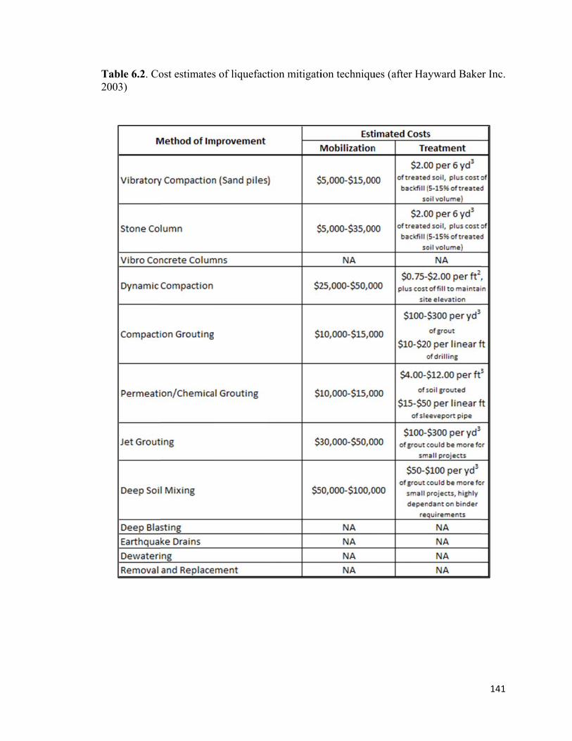
T2

Table 6.2. Co003)

ost estimatess of liquefacttion mitigatiion techniquues (after Hayyward Bake

141

er Inc.

142

with current or past cost data provided from another source to determine site-specific cost

information.

6.4 SUMMARY AND CONCLUSIONS

This chapter has presented many current soil improvement techniques used to

mitigate soil liquefaction. A few methods such as Deep Dynamic Compaction,

Dewatering, and Removal and Replacement have been ruled out as applicable for most

soil profiles in northeast Arkansas due to the significant depth and thickness of the

liquefiable soil layer. Because site-specific conditions change from one project to

another, a range of other possible techniques have been presented as viable options.

These will need to be evaluated on a site-by-site basis using up to date cost information.

The engineer should also recognize the possibility of combining several techniques in

order to achieve the desired level of service.

Site-specific soil conditions and cost considerations prohibit the recommendation

of any one liquefaction mitigation technique. Initially, all reasonable possibilities should

be considered. Then, as soil properties and cost data are considered some of the

techniques will be disqualified, leaving only a few possible alternatives that can produce

the desired outcome.

143

Chapter 7

Conclusions and Recommendations

7.1 CONCLUSIONS

Northeastern Arkansas has some of the largest design earthquake ground motions

in the continental U.S. (e.g., PGA values ranging up to 1.0 g and greater) due to its

location within the New Madrid Seismic Zone (NMSZ). These large earthquake ground

motions are particularly problematic when coupled with the unknown seismic response of

the deep, soft soils of the Mississippi Embayment. Based on empirical standard

penetration test (SPT) liquefaction triggering analyses, many soils in this area exhibit

apparent liquefaction susceptibility at depths up to 30-plus m (100-plus ft). However,

there is very little guidance in the literature on what to do in these situations, because

soils soft enough to liquefy at great depths (i.e. greater than approximately 20 m [65 ft])

have not been documented in the case history databases from previous earthquakes.

The primary task of this research was to help AHTD, and other interested entities

involved with design and construction of deep foundations in the NMSZ, update

procedures used to evaluate earthquake-induced soil liquefaction triggering, particularly

with respect to liquefaction of soils at great depths. Specific subtasks of this research

project included providing recommendations and insights concerning: (1) appropriate use

of SPT-based liquefaction triggering procedures, (2) residual shear strength of liquefied

soils, and (3) potential liquefaction mitigation measures (i.e. possible ground

improvement techniques). The conclusions regarding each of these subtasks are

presented below.

144

7.1.1 SPT-based Liquefaction Triggering Procedures

To help evaluate potential liquefaction susceptibility of deep soil deposits in the

Mississippi Embayment, the three most commonly used SPT-based liquefaction

triggering procedures (Youd et al. 2001, Cetin et al. 2004, and Idriss and Boulanger

2008) have been examined, systematically compared, and programmed into user-friendly

Excel workbooks. This is not a trivial topic, as the most appropriate method to use for

liquefaction triggering is currently debated at the highest levels of the geotechnical

earthquake engineering community (Seed 2010, Finn et al. 2010). These workbooks

allow the liquefaction triggering results (i.e., factors of safety and other depth dependent

variables) from all three procedures to be readily compared at a given site. The

development of these workbooks (including making sure they were user-friendly and

technically accurate) occupied a significant portion of the time dedicated to this project.

These workbooks will be provided free of charge to anyone interested in using them.

Overall, for the sites analyzed herein, which have fairly high to very high peak

ground accelerations, the three procedures agreed in predicting or not predicting

liquefaction at many depths. This should not be misconstrued to mean that the numerical

values of the F.S. estimates were similar at many depths, but rather that in many

circumstances the F.S. estimates were similarly either greater than or less than 1.0,

yielding a similar prediction about liquefaction susceptibility. The agreement between all

three procedures at a given depth lends confidence to these types of deterministic

triggering analyses where a “yes” or “no” answer is required. For situations where the

three procedures do not agree on liquefaction triggering, the author recommends using

the prediction (i.e., “yes” or “no” liquefaction) agreed upon by two out of the three

145

procedures. This seems logical given the debate that is ongoing regarding which

procedure is “best” (Finn et al. 2010).

Site-specific comparisons of the three liquefaction triggering procedures for

boring logs in eastern Arkansas have revealed situations (specific depths at specific sites)

where the three procedures yield nearly identical F.S. estimates, and situations where

they yield significantly different F.S. estimates. Examinations of depth/stress dependent

variables such as rd, CN, (N1)60cs, and Kσ have revealed that no single depth-dependent

variable is exclusively responsible for the differences between the liquefaction triggering

procedures when F.S. estimates disagree. Surprisingly, in some situations the variable rd

was found to vary by as much as 45% - 60% between procedures for the exact same

depth, yet the F.S. estimates for all procedures were nearly identical at these same depths.

In other situations, the impact of smaller variations in rd was evident. In general, it was

found that variations in rd really did not seem to impact the F.S. estimates as much as

anticipated. This is likely because each procedure used its respective rd relationship to

define the CRR boundary curve in the back analyses of the case history database; thereby

influencing both the CSR and CRR in a similar manner for forward analyses.

In general, it can be stated that the Idriss and Boulanger (2008) procedure

typically yields the highest F.S. estimates at depth. While this is somewhat driven by

higher Kσ values at depth (generally ranging from 5% - 15% greater than the other two

procedures), it seems to primarily be a result of significantly higher CN values at depth

(generally ranging from 15% - 60% greater than the other two procedures for higher blow

count material). Specifically, the iterative, blow count defendant CN relationship of Idriss

and Boulanger (2008) tends to yield significantly greater CN values when the raw blow

146

count of the material is greater than about 23. These larger values of CN directly result in

larger (N1)60cs values, which result in higher CRRM=7.5,1atm values and higher F.S.

estimates. Furthermore, as this difference is most pronounced at higher blow counts,

where the CRR relationship is very steep and nonlinear, somewhat subtle differences in

(N1)60cs values can result in very significant differences in CRRM=7.5,1atm values. In-depth

comparisons of the F.S. estimates and depth-dependant variables may be found in

Chapter 4.

7.1.2 Residual Shear Strength

Chapter 5 presented available correlations for estimating the residual shear

strength (Sr) of liquefied soil based on back-analyses of liquefaction-induced slope

failure case histories. The use of these correlations in post-liquefaction performance of

piles, while not entirely accurate, provides the only available alternative for calculating

the residual shear strength of liquefied soils using SPT data. The correlations presented

in Chapter 5 can be categorized into one of two groups; (1) direct estimation of Sr based

on (N1)60cs-Sr values or, (2) estimation of Sr based on the residual shear strength ratio

(Sr/σ’v), which incorporates the influence of the vertical effective stress (σ’v).

When obtaining Sr directly from corrected blow count, without considering σ’v,

the lower-bound relationship proposed by Seed and Harder (1990) may be used if the

most conservative value of Sr is desired. However, the relationship proposed by Idriss

and Boulanger (2008) falls within the upper- and lower-bound of the Seed and Harder

(1990) relationship and it seems reasonable to use if less conservatism is desired (i.e.,

147

higher Sr estimates). Furthermore, the Idriss and Boulanger (2008) relationship is the

only option for estimating Sr directly for soil with blow counts greater than 15.

When obtaining Sr using the residual shear strength ratio (Sr/σ’v) approach, the

available procedures yield similar results for blow counts less than 12. At blow counts

greater than 12, only the relationships proposed by Idriss and Boulanger (2008) provide

an estimate of Sr. In order to estimate Sr using the relationships proposed by Idriss and

Boulanger (2008), the engineer will have to determine whether or not to include the

effects of void redistribution (refer to Section 5.2.3), which can significantly influence

the results (differences in Sr > 200%).

Site-specific information such as corrected blow count, fines content, and depth of

the sample (effective stress) influence the Sr estimates provided by all of these

relationships. This makes it challenging to determine which relationship will provide the

most, or least, conservative estimate of Sr for a given set of conditions without making

the calculations. However, at depth the Sr estimates from Sr/σ’v relationships can be

significantly higher than the direct Sr relationships because a benefit is derived from the

high effective confining pressures. Because site specific data influences the Sr estimates,

the author recommends comparing results from at least three different relationships in

order to assign an estimated Sr with some level of confidence. Examples of how to make

these comparisons on a site-specific basis are provided in Chapter 5.

7.1.3 Ground Improvement Techniques

Chapter 6 presented many current soil improvement techniques used to mitigate

soil liquefaction. A few methods such as Deep Dynamic Compaction, Dewatering, and

148

Removal and Replacement were ruled out as applicable for most soil profiles in northeast

Arkansas due to the significant depth and thickness of the liquefiable soil layer. Because

site-specific conditions change from one project to another, a range of other possible

techniques have been presented as viable options. These will need to be evaluated on a

site-by-site basis using up to date cost information. The engineer should also recognize

the possibility of combining several techniques in order to achieve the desired level of

service.

Site-specific soil conditions and cost considerations prohibit the recommendation

of any one liquefaction mitigation technique. Initially, all reasonable possibilities should

be considered. Then, as soil properties and cost data become available some of the

techniques will be disqualified, leaving only a few possible alternatives that can produce

the desired outcome.

7.2 FUTURE WORK

While the validity of predicting liquefaction susceptibility at significant depths

(i.e. greater than 20 m [65 ft]) using simplified SPT procedures is uncertain given the

shallow depth range of liquefaction case history data points, one thing is certain: often

times all three available procedures predict liquefaction susceptibility at depths of 30-plus

m (100-plus ft) for the soil conditions and design PGA values encountered in eastern

Arkansas. In the short term, it is recommended that design engineers evaluate

liquefaction triggering using all three SPT-based procedures and then use the prediction

(i.e., “yes” or “no” liquefaction) agreed upon by two out of the three procedures.

However, in the long term additional research is needed to understand not only the

149

potential for triggering liquefaction in these deep soil deposits but also the consequences

of liquefaction given it is triggered.

The ambiguity of predicting deep soil liquefaction is currently an ongoing debate

at the highest levels of geotechnical earthquake engineering (Seed 2010, Finn et al.

2010). This argument has particular implications for design and retrofit of dams, and is

now receiving much attention. If it were an easy problem, it would have been solved

already. However, in lieu of knowing which, if any, of the current liquefaction triggering

procedures is “best”, it may be appropriate to take a closer look at the PGA values that

are driving the liquefaction hazard in the New Madrid Seismic Zone (NMSZ). The

AASHTO Guide Specifications for LRFD Seismic Bridge Design (2009) allow seismic

design forces obtained from general, code-based procedures to be reduced up to 33% (i.e.

2/3 of the code-based ground motions) if site-specific ground motion response analyses

are performed. This potential benefit would allow structural seismic loads and peak

ground accelerations used in soil liquefaction analyses and retaining wall designs to be

decreased substantially should the site response analyses indicate it is possible. It is very

likely that this would be the case, especially for short-period ground motions like PGA,

due to soil nonlinearity at significant strains induced by large input rock motions. The

AASHTO Guide Specifications (2009) directly mention deep, soft soil deposits (like

those found within the NMSZ) as locations where site-specific ground motion response

analyses should be performed. Otherwise, "longer-period [i.e. long-span, relatively

flexible] bridges may be under-designed and shorter-period [i.e. short-span, relatively

stiff] bridges may be over-designed". It is recommended that AHTD perform site-

specific ground motion response analyses to investigate the possibility of reducing PGA

150

values to 2/3 of the code-based procedures. This could have a significant impact on the

liquefaction triggering predictions at some sites.

In terms of evaluating the consequences of liquefaction in these deep, thick soil

deposits, much is unknown about the post-liquefaction axial and lateral capacity of pile

foundations. It is possible that blast-induced liquefaction studies could be used to

provide important insights for evaluating axial down-drag (negative skin friction) and

revised p-y curves for predicting lateral load response in liquefiable soils. Conducting

full-scale axial and lateral pile load tests before and after initiating liquefaction via

blasting would be invaluable for confidently evaluating post-liquefaction axial and lateral

capacity of piles in the unique soil conditions of northeast Arkansas. Due to the

significant thickness of the overlying clay layer at typical sites (6 – 9 m [20 – 30 ft]), it is

possible that very significant increases in axial forces caused by down-drag may be

induced as the 15-plus m (50-plus ft) layer of underlying clean sand liquefies and

consolidates. This potential problem needs additional study. While the effects of lateral

spreading also need to be considered, it is possible that lateral spreading may not be as

significant a problem as in many areas because the top of the liquefiable layer may be

below the bottom of the river channel.

151

References

American Association of State Highway and Transportation Officials (2009). “Guide

Specifications for LRFD Seismic Bridge Design.” 1st Edition, Washington, DC.

Andrew, D.C.A., and G.R. Martin. (2000), “Criteria for liquefaction of silty soils.” 12th

World Conference on Earthquake Engineering, January, 29-February 5,

Auckland, New Zealand.

Andrus, R.D., Stokoe, K.H., II, (2000). "Liquefaction Resistance of Soils from Shear -

Wave Velocity." Journal of Geotechnical and Geoenvironmental Engineering,

ASCE, Vol. 126, No. 11, Nov. pgs, 1015-1025

Bray, J.D., and Sancio, R.B. (2006). “Assesment of Liquefaction Susceptibility of Fine-

Grained Soils.” Journal of Geotechnical and Geoenvironmental Engineering,

ASCE, Vol. 132, No. 9, Sep. pp. 1165-1177.

Bray, J.D., Sancio, R.B., Durgunolu, H.T., Onalp, A., Seed, R.B., Stewart, J.P., Youd,

T.L., Baturay, M.L., Cetin, K.O., Christensen, C., Karadayilar, T., and Emrem,

C. (2001). “Ground Failure in Adapazari, Turkey.” Proc. of Earthquake

Geotechnical Engineering Satellite Conference of the XVth International

Conference on Soil Mechanics and Geotechnical Engineering, Istanbul, Turkey,

August 24-25.

Boulanger, R.W. (2003). “High Overburden Stress Effects on Liquefaction Analyses.”

Journal of Geotechnical and Geoenvironmental Engineering, ASCE, Vol. 129,

No. 12, Dec. pp. 1071-1082.

152

Boulanger, R.W., and Idriss, I.M. (2004). “State Normalization of Penetration Resistance

and the Effect of Overburden Stress on Liquefaction Resistance.” Proc. of 11th

International Conf. on Soil Dynamics and Earthquake Engineering, and 3rd

International Conf. on Earthquake Geotechnical Engineering, Berkeley, CA. Vol.

2, pp. 484-491.

Burke, G.K. (2004). “Jet Grouting Systems: Advantages and Disadvantages.” GSP 124,

Proc. Geosupport Conference, Orlando, FL. pp. 1-12.

Cetin, K.O., Seed, R.B., Kiureghain, A.D., Tokimatsu, K., Harder, L.F., Kayen, R.E.,

Moss, R.E.S. (2004). “Standard Penetration Test-Based Probabilistic and

Deterministic Assesment of Seismic Soil Liquefaction Potential.” Journal of

Geotechnical and Geoenvironmental Engineering, ASCE, Vol. 130, No. 12, Dec.

pp. 1314-1340.

Chang, W-J., Rathje, E.M., Stokoe, K.H. II, Cox, B.R. (2004). “Direct Evaluation of

Effectiveness of Prefabricated Vertical Drains in Liquefiable Sand”. Soil

Dynamics and Earthquake Engineering, Vol. 24, pp. 723-731.

Cox, B.R. (2001). “Shear Wave Velocity Profiles at Sites Liquefied by the 1999 Kocaeli,

Turkey Earthquake.” M.S. Thesis, Utah State University, Logan, Utah, p. 274.

Dennis, N.D. (1988). Discussion on “Liquefaction Evaluation Procedure” Journal of

Geotechnical Engineering Division, ASCE, Vol. 114, No. 2, pp. 241-243.

153

Dobson, T. and Slocombe, B. (1982). “Deep Densification of Granular Fills.” 2nd

Geotechnical , Conference and Exhibit on Design and Construction, April 26-28,

Las Vegas, NV.

Finn, W.D.L., Kramer, S. L., O’Rourke, T.D., and Youd, T.L. (2010). “Final Report:

Technical Issues in Dispute with EERI MNO-12, Soil Liquefaction During

Earthquakes.” Ad Hoc Committee on Soil Liquefaction During Earthquakes,

Earthquake Engineering Research Institute, pp, 1-8.

Finn, W. D. L. and Wightman, A. (2010). “Evaluation of Liquefaction Potential by

Simplified Method with Probabilistic Ground Accelerations.” Proc., 9th U.S.

National and 10th Canadian Conference on Earthquake Engineering, July 25-29,

Toronto, Canada, paper no. 1660.

Florin, V.A., and Ivanov, P.L. (1961). “Liquefaction of Saturated Sandy Soils”. Proc., 5th

International Conf. on Soil Mechanics and Foundation Engrg., Paris, France,

1961.

Fuller, M. L. (1912). “The New Madrid Earthquake.” United States Geological Survey,

Bulletin 494, Government Printing Office.

Gibbs, H.J., and Holtz, W.G. (1957). “Research on Determining the Density of Sands by

Spoon Penetration Testing.” Proc., 4th International Conf. on Soil Mechanics and

Foundation Engrg., London, England, 12-14 August 1957. Vol. 1, pp. 35-39.

154

Gillette, D.R., and Bliss, R.M. (1997). “Dewatering for Interim Mitigation of

Liquefaction Hazard at Bradbury Dam.” Ground Improvement, Ground

Reinforcement, Ground Treatment developments 1987-1997, Shaefer, V.R. (ed)

GSP No. 69, ASCE, pp. 525-542.

Golesorkhi, R. (1989). “Factors Influencing the Computational Determination of

Earthquake-Induced Shear Stresses in Sandy Soils, Ph.D. thesis, University of

California at Berkeley, 395 pp.

Gonzalez, L., Abdoun, T., and Sharp, M.K. (2002). “Modelling of Seismically Induced

Liquefaction Under High Confining Stress.” Proc., International Journal of

Physical Modeling in Geotechnics. Vol. 2 No. 3, pp. 1-15

Google (2010). “Google Earth © 2010.” <http://www.google.com/earth/index.html>,

Jan. 29, 2011.

Harder, L.F. (1988). “Use of Penetration Tests to Determine the Cyclic Loading

Resistance of Gravelly Soils During Earthquake Shaking.” Ph.D. Thesis, Dept. of

Civil Engrg., Univ. of California, Berkeley.

Hayden, R.F., and Baez, J.I. (1994). “State of the Practice for Liquefaction Mitigation in

North America.” Proc., 4th U.S.-Japan Workshop on Soil Liquefaction; Remedial

Treatment of Potentially Liquefiable Soils, July 4-6, Tsukuba, Japan, pp. 27-47.

Hayward Baker Inc. (2003). “Services.” <http://www.haywardbaker.com/> (Sep. 13,

2010).

155

Hayward Baker Inc. (2010a) “Earthquake Drains” Informational Brochure, Publication

No. HBWDEQ-A.

Hayward Baker Inc. (2010b). “Techniques”

http://www.haywardbaker.com/WhatWeDo/Techniques/default.aspx (Jan. 18,

2011).

HB Wick Drains (2009). “Earthquake Drains”

<http://www.hbwickdrains.com/WhatWeDo/EarthquakeDrains/default.aspx>

(Jan. 18, 2011).

Hynes, M.E., and Olsen, R.S. (1999). “Influence of Confining Stress on Liquefaction

Resistance.” Proc., International Workshop on Phys. And Mech. of Soil

Liquefaction, Balkema, Rotterdam, The Netherlands, pp. 145-152.

International Code Council, Inc. (ICC). (2009). “International Building Code.”

Washington D.C.

Idriss, I.M. (1999). “An Update of the Seed-Idriss Simplified Proceedure for Evaluating

Liquefaction Potential.” Proc., TRB Workshop on New Approaches to

Liquefaction, Publication No. FHWA-RD-99-165, Federal Highway

Administration, January.

156

Idriss, I.M., and Boulanger, R.W. (2004). “Semi-empirical Procedures for Evaluating

Liquefaction Potential During Earthquakes.” Proc. 11th International Conference

on Soil Dynamics and Earthquake Engineering, and 3rd International Conference

on Earthquake Engineering, D. Doolin et al., eds., Stallion Press, Vol 1, pp. 32-

56.

Idriss, I. M., and Boulanger, R. W. (2008) "Soil Liquefaction during Earthquakes."

MNO-12, Earthquake Engineering Research Institute, Oakland, CA.

Imai, T., Tonouchi, K. and Kanemori, T. (1981). “The Simple Evaluation Method of

Shear Stress Generated by Earthquakes in Soil Ground.” Bureau of Practical

Geologic Investigation, Report No. 3, pp. 39-58.

Ishihara, K. (1977). “Simple Method of Analysis for Liquefaction of Sand Deposits

During Earthquakes.” Soil and Foundations, Vol. 17, No. 3, pp. 1-17.

Iwasaki, T., Tatsuoka, F.,Tokida, K., and Yasuda, S. (1978). “A Practical Method for

Assessing Soil Liquefaction Potential Based on Case Studies as Various Sites in

Japan.” Proc. International Conference on Microzonation for Safer Construction -

Research and Application. Vol. 2, pp. 885-896.

Kayen, R.E., Mitchell, J.K., Seed, R.B., Lodge, A., Nishio, S., and Coutinho, R. (1992).

“Evaluation of SPT-, CPT-, and shear wave-based methods for liquefaction

potential assessment using Loma Prieta data.” Proc., 4th Japan-U.S. Workshop on

Earthquake-Resistant Des. Of Life-line Fac. And Countermeasures of Soil

Liquefaction, Vol. 1, pp. 177-204.

157

Kulhawy, F. H. and Mayne, P.W. (1990). "Manual on Estimating Soil Properties for

Foundation Design." Electric Power Research Institute, Palo Alto, Calif.

Liao, S.S.C., and Whitman, R.V. (1986). “Overburden Correction Factors for SPT in

Sand.” Journal of Geotechnical Engineering Division, ASCE, Vol. 112, No. 3, pp.

373-377.

Marcuson, W.F., and Bieganousky, W.A. (1977a). “Laboratory Standard Penetration

Tests on Fine Sands.” Journal of Geotechnical Engineering Division, ASCE, Vol.

103, No. GT6, pp. 565-587.

Marcuson, W.F., and Bieganousky, W.A. (1977b). “SPT and Relative Density in Course

Sands.” Journal of Geotechnical Engineering Division, ASCE, Vol. 103, No.

GT11, pp. 1295-1309.

Maslov, N.N. (1957). “Questions of Seismic Stability of Submerged Sandy Foundations

and Structures.” Proc., 4th International Conf. on Soil Mechanics and Foundation

Engrg., London, England, 1957.

Mitchell, J.K., Cooke, H.G., and Schaeffer, J.A. (1998). “Design Considerations if

Ground Improvement for Seismic Risk Mitigation.” Proc. Geotechnical

Engineering and Soil Dynamics III, ASCE Geotechnical Special Publication No.

75, Reston, VA, pp. 580-613.

Moseley, M.P., and Kirsch, K. (2004). Ground Improvement. 2nd Edition. Compaction

Grouting pp.197-219, Spon Press, New York, NY.

158

Munfakh, G.A., Abramson, L.W., Barksdale, R.D. and Juran, I. (1987). “Insitu Ground

Reinforcement.” Soil Improvement - A Ten Year Update, ASCE Geotechnical

Special Publication No. 12, pp. 1-17.

Narin van Court, W.A., and Mitchell, J.K. (1995). “New Insights into Explosive

Compaction of Loose, Saturated, Cohesionless Soils.” Geotechnical Special

Publication no. 49, Conf. Soil Improvement for Earthquake Hazard Mitigation,

ASCE, pp. 51-65.

Olsen, S.M. and Stark, T.D. (2002). “Liquefied strength ratio from liquefaction flow

failure case histories.” Canadian Geotechnical Journal, Vol. 39, pp. 629-647.

Peck, R.B., Hansen, W.E., and Thornburn, T.H. (1974). “Foundation Engineering, 2nd

ed.” John Wiley and Sons, Inc., New York, NY.

Pileki, T.J. (1988). Discussion on “Liquefaction Evaluation Procedure” Journal of

Geotechnical Engineering, ASCE, Vol. 114, No. 2, pp. 246-247.

Pillai, V.S., and Byrne, P.M. (1994) “Effect of Overburden Pressure on Liquefaction

Resistance of Sand.” Canadian Geotechnical Journal, Vol. 31, pp. 53-60.

Poulos, S.J., Castro, G., and France, W. (1985). “Liquefaction evaluation procedure.”

Journal of Geotechnical Engineering Division, ASCE, Vol. 111, No. 6, pp. 772-

792

Porbaha, A., Zen, K., and Kobayashi, M. (1999). “Deep Mixing Technology of

Liquefaction Mitigation.” Journal of Infrastructure Systems, Vol. 5, No. 1.

159

Schaefer, V.R., Editor (1997) “Ground Improvement, Ground Reinforcement, Ground

Treatment Developments 1987-1997.” Proc. of Geo-Logan, ASCE Geotechnical

Special Publication No. 69.

Seed, H.B. (1987). “Design Problems in Soil Liquefaction.” Journal of Geotechnical

Engrg. Vol. 113, No. 8, pp. 827-845.

Seed, H.B. (1983). “Earthquake-Resistant Design of Earth Dams.” Proc., Symposium on

Seismic Design of Embankments and Caverns, ASCE, Philadelphia, May 6-10.

Seed, H.B. (1979). “Soil Liquefaction and Cyclic Mobility Evaluation for Level Ground

During Earthquakes.” Journal of Geotechnical Engineering Division, ASCE, Vol.

105, No. 2, pp. 201-255.

Seed, H.B., and Idriss, I.M. (1971). “Simplified Procedure for Evaluating Soil

Liquefaction Potential.” Journal of the Soil Mechanics and Foundation Division,

Proc., of ASCE. Vol. 97, No. SM9.

Seed, H.B. and Idriss, I.M. (1982). “Ground Motions and Soil Liquefaction During

Earthquakes.” Earthquake Engineering Research Institute Monograph No. 5,

Oakland, California.

Seed, H.B., Idriss, I.M., Makdisi, F., and Banerjee, N. (1975). “Representation of

Irregular Stress Time Histories by Equivalent Uniform Stress Series in

Liquefaction Analyses.” Report No. EERC 75-29, Earthquake Engineering

Research Center, University of California at Berkeley, CA, October.

160

Seed, H.B., and Lee, K.L. (1966). “Liquefaction of Saturated Sands During Cyclic

Loading.” Journal of the Soil Mechanics and Foundation Division. Proc. of the

ASCE, Vol. 92, No. SM6.

Seed, H.B., Tokimatsu, K., Harder, L.F., and Chung, R.M. (1985). “The Influence of SPT

procedures in soil liquefaction resistance evaluations.” Journal of Geotechnical

and Geoenvironmental Engineering, ASCE, Vol. 111, No. 12, pp. 1425-1445.

Seed. R.B. (2010). “Technical Review and Comments: 2008 EERI Monograph Soil

Liquefaction During Earthquakes.” Geotechnical Report No. UCB/GT – 2010/01,

University of California at Berkeley.

Seed, R.B., Cetin, K.O., Moss, R.E.S., Kammerer, A.M., Wu, J., Pestana, J.M., and

Riemer, M.F. (2001), “Recent Advances in Soil Liquefaction Engineering and

Seismic Site Response Evaluation.” Proc. 4th International Conf. on Recent

Advances in Geotech. Earthquake Engrg. and Soil Dynamics and Symposium in

Honor of Professor W.D. Liam Finn. San Diego, CA, March 26-31, Paper No.

SPL-2, pp. 1-45.

Seed, R.B., and Harder, L.F. (1990). “SPT- Bases Analysis of Cyclic Pore Pressure

Generation and Undrained Residual Strength.” Proc., of the H.B. Seed Memorial

Symposium, Vol. 2, pp. 351-376.

Sharp, M.K., and Steedman, R.S. (2000). “Cyclically-Induced Pore Pressure at High

Confining Stress.” Report: U.S. Army Corps of Engineers, Engineering Research

and Development Center.

161

Stark, T.D., and Mesri, G. (1992). “Undrained shear strength of liquefied sands for

stability analysis.” Journal of Geotechnical Engineering Division, ASCE, Vol.

118, No. 11, pp. 1727-1747

Stark, T.D., Olsen, S.M., Kramer, S.L., and Youd, T.L. (1998). “Shear strength of

liquefied soils.” Proc. of the Workshop on Post-Liquefaction Shear Strength of

Granular Soils, University of Illinois at Urbana-Champaign, Urbana, Illinois, pp.

288.

Steedman, R.S., Ledbetter, R.H., and Hynes, M.E. (2000). “The influence of high

confining stress on the cyclic behavior of saturated sand.” Proc., of Sessions of

Geo Denver, Soil Dynamics and Liquefaction, Geotechnical Special Publication

107.

Teng, W.C. (1962). “Foundation Design.” Civil engineering and engineering mechanics

series. Prentice-Hall, Inc. Englewood Cliffs, N.J.

Thevanayagam, S., and Jia, W. (2003). “Electric-Osmotic Grouting for Liquefaction

Mitigation in Silty Soils.” Grouting and Ground Treatment (GSP 120). Proc. 3rd

International Specialty Conference on Grouting and Ground Treatment.

Tuttle, M.P., Schweig, E.S., Sims, J.D., Lafferty, R.H., Wolf, L.W., and Haynes, M.L.

(2002). “The Earthquake Potential of the New Madrid Seismic Zone.” Bulletin of

the Seismology Society of America, Vol. 92, No. 6, pp. 2080-2089.

United States Geological Survey (2008). “Seismic Design Parameters Version 2.10”

(CD-ROM) Publication code USGSEIS-1-CD.

162

U.S. National Research Council, (1985). “Liquefaction of Soils During Earthquakes.”

National Academy Press, Washington, D.C.

Vaid, Y.P., Chern, J.C. and Tumi. H. (1985). “Confineing Pressure, Grain Angularity,

and Liquefaction.” Journal of Geotechnical Engineering Division, ASCE, Vol.

111, No. 10, pp. 1229-1235

Youd, T. L., Idriss, I.M., et al. (2001). "Liquefaction resistance of soils: Summary report

from the 1996 NCEER and 1998 NCEER/NSF workshops of evaluation of

liquefaction resistance of soils." Journal of Geotechnical and Geoenvironmental

Engineering, ASCE, Vol. 127, No. 4, pp. 297-313.

Practical Recommendations for Evaluation and Mitigation of ...

Documents

Transcript of Practical Recommendations for Evaluation and Mitigation of ...