
Securing Internet Applications using Homomorphic Encryption Schemes
Upload
khangminh22Category
view
3download
0
Practical Homomorphic Encryption andCryptanalysis
Dissertation
zur Erlangung des Doktorgrades
der Naturwissenschaften (Dr. rer. nat.)
an der Fakultat fur Mathematik
der Ruhr-Universitat Bochum
vorgelegt vonDipl. Ing. Matthias Minihold
unter der Betreuung vonProf. Dr. Alexander May
Bochum
April 2019

First reviewer: Prof. Dr. Alexander May
Second reviewer: Prof. Dr. Gregor Leander
Date of oral examination (Defense): 3rd May 2019
Author’s declaration
The work presented in this thesis is the result of original research carried out by the candidate, partly
in collaboration with others, whilst enrolled in and carried out in accordance with the requirements of
the Department of Mathematics at Ruhr-University Bochum as a candidate for the degree of doctor
rerum naturalium (Dr. rer. nat.). Except where indicated by reference in the text, the work is the
candidates own work and has not been submitted for any other degree or award in any other university
or educational establishment. Views expressed in this dissertation are those of the author.
Place, Date Signature

Chapter 1
Abstract
My thesis on Practical Homomorphic Encryption and Cryptanalysis, is dedicated to efficient homomor-
phic constructions, underlying primitives, and their practical security vetted by cryptanalytic methods.
The wide-spread RSA cryptosystem serves as an early (partially) homomorphic example of a public-
key encryption scheme, whose security reduction leads to problems believed to be have lower solution-
complexity on average than nowadays fully homomorphic encryption schemes are based on.
The reader goes on a journey towards designing a practical fully homomorphic encryption scheme,
and one exemplary application of growing importance: privacy-preserving use of machine learning.
1.1 Cryptography Part: Synopsis
Fully homomorphic encryption empowers users to delegate arbitrary computations in a private-preserving
way on their encrypted data. Surprisingly, in many scenarios the executing party does not actually
need to see the private content in order to return a useful result. This part focuses on efficient ways
transforming ubiquitously present machine learning models into privacy-friendly algorithmic cognitive
models, achieving strong security notions by returning encrypted results later to be decrypted by the
user with the secret key only.
New algorithmic constructions, laying the foundation to CPU/GPU implementations, and the pre-
sented adaptive parameterization are solutions to sensitive real-world applications like evaluating deep
neural networks on private inputs. We propose a practical FHE scheme, FHE–DiNN, tailored to
homomorphic inference, exhibiting performance that is independent of the number of a given neural
network’s layers, and give conclusive, experimental results of our implementation.
Portions of the work presented in this part were previously published at CRYPTO 2018 [BMMP18].
1.2 Cryptanalysis Part: Synopsis
This part advances algorithms for variants of subset problems. Generalization of the subset-sum problem
to sparse, multidimensional cases, and their reductions to the one-dimensional case are given. Impli-
cations to the Learning with Errors (LWE) relate the security of practical cryptographic schemes, as
studied in the previous part, with classical and quantum theoretic complexity considerations.
We introduce the property of equiprobability, when probabilistic solvers return every subset solution
with roughly the same probability, and identify which well-known algorithms need be modified to have it.
Portions of the work presented in this part were previously published at AQIS18 [BMR18].
3


Contents
1 Abstract 3
1.1 Cryptography Part: Synopsis . . . . . . . . . . . . . . . . . . . . . . . . . . . . . . . . . 3
1.2 Cryptanalysis Part: Synopsis . . . . . . . . . . . . . . . . . . . . . . . . . . . . . . . . . 3
I Cryptology and Homomorphic Encryption 13
2 Introduction 15
2.1 Scope of this Thesis and Problem Statement . . . . . . . . . . . . . . . . . . . . . . . . . 16
2.1.1 Community Value of provided Solutions . . . . . . . . . . . . . . . . . . . . . . . 16
2.2 Implementation: From Formulas to working Code . . . . . . . . . . . . . . . . . . . . . . 16
2.2.1 The Advantage of Open-Source Software . . . . . . . . . . . . . . . . . . . . . . . 16
3 Cryptography and Cryptology 17
3.1 Suitable Problems and Algorithms . . . . . . . . . . . . . . . . . . . . . . . . . . . . . . 18
3.1.1 Definition of the Learning with Errors problem . . . . . . . . . . . . . . . . . . . 18
3.2 Complexity Theory . . . . . . . . . . . . . . . . . . . . . . . . . . . . . . . . . . . . . . . 20
3.3 Boolean Gates, Circuits and Functional Completeness . . . . . . . . . . . . . . . . . . . 22
4 Cryptology 23
4.1 Threat Model . . . . . . . . . . . . . . . . . . . . . . . . . . . . . . . . . . . . . . . . . . 23
4.2 Security Definitions . . . . . . . . . . . . . . . . . . . . . . . . . . . . . . . . . . . . . . . 23
4.3 Sources of Entropy . . . . . . . . . . . . . . . . . . . . . . . . . . . . . . . . . . . . . . . 26
4.4 NIST’s Post-Quantum Cryptography Standardization . . . . . . . . . . . . . . . . . . . 26
5 Quantum Computing 27
5.1 Quantum Bits . . . . . . . . . . . . . . . . . . . . . . . . . . . . . . . . . . . . . . . . . . 27
5.2 Quantum Computer and Quantum Algorithms . . . . . . . . . . . . . . . . . . . . . . . 28
5.2.1 Grover’s Algorithm . . . . . . . . . . . . . . . . . . . . . . . . . . . . . . . . . . . 28
5.2.2 Shor’s Algorithm . . . . . . . . . . . . . . . . . . . . . . . . . . . . . . . . . . . . 28
5.2.3 Provable Security and the One-Time Pad . . . . . . . . . . . . . . . . . . . . . . 29
6 Homomorphic encryption (HE) 31
6.1 Definitions and Examples of Homomorphic encryption (HE) . . . . . . . . . . . . . . . . 31
6.1.1 The RSA Cryptosystem and the Factorization Problem . . . . . . . . . . . . . . 31
6.1.2 Paillier Cryptosystem . . . . . . . . . . . . . . . . . . . . . . . . . . . . . . . . . 32
5

II Fully Homomorphic Encryption (FHE) & Artificial Intelligence (AI) 33
7 Cloud Computing 35
7.1 Cloud Computing: Promises, NSA, Chances, Markets . . . . . . . . . . . . . . . . . . . 35
7.2 Hardware Solution: Secure Computing Enclaves . . . . . . . . . . . . . . . . . . . . . . . 37
7.3 Software Solution: FHE and FHE–DiNN . . . . . . . . . . . . . . . . . . . . . . . . . . 37
7.3.1 Limitations . . . . . . . . . . . . . . . . . . . . . . . . . . . . . . . . . . . . . . . 37
8 Mathematical Foundations of FHE 39
8.1 Basic Concepts from Algebra and Probability Theory . . . . . . . . . . . . . . . . . . . 39
8.2 Lattice Problems for Cryptography . . . . . . . . . . . . . . . . . . . . . . . . . . . . . . 41
8.2.1 Discrete Gaussian distribution on Lattices . . . . . . . . . . . . . . . . . . . . . . 41
8.3 Learning With Errors (LWE) . . . . . . . . . . . . . . . . . . . . . . . . . . . . . . . . . 43
8.3.1 Equivalence between the decisional - (dLWE) and search-LWE (sLWE) . . . . . . 44
8.4 Homomorphic Encryption . . . . . . . . . . . . . . . . . . . . . . . . . . . . . . . . . . . 44
8.4.1 Standardization of Homomorphic Encryption . . . . . . . . . . . . . . . . . . . . 47
8.5 An Efficient FHE-scheme for Artificial Intelligence (AI) . . . . . . . . . . . . . . . . . . 47
9 FHE–DiNN 49
9.1 Localization of this Research within the Field . . . . . . . . . . . . . . . . . . . . . . . . 50
9.1.1 Prior Works and Known Concepts . . . . . . . . . . . . . . . . . . . . . . . . . . 50
9.2 Preliminaries . . . . . . . . . . . . . . . . . . . . . . . . . . . . . . . . . . . . . . . . . . 51
9.2.1 Notation and Notions . . . . . . . . . . . . . . . . . . . . . . . . . . . . . . . . . 51
9.2.2 Fully Homomorphic Encryption over the Torus (TFHE) . . . . . . . . . . . . . . 51
9.2.3 TGSW: Gadget Matrix and Decomposition . . . . . . . . . . . . . . . . . . . . . 53
9.2.4 Homomorphic Ciphertext Addition and Multiplication . . . . . . . . . . . . . . . 54
9.3 Artificial Intelligence, Machine learning, Deep Learning . . . . . . . . . . . . . . . . . . 56
9.3.1 Task: Homomorphic Evaluation of Neural Networks . . . . . . . . . . . . . . . . 56
9.3.2 The MNIST Handwritten Digit Database . . . . . . . . . . . . . . . . . . . . . . 57
9.3.3 Cost Functions Measuring Neural Networks’ Performance . . . . . . . . . . . . . 59
9.3.4 Hyperparameters of a Model . . . . . . . . . . . . . . . . . . . . . . . . . . . . . 60
9.3.5 Training: The Learning Phase of a Model . . . . . . . . . . . . . . . . . . . . . . 60
9.4 FHE–DiNN: Framework for Homomorphic Evaluation of Deep Neural Networks . . . . 61
9.4.1 Beyond the MNIST dataset: Medical Applications of Image Recognition . . . . . 61
9.4.2 Training Neural Networks: Back-Propagation and Stochastic Gradient Descent . 62
9.5 Discretized Neural Networks: Training and Evaluation . . . . . . . . . . . . . . . . . . . 62
9.5.1 Discretizing and Evaluation of NNs . . . . . . . . . . . . . . . . . . . . . . . . . . 63
9.5.2 Training a DiNN . . . . . . . . . . . . . . . . . . . . . . . . . . . . . . . . . . . . 64
9.6 Homomorphic Evaluation of a DiNN . . . . . . . . . . . . . . . . . . . . . . . . . . . . . 65
9.6.1 Evaluating the linear Component: The Multisum . . . . . . . . . . . . . . . . . . 65
9.6.2 Homomorphic Computation of the non-linear sign-Function . . . . . . . . . . . . 66
9.6.3 Scale-invariance . . . . . . . . . . . . . . . . . . . . . . . . . . . . . . . . . . . . . 66
9.7 Optimizations within FHE–DiNN over TFHE . . . . . . . . . . . . . . . . . . . . . . . 67
9.7.1 Reducing Bandwidth: Packing Ciphertexts and FFT . . . . . . . . . . . . . . . . 67
9.7.2 Early KeySwitch Allows Faster Bootstrapping . . . . . . . . . . . . . . . . . . . . 69
9.7.3 Programming the Wheel . . . . . . . . . . . . . . . . . . . . . . . . . . . . . . . . 70
9.7.4 Adaptively Changing the Message Space . . . . . . . . . . . . . . . . . . . . . . . 72
9.7.5 Reducing Communication Bandwidth: Hybrid Encryption . . . . . . . . . . . . . 72
9.7.6 Alternative BlindRotate Implementation: Trading-Off Run-Time with Space . . . 75

9.7.7 Support for various Layers of Unlimited Depth . . . . . . . . . . . . . . . . . . . 77
9.7.8 Neural Networks for Image Classification . . . . . . . . . . . . . . . . . . . . . . 78
9.7.9 Interactive Homomorphic Computation of the argmax Function . . . . . . . . . . 79
9.7.10 Beyond Artificial Neural Networks: CapsNets . . . . . . . . . . . . . . . . . . . . 80
9.8 Practical attack vectors against FHE–DiNN using fplll . . . . . . . . . . . . . . . . . 80
9.8.1 Security Reductions: TLWE to appSVPγ . . . . . . . . . . . . . . . . . . . . . . 80
9.8.2 Theoretical attack vectors against FHE–DiNN . . . . . . . . . . . . . . . . . . 81
9.8.3 Security Evaluation and Parameter Choices . . . . . . . . . . . . . . . . . . . . . 82
9.8.4 General Attacks on Variants of LWE . . . . . . . . . . . . . . . . . . . . . . . . . 83
9.9 Experimental Results . . . . . . . . . . . . . . . . . . . . . . . . . . . . . . . . . . . . . . 84
9.10 Comparison with Cryptonets . . . . . . . . . . . . . . . . . . . . . . . . . . . . . . . . . 88
9.10.1 Performance of FHE–DiNN on (clear) inputs x . . . . . . . . . . . . . . . . . . 89
9.10.2 Performance of FHE–DiNN on (encrypted) inputs Enc (x) . . . . . . . . . . . 89
10 FHE & AI on GPUs (cuFHE–DiNN) 91
10.1 Practical FHE evaluation of neural networks using CUDA . . . . . . . . . . . . . . . . . 91
III Cryptanalysis of FHE schemes 93
11 Underlying primitives and the subset-sum problem (SSP) 97
11.1 Introduction . . . . . . . . . . . . . . . . . . . . . . . . . . . . . . . . . . . . . . . . . . . 97
11.1.1 Links between the subset-sum problem and Learning With Errors . . . . . . . . 97
11.2 Solving the subset-sum problem . . . . . . . . . . . . . . . . . . . . . . . . . . . . . . . . 98
11.2.1 Variants of the subset-sum problem . . . . . . . . . . . . . . . . . . . . . . . . . 99
11.3 Contributions . . . . . . . . . . . . . . . . . . . . . . . . . . . . . . . . . . . . . . . . . . 101
11.4 Preliminaries . . . . . . . . . . . . . . . . . . . . . . . . . . . . . . . . . . . . . . . . . . 101
11.4.1 Definitions of subset-sum problems (SSP) . . . . . . . . . . . . . . . . . . . . . . 101
11.4.2 Basic components for solving SSP . . . . . . . . . . . . . . . . . . . . . . . . . . 103
11.4.3 Number of solutions for hard SSP instances . . . . . . . . . . . . . . . . . . . . . 104
11.5 Solution Equiprobability and Equiprobable SSP solvers . . . . . . . . . . . . . . . . . . 106
11.5.1 Equiprobable quantum SSP solvers . . . . . . . . . . . . . . . . . . . . . . . . . . 106
11.5.2 Equiprobable classical solvers . . . . . . . . . . . . . . . . . . . . . . . . . . . . . 109
11.6 Multidimensional subset-sum problem (MSSP) . . . . . . . . . . . . . . . . . . . . . . . 112
11.6.1 Reducing SSP instances . . . . . . . . . . . . . . . . . . . . . . . . . . . . . . . . 113
11.6.2 Conversion into bordered block diagonal form (BBDF) . . . . . . . . . . . . . . . 113
11.6.3 Solving k-MSSP for one BBDF–reduced block . . . . . . . . . . . . . . . . . . . . 114
11.6.4 Assembling the blocks . . . . . . . . . . . . . . . . . . . . . . . . . . . . . . . . . 114
11.6.5 The subset-product problem (SPP) . . . . . . . . . . . . . . . . . . . . . . . . . . 117
11.6.6 Multiplicatively reduced instances and smoothness basis . . . . . . . . . . . . . . 118
11.6.7 Transforming an SPP instance into a k-MSSP instance . . . . . . . . . . . . . . . 118
11.6.8 Full Example for transforming an SPP into k-MSSPand solving the SSP . . . . . 119
11.6.9 The Modular SPP Assumption . . . . . . . . . . . . . . . . . . . . . . . . . . . . 120
11.7 Conclusion and Open Problems . . . . . . . . . . . . . . . . . . . . . . . . . . . . . . . . 120


List of Figures
2.1 Cryptology = Interplay of Cryptanalysis and Cryptography . . . . . . . . . . . . . . . . . 15
3.1 Projection of m-dimensional lattice with basis A = a1,a2, . . . ,am ∈ Zm×nN2 . . . . . . . . 19
3.2 Complexity classes . . . . . . . . . . . . . . . . . . . . . . . . . . . . . . . . . . . . . . . . 21
7.1 NSA performing a ‘Happy Dance!!’ [sic] accessing private data . . . . . . . . . . . . . . . 35
7.2 Overview of today’s ubiquitous cloud computing services . . . . . . . . . . . . . . . . . . . 36
7.3 Four main challenges for FHE-based systems deployed in the Cloud. . . . . . . . . . . . . 38
8.1 Sum x+ = x1 + x2, and product x∗ = x1 · x2 under ring homomorphism f . . . . . . . . . 40
8.2 NearestPlane(s) Algorithms on good (left) vs. bad (right) bases of the lattice L. . . . . . 42
8.3 Three color channels interpreted as RGB-image . . . . . . . . . . . . . . . . . . . . . . . . 48
9.1 Popular neural network activation functions and our choice ϕ1, the sign-function . . . . . 51
9.2 Taxonomy of Deep Learning within Artificial Intelligence. . . . . . . . . . . . . . . . . . . 56
9.3 Neuron computing an activated inner-product in FHE–DiNN. . . . . . . . . . . . . . . . 58
9.4 A generic, dense feed-forward neural network of arbitrary depth d ∈ N. . . . . . . . . . . 59
9.5 Sample forward- and back-propagation through a deep NN, measuring the loss L. . . . . 60
9.6 FFT’s divide-and-conquer strategy for power-of-2 lengths; N = 16. . . . . . . . . . . . . . 68
9.7 Programming the wheel with anti-periodic functions . . . . . . . . . . . . . . . . . . . . . 70
9.8 Programming the wheel . . . . . . . . . . . . . . . . . . . . . . . . . . . . . . . . . . . . . 72
9.9 Hybrid Encryption: On-Line vs. Off-Line Processing . . . . . . . . . . . . . . . . . . . . . 74
9.10 Computing an encryption comes also at the cost of ciphertext expansion. . . . . . . . . . 74
9.11 A convolution layer applies a sliding kernel to the original image, recombining the weights. 78
9.12 Max-Pooling layers work by combining neighbouring values and taking their maximum. . 79
9.13 Model: Malicious Cloud and sources of leakage of FHE–DiNN ciphertexts and keys. . . 82
9.14 Attacking LWE: Lattice reduction and enumeration. . . . . . . . . . . . . . . . . . . . . . 83
9.15 Pre-processing of a Seven from the MNIST test set. . . . . . . . . . . . . . . . . . . . . . 85
9.16 Discretized MNIST image is fed into our neural network with 784:100:10–topology . . . . 86
9.17 Cloud-security model, the user domain is separated from the server . . . . . . . . . . . . 87
11.1 SSP = Knapsack packing. . . . . . . . . . . . . . . . . . . . . . . . . . . . . . . . . . . . . 97
11.2 Intuition: SSP instances with density D. . . . . . . . . . . . . . . . . . . . . . . . . . . . . 99
11.3 Landscape of the (d, k, n, w,+)-subset problem family . . . . . . . . . . . . . . . . . . . . 100
11.4 Left/Right Split. . . . . . . . . . . . . . . . . . . . . . . . . . . . . . . . . . . . . . . . . . 103
11.5 Grover’s search algorithm on a list with N = 2n elements (on a high level). . . . . . . . . 107
11.6 Superposition of 2n3 qubits simulates L2 when searching for collisions, collected in Lout. . 107
11.7 Example of a Johnson graph, here J(5, 2), as used in Theorem 100. . . . . . . . . . . . . . 110
11.8 A (d, n, n,+)-subset problem solver. . . . . . . . . . . . . . . . . . . . . . . . . . . . . . . 113
11.9 A heuristic for solving k-MSSP sparse instances given oracle access to an SSP solver O. . 116
11.10Transforming a (1, n, n, ·)-subset problem to a (d, k, n,+)-subset problem instance. . . . . 119
11.11Modular SSP decomposition and conversion to k-MSSP over G. . . . . . . . . . . . . . . . 121
9


Notations
Z = . . . ,−2,−1, 0,+1,+2, . . . . . . . . . . . . . set of all integers
N = 0, 1, 2, . . . . . . . . . . . . . set natural numbers or non-negative integers
∞ . . . . . . . . . . quantity larger than any n ∈ N
P ⊆ N . . . . . . . . . . prime numbers, i. e. divisible only by 1 and itself
Q,R,C . . . . . . . . . . set of rational, real, resp. complex numbers
(a, b), [a, b), (a, b], [a, b] . . . . . . . . . . (half) open resp. (half) closed interval
Z ⊇ Zq =
[− q2 . . .
q2 ) , q even,
[− q−12 . . . q−1
2 ], q odd.. . . . . . . . . . ring of integers mod q
|Zq| = q . . . . . . . . . . cardinality of a set∑,∏
. . . . . . . . . . Quantifiers for summation resp. multiplication
0, 1n,Znq ,Qn,Rn . . . . . . . . . . vector-spaces of dimension n
b = (b1, b2, . . . , bn) . . . . . . . . . . (row) vectors
wt(b) = |bi : bi 6= 0‖ . . . . . . . . . . (Hamming) weight of vector b ∈ 0, 1n
|b|1 :=∑i |bi| . . . . . . . . . . 1-norm of vector b ∈ Cn
‖b‖ := ‖b‖2 =√∑
i b2i . . . . . . . . . . Euclidean length, or 2-norm of vector b ∈ Cn
‖b‖∞ := maxi |bi| . . . . . . . . . . `∞-, or infinity norm of b ∈ Cn
~0 ,~1 . . . . . . . . . . all-zero, all-one vector
A,B, · · · ∈ Rm×n, . . . . . . . . . . real (m× n)-matrices comprised of (row) vectors
A = (ai)1≤i≤m = (ai,j)1≤i≤m,1≤j≤n . . . . . . . . . . elements ai,j : ith row, jth column of matrix A
In . . . . . . . . . . n× n identity matrix
Im(f) . . . . . . . . . . the image of function f : X → Im(f) ⊆ Y
ker(f) . . . . . . . . . . the kernel of function f : ker(f)→ ~0
e. g., i. e., cf., et al., resp. . . . . . . . . . . commonly used (Latin) abbreviations
11

Greek letters with names
Letter Name Letter Name
α alpha ν nu
β beta ξ, Ξ xi
γ, Γ gamma o omicron
δ, ∆ delta π, Π pi
ε epsilon ρ rho
ζ zeta σ, Σ sigma
η eta τ tau
θ, Θ theta υ, Υ upsilon
ι iota φ, Φ phi
κ kappa χ chi
λ, Λ lambda ψ, Ψ psi
µ mu ω, Ω omega
Capital letters are only shown if they differ from the respective Roman letter.
Frequently used notation requiring more words are the set of binary strings of length n, defined as
0, 1n := (x0, . . . , xn−1) : x0, . . . , xn−1 ∈ 0, 1, n ∈ N,
and binary strings of arbitrary lengths that can be defined or written as the union of sets,
0, 1∗ := (x0, . . . , xn−1) : n ∈ N , , x0, . . . , xn−1 ∈ 0, 1 =⋃n∈N0, 1n.
We have the Kleene star of the binary set is the set of all strings S∗ = (), (0), (1), (0, 0), (0, 1), . . ..Quite frequently, we will use the Landau notations O(·), O(·), Θ(·), Ω(·), ω(·), o(·) defined as follows. We
remark that the equality symbol ′ =′ is historically overloaded for O-notations, meaning that f = O(g)
expresses that f is an element of the set of all functions growing comparably such as g:
Definition 1 (Landau’s Big-O). Let f, g : N→ (0,∞). We define the abbreviations:
• f = O(g) :⇔ ∃ a, n0 ∈ N such that f(n) ≤ a · g(n) for every n > n0, n ∈ N,
• f = Ω(g) :⇔ g = O(f),
• f = o(g) :⇔ ∀ 0 < ε ∈ R,∃n0 ∈ N so f(n) < εg(n) holds for every n > n0,
• f = ω(g) :⇔ g = o(f),
• f = Θ(g) :⇔ f = O(g) ∧ g = O(f).
We alternatively use limits to define the asymptotic notation above, e. g. f = o(g)⇔ g = ω(f) :⇔limn→∞
f(n)g(n) = 0. Analogously, f(n)
g(n) :⇔ ∃ limn→∞
< ∞. We write Ok(·) when dealing with asymptotic
statements that hold for fixed k.

Part I
Cryptology and Homomorphic
Encryption
13


Chapter 2
Introduction
Crypto means Cryptocurrency.—The Internet (2018)
This thesis can be roughly divided into two parts representing both, the constructive and the
destructive aspect of crypto i. e. cryptology. Cryptology comprises cryptography, the design of these
algorithms, and cryptanalysis, the analysis of their security. Both terms however are interchangeably
used for a long time [MVO96], and recently the meaning of the common abbreviation is challenged.
Crptanalysis
Crptography
Fig. 2.1: Cryptology = Interplay ofCryptanalysis and Cryptography
Nowadays, cryptology is heavily used to protect stored and trans-
mitted data against malicious attacks, by algorithmic means.
The first part of Practical Homomorphic Encryption and
Cryptanalysis introduces wide-spread homomorphic cryptosys-
tems. Secondly, in the main part, we explain modern goals of
crypto in the cloud setting, and provide privacy-respecting, con-
structive solutions for real-world problems of the future with to-
day’s tools. Finally, in the third part, we heed the destructive
side, by analyzing the resilience of constructions, the security in
Part II is based on, against cryptanalysis deploying classical and quantum algorithms. We close the
circle, and eventually give an outlook for future research directions in modern cryptology.
The dissertation is organized as follows: Part I sets the stage for crypto. While Part III is dedicated
to cryptanalysis of Subset Sum Problems, the main result—the analysis and practical instantiation of a
FHE scheme—is described in Part II. A discussion on open research problems concludes the dissertation.
15

CHAPTER 2. INTRODUCTION
2.1 Scope of this Thesis and Problem Statement
Everyone is a moon, and has a dark side which he never shows to anybody.—Mark Twain
Today we live in an information society, where choices are made based upon massive processing informa-
tion. Huge amounts of text and data is transmitted over digital networks, filtered and stored everyday.
Topics like protection of sensible information and the need for mechanisms to ensure integrity of data
arise. Companies’ business success depends on how scalable their services are for a global deploy-
ment. People’s fundamental interest in their privacy is systematically left behind, individual rights
are exchanged with arguments for preventing crimes. Chapter 4 focuses on motivations of modern
cryptography, why data protection is necessary, and we illuminate which cryptographic primitives are
suitable for a Cloud computing setting.
2.1.1 Community Value of provided Solutions
Cryptologic research, we believe, should have a return value to the community, by timely communicating
results and making resources easily accessible to the broader public, when widely reaching out to show
useful practical applications and explain technology in simplest possible terms. This is particularly true
if it was funded by the public in the first place, which makes knowledge transfer key.
Hence, this is an argument for providing examples, open access to software source code alongside
an academic paper, demonstrating capabilities and guaranteeing reproducible results.
2.2 Implementation: From Formulas to working Code
Cryptographic schemes need to follow Kerckhoffs principle, and secure implementations need to include
security margins. Even more, it is considered good practice to publish a proof-of-concept open-source
implementation along with the mathematical description of a new scheme for complete coverage. The
theoretical scheme might benefit from public scrutiny and discussions at an early stage, when flaws are
detected and improvements suggested. The time to arrive at working code based on a mathematical
description written in a document is often underestimated, so providing pseudo-code is beneficial for a
later conversion to production-ready code and a proof-of-concept implementation demonstrating in the
appropriate, programming language for the target platform with automated build tools. A reference
implementation eases the verification for reviewers and during security audits, simplifies the task of
practitioners to come up with optimized implementations, and provides comparable efficiency claims.
2.2.1 The Advantage of Open-Source Software
Following modern software development principles, which focuses on manageable small parts and well-
divided functionality from data such that components can be quickly updated, exchanged or altered, we
provide an implementation along our presented research findings on github.com. Considerable effort is
needed to put a cryptographic construction into working code. Security weaknesses can more efficiently
spotted, and modularity allows replacing the concerned parts with reliable components. For example,
the repository around our CRT-RSA Lattice Attack was published in this spirit, for other researcher to
continue the development of fruitful add-ons. This and other provided frameworks focus on modularity
for easy extension, documentation for faster start and deep comprehension, analysis provided in the
accompanying technical document, and applicability through examples. Naturally, implementations
of constructions building on promising, secure protocols that are to be deployed in practice need to
undergo more scrutiny than ones for academic proof-of-concept purposes, just like FHE-DiNN.
16

Chapter 3
Cryptography and Cryptology
A well-defined mathematical algorithm can encrypt something quickly, but to decrypt it
would take billions of years—or trillions of dollars’ worth of electricity to drive the computer.
So cryptography is the essential building block of independence for organizations on the
Internet, just like armies are the essential building blocks of states, because otherwise one
state just takes over another. There is no other way for our intellectual life to gain proper
independence from the security guards of the world, the people who control physical reality.
—Julian Assange (2012)
Since the early days of cryptography the research focus was on secure information transmission, which
historically was above all with focus on military objectives and threat models. To securely transfer
data over an established, insecure channel, additionally to the coding theoretic viewpoint, a step for
scrambling the message blocks before transmission is needed. For completeness-sake, error correcting
procedures are wrapped around the prepared message, since in practice every channel bears some
sources for errors:
Abstractly, in an example where Alice wants to transmit some information I to Bob, encoded in
a language over an alphabet A the flow is:
Information I ⇒ source (en)coding ⇒ x = (x1, x2, . . . , xk) ∈ Ak message block ⇒ encrypt
message x 7→ z ⇒ channel (en)coding ⇒ c = (c1, c2, . . . , cn) ∈ C ⊆ An codeword ⇒ submission
via noisy channel (this is where errors might alter the message)⇒ received message block y = c+e
⇒ decoding⇒ z ≈ z⇒ decrypt message z 7→ x inverse source coding⇒ (received information) I
≈ I (information before transmission) eventually arrives at Bob.
We abstract these coding theoretic constructions when looking at the secure information transmission
process from a cryptographic point of view later on, and assume reliable, authenticated channels for
the purpose of this thesis.
The term cryptography stands for information security in a wide sense nowadays. It deals with
the protection of confidential information, with granting access to systems for authorized users only
and providing a framework for digital signatures. Cryptographic methods and how to apply them,
should not be something only couple of experts know about and just a slightly bigger group of people
is able to use. In contrast, cryptography should become an easy to use technology for various fields of
communication. It can be as easy as a lock symbol appearing in the Internet browser, when logging
on to bank’s website, signalizing a secure channel, for example. Generally speaking any information
that needs to be electronically submitted or stored secretly could profit from an easy access to good
cryptographic methods. On the contrary, an idiom says, it might come at a quality trade-off:
Security is [easy, cheap, good]. Choose two.
17

CHAPTER 3. CRYPTOGRAPHY AND CRYPTOLOGY
Cryptographic primitives can roughly be categorized into two types; symmetric (or private) and asym-
metric (or public) ones. Although we will discuss the role of asymmetric schemes, in the predominant
case when insecure channels connect unacquainted user’s over the Internet, we will also emphasize the
strengths of symmetric primitives and how the two can be blended, in Section 9.7.5.
For the security considerations, we keep the latest cryptanalytic results in mind and even assume a
powerful, fully-functional quantum computer (as in Chapter 5), and regard the impact of such a device
on current state-of-the-art cryptosystems. In this sense, the discussion continues with future needs and
enhancements in the field to prepare cryptographic primitives for a world, where a powerful quantum
computer exists. The question why and how certain systems based on lattices withstand this threat,
and are post-quantum is dealt with for our main construction.
3.1 Suitable Problems and Algorithms
A random instance of an NP-hard problem, which we will define formally later on, is often the initial
point for any cryptographic public-key primitive, along with a secret and the transformed version, which
makes it computationally feasible to solve. One of the first problems in computer science proven to be
among the hardest, or NP-complete, is the subset-sum problem (SSP) which over the years underwent
thorough analysis and appears in numerous applications. Of cryptologic interest were an early candidate
constructions for public-key encryption, cryptographic signature schemes, or pseudorandom number
generation based on SSP, some of which did not withstand cryptanalysis for long. In Part III, we
introduce new algorithms for solving the sparse multiple SSP, from which an efficient subset-product
solver is constructed. Other sources of hard problems, suitable for cryptographic purposes, are
historically intricate number theoretic problems, or more recently stemming from learning theory. A
problem of broad practical relevance still today is the factorization problem, which is not proven nor
believed to be NP-complete. Nevertheless, it is in widely used in the RSA cryptosystem [RSA78],
which we discuss in more detail in Part I, as classical attacks on reasonably-sized instances are considered
infeasible to date. At the core of numerous scientific discussions is the impact of a different, emerging
computer architecture—the quantum computer and foremost Shor’s famous quantum algorithm for
efficient integer factorization.
The Learning with Errors (LWE) problem, of prominent importance in Part II, detailed below, from
the aforementioned field of computational learning theory, exhibits a powerful property: random self-
reducibility. Randomly generated average-case instances of the LWE problem are provably as hard to
solve as worst-case instances of lattice problems, assumed to be among the hardest NP-hard problems,
which together with its quantum resiliency is key.
This property of permitting worst-case-to-average-case reductions, serves as a promising basis for
manifold, modern cryptologic constructions, unless P=NP is counter-intuitively proven one day.
3.1.1 Definition of the Learning with Errors problem
We briefly list the relevant facts about lattices in this section and only provide the main definitions
concerning lattices and the Learning with Errors problem, without reiterating great surveys on lattices
particularly used in cryptography. We instead rather refer to the most comprehensive introduction of
Regev’s lecture notes [Reg09a] or Peikert’s survey [Pei16]. We take an easy problem, and study ways to
make it more difficult as we progress. Being given A = (ai)1≤i≤m = (ai,j)1≤i≤m,1≤j≤n ∈ Z, an m× nmatrix with integer entries and m ≥ n, consider the linear system of m equations, see Figure 3.1:
18
CHAPTER 3. CRYPTOGRAPHY AND CRYPTOLOGY
a1,1s1 + a1,2s2 + . . . + a1,nsn = b1
a2,1s1 + a2,2s2 + . . . + a2,nsn = b2...
... . . ....
...
am,1s1 + am,2s2 + . . . + am,nsn = bm
. (3.1)
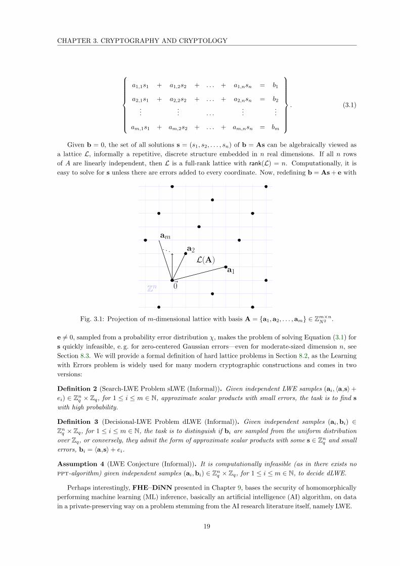
Given b = 0, the set of all solutions s = (s1, s2, . . . , sn) of b = As can be algebraically viewed as
a lattice L, informally a repetitive, discrete structure embedded in n real dimensions. If all n rows
of A are linearly independent, then L is a full-rank lattice with rank(L) = n. Computationally, it is
easy to solve for s unless there are errors added to every coordinate. Now, redefining b = As + e with
~0
a1
a2. . .
am
Zn
L(A)
Fig. 3.1: Projection of m-dimensional lattice with basis A = a1,a2, . . . ,am ∈ Zm×nN2 .
e 6= 0, sampled from a probability error distribution χ, makes the problem of solving Equation (3.1) for
s quickly infeasible, e. g. for zero-centered Gaussian errors—even for moderate-sized dimension n, see
Section 8.3. We will provide a formal definition of hard lattice problems in Section 8.2, as the Learning
with Errors problem is widely used for many modern cryptographic constructions and comes in two
versions:
Definition 2 (Search-LWE Problem sLWE (Informal)). Given independent LWE samples (ai, 〈a,s〉+ei) ∈ Znq × Zq, for 1 ≤ i ≤ m ∈ N, approximate scalar products with small errors, the task is to find s
with high probability.
Definition 3 (Decisional-LWE Problem dLWE (Informal)). Given independent samples (ai,bi) ∈Znq × Zq, for 1 ≤ i ≤ m ∈ N, the task is to distinguish if bi are sampled from the uniform distribution
over Zq, or conversely, they admit the form of approximate scalar products with some s ∈ Znq and small
errors, bi = 〈a,s〉+ ei.
Assumption 4 (LWE Conjecture (Informal)). It is computationally infeasible (as in there exists no
ppt-algorithm) given independent samples (ai,bi) ∈ Znq × Zq, for 1 ≤ i ≤ m ∈ N, to decide dLWE.
Perhaps interestingly, FHE–DiNN presented in Chapter 9, bases the security of homomorphically
performing machine learning (ML) inference, basically an artificial intelligence (AI) algorithm, on data
in a private-preserving way on a problem stemming from the AI research literature itself, namely LWE.
19
CHAPTER 3. CRYPTOGRAPHY AND CRYPTOLOGY
3.2 Complexity Theory
The evidence in favor of P 6= NP and its algebraic counterpart is so overwhelming, and the
consequences of their failure are so grotesque, that their status may perhaps be compared
to that of physical laws rather than that of ordinary mathematical conjectures.—Volker
Strassen (1986)
In this section, we informally recap the main concepts of complexity theory, as part of theoretical
computer science, underpinning all cryptologic research. It is a short introduction to an extend such
that it agrees on vocabulary to describe appropriate problems later-on in this work.
A key concept in any cryptologic discourse are algorithms—effective solution-finding specifications,
attributed to the ancient, middle-eastern mathematician al-Khwarizmi. An algorithm A runs in polyno-
mial time T (n), functionally dependent on the parameter n ∈ N, if T can be represented as polynomial,
i. e. ∃I ⊆ N : T (n) =∑i≤I tin
i with coefficients ti ∈ R. Polynomially dependence is commonly de-
noted in Landau’s big-O notation (cf. Section 1.2) as poly(n) = nO(1), without further specifying the
coefficients or degree, as often in cryptology asymptotic, qualitative statements are sufficient.
We now define two important complexity classes:
Definition 5 (Polynomial Time (P) and Exponential Time (EXP) Complexity Classes). spacespace
Let f : 0, 1∗ → 0, 1 be a problem instance, formally defined as a binary string.
• f ∈ P if there exists a NAND circuit C, which on inputs x ∈ 0, 1∗, outputs C(x) = f(x) in
poly(|x|) steps, i. e. less than p(|x|) steps for some polynomial p : N→ R in the input length.
• f ∈ EXP if there exists a NAND circuit C, which on inputs x ∈ 0, 1∗, outputs C(x) = f(x) in
2poly(|x|) steps, i. e. less than 2p(|x|) steps for some polynomial p : N→ R in the input length.
We typically mean a function is in F ∈ EXP\P if we speak of exponential -time functions.
Intuitively, P can be described as the class of problems whose difficulty grows moderately if we
increase the input size, i. e. the demand for time and memory resources to solve a given problem
instance of size n+ 1 is not too large compared to a size n problem instance.
A problem, where there exists a probabilistic polynomial-time ppt algorithm A solving it with high
probability is used as a synonym for a tractable, or feasible problem and A is referred to as efficient, or
fast. We introduce another complexity class, for which it is not known if it in fact is different from P:
Definition 6 (Bounded Probability Polynomial Time (BPP)). Let f : 0, 1∗ → 0, 1. f ∈ BPP :⇔∃d ∈ N and a probabilistic algorithm A such that
Pr[A(x) = f(x)] ≥ 23
at most p(|x|) = |x|d steps, polynomially in the input length |x| for p : N→ R.
We use similar notations in the quantum setting, where A is permitted non-classical computations.
Given a randomized algorithm A, we denote the action of running A on input(s) (x1, x2, . . .) of a
problem instance parametrized by n with uniform random coins R and assigning the output(s) to
(y1, y2, . . .) by (y1, y2, . . .)←$A(1n, x1, x2, . . . ;R) if we require absolute explicitness. By negl = negl(n)
we denote the set of negligible functions in n, i. e. all functions that can be upper-bounded by 1p (n), for
some polynomial p(n).
Definition 7 (Polynomial Problem Reductions). Let f, g : 0, 1∗ → 0, 1∗ be two problem instances.
f reduces to g, i. e. f ≤p g, if for every for every input x ∈ 0, 1∗, there exists an algorithm A :
0, 1∗ → 0, 1∗ that transforms the instance with
f(x) = g(A(x)).
20
CHAPTER 3. CRYPTOGRAPHY AND CRYPTOLOGY
If f ≤p g and g ≤p f , then f and g are equivalent, i. e. they are in the same complexity class.
Definition 8 (Non-Deterministic Polynomial Time NP). Let f : 0, 1∗ → 0, 1. f ∈ NP :⇔ ∃d ∈ Nand a verification function v : 0, 1∗ → 0, 1 ∈ P with
f(x) = 1⇔ ∃x′ ∈ 0, 1nd : v(xx′) = 1.
We remark that the verification certificate x′ exists, and is polynomial in n = |x|, if f(x) = 1,
whereas if f(x) = 0 then ∀x′ ∈ 0, 1nd , v(xx′) = 0 holds.
Definition 9 (NP-hardness and NP-completeness). Let g : 0, 1∗ → 0, 1. g is NP hard if we can
reduce f ≤p g,∀f ∈ NP. g is NP-complete :⇔ g is NP-hard and g ∈ NP.
We remark that we extend Definition 9 to search-problems, whose associated decisional-problems
fulfill the definition, too. General applicable algorithms to solve NP-complete are guessing a syntac-
tically correct input and brute-force testing, which we use synonymously for exhaustively searching
solutions.
The inclusion P ⊆ NP holds, but the question if the statement NP ⊆ P (and thus P = NP) is also
true, is one of the millennium problems listed in 2000 by the Clay Mathematics Institute in Cambridge.
A solution to this question is worth 1 000 000 US$, which is an additional motivation for mathematicians
and computer scientists. Several cryptographic assumptions are, for performance reasons, based on
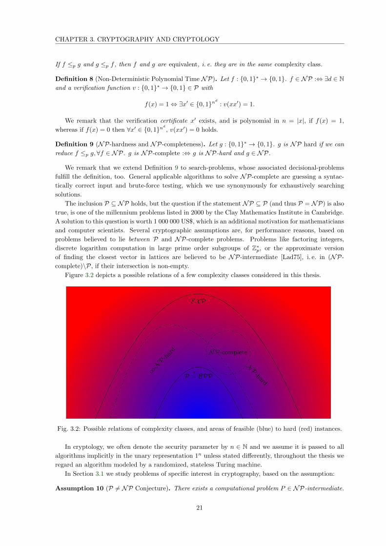
problems believed to lie between P and NP-complete problems. Problems like factoring integers,
discrete logarithm computation in large prime order subgroups of Z∗p, or the approximate version
of finding the closest vector in lattices are believed to be NP-intermediate [Lad75], i. e. in (NP-
complete)\P, if their intersection is non-empty.
Figure 3.2 depicts a possible relations of a few complexity classes considered in this thesis.
P ?= BPP
NP-hard
NP-complete
co-NP-
hard
EXP
Fig. 3.2: Possible relations of complexity classes, and areas of feasible (blue) to hard (red) instances.
In cryptology, we often denote the security parameter by n ∈ N and we assume it is passed to all
algorithms implicitly in the unary representation 1n unless stated differently, throughout the thesis we
regard an algorithm modeled by a randomized, stateless Turing machine.
In Section 3.1 we study problems of specific interest in cryptography, based on the assumption:
Assumption 10 (P 6= NP Conjecture). There exists a computational problem P ∈ NP-intermediate.
21
CHAPTER 3. CRYPTOGRAPHY AND CRYPTOLOGY
3.3 Boolean Gates, Circuits and Functional Completeness
There is no book so bad ... that it does not have something good in it.—Don Quixote (1604)
The binary NAND function, ∧ : 0, 12 7→ 0, 1, ubiquitously used in digital electronics, is defined by
Equation (3.2), or equivalently, can be computed using NAND(a, b) = NOT (AND(a, b)), as charac-
terized by Theorem 11.
NAND(a, b) =
0, a = b = 1,
1, else.(3.2)
Its logic gate symbol is denoted as a ∧ b = a∧b, or a|b, the Sheffer stroke, cf. Theorem 13. Conversely,
NOT , AND, resp. OR can be computed by only NAND function compositions:
Theorem 11 (NAND can compute NOT, AND as well as OR gates.). Unary NOT , binary AND,
resp. OR can be expressed as a composition of binary NAND functions arranged as Boolean circuit.
Proof. Let a, b ∈ 0, 1, then AND(a, a) = a holds, hence NAND(a, a) = NOT (AND(a, a)) =
NOT (a) ∈ 0, 1. As AND(a, b) = NOT (NOT (AND(a, b))) = NOT (NAND(a, b)) ∈ 0, 1 holds,
NAND alone is sufficient to compute AND. By De Morgan’s law we combine AND with NOT to
compute OR writing: OR(a, b) = NOT (AND(NOT (a), NOT (b))) ∈ 0, 1.
One could implement whole programs, even an operating system, via a huge composition of NAND
logic gates, yet with primitives such as additions, multiplications, and comparisons the circuits quickly
become rather unwieldy. For instance, a binary neural network (BNN), introduced in Section 9.1.1,
can be thought of as a Boolean circuit that uses threshold gates (Equation (9.1)) instead of NAND as
its basic component, see Section 3.3. We state the following theorems without a proof:
Theorem 12 (Addition / Multiplication of two n-bit numbers using only NANDs , [She13]). Let n ∈ Nand denote x1, x2 ∈ 0, 1n the binary representation of two n-bit numbers.
• ADDn : 0, 12n → 0, 1n+1 computes the sum x1 + x2. The number of NANDs in the ADDn
circuit is polynomial in n, i. e. a small linear amount, say 100n.
• MULTn : 0, 12n → 0, 12n the product x1 · x2. The number of NANDs in the MULTn circuit
is polynomial in n, i. e. a small quadratic amount, say 1000n2.
That NAND is universal is of importance for first implementations of fully homomorphic schemes.
Theorem 13 (NAND is universal, [She13]). Let n,m ∈ N and a Boolean mapping of n-bits to m-bits
f : 0, 1n → 0, 1m. There exists a NAND-circuit computing f in O(m2n) steps.
We will see later how early FHE schemes achieve universality by implementing the bare minimum—
evaluating a particular function deemed necessary to work with encrypted inputs, and an subsequent
NAND-gate for further compositions.
22

Chapter 4
Cryptology
4.1 Threat Model
They own your every secret, your life is in their files.
The grains of your every waking second sifted through and scrutinized.
They know your every right. They know your every wrong.
Each put in their due compartment - sins where sins belong.
They know you. They see all. They know all indiscretions.
Compiler of your dreams, your indignations.
Following your every single move.
They know you.— Tomas Haake (The Demon’s Name Is Surveillance, 2012)
A threat model defines the scenario and resources of the most potent adversary trying to break a system
or a security design. In cryptology, in stark contrast to security through obscurity, Shannon’s 1949
maxim that the enemy will immediately gain full familiarity with a system, is held high [Sha49]. It is a
reformulation of a much older desideratum, Kerckhoffs established in 1883, in a military tone [Ker83],
the terminology indicating the origin of early cryptologic research and its applications.
Definition 14 (Kerckhoffs’ Desideratum). The security of a cryptosystem should not rely on its secrecy
and can be stolen by the enemy without causing trouble. Only the (small) key shall be kept secret.
Obviously, it is debatable to actively try to keep a wide-spread, or even publicly-scrutinized, cryp-
tographic algorithm secret, which might eventually be efficiently recovered from an implementation
by reverse-engineering techniques. It is essential to understand that design-choices are not necessarily
confidential, but solely the secret key material that security ultimately reduces to needs to be treated
carefully over its life-time. The common scenario, assuming no knowledge of the key, yet full knowledge
about the cryptosystem, as counter-intuitive as it might seem to someone who did not deeply study
the science of secrets – cryptology, is known as the secret-key model. What history taught is that
cryptographic systems, not adhering to Kerckhoffs’ principle, were broken sooner or later. Systems not
coming with a detailed, comprehensive specification along with a security assessment are deemed as
providing merely security-by-obscurity.
4.2 Security Definitions
We mainly follow the notation of [KL14] and May’s lecture notes when the concepts one-way function,
trapdoor function, and the notion of provable security are briefly discussed in this section. Although
cryptographers still look for a rigorous proof, it is conjectured that one way functions exist, imply-
ing many useful cryptographic primitives, pseudorandom generators, functions or secure private key
encryptions [HILL99]:
23
CHAPTER 4. CRYPTOLOGY
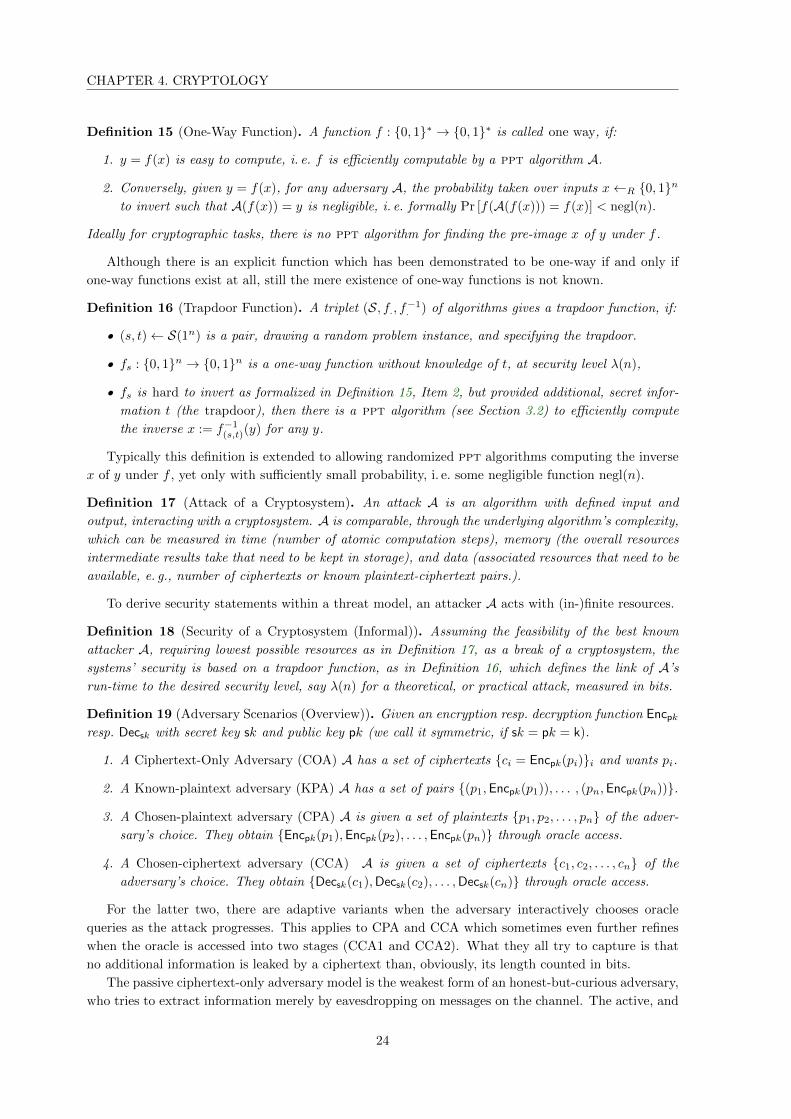
Definition 15 (One-Way Function). A function f : 0, 1∗ → 0, 1∗ is called one way, if:
1. y = f(x) is easy to compute, i. e. f is efficiently computable by a ppt algorithm A.
2. Conversely, given y = f(x), for any adversary A, the probability taken over inputs x←R 0, 1nto invert such that A(f(x)) = y is negligible, i. e. formally Pr [f(A(f(x))) = f(x)] < negl(n).
Ideally for cryptographic tasks, there is no ppt algorithm for finding the pre-image x of y under f .
Although there is an explicit function which has been demonstrated to be one-way if and only if
one-way functions exist at all, still the mere existence of one-way functions is not known.
Definition 16 (Trapdoor Function). A triplet (S, f., f−1. ) of algorithms gives a trapdoor function, if:
• (s, t)← S(1n) is a pair, drawing a random problem instance, and specifying the trapdoor.
• fs : 0, 1n → 0, 1n is a one-way function without knowledge of t, at security level λ(n),
• fs is hard to invert as formalized in Definition 15, Item 2, but provided additional, secret infor-
mation t (the trapdoor), then there is a ppt algorithm (see Section 3.2) to efficiently compute
the inverse x := f−1(s,t)(y) for any y.
Typically this definition is extended to allowing randomized ppt algorithms computing the inverse
x of y under f , yet only with sufficiently small probability, i. e. some negligible function negl(n).
Definition 17 (Attack of a Cryptosystem). An attack A is an algorithm with defined input and
output, interacting with a cryptosystem. A is comparable, through the underlying algorithm’s complexity,
which can be measured in time (number of atomic computation steps), memory (the overall resources
intermediate results take that need to be kept in storage), and data (associated resources that need to be
available, e. g., number of ciphertexts or known plaintext-ciphertext pairs.).
To derive security statements within a threat model, an attacker A acts with (in-)finite resources.
Definition 18 (Security of a Cryptosystem (Informal)). Assuming the feasibility of the best known
attacker A, requiring lowest possible resources as in Definition 17, as a break of a cryptosystem, the
systems’ security is based on a trapdoor function, as in Definition 16, which defines the link of A’s
run-time to the desired security level, say λ(n) for a theoretical, or practical attack, measured in bits.
Definition 19 (Adversary Scenarios (Overview)). Given an encryption resp. decryption function Encpkresp. Decsk with secret key sk and public key pk (we call it symmetric, if sk = pk = k).
1. A Ciphertext-Only Adversary (COA) A has a set of ciphertexts ci = Encpk(pi)i and wants pi.
2. A Known-plaintext adversary (KPA) A has a set of pairs (p1,Encpk(p1)), . . . , (pn,Encpk(pn)).
3. A Chosen-plaintext adversary (CPA) A is given a set of plaintexts p1, p2, . . . , pn of the adver-
sary’s choice. They obtain Encpk(p1),Encpk(p2), . . . ,Encpk(pn) through oracle access.
4. A Chosen-ciphertext adversary (CCA) A is given a set of ciphertexts c1, c2, . . . , cn of the
adversary’s choice. They obtain Decsk(c1),Decsk(c2), . . . ,Decsk(cn) through oracle access.
For the latter two, there are adaptive variants when the adversary interactively chooses oracle
queries as the attack progresses. This applies to CPA and CCA which sometimes even further refines
when the oracle is accessed into two stages (CCA1 and CCA2). What they all try to capture is that
no additional information is leaked by a ciphertext than, obviously, its length counted in bits.
The passive ciphertext-only adversary model is the weakest form of an honest-but-curious adversary,
who tries to extract information merely by eavesdropping on messages on the channel. The active, and
24

CHAPTER 4. CRYPTOLOGY
arguably practically more relevant attacks, combine passive capabilities and try to reveal secrets, not
intended for their pair of eyes, by malicious interaction with the cryptographic communication protocol
or the implementation of the cryptographic system.
Typically this interaction is modeled by a security game, where an adversary of a cryptosystem is
faced, e. g., with the task given a ciphertext and two different plaintexts to determine which one of them
was encrypted to yield the given ciphertext. The two plaintexts are indistinguishable for the adversary
in the strongest sense, sometimes denoted as IND-CCA2-secure, if they can do no better than guessing
which one of the two. We remark that at this point, attackers with unlimited computational power are
allowed, and later we will consider an important metric – run-times of algorithms.
Definition 20 (IND-CCA2 game). The two players in the CCA2 game protocol are a 1n cryptosystem
instance – the challenger – and an attacking party with following adversarial capabilities:
1. An adversary A gets as input a properly generated encryption key pk ∈ 0, 1n from the challenger.
A makes, at most polynomially many, queries T1 = poly(n) to the cryptosystem instance and
performs intermediate computations T ′1 = poly(n) before signifying the end of pre-processing stage.
2. Then A sends an (ordered) message pair m0,m1 ∈ 0, 1n, then receives a challenge c ∈ 0, 1`(n)
from the challenger, and is asked to identify the index bit b′ ←R 0, 1, for which c decrypts to mb′ .
We are assured that c is properly constructed, i. e., c = Encpk(mb), for b←R 0, 1, m←R 0, 1n.
3. The adversary A can make additional queries T2, T′2 = poly(n) before it outputs b.
4. The adversary wins the game if the returned b = b′ match. If A is able to do that, with more than
a negligible quantity in the security parameter, better than mere guessing, the system is insecure.
IND-CCA2-security is classically the strongest security definition a public-key encryption system
can fulfill. In fact FHE cryptosystems, which we study in the next chapters, cannot satisfy that
property. The circular security requirement, cf. Assumption 48, of nowadays FHE cryptosystems, cf.
Definition 44, i. e. to publish the bootstrapping key bk (see Theorem 46) violates even the CCA1 security
definition, as querying the decryption oracle with the bootstrapping key reveals the secret key to the
attacker – resulting in a total break.
Firstly, since FHE schemes do not provide full chosen-ciphertext security we settle for a weaker,
chosen-plaintext-like solution for this setting. We will thus present the IND-CPA game required in
Part II, sorted with ascending power refining what an adversary knows, and model the capabilities to
interact with a cryptosystem:
Definition 21 (IND-CPA game). The two players in the CPA game protocol are a 1n cryptosystem
instance – the challenger – and an attacking party with following adversarial capabilities:
1. An adversary A gets as input a properly generated encryption key pk ∈ 0, 1n from the challenger.
2. Then A provides the (ordered) pair of messages (m0,m1),m0,m1 ∈ 0, 1n, then receives a chal-
lenge c ∈ 0, 1`(n), and is asked to identify the index bit b′ ←R 0, 1 s. t. for which c decrypts
to mb′ . (The game assures that c is properly constructed by the challenger, i. e., c = Encpk(mb),
for b←R 0, 1,m←R 0, 1n.)
3. The adversary wins the game if the returned b = b′ match. If A is able to do that, with more than
a negligible quantity in the security parameter, better than mere guessing, the system is insecure.
Definition 22 (Indistinguishability of Ciphertexts under CPA). An encryption scheme (Gen,Enc,Dec)
works with ciphertexts indistinguishable under CPA, if the advantage of a ppt adversary A winning
the game in Definition 21 is at most negligible over guessing the index bit b:
AdvIND-CPAA (1n) :=
∣∣∣∣12 − Pr[A(1n)]
∣∣∣∣ ≤ negl(n).
25

CHAPTER 4. CRYPTOLOGY
4.3 Sources of Entropy
Simple cryptographic attacks reveal that deterministic encryption inherently allows to construct a
codebook translating message to fixed ciphertext or codeword, when observed. Using randomized
encryption on the other hand, is a paradigm which urges to produce a plethora of different ciphertexts
for any fixed message that decodes to that message (with overwhelming probability) instead.
We will generally assume all encryption and decryption algorithms to be randomized. Hence,
generated (pseudo-) randomness is a must to be unpredictable, yet it requires seeds—bits of initial
entropy. These seeds often originate from the computer or platform the cryptographic system runs
itself. Possible sources are different sensors that measure the environment and feed into the entropy
pool. Sources of entropy for the required cryptographic randomness, with various degrees of reliability,
include:
• time stamp when booting a device, Cloud server or starting a program or process,
• content of initially uninitialized memory of a platform,
• unrelated process IDs currently running on the host system,
• hardware input, e. g. from hard drive and network adapter timings, and
• auxiliary sensors’ measurements, e. g. temperature, of from cameras and microphones.
4.4 NIST’s Post-Quantum Cryptography Standardization
A few years back effectively all used public-key cryptography was threatened by an emerging technology,
quantum computers, which can be mitigated by what is known as Post-Quantum Cryptography.
Unfortunately, Post-Quantum Cryptography repeatedly needs to be contrasted with the quite dif-
ferently natured quantum cryptography, which aims to provide provable security in an information-
theoretical sense assuming only the laws of physics. As promising as this line of research seems, all
participating end-point devices and network links need to be capable of handling sending and receiving
messages encoded as quantum states, requiring a optical fiber infrastructures rather than conventional,
wired networks. International standardization efforts [Nat16] were summarized in a Call for Post-
Quantum Cryptography by the US-American National Institute of Standards and Technology (NIST).
The purpose of the competition is to re-establish confidence in modern cryptographic primitives among
the 69 accepted submissions, listed on NIST’s website, late 2017. Since then particularly those schemes
are scrutinized by cryptanalysis community, re-evaluating existing schemes and comparing them with
novel proposals. In February 2019 the competition’s mailing list displays more than 700 comments,
describing complete breaks of 13 proposals and discuss related security implications.
Even though the standardization process was designed to be a fair comparison and a combined
international effort, the US government shutdown of 2018/2019 delayed the competition, Eventually the
announcement of 26 short-listed schemes, 17 public-key encryption and key-establishment candidates,
and 9 digital signatures, yet to be more closely evaluated in the second round, were published. A
portfolio of final recommendations by NIST is awaited since by followers of the discussion 1.
1https://groups.google.com/a/list.nist.gov/forum/#!topic/pqc-forum/bBxcfFFUsxE
26

Chapter 5
Quantum Computing
To read our E-mail, how mean
of the spies and their quantum machine;
Be comforted though,
they do not yet know
how to factorize
twelve or fifteen1. —Volker Strassen (1998)
Since the invention of digital electronic devices for computing tasks [Wyn31] improvements were
largely achieved due to miniaturization of the computer’s components. Naturally a considerable math-
ematical effort and the theoretic evolution of computer sciences predate these engineering feats. Al-
gorithmic advancements made possible scenarios unthinkable before. In recent years computing per-
formance gains are mainly accomplished by deploying parallelism as physical boundaries are almost
hit. In [Wil11, Ch. 1.1] Williams extrapolates the trend in miniaturization and claims that the sonic
barrier, one atom per bit storage, will be reached around the year 2020. Soon, it might not be possible
to further push development by fine tuning computer chips because of these physical limitations and
the implied quantum effects appearing at this scale.
Classical physics is a model explaining macroscopic observations well, it is seemingly not appropriate
to describe small scale phenomena, which is the domain of quantum physics. New computer architec-
tures use quantum effects in a new, beneficial way to carry out computations rather than compensate
the derogatory implications to classical, digital electronic computers.
5.1 Quantum Bits
The fundamental difference of classical information and quantum information is their basic unit, the
quantum bit (or qubit) is not restricted to merely two states, say 0 and 1, like the classical bit, but
is a vector of length 1 in a 2-dimensional complex vector space. The theoretical model of a qubit is a
generalization of bits, based on systems with two distinguishable states that do not change uncontrol-
lably. In order to read the value of a qubit, the quantum system needs to be measured, an irreversible
step according to the laws of quantum mechanics. Therein lies the main difference of the macroscopic
storage and manipulation of classical bits and the microscopic implementation of a qubit system.
Let |0〉 and |1〉 denote the two basis states of a fixed 2-value quantum system in so-called Bra-ket
or Dirac notation. The laws of quantum mechanics tells us that a qubit can be in more than just one
of the two basis states |0〉 and |1〉, but it can be simultaneously in each of them, yet with a certain
probability only. Upon measurement a qubit is collapses to precisely one of those two distinct states.
1In fact, 15 was long setting the record for numbers factored using Shor’s algorithm. Today it is 21 = 7 · 3 [MLL+12].
27

CHAPTER 5. QUANTUM COMPUTING
Formally, a qubit can be in a superposition of the basis states, say
|ψ〉 = a0 |0〉+ a1 |1〉, |a0|2 + |a1|2 = 1
with complex coefficients a0, a1 ∈ C. Measurement of the qubit |ψ〉 can not recover the coefficients
a0, a1, yet the state |0〉 with probability |a0|2 and hence |1〉 with probability |a1|2 = 1− |a0|2. Mathe-
matically, the canonical or computational basis is|0〉 =
(10
), |1〉 =
(01
)extendable to n-qubit quantum
systems.
Let |0〉, |1〉, . . . , |2n − 1〉 denote the basis states of a n-qubit quantum system. A state can be
represented by a vector in C2 × C2 × · · · × C2︸ ︷︷ ︸n times
= CN , with N = 2n.
5.2 Quantum Computer and Quantum Algorithms
Physical realization of a universal quantum computer seems hard, yet first designs exist in a lab environ-
ments, resulting from massive research efforts. A practical, universally functional quantum computer
might exist in the not so distant future.
We briefly introduce two particularly noteworthy quantum algorithms: Grover’s search algorithm
with an application to solving subset-product problem in Part III, and Shor’s integer factorization
algorithm which is a justification to move from the RSA cryptosystem, as discussed in Part I towards
lattice-based cryptosystems in Part II.
5.2.1 Grover’s Algorithm
Grover’s quantum searching technique is like cooking a souffle. You put the state obtained
by quantum parallelism in a “quantum oven” and let the desired answer rise slowly. Success
is almost guaranteed if you open the oven at just the right time. But the souffle is very
likely to fall – the amplitude of the correct answer drops to zero – if you open the oven too
early.—Kristen Fuchs (1997)
The significance of Grover’s algorithm for this thesis lies in its applicability to the NP-complete SSP.
Any NP-complete search problem instance of N = 2n elements can be reformulated to find one par-
ticular input x = w of a function f , given as an oracle f : 0, 1N → 0, 1 with f(w) := 1 and
f(x) := 0, x 6= w otherwise for a search space of a priori unknown structure. In [BBBV97] general
unstructured search problems are studied from a computational complexity theoretic viewpoint and
the lower bound, O(√N) run-time and O(logN) storage, achievable by a quantum computer is proved.
It is assumed that to call the oracle encoding f takes polynomial time, i. e. run-time O(logkN), for
some k ∈ N. Grover’s algorithm hence yields a quadratic speed-up in the generic case over classical
exhaustive-search techniques with O(N) run-time and O(1) storage. The primordial application of
Grover’s algorithm to cryptography is simply searching for the secret key of a cryptosystem protecting
sensitive data of interest. For symmetric primitives, this attack essentially doubles the secret’s length
in order to remain at the same level of security after a sufficiently powerful quantum computer archi-
tecture is ready. For asymmetric cryptography quantum algorithms can mean a total break, as in the
following Section 5.2.2, or provide generic quadratic speed-ups as explored in Section 11.5.
5.2.2 Shor’s Algorithm
In this section we proceed with introducing one of the most famous quantum algorithms to date. In
1994, the first algorithm necessitating a quantum computer, consisting in a classical and a quantum
28
CHAPTER 5. QUANTUM COMPUTING
part, of tremendous significance to cryptology was formulated, and subsequently published in enhanced
form [Sho99].
Let N = pq be a non-negative composite integer, or bi-prime with primes p, q. A quantum computer
with a quantum register of size logQ ∈ O(logN), can deploy Shor’s algorithm to efficiently factorize
the modulus N , hence break the RSA cryptosystem, in O((logN)3) quantum gate operations.The
best known classical algorithms to solve the factorization problem, Coppersmith’s modifications to the
number field sieve [Cop93], have run-time sub-exponential in N , or super-polynomial in n := logN ,
compared to Shor’s quantum algorithm, we have:
O(e(C+o(1))n
13 (logn)
23
)Shor−→ O(n3).
In 2012, the record for the largest number factored using Shor’s algorithm on a quantum computer
was N := 21 = 3 · 7, which is still the largest reported success. Clearly, this is not actually threatening
deployed RSA or CRT-RSA cryptosystems with keys of typically several thousand bits length.
5.2.3 Provable Security and the One-Time Pad
Already in 1949, Shannon [Sha49] pioneered the field of information theory and defined the term
perfect secrecy. In conclusion, perfect secrecy of a message m ∈ 0, 1` can only be achieved using a
key k ∈ 0, 1L of (at least) equal length ` ≤ L ∈ N. In the provably-secure private-key cryptosystem
known as one-time pad (OTP), where each bit mi of the message m is added mod 2 (or XORed) with
the key bit ki of k assumed truly random and for one-time use only. It satisfies perfect secrecy in the
information theoretic sense, yet it is hard to reach in practice as the generation of random bits (cf.
Section 4.3), the key-distribution already requires a secure channel between two communication parties,
and a flawless implementation of the cryptosystem is seemingly not so straight-forward surprisingly.
29


Chapter 6
Homomorphic encryption (HE)
6.1 Definitions and Examples of Homomorphic encryption (HE)
6.1.1 The RSA Cryptosystem and the Factorization Problem
The famous RSA public key cryptosystem — named after Rivest, Shamir and Adleman — is renowned
in a broader community, and based on the easily explained integer factorization problem: Decomposing
an integer N = pq, the product of two big unknown prime numbers p, q is hard, whereas multiplying
them is easy.
Definition 23 (RSA Cryptosystem). Let n denote a security parameter.
RSA.Gen Generates the public key pk = (N, e) and the private key part sk = d, where the following
relations hold:
– N = p · q with prime numbers p, q ∈ P ⊆ N of equal length such that |N | = n,
– e ∈ N co-prime to ϕ(N) := (p− 1)(q − 1), i. e., gcd(e, ϕ(N)) = 1,
– d ∈ N such that e · d = 1 mod ϕ(N), i. e., d := e−1 mod ϕ(N) s. t. m = me·d
mod N .
RSA.Enc Encryption computes c := me mod N .
RSA.Dec Decryption using d: m = cd = me·d mod N .
We remark that although we present the version of the RSA cryptosystem with ϕ, the function
ϕ(N) := (p− 1)(q − 1) can be replaced by the least common multiple instead of the product λ(N) :=
lcm(p− 1, q − 1) ≤ ϕ(N) to save computational effort. The public key requires a non-negative integer
e ≥ 2, gcd(e, ϕ(N)) = 1 together with the modulus N . The private key is the factorization of N that
is given by the prime numbers p, q, and the multiplicative inverse of e, which is a positive integer d,
such that ed ≡ 1 mod ϕ(N) holds. Using the factors p and q it is possible to calculate d with ease.
Given a plain text encoded as a number m with 2 ≤ m ≤ N−2, the encrypted plain text is obtained
by computing c := me mod N . Receiving 1 ≤ c ≤ N − 1, the owner of the private key can calculate
cd mod N , which of course equals m = med = (me)d mod N the original message.
Although it is an interesting topic — studying the secure choices for p, q, e themselves or the algo-
rithms, for computing the occurring modular powers efficiently, for instance — we refer to the huge
amount of literature on this important branch of cryptography [Bon99]. In Chapter 5 however, we
will see the weakness of RSA under the assumption of a powerful quantum computer, the speedup
that can be achieved compared to the best classical algorithms which ultimately justifies the move to
cryptosystems based on quantum-safe assumptions.
31

CHAPTER 6. HOMOMORPHIC ENCRYPTION (HE)
6.1.2 Paillier Cryptosystem
Paillier’s public-key encryption scheme [Pai99] is a triplet of algorithms, and its CPA security is based
on the composite residuosity assumption—given an element, does its N -th root exist modulo N2, for
composite N? Using the following definitions we demonstrate how we identify the malleability property
of the system as homomorphism between the groups: (ZN ,+)→ (ZN2 , ·).
Definition 24 (Paillier Cryptosystem). Let n denote a security parameter.
Paillier.Gen Generates the public key pk = (N, g) and the private key part sk = (λ, µ), where the
following relations hold:
– N = p · q with prime numbers p, q ∈ P ⊆ N of equal length n,
– g ∈ Z∗N2 co-prime to N , for instance, g = N + 1,
– (λ, µ) such that λ = ϕ(N), µ = ϕ(N)−1 mod N .
Paillier.Enc Encryption computes c := gm · rNmodN2, for random co-prime r.
Paillier.Dec Decryption using (λ, µ): m := (cλ mod N2)−1N · µ mod N .
For messages 0 ≤ m2 ≤ m1 <N2 , we have
m1 ±m2 mod N = Decsk(Encpk(m1) · Encpk(m2)±1 mod N2) ∈ ZN .
In case of the difference, the modular inverse Encpk(m2)−1 ∈ Z∗N2 is efficiently computed using the
extended Euclidean algorithm.
We remark that the cryptosystem can easily be generalized for the case when 0 ≤ m1,m2 < N , e. g.
with unknown sign of the difference m1−m2, or even generalized to the Damgard-Jurik cryptosystem.
For the purpose of introducing homomorphic encryption we omit an overly detailed discussion. Given
two admissible plaintexts we first compute the ciphertexts under the secret key, c0 := Encpk(m0), c1 :=
Encpk(m1) ∈ ZN2 . We then verify that an encryption of the addition m0+m1 mod N can be computed
without the public key, simply by computing the product Encpk(m0) · Encpk(m1) ∈ ZN2 :
c0 · c1 = (gm0 · r0N ) · (gm1 · r1
N ) mod N2
= gm0+m1 · (r0 · r1)N
mod N2
= Encpk(m0 +m1) ∈ ZN2 .
To obtain homomorphisms in two operations, a more complicated task, will be developed as follows.
32

Part II
Fully Homomorphic Encryption
(FHE) & Artificial Intelligence (AI)
33

Chapter 7
Cloud Computing
7.1 Cloud Computing: Promises, NSA, Chances, Markets
Thanks to documents, classified by the US-American National Security Agency (NSA), made public in a
perilous endeavour (or leaked) by Edward Snowden in 2013, light was shed on how privately stored data
at Microsofts SkyDrive cloud service are giving in to pressure of nation-state adversaries. Other exam-
ples, when sharing data unprotected by cryptography, formerly meant for internal use only, were passed
on at scale, is NSA’s top-secret Prism program [GMP+13], whose reaction is sketched in Figure 7.1.
Fig. 7.1: NSA performing a‘Happy Dance!!’ [sic] when access-ing private data circumventing en-cryption.
Regulatory frameworks for asymmetric information monopolies
are being re-thought [And01, And14] and ideally cast into legisla-
tion. Preceding the European General Data Protection Regulation
(GDPR) now serving as a paragon internationally, a data protec-
tion regulation time-line can be reconstructed. Originating in 1970,
namely the Hessian Data Protection Regulation [Hes], is arguably
the first privacy-protection law with respect to the digital sphere
globally. In 1986 an overhauled second version, regulating data pro-
cessing by public authorities in Germany, was extended such that it
is applicable to companies operating on the free-market. It served
as blue-print for the European Data Protection Directive (Directive
95/46/EC), a law for natural person’s data rights in 1995. Adopted
in 2016, this legislation was superseded by the GDPR, which is en-
forceable European-wide since mid 2018, an important step to the
recognition of the digital right to privacy for everybody. Companies
and organizations not adhering to the Privacy by Design-concept
can be fined up to 4 % of their annual global turnover for breach-
ing GDPR, proportional to the severity of infringements. Data processing entities in the Cloud are
compelled to take the security and privacy issues and cryptographic implementations seriously as cases
of negligence might be prosecuted. The Cloud hardware, unlike the Internet of Things hand-held
devices, is off-site, anywhere on the globe, but under control of services providers, who potentially
modify content, eavesdrop on communication and computations, or even maliciously tamper with data.
Despite potential threats stemming from this power of large data companies such as Amazon to date,
the Cloud business is still a market with rising potential. Abstracted interfaces make it convenient
to use, with early, wide-spread e-Mail providers, and a plethora of examples of this technologies being
sketched in Figure 7.2. Several security requirements arise in the scenario of delegated data storage
and data-processing. Sharing data confidentially over the Internet requires an enforced access control
policy with customized definitions at upload which users can retrieve which data.
Data stored in the decentralized Cloud preferably remains illegible to anyone not explicitly autho-
rized, both at rest and during subsequent computations. Even though files that were encrypted under
35
CHAPTER 7. CLOUD COMPUTING
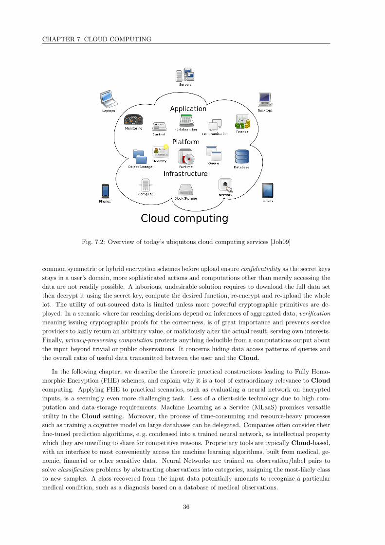
Fig. 7.2: Overview of today’s ubiquitous cloud computing services [Joh09]
common symmetric or hybrid encryption schemes before upload ensure confidentiality as the secret keys
stays in a user’s domain, more sophisticated actions and computations other than merely accessing the
data are not readily possible. A laborious, undesirable solution requires to download the full data set
then decrypt it using the secret key, compute the desired function, re-encrypt and re-upload the whole
lot. The utility of out-sourced data is limited unless more powerful cryptographic primitives are de-
ployed. In a scenario where far reaching decisions depend on inferences of aggregated data, verification
meaning issuing cryptographic proofs for the correctness, is of great importance and prevents service
providers to lazily return an arbitrary value, or maliciously alter the actual result, serving own interests.
Finally, privacy-preserving computation protects anything deducible from a computations output about
the input beyond trivial or public observations. It concerns hiding data access patterns of queries and
the overall ratio of useful data transmitted between the user and the Cloud.
In the following chapter, we describe the theoretic practical constructions leading to Fully Homo-
morphic Encryption (FHE) schemes, and explain why it is a tool of extraordinary relevance to Cloud
computing. Applying FHE to practical scenarios, such as evaluating a neural network on encrypted
inputs, is a seemingly even more challenging task. Less of a client-side technology due to high com-
putation and data-storage requirements, Machine Learning as a Service (MLaaS) promises versatile
utility in the Cloud setting. Moreover, the process of time-consuming and resource-heavy processes
such as training a cognitive model on large databases can be delegated. Companies often consider their
fine-tuned prediction algorithms, e. g. condensed into a trained neural network, as intellectual property
which they are unwilling to share for competitive reasons. Proprietary tools are typically Cloud-based,
with an interface to most conveniently access the machine learning algorithms, built from medical, ge-
nomic, financial or other sensitive data. Neural Networks are trained on observation/label pairs to
solve classification problems by abstracting observations into categories, assigning the most-likely class
to new samples. A class recovered from the input data potentially amounts to recognize a particular
medical condition, such as a diagnosis based on a database of medical observations.
36

CHAPTER 7. CLOUD COMPUTING
7.2 Hardware Solution: Secure Computing Enclaves
“Arguing that you don’t care about the right to privacy because you have nothing to hide
is no different than saying you don’t care about free speech because you have nothing to
say.”—Edward Snowden (2013)
For a long time it was unthinkable to have secure, private, and trustworthy computing delegated to
the Cloud. While FHE can be seen as a software enclave that does not rely on tamper-protected nor
trusted hardware, Intel’s Software Guard Extensions (SGX) promises a hardware solution. The goal is
large scale Homomorphic Encryption (HE) by offering an assumed trusted enclave within the Cloud
provider to communicate authenticated and securely. This enables delegated operations f on the data,
yet the approach necessitates private keys to reside at the Cloud, resulting in a weaker threat model.
7.3 Software Solution: FHE and FHE–DiNN
Cryptography rearranges power: It determines who can gather which data, and how such
data can be processed.—Philip Rogaway (distinguished lecture at Asiacrypt 2015)
Traditionally, except leaving the data unprotected in the first place, there were two unsatisfying solu-
tions to perform useful delegated computation, by evaluating any function f on encrypted data. Either
it was necessary to entrust the service providers with a key for on-site decryption, or deploy the inef-
ficient approach of downloading, processing, re-encrypting, and re-uploading data—else it was simply
deemed impossible.
This thesis will introduce a new and powerful FHE framework [BMMP18] that enables Cloud ser-
vices to offer privacy-preserving predictions of users’ uploaded input data mitigating issues concerning
their privacy. We showcase how to efficiently solve server-side machine learning tasks by computing
the prediction of a neural network on encrypted inputs almost reaching the models’ clear-text accu-
racy. After supervised training on plaintext data, yet unseen, but likewise distributed input data is
encrypted, evaluated, and returned as encrypted label, thus homomorphically classifying the data. Ob-
viously, the confidentiality goal is reached as the private key under which the data is encrypted resides
in the legitimate owner’s controlled domain, who alone can decrypt the result. We address delegated
computation privately performed in the Cloud-threat model, as in Figure 7.3, where an observer only
learns unsubstantial information on top of what is needed for billing the user requesting a classification.
7.3.1 Limitations
We do not consider the problem of privacy-preserving data-mining, when neural networks are trained
on encrypted data as addressed in [AS00]. We assume an already trained neural network in the clear
and focus on the evaluation, or inference phase.
A related concern of service providers is that malicious users might try to recreate the network,
deemed intellectual property, by sending maliciously-formed requests in order to extract information.
We do not explore protection for learning the neural network itself, when considering information
encoded in the weights sensitive. Statistical database in the training phase, as is discussed in the
differential privacy literature [Dwo06], can be used to mitigate such issues or enforcing an upper bound
on user requests.
37
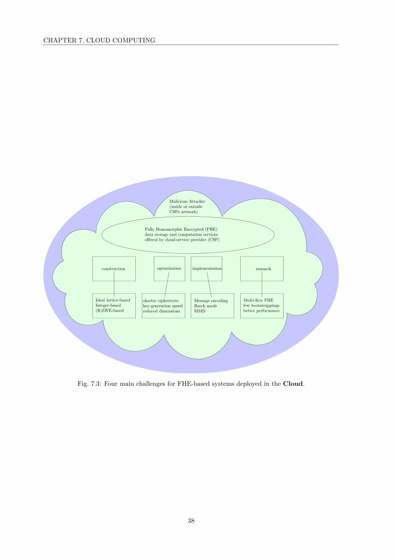
CHAPTER 7. CLOUD COMPUTING
Fully Homomorphic Encrypted (FHE)data storage and computation servicesoffered by cloud-service provider (CSP)
Malicious Attacker(inside or outsideCSPs network)
construction optimization implementation research
Ideal lattice-basedInteger-based(R)LWE-based
shorter ciphertextskey-generation speedreduced dimensions
Message encodingBatch modeSIMD
Multi-Key FHEfew bootstrappingsbetter performance
Fig. 7.3: Four main challenges for FHE-based systems deployed in the Cloud.
38
Chapter 8
Mathematical Foundations of FHE
In order to describe the theory for Fully Homomorphic Encryption (FHE) from scratch, we provide the
most important notions and the mathematical background adapted to our object of studies. We start
with a definition of the mathematical discipline of abstract algebra:
8.1 Basic Concepts from Algebra and Probability Theory
Definition 25 (Abelian Group). Let G be a finite set with a binary operation (often ′+′)
: G×G→ G
(a, b) 7→ a b.
(G, ) is an Abelian group :⇔ ∀a, b, c ∈ G:
1. a (b c) = (a b) c ∈ G, associativity;
2. a b = b a ∈ G, commutativity;
3. ∃1G ∈ G : a 1G = 1G a = a, for a neutral group element 1G;
4. ∃a−1 ∈ G : a a−1 = 1G, an inverse exists within the group.
Next, we need to define an algebraic structure with two operations.
Definition 26 (Ring). Let R be a finite set with two binary operations (often ′+, ·′):
1. (R,+) is an additive Abelian group
2. (R, ·) is a monoid, i. e. ∀a, b, c ∈ R:
• a · (b · c) = (a · b) · c ∈ R, associativity;
• ∃1R ∈ R : a · 1R = 1R · a = a, for a neutral element 1R, the multiplicative unit;
3. · is (left- and right-) distributive over +: a·(b+c) = (a·b)+(a·c) ∈ R, (b+c)·a = (b·a)+(c·a) ∈ R.
This already lets us define fundamental structures underneath FHE. Finally, we look at R-modules,
and their external operation, as we also want to study mappings between these structure.
Definition 27 (Ring Homomorphism). Let (R,+, ·), and(S,⊕,) be two rings. A function f : R→ S
is a ring homomorphism :⇔
• it preserves addition, i. e. f(a+ b) = f(a)⊕ f(b) ∈ S, ∀a, b ∈ R,
• it preserves multiplication, i. e. f(a · b) = f(a) f(b) ∈ S, ∀a, b ∈ R,
39

CHAPTER 8. MATHEMATICAL FOUNDATIONS OF FHE
X Y
x1 • • f(x1)
(R,+, ·) (S,⊕,)
x+ •f
x ∈ X ⇒ f(x) ∈ Y
• f(x+)
x∗ • • f(x)
x2 • f
x /∈ X ⇒ f(x) /∈ Y• f(x2)
Fig. 8.1: Sum x+ = x1 + x2, and product x∗ = x1 · x2 under ring homomorphism f .
• it relabels the multiplicative unit, i. e. f(1R) = 1S ∈ S.
A homomorphism f , according to Definition 27, is a structure-preserving transformation between
two algebraic structures depicted in Figure 8.1, with f(x+) = f(x1) ⊕ f(x2) ∈ S and f(x) =
f(x1) f(x2) ∈ S. Although homomorphisms might leverage cryptanalytic attacks in some contexts,
e. g. exploiting the malleability of RSA, in the following it permits crafting cryptosystems to perform
arithmetic operations on encrypted data without decryption.
Definition 28 (R-Module). Let (R,+, ·) be a commutative ring. M ⊆ R is an R-module :⇔ (M,+)
is an Abelian group and the following mapping fulfills ∀r, r1, r2 ∈ R, and ∀m,m1,m2 ∈M :
• : R×M →M
(r,m) 7→ r •m
1. 1R •m = m ∈M,
2. r1 • (r2 •m) = r1 • (r2 •m) ∈M,
3. (r1 + r2) •m = r1 •m+ r2 •m ∈M (Associativity),
4. r • (m1 +m2) = r •m1 + r •m2 ∈M (Distributivity).
In Section 9.2.2, we deal with a module defined over the one dimensional real torus, called TLWE
in the context of the implementation TFHE for basic operations of an FHE scheme. First, we need to
formally introduce another preliminary ingredient: lattices—discrete sub-groups of Rn.
Definition 29 (q-ary Lattice). We can define a q-ary lattice explicitly as a set of vectors
Lq(A) : =
y ∈ Zn : y = f(z) :=
n∑i=1
zi · bi = Az mod q, zi ∈ Z
(8.1)
= Imf (A) ⊆ Zn, (8.2)
or see it as the image of the linear map f with matrix A ∈ Zn×mq , applied to integer vectors.
40

CHAPTER 8. MATHEMATICAL FOUNDATIONS OF FHE
For m > n ∈ N and a rank m ∈ N matrix, the kernel of A under this map forms a q-ary lattice, too.
The scaled dual of L := Lq(A) is hence defined by
ker f = L⊥q (A) = x ∈ Zn : Ax = 0 mod q ⊆ Zn,
and the algebraic dual of L is denoted as L∗ = y ∈ Span(L) : 〈x ,y〉 ∈ Z,x ∈ L. Its volume, a
basis-independent lattice-invariant, is the non-negative quantity vol(L(A)) := |det(A)|.
8.2 Lattice Problems for Cryptography
The survey on lattices for cryptography [Pei16], identifies five suitable problems.
Definition 30 (NP-hard lattice problems). Let L = L(A) ⊆ Rn denote a lattice, specified by integral,
linear row combinations of the basis matrix A, we specify 5 exemplary hard problems:
• Closest Vector Problem (CVP). Given target t ∈ Rn, the task is to identify a lattice vector
v ∈ L closest to the target with respect to the Euclidean norm ‖.‖2 on the normed space Rn,
v = argminv′∈L ‖t− v′‖2. Figure 8.2 demonstrates two famous algorithmic solutions when given
targets and more (resp. less) orthogonal lattice bases of good (resp. bad) quality.
• Bounded Distance Decoding (BDD) problem. In this variant of CVP, we are promised that
‖t−v‖2 < ε is upper-bounded with ε λ1(L), the first successive minimum λ1, which makes the
solution v unique as λ1(L) := minv 6=~0 ‖v‖2.
• Shortest Vector Problem (SVP). Given L = L(A) ⊆ Rn a lattice, find a shortest vector v ∈ L,
i. e. with distance exactly ‖v‖2 = λ1(L) from the origin.
• approximate Shortest Vector Problem (appSVPγ). In this approximation variant of SVP, we
want to find an approximate shortest vector v ∈ L, which satisfies the relaxed distance condition
‖v‖2 ≤ γ(n) · λ1(L) that allows adjusting hardness by e. g. setting γ(n) = poly(n) [ADRS15].
• unique SVP (uSVPγ). In this approximation variant of SVP, we are promise that a unique shortest
vector exists (up to its sign), i. e. λ2, the second successive minimum, is bounded by γ(n) · λ1.
The closer 1 ≤ γ(n), the lattice gap, is to 1, the harder it generally is to find a suitable vector, as [LM09]
give hardness reductions between the important BDD, uSVPγ , and appSVPγ problem.
To formalize the two suitable lattice-based problems, from Definition 2 and Definition 3, as a basis
for cryptographic constructions, we first introduce useful probability distributions to model the noise
which we need and discuss as part of the phase, cf. Definition 53.
8.2.1 Discrete Gaussian distribution on Lattices
To most conveniently define the discrete Gaussian probability distribution, for our purposes, one does
not choose the mean, a vector v, and the standard deviation, σ, but use parameter s – the so-called
scaled standard deviation, as asymptotically lims→∞ = s/√
2π + o(s).
Then, for real s > 0, we define the Gaussian function %s(v) := exp(−π‖v‖2/s2) with width s. Using
the normalization factor %s(V) =∑
v∈V %s(v), it serves as probability density function over countable
sets V ⊂ Rn, especially when V = L ⊂ Zn is a lattice, we set
DL,s(v) =%s(v)
%s(L)=
e−π‖v‖2/s2∑
v∈L %s(v). (8.3)
41

CHAPTER 8. MATHEMATICAL FOUNDATIONS OF FHE
~0b2
b1
t
H1
π(t)vB
(a) A good basis is preferable to solve the CVP ina lattice L with target point t (red) using Babai’sNearestPlane algorithm in 2 dimensions [Bab85].Here, recursively calling it intermediately projects tonto the closest 1-dimensional hyperplane H1 = b2 +Span(b1), i. e. π(t), then onto the 0-dimensional sub-space H0 ⊆ L to obtain vB (green), an integral linearcombination of lattice basis points.
~0
b1
b2
t
H(1)2
H(1)1
v(2)LP
v(1)LP
(b) A bad basis of the same lattice L might mis-lead Babai’s algorithm incorrectly identifying a closest-vector. The target t (red) in Lindner-Peikert’s al-gorithmic variant [LP11] NearestPlanes is projected
onto multiple hyperplanes instead, e. g. H(1)1 = b2 +
Span(b1), H(1)2 = 2b2 + Span(b1) to output a set of
closest points vLP (green).
Fig. 8.2: NearestPlane(s) Algorithms on good (left) vs. bad (right) bases of the lattice L.
The situation modulo an integer q ≥ 1 is defined via the projection πq : Zn → Znq . For v ∈ Znq we have
DZnq ,s(v) = DZn,s(π−1q (v)).
As sampling random lattice points following a discrete Gaussian distribution is computationally
expensive [GPV08] for arbitrary lattices (and L = Znq ), substituting the distribution is a performance
incentive. Justifying probability distribution exchange without jeopardizing security requires a measure.
Definition 31 (Statistical Distance of Probability Distributions). The statistical distance (variational
distance) between two distributions, X and Y mapping onto Z, is defined by
∆(X,Y ) =1
2
∑z∈Z|P(X = z)− P(Y = z)| := δ ∈ R.
Definition 32 (Statistical/Computational Indistinguishability). Probability ensembles Xnn∈N, Ynn∈N• are statistical indistinguishable, if n 7→ ∆(Xn, Yn) = δ(n) < negl(n),
• are computational indistinguishable, if @ D ppt-distinguisher with advantage AdvD(n) > negl(n).
We remark that statistical indistinguishability implies computational indistinguishability and introduce
an essential quantity, the smoothing parameter of a lattice L via its non-zero elements in the dual L∗.
Definition 33 (Smoothing Parameter ηε(L) [MR07]). For a rank n lattice L ⊆ Rn and real ε > 0, we
call the smallest real width s bounding the Gaussian function by ηε(L) = infs > 0 : %1/s(L∗\~0 ) ≤ ε.
Theorem 34 (Smoothness bound for rank n lattice L ⊆ Rn [MR07]). For real ε > 0, we have that
ηε(L) ≤ λn(L)√
ln(2n(1+1/ε))π , with λn the n-th successive minimum of L and the constant π.
Theorem 35 (Bound for L = Z [ZXZ18, Theorem 1]). For ε < 0.086435, ηε(Z) ≤√
ln(ε/44+2/ε)π .
Example 36. In the self-dual case of L = Z, e. g. ε = 8100 gives the smoothing parameter ηε(Z) ≤ s = 3
2 .
Example 37. For Z, e. g. ε < 2−160, Theorem 35 gives the bound ηε(Z) = ln(2(1 + 1/2−160)
)≤ s = 6.
42
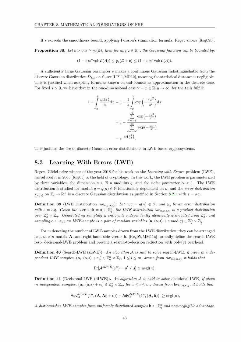
CHAPTER 8. MATHEMATICAL FOUNDATIONS OF FHE
If s exceeds the smoothness bound, applying Poisson’s summation formula, Regev shows [Reg09b]:
Proposition 38. Let ε > 0, s ≥ ηε(Z), then for any c ∈ Rn, the Gaussian function can be bounded by:
(1− ε)snvol(L(A)) ≤ %s(L+ c) ≤ (1 + ε)snvol(L(A)).
A sufficiently large Gaussian parameter s makes a continuous Gaussian indistinguishable from the
discrete Gaussian distributionDL,s on L, see [LP11,MP12], meaning the statistical distance is negligible.
This is justified when adapting formulas known on tail-bounds as approximation in the discrete case.
For fixed s > 0, we have that in the one-dimensional case v = x ∈ R, y →∞, for the tails fulfill:
1−y∫−y
%s(x)
sdx = 1− 1
s
y∫−y
exp(−πx
2
s2
)dx
= 1−
y∑x=−y
exp(−πx2
s2 )
∞∑x=−∞
exp(−πx2
s2 )
= e−Θ(y2
s2
).
This justifies the use of discrete Gaussian error distributions in LWE-based cryptosystems.
8.3 Learning With Errors (LWE)
Regev, Godel-prize winner of the year 2018 for his work on the Learning with Errors problem (LWE),
introduced it in 2005 [Reg05] to the field of cryptology. In this work, the LWE problem is parameterized
by three variables; the dimension n ∈ N a modulus q, and the noise parameter α < 1. The LWE
distribution is studied for moduli q = q(n) ∈ N functionally dependent on n, and the error distribution
χs(α) on Zq → R+ is a discrete Gaussian distribution as justified in Section 8.2.1 with s = αq.
Definition 39 (LWE Distribution lwen,q,s,χ). Let n, q = q(n) ∈ N, and χs be an error distribution
with s = αq. Given the secret sk = s ∈ Znq , the LWE distribution lwen,q,s,χ is a product distribution
over Znq × Zq. Generated by sampling a uniformly independently identically distributed from Znq , and
sampling e← χs, an LWE-sample is a pair of random variables (a, 〈a,s〉+ e mod q) ∈ Znq × Zq.
For m denoting the number of LWE-samples drawn from the LWE distribution, they can be arranged
as a m × n matrix A, and right-hand side vector b. [Reg05, MM11a] formally define the search-LWE
resp. decisional-LWE problem and present a search-to-decision reduction with poly(q) overhead.
Definition 40 (Search-LWE (sLWE)). An algorithm A is said to solve search-LWE, if given m inde-
pendent LWE samples, (ai, 〈a,s〉+ ei) ∈ Znq × Zq, 1 ≤ i ≤ m, drawn from lwen,q,s,χ, it holds that
Pr[AsLWE(1n) = s′ 6= s] ≤ negl(n).
Definition 41 (Decisional-LWE (dLWE)). An algorithm A is said to solve decisional-LWE, if given
m independent samples, (ai, 〈a,s〉+ ei) ∈ Znq × Zq, for 1 ≤ i ≤ m, drawn from lwen,q,s,χ, it holds that∣∣∣AdvdLWEA (1n, (A,As + e))− AdvdLWE
A (1n, (A,b))∣∣∣ ≥ negl(n),
A distinguishes LWE-samples from uniformly distributed samples b← Znq and non-negligible advantage.
43
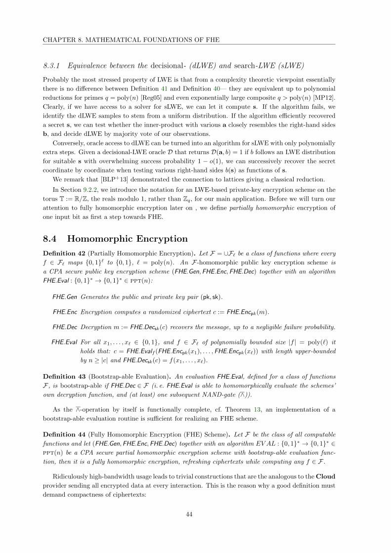
CHAPTER 8. MATHEMATICAL FOUNDATIONS OF FHE
8.3.1 Equivalence between the decisional- (dLWE) and search-LWE (sLWE)
Probably the most stressed property of LWE is that from a complexity theoretic viewpoint essentially
there is no difference between Definition 41 and Definition 40— they are equivalent up to polynomial
reductions for primes q = poly(n) [Reg05] and even exponentially large composite q > poly(n) [MP12].
Clearly, if we have access to a solver for sLWE, we can let it compute s. If the algorithm fails, we
identify the dLWE samples to stem from a uniform distribution. If the algorithm efficiently recovered
a secret s, we can test whether the inner-product with various a closely resembles the right-hand sides
b, and decide dLWE by majority vote of our observations.
Conversely, oracle access to dLWE can be turned into an algorithm for sLWE with only polynomially
extra steps. Given a decisional-LWE oracle D that returns D(a, b) = 1 if b follows an LWE distribution
for suitable s with overwhelming success probability 1 − o(1), we can successively recover the secret
coordinate by coordinate when testing various right-hand sides b(s) as functions of s.
We remark that [BLP+13] demonstrated the connection to lattices giving a classical reduction.
In Section 9.2.2, we introduce the notation for an LWE-based private-key encryption scheme on the
torus T := R/Z, the reals modulo 1, rather than Zq, for our main application. Before we will turn our
attention to fully homomorphic encryption later on , we define partially homomorphic encryption of
one input bit as first a step towards FHE.
8.4 Homomorphic Encryption
Definition 42 (Partially Homomorphic Encryption). Let F = ∪F` be a class of functions where every
f ∈ F` maps 0, 1` to 0, 1, ` = poly(n). An F-homomorphic public key encryption scheme is
a CPA secure public key encryption scheme (FHE.Gen,FHE.Enc,FHE.Dec) together with an algorithm
FHE.Eval : 0, 1∗ → 0, 1∗ ∈ ppt(n):
FHE.Gen Generates the public and private key pair (pk, sk).
FHE.Enc Encryption computes a randomized ciphertext c := FHE.Encpk(m).
FHE.Dec Decryption m := FHE.Decsk(c) recovers the message, up to a negligible failure probability.
FHE.Eval For all x1, . . . , x` ∈ 0, 1, and f ∈ F` of polynomially bounded size |f | = poly(`) it
holds that: c = FHE.Evalf (FHE.Encpk(x1), . . . ,FHE.Encpk(x`)) with length upper-bounded
by n ≥ |c| and FHE.Decsk(c) = f(x1, . . . , x`).
Definition 43 (Bootstrap-able Evaluation). An evaluation FHE.Eval, defined for a class of functions
F , is bootstrap-able if FHE.Dec ∈ F (i. e. FHE.Eval is able to homomorphically evaluate the schemes’
own decryption function, and (at least) one subsequent NAND-gate (∧)).
As the ∧-operation by itself is functionally complete, cf. Theorem 13, an implementation of a
bootstrap-able evaluation routine is sufficient for realizing an FHE scheme.
Definition 44 (Fully Homomorphic Encryption (FHE) Scheme). Let F be the class of all computable
functions and let (FHE.Gen,FHE.Enc,FHE.Dec) together with an algorithm EV AL : 0, 1∗ → 0, 1∗ ∈ppt(n) be a CPA secure partial homomorphic encryption scheme with bootstrap-able evaluation func-
tion, then it is a fully homomorphic encryption, refreshing ciphertexts while computing any f ∈ F .
Ridiculously high-bandwidth usage leads to trivial constructions that are the analogous to the Cloud
provider sending all encrypted data at every interaction. This is the reason why a good definition must
demand compactness of ciphertexts:
44

CHAPTER 8. MATHEMATICAL FOUNDATIONS OF FHE
Definition 45 (Compactness of FHE Ciphertexts). Let (Gen,Encpk,Decsk) be a CPA secure, partial
homomorphic encryption scheme. This scheme is compact iff ∃p(n) : |c| ≤ p(n),∀c ∈ C ciphertexts,
with a suitable polynomial p = poly(n), required to be independent of input length ` or circuit size |f |.
Theorem 46 (Bootstrapping Theorem [Gen09]). Let (Gen,Encpk,Decsk) be a IND-CPA secure, partial
homomorphic encryption scheme with assumed circular security property. For a function family F if
∀c0, c1, arbitrary, but syntactically-correct input ciphertexts, the mapping:
fc0,c1 : sk 7→ (Decsk(c0) ∧ Decsk(c1)) ∈ F ,
it qualifies (Gen,Encpk,Decsk) as a fully homomorphic encryption scheme.
Proof. Let f : 0, 1n → 0, 1 be an efficiently computable function, i. e. there exists an algorithm com-
puting the result in poly(n) steps, cf. Definition 5. Since NAND is a universal function, cf. Theorem 13,
f can be expressed as a Boolean circuit only comprising NAND gates. Let (sk, pk) = Gen(1n) denote
the private resp. public key of the scheme. Assuming circular security, cf. Assumption 48, an encryption
of the secret key bk = Encpk(sk), the so-called bootstrapping-key, is made public at setup time, without
weakening the construction. Let c0, c1 be encryptions of bits c0 = Encpk(m0), c1 = Encpk(m1) ∈ 0, 1.We can use several functions (c, c′) 7→ fc,c′ , to construct a sequence c0, c1, c2 = c0 ∧ c1, c3, c4 =
c2 ∧ c3, . . . , cr = F (c0, c1, c3, . . . ) until arriving at the resulting ciphertext, cr, representing the result
of a circuit f ∈ F evaluated on its n inputs.
Hence, to define the function EV ALbk(f) := FHE.Eval(f, bk), which homomorphically computes
the result of applying the circuit f on its inputs, it suffices to have functions for arbitrary (c0, c1)
evaluating fc0,c1 using the refreshing operation. Given any two consecutive ciphertexts c and c′ in
the sequence c0, c1, . . . , cr), we hard-wire the Boolean function fc0,c1(sk) = (Decsk(c0) ∧ Decsk(c1)) ,
mapping any secret key candidate to 0, 1. We remark that the right side given the correct de-
cryption key sk would do the computation of first decrypting each operands and then evaluating
the NAND-gate on the two intermediate results. The missing link is constructing the Boolean func-
tion EV AL∧(c0, c1) := EV ALbk(fc0,c1) = FHE.Eval(fc0,c1 , bk) = c2 ∈ 0, 1. Decrypting c2 yields
Decsk(c2) = Decsk(EV AL∧(c0, c1)), hence
Decsk(FHE.Eval(fc0,c1 , bk)) = Decsk(FHE.Eval(fc0,c1 ,Encpk(sk))) = fc0,c1(sk) = Decsk(c0) ∧ Decsk(c1),
by construction. Putting all together, we are able to evaluate (Decsk(c0) ∧ Decsk(c1)) = (m0 ∧ m1) =
Decsk(c2) to some valuem2 ∈ 0, 1 and continue with the process for any sequence of a given circuit.
Any function family containing and supporting evaluation of the HE schemes’ decryption algorithm
as a function of the secret key, can be transformed into evaluating any computable function. This is,
until today, they only construction to obtain FHE schemes at all.
Remark 47 (FHE means f Encpk = Encpk f commutates (Informal)). Let f ∈ F be a computable
function, e. g. f = f0 + f1 ·X + · · ·+ fd ·Xd :M2 7→ M of degree d ∈ N, and m1,m2 two plaintexts, if:
(f Encpk)(m1,m2) = f(c1, c2) = c3 ∈ C
= f([m1]pk, [m2]pk)!≈ [f(m1,m2)]pk
= (Encpk f)(m1,m2),
for any m1,m2 ∈M with f(m1,m2) = m3 ∈M = Encpk(M) = C, then a IND-CPA-secure encryption
scheme S with four ppt-algorithms (FHE.Gen,FHE.Enc,FHE.Dec,FHE.Eval) becomes an FHE scheme.
45

CHAPTER 8. MATHEMATICAL FOUNDATIONS OF FHE
In fact, the informally expressed relation of Remark 47 only coincide with high probability for the
respective decryptions. In the general, we have the situation depicted in the commutative diagram:
m1,m2, . . . ,mn c1, c2, . . . , cn
f(m1,m2, . . . ,mn) Encpk (f(m1,m2, . . . ,mn)) ≈ Eval(f(c1, c2, . . . , cn)).
Encpk(.)
f(·) Eval(f, ·)Encpk(.)
Unlike classical, deterministic functions, and like almost all modern encryption functions that fulfill
the goal of semantic security (cf. Definition 19), FHE schemes too require probabilistic encryption, i. e.
same values a = b 6⇒ Encpk(a) = Encpk(b) can be, but are not necessarily mapped to the same string.
Defined in this probabilistic fashion, decryption algorithm is allowed to fail with negligible probability.
As a result of this, currently it is not practical to build a circuit for every function to be evaluated.
Before we can define approximate homomorphisms as used the currently most promising instan-
tiation of an FHE scheme [GSW13], we present some more facts about lattices, cf. Section 3.1.1.
Following [AP14] the 3rd generation FHE schemes are based on the approximate-eigenvector problem,
meaning that ciphertext (matrices) satisfy s·C ≈ s·µ mod q, with secret s, modulus q, and message µ.
An FHE scheme provides a way to encrypt data while supporting computations through the en-
cryption envelope. Given an encryption of a plaintext m, one can compute an encryption of f(m) for
any computable function f . This operation does not require intermediate decryption or knowledge of
the decryption key and therefore can be performed based on public information only.
Metaphorically, FHE can be understood as knitting a scarf. When winter is approaching, a warming,
self-made scarf is nice, yet this skill is not sufficiently taught so we are willing to outsource this task:If
you hand the favourite ball of wool to your half-blind grandmother (or grandfather for that matter),
they will turn it into a beautifully woven, hand-crafted scarf. The muscle-memory will permit the
movements to produce. It is a non-interactive process, delivered when ready. This metaphor lacks an
interpretation of bootstrapping, a necessity in nowadays FHE, for e. g. refreshing the fragile structure
before adding a few new loops. Maybe, if we imagine the yarn as being radioactive with short half-
life which needs to be perpetually repaired, or ... we simply define it abstractly, and precisely as in
Chapter 8.
Applications of FHE are numerous but one particular use of interest is the privacy-preserving
delegation of computations to a remote service. The first construction of FHE dates back to 2009
and is due to Gentry [Gen09]. A number of improvements have followed [vGHV10,SS10,SV10,BV11a,
BV11b, BGV12, GHS12, GSW13, BV14, AP14], leading to a biodiversity of techniques, features and
complexity assumptions.
We will now draw our attention to a concrete implementation of an FHE scheme and our construc-
tions on top of it, for this we require:
Assumption 48 (Circular Security Assumption). Giving bk = FHE.Enc(sk) to adversary A ∈ ppt(n)
in the IND-CPA-game is only negligibly improving the advantage of breaking the FHE cryptosystem:∣∣∣AdvIND-CPAA (1n)− AdvIND-CPA
A (1n, bk)∣∣∣ ≤ negl(n).
Assumption 49 (LWE Security Assumption). An average LWE instance is, even leveraging quantum
algorithms, as hard as solving appSVPγ in the worst-case. Existing (public-/secret-key) LWE-based
cryptosystems only negligibly improve the advantage of solving the appSVPγ-instance.
The appSVPγ problem is a standard lattice problem, which for years demonstrated to be robust
against substantial cryptanalysis advances. In Section 9.8, we will elaborate more on the presumed
practical hardness mentioned in this conjecture.
46

CHAPTER 8. MATHEMATICAL FOUNDATIONS OF FHE
Remark 50 (Dependency: FHE Security from the LWE-Assumption in this work). A partially ho-
momorphic public key encryption scheme (FHE.Gen,FHE.Enc,FHE.Dec,FHE.Eval) is an FHE scheme,
if
• the conditions of the bootstrapping theorem, Theorem 46, are fulfilled,
• the circular security assumption, Assumption 48, holds, and
• the (theoretical and practical) LWE-hardness conjecture, Assumption 49, holds.
We saw how to theoretically construct the holy-grail of cryptography. Finally, we turn our attention
to the implementation side and the TFHE library in Section 9.2.2, which realizes a scale-invariant
version of an FHE scheme based on the hardness of LWE, Assumption 49.
8.4.1 Standardization of Homomorphic Encryption
To balance privacy with convenience, there are efforts to standardize HE, define common Application
Programming Interfaces (APIs), and recommend implementations, e. g. for FHE [ACC+18]. HE allows
editing of encrypted data, to various degrees without sacrificing its confidentiality. The standardiza-
tion effort does only consider fully homomorphic encryption, i. e. homomorphic with respect to two
operations, addition and multiplication, and does not include standardized primitives based on partial
homomorphic encryption (PHE), e. g. the RSA cryptosystem, which is multiplicative homomorphic, or
the Paillier cryptosystem, with its additively homomorphic property.
Several open-source releases of FHE implementations are freely available on the Internet today. At
this stage it is unclear which system among them will become established as each one can be seen as
a collection of unbroken best-practices based on relatively new cryptanalytic techniques, where often
parameters were heuristically chosen in trade-offs with good performance. The following are among
the most well-known, and best analyzed schemes for academic purposes.
HELib [HS14] is an early and widely used library for homomorphic computations developed by
Halevi and Shoup at IBM soon after the BGV scheme [BGV12] was published. It allows amortizing
additions as well as multiplications by deploying parallelism when working with encrypted vectors, yet
a severe efficiently bottleneck is its bootstrapping routine, which needs to be applied coefficientwise. In
the literaturehe vectorization is refered to as batching.
Microsoft’s SEAL [SEA18] implements the BFV cryptosystem [FV12] and comes with easy to
use code examples, recently released in version 3.1. It also implements a variant of BFV, the CKKS
scheme [CKKS17]. The CKKS scheme is central to the HeaAn library, which supports fixed point
arithmetic that mimics approximate arithmetic.
Λ λ, or LOL, is a Haskell implementation library generally targeted at ring-based lattice cryptog-
raphy in a purely functional programming language.
In Section 9.2.2 we explore the TFHE library, which we used in FHE–DiNN.
8.5 An Efficient FHE-scheme for Artificial Intelligence (AI)
After the quest for the holy grail of cryptography ended in 2009, when FHE was first instantiated
(see Section 8.5), privacy-preserving machine learning became a desirable application. A framework
that evaluates neural networks (NN) is a promising step towards bridging the gap between today’s
massive deployment of machine learning and its practical, efficient, and yet most importantly, its
privacy-preserving and inevitable establishment in everyday life.
A first observation towards a solution is represented by the fact that state-of-the-art FHE schemes
cannot support arbitrary operations over the message space R, whereas typically neural networks have
47

CHAPTER 8. MATHEMATICAL FOUNDATIONS OF FHE
real-valued inputs, outputs and internal states. This incompatibility motivated the research looking
for alternatives of how to marry the two originally architectures. It led to our introduction of FHE-
friendly. Discretized Neural Networks (DiNN), in which all the values are carefully discretized and
hence compatible with current FHE schemes.
Obviously, a neural network the set of all numbers assigned to the edges of its representing graph,
is expressing how the machine learning algorithm sees an image, yet this is quite different to the way
humans do. For an neural network to recognize an object, the digital image is stored as a matrix with
gray-scale values, or a tensor filled with numbers—a 3-dimensional array, one for each color channel,
typically red, green, and blue as in Figure 8.3.
For the algorithms colours as such do not matter. At first, samples of 784 = 28 · 28 independent
gray-scale values from the MNIST dataset [LCB98], resp. 12288 = 64 · 64 · 3 integer values, in case of
the catsanddogs [dsp13] colour-image classification challenge with resolution 64 × 64, are presented to
the artificial neural network.
The task can be seen as learning structures in a 784 × 256 = 200704 resp. 3145728 = 12288 · 256-
dimensional vector space over the binary alphabet, as in each channel the saturation is encoded as one
of 256 = 28 values. Ad-hoc, there are 2200704 resp. 23145728 possibilities for states the machine learning
algorithm is trying to find associations in between. In Section 9.3.1 the learning phase tailored to FHE
is discussed when studying private-preserving neural network evaluation.
Fig. 8.3: Random 28× 28 pixel Black & White or Gray-scale (e. g. from 0 to 255) element as possibleFHE–DiNN input, and an RGB-image—gray-scales as red, green, and blue color channels.
In the next sections we will show the main result, which informally expresses:
Main Result 1 (Scale-Invariant Private Evaluation of Neural Networks (Informal)). Given a FHE-
friendly neural network. Arranging neurons vertically, i. e. in one layer, or horizontally, i. e. in con-
secutive layers comes at no added cost when evaluated with FHE–DiNN.
We remark that eural networks with many layers achieve modeling complex non-linearities and
reach state-of-the-art accuracy, while one layer requires exponentially many neurons.
48

Chapter 9
FHE–DiNN
In this chapter, we present our work published in [BMMP18] that deals with a possible solution to the
privacy dilemma in the Cloud-setting: Either sensitive user data must be revealed to the party that
computes the prediction of a cognitive model on these inputs, or the model itself must be provided
to the user, who typically has considerable less computation power available locally, for the requested
evaluation to take place. The rise of machine learning – and most particularly the pervasive nature of
deep neural networks – increases the occurrence of these scenarios.
The use of powerful homomorphic encryption promises to reconcile conflicting interests in the Cloud
when outsourcing, where the computation is performed remotely, yet homomorphically on an encrypted
input hence indecipherable for the service provider. The user decrypts the returned result using their
key. A typical task, brilliantly mastered by neural networks, is that of recognizing and classifying
patterns in images or videos, but the algorithmic run-times to date quickly degrade with the number of
layers in the network. Certainly, deep neural networks comprised of hundreds or possibly thousands of
layers were thought infeasible to evaluate with homomorphic computations. In fact, before introducing
FHE–DiNN in [BMMP18], homomorphic solutions scaled exponentially with the neural network-
depth, which was brought down to linear complexity, where we showed an approach how to achieve
unprecedentedly fast, scale-invariant homomorphic evaluation of deep neural networks.
The scale-invariance property expresses that computations carried out by each individual neuron in
the network are independent of the total number of neurons and layers. This could be done building on
top of LWE-based Torus-FHE construction (ASIACRYPT 2016) and adapting its efficient bootstrap-
ping method to refresh ciphertexts when propagated throughout the network. Discretized, FHE-friendly
neural networks meant rounding weights to signed integers in an interval and activating neurons by the
discrete sign-function. For this purpose, we experimentally trained a network implementing a custom
backpropagation-algorithm, and report experimental results of running the full MNIST dataset. This
show-cased it is possible to have a simple, discretized neural network that recognizes handwritten num-
bers with over 97% accuracy and is evaluated homomorphically in just 1.64 seconds on a single core
of an average-grade laptop CPU.
The following part of this thesis is organized as follows: in Section 9.2 we define our notation,
introduce our notions about FHE, its formulation over the torus, and artificial neural networks; in
Section 9.5 we introduce FHE-friendly Discretized Neural Networks (DiNN) and show how to train and
evaluate them on data in the clear for serving as an experimental baseline; in Section 9.6 we perform
fast homomorphic evaluation of a pre-trained DiNN and present how to obtain a DiNN representing
a suitable cognitive model; in Section 9.9 we contrast experimental results on clear data with the
evaluation of encrypted inputs, draw some conclusions, and identify several open directions for future
research.
We believe that this work bridges the gap in the privacy-dilemma between using machine learning’s
fascinating capabilities and its efficient and privacy-preserving implementation in practice. Eventually,
cuFHE–DiNN pushes forward the functionality presented in FHE–DiNN by introducing algorithmic
enhancements, extend the set of possible models and benefits of implementations on a GPU.
49
CHAPTER 9. FHE–DINN
9.1 Localization of this Research within the Field
We present a scale-invariant approach to the problem of private-preserving predictions on encrypted
data. In our framework, each neuron’s output is refreshed through bootstrapping, resulting in that
arbitrarily deep networks can be homomorphically evaluated. Of course, the entire homomorphic
evaluation of the network will take time proportional to the number of its neurons or, if parallelism is
involved, to the number of its layers. But operating one neuron is now essentially independent of the
dimensions of the network: it just relies on system-wide parameters.
In order to optimize the overall efficiency of the evaluation, we adapt to our use case the bootstrap-
ping procedure of the recent construction by Chillotti et al., known as Torus-FHE [CGGI16]. TFHE
provides a toolkit of schemes and operations based on variants of Ring-LWE and GSW [LPR10,GSW13]
handling values on the Torus T = R/Z = [0, 1) instead of modular integers. A single neuron compu-
tation is a combination of a homomorphic multi-addition followed by a fast bootstrapping procedure
which, besides regularizing the ciphertext’s noise level, applies an activation function for free.
9.1.1 Prior Works and Known Concepts
The Cryptonets paper [DGBL+16] was the first initiative to address the challenge of achieving homo-
morphic classification. The main idea consists in applying a leveled Somewhat Homomorphic Encryp-
tion (SHE) scheme such as BGV [BGV12] to the network inputs and propagating the signals across
the network homomorphically, thereby consuming levels of homomorphic evaluation whenever non-
linearities are met. In NNs, non-linearities come from activation functions which are usually picked
from a small set of non-linear functions of reference (logistic sigmoid, hyperbolic tangent, etc) chosen
for their mathematical convenience. To optimally accommodate the underlying SHE scheme, Cryp-
tonets replace their standard activation by the (depth 1) square function, which only consumes one
level. A number of subsequent works have followed the same approach and improved it, typically by
adopting higher degree polynomials as activation functions for more training stability [ZYC16], or by
renormalizing weighted sums prior to applying the approximate function so that its degree can be kept
as low as possible [CdWM+17]. Practical experiments have shown that training can accommodate
approximated activations and generate NNs with very good accuracy.
However, this approach suffers from an inherent limitation: the homomorphic computation, local
to a single neuron, depends on the total number of levels required to implement the network, which
is itself roughly proportional to the number of its activated layers. Therefore the overall performance
of the homomorphic classification heavily depends on the total multiplicative depth of the circuit and
rapidly becomes prohibitive as the number of layers increases. This approach does not “scale well”
and is not adapted to deep learning, where neural networks can contain tens, hundreds or sometimes
thousands of layers [HZRS15,ZK16].
In our FHE–DiNN framework, unlike in standard neural networks, the neuron inputs and outputs,
the weights and biases, as well as the domain and range of the activation function cannot be real-valued
and must be discretized. We found it optimal to represent signals as ±1 values, weights and biases as
signed integers and to use the sign function as activation function. We call such networks Discretized
Neural Networks or DiNNs. This particular form of neural networks is somehow inspired by a more
restrictive one, referred to as Binarized Neural Networks [CB16] (BNNs) in the literature, where signals
and weights are restricted to the set −1, 1 instead of −W, . . . ,W in the case of DiNNs. Interestingly,
it has been empirically observed by [CB16] that BNNs can achieve accuracies close to the ones obtained
with state-of-the-art classical NNs, at the price of an overhead in the total network size, which is largely
compensated by the obtained performance gains. Since our DiNNs are an extension of BNNs and stand
in between BNNs and classical NNs, we expect the overhead in network size to be somewhat smaller.
Let w = (w1, w2 . . . , wk) be a vector of integers and t ∈ Z. We define the threshold function
50

CHAPTER 9. FHE–DINN
corresponding to weights w, resp. threshold t as the Boolean function Tw,t : 0, 1k → 0, 1
x 7→
1,∑i wixi ≥ t,
0, else.(9.1)
that maps x ∈ 0, 1k to 1 if and only if∑i wixi ≥ t. For example, the threshold function Tw,t
corresponding to w = (1, 1, 1) and t = 2 is simply the majority function MAJ = MAJ3 : 0, 13 →0, 1, see Figure 9.1 for a sample of popular choices for activation functions.
−2.0 −1.5 −1.0 −0.5 0.5 1.0 1.5 2.0 2.5 3.0
−1.0
1.0
2.0
3.0
x
ϕ.(x) ϕ0(x) = tanh(x)ϕ1(x) = sign(x)ϕ2(x) = 2
1+e−x − 12 , ’scaled and shifted sigmoid’
ϕ3(x) = max(0, x), ’ReLU’ϕ4(x) = max(0, x) + min(0, (ex − 1)), ’SELU’ϕ5(x) = max(0, min(1, x
5 + 12 )), ’hard sigmoid’
Fig. 9.1: Several popular neural network activation functions and our choice ϕ1, the sign-function.
9.2 Preliminaries
In this section we recall definitions and constructions the rest of this chapter builds upon.
9.2.1 Notation and Notions
We denote the real numbers by R, the integers by Z and use T to indicate R/Z, i. e., the torus of
real numbers modulo 1. We use B to denote the set 0, 1, and we use R [X] for polynomials in the
variable X with coefficients in R, for any ring R . We use RN [X] to denote R [X] /(XN + 1
)and
ZN [X] to denote Z [X] /(XN + 1
)and we write their quotient as TN [X] = RN [X] /ZN [X], i. e., the
ring of polynomials in X quotiented by(XN + 1
), with real coefficients modulo 1. Vectors are denoted
by lower-case bold letters, and we use ‖·‖1, ‖·‖2, and ‖·‖∞ to denote the L1, L2, and L∞ norm of a
vector, respectively. Given a vector a, we denote its i-th entry by ai. We use 〈a,b〉 to denote the inner
product between vectors a and b.
Given a set A, we write a$← A to indicate that a is sampled uniformly at random from A. If D is
a probability distribution, we will write d← D to denote that d is sampled according to D.
9.2.2 Fully Homomorphic Encryption over the Torus (TFHE)
Anyone who considers arithmetical methods of producing random digits is, of course, in a
state of sin.—John von Neumann (1951)
51
CHAPTER 9. FHE–DINN
We begin with some notation for TFHE using an LWE-based private-key encryption scheme.
Regev’s encryption scheme [Reg05] is based on the hardness of the decisional Learning with Errors
(LWE) assumption, cf. Assumption 49, which assumes it is computationally hard to distinguish between
pairs drawn from a distribution (a, b)← lwen,s,χ and random torus elements (u, v)$← Tn+1. For n ∈ N,
noise distribution χ over R, any secret s ∈ 0, 1n, the LWE distribution is defined by lwen,s,χ =
(a, b = 〈s,a〉+ e), with a$← Tn, e← χ, and b ∈ T = R/Z, the torus mod 1.
The anti-cyclic Module-LWE called TLWE in [CGGI16], with positive k ∈ N, is a unified gener-
alization of the LWE and Ring-LWE introduced in [LPR10], and the basis for an existing fast fully
homomorphic encryption library over the torus (TFHE). Here, χ is an error distribution over the cy-
clotomic ring RN = R [X] /(XN + 1
)with a power of 2 as degree N to implement it efficiently using
fast Fourier transforms. The secret is a vector of polynomials s ∈ RN with binary coefficients.
Messages are now encoded as a torus polynomial of degree less than N,µ ∈ TN [X], and fresh sam-
ples (a, b = a · s + µ+ e) ∈ TN [X]k × TN [X] are well-defined accordingly.
The extended LWE-based private-key encryption scheme defines for given positive I ∈ N:
Setup (n): for a security parameter n, fix N, k and χ; return s$← TN [X]
k
Enc (s, µ): return (a, b), with a$← TN [X]
kand b = a · s + e + µ
2I+1 , where e← χ
Dec (s, (a, b)): return b(b− a · s) · (2I + 1)e
three functions such that Dec (s,Enc (s, µ)) = µ with overwhelming probability at a chosen level λ, e.g.
providing at least 80 bits security. The message polynomials µ(X) ∈ TN [X] have coefficients with
mi ∈ [−I, I] , 0 ≤ i < N encoded as one of the torus’ 2I + 1 total slices.
In addition to the concepts in Section 8.2.1, we require the notion of sub-Gaussian distributions.
Definition 51 (Sub-Gaussians). Let σ > 0 be a real Gaussian parameter, we say that a distribution Dis sub-Gaussian with parameter σ if there exists M > 0 such that for all x ∈ R, we can upper-bound
D (x) ≤M · ρσ (x) .
Lemma 52 plays a big role, when multiple random variables are summed up in our main result 2.
Lemma 52 (Pythagorean additivity of sub-Gaussians). Let D1 and D2 be two sub-Gaussian distribu-
tions with parameters σ1 and σ2, respectively. Then D+, obtained by sampling D1 and D2 and summing
the results, is a sub-Gaussian with parameter√σ2
1 + σ22 .
We introduce the phase indicating plaintexts, and notation for bounding the noise of ciphertexts.
Definition 53 (Phase). Let sk = s ∈ BN [X]k be the secret-key and c = (a, b) ∈ TN [X]k × TN [X] a
TLWE Sample. The phase is defined by ϕs(c) = b− s · a ∈ TN [X]k.
The following is adapted content from [CGGI17], to justify why the inherently approximate homo-
morphic operations using TLWE can be used for correct computations as intended. The considerations
in [CGGI17, Section 2.1] allow us to deduce Corollary 54 and Remark 55.
Corollary 54 (Concentrated sub-Gaussian Distributions). Given a probability distribution χ over
T, (or Tn, or TN [X]k considering individual coefficients as random variables), are σ-sub-Gaussian
with σ ≤√
32 ln(2)(λ+ 1), then ∃τ ∈ T such that the mass of the probability densities (px)x∈T is
concentrated, i. e. Prx∼χ[|x− τ | > 14 ] < 2−λ, negligible in λ for distances farther than 1
4 from τ .
52

CHAPTER 9. FHE–DINN
Remark 55 (Phase, Variance, and Expectation). Let the phase (cf. Definition 53) of ciphertext c, be
ϕs((a, b)) = e+ µ/S, a random variable encoding the message µ, scaled by S = 2I + 1,and e ∼ χ, then
V[ϕs(c)] =
∣∣∣∣minτ∈W
∫x∈T
px|x− τ |2dx∣∣∣∣ ≤ 1
4, and
E[ϕs(c)] = argminτ∈W
∫x∈T
px|x− τ |2dx = µ/S, mathematically recovers the message,
as long as χ is a σ-sub-Gaussian distribution with σ ≤√
32 ln(2)(n+ 1).
With Err(c) = ϕs((a, b))−µ/S the expected error magnitude E[Err(c)] resp. noise variance V[Err(c)]
of the error Err(c) = e ← χ, a 0-centered Gaussian with standard deviation σ, is hence zero resp.
Var(ϕs(c)). From Remark 55 we have that the noise amplitude is bounded by 14 , the phase is linear
for valid TLWE samples. Both facts are at the core of correctness considerations, whereas practically
they are computed differently—by rounding. The phase can be seen as indicating the angle of its input
ciphertext on the torus, and the scaling S = (2I + 1) is dealt with later on, cf. Section 9.7.3.
Decryption can now be described by rounding the (appropriately scaled) phase from the torus T to
the closest torus tick τ on the wheel W. Hence, to retrieve the exact same plaintext that was encrypted,
i. e. decryption correctness is ensured, as long as the error bound on V[Err] is met.
9.2.3 TGSW: Gadget Matrix and Decomposition
TFHE uses TGSW , a torus variant of third-generation FHE, named after Gentry, Sahai, and Waters
(GSW), based on the approximate eigenvector problem. We refer to [GSW13] for descriptions of first-
and second-generation FHE and recapitulate the main concepts from third-generation FHE in this
thesis. The block diagonal matrix with its super-increasing components in Definition 56 serves as a
generating family of the TLWE sample space.
Definition 56 (Gadget Matrix). Let Bg ∈ N be an approximation parameter, e. g. Bg = 28, ` ∈ N a
degree, e. g. ` = 2, we define the gadget matrix h as:
h =
1/Bg 0
......
...
1/B`g 0
. . .
0 1/Bg...
......
0 1/B`g
∈ TN [X]`(k+1)×(k+1).
Typical values for the approximation parameter resp. degree are, Bg = 28 and ` = 2, cf. Section 9.8.3.
Given h, Lemma 57 gives approximated decompositions in the ring TN [X], such that Dech(c) · h =
c, ∀c ∈ TN [X]k × TN [X], adjustable by setting the precision parameter `.
Lemma 57 (Gadget Decomposition Algorithm [CGGI17, Lemma 3.7]). Given a gadget matrix h, there
exists an efficient gadget decomposition algorithm u = Dech,β,ε(v) with quality β, and approximation
53

CHAPTER 9. FHE–DINN
precision ε, which given a TLWE Sample v ∈ TN [X]k×TN [X] outputs a short vector u ∈ ZN [X]`(k+1):
‖u‖∞ ≤ β = 1/Bg,
‖u · h− v‖∞ ≤ ε = 1/(2B`g),
E(u · h− v) = 0.
The gadget decomposition algorithm Dec can be used to round each coefficient of an element ai of
a TLWE Sample (a, b) ∈ TN [X]k+1 to its corresponding closest multiples of 1/Bg on the torus. This
is a necessary step to homomorphically perform costly bootstrapping, or more generally key-switching,
operations on ciphertexts. For completeness, we provide the gadget decomposition in Algorithm 9.1,
returning valid decompositions Dech,β,ε according to Definition 56, whenever β =Bg2 , ε = 1
2Blg.
Algorithm 9.1: Gadget Decomposition of a TLWE Sample
Input : TLWE Sample (a, b) = ((a1, a2, . . . , ak), b = ak+1) ∈ TN [X]k × TN [X]Data: h = h(k,Bg, `)Result: u = (u1,1, . . . uk+1,`) ∈ ZN [X](k+1)`
∀ai we are given the unique coefficients ai,j ∈ T such that ai =∑N−1j=0 ai,jX
j . Find the unique
decomposition ai,j by rounding ai,j to closest multiples of 1B`g
, such that ai,j =∑kp=1 ai,j,p · 1
B`g,
under the constraint ai,j,p ∈ Z ∩ [−Bg/2, Bg/2).for i = 1 to k + 1 do
for p = 1 to ` do
ui,p =∑N−1j=0 ai,j,p ·Xj ∈ ZN [X], with |ai,j,p| ≤ Bg/2.
return u := (ui,p)1≤i≤k+1,1≤p≤`
Definition 58 (TGSW Sample). Let N,α ≥ 0 denote TLWE parameters and s ∈R BN [X]k a secret
key. For l, k ≥ 1, gadget h (cf. Definition 56), a matrix C is a TGSW Sample of message µ ∈ ZN/h⊥,
if it can be decomposed into a sum C = Z+µ ·h, where rows zi of Z = (zi)1≤i≤(k+1)` are homogeneous s
with parameter α. The expectation ϕs(C) ∈ TN [X](k+1)l and the variance are defined component-wise.
Finally, this allows us to encode a message bit µ ∈ B as TGSW Sample Cµ:
Cµ =
TLWEs(0)
...
TLWEs(0)
...
TLWEs(0)
...
TLWEs(0)
+ µ ·
1/Bg 0
......
...
1/B`g 0
. . .
0 1/Bg...
......
0 1/B`g
∈ TN [X]`(k+1). (9.2)
The noise of c′ encrypting µ in Algorithm 9.2 is independent from the input c encrypting µ, too.
9.2.4 Homomorphic Ciphertext Addition and Multiplication
With definitions for TLWE Sample and TGSW Sample we can define arithmetic operations addition
and multiplication of ciphertexts.
54

CHAPTER 9. FHE–DINN
Algorithm 9.2: Bootstrapping Algorithm [Combining Algorithms 4 & 9 of [CGGI17]]
Input : c = (a, b) ∈ TLWEs(µ2 ), an encryption of an encoded message µ ∈ B
Data: bsk = BKs→s′ , ksk = KSs′→s, and an arbitrary element µ1 ∈ T, e. g. µ1 := 14 .
Result: TLWE sample c′ = TLWEs(µ · µ1) =
TLWEs(0), if µ = 0,
TLWEs(µ1), else.
Let µ′ = µ1
2 be the default state to initialize the testVector.Set b := b2Nbe, a′i := b2Naie ∈ [−N,N ], 1 ≤ i ≤ n with a = (ai)iSet t(X) := testVector = (1 +X + · · ·+XN+1)X
2N4 · µ′ ∈ TN [X]
ACC← (Xb′ · (~0 , t)) ∈ TN [X]k+1 . Rotation of the (trivial encryption of) testVector by b.for i = 1 to n do
ACC← [(X−a′i − 1) · bski]ACC . Rotation about differences to fully BlindRotate about s.
Let µ := SampleExtract(ACC) . SampleExtract extracts the coefficient of X0.return c′ ← KeySwitchksk((~0 , µ
′) + µ) . KeySwitch to low noise encryption under s.
Given a secret key s, and two ciphertexts c1 = (a1, b1) ← Encs (µ1), c2 = (a2, b2) ← Encs (µ2) ∈TLWE, for a constant w ∈ Z, we require that
Decs (c3) = Decs ((a1 + w · a2, b1 + w · b2)) = µ1 + w · µ2, (9.3)
with overwhelming probability. This is guaranteed as long as µ1 + w · µ2 ∈ −B,B. Given a secret
key s, and two ciphertexts c1 = (a1, b1) ← Encs (µ1), c2 = (a2, b2) ← Encs (µ2) ∈ lwen,q,s,χ we require
that their sum c3 decrypts to Decs (c3) = Decs ((a1 + a2, b1 + b2)) = µ1 + µ2 ∈ B with overwhelming
probability, see Section 9.6.1.1. Correctness is guaranteed as long as the noise growth can be bounded
||b1 + b2 − (a1 + a2) · s||∞ = ||e1 + e2||∞ < q4 .
Furthermore, we need two operations which allow multiplications in the scheme and which we
re-arranged for more performant use in main result 2.
Definition 59 (External TLWE Sample product with TGSW Sample). Given a TGSW Sample as
matrix C ∈ TN [X]`(k+1)×(k+1) and a TLWE Sample as vector c, their external product is defined by
:
TGSW× TLWE → TLWE
(C, c) 7→ C c = Dech,β,ε(c) · C,
by a matrix-vector multiplication with u = Dech,β,ε(b) ∈ ZN [X](k+1)` output by Algorithm 9.1.
This decomposition’s favorable noise propagation formula encrypting µC ·µc with messages µC resp.
µc encoded by C resp. c, yields a valid TLWE Sample if we can bound [CGGI17, Theorem 2.4]:
V[Err(C c)] ≤ (k + 1)`Nβ2 · V[Err(C)] + ||µC ||22 · (1 + kN)ε2 + ||µC ||22 · V[Err(c)] ≤ 1
4.
Definition 60 (Inner TGSW product). With C ′ = (ci)1≤i≤(k+1)` denoting the rows of C ′, we define
:
TGSW× TGSW → TGSW
(C,C ′) 7→ C C ′ := (C c1, C c2, . . . , C c(k+1)`)T .
Similarly, the decomposition can be used for computing the multiplication of two TGSW Sample
encrypting µC , µC′ to obtain µC · µC′ as a vector of external products with noise variance:
V[Err(C C′)] ≤ (k + 1)`Nβ2 · V[Err(C)] + ||µC ||22 · (1 + kN)ε2 + ||µC ||22 · V[Err(C′)].
55

CHAPTER 9. FHE–DINN
Replacing the slower inner product of Definition 60 with the external product of Definition 59
whenever possible due to noise constraints i. e. working with TLWE instead of TGSW is key for a
practical deployment with fast speeds.
9.3 Artificial Intelligence, Machine learning, Deep Learning
At the core of artificial intelligence, ore more precisely, modern machine learning research, Deep Learning
(DL) approximates functions as composition of simpler non-linear functions. Limitations of earlier
models led to looking into more abstract, deep representations with [Has86] showing theoretic lower
bounds of Boolean circuit-depths.1 On the practical side, Deep Neural Networks (deep NNs) had
revolutionary impact in computer vision [KSH12].
One underlying heuristic assumption is in fact that a that the data under close scrutiny is dis-
tributed as if generated by a hierarchical composition of features—covering only a fraction of all pos-
sible distributions. Choosing one machine learning algorithm over another, fixing hyperparameters (cf.
Section 9.3.4), we are implicitly making similar structural assumptions.
Empirically, this machine learning abstraction corresponds to how humans naturally approach (im-
age) classification tasks. Section 9.3 aids the situatedness of deep NNs within common categorizations.
Next, we look at the main task, private-preserving inference of Neural Networkss.
Artificial Intelligence (AI)e.g. (Un-)Supervised Learning Tasks
Machine Learning (ML)e.g. Multilayer Perceptron (MLP)
Deep Learning (DL)e.g. Deep Neural Networks, Image Recognition, . . .M
atth
iasMinihold
(0x5A44531D)
Fig. 9.2: Taxonomy of Deep Learning within Artificial Intelligence.
9.3.1 Task: Homomorphic Evaluation of Neural Networks
An artificial neural network is a computing system from the field of machine learning inspired by
biological brains. Defining them rigorously is tricky as a satisfying formal treatment is only partially
available in the literature, and abbreviations are often used inconsistently. We follow [GBC16] to
introduce them tailored to our needs, so this aggregation serves as a synopsis of the vast material
available.
Definition 61 (Artificial Neural Networks (ANN)). Formally, any modelM, written as a (non-)linear
weighted composition of functions of depth 1 ≤ d ∈ N, is an artificial neural network
M :
RnI −→ RnO
x 7→ y = ϕ(∑d
`=1 w`g`(x)),
1This research direction is closely related to fundamental questions of theoretical complexity theory, Section 3.2.
56

CHAPTER 9. FHE–DINN
(probabilistically) mapping high-dimensional, real-valued inputs x = (x1, x2, . . . , xnI ) ∈ RnI , nI ∈ Nwith weights w` ∈ R, local transformations g` : R → R, and (sigmoidal) activation functions σ : R →R to outputs y = (y1, y2 . . . , ynO ) ∈ RnO , nO ∈ N, modeling a (randomized) classification process.
Topologically, an ANN, also referred to as deep neural network, can be represented by a dependency
graph between input variables with nodes specifying the transformation functions, and weighted edges
describing their connectivity arranged in logical layers.
Definition 62 (Feed-Forward Neural Networks (NN)). A feed-forward neural network (NN) is an
ANN, whose graph-representation is a directed acyclic graph, with nodes composed of artificial neurons
that are arranged in several independent layers and connected by edges associated to weight values.
The growing popularity of feed-forward neural networks is due to the fact that they have been used
to solve typical machine learning tasks with exceptionally good performance while standard algorithms
struggled, like the important field of high-dimensional data classification. The analogy with a (human)
brain is given by the fact that neural networks learn, meaning that exposed to sufficiently many well-
distributed training samples, they are able to encode complex relations between inputs and outputs.
As learning essentially is mathematical optimization, neural networks that learned to understand and
robustly match input-output pairs, minimize some cost (cf. Section 9.3.3) function with their estimation
theory, to identify or model sample-distribution over x.
It is no surprise that there exists a large variety of layers used for modeling different kinds of
or aspects in data. Each neuron of a fully-connected, dense layer (a strongly-connected component
in the graph), accepts, say nI , real-valued inputs x = (x1, . . . , xnI ) and performs the following two
computations with the assigned weights, and feeds the result ultimately forward to, say nO, output
neurons.
Definition 63 (Artificial Neuron). An artificial neuron g : RnI → R is a node in the graph-representation
of an Neural Networks, with associated weights wi and bias β ∈ R that computes the following:
1. y =∑nIi=1 wixi + β ∈ R is a weighted sum of the inputs and off-set by the bias of the neuron,
2. A non-linear function ϕ, the activation function, is applied and g(x) := ϕ(y) returned.
This following is an adapted introduction to machine learning [GBC16].
• A data-set is a collection of N high-dimensional pairs Ddata = (x(i), y(i)) : x(i) ∈ 0, 1d(p×p),
y(i) ∈ 0, 1L0≤i≤N , with p×p images x of depth d, and assigned labels y, from a set of categories.
• A representative amount m < N of training examples, Dtraining = (x(1), y(1)), . . . , (x(m), y(m)),are given to the model M in the (supervised) learning phase. Ideally, Dtraining comprises only
independently and identically distributed sample points, which M can abstract from.
• The model is then used to infer labels for any images x in the test-set Dtest = Ddata\Dtraining.
Classification correctness can be checked against the according labels, and the accuracy of the
model as the ratio of correct ones among the test-set: accuracy = #correct/|Dtest| ≤ 1.
• Formally,M = argminf Ex,y∼Ddata||y−f(x)||, is the model encoding expected data-points Ddata.
9.3.2 The MNIST Handwritten Digit Database
Elder statesman of deep learning and Turing award winner Yann LeCun is one of the creators of a
widely spread data-set.
The Modified National Institute of Standards and Technology database (MNIST) [LBBH98] serves
as benchmark when comparing neural networks and consists of representative images of handwritten
57

CHAPTER 9. FHE–DINN
digits provided by more than 500 different writers. The MNIST database contains 60 000 training
and 10 000 testing images written largely by high school students and meticulously aligned in post-
processing. The format of the images is 28 × 28 and the value of each pixel represents a level of 8-bit
gray. Moreover, each image x is labeled with the digit y which it intended to depict.
A typical neural network for the MNIST data-set has a 28 · 28 = 784 neuron input layer (one per
pixel), an arbitrary number of hidden layers with an arbitrary number of neurons per layer, and finally
10 output nodes (one per possible label 0, 1, . . . , 9). The output values of the NN can be interpreted
as classification scores they give each digit, with the one that achieves the highest score being the
prediction M(x).
Over the years, the MNIST data-set has been a typical benchmark for various classifiers from
machine learning, and many approaches have been applied: linear classifiers, principal component
analysis, support vector machines, neural networks, convolutional neural networks, to name a few. For
example, architectures for neural networks which compare well with FHE–DiNN’s achieved accuracy
of over 96.3% obtained more than 97% correct classifications. Recent works even surpass 99% of
classification accuracy [CMS12] as the overview table shows [LCB98]. We remark that neuron’s output
can be written as activated inner-product
ϕ (〈w,x〉) = ϕ
(nI∑i=0
wixi
),
if one extends the inputs and the neuron’s weight vector by setting w ← (β,w1, . . . , wnI ) and x ←(1, x1, . . . , xnI ), see Figure 9.3. The neurons of a neural network are organized in successive layers, which
are named according to their activation function. In practice, NNs are usually composed of layers of
various types such as fully-connected (every neuron of the layer takes all incoming signals as inputs),
convolutional (it applies a convolution to its input), pooling that will be discussed in Section 9.7.8.1.
x1
x2
......
w1
w2yΣi
y = ϕ (∑
iwi xi) ,
wi, xi, y ∈ [−B, . . . , B].
Fig. 9.3: Neuron computing an activated inner-product in FHE–DiNN.
Figure 9.4 depicts a directed acyclic graph-representation of a model or perceptron M as left-to-
right sequence of dense layers, and in the following we show for more generic, adaptive feed-forward
NN, how to support the homomorphic evaluation of intermediate results. One input layer I, e. g. one
(encrypted gray-scale) pixel per neuron, followed by d hidden layers H` of varying size, e. g. computing
(a bootstrapped, low-noise encryption of) an activated weighted sum per neuron, and one output layer
O, e. g. representing a classification (ciphertext). The wiring, weighted edges of a matrix W(1) of the
first (` = 1), intermediate (W(`))`, and the last layer W(d+1) are applied to an input vector and fed
forward. Counting the total number of neurons in a dense, feed-forward network, we have the upper
bound nI +∑d`=1 n` + nO < nI + d · nH + nO, where the number of inputs is nI , the maximal hidden
neuron count is nH = max1≤`≤d n`, and nO output neurons in a total of d+ 2 network layers.
We remark that neural networks could in principle be recurrent systems, as opposed to the purely
feed-forward ones, where each neuron is only evaluated once. Beginning with works by Cybenko [Cyb89],
Hornik’s general theorem, stated in Theorem 64, shows the universal capabilities of neural networks,
stating that feed-forward networks with one hidden layer containing a finite amount of neurons, are
58

CHAPTER 9. FHE–DINN
...
x1
x2
x3
xnI−1
xnI
Inputlayer I
...
o1
onO
Ouputlayer O
...
f(1)1 f
(2)1
d Hiddenlayers H`
d
. . . ...
f(d)1
f(d)2
f(d)nd
W (1)
W (d+1)
Fig. 9.4: A generic, dense feed-forward neural network of arbitrary depth d ∈ N.
universal approximators of given smooth function, with constant Lipschitz bound.
Theorem 64 (Universal Approximation Theorem [Hor91, Theorem 4]). Let k,m ∈ N then using any
(non-constant) Ψ : Rk → R, whose m-th derivative is Lipschitz continuous, as activation function can
be used to approximate any function f with bounded derivatives up to m-th order by a neural network
with only one hidden layer and sufficiently many available neurons.
The number of neurons in that layer can grow exponentially, a fact that can be mitigated using
deep neural networks with several layers of non-linearities, which allow to extract increasingly complex
features of the inputs. Hierarchical recognition particularly applies to neural networks in computer
vision for image recognition where it is thought of detecting edges in the first layer, then collections of
edges framing objects, and finally putting together more complex structures.
The FHE–DiNN framework presented in Section 9.4 is able to evaluate such NNs of ad-hoc arbi-
trary depth d, comprising successive layers.
9.3.3 Cost Functions Measuring Neural Networks’ Performance
Cost- or loss functions are defined for samples (x, y) of the data-set Dtraining as a real-valued mea-
sure of deviation of the ground-truth y, provided as labels during supervised training, and the actual
performance of the perceptron y. y is one of the output categories oi, 1 ≤ i ≤ nO.
L0 (y, y) =
0, y = y,
1, else,(9.4)
L1 (y, y) = |y − y|, (9.5)
L2 (y, y) = (y − y)2, (9.6)
Llog (y, y) = −y log y. (9.7)
If a sample matches its label L0 is 1, else 0, disregarding how close the mismatch was. The Mean Squared
Error (MSE) can directly be derived from L2 (y, y) by scaling with the reciprocal training-set size 1m .
The output vector of the computing the loss of all m samples in the training data-set Dtraining can then
e. g. be summed, or analyzed coordinate-wise depending on the application, as L =∑mi=1 L. (yi, yi).
59

CHAPTER 9. FHE–DINN
9.3.4 Hyperparameters of a Model
Hyperparameters, defining the architecture and topology of a neural network, consist of:
• learning rate α and convergence criterion,
• neural network architecture,
• number of hidden neurons per hidden layer,
• choice of activation function, and finally
• learning parameters W(`), 1 ≤ ` ≤ d+ 1.
After the hyperparameters have been fixed, the learning phase tries to find suitable model parameters.
Training the neural network means on a high-level to assign real-values to edges of a graph that links
the inputs and connects them, in some way, with all principally possible outputs which we deal with in
the next section.
9.3.5 Training: The Learning Phase of a Model
In the learning phase the loss function can be viewed depending on the weight parameters w, β which
are adjusted for sufficiently good global prediction across the entire training data set. In order to
approach optimal parameters, a gradient descent algorithm iteratively updates network parameters so
the loss function approaches a (local) minimum. In an experimental implementation of the devised
training algorithm in Section 9.3.5, we stepped in the direction of steepest descent by learning rate α
to adjust the speed:
w← w − α ∂L∂w
, β ← β − α∂L∂β
.
A building blocks of deep learning is to observe the propagation across the entire network during
training. Given a pair (x, y), we can minimize the loss, when observing intermediate values z and
reporting differences (partial derivatives) to the learning algorithm. The weights of the `th fully-
x = x(0)
W(1), f (1)
z(1)
x(1)
W(2), f (2)
z(2) =W(2)x(1)
x(2) = f (2)(z(2))W(d+1)
z(d+1)
x(d+1) = y
L (y, y) ∈ R
∆x(d+1)∆W(1) ∆W(2)
∆x(1) ∆W(d+1)
Fig. 9.5: Sample forward- and back-propagation through a deep NN, measuring the loss L.
connected layer is a n(`) × n(`−1) dimensional matrix describing the linear part of the transformation
of x(`−1) to x(`). The forward propagation algorithm uses the input x(`−1) and weight parameters
W(`) to compute the intermediate outputs x(`), z(`). Backward propagation algorithm outputs the
necessary differences ∆x(`−1),∆W(`) = ∆x(`−1)f (`)(z(`))W(`)x(`−1) for the parameter update rule
W(`) ←W(`) − α∆W(`). [GBC16, Algorithm 6.2] gives details on how forward- and back-propagation
approach the optimal model M∗ = argminME(x,y)∼Ddata ||y −M(x)||
for predicting the outcome,
thus minimizing the term (cf. Section 9.3.3).
60

CHAPTER 9. FHE–DINN
9.4 FHE–DiNN: Framework for Homomorphic Evaluation of
Deep Neural Networks
The presented FHE–DiNN framework, with implementations in C++ for CPU execution and CUDA
using GPUs, builds on top of tools presented in the Section 9.2.2.
In [BMMP18] the research goal of the project was giving Cloud-based service providers the possi-
bility to operate neural networks without forcing their customers to reveal sensitive data. Implementing
our solution to the challenging task of encrypted inference of NNs, particular attention was given to
inevitable size-related issues when practically dealing with real-world use cases. In detail, as deep
learning has become most popular in image recognition, the field provided prominent research topics
in the machine learning community which, in a nutshell, is based on using neural networks which are
composed of a high number of stacked layers (cf. Figure 9.4), in order to obtain a level of abstraction
and an ability to extract relevant features from input data which would be problematic to achieve with
shallow networks. On the other hand, this poses serious problems for homomorphic evaluation which
we tackled deploying cryptologic techniques. Roughly speaking, in previous solutions, the complexity
of the system for homomorphically evaluating some operations is connected to the numbers of com-
putations required, with non-linear operations constituting the biggest hurdle. This directly impacts
the overall efficiency of previous system, as an accurate estimation of the complexity of the evaluation
has to be known in advance to set appropriate parameters. Previously, higher complexity translated to
prohibitively cumbersome solutions.
FHE–DiNN eliminates this issue by providing a depth-invariant solution to the problem of neural
network homomorphic evaluation, meaning that the parameters for the homomorphic system can be
set in advance. As they do not depend on the depth of the neural network that is to be evaluated
it is possible to transparently up-scale the back-bone in the Cloud. This opens the way to private-
preserving evaluation of deep neural networks, with a level of efficiency that does not degrade with
the depth of the network itself, yet naturally scales with the number of neurons—linearly. The way
this goal was achieved is through a clever implementation of a procedure called bootstrapping, which
allows a party who only knows public parameters to refresh an intermediate ciphertext. The level of
noise contained therein is lowered, allowing for further homomorphic computations without potentially
losing correctness. To do so, FHE–DiNN takes advantage of a new and extremely fast bootstrapping
procedure introduced by [CGGI16] which allows to apply typically costly, non-linear functions for free
during the necessary bootstrapping operations. This feature is used to apply an activation function
to the multisum (cf. Definition 66), thus transforming a noisy encryption of a value x into a refreshed
encryption of f(x), for some programmed activation function f . By using bootstrapping, and ensuring
that the output of any layer lies in the same ciphertext-space as its input, FHE–DiNN achieves scale-
invariance, which is the key for an efficient evaluation of arbitrarily deep neural networks, allowing to
continue computations after each layer.
9.4.1 Beyond the MNIST dataset: Medical Applications of Image Recognition
One equally thrilling and thriving application avenue is the one of medical imaging, when Dr. Data tries
to give iatric consultation—remotely. A data set comprising macula-centered retinal images [Det18], for
example, were labeled by 54 experts (opthalmologists) using an internationally standardized Clinical
Diabetic Retinopathy scale to classify them as indicating retinopathy conditions ranging from 0 (none)
to ’1’ (mild), ’2’ (moderate), ’3’ (severe), or ’4’ (proliferative) severity. Instead of training a NN on
the MNIST data-set for classifying digits, we can exchange the data for the retinal fundus. A model
may then be able to recognize symptoms and infer likelihood of diabetic retinopathy—possibly with
super-human performance, which might lead to even better than recognition rates than trained medical
61

CHAPTER 9. FHE–DINN
doctors in the not too distant future.
As bio-medical feature-checks are becoming more pervasive, for instance on airports, our retinal
images become another highly sensitive part of our private-sphere exposed to all-seeing sensors of
big-data systems with never-forgetting storage capabilities. Check-ups for likelihoods of an occurring
disease without sacrificing privacy as retinal scanners, might become a future requirement.
9.4.2 Training Neural Networks: Back-Propagation and Stochastic Gradient Descent
Back-propagation is the standard algorithm for training a neural network, which means finding a
combination of weights that approximates the mapping between inputs and outputs.
Next, we give a high-level overview of the training algorithm and we refer a curious reader to
specialized literature (e. g., [LBOM98]) for more details. The output calculated by the network, shall be
in accordance to the expected output associated to the input. Upon a randomized start, computing an
error function ε (expectedOutput− networkOutput), depending on these quantities is used to introduce
a measure. Incrementally, one modifies the weights of the network in order to minimize the error.
Mathematically, this means following the direction of the error functions’ gradient with respect to the
weights. Calculating the gradient is seemingly the particularly tricky part. In theory, all training pairs
(input, expectedOutput) ∈ Dtraining should be considered. Due to very large data sets this approach may
be impractical, hence applying the stochastic gradient descent (SGD), where the gradient is calculated
by taking only a subset D ⊆ Dtraining of the full training set into account is preferable. Large-scale
machine learning problems verified SGD’s effectiveness in practice also mitigating over-fitting, where
the network learns the training samples by heart, rather than abstracting the underlying structures and
their relationships. In order to prevent over-fitting, regularization techniques model extra terms added
to the error function, by only updating weights with some parameterized fraction, keeping the absolute
value of the weights small. Among many others, these techniques we used in an ad-hoc training for
experiments with FHE–DiNN are described [KH91].
In the specific case of DiNNs, the details of our training procedure are presented in Section 9.5.
9.5 Discretized Neural Networks: Training and Evaluation
In this section we formally define the term discretized neural network (DiNN) and explain how to train
and evaluate them.
First of all, the training phase of DiNNs differs in several ways from the one of classical NNs as
being limited discrete-valued activation functions makes calculating derivatives impossible. Fully ho-
momorphic encryption schemes implementing the state-of-the-art so far cannot support unconstrained
operations on real-valued messages. Traditionally, neural networks also have real-valued weights, which
motivates investigating alternative architectures suitable for homomorphic operations to discretize the
layer’s inputs.
Definition 65 (Discretized Neural Network (DiNN)). A Discretized Neural Network (DiNN) is a feed-
forward artificial neural network whose inputs are integer values in −I, . . . , I and whose weights are
integer values in −W, . . . ,W, for some I,W ∈ N. For every neuron of the network, the activation
function maps the inner product between the incoming inputs vector and the corresponding weights to
integer values in −I, . . . , I.
Before generalizing, we first choose a restricted input space, −1, 1, and sign (·) as a discrete
activation function for hidden layers defined by:
sign (x) =
−1, x < 0,
+1, x ≥ 0.(9.8)
62

CHAPTER 9. FHE–DINN
This unusual activation function, has the same range −1, 1 as the network’s (binarized) input, which
allows us to maintain the same semantics across different network layers. Generally, when performing
homomorphic evaluations over encrypted input, choosing smallest possible message spaces is inspired
by an increased efficiency of the overall evaluation while ensuring correctness.
9.5.1 Discretizing and Evaluation of NNs
In order to make neural network inference FHE friendly, sufficient discretization of the network’s weights
is done by rounding to the closest multiple of a precision parameter τ , the tick size.
In the following, we use daggers (†) to denote weights that have been discretized through the formula
in Equation (9.9).
w† := processWeight (w, τ) = τ ·⌊wτ
⌉(9.9)
The ad-hoc deployed a learning algorithm for the weights and biases of a DiNN, is a customized
back-propagation procedure with adapted gradient descent, checking for non-existent derivatives and
substituting the values, cf. Section 9.5.2.Although more elaborate manipulation of the training routines,
with hindsight to outputting a DiNN, seems a promising solution for creating FHE-friendly NNs,
achieving the best network accuracies was not the scope of our research.
Converting an NN to a DiNN implies a loss of precision, which typically leads to a worse classification
accuracy. However, experiments that we conducted by applying our generic FHE–DiNN framework
to the MNIST dataset [LBBH98], detailed in Section 9.9, showed only limited accuracy drops, as
intermediate results seem to level out when using approximate homomorphic arithmetic.
The parameter τ from Equation (9.9) is sensitively influences the message space that our encryp-
tion scheme must support for correctness, which directly impacts the efficiency of FHE–DiNN. The
homomorphic evaluation of a neural network is correct if the decryptions and assignment of its output
scores to labels on encrypted inputs x corresponds to the scores an evaluation on clear inputs x during
an alternative execution.
Thus, we need to bound 〈w†,x〉 for every neuron, where w† and x are the discretized weights and
the inputs associated to the neuron, respectively, and define:
Definition 66 (Multisum). We refer to y := 〈w†,x〉 =∑i w†ixi as the multisum of a DiNN’s neuron.
Evaluating a single neuron is computing its multisum followed by an activation y = sign(〈w†,x〉
),
where w†i are the processed weights associated to the incoming wires and xi are the corresponding input
values, depicted in Figure 9.3. Then, evaluating a whole discretized network essentially amounts to
processing the weights obtained in the training phase and propagating the inputs through all the layers,
according to the following, Algorithm 9.3. The neural network classifies inputs, by effectively sorting
Algorithm 9.3: FHE–DiNN of a depth d feed-forward network M.
Input : x ∈ [−I, I]nI the input wires, the network M’s topology and weightsData: τ for pre-processing weight matricesResult: M(x) the model predictionfor ` = 1 to d+ 1 do
W†` ← processWeight (w`,i, τ) = τ ·
⌊w`,iτ
⌉, 1 ≤ i ≤ nd . Pre-processing possibly off-line.
for ` = 1 to d+ 1 do
x← sign(W†
` · x)
. Update the current layer’s input to the activated multisum
return W†O · x . Final multiplication with processed weights associated to the output layer
most probable classes according to their obtained score. The monotonic nature of a typical activation
63

CHAPTER 9. FHE–DINN
function, would not have an effect on the order. We remark that we do not apply any activation
function to neurons in the output layer, as we expect a consecutive, user-side decryption.
9.5.2 Training a DiNN
Choosing act (·) := sign (·) with binary range ±1 as activation function for the hidden layers had
efficiency reasons. However, this implies issues in the gradient descent algorithm during training as the
gradient of this function is zero almost everywhere.
During our training (using the powerful tools keras [C+15] and Tensorflow [AAB+15] within a home-
brewed Python script) we experimented with replacing the true gradient ddx sign (x) with the rectangular
function as in [CHS+16],
Π (x) =
1, |x| ≤ 1,
0, otherwise.(9.10)
In order to account for small variations in the output of the last layer, we wanted to use a continuous
activation function. We chose a linear approximation act (x) := Tensorflow.nnet.hard sigmoid (x) =
max(0,min(1, x5 + 12 )) as a continuous substitute for the discontinuous sign, which we denote as act (·).Other
continuous or sigmoidal examples include arctan (·) or tanh (·), are regularly used in the machine learning
literature. In Figure 9.1 we plot the most relevant activation functions.
The training algorithm of our network performs a stochastic gradient descent (SGD) on a parame-
terizeable subset of the training set, called minibatch, adapted to our binarization. Since we require the
weights for the evaluation (using Algorithm 9.3) to be FHE-friendly, discrete values in a certain interval,
we also discretize them during the forward-propagation phase. This gives a discrete approximation of
the real-valued weights which minimizes the classification error.
We only sketch the main steps as depicted in Figure 9.5, yet refer the reader to specialized literature
(e. g., [LBOM98]) for more details. First, we initialize the weights to random values and partition the
training set in sub-sets, then for each such minibatch we proceed with in the following 6 steps:
1. Initialize the input wires x to the inputs, which we update through the layers;
2. For each but the last layer, feed-forward the input to the next layer by computing x := act(W†
` · x)
,
where W†` is the matrix that contains the processed weights associated to the `-th layer;
3. Propagate the result to the output layer by computing y := W†O · x, where W†
O is the matrix of
processed weights associated to the output layer;
4. Calculate the error ε as a function of the difference between y and the expected label;
5. Calculate ∇i :=∂ ε
∂Wifor i ∈ 1, 2, the error functions’ gradient with respect to the weights2;
6. Update the weights according to the formula Wi ←Wi − η (∇i + ξWi), where η is a parameter
called learning rate and ξ is a parameter called regularization factor.
An indicator vector is constructed from the expected output, Item 4, such that a digit d ∈ [0, 9] is
mapped to a vector in Z10, whose entries, but the d-th, which is 1, are all 0. This is the target the
network actually tries to approximate.
Training algorithms operate on real weights to achieve good results—seemingly a necessity [CB16].
2The derivative of the sign function is substituted by Equation (9.10).
64
CHAPTER 9. FHE–DINN
9.6 Homomorphic Evaluation of a DiNN
We give a high level description of our procedure to homomorphically evaluate a DiNN. First thoughts on
the scalability of a scheme evaluating an arbitrarily deep DiNN, with parameters that are independent
of the number of layers, we chose TFHE which performs bootstrapping operations after every neuron in
the hidden layer has been evaluated. This lead to the choice of homomorphically extracting the sign of
the result during bootstrapping. In order to compute the inner product between the encrypted inputs
and the network’s weights we mind bounds the multisum must not exceed to ensure correctness.
9.6.1 Evaluating the linear Component: The Multisum
In our FHE–DiNN framework, we assume that the weights of the network are available to the Cloud
in clear. To compute the linear multisum from Definition 66 performing repeated homomorphic addition
suffices, ensuring that the message space of the chosen encryption scheme is large enough to accommo-
date for the largest possible intermediate result. The scheme’s homomorphic capacity necessitates to
mind the noise level too, which might grow out of bounds and render the result indecipherable.
Extending the message space.
To correctly accommodate for the multisum, we extend the TFHE scheme from [CGGI16], allowing
larger message space, an idea that already appeared in previous works [PW08,KTX08,ABDP15,ALS16].
Construction 67 (Extended LWE-based encryption scheme). Let B be a positive integer and let
m ∈ −B,B be a message. Then we subdivide the torus into 2B + 1 slots, one for each possible
message, and we encrypt and decrypt as follows:
Setup (κ): for a security parameter κ, fix n = n (κ) , σ = σ (κ); return s$← Tn,
Enc (s,m): return (a, b), with a$← Tn, b = 〈s,a〉+ e+ m
2B+1 encoding message m, where e← χσ,
Dec (s, (a, b)): return b(b− 〈s,a〉) · (2B + 1)e.
By scaling with 1/ (2B + 1), input messages m ∈ −B,B are encoded to the center of its corre-
sponding torus slot during encryption, which is reversed by scaling with 2B + 1 during decryption.
9.6.1.1 Correctness of homomorphically evaluating the multisum.
We remark that ciphertexts can be added and scaled by a known constant in the following way: Let
m1,m2 ∈ −B,B denote two messages and c1 = (a1, b1) ← Enc (s,m1), c2 = (a2, b2) ← Enc (s,m2)
be encryptions under a secret key s. For any constant w ∈ Z, we have that
Dec (s, c1 + w · c2) = Dec (s, (a1 + w · a2, b1 + w · b2)) = m1 + w ·m2
as long as (1) m1 +w ·m2 ∈ −B,B, and (2) the noise did not outgrow the homomorphic capacity of
the scheme.
The first condition is easily met by choosing B ≥ ‖M‖1 := maxw ‖w‖1, with ‖w‖1 := maxi |wi|,for all weight vectors w in the neural network at setup time (e. g. by taking their maximum).
Ensuring the first condition by careful parameterization is to prevent overflows that would cause
sign-changes, in our example application of neural networks, as values change from B to −B and vice
versa in a discontinuous way. By design, we have a discontinuity around the value 0 with the sign
activation function. Interpreting the correctness of the classification procedure, the intuitive mitigation
is that the magnitude of a neuron’s output is expressing the confidence that the network has in that
65

CHAPTER 9. FHE–DINN
specific value. In different terms, a sign change due to the neuron outputting +1 instead of −1 is less
serious than one overflowing B to −B.
9.6.1.2 Fixing the noise
Increasing the message space has an impact on the parameter-choice. Evaluating the multisum with
weights w means that, if the standard deviation of the initial noise is σ, then in the worst case the output
noise is as high as ‖w‖2 · σ (see Lemma 52). This can be compensated adjusting the initial standard
deviation to be a factor maxw ‖w‖2 smaller than the one in [CGGI16]. Moreover, for correctness to
hold, we need the noise to remain smaller than half of a slot of the torus, and as we are splitting
the torus in 2B + 1 slices rather than 2, we need to further decrease the noise by a factor B. This
approach might trade-off security: choosing smaller noise can compromise the schemes’ security but we
mitigate this by increase the dimension of the LWE problem n. In the first part of the bootstrapping
procedure more rounding errors are induced through larger dimensions. In conclusion, the best practical
approach seems to be choosing secure parameters and then tweaking the parameter set that guarantees
the highest accuracy.
9.6.2 Homomorphic Computation of the non-linear sign-Function
We take advantage of the flexibility of the bootstrapping technique introduced by Chillotti et al.
[CGGI16] in order to perform the sign extraction and the bootstrapping at the same time. This
only requires changing the testVector to program the values we want to recover after the bootstrapping.
The first step of the bootstrapping basically consists in mapping the torus T to an object that we will
refer to as the wheel. This wheel is split into 2N “ticks” that are associated to the possible values that
are encrypted in the bootstrapped ciphertext. Programming the testVector means choosing N of these
values; the remaining N are automatically set to the opposite values because of the anticyclic property
of TN [X]. In order to extract the sign, we thus want the top part of the wheel to be associated to the
value +1. The bottom part will then be automatically associated to −1.
Another interesting feature of the bootstrapping procedure of Chillotti et al. is that we can dynam-
ically change the message space during the bootstrapping. This allows us to set smaller parameters
and smartly use all the space in the torus to minimize the errors (by taking bigger slices).
From now on, we say that a bootstrapping is correct if, given a valid encryption of a message µ, its
output is a valid encryption of sign (µ) with overwhelming probability.
9.6.3 Scale-invariance
If the parameters are set correctly then, by using the two operations described above, we can homomor-
phically evaluate neural networks of any depth. In particular, the choice of parameters is independent of
the depth of the neural network. This result cannot be achieved with previous techniques of evaluation
relying on somewhat homomorphic evaluations of the network. In fact, they have to choose parameters
that accommodate for the whole computation, whereas our method only requires the parameters to
accommodate for the evaluation of a single neuron. The rest of the computation follows by induction.
More precisely, our choice of parameters only depends on bounds on the norms ‖·‖1, (resp. ‖·‖2) of the
input weights of a neuron. In the following, we denote these bounds by M1 resp. M2.
Then, the scale-invariance is formally defined by the following theorem:
Main Result 2 (Scale-Invariance of FHE–DiNN’s Homomorphic Evaluation). For any DiNNwith
sign-activation of arbitrary depth, let σ be a Gaussian parameter such that the noise of Bootstrap (bk, ksk, ·)is sub-Gaussian with parameter σ. If bootstrapping yields a correct result on input ciphertexts, i. e. an
66

CHAPTER 9. FHE–DINN
element of a message space larger than 2M1 + 1 with sub-Gaussian noise parameter σ′ = σM2
for
M1,M2 ∈ N, then the result of the homomorphic evaluation of the DiNN is correct, too.
Proof. The proof is based around a simple induction argument on the structure of the neural network.
Initially, we remark that the correctness of the evaluation of the first layer on an encrypted input is
implied by the encryption scheme’s parameter choice. If the correctness of the input ciphertext cannot
be guaranteed, an initial bootstrapping operation can be performed in order to ensure this property.
Suppose the evaluation is correct for all neurons of the `-th layer, then the correctness for all neurons
of the (`+ 1)-th layer follows from two previous results:
1. homomorphic evaluation of the multisum results in a valid encryption of the multisum, and
2. the result of the bootstrapping is a valid encryption of the sign of the multisum.
The first statement is implied by the choice of the message space, since the multisum’s value, accord-
ing to Definition 66, is contained in [−M1,M1]—the expected value of the ciphertext output by the
homomorphic multisum is the actual multisum of the expected values of its input ciphertexts per layer.
The second one comes directly from the correctness of the bootstrapping algorithm, because the
homomorphic computation of the multisum on ciphertexts with sub-Gaussian noise of parameter σ
yields a ciphertext with sub-Gaussian noise of parameter at most σM2, according to Lemma 52. The
expected value of the ciphertext output by the bootstrapping algorithm is the actual sign of the expected
value of its input ciphertext in each layer.
Hence, the correctness of the encryption scheme ensures that the ciphertexts in the final DiNN layer
are valid encryptions of the scores, when running Algorithm 9.3.
We note that the output ciphertext’s noise distribution of the bootstrapping procedure is sub-
Gaussian; a bound on its Gaussian parameter is already provided in [CGGI16], together with how to
fix the parameters in order to ensure its correctness.
9.7 Optimizations within FHE–DiNN over TFHE
In this section, we present several improvements achieving better efficiency for the actual FHE–DiNN
implementation. We demonstrate the capability of the newly developed optimizations in detail using
the TFHE library in Section 9.9, but these various techniques can without doubt be applied in other
FHE-based applications.
9.7.1 Reducing Bandwidth: Packing Ciphertexts and FFT
One of the drawbacks of our evaluation process is that encrypting individual values for each input
neuron yields a very large ciphertext, which is inconvenient from a user perspective, as a high bandwidth
requirement is the direct consequence. In order to mitigate this issue, we pack multiple values into one
ciphertext. We use the standard technique of encrypting a polynomial (using the TLWE scheme instead
of LWE) whose coefficients correspond to the different values we want to encrypt:
ct = TLWE.Encrypt
(∑i
xiXi
),
where the xi’s represent the values of the input neurons to be encrypted3. This packing technique is
what made Ring-LWE an attractive variant to the standard LWE problem, as was already presented
in [LPR10], and is widely used in FHE applications to amortize the cost of operations [HS14,HS15].
3If the number of input neurons is bigger than the maximal degree of the polynomials N , we can pack the ciphertextby groups of N , compute partial multisums with our technique, and aggregate them afterwards
67

CHAPTER 9. FHE–DINN
Then, we observe that for each neuron in the first hidden layer, we can compute the multisum with
coefficients wi by scaling the input TLWE ciphertext by∑i wiX
−i.
It follows directly from the distributivity of the multiplication over the addition that the constant
term of(∑
i xiXi)·(∑
i wiX−i) is the inner-product
∑i wixi. We can obtain a private LWE encryption
of it invoking the Extract-algorithm. To speed-up this computation we recall the definition and facts
about the Discrete Fourier Transform (DFT) as in [Bur12], follow [PTVF07, Chapter 12] for imple-
mentation aspects, and depict the data-flow of the processing using its fast variant, the Fast Fourier
Transform (FFT), in Figure 9.6.
Definition 68 (Discrete Fourier Transform (DFT)). Let N ∈ N then the Fourier Transform x =
(x0, x1, . . . , xN−1) of a real vector x = (x0, x1, . . . , xN−1) is defined by
xm = (FN (x))m :=
N−1∑j=0
xj e−πiN mj =
N−1∑j=0
xj ω2mjN , 0 ≤ m < N,
where i is the complex unit and ωmN := e2iπm/N the N−th roots of unity.
The implementation needs to mind precision-issues preventing overflows following [PTVF07], and
the transformation was computed using the well-known FFTW-library [Fri99]. For example, the coef-
ficients of the Fourier transform of a length 16 sequence x, can be expressed in terms of a convolution
of a length 8 signal. This can be further sub-divided into sums requiring length 4 inputs, which are
expressed with two values that terminate the recursion.
x0
x1
x2
x3
x4
x5
x6
x7
x8
x9
x10
x11
x12
x13
x14
x15
x0
x8
x4
x12
x2
x10
x6
x14
x1
x9
x5
x13
x3
x11
x7
x15
× × ×× × ×× × ×× × ×× × ×× × ×× × ×× × ×× × ×× × ×× × ×× × ×× × ×× × ×× × ×× × ×
ω0·016
ω1·016
ω2·016
ω3·016
ω4·016
ω5·016
ω6·016
ω7·016
ω0·116
ω1·116
ω2·116
ω3·116
ω4·116
ω5·116
ω6·116
ω7·116
ω0·08
ω1·08
ω2·08
ω3·08
ω0·18
ω1·18
ω2·18
ω3·18
ω0·08
ω1·08
ω2·08
ω3·08
ω0·18
ω1·18
ω2·18
ω3·18
ω0·04
ω1·04
ω0·14
ω1·14
ω0·04
ω1·04
ω0·14
ω1·14
ω0·04
ω1·04
ω0·14
ω1·14
ω0·04
ω1·04
ω0·14
ω1·14
Fig. 9.6: FFT’s divide-and-conquer strategy for power-of-2 lengths; N = 16.
Clever computation and storage of intermediate roots of unity further increases the practical per-
formance. The justification stems from Corollary 69:
Corollary 69 (Convolution and Efficient (FFT) Multiplication). Let N, I ∈ N be powers of 2, for
instance N = 1024, I = 232. The input polynomial x ∈ TN [X] and the weights are embedded in the
first components of vectors as wj ∈ Z, xj ∈WI ⊆ T, 0 ≤ j < N , then using the fast Fourier transform
allows efficient computation of the multisum (cf. Definition 66), exploiting the recursion
(FN (x))m = (FN2
((x2j)0≤j<N2
))m2
+ ωmN2· (FN
2((x2j+1)0≤j<N
2))m
2 +1,
FN (x ∗w) = FN (x) · FN (w) ∈ C,
Multisum (x,w) = (x ∗w) ≡ F−1N (FN (x) · FN (w)) mod 1.
Proof. Following [PTVF07], we conceptually split the real input data vector of length N into the
68

CHAPTER 9. FHE–DINN
Langrange-Half-Representation to have hj = x2j + i · x2j+1 ∈ C, with x2j , x2j+1 ∈ WI ⊆ T, for
j ∈ 0, 1, . . . , N2 − 1, stored in two double arrays of length N2 . The symmetric properties of the
transformation reveal the recursive relation handy for computation,
xm = (FN (x))m =
N−1∑j=0
xj · ωmjN
=
N2 −1∑j=0
x2j · ωm(2j)N2
+ x2j+1 · ωm(2j)N2
· ωmN2
=(FN
2
((x2j)0≤j<N
2
))m2
+ ωmN2·(FN
2
((x2j+1)0≤j<N
2
))m2 +1
.
This enables the efficient computation of the multisum of two vectors on the torus.
Remark 70. With noise growth of ciphertexts in mind, we note that this approach is equivalent to the
computation of the multisum of LWE ciphertexts—the resulting noise remains unchanged.
We think of x = Encpk(p) ∈ T as an LWE encryption of p a pixel bit (or a whole picture packed into
one TLWE ciphertext x = Encpk(∑
i piXi)∈ TN [X]), and w as public (or company) known weights
per neuron, so we pre-compute the Fourier transform w of w off-line for increased efficiency.
What we end up with is saving bandwidth usage (by a factor up to N , the degree of the polynomials)
basically for free. Furthermore, as the weights of a deployed FHE-friendly neural network stay the same,
we can pre-compute and store the FFT representation of the polynomials∑wiX
−i ∈ TN [X], saving
execution time in the online classification phase.
Summarizing, we reduce the size of the ciphertexts for N plaintexts from N individual LWE ci-
phertexts to 1 packed TLWE ciphertext. In terms of torus elements in T, the cost reduction goes from
N(n + 1) down to N(k + 1). In our practical example, the numbers are 461824 and 2048 respec-
tively, whence we gain a factor n+1k+1 = 225.5 with this optimization while the resulting noise remains
unchanged. The approach allows us to amortize the plaintext input to ciphertext expansion factor
without deploying hybrid encryption techniques (cf. Section 9.7.5) and reduce it by a factor up to the
degree of the involved polynomials.
We remark that the resulting ciphertext is an LWE ciphertext in dimension N , and not the original
n, thus requiring a subsequent key switching step to have the format of a legitimate ciphertext for
further layers in the network. However, this limitation is not a problem thanks to the algorithmic
tweak presented in the following subsection.
9.7.2 Early KeySwitch Allows Faster Bootstrapping
As the size of the bootstrapping key, the final noise level, and the overall run time of external products,
i. e. ExternMulToTLwe in the code, which is the most frequent and costly operation hence a bottleneck
(dealt with in Chapter 10), all depend linearly on the ciphertext dimension, a reduction leads to both,
benefits in memory usage and efficiency. We noticed that the main goal can be achieved simply by
introducing a key switching step in the beginning of the bootstrapping procedure to reduce the LWE
dimension. Experiments with the key switching routine at the end of the bootstrapping procedure
instead yielded worse results, hence we mathematically re-defined the TLWE bootstrapping function:
Bootstrap = SampleExtract BlindRotate KeySwitch,
deviating from Algorithm 9.2. An encoding of the constant coefficient m0 = SampleExtract(c) of a
message polynomial m, with noise variance not larger than c, is obtained by this method. Intuitively,
69

CHAPTER 9. FHE–DINN
the noise produced by KeySwitch will not be multiplied by ‖w‖2 when calculating the multisum with
this technique, yet will only be added at the end. Basically, this algorithmic refinement moved the
noise of the output ciphertext produced by KeySwitch to an overhead noise term and basically reversed
the usage of the two underlying LWE schemes. Staying in the higher dimensional N -LWE domain, the
lower dimensional n-LWE scheme is only used during the time-critical bootstrapping operation. The
noise term added from the key switching key is not critical, as the result is not used for homomorphic
computations afterwards. Having larger noise thus is a trade-off effectively allowing reduced dimensions,
lowering the time per bootstrapping, at the same security level.
Downsides of working with higher dimensional N -LWE samples are slightly more memory usage
on the server side, larger output ciphertexts, which could be circumvented by applying KeySwitch at
the end, if necessary, and slightly slower addition of ciphertexts. Profiling our code showed that this
procedure is instantaneous, in comparison to the heavy bootstrapping operation, so it is not an issue.
9.7.3 Programming the Wheel
Previously in Section 9.6.3, we have discussed how to homomorphic compute of the sign-function for
free while bootstrapping an encrypted multisum. What bootstrapping of a LWE ciphertext basically
achieves is returning a re-encryption of the encrypted value v with a lower noise level In fact, it can be
seen as two steps: First sampling fresh randomness, and second, encrypting a value that decrypts to
f(v) under the same key. Implementations often set f(v) := v to the identity for obvious reasons.
Intuitively, the first step of bootstrapping in FHE–DiNN of a TLWE ciphertext consists in mapping
any point on the (continuous) torus T to an object that we refer to as the wheel W, see Definition 71 for
a rigorous definition. The discrete wheel W ⊆ T is a set of N ticks on the torus with associated possible
values encrypted in the bootstrapped ciphertext. Figure 9.7 gives an intuition of ticks and slots on the
wheel. The half-wheel H ⊆ W is the programmable part of the wheel. There are 2I + 1 ≤ N slots S
f0
f1
f2
f−2
f−1
...
. . .
fI
f−I
f0, f1, . . . , fO = +1
f−1, . . . , f−O = −1
Fig. 9.7: Programming (the upper half of) the wheel with inputs encoding an arbitrary anti-periodicfunction with period 1/2 (left) and accommodate for output values on the torus, e. g. bootstrapping aciphertext with respect to the sign-function, depicting the discontinuity (right).
on the wheel (of fortune) that represent placeholders that we can round ciphertexts to.
Considering implementation aspects, we need to dive deeper into the inner workings of numerical
calculations on a computer. The set of all floating-point numbers defined in IEEE’s 754-2008 standard,
in binary64 representation, denoted by F232 in the following, are commonly called double precision
or 64 bit floats. Any 64 bit float z plays a prominent role in the GPU context, the first sign-bit
signifying if sign(z) is negative, followed by 11 bits for the (shifted) exponent E(z), and the mantissa
specified to a precision of 53 significant M(z) = (b51b50...b0)2, where 52 are explicitly stored, meaning
70

CHAPTER 9. FHE–DINN
z = (−1)sign(z)(1.b51b50...b0) · 2E(z)−1023 ∈ F232 . For example, say
z = 0︸︷︷︸sign
10000000000︸ ︷︷ ︸exponent
1001001000011111101101010100010001000010110100011000︸ ︷︷ ︸mantissa
∈ F232 ,
with the least significant bits at the right end of this representation, we have
z = (−1)0 · (1 + 2570638124657944/252) · 21024−1023
= 1.5707963267948965579989817342720925807952880859375 · 2= 3.141592653589793115997963468544185161590576171875 ≈ π.
In fact, on a classical computer we do not have a (continuous) torus T at any point, but only a
discrete subset representable by the computer’s architecture. In our case, these are all IEEE double
precision floating point numbers, in the interval [0, 1), so T32 := R/Z∩F232 , if we want to be explicit.
Definition 71. The wheel, denoted by WI , is a fixed subset of T32, where I ≤ N is upper-bounded by the
degree of the TLWE polynomials. More explicitly, WI :=((
12I
)Z)/Z ⊆ T32, with only integer-multiples
of 12I . If I = N , we drop the index and write W := WN =
((1
2N
)Z)/Z, for short
The TLWE polynomial degree, and simultaneously the bootstrapping-key’s dimension N in Defini-
tion 71, is determined at FHE.setup()-time as in Table 9.2. If we first specify values fii for each slot
i, possibly different from the identity, and assign them to the right coefficients of the testVector∈ TN [X],
then our bootstrapping-routine does not merely re-encrypt during the on-line phase, but assigns this
chosen value to the result. In more generality, we can consider anti-periodic functions f with period12 ; using f(x + 1
2 ) = −f(x) for 0 ≤ x < 12 , f can be encoded as testVector, if we define point-wise
evaluations fi := f(
i2I+1
)at all available input slots.
The domain of f is scaled by the number of ticks, i. e. inputs from WI , and can be expressed as
f :
WI →WO
i 7→ fi := f(i),
where I is the largest input slot label we can freely choose, and O is the maximal output slot label
that needs to be accommodated for, e. g. in the current layer of the neural network, if we think on the
application implications.
Whenever dealing with the concrete implementation of our functions on a platform, numeric partic-
uliarities need to be taken into account, hence we require methods modSwitchToTorus32 (ν) and its inverse
modSwitchFromTorus32 (ν−1), respectively their equivalents when using the FFT (modSwitchToTorus32FFT,
and modSwitchFromTorus32FFT), to fulfill a precision condition as with rounding from Equation (9.9), e. g.:∣∣∣∣∣∣∣∣∣∣∣∣
∈T︷ ︸︸ ︷ν−1
ν (τp)
︸ ︷︷ ︸∈W
− τ
p
∣∣∣∣∣∣∣∣∣∣∣∣<
1
2p, τ ∈ T, p > 0.
By default, the testVector := tid(X) = 12O+1
∑N−1i=0 iXi, is a polynomial encoding the (appropriately
scaled) identity fi := i. When bootstrapping to the sign of the input, we used the constant value fi := 1
as element in the scheme’s underlying ring [BMMP18]. It turns out that defining the first fi, 0 < i ≤ I,
instead of all 2I + 1 slots, already assigns fI+i = −fi, 0 < i ≤ I, due to the negacyclic property of the
underlying ring, and f2I+2 = f0 holds. We can hence simply set tf (X) = 12O+1
∑N−1i=0 fiX
i ∈ TN [X]
71

CHAPTER 9. FHE–DINN
to program the wheel for suitable f as depicted in Figure 9.8.
H ⊆ T32
0 1/2 10 ≡ 11
2 W
Fig. 9.8: When programming the wheel, we encode and assign values to all ticks of the upper half-torusH. The number of ticks on the torus T32 need to accommodate for values that appear in intermediatecomputations for correctness of all homomorphic operations.
We stress that the values we want to program the wheel with, are encoded on the testVector, but
only for the ticks on the top part of the wheel. The bottom values are fixed by the negacyclic property
of the choice of the ring-ideal in TN [X]. For example, in FHE–DiNN if the value corresponding to
the tick i is (an encryption of) v then −v is assigned to (an encryption of) tick N + i.
In order to refresh a noisy LWE ciphertext c, the bootstrapping procedure, particularly BlindRotate,
is rotating the wheel by the (unknown, encrypted) angle ϕs(c) ticks clockwise, cf. Definition 53, and
rounding to the value assigned of the rightmost tick. We modified BlindRotate for efficiency reasons,
which we discuss in Section 9.7.6.
9.7.4 Adaptively Changing the Message Space
In Section 9.6, we showed how to evaluate the whole neural network by induction, using a message
space of 2B + 1 slots, where B is a bound on the values of the multisums across the whole evaluation.
However, in order to be able to reduce the probability of errors along the way, we are able to use
different message spaces for each layer of the DiNN, and adapt the number of slots to the values given
by the local computations, depending on the values of the weights w. In order to do so, we change the
value of testVector for the current layer ` to
1
2I` + 1
N−1∑i=0
1 ·Xi,
where I` is now indexed, and is a bound on the values of the multisums for the next layer `+ 1, instead
of setting B := max` I`. The point of this manoeuver is that if the number of slots is smaller, the
slices are bigger, and the noise would have to be bigger in order to change the plaintext message. This
trick might seem superfluous, because it decreases a probability that is already negligible. However
sometimes, in practical scenarios, the correctness of the scheme is relaxed, and this trick allows us to
obtain results closer to the expected values without costing any extra computation or storage.
Using the same technique as the one that allowed us to evaluate the sign-function in Section 9.6.2,
we can choose to scale up or scale down the testVector, which will in turn scale the plaintext of the
bootstrapped ciphertext (without changing the noise) by the same factor. This allows us to choose a
different message space for each layer of the network, depending on the values of the weights w.
9.7.5 Reducing Communication Bandwidth: Hybrid Encryption
In recent years, small, connected devices with limited storage and computing power, so-called Internet of
Things (IoT) have acquired more and more popularity. This ascension, together with today’s powerful
cloud services offering storage and computing power, has made outsourcing computations a central
72

CHAPTER 9. FHE–DINN
scenario to study. A user with limited resources is likely willing to store data on a remote server and
benefit from letting the server execute computations on their behalf, which raises security concerns and
privacy challenges.
For example, a user typically does not want any server that is not in their full control, to have full
access to potentially sensitive data, but still wants the server to be able to calculate some function of
the uploaded data. Although this sounds like a paradox, a solution actually exists, theoretically and is
more and more becoming practical, Fully Homomorphic Encryption (FHE). In the simplest setting, say,
Alice encrypts her data under a homomorphic encryption scheme and sends the obtained ciphertexts
to the server. Next in this framework, the server computes some agreed function on encrypted data
under Alices’ public key and sends back an encryption of the result, which can be decrypted by Alice
with the appropriate private key.
Despite its simplicity, this computational model still requires a lot of effort from the user. The most
natural approach, when trying to shift the burden of complex homomorphic computations from the
user to the powerful server, is by only requiring them doing the homomorphic schemes’ key generation
for a session key, using a light-weight symmetric encryption scheme for the bulk of data, and the final
decryption step. In fact, all FHE schemes we know of today, have large keys and comparably heavy
(re-)encryption procedures, so a hybrid framework seems like the way to go.
Details of a hybrid framework.
In a hybrid FHE framework, Alice generates a secret key skSYM for a symmetric encryption scheme,
a pair (pkHOM, skHOM) for a homomorphic public key encryption scheme, and sends pkHOM to the server
together with an encryption HEpk = EncpkHOM(skSYM) of skSYM under pkHOM. Then, Alice encrypts her
data under the symmetric encryption scheme and sends the resulting ciphertexts to the server, which
homomorphically evaluates the decryption circuit of the symmetric encryption scheme, thus obtaining
ciphertexts under the homomorphic scheme. This previous operation is a sort of bootstrapping, or
rather a re-encryption from the HOM scheme to the SYM), which does not involve any circular security
assumption as different keys are used. At this point, the server can homomorphically compute a certain
function f on the resulting ciphertexts and send back the result, encrypted under the homomorphic
encryption scheme and hence decryptable by Alice. Alice can finally recover the result thanks to her
skHOM using the decryption function.
Schematic view of a hybrid stream-cipher framework.
Section 9.7.5 depicts a central trade-off: Shifting on-line to off-line effort by pre-processing key-stream
material. This saves communication bandwidth, as shown in Section 9.7.5, at the user side in exchange
FHE.Encpk(m)
m
k c′ = Enck(m)
FHE.Encpk(k)
for operations on the server side before the usual processing can
continue. The ciphertext expansion, as in Figure 9.10, can be
mitigated:
1. Ciphertexts c = FHE.Encpk(m) (of all known schemes) have
length-expansion factor, 1 ≤ ` = |c||m| .
2. Encrypt message symmetrically c′ = Enck(m) transfer
homomorphically encrypted key K = FHE.Encpk(k) once
along the message(s).
3. Cloud decrypts and applies key K homomorphically to c′
to obtain c.
73

CHAPTER 9. FHE–DINN
CloudAlice
F (k, r) bi
FHE.Evalf (ci)
Kk = Enck(pk)
key-stream
encrypted key-stream
mi
k
r
c′i
r
ci = FHE.Encpk(mi)
on-line
on-lineoff-line
processing
off-line
FHE.EvalF (Kk, r) = FHE.Encpk(F (k, r))
Bi = FHE.Encpk(bi)
Fig. 9.9: Hybrid Encryption: On-Line vs. Off-Line Processing. F is a public PRF (stream-cipher) keyedwith k and random nonce r. An encrypted version of the homomorphic public key is provided along withr and the ciphertext c′i to the cloud for the off-line setup phase (green). The user symmetrically masksthe message bit (yellow) so that the cloud can synthesize a key-stream such that we end up with anhomomorphic encryption of the message bit mi ready for further processing, e. g. by homomorphicallyapplying f (blue).
Enc
Fig. 9.10: Computing an encryption comes also at the cost of ciphertext expansion.
State-of-the-art ciphers for hybrid encryption.
The well-known AES block cipher is a first choice for the symmetric key primitive of a hybrid FHE
implementation [GHS12]. As the homomorphic evaluations of lightweight block ciphers that have been
investigated [LN14] show that there is room for improvements, for instance by optimizing the multiplica-
tive depth of the circuits implementing the design. The rationale behind this is that multiplications of
FHE-ciphertexts are typically more costly then additions. Following the paradigm of low multiplicative
depth calling for HE-dedicated symmetric key ciphers, many designs with low-noise ciphertexts have
been proposed, such as:
• LowMC [ARS+15]: a flexible block cipher based on an substitution-permutation network (SPN)
structure with 80, 128 and 256-bit key variants. It is designed to minimize the multiplicative
complexity, and also has very low multiplicative depth compared to existing block ciphers.
We stress that interpolation attacks are known against some instances of LowMC [DLMW15],
showing that the ciphers do not provide the expected security level. Some 80-bit key instances
can be broken 223 times faster than claimed and all instances at the 128-bit security level can be
broken about 210 times faster than exhaustively enumerating all 2128 possibilities.
• Kreyvium [CCF+16], sometimes misspelled as Keyvrium: a stream cipher based on Trivium, a
80-bit security cipher, aiming at the 128-bit security level. Like Trivium, Kreyvium achieves
comparable multiplicative depth as LowMC, but has smaller throughput and latency [CCF+16].
• FLIP [MJSC16]: a stream cipher construction that claims to achieve the best of both worlds —
constant yet small noise, which corresponds to a high homomorphic capacity.
74

CHAPTER 9. FHE–DINN
The community gained confidence in Trivium, well-analyzed during the eSTREAM competition.
The stream cipher Kreyvium can be seen as a variant with comparable security claims. When vetting
the efficiency of the hybrid construction between Alice and the cloud, the hybrid encryption rate
|c′|/|m| is a measure of size-compression of the necessary data-transmissions. The rate is achievable
to be asymptotically close to 1 as message-size grows, for example, when `m = 1 [GB], the hybrid
construction instantiated with Trivium (resp. Kreyvium), yields an expansion rate of 1.08 (resp. 1.16).
There seems to be a gap between block ciphers and stream ciphers: the former achieve a constant
but small homomorphic capacity, while the latter guarantees a larger capacity for the initial ciphertext
that decreases with the number of blocks. In conclusion, blending symmetric ciphers and FHE is
definitely an interesting idea that could prove fundamental for bringing homomorphic encryption in the
real world. Traditionally, three metrics subject to minimization are considered for hybrid encryption:
1. total number of required ANDs per encrypted block measured in [AND/block],
2. number of ANDs per bit measured in [AND/bit],
3. multiplicative depth of the encryption circuit measured in AND-depth.
It turns out that for FHE–DiNN another metric might be better as it uses the TFHE library which
is suitable for low-complexity circuits, not just low multiplication count, as bootstrapping after every
operation is the default. Since neural networks typically operate on floating-point values, TFHE’s
addition and multiplication cannot be readily used, and one needs to build circuits comprised of logic
gates to evaluate functions on numbers encoded as sequences of bits. Minimizing the number of required
ANDs and XORs per encrypted bit is suggested [OP/bit] leading to homomorphic ops per bit: [hops].
Investigating how secure hybrid encryption is by following the general KEM-DEM framework nota-
tion [AGKS05,HK07], a straight-forward HE scheme does not achieve IND-CCA or even IND-CCCA–
security claims. While most considered HE fulfill the IND-CPA security game, often they are vulnerable
to recovery attacks [CT15] due to lack of CCA1 security. In the cloud setting using hybrid FHE, IND-
CPA security is arguably a sufficient level of security as in practice, the protocol can require Alice to
append a signature (c′, σ(c′)) to not only ensure data confidentiality but also authenticity.
9.7.6 Alternative BlindRotate Implementation: Trading-Off Run-Time with Space
We demonstrate several newly developed techniques over the TFHE library, for fast evaluation of
Neural Networks. At first some remarks on a trade-off to faster evaluate functions that need to use
Bootstrapping, dubbed ’windowed Bootstrapping’ in the following.
Unfolding the loop when computing X〈s,a〉 in the BlindRotate algorithm increases the efficiency in
the bootstrapping procedure by reducing the overall number of external products. The number of loop
iterations halves, hence halving the amount of external products—the most costly operation of the
bootstrapping. The technique introduced in [ZYL+17] is to group the terms of a basic rotation two by
two, using the following formula:
Xas+a′s′ = ss′Xa+a′ + s(1− s′)Xa + (1− s)s′Xa′ + (1− s)(1− s′).
To this new function in one step, the bootstrapping key needs be adapted to contain encryptions of the
values ss′, s(1 − s′), (1 − s)s′, and (1 − s)(1 − s′), expanding its size by a factor 2. The computation
necessitates 4 scalings of TGSW ciphertext matrices by (constant) polynomials, and 3 TGSW additions,
while TFHE’s original BlindRotate only needed 1 scaling of a TLWE ciphertext, and 1 TLWE addition
per iteration. In the homomorphic computation of the multisum 〈s,a〉 rounding errors might be induced
on only n/2 terms instead of n and the ciphertext’s output noise is also different due to this approach.
Comparing their technique, we see that [ZYL+17] are able to reduce the noise due to precision induced
75
CHAPTER 9. FHE–DINN
errors during the gadget decomposition by a factor of 2 while increasing the noise from the bootstrapping
key by a factor of 2.
In this work, we suggest to use another formula in order to compute each term of the unfolded sum.
It is based on the observation that logically for any two (secret key-) bits si, si+1 ∈ B exactly one
of the following four expressions is true (equates to ’1’), while the others are all false (’0’). Working
on the bit level, · = AND, + = − = XOR, just as arithmetic over the field (B,+, ·) is usually defined:
si, si+1 ∈ B : |e = 1|e ∈ si · si+1, si · (1− si+1), si+1 · (1− si), (1− si) · (1− si+1)| = 1.
Whence, the following sum is an invariant constant, regardless of the individual terms’ truth values:
1 = si · si+1 + si · (1− si+1) + si+1 · (1− si) + (1− si) · (1− si+1),
which enables us to express one of the terms as one minus sum of the others, e. g. the last summand:
(1− si) · (1− si+1) = 1 + si · si+1 + si · (1− si+1) + si+1 · (1− si) = 1 + f2(si, si+1).
The resulting alternative BlindRotate algorithm is described in Algorithm 9.4.
Algorithm 9.4: Alternative BlindRotate algorithm with window-size w = 2.
Input : A TLWE Sample c = (a, b).Data: A (possibly noiseless) TLWE encryption ct of the testVector, the window-size w, and the
appropriately extended bootstrapping key bk such that for all i in [n/2], bk3i, bk3i+1, andbk3i+2 are TGSW encryptions of s2is2i+1, s2i(1− s2i+1), and s2i+1(1− s2i), respectively.
Result: A TLWE encryption of Xb−〈s,a〉 · testVectorACC ← Xb · ctfor i = 1 to n/2 do
ACC ← ((Xa2i+a2i+1 − 1)bk3i + (Xa2i − 1)bk3i+1 + (Xa2i+1 − 1)bk3i+2)ACCreturn ACC . The accumulator of individual blind rotations.
Having a constant in the decomposition formula is a valuable advantage, it means that we can move
it out of the external product. Thus, efficiency-wise, we halved the number of external products at the
cost of only 3 scalings of TGSW ciphertexts by constant polynomials, 2 TGSW additions, and 1 TLWE
addition.
For n = 450, w = 2, but generally given appropriately prepared key switching material, we express
pw(X) = Xb−〈a,s〉 = Xbn∏i=1
Xai·si explicitly, for w = 2:
=
n/w∏i=1
[swi · swi+1 ·(Xawi+awi+1 − 1
)+ swi · (1− swi+1) · (Xawi − 1)
+ (1− swi) · swi+1 · (Xawi+1 − 1) + (1− swi) · (1− swi+1)︸ ︷︷ ︸=1+fw(si,si+1)
] ·Xb
=
n/w∏i=1
[swi · swi+1 ·(Xawi+awi+1 − 1
)+ swi · (1− swi+1) · (Xawi − 1)
+ (1− swi) · swi+1 · (Xawi+1 − 1) + (1 + fw(si, si+1))] ·Xb,
which is a promising time-memory trade-off for the online phase. It can be extended for arbitrary w|nto pw(X) =
∏n/wi=1 X
∑w(i+1)−1j=wi aj ·sj , expressing an unrolled loop while extending the bk← bk.
76

CHAPTER 9. FHE–DINN
TFHE ZYLZD17 cuFHE–DiNN
Efficiency
External products n n/2 n/2
Scaled TGSW add. 0 4 3
Scaled TLWE add. 1 0 1
rel. noise overhead δ · 12 · 12rel. out noise(on average)
roundings n(1 + kN)ε2 · 12 · 12from BK n(k + 1)`Nβ2σ2
bk ·2 ·3
rel. out noise(worst case)
roundings n(1 + kN)ε · 12 · 12from BK n(k + 1)`NβAbk ·2 ·3
rel. storage TGSW in the BK n ·2 · 32Tab. 9.1: Comparison of the three alternative BlindRotate algorithms. n denotes the LWE dimensionafter key switching; δ refers to the noise introduced by rounding the LWE samples into [N ] beforewe can BlindRotate; N is the degree of the polynomials in the TLWE scheme; k is the dimension ofthe TLWE ciphertexts; ε is the precision (1/2β)`/2 of the gadget matrix (tensor product between theidentity Idk+1 and the powers of 1/2β arranged as `-dimensional vector (1/2β, . . . , (1/2β)`) ); σbk isthe standard deviation of the noise of the TGSW encryptions in the bootstrapping key, and Abk is abound on this noise. These values were derived using the theorems for noise analysis in [CGGI17].
Multiplying naively by a monomial Xa might be faster than multiplying by a degree 2 polynomial.
Our solution, the FHE–DiNN implementation pre-computes and stores the FFT representation of
the bootstrapping keys (or simply all possibles values for Xa − 1) in order to speed up polynomial
multiplication. A cost reduction when multiplying a polynomial of any degree on-line. The size of the
bootstrapping key bk for w = 2 is a factor of 3/2 larger than bk that TFHE originally used, which is
a compromise between the two previous methods. In [ZYL+17], the noise induced by precision errors
and roundings is halved compared to TFHE’s implementation. We increase the noise coming from
the bootstrapping key by a factor 3 instead, but note that it is possible to reduce this noise without
impacting efficiency by reducing the noise in the bootstrapping key with a different parameter setting.
This is trading-off security (often security of bk is not the bottleneck, so this comes for free). This is a
possible advantage over reducing the noise induced by the precision errors, as efficiency would directly
be impacted, which we recapitulate in Table 9.1.
We remark that the idea could be generalized to larger windowed loop unfoldings consisting of more
than two terms, yielding more possible trade-offs, but we did not explore further because of the dissua-
sive exponential growth in the number of operands in the general formula. Windowed Bootstrapping
works with width w windows, where we choose w = 2 for demonstration, unrolling operations will
increase online performance, but also increase bk size by a factor of 2w−1w .
9.7.7 Support for various Layers of Unlimited Depth
As experts alternate different layers in order to remove redundant information and reduce dimensionality
in the input data, using a deeper topology instead, supporting deep neural networks is key. Such
Multilayer Perceptrons (MLP) have a number of hidden layers with varied numbers of neurons each
and different activation functions.
This layout, the topology of a MLP, is denoted for example by 784:100:10 expressing that the 784–
neuron input layer feed-forward into a hidden layer of 100–neurons and finally one output layer with
77

CHAPTER 9. FHE–DINN
the 10–possible layers. To illustrate what happens if one trains a network with only one hidden layer
and linear activations, the result is that the hidden layer encodes the principal components [DHS01],
as if performing principal component analysis.
9.7.8 Neural Networks for Image Classification
A convolutional neural network (CNN) architecture is deemed suitable for image classification tasks.
Its layers typically repeat convolutional operations on the input image, followed by a pooling step to
focus on the most prominent features and finally a classical, fully connected layer in order to relate
these features with each others. More specifically, these models apply linear filters, represented as
convolutional kernels, at first. Processing all suitable regions selected in the input followed by a non-
linear activation function, each value is updated in this step. Secondly, pooling is applied to previously
recognized features, typically down-sampling, hence reducing the amount of data. A parameterized
tiling of the input selects for instance the maximum value only, hence focusing on strongest features.
Thirdly, a dense layer tries to encode the information content of the preceding layer.
The above described modules can be executed in sequence, leading to deep networks, in order to
increase recognition rate. In the final step either the most-dominant, predicted label of the classification
is output as result, or softmax activation generates a probability distribution of all possible labels.
9.7.8.1 More Variety of Layers and the Maximum
Our scheme is not restricted to classifying MNISTs gray-scale images, but could be applied to more
sophisticated standard image recognition challenges, e. g., CIFAR, ImageNet, or the Clinical Diabetic
Retinopathy database, where each pixel has 3 values for red, green and blue. More general, this
framework can assist in securing a plethora of other settings where AI is used to categorize data.
Especially, convolution layers have received much attention. Cf. Figure 9.11.
3 feature maps
(e.g. RGB)
heigh
th
widthw
n filters of
size k × k × 3
n feature maps
widthw
heigh
th
Convolutionallayer
input imageapply
. . .
. . .
. . .
. . .
. . .
. . .
Fig. 9.11: A convolution layer applies a sliding kernel to the original image, recombining the weights.
So far no non-interactive algorithm to compute the maximum of many inputs homomorphically is
known. The ReLU(x) = max(0, x) as an activation function yields good results in practice. If we are
able to compute max(x, y) for x, y ∈ T on the torus we can use the formula ReLU(x−y)+y = max(x, y).
78
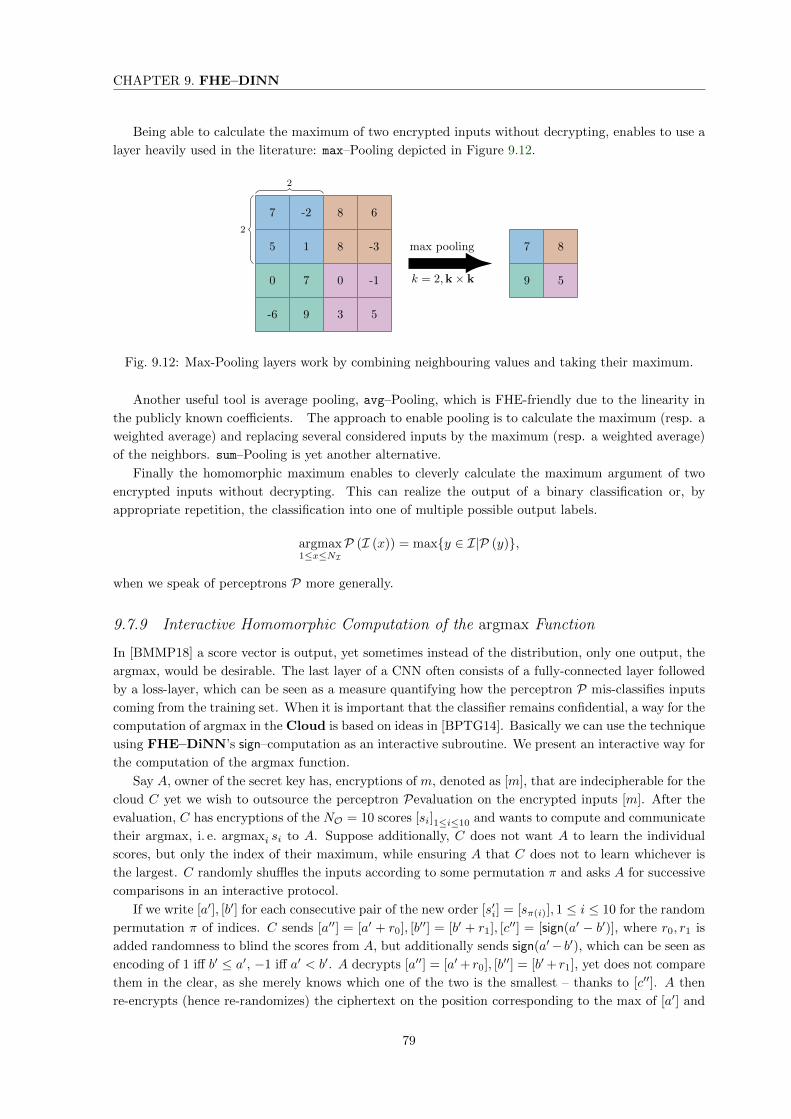
CHAPTER 9. FHE–DINN
Being able to calculate the maximum of two encrypted inputs without decrypting, enables to use a
layer heavily used in the literature: max–Pooling depicted in Figure 9.12.
-6 9 3 5
0 7 0 -1
5 1 8 -3
7 -2 8 6
max pooling
k = 2,k× k 9 5
7 8
2
2
Fig. 9.12: Max-Pooling layers work by combining neighbouring values and taking their maximum.
Another useful tool is average pooling, avg–Pooling, which is FHE-friendly due to the linearity in
the publicly known coefficients. The approach to enable pooling is to calculate the maximum (resp. a
weighted average) and replacing several considered inputs by the maximum (resp. a weighted average)
of the neighbors. sum–Pooling is yet another alternative.
Finally the homomorphic maximum enables to cleverly calculate the maximum argument of two
encrypted inputs without decrypting. This can realize the output of a binary classification or, by
appropriate repetition, the classification into one of multiple possible output labels.
argmax1≤x≤NI
P (I (x)) = maxy ∈ I|P (y),
when we speak of perceptrons P more generally.
9.7.9 Interactive Homomorphic Computation of the argmax Function
In [BMMP18] a score vector is output, yet sometimes instead of the distribution, only one output, the
argmax, would be desirable. The last layer of a CNN often consists of a fully-connected layer followed
by a loss-layer, which can be seen as a measure quantifying how the perceptron P mis-classifies inputs
coming from the training set. When it is important that the classifier remains confidential, a way for the
computation of argmax in the Cloud is based on ideas in [BPTG14]. Basically we can use the technique
using FHE–DiNN’s sign–computation as an interactive subroutine. We present an interactive way for
the computation of the argmax function.
Say A, owner of the secret key has, encryptions of m, denoted as [m], that are indecipherable for the
cloud C yet we wish to outsource the perceptron Pevaluation on the encrypted inputs [m]. After the
evaluation, C has encryptions of the NO = 10 scores [si]1≤i≤10 and wants to compute and communicate
their argmax, i. e. argmaxi si to A. Suppose additionally, C does not want A to learn the individual
scores, but only the index of their maximum, while ensuring A that C does not to learn whichever is
the largest. C randomly shuffles the inputs according to some permutation π and asks A for successive
comparisons in an interactive protocol.
If we write [a′], [b′] for each consecutive pair of the new order [s′i] = [sπ(i)], 1 ≤ i ≤ 10 for the random
permutation π of indices. C sends [a′′] = [a′ + r0], [b′′] = [b′ + r1], [c′′] = [sign(a′ − b′)], where r0, r1 is
added randomness to blind the scores from A, but additionally sends sign(a′− b′), which can be seen as
encoding of 1 iff b′ ≤ a′, −1 iff a′ < b′. A decrypts [a′′] = [a′+ r0], [b′′] = [b′+ r1], yet does not compare
them in the clear, as she merely knows which one of the two is the smallest – thanks to [c′′]. A then
re-encrypts (hence re-randomizes) the ciphertext on the position corresponding to the max of [a′] and
79
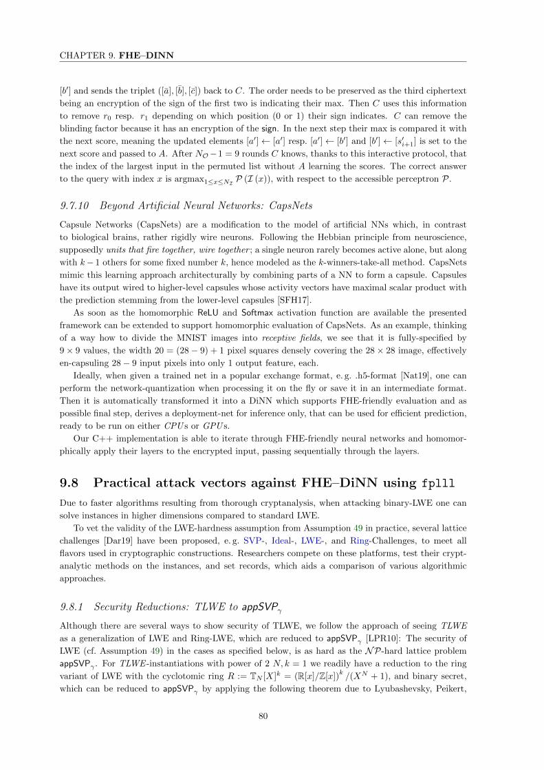
CHAPTER 9. FHE–DINN
[b′] and sends the triplet ([a], [b], [c]) back to C. The order needs to be preserved as the third ciphertext
being an encryption of the sign of the first two is indicating their max. Then C uses this information
to remove r0 resp. r1 depending on which position (0 or 1) their sign indicates. C can remove the
blinding factor because it has an encryption of the sign. In the next step their max is compared it with
the next score, meaning the updated elements [a′]← [a′] resp. [a′]← [b′] and [b′]← [s′i+1] is set to the
next score and passed to A. After NO−1 = 9 rounds C knows, thanks to this interactive protocol, that
the index of the largest input in the permuted list without A learning the scores. The correct answer
to the query with index x is argmax1≤x≤NI P (I (x)), with respect to the accessible perceptron P.
9.7.10 Beyond Artificial Neural Networks: CapsNets
Capsule Networks (CapsNets) are a modification to the model of artificial NNs which, in contrast
to biological brains, rather rigidly wire neurons. Following the Hebbian principle from neuroscience,
supposedly units that fire together, wire together ; a single neuron rarely becomes active alone, but along
with k− 1 others for some fixed number k, hence modeled as the k-winners-take-all method. CapsNets
mimic this learning approach architecturally by combining parts of a NN to form a capsule. Capsules
have its output wired to higher-level capsules whose activity vectors have maximal scalar product with
the prediction stemming from the lower-level capsules [SFH17].
As soon as the homomorphic ReLU and Softmax activation function are available the presented
framework can be extended to support homomorphic evaluation of CapsNets. As an example, thinking
of a way how to divide the MNIST images into receptive fields, we see that it is fully-specified by
9× 9 values, the width 20 = (28− 9) + 1 pixel squares densely covering the 28× 28 image, effectively
en-capsuling 28− 9 input pixels into only 1 output feature, each.
Ideally, when given a trained net in a popular exchange format, e. g. .h5-format [Nat19], one can
perform the network-quantization when processing it on the fly or save it in an intermediate format.
Then it is automatically transformed it into a DiNN which supports FHE-friendly evaluation and as
possible final step, derives a deployment-net for inference only, that can be used for efficient prediction,
ready to be run on either CPU s or GPU s.
Our C++ implementation is able to iterate through FHE-friendly neural networks and homomor-
phically apply their layers to the encrypted input, passing sequentially through the layers.
9.8 Practical attack vectors against FHE–DiNN using fplll
Due to faster algorithms resulting from thorough cryptanalysis, when attacking binary-LWE one can
solve instances in higher dimensions compared to standard LWE.
To vet the validity of the LWE-hardness assumption from Assumption 49 in practice, several lattice
challenges [Dar19] have been proposed, e. g. SVP-, Ideal-, LWE-, and Ring-Challenges, to meet all
flavors used in cryptographic constructions. Researchers compete on these platforms, test their crypt-
analytic methods on the instances, and set records, which aids a comparison of various algorithmic
approaches.
9.8.1 Security Reductions: TLWE to appSVPγ
Although there are several ways to show security of TLWE, we follow the approach of seeing TLWE
as a generalization of LWE and Ring-LWE, which are reduced to appSVPγ [LPR10]: The security of
LWE (cf. Assumption 49) in the cases as specified below, is as hard as the NP-hard lattice problem
appSVPγ . For TLWE -instantiations with power of 2 N, k = 1 we readily have a reduction to the ring
variant of LWE with the cyclotomic ring R := TN [X]k = (R[x]/Z[x])k/(XN + 1), and binary secret,
which can be reduced to appSVPγ by applying the following theorem due to Lyubashevsky, Peikert,
80

CHAPTER 9. FHE–DINN
and Regev [LPR10]. An instantiation with N = 1 and largek is makes TLWE the LWE problem with
binary secret.
Theorem 72 (Quantum Reduction Ring-LWE to appSVPγ). Let N be a power (hence multiple) of 2, a
ring R, β(N) = q/ω(√N logN), for prime q = 1 mod N , γ′(N) = Nω(1), then there exists a uniform
probability distribution χ over R, such that any ppt algorithm A solving RLWEN,q,χ would imply an
efficient quantum algorithm for solving appSVPγ , when setting γ = γ′ · β.
There is a non-tight, classical reduction that incurs only a limited parameter loss [RSW18]. A recent
study predicts the crossover point of classical lattice reduction algorithms, with a quantum algorithm
tailored to the Ring-LWE case exploiting ideal lattice structures [DPW19]. They conclude that their
quantum algorithm provides shorter vectors than BKZ-300, e. g. using the open source version of fplll.
This is roughly meeting the weakest security level of NIST lattice-based candidates, cf. Section 4.4, for
cyclotomic rings of rank larger than about 24000.
9.8.1.1 Reduction ksk to TLWE
Let s, s′ ∈ BN [X]k be two TLWE -keys, we have that s′ ∈R BN [X]k implies s′ · 2−i ∈R BN [X]k. As
an array of TLWE -samples, the hardness of breaking security of the key-switching key, ksks→s′ =
LWEs,α(s′1 · 2−1), LWEs,α(s′2 · 2−2), . . . , LWEs,α(s′n · 2−n) with encryptions of each individually scaled
key-bit as TLWE -sample, reduces immediately to the setting in Theorem 72.
9.8.1.2 Reduction TGSW to TLWE
As TGSW is the matrix equivalent of TLWE (cf. Equation (9.2)), it is an array of TLWE -samples.
9.8.1.3 Reduction bsk to TGSW
As an array of TGSW -samples, the security of the bootstrapping key follows from Section 9.8.1.2.
Before we want to take the perspective of an attacker AFHE–DiNN and study which resources she
can use within the model of Cloud security, in the following, we summarize the theoretical reductions:bsk→ TGSW
ksk
→ TLWE→ appSVPγ .
9.8.2 Theoretical attack vectors against FHE–DiNN
Threat models for the Cloud range from honest, semi-honest to actively malicious ones. Typically, it
is not safe to assume the Cloud as trusted domain, ruling out the honest model option right away.
In the FHE–DiNN use-case model the Cloud does not want to deliberately avoid computational
correctness, for instance outputting nonsense instead of truthfully computing the desired prediction.
Correctness could be enforced by deploying verifiable computation techniques, however. It can actively
try to subvert security by, signaling transmission errors, for example, and requesting multiple ciphertexts
associated with the same plaintext ci = ([µ]s)i, which might naturally differ as the encryption algorithm
is randomized. The client can detect this and prevent the Cloud from obtaining (too many, say
O(N logN)) fresh encryptions, which sets the LWE-sample complexity to N , a small multiple, or at
most O(N), from one TLWE -sample. So the Cloud is left with extracting information from one
ciphertext, the bsk, or the ksk, leading to two different attacks as in Figure 9.13.
Firstly, suppose we have a TLWE Sample c = (a, b) ∈ TN [X]k × TN [X], encrypting the message
µ ∈ TN [X] for s ∈R BN [X]k, chosen uniformly at random with n = kN bits of entropy, we can write
more explicitly: b(X) =∑k`=1 a`(X) · s`(X) + e(X) + µ(X), detailed in Algorithm 9.5.
81

CHAPTER 9. FHE–DINN
Client
g
FHE–DiNN @ Server
DiNN
m
bk = [s]µ
ksk = [s′]µ
c = [µ]µ
security leak?
Fig. 9.13: Model: Malicious Cloud and sources of leakage of FHE–DiNN ciphertexts and keys.
Secondly, a FHE–DiNN-attacker can try to perform key-recovery from bk and ksk, again having
only access to these ciphertexts.
Remark 73 (FHE–DiNN Ciphertext-Only Security). Algorithm 9.5 describes asymptotically the
best-known FHE–DiNN Ciphertext-Only Attacker ACOA(c).
Algorithm 9.5: FHE–DiNN Ciphertext-Only Attacker ACOA(c)
Input : c ∈ TLWEs,α, with sk = s ∈R BN [X]k
Data: N,αResult: µ ∈ B with µ = Decsk(c)Find µ by using best known algorithms to extract the message from the ciphertext (cf.Section 9.8.2) running in time T COA(N,α) = TTLWE(N,α) = N · TLWE(N,α), and requiresSCOA(N,α) = O(N logN) space.
Remark 74 (FHE–DiNN Full Key-Recovery). Algorithm 9.6 describes asymptotically the best-known
FHE–DiNN key-recovery attacker Absk(c) resp. Aksk(.) depending whether the attacker.
Algorithm 9.6: FHE–DiNN Key-Recovery Attacker (KRA) AKRA(.)
Input : bk ∈ BKs→s′,α, resp. ksk ∈ KSKs→s′,α,t, with sk = s ∈R BN [X]k, sk′ = s′ ∈R BN [X]k
Data: N,α, n, l, kResult: s ∈ BN [X]k with si = Decsk(bski) resp. s′i = Decsk(kski)Find s resp. s′ by using best known algorithms to extract the key from the ciphertext (cf.Section 9.8.2) running in time T KRA = minT bsk, T ksk, with
T bsk(N,α) = n · TTGSW (N,n, l, k, α) = n · l · (k+ 1) · TLWE(N,α) = n · l · (k+ 1) · 2(2·log(cqcs
))−1·n,
resp. T ksk(N,α) = n · TLWE(N,α) = n · 2(2·log(cqcs
))−1·n, and SKRA(N,α) = O(N logN) space.
9.8.3 Security Evaluation and Parameter Choices
In Table 9.2 we highlight the main security parameters regarding our ciphertexts, together with an
estimate of the security level that this setting achieves. Other additional parameters, related to the
various operations we need to perform, are the following:
The security parameters we use for the different kinds of ciphertexts. The estimated security
has been extracted from the plot in [CGGI17] and later verified with the estimator from Albrecht
et al. [APS15]:
82
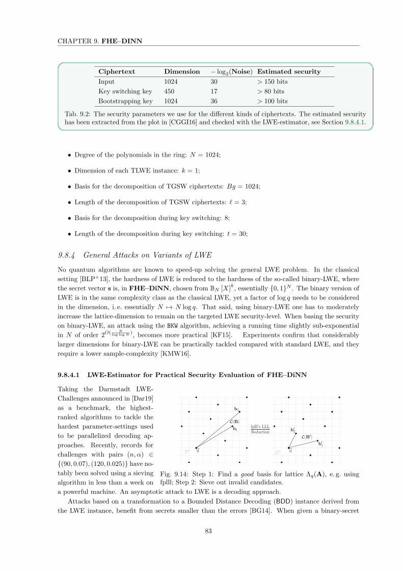
CHAPTER 9. FHE–DINN
Ciphertext Dimension − log2(Noise) Estimated security
Input 1024 30 > 150 bits
Key switching key 450 17 > 80 bits
Bootstrapping key 1024 36 > 100 bits
Tab. 9.2: The security parameters we use for the different kinds of ciphertexts. The estimated securityhas been extracted from the plot in [CGGI16] and checked with the LWE-estimator, see Section 9.8.4.1.
• Degree of the polynomials in the ring: N = 1024;
• Dimension of each TLWE instance: k = 1;
• Basis for the decomposition of TGSW ciphertexts: Bg = 1024;
• Length of the decomposition of TGSW ciphertexts: ` = 3;
• Basis for the decomposition during key switching: 8;
• Length of the decomposition during key switching: t = 30;
9.8.4 General Attacks on Variants of LWE
No quantum algorithms are known to speed-up solving the general LWE problem. In the classical
setting [BLP+13], the hardness of LWE is reduced to the hardness of the so-called binary-LWE, where
the secret vector s is, in FHE–DiNN, chosen from BN [X]k, essentially 0, 1N . The binary version of
LWE is in the same complexity class as the classical LWE, yet a factor of log q needs to be considered
in the dimension, i. e. essentially N 7→ N log q. That said, using binary-LWE one has to moderately
increase the lattice-dimension to remain on the targeted LWE security-level. When basing the security
on binary-LWE, an attack using the BKW algorithm, achieving a running time slightly sub-exponential
in N of order 2O( Nlog logN ), becomes more practical [KF15]. Experiments confirm that considerably
larger dimensions for binary-LWE can be practically tackled compared with standard LWE, and they
require a lower sample-complexity [KMW16].
9.8.4.1 LWE-Estimator for Practical Security Evaluation of FHE–DiNN
~0
b1
b2
Zn
L(B)
~0
b′1
b′2
Zn
L(B′)
fplll’s LLLReduction
Fig. 9.14: Step 1: Find a good basis for lattice Λq(A), e. g. usingfplll; Step 2: Sieve out invalid candidates.
Taking the Darmstadt LWE-
Challenges announced in [Dar19]
as a benchmark, the highest-
ranked algorithms to tackle the
hardest parameter-settings used
to be parallelized decoding ap-
proaches. Recently, records for
challenges with pairs (n, α) ∈(90, 0.07), (120, 0.025) have no-
tably been solved using a sieving
algorithm in less than a week on
a powerful machine. An asymptotic attack to LWE is a decoding approach.
Attacks based on a transformation to a Bounded Distance Decoding (BDD) instance derived from
the LWE instance, benefit from secrets smaller than the errors [BG14]. When given a binary-secret
83

CHAPTER 9. FHE–DINN
LWE instance (Lq(At),b) with error e an attacker can trasform it into a BDD instance by writing(L⊥q (Im |At), (b,~0 )
)(9.11)
with the updated error vector (e, s) ensuring correctness. Solving the original instance is mathematically
equivalent to solving:
(Im |At)
e
s
−b
~0
= 0 mod q. (9.12)
What is the best computational choice depends on the best available implementations and the param-
eterization.
A BDD enumeration instance for LWE with parameters (n, α, q) requires a lattice-basis reduction
algorithm, e. g. fplll’s BKZ algorithm, A ∈ Zm×mq , and a target t ∈ Zmq , promised at most ||t− v|| ∈Θ(αq
√m) away from a lattice vector. The LWE-estimator by Albrecht et al. [APS15] allows looking
up values for the constants cLWE or cBKZ known to the public cryptographic community.
Remark 75 (Asymptotic Complexity of Attacking LWE.). Let α, β ∈ R, q = nα, ‖e‖ = nβ ∈O (poly(n)): TLWE = 2cLWE·n· logn
log(q/‖e‖) , with cLWE(cBKZ) and poly(n)- or 2n-space requirements. At-
tacking LWE in practice consists of two independent steps: lattice reduction and enumeration/sieving.
9.8.4.2 Attacking the Hybrid Approach of FHE–DiNN
FHE–DiNN, based on TFHE, uses a binary secret LWE. One idea of the hybrid scheme is not to
distribute key material as such, but to generate it on the fly using a suitably seeded pseudorandom
number generator (PRNG) adding an additional security assumption to the overall model.
As parameters for a security level of 128 [bit], we set n = m = 450, assume that A is a uniformly
random 450× 450 integer matrix modulo q = 232, interpreted as elements on the torus. The secret and
the error are both vectors of length 450 with independently identically distributed entries according
to a discrete Gaussian distribution of parameter α. In our attack scenario we assume an honest-but-
curious adversary, who observes all devices, other than the users’, obtaining access to full side-channel
information through timing, . . . on the server-side. From a high-level perspective, we obtain N LWE
samples from each TLWE sample , arranged as a matrix (A, b = As + e). The goal is to exploit this
information to mount a lattice-based attack, as parameters in FHE–DiNN were aggressively chosen
in order to allow fast evaluation speeds of neural network. We chose the BDD enumeration algorithm
as most powerful attack combined with pruning strategies to speed-up the decoding, more so as full
enumeration in smaller dimension can be embarrassingly parallelized, for sub-routines [HKM18].
9.9 Experimental Results
You don’t know what you are talking about until you implemented it.—David Naccache
We tried out our proposed FHE–DiNNapproach and list experimental results of our CPU-implementation
in terms of quality of the classification (accuracy) and run-time.
For our test networks, we show a comparison of accuracies when evaluating a trained 784:100:10
network on 10 000 MNIST test images, and contrast it with a network of only 30 hidden neurons.
FHE–DiNN follows the outline presented in Figure 9.17 for our example use-case given a network
able to perform digit recognition.
84

CHAPTER 9. FHE–DINN
Pre-processing the MNIST database.
Initially, we made a pre-processing step of the MNIST data-set actually decreasing the number of inputs
from 784 to 16 · 16 = 256, possibly sacrificing accuracy of our network. Then we proceeded training
Fig. 9.15: Pre-processing of a Seven from the MNIST test set.
networks on the full 784-input pixel images.
Training a DiNN over Plaintext Data
In order to train the neural network, we first chose its topology, i. e., the number of hidden layers and
neurons per hidden layer, which we note separated by ‘:‘. We experimented with several values, and
settled for a neural network with a single hidden layer composed of 100 neurons demonstrating a good
accuracy, run-time trade-off.
For training the network, we fixed the initial value of the learning rate to η = 0.006 and we used
an approach called learning rate decay : η is multiplied by a constant factor (smaller than 1) every few
epochs. In particular, we multiplied the learning rate by 0.95 every 5 epochs of training. The idea
behind this procedure is that of progressively reducing the “width of the step” in the optimization
process. This results in wider steps – which will hopefully set the cost minimization towards the right
direction – at the beginning of the training, followed by narrower steps to “refine” the set of weights
that has been found. The size of the batches has been fixed to 10 and kept constant throughout the
entire training phase.
The discretization of the weights happens according to Equation (9.9), and choosing the final value
of tick size τ we experimented and found that τ = 10 is a good compromise between accuracy (more
possible values for the weights give the network more expressiveness) and the message space the homo-
morphic scheme will have to support.
In order to determine the noise parameters needed to parameterize the message space, we calculated
the maxima over all the L1-, and L2-norms of the weight vectors associated to each neuron per layer.
These values, once computed at pre-processing phase using the clear weights of the given network, define
the theoretical bounds our scheme is able to support. Evaluating the actual multisums of the complete
training set in one inference run, provide more efficient, practical bounds. An aggressive parameter
choice makes it is possible that specific inputs’ multisum exceeds the bounds leading to inaccuracies
during bootstrapping. If the test set distribution matches the training set distribution closely enough,
this should not observable when evaluating the network on new input samples.
In Figure 9.16 we show the FHE-friendly model of a neural network that we considered in this work.
In Table 9.3 we report the theoretical message space we would need to support and the message space
we actually used for our implementation. Equation (9.13) describes the mathematical representation
85
CHAPTER 9. FHE–DINN
p1 p28
p784
1p1
Enc(p1)
2p2
Enc(p2)
3p3
Enc(p3)
p784
Enc(p784)
...
784
Hidden layer
1
1
22...
100
...10
Enc(S0)
Enc(S1)
Enc(S9)
Matth
iasMinihold
(0x5A44531D)
Fig. 9.16: Depiction of our neural network with 784:100:10–topology. It takes as input the pixels thatcompose the image and outputs the scores si assigned to each digit.
FHE–DiNN (784:30:10) FHE–DiNN (784:100:10)
‖W‖ worst. avg. ‖W‖ worst. avg.
1st layer 2338 4676 2500 1372 2744 1800
2nd layer 399 798 800 488 976 1000
1st layer ≈ 119 ≈ 69
2nd layer ≈ 85 ≈ 60
Tab. 9.3: The listed FHE–DiNN-settings show ‖W‖ = maxw ‖w‖1 in the first two rows responsiblefor message space adjustments with theoretical worst-case, and experimental, average-case bounds,resp. ‖W‖ = maxw ‖w‖2 in the last two rows.
of our perceptron M (cf. Definition 61) as composition of linear and non-linear functions, compare to
the general setting in Figure 9.4.
FHE–DiNN computes a weighted composition of functions with one input TLWE Sample c0 as
MFHE–DiNN :
TN [X]k −→ (TN [X]k)10
x := c0 7→ y := ~c2 =
100∑`2=1
ϕ1
(784∑`1=1
(c0)`1 · (w0→1)`1
)︸ ︷︷ ︸
~c1
`2
· (w1→2)`2 ,
(9.13)
with ten TLWE Samples ~cO := ~c2 ∈ (TN [X]k)10 as output, encrypting the perceptrons’ predicted
digit label likelihoods of the encrypted input c0 := cI = Enc(x) ∈ TN [X]k. Two consecutive,
dense layers were adaptively shaped to form a feed-forward DiNN, trained on (MNIST) samples map-
ping RnI → RnO , categorizing images of digits into 10 classes. The weights w0→1, w1→2 were pre-
computed, approximated, and Fourier transformed. The homomorphic evaluation made intermediate,
bootstrapped activations using ϕ1 = sign necessary, yielding a low-noise encryption of a weighted
86
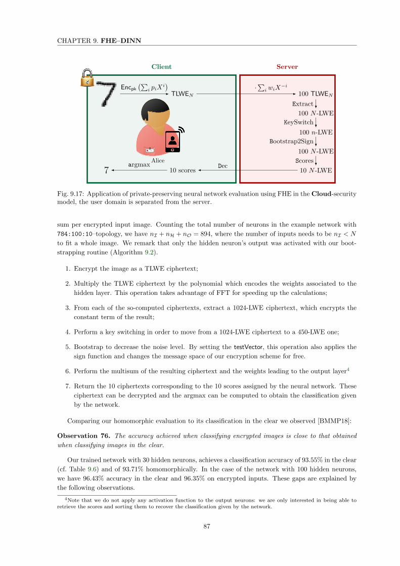
CHAPTER 9. FHE–DINN
ServerClient
COOPER
Alice
TLWEN
Encpk(∑
i piXi)
100 TLWEN
·∑i wiX−i
100 N -LWEExtract
100 n-LWEKeySwitch
100 N -LWEBootstrap2Sign
10 N -LWEScores
10 scores Dec7 argmax
Fig. 9.17: Application of private-preserving neural network evaluation using FHE in the Cloud-securitymodel, the user domain is separated from the server.
sum per encrypted input image. Counting the total number of neurons in the example network with
784:100:10–topology, we have nI + nH + nO = 894, where the number of inputs needs to be nI < N
to fit a whole image. We remark that only the hidden neuron’s output was activated with our boot-
strapping routine (Algorithm 9.2).
1. Encrypt the image as a TLWE ciphertext;
2. Multiply the TLWE ciphertext by the polynomial which encodes the weights associated to the
hidden layer. This operation takes advantage of FFT for speeding up the calculations;
3. From each of the so-computed ciphertexts, extract a 1024-LWE ciphertext, which encrypts the
constant term of the result;
4. Perform a key switching in order to move from a 1024-LWE ciphertext to a 450-LWE one;
5. Bootstrap to decrease the noise level. By setting the testVector, this operation also applies the
sign function and changes the message space of our encryption scheme for free.
6. Perform the multisum of the resulting ciphertext and the weights leading to the output layer4
7. Return the 10 ciphertexts corresponding to the 10 scores assigned by the neural network. These
ciphertext can be decrypted and the argmax can be computed to obtain the classification given
by the network.
Comparing our homomorphic evaluation to its classification in the clear we observed [BMMP18]:
Observation 76. The accuracy achieved when classifying encrypted images is close to that obtained
when classifying images in the clear.
Our trained network with 30 hidden neurons, achieves a classification accuracy of 93.55% in the clear
(cf. Table 9.6) and of 93.71% homomorphically. In the case of the network with 100 hidden neurons,
we have 96.43% accuracy in the clear and 96.35% on encrypted inputs. These gaps are explained by
the following observations.
4Note that we do not apply any activation function to the output neurons: we are only interested in being able toretrieve the scores and sorting them to recover the classification given by the network.
87

CHAPTER 9. FHE–DINN
Observation 77. During the evaluation, some multisum-signs are flipped during the bootstrapping,
which does not significantly decrease the accuracy of the network.
We use aggressive internal parameters (e. g., N , α and, in general, all precision parameters such
as τ) for the homomorphic evaluation, knowing that this could lead the bootstrapping procedure to
return an incorrect result when extracting the sign of a message. In fact, we conjectured that the
neural network would be resilient to perturbations and experimental results proved that this is indeed
the case: when running our experiment over the full test set, we noticed that the number of wrong
bootstrappings is 3383 (respectively, 9088) but this did not change the outcome of the classification in
more than 196 (respectively, 105) cases (cf. Table 9.7).
Observation 78. The classification of an encrypted image might disagree with the classification of the
same image in the clear but this does not significantly worsen the overall accuracy.
This is a property that we expected during the implementation phase and our intuition to explain
this fact is the following: the network is assigning 10 scores to each image, one per digit, and when
two scores are close (i. e., the network is hesitating between two classes), it can happen that the
classification in the clear is correct and the one over the encrypted image is wrong. But the opposite
can also be true, thus leading to classifying correctly an encrypted sample that was misclassified in
the clear. We experimentally verified that disagreements between the evaluations do not automatically
imply that the homomorphic classification is worse than the one in the clear: out of 273 (respectively,
127) disagreements, the classification in the clear was correct 105 (respectively, 61) times, against 121
(respectively, 44) times in favor of the homomorphic one5 (cf. Table 9.7).
Observation 79. Using the modified version of the BlindRotate algorithm presented in Section 9.7.6
decreases the number of wrong bootstrappings.
Before stating some open problems, we conclude with the following note: using a bigger neural
network generally leads to a better classification accuracy, at the cost of performing more calculations
and, above all, more bootstrapping operations. However, the evaluation time will always grow linearly
with the number of neurons. Although it is true that evaluating a bigger network is computationally
more expensive, we stress that the bootstrapping operations are independent of each other and can
thus be performed in parallel. Ideally, parallelizing the execution across a number of cores equal to the
number of neurons in a layer (30 or 100 in our work) would result in that the evaluation of the layer
would take roughly the time of a bootstrapping (i. e., around 15 ms).
9.10 Comparison with Cryptonets
Cryptonets [DGBL+16] propagate real signals encoded as compatible plaintext, encrypted as one huge
input ciphertext. Regarding classification accuracy, the NN used by Cryptonets achieves 98.95 % of
correctly classified samples, when evaluated on the MNIST dataset. In our case, a loss of accuracy occurs
due to the preliminary simplification of the MNIST images, and especially because of the discretization
of the network. We stress however that our prime goal was not accuracy but to achieve a qualitatively
better homomorphic evaluation at the neuron level.
An entire image takes 28 · 28 · 766 kB ≈ 586 MB, a single image pixel takes 2 · 382 · 8192 bits (= 766
kB) with Cryptonets. However, with the same storage requirements, Cryptonets can batch 8192 images
together, so that the amortized size of an encrypted image is reduced to 73.3 kB. In the case of FHE–
DiNN, we are able to exploit the batching technique on a single image, resulting in that each encrypted
image takes ≈ 8.2 kB. Cryptonets has a 784:835:100:10–topology, meaning 945 inner, hidden neurons
5In the remaining cases, the classifications were different but they were both wrong.
88

CHAPTER 9. FHE–DINN
Overall per Image
# Neurons Accuracy Eval [s] |c| [B] Enc [s] Dec [s]
Cryptonets 945 98.95 % 570 586 M 122 5
Cryptonets? 945 98.95 % 0.07 73.3 k 0.015 0.000 6
FHE–DiNN 30 93.71 % 0.49 ≈ 8.2 k 0.000 168 0.000 010 6
FHE–DiNN 100 96.35 % 1.64 ≈ 8.2 k 0.000 168 0.000 010 6
Cryptonets? is amortized per image (accumulating 8192 inferences)Tab. 9.5: Comparison with Cryptonets and its amortized version (denoted by Cryptonets?). We referto FHE–DiNN on DiNNs with one hidden layer composed of 30 and 100 neurons, respectively.
which we compare to FHE–DiNNs 100 neurons. Their complete homomorphic evaluation of the
network takes 570 seconds, whereas in our case it takes 0.49 s, respectively 1.6 s in the case of a 30
resp. 100 hidden neuron network. We remark that the networks that we use for our experiments are
considerably smaller than that used in Cryptonets, so we also compare the time-per-neuron and, in this
case, our solution is faster by roughly a factor 36; moreover, while Cryptonets supports image batching
(8192 images can be, and needs to be classified in 570 seconds), which results in only 0.07 s per image.
In the simplest use-case the user only wants a single image at a time to be classified, Cryptonets’ ability
to batch images together is not useful in this applications, but potentially in others where the same
user wants to classify a large number of samples at once.
Finally, the most distinctive achievement is scale-invariance, meaning that FHE–DiNN can keep on
computing over the encrypted outputs of an arbitrarily deep network, whereas Cryptonets are bounded
by the initial choice of parameters. In Table 9.5 we present a detailed comparison with Cryptonets.
9.10.1 Performance of FHE–DiNN on (clear) inputs x
The first column of Table 9.6 refers to the evaluation of the trained real-valued model in the clear. In
the second and third one all weights and biases have been discretized; and the difference is applying
a sigmoidal– respectively the sign(·)–activation function for every neuron in the hidden layer. These
numbers are contrasted with the full inference with encrypted inputs in the last column.
Table 9.6 serves as a baseline when comparing our originally trained, real-valued network with
discretizations. Furthermore, the percentages in the third column are the numbers to be compared
with accuracy drops in the encrypted setting.
R-NN DiNN w. hard sigmoid DiNN w. sign FHE–DiNN
30 neurons 94.76 % 93.76 % (−1 %) 93.55 % (−1.21 %) 93.71 % (−1.05 %)
100 neurons 96.75 % 96.62 % (−0.13 %) 96.43 % (−0.32 %) 96.35 % (−0.4 %)
Tab. 9.6: Performance metrics on (clear) inputs x.
9.10.2 Performance of FHE–DiNN on (encrypted) inputs Enc (x)
Finally, in Table 9.7, the results of fully homomorphic evaluation using the sign, a window-size of ω = 2
are presented. An image ciphertext providing 80 bits security takes 8.2 [kB] and an average of 1.64
89
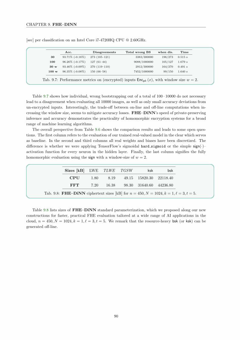
CHAPTER 9. FHE–DINN
[sec] per classification on an Intel Core i7-4720HQ CPU @ 2.60GHz.
Acc. Disagreements Total wrong BS when dis. Time
30 93.71% (-0.16%) 273 (105–121) 3383/300000 196/273 0.515 s
100 96.26% (-0.17%) 127 (61–44) 9088/1000000 105/127 1.679 s
30 w 93.46% (-0.09%) 270 (119–110) 2912/300000 164/270 0.491 s
100 w 96.35% (-0.08%) 150 (66–58) 7452/1000000 99/150 1.640 s
Tab. 9.7: Performance metrics on (encrypted) inputs Encpk (x), with window size w = 2.
Table 9.7 shows how individual, wrong bootstrapping out of a total of 100 · 10000 do not necessary
lead to a disagreement when evaluating all 10000 images, as well as only small accuracy deviations from
un-encrypted inputs. Interestingly, the trade-off between on-line and off-line computations when in-
creasing the window size, seems to mitigate accuracy losses. FHE–DiNN’s speed of private-preserving
inference and accuracy demonstrates the practicality of homomorphic encryption systems for a broad
range of machine learning algorithms.
The overall perspective from Table 9.6 shows the comparison results and leads to some open ques-
tions. The first column refers to the evaluation of our trained real-valued model in the clear which serves
as baseline. In the second and third columns all real weights and biases have been discretized. The
difference is whether we were applying TensorFlow’s sigmoidal hard sigmoid or the simple sign(·)–activation function for every neuron in the hidden layer. Finally, the last column signifies the fully
homomorphic evaluation using the sign with a window-size of w = 2.
Sizes [kB] LWE TLWE TGSW ksk bsk
CPU 1.80 8.19 49.15 15820.30 22118.40
FFT 7.20 16.38 98.30 31640.60 44236.80
Tab. 9.8: FHE–DiNN ciphertext sizes [kB] for n = 450, N = 1024, k = 1, ` = 3, t = 5.
Table 9.8 lists sizes of FHE–DiNN standard parameterization, which we proposed along our new
constructions for faster, practical FHE evaluation tailored at a wide range of AI applications in the
cloud, n = 450, N = 1024, k = 1, ` = 3, t = 5. We remark that the resource-heavy bsk (or ksk) can be
generated off-line.
90
Chapter 10
FHE & AI on GPUs (cuFHE–DiNN)
10.1 Practical FHE evaluation of neural networks using CUDA
Previous sections show that the run time of the external products, i. e. ExternMulToTLwe(), is the most
frequent and costly operation when evaluating our FHE-friendly neural nets, hence a bottleneck. A
possibility is speeding this step up by implementing parallelized processing on a GPU . Experimentally,
in a GPU -focused follow-up implementation of FHE–DiNN using CUDA dubbed cuFHE–DiNN,
we show figures of FFT-based GPU -versions over the plain CPU -version of individual algorithms:
With N = 1024, k = 1, averaging over 10 runs on random data, e. g. multiplication of numbers show
speed-ups more than 740x on NVIDIA RTX2080 TI compared to Intel(R) Xeon(R) CPU E3-1230 v6.
With N = 512, k = 1, we achieved experimental improvements of more than a factor of 50x
polynomial multiplications by using the complete FFT-transformation, point-wise multiplication, and
the inverse FFT-transformation.
Further, more complex routines show the run-time behaviour 40x (MuxRotate), 38x (BlindRotate,
BlindRotateAndExtract, and Bootstrap_woKS), and 8x (TGSW::ExternMulToTLwe()) for N = 512, k = 1, and of
roughly a factor of 12x (MuxRotate), 12x (BlindRotate, BlindRotateAndExtract, and Bootstrap_woKS), and
more than a factor of 14x (TGSW::ExternMulToTLwe()) for N = 1024, k = 1. The observations of how com-
ponent functions translate these figures to the case of the full homomorphic neural network evaluations
with cuFHE–DiNN, strengthen the confidence that FHE-friendly neural networks will benefit in the
near future from clever, yet trickier, GPU implementations as a next step into practicability of this
technology.
Future directions and open problems.
This work reveals a number of future research directions and, raises several interesting open problems:
The first one is about directly training FHE-friendly DiNNs, rather than simply discretizing an
already-trained model: Is the loss in precision inherent, when converting to DiNNs or is there an alter-
native training algorithm or regularization method for FHE-friendly homomorphic neural networks?
Another natural question is whether it is possible to batch several bootstrappings together using
TGSW-based FHE schemes, in order to improve the overall efficiency of the evaluation: Are there
efficient packing, or batching, techniques for refreshing TGSW ciphertexts in a parallelized fashion?
The methodology and use-case presented in this work is by no means limited to image recogni-
tion, but can be applied to other machine learning problems as well: How far can the FHE–DiNN-
framework be pushed to evaluate increasingly more generic cognitive architectures?
The max function is needed to homomorphically evaluate the widely-used max pooling layers. To the
best of our knowledge, only the introduced interactive technique from Section 9.7.9 can solve this: For
an efficient homomorphic evaluation, meeting the non-interactiveness of FHE, is there a homomorphic
routine (based on TFHE) computing the max function?
91


Part III
Cryptanalysis of FHE schemes
93


Cryptanalysis sets the stage of security claims in cryptology.
In this part we introduce new algorithms to solve variants of the subset-sum problem (SSP), in
particular multi-dimensional versions. We also relate previous discussions on lattice-based primitives,
e. g. as in FHE-constructions, to the SSP.
Furthermore, we study the subset-product problem, a variant which seems not to have undergone
much scrutiny despite it appearing in some contexts of practical interest. Our technical novelties rely on
a combination of maximal hypergraph partitioning, a polynomial reduction to the (one dimensional)
SSP. The resulting subset-product solver can take advantage of the problem’s sparsity much more
efficiently than the usual reduction. We study a property some SSP solvers can be endowed hat finds
each solution with equal probability, which we call equiprobability. We advance evidence that there
exist classical and quantum SSP solvers which are equiprobable.
95

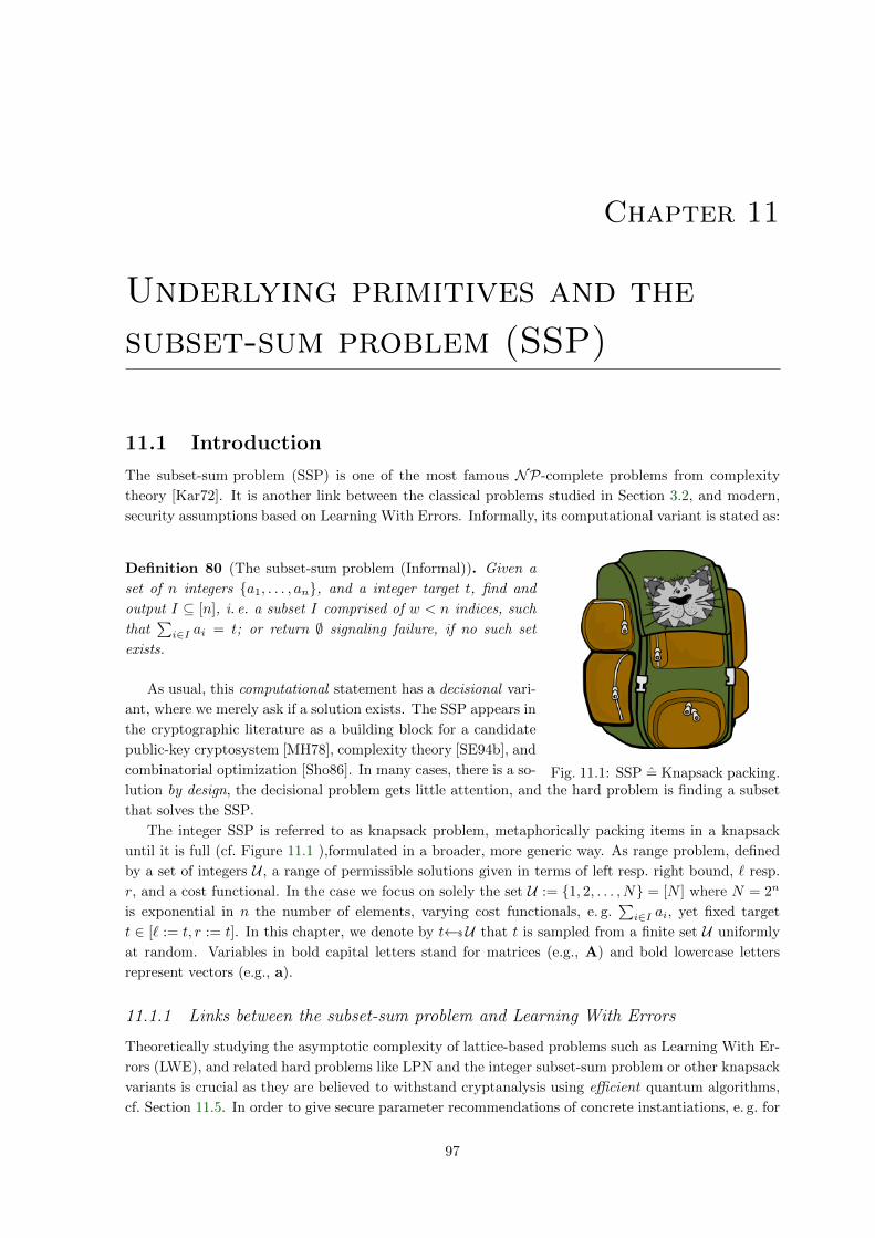
Chapter 11
Underlying primitives and the
subset-sum problem (SSP)
11.1 Introduction
The subset-sum problem (SSP) is one of the most famous NP-complete problems from complexity
theory [Kar72]. It is another link between the classical problems studied in Section 3.2, and modern,
security assumptions based on Learning With Errors. Informally, its computational variant is stated as:
Fig. 11.1: SSP = Knapsack packing.
Definition 80 (The subset-sum problem (Informal)). Given a
set of n integers a1, . . . , an, and a integer target t, find and
output I ⊆ [n], i. e. a subset I comprised of w < n indices, such
that∑i∈I ai = t; or return ∅ signaling failure, if no such set
exists.
As usual, this computational statement has a decisional vari-
ant, where we merely ask if a solution exists. The SSP appears in
the cryptographic literature as a building block for a candidate
public-key cryptosystem [MH78], complexity theory [SE94b], and
combinatorial optimization [Sho86]. In many cases, there is a so-
lution by design, the decisional problem gets little attention, and the hard problem is finding a subset
that solves the SSP.
The integer SSP is referred to as knapsack problem, metaphorically packing items in a knapsack
until it is full (cf. Figure 11.1 ),formulated in a broader, more generic way. As range problem, defined
by a set of integers U , a range of permissible solutions given in terms of left resp. right bound, ` resp.
r, and a cost functional. In the case we focus on solely the set U := 1, 2, . . . , N = [N ] where N = 2n
is exponential in n the number of elements, varying cost functionals, e. g.∑i∈I ai, yet fixed target
t ∈ [` := t, r := t]. In this chapter, we denote by t←$U that t is sampled from a finite set U uniformly
at random. Variables in bold capital letters stand for matrices (e.g., A) and bold lowercase letters
represent vectors (e.g., a).
11.1.1 Links between the subset-sum problem and Learning With Errors
Theoretically studying the asymptotic complexity of lattice-based problems such as Learning With Er-
rors (LWE), and related hard problems like LPN and the integer subset-sum problem or other knapsack
variants is crucial as they are believed to withstand cryptanalysis using efficient quantum algorithms,
cf. Section 11.5. In order to give secure parameter recommendations of concrete instantiations, e. g. for
97

CHAPTER 11. UNDERLYING PRIMITIVES AND THE SUBSET-SUM PROBLEM (SSP)
HE-schemes as discussed in Part II for the use in practice, cryptanalysis needs to consider all alleys of
tackling a problem if necessary, i. e. exponential classical and quantum algorithms. Concrete instan-
tiations like FHE–DiNN discussed earlier, based on LWE ≤ SSP would be jeopardized, when fast,
generic SSP solvers are discovered for average-case instances.
LWE, as defined in Part II of this thesis, is a flexible problem that can be considered with various
error distributions that adds bounded random noise to the system of equations. LWR, a deterministic
version of the problem, has been studied too. There errors are carries occurring when adding numbers
whose sum is overflowing the base leading to deterministic noise.
In [MM11b] Micciancio and Mol analyze the duality of the LWE function family and the knap-
sack function family (defined more generally) and discuss sample-preserving reductions between the
conjectured hard decisional and computational problems, they pose. Regarded even from a greater dis-
tance, both problems can be casted as average-case instances of the bounded distance decoding (BDD)
problem.
Unfortunately, the cryptographic community is not aware of the concrete theoretical connections
between LWE and SSP, in the sense that tight reductions between the two exist.
More specifically, for an integer m ∈ N and a finite, additive Abelian group (G,+) with an element
a ∈ Gm, we define the functional
Fa :
Z −→ G
x 7→ Fa(x) :=∑i xiai.
The functional is conjectured to be a one-way function (cf. Definition 15), only inefficiently invertible
for many choices of Z, and G, i. e. for Z := Zm, G := ZN .
Given a list of integers a := (a1, a2, . . . am) ∈ Zm and a target sum t := Fa(x) =∑i xiai ∈ Z for
a uniformly chosen binary vector x ∈R 0, 1m, the problem of recovering x given (a, t) ∈ Gm+1 is
known as the subset-sum problem. Often a restricted a ∈ Gm is chosen to create an instance of the
subset-sum problem.
Knapsack problems in the group of vectors over Z, G = (Zkq ,+) where the inputs x are sampled from
the given LWE error distribution modulo q can be interpreted as duals of the LWE function family.
A successful attack on the knapsack problem hence possibly means that parameter recommendations
of practical and secure LWE have to be re-assessed and adapted to meet the desired security level.
Any given LWE instance can be translated, with polynomial run-time overhead of the reduction, to
an appropriate knapsack instance, within the same sample-complexity of the error distribution. This
needs to be taken into account in order to derive concrete parameters.
11.2 Solving the subset-sum problem
When we ask ourselves how feasible it is to solve the subset-sum problem, a trivial lower bound is Ω(n),
i. e. the run-time of a solver is necessarily lower bounded by some function linear in n, as clearly we
need to at least read every input ai. Obtaining better, tighter lower bounds requires careful analysis
that often is not straight-forward. It is still an open question whether this lower bound can be improved
in full generality. A natural upper bound is performing an exhaustive search, i. e. computing the cost
functional of all possible subsets and testing if the selected elements sum to the target element, gives
the bound O (2n). We remark that we implicitly omit terms only polynomial in n in the notation here,
and write O(2n), when we want to stress this fact and be more precise about the asymptotic behaviour.
However, we remark that at least some special cases can be tackled more efficiently. Naturally, any
super-increasing sequence, e. g. the powers-of-2, particularly familiar to every mathematician working
in computer-science, do not pose a real challenge, as a ppt algorithm A solving such instances is
98
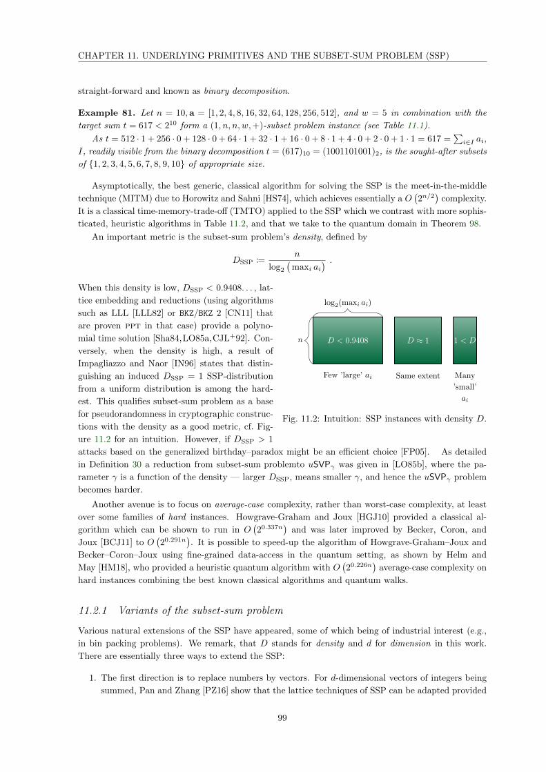
CHAPTER 11. UNDERLYING PRIMITIVES AND THE SUBSET-SUM PROBLEM (SSP)
straight-forward and known as binary decomposition.
Example 81. Let n = 10,a = [1, 2, 4, 8, 16, 32, 64, 128, 256, 512], and w = 5 in combination with the
target sum t = 617 < 210 form a (1, n, n, w,+)-subset problem instance (see Table 11.1).
As t = 512 · 1 + 256 · 0 + 128 · 0 + 64 · 1 + 32 · 1 + 16 · 0 + 8 · 1 + 4 · 0 + 2 · 0 + 1 · 1 = 617 =∑i∈I ai,
I, readily visible from the binary decomposition t = (617)10 = (1001101001)2, is the sought-after subsets
of 1, 2, 3, 4, 5, 6, 7, 8, 9, 10 of appropriate size.
Asymptotically, the best generic, classical algorithm for solving the SSP is the meet-in-the-middle
technique (MITM) due to Horowitz and Sahni [HS74], which achieves essentially a O(2n/2
)complexity.
It is a classical time-memory-trade-off (TMTO) applied to the SSP which we contrast with more sophis-
ticated, heuristic algorithms in Table 11.2, and that we take to the quantum domain in Theorem 98.
An important metric is the subset-sum problem’s density, defined by
DSSP :=n
log2
(maxi ai
) .
D < 0.9408
log2(maxi ai)
n
Few ’large’ ai
D ≈ 1
Same extent
1 < D
Many
’small’
ai
Fig. 11.2: Intuition: SSP instances with density D.
When this density is low, DSSP < 0.9408. . . , lat-
tice embedding and reductions (using algorithms
such as LLL [LLL82] or BKZ/BKZ 2 [CN11] that
are proven ppt in that case) provide a polyno-
mial time solution [Sha84,LO85a,CJL+92]. Con-
versely, when the density is high, a result of
Impagliazzo and Naor [IN96] states that distin-
guishing an induced DSSP = 1 SSP-distribution
from a uniform distribution is among the hard-
est. This qualifies subset-sum problem as a base
for pseudorandomness in cryptographic construc-
tions with the density as a good metric, cf. Fig-
ure 11.2 for an intuition. However, if DSSP > 1
attacks based on the generalized birthday–paradox might be an efficient choice [FP05]. As detailed
in Definition 30 a reduction from subset-sum problemto uSVPγ was given in [LO85b], where the pa-
rameter γ is a function of the density — larger DSSP, means smaller γ, and hence the uSVPγ problem
becomes harder.
Another avenue is to focus on average-case complexity, rather than worst-case complexity, at least
over some families of hard instances. Howgrave-Graham and Joux [HGJ10] provided a classical al-
gorithm which can be shown to run in O(20.337n
)and was later improved by Becker, Coron, and
Joux [BCJ11] to O(20.291n
). It is possible to speed-up the algorithm of Howgrave-Graham–Joux and
Becker–Coron–Joux using fine-grained data-access in the quantum setting, as shown by Helm and
May [HM18], who provided a heuristic quantum algorithm with O(20.226n
)average-case complexity on
hard instances combining the best known classical algorithms and quantum walks.
11.2.1 Variants of the subset-sum problem
Various natural extensions of the SSP have appeared, some of which being of industrial interest (e.g.,
in bin packing problems). We remark, that D stands for density and d for dimension in this work.
There are essentially three ways to extend the SSP:
1. The first direction is to replace numbers by vectors. For d-dimensional vectors of integers being
summed, Pan and Zhang [PZ16] show that the lattice techniques of SSP can be adapted provided
99

CHAPTER 11. UNDERLYING PRIMITIVES AND THE SUBSET-SUM PROBLEM (SSP)
DM
d = 1
d > 1
d > 1k < n
0.9408 1
Coster et al. [CJL+92]
Pan and Zhang [PZ16]
C: Becker et al. [BCJ11]
Q: Helm-May [HM18]
Section 11.6
Figure 11.9
Section 11.6
Figure 11.9
(1, n, n, w,+)-subset problem
(d, n, n, w,+)-subset problem (d, k, n, w,+)-subset problem
(1, n, n, ·)-subset problem
The
orem
106 T
heorem112
The
orem
120
Fig. 11.3: Landscape of the (d, k, n, w,+)-subset problem family, with the best-known (classical Cand quantum Q, average-case complexity) algorithms, as a function of dimension d and general-ized density DM . Note that any (1, k, n, w,+)-subset problem instance is trivially embedded in a(1, n, n, w,+)-subset problem instance. Studying the (1, n, n, w, ·)-subset problem completes the pic-ture.
that the problem has low generalised density
DMSSP :=n
d · log2
(maxi,j ai,j
) < 0.9408 .
2. The second direction is to replace the ’+’ operation by another operation, such as the product ’·’,cf. [Odl84]). Such problems cannot be harder to solve than an equivalent SSP, see Section 11.6.5.
3. A third way to generalize the SSP is to consider sparsity: in many cases of interest, the vectors
in the d-dimensional variant of subset-sum problem have only few non-zero entries. This sparsity
naturally arises in many concrete instances, and to the best of our knowledge has not been
investigated yet (see Section 11.6).
The listed definitions lead us to introduce a generic notation for SSPand its variants, namely, we use n
to indicate the number of elements, d for their dimension, ? for the operation, and k < n for capturing
sparsity (see Table 11.1).
Abbreviation Problem name d k n w F Complexity T (n)
SSP subset-sum 1 n n w + O(
2n·e+o(1))
SPP subset-product 1 n n w · O(r` · 2`·e+o(1) + h
)MSSP multiple subset-sum d n n w + O
(r · 2n·e+o(1)
)k-MSSP k-sparse multiple subset-sum d k < n n w + O
(r` · 2`·e+o(1) + h
)Tab. 11.1: The (d, k, n, w, ?)-subset problem instantiated on some specific choices of parameters givesas special cases the SSP, SPP, MSSP, and k-MSSP. We also summarize the time complexity of ouralgorithms on these problems, in terms of the complexity of solving the SSP with n inputs. The numberof solutions of a problem is denoted by r, e ≤ 1/2 stands for the exponent appearing in the complexityof an equiprobable SSP oracle, while ` denotes the size of the largest hypergraph partition obtainedfor a matrix representing a sparse k-MSSP problem, and assuming a hypergraph partitioning solverrunning in time O (h).
100

CHAPTER 11. UNDERLYING PRIMITIVES AND THE SUBSET-SUM PROBLEM (SSP)
11.3 Contributions
In this chapter we show how to leverage hypergraph partitioning techniques, and a property of SSP
solvers that we call equiprobability, to efficiently solve SSP variants and in particular sparse instances.
Complexity estimates for our algorithms are given in Table 11.1. As an application of our techniques,
we provide a quantum algorithm for the vertex cover problem (which can be seen as a variant of the
SSP) that is faster than the best-known classical algorithm, under the assumption that we have access
to an equiprobable SSP solver.
We prove that at least one simple SSP solver is equiprobable, and conjecture that more efficient
quantum solvers also inherently have this property. We also conjecture that classical solvers that are
not equiprobable can be easily randomized so as to become equiprobable.
Chapter organization. We introduce generic notations to refer to the different variants of SSP.
Section 11.5 defines equiprobability, and we prove that the meet-in-the-middle algorithm with Grover’s
search is equiprobable. We also discuss a variant of LLL giving us a classical equiprobable solver.
We then show how this property allows for efficient reductions for the multi-dimensional SSP, and in
particular the sparse case for which hypergraph decomposition techniques result in measurable speed
up. We provide two applications of our techniques: solving the subset product problem, and designing
a quantum algorithm for the vertex cover problem. For the latter, to the best of our knowledge the
algorithm is new and its complexity is lower than its best known classical counterpart.
11.4 Preliminaries
11.4.1 Definitions of subset-sum problems (SSP)
The existing literature define the subset sum problem in both decisional and computational ways,
tending to create confusion between the versions that are used. To eliminate any chances of potential
mistake, we will define both versions and clearly refer to them. As mentioned in the introduction, we
introduce a notation to capture many variants of the SSPat once:
Definition 82 (Computational MSSP). Let a1,a2, . . . ,an, t be d-dimensional vectors of integers.
The multi-dimensional subset-sum problem (MSSP) asks to find an index set I such that∑i∈I ai = t.
• when the dimension d is set to 1, we simply have the subset-sum problem (SSP).
• the elements in a1,a2, . . . ,an, t are sampled uniformly from a finite domain U , e. g. U = [2n].
Definition 83 (Computational k-MSSP). Let a1,a2, . . . ,an, t be d-dimensional vectors of elements
uniformly sampled from a domain U such that at most k elements are non-zero in the rows defined by
the matrix whose columns are a1, . . . ,an. The k-MSSP asks to find I such that∑i∈I ai = t.
The analogue of the subset-sum problem when the group operator becomes multiplication instead
of addition is the subset product problem, defined as follows:
Definition 84 (Computational SPP). Let a1, a2, . . . , an be a set of integers and t be a target product.
The subset-product problem asks to find I such that∏i∈I ai = t.
For convenience, and later referral, we provide a more explicit generalized Meta-definition for com-
putational SSP variants and a binary operation ?, intending mainly ? = + and ? = ·, here.
Definition 85 (Computational (d, k, n, ?)-Subset Problem). Let a1,a2, . . . ,an, t ∈(Ud)n+1 ⊆
(Nd)n+1
,
such that for each j ∈ [d], |aj,i 6= 0 | i ∈ [n]| ≤ k, where 0 denotes the neutral element for the operation
?. Find a promised solution I ⊆ [n] such that Fi∈Iai = t.
101

CHAPTER 11. UNDERLYING PRIMITIVES AND THE SUBSET-SUM PROBLEM (SSP)
Here k is the sparsity, while n measures the size of the problem. The relationship with classical
problems is presented in Table 11.1.
Remark 86. Not all choices of operations make sense on vectors. For instance, When d > 1 and ? = •,we should consider ~u•~v to be the element-wise multiplication of vector entries: ~u•~v := (ui·vi, . . . , un·vn).
A decisional version of this problem can easily be derived. As mentioned in the introduction, in
most cases of interest the existence of a solution is guaranteed (e.g., in cryptographic schemes) and only
the computational problem is to be solved. However, from a complexity standpoint, every decisional
solver of the SSP problem can be converted into a solver for the computational version, with a loss in
reduction which is polynomial. Informally, the strategy is similar to a binary search: Given Σ a search
space, one checks if the decisional solver finds a solution globally. If this is not the case, the reduction
returns ∅. If solutions are found, we find the subset of Σ that generates the solution by “chopping”
parts in the search space: iteratively, we eliminate one of the n original elements while querying the
decisional solver to see if we are still left with a solution. The loop repeats until convergence (no other
elements can be removed without affecting the subset-sum) while the output consists of the remaining
elements.
Remark 87. When ? = +, it is always possible to turn a (d, k, n,+)-subset problem into an equivalent
(d, n, n,+)-subset problem by adding an appropriate constant to all entries. Similarly, in this setting,
one may assume that all entries are positive. Such a technique is not available in the case that ? = •.Definition 88 (Decisional (d, k, n, ?)-Subset Problem). Let ~a1, ~a2, . . . , ~an, t ∈
(Nd)n+1
, such that
for each j ∈ [d], |~aj,i 6= 0 | i ∈ [n]| ≤ k, where 0 denotes the neutral element for ?. Decide whether
there exists a subset I ⊆ [n] such that Fi∈I ~ai = t.
Remark 89. The reduction from decisional to computational SSP is necessarily polynomial. We briefly
sketch the algorithm. Let I be a set, and denote by I0 and I1 disjoint partitions of I. The following
algorithm terminates in at most log2 |I| steps and O (log2 |I|) calls to a decisional solver D: If D(I) is
false then output ∅. Otherwise, initialize a queue Q = I. While Q 6= ∅, pop Is ∈ Q, and split it into
Is = Is0∪Is1 , e. g. by consecutively singling out elements. If D(Is) then: If D(Isi) then add Isi to Q,
for i = 0, 1; if neither happens then output Is as solution. Repeat the partitioning step until a solution
is found.
Definition 90 (Reduced (d, k, n, ?)-Subset Problem). A (d, k, n, ?)-Subset Problem instance (A =
(a1, . . . ,an),~t) is reduced if the following conditions are met:
1. There is no (column) index i such that ai = ~0.
2. There is no (row) index i such that for all j, ai,j = 0.
Reduced instances are particularly nice to work with. While we may assume that any problem is
provided to us in reduced form. We will in fact make use of an even simpler form: to that end we
introduce the following notions.
Definition 91 (Block and bordered block diagonal form). Let A be a sparse matrix. We say that A is
in block diagonal form (BDF), respectively bordered block diagonal form (BBDF) if it can be written
ABDF =
A1 0 0 . . . 0
0 A2 0 . . . 0
......
.... . .
...
0 0 0 . . . Al
, respectively ABBDF =
A1 0 0 . . . 0
0 A2 0 . . . 0
......
.... . .
...
0 0 0 . . . Al
R1 R2 R3 . . . Rl
.
102

CHAPTER 11. UNDERLYING PRIMITIVES AND THE SUBSET-SUM PROBLEM (SSP)
We refer to these as BDF, resp. BBDF, for short from now on.
If we interpret A as a graph with labeled edges, then the following definitions make sense:
Definition 92 (Strongly connected instance). An instance is said to be strongly connected when the
graph associated to its definition matrix ~B is strongly connected.
The partition of a graph into strongly connected components can be determined exactly in linear
time using for instance Tarjans algorithm. Without loss of generality, we may assume that we work
on a strongly connected instance. Otherwise, we can safely decompose the instance into independent,
smaller, strongly connected instances. Altogether, we have the following:
Lemma 93 (R-form). Without loss of generality, we can work on strongly connected, reduced instances.
Such instances are said to be in R-form.
Finally, some instances can be put in a nicer form by reordering their columns:
Definition 94 (Normal form). A (d, k, n, ?)-subset problem instance ((a1, . . . ,an),~t) = (A,~t) is in
normal form if we can write A =
(S N
), where S is sparse and of minimal width, D is non-sparse
(dense) and of positive width, and the rows of S are ordered in the lexicographic order.
Instances that can not be put in normal form are called maximally sparse.
11.4.2 Basic components for solving SSP
The most straightforward memory, but least time-efficient approach to solving an SSP instances is to
sequentially enumerate all the partitions; this takes time O (2n). As pointed out earlier, low-density
instances are in fact easier and can be dealt with efficiently by lattice reduction techniques. The point
of this section is to introduce tools to tackle hard SSPinstances, below the O (2n) classical and O(2n/2
)quantum (by Grover [Gro96]) complexity upper bounds.
At this point, the fastest algorithm is due to Helm-May [HM18] for the quantum setting and to
Becker-Coron-Joux for the classical case [BCJ11], see Table 11.2.
Next, we will discuss a basic technique for solving the SSP and how exactly the classical and quantum
versions of it differ.
11.4.2.1 Left-Right splits of the search space
Classical split.
Left-Right Split((a1, . . . , an), t):
0. π ∈ Perm(n)
1. P1 ← π1, π2, . . . , πn2
2. P2 ← πn2+1, πn
2+2, . . . , πn
3. S1 ←
(I1,∑
i∈I1⊆P1ai)
4. T ← Store(S1)
5. for each (I2 ⊆ P2):
6. if s2 := t−∑
i∈I2⊆P2∈ T :
7. return I = I1 ∪ I2
Fig. 11.4: Left/Right Split.
The natural extension of the naive exhaustive search algorithm
is a “split” of the index set I = 1, 2, . . . , n in twain, ob-
taining partitions, disjoint subsets, P0 =
1, 2, . . . , n2
and
P1 =n2 + 1, . . . , n
of the same size [HS74]. For the entries
indexed by P1, the algorithm computes all the possible subset
sums over the power-set of P1 and stores them in a table T of
size O(2n/2
). More efficient data structures may be used, such
as variations of Bloom filters. In a second phase, the algorithm
in Section 11.4.2.1 computes all the subset sums indexed by P2
and checks if(t − Fa(I2)
)∈ T, the table of all possible sums
from the left part.
103

CHAPTER 11. UNDERLYING PRIMITIVES AND THE SUBSET-SUM PROBLEM (SSP)
Algorithm Reference log2 T (n)n Q/C Split
Exhaustive Search - 1 C 1
Grover [Gro96] 0.5 Q 1
Left-Right split [HS74] 0.5 C 1/2
Left-Right split + Moduli [SS81] 0.5 C 1/4
Grover + Moduli - 0.375 Q 1/4
Howgrave-Graham-Joux [HGJ10] 0.337 C 1/16
Quantum Left-Right split Theorem 98 0.333 Q 1/2
Quantum Walk - 0.333 Q 1/2
Quantum Walk + Moduli - 0.3 Q 1/4
Becker-Coron-Joux [BCJ11] 0.291 C 1/16
Bernstein-Jeffery-Lange-Meurer [BJLM13] 0.241 Q 1/16
Helm-May (BCJ + Quantum Walk) [HM18] 0.226 Q 1/16
Tab. 11.2: Comparison of the run-time dominating exponents of exponential-time algorithms for solvingthe SSP. Q stands for a quantum algorithm, C for a purely classical one. Domain splits only add apolynomial overhead that we omit in this table.
Quantum splits.
The above algorithm has a quantum counterpart [CRF+09] with time and memory complexity of
O(2n/3
). The speedup is offered by Grover’s search. One should proceed as in the classical case, but
taking two unbalanced splits P1 =
1, 2, . . . , n3
and P1 =n3 + 1, . . . , n
. Storing all the possible
subset sums indexed by P1 requires O(2n/3
)storage space. Checking the subset sums obtained from
P2 occur in the stored table can be done in time O(2n/3
).
11.4.3 Number of solutions for hard SSP instances
Average-case SSP instances.
Throughout this work, we take into consideration only the hard instances of SSP considered in an
average case setting. Such instances can be obtained as follows: let d be the required density of the
problem (say d = 1). The target to set to be t ≈ 2n/d, while (a1, . . . , an)←$ 0, 1, . . . , 2n/d − 1n. Naor
and Impagliazzio [IN96] showed that the hardest random instances are obtained when d = 1. Let ai be
an n-bit number. We define the mapping:
Fa : 0, 1n −→ N, x 7→ Σaixi
Actually the domain is not N but rather some [0, 1, . . . , N < n2n].
Upon generating t by randomly drawing x ∈R 0, 1n and computing t := Fi(ai, xi) you have at
least one solution. The probability for more is low, or more precise: Pr[t = Fa(x) : x ∈R 0, 1n] <
2−n.
Time complexity of the regarded algorithms, in particular the one depicted in Figure 11.8, depends
on the number r of solutions to the SSP. A back-of-the-envelope calculation, using indicator variables
104

CHAPTER 11. UNDERLYING PRIMITIVES AND THE SUBSET-SUM PROBLEM (SSP)
that represent, dependent on the instance (a, t), whether the sum over the given set I evaluates to t,
shows that the expected number of solutions is a small constant.
X(a,t)(I) =
1, if t =
∑i∈I ai,
0, otherwise,
the number of solutions Y(a,t) :=∑I⊆[n]X(a,t)(I), as the probability an |I| = n
2 leads to exactly the one
target t < 2n is 12n and there are 2n sets I ⊆ [n]. We analyze more carefully and state the following:
Theorem 95. Let (a, t) be a (1, n, n, w,+)-subset problem instance with a1, a2, . . . , an being sampled
uniformly at random from the set 0, 1, . . . , N = [N ], with N := 2n. The probability p(a,t) that there
exists multiple solutions for this (1, n, n, w,+)-subset problem instance is upper-bounded by
p(a,t) ≤1√2π· Nσ, where σ2 =
(N + 1)2 − 1
12.
Proof. Let X be a random variable taking its values uniformly in [N ]. Let x1, . . . , xn be n realizations
of X. Let Yk =∑ki=1 xk, for all k ≤ n. The distribution of Y (according to [CR07]) is given by
Pr[Yk = t] =1
(N + 1)k
(k
ty
)N+1
, (11.1)
where(ky
)N+1
stands for the y-th multinomial coefficient occurring in the expansion of the polynomial
(1 + x+ . . .+ xN )kand such coefficients can be developed by the recursive formula:
(k
t
)N+1
=
bt(N−1)/Nc∑i=0
(k
t− i
)(t− ii
)N
. (11.2)
As a consequence of Equation (11.1), the probability that there exists k such that Yk = t is
p(a,t) = Pr[∃k ≤ n, Yk = t] =
n∑k=1
Pr[Yk = t] =
n∑k=1
1
(N + 1)k
(k
t
)N+1
.
Hence the probability, that the given subset-sum problem instance has a solution x1 = aI1 , x2 =
aI2 , . . . , xw = aIw , is p(a,t), when the xi are independent and identically distributed in [N ]. Assuming
independence, which is reasonable when k N , the probability of having two solutions is p2(a,t), p
3(a,t)
for three solutions, and so forth. When independence is not guaranteed, we do not have Pr[Yk = t∧Y ′k =
t] = Pr[Yk = t] · Pr[Y ′k = t] in general, but Pr[Yk = t] · Pr[Y ′k = t] serves an upper bound of the joint
probability. Hence, the expected number of solutions to randomly generated (1, n, n, w,+)-instances is
r : = E[Y(a,t)
]= E
∑I⊆[n]
X(a,t)(I) = E
[∣∣∣∣∣
#I :∑i∈I
ai = t, (a1, . . . , an, t)← [N ]n+1
∣∣∣∣∣]
= (11.3)
=
∞∑n=1
npn(a,t) =p(a,t)
(1− p(a,t))2. (11.4)
We use [Ege14], which estimates the probability of Pr[Yk = t] as follows:
Pr[Yk = t] =1
kσ√
2π· e−(t−k·µ)2
2σ2k , where µ =N
2, and σ2 =
(N + 1)2 − 1
12.
105
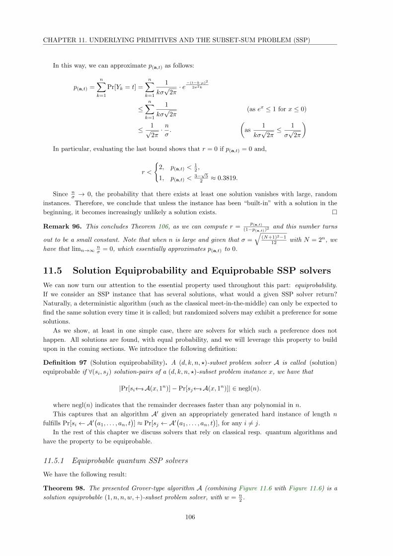
CHAPTER 11. UNDERLYING PRIMITIVES AND THE SUBSET-SUM PROBLEM (SSP)
In this way, we can approximate p(a,t) as follows:
p(a,t) =
n∑k=1
Pr[Yk = t] =
n∑k=1
1
kσ√
2π· e−(t−k·µ)2
2σ2k
≤n∑k=1
1
kσ√
2π(as ex ≤ 1 for x ≤ 0)
≤ 1√2π· nσ.
(as
1
kσ√
2π≤ 1
σ√
2π
)In particular, evaluating the last bound shows that r = 0 if p(a,t) = 0 and,
r <
2, p(a,t) <
12 ,
1, p(a,t) <3−√
52 ≈ 0.3819.
Since nσ → 0, the probability that there exists at least one solution vanishes with large, random
instances. Therefore, we conclude that unless the instance has been “built-in” with a solution in the
beginning, it becomes increasingly unlikely a solution exists.
Remark 96. This concludes Theorem 106, as we can compute r =p(a,t)
(1−p(a,t))2and this number turns
out to be a small constant. Note that when n is large and given that σ =√
(N+1)2−112 with N = 2n, we
have that limn→∞nσ = 0, which essentially approximates p(a,t) to 0.
11.5 Solution Equiprobability and Equiprobable SSP solvers
We can now turn our attention to the essential property used throughout this part: equiprobability.
If we consider an SSP instance that has several solutions, what would a given SSP solver return?
Naturally, a deterministic algorithm (such as the classical meet-in-the-middle) can only be expected to
find the same solution every time it is called; but randomized solvers may exhibit a preference for some
solutions.
As we show, at least in one simple case, there are solvers for which such a preference does not
happen. All solutions are found, with equal probability, and we will leverage this property to build
upon in the coming sections. We introduce the following definition:
Definition 97 (Solution equiprobability). A (d, k, n, ?)-subset problem solver A is called (solution)
equiprobable if ∀(si, sj) solution-pairs of a (d, k, n, ?)-subset problem instance x, we have that
|Pr[si←$A(x, 1n)]− Pr[sj←$A(x, 1n)]| ∈ negl(n).
where negl(n) indicates that the remainder decreases faster than any polynomial in n.
This captures that an algorithm A′ given an appropriately generated hard instance of length n
fulfills Pr[si ← A′(a1, . . . , an, t
)] ≈ Pr[sj ← A′
(a1, . . . , an, t
)], for any i 6= j.
In the rest of this chapter we discuss solvers that rely on classical resp. quantum algorithms and
have the property to be equiprobable.
11.5.1 Equiprobable quantum SSP solvers
We have the following result:
Theorem 98. The presented Grover-type algorithm A (combining Figure 11.6 with Figure 11.6) is a
solution equiprobable (1, n, n, w,+)-subset problem solver, with w = n2 .
106
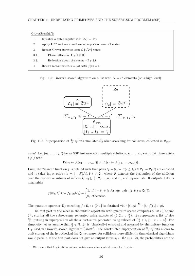
CHAPTER 11. UNDERLYING PRIMITIVES AND THE SUBSET-SUM PROBLEM (SSP)
GroverSearch(f):
1. Initialize a qubit register with |φ0〉 = |1n〉
2. Apply H⊗n to have a uniform superposition over all states
3. Repeat Grover iteration step O(√
2n)
times:
3.1. Phase reflection: Uf
(I⊗H
)3.2. Reflection about the mean: −I + 2A
4. Return measurement x = |φ〉 with f(x) = 1.
Fig. 11.5: Grover’s search algorithm on a list with N = 2n elements (on a high level).
L1|L1| = 3√2n
L2
|L2| =3√
22n
Lout
|Lout| = const
|I1 ∪ I2| = n2
∑i∈I1
ai = t t− t′ =∑i∈I2
ai
Fig. 11.6: Superposition of 2n3 qubits simulates L2 when searching for collisions, collected in Lout.
Proof. Let (a1, . . . , an, t) be an SSP instance with multiple solutions, s1, . . . , sr, such that there exists
i 6= j with:
Pr[si ← A(a1, . . . , an, t
)] 6= Pr[sj ← A
(a1, . . . , an, t
)].
First, the “search” function f is defined such that pairs `2 = (t1 = F (I1), I1) ∈ L1 := L1(t) are encoded
and it takes input pairs (t2 = t − F (I2), I2) ∈ L2, where F denotes the evaluation of the addition
over the respective subsets of indices I1, I2 ⊆ 1, 2, . . . , n and L1 and L2 are lists. It outputs 1 if t is
attainable:
f((t2, I2)) := fL1(t)(`2) =
1, if t = t1 + t2 for any pair (t1, I1) ∈ L1(t),
0, otherwise.
The quantum operator Uf encoding f : L2 7→ 0, 1 is obtained via 1 |`2, y〉Uf−−→ |t2, f(`2)⊕ y〉.
The first part in the meet-in-the-middle algorithm with quantum search computes a list L1 of size
2n3 , storing all the subset-sums generated using subsets of
1, 2, . . . , n3
. L2 represents a list of size
2n3 , putting in superposition all the subset-sums generated using subsets of
n3 + 1, n3 + 2, . . . , n
. For
simplicity, let us assume that n3 ∈ N. L1 is (classically) encoded and accessed by the unitary function
Uf used in Grover’s search algorithm [Gro96]. The constructed superposition of 2n3 qubits allows to
omit storage of the hypothetical list L2 yet search for collisions more efficiently than classical algorithms
would permit. If the first part does not give an output (thus si ← ∅∧ sj ← ∅), the probabilities are the
1We remark that Uf is still a unitary matrix even when multiple roots for f exists.
107

CHAPTER 11. UNDERLYING PRIMITIVES AND THE SUBSET-SUM PROBLEM (SSP)
same:
Pr[(si 6= ∅)← A
(a1, . . . , an, t
)]= Pr
[(sj 6= ∅)← A
(a1, . . . , an, t
)]= 0.
The second part consists of applying the Grover’s algorithm, as generally outlined in Figure 11.5. A
Grover iteration itself consists of two steps, applied to a large initial state:
1. Phase reflection: Let
|φ0〉 =1√2
2n3
(1n
3 +1, 1n3 +2, . . . , 1n)
=1
2n3
(1n
3 +1, 1n3 +2, . . . , 1n)
be the initial state, and the subscript indicate the position inside the state’s vector representation.
Let (i, j) be two indices such that f(xi) = f(xj) = 1 for i 6= j. Phase reflection will negate the
values in positions i and j in |φ0〉, thus obtaining
|φ1〉 =1
2n3
(1n
3 +1, 1n3 +2, . . . ,−1i, . . . ,−1j , . . . , 1n),
or for the general case, if the starting state is
|φ0〉 =1
2n3
(vn
3 +1, vn3 +2, . . . , vn),
we end up with
|φ1〉 =1
2n3
(vn
3 +1, vn3 +2, . . . ,−vi, . . . ,−vj , . . . , vn).
2. Reflection about the mean rotates the state towards the target state: This step computes the
average a of the elements in |φ1〉, and applies a transform v → −v + 2a. Through induction, it
is possible to show that the values of both elements in position i and j will be the same in state
|φ2〉, since the starting state is the same. Thus vi = vj , which means that, if the input state is
|φ1〉 =1
2n3
(vn
3 +1, vn3 +2, . . . ,−vi, . . . ,−vj , . . . , vn).
after the reflection about the mean, we arrive at the state
|φ2〉 =1
2n3
(−vn
3 +1 + 2a,−vn3 +2 + 2a, . . . , vi + 2a, . . . , vj + 2a, . . . ,−vn + 2a
).
Again, through induction, one can easily see that after repeating the previous steps for√
22n3 = O(2
n3 )
times, the state |φ2〉 has the same values for the marked elements (in positions) i and j, since the original
state has the values vi and vj set to 1 — up to the normalization factor. Therefore, the probability
to measure the value corresponding to position i is the same as measuring the value corresponding to
position j identifying the algorithm as solution equiprobable solver.
At this point, conjecturally, it seems that the very nature of quantum SSP algorithms makes them
inherently equiprobable; at the very least we do not have an easy counterexample, which would support
the view that equiprobability is a rather natural property of such algorithms. Therefore, we conjecture
that another quantum SSP solver is equiprobable:
11.5.1.1 Equiprobability of the HGJ solver
Theorem 99. The Howgrave-Graham–Joux algorithm [HGJ10] is an equiprobability SSP-solver.
108
CHAPTER 11. UNDERLYING PRIMITIVES AND THE SUBSET-SUM PROBLEM (SSP)
Proof. Let (a1, . . . , an, t) be a (1, n, n, w,+)-subset problem instance with multiple solution index-sets
denoted J1, . . . , Jr, such that for i 6= j: Pr[Ji ← A(a1, . . . , an, t
)] 6= Pr[Jj ← A
(a1, . . . , an, t
)] holds.
The HGJ-algorithm computes sets Sijk, for each (i, j, k) ∈ 1, 2 × 1, 2 × 1, 2, as a random
collection of exactly r weight- n16 subsets Iijk of Sijk, where r ≤(n/2n/16
), where M,M1, Ii, Iij are random
and M 6= M1. The computation result in the following lists:
1. For each i, j, Lij1 = (∑(Iij1) mod M1, Iij1) : Iij1 ∈ Sij1;
2. For each i, j, Lij2 = (Jij −∑
(Iij2) mod M1, Iij2) : Iij2 ∈ Sij2;
3. For each i, j, Sij of Iij1∪Iij2 for all pairs (Iij1, Iij2) ∈ Sij1×Sij2 such that∑
(Iij1) ≡ Jij−∑
(Iij2)
mod M1;
4. For each i, Li1 = ∑(Ii1) mod M, Ii1) : Ii1 ∈ Si1;
5. For each i, Li2 = (Ji −∑
(Ii2) mod M, Ii2) : Ii2 ∈ Si2;
6. For each i, Si of Ii1∪Ii2 for all pairs (Ii1, Ii2) ∈ Si1×Si2 such that∑
(Ii1) ≡ Ji−∑
(Ii2) mod M
and Ii1 ∩ Ii2 = ;
7. L1 = ∑(I1), I1) : I1 ∈ S1;
8. L2 = (t−∑(I2), I2) : I2 ∈ S2;
9. S of I1 ∪ I2 for all pairs (I1, I2) ∈ S1 × S2 such that∑
(I1) = t−∑(I2) and I1 ∩ I2 = .
We need to show that the algorithm gives a equal probability of the solutions:
Since M1 is choose uniformly at random we are having the same probability of finding a solution.
In [HGJ10], the authors assume that σM values correspond the many solutions well-distributed modulo
M and since we are choosing the moduli at random in a uniform distribution of I1 ∪ I2 we will have
Pr[Ji ← A(a1, . . . , an, t
)] = Pr[Jj ← A
(a1, . . . , an, t
)].
11.5.1.2 Equiprobability of the Helm-May solver
Theorem 100. The Helm-May algorithm [HM18] is an equiprobability SSP-solver.
Proof. In [HM18], Helm and May tackle the problem with quantum walks combined with the algorithmic
techniques presented in [BCJ11].
Let (a1, . . . , an, t) be an SSP instance with multiple solution index sets denoted J1, . . . , Jr. Because
of an initial permutation, that provides equiprobability in each node of the Johnson graph, connecting
nodes that differ by 1 element, e. g. in the example of Figure 11.7, where BCJ is performed.
Each node in the product of Johnson graphs is selected uniformly at random over all nodes, so for
any i 6= j:
Pr[Ji ← A(a1, . . . , an, t
)] = Pr[Jj ← A
(a1, . . . , an, t
)].
As we presented in the proof of Lemma 98, the measuring of a state that represents a marked vertex,
i. e. a solution Ji or Jj is equal for the algorithm, identifying it is an equiprobable solver.
11.5.2 Equiprobable classical solvers
The case of classical algorithms is not as clear cut. Of course, classical SSP solvers that are deterministic
cannot be equiprobable.
We might turn however a deterministic solver into a randomized one, e. g. by initially randomly
shuffling the input, which does not change the solutions if reverted as a last step, and other techniques.
109

CHAPTER 11. UNDERLYING PRIMITIVES AND THE SUBSET-SUM PROBLEM (SSP)
(1,2)
(1,3)
(1,4)(1,5)
(2,3)
(2,4)
(2,5)
(3,4) (3,5)
(4,5)
Fig. 11.7: Example of a Johnson graph, here J(5, 2), as used in Theorem 100.
Definition 101 (Randomized LLL Subset-Sum Solver). Consider a (1, n, n,+)-subset problem instance
given by A = (a1, a2, . . . , an), having D < 0.9408. . . density. The randomized Lenstra–Lenstra–
Lovasz [LLL82] solver performs an initial permutation of the indices of A from which affects the in-
stantiation of the basis matrix for LLL.
In this section, we require a refined definition, and identify the solution set I ⊆ [n] with a binary,
length n-vector x:
Definition 102 ((d, k, n, w,+)-subset problem). The notation of a (d, k, n, w,+)-subset problem in-
stance extends Item 1 of the conditions and specifies the weight wt(x) = |I| = ∑i xi of a solution vector
x.
Definition 103 (Randomized LLL SSP Solver). Let (a, t) denote a hard (1, n, n, w,+)-subset problem
instance, where w := n2 holds for a binary solution vector x, having low-density D < 0.9408. . . , and
let LLL for short, denote the well-known Lenstra-Lenstra Lovasz [LLL82] algorithm. A randomized LLL
solver performs an initial permutation of the indices of a = (a1, a2, . . . , an), which directly affects the
basis matrix B.
Theorem 104. The randomized LLL variant is an equiprobable (1, k, n, w,+)-subset problem solver.
To proof this statement, we are following a line of work of Schnorr et al. [SE94a], take the follow-
ing approach to prove equiprobability of finding solutions of the randomized LLL solver defined as in
Definition 101.
Equivalence of solving the SSP and the associated SVP instance
Starting with the given (1, k, n, w,+)-subset problem instance, a lattice L, resulting from the basis,
as defined in (11.5), is crafted, and we solve it by LLL– or more generally β–BKZ–reducing the matrix
B ∈ Z(n+1)×(n+2) in order to extract a short vector.
Starting with the given (d, k, n, w,+)-subset problem instance, we remark that finding the shortest
non-zero vector in L is equivalent to solving SVP in the lattice defined as intersection of lattices each
embedding one instance L1 ∩ L2 ∩ · · · ∩ Lk [PZ16].
We define a tweak τ ≥ √n for B, a uniformly generated instance of weight wt(x) =∑i xi = n
2 =: w,
which forms an embedding into the lattice basis of L := L(B) by setting
110

CHAPTER 11. UNDERLYING PRIMITIVES AND THE SUBSET-SUM PROBLEM (SSP)
B := Bτ (a, t, w) =
bT0
bT1...
bTn
=
1 1 . . . 1 τw τt
τ τa1
τ τa2
In...
...
τ τan
. (11.5)
Theorem 105 (Casting low-density instances as SVP). Finding a short vector b ∈ Zn+2 in the lattice
L := L(B) solves any given, low-density (d, k, n, w,+)-subset problem instance, if the following hold:
1. b ∈ L,
2. ||b|| is small, e. g. the vector is short
3. |b1| = |b2| = · · · = |bn| = 1,
4. bn+1 = bn+2 = 0.
Proof. Suppose a vector b = (b1, b2, . . . , bn, bn+1, bn+2) ∈ Zn+2, returned by the randomized LLL solver
from Definition 101 satisfies the 4 constraints.
Then it immediately gives a valid solution x to the associated SSP, when simply computing x :=
(x1, x2, . . . , xn) as xi := g−1(bi) = |bi−1|2 ∈ 0, 1 for 1 ≤ i ≤ n, which is guaranteed by (condition 3).
Here, g is a simple affine transform over the reals g(x) = 2x − 1 with inverse g−1(x) = (x + 1)/2.
First of all,∑i xi = w ⇔ bn+1 = 0 holds for the penultimate column of B (cf.conditions 1, 4), and
secondly the last column enforces∑i aixi = t as this is equivalent to bn+2 = 0 (cf.conditions 1, 4).
Point 2 and the lower bound on the tweak τ make the LLL algorithm output a reasonably-short non-zero
vector in polynomial time.
On the other hand, suppose a vector x ∈ 0, 1n ⊆ Zn is a solution of (a, t, w), the given
(d, n, n, w,+)-subset problem instance. In particular, x satisfies∑i aixi = t because of the last column
and wt(x) =∑i xi = w as column n+ 1 ensures hence satisfying condition 4. It also corresponds to a
lattice vector, easily seen as specific coefficient vector c,
(c0, c1, c2, . . . , cn) ·B := (−1, x1, x2, . . . , xn) ·B = (b1, b2, . . . , bn+2) = b,
satisfying condition 1. Furthermore, the first n positions are bi ∈ −1, 0, thus condition 3 is fulfilled
and finally 2 holds as b is indeed short.
This shows the equivalence of efficiently solving the SSP and finding the SV in the constructed
lattice L which is guaranteed to happen in polynomial time as D <0.9408. . . and by construction.
Details on randomizing the solver
The reduction above works with the classical LLL algorithm, to obtain an equiprobable solver based on
the randomized LLL, three small modifications need to be taken into account randomized the algorithm:
1. Perform and remember an initial permutation P of the indices of a = (a1, a2, . . . , an) and construct
the basis matrix and initialize BP := P · Bτ (a, t, w) to embed the SSP instance in a lattice. If
there exists more than one solution x, by permuting the basis matrix in an initial step, none of
them is favored by the β–BKZ-algorithm internals, keeping in mind that LLL is β–BKZ with β = 2.
111

CHAPTER 11. UNDERLYING PRIMITIVES AND THE SUBSET-SUM PROBLEM (SSP)
2. Fully β–BKZ-reduce BP (cf. Equation (11.5)) using the presented Definition 101.
3. The first row vector is a desired solution to the (1, n, n, w,+)-subset problem instance.
During the call, the SVP oracle subroutine finds the shortest vector of the respective β basis’ row
indices by enumeration of all possibilities (i. e. by exhaustively searching the shortest vector in a low-
dimensional sub-lattice), selects the one with smallest norm, and inserts it into the updated matrix.
This is done for consecutive blocks of size β. When random subsets of size β, of the remaining index
list are taken, the work-load hence the run-time does not increase. The algorithm is merely projecting
on sub-spaces as it proceeds identifying short vectors in the lattice. A short vector is found, without
algorithmically biased preferred choice, if this approach is combined with randomly choosing the sign,
so one of the two equally-short vectors, ‖b1‖ = ‖ − b1‖, is chosen in the end.
For a given low-density instance with density as high as D < 0.9408. . . , the presented solver from
Theorem 104 is a polynomial time algorithm, in the number of elements n.
11.6 Multidimensional subset-sum problem (MSSP)
We are now equipped to discuss the case of the multidimensional SSP. The general case is tackled by
reducing it to the one dimensional SSP, for which it suffices to show that increasing the dimension only
causes a polynomial factor to appear in the complexity analysis.
When given access to an equiprobable SSP solver, the reduction is particularly simple to describe.
Theorem 106 (MSSP ≤Cook SSP). Let MSSP denote an instance of the (d, n, n,+)-subset problem
with a promised solution I. Let OSSP be a solution equiprobable (1, n, n,+)-subset problem solver. As-
suming at least a solution, there exists a ppt algorithm A that solves MSSP querying OSSP a polynomial
number of times qualifying A as a ppt MSSP solver.
Proof. The main observation is that any solution I for MSSP is a solution to the (1, n, n,+)-subset problem
SSP` defined by bT` and t`. Thus, if SSP` has no solution, for any i, then we are certain that MSSP has
no solution. However, SSP` may have several solutions, even if MSSP has only one. These observations
lead to the algorithm detailed in Figure 11.8.
It remains to show that A terminates in polynomial time, and makes polynomially-many requests
to OSSP. First observe that if OSSP(bT` , t`) fails on any ` (no solutions), then A terminates by returning
∅ in O (1) steps in the worst case.
We turn to the case where the solution returned by OSSP(bT` , t`) is valid, but it does not satisfy the
MSSP constraint, i.e. the loop fails at some row index `. Let I` = (I1, I2, . . . , Ir) be the set of solutions
to SSP`. Since OSSP is solution equiprobable, it picks uniformly at random one solution Ik from I`.Thus in the worst case, we try O (r) calls to the oracle, and perform O (r) operations. We prove in
Theorem 95 that r is small if the distributions of elements is uniform.
The general case can be specialized in two ways. The first is to consider low-density instances; the
other is to consider sparse instances. The low-density case has already been discussed and can be dealt
with the algorithm of Pan and Zhang [PZ16], using a concrete lattice reduction algorithm such as LLL
as an SVP oracle. However, the sparse instances have not been previously identified as a potentially
interesting family; as we show, the situation k < n lends itself to several improvements that allows for
much faster algorithms.
A first step will be to turn the problem instance into a reduced BBDF form, with blocks A1, . . . ,As
(which may have different dimensions). Then, for each block(Ai,Ri
), we can tackle the k-MSSP
independently.
112

CHAPTER 11. UNDERLYING PRIMITIVES AND THE SUBSET-SUM PROBLEM (SSP)
Algorithm A((b1,b2 . . . ,bd), t,OSSP
):
1. `←$ 1, . . . , d
2. I←$OSSP(bT` , t`)
3. if I = ∅ then return ∅
4. for each row k ∈ 1, 2, . . . , d:
5. t←∑j∈I bk,j
6. If t 6= tk then goto 2 at most O(r) times.
7. return I
Fig. 11.8: A (d, n, n,+)-subset problem solver.
11.6.1 Reducing SSP instances
Consider a d-dimensional SSP instance, with defining matrix A = (a1, . . . ,an). In this section we recall
that transforming A into¡ bordered block form is a special case of the hypergraph partitioning problem:
Definition 107 (Hypergraph Partitioning). Given a hypergraph H = (V,N ), where V is the set of
vertices and N is the set of hyper-edges (or nets) and an overall load imbalance tolerance c such that
c ≥ 1.0, the goal is to partition the set V into ` disjoint subsets, V1, . . . ,V` such that the number of
vertices in each set Vi is bounded by |V|/(c · `) ≤ |Vi| ≤ c · |V|/`, and a function defined over the
hyper-edges is optimized.
The hypergraph partitioning problem, while being hard in general (it is naturallyNP-complete), can
be efficiently approximated on sparse matrices when the number ` of partitions is small. Furthermore,
modern algorithms can leverage the ability of several processors to speed up computation: a parallel
multilevel partitioning algorithm presented in [TK06] has an asymptotic parallel run-time of O (n/p) +
O(p · `2 · log n
), where p is the number of processors.
In the following, we show the conversion into the bordered block diagonal form and will assume,
without loss of generality, that the matrix A defining the (d, k, n,+)-subset problem instance is given
in reduced BBDF.
11.6.2 Conversion into bordered block diagonal form (BBDF)
We detail how to use hypergraph partitioning techniques to turn the defining matrix into a bordered
block diagonal form (BBDF). Note that each block in the matrix can be dealt with independently. If a
(d, k, n,+)-subset problem instance cannot be further decomposed into smaller independent instances,
we say that it forms a single block.
Tewarson [Tew67] shows a transform that extracts the block diagonal form from a sparse, non-
singular matrix A. Aykanat, Pinar and Catalyurek [APC04], show how to use hypergraph techniques
in order to convert any rectangular sparse matrix into a BBDF, a result we use. Concretely, given a
sparse matrix A, matrices P ,Q are constructed such that the resulting matrix is BBDF.
Theorem 108 (Aykanat et al. [APC04]). Let HA = (V,N ) be the hypergraph representation of a given
matrix A. An `-way partition ΠHP = V1, . . . , V` = N1, . . . , N`, NS of HA gives a permutation of
A to an `-way BBDF form, where nodes in Vi, resp. internal nets in Ni, constitute the columns and
113

CHAPTER 11. UNDERLYING PRIMITIVES AND THE SUBSET-SUM PROBLEM (SSP)
rows of the `-th diagonal block of ABBDF , resp. external nets in NS constitute the coupling rows of
ABBDF . Thus,
• minimizing the cutsize minimizes the number of coupling rows;
• balance among subhypergraphs infer balance among diagonal submatrices
We sketch the algorithmic approach described in [APC04]. The natural idea is to use hypergraph
partitioning to generate the blocks. A net ni is created for each row in A, while a vertex vj is set for
each column. Net ni will link the vertices (columns) having non-zero entries in row i. The connectivity
λi is defined as the number of partitions the net connects (all internal nets connecting vertices inside
a single partition have connectivity λ set to 1). Then a hypergraph partitioning is applied and the
matrix is reconstructed in a new form: the columns belonging to a partition Ui placed adjacently, while
the rows are indicated by the nets in the partition. The cost function that is used for the partition is
denoted by the connectivity coefficient of a net component — denoted λi (representing the number of
vertices connected by that net). Thus the cost function is simply set to cost(ΠA) :=∑
(λi − 1) .
Remark 109. In the context of matrix multiplication, the purpose is to minimize the number of par-
titions. However, in our case, under the hypothesis that each partition defines an MSSP with few
solutions, we would benefit from a larger number of partitions, since we would feed the OSSP solver with
a version of the problem as described below.
11.6.3 Solving k-MSSP for one BBDF–reduced block
Henceforth we shall consider a single reduced block of size n, dimension d, and sparsity k. Note that
after reduction, the sparsity coefficient k of the block is not the same as the original problem’s (this is
naturally also true of n and d).
One of the key features of having a reduced instance is that it lends itself to the following: by
summing up all the rows, we get a reduced (1, n, n,+) instance, which we call S. The key point is to
observe that a solution to the original problem is also a solution to S. Thus, we leverage a solution
equiprobable solver and use the following result:
Lemma 110 (Shadow casting). Consider a (d, k, n,+)-subset problem instance, defined by the matrix
B and target ~t. Let a′ be the vector obtained as follows:
a′j =
d∑i=1
Bi,j , ∀j ∈ [n] .
Then a solution to the problem defined by (A,~t) is a fortiori a solution to the (one dimensional) problem
defined by (A′, t′) = ((a′1,a′2, . . . ,a
′n), t1 + t2 + · · ·+ td)
Remark 111. We remark that there may be solutions to the shadow of a SSP instance that are not
a solution to the original MSSP problem. These inconsistent solutions are related yet not always help,
but if we assume access to an equiprobable solver OSSP, one can simply call OSSP a few times until the
correct answer is found for the original problem.
Also, by design, the shadow of a reduced instance does not contain any zero. It is thus indeed a
(1, n, n,+)-subset problem. Lemma 110 is not sufficient to decrease the SSP problem’s density as in the
shadow of an instance the maximal element may only be larger, not smaller, than before shadow–casting.
11.6.4 Assembling the blocks
Once every block has been solved, possibly in parallel, it is straightforward to reassemble a solution to
the original problem. As a result, the worst case complexity for the complete algorithm — which takes
114

CHAPTER 11. UNDERLYING PRIMITIVES AND THE SUBSET-SUM PROBLEM (SSP)
an unreduced d · n SSP matrix as input, and returns a solution if it exists — can be analyzed:
Theorem 112. An instance of the (d, k, n,+)-Subset Problem problem can be solved in time O(r` · 2`·e + h
)using an equiprobable SSP solver OSSP and a hypergraph partitioning solver OHP running in time O (h).
Here, r stands for the maximal number of solutions in a block SSP instance, while ` stands for the width
of the largest block returned by OHP.
Proof. There are two problematic points: one has to deal with the “false positives” resulting from
shadow casting (which is done by repeating the algorithm O(r) times), and one has to check that the
residual rows, denoted as Ri in the BBDF, are taken into correctly compensated by the solution. This
translates to the fact that if (I1, . . . , I`) does not represent a solution set for (R1‖ . . . ‖R`), one may
need to obtain a new set of solutions and check it (or store the current ones and check each new Ii).
Note that while it is possible, for low-density blocks, to use efficient techniques leveraging SVP
oracles, we require that such oracles be equiprobable for the above result to apply.
Lemma 113. Let O be an SSP oracle that is equiprobable according to Definition 97 running in time
O (2n·e), for some positive sub-unitary constant e. The algorithm depicted in Figure 11.9 solving a
k-MSSP instance of dimension d in time at most O(d · 2n·e/k
).
Proof. In our proof, we use the following simplifying assumptions, and present our algorithm in Fig-
ure 11.9.
1. First, without loss of generality, we make the simplifying assumption that no columns in (11.6)
contain only 0 entries. If this is the case, we can simply eliminate such columns from the matrix.
2. Find δ ≤ d rows such that they overlap (see worst-case depicted in Equation (11.6)) and produce
an SSP instance with n nonzero entries, say A = (a1,a2, . . . ,aδ), i. e.∑δi=1 Ai,j 6= 0, ∀j ∈ [n].
3. Solve the SSP, independently defined by the integers in each of the δ rows. Using the currently
fastest algorithm, this can be done in O(2δ·0.226...
)time [HM18].
4. Produce the solution for the k-MSSP, from the set of solutions obtained for each of the δ rows.
A more compact representation of the k-MSSP problem is allowed by the notation introduced in Def-
inition 83 which considers each row as an independent SSP problem denoted ai,∀i ∈ [d]. We write
ki := size(ai) for the number of non-zero entries in ai to quantify sparsity. We make the simplifying
assumption that the matrix representation does not encompass all-zero columns - one can simply re-
move such columns. Also, we point out that the probability to have less than k elements set to 0 is
negligible under the condition that the elements are sampled uniformly. The core idea can be expressed
as a loop over the rows a1, . . .ad, performing: (1) a selection of the minimally-sized ai (once row
i has been selected, it is marked as being visited); (2) obtaining a solution for SSP problem defined
by ai; (3) obtaining an equivalent k-MSSP problem of dimension d − 1 by removing ai and updating
accordingly the target sums. Visually, this last step can be seen in the left side of Figure 11.9.
Correctness. We prove that if the k-MSSP has a solution, the algorithm in Figure 11.9 finds it with
overwhelming probability.
We give an analysis of the algorithm, initialized with the matrix corresponding to the sparse k-MSSP
instance. We perform an iterative search over the columns in A, by selecting a row aj such that the
number of non-zeros entries in such a row is minimized. In case the SSP oracle returns a solution Ij ,
we apply row and column eliminations on the matrix with respect to row i, and continue. However,
if at some latter iteration, no solution Ij is found, we return by backtracking. Thus, we implicitly use
115

CHAPTER 11. UNDERLYING PRIMITIVES AND THE SUBSET-SUM PROBLEM (SSP)
k-MSSP–Solver(A, t):
(A, t) =
a1
. . .
ad
, t =
a1,1 a1,2 . . . , a1,n t1
a2,1 a2,2 . . . , a2,n t2
. . . . . . . . . . . .
ad,1 ad,2 . . . , ad,n td
1. Forall j ∈ [d] times:
2. i←$ 1, . . . , d : ki = size(ai) ≤ kj = size(aj), ∀j ∈ [n]
3. Ij←$OSSP(ai, ti)
4. If Ij = ∅ Then backtrack
5. Forall k ∈ Ij :
5.1. Update (A, t)←
a1,1 a1,2 . . . , a1,i−1 a1,i+1 . . . a1,n t1 − a1,i
a2,1 a2,2 . . . , a2,i−1 a2,i+1 . . . a2,n t2 − a2,i
. . . . . . . . . . . . . . . . . . . . . . . .
ad,1 ad,2 . . . , ad,i−1 ad,i+1 . . . ad,n td − ad,i
6. Update (A, t)←
a1 t1...
...
ai−1 ti−1
ai+1 ti+1
......
ad td
, removing i-th row.
7. Return I1 ∪ · · · ∪ Id
Fig. 11.9: A heuristic for solving k-MSSP sparse instances given oracle access to an SSP solver O.
memory to store the previously solutions. The memory complexity is dominated by the one of the SSP
oracle OSSP, assuming that both n, d are constants.
Worst-case. Our statement makes no assumption about the distribution of the elements among the
entries in the sparse matrix. We only make an assumption about the distribution from which the values
of the elements are sampled. First, we show a worst-case scenario in Equation (11.6) and argue that
for such a case, we there is no solution that avoids solving all SSP problems for each row.
(a11, a12, . . . a1k, 0, 0, . . . 0, 0, 0, . . . 0
)(0, 0, . . . 0, a21, a22, . . . a1k, 0, 0, . . . 0
)...
......
......
......
......
......(
0, 0, . . . , 0 0, 0, . . . 0, ad1, ad2, . . . adk)
(11.6)
Remark 114 (Probabilistic analysis). We first assume that the quantum version of the algorithm will
return a solution with equal probability. Then, we assume the number of solutions for typical hard SSP
and MSSP instances is small (less than n [BJLM13]); formally: rSSP < n and rMSSP < n pointing out
that rSSPi ≤ ri,k-MSSP.
116

CHAPTER 11. UNDERLYING PRIMITIVES AND THE SUBSET-SUM PROBLEM (SSP)
The probability to find the right solution within one oracle query is therefore rSSPrMSSP
. Given a desired
probability p of success, there are on average⌈p · r1,k-MSSP
rSSP1
⌉·⌈p · r2,k-MSSP
rSSP2
⌉· . . . ·
⌈p · rl,k-MSSP
rSSPl
⌉evaluations of the SSP instance, assuming the solutions are equiprobable.
11.6.5 The subset-product problem (SPP)
As an example application of our previously developed techniques, we consider the subset product
problem. Until now we were discussing algorithms applicable only to (d, k, n, w, ?)-subset problem for
the additive operation, i. e. ? = +, whereas here we want to study algorithms for ? = ·, the multiplication
of integers, e. g. all selected integers are multiplied instead of being added.
It seems that little is known about the SPP although it is used in a multiplicative variant of the
Merkle-Hellman knapsack cryptosystem and the attacks by Odlyzko [Odl84]. The (1, n, n, ·)-subset problem
is a less prominent subset problem variant, however is used in the more recent knapsack-based cryptosys-
tem construction by Naccache-Stern [NS97] that relies on the assumption that solving given modular
multiplicative knapsack problem instances are hard. In any case, the SPP can be identified as being
weakly NP-complete as shown in Lemma 116, however in their construction the trapdoor can be
unlocked by the secret key transforming the instance into a ppt-solvable one. So far, no attack nor
a proof of security is known for the Naccache-Stern knapsack cryptosystem nor of its extensions to
polynomial rings, some of which are achieving semantic security CCA1, cf. Definition 19, Item 4.
Definition 115 (3-SAT problem). Given a finite set X of literals the 3-satisfiability problem asks for
determining the satisfiability assignment true, resp. false of a formula C in conjunctive normal form
where each clause Ci is limited to at most three literals.
Lemma 116 (3 − SAT ≤Karp SPP). The (1, n, n, ·)-subset problem is reducible to the 3-satisfiability
problem.
Proof. Given a setX = x1, x2 . . . , x` with ` := |X| appearing literals in a collection C = C1, C2, . . . , CNof its 3-element subsets. We define two ephemeral matrices by setting εi,j = 1, if Cj contains
xi, otherwise εi,j = 0, and εi,j = 1, if Cj contains ¬xi, else εi,j = 0. We remark that 1 ≤∑i εi,j ,
∑i εi,j ,
∑i εi,j + εi,j ≤ 3. Let p1 = 2, p2 = 3, . . . denote the first prime numbers, we now
define Pi := pN+i ·∏Nj=1 p
εi,jj , and P i := pN+i ·
∏Nj=1 p
εi,jj for all i ∈ 1, . . . , `. Pi, resp. P i uniquely
correspond to assigning the truth-value true, resp. false to every literal xi across all clauses. We have
a (1, n, n, ·)-subset problem, if we set n := 2(`+N), and
t :=∏i=1
pN+i ·N∏j=1
p3j , and a :=
(Pi, P i
i=1,2,...,`
,pj , p
2j
j=1,2,...,N
).
Assume I ⊆ [n] is a SPP solution, then exactly one assignment xi resp. ¬xi is true for all i, hence either
Pi, resp. P i divides t. This can be read from every k ∈ I, k ≤ 2`, by first setting k2 := k−12 , i := bk2c+1,
and setting xi := false if k2 ≡ 0 mod 2, else true. What remains is to argue that the transformation
steps are polynomial in the inputs. The first n primes can be generated in time O (n) (e. g. using the
sieve of Eratosthenes) and fit into O(n2 lnn
)space by the prime number theorem as pn ≈ n log n.
To detail on why the SPP is only weakly NP-complete, we emphasize that the target product is
exponential in n and in a strong reduction the input t would remain bounded by a polynomial in n
from a NP-complete problem such as 3-SAT is impossible unless P = NP.
117

CHAPTER 11. UNDERLYING PRIMITIVES AND THE SUBSET-SUM PROBLEM (SSP)
11.6.6 Multiplicatively reduced instances and smoothness basis
The starting point is to consider a (1, n, n, ·) instance, reduced in the appropriate sense:
Definition 117 (Multiplicatively reduced instance). A (1, n, n, ·)-subset problem instance defined by
the sequence a1, . . . , an and target t is multiplicatively reduced if, for all i ∈ [n], gcd(ai, t) 6= 1.
It is immediate that a multiplicatively reduced instance is reduced (in the sense of Definition 90).
Henceforth we will assume without loss of generality that we have a multiplicatively reduced instance.
We then use the following notion:
Definition 118 (Smoothness basis). Let a1, . . . , an; t be a multiplicatively reduced (1, n, n, ·)-subset
problem instance; its smoothness basis is the set
B(a, t) = gcd(ai, t) | i ∈ [n] ∪ gcd(ai, aj) | i < j ∈ [n] .
Computing B(a, t) can be done naively in time O(n2)
using the Euclidean or Lehmer algorithm.
Also note that B(a, t) can be computed by distributing the task to independent computers working in
parallel. Finally, we insist that B(a, t) needs not be composed only of prime numbers.
If one knows the prime factors composing every numbers a1, . . . , an and t, then the set of these
factors can be used as a smoothness basis instead of B(a, t).2
11.6.7 Transforming an SPP instance into a k-MSSP instance
The key idea is that a multiplicatively reduced (1, n, n, ·)-subset problem instance can be transformed
into an equivalent (d, k, n,+)-subset problem instance, which then can be addressed by repeating the
method of solving one BBDF–reduced k-MSSP block at a time (c.f. Section 11.6.3).
In this context, it is often convenient to write this as an infinite product over all the primes, where
all but a finite number have a zero exponent. We define the the multiplicity νpi(ai) as the exponent of
the highest power of the prime pi that divides ai. After a decomposition of a composite number into a
product of smaller integers.
Using the fundamental theorem of arithmetic, that every non-negative integer has a unique repre-
sentation as an infinite product of prime powers, with finitely many associated non-zero exponents we
have: ai,j = νpi(ai), ai =∏p p
νp(n), 1 ≤ j ≤ d.
Lemma 119. Let B(a, t) = p1, . . . , pd, and ai,j be the multiplicity of pi as a divisor of ai. Similarly,
let tj be the multiplicity of pi as divisor of t. Then A = a1,a2, . . . ,an and t form a k-MSSP instance,
with vectors ai = ai,j1≤j≤d, t = tj1≤j≤d.A subset I ⊆ [n] is a solution to the k-MSSP instance iff it is a solution to the SPP instance.
This is illustrated in Figure 11.10. In order to give a sharp analysis, one has to investigate two
important metrics for this problem: the dimension d of the new MSSP instance, and its sparsity k.
Precisely, d ≤ n(n + 1)/2 is the number of distinct elements in the smoothness basis, and k is the
maximal number of factors for a number ai; an upper bound is given by considering the largest number
M in a1, . . . , an, and the average order ω(M) ∼ ln lnM [HR17,Har59].
Theorem 120. Any instance of the (d, k, n, ·)-subset problem can be solved in time O(r` · 2`·e + h
)using an equiprobable SSP solver OSSP and a hypergraph partitioning solver OHP running in time
O (h). Here r stands for the maximal number of solutions of an SSP instance queried in Figure 11.9
while ` stands for the width of largest block returned by OHP.
2Such may be the case in a quantum setting, using Shor’s algorithm. For large values of n this may be advantageousover computing B(a, t).
118
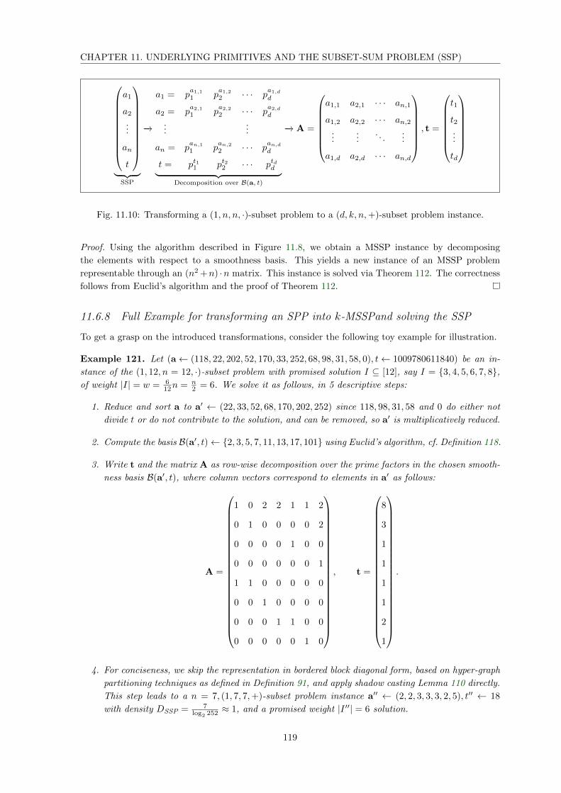
CHAPTER 11. UNDERLYING PRIMITIVES AND THE SUBSET-SUM PROBLEM (SSP)
a1
a2
...
an
t
︸ ︷︷ ︸
SSP
−→
a1 = pa1,11 p
a1,22 · · · p
a1,dd
a2 = pa2,11 p
a2,22 · · · p
a2,dd
......
an = pan,11 p
an,22 · · · p
an,dd
t = pt11 pt22 · · · ptdd︸ ︷︷ ︸Decomposition over B(a, t)
−→ A =
a1,1 a2,1 · · · an,1
a1,2 a2,2 · · · an,2...
.... . .
...
a1,d a2,d · · · an,d
, t =
t1
t2...
td
Fig. 11.10: Transforming a (1, n, n, ·)-subset problem to a (d, k, n,+)-subset problem instance.
Proof. Using the algorithm described in Figure 11.8, we obtain a MSSP instance by decomposing
the elements with respect to a smoothness basis. This yields a new instance of an MSSP problem
representable through an (n2 +n) ·n matrix. This instance is solved via Theorem 112. The correctness
follows from Euclid’s algorithm and the proof of Theorem 112.
11.6.8 Full Example for transforming an SPP into k-MSSPand solving the SSP
To get a grasp on the introduced transformations, consider the following toy example for illustration.
Example 121. Let (a← (118, 22, 202, 52, 170, 33, 252, 68, 98, 31, 58, 0), t← 1009780611840) be an in-
stance of the (1, 12, n = 12, ·)-subset problem with promised solution I ⊆ [12], say I = 3, 4, 5, 6, 7, 8,of weight |I| = w = 6
12n = n2 = 6. We solve it as follows, in 5 descriptive steps:
1. Reduce and sort a to a′ ← (22, 33, 52, 68, 170, 202, 252) since 118, 98, 31, 58 and 0 do either not
divide t or do not contribute to the solution, and can be removed, so a′ is multiplicatively reduced.
2. Compute the basis B(a′, t)← 2, 3, 5, 7, 11, 13, 17, 101 using Euclid’s algorithm, cf. Definition 118.
3. Write t and the matrix A as row-wise decomposition over the prime factors in the chosen smooth-
ness basis B(a′, t), where column vectors correspond to elements in a′ as follows:
A =
1 0 2 2 1 1 2
0 1 0 0 0 0 2
0 0 0 0 1 0 0
0 0 0 0 0 0 1
1 1 0 0 0 0 0
0 0 1 0 0 0 0
0 0 0 1 1 0 0
0 0 0 0 0 1 0
, t =
8
3
1
1
1
1
2
1
.
4. For conciseness, we skip the representation in bordered block diagonal form, based on hyper-graph
partitioning techniques as defined in Definition 91, and apply shadow casting Lemma 110 directly.
This step leads to a n = 7, (1, 7, 7,+)-subset problem instance a′′ ← (2, 2, 3, 3, 3, 2, 5), t′′ ← 18
with density DSSP = 7log2 252 ≈ 1, and a promised weight |I ′′| = 6 solution.
119

CHAPTER 11. UNDERLYING PRIMITIVES AND THE SUBSET-SUM PROBLEM (SSP)
5. This particular problem has(
32
)= 3 solutions, as there is one surplus element 2 in a′′, e. g.
(2, 2, 3, 3, 3, 2, 5), evaluating to (2+2)+3+3+3+5 = 18. By Lemma 110, one of these solutions is
a solution to the original problem. Using an equiprobable solver we hit the promised, hence correct,
solution with probability 13 ; or equivalently, we run the equiprobable SSP solver 3 times on aver-
age before successfully finding the sought-after subset I ′′ = 2, 3, . . . , 7 that easily translates to the
above I = 3, 4, 5, 6, 7, 8, relating to elements in a = (118, 22, 202, 52, 170, 33, 252, 68, 98, 31, 58, 0).
11.6.9 The Modular SPP Assumption
The cryptosystem by Naccache and Stern in [NS97] proposes an interesting cryptographic intractability
assumption based on the modular SPP problem, a variant of the group representation problem.
Definition 122 (Group Representation Problem). Let G be a group of prime order p. Given n + 1
group elements (a1, a2, . . . , an, t) ∈ Gn+1, find (x1, x2 . . . xn) ∈ Gn such that
gk11 · . . . · gknn = t ∈ G.
The security assumption underlying Naccache-Stern’s construction depends on a large prime p and
n chosen such that Pn < p, where Pn := pn# is the n-th primorial number, i. e. product of the first n
primes. Let s←$Zp and set vi ← s√pi, where pi is the i-th prime, i < n. This assumption states that it
is hard to find a string x ∈ 0, 1n such that∏ni=1 v
xii = t. This leads to investigate the modular SPP,
where each vi is sampled uniformly at random.
Definition 123 (Modular SPP). Let G be a group of order p. We limit our consideration the case
where p is prime. Given a1, a2, . . . , an, t ∈ G find (x1, x2 . . . xn) ∈ 0, 1n such that
n∏i=1
axii ≡ t mod p .
Remark 124. The modular SPP problem instance underlying Naccache-Stern’s construction can be
transformed such that it is sufficient to find the secret s with
n∏i=1
pxii ≡ ts mod p.
Lemma 125. The Modular SPP ≤Cook MSSP.
Proof. We tackle the modular SPP by choosing an appropriate basis (g1, g2, . . . , gn) and decomposing
each ai as ai = gki,11 · . . . · gki,nn . Analogously, we do the same with t and end up with an instance (A, t)
of the MSSP problem, cf. Figure 11.11.
Remark 126. In general the obtained matrix A is dense, i. e. is likely not sparse with k < n.
11.7 Conclusion and Open Problems
In this part we introduced new algorithms to solve variants of the subset-sum problem (SSP), in
particular multi-dimensional versions (MSSP) and the subset-product problem (SPP), a variant which
seems not to have undergone so much scrutiny. We studied the equiprobability property, important
to tackle sparse MSSPinstances, proved or endowed state-of-the-art SSP solvers with it. We advance
evidence that there exist classical and quantum SSP solvers which are equiprobable.
120

CHAPTER 11. UNDERLYING PRIMITIVES AND THE SUBSET-SUM PROBLEM (SSP)
Decomposition in G:
a1 = gk1,11,1 · . . . · g
kn,nn,n
a2 = gk1,21,2 · . . . · g
kn,nn,n
......
an = gk1,n1,n · . . . · g
kn,nn,n
t = gk1,t1,t · . . . · g
kn,tn,t
Conversion into a k-MSSP instance:
(a1 = (k1,1, k2,1, . . . , kn,1), t1 = k1,t)
(a2 = (k1,2, k2,2, . . . , kn,2), t2 = k2,t)...
......
......
...
(an = (k1,n, k2,n, . . . , kn,n), tn = kn,t)
Fig. 11.11: Modular SSP decomposition and conversion to k-MSSP over G.
We proposed as open problem, studying relations to other complexity theoretic problems to employ
the k-MSSP technique in order to improve existing time upper-bounds of generic solvers. For example,
the exact vertex cover problem is historically related with the SSP problem, being used in the proof of
its NP-completeness, so tackling the vertex cover problem of covering a graph G = (V,E) with |V | = n
nodes using only a subset of cardinality k. The current lower bound for the vertex cover problem is
due to the work of Chen et al. [CKX10] with time complexity O(1.2738k + kn
)which could be linked
to the sparse, multi-dimensional version k-MSSP problem as promising alley of research.
121


Bibliography
[AAB+15] Martın Abadi, Ashish Agarwal, Paul Barham, Eugene Brevdo, Zhifeng Chen, Craig Citro,
Greg S. Corrado, Andy Davis, Jeffrey Dean, Matthieu Devin, Sanjay Ghemawat, Ian
Goodfellow, Andrew Harp, Geoffrey Irving, Michael Isard, Yangqing Jia, Rafal Jozefowicz,
Lukasz Kaiser, Manjunath Kudlur, Josh Levenberg, Dan Mane, Rajat Monga, Sherry
Moore, Derek Murray, Chris Olah, Mike Schuster, Jonathon Shlens, Benoit Steiner, Ilya
Sutskever, Kunal Talwar, Paul Tucker, Vincent Vanhoucke, Vijay Vasudevan, Fernanda
Viegas, Oriol Vinyals, Pete Warden, Martin Wattenberg, Martin Wicke, Yuan Yu, and
Xiaoqiang Zheng. TensorFlow: Large-scale machine learning on heterogeneous systems,
2015. Software available from tensorflow.org. 64
[ABDP15] Michel Abdalla, Florian Bourse, Angelo De Caro, and David Pointcheval. Simple func-
tional encryption schemes for inner products. In Jonathan Katz, editor, PKC 2015,
volume 9020 of LNCS, pages 733–751, Gaithersburg, MD, USA, March 30 – April 1,
2015. Springer, Heidelberg, Germany. 65
[ACC+18] Martin Albrecht, Melissa Chase, Hao Chen, Jintai Ding, Shafi Goldwasser, Sergey Gor-
bunov, Shai Halevi, Jeffrey Hoffstein, Kim Laine, Kristin Lauter, Satya Lokam, Daniele
Micciancio, Dustin Moody, Travis Morrison, Amit Sahai, and Vinod Vaikuntanathan. Ho-
momorphic encryption security standard. Technical report, HomomorphicEncryption.org,
Toronto, Canada, November 2018. 47
[ADRS15] Divesh Aggarwal, Daniel Dadush, Oded Regev, and Noah Stephens-Davidowitz. Solv-
ing the shortest vector problem in 2n time using discrete Gaussian sampling: Extended
abstract. In Rocco A. Servedio and Ronitt Rubinfeld, editors, 47th ACM STOC, pages
733–742, Portland, OR, USA, June 14–17, 2015. ACM Press. 41
[AGKS05] Masayuki Abe, Rosario Gennaro, Kaoru Kurosawa, and Victor Shoup. Tag-KEM/DEM:
A New Framework for Hybrid Encryption and A New Analysis of Kurosawa-Desmedt
KEM. In EUROCRYPT, volume 3494 of LNCS, pages 128–146. Springer, 2005. 75
[ALS16] Shweta Agrawal, Benoıt Libert, and Damien Stehle. Fully secure functional encryption
for inner products, from standard assumptions. In Matthew Robshaw and Jonathan Katz,
editors, CRYPTO 2016, Part III, volume 9816 of LNCS, pages 333–362, Santa Barbara,
CA, USA, August 14–18, 2016. Springer, Heidelberg, Germany. 65
[And01] Ross J. Anderson. Why information security is hard-an economic perspective. In 17th An-
nual Computer Security Applications Conference (ACSAC 2001), 11-14 December 2001,
New Orleans, Louisiana, USA, pages 358–365. IEEE Computer Society, 2001. 35
[And14] Ross Anderson. Privacy versus government surveillance where network effects meet public
choice. In Proc. 13th Annual Workshop on the Economic of Information Security (WEIS
2014), 2014. 35
123

BIBLIOGRAPHY
[AP14] Jacob Alperin-Sheriff and Chris Peikert. Faster bootstrapping with polynomial error. In
Juan A. Garay and Rosario Gennaro, editors, CRYPTO 2014, Part I, volume 8616 of
LNCS, pages 297–314, Santa Barbara, CA, USA, August 17–21, 2014. Springer, Heidel-
berg, Germany. 46
[APC04] Cevdet Aykanat, Ali Pinar, and Umit V Catalyurek. Permuting sparse rectangular ma-
trices into block-diagonal form. SIAM Journal on Scientific Computing, 25(6):1860–1879,
2004. 113, 114
[APS15] Martin R. Albrecht, Rachel Player, and Sam Scott. On the concrete hardness of learning
with errors. J. Mathematical Cryptology, 9(3):169–203, 2015. 82, 84
[ARS+15] Martin R. Albrecht, Christian Rechberger, Thomas Schneider, Tyge Tiessen, and Michael
Zohner. Ciphers for MPC and FHE. In Elisabeth Oswald and Marc Fischlin, editors, EU-
ROCRYPT 2015, Part I, volume 9056 of LNCS, pages 430–454, Sofia, Bulgaria, April 26–
30, 2015. Springer, Heidelberg, Germany. 74
[AS00] Rakesh Agrawal and Ramakrishnan Srikant. Privacy-preserving data mining. SIGMOD
Rec., 29(2):439–450, May 2000. 37
[Bab85] Laszlo Babai. On Lovasz’ lattice reduction and the nearest lattice point problem (short-
ened version). In Proceedings of the 2Nd Symposium of Theoretical Aspects of Computer
Science, STACS ’85, pages 13–20, London, UK, 1985. Springer-Verlag. 42
[BBBV97] Charles H. Bennett, Ethan Bernstein, Gilles Brassard, and Umesh Vazirani. Strengths
and Weaknesses of Quantum Computing. SIAM J. Comput., 26(5):1510–1523, 1997.
http://dx.doi.org/10.1137/S0097539796300933, website accessed 2013-03-14. 28
[BCJ11] Anja Becker, Jean-Sebastien Coron, and Antoine Joux. Improved generic algorithms for
hard knapsacks. In Annual International Conference on the Theory and Applications of
Cryptographic Techniques, pages 364–385. Springer, 2011. 99, 100, 103, 104, 109
[BG14] Shi Bai and Steven D. Galbraith. Lattice decoding attacks on binary LWE. In Willy
Susilo and Yi Mu, editors, ACISP 14, volume 8544 of LNCS, pages 322–337, Wollongong,
NSW, Australia, July 7–9, 2014. Springer, Heidelberg, Germany. 83
[BGV12] Zvika Brakerski, Craig Gentry, and Vinod Vaikuntanathan. (Leveled) fully homomorphic
encryption without bootstrapping. In Shafi Goldwasser, editor, ITCS 2012, pages 309–
325, Cambridge, MA, USA, January 8–10, 2012. ACM. 46, 47, 50
[BJLM13] Daniel J. Bernstein, Stacey Jeffery, Tanja Lange, and Alexander Meurer. Quantum algo-
rithms for the subset-sum problem. In International Workshop on Post-Quantum Cryp-
tography, pages 16–33. Springer, 2013. 104, 116
[BLP+13] Zvika Brakerski, Adeline Langlois, Chris Peikert, Oded Regev, and Damien Stehle. Clas-
sical hardness of learning with errors. In Dan Boneh, Tim Roughgarden, and Joan Feigen-
baum, editors, 45th ACM STOC, pages 575–584, Palo Alto, CA, USA, June 1–4, 2013.
ACM Press. 44, 83
[BMMP18] Florian Bourse, Michele Minelli, Matthias Minihold, and Pascal Paillier. Fast homomor-
phic evaluation of deep discretized neural networks. pages 483–512, 2018. 3, 37, 49, 61,
71, 79, 87
124

BIBLIOGRAPHY
[BMR18] Gustavo Banegas, Matthias Minihold, and Razvan Rosie. Equiprobability: Faster Algo-
rithms for Subset-Sum Variants and the Vertex Cover Problem. AQIS 2018, 2018. http:
//www.ngc.is.ritsumei.ac.jp/~ger/static/AQIS18/OnlineBooklet/208.pdf. 3
[Bon99] Dan Boneh. Twenty years of attacks on the rsa cryptosystem. NOTICES OF THE AMS,
46:203–213, 1999. 31
[BPTG14] Raphael Bost, Raluca Ada Popa, Stephen Tu, and Shafi Goldwasser. Machine learning
classification over encrypted data. Cryptology ePrint Archive, Report 2014/331, 2014.
https://eprint.iacr.org/2014/331. 79
[Bur12] C. Sidney Burrus. Fast Fourier Transforms. OpenStax CNX, 2012. https://cnx.org/
contents/[email protected]. 68
[BV11a] Zvika Brakerski and Vinod Vaikuntanathan. Efficient fully homomorphic encryption from
(standard) LWE. In Rafail Ostrovsky, editor, 52nd FOCS, pages 97–106, Palm Springs,
CA, USA, October 22–25, 2011. IEEE Computer Society Press. 46
[BV11b] Zvika Brakerski and Vinod Vaikuntanathan. Fully homomorphic encryption from ring-
LWE and security for key dependent messages. In Phillip Rogaway, editor, CRYPTO 2011,
volume 6841 of LNCS, pages 505–524, Santa Barbara, CA, USA, August 14–18, 2011.
Springer, Heidelberg, Germany. 46
[BV14] Zvika Brakerski and Vinod Vaikuntanathan. Lattice-based FHE as secure as PKE. In
Moni Naor, editor, ITCS 2014, pages 1–12, Princeton, NJ, USA, January 12–14, 2014.
ACM. 46
[C+15] Francois Chollet et al. Keras. https://github.com/keras-team/keras, 2015. 64
[CB16] Matthieu Courbariaux and Yoshua Bengio. Binarynet: Training deep neural networks
with weights and activations constrained to +1 or -1. CoRR, abs/1602.02830, 2016. 50,
64
[CCF+16] Anne Canteaut, Sergiu Carpov, Caroline Fontaine, Tancrede Lepoint, Marıa Naya-
Plasencia, Pascal Paillier, and Renaud Sirdey. Stream ciphers: A practical solution for
efficient homomorphic-ciphertext compression. In Thomas Peyrin, editor, FSE 2016, vol-
ume 9783 of LNCS, pages 313–333, Bochum, Germany, March 20–23, 2016. Springer,
Heidelberg, Germany. 74
[CdWM+17] Herve Chabanne, Amaury de Wargny, Jonathan Milgram, Constance Morel, and Em-
manuel Prouff. Privacy-preserving classification on deep neural network. IACR Cryptology
ePrint Archive, 2017:35, 2017. 50
[CGGI16] Ilaria Chillotti, Nicolas Gama, Mariya Georgieva, and Malika Izabachene. Faster fully
homomorphic encryption: Bootstrapping in less than 0.1 seconds. In Jung Hee Cheon
and Tsuyoshi Takagi, editors, ASIACRYPT 2016, Part I, volume 10031 of LNCS, pages
3–33, Hanoi, Vietnam, December 4–8, 2016. Springer, Heidelberg, Germany. 50, 52, 61,
65, 66, 67, 83
[CGGI17] Ilaria Chillotti, Nicolas Gama, Mariya Georgieva, and Malika Izabachene. Faster packed
homomorphic operations and efficient circuit bootstrapping for TFHE. In Tsuyoshi Takagi
and Thomas Peyrin, editors, ASIACRYPT 2017, Part I, volume 10624 of LNCS, pages
377–408, Hong Kong, China, December 3–7, 2017. Springer, Heidelberg, Germany. 52,
53, 55, 77, 82
125
BIBLIOGRAPHY
[CHS+16] M. Courbariaux, I. Hubara, D. Soudry, R. El-Yaniv, and Y. Bengio. Binarized Neural
Networks: Training Deep Neural Networks with Weights and Activations Constrained to
+1 or -1. ArXiv e-prints, February 2016. 64
[CJL+92] Matthijs J. Coster, Antoine Joux, Brian A. LaMacchia, Andrew M. Odlyzko, Claus-Peter
Schnorr, and Jacques Stern. Improved low-density subset sum algorithms. Computational
Complexity, 2:111–128, 1992. 99, 100
[CKKS17] Jung Hee Cheon, Andrey Kim, Miran Kim, and Yong Soo Song. Homomorphic encryption
for arithmetic of approximate numbers. In Tsuyoshi Takagi and Thomas Peyrin, editors,
ASIACRYPT 2017, Part I, volume 10624 of LNCS, pages 409–437, Hong Kong, China,
December 3–7, 2017. Springer, Heidelberg, Germany. 47
[CKX10] Jianer Chen, Iyad A Kanj, and Ge Xia. Improved upper bounds for vertex cover. Theo-
retical Computer Science, 411(40-42):3736–3756, 2010. 121
[CMS12] D. Ciresan, U. Meier, and J. Schmidhuber. Multi-column Deep Neural Networks for Image
Classification. ArXiv e-prints, February 2012. 58
[CN11] Yuanmi Chen and Phong Q. Nguyen. BKZ 2.0: Better lattice security estimates. In
Dong Hoon Lee and Xiaoyun Wang, editors, Advances in Cryptology - ASIACRYPT
2011 - 17th International Conference on the Theory and Application of Cryptology and
Information Security, Seoul, South Korea, December 4-8, 2011. Proceedings, volume 7073
of Lecture Notes in Computer Science, pages 1–20. Springer, 2011. 99
[Cop93] Don Coppersmith. Modifications to the number field sieve. Journal of Cryptology,
6(3):169–180, March 1993. 29
[CR07] Camila CS Caiado and Pushpa N Rathie. Polynomial coefficients and distribution of the
sum of discrete uniform variables. In Eighth Annual Conference of the Society of Special
Functions and their Applications, 2007. 105
[CRF+09] Weng-Long Chang, Ting-Ting Ren, Mang Feng, Lai Chin Lu, Kawuu Weicheng Lin, and
Minyi Guo. Quantum algorithms of the subset-sum problem on a quantum computer. In
2009 WASE International Conference on Information Engineering, 2009. 104
[CT15] Massimo Chenal and Qiang Tang. On Key Recovery Attacks Against Existing Somewhat
Homomorphic Encryption Schemes. In LATINCRYPT, volume 8895 of LNCS, pages
239–258. Springer, 2015. 75
[Cyb89] G. Cybenko. Approximation by superpositions of a sigmoidal function. Mathematics of
Control, Signals and Systems, 2(4):303–314, Dec 1989. 58
[Dar19] TU Darmstadt. LWE challenges. 2019. http://latticechallenge.org/svp-challenge.
80, 83
[Det18] Diabetic Retinopathy Detection. Identify signs of diabetic retinopathy in eye images.
2018. 61
[DGBL+16] Nathan Dowlin, Ran Gilad-Bachrach, Kim Laine, Kristin Lauter, Michael Naehrig, and
John Wernsing. Cryptonets: Applying neural networks to encrypted data with high
throughput and accuracy. Technical report, Microsoft Research Group, February 2016.
50, 88
126

BIBLIOGRAPHY
[DHS01] Richard O. Duda, Peter E. (Peter Elliot) Hart, and David G. Stork. Pattern classification.
Second edition, 2001. 78
[DLMW15] Itai Dinur, Yunwen Liu, Willi Meier, and Qingju Wang. Optimized interpolation attacks
on LowMC. In Tetsu Iwata and Jung Hee Cheon, editors, ASIACRYPT 2015, Part II, vol-
ume 9453 of LNCS, pages 535–560, Auckland, New Zealand, November 30 – December 3,
2015. Springer, Heidelberg, Germany. 74
[DPW19] Lo Ducas, Maxime Planon, and Benjamin Wesolowski. On the shortness of vectors to be
found by the ideal-svp quantum algorithm. Cryptology ePrint Archive, Report 2019/234,
2019. https://eprint.iacr.org/2019/234. 81
[dsp13] Kaggle data science projects. The cats vs dogs image recognition challenge. https:
//www.kaggle.com/c/dogs-vs-cats/data, 2013. 48
[Dwo06] Cynthia Dwork. Differential privacy (invited paper). In Michele Bugliesi, Bart Preneel,
Vladimiro Sassone, and Ingo Wegener, editors, ICALP 2006, Part II, volume 4052 of
LNCS, pages 1–12, Venice, Italy, July 10–14, 2006. Springer, Heidelberg, Germany. 37
[Ege14] Steffen Eger. Stirling’s approximation for central extended binomial coefficients. American
Mathematical Monthly, 121(4):344–349, 2014. 105
[FP05] Abraham D. Flaxman and Bartosz Przydatek. Solving medium-density subset sum prob-
lems in expected polynomial time. In Volker Diekert and Bruno Durand, editors, STACS
2005, pages 305–314, Berlin, Heidelberg, 2005. Springer Berlin Heidelberg. 99
[Fri99] Matteo Frigo. A fast Fourier transform compiler. In Proceedings of the ACM SIGPLAN
1999 Conference on Programming Language Design and Implementation, PLDI ’99, pages
169–180, New York, NY, USA, 1999. ACM. 68
[FV12] Junfeng Fan and Frederik Vercauteren. Somewhat Practical Fully Homomorphic Encryp-
tion. IACR Cryptology ePrint Archive, 2012:144, 2012. 47
[GBC16] Ian Goodfellow, Yoshua Bengio, and Aaron Courville. Deep Learning. MIT Press, 2016.
http://www.deeplearningbook.org. 56, 57, 60
[Gen09] Craig Gentry. A fully homomorphic encryption scheme. PhD thesis, Stanford University,
2009. crypto.stanford.edu/craig. 45, 46
[GHS12] Craig Gentry, Shai Halevi, and Nigel P. Smart. Homomorphic evaluation of the AES
circuit. In Reihaneh Safavi-Naini and Ran Canetti, editors, CRYPTO 2012, volume
7417 of LNCS, pages 850–867, Santa Barbara, CA, USA, August 19–23, 2012. Springer,
Heidelberg, Germany. 46, 74
[GMP+13] Glenn Greenwald, Ewen MacAskill, Laura Poitras, Spencer Ackerman, and Dominic
Rushe. Microsoft handed the NSA access to encrypted messages, 12 July 2013. 35
[GPV08] Craig Gentry, Chris Peikert, and Vinod Vaikuntanathan. Trapdoors for hard lattices and
new cryptographic constructions. In Richard E. Ladner and Cynthia Dwork, editors, 40th
ACM STOC, pages 197–206, Victoria, BC, Canada, May 17–20, 2008. ACM Press. 42
[Gro96] Lov K. Grover. A fast quantum mechanical algorithm for database search. In Proceedings
of the twenty-eighth annual ACM symposium on Theory of computing, pages 212–219.
ACM, 1996. 103, 104, 107
127
BIBLIOGRAPHY
[GSW13] Craig Gentry, Amit Sahai, and Brent Waters. Homomorphic encryption from learning
with errors: Conceptually-simpler, asymptotically-faster, attribute-based. In Ran Canetti
and Juan A. Garay, editors, CRYPTO 2013, Part I, volume 8042 of LNCS, pages 75–92,
Santa Barbara, CA, USA, August 18–22, 2013. Springer, Heidelberg, Germany. 46, 50,
53
[Har59] Godfrey Harold Hardy. Ramanujan: Twelve lectures on subjects suggested by his life and
work. Chelsea Pub. Co., 1959. 118
[Has86] J Hastad. Almost optimal lower bounds for small depth circuits. In Proceedings of the
Eighteenth Annual ACM Symposium on Theory of Computing, STOC ’86, pages 6–20,
New York, NY, USA, 1986. ACM. 56
[Hes] Land Hessen. Datenschutzgesetz (GVBl. II 300-10). Gesetz- und Verordnungsblatt. 35
[HGJ10] Nick Howgrave-Graham and Antoine Joux. New generic algorithms for hard knapsacks.
In Annual International Conference on the Theory and Applications of Cryptographic
Techniques, pages 235–256. Springer Berlin Heidelberg, 2010. 99, 104, 108, 109
[HILL99] Johan Hastad, Russell Impagliazzo, Leonid A. Levin, and Michael Luby. A pseudorandom
generator from any one-way function. SIAM Journal on Computing, 28(4):1364–1396,
1999. 23
[HK07] Dennis Hofheinz and Eike Kiltz. Secure Hybrid Encryption from Weakened Key Encap-
sulation. In CRYPTO, volume 4622 of LNCS, pages 553–571. Springer, 2007. 75
[HKM18] Gottfried Herold, Elena Kirshanova, and Alexander May. On the asymptotic complexity
of solving LWE. Des. Codes Cryptography, 86(1):55–83, 2018. 84
[HM18] Alexander Helm and Alexander May. Subset Sum Quantumly in 1.17n. In Stacey Jeffery,
editor, 13th Conference on the Theory of Quantum Computation, Communication and
Cryptography (TQC 2018), volume 111 of Leibniz International Proceedings in Informatics
(LIPIcs), pages 5:1–5:15, Dagstuhl, Germany, 2018. Schloss Dagstuhl–Leibniz-Zentrum
fuer Informatik. 99, 100, 103, 104, 109, 115
[Hor91] Kurt Hornik. Approximation capabilities of multilayer feedforward networks. Neural
Netw., 4(2):251–257, March 1991. 59
[HR17] Godfrey Harold Hardy and Srinivasa Ramanujan. The normal number of prime factors
of a number n. Quarterly Journal of Mathematics, XLVIII:76–92, 1917. 118
[HS74] Ellis Horowitz and Sartaj Sahni. Computing partitions with applications to the knapsack
problem. J. ACM, 21(2):277–292, 1974. 99, 103, 104
[HS14] Shai Halevi and Victor Shoup. Algorithms in HElib. In Juan A. Garay and Rosario
Gennaro, editors, CRYPTO 2014, Part I, volume 8616 of LNCS, pages 554–571, Santa
Barbara, CA, USA, August 17–21, 2014. Springer, Heidelberg, Germany. 47, 67
[HS15] Shai Halevi and Victor Shoup. Bootstrapping for HElib. In Elisabeth Oswald and Marc
Fischlin, editors, EUROCRYPT 2015, Part I, volume 9056 of LNCS, pages 641–670, Sofia,
Bulgaria, April 26–30, 2015. Springer, Heidelberg, Germany. 67
[HZRS15] Kaiming He, Xiangyu Zhang, Shaoqing Ren, and Jian Sun. Deep residual learning for
image recognition. CoRR, abs/1512.03385, 2015. 50
128

BIBLIOGRAPHY
[IN96] Russell Impagliazzo and Moni Naor. Efficient cryptographic schemes provably as secure
as subset sum. Journal of Cryptology, 9(4):199–216, September 1996. 99, 104
[Joh09] Sam Johnston. Cloud computing. via Wikimedia Commons, 2009. https://
creativecommons.org/licenses/by-sa/3.0. 36
[Kar72] Richard M. Karp. Reducibility among combinatorial problems. In Raymond E. Miller and
James W. Thatcher, editors, Proceedings of a symposium on the Complexity of Computer
Computations, held March 20-22, 1972, at the IBM Thomas J. Watson Research Center,
Yorktown Heights, New York., The IBM Research Symposia Series, pages 85–103. Plenum
Press, New York, 1972. 97
[Ker83] Auguste Kerckhoffs. La cryptographie militaire. Journal des sciences militaires, IX:5–83,
jan 1883. http://www.petitcolas.net/fabien/kerckhoffs/. 23
[KF15] Paul Kirchner and Pierre-Alain Fouque. An improved BKW algorithm for LWE with ap-
plications to cryptography and lattices. In Rosario Gennaro and Matthew J. B. Robshaw,
editors, CRYPTO 2015, Part I, volume 9215 of LNCS, pages 43–62, Santa Barbara, CA,
USA, August 16–20, 2015. Springer, Heidelberg, Germany. 83
[KH91] Anders Krogh and John A. Hertz. A simple weight decay can improve generalization.
In Proceedings of the 4th International Conference on Neural Information Processing
Systems, NIPS’91, pages 950–957, San Francisco, CA, USA, 1991. Morgan Kaufmann
Publishers Inc. 62
[KL14] Jonathan Katz and Yehuda Lindell. Introduction to Modern Cryptography, Second Edi-
tion. Chapman & Hall/CRC, 2nd edition, 2014. 23
[KMW16] Elena Kirshanova, Alexander May, and Friedrich Wiemer. Parallel implementation of bdd
enumeration for lwe. In Applied Cryptography and Network Security: 14th International
Conference, ACNS 2016, Guildford, UK, June 19-22, 2016. Proceedings, pages 580–591.
Springer International Publishing, 2016. 83
[KSH12] Alex Krizhevsky, Ilya Sutskever, and Geoffrey E. Hinton. Imagenet classification with
deep convolutional neural networks. In Proceedings of the 25th International Conference
on Neural Information Processing Systems - Volume 1, NIPS’12, pages 1097–1105, USA,
2012. Curran Associates Inc. 56
[KTX08] Akinori Kawachi, Keisuke Tanaka, and Keita Xagawa. Concurrently secure identifica-
tion schemes based on the worst-case hardness of lattice problems. In Josef Pieprzyk,
editor, ASIACRYPT 2008, volume 5350 of LNCS, pages 372–389, Melbourne, Australia,
December 7–11, 2008. Springer, Heidelberg, Germany. 65
[Lad75] Richard E. Ladner. On the structure of polynomial time reducibility. J. ACM, 22(1):155–
171, January 1975. 21
[LBBH98] Y. LeCun, L. Bottou, Y. Bengio, and P. Haffner. Gradient-based learning applied to
document recognition. Proceedings of the IEEE, 86(11):2278–2324, November 1998. 57,
63
[LBOM98] Yann LeCun, Leon Bottou, Genevieve B. Orr, and Klaus Robert Muller. Efficient Back-
Prop, pages 9–50. Springer Berlin Heidelberg, Berlin, Heidelberg, 1998. 62, 64
129

BIBLIOGRAPHY
[LCB98] Y. LeCun, C. Cortes, and C.J.C. Burges. The mnist database of handwritten digits.
http://yann.lecun.com/exdb/mnist/, 1998. 48, 58
[LLL82] Arjen Klaas Lenstra, Hendrik Willem Lenstra, and Laszlo Lovasz. Factoring polynomials
with rational coefficients. Mathematische Annalen, 261(4):515–534, 1982. 99, 110
[LM09] Vadim Lyubashevsky and Daniele Micciancio. On bounded distance decoding, unique
shortest vectors, and the minimum distance problem. In Shai Halevi, editor,
CRYPTO 2009, volume 5677 of LNCS, pages 577–594, Santa Barbara, CA, USA, Au-
gust 16–20, 2009. Springer, Heidelberg, Germany. 41
[LN14] Tancrede Lepoint and Michael Naehrig. A comparison of the homomorphic encryp-
tion schemes FV and YASHE. In David Pointcheval and Damien Vergnaud, editors,
AFRICACRYPT 14, volume 8469 of LNCS, pages 318–335, Marrakesh, Morocco, May 28–
30, 2014. Springer, Heidelberg, Germany. 74
[LO85a] J. C. Lagarias and Andrew M. Odlyzko. Solving low-density subset sum problems. J.
ACM, 32(1):229–246, 1985. 99
[LO85b] Jeffrey C. Lagarias and Andrew M. Odlyzko. Solving low-density subset sum problems.
Journal of the ACM (JACM), 32(1):229–246, 1985. 99
[LP11] Richard Lindner and Chris Peikert. Better key sizes (and attacks) for LWE-based encryp-
tion. In Aggelos Kiayias, editor, CT-RSA 2011, volume 6558 of LNCS, pages 319–339,
San Francisco, CA, USA, February 14–18, 2011. Springer, Heidelberg, Germany. 42, 43
[LPR10] Vadim Lyubashevsky, Chris Peikert, and Oded Regev. On ideal lattices and learning with
errors over rings. In Henri Gilbert, editor, EUROCRYPT 2010, volume 6110 of LNCS,
pages 1–23, French Riviera, May 30 – June 3, 2010. Springer, Heidelberg, Germany. 50,
52, 67, 80, 81
[MH78] Ralph C. Merkle and Martin E. Hellman. Hiding information and signatures in trapdoor
knapsacks. IEEE Trans. Information Theory, 24(5):525–530, 1978. 97
[MJSC16] Pierrick Meaux, Anthony Journault, Francois-Xavier Standaert, and Claude Carlet. To-
wards stream ciphers for efficient FHE with low-noise ciphertexts. In Marc Fischlin and
Jean-Sebastien Coron, editors, EUROCRYPT 2016, Part I, volume 9665 of LNCS, pages
311–343, Vienna, Austria, May 8–12, 2016. Springer, Heidelberg, Germany. 74
[MLL+12] Martn-Lpez Enrique, Laing Anthony, Lawson Thomas, Alvarez Roberto, Zhou Xiao-
Qi, and O’Brien Jeremy L. Experimental realization of shor's quantum factoring
algorithm using qubit recycling. Nature Photonics, 6:773, October 2012. 27
[MM11a] Daniele Micciancio and Petros Mol. Pseudorandom knapsacks and the sample complexity
of LWE search-to-decision reductions. In Phillip Rogaway, editor, CRYPTO 2011, volume
6841 of LNCS, pages 465–484, Santa Barbara, CA, USA, August 14–18, 2011. Springer,
Heidelberg, Germany. 43
[MM11b] Daniele Micciancio and Petros Mol. Pseudorandom knapsacks and the sample complexity
of LWE search-to-decision reductions. Cryptology ePrint Archive, Report 2011/521, 2011.
http://eprint.iacr.org/2011/521. 98
130
BIBLIOGRAPHY
[MP12] Daniele Micciancio and Chris Peikert. Trapdoors for lattices: Simpler, tighter, faster,
smaller. In David Pointcheval and Thomas Johansson, editors, EUROCRYPT 2012,
volume 7237 of LNCS, pages 700–718, Cambridge, UK, April 15–19, 2012. Springer,
Heidelberg, Germany. 43, 44
[MR07] Daniele Micciancio and Oded Regev. Worst-case to average-case reductions based on
gaussian measures. SIAM J. Comput., 37(1):267–302, 2007. 42
[MVO96] Alfred J. Menezes, Scott A. Vanstone, and Paul C. Van Oorschot. Handbook of Applied
Cryptography. CRC Press, Inc., Boca Raton, FL, USA, 1st edition, 1996. 15
[Nat16] National Institute of Standards and Technology. Post-quantum cryptogra-
phy standardization, December 2016. https://csrc.nist.gov/Projects/
Post-Quantum-Cryptography/Post-Quantum-Cryptography-Standardization. 26
[Nat19] National Center for Supercomputing Applications. Hierarchical Data Format, 2019.
https://www.hdfgroup.org/solutions/hdf5/. 80
[NS97] David Naccache and Jacques Stern. A new public-key cryptosystem. In Walter Fumy, edi-
tor, EUROCRYPT’97, volume 1233 of LNCS, pages 27–36, Konstanz, Germany, May 11–
15, 1997. Springer, Heidelberg, Germany. 117, 120
[Odl84] Andrew M. Odlyzko. Cryptanalytic attacks on the multiplicative knapsack cryptosystem
and on shamir’s fast signature scheme. IEEE Trans. Information Theory, 30(4):594–600,
1984. 100, 117
[Pai99] Pascal Paillier. Public-key cryptosystems based on composite degree residuosity classes. In
Jacques Stern, editor, EUROCRYPT’99, volume 1592 of LNCS, pages 223–238, Prague,
Czech Republic, May 2–6, 1999. Springer, Heidelberg, Germany. 32
[Pei16] Chris Peikert. A decade of lattice cryptography, 2016. Monograph. 18, 41
[PTVF07] William H. Press, Saul A. Teukolsky, William T. Vetterling, and Brian P. Flannery.
Numerical Recipes 3rd Edition: The Art of Scientific Computing. Cambridge University
Press, New York, NY, USA, 3 edition, 2007. 68
[PW08] Chris Peikert and Brent Waters. Lossy trapdoor functions and their applications. In
Richard E. Ladner and Cynthia Dwork, editors, 40th ACM STOC, pages 187–196, Vic-
toria, BC, Canada, May 17–20, 2008. ACM Press. 65
[PZ16] Yanbin Pan and Feng Zhang. Solving low-density multiple subset sum problems with
SVP oracle. J. Systems Science & Complexity, 29(1):228–242, 2016. 99, 100, 110, 112
[Reg05] Oded Regev. On lattices, learning with errors, random linear codes, and cryptography. In
Harold N. Gabow and Ronald Fagin, editors, 37th ACM STOC, pages 84–93, Baltimore,
MA, USA, May 22–24, 2005. ACM Press. 43, 44, 52
[Reg09a] Oded Regev. Lecture notes: Lattices in computer science, 2009. http://www.cims.nyu.
edu/~regev/teaching/lattices_fall_2009/index.htmlas of May 7, 2019. 18
[Reg09b] Oded Regev. On lattices, learning with errors, random linear codes, and cryptography.
Journal of the ACM, 56(6):34, 2009. Preliminary version in STOC’05. 43
[RSA78] Ron L. Rivest, Adi Shamir, and Leonard Adleman. A method for obtaining digital
signatures and public-key cryptosystems. Commun. ACM, 21(2):120–126, February 1978.
18
131

BIBLIOGRAPHY
[RSW18] Miruna Rosca, Damien Stehle, and Alexandre Wallet. On the ring-LWE and polynomial-
LWE problems. In Jesper Buus Nielsen and Vincent Rijmen, editors, EUROCRYPT 2018,
Part I, volume 10820 of LNCS, pages 146–173, Tel Aviv, Israel, April 29 – May 3, 2018.
Springer, Heidelberg, Germany. 81
[SE94a] C. P. Schnorr and M. Euchner. Lattice basis reduction: Improved practical algorithms
and solving subset sum problems. Mathematical Programming, 66(1):181–199, Aug 1994.
110
[SE94b] Claus-Peter Schnorr and Martin Euchner. Lattice basis reduction: Improved practical
algorithms and solving subset sum problems. Mathematical programming, 66(1-3):181–
199, 1994. 97
[SEA18] Simple Encrypted Arithmetic Library (release 3.1.0). https://github.com/Microsoft/
SEAL, December 2018. Microsoft Research, Redmond, WA. 47
[SFH17] Sara Sabour, Nicholas Frosst, and Geoffrey E. Hinton. Dynamic routing between capsules.
CoRR, abs/1710.09829, 2017. 80
[Sha49] Claude E. Shannon. Communication theory of secrecy systems. Bell Systems Technical
Journal, 28(4):656–715, 1949. 23, 29
[Sha84] Adi Shamir. A polynomial-time algorithm for breaking the basic merkle-hellman cryp-
tosystem. IEEE Trans. Information Theory, 30(5):699–704, 1984. 99
[She13] Henry Maurice Sheffer. A set of five independent postulates for boolean algebras, with
application to logical constants. Transactions of the American Mathematical Society,
14(4):481–488, 1913. 22
[Sho86] Peter W Shor. The average-case analysis of some on-line algorithms for bin packing.
Combinatorica, 6(2):179–200, 1986. 97
[Sho99] Peter W Shor. Polynomial-time algorithms for prime factorization and discrete logarithms
on a quantum computer. SIAM review, 41(2):303–332, 1999. 29
[SS81] Richard Schroeppel and Adi Shamir. A t=o(2n/2), s=o(2n/4) algorithm for certain np-
complete problems. SIAM J. Comput., 10(3):456–464, 1981. 104
[SS10] Damien Stehle and Ron Steinfeld. Faster fully homomorphic encryption. In Masayuki Abe,
editor, ASIACRYPT 2010, volume 6477 of LNCS, pages 377–394, Singapore, December 5–
9, 2010. Springer, Heidelberg, Germany. 46
[SV10] Nigel P. Smart and Frederik Vercauteren. Fully homomorphic encryption with relatively
small key and ciphertext sizes. In Phong Q. Nguyen and David Pointcheval, editors,
PKC 2010, volume 6056 of LNCS, pages 420–443, Paris, France, May 26–28, 2010.
Springer, Heidelberg, Germany. 46
[Tew67] RP Tewarson. Row-column permutation of sparse matrices. The Computer Journal,
10(3):300–305, 1967. 113
[TK06] Aleksandar Trifunovic and William Knottenbelt. A general graph model for representing
exact communication volume in parallel sparse matrix–vector multiplication. In Interna-
tional Symposium on Computer and Information Sciences, pages 813–824. Springer, 2006.
113
132

BIBLIOGRAPHY
[vGHV10] Marten van Dijk, Craig Gentry, Shai Halevi, and Vinod Vaikuntanathan. Fully homomor-
phic encryption over the integers. In Henri Gilbert, editor, EUROCRYPT 2010, volume
6110 of LNCS, pages 24–43, French Riviera, May 30 – June 3, 2010. Springer, Heidelberg,
Germany. 46
[Wil11] Colin P. Williams. Explorations in Quantum Computing. Springer, 2nd edition, 2011. 27
[Wyn31] C. E. Wynn-Williams. The Use of Thyratrons for High Speed Automatic Counting of
Physical Phenomena. Proceedings of the Royal Society of London Series A, 132:295–310,
July 1931. 27
[ZK16] Sergey Zagoruyko and Nikos Komodakis. Wide residual networks. CoRR, abs/1605.07146,
2016. 50
[ZXZ18] Zhongxiang Zheng, Guangwu Xu, and Chunhuan Zhao. Discrete gaussian measures and
new bounds of the smoothing parameter for lattices. Cryptology ePrint Archive, Report
2018/786, 2018. https://eprint.iacr.org/2018/786. 42
[ZYC16] Qingchen Zhang, Laurence T. Yang, and Zhikui Chen. Privacy preserving deep compu-
tation model on cloud for big data feature learning. IEEE Transactions on Computers,
65(5):1351–1362, 2016. 50
[ZYL+17] TanPing ZHOU, XiaoYuan YANG, LongFei LIU, Wei ZHANG, and YiTao DING. Faster
bootstrapping with multiple addends. Cryptology ePrint Archive, Report 2017/735, 2017.
http://eprint.iacr.org/2017/735. 75, 77
133
Copyright © 2022 FDOKUMEN