Power and Energy Profiling of Scientific Applications on Distributed Systems

Xizhou Feng, Rong Ge, Kirk W. Cameron Scalable Performance Laboratory

Department of Computer Science and Engineering University of South Carolina, Columbia, SC 29208

{fengx, ge, kcameron}@cse.sc.edu

Abstract

Power consumption is a troublesome design

constraint for emergent systems such as IBM’s BlueGene /L. If current trends continue, future petaflop systems will require 100 megawatts of power to maintain high-performance. To address this problem the power and energy characteristics of high-performance systems must be characterized. To date, power-performance profiles for distributed systems have been limited to interactive commercial workloads. However, scientific workloads are typically non-interactive (batched) processes riddled with inter-process dependences and communication. We present a framework for direct, automatic profiling of power consumption for non-interactive, parallel scientific applications on high-performance distributed systems. Though our approach is general, we use our framework to study the power-performance efficiency of the NAS parallel benchmarks on a 32-node Beowulf cluster. We provide profiles by component (CPU, memory, disk, and NIC), by node (for each of 32 nodes), and by system scale (2, 4, 8, 16, and 32 nodes). Our results indicate power profiles are often regular corresponding to application characteristics and for fixed problem size increasing the number of nodes always increases energy consumption but does not always improve performance. This finding suggests smart schedulers could be used to optimize for energy while maintaining performance. 1. Introduction

Power is becoming an important design constraint for high end distributed systems such as IBM’s BlueGene /L, Earth Simulator and forthcoming petaflop systems. These systems use increasing numbers of power-hungry commercial components in clusters of SMPs to achieve high-performance. Such solutions are or will be highly parallel with tens of

thousands of CPUs, tera- or peta-bytes of main memory, and tens of peta-bytes of storage [1-3].

However, the power needs of these high-end distributed systems may become impractical for two reasons. First, the use of tens of thousands of commodity components to increase peak performance will lead to intolerable operating costs due to their electric power/energy consumption. Earth Simulator requires 18 megawatts of power to achieve 35.6 Teraflop/s benchmark peak performance [4]; and future petaflop systems may require 100 megawatts of power [1], nearly the output of a small power plant (300 megawatts) or the lighting requirements of a small city. At $100 per megawatt hour (or $.10 per kWh), peak operation of such a petaflop machine is $10,000 per hour. Second, it leads to intolerable failure rates. Considering commodity components fail at an annual rate of 2-3% [5], a petaflop system of about 12,000 nodes (CPU, DRAM, NIC and disk) will sustain hardware failures once every twenty-four hours. As component life expectancy decreases 50% for every 10° C (18° F) temperature increase, it can also be doubled when the component’s operating temperature (closely related to its power consumption) is reduced by the same amount.

Operational costs and temperatures for such machines are coupled to application characteristics. While machines require peak power at times, energy consumption (i.e. cost in power usage over time) will vary by application. For example, it costs 535 joules of energy to execute the SPEC swim benchmark for 10 seconds in contrast to 400 joules of energy to execute a directory copy (cp) for 10 seconds on a Pentium III system.

Previous studies of high performance distributed system power consumption focus on building-wide power usage [6]. Such studies do not separate individual systems or components. Other attempts to estimate power consumption for systems such as the ASCI Terascale facilities use rule-of-thumb estimates (e.g. 20% peak power)[6, 7]. Based on past experience,

this approach could be completely inaccurate for future systems as power usage increases exponentially for some components.

There are two compelling reasons for in-depth study of the power usage of distributed applications. First, there is need for a scientific approach to quantify the energy cost of typical high-performance systems. Such cost estimates could be used to accurately estimate future machine operation costs for common application types. Second, a component-level study may reveal opportunities for power and energy savings. For example, component-level profiles could suggest schedules for powering down equipment not being used over time.

In this paper, we present a framework for measuring and analyzing power consumptions on distributed systems. Though our techniques are general and portable, as proof of concept we use this framework to profile the power and energy consumption of NAS parallel benchmark [8] applications on a 32-node Beowulf. 2. Power-Performance Metrics

We use the following four classes of metrics to quantify the power-performance characteristics of distributed systems. Power. Power is responsible for heat dissipation rate or system operating temperature. For a distributed system, power can be defined at various levels of granularity from highest to lowest: system ( systemP ),

node ( nodeP ) and component ( componentP ). We also

note that power consumption varies with workload. The relations among these three powers are described by (1) and (2). For simplicity, we do not consider power consumed by network nodes (such as switches and routers), though it appeared in (1) for completeness.

)()()(1

wPwPwP network

N

i

iinodesystem += ∑

=

(1)

,

1( )

node

Mi i j i

componentj

P P w=

= ∑ (2)

Here, N is the number of nodes, M is number of components on each node, w is workload running on the system, iw is the local workload assigned to node i, )(wPsystem is the power consumed by all nodes and

network equipment under workload w , )( iinode wP is

the power consumed by node i under local

workload iw , )(wPnetwork is the power consumed by

the network; and , ( )component

i j jP w is the power consumed

by component j on node i . Since an application only uses a subset of the nodes

provided by the system, it is necessary to make distinctions between power consumed by the system and the power consumed by the application on a portion of the system. We define the application power

aP as

)()(1

anetwork

N

i

ia

inodea wPwPP

a

+=∑=

(3)

Here aN is the number of nodes used by the

application and aw is the workload produced by the application. The application power can be further divided into idle power and load power. The idle power is the power consumption under zero workload (i.e., system overhead) and the load power is the increased part of the power consumption when workloads execute on a node. Usually, idle power is a constant while load power varies with time and work load. Energy. While power reflects a requirement at a discrete point in time, energy corresponds to system operational cost. Energy for a system is computed by

∫=2

1

t

t systemsystem dtPE (4)

Applying this to our expression of application power given by (3), we get an expression for application energy:

∫=D

aa dtPE0

(5)

Here D is delay which is equivalent to (t2-t1) in Equation (4) or TTS (Time-to-solution for the application). Similarly, application energy consumption can be broken into idle part and load part. Performance. Performance (i.e. reduced TTS) is the critical design constraint in high-performance systems. For fixed workload, speedup can be used to quantify performance comparisons between two alternatives designs or two operating points. Power-performance efficiency. Sometimes, the performance of distributed systems is improved at the cost of more energy consumption. For example, the number of nodes or operating points used by an application directly affects both energy consumption and TTS; for a fixed problem size on an increasing number of nodes, it is likely that there is some

operating point at which point increasing nodes results in largely increased energy consumption with little or no performance gain (i.e. TTS). Therefore, to quantify the power-performance tradeoff of an application on different system configurations, we use energy-delay product, DE ⋅ and/or energy-delay-square product [9] (ED2P), 2DE ⋅ to quantify power-performance efficiency in the context of parallel scalability. 3. Power/Energy Profiling Framework

One of the motivations for power profiling at component granularity is to examine the coupling and interactions among different components under typical workload with the aim to explore system-wide techniques for power/energy saving. Profiling power directly in a distributed system at granularity is challenging. First, we must determine a methodology for separating component power after conversion from AC to DC current in the power supply for a typical server. Next, we must address the physical limitations of measuring the large number of nodes found in typical clusters. Third, we must consider storing and filtering the enormous data sets that result from polling. Fourth, we must synchronize the polling data for parallel programs to analyze parallel power profiles.

The framework described here meets these challenges and provides the capability to automatically measure power consumption at component level in synchronization with specific application phases for energy-performance analysis of distributed systems and applications. Though we do make some simplifying assumptions in our implementation (e.g. the type of multimeter), our tools are built to be portable and require only a small amount of retooling for portability. 3.1 The Measurement System

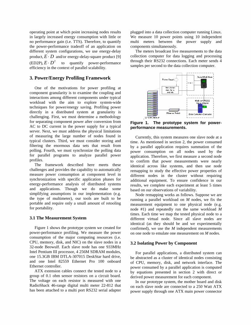
Figure 1 shows the prototype system we created for

power-performance profiling. We measure the power consumption of the major computing resources (i.e. CPU, memory, disk, and NIC) on the slave nodes in a 32-node Beowulf. Each slave node has one 933MHz Intel Pentium III processor, 4 256M SDRAM modules, one 15.3GB IBM DTLA-307015 DeskStar hard drive, and one Intel 82559 Ethernet Pro 100 onboard Ethernet controller.

ATX extension cables connect the tested node to a group of 0.1 ohm sensor resistors on a circuit board. The voltage on each resistor is measured with one RadioShack 46-range digital multi meter 22-812 that has been attached to a multi port RS232 serial adapter

plugged into a data collection computer running Linux. We measure 10 power points using 10 independent multi meters between the power supply and components simultaneously.

The meters broadcast live measurements to the data collection computer for data logging and processing through their RS232 connections. Each meter sends 4 samples per second to the data collection computer.

.

PRINT

HELP

ALPHA

SHIFT

ENTERRUN

DG ER FI

AJ BK CL

7M 8N 9O

DG DG DG

DG T 3U

0V .WX Y Z

TAB

% UTILIZATION

HUB/MAU NIC

2BNC4Mb/s

Figure 1. The prototype system for power-performance measurements.

Currently, this system measures one slave node at a

time. As mentioned in section 2, the power consumed by a parallel application requires summation of the power consumption on all nodes used by the application. Therefore, we first measure a second node to confirm that power measurements were nearly identical across like systems, and then use node remapping to study the effective power properties of different nodes in the cluster without requiring additional equipment. To ensure confidence in our results, we complete each experiment at least 5 times based on our observations of variability.

Node remapping works as follows. Suppose we are running a parallel workload on M nodes, we fix the measurement equipment to one physical node (e.g. node #1) and repeatedly run the same workload M times. Each time we map the tested physical node to a different virtual node. Since all slave nodes are identical (as they should be and we experimentally confirmed), we use the M independent measurements on one node to emulate one measurement on M nodes. 3.2 Isolating Power by Component

For parallel applications, a distributed system can be abstracted as a cluster of identical nodes consisting of CPU, memory, disk, and network interface. The power consumed by a parallel application is computed by equations presented in section 2 with direct or derived power measurement for each component.

In our prototype system, the mother board and disk on each slave node are connected to a 250 Watt ATX power supply through one ATX main power connector

and one ATX peripheral power connector respectively. We experimentally deduce the correspondence between ATX power connectors and node components.

Since disk is connected to a peripheral power connection independently, its power consumption can be directly measured through +12VDC and +5VDC pins on the peripheral power connect. To map the component on the motherboard with the pins on the main power connector, we observe the current changes on all non-COM pins by adding/removing components and running different micro benchmarks which access certain subsets of components each time. Finally, we are able to conclude that CPU is powered through four +5VDC pins; memory, NIC and others are supplied through +3.3VDC; the +12VDC feeds the CPU fan; and other pins are constant and small (or zero) current.

The idle part of memory system power consumption is measured by extrapolation. Each slave node in the prototype has four 256MB memory modules. We measure the power consumptions of the slave node configured with 1, 2, 3, and 4 memory modules separately, then estimate the idle power consumed by the whole memory system

The slave nodes in the prototype are configured with onboard NIC. It is hard to separate its power consumption from other components directly. After, observing that the total system power consumption changes slightly when we disable the NIC or pull out the network cable and consulting the documentation of the NIC (Intel 82559 Ethernet Pro 100), we approximate it with constant value of 0.41 watt.

The CPU power consumption is obtained by measuring all +5VDC pins directly.

For further verification, we compared our measured power consumption for CPU and disk with the specifications provided by Intel and IBM separately and they matched well. Also by running memory access micro benchmarks, we observed that if accessed data size is located within L1/L2 cache, the memory power consumption doesn’t change; while once main memory is accessed, the memory power consumption we measured increases correspondingly.

3.3 Automatic Power Profiling and Analysis

To automate the entire profiling process we require enough multimeters to measure directly, in real-time, a single node. Under this constraint, we fully automate data profiling, measurement and analysis by creating a tool suite named as PowerPack. PowerPack consists of utilities, benchmarks and libraries for controlling, recording and processing power measurements in distributed systems. PowerPack’s software structure is shown in Figure 2

Figure 2. Software Structure for PowerPack.

In PowerPack, PowerMeter control thread reads data samples coming from a group of meter readers which are controlled by globally shared variables. The control thread modifies the shared variables according to messages received from applications running on the cluster. Applications trigger message operations through a set of application level library calls to synchronize the live profiling process with the application source code. These application level library calls can be inserted into the source code of the profiled applications. The common used subset of power profile library API is as follows:

The power profile log and the system status log are

processed with the PowerAnalyzer, a software module that implements functions such as converting DC current to power, interpolating between sampling points, decomposing pins power to component power, computing power and energy consumed by applications and system, and performing related statistical calculations.

4. Experimental Results 4.1 Single Node Power Profiles

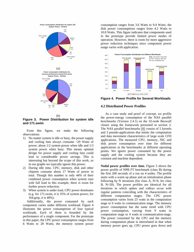
To better understand the power consumption of distributed applications and systems, we first profile the power consumption of a single slave node. Figure 3 provides power distribution breakdown for system idle (3a) and system under load (3b) for the 171.swim benchmark included in SPEC CPU2000 [10].

CPU14%

Memory10%

Disk11%

NIC1%

Other Chipset8%Fans

23%

Pow er Supply33%

Power consumption distribution for system idleSystem Power: 39 Watt

(a)

CPU35%

Memory16%

Disk7%

NIC1%

Other Chipset5%

Fans15%

Pow er Supply21%

Power consumption distribution formemory performance bound (171.swim)

System Power: 59 Watt

(b)

Figure 3. Power Distribution for system idle and 171.swim

From this figure, we make the following

observations: 1) No matter system is idle or busy, the power supply

and cooling fans always consume ~20 Watts of power; about 1/2 system power when idle and 1/3 system power when busy. This means optimal design for power supply and cooling fans could lead to considerable power savings. This is interesting but beyond the scope of this work, so in our graphs we typically ignore this power.

2) During idle time, CPU, memory, disk and other chipsets consume about 17 Watts of power in total. Though this number is only 44% of their combined power consumption when system runs with full load in this example, there is room for further power reduction.

3) When system is under load, CPU power dominates (e.g. for 171.swim, it is 35% of system power; for 164.gzip, it is 48%).

Additionally, the power consumed by each component varies under different workload. Figure 4 illustrates the power consumptions of four typical workloads. Each of them is bounded by the performance of a single component. For the prototype in this paper, the CPU power consumption ranges from 6 Watts to 28 Watts; the memory system power

consumption ranges from 3.6 Watts to 9.4 Watts; the disk power consumptions ranges from 4.2 Watts to 10.8 Watts. This figure indicates that components used in the prototype provide limited power modes of operation. However, there is room for more aggressive power reduction techniques since component power usage varies with application.

0.0

5.0

10.0

15.0

20.0

25.0

30.0

35.0

40.0

idle 171.swim 164.gzip cp scp

CPU Memory Disk NIC

Power Consumption Distribution for Different Workloads

CPU-bound memory-bound

disk-bound

network-bound

Note : only power consumed by CPU, memory, disk and NIC are considered here

Figure 4. Power Profile for Several Workloads 4.2 Distributed Power Profiles

As a case study and proof of concept, we profile the power-energy consumption of the NAS parallel benchmarks (Version 2.4.1) on the 32-node Beowulf cluster using the framework presented in section 3. The NAS parallel benchmarks [8] consist of 5 kernels and 3 pseudo-applications that mimic the computation and data movement characteristics of large scale CFD applications. The measured CPU, memory, NIC and disk power consumption over time for different applications in the benchmarks at different operating points. We ignore power consumed by the power supply and the cooling system because they are constant and machine dependent. Nodal power profiles over time. Figure 5 shows the power profile of NPB FT benchmark (class B) during the first 200 seconds of a run on 4 nodes. The profile starts with a warm up phase and an initialization phase following by N iterations (for class A, N=6; for class B, N=20). The power profiles are identical for all iterations in which spikes and valleys occur with regular patterns coinciding with the characteristics of different computation stages. The CPU power consumption varies from 25 watts in the computation stage to 6 watts in communication stage. The memory power consumption has the same trend with CPU power consumption, varying from 9 watts in computation stage to 4 watts in communication-stage. The power consumed by the CPU and the memory during computation phase is interrelated in that when memory power goes up, CPU power goes down and

the inverse is also true. It is also observed that the disk keeps constant power consumption because there is little disk access in the FT benchmark. The power consumed by the NIC is a constant (0.4 watt) as discussed earlier. For simplification, we ignore the disk and NIC power consumptions in discussions and figures where they do not change.

Figure 5. The first 200 second nodal power profile of FT benchmark (class B) running on 4 nodes.

An in-depth view of the power profile during one

iteration is presented in Figure 6.

Figure 6. In-depth view of the power profile of FT benchmark (class B, NP=4) during one single iteration. Profiled is extracted from Fig 5. Power profiles for different problem size. Figure 7 shows the power profile of NPB FT benchmark (class A) during the first 50 seconds of a run on 4 nodes. From Figure 5 and Figure 7, we observe FT has similar patterns for different problem size. However, iterations are shorter in duration for the smaller (class A) problem set.

Pow

er (w

att)

Figure 7. The first 50 second nodal power profile of FT benchmark (class A) running on 4 nodes. Power profiles for different work node. For the FT benchmark, workload is distributed evenly across all working nodes. We use our node remapping technique to provide power profiles for all nodes in the cluster (in this case just 4 nodes). For FT, there are no significant differences. However, Figure 8 shows a counter example snapshot for a 10 second interval of SP synchronized across nodes. For the SP benchmark, Class A problem sizes running on 4 nodes results in varied power profiles for each node.

Pow

er (w

att)

Figure 8. Power consumption on different nodes for SP benchmark (class A, NP=4). Power profiles during 20-30 seconds on each node are shown in this figure. This figure indicates that different node has slight difference in power consumption. Power profiles for different system scale. The power profile of parallel applications also varies with the number of nodes used in the execution if we fix problem size (i.e. strong scaling). We have profiled the power consumption for all the NPB benchmarks on all execution nodes with different number of processors (up to 32) and several classes of problem sizes. Due to space limitations we only present the profile for problem FT, EP and MG (class A) with different

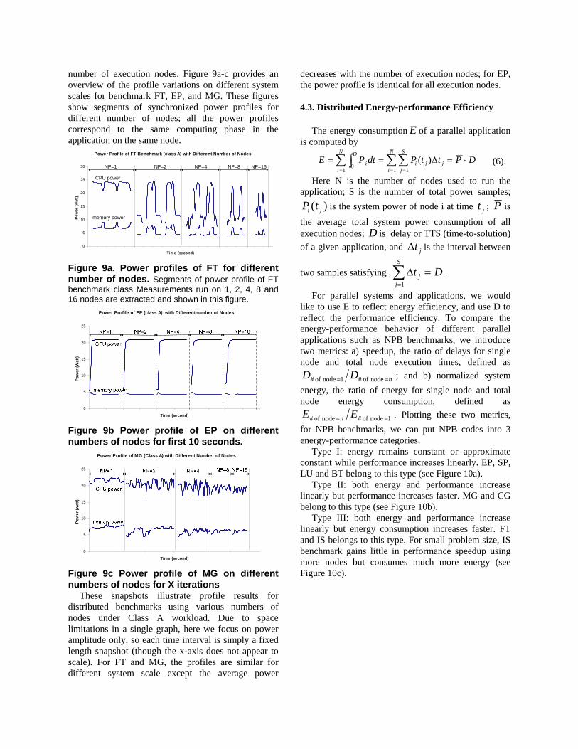
number of execution nodes. Figure 9a-c provides an overview of the profile variations on different system scales for benchmark FT, EP, and MG. These figures show segments of synchronized power profiles for different number of nodes; all the power profiles correspond to the same computing phase in the application on the same node.

Power Profile of FT Benchmark (class A) with Different Number of Nodes

0

5

10

15

20

25

30

Time (second)

Pow

er (w

att)

NP=1 NP=2 NP=4 NP=8 NP=16

CPU power

memory power

Figure 9a. Power profiles of FT for different number of nodes. Segments of power profile of FT benchmark class Measurements run on 1, 2, 4, 8 and 16 nodes are extracted and shown in this figure.

Power Profile of EP (class A) with Differentnumber of Nodes

0

5

10

15

20

25

Time (second)

Pow

er (W

att)

Figure 9b Power profile of EP on different numbers of nodes for first 10 seconds.

Power Profile of MG (Class A) with Different Number of Nodes

0

5

10

15

20

25

Time (second)

Pow

er (w

att)

Figure 9c Power profile of MG on different numbers of nodes for X iterations

These snapshots illustrate profile results for distributed benchmarks using various numbers of nodes under Class A workload. Due to space limitations in a single graph, here we focus on power amplitude only, so each time interval is simply a fixed length snapshot (though the x-axis does not appear to scale). For FT and MG, the profiles are similar for different system scale except the average power

decreases with the number of execution nodes; for EP, the power profile is identical for all execution nodes. 4.3. Distributed Energy-performance Efficiency

The energy consumption E of a parallel application is computed by

DPttPdtPEN

i

S

jjji

N

i

D

i ⋅=∆== ∑∑∑∫= == 1 11

0)(

(6).

Here N is the number of nodes used to run the application; S is the number of total power samples;

)( ji tP is the system power of node i at time jt ; P is

the average total system power consumption of all execution nodes; D is delay or TTS (time-to-solution) of a given application, and jt∆ is the interval between

two samples satisfying . DtS

jj =∆∑

=1

.

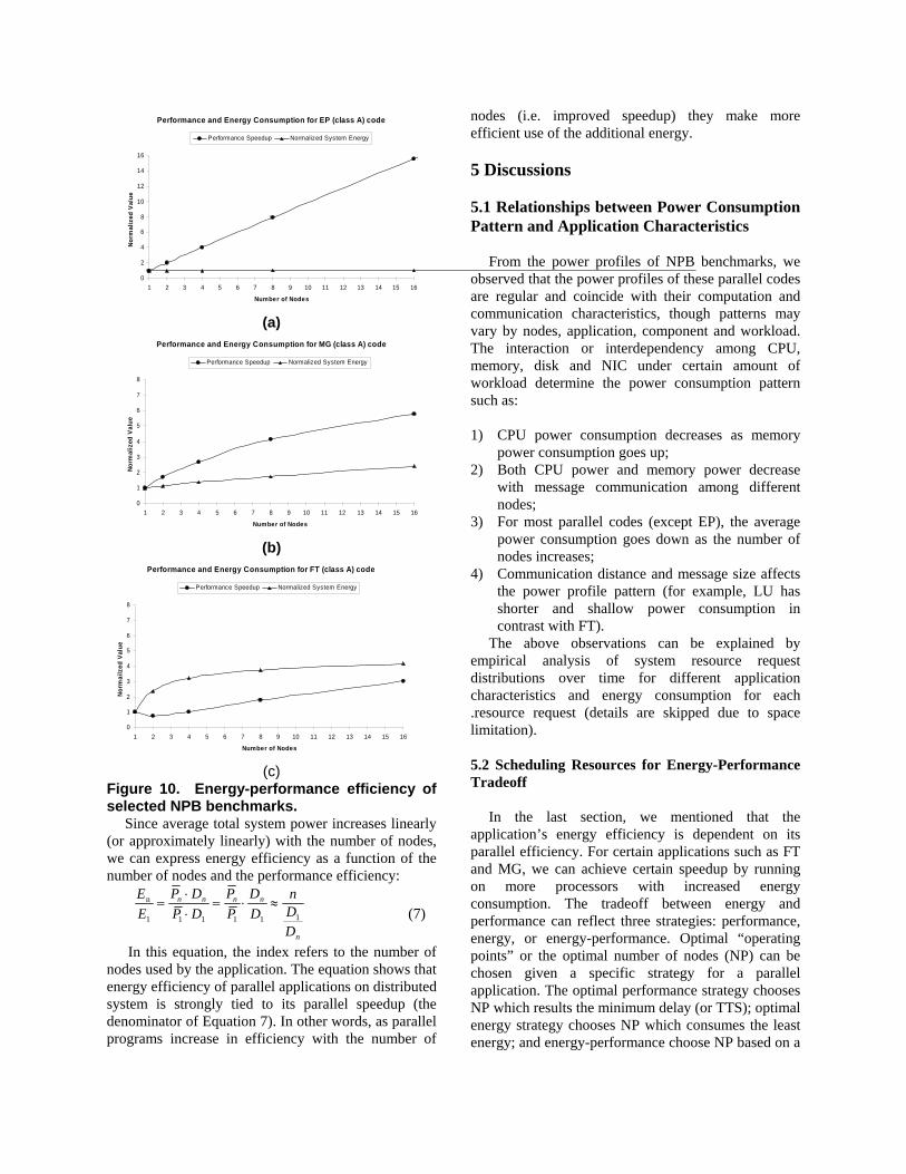
For parallel systems and applications, we would like to use E to reflect energy efficiency, and use D to reflect the performance efficiency. To compare the energy-performance behavior of different parallel applications such as NPB benchmarks, we introduce two metrics: a) speedup, the ratio of delays for single node and total node execution times, defined as

nDD == node of #1 node of # ; and b) normalized system energy, the ratio of energy for single node and total node energy consumption, defined as

1 node of # node of # == EE n . Plotting these two metrics, for NPB benchmarks, we can put NPB codes into 3 energy-performance categories.

Type I: energy remains constant or approximate constant while performance increases linearly. EP, SP, LU and BT belong to this type (see Figure 10a).

Type II: both energy and performance increase linearly but performance increases faster. MG and CG belong to this type (see Figure 10b).

Type III: both energy and performance increase linearly but energy consumption increases faster. FT and IS belongs to this type. For small problem size, IS benchmark gains little in performance speedup using more nodes but consumes much more energy (see Figure 10c).

Performance and Energy Consumption for EP (class A) code

0

2

4

6

8

10

12

14

16

1 2 3 4 5 6 7 8 9 10 11 12 13 14 15 16

Number of Nodes

Norm

aliz

ed V

alue

Performance Speedup Normalized System Energy

(a)

Performance and Energy Consumption for MG (class A) code

0

1

2

3

4

5

6

7

8

1 2 3 4 5 6 7 8 9 10 11 12 13 14 15 16

Number of Nodes

Norm

aliz

ed V

alue

Performance Speedup Normalized System Energy

(b)

Performance and Energy Consumption for FT (class A) code

0

1

2

3

4

5

6

7

8

1 2 3 4 5 6 7 8 9 10 11 12 13 14 15 16

Number of Nodes

Norm

ailz

ed V

alue

Performance Speedup Normalized System Energy

(c)

Figure 10. Energy-performance efficiency of selected NPB benchmarks.

Since average total system power increases linearly (or approximately linearly) with the number of nodes, we can express energy efficiency as a function of the number of nodes and the performance efficiency:

n

11 1 1 1 1

n n n n

n

P D P DE nDE P D P DD

⋅= = ⋅ ≈

⋅

(7)

In this equation, the index refers to the number of nodes used by the application. The equation shows that energy efficiency of parallel applications on distributed system is strongly tied to its parallel speedup (the denominator of Equation 7). In other words, as parallel programs increase in efficiency with the number of

nodes (i.e. improved speedup) they make more efficient use of the additional energy.

5 Discussions 5.1 Relationships between Power Consumption Pattern and Application Characteristics

From the power profiles of NPB benchmarks, we

observed that the power profiles of these parallel codes are regular and coincide with their computation and communication characteristics, though patterns may vary by nodes, application, component and workload. The interaction or interdependency among CPU, memory, disk and NIC under certain amount of workload determine the power consumption pattern such as: 1) CPU power consumption decreases as memory

power consumption goes up; 2) Both CPU power and memory power decrease

with message communication among different nodes;

3) For most parallel codes (except EP), the average power consumption goes down as the number of nodes increases;

4) Communication distance and message size affects the power profile pattern (for example, LU has shorter and shallow power consumption in contrast with FT).

The above observations can be explained by empirical analysis of system resource request distributions over time for different application characteristics and energy consumption for each .resource request (details are skipped due to space limitation).

5.2 Scheduling Resources for Energy-Performance Tradeoff

In the last section, we mentioned that the application’s energy efficiency is dependent on its parallel efficiency. For certain applications such as FT and MG, we can achieve certain speedup by running on more processors with increased energy consumption. The tradeoff between energy and performance can reflect three strategies: performance, energy, or energy-performance. Optimal “operating points” or the optimal number of nodes (NP) can be chosen given a specific strategy for a parallel application. The optimal performance strategy chooses NP which results the minimum delay (or TTS); optimal energy strategy chooses NP which consumes the least energy; and energy-performance choose NP based on a

hybrid metric that considers both energy and performance. As in micro architecture or mobile computing, Energy-Delay Product (EDP) or Energy-Delay-Square Product (ED2P) can be used to compare the energy efficiency of different techniques. The same idea can be used for parallel system scheduling.

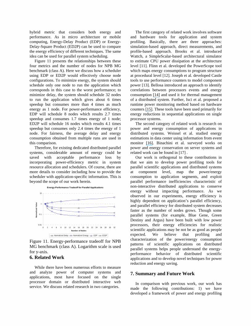
Figure 11 presents the relationships between these four metrics and the number of nodes for NPB MG benchmark (class A). Here we discuss how a scheduler using EDP or ED2P would effectively choose node configurations. To minimize energy, the system should schedule only one node to run the application which corresponds in this case to the worst performance; to minimize delay, the system should schedule 32 nodes to run the application which gives about 6 times speedup but consumes more than 4 times as much energy as 1 node. For power-performance efficiency, EDP will schedule 8 nodes which results 2.7 times speedup and consumes 1.7 times energy of 1 node; ED2P will schedule 16 nodes which results 4.1 times speedup but consumes only 2.4 times the energy of 1 node. For fairness, the average delay and energy consumption obtained from multiple runs are used in this comparison.

Therefore, for existing dedicated distributed parallel systems, considerable amount of energy could be saved with acceptable performance loss by incorporating power-efficiency metric in system resource allocation and schedulers. Of course, there are more details to consider including how to provide the scheduler with application-specific information. This is beyond the scope of our work herein.

Energy-Performance Tradeoff for Parallel Applications

0.01

0.1

1

10

0 2 4 6 8 10 12 14 16 18 20 22 24 26 28 30 32

Number of Nodes

Nor

mal

ized

Val

ue

Normalized Delay Normalized Energy EDP ED2P Figure 11. Energy-performance tradeoff for NPB MG benchmark (class A). Logarithm scale is used for y-axis. 6. Related Work

While there have been numerous efforts to measure

and analyze power of computer systems and applications, most have focused on the single processor domain or distributed interactive web service. We discuss related research in two categories.

The first category of related work involves software and hardware tools for application and system profiling. Basically, there are three approaches: simulation-based approach, direct measurements, and profile-based approach. Brooks et al. introduced Wattch, a SimpleScalar-based architectural simulator to estimate CPU power dissipation at the architecture level [11]. Flinn et al. developed the PowerScope tool which maps energy consumptions to program structure at procedural level [12]. Joseph et al. developed Castle tools to use performance counters to model component power [13]. Bellosa introduced an approach to identify correlations between processors events and energy consumption [14] and used it for thermal management of a distributed system. Further, Isci et al. proposed a runtime power monitoring method based on hardware counters [15]. These tools have been used primarily for energy reductions in sequential applications on single processor systems.

The second category of related work is research on power and energy consumption of applications in distributed systems. Weissel et al. studied energy estimations in data center using information from event monitor [16]. Binachini et al. surveyed works on power and energy conservation on server systems and related work can be found in [17] .

Our work is orthogonal to these contributions in that we aim to develop power profiling tools for parallel scientific applications and distributed systems at component level, map the power/energy consumption to application segments, and exploit parallel performance inefficiencies characteristic of non-interactive distributed applications to conserve energy without impacting performance. As we observed in our experiments, energy efficiency is highly dependent on application’s parallel efficiency, and parallel efficiency for distributed system decreases faster as the number of nodes grows. Though some parallel systems (for example, Blue Gene, Green Destiny and Argus) have been built with low power processors, their energy efficiencies for realistic scientific applications may be not be as good as people expected. We believe that profiling and characterization of the power/energy consumption patterns of scientific applications on distributed parallel systems helps people understand the energy-performance behavior of distributed scientific applications and to develop novel techniques for power reduction and energy saving. 7. Summary and Future Work

In comparison with previous work, our work has made the following contributions: 1) we have developed a framework of power and energy profiling

for non-interactive parallel scientific applications on distributed system; 2) we have created PowerPack, a portable, open source software for automated controlling and recording measurement data; 3) we have analyzed the NAS parallel benchmark suite and observed several interesting observations. This work can be further enhanced by integrating related work mentioned above and made available to the community at large.

The current prototype is limited by the sampling frequency of the hardware and its scalability to measure a very large parallel system. With more advanced equipment with higher sampling rate and fast communications between measuring equipment and data collection systems, the first limitation could be overcome. However, further techniques should be developed for power/energy profiling for large systems to avoid direct measurement on every nodes.

Acknowledgement

The authors would like to thank the National Science Foundation and the Department of Energy for sponsoring this work under grants NSF CCF-#0347683 and DOE DE-FG02-04ER25608 respectively. We also would like to thank Duncan Buell for comments and access to Daniel.

References [1] D. H. Bailey, "Performance of Future High-end Computers," 2003. [2] H. D. Simon, "The Future of Scientific Computing," 2000. [3] G. Bell and J. Gray, "High Performance Computing: Crays, Clusters, and Centers. What Next?," Microsoft Corporation, San Francisco, CA MSR-TR-2001-76, September 2001. [4] D. J. Kerbyson, A. Hoisie, et al., "A comparison between the Earth Simulator and AlphaServer Systems Using Predictive Application Performance Models," presented at IPDPS 2003, Nice, France, 2003. [5] D. A. Patterson and J. L. Hennessy, Computer Architecture: A quantitative approach, 3rd ed. San Fancisco, CA: Morgan Kaufmann Publishers, 2003. [6] LBNL, "Data Center Energy Benchmarking Case Study: Data Center Facility 5," Prepared by Rumsey Engineers for Lawrence Berkeley National Laboratory Environmental Energy Technologies Division, Oakland, CA April 2003. [7] A. M. Bailey, "Accelerated Strategic Computing Initiative (ASCI): Driving the need for the Terascale Simulation Facility (TSF)," presented at Energy 2002 Workshop and Exposition, Palm Springs, CA, 2002. [8] D. Bailey, T. Harris, et al., "The NAS Parallel Benchmarks 2.0," NASA Ames Research Center Technical Report #NAS-95-020 December 1995.

[9] M. Martonosi, D. Brooks, et al., "Modeling and Analyzing CPU Power and Performance: Metrics, Methods, and Abstractions," presented at Tutorials Program - SIGMETRICS 2001 / Performance 2001, Cambridge, Massachusetts, 2001. [10] http://www.spec.org, "The SPEC benchmark suite," Standard Performance Evaluation Corporation, 2002. [11] D. Brooks, V. Tiwari, et al., "Wattch: A Framework for Architectural-Level Power Analysis and Optimizations," presented at 27th International Symposium on Computer Architecture, Vancouver, BC, 2000. [12] J. Flinn and M. Satyanarayanan, "PowerScope: A Tool for Profiling the Energy Usage of Mobile Applications," presented at the Second IEEE Workshop on Mobile Computer Systems and Applications, 1999. [13] R. Joseph, D. Brooks, et al., "Live, runtime power measurements as a foundation for evaluating power/performance tradeoffs," presented at Workshop on Complexity-effective Design, Goteborg, Sweden, 2001. [14] F. Bellosa, "The Case for Event-Driven Energy Accounting," Deaprtment of Computer Science, University of Erlangen TR-I4-01-07, 2001. [15] C. Isci and M. Martonosi, "Runtime Power Monitoring in High-End Processors: Methodology and Empirical Data," presented at 36th Annual IEEE/ACM International Symposium on Microarchitecture (MICRO-36), San Diego, California, 2003. [16] A. Weissel and F. Bellosa, "Process Cruise Control-Event-Driven Clock Scaling for Dynamic Power Management," presented at Proceedings of the International Conference on Compilers, Architecture and Synthesis for Embedded Systems (CASES 2002), Grenoble, France, 2002. [17] P. Bohrer, E. N. Elnozahy, et al., "The Case For Power Management in Web Servers," in Power Aware Computing, R. Graybill and R. Melhem, Eds. IBM Research, Austin TX 78758, USA.: Klewer Academic, 2002.