Saifan

1

Post-Earnings-Announcement Drift

Among Newly Issued Public Companies

in U.S. Capital Markets

Sami Saifan

Professor Connel Fullenkamp, Faculty Advisor

Professor Michelle Connolly, Seminar Instructor

Honors Thesis submitted in partial fulfillment of the requirement for Graduation with

Distinction in Economics in Trinity College of Duke University.

Duke University

Durham, North Carolina

2013

Saifan

2

Acknowledgements

I want to express my sincerest gratitude to all the people who have supported me

during my undergraduate studies and in the completion of this honors thesis.

I am very grateful to my advisors Connel Fullenkamp and Michelle Connolly for

their guidance over the past year.

Connel Fullenkamp – thank you for your candid comments and helping me

motivate the ideas presented in my thesis. Your knowledge and integrity as an

economics professor is impressive, and your character is a motivation to me.

Michelle Connolly – thank you for always thoroughly reading my drafts and for

giving concrete advice on how to improve my research. Throughout this whole process,

you have made yourself available for me. Thank you. I hope to spend time with you

again at the Washington Duke Inn, and perhaps one day win an M&M prize.

Phil Nousak – even though you are not a formal advisor, this paper would have

not been possible without you. Thank you, Phil, for helping me with the data and SAS

programming. I enjoyed our long hours in the office together and talking about hockey

while waiting for SAS programs to finish running. It was a privilege to work with you.

Lastly, I wish to express my appreciation to the entire faculty at Duke’s

Department of Economics. You have provided me with a strong interest in economics

and finance and have prepared me well for my future endeavors.

Saifan

3

Abstract

Post-earnings-announcement drift is the tendency for a stock’s cumulative

abnormal returns to drift in the direction of an earnings surprise for several weeks

following an earnings announcement. I show that the drift is significantly more

pronounced when investigating the unexpected earnings of initial public offerings in

comparison to the aggregate U.S. stock market. My results suggest that this disparity is

attributable to firm-specific characteristics inherent in initial public offerings and the

extraordinary growth numerous young firms experience. Further, I postulate that drift

patterns following earnings announcements for IPO firms differ from those observed in

prior PEAD research.

Saifan

4

I. Introduction

Post-earnings-announcement drift (“PEAD”), first documented in a Ball and

Brown (1968) study, is the tendency for a stock’s share price to drift in the direction of an

earnings surprise for several weeks, or even months, following an earnings

announcement.1 Specifically, stocks with strong positive earnings surprises tend to earn

notably higher returns for a significant period of time after the current quarterly earnings

announcement. Similarly, stocks with larger negative earnings surprises tend to earn

notably lower returns. Since Ball and Brown pioneered this field of analysis, numerous

studies have been conducted implementing various statistical methodologies and different

samples with results corroborating the findings of Ball and Brown. Through exhaustive

empirical analyzes, researchers agree that stock prices do not sufficiently adjust to

information in earnings announcements, and, therefore PEAD can lead to large stock

returns.2 The academic profession has subjected the capital market anomaly to a battery

of tests both in the U.S. and abroad (Booth et al., 1996; Liu et al., 2003), but a rational,

economic explanation for the drift remains elusive (Kothari, 2001).

If the post-earnings-announcement drift hypothesis is one of the best-documented

and most-resilient capital market anomalies, why do investors not regularly capitalize on

the drift with PEAD-oriented trading strategies? Given PEAD is a post-earnings

phenomenon, an investor does not have to predict what the earnings announcement will

be; the direction of the earnings surprise and market reaction is already known. With this

1 Since PEAD studies focus on price reactions to unexpected earnings, the post-earnings-announcement

drift is sometimes referred to as the SUE effect, where SUE is an acronym for Standardized Unexpected

Earnings. 2 Foster, Olsen and Shevlin (1984) found that a drift trading strategy (long position for a positive earnings

surprise and a simultaneous short position is a negative earnings surprise) yields an annualized return of

about 25%, before transaction costs.

Saifan

5

invaluable information the intelligent investor can simply purchase (sell) a stock one to

three days after a positive (negative) earnings surprise, hold the position for a few

months, and then exit the position to make a profit with relatively high probability –a

seemingly simple arbitrage opportunity. Researchers attribute the lack of frequency for

this trading strategy to three particularly important classes of explanations.

First, it appears that at least a portion of the price response to new information is

delayed. This delay may occur either because investors fail to digest available

information or investors underreact to the information conveyed during earnings

announcements. Also, academics from the underreaction camp attribute this market

inefficiency to transaction costs as they exceed gains from immediate exploitation of

information for the average investor (Bhushan, 1994; Ng, Rusticus and Verdi, 2008).7

Second, PEAD occurs because of shifts in the risks of companies with extreme

surprises, which justify higher expected returns to equilibrium. Put differently, drift

represents systematic misestimation of expected returns following earnings surprises.

Real-world arbitrage is risky since investors who would profit from the greater apparent

mispricing of high-arbitrage risk firms must be prepared to bear greater uncertainty

regarding the outcome of a transaction (Mendenhall, 2004). In addition, firms with

extreme positive earnings tend to be those whose riskiness has recently increased (Ball,

Kothari and Watts, 1993).

The third group of explanations is perhaps an extension of the second group: the

apparent drift is due to methodological shortcomings, particularly that the capital-asset-

7 PEAD is positively related to the direct and indirect costs of trading. Trading profits are significantly

reduced by transaction costs (which account for 66% to 100% of the paper profits), as PEAD occurs mainly

in highly illiquid stocks. However, Battalio and Mendenhall (2007) found transaction costs and liquidity

cannot explain PEAD: under a wide range of timing and cost assumptions, an investor could have earned

hedge-portfolio returns of a least 14% between 1993-2002 after trading costs.

Saifan

6

pricing model (“CAPM”) used to measure abnormal returns is either incomplete or

misestimated, as it does not adjust abnormal returns fully for risk (Bernard and Thomas,

1989)8. Other proponents of this class claim a “survivorship bias.” They argue that the

PEAD effect is correlated with factors that proxy for the ex-ante probability of the firm

surviving to be part of the earnings surprise sample (Brown and Pope, 1996).

In my empirical research, I provide an alternative framework for the two main

classes of explanations – market inefficiency and misestimated risk. More importantly,

this paper does not attempt to contradict or refute past evidence of post-earnings-

announcement drift. Merely, this research paper will draw upon the rich array of past

work on post-earnings-announcement drift to add to and extend the application of post-

earnings-announcement drift within the context of a unique sample – the initial public

offering (“IPO”) universe.

This paper is the first extensive study of the post-earnings-announcement drift in

an IPO context. As such, it contributes to our knowledge of how investors and

institutions react to initial public offerings and their respective quarterly accounting

information. To the best of my knowledge no one has looked at post-earnings-

announcement drift among IPOs, isolated IPOs as a subset, or included a comprehensive

list of IPOs within the sample in prior PEAD analysis.9 The IPO methodology of my

paper is the first approach that can be implemented on a dataset which is not restricted to

8 The generally accepted and used capital-asset-pricing model is as follows:

ra = rrf + Ba (rm-rrf)

where,

rrf = the rate of return for a risk-free security

rm = the broad market's expected rate of return

Ba = beta of the asset.

9 In prior research, no dummy variable nor any kind of indicator was utilized to isolate IPOs. In addition,

most prior studies required a company to host at least 10 consecutive quarterly performance results in order

to be included in the sample. Thus, many IPOs fail to meet these inclusion criteria.

Saifan

7

firms with positive earnings, the number of analysts following a firm, and/or long time-

series of accounting data. By focusing on the market power exercised by institutional

investors and the characteristics of young firms usually excluded from these studies, I

hope to provide an alternative explanation to the post-earnings-announcement drift

literature.

Lastly, my research contributes to the PEAD literature by illustrating how the

well-documented, systematic underpricing of IPO shares might be a driving force behind

the drift. Furthermore, IPOs have been shown to significantly underperform, in terms of

return, after the familiar first-day pop. Consider the period from 1980-2010 when the

average 3-year Buy-and-Hold market-adjusted return on IPOs yielded -19.7% after an

average first-day return of 18.0% (Ritter, 2011). Other studies have reported numbers of

similar magnitude. To my knowledge, there is no prior discussion on how underpricing

might lead to a pronounced announcement reaction.

Overall, the purpose of this paper is to build upon existing research on post-

earnings-announcement drift by analyzing the capital market anomaly in the context of

newly issued public companies in the United States. Specifically, this paper will use

empirical data from 2005-2012 to investigate the possible distinct existence of post-

earnings-announcement drift for IPOs as well as possible explanations behind the drift.

The results of this paper indicate that there is a pronounced post-earnings-

announcement drift among initial public offerings in U.S. capital markets during the

studied time period. Undertaking a PEAD trading strategy, where I take a long position

in the portfolio of stocks with the highest unexpected earnings and a short position in the

Saifan

8

portfolio of stocks with the lowest unexpected earnings, yields an estimated abnormal

return of at least 59% on an annualized basis.11

The paper is organized into the following sections. Section II presents a review of

the existing literature on post-earnings-announcement drift. The theoretical framework

of my research is presented in Section III. Section IV discusses the nature of the data

used in this research paper. Section V presents the empirical methodology used in the

analysis and the results of the empirical study. Section VI concludes the research paper.

11

Long-short strategy in terms of PEAD is an investment strategy which involves taking a long position in

firms with the highest earnings surprises (good news) and a short position in firms with the lowest earnings

surprises (bad news).

This result varies from sample to sample. See results section.

Saifan

9

II. Literature Review

In financial economics, there is an extensive body of research reporting empirical

evidence of the post-earnings-announcement drift, a long-standing anomaly that conflicts

with the assumptions of market efficiency. Fama (1998) highlights the drift as an

established anomaly that is “above suspicion” and refers to it as “the granddaddy of all

underreaction events.” Prior studies examine the post-earnings-announcement drift

phenomenon along with possible explanations for the drift. The most cited works belong

to Ball and Brown (1968), Mendenhall (2004), Chordia et al. (2009), and Bernard and

Thomas (1989). Generally, the researchers find evidence signifying the existence of

post-earnings-announcement drift in the capital markets, and they suggest it is likely a

result of delayed price response and unaccounted risk.

The drift phenomenon was initially proposed by Ray J. Ball and P. Brown (1984).

In their study, Ball and Brown empirically analyze the effect of financial information

pertaining to an individual firm’s stock return. To determine if part of this effect can be

associated with earnings, Ball and Brown study how stock prices change when new

earnings information is released to the stock market. They report that on average when

firms report good (bad) news, the announcement returns are positive (negative).

Furthermore, Ball and Brown find evidence that stock prices continue to drift upward

(downward) after initial positive (negative) income news, rendering the initial stock price

reaction to the financial information incomplete and raising questions of market

efficiency.

Saifan

10

Ball and Brown note that there are several explanations for this phenomenon

consistent with their evidence: (1) inefficient information processing by the market, (2)

efficient information processing in the presence of significant transactions costs, and (3)

misspecification in the measurement of abnormal returns. The researchers conclude that

post-earnings-announcement drift is most likely due to market inefficiency (explanation

1).

Richard Mendenhall (2004) examines whether the magnitude of post-earnings-

announcement drift is correlated to the risk faced by arbitrageurs, who may view the

anomaly as a trading opportunity. Consistent with this hypothesis, the magnitude of the

drift is positively correlated to the arbitrage risk measure developed by Wurgler and

Zhuravskaya (2002). He interprets his results as evidence that many investors underreact

to earnings information, and risk impedes arbitrageurs from trying harder to profit from

this underreaction.

Chordia et al. (2009) documents that post-earnings-announcement drift occurs

mainly in highly illiquid stocks. He finds that a long-short strategy that goes long high-

earnings-surprise stocks and short low-earnings-surprise stocks provides a monthly

value-weighted return of 0.04 percent in the most liquid stocks and 2.43 percent in the

most illiquid stocks. Chordia et al. also notes that the illiquid stocks have high trading

costs and high market impact costs. By using a multitude of estimates, Chordia et al.

finds that transaction costs account for 70-100 percent of the return from a PEAD trading

strategy designed to exploit the earnings momentum anomaly.

In addition, Bernard and Thomas (1989) examine the drift for a sample of U.S.

firms over the period 1974-1986. They find that undertaking a long-short strategy and

Saifan

11

holding the positions for 60 trading days yields a size-controlled return of 4.2%, or 18%

on an annualized basis. Bernard and Thomas also find the drift can last up to 240 trading

days although most of the return is disproportionately concentrated in the 3-day periods

surrounding earnings announcement dates. In addition, they carefully note that they were

unable to find “strong evidence that abnormal returns to short positions in bad news

stocks exceed the abnormal returns to long positions in good news stocks, as would be

predicted if restrictions on short sales play a role in causing the drift.” Moreover, they

find that the drift is more pronounced for smaller firms, but still significant for large

firms.

Bernard and Thomas’ (1989) most important conclusion is that of serial

autocorrelation. In their study, Bernard and Thomas show that, following an earnings

surprise, returns around subsequent earnings announcements exhibit positive correlation

with current unexpected earnings for three quarters, and negatively correlated for the

fourth quarter. This is the same autocorrelation pattern that Foster, Olsen and Shevlin

(1984) found for seasonally differenced earnings. Bernard and Thomas demonstrate that

this autocorrelation pattern in returns suggests that investors underestimate the

implications of current earnings for future earnings.

For an illustration, consider the scenario in which earnings in quarter t are up,

relative to the comparable quarter of the prior year. An efficient market should generate

a higher expectation for earnings of quarter t +1 than otherwise. After assimilating the

new information from quarter t earnings, the expectation for quarter t + 1 would be

unbiased, and the mean earnings surprise to the announcement of quarter t + 1 earnings

would be zero. If the market fails to adequately revise its expectations for quarter t + 1

Saifan

12

earnings upon receipt of the earnings announcement for quarter t, the market can be

pleasantly surprised when earnings for quarter t + 1 are up relative to the prior year, and

vice versa.

Bernard and Thomas obtain results that are, in fact, consistent with this

explanation suggesting the equity market fails to recognize the full implications of

current earnings on future earnings when the earnings surprise is large.

Overall, the literature documents some key stylized facts regarding post-earnings-

announcement drift. First, the drift generates most of its return in the 3-day periods

surrounding earnings announcement dates, as opposed to exhibiting a gradually drifting

abnormal return behavior. Second, the long-side of PEAD strategy performs better than

the short-side when standardized unexpected earnings are based on analyst forecasts

(Doyle, Lundholm and Soliman, 2006). Third, the drift is generally larger for small,

lower-priced, less-liquid firms with less institutional and analyst following, greater

forecast dispersion, higher arbitrage risks and less pre-disclosure information.14

This paper builds upon the existing post-earnings-announcement drift literature,

as the literature is still struggling with the driving forces behind the capital market

anomaly. Through an examination of all the initial public offerings that began trading

during 2005 – 2012, I seek to offer alternative explanations for the drift by highlighting

market participants’ behavior surrounding IPOs, the systematic underpricing of IPO

shares, and the firm-specific characteristics of IPO companies.

14

These stylized fact are confirmed through the empirical analyses of Bernard and Thomas, 1989;

Bhushan, 1994; Brown and Han, 2000; Bartov et al., 2002; Mikhail et al., 2003; Mendenhall, 2004.

Saifan

13

III. Theoretical Framework

A. Earnings Surprise and Abnormal Returns

This research paper investigates the post-earnings-announcement drift among

newly issued public companies in U.S. capital markets. Four key papers – Ball and

Brown (1968), Mendenhall (2004), Chordia et al. (2009), and Bernard and Thomas

(1989) – all use similar procedures that are considered to be of high methodological

quality and frequently cited in other PEAD studies.

The theoretical framework used in my research follows the four key studies on

post-earnings-announcement drift. All prior drift studies test for the existence of post-

earnings-announcement drift by estimating unexpected earnings, also known as earnings

surprise. At its basic form, earnings surprise is the difference between reported earnings

and forecast of earnings divided by a deflator, and it can be estimated by using one of two

methods, depending on how forecasts are calculated: an analyst-based model and a time-

series model. Recent studies – including Affleck-Graves and Mendenhall (1992),

Abarbanell and Bernard (1992), Liang (2003), Mendenhall (2004), Francis et al. (2004)

and Livnat (2003) – use analysts’ forecasts and define standardized unexpected earnings

as:

Equation 1: Standardized Unexpected Earnings – Analyst-Based Approach

SUEj,t = (Aj,t – Mj,t) / P j,t

where,

SUEj,t = standardized unexpected earnings per share for firm j, in quarter t;

Aj,t = actual earnings per share reported by firm j, in quarter t;

Mj,t = consensus (median) earnings per share forecasts by analysts for firm j in the

90 days prior to the earnings announcement;

P j,t = price per share for firm j at the end of quarter t.

Saifan

14

The time-series class uses a statistical earnings autoregressive model that is

based on the assumption that earnings follow a seasonal random walk, in which the best

expectation of the earnings in quarter t is the firm’s reported earnings in the same quarter

of the previous fiscal year. Recent studies –including Bartov, Radhakrishnan, and

Krinsky (2000), Collins and Hribar (2000), and Naratanamoorthy (2003) – use some form

of a rolling seasonal random walk model to predict earnings and generally define

standardized unexpected earnings as:

Equation 2: Standardized Unexpected Earnings – Time-Series Approach

SUEj,t = (Xj,t – Xj,t-4 - δ j,t) / σ j,t

where,

SUEj,t = standardized unexpected earnings per share for firm j, in quarter t;

Xj,t = quarterly earnings per share for firm j, in quarter t;

Xj,t-4 = quarterly earnings per share for firm j, during the period (t-4, t);

δ j,t = time-series mean over preceding quarters;

σ j,q = standard deviation of seasonally difference earnings

I estimate SUE by using the analyst-based approach as described in Equation 1.

Consistent with other analyst-based studies, I measure analysts’ expectations as the

median of latest individual analysts’ forecasts issued in the 90 days prior to the earnings

announcement date. Although the time-series method is more commonly used in event

studies, this approach requires long history of earnings (most studies require a minimum

of 10 consecutive quarterly earnings). Thus, the latter approach is not suitable for most

young firms since they do not have sufficient time-series observations for the estimation

of SUE. Using the analyst-based approach alleviates this problem. Furthermore, analyst

forecasted SUE is based on actual earnings as they are reported by the firm originally and

not any subsequent restatement of the original data. Restated data may introduce bias by

Saifan

15

estimating a surprise that was not actually available to the market, and historical SUEs

may be affected by special items that analyst have not included in their forecasts.

To address the existence of outliers and hindsight bias in the earnings surprise-

return relation, I follow the four key drift papers previously addressed and classify firms

into SUE portfolios based on the standing of standardized unexpected earnings relative to

prior-quarter SUE distribution. The prior-quarter SUE distribution is used in the

classification of portfolios to avoid a hindsight bias. It is a methodological error to form

portfolios based on information not available at the time a trading strategy is

implemented.

A hypothetical trading strategy to assess the magnitude of PEAD is to take a long

position on the portfolio with the highest SUE (good news portfolio) and a short position

on the portfolio with the lowest SUE (bad news portfolio). Finally, the excess returns on

those portfolios are examined over 50 trading days following the earnings announcement

date. Consistent with other studies, I calculate abnormal returns as follows:

Equation 3: Abnormal Returns

ARj,t = Rj,t - BRp,t

where,

ARj,t = abnormal return for firm j, day t;

Rj,t = raw return for firm j, day t;

BRp,t = value-weighted index return for all CRSP firms incorporated in the U.S.

on NYSE/AMEX/NASDAQ for day t on the firm size portfolio that firm j is

a member of at the beginning of the calendar year. Firm size is measured by

the market value of common equity.

Part of this evaluation is commonly illustrated in the classic PEAD graph, in

which the upward and downward drifts are evident for the two extreme portfolios. In

Saifan

16

Figure 1 the cumulative abnormal returns for the PEAD long and short position are

presented in a stylized fashion.

Figure 1: Stylized Illustration of the Post-Earnings-Announcement Drift

To complement the graphical analysis, researchers evaluate PEAD using

regression models to test the statistical significance of the drift and the effect of firm size.

Following explanatory variables used in prior research, I run a regression with the

dependent variable, cumulative abnormal returns where it is computed as returns in

excess of CRSP value-weighted index, and regress it on unexpected earnings, firm size

and other instruments. The regression is summarized in Equation 4:

Equation 4: Regression Equation

Cumulative Abnormal Returns = β0 + β1SUE + β2Size + β3Price

where,

the dependent variable is abnormal returns defined as returns in excess of CRSP

value-weighted index post-announcement period;

SUE is standardized unexpected earnings;

Size is the size of the firm measured by market value, defined

as the share price multiplied by the number of shares outstanding.

Cumulative Abnormal

Return (CAR)

Time of Earnings Announcement

Good News Portfolio

Bad News Portfolio

Time

Saifan

17

B. Motivation

Initial public offerings, or IPOs, occur when a private company transforms into a

public company by selling securities to the public for the first time. After the IPO

process, the company shares trade publically in the equity market for the first time and

see a dramatic increase in their liquidity. I focus on newly issued public companies to

see whether they carry their own post-earnings-announcement drift phenomenon and

explore an alternative version of the delayed price response hypothesis. Specifically, I

hypothesize that newly issued public companies have a more pronounced drift effect as a

result of investor irrationality (i.e. market inefficiency) and, perhaps more importantly,

the market power exercised by institutional investors that often surround IPOs and their

systematic underpricing. Under my hypothesis, post-earnings-announcement drift is

particularly strong in new, publicly-listed stocks attributable to investors who do not

possess enough material information to adequately value the underlying stock and rely

almost exclusively on earnings announcements for guidance. In addition, it is well-

documented that investment banks underprice IPOs likely because it is profitable for

them. For example, investment bankers find it less costly to market an IPO that is

underpriced in order to induce investors to participate in the IPO market (Ritter, 1991).

Also, as Hoberg (2003) shows, the more market power that underwriters have, the more

underpricing there will be in equilibrium.

Newly issued public companies are worth considering for several reasons. First,

among IPOs there is inherently higher volatility due to the lack of transparency and

available information compared to mature, highly covered companies. With very scarce

information on a newly issued company’s profitability and financials, the role of

Saifan

18

accounting earnings information in the stock market becomes even more important, as

they are the only reliable measure of a company’s current and expected future

performance.

Second, IPOs carry with them significant behavioral biases. For instance, highly

anticipated IPOs are often thought as the next ‘Google’ or ‘Apple’. Correspondingly,

IPOs can be viewed as crapshoots with the newly issued companies, either striking gold

or tanking. Very seldom does the stock trade near its initial offering price after a year of

trading on a public stock exchange. As Ritter (2013) shows, issuing firms during 1980-

2010 substantially underperformed a sample of matching firms from their closing price

on the first day of public trading to their three-year anniversaries. This pattern is

consistent with an IPO market in which investors are habitually overoptimistic about the

earnings potential of young, growth companies. Intuitively, investors will behave

strongly to earnings announcements, as this is one of the few resources available to shed

light on a young company’s performance. The latter suggests a greater opportunity to

identify a sizeable earnings surprise to profit from a drift strategy trade, and Ritter (1991)

has documented that firms take advantage of IPOs’ “windows of opportunity.”

Third, IPOs are subject to a time window commonly referred to as the “quiet

period.” During this time, issuers, company insiders, analysts, and other parties are

legally restricted in their ability to discuss or promote the upcoming IPO.15

Moreover,

for 45 or 90 calendar days following an IPO’s first day of public trading, insiders and any

underwriters involved in the IPO are restricted from issuing any earnings forecasts or

research reports for the company, providing greater anticipation for earnings

announcements, and an opportunity to capitalize on earnings surprises. Therefore, these

15

U.S. Securities and Exchange Commission, 2005.

Saifan

19

companies can exhibit greater forecast dispersion and face less pre-disclosure information

– all of which have been associated with more pronounced drifts.

Fourth, following Chrodia’s et. al. theory on illiquidity’s role in post-earnings-

announcement drift, IPOs will display an even more pronounced effect. Before a

company goes public, its shares are very illiquid, and once the company is made public

investors should be concerned by expected liquidity and by the uncertainty about its level

when shares start trading on the after-market. This liquidity risk found in IPOs is

analogous to Chordia’s et. al. findings that the drift occurs mainly in highly illiquid

stocks.

Fifth, one of the most studied phenomena related to IPOs is the underpricing of

new shares offered. Underpricing of new shares is usually measured as the difference

between the offer price and the price at the end of first trading day.16

Hoberg (2004)

argues this phenomenon is driven by the market power exercised by large institutional

investors. In his paper, Hoberg examines IPO underpricing and finds that underwriters

who discount more tend to serve institutional, rather than retail, investors. When the

price of a new issue is too low, the issue is often oversubscribed; investors are not able to

purchase all of the shares they want, and underwriters can allocate shares among

subscribers. Hoberg posits that underwriters like “Goldman Sachs and Morgan Stanley

benefit from consistent underpricing because they work with large institutions, with

whom they are able to organize profitable quid pro quo arrangements in exchange for

preferment.” Smaller retail underwriters, on the other hand, work primarily with small

investors and thus do not have the same opportunity for quid pro quo benefits, according

16

The percentage price differential between the offer price and the price at the end of first trading day is

generally referred to as the first day return, or “first day pop,” from the IPO.

Saifan

20

to Hoberg. This suggests that underwriters treat good news and bad news regarding the

firm’s value differently. Underwriters are enticed to reveal bad news in order to have a

reason to lower the IPO price but may conceal good new in order to avoid raising the IPO

price. For the average investor, this information asymmetry places greater importance on

a newly issued firm’s quarterly earnings for its ‘true’ intrinsic value.

Under my framework, I hypothesize that post-earnings-announcement drift is

more pronounced in the context of newly issued public companies as a result of market

inefficiency, misestimated risk, and market power exercised by institutional investors.

Saifan

21

IV. Data

The empirical analysis in this paper utilizes several different databases, starting

with initial public offering data provided by IPO Scoop and the Hoover’s database.

Earnings surprises and earnings per share equity measures are measured from I/B/E/S

quarterly and annual files. Finally, daily data for major exchange-listed stocks is

obtained using the CSRP/Compustat daily files. The CSRP data files provide

monthly/daily returns, market capitalization (defined as share price multiplied by the

number of shares outstanding), volume, and dividends paid.

A. IPO Data

The primary data source for IPOs over 2005-2012 is the IPO Scoop’s IPO Track

Record file. To ensure that the list of IPOs is comprehensive and up to date, I cross

checked the source with Hoover’s IPO database. The compiled data provides a list of

IPO companies across all countries information on an IPO company’s filing and trade

date, offer amount, price range, and underwriter. The sample is comprised of 1,320

initial public offerings in 2005 – 2012 meeting the following criteria: (1) an offer price of

$1.00 per share or more, (2) the offering involved common stock only (unit offers are

excluded), and (3) the company is listed on the CRSP daily files within 6 months of the

offer date. These firms represent 80% of the aggregate initial public offerings in 2005 –

2012. Table 1 presents the distribution of the sample by years in terms of the number of

offers.

Saifan

22

Table 1: Distribution of Initial Public Offerings by Year, 2005 – 2012

Year Number of

IPOs

Avg. Offer Price

($)

Avg. 1st Day Return (%)

2005 236 13.94 9.91

2006 240 14.18 9.99

2007 279 13.72 11.52

2008 50 13.41 2.32

2009 63 15.05 7.18

2010 165 13.14 8.65

2011 143 14.93 9.04

2012 144 15.10 12.18

Totals: 1,320 14.18 8.85

B. I/B/E/S Earnings Data and CRSP/Compustat Daily Files

Quarterly earnings data from the Thomson Reuter’s I/B/E/S Unadjusted Actuals

and Detail Files were collected for 2005-12, which corresponds to around 152,000 and

2,100,000 observations, respectively. The Actuals File is a list of actual reported

earnings and the date on which they were announced. Reported earnings are entered into

the database on the same basis as analyst’s forecasts.17

The file consists of six variables

each of which is defined in Table 2. The Detail File is essentially a timeline of earnings

forecast changes. Specifically, it contains analyst estimates and forecasts as well as long

term growth estimates for each security followed. The file consists of 11 variables each

of which is defined in Table 3.

17

Analysts forecast report earnings that exclude various non-operating expenses and “special items”

required by generally accepted accounting principles (GAAP), known as Street earnings.

Saifan

23

Table 2: I/B/E/S Actuals File Variable Definition

I/B/E/S Data

Variable

Definition

I/B/E/S Ticker Unique identifier supplied by I/B/E/S that identifies a particular

security on an exchange. This variable is used to link data across

files and time periods as it does not change and will remain unique

Measure Data type indicator (i.e., EPS, CPS, DPS etc.)

Periodicity Indicates whether a record is for a quarter or year end

Period End Date Year and month corresponding to the close of a company’s business

period

Value Estimate value of EPS data

Report Date Date corresponding to a company’s release of EPS data

Table 3: I/B/E/S Detail File Variable Definition

I/B/E/S Data Variable Definition

I/B/E/S Ticker Unique identifier supplied by I/B/E/S that identifies a

particular security on an exchange. This variable is used to

link data across files and time periods as it does not change and

will remain unique

Broker Code A numerical code matched to each contributing broker

Analyst Code A numerical code matched to each contributing analyst

Currency Flag

(Estimate Level)

Indicates the current of an individual estimate if it is different

than the company level currency

Primary / Diluted Flag

(Estimate Level)

Indicates whether an individual estimate was received on a

primary basis

Forecast Period End

Date

Forecast period end date (in year/month format) of observed

estimate

Value Estimate value of EPS data

Estimate Date Date that as estimate was entered into the I/B/E/S database

Review Date Most recent date that an estimate was confirmed as accurate

Criteria for inclusion in the sample requires that trading and stock performance data are

available on the CRSP/Compustat Daily Files. Moreover, since the analysis focuses on

analyst-based SUEs, I require that there is at least one analyst forecast from I/B/E/S18

. If

there is not an analyst earnings forecast, the consensus estimate for earnings per share

will be unidentified; hence, the standardized unexpected earnings calculation is not

18

See Mendenhall and Livnat, 2004

Saifan

24

meaningful. Other selection criteria for each observation for firm-quarter t are as

follows:

1) The earnings announcement date in I/B/E/S and Compustat differ by no more

than one calendar day.

2) The price per share is available from CRSP Daily Files as of the end of

quarter t, and is greater than $1.

3) The firm’s shares are traded on the New York Stock Exchange (including

American Stock Exchange) or NASDAQ.

4) Daily returns are available in CRSP from one day before quarter t’s earnings

announcement through one day after the announcement of earnings for quarter

t+1.

5) SUE as defined in Equation 1 can be calculated for the quarter.

C. Adjustments to the Data

Several adjustments are made to the data. The first major alteration is adjusting

for stock splits and dividends for the I/B/E/S data. Traditionally, I/B/E/S provides

forecast data on an adjusted basis, rounded to two decimal places on the “Summary”

files. Adjustment and the corresponding rounding in I/B/E/S carry over the entire time-

series for a given security resulting in potentially significant rounding error. This issue

becomes more pronounced in samples that have stock splits (i.e., better performing firms,

larger firms, etc.).19

Furthermore, the research question at hand focuses on forecast errors

(in calculating SUE) making the rounding error more problematic for the analysis.

19

Payne and Thomas (2003) find that research conclusions are more likely to be affected by the rounding

procedures in samples that have stock splits, as the split factor increases, and if the analysis is dependent on

forecast errors.

Saifan

25

To remedy the rounding error problem, I/B/E/S also provides unadjusted I/B/E/S

data rounded to four decimal places and allows researchers to create their own split-

adjusted forecasts and actuals without falling victim to the rounding error. However, it is

extremely important to make sure that aligned EPS data items are based on the same

number of shares outstanding when merging unadjusted data files. The most accurate

and reliable way of joining the unadjusted I/B/E/S data (EPS estimates and EPS actuals)

is to use the CRSP cumulative adjustment split factor extracted from the CRSP Daily

files as it contains precise information regarding the true split date of a stock. This

method, as described by the Wharton Research Data Service (“WRDS”), involves the

following steps:

1. Merge the I/B/E/S unadjusted Detail file data with unadjusted Actuals file data

matching on the Period End Date and Periodicity variables.

2. Merge the resulting dataset with I/B/E/S-CRSP linking table and select a list of

PERMNOs from the merged dataset.20

3. Extract a subset from CRSP Daily File which contains PERMNO, Date and

Cumulative Share Adjustment Factor by doing inner join with PERMNOs

obtained from step 2.

4. Merge dataset from step 2 with CRSP daily file extract from step 3 by matching

on PERMNO and Estimate Date. This will give a valid adjustment factor as of

the estimate date.

20

PERMNO is a unique permanent security identification number assigned by CRSP to each security.

Unlike ticker symbols or company names, PERMNO is an excellent data linking tool because it neither

changes during an issue’s trading history nor it is reassigned after an issue ceases trading.

Saifan

26

5. Merge dataset from step 4 with CRSP daily file extract from step 3 by matching

on PERMNO and Report Date. This will give a valid adjustment factor as of the

report date.

6. Compute the correct actual value by multiplying unadjusted I/B/E/S actual by the

ration of cumulative adjustment factor as of estimate date to that of report date.

The data are further adjusted for earnings announcement dates that fall on non-trading

days (i.e. earnings announcement that occurs after market hours or on weekends). For all

earnings announcements that fall on non-trading days, a macro is run that adjusts the

announcements to the closest trading day using CRSP trading calendar derived from

“DSI file” provided by WRDS. The latter ensure that no earnings announcements are

unintentionally omitted from the sample.

D. Strength and Limitations

The earnings and securities data used in this research paper is the appropriate data

to use in this research paper for several reasons. First, to the best of my knowledge all

prior PEAD studies have used I/B/E/S, Compustat, and CRSP data. These are by far the

most popular sources to perform an event study. This also allows for an appropriate

means of comparison with other PEAD results. Furthermore, I/B/E/S has updated their

database to include unadjusted data. By using unadjusted data I can avoid rounding

issues which may lead to wrong estimates of earnings surprises. Lastly, I/B/E/S provides

“Street” measures of earnings. That is, the dataset’s reported earnings exclude various

expenses and extraordinary items required by GAAP. Street earnings are generally

considered to be more informative about a business’ operations than GAAP earnings, and

Saifan

27

thus rational investors prefer to rely on these earnings to make their investment decisions

(Brown and Sivakumar, 2003).

There are several limitations that are apparent in the merged I/B/E/S, Compustat,

and CRSP data that are due to the nature of the data itself. For example, in addition to

estimating SUE using the analyst-based method, it would provide for a nice comparison

to estimate using a time-series approach. However, since my sample is made of young,

newly issued companies, a long history of earnings data is unavailable to adequately

forecast earnings for the SUE calculation.

The second limitation comes from the methodology in which SUE is estimated.

As defined in Equation 1, SUE requires that at least one analyst provides an earnings

forecast estimate for a particular earnings announcement date. This not only limits the

firms available to use in the sample but introduces a potentially significant sample-

selection bias. For instance, an analyst may only provide a forecast for a company that he

or she thinks will beat earnings or only for the “sexier” company which can have

different qualitative traits. Nonetheless, Livnat and Mendenhall (2004) performed a

robustness test on whether there are any significant differences between firms that are

covered by only one analyst and those covered by multiple analysts. They found PEAD

results to be “qualitatively identical with no inferences altered.”21

Furthermore, this research paper is limited due to the sheer size of the

consolidated dataset. Merging I/B/E/S, CRSP, and Compustat data over 2005 – 2012 for

about 1,300 IPO firms results in approximately 450 million observations. In performing

my analysis, I did not have enough computing power to run the entire sample. Thus, I

ran multiple subsamples using a random sampling technique (described in Section V).

21

Mendenhall and livnat, pg 203

Saifan

28

The analysis revealed some variance from sample to sample, however, the overall results

and inferences hold.

Another limitation for the data is due to the nature of IPOs. IPOs are young

companies and often times experience abnormal growth, decline and/or otherwise

irrational market behavior. As a result, the SUEs can be very large, providing for several

outliers in the data that can have a dominating role in any particular portfolio, especially

when compared to a more normally distributed sample. Albeit the SUE estimates are

distributed near zero (shown in Section V), the tails are very long. I claim that since the

SUE estimates are distributed around zero and the present exercise is centered on the

firm-specific characteristics embedded in IPOs, the plentiful outliers cannot be omitted as

that would negate the motivation for this exercise. I observe the effects of outliers later

in the analysis.

Lastly, an argument can be made that the sample may be biased in terms of age of

the companies and number of observations for each company. For instance, a newer

company that went public in Q1/2012 will have fundamentally different earnings quality

than a company that went public in Q1/2005. Additionally, a mature company that was

once public, taken private through a buyout and then offered back to public may be

included in the IPO sample. These special cases of IPOs will also have different earnings

quality then a true initial public offering. I reconcile these facts in the following ways:

(1) while it is logical to assume the 2012 and 2005 IPO are fundamentally different, both

companies are considered young in relation to the aggregate equity market observed in

prior research. Also, a company’s growth period is generally thought to last 5 – 7 years,

which corresponds sufficiently to the sample period to assume inferences will not be

Saifan

29

materially altered. (2) The sample is too large to have any “public - private - public”

observations to materially affect any results.

Saifan

30

V. Empirical Methodology and Results

A. Sampling Procedure

Due to approximately 450 million observations in the consolidated dataset and

lack of access to a server, a random sampling procedure had to be implemented since I

was unable to run the universe of IPOs in my whole sample. I accomplished a random

sample by taking a complete list of all the IPO firms in my data, assigning each a number

and then drawing a set of random numbers via Excel algorithm, which identifies n

members of the IPO population to be sampled. Any random number is rejected which is

a repeat of a previously sampled number so that each firm of the IPO population is

sampled only once. That is, sampling is done without replacement. With my available

computing power, I was able to perform the analysis on up to 33%, or approximately 400

firms, of the total IPO population.

For robustness and a test on sample variance, I randomly and independently

collected four samples – hereby referred to as Panel A, Panel B, Panel C and Panel D –

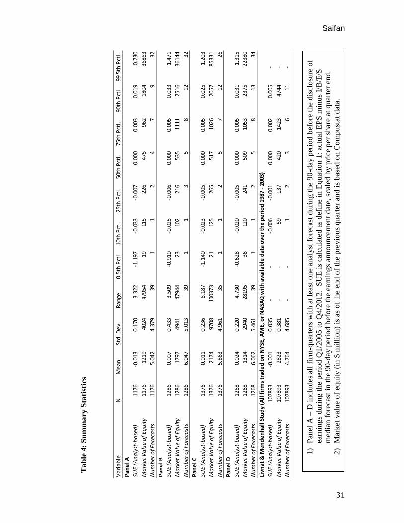
from the IPO universe in an identical fashion as described above. Table 4 provides

summary statistics for each panel as well as the summary statistics shown in Livnat and

Mendenhall’s (2004) PEAD study for comparative means.

As can be seen in the table, for all samples the mean and median SUE are close to

zero, and the distributions look relatively similar to one another. Also, note that SUE

exhibits a wide distribution with several extreme values, hence the need to classify SUE

into portfolios for the present analysis. In comparison to Livnat and Mendenhall’s

sample, which is significantly larger than my sample, IPOs exhibits a related distribution

to the panels within the interquartile range.

Saifan

31

Tab

le 4

: S

um

mary

Sta

tist

ics

1)

Pan

el A

– D

incl

udes

all

fir

m-q

uar

ters

wit

h a

t le

ast

one

anal

yst

fore

cast

duri

ng t

he

90

-day p

erio

d b

efore

the

dis

closu

re o

f

earn

ings

duri

ng t

he

per

iod Q

1/2

005 t

o Q

4/2

012. S

UE

is

calc

ula

ted a

s d

efin

e in

Equat

ion 1

: ac

tual

EP

S m

inus

I/B

/E/S

med

ian f

ore

cast

in t

he

90

-day p

erio

d b

efore

the

earn

ings

announ

cem

ent

dat

e, s

cale

d b

y p

rice

per

shar

e at

quar

ter

end.

2)

Mar

ket

val

ue

of

equit

y (

in $

mil

lion)

is a

s of

the

end o

f th

e pre

vio

us

quar

ter

and i

s bas

ed o

n C

om

pu

stat

dat

a.

Var

iab

leN

Me

anSt

d. D

ev.

Ran

ge0.

5th

Pct

l10

th P

ctl.

25th

Pct

l.50

th P

ctl.

75th

Pct

l.90

th P

ctl.

99.5

th P

ctl.

Pan

el A

SUE

(An

aly

st-b

ase

d)

1176

-0.0

130.

170

3.32

2-1

.197

-0.0

33-0

.007

0.00

00.

003

0.01

90.

730

Ma

rket

Va

lue

of

Equ

ity

1176

1219

4024

4795

419

115

226

475

962

1804

3686

3

Nu

mb

er o

f Fo

reca

sts

1176

5.04

24.

379

391

12

47

932

Pan

el B

SUE

(An

aly

st-b

ase

d)

1286

0.00

70.

433

3.50

9-0

.910

-0.0

25-0

.006

0.00

00.

005

0.03

31.

471

Ma

rket

Va

lue

of

Equ

ity

1286

1797

4941

4794

423

102

216

535

1111

2516

3614

4

Nu

mb

er o

f Fo

reca

sts

1286

6.04

75.

013

391

13

58

1232

Pan

el C

SUE

(An

aly

st-b

ase

d)

1376

0.01

10.

236

6.18

7-1

.140

-0.0

23-0

.005

0.00

00.

005

0.02

51.

203

Ma

rket

Va

lue

of

Equ

ity

1376

2174

9708

1003

7321

125

265

517

1026

2057

8533

1

Nu

mb

er o

f Fo

reca

sts

1376

5.86

34.

961

351

12

57

1226

Pan

el D

SUE

(An

aly

st-b

ase

d)

1268

0.02

40.

220

4.73

0-0

.628

-0.0

20-0

.005

0.00

00.

005

0.03

11.

315

Ma

rket

Va

lue

of

Equ

ity

1268

1314

2940

2819

536

120

241

509

1053

2375

2238

0

Nu

mb

er o

f Fo

reca

sts

1268

6.06

25.

461

391

12

58

1334

Livn

at &

Me

nd

en

hal

l Stu

dy

(All

fir

ms

trad

ed

on

NY

SE, A

ME,

or

NA

SAQ

wit

h a

vail

able

dat

a o

ver

the

pe

rio

d 1

987

- 20

03)

SUE

(An

aly

st-b

ase

d)

1078

93-0

.001

0.03

5-

--0

.006

-0.0

010.

000

0.00

20.

005

-

Ma

rket

Va

lue

of

Equ

ity

1078

9328

230.

381

--

5913

742

014

2347

44-

Nu

mb

er o

f Fo

reca

sts

1078

934.

764

4.68

5-

-1

23

611

-

Saifan

32

This is supportive of my sample as the related distribution suggests each panel is large

enough to produce reliable results. Conversely, all of the panels’ SUE display larger

kurtosis as they have fatter and wider distribution tails and a higher standard deviation

than the Livnat and Mendenhall example. I attribute this to the characteristics embedded

in IPO companies as opposed to a more normal distribution found in the full universe of

publically traded securities as used in the Livnat and Mendenhall (2005) paper. Lastly, it

is worth noting that my IPO sample, for all panels, revealed a greater number of forecasts

than the comprehensive Livnant and Mendenhall sample.

B. Magnitude of the Drift – Graphical Analysis

As discussed above and consistent with prior studies, I estimate the drift by

summing daily returns over the period from the day of the earnings announcement

through the day of the following quarterly earnings announcement date. Then I form

SUE portfolios by ranking the size of the SUE weighted by the market value of equity as

of the end of the previous quarter. Based on SUEs rank, it I classified into one of five

portfolios. Many prior studies classify SUE into 10 portfolios; however, since my sample

size is not as large, I rank them into five portfolios so that any outliers do not have an

overwhelming effect on the portfolio’s drift. Figures 2 – 5 present the CAR plots for

Panels A, B, C and D, respectively, after assigning firms on the basis on the standardized

unexpected earnings. Figures 2, 3, 4 and 5 show the performance of PEAD portfolios

formed based on analyst forecasted SUEs from Day 0 (the day of the announcement) to

the day +50 following the earnings announcement for Panels A, B, C and D, respectively.

Saifan

33

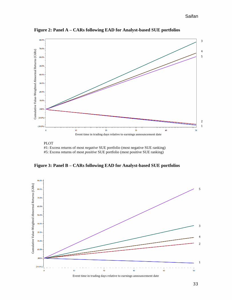
Figure 2: Panel A – CARs following EAD for Analyst-based SUE portfolios

Figure 3: Panel B – CARs following EAD for Analyst-based SUE portfolios

PLOT

#1: Excess returns of most negative SUE portfolio (most negative SUE ranking)

#5: Excess returns of most positive SUE portfolio (most positive SUE ranking)

3

4

5

2

1

3

4

5

2

1

Event time in trading days relative to earnings announcement date

Cu

mu

lati

ve V

alu

e-W

eigh

ted

Ab

no

rmal

Ret

urn

s (C

AR

s)

Cu

mu

lati

ve V

alu

e-W

eigh

ted

Ab

no

rmal

Ret

urn

s (C

AR

s)

Event time in trading days relative to earnings announcement date

Saifan

34

Figure 4: Panel C – CARs following EAD for Analyst-based SUE portfolios

Figure 5: Panel D – CARs following EAD for Analyst-based SUE portfolios

3

4

5

2

1

Event time in trading days relative to earnings announcement date

Cu

mu

lati

ve V

alu

e-W

eigh

ted

Ab

no

rmal

Ret

urn

s (C

AR

s)

3

4

5

2

1

Cu

mu

lati

ve V

alu

e-W

eigh

ted

Ab

no

rmal

Ret

urn

s (C

AR

s)

Event time in trading days relative to earnings announcement date

Event time in trading days relative to earnings announcement date

PLOT

#1: Excess returns of most negative SUE portfolio (most negative SUE ranking)

#5: Excess returns of most positive SUE portfolio (most positive SUE ranking)

Saifan

35

My results for post-earnings-announcement drift among IPO firms for 2005-2012

are drastically different than all of the other results obtained from prior PEAD studies

which focus generally on the aggregate U.S. equity market. There is a significantly

pronounced post-earnings-announcement drift – up to 25 times greater than the 18%

annualized return Bernard and Thomas (1989) suggested. However, prior studies have

concluded that there is post-earnings-announcement drift in the equity market that

increases monotonically in unexpected earnings. As Panels A – D illustrate, this is not

necessarily the case for an IPO sample. While there are similarities across the Panels, it

is clear that variation exists from panel to panel, particularly among SUE portfolio #5,

which represents the most positive SUE ranking. This provides evidence that certain

IPOs with extreme SUE values play a significant role in the magnitude and direction of

the drift.

Upon a closer examination of each individual panel, several interesting inferences

can be made. For instance, in Panel A, illustrated in Figure 2, the SUE portfolios diverge

into 2 distinct directions, positive or negative, without a single portfolio – including the

“zero earnings surprise” portfolio – trading around its initial stock price before an

earnings announcement. This suggests a couple of things: (1) analysts are unable to

adequately forecast earnings for IPO companies due to the lack of public information

available to them, thus there is almost always an earnings surprise; (2) Investors react

more strongly to earnings announcements by IPO firms than more stable, mature firms;

and/or (3) the systematic underpricing in IPOs allows the zero earnings portfolio

(portfolio #3) to drift upwards. Although Panel C supports these notions, they are non-

conclusive since Panel B and D are inconsistent with the findings.

Saifan

36

Panel B, illustrated in Figure 3, displays the most analogous monotonic drift

increase often found in other PEAD studies. Supporting my hypothesis, post-earnings-

announcement drift is intensely more pronounced among the IPO sample in relation to

prior studies. In their research, Bernard and Thomas (1989) find that a long position in

the highest unexpected earnings portfolio and a short position in the lowest portfolio

would have yielded an estimated abnormal return of 18% on an annualized basis for their

respective time period. Foster, Olsen and Shevlin (1984) trading on the same strategy

state an annualized abnormal return of 25%. Implementing an equivalent trading strategy

on Panel B would yield a whopping annualized abnormal return of 464% before

transaction costs. Equivalently, Panel A would yield 421%, Panel C would yield 59%,

and Panel D would yield 351% on an annualized basis before transaction costs. Across

all samples, the drift is dramatically more pronounced among IPO companies.

Panel C, illustrated in Figure 4, appears to be the most inconsistent result when

compared to the other samples. As shown, the most positive SUE portfolio is actually

accruing negative abnormal returns across 50 trading days since an earnings

announcement. I attribute this to the outliers in the sample with extreme SUE values. In

addition, it may be a result of creative accounting that is unfortunately not as rare as one

would expect. For example, Groupon, a recent hot tech IPO, has watched its value free-

fall from a $12.7 billion valuation in its IPO to as low as $3 billion. To catalyze its slide,

Groupon was accused of using “clever” valuation methods to help boost the company’s

earnings in the short-run, which includes but is not limited to, accounting for refunds,

recognizing income immediately, and using a statistic for total all-time customer orders

Saifan

37

in a quarterly results section.22 Refunds clearly have a large effect on earnings and, as a

result, Groupon had to restate Q4 2011 earnings to show a loss of $64.9 million dollars.

Since this analysis, similar to most prior studies, focuses on the original reported

earnings, a company can exhibit large positive unexpected earnings at the announcement

date while experiencing a dramatic decrease in its stock price. Moreover, this suggests

investors respond strongly to other factors, such as qualitative material weaknesses of a

company’s report, in addition to earnings.

Likewise, Panel D appears to have an outlier that plays an overwhelming role in

SUE portfolio #4, which represents somewhat-strong positive unexpected earnings.

Parallel to Panel C, an outlier with positive unexpected earnings experiences abnormal

growth that far exceeds SUE portfolio #5. This corroborates the inference that investors

respond strongly to a qualitative material strength factor in addition to positive earnings.

Also, note that this outlier causes the scale of Panel D to exceed the scale of the other

samples. With an exception of the outlier SUE portfolio, the remaining portfolios

magnitudes are consistent with the other samples.

C. Magnitude of the Drift – Comparison Analysis

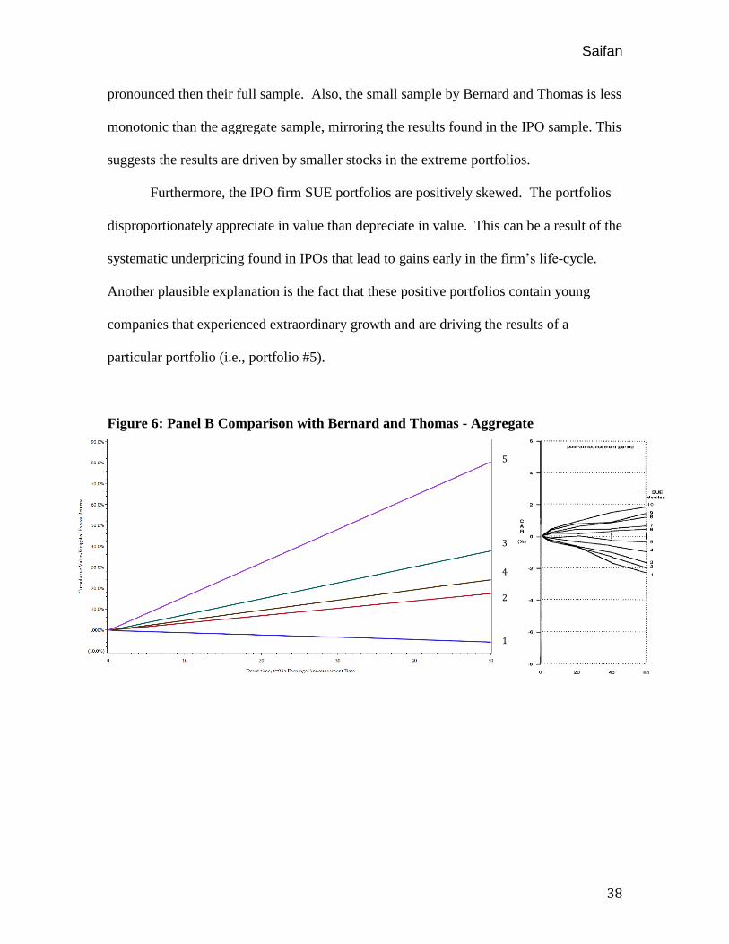
Figure 6 presents Panel B CARs for an IPO sample compared with Bernard and

Thomas’ (1989) CARs for SUE portfolios comprising NYSE/AMEX firms from 1974 to

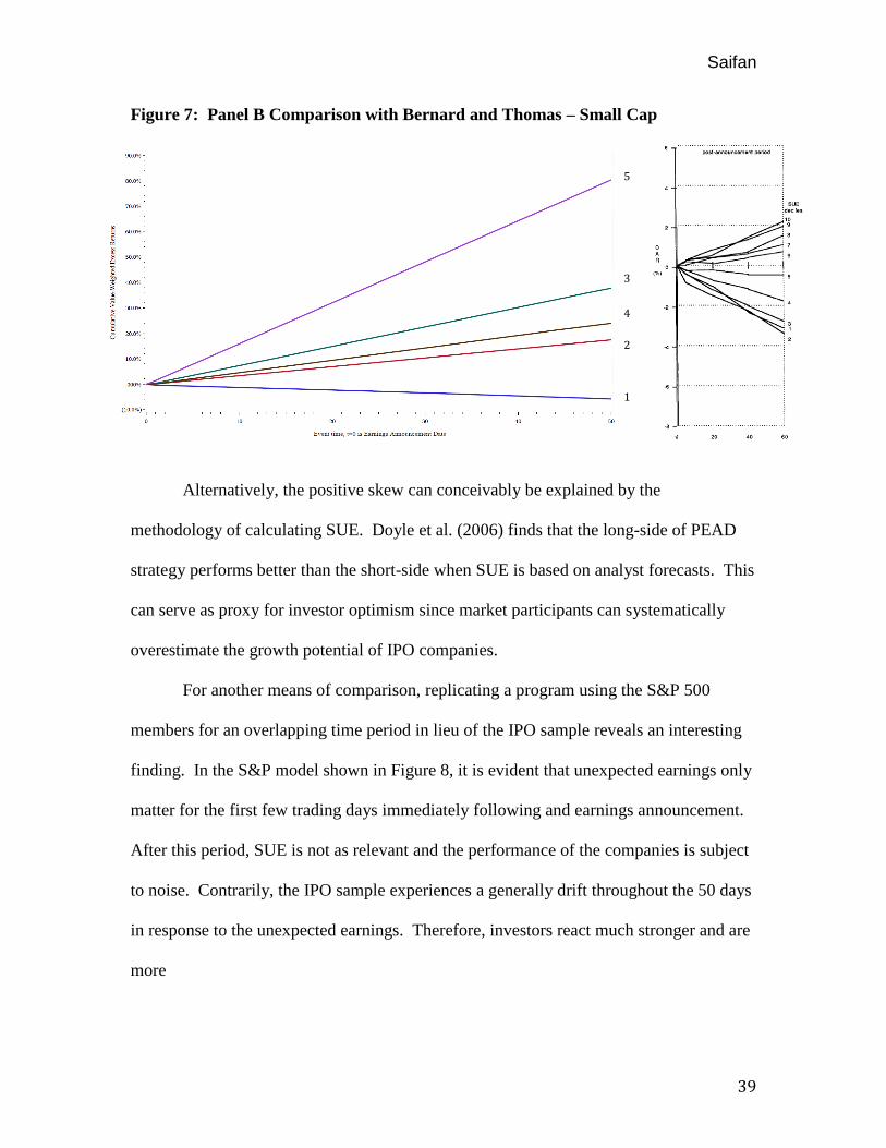
1986. Similarly, Figure 7 presents Panel B CARs compared with Bernard and Thomas’

(1989) CARs for SUE portfolios comprising only small (by market cap) NYSE/AMEX

firms. As shown, the IPO sample is distinctly more pronounced then both of Bernard and

Thomas’ samples, although Bernard and Thomas’ small-size subsample is more

22

Groupon ran into trouble with the Securities and Exchange Commission (SEC) after the SEC challenged

its accounting methodology on its S-1 registration form. Shortly after, Groupon’s founder and now-former

CEO, Andrew Mason, was fired.

Saifan

38

pronounced then their full sample. Also, the small sample by Bernard and Thomas is less

monotonic than the aggregate sample, mirroring the results found in the IPO sample. This

suggests the results are driven by smaller stocks in the extreme portfolios.

Furthermore, the IPO firm SUE portfolios are positively skewed. The portfolios

disproportionately appreciate in value than depreciate in value. This can be a result of the

systematic underpricing found in IPOs that lead to gains early in the firm’s life-cycle.

Another plausible explanation is the fact that these positive portfolios contain young

companies that experienced extraordinary growth and are driving the results of a

particular portfolio (i.e., portfolio #5).

Figure 6: Panel B Comparison with Bernard and Thomas - Aggregate

3

4

5

2

1

Saifan

39

3

4

5

2

1

Figure 7: Panel B Comparison with Bernard and Thomas – Small Cap

Alternatively, the positive skew can conceivably be explained by the

methodology of calculating SUE. Doyle et al. (2006) finds that the long-side of PEAD

strategy performs better than the short-side when SUE is based on analyst forecasts. This

can serve as proxy for investor optimism since market participants can systematically

overestimate the growth potential of IPO companies.

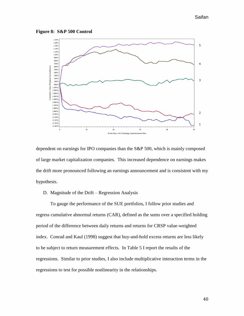
For another means of comparison, replicating a program using the S&P 500

members for an overlapping time period in lieu of the IPO sample reveals an interesting

finding. In the S&P model shown in Figure 8, it is evident that unexpected earnings only

matter for the first few trading days immediately following and earnings announcement.

After this period, SUE is not as relevant and the performance of the companies is subject

to noise. Contrarily, the IPO sample experiences a generally drift throughout the 50 days

in response to the unexpected earnings. Therefore, investors react much stronger and are

more

Saifan

40

Figure 8: S&P 500 Control

dependent on earnings for IPO companies than the S&P 500, which is mainly composed

of large market capitalization companies. This increased dependence on earnings makes

the drift more pronounced following an earnings announcement and is consistent with my

hypothesis.

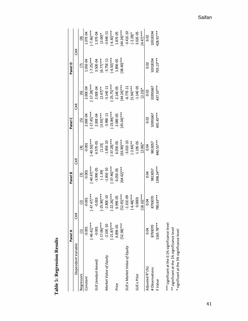
D. Magnitude of the Drift – Regression Analysis

To gauge the performance of the SUE portfolios, I follow prior studies and

regress cumulative abnormal returns (CAR), defined as the sums over a specified holding

period of the difference between daily returns and returns for CRSP value-weighted

index. Conrad and Kaul (1998) suggest that buy-and-hold excess returns are less likely

to be subject to return measurement effects. In Table 5 I report the results of the

regressions. Similar to prior studies, I also include multiplicative interaction terms in the

regressions to test for possible nonlinearity in the relationships.

1

2

3

4

5

Saifan

41

Pan

el A

Pan

el B

Pan

el C

Pan

el D

De

pe

nd

en

t V

aria

ble

CA

RC

AR

CA

RC

AR

Re

gre

sso

rs(1

)(2

)(3

)(4

)(5

)(6

)(7

)(8

)

Co

nst

an

t-0

.001

-0.0

01-0

.001

-0.0

012.

00E-

042.

00E-

041.

05E-

041.

07E-

04

[-46

.41]

***

[-47

.47]

***

[-40

.47]

***

[-40

.50]

***

[-17

.45]

***

[-17

.28]

***

[-7.

25]*

**[-

7.36

]***

SUE

(an

aly

st-b

ase

d)

-0.0

01-0

.003

-3.9

9E-0

56.

57E-

052.

00E-

042.

00E-

043.

50E-

041.

37E-

04

[-17

.06]

***

[-25

.90]

***

[-1.

39]

[1.2

3][3

.93]

***

[2.4

7]**

[6.7

7]**

*[2

.00]

*

Ma

rket

Va

lue

of

Equ

ity

-2.3

3E-1

0-2

.80E

-10

-1.8

5E-1

0-1

.85E

-10

-3.9

8E-1

1-5

.14E

-11

-3.7

5E-1

1-3

.64E

-11

[-21

.87]

***

[-22

.26]

***

[-37

.46]

***

[-37

.28]

***

[-23

.84]

***

[-25

.75]

***

[-6.

50]*

**[-

6.30

]***

Pri

ce6.

89E-

056.

99E-

056.

05E-

056.

05E-

052.

08E-

052.

14E-

051.

89E-

051.

87E-

05

[52.

38]*

**[5

2.05

]***

[64.

42]*

**[6

3.90

]***

[45.

04]*

**[4

4.24

]***

[38.

40]*

**[4

4.24

]***

SUE

x M

ark

et V

alu

e o

f Eq

uit

y-1

.31E

-09

-3.0

1E-1

0-6

.77E

-11

-3.4

1E-1

0

[-6.

48]*

**[-

2.84

]**

[5.9

4]**

*[-

2.28

]*

SUE

x P

rice

0.00

031.

19E-

05-1

.14E

-05

3.02

E-05

[18.

16]*

**[2

.06]

*[2

.23]

*[4

.47]

***

Ad

just

ed

R²

(%)

0.04

0.04

0.04

0.04

0.02

0.02

0.02

0.02

# O

bse

rvat

ion

s87

9307

087

9307

098

1305

798

1305

710

3916

6710

3916

6710

3181

9410

3181

94

F V

alu

e11

65.7

8***

780.

63**

*13

98.2

4***

840.

55**

*69

1.45

***

437.

33**

*70

3.13

***

428.

91**

*

***

sign

ific

ant

at t

he

0.1

% s

ign

ific

ance

leve

l

** s

ign

ific

ant

at t

he

1%

sig

nif

ican

ce le

vel

* si

gnif

ican

t at

th

e 5

% s

ign

ific

ance

leve

l

Tab

le 5

: R

egre

ssio

n R

esu

lts

Saifan

42

The results of previous research and those of Table 5 suggests that abnormal

returns are predictable on the basis of SUE, market value of equity (size), and stock price,

although the explanatory power is low at only .02 - .04% depending on the sample in

terms of adjusted R2. Across all samples with exception of Panel B, when the interaction

terms are excluded, SUE is statistically significant in predicting abnormal returns at the

0.1% significant level. However, notice in Panel A that SUE, unlike prior research, is a

small negative coefficient (statistically significant at the 0.1% significance level). While

it is not uncommon for young firms to produce negative earnings, it is plausible that

negative-earning firms experience appreciation in their stock price on the prospects of

future high growth. For example, a start-up company can be investing all of its capital

into a factory yielding negative earnings in the process; however, the intelligent investor

acknowledges this fact and is willing to overcome short-term loses for extraordinary

future growth. Nonetheless, in Panels C and D, the SUE coefficients are slightly positive,

but smaller in amount than prior studies. Lastly, price is slightly positive and statistically

significant at the 0.1% significance level across all samples.

In columns (2), (4), (6), and (8) I examine the ability of interaction effects in

addition to SUE to explain abnormal returns. Interestingly, the results suggest that

including interaction terms decreases the significance of the main SUE effect; however,

SUE still remains significant at the 1% and 5% significance level for Panel C and D,

respectively. Size and price maintain their original level of significance. Across all

samples, the interaction terms are at least statistically significant at the 5% significance

level. The F-tests shown in Table 5 confirm rejection of the joint hypothesis that each set

of all coefficients relating to SUE and SUE-interactions contains significant explanatory

Saifan

43

power. All F-tests are significant at the 0.1% significance level, indicating that SUE,

market value of equity and price are all significant effects across all panels.

In summary, the regression results show that SUE is statistically significant, but

the overall explanatory power in terms of adjusted R2 is low. Controlling for size and

security price, SUE interacts with size and security price to a significant degree but fails

to contribute any more explanatory power. Finally, the SUE coefficient is considerably

smaller in scale across the IPO sample than prior research, and interestingly negative in

Panel A. This suggests that investors may react to other qualitative material factors in

addition to unexpected earnings.

E. Longevity of the Drift

Bernard and Thomas (1989) examined the longevity of the drift and conclude

most of the drift occurs during the first 60 trading days (about three months) subsequent

to the earnings announcement. Moreover, they highlight that a disproportionately large

amount of the 60-day drift occurs within 3 days of the earnings announcement. Figure 9

illustrates post-earnings-announcement drift for a 3-day holding period in the Panel A

sample.

Interestingly, the IPO sample’s drift does not conclusively follow Bernard’s and

Thomas’ claim. Specifically, holding the drift constant for a 50-day interval, I would

expect 6% of the drift to arise within 3 days. The actual percentage of the 60-day that

occurs with 3 days is about 6.3%. This result is consistent among the other samples.

However, Bernard and Thomas demonstrate that the expected drift and actual drift

disparity is smaller in magnitude when smaller firms make up the sample. For instance,

they found a 12% disparity for large firms, 10% disparity for medium firms, and only a

Saifan

44

5% disparity for small firms. Since IPO firms tend to be smaller relative to the aggregate

U.S. equity market, my results are in line with Bernard’s and Thomas’ assumption.

Lastly, as Bernard and Thomas conclude, my results suggest that if the drift is explained

by an incomplete adjustment for risk, the risk must exist only temporarily and must

persist longer for small firms than for large firms.

Figure 9: Panel A PEAD Drift for Three-Day Holding Period

F. Test for Outliers

The results presented in this paper thus far have included firm-quarter

observations with extreme SUE values. While kurtosis among the IPO sample is

anticipated, certain observations are driving the SUE portfolios, particularly in Panels C

and D. To test the effect of outliers, I omit observations in the most extreme positive and

1 , 2

3

4

5

Saifan

45

negative 0.5% of all subsequent CARs (or approximately +/-100% SUE). This deletion

does not alter inferences in Panels A and B, but rather it causes SUE to become

statistically significant at the 0.1% level in the Panel B regression and the adjusted R2 to

increase from 0.04% to 0.05%.

Panel C without outliers is displayed in Figure 10. After deleting the extreme

observations, SUE portfolio #5 is vastly different than it appeared in Figure 4 where the

outliers are included. Panel C without outliers is much more

Figure 10: Panel C with Outliers Omitted

consistent with the other samples and increases in a monotonic fashion with increased

unexpected earnings. In addition, eliminating the outlier previously driving portfolio

#3’s irregular performance has put the portfolio in line with its expected ranking. Lastly,

the removed observations cause SUE’s significance level to increase in the regressions

and the adjusted R2 to increase from 0.02% to 0.03%.

1 , 2

3

4

5

Saifan

46

Analogous to Panel C, the Panel D drift, shown in Figure 11, changed immensely

after removing outliers. In the previous result, with outliers included, the most positive

SUE portfolio (#5) was being well outperformed by portfolio #4. Although portfolio #4

still outperforms portfolio #5, the discrepancy is much smaller. In addition, the excess

returns scale is now in line with the other panels, and the SUE coefficient increased in

magnitude with an increased level of significance. Finally, the adjusted R2 improved

from 0.02% to 0.07%.

FIGURE 11: Panel D with Outliers Omitted

Overall, I find suggestive evidence that the main drift results are sensitive to

outliers inherent in IPO companies. Nonetheless, I find that – with and without outliers –

many of the inferences formed in the present analysis are supportive of my hypothesis.

The IPO post-earnings-announcement drift is vividly more pronounced than the

NYSE/AMEX/NASDAQ sample frequently cited in prior PEAD studies.

1

2

3

4

5

Saifan

47

VI. Conclusions

The purpose of this paper is to assess potential differences in the magnitude and

pattern of post-earnings-announcement drift generated by portfolios formed on analyst

forecast-based earnings surprise. Specifically, I compare the drift among IPO firms in

the U.S. capital markets over the 2005 to 2012 period with prior drift research that

generally examine the aggregate U.S. capital markets.

The vast majority of drift studies find evidence that verify the existence of the

market anomaly and suggest a PEAD trading strategy yields excess returns of 18% on an

annualized basis. I show that the drift is significantly more pronounced when observing

all of the subsamples in the IPO population. I further show that even after removing

extreme values with which IPOs are associated, my inferences remain unchanged. I

attribute this pronounced drift chiefly to the underlying characteristics of IPO firms. In

detail, the aggregate U.S. equity market has a more normal distribution of unexpected

earnings, making 5-sigma events extremely rare. Conversely, I posit that the IPO market

experiences a much fatter and wider tail distribution, referred to as a kurtosis distribution.

This kurtosis distribution for IPOs can lead one to severely understate the true risk of a

particular company’s stock performance. Therefore, as the drift results documented in

this study show, extraordinary growth in a particular IPO can drive the results of a SUE

portfolio.

The results additionally suggest that there is another qualitative material factor, in

addition to unexpected earnings, that investors respond strongly to. This phenomenon is

illustrated by portfolios, principally portfolio #3 in the present paper, which represent

minimal earnings surprise. Across all samples, portfolio #3 has a positive drift and is

Saifan

48

significant in magnitude. Conversely, prior research describes the minimum SUE

portfolio as stagnant and, at times, showing a slightly negative drift. The performance of

portfolio #3 in relation with prior research suggests a couple of interesting discoveries:

(1) the drift can be attributed to the systematic underpricing of IPOs, which potentially

explains a positive drift when no earnings surprise is present; (2) young firms are

characteristically known to have little to no earnings in their growth stages, therefore

investors reward companies that do not report a loss. However, none of these findings

are conclusive.

I also show that the pattern of the drift around earnings announcement is

markedly different than that documented in previous studies. Specifically, prior research

documents portfolio returns that are equidistant from one portfolio to another. Put

differently, portfolio returns increase on a one-to-one basis with unexpected earnings.

Across the IPO samples, explicitly Panel A, the portfolio abnormal returns tend to

diverge into the positive and negative extremes. Panels C and D, once adjusted for

outliers, vaguely support this assertion. As mentioned previously, this may be an

indication that (1) analysts are unable to adequately forecast earnings for IPO companies

due to the lack of public information available to them, thus there is almost always an

earnings surprise; (2) investors react more strongly to earnings announcements by IPO

firms than more mature firms, even if the earnings surprise is low; or (3) investors are

displaying herd behavior and following the crowd. However, it is empirically difficult to

reconcile the herd behavior proposition since the drifts do not display any kinks or offer

any suggestion of a tipping point. Nonetheless, the findings indicate that inefficiency

exists in capital markets.

Saifan

49

Another noteworthy finding in regards to the pattern of the drift surrounding an

earnings announcement date is the positive skewness found among portfolio abnormal

returns. Consistent across all samples, the magnitude of the drift for the most positive

SUE portfolio significantly exceeds that of the drift for the most negative SUE portfolio.

Other PEAD research suggest a more evenly distributed drift with the most positive SUE

portfolio’s drift similar in magnitude with the that of the most negative SUE portfolio.

The present study’s effect can potentially be explained by a few stylized facts: (1) a

firm’s management can aim to keep future earnings guidance very conservative and, in

turn, analysts forecast conservative earnings, thus a firm can continuously experience

positive unexpected earnings23; (2) if a company has very aggressive analyst estimates

which is often the case for IPOs, and fails to reach those estimates, this does not

necessarily mean it is a bad company. Thus, a negative SUE portfolio can still

experience abnormal returns; (3) contrarily to (2) and akin to (1), if a company has very

conservative analyst estimates and reports positive unexpected earnings, a firm’s stock

can experience abnormal appreciation. Again, I cannot name any of these results to be

conclusive.

Overall, the findings that the drift is significantly larger when investigating the

IPO population and outliers and other qualitative factors may be playing a role in the drift

are critical to both researchers and investors. For researchers this poses the question of

what exactly determines the nature of the drift by exploring the firm-specific

23

Apple Computers, Inc. is a company that historically been known to systematically provide ultra

conservative estimates and, as a result, experience positive earnings surprise for several quarters in a row.

Eventually, analysts readjust their forecasts to higher estimates, ultimately predicting an ‘earnings surprise.’

Thus, a new equilibrium has been reached. In fact, Apple recently failed to ‘beat’ the inflated street

estimates causing the market to view this as a negative earnings surprise. This is a case of the delayed price

response hypothesis.

Saifan

50

characteristics that affect its magnitude and how important a kurtosis observation is in

driving abnormal portfolio returns. For investors who view the drift as a market anomaly

and hope to exploit it should use the earnings surprise signal for an IPO company that

announces earnings to yield abnormal returns.

Saifan

51

References

Abarbanell, J. S., & Bernard, V. L. (1992). Tests of analysts' overreaction/underreaction

to earnings information as an explanation for anomalous stock price behavior. The

Journal of Finance, 47(3), 1181-1207.

Affleck-Graves, J., & Mendenhall, R. R. (1992). The relation between the Value Line

enigma and post-earnings-announcement drift. Journal of Financial Economics, 31(1),

75-96.

Ball, R., & Brown, P. (1968). An empirical evaluation of accounting income numbers.

Journal of accounting research, 159-178.

Ball, R., Kothari, S. P., & Watts, R. L. (1993). Economic determinants of the relation

between earnings changes and stock returns. Accounting Review, 622-638.

Bartov, E., Givoly, D., & Hayn, C. (2002). The rewards to meeting or beating earnings

expectations. Journal of Accounting and Economics, 33(2), 173-204.

Bernard, V. L., & Thomas, J. K. (1989). Post-earnings-announcement drift: delayed price

response or risk premium?. Journal of Accounting research, 27, 1-36.

Booth, G. G., Kallunki, J. P., & Martikainen, T. (1996). POST‐ANNOUNCEMENT

DRIFT AND INCOME SMOOTHING: FINNISH EVIDENCE. Journal of Business

Finance & Accounting, 23(8), 1197-1211.

Bhushan, R. (1994). An informational efficiency perspective on the post-earnings

announcement drift. Journal of Accounting and Economics, 18(1), 45-65.

Brown, L., & Han, J. (1998). Do stock prices fully reflect the implications of current

earnings for future earnings for AR1 firms?.

Brown, S. J., & Pope, P. F. (1996). Post-earnings announcement drift?.

Brown, L. D., & Sivakumar, K. (2003). Comparing the value relevance of two operating

income measures. Review of Accounting Studies, 8(4), 561-572.

Chordia, T., A. Goyal, G. Sadka, R. Sadka, and L. Shivakumar. 2009. “Liquidity and the

post-earnings-announcement drift.” Financial Analysts Journal (65): 18-32.

Collins, D. W., & Hribar, P. (2000). Earnings-based and accrual-based market anomalies:

one effect or two?. Journal of Accounting and Economics, 29(1), 101-123.

Conrad, J., & Kaul, G. (1998). An anatomy of trading strategies. Review of Financial

Studies, 11(3), 489-519.

Saifan

52

Doyle, J. T., Lundholm, R. J., & Soliman, M. T. (2006). The extreme future stock returns

following I/B/E/S earnings surprises. Journal of Accounting Research, 44(5), 849-887.

Fama, E. F. (1998). Market efficiency, long-term returns, and behavioral finance. Journal

of financial economics, 49(3), 283-306.

Foster, G., Olsen, C., & Shevlin, T. (1984). Earnings releases, anomalies, and the

behavior of security returns. Accounting Review, 574-603.

Francis, J., Lafond, R., Olsson, P., & Schipper, K. (2007). Information Uncertainty and

Post‐Earnings‐Announcement‐Drift. Journal of Business Finance & Accounting,

34(3‐4), 403-433.

Freeman and Tse, 1989. “The Multiperiod Information Content of Accounting Earnings:

Confirmation and Contradictions of Previous Earnings Reports.” Journal of

Accounting Research 27: 49-84.

Hoberg, G. (2004). Strategic Underwriting in Initial Public Offers (No. 04-07). Yale ICF

Working Paper.

Kothari, S. P. (2001). Capital markets research in accounting. Journal of accounting and

economics, 31(1), 105-231.

Liang, L. (2003). Post-earnings announcement drift and market participants' information

processing biases. Review of Accounting Studies, 8(2-3), 321-345.

Liu, X., & Ritter, J. R. (2011). Local underwriter oligopolies and IPO underpricing.

Journal of Financial Economics, 102(3), 579-601.

Liu, W., Strong, N., & Xu, X. (2003). Post–earnings–announcement Drift in the UK.

European Financial Management, 9(1), 89-116.

Livnat, J., & Mendenhall, R. R. (2006). Comparing the post–earnings announcement drift

for surprises calculated from analyst and time series forecasts. Journal of Accounting

Research, 44(1), 177-205.

Mikhail, M. B., Walther, B. R., & Willis, R. H. (2003). The effect of experience on

security analyst underreaction. Journal of Accounting and Economics, 35(1), 101-116.

Narayanamoorthy, G. (2006). Conservatism and Cross‐Sectional Variation in the Post–

Earnings Announcement Drift. Journal of Accounting Research, 44(4), 763-789.

Ng, J., Rusticus, T. O., & Verdi, R. S. (2008). Implications of transaction costs for the

post–earnings announcement drift. Journal of Accounting Research, 46(3), 661-696.

Saifan

53

Payne, J. L., & Thomas, W. B. (2003). The implications of using stock-split adjusted

I/B/E/S data in empirical research. The Accounting Review, 78(4), 1049-1067.

Ritter, J. (2011). Equilibrium in the IPO Market. Available at SSRN 1822542.

Ritter, J. R. (1991). The long‐run performance of initial public offerings. The journal of

finance, 46(1), 3-27.

Wurgler, J., & Zhuravskaya, E. (2002). Does Arbitrage Flatten Demand Curves for

Stocks?*. The Journal of Business, 75(4), 583-608.

Saifan

54

APPENDIX

Item 1 – Overview of Prior Studies

Authors Market Time

Period

Portfolio

Construction

Holding

Period

Earnings

Metric

Expected

Earnings

Return

Metric

Risk

Control

PEAD

Return

Long

Position

Drift

Direction

Short

Position

Drift

Direction

This Paper US

IPOs 2005-2012

Event-time 50 days Reported Earnings

Analyst forecasts

CAR

CRSP

value-

weighted

59+% annualized

Positive Negative

Bernard

and

Thomas (1989)

US 1974-

1986 Event-time

240

days

Reported

Earnings

Time-series

model

CAR size-

adjusted

18%

annualized positive negative

Bernard et

al. (1997) US

1973-

1992 Event-time

8

Quarters

Reported

Earnings

Time-

series model

CAR Market-

adjusted

Drift

statistically significant

not reported not reported

Booth et al.

(1996) Finland

1990-

1993 Event-time 10 days

Aggregated

reported earnings

not

reported CAR CAPM

not

reported positive negative

Chorida et.

al (2009) US

1972-

2005

Calendar-

time

3

months

Reported

Earnings

Time-series

model

CAR

Three-factor

and a

liquidity factor

model

Liquid: 0.04% per

month;

Illiquid: 2.43% per

month

positive negative

Kothari et al. (2001)

US 1970-2000

Calendar-time

4 quarters

Aggregated

reported

earnings

Time-

series

model

CAR B/M-

adjusted 3-4% per quarter

not reported not reported

Liu et al. (2003)

UK 1988-1998

Calendar-time

3,6,9,12 months

Reported Earnings

Analyst forecasts

& Time-

series model

BHAR

& monthly

alpha

Three-

factor

model

BHAR: 10.8%;

Monthly

alpha: 0.706%

inconclusive inconclusive

Livnat and

Mendenhall

(2006)

US 1987-2003

not reported 4

quarters Reported Earnings

Analyst forecasts

& Time-

series model

CAR

Size and

B/M-

adjusted

5.21% per quarter

not reported not reported

Saifan

55

Item 2 – iClink Script – common code for all main programs creating iclink and sue_final

************************************************************************

*********************

** FileName: iclink.sas **

** Date: Sept 25, 2006 **

** Author: Rabih Moussawi **

** Description: Create IBES - CRSP Link Table **

** FUNCTION: - Creates a link table between IBES TICKER and CRSP PERMNO

**

** - Scores links from 0 (best link) to 6 **

** **

** INPUT: **

** - IBES: IDUSM file **

** - CRSP: STOCKNAMES file **

** **

** OUTPUT: ICLINK set stored in home directory **

** ICLINK has 15,187 unique IBES TICKER - CRSP PERMNO links

**

** ICLINK contains IBES TICKER and the matching CRSP PERMNO and other

fields: **

** - IBES and CRSP Company names **

** - SCORE variable: lower scores are better and high scores may need further

**

** checking before using them to link CRSP & IBES data. **

** In computing the score, a CUSIP match is considered better than a **

** TICKER match. The score also includes a penalty for differences in **

** company names-- CNAME in IBES and COMNAM in CRSP. The name

penalty is **

** based upon SPEDIS, which is the spelling distance function in SAS. **

** SPEDIS(cname,comnam)=0 is a perfect score and SPEDIS < 30 is usually

good **

** enough to be considered a name match. **

** **

** "SCORE" levels: **

** - 0: BEST match: using (cusip, cusip dates and company names) **

** or (exchange ticker, company names and 6-digit cusip) **

** - 1: Cusips and cusip dates match but company names do not match **

** - 2: Cusips and company names match but cusip dates do not match **

** - 3: Cusips match but cusip dates and company names do not match **

** - 4: Exch tickers and 6-digit cusips match but company names do not match

**

** - 5: Exch tickers and company names match but 6-digit cusips do not match

**

** - 6: Exch tickers match but company names and 6-digit cusips do not match

**

Saifan

56

** **

** ICLINK Example: **

** TICKER CNAME PERMNO COMNAM SCORE

**

** BAC BANKAMERICA CORPORATION 58827 BANKAMERICA CORP

0 **

** DELL DELL INC 11081 DELL INC 0 **

** FFS 1ST FED BCP DEL 75161 FIRST FEDERAL BANCORP DE

3 **

** IBM INTERNATIONAL BUSINESS MACHINES 12490 INTERNATIONAL

BUSINESS MACHS CO 0 **

** MSFT MICROSOFT CORP 10107 MICROSOFT CORP 0

**

** **

************************************************************************

*********************

;;;

** Possible IBES ID (names) file to use (as of April 2006);

** Detail History: ID file : 23808 unique US and Canadian company IBES TICKERs;

** Summary History: IDSUM File: 15576 unique US company IBES TICKERs;

** Recommendation Summary Statistics: RECDSUM File 12465 unique US company

IBES tickers;

** It seems that the Summary History Identifier file IDSUM is best

** because USFIRM dummy is used to designate only US companies;

*x %let IBES1= IBES.IDSUM;

*x %let CRSP1= CRSP.STOCKNAMES;

*x libname home '~'; * Save link table in home directory;

** Step 1: Link by CUSIP **

** IBES: Get the list of IBES TICKERS for US firms in IBES **;

proc sort data=&IBES1 out=IBES1 (keep=ticker cusip CNAME sdates);

where USFIRM=1 and not(missing(cusip));

by ticker cusip sdates;

run;

** Create first and last 'start dates' for CUSIP link **;

proc sql;

create table IBES2

as select *, min(sdates) as fdate, max(sdates) as ldate

from IBES1

group by ticker, cusip

order by ticker, cusip, sdates;

quit;

Saifan

57

** Label date range variables and keep only most recent company name for CUSIP link

**;

data IBES2;

set IBES2;

by ticker cusip;

if last.cusip;

label fdate="First Start date of CUSIP record";

label ldate="Last Start date of CUSIP record";

format fdate ldate date9.;

drop sdates;

run;

** CRSP: Get all PERMNO-NCUSIP combinations **;

proc sort data=&CRSP1 out=CRSP1 (keep=PERMNO NCUSIP comnam namedt

nameenddt);

where not missing(NCUSIP);

by PERMNO NCUSIP namedt;

run;

** Arrange effective dates for CUSIP link **;

proc sql;

create table CRSP2

as select PERMNO,NCUSIP,comnam,min(namedt)as namedt,max(nameenddt) as

nameenddt

from CRSP1

group by PERMNO, NCUSIP

order by PERMNO, NCUSIP, NAMEDT;

quit;

** Label date range variables and keep only most recent company name **;

data CRSP2;

set CRSP2;

by permno ncusip;

if last.ncusip;

label namedt="Start date of CUSIP record";

label nameenddt="End date of CUSIP record";

format namedt nameenddt date9.;

run;

** Create CUSIP Link Table ** ;

** CUSIP date ranges are only used in scoring as CUSIPs are not reused for

different companies overtime **;

proc sql;

create table LINK1_1

as select *

from IBES2 as a, CRSP2 as b

Saifan

58

where a.CUSIP = b.NCUSIP

order by TICKER, PERMNO, ldate;

quit; * 14,591 IBES TICKERs matched to CRSP PERMNOs;

** Score links using CUSIP date range and company name spelling distance **;

** Idea: date ranges the same cusip was used in CRSP and IBES should intersect **;

data LINK1_2;

set LINK1_1;

by TICKER PERMNO;

if last.permno; * Keep link with most recent company name;

name_dist = min(spedis(cname,comnam),spedis(comnam,cname));

if (not ((ldate<namedt) or (fdate>nameenddt))) and name_dist < 30 then SCORE = 0;

else if (not ((ldate<namedt) or (fdate>nameenddt))) then score = 1;

else if name_dist < 30 then SCORE = 2;

else SCORE = 3;

keep TICKER PERMNO cname comnam score;

run;

** Step 2: Find links for the remaining unmatched cases using Exchange Ticker **;

** Identify remaining unmatched cases **;

proc sql;

create table NOMATCH1

as select distinct a.*

from IBES1 (keep=ticker) as a

where a.ticker NOT in (select ticker from LINK1_2)

order by a.ticker;

quit; * 990 IBES TICKERs not matched with CRSP PERMNOs using CUSIP;

** Add IBES identifying information **;

proc sql;

create table NOMATCH2

as select b.ticker, b.CNAME, b.OFTIC, b.sdates, b.cusip

from NOMATCH1 as a, &IBES1 as b

where a.ticker = b.ticker and not (missing(b.OFTIC))

order by ticker, oftic, sdates;

quit; * 4,157 observations;

** Create first and last 'start dates' for Exchange Tickers **;

proc sql;

create table NOMATCH3

as select *, min(sdates) as fdate, max(sdates) as ldate

from NOMATCH2

group by ticker, oftic

order by ticker, oftic, sdates;

quit;

Saifan

59

** Label date range variables and keep only most recent company name **;

data NOMATCH3;

set NOMATCH3;

by ticker oftic;

if last.oftic;

label fdate="First Start date of OFTIC record";

label ldate="Last Start date of OFTIC record";

format fdate ldate date9.;

drop sdates;

run;

** Get entire list of CRSP stocks with Exchange Ticker information **;

proc sort data=&CRSP1 out=CRSP1 (keep=ticker comnam permno ncusip namedt

nameenddt);

where not missing(ticker);

by permno ticker namedt;

run;

** Arrange effective dates for link by Exchange Ticker **;

proc sql;

create table CRSP2

as select permno,comnam,ticker as crsp_ticker,ncusip,

min(namedt)as namedt,max(nameenddt) as nameenddt

from CRSP1

group by permno, ticker

order by permno, crsp_ticker, namedt;

quit; * CRSP exchange ticker renamed to crsp_ticker to avoid confusion with IBES

TICKER;

** Label date range variables and keep only most recent company name **;

data CRSP2;

set CRSP2;

if last.crsp_ticker;

by permno crsp_ticker;

label namedt="Start date of exch. ticker record";

label nameenddt="End date of exch. ticker record";

format namedt nameenddt date9.;

run;

** Merge remaining unmatched cases using Exchange Ticker **;

** Note: Use ticker date ranges as exchange tickers are reused overtime **;

proc sql;

create table LINK2_1

as select a.ticker,a.oftic, b.permno, a.cname, b.comnam, a.cusip, b.ncusip, a.ldate

from NOMATCH3 as a, CRSP2 as b

where a.oftic = b.crsp_ticker and

Saifan

60

(ldate>=namedt) and (fdate<=nameenddt)

order by ticker, oftic, ldate;

quit; * 146 new match of 136 IBES TICKERs;

** Score using company name using 6-digit CUSIP and company name spelling distance

**;

data LINK2_2;

set LINK2_1;

name_dist = min(spedis(cname,comnam),spedis(comnam,cname));

if substr(cusip,1,6)=substr(ncusip,1,6) and name_dist < 30 then SCORE=0;

else if substr(cusip,1,6)=substr(ncusip,1,6) then score = 4;

else if name_dist < 30 then SCORE = 5;

else SCORE = 6;

run;

** Some companies may have more than one TICKER-PERMNO link, **;

** so re-sort and keep the case (PERMNO & Company name from CRSP) **;

** that gives the lowest score for each IBES TICKER (first.ticker=1) **;

proc sort data=LINK2_2; by ticker score; run;

data LINK2_3;

set LINK2_2;

by ticker score;

if first.ticker;

keep ticker permno cname comnam permno score;

run;

** Step 3: Add Exchange Ticker links to CUSIP links ** ;

** Create final link table and save it in home directory **;

data home.&ICLINK;

set LINK1_2 LINK2_3;

run;

proc sort data=home.&ICLINK; by TICKER PERMNO; run;

** Create Labels for ICLINK dataset and variables **;

proc datasets lib=home nolist;

modify &ICLINK (label="IBES-CRSP Link Table");

label CNAME = "Company Name in IBES";

label COMNAM= "Company Name in CRSP";

label SCORE= "Link Score: 0(best) - 6";

run;

quit;

Saifan

61

Item 3 – Common code for all main program s creating CAR plots

** master2b2.inc

Master code include

au: pmn 4/13

ou: pgm_pead_sue3.pdf

***********************************************************

;;;

** Extract file of raw daily returns around and between EADs and link them **

** to Standardized Earnings Surprises for forming SUE-based portfolios **

;;;

proc sql;

create view crsprets

as select a.permno, a.prc, a.date, abs(a.prc*a.shrout) as mcap,

b.rdq1, b.leadrdq1, b.sue1, b.sue2, b.sue3, a.ret,

c.vwretd as mkt, (a.ret-c.vwretd) as exret

/*xfrom crsp.dsf (where=("&bdate"d<=date<="&edate"d)) a inner join */

from crsp.&dsf_in (where=("&bdate"d<=date<="&edate"d)) a inner join

sue_final (where=(nmiss(rdq, leadrdq1, permno)=0 and leadrdq1-rdq1>30)) b

on a.permno=b.permno and b.rdq1-5<=a.date<=b.leadrdq1+5

/*xleft join crspq.dsi (keep=date vwretd) c */

left join crsp.&dsi_in (keep=date vwretd) c

on a.date=c.date

order by a.permno, b.rdq1, a.date;

quit;

** To estimate the drift, sum daily returns over the period from **

** 1 day after the earnings announcement through the day of **

** the following quarterly earnings announcement **

;;;

data temp/view=temp; set crsprets;

by permno rdq1 date;

lagmcap=lag(mcap);

if first.permno then lagmcap=.;

if date=rdq1 then count=0;

else if date>rdq1 then count+1;

format date date9. exret percent7.4;

if rdq1<=date<=leadrdq1;

run;

proc print data=temp(obs=200);

Saifan

62

title2 'Review temp view';

run;

proc sort data=temp out=peadrets nodupkey; by count permno rdq1;run;

proc rank data=peadrets out=peadrets groups=5;

by count; var sue1 sue2 sue3;

ranks sue1r sue2r sue3r;

run;

proc print data=peadrets(obs=50);

title2 'Review peadrets';

run;

**form portfolios on Compustat-based SUEs (=sue1 or =sue2) or IBES-based SUE

(=sue3)**

;;;

%let sue=sue3;

proc sort data=peadrets (where=(not missing(&sue))) out=pead&sue; by count

&sue.r;run;

proc print data=pead&sue(obs=50);

title2 "pead&sue";

run;

proc freq data=pead&sue;

; where lagmcap = .;

; tables exret &sue.r;

title2 "pead&sue";

title3 'where lagmcap = .';

run;

proc print data=pead&sue n;

; where lagmcap = .;

title2 "pead&sue";

title3 'where lagmcap = .';

run cancel;

data reg&sue;

; set pead&sue;

sue3_mcap = sue3 * mcap;

sue3_prc = sue3 * prc;

run;

Saifan

63

proc reg data=reg&sue;

; model exret = sue3 mcap prc;

; model exret = sue3 mcap prc sue3_mcap;

; model exret = sue3 mcap prc sue3_prc;

; model exret = sue3 mcap prc sue3_mcap sue3_prc;

title2 "Analyze reg&sue";

run;

proc means data=pead&sue noprint;

by count &sue.r;

var exret; weight lagmcap;

output out=pead&sue.port mean=/autoname;

run;

proc transpose data=pead&sue.port out=pead&sue.port;

by count; id &sue.r;

var exret_mean;

run;

data pead&sue.port; set pead&sue.port ;

if count=0 then do;

_0=0;_1=0;_2=0;_3=0;_4=0;end;

label

_0='Rets of Most negative SUE port' _1='Rets of SUE Portfolio #2'

_2='Rets of SUE Portfolio #3' _3='Rets of SUE Portfolio #4'

_4='Rets of most positive SUE port';

drop _name_;

run;

**Cumulating Excess Returns**

;;;

proc expand data=pead&sue.port out=pead&sue.port;

id count; where count<=3;

convert _0=sueport1/transformout=(sum);

convert _1=sueport2/transformout=(sum);

convert _2=sueport3/transformout=(sum );

convert _3=sueport4/transformout=(sum);

convert _4=sueport5/transformout=(sum);

quit;

options nodate orientation=landscape;

ods pdf file="&pgm._PEAD_&sue..pdf";

goptions device=pdfc; /* Plot Saved in Home Directory */

axis1 label=(angle=90 "Cumulative Value-Weighted Excess Returns");

axis2 label=("Event time, t=0 is Earnings Announcement Date");

Saifan

64

symbol interpol=join w=4 l=1;

proc gplot data =pead&sue.port;

Title 'CARs following EAD for Analyst-based SUE portfolios';

Title2 'IPO Period: 2005-2012';

Title3 "Sample: &ttltxt.% sample";

plot (sueport1 sueport2 sueport3 sueport4 sueport5)*count

/overlay legend vaxis=axis1 haxis=axis2;

run;

quit;

ods pdf close;

**house cleaning**

;;;

proc sql;

drop view crsprets, ibes_temp, temp, tradedates, sue, eads1;

drop table iclink, medest, ibes, ibes1, comp, ibes_anndats, pead&sue.;

quit;

Saifan

65

Item 4 - Main program used to creat iclink and sue_final using iclink

** smp33b_master2a.sas

Master code with 33b% sample

au: pmn 2/13

rv: pmn 3/13

pmn 4/13

ou: iclink_&suffix

sue_final_&suffix

***********************************************************

;;;

%let pgm = smp33b_master2a

;;;

%let suffix = smp33b

;;;

footnote "pgm: &pgm";

options source2;

options mprint symbolgen;

***********************************************************;

** get setup

***********************************************************;

%include "sami.inc";

***********************************************************;

** identify datasets

***********************************************************;

%let IBES_in = ibesdetu_smp_33b;

%let CRSP_in = crspdaily_smp_33b;

%let ccmxpf_linktable = ccmlinktable_smp_33b;

%let Security = compufunda_smp_33b;

%let CompA_in = &security;

%let FUNDQ_in = compufundq_smp_33b;

%let ACTU_in = ibesactu_smp_33b;

%let DETU_in = &ibes_in;

%let DSF_in = &crsp_in;

%let DSI_in = &crsp_in;

Saifan

66

ods rtf file="&pgm..rtf" style=minimal;

***********************************************************;

** review input data

***********************************************************;

%let sd7lst =

test_ibesunadj_COMP *

test_CRSPdaily_COMP *

ccmxpf_linktable *

test_compustat_qtr_all *

test_compustat_anl_all *

test_ibes_actu

;;;

%macro infoem;

%do i = 1 %to 6;

%let sd7var = %scan(&sd7lst,&i,'*');

proc contents data=sd7src.&sd7var;

title2 "&sd7var";

run;

proc print data=sd7src.&sd7var(obs=5) uniform;

title2 "&sd7var";

run;

%end;

%mend;

run;

*%infoem;

run;

***********************************************************;

** assign dates

***********************************************************;

%let start_in = mdy(01,01,2005); /** start calendar date of fiscal period end */

%let end_in = mdy(12,31,2012); /** end calendar date of fiscal period end */

%let bdate=01JAN2005;

%let edate=31DEC2012;

%let begdt=&start_in;

%let enddt=&end_in;

%let begdate=&start_in;

Saifan

67

%let enddate=&end_in;

%let begindate=&start_in;

%let enddate=&end_in;

***********************************************************;

** set up input datasets

***********************************************************;

data ibes_src;

; set sd7src.&ibes_in;

format sdates mmddyy10.;

sdates = anndats;

usfirm = 1;

run;

proc print data=ibes_src(obs=50);

title2 'Review ibes_src';

run;

data crsp_src;

; set sd7src.&crsp_in;

format namedt mmddyy10.;

namedt = date;

nameenddt = nameendt;

run;

proc print data=crsp_src(obs=50);

title2 'Review crsp_src';

run;

proc sort data=sd7src.&compa_in(where=(tic ne ' '))

out=idxcst_his(keep=gvkey)

nodupkey

; by gvkey;

run;

proc print data=idxcst_his;

title2 'idxcst_his';

run;

%let IBES1= ibes_src;

%let CRSP1= crsp_src;

%let ICLINK = iclink_&suffix;

Saifan

68

%include "&libinc\iclink.inc";

data iclink;

; set home.&iclink;

run;

******************************************************************************

****

** Summary : Calculates quarterly standardized earnings surprises (SUE) based

** on time-series (seasonal random walk model) and analyst EPS forecasts

** using methodology in Livnat and Mendenhall (JAR, 2006)

** Forms SUE-based portfolios,compares drift across Compustat and IBES

** based earnings surprise definitions and across different time periods

**

** Date : February 2008, Modified: Sep, 2011

** Author : Denys Glushkov, WRDS

** Input : SAS dataset containing a set of gvkeys which constitute the universe

** of interest. Application uses members of S&P 500 index as

** an illustrative example. Users can easily substitute their own file

** E.g., gvkeyx='030824' is index for S&P 600 SmallCap index

**

** Variables : - SUE1: SUE based on a rolling seasonal random walk model (LM,p. 185)

** - SUE2: SUE accounting for exclusion of special items

** - SUE3: SUE based on IBES reported analyst forecasts and actuals

** - BEGINDATE: Sample Start Date

** - ENDDATE: Sample End Date

**

** To run the program, a user should have access to CRSP daily and monthly stock,

** Compustat Annual and Quarterly sets, IBES and CRSP/Compustat Merged database

**

******************************************************************************

***

;;;

*%let bdate=01jan1980; **start calendar date of fiscal period end

*%let edate=30jun2011; **end calendar date of fiscal period end

**CRSP-IBES link**

*x %iclink;* (ibesid=ibes.id, crspid=crspq.stocknames, outset=work.iclink);

** Step 1. All companies that were ever included in S&P 500 index as an example **

** Linking Compustat GVKEY and IBES Tickers using ICLINK **

** For unmatched GVKEYs, use header IBTIC link in Compustat Security file **

;;;

proc sql; create table gvkeys

as select

distinct a.gvkey

, b.lpermco as permco

, b.lpermno as permno

, coalesce (b.linkenddt,'31dec9999'd) as linkenddt format date9.

/*x, coalesce (d.ticker, c.ibtic) as ticker */

Saifan

69

, d.ticker as ticker

, b.linkdt format date9.

/*x from comp.idxcst_his (where=(gvkeyx='000003')) a */

from idxcst_his a

/*x left join crsp.ccmxpf_linktable */

left join crsp.&ccmxpf_linktable

(where=(usedflag=1 and linkprim in ('P','C'))) b

on a.gvkey=b.gvkey

left join comp.&security c

on a.gvkey=c.gvkey

left join iclink (where=(score in (0,1))) d

on b.lpermno=d.permno

order by gvkey, linkdt, ticker;

quit;

proc print data=gvkeys;

title2 'review gvkeys';

run;

data gvkeys; set gvkeys(where=(ticker ne ' '));

by gvkey linkdt ticker;

if last.linkdt;

run;

** Extract estimates from IBES Unadjusted file and select **

** the latest estimate for a firm within broker-analyst group **

** "fpi in (6,7)" selects quarterly forecast for the current **

** and the next fiscal quarter **

;;;

proc sql;

create view ibes_temp

as select a.*, b.permno

/*x from ibes.detu_epsus a, */

from ibes.&detu_in a,

(select distinct ticker,permno,

min(linkdt) as mindt,max(linkenddt) as maxdt

from gvkeys group by ticker, permno) b

where a.ticker=b.ticker and b.mindt<=a.anndats<=b.maxdt

and "&bdate"d<=fpedats<="&edate"d and fpi in ('6','7');

**Count number of estimates reported on primary/diluted basis **

;;;

create table ibes

as select a.*, sum(pdf='P') as p_count, sum(pdf='D') as d_count

from ibes_temp a

group by ticker, fpedats

order by ticker,fpedats,estimator,analys,anndats,revdats,anntims,revtims;

quit;

** Determine whether most analysts report estimates on primary/diluted basis**

** following Livnat and Mendenhall (2006) **

Saifan

70

;;;

data ibes; set ibes;

by ticker fpedats estimator analys;

if nmiss(p_count, d_count)=0 then do;

if p_count>d_count then basis='P'; else basis='D'; end;

if last.analys; /*Keep the latest observation for a given analyst*/

keep ticker value fpedats anndats revdats estimator

analys revtims anntims permno basis;

run;

** Link Unadjusted estimates with Unadjusted actuals and CRSP permnos **

** Keep only the estimates issued within 90 days before the report date**

;;;

proc sql;

create table ibes1

(where=(nmiss(repdats, anndats)=0 and 0<=repdats-anndats<=90))

as select a.*, b.anndats as repdats, b.value as act

/*x from ibes as a left join ibes.actu_epsus as b */

from ibes as a left join ibes.&actu_in as b

on a.ticker=b.ticker and a.fpedats=b.pends and b.pdicity='QTR';

** select all relevant combinations of Permnos and Date**

;;;

create table ibes_anndats

as select distinct permno, anndats

from ibes1

union

select distinct permno, repdats as anndats

from ibes1;

** Adjust all estimate and earnings announcement dates to the closest **

** preceding trading date in CRSP to ensure that adjustment factors wont **

** be missing after the merge **

;;;

create view tradedates

as select a.anndats, b.date format=date9.

from (select distinct anndats from ibes_anndats

where not missing(anndats)) a

/*x left join (select distinct date from crspq.dsi) b */

left join (select distinct date from crsp.&dsi_in) b

on 5>=a.anndats-b.date>=0

group by a.anndats

having a.anndats-b.date=min(a.anndats-b.date);

** merge the CRSP adjustment factors for all estimate and report dates **

;;;

create table ibes_anndats

as select a.*, c.cfacshr

from ibes_anndats a left join tradedates b

on a.anndats=b.anndats

/*x left join crspq.dsf (keep=permno date cfacshr) c */

Saifan

71

left join crsp.&dsf_in (keep=permno date cfacshr) c

on a.permno=c.permno and b.date=c.date;

** Put the estimate on the same per share basis as **

** company reported EPS using CRSP Adjustment factors. New_value is the **

** estimate adjusted to be on the same basis with reported earnings **

;;;

create table ibes1

as select a.*, (c.cfacshr/b.cfacshr)*a.value as new_value

from ibes1 a, ibes_anndats b, ibes_anndats c

where (a.permno=b.permno and a.anndats=b.anndats)

and (a.permno=c.permno and a.repdats=c.anndats);

quit;

** Sanity check: there should be one most recent estimate for **

** a given firm-fiscal period end combination **

;;;

proc sort data=ibes1 nodupkey; by ticker fpedats estimator analys;

run;

** Compute the median forecast based on estimates in the 90 days prior to the EAD**

;;;

proc means data=ibes1 noprint;

by ticker fpedats; id basis;

var new_value; id repdats act permno;

output out= medest (drop=_type_ _freq_)

median=medest n=numest;

run;

** Extracting Compustat Data and merging it with IBES consensus **

;;;

proc sql;

create table comp

(keep=gvkey fyearq fqtr conm datadate rdq epsfxq epspxq

prccq ajexq spiq cshoq prccq ajexq spiq cshoq mcap /**Compustat variables**/

cshprq cshfdq rdq saleq atq fyr datafqtr

permno ticker medest numest repdats act basis) /**CRSP and IBES vars **/

as select *, (a.cshoq*a.prccq) as mcap

from comp.&fundq_in

(where=((not missing(saleq) or atq>0) and consol='C' and

popsrc='D' and indfmt='INDL' and datafmt='STD' and not missing(datafqtr))) a

inner join

(select distinct gvkey, ticker, min(linkdt) as mindate,

max(linkenddt) as maxdate from gvkeys group by gvkey, ticker) b

on a.gvkey=b.gvkey and b.mindate<=a.datadate<=b.maxdate

left join medest c

on b.ticker=c.ticker and put(a.datadate,yymmn6.)=put(c.fpedats,yymmn6.);

quit;

** Process Compustat Data on a seasonal year-quarter basis**

;;;

Saifan

72

proc sort data=comp nodupkey; by gvkey fqtr fyearq;run;

data sue/view=sue; set comp;

by gvkey fqtr fyearq;

if dif(fyearq)=1 then do;

lagadj=lag(ajexq); lageps_p=lag(epspxq);lageps_d=lag(epsfxq);

lagshr_p=lag(cshprq);lagshr_d=lag(cshfdq);lagspiq=lag(spiq);

end;

if first.gvkey then do;

lageps_d=.;lagadj=.; lageps_p=.;

lagshr_p=.;lagshr_d=.;lagspiq=.;end;

if basis='P' then do;

actual1=epspxq/ajexq; expected1=lageps_p/lagadj;

actual2=sum(epspxq,-0.65*spiq/cshprq)/ajexq;

expected2=sum(lageps_p,-0.65*lagspiq/lagshr_p)/lagadj;end;

else if basis='D' then do;

actual1=epsfxq/ajexq; expected1=lageps_d/lagadj;

actua2=sum(epsfxq,-0.65*spiq/cshfdq)/ajexq;

expected2=sum(lageps_d,-0.65*lagspiq/lagshr_d)/lagadj;end;

else do;

actual1=epspxq/ajexq; expected1=lageps_p/lagadj;

actual2=sum(epspxq,-0.65*spiq/cshprq)/ajexq;

expected2=sum(lageps_p,-0.65*lagspiq/lagshr_p)/lagadj;end;

sue1=(actual1-expected1)/(prccq/ajexq);

sue2=(actual2-expected2)/(prccq/ajexq);

sue3=(act-medest)/prccq;

format sue1 sue2 sue3 percent7.4 rdq date9.;

label datadate='Calendar date of fiscal period end';

keep ticker permno gvkey conm fyearq fqtr fyr datadate

repdats rdq sue1 sue2 sue3 basis

act medest numest prccq mcap;

run;

** Shifting the announcement date to be the next trading day; **

** Defining the day after the following quarterly EA as leadrdq1 **

;;;

proc sql;

create view eads1

as select a.*, b.date as rdq1 format=date9.

from (select distinct rdq from comp) a

/*x left join (select distinct date from crspq.dsi) b */

left join (select distinct date from crsp.&dsi_in) b

on 5>=b.date-a.rdq>=0

group by rdq

having b.date-a.rdq=min(b.date-a.rdq);

create table sue_final

as select a.*, b.rdq1

label='Adjusted Report Date of Quarterly Earnings'

from sue a left join eads1 b

on a.rdq=b.rdq

order by a.gvkey, a.fyearq desc, a.fqtr desc;

Saifan

73

quit;

** Sanity Check: there should be no duplicates. Descending sort is intentional **

** to define the consecutive earnings announcement date **

;;;

proc sort data=sue_final nodupkey; by gvkey descending fyearq descending fqtr;

run;

proc print data=sue_final;

title2 'Review sue_final - pre-L&M filter';

run;

** Filter from Livnat & Mendenhall (2006): **

**- earnings announcement date is reported in Compustat **

**- the price per share is available from Compustat at fiscal quarter end **

**- price is greater than $1 **

**- the market (book) equity at fiscal quarter end is available and is **

** EADs in Compustat and in IBES (if available)should not differ by more **

** than one calendar day larger than $5 mil. **

;;;

data sue_final;

retain gvkey ticker permno conm fyearq fqtr datadate fyr rdq rdq1 leadrdq1

repdats mcap medest act numest basis sue1 sue2 sue3;

set sue_final;

by gvkey descending fyearq descending fqtr;

leadrdq1=lag(rdq1); /*the next consecutive EAD*/

if first.gvkey then leadrdq1=intnx('month',rdq1,3,'sameday');

if leadrdq1=rdq1 then delete;

if ((nmiss(sue1,sue2)=0 and missing(repdats))

or (not missing(repdats) and abs(intck('day',repdats,rdq))<=1));

if (not missing(rdq) and prccq>1 and mcap>5.0);

keep gvkey ticker permno conm fyearq fqtr datadate fyr rdq rdq1 leadrdq1

repdats mcap medest act numest basis sue1 sue2 sue3;

label

leadrdq1='Lead Adjusted Report Date of Quarterly Earnings'

basis='Primary/Diluted Basis'

act='Actual Reported Earnings per Share'

medest='EPS consensus forecast (median)'

ticker='Historical IBES Ticker'

sue1='Earnings Surprise (Seasonal Random Walk)'

sue2='Earnings Surprise (Excluding Special items)'

sue3='Earnings Surprise (Analyst Forecast-based)'

numest='Number of analyst forecasts used in Analyst-based SUE';

format rdq1 leadrdq1 date9.;

run;

proc print data=sue_final;

title2 'Review sue_final - post-L&M filter';

run;

Saifan

74

data sd7anl.sue_final_&suffix;

; set sue_final;

run;

ods rtf close;

ods listing;

run;