Possibilities of Using Graphical and Numerical Tools in the ...

QUALITY INNOVATION PROSPERITY / KVALITA INOVÁCIA PROSPERITA 23/2 – 2019

ISSN 1335-1745 (print) ISSN 1338-984X (online)

13

Possibilities of Using Graphical and Numerical Tools

in the Exposition of Process Capability

Assessment Techniques

DOI: 10.12776/QIP.V23I2.1219

Josef Tošenovský, Filip Tošenovský

Received: 18 January 2019 Accepted: 17 June 2019 Published: 31 July 2019

ABSTRACT

Purpose: The paper focuses on how the problem of process capability assessment can be handled when taught, using convenient numerical and graphical means. The contents of the paper results from the authors’ own academic and practical experience, which suggested that many important steps are overlooked in the process of selecting and using capability indices.

Methodology/Approach: Selected problems in capability assessment are illustrated with suitable examples and graphs.

Findings: The authors’ experience is reflected in the paper, aiming to emphasize what matters and how, and what does not. Also, a new capability index is introduced.

Research Limitation/implication: The style in which the problems are analysed may serve as a guide for further studies in the field and capability index applications.

Originality/Value of paper: The paper also contains, aside from specific examples, some more advanced techniques, and is therefore accompanied by software readouts, since computer support is required in such cases.

Category: Conceptual paper

Keywords: process capability; capability index selection; process robustness



14

1 INTRODUCTION

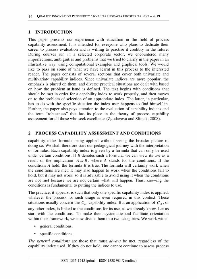
This paper presents our experience with education in the field of process capability assessment. It is intended for everyone who plans to dedicate their career to process evaluation and is willing to practise it credibly in the future. During courses run in a selected corporate sector, we encountered many imperfections, ambiguities and problems that we tried to clarify in the paper in an illustrative way, using computational examples and graphical tools. We would like to pass on some of what we have learnt in this process to the interested reader. The paper consists of several sections that cover both univariate and multivariate capability indices. Since univariate indices are more popular, the emphasis is placed on them, and diverse practical situations are dealt with based on how the problem at hand is defined. The text begins with conditions that should be met in order for a capability index to work properly, and then moves on to the problem of selection of an appropriate index. The latter, in particular, has to do with the specific situation the index user happens to find himself in. Further, the paper also pays attention to the evaluation of capability indices and the term “robustness” that has its place in the theory of process capability assessment for all those who seek excellence (Zgodavova and Slimak, 2008).

2 PROCESS CAPABILITY ASSESSMENT AND CONDITIONS

capability index formula being applied without seeing the broader picture of doing so. We shall therefore start our pedagogical journey with the interpretation of formulas. Each capability index is given by a formula that can only be used under certain conditions. If B denotes such a formula, we can view its use as a result of the implication BA⇒ , where A stands for the conditions. If the conditions A hold, the formula B is true. The formula will certainly work when the conditions are met. It may also happen to work when the conditions fail to hold, but it may not work, so it is advisable to avoid using it when the conditions are not met because we are not certain what will happen. Thus, knowing the conditions is fundamental to putting the indices to use.

The practice, it appears, is such that only one specific capability index is applied, whatever the process, or such usage is even required in this context. These situations usually concern the

pkC capability index. But an application of pkC , or

any other index, is linked to the conditions for its use, as we already know. Let us start with the conditions. To make them systematic and facilitate orientation within their framework, we now divide them into two categories. We work with:

• general conditions,

• specific conditions.

The general conditions are those that must always be met, regardless of the capability index used. If they do not hold, one cannot continue to assess process



15

capability with an index. The problem must be removed before any capability assessment takes place.

The specific conditions are index-specific extra conditions which must hold in addition to the general conditions. These conditions usually accompany the definition of a capability index. Both the general and specific conditions should be verified with statistical tests, or also in combination with suitable graphical methods. Nowadays there are capability indices suitable basically for any situation, so there is no reason to improvise and use a specific index outside the conditions that define its application. In this context, it is perhaps necessary to say that when an organization strictly requires that its suppliers calculate a specific index, such as pkC , regardless of whether the index matches the

suppliers’ production environment, it does not boost its credibility. In these cases, one may ask what good such an index is and how serious the customer is about it. Since, as is known, the customer must be complied with, one way of proceeding is to present the required index with a supplementary explanation what the specific environment of the organization is, and what adequate index should be applied. Such an index should be announced, and the attention should be drawn to the potential discrepancy between the two indices and the unreliability of the required index. Companies often do not comply, if assessed by the required index, but do comply with the standards set by the proper index!

The general conditions are related to the evaluated process, data and tolerance. They are:

• The process is stable.

• The data on the process are independent, without outliers, sufficient in size.

• The tolerance is specified correctly.

If any of the conditions fails, it is advisable not to calculate the capability index. Otherwise, the resulting value is unreliable. It is overestimated or underestimated, depending on which condition failed to hold. The value of the index can also be meaningless. Note that normality of the data is not among the general conditions. Process capability can be evaluated without normality. In relation to these conditions, many questions arise that the user of an index should ask, such as how to verify the validity of the conditions, what exactly happens when they do not hold, or how to proceed in the less favourable situation when they fail. Comparing various scholarly publications on capability assessment, we find out that the set of conditions differs slightly among the authors, however there is definitely a consensus regarding the condition of process stability. This condition is crucial.

A process is stable in the statistical sense of the word when all its monitored quality characteristics lie within the control limits of the corresponding control charts. Of course, this means that control charts must be an established tool in



16

organizations. This, however, can be a problem. It seems that many organizations do not know that when control charts are not available, it is possible to verify the process stability easily, fast and reliably with a statistical test. This is true even when more than one quality characteristic is observed for a process. The truth is that such a test is not commonly implemented in statistical software packages, but the situation is not hopeless. The interested reader may find a theoretical exposition of the tests in Holmes and Mergen (1995), its practical use is implemented, for instance, in the computer program Capa (Tošenovský, 2006).

When analysing a process, defining the tolerance for its quality characteristic(s) and gathering data on the process is how the capability assessment begins. What then follows is the selection of an appropriate capability index.

3 SELECTION OF A CAPABILITY INDEX

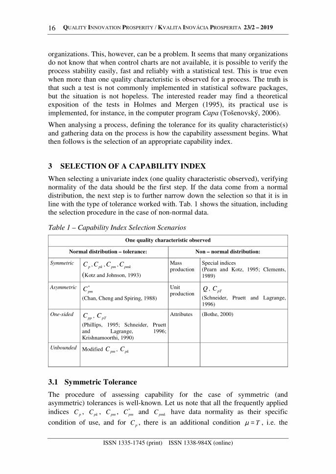
When selecting a univariate index (one quality characteristic observed), verifying normality of the data should be the first step. If the data come from a normal distribution, the next step is to further narrow down the selection so that it is in line with the type of tolerance worked with. Tab. 1 shows the situation, including the selection procedure in the case of non-normal data.

Table 1 – Capability Index Selection Scenarios

One quality characteristic observed

Normal distribution – tolerance: Non – normal distribution:

Symmetric pC ,

pkC ,pmC ,

pmkC

(Kotz and Johnson, 1993)

Mass production

Special indices (Pearn and Kotz, 1995; Clements, 1989)

Asymmetric *pmC

(Chan, Cheng and Spiring, 1988)

Unit production

Q , pTC

(Schneider, Pruett and Lagrange, 1996)

One-sided ppC , pTC

(Phillips, 1995; Schneider, Pruett and Lagrange, 1996; Krishnamoorthi, 1990)

Attributes (Bothe, 2000)

Unbounded Modified pmC , pkC

3.1 Symmetric Tolerance

The procedure of assessing capability for the case of symmetric (and asymmetric) tolerances is well-known. Let us note that all the frequently applied indices pC , pkC , pmC , *

pmC and pmkC have data normality as their specific

condition of use, and for pC , there is an additional condition T=µ , i.e. the



17

process must be centred. Unlike other indices, pC does not reflect the extent to

which the expected value µ of the quality characteristic complies with the defined target T . Thus, it can happen that an uncentered process with small σ can have a better

pC than a centered process with far higher variability σ: for the

specifications LSL = 10, USL = 16, T = 13, for instance, the process for which:

a) µ = T = 13 (a perfectly centered process), σ = 1, the index equals 1;

b) µ = 19 (a process off the target), σ = 0.5, the index equals 2.

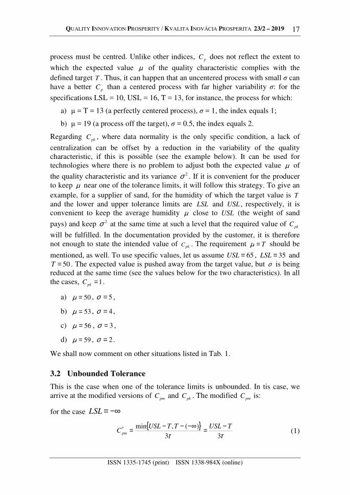
Regarding pkC , where data normality is the only specific condition, a lack of

centralization can be offset by a reduction in the variability of the quality characteristic, if this is possible (see the example below). It can be used for technologies where there is no problem to adjust both the expected value µ of

the quality characteristic and its variance 2σ . If it is convenient for the producer to keep µ near one of the tolerance limits, it will follow this strategy. To give an example, for a supplier of sand, for the humidity of which the target value is T and the lower and upper tolerance limits are LSL and USL , respectively, it is convenient to keep the average humidity µ close to USL (the weight of sand

pays) and keep 2σ at the same time at such a level that the required value of pkC

will be fulfilled. In the documentation provided by the customer, it is therefore not enough to state the intended value of pkC . The requirement T=µ should be

mentioned, as well. To use specific values, let us assume 65=USL , 35=LSL and 50=T . The expected value is pushed away from the target value, but σ is being

reduced at the same time (see the values below for the two characteristics). In all the cases, 1=pkC .

a) 50=µ , 5=σ ,

b) 53=µ , 4=σ ,

c) 56=µ , 3=σ ,

d) 59=µ , 2=σ .

We shall now comment on other situations listed in Tab. 1.

3.2 Unbounded Tolerance

This is the case when one of the tolerance limits is unbounded. In tis case, we arrive at the modified versions of pmC and pkC . The modified pmC is:

for the case −∞=LSL

{ }ττ 33

)(,min* TUSLTTUSLC pm

−=−∞−−= (1)



18

and for the case +∞=USL

{ }ττ 33

,min* LSLTLSLTTC pm

−=−−∞+= (2)

where

∑ −= −

i i Txn 212 )(τ (3)

If no T is defined, one may modify the pkC index. The modified index is

calculated as follows:

for the case −∞=LSL

σµ

3

−= USLC pk (4)

and for the case +∞=USL

σµ

3

LSLC pk

−= (5)

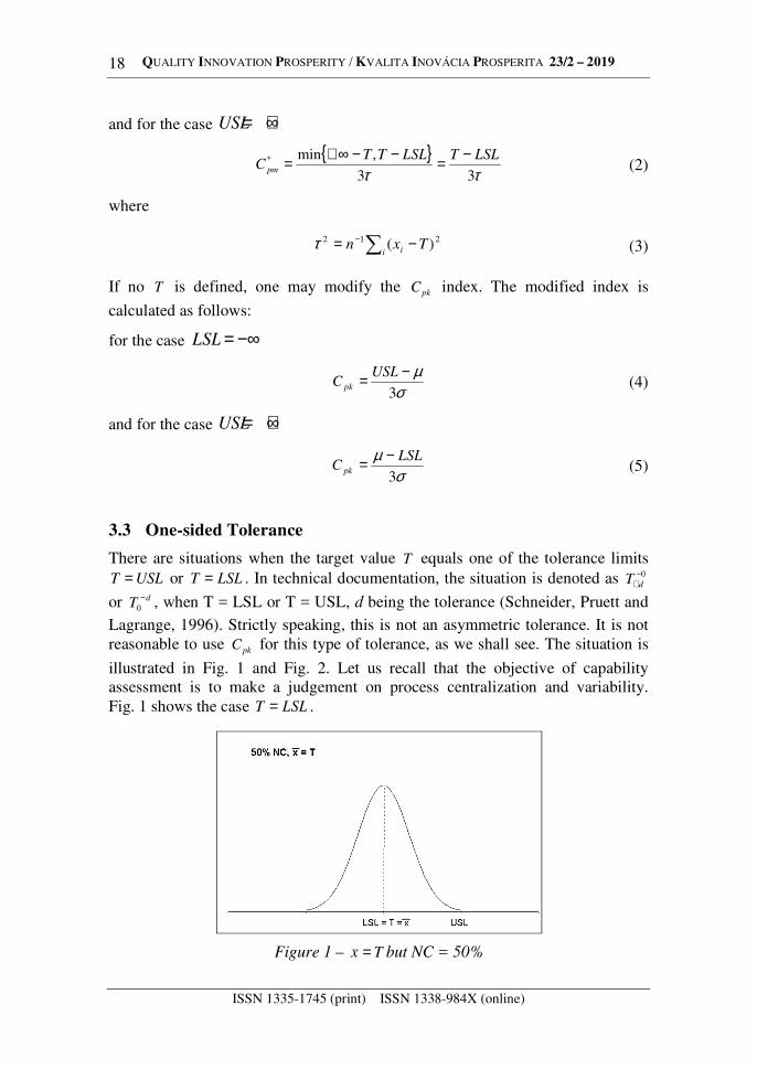
3.3 One-sided Tolerance

There are situations when the target value T equals one of the tolerance limitsUSLT = or LSLT = . In technical documentation, the situation is denoted as 0−

+dT

or dT −0 , when T = LSL or T = USL, d being the tolerance (Schneider, Pruett and

Lagrange, 1996). Strictly speaking, this is not an asymmetric tolerance. It is not reasonable to use pkC for this type of tolerance, as we shall see. The situation is

illustrated in Fig. 1 and Fig. 2. Let us recall that the objective of capability assessment is to make a judgement on process centralization and variability. Fig. 1 shows the case LSLT = .

Figure 1 – Tx = but NC = 50%



19

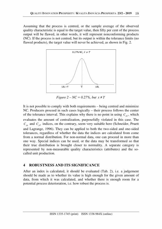
Assuming that the process is centred, or the sample average of the observed quality characteristic is equal to the target value, then fifty per cent of the process output will be flawed, in other words, it will represent nonconforming products (NC). If the process is not centred, but its output is within the tolerance limits (no flawed products), the target value will never be achieved, as shown in Fig. 2.

Figure 2 – NC = 0.27%, but Tx ≠

It is not possible to comply with both requirements – being centred and minimize NC. Producers proceed in such cases logically – their process follows the center of the tolerance interval. This explains why there is no point in using

pkC , which

evaluates the amount of centralization, purposefully violated in this case. The

ppC and pTC indices, on the contrary, seem very suitable here (Schneider, Pruett

and Lagrange, 1996). They can be applied to both the two-sided and one-sided tolerances, regardless of whether the data the indices are calculated from come from a normal distribution. For non-normal data, one can proceed in more than one way. Special indices can be used, or the data may be transformed so that their true distribution is brought closer to normality. A separate category is represented by non-measurable quality characteristics (attributes) and the so-called unit production.

4 ROBUSTNESS AND ITS SIGNIFICANCE

After an index is calculated, it should be evaluated (Tab. 2), i.e. a judgement should be made as to whether its value is high enough for the given amount of data, from which it was calculated, and whether there is enough room for a potential process deterioration, i.e. how robust the process is.



20

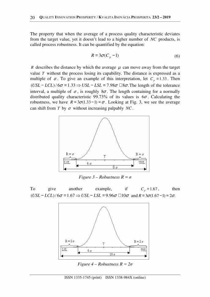
The property that when the average of a process quality characteristic deviates from the target value, yet it doesn’t lead to a higher number of NC products, is called process robustness. It can be quantified by the equation:

)1(3 −= pCR σ (6)

R describes the distance by which the average µ can move away from the target value T without the process losing its capability. The distance is expressed as a multiple of σ . To give an example of this interpretation, let 33.1=pC . Then

.898.733.16/)( σσσ ≅=−⇒=− LSLUSLLCLUSL The length of the tolerance interval, a multiple of σ , is roughly σ8 . The length containing for a normally distributed quality characteristic 99.73% of its values is σ6 . Calculating the robustness, we have σσ =−= )133.1(3R . Looking at Fig. 3, we see the average can shift from T by σ without increasing palpably NC .

Figure 3 – Robustness R = σ

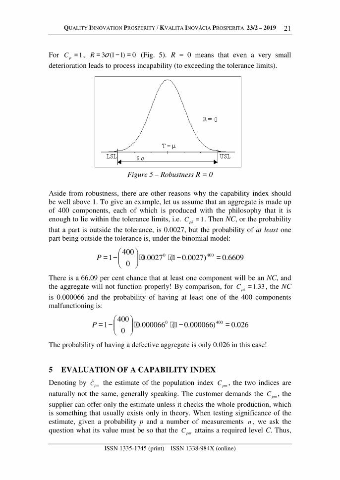
To give another example, if 67.1=pC , then

σσσ 1096.967.16/)( ≅=−⇒=− LSLUSLLCLUSL and .2)167.1(3 σσ ≈−=R

Figure 4 – Robustness R = 2σ



21

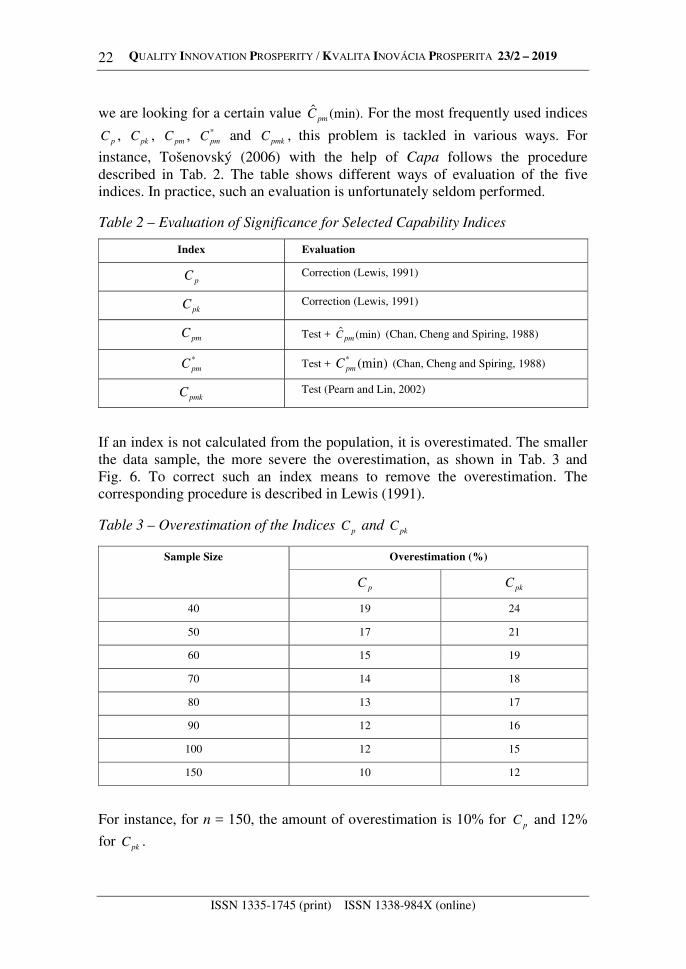
For 1=pC , 0)11(3 =−= σR (Fig. 5). R = 0 means that even a very small

deterioration leads to process incapability (to exceeding the tolerance limits).

Figure 5 – Robustness R = 0

Aside from robustness, there are other reasons why the capability index should be well above 1. To give an example, let us assume that an aggregate is made up of 400 components, each of which is produced with the philosophy that it is enough to lie within the tolerance limits, i.e. 1=pkC . Then NC, or the probability

that a part is outside the tolerance, is 0.0027, but the probability of at least one part being outside the tolerance is, under the binomial model:

6609.0)0027.01(0027.0

0

4001 4000 =−⋅⋅

−=P

There is a 66.09 per cent chance that at least one component will be an NC, and the aggregate will not function properly! By comparison, for 33.1=pkC , the NC

is 0.000066 and the probability of having at least one of the 400 components malfunctioning is:

026.0)000066.01(000066.0

0

4001 4000 =−⋅⋅

−=P

The probability of having a defective aggregate is only 0.026 in this case!

5 EVALUATION OF A CAPABILITY INDEX

Denoting by pmC the estimate of the population index pmC , the two indices are

naturally not the same, generally speaking. The customer demands the pmC , the

supplier can offer only the estimate unless it checks the whole production, which is something that usually exists only in theory. When testing significance of the estimate, given a probability p and a number of measurements n , we ask the question what its value must be so that the pmC attains a required level C. Thus,



22

we are looking for a certain value (min).ˆpmC For the most frequently used indices

pC , pkC , pmC , *pmC and pmkC , this problem is tackled in various ways. For

instance, Tošenovský (2006) with the help of Capa follows the procedure described in Tab. 2. The table shows different ways of evaluation of the five indices. In practice, such an evaluation is unfortunately seldom performed.

Table 2 – Evaluation of Significance for Selected Capability Indices

Index Evaluation

pC Correction (Lewis, 1991)

pkC Correction (Lewis, 1991)

pmC Test + (min)ˆpmC (Chan, Cheng and Spiring, 1988)

*pmC Test + (min)*

pmC (Chan, Cheng and Spiring, 1988)

pmkC Test (Pearn and Lin, 2002)

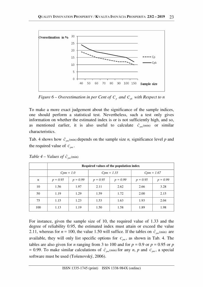
If an index is not calculated from the population, it is overestimated. The smaller the data sample, the more severe the overestimation, as shown in Tab. 3 and Fig. 6. To correct such an index means to remove the overestimation. The corresponding procedure is described in Lewis (1991).

Table 3 – Overestimation of the Indices pC and

pkC

Sample Size Overestimation (%)

pC pkC

40 19 24

50 17 21

60 15 19

70 14 18

80 13 17

90 12 16

100 12 15

150 10 12

For instance, for n = 150, the amount of overestimation is 10% for pC and 12%

for pkC .



23

Figure 6 – Overestimation in per Cent of pC and pkC with Respect to n

To make a more exact judgement about the significance of the sample indices, one should perform a statistical test. Nevertheless, such a test only gives information on whether the estimated index is or is not sufficiently high, and so, as mentioned earlier, it is also useful to calculate (min)ˆ

pmC or similar

characteristics.

Tab. 4 shows how (min)ˆpmC depends on the sample size n, significance level p and

the required value of pmC .

Table 4 – Values of (min)ˆpmC

Required values of the population index

Cpm = 1.0 Cpm = 1.33 Cpm = 1.67

n p = 0.95 p = 0.99 p = 0.95 p = 0.99 p = 0.95 p = 0.99

10 1.56 1.97 2.11 2.62 2.66 3.28

50 1.19 1.29 1.59 1.72 2.00 2.15

75 1.15 1.23 1.53 1.63 1.93 2.04

100 1.13 1.19 1.50 1.58 1.89 1.98

For instance, given the sample size of 10, the required value of 1.33 and the degree of reliability 0.95, the estimated index must attain or exceed the value 2.11, whereas for n = 100, the value 1.50 will suffice. If the tables on (min)ˆ

pmC are

available, they will only list specific options for pmC , as shown in Tab. 4. The

tables are also given for n ranging from 3 to 100 and for p = 0.9 or p = 0.95 or p = 0.99. To make similar calculations of (min)ˆ

pmC for any n, p and pmC , a special

software must be used (Tošenovský, 2006).



24

6 MULTIVARIATE INDICES

The multivariate indices are used if:

a) more operations are performed on a product, so that when evaluating the process (or the sequence of operations), more quality characteristics are observed, or

b) a product is made up of several components, each of which possesses a quality characteristic, and the product is evaluated as a whole.

When more quality characteristics are observed, it is not recommended to evaluate them separately with the aforementioned indices. When they are evaluated separately, then:

a) the process is not assessed as a whole, individual operations or components are evaluated instead,

b) if the characteristics are dependent, then not even a single operation is assessed, as the effect of the other operations is not factored into such a calculation.

In these cases, special multivariate capability indices were designed as well as graphical methods. The multivariate indices are denoted pMC , pkMC , pmMC . For

an index to be selected for use, it must satisfy proper conditions (see Tab. 5).

Table 5 – Conditions to Be Met by Multivariate Indices

pMC , pmMC pkMC

Normally distributed quality characteristics with two-sided tolerances. They do not have to be independent.

Independent quality characteristics iX (this also

concerns attributes) with any type of tolerance. Normality is not necessary.

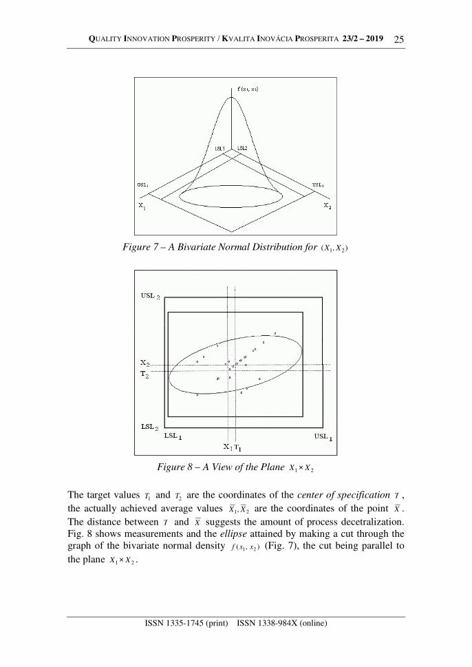
To get the idea about the indices, we illustrate the situation with the bivariate version of the pMC index. Let there be two observed quality characteristics 1X ,

2X , and let the corresponding random vector ),( 21 XX has the normal distribution ),( VN µ . Further, let iT be the target value for iX , iLSL be its lower specification

limit and iUSL be its upper specification limit. The region of admissibility is then represented by a tolerance rectangle defined by the values 1LSL and 1USL on the

1X – axis and the values 2LSL and 2USL on the 2X – axis in the plane (Fig. 7, Fig. 8).



25

Figure 7 – A Bivariate Normal Distribution for ),( 21 XX

Figure 8 – A View of the Plane 21 XX ×

The target values 1T and 2T are the coordinates of the center of specification T , the actually achieved average values 21, XX are the coordinates of the point X . The distance between T and X suggests the amount of process decetralization. Fig. 8 shows measurements and the ellipse attained by making a cut through the graph of the bivariate normal density ),( 21 xxf (Fig. 7), the cut being parallel to the plane 21 XX × .



26

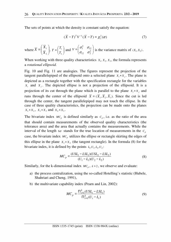
The sets of points at which the density is constant satisfy the equation:

)()()( 2

21 αχ=−− −

TXVTXT (7)

where

=

2

1

X

XX ,

=

2

1

T

TT and

=

2212

1221

σσσσ

V is the variance matrix of ),( 21 XX .

When working with three quality characteristics 321 ,, XXX , the formula represents a rotational ellipsoid.

Fig. 10 and Fig. 11 are analogies. The figures represent the projection of the tangent parallelepiped of the ellipsoid onto a selected plane ji XX × . The plane is

depicted as a rectangle together with the specification rectangle for the variables iX and jX . The depicted ellipse is not a projection of the ellipsoid. It is a

projection of its cut through the plane which is parallel to the plane ji XX × and

runs through the center of the ellipsoid X X X X= ( , , ).1 2 3 Since the cut is led through the center, the tangent parallelepiped may not touch the ellipse. In the case of three quality characteristics, the projection can be made onto the planes

21 XX × , 31 XX × and 32 XX × .

The bivariate index pMC is defined similarly as pC , i.e. as the ratio of the area

that should contain measurements of the observed quality characteristics (the tolerance area) and the area that actually contains the measurements. While the interval of the length σ6 stands for the true location of measurements in the pC

case, the bivariate index pMC utilizes the ellipse or rectangle skirting the edges of

this ellipse in the plane 21 XX × (the tangent rectangle). In the formula (8) for the bivariate index, it is defined by the points 2211 ,,, ULUL :

))((

))((

2211

2211

LULU

LSLUSLLSLUSLMC p −−

−−= (8)

Similarly, for the k-dimensional index pMC , 2>k , we observe and evaluate:

a) the process centralization, using the so-called Hotelling’s statistic (Hubele, Shahriari and Cheng, 1991),

b) the multivariate capability index (Pearn and Lin, 2002):

)(

)(

1

1

iiki

iiki

pLU

LSLUSLMC

−Π−Π=

=

= (9)



27

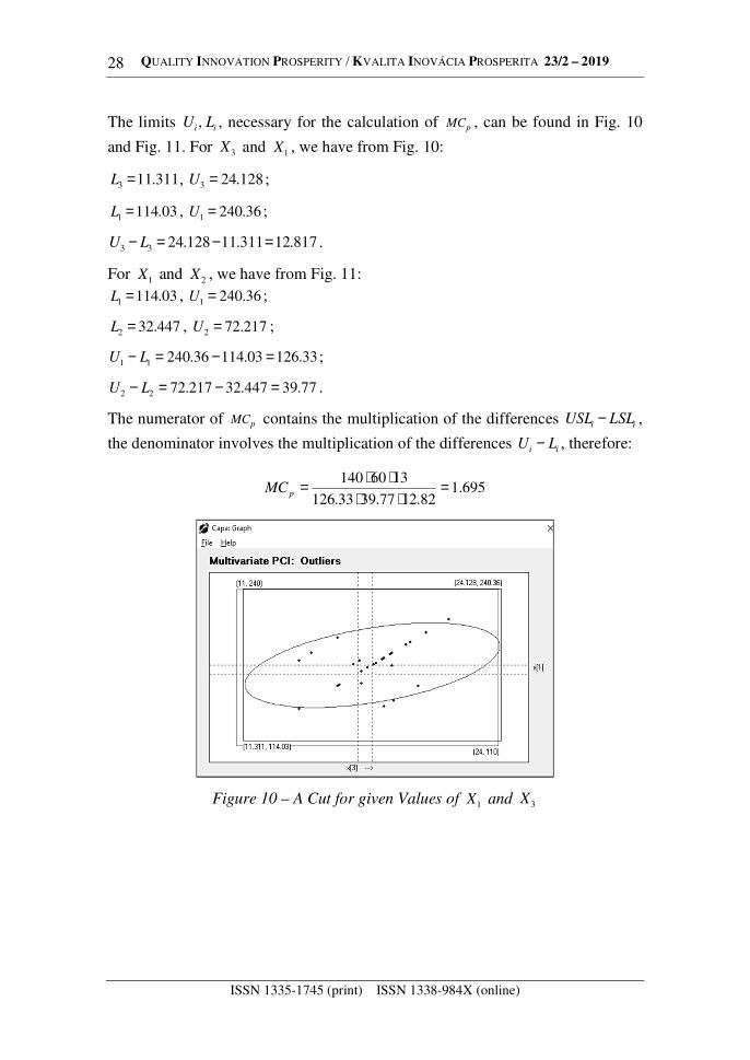
While, for instance, Kotz and Johnson (1993) use in the denominator of pMC the

volume of the rotational ellipsoid, (9) calculates the volume of the tangent parallelepiped, defined by the numbers ii LU , . The required limits ii LU , can be read from Fig. 10 and Fig. 11 (software Capa used in this example):

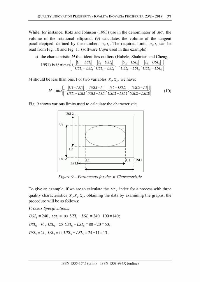
c) the characteristic M that identifies outliers (Hubele, Shahriari and Cheng,

1991) is

−−

−−

−−

−−

=kk

kk

kk

kk

LSLUSL

USLL

LSLUSL

LSLU

LSLUSL

USLL

LSLUSL

LSLUM ,,...,,,1max

11

11

11

11

M should be less than one. For two variables 21, XX , we have:

−−

−−

−−

−−

=22

22,

22

22,

11

11,

11

11,1max

LSLUSL

LUSL

LSLUSL

LSLU

LSLUSL

LUSL

LSLUSL

LSLUM (10)

Fig. 9 shows various limits used to calculate the characteristic.

Figure 9 – Parameters for the M Characteristic

To give an example, if we are to calculate the pMC index for a process with three

quality characteristics 321 ,, XXX , obtaining the data by examining the graphs, the procedure will be as follows:

Process Specifications:

2401 =USL , ,1001 =LSL 14010024011 =−=− LSLUSL ;

802 =USL , ,202 =LSL 60208022 =−=− LSLUSL ;

243 =USL , ,113 =LSL 13112433 =−=− LSLUSL .



28

The limits ii LU , , necessary for the calculation of pMC , can be found in Fig. 10

and Fig. 11. For 3X and 1X , we have from Fig. 10:

311.113 =L , 128.243 =U ;

03.1141 =L , 36.2401 =U ;

817.12311.11128.2433 =−=− LU .

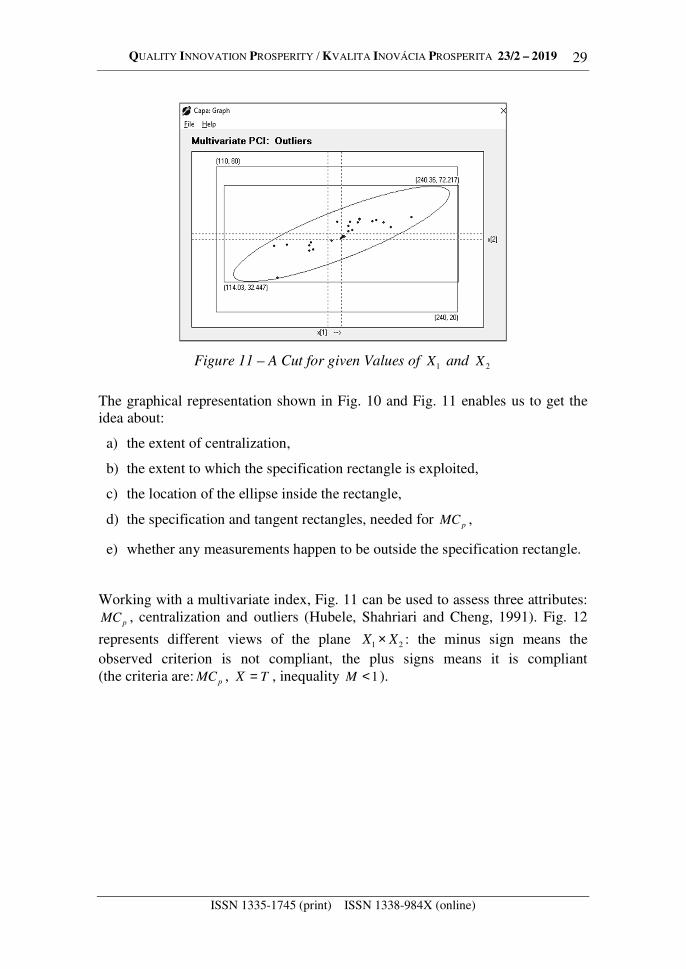
For 1X and 2X , we have from Fig. 11: 03.1141 =L , 36.2401 =U ;

447.322 =L , 217.722 =U ;

33.12603.11436.24011 =−=− LU ;

77.39447.32217.7222 =−=− LU .

The numerator of pMC contains the multiplication of the differences ii LSLUSL − ,

the denominator involves the multiplication of the differences ii LU − , therefore:

695.1

82.1277.3933.126

1360140 =⋅⋅

⋅⋅=pMC

Figure 10 – A Cut for given Values of 1X and 3X



29

Figure 11 – A Cut for given Values of 1X and 2X

The graphical representation shown in Fig. 10 and Fig. 11 enables us to get the idea about:

a) the extent of centralization,

b) the extent to which the specification rectangle is exploited,

c) the location of the ellipse inside the rectangle,

d) the specification and tangent rectangles, needed for pMC ,

e) whether any measurements happen to be outside the specification rectangle.

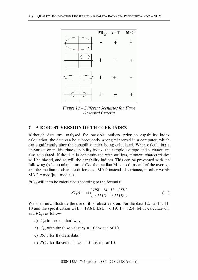
Working with a multivariate index, Fig. 11 can be used to assess three attributes:

pMC , centralization and outliers (Hubele, Shahriari and Cheng, 1991). Fig. 12

represents different views of the plane 21 XX × : the minus sign means the observed criterion is not compliant, the plus signs means it is compliant (the criteria are: pMC , TX = , inequality 1<M ).



30

Figure 12 – Different Scenarios for Three

Observed Criteria

7 A ROBUST VERSION OF THE CPK INDEX

Although data are analysed for possible outliers prior to capability index calculation, the data can be subsequently wrongly inserted in a computer, which can significantly alter the capability index being calculated. When calculating a univariate or multivariate capability index, the sample average and variance are also calculated. If the data is contaminated with outliers, moment characteristics will be biased, and so will the capability indices. This can be prevented with the following (robust) adaptation of Cpk: the median M is used instead of the average and the median of absolute differences MAD instead of variance, in other words MAD = med(|xi – med xi|).

RCpk will then be calculated according to the formula:

−−=MAD

LSLM

MAD

MUSLRCpk

.3,

.3min (11)

We shall now illustrate the use of this robust version. For the data 12, 15, 14, 11, 10 and the specification USL = 18.61, LSL = 6.19, T = 12.4, let us calculate Cpk

and RCpk as follows:

a) Cpk in the standard way;

b) Cpk with the false value x5 = 1.0 instead of 10;

c) RCpk for flawless data;

d) RCpk for flawed data: x5 = 1.0 instead of 10.



31

The results are:

a) Cpk = 0.998 (calculated with Capa);

b) Cpk = 0.26 (average is 10.6; standard deviation equals 5.59);

c) M = 12, MAD = 2,

968.02.3

19.612

.3;102.1

2.3

1261.18

.3=−=−==−=−=

MAD

LSLMRCpL

MAD

MUSLRCpU

968.0=RCpk ;

d) M = 12 and MAD = 2, i.e. the same values as for the correct data, and so the index remains the same.

For the correct data, Cpk and RCpk do not differ significantly. For the wrong data, RCpk keeps its value attained for the correct data.

Knowledge of multivariate data is also used in other calculations, such as regression, where robust techniques are exploited, as well Kutner, Nachtsheim and Neter (2014). A simple and efficient procedure is, for instance, that of obtaining regression coefficients with the generalized-least-squares formula b = (XTWX)-1 XTWY, where W is a matrix of weights. It is a diagonal matrix with elements w. Two widely used weight functions are the Huber and bisquare weight functions. According to Huber, w = 1.345/u, u = e/4.6683, where e is a residual from the classical least-squares estimation method. These techniques, studied in students’ SGS projects, for instance, proved to be robust.

8 CONCLUSION

The aim of the paper was to show how educational process in the field of process evaluation can be complemented with graphical and numerical illustrations of selected chapters on this subject. We believe that visualization and numerical examples are a way to make statistical methods more popular. It is also very convenient to provide students with enough material for their self-training, with a software that provides quick solutions, is up to date in the field and can be used for real-life problems, if possible. We have prepared a 380-pages long training manual with the most frequently occurring real-life problems, illustrated with graphs and solutions. The solutions can also be obtained with the software Capa that is part of the manual (Tošenovský, 2006). Our experience is such that knowledge of modern methods of capability evaluation is needed not only for producers, but also for customers. In the latter case, lack of knowledge often leads to situations when customers require inadequate means of capability assessment.



32

ACKNOWLEDGEMENTS

This paper was prepared under the specific research projects No. SP2018/109, SP2019/62 and SP2019/129 conducted at the Faculty of Materials Science and Technology, VŠB-TU Ostrava, with a support from the Ministry of Education of the Czech Republic.

REFERENCES

Bothe, D.R., 2000. Composite capability index for multiple product Characteristic. Quality Engineering, [e-journal] 12(2), pp.253-258. https://doi.org/10.1080/08982119908962582.

Clements, J.A., 1989. Process capability calculations for non-normal Distributions. Quality Progress, 22, pp.95-100.

Holmes, D.S and Mergen, A.E., 1995. An alternative method to test for randomness of a process. Quality and Reliability Engineering International, 11(3), pp.171-174.

Hubele, N.F., Shahriari, H. and Cheng, C.S., 1991. A bivariate process capability vector in statistics and design in process control. Statistical Process Control in

Manufacturing, pp.299-310.

Chan, L.K., Cheng, S.W. and Spiring, F.A., 1988. A new measure of process capability: Cpm. Journal of Quality Technology, [e-journal] 20(3), pp.162-175. https://doi.org/10.1080/00224065.1988.11979102.

Kotz, S. and Johnson, N., 1993. Process capability indices. London: Chapman & Hall.

Krishnamoorthi, K.S., 1990. Capability indices for process subject to unilateral and positional tolerance. Quality Engineering, [e-journal] 2(4), pp.461-471. https://doi.org/10.1080/08982119008962740.

Kutner, M.H., Nachtsheim, CH.J. and Neter, J., 2014. Applied Linear Regresion

Models. New York: McGraw-Hill.

Lewis, S.S., 1991. Process capability estimates from small samples. Quality

Engineering, 3(3), pp.381-394. https://doi.org/10.1080/08982119108918865.

Pearn, W.L. and Kotz, S., 1995. Application of Clements’ method for calculating second and third generation process capability indices for non-normal Pearson populations. Quality Engineering, [e-journal] 7(1), pp.139-145. https://doi.org/10.1080/08982119408918772.

Pearn, W.L. and Lin, P.C., 2002. Computer program for calculating the p-value in testing process capability index Cpmk. Quality and Reliability Engineering, [e-journal] 18(4), pp.333-342. https://doi.org/10.1002/qre.465.



33

Phillips, G.P., 1995. Target ratio simplifies capability index system, makes it easy to use Cpm. Quality Engineering, [e-journal] 7(2), pp.299-313. https://doi.org/10.1080/08982119408918785.

Schneider, H., Pruett, J. and Lagrange, C., 1996. Uses of process capability indices in the supplier certification process. Quality Engineering, [e-journal] 8(2), pp.225-235.

Tošenovský, J., 2006. Capa. [computer program] Josef Tošenovský. Available at: <[email protected]> [01 March 2006].

Zgodavova, K. and Slimak, I., 2008. Advanced Improvement of Quality. In: DAAM, 19th International Symposium of the Danube-Adria-Association-for-

Automation-and-Manufacturing Location. Trnava, Slovakia, pp.1551-1552.

ABOUT AUTHORS

Josef Tošenovský – The author is a full professor at VŠB-Technical university of Ostrava, specializing in probability, statistics and econometrics. In 1988 he became an associate professor in mathematics and in 2001 a professor in Management of Industrial Systems. E-mail: [email protected], Author’s ORCID: https://orcid.org/0000-0003-4684-1369.

Filip Tošenovský – The author is an assistant professor at VŠB-Technical university of Ostrava, specializing in probability, statistics, econometrics and operations research. E-mail: [email protected], Author’s ORCID: https://orcid.org/0000-0003-3946-7815.

© 2019 by the authors. Submitted for possible open access publication under the

terms and conditions of the Creative Commons Attribution (CC-BY) license

(http://creativecommons.org/licenses/by/4.0/).

Possibilities of Using Graphical and Numerical Tools in the ...

Documents

Transcript of Possibilities of Using Graphical and Numerical Tools in the ...