Working Paper Series

Population Policy through Tradable Procreation Entitlements David de la Croix Axel Gosseries

ECINEQ WP 2007 – 62

ECINEQ 2007-62

March 2007

www.ecineq.org

Population Policy through

Tradable Procreation Entitlements*

David de la Croix† Department of Economics and CORE, Université Catholique de Louvain

Axel Gosseries

FNRS & Hoover Chair, Université Catholique de Louvain

Abstract

Tradable permits are now widely used to control pollution. We investigate the implications of setting up such a system in another area – population control –, either domestically or at the global level. We first generalize the framework with both tradable procreation allowances and tradable procreation exemptions, in order to tackle both over- and under-population problems. The implications of procreation rights for income inequality and education are contrasted. We decompose the scheme’s impact on redistribution into three effects, one of them, the tradability effect, entails the following: with procreation exemptions or expensive enough procreation allowances, redistribution benefits the poor. In contrast, cheap procreation allowances redistribute resources to the rich. As far as human capital is concerned, natalist policy worsens the average education level of the next generation, while population control enhances it. If procreation rights are granted to countries in proportion to existing fertility levels (grandfathering) instead of being allocated equally, population control can be made even more redistributive. Our exploratory analysis suggests that procreation entitlements offer a promising tool to control population without necessarily leading to problematic distributive impact, especially at the global level. Keywords: Tradable permits, Population control, Pronatalist policy, Income inequality, Differential fertility, Grandfathering. JEL Classification: J13, E61, O40.

* David de la Croix acknowledges the financial support from the Belgian French speaking community (Grant ARC 03/08-235 “New macroeconomic approaches to the development problem”) and the Belgian Federal Government (Grant PAI P5/21, “Equilibrium theory and optimization for public policy and industry regulation”). We thank Claude d’Aspremont, Michel De Vroey, Matias Eklöf, Andy Mason, Victor Rios-Rull, Philippe Van Parijs, Fabio Waltenberg, participants to conferences in Ghent, Louvain-la-Neuve, Palma (ECINEQ) and SED06 for their comments on an earlier draft. †. E-mail addresses: delacroix@ires.ucl.ac.be, gosseries@etes.ucl.ac.be Department of Economics, Universit´e catholique de Louvain, place Montesquieu 3, B-1348 Louvain-la-Neuve, Belgium.

Introduction

In many countries, a gap obtains between the actual fertility rate and what is perceived

as the optimal fertility rate. In some cases, fertility is deemed too high, typically out

of concern for the ability of our natural environment to cope with such an anthropic

pressure (climate change being a possible example) or for the capacity of the land to feed

and provide enough space to so many people (a motive present a.o. in China’s one-child

policy, see Greenhalgh (2003)). In other cases, the actual fertility is perceived as too

low. It can be due e.g. to the need to be numerous enough to support an endangered

cultural identity. In some cases, it is the relative size of the various cohorts coexisting in

a country that is at stake, a low fertility rate being one of the factors (together with an

even more significant one: growing life expectancy) threatening the financial viability of

our pension schemes and our health care systems. Other concerns about relative size of

different groups within a population arise as well with respect to ethnic composition or

educational level, fertility and mortality rates differing along such characteristics.

It remains an open question whether each of these grounds is legitimate, especially for

those giving a significant importance to people’s freedom (not) to procreate. Philosophers

have actually shown that the very idea of an optimal population raises an even more

fundamental challenge: as soon as we ask “optimal for whom?”, it becomes clear that the

answer may end up remaining unstable since the very existence of the agent with regard

to whom we need to assess the benefit is itself a choice variable.1 In the present paper,

we shall leave such questions aside, assuming that in a given territory at a given point

in time, it can be meaningful to aim at a fertility rate different from the one expected

in the absence of any state intervention. Hence, assuming that a fertility target may be

defined in a meaningful manner, we shall be concerned here with the means to reach such

a target.

In the presence of under-population, various measures have been proposed and adopted.

For example, at least in some contexts such as post WWII, one justification for the in-

troduction of family benefits was a pro-natalist one. Other measures include extensive

parental (paid or unpaid) leave schemes, parents-friendly workplaces or the public provi-

sion of day-care. Admittedly, such measures may be promoted for reasons other than a

concern for optimal fertility level, such as the need to promote gender equality, to guar-

antee equality among children, to encourage the fidelity of one’s workers (in the specific

1The question of the optimal fertility rate is also present in the social choice literature, for two recentcontributions see Michel and Wigniolle (2006) and Golosov, Jones, and Tertilt (2004).

1

case of family benefits) or to defend the family as an institution. Yet, the pro-natalist

dimension is often present among such justifications - not to mention among the effects

of such policies (Demeny 1987).

In contrast, whenever over-population obtains, there is a variety of measures available

to control population, ranging from information campaigns on contraception means, the

liberalization of abortion or the leveling up of women’s educational level, to China’s one-

child policy. The use of coercive anti-natalist means is problematic both because of the

extent to which it reduced people’s freedom (Sen 1996), but also because it threatens the

ability of such means to actually reach the goals that have been set.

Now, one measure that could serve both pro-natalist and anti-natalist purposes has never

been put in place so far: tradable procreation entitlements. Tradable quotas schemes have

been promoted as a policy tool for several decades. They have typically been proposed

and widely implemented to combat air pollution,2 overproduction (e.g. tradable milk

quotas in the EU), overexploitation of natural resources (e.g. individual transferable fish

quotas). It has also been proposed in other areas - while never being implemented - such

as inflation control (Lerner and Colander 1980), and, more recently, asylum policy (Schuck

(97) and Hathaway and Neve (1997)) or deficit control (Casella 1999). The idea is always

to agree on a cap to reduce the extent of a given problem (over-production, over-inflation,

pollution, excessive unemployment,), to allocate the corresponding rights to the various

actors involved (states, firms and/or individuals), and to allow for tradability of such

rights between the actors, in order to take into account differences in marginal reduction

costs. One of the oldest of such proposals is Boulding (1964)’s idea of tradable procreation

licenses to combat overpopulation.

More than forty years later, population policy is searching for tools able to deal with

both over- and under-population, the latter being a more recent concern in developed

countries. In this paper, we first apply the concept of tradable entitlements to population

control problems. We generalize the framework with both tradable procreation allowances

and tradable procreation exemptions, in order to tackle the two sides of the problem.

Second, we address two central concerns regarding such a scheme, namely distributive

and educational concerns. The former refers to the fact that such a scheme, especially

through its tradability component, would be detrimental to the poor. The latter, refers

to the interdependency of fertility and education choices. Third, we also investigate

2The 1990 Clean Air Act Amendments initiated the first large-scale use of the tradable permit approachto pollution control. The empirical analysis of Joskow, Schmalensee, and Bailey (1998) shows that theemission rights market created in 1990 had become reasonably efficient within four years.

2

the implications of a global version of procreation entitlements, in line with comparable

attempts to fight global warming (Kyoto agreement). While being inspired by earlier

proposals by authors such as Boulding or Tobin, this paper should certainly not be read

as an exercise in the history of economic ideas. It rather aims at exploring some of the

potentialities and shortcomings of the idea of tradable procreation entitlements, with the

view of proposing a new instrument of social policy to face one of today’s problems.

After reviewing the literature in Section 1, we describe our benchmark model with en-

dogenous fertility and education choice in Section 2. We introduce tradable procreation

allowances granted to households in Section 3. We also generalize the system to accom-

modate the reverse situation, when they are tradable procreation exemptions. We look at

how these rights modify the optimality conditions. Next we study the existence of equilib-

rium prices for these rights. We then look at whether tradability will impoverish the poor

further in Section 4. Consequences in terms of education are also analyzed. In Section 5,

we move from the country level to the global level. We illustrate how procreation rights

could modify the fertility levels across the world. We also study the redistributive impact

of an alternative allocation rule of procreation rights, granting rights in proportion to

existing fertility levels (grandfathering). Section 6 concludes.

1 Literature Review

Boulding’s Proposal

Since the middle of the 20th century there is a growing anxiety that our planet may not

be able to sustain an ever increasing population. In an attempt to address this issue,

Kenneth Boulding proposed (1964: 135-136):

I have only one positive suggestion to make, a proposal which now seems so

far-fetched that I find it creates only amusement when I propose it. I think in

all seriousness, however, that a system of marketable licenses to have children

is the only one which will combine the minimum of social control necessary

to the solution to this problem with a maximum of individual liberty and

ethical choice. Each girl on approaching maturity would be presented with a

certificate which will entitle its owner to have, say, 2.2 children, or whatever

number would ensure a reproductive rate of one. The unit of these certificates

3

might be the “deci-child,” and accumulation of ten of these units by purchase,

inheritance, or gift would permit a woman in maturity to have one legal child.

We would then set up a market in these units in which the rich and the

philoprogenitive would purchase them from the poor, the nuns, the maiden

aunts, and so on. The men perhaps could be left out of these arrangements,

as it is only the fertility of women which is strictly relevant to population

control. However, it may be found socially desirable to have them in the plan,

in which case all children both male and female would receive, say, eleven or

twelve deci-child certificates at birth or at maturity, and a woman could then

accumulate these through marriage.

This plan would have the traditional advantage of developing a long-run ten-

dency toward equality in income, for the rich would have many children and

become poor and the poor would have few children and become rich. The price

of the certificate would of course reflect the general desire in a society to have

children. Where the desire is very high the price would be bid up; where it was

low the price would also be low. Perhaps the ideal situation would be found

when the price was naturally zero, in which case those who wanted children

would have them without extra cost. If the price were very high the system

would probably have to be supplemented by some sort of grants to enable the

deserving but impecunious to have children, while cutting off the desires of

the less deserving through taxation. The sheer unfamiliarity of a scheme of

this kind makes it seem absurd at the moment. The fact that it seems absurd,

however, is merely a reflection of the total unwillingness of mankind to face

up to what is perhaps its most serious long-run problem.

Design issues

On top of a separate and short discussion by Tobin (1970) with no reference to Bould-

ing, Heer (1975) and Daly (1991,1993) discuss Boulding’s proposal. They both propose

amendments or complements to the scheme’s design. Such proposals essentially revolve

around four issues: the need for continuous adjustments of the birth rate target, the issue

of shifting up the reproduction age through the system, the problem of early mortality

and the definition of the license beneficiaries.

As to the first issue, Heer suggests that the government (and not only the individual

permit users) could be allowed to buy such permits. A similar issue arises in the field of

4

pollution permits, where e.g. environmental NGOs, despite not being permit users, are

allowed to influence the global cap through buying permits. In the present case, Heer

identifies two reasons why it may be worth allowing the government to be a permit buyer

as well. On one hand, in order to deal with the problem of partial non-compliance, the

government could buy on the market a number of permits corresponding with the number

of unlicensed babies (Heer, 1975: 4). On the other hand, in contrast with the case of

pollution permits, procreation rights are allocated for life rather than for a given period.

And other factors than birth rate affect the size of a given population, most notably

mortality rate and geographical mobility (immigration/emigration). As Heer writes, “(...)

the original Boulding proposal guarantees only that fertility will vary narrowly around

replacement level and cannot guarantee that the rate of natural increase (the crude birth

rate minus the crude death rate) will be nil nor, a fortiori, can it provide for zero population

growth (which would be obtainable with a zero rate of natural increase only provided there

was also no net immigration from abroad)” (1975: 4). A government may thus want to

adjust the amount of birth licenses to the evolution of these other factors. One could

argue that allowing the government to buy permits all along would make it less necessary

to adjust the amount of permits allocated to each birth cohort.

Heer focuses on a second set of amendments aimed at influencing the birth rate through

raising the women’s age of reproduction. Two avenues are proposed, a incentive-based

one and a more standard one. As to the former, one could “allow for the possibility that

individuals, until they reached age 35, could loan their license units to the government and

receive interest during such time as their license units were on loan to the government”

(Heer, 1975: 6). There could thus be a financial incentive to delay reproduction, which

would certainly have an impact on the birth rate. The other way in which Heer proposes to

influence the age of reproduction (hence indirectly the lifelong reproduction rate) consists

in “stipulating that licenses to bear children be granted only at age 18 and that individuals

under this age neither be allowed to purchase licenses nor to be given licenses by other

persons” (Heer, 1975: 8). The two avenues (loan and minimum age) are of course not

exclusive and could therefore be combined.

Child mortality is another concern for both Heer and Daly. They want to prevent the

system from disadvantaging (often poorer) parents experiencing child loss. This leads to

a third set of proposals. Heer proposes that “a woman losing a child before that child

reached its eighteen’s birthday would be given a sufficient number of license units to bear

an additional child; but if a child died after its eighteenth birthday, its mother would

5

receive no additional units” (1975: 8). As to Daly, his approach to the issue of child

mortality implies both that licenses be granted at birth and that they be bequeathable.

This is such that “if a female dies before having a child, then her certificate becomes part

of her estate and is willed to someone else, for example, her parents, who either use it

to have another child or sell it to someone else” (1993: 336). If on top, permits were

allocated both to girls and boys (rather than to girls only), Daly’s allocation at birth

would offer a solution to the problem of early mortality of both girls and boys, allowing

the parents to give birth to more than two children in such a case without having to buy

extra permits. What is clear from this is that the answer provided to the “beneficiary

definition” question has a clear impact on the ability of the scheme to address the “child

mortality” challenge.

Finally, who should receive the licenses: women only, men only, both men and women?

Boulding’s proposal - as well as Tobin’s - consists in a “ladies-only” allocation. For Heer,

the possible merits of a men-only scheme include “a considerable reduction in the incidence

of illegitimate births” (1975: 8) for reasons that are not entirely clear though. But other

reasons are suggested as possible grounds for granting them to women only, such as the

need for compensating the discriminations that women experience. In contrast, issues such

as whether single-sex allocation would not be discriminatory from a gender-orientation

perspective, or as to how to deal with the licenses in case of divorce once they are granted

to both parents, are not examined by these authors.

Distributive Impact

Besides these design issues, other problems are considered by the three authors. The three

most significant ones are: the question of the scheme’s distributive impact, the problem

of enforcement, and the examination of alternative means to reach the same goal.

Regarding distributive impact, Daly, as Boulding, discusses the issue. He traces possible

injustices arising from the scheme back to background distributive injustices that are

present anyway. Not only does he claim that existing injustices will not be worsened by

the introduction of the scheme. He even argues that inequalities will be reduced, for two

reasons. First, the “new marketable asset is distributed equally” (336), which does not

tell us why this would reduce inequalities. Second, “as the rich have more children, their

family per capita incomes are lowered; as the poor have fewer children their family per

capita incomes increase. From the point of view of the children, there is something to

be said for increasing the probability that they will be born richer rather than poorer”

6

(1993: 336). It is not clear of course why the richer would tend to have more children as

a result of the scheme. It is easier to understand why the poorer would tend to have less.

2 Benchmark Model

The salient feature of the benchmark economy in which we shall introduce procreation

entitlements consists in fertility and education choice by households belonging to different

income groups. We consider a model inspired from de la Croix and Doepke (2003). They

propose a tractable framework where households are heterogeneous in terms of human

capital, and low-skilled households choose to have more children than skilled ones. This

theoretical set-up reflects the well-documented fact that fertility is inversely related to

the education level of the mother (Kremer and Chen 2002). Differential fertility will turn

to be a key element in the analysis of procreation entitlements. We first present the

benchmark model without such entitlements.

The model economy is populated by overlapping generations of people who live for two

periods, childhood, and adulthood. Time is discrete and runs from 0 to ∞. All decisions

are made in the adult period of life. There are two types of agents, indexed by i, unskilled

(group i = A) and skilled (group i = B), who differ only in their wage wit. The size of

each group is denoted N it . Agents represent households within a country, but we will also

interpret them as countries within the global economy in Section 5. Adults care about

their own consumption cit, the number of their children ni

t, and the probability π(eit) that

their children will become skilled. This probability depends on the education eit they

receive. Preferences are represented by the following utility function:

ln[cit] + γ ln[ni

tπ(eit)]. (1)

The parameter γ > 0 is the weight attached to children in the households’ objective.

Notice that parents care both about child quantity nit and quality π(ei

t). As we will see

below, the tradeoff between quantity and quality of children is affected by the human

capital endowment of the parents. Notice also that parents do not care about their

children utility, as it would be the case with dynastic altruism, but they care about their

future human capital.

To attain human capital, children have to be educated. Parents freely choose the education

spending per child eit. Apart from the education expenditure, raising one child also takes

7

a constant fraction φ ∈ (0, 1) of an adult’s time. This fraction of time cannot be cut

down. Therefore it limits to 1/φ the number of children one family can possibly raise.

Parents provide education to their children because it raises the probability that their

children will be skilled. Specifically, given education e, the probability πi(e) of becoming

skilled is given by:

πi(e) = τ i (θ + e)η, η ∈ (0, 1).

The parameter θ measures the education level reached by a child in the absence of edu-

cation spending by the parents. This education level is obtained for free and is a perfect

substitute to the education provided by the parents. η measures the elasticity of success

to total educational input θ + e. The parameter τ i depends on the type i, and we assume

the children of skilled parents have, ceteris paribus, a greater chance of becoming skilled

themselves, i.e. τB > τA.3

The budget constraint for an adult with wage wit is given by:

cit =

[wi

t(1 − φnit) − ni

teit

]. (2)

The aggregate production function for the consumption good is linear in both types of

labor input. We have:

Yt = ωALAt + ωBLB

t .

The marginal product of each type of worker is constant and equal to ωA and ωB > ωA

respectively. The total input of the groups are given by LAt and LB

t . The equilibrium

condition on both labor markets N it (1 − φni

t) = Lit will imply that wages are equal to

marginal productivity:

wit = ωi.

Denoting the equilibrium outcome in the benchmark case with hatted variables, we end

up with the following definition:

Definition 1 (Equilibrium)

Given initial population sizes NA0 and NB

0 , an equilibrium is a sequence of individual

quantities (cit, e

it, n

it)i=A,B.t≥0 and group sizes (N i

t )i=A,B.t≥0 such that

3Note that, in what follows, e is always bounded from above; hence we can always define the constantterm τ i as a function of the other parameters of the model such that the function πi() returns values inthe interval [0, 1].

8

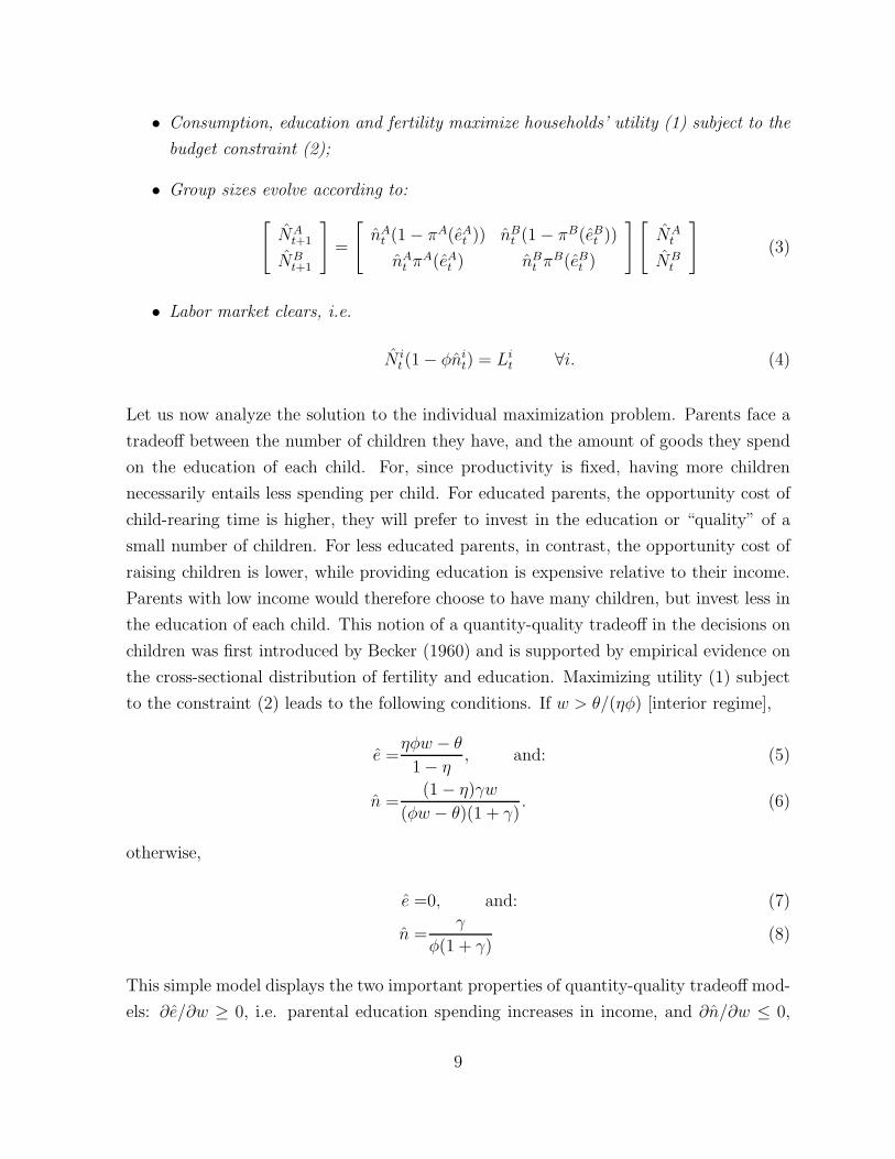
• Consumption, education and fertility maximize households’ utility (1) subject to the

budget constraint (2);

• Group sizes evolve according to:

[

NAt+1

NBt+1

]

=

[

nAt (1 − πA(eA

t )) nBt (1 − πB(eB

t ))

nAt πA(eA

t ) nBt πB(eB

t )

][

NAt

NBt

]

(3)

• Labor market clears, i.e.

N it (1 − φni

t) = Lit ∀i. (4)

Let us now analyze the solution to the individual maximization problem. Parents face a

tradeoff between the number of children they have, and the amount of goods they spend

on the education of each child. For, since productivity is fixed, having more children

necessarily entails less spending per child. For educated parents, the opportunity cost of

child-rearing time is higher, they will prefer to invest in the education or “quality” of a

small number of children. For less educated parents, in contrast, the opportunity cost of

raising children is lower, while providing education is expensive relative to their income.

Parents with low income would therefore choose to have many children, but invest less in

the education of each child. This notion of a quantity-quality tradeoff in the decisions on

children was first introduced by Becker (1960) and is supported by empirical evidence on

the cross-sectional distribution of fertility and education. Maximizing utility (1) subject

to the constraint (2) leads to the following conditions. If w > θ/(ηφ) [interior regime],

e =ηφw − θ

1 − η, and: (5)

n =(1 − η)γw

(φw − θ)(1 + γ). (6)

otherwise,

e =0, and: (7)

n =γ

φ(1 + γ)(8)

This simple model displays the two important properties of quantity-quality tradeoff mod-

els: ∂e/∂w ≥ 0, i.e. parental education spending increases in income, and ∂n/∂w ≤ 0,

9

i.e. fertility decreases in income. Since income in this model reflects human capital, fer-

tility is a decreasing function of the human capital of the parents. Notice also the role of

parameter θ, which captures the education children receive for free (by nature or society).

A higher θ pushes parents to substitute education with number of children.

Observed income inequality ∆B (B for benchmark) can be measured by the difference

between high skilled and low skilled income:

∆B = ωB(1 − φnB) − ωA(1 − φnA). (9)

This measure will be used later to assess the effect of procreation rights on income dif-

ferences. In this respect it is worth emphasizing that the metric adopted in this paper

is income rather than utility differences. Moreover, we focus on differences in income, as

opposed to possible improvement or degradation of the income of the least well off.

The long-run properties of the model can be analyzed by defining the following population

ratio:

zt =NA

t

NBt

.

The dynamic system (3) is reduced to a first-order recurrence equation zt+1 = f(zt). In

Appendix A, we show that the function f(.) satisfies: f(0) > 0, f ′(z) > 0, f ′′(z) < 0.

The last two results are guaranteed by the fact that τB > τA. The dynamics of zt admit

a single positive steady state which is globally stable.

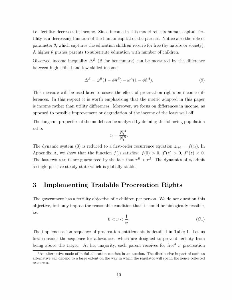
3 Implementing Tradable Procreation Rights

The government has a fertility objective of ν children per person. We do not question this

objective, but only impose the reasonable condition that it should be biologically feasible,

i.e.

0 < ν <1

φ. (C1)

The implementation sequence of procreation entitlements is detailed in Table 1. Let us

first consider the sequence for allowances, which are designed to prevent fertility from

being above the target. At her majority, each parent receives for free4 ν procreation

4An alternative mode of initial allocation consists in an auction. The distributive impact of such analternative will depend to a large extent on the way in which the regulator will spend the hence collectedresources.

10

Table 1: Implementation sequence

Allowances Exemptions(price gt ≥ 0) (price qt ≥ 0)

At majority receives ν rights

At each birth cedes back one right if number births > νreceives 1 right

At menopause if nt < ν < 0gives back ν − nt rights

Over complete life Procreation and exemption rights can be sold and purchased

allowances from the Procreation Agency. We assume that each procreation allowance

corresponds with the right to give birth to one child. Each time she gives birth to a

child, a parent has to cede one procreation allowance back to the Procreation Agency.

Procreation rights can be sold and purchased at any moment in time at a price gt. We

assume that fines are such that everyone will be deterred from violating such rules at

equilibrium.5

We now consider the sequence for exemptions, which are designed to prevent fertility

from being below the target. Each time a parent gives birth to a child, and as soon as

observed parent’s fertility nt becomes larger than ν, she will receive free of charge from the

Procreation Agency one exemption right per additional child. At the standard menopausal

age, each parent having less biological children than ν has to give the Procreation Agency

ν − n exemptions, which she will have purchased on the procreation exemptions market

at a price qt ≥ 0. parents with more children than ν can sell on the market the un-used

exemptions.

Table 1 makes visible three specific properties of a tradable entitlement scheme aimed

at addressing a problem of under-provision. First, the exemptions are allocated ex post

facto rather than initially. Second, in comparison with taxation, our proposal exhibits

two properties. Not only is it quantity focused as opposed to price focused, but the joint

operation of allowances and exemptions guarantees that the target will strictly be met;

5Such fines will have to be targeted in such ways as not to affect the children themselves. Otherwisechildren would be sanctioned as a matter of fact for what they are not responsible for, see Dworkin (2000).

11

in case of tradable exemptions, we see from the table that their amount is not limited

ex ante otherwise than through the biological constraint (nt ≤ 1/φ); in the absence of

an upper limit, reaching strictly the target cannot be guaranteed unless the system is

coupled with a tradable allowances scheme, which is the case here. Third, contrary to a

subsidy, the value of the exemption will fluctuate as a function of market conditions.

In our model there is no child mortality or infertility risk. In a more general set-up, these

issues could addressed these issues by assuming a perfect insurance market which would

cover those risks.

After inclusion of the procreation entitlements, the budget constraint for an adult be-

comes:

cit =

[wi

t(1 − φnit) − ni

teit

]+ gt(ν − ni

t) + qt(nit − ν). (10)

The variable gt is the price of one procreation allowance, while qt is the price of one

procreation exemption. Since the two types of entitlements are put in operation simul-

taneously, only the difference gt − qt matters. We call this difference “procreation price”

and accordingly define

pt = gt − qt.

In equilibrium, pt can be positive or negative. Equilibria with positive procreation price

pt reflect situations where fertility is discouraged, while equilibria with pt negative obtain

in cases in which fertility is promoted. The following definition stresses that there is one

additional market compared to Definition 1.

Definition 2 (Equilibrium with Procreation Rights)

Given initial population sizes NA0 and NB

0 , an equilibrium is a sequence of individual

quantities (cit, e

it, n

it)i=A,B.t≥0, group sizes (N i

t )i=A,B.t≥0, and prices (pt)t≥0 such that

• Consumption, education and fertility maximize households’ utility (1) subject to the

budget constraint (10);

• Group sizes evolve according to (3).

• Labor market clears, i.e. Equation (4) holds.

• Asset market clears, i.e.∑

i

(nit − ν)N i

t = 0 (11)

12

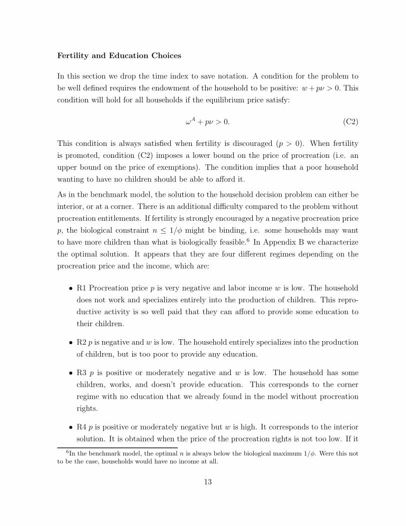
Fertility and Education Choices

In this section we drop the time index to save notation. A condition for the problem to

be well defined requires the endowment of the household to be positive: w + pν > 0. This

condition will hold for all households if the equilibrium price satisfy:

ωA + pν > 0. (C2)

This condition is always satisfied when fertility is discouraged (p > 0). When fertility

is promoted, condition (C2) imposes a lower bound on the price of procreation (i.e. an

upper bound on the price of exemptions). The condition implies that a poor household

wanting to have no children should be able to afford it.

As in the benchmark model, the solution to the household decision problem can either be

interior, or at a corner. There is an additional difficulty compared to the problem without

procreation entitlements. If fertility is strongly encouraged by a negative procreation price

p, the biological constraint n ≤ 1/φ might be binding, i.e. some households may want

to have more children than what is biologically feasible.6 In Appendix B we characterize

the optimal solution. It appears that they are four different regimes depending on the

procreation price and the income, which are:

• R1 Procreation price p is very negative and labor income w is low. The household

does not work and specializes entirely into the production of children. This repro-

ductive activity is so well paid that they can afford to provide some education to

their children.

• R2 p is negative and w is low. The household entirely specializes into the production

of children, but is too poor to provide any education.

• R3 p is positive or moderately negative and w is low. The household has some

children, works, and doesn’t provide education. This corresponds to the corner

regime with no education that we already found in the model without procreation

rights.

• R4 p is positive or moderately negative but w is high. It corresponds to the interior

solution. It is obtained when the price of the procreation rights is not too low. If it

6In the benchmark model, the optimal n is always below the biological maximum 1/φ. Were this notto be the case, households would have no income at all.

13

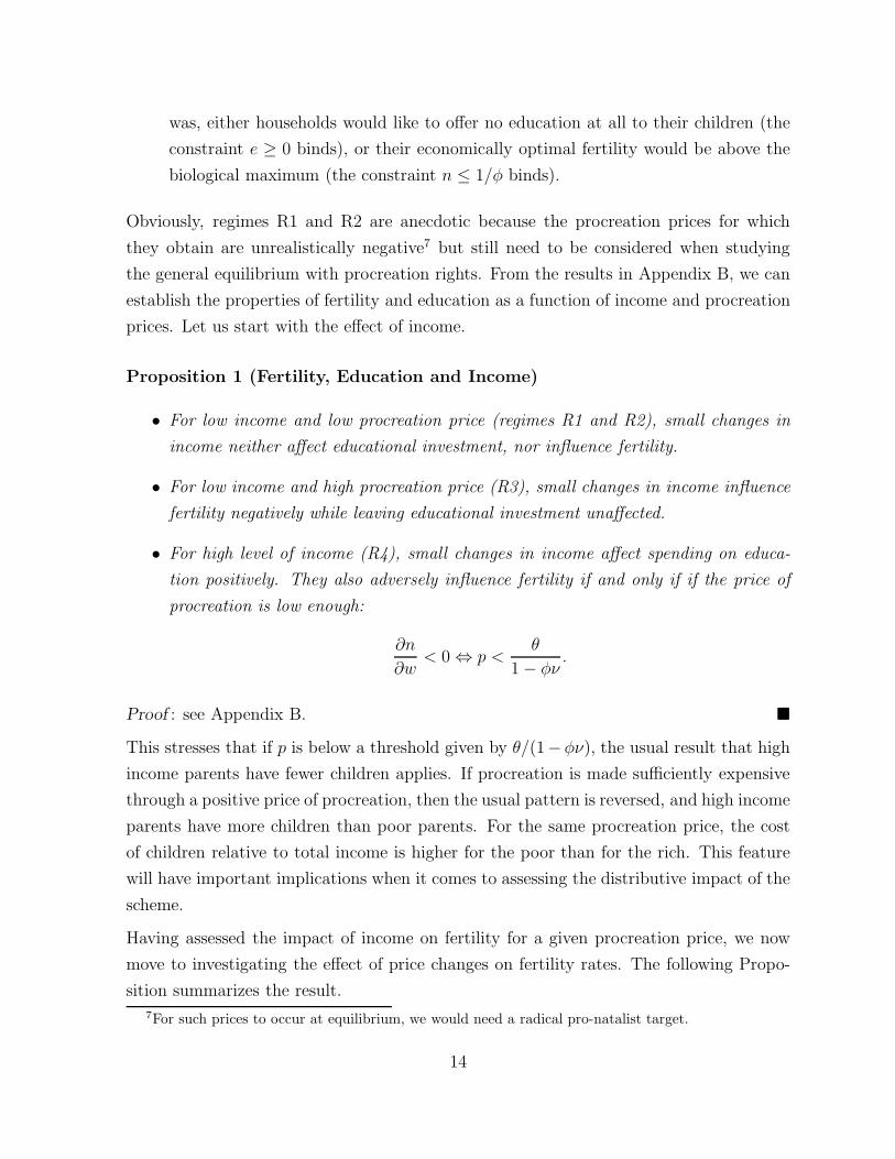
was, either households would like to offer no education at all to their children (the

constraint e ≥ 0 binds), or their economically optimal fertility would be above the

biological maximum (the constraint n ≤ 1/φ binds).

Obviously, regimes R1 and R2 are anecdotic because the procreation prices for which

they obtain are unrealistically negative7 but still need to be considered when studying

the general equilibrium with procreation rights. From the results in Appendix B, we can

establish the properties of fertility and education as a function of income and procreation

prices. Let us start with the effect of income.

Proposition 1 (Fertility, Education and Income)

• For low income and low procreation price (regimes R1 and R2), small changes in

income neither affect educational investment, nor influence fertility.

• For low income and high procreation price (R3), small changes in income influence

fertility negatively while leaving educational investment unaffected.

• For high level of income (R4), small changes in income affect spending on educa-

tion positively. They also adversely influence fertility if and only if if the price of

procreation is low enough:

∂n

∂w< 0 ⇔ p <

θ

1 − φν.

Proof : see Appendix B. �

This stresses that if p is below a threshold given by θ/(1−φν), the usual result that high

income parents have fewer children applies. If procreation is made sufficiently expensive

through a positive price of procreation, then the usual pattern is reversed, and high income

parents have more children than poor parents. For the same procreation price, the cost

of children relative to total income is higher for the poor than for the rich. This feature

will have important implications when it comes to assessing the distributive impact of the

scheme.

Having assessed the impact of income on fertility for a given procreation price, we now

move to investigating the effect of price changes on fertility rates. The following Propo-

sition summarizes the result.

7For such prices to occur at equilibrium, we would need a radical pro-natalist target.

14

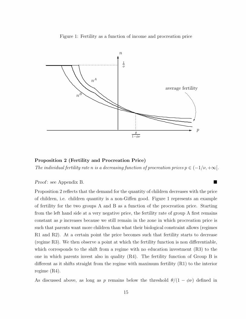
Figure 1: Fertility as a function of income and procreation price6

-..............

n

pθ

1−φν

nA

nB

........................... 1φ

�average fertility

Proposition 2 (Fertility and Procreation Price)

The individual fertility rate n is a decreasing function of procreation prices p ∈ (−1/ν, +∞[.

Proof : see Appendix B. �

Proposition 2 reflects that the demand for the quantity of children decreases with the price

of children, i.e. children quantity is a non-Giffen good. Figure 1 represents an example

of fertility for the two groups A and B as a function of the procreation price. Starting

from the left hand side at a very negative price, the fertility rate of group A first remains

constant as p increases because we still remain in the zone in which procreation price is

such that parents want more children than what their biological constraint allows (regimes

R1 and R2). At a certain point the price becomes such that fertility starts to decrease

(regime R3). We then observe a point at which the fertility function is non differentiable,

which corresponds to the shift from a regime with no education investment (R3) to the

one in which parents invest also in quality (R4). The fertility function of Group B is

different as it shifts straight from the regime with maximum fertility (R1) to the interior

regime (R4).

As discussed above, as long as p remains below the threshold θ/(1 − φν) defined in

15

Proposition 1, the fertility rate of group A is equal to or greater than the fertility rate of

group B. In case p is large, however, the differential fertility is reversed.

Equilibrium

After having analyzed the effect of procreation entitlements on individual behavior, it

now remains to be shown that there is procreation price such that actual average fertility

will meet the demographic target set by the government.

The property outlined above that households’ fertility rates are decreasing functions of the

procreation price implies that average fertility is also a decreasing function of p. Under

the condition that for the lowest possible negative price p (condition (C2)) all groups are

in regime R1, average fertility decreases from 1/φ for very low p to 0 for large positive

p. The continuity of the fertility function is then sufficient to establish the existence of

an equilibrium procreation price, which implies that the target fertility rate ν is reached.

The uniqueness of the equilibrium follows from the monotonicity of the fertility function.

Proposition 3 (Existence and Uniqueness of Equilibrium)

Define:

p(w) ≡θ(1 + γ) − (1 + ηγ)φw

γ(1 − (1 − η)φν) + 1.

If p(ωB) > −1/ν the equilibrium procreation price exists and is unique.

Proof : See Appendix C. �

Besides the technical constraint p(ωB) > −1/ν, it follows that the structure of the econ-

omy as such will not impose constraints as to the possible level of the demographic target

ν. This does not preclude the possibility of constraints due to other reasons, such as

political feasibility or ethical reasons.

At equilibrium, our measure of income inequality ∆T (T for tradable) is given by:

∆T = ωB(1 − φnB) + p(ν − nB) −[ωA(1 − φnA) + p(ν − nA)

]

= ωB(1 − φnB) − ωA(1 − φnA) + p(nA − nB). (12)

Hence, on top of the difference in labor income one should take into account the transfer

which is generated by procreation rights p(nA − nB).

16

4 Effects on Income Inequality and Education

In order to assess the distributive impact resulting from the introduction of a tradable

procreation scheme, it is helpful to first look at a simpler case, which is the impact of

fixed quotas.

Two Effects of Fixed Quotas on Income Inequality

Examining the impact of tradable quotas schemes would not make much sense without

providing a comparison of such effects with either those of a business-as-usual8 situation,

or those of alternative measures aimed at reaching the same demographic target. There

are two families of such alternative policy options. Either, we go for a measure that,

while being quantity-oriented as well, would be of a more rigid type, i.e. fixed rather

than tradable quotas. Or, we go for a variety of price-oriented measures, such as family

allowances, free education,... (in case of underpopulation) or for taxation (in case of

overpopulation). In the case of price-oriented methods, potential parents are totally free

to chose the number of children they wish to have, under the pressure of incentives or

disincentives set up by regulatory authorities. Here, we only compare tradable quotas with

fixed ones, both because this is the closest realistic alternative method, as the Chinese

example suggests, and because a comparison with price-oriented methods would require

a much richer analytic aparatus than the one we wish to rely upon here. Let us stress as

well the fact that when comparing fixed and tradable quotas, we should assume the same

type of initial allocation (here: equality per head).9

Formally, fixed quotas imposes an additional constraint n ≤ ν to the maximization prob-

lem studied in Section 2. If this constraint is tight for the skilled parents, i.e. if they would

otherwise have more children, it will also be tight a fortiori for the unskilled. Hence, the

constraint n ≤ ν is tight for both groups if and only if

ν ≤(1 − η)γωB

(φωB − θ)(1 + γ)= nB,

The reverse situation where the government imposes a minimum fertility level can also

8Benchmark and business-as-usual are used indifferently for the purpose of this paper.9Notice that, in Chinese one child policy, the fixed quotas are not uniformly distributed: two children

are allowed for in the countryside, only one in cities. This illustrates that the uniform allocation is notthe only possible option, and that allocations of quotas on the basis of other factors, such as existingfertility levels, are also possible. This point is further developed in Section 5.

17

be analyzed. In that case, the constraint is written n ≥ ν. It will be tight for the poor

and even more so for the rich if and only if

ν ≥(1 − η)γωA

(φωA − θ)(1 + γ)= nA,

Hereinafter we only envisage the former case, dealing with over-population, unless speci-

fied otherwise. The results we obtain apply mutatis mutandis to the policy dealing with

under-population.

Assuming tight constraints, the solution to the maximization problem is:

If w > θ/(γη(1/ν − φ)) [interior regime],

e =γηw(1/ν − φ) − θ

1 + γη

Otherwise

e = 0.

In the interior regime, we have ∂e/∂ν < 0. This confirms that as parents react to the

quantitative constraint by having less children, they will be able to afford to spend more

on each of their children.

As to income inequality, the difference between high skilled and low skilled income, ∆F

(F for fixed), is given by:

∆F = ωB(1 − φν) − ωA(1 − φν). (13)

Comparing with Equation (12) of the tradable rights case, transfers do not obtain in this

case as a result of population policy.

We compute the change in income difference resulting from the introduction of fixed

quotas:

∆F − ∆B

φ= (n − ν)(ωB − ωA)

︸ ︷︷ ︸

differential productivity effect>0

+ ωB(nB − n) − ωA(nA − n)︸ ︷︷ ︸

differential fertility effect<0

where n = (nANA + nBNB)/(NA + NB) is average fertility in the benchmark case. The

first effect, labeled “differential productivity effect” can be understood as follows. Let us

envisage a hypothetical business-as-usual situation in which high-income and low-income

18

people have the same fertility level n. Assume that this level is higher than the one

required by our demographic target ν. With the introduction of non-tradable quotas the

extent to which the rich will procreate less than the poor is identical. Both the skilled

and the unskilled will increase their income as a result of the time made available by such

lower fertility. However, since the hourly wage (and underlying it, the productivity) of

the high-income is higher than the one of the low-income people, the income of the rich

will increase relatively more than the one of the poor. In short, the introduction of fixed

quotas to fight overpopulation in a world in which the fertility rate does not vary with

the level of income, will make the poor-income relatively poorer than the high-income.

The second effect, labeled “differential fertility effect” relaxes the assumption regarding

the absence of initial fertility differential (and it is equal to zero if nB = nA). In the

benchmark situation low-income people tend to have more children than high-income

people. Here, a second type of effect can be singled out, of a redistributive rather than

of an anti-distributive nature. It can be explained as follows. If the fixed quotas scheme

requires the same fertility level from the poor and the rich, the poor will have to reduce

her fertility level much more than the rich. As a result, she will also increase her working

time more than the rich. This effect will reduce income inequality between the rich and

the poor, when compared with the income differential in the business-as-usual situation.

The sign of the total effect of introducing fixed quotas on income difference depends on

which of the two effects dominates. One parameter affecting the relative weight of the two

effects is the elasticity of educational outcomes over investment in education, represented

by η. Indeed, computing the extreme hypothetical fertility rates of households with zero

income and infinite income leads to:

nmax = limw→0

n =γ

φ(1 + γ)

nmin = limw→∞

n =γ(1 − η)

φ(1 + γ)

The maximum differential fertility is therefore:

nmaxnmin

=1

1 − η.

If this elasticity η is large, the fertility differential will tend to be large as well, to such

an extent that the “differential fertility effect” may actually dominate the differential

productivity effect. The reason underlying this connection between outcome-investment

19

elasticity and fertility differential is the following. The poor is equally concerned about

education as the rich. However, for the poor, the cost of investing in education as well

as the opportunity cost of having children is lower than for the rich. A higher outcome

investment elasticity will not affect the poor much, but will definitely push the rich the

substitute quality to quantity even more. Hence, the differential fertility is larger when η

is large.

Effect of Tradability on Income Inequality

We now replace fixed quotas with tradable quotas. In order to identify the difference it

makes, we compute the change in income gap between the benchmark and the model with

tradeable rights:

∆T − ∆B

φ= (n − ν)(ωB − ωA)

︸ ︷︷ ︸

differential productivity effect >0

+

[ωB(nB − n) − ωA(nA − n)

]−

[ωB(nB − ν) − ωA(nA − ν)

]

︸ ︷︷ ︸

differential fertility effect

+p

φ(nA − nB)

︸ ︷︷ ︸

tradability effect

(14)

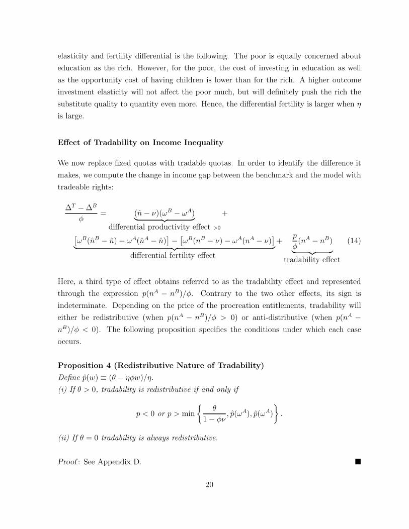
Here, a third type of effect obtains referred to as the tradability effect and represented

through the expression p(nA − nB)/φ. Contrary to the two other effects, its sign is

indeterminate. Depending on the price of the procreation entitlements, tradability will

either be redistributive (when p(nA − nB)/φ > 0) or anti-distributive (when p(nA −

nB)/φ < 0). The following proposition specifies the conditions under which each case

occurs.

Proposition 4 (Redistributive Nature of Tradability)

Define p(w) ≡ (θ − ηφw)/η.

(i) If θ > 0, tradability is redistributive if and only if

p < 0 or p > min

{θ

1 − φν, p(ωA), p(ωA)

}

.

(ii) If θ = 0 tradability is always redistributive.

Proof : See Appendix D. �

20

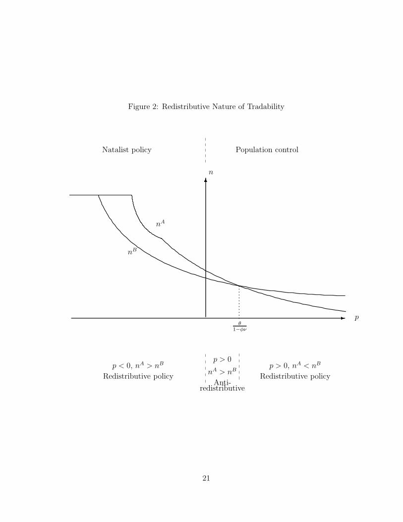
Figure 2: Redistributive Nature of Tradability

6

-..............

Natalist policy Population control

n

pθ

1−φν

p < 0, nA > nB

Redistributive policy

p > 0, nA < nB

Redistributive policy

p > 0

nA > nB

Anti-redistributive

nA

nB

21

Figure 2 helps capturing the intuition underlying Proposition 4. When p is negative,

fertility is encouraged. Poor households have more children than the fertility target while

the rich have less. Poor people sell the exemptions they receive to the rich which reduces

the income gap between the rich and the poor. When p is positive and large, having

children is so expensive that rich people have more children than poor ones. This time,

the poor end up below the target and the rich above.10 Yet this is also redistributive

because poor people sell the procreation allowances they do not use to the rich (this is the

case imagined by Boulding). It is only when the procreation price is modestly positive that

tradability is anti-redistributive.11 In that case the price of allowances is not high enough

to bring the poor under the target, and therefore to reverse the fertility differential. Poor

households thus buy allowances from the rich and the income gap increases. Notice that

if θ is close to zero, this possibility disappears.

One important issue is whether practical indications can be provided as to whether an

actual scheme is likely to fall within the anti-redistributive zone identified in Figure 2.

There is at least one consideration that is relevant here. If we focus on the distributive

impact of tradability alone, if ν is lower but close to the existing fertility level, the price

of the procreation allowances will not be large enough and we are likely to fall within

the anti-redistributive zone. In other words, from the point of view of the tradability

effect alone, the best guarantee for the scheme to have a distributive impact consists in

adopting a radical reform, i.e. one involving a ν that diverges enough from the existing

fertility rate. This is significant as gradual reforms in this field are more likely to be po-

litically feasible than radical ones. Two conclusions can be drawn from this. First, if we

take the tradability effect alone as illustrated in Figure 2, schemes implementing the pro-

posed model are likely in practice to fall within the anti-redistributive zone, since radical

changes are less politically feasible. Second, whether this would tend to make the scheme

anti-redistributive all-things-considered does not necessarily follow as our discussion in

Section 5 will illustrate.

Effects on Education

Let us now turn our attention to the effect of procreation entitlements on education. This

is an important question because both social mobility and long-run income are positively

10At equilibrium the target is always equal to average fertility.11This invites to look with a critical eye the widely shared view, also implied e.g. in Tobin (1970), that

tradability promotes by nature inequality.

22

affected by education spending. The following proposition shows how education depends

on procreation price.

Proposition 5 (Education and Procreation Price)

Define

p ≡−θ

γη(1 − φν)< 0.

Assume that the threshold p = min{p, p(w)} < −1/ν. Investment in education e is

increasing in procreation price p.

Proof : From the expression for e given in Proposition 6. �

An increase in the procreation price reduces fertility (Proposition 2) and increases educa-

tion, which is the usual quantity-quality tradeoff facing a rise in the cost of children. In

this case, natalist policy would be bad for education, social mobility and long-run income,

while population control would be good.12

One of the interesting effects of a pro-natalist policy is intergenerational and illustrates as

well the interaction between the income and the educational impact of demographic poli-

cies. Let us consider two generations: P (parents) and C (children). And let us envisage

a population target such that the procreation price is negative. Such a pro-natalist policy

tends to reduce income inequalities within generation P due to the tradability effect. How-

ever, this raises a serious difficulty. For the very same pro-natalist policy, while reducing

income inequalities within generation P, will also reduce the average level of education

(hence, the income level as well) of generation C. The pro-natalist subsidy is insufficient

to compensate the income loss resulting from the fact that people with more children

tend to work less. This entails that they will earn less and have less money to invest in

education both in total and, a fortiori, per capita. In other words, a pro-natalist policy

will end up leading to a situation such that, while being redistributive for generation P, it

will tend to increase income inequalities between generations P and C. This is a problem

e.g. because we may then end up with a world in which the worst off people are worse off

than in the business-as-usual scenario (i.e. in the absence of pro-natalist policy). Does

this constitute a sufficient reason to reject the proposed scheme altogether? We do not

12A special but practically marginal case arises when p is extremely low and p > −1/ν. In such a case,individual investment in education e is decreasing in p for p < p and increasing in p for p > p. Poorhouseholds are in regime R1; they are entirely specialized into the production of children (n = 1/φ). Asmall rise in p has no effect on fertility, but has a negative income effect, which entails that educationspending is reduced.

23

think so. It rather stresses on the need to couple demographic policy with educational

policy. We could then both get the redistributive impact at the generation P level without

generating the negative impact on education (and income) for generation C. In practice,

this could take the form of education subsidies or publicly provided education.

5 Moving from National to Global Level

Procreation Entitlements at the Global Level

So far, we have assumed that tradable procreation permits were allocated at the domestic

level. There may however be good reasons to look at the way in which the scheme could be

applied to countries rather than to individuals. One such reasons is that those concerned

with the scheme at the domestic level because of moral objections to its enforcement, may

still be ready to accept that less coercive measures at the domestic level be combined with

a scheme of tradable procreation permits among countries. Moreover, those willing on

the contrary to promote the instrument domestically will generally be positively inclined

towards simultaneously implementing it at the global level. Another reason to look more

closely at a global version of the scheme is that one often cited mode of initial allocation,

i.e. grandfathering, could possibly make sense at the global level while being far less

plausible at the individual level.

Applied at the global level, the system would work along the same lines as a domestic one,

involving two key moments. First, a global demographic target should be set for a given

period. Second, we would need to decide about an initial allocation rule to distribute

the quotas to each of the countries. Let us first consider a situation with a uniform

distribution of entitlements, which is the case analyzed so far. Understanding agents in

our model as countries or set of countries, all the results developed above can be applied

at the global level. In particular, the market for procreation entitlements will clear at

the equilibrium price, country specific fertility and education reacting as described by

Propositions 2 and 5. The effect of tradability on income (gross national income here)

will depend on the condition set in Proposition 4.

Numerical Illustration

To illustrate how our set-up would operate at the global level, a version of the model

with a large number of agents (countries) will be solved numerically. In order to associate

24

numerical values to our parameters η, φ; θ, and γ, we first calibrate the benchmark

case of Section 2 on a cross-section of countries. Next we simulate the introduction of

procreation entitlements aiming at reducing the global fertility rate. Results could easily

be generalized to the reverse situation of under-population.

Calibration

One period in the model lasts 25 years. The variables are measured with data from

the World Development Indicators, averaging those available for the years 1998-2002.

Variable n is computed as the net reproduction rate, i.e. “Fertility rate, total (births

per woman)” divided by two in order to obtain a fertility rate per person and multiplied

by (1− “Mortality rate, infant (per 1,000 live births)”/1000) to measure net fertility per

capita. Total education θ + e corresponds to the product of “Adjusted savings: education

expenditure (% of GNI)” and “GNI per capita, PPP (current international $)” loading

to a measure of education spending per capita in PPP dollars. Population size N for

each country is proportional to the population aged 15-64. Productivity per person ω is

unobservable but can be obtained from Gross National Income y as follows:

y = ω(1 − φn/25). (15)

We then estimate by Full Information Maximum Likelihood the parameters φ, θ, η and

γ of the system (5)-(6)-(15):

ei =

0 if ωi ≤θηφ

ηφωi−θ

1−ηif ωi > θ

ηφ)

+ εei (16)

ni =

γ

φ(1+γ)if ωi ≤

θηφ

(1−η)γωi

(φωi−θ)(1+γ)if ωi > θ

ηφ

+ εni (17)

yi =ωi(1 − φni/25)

The estimation results are presented in Table 2. The point estimate for the parameter

η, which measures the elasticity of income to schooling, is located well within the range

of estimates of the elasticity of earnings with respect to schooling (see the discussion in

de la Croix and Doepke (2003)). The estimated value for φ implies that one child takes

25

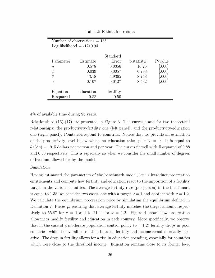
Table 2: Estimation results

Number of observations = 158Log likelihood = -1210.94

StandardParameter Estimate Error t-statistic P-valueη 0.578 0.0356 16.25 [.000]φ 0.039 0.0057 6.798 [.000]θ 43.18 4.9365 8.748 [.000]γ 0.107 0.0127 8.432 [.000]

Equation education fertilityR-squared 0.88 0.50

4% of available time during 25 years.

Relationships (16)-(17) are presented in Figure 3. The curves stand for two theoretical

relationships: the productivity-fertility one (left panel), and the productivity-education

one (right panel). Points correspond to countries. Notice that we provide an estimation

of the productivity level below which no education takes place e = 0. It is equal to

θ/(φη) = 1915 dollars per person and per year. The curves fit well with R-squared of 0.88

and 0.50 respectively. This is especially so when we consider the small number of degrees

of freedom allowed for by the model.

Simulation

Having estimated the parameters of the benchmark model, let us introduce procreation

entitlements and compute how fertility and education react to the imposition of a fertility

target in the various countries. The average fertility rate (per person) in the benchmark

is equal to 1.38; we consider two cases, one with a target ν = 1 and another with ν = 1.2.

We calculate the equilibrium procreation price by simulating the equilibrium defined in

Definition 2. Prices pt ensuring that average fertility matches the target amount respec-

tively to 55.87 for ν = 1 and to 21.44 for ν = 1.2. Figure 4 shows how procreation

allowances modify fertility and education in each country. More specifically, we observe

that in the case of a moderate population control policy (ν = 1.2) fertility drops in poor

countries, while the overall correlation between fertility and income remains broadly neg-

ative. The drop in fertility allows for a rise in education spending, especially for countries

which were close to the threshold income. Education remains close to its former level

26

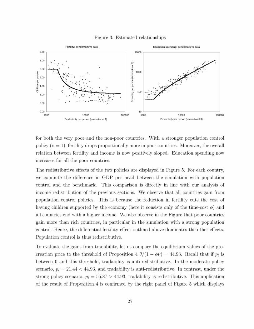
Figure 3: Estimated relationships

Fertility: benchmark vs data

0.00

0.50

1.00

1.50

2.00

2.50

3.00

3.50

1000 10000 100000

Productivity per person (international $)

Chi

ldre

n pe

r pe

rson

Education spending: benchmark vs data

10

100

1000

10000

1000 10000 100000

Productivity per person (international $)

Spe

ndin

g pe

r pe

rson

(in

tern

atio

nal $

)

for both the very poor and the non-poor countries. With a stronger population control

policy (ν = 1), fertility drops proportionally more in poor countries. Moreover, the overall

relation between fertility and income is now positively sloped. Education spending now

increases for all the poor countries.

The redistributive effects of the two policies are displayed in Figure 5. For each country,

we compute the difference in GDP per head between the simulation with population

control and the benchmark. This comparison is directly in line with our analysis of

income redistribution of the previous sections. We observe that all countries gain from

population control policies. This is because the reduction in fertility cuts the cost of

having children supported by the economy (here it consists only of the time-cost φ) and

all countries end with a higher income. We also observe in the Figure that poor countries

gain more than rich countries, in particular in the simulation with a strong population

control. Hence, the differential fertility effect outlined above dominates the other effects.

Population control is thus redistributive.

To evaluate the gains from tradability, let us compare the equilibrium values of the pro-

creation price to the threshold of Proposition 4 θ/(1 − φν) = 44.93. Recall that if pt is

between 0 and this threshold, tradability is anti-redistributive. In the moderate policy

scenario, pt = 21.44 < 44.93, and tradability is anti-redistributive. In contrast, under the

strong policy scenario, pt = 55.87 > 44.93, tradability is redistributive. This application

of the result of Proposition 4 is confirmed by the right panel of Figure 5 which displays

27

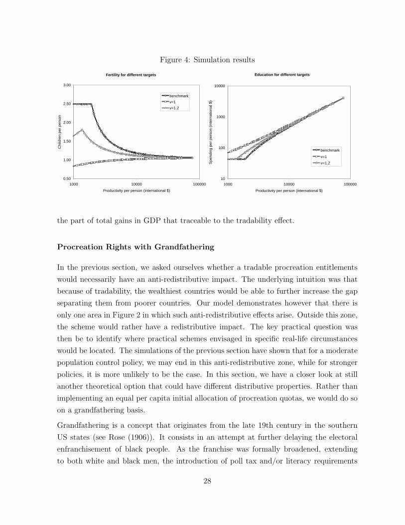
Figure 4: Simulation results

Fertility for different targets

0.50

1.00

1.50

2.00

2.50

3.00

1000 10000 100000

Productivity per person (international $)

Chi

ldre

n pe

r pe

rson

benchmark

v=1

v=1.2

Education for different targets

10

100

1000

10000

1000 10000 100000

Productivity per person (international $)

Spe

ndin

g pe

r pe

rson

(in

tern

atio

nal $

)

benchmark

v=1

v=1.2

the part of total gains in GDP that traceable to the tradability effect.

Procreation Rights with Grandfathering

In the previous section, we asked ourselves whether a tradable procreation entitlements

would necessarily have an anti-redistributive impact. The underlying intuition was that

because of tradability, the wealthiest countries would be able to further increase the gap

separating them from poorer countries. Our model demonstrates however that there is

only one area in Figure 2 in which such anti-redistributive effects arise. Outside this zone,

the scheme would rather have a redistributive impact. The key practical question was

then be to identify where practical schemes envisaged in specific real-life circumstances

would be located. The simulations of the previous section have shown that for a moderate

population control policy, we may end in this anti-redistributive zone, while for stronger

policies, it is more unlikely to be the case. In this section, we have a closer look at still

another theoretical option that could have different distributive properties. Rather than

implementing an equal per capita initial allocation of procreation quotas, we would do so

on a grandfathering basis.

Grandfathering is a concept that originates from the late 19th century in the southern

US states (see Rose (1906)). It consists in an attempt at further delaying the electoral

enfranchisement of black people. As the franchise was formally broadened, extending

to both white and black men, the introduction of poll tax and/or literacy requirements

28

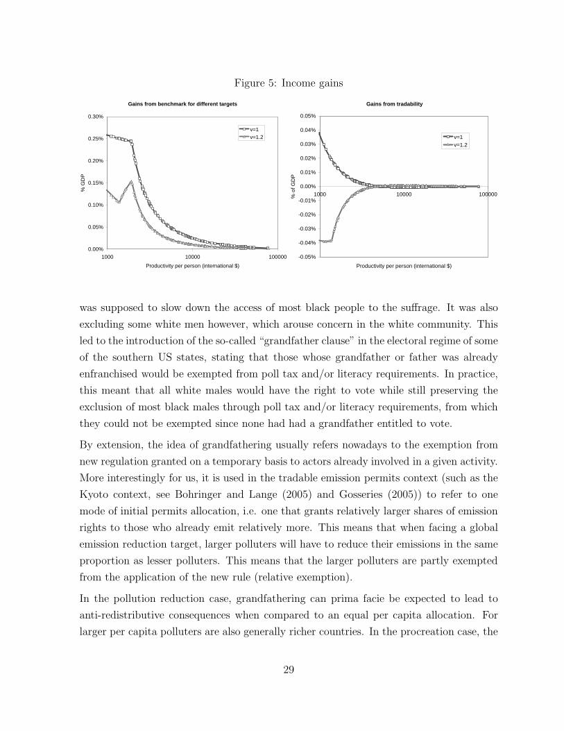
Figure 5: Income gains

Gains from benchmark for different targets

0.00%

0.05%

0.10%

0.15%

0.20%

0.25%

0.30%

1000 10000 100000

Productivity per person (international $)

% G

DP

v=1v=1.2

Gains from tradability

-0.05%

-0.04%

-0.03%

-0.02%

-0.01%

0.00%

0.01%

0.02%

0.03%

0.04%

0.05%

1000 10000 100000

Productivity per person (international $)

% o

f GD

P

v=1v=1.2

was supposed to slow down the access of most black people to the suffrage. It was also

excluding some white men however, which arouse concern in the white community. This

led to the introduction of the so-called “grandfather clause” in the electoral regime of some

of the southern US states, stating that those whose grandfather or father was already

enfranchised would be exempted from poll tax and/or literacy requirements. In practice,

this meant that all white males would have the right to vote while still preserving the

exclusion of most black males through poll tax and/or literacy requirements, from which

they could not be exempted since none had had a grandfather entitled to vote.

By extension, the idea of grandfathering usually refers nowadays to the exemption from

new regulation granted on a temporary basis to actors already involved in a given activity.

More interestingly for us, it is used in the tradable emission permits context (such as the

Kyoto context, see Bohringer and Lange (2005) and Gosseries (2005)) to refer to one

mode of initial permits allocation, i.e. one that grants relatively larger shares of emission

rights to those who already emit relatively more. This means that when facing a global

emission reduction target, larger polluters will have to reduce their emissions in the same

proportion as lesser polluters. This means that the larger polluters are partly exempted

from the application of the new rule (relative exemption).

In the pollution reduction case, grandfathering can prima facie be expected to lead to

anti-redistributive consequences when compared to an equal per capita allocation. For

larger per capita polluters are also generally richer countries. In the procreation case, the

29

relationship between fertility rate and wealth is not so straightforward and might actually

be the reverse. This suggests that grandfathering in the case of tradable procreation

entitlements could well have a distributive impact that differs both from the one exhibited

in the case of grandfathering for tradable emission quotas and from the one unveiled in

the previous section for tradable procreation entitlements allocated on a per capita basis.

We now provide the analysis needed for the latter comparison.

We assume that countries receive an initial endowment of rights proportional to their

fertility rate in the absence of procreation rights (benchmark):13

νi = µ ni |p=0 .

Parameter µ, when larger than one, indicates a pronatalist policy. Conversely, if µ is

lower than one, population policy is restrictive. The previously defined average fertility

target ν relates to the νi through:

NAνA + NBνB = (NA + NB)ν.

Since initial endowments are now different across countries, the income gap between

countries becomes:

∆G = ωB − ωA + p(νB − nB) − p(νA − nA).

where fertility levels with a tilde denote fertility in the grandfathering case. Computing

the difference in income gap between the benchmark case and the grandfathering one, we

13This is standardly done in practice for pollution rights. By referring to a base year preceding theconception of the scheme, we avoid the moral hazard problem consisting in trying to manipulate one’srelative share before the entry into force of the system.

30

obtain:

∆G − ∆B

φ= (n − ν)(ωB − ωA)

︸ ︷︷ ︸

differential productivity effect >0

+

[ωB(nB − n) − ωA(nA − n)

]−

[ωB(nB − ν) − ωA(nA − ν)

]

︸ ︷︷ ︸

differential fertility effect

+p

φ(nA − nB)

︸ ︷︷ ︸

tradability effect

−pµ

φ(nA − nB)

︸ ︷︷ ︸

grandfathering effect

(18)

where the hatted variables represent fertility in case of grandfathering.

We can compare this expression with the one in equation (14). The differential produc-

tivity effect is unchanged. The differential fertility effect and the tradability effect have

the same form as before, but nA and nB in (14) are now replace by nA and nB in (18).

The two latter effects would play the same role as before provided that fertility behavior

is only marginally altered by grandfathering. A fourth effect is the grandfathering effect.

Since the poor country initially received more procreation rights per head than the rich

one, an income transfer from the rich to the poor obtains in exchange for extra entitle-

ments in case of positive procreation price. The direction of transfer is reversed in case

of negative procreation price.

We still need to evaluate whether grandfathering modifies the fertility behavior in a quan-

titatively significant way. From numerical simulations carried on in our global model it

appears that the difference in fertility levels between the model with equal allocation of

rights and the one with grandfathering is very small, typically lower than three percentage

points for any country. Investment in education also remains almost unchanged. Equi-

librium procreation price are not much affected either, with pt = 56.30 instead of 55.87

for the radical policy (ν = 1) and pt = 21.66 instead of 21.44 for the moderate policy

(ν = 1.2). The reason for these negligible effects on behaviors and equilibrium prices is

that grandfathering acts as a lump-sum transfer (it is independent from effective bahav-

ior) generating only a small income effect, without any direct distortion on the price of

procreation.

We conclude from this that the essential difference between (18) and (14) is the last effect,

which is a pure transfer. Grandfathering has a redistributive effect in the case of popu-

lation control, simply by implementing a redistributive initial allocation of rights. While

31

its effect on fertility distribution is small, simulations show the effect of grandfathering

on income distribution can be large, increasing by 50% the gains in GDP for the poor

countries compared to a system with a uniform allocation of rights.

6 Conclusion

In this paper, we explored the idea of tradable procreation entitlements, within a gen-

eral equilibrium model with endogenous fertility. Both tradable allowances and tradable

exemptions were envisaged, aimed at addressing problems of respectively over- and under-

population. An equilibrium with such assets exists. It can thus implement any desired

growth rate of population. Having shown this, we focus on worries as to the possible anti-

redistributive nature of such a scheme, as well as to possibly adverse impacts in terms of

educational investments.

Three effects are identified and contrasted. While two of them also obtain in the case of

fixed quotas schemes, a third one, the tradability effect, is specific to the present scheme.

Insofar as income distribution is concerned, with procreation exemptions (whatever their

price) or allowances if they are expensive enough, tradability redistributes resources from

the rich to the poor. In contrast, cheap procreation allowances redistribute resources

towards the rich. Since high prices are likely to obtain only if fertility target departs

significantly from the benchmark demographic scenario and since radical reforms are

politically more difficult to defend than moderate ones, the risk of an anti-distributive

impact of the scheme is likely in case of initial allocation that would be equal per head.

As far as human capital is concerned, natalist policy would tend to reduce the average

educational level of the next generation, while population control would increase it. In case

of pro-natalist policies, sustaining education through additional measures may turn out to

be helpful for future generations. Restricting ourselves to natalist policy, negative effects

on the level of education should not necessarily be seen as reasons to reject the proposal

altogether. Rather, it requires that the scheme itself be either modified accordingly (e.g.

through changes in the initial allocation of permits) or complemented by other schemes

aimed at countering such effects.

We next consider the global level by applying our model to countries, rather than to

individuals, avoiding some of the enforcement difficulties involved in the domestic forms

of such schemes. Feeding our model with real data from 158 countries we show how a

32

global population control policy with tradable entitlements can reduce fertility in poor

countries and enhance education. We also indicate to what extent an alternative allocation

rule of procreation entitlements, granting rights in proportion to existing fertility levels

(grandfathering) rather than on a per capita basis, can make population control even

more redistributive.

Let us conclude by pointing at two interesting differences with tradable pollution quotas.

First, population control is a two-sided problem, which requires the use of two types of

entitlements, exemptions and allowances. Their joint operation guarantees that any target

can be met. Second, while the rich tend to pollute more than the more, the poor tend to

have more children than the rich. As a result, grandfathering is not always detrimental

to the poor, as insights from environmental economics may suggest.

References

Becker, Gary S. 1960. “An Economic Analysis of Fertility.” Demographic and Economic

Change in Developed Countries. Princeton: Princeton University Press.

Bohringer, Christoph, and Andreas Lange. 2005. “On the design of optimal grandfather-

ing schemes for emission allowances.” European Economic Review 49 (8): 2041–2055

(November).

Boulding, Kenneth. 1964. The Meaning of the Twentieth Century. London: George

Allen and Unwin Ltd.

Casella, Alexandra. 1999. “Tradable Deficit Permits. Efficient Implementation of the

Stability Pact.” Economic Policy 29:323–347.

Daly, Herman. 1991. Steady-State Economics. Second Edition. Washington DC: Island

Press.

. 1993. “The Steady-State Economy: Toward a Political Economy of Biophysical

Equilibrium and Moral Growth.” In Valuing the Earth. Economics, Ecology, Ethics,

edited by H Daly and KTownsend, 325–363. Cambridge/London: The MIT Press.

de la Croix, David, and Matthias Doepke. 2003. “Inequality and growth: Why differential

fertility matters.” American Economic Review 93 (4): 1091–1113.

Demeny, Paul. 1987. “Pronatalist policies in low-fertility countries: patterns, perfor-

mance, and prospects.” In Below-replacement fertility in industrial societies, edited

33

by Kingsley Davis, Mikahail Bernstam, and Rita Ricardo-Campbell. Cambridge MA:

Cambridge University Press.

Dworkin, Ronald. 2000. Sovereign Virtue. The Theory and Practise of Equality. Cam-

bridge: Harvard University Press.

Golosov, Mikhail, Larry E. Jones, and Michele Tertilt. 2004, January. “Efficiency with

Endogenous Population Growth.” Nber working papers 10231, National Bureau of

Economic Research, Inc.

Gosseries, Axel. 2005. “Cosmopolitan luck egalitarianism and climate change.” Canadian

Journal of Philosophy, p. forthcoming.

Greenhalgh, Susan. 2003. “Science, modernity, and the making of china’s one-child

policy.” Population and Development Review 29 (2): 163–196.

Hathaway, James, and Alexander Neve. 1997. “Making International Refugee Law

Relevant Again: A Proposal for a Collectivized and Solution-Oriented Protection.”

Harvard Human Rights Journal 10:115–211.

Heer, David. 1975. “Marketable Licences for Babies: Boulding’s Proposal Revisited.”

Social Biology 22 (1): 1–16.

Joskow, Paul, Richard Schmalensee, and Elizabeth Bailey. 1998. “The market for sulfur

dioxide emissions.” American Economic Review 88 (4): 669–685.

Kremer, Michael, and Daniel L Chen. 2002. “Income Distribution Dynamics with

Endogenous Fertility.” Journal of Economic Growth 7 (3): 227–58 (September).

Lerner, Abba, and David Colander. 1980. MAP. A Market Anti-Inflation Plan. New

York: Harcourt Brace Jovanovich.

Michel, Philippe, and Bertrand Wigniolle. 2006. “On Efficient Child Making.” Economic

Theory 27:1–20.

Rose, John. 1906. “Negro Suffrage: The Constitutional Point of View.” American

Political Science Review 1 (1): 17–643.

Schuck, Peter. 97. “Refugee Burden-Sharing: A Modest Proposal.” Yale Journal of

International Law 22 (2): 243–297.

Sen, Amartya. 1996. “Fertility and Coercion.” University of Chicago Law Review 63

(3): 1035–1061.

34

Tobin, James. 1970. “On limiting the domain of inequality.” Journal of Law and

Economics 13 (2): 263–277.

35

A Dynamics in the benchmark case

Dynamics are described by:

zt+1 =nA(1 − πA)zt + nB(1 − πB)

nAπAzt + nBπB≡ f(zt).

The function f has the following properties:

f(0) =1 − πB

πB> 0

f ′(z) =nAnB(τB − τA)

(nAπAz + nBπB)2> 0

f ′′(z) =2(nA)2πAnB(τA − τB)

(nAπAz + nBπB)3< 0

The dynamics of zt admit a single positive steady state:

z =nA(1 − πA) − nBπB

√

(nBπB − nA(1 − πA))2 + 4nAπAnB(1 − πB)

2nAπA,

which is globally stable thanks to the properties of f(.).

Long-run income per capita is given by

Y

NA + NB=

ωANA(1 − φnA) + ωBNB(1 − φnB)

NA + NB=

ωAz(1 − φnA) + ωB(1 − φnB)

z + 1,

and is a negative function of long-run z.

B Solution to the Household Maximization Problem

We study the following Kuhn-Tucker problem:

maxc,e,n

{ln[c] + γ ln[n] + γη ln[θ + e]; w(1 − φn) − ne + p(ν − n) ≥ c ≥ 0, 1/φ ≥ n, e ≥ 0}

It is obvious from the properties of the utility function (non satiety and u′(0) = +∞) that

optimal consumption is positive and that the budget constraint holds with equality; we

can thus substituting c from the budget constraint into the utility function. The problem

36

becomes:

maxe,n

{ln[w(1 − φn) − ne + p(ν − n)] + γ ln[n] + γη ln[θ + e]; 1/φ ≥ n, e ≥ 0}

The Kuhn-Tucker conditions are:

a +γ η

e + θ−

n

− (e n) + w (1 − n φ) + p (−n + ν)= 0

−b +γ

n+

−e − p − w φ

− (e n) + w (1 − n φ) + p (−n + ν)= 0

a e = 0

b

(

−n +1

φ

)

= 0

a ≥ 0

b ≥ 0

n ≤1

φ

e ≥ 0

The first-four equations define a system that we can solve for (a, b, n, e). There are four

solutions:

b =φ ((1 + γ) θ − w (1 + γη) φ − p (1 + γ − γ (1 − η) νφ))

θ − p (1 − νφ), a = 0,

e =−θ − pγη (1 − νφ)

1 + γη, n =

1

φ(19)

b =φ (wφ + p (1 + γ(1 − νφ)))

p(1 − νφ), a = −

γη

θ−

1

p(1 − νφ), e = 0, n =

1

φ(20)

b =0, a = γ

(1

p + wφ−

η

θ

)

, e = 0, n =γ (w + pν)

(1 + γ) (p + wφ)(21)

b =0, a = 0, e =η (p + wφ) − θ

1 − η, n =

γ (1 − η) (w + pν)

(1 + γ) (p − θ + wφ)(22)

From these equations we can fully characterize the solution to the individual problem.

Proposition 6 (Solution to the Individual Problem) Define the following thresh-

37

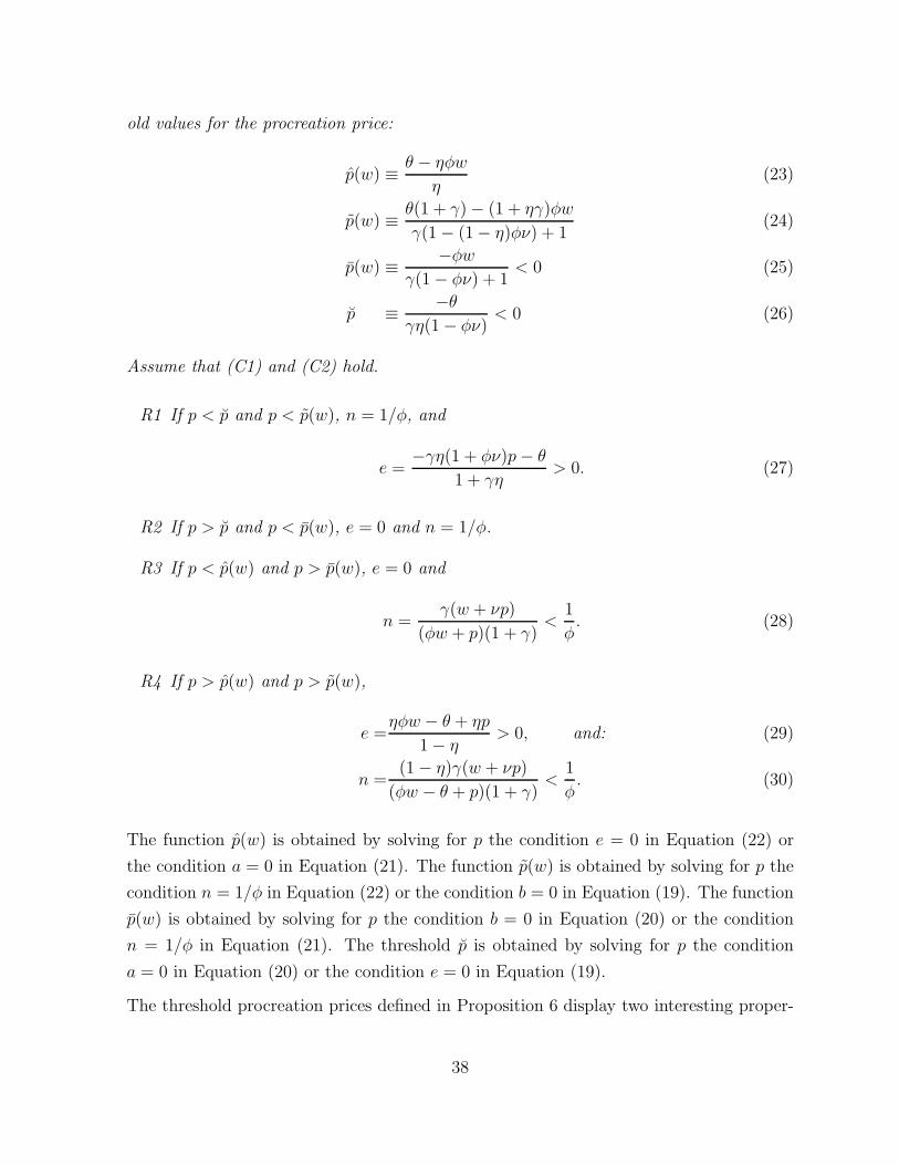
old values for the procreation price:

p(w) ≡θ − ηφw

η(23)

p(w) ≡θ(1 + γ) − (1 + ηγ)φw

γ(1 − (1 − η)φν) + 1(24)

p(w) ≡−φw

γ(1 − φν) + 1< 0 (25)

p ≡−θ

γη(1 − φν)< 0 (26)

Assume that (C1) and (C2) hold.

R1 If p < p and p < p(w), n = 1/φ, and

e =−γη(1 + φν)p − θ

1 + γη> 0. (27)

R2 If p > p and p < p(w), e = 0 and n = 1/φ.

R3 If p < p(w) and p > p(w), e = 0 and

n =γ(w + νp)

(φw + p)(1 + γ)<

1

φ. (28)

R4 If p > p(w) and p > p(w),

e =ηφw − θ + ηp

1 − η> 0, and: (29)

n =(1 − η)γ(w + νp)

(φw − θ + p)(1 + γ)<

1

φ. (30)

The function p(w) is obtained by solving for p the condition e = 0 in Equation (22) or

the condition a = 0 in Equation (21). The function p(w) is obtained by solving for p the

condition n = 1/φ in Equation (22) or the condition b = 0 in Equation (19). The function

p(w) is obtained by solving for p the condition b = 0 in Equation (20) or the condition

n = 1/φ in Equation (21). The threshold p is obtained by solving for p the condition

a = 0 in Equation (20) or the condition e = 0 in Equation (19).

The threshold procreation prices defined in Proposition 6 display two interesting proper-

38

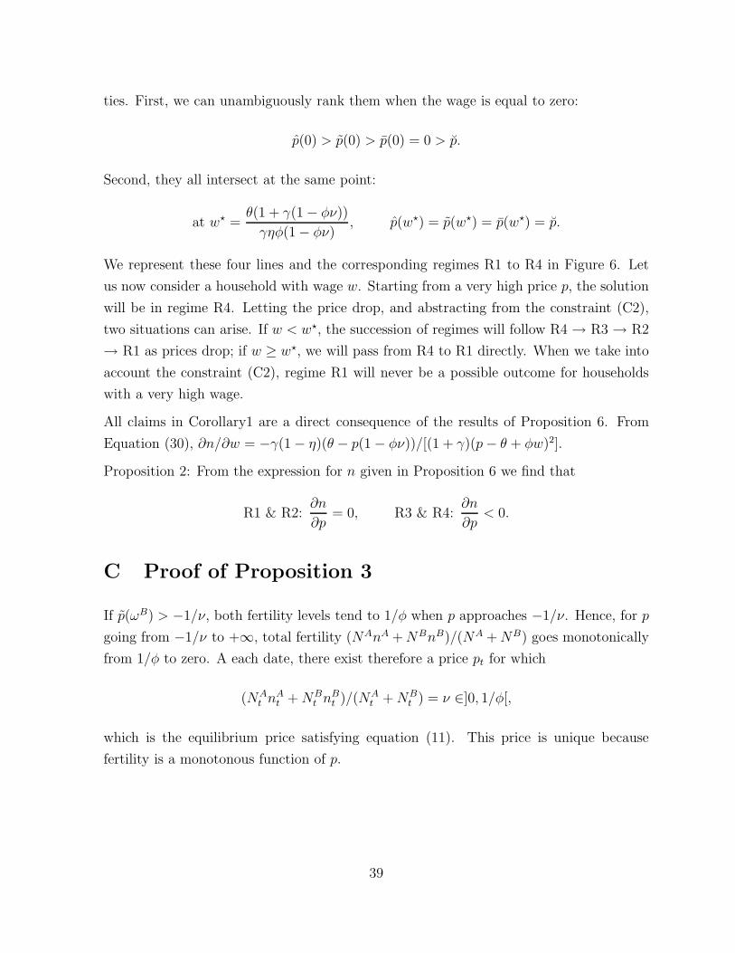
ties. First, we can unambiguously rank them when the wage is equal to zero:

p(0) > p(0) > p(0) = 0 > p.

Second, they all intersect at the same point:

at w⋆ =θ(1 + γ(1 − φν))

γηφ(1 − φν), p(w⋆) = p(w⋆) = p(w⋆) = p.

We represent these four lines and the corresponding regimes R1 to R4 in Figure 6. Let

us now consider a household with wage w. Starting from a very high price p, the solution

will be in regime R4. Letting the price drop, and abstracting from the constraint (C2),

two situations can arise. If w < w⋆, the succession of regimes will follow R4 → R3 → R2

→ R1 as prices drop; if w ≥ w⋆, we will pass from R4 to R1 directly. When we take into

account the constraint (C2), regime R1 will never be a possible outcome for households

with a very high wage.

All claims in Corollary1 are a direct consequence of the results of Proposition 6. From

Equation (30), ∂n/∂w = −γ(1 − η)(θ − p(1 − φν))/[(1 + γ)(p − θ + φw)2].

Proposition 2: From the expression for n given in Proposition 6 we find that

R1 & R2:∂n

∂p= 0, R3 & R4:

∂n

∂p< 0.

C Proof of Proposition 3

If p(ωB) > −1/ν, both fertility levels tend to 1/φ when p approaches −1/ν. Hence, for p

going from −1/ν to +∞, total fertility (NAnA + NBnB)/(NA + NB) goes monotonically

from 1/φ to zero. A each date, there exist therefore a price pt for which

(NAt nA

t + NBt nB

t )/(NAt + NB

t ) = ν ∈]0, 1/φ[,

which is the equilibrium price satisfying equation (11). This price is unique because

fertility is a monotonous function of p.

39

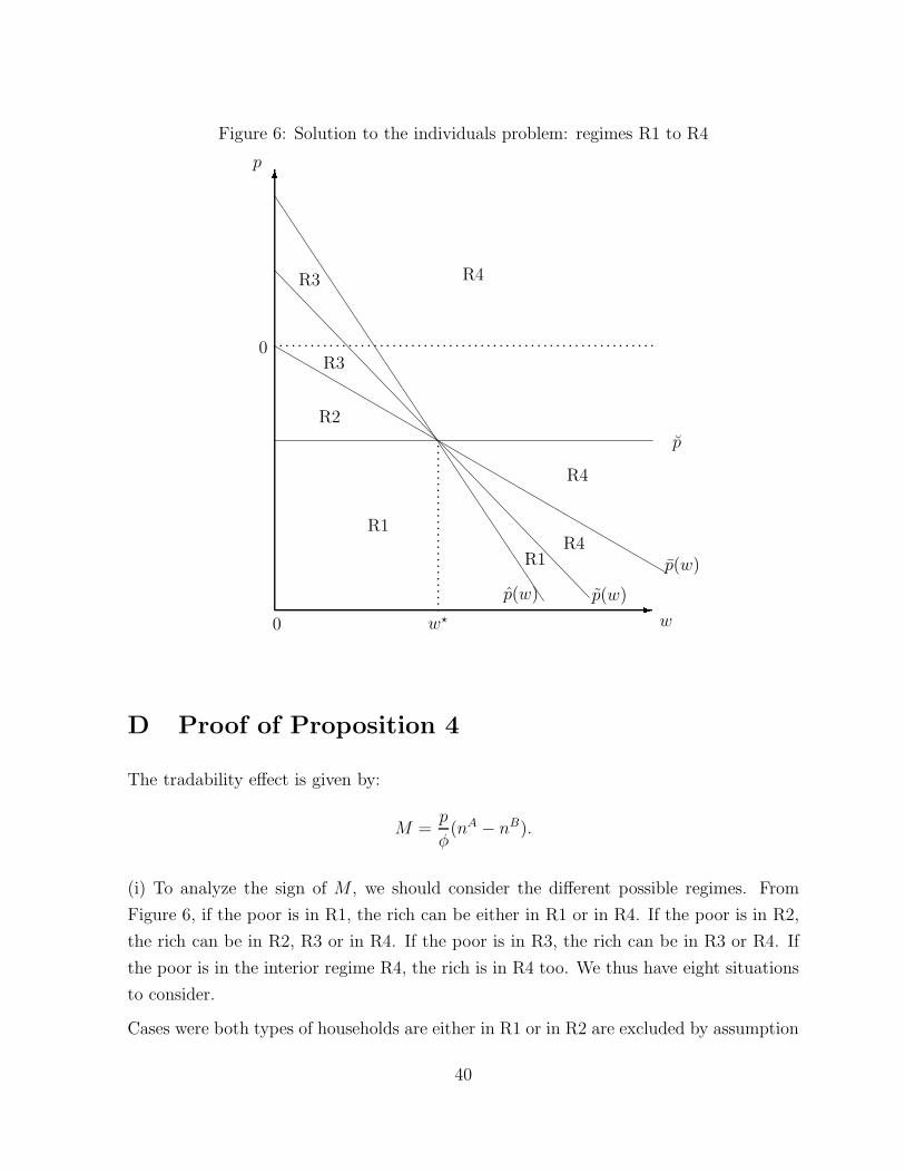
Figure 6: Solution to the individuals problem: regimes R1 to R46

-

. .. .. ... .. .. ... .. .. ... .. .. ... .. .. ... .. .. .. ... .. .. ... .. .. ... ..

p

w

0

0

p

p(w)

p(w)p(w)

R4

R4

R3

R3

R2

R1

R1R4

...........................w⋆

D Proof of Proposition 4

The tradability effect is given by:

M =p

φ(nA − nB).

(i) To analyze the sign of M , we should consider the different possible regimes. From

Figure 6, if the poor is in R1, the rich can be either in R1 or in R4. If the poor is in R2,

the rich can be in R2, R3 or in R4. If the poor is in R3, the rich can be in R3 or R4. If

the poor is in the interior regime R4, the rich is in R4 too. We thus have eight situations

to consider.

Cases were both types of households are either in R1 or in R2 are excluded by assumption

40

(C1). Indeed, in that case, aggregate fertility per person would be 1/φ and the equilibrium

condition (11) would be violated. This leaves us with six different cases.

When the poor is in R2, the procreation price is necessarily negative, and nA = 1/φ > nB.

When both individuals are in R3, the procreation price can be either positive or negative,

but we always have nA > nB because fertility decreases in income in regime R3. Hence,

p < 0 → M < 0 in this regime. When the poor is in R3 and the rich in R4, we also always

have nA > nB (compare (28) to (30)), which implies in this regime p < 0 ↔ M < 0.

Finally, if both individuals are in the interior regime R4, we can use Proposition 1 to

infer that if p < 0 (nA > nB) or if p > θ1−φν

(nB > nA), then M < 0. The min term in

the condition of the proposition gathers the requirement of being in regime R4 with the

condition of Proposition 1.

(ii) If θ = 0 the expression

min

{θ

1 − φν, p(ωA), p(ωA)

}

is negative and the condition in (i) is always true.

41