Polynomial decay for a hyperbolic–parabolic coupled system ☆ ☆ The work is supported by the US...
64
J. Math. Pures Appl. 84 (2005) 407–470 www.elsevier.com/locate/matpur Polynomial decay for a hyperbolic–parabolic coupled system ✩ Jeffrey Rauch a , Xu Zhang b,c , Enrique Zuazua b a Department of Mathematics, East Hall, University of Michigan, Ann Arbor, MI 48109, USA b Departamento de Matemáticas, Facultad de Ciencias, Universidad Autónoma de Madrid, 28049 Madrid, Spain c School of Mathematics, Sichuan University, Chengdu 610064, China Received 28 May 2004 Available online 8 December 2004 Abstract This paper analyzes the long time behavior of a linearized model for fluid-structure interaction. The space domain consists of two parts in which the evolution is governed by the heat equation and the wave equation respectively, with transmission conditions at the interface. Based on the construction of ray-like solutions by means of Geometric Optics expansions and a careful analysis of the transfer of the energy at the interface, we show the lack of uniform decay of solutions in general domains. Also, we prove the polynomial decay result for smooth solutions under a suitable Geometric Control Condition. This condition requires that all rays propagating in the wave domain reach the interface in a uniform time after, possibly, bouncing in the exterior boundary. 2004 Elsevier SAS. All rights reserved. ✩ The work is supported by the US National Science Foundation grant NSF-DMS-0104096, the Grant BFM2002-03345 of the Spanish MCYT, the FANEDD of China (Project No. 200119), the EU TMR Projects “Homogenization and Multiple Scales” and “Smart Systems”, the NSF of China under grant 10371084, and the Project-sponsored by SRF for ROCS, SEM of China. The first and last authors would like to thank the Laboratoire J.-A. Dieudonné at the Université de Nice, and particularly Professors Y. Brenier, D. Chenais and G. Lebeau, for hospitality during their visit. The third author also thanks Professors N. Burq, I. Mundet and V. Munõs for fruitful discussions. E-mail addresses: [email protected] (J. Rauch), [email protected] (X. Zhang), [email protected] (E. Zuazua). 0021-7824/$ – see front matter 2004 Elsevier SAS. All rights reserved. doi:10.1016/j.matpur.2004.09.006
-
Upload
independent -
Category
Documents
-
view
2 -
download
0
Transcript of Polynomial decay for a hyperbolic–parabolic coupled system ☆ ☆ The work is supported by the US...
r
n. Theand thetructionransfermains.ontrol
terface
Grantjects
and theoratoireeau, forruitful
.es
J. Math. Pures Appl. 84 (2005) 407–470
www.elsevier.com/locate/matpu
Polynomial decay for a hyperbolic–paraboliccoupled system
Jeffrey Raucha, Xu Zhangb,c, Enrique Zuazuab
a Department of Mathematics, East Hall, University of Michigan, Ann Arbor, MI 48109, USAb Departamento de Matemáticas, Facultad de Ciencias, Universidad Autónoma de Madrid,
28049 Madrid, Spainc School of Mathematics, Sichuan University, Chengdu 610064, China
Received 28 May 2004
Available online 8 December 2004
Abstract
This paper analyzes the long time behavior of a linearized model for fluid-structure interactiospace domain consists of two parts in which the evolution is governed by the heat equationwave equation respectively, with transmission conditions at the interface. Based on the consof ray-like solutions by means of Geometric Optics expansions and a careful analysis of the tof the energy at the interface, we show the lack of uniform decay of solutions in general doAlso, we prove the polynomial decay result for smooth solutions under a suitable Geometric CCondition. This condition requires that all rays propagating in the wave domain reach the inin a uniform time after, possibly, bouncing in the exterior boundary. 2004 Elsevier SAS. All rights reserved.
The work is supported by the US National Science Foundation grant NSF-DMS-0104096, theBFM2002-03345 of the Spanish MCYT, the FANEDD of China (Project No. 200119), the EU TMR Pro“Homogenization and Multiple Scales” and “Smart Systems”, the NSF of China under grant 10371084,Project-sponsored by SRF for ROCS, SEM of China. The first and last authors would like to thank the LabJ.-A. Dieudonné at the Université de Nice, and particularly Professors Y. Brenier, D. Chenais and G. Lebhospitality during their visit. The third author also thanks Professors N. Burq, I. Mundet and V. Munõs for fdiscussions.
E-mail addresses:[email protected] (J. Rauch), [email protected] (X. Zhang), enrique.zuazua@uam(E. Zuazua).
0021-7824/$ – see front matter 2004 Elsevier SAS. All rights reserved.doi:10.1016/j.matpur.2004.09.006

408 J. Rauch et al. / J. Math. Pures Appl. 84 (2005) 407–470
ractionution estnditionstenuesl’énergiemainesalementiert quetteignentre.
ial
con-ission
fluid-ystem
nd theduce
Résumé
Cet article étudie le comportement asymptotique en temps d’un modèle linéarisé d’intefluide-structure. Le domaine (en espace) est composé de deux parties dans lesquelles l’évolgouvernée par l’équation de la chaleur et l’équation des ondes respectivement, avec des code transmission à l’interface. En s’appuyant sur la construction de solutions type rayon obpar la méthode des dévelopements géométriques, et une analyse précise du transfert deà l’interface, on montre la perte de décroissance uniforme des solutions définies sur des doquelconques. De plus, en supposant une condition de contrôle géométrique, on montre égun résultat de décroissance polynomial pour des solutions régulières. Cette condition requtous les rayons se propageant sur la partie du domaine gouverné par l’équation des ondes al’interface en un temps uniforme, éventuellement après avoir rebondi sur la frontière extérieu 2004 Elsevier SAS. All rights reserved.
Keywords:Fluid-structure interaction; Wave-heat model; Non-uniform decay; Geometric Optics; Polynomdecay; Weakened observability inequality
MSC:primary: 37L15; secondary: 35B37, 74H40, 78M35, 76M45, 93D20, 93B07
1. Introduction
This paper analyzes a linearized model for fluid-structure interaction. This systemsists of a wave and a heat equation coupled through an interface with suitable transmconditions.
Let us describe this system in detail.Let Ω ⊂ R
n (n ∈ N) be a bounded domain boundaryΓ . Let Ω1 be a sub-domain ofΩand setΩ2 = Ω \ Ω1. Denote byγ the interface,Γj = ∂Ωj \ γ (j = 1,2), andνj the unitoutward normal vector ofΩj (j = 1,2). We assumeγ = ∅, andΓ,Γ1,Γ2, and Intγ , therelative interior ofγ , to be ofC1 (unless otherwise stated). Denote bythe d’Alembertoperator∂tt − .
We consider the following hyperbolic-parabolic coupled system:
yt − y = 0 in (0,∞) × Ω1,
z = 0 in (0,∞) × Ω2,
y = 0 on(0,∞) × Γ1,
z = 0 on(0,∞) × Γ2,
y = z,∂y∂ν1
= − ∂z∂ν2
on (0,∞) × γ,
y(0, x) = y0(x) in Ω1,
z(0, x) = z0(x), zt (0, x) = z1(x) in Ω2.
(1.1)
Here and henceforthx = (x1, . . . , xn) = (x1, x′).
This system can be viewed as a simplified and a linearized version of a truestructure interaction model. Of course, more realistic models should combine the sof elasticity for the structure, the Stokes or Navier–Stokes equations for the fluid, atransmission condition should hold along a moving interface. This would certainly pro
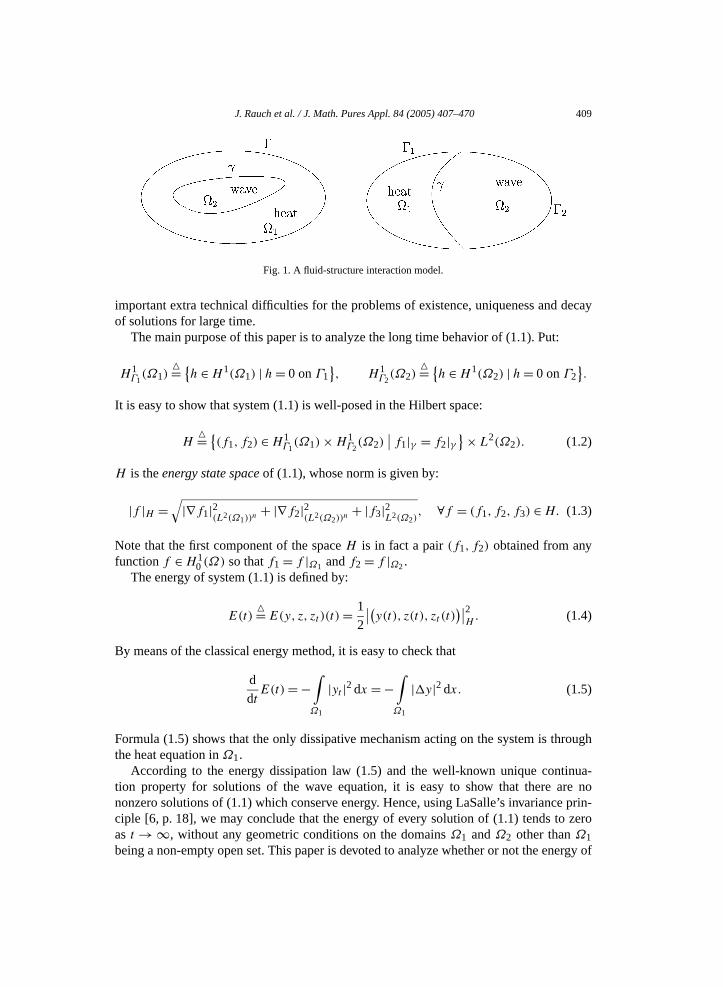
J. Rauch et al. / J. Math. Pures Appl. 84 (2005) 407–470 409
decay
rough
inua-re noe prin-
zero
ergy of
Fig. 1. A fluid-structure interaction model.
important extra technical difficulties for the problems of existence, uniqueness andof solutions for large time.
The main purpose of this paper is to analyze the long time behavior of (1.1). Put:
H 1Γ1
(Ω1)= h ∈ H 1(Ω1) | h = 0 onΓ1
, H 1
Γ2(Ω2)
= h ∈ H 1(Ω2) | h = 0 onΓ2.
It is easy to show that system (1.1) is well-posed in the Hilbert space:
H= (f1, f2) ∈ H 1
Γ1(Ω1) × H 1
Γ2(Ω2)
∣∣ f1|γ = f2|γ× L2(Ω2). (1.2)
H is theenergy state spaceof (1.1), whose norm is given by:
|f |H =√
|∇f1|2(L2(Ω1))n + |∇f2|2(L2(Ω2))
n + |f3|2L2(Ω2), ∀f = (f1, f2, f3) ∈ H. (1.3)
Note that the first component of the spaceH is in fact a pair(f1, f2) obtained from anyfunctionf ∈ H 1
0 (Ω) so thatf1 = f |Ω1 andf2 = f |Ω2.The energy of system (1.1) is defined by:
E(t)= E(y, z, zt )(t) = 1
2
∣∣(y(t), z(t), zt (t))∣∣2
H. (1.4)
By means of the classical energy method, it is easy to check that
d
dtE(t) = −
∫Ω1
|yt |2 dx = −∫Ω1
|y|2 dx. (1.5)
Formula (1.5) shows that the only dissipative mechanism acting on the system is ththe heat equation inΩ1.
According to the energy dissipation law (1.5) and the well-known unique conttion property for solutions of the wave equation, it is easy to show that there anonzero solutions of (1.1) which conserve energy. Hence, using LaSalle’s invariancciple [6, p. 18], we may conclude that the energy of every solution of (1.1) tends toas t → ∞, without any geometric conditions on the domainsΩ1 andΩ2 other thanΩ1being a non-empty open set. This paper is devoted to analyze whether or not the en
410 J. Rauch et al. / J. Math. Pures Appl. 84 (2005) 407–470
t
mpingergy
(in thessing ism (1.1)ave
quiv-es
ation
con-cited
ch esti-uationhile,, a uni-h somedevelop
beamcessaryntial
e heatwill
t thispectrale hy-ishingmainlyby the
solutions of system (1.1) tends to zero exponentially ast → ∞, i.e., whether there existwo positive constantsC andα such that
E(t) CE(0)e−αt , ∀t 0, (1.6)
for every solution of (1.1).Recall that for the pure heat equation and the wave equation with an effective da
in a sub-domain satisfying the Geometric Control Condition (GCC for short), the endecays exponentially (e.g., [3,22]). On the other hand, for the pure wave equationabsence of damping), the energy is conserved. Therefore, the problem we are addrethat of whether the dissipative mechanism that the heat equation introduces in systethrough the subdomainΩ1 suffices to produce the uniform decay of the energy of the wcomponent of the solutions or not.
According to the energy dissipation law (1.5), the uniform decay problem (1.6) is ealent to showing that: there existsT > 0 andC > 0 such that every solution of (1.1) satisfi
∣∣(y0, z0, z1)∣∣2H
C
T∫0
∫Ω1
|yt |2 dx dt, ∀(y0, z0, z1) ∈ H. (1.7)
Inequality (1.7) can be viewed as an observability estimate for Eq. (1.1) with observon the heat subdomainΩ1.
There is an extensive literature on the observability inequalities of PDEs and itsnections with stabilization and control problems ([3–5,12,16,23] and the referencestherein). However, the techniques that have been developed up to now to obtain sumates depend heavily on the nature of the equations. In the context of the wave eqone may use multipliers [12], Carleman inequalities [20], or microlocal analysis [3]; win the context of heat equations, one uses Carleman inequalities [5,4]. Neverthelessfied Carleman estimate for those two equations has not been well developed althougpartial progress has been made in this respect [9,10]. Consequently, we need tonew techniques to analyze the observability problem (1.7) for system (1.1).
To begin with, the classical result by Ralston [15] on the existence of Gaussiansolutions of the wave equation concentrated along rays shows immediately that a necondition for the observability inequality (1.7) to hold, or equivalently, the exponedecay (1.6) of solutions of (1.1) to be fulfilled is that the heat subdomainΩ1 controlsgeometrically the wave domainΩ2 (see Theorem 4.3).
In view of the above negative result, it is natural to address the case where thsubdomain does satisfy the GCC. A “naive” conjecture would be that this conditionlead to the exponential decay of solutions of (1.1). However, in [21] it is shown thaconjecture is not correct even in one space dimension. Indeed, the high frequency sanalysis in [21] shows that the spectrum of system (1.1) in 1-d is split into two parts: thperbolic and the parabolic one. Hyperbolic eigenvalues have an asymptotically vanreal part and this contradicts exponential decay. The corresponding eigenvectors areconcentrated on the wave interval and, consequently, they are very weakly dissipated
J. Rauch et al. / J. Math. Pures Appl. 84 (2005) 407–470 411
eigen-whose
proach
men-arefullyetries.ptics
t com-etric
wavesetry,
ne cantopicqualitylts for
nomial
sults.in the(1.1)ntationtructingedral,) does
neral. Noteaussianomplex-er the
c-
n
damping mechanism introduced by the heat equation. On the other hand, parabolicvalues are asymptotically real and negative and the corresponding eigenvectors,energy is mainly concentrated on the heat interval, are efficiently dissipated. The apin [21], based on spectral analysis, does not apply to multidimensional situations.
The first topic of this article is to show the lack of exponential decay in several disions, as the 1-d spectral analysis suggests. For this purpose, we need to analyze cthe interaction of the wave and heat like solutions on the interface for general geomOur method is based on the WKB method of asymptotic expansion in Geometric O(see for example, [2]). We will show that waves concentrated along rays are almospletely reflected on the interface, which implies that (1.7) fails. The method of GeomOptics determines the reflection coefficient as a function of the angle of incidence ofon the interface. This shows the lack of uniform decay of solutions of (1.1) in any geomeven if the GCC is assumed (see Theorem 4.1).
According to the above analysis, it is easy to see that, even under the GCC, oonly expect a polynomial stability property of smooth solutions. This is the secondaddressed in this paper. To do this, we need to derive a weakened observability inein Theorem 5.1 by means of the energy method and the existing observability resuthe wave equation. Then, based on this theorem, we show in Theorem 5.2 a polydecay rate of smooth solutions for system (1.1) under the GCC.
This paper is organized as follows. In Section 2, we give some preliminary reSection 3 is devoted to the WKB asymptotic analysis for the transmission problemwhole space with flat interface, which implies the lack of exponential decay for Eq.in polyhedral domains. This case is easier to handle and it allows an easier preseof the key ideas, since one needs only to use linear real-valued phases for consthe approximate solutions. This analysis shows that when the wave domain is polyhregardless what the geometry of the heat domain is, the energy of solutions of (1.1not decay uniformly. In Section 4 we perform the WKB asymptotic analysis for geinterfaces and we conclude the lack of uniform decay for Eq. (1.1) in general domainsthat, when treating general interfaces and boundaries, to avoid caustics, we use Gbeams to construct the approximate solutions, where the phases are nonlinear and cvalued. In Section 5, we prove a weakened observability inequality for Eq. (1.1) undGCC, and then derive the polynomial decay rate of its smooth solutions.
Notation. Throughout this paper, for a subsetω ⊂ Rn, we denote its characteristic fun
tion by χω. For anyη > 0, theη-neighborhood ofω is denoted byOη(ω). Also, whenwriting (w1,w2) ∈ Hs(Ω) (respectivelyHs
0(Ω) for s ∈ R, we mean that the functio
w= w1χΩ1 + w2χΩ2 belongs toHs(Ω) (respectivelyHs
0(Ω)). With this convention, itis easy to see thatH = H 1
0 (Ω) × L2(Ω2).Further, ifM ⊂ R
m (m ∈ N) is an open set andf ε is a family of functions inC∞(M)
depending onε ∈ (0,1), we say thatf ε ∼ 0 iff for all compactK ⊂ M , α ∈ Nm, andN ∈ N
there is a constantC > 0 so that
sup∣∣∂α
y f ε(y)∣∣ CεN
y∈K
412 J. Rauch et al. / J. Math. Pures Appl. 84 (2005) 407–470
mple,
nt
blem in
holds for all smallε. In this case we also writef ε = O(ε∞). For two familiesf ε, gε ofsmooth functions,f ε ∼ gε meansf ε −gε ∼ 0. We shall also often writeaε ∼∑∞
j=0 aj εj .
This does not mean that the series converges but rather that for allN ∈ N andα ∈ Nm,
there is a constantC > 0 so that
supy∈M
∣∣∣∣∣∂αy
(aε(y) −
N∑j=0
aj (y)εj
)∣∣∣∣∣ CεN+1
holds for all smallε. In a similar way, we writef (t, x1, x′) ∼ ∑∞
j=0 aj (t, x′)xj
1 andf (t, x1, x
′) = O(|x1|∞).Finally, for any nonnegative real functionsf ε andgε of ε ∈ (0,1), we writef ε ≈ gε if
for sufficiently smallε, there exist constants 0< c < C < ∞ so that
cf ε gε Cf ε.
2. Some preliminaries
2.1. Well-posedness
First, we need the following simple result. (The proof is standard (see, for exa[11]).)
Lemma 2.1. Let Ω be a bounded domain withC1 boundary. Then there is a constaC > 0 such that for any distributionz ∈ D′(Ω) with ∇z ∈ (L2(Ω))n andz ∈ L2(Ω), itholds: ∣∣∣∣ ∂z
∂ν
∣∣∣∣H−1/2(Γ )
C[|∇z|(L2(Ω))n + |z|L2(Ω)
]. (2.1)
Next, we prove the well-posedness of system (1.1) inH . For this purpose, we putX =(y, z, zt ) andX0 = (y0, z0, z1). We define an unbounded operatorA :D(A) ⊂ H → H by
AY = (Y1, Y3,Y2), (2.2)
whereY = (Y1, Y2, Y3) ∈ D(A), and
D(A) = (Y1, Y2, Y3) ∈ H∣∣ (Y1, Y2) ∈ H 2(Ω), Y3 ∈ H 1(Ω2), Y1 ∈ H 1(Ω1),
Y1|Γ1 = Y3|Γ2 = 0 andY1|γ = Y3|γ. (2.3)
Then, it is easy to see that system (1.1) can be re-written as an abstract Cauchy proH as follows:
Xt = AX for t > 0, and X(0) = X0. (2.4)
J. Rauch et al. / J. Math. Pures Appl. 84 (2005) 407–470 413
4
ions
nergy
e
We have the following result:
Theorem 2.1.Denote the resolvent ofA byρ(A). Then0∈ ρ(A), A−1 is compact, andAis the generator of a contractiveC0-semigroupS(t)t0 in H .
We refer to Appendix A for the proof of Theorem 2.1.
Remark 2.1.Although the semigroupS(t)t0 is contractive, Theorem 4.1 in Sectionwill show that, whatever the geometric configuration is, the operator norm ofS(t) is equalto 1 for all t 0. In other words, there is no uniform decay for the energy of solutof (1.1).
Remark 2.2.D(A) is a Hilbert space with its graph norm. Since 0∈ ρ(A), we may definean Hilbert spaceH−1 as the completion ofH with respect to the norm| · |H−1 = |A−1 · |H .
As a consequence of Theorem 2.1, system (1.1) is well-posed in its finite espaceH .
Let us now analyze what happens if the initial data(y0, z0, z1) of (1.1) belong to thelarger Hilbert spaceH−1. To see this, assumeX0 = (y0, z0, z1) ∈ H−1. We may solvesystem (2.4) as follows. Set
X(t) = A−1X0 +t∫
0
X(s)ds. (2.5)
ThenX(t) solves
Xt = AX for t > 0, and X(0) = A−1X0 (∈ H). (2.6)
In view of Theorem 2.1, system (2.6) admits a unique mild solutionX ∈ C([0,∞);H),and
|X|L∞(0,∞;H−1) = ∣∣Xt
∣∣L∞(0,∞;H−1)
= ∣∣AX∣∣L∞(0,∞;H−1)
= ∣∣X∣∣L∞(0,∞;H)
∣∣A−1X0
∣∣H
= |X0|H−1. (2.7)
Consequently, we have proved:
Theorem 2.2.Let (y0, z0, z1) ∈ H−1. Then system(1.1) admits a unique solution in thclass: X = (y, z, zt ) ∈ C([0,∞);H−1), and|(y, z, zt )|L∞(0,∞;H−1) |(y0, z0, z1)|H−1.
2.2. Multiply reflected rays
We first need to recall the definition of rays.
414 J. Rauch et al. / J. Math. Pures Appl. 84 (2005) 407–470
fsitive
es.llowingwave
lyorry
sub-y
e
Consider the hyperbolic operator onRn:
W = ∂tt −n∑
j,k=1
αjk(x)∂xj∂xk
, (2.8)
where(αij )n×n ∈ C2 is strictly positive definite. Put
g(x, ξ)=
n∑j,k=1
αjk(x)ξj ξk, ξ = (ξ1, . . . , ξn). (2.9)
A null bicharacteristicof W is defined to be a solution(x(t), ξ(t)) of the following (gen-erally nonlinear) system of ordinary differential equations:
x(t) = ∇ξ g(x(t), ξ(t)),
ξ (t) = −∇xg(x(t), ξ(t)),
x(0) = x0, ξ(0) = ξ0,
(2.10)
where the initial data(x0, ξ0) are chosen such thatg(x0, ξ0) = 1/4. (Here, the choice o1/4 is only for convenience. Indeed, by scaling, one may replace it by any other poreal number.) It is easy to check that
g(x(t), ξ(t)
)= 1/4, ∀t ∈ R. (2.11)
The projection of the null bicharacteristic to the physical time–space,(t, x(t)), traces acurve inR
1+n, which is called aray of W . Sometimes, we also refer to(t, x(t), ξ(t)) asthe ray. Obviously, for any operatorW with constant coefficients, its rays are straight lin
In the presence of boundaries, rays, when reaching the boundary are reflected fothe usual rules of Geometric Optics. Along this paper we will consider rays in thedomainΩ2. SinceΩ2 is obtained from the global domainΩ by cutting it off by meansof a (n − 1)-dimensional manifoldγ , the domainΩ2 is not necessarily smooth but onpiecewise smooth. In particular, the boundary ofΩ2 in 2-d could have some cornerscusps. All along this paper we will work with rays inΩ2 that never meet the boundaat those exceptional points. In view of this, we consider a bounded domainM ⊂ R
n withpiecewiseC1 boundary∂M , the singular set being localized on a closed (topological)manifold S with dimS n − 2. We now introduce the following definition of multiplreflected ray.
Definition 2.1.A continuous parametric curve,
[0, T ] t → (t, x(t), ξ(t)) ∈ C
([0, T ] × M × Rn),
with a givenT > 0, x(0) ∈ M andx(T ) ∈ M , is called a multiply reflected ray for thoperator in [0, T ] × M if there existm ∈ N, 0 < t0 < t1 < · · · < tm = T , such that
J. Rauch et al. / J. Math. Pures Appl. 84 (2005) 407–470 415
t-
veiply
sc-
e
e
nts. If
heay
geo-
ed
ownflow
each(t, x(t), ξ(t))|ti<t<ti+1 is a straight ray for (i = 0,1,2, . . . ,m − 1), which arrives a∂M \S at timet = ti+1, and is reflected by(t, x(t), ξ(t))|ti+1<t<ti+2 by the law of Geometric Optics wheneveri < m − 1.
We show the following geometric lemma:
Lemma 2.2.Assume that for eachT > 0, there is a multiply reflected ray for the waoperator in [0, T ] × M . Then by a small perturbation, one can find a new multreflected ray which always meets∂M \ S transversally and non-normally.
Remark 2.3.(i) The above result holds also for more general hyperbolic operators aW .(ii) We give below a sketch of the proof of Lemma 2.2 following [7, Vol. III, Se
tion 24.3, p. 441].
Proof of Lemma 2.2. Recall that, for a given time duration[0, T ], the multiply reflectedrays for in M are finite ordered sequences of line segments inM , reflected one by onon ∂M \ S, and contained inM except the reflected pointss1, . . . , sn0. Take any such aray and assume the direction of its first segment to bev. The reflected points of isdivided into two subsetsB1 andB2. The first one,B1, is constituted by those for which thray meets the boundary∂M \ S transversally and non-normally. The second one,B2, isconstituted by the reminding points that will be referred as exceptional reflected poiB2 = ∅, then is exactly what we need. Otherwise, letB2 = si1, . . . , sim (m n0). Then,by continuity, we may make a very small perturbation on the initial directionv so that forthe new ray, the original reflected points of typeB1 remains to be of the same type, but tfirst exceptional reflected pointsi1 becomes of typeB1. Repeating this procedure, one mremove all the exceptional reflected points. This completes the proof of Lemma 2.2.
In view of Lemma 2.2 and Remark 2.3, it is reasonable to introduce the followingmetric assumption onΩ2, which is needed to develop our Geometric Optics analysis.
Assumption 2.1.Assume that for eachT > 0, there is a multiply reflected ray:
[0, T ] t → (t, x(t), ξ(t)) ∈ C
([0, T ] × Ω2 × Rn)
for the wave operator in [0, T ] × Ω2 which meets∂Ω2 \ (Γ2 ∩ γ ) transversally andnon-normally, and∂Ω2 is ofC2 (respectivelyC3) in some neighborhood of every reflectpoint inΓ2 (respectivelyγ ).
Remark 2.4.By Lemma 2.2, ones sees that Assumption 2.1 holds whenΩ2 is a piecewiseC3 domain. This was pointed to us by N. Burq and I. Mundet. The argument, well knin billiard theory, uses the properties of the symplectic form induced by the billiardsand Poincaré’s recurrence theorem (see [18, Lemma 1.7.1]).
416 J. Rauch et al. / J. Math. Pures Appl. 84 (2005) 407–470
con-
qua-ns are.ligible
e
a-
3. WKB asymptotic analysis for the transmission problem with flat interface
This section is devoted to an heuristic exposition of the key ideas leading to thestruction of ray-like solutions for system (1.1).
We consider the case of a flat interfaceγ , say γ = x1 = 0, Ω being the wholespaceRn. In this case, system (1.1) may be written as follows:
yt − y = 0 in (0,∞) × x1 < 0,z = 0 in (0,∞) × x1 > 0,
y = z, yx1 = zx1 on (0,∞) × x1 = 0.(3.1)
The main problem is to describe the behavior of ray-like solutions of the wave etion when reaching the interface. As we will see later, the answer is that the solutioreflected with reflection coefficientr = e2θ i, whereθ ∈ [0,π/2) is the angle of incidenceNote that the reflection coefficient is of modulus one and consequently, only a neghigh frequency wave enters the heat domain.
Throughout this section,τ ∈ R \ 0 andξ = (ξ1, ξ′) ∈ R
n with ξ1 = 0 are given and arassumed to satisfy the condition
τ2 − |ξ |2 = 0, i.e., τ = ±|ξ |. (3.2)
3.1. WKB expansion for the wave equation
We begin by seeking approximate solutions for the wave equationz = 0, with anAnsatz of WKB type with linear phase
zε(t, x) = ei(τ t+ξ ·x)/εaε(t, x), aε(t, x) ∼∞∑
j=0
εjaj (t, x), (3.3)
where the functionsaj (j = 1,2, . . .) will be determined later.Computing zε and setting its O(1/ε2) term equal to zero yields the eikonal equ
tion (3.2). By (3.2), one has
zε = ε−1ei(τ t+ξ ·x)/ε[2i(τ∂t − ξ · ∂x) + ε
]aε.
Define:
v ≡ (v1, v2, . . . , vn)= − ξ
τ.
Then zε = O(ε∞) is equivalent to[∂t + v · ∂x + ε
2τ i
] ∞∑εj aj = O(ε∞). (3.4)
j=0

J. Rauch et al. / J. Math. Pures Appl. 84 (2005) 407–470 417
d
er-rt
k)
sedt the
7).
s the
Setting the leading order term of the left-hand side of (3.4) equal to zero yields
(∂t + v · ∂x)a0 = 0. (3.5)
This is a transport equation. It is easy to check that solutionsa0= a0(t, x) ∈ C1(R1+n)
of (3.5) are of the form:a0(t, x) = g0(x − vt), with g0= g0(x) ∈ C1(Rn).
We now choose a functiong0(x) = a0(0, x) ∈ C∞(Rn) with support in a neighborhooof a point x0 ∈ R
n. Thena0 is, at anyt > 0, concentrated near the pointx = x0 + vt .Therefore, to leading order,
zε(t, x) ∼ ei(τ t+ξ ·x)/εa0(t, x) = ei(τ t+ξ ·x)/εg0(x − vt),
and we see thatzε looks like a localized function transported along the rayx = x0 + vt ,with an oscillating factor ei(τ t+ξ ·x)/ε.
Continuing in this fashion, the profilesaj of the higher order terms are uniquely detmined from their initial dataaj |t=0 = gj ∈ C∞
0 (Rn) by solving recursively the transpoequations
(∂t + v · ∂x)aj + aj−1
2τ i= 0, j = 1,2, . . . . (3.6)
Assume thatgj have support in a compact set independent ofj . Then, the profilesaj aresupported in a tube of rays (i.e., characteristic curves of∂t +v · ∂x ). Indeed, one may checdirectly thataj (t, x) = gj (x −vt)+ it (2τ)−1 aj−1(x −vt) is the unique solution of (3.6such thataj |t=0 = gj .
Remark 3.1.Instead of the Cauchy problem (3.5) and (3.6) with initial condition impoat t = 0, one may consider the same problem but with initial condition imposed ainterfacex1 = 0:
(∂t + v · ∂x)a0 = 0,
(∂t + v · ∂x)aj + aj−12τ i = 0,
a0(t,0, x′) = a00(t, x′), aj (t,0, x′) = a0
j (t, x′),
(3.7)
for any given functionsa00 anda0
j (j = 1,2, . . .) (because the first componentv1 of v isassumed not to vanish). Similar ray-like solutions can be constructed for system (3.
The classical Borel’s theorem (e.g., p. 16 in [7]) allows one to choose aC∞-smoothfunction aε(t, x), which is supported in the above mentioned tube of rays and haexpansion atε = 0:
aε(t, x) ∼∞∑
j=0
εj aj (t, x).
Consequently, we conclude that
418 J. Rauch et al. / J. Math. Pures Appl. 84 (2005) 407–470
ua-
use a
in thetermslittle bit
when
the
of
1), in
in the
Theorem 3.1.The function
zε = ei(τ t+ξ ·x)/εaε(t, x) (3.8)
constructed above isC∞-smooth and it is an infinitely accurate solution of the wave eqtion in the sense that zε = O(ε∞) in Rt × R
nx .
Remark 3.2. The Ansatz (3.3) is not unique. Instead, for example, one may alsodifferent one:
zε(t, x) = ei(τ t+ξ ·x)/εaε(t, x), aε(t, x) ∼∞∑
j=0
εj/2aj (t, x). (3.9)
This Ansatz will be essentially used in Section 3.5 for constructing the reflected rayscase of normal incidence. Note that (3.3) is a special case of (3.9) in which the oddhave been chosen to be identically zero. In the present case, one needs to change athe transport equations fora0, a1, a2, . . . , which now read as follows:
(∂t + v · ∂x)a0 = 0,
(∂t + v · ∂x)a2k−1 = 0, k = 1,2, . . . ,
(∂t + v · ∂x)a2j + a2j−22τ i
= 0, j = 1,2, . . . .
(3.10)
Clearly, system (3.10) is uniquely solvable with initial conditions imposed either att = 0or atx1 = 0. Moreover,zε constructed in this way satisfieszε = O(ε∞), too.
We now need to address the question of the behavior of these localized wavesthey reach the interface. More precisely, chooseτ, ξ with ξ1 > 0 so that
−ξ1
τ= v1 < 0 and τ2 > ξ2
2 + · · · + ξ2n .
Then the asymptotic solutions constructed in Theorem 3.1 move towards the left onx1direction within the wave domainx1 > 0. Taking initial dataaε(0, x) compactly supportedin x1 > 0, zε represents a wave which starts on the wave equation sidex1 > 0 and ap-proaches the interfacex1 = 0. The problem is to describe the behavior of the solutionthe transmission problem (3.1) after the wave reaches the interfacex1 = 0.
The traces of solutions as in (3.8) are rapidly oscillating on the boundaryx1 = 0. Thekey step is to find solutions of the heat equation inx1 < 0 which oscillate onx1 = 0, too.These solutions will be “matched” to produce a solution of the whole system (3.which the wave component is the sum of an incoming wave and a reflected one.
3.2. WKB expansion for the heat equation, non-normal incidence
We now construct infinitely accurate approximate solutions of the heat equationregionx1 < 0 whose trace inx1 = 0 oscillates rapidly,
J. Rauch et al. / J. Math. Pures Appl. 84 (2005) 407–470 419
encee
set in
tquation
e.l
e
yε(t,0, x′) = ei(τ t+ξ ′·x′)/εf ε(t, x′), f ε(t, x′) ∼∞∑
j=0
εjfj (t, x′), (3.11)
whereξ ′ = (ξ2, . . . , ξn) ∈ Rn−1 is assumed to be nonzero. This is the case where incid
is non-normal. The exceptional caseξ ′ = 0 corresponding to normal incidence will bdiscussed in the next section.
The coefficientsfj are assumed to be smooth and vanish outside a fixed compactx1 = 0. The same is true for the functionsf ε for all ε.
Note that in (3.11) the oscillations are equally in the variablest and inx′. This does nofollow the natural heat equation scaling. Consequently, one has to look at the heat ewith the attitude that all the variables are on an equal footing. Hence, the termyε
t is a lowerorder term. It will not intervene in the determination of the phase.
The WKB Ansatz with linear phase for the heat equation(∂t − )y = 0 in x1 < 0 isthen
yε ∼ ei(τ t+x·ξ )/ε∞∑
j=0
εjAj , (3.12)
where ξ = (ξ1, ξ′), ξ1 will be determined later; whileτ and ξ ′ are the same as befor
Injecting it in the heat equation(∂t − )yε = O(ε∞), the 1/ε2 terms yield the eikonaequation
ξ21 + ξ2
2 + · · · + ξ2n = 0, ξ2
1 = −|ξ ′|2.
The requirement of boundedness inx1 < 0 yields Imξ1 < 0. Hence we choose
ξ1 = −i|ξ ′|, (3.13)
and the Ansatz (3.12) becomes:
yε ∼ e|ξ ′|x1/εei(τ t+x′·ξ ′)/ε∞∑
j=0
εjAj . (3.14)
Compute
(∂t − )yε ∼ 1
εe|ξ ′|x1/εei(τ t+x′·ξ ′)/ε
∞∑j=0
εjBj , (3.15)
whereBj (j = 1,2, . . .) will be given later. Note that the 1/ε2 term in (3.15) is absent sincwe choose the phase to satisfy the eikonal equation.
The leading term of (3.15) is:
B0 = (−2|ξ ′|∂x1 − 2iξ ′ · ∂x′ + iτ)A0. (3.16)
420 J. Rauch et al. / J. Math. Pures Appl. 84 (2005) 407–470
factore
:
From then on,
Bj = (−2|ξ ′|∂x1 − 2iξ ′ · ∂x′ + iτ)Aj + (∂t − )Aj−1, for j 1. (3.17)
This leads to an initial value problem forA0:(−2|ξ ′|∂x1 − 2iξ ′ · ∂x′ + iτ)A0 = 0,
A0(t,0, x′) = f0(t, x′).
(3.18)
Because of the complex coefficient this is an ill posed problem. Thanks to thee|ξ ′|x1/ε in (3.14), one is only interested in the regionx1 = O(ε) and it suffices to solve thinitial value problem (3.18) to infinite order atx1 = 0.
To this end, one uses (3.18) to determine the smooth functions∂jx1A0(t,0, x′) for all
j 0. Then we may choose a smooth functionA0(t, x1, x′) which vanishes fort, x′ outside
the support off ε and which has the expansion:
A0(t, x1, x′) ∼
∞∑k=0
∂kx1
A0(t,0, x′)k! xk
1 =∞∑
k=0
xk1
k!(
iτ − 2iξ ′ · ∂x′
2|ξ ′|)k
f0(t, x′).
ThenA0 satisfies the initial condition in (3.18) and for the transport equation one has(−2|ξ ′|∂x1 − 2iξ ′ · ∂x′ + iτ)A0
= 2|ξ ′|[−∂x1A0 +
(iτ − 2iξ ′ · ∂x′
2|ξ ′|)
A0
]= O(|x1|∞
). (3.19)
Similarly, by induction, we may chooseAj(t, x) so that they vanish fort, x′ outside theunion of the supports off0, f1, . . . , fj for all j 1, and
(−2|ξ ′|∂x1 − 2iξ ′ · ∂x′ + iτ)Aj + (∂t − )Aj−1 = O(|x1|∞),
Aj (t,0, x′) = fj (t, x′).
(3.20)
Finally, assuming thatfj have support in a compact set independent ofj , one maychoose a smooth functionφε = φε(t, x) with the same support property and
φε(t, x) ∼∞∑
j=0
εjAj (t, x). (3.21)
Define an approximate solution for the heat equationyt − y = 0 in x1 < 0 by:
yε = e|ξ ′|x1/εei(τ t+ξ ′·x′)/εφε(t, x). (3.22)
Then we have the following result:
J. Rauch et al. / J. Math. Pures Appl. 84 (2005) 407–470 421
e to
tive
or thenng for
)
eat
Theorem 3.2.The functionyε constructed in(3.22)satisfies:
xβ
1 (∂t − )yε = O(ε∞) in x1 < 0, ∀β ∈ N;yε(t,0, x′) ∼ f ε(t, x′)ei(τ t+ξ ′·x′)/ε.
3.3. WKB expansion for the heat equation, normal incidence
This subsection analyzes the caseξ ′ = 0. In this case, we assume the incoming wavbe of the form (3.9) and then the boundary condition (3.11) atx1 = 0 reads:
yε(t,0, x′) = f ε(t, x′)eiτ t/ε, f ε(t, x′) ∼∞∑
j=0
εj/2fj (t, x′), (3.23)
whereτ ∈ R is the same as before, i.e., given by (3.2) withξ = (ξ1,0). Here, we choosethe powerεj/2 instead ofεj to match the solutions of the heat equation with the alternaAnsatz in Remark 3.2 for that of the wave one.
In this case the oscillations of the data are in a direction which is characteristic fheat operator. It is no longer true that the oscillations inx are dominant and there is aeven competition between spatial and temporal oscillations with the classical scalithe heat equation. The WKB Ansatz with linear phase for the heat equation(∂t − )y = 0in x1 < 0 is now:
yε ∼ ei(τ t/ε+η1x1/√
ε)∞∑
j=0
εj/2Bj , (3.24)
whereη1 will be determined later. To avoid the square roots letε= µ2. The Ansatz (3.24
becomes:
yµ ∼ ei(τ t/µ2+η1x1/µ)∞∑
j=0
µjBj . (3.25)
The leading order, O(1/µ2) term, in the expression obtained when applying the hoperator toyµ, yields the eikonal equation,
iτ + η21 = 0, Reη1 > 0, (3.26)
which uniquely determinesη1 from τ .Using the Ansatz (3.25) and the eikonal equation (3.26), one finds:
(∂t − )yµ ∼ µ−1ei(τ t/µ2+η1x1/µ)[−2iη1∂x1 + µ(∂t − )
] ∞∑µjBj . (3.27)
j=0
422 J. Rauch et al. / J. Math. Pures Appl. 84 (2005) 407–470
inci-
” wasetrate
The O(µ−1) term in the right-hand side of (3.27) yields the equations
∂x1B0 = 0, B0|x1=0 = f0.
Thus
B0(t, x1, x′) = f0(t, x
′). (3.28)
Similarly, the order O(µ0) term in the right-hand side of (3.27) yields
−2iη1∂x1B1 + (∂t − )B0 = 0, B1|x1=0 = f1. (3.29)
This determinesB1 uniquely in an obvious way.Continuing this argument, we may find smooth functionsBj , which vanish fort, x′ out-
side the support off ε, and are uniquely determined from their initial valuesBj (t,0, x′) =fj (t, x
′). Choose:
ψµ(t, x) ∼∞∑
j=0
µjBj (t, x), for µ → 0. (3.30)
The approximate solution for the heat equation(∂t −)y = 0 in x1 < 0 is now chosenas
yµ = eη1x1/µeiτ t/µ2ψµ(t, x). (3.31)
Then we have the following result:
Theorem 3.3.The functionyµ constructed in(3.31)satisfies:
xβ
1 (∂t − )yµ = O(µ∞) in x1 < 0, ∀β ∈ N;yµ(t,0, x′) ∼ f µ(t, x′)eiτ t/µ2
.
Remark 3.3. Note that the qualitative behavior is different for the cases of normaldence and non-normal incidence. The “skin thickness” atx1 = 0 is O(µ) = O(
√ε ) in the
case of normal incidence; while in the case of non-normal incidence, the “thicknessO(ε). This is in agreement with the intuition that the normal incident wave should penmore into the heat domain.
3.4. Derivation of the reflection law, non-normal incidence
Let ei(τ t+ξ ·x)/ε∑∞
j=0 εj aj be theincoming wave, with |τ | > |ξ ′| > 0, or equivalently,
ξ1 = 0. Put ξ = (−ξ1, ξ′) and v
= −ξ /|ξ |. There are two linear phases, ei(τ t+ξ ·x)/ε and
J. Rauch et al. / J. Math. Pures Appl. 84 (2005) 407–470 423
-
n
-e
he
ei(τ t+ξ ·x)/ε, which yield the same oscillatory factor ei(τ t+ξ ′·x′)/ε when restricted to the interfacex1 = 0. We now seek a solution to the transmission problem (3.1) which inx1 > 0is a solutionzε of the wave equation of the form
zε(t, x) = ei(τ t+ξ ·x)/ε∞∑
j=0
εjaj + ei(τ t+ξ ·x)/ε∞∑
j=0
εjbj . (3.32)
The second component in the right hand side of (3.32) is refereed to as theoutgoingwave. The strategy is to glue this to an approximate solutionyε of the heat equation giveby (3.22).
Puta0j ≡ a0
j (t, x′) = aj (t,0, x′) (j = 0,1,2, . . .), which are determined by the incom
ing wave. We now need to determine allfj entering in (3.11) for the construction of th
heat solution, andb0j ≡ b0
j (t, x′) = bj (t,0, x′) corresponding to the outgoing wave. T
transmission condition at the interfacex1 = 0 is:
yε(t,0, x′) = zε(t,0, x′), ∂x1yε(t,0, x′) = ∂x1z
ε(t,0, x′). (3.33)
Clearly, the first condition in (3.33) holds if and only iff ε ∼ aε + bε, which is equiva-lent to
fj = a0j + b0
j , ∀j = 0,1,2, . . . . (3.34)
On the other hand, from (3.32), we see that
∂x1zε(t, x1, x
′) ∼ 1
ε
[ei(τ t+ξ ·x)/ε
(iξ1a0 +
∞∑j=1
εj (iξ1aj + ∂x1aj−1)
)
+ ei(τ t+ξ ·x)/ε
(−iξ1b0 +
∞∑j=1
εj (−iξ1bj + ∂x1bj−1)
)].
Similarly from (3.21) and (3.22), we have:
∂x1yε(t, x1, x
′) ∼ 1
εe|ξ ′|x1/εei(τ t+ξ ′·x′)/ε(|ξ ′|φε + ε∂x1φ
ε)
∼ 1
εe|ξ ′|x1/εei(τ t+ξ ′·x′)/ε
[|ξ ′|A0 +
∞∑j=1
εj(|ξ ′|Aj + ∂x1Aj−1
)].
Therefore the second condition in (3.33) holds if and only if, atx1 = 0,
|ξ ′|f0 +∞∑
j=1
εj(|ξ ′|fj + ∂x1Aj−1(t,0, x′)
)∼ iξ1
(a0
0 − b00
)+ ∞∑j=1
εj[iξ1(a0j − b0
j
)+ ∂x1aj−1(t,0, x′) + ∂x1bj−1(t,0, x′)].
(3.35)
424 J. Rauch et al. / J. Math. Pures Appl. 84 (2005) 407–470
ofe all
-metric
ted as
Eq. (3.35) is equivalent to|ξ ′|f0 = iξ1(a
00 − b0
0),
|ξ ′|fj + ∂x1Aj−1(t,0, x′) = iξ1(a0j − b0
j ) + ∂x1aj−1(t,0, x′) + ∂x1bj−1(t,0, x′),
∀j = 1,2, . . . .
(3.36)
Note that from (3.18) and (3.20), one may express∂x1Aj−1(t,0, x′) in terms off0, . . . , fj−1. Also, by Remark 3.1,∂x1bj−1(t,0, x′) can be expressed in termsb0
0, . . . , b0j−1. Consequently, by induction, Eqs. (3.34) and (3.36) uniquely determin
b0j andfj in terms of the incoming coefficientsa0
0, . . . , a0j . This gives an infinitely accu
rate solution of the transmission problem corresponding to the incoming wave of geooptics type.
Let us now analyze some of the qualitative properties of the solutions construcabove. Recall that
(∂t + v · ∂x)a0 = 0 and (∂t + v · ∂x)b0 = 0.
The conditionξ1 > 0 guarantees thatv1 < 0 and thea0 wave moves towardsx1 = 0with velocity v while theb0 wave moves away with velocityv. The former is called theincoming wave and the latter is the reflected one. The angle of incidenceθ ∈ [0,π/2) andreflection coefficientr are defined by:
tanθ = |ξ ′|/ξ1, r= b0
0/a00. (3.37)
The leading order transmission conditions in (3.34) and (3.36) reads:
f0 = a00 + b0
0 and |ξ ′|f0 = iξ1(a0
0 − b00
). (3.38)
Hence,
b00 = iξ1 − |ξ ′|
iξ1 + |ξ ′|a00, f0 = 2iξ1
iξ1 + |ξ ′|a00.
From (3.37) and (3.38), we find
tanθ = |ξ ′|ξ1
= ia00 − ib0
0
a00 + b0
0
= i(1− r)
1+ r. (3.39)
Solving (3.39) forr yields
r = 1+ i tanθ
1− i tanθ= cosθ + i sinθ
cosθ − i sinθ= e2θ i . (3.40)
In particular, from (3.40), we see that for incidence near normal, i.e.,θ close to 0, thereflection coefficientr is close to 1.

J. Rauch et al. / J. Math. Pures Appl. 84 (2005) 407–470 425
ichr
e
3.5. Derivation of the reflection law, normal incidence
Assume now ei(τ t+ξ1x1)/ε∑∞
j=0 εj aj to be the incoming wave. This is the case for whξ ′ = 0. We need to construct the reflected wave inx1 > 0 and the approximate solution fothe heat equation inx1 < 0.
The heat equation solutionsyε constructed by (3.30)–(3.31) satisfies atx1 = 0 (recallε = µ2):
yε(t,0, x′) ∼ eiτ t/ε∞∑
j=0
εj/2fj (t, x′)
= eiτ t/ε
( ∞∑k=0
εkf2k(t, x′) +
∞∑j=0
εj+1/2f2j+1(t, x′))
(3.41)
and
∂x1yε(t,0, x′) ∼ 1√
εeiτ t/ε
η1f0 +
∞∑j=1
εj/2[η1fj + ∂x1Bj−1(t,0, x′)]
= 1√ε
eiτ t/ε
η1f0 +
∞∑k=1
εk[η1f2k + ∂x1B2k−1(t,0, x′)
]+
∞∑j=1
εj−1/2[η1f2j−1 + ∂x1B2j−2(t,0, x′)]
, (3.42)
whereη1 is determined fromτ by (3.26). In order to match theεj−1/2-terms in (3.42) withthose of the wave equation, we modify the reflected wave by seeking a solutionzε to thewave equation inx1 > 0 of the following form:
zε(t, x) = ei(τ t+ξ1x1)/ε∞∑
j=0
εjaj (t, x) + ei(τ t−ξ1x1)/ε∞∑
j=0
εj/2bj (t, x). (3.43)
In view of Remark 3.2, this modification is compatible withzε being solutions of the wav
equation. As before, we seta0j ≡ a0
j (t, x′) = aj (t,0, x′) andb0
j ≡ b0j (t, x
′) = bj (t,0, x′).Then, from (3.43), it is easy to check that
zε(t,0, x′) = eiτ t/ε
∞∑j=0
(εja0
j + εj/2b0j
)
= eiτ t/ε
[ ∞∑εk(a0k + b0
2k
)+ ∞∑εj+1/2b0
2j+1
](3.44)
k=0 j=0
426 J. Rauch et al. / J. Math. Pures Appl. 84 (2005) 407–470
sion
-of
),
and
∂x1zε(t,0, x′)
= 1√ε
eiτ t/ε
iξ1√
ε
(a0
0 − b00
)− iξ1b01 +
∞∑j=1
εj−1/2[iξ1a0j + ∂x1aj−1(t,0, x′)
]+
∞∑j=1
εj/2[−iξ1b0j+1 + ∂x1bj−1(t,0, x′)
]
= 1√ε
eiτ t/ε
iξ1√
ε
(a0
0 − b00
)− iξ1b01 +
∞∑k=1
εk[−iξ1b
02k+1 + ∂x1b2k−1(t,0, x′)
]+
∞∑j=1
εj−1/2[iξ1(a0j − b0
2j
)+ ∂x1aj−1(t,0, x′) + ∂x1b2j−2(t,0, x′)]
. (3.45)
Now, from (3.41), (3.42), (3.44) and (3.45), we conclude that the transmisconditions at the interfacex1 = 0, i.e., yε(t,0, x′) = zε(t,0, x′) and ∂x1y
ε(t,0, x′) =∂x1z
ε(t,0, x′), are equivalent to:
f0 = a00 + b0
0, 0= a00 − b0
0,
η1f0 = −iξ1b01, f1 = b0
1,
f2k = a0k + b0
2k,
f2j+1 = b02j+1,
η1f2k + ∂x1B2k−1(t,0, x′) = −iξ1b02k+1 + ∂x1b2k−1(t,0, x′),
η1f2j−1 + ∂x1B2j−2(t,0, x′) = iξ1(a0j − b0
2j ) + ∂x1aj−1(t,0, x′) + ∂x1b2j−2(t,0, x′),
(3.46)
wherek, j = 1,2, . . . .From (3.46), one may determine uniquely allfj andb0
k in terms of the incoming coefficientsa0
0, . . . , a0j , by which we obtain an infinitely accurate approximate solution
system (3.1). Indeed, it is easy to getb00, f0, b0
1 andf1. By the last four equations in (3.46one has:
b02k+1 = −i
[∂x1b2k−1(t,0, x′) − η1
(a0k + b0
2k
)− ∂x1B2k−1(t,0, x′)]/ξ1,
b02j = a0
j − i[∂x1aj−1(t,0, x′) + ∂x1b2j−2(t,0, x′) − η1b
02j−1 − ∂x1B2j−2(t,0, x′)
]/ξ1.
By induction, this gives allb0j . Finally, from f2k = a0
k + b02k andf2j+1 = b0
2j+1, we getall fj .
For the leading amplitudesa00 andb0
0, one finds:
a0 + b0 = f0, a0 − b0 = 0.
0 0 0 0
J. Rauch et al. / J. Math. Pures Appl. 84 (2005) 407–470 427
erent
order,ller byl
nergy
er ofed
gi-
-e
idered
.1),incerayth
The second relation yields the reflection coefficientr = 1.Thus, though the asymptotic description at normal incidence is qualitatively diff
from that at non-normal incidence, the reflection coefficient is continuous asθ → 0.
3.6. The energy absorbed upon reflection
The fact that the reflection coefficients have modulus one, shows that, to leadingthere is conservation of energy upon reflection. Since the correction term is smaa factorε in the case of non-normal incidence and by a factor
√ε in the case of norma
incidence it is reasonable to expect that upon reflection aboutε% (respectively√
ε%) of theenergy is absorbed. This expectation is confirmed by the following estimate of the eabsorbed in the heat region.
In the case of non-normal incidence, the solution is localized in a boundary laywidth O(ε) asε → 0. The time derivatives∂ty
ε = O(1/ε). Therefore, the energy dissipatbetweent = 0 andt = T is of the order of
T∫0
∫x1<0
|∂tyε|2 dt dx ≈
T∫0
∫−Cε<x1<0
1
ε2dt dx ≈ 1
ε.
On the other hand, the total energy is O(1/ε2). Hence, the energy dissipated is neglible, and the negligible loss can be quantified asε% of the total energy.
In the case of normal incidence, on the heat equation side∂tyε = O(1/ε) in a boundary
layer of thickness O(√
ε ). Therefore the dissipation is O(√
ε(1/ε2)) which is again negligible compared to the initial energy which is O(1/ε2). Also, the negligible loss can bquantified as
√ε% of the total energy.
3.7. Non-uniform decay in polyhedral wave domains
As a consequence of the above analysis, we conclude that
Theorem 3.4.Let the wave domainΩ2 be a polyhedral inRn. Then
(i) For any givenT > 0, there is no constantC > 0 such that(1.7)holds for all solutionsof (1.1);
(ii) The energyE(t) of solutions of system(1.1)does not decay exponentially.
Proof. It suffices to show the first assertion. Since more general cases will be consin the next section, we only give here a sketch of the proof.
The main idea is that, whateverT > 0 is, one can find a sequence of solutions of (1concentrated along a multiply reflected ray (see Definition 2.1), for which (1.7) fails. SΩ2 is a polyhedron inRn, in view of Remark 2.4, one may choose a multiply reflected to be finite ordered sequences of line segments inΩ2, reflected one by one at the smoopoints of∂Ω2, and contained inΩ2 except the reflected points.
428 J. Rauch et al. / J. Math. Pures Appl. 84 (2005) 407–470
n
d
,,
ata
facto
des
e.-
ing
-
For simplicity, we choose a multiply reflected ray with only two line segments, aincoming ray0 and a reflected ray1.
There are two cases. The first one isP ∈ γ . Since∂Ω2 is polyhedral, one may fina hyperplane, sayx1 = 0, containing a (small) neighborhood ofP in ∂Ω2, such thatat least a small neighborhood ofP in the wave domainΩ2 is located inx1 > 0, whilea small neighborhood ofP in the heat domainΩ1 is located inx1 < 0. Assume theincoming wave is given by ei(τ t+ξ ·x)/ε
∑∞j=0 εjaj with ξ1 = 0 andξ ′ = 0. In this case
we construct the approximate heat and wave solutionsyε andzε as in (3.22) and (3.32)respectively; while the initial data for determining the amplitudes ofyε and the reflectedwave ei(τ t+ξ ·x)/ε
∑∞j=0 εj bj are given by (3.36). Choosing the support of the initial d
of the incoming ray to be smaller if necessary, one sees immediately thatzε are in factdefined globally in(0, T ) × Ω2. On the other hand, since the localization effect of thee|ξ ′|x1/ε, multiplyingyε by a cut-off function (with respect tox1) if necessary, one may alsassumeyε is defined globally in(0, T ) × Ω1. From Theorems 3.1 and 3.2, one concluthat(yε, zε) solves:
∂tyε − yε = O(ε∞) in (0, T ) × Ω1,
zε = O(ε∞) in (0, T ) × Ω2,
yε = 0 on(0, T ) × Γ1,
zε = 0 on(0, T ) × Γ2,
yε = zε + O(ε∞),∂yε
∂ν1= − ∂zε
∂ν2+ O(ε∞) on (0, T ) × γ.
(3.47)
However, according to the analysis in Section 3.6, we have:
|∂tyε|2
L2((0,T )×Ω1)= O
(1
ε
), Eε(0) = E(yε, zε, ∂t z
ε)(0) ≈ 1
ε2. (3.48)
The second case isP ∈ Γ2, the exterior boundary ofΩ2. This is an even easier casChoosing a hyperplane, sayx1 = 0, such thatΩ is located inx1 > 0, we seek the solutions of the wave equation in the form of (3.32). To guarantee thatzε satisfy the Dirichletboundary condition onΓ2, we choose initial datab0
j of bj to be equal toa0j for all j . On
the other hand, we chooseyε ≡ 0. Choosing the support of the initial data of the incomray to be smaller if necessary, by Theorem 3.1, one sees that(yε, zε) solves:
∂tyε − yε = 0 in (0, T ) × Ω1,
zε = O(ε∞) in (0, T ) × Ω2,
yε = 0 on(0, T ) × Γ1,
zε = O(ε∞) on (0, T ) × Γ2,
yε = zε,∂yε
∂ν1= − ∂zε
∂ν2on (0, T ) × γ.
(3.49)
Clearly, in this case, we have:
|∂tyε|2
L2((0,T )×Ω1)= 0, Eε(0) = E(yε, zε, ∂t z
ε)(0) ≈ 1
ε2. (3.50)
In both cases, we may correct the approximate solutions(yε, zε) to become exact solutions(yε, zε) of (1.1) (except the initial data) such that
J. Rauch et al. / J. Math. Pures Appl. 84 (2005) 407–470 429
ents,
neral
l-
p-
ed be-iatelyp is of
uenceBeamsidea isuctionary ande
rior
partsomainof the
fined.
|∂tyε|2L2((0,T )×Ω1)= O
(1
ε
), Eε(0) = E(yε, zε, ∂t zε)(0) ≈ 1
ε2. (3.51)
Consequently, (1.7) fails to be true for all solutions of (1.1).As for the general case that is consisted by finite ordered sequences of line segm
one may repeat the above constructions to build a family of wave solutionszε along the rayand a family of heat solutionsyε with negligible energies for all finiteT . This completesthe proof of Theorem 3.4.
4. Non-uniform decay in general domains via Gaussian Beams
In this section we perform a careful analysis of the interaction of waves at a geinterface by means of a Gaussian Beam approach.
4.1. Statement of the main result
The main non-uniform decay result in this paper is stated as follows:
Theorem 4.1.Let Assumption2.1hold. Then
(i) For any givenT > 0, there is no constantC > 0 such that the observability inequaity (1.7)holds for all solutions of(1.1);
(ii) The energyE(t) of solutions of system(1.1)does not satisfy the uniform decay proerty (1.6);
(iii) Accordingly,‖S(t)‖L(H)= sup|h|H =1 |S(t)h|H ≡ 1, ∀t 0.
The main statement in Theorem 4.1 is the first assertion. Indeed, as we mentionfore, once we know that the observability inequality (1.7) fails, we deduce immedthat the exponential decay property (1.6) fails and that the corresponding semigrouunit norm for allt 0.
Similar to the proof of Theorem 3.4, the first assertion in Theorem 4.1 is a conseqof Theorem 4.4 at the end of Section 4.5. The proof of Theorem 4.4 uses Gaussianto construct solutions of system (1.1) which are supported near rays. The mainsimilar to the one we have developed in the previous section. However, the constrof approximate solutions in the general case is more sophisticated since the boundthe interface are not flat. For any givenT > 0, and any ray of Geometric Optics in thwave domain which for 0 t T reflects transversally and non-normally at the exteboundaryΓ2 or at the interfaceγ , we construct a family of solutions(yε, zε) of system (1.1)such that the un-dissipated energy of(yε, zε) is concentrated in the wave domainΩ2, andmore precisely located in a very small neighborhood of the ray, for which a negligibleof the whole un-dissipated energy enters the heat domainΩ1. The analysis of the previousection is not sufficient for this purpose. Indeed, when the boundary of the wave subdis not flat, the phase is generally not longer linear after reflection. Hence the solutionsinvolved eikonal equations may have singularities and may not be globally well-de
430 J. Rauch et al. / J. Math. Pures Appl. 84 (2005) 407–470
alstonalysisutionsat case:gly the
e heatt evene waveuation
sipa-etailed
ction 5,ally.
of
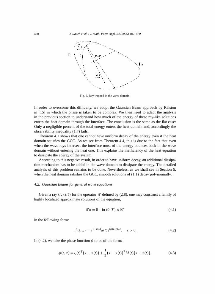
Fig. 2. Ray trapped in the wave domain.
In order to overcome this difficulty, we adopt the Gaussian Beam approach by Rin [15] in which the phase is taken to be complex. We then need to adapt the anin the previous section to understand how much of the energy of these ray-like solenters the heat domain through the interface. The conclusion is the same as the flOnly a negligible percent of the total energy enters the heat domain and, accordinobservability inequality (1.7) fails.
Theorem 4.1 shows that one cannot have uniform decay of the energy even if thdomain satisfies the GCC. As we see from Theorem 4.4, this is due to the fact thawhen the wave rays intersect the interface most of the energy bounces back in thdomain without entering the heat one. This explains the inefficiency of the heat eqto dissipate the energy of the system.
According to this negative result, in order to have uniform decay, an additional distion mechanism has to be added in the wave domain to dissipate the energy. The danalysis of this problem remains to be done. Nevertheless, as we shall see in Sewhen the heat domain satisfies the GCC, smooth solutions of (1.1) decay polynomi
4.2. Gaussian Beams for general wave equations
Given a ray(t, x(t)) for the operatorW defined by (2.8), one may construct a familyhighly localized approximate solutions of the equation,
Wu = 0 in (0, T ) × Rn (4.1)
in the following form:
uε(t, x) = ε1−n/4a(t)eiφ(t,x)/ε, ε > 0. (4.2)
In (4.2), we take the phase functionφ to be of the form:
φ(t, x) = ξ(t)T(x − x(t))+ 1(
x − x(t))T
M(t)(x − x(t)
), (4.3)
2
J. Rauch et al. / J. Math. Pures Appl. 84 (2005) 407–470 431
rt.f
e
de
whereM(t) is a n × n complex symmetric matrix with positive definite imaginary paThe construction of approximate solutions (4.2) requires an appropriate selection oa(t)
andM(t).Denote the energy of (4.1) by:
e(t) ≡ e(u)(t)
= 1
2
∫Rn
[∣∣u(t, x)∣∣2 +
n∑j,k=1
αjk(x)∂xju(t, x)∂xk
u(t, x) + ∣∣ut (t, x)∣∣2]dx. (4.4)
The following result can be found in [15] and [13]:
Theorem 4.2.Let T > 0 be given,αjk ∈ C2(Rn), βj ∈ C1(Rn), and (t, x(t)) be a rayfor W . Then for anyn×n complex symmetric matrixM0 with ImM0 > 0 and anya0 ∈ C\0, there is a complex-valued symmetric matrixM(·) ∈ C2([0, T ];C
n×n) and a complex-valued functiona(·) ∈ C2([0, T ];C \ 0) with
M(0) = M0, ImM(t) > 0, a(0) = a0, (4.5)
such that
(1) Theuε are approximate solutions of(4.1):
supt∈(0,T )
∣∣Wuε(t, ·)∣∣L2(Rn)
= O(ε1/2); (4.6)
(2) The initial energy ofuε is bounded below asε → 0, i.e.,
eε(0) ≡ e(uε)(0) ≈ 1; (4.7)
(3) The energy ofuε is exponentially small off the ray(t, x(t)):
supt∈(0,T )
∫Rn\B
ε1/4(t)
[∣∣uεt (t, x)
∣∣2 + ∣∣∇uε(t, x)∣∣2]dx = O
(e−β/ε
), (4.8)
whereBε1/4(t) is the ball centered atx(t) with radiusε1/4 and β > 0 is a constant,independent ofε.
Remark 4.1. We recall that, by [15] and [13],a(t) in Theorem 4.2 is determined by thODE:
ddt
a(t) = a(t)Wφ(t, x(t)),
a(t0) = a0.
To simplify the presentation, we choosea(t) in (4.2) such that it only depends ont . If as-suming further that the coefficients ofW are infinitely smooth and choosing the amplitu
432 J. Rauch et al. / J. Math. Pures Appl. 84 (2005) 407–470
the
itial
t,
f order
in
al
ny
sys-
sehis
in (4.2) to beaε(t, x), one may obtain infinitely accurate approximate solutions toWu = 0,i.e., instead of (4.6), one may getWuε = O(ε∞). On the other hand,M(t) in Theorem 4.2is determined by the Riccati equation: dM(t)
dt+ M(t)C(t)M(t) + B(t)M(t) + M(t)B(t)T + A(t) = 0,
M(0) = M0,
whereC(t), B(t) andA(t) aren × n matrices whose coefficients are determined byfirst and second derivatives ofg evaluated along the ray(t, x(t), ξ(t)) (recall (2.9) forg).We refer to [15] for the global existence of solutions to this nonlinear ODE with indatumM0 so that ImM0 > 0.
Remark 4.2.Let aijk ∈ C, i, j, k = 1,2, . . . , n, be given so thataijk = ai′j ′k′ for any per-mutationi′, j ′, k′ of i, j, k. Put(x1(t), . . . , xn(t)) ≡ x(t). From [15] and [13], we see thathe conclusions in Theorem 4.2 hold if one replaces the phase functionφ given by (4.3) by
φ(t, x) = ξ(t)T(x − x(t))+ 1
2
(x − x(t)
)TM(t)
(x − x(t)
)+
n∑i,j,k=1
aijk
(xi − xi(t)
)(xj − xj (t)
)(xk − xk(t)
). (4.9)
Indeed, this follows from the fact that the difference between those two phases is o|x − x(t)|3. This observation will play a key role in the sequel.
Remark 4.3. For any giveb ∈ Cn, from [15] and [13], we see that, the conclusions
Theorem 4.2 hold if one replaces the amplitudea(t) by a(t) + bT(x − x(t)). Indeed, thisfollows from the fact that the difference between those two amplitudes is of order|x−x(t)|.This observation will play a key role in the sequel, too.
Remark 4.4.Let χ ∈ C∞0 (R1+n) be any given cut-off function which is identically equ
to 1 in a neighborhood of the ray(t, x(t)) | t ∈ [0, T ]. Then the functionsχuε also sat-isfies (4.6)–(4.8). In view of this, we may chooseuε such that they are supported in agiven (small) neighborhood of the ray.
4.3. Gaussian Beams for the wave equation with curved wavefronts
From now on to the rest of this section, we construct highly localized solutions totem (1.1).
Assume(t, x−(t), ξ−(t)) is a ray for ≡ ∂tt − starting fromΩ2 at timet = 0, i.e.,
x−(0) ∈ Ω2, and arriving at the boundary∂Ω2 at time t = t0, i.e., x0= x−(t0) ∈ ∂Ω2.
We must distinguish two cases, i.e., eitherx0 belongs to the exterior boundaryΓ2 of thewave domainΩ2, or to the interfaceγ . By Assumption 2.1, we exclude the rarely cax0 ∈ Γ 2 ∩ γ . The case wherex0 ∈ γ will be analyzed in the next two subsections. In t
J. Rauch et al. / J. Math. Pures Appl. 84 (2005) 407–470 433
is
lete-
.n-
tnt
is
point
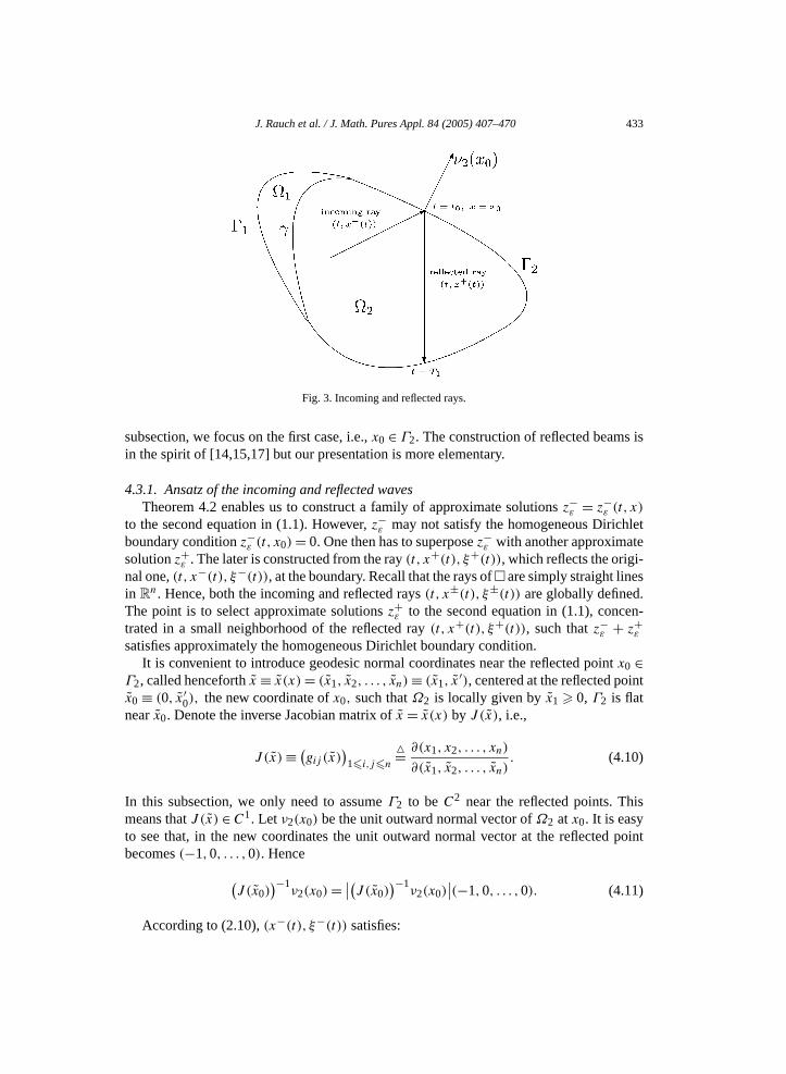
Fig. 3. Incoming and reflected rays.
subsection, we focus on the first case, i.e.,x0 ∈ Γ2. The construction of reflected beamsin the spirit of [14,15,17] but our presentation is more elementary.
4.3.1. Ansatz of the incoming and reflected wavesTheorem 4.2 enables us to construct a family of approximate solutionsz−
ε = z−ε (t, x)
to the second equation in (1.1). However,z−ε may not satisfy the homogeneous Dirich
boundary conditionz−ε (t, x0) = 0. One then has to superposez−
ε with another approximatsolutionz+
ε . The later is constructed from the ray(t, x+(t), ξ+(t)), which reflects the original one,(t, x−(t), ξ−(t)), at the boundary. Recall that the rays ofare simply straight linesin R
n. Hence, both the incoming and reflected rays(t, x±(t), ξ±(t)) are globally definedThe point is to select approximate solutionsz+
ε to the second equation in (1.1), concetrated in a small neighborhood of the reflected ray(t, x+(t), ξ+(t)), such thatz−
ε + z+ε
satisfies approximately the homogeneous Dirichlet boundary condition.It is convenient to introduce geodesic normal coordinates near the reflected poinx0 ∈
Γ2, called henceforthx ≡ x(x) = (x1, x2, . . . , xn) ≡ (x1, x′), centered at the reflected poi
x0 ≡ (0, x′0), the new coordinate ofx0, such thatΩ2 is locally given byx1 0, Γ2 is flat
nearx0. Denote the inverse Jacobian matrix ofx = x(x) by J (x), i.e.,
J (x) ≡ (gij (x))1i,jn
= ∂(x1, x2, . . . , xn)
∂(x1, x2, . . . , xn). (4.10)
In this subsection, we only need to assumeΓ2 to beC2 near the reflected points. Thmeans thatJ (x) ∈ C1. Let ν2(x0) be the unit outward normal vector ofΩ2 atx0. It is easyto see that, in the new coordinates the unit outward normal vector at the reflectedbecomes(−1,0, . . . ,0). Hence(
J (x0))−1
ν2(x0) = ∣∣(J (x0))−1
ν2(x0)∣∣(−1,0, . . . ,0). (4.11)
According to (2.10),(x−(t), ξ−(t)) satisfies:

434 J. Rauch et al. / J. Math. Pures Appl. 84 (2005) 407–470
ted
d-
e may
ryat
x−(t) = 2ξ−(t),
ξ−(t) = 0,
x−(t0) = x0, ξ−(t0) = ξ−(t0).
(4.12)
Also, one assumes that(x+(t), ξ+(t)) satisfies:
x+(t) = 2ξ+(t),
ξ+(t) = 0,
x+(t0) = x0,
ξ+(t0) = ξ−(t0) − 2ξ−(t0) · ν2(x0)ν2(x0).
(4.13)
The choice of the initial dataξ+(t0) is such that the directions of the incoming and reflecrays satisfy the “geometric optics law”, i.e.,
x+(t0) = x−(t0) − 2x−(t0) · ν2(x0)ν2(x0).
On the other hand, from (2.11), one has|ξ−(t0)| = 1/2. Hence, noting|ν2(x0)| = 1, it iseasy to check that|ξ+(t0)| = 1/2. Therefore,
|ξ±(t)| = 1
2, ∀t ∈ R. (4.14)
By Assumption 2.1, we may assumeξ−(t) is transversal and non-normal to the bounary ∂Ω2 at timet = t0, i.e.,
ξ−(t0) · ν2(x0) = 0 and ξ−(t0) ‖ν2(x0). (4.15)
Finally, according to (4.2) and Theorem 4.2, and noting Remarks 4.2 and 4.3, wassume the incoming wave to be of the form
z−ε (t, x) = ε1−n/4[a−(t) + (b−)T(x − x−(t)
)]eiφ−(t,x)/ε, (4.16)
where
φ−(t, x) = ξ−(t)T(x − x−(t))+ 1
2
(x − x−(t)
)TM−(t)
(x − x−(t)
)+
n∑i,j,k=1
a−ijk
(xi − x−
i (t))(
xj − x−j (t))(
xk − x−k (t)). (4.17)
In (4.17),M−(t) is somen×n complex symmetric matrix with positive definite imaginapart, whileb− ∈ C
n anda−ijk , i, j, k = 1,2, . . . , n, are any given complex numbers so th
a− = a−′ ′ ′ for any permutationi′, j ′, k′ of i, j, k.
ijk i j k
J. Rauch et al. / J. Math. Pures Appl. 84 (2005) 407–470 435
ray
er,rk 4.1,
ry
nn
Denote byT1 > 0 the instant when the reflected ray arrives at∂Ω2, i.e.,x+(T1) ∈ ∂Ω2.(Note that, of course, 0< t0 < T1.) Fix any
T ∗ ∈ (t0, T1). (4.18)
Our aim is to find another approximate solution
z+ε (t, x) = ε1−n/4[a+(t) + (b+)T(x − x+(t)
)]eiφ+(t,x)/ε (4.19)
of u = 0, which is concentrated in a small neighborhood of the reflected(t, x+(t), ξ+(t)) such that∣∣z−
ε + z+ε
∣∣H1((0,T ∗)×∂Ω2)
= O(ε1/2). (4.20)
The constructions ofφ+(t, x) anda+(t) are close to that used in [15] and [13]. Howevfor the reader’s convenience, we recall a sketch of the constructions. First, by Remaa+(t) is determined from its initial value att = t0, which is given by:
a+(t0) = −a−(t0). (4.21)
Next, choose:
φ+(t, x) = ξ+(t)T(x − x+(t))+ 1
2
(x − x+(t)
)TM+(t)
(x − x+(t)
)+
n∑i,j,k=1
a+ijk
(xi − x+
i (t))(
xj − x+j (t))(
xk − x+k (t)), (4.22)
whereM+(t) is a suitablen×n complex symmetric matrix with positive definite imaginapart, whilea+
ijk , i, j, k = 1,2, . . . , n, are any given complex numbers so thata+ijk = a+
i′j ′k′for any permutationi′, j ′, k′ of i, j, k. According to Remark 4.1,M+(t) is determinedby its initial dataM+(t0) and the reflected ray(t, x+(t), ξ+(t)). We emphasize that ithis subsection the “reflected coefficients”b+ in (4.19) anda+
ijk in (4.22) may be chosearbitrarily. Therefore, it remains to assignM+(t0).
4.3.2. Assignment ofM+(t0)
Write the expression ofφ±(t, x) in the x-coordinates as
φ±(t, x) = ξ±(t)T(x(x) − x±(t))+ 1
2
(x(x) − x±(t)
)TM±(t)
(x(x) − x±(t)
)+
n∑a±ijk
(xi(x) − x±
i (t))(
xj (x) − x±j (t))(
xk(x) − x+k (t)). (4.23)
i,j,k=1
436 J. Rauch et al. / J. Math. Pures Appl. 84 (2005) 407–470
of
Put
σ± ≡ (σ±1 , σ ′±)
= (J (x0))T
ξ±(t0),
η± ≡ (η±1 , η±
2 , . . . , η±n
)≡ (η±1 , η′±)
= (J (x0))−1
ξ±(t0),(4.24)
whereσ ′±, η′± ∈ Rn−1. Both σ± and η± will be needed to compute the derivatives
φ±(t,0, x′) at (t0, x0) up to second order.The following holds.
Proposition 4.1.Under the assumption(4.15), it holds:
η±1 = 0, η′+ = η′−, σ±
1 = 0, σ ′+ = σ ′− = 0. (4.25)
Proof. First, we claim that((J (x0)
)−1)T(J (x0)
)−1ν2(x0) ‖ ν2(x0). (4.26)
Indeed, denote byT the tangent space to∂Ω2 at the reflected pointx0. Then, it is ob-vious that(J (x0))
−1T = x1 = 0. Noting (4.11), this means that(J (x0))−1ν2(x0) ⊥
(J (x0))−1T . Hence,((J (x0))
−1)T(J (x0))−1ν2(x0) ⊥ T . This yields (4.26).
Next, by the last equation in (4.13) and (4.15), we deduce that
ξ+(t0) · ν2(x0) = −ξ−(t0) · ν2(x0) = 0. (4.27)
Hence, from (4.11), (4.26) and (4.27), we obtain:
η±1 = −
((J (x0)
)−1ξ±(t0),
(J (x0))−1ν2(x0)
|(J (x0))−1ν2(x0)|)
Rn
= −(
ξ±(t0),((J (x0))
−1)T(J (x0))−1ν2(x0)
|(J (x0))−1ν2(x0)|)
Rn
= −|((J (x0))−1)T(J (x0))
−1ν2(x0)||(J (x0))−1ν2(x0)| ξ±(t0) · ν2(x0) = 0. (4.28)
Also, by the last equation in (4.13), we have:(J (x0)
)−1ξ+(t0) = (J (x0)
)−1ξ−(t0) − 2ξ−(t0) · ν2(x0)
(J (x0)
)−1ν2(x0). (4.29)
Hence, in view of (4.11) and (4.29), we see that thej th component of(J (x0))−1ξ+(t0) is
equal to that of(J (x0))−1ξ−(t0) for j = 2, . . . , n. This meansη′+ = η′−.
Similarly, from (4.11) and (4.27), we obtain:
σ±1 = −
((J (x0)
)Tξ±(t0),
(J (x0))−1ν2(x0)
−1
)= −ξ±(t0) · ν2(x0)
−1= 0. (4.30)
|(J (x0)) ν2(x0)| Rn |(J (x0)) ν2(x0)|
J. Rauch et al. / J. Math. Pures Appl. 84 (2005) 407–470 437
ve
his
Also, by the last equation in (4.13), we have:(J (x0)
)Tξ+(t0) = (J (x0)
)Tξ−(t0) − 2ξ−(t0) · ν2(x0)
(J (x0)
)Tν2(x0). (4.31)
Clearly, (4.26) yields (J (x0)
)Tν2(x0) ‖ (J (x0)
)−1ν2(x0). (4.32)
Note that (4.32) and (4.11) imply that(J (x0))Tν2(x0) ‖ (−1,0, . . . ,0). Hence, in
view of (4.31), we see that thej th component of(J (x0))Tξ+(t0) is equal to that of
(J (x0))Tξ−(t0) for j = 2, . . . , n. This meansσ ′+ = σ ′−. It remains to show thatσ ′− =
0. Assume this is not correct, i.e.,σ ′− = 0. Then noting (4.11) and (4.24), we ha(J (x0))
Tξ−(t0) ‖ (J (x0))−1ν2(x0). This, combined with (4.32), implies thatξ−(t0) ‖
((J (x0))T)−1(J (x0))
−1ν2(x0) ‖ ν2(x0), which contradicts our assumption (4.15). Tcompletes the proof of Proposition 4.1.
Denote
M±(t0)= (J (x0)
)TM±(t0)J (x0). (4.33)
Obviously, determiningM+(t0) is equivalent to choseM+(t0). For this purpose, put
x±(t) = x(x±(t)
). (4.34)
Then, one has:
x±(t) = x(x±(t)
). (4.35)
We need several useful technical propositions.
Proposition 4.2.As(t, x′) tends to(t0, x′0), the following estimates hold:
(0, x′) − x±(t) = (−2η±1 (t − t0), x
′ − x′0 − 2η′±(t − t0)
)+ O(|t − t0|2 + |x′ − x′
0|2), (4.36)
φ±(t,0, x′) = O(|t − t0| + |x′ − x′
0|), (4.37)
∂t φ±(t,0, x′) = −1
2+ O(|t − t0| + |x′ − x′
0|), (4.38)
∇x φ±(t,0, x′) = σ± + O
(|t − t0| + |x′ − x′0|), (4.39)
∂tt φ±(t,0, x′) = 4
(η±)TM±(t0)η
± + O(|t − t0| + |x′ − x′
0|), (4.40)
438 J. Rauch et al. / J. Math. Pures Appl. 84 (2005) 407–470
∂t∇x φ±(t,0, x′) = −2M±(t0)η
± + O(|t − t0| + |x′ − x′
0|), (4.41)
∇2x φ±(t,0, x′) = ∇x
((J (x0)
)Tξ±(t0)
)+ M±(t0) + O(|t − t0| + |x′ − x′
0|). (4.42)
The proof of Proposition 4.2 will be given in Appendix B.Denote:
∇x
((J (x0))
Tξ±(t0))≡ (h±
ij
)1i,jn
,
(4.43)
M±(t0) ≡ (m±ij
)1i,jn
≡(
m±11 ϑT±
ϑ± M±)
,
whereϑ± = (m±21, . . . ,m
±n1)
T andM± = (m±ij )2i,jn. Note that allm−
ij are known. We
now assign allm+ij to then obtainM+(t0) in (4.24). First of all, we choose
m+ij = h−
ij + m−ij − h+
ij , 2 i, j n. (4.44)
This determinesM+. By (4.43)–(4.44), we see that
∇x
((J (x0)
)Tξ+(t0)
)+ M+(t0) = ∇x
((J (x0)
)Tξ−(t0)
)+ M−(t0). (4.45)
Next, by (4.24) and (4.43), we see that
M±(t0)η± =(
m±11η
±1 + ϑT±η′±
η±1 ϑ± + M±η′±
). (4.46)
Hence, we choose:
ϑ+ = η−1 ϑ− + M−η′− − M+η′+
η+1
. (4.47)
This determinesm+j1 = m+
1j for j = 2, . . . , n. From (4.46)–(4.47), we get:
M+(t0)η+ = M−(t0)η
−. (4.48)
Finally, from by (4.24) and (4.46), we have:(η±)TM±(t0)η
± = m±11
∣∣η±1
∣∣2 + 2η±1 ϑT±η′± + (η′±)TM±η′±. (4.49)
Therefore, we choose
m+11 = m−
11|η−1 |2 + 2η−
1 ϑT−η′− + (η′−)TM−η′− − 2η+1 ϑT+η′+ − (η′+)TM+η′+
|η+|2 . (4.50)
1
J. Rauch et al. / J. Math. Pures Appl. 84 (2005) 407–470 439
42)
r the
ll.
In view of (4.49)–(4.50), we get:(η+)TM+(t0)η
+ = (η−)TM−(t0)η−. (4.51)
This completes the assignment ofM+(t0), and henceM+(t0).
4.3.3. Properties ofφ±(t, x) andM+(t0)
With the above choice onM+(t0), noting (4.40) and (4.51), (4.41) and (4.48), and (4.and (4.45), respectively, one concludes easily that
Proposition 4.3.As(t, x′) tends to(t0, x′0), the following estimates hold:
∂tt φ+(t,0, x′) − ∂tt φ
−(t,0, x′) = O(|t − t0| + |x′ − x′
0|), (4.52)
∂t∇x′ φ+(t,0, x′) − ∂t∇x′ φ−(t,0, x′) = O(|t − t0| + |x′ − x′
0|), (4.53)
∇2x′ φ+(t,0, x′) − ∇2
x′ φ−(t,0, x′) = O(|t − t0| + |x′ − x′
0|). (4.54)
Remark 4.5.Combining Propositions 4.1–4.3, it is easy to see that the choice ofM+(t0),and hence ofM+(t0), is such that
Ds(t,x′)φ
+(t0, x0) = Ds(t,x′)φ
−(t0, x0) (4.55)
for s = 0,1,2. In other words, all derivatives of orders 2 in the(t, x′) variables coincideat (t0, x0). This is enough in this subsection. Note that in this case, the values ofa±
ijk maybe chosen arbitrarily. However, in Section 4.5 when the ray-like solutions of (1.1) focase that the incoming ray arrives at the interfaceγ at timet = t0 will be constructed, weneed to choosea+
ijk suitably such that (4.55) holds for the third order derivatives as we
Thanks to Taylor’s formula it follows, from Remark 4.5, that
Proposition 4.4.As(t, x′) tends to(t0, x′0), it holds:
φ+(t,0, x′) − φ−(t,0, x′) = O(|t − t0|3 + |x′ − x′
0|3). (4.56)
As mentioned before, it is crucial to show the following result:
Proposition 4.5. Both M+(t0) constructed above and the desiredM+(t0), and henceM+(t), aren × n complex symmetric matrices with positive definite imaginary part.
Proof. First, from (4.44) and noting thath±ij ∈ R, one finds:
Im M+ = Im M−. (4.57)
440 J. Rauch et al. / J. Math. Pures Appl. 84 (2005) 407–470
of of
ble
Next, by (4.47) and (4.57), and noting thatη′+ = η′− ∈ Rn−1 (by Proposition 4.1), we get:
Imϑ+ = η−1
η+1
Imϑ−. (4.58)
Finally, by (4.50), (4.57) and (4.58), we see that
Imm+11 = |η−
1 |2|η+
1 |2 Imm−11. (4.59)
Now, combining (4.57)–(4.59), we arrive at
Im M+(t0) = diag
[η−
1
η+1
,1, . . . ,1
]Im M−(t0)diag
[η−
1
η+1
,1, . . . ,1
].
Recalling that ImM−(t0) > 0, we conclude the desired result. This completes the proProposition 4.5.
We also need the following result:
Proposition 4.6.As(t, x′) tends to(t0, x′0), the following estimate
Im φ±(t,0, x′) c(|t − t0|2 + |x′ − x′
0|2)
(4.60)
holds for some constantc > 0.
The proof of Proposition 4.6 is given in Appendix B.
Remark 4.6.Proposition 4.6 shows that the factors eiφ±(t,0,x′)/ε localizez±ε (t,0, x′) in the
region|t − t0|2 + |x′ − x′0|2 = O(ε).
4.3.4. Verification of (4.20)Now, we are in the position to show that
Lemma 4.1. The approximate solutionsz±ε (t, x) of u = 0, constructed by(4.16)
and (4.19) with a+(t0) and M+(t0) chosen above(but for arbitrary b± and a±ijk), sat-
isfy (4.20).
Proof. Let z±(t, x) be the new coordinate expressions ofz±(t, x). According to Re-mark 4.4, the support ofz±
ε |(0,T ∗)×∂Ω2 being very small, we can use the change of variax → x to get∣∣z−
ε + z+ε
∣∣H1((0,T ∗)×∂Ω )
C∣∣z−
ε (t,0, x′) + z+ε (t,0, x′)
∣∣H1((0,T ∗)×R
n−1). (4.61)
2 x′
J. Rauch et al. / J. Math. Pures Appl. 84 (2005) 407–470 441
Since the O(|x − x(t)|) terms in the amplitudesa±(t) + (b±)T(x − x±(t)) play no rolein this subsection, without loss of generality we may simply takeb± = 0. It is easy to seethat
z−ε (t,0, x′) + z+
ε (t,0, x′) = ε1−n/4[a−(t)eiφ−(t,0,x′)/ε + a+(t)eiφ+(t,0,x′)/ε]. (4.62)
Hence, by (4.62), and noting (4.21) and (4.39), we get:
∇x′(z−ε (t,0, x′) + z+
ε (t,0, x′))
= iε−n/4[a−(t)eiφ−(t,0,x′)/ε∇x′ φ−(t,0, x′) + a+(t)eiφ+(t,0,x′)/ε∇x′ φ+(t,0, x′)]
= iε−n/4a−(t0)∇x′ φ−(t0, x′0)[eiφ−(t,0,x′)/ε − eiφ+(t,0,x′)/ε]
+ eiφ−(t,0,x′)/εO(|t − t0| + |x′ − x′
0|)+ eiφ+(t,0,x′)/εO
(|t − t0| + |x′ − x′0|)
. (4.63)
Also, by Proposition 4.4, we see that
eiφ−(t,0,x′)/ε − eiφ+(t,0,x′)/ε
= i(φ−(t,0, x′) − φ+(t,0, x′))ε
1∫0
ei[φ+(t,0,x′)+s(φ−(t,0,x′)−φ+(t,0,x′))]/ε ds
= i
ε
1∫0
ei[φ+(t,0,x′)+s(φ−(t,0,x′)−φ+(t,0,x′))]/ε ds O(|t − t0|3 + |x′ − x′
0|3). (4.64)
By Proposition 4.6, we see that the factors eiφ±(t,0,x′)/ε andei[φ+(t,0,x′)+s(φ−(t,0,x′)−φ+(t,0,x′))]/ε localize the integrand in the region
|t − t0|2 + |x′ − x′0|2 = O(ε).
Therefore, by (4.63) and (4.64), we conclude that, for some positive constantC it holds∣∣∇x′(z−ε (t,0, x′) + z+
ε (t,0, x′))∣∣2
L2((0,T ∗)×Rn−1x′ )
Cε−n/2∫
|t−t0|2+|x′−x′0|2=O(ε)
[ε−2O
(|t − t0|6 + |x′ − x′0|6)
+ O(|t − t0|2 + |x′ − x′
0|2)]
dt dx′
= O(ε). (4.65)
Similarly, one shows that∣∣z−ε (t,0, x′) + z+
ε (t,0, x′)∣∣H1(0,T ∗)×R
n−1)= O(ε1/2). (4.66)
x′
442 J. Rauch et al. / J. Math. Pures Appl. 84 (2005) 407–470
. This
oint
-sthe,
on the
is,
Finally, combining (4.61), (4.65) and (4.66), we arrive at the desired result (4.20)completes the proof of Lemma 4.1.4.3.5. Highly localized solutions of (1.1) without GCC
Summing up the above analysis, we arrive at the following conclusion:
Proposition 4.7.Let (t, x−(t), ξ−(t)), with x−(0) ∈ Ω2, be an incoming ray for , whicharrives transversely atΓ2 at time t = t0, i.e., the first assumption in(4.15) holds. Let(t, x+(t), ξ+(t)) be the(global) reflected ray constructed above, with the reflected px0 ∈ Γ2. Then there is a family of solutions(yε, zε)ε>0 of system(1.1) in (0, T ∗) × Ω
(the initial conditions being excepted) (recall (4.18)for T ∗), such that
|∂tyε|2L2((0,T ∗)×Ω1)= O(ε), Eε(0) = E(yε, zε, ∂t zε)(0) ≈ 1. (4.67)
Proof. Put
yε ≡ 0, zε= z+
ε + z−ε .
By Remark 4.4, one may assume the supports ofz− and z+ are away from the interfaceγ . Hence, in view of Theorem 4.2, we deduce that(yε, zε) are approximate solutionof system (1.1) in(0, T ∗) × Ω (the initial conditions and the boundary conditions forhyperbolic component being excepted), in the sense that(yε, zε) satisfy the heat equationthe boundary conditions for the parabolic component, the transmission conditionsinterface of (1.1), and
supt∈(0,T ∗)
| zε|L2(Ω2)= O(ε1/2). (4.68)
Moreover,
E(yε, zε, ∂t zε)(0) ≈ 1. (4.69)
We may correct(yε, zε) to become a family of exact solutions of Eq. (1.1). For thlet
yε = yε + vε, zε = zε + wε, (4.70)
where(vε,wε) solves:
∂tvε − vε = 0 in (0, T ∗) × Ω1,
wε = − zε = O(ε1/2) in (0, T ∗) × Ω2,
vε = 0 on(0, T ∗) × Γ1,
wε = −zε on (0, T ∗) × Γ2,
vε = wε,∂vε
∂ν1= − ∂wε
∂ν2on (0, T ∗) × γ,
vε(0) = 0 in Ω1,
w (0) = ∂ w (0) = 0 in Ω .
(4.71)
ε t ε 2
J. Rauch et al. / J. Math. Pures Appl. 84 (2005) 407–470 443
[13],
y
roof oft does
ed
sely ones prov-
to hold
Then, noting (4.20), applying the classical energy method to system (4.71), similar toit is easy to show that
|∂tvε|2L2((0,T ∗)×Ω1)= O(ε). (4.72)
Therefore,(yε, zε) satisfy the conclusion of Proposition 4.7.As a direct consequence of Proposition 4.7, we have the:
Corollary 4.1. Let Assumption2.1 holds andx(t) /∈ γ for any t ∈ [0, T ]. Then there is afamily of solutions(yε, zε, ∂t zε)ε>0 of system(1.1) in [0, T ] × Ω (the initial conditionsbeing excepted), such that
|∂tyε|2L2((0,T )×Ω1)= O(ε), Eε(0) = E(yε, zε, ∂t zε)(0) ≈ 1. (4.73)
From Corollary 4.1, one concludes that
Theorem 4.3.Let T > 0. Suppose the heat subdomainΩ1 does not control geometricallthe wave domainΩ2 in time interval[0, T ], and the boundary∂Ω2 of Ω2 belongs toC2.Then there exists a sequence of initial data(ym
0 , zm0 , zm
1 )∞m=1 ⊂ H such that:
(i) ∣∣(ym0 , zm
0 , zm1
)∣∣H
= 1; (4.74)
(ii) the corresponding solutions(ym, zm, zmt ) of (1.1)satisfy
limm→∞
∣∣ymt
∣∣L2((0,T )×Ω1)
= 0. (4.75)
As for the proof of Theorem 4.3, we may proceed as in the second case in the pTheorem 3.4. Indeed, if the GCC fails, then there exists a multiply reflected ray thanot reach the interfaceγ . In view of Lemma 2.2, the multiply reflected ray can be assumto have only transversal and non-normal reflections.
Remark 4.7. By assuming that the boundary∂Ω2 of Ω2 belongs toC∞ and changingthe above argument by adding more terms on the wave constructions (more precithe constructions of the amplitudea±(t, x) and the phasesφ±(t, x)), one sees that thGaussian Beam construction of approximate solutions for the wave equations allowing that when the GCC fails one may strength (4.75) to get
limm→∞
∣∣ymt
∣∣Hs((0,T )×Ω1)
= 0, ∀s 0,
which means that in this case one can not even expect a weakened version of (1.7)when the norm on its right side is replaced by any stronger Sobolev norm.

444 J. Rauch et al. / J. Math. Pures Appl. 84 (2005) 407–470
in theg the
ronts
e
will,
Remark 4.8. The non-normal incidence assumption in (4.15) has not been usedabove construction. However, we will use it in the next subsection for constructinapproximate solutions for the heat equation when the ray intersects the interfaceγ .
4.4. Highly localized approximate solutions for the heat equation with curved wavef
We now analyze what happens when the incoming ray(t, x−(t)) for arrives at theinterfaceγ at timet0, i.e.,x0 ∈ γ .
We still use the normal coordinates near the reflected pointx0 ∈ γ , called alsox = (x1, x2, . . . , xn) ≡ (x1, x
′), centered at the reflected pointx0, i.e., the new coordinatof x0, such that
(i) γ is flat nearx0 in the new coordinates;(ii) Ω1 is locally given byx1 < 0, and the heat operator is locally as follows:
H = ∂t −n∑
i,j=1
αij (x)∂xi∂xj
−n∑
i=1
βi (x)∂xi; (4.76)
(iii) Ω2 is locally given byx1 > 0, and the operator takes the following form
W = ∂tt −n∑
j,k=1
αjk(x)∂xj∂xk
−n∑
j=1
βj (x)∂xj; (4.77)
(iv) for x belonging to a small neighborhood ofx0, (αij )n×n ∈ C2 is strictly positive defi-nite and symmetric andβj areC1 functions. Moreover one has
α11(x) ≡ 1, α1k(x) ≡ 0 for anyk = 2, . . . , n. (4.78)
Put
F= (αij (x0)
)2i,jn
. (4.79)
ObviouslyF is a positive definite matrix.Assumez−
ε (t, x) to be thex-coordinate expression of the incoming wavez−ε (t, x) given
in (4.16), i.e.,
z−ε (t, x) = ε1−n/4[a−(t) + (b−)T(x(x) − x−(t)
)]eiφ−(t,x)/ε, (4.80)
whereφ−(t, x) is as in (4.23). To construct approximate solutions of system (1.1), weseek reflected wavesz+
ε (t, x) as in the previous subsection and approximate solutions
yε = yε(t, x) = ε1−n/4A(t, x)eiψ(t,x)/ε, (4.81)
J. Rauch et al. / J. Math. Pures Appl. 84 (2005) 407–470 445
imate
tion.ns
uggestsost
rface”
yields
thatth
of the heat equation:
H y = 0. (4.82)
The goal of this subsection is to describe the construction of the parabolic approxsolutionsyε, which will be glued with the hyperbolic approximate solutionsz±
ε (t, x) toproduce approximate solutions of our transmission problem (1.1) in the next subsec
To construct the approximate solutionsyε of (4.82), the idea is to match such solutiogiven by (4.81) to that of the wave equation such that
ψ(t,0, x′) = φ−(t,0, x′). (4.83)
This idea is the same as when the interface is flat. The case of linear phases sus that the case∇x′ φ−(t,0, x′) = 0 corresponding to non-normal incidence is the mnatural one. This is guaranteed by Assumption 2.1. Our treatment for the “flat intealso indicates that by continuityψ should have positive imaginary part inx1 < 0 near theinterface.
We introduce the complex first order partial differential operator:
H = ∂t ψ − 2n∑
i,j=1
αij (x)∂xiψ∂xj
−n∑
i,j=1
αij (x)∂2xi xj
ψ −n∑
j=1
βj ∂xjψ . (4.84)
Then, from (4.76) and (4.81), we get:
H yε = ε1−n/4eiψ/ε
[A
ε2
n∑i,j=1
αij (x)∂xiψ∂xj
ψ + i
εHA + H A
]. (4.85)
First, setting the leading term in the right-hand side of (4.85) to be equal to zerothe eikonal equation,
n∑i,j=1
αij (x)∂xiψ∂xj
ψ = 0, (4.86)
or, by (4.78), equivalently,
(∂x1ψ
)2 = −n∑
i,j=2
αij (x)∂xiψ∂xj
ψ . (4.87)
Since(αij )n×n is positive definite, there are no real solutions for (4.87). To insureIm ψ > 0 in x1 < 0 one determines∂x1ψ(t,0, x′) as the solution of (4.83) and (4.87) wiIm ∂x1ψ < 0. This is possible since by Propositions 4.1 and 4.2, one has:
∇x′ψ(t0, x0) = ∇x′ φ−(t0, x0) = σ ′− = 0.
446 J. Rauch et al. / J. Math. Pures Appl. 84 (2005) 407–470
.83)e, wet up to) the
Note that Eq. (4.87) is a complex equation and the initial value problem (4and (4.87) is in general not solvable. However, similar to the case of flat interfacdo not need to solve (4.87) exactly. Instead, as we see later, it suffices to solve iorder O(|x1|2) near the interface. For this purpose, we determine uniquely from (4.87derivatives∂j
x1ψ(t,0, x′) for j = 0,1,2. More precisely, put:
α0ij
= αij (0, x′), α1ij
= ∂x1αij (t,0, x′), f0 ≡ f0(t,0, x′) = φ−(t,0, x′),
f1 ≡ f1(t,0, x′) = −i
√√√√ n∑i,j=2
α0ij ∂xi
φ−(t,0, x′)∂xjφ−(t,0, x′) ,
f2 ≡ f2(t,0, x′) = − 1
2f1
n∑i,j=2
(2α0
ij ∂xif0∂xj
f1 + α1ij ∂xi
f0∂xjf0).
(4.88)
We choose
ψ(t, x1, x′) =
2∑j=0
fj (t,0, x′)j ! x
j
1 . (4.89)
Then the following result holds:
Proposition 4.8.For any given(t, x′), the functionψ in (4.89)satisfies(4.83)and
n∑i,j=1
αij (x)∂xiψ∂xj
ψ = O(|x1|2
)as x1 → 0. (4.90)
Proof. From (4.88), we see that
f 21 +
n∑i,j=2
α0ij ∂xi
f0∂xjf0 ≡ 0, 2f1f2 +
n∑i,j=2
(2α0
ij ∂xif0∂xj
f1 + α1ij ∂xi
f0∂xjf0)≡ 0.
Therefore, by (4.78) and (4.89), one sees that
n∑i,j=1
αij (x)∂xiψ∂xj
ψ
= (f1 + f2x1)2 +
n∑i,j=2
αij (x)(∂xi
f0 + ∂xif1x1 + O(|x1|2)
)× (∂x f0 + ∂x f1x1 + O
(|x1|2))
j j
J. Rauch et al. / J. Math. Pures Appl. 84 (2005) 407–470 447
= f 21 + 2f1f2x1 +
n∑i,j=2
αij (x)(∂xif0 + ∂xi
f1x1)(∂xjf0 + ∂xj
f1x1) + O(|x1|2
)= f 2
1 + 2f1f2x1 +n∑
i,j=2
(α0
ij + α1ij x1)(
∂xif0 + ∂xi
f1x1)(
∂xjf0 + ∂xj
f1x1)+ O
(|x1|2)
= f 21 +
n∑i,j=2
α0ij ∂xi
f0∂xjf0 +
[2f1f2 +
n∑i,j=2
(2α0
ij ∂xif0∂xj
f1 + α1ij ∂xi
f0∂xjf0)]
x1
+ O(|x1|2
)= O(|x1|2
),
which gives (4.90). We next compute the leading term ofψ(t, x1, x
′).
Proposition 4.9.The functionψ satisfies, for some constantc > 0,
Im ψ(t, x1, x′) c
(|t − t0|2 + |x1| + |x′ − x′0|2),
as(t, x′) → (t0, x′0) and x1 → 0−, (4.91)
and
Im ∂x1ψ(t0, x0) < 0. (4.92)
Proof. Using (4.88) and (4.89), we get:
ψ(t, x1, x′) = φ−(t,0, x′)
− i
√√√√ n∑i,j=2
α0ij ∂xi
φ−(t,0, x′)∂xjφ−(t,0, x′)x1 + O
(|x1|2). (4.93)
By Proposition 4.1 and (4.39) in Proposition 4.2, we see that (recall (4.24) forσ ′−)
∇x′ φ−(t0, x0) = σ ′− = 0.
Hence, we conclude that (recall (4.79) for the positive definite matrixF ),
Re
√√√√ n∑i,j=2
α0ij ∂xi
φ−(t,0, x′)∂xjφ−(t,0, x′)
= Re
√√√√ n∑i,j=2
αij (x0)∂xiφ−(t0, x0)∂xj
φ−(t0, x0) + O(|t − t0| + |x′ − x′
0|)
448 J. Rauch et al. / J. Math. Pures Appl. 84 (2005) 407–470
4.91)
onalof the
ds the
4.97)olve
= Re√
(σ ′−)TFσ ′− + O(|t − t0| + |x′ − x′
0|)
= Re[√
(σ ′−)TFσ ′− + O(|t − t0| + |x′ − x′
0|)]
c > 0, ast → t0. (4.94)
Combining (4.93), (4.60) and (4.94), we arrive at the desired estimates (and (4.92). Remark 4.9. From Proposition 4.9, it is easy to see that for anyT > t0, the factor eiψ/ε
localizesyε as in (4.81) in the region:
Qε = (t, x1, x′) ∈ (0, T ) × (−∞,0) × R
n−1∣∣ |t − t0|2 + |x1| + |x′ − x′
0|2 = O(ε),
(4.95)
and as we will show later, (4.90) is a sufficient approximation of the original eikequation (4.86) in that region. Further, this proposition also tells us that the energyparabolic componentyε is localized in a small neighborhood of the reflected point(t0, x0),of size O(ε) in x1 but O(
√ε ) in t andx′.
Next, setting the second term in the right-hand side of (4.85) to be equal to 0 yielequation
HA = 0. (4.96)
Matching with the incoming wave will lead to the initial conditions forA at x1 = 0, i.e.,for a suitable functiong0(t, x
′), we will have:
A(t,0, x′) = g0(t, x′). (4.97)
This is carried out in the next subsection. The resulting initial value problem (4.96)–(for A is ill posed, but similar to solving the eikonal equation (4.87), it suffices to s(4.96) approximately. For this, we choose:
g1(t, x′) = 1
2∂x1ψ(t,0, x′)
[−2
n∑i,j=2
αij (0, x′)∂xiψ(t,0, x′)∂xj
g0
+(
∂t ψ(t,0, x′) −n∑
i,j=1
αij (0, x′)∂2xi xj
ψ(t,0, x′)
−n∑
βj (0, x′)∂xjψ(t,0, x′)
)g0
]. (4.98)
j=1
J. Rauch et al. / J. Math. Pures Appl. 84 (2005) 407–470 449
nt
ll
and
5)nction2),
rll
Now, put
A(t, x)= g0(t, x
′) + g1(t, x′)x1. (4.99)
Then, similar to the proof of Proposition 4.8, we conclude that
Proposition 4.10.For A as in(4.99), it holds
HA = O(|x1|)
as x1 → 0. (4.100)
We conclude that:
Proposition 4.11.For anyT > t0 and anyg0 ∈ C2, the functionyε defined by(4.81), withψ andA given by(4.89)and(4.99)respectively, satisfies:
T∫0
∫x1<0
∣∣H yε
∣∣2 dt dx = O(ε3). (4.101)
Proof. By (4.85) and Propositions 4.8 and 4.10, we find:
T∫0
∫x1<0
∣∣H yε
∣∣2 dt dx Cε2−n/2
T∫0
∫x1<0
ei2 Im ψ/ε[ε−4O
(|x1|4)+ ε−2O
(|x1|2)+ 1
]dt dx.
From Proposition 4.9, it is easy to see that the factor ei2 Im ψ/ε localizes the above integrain the regionQε defined by (4.95). Hence,
T∫0
∫x1<0
∣∣H yε
∣∣2 dt dx Cε2−n/2∫Qε
[ε−4O
(|x1|4)+ ε−2O
(|x1|2)+ 1
]dt dx = O
(ε3),
which gives the desired result (4.101).Remark 4.10. By (4.95) in Remark 4.9, one sees thatyε is mainly located in a smaneighborhood of the reflected point(t0, x0). Fix any two neighborhoodsOj (j = 1,2) of(t0, x0) in the half space(t, x) | x1 < 0 small enough such that estimate (4.91) holdsO1 is a proper subset ofO2. For any givenC2 functionθ = θ(t, x), with θ ≡ 1 in O1 andθ ≡ 0 in (t, x) | x1 < 0 \O2, replacingyε by θyε, using Proposition 4.9 and noting (4.9in Remark 4.9 again, one finds that Proposition 4.11 remains true for the new fuθyε. In this way,θyε is still a family of approximate solutions of the heat equation (4.8which are supported in a small neighborhood of(t0, x0) but may be defined globally foall x1 < 0, even if, as we do in the next subsection,yε is first only constructed in a smaneighborhood of the reflected point(t0, x0).
450 J. Rauch et al. / J. Math. Pures Appl. 84 (2005) 407–470
ate
waveuation
ion,
)
rs
t
e see
4.5. Highly concentrated solutions of the transmission problem
Assumez−ε (t, x) given by (4.16) to be the incoming wave. First, we seek approxim
solutions(yε, zε) of the transmission problem (1.1) but in the new coordinates(x1, . . . , xn),in which yε is an approximate solution given by (4.81) to the heat equation, andzε is aGaussian Beam solution of the wave equation of the form:
zε = z−ε (t, x) + z+
ε (t, x) = ε1−n/4[a−(t) + (b−)T(x(x) − x−(t))]
eiφ−(t,x)/ε
+ [a+(t) + (b+)T(x(x) − x+(t))]
eiφ+(t,x)/ε, (4.102)
wherez±(t, x) andφ±(t, x) are the new coordinate expressions ofz±(t, x) andφ±(t, x)
given by (4.16), (4.17), (4.19) and (4.22).According to the Gaussian Beam construction for approximate solutions of the
equation in Section 4.3, and the construction of approximate solutions for the heat eqin Section 4.4, one needs to determinea+(t0) andA(t,0, x′), the initial value ofa+(t) att = t0 andA(t, x1, x
′) at x1 = 0, respectively.First, before determininga+(t0) andA(t,0, x′), we recall that in the phasesφ±, defined
by (4.17) and (4.22), we introduce extra terms of order|x −x±(t)|3, which play no roles inSection 4.3 (since their coefficientsa±
ijk can be chosen arbitrarily there). In this subsect
however, as mentioned in Remark 4.5, we need to choosea+ijk suitably such that (4.55
holds for the third order derivatives as well. In other words, we have:
Proposition 4.12. For any given complex numbersa−ijk , i, j, k = 1,2, . . . , n, so that
a−ijk = a−
i′j ′k′ for any permutation i′, j ′, k′ of i, j, k, there are complex numbe
a+ijk , i, j, k = 1,2, . . . , n with a+
ijk = a+i′j ′k′ for any permutationi′, j ′, k′ of i, j, k, such
that the phasesφ± defined by(4.23)satisfy:
φ+(t,0, x′) − φ−(t,0, x′) = O(|t − t0|4 + |x′ − x′
0|4), as(t, x′) → (t0, x
′0). (4.103)
The proof of Proposition 4.12 is given in Appendix C.Next, from the transmission condition on the reflected point(t0, x0), one concludes tha
A(t0, x0) = a−(t0) + a+(t0),
∂x1ψ(t0, x0)A(t0, x0) = ∂x1φ−(t0, x0)a
−(t0) + ∂x1φ+(t0, x0)a
+(t0).(4.104)
However, by (4.39) in Proposition 4.2, noting Proposition 4.1, and recalling (4.24), wthat∂x1φ
±(t0, x0) = σ±1 = 0. Hence, Eq. (4.104) determines uniquelyA(t0, x0) anda+(t0)
in terms ofa−(t0), ∂x1ψ(t0, x0) and∂x1φ±(t0, x0). In particular, we get:
a+(t0) = [∂x1φ−(t0, x0) − ∂x1ψ(t0, x0)]a−(t0)
∂ ψ(t , x ) − ∂ φ+(t , x ). (4.105)
x1 0 0 x1 0 0
J. Rauch et al. / J. Math. Pures Appl. 84 (2005) 407–470 451
3,rder of
,
s
Choosing the initial data
A(t,0, x′) ≡ A(t0, x0), (4.106)
one determinesA(t, x) according to (4.98)–(4.99) withg0(t, x′) = A(t0, x0). In view of
Section 4.4, this completes the construction ofyε.Finally, note that in the amplitudea±(t) + (b±)T(x(x) − x±(t)) of z±
ε in (4.102), wealso introduced extra terms of O(|x − x±(t)|), which play no roles in the Section 4.either. However, as we shall see, this gives us one more freedom to achieve higher oprecision for approximate solutions to the transmission problem. We have:
Proposition 4.13.There is ab± ∈ Cn such that
a±(t) + (b±)T(x(0, x′) − x±(t))= a±(t0) + O
(|t − t0|2 + |x′ − x′0|2)
(4.107)
as(t, x′0) → (t0, x
′0).
Proof. By (4.35) and (4.36), one has:
a±(t) + (b±)T(x(0, x′) − x±(t))
= a±(t0) + a±t (t0)(t − t0) + (b±)TJ (x0)
(−2η±1 (t − t0), x
′ − x′0 − 2η′±(t − t0)
)+ O(|t − t0|2 + |x′ − x′
0|2). (4.108)
We choose
b± = (J (x0)−1)T(a±
t (t0)
2η±1
,0, . . . ,0
)T
. (4.109)
Then, from (4.108) we conclude that (4.107) holds.This completes the construction of the (local) approximate solutions(yε, zε) of the
transmission problem (1.1) (in the new coordinates).Now, putting
zε ≡ zε= z−(t, x) + z+(t, x),
and by Remark 4.10, returning the approximate solutionsθyε to the original coordinatescalled henceforthyε, we actually obtain global approximate solutions(yε, zε) of the trans-mission problem (1.1).
We arrive at the following conclusion:
Lemma 4.2.Let (t, x−(t), ξ−(t)), with x−(0) ∈ Ω2, be an incoming ray, which arrivetransversely and non-normally atγ at time t = t0. Let (t, x+(t), ξ+(t)) be the reflectedray. Then(yε, zε) constructed above satisfy(recall (4.18)for T ∗):
452 J. Rauch et al. / J. Math. Pures Appl. 84 (2005) 407–470
hoodven
1)
2)
(∂t − )yε = r1 in (0, T ∗) × Ω1,
zε = r2 in (0, T ∗) × Ω2,
yε = 0 on (0, T ∗) × Γ1,
zε = r3 on (0, T ∗) × Γ2,
yε = zε + r4,∂yε
∂ν1= − ∂zε
∂ν2+ r5 on (0, T ∗) × γ,
(4.110)
with
|r1|L2((0,T ∗)×Ω1)= O(ε3/2), |r2|L2((0,T ∗)×Ω2)
= O(ε1/2),
|r3|H1((0,T ∗)×Γ2)= O(ε1/2), |r4|H3/2((0,T ∗)×γ ) = O
(ε1/4),
|r5|H3/2(0,T ∗)×γ ) = O(ε1/4),
|∂t yε|2L2((0,T ∗)×Ω1)= O(ε), Eε(0) = E(yε, zε, ∂t zε)(0) ≈ 1.
(4.111)
Moreover,yε can be chosen so that its support is located in any given small neighborof the reflected point; while zε can be chosen so that its support is located in any gineighborhood of the incoming and reflected rays. In particular, one may have:
supprj ⊂ (0, T ∗) × Intγ, j = 4,5. (4.112)
Proof. We only prove the estimate on|r4|H1((0,T ∗)×Γ2). The other estimates in (4.11
can be either treated similarly or known from the analysis in Sections 4.3–4.4. Letr4 bethe expressions ofr4 in the new coordinatex. Then, by (4.81), (4.83), (4.99), (4.10and (4.106), we see that
r4(t,0, x′) = ε1−n/4A(t0, x0)eiφ−(t,0,x′)/ε
− [a−(t) + (b−)T(x(0, x′) − x−(t))]
eiφ−(t,0,x′)/ε
− [a+(t) + (b+)T(x(0, x′) − x+(t))]
eiφ+(t,0,x′)/ε. (4.113)
Hence, using Proposition 4.6, one gets:
|r4|L2((0,T ∗)×γ ) = O(ε). (4.114)
From (4.113), one has:
∂t r4(t,0, x′) = iε−n/4[∂t φ−(t,0, x′)A(t0, x0)e
iφ−(t,0,x′)/ε
− [a−(t) + (b−)T(x(0, x′) − x−(t))]
∂t φ−(t,0, x′)eiφ−(t,0,x′)/ε
− [a+(t) + (b+)T(x(0, x′) − x+(t))]
∂t φ+(t,0, x′)eiφ+(t,0,x′)/ε]
+ eiφ−(t,0,x′)/εO(ε1−n/4)+ eiφ+(t,0,x′)/εO
(ε1−n/4). (4.115)
Noting (4.38) and the first condition in (4.104), we get:

J. Rauch et al. / J. Math. Pures Appl. 84 (2005) 407–470 453
f of
ds
there
∂t φ−(t,0, x′)A(t0, x0)e
iφ−(t,0,x′)/ε
− [a−(t) + (b−)T(x(0, x′) − x−(t))]
∂t φ−(t,0, x′)eiφ−(t,0,x′)/ε
− [a+(t) + (b+)T(x(0, x′) − x+(t))]
∂t φ+(t,0, x′)eiφ+(t,0,x′)/ε
= −a+(t0)
2
[eiφ−(t,0,x′)/ε − eiφ+(t,0,x′)/ε]
+ eiφ−(t,0,x′)/εO(|t − t0| + |x′ − x′
0|)
+ eiφ+(t,0,x′)/εO(|t − t0| + |x′ − x′
0|). (4.116)
Also, by Proposition 4.12, we see that
eiφ−(t,0,x′)/ε − eiφ+(t,0,x′)/ε
= i
ε
1∫0
ei[φ+(t,0,x′)+s(φ−(t,0,x′)−φ+(t,0,x′))]/ε ds O(|t − t0|4 + |x′ − x′
0|4). (4.117)
Now, by (4.115)–(4.117) and Proposition 4.6, and similar to (4.65) in the prooLemma 4.1, we arrive at
|∂t r4|L2((0,T ∗)×γ ) = O(ε1/2). (4.118)
We have the same estimate for∇x′ r4, which combined with (4.114) and (4.118), yiel
|r4|H1((0,T ∗)×γ ) = O(ε1/2). (4.119)
Further, from (4.115) and using (4.107) in Proposition 4.13, we get:
∂tt r4(t,0, x′) = −ε−1−n/4[(∂t φ−(t,0, x′)
)2A(t0, x0)e
iφ−(t,0,x′)/ε
− [a−(t0) + O(|t − t0|2 + |x′ − x′
0|2)](
∂t φ−(t,0, x′)
)2eiφ−(t,0,x′)/ε
− [a+(t0) + O(|t − t0|2 + |x′ − x′
0|2)](
∂t φ+(t,0, x′)
)2eiφ+(t,0,x′)/ε]
+ eiφ−(t,0,x′)/εO(ε−n/4)+ eiφ+(t,0,x′)/εO
(ε−n/4). (4.120)
Using (4.38), (4.40) and (4.41), and noting (4.55) in Remark 4.5, we conclude thatareτ0 ∈ C andτ ∈ C
n−1 such that
∂t φ±(t,0, x′) = −1
2+ τ0(t − t0) + τT(x′ − x′
0) + O(|t − t0|2 + |x′ − x′
0|2). (4.121)
Hence, by (4.83), (4.121) and the first condition in (4.104), one gets:
454 J. Rauch et al. / J. Math. Pures Appl. 84 (2005) 407–470
nd up
d
sired
ec-mpletes
s
(∂t φ
−(t,0, x′))2
A(t0, x0)eiφ−(t,0,x′)/ε
− [a−(t0) + O(|t − t0|2 + |x′ − x′
0|2)](
∂t φ−(t,0, x′)
)2eiφ−(t,0,x′)/ε
− [a+(t0) + O(|t − t0|2 + |x′ − x′
0|2)](
∂t φ+(t,0, x′)
)2eiφ+(t,0,x′)/ε
= a+(t0)
4
[eiφ−(t,0,x′)/ε − eiφ+(t,0,x′)/ε]− τ0a
+(t0)[eiφ−(t,0,x′)/ε − eiφ+(t,0,x′)/ε](t − t0)
− a+(t0)[eiφ−(t,0,x′)/ε − eiφ+(t,0,x′)/ε]τT(x′ − x′
0)
+ eiφ−(t,0,x′)/εO(|t − t0|2 + |x′ − x′
0|2)
+ eiφ+(t,0,x′)/εO(|t − t0|2 + |x′ − x′
0|2). (4.122)
Consequently, combining (4.120), (4.122) and (4.117), and similar to (4.118), we ewith
|∂tt r4|L2((0,T ∗)×γ ) = O(1). (4.123)
We have the same estimate for∇2t,x′ r4, which combined with (4.114), (4.119) an
(4.123), yields
|r4|H2((0,T ∗)×γ ) = O(1). (4.124)
Applying the usual interpolation method to (4.119) and (4.124), we obtain the deestimate forr4.
Finally, noting Remarks 4.4 and 4.10, by multiplying suitable cut-off functions if nessary, one obtains the desired highly concentrated approximate solutions. This cothe proof of Lemma 4.2.
The above analysis yields the following result:
Lemma 4.3.Let the assumptions in Lemma4.2 hold. Then there is a family of solution(yε, zε)ε>0 of system(1.1) in (0, T ∗) (the initial conditions being excepted), such that
|∂tyε|2L2((0,T ∗)×Ω1)= O(ε1/2), Eε(0) = E(yε, zε, ∂t zε)(0) ≈ 1. (4.125)
Proof. We now correct the approximate solutions(yε, zε) of system (1.1), given inLemma 4.2, to become a family of exact solutions of Eq. (1.1). For this, let
yε = yε + v1ε + v2
ε , zε = zε + w1ε + w2
ε , (4.126)
where(viε,w
iε) (i = 1,2) solve respectively (recall Lemma 4.2 forrj , j = 1, . . . ,5)
J. Rauch et al. / J. Math. Pures Appl. 84 (2005) 407–470 455
or any
∂tv1ε − v1
ε = −r1 in (0, T ∗) × Ω1,
w1ε = −r2 in (0, T ∗) × Ω2,
v1ε = 0 on(0, T ∗) × Γ1,
w1ε = −r3 on (0, T ∗) × Γ2,
v1ε = w1
ε ,∂v1
ε
∂ν1= − ∂w1
ε
∂ν2on (0, T ∗) × γ,
v1ε (0) = 0 in Ω1,
w1ε (0) = ∂tw
1ε (0) = 0 in Ω2
(4.127)
and
∂tv2ε − v2
ε = 0 in (0, T ∗) × Ω1,
w2ε = 0 in (0, T +) × Ω2,
v2ε = 0 on(0, T ∗) × Γ1,
w2ε = 0 on(0, T ∗) × Γ2,
v2ε = w2
ε − r4,∂v2
ε
∂ν1= − ∂w2
ε
∂ν2− r5 on (0, T ∗) × γ,
v2ε (0) = 0 in Ω1,
w2ε (0) = ∂tw
2ε (0) = 0 in Ω2.
(4.128)
Similar to (4.72) in the proof of Proposition of 4.7, it is easy to show that
∣∣∂tv1ε
∣∣2L2((0,T ∗)×Ω1)
= O(ε). (4.129)
Then, applying the classical energy method to system (4.128), we conclude that fs′ ∈ [0, T ∗], it holds:
s′∫0
∫Ω1
∣∣∂tv2ε
∣∣2 dx dt + 1
2
∫Ω1
[∣∣∇v2ε (s
′, x)∣∣2 + ∣∣v2
ε (s′, x)∣∣2]dx
+ 1
2
∫Ω2
(∣∣∂tw2ε (s
′, x)∣∣2 + ∣∣∇w2
ε (s′, x)∣∣2 + ∣∣w2
ε (s′, x)∣∣2)dx
= −s′∫
0
∫γ
[∂tw
2ε r5 + ∂v2
ε
∂ν1∂t r4
]dγ dt +
s′∫0
∫Ω1
v2ε ∂t v
2ε dx dt
+s′∫
0
∫Ω2
w2ε∂tw
2ε dx dt. (4.130)
For anys ∈ [0, T ∗], put:
456 J. Rauch et al. / J. Math. Pures Appl. 84 (2005) 407–470
not-
e first
F(s)= 1
2
s∫0
[ ∫Ω1
[∣∣∇v2ε
∣∣2 + ∣∣v2ε
∣∣2]dx +∫Ω2
(∣∣∂tw2ε
∣∣2 + ∣∣∇w2ε
∣∣2 + ∣∣w2ε
∣∣2)dx]dt. (4.131)
For anyλ > 1, multiplying both sides of (4.130) by e−λs′, integrating from 0 tos (with
respect tos′), exchanging the order of integration, using integration by parts, anding (4.131) and (4.112), we get:
s∫0
e−λt − e−λs
λ
∫Ω1
∣∣∂tv2ε
∣∣2 dx dt + e−λsF (s) + λ
s∫0
e−λtF (t)dt
−s∫
0
e−λt − e−λs
λ
∫γ
[∂tw
2ε r5 + ∂v2
ε
∂ν1∂t r4
]dγ dt +
s∫0
e−λtF (t)dt
−s∫
0
e−λt − e−λs
λ
∫γ
∂v2ε
∂ν1∂t r4 dγ dt
+s∫
0
∫γ
e−λt∣∣w2
ε
∣∣(|∂t r5| + |r5|)dγ dt +
s∫0
e−λtF (t)dt. (4.132)
Now, noting (4.112) again, by Lemma 2.1 and the trace theorem, and using thequation in (4.128), we see that
−s∫
0
e−λt − e−λs
λ
∫γ
∂v2ε
∂ν1∂t r4 dγ dt +
s∫0
∫γ
e−λt∣∣w2
ε
∣∣(|∂t r5| + |r5|)dγ dt
e−λs
4
s∫0
e−λt − e−λs
λ
∫Ω1
[∣∣∂tv2ε
∣∣2 + ∣∣∇v2ε
∣∣2]dx dt + 1
2
s∫0
e−λtF (t)dt
+ C(λ)[|∂t r4|2H1/2((0,T ∗)×γ )
+ |r5|2H1((0,T ∗)×γ )
]. (4.133)
Recallingλ > 1 and (4.131), we find:
s∫0
e−λt − e−λs
λ
∫Ω1
|∂tv2ε |2 dx dt + e−λsF (s)
e−λs
4
s∫e−λt − e−λs
λ
∫ [∣∣∂tv2ε
∣∣2 + ∣∣∇v2ε
∣∣2]dx dt + 1
2e−λsF (s). (4.134)
0 Ω1
J. Rauch et al. / J. Math. Pures Appl. 84 (2005) 407–470 457
Combining (4.132)–(4.134), we arrive at
1
2e−λsF (s) + λ
s∫0
e−λtF (t)dt
3
2
s∫0
e−λtF (t)dt + C(λ)[|∂t r4|2H1/2((0,T ∗)×γ )
+ |r5|2H1((0,T ∗)×γ )
], ∀s ∈ [0, T ∗].
(4.135)
By choosingλ = 3/2 in (4.135), we end up with
F(s) C[|∂t r4|2H1/2((0,T ∗)×γ )
+ |r5|2H1((0,T ∗)×γ )
], ∀s ∈ [0, T ∗]. (4.136)
On the other hand, by (4.130), (4.131) and noting (4.112) again, we get:
T ∗∫0
∫Ω1
|∂tv2ε |2 dx dt
T ∗∫0
∫γ
[w2
ε∂t r5 − ∂v2ε
∂ν1∂t r4
]dγ dt + F(T ∗). (4.137)
Similar to (4.133), one deduces that
T ∗∫0
∫γ
[w2
ε∂t r5 − ∂v2ε
∂ν1∂t r4
]dγ dt
1
2
T ∗∫0
∫Ω1
∣∣∂tv2ε
∣∣2 dx dt + 1
2
T ∗∫0
F(t)dt
+ C[|∂t r4|2H1/2((0,T ∗)×γ )
+ |r5|2H1((0,T ∗)×γ )
]. (4.138)
Now, combining (4.136)–(4.138), and recalling (4.111), we conclude that
T ∗∫0
∫Ω1
∣∣∂tv2ε
∣∣2 dx dt C[|∂t r4|2H1/2((0,T ∗)×γ )
+ |r5|2H1((0,T ∗)×γ )
]= O(ε1/2). (4.139)
Finally, combining (4.111), (4.126), (4.129) and (4.139), it is easy to check that(yε, zε)
satisfy the conclusion of Lemma 4.3.Finally, combining Proposition 4.7 and Lemma 4.3, we end up with the:
458 J. Rauch et al. / J. Math. Pures Appl. 84 (2005) 407–470
(1.1)s.
-
It is)
ing
ned
Theorem 4.4.Let Assumption2.1hold. Then there is a family of solutions(yε, zε)ε>0 ofsystem(1.1) in [0, T ] (the initial conditions being excepted), such that
|∂tyε|2L2((0,T )×Ω1)= O(ε), Eε(0) = E(yε, zε, ∂t zε)(0) ≈ 1. (4.140)
5. Weakened observability inequality and polynomial decay rate under the GCC
This section is devoted to deriving a weakened observability inequality for Eq.under the GCC, and then analyzing the polynomial decay rate of its smooth solution
5.1. Weakened observability inequality
To begin with, let us introduce the following assumption:
(H) There existT0 > 0 such that for some constantC > 0, solutions of the following system:
z = 0 in (0, T0) × Ω,
z = 0 on (0, T0) × Γ,
z(0) = z0, zt (0) = z1 in Ω
(5.1)
satisfy
|z0|2H10 (Ω)
+ |z1|2L2(Ω) C
T0∫0
∫Ω1
|zt |2 dx dt, ∀(z0, z1) ∈ H 10 (Ω) × L2(Ω). (5.2)
Obviously, inequality (5.2) is an internal observability estimate for system (5.1).well-known that there are two classes of conditions onT0 andΩ1 guaranteeing that (Hholds. Fix ax0 ∈ R
n, and put
Γ0= x ∈ Γ | (x − x0) · ν(x) > 0
,
whereν(x) is the unit outward normal vector ofΩ at x ∈ Γ . The first one is given bythe classical multiplier condition, i.e., whenΩ1 = Oε0(Γ0) ∩ Ω for someε0 > 0 andT0 > 2 maxx∈Ω\Ω1 |x − x0|. This is the typical situation one encounters when applythe multiplier technique [12]. The second one is whenT0 andΩ1 satisfy theGeometricOptics Conditionintroduced in [3].
Recall thatD(A) is as in (2.3). Under assumption (H), we have the following weakeobservability inequality for system (1.1):
J. Rauch et al. / J. Math. Pures Appl. 84 (2005) 407–470 459
as a
mp-
inter-, fromolation-
21]te like
howndi-
n-ct them (3.3)in the
rate ofe only
Theorem 5.1.SupposeT0 andΩ1 satisfy(H). Then there exists a constantC > 0 such thatfor any(y0, z0, z1) ∈ D(A) and anyT T0, the solution(y, z, zt ) of (1.1)satisfies:
∣∣(y0, z0, z1)∣∣2H
C
T∫0
∫Ω1
(|yt |2 + |ytt |2)dx dt. (5.3)
The proof of Theorem 5.1 is given in Section 5.3. It consists in viewing (1.1)perturbation of the wave equation inΩ .
Remark 5.1. Inequality (5.3) is very likely not sharp. One can expect, under assution (H), the following stronger inequality to hold:∣∣(y0, z0, z1)
∣∣2H
C|yt |2H1/2(0,T ;L2(Ω1)). (5.4)
This is an open problem. Note that, the WKB asymptotic expansion for the flatface developed in Section 3 supports the possible validity of inequality (5.4). IndeedSection 3.6 we see that, in the case of non-normal incidence, by means of interptechniques, for small positive parameterε, the energy|yε
t |2H1/2(0,T ;L2(Ω1))dissipated be
tweent = 0 andt = T is of the order of 1/ε2, the same as the total energy. We refer to [for the spectral analysis result for the 1-d problem which might lead to sharp estima(5.4).
5.2. Polynomial decay rate
Our polynomial decay result in this paper reads as follows:
Theorem 5.2.SupposeT0 andΩ1 satisfy(H). Then there is a constantC > 0 such that forany(y0, z0, z1) ∈ D(A), the solution of(1.1)satisfies:
∣∣(y(t), z(t), zt (t))∣∣2
H C
t
∣∣(y0, z0, z1)∣∣2D(A)
, ∀t > 0. (5.5)
The proof of Theorem 5.2 is given in Section 5.4.
Remark 5.2.The result in Theorem 5.2 is not sharp in general since in [21] we have sthat the energy decay rate is 1/t4 for n = 1. Obviously in one space dimension, the contion (H) is fulfilled wheneverT0 exceeds twice the length of the unobserved intervalΩ \Ω1without any geometric restriction onΩ1. On the other hand, the WKB asymptotic expasion for the flat interface developed in Section 3 shows that it is impossible to expesame decay rate for several space dimensions. Indeed, for an incoming wave of forwith energy≈ 1/ε2, as shown in Section 3.6, the percentage of energy dissipatedtwo cases of non-normal and normal incidence are O(ε) and O(
√ε ) respectively. Note
that more energy is absorbed in the case of normal incidence. This suggests that thedecay in the multidimensional case is slower than in the one dimensional one wher
460 J. Rauch et al. / J. Math. Pures Appl. 84 (2005) 407–470
ed ob-l
n
s]. Inmical
stant
normal incidence occurs. According to Remark 5.1 and the possible sharp weakenservability inequality (5.4), it seems reasonable to expect 1/t2 to be the sharp polynomiadecay rate for smooth solutions of (1.1) with initial data inD(A). This is also an opeproblem.
Remark 5.3. In the absence of the GCC for the heat domainΩ1, instead of (5.2), one haa weaker observability inequality of logarithmical type for the wave equation (5.1) [8view of this and using a similar argument as in this section, we may show a logarithdecay result for smooth solutions of (1.1) without any geometric restriction onΩ1. Thedetails will be presented elsewhere.
5.3. Proof of Theorem 5.1
We set
w = yχΩ1 + zχΩ2. (5.6)
Then, by Eq. (1.1), it is easy to see thatw ∈ C([0, T ];H 10 (Ω)) ∩ C1([0, T ];L2(Ω)) satis-
fies: w = (ytt − yt )χΩ1 in (0, T ) × Ω,
w = 0 on(0, T ) × Γ,
w(0) = y0χΩ1 + z0χΩ2, wt (0) = (y0)χΩ1 + z1χΩ2 in Ω.
(5.7)
We decomposew asw = p + q, wherep andq are respectively solutions ofp = 0 in (0, T ) × Ω,
p = 0 on(0, T ) × Γ,
p(0) = y0χΩ1 + z0χΩ2, pt (0) = (y0)χΩ1 + z1χΩ2 in Ω
(5.8)
and q = (ytt − yt )χΩ1 in (0, T ) × Ω,
q = 0 on (0, T ) × Γ,
q(0) = qt (0) = 0 in Ω.
(5.9)
Recall thatT > T0. Hence, by assumption (H), we conclude that there is a conC > 0 such that solutions of system (5.8) satisfy:
|y0χΩ1 + z0χΩ2|2H10 (Ω)
+ ∣∣(y0)χΩ1 + z1χΩ2
∣∣2L2(Ω)
C
T∫ ∫|pt |2 dx dt. (5.10)
0 Ω1

J. Rauch et al. / J. Math. Pures Appl. 84 (2005) 407–470 461
e
com-
a
a
Now, by (5.6) and (5.10), noting the definition ofH in (1.2) and (1.3), it is easy to sethat
∣∣(y0, z0, z1)∣∣2H
C
[ T∫0
∫Ω1
|qt |2 dx dt +∫Ω1
|yt |2 dx dt
]. (5.11)
However, applying the usual energy method to system (5.9), one finds that
T∫0
∫Ω1
|qt |2 dx dt C
T∫0
∫Ω1
|ytt − yt |2 dx dt C
T∫0
∫Ω1
(|yt |2 + |ytt |2)dx dt. (5.12)
Consequently, combining (5.11) and (5.12), one obtains (5.3) immediately. Thispletes the proof of Theorem 5.1.5.4. Proof of Theorem 5.2
Before giving the proof of Theorem 5.2, we recall two known technical results.The first one is the following (see, for example, Lemma 5.2 in [1]):
Proposition 5.1.Let ak∞k=1 be a sequence of positive numbers satisfying
ak+1 ak − Ca2+αk+1 , ∀k 1,
for some constantsC > 0 andα > −1. Then there is a constantM = M(C,α) > 0 suchthat
ak M
(k + 1)1/(1+α), ∀k 1.
The next one can be found in [19, p. 42, Proposition 3.3].
Proposition 5.2.Let the closed linear operatorA generate a contraction semigroup onBanach spaceV . Then, forv ∈ D(A2), one has:
|Av|2V 4|v|V |A2v|V .
A direct consequence of Proposition 5.2 is as follows:
Corollary 5.1. Let the closed linear operatorA generate a contraction semigroup onBanach spaceV , and0∈ ρ(A). Then, forv ∈ D(A), one has
|v|2V 4|A−1v|V |Av|V . (5.13)
462 J. Rauch et al. / J. Math. Pures Appl. 84 (2005) 407–470
t
),
Proof of Theorem 5.2. The proof is divided into two steps.Step1. Let us derive some dissipation laws for Eq. (1.1). From (1.5), for anyT S 0,
we get:
E(T ) − E(S) = −T∫
S
∫Ω1
|yt |2 dx dt, (5.14)
whereE is defined by (1.4).Denote byψ andφ the heat and wave components ofA−1(y0, z0, z1), respectively. Se
Y = Y(t, x)=
t∫0
y(τ, x)dτ + ψ(x), Z = Z(t, x)=
t∫0
z(τ, x)dτ + φ(x). (5.15)
Then, from (2.5) and (2.6), we see that(Y,Z,Zt ) = X solves (1.1) with initial data(ψ,φ, z0).
We define:
E−1(t)= E(Y,Z,Zt )(t), (5.16)
where(Y,Z,Zt ) is given by (5.15). Recall that(Y,Z,Zt ) satisfies (1.1). Hence, by (5.14we get:
E−1(T ) − E−1(S) = −T∫
S
∫Ω1
|Yt |2 dx dt = −T∫
S
∫Ω1
|y|2 dx dt. (5.17)
Similarly, denoting byξ andη the heat and wave components ofA−2(y0, z0, z1), re-spectively, put
M = M(t, x)=
t∫0
Y(τ, x)dτ + ξ(x), N = N(t, x)=
t∫0
Z(τ, x)dτ + η(x). (5.18)
Then,(M,N,Nt ) solves (1.1) with initial data(ξ, η,φ).We define:
E−2(t)= E(M,N,Nt)(t). (5.19)
Then, by (5.14), we get:
E−2(T ) − E−2(S) = −T∫ ∫
|Mt |2 dx dt. (5.20)
S Ω1
J. Rauch et al. / J. Math. Pures Appl. 84 (2005) 407–470 463
It is obvious that
Y = Yt = y, M = Mt = Y in Ω1,
Z = Ztt = zt , Nt = Z, N = Ntt = Zt = z in Ω2.(5.21)
Finally, we put
E(t)= E−2(t) + E−1(t) + E(t). (5.22)
Then, by (5.14), (5.17) and (5.20), and noting (5.21), we see that
E(S) − E(T ) =T∫
S
∫Ω1
(|Mt |2 + |Yt |2 + |yt |2)dx dt
=T∫
S
∫Ω1
(|Y |2 + |Yt |2 + |Ytt |2)dx dt. (5.23)
Step2. Applying Theorem 5.1 to(Y,Z,Zt ), we get:
E−1(0) C
T∫0
∫Ω1
(|Yt |2 + |Ytt |2)dx dt. (5.24)
Combining (5.23) and (5.24), we see that
E−1(S) C(E(S) − E(T )
), ∀ 0 S T < ∞. (5.25)
Now, let us fixT > T0. We set:
αm = E(mT ), m = 0,1,2, . . . .
Also, put
E1(t) = E(yt , zt , ztt )(t).
Applying (5.13) in Corollary 5.1 toA defined by (2.2)–(2.3), one deduces that
E(t) C√
E−1(t)E1(t), (5.26)
Then, by (5.25) and (5.26), we find:
C(αm − αm+1) α2m , (5.27)
E1(0)
464 J. Rauch et al. / J. Math. Pures Appl. 84 (2005) 407–470
y-
e
whereC > 0 is a constant, independent ofm or (y0, z0, z1).Finally, applying Proposition 5.1 to (5.27), one gets (5.5) easily.
Appendix A. Proof of Theorem 2.1
First, let us show thatD(A) is dense in H . For this purpose, we fix an(f, g,h) ∈ H . Obviously,(f, g) ∈ H 1
0 (Ω). Thus, for any givenδ > 0, there exists a function wδ ∈ C∞
0 (Ω) such that ∣∣wδ − (f, g)∣∣H1
0 (Ω)< δ/2. (A.1)
It is easy to see that there is a sufficiently smallη > 0 such thatOη(γ ∩ supp(wδ)) ⊂ Ω .Obviously, one can find a functionΦ ∈ C∞
0 (Ω) such that Φ(x) = 1 for all
x ∈Oη(γ ∩supp(wδ)). Putf δ = wδ|Ω1, gδ = wδ|Ω2 andφδ = (h−Φwδ)|Ω2. Note thatφδ ∈ L2(Ω2). Thus there is a functionψδ ∈ C∞
0 (Ω2) such that|ψδ − φδ|L2(Ω2)< δ/2.
Now, puthδ = (Φwδ + ψδ)|Ω2. Then∣∣h − hδ∣∣L2(Ω2)
= ∣∣ψδ − φδ∣∣L2(Ω2)
< δ/2. (A.2)
It is easy to check that(f δ, gδ, hδ) ∈ D(A). Furthermore, in view of (A.1) and (A.2), wget: ∣∣(f δ, gδ, hδ
)− (f, g,h)∣∣H
< δ.
Thus, we conclude thatD(A) is dense inH .Next, for anyY = (Y1, Y2, Y3) ∈ D(A), we have:
Re(AY,Y )H = Re((Y1, Y3,Y2), (Y1, Y2, Y3)
)H
= Re[(∇Y1,∇Y1)(L2(Ω1))
n + (∇Y3,∇Y2)(L2(Ω2))n + (Y2, Y3)L2(Ω2)
]= Re
[−|Y1|2L2(Ω1)
+(
Y1,∂Y1
∂ν1
)L2(γ )
+(
Y3,∂Y2
∂ν2
)L2(γ )
− (Y3,Y2)L2(Ω2)+ (Y2, Y3)L2(Ω2)
]= −|Y1|2L2(Ω1)
0. (A.3)
Finally, let us show that 0∈ ρ(A). For this purpose, we fix anyF = (F1,F2,F3) ∈ H
and we look forY = (Y1, Y2, Y3) ∈ D(A) such that
AY = F. (A.4)
J. Rauch et al. / J. Math. Pures Appl. 84 (2005) 407–470 465
e thatf
dix we
By (2.2), (2.3) and (1.2), it follows from (A.4) that
Y3 = F2 ∈ H 1Γ2
(Ω2). (A.5)
Putf = (F1,F3) (∈ L2(Ω)). We solve the following equation:φ = f in Ω,
φ = 0 onΓ.(A.6)
Obviously,φ ∈ H 2(Ω) ∩ H 10 (Ω). Denote
Y1 = φ|Ω1, Y2 = φ|Ω2. (A.7)
Note thatχΩ1f = F1 ∈ H 1Γ1
(Ω1). We see that
Y1 ∈ H 1(Ω1), (Y1, Y2) ∈ H 1(Ω), Y1|Γ1 = Y1|Γ1 = Y2|Γ2 = 0 and(A.8)
Y1|γ = Y3|γ .
From (A.5), (A.8), we see that(Y1, Y2, Y3) ∈ D(A). ThereforeA−1 exists and it is abounded operator inH . Also, it is easy to check thatA−1 is a compact operator inH .
Now, we see thatA generates aC0-semigroup inH .
Appendix B. Proof of Propositions 4.2 and 4.6
This appendix is devoted to the proof of Propositions 4.2 and 4.6. It is easy to sethe last term in (4.23) is equal to O(|x − x±(t)|3), which may be ignored in the proof oPropositions 4.2 and 4.6. Hence, without loss of generality, in the rest of this appenassumea±
ijk = 0 for all i, j, k = 1, . . . , n.
Proof of Proposition 4.2. The computations are as follows.Verification of (4.36): Recalling thatx±(t0) = x(x0) = x0, from (4.12), (4.13) and
(4.24), one finds (recall (4.10) forJ (x))
x±t (t) = (J (x±(t)
))−1x±(t) = 2
(J(x±(t)
))−1ξ±(t)
= 2(J (x0)
)−1ξ±(t0) + O
(|t − t0|)= 2(η±
1 , η′±)T + O(|t − t0|
)(B.1)
as t → t0. Hence, recalling thatx0 = (0, x′0), we see that when(t, x) tends to(t0, x0), it
holds:
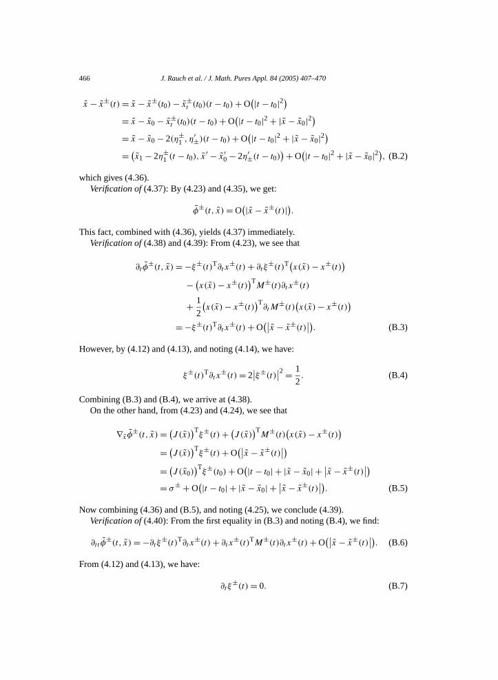
466 J. Rauch et al. / J. Math. Pures Appl. 84 (2005) 407–470
x − x±(t) = x − x±(t0) − x±t (t0)(t − t0) + O
(|t − t0|2)
= x − x0 − x±t (t0)(t − t0) + O
(|t − t0|2 + |x − x0|2)
= x − x0 − 2(η±1 , η′±)(t − t0) + O
(|t − t0|2 + |x − x0|2)
= (x1 − 2η±1 (t − t0), x
′ − x′0 − 2η′±(t − t0)
)+ O(|t − t0|2 + |x − x0|2
), (B.2)
which gives (4.36).Verification of(4.37): By (4.23) and (4.35), we get:
φ±(t, x) = O(|x − x±(t)|).
This fact, combined with (4.36), yields (4.37) immediately.Verification of(4.38) and (4.39): From (4.23), we see that
∂t φ±(t, x) = −ξ±(t)T∂tx
±(t) + ∂t ξ±(t)T(x(x) − x±(t)
)− (x(x) − x±(t)
)TM±(t)∂tx
±(t)
+ 1
2
(x(x) − x±(t)
)T∂tM
±(t)(x(x) − x±(t)
)= −ξ±(t)T∂tx
±(t) + O(∣∣x − x±(t)
∣∣). (B.3)
However, by (4.12) and (4.13), and noting (4.14), we have:
ξ±(t)T∂tx±(t) = 2
∣∣ξ±(t)∣∣2 = 1
2. (B.4)
Combining (B.3) and (B.4), we arrive at (4.38).On the other hand, from (4.23) and (4.24), we see that
∇x φ±(t, x) = (J (x)
)Tξ±(t) + (J (x)
)TM±(t)
(x(x) − x±(t)
)= (J (x)
)Tξ±(t) + O
(∣∣x − x±(t)∣∣)
= (J (x0))T
ξ±(t0) + O(|t − t0| + |x − x0| +
∣∣x − x±(t)∣∣)
= σ± + O(|t − t0| + |x − x0| +
∣∣x − x±(t)∣∣). (B.5)
Now combining (4.36) and (B.5), and noting (4.25), we conclude (4.39).Verification of(4.40): From the first equality in (B.3) and noting (B.4), we find:
∂tt φ±(t, x) = −∂t ξ
±(t)T∂tx±(t) + ∂tx
±(t)TM±(t)∂t x±(t) + O
(∣∣x − x±(t)∣∣). (B.6)
From (4.12) and (4.13), we have:
∂t ξ±(t) = 0. (B.7)
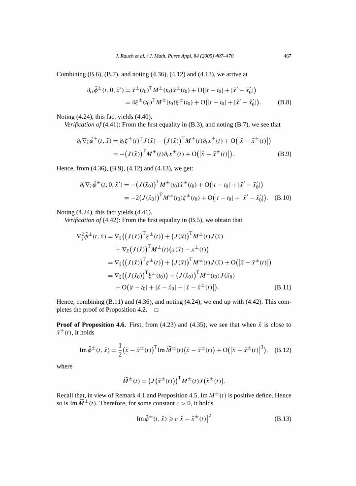
J. Rauch et al. / J. Math. Pures Appl. 84 (2005) 407–470 467
com-
e
Combining (B.6), (B.7), and noting (4.36), (4.12) and (4.13), we arrive at
∂tt φ±(t,0, x′) = x±(t0)
TM±(t0)x±(t0) + O
(|t − t0| + |x′ − x′0|)
= 4ξ±(t0)TM±(t0)ξ
±(t0) + O(|t − t0| + |x′ − x′
0|). (B.8)
Noting (4.24), this fact yields (4.40).Verification of(4.41): From the first equality in (B.3), and noting (B.7), we see that
∂t∇x φ±(t, x) = ∂t ξ
±(t)TJ (x) − (J (x))T
M±(t)∂t x±(t) + O
(∣∣x − x±(t)∣∣)
= −(J (x))T
M±(t)∂t x±(t) + O
(∣∣x − x±(t)∣∣). (B.9)
Hence, from (4.36), (B.9), (4.12) and (4.13), we get:
∂t∇x φ±(t,0, x′) = −(J (x0)
)TM±(t0)x
±(t0) + O(|t − t0| + |x′ − x′
0|)
= −2(J (x0)
)TM±(t0)ξ
±(t0) + O(|t − t0| + |x′ − x′
0|). (B.10)
Noting (4.24), this fact yields (4.41).Verification of(4.42): From the first equality in (B.5), we obtain that
∇2x φ±(t, x) = ∇x
((J (x))T
ξ±(t))+ (J (x)
)TM±(t)J (x)
+ ∇x
(J (x))T
M±(t)(x(x) − x±(t)
)= ∇x
((J (x))T
ξ±(t))+ (J (x)
)TM±(t)J (x) + O
(∣∣x − x±(t)∣∣)
= ∇x
((J (x0)
)Tξ±(t0)
)+ (J (x0))T
M±(t0)J (x0)
+ O(|t − t0| + |x − x0| +
∣∣x − x±(t)∣∣). (B.11)
Hence, combining (B.11) and (4.36), and noting (4.24), we end up with (4.42). Thispletes the proof of Proposition 4.2.Proof of Proposition 4.6. First, from (4.23) and (4.35), we see that whenx is close tox±(t), it holds
Im φ±(t, x) = 1
2
(x − x±(t)
)TIm M±(t)(x − x±(t)
)+ O(∣∣x − x±(t)
∣∣3), (B.12)
where
M±(t) = (J (x±(t)))T
M±(t)J(x±(t)
).
Recall that, in view of Remark 4.1 and Proposition 4.5, ImM±(t) is positive define. Hencso is ImM±(t). Therefore, for some constantc > 0, it holds
Im φ±(t, x) c∣∣x − x±(t)
∣∣2 (B.13)
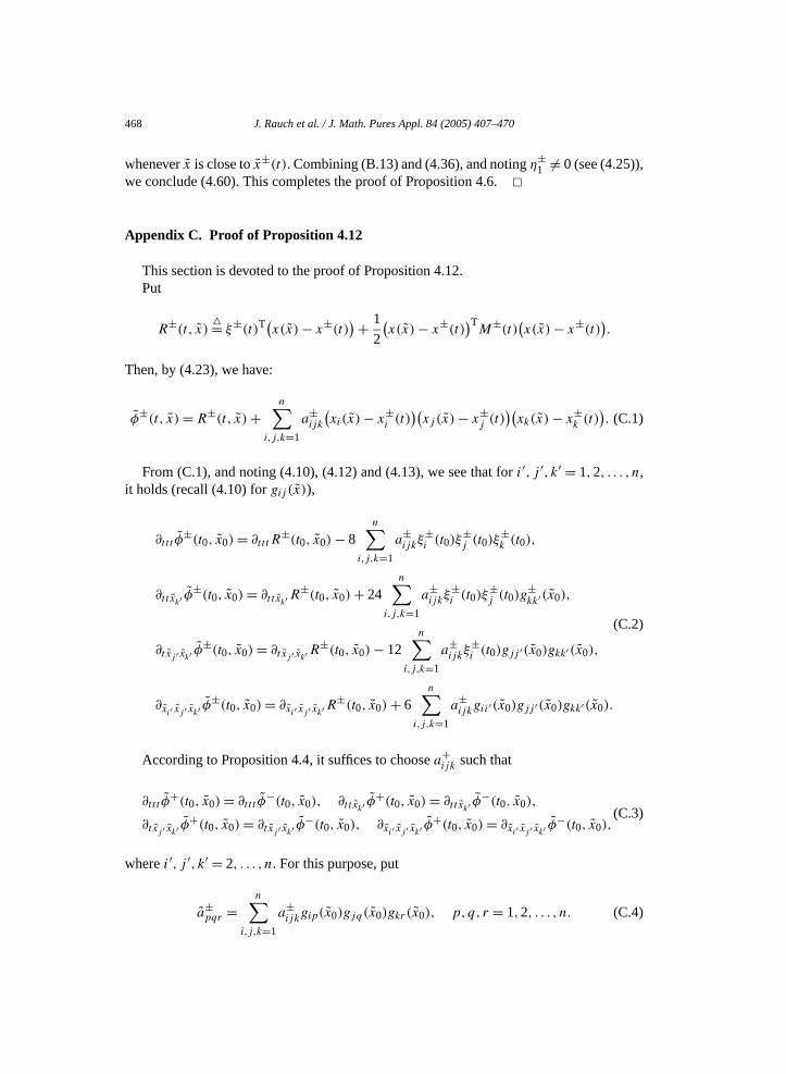
468 J. Rauch et al. / J. Math. Pures Appl. 84 (2005) 407–470
,
wheneverx is close tox±(t). Combining (B.13) and (4.36), and notingη±1 = 0 (see (4.25))we conclude (4.60). This completes the proof of Proposition 4.6.
Appendix C. Proof of Proposition 4.12
This section is devoted to the proof of Proposition 4.12.Put
R±(t, x)= ξ±(t)T(x(x) − x±(t)
)+ 1
2
(x(x) − x±(t)
)TM±(t)
(x(x) − x±(t)
).
Then, by (4.23), we have:
φ±(t, x) = R±(t, x) +n∑
i,j,k=1
a±ijk
(xi(x) − x±
i (t))(
xj (x) − x±j (t))(
xk(x) − x±k (t)). (C.1)
From (C.1), and noting (4.10), (4.12) and (4.13), we see that fori′, j ′, k′ = 1,2, . . . , n,it holds (recall (4.10) forgij (x)),
∂ttt φ±(t0, x0) = ∂tttR
±(t0, x0) − 8n∑
i,j,k=1
a±ijkξ
±i (t0)ξ
±j (t0)ξ
±k (t0),
∂tt xk′ φ±(t0, x0) = ∂ttxk′ R
±(t0, x0) + 24n∑
i,j,k=1
a±ijkξ
±i (t0)ξ
±j (t0)g
±kk′(x0),
∂txj ′ xk′ φ±(t0, x0) = ∂txj ′ xk′ R
±(t0, x0) − 12n∑
i,j,k=1
a±ijkξ
±i (t0)gjj ′(x0)gkk′(x0),
∂xi′ xj ′ xk′ φ±(t0, x0) = ∂xi′ xj ′ xk′ R
±(t0, x0) + 6n∑
i,j,k=1
a±ijkgii′(x0)gjj ′(x0)gkk′(x0).
(C.2)
According to Proposition 4.4, it suffices to choosea+ijk such that
∂ttt φ+(t0, x0) = ∂ttt φ
−(t0, x0), ∂tt xk′ φ+(t0, x0) = ∂ttxk′ φ
−(t0, x0),
∂txj ′ xk′ φ+(t0, x0) = ∂txj ′ xk′ φ
−(t0, x0), ∂xi′ xj ′ xk′ φ+(t0, x0) = ∂xi′ xj ′ xk′ φ
−(t0, x0),(C.3)
wherei′, j ′, k′ = 2, . . . , n. For this purpose, put
a±pqr =
n∑a±ijkgip(x0)gjq(x0)gkr (x0), p, q, r = 1,2, . . . , n. (C.4)
i,j,k=1
J. Rauch et al. / J. Math. Pures Appl. 84 (2005) 407–470 469
.3),
,
t
f
force,
l Sci-
ation of
First, from the fourth equality in (C.3) and (C.2), we get:
a+i′j ′k′ =
∂xi′ xj ′ xk′ R−(t0, x0) − ∂xi′ xj ′ xk′ R
+(t0, x0)
6+ a−
i′j ′k′ , i′, j ′, k′ = 2, . . . , n.
Next, from (4.24) and (4.10), one has:
ξ±i (t0) =
n∑=1
gi(x0)η± . (C.5)
Therefore, by the third equality in (C.2), and noting (C.5) and (C.4), we get
∂txj ′ xk′ φ±(t0, x0) = ∂txj ′ xk′ R
±(t0, x0) − 12n∑
i,j,k,=1
a±ijkgi(x0)gjj ′(x0)gkk′(x0)η
±
= ∂txj ′ xk′ R±(t0, x0) − 12
n∑=1
a±j ′k′η
±
= ∂txj ′ xk′ R±(t0, x0) − 12
n∑=2
a±j ′k′η
± − 12a±
1j ′k′η±1 . (C.6)
Recall thatη+1 = 0 (see Proposition 4.1). Hence, by (C.6) and the third equality in (C
we find:
a+1j ′k′ = 1
η+1
[∂txj ′ xk′ R
+(t0, x0) − ∂txj ′ xk′ R−(t0, x0)
12−
n∑=2
(a+j ′k′η
+ − a−
j ′k′η− ) + a−
1j ′k′η−1
]
wherej ′, k′ = 2, . . . , n.Similarly, one may determinea+
11k′ (k′ = 2, . . . , n) and a+111 from the second and firs
equalities in (C.3) and (C.2), respectively. Therefore, we have determineda+i′j ′k′ for all
i′, j ′, k′ = 1,2, . . . , n.Finally, from (C.4) and noting that the matrixJ (x0) = (gij (x0))1i,jn is invertible,
one may determine the desireda+ijk for all i, j, k = 1,2, . . . , n. This completes the proof o
Proposition 4.12.
References
[1] K. Ammari, M. Tucsnak, Stabilization of Bernoulli–Euler beams by means of a pointwise feedbackSIAM J. Control Optim. 39 (2000) 1160–1181.
[2] V.M. Babich, The higher-dimensional WKB method or ray method, in: Encyclopedia of Mathematicaences, vol. 34, Springer-Verlag, Berlin/New York, 1997, pp. 91–131.
[3] C. Bardos, G. Lebeau, J. Rauch, Sharp sufficient conditions for the observation, control and stabilizwaves from the boundary, SIAM J. Control Optim. 30 (1992) 1024–1065.
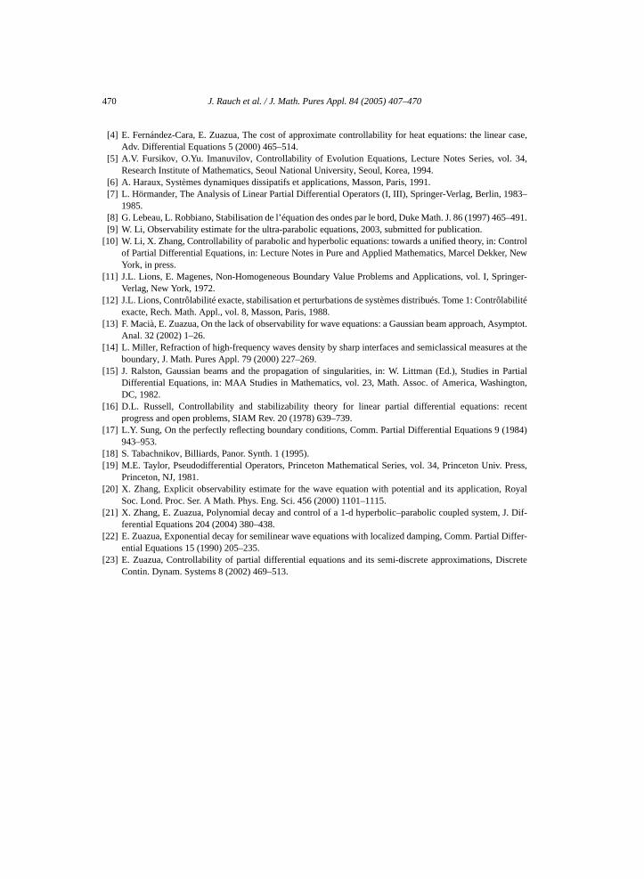
470 J. Rauch et al. / J. Math. Pures Appl. 84 (2005) 407–470
ar case,
34,
83–
5–491.
ntrol, New
ringer-
ôlabilité
ymptot.
s at the
Partialgton,
cent
1984)
Press,
Royal
J. Dif-
Differ-
screte
[4] E. Fernández-Cara, E. Zuazua, The cost of approximate controllability for heat equations: the lineAdv. Differential Equations 5 (2000) 465–514.
[5] A.V. Fursikov, O.Yu. Imanuvilov, Controllability of Evolution Equations, Lecture Notes Series, vol.Research Institute of Mathematics, Seoul National University, Seoul, Korea, 1994.
[6] A. Haraux, Systèmes dynamiques dissipatifs et applications, Masson, Paris, 1991.[7] L. Hörmander, The Analysis of Linear Partial Differential Operators (I, III), Springer-Verlag, Berlin, 19
1985.[8] G. Lebeau, L. Robbiano, Stabilisation de l’équation des ondes par le bord, Duke Math. J. 86 (1997) 46[9] W. Li, Observability estimate for the ultra-parabolic equations, 2003, submitted for publication.
[10] W. Li, X. Zhang, Controllability of parabolic and hyperbolic equations: towards a unified theory, in: Coof Partial Differential Equations, in: Lecture Notes in Pure and Applied Mathematics, Marcel DekkerYork, in press.
[11] J.L. Lions, E. Magenes, Non-Homogeneous Boundary Value Problems and Applications, vol. I, SpVerlag, New York, 1972.
[12] J.L. Lions, Contrôlabilité exacte, stabilisation et perturbations de systèmes distribués. Tome 1: Contrexacte, Rech. Math. Appl., vol. 8, Masson, Paris, 1988.
[13] F. Macià, E. Zuazua, On the lack of observability for wave equations: a Gaussian beam approach, AsAnal. 32 (2002) 1–26.
[14] L. Miller, Refraction of high-frequency waves density by sharp interfaces and semiclassical measureboundary, J. Math. Pures Appl. 79 (2000) 227–269.
[15] J. Ralston, Gaussian beams and the propagation of singularities, in: W. Littman (Ed.), Studies inDifferential Equations, in: MAA Studies in Mathematics, vol. 23, Math. Assoc. of America, WashinDC, 1982.
[16] D.L. Russell, Controllability and stabilizability theory for linear partial differential equations: reprogress and open problems, SIAM Rev. 20 (1978) 639–739.
[17] L.Y. Sung, On the perfectly reflecting boundary conditions, Comm. Partial Differential Equations 9 (943–953.
[18] S. Tabachnikov, Billiards, Panor. Synth. 1 (1995).[19] M.E. Taylor, Pseudodifferential Operators, Princeton Mathematical Series, vol. 34, Princeton Univ.
Princeton, NJ, 1981.[20] X. Zhang, Explicit observability estimate for the wave equation with potential and its application,
Soc. Lond. Proc. Ser. A Math. Phys. Eng. Sci. 456 (2000) 1101–1115.[21] X. Zhang, E. Zuazua, Polynomial decay and control of a 1-d hyperbolic–parabolic coupled system,
ferential Equations 204 (2004) 380–438.[22] E. Zuazua, Exponential decay for semilinear wave equations with localized damping, Comm. Partial
ential Equations 15 (1990) 205–235.[23] E. Zuazua, Controllability of partial differential equations and its semi-discrete approximations, Di
Contin. Dynam. Systems 8 (2002) 469–513.