Play Type Recognition in Real-World Football Video

Sheng Chen, Zhongyuan Feng, Qingkai Lu, Behrooz Mahasseni, Trevor Fiez

and Alan Fern, Sinisa Todorovic

Oregon State University

Abstract

This paper presents a vision system for recognizing the

sequence of plays in amateur videos of American football

games (e.g. offense, defense, kickoff, punt, etc). The sys-

tem is aimed at reducing user effort in annotating foot-

ball videos, which are posted on a web service used by

over 13,000 high school, college, and professional football

teams. Recognizing football plays is particularly challeng-

ing in the context of such a web service, due to the huge

variations across videos, in terms of camera viewpoint, mo-

tion, distance from the field, as well as amateur camerawork

quality, and lighting conditions, among other factors. Given

a sequence of videos, where each shows a particular play of

a football game, we first run noisy play-level detectors on

every video. Then, we integrate responses of the play-level

detectors with global game-level reasoning which accounts

for statistical knowledge about football games. Our empir-

ical results on more than 1450 videos from 10 diverse foot-

ball games show that our approach is quite effective, and

close to being usable in a real-world setting.

1. Introduction

A major part of game planning for American football

teams is the collection, annotation, and analysis of game

video of their own and opponent games. A number of com-

panies offer web services for facilitating this video-based

game planning. However, significant human labor is still in-

volved in using the services, since they usually provide only

basic user interface functionalities for manual organization,

annotation, and sharing of video. For example, video an-

notation for just a single game requires entering data for an

average of around 150 plays. Thus, there is a growing de-

mand for automating at least part of the annotation process.

In this paper, we consider the problem of automatically

annotating videos of plays comprising a football game by

one of five high-level play types. This problem is be-

yond the capabilities of off-the-shelf computer vision tools,

largely due to the huge diversity of football videos. The

videos have large variance in viewing angles/distances, shot

quality, weather/lighting conditions, the color/sizes of field

logos/markings, and the scene around the field, ranging

from crowds, to players on the bench, to construction equip-

ment. The videos are typically captured by amateurs, and

exhibit motion blur, camera jitter, and large camera mo-

tion. Further, there is large variation in team strategies,

formations, and uniforms. All this makes video rectifi-

cation, frame-references, and background detection rather

challenging, which are critical for existing approaches.

Our primary goal is achieving robustness to such wide

variability, while also maintaining a reasonable runtime.

To this end, we exploit knowledge about the structure of

football games and individual plays. Specifically, we first

process each video using noisy detectors for different play

types, designed using domain knowledge. For the sequence

of videos from a game, the noisy detector outputs are pro-

cessed by a Hidden Markov Model (HMM), which encodes

knowledge about the temporal structure of football games

to improve accuracy. To the best of our knowledge this is

the first computer vision system that addresses such fully

automated annotation of full football games for such a large

diversity of football videos.

We conduct this study in close collaboration with one of

the largest companies providing the web service for foot-

ball video having a client base of over 13,000 high school,

college, and professional teams. Our results on a set of 10

diverse, real-world football games, comprising over 1450

play videos, show that our approach is effective, and close

to being deployable in the near future.

2. Background and Problem Statement

Football Video. American football video is organized

around the concept of football plays. Each game involves

a sequence of approximately 150+ plays, each lasting ap-

proximately 10 to 30 seconds, separated by short time inter-

1

vals where no game action occurs, and the teams regroup.

Videos are generally captured with a PTZ camera, showing

a sideline view of the football field from an elevated loca-

tion along the sideline (e.g. Figures 1 and 2). A standard

video acquisition of a game involves recording a sequence

of videos, one for each play in the game, which can then be

automatically organized in temporal order.

Play Types. Each play has a distinct type defined by

the standard taxonomy. In this paper, we focus on the five

highest-level types in the taxonomy. Below, we describe

these play types relative to the annotating team, denoted by

TeamA. The two most common play types are when TeamA

is on Offense (O) or Defense (D), where TeamA is either

trying to move the ball forward (O), or prevent the other

team from moving the ball forward (D). Each such play

starts with both teams lined-up facing each other at the line

of scrimmage— the line parallel to the field lines where the

ball is located. The play starts when the ball is ”snapped”

(or passed) from a player called the center to a player called

the quarterback, and then both teams begin moving and ex-

ecuting their chosen strategies until the play terminates.

Plays that are not of type O or D are called special teams

plays and there are three major types. InKick Off (K) plays,

one team lines up and kicks the ball down the field to the

receiving team. In Punting (P) plays, the offensive team

drop-kicks/punts the ball down the field to the opponent. In

Field Goal (F) plays, the ball is kicked at the goal posts in

order to score points. The number of special teams plays is

generally small compared to the number of O and D plays.

The Problem. Our input is a sequence of temporally

ordered videos comprising all plays from a football game.

The desired output is an accurate labeling of each play by

one of the five play types.

3. Related Work

There are a number of existing approaches for ana-

lyzing football videos. However, it is unlikely that they

would be successful across our videos, due to the restric-

tive assumptions made by these approaches, critical for

their foreground-background and camera-motion estima-

tion, rectification of the football field, and extraction of rel-

evant video features.

For example, the approaches presented in [2, 12, 10]

perform foreground-background estimation, yard-line de-

tection, and camera-motion estimation. These approaches

require high-resolution videos, a fixed scale at which the

players appear in the video, and prior knowledge of the field

model. Consequently, these approaches cannot be used for

our videos. Also, approaches that address videos acquired

by a moving camera (e.g., [17]) typically make the limiting

assumption that a majority of frame pixels fall on the static

background football field. This assumption does not hold

in our setting, due to our large number of close-up shots

and videos with moving audience in the background. Fur-

ther, methods that deal with 3D registration of a visible part

of the field [5, 4, 3] make the assumptions that the videos

are taken under fairly uniform conditions — namely, on the

same or very similar football field (or hockey rink), and

from the same camera viewpoint and distance — and that

outlier pixels belong to moving players, audience, or refer-

ees. Therefore, they cannot be applied in our setting.

Regarding feature extraction, most approaches to play-

type recognition require accurate clip stabilization and reg-

istration to the football field in order to successfully extract

video features relevant for recognition – namely, tracks of

football players [15, 9, 11], or histograms of spatiotemporal

interest points [14]. However, previous work has demon-

strated that successful tracking of football players under ac-

curate video registration is still notoriously difficult [8, 6].

Recent work seeks to relax the mentioned requirements for

feature extraction [1, 16], however they rely on several cru-

cial assumptions that do not reliably hold in our web-service

setting. A key part of their approach is video registration

and background subtraction. This is an expensive process,

and either requires the availability of an overhead view of

the football field or user interaction to register a video frame

of each play. Our experience with similar approaches for

registration and background subtraction has shown that they

are not very robust in cases of amateur camera-persons and

wide variations of viewpoints.

After extracting relevant video features, existing meth-

ods typically employ probabilistic generative models for

play-type recognition, including a Bayesian network [9],

non-stationary Hidden Markov Model [15], topic model

[16], and mixture of pictorial-structure model [7]. These

models are typically used for each video in isolation. The

recent work of [1] has a limited scope, since they make the

assumption that the plays being analyzed are all offensive

plays. Remarkably, the reported accuracies of the above ap-

proaches are often not high, despite their restrictive settings,

indicating fundamental challenges.

To our knowledge, our work is the first to consider pars-

ing entire football games by accounting for constraints be-

tween consecutive plays in the game, arising from the stan-

dard rules of American football. In addition, no previ-

ous work has considered such a large variability of football

videos that we deal with. This variability negates the afore-

mentioned assumptions made by prior work.

4. Overview of Our Approach

Given a sequence of play videos from a football game,

we infer play types in three stages: 1) Partial Rectification

(Section 5), where field lines are extracted, providing a par-

tial frame of reference for the football field, 2) Play-level

recognition (Sections 6-8), where noisy play-type detectors

are run for a subset of the play types, and 3) Game-level

reasoning (Section 9), where a temporal model of football

games is used to reason about the noisy detections across

the full sequence to provide more accurate labels.

Ideally, we would like to have play-level detectors for

each of the play types: O, D, K, F, P. However, our pre-

liminary analysis and experimentation revealed that distin-

guishing F (field goals) from O and D would be extremely

difficult, due to the high visual similarity of these types.

Thus, we do not provide a play-level detector for F plays,

but rather rely on the game-level analysis for their infer-

ence. We do provide the detectors for the remaining types.

Our OD-detector (Section 6) classifies a video as either

O or D. For non-OD plays, the output will be arbitrary, ei-

ther O or D. Our K-detector (Section 7) detects kickoffs. Fi-

nally, we provide a non-P-detector (Section 8) that attempts

to predict with high precision when a video does not show

type P. Our preliminary study revealed that achieving both

high precisions and recall in predicting P would be quite dif-

ficult due to its high similarity with certain O and D plays.

However, achieving high precision on predicting non-P is

feasible, and useful for game-level analysis.

5. Extraction of Field Lines

As reviewed in Section 3, related work relies heavily

on video rectification to help deal with camera motion and

background subtraction. Such rectification for our web-

service videos appears to be beyond the state-of-the-art.

Nevertheless, a partial video rectification based on extract-

ing the field lines can be robustly computed, and still be

used for camera-motion and background estimation. The

field lines (a.k.a. yard lines) are long, white, parallel lines

that repeat every 5 yards along the 100 yards between end-

zones of the football field. The extraction of yard lines pro-

vides a partial rectification in the sense that it does not iden-

tify a complete homography from frames to field coordi-

nates. Rather, it allows verifying if a line passing through

two locations in a frame is parallel to the field lines. This

information is used by our detectors in two ways. First, at

the beginning of plays and during some special team plays

(e.g., kickoffs), the players tend to be aligned with the yard

lines. Second, by observing how video features move rela-

tive to extracted yard lines, we can get a rough estimate of

camera and foreground motion.

We extract the field lines by detecting and tracking the

lines in the Hough space. Given a video, we first extract the

field lines in the first frame, and then track them along with

book-keeping of newly appearing and disappearing lines in

the field-of-view.

Field line extraction: For each video frame, we first

run the Hough transform to get a candidate set of lines

which intersect at a point (see Figure 1), since parallel

lines are bound to intersect at a vanishing point under the

perspective transform of the camera. We can then esti-

Figure 1. (Left) Line extraction: Green lines are the output from

the Hough transform, red lines are the results from RANSAC.

(Right) Line tracking: Blue lines are the tracked lines from last

frame, the red line is the new line detected in this frame.

mate the Hough parameters of the field lines, (ρ, θ), asρ = x0 cos θ + y0 sin θ, where (x0, y0) is the location of

the vanishing point. This estimation problem can be solved

using RANSAC and least squares.

Line tracking: We want to associate extracted lines

from the previous and current frames. For this, we con-

duct meanshift in the Hough space. Since the lines typi-

cally do not move much from one frame to another, mean-

shift converges after 1–2 iterations. To deal with missing

and newly appearing lines caused by the camera motion, we

perform the following post-processing. For missing lines,

the tracked results will be noisy, and thus can be filtered

out by RANSAC. Newly arising peaks in the Hough space,

which do not correspond to previous lines, are added to the

field-line set if they are consistent with the vanishing point

model. Figure 1 illustrates our tracking of the field lines.

6. O-D Detector

Each O or D play begins at the moment-of-snap (MOS)

with the two teams on opposite sides of the line-of-

scrimmage (LOS) (see Figure 2) in either an offensive or

defensive formations. Therefore, our O-D detection, first,

identifies the MOS and the LOS, and then performs two

predictions: i) which side of the LOS (left or right) the of-

fensive team is lined up on at the MOS — called Offensive

Direction Inference; and ii) which side of the LOS TeamA is

lined up on at the MOS— called Team Direction Inference.

Note that in our experiments for each game, we arbitrarily

chose one of the teams to be TeamA.

The frame number of the MOS is highly variable across

videos, depending on when recording begins. Detecting the

MOS is challenging due to unpredictable camera motion

and non-player foreground motion. A recent approach to

this problem [1] relied heavily on having rectified video and

foreground extraction, which is not an option for our set-

ting. Rather, we use another recent approach [13] that does

not have such requirements. In [13], a sophisticated analy-

sis of optical flow was used to achieve relatively good MOS

estimates on average. Across the 1450+ videos in our ex-

periments the resulting MOS estimates are within 5 frames

of the true MOS for 54% of the videos, within 15 frames

for 85% of the videos, and within 30 frames for 89%. This

level of accuracy allows for non-trivial O-D detection.

Figure 2. Two frames showing two wide receivers (in red box)

running from right to left. The detected LOS is shown as as blue

lines in the left image

Offensive Direction Inference. The O and D play types

differ in the spatial formations of players on each team at

the start of the play. However, analyzing these formations

requires a reliable player detector. For example, recent work

[1], detects the foreground players via video registration and

a background model for such analysis, which is unreliable

across our videos. Rather than analyzing the entire forma-

tion, we instead seek to detect offensive players called,wide

receivers (WRs), whose motion is predictive of which side

of the LOS the offense is on. As shown in Fig. 2, WRs

are players that usually line up at the ends of the field, and

are isolated from the other offensive players. A majority

of videos of O-D plays show at least one WR. After a play

starts, the WRs will almost always immediately run in the

direction of the defense. Thus, our approach to offensive

direction inference is to detect the initial motion of one or

moreWRs, and infer that the offense is on the side opposite

to the direction of the motion. Note that there are rare cases

of O-D plays where there are no WRs on the field. In these

cases, our approach will produce arbitrary results.

For detecting WRs, we extract and analyze KLT tracks

in order to infer which ones are likely due to WRs, and then

infer the WR motion direction based on those trajectories.

We run the KLT tracker on a sequence of 45 video frames

following the estimated MOS. The extracted point trajec-

tories typically correspond to player movement, non-player

foreground motion, and background features under camera

motion. When aWR is visible, the KLT tracker is capable of

extracting relatively long trajectories due to the WR’s char-

acteristic swift and straight-line motion. To help remove

KLT trajectories caused by camera motion, we use the ex-

tracted field lines (Section 5), by measuring the relative mo-

tion of each KLT track to its closest field line. Ideally, this

relative motion is small when a KLT track corresponds to

a stationary background feature. This allows removing all

KLT tracks whose relative motion falls below a threshold.

The specific threshold choice is not critical, since the KLT

tracks of WRs generally have very large relative motion.

Given the remaining KLT trajectories, the key to infer-

ring which ones belong to WRs is to use our knowledge

that: i) WRs are typically located at the far ends of the

LOS, and ii) WRs are usually isolated from the majority of

players lined up at the LOS. This requires first inferring the

LOS. For LOS detection, we draw on an idea from [1] that

Figure 3. Plot of one video’s KLT tracks with detected scrimmage

line (purple box) and ranges for WRs (green boxes). Red (blue)

vectors are the KLT tracks outside (inside) the range of the WRs.

the LOS is usually in the region of highest image gradients

corresponding to the “texture” of players on the “uniform”

field. Further, we know that the LOS is always parallel to

the field lines. We use a sliding window to scan across the

frame for the region of highest gradients, where the medial

axis of the window is enforced to pass through the estimated

vanishing point of the field lines (i.e., to be “parallel” under

perspective to the field lines). As we scan, the window size

is adapted to the distance between the detected field lines.

The sliding window with maximum gradient gives a

good estimate of the location of the offensive and defen-

sive lines of players. We use two other windows on each

side of this maximum-gradientwindow to identify likely ar-

eas where WRs are located. Figure 3 shows an example of

extracted KLT tracks, with the maximum-gradient window,

and the two WR windows.

Finally, we estimate the motion direction of WRs using

a weighted average of the KLT trajectories in the two WR

windows. In particular, we linearly weight each KLT track

according to its distance from the center of the maximum-

gradient window. This assigns higher weights to KLT tracks

that are more isolated, and hence more likely to be due to

WR’s motion. We use the direction of the vector resulting

from the weighted average, relative to the field lines, as the

estimated direction of the WR. Note that in cases where ei-

ther the upper or lower WR is not present in the video, this

combination will tend to be biased in favor of the visible

WR, since there will typically be few highly weighted KLT

tracks in the WR window not containing a WR.

Team Direction Inference. A football game consists of

a sequence of plays and can be further grouped into four

quarters. Throughout each quarter, each team will always

face the same direction, and the directions are switched af-

ter the first and third quarters. The directions of the teams

at the start of each half (i.e., the first and third quarters)

are somewhat arbitrary and decided by coin tosses. Based

on this description, we see that games will have long se-

quences of plays where the team direction does not change.

The key to inferring the team direction of plays is to detect

the split points where the team directions change (there is

a maximum of 3 split points). One piece of additional in-

formation that is useful for this analysis is the video time

stamps, which are used by the web-service to temporally

order videos. In particular, between the second and third

quarters, there is a prolonged half-time break that is easily

detectable as the maximum duration gap between plays in a

game. Thus, we can easily determine the starting video of

the third quarter based on the time stamps.We detect the split point s1 in the first half between the

first and second quarters, and the split point s2 in the secondhalf between the third and fourth quarters, where we knowthat the team directions must have changed. Given s1 ands2, we then estimate if there was a change in direction be-tween the two halves, which uniquely identifies the secondand third quarter. Intuitively, at a true split point we shouldnotice the change in color profile of the teams to the left andright of the LOS, since the teams wear different uniforms.Thus, in the first half we evaluate each possible value of s1

(correspondingly s2 in the second half) by the color differ-ences between plays, before and after s1, as follows:

Score(s1) =X

1≤j≤s1

s1+1≤k≤N1

Diff(j, k)

Here N1 is the play number of the final play of the first

half and Diff(j, k) = d(jl, kr) + d(jr, kl), where d() is theEuclidean distance, and jl, jr are the color histograms to

the left and right of the LOS for play j, respectively. To

compute the color histograms, we consider pixels to the left

and right of the LOS within the maximum-gradient window

described above. Using Score(s1) we pick the top scoring

split point s1 as our estimate. Similarly we infer that the

directions between the second and third quarters change if

the corresponding score is above a threshold, or otherwise

that the direction did not change. This gives us the direction

estimation for TeamA across the entire game.

7. Kickoff Detector

Kickoff (K) plays occur at the beginning of the game,

the beginning of the second half of the game, and after any

team scores, when the scoring team kicks the ball off. The

most visually distinct aspect of K plays is the line of players

on the kicking team lining up at one end of the field, usually

spanning the entire width of the field, and running down the

field to tackle whoever catches the ball on the other team.

Figure 4 (left) shows a frame at the start of a kickoff video,

just before the ball is kicked. Players along this line run

at approximately the same speed (full speed), and are rela-

tively evenly distributed along the width of the field.

Our K detector: i) identifies the initial time interval of

the K play where the moving player line is most prominent;

ii) computes mid-level features about this time interval; and

iii) uses the mid-level features in Logistic regression for pre-

dicting whether the play is a kickoff or not, where Logis-

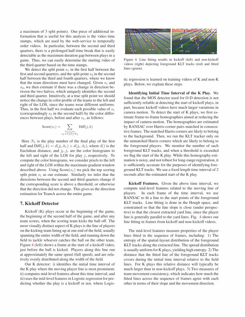
Figure 4. Line fitting results in kickoff (left) and non-kickoff

videos (right) depicting foreground KLT tracks (red) and fitted

lines (green).

tic regression is learned on training videos of K and non-K

plays. Below, we explain these steps.

Identifying Initial Time Interval of the K Play. We

found that the MOS detector used for O-D detection is not

sufficiently reliable at detecting the start of kickoff plays, in

part, because kickoff videos have much larger variations in

camera motion. To detect the start of K plays, we first es-

timate frame-to-frame homographies aimed at reducing the

impact of camera motion. The homographies are estimated

by RANSAC over Harris-corner pairs matched in consecu-

tive frames. The matched Harris corners are likely to belong

to the background. Then, we run the KLT tracker only on

the unmatched Harris corners which are likely to belong to

the foreground players. We monitor the number of such

foreground KLT tracks, and when a threshold is exceeded

we flag the start of the K play. While this homography esti-

mation is noisy, and not robust for long-range registration, it

is sufficiently accurate for the purposes of identifying fore-

ground KLT tracks. We use a fixed length time interval of 2

seconds after the estimated start of the K play.

Kickoff Features. Given the above time interval, we

compute mid-level features related to the moving line of

players. In each frame of the time interval, we use

RANSAC to fit a line to the start points of the foreground

KLT tracks. Line fitting is done in the Hough space, and

constrained so that the line slope is close (under perspec-

tive) to that the closest extracted yard line, since the player

line is generally parallel to the yard lines. Fig. 4 shows our

line fitting in frames from kickoff and non-kickoff videos.

The mid-level features measure properties of the player

lines fitted in the sequence of frames, including: 1) The

entropy of the spatial-layout distribution of the foreground

KLT tracks along the extracted line. The spread distribution

is usually uniform for K plays, yielding high entropy. 2) The

distance that the fitted line of the foreground KLT tracks

covers during the initial time interval relative to the field

lines. For K plays this relative distance will typically be

much larger than in non-kickoff plays. 3) Two measures of

team movement consistency, which indicates how much the

fitted lines across the sequence of frames agree with each

other in terms of their slope and the movement direction.

8. Non-Punt Detection

In punting plays, both teams line up and initially behave

as in O-D plays. However, at the start of the P play, the

punter kicks the ball deep down the field, and the kicking

team runs down the field to tackle the opposing player that

catches the ball. This makes P plays quite similar to O,

D, and K types. Thus, designing a robust P detector is

challenging. However, for our game-level analysis, it is

still quite useful to have a detector that can reliably indi-

cate when a play is not a punt. That is, we here aim for a

high precision detector for non-punt plays, possibly at the

expense of recall.

Our non-punt (non-P) detector is based on two charac-

teristics of P plays. First, since the ball is kicked far down

the field, the camera usually pans fairly rapidly in order to

follow the action. Such rapid panning near the beginning

of a P play is not common for O-D plays. Second, a short

time after the P play begins, most of the players on the kick-

ing team will run down the field, which is uncommon at the

start of O-D plays. We measure these characteristics using

the methods from the above kickoff detector.

In particular, we estimate homographies between con-

secutive frames during a period after the MOS, in order to

detect a significant burst in camera motion. For this, we

looking for sequences of consistently large changes in the

homographies. Next, we also use the lines fit by the kick-

off detector to look for significant team movement down

field in a short period of time. Our final non-P detection

is obtained by thresholding the camera movement and team

movement cues. If neither threshold is exceeded we output

that the play is not a punt, since P plays should exceed at

least one of the thresholds. The thresholds were tuned us-

ing training data of punts and non-punts in order to optimize

the precision without sacrificing recall too much.

9. Game Level Prediction

The input to our game-level analysis is the sequence of

O, D, K, and non-P detections for each play in a game. The

goal of the game-level analysis is to help correct for detec-

tion errors and introduce F labels by taking into account the

statistical regularities in sequences of football plays.

The statistical regularities are captured by a Hidden

Markov Model (HMM), which models a sequence of ob-

servations O1, . . . , OT as being generated by a sequence of

hidden states S1, . . . , ST . In our case, the hidden state St

is the play type of the tth play, which is either O, D, K, F,

P. The observation Ot corresponds to the cross-product of

the detector outputs. An HMM is specified by a state tran-

sition distribution P (St | St−1) which gives the probabilityof transitioning to a particular state St when the previous

state is St−1. For example, the probability of a transition

from St−1 = O to St = O is much higher than a transi-

Figure 5. Game-Level Analysis. Row 1: kickoff detector, T is for

kickoff and F for non-kickoff. Row 2: non-punt detector, T for

non-punt and F for punt. Row 3: OD detector, Row 4: Viterbi

output, Row 5: ground truth. Errors are shown in red.

tion to St = D. The HMM also specifies an observation

distribution P (Ot | St) which gives the probability of ob-

serving observation Ot when the hidden state is St. For

example, for the state St = O the most likely observation

corresponds to the OD detector predicting O, the K detector

predicting false, and the non-punt detector predicting true.

The HMM transition and observation probabilities are

estimated as the Laplace-smoothed Maximum Likelihood

Estimates using hand-labeled training games.

Given the transition and observation distribu-

tions, it is straightforward to use the Bayes rule,

and compose them into a conditional distribution,

P (S1, . . . , ST | O1, . . . , OT ), which gives the probability

of a state sequence given an observation sequence. Thus,

given an observation sequence from a game, we find

the state sequence that maximizes the above conditional

probability, and returns the result as the final assignments

for the game. Computing the most-likely state sequence

can be done using the well-known Viterbi algorithm, which

is a polynomial time dynamic programming algorithm.

Figure 5 illustrates the game-level analysis on one of our

evaluation games. In this case the analysis is able to correct

all detector mistakes except for one, where it predicts K in-

stead of P. Here at the P play, the receiving team loses the

ball and the kicking team directly gets a touchdown which

rarely happens. At the same time, the non-P detector made

a mistake, which gives us no confidence that this is a P play.

Given just this detector input, most human experts would

make the same judgement as our analysis in this situation.

10. Evaluation

We performed empirical evaluation on 10 high-school

football games, which were selected by the web-service

company from their database in an attempt to cover the wide

diversity of video. Each game has a sequence of an aver-

age of 146 videos. The videos were hand-labeled by their

types. We also annotated the true MOS, and team direction

in each play to allow for more refined evaluations. Training

and threshold selecting for all the detectors was done in a

different dataset.

Detector Evaluation. Table 1 shows the results for of-

fense direction inference (WR), team direction inference

Dataset TD* WR* OD* TD WR OD

Game01 1.00 0.97 0.97 0.94 0.83 0.80

Game02 0.99 0.84 0.84 0.98 0.80 0.82

Game03 1.00 0.85 0.85 0.99 0.76 0.76

Game04 0.89 0.79 0.71 0.91 0.62 0.62

Game05 0.96 0.83 0.81 0.90 0.77 0.71

Game06 0.99 0.86 0.85 0.99 0.79 0.78

Game07 0.90 0.66 0.63 0.90 0.63 0.63

Game08 0.98 0.93 0.92 0.94 0.92 0.87

Game09 0.97 0.93 0.91 0.99 0.93 0.92

Game10 0.97 0.89 0.87 0.97 0.82 0.80

Overall 0.97 0.85 0.84 0.95 0.79 0.77

Table 1. Accuracy for OD detector. TD is for team direction, WR

is for offensive direction, and OD is the combined OD detector.

TD*, WR* and OD* are results using ground truth MOS.

(TD), and the combined OD detection accuracy. Accuracy

is computed only with respect to plays that are truly O and

D. This includes plays where a penalty occurred, which

means that there is no player motion and thus our OD de-

tector typically makes errors. Since the OD detector com-

ponents are dependent on MOS estimation, we show results

for the OD detector when using the automatically predicted

MOS, and also the ground truth MOS (denoted as WR*,

TD*, and OD*). We see that using the predicted MOS the

overall OD accuracy is 77% across all games, which is a sig-

nificant improvement over random guessing. Using the true

MOS improves that accuracy to 84%. From the table, the

difference in accuracy between using the predicted and true

MOS is largely due to decreased accuracy of the offensive

direction estimate (WR vs. WR*). This is because, when

the MOS prediction is inaccurate, the KLT tracks analyzed

may sometimes not include WR tracks. Thus, further im-

proving the MOS estimation or extending the WR detector

to search in a wider temporal window around the predicted

MOS are possible ways to improve OD accuracy.

The OD accuracy can vary substantially across games,

primarily due to varying quality of camerawork, containing

more jitter and unnecessary motion for some games. This

indicates that considering efficient ways to more reliably

counteract camera motion would be an important direction

for improvement.

We use a different dataset of 293 plays including 74 kick-

offs to train the parameters of the kickoff detector (ko), and

measure the precision and recall across the 10 games, as

shown in Table 2.

From the table, we achieve non-trivial precision and re-

call overall. However, there are some games with relatively

low precision (Game08) or recall (Game05). This is mainly

caused by the fact that appearance of both the fields and

kicking-team uniforms are dominated by dark green, which

makes Harris corner extraction less accurate. Another rea-

son for errors is that some OD plays look similar to kickoffs,

Dataset Preko Recallko Prenp Recallnp

Game01 100.00% 88.89% 97.30% 90.00%

Game02 75.00% 75.00% 100.00% 73.33%

Game03 100.00% 90.00% 100.00% 78.31%

Game04 100.00% 83.33% 100.00% 76.06%

Game05 90.00% 75.00% 96.52% 86.72%

Game06 80.00% 100.00% 100.00% 83.33%

Game07 78.57% 100.00% 99.17% 80.95%

Game08 61.54% 88.89% 96.99% 87.76%

Game09 100.00% 100.00% 98.02% 83.19%

Game10 85.71% 85.71% 97.56% 56.74%

Overall 85.41% 88.17% 98.57% 79.41%

Table 2. Result of kickoff and non-punt detector. Preko and

Prenp are the precision for kickoff and non-punt respectively.

Recallko and Recallnp are the recall.

because both teams rush toward the same direction after the

MOS, and are relatively uniformly spread out, as in kick-

offs. Table 2 also shows results for the non-punt detector.

As expected, we do get high precision. One reason for the

low recall is that the detector often mistakes a kickoff play

for a punt.

Overall System. Since our HMM requires training of its

parameters, we used a leave-one-game-out strategy for eval-

uation. Thus, we present the average results for each game

using an HMM trained on the other 9 games. In addition to

evaluating our fully automated system, we also test a ver-

sion of the system that replaces each detector by the ground

truth. This allows us to observe which detectors would be

most useful to improve in order to increase overall accuracy.

We denote our kickoff, non-punt, MOS and OD detectors

as ko, np, mos and od, respectively. We use GTd to denote

that we use the ground truth for detector d. Our fully auto-

mated system is denoted as GT∅. The system that replaces

all detectors by ground truth is denoted as GTall. Table 3

shows the results.

First, we see that the overall performance of our fully

automated system GT∅ is 77% compared to the accuracy of

44% for random guessing according to the play type pro-

portion prior (O, D for around 41%, K, P for 6%, N for 5%

and F for 1% in our dataset). This level of accuracy is in

the range of being usable in practice given a proper user in-

terface. The user could change the label of any mislabeled

videos they come across. This type of interface could, for

example, allow team coaches to analyze the types of plays

they are interested more quickly than is currently possible.

From Table 3, even with the ground truth detector in-

put GTall, we still cannot get perfect results. That is, the

upper bound of our performance is below 100% accuracy.

The main reason is that we do not have a field goal detec-

tor, and the game-level analysis does not perfectly predict

where to insert field goal labels. Regarding the impact of

each detector, we see that by far using the ground truth OD

Dataset GTall GT∅ GTmos GTod GTko GTnp

Game01 0.98 0.79 0.94 0.95 0.81 0.81

Game02 0.99 0.85 0.83 0.92 0.88 0.85

Game03 0.98 0.74 0.78 0.94 0.72 0.82

Game04 0.99 0.65 0.76 0.96 0.62 0.71

Game05 0.99 0.72 0.83 0.93 0.77 0.76

Game06 0.99 0.82 0.85 0.96 0.82 0.90

Game07 0.99 0.69 0.71 0.98 0.69 0.75

Game08 0.98 0.77 0.87 0.92 0.81 0.83

Game09 0.98 0.84 0.89 0.96 0.84 0.93

Game10 0.98 0.67 0.91 0.93 0.70 0.85

Overall 0.99 0.77 0.83 0.95 0.79 0.85

Table 3. Accuracy of the overall system

O D K F P

O 0.77 0.14 0.01 0.01 0.07

D 0.13 0.80 0.01 0.02 0.04

K 0.04 0.07 0.84 0.01 0.03

F 0.10 0.07 0.01 0.72 0.09

P 0.27 0.25 0.02 0.01 0.44

Table 4. Confusion matrix for GT∅. Rows correspond to ground

truth labels and columns correspond to predicted labels.

labels has the biggest impact on accuracy. This is largely

because the number of OD labels is dominant and there is

still significant room to improve our OD detector. We can

also achieve an 8% increase with the ground truth non-punt

detector since punts are one of the most common bridges

between OD transitions.

The confusion matrix for our automated system is shown

in Table 4. We see that the least accurate label is P, which

is often predicted as O or D. This is partially due to the fact

that our non-punt detector is biased toward high precision,

so that when it predicts false (the play may be a punt) it is

still quite likely that the play is a non-punt.

Time Complexity. Our primary focus has not yet turned

to time optimization. Nevertheless, we achieve reasonable

runtimes. Our code is implemented in C/C++, and tested on

a Red Hat Enterprise 64 bit, 3.40 GHZ environment. For

the kickoff detector, the processing speed is 25-30 frames

per second on average. The MOS detector processes 30-

35 frames per second on average. The offensive and team

direction estimates require an average of 25 and 20 sec-

onds for a video respectively. The non-punt detector can

be viewed as part of the kickoff detector and thus requires

no additional time. The game-level analysis also takes prac-

tically no time compared with the detectors. Thus, in total,

for a video with 600 frames (20s), the average processing

time will be 85 seconds. If we run the offensive direction

and team direction detector in parallel and the kickoff and

OD detector in parallel, the parallel time will be 45 seconds

which is approximately twice the video length. In addition,

every detector is run independently in our experiment while

some components can be shared across detectors such as

the KLT tracks and line of scrimmage estimation, so there

is still significant room for reducing the running time.

11. Conclusion

We have described the first computer vision system for

recognizing sequences of plays of entire football games.

Our evaluation is based on perhaps the widest variation of

video conditions considered in any prior work on football

analysis. The evaluation shows that currently we are able to

achieve 77% accuracy on labeling plays as either offense,

defense, kickoffs, punting, or field goals, under reasonable

running times. In this sense, our system is close to being us-

able in a real-world web-service setting. We have also iden-

tified most promising directions for prospective improve-

ment of the accuracy and efficiency of our system.

References

[1] I. Atmosukarto, B. Ghanem, S. Ahuja, K. Muthuswamy, and

N. Ahuja. Automatic recognition of offensive team formation in

american football plays. In CVPR Workshops (CVsports), 2013. 2,

3, 4

[2] Y. Ding and G. Fan. Camera view-based american football video

analysis. In IEEE ISM, 2006. 2

[3] B. Ghanem, T. Zhang, and N. Ahuja. Robust video registration ap-

plied to field-sports video analysis. In ICASSP, 2012. 2

[4] A. Gupta, J. Little, and R. Woodham. Using line and ellipse features

for rectification of broadcast hockey video. In Canadian Conference

on Computer and Robot Vision (CRV), 2011. 2

[5] R. Hess and A. Fern. Improved video registration using non-

distinctive local image features. In CVPR, 2007. 2

[6] R. Hess and A. Fern. Discriminatively trained particle filters for com-

plex multi-object tracking. In CVPR, 2009. 2

[7] R. Hess, A. Fern, and E. Mortensen. Mixture-of-parts pictorial struc-

tures for objects with variable part sets. In ICCV, 2007. 2

[8] S. Intille and A. Bobick. Closed-world tracking. In ICCV, 1995. 2

[9] S. S. Intille and A. F. Bobick. Recognizing planned, multiperson

action. Computer Vision and Image Understanding, 81(3):414–445,

2001. 2

[10] B. L. and M. I. Sezan. Event detection and summarization in sports

video. In CBAIVL, 2001. 2

[11] R. Li, R. Chellappa, and S. Zhou. Learning multi-modal densities

on discriminative temporal interaction manifold for group activity

recognition. In CVPR, 2009. 2

[12] T.-Y. Liu, W.-Y. Ma, and H.-J. Zhang. Effective feature extraction

for play detection in american football video. In MMM, 2005. 2

[13] B. Mahasseni, S. Chen, A. Fern, and S. Todorovic. Detecting the

moment of snap in real-world football videos. In IAAI, 2013. 3

[14] B. Siddiquie, Y. Yacoob, and L. S. Davis. Recognizing plays in amer-

ican football videos. Technical report, University of Maryland, 2009.

2

[15] E. Swears and A. Hoogs. Learning and recognizing complex multi-

agent activities with applications to american football plays. In

WACV, 2012. 2

[16] J. Varadarajan, I. Atmosukarto, S. Ahuja, B. Ghanem, and N. Ahuja.

A topic model approach to represent and classify american football

plays. In BMVC, 2013. 2

[17] S. Wu, O. Oreifej, and M. Shah. Action recognition in videos

acquired by a moving camera using motion decomposition of la-

grangian particle trajectories. In ICCV, 2011. 2