Numerical modelling of ground-tunnel support interaction ...
Upload
khangminh22Category
view
2download
0
PLAXIS 3D TUNNELMaterial Models
Manual version 2


TABLE OF CONTENTS
i
TABLE OF CONTENTS
1 Introduction..................................................................................................1-1 1.1 On the use of different models...............................................................1-1 1.2 Limitations .............................................................................................1-2
2 Preliminaries on material modelling ..........................................................2-1 2.1 General definitions of stress...................................................................2-1 2.2 General definitions of strain...................................................................2-3 2.3 Elastic strains .........................................................................................2-5 2.4 Undrained analysis with effective parameters .......................................2-7 2.5 Undrained analysis with undrained parameters ...................................2-10 2.6 The initial preconsolidation stress in advanced models .......................2-11 2.7 On the initial stresses ...........................................................................2-12
3 The Mohr-Coulomb model (perfect-plasticity) ........................................3-1 3.1 Elastic perfectly-plastic behaviour.........................................................3-1 3.2 Formulation of the Mohr-Coulomb model.............................................3-3 3.3 Basic parameters of the Mohr-Coulomb model .....................................3-5 3.4 Advanced parameters of the Mohr-Coulomb model..............................3-8
4 The Jointed Rock model (anisotropy) .......................................................4-1 4.1 Anisotropic elastic material stiffness matrix..........................................4-2 4.2 Plastic behaviour in three directions ......................................................4-4 4.3 Parameters of the Jointed Rock model...................................................4-7
5 The Hardening-Soil model (isotropic hardening) ....................................5-1 5.1 Hyperbolic relationship for standard drained triaxial test ......................5-2 5.2 Approximation of hyperbola by the Hardening-Soil model...................5-3 5.3 Plastic volumetric strain for triaxial states of stress ...............................5-5 5.4 Parameters of the Hardening-Soil model ...............................................5-6 5.5 On the cap yield surface in the Hardening-Soil model ........................5-10
6 Soft-Soil-Creep model (time dependent behaviour).................................6-1 6.1 Introduction............................................................................................6-1 6.2 Basics of one-dimensional creep............................................................6-2 6.3 On the variables τc and εc .......................................................................6-4 6.4 Differential law for 1D-creep.................................................................6-6 6.5 Three-dimensional-model ......................................................................6-8 6.6 Formulation of elastic 3D-strains.........................................................6-10 6.7 Review of model parameters................................................................6-11 6.8 Validation of the 3D-model .................................................................6-14

MATERIAL MODELS MANUAL
ii PLAXIS 3D TUNNEL
7 Applications of advanced soil models.........................................................7-1 7.1 Modelling simple soil tests .................................................................... 7-1
7.1.1 Oedometer test ...........................................................................7-1 7.1.2 Standard triaxial test ..................................................................7-2
7.2 HS model: response in drained and undrained triaxial tests .................. 7-4 7.3 Application of the Hardening-Soil model on real soil tests ................... 7-7 7.4 SSC model: response in one-dimensional compression test ................ 7-12 7.5 Jointed Rock model: failure at different sliding directions.................. 7-15
8 References ....................................................................................................8-1
Appendix A – Symbols

INTRODUCTION
1-1
1 INTRODUCTION
The mechanical behaviour of soils may be modelled at various degrees of accuracy. Hooke's law of linear, isotropic elasticity, for example, may be thought of as the simplest available stress-strain relationship. As it involves only two input parameters, i.e. Young's modulus, E, and Poisson's ratio, ν, it is generally too crude to capture essential features of soil and rock behaviour. For modelling massive structural elements and bedrock layers, however, linear elasticity tends to be appropriate.
1.1 ON THE USE OF DIFFERENT MODELS
Mohr-Coulomb model (MC) The elastic-plastic Mohr-Coulomb model involves five input parameters, i.e. E and ν for soil elasticity; φ and c for soil plasticity and ψ as an angle of dilatancy. This Mohr-Coulomb model represents a 'first-order' approximation of soil or rock behaviour. It is recommended to use this model for a first analysis of the problem considered. For each layer one estimates a constant average stiffness. Due to this constant stiffness, computations tend to be relatively fast and one obtains a first impression of deformations. Besides the five model parameters mentioned above, initial soil conditions play an essential role in most soil deformation problems. Initial horizontal soil stresses have to be generated by selecting proper K0-values.
Jointed Rock model (JR) The Jointed Rock model is an anisotropic elastic-plastic model, especially meant to simulate the behaviour of rock layers involving a stratification and particular fault directions. Plasticity can only occur in a maximum of three shear directions (shear planes). Each plane has its own strength parameters φ and c. The intact rock is considered to behave fully elastic with constant stiffness properties E and ν. Reduced elastic properties may be defined for the stratification direction.
Hardening-Soil model (HS) The Hardening-Soil model is an advanced model for the simulation of soil behaviour. As for the Mohr-Coulomb model, limiting states of stress are described by means of the friction angle, φ, the cohesion, c, and the dilatancy angle, ψ. However, soil stiffness is described much more accurately by using three different input stiffnesses: the triaxial loading stiffness, E50, the triaxial unloading stiffness, Eur, and the oedometer loading stiffness, Eoed. As average values for various soil types, we have Eur ≈ 3 E50 and Eoed ≈ E50, but both very soft and very stiff soils tend to give other ratios of Eoed / E50.
In contrast to the Mohr-Coulomb model, the Hardening-Soil model also accounts for stress-dependency of stiffness moduli. This means that all stiffnesses increase with pressure. Hence, all three input stiffnesses relate to a reference stress, being usually taken as 100 kPa (1 bar).

MATERIAL MODELS MANUAL
1-2 PLAXIS 3D TUNNEL
Soft-Soil-Creep model (SSC) The above Hardening-Soil model is suitable for all soils, but it does not account for viscous effects, i.e. creep and stress relaxation. In fact, all soils exhibit some creep and primary compression is thus followed by a certain amount of secondary compression.
The latter is most dominant in soft soils, i.e. normally consolidated clays, silts and peat, and we thus implemented a model under the name Soft-Soil-Creep model. Please note that the Soft-Soil-Creep model is a relatively new model that has been developed for application to settlement problems of foundations, embankments, etc. For unloading problems, as normally encountered in tunnelling and other excavation problems, the Soft-Soil-Creep model hardly supersedes the simple Mohr-Coulomb model. As for the Mohr-Coulomb model, proper initial soil conditions are also essential when using the Soft-Soil-Creep model. For the Hardening-Soil model and the Soft-Soil-Creep model this also includes data on the preconsolidation stress, as these models account for the effect of overconsolidation.
Analyses with different models It is advised to use the Mohr-Coulomb model for a relatively quick and simple first analysis of the problem considered. When good soil data is lacking, there is no use in further more advanced analyses.
In many cases, one has good data on dominant soil layers, and it is appropriate to use the Hardening-Soil model in an additional analysis. No doubt, one seldomly has test results from both triaxial and oedometer tests, but good quality data from one type of test can be supplemented by data from correlations and/or in situ testing.
Finally, a Soft-Soil-Creep analysis can be performed to estimate creep, i.e. secondary compression in very soft soils. The above idea of analysing geotechnical problems with different soil models may seem costly, but it tends to pay off. First of all due to the fact that the Mohr-Coulomb analysis is relatively quick and simple and secondly as the procedure tends to reduce errors.
1.2 LIMITATIONS
The PLAXIS code and its soil models have been developed to perform calculations of realistic geotechnical problems. In this respect PLAXIS can be considered as a geotechnical simulation tool. The soil models can be regarded as a qualitative representation of soil behaviour whereas the model parameters are used to quantify the soil behaviour. Although much care has been taken for the development of the PLAXIS code and its soil models, the simulation of reality remains an approximation, which implicitly involves some inevitable numerical and modelling errors. Moreover, the accuracy at which reality is approximated depends highly on the expertise of the user regarding the modelling of the problem, the understanding of the soil models and their limitations, the selection of model parameters, and the ability to judge the reliability of the computational results.

INTRODUCTION
1-3
Both the soil models and the PLAXIS code are constantly being improved such that each new version is an update of the previous ones. Some of the present limitations are listed below:
HS-model It is a hardening model that does not account for softening due to soil dilatancy and de-bonding effects. In fact, it is an isotropic hardening model so that it models neither hysteresis and cyclic loading nor cyclic mobility. In order to model cyclic loading with good accuracy one would need a more complex model. Last but not least, the use of the Hardening Soil model generally results in significantly longer calculation times, since the material stiffness matrix is formed and decomposeed in each calculation step.
SSC-model All above limitations also hold true for the Soft-Soil-Creep model. In addition this model tends to overpredict the range of elastic soil behaviour. This is especially the case for excavation problems, including tunnelling.
Interfaces Interface elements are generally modelled by means of the bilinear Mohr-Coulomb model. When a more advanced model is used for the corresponding cluster material data set, the interface element will only pick up the relevant data (c, φ, ψ, E, ν) for the Mohr-Coulomb model, as described in Section 3.5.2 of the Reference Manual. In such cases the interface stiffness is taken to be the elastic soil stiffness. Hence, E = Eur where Eur is stress level dependent, following a power law with Eur proportional to σm. For the Soft-Soil-Creep model, the power m is equal to 1 and Eur is largely determined by the swelling constant κ*.

MATERIAL MODELS MANUAL
1-4 PLAXIS 3D TUNNEL

PRELIMINARIES ON MATERIAL MODELLING
2-1
2 PRELIMINARIES ON MATERIAL MODELLING
A material model is a set of mathematical equations that describes the relationship between stress and strain. Material models are often expressed in a form in which infinitesimal increments of stress (or 'stress rates') are related to infinitesimal increments of strain (or 'strain rates'). All material models implemented in the PLAXIS 3D Tunnel program are based on a relationship between the effective stress rates, ’σ& , and the strain rates, ε& . In the following section it is described how stresses and strains are defined in PLAXIS. In subsequent sections the basic stress-strain relationship is formulated and the influence of pore pressures in undrained materials is described. Later sections focus on initial conditions for advanced material models.
2.1 GENERAL DEFINITIONS OF STRESS
Stress is a tensorial quantity which can be represented by a matrix with Cartesian components:
xx xy xz
yx yy yz
zx zy zz
σ σ σσ σ σ σ
σ σ σ
⎡ ⎤⎢ ⎥= ⎢ ⎥⎢ ⎥⎣ ⎦
(2.1)
In the standard deformation theory, the stress tensor is symmetric, so σxy = σyx , σyz = σzy and σzx = σxz. In this situation, stresses are often written in vector notation, which involve only six different components:
( )T
xx yy zz xy yz zxσ σ σ σ σ σ σ= (2.2)
According to Terzaghi's principle, stresses in the soil are divided into effective stresses, σ', and pore pressures, σ w:
' wσ σ σ= + (2.3)
Water is considered not to sustain any shear stresses. As a result, effective shear stresses are equal to total shear stresses. Positive normal stress components are considered to represent tension, whereas negative normal stress components indicate pressure (or compression).
Material models for soil and rock are generally expressed as a relationship between infinitesimal increments of effective stress and infinitesimal increments of strain. In such a relationship, infinitesimal increments of effective stress are represented by stress rates (with a dot above the stress symbol):
( )' ' ' 'T
xx yy zz xy yz zxσ σ σ σ σ σ σ=& & & & & & & (2.4)

MATERIAL MODELS MANUAL
2-2 PLAXIS 3D TUNNEL
σyy
σxx
σzz σzx
σzy
σxz
σxy
σyxσyz
x
y
z
Figure 2.1 General three-dimensional coordinate system and sign convention for stresses
It is often useful to use principal stresses rather than Cartesian stress components when formulating material models. Principal stresses are the stresses in such a coordinate system direction that all shear stress components are zero. Principal stresses are, in fact, the eigenvalues of the stress tensor. Principal effective stresses can be determined in the following way:
( )' ' 0Det Iσ σ− = (2.5)
where I is the identity matrix. This equation gives three solutions for σ', i.e. the principal effective stresses (σ'1, σ'2, σ'3). In PLAXIS the principal effective stresses are arranged in algebraic order:
1 2 3σ σ σ≤ ≤′ ′ ′ (2.6)
Hence, σ'1 is the largest compressive principal stress and σ'3 is the smallest compressive principal stress. In this manual, models are often presented with reference to the principal stress space, as indicated in Figure 2.2.
Figure 2.2 Principal stress space
-σ'3
-σ'2
-σ'1
-σ'1 = -σ'2 = -σ'3

PRELIMINARIES ON MATERIAL MODELLING
2-3
In addition to principal stresses it is also useful to define invariants of stress, which are stress measures that are independent of the orientation of the coordinate system. Two useful stress invariants are:
p' = ( )13 ' ' 'xx yy zz- σ σ σ+ + (2.7a)
( ) ( ) ( ) ( )( )2 2 2 2 2 212 6xx yy yy zz zz xx xy yz zx-q ' ' ' - ' ' - 'σ σ σ σ σ σ σ σ σ= + + + + + (2.7b)
where p' is the isotropic effective stress, or mean effective stress, and q is the equivalent shear stress. Note that the convention adopted for p' is positive for compression in contrast to other stress measures. The equivalent shear stress, q, has the important property that it reduces to q = │σ1'-σ3'│ for triaxial stress states with σ2' = σ3'.
Principal stresses can be written in terms of the invariants:
( )2 21 3 3' ' sinp qσ θ π− = + − (2.8a)
( )22 3' ' sinp qσ θ− = + (2.8b)
( )2 23 3 3' ' sinp qσ θ π− = + + (2.8c)
in which θ is referred to as Lode's angle (a third invariant), which is defined as:
313 3
27arcsin2
Jq
θ⎛ ⎞
= ⎜ ⎟⎝ ⎠
(2.9)
with
( ) ( ) ( ) ( ) ( ) ( )2 2 23 ' ' ' ' ' ' ' ' ' ' ' ' 2xx yy zz xx yz yy zx zz xy xy yz zxJ - p - p - p - p - p - pσ σ σ σ σ σ σ σ σ σ σ σ= − − − +
(2.10)
2.2 GENERAL DEFINITIONS OF STRAIN
Strain is a tensorial quantity which can be represented by a matrix with Cartesian components:
xx xy xz
yx yy yz
zx zy zz
ε ε εε ε ε ε
ε ε ε
⎡ ⎤⎢ ⎥= ⎢ ⎥⎢ ⎥⎣ ⎦
(2.11)

MATERIAL MODELS MANUAL
2-4 PLAXIS 3D TUNNEL
Strains are the derivatives of the displacement components, i.e. εij = ∂ui / ∂j , where i and j are either x, y or z. According to the small deformation theory, only the sum of complementing Cartesian shear strain components εij and εji results in shear stress. This sum is denoted as the shear strain γ. Hence, instead of εxy, εyx, εyz , εzy, εzx and εxz the shear strain components γxy, γyz and γzx are used respectively. Under the above conditions, strains are often written in vector notation, which involve only six different components:
( )T
xx yy zz xy yz zxε ε ε ε γ γ γ= (2.12)
xxx
uxε
∂=
∂ (2.13a)
yyy
uyε
∂=
∂ (2.13b)
zzz
uzε
∂=
∂ (2.13c)
yxxy xy yx
uuy x
γ ε ε∂∂
= + = +∂ ∂
(2.13d)
y zyz yz zy
u uz y
γ ε ε∂ ∂
= + = +∂ ∂
(2.13e)
xzzx zx xz
uux z
γ ε ε∂∂
= + = +∂ ∂
(2.13f)
Similarly as for stresses, positive normal strain components refer to extension, whereas negative normal strain components indicate compression.
In the formulation of material models, where infinitesimal increments of strain are considered, these increments are represented by strain rates (with a dot above the strain symbol).
( )T
xx yy zz xy yz zxγ γ γε ε ε ε=& & & & & & & (2.14)
In analogy to the invariants of stress, it is also useful to define invariants of strain. A strain invariant that is often used is the volumetric strain, εν, which is defined as the sum of all normal strain components:
1 2 3v xx yy zzε ε ε ε ε ε ε= + + = + + (2.15)
The volumetric strain is defined as negative for compaction and as positive for dilatancy.

PRELIMINARIES ON MATERIAL MODELLING
2-5
For elastoplastic models, as used the PLAXIS 3D Tunnel program, strains are decomposed into elastic and plastic components:
e pε ε ε= + (2.16)
Throughout this manual, the superscript e will be used to denote elastic strains and the superscript p will be used to denote plastic strains.
2.3 ELASTIC STRAINS
Material models for soil and rock are generally expressed as a relationship between infinitesimal increments of effective stress ('effective stress rates') and infinitesimal increments of strain ('strain rates'). This relationship may be expressed in the form:
Mσ ε=′ && (2.17)
M is a material stiffness matrix. Note that in this type of approach, pore-pressures are explicitly excluded from the stress-strain relationship.
The simplest material model in the 3D Tunnel program is Hooke's law for isotropic linear elastic behaviour. This model is available in the Plaxis 3D Tunnel program under the name Linear Elastic model, but it is also the basis of other models. Hooke's law can be given by the equation:
( ) ( ) 12
12
12
1 ' ' ' 0 0 0'' 1 ' ' 0 0 0'' ' 1 ' 0 0 0' '
0 0 0 ' 0 0' 1 2 ' 1 '0 0 0 0 ' 0'0 0 0 0 0 ''
xx xx
yy yy
zz zz
xy xy
yz yz
zx zx
εεεEγγγ
ν ν νσν ν νσν ν νσ
νσ ν ννσ
νσ
−⎡ ⎤⎡ ⎤ ⎡ ⎤⎢ ⎥⎢ ⎥ ⎢ ⎥−⎢ ⎥⎢ ⎥ ⎢ ⎥⎢ ⎥⎢ ⎥ ⎢ ⎥−
= ⎢ ⎥⎢ ⎥ ⎢ ⎥−− + ⎢ ⎥⎢ ⎥ ⎢ ⎥⎢ ⎥⎢ ⎥ ⎢ ⎥−⎢ ⎥⎢ ⎥ ⎢ ⎥
−⎢ ⎥ ⎢ ⎥⎢ ⎥⎣ ⎦ ⎣ ⎦⎣ ⎦
& &
& &
& &
& &
& &
& &
(2.18)
The elastic material stiffness matrix is often denoted as De. Two parameters are used in this model, the effective Young's modulus, E', and the effective Poisson's ratio, ν'. In the remaining part of this manual effective parameters are denoted without dash ('), unless a different meaning is explicitly stated. The symbols E and ν are sometimes used in this manual in combination with the subscript ur to emphasize that the parameter is explicitly meant for unloading and reloading. A stiffness modulus may also be indicated with the subscript ref to emphasize that it refers to a particular reference level (yref) (see further).

MATERIAL MODELS MANUAL
2-6 PLAXIS 3D TUNNEL
The relationship between Young's modulus E and other stiffness moduli, such as the shear modulus G, the bulk modulus K, and the oedometer modulus Eoed, is given by:
( )2 1EG
ν=
+ (2.19a)
( )3 1 2EK
ν=
− (2.19b)
( )( )( )
11 2 1oed
- EE
ν
ν ν=
− + (2.19c)
During the input of material parameters for the Linear Elastic model or the Mohr-Coulomb model the values of G and Eoed are presented as auxiliary parameters (alternatives), calculated from Eq. (2.19). Note that the alternatives are influenced by the input values of E and ν. Entering a particular value for one of the alternatives G or Eoed results in a change of the E modulus.
Figure 2.3 Parameters tab for the Linear Elastic model
It is possible for the Linear Elastic model to specify a stiffness that varies linearly with depth. This can be done by entering the advanced parameters window using the Advanced button, as shown in Figure 2.3. Here one may enter a value for Eincrement which is the increment of stiffness per unit of depth, as indicated in Figure 2.4.

PRELIMINARIES ON MATERIAL MODELLING
2-7
Figure 2.4 Advanced parameter window
Together with the input of Eincrement the input of yref becomes relevant. Above yref the stiffness is equal to Eref. Below the stiffness is given by:
( ) actual ref ref increment refE E y y E y y= + − < (2.20)
The Linear Elastic model is usually inappropriate to model the highly non-linear behaviour of soil, but it is of interest to simulate structural behaviour, such as thick concrete walls or plates, for which strength properties are usually very high compared with those of soil. For these applications, the Linear Elastic model will often be selected together with Non-porous type of material behaviour in order to exclude pore pressures from these structural elements.
2.4 UNDRAINED ANALYSIS WITH EFFECTIVE PARAMETERS
In the PLAXIS 3D Tunnel program it is possible to specify undrained behaviour in an effective stress analysis using effective model parameters. This is achieved by identifying the Type of material behaviour (Material type) of a soil layer as Undrained. In this Section, it is explained how PLAXIS deals with this special option. The presence of pore pressures in a soil body, usually caused by water, contributes to the total stress level. According to Terzaghi's principle, total stresses σ can be divided into effective stresses σ' and pore pressures σw (see also Eq. 2.3). However, water is supposed not to sustain any shear stress, and therefore the effective shear stresses are equal to the total shear stresses:
'xx xx wσ σ σ= + (2.21a)
'yy yy wσ σ σ= + (2.21b)
'zz zz wσ σ σ= + (2.21c)
'xy xyσ σ= (2.21d)
'yz yzσ σ= (2.21e)
'zx zxσ σ= (2.21f)

MATERIAL MODELS MANUAL
2-8 PLAXIS 3D TUNNEL
Note that, similar to the total and the effective stress components, σw is considered negative for pressure.
A further distinction is made between steady state pore stress, psteady, and excess pore stress, pexcess:
w steady excessp pσ = + (2.22)
Steady state pore pressures are considered to be input data, i.e. generated on the basis of phreatic levels. This generation of steady state pore pressures is discussed in Section 3.8 of the Reference Manual. Excess pore pressures are generated during plastic calculations for the case of undrained material behaviour. Undrained material behaviour and the corresponding calculation of excess pore pressures is described below.
Since the time derivative of the steady state component equals zero, it follows:
w excesspσ = && (2.23)
Hooke's law can be inverted to obtain:
'1 ' ' 0 0 0'' 1 ' 0 0 0'' ' 1 0 0 01
0 0 0 2 2 ' 0 0'0 0 0 0 2 2 ' 00 0 0 0 0 2 2 '
exxxx
eyyyy
ezzzz
exyxy
eyzyz
ezxzx
E
σν νεσν νεσν νεσνγσνγσνγ
− −⎡ ⎤ ⎡ ⎤⎡ ⎤⎢ ⎥ ⎢ ⎥⎢ ⎥− −⎢ ⎥ ⎢ ⎥⎢ ⎥⎢ ⎥ ⎢ ⎥⎢ ⎥− −
=⎢ ⎥ ⎢ ⎥⎢ ⎥+⎢ ⎥ ⎢ ⎥⎢ ⎥⎢ ⎥ ⎢ ⎥⎢ ⎥+⎢ ⎥ ⎢ ⎥⎢ ⎥
+⎢ ⎥ ⎢ ⎥⎢ ⎥ ⎣ ⎦ ⎣ ⎦⎣ ⎦
&&
&&
&&
&&
&&
&&
(2.24)
Substituting Eq. (2.21) gives:
1 ' ' 0 0 0' 1 ' 0 0 0' ' 1 0 0 01
0 0 0 2 2 ' 0 0'0 0 0 0 2 2 ' 00 0 0 0 0 2 2 '
exx wxx
eyy wyy
ezz wzz
exyxy
eyzyz
ezxzx
E
σ σν νεσ σν νεσ σν νε
σνγσνγσνγ
−− −⎡ ⎤ ⎡ ⎤⎡ ⎤⎢ ⎥ ⎢ ⎥⎢ ⎥ −− −⎢ ⎥ ⎢ ⎥⎢ ⎥⎢ ⎥ ⎢ ⎥⎢ ⎥ −− −
=⎢ ⎥ ⎢ ⎥⎢ ⎥+⎢ ⎥ ⎢ ⎥⎢ ⎥⎢ ⎥ ⎢ ⎥⎢ ⎥+⎢ ⎥ ⎢ ⎥⎢ ⎥
+⎢ ⎥ ⎢ ⎥⎢ ⎥ ⎣ ⎦ ⎣ ⎦⎣ ⎦
& &&
& &&
& &&
&&
&&
&&
(2.25)
Considering slightly compressible water, the rate of pore pressure is written as:
( )w e e exx yy zzw
K + + n
σ ε ε ε=& & & & (2.26)
in which Kw is the bulk modulus of the water and n is the soil porosity.

PRELIMINARIES ON MATERIAL MODELLING
2-9
The inverted form of Hooke's law may be written in terms of the total stress rates and the undrained parameters Eu and νu:
1 0 0 0 '1 0 0 0 '
1 0 0 0 '10 0 0 2 2 0 00 0 0 0 2 2 00 0 0 0 0 2 2
eu u xxxx
eu u yyyy
eu u zzzz
eu xyuxy
eu yzyz
eu zxzx
E
ν ν σεν ν σεν ν σε
ν σγν σγ
ν σγ
− −⎡ ⎤ ⎡ ⎤ ⎡ ⎤⎢ ⎥ ⎢ ⎥ ⎢ ⎥− −⎢ ⎥ ⎢ ⎥ ⎢ ⎥⎢ ⎥ ⎢ ⎥ ⎢ ⎥− −
=⎢ ⎥ ⎢ ⎥ ⎢ ⎥+⎢ ⎥ ⎢ ⎥ ⎢ ⎥⎢ ⎥ ⎢ ⎥ ⎢ ⎥+⎢ ⎥ ⎢ ⎥ ⎢ ⎥
+⎢ ⎥ ⎢ ⎥⎢ ⎥ ⎣ ⎦ ⎣ ⎦⎣ ⎦
&&
&&
&&
&&
&&
&&
(2.27)
where:
( )2 1 uuE G + ν= ( )( )
' 1 '1 2 1 'u
ν µ νν
µ ν+ +
=+ +
(2.28)
µ = 1
3 'wK
n K
( )'
3 1 2EK
ν=′
− ′ (2.29)
Hence, the special option for undrained behaviour in PLAXIS is such that the effective parameters G and ν are transferred into undrained parameters Eu and νu according to Eq. (2.28) and (2.29). Note that the index u is used to indicate auxiliary parameters for undrained soil. Hence, Eu and νu should not be confused with Eur and νur as used to denote unloading / reloading.
Fully incompressible behaviour is obtained for νu = 0.5. However, taking νu = 0.5 leads to singularity of the stiffness matrix. In fact, water is not fully incompressible, but a realistic bulk modulus for water is very large. In order to avoid numerical problems caused by an extremely low compressibility, νu is taken as 0.495, which makes the undrained soil body slightly compressible. In order to ensure realistic computational results, the bulk modulus of the water must be high compared with the bulk modulus of the soil skeleton, i.e. Kw >>n K'. This condition is sufficiently ensured by requiring ν' ≤ 0.35. Users will get a warning as soon as larger Poisson's ratios are used in combination with undrained material behaviour.
Consequently, for undrained material behaviour a bulk modulus for water is automatically added to the stiffness matrix. The value of the bulk modulus is given by:
( )( ) ( )
3 0.495300 3011 2 1
uw
u
K K K Kn
ν ν ννν ν
− ′ − ′= = >′ ′ ′
+ ′− + ′ (2.30)
at least for ν' ≤ 0.35.

MATERIAL MODELS MANUAL
2-10 PLAXIS 3D TUNNEL
The rate of excess pore pressure is calculated from the (small) volumetric strain rate, according to:
ww v
Knσ ε= && (2.31)
The type of elements used in the PLAXIS 3D Tunnel program are sufficiently adequate to avoid mesh locking effects for nearly incompressible materials.
This special option to model undrained material behaviour on the basis of effective model parameters is available for all material models in the PLAXIS 3D Tunnel program. This enables undrained calculations to be executed with effective input parameters, with explicit distinction between effective stresses and (excess) pore pressures.
Such an analysis requires effective soil parameters and is therefore highly convenient when such parameters are available. For soft soil projects, accurate data on effective parameters may not always be available. Instead, in situ tests and laboratory tests may have been performed to obtain undrained soil parameters. In such situations measured undrained Young's moduli can be easily converted into effective Young's moduli by:
( )2 1 '3 uE E
ν+=′ (2.32)
Undrained shear strengths, however, cannot easily be used to determine the effective strength parameters φ and c. For such projects the PLAXIS 3D Tunnel program offers the possibility of an undrained analysis with direct input of the undrained shear strength (cu or su) and φ = φu = 0°. This option is only available for the Mohr-Coulomb model and the Hardening-Soil model, but not for the Soft Soil Creep model. Note that whenever the Material type parameter is set to Undrained, effective values must be entered for the elastic parameters E and ν!
2.5 UNDRAINED ANALYSIS WITH UNDRAINED PARAMETERS
If, for any reason, it is desired not to use the Undrained option in the PLAXIS 3D Tunnel program to perform an undrained analysis, one may simulate undrained behaviour by selecting the Non-porous option and directly entering undrained elastic properties E = Eu and ν=νu=0.495 in combination with the undrained strength properties c = cu and φ = φu = 0°. In this case a total stress analysis is performed without distinction between effective stresses and pore pressures. Hence, all tabulated output referring to effective stresses should now be interpreted as total stresses and all pore pressures are equal to zero. In graphical output of stresses the stresses in Non-porous clusters are not plotted. If one does want graphical output of stresses one should select Drained instead of Non-porous for the type of material behaviour and make sure that no pore pressures are generated in these clusters. Note that this type of approach is not possible when using the Soft Soil Creep model. In general, an effective stress analysis using the Undrained option in PLAXIS to simulate undrained behaviour is preferable over a total stress analysis.

PRELIMINARIES ON MATERIAL MODELLING
2-11
2.6 THE INITIAL PRECONSOLIDATION STRESS IN ADVANCED MODELS
When using advanced models in the PLAXIS 3D Tunnel program an initial preconsolidation stress has to be determined. In the engineering practice it is common to use a vertical preconsolidation stress, σp, but PLAXIS needs an equivalent isotropic preconsolidation stress, pp
eq to determine the initial position of a cap-type yield surface. If a material is overconsolidated, information is required about the Over-Consolidation Ratio (OCR), i.e. the ratio of the greatest vertical stress previously reached, σp (see Figure 2.5), and the in-situ effective vertical stress, σyy'0 .
0' = OCR
yy
p
σσ
(2.33)
It is also possible to specify the initial stress state using the Pre-Overburden Pressure (POP) as an alternative to prescribing the overconsolidation ratio. The Pre-Overburden Pressure is defined by:
|' - | = POP 0yyp σσ (2.34)
These two ways of specifying the vertical preconsolidation stress are illustrated in Figure 2.5.
POP '0yy
p
σσ
OCR =
0'yyσ 0'
yyσpσ pσ
Figure 2.5 Illustration of vertical preconsolidation stress in relation to the in-situ vertical stress. 2.5a. Using OCR; 2.5b. Using POP
The pre-consolidation stress σp is used to compute ppeq which determines the initial
position of a cap-type yield surface in the advanced soil models. The calculation of ppeq
is based on the stress state:
p' σσ =1 and: pNCK'' σσσ 032 == (2.35)
Where K NC0 is the K 0 -value associated with normally consolidated states of stress.

MATERIAL MODELS MANUAL
2-12 PLAXIS 3D TUNNEL
For the Hardening-Soil model the default parameter settings is such that we have the Jaky formula φK NC sin10 −≈ . For the Soft-Soil-Creep model, the default setting is slightly different, but differences with the Jaky correlation are modest.
2.7 ON THE INITIAL STRESSES
In overconsolidated soils the coefficient of lateral earth pressure is larger than for normally consolidated soils. This effect is automatically taken into account for advanced soil models when generating the initial stresses using the K0-procedure. The procedure that is followed here is described below.
Consider a one-dimensional compression test, preloaded to σyy' = σp and subsequently unloaded to σyy' = σyy'0. During unloading the sample behaves elastically and the incremental stress ratio is, according to Hooke's law, given by (see Figure 2.6):
yy
xx
''
σσ
∆∆
= 0
00
yyp
xxpNC
''K
σσσσ
−
− = ( ) 0
000
1OCROCR
yy
xxyyNC
'''K
σσσ
−
− =
ur
ur
νν−1
(2.36)
where K0nc is the stress ratio in the normally consolidated state. Hence, the stress ratio of
the overconsolidated soil sample is given by:
0
0
''
yy
xx
σσ
= ( )1 - OCR 1
OCR0ur
urNC Kν
ν−
− (2.37)
The use of a small Poisson's ratio, as discussed previously, will lead to a relatively large ratio of lateral stress and vertical stress, as generally observed in overconsolidated soils. Note that Eq. (2.37) is only valid in the elastic domain, because the formula was derived from Hooke's law of elasticity. If a soil sample is unloaded by a large amount, resulting in a high degree of overconsolidation, the stress ratio will be limited by the Mohr-Coulomb failure condition.
-σ'xx
-σ'yy
-σp
-σ'yy0
K0NC
1
νur
1-νur
-σ'xx0
Figure 2.6 Overconsolidated stress state obtained from primary loading and subsequent
unloading

THE MOHR-COULOMB MODEL (PERFECT-PLASTICITY)
3-1
3 THE MOHR-COULOMB MODEL (PERFECT-PLASTICITY)
Plasticity is associated with the development of irreversible strains. In order to evaluate whether or not plasticity occurs in a calculation, a yield function, f, is introduced as a function of stress and strain. A yield function can often be presented as a surface in principal stress space. A perfectly-plastic model is a constitutive model with a fixed yield surface, i.e. a yield surface that is fully defined by model parameters and not affected by (plastic) straining. For stress states represented by points within the yield surface, the behaviour is purely elastic and all strains are reversible.
3.1 ELASTIC PERFECTLY-PLASTIC BEHAVIOUR
The basic principle of elastoplasticity is that strains and strain rates are decomposed into an elastic part and a plastic part:
ε = εε pe + e p ε ε ε= +& & & (3.1)
Hooke's law is used to relate the stress rates to the elastic strain rates. Substitution of Eq. (3.1) into Hooke's law (2.18) leads to:
’σ& = ε&ee D = ( )εε && pe D − (3.2)
According to the classical theory of plasticity (Hill, 1950), plastic strain rates are proportional to the derivative of the yield function with respect to the stresses. This means that the plastic strain rates can be represented as vectors perpendicular to the yield surface. This classical form of the theory is referred to as associated plasticity. However, for Mohr-Coulomb type yield functions, the theory of associated plasticity leads to an overprediction of dilatancy. Therefore, in addition to the yield function, a plastic potential function g is introduced. The case g ≠ f is denoted as non-associated plasticity. In general, the plastic strain rates are written as:
pε& = g ’
λσ
∂∂
(3.3)
in which λ is the plastic multiplier. For purely elastic behaviour λ is zero, whereas in the case of plastic behaviour λ is positive:
λ = 0 for: f < 0 or: T
e f D 0 ’
εσ
∂≤
∂& (Elasticity) (3.4a)
λ > 0 for: f = 0 and: 0T
e f D > ’
εσ
∂∂
& (Plasticity) (3.4b)

MATERIAL MODELS MANUAL
3-2 PLAXIS 3D TUNNEL
σ’
ε
Figure 3.1 Basic idea of an elastic perfectly plastic model
These equations may be used to obtain the following relationship between the effective stress rates and strain rates for elastoplasticity (Smith & Griffith, 1982; Vermeer & de Borst, 1984):
’σ& = T
e e e g fD D D d ’ ’α ε
σ σ⎛ ⎞∂ ∂
−⎜ ⎟∂ ∂⎝ ⎠& (3.5a)
where:
d = T
e f gD ’ ’σ σ
∂ ∂∂ ∂
(3.5b)
The parameter α is used as a switch. If the material behaviour is elastic, as defined by Eq. (3.4a), the value of α is equal to zero, whilst for plasticity, as defined by Eq. (3.4b), the value of α is equal to unity.
The above theory of plasticity is restricted to smooth yield surfaces and does not cover a multi surface yield contour as present in the Mohr-Coulomb model. For such a yield surface the theory of plasticity has been extended by Koiter (1960) and others to account for flow vertices involving two or more plastic potential functions:
pε& = 21 2
11 g g ...
’ ’λ λσ σ
∂ ∂+ +
∂ ∂ (3.6)
Similarly, several quasi independent yield functions (f1, f2, ...) are used to determine the magnitude of the multipliers (λ1, λ2, ...).

THE MOHR-COULOMB MODEL (PERFECT-PLASTICITY)
3-3
3.2 FORMULATION OF THE MOHR-COULOMB MODEL
The Mohr-Coulomb yield condition is an extension of Coulomb's friction law to general states of stress. In fact, this condition ensures that Coulomb's friction law is obeyed in any plane within a material element.
The full Mohr-Coulomb yield condition consists of six yield functions when formulated in terms of principal stresses (see for instance Smith & Griffith, 1982):
( ) ( ) 0cossin'''' 3221
3221
1 ≤−++−= ϕϕσσσσ cf a (3.7a)
( ) ( ) 0cossin'''' 2321
2321
1 ≤−++−= ϕϕσσσσ cf b (3.7b)
( ) ( ) 0cossin'''' 1321
1321
2 ≤−++−= ϕϕσσσσ cf a (3.7c)
( ) ( ) 0cossin'''' 3121
3121
2 ≤−++−= ϕϕσσσσ cf b (3.7d)
( ) ( ) 0cossin'''' 2121
2121
3 ≤−++−= ϕϕσσσσ cf a (3.7e)
( ) ( ) 0cossin'''' 1221
1221
3 ≤−++−= ϕϕσσσσ cf b (3.7f)
The two plastic model parameters appearing in the yield functions are the well-known friction angle φ and the cohesion c. These yield functions together represent a hexagonal cone in principal stress space as shown in Figure 3.2.
-σ1
-σ2
-σ 3
Figure 3.2 The Mohr-Coulomb yield surface in principal stress space (c = 0)

MATERIAL MODELS MANUAL
3-4 PLAXIS 3D TUNNEL
In addition to the yield functions, six plastic potential functions are defined for the Mohr-Coulomb model:
( ) ( ) ψσσσσ sin'''' 3221
3221
1 ++−=ag (3.8a)
( ) ( ) ψσσσσ sin'''' 2321
2321
1 ++−=bg (3.8b)
( ) ( ) ψσσσσ sin'''' 1321
1321
2 ++−=ag (3.8c)
( ) ( ) ψσσσσ sin'''' 3121
3121
2 ++−=bg (3.8d)
( ) ( ) ψσσσσ sin'''' 2121
2121
3 ++−=ag (3.8e)
( ) ( ) ψσσσσ sin'''' 1221
1221
3 ++−=bg (3.8f)
The plastic potential functions contain a third plasticity parameter, the dilatancy angle ψ. This parameter is required to model positive plastic volumetric strain increments (dilatancy) as actually observed for dense soils. A discussion of all of the model parameters used in the Mohr-Coulomb model is given at the end of this section.
When implementing the Mohr-Coulomb model for general stress states, special treatment is required for the intersection of two yield surfaces. Some programs use a smooth transition from one yield surface to another, i.e. the rounding-off of the corners (see for example Smith & Griffith, 1982). In PLAXIS, however, the exact form of the full Mohr-Coulomb model is implemented, using a sharp transition from one yield surface to another. For a detailed description of the corner treatment the reader is referred to the literature (Koiter, 1960; van Langen & Vermeer, 1990).
For c > 0, the standard Mohr-Coulomb criterion allows for tension. In fact, allowable tensile stresses increase with cohesion. In reality, soil can sustain none or only very small tensile stresses. This behaviour can be included in a PLAXIS 3D Tunnel analysis by specifying a tension cut-off. In this case, Mohr circles with positive principal stresses are not allowed. The tension cut-off introduces three additional yield functions, defined as:
f4 = σ1' – σt ≤ 0 (3.9a)
f5 = σ2' – σt ≤ 0 (3.9b)
f6 = σ3' – σt ≤ 0 (3.9c)
When this tension cut-off procedure is used, the allowable tensile stress, σt, is, by default, taken equal to zero. For these three yield functions an associated flow rule is adopted. For stress states within the yield surface, the behaviour is elastic and obeys Hooke's law for isotropic linear elasticity, as discussed in Section 2.2. Hence, besides the plasticity parameters c, φ, and ψ, input is required on the elastic Young's modulus E and Poisson's ratio ν.

THE MOHR-COULOMB MODEL (PERFECT-PLASTICITY)
3-5
3.3 BASIC PARAMETERS OF THE MOHR-COULOMB MODEL
The Mohr-Coulomb model requires a total of five parameters, which are generally familiar to most geotechnical engineers and which can be obtained from basic tests on soil samples. These parameters with their standard units are listed below:
E : Young's modulus [kN/m2]
ν : Poisson's ratio [-]
φ : Friction angle [°]
c : Cohesion [kN/m2]
ψ : Dilatancy angle [°]
Figure 3.3 Parameter tab sheet for Mohr-Coulomb model
Young's modulus (E) PLAXIS uses the Young's modulus as the basic stiffness modulus in the elastic model and the Mohr-Coulomb model, but some alternative stiffness moduli are displayed as well. A stiffness modulus has the dimension of stress. The values of the stiffness parameter adopted in a calculation require special attention as many geomaterials show a non-linear behaviour from the very beginning of loading. In soil mechanics the initial slope is usually indicated as E0 and the secant modulus at 50% strength is denoted as E50 (see Figure 3.4). For materials with a large linear elastic range it is realistic to use E0, but for loading of soils one generally uses E50. Considering unloading problems, as in the case of tunnelling and excavations, one needs Eur instead of E50.
For soils, both the unloading modulus, Eur, and the first loading modulus, E50, tend to increase with the confining pressure. Hence, deep soil layers tend to have greater

MATERIAL MODELS MANUAL
3-6 PLAXIS 3D TUNNEL
stiffness than shallow layers. Moreover, the observed stiffness depends on the stress path that is followed. The stiffness is much higher for unloading and reloading than for primary loading. Also, the observed soil stiffness in terms of a Young's modulus may be lower for (drained) compression than for shearing. Hence, when using a constant stiffness modulus to represent soil behaviour one should choose a value that is consistent with the stress level and the stress path development. Note that some stress-dependency of soil behaviour is taken into account in the advanced models in PLAXIS, which are described in Chapters 5 and 6. For the Mohr-Coulomb model, PLAXIS offers a special option for the input of a stiffness increasing with depth (see Section 3.4).
strain -ε1
|σ1- σ 3| 1
E0E50
1
Figure 3.4 Definition of E0 and E50 for standard drained triaxial test results
Poisson's ratio (ν) Standard drained triaxial tests may yield a significant rate of volume decrease at the very beginning of axial loading and, consequently, a low initial value of Poisson's ratio (ν0). For some cases, such as particular unloading problems, it may be realistic to use such a low initial value, but in general when using the Mohr-Coulomb model the use of a higher value is recommended.
The selection of a Poisson's ratio is particularly simple when the elastic model or Mohr-Coulomb model is used for gravity loading (increasing ΣMweight from 0 to 1 in a plastic calculation). For this type of loading PLAXIS should give realistic ratios of K0 = σh / σν. As both models will give the well-known ratio of σh / σν = ν / (1-ν) for one-dimensional compression it is easy to select a Poisson's ratio that gives a realistic value of K0. Hence, ν is evaluated by matching K0. This subject is treated more extensively in Appendix A of the Reference Manual, which deals with initial stress distributions. In many cases one will obtain ν values in the range between 0.3 and 0.4. In general, such values can also be used for loading conditions other than one-dimensional compression. For unloading conditions, however, it is more common to use values in the range between 0.15 and 0.25.

THE MOHR-COULOMB MODEL (PERFECT-PLASTICITY)
3-7
Cohesion (c) The cohesive strength has the dimension of stress. The PLAXIS 3D Tunnel program can handle cohesionless sands (c = 0), but some options will not perform well. To avoid complications, non-experienced users are advised to enter at least a small value (use c > 0.2 kPa).
The PLAXIS 3D Tunnel program offers a special option for the input of layers in which the cohesion increases with depth (see Section 3.4).
Friction angle (φ ) The friction angle, φ (phi), is entered in degrees. High friction angles, as sometimes obtained for dense sands, will substantially increase plastic computational effort. The computing time increases more or less exponentially with the friction angle. Hence, high friction angles should be avoided when performing preliminary computations for a particular project.
Φ
-σ3
-σ1
-σ2 -σ3 -σ2 -σ1
c normal stress
shear stress
Figure 3.5 Stress circles at yield; one touches Coulomb's envelope
The friction angle largely determines the shear strength as shown in Figure 3.5 by means of Mohr's stress circles. A more general representation of the yield criterion is shown in Figure 3.2. The Mohr-Coulomb failure criterion proves to be better for describing soil behaviour than the Drucker-Prager approximation, as the latter failure surface tends to be highly inaccurate for axisymmetric configurations.
Dilatancy angle (ψ) The dilatancy angle, ψ (psi), is specified in degrees. Apart from heavily over-consolidated layers, clay soils tend to show little dilatancy (ψ ≈ 0). The dilatancy of sand depends on both the density and on the friction angle. For quartz sands the order of magnitude is ψ ≈ φ - 30°. For φ-values of less than 30°, however, the angle of dilatancy is mostly zero. A small negative value for ψ is only realistic for extremely loose sands. For further information about the link between the friction angle and dilatancy, see Bolton (1986).

MATERIAL MODELS MANUAL
3-8 PLAXIS 3D TUNNEL
3.4 ADVANCED PARAMETERS OF THE MOHR-COULOMB MODEL
When using the Mohr-Coulomb model, the <Advanced> button in the Parameters tab sheet may be clicked to enter some additional parameters for advanced modelling features. As a result, an additional window appears as shown in Figure 3.6. The advanced features comprise the increase of stiffness and cohesive strength with depth and the use of a tension cut-off. In fact, the latter option is used by default, but it may be deactivated here, if desired.
Figure 3.6 Advanced Mohr-Coulomb parameters window
Increase of stiffness (Eincrement ) In real soils, the stiffness depends significantly on the stress level, which means that the stiffness generally increases with depth. When using the Mohr-Coulomb model, the stiffness is a constant value. In order to account for the increase of the stiffness with depth the Eincrement-value may be used, which is the increase of the Young's modulus per unit of depth (expressed in the unit of stress per unit depth). At the level given by the yref parameter, the stiffness is equal to the reference Young's modulus, Eref, as entered in the Parameters tab sheet. The actual value of Young's modulus in the stress points is obtained from the reference value and Eincrement. Note that during calculations a stiffness increasing with depth does not change as a function of the stress state.
Increase of cohesion (cincrement ) The PLAXIS 3D Tunnel program offers an advanced option for the input of clay layers in which the cohesion increases with depth. In order to account for the increase of the cohesion with depth the cincrement-value may be used, which is the increase of cohesion per unit of depth (expressed in the unit of stress per unit depth). At the level given by the yref parameter, the cohesion is equal to the (reference) cohesion, cref, as entered in the Parameters tab sheet. The actual value of cohesion in the stress points is obtained from the reference value and cincrement.

THE MOHR-COULOMB MODEL (PERFECT-PLASTICITY)
3-9
Tension cut-off In some practical problems an area with tensile stresses may develop. According to the Coulomb envelope shown in Figure 3.5 this is allowed when the shear stress (radius of Mohr circle) is sufficiently small. However, the soil surface near a trench in clay sometimes shows tensile cracks. This indicates that soil may also fail in tension instead of in shear. Such behaviour can be included in a 3D Tunnel analysis by selecting the tension cut-off. In this case Mohr circles with positive principal stresses are not allowed. When selecting the tension cut-off the allowable tensile strength may be entered. For the Mohr-Coulomb model and the Hardening-Soil model the tension cut-off is, by default, selected with a tensile strength of zero.

MATERIAL MODELS MANUAL
3-10 PLAXIS 3D TUNNEL

THE JOINTED ROCK MODEL (ANISOTROPY)
4-1
4 THE JOINTED ROCK MODEL (ANISOTROPY)
Materials may have different properties in different directions. As a result, they may respond differently when subjected to particular conditions in one direction or another. This aspect of material behaviour is called anisotropy. When modelling anisotropy, distinction can be made between elastic anisotropy and plastic anisotropy. Elastic anisotropy refers to the use of different elastic stiffness properties in different directions. Plastic anisotropy may involve the use of different strength properties in different directions, as considered in the Jointed Rock model. Another form of plastic anisotropy is kinematic hardening. The latter is not considered in the Plaxis 3D Tunnel program.
The Jointed Rock model is an anisotropic elastic perfectly-plastic model, especially meant to simulate the behaviour of stratified and jointed rock layers. In this model it is assumed that there is intact rock with an eventual stratification direction and major joint directions. The intact rock is considered to behave as a transversly anisotropic elastic material, quantified by five parameters and a direction. The anisotropy may result from stratification or from other phenomena. In the major joint directions it is assumed that shear stresses are limited according to Coulomb's criterion. Upon reaching the maximum shear stress in such a direction, plastic sliding will occur. A maximum of three sliding directions ('planes') can be defined, of which the first plane is assumed to coincide with the direction of elastic anisotropy. Each plane may have different shear strength properties. In addition to plastic shearing, the tensile stresses perpendicular to the three planes are limited according to a predefined tensile strength (tension cut-off).
The application of the Jointed Rock model is justified when families of joints or joint sets are present. These joint sets have to be parallel, not filled with fault gouge, and their spacing has to be small compared to the characteristic dimension of the structure.
Some basic characteristics of the Jointed Rock model are:
• Anisotropic elastic behaviour for intact rock Parameters E1, E2, ν1, ν2, G2
• Shear failure according to Coulomb in three directions, i Parameters ci, φi and ψi
• Limited tensile strength in three directions, i Parameters σt,i
major joint direction
stratification
rock formation
Figure 4.1 Visualisation of concept behind the Jointed Rock model
MATERIAL MODELS MANUAL
4-2 PLAXIS 3D TUNNEL
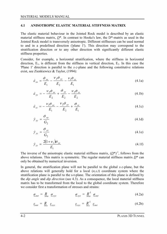
4.1 ANISOTROPIC ELASTIC MATERIAL STIFFNESS MATRIX
The elastic material behaviour in the Jointed Rock model is described by an elastic material stiffness matrix, D*. In contrast to Hooke's law, the D*-matrix as used in the Jointed Rock model is transversely anisotropic. Different stiffnesses can be used normal to and in a predefined direction ('plane 1'). This direction may correspond to the stratification direction or to any other direction with significantly different elastic stiffness properties.
Consider, for example, a horizontal stratification, where the stiffness in horizontal direction, E1, is different from the stiffness in vertical direction, E2. In this case the 'Plane 1' direction is parallel to the x-z-plane and the following constitutive relations exist, see Zienkiewicz & Taylor, (1994):
1
1
2
2
1 EEEzzyyxx
xxσνσνσ
ε&&&
& −−= (4.1a)
2
2
22
2
EEEzzyyxx
yyσνσσν
ε&&&
& −+−= (4.1b)
12
2
1
1
EEEzzyyxx
zzσσνσν
ε&&&
& +−−= (4.1c)
2Gxy
xy
σγ
&& = (4.1d)
2Gyz
yz
σγ
&& = (4.1e)
( )1
112E
zxzx
σνγ&
&+
= (4.1f)
The inverse of the anisotropic elastic material stiffness matrix, (D*)-1, follows from the above relations. This matrix is symmetric. The regular material stiffness matrix D* can only be obtained by numerical inversion.
In general, the stratification plane will not be parallel to the global x-z-plane, but the above relations will generally hold for a local (n,s,t) coordinate system where the stratification plane is parallel to the s-t-plane. The orientation of this plane is defined by the dip angle and dip direction (see 4.3). As a consequence, the local material stiffness matrix has to be transformed from the local to the global coordinate system. Therefore we consider first a transformation of stresses and strains:
σ R = σ xyzσnst σ R = σ nst-σxyz1 (4.2a)
ε R = ε xyzεnst ε R = ε nst-εxyz1 (4.2b)

THE JOINTED ROCK MODEL (ANISOTROPY)
4-3
where
2 2 2
2 2 2
2 2 2
2 2 22 2 22 2 2
x y y z x zx y z
x y y z x zx y z
x y y z x zx y zσ
x x y y z z x y y x y z z y z x x z
x x y y z z x y y
n n n n n nn n n s s s s s ss s s t t t t t tt t tR =
+ + + n s n s n s n s n s n s n s n s n s + s t s t s t s t s x y z z y x z z x
x x y y z z x y y x y z z y z x x z
+ + t s t s t s t s t + + + n t n t n t n t n t n t n t n t n t
⎡ ⎤⎢ ⎥⎢ ⎥⎢ ⎥⎢ ⎥⎢ ⎥⎢ ⎥⎢ ⎥⎢ ⎥⎣ ⎦
(4.3)
and
2 2 2
2 2 2
2 2 2
2 2 22 2 2
x y y z x zx y z
x y y z x zx y z
x y y z x zx y zε
x x y y z z x y y x y z z y z x x z
x x y y z z x y y x y z
n n n n n nn n n s s s s s ss s s t t t t t tt t tR =
+ + + n s n s n s n s n s n s n s n s n s + +s t s t s t s t s t s t
2 2 2z y x z z x
x x y y z z x y y x y z z y z x x z
+ s t s t s t + + + n t n t n t n t n t n t n t n t n t
⎡ ⎤⎢ ⎥⎢ ⎥⎢ ⎥⎢ ⎥⎢ ⎥⎢ ⎥⎢ ⎥⎢ ⎥⎣ ⎦
(4.4)
nx, ny, nz, sx, sy, sz, tx, ty and tz are the components of the normalized n, s and t-vectors in global (x,y,z)-coordinates (i.e. 'sines' and 'cosines'; see 4.3).
It further holds that : -1 TR R
ε σ=
-1 TR Rσ ε
= (4.5)
A local stress-strain relationship in (n,s,t)-coordinates can be transformed to a global relationship in (x,y,z)-coordinates in the following way:
xyznstxyz
xyznst
xyznst
nstnstnst
RDRRRD
εσεεσσεσ
εσ
ε
σ*
*
=⇒⎪⎭
⎪⎬
⎫
===
(4.6)
Hence,
ε R D R = σ xyzε*nst
-σxyz1 (4.7)
Using to above condition (4.5):
ε D = ε R D R = σ xyz*xyzxyzε
*nst
Tεxyz or R D R = D ε
*nst
Tε
*xyz
(4.8)
Actually, not the D*-matrix is given in local coordinates but the inverse matrix (D*)-1.

MATERIAL MODELS MANUAL
4-4 PLAXIS 3D TUNNEL
σ R D R = σ R D R = εεRεσRσσDε
xyzσ
-*nst
Tσxyzσ
-*nst
-εxyz
xyzεnst
xyzσnst
nst*nstnst 111
1
⇒
⎪⎪⎭
⎪⎪⎬
⎫
==
=−
(4.9)
Hence,
R D R = Dσ
-*nst
Tσ
-*xyz
11 or ⎥⎦
⎤⎢⎣⎡ R D R = D σ
-*nst
Tσ
-*xyz
1 1
(4.10)
Instead of inverting the (D*nst)-1-matrix in the first place, the transformation is
considered first, after which the total is numerically inverted to obtain the global material stiffness matrix D*
xyz.
4.2 PLASTIC BEHAVIOUR IN THREE DIRECTIONS
A maximum of 3 sliding directions (sliding planes) can be defined in the Jointed Rock model. The first sliding plane corresponds to the direction of elastic anisotropy. In addition, a maximum of two other sliding directions may be defined. However, the formulation of plasticity on all planes is similar. On each plane a local Coulomb condition applies to limit the shear stress, ⏐τ⏐. Moreover, a tension cut-off criterion is used to limit the tensile stress on a plane. Each plane, i, has its own strength parameters
ψφ iii , ,c and σt,i .
In order to check the plasticity conditions for a plane with local (n,s,t)-coordinates it is necessary to calculate the local stresses from the Cartesian stresses. The local stresses involve three components, i.e. a normal stress component, σn, and two independent shear stress components, τs and τt.
Ti i = Tσ σ (4.11)
where
( )Tn s tiσ σ τ τ= (4.12a)
( )T
xx yy zz xy yz zxσ σ σ σ σ σ σ= (4.12b)
Ti
T = transformation matrix (3x6), for plane i
As usual in PLAXIS, tensile (normal) stresses are defined as positive whereas compression is defined as negative.

THE JOINTED ROCK MODEL (ANISOTROPY)
4-5
α1
s n
y
x
sliding plane
α1
Figure 4.2 Plane strain situation with a single sliding plane and vectors n, s
Consider a plane strain situation as visualised in Figure 4.2. Here a sliding plane is considered under an angle α1 (= dip angle) with respect to the x-axis. In this case the transformation matrix TT becomes: α
2 2
2 2
0 2 0 00 0 0
0 0 0 0
T
- scs c = sc -sc T -s c
-c -s
⎡ ⎤⎢ ⎥+⎢ ⎥⎢ ⎥⎣ ⎦
(4.13)
where
s = sin α1
c = cos α1
In the general three-dimensional case the transformation matrix is more complex, since it involves both the dip angle and the dip direction (Figure 4.3):
2 2 2 2 2 2x y y z z xx y zT
x x y y z z x y y x z y y z z x x z
x x y y z z y x x y y z z y z x x z
n n n n n nn n nT = + + + n s n s n s n s n s n s n s n s n s
+ + + n t n t n t n t n t n t n t n t n t
⎡ ⎤⎢ ⎥⎢ ⎥⎢ ⎥⎣ ⎦
(4.14)
Note that the general transformation matrix, TT, for the calculation of local stresses corresponds to rows 1, 4 and 6 of Rσ (see Eq. 4.3).
After having determined the local stress components, the plasticity conditions can be checked on the basis of yield functions. The yield functions for plane i are defined as:
2 2 tans t n i ii = φ cf τ τ σ+ + − (Coulomb) (4.15a)

MATERIAL MODELS MANUAL
4-6 PLAXIS 3D TUNNEL
,t
n t ii f σ σ= − ( , cott i i i c σ φ≤ ) (Tension cut-off) (4.15b)
Figure 4.3 visualises the full yield criterion on a single plane.
ϕi
σt,i
ci
|τ|
-σn
Figure 4.3 Yield criterion for individual plane
The local plastic strains are defined by:
σλε
j
jj
pj
g =
∂
∂∆ (4.16)
where gj is the local plastic potential function for plane j:
2 2 tans tj n j jg = cσ φτ τ+ + − (Coulomb) (4.17a)
,tj n t jg = σ σ− (Tension cut-off) (4.17b)
The transformation matrix, T, is also used to transform the local plastic strain increments of plane j, ∆ε p
j, into global plastic strain increments, ∆ε p:
p pjj
= Tε ε∆ ∆ (4.18)
The consistency condition requires that at yielding the value of the yield function must remain zero for all active yield functions. For all planes together, a maximum of 6 yield functions exist, so up to 6 plastic multipliers must be found such that all yield functions are at most zero and the plastic multipliers are non-negative.

THE JOINTED ROCK MODEL (ANISOTROPY)
4-7
1 1
T Ti j i jnp npi ie jc c c tj T T
i j i jc tc cj= j=
f g f g = < > < > f f λ λT D T T D T
σ σ σ σ∂ ∂ ∂ ∂
− −∂ ∂ ∂ ∂∑ ∑ (4.19a)
1 1
T Ti j i jnp npi ie jt c t tj T T
i j i jc tt tj= j=
f g f g < > < > f f λ λT D T T D T
σ σ σ σ∂ ∂ ∂ ∂
= − −∂ ∂ ∂ ∂∑ ∑ (4.19b)
This means finding up to 6 values of λi ≥ 0 such that all fi ≤ 0 and λi fi = 0
When the maximum of 3 planes are used, there are 26 = 64 possibilities of (combined) yielding. In the calculation process, all these possibilities are taken into account in order to provide an exact calculation of stresses.
4.3 PARAMETERS OF THE JOINTED ROCK MODEL
Most parameters of the jointed rock model coincide with those of the isotropic Mohr-Coulomb model. These are the basic elastic parameters and the basic strength parameters.
Elastic parameters as in Mohr-Coulomb model (see Section 3.3):
E1 : Young's modulus for rock as a continuum [kN/m2]
ν1 : Poisson's ratio for rock as a continuum [−]
Anisotropic elastic parameters 'Plane 1' direction (e.g. stratification direction):
E2 : Young's modulus in 'Plane 1' direction [kN/m2]
G2 : Shear modulus in 'Plane 1' direction [kN/m2]
ν2 : Poisson's ratio in 'Plane 1' direction [−]
Strength parameters in joint directions (Plane i=1, 2, 3):
ci : Cohesion [kN/m2]
φi : Friction angle [°]
ψ : Dilatancy angle [°]
σt,i : Tensile strength [kN/m2]
Definition of joint directions (Plane i=1, 2, 3):
n : Numer of joint directions (1 ≤ n ≤ 3)
α1,i : Dip angle [°]
α2,i : Dip direction [°]

MATERIAL MODELS MANUAL
4-8 PLAXIS 3D TUNNEL
Figure 4.4 Parameters for the Jointed Rock model
Elastic parameters The elastic parameters E1 and ν1 are the (constant) stiffness (Young's modulus) and Poisson's ratio of the rock as a continuum according to Hooke's law, i.e. as if it would not be anisotropic.
Elastic anisotropy in a rock formation may be introduced by stratification. The stiffness perpendicular to the stratification direction is usually reduced compared with the general stiffness. This reduced stiffness can be represented by the parameter E2, together with a second Poisson's ratio, ν2. In general, the elastic stiffness normal to the direction of elastic anisotropy is defined by the parameters E2 and ν2.
Elastic shearing in the stratification direction is also considered to be 'weaker' than elastic shearing in other directions. In general, the shear stiffness in the anisotropic direction can explicitly be defined by means of the elastic shear modulus G2. In contrast to Hooke's law of isotropic elasticity, G2 is a separate parameter and is not simply related to Young's modulus by means of Poisson's ratio (see Eq. 4.1d and e).
If the elastic behaviour of the rock is fully isotropic, then the parameters E2 and ν2 can be simply set equal to E1 and ν1 respectively, whereas G2 should be set to ½E1/(1+ν1).
Strength parameters Each sliding direction (plane) has its own strength properties ci, φi and σt,i and dilatancy angle ψi. The strength properties ci and φi determine the allowable shear strength according to Coulomb's criterion and σt determines the tensile strength according to the tension cut-off criterion. The latter is displayed after pressing <Advanced> button. By

THE JOINTED ROCK MODEL (ANISOTROPY)
4-9
default, the tension cut-off is active and the tensile strength is set to zero. The dilatancy angle, ψi, is used in the plastic potential function g, and determines the plastic volume expansion due to shearing.
Definition of joint directions It is assumed that the direction of elastic anisotropy corresponds with the first direction where plastic shearing may occur ('Plane 1'). This direction must always be specified. In the case the rock formation is stratified without major joints, the number of sliding planes (= sliding directions) is still 1, and strength parameters must be specified for this direction anyway. A maximum of three sliding directions can be defined. These directions may correspond to the most critical directions of joints in the rock formation.
The sliding directions are defined by means of two parameters: The Dip angle (α1) (or shortly Dip) and the Dip direction (α2). Instead of the latter parameter, it is also common in geology to use the Strike. However, care should be taken with the definition of Strike, and therefore the unambiguous Dip direction as mostly used by rock engineers is used in PLAXIS. The definition of both parameters is visualised in Figure 4.5.
y Nt
n
s*
s α1
α1
α2
sliding plane
Figure 4.5 Definition of dip angle and dip direction
Consider a sliding plane, as indicated in Figure 4.5. The sliding plane can be defined by the vectors (s,t), which are both normal to the vector n. The vector n is the 'normal' to the sliding plane, whereas the vector s is the 'fall line' of the sliding plane and the vector t is the 'horizontal line' of the sliding plane. The sliding plane makes an angle α1 with respect to the horizontal plane, where the horizontal plane can be defined by the vectors (s*,t), which are both normal to the vertical y-axis. The angle α1 is the dip angle, which is defined as the positive 'downward' inclination angle between the horizontal plane and the sliding plane. Hence, α1 is the angle between the vectors s* and s, measured clockwise from s* to s when looking in the positive t-direction. The dip angle must be entered in the range [0°, 90°].

MATERIAL MODELS MANUAL
4-10 PLAXIS 3D TUNNEL
The orientation of the sliding plane is further defined by the dip direction, α2, which is the orientation of the vector s* with respect to the North direction (N). The dip direction is defined as the positive angle from the North direction, measured clockwise to the horizontal projection of the fall line (=s*-direction) when looking downwards. The dip direction is entered in the range [0°, 360°].
N z
x s*
α2
α3
declination
y
Figure 4.6 Definition of various directions and angles in the horiziontal plane
In addition to the orientation of the sliding planes it is also known how the global (x,y,z) model coordinates relate to the North direction. This information is contained in the Declination parameter, as defined in the General settings in the Input program. The Declination is the positive angle from the North direction to the positive z-direction of the model. In order to transform the local (n,s,t) coordinate system into the global (x,y,z) coordinate system, an auxiliary angle α3 is used internally, being the difference between the Dip direction and the Declination:
α3 = α2 − Declination (4.19)
Hence, α3 is defined as the positive angle from the positive z-direction clockwise to the s*-direction when looking downwards.
From the definitions as given above, it follows that:
1 3
1
1 3
sin sincos
sin cos
x
y
z
nn n
n
α αα
α α
−⎡ ⎤⎡ ⎤⎢ ⎥⎢ ⎥= = ⎢ ⎥⎢ ⎥⎢ ⎥⎢ ⎥⎣ ⎦ ⎣ ⎦
(4.20a)
1 3
1
1 3
cos sinsin
cos cos
x
y
z
ss s
s
α αα
α α
−⎡ ⎤⎡ ⎤⎢ ⎥⎢ ⎥= = −⎢ ⎥⎢ ⎥⎢ ⎥⎢ ⎥⎣ ⎦ ⎣ ⎦
(4.20b)

THE JOINTED ROCK MODEL (ANISOTROPY)
4-11
3
3
cos0
sin
x
y
z
tt t
t
α
α
⎡ ⎤⎡ ⎤⎢ ⎥⎢ ⎥= = ⎢ ⎥⎢ ⎥⎢ ⎥⎢ ⎥⎣ ⎦ ⎣ ⎦
(4.20c)
Underneath some examples are shown of how sliding planes occur in a 3D models for different values of α1, α2 and Declination:
α1 = 45º α2 = 0º Declination = 0º
α1 = 45º α2 = 90º Declination = 0º
α1 = 45º α2 = 0º Declination = 90º
Figure 4.7 Examples of failure directions defined by α1 , α2 and Declination
y
z
x
z
x
y
z
x
y

MATERIAL MODELS MANUAL
4-12 PLAXIS 3D TUNNEL

THE HARDENING-SOIL MODEL (ISOTROPIC HARDENING)
5-1
5 THE HARDENING-SOIL MODEL (ISOTROPIC HARDENING)
In contrast to an elastic perfectly-plastic model, the yield surface of a hardening plasticity model is not fixed in principal stress space, but it can expand due to plastic straining. Distinction can be made between two main types of hardening, namely shear hardening and compression hardening. Shear hardening is used to model irreversible strains due to primary deviatoric loading. Compression hardening is used to model irreversible plastic strains due to primary compression in oedometer loading and isotropic loading. Both types of hardening are contained in the present model.
The Hardening-Soil model is an advanced model for simulating the behaviour of different types of soil, both soft soils and stiff soils, Schanz (1998). When subjected to primary deviatoric loading, soil shows a decreasing stiffness and simultaneously irreversible plastic strains develop. In the special case of a drained triaxial test, the observed relationship between the axial strain and the deviatoric stress can be well approximated by a hyperbola.
Such a relationship was first formulated by Kondner (1963) and later used in the well-known hyperbolic model (Duncan & Chang, 1970). The Hardening-Soil model, however, supersedes the hyperbolic model by far. Firstly by using the theory of plasticity rather than the theory of elasticity. Secondly by including soil dilatancy and thirdly by introducing a yield cap. Some basic characteristics of the model are:
• Stress dependent stiffness according to a power law. Input parameter m
• Plastic straining due to primary deviatoric loading. Input parameter Eref50
• Plastic straining due to primary compression. Input parameter Erefoed
• Elastic unloading / reloading. Input parameters Erefur , νur
• Failure according to the Mohr-Coulomb model. Parameters c, φ and ψ
A basic feature of the present Hardening-Soil model is the stress dependency of soil stiffness. For oedometer conditions of stress and strain, the model implies for example
the relationship ( )mrefrefoedoed p / E = E σ . In the special case of soft soils it is
realistic to use m = 1. In such situations there is also a simple relationship between the modified compression index λ*, as used in the the Soft-Soil model and the oedometer loading modulus (see also Section 6.7)
( )0
1
refrefoed
pE
eλ
λλ
∗∗= =
+
where pref is a reference pressure. Here we consider a tangent oedometer modulus at a particular reference pressure pref. Hence, the primary loading stiffness relates to the modified compression index λ*.

MATERIAL MODELS MANUAL
5-2 PLAXIS 3D TUNNEL
Similarly, the unloading-reloading modulus relates to the modified swelling index κ*. There is the approximate relationship:
( )( )0
3 1 2
1
refurref
urp -
= Ee
ν κκ
κ∗
∗ =+
Again, this relationship applies in combination with the input value m = 1.
5.1 HYPERBOLIC RELATIONSHIP FOR STANDARD DRAINED TRIAXIAL TEST
A basic idea for the formulation of the Hardening-Soil model is the hyperbolic relationship between the vertical strain, ε1, and the deviatoric stress, q, in primary triaxial loading. Here standard drained triaxial tests tend to yield curves that can be described by:
150
1 for: 2 1 f
a
q q qE q / q
ε− = <−
(5.1)
Where qa is the asymptotic value of the shear strength. This relationship is plotted in Figure 5.1. The parameter E50 is the confining stress dependent stiffness modulus for primary loading and is given by the equation:
350 50
cotcot
mref
ref
c E E
c pϕ σϕ
⎛ ⎞− ′= ⎜ ⎟+⎝ ⎠
(5.2)
where Eref50 is a reference stiffness modulus for primary loading corresponding to the
reference confining pressure pref. In PLAXIS, a default setting pref = 100 stress units is used. The actual stiffness depends on the minor principal stress, σ3', which is the confining pressure in a triaxial test. Please note that σ'3 is negative for compression. The rate of stress dependency is given by the power m. In order to simulate a logarithmic stress dependency, as observed for soft clays, the power should be taken equal to 1.0. Janbu (1963) reports values of m around 0.5 for Norwegian sands and silts, whilst Von Soos (1980) reports various different values in the range 0.5 < m < 1.0.
The ultimate deviatoric stress, qf, and the quantity qa in Eq. (5.1) are defined as:
( )32sincot and:
1 sinf
f af
qq c q
Rϕ
ϕ σϕ
= − =′−
(5.3)
Again it is remarked that σ'3 is usually negative. The above relationship for qf is derived from the Mohr-Coulomb failure criterion, which involves the strength parameters c and φ. As soon as q = qf , the failure criterion is satisfied and perfectly plastic yielding occurs as described by the Mohr-Coulomb model.

THE HARDENING-SOIL MODEL (ISOTROPIC HARDENING)
5-3
The ratio between qf and qa is given by the failure ratio Rf, which should obviously be smaller than 1. In PLAXIS, Rf = 0.9 is chosen as a suitable default setting.
For unloading and reloading stress paths, another stress-dependent stiffness modulus is used:
3cotcot
mref
ur ur ref
cE E
c pϕ σϕ
⎛ ⎞− ′= ⎜ ⎟+⎝ ⎠
(5.4)
where Erefur is the reference Young's modulus for unloading and reloading, corresponding
to the reference pressure pref. In many practical cases it is appropriate to set Erefur equal
to 3 50refE ; this is the default setting used in PLAXIS.
axial strain -ε1
|σ1-σ3|
1 Eur
E50
1
qa
qf
asymptote
failure line
deviatoric stress
Figure 5.1 Hyperbolic stress-strain relation in primary loading for a standard drained triaxial test
5.2 APPROXIMATION OF HYPERBOLA BY THE HARDENING-SOIL MODEL
For the sake of convenience, restriction is again made to triaxial loading conditions with σ2' = σ3' and σ1' being the major compressive stress. Moreover, it is assumed that q < qf, as also indicated in Figure 5.1. It should also be realised that compressive stress and strain are considered positive. For a more general presentation of the Hardening-Soil model the reader is referred to Schanz et al (1999). In this section it will be shown that this model gives virtually the hyperbolic stress strain curve of Eq. (5.1) when considering stress paths of standard drained triaxial tests. Let us first consider the corresponding plastic strains. This stems from a yield function of the form:
pf f γ= − (5.5)
where f is a function of stress and γ p is a function of plastic strains.

MATERIAL MODELS MANUAL
5-4 PLAXIS 3D TUNNEL
f = 50
211 ura
q q q / qE E
−−
( )1 12 2pp ppv γ εε ε= − − ≈ − (5.6)
with q, qa, E50 and Eur as defined by Eqs. (5.2) to (5.4), whilst the superscript p is used to denote plastic strains. For hard soils, plastic volume changes (ε p
v ) tend to be relatively small and this leads to the approximation pp
12εγ −≈ . The above definition of the strain-hardening parameter γ p will be referred to later.
An essential feature of the above definitions for f is that it matches the well-known hyperbolic law (5.1). For checking this statement, one has to consider primary loading, as this implies the yield condition f = 0. For primary loading, it thus yields γ p = f and it follows from Eqs. (5.6) that:
− 1pε ≈ 1
2 f = 50
12 1 ura
q q E q / q E
−−
(5.7)
In addition to the plastic strains, the model accounts for elastic strains. Plastic strains develop in primary loading alone, but elastic strains develop both in primary loading and unloading / reloading. For drained triaxial test stress paths with σ2' = σ3' = constant, the elastic Young's modulus Eur remains constant and the elastic strains are given by the equations:
−ε e1 =
Equr
−ε e2 = −ε e
3 = Eq ur
urν− (5.8)
where νur is the unloading / reloading Poisson's ratio. Here it should be realised that restriction is made to strains that develop during deviatoric loading, whilst the strains that develop during the very first stage of the test are not considered. For the first stage of isotropic compression (with consolidation), the Hardening-Soil model predicts fully elastic volume changes according to Hooke's law, but these strains are not included in Eq. (5.8).
For the deviatoric loading stage of the triaxial test, the axial strain is the sum of an elastic component given by Eq. (5.8) and a plastic component according to Eq. (5.7). Hence, it follows that:
1 1 150
12 1
e p
a
q E q / q
ε ε ε− = − − ≈−
(5.9)
This relationship holds exactly in absence of plastic volume strains, i.e. when ε pv = 0.
In reality, plastic volumetric strains will never be precisely equal to zero, but for hard soils plastic volume changes tend to be small when compared with the axial strain, so that the approximation in Eq. (5.9) will generally be accurate. It is thus made clear that

THE HARDENING-SOIL MODEL (ISOTROPIC HARDENING)
5-5
the present Hardening-Soil model yields a hyperbolic stress-strain curve under triaxial testing conditions.
For a given constant value of the hardening parameter, γp, the yield condition f = 0, can be visualised in p'-q-plane by means of a yield locus. When plotting such yield loci, one has to use Eq. (5.6) as well as Eqs. (5.2) and (5.4) for E50 and Eur respectively. Because of the latter expressions, the shape of the yield loci depend on the exponent m. For m = 1, straight lines are obtained, but slightly curved yield loci correspond to lower values of the exponent. Figure 5.2 shows the shape of successive yield loci for m = 0.5, being typical for hard soils.
Mean effective stress
|σ 1-σ3| deviatoric stress
Mohr-Coulomb failure line
Figure 5.2 Successive yield loci for various constant values of the hardening parameter γ p
5.3 PLASTIC VOLUMETRIC STRAIN FOR TRIAXIAL STATES OF STRESS
Having presented a relationship for the plastic shear strain, γ p, attention is now focused on the plastic volumetric strain, p
vε . As for all plasticity models, the Hardening-Soil model involves a relationship between rates of plastic strain, i.e. a relationship between
pvε& and pγ& . This flow rule has the linear form:
pvε& = sinψm pγ& (5.10)
Clearly, further detail is needed by specifying the mobilised dilatancy angle ψm. For the present model, the expression:
ϕϕϕϕ
ψcvm
cvmm
sinsin1sinsin
sin−
−= (5.11)
is adopted, where φcν is the critical state friction angle, being a material constant independent of density, and φm is the mobilised friction angle:

MATERIAL MODELS MANUAL
5-6 PLAXIS 3D TUNNEL
ϕσσσσϕ
cot2sin
31
31
c +m −′′′−′
= (5.12)
The above equations correspond to the well-known stress-dilatancy theory by Rowe (1962), as explained by Schanz & Vermeer (1995). The essential property of the stress-dilatancy theory is that the material contracts for small stress ratios (φm < φcν), whilst dilatancy occurs for high stress ratios (φm > φcν). At failure, when the mobilised friction angle equals the failure angle, φ, it is found from Eq. (5.11) that:
ϕϕϕϕ
ψcv
cv sinsin1sinsin
sin−
−= (5.13a)
or equivalently:
ψψ
cv sinsin1sinsinsin
ϕϕϕ
−−
= (5.13b)
Hence, the critical state angle can be computed from the failure angles φ and ψ. PLAXIS performs this computation automatically and so users do not need to specify a value for φcν.
Instead, one has to provide input data on the ultimate friction angle, φ, and the ultimate dilatancy angle, ψ.
5.4 PARAMETERS OF THE HARDENING-SOIL MODEL
Some parameters of the present hardening model coincide with those of the non-hardening Mohr-Coulomb model. These are the failure parameters c, φ and ψ.
Failure parameters as in Mohr-Coulomb model (see Section 3.3):
c : (Effective) cohesion [kN/m2]
φ : (Effective) angle of internal friction [°]
ψ : Angle of dilatancy [°]
Basic parameters for soil stiffness:
Eref50 : Secant stiffness in standard drained triaxial test [kN/m2]
Erefoed : Tangent stiffness for primary oedometer loading [kN/m2]
m : Power for stress-level dependency of stiffness [-]

THE HARDENING-SOIL MODEL (ISOTROPIC HARDENING)
5-7
Advanced parameters (it is advised to use the default setting):
Erefur : Unloading / reloading stiffness (default Eref
ur = 3 Eref50 ) [kN/m2]
νur : Poisson's ratio for unloading-reloading (default νur = 0.2) [-]
pref : Reference stress for stiffnesses (default pref = 100 stress units) [kN/m2]
K nc0 : K0-value for normal consolidation (default K nc
0 = 1-sinφ) [-]
Rf : Failure ratio qf / qa (default Rf = 0.9) (see Figure 5.1) [-]
σtension : Tensile strength (default σtension = 0 stress units) [kN/m2]
cincrement : As in Mohr-Coulomb model (default cincrement = 0) [kN/m3]
Figure 5.3 Basic parameters for the Hardening-Soil model
Stiffness moduli ref50E & ref
oedE and power m
The advantage of the Hardening-Soil model over the Mohr-Coulomb model is not only the use of a hyperbolic stress-strain curve instead of a bi-linear curve, but also the control of stress level dependency. When using the Mohr-Coulomb model, the user has to select a fixed value of Young's modulus whereas for real soils this stiffness depends on the stress level. It is therefore necessary to estimate the stress levels within the soil and use these to obtain suitable values of stiffness. With the Hardening-Soil model, however, this cumbersome selection of input parameters is not required. Instead, a stiffness modulus Eref
50 is defined for a reference minor principal stress of refp=′− 3σ . As a default value, the program uses pref = 100 stress units.

MATERIAL MODELS MANUAL
5-8 PLAXIS 3D TUNNEL
As some PLAXIS users are familiar with the input of shear moduli rather than the above stiffness moduli, shear moduli will now be discussed. Within Hooke's theory of elasticity conversion between E and G goes by the equation E = 2 (1+ν) G. As Eur is a real elastic stiffness, one may thus write Eur = 2 (1+ν) Gur, where Gur is an elastic shear modulus. Please note that PLAXIS allows for the input of Eur and νur but not for a direct input of Gur. In contrast to Eur, the secant modulus E50 is not used within a concept of elasticity. As a consequence, there is no simple conversion from E50 to G50.
In contrast to elasticity based models, the elastoplastic Hardening-Soil model does not involve a fixed relationship between the (drained) triaxial stiffness E50 and the oedometer stiffness Eoed for one-dimensional compression. Instead, these stiffnesses can be inputted independently.
Having defined E50 by Eq. (5.2), it is now important to define the oedometer stiffness. Here we use the equation:
1cotcot
mref
oed oed ref
cE E
c pϕ σϕ
⎛ ⎞− ′= ⎜ ⎟+⎝ ⎠
(5.14)
where Eoed is a tangent stiffness modulus as indicated in Figure 5.4. Hence, Erefoed is a
tangent stiffness at a vertical stress of −σ'1 = pref. Note that we use σ1 rather than σ3 and that we consider primary loading.
-ε1
-σ 1
pref1
refoedE
Figure 5.4 Definition of Erefoed in oedometer test results
Advanced parameters Realistic values of νur are about 0.2 and this value is thus used as a default setting, as indicated in Figure 5.5. In contrast to the Mohr-Coulomb model, K nc
0 is not simply a function of Poisson's ratio, but a proper input parameter. As a default setting PLAXIS uses the correlation K nc
0 = 1−sinφ. It is suggested to maintain this value as the

THE HARDENING-SOIL MODEL (ISOTROPIC HARDENING)
5-9
correlation is highly realistic. However, users do have the possibility to select different values. All possible different input values for K nc
0 cannot be accommodated for. Depending on other parameters, such as E50, Eoed, Eur and νur, there happens to be a certain range of valid K nc
0 -values. K nc0 values outside this range are rejected by PLAXIS.
On inputting values, the program shows the nearest possible value that will be used in the computations.
Figure 5.5 Advanced parameters window
Dilatancy cut-off After extensive shearing, dilating materials arrive in a state of critical density where dilatancy has come to an end, as indicated in Figure 5.6. This phenomenon of soil behaviour can be included in the Hardening-Soil model by means of a dilatancy cut-off. In order to specify this behaviour, the initial void ratio, einit, and the maximum void ratio, emax, of the material must be entered as general parameters. As soon as the volume change results in a state of maximum void, the mobilised dilatancy angle, ψmob, is automatically set back to zero, as indicated in Figure 5.6.
for e < emax: sinψmob = ϕϕ
ϕϕ
cvmob
cvmob
sinsin1sinsin
−−
where: sinφcν = ψϕ
ψϕ
sinsin1
sinsin−
− (5.15a)
for e ≥ emax: ψmob = 0 (5.15b)
The void ratio is related to the volumetric strain, εν by the relationship:
− ( )εε initvv − = ⎟⎟
⎠
⎞⎜⎜⎝
⎛
e + e + init1
1ln (5.16)

MATERIAL MODELS MANUAL
5-10 PLAXIS 3D TUNNEL
where an increment of εv is positive for dilatancy.
dilatancy cut-off ON
maximum porosity reached
ε1
1 – sinψ
εv
dilatancy cut-off OFF
2 sinψ
Figure 5.6 Resulting strain curve for a standard drained triaxial test when including dilatancy cut-off
Figure 5.7 Advanced general properties window
The initial void ratio, einit, is the in-situ void ratio of the soil body. The maximum void ratio is the void ratio of the material in a state of critical void (critical state). As soon as the maximum void ratio is reached, the dilatancy angle is set to zero. The minimum void ratio, emin, of a soil can also be inputted, but this general soil parameter is not used within the context of the Hardening-Soil model. Please note that the selection of the dilatancy cut-off and the input of void ratios is done in the 'general' tab sheet of the material data set window and not in the 'parameters' tab sheet. The selection of the dilatancy cut-off is only available when the Hardening-Soil model has been selected. By default, the dilatancy cut-off is not active.
5.5 ON THE CAP YIELD SURFACE IN THE HARDENING-SOIL MODEL
Shear yield surfaces as indicated in Figure 5.2 do not explain the plastic volume strain that is measured in isotropic compression. A second type of yield surface must therefore be introduced to close the elastic region in the direction of the p-axis. Without such a

THE HARDENING-SOIL MODEL (ISOTROPIC HARDENING)
5-11
cap type yield surface it would not be possible to formulate a model with independent input of both Eref
50 and Erefoed . The triaxial modulus largely controls the shear yield
surface and the oedometer modulus controls the cap yield surface. In fact, Eref50 largely
controls the magnitude of the plastic strains that are associated with the shear yield surface. Similarly, Eref
oed is used to control the magnitude of plastic strains that originate from the yield cap. In this section the yield cap will be described in full detail. To this end we consider the definition of the cap yield surface:
f c = p p + qp22
2
2~−
α (a = c cotφ) (5.17)
where α is an auxiliary model parameter that relates to K nc0 as will be discussed later.
Further more we have p = − (σ1+σ2+σ3) /3 and q~ = σ1+(δ−1)σ2−δσ3 with δ=(3+sinφ) / (3−sinφ). q~ is a special stress measure for deviatoric stresses. In the special case of triaxial compression (−σ1>−σ2=−σ3) it yields q~ = −(σ1−σ3) and for triaxial extension (−σ1=−σ2>−σ3) q~ reduces to q~ = −δ(σ1−σ3). The magnitude of the yield cap is determined by the isotropic pre-consolidation stress pp. We have a hardening law relating pp to volumetric cap strain ε pc
v :
ε pcv = ⎟
⎟⎠
⎞⎜⎜⎝
⎛
−
−
p
p
m refp
m1
1β
(5.18)
The volumetric cap strain is the plastic volumetric strain in isotropic compression. In addition to the well known constants m and pref there is another model constant β. Both α and β are cap parameters, but we will not use them as direct input parameters. Instead, we have relationships of the form:
α ↔ K nc0 (default: K nc
0 = 1−sinφ)
β ↔ Erefoed (default: Eref
oed = Eref50 )
such that K nc0 and Eref
oed can be used as input parameters that determine the magnitude of α and β respectively. For understanding the shape of the yield cap, it should first of all be realised that it is an ellipse in p- q~ -plane, as indicated in Figure 5.8. The ellipse has length pp on the p-axis and αpp on the q~ -axis. Hence, pp determines its magnitude and α its aspect ratio. High values of α lead to steep caps underneath the Mohr-Coulomb line, whereas small α-values define caps that are much more pointed around the p-axis. The ellipse is used both as a yield surface and as a plastic potential. Hence:
pcε& = cf λ
σ∂∂
with: λ = 2
mp p
ref ref
p p
p p pβ ⎛ ⎞
⎜ ⎟⎝ ⎠
& (5.19)

MATERIAL MODELS MANUAL
5-12 PLAXIS 3D TUNNEL
This expression for λ derives from the yield condition f c = 0 and Eq. (5.18) for pp. Input data on initial pp-values is provided by means of the PLAXIS procedure for initial stresses. Here, pp is either computed from the inputted overconsolidation ratio (OCR) or the pre-overburden pressure (POP) (see Section 2.6).
For understanding the yield surfaces in full detail, one should consider both Figure 5.8 and Figure 5.9. The first figure shows simple yield lines, whereas the second one depicts yield surfaces in principal stress space. Both the shear locus and the yield cap have the hexagonal shape of the classical Mohr-Coulomb failure criterion. In fact, the shear yield locus can expand up to the ultimate Mohr-Coulomb failure surface. The cap yield surface expands as a function of the pre-consolidation stress pp.
p
q
pp
αpp
c cot φ
elastic region
~
Figure 5.8 Yield surfaces of Hardening-Soil model in p- q~ -plane. The elastic region
can be further reduced by means of a tension cut-off
-σ1
-σ2
-σ 3
Figure 5.9 Representation of total yield contour of the Hardening-Soil model in
principal stress space for cohesionless soil

SOFT-SOIL-CREEP MODEL (TIME DEPENDENT BEHAVIOUR)
6-1
6 SOFT-SOIL-CREEP MODEL (TIME DEPENDENT BEHAVIOUR)
6.1 INTRODUCTION
As soft soils we consider near-normally consolidated clays, clayey silts and peat. The special features of these materials is their high degree of compressibility. This is best demonstrated by oedometer test data as reported for instance by Janbu in his Rankine lecture (1985). Considering tangent stiffness moduli at a reference oedometer pressure of 100 kPa, he reports for normally consolidated clays Eoed = 1 to 4 MPa, depending on the particular type of clay considered. The differences between these values and stiffnesses for NC-sands are considerable as here we have values in the range of 10 to 50 MPa, at least for non-cemented laboratory samples. Hence, in oedometer testing normally consolidated clays behave ten times softer than normally consolidated sands. This illustrates the extreme compressibility of soft soils.
Another feature of the soft soils is the linear stress-dependency of soil stiffness. According to the Hardening-Soil model we have
Eoed = Erefoed (σ / pref)m
at least for c=0, and a linear relationship is obtained for m = 1. Indeed, on using an exponent equal to one, the above stiffness law reduces to
Eoed = σ / λ* where λ* = pref / Erefoed
For this special case of m=1, the Hardening-Soil model yields ε& = λ* σ& / σ, which can be integrated to obtain the well-known logarithmic compression law ε = λ* lnσ for primary oedometer loading.
For many practical soft-soil studies, the modified compression index λ* will be known and the PLAXIS user can compute the oedometer modulus from the relationship
Erefoed = pref/λ*.
From the above considerations it would seem that the HS-model is perfectly suitable for soft soils. Indeed, most soft soil problems can be analysed using this model, but the HS-model is not suitable when considering creep, i.e. secondary compression. All soils exhibit some creep, and primary compression is thus always followed by a certain amount of secondary compression. Assuming the secondary compression (for instance during a period of 10 or 30 years) to be a percentage of the primary compression, it is clear that creep is important for problems involving large primary compression. This is for instance the case when constructing embankments on soft soils. Indeed, large primary settlements of dams and embankments are usually followed by substantial creep settlements in later years. In such cases it is desirable to estimate the creep from FEM-computations.
Dams or buildings may also be founded on initially overconsolidated soil layers that yield relatively small primary settlements. Then, as a consequence of the loading, a state

MATERIAL MODELS MANUAL
6-2 PLAXIS 3D TUNNEL
of normal consolidation may be reached and significant creep may follow. This is a treacherous situation as considerable secondary compression is not preceded by the warning sign of large primary compression. Again, computations with a creep model are desirable.
Buisman (1936) was probably the first to propose a creep law for clay after observing that soft-soil settlements could not be fully explained by classical consolidation theory. This work on 1D-secondary compression was continued by other researchers including, for example, Bjerrum (1967), Garlanger (1972), Mesri (1977) and Leroueil (1977). More mathematical lines of research on creep were followed by, for example, Sekiguchi (1977), Adachi and Oka (1982) and Borja et al. (1985). This mathematical 3D-creep modelling was influenced by the more experimental line of 1D-creep modelling, but conflicts exist.
3D-creep should be a straight forward extension of 1D-creep, but this is hampered by the fact that present 1D-models have not been formulated as differential equations. For the presentation of the Soft-Soil-Creep model we will first complete the line of 1D-modelling by conversion to a differential form. From this 1D differential equation an extension was made to a 3D-model. This Chapter gives a full description of the formulation of the Soft-Soil-Creep model. In addition, attention is focused on the model parameters. Finally, a validation of the 3D model is presented by considering both model predictions and data from triaxial tests. Here, attention is focused on constant strain rate triaxial tests and undrained triaxial creep tests. For more applications of the model the reader is referred to Vermeer et al. (1998) and Neher & Vermeer (1998).
Some basic characteristics of the Soft-Soil-Creep model are:
• Stress-dependent stiffness (logarithmic compression behaviour)
• Distinction between primary loading and unloading-reloading
• Secondary (time-dependent) compression
• Memory of pre-consolidation stress
• Failure behaviour according to the Mohr-Coulomb criterion
6.2 BASICS OF ONE-DIMENSIONAL CREEP
When reviewing previous literature on secondary compression in oedometer tests, one is struck by the fact that it concentrates on behaviour related to step loading, even though natural loading processes tend to be continuous or transient in nature. Buisman (1936) was probably the first to consider such a classical creep test. He proposed the following equation to describe creep behaviour under constant effective stress:
⎟⎟⎠
⎞⎜⎜⎝
⎛−
tt C = c
Bc logεε for: t > tc (6.1)

SOFT-SOIL-CREEP MODEL (TIME DEPENDENT BEHAVIOUR)
6-3
where εc is the strain up to the end of consolidation, t the time measured from the beginning of loading, tc the time to the end of primary consolidation and CB is a material constant.
Please note that we do not follow the soil mechanics convention that compression is considered positive. Instead, compressive stresses and strains are taken to be negative. For further consideration, it is convenient to rewrite this equation as:
⎟⎟⎠
⎞⎜⎜⎝
⎛ ′+−=
ttt C
c
cBc logεε for t' > 0 (6.2)
with t' = t - tc being the effective creep time.
Based on the work by Bjerrum on creep, as published for instance in 1967, Garlanger (1972) proposed a creep equation of the form:
⎟⎟⎠
⎞⎜⎜⎝
⎛ ′+−=
ττ
αc
cc
t C ee log with: ( )0B eC = C +1α for: t' > 0 (6.3)
Differences between Garlanger’s and Buisman’s forms are modest. The engineering strain ε is replaced by void ratio e and the consolidation time tc is replaced by a parameter τc. Eqs. 6.2 and 6.3 are entirely identical when choosing τc = tc. For the case that τc ≠ tc differences between both formulations will vanish when the effective creep time t’ increases.
For practical consulting, oedometer tests are usually interpreted by assuming tc = 24h. Indeed, the standard oedometer test is a Multiple Stage Loading Test with loading periods of precisely one day. Due to the special assumption that this loading period coincides to the consolidation time tc, it follows that such tests have no effective creep time. Hence one obtains t' = 0 and the log-term drops out of Eq. (6.3) It would thus seem that there is no creep in this standard oedometer test, but this suggestion is entirely false. Even highly impermeable oedometer samples need less than one hour for primary consolidation. Then all excess pore pressures are zero and one observes pure creep for the other 23 hours of the day. Therefore we will not make any assumptions about the precise values of τc and tc.
Another slightly different possibility to describe secondary compression is the form adopted by Butterfield (1979):
⎟⎟⎠
⎞⎜⎜⎝
⎛ ′+
ττ
εεc
cHc
H t C - = ln (6.4)
where εH is the logarithmic strain defined as:
⎟⎟⎠
⎞⎜⎜⎝
⎛⎟⎟⎠
⎞⎜⎜⎝
⎛
e+ + e =
VV = H
00 11lnlnε (6.5)

MATERIAL MODELS MANUAL
6-4 PLAXIS 3D TUNNEL
with the subscript ‘0’ denoting the initial values. The subscript ‘H’ is used for denoting logarithmic strain. We use this particular symbol, as the logarithmic strain measure was originally used by Hencky. For small strains it is possible to show that:
( ) 10ln10ln1 0
C = e+
C = C B
⋅α (6.6)
because then logarithmic strain is approximately equal to the engineering strain. Both Butterfield (1979) and Den Haan (1994) showed that for cases involving large strain, the logarithmic small strain supersedes the traditional engineering strain.
6.3 ON THE VARIABLES τC AND εC
In this section attention will first be focussed on the variable τc. Here a procedure is to be described for an experimental determination of this variable. In order to do so we depart from Eq. (6.4) By differentiating this equation with respect to time and dropping the superscript ‘H’ to simplify notation, one finds:
t +C =
c ′−
τε& or inversely:
Ct + =
c ′
−τ
ε&1
(6.7)
which allows one to make use of the construction developed by Janbu (1969) for evaluating the parameters C and τc from experimental data. Both the traditional way, being indicated in Figure 6.1a, as well as the Janbu method of Figure 6.1b can be used to determine the parameter C from an oedometer test with constant load. The use of the Janbu method is attractive, because both τc and C follow directly when fitting a straight line through the data. In Janbu’s representation of Figure 6.1b, τc is the intercept with the (non-logarithmic) time axis of the straight creep line. The deviation from a linear relation for t < tc is due to consolidation.
εc
1 C
(a)
tc ln t
-ε
(b)
-1/ε
tc
t’τc t
1
C
.
t’ = t - tc
Figure 6.1 Consolidation and creep behaviour in standard oedometer test

SOFT-SOIL-CREEP MODEL (TIME DEPENDENT BEHAVIOUR)
6-5
Considering the classical literature it is possible to describe the end-of-consolidation strain εc, by an equation of the form:
⎟⎟⎠
⎞⎜⎜⎝
⎛−⎟⎟
⎠
⎞⎜⎜⎝
⎛ ′−+
′ σσ
σσ
εεεp0
pc
0
cc
ecc B A = = lnln (6.8)
Note that ε is a logarithmic strain, rather than a classical small strain although we conveniently omit the subscript ‘H’. In the above equation σ0' represents the initial effective pressure before loading and σ' is the final effective loading pressure. The values σp0 and σpc representing the pre-consolidation pressure corresponding to before-loading and end-of-consolidation states respectively. In most literature on oedometer testing, one adopts the void ratio e instead of ε, and log instead of ln, and the swelling index Cr instead of A, and the compression index Cc instead of B. The above constants A and B relate to Cr and Cc as:
( ) 10ln1 0 ⋅+ e C = A r
( )( ) 10ln1 0 ⋅+
−e
CC = B rc (6.9)
Combining Eqs. 6.4 and 6.8 it follows that:
⎟⎟⎠
⎞⎜⎜⎝
⎛ ′+−⎟
⎟⎠
⎞⎜⎜⎝
⎛−⎟⎟
⎠
⎞⎜⎜⎝
⎛ ′−=+=
′ τt C B Aε
c
c
p
pcce τσσ
σσεε lnlnln
00 (6.10)
where ε is the total logarithmic strain due to an increase in effective stress from σ0' to σ' and a time period of tc+t'. In Figure 6.2 the terms of Eq. (6.10) are depicted in a ε−lnσ diagram.
σ’ σpcσp0
A
σ’0
1
A+B
1
NC-line
-εC ln(1+t’/τc)
ln(-σ’)
ecε
ccε
Figure 6.2 Idealised stress-strain curve from oedometer test with division of strain increments into an elastic and a creep component. For t' + tc = 1 day, one arrives precisely on the NC-line

MATERIAL MODELS MANUAL
6-6 PLAXIS 3D TUNNEL
Up to this point, the more general problem of creep under transient loading conditions has not yet been addressed, as it should be recalled that restrictions have been made to creep under constant load. For generalising the model, a differential form of the creep model is needed. No doubt, such a general equation may not contain t' and neither τc as the consolidation time is not clearly defined for transient loading conditions.
6.4 DIFFERENTIAL LAW FOR 1D-CREEP
The previous equations emphasize the relation between accumulated creep and time, for a given constant effective stress. For solving transient or continuous loading problems, it is necessary to formulate a constitutive law in differential form, as will be described in this section. In a first step we will derive an equation for τc. Indeed, despite the use of logarithmic strain and ln instead of log, the formula 6.10 is classical without adding new knowledge. Moreover, the question on the physical meaning of τc is still open. In fact, we have not been able to find precise information on τc in the literature, apart from Janbu’s method of experimental determination.
In order to find an analytical expression for the quantity τc, we adopt the basic idea that all inelastic strains are time dependent. Hence total strain is the sum of an elastic part εe and a time-dependent creep part εc. For non-failure situations as met in oedometer loading conditions, we do not assume an instantaneous plastic strain component, as used in traditional elastoplastic modelling. In addition to this basic concept, we adopt Bjerrum’s idea that the pre-consolidation stress depends entirely on the amount of creep strain being accumulated in the course of time. In addition to Eq. (6.10) we therefore introduce the expression:
0 0ln ln pe c
p A Bσ σε ε ε
σ σ′
⎛ ⎞⎛ ⎞′= + = − −⎜ ⎟ ⎜ ⎟⎝ ⎠ ⎝ ⎠
→
→ 0 expc
p pεB
σ σ⎛ ⎞−
= ⎜ ⎟⎝ ⎠
(6.11)
Please note that εc is negative, so that σp exceeds σp0. The longer a soil sample is left to creep the larger σp grows. The time-dependency of the pre-consolidation pressure σp is now found by combining Eqs. 6.10 and 6.11 to obtain:
ln lnp cc cc
pc c
+ t = B Cσ τε εσ τ
⎛ ⎞ ⎛ ⎞′− − = − ⎜ ⎟⎜ ⎟ ⎝ ⎠⎝ ⎠
(6.12)
This equation can now be used for a better understanding of τc, at least when adding knowledge from standard oedometer loading. In conventional oedometer testing the load is stepwise increased and each load step is maintained for a constant period of tc+t' = τ , where τ is precisely one day.
In this way of stepwise loading the so-called normal consolidation line (NC-line) with σp = σ' is obtained. On entering σp = σ' and t' = τ -tc into Eq. (6.12) it is found that:

SOFT-SOIL-CREEP MODEL (TIME DEPENDENT BEHAVIOUR)
6-7
ln ln cc
pc c
+ tB Cτ τσ
σ τ
⎛ ⎞ −⎛ ⎞′= ⎜ ⎟⎜ ⎟ ⎝ ⎠⎝ ⎠
for: OCR =1 (6.13)
It is now assumed that (τc − tc) << τ. This quantity can thus be disregarded with respect to τ and it follows that:
BC
c pc = τ σ
τ σ
⎛ ⎞′⎜ ⎟⎝ ⎠
or:
BCpc
c = στ τσ
⎛ ⎞⎜ ⎟⎝ ⎠′
(6.14)
Hence τc depends both on the effective stress σ' and the end-of-consolidation pre-consolidation stress σpc. In order to verify the assumption (τc - tc) << τ, it should be realised that usual oedometer samples consolidate for relatively short periods of less than one hour. Considering load steps on the normal consolidation line, we have OCR=1 both in the beginning and at the end of the load step. During such a load step σp increases from σp0 up to σpc during the short period of (primary) consolidation. Hereafter σp increases further from σpc up to σ' during a relatively long creep period. Hence, at the end of the day the sample is again in a state of normal consolidation, but directly after the short consolidation period the sample is under-consolidated with σp<σ'. For the usually very high ratios of B/C ≥ 15, we thus find very small τc-values from Eq. (6.14). Hence not only tc but also τc tend to be small with respect to τ. It thus follows that the assumption (τc− tc) << τ is certainly correct.
Having derived the simple expression 6.14 for τc, it is now possible to formulate the differential creep equation. To this end Eq. (6.10) is differentiated to obtain:
e c
c
C= A+ t
σε ε ε
σ τ′
+ = − −′ ′&
& & & (6.15)
where τc+ t' can be eliminated by means of Eq. (6.12) to obtain:
BC
pce c
c p
C= A σ σε ε εσ τ σ
⎛ ⎞′+ = − − ⎜ ⎟′ ⎝ ⎠
&& & &
with: c
0 exp Bp p εσ σ
⎛ ⎞−= ⎜ ⎟
⎝ ⎠ (6.16)
Again it is recalled that εc is a compressive strain, being considered negative in this manual. Eq. (6.14) can now be introduced to eliminate τc and σpc and to obtain:
BC
e c
p
C= A σ σε ε ε
σ τ σ
⎛ ⎞′ ′+ = − − ⎜ ⎟′ ⎝ ⎠
&& & & (6.17)

MATERIAL MODELS MANUAL
6-8 PLAXIS 3D TUNNEL
6.5 THREE-DIMENSIONAL-MODEL
On extending the 1D-model to general states of stress and strain, the well-known stress invariants for pressure p and deviatoric stress q are adopted. These invariants are used to define a new stress measure named peq:
( )2
2 coteq q = pp
p cM ϕ′ +
′ + (6.18)
isotropic stress p = -(σ1 + σ2+ σ3)/3
deviatoric stress q = σ1 - σ3
peq
1
M
ppeq
ccotϕ
Figure 6.3 Diagram of peq-ellipse in a p-q-plane
In Figure 6.3 it is shown that the stress measure peq is constant on ellipses in p-q-plane. In fact, for c=0 we have the ellipses from the Modified Cam-Clay-Model as introduced by Roscoe and Burland (1968). The soil parameter M represents the slope of the so-called ‘critical state line’ as also indicated in Figure 6.3. We use the general 3D-definition ( Eq. 2.7b) for the deviatoric stress q and:
6sin3 sin
cv
cv
M = ϕϕ−
(6.19)
where φcv is the critical-void friction angle, also referred to as critical-state friction angle. On using Eq. (2.7b) for q, the equivalent pressure peq is constant along ellipsoids in principal stress space. To extend the 1D-theory to a general 3D-theory, attention is now focused on normally consolidated states of stress and strain as met in oedometer testing. In such situations it yields σ2' = σ3' = K NC
0 σ1' , and it follows from Eq. (6.18) that:
( )( )
200
20
3 11 23 1 2
NCNCeq
NC
KKp M K
σ⎡ ⎤−+⎢ ⎥= +′⎢ ⎥+⎣ ⎦
,

SOFT-SOIL-CREEP MODEL (TIME DEPENDENT BEHAVIOUR)
6-9
( )( )
200
20
3 11 23 1 2
NCNCeq
pp NC
KKpM K
σ⎡ ⎤−+⎢ ⎥= +⎢ ⎥+⎣ ⎦
(6.20)
where σ' = K NC0 σ1', and pp
eq is a generalised pre-consolidation pressure, being simply
proportional to the one-dimensional one. For known values of K NC0 , peq can thus be
computed from σ' , and ppeq can thus be computed from σp. Omitting the elastic strain in
the 1D-equation (6.17), introducing the above expressions for peq and ppeq and writing εν
instead of ε it is found that:
Beq C
cv eq
p
pC- = p
ετ
⎛ ⎞⎜ ⎟⎝ ⎠
& where: cv
0 exp eq eqp p = p p
Bε⎛ ⎞−
⎜ ⎟⎝ ⎠
(6.21)
For one-dimensional oedometer conditions, this equation reduces to Eq. (6.17), so that one has a true extension of the 1D-creep model. It should be noted that the subscript ‘0’ is once again used in the equations to denote initial conditions and that εν
c = 0 for time t = 0.
Instead of the parameters A, B and C of the 1D-model, we will now change to the material parameters κ*, λ* and µ*, who fit into the framework of critical-state soil mechanics. Conversion between constants follows the rules:
( )( ) A
ν + ν - = κur
ur*
113
, κλ ** - = B , C = *µ (6.22)
On using these new parameters, Eq. (6.21) changes to become:
* *
*
* eqcv eq
p
p = p
λ κµµ
ετ
−
⎛ ⎞− ⎜ ⎟
⎝ ⎠& with: 0 exp
ceq eq vp p * *
= p p
ελ κ
⎛ ⎞−⎜ ⎟⎝ ⎠−
(6.23)
As yet the 3D-creep model is incomplete, as we have only considered a volumetric creep strain εν
c, whilst soft soils also exhibit deviatoric creep strains. For introducing general creep strains, we adopt the view that creep strain is simply a time-dependent plastic strain. It is thus logic to assume a flow rule for the rate of creep strain, as usually done in plasticity theory. For formulating such a flow rule, it is convenient to adopt the vector notation and considering principal directions:
( )1 2 3Tσ = σ σ σ and: ( )1 2 3
T = ε ε ε ε
where T is used to denote a transpose. Similar to the 1D-model we have both elastic and creep strains in the 3D-model. Using Hooke’s law for the elastic part, and a flow rule for the creep part, one obtains:

MATERIAL MODELS MANUAL
6-10 PLAXIS 3D TUNNEL
1c
-e c gDε = + = σ + λε εσ
∂′
∂ ′& & & & (6.24)
where the elasticity matrix and the plastic potential function are defined as:
11
1 11
ur ur-
ur urur
ur ur
- -D = - -
E - -
ν νν νν ν
⎡ ⎤⎢ ⎥⎢ ⎥⎢ ⎥⎣ ⎦
and: c eq= g p
Hence we use the equivalent pressure peq as a plastic potential function for deriving the individual creep strain-rate components. The subscripts ‘ur’ are introduced to emphasize that both the elasticity modulus and Poisson’s ratio will determine unloading-reloading behaviour. Now it follows from the above equations that:
1 2 31 2 3
eq eq eq eqc c cc
vp p p p+ + λ + + λ λε
pε ε ε α
σ σ σ′ ′ ′
⎛ ⎞∂ ∂ ∂ ∂= = = = = = =⎜ ⎟∂ ∂ ∂ ∂ ′⎝ ⎠& & && (6.25)
Hence we define α = ∂peq/∂p’. Together with Eqs. 6.23 and 6.24 this leads to:
1 1 1* *
* - λ κ
eq * eq eqc µ- -v
eqp
ε p µ p pD Dε = σ + = σ α σ α τ σp
⎛ ⎞∂ ∂−′ ′ ⎜ ⎟∂ ∂′ ′⎝ ⎠
&& & & (6.26)
where:
0 expc
eq eq vp p * *
ε = p pλ κ
⎛ ⎞−⎜ ⎟⎝ ⎠−
or inversely: ( )0
lneqpc * *
v eqp
p = ε λ κ
p
⎛ ⎞− − ⎜ ⎟
⎝ ⎠
6.6 FORMULATION OF ELASTIC 3D-STRAINS
Considering creep strains, it has been shown that the 1D-model can be extended to obtain the 3D-model, but as yet this has not been done for the elastic strains.
To get a proper 3D-model for the elastic strains as well, the elastic modulus Eur has to been defined as a stress-dependent tangent stiffness according to:
( ) ( )3 1 2 3 1 2ur ur ur ur *
pK Eκ
ν ν′
= − = − (6.27)
Hence, Eur is not a new input parameter, but simply a variable quantity that relates to the input parameter κ*. On the other hand νur is an additional true material constant. Hence

SOFT-SOIL-CREEP MODEL (TIME DEPENDENT BEHAVIOUR)
6-11
similar to Eur, the bulk modulus Kur is stress dependent according to the rule Kur= p' / κ*. Now it can be derived for the volumetric elastic strain that:
e *v
ur
p p = = pK
ε κ′ ′
−′
& && or by integration:
0
lne *v
p- = p
ε κ′
⎛ ⎞′⎜ ⎟⎝ ⎠
(6.28)
Hence in the 3D-model the elastic strain is controlled by the mean stress p', rather than by principal stress σ' as in the 1D-model. However mean stress can be converted into principal stress. For one-dimensional compression on the normal consolidation line, we have both -3p'= (1+2 K NC
0 )σ' and -3p0' = (1+2 K NC0 )σ0' and it follows that p'/p0 =
σ'/σ0. As a consequence we derive the simple rule -ενc =κ* ln(σ'/σ0'), whereas the
1D-model involves -ενc =A ln(σ'/σ0'). It would thus seem that κ* coincides with A.
Unfortunately this line of thinking cannot be extended towards overconsolidated states of stress and strain. For such situations, it can be derived that:
0
1 11 1 2
ur
ur
p p K
ν σν σ
+′ ′=
− +′ ′&&
(6.29)
and it follows that:
0
11 1 2
*ure *
vur
+ p σκ- = = ε κ p + K σνν
′ ′−′ ′
& && (6.30)
where K0 depends to a great extent on the degree of overconsolidation. For many situations, it is reasonable to assume K0 ≈ 1 and together with νur ≈ 0.2 one obtains -2εν
c ≈ κ* ln(σ'/σ0'). Good agreement with the 1D-model is thus found by taking κ*≈2A.
6.7 REVIEW OF MODEL PARAMETERS
As soon as the failure yield criterion f (σ', c,φ) = 0 is met, instantaneous plastic strain rates develop according to the flow rule pε& = λ ∂g/∂σ' with g = g (σ', ψ). This gives as additional soil parameters the effective cohesion, c, the Mohr-Coulomb friction angle, φ, and the dilatancy angle ψ. For fine grained, cohesive soils, the dilatancy angle tends to be small, it may often be assumed that ψ is equal to zero. In conclusion, the Soft-Soil-Creep model requires the following material constants:
Failure parameters as in the Mohr-Coulomb model:
c : Cohesion [kN/m2]
φ : Friction angle [°]
ψ : Dilatancy angle [°]

MATERIAL MODELS MANUAL
6-12 PLAXIS 3D TUNNEL
Basic stiffness parameters:
κ* : Modified swelling index [-]
λ* : Modified compression index [-]
µ* : Modified creep index [-]
Advanced parameters (it is advised to use the default setting):
νur : Poisson's ratio for unloading-reloading (default 0.15) [-]
0NCK : σ'xx / σ'yy stress ratio in a state of normal consolidation [-]
M : 0NCK -related parameter (see below) [-]
Figure 6.4 Parameters tab for the Soft-Soil-Creep model
By default, M is calculated from Eq. (6.19), using φcν = φ+0.1°, this is not an experimental finding, but just a practical default value. In addition, the PLAXIS 3D Tunnel program displays the approximate value of K NC
0 that corresponds to the default
setting of M. In general, resulting default values of K NC0 tend to be somewhat higher
than the ones that follow from Jaky's formula K NC0 = 1–sinφ. Alternatively, values of
K NC0 may be entered after which the corresponding value of M is calculated from the
relation (Brinkgreve, 1994):
( )( )
( ) ( ) ( )( ) ( ) ( ) ( )
2
0 0
20 00
1 1 1 2 13
1 2 1 2 1 11 2
NC NC * *ur
NC NC* *NCur ur
K K ν /λ κM
K ν / K νλ κK
− − − −= +
+ − − − ++ (6.31)

SOFT-SOIL-CREEP MODEL (TIME DEPENDENT BEHAVIOUR)
6-13
Hence the user can not enter directly a particular value of M. Instead he can choose values for K NC
0 .
Figure 6.5 Advanced parameters for Soft-Soil-Creep model
Modified swelling index, modified compression index and modified creep index These parameters can be obtained both from an isotropic compression test and an oedometer test. When plotting the logarithm of stress as a function of strain, the plot can be approximated by two straight lines (see Figure 6.2). The slope of the normal consolidation line gives the modified compression index λ*, and the slope of the unloading (or swelling) line can be used to compute the modified swelling index κ*, as explained in Section 6.6. Note that there is a difference between the modified indices κ* and λ* and the original Cam-Clay parameters κ and λ. The latter parameters are defined in terms of the void ratio e instead of the volumetric strain εν. The parameter µ* can be obtained by measuring the volumetric strain on the long term and plotting it against the logarithm of time (see Figure 6.1).
Table 6.1a Relationship to Cam-Clay parameters
+ eλ = λ*
1
+ eκ = κ*
1
- - -
Table 6.1b Relationship to internationally normalized parameters
( )+e.C = λ c*
132
22 3 1
r* C κ . e≈
+ ( )+e.
C = µ α*
132
As already indicated in Section 6.6, there is no exact relation between the isotropic compression index κ or κ* and the one-dimensional swelling index Cr, because the ratio

MATERIAL MODELS MANUAL
6-14 PLAXIS 3D TUNNEL
of horizontal and vertical stress changes during one-dimensional unloading. For the approximation it is assumed that the average stress state during unloading is an isotropic stress state, i.e. horizontal and vertical stresses are equal.
For a rough estimate of the model parameters, one might use the correlation λ*≈Ip(%)/500, the fact that λ* / µ* is in the range between 15 to 25 and the general observation λ*/κ* is in the range between 5 to 10.
For characterising a particular layer of soft soil, it is also necessary to know the initial pre-consolidation pressure σp0. This pressure may e. g. be computed from a given value of the overconsolidation ratio (OCR). Subsequently σp0 can be used to compute the initial value of the generalised pre-consolidation pressure pp
eq (see Section 2.6).
Poisson's ratio In the case of the Soft-Soil-Creep model, Poisson's ratio is purely an elasticity constant rather than a pseudo-elasticity constant as used in the Mohr-Coulomb model. Its value will usually be in the range between 0.1 and 0.2. If the standard setting for the Soft-Soil-Creep model parameters is selected, then the value νur = 0.15 is automatically adopted. For loading of normally consolidated materials, Poisson's ratio plays a minor role, but it becomes important in unloading problems. For example, for unloading in a one-dimensional compression test (oedometer), the relatively small Poisson's ratio will result in a small decrease of the lateral stress compared with the decrease in vertical stress. As a result, the ratio of horizontal and vertical stress increases, which is a well-known phenomenon for overconsolidated materials. Hence, Poisson's ratio should not be based on the normally consolidated K NC
0 -value, but on the ratio of difference in horizontal stress to difference in vertical stress in oedometer unloading and reloading:
1ur xx
ur yy
ν =
νσσ
∆− ∆
(unloading and reloading) (6.32)
6.8 VALIDATION OF THE 3D-MODEL
This section briefly compares the simulated response of undrained triaxial creep behaviour of Haney clay with test data provided by Vaid and Campanella (1977), using the material parameters summarized below. An extensive validation of the Soft-Soil-Creep model is also provided in Stolle et al. (1997). All triaxial tests considered were completed by initially consolidating the samples under an effective isotropic confining pressure of 525 kPa for 36 hours and then allowing them to stand for 12 hours under undrained conditions before starting a shearing part of the test.
The material properties for Haney Clay are:
κ*= 0.016 λ* = 0.105 µ* = 0.004
φmc = 32o ψ = 0o c = 0 kPa
φcs = 32.1o K NC0 = default ν = 0.25

SOFT-SOIL-CREEP MODEL (TIME DEPENDENT BEHAVIOUR)
6-15
0
100
200
300
400
0.00 0.04 0.08 0.12
axial strain ε1
deviatoric stress q=(σ1-σ3)
Soft Soil Creep model
1.10 % per minute
0.15 % per minute
0.00094 % per minute
Figure 6.6 Results of the undrained triaxial tests (CU-tests) with different rates of strain The faster the test the higher the undrained shear strength
The end-of-consolidation pre-consolidation pressure, ppeq, was found to be 373 kPa. This
value was determined by simulating the consolidation part of the test. The pre-consolidation pressure pp
eq of 373 kPa is less than 525 kPa, which would have been required for an OCRo of 1. It is clear that the pre-consolidation pressure not only depends on the applied maximum consolidation stress, but also on creep time as discussed in previous sections. In Figure 6.6 we can see the results of Vaid and Campanella’s tests (1977) for different strain rates and the computed curves, that were calculated with the present creep model. It is observed that the model describes the tests very well.
Constant strain rate shear tests: Undrained triaxial compression tests, as considered in Figure 6.6, performed under constant rates of vertical strain 1ε& and constant horizontal pressure σ3 where the shear stress q can move. This behaviour is shown in Figure 6.7.
During these undrained tests it yields 0=+= cv
evv εεε &&& or equivalently c
ve
v εε && −= . Hence, creep compaction is balanced by elastic swelling of the sample. The slower a test is performed, the larger the creep compaction is and finally the elastic swelling. The expression e
vurKp ε&& =' , where urK is the elastic bulk modulus, shows that elastic swelling implies a decrease of the mean stress.

MATERIAL MODELS MANUAL
6-16 PLAXIS 3D TUNNEL
isotropic stress p = -(σ1 + 2σ3)/3
deviatoric stress q = σ1 - σ3
“Slow” tests
“Fast” tests
Figure 6.7 Strain rate dependency of the effective stress path in undrained triaxial tests
For extremely fast tests there is no time for creep; it yields 0=cvε& and consequently
also 0=evε& . Hence in this extreme case there is no elastic volume change and
consequently neither a change of the mean stress. This implies a straight vertical path for the effective stress in p-q-plane.
On inspecting all numerical results, it appears that the undrained shear strength, cu, may be approximated by the equation:
1 02 0 09 logu*u
c . + . εc
≈ & (6.33)
where cu* is the undrained shear strength in an undrained triaxial test with a strain rate of
1% per hour. This agrees well with the experimental data summarized by Kulhawy and Mayne (1990).
Undrained triaxial creep tests: These tests begin with isotropic consolidation up to a mean stress of 525 kPa. Then a deviatoric stress q is applied in undrained loading. Finally all external stresses are kept constant and the sample is subjected to undrained creep. The amount of creep depends on the applied deviatoric stress q or rather on the applied stress ratio q/p.
For relatively small stress ratios, creep rates are small and they decrease in course of time. For large stress ratios, however, creep rates increase with time and samples will finally fail, i.e. strain rates become infinitely large.
Figure 6.8 shows the actual creep strain evolution for samples with three different deviatoric stresses. The samples were first consolidated under the same isotropic stress. Then undrained samples were loaded up to different deviatoric stresses. Creep under constant deviatoric stress is observed, being well predicted by the Soft-Soil-Creep model.

SOFT-SOIL-CREEP MODEL (TIME DEPENDENT BEHAVIOUR)
6-17
0.00
0.02
0.04
0.06
0.08
1 10 100 10000
axial strain ε1
time [minutes]
Soft Soil Creep model
experimental
1000
q = 323.4 q = 300.3 q = 278.3
Figure 6.8 Results of triaxial creep tests.
1
10
100
1000
10000
260 280 300 340
Creep rupture time [minutes]
deviatoric stress q=(σ1- σ3) [kPa]
Soft Soil Creep model
experimental
320
Figure 6.9 Results of triaxial creep tests. All tests have different constant deviatoric stress. The creep rupture time is the creep time up to a creep rate = ε ∞& , as indicated by the asymptotes in Figure 6.8

MATERIAL MODELS MANUAL
6-18 PLAXIS 3D TUNNEL

APPLICATIONS OF ADVANCED SOIL MODELS
7-1
7 APPLICATIONS OF ADVANCED SOIL MODELS
In this chapter, advanced soil models will be used in various applications in order to illustrate the particular characteristics of those models. For applications of the standard Mohr-Coulomb model, the reader is referred to the Tutorial Manual.
7.1 MODELLING SIMPLE SOIL TESTS
The specific behaviour of the advanced soil models can best be shown in simulations of basic soil tests, such as triaxial tests and oedometer tests. Therefore the first number of applications describe such tests. Before the application itself it is described in this first section how these tests can be modelled in the 3D Tunnel program.
The soil sample in a triaxial test and an oedometer test is cylindrical. In the 2D Plaxis version these tests are therefore simulated using an axisymmetric model. In the 3D Tunnel program, however, cylindrical geometries cannot be generated. It is nevertheless possible to simulate stress paths that correspond with those of triaxial and oedometer tests using cubical models.
In triaxial tests and oedometer tests the external load is usually very large compared with the self weight stresses in the soil sample. As a result, the stress gradient in vertical direction can be considered zero and the soil weight can be neglected in the model. Further, when considering purely drained or fully undrained behaviour without consolidation, the stress state in the soil sample is more or less homogeneous. In triaxial tests this holds true as long as bifurcation and softening do not occur, but this type of behaviour is not considered in the PLAXIS models anyway, so it is not taken into account here.
Under the conditions as mentioned above, the test sample can be idealised in the 3D tunnel program to a cubical model with unit dimensions. Boundary conditions for loads and fixities must be added to complete the model. Because the stress state is uniform, it is not necessary to use a fine mesh. During mesh generation a very coarse mesh is usually sufficient.
7.1.1 OEDOMETER TEST According to the idealisations as mentioned above, an oedometer test can be simulated using a cubical model as visualised in Figure 7.1. In order to create such a model, use unit geometry dimensions (bottom: 0 m; top: 1 m; left: 0 m; right: 1 m). Create a square 2D cross section model of 1x1 m2 and add the following boundary conditions:
• Standard fixities, i.e. horizontal fixities at the vertical sides and a fully fixed bottom.
• A vertical distributed load at the top surface.
Proceed with the creation of a material data set. Select the desired model and corresponding parameters (see applications). Leave the soil weight parameters at zero and assign the data set to the soil cluster.

MATERIAL MODELS MANUAL
7-2 PLAXIS 3D TUNNEL
Before mesh generation, make sure that the global coarseness parameter is set to Very coarse. Then generate the 2D mesh.
Select 3D mesh generation. Enter two sections (z = 0 and z = 1 m) and generate the 3D mesh. The 3D mesh generator will automatically introduce sub-sections (more elements in z-direction). The standard boundary conditions on the front plane and the rear plane correspond with the required boundary conditions for an oedometer test (uz = 0; ux ,uy free).
Advance to the initial conditions mode. Do not generate water pressures or initial stresses. Save the data and advance to the calculations program.
Define a staged construction phase and set the external vertical load on top of the slice to the desired value.
Before starting the calculations, select at least one stress point in the active slice.
1 m
1 m
1 m
Figure 7.1 Simplified 3D model of an oedometer test
1 m
1 m
1 m
Figure 7.2 Simplified 3D model of a standard triaxial test
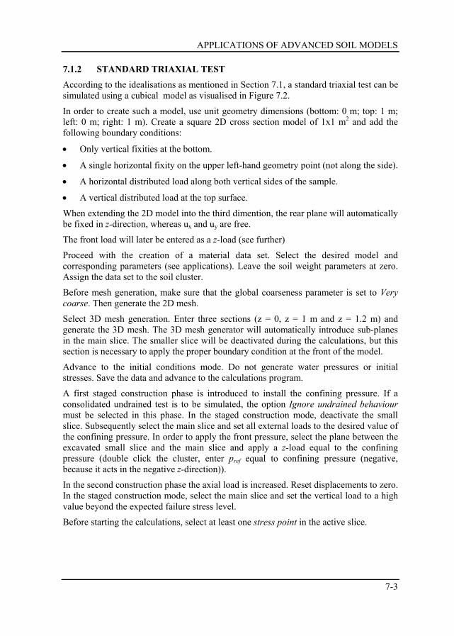
APPLICATIONS OF ADVANCED SOIL MODELS
7-3
7.1.2 STANDARD TRIAXIAL TEST According to the idealisations as mentioned in Section 7.1, a standard triaxial test can be simulated using a cubical model as visualised in Figure 7.2.
In order to create such a model, use unit geometry dimensions (bottom: 0 m; top: 1 m; left: 0 m; right: 1 m). Create a square 2D cross section model of 1x1 m2 and add the following boundary conditions:
• Only vertical fixities at the bottom.
• A single horizontal fixity on the upper left-hand geometry point (not along the side).
• A horizontal distributed load along both vertical sides of the sample.
• A vertical distributed load at the top surface.
When extending the 2D model into the third dimention, the rear plane will automatically be fixed in z-direction, whereas ux and uy are free.
The front load will later be entered as a z-load (see further)
Proceed with the creation of a material data set. Select the desired model and corresponding parameters (see applications). Leave the soil weight parameters at zero. Assign the data set to the soil cluster.
Before mesh generation, make sure that the global coarseness parameter is set to Very coarse. Then generate the 2D mesh.
Select 3D mesh generation. Enter three sections (z = 0, z = 1 m and z = 1.2 m) and generate the 3D mesh. The 3D mesh generator will automatically introduce sub-planes in the main slice. The smaller slice will be deactivated during the calculations, but this section is necessary to apply the proper boundary condition at the front of the model.
Advance to the initial conditions mode. Do not generate water pressures or initial stresses. Save the data and advance to the calculations program.
A first staged construction phase is introduced to install the confining pressure. If a consolidated undrained test is to be simulated, the option Ignore undrained behaviour must be selected in this phase. In the staged construction mode, deactivate the small slice. Subsequently select the main slice and set all external loads to the desired value of the confining pressure. In order to apply the front pressure, select the plane between the excavated small slice and the main slice and apply a z-load equal to the confining pressure (double click the cluster, enter pref equal to confining pressure (negative, because it acts in the negative z-direction)).
In the second construction phase the axial load is increased. Reset displacements to zero. In the staged construction mode, select the main slice and set the vertical load to a high value beyond the expected failure stress level.
Before starting the calculations, select at least one stress point in the active slice.

MATERIAL MODELS MANUAL
7-4 PLAXIS 3D TUNNEL
7.2 HS MODEL: RESPONSE IN DRAINED AND UNDRAINED TRIAXIAL TESTS
In this Section the behaviour of the Hardening-Soil model is illustrated in simulations of drained and undrained triaxial tests using arbitrary sets of model parameters, representing sands of various densities. The parameters for the different data sets are listed in Table 7.1. The main differences involve the stiffness, the friction angle and the dilatancy.
Table 7.1 Arbitrary Hardening-Soil parameters for sands of different densities Parameter Loose Medium Dense Unit
E50ref (for pref = 100 kPa) 20000 30000 40000 kN/m2
Eurref (for pref = 100 kPa) 60000 90000 120000 kN/m2
Eoedref (for pref = 100 kPa) 20000 30000 40000 kN/m2
Cohesion c 0.0 0.0 0.0 kN/m2 Friction angle φ 30 35 40 ° Dilatance angle ψ 0 5 10 ° Poisson's ratio νur 0.2 0.2 0.2 - Power m 0.5 0.5 0.5 - K0
nc (using Cap) 0.5 0.43 0.36 - Tensile strength 0.0 0.0 0.0 kN/m2 Failure ratio 0.9 0.9 0.9 -
The triaxial test is modelled using a cubical model with unit dimensions, as described in Section 0. In the first calculation phase the sample is isotropically compressed up to a confining pressure of p' = 100 kN/m2 assuming drained behaviour. After this phase the displacements are reset to zero. In the second phase the sample is vertically loaded up to failure while the horizontal load (confining pressure) is kept constant. The latter phase is done for drained as well as for undrained material behaviour. These calculations are performed for the three different sets of parameters as listed in Table 7.1. The results of these tests are presented in the graphs of Figure 7.3 to Figure 7.6.
Figure 7.3 shows the development of the principal stress difference as a function of the axial strain. Figure 7.3 and Figure 7.4 show the drained tests. These curves show a hyperbolic relationship between the stress and the strain, which is typical for the Hardening-Soil model. Obviously, the failure level is higher when the sand is denser. The HS model does not include softening behaviour, so after reaching failure the stress level does not reduce, at least in the drained tests. In the undrained tests the failure level is, in principle, lower than in the drained tests. However, on the medium and the dense sands the stress level continues to increase after reaching the failure level due to the fact that dilatancy causes a reduction of excess pore pressures and thus an increase of effective stresses. Care must be taken with this type of behaviour in real projects, since the stress increase at high strains is not realistic. In fact, for undrained materials, the dilatancy angle, should be set to zero.

APPLICATIONS OF ADVANCED SOIL MODELS
7-5
Figure 7.6 shows the development of the excess pore pressures, which confirms the above statement.
Figure 7.4 presents the relationship between the axial strain and the volume strain. This graph clearly shows the influence of dilatancy of the denser sands. In contrast to the Mohr-Coulomb model, the transition from elastic behaviour to failure is much more gradual when using the Hardening-Soil model. In fact, in the HS model, plastic straining occurs from the onset of loading.
0 0.01 0.02 0.03 0.04 0.05 0.06 0
100
200
300
400
ε1
⏐σ1-σ3⏐ [kN/m2]
dense
medium
loose
Figure 7.3 Results of drained triaxial tests using the Hardening-Soil model, Principal stress difference versus axial strain
0 0.01 0.02 0.03 0.04 0.05 0.06 -0.010
-0.005
0.000
0.005
0.010
0.015
-ε1
εv
dense
medium
loose
Figure 7.4 Results of drained triaxial tests using the Hardening-Soil model, Volumetric
strain versus axial strain

MATERIAL MODELS MANUAL
7-6 PLAXIS 3D TUNNEL
0 5.00E-03 0.010 0.015 0.020 0.025 0.030 0
40
80
200
-ε1
⏐σ1-σ3⏐ [kN/m2]
dense
medium
loose
160
120
Figure 7.5 Results of undrained triaxial tests using the Hardening-Soil model, Principal stress difference versus axial strain
0 5.00E-03 0.010 0.015 0.020 0.025 0.030 0
-10
-20
-30
-40
-50
-60
-ε1
pexcess [kPa]
dense
medium
loose
Figure 7.6 Results of undrained triaxial tests using the Hardening-Soil model, Excess
pore pressure vs axial strain

APPLICATIONS OF ADVANCED SOIL MODELS
7-7
0 40 80 120 160 2000
100
200
300
400
-σ'xx [kN/m2]
-σ'yy [kN/m2]
drainedundrained
Figure 7.7 Stress paths for drained and undrained triaxial tests using the HS model
Figure 7.7 shows the effective stress paths during the whole test for the dense sand. The first phase of the test is all drained. In the second phase there is a clear distinction between the drained test and the undrained test. In the undrained test the effective horizontal stress reduces while the vertical stress increases due to the development of excess pore pressures. The decrease in horizontal effective stress is more than when the Mohr-Coulomb model would have been used. This is because of the plastic compaction (Cap hardening) that occurs in the HS model.
7.3 APPLICATION OF THE HARDENING-SOIL MODEL ON REAL SOIL TESTS
In this Section the Hardening-Soil model is subjected to simulations of some laboratory tests on sand in order to validate the response with measured test data. Extensive lab tests were performed on loose and dense Hostun sand. On the basis of these tests the model parameters for the Hardening-Soil model were determined (see also Table 7.2).
Triaxial test The first test that is considered is a standard drained triaxial test on both the loose sand and the dense sand. For the simulation of triaxial tests the configuration is used as described in Section 0. In the first phase the sample is isotropically compressed up to a

MATERIAL MODELS MANUAL
7-8 PLAXIS 3D TUNNEL
confining pressure of p' = 300 kN/m2. In the second phase the sample is vertically loaded up to failure while the horizontal stress (confining pressure) is kept constant. The result of these tests and the comparison with the measured data are presented in Figure 7.8, Figure 7.9 and Figure 7.10.
The calculational results show a reasonable agreement with the test data. There is a gradual transition from elastic to plastic behaviour. The relation between the deviatoric stress and the axial strain can well be approximated by a hyperbola.
The failure level is fully controlled by the friction angle (the cohesion is zero). The test results on dense sand show softening behaviour after the peak load has been reached.
Softening is not included in the Hardening-Soil model, so in contrast to the test data the deviatoric stress remains at the same level. It can also be seen from the test data that the dilatancy reduces during the softening traject. In the Hardening-Soil model the dilatancy continues to infinity, unless the dilatancy cut-off option has been used.
|σ1-σ3| [kPa]
Hardening soil model test data
0
200
400
600
800
1000
1200
1400
0 5 10 15 -ε1 [%]
-2
-1
0
1
εv [%] 0 5 10 15
Figure 7.8 Results of drained triaxial tests on loose Hostun sand, principal stress ratio versus axial strain
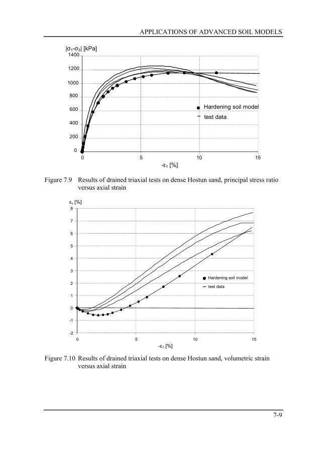
APPLICATIONS OF ADVANCED SOIL MODELS
7-9
0
200
400
600
800
1000
1200
1400
0 5 10 15 -ε1 [%]
|σ1-σ3| [kPa]
Hardening soil model
test data
Figure 7.9 Results of drained triaxial tests on dense Hostun sand, principal stress ratio versus axial strain
-2
-1
0
1
2
3
4
5
6
7
8
0 5 10 15 -ε1 [%]
εv [%]
Hardening soil model
test data
Figure 7.10 Results of drained triaxial tests on dense Hostun sand, volumetric strain
versus axial strain

MATERIAL MODELS MANUAL
7-10 PLAXIS 3D TUNNEL
Oedometer test The second test is an oedometer test on both the loose sand and the dense sand. For the simulation of the oedometer test a simplified geometry with unit dimensions is considered, as described in Section 7.1.1. The same parameters for the Hardening-Soil model are selected as in the triaxial tests (loose and dense sand; see Table 7.2).
Table 7.2 Hardening-Soil parameters for loose and dense Hostun sand Parameter Loose sand Dense sand Unit
Volumetric weight γ 17 17.5 kN/m3
E50ref (pref = 100 kPa) 20000 37000 kN/m2
Eurref (pref = 100 kPa) 60000 90000 kN/m2
Eoedref (pref = 100 kPa) 16000 29600 kN/m2
Cohesion c 0.0 0.0 kN/m2 Friction angle φ 34 41 ° Dilatancy angle ψ 0 14 ° Poisson's ratio νur 0.20 0.20 - Power m 0.65 0.50 - K0
nc 0.44 0.34 - Tensile strength 0.0 0.0 kN/m2 Failure ratio 0.9 0.9 -
From a stress free state the loose sample is subsequently loaded to loads of 25 kPa, 50 kPa, 100 kPa and 200 kPa with intermediate unloadings. The dense sample is loaded to loads of 50 kPa, 100 kPa, 200 kPa and 400 kPa with intermediate unloadings. The results of these tests are presented in Figure 7.11 and Figure 7.12. The results in the figures show a reasonable agreement with the test data. A small offset of 0.15% has been applied to the calculational results of the loose sample in order to account for the relative soft response at the beginning of the test. The results show that it is well possible to back-calculate both triaxial tests and oedometer tests. No doubt, distinction should be made between loose and dense soil, but it seems that for a soil with a certain density the stiffness behaviour under different stress paths can be well captured with a single set of model parameters.
Conclusion The above results have indicated that it is possible to match the results of different tests following different stress paths with the same set of input parameters. This cannot be obtained with simple models like Mohr-Coulomb without changing input parameters. Hence, the parameters in the Hardening-Soil model are consistent and more or less independent from the particular stress path that is followed. This makes the HS model a powerful and accurate model that can be used in many applications.

APPLICATIONS OF ADVANCED SOIL MODELS
7-11
0
100
200
300
400
0 0.005 0.01 0.015 0.02 0.025
-εyy
-σyy [kPa]
Hardening soil model
test data
Figure 7.11 Results of oedometer test on loose Hostun sand, axial stress versus axial
strain
0
100
200
300
400
0 0.005 0.01 0.015 0.02 0.025
-εyy
-σyy [kPa]
Hardening soil model
test data
Figure 7.12 Results of oedometer test on dense Hostun sand, axial stress versus axial
strain

MATERIAL MODELS MANUAL
7-12 PLAXIS 3D TUNNEL
7.4 SSC MODEL: RESPONSE IN ONE-DIMENSIONAL COMPRESSION TEST
In this section the behaviour of the Soft-Soil-Creep model is illustrated on the basis of a one-dimensional compression test on clay. The test is performed assuming drained behaviour to show the logarithmic relationships between strain and stress and the logarithmic time-settlement behaviour on the long term (secondary compression). The Soft-Soil-Creep model parameters used in this example are arbitrarily selected, but they are realistic for normally consolidated clay (see Table 7.3). The vertical preconsolidation stress is installed at 50 kPa (POP = 50 kN/m2). For the simulation of the one-dimensional compression test a simplified geometry with unit dimensions is considered, as described in Section 7.1.1.
Table 7.3 Soft-Soil-Creep model parameters for one-dimensional compression test
Parameter Symbol Value Unit
Unit weight γunsat, sat 0 kN/m3 Modified compression index λ* 0.10 - Modified swelling index κ* 0.02 - Secondary compression index µ* 0.005 - Poisson's ratio νur 0.15 - Cohesion c 1.0 kN/m2 Friction angle φ 30 ° Dilatancy angle ψ 0.0 ° Coeffient of lateral stress K0
nc 0.5 -
In the analysis several calculation phases are used. The load is doubled in every phase using a time increment of 1 day. After the final loading phase an additional creep period of 100 days is introduced without additional loading. The calculation scheme is listed in Table 7.4.
Table 7.4 Calculation scheme for first analysis
Phase Calculation type Load [kPa] Time increment End time
1 Plastic 10 1 1 2 Plastic 20 1 2 3 Plastic 40 1 3 4 Plastic 80 1 4 5 Plastic 160 1 5 6 Plastic 320 1 6 7 Plastic 640 1 7 9 Plastic 80 1 8 8 Plastic 640 100 107

APPLICATIONS OF ADVANCED SOIL MODELS
7-13
1.0 10.0 100.0 1000.0 -0.35
-0.30
-0.25
-0.20
-0.15
-0.10
-0.05
0.00
-sig'-yy [kN/m2]
eps-yy
phase 9, unloading
phase 8, creep
phase 1 - 7, loading
Figure 7.13 Stress-strain curve of oedometer test with Soft-Soil-Creep model; Transient loading with doubling of loading within one day
1000.0 0.1 1.0 10.0 100.0-0.35
-0.30
-0.25
-0.20
-0.15
-0.10
-0.05
0.00
Time [day]
eps-yy
phase 9, unloading
phase 8, creep
phase 1 - 7, loading
Figure 7.14 Time-settlement curve of oedometer test with Soft-Soil-Creep model; Transient loading with doubling of loading within one day

MATERIAL MODELS MANUAL
7-14 PLAXIS 3D TUNNEL
Figure 7.13 shows the load-settlement curve of the analysis. The influence of the preconsolidation stress can clearly be seen, although the transition between reloading and primary loading is not as sharp as when the model would be based on a hardening plasticity formulation. In fact, the results presented here are more realistic. The transition is indeed around the initial preconsolidation stress of 50 kPa. From the inclination of the primary loading line one can back-calculate the modified compression index λ* = ∆ε1 / ln((σ1+∆σ1)/σ1) ≈ 0.10.
Note that 1 mm settlement corresponds with ε1 = 10%. For an axial strain of 30% one would normally use an Updated Mesh analysis. However, in the PLAXIS 3D tunnel program plastic calculations can only be performed according to the small deformation theory.
Figure 7.14 shows the time-settlement curve of the analysis. From the last part of the curve one can back-calculate the secondary compression index µ* = ∆ε1 / ln(∆t/t0) ≈ 0.005 (with t0 = 1 day).
Another interesting phenomenon is the development of the lateral stress. During primary loading, the lateral stress should be given by the value of K0
NC, appropriate for normally consolidated soil. During unloading, the lateral stress decreases much less than the vertical stress, so that the ratio σ′xx / σ′yy increases. In order to show these effects the calculation is continued after step 7 with a drained unloading phase in one day down to a vertical stress of 80 kPa.
Figure 7.15 shows the stress state for two different calculation phases, both at a vertical stress level of 80 kPa. The left hand plot represents the stress state after primary loading In this case, the horizontal stress is found to be approximately 40 kPa. Hence, the stress ratio corresponds to the input value K0
NC = 0.5. The right hand plot represents the final situation after unloading down to 80 kPa.
In this case the horizontal stress is found to be approximately 220 kPa. The decrease of the horizontal stress (∆σ′xx = 100 kPa) during unloading is much less than the decrease of the vertical stress (∆σ′yy = 560 kPa), which results in a situation in which σ′xx is larger than σ′yy.
During sudden unloading in a one-dimensional compression test, the behaviour is almost purely elastic. Hence, the ratio of the horizontal and vertical stress increments is determined by Poisson's ratio νur:
1urxx
yy ur
=
σ νσ ν
∆ ′∆ −′
(7.1)
It is easy to verify that the results correspond with Poisson's ratio νur = 0.15 as listed in Table 7.3.

APPLICATIONS OF ADVANCED SOIL MODELS
7-15
x
y
z
x
y
z
Figure 7.15 Stress states at a vertical stress level of -80 kPa. Above, after primary
loading σxx ≈ -40 kPa. Below, after unloading from -640 kPa σxx ≈ -220 kPa
7.5 JOINTED ROCK MODEL: FAILURE AT DIFFERENT SLIDING DIRECTIONS
In this section the Jointed Rock model is verified for different sliding directions. The sliding direction is defined by means of the parameters α1 (dip angle), α2 (dip direction) and Declination. Therefore a free standing block of rock material is subjected to increased gravity until failure.

MATERIAL MODELS MANUAL
7-16 PLAXIS 3D TUNNEL
The block is 10 m in square and 15 m high (Figure 7.16). The bottom is fully fixed, whereas the remaining sides are free. The behaviour of the rock is modelled by means of the Jointed Rock model with model parameters as listed in Table 7.5.
Figure 7.16 Square rock block subjected to gravity loading
Table 7.5 Jointed Rock model parameters
Parameter Symbol Value Unit
Unit weight γ 22 kN/m3 Young's modulus Ε1 2·105 kN/m2 Poisson's ratio ν1 0.2 - Anisotropic Young's modulus E2 1.2·105 kN/m2 Anisotropic Poisson's ratio ν2 0.2 - Anisotropic shear modulus G2 50000 kN/m2 Cohesion c 50 kN/m2 Friction angle φ 35 ° Dilatancy angle ψ 5 ° Dip angle α1 45 45 45 ° Dip direction α2 0 90 0 ° Declination 0 0 90 °
In order to allow for free displacements in z-direction at the front and the back of the model, small slices are added to the front and the back, and these slices are deactivated in the first calculation phase. In the second calculation phase ΣMweight is increased from 0.0 to 2.0, which causes failure at about 1.9.
Figure 7.17 shows the contours of displacement increments at failure. These figures indicated failure mechanisms that correspond to the mechanisms as shown in Figure 4.6.
10 m
10 m
15 m

APPLICATIONS OF ADVANCED SOIL MODELS
7-17
x
y
z
α1 = 45º α2 = 0º Declination = 0º
x
y
z
α1 = 45º α2 = 90º Declination = 0º
x
y
z
α1 = 45º α2 = 0º Declination = 90º
Figure 7.17 Different failure mechanisms, depending on declination, α1 and α2

MATERIAL MODELS MANUAL
7-18 PLAXIS 3D TUNNEL

REFERENCES
8-1
8 REFERENCES
[1] Adachi, T., Oka, F., (1982). Constitutive equation for normally consolidated clays based on elasto-viscoplasticity. Soils and Foundations 22: 57-70.
[2] Atkinson, J.H., Bransby, P.L., (1978). The Mechanics of Soils. McGraw-Hill, London.
[3] Belytschko, T., Lasry, D., (1989). Localization limiters and numerical strategies for strain-softening materials. Proc. France-US Workshop on Strain localization and size effect due to cracking and Damage (eds. Mazars & Bazant). pp 349-362.
[4] Bjerrum, L., (1967). Engineering geology of Norwegian normally-consolidated marine clays as related to settlements of buildings. Seventh Rankine Lecture. Geotechnique 17: 81-118.
[5] Bolton, M.D., (1986). The Strength and Dilatancy of Sands. Géotechnique, Vol. 36, No. 1, pp. 65-78.
[6] Borja, R.I., Kavazanjian, E, (1985). A constitutive model for the σ-ε-t behaviour of wet clays. Geotechnique 35: 283-298.
[7] Borja, R.I., Lee, S.R., (1990). Cam-clay plasticity, part 1: implicit itegration of elasto-plastic constitutive relations. Computer Methods in Applied Mechanics and Engineering 78: 48-72.
[8] Brinkgreve, R.B.J., Vermeer, P.A., (1992). On the use of Cam-Clay models. Proc. IV Int. Symposium on Numerical Models in Geomechanics (eds. G.N. Pande, S. Pietruszczak). Balkema, Rotterdam, Vol. 2, pp. 557-565.
[9] Brinkgreve, R.B.J., (1994). Geomaterial Models and Numerical Analysis of Softening. Dissertation. Delft University of Technology.
[10] Buisman, K., (1936). Results of long duration settlement tests. Proceedings 1st International Conference on Soil Mechanics and Foundation Engineering, Cambridge, Mass. Vol. 1: 103-107.
[11] Burland, J.B., (1965). The Yielding and Dilation of Clay. (Correspondence). Géotechnique, Vol. 15, pp. 211-214.
[12] Burland, J.B., (1967). Deformation of Soft Clay. Dissertation. Cambridge University.
[13] Butterfield, R., (1979). A natural compression law for soils (an advance on e-log p’). Geotechnique 29:469-480.
[14] Chen, W.F., (1975). Limit Analysis and Soil Plasticity. Elsevier, Amsterdam.
[15] Drucker, D.C., Prager, W., (1952). Soil Mechanics and Plastic Analysis or Limit Design. Quart. Appl. Math. Vol. 10, No. 2, pp. 157-165.
[16] Duncan, J.M., Chang, C.-Y., (1970). Nonlinear Analysis of Stress and Strain in Soil. ASCE J. of the Soil Mech. and Found. Div. Vol. 96, pp. 1629-1653.

MATERIAL MODELS MANUAL
8-2 PLAXIS 3D TUNNEL
[17] Fung, Y.C., (1965). Foundations of Solid Mechanics, Prentice-Hall, New Jersey, USA.
[18] Garlanger, J.E., (1972). The consolidation of soils exhibiting creep under constant effective stress. Geotechnique 22: 71-78.
[19] den Haan, E.J., (1994). Vertical Compression of Soils. Thesis, Delft University.
[20] Hill, R., (1950). The Mathematical Theory of Plasticity, Oxford University Press, London, U.K.
[21] Janbu, N., (1969). The resistance concept applied to soils. Proceedings of the 7h ICSMFE, Mexico City 1:191-196.
[22] Janbu, J., (1963). Soil Compressibility as Determined by Oedometer and Triaxial Tests. Proc. ECSMFE Wiesbaden, Vol. 1, pp. 19-25.
[23] Koiter, W.T., (1960). General Theorems for Elastic-Plastic Solids. In: Progress in Solid Mechanics (eds. I.N. Sneddon, R. Hill), Vol. 1., North-Holland, Amsterdam, pp. 165-221.
[24] Kondner, R.L., (1963). A Hyperbolic Stress Strain Formulation for Sands. 2. Pan. Am. ICOSFE Brazil, Vol. 1, pp. 289-324.
[25] Kulhawy, F. H., Mayne, P.W., (1990). Manual on Estimating Soil Prperties for Foundation Design. Cornell University, Ithaca, New York.
[26] van Langen, H., Vermeer, P.A., (1990). Automatic Step Size Correction for Non-Associated Plasticity Problems. Int. J. Num. Meth. Engng., Vol. 29, pp. 579-598.
[27] Leroueil, S., (1977). Quelques considérations sur le comportement des argiles sensibles. Ph.D. thesis, Laval University, Québec.
[28] Muir Wood, D., (1990). Soil Behaviour and Critical State Soil Mechanics. Cambridge University Press.
[29] Neher, H., Vermeer, P.A. (1998). Formulation and application of a soil model that accounts for creep. Int. J. Numer. Anal. Meth. Geomech.
[30] Prevost, J.-H., (1976). Undrained Stress-Strain-Time Behaviour of Clays. Journal of the Geotechnical Engineering Division GT12: 1245-1259.
[31] Rowe, P.W., (1962). The Stress-Dilatancy Relation for Static Equilibrium of an Assembly of Particles in Contact. Proc. Roy. Soc. A., No. 269, pp. 500-527.
[32] Schanz, T., (1998). Zur Modellierung des Mechanischen Verhaltens von Reibungsmaterialen, Habilitation, Stuttgart Universität.
[33] Schanz, T., Vermeer, P.A., (1996). Angles of Friction and Dilatancy of Sand. Géotechnique 46, pp. 145-151.
[34] Schanz, T., Vermeer, P.A., (1998). Special issue on Pre-failure deformation behaviour of geomaterials. Géotechnique 48, pp. 383-387.

REFERENCES
8-3
[35] Schanz, T., Vermeer, P.A., Bonnier, P.G., (1999). Formulation and verification of the Hardening-Soil Model. In: R.B.J. Brinkgreve, Beyond 2000 in Computational Geotechnics. Balkema, Rotterdam: 281-290.
[36] Sekiguchi, H., (1977). Rheological characteristics of clays. Proceedings of the 9th ICSMFE, Tokyo 1:289-292.
[37] Smith, I.M., Griffith, D.V., (1982). Programming the Finite Element Method, Second Edition. John Wiley & Sons, Chisester, U.K.
[38] von Soos, P., (1990). Properties of Soil and Rock (in German). In: Grundbautaschenbuch Part 4, Edition 4, Ernst & Sohn, Berlin.
[39] Stolle, D.F.E., (1991). An interpretation of initial stress and strain methods, and numerical stability. International Journal for Numerical and Analytical Methods in Geomechanics 15: 399-416.
[40] Stolle, D.F.E., Bonnier, P.G., Vermeer, P.A., (1997). A soft soil model and experiences with two integration schemes. Numerical Models in Geomechanics. Numog 1997: 123-128.
[41] Vaid, Y., Campanella, R.G. (1977). Time-dependent behaviour of undisturbed clay. ASCE Journal of the Geotechnical Engineering Division, 103(GT7), pp. 693-709.
[42] Vermeer, P.A., de Borst, R., (1984). Non-Associated Plasticity for Soils, Concrete and Rock. Heron, Vol 29, No. 3.
[43] Vermeer, P.A., van Langen, H., (1989). Soil collapse computations with finite elements. Ingenieur-Archiv 59: 221-236.
[44] Vermeer, P.A., Stolle, D.F.E., Bonnier, P.G. (1998). From the classical theory of secondary compression to modern creep analysis. Proc. 9th Int. Conf. Comp. Meth. and Adv. Geomech.. Wuhan, China, Vol. 4, pp 2469-2478.
[45] Zienkiewicz , O.C., Taylor, R.L., (1994). The finite element method, 4th edition. McGraw-Hill, London, UK.

MATERIAL MODELS MANUAL
8-4 PLAXIS 3D TUNNEL

APPENDIX A - SYMBOLS
A-1
APPENDIX A - SYMBOLS c : Cohesion Cu , Su : Undrained shear-strength De : Elastic material matrix representing Hooke's law e : Void ratio E : Young's modulus Eoed : Oedometer modulus f : Yield function g : Plastic potential function G : Shear modulus K : Bulk modulus K0 : Coefficient of lateral earth pressure m : Power in stress-dependent stiffness relation M : Slope of critical state line in p'-q space n : Porosity OCR : Overconsolidation ratio p : Isotropic stress or mean stress,
positive for pressure; negative for tension pp : Isotropic preconsolidation stress, positive for pressure POP : Pre overburden pressure q : Equivalent shear stress or deviatoric stress Rf : Failure ratio t : Time u : Vector with displacement components γ : Volumetric weight α1 : Dip angle α2 : Dip direction ε : Vector with Cartesian strain components, normal components
positive for extension; negative for compression εv : Volumetric strain,
negative for compression; positive for extension κ : Cam-Clay swelling index κ* : Modified swelling index λ : Plastic multiplier λ : Cam-Clay compression index λ* : Modified compression index µ* : Modified creep index ν : Poisson's ratio σ : Vector with Cartesian stress components, normal components
positive for tension; negative for pressure σp : Vertical preconsolidation stress, negative for pressure φ : Friction angle ψ : Dilation angle

MATERIAL MODELS MANUAL
A-2 PLAXIS 3D TUNNEL
Copyright © 2022 FDOKUMEN