Plastic collapse in non-associated hardening materials with application to Cam-clay

This article appeared in a journal published by Elsevier. The attachedcopy is furnished to the author for internal non-commercial researchand education use, including for instruction at the authors institution

and sharing with colleagues.

Other uses, including reproduction and distribution, or selling orlicensing copies, or posting to personal, institutional or third party

websites are prohibited.

In most cases authors are permitted to post their version of thearticle (e.g. in Word or Tex form) to their personal website orinstitutional repository. Authors requiring further information

regarding Elsevier’s archiving and manuscript policies areencouraged to visit:

http://www.elsevier.com/copyright

http://www.elsevier.com/copyright

Author's personal copy

Potentials for the modified Cam-Clay model

Nestor Zouain a,*, Ivaldo Pontes b, Jean Vaunat c

a Mechanical Engineering Department, COPPE, EE, UFRJ – Federal University of Rio de Janeiro, C.P. 68503, CEP 21945-970, RJ, Brazilb Civil Engineering Department, UFPE – Federal University of Pernambuco, Recife, PE, Brazilc Department of Geotechnical Engineering and Geosciences, Technical University of Catalonia (UPC), Barcelona, Spain

a r t i c l e i n f o

Article history:Received 21 March 2009Accepted 23 November 2009Available online 27 November 2009

Keywords:Plastic collapseCam-ClayVariational principlesSoil mechanics

a b s t r a c t

Energy and dissipation pseudo-potentials are employed to derive constitutive relationships, in thecontext of thermodynamic concepts, for the widely used Modified Cam-Clay (MCC) model for soilmechanics. A variational formulation of the MCC evolution equations is proposed in this paper. Sinceplastic collapse of MCC soils cannot be embedded in the classical limit analysis theory, finding the criticalamplification of the load that produces plastic collapse is formulated in the form of a system of equationsand inequalities. Then, a mixed minimization principle is proposed for the plastic collapse analysis ofMCC soils. This principle is obtained by the application of the variational formulation for the flow lawintroduced in the first part of the article.

� 2009 Elsevier Masson SAS. All rights reserved.

1. Introduction

The Modified Cam-Clay (MCC) model by Roscoe and Burland(1968) is an important conceptual framework for constitutivebehavior in soil mechanics (Wood, 1990; Houlsby and Puzrin, 2006;Ulm and Coussy, 2003; Borja and Lee, 1990; Vaunat et al., 2000;Einav et al., 2007). It has been widely used in its simpler, classicalform and also in more sophisticated versions that extend itsapplication to a broader variety of situations.

This paper is focused on the formal structure of the classicalMCC model as derived from the energy and dissipation potentialsbased on thermodynamics.

The systematic application of thermodynamic concepts to theformulation of constitutive models of inelastic solids has reacheda sophisticated stage due to pioneering work and manyoutstanding contributions. In a simplified description of thisresearch field, thermodynamic principles are invoked to findenergy and dissipation functionals that are used to derive state andevolution relations in the form of potential laws.

Among many other contributions to the thermodynamicformulation of constitutive equations, we cite first the work ofZiegler (1983). Halphen and Nguyen (1975) (see also Nguyen, 2000)proposed a framework, the Standard Generalized Materials (GSM),which is a widely referenced approach to material behaviormodeling. G. T. Houlsby and coworkers (Collins et al., 1997; Houlsby

and Puzrin, 2006) contributed with the concept of Hyperplasticity,which is a complete methodology to consistently develop consti-tutive equations based on thermodynamic principles. Rich andrigorous contributions to thermomechanics with internal variablesare also found in Maugin (1992), Han and Reddy (1999) and Silhav�y(1997).

We use an extension of the concept of potential laws proposedby de Saxce (1992), based on a special class of functions, namedbipotentials by de Saxce. These functions are, by definition, sepa-rately convex in two independent variables and bounded below bythe scalar product of the variables. Generalized potential laws areobtained, in direct and inverse forms, by partial subdifferentiation(Rockafellar, 1970). This gives implicit constitutive equations,instead of the usual explicit direct and inverse relations. Accord-ingly, the class of material represented by this kind of constitutiveequations is called Implicit Standard Materials (ISM) (de Saxce,1995; de Saxce and Bousshine, 1998; Hjiaj, 1999; Bodoville, 2001). Itis a generalization of GSM.

This paper contains a unified derivation of energy and dissipa-tion potentials for the MCC model, beginning with some knownpotentials.

We propose a mixed approach to the evolution relations ofMCC materials. Throughout this paper, the expressions mixedformulation and mixed potential are used to emphasize thatgeneralized stresses and plastic strains (or strain rates) are takentogether as a pair of independent variables. In the framework ofthis mixed approach, we propose a minimization principle for theMCC flow law.

The mixed variational principles for MCC are applied to theanalysis of plastic collapse of soils. The expression plastic collapse

* Corresponding author. Tel.: þ55 21 2562 8380; fax: þ55 21 2562 8383.E-mail address: [email protected] (N. Zouain).

Contents lists available at ScienceDirect

European Journal of Mechanics A/Solids

journal homepage: www.elsevier .com/locate/e jmsol

0997-7538/$ – see front matter � 2009 Elsevier Masson SAS. All rights reserved.doi:10.1016/j.euromechsol.2009.11.008

European Journal of Mechanics A/Solids 29 (2010) 327–336


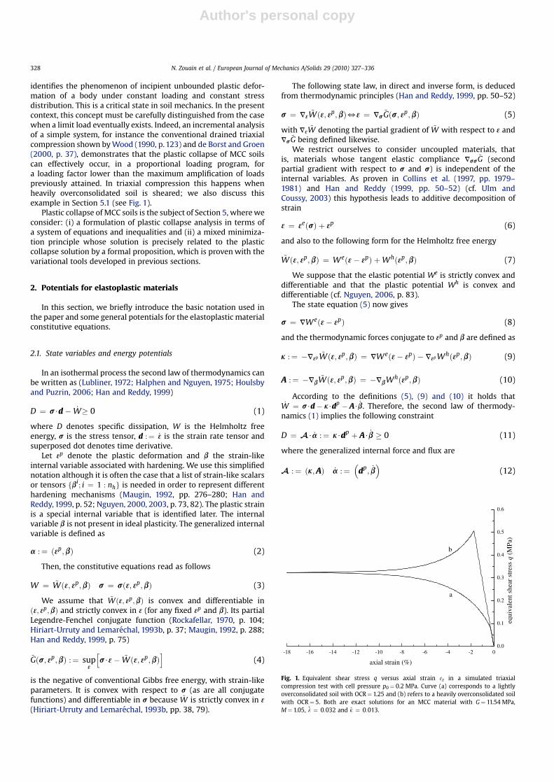
identifies the phenomenon of incipient unbounded plastic defor-mation of a body under constant loading and constant stressdistribution. This is a critical state in soil mechanics. In the presentcontext, this concept must be carefully distinguished from the casewhen a limit load eventually exists. Indeed, an incremental analysisof a simple system, for instance the conventional drained triaxialcompression shown by Wood (1990, p. 123) and de Borst and Groen(2000, p. 37), demonstrates that the plastic collapse of MCC soilscan effectively occur, in a proportional loading program, fora loading factor lower than the maximum amplification of loadspreviously attained. In triaxial compression this happens whenheavily overconsolidated soil is sheared; we also discuss thisexample in Section 5.1 (see Fig. 1).

Plastic collapse of MCC soils is the subject of Section 5, where weconsider: (i) a formulation of plastic collapse analysis in terms ofa system of equations and inequalities and (ii) a mixed minimiza-tion principle whose solution is precisely related to the plasticcollapse solution by a formal proposition, which is proven with thevariational tools developed in previous sections.

2. Potentials for elastoplastic materials

In this section, we briefly introduce the basic notation used inthe paper and some general potentials for the elastoplastic materialconstitutive equations.

2.1. State variables and energy potentials

In an isothermal process the second law of thermodynamics canbe written as (Lubliner, 1972; Halphen and Nguyen, 1975; Houlsbyand Puzrin, 2006; Han and Reddy, 1999)

D ¼ s$d� _W� 0 (1)

where D denotes specific dissipation, W is the Helmholtz freeenergy, s is the stress tensor, d :¼ _3 is the strain rate tensor andsuperposed dot denotes time derivative.

Let 3p denote the plastic deformation and b the strain-likeinternal variable associated with hardening. We use this simplifiednotation although it is often the case that a list of strain-like scalarsor tensors fbi

; i ¼ 1 : nhg is needed in order to represent differenthardening mechanisms (Maugin, 1992, pp. 276–280; Han andReddy, 1999, p. 52; Nguyen, 2000, 2003, p. 73, 82). The plastic strainis a special internal variable that is identified later. The internalvariable b is not present in ideal plasticity. The generalized internalvariable is defined as

a :¼ ð3p;bÞ (2)

Then, the constitutive equations read as follows

W ¼ ~Wð3; 3p;bÞ s ¼ sð3; 3p;bÞ (3)

We assume that ~Wð3; 3p;bÞ is convex and differentiable inð3; 3p;bÞ and strictly convex in 3 (for any fixed 3p and b). Its partialLegendre-Fenchel conjugate function (Rockafellar, 1970, p. 104;Hiriart-Urruty and Lemarechal, 1993b, p. 37; Maugin, 1992, p. 288;Han and Reddy, 1999, p. 75)

~Gðs; 3p;bÞ :¼ sup3

hs$3� ~Wð3; 3p;bÞ

i(4)

is the negative of conventional Gibbs free energy, with strain-likeparameters. It is convex with respect to s (as are all conjugatefunctions) and differentiable in s because ~W is strictly convex in 3

(Hiriart-Urruty and Lemarechal, 1993b, pp. 38, 79).

The following state law, in direct and inverse form, is deducedfrom thermodynamic principles (Han and Reddy, 1999, pp. 50–52)

s ¼ V3~Wð3; 3p;bÞ53 ¼ Vs

~Gðs; 3p;bÞ (5)

with V3~W denoting the partial gradient of ~W with respect to 3 and

Vs~G being defined likewise.We restrict ourselves to consider uncoupled materials, that

is, materials whose tangent elastic compliance Vss~G (second

partial gradient with respect to s and s) is independent of theinternal variables. As proven in Collins et al. (1997, pp. 1979–1981) and Han and Reddy (1999, pp. 50–52) (cf. Ulm andCoussy, 2003) this hypothesis leads to additive decomposition ofstrain

3 ¼ 3eðsÞ þ 3p (6)

and also to the following form for the Helmholtz free energy

~Wð3; 3p;bÞ ¼ Weð3� 3pÞ þWhð3p;bÞ (7)

We suppose that the elastic potential We is strictly convex anddifferentiable and that the plastic potential Wh is convex anddifferentiable (cf. Nguyen, 2006, p. 83).

The state equation (5) now gives

s ¼ VWeð3� 3pÞ (8)

and the thermodynamic forces conjugate to 3p and b are defined as

k :¼ �V3p ~Wð3; 3p;bÞ ¼ VWeð3� 3pÞ � V3p Whð3p;bÞ (9)

A :¼ �Vb~Wð3; 3p;bÞ ¼ �VbWhð3p;bÞ (10)

According to the definitions (5), (9) and (10) it holds that_W ¼ s$d� k$dp � A$ _b. Therefore, the second law of thermody-

namics (1) implies the following constraint

D ¼ A$ _a :¼ k$dp þ A$ _b � 0 (11)

where the generalized internal force and flux are

A :¼ ðk;AÞ _a :¼�

dp; _b�

(12)

-18 -16 -14 -12 -10 -8 -6 -4 -2 00.0

0.1

0.2

0.3

0.4

0.5

0.6

b

a

equi

vale

nt s

hear

str

ess

q (M

Pa)

axial strain (%)

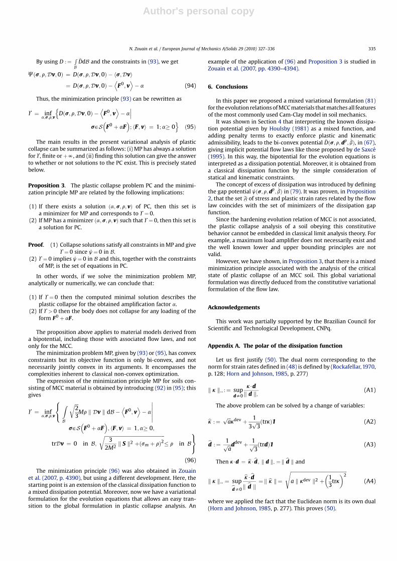
Fig. 1. Equivalent shear stress q versus axial strain 3z in a simulated triaxialcompression test with cell pressure p0¼ 0.2 MPa. Curve (a) corresponds to a lightlyoverconsolidated soil with OCR¼ 1.25 and (b) refers to a heavily overconsolidated soilwith OCR¼ 5. Both are exact solutions for an MCC material with G¼ 11.54 MPa,M¼ 1.05, ~l ¼ 0:032 and ~k ¼ 0:013.

N. Zouain et al. / European Journal of Mechanics A/Solids 29 (2010) 327–336328


2.1.1. The conjugate function of the free energyLet us consider first the conjugate function of the elastic part,

We, of the Helmholtz free energy, i.e.

GeðsÞ :¼ sup3e

�s$3e �Weð3eÞ

�(13)

Then, we have

s ¼ VWeð3eÞ53e ¼ VGeðsÞ5GeðsÞ þWeð3eÞ ¼ s$3e (14)

It follows from the above relations that the partial Gibbs freeenergy, through the duality transformation (4) to the energypotential given by (7), is

~Gðs; 3p;bÞ ¼ GeðsÞ þ s$3p �Whð3p;bÞ (15)

The rest of this subsection is devoted to obtaining the completedual function of the free energy ~Wð3; 3p;bÞ.

First, we consider the conjugate function of the inelastic part,Wh, of the Helmholtz free energy

Ghðr;�AÞ :¼ sup3p;b

nr$3p � A$b�Whð3p;bÞ

o(16)

This transformation may result in a non-differentiable functionGh under the hypothesis that Wh is convex. Indeed, differentiabilityof Gh corresponds to strict convexity of Wh, which is not true forthe Cam-Clay model presented in the next sections. Accordingly,the subdifferential concept (which we use for the dissipationpotential in the following sections) should be applied to Gh inorder to obtain the inverse relations. These inverse relations willnot be needed in our presentation of the MCC model. Thus, wewrite below the inverse relations, under the differentiabilityhypothesis, for completeness and also for the purpose ofcomparing to references.

According to (16), in the differentiable case,

ðr;�AÞ ¼ VWhð3p;bÞ5ð3p;bÞ ¼ VGhðr;�AÞ5Ghðr;�AÞ þWhð3p;bÞ ¼ r$3p � A$b

(17)

The variable r was introduced above as the conjugate of 3p in theduality transformation (16); however, taking into account (8), (9)and (17), it holds that (cf.: Collins et al., 1997, p. 1980; Nguyen, 2006,p. 83)

k ¼ s� r r ¼ V3p Whð3p;bÞ (18)

Thus, r has the meaning of a back-stress.We choose ð3e; 3p;bÞ and ðs;r;AÞ as the dual pair of variables. An

alternative choice may be the pair ð3; 3p;bÞ and ðs; k;AÞ as adopted,for instance, in Collins et al. (1997).

Consequently, we consider the following definition for theHelmholtz potential

Wð3e; 3p;bÞ :¼ Weð3eÞ þWhð3p;bÞ (19)

The complete Gibbs free energy, which is conjugated to theenergy potential given by (7), is now defined as

Gðs; r;AÞ :¼ sup3e;3p;b

½s$3e þ r$3p � A$b�Wð3e; 3p;bÞ� (20)

Thus, taking into account (17) and (14)

Gðs; r;AÞ ¼ GeðsÞ þ Ghðr;�AÞ (21)

and the corresponding state equations are

3e ¼ VGeðsÞ 3p ¼ VrGhðr;�AÞ b ¼ Vð�AÞGhðr;�AÞ (22)

Then, 3 ¼ 3e þ 3p and k ¼ s� r appear as subsidiary equations.

2.2. Evolution equations and dissipation potentials

Because there is no characteristic time in inviscid plasticity, anappropriate dissipation potential for this case

D ¼ D�

_a;a�

(23)

must be positively homogeneous with degree one, with respect to_a ¼ ðdp; _bÞ; that is, Dðc _a;aÞ ¼ cDð _a;aÞ c c > 0. Thus, the value ofthe dissipation function for _a ¼ 0 and any a can only be zero orinfinity; we rule out the latter case.

In addition, the dissipation potential is assumed to be convex,lower semicontinuous and positive for all _as0.

For the material models addressed here, it is necessary toconsider non-differentiable dissipation potentials, although theyare supposed to be within the class of functions endowed with sub-differentiability (Rockafellar, 1970; Hiriart-Urruty and Lemarechal,1993a).

Then, A and _a are related by the constitutive evolution relationif and only if they fulfill the following inclusion

A˛v _aD�

_a;a�

(24)

where v _aDð _a;aÞ denotes the partial subdifferential of D withrespect to _a. The above inclusion is equivalent, by definition, to thefollowing variational inequality

D�

_a*;a�� D

�_a;a�� A$

�_a* � _a

�c _a* (25)

This choice for the evolution equation automatically satisfies thesecond law constraint (11).

We note that the generalized strain-like internal variable a isa passive parameter in this relation.

There is another hypothesis, regarding the coincidence of theinternal forces in (24), (9) and (10), that is implicitly adopted here.This issue is discussed by Houlsby and Puzrin (2006) and resolvedby restricting the class of materials envisaged or, alternatively, byaccepting Ziegler’s principle.

In the following, we focus on the inverse of the evolution Eq.(24), which is classically known as the (direct) plastic flow law. Weshow that it has the following form

_a˛NPðA;aÞ :¼ vIPðaÞðAÞ (26)

where PðaÞ is the domain of plastic admissibility of the generalizedinternal force A, NPðA;aÞ is the cone of normals to PðaÞ at A, theindicator function of PðaÞ is defined as IPðaÞðAÞ :¼ 0 ifA˛PðaÞ andþN otherwise, and vIPðaÞðAÞ is the subdifferential set defined bythe following variational inequality

IPðaÞ�A*�� IPðaÞðAÞ�

�A* �A

�$ _a c A* (27)

This is equivalent to

A˛PðaÞ (28)

A$ _a� A*$ _a c A*˛PðaÞ (29)

In fact, functions like Dð _a;aÞ, that are convex, closed, non-negative and positively homogeneous of degree one in _a (i.e.functions called gauges), are associated, through a bijective rela-tion, with sets PðaÞ in the dual space of the variable A that are

N. Zouain et al. / European Journal of Mechanics A/Solids 29 (2010) 327–336 329


closed, convex and contain the origin (Rockafellar, 1970, p. 128;Hiriart-Urruty and Lemarechal, 1993a, p. 218). This is a well knownduality relation in convex analysis. In the present constitutiverelationship, this means that if we assume that inelastic processeshave no characteristic time then an admissibility domain for thedissipative forces necessarily exists.

There are formulas implementing the bijective relation betweenDð _a;aÞ and PðaÞ. Initially, we know that the dissipation potential isthe support function of the admissibility domain (Rockafellar, 1970,p. 112; Aubin and Ekeland, 1984, p. 204), that is

D�

_a;a�¼ supA

�A$ _a

��A˛PðaÞ�

(30)

This allows the computation of the dissipation function if theplastic admissibility function is given.

Furthermore, the indicator function IPðaÞðAÞ is the conjugate, ina Fenchel transformation, of the dissipation function Dð _a;aÞ. Then,a fundamental theorem in convex analysis (Rockafellar, 1970, p.218; Aubin and Ekeland, 1984, p. 202) states that (24)–(27) and theequation

D�

_a;a�þ IPðaÞðAÞ ¼ A$ _a (31)

are all equivalent expressions of the same relation between _a andA, i.e. these are equivalent evolution equations.

Let us introduce the following representation for the plasticadmissibility set

PðaÞ ¼ fAjf ðA;aÞ� 0g (32)

where f is the plastic admissibility function that is assumed to beregular for the sake of simplicity. Then, the flow law is expressed inthe usual form (Rockafellar, 1970, p. 222).

_a ¼ _lVA f ðA;aÞ (33)

_lf ðA;aÞ ¼ 0 f ðA;aÞ� 0 _l� 0 (34)

If the dissipation function is given, we may compute its polarfunction as follows:

FðA;aÞ ¼ sup_as0

A$ _a

Dð _a; _aÞ (35)

and therefore determine the plastic admissibility set using thefollowing plastic admissibility function

f 0ðA;aÞ ¼ FðA;aÞ � 1� 0 (36)

Notice that the same convex set PðaÞ can be represented bydifferent plastic admissibility functions (some of them being non-convex). However, there is always a unique canonical representa-tion, in the form (36), in terms of the gauge function FðA;aÞassociated with PðaÞ (Rockafellar, 1970, p. 79; Hiriart-Urruty andLemarechal, 1993a, p. 203).

Alternatively, if we suppose that a prescribed set is givenPðaÞ, which is closed, convex and contains the origin, then itsgauge function (Rockafellar, 1970, p. 28), also known as theMinkowski function (Kamenjarzh, 1996, p. 147), is obtained bythe formula

FðA;aÞ ¼ inffz� 0jA˛zPðaÞg (37)

This results in a function that is non-negative, closed, convex,positively homogeneous of degree one and with value zero at theoriginA ¼ 0. If the origin of the generalized stress space is strictlyinterior to the set PðaÞ then FðA;aÞ is always positive, except at the

origin. In the case of the MCC model the origin is exactly on theboundary of the plastic admissible domain.

3. Modified Cam-Clay model

This section is concerned with the energy and dissipationpotentials associated with the Modified Cam-Clay model of Roscoeand Burland (1968). We adopt, in the first part of this section, theassumptions of Collins et al. (1997) and Houlsby and Puzrin (2006).

In Subsection 3.3, we comment on the non-associativity of theMCC equations and justify a re-interpretation of the variables andparameters in the dissipation potential. This leads to the mixedapproach proposed in Section 4.

3.1. MCC state equations

Let us introduce the notation

sm :¼ 13

trs S ¼ sdev :¼ s� sm1 (38)

3v :¼ tr3 3dev :¼ 3� 13ðtr3Þ1 dv :¼ trd (39)

for the following variables: the mean stress sm, the deviatoric partof stress S, the volumetric strain 3v, the deviatoric part of strain 3dev

and the volumetric strain rate dv.We adopt in this paper the basic isotropic elastic potentials (40)

and (41), as given by Houlsby and Puzrin (2006, p. 189). This allowsus to present and discuss the essential features of the ModifiedCam-Clay model without going through more cumbersomeexpressions. In this simplified elastic model the bulk modulusresults proportional to pressure and the shear modulus is assumedconstant (different from the more usual assumption of constantPoisson ratio). However, it is known that in order to improve theadequacy of the ideal model to actual soil behavior more sophis-ticated elastic equations should be adopted. A thorough discussionof this issue is given by Houlsby and Puzrin (2006) in Chapter 9,which also contains non-linear elastic relationships more closelyrepresenting real soils. It is worth mentioning that some otherelastic relations adopted for MCC in the literature are not derivedfrom an energy potential and this may lead to non-reversibleresponses.

Let the Helmholtz free energy be given by

Weð3� 3pÞ ¼ G k 3dev � ð3pÞdevk2 þ~kp0exp�� 3v � 3p

v

~k

�(40)

Whð3pÞ ¼ 12

�~l� ~k

�px0exp

�� 3p

v

~l� ~k

�(41)

where the shear modulus G is assumed to be constant, p0 and px0

are reference values of hydrostatic pressure, ~l is the virgincompression index and ~k is the swell-recompression index.

The corresponding state equations are (cf.: Hjiaj, 1999, p. 61; deBorst and Groen, 2000, p. 33; Vaunat et al., 2000, p. 126; Ulm andCoussy, 2003, p. 293, Houlsby and Puzrin, 2006, p. 189).

S ¼ V3dev We ¼ 2Gh3dev � ð3pÞdev

i(42)

sm ¼ V3vWe ¼ �p0exp

�� 3v � 3p

v

~k

�(43)

r ¼ V3p Wh ¼ �r1 (44)



with

r :¼ 12

px0exp�� 3p

v

~l� ~k

�(45)

Thus

k ¼ sþ r1 (46)

3.2. MCC evolution equations

The dissipation function that characterizes MCC constitutivebehavior, given by

D�dp; 3p

v

�¼ rð3p

v Þ

ffiffiffiffiffiffiffiffiffiffiffiffiffiffiffiffiffiffiffiffiffiffiffiffiffiffiffiffiffiffiffiffiffiffiffiffiffiffiffiffiffiffiffiffiffiffiffiffiffiffiffi2M2

3k dp dev k2 þ

�dp

v

�2

s(47)

was first found by Houlsby (1981). We take this potential as thestarting point for the definition of the evolution equations. In fact,this dissipation function leads to the widely known MCC elasticdomains in the form of ellipses in the stress space, as proven in thefollowing.

It is worth identifying the main features in (47). The followinganalysis shows that the MCC dissipation potential is, in a way,a simple quadratic proposal. Indeed, according to (47):

(1) Shear plastic strain rate components are weighted by a nondi-mensional material parameter M, when compared to thevolumetric plastic strain rate.

(2) The positively homogeneous function expressing the depen-dence of the dissipation with respect to the plastic strain ratedp is the Euclidean norm of the mean and weighted shear strainrate components

k dp k*:¼

ffiffiffiffiffiffiffiffiffiffiffiffiffiffiffiffiffiffiffiffiffiffiffiffiffiffiffiffiffiffiffiffiffiffiffiffiffiffiffiffiffiffiffiffiffiffiffiffiffia�1 k dp dev k2 þ

�dp

v

�2q

(48)

where

a :¼ 32M2 (49)

The function (48) belongs to the class of gauge functions,therefore it is admissible as a dissipation potential. In particular, it isa norm for strain rate tensors, whose polar function is then its dualnorm, computed in Appendix A (cf. de Saxce, 1995, p. 4)

k k k**

:¼ffiffiffiffiffiffiffiffiffiffiffiffiffiffiffiffiffiffiffiffiffiffiffiffiffiffiffiffiffiffiffiffiffiffiffiffiffiffiffiffia k kdev k2 þðkmÞ2

q(50)

(3) The dissipation is proportional to a strength parameter thatonly depends on the volumetric part of the kinematical internalvariable. This is a crucial assumption of this model, which isfounded on experimental evidence (Wood, 1990, p. 89). In thepresent framework, the role of the strength parameter isplayed by the (scalar) back-stress r.

Obtaining the plastic admissibility domain is just a matter ofapplying the tools of convex analysis. Indeed, the polar function ofthe dissipation potential, computed in Appendix A, is

bFðk; 3pv Þ ¼ ½rð3p

v Þ��1k k k

**¼ ½rð3p

v Þ��1

ffiffiffiffiffiffiffiffiffiffiffiffiffiffiffiffiffiffiffiffiffiffiffiffiffiffiffiffiffiffiffiffiffiffiffiffiffiffiffia k kdev k2 þðkmÞ2

q(51)

As a result, the corresponding canonical representation of theplastic admissibility domain Pð3p

v Þ is given by the condition

f 0ðk; 3pv Þ :¼ ½rð3p

v Þ��1

ffiffiffiffiffiffiffiffiffiffiffiffiffiffiffiffiffiffiffiffiffiffiffiffiffiffiffiffiffiffiffiffiffiffiffiffiffiffiffiffia k kdev k2 þðkmÞ2

q� 1� 0 (52)

However, for the sake of convenience, we adopt the followingequivalent plastic admissibility constraint

~f ðk;3pv Þ :¼k k k

**�rð3p

v Þ ¼ffiffiffiffiffiffiffiffiffiffiffiffiffiffiffiffiffiffiffiffiffiffiffiffiffiffiffiffiffiffiffiffiffiffiffiffiffiffia k kdev k2 þðkmÞ2

q� rð3p

v Þ� 0 (53)

The evolution equations are obtained by computing derivativesof the plastic function. This gives

dp dev ¼ _la

k k k**

kdev dpv ¼ _l

km

k k k**

(54)

We note that the above equations imply k dp k*¼ _l.

Finally, we rewrite the plastic admissibility constraint in termsof the true stress by substituting, in view of (46), kdev ¼ S andkm¼ smþ r.

bf ðs; 3pv Þ :¼k sþ rð3p

v Þ1 k**�rð3p

v Þ

¼ffiffiffiffiffiffiffiffiffiffiffiffiffiffiffiffiffiffiffiffiffiffiffiffiffiffiffiffiffiffiffiffiffiffiffiffiffiffiffiffiffiffiffiffiffiffiffiffiffia k S k2 þ½sm þ rð3p

v Þ�2q

� rð3pv Þ� 0 (55)

Accordingly, the flow equations are

dp dev ¼ _labRS dp

v ¼ _lsm þ rbR (56)

_lbf ðs; 3pv Þ ¼ 0 bf ðs; 3p

v Þ� 0 _l� 0 (57)

where

bR :¼ffiffiffiffiffiffiffiffiffiffiffiffiffiffiffiffiffiffiffiffiffiffiffiffiffiffiffiffiffiffiffiffiffiffiffiffiffiffiffiffiffiffiffiffiffiffiffiffiffia k S k2 þ½sm þ rð3p

v Þ�2q

(58)

3.3. Non-associativity of the MCC model

In the previous presentation of the dissipation potential andcorresponding evolution equations, we considered the staticalinternal variable r as a passive parameter, which is a function, givenby a state law, of the kinematical hardening variable 3p

v . However, r

is first considered as an independent state variable and afterwardslinked to 3p

v by the gradients of the Helmholtz and Gibbs energypotentials. Therefore, there is no need, in the framework of theabove development, to include a complementary evolution equa-tion for the dual hardening variable because this is already takeninto account by the second flow law (56).

We now change from the previous approach, discussed above,with respect to the role of r in the dissipation potential and theevolution equations. This will allow some variational formulations forthe constitutive equations of MCC materials to be obtained where theparticipation of the kinematical and statical variables is clearlyunderstood. To this aim, it is convenient to formally identify the strain-like hardening internal variable by an independent symbol, b, which isthe dual of r, and later introduce an additional constraint b¼ 3p

v . Then,the dual pair of generalized stress and strain rate is denoted

S :¼ ðs; rÞ Dp :¼�

dp; _b�

(59)

with scalar product S$Dp :¼ s$dp þ r _b.Accordingly, there is a fixed plastic admissibility domain P in the

space of the generalized stress; in the present notation

S ¼ ðs; rÞ˛P5f ðs; rÞ :¼k sþ r1 k**�r

¼ffiffiffiffiffiffiffiffiffiffiffiffiffiffiffiffiffiffiffiffiffiffiffiffiffiffiffiffiffiffiffiffiffiffiffiffiffiffiffiffiffiffia k S k2 þðsm þ rÞ2

q� r� 0 (60)



The associated flow law (56) cannot be extended as a completeassociated flow law in terms of generalized stress, and at the sametime, have the hardening strength r associated with a flux variable_b that is identical to the volumetric plastic strain rate dp

v . This isproven in the following.

Computing the gradients of the plastic function defined in (60),we get

VSf ¼ aR

S Vsm f ¼ sm þ r

RVrf ¼ sm þ r

R� 1 (61)

where, for simplicity, it is denoted

R :¼k sþ r1 k**¼

ffiffiffiffiffiffiffiffiffiffiffiffiffiffiffiffiffiffiffiffiffiffiffiffiffiffiffiffiffiffiffiffiffiffiffiffiffiffiffiffiffiffia k S k2 þðsm þ rÞ2

q(62)

The first two components of the generalized gradient (61) givethe correct associated fluxes that correspond to true stresscomponents, i.e.

dp dev ¼ _laR

S dpv ¼ _l

sm þ r

R(63)

_lf ðs; rÞ ¼ 0 f ðs; rÞ� 0 _l� 0 (64)

in accordance to (56) and (57). Equivalently

dp ¼_l

R

aS þ sm þ r

31�

(65)

We note, for future use, that the two equations in (63), or (65),imply that

k dp k*¼ _l (66)

Now it is clear, from (61) and (63), that an associated flow for thestrain-like hardening variable _b cannot be adopted because_lVrf ¼ _lðsmþr

R � 1Þsdpv .

In summary, we propose the introduction of the dual pair ofgeneralized stress and strain rate (59) and justify the necessity ofdeveloping a broader formal structure for the evolution equationsin order to accommodate the non-associated hardening flow lawof an MCC material. This structure is the subject of the nextsection.

4. A mixed approach to MCC

We introduce now the mixed dissipation function

~D�S;Dp� ¼ ~D

�s; r;dp; _b

�:¼ r k dp k

*þIPðs; rÞ þ IK

�dp; _b

�¼ r


�dp

v

�2q

þ IPðs; rÞ þ IK

�dp; _b�(67)

where the indicator function IPðs; rÞ equals 0 if k sþ r1 k**� r and

þN otherwise, and the indicator function IKðdp; _bÞ equals 0 if _b ¼dp

v and þN otherwise.In other words, the functions IP and IK include, by exact

penalty in the dissipation potential (47), respectively: the plasticadmissibility constraint for the generalized stress and the kine-matical admissibility constraint for the generalized flux.

We prove in the following proposition that the mixed dissipa-tion (67) gives an implicit potential form of the MCC flow law. Thisresult was first found by de Saxce (1995, p. 4).

Proposition 1. The set of MCC evolution equations (63), togetherwith _b ¼ dp

v , is equivalent to

�dp; _b

�˛vðs;rÞ ~D

�s; r;dp; _b

�(68)

Proof. The subdifferential of a sum can be computed by addingthe two separate contributions if one of the terms is a differentiablefunction (Hiriart-Urruty and Lemarechal, 1993a, p. 261); thus,

vðs;rÞ ~D�

s; r;dp; _b�¼ Vðs;rÞ

�r k dp k

*

�þ vðs;rÞIPðs; rÞ

¼�0; k dp k

*

�þ vðs;rÞIPðs; rÞ (69)

Then ðdp; _bÞ˛vðs;rÞ~Dðs; r;dp; _bÞ is equivalent to

dp dev ¼ _laR

S dpv ¼ _l

smþ r

R_b ¼k dp k

*þ _l

�smþ r

R�1

(70)

_lf ðs; rÞ ¼ 0 f ðs; rÞ� 0 _l� 0 (71)

The first two equations in (70) are equivalent to (63). The thirdone, taking into account (66), gives

_b ¼ _lþ _l

�sm þ r

R� 1 ¼ _l

sm þ r

R¼ dp

v (72)

This completes the proof.

In the following, we verify that the mixed dissipation potential(67) belongs to the class of functions called bipotentials by de Saxce(1992). The function ~DðS;DpÞ complies with the definition ofbipotentials if it is bi-convex, i.e. separately convex in S and Dp, andsatisfies the following condition

~D�S;Dp�� S$Dp c

�S;Dp� (73)

In fact, considering (67), the non-strict convexity with respect toS holds because the mixed dissipation is the sum of a linearfunction in S with an indicator function, which is also non-strictlyconvex. It is also non-strictly convex with respect to Dp for similarreasons.

It only remains to prove the variational inequality below toverify that ~DðS;DpÞ is a bipotential.

~D�

s; r;dp; _b�� s$dp þ r _b c

�s; r;dp; _b

�(74)

Proof. The inequality is trivially valid whenever any indicatorfunction in (67) equals þN. Thus, we have to consider the abovecondition when the admissibility constraints are fulfilled. There-fore, we must prove that

r k dp k*� ðsþ r1Þ$dp c

�s; r;dp�� k sþ r1 k

**� r (75)

We now use the fundamental inequality (A5) for the dual normsk k k

**and k dp k

*and the constraint above to get

ðsþ r1Þ$dp� k sþ r1 k**k dp k

*� r k dp k

*(76)

This is (75) and the proof is complete.

The equivalence of the following relations holds true asa consequence of the verification that the function ~DðS;DpÞ isa bipotential (de Saxce, 1992; see also Zouain et al., 2007, p. 4396).

~D�S;Dp� ¼ S$Dp5Dp˛vS

~D�S;Dp�5S˛vDP

~D�S;Dp� (77)

Moreover, since the second relation above is the flow law (68) ofthe MCC material, we conclude that (77) displays three equivalentforms of the constitutive relation identifying this flow law.



In summary, we use the mixed dissipation ~DðS;DpÞ, defined in(67), to characterize the MCC flow law in the following manner:a generalized stress S and a generalized plastic strain rate Dp arerelated by the flow law, and we denote this by�S;Dp�˛F (78)

if and only if this pair is extremal for the bipotential, i.e. this pairsatisfies one of the equivalent conditions (77).

In general, as discussed by de Saxce and coworkers (de Saxce,1992, 1995; de Saxce and Bousshine, 1998; see also Bodoville,2001), implicit standard materials (ISM) are characterized byevolution equations of this kind.

4.1. The dissipation gap potential

We introduce the concept of potential dissipation excess, whichis represented by the dissipation gap function

j�S;Dp� :¼ ~D

�S;Dp�� S$Dp (79)

For an arbitrary choice of ðS;DpÞ the dissipation gap functiongives the difference between the available power for dissipationand actual dissipated power of the arguments.

The dissipation gap function of the MCC material is, inunabridged notation,

j�

s; r;dp; _b�

:¼ r


�dp

v

�2q

� s$dp � r _b

þ IPðs; rÞ þ IK

�dp; _b�

ð80Þ

The following proposition gives the relation of this dissipationgap function to the flow law.

Proposition 2. Let j be given by (79) and F as in (78), or (77), then

j0 :¼ infS;Dp

j�S;Dp� (81)

is finite and non-negative. Further,

(1) If j0¼ 0 then

�S;Dp�˛F5

�S;Dp�˛ arg inf

S;Dpj�S;Dp� (82)

(2) If j0> 0 then F is empty.

The symbol arg inf above denotes the set of solutions to theminimization problem.

Proof. The dissipation gap function jðS*;Dp* Þ is proper (Rock-afellar, 1970) and non-negative for all ðS*;Dp* Þ, as a consequence ofthe definition of the bipotential. Further, if ðS;DpÞ˛F then using (77),it follows that jðS;DpÞ ¼ 0, which leads directly to the thesis.

It is worth noting that we consider in Proposition 2 that F iseventually empty because this is possible for functions that onlycomply with the hypothesis of the theorem. However, if F is empty,the proposed model for the flow law is not applicable. This situationis detected by the presence of a positive minimum value j0.

In the particular case of the MCC model, the set of stresses andfluxes related by the flow law is not empty because ðS;DpÞ ¼ ð0;0Þ,at least, belongs to F. Thus, according to the proposition above, Fcoincides, for MCC, with the set of solutions of the optimizationproblem (81).

We will show in the next sections that a proposition analogousto the one stated above, for a material point, describes the behaviorof the whole body with respect to the occurrence of plastic collapse.

5. Plastic collapse of MCC soils

Plastic collapse is a phenomenon characterized by (incipient)unbounded plastic deformation in a process where loadings andthe stress distribution remain constant in time. As an example, thisconcept is identified in the case of the drained triaxial compressiontest of an MCC soil.

Then, we consider a precise definition of this critical state,taking into account the particular features introduced whenconsidering non-associated plasticity.

Afterwards, we present a non-standard mixed minimizationprinciple and its relationship with plastic collapse solutions.

5.1. Triaxial compression test and plastic collapse

The influence of non-associated yield laws in the plastic collapsephenomenon can be recognized in the response of an MCC soil toa simulated triaxial compression test. For this purpose we considera cylinder of MCC material under constant confining pressurep0¼ 0.2 MPa and subjected to a displacement-driven loadingprogram imposing an additional variable axial compression q, i.e.sz¼�p0� q and sr¼ sq¼�p0 (r, q and z are cylindrical coordi-nates). In Figs. 1 and 2, we present exact solutions (computed fromclosed form solutions) for an MCC material with constant shearmodulus G¼ 11.54 MPa, and with M¼ 1.05, ~l ¼ 0:032 and~k ¼ 0:013. This example was solved by de Borst and Groen (2000,p. 34) for an MCC material model with constant Poisson ratio n¼ 0.2and same values of M, ~l and ~k (see also Wood, 1990, p. 123).

We compare the incremental responses of two samples havingdifferent overconsolidation ratios OCR:¼ 2r0/p0 (r0 is the initialvalue of the hardening variable): (a) a lightly overconsolidated soilwith OCR¼ 1.25 and (b) a heavily overconsolidated soil, withOCR¼ 5. Two facts are worth noting:

(1) It is apparent in Fig. 1 that, irrespective of the initial conditionsand the loading path, there is a critical load qc¼ 3Mp0/(3�M)¼ 0.323 MPa (Zouain et al., 2007, p. 4393) producingplastic collapse, i.e. unbounded deformation under constant

-18 -16 -14 -12 -10 -8 -6 -4 -2 0

-2.5

-2.0

-1.5

-1.0

-0.5

0.0

0.5b

a

volu

met

ric

stra

in (

%)axial strain (%)

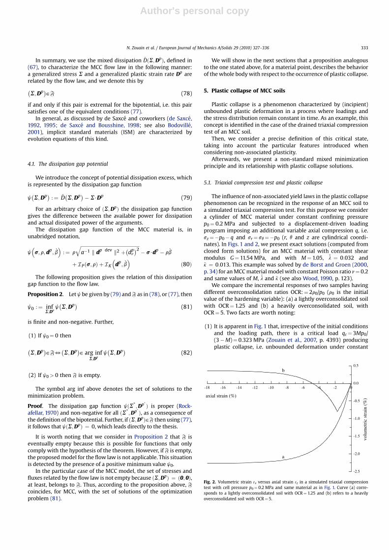
Fig. 2. Volumetric strain 3v versus axial strain 3z in a simulated triaxial compressiontest with cell pressure p0¼ 0.2 MPa and same material as in Fig. 1. Curve (a) corre-sponds to a lightly overconsolidated soil with OCR¼ 1.25 and (b) refers to a heavilyoverconsolidated soil with OCR¼ 5.



loadings and stress distribution. This is a critical state in soilmechanics. In this case the collapse load depends on theconfining pressure p0, not only on material constants.

(2) When the heavily overconsolidated soil (b) is sheared (seeFig. 1) the load q is amplified up to a peak value ofqpeak¼ 0.05 MPa and then decreases asymptotically to thecollapse load qc. Consequently, the collapse load cannot becalled limit load (in the classical sense) for this non-associatedelastoplastic material. Indeed, there is no load greater or equalthan all loading values effectively sustained by the system inany loading path, under constant confining pressure, initiatingat arbitrary maximum past isotropic consolidation pressure (cf.Wood, 1990, p. 188).

(3) Fig. 2 shows that plastic collapse occurs under constant volumedeformation. This is predicted since during the collapsephenomenon: (i) the volumetric elastic strain rate is zerobecause stresses are constant and (ii) hardening must remainfrozen and therefore the volumetric plastic strain rate must bezero because it is associated to hardening evolution in the MCCmaterial.

5.2. Additional notation

In the following the symbol D denotes the linear deformationoperator mapping velocities (displacements) into compatible strainrates (respective strains). The internal power associated witha stress field s and a velocity distribution w is denoted

hs;Dwi :¼ZB

s$DwdB (83)

Likewise, the external power of a load system F is

hF;wi :¼ZB

b$wdB þZGs

s$wdG (84)

where b and s are volume and surface load densities and Gs is partof the boundary G where traction is prescribed (null displace-ments are imposed in Gu, with G ¼ GsWGu and GsXGu empty).The set of stress fields in equilibrium with a given load system F isdefined as

SðFÞ :¼ fsjhs;Dwi ¼ hF;wi c wg (85)

where the virtual velocity w varies in the linear space of admissiblevelocities.

5.3. The plastic collapse equations

When the body undergoes plastic collapse the stress and theinternal thermodynamic forces remain constant. In view of theelastic state equations, a constant stress field induces an elasticdeformation distribution that is also constant in time. This, in turn,means that the strain rate field is at the same time compatible andpurely plastic.

Likewise, according to the state equation relative to internalvariables, internal hardening forces that are constant during plasticcollapse imply that the kinematical internal variables are alsoconstant, that is, _b ¼ 0 at all points in the body (cf. Polizzotto et al.,1991).

This description of plastic collapse is implemented in thefollowing. The computation of the critical factor a that amplifiesa prescribed load system F so as to produce unbounded purelyplastic deformation, when superposed to a fixed (non-amplified)load F0, can be formulated as

PC – The plastic collapse problem. Find ða;s; r; vÞ such that

s˛S�

F0 þ aF�

(86)

hF; vi ¼ 1 (87)

~Dðs; r;Dv;0Þ ¼ s$Dv in B (88)

a� 0 (89)

Condition (87) is only included in order to select one normalizedvelocity distribution, which rules out all its scalar multiples thatwould be solutions otherwise.

The system (86)–(89) represents general conditions for plasticcollapse that are applicable (with minor changes in notation) to anymaterial behavior derived from a bipotential. In addition to theseconditions, MCC materials also obey some particular equations thatwe consider in the following.

For MCC materials, the fact that the internal variable rate _b iszero implies that

dpv ¼ 0 (90)

Thus, plastic collapse for MCC materials takes place underconditions of constant volume deformation. A condition of plasticcollapse under constant volume deformation is known in soilmechanics as a critical state (Schofield and Wroth, 1968; Roscoe andBurland, 1968; Wood, 1990, p. 139; Houlsby and Puzrin, 2006, p.187).

From the condition _b ¼ dpv ¼ 0 and the evolution equation (70)

we get

r ¼ �sm if _l > 0 (91)

We note that this relation only applies to material points havingeffective plastic deformation during collapse.

Finally, we introduce the additional constraint (90) in the mixeddissipation potential, to conclude that for MCC materials under-going plastic collapse

~Dðs; r;Dv;0Þ ¼( ffiffiffi

23

qMr k Dv k if trDv ¼ 0 and f ðs; rÞ� 0

þN otherwise ð92Þ

5.4. Variational plastic collapse analysis

We propose a minimization principle and then explain how it isused to analyze the existence of collapse solutions ða;s; r; vÞ to theplastic collapse problem PC, defined by (86)–(89).

In order to obtain the variational formulation given below, weimpose (88) in the form of a minimization principle as given in (79),but now we attach (86), (87) and (89) as constraints.

MP – A minimization principle

Y ¼ infa;s;r;v

nJðs; r;Dv;0Þ

��s˛S�

F0 þ aF�

; hF; vi ¼ 1; a� 0o

(93)

where J :¼RB

jdB.

The first remark on this variational formulation is the followinglemma, whose proof is straightforward.

Lemma. The infimum Y of the minimization principle MP is finiteand non-negative if the feasible set is nonempty, otherwise it isþN.



By using D :¼RB

~DdB and the constraints in (93), we get

Jðs; r;Dv;0Þ ¼ Dðs; r;Dv;0Þ � hs;Dvi

¼ Dðs; r;Dv;0Þ �D

F0; vE� a (94)

Thus, the minimization principle (93) can be rewritten as

Y ¼ infa;s;r;v

nDðs; r;Dv;0Þ �

DF0; v

E� a

��s˛S

�F0 þ aF

�; hF; vi ¼ 1; a� 0

oð95Þ

The main results in the present variational analysis of plasticcollapse can be summarized as follows: (i) MP has always a solutionfor Y, finite orþN, and (ii) finding this solution can give the answerto whether or not solutions to the PC exist. This is precisely statedbelow.

Proposition 3. The plastic collapse problem PC and the minimi-zation principle MP are related by the following implications:

(1) If there exists a solution ða;s; r; vÞ of PC, then this set isa minimizer for MP and corresponds to Y¼ 0.

(2) If MP has a minimizer ða;s; r; vÞ such that Y¼ 0, then this set isa solution for PC.

Proof. (1) Collapse solutions satisfy all constraints in MP and giveY¼ 0 since j¼ 0 in B.

(2) Y¼ 0 implies j¼ 0 in B and this, together with the constraintsof MP, is the set of equations in PC.

In other words, if we solve the minimization problem MP,analytically or numerically, we can conclude that:

(1) If Y¼ 0 then the computed minimal solution describes theplastic collapse for the obtained amplification factor a.

(2) If Y> 0 then the body does not collapse for any loading of theform F0 þ aF .

The proposition above applies to material models derived froma bipotential, including those with associated flow laws, and notonly for the MCC.

The minimization problem MP, given by (93) or (95), has convexconstraints but its objective function is only bi-convex, and notnecessarily jointly convex in its arguments. It encompasses thecomplexities inherent to classical non-convex optimization.

The expression of the minimization principle MP for soils con-sisting of MCC material is obtained by introducing (92) in (95); thisgives

Y ¼ infa;s;r;v

8<:ZB

ffiffiffi23

rMr k Dv k dB �

DF0; v

E� a

��s˛S

�F0 þ aF

�; hF; vi ¼ 1;a� 0;

trDv ¼ 0 in B;ffiffiffiffiffiffiffiffiffiffiffiffiffiffiffiffiffiffiffiffiffiffiffiffiffiffiffiffiffiffiffiffiffiffiffiffiffiffiffiffiffiffiffiffiffiffiffiffiffi

32M2 k S k2 þðsm þ rÞ2

r� r in B

9=;(96)

The minimization principle (96) was also obtained in Zouainet al. (2007, p. 4390), but using a different development. Here, thestarting point is an extension of the classical dissipation function toa mixed dissipation potential. Moreover, now we have a variationalformulation for the evolution equations that allows an easy tran-sition to the global formulation in plastic collapse analysis. An

example of the application of (96) and Proposition 3 is studied inZouain et al. (2007, pp. 4390–4394).

6. Conclusions

In this paper we proposed a mixed variational formulation (81)for the evolution relations of MCC materials that matches all featuresof the most commonly used Cam-Clay model in soil mechanics.

It was shown in Section 4 that interpreting the known dissipa-tion potential given by Houlsby (1981) as a mixed function, andadding penalty terms to exactly enforce plastic and kinematicadmissibility, leads to the bi-convex potential ~Dðs; r;dp; _bÞ, in (67),giving implicit potential flow laws like those proposed by de Saxce(1995). In this way, the bipotential for the evolution equations isinterpreted as a dissipation potential. Moreover, it is obtained froma classical dissipation function by the simple consideration ofstatical and kinematic constraints.

The concept of excess of dissipation was introduced by definingthe gap potential jðs; r;dp; _bÞ in (79). It was proven, in Proposition2, that the set F of stress and plastic strain rates related by the flowlaw coincides with the set of minimizers of the dissipation gapfunction.

Since the hardening evolution relation of MCC is not associated,the plastic collapse analysis of a soil obeying this constitutivebehavior cannot be embedded in classical limit analysis theory. Forexample, a maximum load amplifier does not necessarily exist andthe well known lower and upper bounding principles are notvalid.

However, we have shown, in Proposition 3, that there is a mixedminimization principle associated with the analysis of the criticalstate of plastic collapse of an MCC soil. This global variationalformulation was directly deduced from the constitutive variationalformulation of the flow law.

Acknowledgements

This work was partially supported by the Brazilian Council forScientific and Technological Development, CNPq.

Appendix A. The polar of the dissipation function

Let us first justify (50). The dual norm corresponding to thenorm for strain rates defined in (48) is defined by (Rockafellar, 1970,p. 128; Horn and Johnson, 1985, p. 277)

k k k**

:¼ supds0

k$dk d k

*

(A1)

The above problem can be solved by a change of variables:

bk :¼ffiffiffiap

kdev þ 1

3ffiffiffi3p ðtrkÞ1 (A2)

bd :¼ 1ffiffiffiap ddev þ 1ffiffiffi

3p ðtrdÞ1 (A3)

Then k$d ¼ bk$bd; k d k*¼k bd k and

k k k**¼ supbds0

bk$bdk bd k ¼k bk k¼

ffiffiffiffiffiffiffiffiffiffiffiffiffiffiffiffiffiffiffiffiffiffiffiffiffiffiffiffiffiffiffiffiffiffiffiffiffiffiffiffiffiffiffiffiffiffia k kdev k2 þ

�13

trk

2s

(A4)

where we applied the fact that the Euclidean norm is its own dual(Horn and Johnson, 1985, p. 277). This proves (50).



The fundamental inequality characterizing dual norms

k k k**k d k

*� k$d c ðk;dÞ (A5)

is a consequence of the definition (A1).Finally

(1) The polar of

D�dp; 3p

v

�¼ rð3p

v Þ k dp k*

(A6)

with respect to dp, is

bFðk; 3pv Þ ¼ ½rð3p

v Þ��1k k k

**(A7)

This is proven by an additional change of variables.

(2) The polar of

~D�

s; r;dp; _b�¼ r k dp k

*þIPðs; rÞ þ IK

�dp; _b

�(A8)

with respect to ðdp; _bÞ, is

~Fðs; rÞ ¼ r�1 k sþ r1 k**

(A9)

Proving this requires using the constraints imposed by exactpenalty and the same changes of variables.

References

Aubin, J.-P., Ekeland, I., 1984. Applied Nonlinear Analysis. John Wiley, Dover Edition.Bodoville, G., 2001. On generalised and implicit normality hypotheses. Meccanica

36, 273–290.Borja, R.I., Lee, S.R., 1990. Cam-clay plasticity, part I: implicit integration of elasto-

plastic constitutive relations. Comput. Methods Appl. Mech. Eng. 78, 49–72.Collins, I.F., Houlsby, G.T., 1997. Application of thermomechanical principles to the

modelling of geotechnical materials. Proc. R. Soc. Lond. A 453, 1975–2001.de Borst, R., Groen, A.E., 2000. Computational strategies for standard soil plasticity

models. In: Zaman, M., Booker, J., Gioda, G. (Eds.), Modeling in Geomechanics,pp. 1–50 (Chapter 2).

de Saxce, G., 1992. Une generalisation de l’inegalite de Fenchel et ses applicationsaux lois constitutives. C.R. Acad. Sci. Paris, Serie II 314, 125–129.

de Saxce, G., 1995. The bipotential method, a new variational and numericaltreatment of the disssipative laws of materials. In: 10th International

Conference on Mathematical and Computer Modelling and ScientificComputing, pp. 1–6.

de Saxce, G., Bousshine, L., 1998. Limit analysis for implicit standard materials:application to the unilateral contact with dry friction and the non-associatedflow rules in soils and rocks. Int. J. Mech. Sci. 40 (4), 387–398.

Einav, I., Houlsby, G., Nguyen, G., 2007. Coupled damage and plasticity models derivedfrom energy and dissipation potentials. Int. J. Solids Struct. 44, 2487–2508.

Halphen, B., Nguyen, Q.S., 1975. Sur les materiaux standard generalises. J. Mec.Theor. Appl. 14, 1–37.

Han, W., Reddy, B.D., 1999. Plasticity: Mathematical Theory and Numerical Analysis.Springer-Verlag, New York.

Hiriart-Urruty, J.-B., Lemarechal, C., 1993a. Convex Analysis and MinimizationAlgorithms, vol. I. Springer-Verlag, Berlin.

Hiriart-Urruty, J.-B., Lemarechal, C., 1993b. Convex Analysis and MinimizationAlgorithms, vol. II. Springer-Verlag, Berlin.

Hjiaj, M., 1999. Sur la classe des materiaux standard implicites: Concept, aspectsdiscretises et estimation de l’erreur a posteriori. Ph.D. thesis, Docteur enSciences Appliquees, Faculte Polytechnique de Mons.

Horn, R.A., Johnson, C.R., 1985. Matrix Analysis. Cambridge University Press.Houlsby, G.T., 1981. A study of plasticity theories and their applicability to soils.

Ph.D. thesis, Cambridge.Houlsby, G.T., Puzrin, A.M., 2006. Principles of Hyperplasticity: An Approach to

Plasticity Theory Based on Thermodynamic Principles. Springer-Verlag, London.Kamenjarzh, J., 1996. Limit Analysis of Solids and Structures. CRC Press.Lubliner, J., 1972. On the thermodynamic foundations of non-linear solid mechanics.

Int. J. Non-Lin. Mech. 7 (3), 237–254.Maugin, G.A., 1992. The Thermomechanics of Plasticity and Fracture. Cambridge

University Press, UK.Nguyen, Q.S., 2000. Stability and Nonlinear Solid Mechanics. Wiley.Nguyen, Q.S., 2003. On shakedown analysis in hardening plasticity. J. Mech. Phys.

Solids 51, 101–125.Nguyen, Q.S., 2006. Min-max duality and shakedown theorems in plasticity. In:

Alart, P., Naisonneuve, O., Rockafellar, R.T. (Eds.), Nonsmooth Mechanics andAnalysis. Springer, pp. 81–92.

Polizzotto, C., Borino, G., Caddemi, S., Fuschi, P., 1991. Shakedown problems formaterial models with internal variables. Eur. J. Mech. A/Solids 10 (6), 621–639.

Rockafellar, R.T., 1970. Convex Analysis. Princeton University Press.Roscoe, K.H., Burland, J.B., 1968. On the generalized behaviour of ‘‘wet’’ clay. Eng.

Plast. 48, 535–609.Schofield, A.N., Wroth, C.P., 1968. Critical State Soil Mechanics. McGraw-Hill,

London, England.Silhav�y, M., 1997. The Mechanics and Thermodynamics of Continuous Media.

Springer, Berlin.Ulm, F.-J., Coussy, O., 2003. In: MIT (Ed.), Mechanics and Durability of Solids, vol. I.

Prentice Hall, New Jersey.Vaunat, J., Cante, J.C., Ledesma, A., Gens, A., 2000. A stress point algorithm for an

elastoplastic model in unsaturated soils. Int. J. Plast. 16, 121–141.Wood, D.M., 1990. Soil Behaviour and Critical State Soil Mechanics. Cambridge

University Press.Ziegler, H., 1983. An Introduction to Thermomechanics. North Holland.Zouain, N., Pontes, I., Borges, L., Costa, L., 2007. Plastic collapse in non-associated

hardening materials with application to Cam-clay. Int. J. Solids Struct. 44 (13),4382–4398.


Plastic collapse in non-associated hardening materials with application to Cam-clay

Documents

Transcript of Plastic collapse in non-associated hardening materials with application to Cam-clay