On the Numerical Implementation of Hyperplasticity Non-Linear Kinematic Hardening Modified Cam Clay...

TECHNICAL PAPER

On the numerical implementation of hyperplasticity non-linear kinematic hardening modified cam

clay model

Dedi Apriadia, Suched Likitlersuanga*, Thirapong Pipatpongsab and Hideki Ohtab

aDepartment of Civil Engineering, Chulalongkorn University, Bangkok, Thailand; bDepartment of International DevelopmentEngineering, Tokyo Institute of Technology, Tokyo, Japan

(Received 12 December 2008; final version received 18 April 2009)

A continuous hyperplasticity model named kinematic hardening modified cam clay (KHMCC) is a constitutive soilmodel based on thermodynamic principles. This model has addressed some shortcomings of the modified cam clay(MCC), specifically on small strain stiffness. Because of employing multiple surfaces plasticity, it can simulate asmooth transition from elastic to plastic behaviour as well as the effect of immediate past stress. This article aims topresent some important issues on the numerical implementation of the continuous hyperplasticity non-linearKHMCC model. The incremental stress–strain response is calculated based on a rate-dependent algorithm. Asignificant advantage of the rate-dependent calculation is that it is not necessary to attach with the consistencycondition during calculation of plastic strains. Effect of time step and number of yield surfaces in rate-dependentalgorithm will be also presented. A discussion on using of numerical integration rules of hardening functions isaddressed. Furthermore, model verification is performed against analytical solution of ideal undrained responsewhich has been obtained from theoretical integration of the MCC function over the imposed stress or strain path.Finally, some numerical demonstrations are also carried out to illustrate several key features of the model.

Keywords: hyperplasticity; small strain; rate-dependent; hardening function

Introduction

In practical geotechnical engineering analysis anddesign, a well-known Mohr-Coulomb and cam claymodels (Roscoe and Burland 1968) have been widelyused for simplifying complex behaviours of soils.Several advanced frameworks have been further pro-posed to include some important aspects of soilbehaviours, such as small strain stiffness or the effectsof immediate past stress by introducing multiple ornested surface model (Mroz andNorris 1982), boundingsurface model (Dafalias and Hermann 1982) andhypoplasticity framework (Kolymbas 1977). Anotherimportant issue is the stress–strain characteristic ofsoils, which is non-linear and irreversible, in that theinitial soil stiffness or small strain tangent stiffnessdepends on the stress level. The interpretation fromexperimental observations of bender element test showsthat the small strain stiffness of soils is a non-linearfunction of the mean effective stress for isotropicallyconsolidated samples as reported by Tanizawa et al.(1994), Kohata et al. (1997), Pennington et al. (1997)and Techavorasinskun and Amomwithayalax (2002)and depend on the stress ratio (Rampello et al. 1997) foranisotropically consolidated samples. The stiffness alsoaffected by other variables, such as the voids ratio,

anisotropic stress state and/or the preconsolidationpressure (Hardin 1978, Houlsby and Wroth 1991,Viggiani 1992, Rampello et al. 1994, Soga et al. 1995).

Because constitutive models relate to physicalphenomena, they must obey certain principles or axiomsthat govern the physical phenomena such as conserva-tion of mass, conservation of energy and laws ofthermodynamics. All models mentioned earlier do notrefer to the Laws of Thermodynamics and they mayviolate one or the other fundamental laws. Models thatviolate thermodynamics may not be used with anyconfidence to describe material behaviour (Houlsby andPuzrin 2006). Therefore, Likitlersuang (Likitlersuang2003, Likitlersuang and Houlsby 2006) proposed thehyperplasticity kinematic hardening modified cam clay(KHMCC) model to address small strain stiffness basedon the thermodynamics principles. The kinematichardening function was included in the energy andyield functions to characterise small strain stiffness andaccommodates smooth transition of stiffness in corre-spondence to loading conditions and stress histories.Hyperbolic function recommended by Puzrin andHoulsby (2001) was employed to express the continuouskinematic hardening function in order to fit with theobserved non-linear stress–strain responses. Continu-ous kinematic hardening function was piece-wised into

*Corresponding author. Email: [email protected]

The IES Journal Part A: Civil & Structural Engineering

Vol. 2, No. 3, August 2009, 187–201

ISSN 1937-3260 print/ISSN 1937-3279 online

� 2009 The Institution of Engineers, Singapore

DOI: 10.1080/19373260902985570

http://www.informaworld.com

Downloaded By: [National University Of Singapore] At: 10:36 27 July 2009

https://www.researchgate.net/publication/284934204_Elastoplastic_and_viscoplastic_constitutive_models_for_soils_with_anisotropic_loading?el=1_x_8&enrichId=rgreq-4933e1791f8171b1edd91b4fee9da0b8-XXX&enrichSource=Y292ZXJQYWdlOzIyODczNzQ2MztBUzoxMjU5MTE0MTIyNTI2NzJAMTQwNzAzMTAyOTAxMA==

https://www.researchgate.net/publication/237897680_A_rate-dependent_constitutive_equation_for_soils_Mech_Research_Comm_4_367-372?el=1_x_8&enrichId=rgreq-4933e1791f8171b1edd91b4fee9da0b8-XXX&enrichSource=Y292ZXJQYWdlOzIyODczNzQ2MztBUzoxMjU5MTE0MTIyNTI2NzJAMTQwNzAzMTAyOTAxMA==

a finite number of multiple yield functions. Therefore,combined responses of activated yield surfaces canrepresent non-linear kinematic hardening behaviours.Calibration of the model in triaxial stress–strain spacewas carried out by Likitlersuang and Houlsby (2007) onBangkok clay. Stress–strain responses under monotonicand cyclic loadings were simulated to show theadvantage of hyperplasticity KHMCC model.

Though the formulation of hyperplasticity KHMCCmodel has been already proposed in the earlier research,the numerical implementation and simulation arerestricted to linear volumetric stress–strain relationshipwith stiffness proportional to pressure. Further, smallstrain stiffness studies of Bangkok clay using benderelement tests on the isotropically consolidated samplesclearly show that the shear modulus is a power functionof pressure (Teachavorasinskun and Amomwithayalax2002) rather than linear function of pressure. Therefore,the numerical implementation for hyperplasticityKHMCC model with non-linear elastic stiffness hasnot been explored. This research aims to extend theprevious research of Likitlersuang and Houlsby (2006)by incorporating small strain stiffness in the form ofpower function of pressure into energy function.Correspondingly, the numerical implementation andpiece-wise multisurface plasticity described by Likitle-rsuang and Houlsby (2007) is enhanced to address ahigher degree of non-linearity and loading history. Also,this article presents an approach to determine thenecessary parameters obtained from bender elementtests for regulating small strain stiffness characteristic ofthe hyperplasticity KHMCC model.

In this study, a numerical implementation of thehyperplasticity non-linear KHMCC model based ontriaxial stress–strain variables using strain-drivenforward-Euler integration scheme is employed. Apower function of pressure proposed by Houlsbyet al. (2005) is adopted in non-linear elastic energyfunction. A hyperbolic function proposed by Puzrinand Houlsby (2001) is adopted in non-linear kine-matic hardening function. For simplicity, thepre-consolidation pressure after the completion ofisotropic consolidation is referred in the initialstiffness of kinematic hardening function. It is foundthat the numerical model implementation has asingularity problem at initialisation stage of internalvariables. To handle the singularity problem, themidpoint quadrature rule is considered to integratethe hardening function of multisurface yield func-tions. An analytical solution of ideal undrainedtriaxial test on normally consolidated clay (Roscoeand Burland 1968, Potts and Ganendra 1994) is usedto verify numerical model implementation undersingle yield surface. Several numerical demonstrationsare performed for monotonic, cyclic and repetitive

loading under undrained conditions for normally andlightly consolidated clays. The developed model ishighlighted through the capabilities of characterisingeffect of immediate stress history (Atkinson et al.1990, Houlsby 1999), dependence of effective stresspath on the immediate stress history during un-drained shear (Stallebrass and Taylor 1997), smoothand irreversible unloading–reloading responses. Allattempts of demonstration are to emphasise theperformance of a hyperplasticity framework, whichcan contain several complicated characteristics ofconstitutive models under the unified framework.

This study is expected to provide a theoreticalbackground and numerical implementation for thosewho are interested in the advancement of modified camclay model under the framework of hyperplasticity.The numerical procedures for describing the non-linearbehaviours of soil in the form of incremental stress–strain relationship are presented in details which can beeasily translated into computer code. The results of thisresearch may give a light to model the complicatedbehaviours of soils observed from advanced laboratorysuch as bender element tests. Nevertheless, theanisotropy can be loosely explained by the immediatestress past. The softening behaviour should beexplored in the future in order to realise the promisingfeatures of the model on soil destructure.

Non-linear kinematic hardening modified cam clay

model

Hyperplasticity formulation

Under the hyperplasticity framework (see Houlsby andPuzrin (2006) for details), the entire constitutivemodel isfundamentally governed by two scalar functions. Theseare energy function and yield function (dissipationfunction). In typical formulation, Gibbs free energyfunction is suggested to associate stresses, materialparameters and material memories (internal variables)to a unique potential function where the referencedpressure for zero volumetric strain is defined at 1 atm.Onemay notice that hyperplasticity framework employsa total energy instead of rate form of energy which iscommonly used in classical plasticity theory. BecauseGibbs free energy is equivalent to a complementaryenergy, negative elastic stored energy, negative dissipa-tion energy and positive hardening energy are combined.It is noted here that soil mechanics sign convention isused throughout this studywhere compression is definedpositive. According toHoulsby et al. (2005), a non-linearversion of KHMCC is created to allocate non-linearelastic moduli at small strain into the Gibbs free energywhich is expressed in the formE ¼ E( p; q; ap; aq; ap; aq)by adding the hyperelastic expressionusing triaxial stressvariables p ¼ 1

3 sa þ 2srð Þ; q ¼ sa � sr where p is mean

188 D. Apriadi et al.


https://www.researchgate.net/publication/233376091_Predictions_of_a_continuous_hyperplasticity_model_for_Bangkok_clay?el=1_x_8&enrichId=rgreq-4933e1791f8171b1edd91b4fee9da0b8-XXX&enrichSource=Y292ZXJQYWdlOzIyODczNzQ2MztBUzoxMjU5MTE0MTIyNTI2NzJAMTQwNzAzMTAyOTAxMA==

https://www.researchgate.net/publication/245411722_Elastic_moduli_of_soils_dependent_on_pressure_A_hyperelastic_formulation?el=1_x_8&enrichId=rgreq-4933e1791f8171b1edd91b4fee9da0b8-XXX&enrichSource=Y292ZXJQYWdlOzIyODczNzQ2MztBUzoxMjU5MTE0MTIyNTI2NzJAMTQwNzAzMTAyOTAxMA==

effective stress, q is stress deviator,sa is axial stress andsris radial stress.

E ¼ � p2�n

e

p1�n

ak 1� nð Þ 2� nð Þ

þ p

k 1� nð Þ � pap þ qaq� �

þZ10

1

2Hpa

2

p þ1

2Hqa2q

� �dZ ð1Þ

where pe ¼ffiffiffiffiffiffiffiffiffiffiffiffiffiffiffiffiffiffiffiffiffiffiffiffip2 þ k 1�nð Þq2

3g

qis defined as equivalent

stress for convenience. k, g, n are dimensionlessmaterial constants calibrated from elastic stress–strainrelation at small strain level. Atmospheric pressure 1atm (approximately 100 kPa) is defined as pa. ap and aqare total isotropic and deviatoric plastic strains,respectively. Integration of differential hardening en-ergy is evaluated in terms of internal coordinate Zwhich is limited between 0 and 1. Z ¼ 0 represents theinitial hardening stage (the highest hardening response)whereas Z ¼ 1 represents the final hardening stage(zero hardening response). ap and aq are kinematicinternal variable functions of Z which can be integratedto obtain ap and aq by Equations (2) and (3) bydefinition. Therefore, ap and aq can be regarded as adefinite integral area of functional variables ap and aqover the domain of Z. It is noted here that all variableswith ‘^’ (hat) throughout this study are referred tointernal variable function of Z.

ap ¼Z10

apdZ; ð2Þ

aq ¼Z10

aqdZ ð3Þ

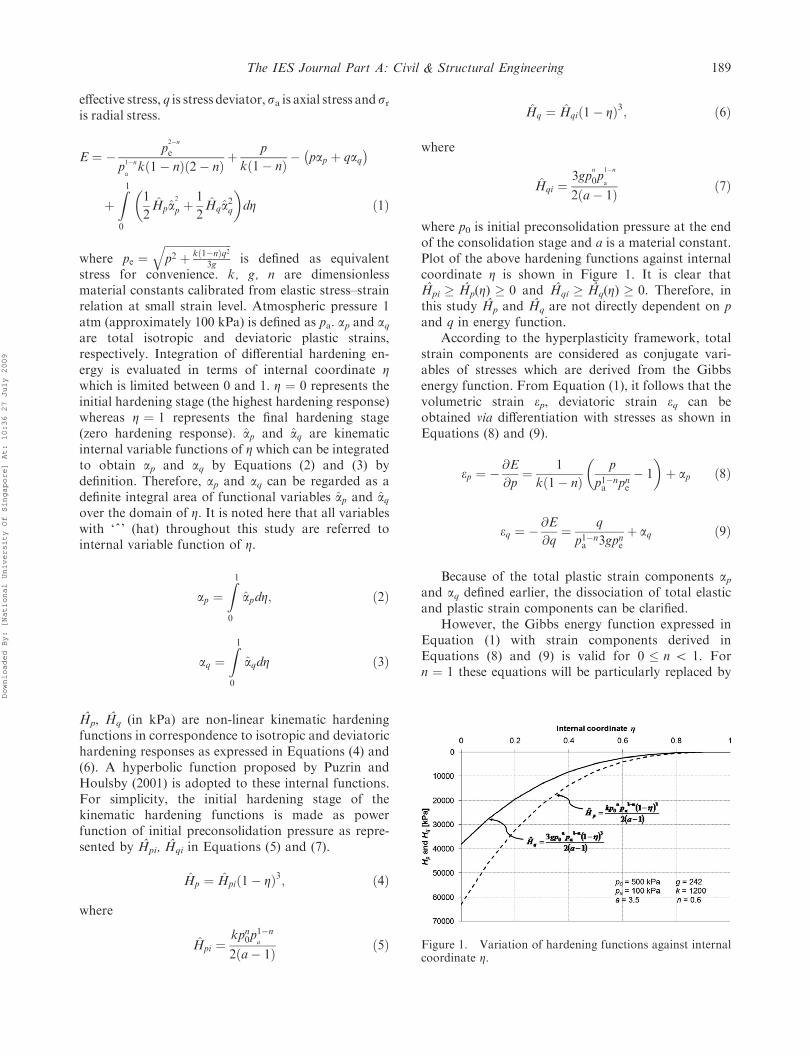
Hp, Hq (in kPa) are non-linear kinematic hardeningfunctions in correspondence to isotropic and deviatorichardening responses as expressed in Equations (4) and(6). A hyperbolic function proposed by Puzrin andHoulsby (2001) is adopted to these internal functions.For simplicity, the initial hardening stage of thekinematic hardening functions is made as powerfunction of initial preconsolidation pressure as repre-sented by Hpi, Hqi in Equations (5) and (7).

Hp ¼ Hpi 1� Zð Þ3; ð4Þ

where

Hpi ¼kpn0p

1�na

2 a� 1ð Þ ð5Þ

Hq ¼ Hqi 1� Zð Þ3; ð6Þ

where

Hqi ¼3gp

n

0p1�n

a

2 a� 1ð Þ ð7Þ

where p0 is initial preconsolidation pressure at the endof the consolidation stage and a is a material constant.Plot of the above hardening functions against internalcoordinate Z is shown in Figure 1. It is clear thatHpi � Hp(Z) � 0 and Hqi � Hq(Z) � 0. Therefore, inthis study Hp and Hq are not directly dependent on pand q in energy function.

According to the hyperplasticity framework, totalstrain components are considered as conjugate vari-ables of stresses which are derived from the Gibbsenergy function. From Equation (1), it follows that thevolumetric strain ep, deviatoric strain eq can beobtained via differentiation with stresses as shown inEquations (8) and (9).

ep ¼ �@E

@p¼ 1

k 1� nð Þp

p1�na pne� 1

� �þ ap ð8Þ

eq ¼ �@E

@q¼ q

p1�na 3gpneþ aq ð9Þ

Because of the total plastic strain components apand aq defined earlier, the dissociation of total elasticand plastic strain components can be clarified.

However, the Gibbs energy function expressed inEquation (1) with strain components derived inEquations (8) and (9) is valid for 0 � n 5 1. Forn ¼ 1 these equations will be particularly replaced by

Figure 1. Variation of hardening functions against internalcoordinate Z.

The IES Journal Part A: Civil & Structural Engineering 189


the following Equations (10)–(12) (Houlsby and Puzrin2006).

E ¼ � p

kln

p

pa

� �� 1

� �� q2

6gp� pap þ qaq� �

þZ10

1

2Hpa

2

p þ1

2Hqa

2

q

� �dZ ð10Þ

ep ¼ �@E

@p¼ 1

kln

p

pa

� �� q2

6gp2þ ap ð11Þ

eq ¼ �@E

@q¼ q

3gpþ aq ð12Þ

According to Equations (8), (9), (11) and (12), totalstrain components are derived as a function of p, q andapðapÞ; aqðaqÞ. By flow rule, rate change of total straincomponents can be obtained. The second derivatives ofGibbs free energy in Equations (13) and (14) arederived in Box 1.

_ep ¼ �@2E

@p2

� �_pþ � @2E

@q@p

� �_q

þZ10

� @2E

@ap@p

� �a�pdZþ

Z10

� @2E

@aq@p

� �_aqdZ ð13Þ

_eq ¼ � @2E

@p@q

� �_pþ �@

2E

@q2

� �_q

þZ10

� @2E

@ap@q

� �a�pdZþ

Z10

� @2E

@aq@q

� �a�qdZ ð14Þ

Rate change of total strain components can besimply written by the following equations. Equation(15) is a compacted form of Equations (13) and (14).Equation (16) expresses rate form of plastic straincomponents while Equation (17) expresses rate form ofelastic strain components.

_ep_eq

� �¼

� @2E@p2

� @2E@p@q

� @2E@p@q

� @2E@q2

2664

3775 � _p

_q

� �

þZ10

� @2E@ap@p

� @2E@aq@p

� @2E@ap@q

� @2E@aq@q

264

375 � a

�p

a�q

8<:

9=;dZ ð15Þ

_ap_aq

� �¼Z10

� @2E@ap@p

� @2E@aq@p

� @2E@ap@q

� @2E@aq@q

264

375 � a

�p

a�q

( )dZ ð16Þ

_eep_eeq

� �¼ _ep

_eq

� �� _ap

_aq

� �¼

�@2E@p2

� @2E@p@q

� @2E@p@q

�@2E@q2

264

375 � _p

_q

� �

ð17Þ

According to Equation (17), the incremental elasticstress–strain relationship can be given as the compli-ance stiffness matrix.

_p_q

� �¼�@

2E@p2

� @2E@p@q

� @2E@p@q

�@2E@q2

264

375�1

�_eep_eeq

� �¼ K J

J 3G

�

_eep_eeq

� �

ð18Þ

Box 1: Second derivatives of Gibbs free energy.

Gibbs free energy E for 0 � n 5 1 in Equation (1) Gibbs free energy for n ¼ 1 in Equation (10)

� @2E

@p2¼ 1

kð1� nÞp1�na pne1� np2

p2e

� �

� @2E

@q2¼ 1

3gp1�na pne1� nkð1� nÞq2

3gp2e

� �

� @2E

@p@q¼ � npq

3gp1�na pnþ2e

� @2E

@p2¼ 1

kp1þ kq2

3gp2

� �

� @2E

@q2¼ 1

3gp

� @2E

@p@q¼ � q

3gp2

Gibbs free energy E for 0 � n � 1

� @2E

@ap@p¼ 1

� @2E

@aq@p¼ 0

� @2E

@ap@q¼ 0

� @2E

@aq@q¼ 1



where K is non-linear bulk modulus, G is non-linearshear modulus and J is non-linear coupling modulus. IfJ is non-zero, the incremental stress–strain response isa stress-induced anisotropic behaviour appeared dur-ing loading stages (Houlsby 1985). J is zero only in thecondition of isotropic consolidation.

K ¼� @2E

@q2

@2E@p2

@2E@q2� @2E

@p@q

� �2 ; G ¼ 1

3

� @2E@p2

@2E@p2

@2E@q2� @2E

@p@q

� �2 ;

J ¼@2E@p@q

@2E@p2

@2E@q2� @2E

@p@q

� �2 ð19Þ

The relation among stress variables does not existin the previous description based on energy function.This relation is described in yield function whichcontains stress variables to couple with energy func-tion. In the non-linear KHMCC model (seeLikitlersuang 2003, Likitlersuang and Houlsby 2006for details), the yield function y in term of triaxialstress parameters is defined:

y ¼ffiffiffiffiffiffiffiffiffiffiffiffiffiffiffiffiffiffiffiffiffiffiffiffiw2p þ w2q=M2

q� c ¼ 0 ð20Þ

where M is a frictional critical state parameter (Roscoeand Burland 1968) which is the value that stress ratioq/p0 attains at critical state, c ¼ HpapZ is a hardeningstress which represents the size of yield surface function,wp and wq are relative stresses in term of volumetric anddeviatoric stresses. Materials behave plastically whenthe yield surface is active (y � 0). Materials behaveelastically when the stress is inside the yield surface(y 5 0). The relative stresses are defined as changing offree energy function with respect to the internalkinematic variables. Gibb’s free energy functional Ecan be defined as the internal energy with respect to Z.So the integration of E throughout the domain of Z isGibb’s free energy as shown in Equation (21).

E ¼Z10

EdZ ð21Þ

According to Equations (1)–(3) and (21), Gibb’s freeenergy functional E is obtained by the followingequation.

E ¼ � p2�ne

p1�na k 1� nð Þ 2� nð Þ þp

k 1� nð Þ

� pap þ qaq� �

þ 1

2Hpa2p þ

1

2Hqa

2

q

� �ð22Þ

Therefore, wp and wq are referred in Equations(23) and (24) as the derivatives of E with respect toap and aq, respectively. It is found that wp andwq can be considered as the difference betweenstress variables and back stresses which is associatedwith kinematic hardening variables. In this study,the derivation of Equations (23) and (24) issimplified because the definitions of ap and aq areinitially adopted in Equations and (3). If ap, aq andap and aq are considered as independent variables inGibb’s free energy, the constraint function usingLagrangian multiplier and Ziegler’s orthogonalitycondition (Ziegler 1983) must be employed. Thisdetailed proof can be found in Houlsby and Puzrin(2006).

wp ¼@E

@ap¼ p� Hpap ð23Þ

wq ¼@E

@aq¼ q� Hqaq ð24Þ

According to Houlsby and Puzrin (2006), theevolution rule of kinematic internal variable functionsap and aq is followed in Equations (25) and (26)respectively as the derivatives of flow potential w withrespect to relative stress variables. One may associatethis kind of evolution rule to flow rule used in classicalplasticity. The flow potential w is defined in relevant toyield function y as shown in Equation (27).

a�p ¼

@w

@wp; ð25Þ

a�q ¼

@w

@wqð26Þ

w ¼ yh i2

2m¼

ffiffiffiffiffiffiffiffiffiffiffiffiffiffiffiffiffiffiffiffiffiffiffiffiw2p þ w2q=M2

q� c

D E22m

ð27Þ

where m is artificial viscosity coefficient imposed tounity and the operator h i are Macaulay brackets

which defines xh i ¼ 0; x < 0x; x � 0

�.

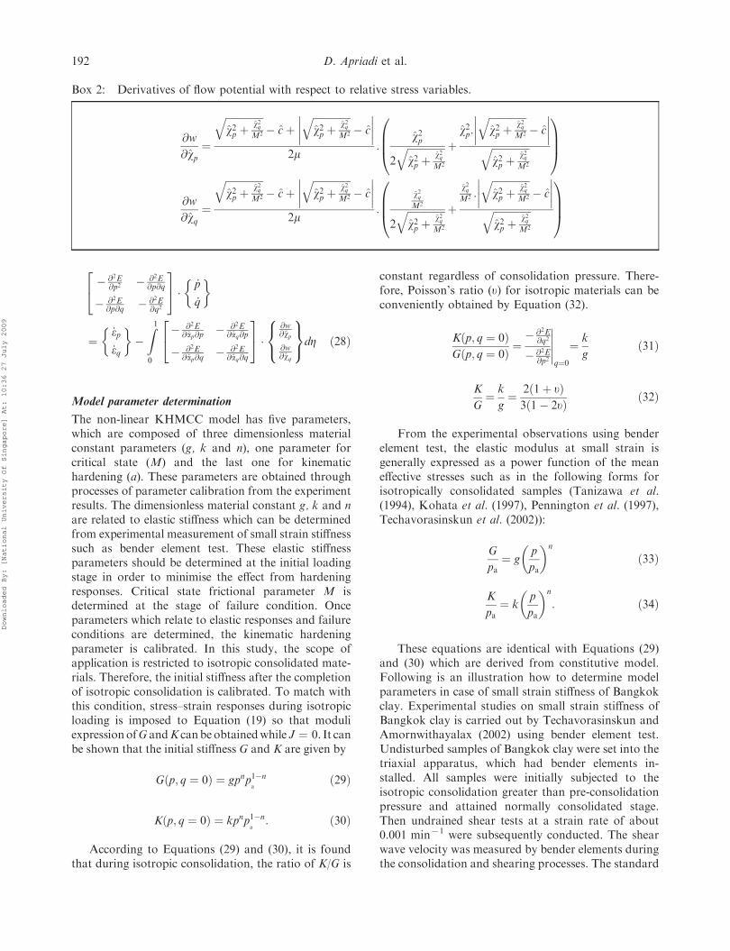
As a consequence of Equations (25)–(27), the rateform of stress–strain relationship obtained in Equation(15) can be expressed. The derivatives of flow potentialw in Equations (25) and (26) are shown in Box 2.



� @2E@p2

� @2E@p@q

� @2E@p@q � @2E

@q2

24

35 � _p

_q

� �

¼_ep_eq

� ��Z10

� @2E@ap@p

� @2E@aq@p

� @2E@ap@q

� @2E@aq@q

24

35 � @w

@wp@w@wq

8<:

9=;dZ ð28Þ

Model parameter determination

The non-linear KHMCC model has five parameters,which are composed of three dimensionless materialconstant parameters (g, k and n), one parameter forcritical state (M) and the last one for kinematichardening (a). These parameters are obtained throughprocesses of parameter calibration from the experimentresults. The dimensionless material constant g, k and nare related to elastic stiffness which can be determinedfrom experimental measurement of small strain stiffnesssuch as bender element test. These elastic stiffnessparameters should be determined at the initial loadingstage in order to minimise the effect from hardeningresponses. Critical state frictional parameter M isdetermined at the stage of failure condition. Onceparameters which relate to elastic responses and failureconditions are determined, the kinematic hardeningparameter is calibrated. In this study, the scope ofapplication is restricted to isotropic consolidated mate-rials. Therefore, the initial stiffness after the completionof isotropic consolidation is calibrated. To match withthis condition, stress–strain responses during isotropicloading is imposed to Equation (19) so that moduliexpressionofG andK canbeobtainedwhile J ¼ 0. It canbe shown that the initial stiffness G and K are given by

G p; q ¼ 0ð Þ ¼ gpnp1�na

ð29Þ

K p; q ¼ 0ð Þ ¼ kpnp1�na

: ð30Þ

According to Equations (29) and (30), it is foundthat during isotropic consolidation, the ratio of K/G is

constant regardless of consolidation pressure. There-fore, Poisson’s ratio (u) for isotropic materials can beconveniently obtained by Equation (32).

K p; q ¼ 0ð ÞG p; q ¼ 0ð Þ ¼

� @2E@q2

� @2E@p2

q¼0

¼ k

gð31Þ

K

G¼ k

g¼ 2 1þ uð Þ

3 1� 2uð Þ ð32Þ

From the experimental observations using benderelement test, the elastic modulus at small strain isgenerally expressed as a power function of the meaneffective stresses such as in the following forms forisotropically consolidated samples (Tanizawa et al.(1994), Kohata et al. (1997), Pennington et al. (1997),Techavorasinskun et al. (2002)):

G

pa¼ g

p

pa

� �n

ð33Þ

K

pa¼ k

p

pa

� �n

: ð34Þ

These equations are identical with Equations (29)and (30) which are derived from constitutive model.Following is an illustration how to determine modelparameters in case of small strain stiffness of Bangkokclay. Experimental studies on small strain stiffness ofBangkok clay is carried out by Techavorasinskun andAmornwithayalax (2002) using bender element test.Undisturbed samples of Bangkok clay were set into thetriaxial apparatus, which had bender elements in-stalled. All samples were initially subjected to theisotropic consolidation greater than pre-consolidationpressure and attained normally consolidated stage.Then undrained shear tests at a strain rate of about0.001 min71 were subsequently conducted. The shearwave velocity was measured by bender elements duringthe consolidation and shearing processes. The standard

Box 2: Derivatives of flow potential with respect to relative stress variables.

@w

@wp¼

ffiffiffiffiffiffiffiffiffiffiffiffiffiffiffiw2p þ

w2qM2

q� cþ


w2qM2

q� c

2m:

w2p

2


w2qM2

q þw2p:


w2qM2

q� c

ffiffiffiffiffiffiffiffiffiffiffiffiffiffiffi

w2p þw2qM2

q0BB@

1CCA

@w

@wq¼


w2qM2

q� cþ


w2qM2

q� c

2m:

w2qM2

2


w2qM2

q þ

w2qM2 :


w2qM2

q� c

ffiffiffiffiffiffiffiffiffiffiffiffiffiffiffi

w2p þw2qM2

q0BB@

1CCA



procedure was used to interpret the shear wavetravelling to shear moduli. The proposed empiricalequation is

G ¼ 1530p0:6 ðin kPaÞ: ð35Þ

This equation can be normalised in the samemanner with Equation (33) in order to obtain smallstrain dimensionless material constant g and n as in thefollowing form

G

pa¼ 242

p

pa

� �0:6

: ð36Þ

Determination of bulk modulus relevant toEquation (34) is suitably based on the result ofEquation (32) by relating to Poisson’s ratio (u). Valueu is ranged in a certain limit and can be related to thecoefficient of earth pressure at-rest K0 as shown inEquation (37).

u ¼ K0

1þ K0ð37Þ

The typical value of K0 of Bangkok clay is around0.68 (Shibuya et al. 2001), therefore using Equation(37) u ¼ 0.41. Finally the constant k is obtainedfrom Equation (38) and the non-linear bulk modulusin Equation (39) is in similar form as that ofEquation (34).

K

G¼ k

g¼ 2 1þ uð Þ

3 1� 2uð Þ ð38Þ

K

pa¼ 1200

p

pa

� �0:6

ð39Þ

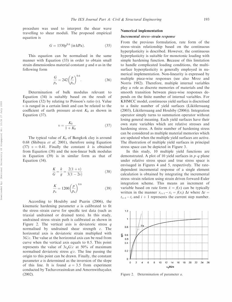
According to Houlsby and Puzrin (2006), thekinematic hardening parameter a is calibrated to fitthe stress–strain curve for specific test data (such astriaxial undrained or drained tests). In this study,undrained stress–strain path is calibrated as shown inFigure 2. The vertical axis is deviatoric stress qnormalised by undrained shear strength c. Thehorizontal axis is deviatoric strain multiplied with3G/c. The value at the horizontal axis can be read fromcurve when the vertical axis equals to 0.5. This pointrepresents the value of 3eqG/c at 50% of maximumnormalised deviatoric stress q/c. The line passing theorigin to this point can be drawn. Finally, the constantparameter a is determined as the inversion of the slopeof this line. It is found a ¼ 3.5 from experimentconducted by Techavorasinskun and Amornwithayalax(2002).

Numerical implementation

Incremental stress–strain response

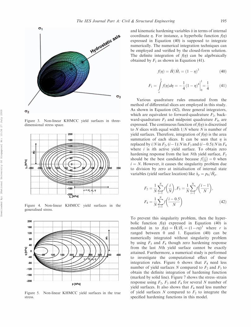
From the previous formulation, rate form of thestress–strain relationship based on the continuoushyperplasticity is described. However, the continuoushyperplasticity is suitable for monotonic loading withsimple hardening function. Because of this limitationto handle complicated loading conditions, the multi-surface hyperplasticity is generally employed in nu-merical implementation. Non-linearity is expressed bymultiple piece-wise responses (see also Mroz andNorris 1982). Therefore, multiple internal variablesplay a role as discrete memories of materials and thesmooth transition between piece-wise responses de-pends on the finite number of internal variables. ForKHMCC model, continuous yield surface is discretisedto a finite number of yield surfaces (Likitlersuang(2003), Likitlersuang and Houlsby (2006)). Integrationoperator simply turns to summation operator withoutlosing general meaning. Each yield surfaces have theirown state variables which are relative stresses andhardening stress. A finite number of hardening stresscan be considered as multiple material memories whichare updated when the multiple yield surfaces are active.The illustration of multiple yield surfaces in principalstress space can be depicted in Figure 3.

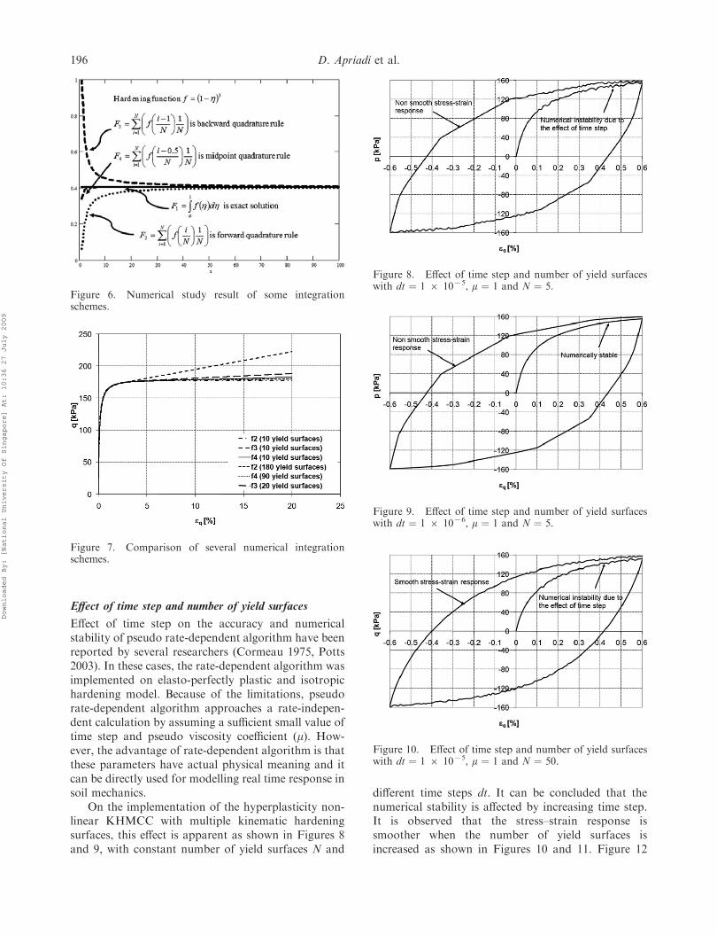
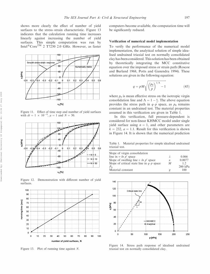
In this study, 10 multiple yield functions aredemonstrated. A plot of 10 yield surfaces in p–q planeunder relative stress space and true stress space isenvisaged in Figures 4 and 5, respectively. The rate-dependent incremental response of a single elementcalculation is obtained by integrating the incrementalstress–strain relation using strain driven forward-Eulerintegration scheme. This means an increment ofvariable based on rate form _x ¼ f(x) can be typicallywritten in the manner xiþ17xi ¼ f(xi) Dt where Dt ¼tiþ17ti and i þ 1 represents the current step number.

Figure 2. Determination of parameter a.



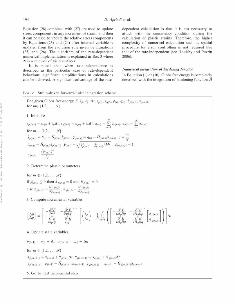
Equation (28) combined with (27) are used to updatestress components in any increment of strain, and thenit can be used to update the relative stress componentsby Equations (23) and (24) after internal variable isupdated from the evolution rule given by Equations(25) and (26). The algorithm of the rate-dependentnumerical implementation is explained in Box 3 whereN is a number of yield surfaces.

It is noted that when rate-independence isdescribed as the particular case of rate-dependentbehaviour, significant simplifications in calculationscan be achieved. A significant advantage of the rate-

dependent calculation is that it is not necessary toattach with the consistency condition during thecalculation of plastic strains. Therefore, the highercomplexity of numerical calculation such as specialprocedure for error controlling is not required likethat of the rate-independent (see Houlsby and Puzrin2006).

Numerical integration of hardening function

In Equation (1) or (10), Gibbs free energy is completelydescribed with the integration of hardening function H

Box 3: Strain-driven forward-Euler integration scheme.

For given Gibbs free-energy E; _ep; _eq; Dt; epðiÞ; eqðiÞ; pðiÞ; qðiÞ; apðm;iÞ; aqðm;iÞ,for m2 {1,2, . . . ,N}

1. Initialise

epðiþ1Þ ¼ epðiÞ þ _epDt; eqðiþ1Þ ¼ eqðiÞ þ _eqDt; apðiÞ ¼PNn¼1

apðn;iÞ; aqðiÞ ¼PNn¼1

aqðn;iÞ

for m 2 {1,2, . . . ,N}

wpðm;iÞ ¼ pðiÞ � Hpðm;iÞapðm;iÞ; wqðm;iÞ ¼ qðiÞ � Hqðm;iÞaqðm;iÞ; Z ¼m

N

cðm;iÞ ¼ Hpðm;iÞapðm;iÞZ; yðm;iÞ ¼ffiffiffiffiffiffiffiffiffiffiffiffiffiffiffiffiffiffiffiffiffiffiffiffiffiffiffiffiffiffiffiffiffiffiffiffiffiffiw2pðm;iÞ þ w2qðm;iÞ=M

2q

� cðm;iÞ; m ¼ 1

wðm;iÞ ¼yðm;iÞ� �2

2m

2. Determine plastic parameters

for m 2 {1,2, . . . ,N}

if y(m,i) � 0 then a�pðm;iÞ ¼ 0 and a

�qðm;iÞ ¼ 0

else a�pðm;iÞ ¼

@wðm;iÞ@wpðm;iÞ

; a�qðm;iÞ ¼

@wðm;iÞ@wqðm;iÞ

3. Compute incremental variables

DpDq

h i¼

� @2E@p2

� @2E@q@p

� @2E@q@p

� @2E@q2

264

375�1

_ep_eq

� �� 1N

PNm¼1

� @2E@ap@p

� @2E@aq@p

� @2E@ap@q

� @2E@aq@q

264

375 a

�pðm;iÞ

a�qðm;iÞ

" #0B@

1CA

264

375Dt

4. Update state variables

p(iþ1) ¼ p(i) þ Dp, q(i þ 1) ¼ q(i) þ Dq

for m 2 {1,2, . . . ,N}

apðm;iþ1Þ ¼ apðm;iÞ þ a�pðm;iÞDt; aqðm;iþ1Þ ¼ aqðm;iÞ þ a

�qðm;iÞDt

wpðm;iþ1Þ ¼ pðiþ1Þ � Hpðm;iþ1Þapðm;iþ1Þ; wqðm;iþ1Þ ¼ qðiþ1Þ � Hqðm;iþ1Þaqðm;iþ1Þ

5. Go to next incremental step



and kinematic hardening variables a in terms of internalcoordinate Z. For instance, a hyperbolic function f(Z)expressed in Equation (40) is supposed to integratenumerically. The numerical integration techniques canbe employed and verified by the closed-form solution.The definite integration of f(Z) can be algebraicallyobtained by F1 as shown in Equation (41).

fðZÞ ¼ H=Hi ¼ 1� Zð Þ3 ð40Þ

F1 ¼Z1o

f Zð ÞdZ ¼ � 1

41� Zð Þ4

1

0

¼ 1

4ð41Þ

Various quadrature rules emanated from themethod of differential slices are employed in this study.As shown in Equation (42), three general integrators,which are equivalent to forward-quadrature F2, back-ward-quadrature F3 and midpoint quadrature F4, areexpressed. The continuous function of f(Z) is discretisedto N slices with equal width 1/N where N is number ofyield surfaces. Therefore, integration of f(Z) is the areasummation of each slices. It can be seen that Z isreplaced by i/N in F2, (i71)/N in F3 and (i70.5)/N in F4

where i is ith active yield surface. To obtain zerohardening response from the last Nth yield surface, F2

should be the best candidate because f iN

� �¼ 0 when

i ¼ N. However, it causes the singularity problem dueto division by zero at initialisation of internal statevariables (yield surface location) like ap ¼ p0=Hp.

F2 ¼1

N

XNi¼1

fi

N

� �;F3 ¼

1

N

XNi¼1

fi� 1

N

� �;

F4 ¼1

N

XNi¼1

fi� 0:5

N

� �ð42Þ

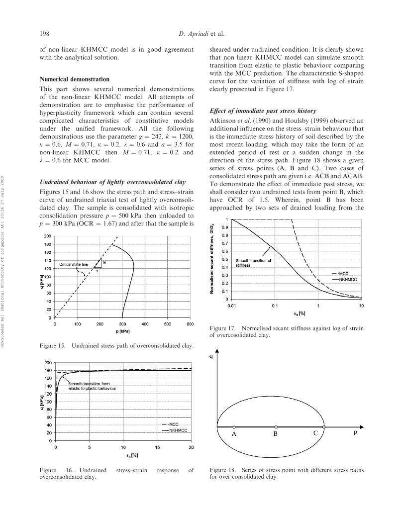
To prevent this singularity problem, then the hyper-bolic function f(Z) expressed in Equation (40) ismodified in to f(Z) ¼ H/Hi ¼ (17rZ)3 where r isranged between 0 and 1. Equation (40) can benumerically integrated without singularity problemby using F3 and F4 though zero hardening responsefrom the last Nth yield surface cannot be exactlyattained. Furthermore, a numerical study is performedto investigate the computational effect of theseintegration rules. Figure 6 shows that F4 need lessnumber of yield surfaces N compared to F2 and F3 toobtain the definite integration of hardening function(marked by solid line). Figure 7 shows the stress–strainresponse using F2, F3 and F4 for several N number ofyield surfaces. It also shows that F4 need less numberof yield surfaces N compared to F2 to integrate thespecified hardening functions in this model.

Figure 3. Non-linear KHMCC yield surfaces in three-dimensional stress space.

Figure 4. Non-linear KHMCC yield surfaces in thegeneralised stress.

Figure 5. Non-linear KHMCC yield surfaces in the truestress.



Effect of time step and number of yield surfaces

Effect of time step on the accuracy and numericalstability of pseudo rate-dependent algorithm have beenreported by several researchers (Cormeau 1975, Potts2003). In these cases, the rate-dependent algorithm wasimplemented on elasto-perfectly plastic and isotropichardening model. Because of the limitations, pseudorate-dependent algorithm approaches a rate-indepen-dent calculation by assuming a sufficient small value oftime step and pseudo viscosity coefficient (m). How-ever, the advantage of rate-dependent algorithm is thatthese parameters have actual physical meaning and itcan be directly used for modelling real time response insoil mechanics.

On the implementation of the hyperplasticity non-linear KHMCC with multiple kinematic hardeningsurfaces, this effect is apparent as shown in Figures 8and 9, with constant number of yield surfaces N and

different time steps dt. It can be concluded that thenumerical stability is affected by increasing time step.It is observed that the stress–strain response issmoother when the number of yield surfaces isincreased as shown in Figures 10 and 11. Figure 12

Figure 6. Numerical study result of some integrationschemes.

Figure 7. Comparison of several numerical integrationschemes.

Figure 8. Effect of time step and number of yield surfaceswith dt ¼ 1 6 1075, m ¼ 1 and N ¼ 5.





shows more clearly the effect of number of yieldsurfaces to the stress–strain characteristic. Figure 13indicates that the calculation running time increaseslinearly against increasing the number of yieldsurfaces. This simple computation was run byIntel1CoreTM 2 T7250 2.0 GHz. However, as faster

computers become available, the computation time willbe significantly reduced.

Verification of numerical model implementation

To verify the performance of the numerical modelimplementation, the analytical solution of simple idea-lised undrained triaxial test on normally consolidatedclayhasbeenconsidered.This solutionhasbeenobtainedby theoretically integrating the MCC constitutiveequation over the imposed stress or strain path (Roscoeand Burland 1968, Potts and Ganendra 1994). Thesesolutions are given in the following equation:

q ¼ pM

ffiffiffiffiffiffiffiffiffiffiffiffiffiffiffiffiffiffiffiffiffiffiffiffiffiffip0p

� �1=L

� 1

sð43Þ

where p0 is mean effective stress on the isotropic virginconsolidation line and L ¼ 1� k

l. The above equationprovides the stress path in q–p space, as p0 remainsconstant in an undrained test. The material propertiesassumed in this verification are given in Table 1.

In this verification, full pressure-dependent isconsidered for non-linear KHMCC model under singleyield surface using n ¼ 1, and other parameters arek ¼ 232, a ¼ 1.1. Result for this verification is shownin Figure 14. It is shown that the numerical prediction


Figure 12. Demonstration with different number of yieldsurfaces.

Figure 13. Plot of running time against N.

Table 1. Material properties for simple idealised undrainedtriaxial test.

Slope of virgin consolidationline in n–ln p0 space l 0.066Slope of swelling line n–ln p0 space k 0.0077Slope of critical state line in q–p space M 1.2P0 200 kPaMaterial constant g 100

Figure 14. Stress path response of idealised undrainedtriaxial test on normally consolidated clay.



of non-linear KHMCC model is in good agreementwith the analytical solution.

Numerical demonstration

This part shows several numerical demonstrationsof the non-linear KHMCC model. All attempts ofdemonstration are to emphasise the performance ofhyperplasticity framework which can contain severalcomplicated characteristics of constitutive modelsunder the unified framework. All the followingdemonstrations use the parameter g ¼ 242, k ¼ 1200,n ¼ 0.6, M ¼ 0.71, k ¼ 0.2, l ¼ 0.6 and a ¼ 3.5 fornon-linear KHMCC then M ¼ 0.71, k ¼ 0.2 andl ¼ 0.6 for MCC model.

Undrained behaviour of lightly overconsolidated clay

Figures 15 and 16 show the stress path and stress–straincurve of undrained triaxial test of lightly overconsoli-dated clay. The sample is consolidated with isotropicconsolidation pressure p ¼ 500 kPa then unloaded top ¼ 300 kPa (OCR ¼ 1.67) and after that the sample is

sheared under undrained condition. It is clearly shownthat non-linear KHMCC model can simulate smoothtransition from elastic to plastic behaviour comparingwith the MCC prediction. The characteristic S-shapedcurve for the variation of stiffness with log of strainclearly presented in Figure 17.

Effect of immediate past stress history

Atkinson et al. (1990) and Houlsby (1999) observed anadditional influence on the stress–strain behaviour thatis the immediate stress history of soil described by themost recent loading, which may take the form of anextended period of rest or a sudden change in thedirection of the stress path. Figure 18 shows a givenseries of stress points (A, B and C). Two cases ofconsolidated stress path are given i.e. ACB and ACAB.To demonstrate the effect of immediate past stress, weshall consider two undrained tests from point B, whichhave OCR of 1.5. Wherein, point B has beenapproached by two sets of drained loading from the

Figure 15. Undrained stress path of overconsolidated clay.

Figure 16. Undrained stress–strain response ofoverconsolidated clay.

Figure 17. Normalised secant stiffness against log of strainof overcosolidated clay.

Figure 18. Series of stress point with different stress pathsfor over consolidated clay.



direction of point A and C. Also shown in Figure 18,all stress histories located within the MCC surface.

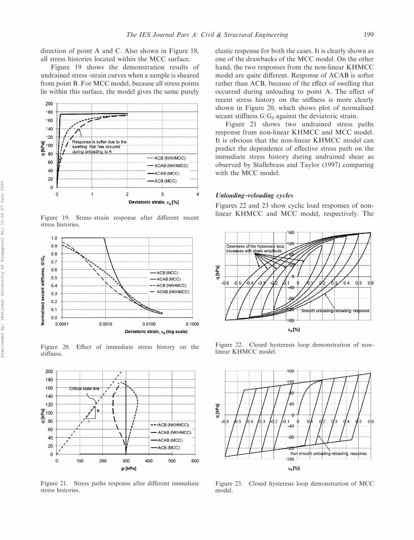
Figure 19 shows the demonstration results ofundrained stress–strain curves when a sample is shearedfrom point B. For MCCmodel, because all stress pointslie within this surface, the model gives the same purely

elastic response for both the cases. It is clearly shown asone of the drawbacks of the MCC model. On the otherhand, the two responses from the non-linear KHMCCmodel are quite different. Response of ACAB is softerrather than ACB, because of the effect of swelling thatoccurred during unloading to point A. The effect ofrecent stress history on the stiffness is more clearlyshown in Figure 20, which shows plot of normalisedsecant stiffness G/G0 against the deviatoric strain.

Figure 21 shows two undrained stress pathsresponse from non-linear KHMCC and MCC model.It is obvious that the non-linear KHMCC model canpredict the dependence of effective stress path on theimmediate stress history during undrained shear asobserved by Stallebrass and Taylor (1997) comparingwith the MCC model.

Unloading–reloading cycles

Figures 22 and 23 show cyclic load responses of non-linear KHMCC and MCC model, respectively. The

Figure 19. Stress–strain response after different recentstress histories.

Figure 20. Effect of immediate stress history on thestiffness.

Figure 21. Stress paths response after different immediatestress histories.

Figure 22. Closed hysteresis loop demonstration of non-linear KHMCC model.

Figure 23. Closed hysteresis loop demonstration of MCCmodel.



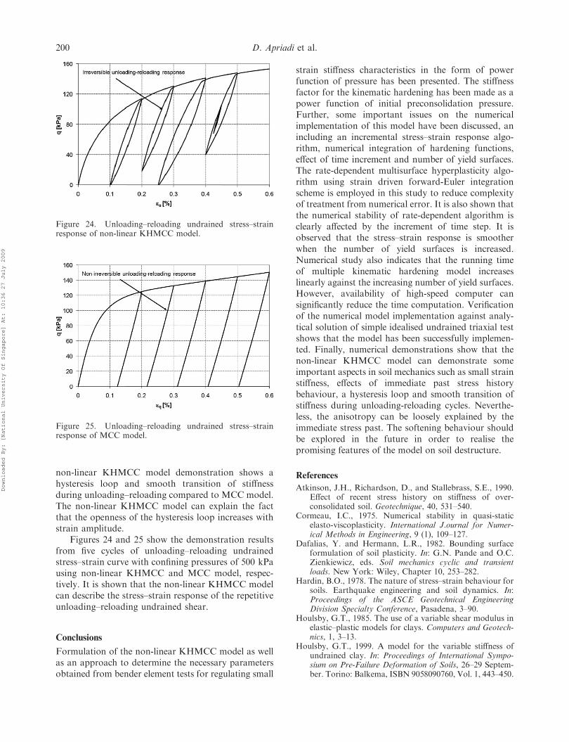
non-linear KHMCC model demonstration shows ahysteresis loop and smooth transition of stiffnessduring unloading–reloading compared to MCC model.The non-linear KHMCC model can explain the factthat the openness of the hysteresis loop increases withstrain amplitude.

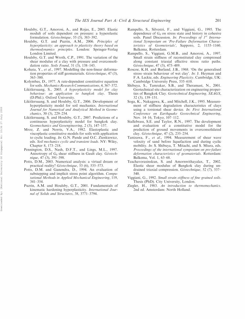
Figures 24 and 25 show the demonstration resultsfrom five cycles of unloading–reloading undrainedstress–strain curve with confining pressures of 500 kPausing non-linear KHMCC and MCC model, respec-tively. It is shown that the non-linear KHMCC modelcan describe the stress–strain response of the repetitiveunloading–reloading undrained shear.

Conclusions

Formulation of the non-linear KHMCC model as wellas an approach to determine the necessary parametersobtained from bender element tests for regulating small

strain stiffness characteristics in the form of powerfunction of pressure has been presented. The stiffnessfactor for the kinematic hardening has been made as apower function of initial preconsolidation pressure.Further, some important issues on the numericalimplementation of this model have been discussed, anincluding an incremental stress–strain response algo-rithm, numerical integration of hardening functions,effect of time increment and number of yield surfaces.The rate-dependent multisurface hyperplasticity algo-rithm using strain driven forward-Euler integrationscheme is employed in this study to reduce complexityof treatment from numerical error. It is also shown thatthe numerical stability of rate-dependent algorithm isclearly affected by the increment of time step. It isobserved that the stress–strain response is smootherwhen the number of yield surfaces is increased.Numerical study also indicates that the running timeof multiple kinematic hardening model increaseslinearly against the increasing number of yield surfaces.However, availability of high-speed computer cansignificantly reduce the time computation. Verificationof the numerical model implementation against analy-tical solution of simple idealised undrained triaxial testshows that the model has been successfully implemen-ted. Finally, numerical demonstrations show that thenon-linear KHMCC model can demonstrate someimportant aspects in soil mechanics such as small strainstiffness, effects of immediate past stress historybehaviour, a hysteresis loop and smooth transition ofstiffness during unloading-reloading cycles. Neverthe-less, the anisotropy can be loosely explained by theimmediate stress past. The softening behaviour shouldbe explored in the future in order to realise thepromising features of the model on soil destructure.

References

Atkinson, J.H., Richardson, D., and Stallebrass, S.E., 1990.Effect of recent stress history on stiffness of over-consolidated soil. Geotechnique, 40, 531–540.

Cormeau, I.C., 1975. Numerical stability in quasi-staticelasto-viscoplasticity. International J.ournal for Numer-ical Methods in Engineering, 9 (1), 109–127.

Dafalias, Y. and Hermann, L.R., 1982. Bounding surfaceformulation of soil plasticity. In: G.N. Pande and O.C.Zienkiewicz, eds. Soil mechanics cyclic and transientloads. New York: Wiley, Chapter 10, 253–282.

Hardin, B.O., 1978. The nature of stress–strain behaviour forsoils. Earthquake engineering and soil dynamics. In:Proceedings of the ASCE Geotechnical EngineeringDivision Specialty Conference, Pasadena, 3–90.

Houlsby, G.T., 1985. The use of a variable shear modulus inelastic–plastic models for clays. Computers and Geotech-nics, 1, 3–13.

Houlsby, G.T., 1999. A model for the variable stiffness ofundrained clay. In: Proceedings of International Sympo-sium on Pre-Failure Deformation of Soils, 26–29 Septem-ber. Torino: Balkema, ISBN 9058090760, Vol. 1, 443–450.

Figure 24. Unloading–reloading undrained stress–strainresponse of non-linear KHMCC model.

Figure 25. Unloading–reloading undrained stress–strainresponse of MCC model.



Houlsby, G.T., Amorosi, A., and Rojas, E., 2005. Elasticmoduli of soils dependent on pressure: a hyperelasticformulation. Geotechnique, 55 (5), 383–392.

Houlsby, G.T. and Puzrin, A.M., 2006. Principles ofhyperplasticity: an approach to plasticity theory based onthermodynamics principles. London: Springer-VerlagLondon Limited.

Houlsby, G.T. and Wroth, C.P., 1991. The variation of theshear modulus of a clay with pressure and overconsoli-dation ratio. Soils Found, 31 (3), 138–143.

Kohata, Y., et al., 1997. Modelling the non-linear deforma-tion properties of stiff geomaterials. Geotechnique, 47 (3),563–580.

Kolymbas, D., 1977. A rate-dependent constitutive equationfor soils.Mechanics Research Communications, 4, 367–372.

Likitlersuang, S., 2003. A hyperplasticity model for claybehaviour: an application to bangkok clay. Thesis(D.Phil.). Oxford University.

Likitlersuang, S. and Houlsby, G.T., 2006. Development ofhyperplasticity model for soil mechanics. InternationalJournal for Numerical and Analytical Method in Geome-chanics, 30 (3), 229–254.

Likitlersuang, S. and Houlsby, G.T., 2007. Predictions of acontinuous hyperplasticity model for bangkok clay.Geomechanics and Geoengineering, 2 (3), 147–157.

Mroz, Z. and Norris, V.A., 1982. Elastoplastic andviscoplastic constitutive models for soils with applicationto cyclic loading. In: G.N. Pande and O.C. Zienkiewicz,eds. Soil mechanics cyclic and transient loads. NY: Wiley,Chapter 8, 173–218.

Pennington, D.S., Nash, D.F.T., and Lings, M.L., 1997.Anisotropy of G0 shear stiffness in Gault clay. Geotech-nique, 47 (3), 391–398.

Potts, D.M., 2003. Numerical analysis: a virtual dream orpractical reality? Geotechnique, 53 (6), 535–573.

Potts, D.M. and Ganendra, D., 1994. An evaluation ofsubstepping and implicit stress point algorithm. Compu-tational Methods in Applied Mechanical Engineering, 119,341–354.

Puzrin, A.M. and Houlsby, G.T., 2001. Fundamentals ofkinematic hardening hyperplasticity. International Jour-nal of Solids and Structures, 38, 3771–3794.

Rampello, S., Silvestri, F., and Viggiani, G., 1995. Thedependence of G0 on stress state and history in cohesivesoils. Panel Discussion. In: Proceedings of 1st Interna-tional Symposium on ‘Pre-Failure Deformation Charac-teristics of Geometerials’, Sapporo, 2, 1155–1160.Balkema, Rotterdam.

Rampello, S., Viggiani, G.M.B., and Amorosi, A., 1997.Small strain stiffness of reconstituted clay compressedalong constant triaxial effective stress ratio paths.Geotechnique, 47 (3), 475–489.

Roscoe, K.H. and Burland, J.B., 1968. ‘On the generalisedstress–strain behaviour of wet clay’. In: J. Heyman andF.A. Leckie, eds. Engineering Plasticity. Cambridge, UK:Cambridge University Press, 535–610.

Shibuya, S., Tamrakar, S.B., and Theramast, N., 2001.Geotechnical site characterization on engineering proper-ties of Bangkok Clay. Geotechnical Engineering, SEAGS,32 (3), 139–151.

Soga, K., Nakagawa, K., and Mitchell, J.K., 1995. Measure-ment of stiffness degradation characteristics of claysusing a torsional shear device. In: First InternationalConference on Earthquake Geotechnical Engineering,Nov. 14–16, Tokyo, 107–112.

Stallebrass, S.E. and Taylor, R.N., 1997. The developmentand evaluation of a constitutive model for theprediction of ground movements in overconsolidatedclay. Geotechnique, 47 (2), 235–254.

Tanizawa, F., et al., 1994. Measurement of shear wavevelocity of sand before liquefaction and during cyclicmobility. In: S. Shibuya, T. Mitachi, and S. Miura, eds.Proceedings of the international symposium on pre-failuredeformation characteristics of geomaterials. Rotterdam:Balkema, Vol. 1, 63–68.

Teachavorasinskun, S. and Amornwithayalax, T., 2002.Elastic shear modulus of Bangkok clay during un-drained triaxial compression. Geotechnique, 52 (7), 537–540.

Viggiani, G., 1992. Small strain stiffness of fine grained soils.Thesis (PhD). City University, London.

Ziegler, H., 1983. An introduction to thermomechanics.2nd ed. Amsterdam: North Holland.



On the Numerical Implementation of Hyperplasticity Non-Linear Kinematic Hardening Modified Cam Clay...

Documents

Transcript of On the Numerical Implementation of Hyperplasticity Non-Linear Kinematic Hardening Modified Cam Clay...