Plantwide control: the search for the self-optimizing control structure

Plantwide control: The search for the self-optimizingcontrol structure

SigurdSkogestad�

Departmentof ChemicalEngineering

NorwegianUniversityof ScienceandTechnology

N–7491TrondheimNorway

May 5, 2000

Abstract

Plantwidecontrolisconcernedwith thestructuraldecisionsinvolvedin thecontrolsystemdesignof achemicalplant (Foss1973); “Which variablesshouldbe controlled,which variablesshouldbe measured,which inputsshouldbemanipulated,andwhich links shouldbemadebetweenthem?”In particular, thefirst issueaboutwhichvariablesto control hasreceived little attention. It is arguedthat the answeris relatedto finding a simpleandrobust way of implementingthe economicallyoptimal operatingpolicy. The goal is to find a setof controlledvariableswhich, whenkept at constantsetpoints,indirectly leadto near-optimaloperationwith acceptableloss.This is denoted“self-optimizing” control. Sincetheeconomicsaredeterminedby theoverall plantbehavior, it isnecessaryto take a plantwideperspective. A systematicprocedurefor finding suitablecontrolledvariablesbasedononly steady-stateinformationis presented.Importantstepsaredegreeof freedomanalysis,definitionof optimaloperation(costandconstraints),andevaluationof thelosswhenthecontrolledvariablesarekeptconstantratherthanoptimallyadjusted.A casestudyyieldsvery interestinginsightsinto thecontrolandmaximumthroughputofdistillationcolumns.

Preparedfor JPC(extendedversionof paperfromIFAC World Congress,July 1999)Submitted:Oct 1999;Revised:Jan. 2000;March 2000

Note: Thisversiondoesnot containsomeof thelatestcorrectionsin thejournal version

�E-mail: [email protected];phone:+47-7359-4154;fax: +47-7359-4080

1

1 Introduction

If we considerthe control systemin a chemicalplant, thenwe find that it is structuredhierarchicallyinto several layers,eachoperatingon a differenttime scale.Typically, layersincludeincludeschedul-ing (weeks),site-wide(real-time)optimization(day), local optimization(hour),supervisory/predictivecontrol (minutes)andstabilizingandregulatorycontrol (seconds);seeFigure 1. The layersareinter-connectedthroughthecontrolled variables. Moreprecisely,

Thesetpointsof thecontrolledvariables( �� ) arethe(internal)variablesthatlink two layersin a controlhierarchy, wherebytheupperlayercomputesthevalueof �� to beimplementedby thelower layer.

Weusuallyassumetime-scaleseparationwhich for ourpurposesimpliesthatthesetpoints�� canbeassumedto be immediatelyimplementedby the layersbelow. Thequestionwe want to answerin thispaperis: Whichshouldtheseinternalcontrolledvariables� be?Thatis, whatshouldwe control?

Moregenerally, theissueof selectingcontrolledvariablesis thefirst subtaskin theplantwide controlor control structure design problem(Foss1973);(Morari 1982);(SkogestadandPostlethwaite1996):

1. Selectionof controlled variables�2. Selectionof manipulatedvariables�3. Selectionof measurements� (for controlpurposesincludingstabilization)

4. Selectionofacontrol configuration (structureof thecontrollerthatinterconnectsmeasurements/setpointsandmanipulatedvariables)

5. Selectionof controller type(control law specification,e.g.,PID, decoupler, LQG, etc.).

Eventhoughcontrolengineeringis well developedin termsof providing optimalcontrolalgorithms,itis clearthatmostof theexistingtheoriesprovide little helpwhenit comesto makingtheabovestructuraldecisions.

The methodpresentedin this paperfor selectingcontrolledvariables(task1) follows the ideasofMorari et al. (1980)andSkogestadandPostlethwaite (1996)andis very simple. Thebasisis to definemathematicallythequalityof operationin termsof ascalarcostfunction

�to beminimized.To achieve

truly optimaloperationwewouldneedaperfectmodel,wewouldneedto measureall disturbances,andwe would needto solve the resultingdynamicoptimizationproblemon-line. This is unrealistic,andthequestionis if it is possibleto find a simplerimplementationwhich still operatessatisfactorily (withan acceptableloss). More precisely, the loss � is definedas the differencebetweenthe actualvalueof the cost function obtainedwith a specificcontrol strategy, and the truly optimal valueof the costfunction,i.e. � ��

. Thesimplestoperationwould resultif we couldselectcontrolledvariablessuchthatweobtainedacceptableoperationwith constantsetpoints,thuseffectively turningthecomplexoptimizationprobleminto a simplefeedbackproblemandachieve what we herecall “self-optimizingcontrol”:

Self-optimizing control is whenwe canachieve an acceptablelosswith constantsetpointvaluesfor thecontrolledvariables(without theneedto reoptimizewhendisturbancesoccur)

(The readeris probablyfamiliar with the term self-regulation,which is whenacceptabledynamiccontrol performancecan be obtainedwith constantmanipulatedinputs. Self-optimizingcontrol is adirectgeneralizationto thecasewherewecanachieveacceptable(economic)performancewith constantcontrolledvariables.)The term“self-optimizing control” is shortanddescriptive, but alsoothertermshave beenusedto describethesameidea,suchas“feedbackoptimizingcontrol” (Morari et al. 1980),and“indirect optimizingcontrol (throughsetpointcontrol)”(HalvorsenandSkogestad1998).A simpleexampleof self-optimizingcontrolis theprocessof bakingacake,wheretheoperationis indirectlykeptcloseto its optimum(“a well-baked cake”) by controlling theoventemperatureandbakingtime at thesetpointsgivenin thecookbook(which in thiscaseis the“optimizer”).

2

�Scheduling

(weeks)

Site-wideoptimization(day)� � � � � �

Localoptimization(hour)

��

�Supervisory

control(minutes)

��

Regulatorycontrol

(seconds)

�� ! """"" #Controllayer

Figure1: Typical controlhierarchyin achemicalplant.

C = constant

C = constant

Reoptimized J (d)opt

1,s

2,s

d*

Cost J

Disturbance d

Loss

Figure2: Lossimposedby keepingconstantsetpointfor thecontrolledvariable

3

The ideais further illustratedin Figure2, wherewe seethat thereis a lossif we keepa constantsetpointratherthanreoptimizingwhenadisturbancemovestheprocessawayfrom its nominallyoptimaloperatingpoint (denoted$ ). For thecaseillustratedin thefigureit is better(with asmallerloss)to keepthesetpoint�&%'� constantthanto keep ��()� constant.

An additionalconcernwith theconstantsetpointpolicy is thattherewill alwaysbeanimplementationerror *,+- � � � � , e.g. causedby measurementerror. The implementationerror may causea largeadditionallossif theoptimumsurfaceis “sharp”. To bemorespecific,wemay, asillustratedin Figure3,distinguishbetweenthreeclassesof problemswhenit comesto theactualimplementation:

(a) Constrainedoptimum. In thefigure is shown thecasewheretheminimumvalueof thecost�is obtainedfor � ��.0/21 . In this casethereis no loss imposedby keepinga constant� � � .0/21 . In addition,implementationof an “active” constraintis usuallyeasy, e.g., it is

easyto keepavalve closed.

(b) Unconstrained flat optimum. In this casethe cost is insensitive to valueof the controlledvariable� , andimplementationis againeasy.

(c) Unconstrainedsharpoptimum. Themoredifficult problemsfor implementationis whenthecost(operation)is sensitive to valueof thecontrolledvariable� . In this case,we wantto findanothercontrolledvariable � in which theoptimumis flatter.

Thelatterunconstrainedproblemsarethefocusof thispaper.

Important notation� - controlledvariables(selectedfrom the setsof 3 and � to replace 4 as degreesof freedomforoptimization;specialcase� 54 )� ��6 *87 - optimalvalueof � whichminimizescost

�for given * .�9� - setpointvaluefor � ; in thispaper, �� :6 * � 7* - disturbancevariables* � - nominalvalueof disturbances*;+0 � � � � - implementationerror< + � �� 96 *=7 - setpointerror< + < +?> * + � � � ��6 *87 - overall error� ��@ 6 4?A)*87B � + 6 � A)*87 - scalarcostfunctionto beminimized� ��C��6 *87 - minimumvalueof

�(minimizedwith respectto 4 or � )�D � + 6 � A)*87 �� 96 *=7 - loss� - manipulatedvariables(controldegreesof freedom)� (assubscript)- measuredE - noiseonmeasurementsof 3F . - no. of degreesof freedomfor controlF �� FG@ F + - no. of degreesof freedomfor optimizationF ��IH JLKNMIM

- no. of unconstraineddegreesof freedomfor optimization4 - “baseset” for theFO@

optimizationdegreesof freedom� - all availablemeasurements(including ��. , * . , 3 . )3 - dependent“output” variables;usuallymeasured

4

2 Previous work

Inspiredby thework of Findeisenetal. (1980),thebasicideaof self-optimizingcontrolwasformulatedabouttwentyyearsagoby Morari etal. (1980).Morari etal. (1980)write that“in attemptingto synthe-sizea feedbackoptimizingcontrolstructure,our mainobjective is to translatetheeconomicobjectivesinto processcontrol objectives. In otherwords,we want to find a function � of the processvariableswhich whenheldconstant,leadsautomaticallyto theoptimaladjustmentsof themanipulatedvariables,andwith it, theoptimal operating conditions. [...] This meansthatby keepingthe function � 6 4?A)*87 atthe setpoint � � , throughthe useof the manipulatedvariables4 , for variousdisturbances* , it followsuniquelythat theprocessis operatingat theoptimalsteady-state.” If we replacethe term“optimal ad-justments”by “acceptableadjustments(in termsof the loss)” thentheabove is a precisedescriptionofwhatwe in this paperdenotea self-optimizingcontrolstructure.Theonly factorthey fail to consideristheeffectof implementationerror � � �� . Morari etal. (1980)proposeto selectthebestsetof controlledvariablesbasedon minimizing the loss(“feedbackoptimizingcontrolcriterion1”). They alsoproposethatMonteCarlosimulationsshouldbeusedto evaluatethe lossif thedisturbanceshave a probabilitydistribution.

Somewhat surprisingly, the ideaof “feedbackoptimizing control” of Morari et al. (1980)hasupto now received very little attention. Onereasonis probablythat the paperalsodealtwith the issueof finding theoptimal operation(andnot only on how to implementit), andanotherreasonis that theonly examplein thepaperhappenedto resultin animplementationwith thecontrolledvariablesat theirconstraints. This constrainedcaseis usually “easy” from an implementationpoint of view, becausean optimal implementationis to simply maintainthe constrainedvariablesat their constraints(“activeconstraintcontrol” (Maarleveld and Rijnsdrop1970)). No examplewas given for the more difficultunconstrainedcase,the focus of this paper, wherethe choiceof controlled(feedback)variablesis acritical issue. The follow-up paperby Arkun andStephanopoulos(1980)concentratedfurther on theconstrainedcaseandtrackingof active constraints.

At aboutthesametime,Shinnar(1981)publishedamoreintuitive process-orientedapproachfor se-lectingcontrolledvariables,andappliedit to thecontrolof afluidizedcatalyticcracker (FCC).Theworkmayatfirst seemunrelated,but if onetranslatesthewordsandnotation,thenonerealizesthatShinnar’sideasarecloseto the ideaspresentedin this paperandin Morari et al. (1980). ThemaindifferenceisthatShinnarassumesthat theoverall objective of theoperationis to controla setof “primary” processvariablesP8Q at their specifications,whereaswe in this paperfollow Morari et al. (1980)andconciderthemoregeneralcasewheretheobjective is to minimizesomeeconomiccostfunction

�. In bothcases

it is assumedthattheoverall objective maybeindirectlyachievedby controllingsomeothervariablesattheirsetpoint;thesecontrolledvariablesaredenotedP +SR by Shinnar(1981)and � by Morari etal. (1980)(andin thispaper).

The similar later paperby Arbel et al. (1996) extendedthe FCC casestudy, and introducedtheconceptsof “dominantvariables”and“partial control”. Thedominantvariablesaretheprocessvariablesthattendto dominatetheprocessbehavior, for example,thetemperaturein areactor, andwhichthereforeintuitively may be good candidatesas controlledvariables. By partial control is meantthat controlof thesedominantvariablesindirectly achieves acceptablecontrol of the primary variables1 P8Q . Theauthorsprovidesomeintuitive ideasandexamplesfor selectingdominantvariableswhichmaybeusefulin somecases,especiallywhenno modelinformationis available. However, it is not clearhow helpfulthe ideaof “dominant” variableis, sincethey arenot really definedandno explicit procedureis givenfor identifying them. Indeed,Arbel et al. (1996)write that “the problemsof partial controlhave beendiscussedin a heuristicway” andthat “considerablyfurther researchis neededto fully understandtheproblemsis steady-statecontrol of chemicalplants”. It is believed that theapproachpresentedin thispaper, basedon usinga (steady-state)modelto evaluatethe(economic)loss,providesanimportantpart

1Theterms“partial control” and“partially controlledsystem”areusedby otherauthors(Waller et al. 1988)(SkogestadandPostlethwaite1996)in a moregeneralsense,to meanthesystemasit is appearsfrom somehigherlayerin thecontrolhierarchywith someloopsalreadyclosed(e.g.a plantwheretheliquid level loopsareclosed).

5

of thismissingtheoreticalframework.Tyreus(1999)providessomeadditionalinterestingideasonhow to selectdominantvariables,partly

basedon theextensive variableideaof Georgakis(1986)andthe thermodynamicideasof Ydstie,e.g.(AlonsoandYdstie1996),but againno procedurefor selectingsuchvariablesarepresented.

Luyben(1988)introducedtheterm“eigenstructure”to describetheinherentlybestcontrolstructure(with thebestself-regulatingandself-optimizingproperty).However, hedid not really definetheterm,andalsothenameis unfortunatesince“eigenstructure”hasa anotherunrelatedmathematicalmeaningin termsof eigenvalues.Apart from this, Luybenandcoworkers(e.g. Luyben(1975),Yi andLuyben(1995))havestudiedunconstrainedproblems,andsomeof theexamplespresentedpoint in thedirectionof theselectionmethodspresentedin thispaper. However, Luybenproposesto selectcontrolledoutputswhichminimizesthesteady-statesensitive of themanipulatedvariable( 4 ) to disturbances,i.e. to selectcontrolledoutputs( � ) suchthat

6UT 4WV T *87 + is small, whereaswe really want to minimize the steady-statesensitivity of theeconomicloss( � ) to disturbances,i.e. to selectcontrolledoutputs( � ) suchthat6UT �XV T *=7 + is small.

Fisheretal. (1988)discussselectionof controlledvariables,mainlyfocusedtowardsactiveconstraintcontrol.However, somewhathiddenin theirHDA example(p. 614)onefindsstatementsaboutselectingcontrolledvariableswhich optimal valuesare insensitive to disturbances(requirement1 for variableselectionpresentedin thispaper).

In hisbookRijnsdorp(1991)givesonpage99astepwisedesignprocedurefor designingoptimizingcontrolsystemsfor processunits.Onestepis to “transfertheresultinto on-linealgorithmsfor adjustingthedegreesof freedomfor optimization”. He statesthat this “requiresgoodprocessinsightandcontrolstructureknow-how. It is worthwhilebasingthealgorithmasfar aspossibleon processmeasurements.In any case,it is impossibleto give aclear-cut recipehere.”

Narraway et al. (1991),Narraway andPerkins(1993)andNarraway andPerkins(1994))stronglystresstheneedto basethe selectionof the control structureon economics,andthey discusstheeffectof disturbanceson theeconomics.However, they do not formulateany rulesor proceduresfor selectingcontrolledvariables.

In astudyof theTenesseeEastmanchallangeproblem,Ricker (1996)notesthatwhenapplyingbothMPCanddecentralizedmethods,oneneedsto makecritical decisionswithoutquantitative justifications.The foremostof theseis the selectionof the controlledvariables,andhe found existing quantititativemethodsfor thereselectionto beinadequate.His approachin thecasestudyis consistentwith theideasof self-optimizingcontrol.

Mizoguchi et al. (1995)andMarlin andHrymak (1997)stressthe needto find a goodway of im-plementingtheoptimal solutionin termshow thecontrol systemshouldrespondto disturbances,“i.e.the key constraintsto remainactive, variablesto be maximizedor minimized, priority for adjustingmanipulatedvariables,andso forth.” They suggestthat an issuefor improvementin today’s real-timeoptimizationsystemsis to selectthecontrol systemthat yields thehighestprofit for a rangeof distur-bancesthatoccurbetweeneachexecutionof theoptimization.This is similar to the ideaspresentedinthispaper.

Finally, Zhengetal. (1999)presentaprocedurefor selectingcontrolledvariablesbasedoneconomicpenaltieswhich is similar to the approachpresentedin this paper(apparently, the work hasbeenper-formedindependently),but they donotconsidertheimplementationerror. Theprocedureis appliedto areactor-separator-recycle system.

In summary, it is clearthatmany authorshavebeenawareof theimportanceof theideaspresentedinthis paper. Themaincontribution of thepresentpaperis to bring theideastogetherandformulatethemmoreclearly, to includetheimplementationerrorin theanalysis,andto presentsomegoodcasestudies.

6

3 Degrees of freedom for control and optimization

Thenumberof degreesof freedomfor control,F . , is usuallyeasilyobtainedfrom processinsightasthe

numberof independentvariablesthatcanbemanipulatedby externalmeans(which in processcontrolisthenumberof numberof adjustablevalvesplusthenumberof otheradjustableelectricalandmechanicalvariables).

In this paperwe areconcernedwith thethenumberof degreesof freedomfor optimization,F �� F + FG@ , which is generallylessthanthenumberof controldegreesof freedom,

F . . WehaveF �� F . �YFGZ (1)

whereF[Z F . Z > FG\CZ is thenumberof variableswith noeffect on thecostfunction

�.F . Z - numberof manipulatedinputs( 4 ’s),or combinationsthereof,with no effecton the�

.FO\�Z- numberof controlledoutputvariableswith no effecton

�.

In mostcases�

dependson the steady-stateonly, andFG\CZ

usuallyequalsthe numberof liquid levelswith no steady-stateeffect (including mostbuffer tank levels). However, notethat someliquid levelsdo have a steady-stateeffect, suchas the level in a non-equilibriumliquid phasereactor, and levelsassociatedwith adjustableheattransferareas.Also, we shouldnot includein

FG\CZany liquid holdups

thatareleft uncontrolled,suchasinternalstageholdupsin distillationcolumns.A simpleexamplewhereF . Z is non-zerois a heatexchangerwith bypasson both sides(i.e.F . ^] ). Here

F ��C� `_ sincethereat steady-stateis only oneoperationaldegreeof freedom,namelytheheattransferrate a (whichatsteady-statemaybeachievedby many combinationsof thetwo bypasses),sowe have

F . Z b_ .Theoptimizationis generallysubjectto severalconstraints,andthe

F ��degreesof freedomshould

be usedto 1) satisfytheconstraints,and2) “optimize theoperation”. We considerthecasewherewehave a feasiblesolution, thatis, all theconstraintscanbesatisfied.If thenumberof “active” constraints(satisfiedas equalities)is denoted

F[ced �Nf g)M, then the numberof of “free” (unconstrained)degreesof

freedomthatcanbeusedto optimizetheoperationis equaltoF ��C�'H JhKiMSM F �� YF[ced �if g)M (2)

Thisis usuallytheimportantnumberfor us,sinceit is generallyfor theunconstraineddegreesof freedomthattheselectionof controlledvariablesis acritical issue.

4 Optimal operation and its implementation

Above we usedtheexpression“optimize theoperation”,andthis needsto bequantified.Theremaybemany issuesinvolved, andto tradethemoff againsteachother in a systematicmannerwe quantify ascalarperformance(cost)index

�whichshouldbeminimized.In many casesthis index is aneconomic

measure,e.g.theoperationcost.For example,�

couldbeof theform� ��@ 6 4?A)*87B jlkZ`m 6 4nA)*87o*;p (3)

where4 arethedegreesof freedomfor optimization,* aretime-varyingdisturbances,and q is thetotaloperationtime.

In thispaperwewill for simplicity usesteady-statemodelsandtheintegrationin (3) maybereplacedby time-averagingover thevarioussteady-states.Themainjustificationfor usingasteady-stateanalysisis that the economicperformanceis primarily determinedby steady-stateconsiderations.The effectof the dynamiccontrol performancecanbe partly includedin the economicanalysisby introducingacontrolerrortermasanadditionaldisturbance.

Remark.Althoughweuseasteady-stateanalysisin thispaper, it maybeextendedto truly unsteady-state-processes,like during a gradetransitionor for a batchprocess,by using a dynamicmodelandletting thesetpoints�9� beprecomputedtrajectoriesasa functionof timeor of statevariables.

7

4.1 The optimization problem

Theoptimizingcontrolproblemcanbeformulatedasrtsvu@ ��@ 6 4nA)*87 (4)

subjectto theinequalityconstraints w 6 4?A)*=7yx{z (5)

where 4 arethe independentvariableswe canaffect (degreesof freedomfor optimization),and * areindependentvariableswe cannotaffect (disturbances).Heretheconstraintsfor instancemaybe| productspecifications(e.g.minimumpurity)| manipulatedvariableconstraints(e.g.nonzeroflow)| otheroperationallimitations(e.g.maximumtemperature)

Conflicting constraintsmay result in a problemwithout a feasiblesolution. For example,if we makea productby blendingtwo streamsthenwe cannotachieve a productspecificationoutsidetherangeoffeedcompositions.

Remark.We have assumedthatall dependent(state)variables} have beeneliminatedsuchthat thecostfunctionandconstraintsarein termsof theindependentvariables4 and * . However, in somecasesit is moreconvenientto keepthestatevariables} andcorrespondingmodelequations

w % 6 }?A�4?A)*=7~�z ,andformulatetheoptimizationproblemas rtsvu@ �� 6 }?A�4nA)*87 (6)

subjectto theconstraints w % 6 }nA�4?A)*87B�z (7)w ( 6 }nA�4?A)*87�x{z (8)

4.2 Implementing the optimal solution

Therearetwo main issueswhenit comesto optimizing control. Thefirst is themathematicalandnu-mericalproblemof solving theoptimizationproblemin (4) to obtaintheoptimaloperatingpoint. Theoptimizationproblemmay be very large, with hundredsof thousandsof equationsand hundredsofdegreesof freedom(e.g. for a completeethyleneplant), but with todayscomputersandoptimizationmethodsthisproblemis solvable,andit is indeedsolvedroutinelytodayin someplants.Thesecondis-sue,thefocusof thispaper, is how theoptimalsolutionshouldbeimplementedin practice.Surprisingly,this issuehasreceivedmuchlessattention.

To betterunderstandtheissuesconsiderthethreealternative structuresfor optimizingcontrolshownin Figure4:

(a) Open-loopimplementation.

(b) Closed-loopimplementationwith aseparatecontrollayer.

(c) Integratedoptimizationandcontrol.

In thefiguretheblock “process”denotestheprocessasseenfrom theoptimizationlayer, so it mayactuallybea partially controlledplantwhich includes,for example,stabilizinglevel loops.This meansthat the independentvariables4 for theoptimizationmay includesomeof the “original” manipulatedvariables( � ) aswell asthesetpointsusedin thelower-layercontrollers.

If therewereno unmeasureddisturbances* then the threeimplementationswould give the sameresult. The key to understandwhy the threestructuresdiffer, is thereforeto considerwhat happenstothedegreesof freedom4 in responseto a disturbance* (moregenerally* mayincludeany uncertainty,includingerrorsin themodelusedfor theoptimizationandcontrol).

8

c

J

[

(a) Implementationeasy: Ac-tiveconstraintcontrol

c

J

(b) Implementationeasy: In-sensitive to errorin �

c

J

(c) Implementation difficult:Look for another controlledvariable

Figure3: Implementingthecontrolledvariable

�

� �

.

�

��

� �

� � �

� � ��

��

OptimizerOptimizer OptimizingController

Controller

Process ProcessProcess

ObjectiveObjective Objective

Disturbance

(a) (b) (c)

Measurement

u

Measurements

u

d

n

d

u

d

noise

v

n

cs c m

-

Figure4: Alternativestructuresfor optimizingcontrol.Structure(b) is studiedin this paper

9

(a) For theopen-loopimplementationthereis no feedback,and 4 remainsunchangedwhenthereis adisturbance* .

(b) For theclosed-loopimplementationwith aseparatecontrollayer, thedisturbance* affectsthemea-surement�C. , andthecontrolleradjust4 sothat ��. returnsapproximatelyto its setpoint,�9� .

(c) For theintegratedoptimizationandcontrol,all availablemeasurements� (including � . ) areusedtoidentify thedisturbanceandupdatethemodel,andthendynamicon-lineoptimizationis usedtorecomputeanew optimalvaluefor 4

In general,theopen-loopimplementation(a) is notacceptablebecausethereis noattemptto correctfor disturbances* .

Ontheotherhand,thecentralizedimplementationin (c) with asingleoptimizingcontroller, althoughoptimal from a mathematicalpoint of view, is not likely to be usedin practice,even with tomorrowscomputingpower. Oneimportantreasonis the costof obtaininga dynamicmodel; in the centralizedcontrollerit is critical thatthismodelisaccuratesincetherearenopredeterminedlinks,andthecontrollermustrely entirelyon themodelto take theright action.

Therefore,in practice,we usetheclosed-loopimplementation(b) wherethe control systemis de-composedinto separatelayers.In thesimplestcaseshown in Figure4b we mayhave two layers:| A steady-stateoptimizationlayerwhichcomputestheoptimalsetpoints�� for thecontrolledvari-

ables,and| A feedbackcontrol layerwhich implementsthesetpoints,to get �y��9� .In processcontrol applications,the feedbackcontrol layer usuallyoperatescontinuously, whereastheoptimizationlayer (which may be an engineer)recomputesnew setpoints�� only quite rarely; maybeonceanhouror onceaday(whentheplanthassettledto anew steady-state).Theideais thatby locallycontrollingtheright variables� , we cantake careof mostof thedisturbances,andthusreducetheneedfor continuousreoptimization.This alsoreducestheneedfor modelinformationandtendsto make theimplementationmorerobust. On theotherhand,it usuallyimpliesa performancelosscomparedto the“true” optimal (centralized)solution,andthe challengeis to find a “self-optimizing” control structure(i.e. to find theright controlledvariables� ) for which theloss � is acceptable.

Comment on active constraint control. In somecasesthereis noperformancelosswith thehierar-chicalstructurein Figure4(b)with aseparateoptimizationandcontrollayer. This is whentheoptimumliesatsomeconstraints,andweuseactiveconstraint control wherewechoosetheconstrainedvariablesasthecontrolledvariables� (MaarleveldandRijnsdrop1970)(Arkun andStephanopoulos1980)(Fisheret al. 1988). This is a commonsituation,sinceif theprocessmodelis not too non-lineartheoptimumoperatingpoint is at the intersectionof asmany constraintsas therearedegreesof freedomfor opti-mization(Maarleveld andRijnsdrop1970). However, in many casesthe constraintsmove dependingon theoperatingpoint,anda changein theactive constraintsmayrequirereconfigurationof thecontrolloops.To avoid suchanoftencomplicatedlogic system,we mayusein thelower layera multivariablecontrollerthatexplicitly handlesconstraints.In particular, modelpredictive control (MPC), which hasgainedwidespreadusein industryover thelast20years,providesasimpleandefficient tool for trackingactive constraints.

4.3 Introductory example

To give thereadersomeappreciationof theissues,we considera distillation plantwheretheplanteco-nomicsaremainlydeterminedby its steady-statebehavior. With agivenfeed(includinggivenfeedrate)anda specifiedcolumnpressure,a conventionaltwo-productdistillation column,asshown in Figure5,hastwo degreesof freedomatsteadystate(

FG@ F �� ] ). (Fromacontrolpoint of view thecolumnhas

F . �� degreesof freedom,but two degreesof freedomareneededto stabilizethe reboilerandcondenserholdups,which have no steady-stateeffect, andonedegreeof freedomis usedto control the

10

pressureat its givenvalue2). Thetwo steady-statedegreesof freedom,e.g.selectedto bethevaporflow(boilup) � andthedistillateflow � , 4-`� ��(this is not a uniquechoice),maybeusedto optimizetheoperationof theplant. However thequestionwe want to answeris: How shouldtheoptimalsolutionbe implemented, that is, which two variables�shouldbespecifiedandcontrolledduringoperation?

To answerthisquestionin aquantitative manner, we needto definetheconstraintsfor theoperationandthecostfunction

�to beminimized.

Constraints. We assumethat themolefractionof light componentin thedistillateproduct }�� mustbeabove }�� H .0/21 , andthatto avoid floodingthecapacityof thecolumnis limited by amaximumallowedvaporload, ��x�� .B� � .

Cost function. Ratherthanminimizing the cost�

, it is morenaturalin this caseto maximizetheprofit ��

, which is theproductvalueminusthefeedcostsandtheoperational(energy) costswhichareproportionalto thevaporflow � ,��D�� > �� ¡0� (9)

Constrained operation. Let usfirst consideracasewhere| distillateis themorevaluableproduct(��£¢¤�� )| energy costsarelow (��¡ is small)

In thiscase,it is optimalto operatethecolumnat maximumload(to reducethelossof light componentin the bottom) andwith the distillate compositionat its specification(to maximizedistillate flow byincludingasmuchheavy componentaspossible)(Gordon1986),i.e.� �� ¥� .�� =¦ }W� H § Q:¨©�}�� H .0/21Thus,theoptimumlies at constraints(

F ��'H JhKiMSM FG ��ª�«F ced �Nf g)M ¬] � ]�z ) andimplementationisobvious:Weshouldselectthevaporrate � andthedistillatecomposition}W� asthecontrolledvariables(“active constraintcontrol”), � `� �}W� � ¦ � � ®� � .�� }�� H .B/L1 �In practice,we may implementthis usinga lower-level feedbackcontrol systemwherewe adjusttheboilup � to keepthe pressuredrop over the column(an indicatorof flooding, i.e. of � .�� ) below acertainlimit, and adjustthe reflux � (or someother flow, dependingon how the level and pressurecontrolsystemis configured)sothat }W� is keptconstant.

Unconstrained operation. Next, consideracasewhere| bottomsproductis themorevaluableproduct(��¯¢¤�W� )| energy costsarerelatively high (theterm ��¡0� contributessignificantlyto�

)

In thiscasetheoptimummaybeunconstrainedin bothvariables(F ��IH JhKiMSM F �� ] ), thatis,� ��X° � .�� =¦ }W� H § Q:¨ª±{}�� H .0/21

Implementationin thiscaseis notobvious.Fivecandidatesetsof controlledvariablesare� % `� }��}W�²� ¦ � ( `� q�¨ § Qq´³ ¨ . � ¦ �9µ `� �}��¶� ¦ ��· `� ��Y� ¦ ��¸ ®� ��V¹��V¹��2If columnpressureis free we often find that the optimal choiceis to have maximumcooling correspondingto minimum

pressure(“floating pressurecontrol” assuggestedby Shinskey (1984))becausetherelative volatility is usuallyimprovedwhenpressureis lowered.

11

andtherearemany others.Controlledvariables�&% and ��( will yield a “two-point” controlsystemwherewe closetwo loopsfor quality control; � µ yieldsa “one-point” control systemwhereonly onequalityloop is closed;whereas� · and � ¸ are“open-loop”policieswhich requireno additionalfeedbackloops(exceptfor thelevel andpressureloopsalreadymentioned).All of thesechoicesof controlledvariableswill have differentself-optimizingcontrolproperties.

At theendof thepaper, we studyanotherdistillation example,wheretheoptimumis constrainedinonevariableandunconstrainedin theother(

F ��IH JhKiMSM º_ ). We alsoconsiderthecasewherethe feedrateis adegreeof freedomfor theoptimization.

5 Selection of controlled variables

In this sectionwe threemethodsfor the selectingcontrolledvariables� , but let us first formulatetheproblemabit clearer.

5.1 Problem formulation

Let the“baseset” for theoptimizationdegreesof freedombedenoted4 (this is notauniqueset),andlet* denotethe(important)disturbances.For agivendisturbance* we cansolve theoptimizationproblem(4) with constraints(5), andif a feasiblesolutionexists,obtaintheoptimalvalue 4 ��96 *=7 ,rtsvu»¼)½¾»�¿ ÀoÁÃÂÅÄ � @ 6 4?A)*=70 � @ 6 4 ��C� 6 *87CA)*=70 �� 6 *87 (10)

However, in actualoperationthevalueof 4 will differ from thetheoptimalvalue 4 ��C��6 *87 , andthisresultsin a loss 3 � betweentheactualoperatingcostsandtheoptimaloperatingcosts,�D�� @ 6 4?A)*87B ��@ 6 4?A)*=7 �� 6 *87 (11)

Themagnitudeof thelosswill dependonthecontrolstrategy usedfor adjusting4 duringoperation,andto understandthisbetterconsiderthe“open-loop”and“closed-loop”strategies.| In the“open-loop”strategy we attemptto keep 4 constantat its setpoint4 � (moreprecisely, 4Æ4 � > * @ where* @ is theimplementationerrorfor 4 )| In the“closed-loop”strategy we adjust4��Ç + 6 � A)*=7 in a feedbackfashionin anattemptto keep �

constantat its setpoint�� (moreprecisely, � �� > * + , where* + is theimplementationerrorfor � )wherewehaveassumesthatthecontrolledvariables� havebeenselectedsuchthatthefunction ÇÈ+ existsandis unique.In thispaperweusefor simplicity thenominaloptimalvaluesassetpoints,i.e.4 � 54 ��C� 6 * � 7 ¦ � � � �� 6 * � 7 (12)

where* � denotethenominalvalueof thedisturbancefor which theoptimizationwasperformed.Theopen-looppolicy is oftenpoor;bothbecausetheoptimalinput 4 ��96 *=7 dependsstronglyon the

disturbance* (soit is notagoodpolicy to keep4 � constant),andbecausewe arenot ableto implement4 accurately(sotheimplementationerror * @ is large).The questionwe want to answeris therefore:Whatis a goodchoicefor the

F +[ F @controlled

variables � to usein theclosed-looppolicy? If we allow for combinationsof measurements,thenthereareinfinitely many choices.Notethattheopen-looppolicy is includedasthespecialcase� �4 .

We now presentthreeapproachesfor selectingcontrolledvariables. We first considerthe error,4 � 4 ��6 *87 , andbasedon this proposefour requirementsof thecontrolledvariable.We next considera relatedmethodbasedon maximizingtheminimumsingularvalue. Finally, we proposea moreexactstepwiseprocedurebasedon explicitly evaluatingtheloss.

3It is not really necessaryto introducethelossfunction,andwe mayinsteadwork directly with theactualcost É . However,thelossprovidesa better“absolutescale”on which to judgewhethera givensetof controlledvariables� is “good enough”,andthusis self-optimizing.

12

5.2 Requirements for controlled variables

Considera closed-loopimplementationwherewe attemptto keep � constantat thevalue � � . With thisimplementationtheoperationmaybenon-optimal(with apositive loss)dueto thepresenceof asetpointerrorandanimplementationerror.

1. Thesetpointerror, < + � �� 6 *=7 , is thedifferencebetweenthesetpointandthetruly optimalvalue.

2. Theimplementationerror, * + � � �� , is thedifferencebetweentheactualvalueandthesetpoint.

Thesetwo errorsaregenerallyindependent;thesetpointerroris causedby disturbances(changesin theoperatingpoint), whereasthe implementationerror is causedby measurementerror andpoor control.Theoverall error < + � � � ��:6 *87 (which causesapositive loss),is thenthesumof thetwo,< + < + � > * + (13)

Clearly, wewant < + to besmall. In addition,wewould like thata largevalueof < + resultsin only asmallvalueof the“baseset” error < @ , that is, we want 4 to beinsensitive to changesin � (or equivalently, wewant � to besensitive to changesin 4 ).

From this, we canderive the following four requirements for of a good candidate controlled �variable (alsoseeSkogestadandPostlethwaite(1996),page404):

Requirement 1. Its optimalvalueshouldbeinsensitive to disturbances(sothatthesetpointerror < + � issmall)

Requirement 2. It shouldbeeasyto measureandcontrolaccurately(sothat theimplementationerror* + is small)

Requirement 3. Its valueshouldbesensitive to changesin themanipulatedvariables4 , thatis, thegainfrom 4 to � is large (so thateven a large error in thecontrolledvariable � resultsin only a smallerrorin 4 ). Alternatively, theoptimumshouldbe“flat” with respectto thevariable� .

Requirement 4. For caseswith two or morecontrolledvariables,theselectedvariablesshouldnot becloselycorrelated.

In short,weshouldselectvariables � for which thevariation in optimalvalueand implementationerror is smallcomparedto their adjustablerange (therange� mayreachby varying 4 ) (SkogestadandPostlethwaite(1996),page408).

As a minor remarkwe mentionthatMorari et al. (1980)claim that “ideally onetries to select� insuchawaysuchthatsomeor all theelementsin � areindependentof thedisturbances* .” Thisstatementis generallynot true, becausewe needto be able to detectthe disturbancesthroughthe variables � .A betterrequirementis that the optimal valuesof the elementsin � are insensitive to disturbances*(requirement1).

All four requirementsshouldbesatisfied.For example,assumewe have a mixtureof threecompo-nents,andwe have a measurementof the sumof the threemole fractions, � ^}ËÊ > } � > }�Ì . Thismeasurementis always1 andthusindependentof disturbances(so requirement1 is satisfied),but it isof coursenot a suitablecontrolledvariablebecauseit is also insensitive to the manipulatedvariables4 (so requirement3 is not satisfied).Requirement3 alsoeliminatesvariablesthat have an extremum(maximumor minimum)whenthecosthasits minimum,becausethegainis zerofor suchvariables.

5.3 Minimum singular value rule

We hereconsidertheremainingunconstrainedproblemwhereany active constraintshave alreadybeenimplemented(i.e. keptconstant).For smallvariationswe mayusea linearizedrelationshipbetweenthe(remaining)unconstraineddegreesof freedom4 andany candidatesetof controlledvariables� .Í � ¥Î Í 4 (14)

13

Let Ï 6 ÎÐ7 denotetheminimumsingularvalueof thesteady-stategainmatrix Î . If we assumethateachcontrolledvariable� hasbeenscaledsuchthatthesumof its optimalrangeandits implementationerroris unity (i.e. Ñ < + Ñ Ò_ ) (this takescareof requirements1 and2), andthat each“basevariable” 4 hasbeenscaledsuchthat a unit changehasthe sameeffect on the costfunction

�, thenwe shouldprefer

setsof controlledvariablefor which Ï 6 ÎÐ7 is maximized(maximizingthegaintakescareof requirement3 andusingthe minimum singularvalue Ï 6 ÎÐ7 takescareof requirement4) This conditionis derivedin SkogestadandPostlethwaite (1996)(page406). Theminimumsingularvaluecanalsobeusedasatool for selectingmanipulatedinputsvariables(Morari 1983),but this is actuallyanunrelatedconditionwhich requiresadifferentscalingof thevariables.

Let usbriefly go throughthederivationof SkogestadandPostlethwaite (1996). For a givendistur-bance* , asecondorderTaylorseriesexpansionof thelossaroundtheoptimalvalue 4 § Q�¨ 6 *87 gives

� ��@ 6 4?A)*=7 �D��@ 6 4 § Q�¨�A)*87 � _] 6 4 � 4 �� 7 kDÓ T ( ��@T 4 (�Ô �� 6 4 � 4 �� 7 (15)

(wherewe have assumedthat theproblemis unconstrainedin 4 , so that thefirst-ordertermT � V T 4 is

zero.) Thus,the lossdependson thequantity 4 � 4 § Q�¨ which we obviously wantassmallaspossible.Now, for smalldeviationsfrom theoptimaloperatingpoint we have that thecandidateoutputvariablesarerelatedto theindependentvariablesby � � � § Q:¨©¥Î 6 4 � 4 § Q�¨'7 , or4 � 4 § Q�¨n�ÎGÕ % 6 � � � § Q�¨'7 (16)

Sincewewant 4 � 4 § Q�¨ assmallaspossible,it thereforefollowsthatweshouldselectthesetof controlledoutputs� suchthat theproductof Î Õ % and � � � § Q�¨ is assmallaspossible.Thus,from SkogestadandPostlethwaite(1996)we have thefollowing rule:

Assumewe havescaledeach variable � such that the expectedvariation in � � � § Q�¨ is ofmagnitude1 (including the effect of both disturbancesand control error), thenselectthecontrolled variables� thatminimizethenormof Î Õ % , which in termsof thetwo-normis thesameasmaximizingtheminimumsingularvalueof Î , Ï 6 ÎÐ7 .

Interestingly, wenotethatthisruledoesnotdependontheactualexpressionfor theobjectivefunction�, but it doesenterindirectly throughthevariationof � § Q�¨ with * , which entersinto thescaling. Also

notethatin themultivariablecasewe shouldscaletheinputs 4 suchthattheHessianÖ,×ÙØ)Ú »× @ Ø�Û is closetounitary;seeSkogestadandPostlethwaite(1996)for details.

The above four requirementsor the useof the minimum singularvalue may be very useful foridentifying goodcandidatecontrolledvariables.However, for a moreexactevaluationoneshouldusethe proceduredescribednext which is basedon evaluatingthe loss imposedby keepingthe selectedcontrolledvariablesconstant.

5.4 Stepwise procedure for evaluating the loss

Weherepresentyastepwiseprocedurefor selectingcontroll variables.Steps1 to 5 provide theproblemdefinition,andin step6 wecomparealternative choicesfor thecontrolledvariables� by evaluatingwith� �� > * + theloss � for theexpectedsetof disturbances*ÝÜÆÞ , andexpectedsetof implementation(control)errors *;+yÜlÞÐ+ . Self-optimizingcontrolis achievedwhenthevalueof theloss � is acceptable.

Step 1: Degree of freedom analysis. Determinethe numberof degreesof freedom(F �� FO@

)availablefor optimization,andidentify a setof basevariables( 4 ) for thedegreesof freedom.

Step 2: Cost function and constraints. Definetheoptimaloperationproblemby formulatinga scalarcostfunction

�to beminimizedfor optimaloperation,andspecifytheconstraintsthatneedto be

satisfiedduringoperation.

14

Step 3: Identify the most important disturbances (uncertainty). Thesemaybecausedby| Errors(uncertainty)in theassumed(nominal)modelusedin theoptimization(includingtheeffectof incorrectvaluesfor thenominaldisturbances* � usedin theoptimization)| Disturbances( * � * � ) (includingparameterchanges)thatoccurduringoperation| Implementationerrors( *;+ ) for the controlledvariables� (e.g. dueto measurementerror orpoorcontrol)

Fromthisonedefinesthesetof disturbancesÞ andsetof implementationerrors Þ + to beconsid-ered. Often it is a finite setof disturbancecombinations,for example,consistingof theextremevaluesfor theindividual disturbances.In addition,onemustdeterminehow to evaluatethemeancostfunction

� .�ß'�à1 . Therearemany possibilities,for example

1. Averagecostfor afinite setof disturbances(usedin thispaper)

2. Meancostfrom Monte-Carloevaluationof adistribution of * and * + .3. Worst-caseloss

Step 4: Optimization.

1. First solve thenominaloptimizationproblem,that is, find 4 ��96 * � 7 . Fromthis mayonealsoobtaina tablewith thenominaloptimalvaluesfor all othervariables(includingthecandidatecontrolledvariables).

2. Unlessit involvestoomucheffort wethensolvetheoptimizationproblemfor thedisturbances* in question(definedin step3). This is neededto checkwhetherthereexists a feasiblesolution4 ��96 *87 for all disturbances* , andto find theoptimalcost

� �� @ 6 4 �� A)*=7 neededif we wantto evaluatetheloss. It mayalsobeusedin step5 to identify candidatecontrolledvariables.

Step 5: Identify candidate controlled variables. We normally implementtheconstraintsthatareac-tive for all disturbances(“active constraintcontrol”). This leaves

F ��IH JLKNMIMdegreesof freedom

for which we want to selectcontrolledvariables.Typically, they aremeasuredvariablesor sim-ple combinationsthereof. The four requirementspresentedearlierareusefulin identifying goodcandidates.For example,basedon theoptimizationin step4, onemay look for variableswhichoptimalvalueis only weaklydependentof disturbances(requirement1). Thevariableshouldalsobeeasyto controlandmeasure(requirement2), andit shouldbesensitive to changesin thema-nipulatedinputs(requirement3). If thereis morethanonevariable,thentheselectedvariablesinthesetshouldbe independent(requirement4). Insightandexperience,e.g. into whatconstitutethe“dominant” processvariables,mayalsobehelpful at this stage,becausethepossiblenumberof variables,andespeciallyvariablecombinations,maybeextremelylarge.

Step 6: Evaluation of loss. Computethemeanvalueof thelossfor alternative setsof controlledvari-ables� . This is doneby evaluatingtheloss� @ 6 4?A)*87B � @ 6 4?A)*=7 �� 6 *87 ¦ 4-�ÇÈ+ 6 � � > *;+9A)*87 (17)

with fixed setpoints�� for the defineddisturbances*£ÜáÞ andimplementationerrors * + Ü�Þ + .(Weusuallyselectthesetpointsasthenominaloptimalvalues,�9� � ��96 * � 7 , but it is alsopossibleto let thevalueof � � besubjectto anoptimization.)

Step 7: Further analysis and selection. Selectfor furtherconsiderationthesetsof controlledvariableswith acceptableloss(andwhich thusyield self-optimizingcontrol).Thesecouldthenbeanalyzedto seeif they areadequatewith respectto othercriteria thatmayberelevant,suchlike theregionof feasibilityandtheexpecteddynamiccontrolperformance(input-outputcontrollability)

15

5.5 Toy example

We considerfirst a simple“toy example”. Step1: Theproblemhasonedegreeof freedom4 . Step2:Thecostfunction to be minimizedis

��@ 6 4 � *=7 ( andthereareno furtherconstraints.Step3: Wenominallyhave * � �z andweconsideradisturbanceof magnitudeÑ *WÑ=x�_ . Step4: For thisproblemwealwayshave

� ��C�:6 *87~bz correspondingto 4 ��96 *=7â�* . Step5: We considerthreealternative choicesfor thecontrolledvariable(measurements),�&% �z=ãv_ 6 4 � *87 ¦ �9( �]ÈzÈ4 ¦ � µ ä_�zÈ4 � �È*wherethevariableshave beenscaledsuchthat Ñ *,+ / ÑÅ�Ñ � / � ��åÙæ Ñ=x�_ÈA æ b_ÈAà]8Aàç (i.e. sameimplementa-tion errorfor all threevariables).Since4 ��96 *=70�* , theoptimalvalueof threealternativesasa functionof thedisturbanceare �&% H § Q�¨ 6 *87��z ¦ �9( H § Q�¨ 6 *87��]ÈzÅ* ¦ � µ H § Q�¨n��È*Nominally * � �z and ��/ H § Q�¨ 6 * � 7è�z , sowe selectin all threecases��/é� �z=A æ b_ÈAà]8Aàç .

Let usfirst evaluatehow thethreecandidatevariablesmeettheproposedrequirementsfor controlledvariables.

1. Its optimalvalueis insensitiveto disturbances.Fromthis point of view, thepreferredcontrolledvariableis �&% (zerosensitivity), followedby � µ (sensitivity 5) and ��( (sensitivity 20).

2. It is easyto control accurately. Thereis nodifferenceheresincetheimplementationerror * + is thesamefor thethreevariables.

3. Its valueis sensitiveto changesin 4 . This favors �9( (gain20), followedby � µ (gain10), whereasvariable � % (gain0.1) is very poorin this respect.

Requirements1 and3 arein conflict,andit is not clearwhichcontrolledvariableis thebest.Let us next considerthe minimum singularvaluerule. For the scalarcasethe minimum singular

valueis simply theabsolutevalueof thegain Î from 4 to � , soweprefercontrolledvariablesfor whichthevalueof ÑêÎtÑ is large. We mustfirst scalethevariablesproperly. For �Ù% the “unscaled”gain is 0.1,andthescalingfactoris Ñ �&% � �&% H § Q:¨)Ñë^_ > zì^_ (thecontrolerror is _ plus thevariationin �&% H § Q�¨ 6 *87dueto disturbanceswhich is z ), sothescaledgainis Î % �z=ãv_ÙVíÑ �&% � �&% H § Q�¨CÑ,�z=ãv_ÙV8_O�z=ãv_ . Similarly,Î ( �]Èz;VíÑ �9( � �9( H § Q�¨CÑ��]Èz;VíÑL_ > ]ÈzëÑ=�z=ãïîÅ� , and Î µ b_�z;VíÑ � µ � � µ H § Q�¨àÑ�b_�z;VíÑL_ > �ðÑ,ä_Èãïñ�ò . Thus,thesingularvaluerule saysthat � µ is thebestchoice(gain1.67),quitecloselyfollowed by �9( (gain0.95),whereas�Ù% is theworst(gain0.1).

Let usfinally evaluatethelosses(step6 in themoreexactprocedure).For this simpleexampletheycanbeevaluatedanalytically, andwe find for thethreealternatives� % 6 _�zÅ*;+ % 7 ( ¦ � ( 6 z=ã¾z��È*,+ ( � *87 ( ¦ � µ 6 z=ãv_�*;+ µ � z=ãï�È*87 ((For example,for � µ we have 4� 6 � µ > �È*=7�V8_�z andwith � µ � µ � > * + µ ®z > * + µ we get

��@ 6 4 � *=7 ( 6 z=ãv_�* + µ > z=ãï�È* � *87 ( ). With Ñ *�Ñ�b_ and Ñ * + ÑÅä_ theworst-casevaluesof thelossesare� % b_�zÅz ¦ � ( ä_Èã¾z�� ( b_Èãv_�z�]Å� ¦ � µ �z=ãïñ ( �z=ãïçÅñIn accordancewith the singularvalue rule, we find that output � µ is the bestoverall choice for self-optimizingcontrol (with thesmallestloss),and �&% is theworst. Notethatwith no implementationerror( * + �z ) �&% wouldbethebest,andwith nodisturbance( *�z ) �9( wouldbethebest.

6 Reactor example

We hereillustratethestepwiseprocedurefor selectingcontrolledvariableswith a simpleexamplethatcaneasilybe reproducedby the reader. Considera continuouslystirredtank reactor(CSTR),seeFig-ure6, wheretwo irreversiblefirst-orderreactionstake placeó�ô � ¦ õ Ê �ö Ê } Ê ÷ ø9Õ %�ù

16

� ôûú ¦ õ �«�ö;�ª}W� ÷ ø Õ % ùComponentB is thedesiredproductandits concentrationasa functionof theresidencetimehasapeakvalue,atwhichwe wantto operatethereactor.

Model. Let ü / and } / denotemolefractionsof componentæ in thefeedandreactor, respectively, andlet � [mol/s] bethefeedrateand ý [mol] thereactorholdup. Thereareonly threecomponents,A, BandC, andsteady-statematerialbalancesyieldü Ê � � } Ê � � ö Ê } Ê ýþ�zü¹�è� � }W�è� > ö Ê } Ê ý � ö;�ª}W��ýÿ�z}�Ì b_ � }ËÊ � } �Thefeedcontainsonly componentsA andC, i.e. ü Ì b_ � ü Ê . Weconsiderthefollowing nominaldata:ü Ê �z=ã � ¦ ö Ê b_ å Õ % ¦ ö;�«b_ å Õ % ¦ ��b_ r�� V øStep 1: Degree of freedom analysis

With agivenfeedrateandfeedcompositionthereactorhasonedegreeof freedomatsteady-state,whichmaybeselectedasthereactorholdup,i.e 4-�ý ÷ r�� ùThevalueof ý shouldbeadjustedto optimizetheoperation.

Step 2: Cost function and constraints

In this examplecomponent� is thedesiredproductandtheobjective is to maximizetheconcentrationof B, i.e. we choosethecostfunction � � _�zÅz��}��(in mostcaseswewould recycle unreactedA, but this is not thecasein thisexample).Wewould like tofind acontrolledvariablewhich resultsin ameanlossof lessthan0.5whentherearedisturbances.

Thereareno extraconstraints,exceptfor physicalconstraintssuchas z²xáý °�.

Step 3: Disturbances

Wewill considerthefollowing disturbances(errors):| * % : Feedratereducedby 30%| * ( : Feedfractionof A reducedfrom 0.8to 0.6| * µ : Feedfractionof A increasedfrom 0.8to 10.0| * · : Rateconstantö Ê increasedby 50%| * ¸ : Rateconstantö � increasedby 50%| *,+ : Implementationerrorfor thecontrolledvariable,e.g.,dueto measurementerror: seestep5.

Themeanlossis herechosenastheaverageof thelossresultingfrom eachof thesesix disturbances(oneata time).

17

�

�

k��

�

� �

� ��

� ��

ý«�

ýD�

Figure5: Typicaldistillationcolumncontrolledwith the��

-configuration

A -> B

B -> C

Figure6: Reactorexamplewheretheobjective is to maximizefractionof B, � �

18

Step 4: Optimization

For many reactorsit is optimalto operatewith maximumholdup ý , for example,thiswouldbethecaseif theobjectivewereto maximizetheproductionor concentrationof componentC. However, in ourcasewe want to maximizethe concentrationof intermediateproductB which goesthrougha maximumaswe increasetheholdup ý ; seeFigure7.

Fromtheabove model,we find that theoptimalholdupandcorrespondingoptimalcompositionsinthenominalcaseare:

� ��rtsÃu��)sÃr��ðr! ý � b_Èã¾z r�� ¦ } �Ê �z=ã#"íA�} �� z=ãï]8A�} �Ì �z=ã#"correspondingto

� � � _�zÅzÈ} �� ]Èz . Whentherearedisturbances,the optimal valueschangeasgivenin Table1.

Step 5: Candidate controlled variables

As mentioned,the reactorhasonesteady-statedegreeof freedomduring operation.How shouldthisdegreeof freedombeset,i.e.,whichvariableshouldbekeptconstant?Thefollowing candidatesfor thecontrolledvariable� aresuggested|á�&% �ý (holdup)|á�9( �ý�V¹� (residencetime)|á� µ 5} Ê|á� · 5}W�|á� ¸ 5} Ì|á�%$ 5}W�0V&} Ê|á�'& )( % 5}�Ê > ]¹} � > ç¹}�Ì (apropertyvariable)|á�%* )( ( 5}�Ê > ç¹} � > ]¹}�Ì (apropertyvariable)

Alternatives1 and2 areopen-looppolicies(with feedforwardactionfrom � for �9( ), whereastheotherare feedbackpolicies. Theseareessentiallythe availablemeasurementsin the reactor. The propertyvariablesin alternatives7 and8 may representa boiling temperature,a viscosity, a refractionindex orsimilar. Weselectthesetpointfor eachvariableasits nominallyoptimalvalue, �� .

We needto identify theimplementationerror * + for eachof thecandidatecontrolledvariables.As-sumingthattheimplementationerror is mainly to dueto measurementerrorsandthatthemeasurementerroris 10%for ý and � , and5%for themolefractions,we usethefollowing valuesfor * + :| ý : 10%| ý�V¹� : 20%| }�Ê , } � and }WÌ : 5%| } Ê V&}W� : 10%| ( % and ( ( : 0.1unit (about5%)

Which controlledvariableis preferred? It seemsclear that it will be betterto keep ý�V¹� ratherthan ý constant,becausethe optimal residencetime ý5V¹� is independentof the feed rate,whereasthe optimal valueof the holdup ý clearly dependson the feed rate. It is also ratherobvious that apolicy basedon keeping}W� constantis mostlikely to fail, because}W� goesthrougha maximumasweincreaseý , andif wespecifyavalueof }W� above thismaximum,thenoperationis infeasible.However,otherwiseit is notatall clear, evenin thissimplecase,whatthebestchoiceof thecontrolledvariableis.

19

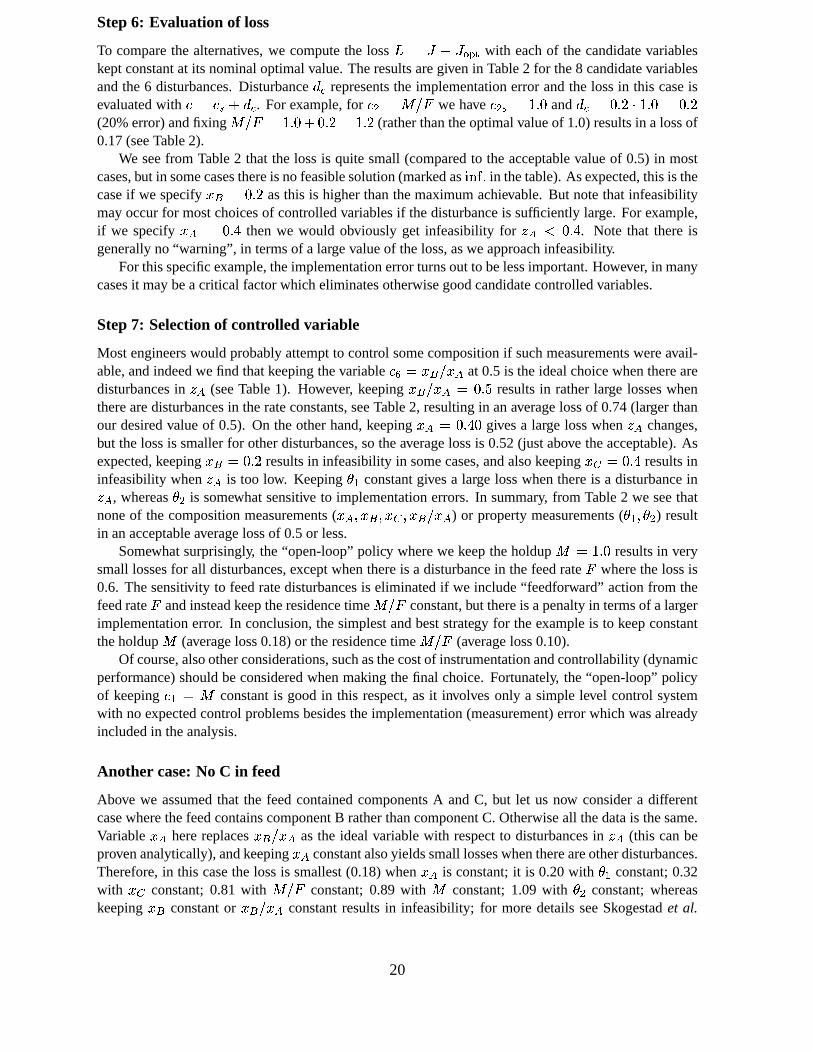
Step 6: Evaluation of loss

To comparethe alternatives,we computethe loss �b �Æ�� C�with eachof the candidatevariables

keptconstantat its nominaloptimalvalue.Theresultsaregivenin Table2 for the8 candidatevariablesandthe6 disturbances.Disturbance* + representsthe implementationerrorandthe lossin this caseisevaluatedwith � �� > * + . For example,for �9( äý�V¹� we have �9()� ^_Èã¾z and * + ¬z=ãï]+�8_Èã¾z¶bz=ãï](20%error)andfixing ý�V¹�¬b_Èã¾z > z=ãï][b_Èãï] (ratherthantheoptimalvalueof 1.0)resultsin a lossof0.17(seeTable2).

We seefrom Table2 that the lossis quitesmall (comparedto theacceptablevalueof 0.5) in mostcases,but in somecasesthereis nofeasiblesolution(markedas sÃu-, ã in thetable).As expected,this is thecaseif we specify }W�ábz=ãï] asthis is higherthanthemaximumachievable. But notethat infeasibilitymayoccurfor mostchoicesof controlledvariablesif thedisturbanceis sufficiently large. For example,if we specify } Ê Òz=ã#" thenwe would obviously get infeasibility for ü Ê ° z=ã#" . Note that thereisgenerallyno “warning”, in termsof a largevalueof theloss,aswe approachinfeasibility.

For thisspecificexample,theimplementationerrorturnsout to belessimportant.However, in manycasesit maybeacritical factorwhicheliminatesotherwisegoodcandidatecontrolledvariables.

Step 7: Selection of controlled variable

Most engineerswould probablyattemptto controlsomecompositionif suchmeasurementswereavail-able,andindeedwe find thatkeepingthevariable �.$ �}��BV&} Ê at 0.5 is theidealchoicewhentherearedisturbancesin ü Ê (seeTable1). However, keeping }��V&} Ê z=ãï� resultsin ratherlarge losseswhentherearedisturbancesin therateconstants,seeTable2, resultingin anaveragelossof 0.74(larger thanour desiredvalueof 0.5). On theotherhand,keeping} Ê �z=ã#"�z givesa large losswhen ü Ê changes,but thelossis smallerfor otherdisturbances,sotheaveragelossis 0.52(just above theacceptable).Asexpected,keeping}W�D¥z=ãï] resultsin infeasibility in somecases,andalsokeeping} Ì ¥z=ã#" resultsininfeasibility when ü Ê is too low. Keeping( % constantgivesa large losswhenthereis a disturbanceinü Ê , whereas( ( is somewhatsensitive to implementationerrors. In summary, from Table2 we seethatnoneof thecompositionmeasurements( } Ê A�}��XA�} Ì A�}��0V&} Ê ) or propertymeasurements( ( % A/( ( ) resultin anacceptableaveragelossof 0.5or less.

Somewhatsurprisingly, the“open-loop”policy wherewe keeptheholdup ý _Èã¾z resultsin verysmall lossesfor all disturbances,exceptwhenthereis a disturbancein thefeedrate � wherethelossis0.6. Thesensitivity to feedratedisturbancesis eliminatedif we include“feedforward” actionfrom thefeedrate � andinsteadkeeptheresidencetime ý5V¹� constant,but thereis apenaltyin termsof a largerimplementationerror. In conclusion,thesimplestandbeststrategy for theexampleis to keepconstanttheholdup ý (averageloss0.18)or theresidencetime ý5V¹� (averageloss0.10).

Of course,alsootherconsiderations,suchasthecostof instrumentationandcontrollability(dynamicperformance)shouldbeconsideredwhenmakingthefinal choice.Fortunately, the“open-loop”policyof keeping �&% �ý constantis goodin this respect,asit involvesonly a simplelevel control systemwith no expectedcontrolproblemsbesidestheimplementation(measurement)errorwhich wasalreadyincludedin theanalysis.

Another case: No C in feed

Above we assumedthat the feedcontainedcomponentsA andC, but let us now considera differentcasewherethefeedcontainscomponentB ratherthancomponentC. Otherwiseall thedatais thesame.Variable }ËÊ herereplaces} � V&}�Ê asthe ideal variablewith respectto disturbancesin üÙÊ (this canbeprovenanalytically),andkeeping} Ê constantalsoyieldssmalllosseswhenthereareotherdisturbances.Therefore,in this casethe lossis smallest(0.18)when } Ê is constant;it is 0.20with ( % constant;0.32with } Ì constant;0.81 with ý5V¹� constant;0.89 with ý constant;1.09 with ( ( constant;whereaskeeping }W� constantor }��BV&} Ê constantresultsin infeasibility; for moredetailsseeSkogestadet al.

20

0 0.5 1 1.5 2 2.5−20

−18

−16

−14

−12

−10

−8

−6

−4

−2

0

HOLDUP M

CO

ST

J

Figure7: Reactorexample:Costfunction 0214365�787 � � asa functionof holdup 9

É : ; < =?> =A@ =?B C%DC%EFHG F'I

JLKHMONQPARTS ULVTWYX WZW [ZX WZW [HX WHW\W�X ]ZW^W�X#VTW^W�X ]ZW\W�X#_TW`V�X WZW [ZX aZWb GdcZegf W�Xih ULVTWYX WZWjWYX#hTW [HX WHW\W�X ]ZW^W�X#VTW^W�X ]ZW\W�X#_TW`V�X WZW [ZX aZWb I�cHk > f WYX l Um[._�X WZW [ZX WZW [HX WHW\W�X nHW^W�Xo[._\W�X#_H_jW�X#_TW`V�X VZ_ [ZX ap_bZq cHk > f [ZX W ULVH_�X WZW [ZX WZW [HX WHW\W�X#_TW^W�X#VH_\W�X#VH_jW�X#_TW [ZX#hH_ [ZX#hH_bZr cZs > f [HX#_ ULV']AX VT]\WYX apV\W�X aZVjW�X nHl^W�X#V']`W�X ]ZW\W�X lph\V�X WH] [ZX aZabpt cZs @ f [ZX _ Um[ulYXQ[.ljWYX apV\W�X aZVjW�X ]H]`W�Xo[ul^W�X ]ZW\W�X nph [ZX vZl [ZX#hHV

Table1: Reactorexample:Optimalvaluesfor variousdisturbances

w�Kpxyx{z|NQ}y~ w�Kpxyx{z|N�}�~ w�KZx�x{z|N�}�~ w�KZx�x�z|NQ}y~ w�KZx�x�z|NQ}y~ w�KZx�x�z|NQ}y~ w�Kpxyx�z|N�}�~ w�Kpxyx�z|N�}�~: f [HX W ; < f [ZX W = > f WYX ] = @ f W�X#V = B f WYX ] C.DC%E

f WYX _ F G f V�X W F I f [HX aHWJ�KZMONQPYRHS W W W W W W W Wb G�cHe�f W�Xih WYX lpV W W W W W W Wb I�cZk > f WYX l WYX WZW WYX WZW [HX lph NoP��X [._�X WÈ� W nYX np_ WYX nZlbZq cZk > f [ZX W WYX WZW WYX WZW [HX WHW _�X WHW [HXihT_ W [ZX nZv WYX VHab r�cZs > f [HX#_ WYX VT] WYX VT] W�X#V'] ]YX#V'] W [ZX nZv WYX WZl WYX apVb t�cps @ f [ZX _ WYXQ[.l WYXQ[.l W�Xo[ul NoP��X W V�X aZn WYX WH] WYX#hHVb�� c NoMO��S�X%�u�y��KH� WYX Wp_ WYXQ['h W�X WZ_ NoP��X W�X WZ_ WYX VHW WYX VHv [ZX#hHV

�L� ��RT�Z��SoKZx�x WYXQ[.a WYXQ[.W W�X#_HV NoP��X V�X aHWÈ� WYX#h'] WYX aZl WYX lp_��RHP��NQPY� V [ n a h _ l ]NoP��X

denotesinfeasibleoperation�At thelimit to infeasibility ( :�� egf W ) for

k > =0.6.

Impl.error: : f [HXo[H� :�� e2f [HX#V�� = > f W�X ]pV�� = @ f W�X#V�[Z� = B f W�X ]pV�� = @ �'= > f WYX _Z_�� F G f V�XQ[Z� F I f [ZX v

Table2: Reactorexample:Lossfor alternativecontrolledvariables

21

(1999).Thuswefind, somewhatsurprisingly, thattherankingis almostreversedcomparedto thatfoundwith C in thefeed.

Conclusion

We have consideredalternative controlledvariablesfor a reactorexample.In onecase(with C in feed)theresidencetimewasthebestcontrolledvariable,whereasin anothercase(noC in feed)theconcentra-tion of componentA wasthebestchoice.It is noteasyto explainphysicallywhy theparticularvariablesarepreferredin thetwo cases.This shows thatit maybedifficult to rely on physicalinsight,e.g.about“dominant” variables,whenselectingcontrolledvariables.Instead,oneshouldevaluatethe(economic)performanceof theplant, to seewhich choiceof controlledvariablekeepstheoperationclosestto theoptimalwhentherearedisturbances.

7 Distillation case study

We considera binarymixturewith constantrelative volatility �« _Èãv_:] to beseparatedin a distillationcolumnwith 110 theoreticalstagesand the feedenteringat stage39 (countedfrom the bottomwiththe reboilerasstage1). Nominally, the feedcontains65 mole%of light component( ü&�¥ z=ãïñÅ� ) andis saturatedliquid ( � � _Èã¾z ). This is “column D” of SkogestadandMorari (1988)andrepresentsapropylene-propanesplitterwherepropylene(light component)is takenoverheadasa final productwithat least99.5%purity ( }��z=ãïîÅîÅ� ), whereasunreactedpropane(heavy component)is recycled to thereactorfor reprocessing.Weassumefirst thereis nocapacitylimit in thecolumn.

Step 1: Degree of freedom analysis

As mentionedin theintroductoryexample,for a givenfeedrateandgivenpressurethecolumnhastwodegreesof freedomatsteadystate,i.e.

F �� FO@ �] . Thesemayfor instancebeselectedasthevaporanddistillateflows, 4-`� �� We couldhave introduced� asa third degreeof freedomandaddedtheconstraint�^x�� .B� � , but thiswouldgive thesameresultasit is optimalto have �� .�� in this casewith no capacitylimit.

Step 2: Cost function and constraints

Ideally, theoptimaloperationof thecolumnshouldfollow from consideringtheoverall planteconomics.However, to beableto analyzethecolumnseparately, we introducepricesfor all streamsenteringandexiting thecolumnandconsiderthefollowing profit function � which shouldbemaximized(i.e.

� � � ) ��D�� > �� ¡0� (18)

Weusethefollowing prices[$/kmol]� � �]Èz=A � � b_�z � ]ÈzÈ} � A � � ä_�z=A � ¡ �z=ãv_Theprice ��¡áäz=ãv_ [$/kmol] on boilup includesthecostsfor heatingandcoolingwhich both increaseproportionallywith the boilup � . The price for the feed is �� _�z [$/kmol], but its valuehasnosignificanceon the optimal operationfor the casewith a given feedrate. The price for the distillateproductis 20 [$/kmol], andits purity specificationis}��{z=ãïîÅîÅ�

22

Thereis nopurity specificationonthebottomsproduct,but wenotethatits priceis reducedin proportionto theamountof light component(becausetheunneccessaryreprocessingof light componentreducestheoverall capacityof theplant;thisdependency is not really importantbut it it realistic).

With anominalfeedrate �b¬_ kmol/min theprofit value � of thecolumnis of theorder4 [$/min],andwe would like to find a controlledvariablewhich resultsin a loss � lessthan0.04[$/min] for eachdisturbance(correspondingto ayearlylossof lessthanabout$20000).

Step 3: Disturbances

Weconsiderfivedisturbances:* % : An increasein feedrate � from 1 to 1.3kmol/min.* ( : A decreasein feedcompositionü&� from 0.65to 0.5* µ : An increasein feedcompositionü&� from 0.65to 0.75* · : A decreasein feedliquid fraction �:� from 1.0(pureliquid) to 0.5(50%vaporized)*,+ : An increaseof thepurity of distillateproduct} � from 0.995(its desiredvalue)to 0.996

Thelatter is a possiblesafetymargin for }�� which maytake into accountits implementationerror. Inaddition,we will considerimplementationerrorsfor theotherselectedcontrolledvariable(seebelow).

Step 4: Optimization

In Table3 we give theoptimaloperatingpoint for thefivedisturbances;larger feedrate( �ä _Èãïç ), lessandmorelight componentin the feed( ü&��z=ãï� and üÙ�� z=ãïñÅ� ), a partly vaporizedfeed( �:�� z=ãï� ),andapurerdistillateproduct( }W�{�z=ãïîÅîÅñ ). In addition,we have consideredtheeffectof ahigherpricefor thedistillateproduct(�W��çÈz ) andafive timeshigherenergy price(�W¡¯�z=ãï� ).

As expected,theoptimalvalueof all thevariableslistedin thetable( }W�âA�}W�XA)�lV¹�yA)��V¹�yAC��V¹�yA)�~V¹� )arecompletelyinsensitive to the feedrate,sincethecolumnshasno capacityconstraints,andtheeffi-ciency is assumedindependentof thecolumnload.

Step 5: Candidate controlled variables

Thebottomproductpurity constraintis alwaysactive, thatis, it is alswaysoptimalto have } � �z=ãïîÅîÅ� ,sothedistillatecomposition}�� shouldbeselectedasacontrolledvariable.

Wearethenleft with oneunconstraineddegreeof freedom(F ��'H JhKiMSM b_ ) whichwewantto specify

by keepingthesetpointof acontrolledvariableataconstantvalue.FromTable3 weseethat,exceptin thelastcasewith amuchhigherenergy price,theoptimalbottom

composition} � staysfairly constantaround0.04. This indicatesthata goodstrategy for implementa-tion may be to control }W� at a constantvalueof 0.04. However, thereat leasttwo practicalproblemsassociatedwith thischoice.First,on-linecompositionmeasurementsareoftenunreliableandexpensive.Second,dynamicperformancemaybepoorbecauseit is generallydifficult to controlbothproductcom-positions(“dual or “two-point” control)dueto stronginteractions.e.g.(Shinskey 1984)(SkogestadandMorari 1987).Thus,if possible,we would like to controlsomeothervariable.

Thefollowing six alternative controlledvariablesareconsidered}W� ¦ �-V¹� ¦ � ¦ �XV¹� ¦ ��V¹� ¦ �XV¹�We considerimplementationerrorsof about20% in all variables,including } � (the othercontrolledvariable). From Table3 we seethat the optimal valueof �lV¹� variesconsiderably, so we expect thisto bea poorchoicefor thecontrolledvariable(asit violatesrequirement1). For theotheralternatives,it is not easyto sayfrom our requirementsof from physicalinsight which variableto prefer. We willthereforeevaluatetheloss.

23

Step 6: Evaluation of loss

In Table4 weshow for ��b_ [lmol/min] theloss �� C�W� � [$/min] wheneachof thesix candidatecontrolledvariablesarekeptconstantat their nominallyoptimalvalues.Recallthatwe would like thelossto be lessthan0.04[$/min] for eachdisturbance.We have the following commentsto the resultsgivenin Table4:

1. As expected,we find thatthelossesaresmallwhenwe keep}�� constant.

2. Somewhatsurprisingly, for disturbancesin feedcompositionüÙ� it is evenbetterto keep �XV¹� or��V¹� constant.

3. Not surprisingly, keeping �-V¹� (or � ) constantis not an acceptablepolicy, e.g., operationisinfeasiblewhen ü � is reducedfrom 0.65to 0.5.

4. All alternativesareinsensitive to disturbancesin feedenthalpy ( � � ).

5. �XV¹� is not a goodcontrolledvariable,primarily becauseits optimal valueis rathersensitive tofeedcompositionchanges.

6. For a implementationerror (overpurification)in }�� where }�� is 0.996ratherthan0.995all thealternativesgiveanunacceptablelossof about0.09.Weconcludethatweshouldtry to control }W�closeto its specification.

7. For reflux � andboilup � oneneedsto include“feedforward” actionfrom � (i.e. keep ��V¹� and��V¹� constant).

8. However, useof ��V¹� or �BV¹� ascontrolledvariablesis rathersensitive to implementationerrors.

9. Othercontrolledvariableshavealsobeenconsidered(notshown in Table).Forexample,aconstantcomposition(temperature)on stage19 (towardsthe bottom), } %�� ¤z=ãï]Èz , givesa lossof 0.064when ü&� is reducedto 0.5,but otherwisethelossesaresimilar to thosewith }�� constant.

10. We have not computedthe effect of changesin pricesin Table 4, becausethesedo not effectcolumnbehavior, soall alternativesbehave thesame(with thesameloss).Thus,if therearepricechanges,thenonemustrecomputenew optimalvaluesfor thevariables.

Step 7: Selection of controlled variables

FromTable4 thefollowing threecandidatesetsof controlledvariablesyield thelowestlosses�&% `� }��}�� ¦ �9( `� ��V¹�}�� ¦ � µ `� ��V¹�}�� ¦As mentioned,the“two-point” controlstructure� % wherebothcompositionsarecontrolled,results

in a difficult control problem. The losswill thenbe larger thanindicated,andit is probablybettertokeep �XV¹� or ��V¹� constant.Sinceit is usuallysimplerto keepa liquid flow ��V¹� ratherthana vaporflow ��V¹� constant(lessimplementationerror),we concludeasfollows:

Proposedcontrol system.| � is used4 to keep}��£�z=ãïîÅîÅ� .| �XV¹�¬b_:�8ã¾z;ò is keptconstant.

Alternativecontrol system.| � is usedto keep}W�{�z=ãïîÅîÅ� .| ��V¹�¬ä_:�8ãhò¹z is keptconstant.

Remark.If it turnsout to bedifficult to keep��V¹� (or ��V¹� ) constant,thenwemayconsideringusing� (or � ) to keepa temperaturetowardsthebottomof thecolumnconstant.

4Thereareotherpossiblechoicesfor controlling =?� , e.g. we couldusethedistillateflow . However, ¡ hasa moredirecteffect.

24

� � � � �£¢?� ��¢?� ¤¢?� ��¢?� ¥�¢A�¦+§8¨ª©�«¬?® 7°¯Q±8±-² 7°¯o7A³-7 7°¯Q´8µ8± 5�²{¯Q78´-² 5�²{¯o¶?7?³ ·?µ°¯o²8¶ ³¸¯o²8·?¹� 1º58¯Qµ 7°¯Q±8±-² 7°¯o7A³-7 7°¯Q´8µ8± 5�²{¯Q78´-² 5�²{¯o¶?7?³ ·?µ°¯o²8¶ ³¸¯o²8·?¹� � 1»7°¯o² 7°¯Q±8±-² 7°¯o7?µ-· 7°¯�³-¹8´ 5�²{¯o·?7-· 5�²{¯o²8·8² µ°58¯o·?¹ ·{¯Q±-¶?¹� � 1�7°¯o¶8² 7°¯Q±8±-² 7°¯o78²?7 7°¯o¶A³¸5 5�³¸¯o²A³-µ 5�²{¯o·?¹?³ 5�±°¯Q´-· ²{¯Q´-·?7¼ � 1»7°¯o² 7°¯Q±8±-² 7°¯o7A³-7 7°¯Q´8µ8± 5�²{¯½5�µ8µ 5�²{¯o·8¶8· ·?µ°¯Q´8¹ ³¸¯o²8¶{5� � 1»7°¯Q±8±8´ 7°¯Q±8±8´ 7°¯o7A³�· 58¯o·8¶A³ 5�²{¯o²?±?³ 5�´°¯o·?µ-· ·A³¸¯�³�¶ ³¸¯�³8³-µ� � 1»µ?7 7°¯Q±8±-² 7°¯o7?µ-² 7°¯Q´?³¸5 5�²{¯o¶{5�³ 5�´°¯Qµ-²8² ·A³¸¯o²{5� ¡ 1»7{¯¾² 7°¯Q±8±-² 7°¯�5�µ8¹ 7°¯o²?±-¶ 5858¯Q7-·?´ 5858¯Q´-·?µ 5�¹°¯�³�¶

Nominalvalues:e�f [Z� k < f W�X lZ_��y¿ < f [ZX W , À � f VTW , À-Á f WYXQ[

Table3: Optimaloperatingpoint (with maximumprofit¥+¢?�

) for distillationcasestudy

� � 1»7°¯Q7?³ �£¢?� 1Â7°¯o´?µ8± � 145�²{¯Q78´-² �Ã¢A� 145�²{¯Q78´-² ¤¢?� 145�²{¯o¶?7?³ ��¢?� 1!·?µ°¯o²8¶¦+§8¨Ä©Å«¬?® 7 7 7 7 7 7� 1458¯Qµ 7 7 Æ|¯oÇ|È�É 7 7 7� � 1»7°¯o² 7°¯Q7-·?µ ©Å«°Ê ¯ 7°¯o7?787 7{¯o787?7 7°¯o7?7°5 È¯oÆÌË�Í� � 1�7°¯o¶8² 7°¯Q7°5�± Î|¯oÇ�ÏÆ 7°¯o7?78´ 7{¯o787?´ 7°¯o7?7?³ Æ|¯ÅÈ�Î�Ë¼ � 1»7{¯¾² 7°¯Q78787 7°¯o7?787 7°¯o7?7°5 7{¯o787{5 7°¯o7?78µ 7°¯Q78787� � 1»7{¯o±8±?´ Æ|¯oÆÌÐ�Í Æ�¯QÆÌÐ�Ë Æ|¯QÆÌË�È Æ|¯QÆÑË|È Æ|¯QÆÌË�È Æ|¯oÆÌË�Ï

·?7-Ò ©�¨ªÓ¸® ¯QÔZÕ.Õ § Õ 7°¯Q7°5�· ©Å«°Ê ¯ Æ|¯�È�È{Ë Æ|¯�ÈÌÈ�Ë Æ|¯�È�Î×Ö Æ|¯ÅÈ�ÏÆNoP��X

denotesinfeasibleoperation

Nominalvalues:ØAÙ�Ú�ÛYÜ ÝZÝZÞ�ßyà%áâÚ£ÛYÜ ãpÞ�ß�ä�áåÚçæHÜ Û20%impl.error: ØAèªÚéÛ�Ü ÛTêpë�ßyìîí'ïéÚéÛ�Üið'ãHãYßyñòÚ�æ.ë�Ü ÛHë�ß�ñ×íTïéÚ�æ.ë�Ü ÛHë�ß�óÑíTïôÚ�æ.ë�Ü ëZÞ�ßyñ×íTìÚ�õHë�Ü#õTë

Uacceptableloss(largerthan0.04)shown in bold face

Table4: Loss[$/min] for distillationcasestudy.

25

Another case: Column with capacity limitations

Abovewe assumedthatthefeedratewasgivenandthatthecolumnhadno capacitylimit. However, allcolumnshave acapacitylimit, andthiswill obviously affect its operation.

To understandthis better, let us includethe feedrateasa degreeof freedom,i.e. we have ö+÷ùø.úOûö+üéûþý . The capacitylimit on the columnis given in termsof a maximumvalueon the vaporflow(boilup), ÿ��ÿ �� û�� Thefeedrateis adegreeof freedom,but it hasanupperlimit,

� � � ��wherewewill heretreatthe“available” feedrate

� �� asaparameter. Otherwise,thespecificationsandcostdataareasabove. In summary, we have threesteady-statedegreesof freedom(e.g.,

�,ÿ

and � )andthreeconstraints(on

�,ÿ

and � � ).We find againthat the constrainton � � is always active, but we find that the effect of the two

constraintsonÿ

and�

dependson thevalueof� �� . Let usfirst recallthecasestudiedabove with no

capacitylimitations,for which we found !ÿ� �#" ÷ùøuúÃû%$'&�(*)+ (nominally)correspondingto � , û-.(/0 .

Withÿ ��1� û2� this operationis optimal for

� � ÿ �� .!ÿ� �3" ÷ùø.úÃû2�4��$'&�(*)+òû5$(6�7)�0 [kmol/min].

Is this the largestfeedratewe shouldaccept?No, somemorecarefulthinking revealsthat if we havereached

ÿûÿ �� , andarefreeto decideon thefeedrate,thenwe shouldtry to optimize(maximize)�8� ÿ (insteadof �9� � asdoneabove). With the given columndata,we find that ! �8� ÿ " ÷ùø.ú û:.(�ý�ý.$

[$/kmol] is obtainedwhen � ,ºû;.(/7< ,ÿ� � û=$'��(*)>) and ?�� û=$'��(@$'& . Thus, with

ÿ �� ûA�[kmol/min], the optimal profit is obtainedwith a feedrateof

� ÷ùø.úîûB�4��$'��(*)>)�ûC$(6&>D>D [kmol/min],which is thenthelargestfeedrateweshouldaccept.

Let us try to explain this in words. The distillate is the mostvaluableproduct,so to maximizeitsflow we want to have it as“unpure” aspossible(this alsosavesenergy), i.e. we keepits purity at theminimumspecification( ��gûE.(6<><>& in ourcase).To maximizethedistillateflow wealsowantto avoidputtinglight componentinto thebottomproduct,sowe wantthebottomproductas“pure” aspossible.However, this costsenergy (

ÿ), andwe have that theoptimumtrade-off in our caseis obtainedfor � ,

about0.04. This appliesaslong asthereareno capacitylimitationswithin thecolumn,but if thevaporflow

ÿexceedsits maximumvalue,thenweareforcedto putmorelight component(i.e. alargerfraction

of thefeed)into thebottomproduct.For caseswherethebottomproductis worth lessthanthefeed(asin our case),we will eventuallyloosemoney by forcing morefeedthroughthecolumnandthecolumnbecomesa realbottle-neckfor theoverall plant(thisoccursfor � ,ôûF.(/7< in ourcase),

In summary, whenwe introducetheconstraintÿ ��1� û�� [kmol/min] andincludethefeedrate

�asadegreeof freedom,wehave thefollowing threecasesdependingon theavailablefeedrate

� �� :1. Low available feed rates;

� �� $(6�7)�0 [kmol/min]). This is thecasewestudiedabovewhereitis optimalto operatethecolumnbelow its vaporcapacitylimit andto keep

� û � �� . Thus,theoptimalsolutionis unconstrainedin onevariable,andthenominallyoptimalvalueof � , is 0.04.

Proposedcontrol system:G ? is usedto keep � ��ûF.(6<><>& (active constraint).G ÿ

is adjustedto keepÿ� � ûH$'&�(*)+ constantG �

is keptat its maximumavailablevalue� �� (active constraint).

This is the“alternative controlsystem”proposedabove,but is chosenherebecausewecanusethesamecompositioncontrollerasfor cases2 and3 (seebelow).

2. Intermediate available feed rates; $(6�7)�0JI � �� IK$(6&>D>D [kmol/min]. It is optimal to operateatmaximumvaporcapacity

ÿûÿ �� ûE� [kmol/min], andto processasmuchfeedaspossible,

i.e.� û � �� . With ��ûF.(6<><>& therearethennoremainingdegreesof freedom(i.e. all degrees

26

of freedomareconsumedfor “active constraintcontrol”). As� ��1� is increasedfrom 1.274to

1.566,theoptimalvalue � , of increasesfrom 0.04and0.09.


is keptatÿ ��1� ûE� (active constraint).G �

is keptat its maximumavailablevalue� �� (active constraint).

3. Large available feed rates;� ��ML $(6&>D>D [kmol/min]). It is optimal to operatethe columnat

maximumvaporcapacityÿûÿ ��1� ûN� [kmol/min], andto maintainacceptablebottompurity

we shouldnot processall theavailablefeed,i.e. it is optimalkeepkeep� ûO$(6&>D>D�I � �� (the

nominallyoptimalvalueof ��, is 0.09in thiscase).In thiscasethecolumnis a bottleneckfor theoverall plantthroughput.


is keptatÿ ��1� ûE� (active constraint).G �

is adjustedto keepÿ� � û2$'��(*)>) constant(alternatively, wemaykeep

� ûN$(6&>D>D constant,but using

ÿ� � is betterif thevalueof

ÿ �� changes)

Thethreeabovecasesfor theavailablefeedratecaneasilybeimplementedin asinglecontrolsystemusingsimplelogic.

In summary, thedistillation casestudyshows the importanceof selectingthe right controlledvari-ableswhenimplementingtheoptimalsolution,andhow thecolumnmaylimit themaximumthroughputof the plant. The analysiswasmostly basedon economicconsiderations(loss),but the bottomcom-position � , wasexcludedasa controlledvariablebasedon otherconsiderations,namelythe costofmeasurementandcontrollability.

We note that the implementationerror was not importantin this casestudy, but we stressthat itshouldbe includedin theanalysis.For example,the implementationerror is themain reasonwhy werarelyselecttemperaturesnearthecolumnendsascontrolledvariables(becausethemeasurementerroris too largecomparedto its sensitivity), but insteadcontrola temperatureaway from thecolumnend.

8 Discussion

8.1 Region of feasibility

In this paperwe have evaluatedthe (economic)loss for disturbancesof a given magnitude.Anotherimportantissueto consideris theregion of feasibility (stability) (Zhenget al. 1999).Wecouldevaluatefeasibility loss, definedas the differencebetweenthe disturbanceregion wherefeasibleoperationispossible(usingtheoptimal P ) andthedisturbanceregionwe canhandlewith constantvaluesof Q , to beassmallaspossible.

For example,considera casewherethereis an inequality constrainton an input variablewhichoptimally is activeonly undercertainconditions(disturbances),but thisconstrainedinputvariableis notincludedasacontrolledvariable.Hereonemustbecarefulto avoid infeasibilityduringimplementation,for example,theremaybeadisturbancesuchthatthespecifiedvalueof thecontrolledvariablecanonlybeachievedwith anonphysicalvalueof theinput (e.g.a negative flowrate).

The on-line optimizationis usuallyfor simplicity basedon the nominaldisturbance( RTS ), andtwoapproachesto avoid infeasibility in suchacaseareto

1. use“back-offs” for thesetpointsduringimplementation(Narraway etal. 1991),or

2. add“safetymargins” to theconstraintsduringthe(nominal)optimization

27

Oneapproachfor obtainingthe valuesfor the back-offs or safetymargins may be to solve a “robustoptimizationproblem”(Glemmestadet al. 1999))whereoneconsidersall possibledisturbances.Thereis clearlyaneedfor moreresearchin thisarea.

A third, andbetterapproachin termsof minimizing the loss, is to track the active constraint. Inparticular, modelpredictive control is very well suitedandmuchusedfor trackingactive constraints.However, evenif wetrackactiveconstaints,westill needto selecttheunconstrainedcontrolledvariables,sotheanalysispresentedin thispaperis still needed.

8.2 Additional examples

Additionalexamplefor selectingcontrolledvariablesareavailablein anumberof publicationsandPh.D.theses,e.g.

G Ph.D.thesisof Morud (1995),chapter8: CSTRwith chemicalreactionG Glemmestadet al. (1999)andPh.D.thesisof Glemmestad(1997):Applicationto heatexchanger

networks;specialemphasison feasibility issues.G Ph.D.thesisof Havre (1998):Applicationto selectionof temperaturelocationin distillation.G HalvorsenandSkogestad(1998)andHalvorsenandSkogestad(1999): Applicationto integrated

Petlyukdistillation columns.

ThePetlyukdistillation exampleis particularlyinterestingbecausein this casethechoiceof controlledvariablesmakesa big difference(whereasthe differencesfor the rathersimpleexamplespresentedinthispaperadmittedlywerequitesmall).

9 Conclusion

The focus in this paperhasnot beenon finding the optimal operationpolicy, but ratheron how toimplementit in a simplemannerin thecontrolsystem.Theideais to find a setof controlledvariablesQwhich,whenkeptat constantsetpoints,indirectly leadto near-optimaloperation(with acceptableloss).This is denoted“self-optimizing” control.

To assistin selectinggoodcandidatevariablesoneshouldlook for variablesthatsatisfythefollowingrequirements:

Requirement 1. Its optimalvalueis insensitive to disturbances

Requirement 2. It is easyto measureandcontrolaccurately

Requirement 3. Its valueis sensitive to changesin themanipulatedvariables

Requirement 4. For caseswith two or morecontrolledvariables,theselectedvariablesshouldnot betoocloselycorrelated.

In addition,we have presenteda systematicprocedurefor selectingcontrolledvariablesbasedonevaluatingthe loss UWVFU�÷ùø.ú for possibledisturbances.The procedurerequiresa steady-stateprocessmodelandacleardefinitionof thecostfunction U to beminimizedduringoperation(obviously, withoutsucha costfunctiononecannotjudgewhatoperationis thebest). Theprocedurewasappliedto threeexample; to a simple ”toy” example,to a somewhat academicCSTRexample,andfinally to a morerealisticdistillation columnexample.

Oneproblemis that in generalit not is clearoffhandif a self-optimizingstructureexists,andgoingthroughthe variousalternatives, for exampleusingthe given procedure,canbe quite tedious. On theotherhand,sincethe issueof finding goodcontrolledvariablesis a structural problem,thenwe oftenfind thata goodstructureobtainedfor a particularcase,alsoworkswell on anothersimilar processcasewith differentparametervalues.Thus,if we canactuallyfind a self-optimizingstructurefor a process,thenit is almostlike aninventionwhichmaypobablybepatented.

28

Acknowledgment. Theideasin this paperhavedevelopedgradually over several years. Valu-ablediscussionswith and contributionsfrom J.C. Morud, B. GlemmestadI.J. Halvorsen,K. Havre, T.Larsson,andM.S.Govatsmarkaregratefullyacknowledged.

References

Alonso,A.A. andB.E.Ydstie(1996).Processsystems,passivity andthesecondlaw of thermodynamics.Comp.Chem.Engng. (Suppl.)20, S1119–S1124.

Arbel, A., I.H. RinardandR. Shinnar(1996).Dynamicsandcontrolof fluidizedcatalyticcrackers.3.designingthe control system:Choiceof manipulatedandmeasuredvariablesfor partial control.Ind. Eng. Chem.Res.35(7), 2215–2233.

Arkun, Y. andG. Stephanopoulos(1980).Studiesin the synthesisof control structuresfor chemicalprocesses:Part iv. designof steady-stateoptimizingcontrolstructuresfor chemicalprocessunits.AIChEJournal 26(6), 975–991.

Findeisen,W, F.N. Bailey, M. Brdys,K. Malinowski, P. Tatjewski andA. Wozniak(1980).Control andcoordinationin Hierarchical Systems. JohnWiley & sons.

Fisher, W.R., M.F. Doherty and J.M. Douglas(1988).The interfacebetweendesignand control. 3:Selectingasetof controlledvariables..Ind. Eng. Chem.Res.27(4), 611–615.

Foss,C.S.(1973).Critiqueof chemicalprocesscontroltheory. AIChEJournal 19(2), 209–214.

Georgakis, C. (1986).On the useof extensive variablesin processdynamicsand control. ChemicalEngineeringScience47(6), 1471–1484.

Glemmestad, B. (1997). Optimal operation of integrated processes: Studies on heat recov-ery systems.PhD thesis. Norwegian University of Scienceand Technology. Available fromhttp://www.chembio.ntnu.no/users/skoge/.

Glemmestad,B., S.SkogestadandT. Gundersen(1999).Optimaloperationof heatexchangernetworks.Comp.Chem.Engng. 23, 509–522.

Gordon, M.L. (1986). Simple optimization for dual compositioncontrol. Hydrocarbon Processingpp.59–62.

Halvorsen,I.J.andS.Skogestad(1998).Useof feedbackfor indirectoptimizingcontrol:Applicationtopetlyukdistillation.5th IFAC SymposiumonDynamicsandControl of ProcessSystems(DYCOPS-5), Corfu,Greece, June8-10,1998pp.399–404.

Halvorsen,I.J. andS. Skogestad(1999).Optimizingcontrolof petlyukdistillation: Understandingthesteady-statebehavior. J. Proc.Control 9, 407–424.

Havre, K. (1998).Studieson controllability analysisandcontrol structuredesign.PhD thesis.NTNUTrondheim.Availablefrom http://www.chembio.ntnu.no/users/skoge/.

Luyben,W.L. (1975).Steady-stateenergy conservation aspectsof distillation columncontrol systemdesign.Ind. Eng. Chem.Fundam.14(4), 321–325.

Luyben,W.L. (1988).Theconceptof eigenstructurein processcontrol.Ind.Eng. Chem.Res.27(1),206–208.

Maarleveld,A. andJ.E.Rijnsdrop(1970).Constraintcontrolof distillationcolumns.Automatica6, 51–58.

Marlin, T.E. and A.N. Hrymak (1997). Real-timeoperationsoptimization of continuousprocesses.In: Fifth internationalconferenceon chemicalprocesscontrol (CPC-5),Lake Tahoe, Jan. 1996.Vol. 93 of AIChESymposiumSeries. pp.156–164.

29

Mizoguchi,A., T.E. Marlin andA.N. Hrymak(1995).Operationsopimizationandcontroldesignfor apetroleumdistillation process.CanadianJ. of Chem.Engng. 73, 896–907.

Morari, M. (1982).Integratedplantcontrol: A solutionat handor a researchtopic for thenext decade?.In: Proc. of Secondinternationalconferenceon chemicalprocesscontrol (CPC-2),SeaIsland,Georgia, Jan.1981. pp.467–495.

Morari, M. (1983). Design of Resilient ProcessingPlants -III. Chemical Engineering Science38(11),1881–1891.

Morari, M., G. StephanopoulosandY. Arkun (1980).Studiesin thesynthesisof control structuresforchemicalprocesses.Part I: Formulationof theproblem.Processdecompositionandtheclassifica-tion of thecontroltask.Analysisof theoptimizingcontrolstructures..AIChEJournal 26(2), 220–232.

Morud,J. (1995).Studieson thedynamicsandoperationof integratedplants.PhDthesis.UniversityofTrondheim.Availablefrom http://www.chembio.ntnu.no/users/skoge/.

Narraway, L. andJ. Perkins(1994).Selectionof processcontrol structuresbasedon economics.Com-puters chem.Engng. (Suppl.)18, S511–S515.

Narraway, L.T. andJ.D.Perkins(1993).Selectionof processcontrolstructurebasedon lineardynamiceconomics.Ind. Eng. Chem.Res.32(11),2681–2692.

Narraway, L.T., J.D.PerkinsandG.W. Barton(1991).Interactionbetweenprocessdesignandprocesscontrol: economicanalysisof processdynamics.J. Proc.Cont.1, 243–250.

Ricker, N.L. (1996).Decentralizedcontrolof theTennesseeEastmanChallengeProcess.J. Proc.Cont.pp.205–221.

Rijnsdorp,J.E.(1991).IntegratedProcessControl andAutomation. Elsevier.

Shinnar, R. (1981).Chemicalreactormodellingfor purposesof controllerdesign.Cheng. Eng. Commun.9, 73–99.

Shinskey, F.G. (1984).Distillation Control. 2 ed..McGraw-Hill Book Company.

Skogestad,S.andI. Postlethwaite(1996).Multivariable Feedback Control. JohnWiley & Sons.

Skogestad,S. andM. Morari (1987).Controlconfigurationselectionfor distillation columns.AIChEJ33(10),1620–1635.

Skogestad,S.andM. Morari (1988).Understandingthedynamicbehavior of distillation columns.Ind.Eng. Chem.Res.27(10),1848–1862.

Skogestad,S., I.J. Halvorsen,T. LarssonandM.S. Govatsmark(1999).Plantwidecontrol: Thesearchfor theself-optimizingcontrolstructure.In: Preprints14thIFAC World Congress,Beijing. Vol. N.pp.325–330.

Tyreus,B.D. (1999).Dominantvariablesfor partialcontrol;part1 and2. Ind.Eng. Chem.Res.38, 1432–1455.

Waller, K.V., D.H. Finerman,P.M. Sandelin,K.E. HaggblomandS.E.Gustafsson(1988).An experi-mentalcomparisonof four controlstructuresfor two-pointcontrolof distillation. Ind. Eng. Chem.Res.27(4), 624–630.

Yi, C.K. andW.L. Luyben(1995).Evaluationof plant-widecontrol structuresby steady-statedistur-bancesensitivity analysis.Ind. Eng. Chem.Res.34, 2393–2405.

Zheng,A., R.V. Mahajannamand J.M. Douglas(1999). Hierchical procedurefor plantwidecontrolsystemsynthesis.AIChEJournal 45, 1255–1265.

30

Plantwide control: the search for the self-optimizing control structure

Documents

Transcript of Plantwide control: the search for the self-optimizing control structure