Optimizing Shipping Container Damage Prediction and ...
170
Optimizing Shipping Container Damage Prediction and Maritime Vessel Service Time in Commercial Maritime Ports through High Level Information Fusion A Thesis submitted in Partial Fulfillment of the Requirements for the Doctorate in Philosophy in Computer Science Ashwin Panchapakesan c Ashwin Panchapakesan, Ottawa, Canada, 2019
-
Upload
khangminh22 -
Category
Documents
-
view
3 -
download
0
Transcript of Optimizing Shipping Container Damage Prediction and ...
Optimizing Shipping Container
Damage Prediction and Maritime
Vessel Service Time in Commercial
Maritime Ports through High Level
Information FusionA Thesis submitted in Partial Fulfillment of the Requirements
for the Doctorate in Philosophy in Computer Science
Ashwin Panchapakesan
c© Ashwin Panchapakesan, Ottawa, Canada, 2019

Abstract
The overwhelming majority of global trade is executed over maritime infrastructure,
and port-side optimization problems are significant given that commercial maritime
ports are hubs at which sea trade routes and land/rail trade routes converge. There-
fore, optimizing maritime operations brings the promise of improvements with global
impact. Major performance bottlenecks in maritime trade process include the han-
dling of insurance claims on shipping containers and vessel service time at port. The
former has high input dimensionality and includes data pertaining to environmental
and human attributes, as well as operational attributes such as the weight balance
of a shipping container; and therefore lends itself to multiple classification method-
ologies, many of which are explored in this work. In order to compare their perfor-
mance, a first-of-its-kind dataset was developed with carefully curated attributes.
The performance of these methodologies was improved by exploring metalearning
techniques to improve the collective performance of a subset of these classifiers.
The latter problem formulated as a schedule optimization, solved with a fuzzy sys-
tem to control port-side resource deployment; whose parameters are optimized by a
multi-objective evolutionary algorithm which outperforms current industry practice
(as mined from real-world data). This methodology has been applied to multiple
ports across the globe to demonstrate its generalizability, and improves upon current
industry practice even with synthetically increased vessel traffic.
ii

Acknowledgments
It takes a village... and mine was possibly the best. My mentors and supervisors
always stood by my side, never giving up on me. Panch Mama, Dr. Emil Petriu,
Dr. Rami Abielmona, and Dr. Rafael Falcon always offered me the guidance I
needed. Meanwhile, Wayne Smith and Montreal Terminal Gateway Partnerships
provided much needed insights from the industry, without which I would have been
unable to formulate the problems I worked on, much less the solutions I designed
and discussed with Alyssa Wai-Yi Fred Wong. I would be remiss if I didn’t thank
Tapan Oza for continuing to help draw my graphs the night before a submission
deadline. I’ve always found it interesting how my friendships evolve over time, and
none offers more pause for reflection than that I now get to call Phil Dr. Curtis and
thank him for all the professional support through seemingly impossible challenges;
speaking of which, I must thank Alex Teske, Patrick Santos and Jonathan Ermel
for the overwhelming amounts of help with various code snippets and databases for
my experiments.
Aside from technical expertise, this entire process of my PhD would have been
impossible without my physical health - thanks to Sharat “The Hulk” Akhoury for
coaching me through my gym routine and Gordon Ramsay for finally teaching me
to cook (which turned out to be a very useful stress reliever) and eat healthy. And
of course, no village is complete without the friends that help keep my sanity. So
a shout-out to everyone in the Skidaddle group (especially Kat) - who helped me
learn to ski; to my parents who were always in my corner and my cousins for never
talking me up even when I was ready to give up on myself.
iii
Contents
Abstract ii
1. Introduction 1
1.1. Problem Definition . . . . . . . . . . . . . . . . . . . . . . . . . . . . 2
1.1.1. Predicting Shipping Container Damage . . . . . . . . . . . . . 3
1.1.2. Improving Shipping Container Claims Prediction with Met-
alearning . . . . . . . . . . . . . . . . . . . . . . . . . . . . . . 4
1.1.3. Dynamic Allocation of Port-side Resources to Optimize Vessel
Service Time . . . . . . . . . . . . . . . . . . . . . . . . . . . 4
1.2. Motivation . . . . . . . . . . . . . . . . . . . . . . . . . . . . . . . . . 5
1.3. Use Case . . . . . . . . . . . . . . . . . . . . . . . . . . . . . . . . . . 7
1.4. Thesis Contribution . . . . . . . . . . . . . . . . . . . . . . . . . . . . 8
1.4.1. Predicting Insurance Claims on Shipping Containers . . . . . 8
1.4.2. Dynamic Allocation of Port-side Resources to Optimize Vessel
Service Time . . . . . . . . . . . . . . . . . . . . . . . . . . . 8
1.4.3. Improving Shipping Container Claims Prediction with Met-
alearning . . . . . . . . . . . . . . . . . . . . . . . . . . . . . . 9
1.5. Thesis Organization . . . . . . . . . . . . . . . . . . . . . . . . . . . . 11
1.6. Publications Arising from this Thesis . . . . . . . . . . . . . . . . . . 11
iv
2. Literature Survey 14
2.1. Port-side Vessel Servicing Operations . . . . . . . . . . . . . . . . . . 14
2.1.1. Vessel Arrival and Departure Schedules . . . . . . . . . . . . . 14
2.1.2. Environmental Effects . . . . . . . . . . . . . . . . . . . . . . 17
2.1.3. Vessel Loading and Unloading and Container Storage . . . . . 18
2.1.4. Summary . . . . . . . . . . . . . . . . . . . . . . . . . . . . . 18
2.2. Data Fusion . . . . . . . . . . . . . . . . . . . . . . . . . . . . . . . . 19
2.2.1. Definition . . . . . . . . . . . . . . . . . . . . . . . . . . . . . 19
2.2.2. Endsley’s Situation Awareness Model . . . . . . . . . . . . . . 20
2.2.3. State Transition Data Fusion (STDF) Model . . . . . . . . . . 22
2.2.4. JDL/DFIG Model . . . . . . . . . . . . . . . . . . . . . . . . 23
2.2.5. Summary . . . . . . . . . . . . . . . . . . . . . . . . . . . . . 32
2.3. Maritime Port Optimization . . . . . . . . . . . . . . . . . . . . . . . 33
2.3.1. Surveying Domain Experts . . . . . . . . . . . . . . . . . . . . 33
2.3.2. Modeling and Simulation . . . . . . . . . . . . . . . . . . . . . 36
2.3.3. CI Methodologies in Maritime Operations . . . . . . . . . . . 40
2.3.4. Other Relevant CI Methodologies . . . . . . . . . . . . . . . . 41
2.4. Fuzzy Systems . . . . . . . . . . . . . . . . . . . . . . . . . . . . . . . 45
2.5. Resource Deployment . . . . . . . . . . . . . . . . . . . . . . . . . . . 45
2.6. Solution Approach . . . . . . . . . . . . . . . . . . . . . . . . . . . . 47
2.6.1. Predicting Insurance Claims on Shipping Container Damage . 47
2.6.2. Dynamic Resource Allocation . . . . . . . . . . . . . . . . . . 47
3. Methodology 48
3.1. Data Collection Methodology . . . . . . . . . . . . . . . . . . . . . . 48
3.1.1. Vessel Track Data . . . . . . . . . . . . . . . . . . . . . . . . . 48
3.1.2. Container Damage Data . . . . . . . . . . . . . . . . . . . . . 49
v
3.1.3. Weather and Environmental Data . . . . . . . . . . . . . . . . 50
3.1.4. Domain Specific Knowledge Regarding Container Damage Causes 50
3.1.5. Vessel Departure Delay . . . . . . . . . . . . . . . . . . . . . . 52
3.1.6. Vessel Service . . . . . . . . . . . . . . . . . . . . . . . . . . . 53
3.1.7. Summary . . . . . . . . . . . . . . . . . . . . . . . . . . . . . 57
3.2. DataSet Synthesis . . . . . . . . . . . . . . . . . . . . . . . . . . . . . 57
3.2.1. Container Damage Feature Weights . . . . . . . . . . . . . . . 57
3.2.2. Shipping Tracks . . . . . . . . . . . . . . . . . . . . . . . . . . 58
3.2.3. Weather and Sea State . . . . . . . . . . . . . . . . . . . . . . 59
3.2.4. Shipping Lines . . . . . . . . . . . . . . . . . . . . . . . . . . 59
3.2.5. Container Weight Distribution . . . . . . . . . . . . . . . . . . 61
3.2.6. Commercial Value of Cargo . . . . . . . . . . . . . . . . . . . 61
3.2.7. Cargo Fragility and Sensitivity . . . . . . . . . . . . . . . . . . 63
3.2.8. Container Weight Balance . . . . . . . . . . . . . . . . . . . . 63
3.2.9. Quay Crane Operator . . . . . . . . . . . . . . . . . . . . . . 65
3.2.10. Packing and Loading Season . . . . . . . . . . . . . . . . . . . 65
3.2.11. Customer Identity . . . . . . . . . . . . . . . . . . . . . . . . 65
3.2.12. Logistics Company . . . . . . . . . . . . . . . . . . . . . . . . 66
3.2.13. Time in Storage Yard . . . . . . . . . . . . . . . . . . . . . . . 67
3.2.14. Port Situation Reports . . . . . . . . . . . . . . . . . . . . . . 67
3.2.15. Summary . . . . . . . . . . . . . . . . . . . . . . . . . . . . . 69
3.3. Prediction of Container Damage Insurance Claims for Optimized Mar-
itime Port Operations [1] . . . . . . . . . . . . . . . . . . . . . . . . . 71
3.4. Improving Container Damage Claims Classifier Performance Veracity
with Leave One Batch Out Training . . . . . . . . . . . . . . . . . . . 74
3.4.1. Removing Weather Features from the Dataset . . . . . . . . . 74
vi
3.4.2. Using a Validation Batch . . . . . . . . . . . . . . . . . . . . . 75
3.4.3. Cross Validation with LOBO . . . . . . . . . . . . . . . . . . 76
3.4.4. Conclusions . . . . . . . . . . . . . . . . . . . . . . . . . . . . 78
3.5. Improving Container Damage Claims Classifier Performance with Met-
alearning . . . . . . . . . . . . . . . . . . . . . . . . . . . . . . . . . . 80
3.5.1. Dataset Generation . . . . . . . . . . . . . . . . . . . . . . . . 80
3.5.2. Methodology . . . . . . . . . . . . . . . . . . . . . . . . . . . 84
3.6. Adaptive Resource Deployment with Level-4 Soft-Hard Information
Fusion . . . . . . . . . . . . . . . . . . . . . . . . . . . . . . . . . . . 89
3.6.1. Fuzzy System . . . . . . . . . . . . . . . . . . . . . . . . . . . 90
3.6.2. Multi-objective Evolutionary Algorithm . . . . . . . . . . . . . 92
3.7. Summary . . . . . . . . . . . . . . . . . . . . . . . . . . . . . . . . . 98
4. Results 99
4.1. Classifier Claims Prediction . . . . . . . . . . . . . . . . . . . . . . . 99
4.2. Improving Container Damage Claims Classifier Performance Veracity
with Leave One Batch Out Training . . . . . . . . . . . . . . . . . . . 102
4.3. Metadata Based Algorithm Selection . . . . . . . . . . . . . . . . . . 104
4.3.1. Example . . . . . . . . . . . . . . . . . . . . . . . . . . . . . . 105
4.4. Adaptive Resource Deployment with Level-4 Soft-Hard Information
Fusion . . . . . . . . . . . . . . . . . . . . . . . . . . . . . . . . . . . 105
4.4.1. Data Source Selection . . . . . . . . . . . . . . . . . . . . . . 112
4.4.2. Optimizer Robustness . . . . . . . . . . . . . . . . . . . . . . 117
5. Conclusions and Future Work 118
5.1. Conclusions . . . . . . . . . . . . . . . . . . . . . . . . . . . . . . . . 118
5.2. Limitations of this Work . . . . . . . . . . . . . . . . . . . . . . . . . 120
5.3. Future Work . . . . . . . . . . . . . . . . . . . . . . . . . . . . . . . . 121
vii
Bibliography 122
A. Shipping Container Damage Prediction Results Data 134
A.1. Container Damage Claims Classifier Performance Veracity with Leave
One One Batch Out Training . . . . . . . . . . . . . . . . . . . . . . 134
A.1.1. Improving Container Damage Claims Classifier Performance
Veracity with Leave One One Batch Out Training . . . . . . . 134
B. Approval from the Research Ethics Board of the University of Ottawa 139
C. Survey Questions to Maritime Domain Experts 142
viii
List of Figures
2.1. Discrete Berths . . . . . . . . . . . . . . . . . . . . . . . . . . . . . . 15
2.2. Berth Types [2] . . . . . . . . . . . . . . . . . . . . . . . . . . . . . . 16
2.3. Endsley’s Situation Awareness Model [3] . . . . . . . . . . . . . . . . 20
2.4. State Transition Data Fusion Model [4] . . . . . . . . . . . . . . . . . 23
2.5. Level 0 Process . . . . . . . . . . . . . . . . . . . . . . . . . . . . . . 24
2.6. Level 1 Process . . . . . . . . . . . . . . . . . . . . . . . . . . . . . . 24
2.7. Level 2 Process . . . . . . . . . . . . . . . . . . . . . . . . . . . . . . 25
2.8. Level 3 Process . . . . . . . . . . . . . . . . . . . . . . . . . . . . . . 26
2.9. Level 4 Process . . . . . . . . . . . . . . . . . . . . . . . . . . . . . . 27
2.10. Deactivating a Redundant Sensor Node Does not Decrease Informa-
tion Gain . . . . . . . . . . . . . . . . . . . . . . . . . . . . . . . . . 30
2.11. A Sensor Node Reporting Low Temperatures Near an Otherwise Un-
observed Fire has Low Information Quality Despite having High In-
formation Gain . . . . . . . . . . . . . . . . . . . . . . . . . . . . . . 31
2.12. The RANSAC Algorithm . . . . . . . . . . . . . . . . . . . . . . . . . 44
2.13. The ROAR Algorithm . . . . . . . . . . . . . . . . . . . . . . . . . . 44
3.1. Structure of an AIS Location Data Packet . . . . . . . . . . . . . . . 49
3.2. An Example Vessel Service Track . . . . . . . . . . . . . . . . . . . . 56
3.3. Shipping Container Weight Distribution . . . . . . . . . . . . . . . . 62
ix
3.4. Container Weight Balance . . . . . . . . . . . . . . . . . . . . . . . . 64
3.5. Using a Validation Batch . . . . . . . . . . . . . . . . . . . . . . . . . 76
3.6. Cross-Validation with LOBO . . . . . . . . . . . . . . . . . . . . . . . 77
3.7. Relative Performance across Drop-Weather, LOBO, and Cross Vali-
dation with LOBO . . . . . . . . . . . . . . . . . . . . . . . . . . . . 78
3.8. Augmenting the Original Dataset (with a set F of features and a set
C of classifiers) for Algorithm Selection . . . . . . . . . . . . . . . . . 81
3.9. Determining the Spanning Classfiers from the Grouped Dataset . . . 82
3.10. Computing the Algorithm Selection Dataset from the Grouped Dataset 84
3.11. Most Likely Classifier Choice . . . . . . . . . . . . . . . . . . . . . . . 86
3.12. Hard Voting Classifier Choice . . . . . . . . . . . . . . . . . . . . . . 87
3.13. Soft Voting Classifier Choice . . . . . . . . . . . . . . . . . . . . . . . 88
3.14. Weighted Soft Voting Classifier Choice . . . . . . . . . . . . . . . . . 89
3.15. Trapezoidal Membership Function . . . . . . . . . . . . . . . . . . . . 91
3.16. Chromosomal Structure for Trapezoidal Individual . . . . . . . . . . . 92
3.17. Example Crossover . . . . . . . . . . . . . . . . . . . . . . . . . . . . 96
3.18. Example Mutation (notice the changed B value in membership to
medium_congestion) . . . . . . . . . . . . . . . . . . . . . . . . . . . 97
4.1. Relative Feature Importances . . . . . . . . . . . . . . . . . . . . . . 100
4.2. Predictive Performance without Weather Data and Using LOBOMethod-
ologies . . . . . . . . . . . . . . . . . . . . . . . . . . . . . . . . . . . 103
4.3. Metalearning Methodology Performance . . . . . . . . . . . . . . . . 104
4.4. Mean Fuzzy Membership Functions . . . . . . . . . . . . . . . . . . . 106
4.5. Vessel Service Schedules . . . . . . . . . . . . . . . . . . . . . . . . . 108
4.6. Mean Fuzzy Membership Functions for Fuzzy System for Port of Halifax109
4.7. Optimized Service Schedule for Port of Halifax . . . . . . . . . . . . . 110
x

4.8. Mean Fuzzy Membership Functions for Fuzzy System for Victoria Port111
4.9. Optimized Service Schedule for Port of Halifax . . . . . . . . . . . . . 111
4.10. Distribution of Records by Data Source . . . . . . . . . . . . . . . . . 113
xi

List of Tables
3.1. Feature Importances . . . . . . . . . . . . . . . . . . . . . . . . . . . 51
3.2. Weights of Features . . . . . . . . . . . . . . . . . . . . . . . . . . . . 58
3.3. Data Resolution . . . . . . . . . . . . . . . . . . . . . . . . . . . . . . 59
3.4. Douglas Sea Scale[5] . . . . . . . . . . . . . . . . . . . . . . . . . . . 60
3.5. Examples of Synthetic Situation Reports . . . . . . . . . . . . . . . . 69
3.6. Examples of Real-world Situation Reports . . . . . . . . . . . . . . . 70
3.7. Feature Correlations to Container Damage Claims . . . . . . . . . . . 73
3.8. Representation of Classifiers in Algorithm Selection Dataset . . . . . 83
3.9. Training Time Complexity of Classifiers in Algorithm Selection Dataset
(where F is the number of features in the dataset and S is the number
of samples in the training set) . . . . . . . . . . . . . . . . . . . . . . 83
4.1. Discovered Feature Correlations . . . . . . . . . . . . . . . . . . . . . 101
4.2. Performance of Evolved Fuzzy Systems . . . . . . . . . . . . . . . . . 106
4.3. Mean Characteristics of Evolved Fuzzy Systems . . . . . . . . . . . . 106
4.4. Performance of Evolved Fuzzy Systems at Port of Halifax . . . . . . . 108
4.5. Mean Characteristics of Evolved Fuzzy Systems at Port of Halifax . . 109
4.6. Performance of Evolved Fuzzy Systems at Victoria Port . . . . . . . . 109
4.7. Mean Characteristics of Evolved Fuzzy Systems at Victoria Port . . . 110
4.8. Distribution of Records by Data Source . . . . . . . . . . . . . . . . . 112
xii

4.9. Optimizer Performance Expectation . . . . . . . . . . . . . . . . . . . 114
4.10. Optimization Results on Split Datasets . . . . . . . . . . . . . . . . . 116
4.11. Vessel Services Per Data Set . . . . . . . . . . . . . . . . . . . . . . . 116
4.12. Creating a New AIS Contact . . . . . . . . . . . . . . . . . . . . . . . 117
A.1. Performance Metrics of Various Classifiers . . . . . . . . . . . . . . . 135
A.2. Classifier Performance on the Drop-weather Dataset . . . . . . . . . . 136
A.3. Classifier Performance on the LOBO methodology . . . . . . . . . . . 137
A.4. Classifier Performance on the LOBO Cross Validation Methodology . 138
xiii
Nomenclature
AIS Automated Identification System
AOI Area of Interest
ATA Actual Time of Arrival
ATD Actual Time of Departure
AUC Area Under the Curve
BAP Berth Allocation Problem
CART Classification and Regression Tree
CI Computational Intelligence
DFIG Data Fusion Information Group
DSS Douglas Sea Scale
EOI Event of Interest
ETA Estimated Time of Arrival
ETD Estimated Time of Departure
GA Genetic Algorithm
GPS Global Positioning System
HLIF High Level Information Fusion
xiv

List of Tables
IMO International Maritime Organization
JDL Joint Directors of Laboratories
KNN k-Nearest Neighbors
LLIF Low Level Information System
LOBO Leave One Batch Out
MIP Mixed Integer Programming
ML Machine Learning
MMSI Maritime Mobile Service Identity
MOE Measure of Effectiveness
MOEA Multi-objective Evolutionary Algorithm
MOP Measure of Performance
NN Neural Network
NOAA National Oceanographic and Atmospheric Administration
POI Period of Interest
RANSAC Random Sample Consensus
ROAR Random Online Aggressive Racing
SAW Situational Awareness
SMAC Sequential Model-based Optimization for General Algorithm Configuration
SOSCIP Southern Ontario Smart Computing for Innovation Platform
STDF State Transition Data Fusion
SVM Support Vector Machine
TEU Twenty-foot equivalent Unit
xv
1. Introduction
The overwhelming majority of global trade is conducted over maritime infrastruc-
ture, implying that improvements in the efficiency of maritime operations improve
global trade efficiency. Specifically, commercial maritime ports are large and com-
plex hubs where marine traffic and land and rail traffic converge, connecting global
trade to local infrastructure. Thus, optimizing operations in commercial maritime
ports is the first front at which such optimization efforts would be maximally effec-
tive.
Commercial maritime ports face many challenges in the optimization of their internal
processes. Broadly, these processes can be classified into the following two types:
1. processes that interrupt regular port operations, which must be minimized in
order to minimize interruptions to regular port operations
2. regular port operations, in order to optimize process efficiency
One frequently occurring process that interrupts regular port operations is the work-
flow induced by the filing of an insurance claim on a damaged shipping container
(independently of its contents, which may also be damaged; however, that problem
is out of the scope of the current work). This induces extensive review by port-side
personnel in an investigation of the various operations that may have caused the
container to sustain damage. Automating the prediction of such damage and identi-
fying the potential cause thereof is therefore an avenue of improvement, which would
1
1.1 Problem Definition
minimize the interruptions this process would cause to regular port operations. This
problem is discussed in more detail in Sec. 1.1.1.
On the other hand, a process at the core of commercial maritime port operations
is the loading and unloading of shipping containers from cargo vessels. Central to
this process are the quay cranes (and their respective operators) that physically
move the containers between the vessel and port. Optimizing the number of quay
cranes deployed at any one time would therefore optimize the process of moving
shipping containers between a vessel and the port, thus minimizing the total time
required to service any given vessel at its berth. Minimizing vessel service time
by increasing the deployment of port-side personnel and resources comes at the
increased operational cost of these resources and personnel (in the form of wages).
Therefore, this optimization must account for both of these optimization parameters,
to identify a solution that strikes an acceptable balance between the two. This
problem is discussed in more detail in Sec. 1.1.3.
1.1. Problem Definition
Optimizing maritime port operations can be broken down into the two primary
problems, namely predicting shipping container damage and optimizing maritime
vessel service time. Advances made in the former problem alleviate the interruptions
caused to the otherwise regular flow of commercial maritime port operations, which
in turn reduces disruptions to the efficiency at which the port operates. On the other
hand, advances made in the latter problem improve the operational efficiency of
commercial maritime ports, which in turn improves their throughput and operational
capacity, increasing the global capacity for maritime trade. These problems are
specified more formally in this section.
2
1.1 Problem Definition
1.1.1. Predicting Shipping Container Damage
Predicting shipping container damage can help alleviate port-side operational bot-
tlenecks, by narrowing the scope of shipping container whose data must be analyzed
(and the breadth of the relevant analysis as well). In order to do so, data is collected
on the features of the shipping container, pertaining to
• cargo value
• presence of hazardous cargo in the container
• cargo longevity
• cargo sensitivity
• mass distribution of cargo in the shipping container
• amount of time spent in the storage yard
• exposure to rough seas along voyage from source to destination ports
• exposure to calm seas along voyage from source to destination ports
• container packing season
• container loading season
• cargo fragility
• quay crane operator
Given this data, classifiers may be trained to predict which shipping containers may
be damaged and therefore filed claims upon (as a binary classification problem).
Doing so allows for automating the collation and analysis of the relevant data in order
to determine the most likely point of damage for the Insurance Claims Coordinator
to analyze in a more targeted manner, thereby streamlining this process. This is
further explained in Sec. 2.6.1.
3
1.1 Problem Definition
1.1.2. Improving Shipping Container Claims Prediction with
Metalearning
While the problems discussed thus far pertain to the optimization of port-side op-
erations, they optimize these operations on a per-instance basis - insights gained
from previous runs of the optimization are lost and are not used in future optimiza-
tion efforts. Thus, training a model to on historical performance data will allow
for the optimization of algorithm selection and algorithm parameter selection for
the handling of a new unseen data record by discovering correlations between data
meta-features and the performance of the trained classifiers. These correlations al-
low for the intelligent combining of the outputs of multiple classifiers in order to
improve the overall classification accuracy. The exact methodologies used for this
are explored in detail in Sec. 3.5.
1.1.3. Dynamic Allocation of Port-side Resources to Optimize
Vessel Service Time
While predicting shipping container damage does indeed alleviate operational bot-
tlenecks, port-side operations can be further streamlined by reducing the probability
of port-side shipping container damage. Since this may be caused by increased op-
erational speed (as opposed to increasing operational throughput without increasing
speed at which various operational components function), While guidelines on oper-
ational speed are known [6], operational throughput can be improved by optimizing
the deployment of port-side resources. The deployment of resources is performed by
means of adapting the number of quay cranes used to service an incoming vessel,
while the congestion of maritime vessels in a port’s waters is used as a performance
measure to guide the optimization. This is therefore a proactively adaptive resource
4
1.2 Motivation
deployment problem as explained in Sec. 2.6.2.
1.2. Motivation
Commercial Maritime Ports are significant hubs of commerce to any national econ-
omy and account for over $250M per month in Canada [7]. These ports are typically
partitioned into terminals, within which shipping companies may load and discharge
ships with cargo. Therefore, commercial operations within these terminals are of
significant importance and improving their efficiency, efficacy, and throughput is of
paramount concern, second only to various safety factors including safety to human
life, infrastructure, and equipment. Improving internal processes within commer-
cial maritime ports therefore help improve global economies, quality of living, and
human and material safety.
A commercial maritime terminal faces challenges pertaining to:
• vessel arrival and departure schedules
• weather at port and at sea, as relating to the safety of cargo and personnel
• shipping container loading, unloading, storage and transportation, both within
the port, and on board a shipping vessel while at sea
• the proper storage of shipping containers in order to expedite the process of
loading and/or discharging a vessel, and to minimize risk exposure
• the deployment of equipment and personnel to increase throughput at minimal
operating cost
Given these challenges, two optimization problems are identified and presented here
(and will be explored in further detail throughout this thesis).
5
1.2 Motivation
Predicting Shipping Container Damage An important aspect of port operational
efficacy pertains to the safety and integrity of the cargo moving through the port’s
terminals. Such damage claims typically come with a large cost to companies op-
erating at such ports. Not only does the settling of a claim have an associated
financial cost, the investigation into the handling of the claim involves a complex
decision making process, including identifying the various operators that handled
the cargo, both internal and external to the port (from event logs, and surveillance
data, and operational environment data). Fusing information from various sources
(including ship voyage tracks, weather data, sea state data, commercial value of the
cargo, vessel operator data, port side operator data, etc) helps construct a compre-
hensive understanding of the adversities faced by the ship, the shipping containers
thereupon, and the cargo therein, to compute a profile of when and where any dam-
ages were incurred. As a result of such data fusion, it becomes feasible to compute
a meaningful risk metric at each point along the life cycle of a shipping container,
allowing for the automation within a decision support system to assist Bruce in the
investigation of damage claims so that he can focus his efforts more on analyzing
the already-collated data, rather than on meticulously collating it in the first place.
This is further explored in Sec. 3.3.
Scheduling Quay Cranes to Improve Vessel Throughput In addition to work-
flows induced by claims on damaged shipping containers, ports are also concerned
with increasing vessel service throughput. While this can be achieved by expand-
ing infrastructure, doing so comes at a large capital cost [8]. On the other hand,
intelligently deploying personnel and resources achieves the same goals of improv-
ing throughput without any additional capital costs, but with increased operational
costs and related incidental costs. Doing so in a meaningful manner requires not
only adequate reaction to current vessel servicing demand, but also accurate predic-
6
1.3 Use Case
tion of future demands on the port’s resources to proactively respond to foreseeable
demands. This is further explored in Sec. 4.4.
1.3. Use Case
Vessels arrive and leave the fictional maritime Port of Miranda (PoM) as part of
the normal course of operations. Sometimes, the Insurance and Claims Coordinator
(suppose his name is Bruce) receives an email from a customer about filing a claim
on a damaged shipping container. Bruce must then review various personnel logs
and surveillance footage to determine whether the damage occurred within PoM
and whether the claim should therefore be disputed or settled. Predicting whether
Bruce will receive a claim for a given shipping container will therefore allow for au-
tomated data collection for that container. Additionally, it allows for the automated
prediction of the location of damage, so that Bruce is presented with a prioritized
verification list to determine the point of damage.
While container damage prediction alleviates bottlenecks in the Insurance and Claims
Coordinator’s daily workflow, PoM’s throughput is affected by the Quay Crane De-
ployment Problem (QCDP) [9, 10]. Rushing to increase the container handling
throughput of these cranes does cause shipping container damage, which can there-
fore be alleviated by adjusting the number of cranes currently deployed to serve a
given vessel. Allocating sufficient infrastructural and human resources to service
such vessels allows for the timely and effective servicing of these vessels, reducing
their exposure to risk of damage from port-side sources. This would further alleviate
Bruce’s workload, while improving the personnel scheduling on the port side as well.
7
1.4 Thesis Contribution
1.4. Thesis Contribution
The contributions of this thesis are discussed in this section.
1.4.1. Predicting Insurance Claims on Shipping Containers
In order to alleviate operational bottlenecks caused by the filing of insurance claims
on damaged shipping containers, many CI algorithms were used to determine the
relationship between various features pertaining to a shipping container and whether
it was damaged and ultimately claimed. In order to determine which features are
indeed relevant to this study, a survey was created to capture this knowledge held by
Canadian domain experts (see Sec. 3.1.4). This work is extended with metalearning
(see Sec. 1.4.3) to explore the dynamic fusion the outputs of multiple classifiers to
improve classification accuracy.
Given that this thesis (and publications arising therefrom) were the first in the
literature to study this problem, the incremental contribution of this optimization
is the most significant contribution to the existing body work.
1.4.2. Dynamic Allocation of Port-side Resources to Optimize
Vessel Service Time
In order to further optimize port processes to reduce vessel service time and there-
fore improve throughput, port-side resources (personnel, equipment, and infrastruc-
ture) may be proactively deployed. This requires knowledge of vessel inbound and
outbound schedules, which are known to ports. Since the primary point of contact
between a vessel and port (with respect to loading and discharging cargo) is the quay
crane at the berth, the primary optimization parameter pertains to the deployment
8
1.4 Thesis Contribution
of equipment and personnel to operate the quay cranes. Deploying equipment and
personnel to service vessels in a timely manner also reduces the pressure on the
terminal to hurriedly complete vessel service on time. Since increasing container
handling speed causes increased risk to container damage [6], maintaining the time-
liness of vessel service by increasing resource deployment reduces operational risk,
which reduces the probability that a shipping container will sustain damage, which
in turn reduces the number of claims sent to Bruce.
This is further explored in Sec. 4.4.
1.4.3. Improving Shipping Container Claims Prediction with
Metalearning
The application of CI methodologies to maritime process optimization is not novel
in and of itself. Additionally, the breadth of available CI methodologies highlights
the role of nuance in the selection of an optimal algorithm to solve a given problem.
This creates an opportunity to apply CI methodologies to determine the best CI
technique to use for a given problem. This idea is currently being applied to the
CI methodologies to select between CI methodologies used in predicting shipping
container claims, and is further discussed in Sec. 1.4.3.1.
In order to address this, experiments are run to determine the correlations between
artifacts of the values of features in a dataset (i.e. meta-features) and the best
classifier or predictor to use given those meta-features. The correlations between
classifier MOPs and the values of meta-features therefore determines the optimal
classifier selection on new, unseen data. Experiments will also be run to discover
correlations between classifier MOEs and data sources in order to guide optimal data
source selection on new, unseen data. These are explored further with an example
9

1.4 Thesis Contribution
in Sec. 4.3.
The overarching idea is that rather than asking a single classifier for the claims
classification of a single shipping container, Bruce would query a meta-learner to
identify the best classifier to predict the claims classification of that shipping con-
tainer. He would then ask that classifier to perform the prediction, based on which
he make his decisions.
1.4.3.1. Dynamic Algorithm Selection through Metalearning
Within the context of this thesis, algorithms can be dynamically selected, specifically
for data processing. These algorithms refer to process incoming data in Levels 1 and
2 of the DFIG Data Fusion model, and the threat and impact assessment algorithms
in Level 3, including:
1. signals processing algorithms in Level 0
2. sub-object and object recognition algorithms in Level 1
3. situation assessment algorithms in Level 2
4. threat and impact assessment algorithms in Level 3
All of these algorithms can be evaluated for their efficiency (in terms of the amount
of computational effort spent in executing the algorithm), and the accuracy (in terms
of the difference between the computed value and the actual value) and efficacy (in
terms of the relevance of the value computed by the algorithm to the objective)
of their outputs. Therefore, a trust/veracity metric can be established for each
algorithm, based on their historic performance.
10
1.5 Thesis Organization
1.4.3.2. Dynamic Datasource Selection
Within the context of this thesis, data sources are evaluated for the quality of the
solutions they yield. For example, given two datasources (namely S1 and S2), the
same methodology is used to train a model with data from either source (namely,
models M1 and M2). The trained models are then evaluated in fitness space. If M1
outperforms M2, then datasource S1 is considered to be of better quality than S2.
This is explored further in Sec. 4.4.1.
1.5. Thesis Organization
The remainder of this thesis is organized as follows. Some contextual information
is presented in Sec. 2.1 and Sec. 2.2. Prior, related work to the previously men-
tioned classification and optimization problems are discussed in Sec. 2.3. Finally,
the proposed optimization frameworks and methodologies are presented in chapter 4.
Additionally, prior publications arising from this work are presented in Sec. 1.6.
1.6. Publications Arising from this Thesis
1. Panchapakesan, A., Abielmona, R., Falcon, R., & Petriu, E. (2018). Pre-
diction of Container Damage Insurance Claims for Optimized Maritime Port
Operations. In Advances in Artificial Intelligence: 31st Canadian Conference
on Artificial Intelligence, Canadian AI 2018, Toronto, ON, Canada, May 8–11,
2018, Proceedings 31 (pp. 265-271). Springer International Publishing.
This publishes the results presented in Sec. 4.1.
2. Panchapakesan, A. (2018, Oct). Prediction of Container Damage Insurance
Claims for Optimized Maritime Port Operations. Paper presented at the 2018
11
1.6 Publications Arising from this Thesis
workshop of Canadian Tracking and Fusion Group, Ottawa, ON, Canada.
This publishes the results presented in Sec. 4.2.
3. Panchapakesan, A. (2019, Mar). Improving Shipping Container Damage Pre-
diction Through Machine Learning based Level 4 Information Fusion. Poster
presented at the 2019 Engineering and Computer Science Graduate Poster
Competition, University of Ottawa, Ottawa, ON, Canada.
This publishes the results presented in Sec. 4.3.
4. Panchapakesan, A., Abielmona, & Petriu, E. (Submitted May 2019). Improv-
ing Shipping Container Damage Claims Prediction Through Level 4 Informa-
tion Fusion. Manuscript submitted for publication to International Journal of
Logistics Systems and Management.
This publishes the results presented in Sec. 4.3.
5. Panchapakesan, A., Abielmona, R., Petriu, E. (2019). Optimizing Maritime
Vessel Service Time with Adaptive Quay Crane Deployment Through Level 4
Hard-Soft Information Fusion. In Proceedings of 22nd International Confer-
ence on Information Fusion (Accepted for publication). IEEE.
This publishes the results presented in Sec. 4.4.
6. Panchapakesan, A., Abielmona, & Petriu, E. (Submitted May 2019). Opti-
mizing Commercial Port Operations through High-Level Information Fusion.
Manuscript submitted for publication to International Journal of Logistics Sys-
tems and Management.
This publishes the results presented in Sec. 4.4.1.
7. E.M. Petriu, R. Abielmona, R. Falcon, R. Palenychka, I. Abualhaol, F. Cher-
aghchi, A. Teske, N. Primeau, A. Panchapakesan, “Big Data Analytics for the
Maritime Internet of Things,” Canada School of Public Service Presentations
- Artificial Intelligence for Insights into Regulations, Ottawa, ON, October 19,
12

1.6 Publications Arising from this Thesis
2018.
13
2. Literature Survey
An overview of the relevant literature that guide the methodology in this thesis
along with the prior work relating to the thesis contributions are presented in this
chapter.
2.1. Port-side Vessel Servicing Operations
Relevant background information on the port-side operations involving the servicing
of vessels is presented in this section.
2.1.1. Vessel Arrival and Departure Schedules
While ports do have outbound land and/or rail traffic, global shipping container
traffic is primarily through marine vessel traffic. When a vessel does enter port,
it must berth at one of many berthing locations at the port. The optimization of
scheduling berths to incoming (and outgoing) ships based on their schedules is the
well-known Berth Allocation Problem (BAP) [2, 11, 12, 13], of which there are three
major variants. Ultimately, BAP is related to resource allocation problems involving
the various personnel and equipment at port, in the optimization of processing each
vessel, thereby optimizing port throughput.
14
2.1 Port-side Vessel Servicing Operations
2.1.1.1. Berthing Space
The berthing locations of a ship entering port may be discrete or continuous. Each
has its own advantages and disadvantages in port operation optimization.
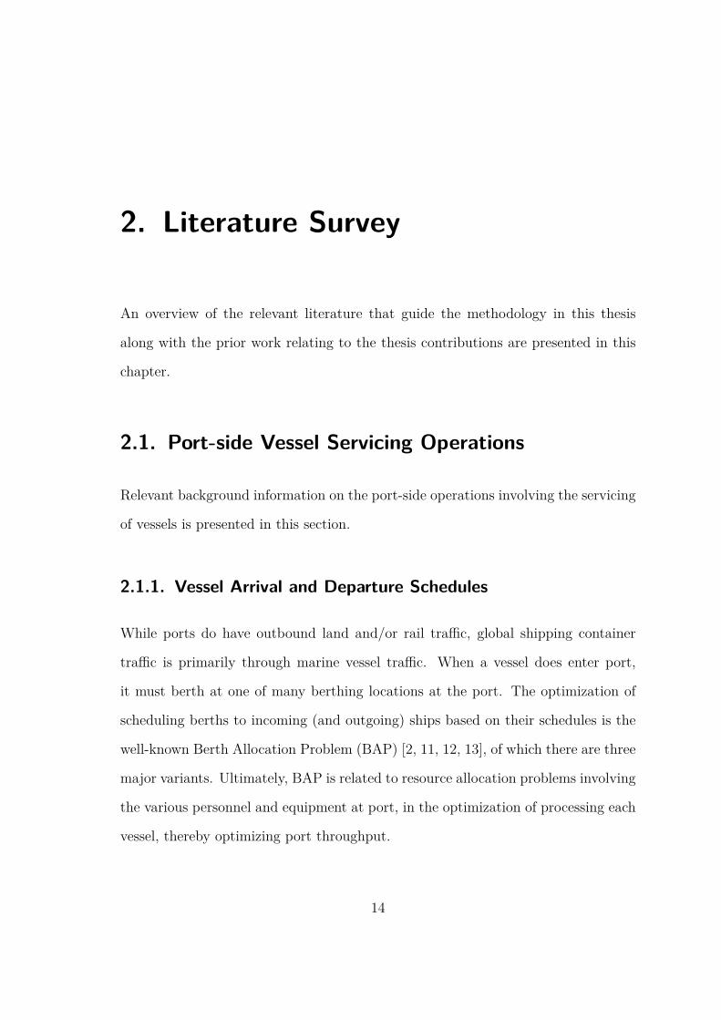
Discrete Berthing A discrete berth is a section of the port at which a ship may
berth. It is also surrounded by an area in which the ship may not berth [2]. Thus
the berthing locations are discrete along the port’s quay [2]. Discrete berths at the
Port of Montreal are highlighted in Fig. 2.1.
Figure 2.1.: Discrete Berths
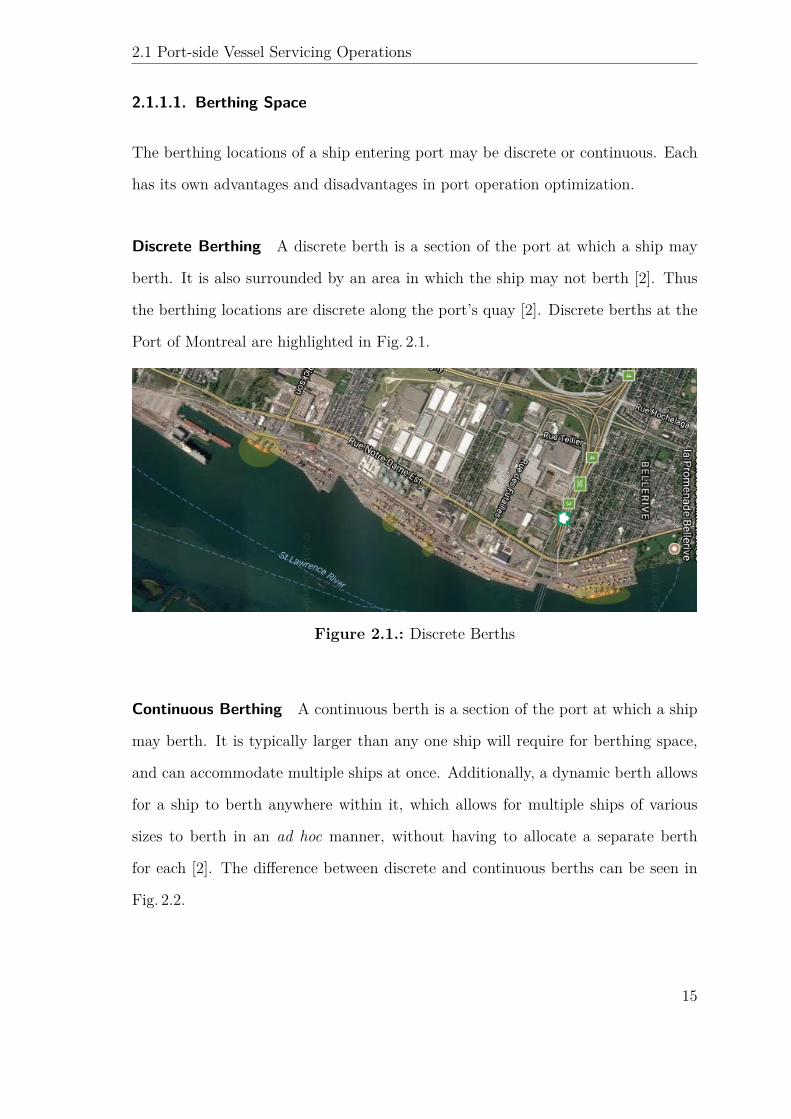
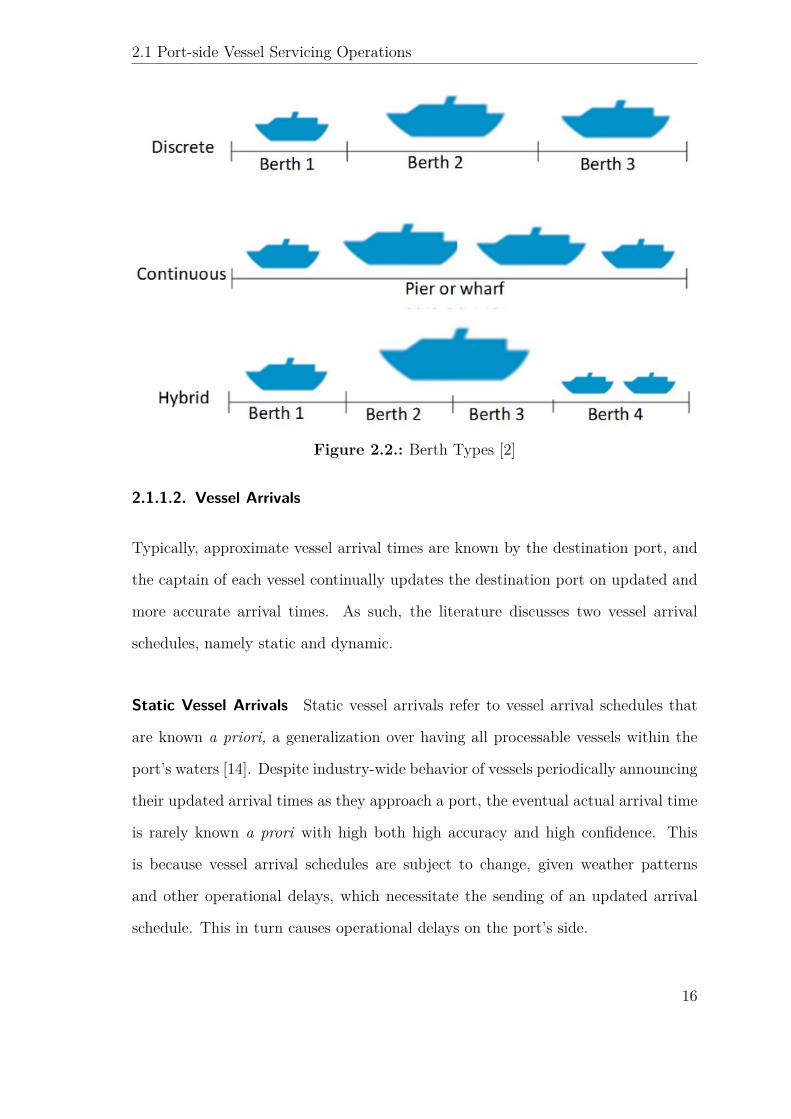
Continuous Berthing A continuous berth is a section of the port at which a ship
may berth. It is typically larger than any one ship will require for berthing space,
and can accommodate multiple ships at once. Additionally, a dynamic berth allows
for a ship to berth anywhere within it, which allows for multiple ships of various
sizes to berth in an ad hoc manner, without having to allocate a separate berth
for each [2]. The difference between discrete and continuous berths can be seen in
Fig. 2.2.
15
2.1 Port-side Vessel Servicing Operations
Figure 2.2.: Berth Types [2]
2.1.1.2. Vessel Arrivals
Typically, approximate vessel arrival times are known by the destination port, and
the captain of each vessel continually updates the destination port on updated and
more accurate arrival times. As such, the literature discusses two vessel arrival
schedules, namely static and dynamic.
Static Vessel Arrivals Static vessel arrivals refer to vessel arrival schedules that
are known a priori, a generalization over having all processable vessels within the
port’s waters [14]. Despite industry-wide behavior of vessels periodically announcing
their updated arrival times as they approach a port, the eventual actual arrival time
is rarely known a prori with high both high accuracy and high confidence. This
is because vessel arrival schedules are subject to change, given weather patterns
and other operational delays, which necessitate the sending of an updated arrival
schedule. This in turn causes operational delays on the port’s side.
16

2.1 Port-side Vessel Servicing Operations
Dynamic Vessel Arrivals Dynamic vessel arrivals refer to vessel arrival schedules
that are not known a priori, a generalization over having only a fraction of the
processable vessels within the port’s waters [14, 15]. This also refers to uncertain-
ties in vessel arrival schedules and the induced necessity to modify vessel handling
processes on the fly, as vessels arrive.
2.1.1.3. Vessel Handling Times
Vessel handling time refers to the amount of time required to discharge, maintain,
and reload a vessel, i.e. the amount of time from when the vessel berths, to when
the vessel leaves the berth (and subsequently, the port).
Static Vessel Handling Time Static vessel handling time refers to cases in which
the handling time for each vessel is known before the arrival of the vessel [14]. These
are therefore considered inputs to any optimizer.
Dynamic Vessel Handling Time Dynamic vessel handling time refers to cases in
which the handling time for each vessel is not known beforehand and must therefore
be computed based on the vessel attributes and environment variables [14]. These
are therefore not considered inputs to any optimizer.
2.1.2. Environmental Effects
Environmental artifacts impose operational constraints on port operations. For
instance, high winds, rain, snow, and visibility affect the ability of quay cranes
(and their operators) to discharge a berthed vessel; storms and rough seas affect
ship piloting and cargo integrity; and geographical artifacts (such as earthquakes,
storms, etc) and environmental artifacts (such a traffic flow, road design, etc) affect
17
2.1 Port-side Vessel Servicing Operations
shipping container and cargo integrity while the container is in transit, terrestrially
outbound from a port. Thus, mining correlations between environment artifacts and
damage claims can help identify causal relationships between certain environmental
artifacts and damage claims. Identifying these would help improve risk profiling
when investigating the cause of container damage, when a claim is submitted. The
specific sources of such data are further discussed in Sec. 3.1.
2.1.3. Vessel Loading and Unloading and Container Storage
Vessel loading and discharging are at the core of port operations, optimizing which,
is of paramount concern. Indeed, these operations are associated with their own op-
timization parameters, which rely on the optimal storage conditions of the shipping
containers, the presence of hazardous materials, the duration of time for which the
containers are expected to stay within the port before being loaded onto another
ship, or rail or a truck for delivery. For instance, storing containers by outbound date
causes intra-port traffic bottlenecks, leading to sub-optimal performance [16, 17, 18].
Similarly, vessel loading and unloading are well studied problems, that account for
vessel balance and cargo priority [19, 20]. Note that while the literature typically
discusses containers in twenty-foot equivalent units (TEUs), the specific operational
handling times of shipping containers are agnostic to the actual shipping container
size, as long as the collection of shipping containers to be processed is homogeneously
sized.
2.1.4. Summary
While vessel inbound and outbound schedules are typically known to ports, the
optimal berth and resource allocation can not always be computed a priori, as
18
2.2 Data Fusion
unforeseen effects of environmental affects and operational variances can cause sig-
nificant deviations from the predetermined, ideal schedule. Instead of attempting
to predict all possible delays, dynamically reacting to updated vessel arrival sched-
ules, container storage locations, and port congestion indicators paves the way to
investigate the optimization of port operations to maintain port-side throughput.
Such flexibility requires ingesting data from different sources and combining them
to form a coherent operational model. There are many models for such data fusion,
which are examined in the following section.
2.2. Data Fusion
2.2.1. Definition
Data Fusion can be defined as “the process of utilising [sic] one or more data sources
over time to assemble a representation of aspects of interest in an environment”
[21, 22, 23]. It is a process that allows for the ingestion of information (of various
degrees of redundancy) from multiple sources and over multiple communication
modalities, in order to formulate a more comprehensive description of the operational
environment. Over time, however, Data Fusion has grown to encompass not only
situational awareness (SAW), but also threat assessment, course of action generation,
impact assessment, measures of effectiveness and performance, process refinement,
etc. These are explained in the following subsections.
Many models for data fusion have been developed for use in various applications.
19
2.2 Data Fusion
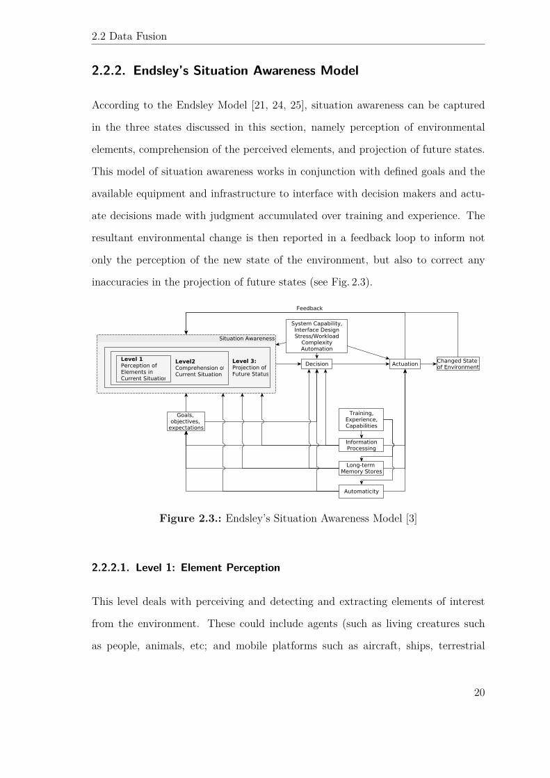
2.2.2. Endsley’s Situation Awareness Model
According to the Endsley Model [21, 24, 25], situation awareness can be captured
in the three states discussed in this section, namely perception of environmental
elements, comprehension of the perceived elements, and projection of future states.
This model of situation awareness works in conjunction with defined goals and the
available equipment and infrastructure to interface with decision makers and actu-
ate decisions made with judgment accumulated over training and experience. The
resultant environmental change is then reported in a feedback loop to inform not
only the perception of the new state of the environment, but also to correct any
inaccuracies in the projection of future states (see Fig. 2.3).
Figure 2.3.: Endsley’s Situation Awareness Model [3]
2.2.2.1. Level 1: Element Perception
This level deals with perceiving and detecting and extracting elements of interest
from the environment. These could include agents (such as living creatures such
as people, animals, etc; and mobile platforms such as aircraft, ships, terrestrial
20
2.2 Data Fusion
vehicles, remotely controlled entities, etc) and environmental entities (such as geo-
graphical artifacts including mountains, cliffs, and paths; biospherical artifacts such
as wooded areas, animal nests and trails; and relevant environmental aspects such
as atmospheric CO2 levels, etc). This is the first step to making sense of one’s en-
vironment in order to develop a plan of action to move towards accomplishing the
defined objectives [3].
2.2.2.2. Level 2: Situation Perception
This level deals with identifying the entities detected in Level 1, and understanding
the various relationships between them. For example, the following fall under the
scope of Level 2:
• detecting pursuit and evasion
• detecting imminent threats (such as incoming missiles, intruders, etc)
• detecting convoy behavior
• detecting adversarial and cooperative behavior
The processes in this level have more to do with sensemaking and comprehension of
the behavior of the various environmental entities. It is at this level (of perception)
that many mistakes are made, as it has to do with evaluating the current state of the
components of the environment that are relevant to achieving the defined objectives
[3].
2.2.2.3. Level 3: Future State Projection
Given the relationships between the elements detected in Level 1, as detected in Level
2, Level 3 aims to compute the state of these elements in the future. Thus, prediction
and estimation of the future states of various elements falls within the scope of Level
21
2.2 Data Fusion
3. With adequate predictions of the likely future states, it is possible to assess these
future states in order to adequately address and respond to them. This includes
predicting the level of risk posed by the environmental variables upon entities of
interest, and computing the impact force (the amount of perceived damage, and
the resource requirements to fix the projected damage) thereupon. It also affords
the evaluation of a proposed set of actions, to determine their efficacy in moving
towards the defined objectives [3].
2.2.3. State Transition Data Fusion (STDF) Model
The State Transition Data Fusion (STDF) model [21] represents and describes the
world as a set of states with transitions between them. A state is described as having
the following properties:
• being spatiotemporally bounded
• capturing the world in a set of variables that are relevant to the problem at
hand
• describing those variables no more or less than sufficiently, as required to
understand and solve the problem at hand
• identifying the persistent elements of the environment. These could be static
object states and/or transitions, or cycles in the directed graph representation
of state nodes connected by transition edges. For instance, though the low-
level mechanics of driving a car cannot be described as very static, the state
of driving a car from a source to a destination can be captured in a dynamic
state, as it is in a closed cycle involving the various actions associated with
driving a car.
The STDF model maintains this notion of states and transitions over multiple levels
22
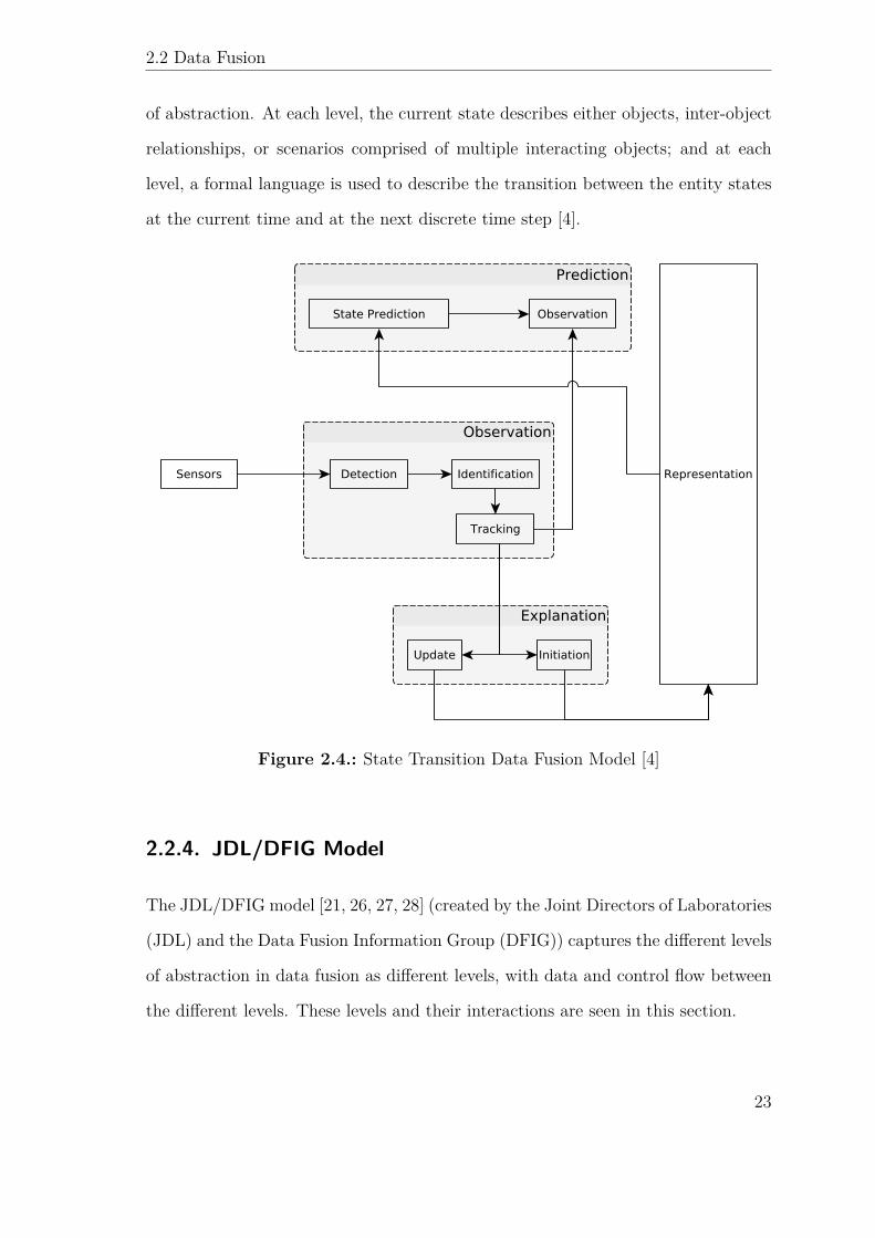
2.2 Data Fusion
of abstraction. At each level, the current state describes either objects, inter-object
relationships, or scenarios comprised of multiple interacting objects; and at each
level, a formal language is used to describe the transition between the entity states
at the current time and at the next discrete time step [4].
Figure 2.4.: State Transition Data Fusion Model [4]
2.2.4. JDL/DFIG Model
The JDL/DFIG model [21, 26, 27, 28] (created by the Joint Directors of Laboratories
(JDL) and the Data Fusion Information Group (DFIG)) captures the different levels
of abstraction in data fusion as different levels, with data and control flow between
the different levels. These levels and their interactions are seen in this section.
23
2.2 Data Fusion
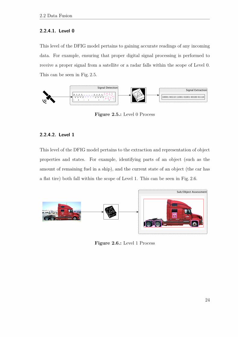
2.2.4.1. Level 0
This level of the DFIG model pertains to gaining accurate readings of any incoming
data. For example, ensuring that proper digital signal processing is performed to
receive a proper signal from a satellite or a radar falls within the scope of Level 0.
This can be seen in Fig. 2.5.
Figure 2.5.: Level 0 Process
2.2.4.2. Level 1
This level of the DFIG model pertains to the extraction and representation of object
properties and states. For example, identifying parts of an object (such as the
amount of remaining fuel in a ship), and the current state of an object (the car has
a flat tire) both fall within the scope of Level 1. This can be seen in Fig. 2.6.
Figure 2.6.: Level 1 Process
24
2.2 Data Fusion
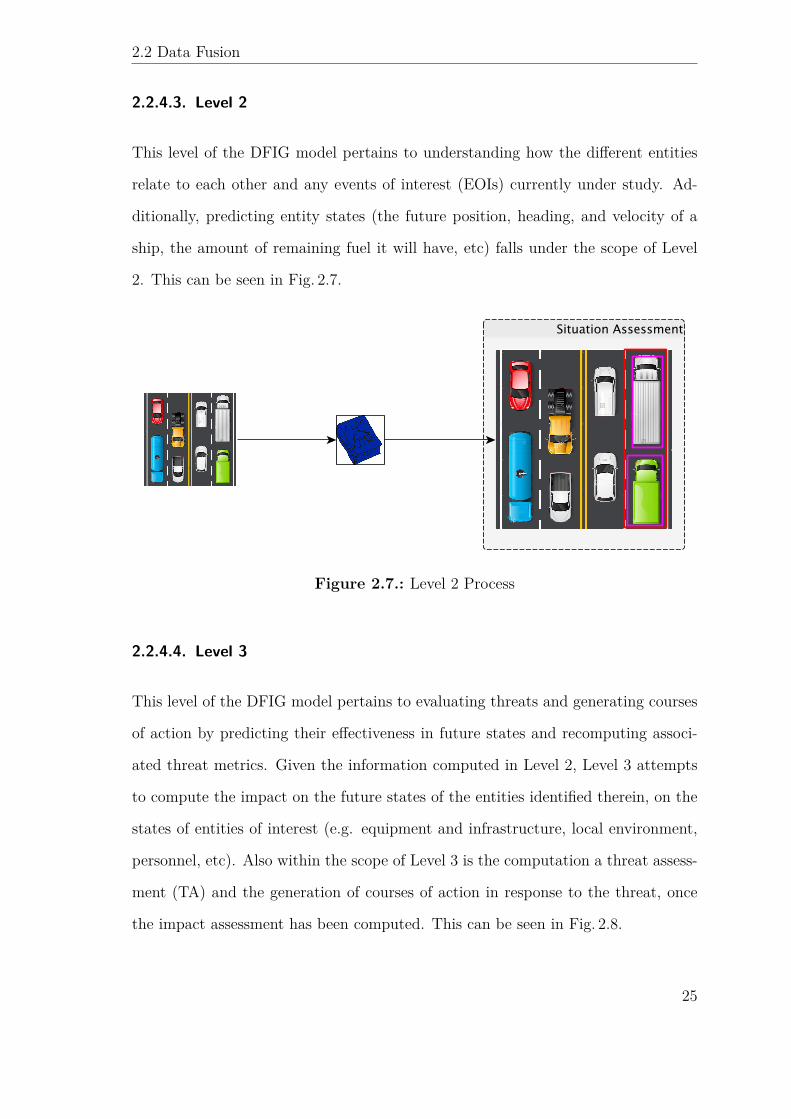
2.2.4.3. Level 2
This level of the DFIG model pertains to understanding how the different entities
relate to each other and any events of interest (EOIs) currently under study. Ad-
ditionally, predicting entity states (the future position, heading, and velocity of a
ship, the amount of remaining fuel it will have, etc) falls under the scope of Level
2. This can be seen in Fig. 2.7.
Figure 2.7.: Level 2 Process
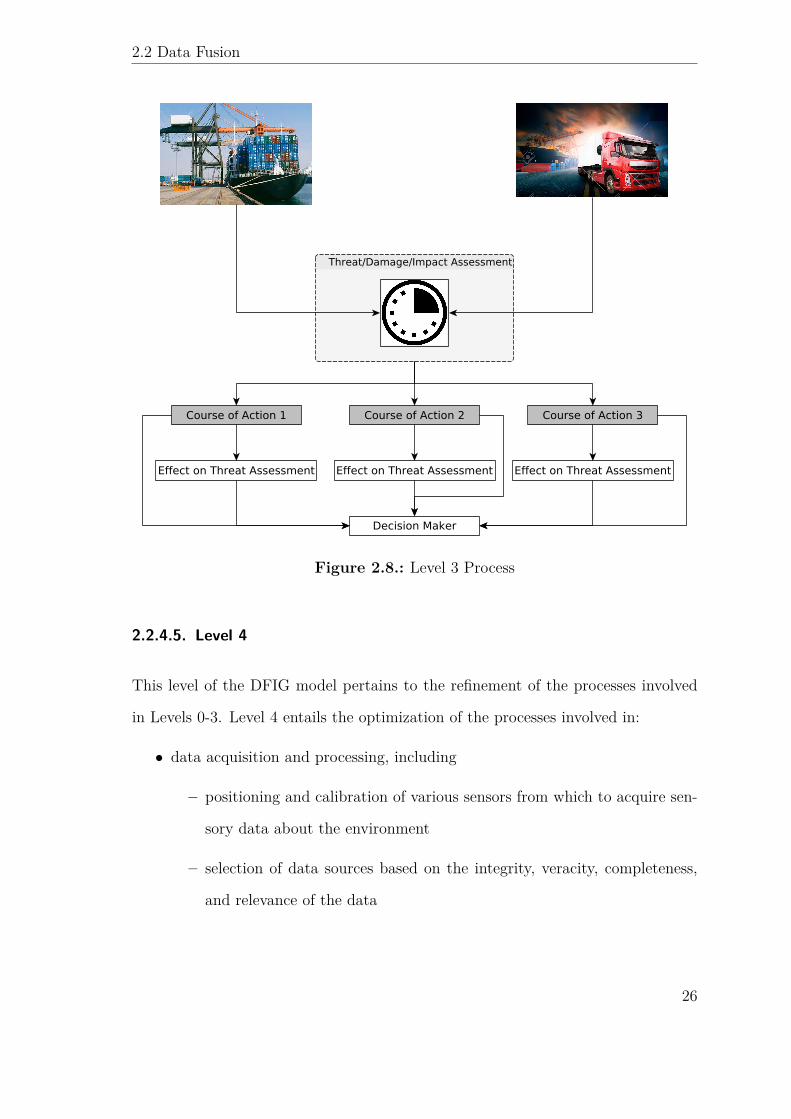
2.2.4.4. Level 3
This level of the DFIG model pertains to evaluating threats and generating courses
of action by predicting their effectiveness in future states and recomputing associ-
ated threat metrics. Given the information computed in Level 2, Level 3 attempts
to compute the impact on the future states of the entities identified therein, on the
states of entities of interest (e.g. equipment and infrastructure, local environment,
personnel, etc). Also within the scope of Level 3 is the computation a threat assess-
ment (TA) and the generation of courses of action in response to the threat, once
the impact assessment has been computed. This can be seen in Fig. 2.8.
25
2.2 Data Fusion
Figure 2.8.: Level 3 Process
2.2.4.5. Level 4
This level of the DFIG model pertains to the refinement of the processes involved
in Levels 0-3. Level 4 entails the optimization of the processes involved in:
• data acquisition and processing, including
– positioning and calibration of various sensors from which to acquire sen-
sory data about the environment
– selection of data sources based on the integrity, veracity, completeness,
and relevance of the data
26
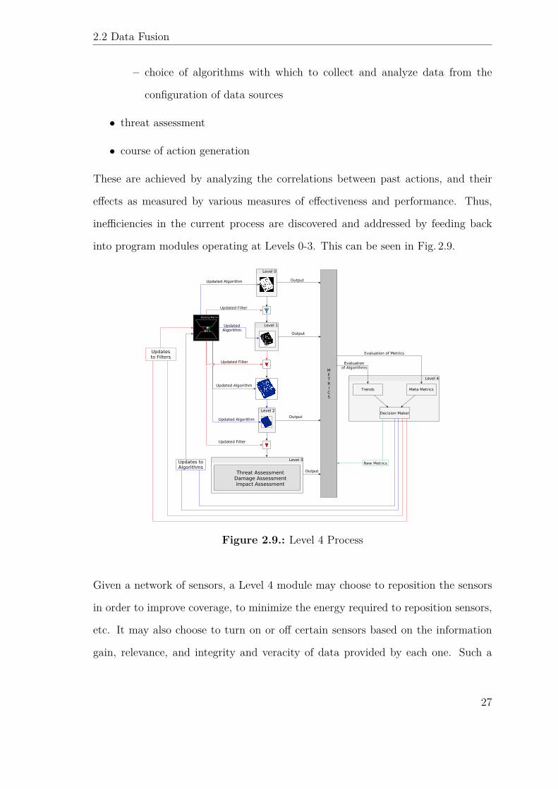
2.2 Data Fusion
– choice of algorithms with which to collect and analyze data from the
configuration of data sources
• threat assessment
• course of action generation
These are achieved by analyzing the correlations between past actions, and their
effects as measured by various measures of effectiveness and performance. Thus,
inefficiencies in the current process are discovered and addressed by feeding back
into program modules operating at Levels 0-3. This can be seen in Fig. 2.9.
Figure 2.9.: Level 4 Process
Given a network of sensors, a Level 4 module may choose to reposition the sensors
in order to improve coverage, to minimize the energy required to reposition sensors,
etc. It may also choose to turn on or off certain sensors based on the information
gain, relevance, and integrity and veracity of data provided by each one. Such a
27

2.2 Data Fusion
Level 4 module may also decide to change the algorithms with which certain data
streams are processed, so that noisy data are processed with more robust algorithms,
while relatively clean data are processed with fast and naive algorithms. These
decisions are made to optimize Measures of Effectiveness (MOEs) and Measures of
Performance (MOPs).
Measures of Effectiveness (MOEs) Measures of effectiveness typically fall under
the broad definition of (IFE) and its metrics [21]. These differ from MOPs in some
key ways. While a fast algorithm will have a high-scoring MOP, it mat have a
low-scoring MOE if it returns results when they are no longer needed. For instance,
if the fastest classification algorithm correctly classifies shipping container damage,
it is only useful to Bruce if it is able to return the classification outcome before
Bruce receives an insurance claim on the container. Therefore, while the algorithm’s
accuracy affords it a high MOP, it will have a very poor MOE if the results are not
timely.
Another key difference between MOPs and MOEs has to do with an algorithm’s
robustness, or its ability to cope with variations in real-world data. While a high-
performant algorithm may have a high accuracy, yielding a high-scoring MOP, the
algorithm may still have a low-scoring MOP if the accuracy was computed on a
dataset with extreme sample bias, leading to poor algorithmic bias when tested
with unseen data that lies sufficiently far from the mean in the training set. This
inability to maintain its performance in the face of variation in the real-world data
would cause the algorithm to have a low-scoring MOE.
28

2.2 Data Fusion
IFE is computed as shown in Eq. 2.1.
IFE = Information Gain×Quality× Robustness (2.1)
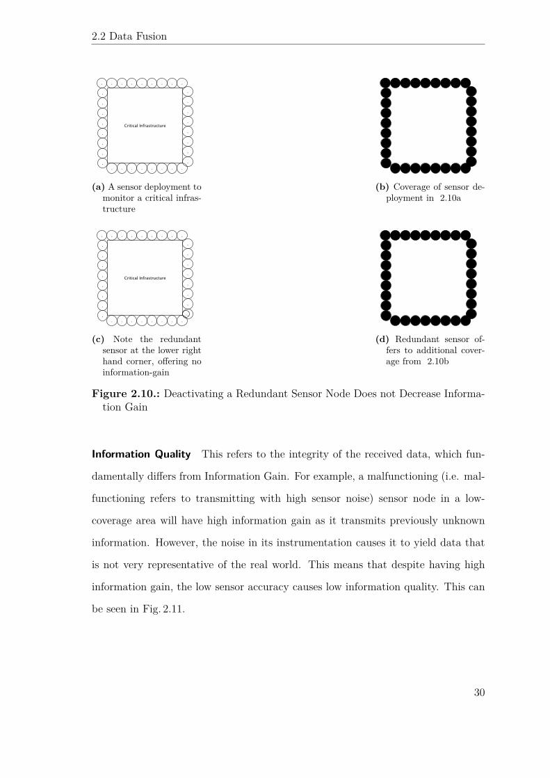
Information Gain This refers to the amount of new information brought into the
knowledge base as a result of fusing a given data source (or otherwise performing
any other fusion operation). A sensor network with a wider coverage will therefore
afford a higher information gain than its low-coverage counterpart. Similarly, the
choice to not activate a certain sensor node based on redundant coverage (i.e. the
segment of the environment covered by the sensor was already covered by some
subset of the already activated sensor nodes) is based on the notion of information
gain, i.e. that no new information will be collected by activating that sensor node
(assuming that all sensor nodes have the same sensor capabilities). This can be seen
in Fig. 2.10.
29
2.2 Data Fusion
(a) A sensor deployment tomonitor a critical infras-tructure
(b) Coverage of sensor de-ployment in 2.10a
(c) Note the redundantsensor at the lower righthand corner, offering noinformation-gain
(d) Redundant sensor of-fers to additional cover-age from 2.10b
Figure 2.10.: Deactivating a Redundant Sensor Node Does not Decrease Informa-tion Gain
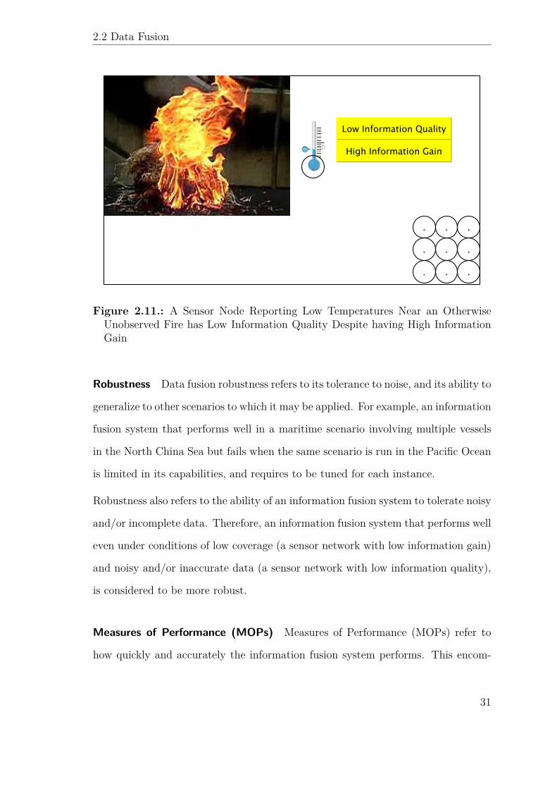
Information Quality This refers to the integrity of the received data, which fun-
damentally differs from Information Gain. For example, a malfunctioning (i.e. mal-
functioning refers to transmitting with high sensor noise) sensor node in a low-
coverage area will have high information gain as it transmits previously unknown
information. However, the noise in its instrumentation causes it to yield data that
is not very representative of the real world. This means that despite having high
information gain, the low sensor accuracy causes low information quality. This can
be seen in Fig. 2.11.
30
2.2 Data Fusion
Figure 2.11.: A Sensor Node Reporting Low Temperatures Near an OtherwiseUnobserved Fire has Low Information Quality Despite having High InformationGain
Robustness Data fusion robustness refers to its tolerance to noise, and its ability to
generalize to other scenarios to which it may be applied. For example, an information
fusion system that performs well in a maritime scenario involving multiple vessels
in the North China Sea but fails when the same scenario is run in the Pacific Ocean
is limited in its capabilities, and requires to be tuned for each instance.
Robustness also refers to the ability of an information fusion system to tolerate noisy
and/or incomplete data. Therefore, an information fusion system that performs well
even under conditions of low coverage (a sensor network with low information gain)
and noisy and/or inaccurate data (a sensor network with low information quality),
is considered to be more robust.
Measures of Performance (MOPs) Measures of Performance (MOPs) refer to
how quickly and accurately the information fusion system performs. This encom-
31

2.2 Data Fusion
passes such metrics as:
• device uptime
• resource utilization
• prediction accuracy
• communication latency
• data compression ratio
• resource requirements to reconfigure the sensor network when necessary
• sensor network adaptability (the ability of the sensor network to continue at
high performance levels when for example, a sensor node goes offline)
2.2.4.6. Level 5
This level of the DFIG model pertains to managing the data fusion process within
the context of the human operators that interact with it. Within the scope of
Level 5, are changes to the structure of the dissemination of information and the
decision making hierarchy, user interface design and human-computer interaction,
and information compartmentalization and access.
2.2.5. Summary
Level 4 of the JDL/DFIG model (see Sec.2.2.4.5) will be used to drive the optimiza-
tion earlier identified problems. Further, the MOPs and MOEs of the used machine
learning algorithms will be used to guide the improvement of not only their individ-
ual performances, but also the performance of any combined, ensemble methods that
may be borne from this exercise. This will likely result in improved performance in
32
2.3 Maritime Port Optimization
not only port operations, but also in the optimization of port performance. Yet, be-
fore combined performance can be evaluated and tuned, the performance of simpler
models on individual problems must be evaluated in order to establish a benchmark.
These are analyzed in the following section.
2.3. Maritime Port Optimization
Research into the factors associated with container damage and claims is not very
well represented in the literature, as opposed to ship damage or other related prob-
lems. The literature is also very sparse in the application of machine learning
techniques to this problem, which constrains the scope of the current knowledge.
Accurate container damage predictions enable discussing the selection and dynamic
selection between data sources and algorithms used to process the data therefrom.
This information may be used in a decision support system that can then be in-
tegrated into a terminal operating system (such as N4 [29], used to track shipping
container positions around the port from the time of entry to the time of exit) to
help identify root causes of container damage, to help alleviate bottlenecks from
data collation and analysis.
Though this particular problem is not very well researched, similar problems indeed
have been, and a subset of the insights and methodologies presented in the relevant
literature is applicable to this problem. These are presented in this section.
2.3.1. Surveying Domain Experts
Surveys of Taiwanese domain experts reveal a taxonomy of risks posed to refrigerated
containers in their port-to-port travel with the following three categories:
33
2.3 Maritime Port Optimization
Operational Risk including improper temperature and ventilation settings
Hardware Risk including a malfunctioning container thermostat
Consignor’s Risk pertaining to any errors made on the part of the consignor in slow
cargo loading, leading to cargo spoilage, etc
Risk factors involving human error had the highest combined perceived (by domain
experts), severe (the monetary loss in the affected cargo), and frequently occurring
risk to shipping container damage [30]. Thus, human error will be modeled in this
study.
A study of the determining factors of consignors’ port choice highlights attributes
correlated with such decisions [31], including the consignor’s proximity to the port
(which is correlated positively with their port of choice, as increased container travel
times increase the logistic shipping costs and the probability of en route damage),
the annual traffic through the port, and the number of shipping routes served by
the port. Since the present study only models one port, the latter two attributes
are less relevant.
The port choice behavior [31] is captured in three models that were generated to be
true to the survey data, namely:
Basic Model includes parameters for alternative ports and routes, frequency of
weekly port departures, and travel time and cost. This model deems travel
time (and cost) of a container to port to be the most important features.
Experienced Model decides between alternative port choices based on previous ex-
perience. This model uses the number of possible alternative routes from the
consignor’s facility to the port as the primary deciding factor.
Competitive Model decides between alternative ports based on a holistic consider-
ation of all port properties. Travel time (and costs) to port are again the most
34

2.3 Maritime Port Optimization
important features, but can be offset by the number of routes an alternative
port services, or the weekly departure frequency.
Given the arguments for the consignors’ selection of the nearer ports, container
damage risks during maritime travel were included in the present study. The primary
risk factors in travel stem from:
• sea state and weather conditions along the ship’s voyage
• human error induced by low crew morale
• cognitive operational alertness, etc. [32]
• the ship’s pilot’s skills in safely berthing the ship
• the health and operational integrity of the ship and the equipment therein
equipment
• crew morale and skill
• the power, health and operational integrity of the tugboat
• the tugboat pilot’s skill level
• the skill level, attitude, and morale of the linesmen personnel involved in ship
berthing
• the robustness, availability, and accessibility of docking equipment such as
wind lasses and line handling boats
• port management policies, including marine piloting laws, ship lane rules, etc.
• the physical and mental health of operating staff
• weather and geography [33]
Although these factors are important, incomplete Port Policy and Procedure doc-
uments do not standardize marine critical procedures for pilots in the the port’s
35
2.3 Maritime Port Optimization
waters. Since the associated incident reports are confidential, this information can-
not be used in the current study. Yet, probability distributions that model other
factors pertaining to the operational capabilities of personnel and equipment were
included within this study.
2.3.2. Modeling and Simulation
A case study of the voyage of a ship destined for Seattle in late October, 1998
[34] discusses mathematical constructs and simulation software in their abilities to
predict kinematic properties (including pitch and yaw) of a ship at sea, subject to
prevailing sea state and weather patterns. Two software tools are used:
FREDYN This is a ship motion simulator that accurately predicts the parametric
roll angles of a ship, as subjected to winds, waves, etc, while at sea. Yet, it did not
accurately predict variations in ship speed and roll amplitude, tuning which could
yield better results. Additionally, it is specific to measuring and predicting the
various forces upon, and the kinematics of a ship at sea [34]. Thus, it is too narrow
for the present study. Yet, the parameters used to guide the investigation have
broader applicability and are used in this work, including:
• wind speed
• wind direction
• hurricane rating
• wave height
• wave dissipation
• wave interaction
• wave propagation/swell
36
2.3 Maritime Port Optimization
• wave confusion
Some of the data sources used were found to be publicly available, and were therefore
included in this work, along with other data sources, including:
• Global sea state data from the National Oceanographic and Atmospheric Ad-
ministration (NOAA) [35]
• Local weather data from Environment Canada [36]
• Global weather data from (NOAA)
LAMP LAMP (Large Amplitude Motion Program) is a numerical investigation
tool, which accurately predicts:
1. the roll angle of a ship
2. roll event buildup (the accumulation of rolling momentum from continuous
the side-to-side rolling of a ship)
3. the changing of the roll period
It is also noted that LAMP is sensitive to the topology of a ship’s hull, its weight
distribution, and roll damping coefficient (a function of the sea state, wave char-
acteristics, ship kinematics, and ship topology), requiring specific characteristics of
ship bow flares in order to ensure accuracy [34]. Such preconditions are difficult to
guarantee, making such analysis out of the scope of the current work.
It was noted in the investigation that post-Panamax class ships were fitted with
a lashing bridge to improve a ship’s cargo capacity and efficacy in ensuring cargo
safety. Yet, these ships face challenges from the same environmental sources (namely
weather and sea state) in transporting cargo between sea ports [34].
While these studies highlight important features of a shipping container along its
voyage on board a ship, and the relevant modeling and simulation software, they
37
2.3 Maritime Port Optimization
do not use any Computational Intelligence (CI) [37] methodologies or data-driven
approaches to compute feature importance.
Data for such methodologies (e.g., from Lloyd’s Register [38]) can be used to extract
ship characteristics and correlate them with maritime accidents. Indeed, Kelangath
et. al. [39] use such historical data to construct a Bayesian Network, which captures
dependence relationships between the various ship and cargo features, and the type
and intensity of an accident to the ship. Traversing with off-the-shelf software (such
as GeNIe [40]) correlates accident type and intensity to ship features including ship
age, type, and location (whether the accident occurred at sea or at port), cargo type
(was the cargo considered hazardous or dangerous, etc), and weather adversity.
From this data, it was determined that ship age, on board hazardous cargo, time of
loading, and when the ship was at sea, most highly correlated with the occurrence
of an accident. These features are therefore included in our data.
Computer simulations have also been used to study the effects of weather and vis-
ibility on the time requirements for loading and unloading oil tankers in a Chilean
port [41]. Wind, visibility, precipitation, and the buildup of ice, were found to
determine the time requirements to load and unload an oil tanker. These factors
also determine the safe speed limits for incoming and outgoing ships and intra-port
vehicles. For instance, berthed oil carriers are not cleared to leave the port, and
new tankers are prohibited from entering the port when wind speeds exceed 15 m/s.
Similarly, reduced visibility impedes ship approach and restricts new departures.
The effects of ice buildup within this model are limited to the thickness of ocean
surface ice, not including the effects of ice on roads within the terminal which may
affect the movement of intra-port vehicles and personnel. This model also ignores
effects of rain or snow on terrestrial and maritime vehicles and their piloting. These
attributes are used in a discrete event simulator, along with the probability densi-
38
2.3 Maritime Port Optimization
ties of environmental behavior learned from historical data (provided by the Chilean
Government), to determine port storage capacity. The attributes included in these
models are also included in the present study, along with marine and terrestrial
precipitation (rain and snow).
Discrete event simulators typically struggle with computational deadlock when pro-
cessing such large-scale simulations. Bielli et. al. address this in their Container
Terminal Simulator [42], which simulates events and entities (equipment, vehicles,
and human agents) that are common to commercial maritime ports, and operations
including events involving Roll-On/Roll-Off ships (Ro-Ro ships), Load-On/Load-Off
ships (Lo-Lo ships), quay cranes, shunting trucks (and Fatuzzis), and large gantry
cranes to move shipping containers within the storage yard. The software notably
focuses on simulating details of port-side personnel and vehicular behavior, with
which port management and safety policies are evaluated, on metrics such as av-
erage equipment utilization, containers moved per simulation, etc., with additional
parameters that may be calibrated. While this software makes advances in dis-
tributed, discrete event simulation as applied to commercial maritime ports and
the container yards therein. However, it does not account for risks stemming from
behavioral effects (such as human error) or equipment failure; nor does it account
for the effects of weather, geography, or sea state, as others have done.
Other numerical simulations have studied the effects of ocean states on seafaring
vessels [43, 44], while others still have used such techniques to optimize shipping
container placement in storage yards [45], as well as in assigning quay cranes to
vessels to handle increased process load [46].
39

2.3 Maritime Port Optimization
2.3.3. CI Methodologies in Maritime Operations
While modeling and simulation tools evaluate policy efficacy against ship damage
and discover root causes of delays, etc., few publications explicitly discuss the root
and/or composite causes of shipping container damage by applying CI techniques
[37] to a data set. One study compared the efficacy of decision trees in predicting
the total loss and damage to a ship, given its attributes [47], including:
• CHi-squared Automatic Interaction Detection (CHAID) trees, which com-
pound multiple variables together if their individual predictive abilities fall
below a parametric threshold [48]
• QUEST trees, which performed well, but did not generalize well to more com-
plex problems, and had already sustained scrutiny for a lack of reliable con-
vergence [49] and a lack of improvement in its accuracy over Davenport’s q
method, upon which it is based [50]
CHAID trees had the highest predictive accuracy, and a later study by the same
author [51] improves upon its prediction accuracy. However, this algorithm works
only with multi-class classification problems (and not binary classification problems),
and are therefore infeasible for the current study. Yet, this supports the use of a
binary class decision tree algorithm (such as CART), which was also used in the
former publication. This is further supported by the use of an information-gain based
decision tree to classify the root cause underlying a maritime casualty [52], among six
classes, namely equipment failure, human error, adverse weather conditions, force
majeur, and a nominal “other” class. The classification is performed with ship’s
attributes including ship age (older ships were more likely to have an accident), the
weather and geography at the time of the incident (adverse weather conditions and
rougher seas were more likely to induce an accident. Additionally, ships in shallower
40
2.3 Maritime Port Optimization
waters were more likely to be grounded), the initial cause of the accident (human
error was the leading underlying cause of accidents), and damage sustained by the
ship and loss of human life. These attributes and their effects on the likelihood of
a maritime casualty incident were used in the current study, to generate realistic
data with which to train classifiers; as have relevant attributes from the previously
discussed studies.
2.3.4. Other Relevant CI Methodologies
Once multiple CI models have been trained to classify shipping container damage,
an implementation of a Level-4 algorithm would consider the historical performance
of each of these models and attempt to learn correlations between features of the
data and classifier performance. This would allow for the dynamic selection between
classifier algorithms on unseen data, to boost the overall performance of a composite
system comprised of heterogeneous algorithms, each with its relative strengths and
weaknesses [21].
The problem of tuning model parameters has been well studied with Sequential
Model-based Optimization for General Algorithm Configuration (SMAC) [53, 54],
Random Sample Consensus (RANSAC) [55, 56], Random Online Aggressive Racing
(ROAR), etc. RANSAC excels at estimating model parameters and detecting out-
liers in the data. This is achieved by repeatedly sampling the training data, training
a model on the sample and reporting the error on the trained model. In each (in-
dependent) iteration, the model starts from a random initial state (as dictated by
the learning procedure of the model). Finally, the trained model (trained on the
sample of the training data) is tested against the entire dataset and its prediction
error is recorded. Over multiple iterations, the trained model with the best predic-
tion error is reported as the best general model to estimate the data (this process
41
2.3 Maritime Port Optimization
is illustrated in Fig. 2.12). This approach of searching for the model with the best
error is especially useful when attempting to fit a model with no prior solutions, in
the absence of a known maximal error tolerance threshold. However, RANSAC by
itself is capable of only estimating the parameters of a given model and needs to be
extended to include a heterogeneous collection of algorithms as well. Additionally,
since the distribution of outliers in the dataset is unknown and the training on this
dataset was originally performed on 70% of the data [1], RANSAC’s false positive
outlier detection probability increases. This can be remedied by increasing the size
of the subsample upon which the model is trained in each iteration of the algorithm,
which negates the improvements in speed that RANSAC offers.
In contrast, ROAR uses the entire dataset and iteratively evaluates randomly se-
lected parameter configurations (as seen in Fig. 2.13). In each iteration, the param-
eter configurations are chosen uniformly at random, rather than with any method
with analytic intelligence. In each iteration, ROAR compares the performance of
the model on the selected parameters to previously tested parameters and either
accepts or rejects the new parameters based on its test error. However, this has
been criticized for being demonstrably too aggressive [54, 57], and has therefore
been excluded from this study.
While such algorithms as cross validation perform an exhaustive grid search on a
model’s parameter space to find the global best parameter vector, ROAR takes
a more probabilistic approach whose limiting case as the number of iterations in-
creases, is cross validation (as illustrated in Fig. 2.13). However, the probabilistic
search is performed in a uniform random manner in which each iteration is indepen-
dent of the rest and therefore wastes all residual information gain from previously
visited points in the search space. Typically, such information can be taken advan-
tage of in the form of linear or nonlinear algebraic analysis or regression. When
42

2.3 Maritime Port Optimization
faced with the ineffectiveness of such methods, other methodologies such as Genetic
Algorithms randomly combine portions of good solutions (points in the parameter
space, in this case) in the hopes that this would lead to exploring better points in
the search space (this has been proven in John Holland’s Schema Theorem [58]).
While ROAR has been shown to indeed perform well, it does still suffer from its
own limitations in disregarding useful, residual information from previous iterations
to guide the search. In contrast, SMAC repeatedly subsamples the dataset and
trains a separate instance of a given model on each sample and computes the test
error on each (similar to RANSAC). Using this information, it attempts to fit a
“metamodel” to predict the test error, given a point in the parameter space, which
it then uses to guide the search within the parameter space [53, 54, 59, 60]. This
guidance improves the probability with which high fitness points in the search space
are explored. Yet, ROAR, SMAC, RANSAC, and other similar algorithms output
one tuned classifier that outperforms all others on a given dataset rather than use a
collection of trained models that can be dynamically deployed. Along the same lines
of investigation used in researching neural networks (i.e. to model the behavior of the
human brain through interconnected neurons), investigating the use of an ensemble
of multiple models (as has been done herein) attempts to model the functionality
of the human brain as a collection of highly specialized modules [61]. To the best
of our knowledge, this is the first study to investigate the dynamic deployment of
multiple trained classifier models to accurately classify shipping container damage.
43
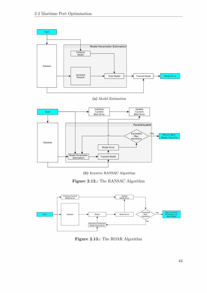
2.3 Maritime Port Optimization
(a) Model Estimation
(b) Iterative RANSAC Algorithm
Figure 2.12.: The RANSAC Algorithm
Figure 2.13.: The ROAR Algorithm
44
2.4 Fuzzy Systems
2.4. Fuzzy Systems
Fuzzy controllers have been used to dynamically allocate resources in large-scale
job scheduling environments with strict job completion deadlines [62]. This was
performed by phrasing the job scheduling problem as a prediction optimization
problem of job completion times given resource availability. The estimator that
predicts job completion time is formulated as a fuzzy system that considers the
job requirements and resource availability as inputs to output a deadline-aware
scheduling for a given job. Others have suggested a continuously evolving fuzzy
system to circumvent the limitations of rule bases fixed at design time, that therefore
fall short of changing objectives [63]. While this methodology is impressive and
powerful, the authors note that it is in excess of the requirements of problems similar
to the one studied here (deploying existing resources to meet queued demand); and
approaches from classical control theory will still suffice. Wang et. al. do indeed use
such a fuzzy system to adaptively deploy resources to handle database load within a
virtual environment to handle incoming query loads [64]. This system also updates
online, making it reactively adaptive to dynamic workloads.
2.5. Resource Deployment
Fuzzy controllers have been used to dynamically allocate resources in large-scale
job scheduling environments with strict job completion deadlines [62]. This was
performed by phrasing the job scheduling problem as a prediction optimization
problem of job completion times given resource availability. The estimator that
predicts job completion time is formulated as a fuzzy system that considers the
job requirements and resource availability as inputs to output a deadline-aware
scheduling for a given job. Others have suggested a continuously evolving fuzzy
45

2.5 Resource Deployment
system to circumvent the limitations of rule bases fixed at design time, that therefore
fall short of changing objectives [63]. While this methodology is impressive and
powerful, the authors note that it is in excess of the requirements of problems similar
to the one studied here (deploying existing resources to meet queued demand); and
approaches from classical control theory will still suffice. Wang et. al. do indeed use
such a fuzzy system to adaptively deploy resources to handle database load within a
virtual environment to handle incoming query loads [64]. This system also updates
online, making it reactively adaptive to dynamic workloads.
Existing solutions to resource deployment in the maritime space suffer from be-
ing offline, i.e. they require a priori knowledge of incoming vessel schedules and
their respective service load requirements. Some of these have been formulated as
Mixed Integer Programming (MIP) problems [6], while others have attempted a job
scheduling formulation with a homogeneous pool of processors [65]. Both meth-
ods require prior knowledge of incoming vessel schedules and service requirements,
which is inconsistent with real-world practice. Moreover, these methods are unable
to adapt to changing vessel schedules and operational faults such as delays in ves-
sel arrival times (often caused by unfavorable weather conditions, etc [66]). Finally,
GAs have been used in optimizing resource deployment and scheduling [67], but only
in an offline fashion yet again. The methodology presented in this work proves to be
robust against vessel schedule changes, while maintaining high service throughput
and simultaneously minimizing operational cost.
46
2.6 Solution Approach
2.6. Solution Approach
2.6.1. Predicting Insurance Claims on Shipping Container
Damage
Per the brief discussion in Sec.1.1.1, a dataset is collated and synthesized to predict
whether a given container is damaged and will therefore be filed for an insurance
claim. The details of the data collection and the synthesis of the dataset are dis-
cussed in more detail in Sec. 3.1 and Sec. 3.2. Once the dataset is created, many
CI methodologies (made available in Python’s scikit-learn library [68]) are used
to predict shipping container damage. These results can then be improved upon by
altering the learning strategy to include techniques inspired by cross-validation (see
Sec. 3.4.2 and Sec. 3.4.3).
2.6.2. Dynamic Resource Allocation
The results in [69] highlight methodologies to measure maritime vessel congestion
in a port’s waters. These are then used to determine whether and how to alter the
current resource deployment in response to projected future workload, reducing the
necessity for operational speed while maintaining or increasing operational through-
put. This is performed by a fuzzy system as is popularly used in adaptive resource
deployment problems [70, 71].
This is performed as a multi-objective optimization considering multiple optimiza-
tion objectives to adequately capture trade-offs between multiple operational deci-
sion objectives for a decision maker. The specific model used to perform this analysis
are discussed in more detail in Sec. 4.4.
47
3. Methodology
3.1. Data Collection Methodology
The proposed data gathering methodologies for this study are outlined in this sec-
tion. In order to adequately learn the cause of container damage, it is necessary to
know the conditions faced by the shipping container and any ship/truck/rail it was
on, during its life-cycle from the consignor to the customer. Therefore, it is necessary
to ingest navigational information pertaining to the voyage of the ship the container
was brought to port on. This data is not readily available and must be computed
from ship track data and container damage data. The ship track data must then
be fused with sea state data and local and global weather data. Finally, certain
domain specific knowledge may be useful, which must be captured from experts in
the industry.
3.1.1. Vessel Track Data
Vessel track data is typically found as vessel contact data, and is available from
vendors such as Lloyd’s Register [38]. This data is generated by an Automated
Identification System (AIS) transponder on board any cargo vessel and is broad-
casted periodically. Vendors (such as Lloyd’s Register) then receive these broad-
casted packets (through either satellite constellations, or terrestrial base stations)
48
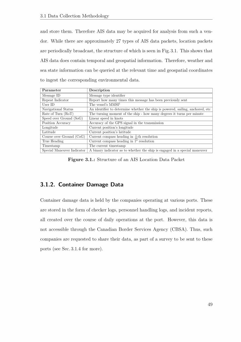
3.1 Data Collection Methodology
and store them. Therefore AIS data may be acquired for analysis from such a ven-
dor. While there are approximately 27 types of AIS data packets, location packets
are periodically broadcast, the structure of which is seen in Fig.3.1. This shows that
AIS data does contain temporal and geospatial information. Therefore, weather and
sea state information can be queried at the relevant time and geospatial coordinates
to ingest the corresponding environmental data.
Parameter DescriptionMessage ID Message type identifierRepeat Indicator Report how many times this message has been previously sentUser ID The vessel’s MMSI1Navigational Status An identifier to determine whether the ship is powered, sailing, anchored, etcRate of Turn (RoT) The turning moment of the ship - how many degrees it turns per minuteSpeed over Ground (SoG) Linear speed in knotsPosition Accuracy Accuracy of the GPS signal in the transmissionLongitude Current position’s longitudeLatitude Current position’s latitudeCourse over Ground (CoG) Current compass heading in 1
10th resolutionTrue Heading Current compass heading in 1o resolutionTimestamp The current timestampSpecial Maneuver Indicator A binary indicator as to whether the ship is engaged in a special maneuver
Figure 3.1.: Structure of an AIS Location Data Packet
3.1.2. Container Damage Data
Container damage data is held by the companies operating at various ports. These
are stored in the form of checker logs, personnel handling logs, and incident reports,
all created over the course of daily operations at the port. However, this data is
not accessible through the Canadian Border Services Agency (CBSA). Thus, such
companies are requested to share their data, as part of a survey to be sent to these
ports (see Sec. 3.1.4 for more).
49
3.1 Data Collection Methodology
3.1.3. Weather and Environmental Data
The National Oceanographic and Atmospheric Administration (NOAA) [35] pub-
lishes several global weather forecasts that can be used to describe the weather at
the given time and location of a shipping container. These can thus be queried
along the voyage of a vessel carrying a shipping container, to build a profile of en-
vironmental patterns faced by a shipping container along its voyage on the vessel.
The forecasts and historical records are publicly available on NOAA’s website, at a
geospatial resolution of 0.5◦ latitude and longitude, and a temporal resolution of one
hour. This data is then interpolated to realize the specific environmental conditions
at the given exact geospatial and temporal coordinates.
3.1.4. Domain Specific Knowledge Regarding Container
Damage Causes
Domain specific knowledge and experiential intuition have not been captured in any
publication thus far. Since much of the data pertaining to this study is confidential
and internal to the companies operating at various ports, it is plausible that these
companies will refuse to share their data. As a result, such domain specific knowl-
edge can help impute data as necessary. Thus, in order to capture and analyze such
domain specific expertise, a survey has been designed, to be filled out by companies
operating at terminals in Canadian ports. The survey has been reviewed by uOt-
tawa’s Office of Research Ethics and Integrity, and captures information including:
• correlations between container damage claims and
– the consignor
– the customer
50
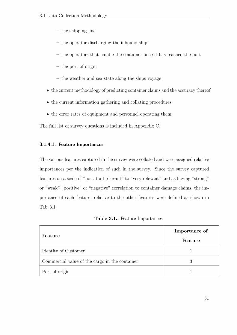
3.1 Data Collection Methodology
– the shipping line
– the operator discharging the inbound ship
– the operators that handle the container once it has reached the port
– the port of origin
– the weather and sea state along the ships voyage
• the current methodology of predicting container claims and the accuracy thereof
• the current information gathering and collating procedures
• the error rates of equipment and personnel operating them
The full list of survey questions is included in Appendix C.
3.1.4.1. Feature Importances
The various features captured in the survey were collated and were assigned relative
importances per the indication of such in the survey. Since the survey captured
features on a scale of “not at all relevant” to “very relevant” and as having “strong”
or “weak” “positive” or “negative” correlation to container damage claims, the im-
portance of each feature, relative to the other features were defined as shown in
Tab. 3.1.
Table 3.1.: Feature Importances
FeatureImportance of
Feature
Identity of Customer 1
Commercial value of the cargo in the container 3
Port of origin 1
51
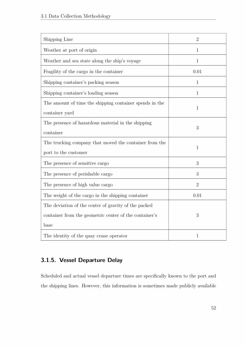
3.1 Data Collection Methodology
Shipping Line 2
Weather at port of origin 1
Weather and sea state along the ship’s voyage 1
Fragility of the cargo in the container 0.01
Shipping container’s packing season 1
Shipping container’s loading season 1
The amount of time the shipping container spends in the
container yard1
The presence of hazardous material in the shipping
container3
The trucking company that moved the container from the
port to the customer1
The presence of sensitive cargo 3
The presence of perishable cargo 3
The presence of high value cargo 2
The weight of the cargo in the shipping container 0.01
The deviation of the center of gravity of the packed
container from the geometric center of the container’s
base
3
The identity of the quay crane operator 1
3.1.5. Vessel Departure Delay
Scheduled and actual vessel departure times are specifically known to the port and
the shipping lines. However, this information is sometimes made publicly available
52
3.1 Data Collection Methodology
(e.g. [72]). Since historical data is unavailable for scheduled departure times (but is
indeed available for actual departure times) scheduled departure times are periodi-
cally polled, and correlated against historical data on actual departure times. The
difference between these gives the delay in vessel departure from port, as shown in
Eq. 3.1.
DepartureDelay(M) = ATD(M)− ETD(M) (3.1)
Where
M is the MMSI of the vessel.
ATD(M) is the actual departure time of the vessel with MMSI M , reported as
seconds from epoch.
ETD(M) is the scheduled departure time of the vessel of the vessel with MMSI M ,
reported as seconds from epoch.
3.1.6. Vessel Service
Given known vessel tracks (as described in Sec. 3.2.2), the methodology of mining
real-world vessel service at port is described in this section.
First, instances of a vessel’s visit to port are detected. Typically this would be
accomplished by identifying the port’s latitude and longitude coordinates and iden-
tifying segments of the vessel’s track with a reported speed of 0 knots and a minimal
distance between the vessel and port. However, due to errors in the GPS signal and
map projection, this method proves to be too noisy to yield useful data. Therefore,
the coastline along which the port is located is modeled as a series of line segments,
53
3.1 Data Collection Methodology
whose end-points are specified as latitude-longitude geospatial coordinates.
Next, stationary segments of the vessel’s track are detected - these are contiguous
subsequences of time-sorted AIS contacts from the vessel that report a speed of
0.5 knots or lower [73]. These segments are then filtered based on geospatial dis-
tance from port, so that segments describing stationery vessels in open waters are
appropriately excluded from the analysis.
The first contact of a segment is the actual arrival time of the vessel at port, while
the last contact of the segment describes its actual departure time. The differ-
ence between the two is the calculated vessel service time (as shown in Eq. 3.2 and
illustrated in Fig. 3.2).
The Maritime Mobile Service Identity (MMSI) of each of these vessels can then
be correlated against historically available AIS messages which report the draught
of the vessel, along with its physical dimensions (length and width). This is used
to calculate the volume of water displaced (as seen in Eq. 3.3 and Eq. 3.4), which
when multiplied by the density of water gives the mass of displaced water (as seen in
Eq.3.5). This is the total mass of the vessel including fuel, crew, and the mass of the
shipping containers on board. Assuming that the remaining weights are negligible
in the absence of more specific information (or otherwise allowing for such values
within a margin of error), the mass of the displaced water is the combined mass of
the shipping containers on board the vessel. The number of shipping containers on
board (given the draught and physical dimensions of a vessel) is therefore computed
by dividing the mass of displaced water by the average mass of a shipping container
(as seen in Eq. 3.6). Yet, since some vessels may be loaded with heavier containers
than others on average, the average mass of a shipping container is drawn from a
normal distribution with µ =75 tons and σ =10 tons [1], capturing the range of
54
3.1 Data Collection Methodology
weights of a loaded shipping container.
ServiceT ime(M) = ATD(M)− ATA(M) (3.2)
Where
M is the MMSI of the vessel.
ATD(M) is the actual departure time of the vessel with MMSI M , reported as
seconds from epoch.
ATA(M) is the actual arrival time of the vessel of the vessel with MMSIM , reported
as seconds from epoch.
ServiceT ime(M) is the service time of the vessel with MMSI M , reported as sec-
onds.
totalDraught(v) = do(v) + di(v) (3.3)
volumewater = totalDraught(v)× L(v)×W (v) (3.4)
masswater = Vwater ×Dwater (3.5)
numContainers = masswater
N (µ = 75, σ = 10) (3.6)
Where
di(v) is the draught (in meters) of vessel v as it enters the port
do(v) is the draught (in meters) of vessel v as it exits the port
L(v) is the length (in meters) of vessel v as reported in AIS messages
W (v) is the width (in meters) of vessel v as reported in AIS messages
55

3.1 Data Collection Methodology
Figure 3.2.: An Example Vessel Service Track
Dwater is the density of water (1000Kg/m3)
Finally, the real-world resource deployment is mined in order to benchmark the
performance of this optimization against established practices in the real world.
Since the given start and end times of each vessel service from the publicly available
schedule are only estimates, the actual start and end times of each vessel service
are mined by computing the time at which the vessel arrives at a berth and the
time at which it departs from the berth. As previously described, the draught
measures and other AIS values give the total number of containers processed during
this vessel’s service period. In the absence of additional data, it is assumed that
the rate of processing containers remains approximately constant throughout the
vessel’s service period. Therefore, dividing the number of processed containers by
the time period of the service window yields the number of containers processed
per eight-hour shift in the service window. Given that a single crane can load or
unload a single container from a vessel requires two minutes [6], the total resource
deployment is computed as the number of individual cranes required to process the
computed number of shipping containers over all vessels being serviced. Note that
this must be computed per eight-hour shift, in order to capture the notion that
56
3.2 DataSet Synthesis
personnel may be scheduled to work in an integer number of eight hour shifts.
3.1.7. Summary
Data was collected from CBSA, AIS messages, NOAA, and such sources. This data
was then processed to be a part of the dataset used in the analyses presented in
this thesis proposal. Certain additional data could not be captured from publicly
available sources and needed to be synthesized per the specifications outlined in the
data captured by the survey of industry experts (see Sec. 3.1.4). The methodologies
used to synthesize this data are explained in detail in Sec. 3.2.
3.2. DataSet Synthesis
Datasets were created in order to perform the necessary experiments. However, since
some data was not available from real-world sources, they needed to be synthesized.
The synthesis of such data is discussed in this section.
3.2.1. Container Damage Feature Weights
Based on the results from the survey of Canadian domain experts (discussed in
Sec. 3.3), values of shipping container features, necessary to make insurance claims
prediction were synthesized. These attributes and the synthesis of their values are
discussed in this section. Each feature was assigned a value drawn from a specific
distribution, weighted by the strength of the correlation indicated in the survey
results. The sum of these weighted values comprises a damage value, which informs
whether the shipping container was claimed for damages. The weights of the different
features are shown in Tab. 3.2.
57
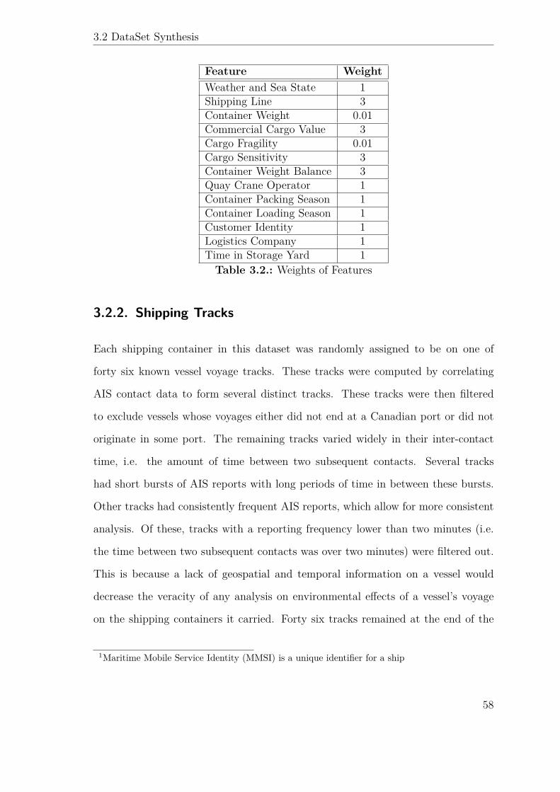
3.2 DataSet Synthesis
Feature WeightWeather and Sea State 1Shipping Line 3Container Weight 0.01Commercial Cargo Value 3Cargo Fragility 0.01Cargo Sensitivity 3Container Weight Balance 3Quay Crane Operator 1Container Packing Season 1Container Loading Season 1Customer Identity 1Logistics Company 1Time in Storage Yard 1Table 3.2.: Weights of Features
3.2.2. Shipping Tracks
Each shipping container in this dataset was randomly assigned to be on one of
forty six known vessel voyage tracks. These tracks were computed by correlating
AIS contact data to form several distinct tracks. These tracks were then filtered
to exclude vessels whose voyages either did not end at a Canadian port or did not
originate in some port. The remaining tracks varied widely in their inter-contact
time, i.e. the amount of time between two subsequent contacts. Several tracks
had short bursts of AIS reports with long periods of time in between these bursts.
Other tracks had consistently frequent AIS reports, which allow for more consistent
analysis. Of these, tracks with a reporting frequency lower than two minutes (i.e.
the time between two subsequent contacts was over two minutes) were filtered out.
This is because a lack of geospatial and temporal information on a vessel would
decrease the veracity of any analysis on environmental effects of a vessel’s voyage
on the shipping containers it carried. Forty six tracks remained at the end of the
1Maritime Mobile Service Identity (MMSI) is a unique identifier for a ship
58
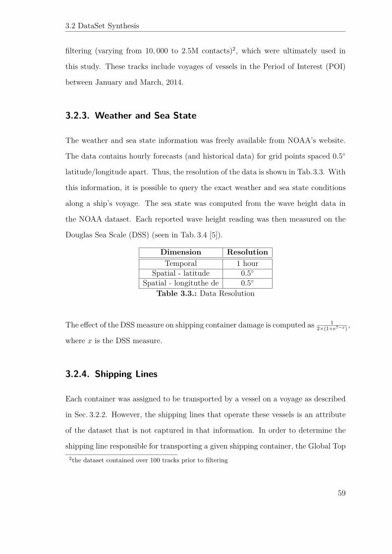
3.2 DataSet Synthesis
filtering (varying from 10, 000 to 2.5M contacts)2, which were ultimately used in
this study. These tracks include voyages of vessels in the Period of Interest (POI)
between January and March, 2014.
3.2.3. Weather and Sea State
The weather and sea state information was freely available from NOAA’s website.
The data contains hourly forecasts (and historical data) for grid points spaced 0.5◦
latitude/longitude apart. Thus, the resolution of the data is shown in Tab.3.3. With
this information, it is possible to query the exact weather and sea state conditions
along a ship’s voyage. The sea state was computed from the wave height data in
the NOAA dataset. Each reported wave height reading was then measured on the
Douglas Sea Scale (DSS) (seen in Tab. 3.4 [5]).
Dimension ResolutionTemporal 1 hour
Spatial - latitude 0.5◦Spatial - longituthe de 0.5◦
Table 3.3.: Data Resolution
The effect of the DSS measure on shipping container damage is computed as 12×(1+e7−x) ,
where x is the DSS measure.
3.2.4. Shipping Lines
Each container was assigned to be transported by a vessel on a voyage as described
in Sec. 3.2.2. However, the shipping lines that operate these vessels is an attribute
of the dataset that is not captured in that information. In order to determine the
shipping line responsible for transporting a given shipping container, the Global Top2the dataset contained over 100 tracks prior to filtering
59
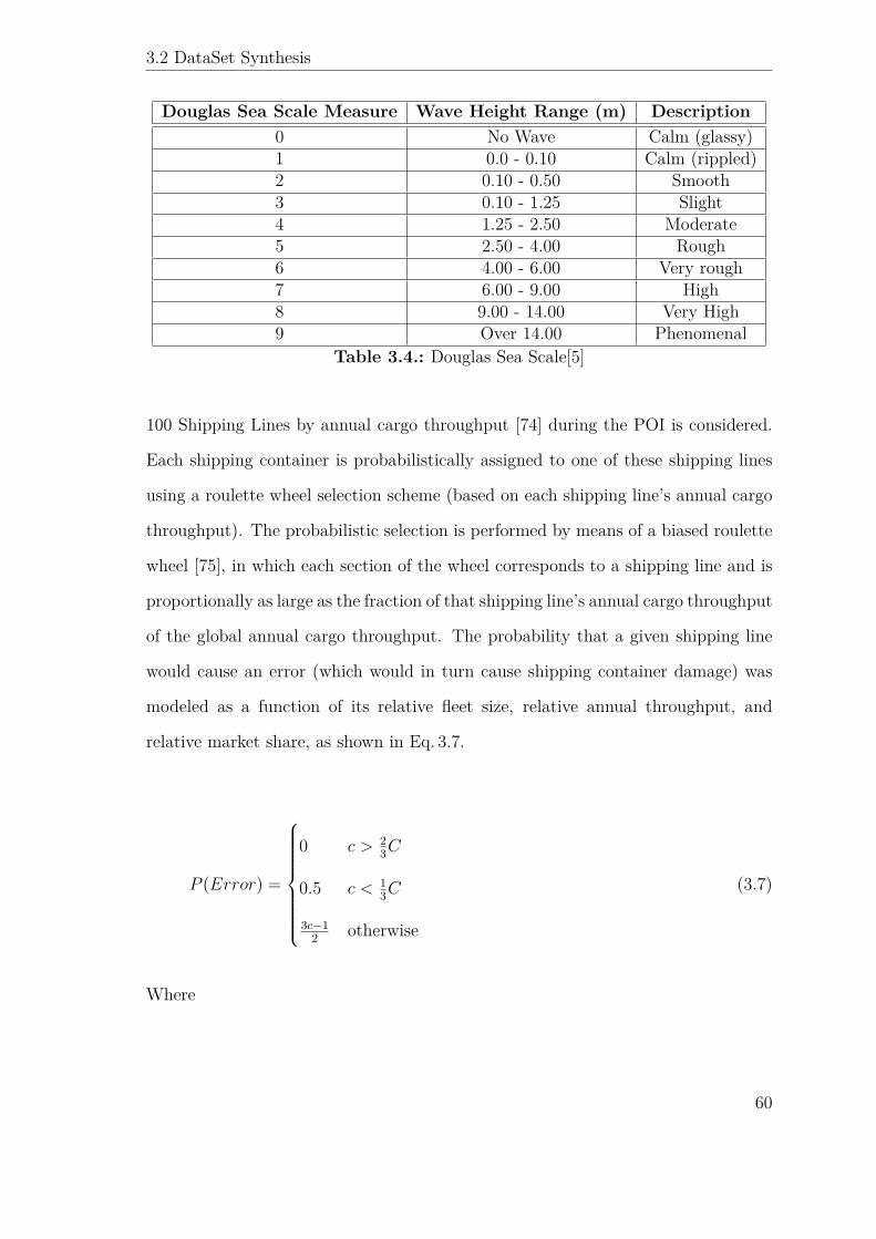
3.2 DataSet Synthesis
Douglas Sea Scale Measure Wave Height Range (m) Description0 No Wave Calm (glassy)1 0.0 - 0.10 Calm (rippled)2 0.10 - 0.50 Smooth3 0.10 - 1.25 Slight4 1.25 - 2.50 Moderate5 2.50 - 4.00 Rough6 4.00 - 6.00 Very rough7 6.00 - 9.00 High8 9.00 - 14.00 Very High9 Over 14.00 Phenomenal
Table 3.4.: Douglas Sea Scale[5]
100 Shipping Lines by annual cargo throughput [74] during the POI is considered.
Each shipping container is probabilistically assigned to one of these shipping lines
using a roulette wheel selection scheme (based on each shipping line’s annual cargo
throughput). The probabilistic selection is performed by means of a biased roulette
wheel [75], in which each section of the wheel corresponds to a shipping line and is
proportionally as large as the fraction of that shipping line’s annual cargo throughput
of the global annual cargo throughput. The probability that a given shipping line
would cause an error (which would in turn cause shipping container damage) was
modeled as a function of its relative fleet size, relative annual throughput, and
relative market share, as shown in Eq. 3.7.
P (Error) =
0 c > 23C
0.5 c < 13C
3c−12 otherwise
(3.7)
Where
60
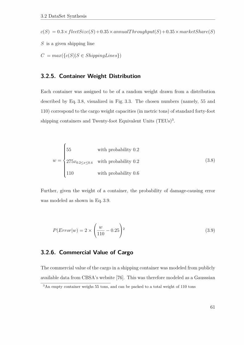
3.2 DataSet Synthesis
c(S) = 0.3×fleetSize(S)+0.35×annualThroughput(S)+0.35×marketShare(S)
S is a given shipping line
C = max({c(S)|S ∈ ShippingLines})
3.2.5. Container Weight Distribution
Each container was assigned to be of a random weight drawn from a distribution
described by Eq. 3.8, visualized in Fig. 3.3. The chosen numbers (namely, 55 and
110) correspond to the cargo weight capacities (in metric tons) of standard forty-foot
shipping containers and Twenty-foot Equivalent Units (TEUs)3.
w =
55 with probability 0.2
275x0.2≤x≤0.4 with probability 0.2
110 with probability 0.6
(3.8)
Further, given the weight of a container, the probability of damage-causing error
was modeled as shown in Eq. 3.9.
P (Error|w) = 2× w
110 − 0.252 (3.9)
3.2.6. Commercial Value of Cargo
The commercial value of the cargo in a shipping container was modeled from publicly
available data from CBSA’s website [76]. This was therefore modeled as a Gausssian3An empty container weighs 55 tons, and can be packed to a total weight of 110 tons
61
3.2 DataSet Synthesis
Figure 3.3.: Shipping Container Weight Distribution
distribution with µ = 105
2 and σ =√
1010. While it is valid to think of this value
as being positively correlated with cargo weight, it is not necessarily the case, as
cases of lighter and more expensive materials do exist. As a result, it is impossible
to correlate the two, making them indeed independent distributions.
Given the commercial value of the cargo inside a shipping container (v ∈ [0, V ]), the
probability of damage-causing error was modeled as shown in Eq. 3.10.
P (Error|v) =
0 v ≤ V3
0.5 v ≥ V3
0.5× vV− 0.5 otherwise
(3.10)
62
3.2 DataSet Synthesis
3.2.7. Cargo Fragility and Sensitivity
Cargo fragility refers to whether the cargo is marked as being fragile. This is there-
fore implemented as a binary flag, drawn from a uniform distribution over [0, 1].
Cargo sensitivity is reported by the consignor or customer. From the surveys, it
is known that shipping containers with sensitive cargo have a higher likelihood of
being claimed in the event of container damage. As a result, this attribute was
included in the dataset and was also modeled as a binary flag drawn from a uniform
distribution over [0, 1].
The probability of damage-causing errors given the fragility and the sensitivity of
the cargo within a given shipping container are shown respectively in Eq. 3.11 and
Eq. 3.12.
P (Error|f) = 0.01× f (3.11)
P (Error|s) = 0.5× s (3.12)
3.2.8. Container Weight Balance
The weight balance of a shipping container was modeled as the linear distance
between the center of mass projected onto the container’s base (as seen in Fig. 3.4),
and the geometric center of the container’s base. Given that the dataset contains
data describing 40ft containers, this distance is limited to half the length of the
diagonal of the base of the shipping container, namely 20.4ft.
63
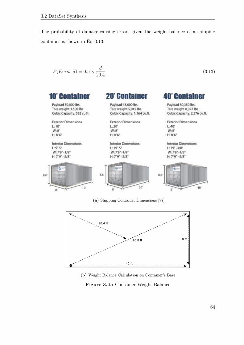
3.2 DataSet Synthesis
The probability of damage-causing errors given the weight balance of a shipping
container is shown in Eq. 3.13.
P (Error|d) = 0.5× d
20.4 (3.13)
(a) Shipping Container Dimensions [77]
(b) Weight Balance Calculation on Container’s Base
Figure 3.4.: Container Weight Balance
64
3.2 DataSet Synthesis
This value is considered agnostic of the nature of the cargo within the container.
Oddly shaped cargo or cargo with otherwise non-uniform mass distribution directly
affect the container weight balance, which is described by this feature, without
considering the specifics of the contained cargo. However, non-solid cargo (such
liquid or dry bulk) are out of the scope of this study and a left as future work.
3.2.9. Quay Crane Operator
The identity of the quay crane operator who unloaded a given container from the
vessel carrying it onto an intra-port truck was drawn from a uniform distribution
over a pool of available operators.
3.2.10. Packing and Loading Season
In order to capture the effects of seasonal changes on container damage, the season in
which a container was packed (and/or loaded) was drawn uniformly at random from
the set {summer, winter, spring, fall}. The probability of damage-causing errors
given the packing and loading season of a container were each set to 0.5 (and 0
otherwise) if the container was packed or loaded in the fall or spring seasons.
3.2.11. Customer Identity
The customer is defined as the person or organization to whom the shipping con-
tainer will be ultimately deposited. In order to capture the notion that some cus-
tomers are more litigious than others, the customer’s identity was drawn from a
random uniform distribution. The probability of a claim being filed by a given cus-
tomer was drawn from a uniform distribution over [0, 0.5], and the claim amount
was drawn from a uniform distribution over [0, 108].
65
3.2 DataSet Synthesis
3.2.12. Logistics Company
Each container was assigned to be transported by a truck from a logistics company
with a fleet of terrestrial trucks. In order to determine the trucking company re-
sponsible for transporting a given shipping container, the Global Top 100 trucking
companies by annual cargo throughput [78] during the POI is considered. Each ship-
ping container is then probabilistically assigned to one of these trucking companies
using a roulette wheel selection scheme (based on each shipping line’s annual cargo
throughput). The probabilistic selection is performed by means of a biased roulette
wheel [75], in which each section of the wheel corresponds to a trucking company
and is proportionally as large as the fraction of that shipping line’s annual cargo
throughput of the global annual cargo throughput.
The probability that a given logistics company would cause an error (which would
in turn cause shipping container damage) was modeled as a function of its relative
fleet size, relative annual throughput, and relative age, as shown in Eq. 3.14.
P (Error) =
0 c > 23C
0.5 c < 13C
3c−12 otherwise
(3.14)
Where:
c(t) = 0.3× fleetSize(t) + 0.35× annualThroughput(t) + 0.35× age(t)
t is a given logistics company
C = max({c(t)|t ∈ logisticsCompanies})
66
3.2 DataSet Synthesis
3.2.13. Time in Storage Yard
After being unloaded at the destination port, a shipping container is stored in the
storage yard at that port before it is picked up by a truck for final delivery to
the customer. As a result, the amount of time a shipping container spends in the
storage yard is a recorded feature of this dataset, drawn uniformly at random from
[0, 364] days. The lower limit of 0 captures the notion that shipping containers
are sometimes dispatched from the port on the day that they are received. The
upper limit of 364 captures the notion that shipping containers are not stored in
a storage yard for a period of time exceeding one year. Given the duration over
which a shipping container is stored in a port’s storage yard, the probability of
damage-causing error is shown in Eq. 3.15.
P (Error|t) = 366365− t (3.15)
3.2.14. Port Situation Reports
Ports write daily situation reports (an example of this is seen in [79]). Since such
reports are extremely sensitive to the port and are not publicly available, similar
reports were manually synthesized for use in this study (examples of the relevant
sections of such synthetic reports are listed in Tab. 3.5, and an example situation
report is seen in Tab. 3.6). As seen in this example, the situation report contains
the name of the inbound vessel, a unique identifier for its visit to port, its list of
port calls to subsquent ports, the last visited port, the vessel’s current geolocation,
its arrival schedule to this port, and the immediately subsequent ports for it to
visit. The final column contains notes pertaining to any delays this vessel may face,
67

3.2 DataSet Synthesis
which is of particular importance to this study. Mining these notes provide insights
into the expected delays at ports, which can be used to optimize port-side resource
deployment.
From the example report [79], it is evident that reports of any foreseeable delays in
port operations are only present when such a delay is expected. When no delay is
expected, these reports are left empty. The specifics of the usage of these synthetic
reports are discussed in Sec. 3.6.2.
The current resource deployment is known at any given time. The difference in
time between the the given moment and the start of the current shift is trivially
computed, and computing the number of two minute intervals in this period gives the
number of containers processed thus far in this shift. While this calculation yields
the number of remaining containers to be processed, the incoming vessel schedule
provides another source of shipping containers to be processed. Adding the data
from these two streams together yields the size of the backlog (i.e. the number of
remaining containers to be processed) at any given time. An increase in the size of
this backlog at the end of a given day indicates impending vessel service delay, a
the situation report is synthesized to include a comment indicative thereof. On the
other hand, if the backlog decreases, the comment section is left empty.
It is therefore clear that situation reports must be generated adaptively, in response
to the current backlog, which is dictated by the current resource deployment; which
in turn is dictated by the optimizer (explained in Sec.3.6). Therefore, the generation
of these situation reports occurs as part of the fitness evaluation function of the
multi-objective evolutionary algorithm (described in Sec. 3.6.2) in response to the
size of the current backlog at the end of each simulated day). Further, as discussed
in Sec. 3.6.2, these situation reports are ingested as soft data in order to optimize
resource deployment.
68

3.2 DataSet Synthesis
Example Situation Reportextreme delay due to weather
delay due to unavailable port-side resourcescongestion-induced delay
inbound delay due to weatherservice delays caused outbound delay
Table 3.5.: Examples of Synthetic Situation Reports
3.2.15. Summary
The methodologies used to synthesize unavailable data are discussed in this section.
These data are typically known to real-world stakeholders, but are unavailable for
an academic study. As a result, a survey was used to capture the characteristics
of the distributions of the values of these features (see Sec. 3.1.4), based on which
synthetic data was created to complete an otherwise feature-incomplete dataset.
69
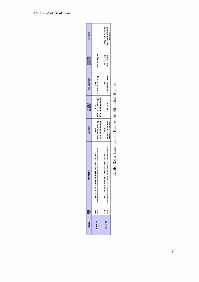
3.2 DataSet Synthesis
Tab
le3.6.:Ex
amples
ofReal-w
orld
SituationRep
orts
70
3.3 Prediction of Container Damage Insurance Claims for Optimized MaritimePort Operations [1]
3.3. Prediction of Container Damage Insurance
Claims for Optimized Maritime Port Operations
[1]
Commercial maritime ports require the optimization of highly involved workflows,
which are typically induced by the incidence of an insurance claim on a damaged
shipping container. These workflows involve data gathering and collation from multi-
ple sources, and filtering this data based on relevance to the specific incident [80, 81].
Thus, the process includes:
• visual inspection logs from the quay crane operators (who unloaded the ship-
ping container from the ship)
• visual inspection logs from various checkers in the container yard
• cargo manifests that describe properties such as commercial value and fragility
of the cargo
• surveillance camera footage from throughout the port
• weather data (e.g. visibility, precipitation, wind speed, sea state, etc) pertain-
ing to the route traveled by the ship while inbound to the port
Once processed, the information extracted form this data is used to determine the
point of incidence of the damage, which in turn advises port officials whether the
insurance claim should be disputed, settled, or redirected to a third party responsible
for the damage [82, 83, 84]. While data gathering and collation are fairly fast and
accurate, they do entail a high computational burden due to the computational costs
associated with processing noisy, inaccurate, and often incomplete data (such as
personnel logs, etc). This motivates the need to predict shipping container damage
and insurance claims to narrow the subset of shipping containers for which to collect
71
3.3 Prediction of Container Damage Insurance Claims for Optimized MaritimePort Operations [1]
and process data. This data may then be presented to port officials upon the
incidence of an insurance claim on a specific shipping container.
Data collection and processing aside, the human expert predictions are known to be
erroneous. A study of the effects of prediction specificity on prediction accuracy in
sports bets showed that both experts and novices have higher prediction accuracy
when making general predictions (in the form of predicting the winning team in a
soccer match) rather than very specific predictions (in the form of predicting the
final score of the soccer match). This effect was statistically significant even when
the experiment was controlled for gambling rewards (such as monetary rewards for
correct prediction) [85]. This effect is not necessarily due to the increase in the
number of alternative prediction outcomes, but also has causes rooted in human
cognitive biases which narrow focus onto a subset of facts, detracting from a more
preferred, holistic consideration of all available information[86]. This problem is
further exacerbated when the predictions are to be made on longer-duration time
series data [86]. Additionally, human experts are often swayed by risk aversive
tendencies and confirmation bias, which negatively impacts their prediction accuracy
[85, 87]. Finally, a NASA study shows that an increase in the number of simultaneous
predictions decreases the accuracy of each prediction [81].
A survey was conducted to capture some of the domain-specific expertise in the
industry. This survey captured aspects of commercial maritime port operations
including:
• correlations between container damage claims and
– the consignor
– the customer
– the shipping line
72
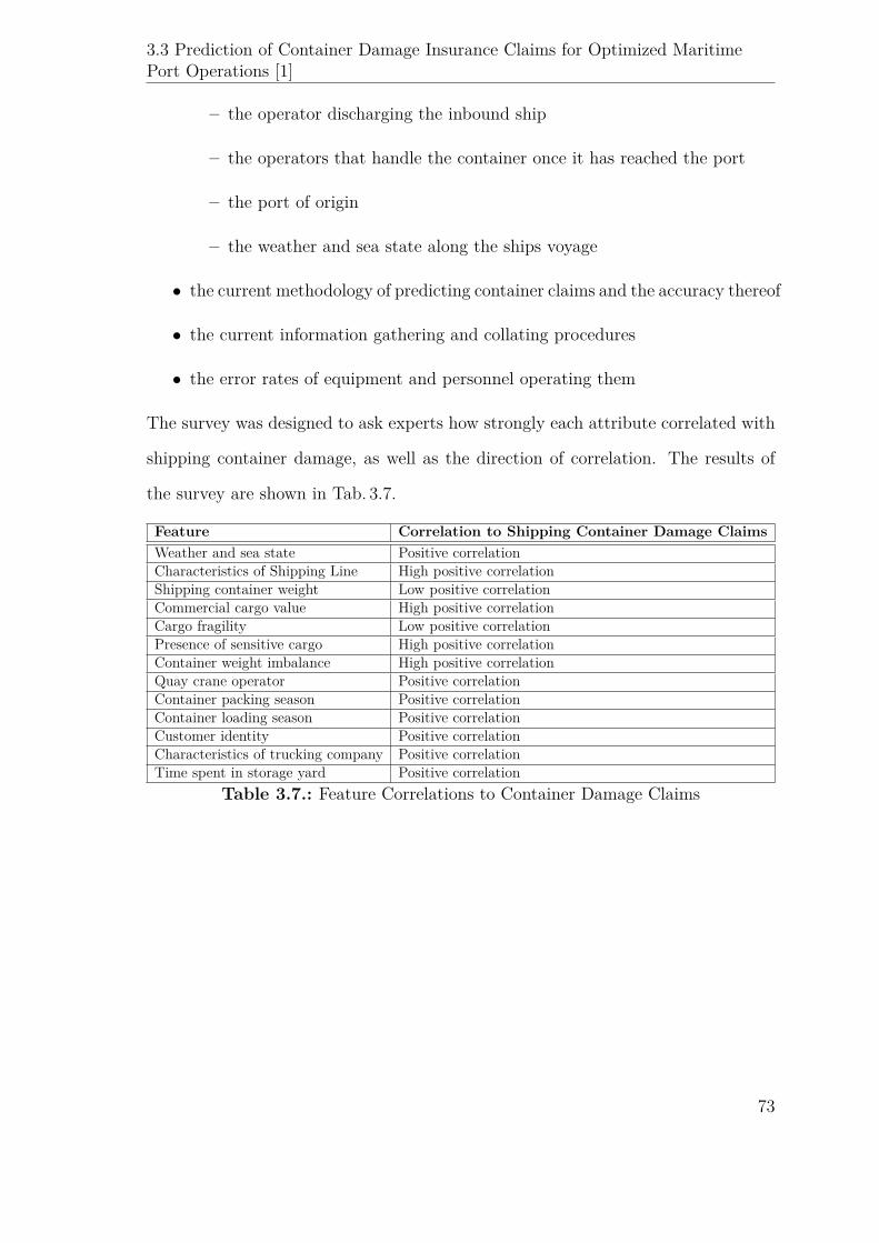
3.3 Prediction of Container Damage Insurance Claims for Optimized MaritimePort Operations [1]
– the operator discharging the inbound ship
– the operators that handle the container once it has reached the port
– the port of origin
– the weather and sea state along the ships voyage
• the current methodology of predicting container claims and the accuracy thereof
• the current information gathering and collating procedures
• the error rates of equipment and personnel operating them
The survey was designed to ask experts how strongly each attribute correlated with
shipping container damage, as well as the direction of correlation. The results of
the survey are shown in Tab. 3.7.
Feature Correlation to Shipping Container Damage ClaimsWeather and sea state Positive correlationCharacteristics of Shipping Line High positive correlationShipping container weight Low positive correlationCommercial cargo value High positive correlationCargo fragility Low positive correlationPresence of sensitive cargo High positive correlationContainer weight imbalance High positive correlationQuay crane operator Positive correlationContainer packing season Positive correlationContainer loading season Positive correlationCustomer identity Positive correlationCharacteristics of trucking company Positive correlationTime spent in storage yard Positive correlation
Table 3.7.: Feature Correlations to Container Damage Claims
73
3.4 Improving Container Damage Claims Classifier Performance Veracity withLeave One Batch Out Training
3.4. Improving Container Damage Claims Classifier
Performance Veracity with Leave One Batch
Out Training
While presenting [1], a concern was raised that since the size of the dataset is much
larger than 46 (the number of known shipping tracks in the dataset), the machine
learning algorithms likely did not use the weather features along a vessel’s voyage
at sea as learned parameters, giving them an undue advantage and inflating their
performance values. This inflation of a classifier’s MOE lowers its MOPs, which
ultimately leads to poorer performance and generalization in the long term. In
order to address this concern, three experiments were designed and are presented in
this section.
3.4.1. Removing Weather Features from the Dataset
The experiments in [1] were rerun, but with the weather features removed from
the dataset. If the results from these new experiments are significantly worse (as
indicated by lower MOPs) than those in [1], it would indicate that the results in [1]
were indeed biased and that further experiments need to be performed to correct for
this bias. However, these worse classifiers would indeed have higher MOEs as they
would be performing the required interpolation of weather features, as opposed to
some bias-inducing memorization. This can be described as a lack of resilience in
the face of lower dimensional data features, which describes a lower MOE [21]. The
performance of various classifiers in this dataset are shown in Tab.A.2.
74
3.4 Improving Container Damage Claims Classifier Performance Veracity withLeave One Batch Out Training
3.4.2. Using a Validation Batch
The dataset used in [1] contains 23 features, 9 of which pertain to weather and sea
state along the voyage of a vessel carrying a given shipping container. Using the
vector of these nine features as a signature, all shipping containers in the dataset
can be grouped by their signature. One group is held out in accordance with a Leave
One Batch Out (LOBO) learning methodology, while 10x10 fold cross validation is
performed on the remainder of the dataset, comprised of the individual records from
all other batches (this process is visualized in Fig. 3.5). All the experiments in [1]
were then performed under this experimental methodology.
A statistically significantly worse performance under this methodology as compared
to [1] (lower MOPs, regardless of the difference in MOEs) would suggest that further
study is required.
The performance of various classifiers with this LOBO methodology are shown in
Tab.A.3 and a combined graph showing the relative performances across all datasets
is shown in Fig. 3.7.
75

3.4 Improving Container Damage Claims Classifier Performance Veracity withLeave One Batch Out Training
Figure 3.5.: Using a Validation Batch
3.4.3. Cross Validation with LOBO
Similar to the methodology in Sec. 3.4.2, the records in the dataset are partitioned
into batches by the signatures of their weather and sea state values. In each iteration
of the 10x10 fold cross validation, one batch is left out for testing. Finally, the
machine learning model is tested for performance on a batch that was previously
held out and never used in training. This process is illustrated in Fig. 3.6.
76
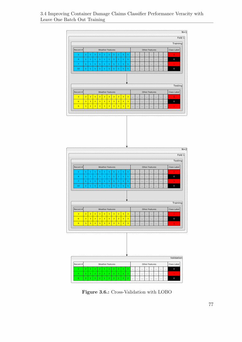
3.4 Improving Container Damage Claims Classifier Performance Veracity withLeave One Batch Out Training
Figure 3.6.: Cross-Validation with LOBO
77
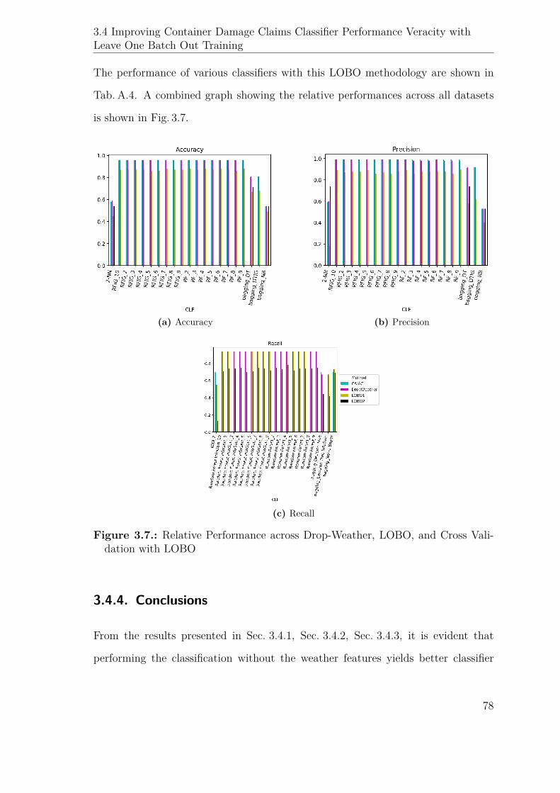
3.4 Improving Container Damage Claims Classifier Performance Veracity withLeave One Batch Out Training
The performance of various classifiers with this LOBO methodology are shown in
Tab. A.4. A combined graph showing the relative performances across all datasets
is shown in Fig. 3.7.
(a) Accuracy (b) Precision
(c) Recall
Figure 3.7.: Relative Performance across Drop-Weather, LOBO, and Cross Vali-dation with LOBO
3.4.4. Conclusions
From the results presented in Sec. 3.4.1, Sec. 3.4.2, Sec. 3.4.3, it is evident that
performing the classification without the weather features yields better classifier
78

3.4 Improving Container Damage Claims Classifier Performance Veracity withLeave One Batch Out Training
performance than when the weather features are included during classification. This
is counter to the expectations outlined at the outset. This could potentially be
explained by the dataset synthesis methodology (see Sec. 3.2); specifically, the non-
weather features are drawn from simple distributions that are easily learned by
machine learning algorithms. Therefore, these results do not adequately address the
concern of learning bias requiring further analysis.
Following up the inconclusive analysis in Sec. 3.4.1, the dataset is partitioned based
on the values of the weather features (as described in Sec.3.4.2). One such partition
is held out as a validation set, while training and testing are performed on the
remainder of the dataset. The results from these experiments (shown in Tab. A.3)
show that the classifiers outperform their counterparts in Sec. 3.4.1. This suggests
that this cross-validated training method is superior to training method and warrants
more investigation for a new publication as it promises better generalization.
Given the performance increase noted in Tab.A.3, the extension of that methodology
(used in Sec. 3.4.3) promises better results. However, since this observed to not be
the case (see Tab. A.4), concluding that the former training methodology affords
better generalizability than the latter. This is especially relevant to information
fusion effectiveness as these experiments have been performed with data restricted
to a three month POI (and therefore, limited variance in weather patterns across
the dataset). Performing these experiments against a larger data set with a one-year
POI will reconfirm the conclusions about the generalizability of LOBO methodology.
Yet, the argument still holds that the superior performance of using a validation
batch over performing cross-validation with LOBO could be an artifact of the re-
stricted POI of the dataset which captures only a subset of annual weather patterns.
Unfortunately, since no other maritime voyage track data is available, this criticism
cannot be further investigated at the moment. However, negotiations are currently
79
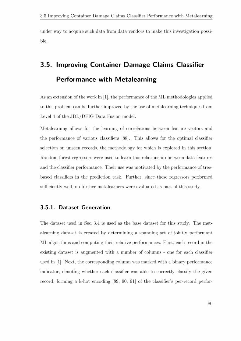
3.5 Improving Container Damage Claims Classifier Performance with Metalearning
under way to acquire such data from data vendors to make this investigation possi-
ble.
3.5. Improving Container Damage Claims Classifier
Performance with Metalearning
As an extension of the work in [1], the performance of the ML methodologies applied
to this problem can be further improved by the use of metalearning techniques from
Level 4 of the JDL/DFIG Data Fusion model.
Metalearning allows for the learning of correlations between feature vectors and
the performance of various classifiers [88]. This allows for the optimal classifier
selection on unseen records, the methodology for which is explored in this section.
Random forest regressors were used to learn this relationship between data features
and the classifier performance. Their use was motivated by the performance of tree-
based classifiers in the prediction task. Further, since these regressors performed
sufficiently well, no further metalearners were evaluated as part of this study.
3.5.1. Dataset Generation
The dataset used in Sec. 3.4 is used as the base dataset for this study. The met-
alearning dataset is created by determining a spanning set of jointly performant
ML algorithms and computing their relative performances. First, each record in the
existing dataset is augmented with a number of columns - one for each classifier
used in [1]. Next, the corresponding column was marked with a binary performance
indicator, denoting whether each classifier was able to correctly classify the given
record, forming a k-hot encoding [89, 90, 91] of the classifier’s per-record perfor-
80
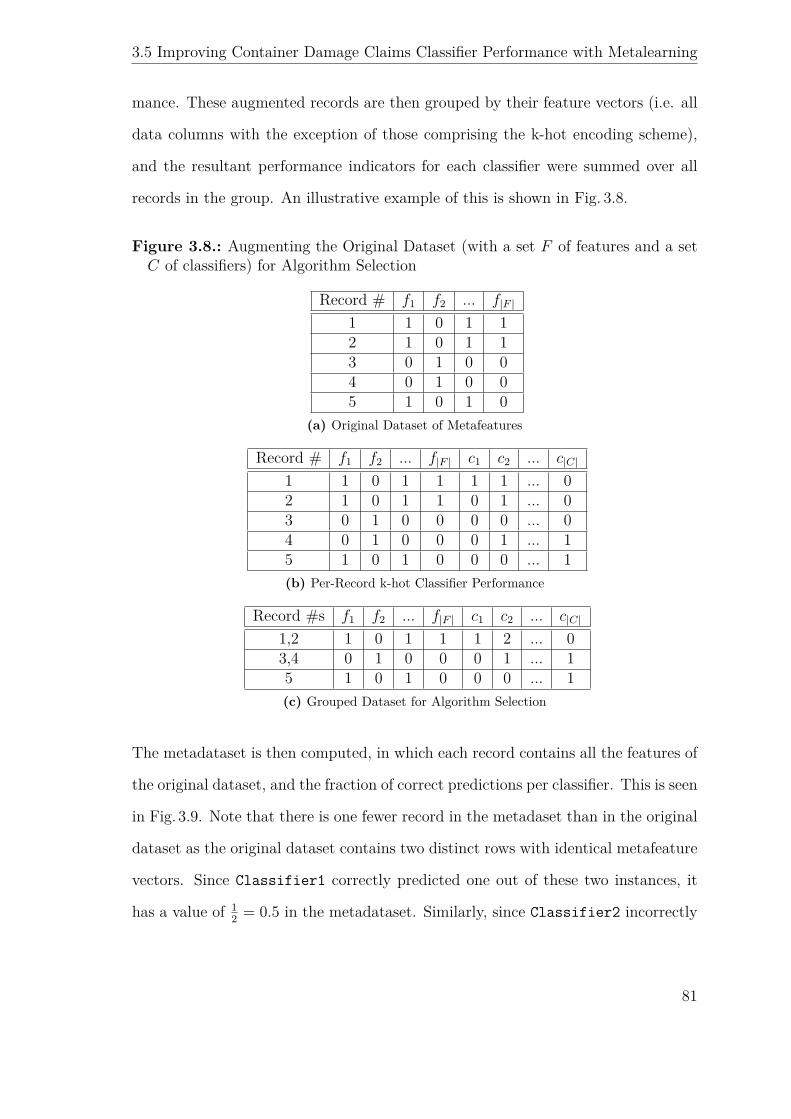
3.5 Improving Container Damage Claims Classifier Performance with Metalearning
mance. These augmented records are then grouped by their feature vectors (i.e. all
data columns with the exception of those comprising the k-hot encoding scheme),
and the resultant performance indicators for each classifier were summed over all
records in the group. An illustrative example of this is shown in Fig. 3.8.
Figure 3.8.: Augmenting the Original Dataset (with a set F of features and a setC of classifiers) for Algorithm Selection
Record # f1 f2 ... f|F |
1 1 0 1 12 1 0 1 13 0 1 0 04 0 1 0 05 1 0 1 0
(a) Original Dataset of Metafeatures
Record # f1 f2 ... f|F | c1 c2 ... c|C|
1 1 0 1 1 1 1 ... 02 1 0 1 1 0 1 ... 03 0 1 0 0 0 0 ... 04 0 1 0 0 0 1 ... 15 1 0 1 0 0 0 ... 1(b) Per-Record k-hot Classifier Performance
Record #s f1 f2 ... f|F | c1 c2 ... c|C|
1,2 1 0 1 1 1 2 ... 03,4 0 1 0 0 0 1 ... 15 1 0 1 0 0 0 ... 1(c) Grouped Dataset for Algorithm Selection
The metadataset is then computed, in which each record contains all the features of
the original dataset, and the fraction of correct predictions per classifier. This is seen
in Fig. 3.9. Note that there is one fewer record in the metadaset than in the original
dataset as the original dataset contains two distinct rows with identical metafeature
vectors. Since Classifier1 correctly predicted one out of these two instances, it
has a value of 12 = 0.5 in the metadataset. Similarly, since Classifier2 incorrectly
81

3.5 Improving Container Damage Claims Classifier Performance with Metalearning
predicted both instances, it has a value of 0 in the metadataset. Since it is known
that no one classifier performs at 100% accuracy across the entire dataset, the next
step is to determine the classifier with the highest likelihood of correct prediction
based on the metadataset. That classifier is then used to classify the new unseen
data record. While this comes with a small MOE decrease in that predictions on
new data will require an additional step, it is likely to improve overall MOEs in
increased accuracy over all new data.
Figure 3.9.: Determining the Spanning Classfiers from the Grouped Dataset
Record #s f1 f2 ... f|F | c1 c2 ... c|C|
1,2 1 0 1 1 1 2 ... 03,4 0 1 0 0 0 1 ... 15 1 0 1 0 0 0 ... 1(a) Grouped Dataset for Algorithm Selection
Record #s c1 c2 ... c|C|
1,2 2 1 ... 43,4 4 2 ... 35 4 3 ... 1
Summed Ranks 10 6 ... 8(b) Computing Ranks from the Grouped
Dataset
Record #s c1 ... c|C|
Removed3,4 4 ... 35 4 ... 1
Summed Ranks 10 ... 8(c) Removing c2 and Relevant Groups from
the Grouped Dataset
This process yields four classifiers, namely:
1. Adaboosted Decision Trees with the Information Gain impurity measure
2. Adaboosted Decision Trees with the√Gini impurity measure
3. Bagging Decision Trees with the√Gini impurity measure
82
3.5 Improving Container Damage Claims Classifier Performance with Metalearning
4. Random Forests with 15√Gini decision trees
The representation of these classifiers in the dataset is shown in Tab. 3.8, while the
computational complexity of their training times is shown in Tab. 3.9.
Classifier Percentage of BestPerformant Records
AdaBoosted Decision Trees (with the√Gini
impurity measure) 97.09%
AdaBoosted Decision Trees (with the InformationGain impurity measure) 2.79%
Bagging with Decision Trees 0.12%Random Forests with 15
√Gini Decision Trees 6.67× 10⁻³%
Table 3.8.: Representation of Classifiers in Algorithm Selection Dataset
Classifier Training TimeComplexity
Decision Trees with the√Gini impurity measure O(F · S log(S)) [68]
AdaBoosted Decision Trees (with the√Gini
impurity measure) O(F 2S log(S))
AdaBoosted Decision Trees (with the InformationGain impurity measure) O(F 2S log(S))
Bagging with Decision Trees O(S2√F )
Random Forests with 15√Gini Decision Trees O(F · S log(S))
Table 3.9.: Training Time Complexity of Classifiers in Algorithm Selection Dataset(where F is the number of features in the dataset and S is the number of samplesin the training set)
Finally, we revisit the dataset with the k-hot encoding and compute the posterior
probability with which each classifier in the previously identified spanning set of
classifiers is likely to correctly classify a record, given its features. The resultant
Algorithm Selection dataset includes all the features of the original dataset, plus four
additional columns, one for each of these four classifiers, describing the probability
with which the classifier correctly predicts the class label of that record. This process
is seen in Fig. 3.10.
83
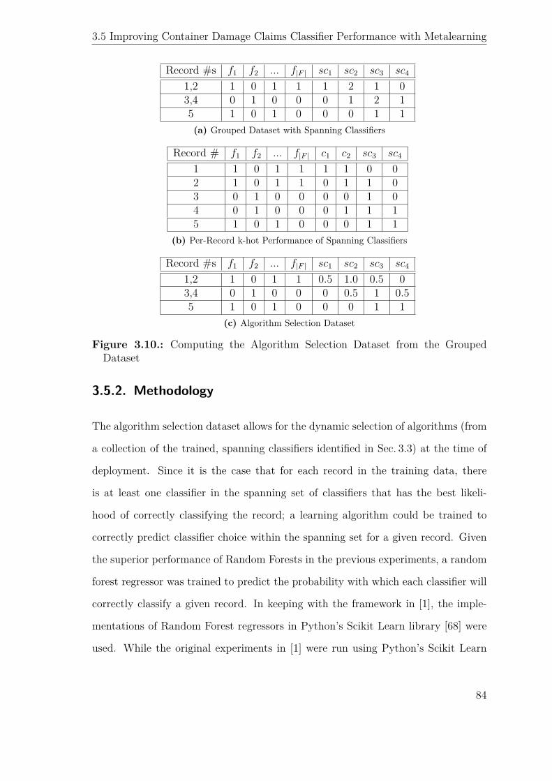
3.5 Improving Container Damage Claims Classifier Performance with Metalearning
Record #s f1 f2 ... f|F | sc1 sc2 sc3 sc4
1,2 1 0 1 1 1 2 1 03,4 0 1 0 0 0 1 2 15 1 0 1 0 0 0 1 1(a) Grouped Dataset with Spanning Classifiers
Record # f1 f2 ... f|F | c1 c2 sc3 sc4
1 1 0 1 1 1 1 0 02 1 0 1 1 0 1 1 03 0 1 0 0 0 0 1 04 0 1 0 0 0 1 1 15 1 0 1 0 0 0 1 1
(b) Per-Record k-hot Performance of Spanning Classifiers
Record #s f1 f2 ... f|F | sc1 sc2 sc3 sc4
1,2 1 0 1 1 0.5 1.0 0.5 03,4 0 1 0 0 0 0.5 1 0.55 1 0 1 0 0 0 1 1
(c) Algorithm Selection Dataset
Figure 3.10.: Computing the Algorithm Selection Dataset from the GroupedDataset
3.5.2. Methodology
The algorithm selection dataset allows for the dynamic selection of algorithms (from
a collection of the trained, spanning classifiers identified in Sec. 3.3) at the time of
deployment. Since it is the case that for each record in the training data, there
is at least one classifier in the spanning set of classifiers that has the best likeli-
hood of correctly classifying the record; a learning algorithm could be trained to
correctly predict classifier choice within the spanning set for a given record. Given
the superior performance of Random Forests in the previous experiments, a random
forest regressor was trained to predict the probability with which each classifier will
correctly classify a given record. In keeping with the framework in [1], the imple-
mentations of Random Forest regressors in Python’s Scikit Learn library [68] were
used. While the original experiments in [1] were run using Python’s Scikit Learn
84
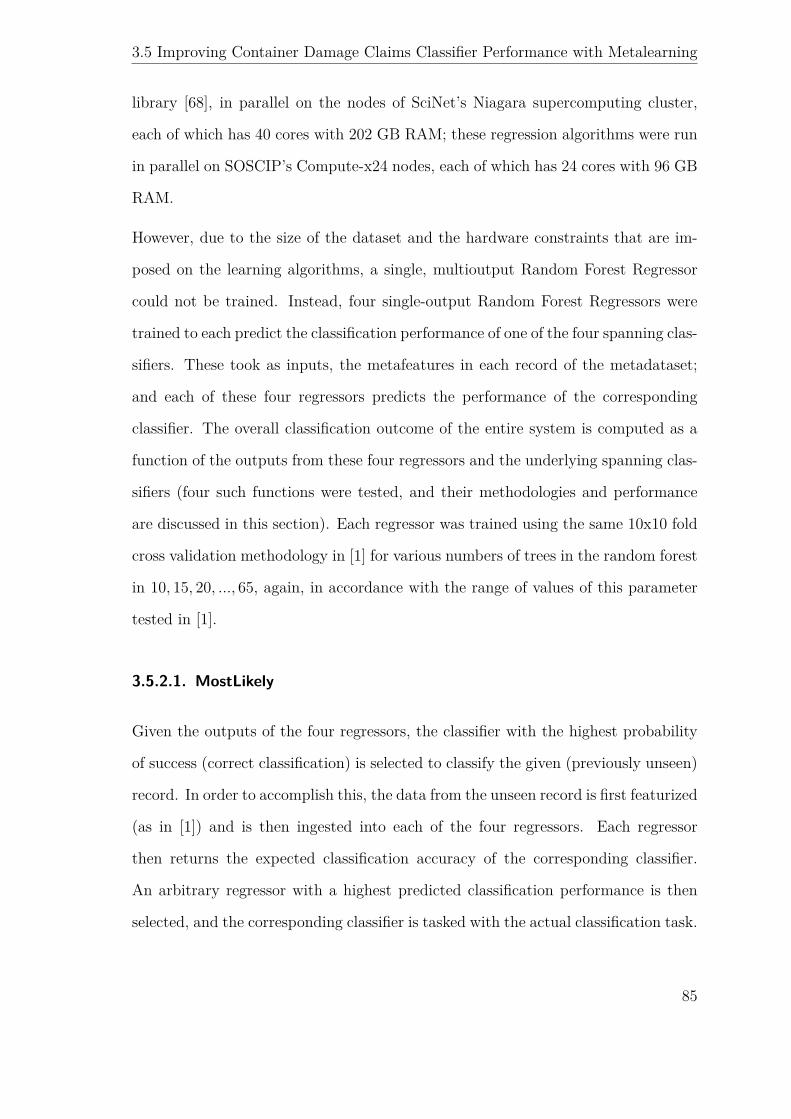
3.5 Improving Container Damage Claims Classifier Performance with Metalearning
library [68], in parallel on the nodes of SciNet’s Niagara supercomputing cluster,
each of which has 40 cores with 202 GB RAM; these regression algorithms were run
in parallel on SOSCIP’s Compute-x24 nodes, each of which has 24 cores with 96 GB
RAM.
However, due to the size of the dataset and the hardware constraints that are im-
posed on the learning algorithms, a single, multioutput Random Forest Regressor
could not be trained. Instead, four single-output Random Forest Regressors were
trained to each predict the classification performance of one of the four spanning clas-
sifiers. These took as inputs, the metafeatures in each record of the metadataset;
and each of these four regressors predicts the performance of the corresponding
classifier. The overall classification outcome of the entire system is computed as a
function of the outputs from these four regressors and the underlying spanning clas-
sifiers (four such functions were tested, and their methodologies and performance
are discussed in this section). Each regressor was trained using the same 10x10 fold
cross validation methodology in [1] for various numbers of trees in the random forest
in 10, 15, 20, ..., 65, again, in accordance with the range of values of this parameter
tested in [1].
3.5.2.1. MostLikely
Given the outputs of the four regressors, the classifier with the highest probability
of success (correct classification) is selected to classify the given (previously unseen)
record. In order to accomplish this, the data from the unseen record is first featurized
(as in [1]) and is then ingested into each of the four regressors. Each regressor
then returns the expected classification accuracy of the corresponding classifier.
An arbitrary regressor with a highest predicted classification performance is then
selected, and the corresponding classifier is tasked with the actual classification task.
85
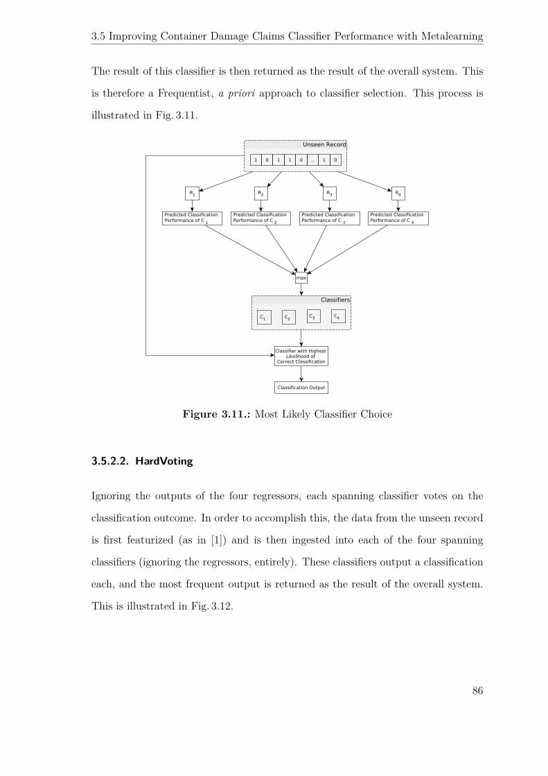
3.5 Improving Container Damage Claims Classifier Performance with Metalearning
The result of this classifier is then returned as the result of the overall system. This
is therefore a Frequentist, a priori approach to classifier selection. This process is
illustrated in Fig. 3.11.
Figure 3.11.: Most Likely Classifier Choice
3.5.2.2. HardVoting
Ignoring the outputs of the four regressors, each spanning classifier votes on the
classification outcome. In order to accomplish this, the data from the unseen record
is first featurized (as in [1]) and is then ingested into each of the four spanning
classifiers (ignoring the regressors, entirely). These classifiers output a classification
each, and the most frequent output is returned as the result of the overall system.
This is illustrated in Fig. 3.12.
86
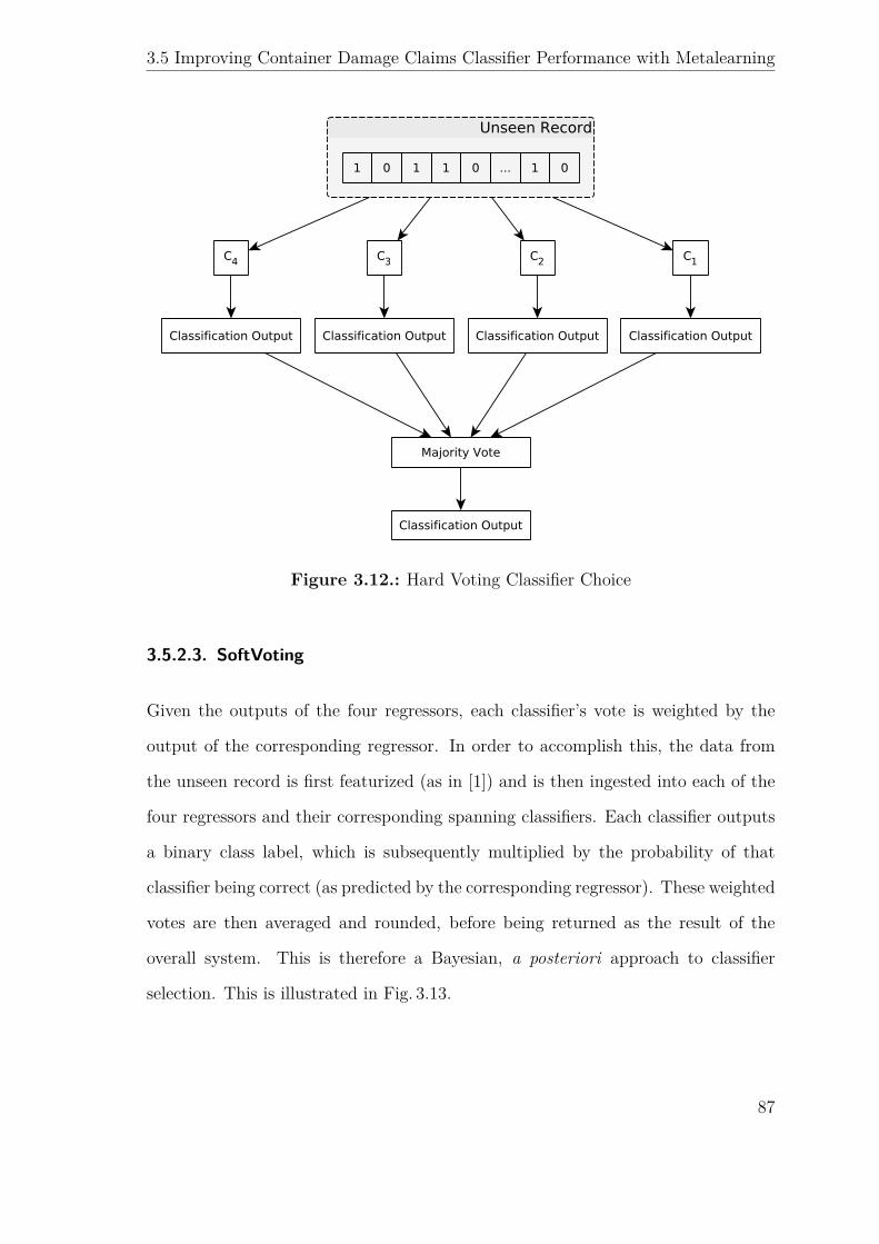
3.5 Improving Container Damage Claims Classifier Performance with Metalearning
Figure 3.12.: Hard Voting Classifier Choice
3.5.2.3. SoftVoting
Given the outputs of the four regressors, each classifier’s vote is weighted by the
output of the corresponding regressor. In order to accomplish this, the data from
the unseen record is first featurized (as in [1]) and is then ingested into each of the
four regressors and their corresponding spanning classifiers. Each classifier outputs
a binary class label, which is subsequently multiplied by the probability of that
classifier being correct (as predicted by the corresponding regressor). These weighted
votes are then averaged and rounded, before being returned as the result of the
overall system. This is therefore a Bayesian, a posteriori approach to classifier
selection. This is illustrated in Fig. 3.13.
87
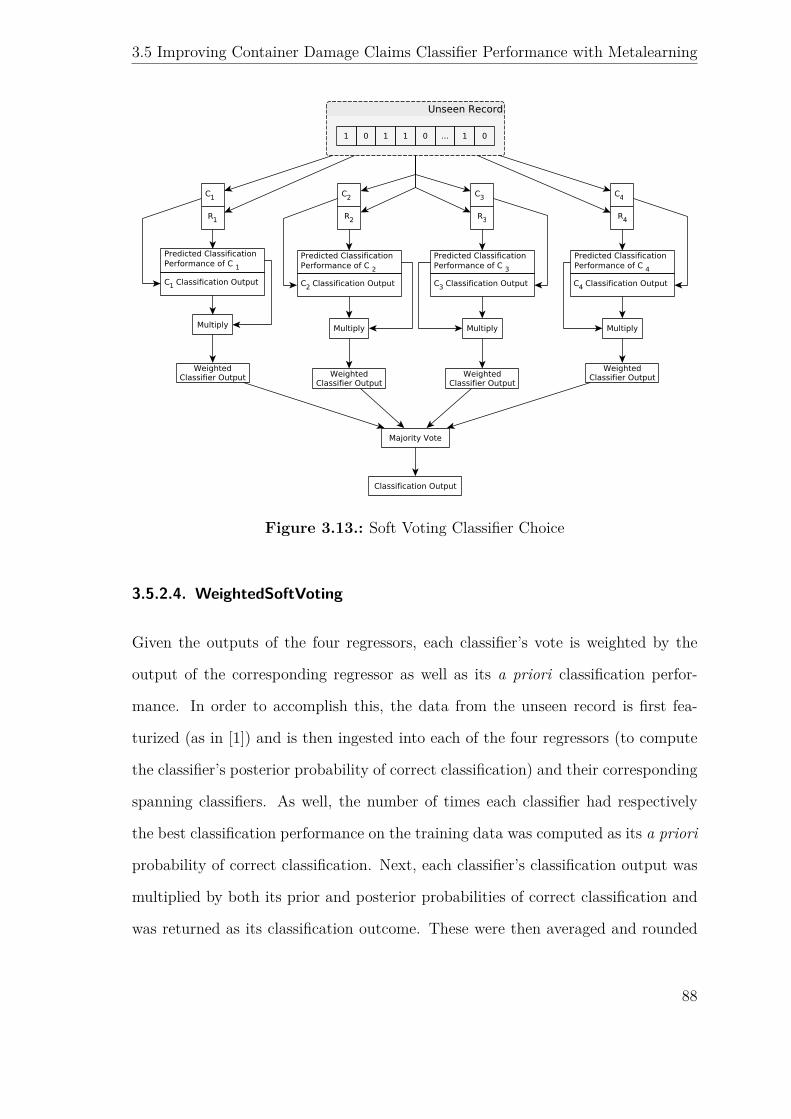
3.5 Improving Container Damage Claims Classifier Performance with Metalearning
Figure 3.13.: Soft Voting Classifier Choice
3.5.2.4. WeightedSoftVoting
Given the outputs of the four regressors, each classifier’s vote is weighted by the
output of the corresponding regressor as well as its a priori classification perfor-
mance. In order to accomplish this, the data from the unseen record is first fea-
turized (as in [1]) and is then ingested into each of the four regressors (to compute
the classifier’s posterior probability of correct classification) and their corresponding
spanning classifiers. As well, the number of times each classifier had respectively
the best classification performance on the training data was computed as its a priori
probability of correct classification. Next, each classifier’s classification output was
multiplied by both its prior and posterior probabilities of correct classification and
was returned as its classification outcome. These were then averaged and rounded
88
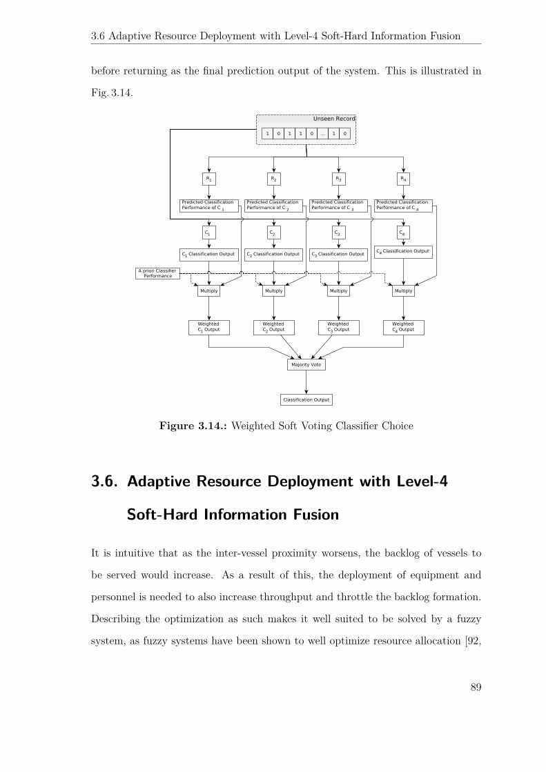
3.6 Adaptive Resource Deployment with Level-4 Soft-Hard Information Fusion
before returning as the final prediction output of the system. This is illustrated in
Fig. 3.14.
Figure 3.14.: Weighted Soft Voting Classifier Choice
3.6. Adaptive Resource Deployment with Level-4
Soft-Hard Information Fusion
It is intuitive that as the inter-vessel proximity worsens, the backlog of vessels to
be served would increase. As a result of this, the deployment of equipment and
personnel is needed to also increase throughput and throttle the backlog formation.
Describing the optimization as such makes it well suited to be solved by a fuzzy
system, as fuzzy systems have been shown to well optimize resource allocation [92,
89
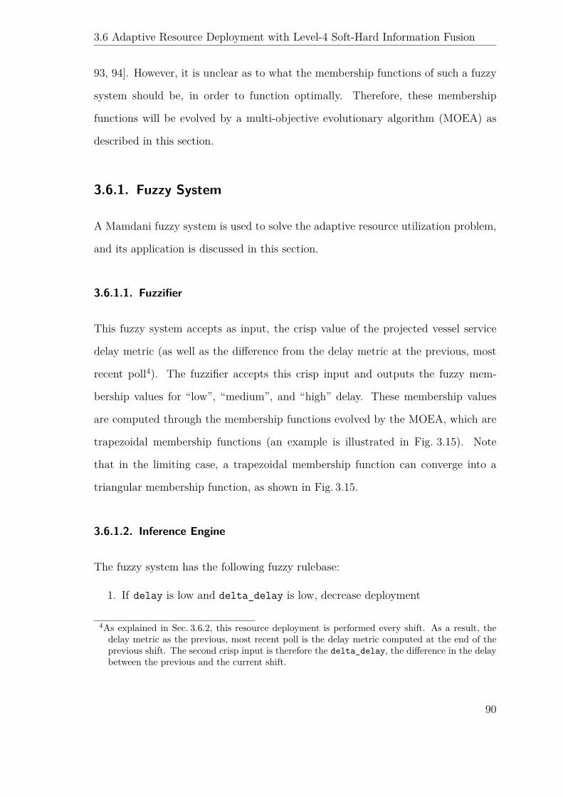
3.6 Adaptive Resource Deployment with Level-4 Soft-Hard Information Fusion
93, 94]. However, it is unclear as to what the membership functions of such a fuzzy
system should be, in order to function optimally. Therefore, these membership
functions will be evolved by a multi-objective evolutionary algorithm (MOEA) as
described in this section.
3.6.1. Fuzzy System
A Mamdani fuzzy system is used to solve the adaptive resource utilization problem,
and its application is discussed in this section.
3.6.1.1. Fuzzifier
This fuzzy system accepts as input, the crisp value of the projected vessel service
delay metric (as well as the difference from the delay metric at the previous, most
recent poll4). The fuzzifier accepts this crisp input and outputs the fuzzy mem-
bership values for “low”, “medium”, and “high” delay. These membership values
are computed through the membership functions evolved by the MOEA, which are
trapezoidal membership functions (an example is illustrated in Fig. 3.15). Note
that in the limiting case, a trapezoidal membership function can converge into a
triangular membership function, as shown in Fig. 3.15.
3.6.1.2. Inference Engine
The fuzzy system has the following fuzzy rulebase:
1. If delay is low and delta_delay is low, decrease deployment
4As explained in Sec. 3.6.2, this resource deployment is performed every shift. As a result, thedelay metric as the previous, most recent poll is the delay metric computed at the end of theprevious shift. The second crisp input is therefore the delta_delay, the difference in the delaybetween the previous and the current shift.
90
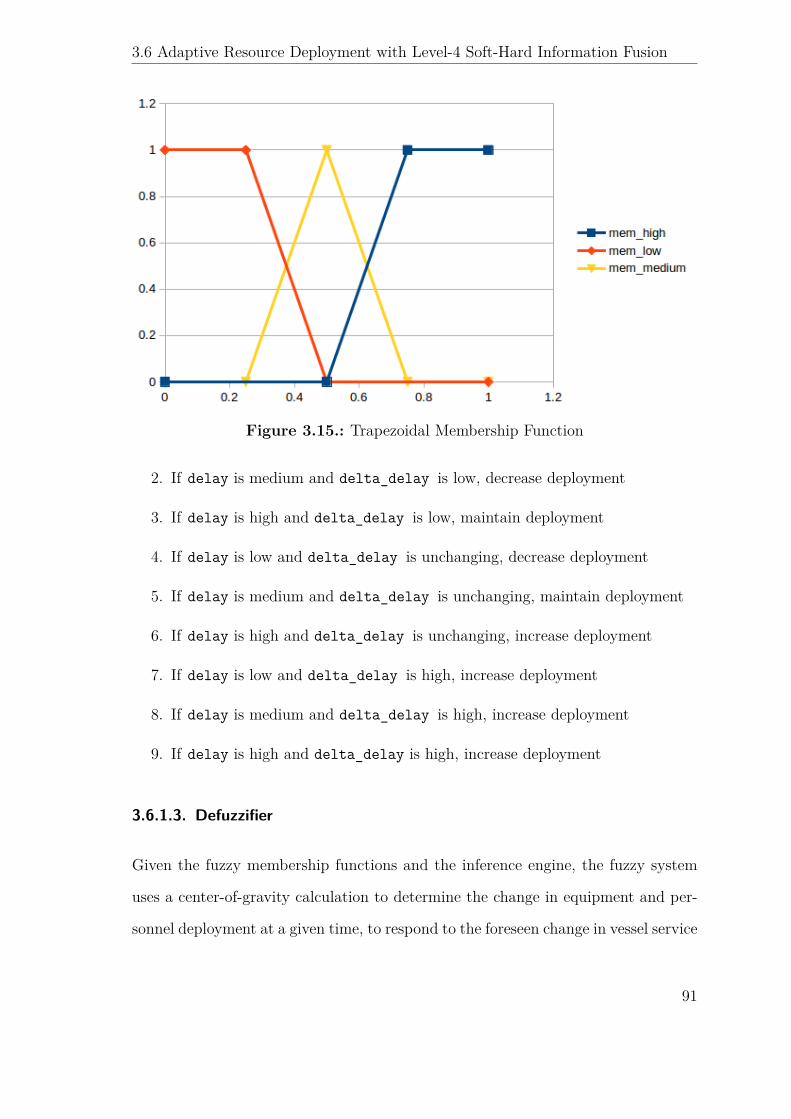
3.6 Adaptive Resource Deployment with Level-4 Soft-Hard Information Fusion
Figure 3.15.: Trapezoidal Membership Function
2. If delay is medium and delta_delay is low, decrease deployment
3. If delay is high and delta_delay is low, maintain deployment
4. If delay is low and delta_delay is unchanging, decrease deployment
5. If delay is medium and delta_delay is unchanging, maintain deployment
6. If delay is high and delta_delay is unchanging, increase deployment
7. If delay is low and delta_delay is high, increase deployment
8. If delay is medium and delta_delay is high, increase deployment
9. If delay is high and delta_delay is high, increase deployment
3.6.1.3. Defuzzifier
Given the fuzzy membership functions and the inference engine, the fuzzy system
uses a center-of-gravity calculation to determine the change in equipment and per-
sonnel deployment at a given time, to respond to the foreseen change in vessel service
91

3.6 Adaptive Resource Deployment with Level-4 Soft-Hard Information Fusion
backlog
3.6.2. Multi-objective Evolutionary Algorithm
In order to optimize the fuzzy system, a MOEA is used to evolve the fuzzy member-
ship functions. This choice of an evolutionary algorithm to optimize the parameters
of a fuzzy system come from previous studies [95] that have used evolutionary algo-
rithms to optimize fuzzy systems. The structure and functioning of this MOEA is
described in this section.
3.6.2.1. Individual Structure
Each individual is comprised of three chromosomes which encode the values of
the vertices of a trapezoidal fuzzy membership, respectively to low delay, medium
delay, and high delay. An example of this tri-chromosomal structure is shown in
Fig. 3.16.
A B C Dµlow_delay 0.33 0.5 0.66 1µmedium_delay 0.33 0.5 0.66 1µhigh_delay 0.33 0.5 0.66 1
Figure 3.16.: Chromosomal Structure for Trapezoidal Individual
mem_low(x) =
1 x < 0.33
100−100x17 0.33 ≤ x < 0.5
0 0.5 ≤ x
(3.16)
92
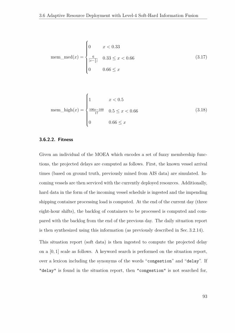
3.6 Adaptive Resource Deployment with Level-4 Soft-Hard Information Fusion
mem_med(x) =
0 x < 0.33
6|x− 1
2 |0.33 ≤ x < 0.66
0 0.66 ≤ x
(3.17)
mem_high(x) =
1 x < 0.5
100x−10017 0.5 ≤ x < 0.66
0 0.66 ≤ x
(3.18)
3.6.2.2. Fitness
Given an individual of the MOEA which encodes a set of fuzzy membership func-
tions, the projected delays are computed as follows. First, the known vessel arrival
times (based on ground truth, previously mined from AIS data) are simulated. In-
coming vessels are then serviced with the currently deployed resources. Additionally,
hard data in the form of the incoming vessel schedule is ingested and the impending
shipping container processing load is computed. At the end of the current day (three
eight-hour shifts), the backlog of containers to be processed is computed and com-
pared with the backlog from the end of the previous day. The daily situation report
is then synthesized using this information (as previously described in Sec. 3.2.14).
This situation report (soft data) is then ingested to compute the projected delay
on a [0, 1] scale as follows. A keyword search is performed on the situation report,
over a lexicon including the synonyms of the words “congestion” and “delay”. If
“delay” is found in the situation report, then “congestion” is not searched for,
93
3.6 Adaptive Resource Deployment with Level-4 Soft-Hard Information Fusion
since mentions of delays describe impending vessel service delays more accurately
than mentions of congestion which are simply a reason thereof. If no keyword from
the lexicon is found in the situation report, a projected delay of 0 is reported. If a
keyword is found, however, a projected delay of 0.5 is noted, pending further analy-
sis. Once the keyword is found, any adjectives modifying the keyword are searched
for by simply searching the words appearing prior to the found keywords. If not
adjectives are found, then the previously noted delay of 0.5 is reported. However, if
an adjective is found, then it is tested for membership within two disjoint lexicons,
namely “diminutive” and “exaggerative”, mined from real-world situation reports.
The “diminutive” lexicon includes adjectives that decrease the intensity of the word
they modify such as “small”, “minor”, “some”, etc. On the other hand, the “ex-
aggerative” lexicon includes adjectives that increase the intensity of the word they
modify such as “significant”, “large”, etc. Given these lexicons, if the found ad-
jective is a member of the “diminutive” lexicon, then the reported delay value must
be reduced from the previously noted value of 0.5. In order to achieve this effect, it
is multiplied by a uniformly distributed random number in [0.7, 1]. Conversely, if the
found adjective is a member of the “exaggerative” lexicon, then the reported delay
value must be increased from the previously noted value of 0.5. In order to achieve
this effect, it is multiplied by a uniformly distributed random number, drawn from
[1, 1.3]. Finally, the modified delay value is reported as the projected delay on a
[0, 1] scale, which is then used as the crisp input to the fuzzy system described by
the given individual.
The fuzzy system then returns the resource deployment which is then used to com-
pute the number of shipping containers processed in the following shifts. Since each
crane (and operator) can process one container every two minutes, the container
processing capacity of the deployment of resources over a shift is the number of
94
3.6 Adaptive Resource Deployment with Level-4 Soft-Hard Information Fusion
two-minute segments in the shift scaled by the resource deployment. The fitness of
the given individual is then reported as a point on a two dimensional non-dominated
front spanning the sum of the service times for all vessels, and the total resource
deployment (summed over all shifts).
3.6.2.3. Selection
Since crossover requires two individuals, a selection mechanism is required to select
these two individuals from the population. First, the fitness of each individual
is computed as previously described, and the individuals are sorted into fitness
fronts. Next, two parents are independently, randomly selected such that a random
individual from front i is selected with probability 1i+1 (the i+ 1 in the denominator
allows for the selection of an individual in the Pareto front to be selected with
probability 0.5 instead of 1) [67].
3.6.2.4. Crossover
Crossover is performed by means of a fitness proportional variant of the Weighted
Arithmetic Crossover [96], which we will call “FitWAM”. However, since a fitness
proportional crossover requires a scalar (i.e. uni-dimensional) fitness measure, a
relative fitness measure (Fr) is defined. This is computed as the average distance
from the mean of a given individual, along each dimension of the two-dimensional
fitness plane, from the population’s average along each dimension. This is more
formally defined in Eq. 3.19 and Eq. 3.20.
95
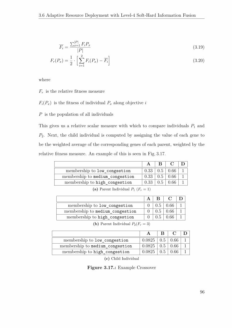
3.6 Adaptive Resource Deployment with Level-4 Soft-Hard Information Fusion
Fi =∑|P |
x=1 FiPx
|P |(3.19)
Fr(Px) = 12 ·[ 2∑
i=1Fi(Px)− Fi
](3.20)
where
Fr is the relative fitness measure
Fi(Px) is the fitness of individual Px along objective i
P is the population of all individuals
This gives us a relative scalar measure with which to compare individuals P1 and
P2. Next, the child individual is computed by assigning the value of each gene to
be the weighted average of the corresponding genes of each parent, weighted by the
relative fitness measure. An example of this is seen in Fig. 3.17.
A B C Dmembership to low_congestion 0.33 0.5 0.66 1
membership to medium_congestion 0.33 0.5 0.66 1membership to high_congestion 0.33 0.5 0.66 1
(a) Parent Individual P1 (Fr = 1)
A B C Dmembership to low_congestion 0 0.5 0.66 1
membership to medium_congestion 0 0.5 0.66 1membership to high_congestion 0 0.5 0.66 1
(b) Parent Individual P2(Fr = 3)
A B C Dmembership to low_congestion 0.0825 0.5 0.66 1
membership to medium_congestion 0.0825 0.5 0.66 1membership to high_congestion 0.0825 0.5 0.66 1
(c) Child Individual
Figure 3.17.: Example Crossover
96
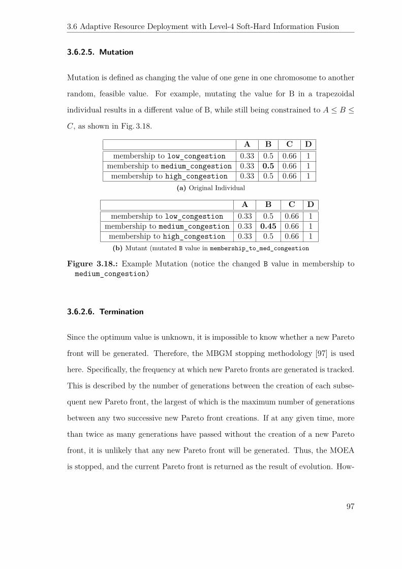
3.6 Adaptive Resource Deployment with Level-4 Soft-Hard Information Fusion
3.6.2.5. Mutation
Mutation is defined as changing the value of one gene in one chromosome to another
random, feasible value. For example, mutating the value for B in a trapezoidal
individual results in a different value of B, while still being constrained to A ≤ B ≤
C, as shown in Fig. 3.18.
A B C Dmembership to low_congestion 0.33 0.5 0.66 1
membership to medium_congestion 0.33 0.5 0.66 1membership to high_congestion 0.33 0.5 0.66 1
(a) Original Individual
A B C Dmembership to low_congestion 0.33 0.5 0.66 1
membership to medium_congestion 0.33 0.45 0.66 1membership to high_congestion 0.33 0.5 0.66 1(b) Mutant (mutated B value in membership_to_med_congestion
Figure 3.18.: Example Mutation (notice the changed B value in membership tomedium_congestion)
3.6.2.6. Termination
Since the optimum value is unknown, it is impossible to know whether a new Pareto
front will be generated. Therefore, the MBGM stopping methodology [97] is used
here. Specifically, the frequency at which new Pareto fronts are generated is tracked.
This is described by the number of generations between the creation of each subse-
quent new Pareto front, the largest of which is the maximum number of generations
between any two successive new Pareto front creations. If at any given time, more
than twice as many generations have passed without the creation of a new Pareto
front, it is unlikely that any new Pareto front will be generated. Thus, the MOEA
is stopped, and the current Pareto front is returned as the result of evolution. How-
97
3.7 Summary
ever, since the search space is substantially large, fitness improvements were not
immediately observed, this termination criterion was applied only after 100 genera-
tions.
Experiment Environment
The computational experiments were run independently on a consumer laptop with
an Intel(R) Core(TM) i7-3520M CPU @ 2.90GHz CPU and 16GB RAM.
3.7. Summary
Drawing from several studies across multiple disciplines, multiple factors have been
considered for the stated purposes of predicting shipping container damage and the
causes thereof. Conventional wisdom from industry has also been captured in a
survey against which the results of our study have been compared. The published
results contradict expert opinions from the industry and warrant further study.
Further, classifier accuracy has been improved with the inclusion of Leave One
Batch Out learning.
98

4. Results
4.1. Classifier Claims Prediction
Data was synthesized based on survey responses (as discussed in Sec. 3.2), and a
study was conducted to determine the factors most correlated with shipping con-
tainer damage on maritime vessels. Over 70 computational learning algorithms from
Python’s scikit-learn library were used to learn the correlations between the fea-
tures in the data and container damage claims. These included some rudimentary
neural networks, but no deep learning strategies. This is because this thesis is the
first study to explore this problem and simpler models with fewer tunable param-
eters were chosen over models with more tunable parameters and larger training
times, such as deep neural networks, convolutional neural networks, etc.
The performance of the eleven best classifiers are shown in Tab. A.1, while the
relative importances of the various features in the dataset are shown in Fig. 4.1.
These discovered relative feature importances are counter to the expert opinions
captured in the surveys.
This study revealed that opinions held by experts in the industry did not align
with the discovered causes of shipping container damage from the data. Since in-
vestigations are triggered by incoming claims, false negatives are less favorable than
false positives. It is therefore important to compare the accuracy of classifiers that
99
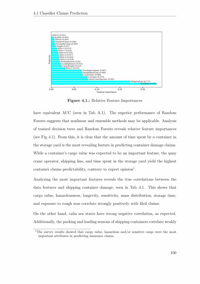
4.1 Classifier Claims Prediction
0.00 0.05 0.10 0.15 0.20Feature Importance
Features
YardTime (0.231) ShippingLine (0.173)
QuayCraneOperator (0.081) Customer (0.079)
CargoValue (0.069) WeightBalancing (0.068) TruckingCompany (0.067)
DSS=1 (0.031) CargoWeight (0.023) LoadingSeason (0.022)
PackingSeason (0.02) DSS=5 (0.018) DSS=4 (0.018) DSS=3 (0.017) DSS=6 (0.016) DSS=7 (0.014) DSS=2 (0.013)
Fragile (0.01) PerishableCargo (0.008) SensitiveCargo (0.008) DSS=8 (0.007) HazMat (0.005)
DSS=9 (0.001)
Figure 4.1.: Relative Feature Importances
have equivalent AUC (seen in Tab. A.1). The superior performance of Random
Forests suggests that nonlinear and ensemble methods may be applicable. Analysis
of trained decision trees and Random Forests reveals relative feature importances
(see Fig. 4.1). From this, it is clear that the amount of time spent by a container in
the storage yard is the most revealing feature in predicting container damage claims.
While a container’s cargo value was expected to be an important feature, the quay
crane operator, shipping line, and time spent in the storage yard yield the highest
container claims predictability, contrary to expert opinion1.
Analyzing the most important features reveals the true correlations between the
data features and shipping container damage, seen in Tab. 4.1. This shows that
cargo value, hazardousness, longevity, sensitivity, mass distribution, storage time,
and exposure to rough seas correlate strongly positively with filed claims.
On the other hand, calm sea states have strong negative correlation, as expected.
Additionally, the packing and loading seasons of shipping containers correlate weakly
1The survey results showed that cargo value, hazardous and/or sensitive cargo were the mostimportant attributes in predicting insurance claims
100
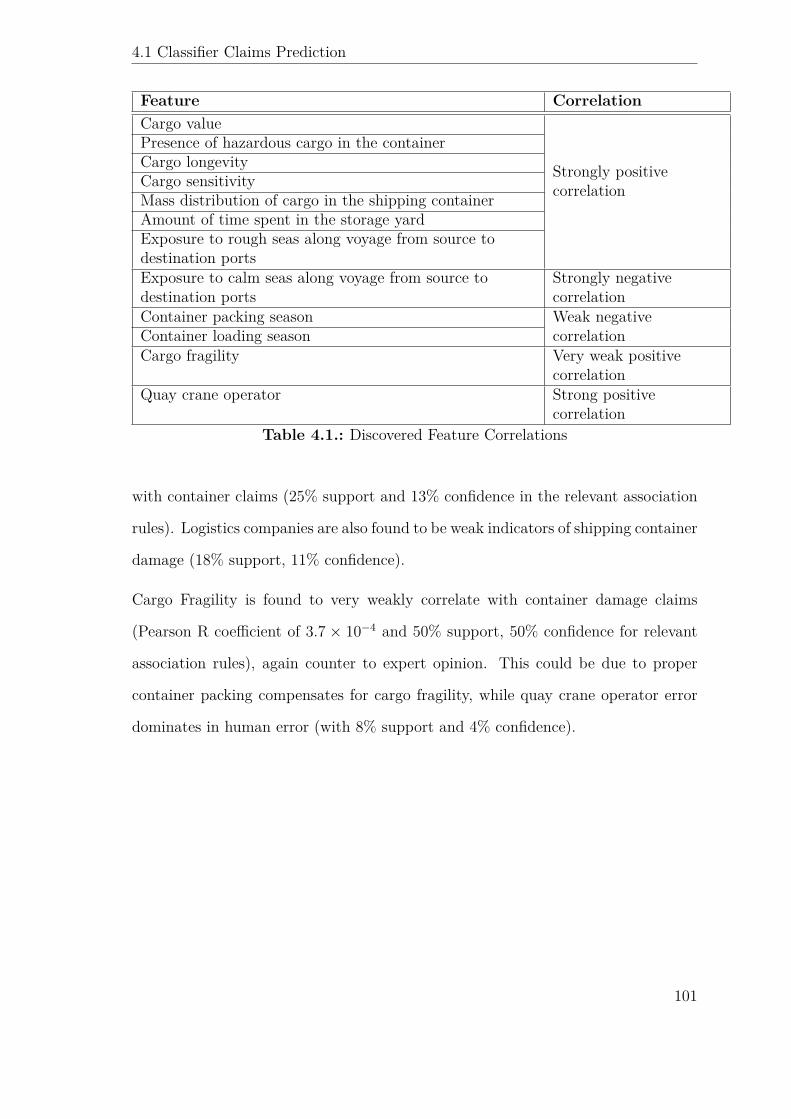
4.1 Classifier Claims Prediction
Feature CorrelationCargo value
Strongly positivecorrelation
Presence of hazardous cargo in the containerCargo longevityCargo sensitivityMass distribution of cargo in the shipping containerAmount of time spent in the storage yardExposure to rough seas along voyage from source todestination portsExposure to calm seas along voyage from source todestination ports
Strongly negativecorrelation
Container packing season Weak negativecorrelationContainer loading season
Cargo fragility Very weak positivecorrelation
Quay crane operator Strong positivecorrelation
Table 4.1.: Discovered Feature Correlations
with container claims (25% support and 13% confidence in the relevant association
rules). Logistics companies are also found to be weak indicators of shipping container
damage (18% support, 11% confidence).
Cargo Fragility is found to very weakly correlate with container damage claims
(Pearson R coefficient of 3.7 × 10⁻⁴ and 50% support, 50% confidence for relevant
association rules), again counter to expert opinion. This could be due to proper
container packing compensates for cargo fragility, while quay crane operator error
dominates in human error (with 8% support and 4% confidence).
101
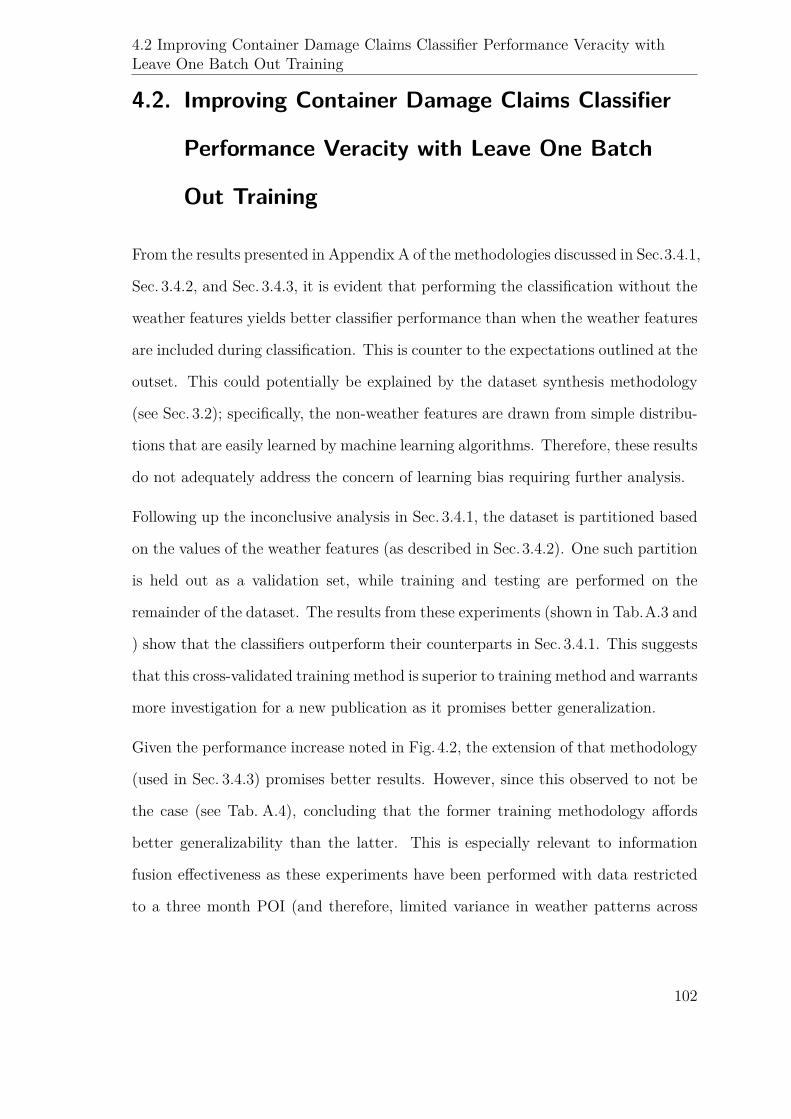
4.2 Improving Container Damage Claims Classifier Performance Veracity withLeave One Batch Out Training
4.2. Improving Container Damage Claims Classifier
Performance Veracity with Leave One Batch
Out Training
From the results presented in Appendix A of the methodologies discussed in Sec.3.4.1,
Sec. 3.4.2, and Sec. 3.4.3, it is evident that performing the classification without the
weather features yields better classifier performance than when the weather features
are included during classification. This is counter to the expectations outlined at the
outset. This could potentially be explained by the dataset synthesis methodology
(see Sec. 3.2); specifically, the non-weather features are drawn from simple distribu-
tions that are easily learned by machine learning algorithms. Therefore, these results
do not adequately address the concern of learning bias requiring further analysis.
Following up the inconclusive analysis in Sec. 3.4.1, the dataset is partitioned based
on the values of the weather features (as described in Sec.3.4.2). One such partition
is held out as a validation set, while training and testing are performed on the
remainder of the dataset. The results from these experiments (shown in Tab.A.3 and
) show that the classifiers outperform their counterparts in Sec. 3.4.1. This suggests
that this cross-validated training method is superior to training method and warrants
more investigation for a new publication as it promises better generalization.
Given the performance increase noted in Fig.4.2, the extension of that methodology
(used in Sec. 3.4.3) promises better results. However, since this observed to not be
the case (see Tab. A.4), concluding that the former training methodology affords
better generalizability than the latter. This is especially relevant to information
fusion effectiveness as these experiments have been performed with data restricted
to a three month POI (and therefore, limited variance in weather patterns across
102
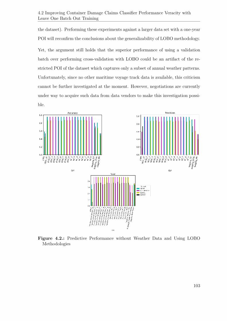
4.2 Improving Container Damage Claims Classifier Performance Veracity withLeave One Batch Out Training
the dataset). Performing these experiments against a larger data set with a one-year
POI will reconfirm the conclusions about the generalizability of LOBO methodology.
Yet, the argument still holds that the superior performance of using a validation
batch over performing cross-validation with LOBO could be an artifact of the re-
stricted POI of the dataset which captures only a subset of annual weather patterns.
Unfortunately, since no other maritime voyage track data is available, this criticism
cannot be further investigated at the moment. However, negotiations are currently
under way to acquire such data from data vendors to make this investigation possi-
ble.
Figure 4.2.: Predictive Performance without Weather Data and Using LOBOMethodologies
103
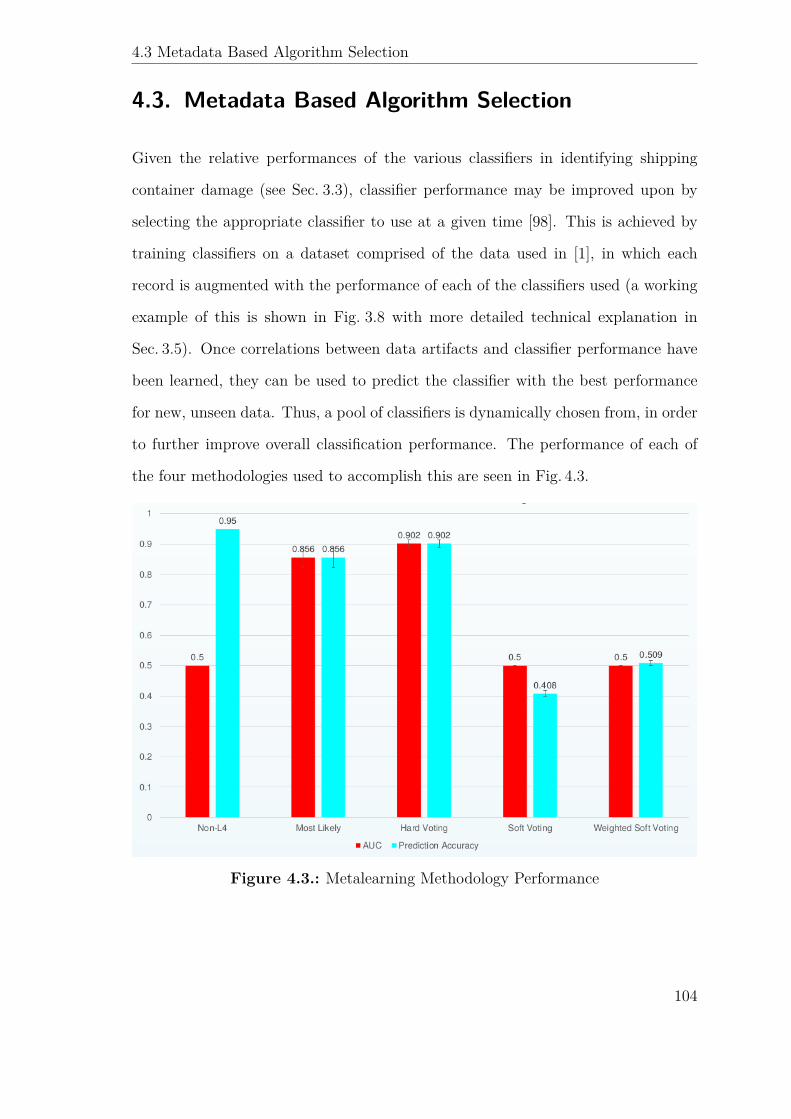
4.3 Metadata Based Algorithm Selection
4.3. Metadata Based Algorithm Selection
Given the relative performances of the various classifiers in identifying shipping
container damage (see Sec. 3.3), classifier performance may be improved upon by
selecting the appropriate classifier to use at a given time [98]. This is achieved by
training classifiers on a dataset comprised of the data used in [1], in which each
record is augmented with the performance of each of the classifiers used (a working
example of this is shown in Fig. 3.8 with more detailed technical explanation in
Sec. 3.5). Once correlations between data artifacts and classifier performance have
been learned, they can be used to predict the classifier with the best performance
for new, unseen data. Thus, a pool of classifiers is dynamically chosen from, in order
to further improve overall classification performance. The performance of each of
the four methodologies used to accomplish this are seen in Fig. 4.3.
Figure 4.3.: Metalearning Methodology Performance
104
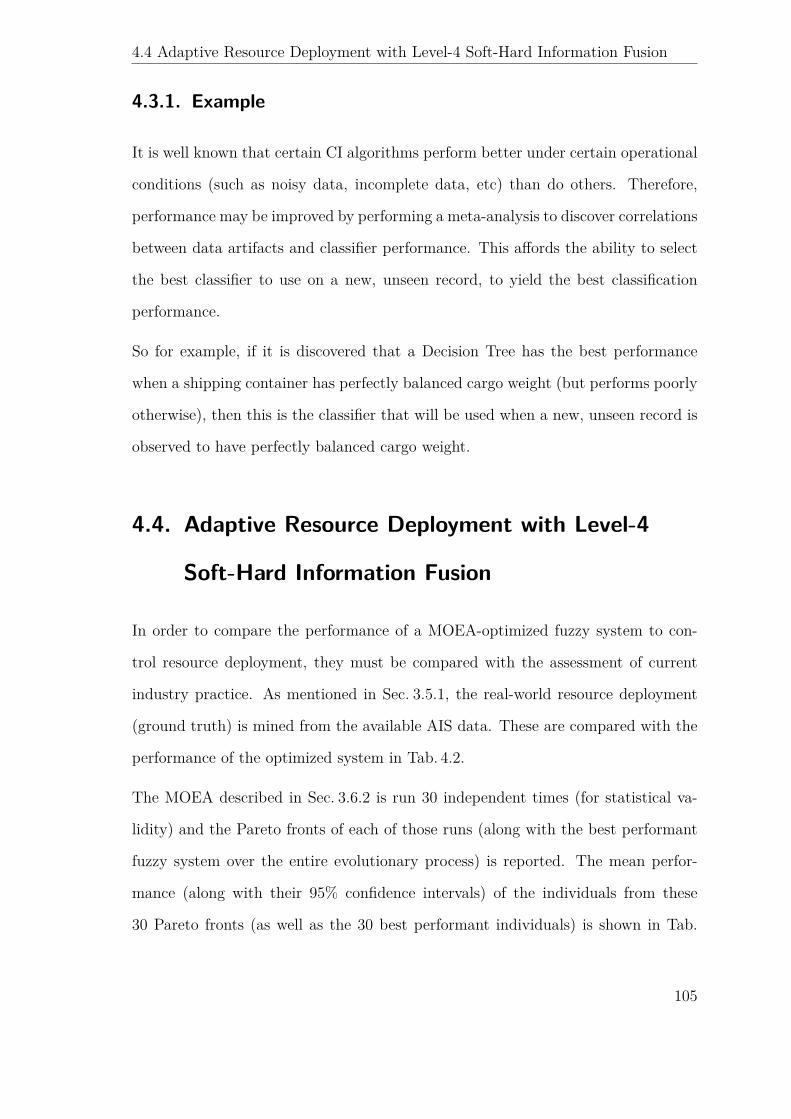
4.4 Adaptive Resource Deployment with Level-4 Soft-Hard Information Fusion
4.3.1. Example
It is well known that certain CI algorithms perform better under certain operational
conditions (such as noisy data, incomplete data, etc) than do others. Therefore,
performance may be improved by performing a meta-analysis to discover correlations
between data artifacts and classifier performance. This affords the ability to select
the best classifier to use on a new, unseen record, to yield the best classification
performance.
So for example, if it is discovered that a Decision Tree has the best performance
when a shipping container has perfectly balanced cargo weight (but performs poorly
otherwise), then this is the classifier that will be used when a new, unseen record is
observed to have perfectly balanced cargo weight.
4.4. Adaptive Resource Deployment with Level-4
Soft-Hard Information Fusion
In order to compare the performance of a MOEA-optimized fuzzy system to con-
trol resource deployment, they must be compared with the assessment of current
industry practice. As mentioned in Sec. 3.5.1, the real-world resource deployment
(ground truth) is mined from the available AIS data. These are compared with the
performance of the optimized system in Tab. 4.2.
The MOEA described in Sec. 3.6.2 is run 30 independent times (for statistical va-
lidity) and the Pareto fronts of each of those runs (along with the best performant
fuzzy system over the entire evolutionary process) is reported. The mean perfor-
mance (along with their 95% confidence intervals) of the individuals from these
30 Pareto fronts (as well as the 30 best performant individuals) is shown in Tab.
105
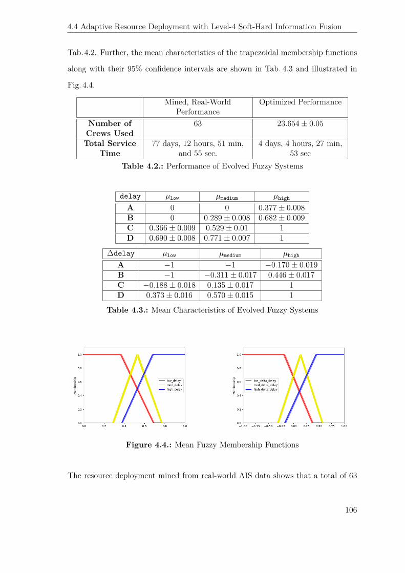
4.4 Adaptive Resource Deployment with Level-4 Soft-Hard Information Fusion
Tab.4.2. Further, the mean characteristics of the trapezoidal membership functions
along with their 95% confidence intervals are shown in Tab. 4.3 and illustrated in
Fig. 4.4.
Mined, Real-WorldPerformance
Optimized Performance
Number ofCrews Used
63 23.654± 0.05
Total ServiceTime
77 days, 12 hours, 51 min,and 55 sec.
4 days, 4 hours, 27 min,53 sec
Table 4.2.: Performance of Evolved Fuzzy Systems
delay µlow µmedium µhigh
A 0 0 0.377± 0.008B 0 0.289± 0.008 0.682± 0.009C 0.366± 0.009 0.529± 0.01 1D 0.690± 0.008 0.771± 0.007 1
∆delay µlow µmedium µhigh
A −1 −1 −0.170± 0.019B −1 −0.311± 0.017 0.446± 0.017C −0.188± 0.018 0.135± 0.017 1D 0.373± 0.016 0.570± 0.015 1
Table 4.3.: Mean Characteristics of Evolved Fuzzy Systems
Figure 4.4.: Mean Fuzzy Membership Functions
The resource deployment mined from real-world AIS data shows that a total of 63
106
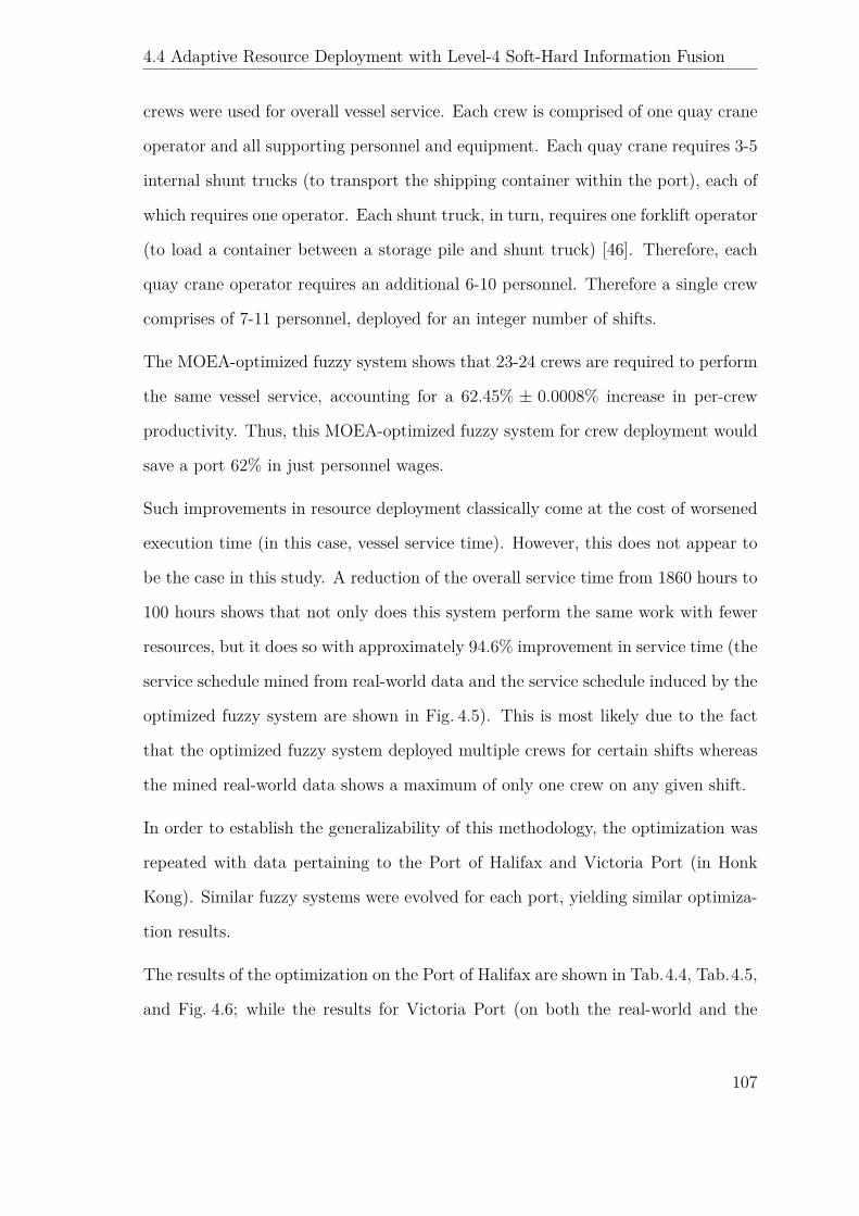
4.4 Adaptive Resource Deployment with Level-4 Soft-Hard Information Fusion
crews were used for overall vessel service. Each crew is comprised of one quay crane
operator and all supporting personnel and equipment. Each quay crane requires 3-5
internal shunt trucks (to transport the shipping container within the port), each of
which requires one operator. Each shunt truck, in turn, requires one forklift operator
(to load a container between a storage pile and shunt truck) [46]. Therefore, each
quay crane operator requires an additional 6-10 personnel. Therefore a single crew
comprises of 7-11 personnel, deployed for an integer number of shifts.
The MOEA-optimized fuzzy system shows that 23-24 crews are required to perform
the same vessel service, accounting for a 62.45% ± 0.0008% increase in per-crew
productivity. Thus, this MOEA-optimized fuzzy system for crew deployment would
save a port 62% in just personnel wages.
Such improvements in resource deployment classically come at the cost of worsened
execution time (in this case, vessel service time). However, this does not appear to
be the case in this study. A reduction of the overall service time from 1860 hours to
100 hours shows that not only does this system perform the same work with fewer
resources, but it does so with approximately 94.6% improvement in service time (the
service schedule mined from real-world data and the service schedule induced by the
optimized fuzzy system are shown in Fig. 4.5). This is most likely due to the fact
that the optimized fuzzy system deployed multiple crews for certain shifts whereas
the mined real-world data shows a maximum of only one crew on any given shift.
In order to establish the generalizability of this methodology, the optimization was
repeated with data pertaining to the Port of Halifax and Victoria Port (in Honk
Kong). Similar fuzzy systems were evolved for each port, yielding similar optimiza-
tion results.
The results of the optimization on the Port of Halifax are shown in Tab.4.4, Tab.4.5,
and Fig. 4.6; while the results for Victoria Port (on both the real-world and the
107
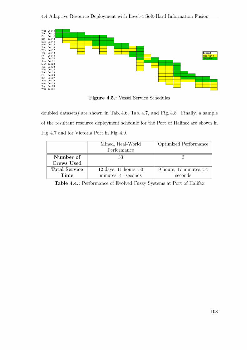
4.4 Adaptive Resource Deployment with Level-4 Soft-Hard Information Fusion
Figure 4.5.: Vessel Service Schedules
doubled datasets) are shown in Tab. 4.6, Tab. 4.7, and Fig. 4.8. Finally, a sample
of the resultant resource deployment schedule for the Port of Halifax are shown in
Fig. 4.7 and for Victoria Port in Fig. 4.9.
Mined, Real-WorldPerformance
Optimized Performance
Number ofCrews Used
33 3
Total ServiceTime
12 days, 11 hours, 50minutes, 41 seconds
9 hours, 17 minutes, 54seconds
Table 4.4.: Performance of Evolved Fuzzy Systems at Port of Halifax
108
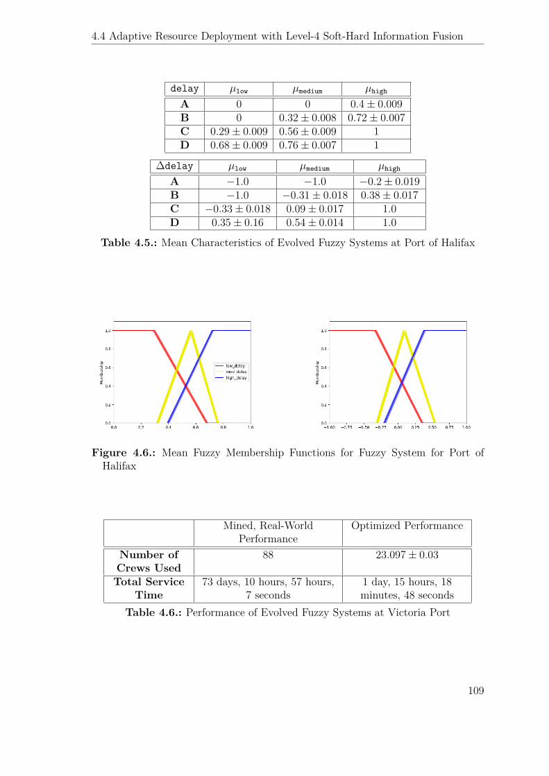
4.4 Adaptive Resource Deployment with Level-4 Soft-Hard Information Fusion
delay µlow µmedium µhigh
A 0 0 0.4± 0.009B 0 0.32± 0.008 0.72± 0.007C 0.29± 0.009 0.56± 0.009 1D 0.68± 0.009 0.76± 0.007 1
∆delay µlow µmedium µhigh
A −1.0 −1.0 −0.2± 0.019B −1.0 −0.31± 0.018 0.38± 0.017C −0.33± 0.018 0.09± 0.017 1.0D 0.35± 0.16 0.54± 0.014 1.0
Table 4.5.: Mean Characteristics of Evolved Fuzzy Systems at Port of Halifax
Figure 4.6.: Mean Fuzzy Membership Functions for Fuzzy System for Port ofHalifax
Mined, Real-WorldPerformance
Optimized Performance
Number ofCrews Used
88 23.097± 0.03
Total ServiceTime
73 days, 10 hours, 57 hours,7 seconds
1 day, 15 hours, 18minutes, 48 seconds
Table 4.6.: Performance of Evolved Fuzzy Systems at Victoria Port
109
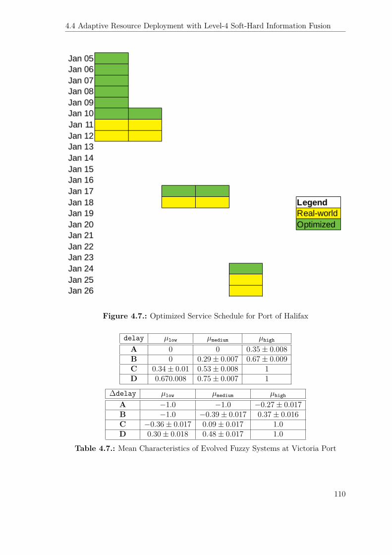
4.4 Adaptive Resource Deployment with Level-4 Soft-Hard Information Fusion
Figure 4.7.: Optimized Service Schedule for Port of Halifax
delay µlow µmedium µhigh
A 0 0 0.35± 0.008B 0 0.29± 0.007 0.67± 0.009C 0.34± 0.01 0.53± 0.008 1D 0.670.008 0.75± 0.007 1
∆delay µlow µmedium µhigh
A −1.0 −1.0 −0.27± 0.017B −1.0 −0.39± 0.017 0.37± 0.016C −0.36± 0.017 0.09± 0.017 1.0D 0.30± 0.018 0.48± 0.017 1.0
Table 4.7.: Mean Characteristics of Evolved Fuzzy Systems at Victoria Port
110
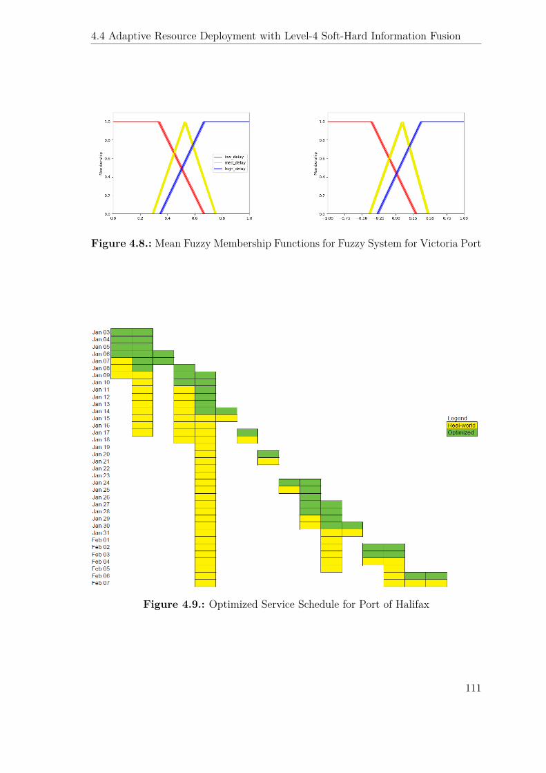
4.4 Adaptive Resource Deployment with Level-4 Soft-Hard Information Fusion
Figure 4.8.: Mean Fuzzy Membership Functions for Fuzzy System for Victoria Port
Figure 4.9.: Optimized Service Schedule for Port of Halifax
111

4.4 Adaptive Resource Deployment with Level-4 Soft-Hard Information Fusion
4.4.1. Data Source Selection
In order to meaningfully select between data sources, each data source was evaluated
for its quality. The optimality of a data source is determined by training a model on
data exclusively from this source and testing the performance of the trained model.
The training and testing were performed in the same methodology as described in
Sec. 3.6. In order to create the datasets for each data source, the original dataset
was split into six sets, each one corresponding to one of the six AIS data sources
present in the original dataset. The number of records from each data source is
specified in Tab. 4.8 and shown in Fig. 4.10. Since Source 1 and Source 5 each have
approximately 50% of all the records in the entire dataset, they were used for this
analysis. On the other hand, since Source 2, 3, 4, and 6 contained a negligible
number of AIS records, they did not provide sufficiently many records to perform
this analysis and were preemptively filtered out.
Source Number of RecordsSource 1 4,048,309Source 2 2,243Source 3 408Source 4 12,051Source 5 3,932,275Source 6 1
Table 4.8.: Distribution of Records by Data Source
With the separated data from Sources 1 and 5, three datasets were created. The
first contained data from only Source 1, the second from only Source 5, and the
last from both Source 1 and Source 5. Next, three models were evolved using
the same methodology as described in Sec. 3.6, one using each of the three new
datasets. The resulting models were then run to determine the two-dimensional
fitness values of their respective performances, so that they could be compared.
The quality of each data source is measured as the optimality of the model resulting
112
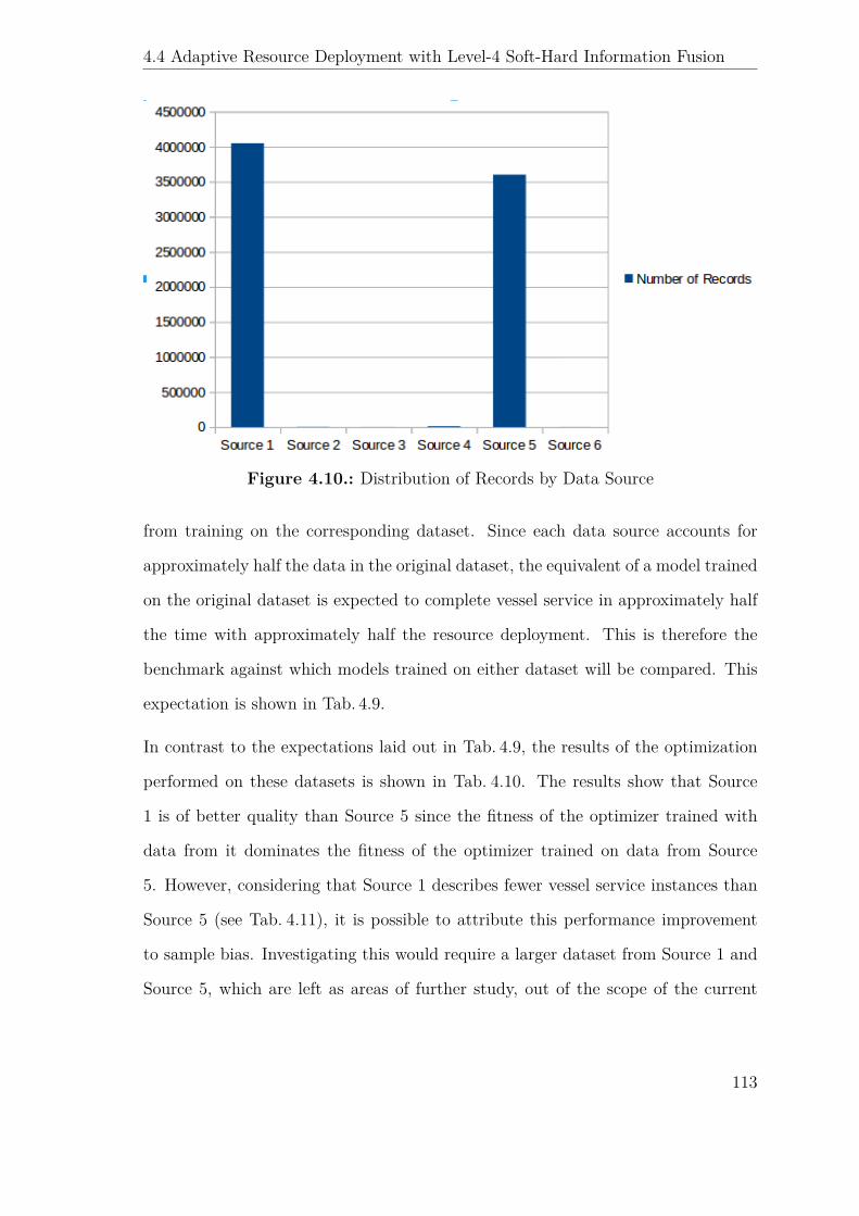
4.4 Adaptive Resource Deployment with Level-4 Soft-Hard Information Fusion
Figure 4.10.: Distribution of Records by Data Source
from training on the corresponding dataset. Since each data source accounts for
approximately half the data in the original dataset, the equivalent of a model trained
on the original dataset is expected to complete vessel service in approximately half
the time with approximately half the resource deployment. This is therefore the
benchmark against which models trained on either dataset will be compared. This
expectation is shown in Tab. 4.9.
In contrast to the expectations laid out in Tab. 4.9, the results of the optimization
performed on these datasets is shown in Tab. 4.10. The results show that Source
1 is of better quality than Source 5 since the fitness of the optimizer trained with
data from it dominates the fitness of the optimizer trained on data from Source
5. However, considering that Source 1 describes fewer vessel service instances than
Source 5 (see Tab. 4.11), it is possible to attribute this performance improvement
to sample bias. Investigating this would require a larger dataset from Source 1 and
Source 5, which are left as areas of further study, out of the scope of the current
113
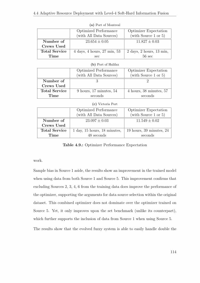
4.4 Adaptive Resource Deployment with Level-4 Soft-Hard Information Fusion
(a) Port of Montreal
Optimized Performance(with All Data Sources)
Optimizer Expectation(with Source 1 or 5)
Number ofCrews Used
23.654± 0.05 11.827± 0.03
Total ServiceTime
4 days, 4 hours, 27 min, 53sec
2 days, 2 hours, 13 min,56 sec
(b) Port of Halifax
Optimized Performance(with All Data Sources)
Optimizer Expectation(with Source 1 or 5)
Number ofCrews Used
3 2
Total ServiceTime
9 hours, 17 minutes, 54seconds
4 hours, 38 minutes, 57seconds
(c) Victoria Port
Optimized Performance(with All Data Sources)
Optimizer Expectation(with Source 1 or 5)
Number ofCrews Used
23.097± 0.03 11.549± 0.02
Total ServiceTime
1 day, 15 hours, 18 minutes,48 seconds
19 hours, 39 minutes, 24seconds
Table 4.9.: Optimizer Performance Expectation
work.
Sample bias in Source 1 aside, the results show an improvement in the trained model
when using data from both Source 1 and Source 5. This improvement confirms that
excluding Sources 2, 3, 4, 6 from the training data does improve the performance of
the optimizer, supporting the arguments for data source selection within the original
dataset. This combined optimizer does not dominate over the optimizer trained on
Source 5. Yet, it only improves upon the set benchmark (unlike its counterpart),
which further supports the inclusion of data from Source 1 when using Source 5.
The results show that the evolved fuzzy system is able to easily handle double the
114

4.4 Adaptive Resource Deployment with Level-4 Soft-Hard Information Fusion
service throughput without any significant additional resource requirements, making
this a very robust optimized solution. There is a noted insignificant increase in the
resource deployment at Victoria Port. However, since both the real-world load and
the synthetically doubled load, both require 24 cranes, this difference is considered
negligible. The limits of such an optimized resource deployment model are difficult
to identify, without additional data and are therefore left as future directions of
investigation.
115
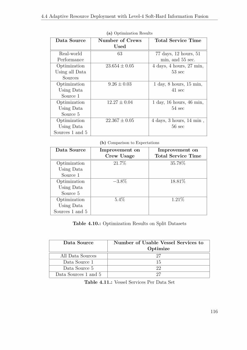
4.4 Adaptive Resource Deployment with Level-4 Soft-Hard Information Fusion
(a) Optimization Results
Data Source Number of CrewsUsed
Total Service Time
Real-worldPerformance
63 77 days, 12 hours, 51min, and 55 sec.
OptimizationUsing all Data
Sources
23.654± 0.05 4 days, 4 hours, 27 min,53 sec
OptimizationUsing DataSource 1
9.26± 0.03 1 day, 8 hours, 15 min,41 sec
OptimizationUsing DataSource 5
12.27± 0.04 1 day, 16 hours, 46 min,54 sec
OptimizationUsing Data
Sources 1 and 5
22.367± 0.05 4 days, 3 hours, 14 min ,56 sec
(b) Comparison to Expectations
Data Source Improvement onCrew Usage
Improvement onTotal Service Time
OptimizationUsing DataSource 1
21.7% 35.78%
OptimizationUsing DataSource 5
−3.8% 18.81%
OptimizationUsing Data
Sources 1 and 5
5.4% 1.21%
Table 4.10.: Optimization Results on Split Datasets
Data Source Number of Usable Vessel Services toOptimize
All Data Sources 27Data Source 1 15Data Source 5 22
Data Sources 1 and 5 27Table 4.11.: Vessel Services Per Data Set
116
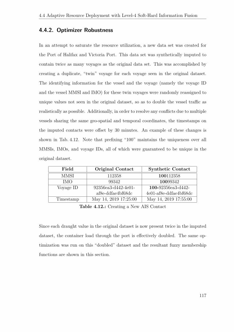
4.4 Adaptive Resource Deployment with Level-4 Soft-Hard Information Fusion
4.4.2. Optimizer Robustness
In an attempt to saturate the resource utilization, a new data set was created for
the Port of Halifax and Victoria Port. This data set was synthetically imputed to
contain twice as many voyages as the original data set. This was accomplished by
creating a duplicate, “twin” voyage for each voyage seen in the original dataset.
The identifying information for the vessel and the voyage (namely the voyage ID
and the vessel MMSI and IMO) for these twin voyages were randomly reassigned to
unique values not seen in the original dataset, so as to double the vessel traffic as
realistically as possible. Additionally, in order to resolve any conflicts due to multiple
vessels sharing the same geo-spatial and temporal coordinates, the timestamps on
the imputed contacts were offset by 30 minutes. An example of these changes is
shown in Tab. 4.12. Note that prefixing “100” maintains the uniqueness over all
MMSIs, IMOs, and voyage IDs, all of which were guaranteed to be unique in the
original dataset.
Field Original Contact Synthetic ContactMMSI 112358 100112358IMO 99342 10099342
Voyage ID 92356ea3-d442-4e01-af8e-ddfae4bf68dc
100-92356ea3-d442-4e01-af8e-ddfae4bf68dc
Timestamp May 14, 2019 17:25:00 May 14, 2019 17:55:00Table 4.12.: Creating a New AIS Contact
Since each draught value in the original dataset is now present twice in the imputed
dataset, the container load through the port is effectively doubled. The same op-
timization was run on this “doubled” dataset and the resultant fuzzy membership
functions are shown in this section.
117
5. Conclusions and Future Work
5.1. Conclusions
By fusing data from multiple sources, a shipping container damage classification
model was built in the first publication to address this problem. This was further
improved in a follow-up study, by combining the outputs of multiple classifiers and
using some metalearning techniques (in their first documented application to this
problem space) to improve the overall prediction accuracy of the classification out-
come by 80%. These studies have also resulted in the creation of first documented
datasets that may be used in any further investigations. Since the dataset creation
methodology is also documented, these datasets can be created and used for similar
study by any other research team, globally. To the best of my knowledge, this was
the first study in documented literature to investigate shipping container damage
and also to apply machine intelligence techniques to this problem.
Criticisms on the robustness of the classification performance due to the presence of
some testing data in the training set were addressed and dismissed by experiments
using the Leave One Batch Out (LOBO) methodology. Thus, the trained classifiers
and the learning methodologies have been shown to be robust against bias in the
data and may therefore be deployed on sparser data sets in the future.
These advancements make it possible to determine whether a container will be
118
5.1 Conclusions
damaged before it even arrives at the port. Therefore, if a claim were to be filed
upon that container, Bruce (from the fictional Port of Miranda) will have already
been alerted to it and will not need to follow up on such a claim. Rather, he will
simply need to inform the claimant that the container was damaged outside his
custody and any action should therefore be taken against other parties.
In order to optimize vessel service time at port, a fuzzy system evolved by a multi-
objective genetic algorithm has been created. It has been shown to outperform
current industry practice in vessel service time (by almost 80% in some cases) and
the amount of resources deployed (by 50% in some cases) to do so. In order to boost
the efficacy of this methodology, a new genetic crossover mechanism was developed
called FitWAM and applied here for the first time in documented literature. To the
best of my knowledge, this was the first study in documented literature to apply a
genetically evolved fuzzy system to this problem.
This methodology has also been shown to generalize to multiple geographical regions.
Further, the evolved fuzzy systems are able to handle twice the service throughput
currently observed in the real-world data without significant additional resource
deployment. This supports the claim that this learning methodology yields high
performant optimization algorithms that are not constrained by service load or ge-
ography, and may thus be deployed to other container ports, globally. In addition,
this study has yielded a previously nonexistent data set for future investigations.
Finally, filtering vessel locations by port proximity allows for this methodology to be
robust against incorrect or incomplete automated messages from vessels increasing
its robustness against system and human errors.
These advancements make it possible to operate the Port of Miranda with fewer
personnel and at reduced operational costs. This automation also frees person-
nel from creating, implementing, managing, and executing a resource deployment
119
5.2 Limitations of this Work
schedule, further reducing the overhead costs of running the Port of Miranda, even
at increased throughput.
These advancements could be incorporated into terminal operating systems (such
as Navis N4 [29]) to alert port-side personnel to check specific incoming containers
more thoroughly and record any observed damage as they may be predicted to have
a higher probability of having an insurance claim filed for. Additionally, such a
system could also alert operators at the end of the service of a vessel that their shift
is not yet complete.
5.2. Limitations of this Work
The necessity to synthesize parts of the dataset from publicly available information
came from the lack of high-veracity data available for this study. This could be
improved by forming partnerships with commercial maritime ports and other stake-
holders in the supply chain. Such partnerships could yield the container specific
data mentioned in Sec. 3.2 as well as the port-side data pertaining to on-shift per-
sonnel and internal logs pertaining to delays and container throughput. Container
throughput data would eliminate the dependency of this study on the crude mining
of this information from AIS data, while internal delay logs would eliminate the
need for their synthesis, and allow for higher veracity in extracting meaning from
more realistic logs.
The limitations of the computational infrastructure imposed constraints on software
packages that could be used in the optimization. As a result, certain techniques
(including Petri Nets and multi-output regressors) were not used. The removal
of these constraints would afford a broader avenues to explore in the optimization
space.
120
5.3 Future Work
5.3. Future Work
Attempting to apply the same machine learning strategies used to predict shipping
container damage, on real-world shipping container damage data (as opposed to
approximations thereof) are likely to yield analyses with better veracity that more
accurately reflect the real-world benefits of this study. Additional classifier and
regression models may also be tested for their viability in this study, and this is left
as an avenue of further study.
While advancements in port-side resource deployment have been shown to outper-
form current industry practice, this was accomplished by evolving only one part of
the fuzzy controller. Evolving the fuzzy rule base as well as the membership func-
tions in the defuzzifier may yield a better performing fuzzy system. These are left
as avenues of further study.
Further, all natural language processing was limited to keyword searches and per-
tained only to the English language. More sophisticated natural language processing
techniques (perhaps using word2vec [99]) may help more accurately read port-side
situation reports in order to better tune the fuzzy controller. They may also aug-
ment the generalizability of this methodology to ports whose situation reports are
not in English. These are left as avenues of further study.
Finally, more real-world data pertaining to the number of containers serviced for
each vessel would help improve the veracity of the optimization by eliminating noise
from ballast, fuel, etc on board a vessel, eliminating the need to estimate the number
of containers from vessel draught.
121
Bibliography
[1] A. Panchapakesan, R. Abielmona, R. Falcon, and E. Petriu, “Prediction of
Container Damage Insurance Claims for Optimized Maritime Port Operations,”
in Advances in Artificial Intelligence: 31st Canadian Conference on Artificial
Intelligence, Canadian AI 2018, Toronto, ON, Canada, May 8–11, 2018, Pro-
ceedings 31, pp. 265–271, Springer, 2018.
[2] I. B. G. Rodrigues, R. d. A. Rosa, T. C. Gomes, and G. M. Ribeiro, “Mathe-
matical model for the Berth Allocation Problem in ports with cargo operation
limitations along the pier,” Gestão & Produção, vol. 23, no. AHEAD, p. 0, 2016.
[3] M. R. Endsley and D. J. Garland, “Theoretical underpinnings of situation
awareness: A critical review,” Situation Awareness Analysis and Measurement,
vol. 1, p. 24, 2000.
[4] D. Lambert, S. Wark, E. Bosse, L. Pigeon, C. Blackman, and M. Hinman, “A
coalition approach to higher-level fusion,” tech. rep., Air Force Research Lab
Rome NY Information Directorate, 2009.
[5] EuroWeather, “Douglas Scale.” http://www.eurometeo.com/english/read/doc_douglas,
1995.
[6] C. Zhang, Y.-W. Wan, J. Liu, and R. J. Linn, “Dynamic crane deployment
122
Bibliography
in container storage yards,” Transportation Research Part B: Methodological,
vol. 36, no. 6, pp. 537–555, 2002.
[7] CBSA, “Access to Information Act Requested Report.” Technical Report A-
2017-020703/JS, 2017.
[8] A. Becker, A. Hippe, and E. L. Mclean, “Cost and Materials Required to
Retrofit US Seaports in Response to Sea Level Rise: A Thought Exercise for
Climate Response,” Journal of Marine Science and Engineering, vol. 5, no. 44,
2017.
[9] C. Bierwirth and F. Meisel, “A survey of berth allocation and quay crane
scheduling problems in container terminals,” European Journal of Operational
Research, vol. 202, pp. 615–627, May 2010.
[10] P. Legato, D. Gullì, and R. Trunfio, “The Quay Crane Deployment Problem At
A Maritime Container Terminal,” Submitted to the 22nd European Conference
on Modelling and Simulation.
[11] A. Imai, E. Nishimura, and S. Papadimitriou, “The dynamic berth allocation
problem for a container port,” Transportation Research Part B: Methodological,
vol. 35, no. 4, pp. 401–417, 2001.
[12] J.-F. Cordeau, G. Laporte, P. Legato, and L. Moccia, “Models and tabu search
heuristics for the berth-allocation problem,” Transportation Science, vol. 39,
no. 4, pp. 526–538, 2005.
[13] Y. Guan and R. K. Cheung, “The berth allocation problem: models and solu-
tion methods,” OR Spectrum, vol. 26, no. 1, pp. 75–92, 2004.
[14] M. M. Golias, G. K. Saharidis, M. Boile, S. Theofanis, and M. G. Ierapetri-
tou, “The berth allocation problem: Optimizing vessel arrival time,” Maritime
Economics & Logistics, vol. 11, no. 4, pp. 358–377, 2009.
123
Bibliography
[15] A. De, S. Pratap, A. Kumar, and M. Tiwari, “A hybrid dynamic berth allo-
cation planning problem with fuel costs considerations for container terminal
port using chemical reaction optimization approach,” Annals of Operations Re-
search, pp. 1–29, 2018.
[16] Y. Hirashima, K. Takeda, S. Harada, D. Mingcong, and A. Inoue, “A Q-learning
for group-based plan of container transfer scheduling,” JSME International
Journal Series C Mechanical Systems, Machine Elements and Manufacturing,
vol. 49, no. 2, pp. 473–479, 2006.
[17] Y. A. Saanen and R. Dekker, “Intelligent stacking as way out of congested
yards? part 1,” Port Technology International, vol. 31, pp. 87–92, 2007.
[18] Y. A. Saanen and R. Dekker, “Intelligent stacking as way out of congested
yards? part 2,” Port Technology International, vol. 31, pp. 87–92, 2007.
[19] D. Ambrosino, A. Sciomachen, and E. Tanfani, “Stowing a containership: the
master bay plan problem,” Transportation Research Part A: Policy and Prac-
tice, vol. 38, no. 2, pp. 81–99, 2004.
[20] R. Dekker, P. Voogd, and E. van Asperen, “Advanced methods for container
stacking,” Container terminals and cargo systems, vol. 28, no. 4, pp. 563–586,
2006.
[21] E. Blasch, E. Bosse, and D. A. Lambert, High-Level Information Fusion Man-
agement and Systems Design. Artech House; 1 edition, 2012.
[22] D. A. Lambert, “Situations for situation aware-
ness,” Proceedings of Fusion 2001, 2001; Available:
https://pdfs.semanticscholar.org/dc07/62a16e8bd04416a06108fe50724d4914fda4.pdf.
[23] D. A. Lambert, “Grand challenges of information fusion,” in Proceedings of the
6th International Conference on Information Fusion, vol. 1, pp. 213–220, 2003.
124
Bibliography
[24] J. Webb, A. Ahmad, S. B. Maynard, and G. Shanks, “A situation aware-
ness model for information security risk management,” Computers & Security,
vol. 44, pp. 1–15, 2014.
[25] M. R. Endsley, “Toward a theory of situation awareness in dynamic systems,”
Human Factors, vol. 37, no. 1, pp. 32–64, 1995.
[26] E. Blasch and S. Plano, “Dfig level 5 (user refinement) issues supporting situ-
ational assessment reasoning,” in 2005 7th International Conference on Infor-
mation Fusion, vol. 1, pp. xxxv–xliii, IEEE, 2005.
[27] E. Blasch, J. Llinas, D. Lambert, P. Valin, S. Das, C. Chong, M. Kokar, and
E. Shahbazian, “High level information fusion developments, issues, and grand
challenges: Fusion 2010 panel discussion,” in 2010 13th International Confer-
ence on Information Fusion, pp. 1–8, IEEE, 2010.
[28] E. P. Blasch, D. A. Lambert, P. Valin, M. M. Kokar, J. Llinas, S. Das, C. Chong,
and E. Shahbazian, “High level information fusion (hlif): Survey of models, is-
sues, and grand challenges,” IEEE Aerospace and Electronic Systems Magazine,
vol. 27, no. 9, pp. 4–20, 2012.
[29] Navis, “Get More With N4 | Navis.” http://navis.com/get-more-n4.
[30] W.-J. Tseng et al., “Risk analysis of cargos damages for aquatic products of re-
frigerated containers: shipping operators’ perspective in Taiwan,” Information
Management and Business Review, vol. 4, no. 2, pp. 86–94, 2012.
[31] A.-S. Nir, K. Lin, and G.-S. Liang, “Port choice behaviour–from the perspective
of the shipper,” Maritime Policy & Management, vol. 30, no. 2, pp. 165–173,
2003.
[32] W. K. Hsu, S. S. Huang, and R. J. Yeh, “An assessment model of safety factors
125
Bibliography
for product tankers in coastal shipping,” Safety Science, vol. 76, pp. 74–81,
2015.
[33] W.-K. K. Hsu et al., “Assessing the Safety Factors of Ship Berthing Opera-
tions,” Journal of Navigation, vol. 68, no. 03, pp. 576–588, 2015.
[34] W. N. France et al., “An investigation of head-sea parametric rolling and its
influence on container lashing systems,” Marine Technology, vol. 40, no. 1, 2003.
[35] National Oceanic and Atmospheric Administration, “Climate Data Online
(CDO) - The National Climatic Data Center’s (NCDC) Climate Data Online
(CDO) provides free access to NCDC’s archive of historical weather and cli-
mate data in addition to station history information. | National Climatic Data
Center (NCD).” https://www.ncdc.noaa.gov/cdo-web/.
[36] “Hourly Data Report - Climate - Environment Canada.”
http://climate.weather.gc.ca/historical_data/search_historic_data_e.html,
2015.
[37] J. Kacprzyk and W. Pedrycz, Springer Handbook of Computational Intelligence.
Springer, 2015.
[38] Lloyd’s Register, “Lloyd’s Register.” http://www.lr.org/en/, 2016.
[39] S. Kelangath et al., “Risk analysis of damaged ships–a data-driven Bayesian
approach,” Ships and Offshore Structures, vol. 7, no. 3, 2012.
[40] BayesFusion, “GeNIe.” https://download.bayesfusion.com/, 2016.
[41] T. Stanivuk et al., “How to predict cargo handling times at the sea port affected
by weather conditions,” Croatian Operational Research Review, vol. 3, no. 1,
2012.
[42] M. Bielli, A. Boulmakoul, and M. Rida, “Object oriented model for container
126
Bibliography
terminal distributed simulation,” European Journal of Operational Research,
vol. 175, no. 3, pp. 1731–1751, 2006.
[43] B. Ferrier and R. Ernst, “Fire Scout Launch and Recovery Considerations in
Unexpected Ship Roll Motion Conditions,” Naval Engineers Journal, vol. 129,
no. 4, pp. 87–98, 2017.
[44] L. Wang, Y. Tang, X. Zhang, and J. Zhang, “Studies on parametric roll motion
of ship under wave group by numerical simulation,” Ocean Engineering, vol. 163,
pp. 391–399, 2018.
[45] P. Chen, Z. Fu, A. Lim, and B. Rodrigues, “Port yard storage optimization,”
IEEE Transactions on Automation Science and Engineering, vol. 1, no. 1,
pp. 26–37, 2004.
[46] A. Karam, A. B. Eltawif, and N. A. Harraz, “An improved approach for the
quay crane assignment problem with limited availability of internal trucks in
container terminal,” in 2014 IEEE International Conference on Industrial En-
gineering and Engineering Management, pp. 112–116, IEEE, Dec 2014.
[47] D. X. Kokotos et al., “A classification tree application to predict total ship
loss,” Journal of Transportation and Statistics, vol. 8, no. 2, p. 31, 2005.
[48] G. V. Kass, “An exploratory technique for investigating large quantities of
categorical data,” Applied Statistics, pp. 119–127, 1980.
[49] Y. Cheng and M. D. Shuster, “Robustness and Accuracy of the QUEST Algo-
rithm,” Advances in the Astronautical Sciences, vol. 127, pp. 41–61, 2007.
[50] F. L. Markley and D. Mortari, “Quaternion attitude estimation using vector
observations.,” Journal of the Astronautical Sciences, vol. 48, no. 2, pp. 359–
380, 2000.
[51] D. X. Kokotos and D. S. Linardatos, “An application of data mining tools for
127
Bibliography
the study of shipping safety in restricted waters,” Safety Science, vol. 49, no. 2,
pp. 192–197, 2011.
[52] A. B. Alexopoulos, G. Dounias, E. Kalivas, and M. Lekakou, “Accident Anal-
ysis of Ro-Ro Ships in the Greek Sea-Short Shipping using Data-Mining Tech-
niques,” Management Science & Regional Development Journal, pp. 145–152,
2001.
[53] M. Lindauer, K. Eggensperger, M. Feurer, S. Falkner, A. Biedenkapp, and
F. Hutter, “SMAC v3: Algorithm Configuration in Python,” 2017.
[54] F. Hutter, H. H. Hoos, and K. Leyton-Brown, “Sequential model-based opti-
mization for general algorithm configuration,” in International Conference on
Learning and Intelligent Optimization, pp. 507–523, Springer, 2011.
[55] M. A. Fischler and R. C. Bolles, “Random sample consensus: a paradigm for
model fitting with applications to image analysis and automated cartography,”
Communications of the ACM, vol. 24, no. 6, pp. 381–395, 1981.
[56] R. S. Consensus, “A Paradigm for Model Fitting with Applications to Im-
age Analysis and Automated Cartography,” MA Fischler, RC Bolles, vol. 6,
pp. 381–395, 1981.
[57] K. Eggensperger, F. Hutter, H. Hoos, and K. Leyton-Brown, “Efficient bench-
marking of hyperparameter optimizers via surrogates,” in Twenty-Ninth AAAI
Conference on Artificial Intelligence, 2015.
[58] A. H. Wright, “Genetic algorithms for real parameter optimization,” in Foun-
dations of Genetic Algorithms, vol. 1, pp. 205–218, Elsevier, 1991.
[59] C. Thornton, F. Hutter, H. H. Hoos, and K. Leyton-Brown, “Auto-WEKA:
Combined selection and hyperparameter optimization of classification algo-
128
Bibliography
rithms,” in Proceedings of the 19th ACM SIGKDD International Conference
on Knowledge Discovery and Data Mining, pp. 847–855, ACM, 2013.
[60] M. M. Salvador, M. Budka, and B. Gabrys, “Towards automatic composition
of multicomponent predictive systems,” in International Conference on Hybrid
Artificial Intelligence Systems, pp. 27–39, Springer, 2016.
[61] N. Kanwisher, “The modular structure of human visual recognition: Evidence
from functional imaging,” Advances in Psychological Science, vol. 2, pp. 199–
213, 1998.
[62] D. Cheng, J. Rao, C. Jiang, and X. Zhou, “Resource and deadline-aware job
scheduling in dynamic hadoop clusters,” in 2015 IEEE International Parallel
and Distributed Processing Symposium, pp. 956–965, IEEE, 2015.
[63] P. Jamshidi, A. Sharifloo, C. Pahl, H. Arabnejad, A. Metzger, and G. Estrada,
“Fuzzy self-learning controllers for elasticity management in dynamic cloud ar-
chitectures,” in 2016 12th International ACM SIGSOFT Conference on Quality
of Software Architectures (QoSA), pp. 70–79, IEEE, 2016.
[64] L. Wang, J. Xu, M. Zhao, Y. Tu, and J. A. Fortes, “Fuzzy modeling based
resource management for virtualized database systems,” in 2011 IEEE 19th
Annual International Symposium on Modelling, Analysis, and Simulation of
Computer and Telecommunication Systems, pp. 32–42, IEEE, 2011.
[65] R. I. Peterkofsky and C. F. Daganzo, “A branch and bound solution method
for the crane scheduling problem,” Transportation Research Part B: Method-
ological, vol. 24, no. 3, pp. 159–172, 1990.
[66] F. Cheraghchi, I. Abualhaol, R. Falcon, R. Abielmona, B. Raahemi, and
E. Petriu, “Big-data-enabled modelling and optimization of granular speed-
129
Bibliography
based vessel schedule recovery problem,” in Proceedings of the 2017 IEEE In-
ternational Conference on Big Data (Big Data), pp. 1786–1794, IEEE, 2017.
[67] S. Wesolkowski, N. Francetic, and S. C. Grant, “TraDE: Training device selec-
tion via multi-objective optimization,” Proceedings of the 2014 IEEE Congress
on Evolutionary Computation (CEC), pp. 2617–2624, 2014.
[68] F. Pedregosa et al., “Scikit-learn: Machine learning in Python,” Journal of
Machine Learning Research, vol. 12, pp. 2825–2830, 2011.
[69] I. AbuAlhaol, R. Falcon, R. Abielmona, and E. Petriu, “Mining port congestion
indicators from big ais data,” in 2018 International Joint Conference on Neural
Networks (IJCNN), pp. 1–8, IEEE, 2018.
[70] P. Jamshidi, A. Ahmad, and C. Pahl, “Autonomic resource provisioning for
cloud-based software,” in Proceedings of the 9th International Symposium on
Software Engineering for Adaptive and Self-managing Systems, pp. 95–104,
ACM, 2014.
[71] L. Wang, J. Xu, M. Zhao, Y. Tu, and J. A. B. Fortes, “Fuzzy modeling based
resource management for virtualized database systems,” in 2011 IEEE 19th
Annual International Symposium on Modelling, Analysis, and Simulation of
Computer and Telecommunication Systems, pp. 32–42, IEEE, 2011.
[72] M. G. T. Partnership, “Vessel schedule - Future.”
https://www.mtrtml.com/vs/vessel-visit-future-sommaire.php.
[73] I. Abualhaol, R. Falcon, R. Abielmona, and E. Petriu, “Data-Driven Vessel
Service Time Forecasting using Long Short-Term Memory Recurrent Neural
Networks,” in 2018 IEEE International Conference on Big Data (Big Data),
pp. 2580–2590, IEEE, 2018.
[74] Wikipedia, “List of Shipping Lines.” bit.ly/2VTlpRq, 2017.
130
Bibliography
[75] A. Lipowski and D. Lipowska, “Roulette-wheel selection via stochastic accep-
tance,” Physica A: Statistical Mechanics and its Applications, vol. 391, no. 6,
pp. 2193–2196, 2012.
[76] C. B. S. Agency, “Canada Border Services Agency.” https://www.cbsa-
asfc.gc.ca/menu-eng.html, 2017.
[77] “It turns out not all containers are exactly the same size.” https://i.pinimg.
com/originals/81/49/9a/81499a43835c88deebe7078ae9745489.jpg. Ac-
cessed: 2019-08-13.
[78] T. Trucking, “Top 100.” www.todaystrucking.com/top100/2015, 2015.
[79] RFairbrother, “MATSON Daily Sitrep.” www.matson.co.nz, 2018.
[80] K. M. Gupta, D. W. Aha, and P. Moore, “Case-Based Collective Inference
for Maritime Object Classification,” in Case-Based Reasoning Research and
Development, pp. 443–449, 2009.
[81] S. G. Hart and L. E. Staveland, “Development of NASA-TLX
(Task Load Index): Results of Empirical and Theoretical Research.”
http://stavelandhfe.com/images/NASA-TLX_paper.pdf, 2017.
[82] K. Bichou, Port Operations, Planning and Logistics. CRC Press, 2014.
[83] R. Stahlbock and S. Voß, “Operations research at container terminals: a liter-
ature update,” OR Spectrum, vol. 30, no. 1, pp. 1–52, 2008.
[84] P. Alderton and G. Saieva, Port Management and Operations. Taylor & Francis,
2013.
[85] S.-O. Yoon et al., “The Devil Is in the Specificity : The Negative Effect of
Prediction Specificity on Prediction Accuracy,” Psychological Science, vol. XX,
pp. 1–7, 2010.
131
Bibliography
[86] Theresa F. Kelly and Joseph P. Simmons, “When does making detailed predic-
tions make predictions worse?,” Journal of Experimental Psychology: General,
vol. 145, no. 10, pp. 1298–1311, 2016.
[87] C. Caponecchia et al., “It Won’t Happen to Me: An Investigation of Optimism
Bias in Occupational Health and Safety,” Journal of Applied Social Psychology,
vol. 40, pp. 601–617, Mar 2010.
[88] P. Flach, Machine learning: the art and science of algorithms that make sense
of data. Cambridge University Press, 2012.
[89] M. H. B. Jamaa, D. Atienza, G. De Micheli, K. E. Moselund, D. Bouvet,
A. M. Ionescu, and Y. Leblebici, “Fault-tolerant multi-level logic decoder for
nanoscale crossbar memory arrays,” in Computer-Aided Design, 2007. ICCAD
2007. IEEE/ACM International Conference on, pp. 765–772, IEEE, 2007.
[90] J. VanTassel, Covertly Embedded Finite State Machines and Their Detection
in One-hot Encoded Circuits. PhD Thesis, State University of New York at
Binghamton, 2011.
[91] S. Yun and K. Lee, “Optimization of regular expression pattern matching circuit
using at-most two-hot encoding on FPGA,” in Field Programmable Logic and
Applications (FPL), 2010 International Conference on, pp. 40–43, IEEE, 2010.
[92] J. Xu, M. Zhao, J. Fortes, R. Carpenter, and M. Yousif, “Autonomic resource
management in virtualized data centers using fuzzy logic-based approaches,”
Cluster Computing, vol. 11, no. 3, pp. 213–227, 2008.
[93] L. Wang, J. Xu, M. Zhao, Y. Tu, and J. A. Fortes, “Fuzzy modeling based
resource management for virtualized database systems,” in 2011 IEEE 19th
Annual International Symposium on Modelling, Analysis, and Simulation of
Computer and Telecommunication Systems, pp. 32–42, IEEE, 2011.
132
Bibliography
[94] Y. Sun, L. Meng, and Y. Song, “Autoscale: Adaptive qos-aware container-based
cloud applications scheduling framework.,” KSII Transactions on Internet &
Information Systems, vol. 13, no. 6, 2019.
[95] A. Teske, R. Falcon, R. Abielmona, and E. Petriu, “Automating maritime risk
assessment with genetic fuzzy systems,” in Proc. 2nd Int. Symp. Fuzzy Rough
Sets (ISFUROS), pp. 1–10, 2017.
[96] S. N. Sivanandam and S. N. Deepa, Introduction to Genetic Algorithms.
Springer Science & Business Media, 2007.
[97] L. Marti, J. Garcia, A. Berlanga, and J. M. Molina, “A cumulative evidential
stopping criterion for multiobjective optimization evolutionary algorithms,” in
Proceedings of the 9th Annual Conference Companion on Genetic and Evolu-
tionary Computation, pp. 2835–2842, ACM, 2007.
[98] P. Brazdil and C. Giraud-Carrier, “Metalearning and algorithm selection:
progress, state of the art and introduction to the 2018 special issue,” Machine
Learning, vol. 107, pp. 1–14, Jan 2018.
[99] X. Zhang, J. Zhao, and Y. LeCun, “Character-level convolutional networks
for text classification,” in Advances in neural information processing systems,
pp. 649–657, 2015.
133

A. Shipping Container Damage
Prediction Results Data
A.1. Container Damage Claims Classifier
Performance Veracity with Leave One One
Batch Out Training
A.1.1. Improving Container Damage Claims Classifier
Performance Veracity with Leave One One Batch Out
Training
134
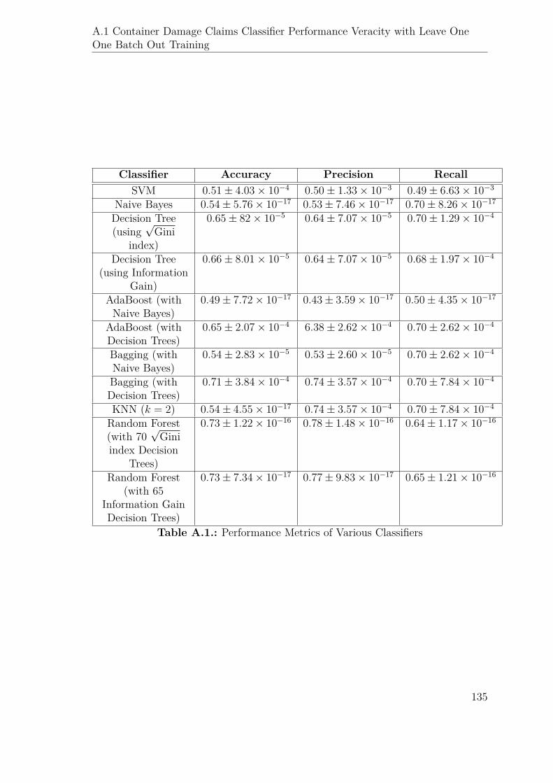
A.1 Container Damage Claims Classifier Performance Veracity with Leave OneOne Batch Out Training
Classifier Accuracy Precision RecallSVM 0.51± 4.03× 10⁻⁴ 0.50± 1.33× 10⁻³ 0.49± 6.63× 10⁻³
Naive Bayes 0.54± 5.76× 10⁻¹⁷ 0.53± 7.46× 10⁻¹⁷ 0.70± 8.26× 10⁻¹⁷
Decision Tree(using
√Gini
index)
0.65± 82× 10−5 0.64± 7.07× 10⁻⁵ 0.70± 1.29× 10⁻⁴
Decision Tree(using Information
Gain)
0.66± 8.01× 10⁻⁵ 0.64± 7.07× 10⁻⁵ 0.68± 1.97× 10⁻⁴
AdaBoost (withNaive Bayes)
0.49± 7.72× 10⁻¹⁷ 0.43± 3.59× 10⁻¹⁷ 0.50± 4.35× 10⁻¹⁷
AdaBoost (withDecision Trees)
0.65± 2.07× 10⁻⁴ 6.38± 2.62× 10⁻⁴ 0.70± 2.62× 10⁻⁴
Bagging (withNaive Bayes)
0.54± 2.83× 10⁻⁵ 0.53± 2.60× 10⁻⁵ 0.70± 2.62× 10⁻⁴
Bagging (withDecision Trees)
0.71± 3.84× 10⁻⁴ 0.74± 3.57× 10⁻⁴ 0.70± 7.84× 10⁻⁴
KNN (k = 2) 0.54± 4.55× 10⁻¹⁷ 0.74± 3.57× 10⁻⁴ 0.70± 7.84× 10⁻⁴
Random Forest(with 70
√Gini
index DecisionTrees)
0.73± 1.22× 10⁻¹⁶ 0.78± 1.48× 10⁻¹⁶ 0.64± 1.17× 10⁻¹⁶
Random Forest(with 65
Information GainDecision Trees)
0.73± 7.34× 10⁻¹⁷ 0.77± 9.83× 10⁻¹⁷ 0.65± 1.21× 10⁻¹⁶
Table A.1.: Performance Metrics of Various Classifiers
135
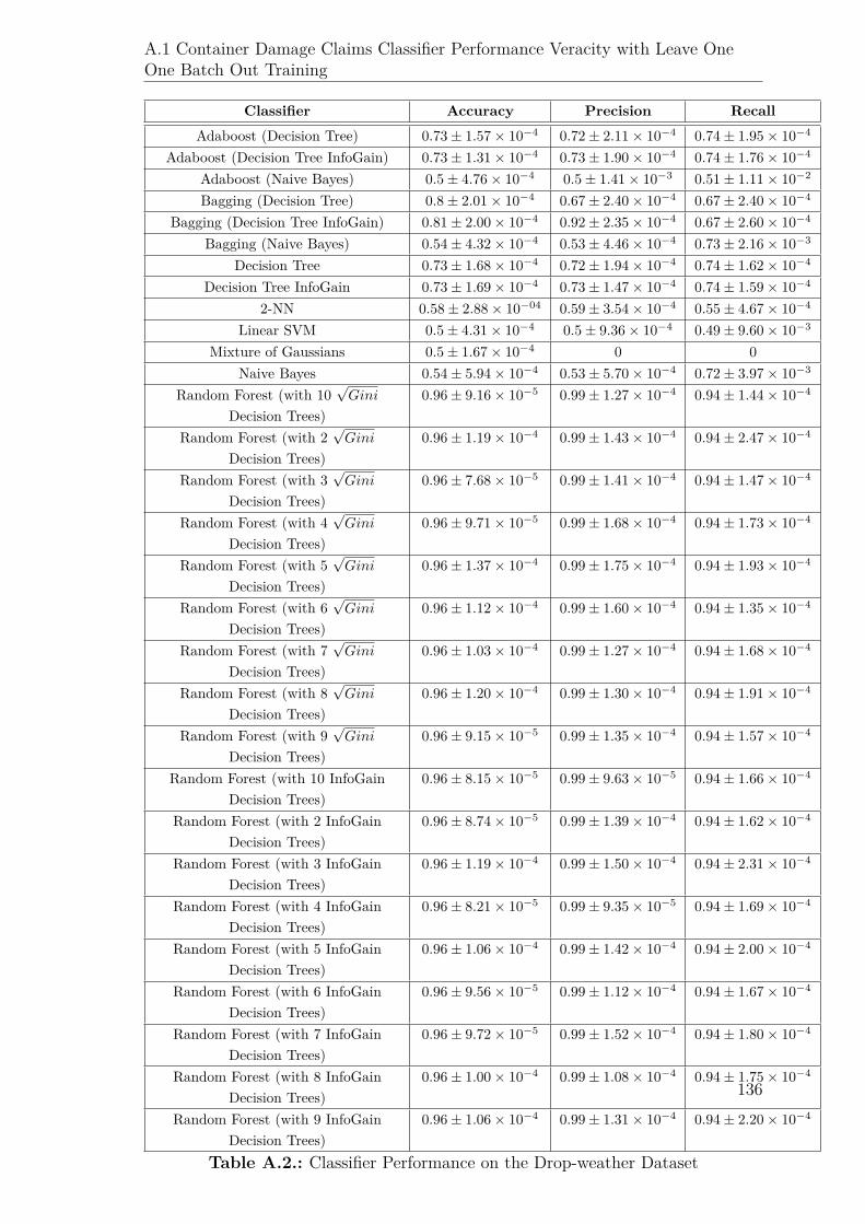
A.1 Container Damage Claims Classifier Performance Veracity with Leave OneOne Batch Out Training
Classifier Accuracy Precision RecallAdaboost (Decision Tree) 0.73± 1.57× 10⁻⁴ 0.72± 2.11× 10⁻⁴ 0.74± 1.95× 10⁻⁴
Adaboost (Decision Tree InfoGain) 0.73± 1.31× 10⁻⁴ 0.73± 1.90× 10⁻⁴ 0.74± 1.76× 10⁻⁴
Adaboost (Naive Bayes) 0.5± 4.76× 10⁻⁴ 0.5± 1.41× 10⁻³ 0.51± 1.11× 10⁻²
Bagging (Decision Tree) 0.8± 2.01× 10⁻⁴ 0.67± 2.40× 10⁻⁴ 0.67± 2.40× 10⁻⁴
Bagging (Decision Tree InfoGain) 0.81± 2.00× 10⁻⁴ 0.92± 2.35× 10⁻⁴ 0.67± 2.60× 10⁻⁴
Bagging (Naive Bayes) 0.54± 4.32× 10⁻⁴ 0.53± 4.46× 10⁻⁴ 0.73± 2.16× 10⁻³
Decision Tree 0.73± 1.68× 10⁻⁴ 0.72± 1.94× 10⁻⁴ 0.74± 1.62× 10⁻⁴
Decision Tree InfoGain 0.73± 1.69× 10⁻⁴ 0.73± 1.47× 10⁻⁴ 0.74± 1.59× 10⁻⁴
2-NN 0.58± 2.88× 10−04 0.59± 3.54× 10⁻⁴ 0.55± 4.67× 10⁻⁴
Linear SVM 0.5± 4.31× 10⁻⁴ 0.5± 9.36× 10⁻⁴ 0.49± 9.60× 10⁻³
Mixture of Gaussians 0.5± 1.67× 10⁻⁴ 0 0Naive Bayes 0.54± 5.94× 10⁻⁴ 0.53± 5.70× 10⁻⁴ 0.72± 3.97× 10⁻³
Random Forest (with 10√
Gini
Decision Trees)0.96± 9.16× 10⁻⁵ 0.99± 1.27× 10⁻⁴ 0.94± 1.44× 10⁻⁴
Random Forest (with 2√
Gini
Decision Trees)0.96± 1.19× 10⁻⁴ 0.99± 1.43× 10⁻⁴ 0.94± 2.47× 10⁻⁴
Random Forest (with 3√
Gini
Decision Trees)0.96± 7.68× 10⁻⁵ 0.99± 1.41× 10⁻⁴ 0.94± 1.47× 10⁻⁴
Random Forest (with 4√
Gini
Decision Trees)0.96± 9.71× 10⁻⁵ 0.99± 1.68× 10⁻⁴ 0.94± 1.73× 10⁻⁴
Random Forest (with 5√
Gini
Decision Trees)0.96± 1.37× 10⁻⁴ 0.99± 1.75× 10⁻⁴ 0.94± 1.93× 10⁻⁴
Random Forest (with 6√
Gini
Decision Trees)0.96± 1.12× 10⁻⁴ 0.99± 1.60× 10⁻⁴ 0.94± 1.35× 10⁻⁴
Random Forest (with 7√
Gini
Decision Trees)0.96± 1.03× 10⁻⁴ 0.99± 1.27× 10⁻⁴ 0.94± 1.68× 10⁻⁴
Random Forest (with 8√
Gini
Decision Trees)0.96± 1.20× 10⁻⁴ 0.99± 1.30× 10⁻⁴ 0.94± 1.91× 10⁻⁴
Random Forest (with 9√
Gini
Decision Trees)0.96± 9.15× 10⁻⁵ 0.99± 1.35× 10⁻⁴ 0.94± 1.57× 10⁻⁴
Random Forest (with 10 InfoGainDecision Trees)
0.96± 8.15× 10⁻⁵ 0.99± 9.63× 10⁻⁵ 0.94± 1.66× 10⁻⁴
Random Forest (with 2 InfoGainDecision Trees)
0.96± 8.74× 10⁻⁵ 0.99± 1.39× 10⁻⁴ 0.94± 1.62× 10⁻⁴
Random Forest (with 3 InfoGainDecision Trees)
0.96± 1.19× 10⁻⁴ 0.99± 1.50× 10⁻⁴ 0.94± 2.31× 10⁻⁴
Random Forest (with 4 InfoGainDecision Trees)
0.96± 8.21× 10⁻⁵ 0.99± 9.35× 10⁻⁵ 0.94± 1.69× 10⁻⁴
Random Forest (with 5 InfoGainDecision Trees)
0.96± 1.06× 10⁻⁴ 0.99± 1.42× 10⁻⁴ 0.94± 2.00× 10⁻⁴
Random Forest (with 6 InfoGainDecision Trees)
0.96± 9.56× 10⁻⁵ 0.99± 1.12× 10⁻⁴ 0.94± 1.67× 10⁻⁴
Random Forest (with 7 InfoGainDecision Trees)
0.96± 9.72× 10⁻⁵ 0.99± 1.52× 10⁻⁴ 0.94± 1.80× 10⁻⁴
Random Forest (with 8 InfoGainDecision Trees)
0.96± 1.00× 10⁻⁴ 0.99± 1.08× 10⁻⁴ 0.94± 1.75× 10⁻⁴
Random Forest (with 9 InfoGainDecision Trees)
0.96± 1.06× 10⁻⁴ 0.99± 1.31× 10⁻⁴ 0.94± 2.20× 10⁻⁴
Table A.2.: Classifier Performance on the Drop-weather Dataset
136
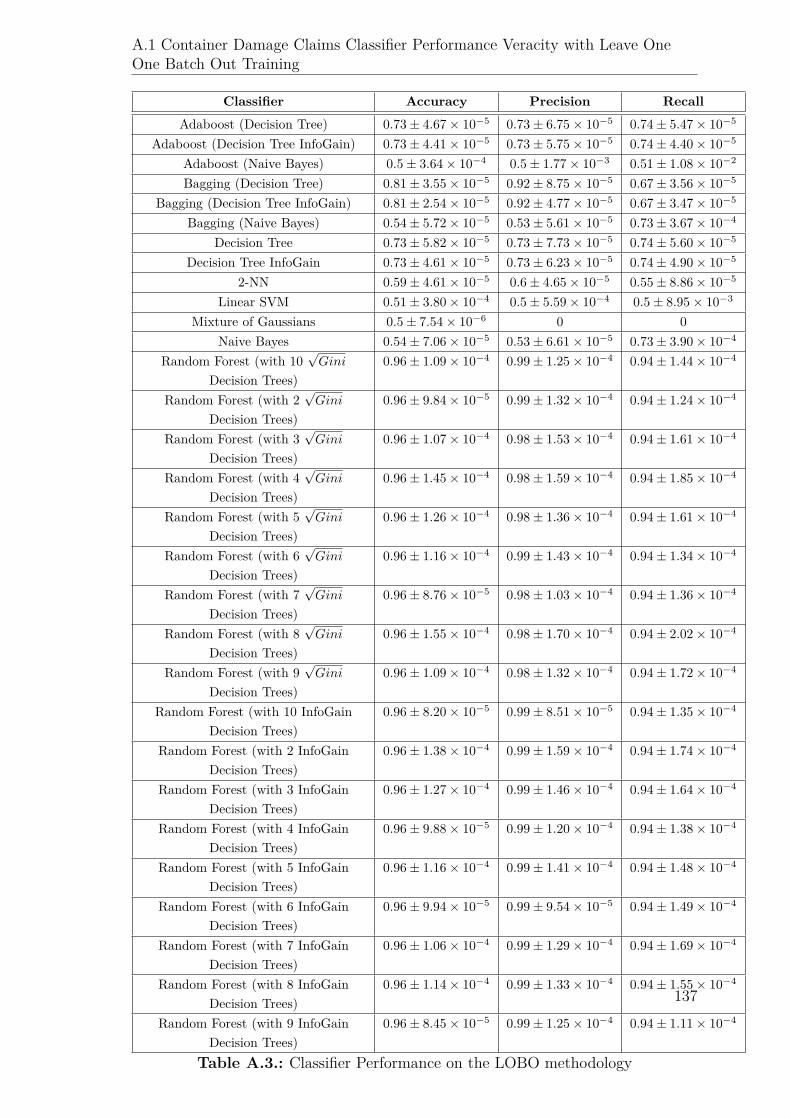
A.1 Container Damage Claims Classifier Performance Veracity with Leave OneOne Batch Out Training
Classifier Accuracy Precision RecallAdaboost (Decision Tree) 0.73± 4.67× 10⁻⁵ 0.73± 6.75× 10⁻⁵ 0.74± 5.47× 10⁻⁵
Adaboost (Decision Tree InfoGain) 0.73± 4.41× 10⁻⁵ 0.73± 5.75× 10⁻⁵ 0.74± 4.40× 10⁻⁵
Adaboost (Naive Bayes) 0.5± 3.64× 10⁻⁴ 0.5± 1.77× 10⁻³ 0.51± 1.08× 10⁻²
Bagging (Decision Tree) 0.81± 3.55× 10⁻⁵ 0.92± 8.75× 10⁻⁵ 0.67± 3.56× 10⁻⁵
Bagging (Decision Tree InfoGain) 0.81± 2.54× 10⁻⁵ 0.92± 4.77× 10⁻⁵ 0.67± 3.47× 10⁻⁵
Bagging (Naive Bayes) 0.54± 5.72× 10⁻⁵ 0.53± 5.61× 10⁻⁵ 0.73± 3.67× 10⁻⁴
Decision Tree 0.73± 5.82× 10⁻⁵ 0.73± 7.73× 10⁻⁵ 0.74± 5.60× 10⁻⁵
Decision Tree InfoGain 0.73± 4.61× 10⁻⁵ 0.73± 6.23× 10⁻⁵ 0.74± 4.90× 10⁻⁵
2-NN 0.59± 4.61× 10⁻⁵ 0.6± 4.65× 10⁻⁵ 0.55± 8.86× 10⁻⁵
Linear SVM 0.51± 3.80× 10⁻⁴ 0.5± 5.59× 10⁻⁴ 0.5± 8.95× 10⁻³
Mixture of Gaussians 0.5± 7.54× 10⁻⁶ 0 0Naive Bayes 0.54± 7.06× 10⁻⁵ 0.53± 6.61× 10⁻⁵ 0.73± 3.90× 10⁻⁴
Random Forest (with 10√
Gini
Decision Trees)0.96± 1.09× 10⁻⁴ 0.99± 1.25× 10⁻⁴ 0.94± 1.44× 10⁻⁴
Random Forest (with 2√
Gini
Decision Trees)0.96± 9.84× 10⁻⁵ 0.99± 1.32× 10⁻⁴ 0.94± 1.24× 10⁻⁴
Random Forest (with 3√
Gini
Decision Trees)0.96± 1.07× 10⁻⁴ 0.98± 1.53× 10⁻⁴ 0.94± 1.61× 10⁻⁴
Random Forest (with 4√
Gini
Decision Trees)0.96± 1.45× 10⁻⁴ 0.98± 1.59× 10⁻⁴ 0.94± 1.85× 10⁻⁴
Random Forest (with 5√
Gini
Decision Trees)0.96± 1.26× 10⁻⁴ 0.98± 1.36× 10⁻⁴ 0.94± 1.61× 10⁻⁴
Random Forest (with 6√
Gini
Decision Trees)0.96± 1.16× 10⁻⁴ 0.99± 1.43× 10⁻⁴ 0.94± 1.34× 10⁻⁴
Random Forest (with 7√
Gini
Decision Trees)0.96± 8.76× 10⁻⁵ 0.98± 1.03× 10⁻⁴ 0.94± 1.36× 10⁻⁴
Random Forest (with 8√
Gini
Decision Trees)0.96± 1.55× 10⁻⁴ 0.98± 1.70× 10⁻⁴ 0.94± 2.02× 10⁻⁴
Random Forest (with 9√
Gini
Decision Trees)0.96± 1.09× 10⁻⁴ 0.98± 1.32× 10⁻⁴ 0.94± 1.72× 10⁻⁴
Random Forest (with 10 InfoGainDecision Trees)
0.96± 8.20× 10⁻⁵ 0.99± 8.51× 10⁻⁵ 0.94± 1.35× 10⁻⁴
Random Forest (with 2 InfoGainDecision Trees)
0.96± 1.38× 10⁻⁴ 0.99± 1.59× 10⁻⁴ 0.94± 1.74× 10⁻⁴
Random Forest (with 3 InfoGainDecision Trees)
0.96± 1.27× 10⁻⁴ 0.99± 1.46× 10⁻⁴ 0.94± 1.64× 10⁻⁴
Random Forest (with 4 InfoGainDecision Trees)
0.96± 9.88× 10⁻⁵ 0.99± 1.20× 10⁻⁴ 0.94± 1.38× 10⁻⁴
Random Forest (with 5 InfoGainDecision Trees)
0.96± 1.16× 10⁻⁴ 0.99± 1.41× 10⁻⁴ 0.94± 1.48× 10⁻⁴
Random Forest (with 6 InfoGainDecision Trees)
0.96± 9.94× 10⁻⁵ 0.99± 9.54× 10⁻⁵ 0.94± 1.49× 10⁻⁴
Random Forest (with 7 InfoGainDecision Trees)
0.96± 1.06× 10⁻⁴ 0.99± 1.29× 10⁻⁴ 0.94± 1.69× 10⁻⁴
Random Forest (with 8 InfoGainDecision Trees)
0.96± 1.14× 10⁻⁴ 0.99± 1.33× 10⁻⁴ 0.94± 1.55× 10⁻⁴
Random Forest (with 9 InfoGainDecision Trees)
0.96± 8.45× 10⁻⁵ 0.99± 1.25× 10⁻⁴ 0.94± 1.11× 10⁻⁴
Table A.3.: Classifier Performance on the LOBO methodology
137
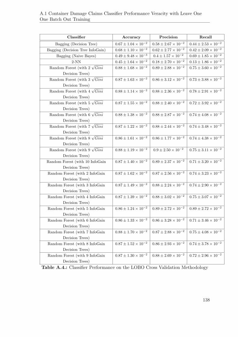
A.1 Container Damage Claims Classifier Performance Veracity with Leave OneOne Batch Out Training
Classifier Accuracy Precision RecallBagging (Decision Tree) 0.67± 1.04× 10⁻² 0.58± 2.67× 10⁻² 0.44± 2.53× 10⁻²
Bagging (Decision Tree InfoGain) 0.68± 1.10× 10⁻² 0.62± 2.77× 10⁻² 0.42± 2.09× 10⁻²
Bagging (Naive Bayes) 0.49± 9.48× 10⁻³ 0.4± 1.57× 10⁻² 0.69± 1.85× 10⁻²
2-NN 0.45± 1.64× 10⁻² 0.18± 2.70× 10⁻² 0.13± 1.86× 10⁻²
Random Forest (with 2√
Gini
Decision Trees)0.88± 1.68× 10⁻² 0.89± 2.88× 10⁻² 0.75± 3.60× 10⁻²
Random Forest (with 3√
Gini
Decision Trees)0.87± 1.63× 10⁻² 0.86± 3.12× 10⁻² 0.73± 3.88× 10⁻²
Random Forest (with 4√
Gini
Decision Trees)0.88± 1.14× 10⁻² 0.88± 2.36× 10⁻² 0.78± 2.91× 10⁻²
Random Forest (with 5√
Gini
Decision Trees)0.87± 1.55× 10⁻² 0.88± 2.40× 10⁻² 0.72± 3.92× 10⁻²
Random Forest (with 6√
Gini
Decision Trees)0.88± 1.38× 10⁻² 0.88± 2.87× 10⁻² 0.74± 4.08× 10⁻²
Random Forest (with 7√
Gini
Decision Trees)0.87± 1.22× 10⁻² 0.88± 2.44× 10⁻² 0.74± 3.48× 10⁻²
Random Forest (with 8√
Gini
Decision Trees)0.86± 1.61× 10⁻² 0.86± 1.77× 10⁻² 0.74± 4.38× 10⁻²
Random Forest (with 9√
Gini
Decision Trees)0.88± 1.19× 10⁻² 0.9± 2.50× 10⁻² 0.75± 3.11× 10⁻²
Random Forest (with 10 InfoGainDecision Trees)
0.87± 1.40× 10⁻² 0.89± 2.37× 10⁻² 0.71± 3.20× 10⁻²
Random Forest (with 2 InfoGainDecision Trees)
0.87± 1.62× 10⁻² 0.87± 2.56× 10⁻² 0.74± 3.23× 10⁻²
Random Forest (with 3 InfoGainDecision Trees)
0.87± 1.49× 10⁻² 0.88± 2.24× 10⁻² 0.74± 2.90× 10⁻²
Random Forest (with 4 InfoGainDecision Trees)
0.87± 1.39× 10⁻² 0.88± 3.02× 10⁻² 0.75± 3.07× 10⁻²
Random Forest (with 5 InfoGainDecision Trees)
0.86± 1.24× 10⁻² 0.89± 2.72× 10⁻² 0.89± 2.72× 10⁻²
Random Forest (with 6 InfoGainDecision Trees)
0.86± 1.33× 10⁻² 0.86± 3.28× 10⁻² 0.71± 3.46× 10⁻²
Random Forest (with 7 InfoGainDecision Trees)
0.88± 1.70× 10⁻² 0.87± 2.88× 10⁻² 0.75± 4.08× 10⁻²
Random Forest (with 8 InfoGainDecision Trees)
0.87± 1.52× 10⁻² 0.86± 2.93× 10⁻² 0.74± 3.78× 10⁻²
Random Forest (with 9 InfoGainDecision Trees)
0.87± 1.30× 10⁻² 0.88± 2.69× 10⁻² 0.72± 2.96× 10⁻²
Table A.4.: Classifier Performance on the LOBO Cross Validation Methodology
138

B. Approval from the Research
Ethics Board of the University of
Ottawa
139

FINAL REPORT Research project
As stipulated in Article 6.14 of the Tri-Council Policy Statement (TCPS 2), researchers must provide a final report for projects that have been approved by the Research Ethics Board (REB). The REB must therefore receive the information requested in this form in order to close all REB-approved files. Name of Principal Investigator (or Supervisor): (Note: If this is a student project, indicate your supervisor’s name) Address (Include building name and room number):
Department/School: EECS Faculty:Engineering E-mail: Phone: Fax:
Co-investigators and students (4th year, Master’s or Doctoral levels) Name: Department/School: EECS Address: Faculty:
Engineering E-mail: Phone: Fax:
Name: Department/School: Address: Faculty:
E-mail: Phone: Fax:
Have any team members left or been added to the research team? Yes No
If yes, please provide their names, their role in the project and their contact information (for a new member of the research team). Preferred language of correspondence: French English
Ethics File number: H06-17-05
Title of the research project: Assessing the Causes of Shipping Container Claims
Initial date of approval: July 13, 2017
Date of renewal(s) (if applicable): N/A
Did you receive funding? Yes No
Approval from the Research Ethics Board of the University of Ottawa
140

Email: a.caPhone: ( x: (613) 562-5338
Notice of Collection of Personal Information : Your personal information is collected under the authority of the University of Ottawa Act and is indented to be used for the purpose of and those consistent with the administration and the evaluation of the eligibility of your project for ethics approval. If you have any questions regarding this collection of personal information, please contact us by telephone at or by email at
Approval from the Research Ethics Board of the University of Ottawa
141

C. Survey Questions to Maritime
Domain Experts
This section presents all the questions posed to domain experts, regarding maritime
port operations.
142
8/14/2019 Bottlenecks in Port Operations
https://docs.google.com/forms/d/19QeWOvsMnOQW1mAny2BYtiCChPixbekLs256EkbCnp0/edit 1/13
Bottlenecks in Port OperationsGreetings,
My name is Ashwin Panchapakesan and I am a Ph.D. candidate at the University of Ottawa. My work
(under the supervision of Dr. Emil Petriu and Dr. Rami Abielmona) focuses on the Process Refinement
aspects of Data Fusion, and optimization in general.
My work entails predicting container damage classification in Canadian maritime ports, for which I
require knowledge from domain experts such as yourself.
Please rest assured that all your responses are kept confidential (by means of encrypted data storage
solutions) and will not be shared with third parties. Any publications resulting from data acquired by this
survey will also anonymize yourself and your company.
If it becomes necessary to publish identifying information, that will not be done without first getting your
written consent.
I am also willing to sign any Non-Disclosure Agreements (NDAs) that you may deem necessary for data
sharing.
This survey should take no more than 30 minutes to complete.
Should you feel the need to do so, you may withdraw from the survey at any point, without any
repercussions.
The ethical aspects of this research project have been approved by Research Ethics Board at the
University of Ottawa. They may be contacted at 613-562-5387 or by email at should
you wish to do so, for any reason.
As previously mentioned, my research is performed under the supervision of Dr. Emil Petriu and Dr.
Rami Abielmona. Their affiliations and contact information are listed below:
PhD Thesis Supervisor
Professor, University of Ottawa
School of Electrical Engineering and Computer Science
email:
website:
PhD Thesis Co-Supervisor
V.P. Larus Technologies
Ottawa
email:
As a direct consequence of filling out this survey, there are no relevant, foreseeable risks that you may
be unaware of, that need to be addressed
Please rest assured that all your responses are kept confidential (by means of encrypted data storage
solutions) and will not be shared with third parties
Please note that due to the anonymous nature of this survey, it will be impossible to withdraw data after
submission, unless identifying contact information is also provided
Please print and/or save a copy of this consent form for your records
* Required
Survey Questions to Maritime Domain Experts
143

8/14/2019 Bottlenecks in Port Operations
https://docs.google.com/forms/d/19QeWOvsMnOQW1mAny2BYtiCChPixbekLs256EkbCnp0/edit 2/13
1. Do you consent to completing this survey, and would you like to take the survey? *Mark only one oval.
Yes Skip to question 2.
No Stop filling out this form.
Bottlenecks in Port OperationsShipping containers are packed at the port of embarkment and are loaded onto container ships which
bring them to your port. A ship’s voyage may encounter rough seas and other perils that threaten the
safety and fidelity of not only the shipping containers, but also the contents therein. When the shipping
container is finally taken to the customer’s distribution center, the customer may notice damage sustained
by the container and file an intent to claim to your company. At this point, it falls on you to determine
whether the damage to the container was sustained while the container was in your custody, or
elsewhere.
The investigation required to make this determination is an involved process, as it requires the collation of
security video footage of the container as it moved through the premises of your storage yard, and various
personnel logs including the various handlers and supervisors who came into contact with this container
during this time.
2. How strongly would you agree with the above statement?Mark only one oval.
Strongly disagree
Disagree
Neutral
Agree
Strongly agree
Not Applicable
Bottlenecks in Port OperationsIn order to expedite the process of investigating such claims, it may help to note that containers with
certain properties (such as the commercial value of the container’s contents, the port of origin, etc) are
more likely to be claimed. Please indicate the relevance of such properties.
If you are unsure about any of these questions, please simply ignore them
3. Who the customer isMark only one oval.
Not relevant at all
Somewhat relevant
Extremely relevant
Not Applicable
4. The commercial value of goods in containerMark only one oval.
Not relevant at all
Somewhat relevant
Extremely relevant
Not Applicable
Survey Questions to Maritime Domain Experts
144

8/14/2019 Bottlenecks in Port Operations
https://docs.google.com/forms/d/19QeWOvsMnOQW1mAny2BYtiCChPixbekLs256EkbCnp0/edit 3/13
5. The port of originMark only one oval.
Not relevant at all
Somewhat relevant
Extremely relevant
Not Applicable
6. The shipping lineMark only one oval.
Not relevant at all
Somewhat relevant
Extremely relevant
Not Applicable
7. The weather at the port of originMark only one oval.
Not relevant at all
Somewhat relevant
Extremely relevant
Not Applicable
8. The weather and sea state along the ship's voyage to your portMark only one oval.
Not relevant at all
Somewhat relevant
Extremely relevant
Not Applicable
9. The fragility of the goods in the shipping containerMark only one oval.
Not relevant at all
Somewhat relevant
Extremely relevant
Not Applicable
10. The season (fall/winter/spring/summer) when the container was packedMark only one oval.
Not relevant at all
Somewhat relevant
Extremely relevant
Not Applicable
Survey Questions to Maritime Domain Experts
145

8/14/2019 Bottlenecks in Port Operations
https://docs.google.com/forms/d/19QeWOvsMnOQW1mAny2BYtiCChPixbekLs256EkbCnp0/edit 4/13
11. The season (fall/winter/spring/summer) when the container was loaded onto the shipMark only one oval.
Not relevant at all
Somewhat relevant
Extremely relevant
Not Applicable
12. The amount of time the container spent in your storage yard before it was picked up fordelivery to the customer (at their distribution center, warehouse, etc)Mark only one oval.
Not relevant at all
Somewhat relevant
Extremely relevant
Not Applicable
13. The presence of hazardous material in the containerMark only one oval.
Not relevant at all
Somewhat relevant
Extremely relevant
Not Applicable
14. The trucking company that picked up the container from your storage yard and delivered it tothe customerMark only one oval.
Not relevant at all
Somewhat relevant
Extremely relevant
Not Applicable
15. Are there any other properties that you feel I may have missed?Mark only one oval.
Yes Skip to question 16.
No Skip to question 19.
Additional Properties
16. Please list a property of a container that makesit more likely to be claimed
Survey Questions to Maritime Domain Experts
146

8/14/2019 Bottlenecks in Port Operations
https://docs.google.com/forms/d/19QeWOvsMnOQW1mAny2BYtiCChPixbekLs256EkbCnp0/edit 5/13
17. Please indicate the relevance of this propertyMark only one oval.
Not relevant at all
Somewhat relevant
Extremely relevant
18. Would you like to list another property?Mark only one oval.
Yes Skip to question 16.
No Skip to question 19.
Prediction Accuracy
19. Given the relevance of these properties in inducing shipping container damage claims, do youtry to predict which containers may be damaged (and therefore claimed) before the claim issubmitted to you?Mark only one oval.
Yes Skip to question 20.
No Skip to question 24.
Prediction AccuracyYou had indicated that you try to predict which containers may be damaged (and therefore claimed)
before the claim is submitted to you.
20. How accurate are your predictions?Mark only one oval.
We do not predict
0-25% accurate
25-50% accurate
50-75% accurate
75-100% accurate
Not Applicable
21. How long (in person hours) on average wouldyou say it takes for a human operator to gatherall the relevant data about a claim BEFORE theclaim is made by the customer?
22. How long (in person hours) on average wouldyou say it takes for a human operator to gatherall the relevant data about a claim AFTER theclaim is made by the customer?
Survey Questions to Maritime Domain Experts
147

8/14/2019 Bottlenecks in Port Operations
https://docs.google.com/forms/d/19QeWOvsMnOQW1mAny2BYtiCChPixbekLs256EkbCnp0/edit 6/13
23. How long (in person hours) on average wouldyou say it takes for all the relevant data abouta claim to be collected, collated and analyzed,before a decision is made?
Information CollectionWhen a claim does occur, the collection and collation of the necessary information (security video footage,
personnel logs, etc) are the longest and most involved processes, causing a bottleneck in the decision-
making process.
24. How strongly would you agree with this statement?Mark only one oval.
Strongly disagree
Somewhat disagree
Neither agree nor disagree
Somewhat agree
Strongly agree
Not Applicable
FantuzzisDo you use Fantuzzis or similar equipment (forklifts with spreaders) within the port?
25. Do you use Fantuzzis or similar equipment (forklifts with spreaders) within the port?Mark only one oval.
Yes Skip to question 26.
No Skip to question 29.
Fantuzzi QuestionsYou had indicated that you use Fantuzzis or similar equipment in your terminal
26. How many operators for such equipment aretypically working at your terminal at any givenpoint in time?
27. Would you agree that there is a correlation between claims for damaged containers and theoperators of the Fantuzzi equipment that handled such containers?Mark only one oval.
Yes Skip to question 28.
No Skip to question 29.
Fantuzzi CorrelationYou had indicated that there is a correlation between claims for damaged containers and the operators of
the Fantuzzi equipment that handled such containers.
Survey Questions to Maritime Domain Experts
148

8/14/2019 Bottlenecks in Port Operations
https://docs.google.com/forms/d/19QeWOvsMnOQW1mAny2BYtiCChPixbekLs256EkbCnp0/edit 7/13
28. Please indicate the strength and the direction of this correlationMark only one oval.
An increase in the number of containers handled by a given Fantuzzi operator often results in
a decrease in the number damaged/claimed containers transported by that shipping line
An increase in the number of containers handled by a given Fantuzzi operator sometimes
results in a decrease in the number damaged/claimed containers transported by that shipping line
An increase in the number of containers handled by a given Fantuzzi operator results in no
significant/noticeable increase or decrease in the number damaged/claimed containers transported
by that shipping line
An increase in the number of containers handled by a given Fantuzzi operator sometimes
results in an increase in the number damaged/claimed containers transported by that shipping line
An increase in the number of containers handled by a given Fantuzzi operator often results in
an increase in the number damaged/claimed containers transported by that shipping line
Shipping Lines
29. How strongly would you agree with the claim that there is a correlation between shipping linesand container damage/claims (i.e. a shipping line whose containers are more likely to beclaimed for damage)?Mark only one oval.
Strongly disagree Skip to question 36.
Somewhat disagree Skip to question 36.
Neither agree nor disagree Skip to question 36.
Somewhat agree Skip to question 30.
Strongly agree Skip to question 30.
Not Applicable Skip to question 36.
Shipping line correlationYou had indicated that there is a correlation between shipping lines and container damage/claims
30. Please indicate the strength and direction of this correlationMark only one oval.
An increase in the number of containers transported by a given shipping line often results in a
decrease in the number damaged/claimed containers transported by that shipping line
An increase in the number of containers transported by a given shipping line sometimes
results in a decrease in the number damaged/claimed containers transported by that shipping line
An increase in the number of containers transported by a given shipping line results in no
significant/noticeable increase or decrease in the number damaged/claimed containers transported
by that shipping line
An increase in the number of containers transported by a given shipping line sometimes
results in an increase in the number damaged/claimed containers transported by that shipping line
An increase in the number of containers transported by a given shipping line often results in
an increase in the number damaged/claimed containers transported by that shipping line
Survey Questions to Maritime Domain Experts
149
8/14/2019 Bottlenecks in Port Operations
https://docs.google.com/forms/d/19QeWOvsMnOQW1mAny2BYtiCChPixbekLs256EkbCnp0/edit 8/13
31. Please indicate which shipping lines have strong negative correlations in this respect
32. Please indicate which shipping lines have weak negative correlations in this respect
33. Please indicate which shipping lines have neutral correlations in this respect
34. Please indicate which shipping lines have weak positive correlations in this respect
35. Please indicate which shipping lines have strong positive correlations in this respect
Trucking Companies
Survey Questions to Maritime Domain Experts
150

8/14/2019 Bottlenecks in Port Operations
https://docs.google.com/forms/d/19QeWOvsMnOQW1mAny2BYtiCChPixbekLs256EkbCnp0/edit 9/13
36. How strongly would you agree with the claim that there is a correlation between truckingcompanies and container damage/claims (i.e. a trucking company whose containers are morelikely to be claimed for damage)?Mark only one oval.
Strongly disagree Skip to question 38.
Disagree Skip to question 38.
Neutral Skip to question 38.
Agree Skip to question 37.
Strongly agree Skip to question 37.
Not Applicable Skip to question 38.
Trucking Company CorrelationYou had indicated that there is a correlation between trucking companies and container damage/claims
(i.e. a trucking company whose containers are more likely to be claimed for damage)
37. Please indicate the strength and direction of this correlationMark only one oval.
An increase in the number of containers transported by a given trucking company often
results in a decrease in the number damaged/claimed containers transported by that trucking
company
An increase in the number of containers transported by a given trucking company sometimes
results in a decrease in the number damaged/claimed containers transported by that trucking
company
An increase in the number of containers transported by a given trucking company results in no
significant/noticeable increase or decrease in the number damaged/claimed containers transported
by that trucking company
An increase in the number of containers transported by a given trucking company sometimes
results in an increase in the number damaged/claimed containers transported by that trucking
company
An increase in the number of containers transported by a given trucking company often
results in an increase in the number damaged/claimed containers transported by that trucking
company
Cargo Types
38. How strongly would you agree with the claim that there is a correlation between cargo typesand container damage/claims (i.e. containers holding a certain type of cargo, say farmequipment, are more likely to be claimed for damage)?Mark only one oval.
Strongly disagree Skip to question 40.
Disagree Skip to question 40.
Neutral Skip to question 40.
Agree Skip to question 39.
Strongly agree Skip to question 39.
Not Applicable Skip to question 40.
Cargo Types Correlation
Survey Questions to Maritime Domain Experts
151

8/14/2019 Bottlenecks in Port Operations
https://docs.google.com/forms/d/19QeWOvsMnOQW1mAny2BYtiCChPixbekLs256EkbCnp0/edit 10/13
You had indicated that there is a correlation between cargo types and container damage/claims (i.e.
containers holding a certain type of cargo, say farm equipment, are more likely to be claimed for
damage).
39. Please elaborate on which cargo types tend to be associated with a higher probability ofcontainer damage/claims.
Gantry Crane
40. How strongly would you agree with the claim that there is a correlation between the ship-to-shore gantry crane operator and container damage/claims (i.e. containers handled by aspecific gantry crane operator are more likely to be claimed for damage)?Mark only one oval.
Strongly disagree Skip to question 42.
Disagree Skip to question 42.
Neutral Skip to question 42.
Agree Skip to question 41.
Strongly agree Skip to question 41.
Not Applicable Skip to question 42.
Gantry Crane CorrelationYou had indicated that there is a correlation between the ship-to-shore gantry crane operator and
container damage/claims (i.e. containers handled by a specific gantry crane operator are more likely to be
claimed for damage).
41. Please indicate the strength and direction of this correlationMark only one oval.
An increase in the number of containers transported by a given gantry crane operator often
results in a decrease in the number damaged/claimed containers transported by that gantry crane
operator
An increase in the number of containers transported by a given gantry crane operator
sometimes results in a decrease in the number damaged/claimed containers transported by that
gantry crane operator
An increase in the number of containers transported by a given gantry crane operator results
in no significant/noticeable increase or decrease in the number damaged/claimed containers
transported by that gantry crane operator
An increase in the number of containers transported by a given gantry crane operator
sometimes results in an increase in the number damaged/claimed containers transported by that
gantry crane operator
An increase in the number of containers transported by a given gantry crane operator often
results in an increase in the number damaged/claimed containers transported by that gantry crane
operator
Survey Questions to Maritime Domain Experts
152
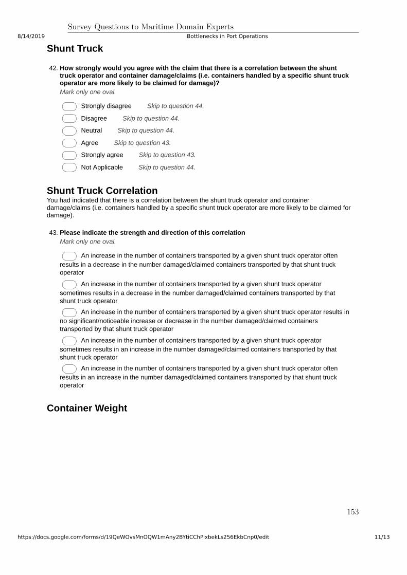
8/14/2019 Bottlenecks in Port Operations
https://docs.google.com/forms/d/19QeWOvsMnOQW1mAny2BYtiCChPixbekLs256EkbCnp0/edit 11/13
Shunt Truck
42. How strongly would you agree with the claim that there is a correlation between the shunttruck operator and container damage/claims (i.e. containers handled by a specific shunt truckoperator are more likely to be claimed for damage)?Mark only one oval.
Strongly disagree Skip to question 44.
Disagree Skip to question 44.
Neutral Skip to question 44.
Agree Skip to question 43.
Strongly agree Skip to question 43.
Not Applicable Skip to question 44.
Shunt Truck CorrelationYou had indicated that there is a correlation between the shunt truck operator and container
damage/claims (i.e. containers handled by a specific shunt truck operator are more likely to be claimed for
damage).
43. Please indicate the strength and direction of this correlationMark only one oval.
An increase in the number of containers transported by a given shunt truck operator often
results in a decrease in the number damaged/claimed containers transported by that shunt truck
operator
An increase in the number of containers transported by a given shunt truck operator
sometimes results in a decrease in the number damaged/claimed containers transported by that
shunt truck operator
An increase in the number of containers transported by a given shunt truck operator results in
no significant/noticeable increase or decrease in the number damaged/claimed containers
transported by that shunt truck operator
An increase in the number of containers transported by a given shunt truck operator
sometimes results in an increase in the number damaged/claimed containers transported by that
shunt truck operator
An increase in the number of containers transported by a given shunt truck operator often
results in an increase in the number damaged/claimed containers transported by that shunt truck
operator
Container Weight
Survey Questions to Maritime Domain Experts
153

8/14/2019 Bottlenecks in Port Operations
https://docs.google.com/forms/d/19QeWOvsMnOQW1mAny2BYtiCChPixbekLs256EkbCnp0/edit 12/13
44. How strongly would you agree with the claim that there is a correlation between the weight ofthe container (including the weight of the cargo it contains) and container damage/claims (i.e.containers that fall within certain weight ranges are more likely to be claimed for damage)?Mark only one oval.
Strongly disagree Skip to question 46.
Somewhat disagree Skip to question 46.
Neither agree nor disagree Skip to question 46.
Somewhat agree Skip to question 45.
Strongly Agree Skip to question 45.
Not Applicable Skip to question 46.
Container Weight CorrelationYou had indicated that there is a correlation between the weight of the container (including the weight of
the cargo it contains) and container damage/claims (i.e. containers that fall within certain weight ranges
are more likely to be claimed for damage).
45. please elaborate on which weight ranges tend to be associated with a higher probability ofcontainer damage/claims.
Ship Piloting Procedure
46. When a ship encounters a wave while at sea, is there a recommended or conventionalprocedure describing the angle at which the ship should approach the wave? I.e. should italways travel parallel/perpendicular to the wave, or should it always approach the wave at a 45degree angle? or should it change its approach angle based on the height of the wave, andthe size and the weight of the ship?
Additional CommentsPlease leave any additional comments that you feel may help me out
Contact
Survey Questions to Maritime Domain Experts
154

8/14/2019 Bottlenecks in Port Operations
https://docs.google.com/forms/d/19QeWOvsMnOQW1mAny2BYtiCChPixbekLs256EkbCnp0/edit 13/13
Powered by
47. May I contact you for additional clarifications on your responses in this survey?Mark only one oval.
Yes Skip to question 48.
No Skip to "Thank You."
Contact Information
48. Please provide information about how you'd prefer to be contacted
Thank YouThank you for taking the time to answer the survey. I really do appreciate it
Survey Questions to Maritime Domain Experts
155