Planck pre-launch status: Low Frequency Instrument calibration and expected scientific performance
19
arXiv:1001.4562v1 [astro-ph.IM] 25 Jan 2010 Astronomy & Astrophysics manuscript no. lfi˙instrument˙calibration c ESO 2010 January 25, 2010 Planck pre-launch status: Low Frequency Instrument calibration and expected scientific performance A. Mennella 1 , M. Bersanelli 1 , R. C. Butler 2 , F. Cuttaia 2 , O. D’Arcangelo 3 , R. J. Davis 4 , M. Frailis 5 , S. Galeotta 5 , A. Gregorio 6 , C. R. Lawrence 7 , R. Leonardi 8 , S. R. Lowe 4 , N. Mandolesi 2 , M. Maris 5 , P. Meinhold 8 , L. Mendes 9 , G. Morgante 2 , M. Sandri 2 , L. Stringhetti 2 , L. Terenzi 2 , M. Tomasi 1 , L. Valenziano 2 , F. Villa 2 , A. Zacchei 5 , A. Zonca 10 , M. Balasini 11 , C. Franceschet 1 , P. Battaglia 11 , P. M. Lapolla 11 , P. Leutenegger 11 , M. Miccolis 11 , L. Pagan 11 , R. Silvestri 11 , B. Aja 12 , E. Artal 12 , G. Baldan 11 , P. Bastia 11 , T. Bernardino 13 , L. Boschini 11 , G. Cafagna 11 , B. Cappellini 10 , F. Cavaliere 1 , F. Colombo 11 , L. de La Fuente 12 , J. Edgeley 4 , M. C. Falvella 14 , F. Ferrari 11 , S. Fogliani 5 , E. Franceschi 2 , T. Gaier 7 , F. Gomez 15 , J. M. Herreros 15 , S. Hildebrandt 15 , R. Hoyland 15 , N. Hughes 16 , P. Jukkala 16 , D. Kettle 4 , M. Laaninen 17 , D. Lawson 4 , P. Leahy 4 , S. Levin 15 , P. B. Lilje 18 , D. Maino 1 , M. Malaspina 2 , P. Manzato 5 , J. Marti-Canales 19 , E. Martinez-Gonzalez 13 , A. Mediavilla 12 , F. Pasian 5 , J. P. Pascual 12 , M. Pecora 11 , L. Peres-Cuevas 20 , P. Platania 3 , M. Pospieszalsky 21 , T. Poutanen 22,23,24 , R. Rebolo 16 , N. Roddis 4 , M. Salmon 13 , M. Seiffert 7 , A. Simonetto 3 , C. Sozzi 3 , J. Tauber 20 , J. Tuovinen 25 , J. Varis 25 , A. Wilkinson 4 , and F. Winder 4 (Affiliations can be found after the references) ABSTRACT We give the calibration and scientific performance parameters of the Planck Low Frequency Instrument (LFI) measured during the ground cryogenic test campaign. These parameters characterise the instrument response and constitute our best pre-launch knowledge of the LFI scientific performance. The LFI shows excellent 1/f stability and rejection of instrumental systematic effects; measured noise performance shows that LFI is the most sensitive instrument of its kind. The set of measured calibration parameters will be updated during flight operations through the end of the mission. Key words. Cosmic Microwave Baground, Cosmology, Space Instrumentation, Coherent Receivers, Calibration and Testing 1. Introduction The Low Frequency Instrument (LFI) is an array of 22 coherent differential receivers at 30, 44, and 70 GHz on board the European Space Agency Planck 1 satel- lite. In 15 months 2 of continuous measurements from the Lagrangian point L 2 Planck will provide cosmic- variance- and foreground-limited measurements of the Cosmic Microwave Background temperature anisotropies by scanning the sky in near great circles with a 1.5 m dual reflector aplanatic telescope (Tauber 2009; Martin et al. 2004; Villa et al. 2002; Dupac & Tauber 2005). The LFI shares the focal plane of the Planck telescope with the High Frequency Instrument (HFI), an array of 52 bolometers in the 100–857GHz range, cooled to 0.1 K. This wide frequency coverage, required for optimal com- ponent separation, constitutes a unique feature of Planck and a formidable technological challenge, with the integra- Send offprint requests to : Aniello Mennella 1 Planck (http://www.esa.int/Planck) is a project of the European Space Agency - ESA - with instruments provided by two scientific Consortia funded by ESA member states (in par- ticular the lead countries: France and Italy) with contributions from NASA (USA), and telescope reflectors provided in a col- laboration between ESA and a scientific Consortium led and funded by Denmark. 2 There are enough consumables on board to allow operation for an additional year. tion of two different technologies with different cryogenic requirements in the same focal plane. Excellent noise performance is obtained with receivers based on indium phosphide high electron mobility transis- tor amplifiers, cryogenically cooled to 20 K by a vibration- less hydrogen sorption cooler, which provides more than 1 W of cooling power at 20 K. The LFI thermal design has been driven by an optimisation of receiver sensitivity and available cooling power; in particular radio frequency (RF) amplification is divided between a 20 K front-end unit and a ∼300 K back-end unit connected by composite waveguides (Bersanelli et al. 2009). The LFI has been developed following a modular ap- proach in which the various sub-units (passive components, receiver active components, electronics, etc.) have been built and tested individually before proceding to the next integration step. The final integration and testing phases have been the assembly, verification, and calibration of the individual radiometer chains (Villa et al. 2009) and of the integrated instrument. In this paper we focus on calibration, i.e., the set of parameters that provides our current best knowledge of the instrument’s scientific performance. After an overview of the calibration philosophy we focus on the main calibration parameters measured during test campaigns performed at instrument and satellite levels. Information concerning the test setup and data analysis methods is provided where
-
Upload
independent -
Category
Documents
-
view
2 -
download
0
Transcript of Planck pre-launch status: Low Frequency Instrument calibration and expected scientific performance
arX
iv:1
001.
4562
v1 [
astr
o-ph
.IM
] 2
5 Ja
n 20
10Astronomy & Astrophysics manuscript no. lfi˙instrument˙calibration c© ESO 2010January 25, 2010
Planck pre-launch status: Low Frequency Instrument calibration
and expected scientific performance
A. Mennella1, M. Bersanelli1, R. C. Butler2, F. Cuttaia2, O. D’Arcangelo3, R. J. Davis4, M. Frailis5, S.Galeotta5 , A. Gregorio6, C. R. Lawrence7, R. Leonardi8, S. R. Lowe4, N. Mandolesi2, M. Maris5, P.
Meinhold8, L. Mendes9, G. Morgante2, M. Sandri2, L. Stringhetti2, L. Terenzi2, M. Tomasi1, L. Valenziano2,F. Villa2, A. Zacchei5, A. Zonca10, M. Balasini11, C. Franceschet1, P. Battaglia11 , P. M. Lapolla11, P.
Leutenegger11, M. Miccolis11, L. Pagan11, R. Silvestri11, B. Aja12, E. Artal12, G. Baldan11, P. Bastia11, T.Bernardino13, L. Boschini11, G. Cafagna11, B. Cappellini10, F. Cavaliere1, F. Colombo11, L. de La Fuente12,
J. Edgeley4, M. C. Falvella14 , F. Ferrari11, S. Fogliani5, E. Franceschi2, T. Gaier7, F. Gomez15, J. M.Herreros15, S. Hildebrandt15, R. Hoyland15, N. Hughes16, P. Jukkala16, D. Kettle4, M. Laaninen17, D.
Lawson4, P. Leahy4, S. Levin15, P. B. Lilje18, D. Maino1, M. Malaspina2, P. Manzato5, J. Marti-Canales19, E.Martinez-Gonzalez13 , A. Mediavilla12, F. Pasian5, J. P. Pascual12, M. Pecora11, L. Peres-Cuevas20, P.
Platania3, M. Pospieszalsky21, T. Poutanen22,23,24, R. Rebolo16, N. Roddis4, M. Salmon13, M. Seiffert7, A.Simonetto3, C. Sozzi3, J. Tauber20, J. Tuovinen25, J. Varis25, A. Wilkinson4, and F. Winder4
(Affiliations can be found after the references)
ABSTRACT
We give the calibration and scientific performance parameters of the Planck Low Frequency Instrument (LFI) measured duringthe ground cryogenic test campaign. These parameters characterise the instrument response and constitute our best pre-launchknowledge of the LFI scientific performance. The LFI shows excellent 1/f stability and rejection of instrumental systematic effects;measured noise performance shows that LFI is the most sensitive instrument of its kind. The set of measured calibration parameterswill be updated during flight operations through the end of the mission.
Key words. Cosmic Microwave Baground, Cosmology, Space Instrumentation, Coherent Receivers, Calibration and Testing
1. Introduction
The Low Frequency Instrument (LFI) is an array of22 coherent differential receivers at 30, 44, and 70GHzon board the European Space Agency Planck1 satel-lite. In 15 months2 of continuous measurements fromthe Lagrangian point L2 Planck will provide cosmic-variance- and foreground-limited measurements of theCosmic Microwave Background temperature anisotropiesby scanning the sky in near great circles with a 1.5m dualreflector aplanatic telescope (Tauber 2009; Martin et al.2004; Villa et al. 2002; Dupac & Tauber 2005).
The LFI shares the focal plane of the Planck telescopewith the High Frequency Instrument (HFI), an array of52 bolometers in the 100–857GHz range, cooled to 0.1K.This wide frequency coverage, required for optimal com-ponent separation, constitutes a unique feature of Planckand a formidable technological challenge, with the integra-
Send offprint requests to: Aniello Mennella1 Planck (http://www.esa.int/Planck) is a project of the
European Space Agency - ESA - with instruments provided bytwo scientific Consortia funded by ESA member states (in par-ticular the lead countries: France and Italy) with contributionsfrom NASA (USA), and telescope reflectors provided in a col-laboration between ESA and a scientific Consortium led andfunded by Denmark.
2 There are enough consumables on board to allow operationfor an additional year.
tion of two different technologies with different cryogenicrequirements in the same focal plane.
Excellent noise performance is obtained with receiversbased on indium phosphide high electron mobility transis-tor amplifiers, cryogenically cooled to 20K by a vibration-less hydrogen sorption cooler, which provides more than1W of cooling power at 20K. The LFI thermal design hasbeen driven by an optimisation of receiver sensitivity andavailable cooling power; in particular radio frequency (RF)amplification is divided between a 20K front-end unit and a∼300K back-end unit connected by composite waveguides(Bersanelli et al. 2009).
The LFI has been developed following a modular ap-proach in which the various sub-units (passive components,receiver active components, electronics, etc.) have beenbuilt and tested individually before proceding to the nextintegration step. The final integration and testing phaseshave been the assembly, verification, and calibration of theindividual radiometer chains (Villa et al. 2009) and of theintegrated instrument.
In this paper we focus on calibration, i.e., the set ofparameters that provides our current best knowledge of theinstrument’s scientific performance. After an overview ofthe calibration philosophy we focus on the main calibrationparameters measured during test campaigns performed atinstrument and satellite levels. Information concerning thetest setup and data analysis methods is provided where
2 A. Mennella et al: LFI calibration and expected performance
necessary, with references to appropriate technical articlesfor further details. The companion article that describes theLFI instrument (Bersanelli et al. 2009) is the most centralreference for this paper.
The naming convention that we use for receivers andindividual channels is given in Appendix A.
2. Overview of the LFI pseudo correlation
architecture
In this section we briefly summarise the LFI pseudo-correlation architecture. Further details and a more com-plete treatment of the instrument can be found inBersanelli et al. (2009).
In the LFI each receiver couples with the Planck tele-scope secondary mirror via a corrugated feed horn feed-ing an orthomode transducer (OMT) that splits the in-coming wave into two perpendicularly polarised compo-nents, which propagate through two independent pseudocorrelation receivers with HEMT (High Electron MobilityTransistor) amplifiers split between a cold (∼20 K) and awarm (∼300 K) stage connected by composite waveguides.
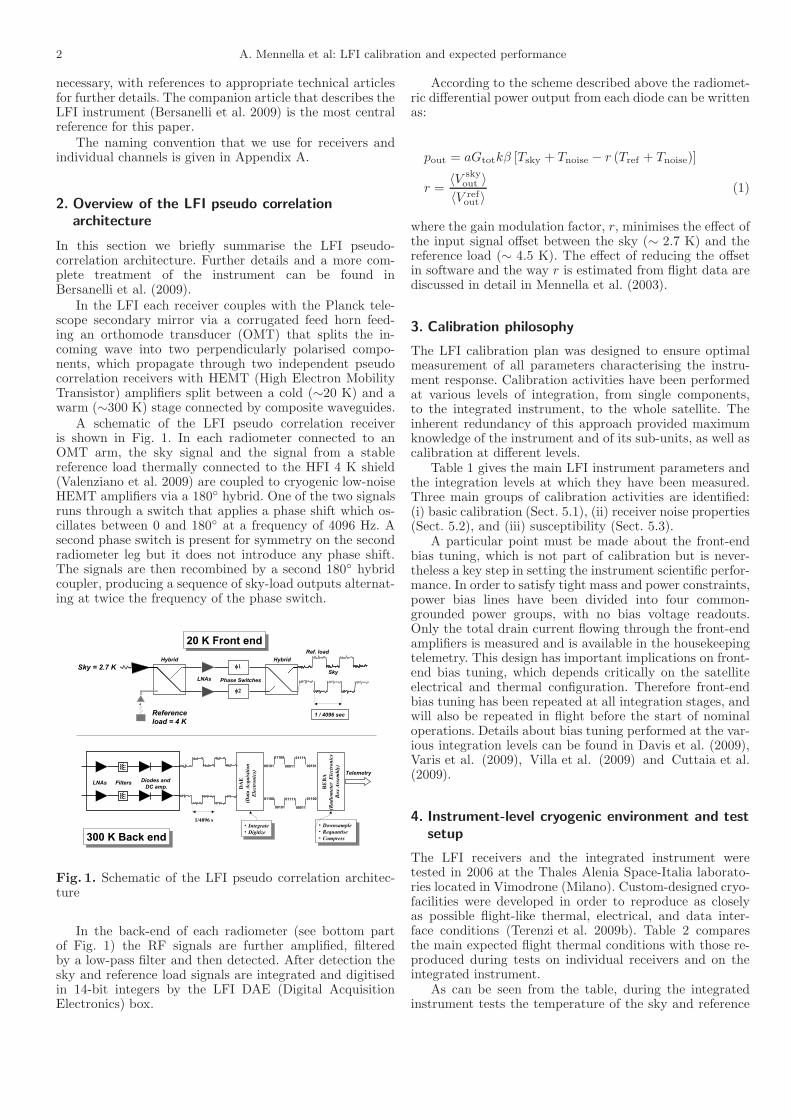
A schematic of the LFI pseudo correlation receiveris shown in Fig. 1. In each radiometer connected to anOMT arm, the sky signal and the signal from a stablereference load thermally connected to the HFI 4 K shield(Valenziano et al. 2009) are coupled to cryogenic low-noiseHEMT amplifiers via a 180◦ hybrid. One of the two signalsruns through a switch that applies a phase shift which os-cillates between 0 and 180◦ at a frequency of 4096 Hz. Asecond phase switch is present for symmetry on the secondradiometer leg but it does not introduce any phase shift.The signals are then recombined by a second 180◦ hybridcoupler, producing a sequence of sky-load outputs alternat-ing at twice the frequency of the phase switch.
Fig. 1. Schematic of the LFI pseudo correlation architec-ture
In the back-end of each radiometer (see bottom partof Fig. 1) the RF signals are further amplified, filteredby a low-pass filter and then detected. After detection thesky and reference load signals are integrated and digitisedin 14-bit integers by the LFI DAE (Digital AcquisitionElectronics) box.
According to the scheme described above the radiomet-ric differential power output from each diode can be writtenas:
pout = aGtotkβ [Tsky + Tnoise − r (Tref + Tnoise)]
r =〈V sky
out 〉〈V ref
out〉(1)
where the gain modulation factor, r, minimises the effect ofthe input signal offset between the sky (∼ 2.7 K) and thereference load (∼ 4.5 K). The effect of reducing the offsetin software and the way r is estimated from flight data arediscussed in detail in Mennella et al. (2003).
3. Calibration philosophy
The LFI calibration plan was designed to ensure optimalmeasurement of all parameters characterising the instru-ment response. Calibration activities have been performedat various levels of integration, from single components,to the integrated instrument, to the whole satellite. Theinherent redundancy of this approach provided maximumknowledge of the instrument and of its sub-units, as well ascalibration at different levels.
Table 1 gives the main LFI instrument parameters andthe integration levels at which they have been measured.Three main groups of calibration activities are identified:(i) basic calibration (Sect. 5.1), (ii) receiver noise properties(Sect. 5.2), and (iii) susceptibility (Sect. 5.3).
A particular point must be made about the front-endbias tuning, which is not part of calibration but is never-theless a key step in setting the instrument scientific perfor-mance. In order to satisfy tight mass and power constraints,power bias lines have been divided into four common-grounded power groups, with no bias voltage readouts.Only the total drain current flowing through the front-endamplifiers is measured and is available in the housekeepingtelemetry. This design has important implications on front-end bias tuning, which depends critically on the satelliteelectrical and thermal configuration. Therefore front-endbias tuning has been repeated at all integration stages, andwill also be repeated in flight before the start of nominaloperations. Details about bias tuning performed at the var-ious integration levels can be found in Davis et al. (2009),Varis et al. (2009), Villa et al. (2009) and Cuttaia et al.(2009).
4. Instrument-level cryogenic environment and test
setup
The LFI receivers and the integrated instrument weretested in 2006 at the Thales Alenia Space-Italia laborato-ries located in Vimodrone (Milano). Custom-designed cryo-facilities were developed in order to reproduce as closelyas possible flight-like thermal, electrical, and data inter-face conditions (Terenzi et al. 2009b). Table 2 comparesthe main expected flight thermal conditions with those re-produced during tests on individual receivers and on theintegrated instrument.
As can be seen from the table, during the integratedinstrument tests the temperature of the sky and reference
A. Mennella et al: LFI calibration and expected performance 3
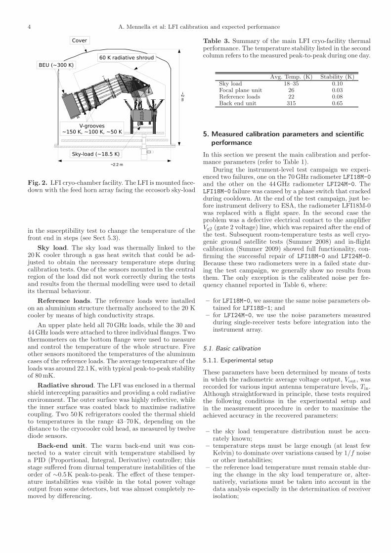
Table 1. Main instrument parameters and stages at which they have been / will be measured. In bodface we highlightcalibration parameters defining the instrument scientific performance that are discussed in this paper.
Category Parameters Additional Individual Integrated Satellite In flightReference radiometers instrument
Bias tuning Front-end ampli-fiers
Cuttaia et al.(2009)
Y Y Y Y
Phase switches Cuttaia et al.(2009)
Y Y Y Y
Calibration
Basic calibra-tion
Photometriccalibration
Villa et al. (2009) Y Y Y Y
Linearity Mennella et al.(2009)
Y Y N N
Isolation Villa et al. (2009) Y Y N N
In-band response Zonca et al.(2009)
Y N N N
Noise perfor-mance
White noise Meinhold et al.(2009)
Y Y Y Y
Knee fre-quency
Meinhold et al.(2009)
Y Y Y Y
1/f slope Meinhold et al.(2009)
Y Y Y Y
Susceptibility Front-end tem-perature fluc-tuations
Terenzi et al.(2009c)
Y Y Y Y
Back-end temper-ature fluctuations
Y Y N N
Front-end biasfluctuations
Y Y N N
Table 2. Summary of main thermal conditions in flightand in the various testing facilities.
Temperatures Flight Receiver Instr.Sky ∼ 3 K & 8 K & 18.5 KRef. ∼ 4.5 K & 8 K & 18.5 KFront-end ∼ 20 K ∼ 20 K ∼ 26 KBack-end ∼ 300 K ∼ 300 K ∼ 300 K
loads was much higher than expected in flight (18.5K vs. 3–4.5K). To compensate for this, receiver-level tests wereconducted with the sky and reference loads at two tem-peratures, one near flight, the other near 20K (Villa et al.2009). During the instrument-level tests, parameters depen-dent on the sky and reference load temperatures (such asthe white noise sensitivity and the photometric calibrationconstant) could be extrapolated to flight conditions.
4.1. Thermal setup
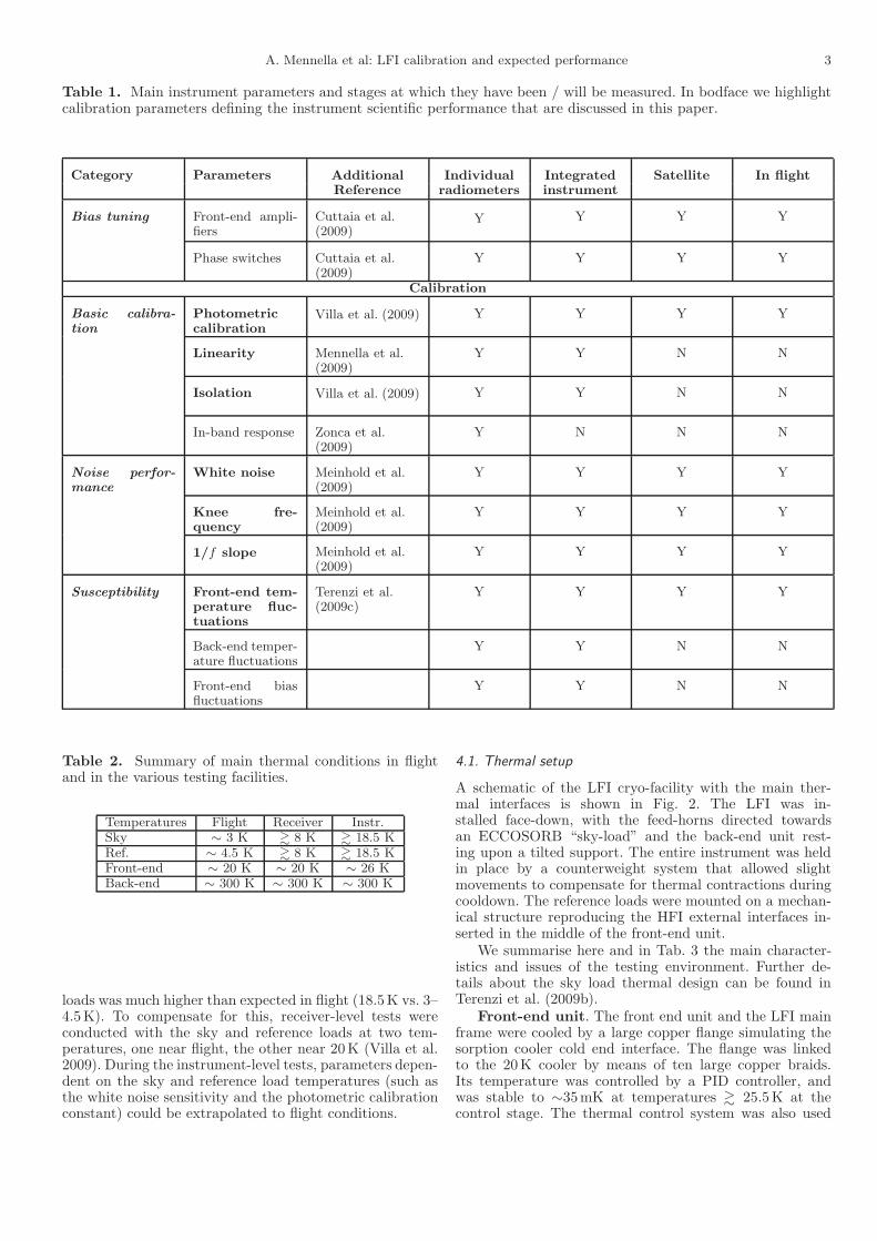
A schematic of the LFI cryo-facility with the main ther-mal interfaces is shown in Fig. 2. The LFI was in-stalled face-down, with the feed-horns directed towardsan ECCOSORB “sky-load” and the back-end unit rest-ing upon a tilted support. The entire instrument was heldin place by a counterweight system that allowed slightmovements to compensate for thermal contractions duringcooldown. The reference loads were mounted on a mechan-ical structure reproducing the HFI external interfaces in-serted in the middle of the front-end unit.
We summarise here and in Tab. 3 the main character-istics and issues of the testing environment. Further de-tails about the sky load thermal design can be found inTerenzi et al. (2009b).
Front-end unit. The front end unit and the LFI mainframe were cooled by a large copper flange simulating thesorption cooler cold end interface. The flange was linkedto the 20K cooler by means of ten large copper braids.Its temperature was controlled by a PID controller, andwas stable to ∼35mK at temperatures & 25.5K at thecontrol stage. The thermal control system was also used
4 A. Mennella et al: LFI calibration and expected performance
Fig. 2. LFI cryo-chamber facility. The LFI is mounted face-down with the feed horn array facing the eccosorb sky-load
in the susceptibility test to change the temperature of thefront end in steps (see Sect 5.3).
Sky load. The sky load was thermally linked to the20K cooler through a gas heat switch that could be ad-justed to obtain the necessary temperature steps duringcalibration tests. One of the sensors mounted in the centralregion of the load did not work correctly during the testsand results from the thermal modelling were used to detailits thermal behaviour.
Reference loads. The reference loads were installedon an aluminium structure thermally anchored to the 20 Kcooler by means of high conductivity straps.
An upper plate held all 70GHz loads, while the 30 and44GHz loads were attached to three individual flanges. Twothermometers on the bottom flange were used to measureand control the temperature of the whole structure. Fiveother sensors monitored the temperatures of the aluminumcases of the reference loads. The average temperature of theloads was around 22.1K, with typical peak-to-peak stabilityof 80mK.
Radiative shroud. The LFI was enclosed in a thermalshield intercepting parasitics and providing a cold radiativeenvironment. The outer surface was highly reflective, whilethe inner surface was coated black to maximise radiativecoupling. Two 50K refrigerators cooled the thermal shieldto temperatures in the range 43–70K, depending on thedistance to the cryocooler cold head, as measured by twelvediode sensors.
Back-end unit. The warm back-end unit was con-nected to a water circuit with temperature stabilised bya PID (Proportional, Integral, Derivative) controller; thisstage suffered from diurnal temperature instabilities of theorder of ∼0.5K peak-to-peak. The effect of these temper-ature instabilities was visible in the total power voltageoutput from some detectors, but was almost completely re-moved by differencing.
Table 3. Summary of the main LFI cryo-facility thermalperformance. The temperature stability listed in the secondcolumn refers to the measured peak-to-peak during one day.
Avg. Temp. (K) Stability (K)Sky load 18–35 0.10Focal plane unit 26 0.03Reference loads 22 0.08Back end unit 315 0.65
5. Measured calibration parameters and scientific
performance
In this section we present the main calibration and perfor-mance parameters (refer to Table 1).
During the instrument-level test campaign we experi-enced two failures, one on the 70GHz radiometer LFI18M-0and the other on the 44GHz radiometer LFI24M-0. TheLFI18M-0 failure was caused by a phase switch that crackedduring cooldown. At the end of the test campaign, just be-fore instrument delivery to ESA, the radiometer LFI18M-0was replaced with a flight spare. In the second case theproblem was a defective electrical contact to the amplifierVg2 (gate 2 voltage) line, which was repaired after the end ofthe test. Subsequent room-temperature tests as well cryo-genic ground satellite tests (Summer 2008) and in-flightcalibration (Summer 2009) showed full functionality, con-firming the successful repair of LFI18M-0 and LFI24M-0.Because these two radiometers were in a failed state dur-ing the test campaign, we generally show no results fromthem. The only exception is the calibrated noise per fre-quency channel reported in Table 6, where:
– for LFI18M-0, we assume the same noise parameters ob-tained for LFI18S-1; and
– for LFI24M-0, we use the noise parameters measuredduring single-receiver tests before integration into theinstrument array.
5.1. Basic calibration
5.1.1. Experimental setup
These parameters have been determined by means of testsin which the radiometric average voltage output, Vout, wasrecorded for various input antenna temperature levels, Tin.Although straightforward in principle, these tests requiredthe following conditions in the experimental setup andin the measurement procedure in order to maximise theachieved accuracy in the recovered parameters:
– the sky load temperature distribution must be accu-rately known;
– temperature steps must be large enough (at least fewKelvin) to dominate over variations caused by 1/f noiseor other instabilities;
– the reference load temperature must remain stable dur-ing the change in the sky load temperature or, alter-natively, variations must be taken into account in thedata analysis especially in the determination of receiverisolation;
A. Mennella et al: LFI calibration and expected performance 5
– data points must be acquired at multiple input tem-peratures to increase accuracy in estimating responselinearity.
These conditions were all met during receiver-level testsin which several steps were obtained over a temperaturespan ranging from ∼8 K to ∼30 K and where the sky-load temperature distrubution was very well known bothexperimentally and from thermal modelling (Terenzi et al.2009a; Villa et al. 2009).
On the other hand, during instrument-level tests theseconditions were not as well-met:
– the total number of available temperature controllersallowed us to place only three sensors on the sky load,one on the back metal plate, one on the side, and one onthe tip of the central pyramid. The input temperaturewas then determined using the measurements from thesethree sensors in a dedicated thermal model of the skyload itself;
– the minimum and maximum temperatures that couldbe set without impacting the focal plane and referenceload temperatures were 17.5K and 30K, half the rangeobtained during receiver-level tests;
– the time needed to change the sky load temperature fewkelvin was large, of the order of several hours, because ofits large thermal mass. This limited to three the numberof temperature steps that could be performed in theavailable time.
The reduced temperature range and number of discretetemperatures that could be set precluded determination ofthe linearity factor. which was therefore excluded from thefit and constrained to ±1% around the value found duringcalibration of individual receivers (see Sect. 5.1.2).3
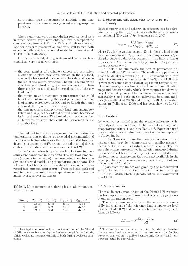
Table 4 summarises temperatures for the three temper-ature steps considered in these tests. The sky load tempera-ture (antenna temperature), has been determined from thesky load thermal model using temperature sensor data. Thereference load temperature is a direct measurement con-verted into antenna temperature. Front-end and back-endunit temperatures are direct temperature sensor measure-ments averaged over all sensors.
Table 4. Main temperatures during basic calibration tem-perature steps.
Step # Tsky(K) Tref (K) TFEU (K) TBEU (C)1 22.05 22.34 26.40 37.532 28.96 22.20 26.45 37.483 32.91 22.32 26.40 37.67
3 The slight compression found in the output of the 30 and44GHz receivers is caused by the back-end amplifier and diode,which worked at the same conditions both during both test cam-paigns.
5.1.2. Photometric calibration, noise temperature andlinearity
Noise temperatures and calibration constants can be calcu-lated by fitting the Vout(Tsky) data with the most represen-tative model (Daywitt 1989; Mennella et al. 2009):
Vout =G0(Tsky + Tnoise)
1 + bG0(Tsky + Tnoise)(2)
where Vout is the voltage output, Tsky is the sky load inputantenna temperature, Tnoise is the noise temperature, G0 isthe photometric calibration constant in the limit of linearresponse, and b is the nonlinearity parameter. For perfectlylinear receivers b = 0.
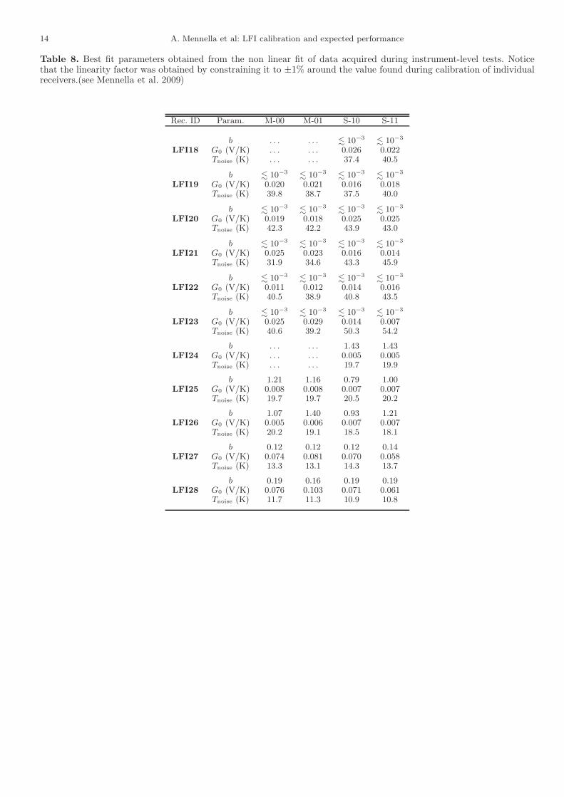
In Table 8 we summarise the best-fit parameters ob-tained for all the LFI detectors. The nonlinearity parameterb for the 70GHz receivers is . 10−3, consistent with zerowithin the measurement uncertainty. The 30 and 44GHz re-ceivers show some compression at high input temperatures.This nonlinearity arises from the back-end RF amplificationstage and detector diode, which show compression down tovery low input powers. The nonlinear response has beenthoroughly tested both on the individual back end mod-ules (Mennella et al. 2009) and during the RCA calibrationcampaign (Villa et al. 2009) and has been shown to fit wellEq. (2).
5.1.3. Isolation
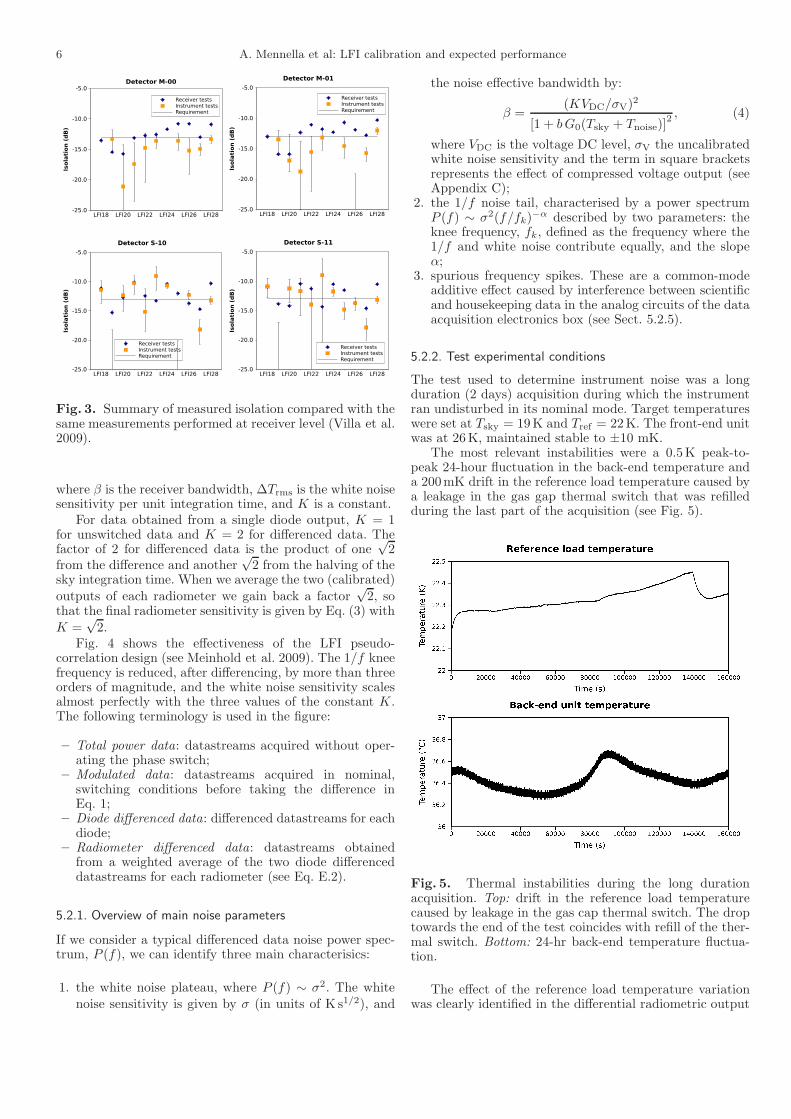
Isolation was estimated from the average radiometer volt-age outputs, Vsky and Vref , at the two extreme sky loadtemperatures (Steps 1 and 3 in Table 4)4. Equations usedto calculate isolation values and uncertainties are reportedin Appendix B.
In Fig. 3 we summarise the measured isolation for alldetectors and provide a comparison with similar measure-ments performed on individual receiver chains. The re-sults show large uncertainties in isolation measured duringinstrument-level tests, caused by 1/f noise instabilities inthe total power datastreams that were not negligible in thetime span between the various temperature steps that wasof the order of few days.
Apart from the limitations given by the measurementsetup, the results show that isolation lies in the range−10dB to −20 dB, which is globally within the requirementof −13 dB.
5.2. Noise properties
The pseudo-correlation design of the Planck-LFI receivershas been optimised to minimise the effects of 1/f gain vari-ations in the radiometers.
The white noise sensitivity of the receivers is essen-tially independent of the reference load temperature level(Seiffert et al. 2002) and can be written, in its most generalform, as follows:
∆Trms = KTsky + Tnoise√
β(3)
4 The test can be conducted, in principle, also by changingthe reference load temperature. In the instrument cryofacility,however, this was not possible because only the sky load tem-perature could be controlled.
6 A. Mennella et al: LFI calibration and expected performance
Detector M-00
LFI18 LFI20 LFI22 LFI24 LFI26 LFI28-25.0
-20.0
-15.0
-10.0
-5.0
Isola
tio
n (
dB
)
Receiver testsInstrument testsRequirement
Detector M-01
LFI18 LFI20 LFI22 LFI24 LFI26 LFI28-25.0
-20.0
-15.0
-10.0
-5.0
Isola
tio
n (
dB
)
Receiver testsInstrument testsRequirement
Detector S-10
LFI18 LFI20 LFI22 LFI24 LFI26 LFI28-25.0
-20.0
-15.0
-10.0
-5.0
Isola
tio
n (
dB
)
Receiver testsInstrument testsRequirement
Detector S-11
LFI18 LFI20 LFI22 LFI24 LFI26 LFI28-25.0
-20.0
-15.0
-10.0
-5.0
Isola
tio
n (
dB
)
Receiver testsInstrument testsRequirement
Fig. 3. Summary of measured isolation compared with thesame measurements performed at receiver level (Villa et al.2009).
where β is the receiver bandwidth, ∆Trms is the white noisesensitivity per unit integration time, and K is a constant.
For data obtained from a single diode output, K = 1for unswitched data and K = 2 for differenced data. Thefactor of 2 for differenced data is the product of one
√2
from the difference and another√2 from the halving of the
sky integration time. When we average the two (calibrated)
outputs of each radiometer we gain back a factor√2, so
that the final radiometer sensitivity is given by Eq. (3) with
K =√2.
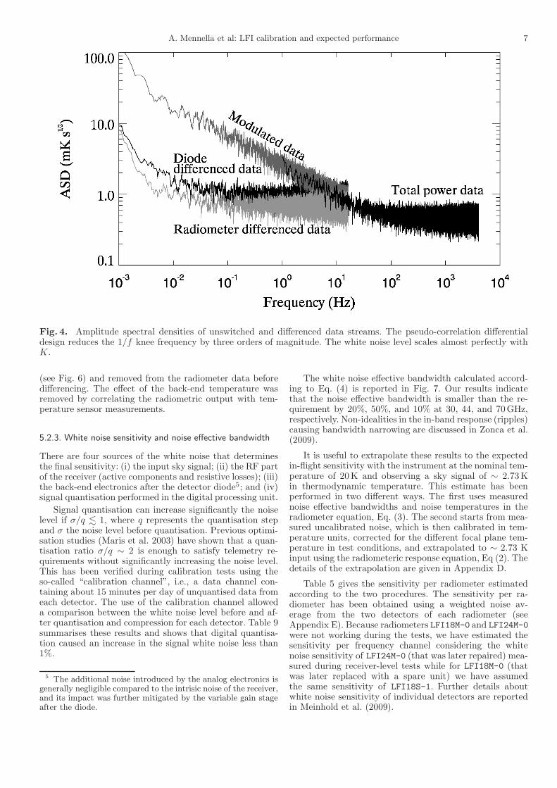
Fig. 4 shows the effectiveness of the LFI pseudo-correlation design (see Meinhold et al. 2009). The 1/f kneefrequency is reduced, after differencing, by more than threeorders of magnitude, and the white noise sensitivity scalesalmost perfectly with the three values of the constant K.The following terminology is used in the figure:
– Total power data: datastreams acquired without oper-ating the phase switch;
– Modulated data: datastreams acquired in nominal,switching conditions before taking the difference inEq. 1;
– Diode differenced data: differenced datastreams for eachdiode;
– Radiometer differenced data: datastreams obtainedfrom a weighted average of the two diode differenceddatastreams for each radiometer (see Eq. E.2).
5.2.1. Overview of main noise parameters
If we consider a typical differenced data noise power spec-trum, P (f), we can identify three main characterisics:
1. the white noise plateau, where P (f) ∼ σ2. The whitenoise sensitivity is given by σ (in units of K s1/2), and
the noise effective bandwidth by:
β =(KVDC/σV)
2
[1 + bG0(Tsky + Tnoise)]2 , (4)
where VDC is the voltage DC level, σV the uncalibratedwhite noise sensitivity and the term in square bracketsrepresents the effect of compressed voltage output (seeAppendix C);
2. the 1/f noise tail, characterised by a power spectrumP (f) ∼ σ2(f/fk)
−α described by two parameters: theknee frequency, fk, defined as the frequency where the1/f and white noise contribute equally, and the slopeα;
3. spurious frequency spikes. These are a common-modeadditive effect caused by interference between scientificand housekeeping data in the analog circuits of the dataacquisition electronics box (see Sect. 5.2.5).
5.2.2. Test experimental conditions
The test used to determine instrument noise was a longduration (2 days) acquisition during which the instrumentran undisturbed in its nominal mode. Target temperatureswere set at Tsky = 19K and Tref = 22K. The front-end unitwas at 26K, maintained stable to ±10 mK.
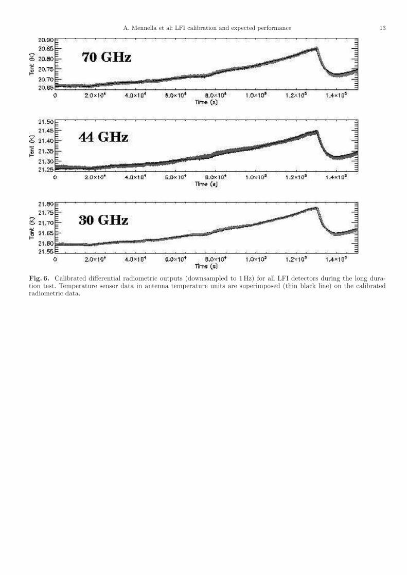
The most relevant instabilities were a 0.5K peak-to-peak 24-hour fluctuation in the back-end temperature anda 200mK drift in the reference load temperature caused bya leakage in the gas gap thermal switch that was refilledduring the last part of the acquisition (see Fig. 5).
Fig. 5. Thermal instabilities during the long durationacquisition. Top: drift in the reference load temperaturecaused by leakage in the gas cap thermal switch. The droptowards the end of the test coincides with refill of the ther-mal switch. Bottom: 24-hr back-end temperature fluctua-tion.
The effect of the reference load temperature variationwas clearly identified in the differential radiometric output
A. Mennella et al: LFI calibration and expected performance 7
Fig. 4. Amplitude spectral densities of unswitched and differenced data streams. The pseudo-correlation differentialdesign reduces the 1/f knee frequency by three orders of magnitude. The white noise level scales almost perfectly withK.
(see Fig. 6) and removed from the radiometer data beforedifferencing. The effect of the back-end temperature wasremoved by correlating the radiometric output with tem-perature sensor measurements.
5.2.3. White noise sensitivity and noise effective bandwidth
There are four sources of the white noise that determinesthe final sensitivity: (i) the input sky signal; (ii) the RF partof the receiver (active components and resistive losses); (iii)the back-end electronics after the detector diode5; and (iv)signal quantisation performed in the digital processing unit.
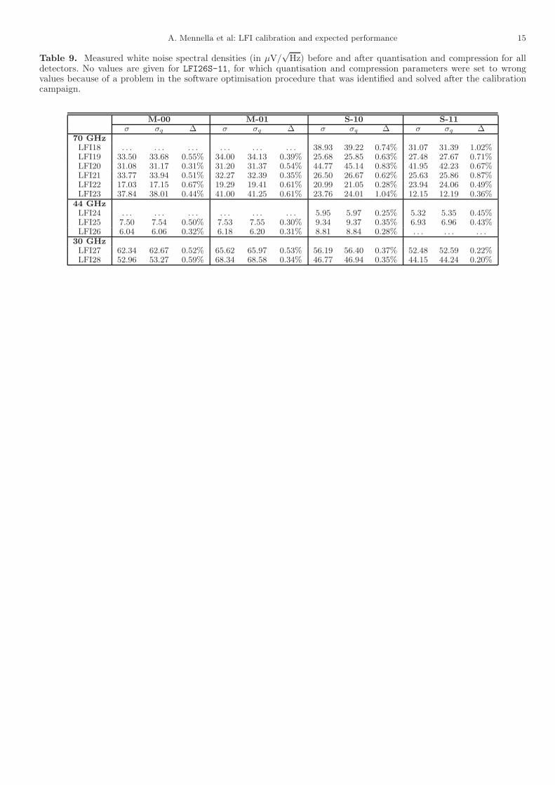
Signal quantisation can increase significantly the noiselevel if σ/q . 1, where q represents the quantisation stepand σ the noise level before quantisation. Previous optimi-sation studies (Maris et al. 2003) have shown that a quan-tisation ratio σ/q ∼ 2 is enough to satisfy telemetry re-quirements without significantly increasing the noise level.This has been verified during calibration tests using theso-called “calibration channel”, i.e., a data channel con-taining about 15 minutes per day of unquantised data fromeach detector. The use of the calibration channel alloweda comparison between the white noise level before and af-ter quantisation and compression for each detector. Table 9summarises these results and shows that digital quantisa-tion caused an increase in the signal white noise less than1%.
5 The additional noise introduced by the analog electronics isgenerally negligible compared to the intrisic noise of the receiver,and its impact was further mitigated by the variable gain stageafter the diode.
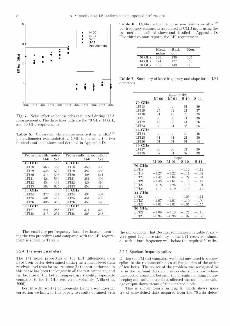
The white noise effective bandwidth calculated accord-ing to Eq. (4) is reported in Fig. 7. Our results indicatethat the noise effective bandwidth is smaller than the re-quirement by 20%, 50%, and 10% at 30, 44, and 70GHz,respectively. Non-idealities in the in-band response (ripples)causing bandwidth narrowing are discussed in Zonca et al.(2009).
It is useful to extrapolate these results to the expectedin-flight sensitivity with the instrument at the nominal tem-perature of 20K and observing a sky signal of ∼ 2.73Kin thermodynamic temperature. This estimate has beenperformed in two different ways. The first uses measurednoise effective bandwidths and noise temperatures in theradiometer equation, Eq. (3). The second starts from mea-sured uncalibrated noise, which is then calibrated in tem-perature units, corrected for the different focal plane tem-perature in test conditions, and extrapolated to ∼ 2.73 Kinput using the radiometeric response equation, Eq (2). Thedetails of the extrapolation are given in Appendix D.
Table 5 gives the sensitivity per radiometer estimatedaccording to the two procedures. The sensitivity per ra-diometer has been obtained using a weighted noise av-erage from the two detectors of each radiometer (seeAppendix E). Because radiometers LFI18M-0 and LFI24M-0
were not working during the tests, we have estimated thesensitivity per frequency channel considering the whitenoise sensitivity of LFI24M-0 (that was later repaired) mea-sured during receiver-level tests while for LFI18M-0 (thatwas later replaced with a spare unit) we have assumedthe same sensitivity of LFI18S-1. Further details aboutwhite noise sensitivity of individual detectors are reportedin Meinhold et al. (2009).
8 A. Mennella et al: LFI calibration and expected performance
LFI18 LFI19 LFI20 LFI21 LFI22 LFI23 LFI24 LFI25 LFI26 LFI27 LFI280
5
10
15
20
Eff
bw
(G
Hz)
M-00M-01S-10S-11Requirement
Fig. 7. Noise effective bandwidths calculated during RAAmeasurements. The three lines indicate the 70 GHz, 44 GHzand 30 GHz requirements.
Table 5. Calibrated white noise sensitivities in µKs1/2
per radiometer extrapolated at CMB input using the twomethods outlined above and detailed in Appendix D.
From uncalib. noiseM-0 S-1
70 GHzLFI18 468 468LFI19 546 522LFI20 574 593LFI21 424 530LFI22 454 463LFI23 502 63544 GHzLFI24 372 447LFI25 501 492LFI26 398 39230 GHzLFI27 241 288LFI28 315 251
From radiom. equationM-0 S-1
70 GHzLFI18 450 450LFI19 482 466LFI20 498 511LFI21 381 496LFI22 428 410LFI23 453 41944 GHzLFI24 404 407LFI25 451 462LFI26 455 42830 GHzLFI27 311 320LFI28 305 268
The sensitivity per frequency channel estimated accord-ing the two procedures and compared with the LFI require-ment is shown in Table 6.
5.2.4. 1/f noise parameters
The 1/f noise properties of the LFI differenced datahave been better determined during instrument-level thanreceiver-level tests for two reasons: (i) the test performed inthis phase has been the longest in all the test campaign, and(ii) because of the better temperature stability, especiallycompared to the 70 GHz receivers cryofacility (Villa et al.2009).
best fit with two 1/f components. Being a second-ordercorrection we limit, in this paper, to results obtained with
Table 6. Calibrated white noise sensitivities in µKs1/2
per frequency channel extrapolated at CMB input using thetwo methods outlined above and detailed in Appendix D.The third column reports the LFI requirement.
Meas.noise
Rad.eq.
Req.
70 GHz 146 130 10544 GHz 174 177 11330 GHz 135 149 116
Table 7. Summary of knee frequency and slope for all LFIdetectors.
fknee (mHz)M-00 M-01 S-10 S-11
70 GHzLFI18 . . . . . . 61 59LFI19 25 32 27 37LFI20 21 19 23 28LFI21 28 30 41 38LFI22 46 39 41 76LFI23 30 31 58 7544 GHzLFI24 . . . . . . 39 46LFI25 31 31 21 30LFI26 61 61 61 1430 GHzLFI27 30 30 27 26LFI28 37 31 37 39
slopeM-00 M-01 S-10 S-11
70 GHzLFI18 . . . . . . −1.12 −1.12LFI19 −1.27 −1.22 −1.11 −1.02LFI20 −1.47 −1.64 −1.27 −1.24LFI21 −1.48 −1.61 −1.15 −1.17LFI22 −1.18 −1.26 −1.19 −1.01LFI23 −1.11 −1.19 −1.15 −1.1244 GHzLFI24 . . . . . . −1.06 −1.11LFI25 −1.07 −1.03 −1.10 −1.00LFI26 −1.01 −1.01 −1.05 −1.5530 GHzLFI27 −1.06 −1.13 −1.25 −1.13LFI28 −0.94 −0.93 −1.07 −1.06
the simple model that Results, summarised in Table 7, showvery good 1/f noise stability of the LFI receivers, almostall with a knee frequency well below the required 50mHz.
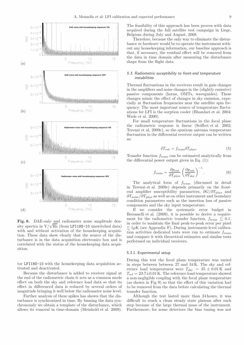
5.2.5. Spurious frequency spikes
During the FM test campaign we found unwanted frequencyspikes in the radiometeric data at frequencies of the orderof few hertz. The source of the problem was recognised tobe in the backend data acquisition electronics box, whereunexpected crosstalk between the circuits handling house-keeping and radiometric data affected the radiometer volt-age output downstream of the detector diode.
This is shown clearly in Fig. 8, which shows spec-tra of unswitched data acquired from the 70GHz detec-
A. Mennella et al: LFI calibration and expected performance 9
(a)
DAE noise with housekeeping sequencer ON
(b)
DAE noise with housekeeping sequencer OFF
(c)
Radiometer noise with housekeeping sequencer ON
(d)
Radiometer noise with housekeeping sequencer OFF
Fig. 8. DAE-only and radiometer noise amplitude den-sity spectra in V/
√Hz (from LFI18S-10 unswitched data)
with and without activation of the housekeeping acquisi-tion. These data show clearly that the source of the dis-turbance is in the data acquisition electronics box and iscorrelated with the status of the housekeeping data acqui-sition.
tor LFI18S-10 with the housekeeping data acquisition ac-tivated and deactivated.
Because the disturbance is added to receiver signal atthe end of the radiometric chain it acts as a common modeeffect on both the sky and reference load data so that itseffect in differenced data is reduced by several orders ofmagnitude bringing it well below the radiometer noise level.
Further analysis of these spikes has shown that the dis-turbance is synchronized in time. By binning the data syn-chronously we obtain a template of the disturbance, whichallows its removal in time-domain (Meinhold et al. 2009).
The feasibility of this approach has been proven with dataacquired during the full satellite test campaign in Liege,Belgium during July and August, 2008.
Therefore, because the only way to eliminate the distur-bance in hardware would be to operate the instrument with-out any housekeeping information, our baseline approach isthat, if necessary, the residual effect will be removed fromthe data in time domain after measuring the disturbanceshape from the flight data.
5.3. Radiometric suceptibility to front-end temperatureinstabilities
Thermal fluctuations in the receivers result in gain changesin the amplifiers and noise changes in the (slightly emissive)passive components (horns, OMTs, waveguides). Thesechanges mimic the effect of changes in sky emission, expe-cially at fluctuation frequencies near the satellite spin fre-quency. The most important source of temperature fluctu-ations for LFI is the sorption cooler (Bhandari et al. 2004;Wade et al. 2000).
For small temperature fluctuations in the focal planethe radiometric response is linear (Seiffert et al. 2002;Terenzi et al. 2009c), so the spurious antenna temperaturefluctuation in the differential receiver output can be writtenas:
δTout = ftransδTphys. (5)
Transfer function ftrans can be estimated analytically fromthe differential power output given in Eq. (1):
ftrans =∂pout∂Tphys
(
∂pout∂Tsky
)−1
. (6)
The analytical form of ftrans (discussed in detailin Terenzi et al. 2009c) depends primarily on the front-end amplifier susceptibility parameters, ∂G/∂Tphys and∂Tnoise/∂Tphys as well as on other instrument and boundarycondition parameters such as the insertion loss of passivecomponents and the sky input temperature.
If we consider the systematic error budget inBersanelli et al. (2009), it is possible to derive a require-ment for the radiometric transfer function, ftrans . 0.1,in order to maintain the final peak-to-peak error per pixel. 1µK (see Appendix F). During instrument-level calibra-tion activities dedicated tests were run to estimate ftransand compare it with theoretical estimates and similar testsperformed on individual receivers.
5.3.1. Experimental setup
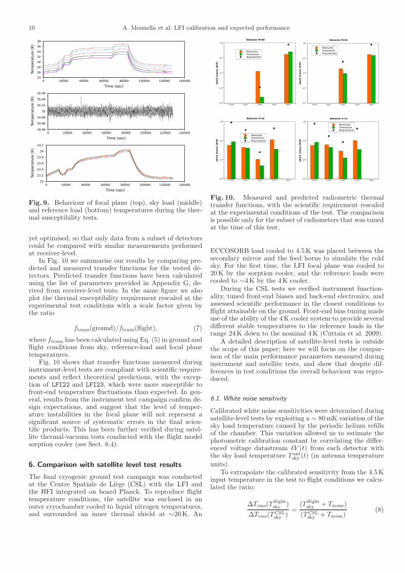
During this test the focal plane temperature was variedin steps between between 27 and 34K. The sky and ref-erence load temperatures were Tsky = 35 ± 0.01K andTref = 23.7±0.01K. The reference load temperature showeda non-negligible coupling with the focal plane temperature(as shown in Fig 9) so that the effect of this variation hadto be removed from the data before calculating the thermaltransfer function.
Although the test lasted more than 24 hours, it wasdifficult to reach a clean steady state plateau after eachstep because of the large thermal mass of the instrument.Furthermore, for some detectors the bias tuning was not
10 A. Mennella et al: LFI calibration and expected performance
0 20000 40000 60000 80000 100000 120000 140000
Time (sec)
24
26
28
30
32
34
36
38
Tem
pera
ture
(K
)
0 20000 40000 60000 80000 100000 120000 140000
Time (sec)
34.94
34.96
34.98
35
35.02
35.04
35.06
Tem
pera
ture
(K
)
0 20000 40000 60000 80000 100000 120000 140000
Time (sec)
23
23.2
23.4
23.6
23.8
24
24.2
Tem
pera
ture
(K
)
Fig. 9. Behaviour of focal plane (top), sky load (middle)and reference load (bottom) temperatures during the ther-mal susceptibility tests.
yet optimised, so that only data from a subset of detectorscould be compared with similar measurements performedat receiver-level.
In Fig. 10 we summarise our results by comparing pre-dicted and measured transfer functions for the tested de-tectors. Predicted transfer functions have been calculatedusing the list of parameters provided in Appendix G, de-rived from receiver-level tests. In the same figure we alsoplot the thermal susceptibility requirement rescaled at theexperimental test conditions with a scale factor given bythe ratio
ftrans(ground)/ftrans(flight), (7)
where ftrans has been calculated using Eq. (5) in ground andflight conditions from sky, reference-load and focal planetemperatures.
Fig. 10 shows that transfer functions measured duringinstrument-level tests are compliant with scientific require-ments and reflect theoretical predictions, with the excep-tion of LFI22 and LFI23, which were more susceptible tofront-end temperature fluctuations than expected. In gen-eral, results from the instrument test campaign confirm de-sign expectations, and suggest that the level of temper-ature instabilities in the focal plane will not represent asignificant source of systematic errors in the final scien-tific products. This has been further verified during satel-lite thermal-vacuum tests conducted with the flight modelsorption cooler (see Sect. 6.4).
6. Comparison with satellite level test results
The final cryogenic ground test campaign was conductedat the Centre Spatiale de Liege (CSL) with the LFI andthe HFI integrated on board Planck. To reproduce flighttemperature conditions, the satellite was enclosed in anouter cryochamber cooled to liquid nitrogen temperatures,and surrounded an inner thermal shield at ∼20K. An
LFI19 LFI21 LFI22 LFI23 LFI2710-4
10-3
10-2
10-1
100
ab
s(f
_tr
an
s)
(K/K
)
Detector M-00
MeasuredTheoreticalRequirement
LFI19 LFI21 LFI22 LFI23 LFI2710-4
10-3
10-2
10-1
100
ab
s(f
_tr
an
s)
(K/K
)
Detector M-01
MeasuredTheoreticalRequirement
LFI19 LFI21 LFI22 LFI23 LFI2710-3
10-2
10-1
100
ab
s(f
_tr
an
s)
(K/K
)
Detector S-10
MeasuredTheoreticalRequirement
LFI19 LFI21 LFI22 LFI23 LFI2710-3
10-2
10-1
100
ab
s(f
_tr
an
s)
(K/K
)
Detector S-11
MeasuredTheoreticalRequirement
Fig. 10. Measured and predicted radiometric thermaltransfer functions, with the scientific requirement rescaledat the experimental conditions of the test. The comparisonis possible only for the subset of radiometers that was tunedat the time of this test.
ECCOSORB load cooled to 4.5K was placed between thesecondary mirror and the feed horns to simulate the coldsky. For the first time, the LFI focal plane was cooled to20K by the sorption cooler, and the reference loads werecooled to ∼4K by the 4K cooler.
During the CSL tests we verified instrument function-ality, tuned front-end biases and back-end electronics, andassessed scientific performance in the closest conditions toflight attainable on the ground. Front-end bias tuning madeuse of the ability of the 4K cooler system to provide severaldifferent stable temperatures to the reference loads in therange 24K down to the nominal 4K (Cuttaia et al. 2009).
A detailed description of satellite-level tests is outsidethe scope of this paper; here we will focus on the compar-ison of the main performance parameters measured duringinstrument and satellite tests, and show that despite dif-ferences in test conditions the overall behaviour was repro-duced.
6.1. White noise sensitivity
Calibrated white noise sensitivities were determined duringsatellite-level tests by exploiting a ∼ 80mK variation of thesky load temperature caused by the periodic helium refillsof the chamber. This variation allowed us to estimate thephotometric calibration constant by correlating the differ-enced voltage datastream δV (t) from each detector withthe sky load temperature T ant
sky (t) (in antenna temperature
units).To extrapolate the calibrated sensitivity from the 4.5K
input temperature in the test to flight conditions we calcu-lated the ratio:
∆Trms(Tflightsky )
∆Trms(TCSLsky )
=(T flight
sky + Tnoise)
(TCSLsky + Tnoise)
(8)
A. Mennella et al: LFI calibration and expected performance 11
using the noise temperature found from the non-linearmodel fit from the receiver-level test campaign (Villa et al.2009). This ratio ranges from a minimum of ∼0.96 to amaximum of ∼0.98. Exact values for each detector are notreported here for simplicity.
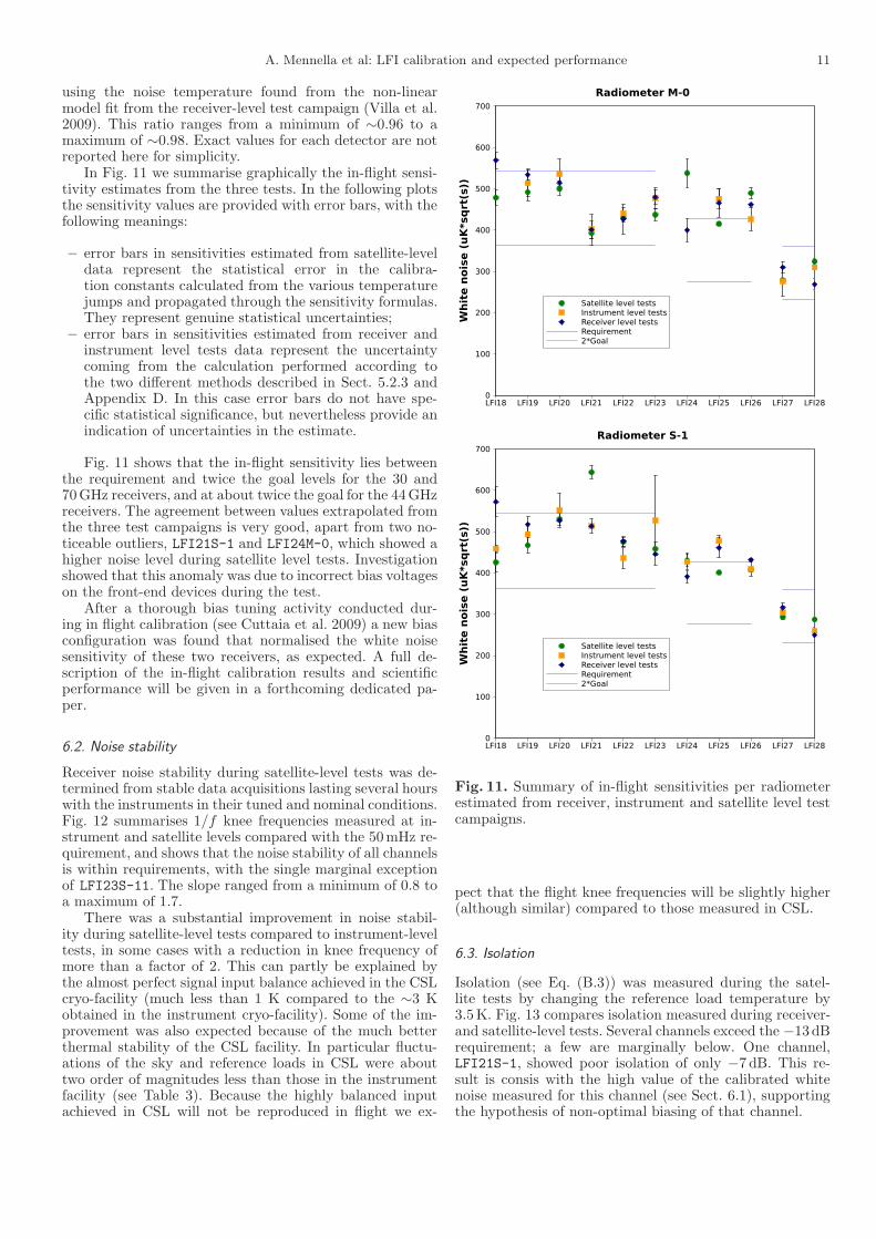
In Fig. 11 we summarise graphically the in-flight sensi-tivity estimates from the three tests. In the following plotsthe sensitivity values are provided with error bars, with thefollowing meanings:
– error bars in sensitivities estimated from satellite-leveldata represent the statistical error in the calibra-tion constants calculated from the various temperaturejumps and propagated through the sensitivity formulas.They represent genuine statistical uncertainties;
– error bars in sensitivities estimated from receiver andinstrument level tests data represent the uncertaintycoming from the calculation performed according tothe two different methods described in Sect. 5.2.3 andAppendix D. In this case error bars do not have spe-cific statistical significance, but nevertheless provide anindication of uncertainties in the estimate.
Fig. 11 shows that the in-flight sensitivity lies betweenthe requirement and twice the goal levels for the 30 and70GHz receivers, and at about twice the goal for the 44GHzreceivers. The agreement between values extrapolated fromthe three test campaigns is very good, apart from two no-ticeable outliers, LFI21S-1 and LFI24M-0, which showed ahigher noise level during satellite level tests. Investigationshowed that this anomaly was due to incorrect bias voltageson the front-end devices during the test.
After a thorough bias tuning activity conducted dur-ing in flight calibration (see Cuttaia et al. 2009) a new biasconfiguration was found that normalised the white noisesensitivity of these two receivers, as expected. A full de-scription of the in-flight calibration results and scientificperformance will be given in a forthcoming dedicated pa-per.
6.2. Noise stability
Receiver noise stability during satellite-level tests was de-termined from stable data acquisitions lasting several hourswith the instruments in their tuned and nominal conditions.Fig. 12 summarises 1/f knee frequencies measured at in-strument and satellite levels compared with the 50mHz re-quirement, and shows that the noise stability of all channelsis within requirements, with the single marginal exceptionof LFI23S-11. The slope ranged from a minimum of 0.8 toa maximum of 1.7.
There was a substantial improvement in noise stabil-ity during satellite-level tests compared to instrument-leveltests, in some cases with a reduction in knee frequency ofmore than a factor of 2. This can partly be explained bythe almost perfect signal input balance achieved in the CSLcryo-facility (much less than 1 K compared to the ∼3 Kobtained in the instrument cryo-facility). Some of the im-provement was also expected because of the much betterthermal stability of the CSL facility. In particular fluctu-ations of the sky and reference loads in CSL were abouttwo order of magnitudes less than those in the instrumentfacility (see Table 3). Because the highly balanced inputachieved in CSL will not be reproduced in flight we ex-
LFI18 LFI19 LFI20 LFI21 LFI22 LFI23 LFI24 LFI25 LFI26 LFI27 LFI280
100
200
300
400
500
600
700
Wh
ite n
ois
e (
uK
*sq
rt(
s))
Radiometer M-0
Satellite level testsInstrument level testsReceiver level testsRequirement2*Goal
LFI18 LFI19 LFI20 LFI21 LFI22 LFI23 LFI24 LFI25 LFI26 LFI27 LFI280
100
200
300
400
500
600
700
Wh
ite n
ois
e (
uK
*sq
rt(
s))
Radiometer S-1
Satellite level testsInstrument level testsReceiver level testsRequirement2*Goal
Fig. 11. Summary of in-flight sensitivities per radiometerestimated from receiver, instrument and satellite level testcampaigns.
pect that the flight knee frequencies will be slightly higher(although similar) compared to those measured in CSL.
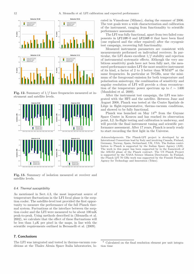
6.3. Isolation
Isolation (see Eq. (B.3)) was measured during the satel-lite tests by changing the reference load temperature by3.5K. Fig. 13 compares isolation measured during receiver-and satellite-level tests. Several channels exceed the −13dBrequirement; a few are marginally below. One channel,LFI21S-1, showed poor isolation of only −7 dB. This re-sult is consis with the high value of the calibrated whitenoise measured for this channel (see Sect. 6.1), supportingthe hypothesis of non-optimal biasing of that channel.
12 A. Mennella et al: LFI calibration and expected performance
LFI18 LFI19 LFI20 LFI21 LFI22 LFI23 LFI24 LFI25 LFI26 LFI27 LFI280
20
40
60
80
100
fk (
mH
z)
Detector M-00
Instrument testsSatellite testsReqirement
LFI18 LFI19 LFI20 LFI21 LFI22 LFI23 LFI24 LFI25 LFI26 LFI27 LFI280
20
40
60
80
100
fk (
mH
z)
Detector M-01
Instrument testsSatellite testsReqirement
LFI18 LFI19 LFI20 LFI21 LFI22 LFI23 LFI24 LFI25 LFI26 LFI27 LFI280
20
40
60
80
100
fk (
mH
z)
Detector S-10
Instrument testsSatellite testsReqirement
LFI18 LFI19 LFI20 LFI21 LFI22 LFI23 LFI24 LFI25 LFI26 LFI27 LFI280
20
40
60
80
100fk
(m
Hz)
Detector S-11
Instrument testsSatellite testsReqirement
Fig. 12. Summary of 1/f knee frequencies measured at in-strument and satellite levels.
LFI18 LFI19 LFI20 LFI21 LFI22 LFI23 LFI24 LFI25 LFI26 LFI27 LFI28-25.0
-20.0
-15.0
-10.0
-5.0
0.0
Isola
tio
n (
dB
)
RequirementReceiver testsSatellite tests
Detector M-00
LFI18 LFI19 LFI20 LFI21 LFI22 LFI23 LFI24 LFI25 LFI26 LFI27 LFI28-25.0
-20.0
-15.0
-10.0
-5.0
0.0
Isola
tio
n (
dB
)
RequirementReceiver testsSatellite tests
Detector M-01
LFI18 LFI19 LFI20 LFI21 LFI22 LFI23 LFI24 LFI25 LFI26 LFI27 LFI28-25.0
-20.0
-15.0
-10.0
-5.0
0.0
Isola
tio
n (
dB
)
RequirementReceiver testsSatellite tests
Detector S-10
LFI18 LFI19 LFI20 LFI21 LFI22 LFI23 LFI24 LFI25 LFI26 LFI27 LFI28-25.0
-20.0
-15.0
-10.0
-5.0
0.0
Isola
tio
n (
dB
)
RequirementReceiver testsSatellite tests
Detector S-11
Fig. 13. Summary of isolation measured at receiver andsatellite levels.
6.4. Thermal susceptibility
As mentioned in Sect. 4.3, the most important source oftemperature fluctuations in the LFI focal plane is the sorp-tion cooler. The satellite-level test provided the first oppor-tunity to measure the performance of the full Planck ther-mal system. Fuctuations at the interface between the sorp-tion cooler and the LFI were measured to be about 100mKpeak-to-peak. Using methods described in (Mennella et al.2002), we calculate that the effect of these fluctuations willbe less than 1µK per pixel in the maps, in line with thescientific requirements outlined in Bersanelli et al. (2009).
7. Conclusions
The LFI was integrated and tested in thermo-vacuum con-ditions at the Thales Alenia Space Italia laboratories, lo-
cated in Vimodrone (Milano), during the summer of 2006.The test goals were a wide characterisation and calibrationof the instrument, ranging from functionality to scientificperformance assessment.
The LFI was fully functional, apart from two failed com-ponents in LFI18M-0 and LFI24M-0 that have been fixed(one replaced and the other repaired) after the cryogenictest campaign, recovering full functionality.
Measured instrument parameters are consistent withmeasurements performed on indivudual receivers. In par-ticular, the LFI shows excellent 1/f stability and rejectionof instrumental systematic effects. Although the very am-bitious sensitivity goals have not been fully met, the mea-sured performance makes LFI the most sensitive instrumentof its kind, a factor of 2 to 3 better than WMAP6 at thesame frequencies. In particular at 70GHz, near the mini-mum of the foreground emission for both temperature andpolarisation anisotropy, the combination of sensitivity andangular resolution of LFI will provide a clean reconstruc-tion of the temperature power spectrum up to ℓ ∼ 1400(Mandolesi et al. 2009).
After the instrument test campaign, the LFI was inte-grated with the HFI and the satellite. Between June andAugust 2008, Planck was tested at the Centre Spatiale deLiege in flight-representative, thermo-vacuum conditions,and showed to be fully functional.
Planck was launched on May 14th from the GuyaneSpace Centre in Kourou and has reached its observationpoint, L2. In-flight testing and calibration is underway, andwill provide the final instrument tuning and scientific per-formance assessment. After 17 years, Planck is nearly readyto start recording the first light in the Universe.
Acknowledgements. The Planck-LFI project is developed by anInterntional Consortium lead by Italy and involving Canada, Finland,Germany, Norway, Spain, Switzerland, UK, USA. The Italian contri-bution to Planck is supported by the Italian Space Agency (ASI).The work in this paper has been supported by in the framework ofthe ASI-E2 phase of the Planck contract. The US Planck Projectis supported by the NASA Science Mission Directorate. In Finland,the Planck LFI 70 GHz work was supported by the Finnish FundingAgency for Technology and Innovation (Tekes).
6 Calculated on the final resolution element per unit integra-tion time
A. Mennella et al: LFI calibration and expected performance 13
Fig. 6. Calibrated differential radiometric outputs (downsampled to 1Hz) for all LFI detectors during the long dura-tion test. Temperature sensor data in antenna temperature units are superimposed (thin black line) on the calibratedradiometric data.
14 A. Mennella et al: LFI calibration and expected performance
Table 8. Best fit parameters obtained from the non linear fit of data acquired during instrument-level tests. Noticethat the linearity factor was obtained by constraining it to ±1% around the value found during calibration of individualreceivers.(see Mennella et al. 2009)
Rec. ID Param. M-00 M-01 S-10 S-11
b . . . . . . . 10−3 . 10−3
LFI18 G0 (V/K) . . . . . . 0.026 0.022Tnoise (K) . . . . . . 37.4 40.5
b . 10−3 . 10−3 . 10−3 . 10−3
LFI19 G0 (V/K) 0.020 0.021 0.016 0.018Tnoise (K) 39.8 38.7 37.5 40.0
b . 10−3 . 10−3 . 10−3 . 10−3
LFI20 G0 (V/K) 0.019 0.018 0.025 0.025Tnoise (K) 42.3 42.2 43.9 43.0
b . 10−3 . 10−3 . 10−3 . 10−3
LFI21 G0 (V/K) 0.025 0.023 0.016 0.014Tnoise (K) 31.9 34.6 43.3 45.9
b . 10−3 . 10−3 . 10−3 . 10−3
LFI22 G0 (V/K) 0.011 0.012 0.014 0.016Tnoise (K) 40.5 38.9 40.8 43.5
b . 10−3 . 10−3 . 10−3 . 10−3
LFI23 G0 (V/K) 0.025 0.029 0.014 0.007Tnoise (K) 40.6 39.2 50.3 54.2
b . . . . . . 1.43 1.43LFI24 G0 (V/K) . . . . . . 0.005 0.005
Tnoise (K) . . . . . . 19.7 19.9
b 1.21 1.16 0.79 1.00LFI25 G0 (V/K) 0.008 0.008 0.007 0.007
Tnoise (K) 19.7 19.7 20.5 20.2
b 1.07 1.40 0.93 1.21LFI26 G0 (V/K) 0.005 0.006 0.007 0.007
Tnoise (K) 20.2 19.1 18.5 18.1
b 0.12 0.12 0.12 0.14LFI27 G0 (V/K) 0.074 0.081 0.070 0.058
Tnoise (K) 13.3 13.1 14.3 13.7
b 0.19 0.16 0.19 0.19LFI28 G0 (V/K) 0.076 0.103 0.071 0.061
Tnoise (K) 11.7 11.3 10.9 10.8
A. Mennella et al: LFI calibration and expected performance 15
Table 9. Measured white noise spectral densities (in µV/√Hz) before and after quantisation and compression for all
detectors. No values are given for LFI26S-11, for which quantisation and compression parameters were set to wrongvalues because of a problem in the software optimisation procedure that was identified and solved after the calibrationcampaign.
M-00 M-01 S-10 S-11σ σq ∆ σ σq ∆ σ σq ∆ σ σq ∆
70 GHzLFI18 . . . . . . . . . . . . . . . . . . 38.93 39.22 0.74% 31.07 31.39 1.02%LFI19 33.50 33.68 0.55% 34.00 34.13 0.39% 25.68 25.85 0.63% 27.48 27.67 0.71%LFI20 31.08 31.17 0.31% 31.20 31.37 0.54% 44.77 45.14 0.83% 41.95 42.23 0.67%LFI21 33.77 33.94 0.51% 32.27 32.39 0.35% 26.50 26.67 0.62% 25.63 25.86 0.87%LFI22 17.03 17.15 0.67% 19.29 19.41 0.61% 20.99 21.05 0.28% 23.94 24.06 0.49%LFI23 37.84 38.01 0.44% 41.00 41.25 0.61% 23.76 24.01 1.04% 12.15 12.19 0.36%
44 GHzLFI24 . . . . . . . . . . . . . . . . . . 5.95 5.97 0.25% 5.32 5.35 0.45%LFI25 7.50 7.54 0.50% 7.53 7.55 0.30% 9.34 9.37 0.35% 6.93 6.96 0.43%LFI26 6.04 6.06 0.32% 6.18 6.20 0.31% 8.81 8.84 0.28% . . . . . . . . .
30 GHzLFI27 62.34 62.67 0.52% 65.62 65.97 0.53% 56.19 56.40 0.37% 52.48 52.59 0.22%LFI28 52.96 53.27 0.59% 68.34 68.58 0.34% 46.77 46.94 0.35% 44.15 44.24 0.20%
16 A. Mennella et al: LFI calibration and expected performance
Appendix A: LFI receiver and channel naming
convention
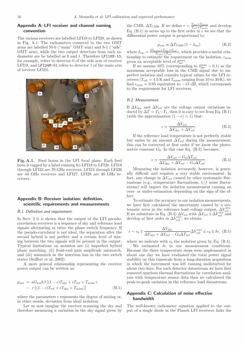
The various receivers are labelled LFI18 to LFI28, as shownin Fig. A.1. The radiometers connectd to the two OMTarms are labelled M-0 (“main” OMT arm) and S-1 (“side”OMT arm), while the two output detectors from each ra-diometer are be labelled as 0 and 1. Therefore LFI18S-10,for example, refers to detector 0 of the side arm of receiverLFI18, and LFI24M-01 refers to detector 1 of the main armof receiver LFI24.
Fig.A.1. Feed horns in the LFI focal plane. Each feedhorn is tagged by a label running fro LFI18 to LFI28. LFI18through LFI23 are 70 GHz receivers, LFI24 through LFI26are 44 GHz receivers and LFI27, LFI28 are 30 GHz re-ceivers.
Appendix B: Receiver isolation: definition,
scientific requirements and measurements
B.1. Definition and requirement.
In Sect. 2 it is shown that the output of the LFI pseudo-correlation receivers is a sequence of sky and reference loadsignals alternating at twice the phase switch frequency. Ifthe pseudo-correlator is not ideal, the separation after thesecond hybrid is not perfect and a certain level of mix-ing between the two signals will be present in the output.Typical limitations on isolation are (i) imperfect hybridphase matching, (ii) front-end gain amplitude mismatch,and (iii) mismatch in the insertion loss in the two switchstates (Seiffert et al. 2002).
A more general relationship representing the receiverpower output can be written as:
pout = aGtotkβ [(1− ǫ)Tsky + ǫTref + Tnoise+
− r ((1− ǫ)Tref + ǫTsky + Tnoise)] (B.1)
where the parameters ǫ represents the degree of mixing or,in other words, deviation from ideal isolation.
Let us now imagine the receiver scanning the sky andtherefore measuring a variation in the sky signal given by
the CMB, ∆TCMB. If we define r =Tsky+Tnoise
Tref+Tnoiseand develop
Eq. (B.1) in series up to the first order in ǫ we see that thedifferential power output is proportional to:
pout ∝ ∆TCMB (1− δiso) (B.2)
where δiso =2Tnoise+Tsky+Tref
Tnoise+Trefǫ, which provides a useful rela-
tionship to estimate the requirement on the isolation, ǫmax
given an acceptable level of δmaxiso .
If we assume 10% (corresponding to δmaxiso ∼ 0.1) as the
maximum acceptable loss in the CMB signal due to im-perfect isolation and consider typical values for the LFI re-ceivers (Tref = 4.5 K and Tnoise ranging from 10 to 30K), wefind ǫmax = 0.05 equivalent to −13 dB, which correspondsto the requirement for LFI receivers.
B.2. Measurement.
If ∆Vsky and ∆Vref are the voltage output variations in-duced by ∆T = T2−T1, then it is easy to see from Eq. (B.1)(with the approximation (1− ǫ) ≃ 1) that:
ǫ ≃ ∆Vref
∆Vsky +∆Vref. (B.3)
If the reference load temperature is not perfectly stablebut varies by an amount ∆Tref during the measurement,this can be corrected at first order if we know the photo-metric constant G0. In this case Eq. (B.3) becomes:
ǫ ≃ ∆Vref −G0∆Tref
∆Vsky +∆Vref −G0∆Tref. (B.4)
Measuring the isolation accurately, however, is gener-ally difficult and requires a very stable environment. Infact, any change in ∆Vref caused by other systematic fluc-tuations (e.g., temperature fluctuations, 1/f noise fluctu-ations) will impact the isolation measurement causing anover- or under-estimation depending on the sign of the ef-fect.
To estimate the accuracy in our isolation measurements,we have first calculated the uncertainty caused by a sys-tematic error in the reference load voltage output, ∆V sys
ref .If we substitute in Eq. (B.4) ∆Vref with ∆Vref ±∆V sys
ref anddevelop at first order in ∆V sys
ref , we obtain
ǫ ∼ ǫ0∓∆Vsky
∆Vsky +∆Vref −G0∆Tref∆V sys
ref ≡ ǫ0∓ δǫ, (B.5)
where we indicate with ǫ0 the isolation given by Eq. (B.4).We estimated δǫ in our measurement conditions.
Because the three temperature steps were implemented inabout one day we have evaluated the total power signalstability on this timescale from a long-duration acquisitionin which the instrument was left running undisturbed forabout two days. For each detector datastream we have firstremoved spurious thermal fluctuations by correlation anal-ysis with temperature sensor data then we calculated thepeak-to-peak variation in the reference load datastream.
Appendix C: Calculation of noise effective
bandwidth
The well-known radiometer equation applied to the out-put of a single diode in the Planck LFI receivers links the
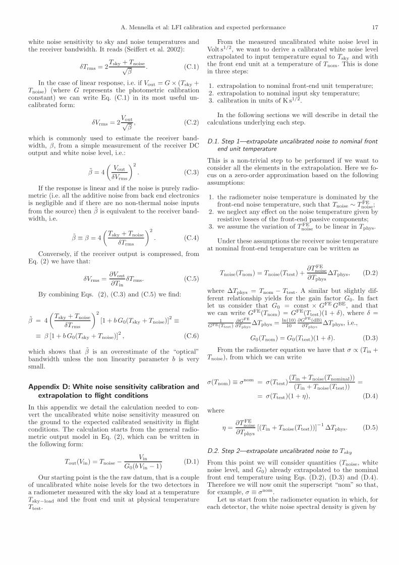
A. Mennella et al: LFI calibration and expected performance 17
white noise sensitivity to sky and noise temperatures andthe receiver bandwidth. It reads (Seiffert et al. 2002):
δTrms = 2Tsky + Tnoise√
β. (C.1)
In the case of linear response, i.e. if Vout = G× (Tsky +Tnoise) (where G represents the photometric calibrationconstant) we can write Eq. (C.1) in its most useful un-calibrated form:
δVrms = 2Vout√β, (C.2)
which is commonly used to estimate the receiver band-width, β, from a simple measurement of the receiver DCoutput and white noise level, i.e.:
β = 4
(
Vout
δVrms
)2
. (C.3)
If the response is linear and if the noise is purely radio-metric (i.e. all the additive noise from back end electronicsis negligible and if there are no non-thermal noise inputsfrom the source) then β is equivalent to the receiver band-width, i.e.
β ≡ β = 4
(
Tsky + Tnoise
δTrms
)2
. (C.4)
Conversely, if the receiver output is compressed, fromEq. (2) we have that:
δVrms =∂Vout
∂TinδTrms. (C.5)
By combining Eqs. (2), (C.3) and (C.5) we find:
β = 4
(
Tsky + Tnoise
δTrms
)2
[1 + bG0(Tsky + Tnoise)]2 ≡
≡ β [1 + bG0(Tsky + Tnoise)]2 , (C.6)
which shows that β is an overestimate of the “optical”bandwidth unless the non linearity parameter b is verysmall.
Appendix D: White noise sensitivity calibration and
extrapolation to flight conditions
In this appendix we detail the calculation needed to con-vert the uncalibrated white noise sensitivity measured onthe ground to the expected calibrated sensitivity in flightconditions. The calculation starts from the general radio-metric output model in Eq. (2), which can be written inthe following form:
Tout(Vin) = Tnoise −Vin
G0(b Vin − 1)(D.1)
Our starting point is the the raw datum, that is a coupleof uncalibrated white noise levels for the two detectors ina radiometer measured with the sky load at a temperatureTsky−load and the front end unit at physical temperatureTtest.
From the measured uncalibrated white noise level inVolt s1/2, we want to derive a calibrated white noise levelextrapolated to input temperature equal to Tsky and withthe front end unit at a temperature of Tnom. This is donein three steps:
1. extrapolation to nominal front-end unit temperature;2. extrapolation to nominal input sky temperature;3. calibration in units of K s1/2.
In the following sections we will describe in detail thecalculations underlying each step.
D.1. Step 1—extrapolate uncalibrated noise to nominal frontend unit temperature
This is a non-trivial step to be performed if we want toconsider all the elements in the extrapolation. Here we fo-cus on a zero-order approximation based on the followingassumptions:
1. the radiometer noise temperature is dominated by thefront-end noise temperature, such that Tnoise ∼ TFE
noise;2. we neglect any effect on the noise temperature given by
resistive losses of the front-end passive components;3. we assume the variation of TFE
noise to be linear in Tphys.
Under these assumptions the receiver noise temperatureat nominal front-end temperature can be written as
Tnoise(Tnom) = Tnoise(Ttest) +∂TFE
noise
∂Tphys∆Tphys, (D.2)
where ∆Tphys = Tnom − Ttest. A similar but slightly dif-ferent relationship yields for the gain factor G0. In factlet us consider that G0 = const × GFEGBE, and thatwe can write GFE(Tnom) = GFE(Ttest)(1 + δ), where δ =
1GFE(Ttest)
∂GFE
∂Tphys∆Tphys =
ln(10)10
∂GFE(dB)∂Tphys
∆Tphys, i.e.,
G0(Tnom) = G0(Ttest)(1 + δ). (D.3)
From the radiometer equation we have that σ ∝ (Tin +Tnoise), from which we can write
σ(Tnom) ≡ σnom = σ(Ttest)(Tin + Tnoise(Tnominal))
(Tin + Tnoise(Ttest))=
= σ(Ttest)(1 + η), (D.4)
where
η =∂TFE
noise
∂Tphys[(Tin + Tnoise(Ttest))]
−1∆Tphys. (D.5)
D.2. Step 2—extrapolate uncalibrated noise to Tsky
From this point we will consider quantities (Tnoise, whitenoise level, and G0) already extrapolated to the nominalfront end temperature using Eqs. (D.2), (D.3) and (D.4).Therefore we will now omit the superscript “nom” so that,for example, σ ≡ σnom.
Let us start from the radiometer equation in which, foreach detector, the white noise spectral density is given by
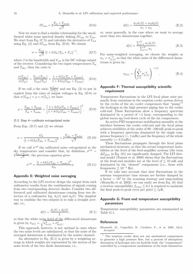
18 A. Mennella et al: LFI calibration and expected performance
δTrms = 2Tin + Tnoise√
β. (D.6)
Now we want to find a similar relationship for the uncal-ibrated white noise spectral density linking δVrms to Vout.We start from Eq. (C.5) and calculate the derivative of Vout
using Eq. (2) and δTrms from Eq. (D.6). We obtain
σ =Vout√β
[1 + bG0 (Tin + Tn)]−1
, (D.7)
where β is the bandwidth and Vout is the DC voltage outputof the receiver. Considering the two input temperatures Tin
and Tsky, then the ratio is
σ(Tsky)
σ(Tin)=
Vout(Tsky)
Vout(Tin)× 1 + bG0(Tin + Tnoise)
1 + bG0(Tsky + Tnoise). (D.8)
If we call ρ the ratioσ(Tsky)σ(Tin)
and use Eq. (2) to put in
explicit form the ratio of output voltages in Eq. (D.8) sothat σ(Tsky) = ρ× σ(Tin), we have
ρ =Tsky + Tnoise
Tin + Tnoise×[
1 + bG0(Tin + Tnoise)
1 + bG0(Tsky + Tnoise)
]2
. (D.9)
D.3. Step 4—calibrate extrapolated noise
From Eqs. (D.7) and (2) we obtain
σ =G0
[1 + bG0(Tsky + Tnoise)]2 × 2
Tsky + Tnoise√β
. (D.10)
If we call σcal the calibrated noise extrapolated at thesky temperature and consider that, by definition, σcal =
2Tsky+Tnoise√
β, the previous equation gives
σcal =[1 + bG0(Tsky + Tnoise)]
2
G0σ. (D.11)
Appendix E: Weighted noise averaging
According to the LFI receiver design the output from eachradiometer results from the combination of signals comingfrom two corresponding detector diodes. Consider two dif-ferenced and calibrated datastreams coming from two de-tectors of a radiometer leg, d1(t) and d2(t). The simplestway to combine the two outputs is to take a straight aver-age, i.e.,
d(t) =d1(t) + d2(t)
2, (E.1)
so that the white noise level of the differenced datastreamis given by σd(t) =
√
σ2d1(t)
+ σ2d2(t)
.
This approach, however, is not optimal in cases wherethe two noise levels are unbalanced, so that the noise of theaveraged datastream is dominated by the noisier channel.
An alternative to Eq. (E.1) is given by a weighting av-erage in which weights are represented by the inverse of thenoise levels of the two diode datasteams, i.e.,
d(t) =w1d1(t) + w2d2(t)
w1 + w2, (E.2)
or, more generally, in the case where we want to averagemore than two datastreams together,
d(t) =
∑Nj=1 wjdj(t)∑N
j=1 wj
. (E.3)
For noise-weighted averaging, we choose the weights aswj = σ−2
dj(t)so that the white noise of the differenced datas-
tream is given by:
σd(t) =
N∑
j=1
σ−2dj(t)
−1/2
. (E.4)
Appendix F: Thermal susceptibility scientific
requirement
Temperature fluctuations in the LFI focal plane arise pri-marily from variations in the sorption cooler system drivenby the cycles of the six cooler compressors that “pump”7
the hydrogen in the high pressure piping line to the coolercold-end. These fluctuations show a frequency spectrumdominated by a period of ∼1 hour, corresponding to theglobal warm-up/cool-down cycle of the six compressors.
An active PID temperature stabilisation assembly at theinterface between the cooler cold-end and the focal planeachieves stabilities of the order of 80−100mK peak-to-peakwith a frequency spectrum dominated by the single com-pressor frequency (∼ 1mHz) and the frequency of the wholeassembly (∼ 0.2mHz).
These fluctuations propagate through the focal planemechanical structure, so that the actual temperature insta-bilities at the level of the feed-amplifier systems (the term∆Tphys in Eq. (6)) are significantly damped. The LFI ther-mal model (Tomasi et al. 2009) shows that the fluctuationsat the front-end modules are at the level of . 10 mK anddominated by the “slowest” components (i.e., those withfrequencies . 10−2 Hz).
If we take into account that slow fluctuations in theantenna temperature time stream are further damped bya factor ∼ 103 by the scanning strategy and map-making(Mennella et al. 2002), we can easily see from Eq. (6) thata receiver susceptibility ftrans . 0.1 is required to maintainthe final peak-to-peak error per pixel . 1µK.
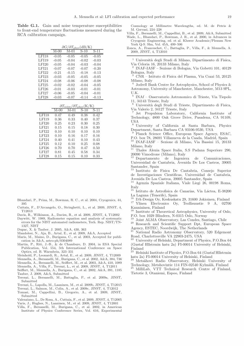
Appendix G: Front-end temperature susceptibility
parameters
Temperature susceptibility parameters are summarised inTable G.1.
References
Bersanelli, M., Cappellini, B., Cavaliere, F., et al. 2009, A&A,Accepted
7 The sorption cooler does not use mechanical compressorsto generate a high pressure flow, but a process of absorption-desorption of hydrogen into six hydride beds, the “compressors”controlled by a temperature modulation of the beds themselves.
A. Mennella et al: LFI calibration and expected performance 19
Table G.1. Gain and noise temperature susceptibilitiesto front-end temperature fluctuations measured during theRCA calibration campaign.
∂G/∂Tphys(dB/K)M-00 M-01 S-10 S-11
LFI18 -0.05 -0.05 -0.05 -0.05LFI19 -0.05 -0.04 -0.02 -0.03LFI20 -0.05 -0.04 -0.03 -0.04LFI21 -0.07 -0.07 -0.07 -0.20LFI22 -0.21 -0.15 -0.18 -0.13LFI23 -0.03 -0.05 -0.05 -0.05LFI24 -0.08 -0.06 -0.08 -0.08LFI25 -0.02 -0.02 -0.04 -0.05LFI26 -0.01 -0.03 -0.01 -0.01LFI27 -0.06 -0.05 -0.04 -0.01LFI28 -0.03 -0.07 -0.14 -0.13
∂Tnoise/∂Tphys(K/K)M-00 M-01 S-10 S-11
LFI18 0.47 0.49 0.38 0.42LFI19 0.36 0.33 0.40 0.37LFI20 0.25 0.23 0.30 0.25LFI21 0.15 0.15 0.18 0.30LFI22 0.10 0.10 0.10 0.10LFI23 0.10 0.16 0.17 0.16LFI24 0.40 0.41 0.10 0.43LFI25 0.12 0.10 0.25 0.08LFI26 0.70 0.70 0.47 0.50LFI27 0.81 0.45 0.58 0.34LFI28 0.15 0.15 0.10 0.33
Bhandari, P., Prina, M., Bowman, R. C., et al. 2004, Cryogenics, 44,395
Cuttaia, F., D’Arcangelo, O., Stringhetti, L., et al. 2009, JINST, 4,T12013
Davis, R., Wilkinson, A., Davies, R., et al. 2009, JINST, 4, T12002Daywitt, W. 1989, Radiometer equation and analysis of systematic
errors for the NIST automated radiometers, Tech. Rep. NIST/TN-1327, NIST
Dupac, X. & Tauber, J. 2005, A&A, 430, 363Mandolesi, N., Aja, B., Artal, E., et al. 2009, A&A, AcceptedMaris, M., Maino, D., Burigana, C., et al. 2003, Accepted for publi-
cation in A&A, astro-ph/0304089Martin, P., Riti, J.-B., & de Chambure, D. 2004, in ESA Special
Publication, Vol. 554, 5th International Conference on SpaceOptics, ed. B. Warmbein, 323–331
Meinhold, P., Leonardi, R., Artal, E., et al. 2009, JINST, 4, T12009Mennella, A., Bersanelli, M., Burigana, C., et al. 2002, A&A, 384, 736Mennella, A., Bersanelli, M., Seiffert, M., et al. 2003, A&A, 410, 1089Mennella, A., Villa, F., Terenzi, L., et al. 2009, JINST, 4, T12011Seiffert, M., Mennella, A., Burigana, C., et al. 2002, A&A, 391, 1185Tauber, J. 2009, A&A, SubmittedTerenzi, L., Bersanelli, M., Battaglia, P., et al. 2009a, JINST,
SubmittedTerenzi, L., Lapolla, M., Laaninen, M., et al. 2009b, JINST, 4, T12015Terenzi, L., Salmon, M., Colin, A., et al. 2009c, JINST, 4, T12012Tomasi, M., Cappellini, B., Gregorio, A., et al. 2009, JINST,
SubmittedValenziano, L., De Rosa, A., Cuttaia, F., et al. 2009, JINST, 4, T12005Varis, J., Hughes, N., Laaninen, M., et al. 2009, JINST, 4, T12001Villa, F., Bersanelli, M., Burigana, C., et al. 2002, in American
Institute of Physics Conference Series, Vol. 616, Experimental
Cosmology at Millimetre Wavelengths, ed. M. de Petris &M. Gervasi, 224–228
Villa, F., Bersanelli, M., Cappellini, B., et al. 2009, A&A, SubmittedWade, L., Bhandari, P., Bowman, J. R., et al. 2000, in Advances in
Cryogenic Engineering, ed. et al. Kluwer Academic/Plenum NewYork Q-S. Shu, Vol. 45A, 499–506
Zonca, A., Franceschet, C., Battaglia, P., Villa, F., & Mennella, A.2009, JINST, 4, T12010
1 Universita degli Studi di Milano, Dipartimento di Fisica,Via Celoria 16, 20133 Milano, Italy2 INAF-IASF – Sezione di Bologna, Via Gobetti 101, 40129Bologna, Italy3 CNR – Istituto di Fisica del Plasma, Via Cozzi 53, 20125Milano, Italy4 Jodrell Bank Centre for Astrophysics, School of Physics &Astronomy, University of Manchester, Manchester, M13 9PL,U.K.5 INAf – Osservatorio Astronomico di Trieste, Via Tiepolo11, 34143 Trieste, Italy6 Universita degli Studi di Trieste, Dipartimento di Fisica,Via Valerio 2, 34127 Trieste, Italy7 Jet Propulsion Laboratory, California Institute ofTechnology, 4800 Oak Grove Drive, Pasadena, CA 91109,USA8 University of California at Santa Barbara, PhysicsDepartment, Santa Barbara CA 93106-9530, USA9 Planck Science Office, European Space Agency, ESAC,P.O. box 78, 28691 Villanueva de la Caada, Madrid, Spain10 INAF-IASF – Sezione di Milano, Via Bassini 15, 20133Milano, Italy11 Thales Alenia Space Italia, S.S Padana Superiore 290,20090 Vimodrone (Milano), Italy12 Departamento de Ingeniera de Comunicaciones,Universidad de Cantabria, Avenida De Los Castros, 39005Santander, Spain13 Instituto de Fisica De Cantabria, Consejo Superiorde Investigaciones Cientificas, Universidad de Cantabria,Avenida De Los Castros, 39005 Santander, Spain14 Agenzia Spaziale Italiana, Viale Liegi 26, 00198 Roma,Italy15 Istituto de Astrofisica de Canarias, Vıa Lactea, E-38200La Laguna (Tenerife), Spain16 DA-Design Oy, Keskuskatu 29, 31600 Jokioinen, Finland17 Ylinen Electronics Oy, Teollisuustie 9 A, 02700Kauniainen, Finland18 Institute of Theoretical Astrophysics, University of Oslo,P.O. box 1029 Blindern, N-0315 Oslo, Norway19 Joint ALMA Observatory, Las Condes, Santiago, Chile20 Research and Scientific Support Dpt, European SpaceAgency, ESTEC, Noordwijk, The Netherlands21 National Radio Astronomy Observatory, 520 EdgemontRoad, Charlottesville VA 22903-2475, USA22 University of Helsinki, Department of Physics, P.O.Box 64(Gustaf Hllstrmin katu 2a) FI-00014 University of Helsinki,Finland23 Helsinki Institute of Physics, P.O.Box 64 (Gustaf Hllstrminkatu 2a) FI-00014 University of Helsinki, Finland24 Metsahovi Radio Observatory, Helsinki University ofTechnology, Metshovintie 114 FIN-02540 Kylmala, Finland25 MilliLab, VTT Technical Research Centre of Finland,Tietotie 3, Otaniemi, Espoo, Finland