Phytoplankton community in the Algarve coastal region

2021

UNIVERSIDADE DE LISBOA

FACULDADE DE CIÊNCIAS

DEPARTAMENTO DE BIOLOGIA VEGETAL

Phytoplankton community in the Algarve coastal region:

Implications to bivalve aquaculture production

André Sobral da Fonseca

Mestrado em Ciências do Mar

Dissertação orientada por:

Doutora Ana C. Brito

II

Acknowledgments

I would like to thank all the people and institutions that allowed and contributed in some way

in the development of this dissertation.

First, I would like to thank Dr. Ana C. Brito for all the support, wisdom and dedication to me

and my work from day one.

I would like to thank Marine and Environmental Sciences Centre (MARE-ULisboa), where

most of my work was carried out, as well as the entire AQUIMAR team.

I also thank Afonso Ferreira, Joana Cruz, Andreia Tracana and Luciane Favareto for all their

help in obtaining and analysing results.

Last but not least, my family and Rita for being the main pillar of constant help and support.

This dissertation was developed in the AQUIMAR project- Marine Knowledge Supporting

Aquaculture (MAR-02.01.01-FEAMP-0107. Website: https://www.aquimar.hidrografico.pt

III

Resumo

A aquacultura de organismos aquáticos, incluindo peixes, moluscos, crustáceos e plantas

aquáticas é o sistema de produção de alimentos de crescimento mais rápido em todo o mundo, com um

aumento de 527% na produção global de aquacultura de 1990 a 2018. Nesta conjuntura global, em que

se verificam cada vez mais restrições à exploração pesqueira, a produção aquícola na costa portuguesa

apresenta um enorme potencial a ser explorado dada a excelência da sua localização geográfica.

Portugal é também um dos países onde mais se consome pescado, registando um consumo médio per

capita de 55,6 kg / ano, valor que se encontra bastante acima da média mundial. A aquacultura em

Portugal apresentou, nos últimos anos, um grande desenvolvimento não só ao nível da tecnologia e

estruturas utilizadas, mas também na introdução de novas espécies com maior valor comercial. Desde

a década de 1970 houve um maior investimento na aquacultura de várias espécies de bivalves, tais

como o mexilhão e a ostra. No entanto, a produção total da aquacultura marinha de Portugal mantém-

se aquém do esperado, sendo que em 2017 representou menos de 1% da produção de alguns países

europeus. Neste momento, a produção de bivalves em aquacultura representa, anualmente, cerca de

metade da produção aquícola total, sendo a outra metade constituída maioritariamente pela produção

de peixe.

A aquacultura offshore realizada em longlines instaladas em pontos ao longo da costa é um

dos métodos mais utilizados mundialmente para a produção de bivalves e, dada a extensão da costa

portuguesa, apresenta-se como método com elevado potencial de rentabilidade e sustentabilidade.

Comparada com a produção de peixes em gaiolas, este é um método que se apresenta vantajoso uma

vez que os bivalves, sendo organismos filtradores, se alimentam principalmente de fitoplâncton e de

outros compostos orgânicos presentes naturalmente na coluna de água, ao contrário dos peixes em que

é necessária a introdução de alimento. É na costa do Algarve que se pode observar maior quantidade

de unidades de aquacultura offshore. Na verdade, esta é a área da costa portuguesa que apresenta uma

área marítima com maior proteção da agitação marítima e onde a temperatura e outros fatores

ambientais são mais favoráveis à produção de várias espécies. Contudo, a escolha dos locais de

produção é tipicamente empírica, por vezes não tendo em conta todos os fatores bióticos e abióticos

que embora favoráveis à aquacultura apresentam, no entanto, alguma variabilidade ao longo da costa

sul. Hoje em dia, de acordo com a informação disponibilizada no geoportal aquicultura da DGRM,

existem na costa do Algarve 9 unidades de aquacultura offshore apenas para a produção de mexilhões

e ostras, representando mais de 200 hectares. No resto da costa portuguesa existe apenas uma unidade

de produção de mexilhões localizada perto de Peniche. A espécie de mexilhão mais produzida em

Portugal e no mundo é o Mytilus edulis com a produção em Portugal a atingir 1746 toneladas em 2018

e a espécie de ostra mais produzida em Portugal é a Crassostrea Gigas, com um valor total de

produção de 3451 toneladas em 2018. Estas duas espécies são frequentemente escolhidas pela sua

grande distribuição geográfica natural, pelo seu ciclo de vida ter sido já estudado e compreendido ao

pormenor, por já possuírem um mercado bem desenvolvido, por apresentarem grande eficiência na sua

produção e também pelo seu elevado valor nutritivo quando consumido.

Deste modo, o principal objetivo deste trabalho é compreender a distribuição espacial das

comunidades fitoplanctónicas na costa do Algarve para avaliar as implicações na seleção de áreas para

a produção de bivalves offshore. De forma a atingir este objetivo, foram estabelecidas diversos

objetivos específicos: i) Avaliar como os fatores ambientais afetam a distribuição espacial das

comunidades fitoplanctónicas na costa Algarvia; ii) Identificar áreas com elevada produção de

biomassa fitoplanctónica ao longo da costa Algarvia e avaliar quais os grupos fitoplanctónicos que

IV

mais contribuem para esta produção; iii) Identificar os locais com maior potencial para implantação de

unidades de aquacultura offshore, de acordo com a biomassa fitoplanctónica e condições ambientais.

Assim, com base numa campanha oceanográfica inserida no projeto AQUIMAR e a bordo do

navio oceanográfico NRP Almirante Gago Coutinho, foi feita a amostragem da coluna de água para 52

estações ao longo de toda a costa algarvia, durante o mês de outubro de 2018. Foram estudados fatores

ambientais como a temperatura, salinidade, oxigénio dissolvido, correntes oceânicas e também alguns

nutrientes tais como sílica, fósforo, o azoto inorgânico dissolvido (DIN) e a forma como estes estão

espacialmente distribuídos. Os valores em temperatura, salinidade e de oxigénio dissolvido

encontraram-se dentro dos valores descritos para a costa do Algarve, ao contrário da distribuição dos

nutrientes que foi observada em concentrações bastante baixas. Quanto às correntes foi observada uma

direção de corrente maioritariamente vinda de sudoeste e com uma magnitude média entre 100 e 150

mm/s.

Foi também estudada em detalhe, através da análise quimio-taxonómica (HPLC-CHEMTAX),

a constituição em classes da comunidade fitoplanctónica, tendo sido observadas em maior

concentração as classes Bacillariophyceae e Dinophyceae. A variação geográfica destas classes e a

influência dos fatores ambientais na sua distribuição foi ainda estudada através de uma análise de

correspondência canônica. Os parâmetros que maior influência apresentaram na distribuição da

comunidade fitoplanctónica foram a distância à costa, a temperatura, o DIN e a sílica.

Foram combinados todos os parâmetros relevantes para identificação das áreas com maior

potencial na produção de bivalves ao longo da costa sul portuguesa, o que resultou na formulação de

um índice de aptidão que se propõe como nova metodologia a aplicar. Os parâmetros utilizados foram

a distância à costa, a temperatura, a presença em DIN, a distribuição da biomassa fitoplanctónica e

ainda a presença das classes Bacillariophyceae e Dinophyceae. Para a distância à costa foram

consideradas adequadas as estações a uma distância máxima de 6 milhas náuticas por ser esta a

distância máxima de acesso à carta mínima para condução de embarcações em Portugal e também

devido à acessibilidade e redução de custos. A temperatura adequada para mexilhões e ostras de

diferentes regiões geográficas varia entre 18 e 25ºC, tendo sido este o intervalo considerado adequado

para a sua produção. Para o DIN, foram consideradas adequadas as estações cujo valor de

concentração estava entre os mais elevados, neste caso foi superior o percentil 90. As concentrações

de DIN foram usadas porque o azoto é um nutriente limitante e pode ser um potencial indicador para a

produção primária. Para a biomassa fitoplanctónica foi aplicada a mesma abordagem, tendo sido

consideradas adequadas as estações cujo valor da concentração em clorofila a foi superior ao percentil

90. Como indicador para a presença da biomassa fitoplanctónica, foi ainda considerado um parâmetro

referindo-se especificamente à dominância das classes Bacillariophyceae e Dinophyceae, por estas

serem consideradas as mais importantes no crescimento e desenvolvimento na produção de bivalves.

Para as classes Bacillariophyceae e Dinophyceae, foram consideradas adequadas as estações em que a

soma da concentração destes dois grupos foi superior ao valor médio. Para a construção deste índice,

foi ainda considerado adicionar os dados das correntes oceânicas, mas por haver apenas uma estação

de amostragem, estes dados não foram incluídos.

Utilizando os dados da campanha de outubro de 2018 e através do índice de aptidão, foram

observadas as áreas numa zona compreendida desde a costa de Sagres, Lagos, Portimão e Faro até

uma distância de 6 milhas náuticas. Ao observar a localização das unidades de aquacultura já

existentes no Algarve, é possível constatar que se localizam nas áreas identificadas neste trabalho

como tendo o maior potencial ou sendo mais adequadas. É possível concluir-se que estes tenham sido

os locais onde, ao longo dos anos e empiricamente, a produção de bivalves se tenha mostrado mais

eficiente. Este método foi desenvolvido utilizando dados de uma única campanha como um estudo de

V

caso, no entanto, a aplicação do índice proposto a um maior conjunto de dados com maior

variabilidade sazonal e para toda a costa de Portugal, poderá no futuro expandir as possibilidades de

exploração desta produção no nosso país, aproximando-o do máximo da sua potencialidade.

Palavras-chave: Aquacultura Offshore, Bivalves, Fitoplâncton, HPLC-CHEMTAX, Algarve.

VI

Abstract

Aquaculture in Portugal has shown, in recent years, a great development not only regarding

technology, but also in terms of the species used, with the introduction of new species with great

commercial value. Since the 1970's, there has been a great investment in aquaculture of several

bivalve species, such as mussels and oysters. At the moment, in Portugal, the production of bivalves in

aquaculture represents, annually, about half of the total production, with the other half constituted

mainly by the production of finfish aquaculture. Offshore aquaculture, carried out at locations along

the coast, is one of the most used methods worldwide for the production of bivalves. Given that

Portugal is a country with an extensive coast, it can be assumed that there is great potential for this

type of production. The bivalve offshore aquaculture has greater potential in terms of sustainability

when compared to the production of fish in cages. This is mainly caused by the fact that finfish needs

to be feed to survive and grow while for the bivalves the natural food present in environment (water

column) is taken up by them, as these are filtering organisms that mainly feed on phytoplankton in

ocean environments. It is on the Algarve coast that offshore aquaculture units can be seen in greater

numbers since the Portuguese south coast presents a coastal maritime area with greater protection from

sea agitation and where temperature and other environmental factors are more favorable to the

production of various species. However, the choice of the production sites is typically empirical,

sometimes not taking into account all the biotic and abiotic factors, which although favorable to

aquaculture, have some variability along the south coast. In this work, through an oceanographic

campaign inserted in the AQUIMAR project and on board the NRP Almirante Gago Coutinho

oceanographic vessel, sampling was carried out in 52 stations along the entire Algarve coast during the

month of October 2018. The main environmental factors studied were temperature, salinity, dissolved

oxygen, as well as nutrient concentrations. Additional water samples were also collected to evaluate

the spatial distribution of phytoplankton biomass, using chlorophyll a concentration as a proxy.

Moreover, phytoplankton community composition (main groups) of samples was also analyzed

through chemotaxonomy (HPLC-CHEMTAX), an approach that uses the pigment signature of the

different phytoplankton groups. These data were then used to analyze the how the environmental

factors influence the spatial distribution of phytoplankton in the Algarve coast. Phytoplankton is

probably the most important source of food for the growth of bivalve organisms in open waters. To

identify the areas with the greatest potential to produce these organisms along the south coast of

Portugal, all relevant factors, with enough spatial resolution, were combined in an integrated analysis.

A novel suitability index methodology is proposed herein. Using the data from the campaign of

October 2018, the suitability index indicated that the areas closer than 6 nautical miles to the shoreline

of Sagres, Lagos, Portimão and Faro are the locations with the greatest potential for the

implementation of structures for aquaculture of offshore bivalves in the Algarve. In the future, this

methodology should be applied to a more comprehensive dataset.

Keywords: Offshore Aquaculture, Bivalves, Phytoplankton communities, HPLC-CHEMTAX,

Algarve.

VII

Table of contents Acknowledgments ............................................................................................................................. II

Resumo ............................................................................................................................................ III

Abstract ........................................................................................................................................... VI

List of figures .................................................................................................................................. IX

List of tables ...................................................................................................................................... X

Abbreviations and Symbols.............................................................................................................. XI

1. Introduction.............................................................................................................................1

1.1. Aquaculture .....................................................................................................................1

1.2. Bivalve offshore aquaculture and life cycle ......................................................................2

1.3. The importance of phytoplankton to bivalve aquaculture ..................................................4

1.4. Study site .........................................................................................................................5

1.5. Aim and objectives ..........................................................................................................7

2. Materials and Methods ............................................................................................................8

2.1. Sampling strategy ............................................................................................................8

2.2. Seawater sample collection ..............................................................................................8

2.3. Oceanic currents characterization .....................................................................................9

2.4. Laboratory analysis ........................................................................................................ 10

2.4.1. Seawater physico-chemical characterization ............................................................... 10

2.4.2. Seawater biological characterization .......................................................................... 10

2.5. Data analysis ................................................................................................................. 11

2.5.1. Chemotaxonomic analysis (HPLC-CHEMTAX) ........................................................ 11

2.6. Statistical analysis.......................................................................................................... 12

2.7. Potential areas identification .......................................................................................... 13

3. Results .................................................................................................................................. 15

3.1. Environmental conditions .............................................................................................. 15

3.2. Nutrient distribution ....................................................................................................... 17

3.3. Chlorophyll a concentration ........................................................................................... 18

3.4. Phytoplankton pigments and chemotaxonomy (CHEMTAX) ......................................... 19

3.5. Phytoplankton response to environmental drivers ........................................................... 21

3.6. Identification of the most suitable locations .................................................................... 22

4. Discussion ............................................................................................................................. 24

4.1. Spatial distribution of physico-chemical parameters ....................................................... 24

4.2. Spatial distribution of phytoplankton.............................................................................. 25

4.3. Phytoplankton response to environmental drivers ........................................................... 26

4.4. Searching for the most suitable locations for offshore aquaculture .................................. 27

4.5. Conclusions and recommendations ................................................................................ 28

VIII

References ........................................................................................................................................ 30

Attachments ...................................................................................................................................... 38

IX

List of figures

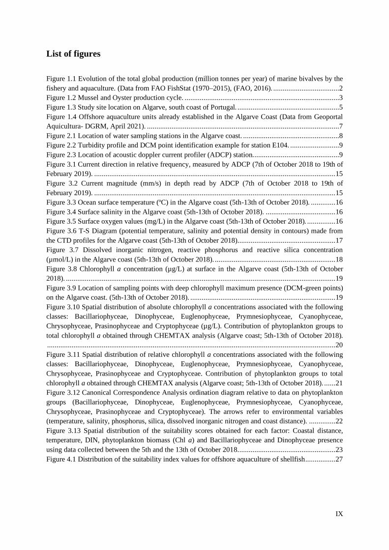
Figure 1.1 Evolution of the total global production (million tonnes per year) of marine bivalves by the

fishery and aquaculture. (Data from FAO FishStat (1970–2015), (FAO, 2016). ...................................2

Figure 1.2 Mussel and Oyster production cycle. ..................................................................................3

Figure 1.3 Study site location on Algarve, south coast of Portugal. ......................................................5

Figure 1.4 Offshore aquaculture units already established in the Algarve Coast (Data from Geoportal

Aquicultura- DGRM, April 2021). ......................................................................................................7

Figure 2.1 Location of water sampling stations in the Algarve coast. ...................................................8

Figure 2.2 Turbidity profile and DCM point identification example for station E104. ..........................9

Figure 2.3 Location of acoustic doppler current profiler (ADCP) station. .............................................9

Figure 3.1 Current direction in relative frequency, measured by ADCP (7th of October 2018 to 19th of

February 2019). ................................................................................................................................ 15

Figure 3.2 Current magnitude (mm/s) in depth read by ADCP (7th of October 2018 to 19th of

February 2019). ................................................................................................................................ 15

Figure 3.3 Ocean surface temperature (ºC) in the Algarve coast (5th-13th of October 2018). ............. 16

Figure 3.4 Surface salinity in the Algarve coast (5th-13th of October 2018). ..................................... 16

Figure 3.5 Surface oxygen values (mg/L) in the Algarve coast (5th-13th of October 2018). ............... 16

Figure 3.6 T-S Diagram (potential temperature, salinity and potential density in contours) made from

the CTD profiles for the Algarve coast (5th-13th of October 2018). ................................................... 17

Figure 3.7 Dissolved inorganic nitrogen, reactive phosphorus and reactive silica concentration

(µmol/L) in the Algarve coast (5th-13th of October 2018). ................................................................ 18

Figure 3.8 Chlorophyll a concentration (µg/L) at surface in the Algarve coast (5th-13th of October

2018). ............................................................................................................................................... 19

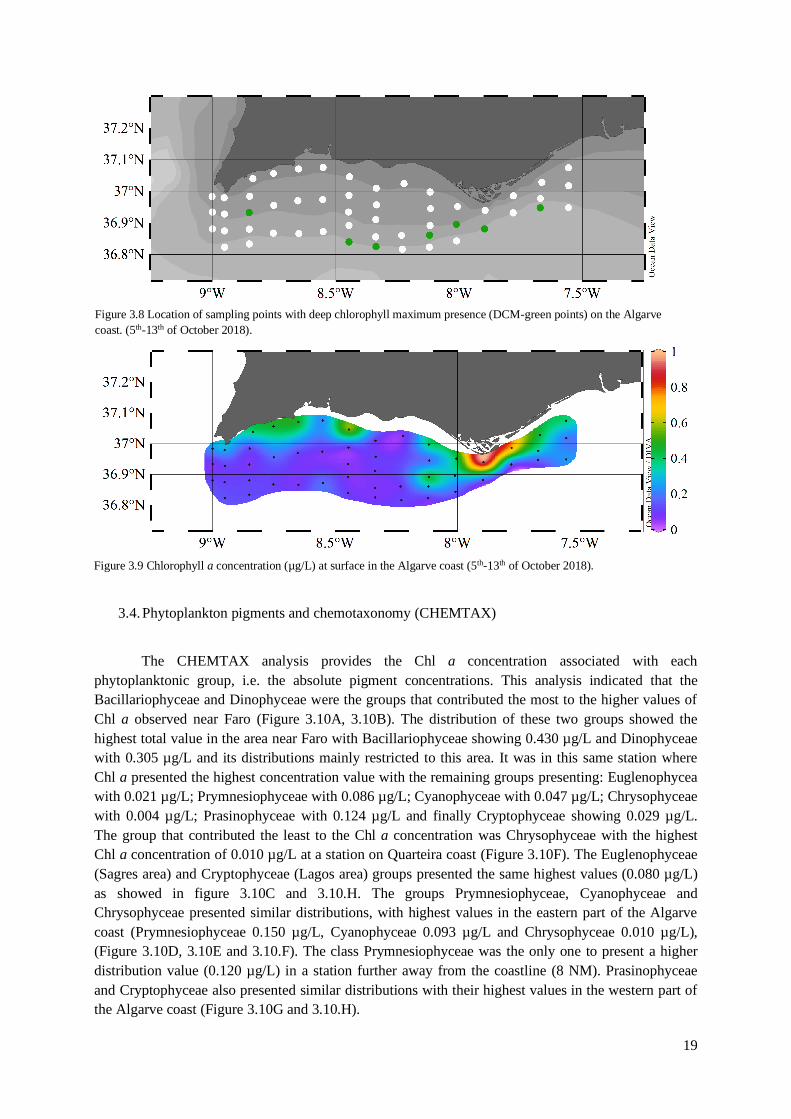
Figure 3.9 Location of sampling points with deep chlorophyll maximum presence (DCM-green points)

on the Algarve coast. (5th-13th of October 2018). ............................................................................. 19

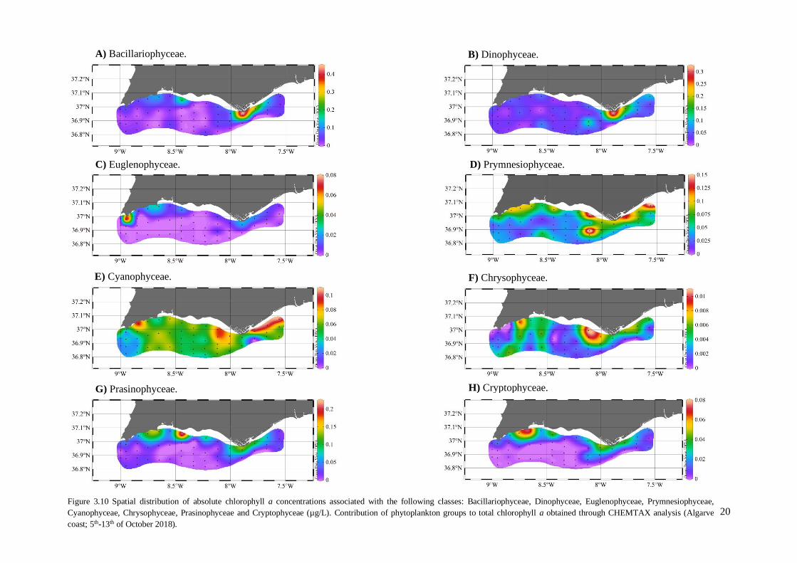
Figure 3.10 Spatial distribution of absolute chlorophyll a concentrations associated with the following

classes: Bacillariophyceae, Dinophyceae, Euglenophyceae, Prymnesiophyceae, Cyanophyceae,

Chrysophyceae, Prasinophyceae and Cryptophyceae (µg/L). Contribution of phytoplankton groups to

total chlorophyll a obtained through CHEMTAX analysis (Algarve coast; 5th-13th of October 2018).

......................................................................................................................................................... 20

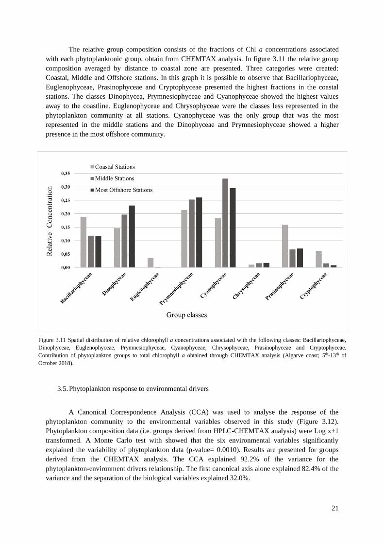
Figure 3.11 Spatial distribution of relative chlorophyll a concentrations associated with the following

classes: Bacillariophyceae, Dinophyceae, Euglenophyceae, Prymnesiophyceae, Cyanophyceae,

Chrysophyceae, Prasinophyceae and Cryptophyceae. Contribution of phytoplankton groups to total

chlorophyll a obtained through CHEMTAX analysis (Algarve coast; 5th-13th of October 2018). ...... 21

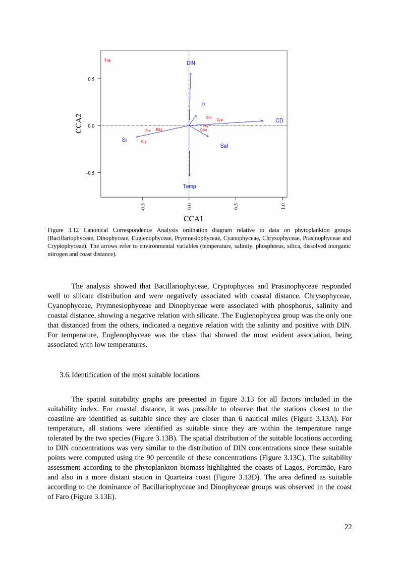
Figure 3.12 Canonical Correspondence Analysis ordination diagram relative to data on phytoplankton

groups (Bacillariophyceae, Dinophyceae, Euglenophyceae, Prymnesiophyceae, Cyanophyceae,

Chrysophyceae, Prasinophyceae and Cryptophyceae). The arrows refer to environmental variables

(temperature, salinity, phosphorus, silica, dissolved inorganic nitrogen and coast distance). .............. 22

Figure 3.13 Spatial distribution of the suitability scores obtained for each factor: Coastal distance,

temperature, DIN, phytoplankton biomass (Chl a) and Bacillariophyceae and Dinophyceae presence

using data collected between the 5th and the 13th of October 2018. ................................................... 23

Figure 4.1 Distribution of the suitability index values for offshore aquaculture of shellfish ................ 27

X

List of tables

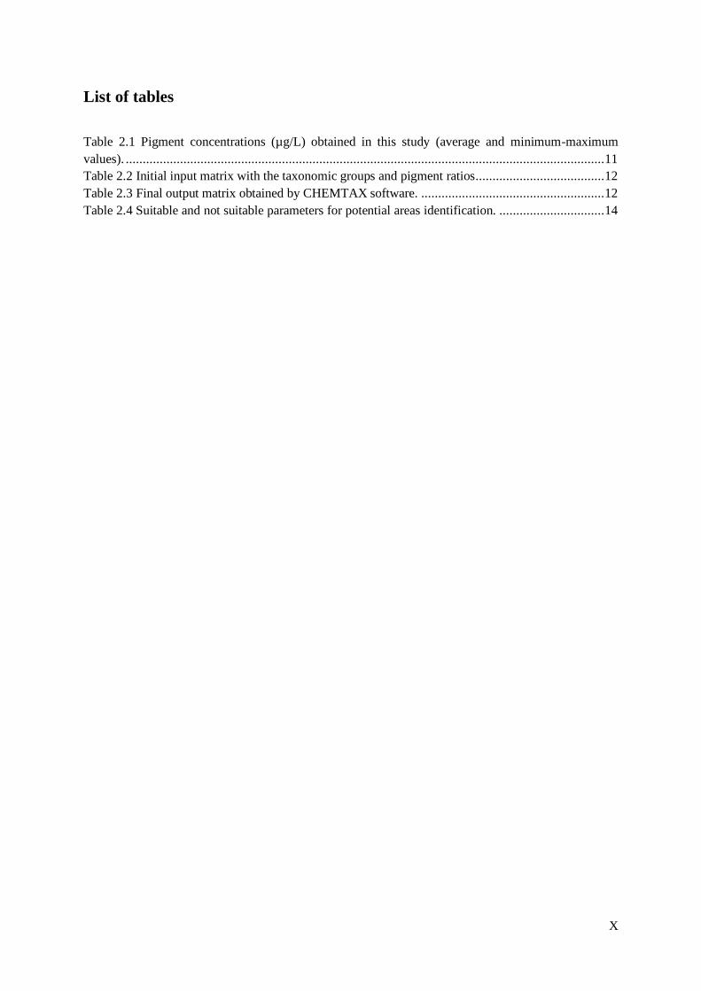
Table 2.1 Pigment concentrations (µg/L) obtained in this study (average and minimum-maximum

values). ............................................................................................................................................. 11

Table 2.2 Initial input matrix with the taxonomic groups and pigment ratios ...................................... 12

Table 2.3 Final output matrix obtained by CHEMTAX software. ...................................................... 12

Table 2.4 Suitable and not suitable parameters for potential areas identification. ............................... 14

XI

Abbreviations and Symbols

Allo Alloxanthin

But-fuco 19'-Butanoyloxyfucoxanthin

CCA Canonical Correspondence Analysis

Chl a Chlorophyll a

Chl b Chlorophyll b

Chl c1 Chlorophyll c1



Chlide a Chlorophyllide a

CTD Conductivity, Temperature and Depth

DCM Deep Chlorophyll Maximum

DGRM Direcção-Geral de Recursos Naturais, Segurança e Serviços Marítimos

Diadino Diadinoxanthin

Diato Diatoxanthin

DIN Dissolved inorganic nitrogen

FAO Food and Agriculture Organization of the United States

Fuco Fucoxanthin

Hex-fuco 19'-Hexanoyloxyfucoxanthin

HPLC High Performance Liquid Chromatography

INE Instituto Nacional de Estatística

IPMA Instituto Português do Mar e da Atmosfera

Lut Lutein

Mg DVP Mg-2,4-divinylpheoporphyrin a5 monomethyl ester

Neo Neoxanthin

Perid Peridinin

Phe a Pheophytin a

Prasino Prasinoxanthin

Viola Violaxanthin

Zea Zeaxanthin

β,β-Car β,β -Carotene

β,ε-Car β,ε-Carotene

1

1. Introduction

1.1. Aquaculture

The farming of aquatic organisms, including fish, mollusks, crustaceans, and aquatic plants is

the fastest growing food production system globally, with an increase of 527% in global aquaculture

production from 1990 to 2018 (FAO, 2020). In 2018, Aquaculture accounted for 46 percent of the

total fish production and 52 percent of fish for human consumption (FAO, 2020). Since natural

fisheries rely on wild stocks, which are often overexploited, aquaculture can slow down this

overexploitation to natural ecosystems (Naylor et al., 2000) and reduce it by alleviating pressure on

wild fish stocks (Diana, 2009; Stotz, 2000). Offshore aquaculture appears to have several advantages

over the inland culturing methods, including fewer spatial conflicts and a higher water quality,

highlighting the opportunities for sustainable marine development (Gentry et al., 2017; Holmer, 2010).

In this global situation, in which there are more and more restrictions on fishing exploitation,

and with a position of excellence due to its geographical location, Portugal aquaculture production

shows an enormous potential to be explored. Portugal is also one of the countries where more fish is

consumed, registering an average consumption per capita of 55,6 kg / year, a value that is well above

the world average value (19.2 kg / year; FAO, 2020).

Aquaculture in Portugal has progressed greatly since the 1970’s with the beginning of

shellfish cultivation. After the Structural Policy in the European Community was applied in Portugal

(early 1980’s) and also because geography, politics, market conditions, environmental constraints and

history, aquaculture began to be seen as a complement to the fishing industry and also as an alternative

source of animal protein for human consumption (Bernardino, 2000; INE, 1998). According to data

provided by the Portuguese national statistics institute (INE) and Directorate-General for Natural

Resources, safety and maritime services (DGRM), in 1986 the total aquaculture production in Portugal

was already above 10 000 tonnes and the activity was mainly focused on the production of fish species

with low commercial value, in land-based tanks and with a small production value. In the early 90s, a

significant contribution to the local economy has started to come from the production of 300 tons of

oysters at Sagres (Cachola, 1995). Although, at a global scale, the production of finfish in aquaculture

has always been higher than the production of bivalves or mollusks (FAO, 2018), in Portugal, the total

production of shellfish aquaculture in 2017 represented 56,7% of the total production and finfish less

than 40% (INE/DGRM, 2018). In terms of value, shellfish production represented 48 million euros,

from a national total of 83 million euros (INE/DGRM, 2019). In 2017, the total marine aquaculture

production of Portugal represented less than 1% of the production of some European countries, with

Norway in a lead position (Organization for Economic Co-operation and Development, 2016). This

difference is surprising in this context, given the Portuguese coast in terms of extent, morphological

diversity and the excellent water quality. The Portuguese coast, located in the far west of Europe, is a

highly energetic region (Coelho et al., 2009) and this may be the main cause of the low values in the

offshore aquaculture of Portugal, both for finfish and shellfish production. This energy in the marine

environment can cause major damage not only to the offshore fish production as it has larger and more

complex structures but also to the longlines where offshore bivalves are produced. In longline systems,

mussels are cultured on ropes that remain suspended in the water from a long line composed of buoys,

whereas oysters are introduced in trays or “poches”, attached to the rope. The long lines can be semi-

submerged, submerged or buoyant depending on the farming environment. Another challenge is the

legislation that permits the licensing of geographic areas for this production since these areas are often

exploited by local fisheries.

2

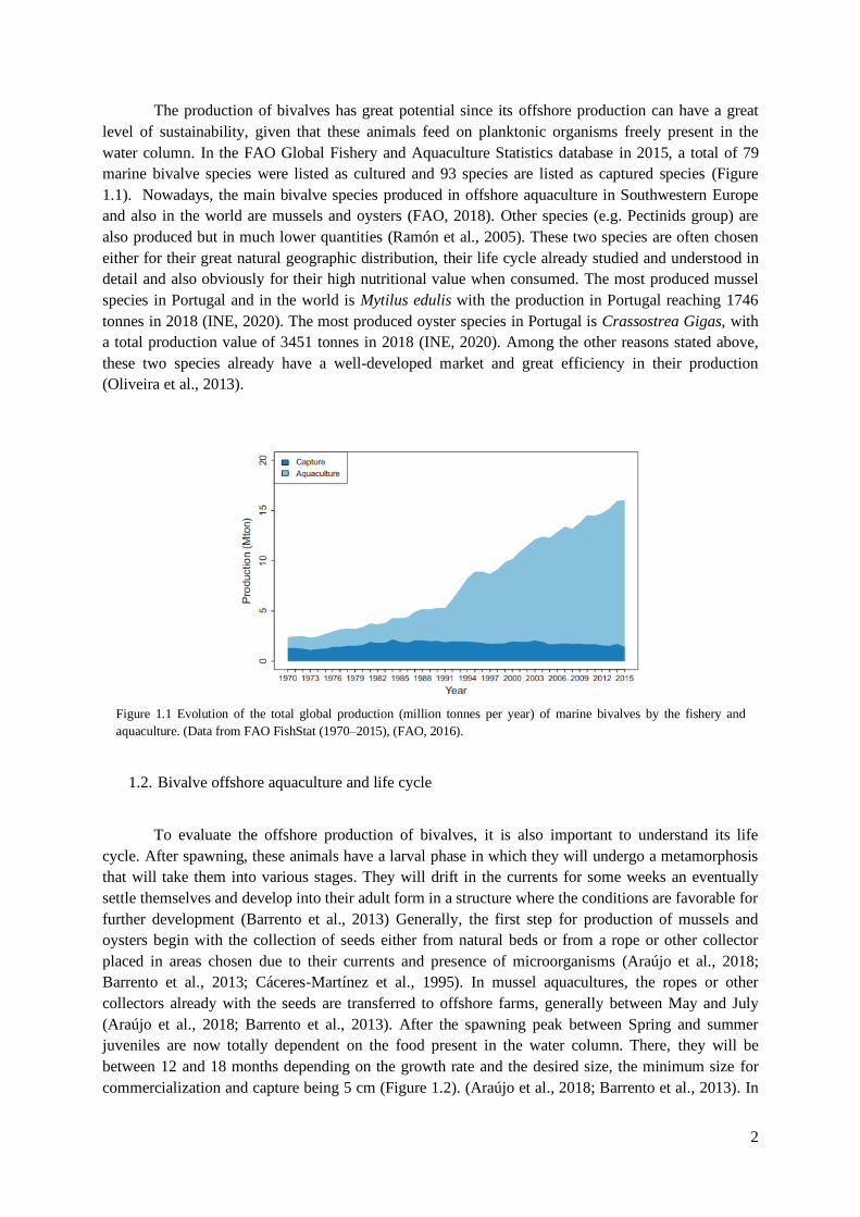
The production of bivalves has great potential since its offshore production can have a great

level of sustainability, given that these animals feed on planktonic organisms freely present in the

water column. In the FAO Global Fishery and Aquaculture Statistics database in 2015, a total of 79

marine bivalve species were listed as cultured and 93 species are listed as captured species (Figure

1.1). Nowadays, the main bivalve species produced in offshore aquaculture in Southwestern Europe

and also in the world are mussels and oysters (FAO, 2018). Other species (e.g. Pectinids group) are

also produced but in much lower quantities (Ramón et al., 2005). These two species are often chosen

either for their great natural geographic distribution, their life cycle already studied and understood in

detail and also obviously for their high nutritional value when consumed. The most produced mussel

species in Portugal and in the world is Mytilus edulis with the production in Portugal reaching 1746

tonnes in 2018 (INE, 2020). The most produced oyster species in Portugal is Crassostrea Gigas, with

a total production value of 3451 tonnes in 2018 (INE, 2020). Among the other reasons stated above,

these two species already have a well-developed market and great efficiency in their production

(Oliveira et al., 2013).

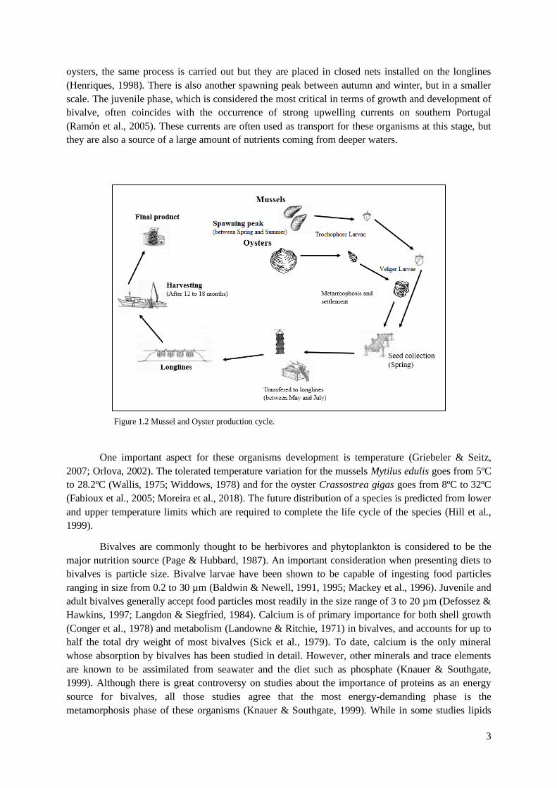
1.2. Bivalve offshore aquaculture and life cycle

To evaluate the offshore production of bivalves, it is also important to understand its life

cycle. After spawning, these animals have a larval phase in which they will undergo a metamorphosis

that will take them into various stages. They will drift in the currents for some weeks an eventually

settle themselves and develop into their adult form in a structure where the conditions are favorable for

further development (Barrento et al., 2013) Generally, the first step for production of mussels and

oysters begin with the collection of seeds either from natural beds or from a rope or other collector

placed in areas chosen due to their currents and presence of microorganisms (Araújo et al., 2018;

Barrento et al., 2013; Cáceres-Martínez et al., 1995). In mussel aquacultures, the ropes or other

collectors already with the seeds are transferred to offshore farms, generally between May and July

(Araújo et al., 2018; Barrento et al., 2013). After the spawning peak between Spring and summer

juveniles are now totally dependent on the food present in the water column. There, they will be

between 12 and 18 months depending on the growth rate and the desired size, the minimum size for

commercialization and capture being 5 cm (Figure 1.2). (Araújo et al., 2018; Barrento et al., 2013). In

Figure 1.1 Evolution of the total global production (million tonnes per year) of marine bivalves by the fishery and

aquaculture. (Data from FAO FishStat (1970–2015), (FAO, 2016).

3

oysters, the same process is carried out but they are placed in closed nets installed on the longlines

(Henriques, 1998). There is also another spawning peak between autumn and winter, but in a smaller

scale. The juvenile phase, which is considered the most critical in terms of growth and development of

bivalve, often coincides with the occurrence of strong upwelling currents on southern Portugal

(Ramón et al., 2005). These currents are often used as transport for these organisms at this stage, but

they are also a source of a large amount of nutrients coming from deeper waters.

One important aspect for these organisms development is temperature (Griebeler & Seitz,

2007; Orlova, 2002). The tolerated temperature variation for the mussels Mytilus edulis goes from 5ºC

to 28.2ºC (Wallis, 1975; Widdows, 1978) and for the oyster Crassostrea gigas goes from 8ºC to 32ºC

(Fabioux et al., 2005; Moreira et al., 2018). The future distribution of a species is predicted from lower

and upper temperature limits which are required to complete the life cycle of the species (Hill et al.,

1999).

Bivalves are commonly thought to be herbivores and phytoplankton is considered to be the

major nutrition source (Page & Hubbard, 1987). An important consideration when presenting diets to

bivalves is particle size. Bivalve larvae have been shown to be capable of ingesting food particles

ranging in size from 0.2 to 30 µm (Baldwin & Newell, 1991, 1995; Mackey et al., 1996). Juvenile and

adult bivalves generally accept food particles most readily in the size range of 3 to 20 µm (Defossez &

Hawkins, 1997; Langdon & Siegfried, 1984). Calcium is of primary importance for both shell growth

(Conger et al., 1978) and metabolism (Landowne & Ritchie, 1971) in bivalves, and accounts for up to

half the total dry weight of most bivalves (Sick et al., 1979). To date, calcium is the only mineral

whose absorption by bivalves has been studied in detail. However, other minerals and trace elements

are known to be assimilated from seawater and the diet such as phosphate (Knauer & Southgate,

1999). Although there is great controversy on studies about the importance of proteins as an energy

source for bivalves, all those studies agree that the most energy-demanding phase is the

metamorphosis phase of these organisms (Knauer & Southgate, 1999). While in some studies lipids

Figure 1.2 Mussel and Oyster production cycle.

4

are indicated as the major source of energy for Ostrea edulis during the metamorphosis phase

(Holland, 1973), in others the protein has been identified as the largest source of energy during

metamorphosis of the same species (Rodriguez et al., 1990). In offshore aquaculture, this phase of

greatest energy demand during metamorphosis has already been overcome and therefore it is not so

important to fulfill these requirements when choosing the location of the aquaculture units (Holland,

1973).

1.3. The importance of phytoplankton to bivalve aquaculture

Phytoplankton is at the basis of all marine food chains (Benemann, 1992) and is probably the

most important natural food source for bivalves, as already stated above. Other marine organisms,

such as fish, will also depend on this primary production, having indirect links with phytoplankton. In

terms of offshore shellfish production, the local dynamics of phytoplankton communities is of great

relevance. Thus, it is key to understand how phytoplankton cells are distributed geographically and

vertically along the water column to try to optimize the production of shellfish with this spatial

variation. In addition, it is also key to understand when the most important phytoplankton blooms are

expected in the region. Shellfish organisms are highly dependent on what naturally occurs in the

region where the production units are located. The knowledge on the types of phytoplankton (main

groups) needed to ensure the nutritional values that constitute the diets of different organisms is also

highly important (Berntsson et al., 1997; Delaporte et al., 2003). It is also crucial to know the main

environmental factors that affect and influence the phytoplankton spatial distribution and composition,

as well as the current pattern along the Portuguese coast (Ferreira et al., 2007).

The value of phytoplankton species as food for bivalve mollusks is important in determining

suitable diets for larval and juvenile development in aquaculture systems (Chu et al., 1982). Live

microalgae have been used as food in indoor bivalve hatcheries since the 1940s and a great number of

microalgal species have since been tested for their food value for different life stages of bivalves

(Brown et al., 1989; Bruce et al., 1940; Gui et al., 2016). Conditions under which phytoplankton grow

dictate biochemical composition and can affect energy and nutrient value of bivalves (Fabregas et al.,

1985). Recent experimental studies tend to indicate that bivalve mass growth is significantly affected

by diet quantity and quality (Pleissner et al., 2012), and that mussels may even modify their feeding

behavior according to local food composition (Toupoint et al., 2012). Most studies highlight the

importance of diatoms for mussel development (Maloy et al., 2013; Pronker et al., 2008), and also

dinoflagellates (Trottet et al., 2008). This also suggests that phytoplankton size presents an important

role since these two groups, which compose the microphytoplankton size class (20-200 µm), have

large dimensions when compared to the rest (Picoche et al., 2014). At indoor bivalve aquacultures, a

combination of microalgae including diatoms and flagellates is usually used because this has shown to

produce higher growth and survival rates due to the provision of a more balanced and complete diet

(Brown et al., 1997). The production of microalgae to feed juveniles in indoor aquacultures therefore

has high costs, which represents a disadvantage when compared to the use of what is present in the

natural environment for offshore production.

However, in the natural environment the constitution of the phytoplankton community is not

so regular and not necessarily in accordance with what has been identified as the best species or

groups for shellfish aquaculture. The community composition is diverse and changes with time, due to

the joint influence of factors such as temperature, salinity, light and nutrient availability and water

column stratification (Loureiro et al., 2018). Moreover, if environmental conditions are appropriate,

5

harmful microalgae with toxic potential for humans can occur, which can spell disaster in aquaculture

units (Sirakov et al., 2015). The toxins from some algal species can bioaccumulate in shellfish and

decrease fecundity, promote disease and render shellfish unsafe for human consumption (Burkholder,

1998; Shumway, 1990).

1.4. Study site

The Algarve coast in southern Portugal (Figure 1.3) is a region sheltered from the dominant

and most important swell source in Europe, the North Atlantic (Fiúza et al., 1982). This swell is

responsible for most storms on the Portuguese coast. Northerly winds along the west coast of the

Iberian Peninsula produce conditions for seasonal upwelling from early spring to late summer, whilst

occasional upwelling occurs along the southern coast of Portugal (Algarve) with favorable westerly

winds (Fiúza et al., 1982; Loureiro et al., 2005b). After a prolonged period of northerly winds,

enriched water can circulate around the Cabo S. Vincente, the southwestern tip of the peninsula, and

flow eastwards along the southern coastal shelf. These water transport around Sagres contribute to an

important dissipation of storm energy and wave height (Almeida et al., 2011). This makes the south

Portuguese coast much calmer in terms of waves and maritime agitation than the west coast. Also, the

presence of the São Vicente and Portimão canyons are two very important characteristics in the

geomorphology of the Algarve coast since they are also responsible for the strong presence of

upwelling in this area that bring waters rich in nutrients to the surface (Fiúza, 1983).

These characteristics of the southern coast show great potential for the production of bivalves

in offshore aquaculture structures. The offshore aquaculture in this area is almost only dependent on

the enrichment of the coastal waters by upwelling as there are no permanent rivers or streams in the

southwest area and the anthropogenic contribution is minimal because of the low resident population

and limited agriculture (Loureiro et al., 2005a).

50

100 m 200 m

Figure 1.3 Study site location on Algarve, south coast of Portugal.

6

In the Algarve coast, the presence of estuarine zones such as the Ria de Alvor or the Ria

Formosa can lead to deterioration of water quality in these coastal zones and their adjacent watersheds.

These coastal lagoons are vulnerable to human pressures produced by urbanization, industry,

agriculture, fish and shellfish culture, dredging, sewage discharges, and recreational activities (Vallejo,

1982). One of the potential consequences of these pressures is eutrophication, which is defined in the

Directives (91/271/EEC) of the European Union as an enrichment of waters by nutrients, especially

compounds of nitrogen and phosphorus, causing an accelerated growth of algae that may induce an

undesirable disturbance to the balance of the living organisms and water quality. This introduction of

nutrients can be both beneficial and harmful to marine life in adjacent coastal areas and it will depend

upon the assimilative capacity of a system (Bricker et al., 1999) that is modulated by the relative

changes in algal production, consumption and decomposition (Malone et al., 1996), as well as by the

degree of advective transport in open systems.

The water temperatures described for the Algarve coastline present average values around

18ºC and the peak of summer heating occurs from July to October when temperatures exceed 20ºC

(Baptista et al., 2018; Moita, 2001; Sánchez & Relvas, 2003). The average surface water salinity

described for the Algarve is 36 (Moita, 2001; Sánchez & Relvas, 2003).

The average satellite chlorophyll a water concentration values from 1997 to 2018 for this area

were 1 µg / L (Ferreira et al., 2021). Studies carried out to date on the phytoplankton community of

the Algarve have shown agreement on the presence and seasonality of the main groups. During the

whole year there is a predominance of diatoms introduced by currents that come from west and that

makes Sagres one of the areas with greatest potential since this concentration decreases along the coast

towards east (Coelho et al., 2007; Goela et al., 2014). This group is one of the main responsible for the

seasonal blooms since the diatoms have a great correlation with the presence in Chl a and have a

negative correlation with the increase in temperature. In the study by Loureiro et al. (2011) the

dominance of diatoms is related to cold waters, rich in nutrients that are introduced by the upwelling

currents on the Algarve coast. Turbulence is also a favorable factor for diatoms since they do not have

the capacity to move along the water column and so they use these vertical currents. Other groups also

identified in these studies were dinoflagellate, Chrysophytes and cyanobacteria but at much lower

values (Goela et al., 2014).

In the study by Silvano et al. (2012) the variation and patterns of the phytoplanktonic

community were studied, by subareas of the south Algarve coast, between 1998 and 2011. The coast

was divided into 3 zones: Cabo de São Vicente, west of Cabo de Santa Maria and east of Cabo de

Santa Maria. For the three zones, the seasonality patterns were very similar. The values of

phytoplankton primary production, obtained by Chl a concentration, were higher in the area west of

the Cabo de Santa Maria, and the months with the highest production for the entire coast were July

and August. The months of lowest production for the entire coast were January and December and it

was in Cabo de São Vicente where the lowest values were observed. This is also consistent with the

results of Ferreira et al. (2021).

Some of the factors that are described in previous works as potentially responsible for these

differences in distribution are, for example, the zone of strong seasonal upwelling currents next to the

tip of Sagres that will benefit groups that have greater benefit with lower temperatures or the areas of

discharges in organic matter or freshwater bodies in the coast that can also benefit the distribution of

groups that find crucial nutrients to their development here (Loureiro et al., 2011; Silvano et al., 2012).

7

Nowadays in the Algarve coast, according to the aquaculture geoportal platform of DGRM

(details in www.dgrm.mm.gov.pt), there are 9 offshore aquaculture units just for mussel and oyster

production that represent more than 200 hectares (Figure 1.4). In the rest of the Portuguese coast there

is only one more offshore aquaculture unit located in Peniche (Geoportal Aquicultura, DGRM, 2021).

The orange areas are units already in production and the areas marked in green are areas that are

available for production. The choice of location for these structures is typically empirical, sometimes

not taking into account all the biotic factors such as the presence and usage of these phytoplankton

communities.

1.5. Aim and objectives

The main goal of this study is to understand the spatial distribution of phytoplankton

communities in the Algarve coastal zone to evaluate the implications to the site selection for offshore

aquaculture units, taking into account the different abiotic factors. To achieve this goal, several

specific objectives were established: i) Evaluate how environmental factors affect the spatial

distribution of phytoplankton communities on the Algarve coast; ii) Identify areas that have high

phytoplankton biomass production along the Algarve coast and evaluate which phytoplankton groups

contribute the most to this production; iii) Identify the locations with the greatest potential for

implementing offshore aquaculture units, according to phytoplankton biomass, optimal temperature

and current conditions.

Figure 1.4 Offshore aquaculture units already established in the Algarve Coast (Data from Geoportal Aquicultura-

DGRM, April 2021).

8

2. Materials and Methods

2.1. Sampling strategy

Sampling was conducted between the 5th and 13th October 2018 on board of NRP “Almirante

Gago Coutinho” of the Portuguese Navy. This sampling campaign was performed within the scope of

the AQUIMAR project. Using a Neil Brown MKIIIC CTD (conductivity, temperature and depth)

profiler equipped with an Aquatracka nephelometer (turbidimeter), data were collected, at several

depths, for temperature, salinity and turbidity, and profiles were also built. Some profiles data were

removed from the analysis after implementing quality control procedures, mainly due to data problems

at greater depth. From a total of 127 stations where CTD profiles were made, as shown in annex

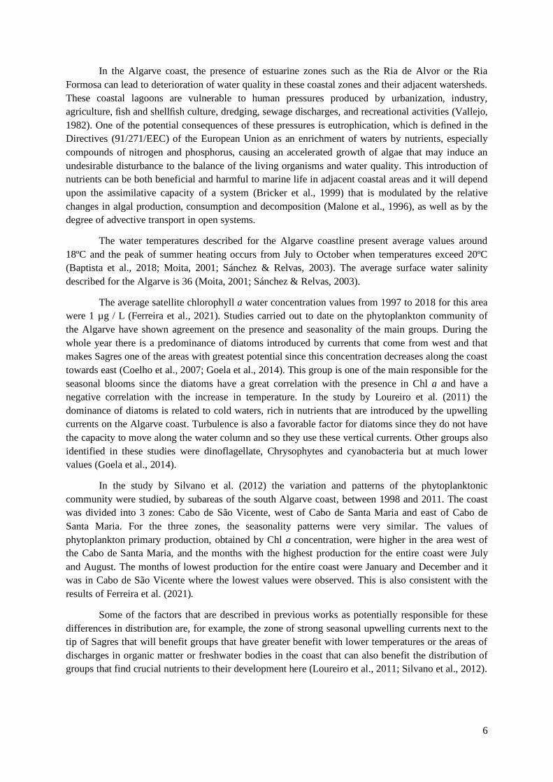
Figure A1, 52 of these stations were selected for water sampling (Figure 2.1). These stations were

selected in order to uniformly cover the Algarve coast completely. The stations were located along the

entire coast of the Algarve with a range from 1.5 to 15 nautical miles from the coastline and with a

depth ranging between 25 and 350 meters.

2.2. Seawater sample collection

Water samples were collected using a rosette sampler (12 Niskin bottles of 8 L). Water

samples for oxygen levels and nutrient analysis were collected at surface, 25 meters and 50 meters

depth. In addition, for phytoplankton pigment characterization (identification and quantification),

samples were also taken from the surface at all stations and whenever a deep chlorophyll maximum

(DCM) was detected. A DCM occurs when there is the presence of a maximum peak of Chl a in

deeper levels of the water column. DCM is the result of an accumulation of phytoplankton organisms

that find optimal growth conditions, particularly in terms of light and nutrients availability, at a

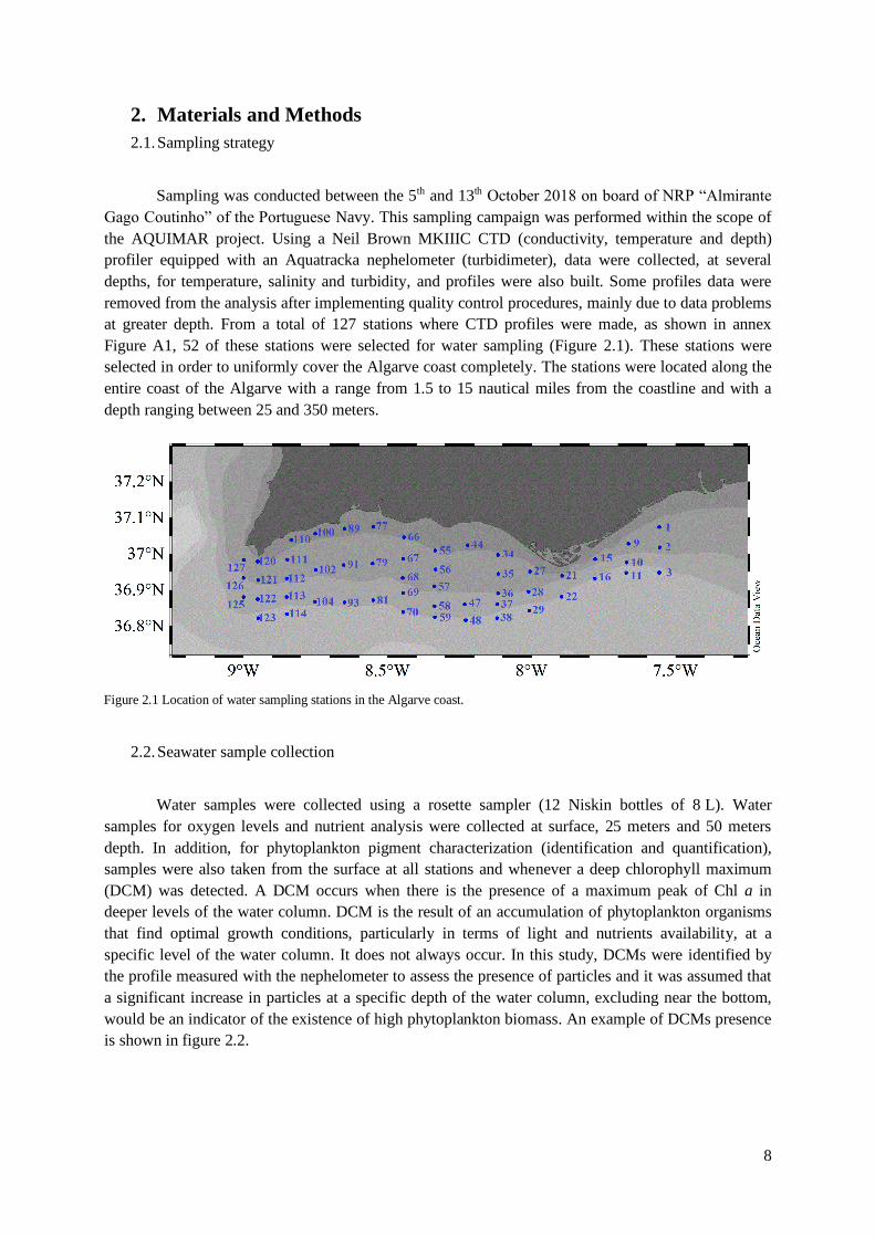
specific level of the water column. It does not always occur. In this study, DCMs were identified by

the profile measured with the nephelometer to assess the presence of particles and it was assumed that

a significant increase in particles at a specific depth of the water column, excluding near the bottom,

would be an indicator of the existence of high phytoplankton biomass. An example of DCMs presence

is shown in figure 2.2.

Figure 2.1 Location of water sampling stations in the Algarve coast.

9

2.3. Oceanic currents characterization

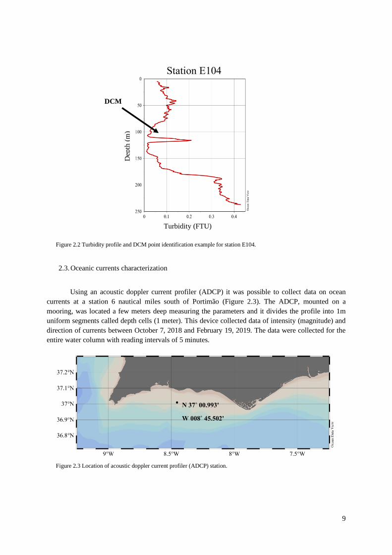
Using an acoustic doppler current profiler (ADCP) it was possible to collect data on ocean

currents at a station 6 nautical miles south of Portimão (Figure 2.3). The ADCP, mounted on a

mooring, was located a few meters deep measuring the parameters and it divides the profile into 1m

uniform segments called depth cells (1 meter). This device collected data of intensity (magnitude) and

direction of currents between October 7, 2018 and February 19, 2019. The data were collected for the

entire water column with reading intervals of 5 minutes.

DCM

Dep

th (

m)

Turbidity (FTU)

Station E104

Figure 2.2 Turbidity profile and DCM point identification example for station E104.

N 37˚ 00.993'

W 008˚ 45.502'

Figure 2.3 Location of acoustic doppler current profiler (ADCP) station.

10

2.4. Laboratory analysis

2.4.1. Seawater physico-chemical characterization

Seawater samples were collected using glass bottles at each station. The appropriate reagents

were added in situ and the bottle protected from any air contact (Grasshoff et al., 1999). The bottles

were transported as soon as possible to the laboratory, where they were analyzed following the method

presented by Grasshoff et al.(1999) which is based on the method first proposed by Winkler (1888).

For nutrient determination, water samples were independently homogenized and filtered using

a 0.45 μm pore size cartridge (Pall, AquaPrep 600), and approximately 200 mL of filtered water was

retained in high-density polyethylene bottles and immediately stored in a freezer at a temperature of -

18ºC to be further analyzed in the laboratory. Nutrient concentrations (nitrate, nitrite, ammonium,

reactive phosphate and silicate) were later determined in the laboratory using a Skalar SANplus

Segmented Flow AutoAnalyzer specially developed for the analysis of saline waters. N–NOx and N–

NO2 were determined according to (Strickland & Parsons, 1972), with N–NO3 being estimated by the

difference between the previous two; N– NH4 and Si–SiO2 were determined according to (Koroleff,

1976); P–PO4 was determined according to (Murphy & Riley, 1962). The dissolved inorganic

nitrogen data resulted from the sum of nitrite, nitrate and ammoniacal nitrogen data. All methods were

adapted to the methodology of segmented flow analysis and uncertainties were determined following

Borges et al. (2019).

2.4.2. Seawater biological characterization

Phytoplankton pigments were analyzed through High Performance Liquid Chromatography

(HPLC). For this, two liters of water were filtered to concentrate its content on the surface of a 25 mm

diameter GF/F (Whatman glass microfiber) filter, with pore size of 0.7 μm. For some coastal stations

with higher concentration of phytoplankton cells, a lower sample volume (e.g. 500 mL of seawater)

was needed. Seawater was added consecutively until the filter got the desired colour. The filtration

should be carried out as soon as possible after sampling and in dark and cold conditions. Each filter

was then folded to and packed in properly labeled aluminum foil (containing the following

information: station, depth, date and filtered volume) and then stored in liquid nitrogen to preserve the

material. Samples were transported to the laboratory as soon as possible, where they were preserved at

-80ºC until further analysis.

The phytoplanktonic pigments were extracted (macerating the filter) with 95% cold buffered

methanol (2% ammonium acetate) enriched with a concentration of 0.005 mg / L of trans-beta-apo-8'-

carotenal for 30 minutes at -20 ° C, in the dark. Halfway through the extraction period, the samples

were placed on the ultrasound for 5 min and, after the extraction period, centrifuged for 10 min at

4000 RPM and 4 ° C. All extracts were filtered (on Fluoropore PTFE filter membranes, with a pore

size of 0.2 μm) and immediately injected into the vial with 0.4 ml of ultra-pure water and inserted into

the HPLC for reading the sample. Samples were analyzed in the laboratory using a Shimadzu

Prominence-i LC-2030C 3D equipment with RF-20ª Prominence ex fluorescence detector 350nm-

800nm using a reverse phase C8 colum (Symmetry; 15 cm long; 4.6 cm in diameter, 100 pm pore size

and 3.5 µm particle size, 337 m2g-1 area and 12.27% carbon). The C8 method developed by Zapata et

al. (2000) was used. This reverse phase method uses these solvents: A) Methanol + Acetonitrile +

Aqueous Pyridine and B) Methanol + Acetonitrile + Acetone, with an injection volume of 100µl and

11

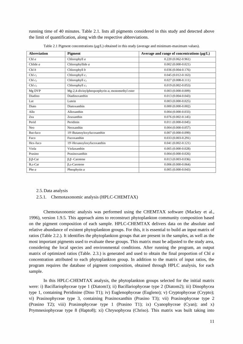
running time of 40 minutes. Table 2.1. lists all pigments considered in this study and detected above

the limit of quantification, along with the respective abbreviations.

Table 2.1 Pigment concentrations (µg/L) obtained in this study (average and minimum-maximum values).

2.5. Data analysis

2.5.1. Chemotaxonomic analysis (HPLC-CHEMTAX)

Chemotaxonomic analysis was performed using the CHEMTAX software (Mackey et al.,

1996), version 1.9.5. This approach aims to reconstruct phytoplankton community composition based

on the pigment composition of each sample. HPLC-CHEMTAX delivers data on the absolute and

relative abundance of existent phytoplankton groups. For this, it is essential to build an input matrix of

ratios (Table 2.2.). It identifies the phytoplankton groups that are present in the samples, as well as the

most important pigments used to evaluate these groups. This matrix must be adjusted to the study area,

considering the local species and environmental conditions. After running the program, an output

matrix of optimized ratios (Table. 2.3.) is generated and used to obtain the final proportion of Chl a

concentration attributed to each phytoplankton group. In addition to the matrix of input ratios, the

program requires the database of pigment composition, obtained through HPLC analysis, for each

sample.

In this HPLC-CHEMTAX analysis, the phytoplankton groups selected for the initial matrix

were: i) Bacillariophyceae type 1 (Diatom1); ii) Bacillariophyceae type 2 (Diatom2); iii) Dinophycea

type 1, containing Peridinine (Dino T1); iv) Euglenophyceae (Eugleno); v) Cryptophyceae (Crypto);

vi) Prasinophyceae type 3, containing Prasinoxanthin (Prasino T3); vii) Prasinophyceae type 2

(Prasino T2); viii) Prasinophyceae type 1 (Prasino T1); ix) Cyanophyceae (Cyan); and x)

Prymnesiophyceae type 8 (Hapto8); xi) Chrysophycea (Chriso). This matrix was built taking into

Abreviation Pigment Average and range of concentrations (µg/L)

Chl a Chlorophyll a 0.220 (0.062-0.961)

Chlide a Chlorophyllide a 0.002 (0.000-0.021)

Chl b Chlorophyll b 0.036 (0.004-0.176)

Chl c1 Chlorophyll c1 0.045 (0.012-0.163)



Mg DVP Mg-2,4-divinylpheoporphyrin a5 monomethyl ester 0.003 (0.000-0.009)

Diadino Diadinoxanthin 0.013 (0.004-0.043)

Lut Lutein 0.003 (0.000-0.025)

Diato Diatoxanthin 0.000 (0.000-0.002)

Allo Alloxanthin 0.004 (0.000-0.033)

Zea Zeaxanthin 0.076 (0.002-0.145)

Perid Peridinin 0.011 (0.000-0.045)

Neo Neoxanthin 0.004 (0.000-0.057)

But-fuco 19'-Butanoyloxyfucoxanthin 0.007 (0.000-0.099)

Fuco Fucoxanthin 0.033 (0.003-0.291)

Hex-fuco 19'-Hexanoyloxyfucoxanthin 0.041 (0.002-0.121)

Viola Violaxanthin 0.005 (0.000-0.028)

Prasino Prasinoxanthin 0.004 (0.000-0.026)

β,β-Car β,β -Carotene 0.013 (0.003-0.036)

Β,ε-Car β,ε-Carotene 0.006 (0.000-0.064)

Phe a Pheophytin a 0.005 (0.000-0.043)

12

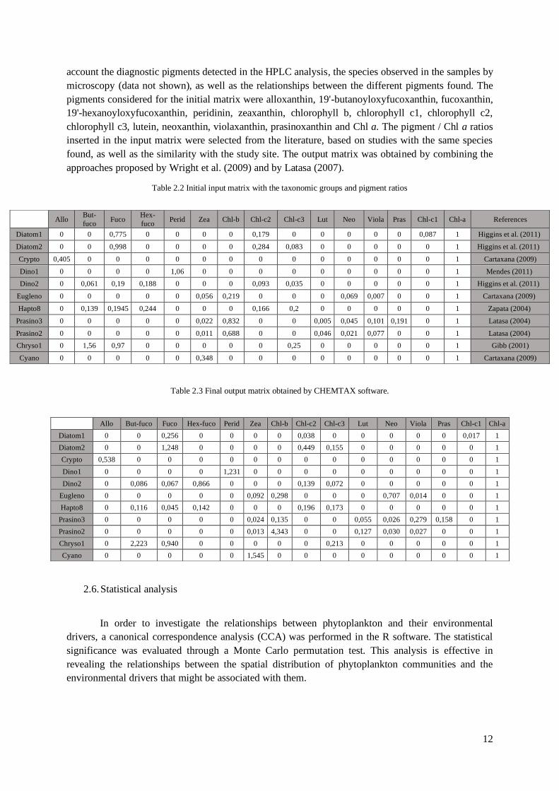
account the diagnostic pigments detected in the HPLC analysis, the species observed in the samples by

microscopy (data not shown), as well as the relationships between the different pigments found. The

pigments considered for the initial matrix were alloxanthin, 19'-butanoyloxyfucoxanthin, fucoxanthin,

19'-hexanoyloxyfucoxanthin, peridinin, zeaxanthin, chlorophyll b, chlorophyll c1, chlorophyll c2,

chlorophyll c3, lutein, neoxanthin, violaxanthin, prasinoxanthin and Chl a. The pigment / Chl a ratios

inserted in the input matrix were selected from the literature, based on studies with the same species

found, as well as the similarity with the study site. The output matrix was obtained by combining the

approaches proposed by Wright et al. (2009) and by Latasa (2007).

Table 2.2 Initial input matrix with the taxonomic groups and pigment ratios

Table 2.3 Final output matrix obtained by CHEMTAX software.

2.6. Statistical analysis

In order to investigate the relationships between phytoplankton and their environmental

drivers, a canonical correspondence analysis (CCA) was performed in the R software. The statistical

significance was evaluated through a Monte Carlo permutation test. This analysis is effective in

revealing the relationships between the spatial distribution of phytoplankton communities and the

environmental drivers that might be associated with them.

Allo But-

fuco Fuco

Hex-

fuco Perid Zea Chl-b Chl-c2 Chl-c3 Lut Neo Viola Pras Chl-c1 Chl-a References

Diatom1 0 0 0,775 0 0 0 0 0,179 0 0 0 0 0 0,087 1 Higgins et al. (2011)

Diatom2 0 0 0,998 0 0 0 0 0,284 0,083 0 0 0 0 0 1 Higgins et al. (2011)

Crypto 0,405 0 0 0 0 0 0 0 0 0 0 0 0 0 1 Cartaxana (2009)

Dino1 0 0 0 0 1,06 0 0 0 0 0 0 0 0 0 1 Mendes (2011)

Dino2 0 0,061 0,19 0,188 0 0 0 0,093 0,035 0 0 0 0 0 1 Higgins et al. (2011)

Eugleno 0 0 0 0 0 0,056 0,219 0 0 0 0,069 0,007 0 0 1 Cartaxana (2009)

Hapto8 0 0,139 0,1945 0,244 0 0 0 0,166 0,2 0 0 0 0 0 1 Zapata (2004)

Prasino3 0 0 0 0 0 0,022 0,832 0 0 0,005 0,045 0,101 0,191 0 1 Latasa (2004)

Prasino2 0 0 0 0 0 0,011 0,688 0 0 0,046 0,021 0,077 0 0 1 Latasa (2004)

Chryso1 0 1,56 0,97 0 0 0 0 0 0,25 0 0 0 0 0 1 Gibb (2001)

Cyano 0 0 0 0 0 0,348 0 0 0 0 0 0 0 0 1 Cartaxana (2009)

Allo But-fuco Fuco Hex-fuco Perid Zea Chl-b Chl-c2 Chl-c3 Lut Neo Viola Pras Chl-c1 Chl-a

Diatom1 0 0 0,256 0 0 0 0 0,038 0 0 0 0 0 0,017 1

Diatom2 0 0 1,248 0 0 0 0 0,449 0,155 0 0 0 0 0 1

Crypto 0,538 0 0 0 0 0 0 0 0 0 0 0 0 0 1

Dino1 0 0 0 0 1,231 0 0 0 0 0 0 0 0 0 1

Dino2 0 0,086 0,067 0,866 0 0 0 0,139 0,072 0 0 0 0 0 1

Eugleno 0 0 0 0 0 0,092 0,298 0 0 0 0,707 0,014 0 0 1

Hapto8 0 0,116 0,045 0,142 0 0 0 0,196 0,173 0 0 0 0 0 1

Prasino3 0 0 0 0 0 0,024 0,135 0 0 0,055 0,026 0,279 0,158 0 1

Prasino2 0 0 0 0 0 0,013 4,343 0 0 0,127 0,030 0,027 0 0 1

Chryso1 0 2,223 0,940 0 0 0 0 0 0,213 0 0 0 0 0 1

Cyano 0 0 0 0 0 1,545 0 0 0 0 0 0 0 0 1

13

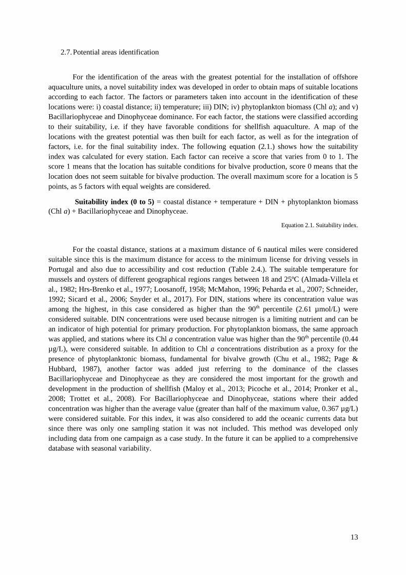
2.7. Potential areas identification

For the identification of the areas with the greatest potential for the installation of offshore

aquaculture units, a novel suitability index was developed in order to obtain maps of suitable locations

according to each factor. The factors or parameters taken into account in the identification of these

locations were: i) coastal distance; ii) temperature; iii) DIN; iv) phytoplankton biomass (Chl a); and v)

Bacillariophyceae and Dinophyceae dominance. For each factor, the stations were classified according

to their suitability, i.e. if they have favorable conditions for shellfish aquaculture. A map of the

locations with the greatest potential was then built for each factor, as well as for the integration of

factors, i.e. for the final suitability index. The following equation (2.1.) shows how the suitability

index was calculated for every station. Each factor can receive a score that varies from 0 to 1. The

score 1 means that the location has suitable conditions for bivalve production, score 0 means that the

location does not seem suitable for bivalve production. The overall maximum score for a location is 5

points, as 5 factors with equal weights are considered.

Suitability index (0 to 5) = coastal distance + temperature + DIN + phytoplankton biomass

(Chl a) + Bacillariophyceae and Dinophyceae.

Equation 2.1. Suitability index.

For the coastal distance, stations at a maximum distance of 6 nautical miles were considered

suitable since this is the maximum distance for access to the minimum license for driving vessels in

Portugal and also due to accessibility and cost reduction (Table 2.4.). The suitable temperature for

mussels and oysters of different geographical regions ranges between 18 and 25ºC (Almada-Villela et

al., 1982; Hrs-Brenko et al., 1977; Loosanoff, 1958; McMahon, 1996; Peharda et al., 2007; Schneider,

1992; Sicard et al., 2006; Snyder et al., 2017). For DIN, stations where its concentration value was

among the highest, in this case considered as higher than the 90th percentile (2.61 µmol/L) were

considered suitable. DIN concentrations were used because nitrogen is a limiting nutrient and can be

an indicator of high potential for primary production. For phytoplankton biomass, the same approach

was applied, and stations where its Chl a concentration value was higher than the 90th percentile (0.44

µg/L), were considered suitable. In addition to Chl a concentrations distribution as a proxy for the

presence of phytoplanktonic biomass, fundamental for bivalve growth (Chu et al., 1982; Page &

Hubbard, 1987), another factor was added just referring to the dominance of the classes

Bacillariophyceae and Dinophyceae as they are considered the most important for the growth and

development in the production of shellfish (Maloy et al., 2013; Picoche et al., 2014; Pronker et al.,

2008; Trottet et al., 2008). For Bacillariophyceae and Dinophyceae, stations where their added

concentration was higher than the average value (greater than half of the maximum value, 0.367 µg/L)

were considered suitable. For this index, it was also considered to add the oceanic currents data but

since there was only one sampling station it was not included. This method was developed only

including data from one campaign as a case study. In the future it can be applied to a comprehensive

database with seasonal variability.

14

Table 2.4 Suitable and not suitable parameters for potential areas identification.

Parameter Suitable Not suitable

Coastal distance ≤ 6 NM > 6 NM

Temperature ≥ 18º and ≤ 25ºC <18ºC and >25ºC

DIN ≥ 2.61 µmol/L < 2.61 µmol/L

Phytoplankton biomass (Chl a) ≥ 0.44 µg/L Chl a < 0.44 µg/L Chl a

Bacillariophyceae and Dinophyceae ≥ 0.367 µg/L < 0.367 µg/L

15

3. Results

3.1. Environmental conditions

Through the data obtained by the ADCP apparatus, schematic representations were made to

characterize the currents. The direction frequency from the current is presented in figure 3.1. In this

graph it is possible to observe that 77.3% of the current readings indicated that Southwest was the

main direction of the current. It was also observed that for 9.1% of the readings the direction was from

the South. There were also current readings from the Northwest, East and Southeast, but these were

only observed in 4.5% of the total readings during the sampling period.

For the current magnitude, it was observed that the mean current magnitude varied between

100 and 150 mm/s for depths starting at 3.5 meters and that it was approaching 100 mm/s with the

increase in depth (Figure 3.2). The maximum value of current magnitude was 518 mm/s. From the

surface down to 3.5 meters, the mean magnitude was less than 100 mm/s, reducing near the surface to

approximately 25 mm/s.

Figure 3.1 Current direction in relative frequency, measured by ADCP (7th of October 2018 to 19th of February

2019).

0 50 100 150 200 250

21,5

19,5

17,5

15,5

13,5

11,5

9,5

7,5

5,5

3,5

1,5

magnitude (mm/s)

dep

th (

met

ers)

Figure 3.2 Current magnitude (mm/s) in depth read by ADCP (7th of October 2018 to 19th of

February 2019).

16

Temperatures measured at the sea surface varied between 20º and 24ºC (Figure 3.3). In

general, and as expected, the highest temperature values were recorded further east of the Algarve

coast and the lowest sea surface temperatures values in the most western zone. The station with the

highest temperature was located near Lagos, and the lowest temperature was recorded in a station

further away from the coast and south of Cabo de Sagres.

The salinity at the surface showed the lowest values (36) at the most western stations and the

highest (36.8) values at offshore stations in the central coast of the Algarve. The stations closest to the

coast showed similarity in their salinity values of around 36.5 (Figure 3.4). The oxygen values showed

the maximum value of 8 mg/L in 17 stations along the entire coast and the minimum value of 6 mg/L

in only two offshore stations on the Algarve coast (Figure 3.5).

Figure 3.3 Ocean surface temperature (ºC) in the Algarve coast (5th-13th of October 2018).

Figure 3.4 Surface salinity in the Algarve coast (5th-13th of October 2018).

Figure 3.5 Surface oxygen values (mg/L) in the Algarve coast (5th-13th of October 2018).

17

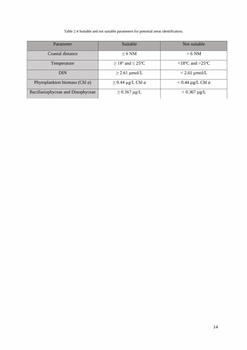
The potential temperature (obtained through in situ temperature and pressure measured by

CTD) represents which temperature the water would present ignoring the pressure that is being carried

out on it. By plotting these values with salinity, i.e. producing a TS diagram, it is possible to identify

different water masses along the water column. This diagram also allows the representation of the

potential density (ignoring the pressure to which it is subjected). In the TS diagram presented in figure

3.6 it is possible to see that the density down to 40 meters is very variable, indicating that this segment

(0 to 40 meters) is well mixed.

3.2. Nutrient distribution

In general terms, the spatial distribution, at surface, of nutrient concentrations, such as

dissolved inorganic nitrogen, (DIN, composed of nitrite + nitrate + ammoniacal nitrogen), phosphate

and silica were similar (Figure 3.7). DIN concentrations varied between 0.15 and 9.47 µmol/L,

Phosphate varied between 0.10 and 1.48 µmol/L and silica varied between 0.70 and 25.00 µmol/L.

Lower concentrations were observed over the entire sampling area for DIN and silica, except near the

coast of Portimão and at offshore stations in front of Faro, where high nutrient concentrations were

observed (Figures 3.7A and 3.7C). For phosphate high concentrations were found in different offshore

stations in the eastern zone, in Albufeira and Tavira coastal areas (Figure 3.7B).

Depth (m)

Salinity

Figure 3.4 T-S Diagram (potential temperature, salinity and potential density in contours) made from the CTD

profiles for the Algarve coast (5th-13th of October 2018).

18

3.3. Chlorophyll a concentration

The seven stations where DCMs were detected through the nephelometer are shown in figure

3.8. The DCM depths ranged between 65 and 110 meters and the distance from the coast between 1

and 15 nautical miles. These DCMs were identified through the CTD but for logistical reasons it was

not possible to collect samples at these depths for HPLC analysis. Anyway, the depths where DCMs

were identified were too deep for the installation of offshore aquaculture units, therefore, in this work

only the concentrations in Chl a closer to the surface were analyzed.

The spatial distribution of Chl a concentrations at surface, used as a proxy of phytoplankton

biomass, are presented in figure 3.9. The Chl a concentration varied between 0.05 and 0.96 µg/L. The

station where the highest Chl a concentration was registered was located near the coast of Faro and

yielded a concentration of 0.96 µg/L. In October 2018, the highest concentrations of Chl a were

observed near the coastal zones of Lagos, Portimão, Faro and Tavira.

A) Dissolved inorganic nitrogen (µmol/L).

B) Reactive phosphorus (µmol/L).

C) Reactive silica (µmol/L).

Figure 3.5 Dissolved inorganic nitrogen, reactive phosphorus and reactive silica concentration (µmol/L) in the

Algarve coast (5th-13th of October 2018).

19

3.4. Phytoplankton pigments and chemotaxonomy (CHEMTAX)

The CHEMTAX analysis provides the Chl a concentration associated with each

phytoplanktonic group, i.e. the absolute pigment concentrations. This analysis indicated that the

Bacillariophyceae and Dinophyceae were the groups that contributed the most to the higher values of

Chl a observed near Faro (Figure 3.10A, 3.10B). The distribution of these two groups showed the

highest total value in the area near Faro with Bacillariophyceae showing 0.430 µg/L and Dinophyceae

with 0.305 µg/L and its distributions mainly restricted to this area. It was in this same station where

Chl a presented the highest concentration value with the remaining groups presenting: Euglenophycea

with 0.021 µg/L; Prymnesiophyceae with 0.086 µg/L; Cyanophyceae with 0.047 µg/L; Chrysophyceae

with 0.004 µg/L; Prasinophyceae with 0.124 µg/L and finally Cryptophyceae showing 0.029 µg/L.

The group that contributed the least to the Chl a concentration was Chrysophyceae with the highest

Chl a concentration of 0.010 µg/L at a station on Quarteira coast (Figure 3.10F). The Euglenophyceae

(Sagres area) and Cryptophyceae (Lagos area) groups presented the same highest values (0.080 µg/L)

as showed in figure 3.10C and 3.10.H. The groups Prymnesiophyceae, Cyanophyceae and

Chrysophyceae presented similar distributions, with highest values in the eastern part of the Algarve

coast (Prymnesiophyceae 0.150 µg/L, Cyanophyceae 0.093 µg/L and Chrysophyceae 0.010 µg/L),

(Figure 3.10D, 3.10E and 3.10.F). The class Prymnesiophyceae was the only one to present a higher

distribution value (0.120 µg/L) in a station further away from the coastline (8 NM). Prasinophyceae

and Cryptophyceae also presented similar distributions with their highest values in the western part of

the Algarve coast (Figure 3.10G and 3.10.H).

Figure 3.8 Location of sampling points with deep chlorophyll maximum presence (DCM-green points) on the Algarve

coast. (5th-13th of October 2018).

Figure 3.9 Chlorophyll a concentration (µg/L) at surface in the Algarve coast (5th-13th of October 2018).

20

A) Bacillariophyceae.

C) Euglenophyceae.

E) Cyanophyceae.

G) Prasinophyceae.

B) Dinophyceae.

D) Prymnesiophyceae.

F) Chrysophyceae.

H) Cryptophyceae.

Figure 3.10 Spatial distribution of absolute chlorophyll a concentrations associated with the following classes: Bacillariophyceae, Dinophyceae, Euglenophyceae, Prymnesiophyceae,

Cyanophyceae, Chrysophyceae, Prasinophyceae and Cryptophyceae (µg/L). Contribution of phytoplankton groups to total chlorophyll a obtained through CHEMTAX analysis (Algarve

coast; 5th-13th of October 2018).

21

The relative group composition consists of the fractions of Chl a concentrations associated

with each phytoplanktonic group, obtain from CHEMTAX analysis. In figure 3.11 the relative group

composition averaged by distance to coastal zone are presented. Three categories were created:

Coastal, Middle and Offshore stations. In this graph it is possible to observe that Bacillariophyceae,

Euglenophyceae, Prasinophyceae and Cryptophyceae presented the highest fractions in the coastal

stations. The classes Dinophycea, Prymnesiophyceae and Cyanophyceae showed the highest values

away to the coastline. Euglenophyceae and Chrysophyceae were the classes less represented in the

phytoplankton community at all stations. Cyanophyceae was the only group that was the most

represented in the middle stations and the Dinophyceae and Prymnesiophyceae showed a higher

presence in the most offshore community.

3.5. Phytoplankton response to environmental drivers

A Canonical Correspondence Analysis (CCA) was used to analyse the response of the

phytoplankton community to the environmental variables observed in this study (Figure 3.12).

Phytoplankton composition data (i.e. groups derived from HPLC-CHEMTAX analysis) were Log x+1

transformed. A Monte Carlo test with showed that the six environmental variables significantly

explained the variability of phytoplankton data (p-value= 0.0010). Results are presented for groups

derived from the CHEMTAX analysis. The CCA explained 92.2% of the variance for the

phytoplankton-environment drivers relationship. The first canonical axis alone explained 82.4% of the

variance and the separation of the biological variables explained 32.0%.

Figure 3.11 Spatial distribution of relative chlorophyll a concentrations associated with the following classes: Bacillariophyceae,

Dinophyceae, Euglenophyceae, Prymnesiophyceae, Cyanophyceae, Chrysophyceae, Prasinophyceae and Cryptophyceae.

Contribution of phytoplankton groups to total chlorophyll a obtained through CHEMTAX analysis (Algarve coast; 5th-13th of

October 2018).

22

The analysis showed that Bacillariophyceae, Cryptophycea and Prasinophyceae responded

well to silicate distribution and were negatively associated with coastal distance. Chrysophyceae,

Cyanophyceae, Prymnesiophyceae and Dinophyceae were associated with phosphorus, salinity and

coastal distance, showing a negative relation with silicate. The Euglenophycea group was the only one

that distanced from the others, indicated a negative relation with the salinity and positive with DIN.

For temperature, Euglenophyceae was the class that showed the most evident association, being

associated with low temperatures.

3.6. Identification of the most suitable locations

The spatial suitability graphs are presented in figure 3.13 for all factors included in the

suitability index. For coastal distance, it was possible to observe that the stations closest to the

coastline are identified as suitable since they are closer than 6 nautical miles (Figure 3.13A). For

temperature, all stations were identified as suitable since they are within the temperature range

tolerated by the two species (Figure 3.13B). The spatial distribution of the suitable locations according

to DIN concentrations was very similar to the distribution of DIN concentrations since these suitable

points were computed using the 90 percentile of these concentrations (Figure 3.13C). The suitability

assessment according to the phytoplankton biomass highlighted the coasts of Lagos, Portimão, Faro

and also in a more distant station in Quarteira coast (Figure 3.13D). The area defined as suitable

according to the dominance of Bacillariophyceae and Dinophyceae groups was observed in the coast

of Faro (Figure 3.13E).

Figure 3.12 Canonical Correspondence Analysis ordination diagram relative to data on phytoplankton groups

(Bacillariophyceae, Dinophyceae, Euglenophyceae, Prymnesiophyceae, Cyanophyceae, Chrysophyceae, Prasinophyceae and

Cryptophyceae). The arrows refer to environmental variables (temperature, salinity, phosphorus, silica, dissolved inorganic

nitrogen and coast distance).

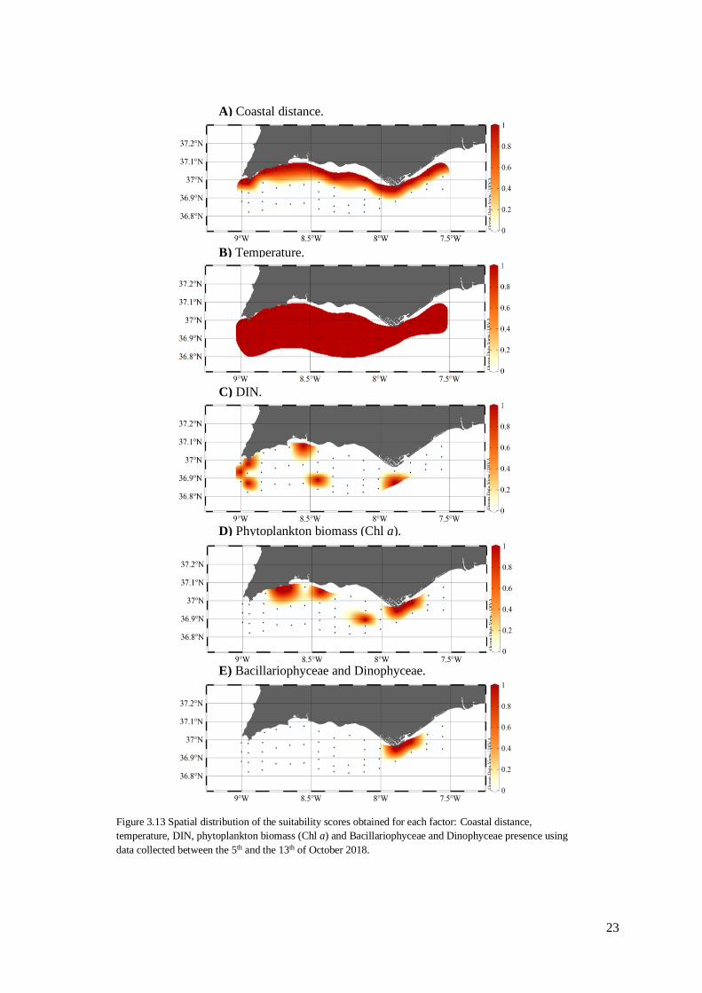
23

A) Coastal distance.

E) Bacillariophyceae and Dinophyceae.

D) Phytoplankton biomass (Chl a).

C) DIN.

B) Temperature.

Figure 3.13 Spatial distribution of the suitability scores obtained for each factor: Coastal distance,

temperature, DIN, phytoplankton biomass (Chl a) and Bacillariophyceae and Dinophyceae presence using

data collected between the 5th and the 13th of October 2018.

24

4. Discussion

4.1. Spatial distribution of physico-chemical parameters

Regarding the direction of sea currents, it was possible to observe that for the period (5th-13th

of October 2018) considered in this study, the main direction of the currents was from SW with 77,3%

of frequency. Several studies on the Algarve coast to study oceanic conditions have already been

performed and provided similar outputs (e.g. Costa et al., 2001; Fiúza et al., 1982). The south coast of

Portugal, as it is not directly exposed to the predominant agitation components on the west coast,

specifically the NW swell generated in the North Atlantic, presents much less severe average

conditions when compared to the rest of the Portuguese coast (Costa et al., 2001; Fiúza et al., 1982).

Considering the study of Costa et al. (2001) that sampled from 1980 to 2002, the results

presented herein are similar, i.e. the frequency of the direction of the currents in the winter months was

SW, replacing the direction of W present during the summer months. Also, the unidirectional storm

currents on the south coast come essentially from SW (64%) and SE (32%), both having a short

duration (máx. 5 days) and reduced severity (waves with average size of 2-5 meters and maximum

size of 6 meters) (Costa et al., 2001). Thus, it is possible to observe a consistency in the calm

conditions for the Algarve coast, only altered by storm situations with a maximum duration of 5 days.

In the study of Almeida et al. (2011), historical variations and trends in storminess for the

south coast of Portugal were investigated for the period from 1952 to 2009, using both measured and

modelled data (derived from wind data) for direction and magnitude. The same study also identified

that the average direction of the current was of SW. It was concluded that for the Algarve coast no

statistically significant linear trend was found for any of the storm characteristics over the period of

interest (Almeida et al., 2011). It is important to note that, considering the predominant direction of

SW, the coastal area of Lagos is the most protected from this current direction.

The currents can affect several factors in offshore aquacultures, such as the dispersion of food

and cultured organisms’ secretions, the renovation of water and the safety of the cultivation structure.

As such, the current magnitude must be taken into account when choosing the offshore cultivation

sites (Cardia & Lovatelli, 2016).

Some tests have already been done to study the influence of currents magnitude on the growth

rate of these organisms but only for current magnitudes up to 40 mm/s. The results of these studies

with Mytilus edulis indicated that the growth of the bivalves increased with the increase in the

magnitude of the current supplied (Rosenberg & Loo, 1983; Wildish & Kristmanson, 1985). As

literature suggests, higher current magnitude values as those collected from the Algarve coast from 5th

of October 2018 to 9th of February 2019, shows potential for higher growth rates on these organisms.

According to data obtained from FAO Fisheries and Aquaculture Proceedings No. 24 (2013),

the technical limits on longlines are at current speeds from 100 to 1000 mm/s), (FAO, 2013). For the

ADCP station location, the maximum value of current magnitude was 518 mm/s (probably during a

storm event), showing that this area seems to be safe for the installation of this type of structures, at

least during the period analyzed. It is also important to note that the analyzed period includes the

winter and consequently the storms of this season.

The values for salinity and dissolved oxygen for the coast of the Algarve between 5th-13th of

October 2018 were similar to the results of other works carried out in the same region but the

temperature values were a little higher than the measurements for this time of the year (20ºC),

(Baptista et al., 2018; Moita, 2001; Sánchez & Relvas, 2003). This shows that the data from the

25

present work was in the vast majority representative for this region at this time of the year. The values

of temperature and salinity are of great influence for bivalve aquacultures since these are factors of

high importance in the growth rate of these organisms (Almada-Villela, 1984; Almada-Villela et al.,

1982).

In the westernmost zone, it was possible to observe an area in which the water at surface had

lower temperature and also lower salinity. At this time, these characteristics in this area of the Algarve

coast may suggest the occurrence of an upwelling event with colder water and low salinity coming

from depth. In this area this is described to be caused by winds and currents due to the location of the

São Vicente cannon in the area of Cabo de Sagres, as already analyzed in other works (Fiúza, 1983;

Sánchez & Relvas, 2003). For this work data, and also found in other works from this area (Moita,

2001), it is possible to observe that sometimes the salinity decreases with depth. This is contradictory

to what is generally observed since the water with higher salinity values is denser and therefore is

found in greater depth.

In the central area of the Algarve coast, it is also possible to identify an area where the salinity

and temperature of surface water samples are higher. This area may have been influenced by the

Mediterranean outflow that is known to be formed by the density driven overflow of saline water from

the Mediterranean Sea. This outflow is divided into two paths, one of which is superficial, and which

influences this area of the Algarve coast (Van Aken, 2000; Zenk, 1975).

In the T-S diagram, the potential density calculated by the potential temperature and salinity, it

is shown that the surface layer (0 to 40 meters) is well mixed because it has a great variation in the

density of the samples. This dispersion presented by the data, when compared with the depth data

where there is no dispersion, shows that the depth water mass is more homogeneous in its density

(Van Aken, 2000). The potential density calculated for these samples are in accordance with densities

calculated in previous works for the same zone (Criado-Aldeanueva et al., 2006; García-Lafuente et

al., 2006; Moita, 2001).

4.2. Spatial distribution of phytoplankton

When defining the location to install bivalve offshore units, it is of great importance to take

into account the natural distribution of the phytoplankton community since this is the main source of

food for the production of these organisms (Chu et al., 1982; Page & Hubbard, 1987).

Through the distribution of Chl a, we were able to make an analysis of the sites with the

highest phytoplankton biomass and verify that, in general, the stations that presented higher values are

closer to the coast. This is in agreement with previously studies conducted in the same region and at

the same time of the year (Moita, 2001). The Ria Formosa coastal area was the one where the Chl a

concentration showed its maximum value. When evaluating, through the HPLC-CHEMTAX analysis,

the groups that contributed the most to this area were Bacillariophyceae and Dinophyceae. In the

works also carried out on the Algarve coast, the high concentrations in Chl a were associated with

blooms of diatoms that were probably benefiting from the increase in nutrient concentrations

(Loureiro et al., 2005b).

The stations in the coastal area between Sagres, Lagos and Portimão also showed higher

values in Chl a when compared to stations away from the coastline, in which the groups identified by

the HPLC-CHEMTAX analysis were Prymnesiophyceae and Prasinophycea. As shown in Moita

26

(2001), during the fall, São Vicente area also showed the highest concentrations of Chl a in the entire

Portuguese coast due to the upwelling currents in this same area. This upwelling events near the São

Vicente cape start in May and extend until later in the autumn when compared with events in other

areas of the coast allowing it to have higher values of phytoplankton biomass that takes advantage of

this enrichment in nutrients (Brotas et al., 2014).

In the study conducted by Ferreira et al. (2021), the phytoplankton bloom phenology was

studied for the Western Iberia Coast using data from 1997 to 2018. It was on the Algarve coast that the

longest blooms were observed for the entire study area. This bloom is observed near Cabo de São

Vicente and lasts from April / June to October (approx. 160 days) with the peak occurring between

July / August. For the rest of the Algarve coast, the phytoplankton bloom is observed starting earlier

between January / February and being shorter, ending in May (approx. 100 days). Regarding the Chl a

concentration for these booms, it was in the area located off the coast of Tavira that the maximum

concentration of 3 µg / L is found with the mean bloom amplitude of 2 µg / L. The concentration

values in Chl a for the rest of the Algarve coast are lower, with the maximum observed being 1 µg / L

and the mean bloom value of 0.5 µg / L (Ferreira et al., 2021). This shows that, although with a similar

distribution as this study, the Chl a concentration values observed in in situ sampling between 5th-13th

of October 2018 are very low when compared to the mean values for this coastal area. These results

were carried out in October 2018 during the autumn which in previous works showed that, together

with the summer, are the seasons with the highest concentrations of phytoplankton biomass in the

Algarve (Moita, 2001).

4.3. Phytoplankton response to environmental drivers

The phytoplankton groups observed to have the highest percentages in these in situ samples

from the Algarve coast were Bacillariophycea and Dinophyceae. This results is in agreement with the

results of previous work done for the same place and at the same time of the year (Goela et al., 2014;

Moita, 2001; Sañé et al., 2019). The presence of the Bacillariophyceae and Dinophyceae classes in

high abundance may suggest the potential of this coast since these two classes have shown that they

are essential in the growth of bivalves (Maloy et al., 2013; Pronker et al., 2008; Trottet et al., 2008).

One of the reasons for the selection of these classes is the fact that they are much larger when

compared to other classes (Picoche et al., 2014), thus cells may have higher nutritional value. The

distribution and variety of phytoplankton taxa is controlled by a combination of abiotic and biotic

factors being the upwelling identified as the major source of seasonal and spatial variability of

phytoplankton biomass and composition (Loureiro et al., 2005b; Moita, 2001). Through the CCA

analysis, it was possible to understand the most important factors affecting the spatial distribution of

the different phytoplankton groups. It was possible to verify that the distance to the coastline was one

of the variables that most influenced the distribution of phytoplankton groups. Although in this work

nutrients are low on the shoreline, in general terms, this is where nutrient concentrations are typically

highest due to freshwater input and runoff from the shore (Bricker et al., 1999; Vallejo, 1982). This

was the most likely reason for the importance that coastal distance had on the distribution of

phytoplankton classes. In the Chl a distribution graph it was also showed that the stations with higher

values were closer to the coast and no DCM were identified. This is a positive factor for aquaculture

because the bivalve aquaculture structures are installed in the first meters of the water column and so,

the largest biomass would be located below these structures. Regarding nutrient concentrations, it was

possible to verify that silica and DIN had greater influence on the distribution of phytoplankton

compared to phosphorus. DIN only influenced axis 2 of the CCA analysis, which explains only 9.8%

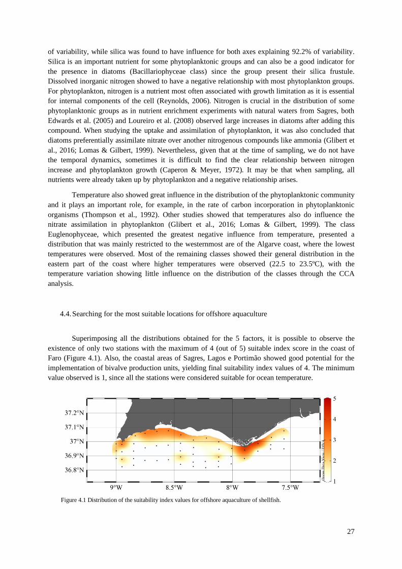
27

of variability, while silica was found to have influence for both axes explaining 92.2% of variability.

Silica is an important nutrient for some phytoplanktonic groups and can also be a good indicator for

the presence in diatoms (Bacillariophyceae class) since the group present their silica frustule.

Dissolved inorganic nitrogen showed to have a negative relationship with most phytoplankton groups.

For phytoplankton, nitrogen is a nutrient most often associated with growth limitation as it is essential

for internal components of the cell (Reynolds, 2006). Nitrogen is crucial in the distribution of some

phytoplanktonic groups as in nutrient enrichment experiments with natural waters from Sagres, both

Edwards et al. (2005) and Loureiro et al. (2008) observed large increases in diatoms after adding this

compound. When studying the uptake and assimilation of phytoplankton, it was also concluded that

diatoms preferentially assimilate nitrate over another nitrogenous compounds like ammonia (Glibert et

al., 2016; Lomas & Gilbert, 1999). Nevertheless, given that at the time of sampling, we do not have

the temporal dynamics, sometimes it is difficult to find the clear relationship between nitrogen

increase and phytoplankton growth (Caperon & Meyer, 1972). It may be that when sampling, all

nutrients were already taken up by phytoplankton and a negative relationship arises.

Temperature also showed great influence in the distribution of the phytoplanktonic community

and it plays an important role, for example, in the rate of carbon incorporation in phytoplanktonic

organisms (Thompson et al., 1992). Other studies showed that temperatures also do influence the

nitrate assimilation in phytoplankton (Glibert et al., 2016; Lomas & Gilbert, 1999). The class

Euglenophyceae, which presented the greatest negative influence from temperature, presented a

distribution that was mainly restricted to the westernmost are of the Algarve coast, where the lowest

temperatures were observed. Most of the remaining classes showed their general distribution in the

eastern part of the coast where higher temperatures were observed (22.5 to 23.5ºC), with the

temperature variation showing little influence on the distribution of the classes through the CCA

analysis.

4.4. Searching for the most suitable locations for offshore aquaculture

Superimposing all the distributions obtained for the 5 factors, it is possible to observe the

existence of only two stations with the maximum of 4 (out of 5) suitable index score in the coast of

Faro (Figure 4.1). Also, the coastal areas of Sagres, Lagos e Portimão showed good potential for the

implementation of bivalve production units, yielding final suitability index values of 4. The minimum

value observed is 1, since all the stations were considered suitable for ocean temperature.

Figure 4.1 Distribution of the suitability index values for offshore aquaculture of shellfish.

28

The phytoplankton biomass location and the Bacillariophyceae and Dinophyceae were the two

factors that most influenced the location of the two stations where the maximum suitability was

observed. It is also important to note that these Chl a concentration values are far below the average

recorded for the Algarve coast. The mean satellite Chl a concentration values during 1997-2018 for

the Algarve coast was 1 µg/L (Ferreira et al., 2021). This reinforces the need to further apply this

methodology with a more comprehensive dataset, covering the seasonal and inter-annual variability of

all factors.

The coastal proximity also proved to be one of the most important factors in the selection of

sites for aquaculture production in offshore waters, not only because it has showed to be one of the

factors that influence the most the distribution of the phytoplankton communities but also due to

accessibility reasons, in terms of installation and maintenance of production units. On the Algarve

coast, several offshore aquaculture structures are already installed. These are closer to the coastline

than the study area analyzed in this work. The choice of these locations, made based on empirical

evaluations, also suggests that this is the area where the production of bivalves has shown to have

greater viability and efficiency in their production. The stations closest to the coast (less than 6

nautical miles) were selected with the greatest potential for this parameter.

When we compare this figure with the location of the already existing aquaculture units in the

Algarve, it is possible to observe that they are located in the areas identified in this work as with the

greatest potential or most suitable. This may possibly be due to the fact that, based on experience,

these were the locations where bivalves were produced more efficiently over the years and therefore

selected for their production.

Again, it is important to note that in the present work the data has no seasonal or interannual

variability. It would be interesting to use this same methodology with a more comprehensive dataset.

For an appropriate evaluation of site selection, it is essential to integrate the temporal variability, as

well as to consider the inclusion of other parameters that could be of relevance for the site selection

exercise. This should be done in the near future.

Also, in the study carried out by Fragoso and Icely (2009), biofouling was recorded and

analyzed for the coast of Sagres near an oyster aquaculture unit. This biofouling consists in the

aggregation of various types of organism’s larvae to oceanic structures. In the study, high values of

mussel larvae have been recorded among other species. The high importance of biofouling was

observed during October, and it was also suggested that it was due to the upwelling events at this time

of year (Fragoso & Icely, 2009). This fact can also be indicative that the enrichment in phytoplankton

at this time of the year is decisive in shellfish production.

4.5. Conclusions and recommendations

The main objective of this thesis was to understand the spatial distribution of phytoplankton

communities in the Algarve coastal zone to evaluate its implications to the site selection for offshore

aquaculture units, taking into account the different abiotic factors. It was supported by resolving the

three specific objectives: i) Evaluate how environmental factors affect the spatial distribution of

phytoplankton communities on the Algarve coast; ii) Identify areas that have high phytoplankton

biomass production along the Algarve coast and evaluate which phytoplankton groups contribute the

most to this production; iii) Identify the locations with the greatest potential for implementing offshore

29

aquaculture units, according to phytoplankton biomass, optimal temperature and currents location. All

objectives were met, as detailed below.

Considered the data collected between the 5th and 13th October 2018, it was observed that the

main environmental factors affecting the spatial distribution of phytoplankton communities on the

Algarve coast were coastal distance, the water temperature, silica concentrations and also DIN

concentrations. The areas identified with highest potential in terms of phytoplankton biomass along

the coast were located in Sagres, Lagos, Portimão and Faro, where the highest Chl a concentration was

observed. It was also observed that the main groups contributing for this biomass were

Bacillariophyceae and Dinophyceae. The identification of the best locations for implementing offshore

aquaculture units was done through the application of a novel suitability index that uses several factors

such as coastal distance, ocean temperature, DIN concentrations and phytoplankton biomass and

composition. This suitability index indicated that the areas with the highest potential were located

closest to the coast of Sagres, Lagos, Portimão and Faro. It may also be interesting to extend the

application of this index to the rest of the Portuguese coastline.

If new offshore aquaculture units for bivalves are considered in the coast of Algarve, an

integrated assessment should be conducted including new elements, such as:

• It would be beneficial to apply the suitability index to the overall database of the

AQUIMAR project to incorporate the seasonal and interannual variability of all

factors;

• Research development regarding the bivalves feeding while in offshore structures and

possible limitations to their growth;

• Detailed information on the already existing mussel and oyster production units on the

Algarve coast, such as: type of structures used and their limitations, timing of

transport of the organisms to and from the units, difficulties observed in the in situ

process and also production values should be obtained in order to perform an

integrated analysis.

30

References Almada-Villela, P. C. (1984). The effect of reduced salinity on the shell growth of small Mytilus

edulis. Journal of the Marine Biological Association of the UK, 64, 171–182.

Almada-Villela, P. C., Davenport, J., Gruffydd, L. D. (1982). The effects of temperature on the shell

growth of young Mytilus edulis L. Journal of Experimental Marine Biology and Ecology.

https://doi.org/10.1016/0022-0981(82)90121-6

Almeida, L. P., Ferreira, Ó., Vousdoukas, M. I., Dodet, G. (2011). Historical variation and trends in

storminess along the Portuguese South Coast. Natural Hazards and Earth System Science.

https://doi.org/10.5194/nhess-11-2407-2011

Araújo, J., Soares, F., & Pousão-Ferreira, P. (2018). Offshore Production of Mediterranean Mussels in

Southern Portugal. World Aquaculture, 49(2), 55–57.

Baldwin, B. S. & Newell, R. I. (1991). Omnivorous feeding by planktotrophic larvae of the eastern oyster Crassostrea virginica. Marine Ecology Progress Series.

https://doi.org/10.3354/meps078285

Baldwin, B. S., & Newell, R. I. (1995). Relative importance of different size food particles in the

natural diet of oyster larvae (Crassostrea virginica). Marine Ecology Progress Series.


Baptista, V., Silva, P. L., Relvas, P., Teodósio, M. A., Leitão, F. (2018). Sea surface temperature

variability along the Portuguese coast since 1950. International Journal of Climatology, 38(3).

https://doi.org/10.1002/joc.5231

Barrento, S., Keay, I., Lupatsch, I., Shields, S. (2013). Protocol on Best Practice Guide on Holding

and Conditioning Mussels. Techmical Report supported by Project No. 243452, FP7-SME

MusselsAlive. 59.

Benemann, J. R. (1992). Microalgae aquaculture feeds. Journal of Applied Phycology.

https://doi.org/10.1007/BF02161209

Bernardino, F. N. V. (2000). Review of aquaculture development in Portugal. Journal of Applied

Ichthyology. https://doi.org/10.1046/j.1439-0426.2000.00262.x

Berntsson, K. M., Jonsson, P. R., Wängberg, S. Å., Carlsson, A. S. (1997). Effects of broodstock diets

on fatty acid composition, survival and growth rates in larvae of the European flat oyster, Ostrea

edulis. Aquaculture. https://doi.org/10.1016/S0044-8486(97)00041-0

Borges, C., Palma, C., Da Silva, R. B. (2019). Optimization of River Sampling: Application to

Nutrients Distribution in Tagus River Estuary. Analytical Chemistry.

https://doi.org/10.1021/acs.analchem.8b05781

Bricker, S. B., Clement, C. G., Pirhalla, D. E., Orlando, S. P., Farrow, D. R. G. (1999). National Estuarine Eutrophication Assessment: Effects of Nutrient Enrichment in the Nation’s Estuaries.

NOAA: National Ocean Service, Special Projects Office and the National Centers for Coastal

Ocean Science.

Brotas, V., Couto, A. B., Sá, C., Amorim, A., Brito, A., Laanen, M., Peters, S., Poser, K., Eleveld, M.,

Miller, P., Kurekin, A., Groom, S., Åtland, Å., Dale, T., Sørensen, K., Ledang, A. B., Hansen, L. B., Huber, S., Kaas, H., … Fragoso, B. (2014). Deriving Aquaculture indicators from Earth

Observation in the AQUA- USERS project (AQUAculture USEr driven operational Remote

Sensing information Services). Ocean Optics XXII, November, 9.

https://doi.org/10.13140/2.1.1626.0804

Brown, M. R., Jeffrey, S. W., Garland, C. D. (1989). Nutritional aspects of microalgae used in

mariculture; a literature review. REP. CSIRO MAR. LAB. AI :ISSN 0725-4598 .

31

Brown, M. R., Jeffrey, S. W., Volkman, J. K., Dunstan, G. A. (1997). Nutritional properties of

microalgae for mariculture. Aquaculture. https://doi.org/10.1016/S0044-8486(96)01501-3

Bruce, J. R., Knight, M., Parke, M. W. (1940). The rearing of oyster larvae on an algal diet. Journal of

the Marine Biological Association of the United Kingdom, 24(1), 337–374.

https://doi.org/10.1017/S0025315400054606

Burkholder, J. A. M. (1998). Implications of harmful microalgae and heterotrophic dinoflagellates in

management of sustainable marine fisheries. Ecological Applications, 8(1 SUPPL.).

https://doi.org/10.2307/2641362

Cáceres-Martínez, J., Robledo, J. A. F., Figueras, A. (1995). Presence of Bonamia and its relation to age, growth rates and gonadal development of the flat oyster, Ostrea edulis, in the Ría de Vigo,

Galicia (NW Spain). Aquaculture, 130(1), 15–23. https://doi.org/10.1016/0044-8486(94)00152-E

Cachola, R. (1995). Aquacultura «offshore» em Sagres. 8o Congres, 861–867.

Caperon, J. & Meyer, J. (1972). Nitrogen-limited growth of marine phytoplankton-II. Uptake kinetics

and their role in nutrient limited growth of phytoplankton. Deep-Sea Research and

Oceanographic Abstracts, 19(9), 619–632. https://doi.org/10.1016/0011-7471(72)90090-3

Cardia, F. & Lovatelli, A. (2016). Aquaculture operations in floating HDPE cages. In Fisheries and

Aquaculture (Vol. 593). http://www.fao.org/3/a-i4508e.pdf

Cartaxana, P., Mendes, C. R., Brotas, V. (2009). Phytoplankton and ecological assessment of brackish

and freshwater coastal lagoons in the Algarve, Portugal. Lakes and Reservoirs: Research and

Management, 14(3), 221–230. https://doi.org/10.1111/j.1440-1770.2009.00405.x

Chu, F. L. E., Dupuy, J. L., Webb, K. L. (1982). Polysaccharide composition of five algal species used

as food for larvae of the American oyster, Crassostrea virginica. Aquaculture.

https://doi.org/10.1016/0044-8486(82)90138-7

Coelho, C., Silva, R., Veloso-Gomes, F., Taveira-Pinto, F. (2009). Potential effects of climate change

on northwest portuguese coastal zones. ICES Journal of Marine Science.

https://doi.org/10.1093/icesjms/fsp132

Coelho, S., Gamito, S., Pérez-Ruzafa, A. (2007). Trophic state of Foz de Almargem coastal lagoon (Algarve, South Portugal) based on the water quality and the phytoplankton community.

Estuarine, Coastal and Shelf Science. https://doi.org/10.1016/j.ecss.2006.07.017

Conger, K. A., Swift, M. L., Reeves, J. B., Lakshmanan, S. (1978). Shell growth of unfed oysters in

the laboratory: A sublethal bioassay system for pollutants. Life Sciences.

https://doi.org/10.1016/0024-3205(78)90525-8

Costa, M., Silva, R., Vitorino, J. (2001). Contribuição para o Estudo do Clima de Agitação Marítima

na Costa Portuguesa (in Portuguese). Instituto Hidrográfico.

Criado-Aldeanueva, F., García-Lafuente, J., Vargas, J. M., Del Río, J., Vázquez, A., Reul, A.,

Sánchez, A. (2006). Distribution and circulation of water masses in the Gulf of Cadiz from in

situ observations. Deep-Sea Research Part II: Topical Studies in Oceanography, 53(11–13),

1144–1160. https://doi.org/10.1016/j.dsr2.2006.04.012

Defossez, J. M. & Hawkins, A. J. S. (1997). Selective feeding in shellfish: Size-dependent rejection of large particles within pseudofaeces from Mytilus edulis, Ruditapes philippinarum and Tapes

decussatus. Marine Biology. https://doi.org/10.1007/s002270050154

Delaporte, M., Soudant, P., Moal, J., Lambert, C., Quéré, C., Miner, P., Choquet, G., Paillard, C.,

Samain, J. F. (2003). Effect of a mono-specific algal diet on immune functions in two bivalve species - Crassostrea gigas and Ruditapes philippinarum. Journal of Experimental Biology,

206(17), 3053–3064. https://doi.org/10.1242/jeb.00518

32

DGRM (2021). Geoportal de Aquicultura. From:

https://webgis.dgrm.mm.gov.pt/portal/apps/webappviewer/index.html?id=9bc91b21cc8b420ba78

4829970cb5059

Diana, J. S. (2009). Aquaculture production and biodiversity conservation. BioScience, 59(1), 27–38.

https://doi.org/10.1525/bio.2009.59.1.7

Edwards, V., Icely, J., Newton, A., Webster, R. (2005). The yield of chlorophyll from nitrogen: A

comparison between the shallow Ria Formosa lagoon and the deep oceanic conditions at Sagres

along the southern coast of Portugal. Estuarine, Coastal and Shelf Science.

https://doi.org/10.1016/j.ecss.2004.09.004

Fabioux, C., Huvet, A., Le Souchu, P., Le Pennec, M., Pouvreau, S. (2005). Temperature and

photoperiod drive Crassostrea gigas reproductive internal clock. Aquaculture, 250(1–2), 458–

470. https://doi.org/10.1016/j.aquaculture.2005.02.038

Fabregas, J., Herrero, C., Cabezas, B., Abalde, J. (1985). Mass culture and biochemical variability of

the marine microalga Tetraselmis suecica Kylin (Butch) with high nutrient concentrations.

Aquaculture. https://doi.org/10.1016/0044-8486(85)90082-1

FAO (2014). The State of World Fisheries and Aquaculture, Opportunities and challenges. Rome.

FAO (2016). The State of World Fisheries and Aquaculture 2016 – Contributing to food security and

nutrition for all. Rome. 200 pp.

FAO (2018). Fisheries and Aquaculture Statistics 2016. Rome. doi:10.5860/CHOICE.50-5350.

FAO (2020). Fisheries and Aquaculture. Cultured Aquatic Species Information Programme,

Dicentrarchus labrax (Linnaeus, 1758). Available at:

http://www.fao.org/fishery/culturedspecies/Dicentrarchus_labrax/en [Accessed January 22,

2020].

Ferreira, A., Brotas, V., Palma, C., Borges, C., Brito, A. C. (2021). Assessing Phytoplankton Bloom

Phenology in Upwelling-Influenced Regions Using Ocean Color Remote Sensing. Remote

Sensing, 13(4), 675. https://doi.org/10.3390/rs13040675

Ferreira, J. G., Hawkins, A. J. S., Bricker, S. B. (2007). Management of productivity, environmental effects and profitability of shellfish aquaculture - the Farm Aquaculture Resource Management

(FARM) model. Aquaculture, 264(1–4), 160–174.

https://doi.org/10.1016/j.aquaculture.2006.12.017

Fiúza, A. F. G. (1983). Upwelling patterns off Portugal. NATO Conference Series, (Series) 4: Marine

Sciences. https://doi.org/10.1007/978-1-4615-6651-9_5

Fiúza, A. F. G., de Macedo, M. E., Guerreiro, M. R. (1982). Climatological space and time variation

of the Portuguese coastal upwelling. Oceanologica Acta.

Fragoso, B. & Icely, J. D. (2009). Upwelling events and recruitment patterns of the major fouling

species on coastal aquaculture (Sagres, Portugal). Journal of Coastal Research.

García-Lafuente, J., Delgado, J., Criado-Aldeanueva, F., Bruno, M., del Río, J., Miguel Vargas, J.

(2006). Water mass circulation on the continental shelf of the Gulf of Cádiz. Deep-Sea Research

Part II: Topical Studies in Oceanography, 53(11–13), 1182–1197.

https://doi.org/10.1016/j.dsr2.2006.04.011

Gentry, R. R., Froehlich, H. E., Grimm, D., Kareiva, P., Parke, M., Rust, M., Gaines, S. D., Halpern,

B. S. (2017). Mapping the global potential for marine aquaculture. Nature Ecology and

Evolution, 1(9), 1317–1324. https://doi.org/10.1038/s41559-017-0257-9

Gibb, S. W., Cummings, D. G., Irigoien, X., Barlow, R. G., Fauzi, R., Mantoura, C. (2001). Phytoplankton pigment chemotaxonomy of the northeastern Atlantic. Deep-Sea Research Part

33

II: Topical Studies in Oceanography, 48(4–5), 795–823. https://doi.org/10.1016/S0967-

0645(00)00098-9

Glibert, P. M., Wilkerson, F. P., Dugdale, R. C., Raven, J. A., Dupont, C. L., Leavitt, P. R., Parker, A.

E., Burkholder, J. M., Kana, T. M. (2016). Pluses and minuses of ammonium and nitrate uptake and assimilation by phytoplankton and implications for productivity and community

composition, with emphasis on nitrogen-enriched conditions. Limnology and Oceanography.

https://doi.org/10.1002/lno.10203

Goela, P. C., Danchenko, S., Icely, J. D., Lubian, L. M., Cristina, S., Newton, A. (2014). Using CHEMTAX to evaluate seasonal and interannual dynamics of the phytoplankton community off

the South-west coast of Portugal. Estuarine, Coastal and Shelf Science.


Grasshoff, K., Kremling K., Ehrhardt, M. (1999). Methods of Seawater Analysis. Verlag Chemie,

Weinheim. In Book.

Griebeler, E. M. & Seitz, A. (2007). Effects of increasing temperatures on population dynamics of the zebra mussel Dreissena polymorpha: Implications from an individual-based model. Oecologia,

151(3), 530–543. https://doi.org/10.1007/s00442-006-0591-0

Gui, Y., Zamora, L., Dunphy, B. J., Jeffs, A. G. (2016). Evaluation of the formulated diet MySpat for

feeding hatchery-reared spat of the green-lipped mussel, Perna canaliculus (Gmelin, 1791).

Aquaculture Research. https://doi.org/10.1111/are.12841

Henriques, M. (1998). Manual de aquacultura: ostra, amêijoa, camarão, truta, tilápia, enguia, dourada,

robalo, pregado. ICBAS, 59–75.

Higgins, H. W., Wright, S. W., Schlüter, L. (2011). Quantitative interpretation of chemotaxonomic

pigment data. In Phytoplankton Pigments. https://doi.org/10.1017/cbo9780511732263.010

Hill, J. K., Thomas, C. D., Huntley, B. (1999). Climate and habitat availability determine 20th century

changes in a butterfly’s range margin. Proceedings of the Royal Society B: Biological Sciences.

https://doi.org/10.1098/rspb.1999.0763

Holland, D. L. (1973). Biochemical changes in fed and starved oysters, Ostrea edulis l. during larval

development, metamorphosis and early spat growth. Journal of the Marine Biological

Association of the United Kingdom. https://doi.org/10.1017/S002531540002227X

Holmer, M. (2010). Environmental issues of fish farming in offshore waters: Perspectives, concerns

and research needs. In Aquaculture Environment Interactions. https://doi.org/10.3354/aei00007

Hrs-Brenko, M., Claus, C., Bubic, S. (1977). Synergistic effects of lead, salinity and temperature on embryonic development of the mussel Mytilus galloprovincialis. Marine Biology.

https://doi.org/10.1007/BF00386951

INE (1998). Estatísticas da Pesca - 1998. Lisboa. From:

www:<url:https://www.ine.pt/xurl/pub/259349571>. ISSN 0377-225-x. ISBN 972-673-350-2

INE (2020). Estatísticas da Pesca - 2019. Lisboa. From: www:<url:https://www.ine.pt/xurl/pub/435690295>. ISSN 0377-225-X. ISBN 978-989-25-0540-

4

Knauer, J. & Southgate, P. C. (1999). A Review of the Nutritional Requirements of Bivalves and the

Development of Alternative and Artificial Diets for Bivalve Aquaculture. Reviews in Fisheries

Science, 7(3–4), 241–280. https://doi.org/10.1080/10641269908951362

Koroleff, F. (1976). Determination of nutrients. In Methods of seawater analysis.

Landowne, D. & Ritchie, J. M. (1971). On the control of glycogenolysis in mammalian nervous tissue

by calcium. The Journal of Physiology. https://doi.org/10.1113/jphysiol.1971.sp009338

34

Langdon, C. J. & Siegfried, C. A. (1984). Progress in the development of artificial diets for bivalve

filter feeders. Aquaculture. https://doi.org/10.1016/0044-8486(84)90262-X

Latasa, M. (2007). Improving estimations of phytoplankton class abundances using CHEMTAX.

Marine Ecology Progress Series. https://doi.org/10.3354/meps329013

Lomas, M. W. & Gilbert, P. M. (1999). Temperature regulation of nitrate uptake: A novel hypothesis about nitrate uptake and reduction in cool-water diatoms. Limnology and Oceanography.

https://doi.org/10.4319/lo.1999.44.3.0556

Loosanoff, V. L. (1958). Some aspects of behavior of oysters at different temperatures. The Biological

Bulletin. https://doi.org/10.2307/1538965

Loureiro, S., Icely, J., Newton, A. (2008). Enrichment experiments and primary production at Sagres (SW Portugal). Journal of Experimental Marine Biology and Ecology.

https://doi.org/10.1016/j.jembe.2008.03.001

Loureiro, S., Newton, A., Icely, J. (2005a). Effects of nutrient enrichments on primary production in

the Ria Formosa coastal lagoon (Southern Portugal). Hydrobiologia, 550(1), 29–45.

https://doi.org/10.1007/s10750-005-4357-1

Loureiro, S., Newton, A., Icely, J. D. (2005b). Microplankton composition, production and upwelling dynamics in Sagres (SW Portugal) during the summer of 2001. Scientia Marina, 69(3), 323–341.

https://doi.org/10.3989/scimar.2005.69n3323

Loureiro, S., Reñé, A., Garcés, E., Camp, J., Vaqué, D. (2011). Harmful algal blooms (HABs),

dissolved organic matter (DOM), and planktonic microbial community dynamics at a near-shore

and a harbour station influenced by upwelling (SW Iberian Peninsula). Journal of Sea Research.

https://doi.org/10.1016/j.seares.2011.03.004

Mackey, M. D., Mackey, D. J., Higgins, H. W., Wright, S. W. (1996). CHEMTAX - A program for

estimating class abundances from chemical markers: Application to HPLC measurements of

phytoplankton. Marine Ecology Progress Series. https://doi.org/10.3354/meps144265

Malone, T. C., Conley, D. J., Fisher, T. R., Glibert, P. M., Harding, L. W., Sellner, K. G. (1996). Scales of nutrient-limited phytoplankton productivity in Chesapeake Bay. Estuaries.

https://doi.org/10.2307/1352457

Maloy, A. P., Nelle, P., Culloty, S. C., Slater, J. W., Harrod, C. (2013). Identifying trophic variation in

a marine suspension feeder: DNA- and stable isotope-based dietary analysis in Mytilus spp.

Marine Biology, 160(2), 479–490. https://doi.org/10.1007/s00227-012-2105-4

McMahon, R. F. (1996). The physiological ecology of the zebra mussel, dreissena polymorpha, in

north america and europe. American Zoologist. https://doi.org/10.1093/icb/36.3.339

Mendes, Carlos Rafael, Sá, C., Vitorino, J., Borges, C., Tavano Garcia, V. M., Brotas, V. (2011).

Spatial distribution of phytoplankton assemblages in the Nazaré submarine canyon region

(Portugal): HPLC-CHEMTAX approach. Journal of Marine Systems.

https://doi.org/10.1016/j.jmarsys.2011.03.005

Moita, M. T. (2001). Estrutura , variabilidade e dinâmica do Fitoplâncton na Costa de Portugal

Continental. 273.

Moreira, A., Figueira, E., Libralato, G., Soares, A. M. V. M., Guida, M., Freitas, R. (2018).

Comparative sensitivity of Crassostrea angulata and Crassostrea gigas embryo-larval

development to As under varying salinity and temperature. Marine Environmental Research,

140, 135–144. https://doi.org/10.1016/j.marenvres.2018.06.003

Murphy, J. & Riley, J. P. (1962). A modified single solution method for the determination of

phosphate in natural waters. Analytica Chimica Acta. https://doi.org/10.1016/S0003-

35

2670(00)88444-5

Naylor, R. L., Goldburg, R. J., Primavera, J. H., Kautsky, N., Beveridge, M. C. M., Clay, J., Folke, C.,

Lubchenco, J., Mooney, H., Troell, M. (2000). Effect of aquaculture on world fish supplies. In

Nature. https://doi.org/10.1038/35016500

Oliveira, J., Castilho, F., Cunha, Â., Pereira, M. J. (2013). Bivalve harvesting and production in Portugal: An overview. Journal of Shellfish Research, 32(3), 911–924.

https://doi.org/10.2983/035.032.0334

Orlova, M. I. (2002). Dreissena (D.) Polymorpha: Evolutionary Origin and Biological Peculiarities as

Prerequisites of Invasion Success. In Invasive Aquatic Species of Europe. Distribution, Impacts

and Management. https://doi.org/10.1007/978-94-015-9956-6_14

Page, H. M. & Hubbard, D. M. (1987). Temporal and spatial patterns of growth in mussels Mytilus

edulis on an offshore platform: relationships to water temperature and food availability. Journal

of Experimental Marine Biology and Ecology. https://doi.org/10.1016/0022-0981(87)90053-0

Peharda, M., Župan, I., Bavčević, L., Frankić, A., Klanjšček, T. (2007). Growth and condition index of

mussel Mytilus galloprovincialis in experimental integrated aquaculture. Aquaculture Research.

https://doi.org/10.1111/j.1365-2109.2007.01840.x

Picoche, C., Le Gendre, R., Flye-Sainte-Marie, J., Françoise, S., Maheux, F., Simon, B., Gangnery, A.

(2014). Towards the determination of Mytilus edulis food preferences using the Dynamic Energy

Budget (DEB) theory. PLoS ONE, 9(10). https://doi.org/10.1371/journal.pone.0109796

Pleissner, D., Eriksen, N. T., Lundgreen, K., Riisgård, H. U. (2012). Biomass Composition of Blue

Mussels, Mytilus edulis , is Affected by Living Site and Species of Ingested Microalgae . ISRN

Zoology, 2012, 1–12. https://doi.org/10.5402/2012/902152

Pronker, A. E., Nevejan, N. M., Peene, F., Geijsen, P., Sorgeloos, P. (2008). Hatchery broodstock

conditioning of the blue mussel Mytilus edulis (Linnaeus 1758). Part I. Impact of different micro-

algae mixtures on broodstock performance. Aquaculture International, 16(4), 297–307.

https://doi.org/10.1007/s10499-007-9143-9

Ramón, M., Cano, J., Peña, J. B., Campos, M. J. (2005). Current status and perspectives of mollusc

(bivalves and gastropods) culture in the Spanish Mediterranean. Boletin - Instituto Espanol de

Oceanografia.

Reynolds, C. S. (2006). The Ecology of Phytoplankton. Cambridge University Press.

https://doi.org/10.1017/CBO9780511542145

Rodriguez, J. L., Sedano, F. J., García-Martín, L. O., Pérez-Camacho, A., Sánchez, J. L. (1990). Energy metabolism of newly settled Ostrea edulis spat during metamorphosis. Marine Biology.

https://doi.org/10.1007/BF02114680

Rosenberg, R. & Loo, L.-O. (1983). Energy-flow in a Mytilus edulis culture in western Sweden.

Aquaculture, 35, 151–161. https://doi.org/10.1016/0044-8486(83)90082-0

Sánchez, R. F. & Relvas, P. (2003). Spring-summer climatological circulation in the upper layer in the region of Cape St. Vincent, Southwest Portugal. ICES Journal of Marine Science, 60(6), 1232–

1250. https://doi.org/10.1016/S1054-3139(03)00137-1

Sañé, E., Valente, A., Fatela, F., Cabral, M. C., Beltrán, C., Drago, T. (2019). Using CHEMTAX to

evaluate seasonal and interannual dynamics of the phytoplankton community off the South-west

coast of Portugal. Journal of Sea Research, 146, 33–45.


Schneider, D. W. (1992). A bioenergetics model of zebra mussel, Dreissena polymorpha, growth in

the Great Lakes. Canadian Journal of Fisheries and Aquatic Sciences.

36

https://doi.org/10.1139/f92-156

Shumway, S. E. (1990). A review of the effects of algal blooms on shellfish and aquaculture. Journal

of the World Aquaculture Society, 21(2), 65–104.

Sicard, M. T., Maeda-Martínez, A. N., Lluch-Cota, S. E., Lodeiros, C., Roldán-Carrillo, L. M.,

Mendoza-Alfaro, R. (2006). Frequent monitoring of temperature: An essential requirement for site selection in bivalve aquaculture in tropical-temperate transition zones. Aquaculture

Research, 37(10), 1040–1049. https://doi.org/10.1111/j.1365-2109.2006.01527.x

Sick, L. V., Johnson, C. C., Siegfried, C. A. (1979). Fluxes of dissolved and particulate calcium in

selected tissues of Crassostrea virginica. Marine Biology. https://doi.org/10.1007/BF00395435

Silvano, K. M., Barbosa, A. B., Domingues, R. B., Galvão, H. M., Luís, J., Platt, T., Relvas, P., Krug, L. A., Sathyendranath, S. (2012). Connections between upwelling patterns and phytoplankton

variability under different coastal regimes in SW Iberia Peninsula. 21st Ocean Optics

Conference, May 2017, 11.

Sirakov, I., Velichkova, K., Stoyanova, S., Staykov, Y. (2015). The importance of microalgae for

aquaculture industry . Review . International Journal of Fisheries and Aquatic Studies.

Snyder, J., Boss, E., Weatherbee, R., Thomas, A. C., Brady, D., Newell, C. (2017). Oyster aquaculture site selection using landsat 8-derived sea surface temperature, turbidity, and chlorophyll a.

Frontiers in Marine Science, 4(JUN). https://doi.org/10.3389/fmars.2017.00190

Stotz, W. (2000). When aquaculture restores and replaces an overfished stock: Is the conservation of

the Species assured? The case of the scallop Argopecten purpuratus in Northern Chile.

Aquaculture International. https://doi.org/10.1023/a:1009215119051

Strickland, J. D. H. & Parsons., T. R. (1972). A practical handbook for seawater analysis. Second

Edition. In Fisheries Research Board of Canada. Ottowa, Canada.

Thompson, P. A., Guo, M. X., Harrison, P. J. (1992). Effects of Variation in Temperature. I. on the

Biochemical Composition of Eight Species of Marine Phytoplankton. In Journal of Phycology

(Vol. 28, Issue 4, pp. 481–488). https://doi.org/10.1111/j.0022-3646.1992.00481.x

Toupoint, N., Gilmore-Solomon, L., Bourque, F., Myrand, B., Pernet, F., Olivier, F., Tremblay, R. (2012). Match/mismatch between the Mytilus edulis larval supply and seston quality: Effect on

recruitment. Ecology, 93(8), 1922–1934. https://doi.org/10.1890/11-1292.1

Trottet, A., Roy, S., Tamigneaux, E., Lovejoy, C., Tremblay, R. (2008). Impact of suspended mussels

(Mytilus edulis L.) on plankton communities in a Magdalen Islands lagoon (Québec, Canada): A

mesocosm approach. Journal of Experimental Marine Biology and Ecology, 365(2), 103–115.

https://doi.org/10.1016/j.jembe.2008.08.001

Vallejo, S. M. A. (1982). Development and management of coastal lagoons. Oceanologica Acta.

N.SP., 397-401.

Van Aken, H. M. (2000). The hydrography of the mid-latitude Northeast Atlantic Ocean II: The

intermediate water masses. In Deep-Sea Research Part I: Oceanographic Research Papers (Vol.

47, Issue 5). https://doi.org/10.1016/S0967-0637(99)00112-0

Wallis, R. L. (1975). Thermal tolerance of Mytilus edulis of Eastern Australia. Marine Biology, 30(3),

183–191. https://doi.org/10.1007/BF00390741

Widdows, J. (1978). Combined effects of body size, food concentration and season on the physiology

of Mytilus edulis. Journal of the Marine Biological Association of the United Kingdom, 58(1),

109–124. https://doi.org/10.1017/S0025315400024449

Wildish, D. J. & Kristmanson, D. D. (1985). Control of suspension feeding bivalve production by current speed. Helgoländer Meeresuntersuchungen, 39(3), 237–243.

37

https://doi.org/10.1007/BF01992771

Winkler, L. W. (1888). Die Bestimmung des im Wasser gelösten Sauerstoffes. Berichte Der

Deutschen Chemischen Gesellschaft. https://doi.org/10.1002/cber.188802102122

Wright, S. W., Ishikawa, A., Marchant, H. J., Davidson, A. T., Van Den Enden, R. L., Nash, G. V.

(2009). Composition and significance of picophytoplankton in Antarctic waters. Polar Biology.

https://doi.org/10.1007/s00300-009-0582-9

Zapata, M., Jeffrey, S. W., Wright, S. W., Rodríguez, F., Garrido, J. L., Clementson, L. (2004).

Photosynthetic pigments in 37 species (65 strains) of Haptophyta: Implications for oceanography

and chemotaxonomy. Marine Ecology Progress Series. https://doi.org/10.3354/meps270083

Zapata, M., Rodríguez, F., Garrido, J. L. (2000). Separation of chlorophylls and carotenoids from marine phytoplankton: A new HPLC method using a reversed phase C8 column and pyridine-

containing mobile phases. Marine Ecology Progress Series, 195, 29–45.


Zenk, W. (1975). On the origin of the intermediate double-maxima in T/S profiles from the North

Atlantic. Meteor Forschungs-Ergebnisse, A(16), 35–43.

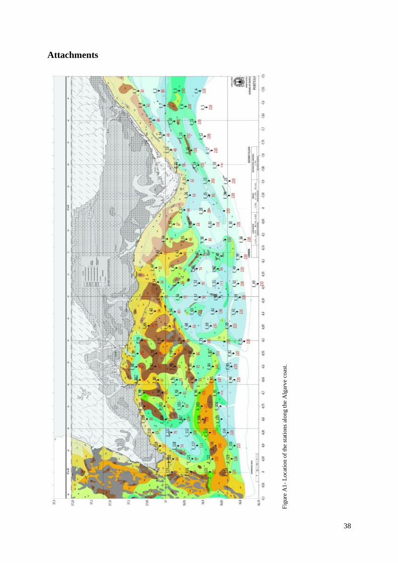
38

Attachments

Fig

ure

A1

- L

oca

tion o

f th

e st

atio

ns

along t

he

Alg

arve

coas

t.

Phytoplankton community in the Algarve coastal region

Documents

Transcript of Phytoplankton community in the Algarve coastal region