
PhDThesis - Medical X-ray Images of the Human Thorax
234
Carlos Alberto Afonso Vinhais Medical X-ray Images of the Human Thorax Segmentation, Decomposition and Reconstruction PhD Thesis Submitted to the Faculty of Engineering, University of Porto Porto, July 2007
-
Upload
khangminh22 -
Category
Documents
-
view
0 -
download
0
Transcript of PhDThesis - Medical X-ray Images of the Human Thorax

Carlos Alberto Afonso Vinhais
Medical X-ray Images
of the Human Thorax
Segmentation, Decomposition
and Reconstruction
PhD Thesis
Submitted to theFaculty of Engineering, University of Porto
Porto, July 2007


To Cat


ACKNOWLEDGEMENTS
I wish to express sincere gratitude to Professor Aurelio Campilho, my advisor, forhis academic guidance for my PhD education at INEB - Instituto de EngenhariaBiomedica. Throughout the three years of research work, his continuous help, en-thusiasm and technical insights encourages me to overcome the problems and enrichmy knowledge and skills.
Thanks to the all students, lab members and staff I have worked with at INEB.As the member of the lab, I benefit a lot from their friendship.
I would like to acknowledge the medical staff and technicians of the Hospital SaoJoao, Porto, and Hospital Pedro Hispano, Matosinhos, who generously gave theirtime and expertise.
I am deeply grateful to my nuclear family for their encouragement and loveduring my life and studies.
Lastly, I wish to convey special thanks to Catarina for her undying love andsupport.

ABSTRACT
Medical image segmentation methods have been developed for different anatomi-cal structures using image data acquired from a variety of modalities. This thesispresents fully automated computer algorithms to segment, decompose and recon-struct medical X-ray images of the human thorax. Focus is on postero-anterior (PA)chest radiographs and computed tomography (CT) images.
Two segmentation methods are proposed to accurately identify the unobscuredregions that define the lung fields in digital PA chest radiographs. The first approachis a contour delineation method that uses an optimal path finding algorithm based ondynamic programming. The second approach is a non-rigid deformable registrationframework, where the lung field segmentation is reformulated as an optimizationproblem. A flexible optimization strategy based on genetic algorithms is adopted.Both methods can be used in computer-aided diagnosis systems by providing therequired pre-processing step before further analysis of such images can be appliedsuccessfully.
Algorithms for the construction of 3D patient-specific phantoms from volumetricCT images of the human thorax are also provided. Based on material basis decom-position applied to CT numbers, CT images are decomposed into known interveningmaterials, providing voxelized anthropomorphic phantoms suitable for several com-puter simulations in diagnostic radiology and nuclear medicine. The method is ex-tended for extracting the lung region of interest usually required by most pulmonaryimage analysis applications. A robust 3D optimal surface detection algorithm is usedfor accurately separating the lungs.
Lastly, a methodology for recovering the 3D shape of anatomical structures fromsingle radiographs is presented. Voxelized phantoms resulting from CT image de-composition are used to simulate radiological density images and reconstruct es-timated thickness maps of the structures to be recovered. A formal relationshipbetween CT data and radiographic measurements is derived to support the designof subtraction and tissue cancellation algorithms.


RESUMO
Inumeros metodos de segmentacao de imagens medicas tem sido desenvolvidos paradiferentes estruturas anatomicas usando dados provenientes de diversas modali-dades. Esta tese apresenta algoritmos computacionais automaticos para segmentar,decompor e reconstruir imagens medicas do torax humano, nomeadamente radio-gramas toracicos em incidencia postero-anterior (PA) e tomogramas computorizados(TC).
Dois metodos de segmentacao sao propostos para identificar as regioes que de-finem os campos pulmonares em radiogramas digitais PA do torax. O primeirometodo consiste em delinear os contornos pulmonares usando um algoritmo depesquisa do trajecto optimo baseado em programacao dinamica. O segundo ebaseado no alinhamento nao-rıgido de um modelo deformavel formulando a seg-mentacao dos campos pulmonares num problema de optimizacao. Para o efeito,e usada uma estrategia flexıvel de optimizacao baseada em algoritmos geneticos.Ambos os metodos podem ser usados em sistemas computacionais de apoio ao di-agnostico medico, fornecendo o pre-processamento necessario para que a analise aposteriori de tais imagens possa ser aplicada com sucesso.
Algoritmos para a construcao de fantomas 3D especıficos de cada paciente re-sultantes de tomogramas volumetricos sao providos. Baseado na decomposicao emmateriais de base aplicada aos numeros de TC, estas imagens sao decompostas emmateriais conhecidos, fornecendo fantomas antropomorficos voxelizados, apropriadospara diversas simulacoes computacionais com aplicacoes na radiologia diagnosticae medicina nuclear. Uma outra aplicacao deste metodo e a extracao da regiao deinteresse pulmonar, requerida pela grande maioria das aplicacoes de analise de im-agem pulmonar. E ainda proposto uma algoritmo robusto de deteccao optima desuperfıcie 3D para a separacao rigorosa dos pulmoes.
Por ultimo, e apresentada uma metodologia para a reconstrucao 3D da formade estruturas anatomicas partindo de apenas um radiograma. Fantomas voxeliza-dos resultantes da decomposicao de imagens TC sao usados para simular imagensradiologicas de densidade e estimar mapas de espessuras de cada estrutura que sepretende reconstruir. A relacao formal entre dados TC e medidas radiologicas ededuzida viabilizando a implementacao de algoritmos de eliminacao e subtracao detecidos.


RESUME
Quelques methodes de segmentation d’images medicales ont ete developpees pourdifferentes structures anatomiques en utilisant des donnees d’image acquises d’unevariete de modalites. Cette these presente des algorithmes d’ordinateur entierementautomatises pour segmenter, decomposer et reconstruir des images medicales auxrayons X du thorax humain. L´etude est centree sur les radiographies postero-anterieures (PA) et les images volumetriques de tomographie calculee (TC).
On propose deux methodes de segmentation pour identifier les regions qui defineles poumons en radiographies digitales PA. La premiere approche est une methode dedelineation de contours qui emploie un algorithme optimal de conclusion de cheminbase sur la programmation dynamique. La deuxieme approche considere un aligne-ment non-rigide d´un modele deformable, ou la segmentation des poumons est re-formulee comme un probleme d’optimisation. Une strategie flexible d’optimisationbasee sur des algorithmes genetiques est adoptee. Les deux methodes peuvent etreemployees dans les systemes de diagnostic assiste par ordinateur en fournissantl’etape de pretraitement exigee avant que davantage d’analyse de telles images puisseetre appliquee avec succes.
Des algorithmes pour la construction de fantomes 3D specifiques du patient apartir d´images volumetriques de TC du thorax humain sont egalement fournis.Suivant la decomposition de materiaux de base appliquee aux nombres de TC, desimages de TC sont decomposees en materiaux intervenants connus, fournissant desfantomes anthropomorphes voxelizes appropries a plusieurs simulations sur ordi-nateur dans la radiologie diagnostique et la medecine nucleaire. La methode estetendue pour extraire la region d’interet des poumons habituellement exigee par laplupart des applications d’analyse d’images pulmonaire. Un algorithme robuste dedetection optimale de surface 3D est employe pour separer les poumons.
Pour finir, on presente une methodologie pour reconstruire la forme 3D de struc-tures anatomiques a partir de simples radiographies. Des fantomes de voxilizesresultant de la decomposition d’image de TC sont employes pour simuler des im-ages radiologiques de densite et estimer l’epaisseur des structures pretendues. Unrapport formel entre les donnees TC et les mesures radiographiques est derive pourpermettre le developement d´algorithmes de soustraction de tissus.


CONTENTS
Acknowledgments . . . . . . . . . . . . . . . . . . . . . . . . . . . . . . . . v
Abstract . . . . . . . . . . . . . . . . . . . . . . . . . . . . . . . . . . . . . . vii
Resumo . . . . . . . . . . . . . . . . . . . . . . . . . . . . . . . . . . . . . . ix
Resume . . . . . . . . . . . . . . . . . . . . . . . . . . . . . . . . . . . . . . xi
List of Figures . . . . . . . . . . . . . . . . . . . . . . . . . . . . . . . . . . xix
List of Tables . . . . . . . . . . . . . . . . . . . . . . . . . . . . . . . . . . . xxi
List of Abbreviations . . . . . . . . . . . . . . . . . . . . . . . . . . . . . . xxiii
Notation . . . . . . . . . . . . . . . . . . . . . . . . . . . . . . . . . . . . . . xxv
1. Introduction . . . . . . . . . . . . . . . . . . . . . . . . . . . . . . . . . . 11.1 Motivation . . . . . . . . . . . . . . . . . . . . . . . . . . . . . . . . . 11.2 Main Contributions . . . . . . . . . . . . . . . . . . . . . . . . . . . . 21.3 Outline of the Thesis . . . . . . . . . . . . . . . . . . . . . . . . . . . 3
2. Medical X-ray Imaging Systems . . . . . . . . . . . . . . . . . . . . . 72.1 Background . . . . . . . . . . . . . . . . . . . . . . . . . . . . . . . . 72.2 Medical X-ray Production . . . . . . . . . . . . . . . . . . . . . . . . 82.3 Interactions of X-rays with Matter . . . . . . . . . . . . . . . . . . . 9
2.3.1 Photoelectric Absorption . . . . . . . . . . . . . . . . . . . . . 102.3.2 Compton Scattering . . . . . . . . . . . . . . . . . . . . . . . 102.3.3 Rayleigh Scattering . . . . . . . . . . . . . . . . . . . . . . . . 12
2.4 X-ray Attenuation . . . . . . . . . . . . . . . . . . . . . . . . . . . . 122.4.1 Attenuation Coefficients . . . . . . . . . . . . . . . . . . . . . 142.4.2 X-ray Tables . . . . . . . . . . . . . . . . . . . . . . . . . . . 16
2.5 Projection Radiography . . . . . . . . . . . . . . . . . . . . . . . . . 182.5.1 X-ray Source Simulation . . . . . . . . . . . . . . . . . . . . . 182.5.2 Imaging System Geometry . . . . . . . . . . . . . . . . . . . . 192.5.3 X-ray Detectors Considerations . . . . . . . . . . . . . . . . . 222.5.4 Digital Radiography . . . . . . . . . . . . . . . . . . . . . . . 23
2.6 Computed Tomography . . . . . . . . . . . . . . . . . . . . . . . . . . 24

xiv Contents
2.6.1 Image Acquisition Principles . . . . . . . . . . . . . . . . . . . 252.6.2 Tomographic Imaging . . . . . . . . . . . . . . . . . . . . . . . 262.6.3 Reconstruction Algorithms . . . . . . . . . . . . . . . . . . . . 26
2.7 Dual-Energy Radiography . . . . . . . . . . . . . . . . . . . . . . . . 292.7.1 Basis Material Decomposition . . . . . . . . . . . . . . . . . . 292.7.2 Single Projection Imaging . . . . . . . . . . . . . . . . . . . . 312.7.3 Contrast Cancellation . . . . . . . . . . . . . . . . . . . . . . 33
2.8 Summary . . . . . . . . . . . . . . . . . . . . . . . . . . . . . . . . . 34
3. Image Processing Techniques . . . . . . . . . . . . . . . . . . . . . . . 353.1 Image Representation . . . . . . . . . . . . . . . . . . . . . . . . . . . 353.2 Image Filtering and Processing . . . . . . . . . . . . . . . . . . . . . 35
3.2.1 Smoothing and Resampling . . . . . . . . . . . . . . . . . . . 353.2.2 Image Feature Extraction . . . . . . . . . . . . . . . . . . . . 38
3.3 Image Segmentation . . . . . . . . . . . . . . . . . . . . . . . . . . . 433.3.1 Optimal Thresholding . . . . . . . . . . . . . . . . . . . . . . 433.3.2 Region Growing Techniques . . . . . . . . . . . . . . . . . . . 46
3.4 Model-Based Image Segmentation . . . . . . . . . . . . . . . . . . . . 483.4.1 Lung Contour Model . . . . . . . . . . . . . . . . . . . . . . . 483.4.2 Dynamic Programming . . . . . . . . . . . . . . . . . . . . . . 49
3.5 Statistical Shape Models . . . . . . . . . . . . . . . . . . . . . . . . . 503.5.1 Point Distribution Models . . . . . . . . . . . . . . . . . . . . 503.5.2 Principal Component Analysis . . . . . . . . . . . . . . . . . . 523.5.3 Mean Shape Triangulation . . . . . . . . . . . . . . . . . . . . 54
3.6 Deformable Models . . . . . . . . . . . . . . . . . . . . . . . . . . . . 563.6.1 Free Form Deformation . . . . . . . . . . . . . . . . . . . . . . 563.6.2 Thin-Plate Splines . . . . . . . . . . . . . . . . . . . . . . . . 57
3.7 Optimization Techniques . . . . . . . . . . . . . . . . . . . . . . . . . 593.7.1 Genetic Algorithms . . . . . . . . . . . . . . . . . . . . . . . . 603.7.2 Simulated Annealing . . . . . . . . . . . . . . . . . . . . . . . 63
3.8 Validation . . . . . . . . . . . . . . . . . . . . . . . . . . . . . . . . . 643.9 Final Remarks . . . . . . . . . . . . . . . . . . . . . . . . . . . . . . . 67
4. Segmentation of 2D PA Chest Radiographs . . . . . . . . . . . . . . 694.1 Introduction . . . . . . . . . . . . . . . . . . . . . . . . . . . . . . . . 694.2 Segmentation Methods . . . . . . . . . . . . . . . . . . . . . . . . . . 71
4.2.1 Anatomical Model . . . . . . . . . . . . . . . . . . . . . . . . 714.2.2 Proposed Algorithms . . . . . . . . . . . . . . . . . . . . . . . 724.2.3 Cost Images . . . . . . . . . . . . . . . . . . . . . . . . . . . . 75
4.3 Contour Delineation . . . . . . . . . . . . . . . . . . . . . . . . . . . 774.3.1 Symmetry Axis Detection . . . . . . . . . . . . . . . . . . . . 784.3.2 Optimal Path Finding . . . . . . . . . . . . . . . . . . . . . . 784.3.3 Segmentation Output . . . . . . . . . . . . . . . . . . . . . . . 83
4.4 Model-to-Image Registration . . . . . . . . . . . . . . . . . . . . . . . 834.4.1 Registration Framework . . . . . . . . . . . . . . . . . . . . . 84

Contents xv
4.4.2 Genetic Algorithm Implementation . . . . . . . . . . . . . . . 91
4.5 Experimental Results . . . . . . . . . . . . . . . . . . . . . . . . . . . 96
4.5.1 Image Databases . . . . . . . . . . . . . . . . . . . . . . . . . 96
4.5.2 Experiments . . . . . . . . . . . . . . . . . . . . . . . . . . . . 98
4.5.3 Validation . . . . . . . . . . . . . . . . . . . . . . . . . . . . . 99
4.6 Discussion . . . . . . . . . . . . . . . . . . . . . . . . . . . . . . . . . 100
4.7 Conclusions . . . . . . . . . . . . . . . . . . . . . . . . . . . . . . . . 107
5. Decomposition of 3D CT Images . . . . . . . . . . . . . . . . . . . . . 109
5.1 Introduction . . . . . . . . . . . . . . . . . . . . . . . . . . . . . . . . 109
5.2 Basis Set Decomposition . . . . . . . . . . . . . . . . . . . . . . . . . 111
5.3 CT Image Segmentation . . . . . . . . . . . . . . . . . . . . . . . . . 114
5.3.1 Anatomical Model . . . . . . . . . . . . . . . . . . . . . . . . 114
5.3.2 Proposed Algorithms . . . . . . . . . . . . . . . . . . . . . . . 116
5.4 3D Patient-Specific Phantom . . . . . . . . . . . . . . . . . . . . . . . 116
5.4.1 Patient Segmentation . . . . . . . . . . . . . . . . . . . . . . . 116
5.4.2 Lung Decomposition . . . . . . . . . . . . . . . . . . . . . . . 120
5.4.3 Body Decomposition . . . . . . . . . . . . . . . . . . . . . . . 125
5.5 Lung Field Segmentation . . . . . . . . . . . . . . . . . . . . . . . . . 127
5.5.1 Lung Region of Interest Extraction . . . . . . . . . . . . . . . 128
5.5.2 Right and Left Lung Separation . . . . . . . . . . . . . . . . . 130
5.6 Experimental Results . . . . . . . . . . . . . . . . . . . . . . . . . . . 134
5.6.1 CT Image Database . . . . . . . . . . . . . . . . . . . . . . . 134
5.6.2 Computed Threshold Values . . . . . . . . . . . . . . . . . . . 134
5.6.3 Phantom Composition . . . . . . . . . . . . . . . . . . . . . . 136
5.7 Validation . . . . . . . . . . . . . . . . . . . . . . . . . . . . . . . . . 139
5.7.1 Large Airways . . . . . . . . . . . . . . . . . . . . . . . . . . . 139
5.7.2 Lung Region of Interest . . . . . . . . . . . . . . . . . . . . . 139
5.7.3 Lung Separation . . . . . . . . . . . . . . . . . . . . . . . . . 143
5.8 Conclusions . . . . . . . . . . . . . . . . . . . . . . . . . . . . . . . . 143
6. 3D Shape Reconstruction from Single Radiographs . . . . . . . . . 145
6.1 Introduction . . . . . . . . . . . . . . . . . . . . . . . . . . . . . . . . 145
6.2 Digitally Reconstructed Radiographs . . . . . . . . . . . . . . . . . . 147
6.2.1 Monte Carlo Simulations . . . . . . . . . . . . . . . . . . . . . 147
6.2.2 Ray Casting Techniques . . . . . . . . . . . . . . . . . . . . . 153
6.3 Shape from Radiological Density . . . . . . . . . . . . . . . . . . . . 155
6.3.1 Thickness Maps . . . . . . . . . . . . . . . . . . . . . . . . . . 156
6.3.2 3D Shape Recovery . . . . . . . . . . . . . . . . . . . . . . . . 160
6.3.3 System Calibration . . . . . . . . . . . . . . . . . . . . . . . . 162
6.4 Concluding Remarks . . . . . . . . . . . . . . . . . . . . . . . . . . . 164
7. General Conclusions and Future Directions . . . . . . . . . . . . . . 167

xvi Contents
A. C++ Open Source Toolkits . . . . . . . . . . . . . . . . . . . . . . . . 173A.1 ITK - The Insight Segmentation and Registration Toolkit . . . . . . . 173A.2 VTK - The Visualization Toolkit . . . . . . . . . . . . . . . . . . . . 175A.3 FLTK - The Fast Light Toolkit . . . . . . . . . . . . . . . . . . . . . 175
B. 2D PA Chest Radiograph Segmentation Results . . . . . . . . . . . 179
C. 3D CT Image Segmentation Results . . . . . . . . . . . . . . . . . . . 191
D. Radiological Density from Digital Planar Radiograph . . . . . . . . 193
Bibliography . . . . . . . . . . . . . . . . . . . . . . . . . . . . . . . . . . . 195

LIST OF FIGURES
2.1 The Electromagnetic Spectrum . . . . . . . . . . . . . . . . . . . . . 82.2 Bremsstrahlung and Characteristic Radiation . . . . . . . . . . . . . 92.3 Medical X-ray Output Spectrum . . . . . . . . . . . . . . . . . . . . . 102.4 Photoelectric Absorption . . . . . . . . . . . . . . . . . . . . . . . . . 112.5 Compton and Rayleigh Scattering . . . . . . . . . . . . . . . . . . . . 122.6 X-ray Beam Attenuation . . . . . . . . . . . . . . . . . . . . . . . . . 132.7 X-ray Mass Attenuation Coefficients . . . . . . . . . . . . . . . . . . 172.8 Computer Generated X-ray Spectra . . . . . . . . . . . . . . . . . . . 192.9 Point Source Geometry . . . . . . . . . . . . . . . . . . . . . . . . . . 202.10 Intensity Falloff . . . . . . . . . . . . . . . . . . . . . . . . . . . . . . 212.11 PA Chest Radiography Imaging System . . . . . . . . . . . . . . . . . 242.12 Computed Tomography . . . . . . . . . . . . . . . . . . . . . . . . . . 252.13 Tomographic Imaging . . . . . . . . . . . . . . . . . . . . . . . . . . . 272.14 Multi-Planar Reconstructions . . . . . . . . . . . . . . . . . . . . . . 292.15 Dual Energy Radiography . . . . . . . . . . . . . . . . . . . . . . . . 33
3.1 Geometrical Concepts of an Image . . . . . . . . . . . . . . . . . . . 363.2 Image Smoothing/Resampling Pipeline . . . . . . . . . . . . . . . . . 373.3 Smoothing/Resampling Effects . . . . . . . . . . . . . . . . . . . . . . 373.4 Receptive Fields and Filter Kernels . . . . . . . . . . . . . . . . . . . 393.5 Directional Filtering . . . . . . . . . . . . . . . . . . . . . . . . . . . 403.6 Image Feature Extraction Pipeline . . . . . . . . . . . . . . . . . . . 423.7 Normalized Responses . . . . . . . . . . . . . . . . . . . . . . . . . . 423.8 Pixel and Voxel Connectivity . . . . . . . . . . . . . . . . . . . . . . 463.9 Seeded Region Growing . . . . . . . . . . . . . . . . . . . . . . . . . . 483.10 Lung Contour Model . . . . . . . . . . . . . . . . . . . . . . . . . . . 493.11 Point Distribution Model . . . . . . . . . . . . . . . . . . . . . . . . . 523.12 Independent Principal Components . . . . . . . . . . . . . . . . . . . 543.13 Mean Shape Triangulation . . . . . . . . . . . . . . . . . . . . . . . . 553.14 Deformable Model using Thin-Plate Splines . . . . . . . . . . . . . . 593.15 Flow Chart of a Simple Genetic Algorithm . . . . . . . . . . . . . . . 613.16 Confusion Matrix . . . . . . . . . . . . . . . . . . . . . . . . . . . . . 65
4.1 Anatomical Model (PA Chest Radiograph) . . . . . . . . . . . . . . . 724.2 Chest Radiograph Segmentation Pipeline . . . . . . . . . . . . . . . . 744.3 Cost Images . . . . . . . . . . . . . . . . . . . . . . . . . . . . . . . . 774.4 Hemidiaphragm and Costal Edge Delineation . . . . . . . . . . . . . 80

xviii List of Figures
4.5 Top Section and Mediastinal Edge Delineation . . . . . . . . . . . . . 824.6 Contour Delineation Output . . . . . . . . . . . . . . . . . . . . . . . 834.7 Model-to-Image Registration Pipeline . . . . . . . . . . . . . . . . . . 854.8 Deformable Model . . . . . . . . . . . . . . . . . . . . . . . . . . . . 924.9 Fitness Evolution . . . . . . . . . . . . . . . . . . . . . . . . . . . . . 954.10 Model-to-Image Registration Output . . . . . . . . . . . . . . . . . . 964.11 Segmentation Performance Measures (DP/JSRT, all 247 images) . . . 1014.12 Segmentation Outputs (DP/JSRT, best/worst 3 of 247 images) . . . 1024.13 Segmentation Outputs (DP/HSJ, best/worst 3 of 39 images) . . . . . 1054.14 Segmentation Outputs (GA/HSJ, best/worst 3 of 39 images) . . . . . 106
5.1 Anatomical Model (CT Image) . . . . . . . . . . . . . . . . . . . . . 1155.2 CT Image Segmentation Pipeline . . . . . . . . . . . . . . . . . . . . 1175.3 CT Number Distribution . . . . . . . . . . . . . . . . . . . . . . . . . 1185.4 Patient Segmentation . . . . . . . . . . . . . . . . . . . . . . . . . . . 1195.5 Patient Segmentation with Background Extraction . . . . . . . . . . 1215.6 Lung Decomposition . . . . . . . . . . . . . . . . . . . . . . . . . . . 1225.7 Large Airways Identification . . . . . . . . . . . . . . . . . . . . . . . 1235.8 Large Airways Segmentation Results . . . . . . . . . . . . . . . . . . 1235.9 Body Decomposition . . . . . . . . . . . . . . . . . . . . . . . . . . . 1265.10 Lung Region of Interest Extraction . . . . . . . . . . . . . . . . . . . 1295.11 Lung Region of Interest Extraction Results . . . . . . . . . . . . . . . 1295.12 3D Optimal Surface Detection . . . . . . . . . . . . . . . . . . . . . . 1325.13 Right and Left lung Separation . . . . . . . . . . . . . . . . . . . . . 1335.14 Surface Rendering of Lung Structures . . . . . . . . . . . . . . . . . . 1335.15 Surface Rendering of Bone Structures . . . . . . . . . . . . . . . . . . 1385.16 Basis Plane Representation of CT Image Decomposition . . . . . . . 1395.17 Large Airways Segmentation Results (best/worst 4 of 30 images) . . . 1405.18 Lung Field Segmentation Results . . . . . . . . . . . . . . . . . . . . 1405.19 Manual Contouring of the Lungs . . . . . . . . . . . . . . . . . . . . 141
6.1 Source Sampling . . . . . . . . . . . . . . . . . . . . . . . . . . . . . 1496.2 Scattering Angular Deflections . . . . . . . . . . . . . . . . . . . . . . 1516.3 Maximum Intensity Projection . . . . . . . . . . . . . . . . . . . . . . 1546.4 Ray Casting Technique . . . . . . . . . . . . . . . . . . . . . . . . . . 1556.5 Radiological Density Images from CT . . . . . . . . . . . . . . . . . . 1566.6 Thickness Maps of Lung Structures . . . . . . . . . . . . . . . . . . . 1586.7 Thickness Maps of Body Structures . . . . . . . . . . . . . . . . . . . 1596.8 Mean Thickness Maps . . . . . . . . . . . . . . . . . . . . . . . . . . 1616.9 3D Shape Recovery from Single Radiograph . . . . . . . . . . . . . . 1636.10 Radiological Density Correspondence . . . . . . . . . . . . . . . . . . 164
A.1 ITK Image Iterator . . . . . . . . . . . . . . . . . . . . . . . . . . . . 174A.2 VTK Visualization Examples . . . . . . . . . . . . . . . . . . . . . . 175A.3 FLTK Graphical User Interface . . . . . . . . . . . . . . . . . . . . . 176

List of Figures xix
A.4 FLTK Time Probes Utility . . . . . . . . . . . . . . . . . . . . . . . . 177
B.1 Segmentation Outputs (DP/JSRT, best 20 of 247 images) . . . . . . 181B.2 Segmentation Outputs (DP/JSRT, worst 20 of 247 images) . . . . . . 183B.3 Segmentation Outputs (DP/HSJ, all 39 images, contours) . . . . . . . 186B.4 Segmentation Outputs (GA/HSJ, all 39 images, contours) . . . . . . 187B.5 Segmentation Outputs (DP/HSJ, all 39 images, confusion matrix) . . 188B.6 Segmentation Outputs (GA/HSJ, all 39 images, confusion matrix) . . 189
C.1 Large Airways Segmentation Results (HPH, all 30 images) . . . . . . 192


LIST OF TABLES
2.1 Material Basis Decomposition . . . . . . . . . . . . . . . . . . . . . . 302.2 Bone Decomposition . . . . . . . . . . . . . . . . . . . . . . . . . . . 31
3.1 Point Distribution Model Specification . . . . . . . . . . . . . . . . . 55
4.1 Normalized Responses Combination . . . . . . . . . . . . . . . . . . . 764.2 Genetic Algorithm Parameters . . . . . . . . . . . . . . . . . . . . . . 974.3 Lung Field Segmentation Experiments . . . . . . . . . . . . . . . . . 984.4 Segmentation Performance Measures (DP/JSRT) . . . . . . . . . . . 1014.5 Segmentation Performance Measures (DP/HSJ) . . . . . . . . . . . . 1044.6 Segmentation Performance Measures (GA/HSJ) . . . . . . . . . . . . 104
5.1 CT Material Decomposition . . . . . . . . . . . . . . . . . . . . . . . 1155.2 Computed Threshold Values . . . . . . . . . . . . . . . . . . . . . . . 1355.3 CT Image Decomposition Results . . . . . . . . . . . . . . . . . . . . 1355.4 Segmentation Performance Measures (CT) . . . . . . . . . . . . . . . 1425.5 Segmentation Performance Measures (CT/inter-observer) . . . . . . . 142
B.1 Segmentation Results (DP/JSRT, best 20 of 247 images) . . . . . . . 180B.2 Segmentation Results (DP/JSRT, worst 20 of 247 images) . . . . . . 182B.3 Segmentation Results (DP/HSJ, all 39 images) . . . . . . . . . . . . . 184B.4 Segmentation Results (GA/HSJ, all 39 images) . . . . . . . . . . . . 185


LIST OF ABBREVIATIONS
2D Two Dimensional3D Three DimensionalCR Computed RadiographyCT Computed TomographyDOF Degree of FreedomDR Digital RadiographyDRR Digital Reconstructed RadiographDP Dynamic ProgrammingFFD Free Form DeformationFLTK Fast Light ToolkitFN False NegativeFP False PositiveGA Genetic AlgorithmHPH Hospital Pedro HispanoHSJ Hospital Sao JoaoITK Insight Segmentation and Registration ToolkitJSRT Japanese Society of Radiological TechnologyMRI Magnetic Resonance ImagingMIP Maximum Intensity ProjectionMC Monte CarloPDM Point Distribution ModelPA Postero-AnteriorPCA Principal Component AnalysisRCGA Real Coded Genetic AlgorithmSA Simulated AnnealingSRG Seeded Region GrowingTPS Thin Plate SplineTP True PositiveTN True NegativeVTK Visualization Toolkit


NOTATION
E Energyh Planck’s constantν Frequencyc Speed of lightλ Wavelength, path lengthγ Reduced energy
m0 Mass of electron at restA Atomic massZ Atomic numberu Atomic mass unit
NA Avogadro’s numberσatom Total cross-section per atom
Ng Electron mass densityµ Linear attenuation coefficientρ Mass density
α, β, ξ Material, mixture, compoundε Absorption ratio (efficiency)t TimeI IntensityT TransmissionD Optical densityR Radiological densityH CT number
k, K Calibration constants
xxvi List of Tables
OXYZ Physical space coordinate systemO Space origin
X, Y, Z Direction (axis)dX, dY , dZ Pixel/voxel/node spacing
∆X, ∆Y, ∆Z Physical extentx, y, z Cartesian coordinatesr, θ, φ Polar/Spherical coordinates
Ω Solid angled Length, distanceV Volume
X (x, y) 2D digital grid/image/graphH (x, y, z) 3D digital grid/image/graph
p = (x, y)T 2D point/pixel/node
p = (x, y, z)T 3D point/voxel/nodeP = pn Set of N points, n = 0, 1, . . . , N − 1
⊗ Convolution operationR Rotation transformationA Affine transformationT Thin-Plate Spline transformN Normal distributionσ Standard deviation
δ, ∆ Perturbation, displacement, variationu Random number

Chapter 1
INTRODUCTION
Diagnostic imaging is an invaluable tool in medicine today. Computed Radiography,
Computed Tomography, Digital Mammography and Magnetic Resonance Imaging
are, among others, medical imaging modalities that provide effective means for map-
ping the anatomy of a subject. These technologies have greatly increased knowledge
of normal and diseased anatomy and are a critical component in diagnosis and treat-
ment planning.
Medical images can be used qualitatively for aid in making a diagnosis. However,
their use in medical research requires extraction of quantitative and objective infor-
mation from images. Several rather distinct entities can be measured quantitatively.
These include measuring physical properties or characterizing shape of anatomical
structures. Of course, before any values can be computed, structures of interest
must be delineated. With the increasing size and number of medical images, the use
of computers in facilitating their processing and analysis has become necessary. In
particular, image segmentation computer algorithms for the delineation of anatom-
ical structures of interest are a key component in assisting and automating specific
radiologic tasks.
1.1 Motivation
There is currently no single segmentation method that yields acceptable results for
every medical image. Methods do exist that are more general and can be applied to
a variety of data. Selection of an appropriate approach to a segmentation problem
can therefore be a difficult dilemma.
Image segmentation can be, in principle, performed manually by a trained clini-
cian with suitable equipment. However, manual segmentation has several drawbacks.
First, the amount of acquired data is enormous and performing the structure extrac-
tion manually, or even semi-automatically, can be costly, if feasible at all. Second,

2 Chapter 1. Introduction
when several experts are processing the images, the reproducibility and the compa-
rability of the processed images are reduced. This is simply due to the divergent
opinions and the individual working habits of the people involved.
These considerations call for automatic methods to perform the structure extrac-
tion. In particular, the automated segmentation of anatomical structures in chest
radiographs and thoracic CT images, such as the lung region of interest, is of great
importance for the development of dedicated Computer-Aided Diagnosis (CAD)
systems. As CAD in chest radiography and computed tomography becomes the fo-
cus of researchers, X-ray image segmentation methods have received a considerable
amount of attention in the literature.
Automation of medical image analysis is complicated and requires advanced tech-
niques, because 1) intensity values in an image do not solely define the (biologically
meaningful) structure of interest, as their spatial organization is also very impor-
tant; 2) images are characterized by individual variability. The spatial relationships
between different structures in a medical image are often a priori known based on
existing anatomical knowledge. This has to be taken into account when segmenting
images. Methods that are specialized to particular applications often achieve better
performance by taking into account this available source of information. The high-
level prior knowledge simplifies the segmentation problem, but at the same time
algorithms capable of utilizing it can become more complicated than segmentation
algorithms relying only on the image data.
1.2 Main Contributions
In order to contribute to the required methodological knowledge, our efforts have
been directed towards the development of fully automated computer algorithms to
segment, decompose and reconstruct medical X-ray images of the human thorax.
The main contributions of this thesis, focused on postero-anterior (PA) chest radio-
graphs and volumetric computed tomography (CT) images, can be summarized as
follows:
• Two methods to segment the lung fields in digital standard PA chest radio-
graphs. The complete lung boundaries, including the costal, mediastinal, lung
top sections and diaphragmatic edges are delineated by using a contour de-
lineation method based on dynamic programming. The second approach is a
non-rigid deformable registration method. The segmentation of the lung fields

1.3. Outline of the Thesis 3
is reformulated as an optimization problem solved with a flexible optimization
strategy based on genetic algorithms. Both methods can be used in CAD sys-
tems by providing the required pre-processing step before further analysis of
such images can be applied successfully.
• The construction of 3D patient-specific phantoms from volumetric CT im-
ages of the human thorax. Based on dual-energy principles, the mathematical
framework that reflects material basis decomposition applied to CT numbers
is derived, providing a method for CT image decomposition into known inter-
vening materials. Voxelized anthropomorphic phantoms that result from the
proposed algorithms are suitable for several computer simulations in diagnostic
radiology and nuclear medicine.
• A method for extracting the lung fields from CT images. This is an extension of
the proposed method for decomposing CT images that results in the accurate
delineation of such anatomical region of interest, usually required by most
pulmonary image analysis applications in CAD. The segmentation algorithm
provides also a valuable visualization tool.
• The implementation of a robust algorithm for separating the right and left
lungs. A 3D optimal surface detection algorithm is suggested for accurately
separating the lungs, once they have been segmented. The algorithm provides
the proper means for simultaneously detecting the anterior and posterior junc-
tions lines.
• A methodology for recovering the 3D shape of anatomical structures of interest
from single radiographs. Voxelized anthropomorphic phantoms are used to
simulate radiological density images and reconstruct estimated thickness maps.
The physical relationship between CT data and radiographic measurements
is formally derived to provide the adequate methodology to develop chest
radiograph enhancement techniques based on tissue cancellation algorithms.
1.3 Outline of the Thesis
This thesis is organized as follows.
Chapter 2 describes the fundamental concepts underlying the image formation
in Digital Radiography and Computed Tomography. Medical X-ray imaging sys-
tems are characterized in terms of their physical and geometrical properties and

4 Chapter 1. Introduction
several topics on radiation physics, such as medical X-ray production, interaction of
radiation with matter and image receptors are briefly discussed to provide the basic
understanding of X-ray physics in diagnostic radiology. Attenuation coefficients are
discussed in detail and the principles of dual-energy radiography are described to
introduce the concept of material basis decomposition, which should prove particu-
larly useful in Chapter 5 and Chapter 6.
Chapter 3 reviews standard image processing techniques. Special emphasis is
given to those that support the proposed methods for segmenting planar radio-
graphs and volumetric CT images of the human thorax, described in Chapter 4 and
Chapter 5, respectively. The construction of a prior geometrical lung contour model
is explained in detail and model-based image segmentation approaches based on
statistical shapes and deformable models are presented. Several optimization strate-
gies, namely dynamic programming, genetic algorithms and simulated annealing are
briefly described and similarity measures are defined to evaluate the performance of
the segmentation algorithms.
Chapter 4 presents two segmentation approaches to automatically extract the
lung fields from PA chest radiographs, namely the contour delineation method based
on dynamic programming and the model-to-image registration method based on ge-
netic algorithms. A detailed description of both methods is provided and experi-
mental results are reported after applying them on two different image databases.
Performance analysis is done by comparing the computer-based segmentation out-
puts with results obtained by manual analysis.
Chapter 5 is dedicated to the segmentation of CT images of the human thorax.
Fully automated segmentation algorithms are described to decompose such volumet-
ric images and construct realistic computer models of the thoracic anatomy. Exper-
imental results of phantom construction obtained from a private image database are
reported and qualitatively evaluated. A method for extracting the lung region of
interest in thoracic CT images is also explained in detail. Quantitative analysis of
the performance of such procedure is provided by comparing segmentation outputs
with those obtained from manual contouring, for which inter-human variability is
also investigated.
Chapter 6 addresses the problem of the 3D shape recovery of anatomical struc-
tures of interest from single planar radiographs. Simulation of the medical X-ray
systems described in Chapter 2 is now considered and the methods presented in
Chapter 4, for segmenting 2D chest radiographs, and Chapter 5, for decomposing
3D CT images, are integrated into a unique inter-modality registration framework.

1.3. Outline of the Thesis 5
The general characteristics of the Monte Carlo and ray casting techniques are briefly
presented as possible methods to generate simulated radiographs and create thick-
ness maps. The 3D reconstruction from a single radiograph is finally illustrated for
a simple case, by recovering the lungs, the body and the patient itself.
The main contributions of this thesis are finally summarized in Chapter 7 and
future directions are pointed out.


Chapter 2
MEDICAL X-RAY IMAGING
SYSTEMS
Many medical imaging systems measure the transmission of X-rays through the hu-
man body. In this Chapter, we review the underlying X-ray physics of diagnostic
radiology. The fundamental principles of radiation physics, such as medical X-ray
production, interaction of radiation with matter and image receptors are briefly dis-
cussed to provide the basic information of the formation of the radiological image.
Analytical expressions that describe the resultant image in terms of physical param-
eters are derived through a simple and formal mathematical structure which should
prove useful in further, more detailed analysis.
2.1 Background
Electromagnetic radiation used in diagnostic imaging include, among others, γ-rays
emitted by radioactive atoms for imaging the distribution of a radiopharmaceutical
in nuclear medicine, X-rays, used in Digital Radiography and Computed Tomogra-
phy, and radiofrequency radiation as the transmission and reception signal for Mag-
netic Resonance Imaging. The electromagnetic spectrum illustrated in Figure 2.1
shows these different categories of radiation.
Electromagnetic radiation can exhibit particle like behavior. The energy of these
particles, photons or quanta, is given by
E = hν = hc
λ, (2.1)
where h is the Planck’s constant and c, λ and ν are, respectively, the speed, wave-
length and frequency of the radiation, with c = λν. The energy of a photon is
usually expressed in electron-volt, eV. One electron-volt is defined as the energy

8 Chapter 2. Medical X-ray Imaging Systems
PHOTON ENERGY (x 1.24 keV)
WAVELENGTH (nm)
Visible
Gamma Rays
Ultraviolet
Infrared
Radiant Heat
1015 1012 109 106 103 100 10-3
10-3 10010-610-12 10-910-15 103
X-Rays
diagnostic therapeutic
RadioRadarMRI
Figure 2.1: The electromagnetic spectrum.
acquired by an electron as it traverses an electric potential difference of 1 volt (V)
in vacuum. Multiples of the eV common to medical imaging are the keV and MeV.
The Planck’s constant is h = 6.62 × 10⁻³⁴ J · s = 4.13 × 10⁻¹⁸ keV · s.
2.2 Medical X-ray Production
The apparatus for X-photon production is a typical electronic vacuum tube con-
taining cathode and anode. In clinical terminology, the anode of the X-ray tube is
frequently referred to as the target, while the cathode is sometimes called the fila-
ment. The heating of the filament results in the emission of electrons and the high
voltage between cathode and anode causes the electrons to be accelerated towards
the target. The X-ray energy results from collisional interactions between the accel-
erated electrons and the atoms of the target material being bombarded. The X-ray
tube has shown sufficient intensity to provide usable images in reasonable exposures
for medical applications.
The interactions of the incoming electron striking an atom of the target material
are diagrammed in Figure 2.2. Two possibilities for interaction are common. The
first and most frequent interaction is termed Bremsstrahlung or ”braking” radiation
(Figure 2.2(a)). In this interaction, the accelerated electron passes relatively close
to the nucleus of the atom. The path of the accelerated electron is affected by
the nucleus with a resulting change in direction and dissipation of energy. The
difference in the kinetic energy before and after interacting with the nucleus is

2.3. Interactions of X-rays with Matter 9
K
L
M
NUCLEUS
INCIDENT ELECTRONS
2
31
(a)
K
L
M
INCIDENT ELECTRON
2
3
1
Ejected K-SHELL ELECTRON
REBOUNDING ELECTRON
(b)
Figure 2.2: (a) Bremsstrahlung (”braking” radiation): incident electron impact with thenucleus of the atom target results in the maximum energy of the X-ray photon (1); Closeand distant interactions yield photons with moderate (2) and low (3) energies, respectively;(b) Characteristic radiation emission results from electronic decays between orbital shells:(1) incident electron, (2) ejected electron, (3) radiative decay.
radiated as an X-ray photon. Bremsstrahlung interactions can result in photons of
almost any energy, limited only by the tube potential. In the second interaction, the
accelerated electron interacts directly with an electron in an orbital shell of the target
atom (Figure 2.2(b)). The orbital electron is displaced but the orbital gap is rapidly
filled by an electron from a more distant orbit. The difference in the energies of the
two electron orbits is radiated as an X-photon with an energy that is characteristic
for the specific element and the specific orbital shell. This results in superimposed
characteristic photon spikes to the Bremsstrahlung radiation spectrum.
A typical radiation spectrum from a medical X-ray tube is illustrated in Fig-
ure 2.3. The anode voltage actually corresponds to a photon energy distribution,
whose maximum allowed photon energy is the electron energy Emax. Typical values
are Emax = 25 keV in mammography and Emax = 125 keV in digital chest radio-
graphy and computed tomography. As seen from the spectrum, the most frequent
photon energy is approximately one third of the tube potential voltage.
2.3 Interactions of X-rays with Matter
This Section discusses the nature of the different interaction processes between X-
rays and matter. A large number of processes have been postulated, but only some

10 Chapter 2. Medical X-ray Imaging Systems
0 50 100 1500
0.1
0.2
0.3
0.4
0.5
0.6
0.7
0.8
0.9
1
Energy (keV)
Out
put S
pect
rum
Figure 2.3: Medical X-ray production. Typical output spectrum of a X-ray tube used inmedical imaging applications. Bremsstrahlung (smooth curve) and characteristic radiation(spikes). The maximum energy of a photon is limited by the tube voltage.
of them have any relevance to diagnostic radiology and will be considered here.
2.3.1 Photoelectric Absorption
In the case of photoelectric interaction, the incoming photon is absorbed by trans-
ferring all of its energy to a tightly bound electron, which is ejected from the atom.
The photoelectric effect is illustrated in Figure 2.4(a). The resulting vacancy is then
filled in a very short period of time by an electron falling into it, usually from the
next shell. This is accompanied by the emission of characteristic X-ray photons
called fluorescent radiation, as shown in Figure 2.4(b). In order to photoelectric ab-
sorption occur, the energy E of the incident photon must be greater than or equal
to the binding energy E0 of the orbital electron. The kinetic energy ∆E = E − E0
of the ejected photo-electron is dissipated in the surrounding matter. Photoelectric
absorption dominates in materials with higher atomic number. Lower energy radi-
ation is absorbed in the M and L shells, while higher-energy excitation is absorbed
in the inner K shell.
2.3.2 Compton Scattering
Compton scattering, also called inelastic, incoherent or non classical scattering, is
the predominant interaction of X-ray photons in the diagnostic energy range with

2.3. Interactions of X-rays with Matter 11
INCIDENT PHOTON
K
L
M
(a)
K
L
M
(b)
Figure 2.4: Photoelectric absorption. Schematic representation of (a) Photo-electron
ejection; (b) characteristic radiation emission.
soft tissues. This interaction, illustrated in Figure 2.5(a), is most likely to occur
between photons and valence shell electrons. In Compton scattering, a fraction
of the incident photon energy is transferred to the atomic electron, resulting in
the ionization of the atom and the scattering of the incident photon. The kinetic
energy of the ejected electron is lost via excitation and ionization of atoms in the
surrounding material.
As with all types of interactions, both energy and momentum must be conserved.
The binding energy of the electron that was ejected is comparatively small and can
be ignored. The energy of the incoherent scattered photon, E ′, depends upon the
initial photon energy E and is related to the scattering angle θ relative to the incident
path, according to the Compton Angle-Wavelength relation,
E ′ =E
1 + γ (1 − cos θ), (2.2)
where γ = E/m0c2 is the reduced energy and m0c
2 is the rest mass of the electron
(510.975 keV).
As the energy of the incident photon increases, both scattered photons and elec-
trons are scattered more towards the forward direction. The Compton scattered
photons may traverse the medium without interaction or may undergo subsequent
interactions such as photoelectric absorption, Compton scattering or Rayleigh scat-
tering.

12 Chapter 2. Medical X-ray Imaging Systems
K
L
M
INCIDENT PHOTON
COMPTONELECTRON
(a)
K
L
M
INCIDENT PHOTON
SCATTEREDPHOTON
(b)
Figure 2.5: Schematic representation of (a) Compton scattering; (b) Rayleigh scattering.
2.3.3 Rayleigh Scattering
Coherent or Rayleigh scattering is the apparent deflection of X-ray beams caused
by atoms being excited by the incident radiation. The incoming photon interacts
with and excites the total atom, as opposed to individual electrons as in Compton
scattering or photoelectric effect. During the Rayleigh scattering event, the electric
field of the incident photon´s electromagnetic wave expands energy, causing all of
the electrons in the scattering atom to oscillate in phase. The atom´s electron cloud
immediately radiates this energy, by emitting a photon of the same energy but in a
slightly different direction, as shown in Figure 2.5(b). In this interaction, electrons
are not ejected and thus ionization does not occur. Coherent scattering only results
in a change in the direction of the photon since the momentum change is transferred
to the whole atom.
This interaction occurs mainly with very low energy diagnostic X-rays, as used
in mammography (15 to 30 keV). Compton and Rayleigh scattering have deleterious
effect on image quality. In X-ray transmission imaging, scattered photons are much
more likely to be detected by the image receptor, thus reducing the image contrast.
2.4 X-ray Attenuation
The total attenuation of a X-ray beam when passing through matter is illustrated
using the simple geometry of Figure 2.6, where a parallel beam of X-ray photons
traverses a slab of a given material. The beam is partially absorbed and scattered

2.4. X-ray Attenuation 13
s
ds
I(s,E)I0(E)
Figure 2.6: Schematic representation of the parallel beam geometry for measuring X-rayattenuation.
in the slab with the remaining transmitted energy traveling in straight lines to the
detector plane. In this geometry, a collimated X-ray source is assumed such as would
be produced by a point source at infinity. The assumption of a parallel geometry
avoids the geometrical distortions due to a finite source close to the object.
Let N be the photon flux of the incident beam, defined as the number of photons
passing through a unit cross-sectional area of the slab, per unit time. The photon
flux, typically expressed in photons · cm−2s−1, decreases as the beam penetrates a
layer of material. The number of photons dN interacting with particles of matter
and removed from the beam, in a layer of thickness ds, is given by
dN = −µNds, (2.3)
where µ is a constant of proportionality known as the linear attenuation coefficient.
The number of photons interacting is proportional to the incident flux, the inter-
acting distance and the material. The probability of a photon interaction is the
total cross-section per atom σatom that is related to the density ρ of the material
according to
µ =ρ
uAσatom. (2.4)
In the above equation, u = 1.6605402 × 10⁻²⁴ g is the atomic mass unit and A is
the relative atomic mass of the material. Attenuation coefficients will be discussed
in more detail in the Section 2.4.1.
If Nin is the incident flux of a narrow beam of monoenergetic photons, the number
of transmitted photons Nout emerging from the slab of thickness s is computed from
Eq. 2.3 asNout∫
Nin
dN
N= − µ
s∫
0
ds. (2.5)

14 Chapter 2. Medical X-ray Imaging Systems
By solving Eq. 2.5, the total attenuation of the beam is given by the classical expo-
nential attenuation law
Nout = Nin exp (−µs) . (2.6)
The intensity I of a beam is defined as the energy flux and can expressed in terms
of the photon flux weighted by the energy per photon E. In the more general case,
the incident beam is polyenergetic since its spectrum contains different energies.
Since attenuation coefficients, photon interaction cross-sections and related quanti-
ties depend on the photon energy, the intensity I (s) at the detector plane is given
by
I (s) =
Emax∫
0
I0 (E) exp
−s
∫
0
µ (E) ds
dE, (2.7)
where I0 (E) is the incident spectral intensity of the beam and µ (E) is the linear
attenuation coefficient as a function of the energy, at each position within the object
of interest. In Eq. 2.7, the integral is computed from 0 to Emax, the maximum photon
energy emitted by the X-ray source (see Section 2.2).
At the detector, the bracketed term in Eq. 2.7 represents the X-ray transmission
T through a thickness s of the slab at each photon energy E, as given by
T (s, E) = exp
−s
∫
0
µ (E) ds
. (2.8)
As µ is uniform throughout the slab, Eq. 2.8 becomes, for a particular energy
E0,
T (s, E0) = exp [−µ (E0) s] , (2.9)
where µ (E0) is the linear attenuation coefficient at E0.
2.4.1 Attenuation Coefficients
The total cross-section σatom for an interaction by the photon can be written as
the sum over independent contributions from the principal attenuation mechanisms
(see Section 2.3). In the diagnostic range of energies, the total linear attenuation
coefficient expressed by Eq. 2.4 can be decomposed into
µ (E) = µphoto + µincoh + µcoh, (2.10)

2.4. X-ray Attenuation 15
where µphoto, µincoh and µcoh are the photoeffect, Compton and Rayleigh attenuation
contributions, respectively. For composite materials, the analytical expressions for
the various components as a function of energy and specific material characteristics,
namely the atomic number Z, take the form
µ (E) = ρNg
fC (E) + CPZ
mP
En+ CR
ZkR
El
, (2.11)
In the above equation, CP and CR are the magnitudes of the photoelectric and
Rayleigh components, fC (E) is the energy-dependent Compton scattering function,
E is the photon energy in keV and Ng is the electron mass density or electron per
gram,
Ng =∑
i
Ngi = NA
∑
i
ωiZi
Ai
, (2.12)
where ωi is the fraction by weight of the ith constituent of the composite material
and NA = 6.022045 ·1023 mol−1 is the Avogrado’s number. In this material, ZR and
ZP are the effective atomic numbers as given by
ZR =
(
∑
i
αiZki
) 1k
, ZP =
(
∑
i
αiZmi
) 1m
, (2.13)
and αi is the electron fraction of the ith element
αi =Ngi
∑
j
Ngj
. (2.14)
In Eq. 2.11 and Eq. 2.13, the exponents in the Rayleigh and photoelectric com-
ponents have been experimentally determined as k = 2.0, l = 1.9, m = 3.8 and
n = 3.2, and the constants as CR = 1.25 × 10⁻²⁴ and CP = 9.8 × 10⁻²⁴ [1].
The Compton scattering function fC (E), which is independent of the atomic
number Z, can be given with a high degree of accuracy by the Klein-Nishina func-
tion [2]:
fC (E) =1 + γ
γ2
[
2 (1 + γ)
1 + 2γ− 1
γln (1 + 2γ)
]
+1
2γln (1 + 2γ) − (1 + 3γ)
(1 + 2γ)2 , (2.15)
where γ is the reduced energy, as in Eq. 2.2.
One important attenuation mechanism in the diagnostic energy range is the
photoelectric component having a very strong atomic number Z dependence. The

16 Chapter 2. Medical X-ray Imaging Systems
attenuation due to photoelectric absorption varies approximately as the third power
of the atomic number of the material so that the linear coefficient attenuation will
vary approximately as the fourth power. Thus photoelectric absorption becomes
increasingly important with higher atomic number materials. Photoelectric ab-
sorption dominates the lower energies while the Z independent Compton scattering
component dominates the higher energies.
2.4.2 X-ray Tables
The linear attenuation coefficient µ of all materials depends on the photon energy
of the beam and the atomic number of the elements that compose the mixture.
In Eq. 2.4 and Eq. 2.11, µ is linearly dependent on the density ρ of the material.
Since it is the mass of the material itself that provides the attenuation, attenuation
coefficients are often characterized by µ/ρ, the mass attenuation coefficient, usually
expressed in cm2g−1. These coefficients are then multiplied by the density to get
the linear attenuation coefficient µ in cm−1.
Figure 2.7 shows the total mass attenuation coefficients of water and cortical
bone plotted as a function of photon energy, from 1 keV to 1 MeV. The PC based
program XCOM 1 [3] was used to compute the cross-section data (mass attenuation
coefficients) of these mixtures, by considering Eq. 2.11 through the following relation
µ (E)
ρ=
∑
i
ωiµi (E)
ρi
, (2.16)
where ωi is the fraction by weight of the ith element that compose the mixture, as
specified in ICRU Report 44 [4].
The relative strengths of the photon interactions versus energy show two distinct
regions of single interaction dominance: the photoelectric effect is mainly below
while Compton effect is above 30 keV. Rayleigh attenuation process is relatively
unimportant in the energies used in diagnostic radiology. De facto, this type of
interaction has a low probability of occurrence in the diagnostic energy range, as
seen in Figure 2.7. In water, coherent scattering accounts for less than 5% of X-
ray interactions above 70 keV and at most only accounts for 12% of interactions at
approximately 30 keV.
1 XCOM (also called NIST Standard Reference Database 8 XGAM) can be used to calcu-late photon cross sections for scattering, photoelectric absorption and pair production, for anyelement, compound or mixture, at energies from 1 keV to 100 GeV. Web version of XCOM:http://physics.nist.gov/PhysRefData/Xcom/Text/XCOM.html

2.4. X-ray Attenuation 17
100
101
102
103
10−6
10−4
10−2
100
102
104
Energy (keV)
Mas
s A
ttenu
atio
n C
oeffi
cien
t (cm
2/g)
TOTAL
PHOTOELECTRIC
RAYLEIGHCOMPTON
(a)
100
101
102
103
0
10
20
30
40
50
60
70
80
90
100
Energy (keV)
Fra
ctio
n of
Tot
al A
ttenu
atio
n (%
)
COMPTONPHOTOELECTRIC
RAYLEIGH
(b)
100
101
102
103
10−6
10−4
10−2
100
102
104
Energy (keV)
Mas
s A
ttenu
atio
n C
oeffi
cien
t (cm
2/g)
PHOTOELECTRIC
RAYLEIGHCOMPTON
TOTAL
(c)
100
101
102
103
0
10
20
30
40
50
60
70
80
90
100
Energy (keV)
Fra
ctio
n of
Tot
al A
ttenu
atio
n (%
)
PHOTOELECTRIC COMPTON
RAYLEIGH
(d)
Figure 2.7: X-ray mass attenuation coefficients. The components (left column) andrelative contribution of each process (right column) of photon cross sections, are plottedas function of the photon energy, in the diagnostic range from 1 keV to 1 MeV, for water(first row) and cortical bone (second row).

18 Chapter 2. Medical X-ray Imaging Systems
Values of attenuation coefficients can be expressed in barns (e.g. data from
Storm and Israel [5]). The appropriate conversion between cm2g−1 and barns can
be made using the following expression [6],
µ (E)
ρ
(
cm2g−1)
=N0
A
µ (E)
ρ(barns) , (2.17)
where N0 = NA × 10−24 and NA is the Avogrado’s number. Attenuation coefficient
data can show quite large variations as compared to others. A comparison of some
data tables can be found in [6].
2.5 Projection Radiography
In this Section, we will describe a physical model for simulating imaging systems
based on the measurement of X-ray transmission. The basics concepts and geometri-
cal aspects involved in these systems are described to provide a good understanding
of the imaging process involved in X-ray projection radiography.
2.5.1 X-ray Source Simulation
Computer simulation of X-ray spectra is one of the most important tools in diagnos-
tic radiology for characterizing the quality of imaging systems. Accurate methods
for simulating of X-ray spectra are still needed owing to the fact that experimental
measurements requires special equipment.
X-ray spectral reconstruction from transmission data has been achieved by us-
ing spectral algebra [7], and general purpose Monte Carlo computer codes have been
used for the simulation of X-ray spectra in diagnostic radiology [8] and mammog-
raphy [9]. Bremsstrahlung and characteristic X-ray production were considered in
these works. The use of Monte Carlo methods is the most accurate means of predict-
ing the X-ray spectra even in complex geometries owing to more accurate physics
modeling and incorporation of appropriate interaction cross-section data. The prin-
ciples of these methods applied to radiation transport simulations will be discussed
in Section 6.2.1.
The simulation of various target/filter combinations is also required in the di-
agnostic radiology energy range. For investigating the effect of tube voltage, target
material and filter thickness, the code described in [10] was used to generate Tung-
sten anode X-ray spectra. Different values of added Aluminum filtration thickness,

2.5. Projection Radiography 19
0 50 100 1500
0.1
0.2
0.3
0.4
0.5
0.6
0.7
0.8
0.9
1
Energy (keV)
Rel
ativ
e P
hoto
n F
luen
ce
0 mm
1 mm
2 mm
(a)
0 50 100 1500
0.1
0.2
0.3
0.4
0.5
0.6
0.7
0.8
0.9
1
Energy (keV)
Rel
ativ
e P
hoto
n F
luen
ce
0 %
10 %
20 %
(b)
Figure 2.8: Computer generated X-ray spectra, simulated for different values of (a)Aluminum added filtration and (b) % of voltage ripple.
in mm, and voltage ripple of the source, in percent, were considered to simulate
the spectra plotted in Figure 2.8. In all cases, the input tube voltage was set to
Vtube = 150 kV and the output is an array containing the generated spectrum ex-
pressed in photons · cm−2 per energy bin, with the energy E, in keV, corresponding
to the index number. For example, at energy E = 50 keV, the output contains the
X-ray photon fluence (number of emitted photons per unit area) for that spectrum
in the energy region 49.5 keV to 50.5 keV.
2.5.2 Imaging System Geometry
For studying the geometrical properties of a projective X-ray imaging system with
respect to the image distortion and resolution, the point source geometry of Fig-
ure 2.9 is usually adopted. The system is formed by an ideal point source, s, of
X-ray photons, located at (0, 0, d), defined in a cartesian coordinates system OXYZ,
lying on the Z (optical) axis at a distance z = +d from the origin O. The output
of the system, measured at each point pd = (xd, yd, 0)T of image plane OXY per-
pendicular to the optical axis, is given by the line integral of the linear attenuation
coefficient µ (x, y, z, E) of the various rays.
For convenience, a monoenergetic X-ray source is assumed. This represents no
loss of generality since we can return to the general relationship as expressed in

20 Chapter 2. Medical X-ray Imaging Systems
O
Y
Zz
p
s
r
(a)
Y
yd
xd XO
rd
pd
a
(b)
Figure 2.9: (a) Schematics representation of an imaging system using the point sourcegeometry. (b) Image (detector) plane with a centered-image coordinate system OXY.
Eq. 2.7. The detector output Id (xd, yd) is given by
Id (xd, yd) = Ii (xd, yd) exp
−pd∫
s
µ (x, y, z, E0) dr
, (2.18)
where Ii (xd, yd) is the intensity of the beam incident on the detector plane in the
absence of any attenuating object and µ (x, y, z, E0) is the linear attenuation coeffi-
cient at energy E0, at a given point p = (x, y, z)T. The integral is performed over
the straight line from the point source s and to the detector point pd, as given by
pd∫
s
dr = r =√
x2d + y2
d + d2, (2.19)
where d is the distance from the source to the image plane, considered to be constant,
and r is the radiologic path defined as the distance from point s to point pd.
The intensity Ii (xd, yd) in the absence of any attenuating object can be evaluated
with the aid of Figure 2.10. Let the source be a point radiator emitting N photons
per second isotropically during the exposure interval. The intensity at a point pd in
the detector plane is proportional to the number of photons per unit area at that
point, as given by
Ii (xd, yd) = N (E) EΩ
4πa, (2.20)

2.5. Projection Radiography 21
d
r
OZ
pd
s
a
yd
Figure 2.10: Point source geometry intensity falloff.
where Ω is the solid angle intercepted by the incremental area a defined as
Ω =a cos θ
r2. (2.21)
The intensity Ii (xd, yd) can be specified in terms of I0, its value at the origin O,
where θ = 0, as
I0 =N (E) E
4πd2 . (2.22)
Since cos θ/r2 = cos3 θ/
d2, the incident intensity at point pd is expressed as
Ii = I0 cos3 θ = I01
(
1 + r2d
/
d2)3/2
, (2.23)
with r2d = x2
d + y2d. In the above equation, the term cos3 θ is interpreted as the
product of an inverse square falloff with distance, providing a cos2 θ dependence,
multiplied by a cos θ dependence due to the obliquity between the rays and the
detector plane.
Thus far the source has been assumed to be monoenergetic. For a polychromatic
source, the detector output becomes
Id (xd, yd) =
Emax∫
0
Ii (xd, yd, E) exp
−pd∫
s
µ (x, y, z, E) dr
dE. (2.24)

22 Chapter 2. Medical X-ray Imaging Systems
Beam Hardening
Low-energy photons are preferentially absorbed when passing through matter. As
a result, the energy spectrum is shifted towards higher photon energies. This pro-
duces the well known beam hardening effect, where thick or dense body regions
transmit photons with a ”hardened” spectrum, having a larger proportion of higher
energy photons, in comparison with low-attenuating or thin regions. Beam hard-
ening can introduce contrast variations that depend on the choice of the radiologic
path through a region of the body, rather than by the local tissue characteristics of
the region itself.
2.5.3 X-ray Detectors Considerations
In diagnostic X-ray imaging, one of the important factors that affects image quality
is degradation of contrast due to scattered radiation. The most commonly used
antiscatter method is insertion of a grid between the patient and the recording
system. The grid selectively absorbs a larger of amount of scattered radiation than
primary radiation. Thus, the detected primary exposure is reduced by a factor equal
to the primary transmission of the grid.
Let Eps (xd, yd) be the total energy imparted to the detector screen incident
on the area around the point pd. Eps (xd, yd) contains both primary and scatter
components. The primary component Ep (xd, yd) is determined by subtracting a
scatter estimate Es from the total energy:
Eps = Ep + Es. (2.25)
In practice, the primary Ep (xd, yd) represents the total radiation one expects to
be detected Following Eq. 2.24,
Ep = Ida∆t, (2.26)
where a is the exposed area during the time ∆t of the radiographic examination.
The theoretical value of the imparted energy is then rewritten as a function of the

2.5. Projection Radiography 23
incident spectral intensity N ′ (E) = dN (E)/dE as
Ep (xd, yd) =cos3 θ
4πd2 a∆t·
·Emax∫
0
N ′ (E) Eε (E) exp
−pd∫
s
µ (x, y, z, E) dr
G (E) dE.
(2.27)
In Eq. 2.27, ε (E) is the absorption ratio of the detector and G (E) the transmis-
sion ratio of the grid for primary photons of energy E. In the absence of attenuating
material, the expected imparted energy takes the form
Epi (xd, yd) =cos3 θ
4πd2 a∆t
Emax∫
0
N ′ (E) Eε (E) G (E) dE. (2.28)
The optical density is the log of the inverse of the transmitted intensity relative to
the intensity incident on the film, D = log [1/T ] and is often related to the imparted
energy Ep through the relationship
D (xd, yd) = η1 log [η2Ep (xd, yd)] , (2.29)
where η1 and η2 are related to the detector response. For conventional radiographic
systems, the exposure incident on the detector has to be increased when a grid
technique is employed so that the proper optical densities of the film are maintained.
This results in an increase in patient exposure. For digital radiographic systems, the
increase of incident exposure is not necessary when a grid is used, since the detected
signal may be amplified optical or electronically by the system before being processed
and displayed. The use of an antiscatter grid in a digital imaging system thus need
not cause an increase in patient exposure.
2.5.4 Digital Radiography
The process of digitalization results in a digital image, or planar radiograph. Planar
radiographs can be thought of as two-dimensional (2D) arrays of gray values. Each
array element or pixel (picture element) represents exactly one image point of the
detector, which gray level encodes the optical density as given by Eq. 2.29, related
to the amount of the transmitted energy imparted at the corresponding pixel area.
At each pixel location it is assumed that the 2D digital image X (xd, yd) is linearly

24 Chapter 2. Medical X-ray Imaging Systems
s
(a) (b)
Figure 2.11: (a) Schematic representation of the X-ray imaging system for digital PAchest radiography. (b) The digital image (planar radiograph) is of size NX × NY =1760 × 2144 pixels, in X and Y direction, respectively with isotropic resolution (pixelspacing) dX = dY = 0.200 mm. The physical extent of the image is ∆X×∆Y = 35.2×43.0cm and corresponds to a standard screen size.
related to the transmission, such that
T (xd, yd) = c1X (xd, yd) + c2. (2.30)
where c1 and c2 are constants determined by system calibration.
A typical digital PA chest radiograph is shown in Figure 2.11. PA stands for
posterior-anterior which means that the patient faces the observer (the radiation
passes through the patient from back to front). By convention, the brightness indi-
cates absorbed radiation.
2.6 Computed Tomography
In single projection radiography the three-dimensional (3D) anatomy of the patient
is reduced to a 2D projection image. The optical density and therefore the intensity
transmission at a given pixel represents the X-ray attenuation properties within
the patient along a line, or ray, between the X-ray focal spot of the source s and
the point pd on the detector. The resultant image is the superposition of all the
planes normal to the direction of X-ray emission, through the information along
the direction parallel to the X-ray beam is lost. This fact difficults diagnosis of
the characteristics of a section at a given depth plane. This is particularly true

2.6. Computed Tomography 25
s
X
Ypd
(a)
Z
s
pd
(b)
Figure 2.12: Computed Tomography. Schematic representation of (a) fan beam geometryand (b) helical CT scanner with multi-row detector.
in pulmonary imaging, where the visualization of lung lesions is obscured by the
superimposed rib structures.
Computed Tomography (CT) is a well established process of generating a patient-
specific attenuation coefficients map by using an external source of radiation. Pro-
jection data acquired by the CT scanner are used by image reconstruction algorithms
to recover 3D information of the patient anatomy, thus providing a distinct improve-
ment in the ability to visualize structures of interest. CT scanner technology today
is used not only as a diagnostic tool in medicine, but in many other applications,
such as non destructive testing and soil core analysis [11].
The basic principles involved in the image acquisition and reconstruction from
projection data in X-ray CT imaging are now discussed.
2.6.1 Image Acquisition Principles
All modern CT scanners incorporate the fan beam geometry in the acquisition and
reconstruction process. This imaging geometry is illustrated in Figure 2.12(a), where
the X-ray source is collimated into a narrow beam and scanned through the plane of
interest (OXY). CT scanners have been developed and evolved to incorporate slip
ring technology that allows the gantry to rotate freely and continuously throughout
the entire patient examination.

26 Chapter 2. Medical X-ray Imaging Systems
CT scanners are designed to acquire data while the table of the scanner is moving;
as a result, the X-ray tube moves in a helical pattern around the patient. Avoiding
the time required to translate the patient table, the total scan time required to image
the patient can be much shorter. Entire scans can be performed within a single
breath-hold, avoiding inconsistent levels of inspiration. An important consideration
is the speed of the table motion relative to the rotation of the CT gantry, described by
a parameter known as pitch. State-of-the-art CT scanners use multi detector arrays.
With the introduction of multi detector arrays, the slice thickness is determined by
the detector size and not by the collimator. This represents a major advance in CT
technology.
2.6.2 Tomographic Imaging
Consider the imaging geometry of Figure 2.13 in which radiation of an external X-
ray source with incident intensity Ii is transmitted through the object of interest
represented by a 2D distribution of linear attenuation coefficients µ = µ (x, y). As
the radiation passes through the scanned volume of the patient, the transmitted
intensity distribution Id (x′, φ) is recorded on a scanning detector at each position of
the scan. The acquisition of a single axial CT image or axial slice involves a large
number of transmission measurements. This process is repeated at multiple angles
φ, measured with respect to the X-axis of the object.
Eq. 2.18 is now used to relate the acquired detector signals I to the linear at-
tenuation coefficient. Considering the logarithmic transmission and assuming a mo-
noenergetic photon source E0,
p (x′, φ) = ln
(
Ii
Id (x′, φ)
)
=
pd∫
s
µ (x, y, E0) dy′, (2.31)
where p (x′, φ) is the projection, or sinogram, of the acquired data (Figure 2.13(a))
and the integration is performed along the radiologic path (Y′ axis) from the X-ray
source s to the detector point pd. The integral equation represented by Eq. 2.31 is
known as the X-ray or Radon transform [12].
2.6.3 Reconstruction Algorithms
Recent advances in acquisition geometry, detector technology, multiple detector ar-
rays and X-ray tube design have led to scan times that allows computerized recon-

2.6. Computed Tomography 27
p(x’)
Y’X’
x’
pd
(a)
pd
(b)
Figure 2.13: Tomographic Imaging. (a) Projection data; (b) Cross-section reconstruc-tion.
struction of the image data essentially in real time. The raw data acquired by a CT
scanner is preprocessed before reconstruction through numerous filtering steps. Cali-
bration data are used to adjust and correct the gain of each detector in the array, and
electronic detector systems produce a digitized data set that is easily processed by a
computer. Tomographic reconstruction performs the inverse operation of Eq. 2.31.
The image reconstruction problem is therefore to obtain an estimate of the linear at-
tenuation coefficient distribution µ = µ (x, y) from the set of all projections p (x′, φ)
and form a cross-sectional image of the patient (Figure 2.13(b)).
Tomographic reconstruction is a well-understood problem. The most straight-
forward, although computationally inefficient solution involves linear algebra. An
initial distribution is assumed and it is compared with the measured projections.
Using iterative algorithms, either additive or multiplicative, each reconstructed el-
ement or pixel is successively modified. This method is known as the Algebraic
Reconstruction Technique [2, 13, 14].
The best known solution of the reconstruction problem is the filtered back pro-
jection algorithm [15]. This approach is a direct reconstruction method based on
the central section theorem. Each projection is individually transformed, weighted,
inverse transformed and back projected, using the convolution theorem of Fourier
transforms [16, 17].

28 Chapter 2. Medical X-ray Imaging Systems
Other reconstruction methods, usually iterative, include mathematical models of
the underlying physics of the image acquisition process including photon attenua-
tion, Poisson statistics, scatter radiation and the geometric response of the detector.
These methods have been considered in Positron Emission Tomography, to improve
the signal-to-noise radiation of the reconstructed image [18, 19].
CT Numbers
As discussed in Section 2.5.2, beam hardening leads to transmission images in which
the reconstructed attenuation value of a tissue depends on the location within the
patient. Beam hardening effects are corrected to a high degree of accuracy in all
modern CT scanners [20]. Calibration data are usually determined from air scans
and do not result in absolute calibration of the reconstructed attenuation coefficients
µ (x, y). The 3D CT image H (x, y, z) is reconstructed inside the field of view (FOV)
of the scanner by assigning to each point p located at spatial coordinates (x, y, z)
a gray value or CT number. For a given material ξ, the corresponding CT number
Hξ is defined as
Hξ =
(
µξ
µw
− 1
)
K, (2.32)
where µξ and µw are the linear attenuation coefficients of material ξ and water,
respectively, and K is a calibration constant. CT numbers are often scaled as
Hounsfield Units (HU) by setting, in Eq. 2.32, K = 1000 which is the standard means
of representing CT images from clinical scanners. Air has a value near H = −1000
HU and, following Eq. 2.32, water corresponds to H = 0 HU. Tissues denser than
water have values H > 0, such as soft tissues, blood, muscle and compact bone,
whereas fat (adipose) tissues, for example, typically has values near H = −100 HU.
As planar radiographs, X-ray CT image data sets are provided in digital format
organized as a stack of axial slices, defining a 3D volume array or rectangular grid
of voxels. Each voxel represented by the point p = (x, y, z)T within the 3D or
volumetric image displays the average X-ray attenuation of the material ξ in that
voxel, for which the corresponding gray level is the CT number Hξ. A reconstructed
cross section of the human thorax is shown in Figure 2.14(a). The image H (x, y, 0)
corresponds to an axial slice (plane OXY) reconstructed at E0 = 125 keV, with a
slice thickness of dZ = 5.0 mm. Multi Planar Reconstruction (MPR) techniques are
used to display the spatial distributions of CT numbers H (x, 0, z) and H (0, y, z).
These are the coronal (plane OXZ) and saggital (plane OYZ) views of a CT scan,
as illustrated in Figure 2.14(b) and (c), respectively.

2.7. Dual-Energy Radiography 29
(a) (b) (c)
Figure 2.14: Multi planar reconstructions. 2D views of (a) axial, (b) coronal and (c)sagittal planes of a volumetric CT dataset of the human thorax.
2.7 Dual-Energy Radiography
Dual-energy radiography is an effective technique proposed by Alvarez and Macov-
sky [21] and Lehmann et al. [1], that allows removal of contrast between pairs of
materials by a linear combination of two images acquired at different energies (low
and high energy). In this way, it is possible to display details of interest by removing
the background.
2.7.1 Basis Material Decomposition
The dual-energy procedure relies on the physical property that the X-ray mass
attenuation coefficient of any material can, to a good approximation, be written as
a linear combination of two energy dependent basis functions fP and fC . These
functions characterize the principal means of attenuation in the diagnostic energy
range: photoelectric absorption and Compton scatter. Neglecting the relatively
small Rayleigh component discussed in Section 2.4.2, and following Eq. 2.11, the
attenuation coefficient of any material can be expressed as
µ (E)
ρ≃ aCfC (E) + aP fP (E) . (2.33)
In the above equation, the constant coefficients aC and aP are the Compton
and photoelectric components. Since the basis functions fP and fC are linearly
independent, the mass attenuation coefficient of a given material ξ can be written,
within a particular energy range, as a linear combination of the mass attenuation

30 Chapter 2. Medical X-ray Imaging Systems
Table 2.1: Comparison of accuracies of material basis decomposition using Aluminum(α) and PMMA (β) as basis materials (least squares fit, energy range: 40 - 110 keV).
MaterialDecomposition Decomposition
reported in [1] computed with XCOM [3]
ξ a1 a2 rms a1calc a2calc rms(%) (%)
Aluminum 1.0000 0.0000 0.000 1.0000 0.0000 0.000
PMMA 0.0000 1.0000 0.000 0.0000 1.0000 0.000
Muscle 0.9496 0.0803 0.039 0.9483 0.0804 0.004
Bone 0.2369 0.8325 0.259 -0.1510 1.2360 0.001
Water 0.9679 0.0708 0.053 0.9645 0.0731 0.000
Tissue - - - 0.9476 0.0811 0.000
Iodine -58.664 68.074 2.737 -50.291 61.070 0.234
coefficients of two other materials, α and β, also called basis set materials [1]. From
Eq. 2.33,µξ (E)
ρξ
≃ a1µα (E)
ρα
+ a2µβ (E)
ρβ
, (2.34)
where a1 and a2 can be computed from Eq. 2.11 through Eq. 2.15, as given by
a1 =Ngξ
(
Zmξ − Zm
β
)
Ngα
(
Zmα − Zm
β
) , (2.35a)
a2 =Ngξ
(
Zmξ − Zm
α
)
Ngβ
(
Zmβ − Zm
α
) . (2.35b)
To experimentally validate the approximation used in Eq. 2.34, Table 2.1 illus-
trates the accuracy to which the basis decomposition holds over the range of energies
from 40 to 110 keV, for 1 keV steps, using Aluminum and polymethyl methacrylate
(PMMA) as the chosen basis materials. The coefficients a1calc and a2calc are the
results of a least squares fit of the total mass attenuation coefficients values, taken
from the tables produced by XCOM [3]. The results obtained by Lehmann et al. [1]
are compared, considering the same basis materials and energy range. In all cases,
the root mean square (rms) error is less than 3%.
Partial results of bone decomposition are presented in Table 2.2 using the least
square fit of Table 2.1. Aluminum and PMMA have been used in the past as basis

2.7. Dual-Energy Radiography 31
Table 2.2: Actual and fitted mass attenuation coefficients of bone (material ξ) decom-position using Aluminum (α) and PMMA (β) as basis materials.
Eµξ(E)
ρξa1
µα(E)ρα
+ a2µβ(E)
ρβ
(keV) (cm2g−1) (cm2g−1)
40 0.66560 0.66706
50 0.42420 0.42365
60 0.31480 0.31431
70 0.25700 0.25685
80 0.22290 0.22298
90 0.20080 0.20101
100 0.18550 0.18583
110 0.17430 0.17465
materials [1] because they encompass the range of atomic numbers of organic tissues
in general diagnostic radiology. The physical properties of these materials are similar
to bone and soft tissue and they can be easily fabricated for calibration. Linear
combinations of other basis functions such as the mass attenuation coefficients of
tissue and bone can be also chosen as a new basis [22]. A dual energy procedure
for signal-to-noise ratio evaluation in mammography with synchrotron radiation is
reported in [23], where PMMA and polyethylene were chosen as basis materials α
and β in order to discriminate breast tissues.
2.7.2 Single Projection Imaging
The convenience of identifying a material ξ in terms of its density ρξ and thickness
tξ is now described. Multiplying both terms of Eq. 2.34 by the thickness and density
of the material, the logarithmic transmission (see Eq. 2.8 and 2.9) is expressed as
the combination of the linear attenuation coefficients of the basis materials α and
β, as given by
R = tξµξ (E) = A1µα (E) + A2µβ (E) , (2.36)
where, from Eq. 2.34,
A1 = tξa1ρξ
ρα
,
A2 = tξa2ρξ
ρβ
.(2.37)
The coefficients A1 and A2 have dimension of length. Lehmann et al [1] have

32 Chapter 2. Medical X-ray Imaging Systems
shown the convenience of representing the logarithmic transmission of the material
ξ by a vector in a two-dimensional basis plane. In this plane, the cartesian axes are
associated with the base materials, and A1 and A2 are the projection of the vector
R on the two axes. The length of the vector is therefore |R| =√
A21 + A2
2, which
is proportional to the thickness of the material ξ. The characteristic angle of the
material in the basis plane can be defined from Eq. 2.35 and 2.37 as
θξ = tan−1
(
A2
A1
)
= tan−1
[
ραNgα
(
Zmα − Zm
ξ
)
ρβNgβ
(
Zmξ − Zm
β
)
]
, (2.38)
and depends only on the material’s atomic number Zξ and the basis plane definition.
The dual-energy problem is to determine the values of A1 and A2. These con-
stants can be found by measuring (or simulating) the logarithmic transmission of
a monochromatic X-ray beam at two different energies, namely low energy El and
high energy Eh. From Eq. 2.36, the following relations are obtained:
Rl = A1µα (El) + A2µβ (El) ,
Rh = A1µα (Eh) + A2µβ (Eh) .(2.39)
The solutions of the above linear system are
A1 =Rhµβ (El) − Rlµβ (Eh)
µα (Eh) µβ (El) − µβ (Eh) µα (El)
A2 =Rlµα (Eh) − Rhµα (El)
µα (Eh) µβ (El) − µβ (Eh) µα (El)
. (2.40)
The display of A1 and A2, at every point, produces two basis images containing
all the energy information inherent in the initial X-ray image. When the vector
(A1, A2) is projected onto the unit vector directed outwards from the basis plane
origin at angle φ, as illustrated in Figure 2.15(a), and the length of the projection
C is displayed at every point, the resulting image is called a basis projection image,
computed through the following relation
C = A1 cos (φ) + A2 sin (φ) . (2.41)
The effective atomic number of an unknown sample of material can be identified
by computing basis projection images and varying the angle φ until C = 0 at every
pixel. Then, φ is perpendicular to the characteristic angle θξ of the unknown.

2.7. Dual-Energy Radiography 33
C
(a)
I2I1
I
(b)
R1
R2
C
2
1
(c)
Figure 2.15: Dual Energy Radiography. (a) Basis Plane Representation; (b) Inten-sity transmission trough different combinations of materials; (c) Logarithmic transmissionrepresented in the basis plane.
2.7.3 Contrast Cancellation
The selective cancellation of unwanted tissues can be accomplished using dual energy
radiography principles. Consider a material ψ embedded in a volume of material ξ as
illustrated in Figure 2.15(b). An incident monochromatic X-ray beam is attenuated
in different ways depending on the relative thickness of the two materials. Thus, a
given logarithmic transmission R can correspond to many possible thickness com-
binations of the materials ψ and ξ. Figure 2.15(b) shows an example of two beams
I1, transmitted trough material ψ and ξ, and I2 transmitted only through material
ξ. If the logarithmic transmission is represented in the basis plane as shown in
Figure 2.15(c), the vertex of the corresponding vectors R1 and R2 lies on the same
line. This line is called the iso-transmission line [24] and describes all logarithmic
transmission vectors.
Associating a gray level with the length of each vector, a radiographic image is
obtained. If the vectors R1 and R2 are projected on a direction C defined by the
angle φ, with C being perpendicular to the iso-transmission line, all the projected
vectors have the same modulus. The gray levels associated with the projected vectors
results then in a homogeneous basis projection image, C, where the contrast between
materials ψ and ξ is forced to vanish. In this particular case, the angle φ is the so-
called contrast cancellation angle.
Both simulated and experimental transmission data can be used to perform
dual-energy decomposition calculations. A comparison of four different methods
is reported in [24] and further details about the contrast cancellation algorithm

34 Chapter 2. Medical X-ray Imaging Systems
can be found in [25]. Dual-energy has not entirely evolved into a routine clinical
examination because of the limitations of conventional imaging systems. Due to
the broad band of energy spectrum of conventional X-ray source, a true separation
between the low and high energy is not possible. Two approaches [26, 27, 28] have
been taken so far: the kVp imaging in which the X-ray generator tube potential is
switched between two voltages, and single exposures with a filter that preferentially
filters out low energy radiation.
2.8 Summary
In this Chapter, we have presented a simple and formal description of the under-
lying physics in medical X-ray imaging systems, such as digital chest radiography
and computed tomography. X-ray imaging systems were characterized in terms of
their physical and geometrical properties. Medical X-ray production, interaction
of radiation with matter and image receptors are topics covered in this Chapter.
Attenuation coefficients are discussed in detail and the principles of dual-energy ra-
diography are described to introduce the concept of material basis decomposition,
which should prove particularly useful in Chapter 5 and Chapter 6.

Chapter 3
IMAGE PROCESSING TECHNIQUES
Image segmentation is an essential process for most subsequent image analysis
tasks. In particular, many of the existing techniques for image description and
recognition [29] and image visualization [30] highly depend on the segmentation
results. Many techniques have been proposed to deal with the image segmenta-
tion problem [31]. Since a large amount of literature has been published on this
topic [12, 32, 33] the discussion presented in this Chapter is restricted to some of
the most frequently used algorithms with emphasis on the ones that will be applied
to medical X-ray images of the human thorax, as discussed in Chapter 4 and 5.
3.1 Image Representation
The individual position of a pixel inside the image is identified by a unique index.
An index is an array of integers that defines the position of the pixel along each
coordinate dimension of the image. Figure 3.1 illustrates the main geometrical
concepts associated with a digital image. Pixel spacing is measured between the
pixel centers, represented as circles and can be different along each dimension. The
image origin is associated with the coordinates of the first pixel in the image. A
pixel is considered to be the rectangular region surrounding the pixel center holding
the data value.
3.2 Image Filtering and Processing
3.2.1 Smoothing and Resampling
X-ray image data has a level of uncertainty that is manifested in the variability of
measures assigned to pixels. This uncertainty, mainly due to scattered radiation in
X-ray images, can be interpreted as noise and considered an undesirable component

36 Chapter 3. Image Processing Techniques
dY
dX
image origin
X
Y
O X
Y
Figure 3.1: Geometrical concepts associated with a digital image (adapted from [34]).
of the image data. Several methods that can be applied to reduce noise on images,
by attenuating high spatial frequencies of the image spectrum. It is usually imple-
mented in the form of the input image convolution with a kernel filter. Given a 2D
digital input image I0 (x, y), the filtered image I (x, y) is available by computing the
convolution of the image with a kernel G (x, y), denoted as
I = G ⊗ I0, (3.1)
where ⊗ denotes the spatial convolution operator of image I0 with the kernel filter
G, as given by
G (x, y) ⊗ I0 (x, y) =
∫∫
G (x′ − x, y′ − y) I0 (x, y) dx′dy′. (3.2)
Smoothing an image can be performed in different manners since different kernels
attenuate the spatial frequencies in different ways. One of the most commonly used
kernels is the Gaussian defined in terms of its standard deviation σ0 as
Gσ0 (x, y) =1
σ0
√2π
exp
[
−(
x2
2σ20
+y2
2σ20
)]
. (3.3)
The classical method of smoothing an image by convolution with a Gaussian
kernel slows down when the standard deviation σ0 increases. This is due to the
larger size of the kernel, which results in a higher number of computations per pixel.
Image resampling is a common operation which varies the sampling grid spac-
ing. It is usually combined with prior smoothing in order to generate a new image
with different resolution without changing its physical extent. The image filtering

3.2. Image Filtering and Processing 37
dX dY
InputIMAGE
FilteredIMAGE
SmoothFilter
ResampleFilter
0
Figure 3.2: Collaboration diagram (pipeline) of the image smoothing/resampling algo-rithm.
(a) (b) (c)
Figure 3.3: (a) PA Chest radiograph with pixel spacing dX = dY = 0.2 mm; Effects ofsmoothing and resampling with parameters set to (b) σ0 = dX = dY = 1.0 mm, and (c)σ0 = dX = dY = 9.0 mm. Images have been resized for display. True sizes (horizontal ×vertical) are 1760 × 2144, 352 × 428 and 39 × 47 pixels, respectively.
pipeline for image smoothing/resampling is shown in Figure 3.2. The resolution of
the resulting image is selected by fixing the pixel spacing dX and dY of the output
image. One can select different combinations of the values of dX and dY , as well
as the standard deviation σ0 for smoothing. When dX = dY , the input image is
resampled isotropically. Consider the X-ray chest image displayed in Figure 3.3(a).
The image is of size 1760×1760 pixels and spatial resolution or pixel spacing 0.2×0.2
mm. The following parameters σ0 = dX = dY = 1.0 mm and σ0 = dX = dY = 9.0
mm were used to produce, respectively, the results of Figure 3.3(b) and (c).
The discretization of the image is more visible on the output image in Fig-
ure 3.3(c) due to the choice of a low resolution, while the effects of smoothing are
more pronounced by choosing higher values of σ0 of the Gaussian kernel. Smoothing
and resampling are optional image processing steps and therefore can be omitted in

38 Chapter 3. Image Processing Techniques
the following discussion. By considering images with lower resolutions, computation
time of further image processing tasks on the filtered image can be reduced.
3.2.2 Image Feature Extraction
The borders between anatomical structures observed in chest radiographs often
largely coincide with image edges and ridges. Compared to other medical image
modalities such as CT or MRI, edges are more difficult to extract from X-ray pro-
jection images. This Section provides a description of the proposed image processing
for enhancing such features. Image enhancement is performed in analogy with the
processing of stimuli by retinal and simple cells present in the human visual cortex,
as described next.
Receptive Fields and Filter Kernels
Several filters have been proposed as convolution kernels for extracting visual fea-
tures from an image. The shape and size of the kernel attempt to simulate the
receptive field function of retinal cells. The receptive field (RF) of a cell in the
visual system is defined as the region of the retina over which one can influence the
firing of that cell [35]. RF of retinal ganglion cells are circular with either an on
center (excitatory) and an off (inhibitory) surround, or the reverse (center off -
surround on), thus presenting two types of polarity. As illustrated in Figure 3.4,
Gaussian functions Gσ (x, y) were used in Eq. 3.3 as kernel filters to simulate these
type of RF and used in the filtering step described in Section 3.2.1. An on re-
sponse is characterized by an increased firing rate of the cell to a light stimulus:
a spot of light filling the on center causes the cell to fire vigorously. Cells of the
lateral geniculate boby or LG neurons, have characteristics similar to retinal gan-
glion cells, since the receptive field of these cells is concentric and has an on or off
center with reverse type of surround. Ganglion cells and LG neurons are also called
center-surround cells [35].
Directional Filtering
Simple cortical cells have elongated RF and respond better to oriented stimuli such
as lines and bars within the image. Linear and complex Gabor functions [36, 37]
have been proposed as computational models of simple cells. Several parameters,
such as the orientation of the filter and spatial aspect ratio, are tuned to deter-
mine the preferred orientation and ellipticity of the receptive field of a particular

3.2. Image Filtering and Processing 39
(a) (b) (c) (d)
Figure 3.4: 3D view of Gaussian functions Gσ (x, y) simulating the receptive field ofcenter-surround cells. (a) GA = GσA
(x, y) with standard deviation σA = 1.0 mm and (b)GB = GσB
(x, y) with σB = 3.0 mm. (c) Sum of Gaussians, GA + GB and (d) differenceof Gaussians, GA − GB.
cell. Gabor filters have been used in several computer vision tasks, including image
enhancement [38] and edge detection [39].
Directional filtering was performed in 2 directions, namely X (horizontal) and Y
(vertical) directions, to provide the means for enhancing anatomical structures such
as the lung fields and their boundaries. For simplicity, 2D Gaussian functions were
used for extracting image features from the input chest radiograph to be segmented,
although other type of filters can be used as well. The choice of a Gaussian kernel
is based on the reduction of the number of parameters, since only one is needed to
define it. We presented in [40] results of processing chest radiographs with Gabor
filters.
Several features I1 (x, y) were computed by convolving the input X-ray image
with spatial derivatives of Gaussian filters, as given by
I1 (x, y) = Gnm,σ (x, y) ⊗ I (x, y) , (3.4)
where ⊗ denotes the spatial convolution operation of the input image I (x, y) with
the 2D Gaussian kernel Gnm,σ as defined by
Gnm,σ (x, y) =∂n
∂xn
∂m
∂ymGσ (x, y) . (3.5)
The parameters n and m of the filter are, respectively, the order of the derivatives
in X and Y directions, and σ is the standard deviation of the Gaussian function. Ex-
amples of such kernels are shown in Figure 3.5. Smoothing the image by convolving
it with a Gaussian kernel before applying a differential operator is less sensitive to
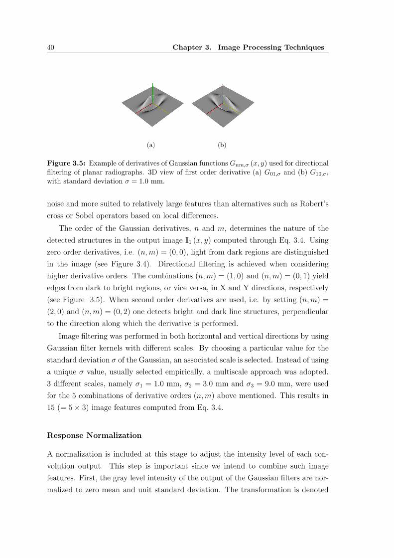
40 Chapter 3. Image Processing Techniques
(a) (b)
Figure 3.5: Example of derivatives of Gaussian functions Gnm,σ (x, y) used for directionalfiltering of planar radiographs. 3D view of first order derivative (a) G01,σ and (b) G10,σ,with standard deviation σ = 1.0 mm.
noise and more suited to relatively large features than alternatives such as Robert’s
cross or Sobel operators based on local differences.
The order of the Gaussian derivatives, n and m, determines the nature of the
detected structures in the output image I1 (x, y) computed through Eq. 3.4. Using
zero order derivatives, i.e. (n,m) = (0, 0), light from dark regions are distinguished
in the image (see Figure 3.4). Directional filtering is achieved when considering
higher derivative orders. The combinations (n,m) = (1, 0) and (n,m) = (0, 1) yield
edges from dark to bright regions, or vice versa, in X and Y directions, respectively
(see Figure 3.5). When second order derivatives are used, i.e. by setting (n,m) =
(2, 0) and (n,m) = (0, 2) one detects bright and dark line structures, perpendicular
to the direction along which the derivative is performed.
Image filtering was performed in both horizontal and vertical directions by using
Gaussian filter kernels with different scales. By choosing a particular value for the
standard deviation σ of the Gaussian, an associated scale is selected. Instead of using
a unique σ value, usually selected empirically, a multiscale approach was adopted.
3 different scales, namely σ1 = 1.0 mm, σ2 = 3.0 mm and σ3 = 9.0 mm, were used
for the 5 combinations of derivative orders (n,m) above mentioned. This results in
15 (= 5 × 3) image features computed from Eq. 3.4.
Response Normalization
A normalization is included at this stage to adjust the intensity level of each con-
volution output. This step is important since we intend to combine such image
features. First, the gray level intensity of the output of the Gaussian filters are nor-
malized to zero mean and unit standard deviation. The transformation is denoted
3.2. Image Filtering and Processing 41
by I1 (x, y) → I2 (x, y), where I1 (x, y) is the output of the convolution operation as
given by Eq. 3.4. Then, a non-linear intensity mapping is performed on the image
I2 by using a standard Sigmoid filter. A flexible implementation of this filter [34]
includes several parameters that can be tuned to select its input and output in-
tensity ranges. The following equation represents the Sigmoid intensity transform
I2 (x, y) → I3 (x, y) applied pixel-wise:
I3 (x, y) = (b − a)1
1 + e−I2(x,y)−c
d
− a. (3.6)
In the above equation, the parameters a and b are the minimum and maximum
values of the output image I3, d defines the width of the input intensity range and
c defines the intensity around which the range is centered. The parameters were set
to a = −1, b = 1, c = 0 and d = 1, such that −1 ≤ I3 (x, y) ≤ 1.
The normalization includes a final step that incorporates an analog threshold
element. This element has been previously suggested as part of a multilayered
network for visual feature extraction [41]. Here, the function of such element was
considered equivalent to that of a neuron. The output of a threshold element is an
analog value, positive or zero, linearly proportional to the input providing that is
greater than the threshold. The threshold value was set to c = 0, as in Eq. 3.6. More
precisely, we defined the non-linear characteristic transfer function of the analog
threshold element as follow:
R(p)nm,σ (x, y) = max 0, (−1)p I3 (x, y) , p = 0, 1 . (3.7)
The image features extraction step is a composition of a convolution operation
and normalization. From Eq. 3.4, 3.6 and 3.7, this step is described by the following
processing pipeline: I (x, y) → Gnm,σ → I1 → I2 → I3 → R(p)nm,σ (x, y). A schematics
of this pipeline is shown in Figure 3.6.
The output of the analog element is a normalized response R(p)nm,σ with positive
values, such that 0 ≤ R(p)nm,σ (x, y) ≤ 1. The thresholding operation described by
Eq. 3.7 is actually equivalent to a half-wave rectification.
Since the Sigmoid transform results in images I3 with both positive and nega-
tive values, two opposite contrast polarities were used by including the parameter
p in Eq. 3.7. By switching this parameter, p = 0, 1, each convolution of the in-
put chest radiograph with a particular filter Gnm,σ yields two normalized responses
R(p)nm,σ, one for each value of p. Responses with opposite polarities were constructed

42 Chapter 3. Image Processing Techniques
FilteredIMAGE
ProcessedIMAGE
Derivative Filter 1
Derivative Filter 2
dir 1
n
dir 2
m
dc
a b
p
NormalizeSigmoid
FilterAnalog
Threshold
1 2
Figure 3.6: Collaboration diagram (pipeline) of the image feature extraction algorithm.The input image of the pipeline is a filtered version of the digital chest radiograph (seeFigure 3.2).
Figure 3.7: Examples of normalized responses R(p)nm,σ (x, y), using the image processing
pipeline of Figure 3.6. The chest radiograph of Figure 3.3(b) (filtered image) was pro-cessed with different derivatives of 2D Gaussian convolution kernels. σ is the width of theGaussian and n and m are the order of the derivatives in X (horizontal) and Y (vertical)directions, respectively. From left to right: R00,1, R10,3, R01,3, R20,9 and R02,9. First rowdisplays responses with polarity p = 0, while second row corresponds to p = 1. All response
intensity values range between 0 (black) and 1 (white), that is, 0 ≤ R(p)nm,σ (x, y) ≤ 1.

3.3. Image Segmentation 43
to distinguish light from dark regions and discriminate light-dark from dark-light
transitions.
Since 15 image features were extracted and 2 opposite polarities are considered,
a total of 30 normalized responses were computed for each input radiograph to
be segmented. Some responses R(p)nm,σ are displayed in Figure 3.7. Each response
correspond to a particular combination of the Gaussian filter parameters n, m and
σ. For each case, responses are shown for the two opposite polarities p.
3.3 Image Segmentation
Medical image segmentation plays a crucial role in many imaging applications by
automating or facilitating the delineation of anatomical structures and other regions
of interest. The general segmentation problem involves the partitioning of an input
image into a number of homogeneous segments, such as contours and surfaces, that
define the region of the object of interest as spatially connected groups of pixels.
Alternatively, segmentation can be considered as a pixel labeling process in the sense
that all pixels that belong to the same homogeneous region are assigned the same
label.
3.3.1 Optimal Thresholding
Thresholding is used to change or identify pixel values based on specifying one or
more values, called the threshold values. When more than one threshold value
is considered we have a multithresholding technique [42]. The easiest method of
grouping pixels into coherent regions is simply to threshold their gray values so that
all pixels whose values are in a given range fall into the same class. More often,
thresholding is used to binarize images so that the image foreground is separated
from its background. Binary images are created by turning all pixels below a certain
threshold to zero and all pixels above that threshold to one. In particular, the output
of the analog threshold element R(p)nm,σ as given by Eq. 3.7, is a thresholded version
of the image I3 at threshold T . For polarity p = 0 and threshold T = 0, Eq. 3.7 can
be rewritten as
R(0)nm,σ (x, y) =
1, if I3 (x, y) ≥ T ,
0, otherwise.(3.8)
The gray level distribution characterized by the image histogram is used for

44 Chapter 3. Image Processing Techniques
computing the threshold. Local maxima of the histogram generally correspond to
objects of interest in the image scene so that threshold values are best placed at
local minima of the histogram to separate such objects.
Although this approach is quite effective in many cases, the choice of the thresh-
old value is difficult and may lead to strange and unacceptable results. Often thresh-
olding is not fully automatic as the choice of the threshold requires manual inter-
vention. Several unsupervised clustering methods have been devised for selecting
automatically the threshold. One of the most well known algorithm is the iso-
data [43]. The isodata clustering is an iterative algorithm that searches for suitable
cluster centers (usually in good agreement with the local maxima of the image his-
togram) such that the distances between the cluster centers and the members of the
cluster are minimized. A fixed number of clusters to be detected must be initially
provided. The procedure is then repeated until the cluster centers remain stable.
A proof of the convergence of the isodata algorithm is given in [44]. For bi-level
thresholding, the optimal threshold [45] can be computed as follow. Let T (i) be the
segmentation threshold at step i. To choose a new threshold value, the image is
thresholded using T (i) in Eq. 3.8 to separate background from foreground pixels.
Let H(i)1 and H
(i)2 be the mean gray-level of the groups after segmenting a given
image H with threshold T (i). Then the new threshold for step i + 1 is
T (i+1) =H
(i)1 + H
(i)2
2. (3.9)
This iterative threshold update is repeated until there is no change in the thresh-
old, i.e., T (i+1) = T (i). This method works well if the spreads of the distributions are
approximately equal, but it does not handle well the case where the distributions
have differing variances.
Another criterion for classifying pixels is to minimize the error of misclassifica-
tion. The goal is to find a threshold that classifies the image into two clusters such
that we minimize the area under the histogram for one cluster that lies on the other
cluster’s side of the threshold. This is equivalent to minimizing the within class
variance or, equivalently, maximizing the between class variance of foreground and
background pixels. Using discriminant analysis, the method proposed by Otsu [46]
defines the between-class variance σ2b of the thresholded image as
σ2b (T ) = n1 (T ) n2 (T )
[
H2 (T ) − H1 (T )]2
. (3.10)

3.3. Image Segmentation 45
where n1 (T ) and n2 (T ) are the number of background and foreground pixels. For
bi-level thresholding, Otsu verified that the optimal threshold T ∗ is chosen so that
the between-class variance σ2b is minimized, that is,
T ∗ = arg minT
σ2b (T )
. (3.11)
Eq. 3.10 shows that the threshold depends only on the difference between the
means of the two clusters. The optimal threshold is computed by updating n1 (T )
and n2 (T ) and the respective cluster means H1 (T ) and H2 (T ) as pixels move
from one cluster to the other as T increases. Using simple recurrence relations
the between-class variance is updated as each threshold is successively tested:
n1 (T + 1) = n1 (T ) + n (T )
n2 (T + 1) = n2 (T ) − n (T )
H1 (T + 1) =n1 (T ) H1 (T ) + n (T ) T
n1 (T + 1)
H2 (T + 1) =n2 (T ) H2 (T ) − n (T ) T
n2 (T + 1)
. (3.12)
Whereas the Otsu’s method separates the two clusters according to the threshold
and try to optimize some statistical measure, mixture modeling assumes that there
already exists two distributions. The image histogram is usually considered as being
the sample probability density function of a mixture of Gaussians and therefore the
segmentation problem is reformulated as one of parameter estimation followed by
pixel classification [33].
Thresholding considers only the value of all the pixels, not any contextual re-
lationship between them, and thus, there is no guarantee that the pixels identified
by the thresholding process are contiguous. This cause it to be sensitive to noise
and image inhomogeneities. These artifacts essentially corrupt the histogram of the
image making the separation more difficult. When the distribution of the pixel val-
ues is noisy, the image (or its histogram) is usually smoothed before trying to find
separate modes or clusters. A survey on thresholding techniques is provided in [42].
More recently, a quantitative performance evaluation of thresholding methods has
been presented in [47].

46 Chapter 3. Image Processing Techniques
(a) (b) (c) (d)
Figure 3.8: Pixel and voxel connectivity. (a) 4 and 8 pixel connectivity (2D); (b) to (d)6, 10 and 26 voxel connectivity, respectively (3D).
3.3.2 Region Growing Techniques
Region growing algorithms have proven to be an effective approach for image seg-
mentation. Region growing is a procedure that group pixels or sub regions into
larger regions based on a predefined criteria. The basic approach is to start with
a set of seed points and from these grow regions by appending to each seed those
neighboring pixels that have properties similar to the seed. The selection of a set
of one or more starting points and similarity criteria is often based on the nature
of the problem. Region growing algorithms vary depending on the criteria used to
decide whether a pixel should be included in the region or not, the type connectivity
used to determine neighbors, as illustrated in Figure 3.8, and the strategy used to
visit neighboring pixels.
The initialization of a Seeded Region Growing (SRG) algorithm requires, at least,
one seed point. It is convenient that this point be placed in a typical region of the
anatomical structure to be segmented. A simple similarity criterion for including
connected pixels in the region is based on their gray level so that pixels having gray
level I (x, y) in the same interval receive the same class label. If TL and TU are the
lower and upper thresholds that define that interval, the region growing algorithm
includes those pixels p = (x, y)T connected to the seed that satisify
TL ≤ I (x, y) ≤ TH . (3.13)
The lower and upper thresholds TL and TU define the interval in which pixel
values should fall in order to be included in the region. Setting the threshold values
too close will not allow enough flexibility for the region to grow. Setting them too
far apart will result in a region that engulfs the image.
Criteria based on statistics of the current region may be used [33]. In the simplest

3.3. Image Segmentation 47
case, the algorithm first computes the mean m and standard deviation σ of values
for all the pixels currently included in the region. By providing a factor k to define
a range around the mean, neighbor pixels whose values fall inside the range are
accepted and included in the region, that is,
m − kσ ≤ I (x, y) ≤ m + kσ. (3.14)
When no more neighbor pixels are found that satisfy the criterion, the algorithm
is considered to have finished its first iteration. At that point, the mean and standard
deviation of the intensity levels are recomputed using all the pixels currently included
in the region. This mean and standard deviation defines a new intensity range
that is used to visit current region neighbors and evaluate whether their intensity
falls inside the range. This iterative process is repeated until no more pixels are
added or the maximum number of iterations is reached. The number of iterations is
specified based on the homogeneity of the intensities of the anatomical structure to
be segmented. Highly homogeneous regions may only require a couple of iterations.
Noise present in the image can reduce the capacity of the SRG algorithm to grow
large regions. When faced with noisy images, it is usually convenient to pre-process
the image by using an edge preserving smoothing filter.
A close variant of the SRG technique is illustrated in Figure 3.9. If two seeds,
p1 and p2, and a lower threshold TL are provided, the algorithm can be applied
to grow a region connected to the first seed and not connected to the second one.
In order to do this, the iterative procedure finds a value that could be used as
upper threshold for the first seed. A binary search is used to find the value that
separates both seeds. Major anatomical structures can be segmented by providing
seed pairs in the appropriate locations. Selecting one seed in one structure and the
other seed in the adjacent structure creates the appropriate setup for computing
the threshold TU that will separate both structures. As an example, consider the
input image Figure 3.9(a), filtered as described in Section 3.2.1. The image is
of size 352 × 428 pixels with gray levels ranging from 0 to 1024. The two seeds
(white circles) p1 and p2 defined by the pair of coordinates (x1, y1) = (8, 5) and
(x2, y2) = (103, 137) were manually identified in the right side of the image, and TL
was set to 0. The segmentation output of the SRG algorithm, shown in Figure 3.9(b)
and (c) for which TU = 437 was computed, are binary images with zero-value pixels
everywhere except on the extracted regions. The same algorithm was applied to the
left side, and TU = 403 was found for the pair of seeds p3 and p4, (x3, y3) = (342, 8)

48 Chapter 3. Image Processing Techniques
(a) (b) (c) (d)
Figure 3.9: Example illustrating the seeded region growing (SRG) technique. (a) Filteredinput image with seeds p1 and p2 (white circles); (b) Segmented region connected to seedp1 and (c) connected to seed p2 but not connected to p1. (d) Resulting image labelingafter applying SRG on both sides of the image. Input values range from 0 to 1024 andthe threshold is TU = 437 and TU = 403 for the right and left side, respectively.
and (x4, y4) = (233, 137). This algorithm is intended to be used in cases where
adjacent anatomical structures are difficult to separate. Applying twice the SRG
algorithm results in the segmentation output shown Figure 3.9(d). As illustrated
by the example, this technique provides a suitable method for separating the lung
fields from the supra-clavicular region of the thorax.
Image segmentation using SRG should be performed on smoothed version of the
image since the distribution of pixel values could be quite different from that of the
input (non-filtered) image. Like thresholding, region growing is sensitive to noise
and is not often used alone but within a set of image processing operations. Fuzzy
analogies with region growing have also been developed [48].
3.4 Model-Based Image Segmentation
3.4.1 Lung Contour Model
A simple geometrical model of the lungs was adopted by defining a set of landmarks
to describe conveniently its shape. Connecting the landmarks will result in several
segments that are used to represent the boundaries between the lung regions and
other anatomical structures observed in chest radiographs. The landmarks were
chosen to reflect as much as possible the location of prominent visual features within
the image. As shown in Figure 3.10(a), the selected landmarks, labeled from A
to E, were superimposed on a PA chest radiograph to illustrate their anatomical

3.4. Model-Based Image Segmentation 49
1
2
3
C
BA
4
D
E
F
(a)
1
20
16060
200
101121
100
50
(b)
Figure 3.10: Lung contour model for PA chest radiograph segmentation. (a) The modelis constructed by defining several segments (1 to 4) between landmarks (A to F ), withanatomical correspondence. (b) A set of (200) interpolated points representing a templateof the lung shape, manually delineated on the corresponding image.
correspondence.
A lung contour model is easily constructed, for each lung, by considering four
segments: the hemidiaphragm (segment 1 - AFB), the costal edges or rib cage
(segment 2 - BC), the lung top section or lung apex (segment 3 - CDE) and the
mediastinal edges (segment 4 - EF ). The junction of these four segments forms a
closed contour denoted by the sequence [FBCDE], that represents the unobscured
region of the lung.
Defining several paths that contain at least one segment (or part of a segment)
of the contour model, a method for segmenting the lung fields is proposed and ex-
plained in detail in Chapter 4, Section 4.3. The method is based on the automated
and accurate delineation of such paths, based on the observation that the lateral
edges (segments 2 and 4) are nearly vertical while, on the other hand, the hemidi-
aphragms (segments 1) are nearly horizontal and the lung top sections (segment 3)
are approximately circular.
3.4.2 Dynamic Programming
The detection of optimal paths can be achieved by using an optimization algo-
rithm based on dynamic programming we now introduce. Dynamic programming
is a method of finding the global optimum of multistage processes. It is based on
Bellman’s principle of optimality [49] which state that the optimum path between
50 Chapter 3. Image Processing Techniques
two given points is also optimum between any two points lying on the path. Typi-
cal applications of the use of dynamic programming in boundary tracking problems
are tracing borders of elongated objects like roads and rivers in aerial photographs
and the segmentation of handwritten characters. Medical applications include the
segmentation of mammographic masses [50] and boundary detection in ultrasonic
images [51] for automated measurement of the carotid artery [52]. Boundary de-
lineation based on dynamic programming can be formulated as a graph searching
problem where the goal is to find the optimal path between a set of starting nodes
and a set of ending nodes. The optimal path is defined as the minimum cost path
and the cumulative cost of a path (cost path) is the sum of the local costs of each
pixel on the path. Application of the local cost to all pixels results in the so-called
cost function. More details on constructing cost images are found in Section 4.2.3.
3.5 Statistical Shape Models
We now describe how to construct a 2D statistical shape model of the lungs from
PA chest radiographs. The resulting model is intended to be used in a model-to-
image registration algorithm for segmenting the lung fields from unseen images. The
complete description of the proposed method is provided in Section 4.4.
Statistical shape models capture shape information from the set of labeled train-
ing data. A prerequisite for such models is a set of points located at corresponding
positions on all training shapes. A popular method to describe shapes of objects is
the Point Distribution Model (PDM), where each training shape is specified by a
set of points lying on the contour or surface of the object [53, 54]. This particular
multivariate model has proven to be especially useful for medical image segmenta-
tion.
3.5.1 Point Distribution Models
To construct the model, the outline of each lung field were hand traced on each digital
chest radiograph of a private database by an experienced radiologist. A software
system was specifically developed to perform this task. The software consists on a
mouse-controlled graphical user interface that allows outlining/editing of 2D points
and contours. Image contouring was performed at the lower resolution (σ0 = dX =
dY = 1.0 mm), by first delineating the right lung, then the left lung, according
to the following sequence: hemidiaphragm (1), costal edge (2), lung top (3) and
3.5. Statistical Shape Models 51
mediastinal edge (4), as illustrated in Figure 3.10(a). Each lung is annotated by
manually placing points around its border and spline interpolation was used to
define the corresponding contour. Manual contours were stored in separated files
and later used as the ”gold standard” to evaluate the performance of the automated
lung field detection algorithms.
The lung shape is represented by a set of N points P = pn, n = 0, 1, . . . , N−1,
where pn = (xn, yn)T is a point of the lung contour interpolated from the points
provided by the user. Figure 3.10(b) shows an example of image contouring for
which some contour points are indicated. The model was constructed such that,
for each lung, 20, 40 and 40 points were interpolated to delineate, respectively, the
segments AB, BD and DF . The total number of points of the resulting contour
model is therefore N = 200. Note that due to the bilateral symmetry observed in
chest radiographs, points pn and pn+N/2, n = 0, 1, . . . , N/2 − 1, can be defined as
points with symmetry correspondence.
Mean Shape
From the set of points P we are able to derive a template of the shape. By concate-
nating the coordinates for each point into a shape vector, we can represent every
template with a single location x in a 2N -dimensional space:
x = (x0, y0, x1, y1, . . . , xN−1, yN−1)T . (3.15)
If the object is three-dimensional, then the space is 3N -dimensional. Some areas
of the space (the shape-space) spanned by these vectors will be more densely pop-
ulated than others and, by taking several examples of the input class, we can infer
a model of the distribution, the point distribution model. Once the corresponding
points in all the contours are constructed, each template is represented by a shape
vector and the mean shape is given by
x =1
S
S−1∑
s=0
xs, (3.16)
where S is the number of examples in the training set. Figure 3.11(a) shows the lung
contours manually extracted from a dataset of S = 39 chest radiographs. From this
training set, the mean shape plotted in Figure 3.11(b) was computed and clearly
exhibits the expected bilateral symmetry of the human anatomy observed in PA
chest radiographs.

52 Chapter 3. Image Processing Techniques
(a) (b) (c)
Figure 3.11: Point distribution model of the lungs. (a) Unaligned training shapes (con-tours) used to construct the mean shape (b), the lung contour model; (c) same contoursafter alignment using the Procrustes algorithm.
When modeling the different shapes of the templates it is usual to remove the
spurious effects of the template location and orientation before transforming the
examples into the space. This can be done by using the Procrustes algorithm [55, 56]
to align all the shapes before the mean shape is produced. Aligned training shapes
using the Procrustes algorithm are plotted in Figure 3.11(c).
3.5.2 Principal Component Analysis
The analysis of the shape vectors derived manually from the set of training examples
gives insight in the typical variations in shape of the lungs and their correlation. The
modes of variation, the way in which the model points tend to move together, can
be found by applying the Principal Component Analysis (PCA) to the deviation
from the mean shape as follow. The covariance matrix C of the training data is first
computed using
C =1
S − 1
S−1∑
s=0
(xs − x) (xs − x)T. (3.17)
The covariance matrix C is a matrix of size 2N × 2N and describes the modes
of variation of the points of the shape. C is eigen-decomposed to give a set of
unit eigenvectors ek, k = 0, 1, . . . , 2N − 1, and the corresponding eigenvalues λk,
λk ≥ λk+1, such that
Cek = λkek, (3.18a)
eTk ek = 1. (3.18b)
3.5. Statistical Shape Models 53
The shape modes are not of equal importance. It can be shown that the eigen-
vectors of the covariance matrix corresponding to the largest eigenvalues describe
the most significant modes and that the proportion of the total variance explained
by each eigenvector is equal to the corresponding eigenvalue [57].
In many cases, a relatively small number of modes m (m < 2N) is used to
approximate the original data while still representing a large fraction of its variation.
The value of m can be determined by the number of principal components that are
required to account for a sufficiently large proportion of λT , typically between 90%
and 99%, of the total variance of all the variables, where
λT =2N−1∑
k=0
λk. (3.19)
The corresponding eigenvectors allow us to approximate any member of the
original data set and can be treated as deformations of the whole model. New shapes
x are generated by combining vectors, one for each mode, using an m-dimensional
vector b:
x = x + Φb, (3.20)
where Φ = (e0, e1, . . . , em−1) is the matrix of the first m eigenvectors and b =
(b0, b0, . . . , bm−1)T is a vector of weigths, one for each eigenvector, controlling the
modes of shape variation. Since the eigenvectors are orthogonals, ΦTΦ = 1 and
b = ΦT (x − x) . (3.21)
The above equation allows to generate new examples of the lung shape by varying
the parameters b with suitable limits so that the new shapes can be considered as
extracted from the training set.
Another way of visualizing which parts of the objects exhibit most shape vari-
ation is the independent PCA, applied to each model point pn = (xn, yn)T, by
considering x = pn in Eq. 3.15. In this case, the dimension of the shape vectors
is reduced to N = 2, the dimension of the points. The result is displayed in Fig-
ure 3.12, where independent PCA has been applied without and with Procrustes
alignment of the training set, as illustrated in Figure 3.12 (a) and (b), respecively.
In both cases, the spread of each model point pn is described by an ellipse with cen-
ter at pn, whose semi-axis have the directions of the computed eigenvectors e0 and
e1 and length equal to bk =√
λk, k = 0, 1, where λk is the corresponding eigenvalue

54 Chapter 3. Image Processing Techniques
(a) (b)
Figure 3.12: Independent principal component analysis for visualizing the spread of eachpoint of the lung contour model, (a) before and (b) after alignment of the training shapes.
of ek.
3.5.3 Mean Shape Triangulation
The mean shape computed from the PDM described above is a geometrical repre-
sentation that results in the partitioning of a given chest radiograph. In fact, beside
the delineation of the lung fields, this approach is suitable to describe other general
anatomical structures as connected regions within the thorax. For example, con-
sidering the landmarks A, F and E of both lungs (see Figure 3.10(a)), the model
defines the cardiac silhouette as the closed contour [(AFE)r (EFA)l], where the
subscripts r and l stand for right and left. This is actually equivalent to the region
defined between the mediastinal edges, below the lung top sections and above the
hemidiaphragms. Similarly, connecting the landmarks [(BFA)r (AFB)l] will result
in the subdiaphragmatic region of the patient.
For each anatomical structure, the corresponding region can be described by a set
of points, uniformly sampled in its interior. First an initial distribution of equilateral
triangles is first created within the region by choosing the initial edge length of the
triangles. Then, the resulting mesh is iteratively smoothed until the mesh points
move less than a given tolerance. Figure 3.13 shows the result of such triangulation.
The specification of the triangulated mean shape is reported in Table 3.1, and will
be denoted as the parametric representation pm = (xm, ym)T, m = 0, 1, · · · ,M − 1,
corresponding to the set P = pm of M points, M ≥ N , where N is the number
of interpolated points that define the mean shape.

3.5. Statistical Shape Models 55
(a) (b) (c) (d)
Figure 3.13: Mean Shape Triangulation. (a) Lung mean shape triangulated with initialedge length 10.0 mm and distance tolerance 0.01 mm; Anatomical regions corresponding to(b) interior of the lungs, (c) subdiaphragmatic region of the patient and (d) mediastinum.
Table 3.1: Specification of the lung contour model (triangulated mean shape) of Fig-ure 3.13(a).
Image Database HSJ (private)
Images in training set S 39 (all)
Contours in image (lung fields) 2 (manual)
Segments in contour (both fields) 3
Points in segments (one field) 20, 40, 40 (interpolated)
Points in contour model N 200 (interpolated)
Initial edge length 10 mm
Edge tolerance 0.01 mm
Points inside right lung 207 (triangulated)
Points inside left lung 185 (triangulated)
Points below hemidiaphragms 119 (triangulated)
Points inside mediastinum 202 (triangulated)
Points in triangulated model M 913 (total)

56 Chapter 3. Image Processing Techniques
3.6 Deformable Models
Two and three-dimensional objects, such as surfaces and contours, can be manipu-
lated in the normal ways. Linear transforms include translation, rotation and scal-
ing. These are all operations that take place on the vertices of the model alone, since
the connectivity of the points remains unchanged. Any set of such linear transforms
can be encapsulated in a 4 × 4 transform matrix, by making use of homogeneous
coordinates. Others operations, namely reflection and shearing, are also possible
within such a framework but will not be considered here. Non-linear transforms,
on the other hand, can change not only the position and orientation of objects but
also their shape. By definition, two objects have the same shape if there exists a
linear transform that exactly maps one onto the other. One of the many ways to
specify a linear transformation is to give two sets of points and use the transform
that maps one to the other. In general there will not exist a linear transform that
exactly maps the points onto one another and so an error term must be minimized
to find the best solution.
Two non-linear transforms are presented, namely the Free Form Deformation
(FFD) and the Thin-Plate Spline (TPS) transform. FFD is a method for non-rigid
warping with local control, through the use of cubic B-splines, while, by contrast,
TPS does a global nonrigid warping controlled by a set of landmarks. Landmark-
based transform will be used in Section 4.4 for the automated lung field segmentation
of PA chest radiographs using a model-to-image registration framework.
3.6.1 Free Form Deformation
The deformation of a prior model can be accomplished using Free Form Deformation
(FFD), a popular deformation technique in computer graphics [58]. The FFD is
controlled by a rectangular deformation grid, of size Nx × Ny, that surrounds the
model (or just a portion of it). The grid is defined by the lattice or set of control
points U = uij, i = 0, 1, · · · , Nx − 1, j = 0, 1, · · · , Ny − 1, and, when one or more
points of the grid are moved to new positions, the model is deformed correspondingly.
Consider a geometrical model defined by the set of points P = pm, m =
0, 1, · · · ,M − 1, where pm = (xm, ym)T. To deform the model using FFD, the local
coordinates(
sm, tm)
, 0 ≤ sm, tm ≤ 1, of each point pm in the model point set are
first computed with respect to the undisplaced FFD grid U. The new position qm of
each point m in the deformed model, after moving the control points uij = (xij, yij)T
to new positions vij = (xij, yij)T, can be calculated using a bivariate tensor product:

3.6. Deformable Models 57
qm =Nx−1∑
i=0
Ny−1∑
j=0
Bi,Nx(sm) Bj,Ny
(
tm)
vij, (3.22)
where Bi,N (s) is the Bernstein polynomial blending function of degree N , defined
as
Bi,N (s) =N !
i! (N − i)!si (1 − s)N−i . (3.23)
The deformation of the model depends on the displacement of each control point
denoted ∆uij = (∆xij, ∆yij)T, for which vij = uij + ∆uij. FFD is then repre-
sented by the set of displacement vectors ∆U = ∆uij, i = 0, 1, · · · , Nx − 1,
j = 0, 1, · · · , Ny − 1, also called the displacement vector field.
3.6.2 Thin-Plate Splines
One particular and useful non-linear transform is the Thin-Plate Spline (TPS) [59].
TPS is frequently found in image analysis. For example, this transform has been
used with velocity encoded MR images [60], to calculate cardiac strain from MR
images [61], and analyzing bone structure on radiographs [62]. As with the landmark
transform, a TPS transform is specified by two sets of corresponding points. With
TPS, one of the sets of landmarks, the source landmarks, is exactly mapped onto
the other, the target landmarks, and a deforming transform is interpolated between
them. The interpolation is chosen such that it minimizes a bending energy, ensuring
that the deformation is smooth and no discontinuities appear. Since we will make
use of this landmark transforms at many stages, the algorithm is herein presented.
Consider the triangulated geometrical model of Figure 3.14(a), defined by the set
of points P = pm, m = 0, 1, · · · ,M − 1, where pm = (xm, ym)T. Let m = ml,l = 0, 1, · · · , L−1, be a set of parameters which generates L ≤ M sequentially given
source landmarks u (ml) in the model. We assume that those landmarks represent
the shape well. For simplicity, denote u (ml) = ul and U = ul the set of the
source landmarks. The target landmarks vl form the set V = vl and represent
the deformed model. According to the statistical shape theory [63], U and V can
be regarded as the landmark representation of the shape and the deformed shape,
respectively.
The TPS transform is specified by mapping the source landmarks U to the cor-
responding target landmarks V. The deformation is characterized by the transform

58 Chapter 3. Image Processing Techniques
T = (f, g)T, such that V = T (U), i.e., vl = T (ul), l = 0, 1, · · · , L − 1, where
f (u) = a0 + a1x + a2y +L−1∑
l=0
clU (u,ul), (3.24a)
g (u) = b0 + b1x + b2y +L−1∑
l=0
dlU (u,ul), (3.24b)
and U is the basis function. In 2D we use U (r) = r2 log r, while in 3D we simply
use U (r) = r. In Eq. 3.24, the parameters a = (a0, a1, a2)T, b = (b0, b1, b2)
T,
c = (c0, c1, . . . , cL−1)T and d = (d0, d1, . . . , dL−1)
T can be calculated by solving the
following matrix equation
(
K Q
QT 0
) (
c d
a b
)
=
(
x y
0 0
)
, (3.25)
where, Kij = U (ui,uj) = ‖ui − uj‖2 log ‖ui − uj‖, i, j = 0, 1, . . . , L − 1, Q =
(1, x, y) and 0 is an array of zeroes.
Note that in the above equation, x = (x0, x1, . . . , xL−1)T, y = (y0, y1, . . . , yL−1)
T,
x = (x0, x1, . . . , xL−1)T and y = (y0, y1, . . . , yL−1)
T, where ul = (xl, yl)T and vl =
(xl, yl)T are corresponding landmarks of U and V, respectively. It can be shown that
the TPS transform minimizes the following so-called bending energy function [59]
E (T ) =
∫∫
ℜ2
(L (f) + L (g)) dxdy, (3.26)
where
L (·) =
(
∂2
∂x2
)2
+ 2
(
∂2
∂x∂y
)2
+
(
∂2
∂y2
)2
. (3.27)
Substituting Eq. 3.24 and Eq. 3.25 into Eq. 3.26 yields
E (T ) = cTKc + dTKd. (3.28)
The thin-plate bending energy E is invariant to affine transforms and makes
TPS especially suitable for describing nonrigid shape deformations in biological and
medical applications. In the image analysis domain, thin-plate splines provide a
natural way to move from point correspondences to entire image warps.
The TPS warping function is the transform that minimizes the bending energy
(Eq. 3.26, 3.28) and simultaneously maps all points pm of the undeformed model

3.7. Optimization Techniques 59
(a) (b) (c)
Figure 3.14: Lung model deformation using thin-plate splines (TPS) transform. (a)Undeformed model (triangulated mean shape) with a set of 14 source landmarks selectedon the lung contour; (b) The model deformation using thin-plate splines is achieved bymapping the source landmarks to the corresponding target landmarks (source landmarksrandomly displaced from their original position); (c) Corresponding displacement vectorfield, shown for all points of the triangulated model.
exactly onto their corresponding points qm in the deformed model:
qm = T (pm) . (3.29)
An example of the lung model deformation using TPS is illustrated in Figure 3.14,
where the source landmarks ul were selected from the points of the lung contour
model (Figure 3.14(a)) and randomly displaced from their original position (Fig-
ure 3.14(b)) to create the target landmarks vl. As for FFD, model deformation
using TPS defined by the corresponding sets of source and target landmarks can
be represented by vl = ul + ∆ul, where ∆ul = (∆xl, ∆yl)T is the displacement
of the landmark ul. Again, the deformation is described by the corresponding dis-
placement vector field ∆U = ∆ul, l = 0, 1, . . . , L − 1, where L is the number
of landmarks. Note that, as illustrated in Figure 3.14(c), the vector field can be
computed from all the undeformed and transformed model points and therefore the
displacements correspond to the vectors ∆pm = qm − pm, m = 0, . . . ,M − 1.
3.7 Optimization Techniques
This Section describes the basic principles of two common optimization techniques,
namely genetic algorithms (GA) and Simulated Annealing (SA). Both search al-
gorithms can be used as an optimizer in the model-to-image registration method
reported in Section 4.4.1 for segmenting the lung fields from PA chest radiographs.

60 Chapter 3. Image Processing Techniques
A proposed GA implementation is provided in Section 4.4.2.
3.7.1 Genetic Algorithms
In The Origin of Species [64], Charles Darwin stated the theory of natural evolution.
Over many generations, biological organisms evolve according to the principles of
natural selection like ”survival of the fittest” to reach some remarkable forms of
accomplishment. GA were originally devised as a model of adaptation in an artificial
system by Holland [65].
Genetic Algorithms are probabilist search algorithms characterized by the fact
that a number C of potential solutions wc of the optimization problem simultane-
ously sample the search space of all possible individuals. This population W = wc,c = 0, 1, · · · , C −1, is modified according to the natural evolution process: after ini-
tialization, selection and recombination are executed in a loop until some termination
criteria is reached. Each run of the loop is called a generation and W(t) denotes the
population at generation t.
The flow chart of a simple GA is diagrammed in Figure 3.15(a). It is assumed
that selection and recombination are done sequentially: first, a selection phase cre-
ates an intermediate population, W′, and then recombination is performed with
a certain probability on the individuals of this intermediate population to get the
population W(t+1) for the next generation. Mimicking the natural selection and
reproduction, an initial population W(0) can be evolved to the best solution w∗ of
the problem.
The selection operator is intended to improve the average quality of the pop-
ulation by giving individuals of higher quality a higher probability to be copied
into the next generation. Selection thereby focuses the search on the exploration of
promising regions in the search space. Recombination changes the genetic material
in the population, either by crossover or mutation, in order to exploit new points in
the search space. A schematic representation of standard recombination operators
is given in Figure 3.15(b).
Solution Representation and Evaluation
In a standard GA, a solution is encoded as a string of genes to form a chromosome
w representing an individual in the population. Each gene can take one or sev-
eral values or alleles. Holland [65] showed that long chromosomes, with few alleles
per gene are preferable to shorter chromosomes with many alleles per genes. This

3.7. Optimization Techniques 61
PROBLEM SOLVED ?
NO
YES
SELECTION
RECOMBINATION
EVALUATION
INITIALPOPULATION
BESTSOLUTION
(a)
crossover
mutation
(b)
Figure 3.15: (a) Flow chart of a simple genetic algorithm. (b) Standard recombinationoperators, crossover and mutation, applied to chromosomes with binary alleles.
imply that the optimal case is to consider binary alleles. Consequently, in many
optimization problems involving real-valued variables, the chromosomes are simply
bit strings.
The quality of an individual is measured by an objective function, fc, which
can decode the chromosome wc and assign a fitness value to the individual the
chromosome represents. In many applications, the fitness is simply the objective
function evaluated at the point in the search space represented by the chromosome.
Selection Functions
There are several schemes for the selection process, such as roulette wheel selection
and its extensions, scaling techniques, tournament, elitist models and ranking meth-
ods [66, 67]. For selection only the fitness value of the individuals are taken into
account. Hence, the state of the population is completely described by the fitness
function.
Roulette wheel - A problem is the possible existence of a super individual
in the population, i.e., an individual with an unusually high fitness. With fitness-
proportionate selection this individual will get many copies in successive generations

62 Chapter 3. Image Processing Techniques
and rapidly come to dominate the population thus causing premature convergence to
a possibly local optimum. It is possible to partially avoid this effect by suitably scal-
ing the evaluation function which amounts to the use of a modified fitness measure.
Several scaling methods have been suggested [66]. Another approach to mitigate the
above effect is to use selection methods that do not allocate trials proportionally to
fitness, such as common methods described next.
Linear ranking - In this selection, the individuals are sorted by fitness. A rank
C is assigned to the best individual and the rank 1 to the worst individual. Thus, the
best individual receives a predetermined multiple of the number of copies than the
worst one. The selection probability is linearly assigned to the individuals according
to their rank. Rank selection reduces the dominating effects of super individuals
without need for scaling and, at the same time, it exacerbates the difference between
close fitness values, thus increasing the selection pressure in stagnant populations.
Tournament - This type of selection runs a tournament among a few indi-
viduals: at generation t, a number k of individuals is selected randomly from the
population W(t) with uniform probability, and the best one among them, the one
with the highest fitness from this group, is copied into the intermediate population
W′. The winner can also be chosen probabilistically. The process is then repeated
C times, the constant number of individuals in the population. A widely used tour-
nament is held only between two individuals (binary tournament with k = 2) but
a generalization is possible to an arbitrary group size k called tournament size. A
1-way tournament of size k = 1 is equivalent to random selection. The selection
pressure is proportional to the tournament size. The chosen individual can be re-
moved from the population that the selection is made from if desired, otherwise
individuals can be selected more than once for the next generation. Tournament
selection has the advantage that it need not be global so that local tournaments can
be held simultaneously in a spatially organized population.
Truncation - In truncation selection with threshold T only the fraction T best
individuals can be selected and they all have the same selection probability.
Recombination Operators
Recombination includes crossover and mutation or any operator that changes the
genetic material of the chromosomes. Crossover is the process whereby two selected
parent chromosomes are combined together to create offspring. This operator mimics

3.7. Optimization Techniques 63
the genetic crossover of DNA1 in nature and serves to increase the variety in the
population, allowing the algorithm to explore most of the search space. In this way,
the GA manages to find the approximate global optimum in very large search spaces
in relatively short times. Mutation is a background operator which selects a gene
at random on a given individual and mutates the allele for that gene (for bit strings
the bit is complemented). Mutation is used to reintroduce alleles which may have
been lost from the population for purely stochastic reasons. Schematics of these
operators are given in Figure 3.15(b) for the case of binary alleles.
The balance between exploitation and exploration can be adjusted either by the
selection pressure of the selection operator or by the recombination operator, e.g.
the probability of crossover pcross and mutation pmut. As this balance is critical for
the behavior of the GA, the properties of selection and recombination operators are
of great interest to understand their influence on the convergence speed.
GA have been quite successful in optimization problems, especially when stan-
dard mathematical methods are hard to apply e.g. for noisy, discontinuous or non-
differentiable functions. GA have shown to solve linear and nonlinear problems by
exploring all regions of the state space and exponentially exploiting promising areas
through the selection and recombination operations. A more complete discussion
of genetic algorithms, including extensions and related topics can be found in the
books by Davis [68], Goldberg [66], Michalewicz [67] and a useful tutorial is provided
in Whitley [69].
3.7.2 Simulated Annealing
Simulated annealing [70] is a stochastic decent technique derived from statistical
mechanics. When crystalline material is slowly cooled through its melting point,
highly ordered, low-energy crystals are formed. The slower the cooling, the lower
the final lattice energy. This physical process is a natural optimization method
where the lattice energy E is the objective function to be minimized. Numerical
systems can be run through a similar optimization process if the parameters of the
system are identified with state space variables, and the objective function of the
optimization problem with the energy E.
Thermal fluctuations in the system are simulated by randomly perturbing its pa-
rameters, and the size of the fluctuations are controlled by a temperature parameter
T . If a system is at equilibrium at temperature T , the probability that the system
1 Deoxyribonucleic Acid

64 Chapter 3. Image Processing Techniques
is in a particular atomic configuration is
p (E) = exp
(
− E
kBT
)
, (3.30)
where E is the energy of the configuration and kB is the Boltzmann constant. Sim-
ulated annealing attempts to reach the minimum energy state through a series of
atomic reconfigurations or local perturbations which are accepted if the energy is
decreased, and accepted with probability p (∆E) = exp (−∆E/kBT ) if the energy
is increased. For T > 0, there is always some probability that a detrimental step
will be accepted, thus allowing the algorithm to escape from local minima.
In contrast to simulated annealing which uses an analogy with a physical opti-
mization process, GA are based on the genetic processes of biological evolution. A
good comparison of these optimization algorithms with Monte Carlo techniques is
given in [71].
3.8 Validation
In order to quantify the performance of a segmentation method, validation exper-
iments are necessary. Validation is typically performed using one of two different
types of truth models. The most straightforward approach to validation is by com-
paring the automated segmentation with manually obtained segmentations. This
approach does not guarantee a perfect true model since an operator’s performance
can also be flawed. The other common approach to validating segmentation meth-
ods is through the use of physical phantoms [72] or computational phantoms [73].
Physical phantoms provide an accurate depiction of the image acquisition process
but typically do not present a realistic representation of anatomy. On the other
hand, computational phantoms can be more realistic in this latter regard but often
simulate the image acquisition process using only simplified models.
Once a truth model is available, a figure of merit must be defined for quantifying
the performance [74, 75, 76]. The choice of the performance measure is dependent
on the application and can be based on region information such as the number of
pixels misclassified, or boundary information such as distance to the true boundary.
A survey on this topic is provided in [77].
The proposed methods for automated lung field extraction from chest radio-
graphs and volumetric CT images, as described respectively in Chapter 4 and Chap-
ter 5, are expected to produce binary masks as the final segmentation output. The

3.8. Validation 65
TP
TN FP
FN
A
B
Figure 3.16: Confusion Matrix. Binary images A and B are compared pixel-wise toclassify each pixel as true positive (TP), true-negative (TN), false-positive (FP) and false-negative (FN), when considering the contour in A as the reference.
binary images were compared pixel-wise with the corresponding hand-segmented
images to classify each pixel in the image in one of four categories, as illustrated in
Figure 3.16: true positive (TP) where both the algorithm and the human observer
considered the pixel to be within the lung; true-negative (TN) where both consid-
ered the pixel to be outside the lung; false-positive (FP) where the computer found
the pixel inside the lung and the observer did not; and false-negative (FN), where
the observer detected the pixel in the lung but the algorithm did not. The number
of pixels N in each category was found as a fraction of the total number of pixels in
the image. These quantities were used to calculate the classical accuracy [78],
accuracy =NTP + NTN
NTP + NTN + NFP + NFN
, (3.31)
to measure the segmentation performance. The sensitivity and specificity are defined
per convention:
sensitivity =NTP
NTP + NFN
, (3.32a)
specificity =NTN
NTN + NFP
. (3.32b)
Considering the problem as the segmentation between lung and background and
following the approach introduced in [79], we computed the accuracy, sensitivity and
specificity to compare our results with other studies reported in the literature [80,
81, 82, 83].
Other methods can be used to evaluate the performance of segmentation algo-

66 Chapter 3. Image Processing Techniques
rithms. Among them, we focused on two standard performance indicators, namely
degree of overlap and F-score [84]. The degree of overlap was also used to evaluate
the results of a segmentation method applied to digital lateral chest radiographs [85]
and mammograms for detecting mass lesions [50]. These two additional measures
were considered for comparative purposes. Unlike accuracy, as given by Eq. 3.31,
they are independent of the true negative fraction, the part of the image correctly
classified as background.
The degree of overlap between the two segmentation masks was computed as the
ratio:
overlap =NTP
NTP + NFP + NFN
=|A ∩ B||A ∪ B| . (3.33)
where A and B are respectively the segmented lung region or set of non-zero pixels
in the first and second binary mask. In Eq. 3.33, ∩ represents the intersection and
∪ the union of two sets, and the operator | · | represents the size (number of pixels)
of a set. NTP is the part of the image that have been correctly classified as lung and
therefore NTP = |A ∩ B|. With this definition, the overlap represents also the true
positive fraction relative to |A ∪ B|.
By computing the area of the respective lungs, |A| and |B|, for both the manual
and automated segmentation, the precision and recall were calculated as follows:
precision =NTP
NTP + NFP
=|A ∩ B||B| , (3.34a)
recall =NTP
NTP + NFN
=|A ∩ B||A| . (3.34b)
Note that recall defined by Eq. 3.34b is actually sensitivity as given by Eq. 3.32a.
Taking the weighted average of precision P and recall R leads to the F-score,
F =PR
αP + (1 − α) R=
|A ∩ B|α |A| + (1 − α) |B| , (3.35)
where α is a parameter to the F-score used to control the weight assigned to precision
and recall. We used α = 0.5, a value often used [86, 87], to determine the relative
importance of each term, by expressing no preference for either. For this particualr
case, and following Eq. 3.35, the measure is computed as F = 2 |A ∩ B|/(|A| + |B|).

3.9. Final Remarks 67
3.9 Final Remarks
This Chapter focused on the presentation of basic techniques for the analysis of 2D
and 3D images. Generally, solutions to practical segmentation problems are obtained
by applying such methods in sequence. For the shake of simplicity, they have been
illustrated for 2D images although some of them are easily generalized to 3D. For
instance, elementary algorithms such as smoothing, resampling and directional fil-
tering were introduced to extract prominent visual features in chest radiographs and
compute normalized responses suitable for detecting the borders between anatomical
structures that largely coincide with edges and ridges in such images.
Optimal thresholding and region growing present some limitations for performing
segmentation by itself. These limitations are particularly noticeable in noisy images
and in images lacking spatial uniformity, as is the case with planar radiographs.
However, such techniques will prove particularly useful for extracting anatomical
structures of interest from volumetric CT images.
Based on prior knowledge, we have described the construction of a statistical
shape model of the lungs. A main drawback of the approach is the point correspon-
dence problem in the model construction phase. On every training sample, points
have to be placed in a consistent manner. In order to describe the lung shape and
its variations correctly, points on all training samples have to be located at corre-
sponding anatomical positions. Although the number of training shapes is small,
the geometrical model reflects well the expected reflectional symmetry observed in
PA chest radiographs and will be used as the basis of model-based segmentation
methods, namely contour delineation based on dynamic programming and model-
to-image registration based on genetic algorithms. For the latter, the deformation
of the model was considered by means of landmark-based non-rigid transforms, such
as Free-Form Deformations and Thin-Plate Splines.
Finally, several figures of merit were defined for quantifying the performance of
segmentation methods. These measures are mainly based on a pixel-wise comparison
of binary masks that correspond to the region of segmented objects.


Chapter 4
SEGMENTATION OF 2D PA CHEST
RADIOGRAPHS
Several toolkits were used to develop the computer algorithms that support the
proposed segmentation methods, namely the Insight Segmentation and Registration
Toolkit (ITK), for image filtering and processing, the Visualization Toolkit (VTK),
for image display and visualization and the Fast Light Toolkit (FLTK) for con-
structing graphical user interfaces. A brief description of the toolkits is provided in
Appendix A.
4.1 Introduction
The automatic segmentation of anatomical structures from medical images provides
useful information required by many computer-aided diagnosis (CAD) systems. In
chest radiography, CAD schemes are mainly developed for automated detection of
abnormalities. Most of the techniques for segmenting the lung region from thoracic
images have in mind as ultimate goal the identification of pulmonary nodules [88,
89, 90, 91]. The delineation of the boundaries of the lungs have also been used as
indicators of cardiomegaly [92, 93, 94] or pneumothorax [95]. Accurate identification
of the lung fields is thus an essential pre-processing step before further analysis of
thoracic images can be applied successfully. It is also a useful tool for automatic
region-based image processing and data compression [96].
Region-based and edge-based image segmentation methods have been applied to
solve the lung field segmentation problem in conventional chest X-ray images [97].
The first category assigns each pixel to a particular object or region. Examples are
split-and-merge algorithms and region growing techniques. The second category are
edge-based algorithms. Instead of dividing the image into object and background
pixels, the boundary of the object is detected by first constructing the so-called
70 Chapter 4. Segmentation of 2D PA Chest Radiographs
edge-image. In the edge image each pixel is assigned a value according to the edge
strength. Based on this image, pixels with strong edge are selected and linked to
each other. The linked pixels often represent object boundaries.
The methods use two general approaches that have been classified as rule-based
reasoning and pixel classification [83]. Rule-based systems apply a sequence of al-
gorithms consisting of a series of image processing operations such as image linear
combination, spatial filtering, thresholding, and morphological operations to delin-
eate the lung field boundaries. Each of these steps contain specific processing and,
usually, certain adjustable parameters. For the segmentation of lung fields, such
schemes have been proposed by several authors [98, 99, 100, 101, 102], by using
heuristic edge-tracing approach [79], a technique for thresholding chest images on
the basis of global gray-level histogram analysis [85], or the detection of rib cage
boundaries and diaphragm edges on the basis of a derivative method [103]. A sys-
tem to extract lung edges that employs reasoning mechanisms has been presented
in [104]. The thoracic cage boundary has also received some attention [103, 105],
since it delimits the area of search of the ribs. The derivative-based approach for
detecting rib cage boundaries [92, 103, 100] based on the second derivatives of the
image profiles were used to detect the edges of the ribcage and polynomial curve
fitting was applied to detected edges to estimate the complete rib cage. A method
based on image features extraction and edge detection from derivatives of image
profiles is also reported in [81].
In pixel classification, each pixel in the image is individually classified as lung
or non-lung based on features such as image data magnitude, location, and local
texture measures [106]. Lung segmentation by pixel classification using neural net-
works has also been investigated [89, 107, 108, 109]. The use of an adaptive-sized
hybrid neural network [96] has also been proposed for segmenting chest radiographs.
Other approach considers a pixel classifier for the identification of lung regions us-
ing Markov random field modeling [80, 110]. A hybrid segmentation scheme that
combines the strengths of a rule-based approach and pixel classification was also
proposed [83].
Either approaches can utilize global knowledge, such as human thorax anatomy,
implicitly through constraints and tests in the algorithm logic, and explicitly through
a series of rules expressed as logical constraints [104] or with statistical shape models
trained on hand digitized contours [111]. A comparative study on a public database
on the segmentation of anatomical structures in chest radiographs using supervised
methods is provided in [94].

4.2. Segmentation Methods 71
Most of the published work focus on automated segmentation of lung fields in
standard PA chest radiographs. An overview of the literature on lung field seg-
mentation, rib detection and methods for selection of lung nodule candidates can
be found in [112]. Segmentation approaches applied to lateral chest images can be
found in [85, 102]. Dual-energy chest X-ray images have also been used to develop
and test a method for delineating the lung fields [82]. The segmenting method
exploits the characteristics of dual-energy subtraction images [1] to improve lung
field segmenting performance, by using soft-tissue and spatial frequency-dependent,
background-subtracted images. The soft-tissue images provided by dual-energy tech-
nology eliminate ribs, which are a major source of errors in these CAD systems.
Since chest radiographs are projection images, the lung fields contain several
superimposed structures, such as lung vasculature, posterior and anterior ribs, and
clavicles. Image analysis should differentiate between these structures that do not
make up the borders of the lung fields, as opposed to other structures such as
the mediastinum and the diaphragm. This is only possible by the incorporation
of knowledge. Knowledge-based processing is thus mandatory to solve the task
of segmenting planar radiographs. Beside the nature of projection images, large
anatomical variations from person to person and different levels of inspiration of
the subject(s) during the examination make the automatic segmentation of chest
radiographs a hard problem from a computer vision point of view. The accurate
segmentation of anatomical structures in chest X-ray images is still an open problem
and manual extraction is often considered as the most reliable technique.
4.2 Segmentation Methods
4.2.1 Anatomical Model
A tutorial on chest anatomy is beyond the scope of this Chapter. We only briefly
present the anatomy of the human thorax to provide some minimal knowledge of
chest images. A normal PA chest radiograph is shown in Figure 4.1 with several
normal structures labeled. The left side of the image shows the right lung. The right
and left lungs are radiolucent since they are mainly composed of air and therefore
show up as black in the image. A darker vertical stripe indicates the trachea. Within
the lung fields, only bony structures and blood vessels are visible, such as the heart,
the aortic arch where the aorta bends and the hilum where the arteries and veins
enter the lungs. The posterior ribs in the back of the patient are usually visible more

72 Chapter 4. Segmentation of 2D PA Chest Radiographs
1
12
2
0
5
4
6
3
7 9
10
11
8
(a) (b) (c)
Figure 4.1: Normal anatomy of the human thorax observed in a 2D PA chest radiograph:(0) air outside the patient, (1) right lung, (2) left lung, (3) right hilum (lung root), (4)large airways (trachea), (5) mediastinum (left ventricle), (6) aortic arch, (7) right hemidi-aphragm, (8) stomach gases, (9) spine, (10) shoulderblade, (11) posterior ribs turning intothe anterior ribs, (12) clavicle (see also Figure 5.1). Typical lung field segmentation outputof the proposed methods: (b) contour delineation method based on dynamic programmingand (c) model-to-image registration based on genetic algorithms.
clearly than the anterior ribs. If there is enough contrast in the mediastinum (the
area projected between the lung fields) the spine may be visible. Below the lung
fields diaphragm starts. Usually stomach gases can be seen in the left diaphragm.
As noted elsewhere [80, 83], the lung boundaries define actually the regions of
the lungs not obscured by the mediastinum, heart, or diaphragm. It has been es-
timated [113] that approximately 26% of the lung volume and 43% of the total
projected area is obscured by one of these structures. Therefore, when focusing on
segmentation of standard PA chest radiographs, the lung fields are defined as those
regions of the image for which the radiation has passed through the lungs. Methods
to segment and process the remaining parts of the lungs are important. Unfortu-
nately, segmenting the total projected area of both lungs from a chest radiograph
is substantially more difficult than segmenting the unobscured regions and it is the
subject of ongoing research [88].
4.2.2 Proposed Algorithms
The two methods reported herein are segmentation schemes that accurately segment
the lung fields from standard PA chest radiographs. Actually, two approaches are

4.2. Segmentation Methods 73
proposed to achieve this goal:
• Contour Delineation (method 1) - Based on the contour model defined in
Section 3.4.1, the complete lung boundaries, including the costal, mediastinal
and diaphragmatic edges are depicted by using an edge tracing algorithm based
on dynamic programming (DP) (see Section 3.4.2). This technique is typically
used as a search method for border detection. A description of the method
is presented in Section 4.3 and a typical output of the method is given in
Figure 4.1(b).
• Model-to-Image Registration (method 2) - Using the prior geometrical
model (statistical shape) of the lungs (see Section 3.5 and Section 3.6), this
method treats the lung field segmentation as an optimization problem using a
genetic algorithm (GA) (see Section 3.7). The approach is based on a non-rigid
deformable model to image registration framework described in Section 4.4,
and a typical output is shown in Figure 4.1(c).
Both image segmentation methods are model-based approaches that consist on
several algorithms applied sequentially. A schematic of the image processing pipeline
is shown in Figure 4.2 and the corresponding list of steps is given below.
// Algorithm - Lung Field Segmentation
// -----------------------------------
1. Read input IMAGE (planar radiograph)
2. Smooth and resample IMAGE (optional)
3. Process IMAGE and compute normalized RESPONSES
4. Combine RESPONSES and construct COST images:
5. Segment lung fields based on:
- Contour Delineation, using DP
AND/OR
- Model-to-Image Registration, using GA
The segmentation procedure is constructed in such a way that both approaches
share the same initial steps. These correspond to the image processing steps pre-
sented in Section 3.2: first, an optional image filtering step is performed to smooth
and resample the input chest radiograph (see Section 3.2.1), then, based on the con-
volution of the image with derivatives of a Gaussian, image features are extracted
from the filtered image resulting in normalized responses R(p)nm,σ (x, y) as described
in Section 3.2.2.
The common steps are intended to provide cost images. Actually, four cost im-
ages were computed for segmenting the lungs. As described below, these images are

74 Chapter 4. Segmentation of 2D PA Chest Radiographs
InputIMAGE
ImageFiltering
Feature Extraction
ResponseCombination
Contour DELINEATION
Model to ImageREGISTRATION
SegmentedIMAGE
SegmentedIMAGE
NormalizedRESPONSES
CostIMAGES
Manual Contouring
Image DATABASE
ModelConstruction
DeformableMODEL
ModelDefinition
ContourMODEL
(GA)(DP)
Figure 4.2: Proposed methods for automated lung field segmentation from PA chestradiographs. The contour delineation method is based on dynamic programming (DP)while a genetic algorithm (GA) is used by the model-to-image registration method. Atypical output of both methods is shown in Figure 4.1(b) and (c), respectively.

4.2. Segmentation Methods 75
suitable for applying an optimal path finding algorithm based on dynamic program-
ming when method 1 is chosen. If method 2 is adopted, cost images are used to
compute the objective function in a registration framework using an optimization
genetic algorithm.
4.2.3 Cost Images
The cost function is defined as a weighted sum of terms that include local mea-
surements such as pixel intensity, gradient intensity of the image or geometrical
constraints of the shape of the detected border [50]. Local costs assigned to each
pixel in the image should embody the notion of a good boundary, that is, pixels
that reflect many characteristics of the searched boundary correspond to low costs
and vice versa. As most lung contours exhibit strong edges, we want to assign a
low cost to pixels with strong image features. Here, we propose a different way
of computing cost images by combining multiple normalized responses, based on a
winner-takes-all, mutliscale approach. Three cost images were computed for locat-
ing and delineating all the segments of the lungs. An additional cost image was
built for detecting the thorax centerline.
For one particular structure, the associated cost image c (x, y) is computed as
follows. We first determine the normalized responses R(p)nm,σ (x, y) that should be
considered, or not, for computing the corresponding cost image. Then, the selected
responses were combined pixel-wise according to the following equation:
c (x, y) =
ωR(p)nm,σ (x, y) , if R
(p)nm,σ (x, y) > |c (x, y)|
c (x, y) , otherwise, (4.1)
where the weighting factor ω has been included to distinguish excitatory from in-
hibitory responses. The pixel value of the cost image c (x, y) is initially set to zero
and sequentially updated through Eq. 4.1 by considering all the selected responses,
one at a time. Since all response intensity values R(p)nm,σ (x, y) range between 0 and
1, any cost image computed via Eq. 4.1 is such that −1 ≤ c (x, y) ≤ 1.
The selection of a given response is motivated by visual inspection of Figure 3.7,
depending on its brightness characteristics. A response R(p)nm,σ (x, y) is excitatory
(ω = −1) or inhibitory (ω = 0, 1), if its brightness should assign to pixels (x, y)
in the final cost image c a lower or higher cost, respectively. When a multiscale
approach is adopted, the above equation is applied for any σ value of the Gaussian
kernel filters used for computing the normalized responses. We recall that, since

76 Chapter 4. Segmentation of 2D PA Chest Radiographs
Table 4.1: Combination of selected normalized responses R(p)nm,σ (x, y) for constructing
the cost images c (x, y) shown in Figure 4.3, with Eq. 4.1. When the index σ is omitted,all scales of the response σ1 = 1, σ2 = 3 and σ3 = 9 (mm) are considered.
Structure Cost ImageNormalized Response R
(p)nm
ω = −1 ω = 0 ω = 1
Thorax centerline c0 R(0)00 , R
(0)10,9, R
(1)10,9
Hemidiaphragms c1 R(1)01 R
(1)00 R
(0)00
Costal edgesc2 R
(0)20,9, R
(0)02,9 R
(1)00 R
(0)00
Top sections
Right mediastinal edge c3 R(1)10 R
(0)10
Left mediastinal edge −c3 R(0)10 R
(1)10
responses are combined together, the normalization algorithm included in the image
feature extraction step (see Section 3.2.2) is mandatory.
Many combinations of responses are possible to construct a single cost image
and therefore several tests were performed to evaluate the output of Eq. 4.1. We
noted that, as expected, some combinations are more indicated for visually detecting
one or another anatomical structure. The chosen combinations and corresponding
weights ω are reported in Table 4.1, where the index σ has been omitted when all
scales were considered in Eq. 4.1 for computing the cost image.
The resulting cost images are shown in Figure 4.3. Figure 4.3(a) displays the cost
image c0 (x, y) where the thorax centerline is easily detected as low cost pixels lying
on a nearly vertical axis centered in the image. The hemidiaphragms correspond
to prominent visual features on the cost image c1 (x, y), displayed in Figure 4.3(b),
while the right and left costal edges and top sections of both lungs are visually
identified as ridges on the single cost image c2 (x, y), as shown in Figure 4.3(c). As
reported in Table 4.1, no first order responses was used (n,m 6= 1) to construct c2.
Finally, the cost image c3 (x, y), shown in Figure 4.3(d) is suitable for detecting both
the right and left mediastinal edges. Since these edges are of the same nature but
opposite polarities (dark to light and light to dark transitions), the image c3 and
its symmetric −c3 were used for detecting them. Note that for computing c1 and
c3, only responses of zero and first orders (n,m 6= 2) were selected since these edge
structures correspond to dark to light transitions.

4.3. Contour Delineation 77
(a) (b) (c) (d)
Figure 4.3: Cost images computed from the selected normalized responses R(p)nm,σ of
Figure 3.7 (see also Table 4.1). (a) The cost image c0 (x, y) is computed for detectingthe thorax centerline corresponding to the bilateral symmetry axis of the image. (b) to(d) The cost images c1 (x, y), c2 (x, y) and c3 (x, y) are used for delineating, respectively,the hemidiaphragm edges, the costal edges and lung top sections, and the right and leftmediastinal edges. All cost image values range between −1 (black) and 1 (white), that is,−1 ≤ c (x, y) ≤ 1.
4.3 Contour Delineation
The following steps summarize the proposed method for lung field segmentation
using dynamic programming (DP):
// Algorithm - Contour Delineation (DP)
// ------------------------------------
1. Detect SYMMETRY axis, using c0(x,y)
2. Optimal PATH finding algorithms
- HEMIDIAPHS delineation, using c1(x,y)
- RIGTH/LEFT COSTOS delineation, using c2(x,y)
- TOP POLAR delineation, using c2(r,theta)
- RIGTH/LEFT HEART delineation, using +/- c3(x,y)
3. Create segmentation OUTPUT
Relabel IMAGE as LUNG if pixel is:
- left of RIGTH COSTO PATH and right of RIGTH HEART PATH
- left of LEFT COSTO PATH and right of LEFT HEART PATH
- below TOP PATH
- above HEMIDIAPHS PATH
In the following, we will assume that the upper left corner of any cost image
c (x, y) corresponds to its origin and coincides with the origin of the coordinate
system OXY. The entire image is the spatial region located in positive x and y, such
that for any point p located at coordinates (x, y) within the image, 0 ≤ x ≤ xmax
and 0 ≤ y ≤ ymax. The algorithms that compose the segmentation method are now
described.

78 Chapter 4. Segmentation of 2D PA Chest Radiographs
4.3.1 Symmetry Axis Detection
The thorax centerline is detected as the straight line corresponding to the bilateral
symmetry axis observed in PA chest radiographs. The centerline separates the
right from left side of the patient and, more often, it has been selected at the
largest pixel value near the center of the horizontal profile of the input image. This
approach presents some limitations when a large lateral inclinations of the patient
are observed.
In [114], we described an iterative method based on genetic algorithms to over-
come this problem. Here, we describe a simpler technique to detect the symmetry
axis by using the associated cost image c0 (x, y) (see Figure 4.3(a)). In this im-
age, straight lines were constructed by connecting points p1 lying on the X axis
for which y1 = 0, to points p2 lying on the bottom border of the image such that
y2 = ymax. The symmetry axis is then selected as the line, denoted x = f0 (y),
0 ≤ y ≤ ymax, joining p1 to p2 for which the mean gray scale value of the profile
computed from the cost image c0 is minimum. This exhaustive search was re-
stricted to straight lines, nearly vertical, by considering points p1 and p2 for which
0.25xmax ≤ x1, x2 ≤ 0.75xmax. The result of detecting the centerline is shown in
Figure 4.4(a).
4.3.2 Optimal Path Finding
An optimal path finding algorithm was developed to accurately detect the segments
that make up the lung contour model defined in Section 3.4.1. The delineation
of the searched segments is based on optimal graph searching techniques by first
defining several paths that contain at least one segment (or part of a segment) in
the model. For each segment, the algorithm considers the corresponding cost image
(see Table 4.1) as a 2D graph in which dynamic programming should find the optimal
path. The graph nodes correspond to image pixels and, to each node, a local cost
is assigned. The optimal path is found by selecting those nodes (pixels) that linked
(connected) together form the path with the lower cost.
Hemidiaphragms
The delineation of the right and left hemidiaphragms is based on the observation
that these two segments are nearly horizontal. Therefore, the optimal path finding
algorithm is applied on the cost image c1 (x, y) to search for a single path, denoted

4.3. Contour Delineation 79
p1 → p2, running in the horizontal direction, that includes the hemidiaphragm of
both lungs. We define horizontal paths by connecting a point p1 lying on the Y
axis and a point p2 lying in the right border of the image, for which x1 = 0 and
x2 = xmax, respectively. Note that the searched path can be represented as the
function y = f1 (x), 0 ≤ x ≤ xmax.
Border detection based on dynamic programming requires the choice of starting
points and ending points. To delineate a horizontal path, from left to right, the
pixels of the first column of the cost image c1 represent the starting nodes, whereas
the ending nodes are represented by the pixels in the last column of the image. The
cumulative cost of each path is stored in a cumulative cost matrix C1 (x, y). The
construction of the matrix C1 involves two steps: first, the cumulative cost of pixels
in the last column are set to the cost of these pixels C1 (xmax, y) = c1 (xmax, y), then
the cumulative cost for other pixels is calculated, from the right to the left side of
the image, through the following recursive relation:
C1 (x, y) = c1 (x, y) + miny∈[y−kdY,y+kdY ]
C1 (x + dX, y) , (4.2)
where dX and dY are the pixel spacings in X and Y direction, respectively. The
additional cost of a segment of a path, y = f1 (x), from (column) x to (column)
x + dX , depends only on the local cost value of the pixel (x, y). In the above
equation, the parameter k is used to control the smoothness of the path. This
connectivity constraint, expressed as |f1 (x + dX) − f1 (x)| ≤ kdY , is introduced to
guarantee the continuity of the contour in 2D. The optimal path p∗1 → p∗
2 is found
by backtracking the path from the starting pixel with the lower cumulative cost, p∗1,
to one of the pixels p∗2 in the last column. The result of such procedure is shown
in Figure 4.4(b), for which k = 1, such that the pixels belonging to the path are
8-connected.
Costal Edges
For detecting the costal edges, the same reasoning is adopted. Each of these segments
is approximately vertical. The optimal path finding algorithm is then applied to
search for paths running along the Y direction by constructing the cumulative cost
matrix C (x, y) through the following expression, similar to Eq. 4.2:
C (x, y) = c (x, y) + minx∈[x−kdX,x+kdX]
C (x, y + dY ) . (4.3)

80 Chapter 4. Segmentation of 2D PA Chest Radiographs
(a) (b) (c)
Figure 4.4: Lung contour delineation using the optimal path finding algorithm. (a)Detected thorax centerline corresponding to the bilateral symmetry axis of the PA chestradiograph. Output of the optimal path finding algorithm based on dynamic program-ming for delineating (b) the hemidiaphragms and (c) the costal edges, below the (white)horizontal line y = 0.25ymax. Above this line, the lungs are delimited by their top sections.
Note that the cumulative cost given by Eq. 4.3 is computed from bottom to
top, by setting C (x, ymax) = c (x, ymax), and used to delineate paths p1 → p2 that
connect the points p1 and p2, for which y1 = 0 and y2 = ymax, respectively. Each
costal edge is then included in a path assuming the form x = f2 (y), 0 ≤ y ≤ ymax.
From Table 4.1, the delineation is achieved by considering c (x, y) = c2 (x, y)
in Eq. 4.3. Before the optimal path finding algorithm is applied, additional search
constraints have been included. The local cost of all nodes (x, y) located below the
detected path y = f1 (x) (hemidiaphragms), and within the upper region of the
image above the line y = 0.25ymax is set to zero, that is, c2 (x, y) = 0, 0 ≤ y ≤0.25ymax, f1 (x) ≤ y ≤ ymax. In this region, we assume that the lungs are delimited
by their top sections.
Figure 4.4(c) shows the optimal paths that result from the dynamic programming
algorithm, applied once on each side of the image for delineating sequentially the
right and the left costal edges. With a connectivity parameter k = 1, the optimal
paths p∗1 → p∗
2 were found by backtracking the paths in the cumulative cost matrix
C2 (x, y) from a starting pixel located at one of the upper corners of the image,
p∗1 = (0, 0)T (for the right costal edge) and p∗
1 = (xmax, 0)T (for the left costal edge),
to one of the pixels p∗2 in the last row.

4.3. Contour Delineation 81
Lung Top Sections
To apply dynamic programming to find the lung top sections, we notice that they
are approximately circular. This circularity constraint is implemented by carrying
out the calculations in polar space. The transform is restricted to a rectangular
region of interest (ROI) in the cost image c2 (x, y). The ROI is the region where the
top sections are expected to appear and includes all pixels (x, y) lying above the line
y = 0.25ymax. The polar transform is applied with the center (xc, yc) = (xc, 0.25ymax)
lying on the symmetry axis, with xc = f0 (yc), and radius rmax.
The center defines the origin for the coordinate transform and the radius should
be chosen large enough to allow application of the algorithm within the ROI. A
radius rmax = 0.5ymax was considered. All pixels inside the ROI in the original cost
image c2 (x, y) are transformed to the polar ROI c2 (r, θ) shown in Figure 4.5(a-top).
The horizontal axis in the polar image represents the angle θ from π to 2π (from
right to left) measured with respect to the X axis of the image, and the vertical axis
represents the radius from 0 to rmax (from bottom to top).
The dynamic programming algorithm is applied to the polar ROI by constructing
the cumulative cost matrix C2 (r, θ), shown in Figure 4.5(a-bottom), and the optimal
path is found by backtracking the path from one of the pixels in the first column to
one of the pixels in the last column. Actually, this procedure is analogous to that
used for delineating the hemidiaphragms. Following Eq. 4.2,
C2 (r, θ) = c2 (r, θ) + minr∈[r−kdr,r+kdr]
C2 (r, θ + dθ) , (4.4)
where dθ and dr are the pixel spacings of the polar image along the horizontal and
vertical direction, respectively. The optimal path is finally transformed back to
rectangular coordinates in the original image providing the segmentation shown in
Figure 4.5(b).
To guarantee the continuity of the top sections and lateral segments of the lung
contour, the optimal path p∗1 → p∗
2 is calculated under the constraint that the
starting point p∗1 and the ending point p∗
2 belong to the right and left costal edge,
respectively. Since for any pixel (x, y) in the path that includes the right costal edge,
x = f(r)2 (y), this is accomplished by choosing the starting point p∗
1 = (r1, θ1)T such
that θ1 = π and r1 = xc − f(r)2 (yc). Then the optimal path is found by backtracking
the path to the ending point p∗2 = (r2, θ2)
T in the last column, for which θ2 = 2π.
The optimal path is forced to end at point p∗2 by adding extra cost to all points in

82 Chapter 4. Segmentation of 2D PA Chest Radiographs
(a) (b) (c)
Figure 4.5: Lung contour delineation using the optimal path finding algorithm. (a) Topsections delineation using the polar transform: cost image c2 (r, θ) in polar coordinates(top) and corresponding cumulative cost image C2 (r, θ) (bottom) showing the detectedoptimal path. (b) Resulting lung top sections superimposed on the input chest radio-graph; (c) Mediastinal edges delineated from top to bottom of the image, using the samealgorithm.
the last column of the cost matrix except to point in row r2. Since p∗2 belongs to
the left costal edge (path), r2 = f(l)2 (yc) − xc.
Mediastinal Edges
The detection of the right and left mediastinal edges is achieved with the aid of the
cost image c3 (x, y). We assume these segments are part of vertical paths described
by, respectively, the functions x = f(r)3 (y) and x = f
(l)3 (y), 0 ≤ y ≤ ymax. The same
approach used for delineating the costal edges is now adopted and therefore these
boundaries are detected by using Eq. 4.3 for computing the cumulative cost matrix.
For the right segment the image c3 (x, y) is used while −c3 (x, y) is considered for
the left part of the contour.
Before the cumulative matrix is computed search constraints can be applied. In
each case, the local cost was set to zero except in a central region of the image: for all
pixels (x, y) below the detected hemidiaphragms f1 (x) ≤ y ≤ ymax (as for the costal
edges) and above the delineated top sections 0 ≤ y ≤ f(θ)2 (x), c3 (x, y) = 0. The
resulting optimal paths, backtracked from top to bottom, are shown in Figure 4.5(c).

4.4. Model-to-Image Registration 83
(a) (b) (c)
Figure 4.6: Lung field segmentation from PA chest radiographs using the contour delin-eation method based on the optimal path finding algorithm (dynamic programming). (a)Resulting labeled image; (b) Extracted lung fields; (c) Final segmentation output.
4.3.3 Segmentation Output
Figure 4.6(c) shows the final results of applying sequentially the optimal path finding
algorithm for delineating all the segments defined in the lung boundary model.
The contour delineation method allows to represent the chest radiographs as the
partitioning of the image into connected regions with anatomical correspondence.
The corresponding labeled chest radiograph is displayed in Figure 4.6(a), where
the lung fields are easily extracted as the region defined in between the costal and
mediastinal edges, above the hemidiaphragms and below the top sections. The
segmentation output is then created either as the mask shown in Figure 4.6(b) or
as the corresponding borders seen in Figure 4.6(c).
4.4 Model-to-Image Registration
Image registration emerged in medical image processing to match two independently
acquired images. To register images, the geometrical relationship between them has
to be determined. Matching all the geometric data available for a patient (intra-
patient registration) provides better diagnostic capability, better understanding of
data, and improves surgical and therapy planning and evaluation. In particular, an
application for matching radiographs of the same patient taken at different times
in order to investigate interval change has been reported in [115, 116]. Although
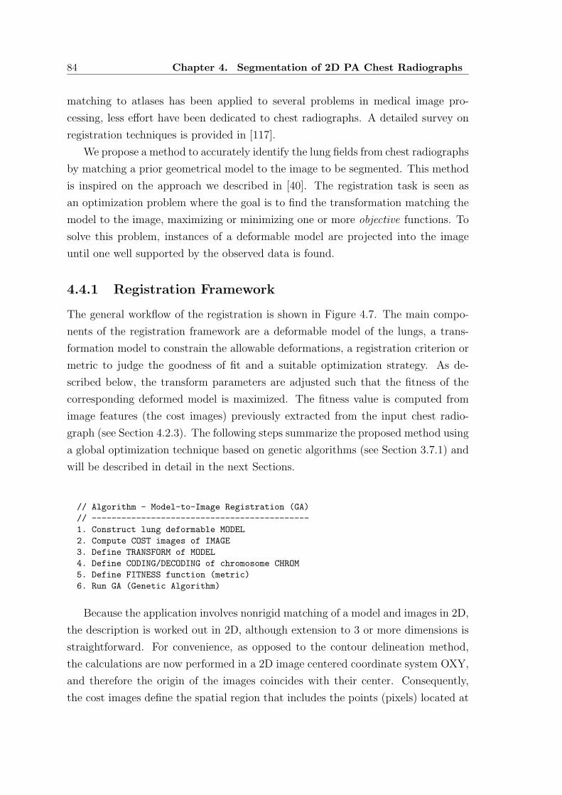
84 Chapter 4. Segmentation of 2D PA Chest Radiographs
matching to atlases has been applied to several problems in medical image pro-
cessing, less effort have been dedicated to chest radiographs. A detailed survey on
registration techniques is provided in [117].
We propose a method to accurately identify the lung fields from chest radiographs
by matching a prior geometrical model to the image to be segmented. This method
is inspired on the approach we described in [40]. The registration task is seen as
an optimization problem where the goal is to find the transformation matching the
model to the image, maximizing or minimizing one or more objective functions. To
solve this problem, instances of a deformable model are projected into the image
until one well supported by the observed data is found.
4.4.1 Registration Framework
The general workflow of the registration is shown in Figure 4.7. The main compo-
nents of the registration framework are a deformable model of the lungs, a trans-
formation model to constrain the allowable deformations, a registration criterion or
metric to judge the goodness of fit and a suitable optimization strategy. As de-
scribed below, the transform parameters are adjusted such that the fitness of the
corresponding deformed model is maximized. The fitness value is computed from
image features (the cost images) previously extracted from the input chest radio-
graph (see Section 4.2.3). The following steps summarize the proposed method using
a global optimization technique based on genetic algorithms (see Section 3.7.1) and
will be described in detail in the next Sections.
// Algorithm - Model-to-Image Registration (GA)
// --------------------------------------------
1. Construct lung deformable MODEL
2. Compute COST images of IMAGE
3. Define TRANSFORM of MODEL
4. Define CODING/DECODING of chromosome CHROM
5. Define FITNESS function (metric)
6. Run GA (Genetic Algorithm)
Because the application involves nonrigid matching of a model and images in 2D,
the description is worked out in 2D, although extension to 3 or more dimensions is
straightforward. For convenience, as opposed to the contour delineation method,
the calculations are now performed in a 2D image centered coordinate system OXY,
and therefore the origin of the images coincides with their center. Consequently,
the cost images define the spatial region that includes the points (pixels) located at

4.4. Model-to-Image Registration 85
Coding
DeformedMODEL
DeformableMODEL
INITIALChromosomes
CostIMAGES
pixels
Fitness value
Transformparameters
points
NEWChromosomes
t = 0c = 0
t = t + 1
c < C ?
no
yes
Decoding EvaluationTransform
Interpolation
metric
TransformationMODEL
GA Operators
points
chroms
c = 0 c = c + 1
GAparameters
Figure 4.7: Lung field segmentation from PA chest radiographs using the model-to-image registration method. The registration task is an optimization problem solved witha genetic algorithm (GA), where C solutions are encoded as chromosomes (chroms), eachrepresenting a solution (transformation parameters) in the search space. The optimalsolution is obtained by evolving an initial population of random solutions.

86 Chapter 4. Segmentation of 2D PA Chest Radiographs
coordinates (x, y) for which −∆X/2 ≤ x ≤ ∆X/2 and −∆Y/2 ≤ y ≤ ∆Y/2, where
∆X and ∆Y are the physical extent of the images along the X and Y direction,
respectively. Before the registration is performed, the center of the bounding box of
the model is automatically computed and moved to coincide with the center of the
image.
Transformation Model
We have proposed an approach to warp a model to chest radiographs in [40] which is
based on Free Form Deformation (see Section 3.6.1). Here, the adopted parametriza-
tion of the deformation model is based on the Thin Plate Splines transform (see
Section 3.6.2) we now described.
In Section 3.5, we have presented the construction of a 2D statistical shape
model of the lungs. The resulting lung mean shape (lung contour) is now used
as the deformable model, represented by the set of N points P = pn, where
pn = (xn, yn)T, n = 0, 1, . . . , N − 1, is a point of the lung contour.
To deform the model, L source landmarks ul = (xl, yl)T, l = 0, 1, . . . , L − 1, are
selected from the contours of both lungs to form the set U = ul. Moving the
landmarks to new position vl = ul +∆ul results in the set of target landmarks V =
vl ,vl = (xl, yl)T, where the displacement vectors ∆ul represent the deformation
field of the transform denoted by ∆U = V − U = ∆ul. In 2D, the deformation
field can be parametrized by the 2L-dimensional vector
∆U = (∆x0, ∆y0, ∆x1, ∆y1, . . . , ∆xL−1, ∆yL−1)T . (4.5)
As discussed in Section 3.6.2, the TPS transform, denoted V = T (U), is com-
puted from the sets of source and target landmarks and allows to generate instances
of the deformable model.
Ideally, the transformation model should allow just enough degrees of freedom
(DOF) to model any physical transformation. Because the training set of manual
contours with and without global rigid alignment can be used to construct the lung
mean shape, an affine transformation component A is included in the transformation
model. This transform can be parametrized as a set of vectors A = ai, i = 0, 1, 2.
In 2D, and introducing a 0 element for convenience, A is the set of parameters
A = sX, sY, θZ, 0, dX, dY . (4.6)

4.4. Model-to-Image Registration 87
The affine transformation A = (A2 A1 A0) is an ordered concatenation of
5 rigid model transformations, namely anisotropic scaling in X and Y directions,
rotation around the Z axis and translation along X and Y directions, with translation
parameters a2 = (dX, dY)T, in mm, rotation parameter a1 = (θZ, 0)T, in radian, and
a0 = (sX, sY)T as scaling factors. In 3D, 9 parameters are used to described A.
The transformation model is now completely characterized by combining the
Thin Plate Splines and affine components. Following Eq. 3.29, the final transform
is the point-to-point correspondence
qn = (A T ) (pn) , (4.7)
defining the N contour points qn of the deformed model.
Solution Coding/Decoding
To search for the optimal transformations T and A, a genetic algorithm (GA) was
used, where allowable transforms are described by a population (or set) of C indi-
viduals (solutions), W = wc, c = 0, 1, · · · , C − 1. The proposed GA considers
each chromosome wc (the genotype) as a single solution (the fenotype) in the search
space of the deformable registration problem. For a particular transform (A T )c
the corresponding chromosome wc is constructed by concatenating the parameters
of the TPS and affine components,
wc = ∆Uc, ∆Ac = ∆ulc, ∆aic , (4.8)
where ∆Uc is the deformation field and ∆Ac represent the deviation of the affine
parameters from their default values a0 = (1, 1)T (scaling), a1 = (0, 0)T (rotation)
and a2 = (0, 0)T (translation).
A key feature of genetic algorithms is the representation of physical variables of
interest by a simple string data structure. In the GA, the chromosome wc repre-
senting the transform parameters ∆ulc and ∆aic is rewritten as the string of genes
wc = ucg , g = 0, 1, . . . , G − 1. From Eq. 4.5 and Eq. 4.6, the coding results in a
vector of G alleles:
wc = (uc0, uc1, . . . , ucg, . . . , uc,G−1)T . (4.9)
When a number L of landmarks are chosen and the registration is performed in
2D, the chromosome length is G = 2L+6. For the 3D case, G = 3L+9, accounting
for 9 parameters (DOFs) of the affine component.

88 Chapter 4. Segmentation of 2D PA Chest Radiographs
Binary coding has been the usual individual representation in genetic algorithms
for a long time. Binary strings are sufficiently general but they are not always
the more natural or the more adequate representation. This is especially important
with deformable models because meaningful but random initial populations are hard
or even impossible to construct. Instead of the traditional binary coding, a Real-
Coded Genetic Algorithm (RCGA) is used [118]. With RCGA implementations a
more natural floating point representation is adopted and therefore it is possible to
define recombination operators that can do well in a particular problem domain.
The RCGA representation was used to codify the transform parameters. This
approach allows to decode in a straightforward manner a particular chromosome wc
back to the transform (A T )c it represents. Given wc = ucg with G alleles, the
deformation field ∆Uc = ∆ulc and therefore the TPS transform are obtained by
first defining, for each landmark l, a local perturbation. The perturbation δulc is a
gene with 2 alleles (in 2D) that is related to the displacement vector of the landmark
ulc.
If the perturbation is the displacement itself, ∆ulc = δulc resulting in 2D in the
simple decoding of the deformation field:
δulc = (ucg, uc,g+1)T , (4.10)
where g = 2l and l = 0, 1, . . . , L−1 (for 3D, g = 0, 3, . . . , 3L−1). The parameters a0
(scaling), a1 (rotation) and a2 (translation) are given by the last G−2L alleles of the
chromosome and, From Eq. 4.6, the decoding of the affine component is performed
by introducing the perturbation vector δaic where, for i = 0, 1, 2,
δaic = (uc,2L+i, uc,2L+i+1)T . (4.11)
Performing independent PCA to all contour points in the model as described in
Section 3.5.2 allows to take into account the spread of each landmark coordinate
observed in the training set. In fact, the perturbation can be seen as the vector
of weights, blc, controlling the modes of variation of a single landmark. Instead of
using Eq. 4.10, and following Eq. 3.20, we propose to decode the TPS component
as
∆ulc = Φlδulc, (4.12)
where we consider Φl =(√
λgeg,√
λg+1eg+1
)
and, as before, g = 2l and l =
0, 1, . . . , L− 1. The matrix Φl is related to the principal directions (eigenvectors e)

4.4. Model-to-Image Registration 89
of the landmark displacement and corresponding amplitudes (eigenvalues λ). When
constructing the statistical lung model, alignment of the training contours can be
done before the mean shape is computed and similar component analysis can be
performed to the affine parameters. The corresponding decoding is given by
∆aic = Ωiδaic, (4.13)
where i = 0, 1, 2 and Ωi = (σi0, σi1) is a 2D vector describing the variation of the
parameters of each affine transformation ai. Note, from Eq. 4.6, that σ11 = 0.
Decoding the chromosome wc results in the final affine transform components given
by aic = aic + ∆aic.
Fitness and Objective Functions
When GA is running, an objective function f is supplied which decodes the chro-
mosomes and assign a fitness, fc, to the individual the chromosome wc represents.
During evolution, at a given generation t, the fitness is computed for all the chromo-
somes in the population W(t) by evaluating the objective function at samples points
in the search space of transformations. To solve the problem of registering the lung
model to a chest radiograph, all the N points on the lung contour are selected and
deformed for computing the fitness according to
q(t)nc = (A T )(t)
c (pn) , (4.14)
where q(t)nc is the deformed model point pn at time t, given by Eq. 4.7 after the
chromosome is decoded.
To perform the experiments described below a simple metric was used. Given the
chromosome w(t)c , the following fitness function is proposed to evaluate the goodness
of the corresponding solution:
f (t)c = 0.5
(
1 − f(t)1c + f
(t)2c + f
(t)3c
N
)
, (4.15)
where each component of the fitness, a time dependent objective function, is com-
puted by using the cost images c (x, y) (see Section 4.2.3) as

90 Chapter 4. Segmentation of 2D PA Chest Radiographs
f(t)1c =
n1−1∑
n=0
c1
(
q(t)nc
)
+
n1−1∑
n=0
c1
(
q(t)n+N/2,c
)
, (4.16a)
f(t)2c =
n2−1∑
n=n1
c2
(
q(t)nc
)
+
n2−1∑
n=n1
c2
(
q(t)n+N/2,c
)
, (4.16b)
f(t)3c =
N/2−1∑
n=n2
c3
(
q(t)nc
)
−N/2−1∑
n=n2
c3
(
q(t)n+N/2,c
)
, (4.16c)
and c (qn) = c (xn, yn) denotes the cost value interpolated in the image c at point
qn. An interpolator based on the nearest point was used since it reduces the overall
time of registration.
When the fitness is used to evaluate instantiations of the deformable model,
one seeks to minimize the objective functions (Eq. 4.16) or maximize the fitness
(Eq. 4.15), thus favouring solutions for which the deformed contour points have low
cost. Note that the same reasoning was adopted in the contour delineation method,
using the same cost images.
The objective functions in Eq. 4.16 are defined as follows. The first terms of each
function is the contribution of model points qn, n = 0, 1, . . . , N/2 − 1, that belong
to the right contour of the deformed model. Based on the reflectional symmetry
of chest radiographs, the second terms evaluate the corresponding points qn+N/2
of the left lung. Alternatively, Eq. 4.15 could be expressed as the sum of two
terms, one for each lung contour. The function f1 evaluates the hemidiaphragm
segments by considering, in Eq. 4.16a, the first n1 = 20 model points and the cost
image c1 (x, y) corresponding to this structure. Similarly, for computing f2 using
Eq. 4.16b, n2 = 65 was used to interpolate 2×45 points within c2 corresponding the
costal and lung top sections segments. Finally, the mediastinal edges are evaluated
in c3 (Eq. 4.16c) with the remaining 70 points of both lung contours. For any cost
image −1 ≤ c (x, y) ≤ 1, and the fitness is constrained to the values 0 ≤ f(t)c ≤ 1.
If the transformed point falls outside the spatial region of the image, a violation
as occurred and the cost is set to c (qn) = 1. Actually, introducing this penalty
function forces the deformable model to remain within the spatial region of interest
during the optimization process.

4.4. Model-to-Image Registration 91
4.4.2 Genetic Algorithm Implementation
Although well suited for multi-objective optimization, the registration problem is
solved with a simple genetic algorithm. The following pseudo-code summarize the
proposed lung field segmentation method based on this global optimization tech-
nique, diagrammed in the right side of Figure 4.7:
// Genetic Algorithm Optimization (Run GA)
// ---------------------------------------
// population W with C chromosomes
// tmax = -1 for continuous optimization
t = 0
Generate initial POP W(0) with C random CHROMS
Evaluate initial POP W(0) (all CHROMS)
Copy POP W(0) to POP W(t)
// Main loop of GA
while ( t > tmax )
Generate NEW POP W(t+1) from POP W(t)
Evaluate NEW POP W(t+1) (all CHROMS)
Get best CHROM w* from W(t+1)
Copy POP W(t) to POP W(t+1)
t = t + 1
end
// Generate NEW POP W(t+1) from POP W(t)
select C CHROMS from POP W(t) to POP W’
recombine CHROMS from POP W’ to POP W(t+1)
// Evaluate POP (all CHROMS)
c = 0
while ( c < C )
decode CHROM to TRANSFORM
deform MODEL with TRANSFORM
compute FITNESS of CHROM
c = c + 1
end
Initial Population
At t = 0, the GA begins with an initial population W(0) of C individuals represent-
ing random transformations. The strategy proposed in this study is to construct
each chromosome, w(0)c , c = 0, 1, . . . , C − 1, by sampling alleles, the components of
perturbation vectors δulc and δaic, from a normal distribution with zero mean and
unit standard deviation:
u(0)cg = N (0, 1) , (4.17)

92 Chapter 4. Segmentation of 2D PA Chest Radiographs
(a) (b)
Figure 4.8: Deformable model under random transformations. A set of landmarks isused to deform all contour points. The transformation of the model is coded as localperturbations of each landmark around their original position. (a) Random displacementsof the landmarks are used to deform the model under TPS; (b) A combination of TPSand affine transformation applied to the prior model.
with g = 0, 1, . . . , G − 1. Once the initial population has been created, all chromo-
somes w(0)c are decoded by using Eq. 4.12 and Eq. 4.13 (the PCA decoding) and the
model points pn are deformed with the corresponding transform (A T )(0)c , as given
by Eq. 4.14. Instances of the deformable model under random transformations are
illustrated in Figure 4.8. Next, initial solutions are evaluated by computing their
fitness value with the aid of Eq. 4.15. The best chromosome w∗ encoding the op-
timal solution (A T )∗ is then obtained by evolving W(0), until some criterion has
been reached.
Selection
The selection process identifies individuals in a current population W(t) as the par-
ents based on the their fitness to participate the reproduction. Many methods of
selection exist in genetic algorithms and tournament selection was chosen. This
technique runs a ”tournament” among k individuals chosen at random from the
population and selects the winner, the one with the best fitness, for crossover (see
Section 3.7.1). Tournament selection has several benefits: it is efficient to code
and allows the selection pressure to be easily adjusted by changing the tournament
size k. If the tournament size is larger, weak individuals have a smaller chance
to be selected. The selected parents are copied to an intermediate population W′
where suitable recombination operators can be applied to produce the randomness

4.4. Model-to-Image Registration 93
in shapes.
Recombination
The selected parents of the intermediate population W′ will take part in the re-
production to create new individuals with crossover probability pcross and form the
population W(t+1) for the next generation. In [114], we proposed a method for
detecting the symmetry axis in chest radiographs based on a probabilistic genetic
algorithm, where an Unimodal Normal Distributed Crossover operator (UNDX) was
used to create offspring normally distributed around the mean vector determined by
parents. Other similar schemes exist, such as the Simplex Crossover operator (SPX)
for which the offspring are uniformly distributed around the mean vector within the
predefined space, and the Parent-centric Crossover operator (PCX), where the off-
spring have more probability to be distributed around each parent.
By introducing the notion of interval schemata for RCGA [119], a blend crossover
(BLX-α) operator was suggested and will be used for the experiments. For two
parent solutions w(t)1 and w
(t)2 selected at random from W′, and assuming that
∆u(t)g = u
(t)2g − u
(t)1g > 0, the BLX-α randomly creates the solution w(t+1) =
u(t+1)g
such that
u(t)1g − αcross∆u(t)
g ≤ u(t+1)g ≤ u
(t)2g + αcross∆u(t)
g , (4.18)
where αcross ≥ 0. The above equation can be rewritten in a more convenient form
to express the child solution. If r is a random number between 0 and 1, then
u(t+1)g = (1 − γcross) u
(t)1g + γcrossu
(t)2g , (4.19)
where γcross = (1 + 2αcross) r − αcross. Note that the factor γcross is uniformly dis-
tributed for a fixed value of αcross. If αcross = 0, the crossover operator creates a
random solution such that u(t)1g ≤ u
(t+1)g ≤ u
(t)2g . The BLX-α has an interesting prop-
erty: the location of the child solution depends on the difference in parent solutions.
This is clear if Eq. 4.19 is rewriten as
u(t+1)g − u
(t)1g = γcross
(
u(t)2g − u
(t)1g
)
= γcross∆u(t)g . (4.20)
If the difference between the parent solutions is small, the difference between the
child and parent solutions is also small. This is an essential property for any search
algorithm to exhibit self-adaptation, since the spread of the current population dic-

94 Chapter 4. Segmentation of 2D PA Chest Radiographs
tates the spread of solutions in the resulting population.
The choice of value of the BLX-α crossover is a trade off between computation
time and the goodness of the result. Better optimization results may be achieved at
the expense of longer computation time by increasing αcross.
We assume that mutation can occur, with constant probability pmut, by randomly
selecting one parameter (allele) from the transformation vector of each parent, re-
placing it with random number as given by Eq. 4.17, while keeping other parameters
unchanged. If pmut is high, a lot of the computation time is wasted by evaluating
mutated models that are of irregular shape and hence have low fitness.
Fitness Evolution
The number of chosen landmarks is a trade-off between computation time and the
number of DOFs of the deformation. To perform the registration, L = 14 source
landmarks were selected from the contour model resulting in G = 2L + 6 = 34
transform parameters (alleles) to optimize. Several tests were performed to judge for
the best combination of selection and recombination operators. Some comparative
results are plotted in Figure 4.9 where tournament and roulette-wheel were used
as selections schemes. Experiments with the tournament selection were performed
with the size k = 3, corresponding to 6% of the constant number C of individuals
in the population. The BLX-α was compared with standard crossover operators,
such as the one-point crossover (illustrated in Figure 3.15(b)). We believe that a
good compromise between exploration of the search space and computation time of
the algorithm is achieved by setting αcross = 0.3 when using BLX. Two different
probabilities were considered, namely pcross = 1 and pcross = 0.8 for crossover and
pmut = 0 and pmut = 0.005 for mutation.
The registration output corresponding to the fitness evolution of Figure 4.9(a)
is shown in Figure 4.10 for which the genetic operators and related parameters are
listed in Table 4.2. By comparing the tested combinations, these were considered as
representing the best behavior of the proposed GA.
GA Parameters
For the GA parameters, we have employed standard values, namely a population
of C = 50 individuals. In general, a fixed maximum number of fitness function
evaluations is allowed. Here, the number of generations (iterations of the GA) was
set to tmax = 100 corresponding to 5000 evaluation for the main loop, plus 50 to take

4.4. Model-to-Image Registration 95
0 20 40 60 80 1000
0.1
0.2
0.3
0.4
0.5
0.6
0.7
0.8
0.9
1
Time (generation)
Fitn
ess
(a)
0 20 40 60 80 1000
0.1
0.2
0.3
0.4
0.5
0.6
0.7
0.8
0.9
1
Time (generation)F
itnes
s
(b)
0 20 40 60 80 1000
0.1
0.2
0.3
0.4
0.5
0.6
0.7
0.8
0.9
1
Time (generation)
Fitn
ess
(c)
0 20 40 60 80 1000
0.1
0.2
0.3
0.4
0.5
0.6
0.7
0.8
0.9
1
Time (generation)
Fitn
ess
(d)
Figure 4.9: Fitness evolution of the model-to-image registration using a genetic algo-rithm. The size of the population is C = 50 individuals with chromosome length G = 34(L = 14 model landmarks, 6 affine parameters), and tmax = 100 generations were sim-ulated with different combination of selection and recombination operators, with proba-bilities pcross and pmut. (a) Tournament, BLX-α, pcross = 1, pmut = 0 (see Figure 4.10for the registration output); (b) Tournament, BLX-α, pcross = 0.8, pmut = 0.005; (c)Roulette-wheel (fitness-proportionate selection), BLX-α, pcross = 1, pmut = 0.005; (d)Roulette-wheel, one-point crossover, pcross = 1, pmut = 0.005. A tournament size k = 3(6% of C) was used and αcross = 0.3 for BLX crossover. In all cases, the upper and lowercurves correspond to the maximum and minimum fitness value observed in the population.

96 Chapter 4. Segmentation of 2D PA Chest Radiographs
(a) (b) (c)
Figure 4.10: Lung field segmentation from PA chest radiographs using the model-to-image registration method. This optimization problem is solved with a genetic algorithm(GA). (a) Undeformed lung model; (b) Instance of the deformable model during optimiza-tion (evolution); (c) Final model best fitted to image after 100 iterations (generations).GA parameters are reported in Table 4.2 and the corresponding fitness evolution in plottedin Figure 4.9(a).
into account the population W(0). All the parameters are listed in Table 4.2 (see
the results of the segmentation shown in Figure 4.10. and the corresponding fitness
evolution, f (t), plotted in Figure 4.9(a)). Analysis of the computation time of the
whole registration process (about 1 min for one chest radiograph) was performed
with the FLTK time probes utility (see Appendix A, Section A.3).
4.5 Experimental Results
To evaluate the performance of the proposed methods, the lung contour delineation
and model-to-image registration were performed on two different image databases
described in the next Sections.
4.5.1 Image Databases
Public Database (JSRT)
The JSRT database was established by the Japanese Society of Radiological Tech-
nology. This is a publicly available database with 247 PA chest radiographs collected
from 13 institutions in Japan and one in the United States. 154 images contain ex-
actly one pulmonary lung nodule (LN) each; the other 93 images contain no lung
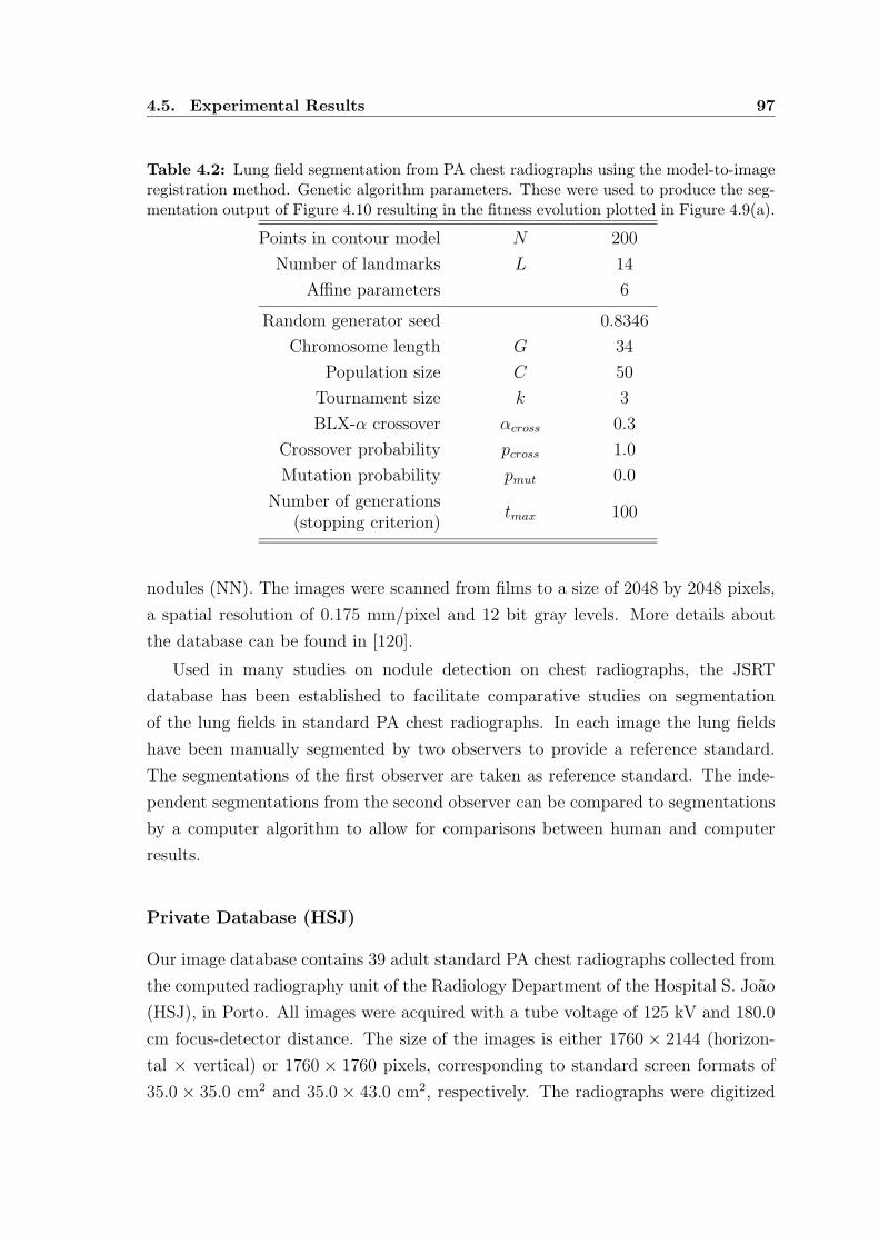
4.5. Experimental Results 97
Table 4.2: Lung field segmentation from PA chest radiographs using the model-to-imageregistration method. Genetic algorithm parameters. These were used to produce the seg-mentation output of Figure 4.10 resulting in the fitness evolution plotted in Figure 4.9(a).
Points in contour model N 200
Number of landmarks L 14
Affine parameters 6
Random generator seed 0.8346
Chromosome length G 34
Population size C 50
Tournament size k 3
BLX-α crossover αcross 0.3
Crossover probability pcross 1.0
Mutation probability pmut 0.0
Number of generationstmax 100
(stopping criterion)
nodules (NN). The images were scanned from films to a size of 2048 by 2048 pixels,
a spatial resolution of 0.175 mm/pixel and 12 bit gray levels. More details about
the database can be found in [120].
Used in many studies on nodule detection on chest radiographs, the JSRT
database has been established to facilitate comparative studies on segmentation
of the lung fields in standard PA chest radiographs. In each image the lung fields
have been manually segmented by two observers to provide a reference standard.
The segmentations of the first observer are taken as reference standard. The inde-
pendent segmentations from the second observer can be compared to segmentations
by a computer algorithm to allow for comparisons between human and computer
results.
Private Database (HSJ)
Our image database contains 39 adult standard PA chest radiographs collected from
the computed radiography unit of the Radiology Department of the Hospital S. Joao
(HSJ), in Porto. All images were acquired with a tube voltage of 125 kV and 180.0
cm focus-detector distance. The size of the images is either 1760 × 2144 (horizon-
tal × vertical) or 1760 × 1760 pixels, corresponding to standard screen formats of
35.0 × 35.0 cm2 and 35.0 × 43.0 cm2, respectively. The radiographs were digitized

98 Chapter 4. Segmentation of 2D PA Chest Radiographs
Table 4.3: Lung field segmentation from PA chest radiographs. Experiments were per-formed on a public image database (JSRT) and a private database (HSJ) to evaluate theperformance of the proposed methods based on dynamic programming (DP) and geneticalorithms (GA).
Method Database
Images
Original Filtered
# size spacing size spacing(pixel) (mm) (pixel) (mm)
DP JSRT 247 2048 × 2048 0.175 348 × 348 1.0
DP HSJ 391760 × 2144
0.200352 × 428
1.01760 × 1760 352 × 352
GA HSJ 391760 × 2144
0.200352 × 428
1.01760 × 1760 352 × 352
with a DIGISCAN 2T Plus imaging plate system (Siemens, Erlangen, Germany)
and provided in DICOM format with a pixel resolution of 0.200 mm × 0.200 mm,
and 10 bits per pixel. These images are a reasonable representation of both normal
and abnormal radiographic findings, from both genders, showing regular and irreg-
ular lung shapes and abnormalities such as enlarged heart size, lung consolidation
and emphysema, among others (see Appendix B). We did not exclude any image for
which our rule-based segmentation scheme could fail to produce any acceptable out-
put, since robust segmentation methods should give good performance on abnormal
images as well.
4.5.2 Experiments
Experiments are reported in Table 4.3. For the registration method, the parameters
listed in Table 4.2 were used. The original images were previously smoothed and
reduced in format for segmentation as described in Section 3.2.1. For both databases,
the images were subsampled to a resolution of σ0 = dX = dY = 1.0 mm, in both
the horizontal (X) and the vertical (Y) directions. We used one implementation
of Gaussian smoothing available in the ITK toolkit [34]. This filter implements an
approximation of convolution with the Gaussian and its derivatives and requires a
constant number of operations regardless of the σ0 value [121, 122]. The standard
deviation of the Gaussian filter kernel was set to σ0 = 1.0 mm, the value of the
final pixel spacing dX. For the HSJ database, this corresponds to a reduction by a

4.5. Experimental Results 99
factor of 5. The original gray level range of the lower spatial resolution images was
maintained. The smoothing/resampling step was performed to reduce the amount
of data for each radiograph in order to speed up the computational process while
preserving enough resolution to identify the lung fields.
All the images of the JSRT database have been considered and subdivided in
two folds. To ensure the integrity of the results, the images and reference standard
in one fold (fold 1 - all odd numbered images) were used to train and tune the
algorithms of the contour delineation method, applied to segment the images in the
other fold (fold 2 - all even numbered images).
4.5.3 Validation
Segmentation performance was assessed by comparing the output of the automatic
computer based segmentation methods with results obtained by manual analysis of
a human observer. For that purpose, a dedicated algorithm was developed. For
each subject, the program reads the file containing the point coordinates of the
manual contours and constructs a binary image, with zero-value pixels everywhere
except on the region enclosed by each lung contour. The output of the automated
method is provided as a second binary image, where the non-zero pixels correspond
to segmented lung fields. A pixel by pixel analysis was then performed to measure
the similarity between the set of non-zero pixels of the two segmentation masks (see
Section 3.8).
The computed measures used to evaluate the performance of the proposed seg-
mentation schemes are reported Table 4.4, Table 4.5 and Table 4.6. The results are
discussed in the following Section. Separate analysis was performed for the right
lung and the left lung, by computing the accuracy, degree of overlap and F-score.
For each experiment listed in Table 4.3, the average (mean), standard deviation
(std), minimum (min) and maximum (max) values of each measure were computed
and can be used as a figure of merit regarding the performance of the corresponding
method. The results are reported and discussed in the next Section. We assumed
equal importance of recall and precision when computing F-score. The sensitivity,
specificity, precision and recall (= sensitivity) are also listed for comparison. All
similarity measures range from 0 to 1.

100 Chapter 4. Segmentation of 2D PA Chest Radiographs
4.6 Discussion
Accuracy, sensitivity, and specificity have been used or can be calculated from results
reported in several studies. A range of accuracies for several lung field segmenting
methods reported in the literature is listed in [83] where a table of their values is
provided. In this study, the highest attainable accuracy of a segmenting method was
estimated as the inter-observer variability, mainly due to the difficulty in assessing
the exact borders of mediastinum. An accuracy of 0.9846 ± 0.0048 is provided as
the theoretical upper bound. Based on these measures, the results presented here
show that the proposed segmentation methods, surprisingly with the same mean
accuracy of 0.98, perform better than the reported methods. In a more recent
study [94], several schemes were applied to the JSRT (public) image database and
comparison was made by using the degree of overlap as the reference figure of merit.
The value of 0.946 ± 0.018 was obtained when quantifying inter-human variability.
Characterized by a mean overlap of 0.91 and 0.90 for, respectively, the right lung
and left lung, our contour delineation method compares favorably with the reported
results.
Performance measures computed in the first experiment (DP/JSRT) are reported
in Table 4.4. These correspond to the lung contour delineation method based on
dynamic programming, using the JSRT image database. The results reflect a similar
performance for both lungs, as illustrated in Figure 4.11(a), where the similarity
measures were sorted in ascending order for the 247 images. To place the results
in perspective, Figure 4.11(b) shows the histograms of the degree of overlap for the
right and left lung fields. Figure 4.12 shows the lung contours generated by the
proposed method superimposed on the original images, corresponding to the best
and worst 3 segmentation outputs. In Appendix B, similar results are shown for
20 images. Clearly, the optimal path finding algorithm failed when detecting the
costal edges. Since the cost images computed for delineating such segments depend
on the first order derivative along the horizontal direction, unexpected high values
of this feature due to the borders of the image confuse the algorithm. Although less
noticeable, a similar error occurs in both sides of the image due to the breast, as seen
in some images presented in Appendix B. Consequently, the method is expected to
perform differently, depending on the gender of the patient being examined.
In the second and third experiments, both the contour delineation and the model-
to-image segmentation method based on genetic algorithms were applied to the same
private image database. Results of comparing the methods with manual analysis

4.6. Discussion 101
Table 4.4: Lung field segmentation from PA chest radiographs. Performance measuresof the contour delineation method based on dynamic programming (DP), using the publicimage database (JSRT). Best and worst segmentation outputs (overlap) are shown inFigure 4.12 (see also Appendix B).
Measure Right Lung Left Lung
(DP/JSRT) min max mean ± std min max mean ± std
accuracy 0.88 0.99 0.98 ± 0.01 0.87 0.99 0.98 ± 0.01
sensitivity 0.76 1.00 0.96 ± 0.03 0.78 1.00 0.97 ± 0.02
specificity 0.85 1.00 0.99 ± 0.01 0.86 1.00 0.99 ± 0.01
overlap 0.63 0.96 0.91 ± 0.04 0.51 0.96 0.90 ± 0.06
precision 0.64 0.99 0.95 ± 0.04 0.51 0.98 0.92 ± 0.06
recall 0.76 1.00 0.96 ± 0.03 0.78 1.00 0.97 ± 0.02
F-score 0.78 0.98 0.95 ± 0.02 0.67 0.98 0.95 ± 0.04
1 50 100 150 200 2470.5
0.6
0.7
0.8
0.9
1
Images
Per
form
ance
Mea
sure
0.5 0.6 0.7 0.8 0.9 10
20
40
60
80
100
120
Overlap
Num
ber
of C
ases
Right lungLeft lung
Figure 4.11: Performance measures of the contour delineation method using the publicimage database (DP/JSRT). (a) The measures are sorted in ascending order for the 247images: accuracy (dotted lines), F-score (dashed lines) and overlap (solid lines). For eachmeasure, the upper and lower curves correspond to the right and left lung, respectively.To the left of the graph, where images are hard to segment, the differences between thevarious measures are most clear. (b) The distribution of overlap values for both lungs (seealso Table 4.4).

102 Chapter 4. Segmentation of 2D PA Chest Radiographs
Figure 4.12: Segmentation outputs (contours and confusion matrix) of the contour de-lineation method using the public image database (DP/JSRT). Results are shown for thebest (first rows) and worst (last rows) 3 of 247 images. True negative pixels (TN) arewhite, true positive (TP) light gray, false positive (FP) dark gray, and false negative (FN)black (see also Appendix B).

4.6. Discussion 103
are reported in Table 4.5 and Table 4.6, respectively. It is interesting to note that
delineation and registration perform equally, although one could expect to obtain
such results since both methods are based on the same image features and therefore
the same cost images for computing either the cumulative cost of a path or the
fitness of an instance of the deformable model.
Performance measures computed in these experiments can be loosely compared
with those obtained in the first one. Strict comparison is not possible since they
were applied on different data sets. Actually, the JSRT database contains images
of good technical quality, and very few images with gross abnormalities. Since
segmentation errors are more likely to occur when the image contains pathology or
unusual anatomy, we believe that some images of the private database are much
harder to segment.
In order to identify the main sources of the errors of computer algorithms, the
worst results were presented to a radiologist who rated the performance on a qual-
itative scale. The best and worst 3 segmentation outputs obtained by using the
contour delineation method and the model-to-image registration approach are pre-
sented, respectively, in Figure 4.13 and Figure 4.14. Examples of following wrong
edges are evident. This is due to severe pathologies present in such images, namely
consolidation of the right lung and cardiomegaly observed, respectively, in the first
and all images of Figure 4.13. These radiological findings result in the loss of an
edge-like appearance of the hemi-diaphragms and a poor definition of the cardiac
silhouette, corresponding to the border between heart and lung.
Results of segmenting all images of the private images database are reported in
Appendix B. In a few cases, the detection of the lung apices has failed. To solve this
problem, the proposed contour-based approach can be combined with the strength of
a region growing technique. In fact, in PA chest radiographs the lung fields and the
supraclavicular regions are adjacent, and both regions correspond to low intensity
pixels. We believe that their separation could be effectively achieved by using the
ISRG algorithm, as suggested by the example provided in Figure 3.9. Therefore
this algorithm is suggested to constrain or even correct the vertical position of the
lung top sections. Alternatively, ISGR could be used as a robust initialization when
detecting this particular segment. Note that this error has not been observed when
applying the model-to-image registration method.

104 Chapter 4. Segmentation of 2D PA Chest Radiographs
Table 4.5: Lung field segmentation from PA chest radiographs. Performance measuresof the contour delineation method based on dynamic programming (DP), using the pri-vate image database (HSJ). Best and worst segmentation outputs (overlap) are shown inFigure 4.13 (see also Appendix B).
Measure Right Lung Left Lung
(DP/HSJ) min max mean ± std min max mean ± std
accuracy 0.86 0.99 0.98 ± 0.02 0.93 1.00 0.98 ± 0.01
sensitivity 0.81 0.97 0.92 ± 0.04 0.77 0.97 0.92 ± 0.05
specificity 0.85 1.00 0.99 ± 0.02 0.94 1.00 0.99 ± 0.01
overlap 0.38 0.95 0.87 ± 0.09 0.62 0.95 0.87 ± 0.09
precision 0.40 1.00 0.94 ± 0.09 0.71 1.00 0.93 ± 0.08
recall 0.81 0.97 0.92 ± 0.04 0.77 0.97 0.92 ± 0.05
F-score 0.55 0.97 0.93 ± 0.07 0.77 0.97 0.93 ± 0.05
Table 4.6: Lung field segmentation from PA chest radiographs. Performance measuresof the model-to-image registration method based on genetic algorithm (GA), using theprivate image database (HSJ). Best and worst segmentation outputs (overlap) are shownin Figure 4.14 (see also Appendix B).
Measure Right Lung Left Lung
(GA/HSJ) min max mean ± std min max mean ± std
accuracy 0.94 0.99 0.98 ± 0.01 0.96 0.99 0.98 ± 0.01
sensitivity 0.87 0.99 0.93 ± 0.03 0.85 0.98 0.93 ± 0.03
specificity 0.93 1.00 0.99 ± 0.01 0.96 1.00 0.99 ± 0.01
overlap 0.58 0.93 0.86 ± 0.08 0.65 0.93 0.87 ± 0.07
precision 0.62 1.00 0.92 ± 0.08 0.67 0.99 0.93 ± 0.08
recall 0.87 0.99 0.93 ± 0.03 0.85 0.98 0.93 ± 0.03
F-score 0.74 0.97 0.92 ± 0.05 0.79 0.97 0.93 ± 0.04

4.6. Discussion 105
Figure 4.13: Segmentation outputs (contours and confusion matrix) of the contour de-lineation method using the private image database (DP/HSJ). Results are shown for thebest (first rows) and worst (last rows) 3 of 39 images. TN - white, TP - light gray, FP -dark gray, FN - black (see also Appendix B).

106 Chapter 4. Segmentation of 2D PA Chest Radiographs
Figure 4.14: Segmentation outputs (contours and confusion matrix) of the model-to-image registration method using the private image database (GA/HSJ). Results are shownfor the best (first rows) and worst (last rows) 3 of 39 images. TN - white, TP - light gray,FP - dark gray, FN - black (see also Appendix B).

4.7. Conclusions 107
4.7 Conclusions
In this Chapter, we described two fully automated segmentation methods for ac-
curately extracting the lung fields on digital standard PA chest radiographs. The
proposed approaches are model-based image segmentation methods that consist on
several algorithms applied sequentially. The segmentation framework was designed
in such a way that both methods use the same cost images. To compute such
cost functions, one for each of the segments defined in the lung contour model, we
proposed a combination of multiple normalized image feature based on a winner-
takes-all, mutliscale approach.
The first method is a contour delineation method, for which an optimal path
finding algorithm was developed to accurately detect the segments that make up
the lung contour model. Based on dynamic programming, this border detection
algorithm is a simple and effective technique that provides with a complete lung
boundary description, including the costal, mediastinal, lung top sections and di-
aphragmatic edges. The second scheme employs a non-rigid deformable model-to-
image registration framework. The construction of the deformable model is based on
standard techniques by using a training set of templates manually delineated. The
point distribution model was adopted to represent the lung mean shape, allowing
the incorporation of statistical information about its expected variation. Thin-Plate
Splines are then used to define a model transformation and the lung field segmenta-
tion is reformulated as an optimization problem to search for the best transformation
parameters. Due to their flexibility, genetic algorithms were chosen as the optimiza-
tion tool to solve the problem.
Experimental results are reported after applying them on two different image
databases and performance analysis was done by comparing the computer-based
segmentation outputs with results obtained by manual analysis. Several similarity
measures were considered and qualitative evaluation of segmentation outputs was
made to identify possible source of errors. The accuracy of the proposed segmen-
tation schemes is comparable to other methods published so far, reflecting their
applicability in CAD systems.


Chapter 5
DECOMPOSITION OF 3D CT IMAGES
In this Chapter, we present a method for segmenting anatomical structures from
thoracic CT images. The approach is based on the principles of material basis
decomposition described in Chapter 2 and integrates several image processing tech-
niques described in Chapter 3.
5.1 Introduction
Models of the human anatomy serve an important role in several aspects of diag-
nostic and therapy related image processing. Transmission X-ray computer tomog-
raphy supplies the required high resolution 3D human anatomy necessary to create
a computerized 3D volume array modeling all major internal structures of the body.
Computerized anthropomorphic phantoms can either be defined by mathematical
(analytical) functions or digital voxel-based volume arrays where each voxel of the
volume contains a label or index number designating it as belonging to a given organ
or internal structure [123]. This volume models the human anatomy and can serve as
a patient-specific voxel-based phantom suitable for many computer-based modeling
and simulation. Computer models have been applied to better understand the image
formation process in diagnostic radiology, particularly for analyzing scatter and at-
tenuation problems in nuclear medicine. Compared to dosimetry calculations, much
higher statistics are necessary to perform imaging simulations. In the field of oncol-
ogy, internal and external radiotherapy sources have become more sophisticated in
their design and application. The calculation involved in clinical therapy planning
can be more effectively investigated with computerized realistic human models.
Another application of CT imaging lies in the broader context of the development
of computer aided diagnosis (CAD) systems to detect the presence of pulmonary dis-
ease, quantify and follow-up its evolution. Therefore, accurate and robust segmen-
tation of the lung fields from X-ray CT images is a prerequisite for most pulmonary

110 Chapter 5. Decomposition of 3D CT Images
image analysis applications. The immediate goal of the lung segmentation algo-
rithm is to separate lung voxels from surrounding anatomy. Robust and accurate
algorithms that require minimal (semi-automated methods) or no human interaction
(fully automated methods) must be designed to identify the precise boundaries of
the lungs.
In earlier works, a single segmentation threshold was selected to segment the
lungs as low-density cavities inside of the patient [124, 125]. Lung contours have been
extracted in 2D, using a slice by slice analysis [124, 126, 127], thus not considering the
hypothesis that more than one contour could be needed for delineating each lung in
a particular slice of the volumetric image. Several studies published so far [126, 128]
have considered lung region segmentation without extracting the trachea or large
airways. Knowledge-based segmentation algorithms that use explicit anatomical
knowledge such as the expected size, shape, relative positions and expected X-ray
attenuation coefficients of objects have also been proposed [129, 130, 131] for seg-
menting dynamic chest CT images. Most of the proposed techniques for segmenting
the lung region are developed for lung nodule detection [124, 126, 128, 131, 132]. In
fact, CAD methods are effective for assisting radiologists as a viable alternative to
double reading in the early detection of lung cancer in thoracic CT scans. Several
schemes have been proposed to automatically evaluate the growth of pulmonary
nodules by quantifying their volume and change over time [133, 134]. This goal can
be achieved by means of registration and matching of lung surfaces [135, 136] in
temporal CT scans. Methods for matching thoracic structures across individuals
were used to create a normative human lung atlas [137]. Other applications that
require the accurate lung region segmentation as the basis for computer assisted
techniques include quantitative analysis of emphysema [138] and differential lung
function [127, 139]. The segmentation of the lung fields from High-Resolution Com-
puted Tomography (HRCT) scans has been considered [140]. The use of anatomic
pulmonary atlas to automatically segment the oblique lobar fissures in HRCT has
been demonstrated in [141]. The goal of the pulmonary atlas used in this method
is not to precisely represent all of the pulmonary anatomy, but simply to initialize
the subsequent fissure detection. A review of the literature on computer analysis of
the lungs in CT scans addressing the segmentation of various pulmonary structures,
registration of chest scans, and applications aimed at detection, classification and
quantification of chest abnormalities is presented in [142].
Aside from its applications as a pre-processing step for CAD methods, the auto-
mated lung field segmentation may be used for image data visualization. A single

5.2. Basis Set Decomposition 111
thoracic CT examination may result in acquisition of more than 300 sections for 1
mm reconstruction intervals. The interpretation of such amount of data requires
the radiologist to mentally reconstruct a three dimensional representation of the
patient anatomy. In this context, CT image segmentation can be required for the
surface/volume rendering of structures of interest as a visual aid for the radiologist’s
diagnostic task.
In an effort to contribute to the required methodological knowledge, we describe
fully automated segmentation algorithms for decomposing volumetric CT images
into several anatomical structures. A voxel classification strategy is adopted to con-
struct a 3D patient-specific anthropomorphic phantom and accurately extract the
lung region of interest. The proposed method follows a hierarchical representation
of the patient anatomy. First, the thorax of the patient is segmented from the sur-
rounding background image and decomposed into body and lung structures. Then,
the large airways are identified and extracted from the lung parenchyma. Since the
method can be specifically directed towards CAD applications, the lung fields are
finally extracted and the corresponding mask is created as the final output of the
segmentation procedure.
There are several distinctions between our method and previous work. The
method is based on the principle of dual-energy radiography [1, 21] discussed in
Section 2.7. This novel approach explores the concept of material decomposition
applied to CT numbers and provides a simple anatomical model describing the major
structures of the human thorax in terms of their composition and physical properties.
This is particularly important when constructing realistic computer models. The
segmentation procedure results in a set of automatically computed threshold values
that reflects the gray-scale characteristics of a specific dataset. Instead of using a
unique fixed threshold value, two thresholds are used to segment the lung region from
CT images. We also propose the use of an optimal surface detection algorithm based
on dynamic programming for separating the left and right lungs. Our automatic
computer-based segmentation was tested on several images of a private database
and compared with results obtained by manual analysis. Preliminary results of the
method based on material decomposition are reported in [143].
5.2 Basis Set Decomposition
As discussed in Section 2.7.1, the principle of dual-energy radiography allows to
express the mass attenuation coefficient µξ/ρξ of a given material ξ of density ρξ,

112 Chapter 5. Decomposition of 3D CT Images
in terms of the mass attenuation coefficients of two basis materials α and β. For a
particular photon energy E within the diagnostic energy range [Emin, Emax],
µξ (E)
ρξ
= a1µα (E)
ρα
+ a2µβ (E)
ρβ
. (5.1)
Introducing the energy dependency of the linear attenuation coefficient, the CT
number Hξ corresponding to the material ξ, Eq. 2.32 is now rewritten as
Hξ (E) =
(
µξ (E)
µw (E)− 1
)
K. (5.2)
We define the CT number Hξ as a function of the attenuation of materials α and
β by considering the material decomposition expressed by Eq. 5.1:
Hξ (E) =
[
K
µw (E)
(
a1µα (E)
ρα
+ a1µβ (E)
ρβ
)]
ρξ − K, (5.3)
In terms of Hα and Hβ, the CT numbers of materials α and β, respectively, the
above equation assumes a more convenient form,
Hξ (E) = a1ρξ
ρα
Hα (E) + a2ρξ
ρβ
Hβ (E) +
(
a1ρξ
ρα
+ a2ρξ
ρβ
− 1
)
K, (5.4)
or, equivalently,
Hξ (E) = b1Hα (E) + b2Hβ (E) + (b1 + b2 − 1) K, (5.5)
where b1 = a1 (ρξ/ρα) and b2 = a2 (ρξ/ρβ) are energy independent. Since a1 and
a2 represent fraction by weight (see Eq. 2.16 and 2.34), the coefficients b1 and b2
represent fraction by volume.
The mean CT number Hξ of a given material ξ is now computed. In CT the
detector signal and therefore the CT numbers in the image depend on the incident
spectral intensity N ′ (E) of the external source and the average absorbed energy
Eε (E) for X-ray photon of energy E [144, 145]. The intrinsic efficiency ε (E) denotes
the fraction of detected photons (see Section 2.5.3). The mean CT number Hξ is
computed by integrating Eq. 5.5 over the chosen diagnostic energy range for which

5.2. Basis Set Decomposition 113
material decomposition as given by Eq. 5.1 is considered valid,
Hξ =
Emax∫
Emin
N ′
0 (E) Eε (E) Hξ (E) dE, (5.6)
where N ′0 (E) is the relative spectral intensity of the source. From Eq. 5.5
Hξ = b1Hα + b2Hβ + (b1 + b2 − 1) K. (5.7)
The condition b1 + b2 = 1 is satisfied since b1 and b2 are volume fractions and
therefore the mean CT number of any material ξ can be expressed independently of
the calibration constant K of the scanner, as a linear combination of the mean CT
numbers Hα and Hβ of basis materials α and β:
Hξ = b1Hα + b2Hβ, (5.8a)
b1 + b2 = 1. (5.8b)
The above expressions reflect the material decomposition applied to CT numbers
and can be applied to any voxel p located at coordinates (x, y, z) in a CT image
H (x, y, z).
Consider now a structure (as well as the CT image itself) made up of material
ξ with corresponding mean CT number Hξ and enclosing a volume V0. If n0 is the
total number of voxels in the structure ξ, then V0 = n0dV , where dV = dXdY dZ
is the volume of one voxel p. Material decomposition of the volumetric structure ξ
into basis materials α and β can therefore be applied to all the voxels inside ξ and
following Eq. 5.8,
n0Hξ = n1Hα + n2Hβ, (5.9a)
n1 + n2 = n0, (5.9b)
where n1 and n2 are defined as the total number of voxels of two non-overlapping
regions of volume V1 and V2, within the decomposed structure ξ made up of material
α and β, respectively. Using Eq. 2.38, the material ξ can be represented by its
characteristic angle θξ in the basis plane. It is interesting to note that θξ is simply
given by
tan θξ =n2
n1
=b2
b1
=a2
a1
. (5.10)

114 Chapter 5. Decomposition of 3D CT Images
The material decomposition described above will be used to guide the segmen-
tation of CT images, as explained in the following Sections, where different com-
binations or contents of basis materials are considered to define and compute the
composition/decomposition of several thoracic structures of interest.
5.3 CT Image Segmentation
5.3.1 Anatomical Model
As for chest radiographs, a simple anatomical model is adopted for describing the
major internal structures of interest that are found in thoracic CT images. Fig-
ure 5.1(a) displays the normal anatomy of the human thorax expected to be ob-
served in a volumetric CT image, for one slice at the level of the carina where the
trachea divides into the main bronchi. The adopted anatomical model is shown in
Figure 5.1(b) and includes a hierarchical description of anatomical structures within
the patient, approximately centered inside the field of view (FOV) of the scanner.
The lungs are the region of interest in pulmonary applications, mainly composed
by air and lung tissue. We assume that they include the right lung, the left lung
and the large airways containing the trachea and main bronchi. The body of the
patient represents dense structures, mainly composed by fat, soft tissue and bone
structures such as mediastinum, muscles and ribcage.
Each structure described in the model is assumed to be a combination of the
intervening materials reported in Table 5.1. Equivalently, each structure can be
decomposed into these materials, as illustrated in Figure 5.1(b). For each material,
Eq. 5.2 and Eq. 5.6 were used to compute the corresponding mean CT number,
by using the photon cross-section libraries published by NIST [3] and considering
tissue composition taken from ICRU-44 [4]. The diagnostic energy range was de-
fined from Emin = 40 keV to Emax = 150 keV. In Eq. 5.6, the weighting function
N ′0 (E) corresponds to the simulated X-ray source spectrum, generated with the
code described in [10]. Al-added filtration of 1 mm and no voltage ripple were used
(see Section 2.5.1 and Figure 2.8). An ideal CT detector was considered by setting
the absorption efficiency ε = 1. For comparison purpose, the mean CT numbers
computed for a monochromatic beam of E = 125 keV are also listed.

5.3. CT Image Segmentation 115
2
3
0
13
5
8
1
12
7
6
10
11
9
4
(a)
LargeAIRWAYS
Lungs Body
Patient
CTIMAGE
LungPARENCHYMA
BonesTissues
AIR LUNG SOFTFAT BONE
Increasing CT numbers
5, 70, 1, 2, 3, 4 3, 5, 6, 81, 2, 3, 4 9, 10, 11, 12
(b)
Figure 5.1: (a) Normal anatomy of the human thorax observed in a single slice ofa thoracic CT image at the level of the carina: (0) air outside the patient, (1) rightlung, (2) left lung, (3) right hilum (lung root), (4) large airways (main bronchi), (5)mediastinum (great vessels), (6) descendant aorta, (7) fat tissue, (8) soft tissue, (9)spine, (10) scapula, (11) rib, (12) sternum, (13) table of the scanner (see also Figure 4.1);(b) 3D patient-specific phantom construction: hierarchical representation of anatomicalstructures and corresponding material composition/decomposition.
Table 5.1: Material specification of the anatomical model used for decomposing CTimages. Mean CT numbers Hξ are computed from Eq. 5.6.
Material Designation Density Mean CT Number
ξ (ref. [4]) ρξ Hξ
(gcm−3) (40 − 150 keV) (125 keV)
air Air (sea level) 0.001 −999 −999fat Adipose Tissue 0.950 −92 −55
water Water Liquid 1.000 0 0lung Lung Tissue 1.050 +48 +42soft Soft Tissue 1.060 +55 +51bone Cortical Bone 1.920 +2032 +953
least squaresHξ = mρξ − K
m 991.2 994.4without K 1002.7 999.9bone r2 0.998 0.999

116 Chapter 5. Decomposition of 3D CT Images
5.3.2 Proposed Algorithms
A schematic of the image processing pipeline of the proposed method for decom-
posing CT images is given in Figure 5.2. The automated segmentation and decom-
position is achieved by means of several algorithms discussed below. To describe
the patient anatomy, a computerized 3D volume array or rectangular grid of voxels
of the same size and spacial resolution of the input CT image is first created. A
voxel classification strategy is then adopted to classify each voxel of the grid by an
indexing number, or label, designating it as belonging to a given structure of the
anatomical model defined in the previous Section. Actually, two main outputs are
expected from the decomposition of a single CT image:
• 3D Patient-Specific Phantom (algorithms I or II, III and IV): this sequence
provides a method for decomposing the whole patient into known materials.
The computerized 3D volume array is labeled accordingly and results in a
suitable voxelized phantom for computer simulations. A description of the
method is given in Section 5.4.
• Lung Region of Interest (algorithms I or II, III, V and VI): this sequence
corresponds to the lung field segmentation from CT images and provides the
means for defining the lung region of interest, specifically dedicated to pul-
monary imaging applications. The proposed segmentation method is described
in Section 5.5.
Both methods correspond to a rule-based combination of material decomposi-
tions applied to CT numbers with different image processing techniques described
in Chapter 3, namely histogram analysis, global thresholding and seeded region
growing. The proposed algorithms correspond to a step by step procedure and each
algorithm results in the segmentation of at least one of the structure of interest
defined in the thoracic model.
5.4 3D Patient-Specific Phantom
5.4.1 Patient Segmentation
The distribution of CT numbers is typically bimodal in thoracic CT images since
they contain mainly two types of voxels: 1) low density or attenuation voxels, within
the lung parenchyma, large airways and air surrounding the subject, and 2) high

5.4. 3D Patient-Specific Phantom 117
Optimal Surface Detection
SegmentLarge Airways ?
yes
Lung ROIExtration
LungROI
PHANTOM
(algorithm III)
(algorithms I / II)
LUNGS BODY
CTIMAGE
PATIENTDecomposition
IMAGEDecomposition
BODYDecomposition
LUNGSDecomposition
Large AirwaysIdentification
ConnectivityAnalysis
SegmentLung Fields ?
SeparateLungs ?
(algorithm IV)
(algorithms V / VI)
yes
yes
Figure 5.2: CT image segmentation and decomposition pipeline. For the 3D patient-specific phantom construction, the large airways identification step is not necessary. Theoptimal surface detection algorithm is intended to separate the right and left lungs. Itrepresents an optional step in the lung field segmentation algorithm.

118 Chapter 5. Decomposition of 3D CT Images
−1000 −500 0 500 10000
0.1
0.2
0.3
0.4
0.5
0.6
0.7
0.8
0.9
1
CT Number
Rel
ativ
e N
umbe
r of
Cou
nts
(a)
−1000 −500 0 500 10000
0.1
0.2
0.3
0.4
0.5
0.6
0.7
0.8
0.9
1
CT Number
Rel
ativ
e N
umbe
r of
Cou
nts
(b)
Figure 5.3: CT number distribution (image histogram) of gray levels considering (a) allvoxels within the whole CT image; (b) all voxels that belong only to the thoracic regionof the patient in the scanned volume.
density voxels, corresponding to the dense structures of the thorax. Because ma-
terials with higher densities will contrast more with background voxels, a simple
histogram analysis can be used to identify all voxels belonging to the patient from
the surrounding background image.
Consider a CT image H (x, y, z) and its gray-level histogram shown in Fig-
ure 5.3(a). The histogram was constructed by considering all image voxels, including
those lying outside the FOV. Figure 5.3(b) shows the histogram of the same image,
restricted to the thoracic region of the patient, once segmented as described next.
Note that the distributions are similar except for that region of low attenuation,
corresponding to the background image. For display purposes, only values between
+1000 and +1000, previously normalized, are plotted.
From the CT number distribution of the image, low and high density voxels are
separated according to a particular segmentation threshold T0. The expected value
of T0 should fall into the region between two main peaks of the histogram. Equiv-
alently, if Hα and Hβ denote, respectively, the mean CT number of low and high
density voxels, T0 should satisfy Hα (T0) ≤ T0 ≤ Hβ (T0). Two optimal threshold-
ing techniques, namely Otsu’s method and the isodata algorithm (see Section 3.3.1)
were used to automatically compute T0. Both techniques use an iterative procedure
and provided the same optimal threshold, T0 =(
Hα + Hβ
)/
2.
Once T0 has been computed, the body of the patient is extracted from high
density voxels, using a threshold-based 3D seeded region-growing (SRG) technique.

5.4. 3D Patient-Specific Phantom 119
(a) (b) (c) (d)
Figure 5.4: Patient segmentation without background extraction. (a) Middle slice of 3Dinput CT image; (b) Body and (c) lungs, segmented from (a) using 3D SRG. The lungs areboth connected through the large airways; (d) image voxels labeled as body (light gray),lungs (dark gray) and background (black) surrounding the patient (see also Figure 5.5).
From a starting voxel or seed point s0, this recursive procedure involves checking
its 26-connected neighbors: any voxel with CT number greater than T0, previously
computed, is included in the body, its neighbors are also checked, and so on (see Sec-
tion 3.3.2). The seed s0 is automatically selected from the base axial slice H (x, y, 0)
of the CT image. The slice is iterated from its center until a pixel with CT number
above T0 is found, and this pixel is selected as the seed. The 3D SRG algorithm
is applied repeatedly until every one-voxel is included in the contiguous set. As a
result, the binary image shown in Figure 5.4(b) is constructed such that all pixels
connected to s0 are turned ”on” (i.e. assigned the value 1: white pixels) and all
other pixels are turned ”off” (value 0: black pixels).
To discriminate the lungs from other low -density regions within the patient, an-
other 3D SRG is applied to connect voxels of the input image with CT numbers below
T0. A new seed, s1, is automatically selected from the middle slice H (x, y, zmax/2) of
the image (see Figure 5.4(a)), providing that its CT number is lower than T0. Start-
ing from s1, both lungs are segmented as a single structure since they are expected
to be connected through the large airways. The result of the 3D SGR algorithm is
shown in Figure 5.4(c), for one slice of the CT image.
The following steps summarize the proposed algorithm:
// Algorithm I - Patient Segmentation
// ----------------------------------
1. Construct histogram of whole CT IMAGE (compute T0)
2. Find seed s0 and connect BODY (3D SRG using T0)
3. Find seed s1 and connect LUNGS (3D SRG using T0)
4. Label IMAGE voxels as BODY and LUNGS
5. Label remaining IMAGE voxels as BACKGROUND

120 Chapter 5. Decomposition of 3D CT Images
By performing two 3D SGR based on the same threshold value T0, the patient
segmentation algorithm results in voxel labeling of the input CT image into three
different structures: body, lungs and background, as shown in Figure 5.4(d).
Ideally a threshold value equal to the average of densities of the body and lungs
should be used to decompose the segmented patient. Therefore, the use of a new
threshold value T1 is suggested to connect the lungs. From Figure 5.4(b), the back-
ground is first identified as regions that include the corners of the image. Once
more, 3D SGR is used to connect these regions. A logical NOT operation is then
performed on the background mask and used to label image voxels as belonging to
the thoracic region of the patient, as shown in Figure 5.5(a) and (b), respectively.
The optimal threshold T1 is now computed by using the same clustering techniques
as before. This time, only voxels that belong to the patient are considered to con-
struct the histogram plotted in Figure 5.3(b). Connected lungs using T1 are shown
in Figure 5.5(c) and the resulting image labeling is displayed in Figure 5.5(d).
The patient segmentation algorithm, including the background identification, is
finally rewritten as follow:
// Algorithm II - Patient Segmentation
// -----------------------------------
1. Construct histogram of whole CT IMAGE (compute T0)
2. Find seed s0 and connect BODY (3D SRG using T0)
3. From corners of IMAGE, connect BACKGROUND (3D SRG using T0)
4. Label IMAGE voxels as BACKGROUND
5. Label remaining IMAGE voxels as PATIENT
6. Construct histogram of PATIENT (compute T1)
7. Find seed s1 and connect LUNGS (3D SRG using T1)
8. Relabel PATIENT voxels as BODY and LUNGS
By restricting the region of interest to the patient, the optimal threshold T1 is
a better estimate than T0, that was computed using all image voxels. Although
the resulting image labeling provided by the two algorithms is visually very similar,
as seen through comparison of Figure 5.4(d) and Figure 5.5(d), thresholds T0 and
T1 are quite different, as observed in experimental results. In the present example,
optimal values T0 = −467 and T1 = −409 were obtained.
5.4.2 Lung Decomposition
The lungs segmented from the previous algorithms contain the trachea and main
stem bronchi that define the large airways. The remaining part of the lungs is the

5.4. 3D Patient-Specific Phantom 121
(a) (b) (c) (d)
Figure 5.5: Patient segmentation with background extraction. (a) Connected back-ground (white) by applying 3D SGR from the corners of the image; (b) Segmented patient(negation of the background); (c) Connected lungs using 3D SRG; (d) Corresponding im-age labeling: body (light gray), lungs (dark gray) and background (black) surrounding thepatient (see also Figure 5.4).
lung parenchyma that contains the right and left lungs. All structures included
in the lungs are expected to contain air-filled regions surrounded by a tissue with
higher density. Consequently, air and lung tissue were chosen from Table 5.1 as
the basis materials to decompose the lungs. As explained later in Section 5.5.2,
the large airways should be detected and separated from the lung parenchyma to
improve the robustness of the right and left lung separation algorithm.
In this Section, two different material decompositions applied to lung voxels
are considered and included into a single algorithm. The first decomposition is
performed to identify air within the large airways, while the second decomposition
is used to distinguish air from lung tissue within the whole lungs.
Large Airways Identification
Let n0 be the total number of voxels labeled as lungs and Hξ the mean value of CT
numbers observed in the segmented patient (see Figure 5.5(b)). Using the data listed
in Table 5.1, the material decomposition of lung voxels, with CT number Hξ, into
air (material α) and lung tissue (material β) is performed by setting in Eq. 5.9a,
Hα = −999 and Hβ = +48. Respecting Eq. 5.9b, the number of air voxels within
the decomposed lungs is computed as n1 = n0
(
Hξ − Hβ
)/(
Hα − Hβ
)
. This number
is now related to a new threshold value T2 that is determined from the gray-level
histogram n (H) of the segmented lungs as
T2 = arg maxT
T∑
H=Hmin
n (H) ≤ n1
, (5.11)

122 Chapter 5. Decomposition of 3D CT Images
(a) (b)
Figure 5.6: Material decomposition of the lungs into air (black) and lung tissue (darkgray). Results are shown after performing (a) a first decomposition for identifying air
inside the large airways (white) and (b) a second decomposition for identifying air insidethe whole lungs (see also Figure 5.7).
where Hmin the minimum CT number found inside the lungs. Consequently, lung
voxels with CT number below T2 are relabeled as being composed of air, as shown
in Figure 5.6(a) and 5.7(a). Following the example, Hξ = −261 (segmented patient)
and T2 = −897 were obtained, corresponding to the volume fraction b1 = n1/n0 =
0.29 (air). Equivalently, one can consider that 29% of voxels within the lungs are
pure air.
To identify the large airways, a seed s2 is automatically selected from the top
slice H (x, y, zmax) of the CT image, where one expects the trachea to appear as
a large, circular, air-filled object near the center of the body. The top slice is
iterated until a pixel currently labeled as air is found. From the starting pixel s2,
the 3D SRG algorithm is used to grow the large airways based on T2, by selecting
among air voxels those connected to the seed. The corresponding result is shown
in Figure 5.7(b), for a single slice of the volumetric image.
Parenchyma Decomposition
The above decomposition represents only an intermediate algorithm for identifying
the large airways among air voxels within the lungs. Actually, if the decomposition
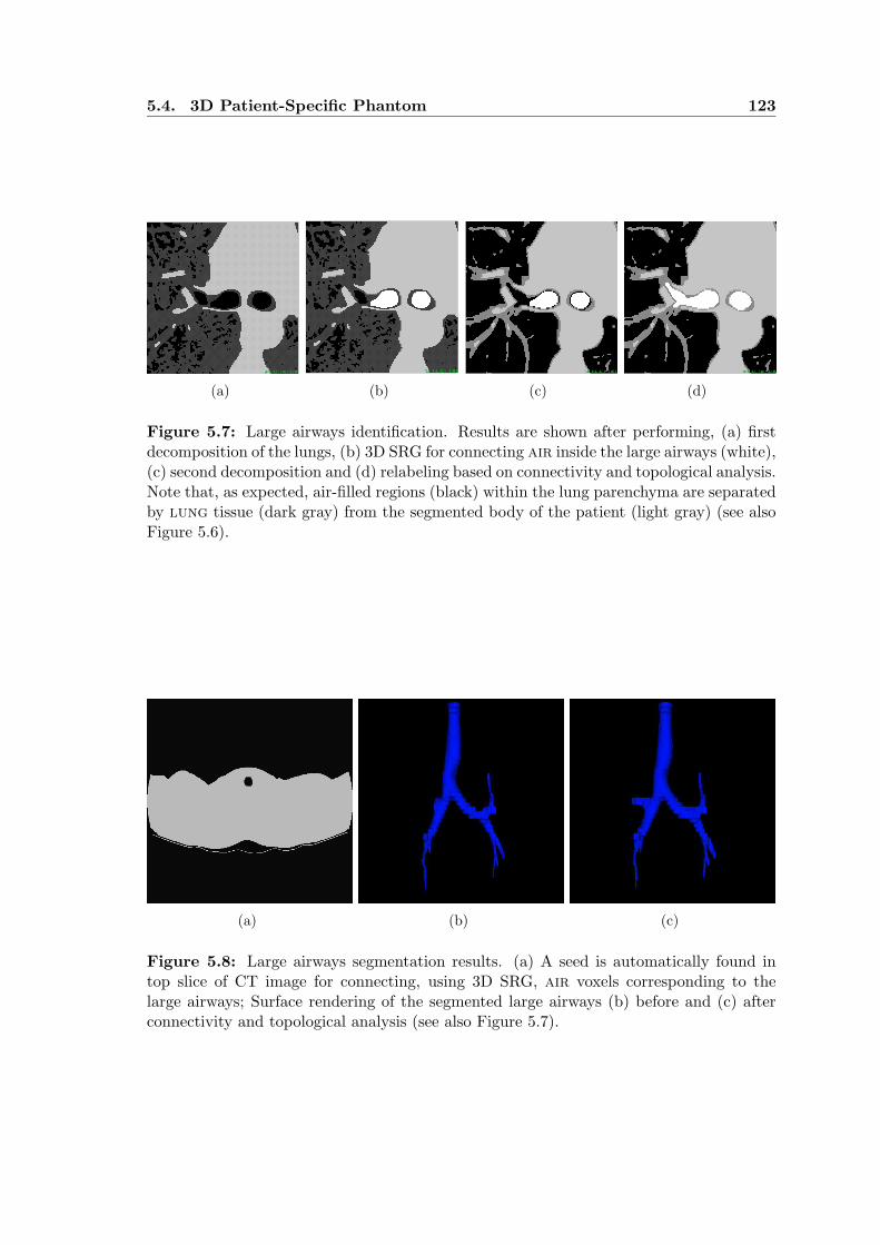
5.4. 3D Patient-Specific Phantom 123
(a) (b) (c) (d)
Figure 5.7: Large airways identification. Results are shown after performing, (a) firstdecomposition of the lungs, (b) 3D SRG for connecting air inside the large airways (white),(c) second decomposition and (d) relabeling based on connectivity and topological analysis.Note that, as expected, air-filled regions (black) within the lung parenchyma are separatedby lung tissue (dark gray) from the segmented body of the patient (light gray) (see alsoFigure 5.6).
(a) (b) (c)
Figure 5.8: Large airways segmentation results. (a) A seed is automatically found intop slice of CT image for connecting, using 3D SRG, air voxels corresponding to thelarge airways; Surface rendering of the segmented large airways (b) before and (c) afterconnectivity and topological analysis (see also Figure 5.7).

124 Chapter 5. Decomposition of 3D CT Images
of a CT image is performed for constructing a 3D patient-specific phantom, this
algorithm can be considered as optional.
Actually, the lungs should be more accurately decomposed if only voxels be-
longing to that structure are used to compute its mean CT number. Therefore,
material decomposition is now performed by first computing the mean CT number
Hξ of lungs voxels, and considering again air and lung tissue as the basis set. A
new threshold T3 is computed by using Eq. 5.11 to identify, this time, air from
lung tissue voxels within the parenchyma. Results of the second decomposition
are displayed in Figure 5.6(b). In this example, the mean CT number Hξ = −850
(segmented lungs) and threshold T3 = −794 were computed, corresponding to the
volume fractions b1 = 0.86 (air) and b2 = 0.14 (lung tissue).
The segmentation of the large airways is finally achieved through connectivity
and topological analysis: small objects labeled as air after the second decomposition
and connected to the large airways, as illustrated in Figure 5.7(c), are included in this
structure and relabeled accordingly. The final result is illustrated in Figure 5.7(d).
The following steps summarize the large airways identification and parenchyma
decomposition algorithms:
// Algorithm III - Lung Decomposition
// ----------------------------------
1. Construct histogram of LUNGS
// Large Airways Identification - 1st decomposition:
2. Compute mean CT number of PATIENT
3. Decompose LUNGS as AIR and LUNG tissue (compute T2)
4. Relabel LUNGS voxels as AIR (H < T2)
5. Find seed S2 and connect LARGE AIRWAYS (3D SRG using T2)
6. Relabel AIR voxels as LARGE AIRWAYS
// Parenchyma Decomposition - 2nd decomposition:
7. Compute mean CT number of LUNGS
8. Decompose LUNGS as AIR and LUNG tissue (compute T3)
9. Relabel LUNGS voxels as AIR (H < T3)
10. Relabel remaining LUNGS voxels as LUNG tissue
// Connectivity and Topological Analysis:
11. Relabel AIR voxels as LARGE AIRWAYS
The steps are applied sequentially, as illustrated in Figure 5.7(a) to (d) for the
central region of a slice at the level of the carina. Other results of the proposed
algorithm are presented in Figure 5.8. The top slice of the CT image is displayed
in Figure 5.8(a) where the seed s2 was automatically selected and used to grow the

5.4. 3D Patient-Specific Phantom 125
large airways. Surface rendering of such structure, before and after connectivity and
topological analysis is shown in Figure 5.8(b) and (c) respectively.
5.4.3 Body Decomposition
The final algorithm for constructing a 3D patient-specific phantom is now described.
It represents the decomposition of the body into fat (adipose) tissue, soft tissues
(including blood) and higher density structures herein referred to as bones, corre-
sponding mainly to the whole skeleton of the patient (see Figure 5.1). The bones
are expected to include the spine, ribs, clavicles, scapula and sternum, as well as
bone marrow (soft tissue filling spaces within some bones).
The first step of the algorithm consists of separating bones from non-bones struc-
tures. To achieve this goal, a segmentation threshold T4 is used to distinguish low
density from high density voxels within the segmented body. Ideally, the thresh-
old value should be chosen (or computed) such that: 1) voxels with CT number
below T4 (low density voxels) should correspond to spatial regions made up of fat
and soft tissue only, and 2) bone structures should be identified as voxels with
CT number above T4 (high density voxels). Based on a few experiments performed
on some CT images, the value T4 = +140 was selected for thresholding the body
and relabel its voxels as bones and non-bones. To ensure that the condition 1) is
fulfilled, the regions currently labeled as bones are further dilated. The dilatation
was performed using a 3 × 3 × 3 structuring element and the dilated bones were
relabeled accordingly. As visualized in a single axial slice of the labeled CT image,
displayed in Figure 5.9(a), this operation tends to merge the vertebral column, ribs
and skeletal muscles into a single 3D connected region.
Once identified, non-bones structures are decomposed into fat and soft tis-
sues. Material decomposition expressed by Eq. 5.9 is now performed by considering,
respectively, Hα = −93 and Hβ = +55 as the mean CT number of these two ba-
sis materials (see Table 5.1) and Hξ the mean CT number computed within the
non-bones region being decomposed. As a result, a decomposition threshold T5 is
automatically computed and used to relabel non-bones voxels as fat or soft tissue,
if their CT number is below or above T5, respectively. Figure 5.9(b) shows an exam-
ple of such decomposition, for which Hξ = −20 (non-bones), T5 = +12, b1 = 0.51
(fat) and b2 = 0.49 (soft).
The last step of the algorithm is based on the assumption that the dilated bones
can be expressed as a combination of bone and soft tissue, erroneously included due

126 Chapter 5. Decomposition of 3D CT Images
(a) (b)
(c) (d)
Figure 5.9: Body decomposition. (a) Dilated bones, in white, after body thresholding;(b) Decomposition of non-bones voxels within the body, into fat and soft tissues; (c)Dilated bones decomposition into soft tissue and bones structures forming the skeleton;(d) Surface rendering of the segmented bone structures.

5.5. Lung Field Segmentation 127
to the dilatation. Based on material decomposition, we finally separate these two
groups of voxels according to a new threshold T6. In this case, Hα = +55 (for soft
tissue) and Hβ should reflect as much as possible the contents of bone. To compute
this value, the dilated bones are first eroded (actually, this is a closing operation)
and the mean CT number Hβ is then estimated within the resulting region. Using
the computed threshold, voxels with CT number below T6 are relabeled as soft
tissue. The whole decomposition of the body is illustrated in Figure 5.9(c). In
the provided example, Hξ = +231 (dilated bones), Hβ = +362 (closed bones)
and T6 = +133 were computed, corresponding to the volume fractions b1 = 0.43
(soft) and b2 = 0.57 (bones). Surface rendering of the segmented bones is shown
in Figure 5.9(d).
The proposed algorithm for decomposing the body of the patient is described by
the following steps:
// Algorithm IV - Body Decomposition
// ---------------------------------
1. Construct histogram of BODY
2. Set threshold value T4 = 140
3. Relabel BODY voxels as BONES (H > T4)
4. Dilate BONES and create BONES_DILATED
5. Relabel BODY voxels as NON-BONES
// 1st Material Decomposition:
6. Decompose NON-BONES as FAT and SOFT tissue (compute T5)
7. Relabel NON-BONES voxels as FAT tissue (H < T5)
8. Relabel remaining NON-BONES voxels as SOFT tissue
// 2nd Material Decomposition:
9. Erode BONES_DILATED and create BONES_CLOSED
10. Compute mean CT number of BONES from BONES_CLOSED
11. Decompose BONES_DILATED as SOFT tissue and BONES (compute T6)
12. Relabel BONES_DILATED voxels as SOFT tissue (H < T6)
13. Relabel remaining BONES_DILATED voxels as BONES
5.5 Lung Field Segmentation
A 3D region or volume of interest that includes the lung parenchyma is usually re-
quired by most pulmonary image analysis applications. In this Section, a method
for segmenting such region of interest is described. The proposed method consists of
a sequence of algorithms (see Figure 5.2) that include, at first, the patient segmen-
tation (Section 5.4.1) and the large airways identification algorithms (Section 5.4.2).

128 Chapter 5. Decomposition of 3D CT Images
5.5.1 Lung Region of Interest Extraction
To identify the lung region of interest (lung ROI) a constrained dilatation is per-
formed on the two segmented regions that actually contain air within the lungs:
air within the large airways and air within the lung parenchyma. These air-filled
regions are shown in Figure 5.10(a) and result from the large airways identification.
The dilatation is performed as follow. First, the large airways are dilated: any voxel
labeled as lung tissue within the 26-neighborhood of the connected large airways is
included in such structure and relabeled accordingly. Next, the same rule is applied
when considering the neighborhood of air voxels within the lungs. This sequential
procedure is applied repeatedly until all lung tissue voxels have been relabeled as
belonging to large airways or lung parenchyma (Figure 5.10(b) and (e)).
The constrained dilatation is then followed by a 2D connectivity analysis, per-
formed in each slice of the CT image, to identify and eliminate small unwanted
interior cavities inside the lung parenchyma (Figure 5.10(c) and (f)). These steps
actually correspond to a 2D filling operation of the lung parenchyma (Figure 5.10(d)
and (g)). The final output of the lung ROI extraction step is a 3D connected and
filled region, displayed in Figure 5.11(a) as a binary mask for one slice of the im-
age. Figure 5.11(b) shows the corresponding lung ROI extracted in the same slice
of the original CT image, while the surface rendering of such structure is shown in
Figure 5.11(c).
The steps that follow summarize the lung region of interest extraction algorithm:
// Algorithm V - Lung Field Segmentation
// -------------------------------------
1. Find voxels borders of AIR and LARGE AIRWAYS
2. Dilate LARGE AIRWAYS and AIR, by "conquering" LUNG tissue
3. Compute statistics of LARGE AIRWAYS and lung PARENCHYMA
4. Connect BODY in 2D slices (2D SRG)
5. Fill PARENCHYMA (2D SRG)
6. Extract lung ROI
7. Compute statistics of ROI
The mean CT numbers of the segmented lung structures are finally updated.
In this example, the following values were obtained: Hξ = −862, Hξ = −850 and
Hξ = −846 within, respectively, the dilated large airways, lung parenchyma and
the extracted lung ROI. Note that beside air surrounded by lung tissue, the lung
ROI contains additional soft tissue, such as arteries and veins, due to the filling
operation and therefore the mean density of this structure is slightly increased.
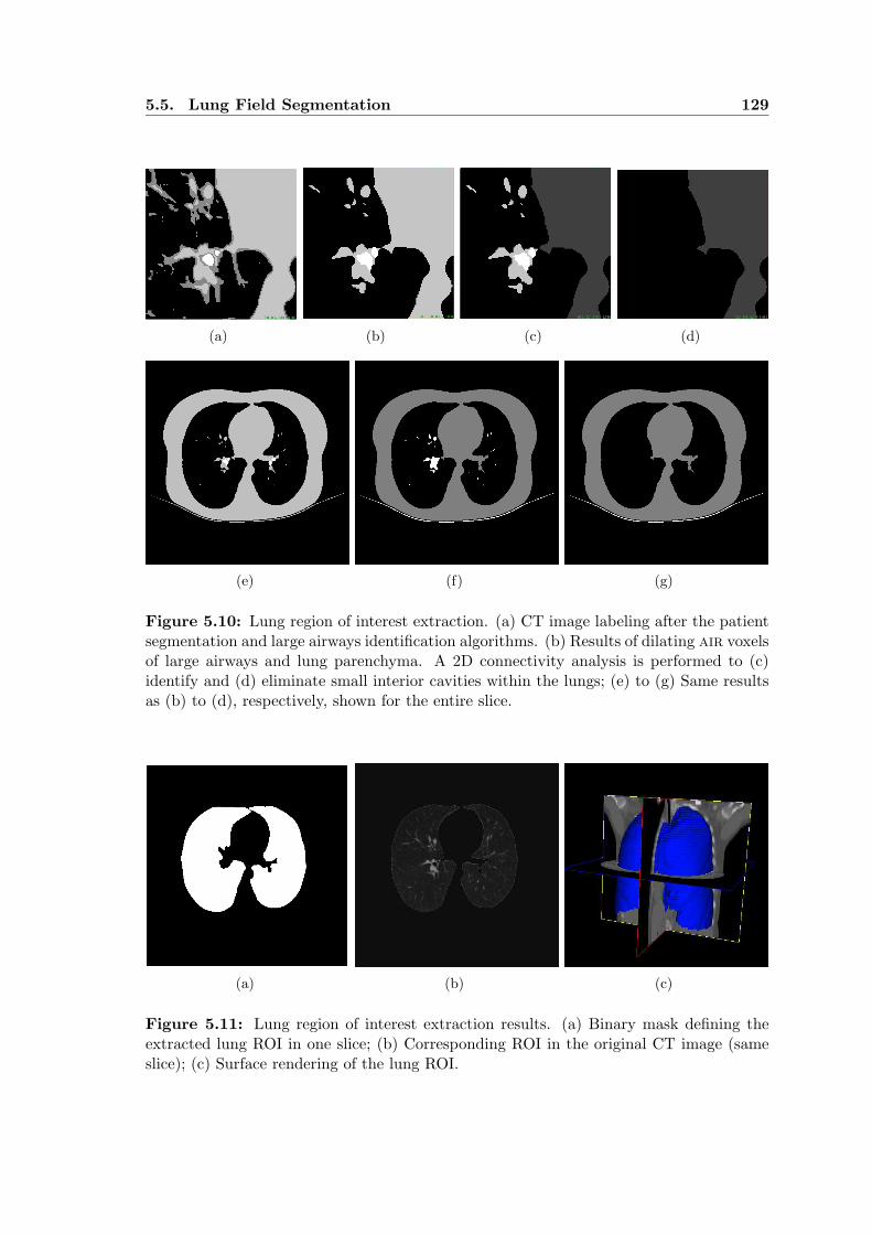
5.5. Lung Field Segmentation 129
(a) (b) (c) (d)
(e) (f) (g)
Figure 5.10: Lung region of interest extraction. (a) CT image labeling after the patientsegmentation and large airways identification algorithms. (b) Results of dilating air voxelsof large airways and lung parenchyma. A 2D connectivity analysis is performed to (c)identify and (d) eliminate small interior cavities within the lungs; (e) to (g) Same resultsas (b) to (d), respectively, shown for the entire slice.
(a) (b) (c)
Figure 5.11: Lung region of interest extraction results. (a) Binary mask defining theextracted lung ROI in one slice; (b) Corresponding ROI in the original CT image (sameslice); (c) Surface rendering of the lung ROI.

130 Chapter 5. Decomposition of 3D CT Images
5.5.2 Right and Left Lung Separation
Since many lung diseases show specific regional distribution or preferences, the lung
region of interest extraction includes an additional step to separate the left and the
right lung. The anterior and posterior junction lines separating the lungs can be very
thin. The attenuation of this interface may be reduced such that the corresponding
CT numbers, along such junction lines, fall below the threshold T1. Remember from
Section 5.4.1 that T1 was automatically computed for segmenting the whole lungs
within the patient.
The goal of the lung separation algorithm is to identify a 3D surface representing
the boundary between the left and right lung. Therefore, an optimal 3D surface
detection algorithm [45] is suggested for simultaneously delineating the anterior and
posterior junction lines in each axial slice (OXY plane) of the joining region. Since
the searched surface is expected to be approximately parallel to the sagittal (OYZ)
plane, it assumes the form x = f (y, z).
Let H (x, y, z) be a 3D CT image defined in its physical extents ∆X = xmax −xmin, ∆Y = ymax − ymin and ∆Z = zmax − zmin in the coordinate system OXYZ.
The optimal surface detection algorithm considers a 3D graph that represents the
image H with the same size. The graph nodes, p = (x, y, z)T, correspond to CT
image voxels and, to each node, a local cost c (x, y, z) is assigned. The construction
of the optimal surface is based on optimal graph searching techniques and consists
of selecting those voxels that linked together form the surface with the lowest cost.
The total cost cf associated with the surface f (y, z) is calculated as the sum of
individual costs of all nodes forming the surface,
cf =
ymax∑
y=ymin
zmax∑
z=zmin
c (f (y, z) , y, z), (5.12)
where c (f (y, z) , y, z) is the local cost of the node located at (x, y, z) in the CT
image, for which xmin ≤ x ≤ xmax, ymin ≤ y ≤ ymax and zmin ≤ z ≤ zmax.
The legality of the surface is defined by 3D surface connectivity requirements
that depend on the application at end. The connectivity constraint is introduced to
guarantee surface continuity in 3D. In the following, the parameter d represents the
maximum allowed change in the x coordinate of the surface along the unit distance
(pixel spacings) dY and dZ in the Y and Z directions, respectively. If d is small, the
legal surface is stiff and the stiffness decreases with larger values of d. For all nodes

5.5. Lung Field Segmentation 131
of the surface, the connectivity constraint is expressed as follow:
|f (y, z) − f (y − dY, z)| ≤ d,
|f (y, z) − f (y, z − dZ)| ≤ d.(5.13)
The cumulative surface cost is defined as the sum of the local cost associated
with the node (x, y, z) and the sum of the two cost minima identified in the two
lines constructed in the 3D graph that represent the immediate predecessors:
C (x, y, z) = c (x, y, z)
+ minx∈[x−d,x+d]
C (x, y − dY, z)
+ minx∈[x−d,x+d]
C (x, y, z + dZ) .
(5.14)
The graph is searched starting from the line with coordinates (x, ymin, zmax) for
which C (x, ymin, zmax) = c (x, ymin, zmax), in X-Z-Y coordinate order, towards the
line (x, ymax, zmin). The optimal surface construction proceeds in the reversed X-Y-
Z order and propagation of the connectivity constraint guarantees the legacy of the
resulting surface. The x coordinate of the optimal surface-node in the line (y, z),
denoted by f ∗ (y, z), is defined as
f ∗ (y, z) = x : C (x, y, z) = minx∈[x1,x2]
C (x, y, z) , (5.15)
wherex1 = min (xmax, f
∗ (y + dY, z) + d, f ∗ (y, z − dZ) + d),
x2 = max (xmin, f∗ (y + dY, z) − d, f ∗ (y, z − dZ) − d),
(5.16)
and the backtracking process continues until the optimal node is found in the line
(x, ymin, zmax).
To reduce the computational time of the graph-searching algorithm, the opti-
mal 3D surface was detected only in a region that corresponds in size with the
bounding box of the lung ROI, once segmented as explained in Section 5.5.1. The
bounding box is automatically computed to define the points (xmin, ymin, zmin) and
(xmax, ymax, zmax). Within this spatial region, the local cost of a node is the gray
level or CT number of the corresponding voxel. If the voxel is labeled as belonging
to the body, the local cost is set to zero.
The steps below summarize the optimal surface detection algorithm used for
separating right and left lungs.
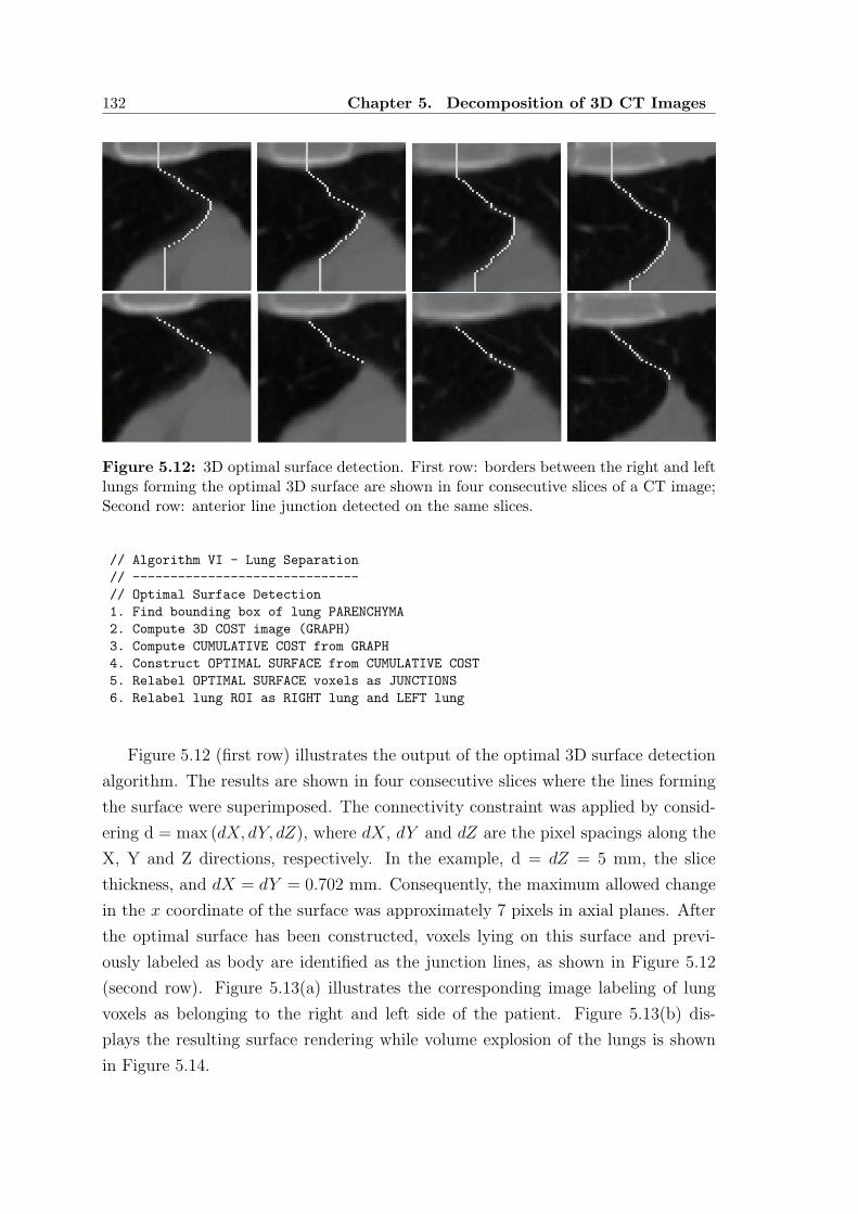
132 Chapter 5. Decomposition of 3D CT Images
Figure 5.12: 3D optimal surface detection. First row: borders between the right and leftlungs forming the optimal 3D surface are shown in four consecutive slices of a CT image;Second row: anterior line junction detected on the same slices.
// Algorithm VI - Lung Separation
// ------------------------------
// Optimal Surface Detection
1. Find bounding box of lung PARENCHYMA
2. Compute 3D COST image (GRAPH)
3. Compute CUMULATIVE COST from GRAPH
4. Construct OPTIMAL SURFACE from CUMULATIVE COST
5. Relabel OPTIMAL SURFACE voxels as JUNCTIONS
6. Relabel lung ROI as RIGHT lung and LEFT lung
Figure 5.12 (first row) illustrates the output of the optimal 3D surface detection
algorithm. The results are shown in four consecutive slices where the lines forming
the surface were superimposed. The connectivity constraint was applied by consid-
ering d = max (dX, dY, dZ), where dX, dY and dZ are the pixel spacings along the
X, Y and Z directions, respectively. In the example, d = dZ = 5 mm, the slice
thickness, and dX = dY = 0.702 mm. Consequently, the maximum allowed change
in the x coordinate of the surface was approximately 7 pixels in axial planes. After
the optimal surface has been constructed, voxels lying on this surface and previ-
ously labeled as body are identified as the junction lines, as shown in Figure 5.12
(second row). Figure 5.13(a) illustrates the corresponding image labeling of lung
voxels as belonging to the right and left side of the patient. Figure 5.13(b) dis-
plays the resulting surface rendering while volume explosion of the lungs is shown
in Figure 5.14.

5.5. Lung Field Segmentation 133
(a) (b)
Figure 5.13: Right and left lung separation. (a) Segmented structures defining the lungROI: right lung (white) and left lung (light gray). (b) The lungs are separated by the3D optimal surface detection algorithm. The optimal surface (red) is searched within thebounding box of the ROI (the outline of the CT image is also shown).
(a) (b)
Figure 5.14: Lung field segmentation from CT images. (a) Surface rendering of seg-mented lung structures: large airways (white), right lung (green) and left lung (yellow);(b) Corresponding volume explosion.

134 Chapter 5. Decomposition of 3D CT Images
5.6 Experimental Results
In this Section, experimental results of the 3D patient-specific phantom construction
and the lung region of interest extraction are reported.
5.6.1 CT Image Database
The proposed segmentation algorithms were evaluated on a private image database
that consists on 3D X-ray CT images acquired from 30 subjects using a LightSpeed
CT scanner (GE Medical Systems; Milwaukee, WI) from the Radiology Department
of the Hospital Pedro Hispano (HPH), in Matosinhos. Each volume in the database
contains a stack of 45 to 74 contiguous axial slices. Each slice is a matrix of 512×512
square pixels, with a resolution (pixel spacing) ranging from 0.514 to 0.811 mm per
pixel (mean value 0.702 mm). The slice thickness of 5 mm is the same for all the
CT images in our database. The data sets are provided by the scanner in DICOM
format and 16 bits per pixel are used to express CT numbers. It is assumed that
the calibration of the scanner reflects the mean CT number of each material listed
in Table 5.1, thus ignoring the small variation in tissue densities expected across the
population of subjects that were included in the database.
The FOV corresponds to the reconstruction of the scanned patient in supine
position. Although cross-sections of the patient thorax are not always completely
inside the FOV, all thoracic 3D CT images include the entire lung region of interest
to be segmented.
5.6.2 Computed Threshold Values
The threshold values automatically computed by the proposed segmentation method
are reported in Table 5.2. Mean values and standard deviations (std) are listed in the
same sequence they were computed for each image of the database. Each algorithm
results in the segmentation of at least one particular structure previously defined
in the anatomical model. The CT image itself and the patient are segmented with
optimal thresholds, while material decomposition is used for the lungs and the body.
The thresholds T0 and T1 were computed for segmenting the patient from the
image background (T0) and for separating the lungs from the body within the patient
(T0 or T1). The corresponding segmentation algorithms are provided in Section 5.4.1.
Both algorithms were tested by using two different techniques for computing optimal
threshold values and, for each input CT image to be segmented, equal values of T0

5.6. Experimental Results 135
Table 5.2: 3D patient-specific phantom construction. Computed threshold values for CTimage decomposition. Mean values and standard deviations (std) were computed from the30 images of the database (see also Table 5.3).
Segmented Structure Computed Threshold
Algorithm ξ Type T mean std
I CT Image optimal T0 −468 13
II Patient optimal T1 −399 28
III Lungs(decomposition) T2 −886 25decomposition T3 −772 26
IVBody fixed T4 +140
Non-Bones decomposition T5 +6 10Dilated Bones decomposition T6 +128 8
Table 5.3: 3D patient-specific phantom construction. Material decomposition of struc-tures segmented from 3D CT images. Mean values and standard deviations (std) werecomputed from the 30 images of the database (see also Table 5.2).
Decomposed Material Decomposition
Structure Basis Materials Volume Fractions
ξ Hξ std α β b1 b2 std
CT Image Background Patient 0.50 0.50 0.08
Patient −216 39 Lungs Body 0.28 0.72 0.05
Lungs(Patient)
air lung0.26 0.74 0.04
−829 33 0.84 0.16 0.03
Large Airways −863 22Parenchyma −828 33Lung ROI −822 33
Body +23 25 Non-Bones Dilated Bones 0.82 0.18 0.09
Non-Bones −16 19 fat soft 0.48 0.52 0.13Dilated Bones +196 41 soft Bones 0.46 0.54 0.07
Fat tissue −93 7Soft tissue +44 5
Bones +339 53

136 Chapter 5. Decomposition of 3D CT Images
and T1 were obtained. Considering the 30 images, the mean values T0 = −468 and
T1 = −399 were obtained. The threshold T0 depends on the value of all voxels in
the image, including those lying outside the FOV. The corresponding CT number of
these voxels is dependent of the scanner used to acquire the data and usually equal to
H = −1024 or H = −3071. Consequently, a pre-processing algorithm was included
to correct properly this value to H = −999, the CT number of air expected to
be found in the entire background. T1 should be used instead of T0 for identifying
the lungs since, by considering the patient region, T1 only depends on the scanned
volume of interest and provides a better estimate of the volume fractions of lungs
and body within the segmented patient. The value of T1 = −399 (quite different
from T0) is actually coherent with a study from Kemerink [138] that investigates the
influence of the threshold and shows the value of −400 (HU) as adequate in most
of the cases.
As described in Section 5.4.2, the segmentation of the large airways was achieved
by computing the threshold T2 (first material decomposition), while another value
T3 was used to decompose the lung parenchyma into materials air and lung tis-
sue (second decomposition). Considering all images, T2 = −886 and T3 = −772,
as reported in Table 5.2. These thresholds are patient-dependent (as T0 and T1)
and reflect the variability of the large airways and lung parenchyma composition
within the database. The first decomposition is optional since the segmentation of
this structure is only needed for extracting the lung ROI. The 3D patient-specific
phantom can be constructed by simply decomposing the lungs as air and lung
tissue.
The final algorithm of the phantom construction consists on decomposing the
body to identify non-bones from bone structures. To achieved this goal, the same
fixed value T4 = +140 was used for all images. Note that this threshold is only used
for initializing the whole body decomposition process, since the mean CT number
of bone structures is updated after the closing operation is performed, as explained
in Section 5.4.3.
5.6.3 Phantom Composition
The 3D patient-specific phantom construction from a single CT image results in the
sequential decomposition of the structures previously defined in the model. Applying
the proposed algorithms to all the images in the database, the mean CT number Hξ
and therefore the expected composition, the volume fraction b, of each anatomical
5.6. Experimental Results 137
structure can be computed. Mean values and standard deviation (std) are reported
in Table 5.3. Note that the corresponding material decompositions are such that α
(β) corresponds to a basis material with density lower (higher) than the decomposed
structure ξ.
The first material decomposition corresponds to the segmentation of the CT
image for separating the patient from the image background. This step was achieved
by computing the optimal threshold T0 (see Table 5.2). We note that the resulting
mean volume fractions b1 and b2 are 50% for both structures. Altough the values
are the same, we believe there is no particular reason for that occurence. In fact,
the volume fraction b2 (patient) observed in the database can be as high as 65%
(T0 = −497), while the minimum value found is b2 = 34% (T0 = −468).
The next algorithm (algorithm II) was performed on the segmented patient to
decompose it as non-overlapping regions, namely the lungs and the body. The results
reported were obtained by using T1 as the segmentation threshold. As expected, the
lungs are characterized by a lower density Hα = −829 ± 33 than voxels labeled as
body inside the patient, Hβ = +23 ± 25. From the experiments, one can conclude
that, since the lungs are 0.28% of the scanned volume (patient), they only account
for 0.14% of the entire volumetric CT image, including voxels outside the FOV of
the scanner. Actually, this is a surprising result since most applications focuse on
the analysis of this particular structure.
We assumed that the lungs are composed of air and lung tissue. As described in
Section 5.4.2, the large airways were identified as pure air voxels within of the whole
lung region. About 28% of lung voxels are candidates for being part of the large
airways. The true lung decomposition is achieved when using its mean CT number.
In this case, mean values of 84% of air and 16% of lung tissue were obtained
in the database. Of all the computed volume fractions, these values represent the
contents that show the lowest variation. The lung parenhyma was defined as the
lungs without the large airways and its CT number should increase. The same is
expected to happen when segmenting the lung region of interest since pulmonary
veins and arteries have been included due to the filling operation (see Section 5.5.1).
Material decomposition allows to predict the contents of fat tissue, soft tissue
and bone structures within the segmented body of a patient. First, non-bones are
identified and further decomposed, resulting into fat and soft volume fractions of
48% and 52%, respectively. Table 5.3 shows that the variation of these contents is
the highest value. We believe this is a consequence of the variability of the amount
of fat tissue among all the patients in the population. In fact, decompositions

138 Chapter 5. Decomposition of 3D CT Images
Figure 5.15: 3D patient-specific phantom construction. Surface rendering of segmentedstructures labeled as bones, for 3 different CT images of the database.
resulting in 22% and 78% (fat/soft) and 77% and 23% were observed.
The final decomposition is performed on the highest attenuation voxels in the
entire CT image. The body include the dilated bones, expected to contain only soft
and bone structures such as the skeleton of the patient, as show in Figure 5.15.
Note that the corresponding mean CT number, Hξ = +339 ± 53, shows the largest
standard deviation when computed from the database. This is quite acceptable
since these are high density structures that include CT numbers up to +3071.
Basis Plane Representation
As discussed in Section 2.7.2, all the segmented structures ξ that compose a given
CT image can be conveniently represented in the basis plane. The volume fractions
b1 and b2 of the corresponding intervening materials α and β define the structure ξ
in the plane by the vector (b1, b2). From Eq. 5.10, the characteristic angle is then
computed as θξ = tan−1 (b2/b1), under the condition b1 + b2 = 1. Considering the
volume fractions listed in Table 5.3, θξ can be computed for each decomposition.
The following values were obtained: θ0 = 45.0o (CT image), θ1 = 68.7o (patient),
θ3 = 10.8o (lungs), θ4 = 12.4o (body), θ5 = 47.3o (non-bones) and θ6 = 49.6o (dilated
bones). Note that θi corresponds to the characteristic angle of the structure decom-
posed by using the segmentation threshold Ti, reported in Table 5.2. Figure 5.16
shows the resulting basis plane representation of CT image decomposition. Similar
representation could be drawn for a single CT image. Each intervening materials
is separated geometrically and, since all the segmented anatomical structures are
non-overlapping regions, the overall vector sum is the volumetric CT image itself.

5.7. Validation 139
CT Im
age
-
Background -
- Lungs -
0
- N
on-B
ones
-
D. Bones -
1
3
4
5
P
atie
nt
-
AIR
FAT
SOFT
Bones
B
ody
-
LUNG
SOFT
6
Figure 5.16: Basis plane representation of CT image decomposition. Each structure inthe anatomical model is defined as a vector in the plane, whose components correspondto the contents (fraction by volume) of the intervening materials of that structure. Thecharacteristic angles are: θ0 = 45.0o (CT image), θ1 = 68.7o (patient), θ3 = 10.8o (lungs),θ4 = 12.4o (body), θ5 = 47.3o (non-bones) and θ6 = 49.6o (dilated bones). Note that soft
tissue is identified by decomposing both non-bones and dilated bones. (see also Table 5.3).
5.7 Validation
5.7.1 Large Airways
Surface rendering of the large airways segmented from all images of the database
can be visualized in Appendix C. These segmentation outputs were qualitatively
evaluated by an experienced radiologist. By visual inspection, the best and worst
results were selected to judge for the performance of this particular extraction algo-
rithm. The selected outputs are presented in Figure 5.17. In all cases, the trachea
and main stem bronchi have been correctly identified by the computer.
5.7.2 Lung Region of Interest
Some results of the lung field segmentation algorithm are given in Figure 5.18. The
performance of the method was assessed by comparing the automatic computer-
based segmentation with results obtained by manual analysis. For this purpose, two
image data sets, set 1 and set 2, were taken from the database. The pixel spacing
(resolution) in each slice of both datasets is dX = dY = 0.702 mm, actually the

140 Chapter 5. Decomposition of 3D CT Images
Figure 5.17: Large airways segmentation results (surface rendering). The results, qual-itatively evaluated by an experienced radiologist, are shown for the best (first row) andworst (last row) 4 of 30 CT images of a private database (HPH) (see also Appendix C).
Figure 5.18: Lung field segmentation results shown for 3 different images of the database:surface rendering of the large airways (white), right lung (green) and left lung (yellow).

5.7. Validation 141
Figure 5.19: Manual contouring of the lung region of interest (ROI). The lung ROI man-ually delineated by an experienced radiologist (human A) in two images of the database:set 1 (left) and set 2 (right). In each case, the results of manual contouring are shown foreven numbered slices only.
mean value across the image database. This represents the unique criterion used for
choosing these images. Although the number of slices in the volumes is different (64
for set 1 and 57 for set 2), quantitative comparison of the corresponding segmentation
outputs is independent of the image resolution. One experienced radiologist A and
two image analysts B and C manually traced the lung borders on every slice of the
two chosen sets. The operators worked independently of each other using the same
software system specifically developed to perform manual analysis. Overall, each
human operator traced lung borders on 121 slices. In each slice, more than one
contour could be delineated for each lung and manual contours were then stored for
later evaluation. The manual delineation of the lung ROI performed by A on the
two images is shown in Figure 5.19. For display purposes, only contours of even
numbered slices are shown.
We evaluated the performance of the method by using the same similarity mea-
sures as for the case of chest radiographs, namely accuracy, degree of overlap and
F -score (see Section 4.5.3). The degree of overlap corresponds to the true positive
volume fraction, as given by Eq. 3.33. Results of comparing the proposed method
with manual analysis are reported in Table 5.4. When computing the accuracy, sen-
sitivity and specificity, the segmentation performed by the observers is considered
as the ground truth, while equal importance of recall and precision is assumed for
calculating the F-measure.
Although the variability that occurs when comparing the automated segmenta-
tion with human delineations is very small, the results serve to lower the measures
at which the proposed computerized scheme may be expected to perform. From

142 Chapter 5. Decomposition of 3D CT Images
Table 5.4: Lung field segmentation from CT images. Performance measures of the lungROI extraction algorithm computed for two CT images of a private database (HPH).The segmentation output of the computer-based method is compared with the manualcontours performed by three different humans (A, B and C) on every slice of both images.See Table 5.5 for inter-human variability.
MeasureCT Image 1 CT Image 2
A B C A B C
accuracy 0.997 0.997 0.997 0.994 0.995 0.995
sensitivity 0.988 0.985 0.986 0.985 0.981 0.980
specificity 0.998 0.999 0.999 0.996 0.997 0.997
overlap 0.975 0.978 0.977 0.961 0.963 0.964
precision 0.986 0.993 0.991 0.975 0.982 0.984
recall 0.988 0.985 0.986 0.985 0.981 0.980
F-score 0.987 0.989 0.989 0.980 0.981 0.982
Table 5.5: Lung field segmentation from CT images. Analysis of inter-observer vari-ability. Performance measures were computed by comparing manual segmentation of thelung ROI delineated on two CT images of a private database (HPH). Manual contouringwas performed by three different human operators (A, B and C) on every slice of the3D images. See Table 5.4 for comparing with the performance measures of the proposedcomputer-based segmentation method.
MeasureCT Image 1 CT Image 2
A/B A/C B/C A/B A/C B/C
accuracy 0.997 0.996 0.997 0.995 0.995 0.996
sensitivity 0.991 0.989 0.987 0.990 0.989 0.987
specificity 0.997 0.997 0.999 0.996 0.996 0.998
overlap 0.973 0.972 0.978 0.969 0.964 0.973
precision 0.981 0.983 0.991 0.978 0.975 0.986
recall 0.991 0.989 0.987 0.990 0.989 0.987
F-score 0.986 0.986 0.989 0.984 0.982 0.987

5.8. Conclusions 143
Table 5.4, and considering the overlap as the reference measure, 96.1% of voxels
identified by the radiologist have been correctly labeled by the computer as belong-
ing to the lung region of interest. This is the worst case when evaluating the method
with set 2. We also evaluated the variability that occurs between the manual seg-
mentation performed by the three observers. Results of such analysis are reported
in Table 5.5. When computing the accuracy, sensitivity and specificity, the segmen-
tation performed by the radiologist (observer A) is considered as the ground truth
(when comparing B and C, B is the gold standard).
5.7.3 Lung Separation
To evaluate the optimal surface detection algorithm, junction lines positioning ac-
curacy was assessed by computing a distance-based metric. For each voxel p∗n =
(x, y, z)T that belongs to one of the detected junction lines, as shown in Figure 5.12
(first row), the closest points p(r)n and p
(l)n are identified on the contours manually
delineated for the left and the right lung, respectively. By computing the distance
d (p∗n) between the node p∗
n and the midpoint lying between p(r)n and p
(l)n , we defined
the positioning accuracy as the mean distance d =∑N−1
n=0 d (p∗n)
/
N , where N is the
total number of voxels on the computer-defined junction lines. The optimal surface
detection accuracy was computed by considering the contours delineated by the hu-
man operators A, B and C. The mean values and standard deviations, expressed in
percent of the pixel spacing dX are, respectively, dA = 0.71± 0.57, dB = 0.62± 0.51
and dC = 0.92± 0.70. In all cases, d is less than dX = 0.702 mm, the image resolu-
tion in the axial plane. The accuracy was only computed for set 1, since no junction
lines were detected in set 2.
5.8 Conclusions
In this Chapter, a fully automated method for segmenting volumetric CT images
was described. The proposed method is based on a simple description of the thoracic
anatomy and contains knowledge specific to the CT modality. We have applied the
method on 30 CT images of a private image database. Providing a reproducible set of
threshold values, the decomposition of a given CT image results in the identification
of several structures of the human thorax, namely the central tracheo-bronchial and
lung parenchyma, fat and soft tissues within the body and bone structures such as
the skeleton of the patient. Each segmented structures have been specified in terms

144 Chapter 5. Decomposition of 3D CT Images
of its mean CT number and volume fraction within the image.
Using dual-energy principles applied to CT numbers, the concept of basis mate-
rial decomposition was explored to provide the means for constructing 3D patient-
specific voxel-based phantoms from CT scans. Anthropomorphic phantoms have
several applications in the radiologic sciences. In the field of diagnostic imaging,
such segmented data can be used to create realistic digital reconstructed radio-
graphs which closely resemble clinical data. They also prove especially interesting
in testing and improving tomographic reconstruction algorithms.
In CAD systems, the lungs are the structure of interest for most diagnostic pur-
poses in thoracic CT imaging. Because of the large amount of data acquired during
in a single CT scan, it is critical to develop an efficient method that does not re-
quire human interaction for accurately delineate such organs. Several algorithms
were included in the segmentation framework to extract the lung region of interest,
and segmentation outputs were compared with manual analysis. Because it is fully
automated it can be applied to a CT data set prior to clinical review, and the com-
putation time is acceptable for most of pulmonary applications. With the additional
step of lung separation, the method can also provide functional information about
the individual right and left lung.

Chapter 6
3D SHAPE RECONSTRUCTION
FROM SINGLE RADIOGRAPHS
In this Chapter, we describe a strategy to solve the problem of recovering the 3D
shape of anatomical structures from single planar radiographs. The proposed ap-
proach is based on the simulation of X-ray images and addresses the problem of
registering CT images to planar radiographs by directly exploiting the relationship
between the two imaging modalities.
6.1 Introduction
Registration of medical data from different imaging devices has proven to be an
important tool in the field of computer-aided surgery and image-guided therapy [146,
147]. A crucial module of many 2D-3D registration algorithms is the generation
of simulated X-ray images or Digitally Reconstructed Radiographs (DRRs), often
compared to radiographs or portal images. Since registration is usually an iterative
process, fast generation of DRRs is desired. To compute such virtual images, DRR
volume rendering, also called simulated X-ray volume rendering, has been used as a
direct volume rendering technique that consists of simulating X-rays passing through
the reconstructed CT volume thus generating an X-ray like image. During the last
two decades, lots of volume rendering techniques were proposed. However, rendering
of large medical datasets is still a challenge due to the fast development of scanning
techniques. For an N × N × N volume, most volume rendering techniques, such
as ray casting [148] or splatting [149, 150], have O (N3) time complexity, which
makes these algorithms not efficient for large datasets. Siddon’s method [151] is
essentially a ray-casting technique that takes the points of intersection between the
ray and planes as sample points instead of intersection between the ray and voxels.
Although it improves the speed of sampling, its computation complexity is still

146 Chapter 6. 3D Shape Reconstruction from Single Radiographs
O (N3). A recent DRR generation technique is the adaptive Monte Carlo Volume
Rendering [152]. In this method the entire volume domain is adaptively divided into
sub-domains using importance separation and then sampling is performed in these
sub-domains. It is based on the conventional Monte Carlo volume rendering [153,
154] that is very efficient for large medical datasets since the involved projection
process is independent of the size of the datasets.
Computer simulations of medical imaging systems that make use of the Monte
Carlo algorithm are also particularly useful and efficient experimentation tools in
the study of image quality parameters in diagnostic radiology. In this context, the
Monte Carlo method has been extensively used to study contrast, noise, absorbed
dose and grid performance [155]. Monte Carlo simulations have been performed
to yield diagnostically realistic images of internal distribution of radiopharmaceuti-
cals [156]. Since we are able to model a known source distribution and known at-
tenuation distribution, dose calculations for internal and external radiation sources
using anthropomorphic phantoms can give new insights in the field of health physics
and therapy. Overviews of the Monte Carlo method and its applications in different
fields of radiation physics are found in [157, 158]. A useful review of Monte Carlo
techniques in medical radiation physics, including diagnostic radiology, radiotherapy
and radiation protection can be found in [159] and methodologies applied to nuclear
medicine problems are outlined in [160].
In X-ray projective imaging, an important source of 3D information is available:
the selective absorption of X-ray photons by the different tissues being imaged. Such
source of information is used in CT for the reconstruction of a density image from a
complete set of projections. Unfortunately, when the number of projections available
is small, image reconstruction becomes an extremely ill-posed problem. Here, we
address the most interesting possibility of recovering the 3D shape of anatomical
structures of interest starting from a single conventional radiograph.
The shape reconstruction strategy hereafter proposed considers as input a digital
2D PA chest radiograph, from which several thoracic structures are to be recovered.
Based on a geometrical representation of the imaging system, the computation of
DRRs from previously segmented volumetric CT images are used for registering X-
ray CT data with the planar radiograph. The registration is achieved through the
delineation of the lung fields in the real and simulated images. We assume that a
segmentation method is available to delineate such regions, providing a point-to-
point correspondence between the resulting contours.
The proposed approach involves several steps. First, 3D patient-specific phan-
6.2. Digitally Reconstructed Radiographs 147
toms constructed from CT images are used for computing DRRs. The construction
of the phantoms is described in Chapter 5. We are currently developing a X-ray
simulation tool based on the Monte Carlo algorithm to provide the necessary simu-
lated images. Although no experimental results will be reported herein, the formal
description of the adopted models for performing these simulations is given in the
next Section, providing the necessary information to understand the details of the
algorithm. Next, radiological density images are computed, from which we estimate
the thickness of each structure we intend to recover from the original image. Instead
of using Monte Carlo simulations, volume rendering based on ray casting techniques
was implemented to achieve this task. Finally, a proper linearization algorithm of the
original radiograph is described and the 3D shape recovery algorithm is illustrated
for a simple case.
6.2 Digitally Reconstructed Radiographs
In this Section, the general characteristics of the Monte Carlo simulation of photon
transport are briefly presented. For the sake of simplicity, the discussion is limited
to the conventional method where all the interaction events experienced by a photon
are simulated in chronological succession.
6.2.1 Monte Carlo Simulations
The Monte Carlo simulation of radiation transport is a stochastic method based on
the random sampling of variables from a probability distribution. It is used to follow
a large number of photon histories in order to determine the spatial, directional and
spectral distribution of the radiation. The history or track of a particle is viewed as a
random sequence of free flights that end with an interaction event where the particle
changes its direction of movement and loses energy. To simulate these histories an
interaction model of the relevant interaction mechanisms is used to determine the
probability distribution functions (PDF) of the random variables that characterize
a track: 1) free path between successive interaction events, 2) type of interaction
taking place and 3) energy loss and angular deflection in a particular event. Once
these PDFs are known, random histories can be generated by using appropriate
sampling methods. If the number of generated histories is large enough, quantitative
information on the transport process may be obtained by simply averaging over the
simulated histories. The simulation of a single photon history requires the following

148 Chapter 6. 3D Shape Reconstruction from Single Radiographs
steps described next.
// Algorithm - Monte Carlo Photon Transport Simulation
// ---------------------------------------------------
1. Sampling for source photon energy
2. Sampling for emission direction (laboratory frame)
3. Sampling for path length
4. Calculation of position using direction and path length
5. Sampling for interaction process
6. Sampling for new photon energy
7. Calculation of polar angle (scattering)
8. Sampling for azimuthal angle (scattering)
9. Calculation of the new photon direction (laboratory frame)
10. Loop back to step 3.
Source Photon Energy and Emission Direction
Each particle track starts off at a given position, with initial direction and energy
in accordance with the characteristics of the source. In radiation-transport theory,
the direction of motion of a particle is usually described by a unit vector e. Given
a reference coordinate system OXYZ, the direction e can be specified by giving
either its direction cosines (ex, ey, ez), i.e. the projections of e on the directions
of the coordinate axes, or the polar angle θ and the azimuthal angle φ, defined as
illustrated in Figure 6.1(a),
e = (ex, ey, ez)T = (sin θ cos φ, sin θ sin φ, cos θ)T . (6.1)
If the emission is simulated for the isotropic case, the direction vector can be
regarded as a point on the surface of the unit sphere and the polar and azimuthal
angles are uniformly sampled such that 0 ≤ θ ≤ π and 0 ≤ φ ≤ 2π.
For generating a photon beam, we are currently simulating the anode X-ray
tube with the Tungsten anode X-ray spectrum of Figure 2.8. Figure 6.1(b) shows
the sampled source spectrum using the rejection method [160] and, by using a point
source geometry, the spatial distribution of the imparted energy at the detector plane
is shown in Figure 6.1(c), for which a source-to-detector distance of d = 1800mm
and a typical value of the anode angle θmax = π/15 (∼ 10o) were considered. For
each emitted photon, the polar and azimuthal angles of the emission direction were
randomly sampled as θ = π− uθmax and φ = 2πu. Hereafter, u stands for a random
number uniformly distributed in the interval [0, 1].
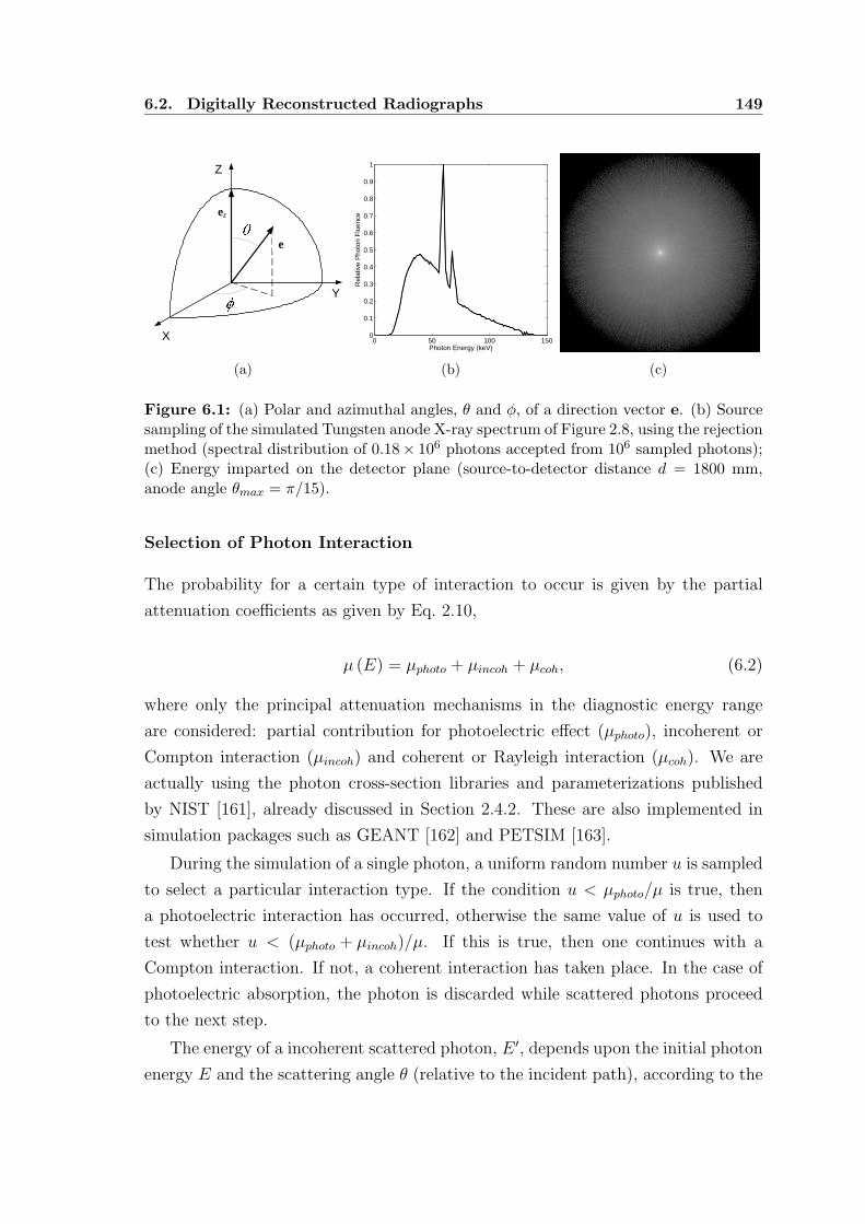
6.2. Digitally Reconstructed Radiographs 149
Y
Z
X
ez
e
(a)
0 50 100 1500
0.1
0.2
0.3
0.4
0.5
0.6
0.7
0.8
0.9
1
Photon Energy (keV)R
elat
ive
Pho
ton
Flu
ence
(b) (c)
Figure 6.1: (a) Polar and azimuthal angles, θ and φ, of a direction vector e. (b) Sourcesampling of the simulated Tungsten anode X-ray spectrum of Figure 2.8, using the rejectionmethod (spectral distribution of 0.18× 10⁶ photons accepted from 106 sampled photons);(c) Energy imparted on the detector plane (source-to-detector distance d = 1800 mm,anode angle θmax = π/15).
Selection of Photon Interaction
The probability for a certain type of interaction to occur is given by the partial
attenuation coefficients as given by Eq. 2.10,
µ (E) = µphoto + µincoh + µcoh, (6.2)
where only the principal attenuation mechanisms in the diagnostic energy range
are considered: partial contribution for photoelectric effect (µphoto), incoherent or
Compton interaction (µincoh) and coherent or Rayleigh interaction (µcoh). We are
actually using the photon cross-section libraries and parameterizations published
by NIST [161], already discussed in Section 2.4.2. These are also implemented in
simulation packages such as GEANT [162] and PETSIM [163].
During the simulation of a single photon, a uniform random number u is sampled
to select a particular interaction type. If the condition u < µphoto/µ is true, then
a photoelectric interaction has occurred, otherwise the same value of u is used to
test whether u < (µphoto + µincoh)/µ. If this is true, then one continues with a
Compton interaction. If not, a coherent interaction has taken place. In the case of
photoelectric absorption, the photon is discarded while scattered photons proceed
to the next step.
The energy of a incoherent scattered photon, E ′, depends upon the initial photon
energy E and the scattering angle θ (relative to the incident path), according to the

150 Chapter 6. 3D Shape Reconstruction from Single Radiographs
Compton Angle-Wavelength relation described by Eq. 2.2:
E ′ =E
1 + γ (1 − cos θ), (6.3)
where γ = E/m0c2 is the reduced energy. One very commonly used method to
sample the energy and direction of Compton scattered photon is the algorithm
developed by Kahn [164]. Kahn´s sampling method is based on a mixed method
and given by the following set of statements [157, 160]:
// Algorithm - Kahn´s Sampling Method
// ----------------------------------
// function t = kahn(gama,test)
gama = E/(m0*c*c)
test = (2*gama + 1) / (2*gama + 9)
r = 2*u1
if ( u2 < test )
UU = 1 + gama*r
if ( u3 > 4*(UU - 1)/(UU*UU) )
t = kahn(gama,test)
t = 1 - r
else
UU = (2*gama + 1)/(gama*r + 1)
t = 1 - (UU - 1)/gama
if ( u4 > (0.5*t*t + 1/UU )
t = kahn(gama,test)
Photon Path Length
Once the interaction type has been selected, the polar scattering angle θ and the
energy loss W are sampled and the azimuthal scattering angle is generated according
to the uniform distribution in [0, 2π], as φ = 2πu. The state of a particle immediately
after an interaction (or after entering the sample or starting its trajectory) is defined
by its position coordinates p = (x, y, z)T, energy E and direction cosines of the
direction of flight, i.e., the components of the unit vector e = (ex, ey, ez)T, as seen
from the laboratory frame OXYZ. Each simulated track is thus characterized by a
series of states p(t), E(t), e(t), where p(t) is the position of the scattering event at
time t, and E(t) and e(t) are the energy and direction cosines of the direction of
movement just after that event.
Let us assume that a track has already been simulated up to a state p(t), E(t),
e(t). The length λ of the photon path to the next collision is then calculated to
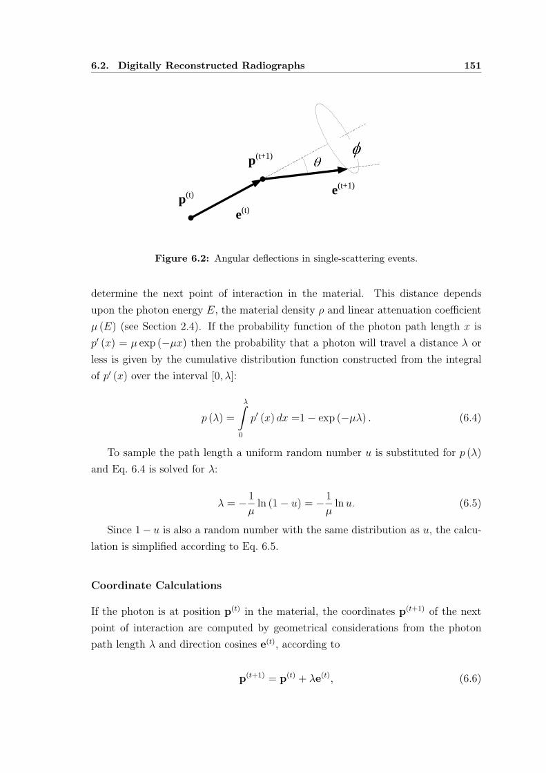
6.2. Digitally Reconstructed Radiographs 151
p(t+1)
e(t)p(t) e(t+1)
Figure 6.2: Angular deflections in single-scattering events.
determine the next point of interaction in the material. This distance depends
upon the photon energy E, the material density ρ and linear attenuation coefficient
µ (E) (see Section 2.4). If the probability function of the photon path length x is
p′ (x) = µ exp (−µx) then the probability that a photon will travel a distance λ or
less is given by the cumulative distribution function constructed from the integral
of p′ (x) over the interval [0, λ]:
p (λ) =
λ∫
0
p′ (x) dx =1 − exp (−µλ) . (6.4)
To sample the path length a uniform random number u is substituted for p (λ)
and Eq. 6.4 is solved for λ:
λ = − 1
µln (1 − u) = − 1
µln u. (6.5)
Since 1− u is also a random number with the same distribution as u, the calcu-
lation is simplified according to Eq. 6.5.
Coordinate Calculations
If the photon is at position p(t) in the material, the coordinates p(t+1) of the next
point of interaction are computed by geometrical considerations from the photon
path length λ and direction cosines e(t), according to
p(t+1) = p(t) + λe(t), (6.6)

152 Chapter 6. 3D Shape Reconstruction from Single Radiographs
where λ is the distance between the previous point p(t) and the new position p(t+1).
The energy of the particle is reduced, E ′ = E − W , and the direction of movement
after the interaction, e(t+1) =(
e′x, e′y, e
′z
)Tis obtained by performing a rotation of
e(t) = (ex, ey, ez)T (see Figure 6.2). The rotation matrix R (θ, φ) is determined by
the polar and azimuthal scattering angles. To explicitly obtain the direction vector
e(t+1) = R (θ, φ) e(t) after the interaction, we first note that, if the initial direction
is along the Z axis, e(t) = eZ = (0, 0, 1)T, the direction after the collision is
sin θ cos φ
sin θ sin φ
cos θ
= RZ (φ)RY (θ)
0
0
1
, (6.7)
where
RY (θ) =
cos θ 0 sin θ
0 1 0
− sin θ 0 cos θ
, RZ (φ) =
cos φ − sin φ 0
sin φ cos φ 0
0 0 1
, (6.8)
are rotation matrices corresponding to active rotations of angles θ and φ about the Y
and Z axes, respectively. On the other hand, if Θ and Φ are the polar and azimuthal
angles of the initial direction
e(t) = (sin Θ cos Φ, sin Θ sin Φ, cos Θ)T , (6.9)
the rotation RY (−Θ)RZ (−Φ) transforms the vector e(t) into eZ. It is then clear
that the final direction vector e(t+1) can be obtained by performing the following
sequence of rotations of the initial direction vector: 1) RY (−Θ)RZ (−Φ), which
transforms e(t) into eZ; 2) RZ (φ)RY (θ), which rotates eZ according to the sampled
polar and azimuthal scattering angles; and 3) RZ (Φ)RY (Θ), which inverts the
rotation of the first step. Hence
R (θ, φ) = RZ (Φ)RY (Θ)RZ (φ)RY (θ)RY (−Θ)RZ (−Φ) . (6.10)
The final direction vector is
e(t+1) = R (θ, φ) e(t) = RZ (Φ)RY (Θ)
sin θ cos φ
sin θ sin φ
cos θ
, (6.11)

6.2. Digitally Reconstructed Radiographs 153
and its direction cosines are
e′x = ex cos θ + sin θ (ez cos φ cos Φ − sin φ sin Φ) ,
e′y = ey cos θ + sin θ (ez cos φ sin Φ + sin φ cos Φ) ,
e′z = ez cos θ − sin θ (sin Θ cos φ) .
(6.12)
The simulation of the track then proceeds by repeating these steps. A track
is finished either when the photon hits the detector, leaves the material system or
when its energy becomes smaller than a given energy, which is the energy where
particles are assumed to be effectively stopped and absorbed in the medium.
In order to reduce the statistical noise to an acceptable level, the number of
photon histories must usually be large, hence leading to a heavy computational
load, still not acceptable in our applied research. The necessity to have a practical
simulation tool at disposal lead to the development of an alternative solution based
on ray tracing techniques we describe next.
6.2.2 Ray Casting Techniques
Volume rendering is typically used to generate images that represent an entire 3D
image dataset in a 2D image. Image-order volume rendering [165], often referred to
as ray casting or ray tracing, is a flexible technique that can be used to render any
volumetric 3D image dataset and can produce a variety of images. The basic idea
is to determine the value of each pixel in the image by sending a ray through the
pixel into the volume according to the geometry parameters of the imaging system.
The data encountered along the ray is evaluated by using some specified function in
order to compute the pixel value.
Using a parallel beam geometry in which all rays are parallel to each other
and perpendicular to the image plane, the Maximum Intensity Projection (MIP) is
probably the simplest way to visualize volumetric data. This case is the standard or-
thographic projection where the ray function determines the maximum value along
the ray producing an image that provides an intuitive understanding of the under-
lying data. Examples are shown in Figure 6.3 where the projections were obtained
from a thoracic CT image from which the patient has been previously segmented as
described in Section 5.4.1. One problem with the MIP is that it is not possible to
tell where the maximum value occurred along the ray.
We now consider ray casting applied to more realistic imaging systems, as illus-
trated in Figure 6.4, corresponding to the point source geometry. The simulated

154 Chapter 6. 3D Shape Reconstruction from Single Radiographs
(a) (b) (c)
Figure 6.3: Maximum intensity projections of a thoracic CT image along a directionperpendicular to the (a) axial, (b) coronal and (c) sagittal plane.
imaging system considers the source, s, located at coordinates (0, 0, d), lying on
the Z axis at a distance d from the origin of the laboratory frame OXYZ. Based
on Eq. 2.18, the simplified monoenergetic case, one can develop a more useful for-
mulation which directly illustrates the distortion due to the point source geometry.
The detector output measured at a point pd = (xd, yd)T lying in the image plane
OXY is given as a function of the logarithmic transmission, also referred to as the
radiological density [166],
Rct (xd, yd) =
pd∫
s
µ (x, y, z) dr, (6.13)
where µ (x, y, z) is the linear attenuation coefficient of the tissue at coordinates
(x, y, z) within a given CT image H (x, y, z). In Eq. 6.13, dr is the line integral
element, dr =√
dx2 + dy2 + dz2 and the ray cast or line integration from s to pd
takes place along a line defined as
x =d − z
dxd,
y =d − z
dyd.
(6.14)
The 2D transmission function at any plane z is therefore magnified by (d − z)/d
at the detector plane.
To compute Eq. 6.13, the size and resolution of the output DRR image is first
specified. The coordinates (xd, yd) for each of the pixels pd in the output image
are first generated and used to determine, from Eq. 6.14, the equation of each

6.3. Shape from Radiological Density 155
Y
Z
X
s
pd
CT Image Detector plane
O
Figure 6.4: Schematic representation of volume rendering using the ray casting technique.
corresponding ray which is cast through the input volume. The position of the CT
volume H between the ray source and screen is such that the normal from the image
plane to the ray source passes directly through the center of the DRR. The ray is
then uniformly sampled and the value of µ is interpolated at intersections of the ray
with equally spaced, parallel planes z. For each ray, the radiological density can be
rewritten in terms of each anatomical structure ξ contained in the volume,
Rct (xd, yd) =∑
ξ
µξMξ (xd, yd), (6.15)
where Mξ (xd, yd) denotes the total thickness of the structure ξ along the ray of
projection that crosses the image plane in pd.
Using the method described in Chapter 5, thoracic CT images of a private im-
age database (HPH) were previously segmented in several anatomical structures
within the patient (body and lungs) and further decomposed into known materials
ξ, namely air, lung tissue, fat tissue, soft tissue and bones structures. Since the
linear attenuation µξ of these intervening materials is available (see Table 5.1), real-
istic radiographic images can be obtained by using the simple ray casting technique.
6.3 Shape from Radiological Density
3D shape recovering of anatomical structures from a single planar radiograph is
an inverse, severely ill-posed problem that has an infinite number of solutions. To
transform it into a problem with a single solution, the typical characteristic of the
structures to be recovered must be taken into account. Therefore, the first step of

156 Chapter 6. 3D Shape Reconstruction from Single Radiographs
Figure 6.5: Radiological density images R(s)ct (xd, yd) generated from 3D patient-specific
voxelized phantoms using the ray casting technique. The phantoms correspond to seg-mented CT images of a private database (HPH) using the method based on materialdecomposition described in Section 5.4.
the proposed reconstruction method is the estimation of thickness maps whose gray
level at every pixel in the image plane is the expected thickness of the anatomical
structures of interest along the ray of projection that crosses that pixel. Such maps
can be computed as follows.
6.3.1 Thickness Maps
Let H(s) (x, y, z), s = 0, 1, . . . , S − 1, be a volumetric CT image of the database
containing S images. For each volumetric image H(s), volume rendering was imple-
mented to generate DRR images from the corresponding 3D patient-specific vox-
elized phantom obtained after the material decomposition has been applied. From
Eq. 6.15, the DRR output is the radiological density image computed as
R(s)ct (xd, yd) =
∑
ξ
µξM(s)ξ (xd, yd). (6.16)
Results of such projections are shown in Figure 6.5 for some CT images of the
database. The simulated images, of size 352 × 352 and pixel spacing dX = dY =
1.0 mm, were obtained with a source-to-detector distance d = 1800 mm. The
thickness maps M(s)ξ (xd, yd) corresponding to the 4 images of the first row are shown
in Figure 6.6 and Figure 6.7. The maps were computed for all structures ξ segmented

6.3. Shape from Radiological Density 157
in the patient during the 3D phantom construction algorithm. Figure 6.6 shows the
maps corresponding to the intervening materials of the lung structures, namely air
within the lung parenchyma, air contained in the large airways and lung tissue.
For the body of the patient, mainly composed of fat tissue, soft tissue and bones
structures, the results are shown in Figure 6.7 for the same volumetric datasets.
Let suppose that the model-to-image registration method described in Section 4.4
is now applied for segmenting the lung fields in each of the radiological density images
R(s)ct . Using the mean shape to represent these regions in each simulated image, a
point-to-point correspondence exists between the detected lung contour points and
simulated images can be warped to each other. This is a typical model-to-model
registration problem with point correspondence from which mean thickness maps
are now computed for each structure. Consider now the lung deformable model
represented by its mean shape, the set of N points P = pn, where pn = (xn, yn)T,
n = 0, · · · , N−1, is a point of the lung contour. The lung field segmentation from the
radiological density image R(s)ct (xd, yd) results in the deformed model Q(s) =
q(s)n
,
such that q(s)n =
(
x(s)n , y
(s)n
)T
corresponds to the deformed point pn. The point
correspondence between the two sets P and Q(s) allows to specify a Thin-Plate
Spline (TPS) transform T (s) that maps exactly the set of source landmarks pn onto
the set of target landmarks q(s)n , that is,
q(s)n = T (s) (pn) . (6.17)
Computing S TPS transforms, the simulated images R(s)ct are warped to a com-
mon space, the model space, defined as a rectangular grid of points pd coincident
with the pixels in the image plane. The mean radiological density image Rct (xd, yd)
is then computed for all pixels pd as
Rct (pd) =1
S
S−1∑
s=0
R(s)ct
(
q(s)d
)
, (6.18)
where R(s)ct
(
q(s)d
)
is the density value interpolated in the image R(s)ct , at location
q(s)d , for which q
(s)d = T (s) (pd). From Eq. 6.16, the above expression becomes
Rct (pd) =1
S
S−1∑
s=0
∑
ξ
µξM(s)ξ
(
q(s)d
)
, (6.19)
or

158 Chapter 6. 3D Shape Reconstruction from Single Radiographs
Figure 6.6: Thickness maps M(s)ξ (xd, yd) of segmented lung structures generated from
4 different 3D patient-specific voxelized phantoms using the ray casting technique. Thephantoms correspond to segmented CT images of a private database (HPH) (see Sec-tion 5.4). First row: air within the lung parenchyma; Second row: air within the largeairways; Last row: lung tissue.

6.3. Shape from Radiological Density 159
Figure 6.7: Thickness maps M(s)ξ (xd, yd) of segmented body structures generated from
4 different 3D patient-specific voxelized phantoms using the ray casting technique. Thephantoms correspond to segmented CT images of a private database (HPH) (see Sec-tion 5.4). First row: fat tissue; Second row: soft tissue; Last row: bone structures.

160 Chapter 6. 3D Shape Reconstruction from Single Radiographs
Rct (pd) =∑
ξ
µξ
[
1
S
S−1∑
s=0
M(s)ξ
(
q(s)d
)
]
, (6.20)
and, considering Eq. 6.18,
Rct (pd) =∑
ξ
µξMξ (pd). (6.21)
As expected, the mean radiological density Rct (xd, yd) is calculated from the
mean thickness map Mξ (xd, yd) determined for each structure ξ. These maps are
shown in Figure 6.8. The results were obtained by considering 30 decomposed CT
images of the database. Actually, manual contouring was performed in the corre-
sponding simulated images for delineating the lung fields. Although the model-to-
image registration method has not been tested yet in such images, an automatic seg-
mentation algorithm should be used when a larger database is available to compute
thickness maps. Nevertheless, manual delineation has the advantage of reducing
misregistration errors that could result from a poor computer-based segmentation.
6.3.2 3D Shape Recovery
The 3D reconstruction of anatomical structures of interest from an input digital
chest radiograph X is now considered. We assume that this real image is defined
in the same plane as the simulated images discussed above. We can also hypoth-
esise that the same intervening materials ξ that define the 3D voxelized phantoms
constructed from CT images are present in the planar radiograph X. Therefore, a
similar expression to Eq. 6.21 can be used to express the corresponding radiological
density:
Rxray (xd, yd) =∑
ξ
µξM(X)ξ (xd, yd). (6.22)
The 3D shape recovery is then formulated as the problem of computing, in the
above equation, the maps M(X)ξ at each pixel (xd, yd) in the image, i.e., the total
thickness of each material or structure ξ at that pixel.
We will only consider the simple case of 3D shape recovery, for which a small and
negligible inter-patient variability is assumed. Under this approximation, the mean
thickness maps Mξ in Eq. 6.21 are the solution of the problem and the 3D patient
anatomy is reconstructed by using a point-to-point correspondence. Suppose that
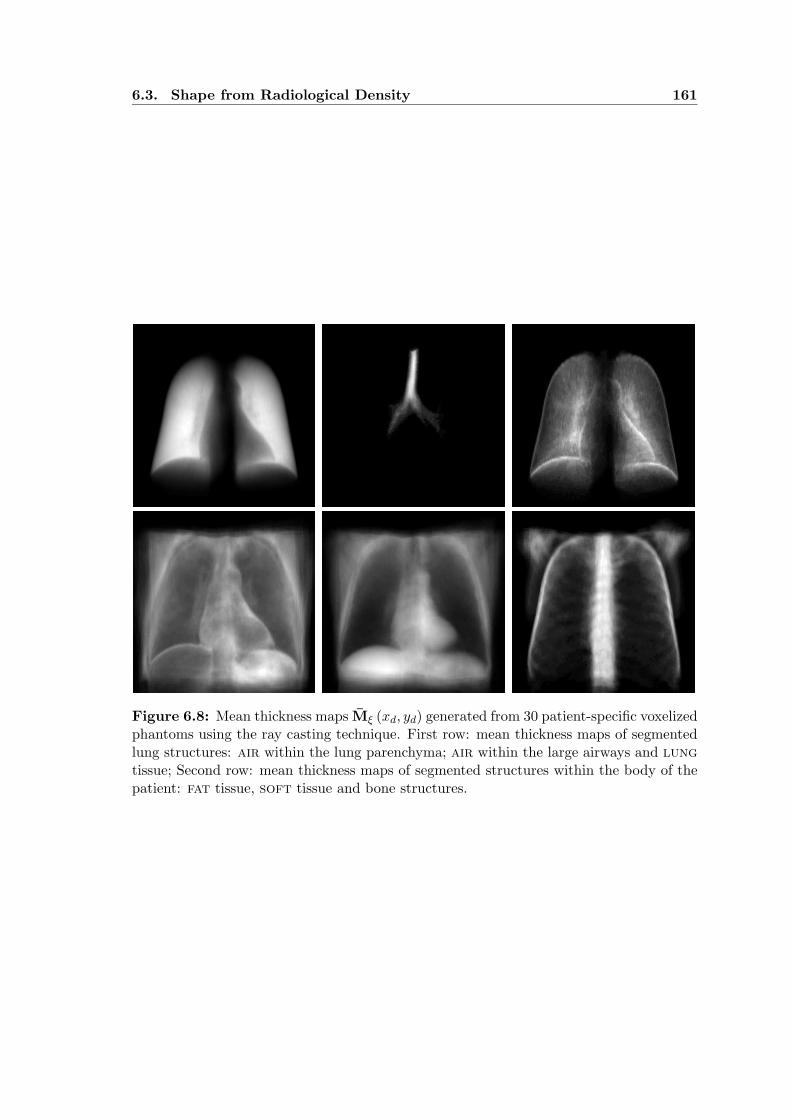
6.3. Shape from Radiological Density 161
Figure 6.8: Mean thickness maps Mξ (xd, yd) generated from 30 patient-specific voxelizedphantoms using the ray casting technique. First row: mean thickness maps of segmentedlung structures: air within the lung parenchyma; air within the large airways and lung
tissue; Second row: mean thickness maps of segmented structures within the body of thepatient: fat tissue, soft tissue and bone structures.

162 Chapter 6. 3D Shape Reconstruction from Single Radiographs
the lung fields have been previously segmented from the chest radiograph X. Using
the model-based segmentation method, the deformed model Q = qn is obtained
and the set of source landmarks qn defines the TPS transform pn = T (qn) that
maps each point qn to the corresponding point pn in the undeformed lung model.
Consequently, the approximate reconstruction is equivalent to assume that
Rxray (qd) ≃ Rct (pd) , (6.23)
where pd = T (qd), for each point pd in the model space, and one solution of the
reconstruction problem is given by
M(X)ξ (qd) ≃ Mξ (pd) . (6.24)
Results of such reconstruction are shown in Figure 6.9. The surfaces represent
the total thickness of the lungs (i.e., the sum of air and lung tissue thicknesses), the
body (fat, soft tissue and bones structures) and the patient (lungs and body). For
each of these structures, the corresponding surface is a function assuming the form
zξ = f (xm, ym), where zξ is the value interpolated at point pm in the map Mξ (pm),
that is, the thickness M(X)ξ (qm) is interpolated at the corresponding point qm. Ac-
tually, the surfaces were reconstructed at each point pm of the triangulated mean
shape of the lung model, although the location of pixels in the entire image could
be considered as well. Note that since the original structures are non-symmetric,
the recovered surfaces are only an approximation of such structures. However, some
properties such as the volume are preserved. It should be noted that if additional
projections of the imaged structures are available, asymmetry constraints can be
directly derived from these images and added to the reconstruction process.
6.3.3 System Calibration
In order to investigate the goodness of the approximation expressed by Eq. 6.23, the
theoretical relationship between the radiological density Rxray (xd, yd) and the gray
level X (xd, yd) of any pixel in digital planar radiograph, measured at the detector
plane, was first derived. The following expression was obtained and reflects the
relationship between these two physical quantities:
Rxray (xd, yd) = k3 ln [X (xd, yd) + k1] + k2 . (6.25)
The above equation is derived in Appendix D, where k1, k2 and k3 are defined

6.3. Shape from Radiological Density 163
Figure 6.9: 3D shape recovery from single radiograph. Different views of the recoveredlung shape (red), body (blue) and patient (green). The thickness of each structure is onlyreconstructed in the region corresponding to the lung fields of the PA chest radiograph.Some landmarks (white spheres) of the segmented lung contour, using the model-to-imageregistration method, are also shown.

164 Chapter 6. 3D Shape Reconstruction from Single Radiographs
0 1 2 3 4 50
1
2
3
4
5
Rxray
Rct
(a)
0 1 2 3 4 50
1
2
3
4
5
Rxray
Rct
(b)
0 1 2 3 4 50
1
2
3
4
5
Rxray
Rct
(c)
Figure 6.10: Radiological density correspondence between calibrated values computedfrom a real planar radiograph, Rxray (xm, ym), and simulated mean values computed fromCT, Rct (xm, ym). Correspondence is plotted for the 913 points pm of the triangulatedmean shape of the lung model for different sets of calibration parameters (k1, k2, k3): (a)(1.01, 0.11, 5.26), (b) (1.01, 0.68, 2.49) and (c) (0.81, 0.08, 5.26).
as calibration constants related to the physical and geometrical parameters of the
X-ray imaging system used to acquire the original radiograph.
Once the image formation has been linearized, different sets of calibration pa-
rameters (k1, k2, k3) were used to evaluate Eq. 6.25. The radiological density images
were matched point-wise by plotting the pairs(
Rxray, Rct
)
for each point pm of the
triangulated mean shape of the lung contour. Figure 6.10 illustrates the resulting
correspondence, for which the constants were manually set to k1 = 1.01, k2 = 0.11,
k3 = 5.26 (Figure 6.10(a)), k1 = 1.01, k2 = 0.68, k3 = 2.49 (Figure 6.10(b)), and
k1 = 0.81, k2 = 0.08, k3 = 5.26 (Figure 6.10(c)). For the case of perfect match,
one should obtain Rxray = Rct for each point pm. Actually, the constants should be
experimentally determined by using precisely manufactured calibration objects.
6.4 Concluding Remarks
We have proposed a method for estimating the thickness of the major anatomical
structures present in a single PA chest radiograph. To recover the 3D shape of such
structures, volume rendering of segmented CT images was performed to obtain real-
istic simulated radiological density images. Taking into account the characteristics
of the X-ray imaging system used to acquire the input radiograph, such DRRs con-
tain the necessary information of the anatomy. A potentially significant difference
between simulated and real radiographs can arise because of changes or differences

6.4. Concluding Remarks 165
in the patient or environment.
Although the proposed algorithm was illustrated for a simple case, we believe
that the adopted approach for 3D shape recovery from a single radiograph is promis-
ing. Incorporating dual-energy radiography principles, algorithms for selective can-
cellation of unwanted tissues are currently under development. Experimental cali-
bration of the medical X-ray imaging system is still needed.


Chapter 7
GENERAL CONCLUSIONS AND
FUTURE DIRECTIONS
The work presented in this thesis is centered on the segmentation of medical X-ray
images of the human thorax for which knowledge-based approaches were adopted
and fully automated computer algorithms were developed. These are now discussed
in the light of the results reported in the thesis which has focused on the lung
field extraction from standard PA chest radiographs and the material decomposi-
tion of volumetric CT images. Exploiting the relationship between CT data and
radiographic measurements, 3D reconstruction algorithms were designed to inte-
grate such imaging modalities into a single application for recovering the 3D shape
of anatomical structures from single radiographs.
In Chapter 4, two methods were presented to accurately identify the unobscured
regions that define the lung fields in digital PA chest radiographs. The proposed
methods exploit both the strength of model-based approaches and optimization
techniques. The first method is a contour delineation method for which an optimal
path finding algorithm based on dynamic programming was implemented. The
second approach consists on a model-to-image registration framework where genetic
algorithms are used as a global optimization technique.
Several aspects are common to both methods. First, they are based on the same
geometrical model that defines the lung region of interest. From a training set of
manually contoured images, a point distribution model, the lung contour model,
was constructed to reflect the normal anatomy of such structure observed in chest
radiographs. The optimal path finding algorithm was used to search for the segments
defined in the contour model and non-rigid deformations of the same model were
considered in the registration method. Second, the same cost images were used to
compute the cumulative cost of the searched paths and define the fitness functions
of the genetic algorithm, in order to evaluate each individual in the population.

168 Chapter 7. General Conclusions and Future Directions
The construction of the cost images, as well as the geometrical model, is based on
the characteristics of the detected lung borders. To compute these images, a multi-
resolution bank of Gaussian filters was used although other kernel filters could be
considered as well. Since this processing step is time consuming, directional filtering
was performed on the input radiograph by using only 2 directions and 3 different
scales. Image features resulting from this step, previously normalized, were finally
combined to compute the cost images.
The main difference between the two proposed segmentation methods is that
dynamic programming is applied to search for each optimal path, one-by-one, while
the genetic algorithm is used to search for the best location of anatomical landmarks
and therefore the position of all the model points simultaneously.
Using the contour delineation method, segments are detected by using the same
sequence adopted for manually delineating lung contours in the training set: first,
hemi-diaphragms, then costal edges, lung top sections and lastly mediastinal edges
defining the borders of heart and lung. Once a path has been detected, spatial con-
straints were included to search for the remaining segments, by simply masking their
corresponding cost images. Although defined in different directions, optimal paths
should be more dependent to each other by applying harder geometrical constraints.
To implement the model-to-image registration a real coded genetic algorithm was
adopted. We proposed a very simple representation of initial solutions: strings of
random numbers sampled from a normal distribution. In fact, this approach is intu-
itive and naturally encodes instances of the deformed model by defining landmarks
displacements as local random perturbations. Using this representation, decoding
is straightforward and statistical information derived for each landmark during the
model construction step is easily added. To deform the model, a thin-plate splines
landmark-based transform was used. The choice of the number of landmarks is a
compromise between the number of degrees of freedom of the deformable model and
the time spent to segment a chest radiograph. Actually, this is the main bottleneck
in terms of execution speed of the segmentation-by-registration method.
The model-to-image registration method is flexible enough to consider other
transformation models, optimizers and metrics. With genetic algorithms, additional
care is required since the evolution of the registration process highly depends on the
choice of recombination operators. Some improvements in the design of such opti-
mization technique are currently being investigated. For example, implementations
of new crossover and mutation operators based on the bilateral symmetry observed
in PA chest radiographs have already been included in the proposed segmentation
169
method. These are under evaluation. We are also considering the incorporation of
local hill climbers. Because principal component analysis was used to construct the
statistical shape model, we believe that active shape models can be included into
the registration method in a straightforward manner.
Evaluated on the private image database, the two proposed segmentation meth-
ods performed equally. An interesting observation is that, for the same radiograph,
different types of segmentation failures occur. This suggest the implementation of
a mixed method that exploits the strength of both approaches, although none of
the methods was designed to take into account possible abnormal findings. In fact,
lung pathologies such as cardiomegaly and lung consolidation, as observed in the
private database, has negative influence on the performance of lung fields segmen-
tation schemes. The age of the patient also has a large impact on the appearance
of the anatomy. Therefore, specific classes of images should be treated separately.
The use of different specific databases for different patient groups e.g. based on age
and sex should also improve the performance of such segmentation algorithms.
Although the applicability of the proposed segmentation methods has proven to
be effective in standard PA chest radiographs, the methods are sufficiently general to
be applied in lateral radiographs as well. Both the contour delineation method and
the model-to-image registration approach are intended to be used in such images,
by taking into account most of the considerations above mentioned.
In Chapter 5, fully automated segmentation algorithms for decomposing vol-
umetric CT images into several anatomical structures are presented. Based on
material decomposition applied to CT numbers, a voxel classification strategy was
adopted to construct a 3D patient-specific anthropomorphic phantom from a single
CT image. The resulting voxelized phantom is suitable for radiotherapy planning
and image guided surgery. It is also well indicated for performing several computer
simulations, namely in diagnostic radiology and nuclear medicine. Applications
specifically directed towards CAD were also considered and the method was ex-
tended to accurately extract the lung region of interest from CT images as the final
output of the segmentation procedure.
The proposed decomposition method follows a hierarchical representation of the
patient anatomy. First the thorax of patient is separated from the background
image and, within the patient, the lungs from the body. Combinations of global
thresholding and seeded region growing techniques were used to achieve this goal.
These structures were further decomposed into known intervening materials, namely
air, lung, fat and soft tissues and bony structures, defined in a simple anatomical

170 Chapter 7. General Conclusions and Future Directions
model. Such decomposition was conveniently illustrated by using the basis plane
representation. The identification of high density structures containing the skeleton
is one of the final steps of the segmentation method. We plan to include suitable
algorithms to further decompose the skeleton into its different components such as
the scapula, vertebrae and individual ribs. The segmentation of other structures
like the sternum could represent a harder task since the corresponding CT numbers
are often similar to those of soft tissues. It is also our intention to obtain a more
realistic representation of the human thorax by including other anatomical structures
in the model. For example, a specific algorithm should be designed to delineate the
mediastinum and therefore distinguish it from other soft tissues lying outside the
thoracic cage.
We are currently collecting several thoracic CT datasets into a single image
database. Although a small number of images is available at the moment, results
of applying the proposed method to all of them reflect its robustness. A set of
reproducible segmentation thresholds was obtained. Although different threshold
values were used to separate the patient from the background image and extract the
lungs from the body, local thresholding techniques applied near the boundary of such
adjacent structures should be used to improve the detection of the corresponding
interfaces.
Voxelized phantoms were used to characterize each of the segmented anatomical
structures in terms of their physical and geometrical properties, by computing their
mean CT number and volume fraction. Using such information, the construction
of realistic physical phantoms for the calibration and optimization of medical X-ray
imaging systems is under consideration.
In the broader context of CAD, the method was extended for extracting the lung
fields, providing an accurate delineation of such anatomical region of interest usually
required by most pulmonary image analysis applications. Here, we implemented an
algorithm to identify and extract the large airways from the lung parenchyma. This
was used to improve the separation of the right and the left lung, by means of a
robust 3D optimal surface detection algorithm based on dynamic programming.
Chapter 6 exploits the relationship between CT data and radiographic measure-
ments. Several reconstruction algorithms are proposed to integrate such imaging
modalities into a single application for recovering the 3D shape of anatomical struc-
tures from single radiographs. To achieve this goal, CT images were previously
decomposed and the resulting voxelized phantoms were used to create realistic digi-
tally reconstructed radiographs. The proposed reconstruction approach is based on

171
thickness maps estimated for each structure to be recovered. Preliminary results
of the 3D shape recovery algorithm are reported. In order to perform a reasonable
reconstruction, all the geometry and the calibration of the original X-ray imaging
device has to be known precisely. For the latter, a formal relationship was derived
to establish the correspondence between the radiological density and the gray level
of any pixel in digital planar radiograph.
Recovering the shape of anatomical structures from single radiographs will likely
produce a number of different radiological images. Statistical models of the appear-
ance of normal chest radiographs may be fitted to input images and subtracted to
enhance possibly abnormal structures. In many digital chest units it is technically
feasible to make two radiographs with different energies at the same time and to
subtract these in order to obtain a dual energy subtraction image in which the bony
structures or other unwanted tissue are virtually invisible. Such images have not
been used in clinical practice, although we believe that sophisticated subtraction
algorithms are likely to become extremely useful and a standard in pre-processing
for CAD in chest radiography.


Appendix A
C++ OPEN SOURCE TOOLKITS
The decision to use the following toolkits was taken due to the quantity of segmen-
tation and visualization tools they offer. As the libraries are implemented in C++
they can be used on most platforms such as Linux, Mac OS and Windows.
A.1 ITK - The Insight Segmentation and
Registration Toolkit
All the computer algorithms presented in the thesis that support the proposed
method were implemented in C++, using the Insight Segmentation and Registra-
tion Toolkit (ITK). ITK is an open-source cross-platform toolkit containing a large
collection of C++ standard template libraries for medical data representation and
processing. It has been developed since 1999 on the initiative of the US National Li-
brary of Medicine, and can be downloaded freely from the ITK web page1. Currently
under active development, ITK employs leading-edge segmentation and registration
algorithms in two, three, and more dimensions [167]. It follows a data-flow approach
that is based on data objects for (image representation) that are manipulated by
filter objects (image processing).
Example Code
The following example code can used for computing the normalized responses R(p)nm,σ
(Eq. 3.4 to Eq. 3.7). The corresponding image processing pipeline is diagrammed in
Figure 3.6. For different values of the parameters σ, n and m, several output image
features are extracted, as shown in Figure 3.7.
1 http://www.itk.org/
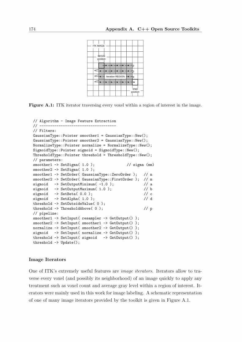
174 Appendix A. C++ Open Source Toolkits
Iteration REGION
ITK IMAGE
BEGINposition
ENDposition
Figure A.1: ITK iterator traversing every voxel within a region of interest in the image.
// Algorithm - Image Feature Extraction
// ------------------------------------
// Filters:
GaussianType::Pointer smoother1 = GaussianType::New();
GaussianType::Pointer smoother2 = GaussianType::New();
NormalizeType::Pointer normalize = NormalizeType::New();
SigmoidType::Pointer sigmoid = SigmoidType::New();
ThresholdType::Pointer threshold = ThresholdType::New();
// parameters:
smoother1 -> SetSigma( 1.0 ); // sigma (mm)
smoother2 -> SetSigma( 1.0 );
smoother1 -> SetOrder( GaussianType::ZeroOrder ); // n
smoother2 -> SetOrder( GaussianType::FirstOrder ); // m
sigmoid -> SetOutputMinimum( -1.0 ); // a
sigmoid -> SetOutputMaximum( 1.0 ); // b
sigmoid -> SetBeta( 0.0 ); // c
sigmoid -> SetAlpha( 1.0 ); // d
threshold -> SetOutsideValue( 0 );
threshold -> ThresholdAbove( 0 ); // p
// pipeline:
smoother1 -> SetInput( resampler -> GetOutput() );
smoother2 -> SetInput( smoother1 -> GetOutput() );
normalize -> SetInput( smoother2 -> GetOutput() );
sigmoid -> SetInput( normalize -> GetOutput() );
threshold -> SetInput( sigmoid -> GetOutput() );
threshold -> Update();
Image Iterators
One of ITK’s extremely useful features are image iterators. Iterators allow to tra-
verse every voxel (and possibly its neighborhood) of an image quickly to apply any
treatment such as voxel count and average gray level within a region of interest. It-
erators were mainly used in this work for image labeling. A schematic representation
of one of many image iterators provided by the toolkit is given in Figure A.1.

A.2. VTK - The Visualization Toolkit 175
(a) (b)
Figure A.2: Visualization examples using VTK. (a) Surface rendering of the segmentedlung parenchyma from a CT image: large airways (blue), lung right (green) and left lung(yellow). Surface clipping of the segmented patient is also shown in the central axial sliceof the image. (b) Visualization of the simulated medical X-ray imaging system for DRRgeneration.
A.2 VTK - The Visualization Toolkit
However, ITK lacks visualization capabilities as its focus is on segmentation and
registration. The ITK framework has a layer that allows it to integrate the Visu-
alization Toolkit (VTK), an open-source, freely available2 software system for 3D
computer graphics, image processing, and visualization [165]. As ITK, VTK con-
sists of a C++ class library designed to support an object oriented paradigm which
allows base image filters to be chained together in a program. VTK was used in
particular pieces of the processing pipeline to produce the image displays and sur-
faces rendering presented in this thesis. Examples illustrating the VTK capabilities
are shown in Figure A.2.
A.3 FLTK - The Fast Light Toolkit
The Fast Light Toolkit (FLTK), a C++ open-source toolkit freely available3, was
used for constructing the graphical user interface displayed in Figure A.3. The
application was developed for the automated segmentation of the lung fields from
2 http://www.vtk.org/3 http://www.fltk.org/

176 Appendix A. C++ Open Source Toolkits
Figure A.3: Lung field segmentation from PA chest radiographs. FLTK graphical userinterface of the application.
chest radiographs to perform the experiments reported in Table 4.3.
The user is allowed to choose one of the two segmentation methods described
in Chapter 4, namely contour delineation (Section 4.3), based on dynamic pro-
gramming (Segment DP) and model-to-image registration (Section 4.4) based on
genetic algorithms (Run SGA). As described in Section 4.5.1, two image databases
are currently available.
The FLTK time probes utility, shown in Figure A.4, was particularly useful to
evaluate the computation time performance of the iterative registration method.
The displayed output and time probes were obtained with the parameters (left side
of the application) listed in Table 4.2. The corresponding fitness evolution is plotted
in Figure 4.9(a).

A.3. FLTK - The Fast Light Toolkit 177
Figure A.4: FLTK time probes utility.


Appendix B
2D PA CHEST RADIOGRAPH
SEGMENTATION RESULTS
The results of the proposed segmentation methods of PA chest radiographs (see Sec-
tion 4.3 and 4.4) are presented in this Appendix and correspond to the experiments
reported in Table 4.3. The results of the contour delineation (DP) and model-to-
image registration (GA) methods using the image databases HSJ and JSRT are
organized as follow:
• DP/JSRT: Table B.1 and Figure B.1 (best 20 of 247 images)
• DP/JSRT: Table B.2 and Figure B.2 (worst 20 of 247 images)
• DP/HSJ : Table B.3, Figure B.3 and Figure B.5 (all 39 images)
• GA/HSJ : Table B.4, Figure B.4 and Figure B.6 (all 39 images)
The segmentation performances are expressed in percent and represent the true
positive fraction (TPF), actually the degree of overlap defined by Eq. 3.33, false
negative fraction (FNF) and false positive fraction (FPF):
TPF =NTP
NTP + NFP + NFN
=|A ∩ B||A ∪ B| , (B.1a)
FNF =NFN
NTP + NFP + NFN
=|A ∩ Bc||A ∪ B| , (B.1b)
FPF =NFP
NTP + NFP + NFN
=|Ac ∩ B||A ∪ B| , (B.1c)
where Ac denotes the set of all pixels not belonging to A. In the above equations,
A and B are the segmented lung region (set of non-zero pixels) resulting from the
manual contouring and the automated methods, respectively. ∩ represents the in-
tersection, ∪ the union of two sets and the operator | · | represents the size (number
of pixels) of a set (see Section 3.8).

180 Appendix B. 2D PA Chest Radiograph Segmentation Results
Table B.1: Lung field segmentation from PA chest radiographs. Segmentation perfor-mance of the contour delineation method using the public image database (DP/JSRT, best20 of 247 images). Segmentation outputs are shown in Figure B.1 .(see also Table 4.4).
ImageRight Lung Left Lung Both Lungs
TPF FNF FPF TPF FNF FPF TPF FNF FPF
NN089 0.95 0.03 0.02 0.95 0.02 0.03 0.95 0.03 0.02NN044 0.94 0.01 0.05 0.95 0.01 0.04 0.95 0.01 0.04NN032 0.95 0.03 0.02 0.95 0.02 0.03 0.95 0.03 0.02NN030 0.96 0.01 0.03 0.95 0.01 0.04 0.95 0.01 0.04NN020 0.95 0.03 0.02 0.95 0.02 0.03 0.95 0.02 0.03LN147 0.96 0.03 0.01 0.94 0.01 0.05 0.95 0.02 0.03LN132 0.96 0.01 0.03 0.93 0.01 0.06 0.95 0.01 0.04LN129 0.94 0.03 0.03 0.95 0.01 0.04 0.95 0.02 0.03LN107 0.96 0.02 0.02 0.94 0.02 0.04 0.95 0.02 0.03LN092 0.94 0.04 0.02 0.96 0.01 0.03 0.95 0.03 0.02NN086 0.94 0.03 0.03 0.95 0.01 0.04 0.94 0.02 0.04NN077 0.94 0.01 0.05 0.94 0.01 0.05 0.94 0.01 0.05NN069 0.94 0.03 0.03 0.94 0.00 0.06 0.94 0.02 0.04NN063 0.94 0.02 0.04 0.94 0.02 0.04 0.94 0.02 0.04NN061 0.94 0.02 0.04 0.94 0.02 0.04 0.94 0.02 0.04NN060 0.95 0.02 0.03 0.92 0.02 0.06 0.94 0.02 0.04NN059 0.93 0.03 0.04 0.94 0.01 0.05 0.94 0.02 0.04NN054 0.94 0.03 0.03 0.94 0.01 0.05 0.94 0.02 0.04NN051 0.95 0.02 0.03 0.94 0.01 0.05 0.94 0.02 0.04NN049 0.95 0.01 0.04 0.94 0.03 0.03 0.94 0.02 0.04

181
Figure B.1: Segmentation outputs of the contour delineation method using the publicimage database (DP/JSRT, best 20 of 247 images). Performance measures are reportedin Table B.1.

182 Appendix B. 2D PA Chest Radiograph Segmentation Results
Table B.2: Lung field segmentation from PA chest radiographs. Segmentation perfor-mance of the contour delineation method using the public image database (DP/JSRT,worst 20 of 247 images). Segmentation outputs are shown in Figure B.2 (see also Ta-ble 4.4).
ImageRight Lung Left Lung Both Lungs
TPF FNF FPF TPF FNF FPF TPF FNF FPF
LN077 0.93 0.04 0.03 0.51 0.01 0.48 0.68 0.02 0.30LN021 0.94 0.04 0.02 0.51 0.02 0.47 0.69 0.03 0.28LN034 0.77 0.02 0.21 0.69 0.01 0.30 0.73 0.01 0.26LN103 0.63 0.02 0.35 0.92 0.05 0.03 0.74 0.03 0.23LN048 0.87 0.12 0.01 0.61 0.02 0.37 0.75 0.07 0.18LN044 0.77 0.05 0.18 0.77 0.01 0.22 0.77 0.04 0.19LN010 0.82 0.03 0.15 0.78 0.07 0.15 0.80 0.05 0.15LN029 0.83 0.01 0.16 0.77 0.01 0.22 0.80 0.01 0.19LN090 0.93 0.04 0.03 0.68 0.10 0.22 0.80 0.07 0.13LN128 0.82 0.02 0.16 0.80 0.03 0.17 0.81 0.02 0.17NN066 0.80 0.04 0.16 0.83 0.02 0.15 0.81 0.03 0.16LN004 0.85 0.02 0.13 0.78 0.03 0.19 0.82 0.02 0.16LN043 0.83 0.04 0.13 0.80 0.07 0.13 0.82 0.05 0.13LN071 0.93 0.04 0.03 0.73 0.02 0.25 0.82 0.03 0.15NN007 0.75 0.24 0.01 0.90 0.03 0.07 0.82 0.15 0.03LN006 0.85 0.03 0.12 0.81 0.02 0.17 0.83 0.03 0.14LN137 0.83 0.11 0.06 0.83 0.12 0.05 0.83 0.11 0.06LN154 0.90 0.07 0.03 0.74 0.21 0.05 0.83 0.13 0.04LN110 0.84 0.03 0.13 0.83 0.01 0.16 0.84 0.02 0.14NN087 0.79 0.13 0.08 0.91 0.02 0.07 0.84 0.08 0.08

183
Figure B.2: Segmentation outputs of the contour delineation method using the publicimage database (DP/JSRT, worst 20 of 247 images). Performance measures are reportedin Table B.2.

184 Appendix B. 2D PA Chest Radiograph Segmentation Results
Table B.3: Lung field segmentation from PA chest radiographs. Segmentation perfor-mance of the contour delineation method using the private image database (DP/HSJ,all 39 images). Segmentation outputs are shown in Figure B.3 and Figure B.5 (see alsoTable 4.5).
ImageRight Lung Left Lung Both Lungs
TPF FNF FPF TPF FNF FPF TPF FNF FPF
HSJ01 0.87 0.10 0.03 0.92 0.07 0.01 0.89 0.09 0.02HSJ02 0.91 0.04 0.05 0.95 0.02 0.03 0.93 0.03 0.04HSJ03 0.91 0.04 0.05 0.87 0.04 0.09 0.89 0.04 0.07HSJ04 0.95 0.03 0.02 0.95 0.03 0.02 0.95 0.03 0.02HSJ05 0.77 0.18 0.05 0.69 0.15 0.16 0.73 0.17 0.10HSJ06 0.82 0.11 0.07 0.90 0.10 0.00 0.86 0.10 0.04HSJ07 0.85 0.08 0.07 0.62 0.19 0.19 0.73 0.14 0.13HSJ08 0.91 0.05 0.04 0.90 0.04 0.06 0.91 0.04 0.05HSJ09 0.94 0.04 0.02 0.95 0.03 0.02 0.94 0.03 0.03HSJ10 0.89 0.06 0.05 0.89 0.05 0.06 0.89 0.05 0.06HSJ11 0.86 0.09 0.05 0.88 0.08 0.04 0.87 0.09 0.04HSJ12 0.92 0.04 0.04 0.93 0.04 0.03 0.92 0.04 0.04HSJ13 0.95 0.03 0.02 0.94 0.04 0.02 0.95 0.03 0.02HSJ14 0.87 0.04 0.09 0.69 0.02 0.29 0.78 0.03 0.19HSJ15 0.92 0.05 0.03 0.92 0.03 0.05 0.92 0.04 0.04HSJ16 0.91 0.06 0.03 0.91 0.04 0.05 0.91 0.05 0.04HSJ17 0.93 0.05 0.02 0.85 0.04 0.11 0.89 0.04 0.07HSJ18 0.93 0.04 0.03 0.93 0.05 0.02 0.93 0.04 0.03HSJ19 0.92 0.05 0.03 0.88 0.06 0.06 0.90 0.06 0.04HSJ20 0.89 0.07 0.04 0.69 0.08 0.23 0.80 0.07 0.13HSJ21 0.87 0.07 0.06 0.90 0.07 0.03 0.88 0.07 0.05HSJ22 0.90 0.05 0.05 0.91 0.06 0.03 0.90 0.06 0.04HSJ23 0.93 0.05 0.02 0.93 0.04 0.03 0.93 0.05 0.02HSJ24 0.81 0.18 0.01 0.92 0.04 0.04 0.87 0.11 0.02HSJ25 0.83 0.05 0.12 0.89 0.05 0.06 0.86 0.05 0.09HSJ26 0.90 0.05 0.05 0.88 0.10 0.02 0.89 0.07 0.04HSJ27 0.85 0.09 0.06 0.90 0.05 0.05 0.88 0.07 0.05HSJ28 0.84 0.06 0.10 0.65 0.09 0.26 0.74 0.08 0.18HSJ29 0.83 0.16 0.01 0.89 0.09 0.02 0.86 0.13 0.01HSJ30 0.89 0.08 0.03 0.81 0.12 0.07 0.85 0.10 0.05HSJ31 0.89 0.09 0.02 0.73 0.21 0.06 0.81 0.15 0.04HSJ32 0.88 0.11 0.01 0.92 0.07 0.01 0.90 0.09 0.01HSJ33 0.86 0.05 0.09 0.77 0.10 0.13 0.81 0.07 0.12HSJ34 0.85 0.04 0.11 0.87 0.12 0.01 0.86 0.08 0.06HSJ35 0.88 0.04 0.08 0.92 0.05 0.03 0.90 0.05 0.05HSJ36 0.88 0.05 0.07 0.90 0.08 0.02 0.89 0.07 0.04HSJ37 0.83 0.13 0.04 0.90 0.09 0.01 0.86 0.11 0.03HSJ38 0.84 0.15 0.01 0.88 0.11 0.01 0.87 0.13 0.00HSJ39 0.38 0.04 0.58 0.89 0.11 0.00 0.52 0.06 0.42

185
Table B.4: Lung field segmentation from PA chest radiographs. Segmentation per-formance of the model-to-image registration method using the private image database(GA/HSJ, all 39 images). Segmentation outputs are shown in Figure B.4 and Figure B.6(see also Table 4.6).
ImageRight Lung Left Lung Both Lungs
TPF FNF FPF TPF FNF FPF TPF FNF FPF
HSJ01 0.90 0.07 0.03 0.87 0.05 0.08 0.89 0.06 0.05HSJ02 0.93 0.01 0.06 0.92 0.02 0.06 0.92 0.02 0.06HSJ03 0.90 0.06 0.04 0.93 0.05 0.02 0.91 0.05 0.04HSJ04 0.93 0.01 0.06 0.92 0.04 0.04 0.93 0.02 0.05HSJ05 0.83 0.12 0.05 0.79 0.06 0.15 0.81 0.09 0.10HSJ06 0.58 0.07 0.35 0.65 0.03 0.32 0.61 0.05 0.34HSJ07 0.79 0.05 0.16 0.70 0.05 0.25 0.74 0.05 0.21HSJ08 0.88 0.09 0.03 0.92 0.05 0.03 0.90 0.07 0.03HSJ09 0.93 0.02 0.05 0.93 0.03 0.04 0.93 0.02 0.05HSJ10 0.91 0.05 0.04 0.90 0.03 0.07 0.91 0.04 0.05HSJ11 0.83 0.05 0.12 0.84 0.03 0.13 0.83 0.04 0.13HSJ12 0.89 0.06 0.05 0.89 0.04 0.07 0.89 0.05 0.06HSJ13 0.92 0.05 0.03 0.92 0.04 0.04 0.92 0.04 0.04HSJ14 0.81 0.05 0.14 0.85 0.05 0.10 0.83 0.05 0.12HSJ15 0.93 0.03 0.04 0.92 0.05 0.03 0.93 0.04 0.03HSJ16 0.90 0.03 0.07 0.89 0.06 0.05 0.90 0.05 0.05HSJ17 0.85 0.12 0.03 0.90 0.08 0.02 0.87 0.10 0.03HSJ18 0.87 0.12 0.01 0.91 0.05 0.04 0.89 0.09 0.02HSJ19 0.85 0.10 0.05 0.86 0.05 0.09 0.86 0.08 0.06HSJ20 0.83 0.06 0.11 0.69 0.06 0.25 0.77 0.06 0.17HSJ21 0.86 0.04 0.10 0.78 0.12 0.10 0.82 0.08 0.10HSJ22 0.92 0.06 0.02 0.93 0.03 0.04 0.92 0.05 0.03HSJ23 0.93 0.04 0.03 0.93 0.03 0.04 0.93 0.04 0.03HSJ24 0.88 0.10 0.02 0.92 0.04 0.04 0.90 0.07 0.03HSJ25 0.86 0.06 0.08 0.91 0.03 0.06 0.88 0.05 0.07HSJ26 0.91 0.04 0.05 0.88 0.09 0.03 0.90 0.06 0.04HSJ27 0.90 0.03 0.07 0.91 0.06 0.03 0.91 0.05 0.04HSJ28 0.81 0.07 0.12 0.92 0.06 0.02 0.86 0.07 0.07HSJ29 0.87 0.13 0.00 0.89 0.10 0.01 0.88 0.12 0.00HSJ30 0.76 0.04 0.20 0.78 0.06 0.16 0.77 0.05 0.18HSJ31 0.86 0.11 0.03 0.86 0.11 0.03 0.86 0.11 0.03HSJ32 0.88 0.11 0.01 0.86 0.12 0.02 0.87 0.12 0.01HSJ33 0.88 0.05 0.07 0.91 0.08 0.01 0.90 0.06 0.04HSJ34 0.91 0.07 0.02 0.87 0.13 0.00 0.89 0.10 0.01HSJ35 0.85 0.10 0.05 0.84 0.15 0.01 0.85 0.13 0.02HSJ36 0.88 0.07 0.05 0.89 0.09 0.02 0.89 0.08 0.03HSJ37 0.86 0.10 0.04 0.88 0.06 0.06 0.87 0.08 0.05HSJ38 0.60 0.03 0.37 0.90 0.09 0.01 0.75 0.06 0.19HSJ39 0.84 0.03 0.13 0.82 0.06 0.12 0.83 0.05 0.12

186 Appendix B. 2D PA Chest Radiograph Segmentation Results
Figure B.3: Segmentation outputs of the contour delineation method using the privateimage database (DP/HSJ, all 39 images, contours). Performance measures are reportedin Table B.3.

187
Figure B.4: Segmentation outputs of the model-to-image registration method using theprivate image database (GA/HSJ, all 39 images, contours). Performance measures arereported in Table B.4.

188 Appendix B. 2D PA Chest Radiograph Segmentation Results
Figure B.5: Segmentation outputs of the contour delineation method using the privateimage database (DP/HSJ, all 39 images, confusion matrix). Performance measures arereported in Table B.3.

189
Figure B.6: Segmentation outputs of the model-to-image registration method using theprivate image database (GA/HSJ, all 39 images, confusion matrix). Performance measuresare reported in Table B.4.


Appendix C
3D CT IMAGE SEGMENTATION
RESULTS
In this Appendix, segmentation outputs of the large airways identification algorithm
are presented. The results, shown in Figure C.1, were qualitatively evaluated by an
experienced radiologist to select the best and worst segmentation results from CT
images of a private database (HPH).

192 Appendix C. 3D CT Image Segmentation Results
Figure C.1: Large airways segmentation results (surface rendering). The results areshown for all 30 CT images of a private database (HPH). Qualitative evaluation was usedto select the best and worst segmentation outputs shown in Figure 5.17.

Appendix D
RADIOLOGICAL DENSITY FROM
DIGITAL PLANAR RADIOGRAPH
In this Appendix, the relationship expressed by Eq. 6.25 is deduced. The radiological
density Rxray and the gray level of a digital planar radiograph X are related to each
other by considering the point source geometry of Figure 2.9. We assume that the
X-ray source s is located at position (0, 0, d). The optical transmission at point
pd = (xd, yd)T of the digital image measured at the pixel detector plane OXY is
given by
T (xd, yd) = c1X (xd, yd) + c2, (D.1)
where c1 and c2 are constants related to the process of digitalization. Since the
optical density D = log [1/T ] is related to the imparted energy through Eq. 2.29,
D = η1 log [η2Ep],
log
[
1
c1X (xd, yd) + c2
]
= η1 log [η2Ep (xd, yd, E0)] , (D.2)
and, from Eq. 2.27 and Eq. 2.28,
log
[
1
c1X (xd, yd) + c2
]
=
η1 log
η2Epi (xd, yd, E0) exp
−pd∫
s
µ (x, y, z, E0) dr
.
(D.3)
Equivalently,
log
[
1
c1X (xd, yd) + c2
]
= c3 + c4 log
exp
−pd∫
s
µ (x, y, z, E0) dr
, (D.4)

194 Appendix D. Radiological Density from Digital Planar Radiograph
where the constants c3 and c4 are defined as
c3 = η1 log [η2Epi (xd, yd, E0)] ,
c4 = η1.(D.5)
Since log (x) = c3 + c4 log (y) ⇔ x = 10c3yc4 , Eq. D.4 is rewritten as
1
c1X (xd, yd) + c2
= 10c3
exp
−c4
pd∫
s
µ (x, y, z, E0) dr
, (D.6)
and
1
X (xd, yd) + k1
= c110c3 exp
−c4
pd∫
s
µ (x, y, z, E0) dr
, (D.7)
where the constant k1 = c2/c1 has been introduced. The above relation is equivalent
to
ln [X (xd, yd) + k1] = − ln (c110c3) + c4
pd∫
s
µ (x, y, z, E0) dr. (D.8)
At point (xd, yd) in the detector plane, the final relationship between the radiologic
density Rxray,
Rxray (xd, yd) =
pd∫
s
µ (x, y, z, E0) dr, (D.9)
and the pixel gray level of the digital planar radiograph X is obtained for the
monochromatic case:
Rxray (xd, yd) = k3 ln [X (xd, yd) + k1] + k2 , (D.10)
where the constants k1, k2 and k3 can be computed as
k1 = c2/c1,
k2 = ln (c110c3) ,
k3 = 1/c4.
(D.11)

BIBLIOGRAPHY
[1] L. A. Lehmann, R. E. Alvarez, A. Macovski, and W. R. Brody, “GeneralizedImage Combinations in Dual KVP Digital Radiography,” Medical Physics,vol. 8, no. 5, pp. 659–667, 1981.
[2] A. Macovski, Medical Imaging Systems. Information and Systems ScienceSeries, Englewood Cliffs, NJ: Prentice Hall, 1983.
[3] M. J. Berger and J. H. Hubbell, “XCOM: Photon Cross Sections on a PersonalComputer,” NBSIR 87-3597, 1987.
[4] ICRU, “Tissue substitutes in radiation dosimetry and measurement,” Report
44 of the International Commission on Radiation Units and Measurements,Bethesda, MD, 1989.
[5] E. Storm and H. I. Israel, “Photon cross sections from 1 keV to 100 MeV, forelements Z=1 to Z=100,” Nuclear Data Tables, vol. A7, pp. 565–681, 1970.
[6] J. M. Boone and A. E. Chavez, “Comparison of x-ray cross sections for di-agnostic and therapeutic medical physics,” Medical Physics, vol. 23, no. 12,pp. 1997–2005, 1996.
[7] P. Francois, A. Catala, and C. Scouarnec, “Simulation of x-ray spectral recon-struction from transmission data by direct resolution of the numeric systemAF=T,” Medical Physics, vol. 20, pp. 1695–1703, July 1993.
[8] H. Zaidi, “Relevance of accurate Monte Carlo modeling in nuclear medicalimaging,” Medical Physics, vol. 26, no. 4, pp. 574–608, 1999.
[9] M. R. Ay, M. Shahriari, S. Sarkar, M. Adib, and H. Zaidi, “Monte Carlosimulation of x-ray spectra in diagnostic radiology and mammography usingMCNP4C,” Phys. Med. Biol., vol. 49, pp. 4897–4917, October 2004.
[10] J. M. Boone and J. A. Seibert, “An accurate method for computer-generatingtungsten anode x-ray spectra from 30 to 140 keV,” Medical Physics, vol. 24,no. 11, pp. 1661–1670, 1997.
[11] J. M. Oliveira, A. C. G. Martins, and J. A. Milito, “Analysis of concretematerial through gamma ray computerized tomography,” Brazilian Journal of
Physics, vol. 34, pp. 1020–1023, September 2004.

196 Bibliography
[12] A. Rosenfeld and A. Kak, Digital Picture Processing, vol. I/II. San Diego,CA: Academic Press, 2nd ed., 1982.
[13] R. A. Brooks and G. Dichiro, “Principles of computer assisted tomographyCAT in radiographic and radioisotopic imaging,” Phys. Med. Biol., vol. 21,pp. 689–732, 1976.
[14] G. T. Herman, Image Reconstruction from Projections. New York: AcademicPress, 1980.
[15] A. C. Kak and M. Stanley, Principles of Computerized Tomographic Imaging.New York: IEEE Press, 1988.
[16] R. N. Bracewell, The Fourier Transform and Its Applications. New York:McGraw-Hill Book Company, 1965.
[17] J. W. Goodman, Introduction to Fourier Optics. San Francisco: McGraw-Hill,1968.
[18] J. M. Ollinger and J. A. Fessler, “Positron emission tomography,” IEEE Signal
Processing Magazine, vol. 14, pp. 43–55, 1997.
[19] R. Leahy and J. Qi, “Statistical approaches in quantitative positron emissiontomography,” Stat. Comput., vol. 10, pp. 147–165, 2000.
[20] P. M. Joseph and R. D. Spital, “A method for correcting bone induced artifactsin computed tomography scanners,” Jornal of Comput. Assist. Tomog., vol. 2,pp. 100–108, 1978.
[21] R. E. Alvarez and A. Macovski, “Energy-selective Reconstruction in X-rayComputorized Tomography,” Phys. Med. Biol., vol. 21, pp. 733–744, 1976.
[22] S. J. Riederer, R. A. Kruger, and C. A. Mistretta, “Limitations to iodineisolation using a dual beam non-K-edge approach,” Medical Physics, vol. 8,no. 1, pp. 54–61, 1981.
[23] S. Fabbri, A. Taibi, R. Longo, M. Marziani, A. Olivo, and S. Pani, “Signal-to-noise ratio evaluation in dual-energy radiography with synchrotron radiation,”Phys. Med. Biol., vol. 47, pp. 4093–4105, Octobrer 2002.
[24] K. Chuang and H. Huang, “Comparison of four dual energy image decompo-sition methods,” Phys. Med. Biol., vol. 33, pp. 455–466, August 1988.
[25] M. Marziani, A. Taibi, A. Tuffanelli, and M. Gambaccini, “Dual energy tissuecancellation in mammography with quasi-monochromatic x-rays,” Phys. Med.
Biol., vol. 47, pp. 305–313, 2002.
[26] J. M. Boone, G. S. Shaber, and M. Tecotzky, “Dual energy mammography: adetector analysis,” Medical Physics, vol. 17, pp. 665–675, 1990.

Bibliography 197
[27] D. M. Gauntt and G. T. Barnes, “X-ray tube potencial, filtration and detectorconsiderations in dual energy chest radiography,” Medical Physics, vol. 21,pp. 203–218, 1994.
[28] H. Jung-Tsuoe, R. A. Kruger, and A. S. James, “Comparision of dual andsingle exposure techniques in dual-energy chest radiography,” Medical Physics,vol. 16, pp. 202–209, 1989.
[29] P. Suetens, P. Fua, and A. J. Hanson, “Computational strategies for objectrecognition,” ACM Comput. Surv., vol. 24, pp. 5–61, March 1992.
[30] K. Hohne, H. Fuchs, and S. Pizer, 3D Imaging in Medicine: Algorithms, Sys-
tems, Applications. Berlin, Germany: Springer-Verlag, 1990.
[31] N. Pal and S. Pal, “A review on image segmentation techniques,” Pattern
Recognition, vol. 26, pp. 1277–1294, 1993.
[32] A. K. Jain, Fundamentals of Digital Image Processing. Englewood Cliffs, NJ:Prentice Hall, Inc., 1989.
[33] R. M. Haralick and L. G. Shapiro, Computer and Robot Vision, vol. 1. Reading,MA: Addison-Wesley, 1992.
[34] L. Ibanez, W. Schroeder, L. Ng, and J. Cates, The ITK Software Guide.Kitware, Inc., 2005.
[35] M. B. Carpenter, Core Text of Neuroanatomy. Baltimore, USA: Willams andWilkins, 4th ed., 1991.
[36] D. J. Field, “Relations between the statistics of natural images and the re-sponse properties of cortical cells,” J. of The Optical Society of America A,vol. 4, no. 12, pp. 2379–2394, 1987.
[37] N. Petkov and P. Kruizinga, “Computational models of visual neurons spe-cialised in the detection of periodic and aperiodic oriented visual stimuli: barand grating cells,” Biol. Cybern., vol. 76, pp. 83–96, 1997.
[38] G. Cristobal and R. Navarro, “Space and frequency variant image enhance-ment based on Gabor representation,” Pattern Recognition Letters, vol. 15,pp. 273–277, 1994.
[39] R. Mehrotra, K. R. Namuduri, and N. Ranganathan, “Gabor filter-based edgedetection,” Pattern Recognition, vol. 25, no. 12, pp. 1479–1494, 1992.
[40] C. Vinhais and A. Campilho, “Genetic model-based segmentation of chest x-ray images using free form deformations,” International Conference ICIAR -
Image Analysis and Recognition, Springer LNCS, vol. 3656, pp. 958–965, 2005.

198 Bibliography
[41] K. Fukushima, “Visual Feature Extraction by a Multilayered Network of Ana-log Threshold Elements,” IEEE Trans. on Systems Science and Cybernetics,vol. SSC-5, pp. 321–333, October 1969.
[42] S. Sahoo, A. Wong, and Y. Chen, “Survey of Thresholding Techniques,” Com-
puter Vision, Graphics and Image Processing, vol. 41, pp. 233–260, 1988.
[43] G. H. Ball and D. J. Hall, “Isodata: a novel method of data analysis andpattern classification,” in Intern. Communications Conference, (Philadelphia,PA), June 1966.
[44] J. C. Bezdek, “A convergence theorem for the fuzzy isodata clustering algo-rithms,” IEEE Trans. on Pattern Analysis and Machine Intelligence, vol. 2,no. 1, pp. 1–8, 1980.
[45] M. Sonka, V. Hlavac, and R. Boyle, Image Processing, Analysis and Machine
Vision. Pacific Grove, CA: PWS Publishing, 1999.
[46] N. Otsu, “A threshold Selection Method from Grey-level Histograms,” IEEE
Trans. on Systems, Man, and Cybernetics, vol. SMC-9, no. 1, pp. 62–66, 1979.
[47] M. Sezgin and B. Sankur, “Survey over image thresholding techniques andquantitative performance evaluation,” Jornal of Electronic Imaging, vol. 13,pp. 146–165, January 2004.
[48] J. K. Udupa and S. Samarasekera, “Fuzzy connectedness and object defini-tion,” Graph. Mod. Im. Proc., vol. 58, no. 3, pp. 246–261, 1996.
[49] R. E. Bellman and S. Dreyfus, Applied Dynamic Programming. Princeton, N.J.: Princeton University Press, 1962.
[50] S. Timp and N. Karssemeijer, “A new 2D segmentation method based on dy-namic programming applied to computer aided detection in mammography,”Medical Physics, vol. 31, no. 5, pp. 958–971, 2004.
[51] Q. Liang, I. Wendelhag, J. Wilkstrand, and T. Gustavsson, “A multiscaledynamic programming procedure for boundary detection in ultrasonic arteryimages,” IEEE Trans. on Medical Imaging, vol. 19, no. 2, pp. 127–142, 2000.
[52] T. Gustavsson, Q. Liang, I. Wendelhag, and J. Wilkstrand, “A dynamic pro-gramming procedure for automated ultrasonic measurement of the carotidartery,” Proc. IEEE Computers Cardiology, pp. 297–300, 1994.
[53] T. F. Cootes, A. Hill, C. J. Taylor, and J. Haslam, “The Use of Active ShapeModels for Locating Structures in Medical Images,” Image and Vision Com-
puting, vol. 12, no. 6, pp. 355–366, 1994.

Bibliography 199
[54] T. F. Cootes, C. J. Taylor, D. H. Cooper, and J. Graham, “Active shapemodels - their training and application,” Computer Vision and Image Under-
standing, vol. 61, no. 1, pp. 38–59, 1995.
[55] J. Gower, “Generalized procrustes analysis,” Psychometrika, vol. 40, pp. 33–51, 1975.
[56] C. Goodall, “Procrustes methods in the statistical analysis of shape,” Journal
of the Royal Statistical Society B, vol. 53 (2), pp. 285–339, 1991.
[57] R. A. Johnson and D. W. Wichern, Multivariate Statistics, a Pratical Ap-
proach. Chapman and Hall, 1988.
[58] T. W. Sederberg and S. R. Parry, “Free-Form Deformation of Solid GeometricModels,” ACM SIGGRAPH Computer Graphics, vol. 20, no. 4, pp. 151–160,1986.
[59] F. L. Bookstein, “Principal warps: Thin-plate splines and the decompositionof deformations,” IEEE Trans. on Pattern Analysis and Machine Intelligence,vol. 11, pp. 567–585, June 1989.
[60] G. I. Sanchez-Ortiz, D. Rueckert, and P. Burger, “Motion and deformationanalysis of the heart using thin-plate splines and density and velocity encodedMR images,” in 16th Statistical Workshop on Image Fusion and Shape Vari-
ability, (Leeds, UK), pp. 71–78, July 1996.
[61] M. Griffin, “Measuring cardiac strain using thin plate splines,” in Proc. Com-
putational Techniques and Applications, (Brisbane, Australia), July 2001.
[62] H. P. Chang, P. H. Liu, H. F. Chang, and C. H. Chang, “Thin-plate spine(tps) graphical analysis of the mandible on cephalometric radiographs,” Den-
tomaxillofacial Radiology, vol. 31, pp. 137–141, 2002.
[63] D. G. Kendall, D. Barden, T. K. Carne, and H. Le, Shape Theory. John Wileyand Sons, LTD, 1999.
[64] C. Darwin, On the origin of species by means of natural selection. London:John Murray, 1st ed., 1859.
[65] J. H. Holland, Adaptation in Natural and Artificial Systems. Ann Arbor, USA:The University of Michigan Press, 1975.
[66] D. E. Goldberg, Genetic Algorithms in Search, Optimization and Machine
Learning. Reading, MA: Addison-Wesley, 1989.
[67] Z. Michalewicz, Genetic Algorithms + Data Structures = Evolution Programs.AI Series, New York: Springer Verlag, 1994.

200 Bibliography
[68] L. Davis, The Handbook of Genetic Algorithms. New York: Van NostrandReingold, 1991.
[69] D. L. Whitley, “A genetic algorithm tutorial,” Stat. Comput., vol. 4, pp. 65–85,1994.
[70] S. Kirkpatrick, C. Gelatt, and M. P. Vecchi, “Optimisation by simulated an-nealing,” Science, vol. 220, pp. 671–680, 1983.
[71] K. Mosegaard and M. Sambridge, “Monte Carlo analysis of inverse problems,”Inverse Problems, vol. 18, pp. R29–R54, April 2002.
[72] T. Lei and W. Sewchand, “Statistical Approach to X-ray CT imaging andits applications in image analysis - part II: a new stochastic model-based im-age segmentation technique for X-ray CT image,” IEEE Trans. on Medical
Imaging, vol. 11, no. 1, pp. 62–69, 1992.
[73] D. L. Collins, A. P. Zijdenbos, V. Kollokian, J. G. Sled, and N. J. Kabani,“Design and construction of a realistic digital brain phantom,” IEEE Trans.
on Medical Imaging, vol. 17, pp. 463–468, 1998.
[74] V. Chalana and Y. Kim, “A methodology for evaluation of boundary detectionalgorithms on medical images,” IEEE Trans. on Medical Imaging, vol. 16,pp. 642–652, October 1997.
[75] J. S. Cardoso and L. Corte-Real, “Toward a Generic Evaluation of Image Seg-mentation,” IEEE Trans. on Medical Imaging, vol. 14, pp. 1773–1782, 2005.
[76] F. C. Monteiro and A. Campilho, “Performance Evaluation of Image Segmen-taion,” Image Analysis and Recognition, Springer LNCS, vol. 4141, pp. 248–259, 2006.
[77] Y. J. Zhang, “A survey on evaluation methods for image segmentation,” Pat-
tern Recognition Letters, vol. 29, pp. 1335–1346, 1996.
[78] H. H. Barrett and W. Swindell, Radiological Imaging, vol. 2. New York: Aca-demic, 1981.
[79] J. Duryea and J. M. Boone, “A fully automated algorithm for the segmentationof lung fields on digital chest radiographic images,” Medical Physics, vol. 22,no. 2, pp. 183–191, 1995.
[80] N. F. Vittitoe, R. Vargas-Voracek, and C. F. Floyd, “Identification of lungregions in chest radiographs using Markov random field modeling,” Medical
Physics, vol. 25, pp. 976–985, 1998.
[81] L. Li, Y. Zheng, M. Kellergi, and R. Clark, “Improved Method for AutomaticIdentification of Lung Regions on Chest Radiographs,” Academic Radiology,vol. 8, pp. 629–638, July 2001.

Bibliography 201
[82] R. E. Alvarez, “Lung Field Segmenting in Dual-Energy Subtraction ChestX-ray Images,” Journal of Digital Imaging, vol. 17, no. 1, pp. 45–56, 2004.
[83] B. van Ginneken and B. H. Romeny, “Automatic segmentation of lung fieldsin chest radiographs,” Medical Physics, vol. 27, no. 10, pp. 2445–2455, 2000.
[84] C. J. V. Rijsbergen, Information Retrieval. London: Butterworths, 2nd ed.,1979.
[85] S. G. Armato, III, M. L. Giger, K. Ashizawa, and H. MacMahon, “Auto-mated lung segmentation in digital lateral chest radiographs,” Medical Physics,vol. 25, no. 8, pp. 1507–1520, 1998.
[86] A. P. Zijdenbos, B. M. Dawant, R. A. Margolin, and A. C. Palmer, “Mor-phometric Analysis of White Matter Lesions in MR Images: Method andValidation,” IEEE Trans. on Medical Imaging, vol. 13, no. 4, pp. 716–724,1994.
[87] R. J. O’Callaghan and D. R. Bull, “Combined Morphological-Spectral Un-supervised Image Segmentation,” IEEE Trans. on Image Processing, vol. 14,pp. 49–62, January 2005.
[88] P. Campadelli, E. Casiraghi, and D. Artioli, “A Fully Automated Methodfor Lung Nodule Detection From Postero-Anterior Chest Radiographs,” IEEE
Trans. on Medical Imaging, vol. 25, pp. 1588–1603, December 2006.
[89] S. B. Lo, S. A. Lou, J. Lin, T. Freedman, M. Chien, and S.Mun, “ArtificialConvolution Neural Network Techniques and Applications for Lung NoduleDetection,” IEEE Trans. on Medical Imaging, vol. 14, no. 4, pp. 711–718,1995.
[90] X. Xu, K. Doi, T. Kobayashi, H. MacMahon, and M. L. Giger, “Developmentof an Improved CAD Scheme for Automated Detection of Lung Nodules inDigital Chest Images,” Medical Physics, vol. 24, no. 9, pp. 1395–1403, 1997.
[91] M. Carreira, D. Cabello, M. Penedo, and A. Mosquera, “Computer-AidedDiagnosis: Automatic Detection of Lung Nodules,” Medical Physics, vol. 25,no. 10, pp. 1998–2006, 1998.
[92] N. Nakamori, K. Doi, V. Sabeti, and H. MacMahon, “Image feature analy-sis and computer-aided diagnosis in digital radiography: automated analysisof sizes of heart and lung in chest images,” Medical Physics, vol. 17, no. 3,pp. 342–35, 1990.
[93] N. Nakamori, K. Doi, H. MacMahon, Y. Sasaki, and S. M. Montner, “Effecton heart-size parameters computed from digital chest radiographs on detec-tion of cardiomegaly: Potencial usefulness for computer-aided diagnosis,” Inv.
Radiology, vol. 26, pp. 546–550, 1991.

202 Bibliography
[94] B. van Ginneken, M. Stegmann, and M. Loog, “Segmentation of anatomicalstructures in chest radiographs using supervised methods: a comparative studyon a public database,” Medical Image Analysis, vol. 10, pp. 19–40, 2006.
[95] S. Sanada, K. Doi, and H. MacMahon, “Image feature analysis and computer-aided diagnosis in digital radiography: Automated detection of pneumothoraxin chest images,” Medical Physics, vol. 19, no. 5, pp. 1153–1160, 1992.
[96] O. Tsujii, M. T. Freedman, and S. K. Mun, “Automated segmentation ofanatomical regions in chest radiographs using an adaptive-sized hybrid neuralnetwork,” Medical Physics, vol. 25, pp. 998–1007, 1998.
[97] B. van Ginneken, Computer-Aided Diagnosis in Chest Radiography. PhD the-sis, Image Sciences Institute, University Medical Center Utrecht, The Nether-lands, 2001.
[98] D. Cheng and M. Goldberg, “An algorithm for segmenting chest radiographs,”Proc. SPIE, vol. 1001, pp. 261–268, 1988.
[99] E. Pietka, “Lung segmentation in digital chest radiographs,” J. Digital Imag-
ing, vol. 7, pp. 79–84, 1994.
[100] X. Xu and K. Doi, “Image feature analysis for computer-aided diagnosis: De-tection of right and left hemidiaphragm edges and delineation of lung fieldchest radiographs,” Medical Physics, vol. 23, pp. 1613–1624, 1996.
[101] G. Armato, M. L. Giger, and H. MacMahon, “Automated lung segmentationin digitized posteroanterior chest radiographs,” Academic Radiology, vol. 5,pp. 245–255, 1998.
[102] F. M. Carrascal, J. M. Carreira, M. Souto, P. G. Tahoces, L. Gomez, andJ. J. Vidal, “Automatic calculation of total lung capacity from automati-cally traced lung boundaries in postero-anterior and lateral digital chest ra-diographs,” Medical Physics, vol. 25, pp. 1118–1131, 1998.
[103] X. Xu and K. Doi, “Image feature analysis for computer-aided diagnosis:Accurate determination of ribcage boundary in chest radiographs,” Medical
Physics, vol. 22, no. 5, pp. 617–626, 1995.
[104] M. S. Brown, L. S. Wilson, B. D. Doust, R. W. Gill, and C. Sun, “Knowledge-based method for segmentation and analysis of lung boundaries in chest X-rayimages,” Computorized Medical Imaging and Graphics, vol. 22, pp. 463–477,1998.
[105] Z. Yue, A. Goshtasby, and L. V. Ackerman, “Automatic Detection of RibBorders in Chest Radiographs,” IEEE Trans. on Medical Imaging, vol. 14,no. 3, pp. 525–536, 1995.

Bibliography 203
[106] B. van Ginneken, S. Katsuragawa, B. M. ter Haar Romeny, K. Doi, and M. A.Viergever, “Automatic detection of abnormalities in chest radiographs usinglocal texture analysis,” IEEE Trans. on Medical Imaging, vol. 21, pp. 139–149,February 2002.
[107] M. F. McNitt-Gray, J. W. Sayre, H. K. Huang, and M. Razavi, “A patternclassification approach to segmentation of chest radiographs,” Proc. SPIE,vol. 1898, pp. 160–170, 1993.
[108] A. Hasegawa, S. C. Lo, M. T. Freedman, and S. K. Mun, “Convolution neuralnetwork based detection of lung structures,” Proc. SPIE, vol. 2167, pp. 654–662, 1994.
[109] M. F. McNitt-Gray, H. K. Huang, and J. W. Sayre, “Feature Selection in thePattern Classification Problem of Digital Chest Radiograph Segmentation,”IEEE Trans. on Medical Imaging, vol. 14, no. 3, pp. 537–547, 1995.
[110] N. F. Vittitoe, R. Vargas-Voracek, and C. E. Floyd., “Markov random fieldmodeling in posteroanterior chest radiograph segmentation,” Medical Physics,vol. 26, pp. 1670–1677, 1999.
[111] B. van Ginneken, A. F. Frangi, J. J. Staal, B. H. Romeny, and M. A. Viergever,“Active shape model segmentation with optimal features,” IEEE Trans. on
Medical Imaging, vol. 21, 2002.
[112] B. van Ginneken, B. H. Romeny, and M. A. Viergever, “Computer-aided Di-agnosis in Chest Radiography: A survey,” IEEE Trans. on Medical Imaging,vol. 20, pp. 1228–1241, December 2001.
[113] H. G. Chotas and C. E. Ravin, “Chest radiography: estimated lung volumeand projected area obscured by the heart, mediastinum, and diaphragm,”Radiology, vol. 193, pp. 403–404, 1994.
[114] C. Vinhais and A. Campilho, “Optimal Detection of Symmetry Axis in DigitalChest X-ray Images,” 1st Iberian Conference IbPRIA 2003 - Pattern Recog-
nition and Image Analysis, Springer LNCS, vol. 2652, pp. 1082–1089, 2003.
[115] A. Kano, K. Doi, H. MacMahon, D. D. Hassell, and M. L. Giger, “Digital im-age subtraction of temporally sequential chest images for detection of intervalchange,” Medical Physics, vol. 21, pp. 453–461, 1994.
[116] T. Ishida, S. Katsuragawa, K. Nakamura, H. MacMahon, and K. Doi, “It-erative image warping technique for temporal subtraction of sequential chestradiographs to detect interval change,” Medical Physics, vol. 26, pp. 1320–1329, 1999.
[117] J. B. A. Maintz and M. A. Viergever, “A survey of medical image registration,”Medical Image Analysis, vol. 2, no. 1, pp. 1–36, 1998.

204 Bibliography
[118] F. Herrera, M. Lonzano, and J. L. Verdegay, “Tackling real-coded geneticalgorithms: Operators and tools for behavioral analysis,” Artificial Intelligence
Review, vol. 12, no. 4, 1998.
[119] L. J. Eshelman and J. D. Schaffer, Real-coded genetic algorithms and interval
schemata. Foundations of Genetic Algorithms II, Morgan Kaufmann Publish-ers, 1993.
[120] J. Shiraishi, S. Katsuragawa, J. Ikezoe, T. Matsumoto, T. Kobayashi, K. Ko-matsu, M. Matsui, H. Fujita, Y. Kodera, and K. Doi, “Development of a digitalimage database for chest radiographs with and without a lung nodule: Re-ceiver operating characteristic analysis of radiologists’ detection of pulmonarynodules,” Amer. J. Roentgenol., vol. 174, pp. 71–74, 2000.
[121] R. Deriche, “Fast algorithms for low level vision,” IEEE Trans. on Pattern
Analysis and Machine Intelligence, vol. 12, no. 1, pp. 78–87, 1990.
[122] R. Deriche, “Recursively implementing the gaussian and its derivatives,” tech-nical report 1883, Unite de recherche INRIA Sophia-Antipolis, April 1993.
[123] I. G. Zubal, C. R. Harrell, E. O. Smith, Z. Rattner, G. Gindi, and B. P. Hoffer,“Computerized 3-dimensional segmented human anatomy,” Medical Physics,vol. 21, no. 2, pp. 299–302, 1994.
[124] S. G. Armato, M. L. Giger, C. J. Moran, K. Doi, and H. MacMahon, “Comput-erized Detection of Lung Nodules in Computed Tomography Scans,” Proceed-
ings of the 1st International Workshop on Computer-Aided Diagnosis, pp. 119–124, 1998.
[125] S. Hu, E. A. Hoffman, and J. M. Reinhardt, “Automatic Lung Segmentationfor Accurate Quantitation of Volumetric X-Ray CT Images,” IEEE Trans. on
Medical Imaging, vol. 20, no. 6, pp. 490–498, 2001.
[126] S. G. Armato, III, M. L. Giger, C. J. Morgan, J. T. Blackburn, K. Doi,and H. MacMahon, “Computorized Detection of Pulmonary Nodules on CTScans,” RadioGraphics, vol. 19, no. 5, pp. 1303–1311, 1999.
[127] J. K. Leader, B. Zheng, R. M. Rogers, F. C. Sciurba, A. Perez, B. E. Chapman,S. Patel, C. R. Fuhrman, and D. Gur, “Automated Lung Segmentation inX-ray Computed Tomography: Development and Evaluation of a HeuristicThreshold-Based Scheme,” Academic Radiology, vol. 10, pp. 1224–1236, 2003.
[128] M. N. Gurcan, B. Sahiner, N. Petrick, H.-P. Chan, E. A. Kazerooni, P. N. Cas-cade, and L. Hadjiiski, “Lung nodule detection on thoracic computed tomog-raphy images: Preliminary evaluation of a computer-aided diagnosis system,”Medical Physics, vol. 29, no. 11, pp. 2552–2558, 2002.

Bibliography 205
[129] M. S. Brown, M. F. McNitt-Gray, N. J. Mankovich, J. G. Goldin, J. Hiller,L. S. Wilson, and D. R. Aberle, “Method for Segmenting Chest CT Image Datausing an Anatomical Model: Preliminary Results,” IEEE Trans. on Medical
Imaging, vol. 16, no. 6, pp. 828–839, 1997.
[130] M. S. Brown, J. G. Goldin, M. F. McNitt-Gray, L. E. Greaser, A. Sapra,K.-T. Li, J. W. Sayre, K. Martin, and D. R. Aberle, “Knowledge-based seg-mentation of thoracic computed tomography images for assessment of splitlung function,” Medical Physics, vol. 27, no. 3, pp. 592–598, 2000.
[131] M. S. Brown, M. F. McNitt-Gray, J. G. Goldin, R. D. Suh, J. W. Sayre,and D. R. Aberle, “Patient-Specific Models for Lung Nodule Detection andSurveillance in CT Images,” IEEE Trans. on Medical Imaging, vol. 20, no. 12,pp. 1242–1250, 2001.
[132] S. G. Armato, III, and W. F. Sensakovic, “Automated Lung Segmentation forThoracic CT: Impact on Computer-Aided Diagnosis,” Academic Radiology,vol. 11, pp. 1011–1021, 2004.
[133] J. Ko and M. Betke, “Chest CT: Automated Nodule Detection and Assessmentof Change over Time: Preliminary Experience,” Radiology, vol. 218, pp. 267–273, January 2001.
[134] W. Mullally, M. Betke, and J. Wang, “Segmentation of nodules on chest com-puted tomography for growth assessment,” Medical Physics, vol. 31, no. 4,pp. 839–848, 2004.
[135] M. Betke, H. Hong, and J. P. Ko, “Automatic 3D Registration of Lung Surfacesin Computed Tomography Scans,” 4th Intern. Conference On Medical Image
Computing and Computer Assisted Intervention - MICCAI’2001, pp. 735–733,2001.
[136] H. Hong, J. Lee, Y. Yim, and Y. G. Shin, “Automatic Segmentation and Reg-istration of Lung Surfaces in Temporal Chest CT Scans,” 3rd Iberian Confer-
ence IbPRIA 2005 - Pattern Recognition and Image Analysis, LNCS, vol. 3523,pp. 463–470, 2005.
[137] B. Li, G. E. Christensen, E. A. Hoffman, G. McLennan, and J. M. Reinhardt,“Establishing a Normative Atlas of the Human Lung: Intersubject Warpingand Registration of Volumetric CT Images,” Academic Radiology, vol. 10,pp. 255–265, 2003.
[138] G. J. Kemerink, R. J. S. Lamers, B. J. Pellis, H. H. Kruize, and J. M. A. vanEngelshoven, “On segmentation of lung parenchyma in quantitative computedtomography of the lung,” Medical Physics, vol. 25, no. 12, pp. 2432–2439, 1998.

206 Bibliography
[139] M. S. Brown, M. F. McNitt-Gray, J. G. Goldin, L. E. Greaser, and D. R.Aberle, “Knowledge-Based Method for Segmentation and Quantitative Anal-ysis of Lung Function from CT,” Proceedings of the 1st International Workshop
on Computer-Aided Diagnosis, pp. 113–118, 1998.
[140] I. Sluimer, M. Prokop, and B. van Ginneken, “Toward Automated Segmen-tation of the Pathological Lung in CT,” IEEE Trans. on Medical Imaging,vol. 24, pp. 1025–1038, August 2005.
[141] L. Zhang, E. A. Hoffman, and J. M. Reinhardt, “Atlas-Driven Lung Lobe Seg-mentation in Volumetric X-Ray CT Images,” IEEE Trans. on Medical Imag-
ing, vol. 25, pp. 1–16, January 2006.
[142] I. Sluimer, A. Schilham, M. Prokop, and B. van Ginneken, “Computer Analysisof Computed Tomography Scans of the Lung: A Survey,” IEEE Trans. on
Medical Imaging, vol. 25, pp. 385–405, April 2006.
[143] C. Vinhais and A. Campilho, “Lung parenchyma segmentation from CT im-ages based on material decomposition,” International Conference ICIAR -
Image Analysis and Recognition, Springer LNCS, vol. 4142, pp. 624–635, 2006.
[144] P. Homolka, A. Gahleitner, M. Prokop, and R. Nowotny, “Optimization ofthe composition of phantom materials for computed tomography,” Phys. Med.
Biol., vol. 47, pp. 2907–2916, August 2002.
[145] C. Ruth and P. M. Joseph, “Estimation of a photon energy spectrum for acomputed tomography scanner,” Medical Physics, vol. 24, pp. 695–702, 1997.
[146] D. Tomazevic, B. Likar, T. Slivnik, and F. Pernus, “3-D/2-D Registration ofCT and MR to X-Ray Images,” IEEE Trans. on Medical Imaging, vol. 22,no. 11, pp. 1407–1416, 2003.
[147] H. Livyatan, Z. Yaniv, and L. Joskowicz, “Gradient-Based 2-D/3-D RigidRegistration of Fluoroscopic X-Ray to CT,” IEEE Trans. on Medical Imaging,vol. 22, pp. 1395–1406, November 2003.
[148] M. Levoy, “Display of surfaces from volume data,” IEEE Comput. Graph.
Appl., vol. 8, pp. 29–37, 1988.
[149] W. Birkfellner, R. Seemann, M. Figl, J. Hummel, C. Ede, P. Homolka,X. Yang, P. Niederer, and H. Bergmann, “Wobbled splatting - a fast per-spective volume rendering method for simulation of x-ray images from CT,”Phys. Med. Biol., vol. 50, pp. N73–N84, April 2005.
[150] L. Westover, “Footprint evaluation for volume rendering,” ACM Comput.
Graph., vol. 24, pp. 367–376, 1990.
[151] R. L. Siddon, “Fast calculation of the exact radiological path for a three-dimensional CT array,” Medical Physics, vol. 12, pp. 252–255, March 1985.

Bibliography 207
[152] X. Li, J. Yang, and Y. Zhu, “Digitally reconstructed radiograph generation byan adaptive Monte Carlo method,” Phys. Med. Biol., vol. 51, pp. 2745–2752,May 2006.
[153] B. Csebfalvi and L. Szirmay-Kalos, “Monte Carlo volume rendering,” Proc.
IEEE Visualization Conf. 2003, pp. 449–456, 2003.
[154] B. Csebfalvi, “Interactive transfer function control for Monte Carlo volumerendering,” Proc. IEEE Symp. on Volume Visualization and Graphics 2004,pp. 33–38, 2004.
[155] M. Sandborg, G. McVey, D. R. Dance, and G. A. Carlsson, “Schemes forthe optimization of chest radiography using a computer model of the patientand X-ray imaging system,” Medical Physics, vol. 28, pp. 2007–2019, October2001.
[156] I. G. Zubal, C. H. Harrell, and P. D. Esser, “Voxel based Monte Carlo Cal-culations of Nuclear Medicine Images and Applied Variance Reduction Tech-niques,” Image and Vision Computing, vol. 10, pp. 342–348, 1992.
[157] D. E. Raeside, “Monte Carlo principles and applications,” Phys. Med. Biol.,vol. 21, pp. 181–197, March 1976.
[158] J. E. Turner, H. A. Wright, and R. N. Hamm, “A Monte Carlo primer forhealth physicists,” Health Phys., vol. 48, pp. 717–733, 1985.
[159] P. Andreo, “Monte Carlo techniques in medical radiation physics,” Phys. Med.
Biol., vol. 36, pp. 861–920, February 1991.
[160] M. Ljungberg, S. Strand, and M. A. King, Monte Carlo Calculations in Nu-
clear Medicine - Applications In Diagnostic Imaging. Medical Science Series,Institute of Physics, 1998.
[161] J. H. Hubbell and S. M. Seltzer, Tables of X-rays Mass Attenuation Coeffi-
cients and Mass Energy-Absorption Attenuation Coefficients. Gaithersburg,MD: National Institute of Standards and Technology, 1997.
[162] R. Brun, F. Bruyant, M. Maire, A. C. McPherson, and P. Zanarini, “GEANT3,” CERN, vol. DD/EE/84-1, 1987.
[163] Y. Picard, C. J. Thompson, and S. Marrett, “Improving the precision andaccuracy of Monte Carlo simulation in positron emission tomography,” IEEE
Trans. on Nucl. Sci., vol. 39, pp. 1111–1116, 1992.
[164] H. Kan, “Application of Monte Carlo,” Report, RM-1237-AEC (abstract),1956.
[165] W. Schroeder, K. Martin, and B. Lorensen, The Visualization Toolkit: An
Object-Oriented Approach To 3D Graphics. Prentice Hall, 4th ed., 2006.

208 Bibliography
[166] R. Polli and G. Valli, “Shape from radiogical density,” Computer Vision and
Image Understanding, vol. 65, pp. 361–381, March 1997.
[167] T. Yoo, Insight into Images, Principles and Practice for Segmentation, Regis-
tration, and Image Analysis. A K Peters, Ltd., 2004.