Soft X-ray Reflectometry and X-ray Absorption Spectroscopy of

Transition Metal Oxide Thin-Films on Various Substrates: Cobaltate

(CoO) and Lanthanum Cobaltate (LaCoO3)

by

Abdullah Radi

M.Sc. Chemistry, the University of Waterloo, 2009 B.Sc. Physics, the University of Jordan, 2005

B.A. Psychology, the University of Jordan, 2001

A THESIS SUBMITTED IN PARTIAL FULFILLMENT OF THE REQUIREMENTS FOR THE DEGREE OF

DOCTOR OF PHILOSOPHY

in

The Faculty of Graduate & Postdoctoral Studies

(Chemistry)

THE UNIVERSITY OF BRITISH COLUMBIA (Vancouver)

March 2017

© Abdullah Radi, 2017

ii

ABSTRACT

The newly developed Soft X-ray Reflectometry (SXR) has been used to study the

electronic structure of Transition Metal Oxide (TMO) thin-films. The technique is non-

destructive, element specific and depth sensitive. The experiments were carried out in the

newly installed Resonant Soft X-ray Scattering (RSXS) endstation1 of the 10ID-2 beamline,

the Canadian Light Source (CLS).2 Simulating and fitting the data required a special home-

written software “ReMagX”3.

X-ray Absorption Spectroscopy (XAS) was measured in Total Fluorescence Yield

(TFY) and Total Electron Yield (TEY), followed by on- and off-Resonant Soft X-ray

Reflectometry (RSXR) at constant energy and at fixed momentum transfer vector in the z-

direction (fixed Qz). The needed samples for the current research were readily available

through research collaborators. CoO thin-films were grown with Molecular Beam Epitaxy

(MBE) on MgO substrate as an example of compressive strain. The LaCoO3 thin-films were

grown with Pulsed Laser Deposition (PLD), with or without a LaAlO3 cap, on LaAlO3,

NdGaO3 or SrTiO3 substrates as examples of compressive and tensile strain.

TEY analysis of the CoO on MgO sample indicates a reduction of symmetry from

cubic octahedral to distorted tetragonal with the crystal compressed in the xy plane. The

surface contamination layer appears as a distinctive feature in the measured reflectivities.

The uncapped LaCoO3 thin-films show distinctive reconstructed surfaces with more

pronounced densities of Co2+ that are energy-feasible ways of compensating the polar

surface. The change in the LaCoO3 on SrTiO3 sample results in vertical stripes which are

believed to have Co ions in mixed valencies and spin-states and were discussed in two

models. The samples have been modeled in ReMagX and the measured TEY signals have

been used to generate the needed refractive indices and atomic scattering factors.

iii

PREFACE

The current thesis forms an original work in both experiment and data analysis. Most

of the figures and illustrations were produced, with 3d Max and Adobe professional

programs, for the current write up or reproduced from reviewed published work as indicated.

The nature of the experimental work required collaboration from several institutes and

research groups each in their specialized area. Our group has been responsible for

suggesting the suitable samples, which we then received from the growers and ran the

analysis experiments. Following that, we constructed the theoretical models for computer

simulation and fitting of the resulted data.

In chapters 1 through 3, I tried to give a brief introduction for the current thesis.

Figure 2.4, Figure 3.1, Figure 3.2 and Figure 3.4 are used from the published work of

Haverkort et al.57, Nielsen et al.72 Attwood at al.73 and Figure 3.5 was reproduced from the

published work of Nielsen et al.72

My part of the experimental work was carried out using the Soft X-ray Scattering

(SXS) endstation which is permanently installed at the Resonant Elastic and Inelastic X-ray

Scattering (REXIS) 10ID-2 beamline, the Canadian Light Source (CLS), Saskatoon,

Canada.2 The machine was designed and manufactured by the group of Dr. Sawatzky,

University of British Columbia (UBC) and Groningen University, as a part of the triple

chamber project which is explained in the current thesis. I was one of the first users for the

SXS endstation and participated in the preparation of the system for commissioning with Dr.

Hawthorn and Dr. He as indicated in Chapter 4: “Experiment and data analysis”. Part of the

chapter depends on a publication with Dr. Hawthorn entitled: “An in-vacuum diffractometer

for resonant elastic soft X-ray scattering”.1 Figure 4.2 is used from the website of the REIXS

beamline and Figure 4.3 is taken from the mutual work with Dr. Hawthorn et al.1 Part of the

chapters depends also on the software documentation of the home-built software ReMagX

which can be found on the program website (www.remagx.org).3 I was one of the first users

of ReMagX and helped Dr. Macke with discussions and suggestions to improve the software

Chapter 5 is a published work as: “Element Specific Monolayer Depth Profiling” S.

Macke, A. Radi, J. E. Hamann-Borrero, A. Verna, M. Bluschke, S. Brück , E. Goering, R.

Sutarto , F. He, G. Cristiani, M. Wu, E. Benckiser, H-U. Habermeier, G. Logvenov, N.

Gauquelin, G. A. Botton, A. P. Kajdos, S. Stemmer, G. A. Sawatzky, M. W. Haverkort, B.

Keimer, V. Hinkov (2014).4 I helped with the measurements of the samples in the REIXS

beamline in the CLS and the discussion of the resulted data and the simulated models. I

iv

have the permission of the authors to use it as a part of the current thesis with minor

changes to the position of figures in the text.

Chapter 6, 7 and 9 are original unpublished work by the author. The needed samples

measured have been received from the group of L. H. Tjeng of Max Planck Institute (MPI) in

Dresden and the group of H. N. Lee at Oak Ridge National Lab (ORNL). Figure 7.2 and

Figure 9.1 are used from the published work of Choi et al.37 and Biskup et al.38

Chapter 8 is a published work as: “Valence-state Reflectometry of Complex Oxide

Heterointerfaces” J. E. Hamann-Borrero, S. Macke, W. S. Choi, R. Sutarto, F. He, A. Radi, I.

Elfimov, R. J. Green, M. W. Haverkort, V. B. Zabolotnyy , H. N. Lee, G. A. Sawatzky, V.

Hinkov (2016). 5 I have the permission of the authors to use it as a part of the thesis. I

helped in the data acquisition and analysis.

In chapter 10, I tried to present some final thoughts and to point out how the current

research could be improved.

It is worth mentioning that during the current study and being in contact with large

groups in both UBC and MPI, I managed to learn several techniques that were very valuable

but were not mainly used in the current work, such as ambient Scanning Tunnelling

Microscopy (STM) with the group of Dr. Bonn, Superconducting Quantum Interference

Device (SQUID) and X-ray Diffraction (XRD) in the Advanced Materials and Process

Engineering Laboratory (AMPEL) research facilities, X-ray Photoelectron Spectroscopy

(XPS), Ultraviolet Photoelectron Spectroscopy (UPS), Scanning Electron Microscopy (SEM),

Auger Electron Spectroscopy (AES), ultrahigh vacuum Scanning Tunneling Microscopy

(STM) all in the omicron Multiprobe X-ray Photoelectron Spectroscopy with Scanning

Tunneling Microscopy (MXPS-STM) chamber in the REIXS beamline in the Canadian Light

Source (CLS).2 In addition to that, I was trained to operate the Molecular Beam Epitaxy

(MBE) chamber and helped growing some Sr-containing samples.

I supported the REXIS beamline users and I trained them to use the facility. I also

helped running experiments on the High Resolution Spherical Grating Monochromator

(SGM) 11ID-1 beamline of the Canadian Light Source,2 in collaboration with the group of Dr.

Damascelli, UBC.

v

TABLE OF CONTENTS

ABSTRACT ........................................................................................................................... ii

PREFACE ............................................................................................................................ iii

TABLE OF CONTENTS ........................................................................................................ v

LIST OF TABLES ............................................................................................................... viii

LIST OF FIGURES ............................................................................................................... ix

LIST OF ABBREVIATIONS .............................................................................................. xxiv

LIST OF SYMBOLS ......................................................................................................... xxvi

ACKNOWLEDGEMENTS................................................................................................. xxvii

DEDICATION ................................................................................................................... xxix

1 General Introduction ...................................................................................................... 1

1.1 Motivation .............................................................................................................. 1

1.2 Background ............................................................................................................ 4

2 Co-Containing Transition Metal Oxide: A Brief Summary , ............................................. 9

2.1 Introduction ............................................................................................................ 9

2.2 Crystal Field Theory ..............................................................................................10

2.3 (3 d) Transition Metals and Transition Metal Oxide thin-films ................................16

2.4 Perovskite Structure ..............................................................................................17

2.5 Polar Surfaces and Surface Reconstruction ..........................................................18

2.5.1 Surfaces of Ionic Crystals...............................................................................18

2.5.2 Polar Catastrophe ..........................................................................................23

2.6 CoO ......................................................................................................................29

2.7 LaCoO3 .................................................................................................................30

3 X-ray Optics,,,, ...............................................................................................................33

3.1 Introduction ...........................................................................................................33

3.2 X-ray Optics ..........................................................................................................33

3.2.1 X-ray Scattering (Semi-classical Approach) ...................................................36

3.2.2 Refractive Index .............................................................................................41

3.2.3 X-ray Scattering (Quantum Mechanical Approach).........................................45

3.2.4 X-ray Reflectometry .......................................................................................48

3.2.5 X-ray Diffraction .............................................................................................53

3.2.6 X-rays to Study Transition Metal Oxides ........................................................54

vi

4 Experiment and Data Analysis .....................................................................................55

4.1 Experiment and Experimental Setup .....................................................................55

4.1.1 Triple Chamber System .................................................................................55

4.1.2 RSXS Endstation1,2 ........................................................................................57

4.1.3 CoO and LaCoO3 Samples ............................................................................65

4.2 Computer Simulation and Data Fit ........................................................................67

5 Element Specific Monolayer Depth Profiling4 ................................................................73

5.1 Experiment ............................................................................................................85

6 X-ray Scattering Experiment and Theoretical Modelling of Compressively Strained CoO

Thin-Film on MgO Supporting Substrate as an Example d7 Binary Oxide Thin-Film ............88

6.1 Introduction ...........................................................................................................88

6.2 Experimental Results ............................................................................................92

6.2.1 XAS of the Uncapped CoO//MgO Sample ......................................................93

6.2.2 SXR of the Uncapped CoO//MgO Sample ......................................................96

6.2.3 Data Simulation and Fitting ............................................................................99

6.3 Discussion........................................................................................................... 101

6.4 Concluding Remarks ........................................................................................... 111

7 X-ray Scattering Study and Theoretical Modelling of Compressively Strained

Lanthanum Cobaltate (LaCoO3) Thin-Films on Lanthanum Aluminate (LaAlO3) Substrates;

Uncapped and Capped with a Layer of Lanthanum Aluminate .......................................... 114

7.1 Introduction ......................................................................................................... 114

7.2 Experiment and Results ...................................................................................... 117

7.2.1 XAS of the Capped and Uncapped LCO//LAO Samples .............................. 118

7.2.2 SXR of the Capped and Uncapped LCO//LAO Samples .............................. 121

7.3 Data Simulation and Fitting ................................................................................. 122

7.4 Discussion........................................................................................................... 123

7.5 Concluding Remarks ........................................................................................... 129

8 Valence-state Reflectometry of Complex Oxide Heterointerfaces5 ............................. 131

8.1 Introduction ......................................................................................................... 131

8.2 Results ................................................................................................................ 133

8.2.1 Choice of the Experimental Technique ......................................................... 133

8.2.2 Sample System ............................................................................................ 134

8.2.3 Obtaining the Optical Constants from XAS ................................................... 135

8.2.4 RXR Measurements and Fits ....................................................................... 136

vii

8.3 Discussion........................................................................................................... 140

8.4 Material and Methods .......................................................................................... 142

8.4.1 Sample Synthesis ........................................................................................ 142

8.4.2 Optical Constant Determination by XAS ....................................................... 142

8.4.3 Valence-state Profiling Based on RXR Data................................................. 143

9 Soft X-ray Reflectivity Study of the Valence, Orbital and Spin Reconstruction of LaCoO3

(LCO) Thin-Film on SrTiO3 (STO) Substrates: The Puzzle of the Vertical Stripes .............. 145

9.1 Introduction ......................................................................................................... 145

9.2 Experiment and Results ...................................................................................... 148

9.2.1 XAS of the Capped and Uncapped LCO//STO Samples .............................. 149

9.2.2 SXR of the Capped and Uncapped LCO//STO Samples .............................. 153

9.2.3 Data Simulation and Fitting .......................................................................... 154

9.3 Discussion........................................................................................................... 159

9.4 Concluding Remarks ........................................................................................... 168

10 General Concluding Remarks ................................................................................. 171

10.1 Suggested Systematic Way to Study Co-containing Materials ............................ 173

References ........................................................................................................................ 178

viii

LIST OF TABLES

Table 2.1 Lattice parameter, polarity, conductivity and lattice structure of various rock salt

and perovskite materials. .................................................................................................... 22

ix

LIST OF FIGURES

Figure 1.1 X-ray measurements of the LaCoO3 (LCO) thin-film on the LaAlO3 (LAO)

substrate capped with a layer of LAO with σ-polarized light at 300K and sample (θ)/detector

(2θ) angles of 20.65°/41.3°. (a) Total electron yield TEY signal, (b) total fluorescence yield

(TFY) and (c) Soft X-ray Reflectometry (SXR) at fixed quantum transfer vector perpendicular

to the sample surface (fixed Qz) at 0.2681 Å-1. All signals are taken around the L2,3

absorption edge of the Co ion at ~779.2 and 793.3 eV respectively. ..................................... 3

Figure 2.1 The five 3d-orbitals reproduced from Ref "". (a) x2-y2, (b) 3z2-r2, (c) xz, (d) yz and

(e) xy. .................................................................................................................................. 10

Figure 2.2 Simplified ball and stick model of the different crystal field symmetries, the white

central ball is the cation and the surrounding purple balls are the anions. (a) Square Planar,

(b) Tetrahedral (Td), (c) Octahedral (Oh), (d) Square Pyramidal, (e) Square Prismatic, (f)

Trigonal Bipyramidal and (g) Pentagonal Bipyramidal. ........................................................ 11

Figure 2.3 Energy diagram for the five 3d orbitals of an element placed in (a) Spherical, (b)

Tetrahedral (Td), (c) Octahedral (Oh) and (d) Square planar crystal fields. It shows the

energy levels further splitting depending on the type of the element coordination. The figures

were reproduced from Ref.61 ............................................................................................... 11

Figure 2.4 Energy level diagram of d5, d6 and d7 for the Co4+, Co3+ and Co2+ ions. It shows

the high (HS), intermediate (IS) and low spin (LS) configurations for each valence state

Ref.57 ................................................................................................................................... 13

Figure 2.5 Energy diagram of the electrons distribution in the 3d orbitals of a d6 model ion in

an Oh crystal field and the changes in the energy levels because of the unit cell expansion in

the 𝑥𝑦 plane as expected in the case of growing Co-containing compound on a supporting

substrate with larger lattice parameter. Jh represents the Hund’s rule exchange like

interaction and ΔOh represents the Oh crystal field splitting. The red arrows represent the

electrons in spin up and spin down. The figure shows how the energy levels change when

ΔOh is larger than Jh and that will stabilize a low spin electron distribution with S = 0. ......... 14

Figure 2.6 Energy diagram of the electrons distribution in the 3d orbitals of a d6 model ion

and the changes in the energy levels because of elongation in the 𝑥𝑦 plane as expected in

the case of growing Co-containing compound on a supporting substrate with larger lattice

x

parameter. 𝐽 ℎ represents the Hund’s rule exchange like interaction and 𝛥𝑂ℎ represents the

Oh crystal field splitting energy. The red arrows represent the electrons in spin up and spin

down. .................................................................................................................................. 15

Figure 2.7 Models of the rock salt structure unit cell for (a) CoO and (b) MgO single crystals.

The numbers on the left of each cell represent the charge of each plane in the (001)

direction. The lattice parameters, structural type and polarity of each crystal can be found in

Table 2.1 ............................................................................................................................. 19

Figure 2.8 Models of the CoO single crystal grown along various direction (a) the (001)

plane, (b) (011) plane and (c) the (111) plane. The numbers on the left of each model

represent the net charge of the specific plane. .................................................................... 20

Figure 2.9 Models of the perovskite structure unit cells for (a) LaCoO3, (b) LaAlO3, (c)

NdGaO3 and (d) SrTiO3 single crystals. The numbers on the left of each cell represent the

charge of each plane in the (001) direction. The lattice parameters, structural type and

polarity of each crystal can be found in Table 2.1. ............................................................... 20

Figure 2.10 Models of the perovskite single crystal grown along various direction. The figure

show that growing the crystal in a specific lattice direction changes the polarity of the crystal

surface. (a) LCO, (b) LAO and (c) NGO are polar in all the directions, with plane charges of

(1±) in along the (001) direction, (4±) in the (011) direction and (3±) in the (111) direction. (d)

The STO crystal along the (001) direction is nonpolar with zero net charges on each plane

but the sample is polar in the (011) and (111), with charges of (4±) in the alternating planes.

............................................................................................................................................ 21

Figure 2.11 Four atomic layer model of the crystal structure of (a) a perfect non-

reconstructed CoO2 terminated LaCoO3 substrate. The associated graph of the electrostatic

potential V (V) versus substrate thickness z (Å), illustrates the divergent potential at the

surface as the ionic crystal undergoes the famous polar catastrophe problem. (b) The polar

crystal undergoes electronic reconstruction by transferring one half charge to the

underneath layers ending up with a finite manageable potential as in the associated graph.

The top layer in the current scenario have a valance change of 50% of the cations from Co3+

to Co4+ reducing the layer charge from (1-) for the unreconstructed 𝐶𝑜3 + 𝑂22 − layer to

(0.5-) for the reconstructed 𝐶𝑜0.53 + 𝐶𝑜0.54 + 𝑂22 − with the bottom layer at (0.5+) through

the add atoms. Other scenarios are also possible and are introduced in later chapters. ...... 23

xi

Figure 2.12 (a) Model of the reconstructed polar LAO crystal. (b) Clean AlO2 terminated LAO

crystal at high temperature during the pulsed laser deposition growing of LCO thin-film. (c)

Model of the reconstructed uncapped LCO thin-film on LAO substrate. (d) Model of the

reconstructed LCO thin-film on LAO substrate capped with a LAO layer. All models have

adspecies and contamination layers that affects the electronic reconstruction process. ...... 26

Figure 2.13 Models of the possible scenarios for the electronic reconstruction of the LCO

thin-film on STO substrate surface to compensate the plane charges and solve the polar

catastrophe problem. The three models show the changes to the top most TiO2 layer of the

STO substrate by valence change of the Ti4+ ion to Ti3+ ion and reduce the plane charge

from 1.0 - to 0.5 – and the changes to the top most layer(s) of the LCO thin-film as (a) 50%

of the Co3+ ions change to Co4+ in high spin and the CoO2 plane charge is reduced from 1.0

- to 0.5-, (b) 50% of the Co3+ ions change to Co2+ in high spin and the CoO2 plane charge

is increased from 1.0 – to 1.5-, together with the LaO plane, which is still at 1.0 +, gives the

needed half plane charge of 0.5- and last (c) it is the same as in (b) but with a top most layer

of the neutral CoO plane with 0 charge which stabilizes the structure.. ............................... 29

Figure 3.1 Models representing the quantum mechanical view of the interaction of radiation

with matter and the resulted interaction Hamiltonian for each case. (a) and (b) are

absorption and Thomson scattering respectively and the Hamiltonian for them ca be

produced using the first order perturbation theory while (c) is the resonant scattering with

second order perturbation. The model shows the two steps transition: Step 1 shows the core

electron as it absorbs an incident photon and move to an empty higher valence state exactly

above the chemical potential (and this is the XAS process) and in Step 2, electron with

similar energy fills the core hole back and emits a photon to complete the fluorescence

process. The figure is taken from Ref.”72” and part c was slightly modified to explain the two-

step process.72 .................................................................................................................... 35

Figure 3.2 Theoretical calculation of the dispersion corrections 𝑓𝑠′𝜔, 𝑓𝑠′′(𝜔) of an arbitrary

system using the equations derived in the script. The imaginary part 𝑓𝑠′′(𝜔), peaks at the

values where 𝜔 = 𝜔𝑠 at the normalized x-axis accompanied by a steep decrease in the real

part 𝑓𝑠′𝜔 and vise versa for the other peak position. The figure is taken from Ref.72 ........... 39

Figure 3.3 The scattering corrections, as a function of energy, near Co L2,3 edges, drawn

from the theoretical Chantler tables.81 ................................................................................. 41

xii

Figure 3.4 The real part of the refractive index near various absorption edges, at different

regions of the radiation spectrum taken from Ref.73 ............................................................. 44

Figure 3.5 (Top) Schematic drawing of multiple reflections and refractions between various

layered materials with different refractive indices (n) within an infinite slab with a total

thickness d the film is composed of N=2 layers and a supporting substrate. (Bottom)

Schematic drawing of Reflection and Refraction across interfaces of materials with different

refractive indices (n). It shows the electric and magnetic fields of the incident, reflected and

transmitted radiation in addition to the momentum associated with each of them. ............... 50

Figure 4.1 The 10ID-2 (REIXS) beamline of the Canadian Light Source (CLS)2 components.

(a) the energy monochromator, (b) the soft X-ray scattering (RSXS) endstation and (c) an

AutoCAD diagram shows the final planned triple chamber system: the RSXS chamber, the

omicron multi-probe system, the molecular beam epitaxy (MBE) chamber and all are

connected through the transfer chamber. ............................................................................ 56

Figure 4.2 The diffractometer inside the RSXS endstation. The 9 motions and the 4

detectors are marked with the white text boxes and the figure was taken from Ref.1 ........... 59

Figure 4.3 A schematic diagram representing the directions for the incident, and scattered

photon. The four polarizations used are: circular left (cl), circular right (cr), linear vertical (σ)

and linear horizontal (π) polarizations with respect to the plane of incidence. The

sample/detector angles or θ/2θ are shown. It also shows the perpendicular direction of the

momentum transfer vector in the z-direction Qz. together with the incident and reflected

momentum vectors. ............................................................................................................. 60

Figure 4.4 (a) Normalized XAS signal (black) in TEY mode for the LCO//LAO sample fitted

off-resonant to the theoretical XAS signal of LCO (purple) which is calculated from the

theoretical Chantler tables near both the Co L2,3 and La M4,5 edges. The two curves are

identical off-resonant where the signal is independent of the chemical environment of the

element and vary substantially on-resonant where the theoretical data is invalid. (c) The

imaginary part (𝑓,,) and the real part (𝑓,) of the Atomic Scattering Factor for the Co element.

............................................................................................................................................ 69

Figure 5.1 Schematic representation of the element specific method. (a) Real (light lines)

and imaginary (dark lines) part of the scattering factors of three different elements; as a

xiii

specific example, we use La3+ (red), Ni3+ (blue) and Pr3+ (green). (b) Assumed chemical

depth profile, i.e. molar concentration for each element. (c) In a first step, the depth profile of

the real and imaginary parts of the susceptibility 𝜒 (𝑧, 𝜔) are calculated. (d) In a second step,

a reflectivity map is calculated. Subsequently, it is compared to a measured map, the

chemical profile is adjusted and steps 1 and 2 are repeated, until convergence is achieved.

............................................................................................................................................ 75

Figure 5.2 SrTiO3 sample 𝛿-doped with Lanthanum. (a) XAS data around the La M5 and M4

edges in total electron yield (TEY) and fluorescence yield (FY) mode. (b) Constant-q

reflectivity scans, measured within the same energy range as the data in a), and compared

with fitted simulation. (c) Constant energy reflectivity scans, compared with fitted simulation.

For clarity, the curves have been multiplied by a factor of 100 with respect to each other.

The two vertical lines mark the oscillations stemming from the STO overlayer. The inset

shows a magnified view of the curve, exposing thickness fringes stemming from the STO

buffer layer, which are marked by vertical lines. (d) Corresponding concentration profile,

encompassing the surface and the buried LaxSr1−xTiO3 layer, obtained from the fits to the

data. The resulting fitted parameters are: 𝑥 = 0.006 and 𝑡0 = (96 ± 1) Å, and the total

thickness of the synthesized heterostructure, including the buffer layer, is 𝑡0 = (1106 ±

10) Å. The inset schematically shows the structure of the entire sample. ........................... 77

Figure 5.3 RXR results on the PrNiO3 film. (a) Representative measured (red lines) and

fitted (black lines) reflectivity scans. (b) Comparison between the measured and the fitted

reflectivity map comprising a total of "31" individual scans, including those shown in a). The

energies of the four resonances La M5, La M4, Ni L3 and Ni L2 are marked with arrows....... 78

Figure 5.4 Initial molar concentration profiles, along with the corresponding fitting

parameters for the PNO/LSAT sample. The three layers into which the sample was

subdivided for the analysis are marked with vertical lines. (D: concentration of the individual

element in the layer, t: thickness of the layer, σ: roughness of the interface of the top of the

layer). .................................................................................................................................. 79

Figure 5.5 Comparison between EELS and RXR results on the PrNiO3 film. (a),

Representative EELS profile around the Pr M4 and Ni L3 edges. The same constant

background was subtracted for both profiles. For each panel, the color scale was chosen

such that the maximal intensity at the corresponding edge is dark red. (b), Elemental depth

xiv

profile for the three elements present in the film, Pr, Ni, and O, obtained from fits to the RXR

data shown in Figure 5.3. The region at the surface marked with darker red contains other

light elements such as carbon and hydrogen, in addition to oxygen. The three layers into

which the sample was subdivided for the analysis are marked with vertical lines. The table

shows the fitting results for the thickness, roughness and concentration characterizing the

profile of each element in the corresponding layer. Roughnesses are valid for the top

interface of the corresponding layer. Note that in the element specific method, not all

elements are present in all layers, and thicknesses can be different within the same layer. 80

Figure 5.6 Comparison of original simulation, based on the thicknesses, roughnesses and

densities obtained from the fit (Figure 5.3 and Figure 5.5), with simulation in which we have

intentionally modified these parameters from their optimal values. The chosen energies

represent an off-resonant value (800 eV), the La M5 edge (834 eV), the Ni L3 (854 eV) and L2

(870 eV) edge, and the Pr M4 edge (948 eV). The original fit exhibits a χ2 value of 2.33

(dashed line). Increasing the substrate interface roughness by one unit cell increases χ2 to

21.14 (yellow line); removing the Pr top layer, i.e. cancelling the thickness difference

between the Ni and the Pr profile, results in χ2 = 4.79 (green line); removing the oxygen

contamination layer results in χ2 = 7.75 (cyan line); Increase the total film thickness by

0.5 u. c. yields χ2 = 3.6 (blue line); and reducing the total density (atomic concentration) of

the film by 20% yields χ2 = 4.94 (magenta line). ................................................................ 82

Figure 5.7 Atomic resolution STEM-EELS measurements of the substrate-film interface of

the PrNiO3 film. The left panel shows an annular dark-field (ADF) STEM measurement,

recorded simultaneously during the EELS spectrum image acquisition. The three right

panels show atomically resolved EELS maps recorded at the La M5, Ni L3 and Pr M5 edges.

The overlap of the Ni L3 and the La M4 edge lead to the false impression of the presence of

Ni in the substrate (see also Figure 5.8). ............................................................................. 83

Figure 5.8 STEM-EELS projected maps at the different edges of the relevant cations in the

PrNiO3 sample. The left panel shows an annular dark-field (ADF) STEM measurement. The

right panels show EELS projected spectra, laterally integrated over the four lattice spacings

shown in the ADF panel (sum over all pixels on each line) to reduce noise. Results are

shown for the La M5 and M4, the Ni L3 and L2, and the Pr M5 and M4 edges. ....................... 84

xv

Figure 5.9 Imaginary part of the individual scattering factors of the elements present in our

films. The scattering factors were obtained from XAS-TEY data, background corrected and

fitted to the tabulated off-resonant values from Chantler tables.81 ........................................ 87

Figure 6.1 Schematic draw of the samples used in the current study, it shows the CoO thin-

films with 8 and 40 nm thickness grown on MgO sample with and without an Al2O3 Capping

layer in addition to one last CoO 8 nm thin-film sandwiched between MgO supporting

substrate and crystalline MgO capping layer. ...................................................................... 92

Figure 6.2 (a) XAS scans of several points across the CoO 8 nm thin-film grown on MgO

substrate. (b) Sketch of the sample holder with the sample as the square in the middle and

the selected points to measure the XAS scans are marked as the red small circles. ........... 93

Figure 6.3 XAS spectra for (a) the capped and (b) the uncapped 8nm CoO thin-film

epitaxially grown on MgO supporting substrate. A comparison between the XAS spectra of

the capped and the uncapped samples taken with (c) σ-polarized and (d) π-polarized light.

All spectra have been taken at room temperature. .............................................................. 94

Figure 6.4 The XAS spectra of the uncapped CoO//MgO sample in TEY mode (a, b) and

TFY mode (c, d) around the (a, c) O K and (b, d) Co L2,3 edges with σ-polarized light and at

300 K. ................................................................................................................................. 95

Figure 6.5 SXR measured at constant energy at 776.3 eV and at (a) 300 and (b) 20 K for the

CoO (8 nm)//MgO with σ-polarized light. The measurements were taken at various times

during the beamtime to track the time evolution of the sample and any possible substantial

changes to the sample. ....................................................................................................... 97

Figure 6.6 (a) TEY signal of the CoO (8 nm)//MgO sample near the O K and Co L2,3 edges at

300K and with σ-polarized light. The vertical red lines are at the selected energies where

reflectivities at constant energies have been measured. (b) The reflectivity at constant

energy of 776.3 eV taken with σ-polarized light and at 300 K. The red vertical lines represent

the Qz values at which the reflectivities at fixed Qz have been measured. ........................... 98

Figure 6.7 X-ray reflectivities near the Co L2,3 absorption edges measured at three fixed Qz

values of (a) 0.0751, (b) 0.3815 and (c) 0.3912 Å-1 with both (I) σ-polarization and (II) π-

polarization in addition to the difference between the spectra in both polarizations (III). The

measurements were taken at temperatures started from 20 K (blue curves) then heated to

xvi

70 (red curves), 160 (green curves) and finally 300 K (black curves). The red vertical lines

are at 776.3, 776.9, 777.5, 777.7, 778.3, 779.2, 779.8, 781, 792.9 and 793.9 eV from (1) to

(10) respectively. ................................................................................................................. 99

Figure 6.8 (a) Reference pure spectra of Co2+ HS (black), Co3+ LS (olive) and Co3+ HS

(magenta), all in octahedral (Oh) symmetry,41 and the Co2+ HS in tetrahedral (Td) symmetry

(cyan). The dashed lines are exactly at the energies of 776.3, 776.9, 777.5, 778.1, 778.8,

779.2, 781, 792.9, 793.3, 793.7, 794.4, and 795.0 eV respectively from (1) to (12) and spans

both L2 and L3 of the Co edge. (b) The imaginary part of the Co scattering factor generated

from the experimental TEY signal (red) of the Co L2,3 edges in CoO//MgO film corrected and

aligned of-resonant to the theoretical Chantler database (green). ..................................... 100

Figure 6.9 A comparison between the XAS spectra around the Co L2,3 edges of the

uncapped 8 nm thick CoO thin-film on MgO (red) taken at 300K and σ-polarized light with

(a) the 9 nm thick CoO//Ag (blue) take at 400 K and 90° angle of incidence,106 and (b) bulk

CoO single crystal.41 .......................................................................................................... 102

Figure 6.10 X-ray reflectivity maps of the CoO(8 nm)//MgO sample taken in the fixed Qz

region between 0.2 - 0.5 Å-1 and at two energy regions (a) 600 - 750 eV and (b) 786 - 792

eV. Both regions are marked with the blue boxes in (c). The sample was measured with σ-

polarized light and at 20 K. ................................................................................................ 104

Figure 6.11 Temperature-dependent SXR at constant energies of the CoO (8 nm)//MgO

sample with σ- and π-polarized light and at (a) 776.3 (b) 791.4 (c) 793.3 (d) 789.7 eV and

various temperatures. ........................................................................................................ 105

Figure 6.12 SXR at constant energies measured at various photon energies off- and on-

resonant for the Co L2,3 absorption edges (black circles) together with the simulated curves

(red curves) for the uncapped CoO//MgO sample at 300 K with σ-polarized light (a) with an

upper O-containing contamination layer or (b) without any contamination layer. The energies

on the right side are in (eV) and the curves are shifted vertically for clarity. The vertical

purple lines are at fixed Qz values 0.0751, 0.1502, 0.1837, 0.2268, 0.2627, 0.3043, 0.3419,

0.3945 and 0.4598 Å-1, at which the scans in Figure 6.13 are measured. .......................... 106

Figure 6.13 SXR at fixed Qz measured at various values around the Co L2,3 absorption

edges (black circles) together with the simulated curves (red curves) for the uncapped

xvii

CoO//MgO sample at 300 K with σ-polarized light. The vertical purple lines are at 776.3,

777.2, 778.4, 779.2 and 781.4 eV. The associated simulated theoretical model can be seen

in Figure 6.14.a. ................................................................................................................ 107

Figure 6.14 Atomic density profiles of each element in the model system used to simulate

the uncapped CoO//MgO at 300 K taken with σ-polarized light as resulted from the element

specific density profile fit after 80 iterations using the evolution algorithm in ReMagX3 (a)

with an O-containing contamination layer and (b) without any contamination layer. The

dashed lines represent the interfaces between the various layers. The models show the

thickness, roughness and density of each element in each layer for both models. ............ 109

Figure 6.15 Theoretical simulated reflectivity map of the CoO (8 nm)//MgO sample produced

with ReMagX3 without the top oxygen contamination layer. The inner rectangle marks the

region which was measured experimentally and has been shown in Figure 6.10.b. .......... 110

Figure 6.16 Reflectivities at constant energies for the CoO on MnO sample before (KBE)

and after (KE) the physisorption of Xe gas on the susrface at 20 K and with various

exposure time, in addition to measurements at 300 K, before (KBC) and after (CAH) cooling

down, all with π-polarized light. ......................................................................................... 113

Figure 7.1 Models of the perovskite structure unit cells for (a) LaCoO3, and (b) LaAlO3,

single crystals. The numbers on the left of each cell represent the charge of each plane in

the (001) direction.67 .......................................................................................................... 115

Figure 7.2 TEM image of the LCO thin-film grown on LAO substrate as it appears in (a)

Ref.39 (b) Ref.37 The white bright dots are traces of the La metal and the dark horizontal

lines with a distance of approximately 3 u.c. are clear and highly organized in (a) and barely

visible in (b). ...................................................................................................................... 115

Figure 7.3 Schematic drawing of the samples used in the current study, it shows from left to

right the LAO/LCO//LAO, LCO//LAO samples and LAO substrate all with the (001)

termination. ....................................................................................................................... 117

Figure 7.4 The XAS spectra of the capped and uncapped LCO//LAO samples in TEY mode

(a, b) and TFY mode (c, d) around the (a, c) Co L2,3 and (b, d) La M4,5 edges with vertical-

polarized light and at 300 K. The inset show the major difference in the shape between the

capped and uncapped LCO//LAO TEY signals at the energies 776.3 and 777.5 eV. ......... 118

xviii

Figure 7.5 (a) TEY pure spectra of Co2+ HS (black), Co3+ LS (olive) and Co3+ HS (magenta),

all in octahedral (Oh) symmetry,41 in addition to the Co2+ HS in tetrahedral (Td) symmetry

(cyan).107 The dashed vertical lines are exactly at the energies of 776.3, 776.9, 777.5, 778.1,

778.8, 779.2, 781.0, 792.9, 793.3, 793.7, 794.4, and 795.0 eV respectively from (1) to (12)

and spans both Co L2,3 edges. (b) The normalized and corrected TEY signal of capped

(blue) and uncapped (red) LCO//LAO samples for 𝜎-polarization at 300 K. (c) Comparison

between the normalized TEY signals of pure Co2+ HS in Oh symmetry (black) and the

excess signal (orange). The numbers from (i) to (iv) are assigned at 777.5, 778.1, 778.8 and

780.0 eV respectively. ....................................................................................................... 120

Figure 7.6 SXR measured at various photon energies off- and on-resonant for the Co L2,3

and La M4,5 absorption edges for the capped LAO/LCO//LAO samples at 300 K with σ-

polarized light. Constant energy scans are on the right side and fixed Qz scans on the left.

The red lines represent the simulated curves and the black circles are the experimental

data. The energies on the right side are in (eV) and the curves are shifted vertically for

clarity. The dashed blue lines indicate the Qz values of the associated measurement that

can be found on the left side, the curves where scaled individually to show their details. The

associated simulated theoretical models can be seen in Figure 7.8.a. .............................. 124

Figure 7.7 SXR measured at various photon energies off- and on-resonant for the Co L2,3

and La M4,5 absorption edges for the uncapped LCO//LAO samples at 300 K with σ-

polarized light. Constant energy scans are on the right side and fixed Qz scans on the left.

The red lines represent the simulated curves and the black circles are the experimental

data. The energies on the right side are in (eV) and the curves are shifted vertically for

clarity. The dashed blue lines indicate the Qz values of the associated measurement that

can be found on the left side, the curves where scaled individually to show their details. The

associated simulated theoretical models can be seen in Figure 7.8.b. .............................. 125

Figure 7.8 Atomic density profiles of each element and valence state in the model systems

used to simulate (a) capped LAO/LCO//LAO at 300 K, and (b) uncapped LCO//LAO as

resulted from the element specific density profile fit using the evolution algorithm in

ReMagX.3 The dashed vertical lines represent the interfaces between the various layers. It

shows the thickness, roughness and density of each element in each layer including the

capped LCO//LAO atomic scattering factor atomic scattering factor and the excess signal, in

addition to the contamination layer represented by an oxygen surface layer. .................... 126

xix

Figure 7.9 The suggested models for (a) the reconstructed polar LAO crystal (with the

surface charge fully compensated through oxygen vacancies or possible adspecies), (b)

clean AlO2 terminated LAO crystal at high temperature during the pulsed laser deposition

growing of LCO thin-film (assuming the oxygen vacancies were filled back), (c) the

reconstructed uncapped LCO thin-film on LAO substrate and the top CoO2 layer shows the

change from Co3+ to Co2+ (with the surface fully compensated through the combined charge

of the top most two layers as shown) and (d) the reconstructed LCO thin-film on LAO

substrate capped with a LAO layer and the surface of the capping layer is full compensated

with in a similar fashion as for the single crystal LAO. All models have adspecies and

contamination layers that affects the electronic reconstruction process. ............................ 128

Figure 8.1 Schematic composition of the samples and scattering geometry. Both samples

consist of LaCoO3 films, about 40 u.c. thick, grown by pulsed laser epitaxy on NdO-

terminated (001)-NdGaO3, with or without an additional LAO capping. All three materials are

polar along the growth direction. We have chosen the z axis of the coordinate system to

point along the surface normal. (a) In the first sample, the polar–nonpolar interface is

vacuum/LCO. (b) In the second sample, the LCO surface is covered by two u.c. of LAO, and

the polar–nonpolar interface is shifted away from LCO to the LAO surface. (c) Specular

scattering geometry with the transferred scattering wave vector q = (0, 0, qz) perpendicularly

to the surface. ................................................................................................................... 133

Figure 8.2 XAS spectra in the vicinity of the Co L3 and L2 absorption edges. Data for the

uncapped sample are shown in black, and for the LAO-capped sample in red. (a) Spectra

measured in TEY mode, scaled with respect to each other as described in the Materials and

Methods section. The blue curve shows the difference spectrum, which we attribute to Co2+.

The inset shows an enlargement around 776 eV, the energy at which Co2+ shows a

characteristic prepeak. (b) Spectra measured in total-fluorescence yield (TFY) mode. (c)

Comparison between our measured difference spectrum from (a), shown in blue, and results

for Co2+ from ref.41, shown in green. .................................................................................. 134

Figure 8.3 RXR data and fits. Data measured in the constant-energy and constant-qz modes

(black symbols) are shown, along with the best obtained fits (red lines), based on the

profiles shown in Figure 8.4. Data points at low qz were corrected for geometry effects111

(see also the Materials and Methods section). (a) Constant-energy scans for the uncapped

sample. (b) Constant-qz scans for the uncapped sample. (c) Constant-energy scans for the

xx

capped sample. (d) Constant-qz scans for the capped sample. The constant-energy data are

shown on a logarithmic scale, the constant-qz on a linear scale. For clarity, the scans have

been shifted along the y axis with respect to each other in (a and c). The constant-qz scans

in (b and d) were measured at the qzi positions marked with blue numbers i in (a and c). .. 136

Figure 8.4 Element and valence depth concentration profiles. (a) Profiles of the uncapped

sample. (b) Profiles of the capped sample. The region at the surface of the samples marked

in lighter red is likely to contain further light elements such as carbon, in addition to oxygen.

All results were obtained by the fitting procedure explained in the main text. .................... 137

Figure 8.5 Crystal structures and schematic charge and valence profiles for both samples.

(a) Uncapped sample with the electronically reconstructed surface following from our

analysis. (b) Sample capped with LAO. The reconstruction of the LAO surface is not known

and beyond the scope of this work. A charge of − 0.5e proximate to the surface follows from

the reconstruction. ............................................................................................................. 139

Figure 8.6 Reconstruction scheme at different stages during the epitaxial sample growth. (a)

The reconstructed substrate surface and backside carry effective charges of − e/2 and e/2

per u.c., respectively. (b,c) With each newly deposited film monolayer, the negative charge

travels to the sample surface, whereas the charge at the substrate back remains

unchanged. ....................................................................................................................... 139

Figure 9.1 TEM image of the uncapped LCO//STO sample taken from the work of Choi et

al.37 The light circles are for the heavy La atoms. Horizontally, two unit cells look to be

normal and retains the lattice parameter of the supporting STO substrate (3.905 Å) and the

third is elongated abnormally (4.544 Å) as reported also in a separated study by Biskup et

al.38 ................................................................................................................................... 146

Figure 9.2 Reproduced models of the two conventional unit cells for the LCO thin-film on

STO substrates that were suggested to explain the observed stripe pattern noticed in the

TEM images. (a) The conventional unit cell La6Co2(HS)Co4(LS)O18, which was suggested in

Ref.37 to explain the stripe pattern and was referred to in the text as the SST model. The

model has Co3+ in HS in the stripe column and Co3+ LS elsewhere and both are in Oh

symmetry. (b) The large conventional unit cell that combines the Brownmillerite-like and the

perovskite structures (LaCoO2 + LaCoO3), which was suggested in Ref.38 and referred to in

the text as BM-P model. It represents the oxygen vacancies rich state with Co2+ in

xxi

tetrahedral symmetry (Td) at the stripe column and alternating Co2+ and Co3+ in the other two

columns in HS and LS respectively and both are in Oh symmetries. The mesh spheres

represent front oxygens. .................................................................................................... 147

Figure 9.3 Schematic draw of the samples used in the current study, it shows the LCO on

STO samples with and without an LAO capping layer in addition to the STO substrate. The

exact PLD growing conditions can be found in Ref.37 ........................................................ 149

Figure 9.4 The XAS spectra of the capped and uncapped LCO//STO samples in TEY mode

(a, b) and TFY mode (c, d) around the (a, c) Co L2,3 and (b, d) La M4,5 edges with σ-

polarized light and at 300 K. The inset show the major difference in the shape between the

capped and uncapped LCO//STO TEY signals at the energies 776.3 and 777.5 eV.......... 150

Figure 9.5 (a) Subtracting the background of the XAS spectra of the capped (blue) and

uncapped (red) LCO//STO samples in TEY mode near the Co L2,3 edge with two steps

𝑡𝑎𝑛ℎ (𝐸) function (green curves). The inset clearly shows the fit of the function to the 3d and

4s steps of the XAS curve. (b) The normalized TEY signal around the Co L2,3 edges of the

capped (blue) and uncapped (red) LCO//STO samples for 𝜎-polarization at 300 K. (c) The

excess signal (orange) as resulted from the subtraction of the normalized capped from the

uncapped samples. The black curve is the normalized pure Co2+ HS in Oh symmetry with the

background subtracted with a two-step 𝑡𝑎𝑛ℎ(𝐸) function. The numbers from (i) to (v) are

assigned at 777.5, 778.1, 778.8, 780.0 and 781.0 eV and from (vii) to (x) are assigned at

792.5, 792.9, 794.4 and 795.0 respectively. ...................................................................... 151

Figure 9.6 Reference TEY pure spectra of Co2+ HS (black), Co3+ LS (olive) and Co3+ HS

(magenta), all in Oh symmetry,41 in addition to the Co2+ HS in Td symmetry (cyan).107 The

dashed vertical lines are exactly at the energies of 776.3, 776.9, 777.5, 778.1, 778.8, 779.2,

781.0, 792.9, 793.3, 793.7, 794.4, and 795.0 eV respectively from (1) to (12) and spans both

Co L2,3 edges. .................................................................................................................... 151

Figure 9.7 Combining the pure reference signals to construct a fitted TEY and compare it

with the experimental signal measured at 300K with σ-polarized light, for the (a and c)

capped sample and the (b and d) uncapped sample. Co3+ LS, Co3+ HS and Co2+ HS in Oh

symmetry are used produce the fitted TEY signal depending on the SST model (a and b).

Similarly, Co3+ LS, Co2+ in Oh symmetry and Co2+ in Td symmetry are used to test the

xxii

assumptions of the BM+P model. The curves were normalized by subtracting a two-step

𝑡𝑎𝑛ℎ(𝐸) function for each of them to eliminate the background. ........................................ 153

Figure 9.8 Atomic density profiles of each element and valence state in the model systems

used to simulate (a,b,c) capped and (d, e, f) uncapped at 300K as resulted from the element

specific density profile with 80 iterations in the evolution algorithm in ReMagX.3 The dashed

lines represent the interfaces between the various layers. It shows the thickness, roughness

and density of each element in each layer. The three possible models are shown as (a,d) C-

ES model, here ES is the excess signal and CS stands for the capped sample, (b,e) SST

and (e,f) BM+P model. The large contamination layer is represented as O surface layer. . 156

Figure 9.9 X-ray reflectivities at constant energies measured at various photon energies off-

and on-resonant for the Co L2,3, La M4,5 absorption edges for the capped (a,b,c) and the

uncapped (d,e,f) samples at 300 K with σ-polarized light. The green, blue and red coloured

lines represent the simulated curves for the samples following the (a,d) C-ES, (b,e) SST,

and (c,f) BM+P models while the black circles are the experimental data. The energies on

the right side are in (eV) and the curves were shifted vertically for clarity. The simulated

theoretical models can be found in Figure 9.8. .................................................................. 159

Figure 9.10 X-ray reflectivities at fixed Qz values for the capped (a,b,c) and uncapped (d,e,f)

LCO//STO samples at 300 K with σ-polarized light. The Qz values have been selected at

local maximum (completely constructive), minimum (completely destructive) and in between

for the constant energy SXR scan at the resonant energy of the L3 Co peak of 776.3 eV. The

green, blue and red coloured lines represent the simulated curves for the sample following

the (a,d) C-ES, (b,e) SST and (c,f) BM+P models while the black circles are the

experimental data. The curves where scaled individually to show their details. The simulated

theoretical model can be found in Figure 9.8. .................................................................... 160

Figure 9.11 (a) Model of the nonpolar STO crystal in the (001) plane. (b) Clean TiO2

terminated STO crystal at high temperature during the pulsed laser deposition of LCO thin-

film. (c) Model of the reconstructed uncapped LCO thin-film on STO substrate, it shows the

change in valency in the top CoO2 layer from Co3+ to Co4+ which reduces the plane charge

to half the nominal value as the film surface reconstruct to resolve the polar catastrophe

problem. (d) Model of the reconstructed LCO thin-film on STO substrate capped with a LAO

layer, it shows that the top CoO2 does not reconstruct with the top LAO capping layer

xxiii

compensating for the surface broken symmetry. All models have adspecies and

contamination layers that affects the electronic reconstruction process. Detailed models of

LCO on STO stripes pattern will be shown in later discussions. ........................................ 163

Figure 9.12 Three scenarios describing the possible electronic reconstruction mechanisms

that the uncapped LCO thin-film on STO substrate can undergo depending on the analysis

of both the XAS and the SXR measurements. In the three scenarios, the film starts to grow

with a LaO layer with (1+) charge and compensation for the charge occurs with 50% of the

Ti4+ change valency to Ti3+ in the underneath TiO2 layer and the charge changes from (0.0)

to (0.5-). Depending on the way the top most layer reconstructs to resolve the polar

catastrophe problem, the scenarios are: (a) Half the cations in the top CoO2 layer change in

valency from Co3+ to Co4+ and the charge is reduced to half the plane nominal value (0.5-)

which is needed to fully compensate the surface. (b) Half the cations in the top CoO2 layer

change in valency from Co3+ to Co2+ and the charge is increased by half the plane nominal

value (1.5-), with the top LaO layer stays at (1.0+), both layers give the needed half charge

to compensate the surface and the structure is stable. (c) Similar as in (b), but a top neutral

CoO layer caps the film and the structure is even more stable and closer the realistic

scenario. ........................................................................................................................... 165

Figure 9.13 Suggested models for the possible surface reconstruction scenarios for the

uncapped LCO on STO sample based on the explanations of the stripe patterns. (a) The

reconstructed SST model which is based on the postulates suggested in Ref.37 shows that

the sample reconstructs at the interface region by changing 50% of the Ti4+ in the top TiO2

layer of the STO supporting substrate to Ti3+ and the plane charge changes from (0) to (0.5-

). On the surface region the LCO film undergoes a valence change of 50% of the Co3+ in the

CoO2 to Co2+ and the plane charge changes to (1.5-). Together with the top LaO layer with a

net charge of (1+) produce the needed half charge to compensate the surface. (b)

Reconstructed BM+P model as suggested in Ref.38. The numbers directly to the left are the

plane charges and the numbers further to the left are the bilayer charges for three columns

conventional cell. The numbers should be divided by 3 to give the average calculations for

each unit cell and the alternating bilayer charges of (1/3 -), (1/3+) at an inter-planar distance

2d. The sample reconstructs by changing (1/6) of the Ti4+ in the top TiO2 plane of the STO

substrate to Ti3+, and on the other end (1/6) of the Co2+ is changed to Co3+ and the charges

on both ends are (1/6-) and (1/6+) respectively. ................................................................ 168

xxiv

LIST OF ABBREVIATIONS

AES Auger Electron Spectroscopy

AFM Atomic Force Microscopy

AMPEL Advanced Materials and Process Engineering Laboratory

CLS Canadian Light Source

CoO Cobaltate

D4h Tetragonal Distortion

EELS Electron Energy Loss Spectroscopy

EPU Elliptical Polarization Undulator

HAXPES Hard X-ray Photoemission Spectroscopy

HS High Spin

IS Intermediate Spin

LAO LaAlO3

LCO LaCoO3

LEED Low Energy Electron Diffraction

LS Low Spin

LSTO Lax Sr1− xTiO3: 0 < x < 1.

MBE Molecular Beam Epitaxy

MCP Multi-Channeltron Plate

MPI Max Planck Institute

MXPS-STM Multiprobe X-ray Photoelectron Spectroscopy with Scanning Tunneling

Microscopy

NGO NdGaO3

Oh Octahedral Crystal field Symmetry

ORNL Oak Ridge National Lab

PFY Partial Fluorescence Yield

PLD Pulsed Laser Deposition

PNO PrNiO3

LSAT (LaAlO3)x(Sr2AlTaO6)1-x 0 < x < 1.

QCM Quartz Crystal Micro-balance

QMI Quantum Matter Institute

Qz momentum transfer value perpendicular to the samples surface

xxv

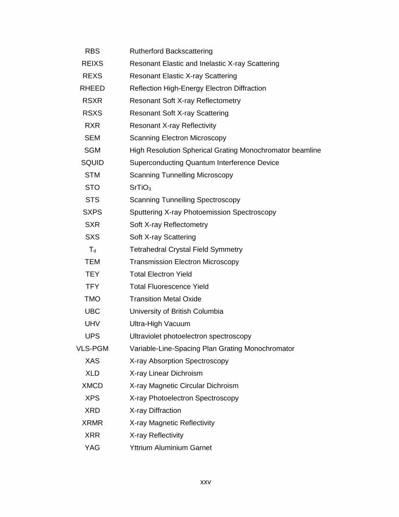
RBS Rutherford Backscattering

REIXS Resonant Elastic and Inelastic X-ray Scattering

REXS Resonant Elastic X-ray Scattering

RHEED Reflection High-Energy Electron Diffraction

RSXR Resonant Soft X-ray Reflectometry

RSXS Resonant Soft X-ray Scattering

RXR Resonant X-ray Reflectivity

SEM Scanning Electron Microscopy

SGM High Resolution Spherical Grating Monochromator beamline

SQUID Superconducting Quantum Interference Device

STM Scanning Tunnelling Microscopy

STO SrTiO3

STS Scanning Tunnelling Spectroscopy

SXPS Sputtering X-ray Photoemission Spectroscopy

SXR Soft X-ray Reflectometry

SXS Soft X-ray Scattering

Td Tetrahedral Crystal Field Symmetry

TEM Transmission Electron Microscopy

TEY Total Electron Yield

TFY Total Fluorescence Yield

TMO Transition Metal Oxide

UBC University of British Columbia

UHV Ultra-High Vacuum

UPS Ultraviolet photoelectron spectroscopy

VLS-PGM Variable-Line-Spacing Plan Grating Monochromator

XAS X-ray Absorption Spectroscopy

XLD X-ray Linear Dichroism

XMCD X-ray Magnetic Circular Dichroism

XPS X-ray Photoelectron Spectroscopy

XRD X-ray Diffraction

XRMR X-ray Magnetic Reflectivity

XRR X-ray Reflectivity

YAG Yttrium Aluminium Garnet

xxvi

LIST OF SYMBOLS

𝜒2

A measurement to determine the goodness of the fit and equals to the

sum of squares of the difference between measured and simulated

curves

𝛿 Imaginary part of the complex refractive index

𝜓 The wave function

𝜎 Vertically polarized light

𝜔 natural frequency

𝜋 Horizontally polarized light

𝑛(𝜔) Complex Refractive Index

𝛽 Real part of the complex refractive index

𝑧 Film thickness

𝜒(𝑧, 𝜔) Complex susceptibility

𝑓′ Real part of the complex atomic scattering factor

𝑓′′ Imaginary part of the atomic scattering factor

𝑁𝐴 Avogadro Number

𝑟𝑒𝑙 The classical electron radius

𝑘0 The wave vector of the incoming beam

xxvii

ACKNOWLEDGEMENTS

My deepest appreciation goes to my supervisor Dr. George Sawatzky for giving me

the chance of perusing the Ph.D. research in his group at the University of British Columbia.

His guidance in both social and scientific scopes of my life in the last 8 years helped in

making this project see the light. I particularly appreciate his patience and never ending

support whenever he can do anything to make my life easier.

I am greatly thankful to Dr. Andrew McFarlane, Dr. Andrea Damascelli, Dr. Elliott

Burnell, Dr. Mel Comisarow, Dr. Mona Berciu and Dr. Alireza Nojeh for serving in the Ph.D.

supervisory committee and/or the Ph.D. final oral examination committee.

I would like to thank both Sawatzky and Hinkov groups at Max-Planck – University of

British Columbia Quantum Matter Institute for all their support in every aspect of life. My

existence among such a great number of scientist helped to sculpture my experience in

research and completed all the gaps in my knowledge leading to the final appearance of this

project. I appreciate the great help and support of Dr. Vladimir Hinkov, who stood firmly and

helped in gaining the needed support for me and the current research. In particular, I would

like to thank Dr. Sebastian Macke, the man behind most of the theoretical part and the

computer simulations that I needed in the current research. His never-ending effort to give a

very close one to one support, write and continually modify the ReMagX software in addition

to many other analysis software which made the analysis techniques take a leap in speed

and quality of the outcome. My great appreciation goes to Dr. Adriano Verna with whom

running experiments in the Canadian light source and locally in UBC are a major scientific

experience in my life. I am greatly thankful for Dr. Jorge Hamman-Burrero with whom I

started running the scattering experiment in the Canadian Light Source. His experimental

skills and work ethics enabled me to learn the technique quickly and efficiently.

My respect goes to Dr. Maurits Haverkort, the man behind all the theoretical cluster

calculations. His Ph.D. research and analysis inspired large part of the current thesis in

addition to the lengthy discussions and instructions in both theoretical and experimental

aspect of the current research.

I appreciate the great help of Dr. Ronny Sutarto and Dr. Feizhou He; the research

associate and the beamline scientist of the REXIS beamline of the Canadian Light Source.

The flexibility and willing to help of Dr. He enabled me to run more than 30 beamtimes at a

very relaxed and friendly environment. Dr. Sutarto was absolutely the greatest help always

for me and for any of the REIXS beamline users through his voluntary existence when help

xxviii

is needed even during holidays and weekends. The scientific discussion and company of Dr.

Sutarto made the stressful beamtime a joyful experience.

I would like to thank Dr. David Hawthorn of the University of Waterloo, Dr. Hiroki

Wadati of Tokyo University, and Dr. Ryan Weckes for their help in learning the machines in

both UBC in Vancouver and the Canadian Light Source in Saskatoon. I am thankful to Dr.

Woo Seok of Oak Ridge National Lab and Dr. Diana Rata of Max Planck Institute in

Dresden for offering the samples for the current research.

My appreciation goes to my collages in the Chemistry department and the staff of the

first-year Chemistry labs, Dr. Sophia Nussbaum, Miss. Ann Thomas, Mr. Kristoffer Asperin

and Miss Emily Lai, whom made my 8 years teaching assistance calm and joyful.

The current work was supported by the Canadian organizations NSERC, CFI,

CIFAR, and CRC and by the German Max-Planck Society. Part of the research was carried

out at the Max-Planck-UBC Centre for Quantum Matter and the other part of was performed

at the Canadian Light Source, which is funded by the Canada Foundation for Innovation, the

Natural Sciences and Engineering Research Council of Canada, the National Research

Council Canada, the Canadian Institutes of Health Research, the Government of

Saskatchewan, Western Economic Diversifi cation Canada, and the University of

Saskatchewan. The electron microscopy and EELS was carried out at the Canadian Centre

for Electron Microscopy, a National Facility supported by NSERC and McMaster University.

xxix

DEDICATION

To my mother and father

1

1 General Introduction

1.1 Motivation

In the past years, there have been enormous advances in the thin-film epitaxial

growth techniques such as Pulsed Laser Deposition (PLD) and Molecular Beam Epitaxy

(MBE),6 with the huge rush to find new quantum materials for various applications.

Considerable attention was directed to growing Transition Metal Oxides (TMOs) due to the

large number of possible combinations they can have by altering their chemical composition

and their applications in semiconducting, dielectric, metallic, and magnetic properties.7 A

history changing moment was when Ohtomo and Hwang observed metallic conductivity at

the interface of two band insulating TMOs, LaAlO3 (LAO) and SrTiO3 (STO).8 Large

numbers of similar heterostructured materials have been grown and they exhibited

spectacular properties such as superconductivity and colossal magnetoresistance and many

other unconventional magnetic and electric properties.9,10,11,12,13,14,15,16,17,18,19,20,21,22 Such

possibilities make them the candidates for potential applications in the next generation of

electronic devices at extremely small dimensions.23 The new properties can be traced back

to the changes in the electronic structure in the newly formed heterointerface.18,21,24,25

Our main motivation is to develop a systematic non- destructive technique to

characterize and investigate the electronic structure at the buried non-directly-accessible

interfaces.26,27,28,29,30 Various techniques proved to be suitable to study various regions of the

film including X-ray Photoelectron Spectroscopy (XPS), Low Energy Electron Diffraction

(LEED), X-ray Absorption Spectroscopy (XAS), Transmission Electron Microscopy (TEM)

and Electron Energy Loss Spectroscopy (EELS) among others.31,32,33,34,35,36 The depth

limitation of these techniques as well as the destructive nature of some of them forced a

limitation on using them to study such delicate systems. The current research has two main

goals, to develop the understanding of the Resonant Elastic Soft X-ray Scattering (REXS)

technique and to deploy that as a non-destructive technique to investigate the geometric

and electronic structure of a perovskite model system. The system of choice was the

LaCoO3 (LCO) perovskite thin-film and heterostructure on various substrates which was

widely studied in earlier research.9,14,15,37,38,39,40,41,42,43,44,45,46 ,47,48

X-ray scattering is an important technique to investigate the geometry and electronic

structure of various materials. The technique becomes invaluable in the soft X-ray region

2

between 200 – 2000 eV. Within this range, most of the absorption edges of the 3d TMOs

reside, between 400-1000 eV, and rare earth metals go up to 2000 eV in addition to the

oxygen edge ~500 eV as well as the Carbon (280 eV) and Nitrogen (340eV) which are not

only important in detecting the surface contamination but also for future studies of carbides,

and nitrides. X-ray Absorption (XAS), as a part of the Soft X-ray Scattering (SXS) technique,

is well-developed and has been used to study the electronic structure of various materials

for several decades since the introduction of synchrotron radiation sources in the 1980s.

The technique is highly developed, and has been tested against theoretical models.43,57

Although XAS can reveal information about the valence, orbital and spin-states of any

system, it has major limitations; such as the probing depth and spatial resolution, which

prevents the distinction between what is happening at buried interfaces from that of the bulk

and the surface. The XAS spectra are merely an averaging of the signal coming from

various parts of the sample thickness, which is about 100 Å when the escaping electrons

upon the decay of the excitation are detected and much larger (about 1000 Å or more) if the

soft X-rays produced by fluorescent decay of the excitation is measured. The results will be

representative when the material within the detected thickness is homogeneous. If the

material is nonhomogeneous, for example, the existence of an interface or a surface layer,

XAS fails to determine the contribution of the various components within the detected

thickness. On the other hand, Soft X-ray Reflectometry (SXR) with better probing depth and

spatial resolution can provide much more information about the system. While SXR at

constant energy provides important information about the thickness, roughness and density,

SXR at fixed momentum transfer vector normal to the sample surface (fixed Qz) provides

much more details about the electronic structure in a depth dependent fashion as will be

explained in chapter 4.

Figure 1.1 shows a comparison between XAS signal in both Total Electron Yield

(TEY) and Total Fluorescence Yield (TFY) modes in addition to the fixed Qz SXR signal,

simultaneously measured for the same sample and at the same angle and beam attributes

at the Co L2,3 edge. While XAS displays an averaging of the signal of the components, SXR

at fixed Qz reveals more resolved details about the components and transitions within the

same component. Together SXR at constant energy and at fixed Qz can reveal the spin-

state transitions, orbital anisotropy and magnetic layers within the film as a function of the

depth from the surface or interface. The great strength of SXR is the ability to provide a

detailed description of the electronic structure of transition metal oxides TMOs in thin-films

and hetero-interfaces that are inaccessible by other techniques.

3

Figure 1.1 X-ray measurements of the LaCoO3 (LCO) thin-film on the LaAlO3 (LAO) substrate capped with a layer of LAO with σ-polarized light at 300K and sample (θ)/detector (2θ) angles of 20.65°/41.3°. (a) Total electron yield TEY signal, (b) total fluorescence yield (TFY) and (c) Soft X-ray Reflectometry (SXR) at fixed quantum transfer vector perpendicular to the sample surface (fixed Qz) at 0.2681 Å-1. All signals are taken around the L2,3 absorption edge of the Co ion at ~779.2 and 793.3 eV respectively.

The vast number of possibilities TMOs have in producing new materials suitable for

various applications, makes any technique, that can analyze them in detail, important. On

the other hand, the analysis of SXS experiments as a newly developed technique is highly

challenging and requires deeper understanding of modeling, simulating and fitting the

various parameters of the thin-films components. The improvement includes the creation of

computer simulating software to generate the theoretical models with the ability to examine

the results against the theoretical findings and the reported literature. The study of a well-

known model material is of great importance for the development of SXS technique and

analysis procedures. It helps test the theoretical models with familiar systems which then

can be upgraded to study more complicated ones. For this purpose, CoO thin-films grown

on various substrates, with various strains, as model systems are used to study the SXR

technique and to test theoretical models used to describe the experimental results. In CoO

thin-films, the electronic structure is well known and the influence of the strain can be

calculated as changes in the multiplet structure. Since detailed XAS for CoO thin-films have

been studied previously,57 including also theoretical calculations of the temperature

dependence resulting from the spin orbit coupling of the d electrons, they are ideal test

cases to develop our understanding of the new SXR technique. This can then be extended

to the more complicated SXS experiments which we are applying to systems in which the

electronic structure is not known in detail like for example LCO thin-films.

4

The unconventional properties noted for the TMOs, as highly correlated systems, are

attributed to the partially filled d orbitals. Because of the strong correlation effects, electrons

in these open shell orbitals will retain a lot of their atomic character and so transitions into

and out of these orbitals can be modelled well with modified atomic theory to include the

change from spherical to a lower symmetry but retaining the importance of the multiplet

interactions resulting in Hund’s’ rules.61 Any change in the transition element’s chemical

environment will be reflected as a change in the electronic structure of the orbital and

appear as a new property. Furthermore, stacking various TMOs on each other was found to

create completely new properties opening the door wider for more possibilities in the field of

TMOs studies. The development of thin-film growing techniques, such as PLD and MBE,

provided the possibility of creating hetero-structured quantum materials reaching very

advanced levels of accuracy and control. The challenge is to find an analysis technique that

has both, enough details about the system and does not force new variables by deforming

or destroying the samples. The answer for that can at least in part come from SXS as will be

shown in the current thesis.

Considering the important role of the orbital occupancy and the spin-state at the

hetero-interfaces of TMOs, a model d6 Co3+ electron system, namely epitaxial grown LCO

perovskite thin-film heterostructures will be investigated using SXS techniques. The system

is complicated and gives a very important rich example of the changes within the film that

evokes changes in the electronic structure. Growing samples on LAO, STO and NdGaO3

(NGO) substrates enables to test a matrix of variables that may cause changes in the

electronic structure of the Co ion and the whole perovskite structure as will be shown.

1.2 Background

Transition metal oxides (TMOs) with the perovskite structure have a range of

physical properties which depend on the electronic degrees of freedom of the metal ions in

their respective crystal field. New states of matter, with completely different properties,

emerge at the interfaces between two different TMOs as, for instance, high-density 2D

electron gas and superconductivity.8 Of particular interest, LCO thin-films show interesting

magnetic and electronic properties that depend on the film thickness and the supporting

substrate as a result of the changes in the ion’s ligand fields in addition to the polar

continuity across the interface which is found to be very important in the final structure.

5

The interface physics developed into an important field of research in solid-state

physics and material science. A breakthrough was initiated by the work of Ohtomo and

Hwang,8 in which they recognized high electron mobility at the interface between the two

band insulators LAO and STO. Following that, many works further reported a coexistence of

ferromagnetism and superconductivity at the interface of these two non-magnetic materials,

which is very rare in most cases and it has inspired a great deal of research in TMO

heterostructures in general.25,49,50,51,52,53,54,55

The cobalt containing TMO heterostructures, in which the transport and magnetic

properties are attributed to a temperature dependent spin-state cross over, has been the

source of an increasing interest.9,14,15,37,38,39,41,42,43,44,56 Here, the Co atom has a 3d74s2

electronic configuration which becomes 3d64s0 in the Co3+ ion at the center of the CoO6

octahedra in the perovskite LCO structure. The crystal field effect partially lifts the orbital

degeneracy of the Co3+ 5 d-orbitals into t2g and eg energy levels. The Co3+ ion then can exist

in three possible spin-states under different conditions, low (LS), intermediate (IS) and high

(HS) spin-states with total spins of S = 0,1 and 2, respectively. In the LS state the t2g level is

full with paired electrons, while in the IS and HS states the ion has unpaired electrons at

both t2g and the eg levels. This causes the system to be nonmagnetic when it is in the LS

state and magnetic when it is in the IS or HS state.

Fuchs et al.39 showed by comparing bulk, polycrystalline and epitaxial LCO thin-films

that only epitaxial LCO thin-films exhibit ferromagnetism at low temperature as the system

exists in an increased population of IS or HS states with a Tc ~ 85K. By growing LCO films

with different thicknesses, they demonstrated that ferromagnetic order spans the whole film

as indicated by the linear increase of the magnetisation with increasing film thickness. They

proved that the lattice strain in the LCO epitaxial film, grown on different substrates, induces

the transition of the spin-state to a higher population of IS and HS states.42 Even at low

temperature, 30 K, the system remains in a mixed state because the epitaxial strain inhibits

the transition to the LS state as a result of the lower than cubic symmetry caused by the

lattice mismatch.

Sterbinsky et al.45 showed that coherent strain, in which the film lattice parameter is

equal to the substrate lattice parameter, is a condition for the ferromagnetic order in LCO on

different substrates. While thin-films of LCO grown on STO are coherently strained and

retain ferromagnetic order, those grown on LAO have higher degrees of misfit resulting in a

frustrated interaction.45 In general, the coherent strain is only expected to exist for film

thicknesses below a certain threshold which can be as high as 400 nm, beyond which the

6

films usually revert back to their native crystal structure leaving behind a very disordered

extended interface layer.45

Merz et al.43 studied the effect of hole or electron doping on the oxidation state and

transition temperature of the LCO thin-films. By doping the LCO epitaxial strained film with

electrons, addition of 30% Ce4+, or holes, addition of 30% Sr2+, the system responds to that

by changing the oxidation state and substitutes Co3+ HS oxidation state with Co2+ HS and

Co4+ HS oxidation states respectively.43 This substitution shifts the transition temperature

down to 23 K for electron doped system and up to 194 K for hole-doped systems.

Research showed that, regardless of the accuracy of growing, PLD has an inherited

limitation. When growing pure LCO thin-films on various substrates, the XAS signal of the

film shows a small mixing of Co3+ with Co2+.43 Although the Co2+ exists in a magnetic HS

state, it is evident that the Co3+ determines the magnetic property of the system.43 They

were unable to clarify the nature or the position the mixed valencies in the sample, where

they can be in a specific layer at the surface or/and the interface in addition to coexistence

with the Co3+ within the thin-film. Chang et al.41 used XAS to study the oxidation and spin-

states of different cobaltate compounds and found a characteristic feature attributable to

each of the oxidation and spin-states of different cobalt ions.41 They found a characteristic

pre-peak at 776.3 eV near to the L3 edge associated with the Co2+ ions in octahedral (Oh)

symmetry which was proven to be important in the determination of the electronic structure

and the valence intermixing of the LCO surfaces as will be shown in later chapters. In a

separate simulation, Merz et al.43 presented possible theoretical spectral shapes for each

valency and spin-state of the cobalt ions.

Despite the efforts made to understand the phenomena, the underlying mechanism

behind the long-range ferromagnetic order in strained films is still not well understood. The

ferromagnetic order in the pure LCO is believed to result from super exchange between two

Co3+ ions in LS and HS states. The ion crystal field effect and the broken symmetry, as

coupled with the electronic degrees of freedom, is believed to play an important role in the

electronic spin-state cross over between the different states.44

Benckiser et al.12 presented a powerful method to quantify the d orbital occupancy in

LaNiO3/LaAlO3 (LNO/LAO) superlattices using RSXS technique and a new method of data

simulation. They realized that differences in orbital occupancies appear in the linear dichroic

reflectivity curves measured at fixed Qz. SXR is ideal to study surfaces and interfaces due to

the surface sensitivity and the possibility to probe buried interfaces. Tuning the energy and

7

the polarization of the incident photon enables probing the electronic anisotropy, e.g., orbital

occupation or electronic reconstruction, of a particular ion at a given interface.12

Many experimental and theoretical works on the CoO thin-films have been

performed,57 including XAS, linear dichroism and X-ray Magnetic Circular Dichroism (XMCD)

of the CoO sample on various materials. XAS and SXR results are compared to analyze and

simulate the spectra. The experiment is concerned with the use of the newly developed SXR

technique to study the changes in the electronic structure of the Co2+ ion because of the

lattice mismatch at the interface between CoO and MgO or MnO substrates as examples of

compressive and tensile strain, in addition to studying the temperature dependence of the

SXS spectra. Previous XAS measurements reveal the multiplet structure of the Co edge and

the differences in the occupied states as a result of the spin-orbit coupling of the 3d orbitals.

Orbital anisotropy appears as a difference in the multiplet structure of the Co edge

measured at fixed Qz vectors for vertical and horizontal polarization.57 Sample surfaces

under ambient conditions are usually contaminated with a thin layer of an absorbed species,

such as water or CO2 etc. Although these low mass elements, with X-ray resonances far

from the 2p edges of the transition metals, are not expected to influence the reflectometry

results, experience shows that even very thin layers of adsorbed species can cause some

refraction of the X-ray beam and therefore influence the analysis. This can be considered

theoretically in principle, but a systematic way is needed to investigate the phenomena and

to use the finding in improving the model systems. In order to better understand the surface

contamination layer effect of the SXS spectra, a systematic study of growing layers of inert

gas with various thickness on the surface of CoO reveal the relation between the surface

contaminant on the SXR spectra and any possible changes to the top most layer of the film.

The first step is to test the suitability of the technique to detect buried interfaces as

well as element specific detection. Also, the in-house software that is used for modeling the

system and simulate the data should be tested. In order to do that two samples have been

studied; the first was a MBE grown multilayer thin-film of SrTiO3 /Lax Sr1− xTiO3 (LSTO,

1monolayer)/SrTiO3 (buffer) on SrTiO3 substrate along the (001) direction, with a nominal La

content of 𝑥 = 0.005. Studying such a system illustrates the suitability of the technique and

the analysis method in determining very small thicknesses and element densities. The

second sample was PrNiO3 grown on (LaAlO3)0.3(Sr2AlTaO6)0.7 substrate. Studying the

sample shows the element specific nature of both the SXR technique and the analysis

software ReMagX.

8

Following that, the well-studied CoO thin-films are examined to associate the SXR

results with the electronic states of the film. CoO as an example of a strongly coupled

material, is an antiferromagnetic insulator with a Neel temperature of about 291 K.58

Experiments show that the magnetic properties of CoO depend largely on the temperature;

where changing the temperature changes the occupation of the different states.

Co2+ has 7 electrons in the 3d orbital. In a spherical symmetry, the 5 3d orbitals are

at the same energy level and 5 of the electrons distribute in the orbitals parallel to each

other due to the large Hund’s rule atomic exchange like interaction. The other 2 electrons

pair up with any of the other electrons. In the CoO crystal, Co2+ is in Oh crystal field. In such

symmetry, the orbital splits into two levels; lower three-fold degenerate (t2g) and higher two-

fold degenerate (eg) orbitals. The Hund’s rule exchange and crystal field splitting energies

dictate how the electrons are distributed over the various orbitals. 5 of the electrons, with

spin up, distribute as 3 in the lower t2g and 2 in the higher eg. The last two electrons, with

spin down, pair with another two electrons in the lower energy t2g as will be discussed in

detail in chapter 2. These interactions are a lot larger than the spin orbit coupling. With the

spin orbit coupling in the picture, further splitting occurs of the 3d orbital forming three

different states with pseudo total angular momentum of 1/2, 3/2 and 5/2, with two-, four- and

six-fold degeneracy. When the material is grown as a thin-film on a supporting substrate, the

lattice mismatch and the broken inversion symmetry alter (distort) the crystal filed and spin

orbit coupling effects will be more apparent. The orbital angular momentum is coupled to the

lattice and results in the large magnetic anisotropy of Co2+ systems which can be probed

with polarization dependent XAS and SXR.

The research also extends the work of Fuchs et al.39 by concentrating on the SXR

measurement of the LCO thin-film grown on two different polar and nonpolar substrates,

which is expected to clarify the role of lattice strain in inducing the interfacial orbital order

and spin-states hence changing the magnetic properties of the film. It will also extend the

work of Benckiser et al.12 by using the improved measurement technique of collecting data

maps around the resonances and the element specific method of simulation to give the

chemical profile of the thin-films. In addition to the usual XAS in both modes, we conduct a

spatial probing of the film with SXR measurements at constant energy and at fixed Qz.

9

2 Co-Containing Transition Metal Oxide: A Brief Summary59 ,60

2.1 Introduction

What makes Co-containing transition metal oxides (TMOs) interesting arises from

the partially filled 3d orbitals. Under certain conditions the ion can have valency of 2+, 3+

and 4+ with 7,6,5 d electrons respectively and each valency can have various spin-states

ranging from High to Intermediate to Low (HS, IS and LS) which is explained in details

below in section 2.2 “Crystal Field Theory”. Furthermore, Co containing materials have

different lattice symmetries also affects the electronic structure and participate in the

richness of the resulting properties will be shown in section 2.2 when we discuss Crystal

Field Theory. Careful preparation of Co containing materials with specific combinations of

components, considering the valence, spin-state and lattice symmetry opens the door for

enormous possibilities of quantum materials that have a vast variety of properties.

To further control the symmetry of the elements, growing TMOs in the form of

heterostructure alters the local symmetry around the elements and helps stabilize certain

electronic configurations which are unattainable in the bulk form for the single crystal. TMOs

form ionic crystals and in specific crystal directions, their unit cells can carry electric dipole

moments that results in a net dipole moment perpendicular to the surface.

The electric potential from each unit cell adds up at the sample surface and that

results in what is known as the polar catastrophe and the crystal is unstable due to the

divergent surface energy as will be shown below in section 2.5.2. One of the ways with

which the material compensates for the polar problem, known as electronic surface

reconstruction, has been found to be important in determining the final stable electronic

structure. In addition, the phenomena were particularly important in explaining the changes

in the thin-film structures grown on various substrates, polar and nonpolar, and in explaining

some of the emergent properties for the heterostructures.

In the current chapter, a brief introduction of the crystal field symmetry will be

presented followed a discussion of the polar catastrophe problem and the way systems

reconstruct to solve the problem in bulk and thin-film (section 2.5). Finally, a closer look at

the Co in a rock salt (CoO, section 2.6) or perovskite (LaCoO3, section 2.7) structure will be

given.

10

2.2 Crystal Field Theory

Transition metal oxides are an example of highly correlated systems in which the

attributes of the system can be explained through the electron-electron interaction.

Together, the charge, orbital occupation and spin-state coupled with the lattice degrees of

freedom dictate the physical and chemical properties of the material. The electron

distribution in the partially filled d-orbitals shed the light on the microscopic origin of these

properties.

In a free ion, the d-shell has five degenerate orbitals (Figure 2.1). The ion, in

principal, can exist in various crystal symmetries as shown in Figure 2.2. The orbitals split

into different levels depending on their position in a crystal structure with specific symmetry,

some of which are shown in Figure 2.3.

Figure 2.1 The five 3d-orbitals reproduced from Ref "61". (a) x2-y2, (b) 3z2-r2, (c) xz, (d) yz and (e) xy.

11

Figure 2.2 Simplified ball and stick model of the different crystal field symmetries, the white central ball is the cation and the surrounding purple balls are the anions. (a) Square Planar, (b) Tetrahedral (Td), (c) Octahedral (Oh), (d) Square Pyramidal, (e) Square Prismatic, (f) Trigonal Bipyramidal and (g) Pentagonal Bipyramidal.

Figure 2.3 Energy diagram for the five 3d orbitals of an element placed in (a) Spherical, (b) Tetrahedral (Td), (c) Octahedral (Oh) and (d) Square planar crystal fields. It shows the energy levels further splitting depending on the type of the element coordination. The figures were reproduced from Ref.61

The most common cation site symmetry for the perovskite TMOs is the octahedral

(Oh), but under certain circumstances and upon the change in the crystal structure, this can

change to other symmetries. The change in symmetry is usually accompanied by a change

12

in the electronic configurations and the macroscopic properties of the system. The way the

electrons distribute in the split d-orbitals is controlled by a balance between the crystal field

effect and Hund's first rule of maximum multiplicity. The upper hand is given to the crystal

field effect, since it is the condition that can be experimentally controlled. To study the two

chosen systems for the current study, one must have a clear idea about the fundamentals of

both factors, namely crystal field and Hund's rule.

Crystal field theory deals with the electronic structure of the metal ion. In this theory,

the ligand anions interact with the central cation with a pure electrostatic force that affects

the energy levels of the d orbitals. The interaction is highly affected by the symmetry of the

crystal, where the electrons preferably occupy the orbitals with the minimum interaction with

those of the ligands. The orientations of the five 3d orbitals play vital roles in determining the

level of interaction that each of them will have in the specific symmetry (Figure 2.1). The

symmetries are classified into: square planar, tetrahedral (Td), octahedral (Oh), square

pyramidal, square prismatic, trigonal bipyramidal and pentagonal bipyramidal (Figure 2.2).

In the Oh symmetry, the metal ion is bound to six ligands (Figure 2.2.c). Since two of

the 𝑑𝑥2−𝑦2 and 𝑑𝑧2 orbitals, have their lobes of maximum probability pointing directly

towards the ligands, they form one high energy level called eg (Figure 2.1). The energy level

is at +6Dq energy relative to the spherical symmetry energy level (Figure 2.3.c). The

geometry of the other three orbitals dxy, dxz, and dyz puts them in minimum contact with

surrounding ligands hence forming a lower energy triply degenerate level t2g as shown in

Figure 2.1. The energy level is at -4Dq, making the difference between the high and low

energy levels 10Dq (Figure 2.3). The difference in energy (ΔOh) is called the Oh crystal field

splitting energy. The factor that controls the way the electrons are arranged in the different

energy levels is the competition between Hund’s first rule of maximum multiplicity (Jh) which

is characterized by the Coulomb repulsive interaction between electrons, and the ΔOh as

shown in the energy diagram of Figure 2.5.

To clarify this relation, let us consider the case of Co ions. The Co atom has a 3d74s2

electronic configuration which becomes 3d74s0, 3d64s0 and 3d54s0 in the Co2+, Co3+ and Co4+

ions by losing 2, 3 or 4 electrons. Each of the ions can exist in various spin-states such as

low, intermediate, or high spin-states depending on the occupation of the d orbitals. For

example, the Co2+ ion can have two cases; LS (S=1/2) and HS (3/2), while Co3+ can have

three cases; LS (0), IS (1) and HS (2) and finally Co4+ can have LS (1/2), IS (3/2) and HS

(5/2) (Figure 2.4). Some of these spin-states are unlikely and never exist under normal

conditions at least within the scope of the current research. Research shows that by

13

controlling the chemical and physical environment of the ion, it can undergo the energy

allowed change from one valency to another and can transition from one spin-state to

another.43 The various components can also exist together and various research shows the

way by which they interact to produce final properties of the material.43 Usually, such

changes result in the emergence of new unparalleled properties of the material. The

presence of any valence and spin-state can be controlled in a variety of ways including

chemical doping with electrons or holes, temperature and pressure changes.37,38,39,40,43

Figure 2.4 Energy level diagram of d5, d6 and d7 for the Co4+, Co3+ and Co2+ ions. It shows the high (HS), intermediate (IS) and low spin (LS) configurations for each valence state Ref.57

Let us now discuss the case of spin-state transition and the coupling with lattice

symmetry. If we take the most common case of Co3+ ion in Oh crystal symmetry, the spin-

state transition mechanism can be explained. In a strong crystal field, the crystal field

splitting is stronger than the Hund’s rule interaction ΔOh> Jh. The electrons hence pair up in

the lower energy t2g rather than spreading to the higher energy eg orbitals and the ion is said

to be in low spin (LS) state with a total spin of (S=0) (Figure 2.5). In a weak crystal field, the

case is flipped with ΔOh< Jh, and the electrons arrange in parallel spins filling both the t2g

and eg orbitals where the system is in high spin (HS) state with a total spin (S = 2), Figure

2.5.

14

Figure 2.5 Energy diagram of the electrons distribution in the 3d orbitals of a d6 model ion in an Oh crystal field and the changes in the energy levels because of the unit cell expansion in the 𝑥𝑦 plane as expected in the case of growing Co-containing compound on a supporting substrate with larger lattice parameter. Jh represents the Hund’s rule exchange like interaction and ΔOh represents the Oh crystal field splitting. The red arrows represent the electrons in spin up and spin down. The figure shows how the energy levels change when ΔOh is larger than Jh and that will stabilize a low spin electron distribution with S = 0.

Under certain circumstances, Oh complexes distort in order to stabilize the electronic

structure. An Oh configuration with an anisotropic occupation of the eg orbital tends to distort

raising the energy of one of the two orbitals, hence lifting the degeneracy within the eg level

as can be seen for the case of tetragonal distortion (D4h) of the Oh symmetry in Figure 2.6. If

we continue our discussion with the Co3+ ion, when the compound is subject to tensile strain

in the xy plane, for example, when the system is grown on a supporting substrate with

higher lattice parameter, it undergoes tetragonal distortion. Because of that, the energy of

some of the orbitals in both t2g and eg shells increases, namely 𝑑3𝑧2−𝑟2, 𝑑𝑥𝑧 and 𝑑𝑦𝑧 and for

the other orbitals it decreases (Figure 2.6). When the distortion is small, the system

continues to exist in a LS state with the Coulomb repulsion still strong in comparison to the

new D4h energy splitting. With increasing distortion, the system reaches a level where the

energy splitting is higher than the Coulomb repulsion and rather than having unpaired

electrons, the electrons start to pair up producing IS and even HS states (Figure 2.6). It

should be noted that not always the distortion causes a spin-state transition but rather can

result in changing the orbital occupation. For in the case of CoO grown on MgO, the

compressive strain on the CoO unit cell as a result of the lattice mismatch with the

supporting lower lattice parameter MgO substrate, distorts the Oh symmetry of the Co2+

15

cation and causes a reduction of the degeneracy from 3 to 1 for the t2g shell and confines

the hole to the xy orbital as will be discussed in details in chapter 6.

Figure 2.6 Energy diagram of the electrons distribution in the 3d orbitals of a d6 model

ion and the changes in the energy levels because of elongation in the 𝑥𝑦 plane as expected in the case of growing Co-containing compound on a supporting substrate with larger lattice parameter. 𝐽 ℎ represents the Hund’s rule exchange like interaction and 𝛥𝑂ℎ represents the Oh crystal field splitting energy. The red arrows represent the electrons in spin up and spin down.

At this point it is important to consider a different cation symmetry, the Td symmetry,

which is less common for TMOs, but it was found to be important in some systems where

some phenomena are driven by oxygen vacancies as will be shown in chapter 9. The cation

in this symmetry has 4 coordination groups alternate at the corners of a cube bound to a

central metal cation (Figure 2.2.b). Unlike the case for the Oh, the metal dxy, dxz and dyx

16

orbitals are the ones closer to the ligands with the least interaction for the 𝑑𝑧2 and the

𝑑𝑥2−𝑦2 orbitals. The eg orbitals are at the low energy level and the t2g orbitals are at the

higher energy level. Since none of the orbitals points directly to the ligands, the crystal field

splitting energy is smaller than that in Oh complexes ΔTd = 4/9ΔOh (Figure 2.3.b).

The square planar symmetry is associated with a distorted form of the Oh symmetry

(Figure 2.2.a). The ligands along the z axis are moved far enough away, and their

interaction with the metal reduces drastically while the ligands along the x and y move

closer. You can think of the system when a unit cell such as LCO is grown on smaller unit

cell such as LAO. The compressive strain in xy shrinks the LCO unit cell in the xy direction

and accordingly the crystal elongates in the 𝑧 direction as will be shown in chapter 7. The

conventional two energy levels of the Oh splits further reducing the energy of the 𝑑𝑧2 orbital

and 𝑑𝑥𝑧 and 𝑑𝑦𝑧 and increasing that for orbitals with 𝑥 or 𝑦 components only like 𝑑𝑥2−𝑦2 and

𝑑𝑥𝑦 (Figure 2.3.b). Other symmetries exist but they are less frequent for the systems of

interest (Figure 2.2).

2.3 (3 d) Transition Metals and Transition Metal Oxide thin-films

Transition metals are the elements starting from group 3 through group 12, with their

valence electrons residing in the d shell. The metals are quite electro positive and interact

preferably with the electronegative anions (group 16 and 17) or ligands. In the current study,

we are interested in the third period transition metals with their valence electrons in the 3d

and 4s orbitals. The metals form Chalcogenides or Halides by first losing the 4s electrons,

leaving the 3d electrons to dictate the chemical bonding and the physical properties.

The 3d TMOs have various crystal structures with the most important for the current

work to be rock salt and perovskite structures. The way in which the metal interacts with the

ligands and with the other cations in the crystal affects the electronic structure of the cation

and the structure of the resulting crystal. Transition Metal Oxide (TMO) thin-films are

different from the bulk and exhibit new emerging properties. The oxide/vacuum and

oxide/support interfaces are responsible for the production of new phases of matter.

The choice was made to study two Co-containing compounds: CoO and LaCoO3

(LCO). In the bulk form CoO and LCO have rock salt and perovskite pseudo-cubic structures

respectively. The distribution of the electrons in the five 3d orbitals of the Co ions dictates

the chemical and physical properties of the system. It was found that many variables affect

17

the distribution of electrons and by controlling these variables new quantum materials with

novel properties can be produced. Such variables range from the temperature of the

system, pressure on the unit cell and the introduction of chemical agents.43

One practical way of tuning the amount and the direction of pressure on the unit cell

was found to be growing the material as a thin-film on another substrate. The lattice

mismatch between the film and the supporting substrates distorts the crystal structure of the

film and changes the crystal field of the ions. The lattice mismatch with respect to the film

material can produce compressive or tensile strain. In both cases the crystal structure is

distorted to a certain degree and the symmetry around an element may change slightly,

such as in the case of tetragonal distortion, or can change substantially, such as changing

from Oh to tetrahedral (Td) symmetry. A change in the electronic structure is accompanied by

possible changes in valency, change in the orbital occupation and spin-state of the system.

The electronic structure on a macroscopic level appears as the new emergent physical

property of the system.

Growing thin-films on supporting substrates is a precise process and some

conditions must be met to achieve the desired epitaxial growth and keep the film intact. An

important factor is the lattice mismatch between the film and the supporting substrate which

should not exceed 4% in both compressive or tensile strain. The thickness of the film also

should not exceed a certain critical thickness, which is approximately 400 nm. Beyond the

critical thickness the film is believed to retain the lattice parameters of the bulk and the film

usually cracks close to the interface.

2.4 Perovskite Structure

The Perovskite family consists of a very large number of compounds that are related

in their crystal structure to the mineral perovskite CaTiO3 and one of the most studied

structures in the present time. Ideally the structure is cubic and has a rare-earth metal at

each corner with a cation in the center sharing oxygen octahedra and it has the formula

ABX3 such as LaCoO3, LaAlO3, NdGaO3 and SrTiO3. However, the structure, usually, exists

in a deformed state in various compounds with reduced symmetry and occurs generally by

rotation of the ligand octahedron or by directional pressure applied along a certain direction

as in the case of thin-film on various substrates as will be shown in chapters 6 through 9.

The deformation of the perovskite unit cell affects the electronic structure of the transition

metal cations, such as the valency, orbital occupation and spin-states and stabilizes

18

structures that are not possible under ideal cubic conditions such as the HS state at low

temperature for the LCO strained thin-film as will be shown. Intentional deformation of the

structure is a powerful means to control the characteristics of the perovskite and perovskite

like materials.

2.5 Polar Surfaces and Surface Reconstruction

One of the most interesting, though very complicated, systems to study are surfaces.

Every surface undergoes some sort of surface reconstruction because of the broken

inversion symmetry of the crystal and to reduce the surface energy.62,63,64,65,66 The

reconstruction can be structural, chemical or in special cases electronic. Particularly

important to the current study is the ionic crystal in which the planes in specific directions

may carry a net charge due to the partially satisfied bonds between the cations and the

anions in the planes. Accordingly, the surface of these crystals can have a net electric dipole

moment perpendicular to the surface which may give rise to a divergent surface energy.

Electronic reconstruction is expected in such surfaces, but before talking about the possible

solutions let us take a deeper look at the problem.

2.5.1 Surfaces of Ionic Crystals

A closer look at the surface of ionic materials, such as TMOs, helps to classify them

in three types depending on the existence of a net dipole moment in the unit cell

perpendicular to the surface as well as the existence of a net charge in each of the planes.

The first type is nonpolar neutral surface with zero net charge on each of the planes, as can

be seen for the (001) planes of the CoO, MgO and STO single crystal in Figure 2.7 and

Figure 2.9 in addition to the CoO/ MgO in the (011) plane as shown in Figure 2.8.b. For

example, the STO crystal alternates between SrO and TiO2 planes with a zero-net charge in

each of the planes and the unit cells in the whole material does not have any dipole

moment. The second type is also nonpolar neutral surface with zero net dipole moment

perpendicular to the surface but the planes carry a net charge as can be found in the case

of TiS2, LiFeAs single crystals.63 TiS2 crystal, for example, has alternating S2- and T4+ planes

with a zero net dipole moment in the unit cell. Both types of surfaces carry mild surface

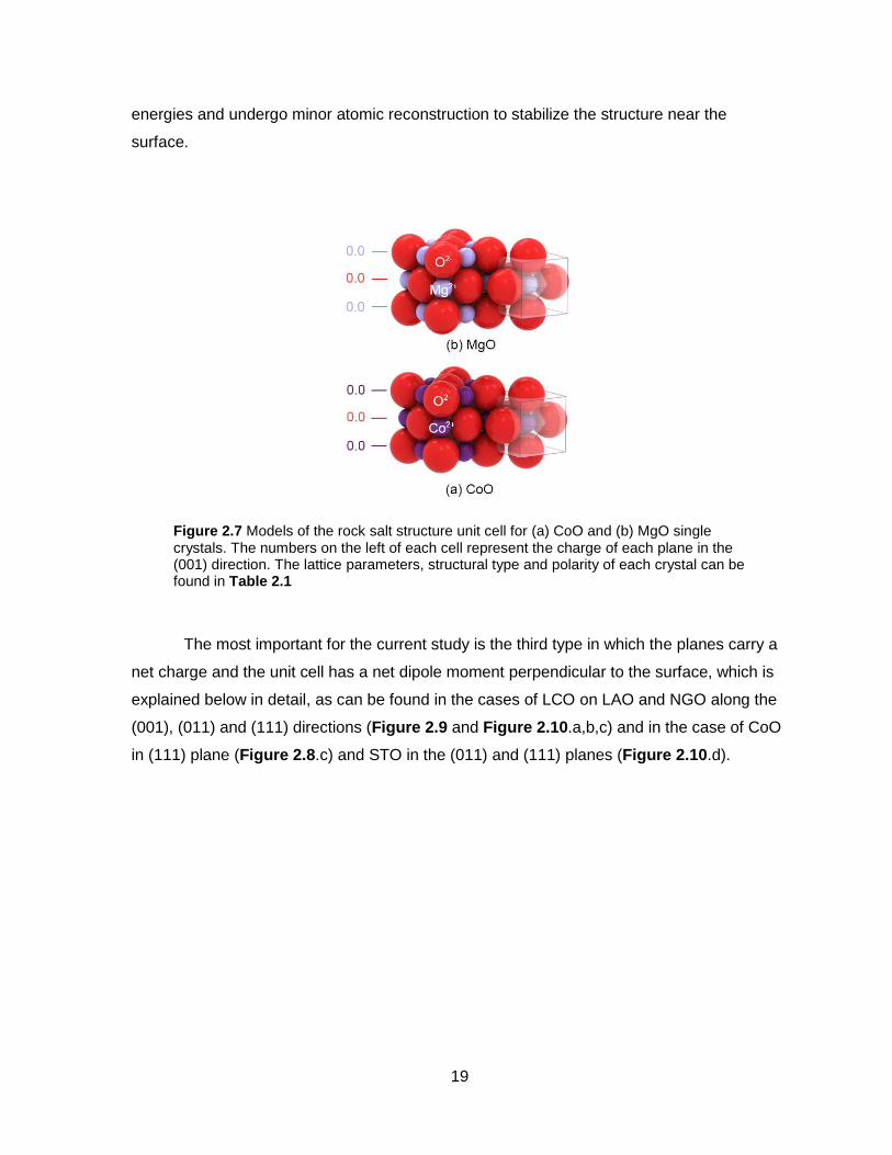
19

energies and undergo minor atomic reconstruction to stabilize the structure near the

surface.

Figure 2.7 Models of the rock salt structure unit cell for (a) CoO and (b) MgO single crystals. The numbers on the left of each cell represent the charge of each plane in the (001) direction. The lattice parameters, structural type and polarity of each crystal can be found in Table 2.1

The most important for the current study is the third type in which the planes carry a

net charge and the unit cell has a net dipole moment perpendicular to the surface, which is

explained below in detail, as can be found in the cases of LCO on LAO and NGO along the

(001), (011) and (111) directions (Figure 2.9 and Figure 2.10.a,b,c) and in the case of CoO

in (111) plane (Figure 2.8.c) and STO in the (011) and (111) planes (Figure 2.10.d).

20

Figure 2.8 Models of the CoO single crystal grown along various direction (a) the (001) plane, (b) (011) plane and (c) the (111) plane. The numbers on the left of each model represent the net charge of the specific plane.

Figure 2.9 Models of the perovskite structure unit cells for (a) LaCoO3, (b) LaAlO3, (c) NdGaO3 and (d) SrTiO3 single crystals. The numbers on the left of each cell represent the charge of each plane in the (001) direction. The lattice parameters, structural type and polarity of each crystal can be found in Table 2.1.67

21

Figure 2.10 Models of the perovskite single crystal grown along various direction. The figure show that growing the crystal in a specific lattice direction changes the polarity of the crystal surface. (a) LCO, (b) LAO and (c) NGO are polar in all the directions, with plane charges of (1±) in along the (001) direction, (4±) in the (011) direction and (3±) in the (111) direction. (d) The STO crystal along the (001) direction is nonpolar with zero net charges on each plane but the sample is polar in the (011) and (111), with charges of (4±) in the alternating planes.

22

Table 2.1 Lattice parameter, polarity, conductivity and lattice structure of various rock salt and perovskite materials.

Material Lattice Parameter (Å) Plane Polarity Plane Charge

CoO 4.27

(001) Nonpolar 0

011

111 Polar 2 ±

MgO 4.21

(001) Nonpolar 0

011

111 Polar 2 ±

LaCoO3 3.83

(001)

Polar

1 ±

011 4 ±

111 3 ±

LaAlO3 3.78

(001)

Polar

1 ±

011 4 ±

111 3 ±

SrTiO3 3.91

(001) Nonpolar 0

011 Polar 4 ±

111

NdGaO3 3.85

(001)

Polar

1 ±

011 4 ±

111 3 ±

The LCO crystal along the (001) direction, for example, alternates between 𝐿𝑎3+𝑂2−

and 𝐶𝑜3+𝑂22− with net charges of (1+) and (1-) respectively and the unit cell has a net dipole

moment perpendicular to the surface (Figure 2.11.a). It should be clear at this stage that the

net charge of the unit cell should always add up to zero regardless of the plane charges or

the net dipole moment. For example, for the LCO unit cell we have:

(1

8 8) 𝐿𝑎3+, (

1

26) 𝑂2− 𝑎𝑛𝑑 (11)𝐶𝑜3+

The added charges will give a net zero charge for the unit cell but the dipole

moments between the planes line up and result in a net dipole moment. Such a system has

a high surface energy and requires in principle substantial change to stabilize the structure.

It is for this kind of crystals that the polar catastrophe takes place and many possibilities of

surface reconstruction can be used to stabilize the structure. In the next section, polar

catastrophe and possible surface reconstruction routes to help reduce the surface energy

and stabilize the structure will be presented.

23

2.5.2 Polar Catastrophe

To understand the phenomenon, a model system of 4 atomic planes for the LCO

single crystal in the (001) direction has been used (Figure 2.11). The crystal is shown in

Figure 2.11.a before any kind of surface reconstruction. The planes carry the nominal

valencies of 𝐿𝑎3+𝑂2− and 𝐶𝑜3+𝑂22− (1+) and (1-) respectively. If we imagine crystal planes

as stacked charged planes of opposite but equal charges, the resulting configuration will

resemble that of two capacitors stacked in series (Figure 2.11.a).

Figure 2.11 Four atomic layer model of the crystal structure of (a) a perfect non-reconstructed CoO2 terminated LaCoO3 substrate. The associated graph of the electrostatic potential V (V) versus substrate thickness z (Å), illustrates the divergent potential at the surface as the ionic crystal undergoes the famous polar catastrophe problem. (b) The polar crystal undergoes electronic reconstruction by transferring one half charge to the underneath layers ending up with a finite manageable potential as in the associated graph. The top layer in the current scenario have a valance change of 50% of the cations from Co3+ to Co4+ reducing the layer charge from (1-) for the

unreconstructed 𝐶𝑜3+𝑂22− layer to (0.5-) for the reconstructed 𝐶𝑜0.5

3+𝐶𝑜0.54+𝑂2

2− with the bottom layer at (0.5+) through the add atoms. Other scenarios are also possible and are introduced in later chapters.

24

Each of the capacitors will carry a net electric charge of (1+) and an electric field E1

which value can be found by applying Gauss’s law for infinite charge carrying plane:

𝐸1 = 𝑄/𝐴𝜖0

where 𝑄 is the electric charge on the plane (e-charge), A is the surface area of the

plane and 𝜖0 is the permittivity of free space. The net potential at the surface is given by:

𝑉 = 𝑁 𝐸1 𝑑

where d is the inter-planer distance (half the lattice parameter) and the potential

increases with a multiplication of N numbers of unit cell repetitions.63 The graph of Figure

2.11.a shows the relation between the surface potential (V) and the crystal thickness (z)

perpendicular to the (001) plane of the LCO single crystal with d as the interplanar distance.

It clearly shows that the potential adds up at the surface and if the crystal has multiple

layers, it carries a large surface energy and the potential diverges at the surface. The

phenomenon of the divergent potential at the surface of ionic crystals is well known as “the

polar catastrophe”.

Such high energy cannot exist in a normal situation which probably, if it was not

handled and the energy was reduced to manageable levels, will result in the collapse of the

crystal structure. One way to compensate for this is through an electronic reconstruction

which is believed to be the case for polar TMOs systems. In the electronic reconstruction,

half the charge of the plane at the surface is transferred to the underneath layers and the

structure is stabilized (Figure 2.11.b). In this scenario, the top most surface layers in both

ends of the crystal will have half their nominal charge. If the infinite charged plane stack is

used again, one can notice the change from what looks to be charged capacitors connected

in series to more like alternating electric field that changes in direction successively between

each of the planes (Figure 2.11.b). Since the charge on the first and last plane are half that

of the nominal charge of the unreconstructed system 𝑄/2, the value of the electric field

between each plane pairs will be (𝐸2) with a value of:

𝐸2 =𝑄

2𝐴𝜖0=

𝐸1

2

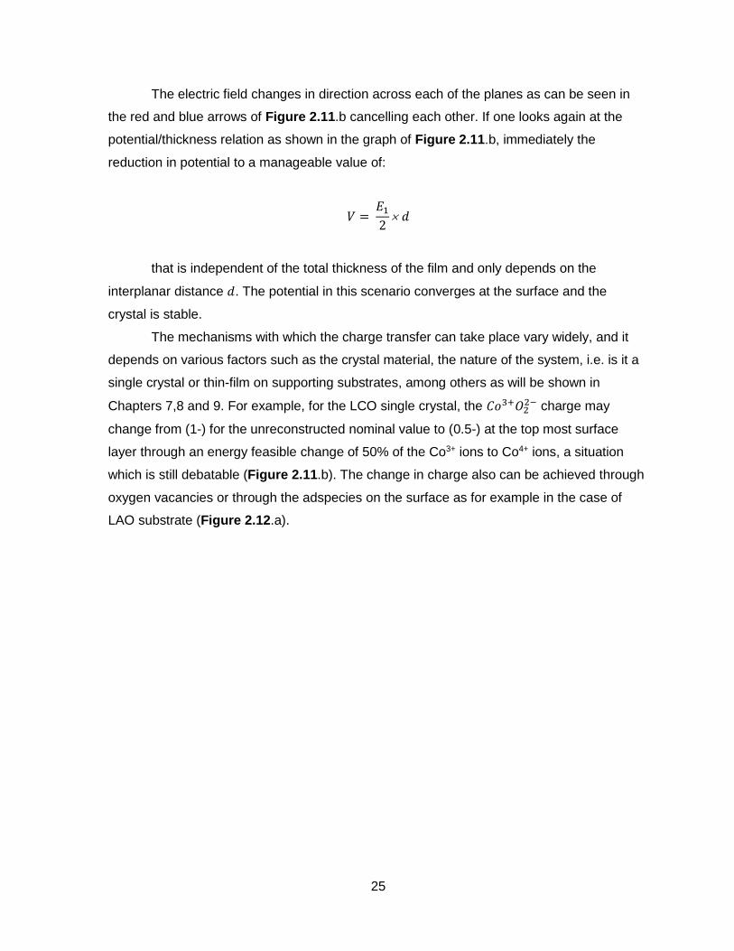
25

The electric field changes in direction across each of the planes as can be seen in

the red and blue arrows of Figure 2.11.b cancelling each other. If one looks again at the

potential/thickness relation as shown in the graph of Figure 2.11.b, immediately the

reduction in potential to a manageable value of:

𝑉 = 𝐸1

2 𝑑

that is independent of the total thickness of the film and only depends on the

interplanar distance 𝑑. The potential in this scenario converges at the surface and the

crystal is stable.

The mechanisms with which the charge transfer can take place vary widely, and it

depends on various factors such as the crystal material, the nature of the system, i.e. is it a

single crystal or thin-film on supporting substrates, among others as will be shown in

Chapters 7,8 and 9. For example, for the LCO single crystal, the 𝐶𝑜3+𝑂22− charge may

change from (1-) for the unreconstructed nominal value to (0.5-) at the top most surface

layer through an energy feasible change of 50% of the Co3+ ions to Co4+ ions, a situation

which is still debatable (Figure 2.11.b). The change in charge also can be achieved through

oxygen vacancies or through the adspecies on the surface as for example in the case of

LAO substrate (Figure 2.12.a).

26

Figure 2.12 (a) Model of the reconstructed polar LAO crystal. (b) Clean AlO2 terminated LAO crystal at high temperature during the pulsed laser deposition growing of LCO thin-film. (c) Model of the reconstructed uncapped LCO thin-film on LAO substrate. (d) Model of the reconstructed LCO thin-film on LAO substrate capped with a LAO layer. All models have adspecies and contamination layers that affects the electronic reconstruction process.

27

When the systems are thin-films on various substrates, the situation is more

complicated; but can be thought of in a similar manner. The polar nature of both the film and

the substrate materials dictates the way and the mechanism with which the surface will

compensate for the needed half charge. A special case occurs when both materials have

the same polarity and the same charges on the planes as in the cases of LCO thin-film

grown on LAO or NGO substrate where the heterointerface is continuous in comparison to

the situation when the supporting material is nonpolar as in the case of LCO thin-film on

STO substrate. The reconstructed surface charge of the substrate, which is half the nominal

plane charge, will migrate to the surface of the film to stabilize both crystal structures of the

film and the substrate. The mechanism of the charge transfer, though, can be different

between the two surfaces. For example, for the case of LCO thin-film on LAO substrate,

both are polar materials and have (1-), (1+) alternating planes (Figure 2.9 a and b). The

surface of the polar AlO2 terminated LAO substrate reconstructs by a charge reduction from

(1-) to (0.5-) under the influence of most probably oxygen vacancies and a loss of 1/8

oxygen per unit cell (Figure 2.12.a). When the LCO thin-film is grown on the top of that, the

AlO2 plane gain back the oxygens and the plane charge returns to the nominal charge of (1-

), Figure 2.12.b. The LCO planes then grow with alternating charge of (1+, 1-) till the

surface layer of CoO2. The surface CoO2 layer reconstructs to reduce the charge from (1-) to

(1.5-) with a valence change of the 50% of the Co3+ ions to Co2+ and the LaO layer on top of

that stays at (1+). Both layers together will result in a charge of (0.5-) and the whole film and

substrate structure are stabilized for the uncapped LCO thin-film (Figure 2.12.c). A similar

trend can be notice if the LCO thin-film has been capped with a layer of LAO. Again, the

CoO2 plane undergoes a valance change of the Co2+ to Co3+ and the plane charge returns to

the nominal value (1-). The LAO layers alternate between (1+) and (1-) till the final surface

AlO2 atomic layer where the charge is changed to (0.5-) under the influence of most

probably the oxygen vacancies and the surface is fully compensated (Figure 2.12.d). The

model has been explained in detail in chapter 8.5

In the case of the polar discontinuous interface between two materials one polar and

the other is nonpolar, the situation is more challenging. For example, in the case of LCO

thin-film on STO substrate, as will be shown in detail in chapter 9, the STO substrate has a

neutral surface with neutral planes and the surface energy is manageable (Figure 2.9.d).

The substrate does not require substantial surface reconstruction as in the case of the polar

LAO or LCO. When the LCO film is grown, which is most probably on the TiO2 plane, the

film starts to grow with the LaO plane which will be at (1+) charge and continuous with

28

alternating negative and positive equal charges till the surface of the thin-film. Again, the

polar catastrophe problem appears with the diverging potential at the polar surface of the

LCO. The crystal must undergo a surface reconstruction at both ends to stabilize the

structure. Rather than having the charge of the first LaO plane reduce from the (1+) to (0.5+)

charge, the underneath TiO2 layer undergoes a valence change of 50% of the Ti4+ ions to

Ti3+, since, unlike the monovalent La3+, the titanium ion has two accessible valences. The

charge of the TiO2 plane changes from (0) to (0.5-), Figure 2.13 leaving the LaO plane with

the nominal (1+) charge. The surface of the LCO thin-film also undergoes an electronic

reconstruction to compensate the surface and stabilize the structure. In Figure 2.13, we

introduce possible scenarios for the mechanisms by which the film reduces the plane charge

by half at the surface as supposed for the structure to be stable.63 For example, in Figure

2.13.a 50% of the surface Co3+ ions in the CoO2 layer are changed to Co4+ in high spin and

accordingly the plane charge is reduced to 0.5+ and the surface is fully compensated. In

another scenario, the top two layers, CoO2 and on top of it LaO layers, together produce the

needed half charge. In the suggested scenario, 50% of the Co3+ ions in the CoO2 layer are

changed to Co2+ in and the plane charge changes from (1-) to (1.5-). The top LaO layer

stays at (1+) and both layers together give the (0.5-) charge needed to compensate the

surface (Figure 2.13.b). It was found that by adding a top most CoO neutral layer on the top

of that, the system is more stable and it has more realistic structure as shown in Figure

2.13.c and will be explained in details in chapter 9.

29

Figure 2.13 Models of the possible scenarios for the electronic reconstruction of the LCO thin-film on STO substrate surface to compensate the plane charges and solve the polar catastrophe problem. The three models show the changes to the top most TiO2 layer of the STO substrate by valence change of the Ti4+ ion to Ti3+ ion and reduce the plane charge from 1.0 - to 0.5 – and the changes to the top most layer(s) of the LCO thin-film as (a) 50% of the Co3+ ions change to Co4+ in high spin and the CoO2 plane charge is reduced from 1.0 - to 0.5-, (b) 50% of the Co3+ ions change to Co2+ in high spin and the CoO2 plane charge is increased from 1.0 – to 1.5-, together with the LaO plane, which is still at 1.0 +, gives the needed half plane charge of 0.5- and last (c) it is the same as in (b) but with a top most layer of the neutral CoO plane with 0 charge which stabilizes the structure..

2.6 CoO

As one of the Co-containing systems chosen for the current study, CoO has a rock

salt structure, in which two face centred cubes (fcc) of Co and O infuse to form the crystal

(Figure 2.7.a). The material is nonpolar in the (001) planes and polar in the other two low-

index planes as explained in Figure 2.7, Figure 2.8 and in Table 2.1. In normal conditions,

CoO is an antiferromagnetic insulator with Co in the d7 electronic configuration and has Co2+

HS.58 The crystal field affects the electronic structure of the ion as it changes in response to

the lattice mismatch in the Co thin-film on various substrates. Co was reported to exist in two

local symmetries; Oh and Td whether in the bulk or as a thin-film. In the Oh symmetry the

30

electrons are distributed between lower three-fold degenerate t2g and higher two-fold

degenerate eg orbitals (Figure 2.3.c). Further splitting occurs due to the spin orbit coupling

of the 3d orbital forming three different states with pseudo orbital momentum of 1/2, 3/2 and

5/2, with two-, four- and six-fold degeneracy. Experiments show that the occupation of the d

states in CoO depends largely on the temperature; where changing the temperature

changes the occupation of the different states. At very low temperature the state with 1/2

total angular momentum is occupied and by increasing the temperature other states with 3/2

and 5/2 start to be filled.

In the current study CoO thin-films have been grown with molecular beam epitaxy

(MBE) on the (001) plane of the MgO substrate. Both materials have neutral surface with

zero net charge on each plane. The lattice mismatch between the thin-film and the substrate

results in a compressive strain of the system in the 𝑥𝑦 plane. It is expected that the

compressive strain will change the electronic configurations of the Co2+ ion and confine the

available hole to the lowest t2g shell to one of the three orbitals,57 as will be shown in chapter

6.

2.7 LaCoO3

LCO single crystal, under normal conditions, has the well known cubic perovskite

structure with a central cation surrounded by oxygen octahedron and eight cations of the

rare earth metal La on the corners of the unit cell (Figure 2.9.a). Studies show that the Co

ion can exist in the perovskite crystal in any of the three valencies namely Co2+, Co3+, Co4+,

and in possible different spin values, low (LS), Intermediate (IS) and high spin (HS). In

addition to that the ion can be in various symmetries that further affect the electronic

structure. For example, Co2+ HS can exist in Oh symmetry or in Td symmetry under certain

circumstances as will be shown in the analysis of thin-film LCO on STO substrate in chapter

9.

The nominal valency for the Co ion in the LaCoO3 perovskite crystal under normal

situation is Co3+ which can exist in LS, HS or even the less frequently occurring IS states

depending on the crystal field of the ion. In bulk LCO the most common symmetry is Oh in

which the five d-orbitals splits into lower triplet t2g and upper doublet eg shells (Figure 2.3).

Once more as described earlier the interaction between Hund’s rule exchange and the

crystal field splitting dictates which spin-state the ion can exist in. At low temperature, Co3+

ions in LCO crystal are in LS state (S=0) with the 6-electron paired up in the lower t2g three

orbitals leaving an empty eg shell. Hund’s rule interaction at that temperature is weaker than

31

the Oh crystal field splitting (Figure 2.5). Due to the lack of unpaired electron the crystal is

nonmagnetic and insulating at low temperature which was reported earlier.39 When the

temperature of the system is increased above 100 K, the higher energy states namely the

high spin-state will be populated and that cases an increase in the Co-O bond length and

accompanied by a decrease in the crystal field splitting and the Hund’s rule interaction

acquires the upper hand. The system undergoes a spin-state transition to most probably the

HS state (S=2) with the four d orbitals singly occupied and one electron pair in one of the t2g

shell orbitals (Figure 2.5). The crystal now in principle becomes paramagnetic as unpaired

electrons are evident in the crystal. The debateable IS state requires certain deformation of

the unit cell to be stable in the crystal which are not attainable in single crystal LCO under

normal conditions but are possible in strained thin-films as will be shown.68,69 When the

temperature of the crystal is further increased above 500 K, the mobility of the electrons and

the system reaches a metallic state.70,71

In the case of thin-film LCO on various materials, the lattice mismatch, tensile or

compressive, plays an important rule in stabilizing certain spin-states for the system. At a

low temperature below 85 K, strained LCO thin-films in general exhibit ferromagnetic

properties that are only possible when the Co cation exists in higher spin-states with

unpaired electrons. In this case the lattice mismatch exerts enough mechanical pressure to

distort the crystal structure and elongate or shrink the crystal in a specific direction. This

weakens the crystal field below Hund's interaction ΔOh< JH, and the energy levels change

accordingly with the electrons passing to the eg levels and the ion undergoes a spin-state

transition to HS state (Figure 2.6). The highly debatable case of the IS, can be stabilized

also by the distortion of the unit cell as in the case of tetragonal distortion or even the crystal

field can change to square planar while elongating the crystal in the 𝑥𝑦 plane (Figure 2.6).

Superconducting Quantum Interference Device (SQUID) magnetometer measurements

showed a strong ferromagnetic signal for the LCO thin-film on STO substrate and a weaker

signal for that on the STO substrate.37,38,40,42,45 The systems has a Curie temperature of 85 K

above which sustaining a long range order of the dipoles is not possible and the system

becomes paramagnetic. Bulk LCO is nonmagnetic below 100 K contrary to the strained thin-

film, but above that it becomes paramagnetic and both the film and the bulk acts

similarly.40,42

In both forms bulk or thin-film, LCO crystals show the possibility of the ion to exist in

other valencies and spin-states. Oxygen vacancies and adsorbed species among others can

maintain the existence of the ions in a specific valency. For example, X-ray absorption

32

signals of both bulk and thin-film LCO, where the majority of ions are in Co3+, show a low

energy transition at 776.3 eV which is a hallmark for the Co2+ ion in Oh crystal field.41,57

Careful analysis of the surface of LCO crystals in general show that the system undergoes a

surface reconstruction process in response to the polar catastrophe problem by a valance

change of 50% Co3+ to Co2+ as explained earlier (Figure 2.11). Such surface reconstruction

was evident in the case of LCO thin-film on LAO, NGO and STO as will be shown in later

chapters. Research also reported, in the analysis of LCO thin-film on STO substrate, the

existence of a charge order that spans all the film with 30% of the Co3+ ions change to Co2+

in Oh symmetry and another 30% to Co2+ in Td symmetry, with the latter driven by the

oxygen vacancies giving rise to what known as the Brownmillerite + Perovskite structure.38

The LCO thin-film responds to the strong lattice mismatch with the STO substrate by

creating oxygen vacancies and this change not only the valence state, but the symmetry of

the ions also, giving rise to a stripe like pattern which was evident in the transmission

electron microscopy (TEM) images and the low energy electron diffraction (LEED)

measurements as will be discussed in details in chapter 9.

The existence of Co4+ in the perovskite LCO crystal under normal situation is still

debatable and requires deeper analysis as we will present also in chapter 9. Systems that

require positive charge increase near the surface in response to the polar catastrophe

problem are believed to undergo a transition from Co3+ to Co4+, a case which is still unclear.

33

3 X-ray Optics72,73,74,75,76

3.1 Introduction

One of the main goals of the current research is to develop an understanding of the

SXR technique using a model 3d6 CoO layered system. The results will help set the rules for

further application of the technique to study more complicated systems like the 3d7

perovskite LaCoO3 structure. The newly implemented REIXS beamline in the Canadian

Light Source (CLS)2 opened a door of possibilities for running experiments and

combinations of experiments to obtain a wealth of information needed about hetero-

structured systems. The in ultra-high vacuum diffractometer and associated beamline set up

at the CLS operates in the soft X-ray region 300 eV to 1800 eV in which range all the

important transitions of the 3d transition metals and the rare earths exist as will be explained

in later chapter in details.1

In the present chapter, I start with a brief review of X-ray scattering, followed by a

derivation of the complex refractive index of a sample in terms of the complex strongly

energy dependent and spatially dependent dielectric constant. Reflection and refraction then

will be explained and the necessary theoretical aspect will be formulated including Fresnel’s

equation and Paratt’s formalism developed for the treatment of multilayer systems.72,77

3.2 X-ray Optics

X-rays form a relatively wide range of the electromagnetic spectrum starting from the

extreme ultra violet region at about 50 eV and ending with the gamma ray region at 100

keV. Depending on the energy range we can divide the spectrum into two regions of soft 50

eV to 2 keV and hard X-rays above about 2 keV.

When a material is irradiated with X-rays, the energy and momentum from the

incoming radiation can be transferred to the material. Depending on the way the photon

interacts with the system and the outcome of the interaction, it can undergo absorption or

scattering.73 In X-ray absorption, all the energy and momentum of the incident photon are

transferred to the system and can be absorbed by a core electron, for example, which can

then be excited to the conduction band, or vacuum as in X-ray Absorption Spectroscopy

(XAS) and X-ray Photoelectron Spectroscopy (XPS), respectively (Figure 3.1 a and step 1

in Figure 3.1.c). In other cases, X-ray energy and momentum is transferred to an electron in

34

a bound state of an atom after which the excited electron oscillates as a dipole and emits a

photon back. In this case of a locally bound state the momentum is transferred to the crystal

and because of the heavy mass of the crystal the energy loss is negligibly small. This is a

process like that in the recoil-free fraction of the Mossbauer effect experiment. The photon

undergoes inelastic X-ray scattering when it loses part of its energy and momentum to the

system. In the elastic scattering processes, such as Thomson scattering, while the photon

energy is conserved, it suffers a change in momentum as in X-ray Diffraction (XRD) and X-

ray Reflectometry (XRR). The focus of the current thesis is on the elastic scattering where

the momentum transfer of the light is the main probe for studying various characteristics of a

material such as geometry and, as it will be later explained, the electronic structure.

Scattering of a photon can be further classified to resonant and off-resonant

scattering depending on the energy of the incident photon. Each element has characteristic

absorption edges at specific energies representing, in a simple glance, the difference in

energy between the electron in a core level and that of the electron excited to the

conduction band. At such energies, the system reacts in a completely different manner from

energies well removed from the edges and the resultant scattering is known as resonant

scattering while at the other energies it is non-resonant scattering.

Off-resonant scattering is helpful in determining the geometry of the system while

resonant scattering exceeds that by detecting the electronic structure since it is sensitive to

the chemical composition and the oxidation state of the element. XAS, in principle, is the

technique with which one can start to locate the characteristic absorption edges followed by

X-ray scattering in both modes.

Soft X-ray scattering provides a non-destructive method to probe the electronic and

structural properties of the various materials. Furthermore, the high-intensity synchrotron

radiation sources enable studies of low-dimensional objects with the possibility of

wavelength (energy) tuning, which offers an element specific detection utilizing the so-called

resonance effects at specific energies corresponding to atomic transitions.

35

Figure 3.1 Models representing the quantum mechanical view of the interaction of radiation with matter and the resulted interaction Hamiltonian for each case. (a) and (b) are absorption and Thomson scattering respectively and the Hamiltonian for them ca be produced using the first order perturbation theory while (c) is the resonant scattering with second order perturbation. The model shows the two steps transition: Step 1 shows the core electron as it absorbs an incident photon and move to an empty higher valence state exactly above the chemical potential (and this is the XAS process) and in Step 2, electron with similar energy fills the core hole back and emits a photon to complete the fluorescence process. The figure is taken from Ref.”72” and part c was slightly modified to explain the two-step process.72

Transition metal oxides (TMOs) form an important field of study using the X-ray

based probing techniques. The properties of TMOs originate from the partially filled d-

Step 1 Step 2

36

orbitals that split into different energy levels as a response to the nonspherical symmetry of

the metal ions. The d shell has five orbitals and under the crystal field effect, they split into

different configurations for different symmetries. The balance between the crystal field

splitting and Hund's first rule of maximum spin multiplicity dictates the distribution of

electrons in the orbitals as explained in chapter 2. The physical and chemical properties of

the material heavily depend on this arrangement. The different X-ray techniques give us

insight into the charge, orbital and spin organization of the d electrons hence can provide

information regarding the relationship with the physical properties and perhaps explain some

emerging phenomena. Each element has absorption edges associated with the thresholds

of possible electronic transitions from each of the core states. X-ray absorption

measurements help to identify and quantify the concentration of elements within the

samples and their oxidation state. Controlling the polarization of the incident radiation and

following the dipole selection rules, X-ray absorption and the related resonant X-ray

reflectometry offers a powerful technique to provide information about the orbital, spin, and

oxidation state of the elements within the samples.

3.2.1 X-ray Scattering (Semi-classical Approach)

To understand the scattering phenomenon closely, in this section resonant X-ray

scattering will be reviewed from a semi-classical point of view as a starting step and will be

followed by the more realistic situation from a quantum mechanical point. It is convenient to

start by choosing a simple representative model such as the forced charged oscillator model

for a single bound electron,72 and then extend that to the case of multi-electron atom. The

electron in the atom will act as a damped harmonic oscillator resonating at natural frequency

𝜔𝑠 with a damping constant 𝛾. The radiation energy produces the driving force with

frequency 𝜔 that changes the electron state. The electron will have a mechanical force that

tries to resist the change on the electron state (restoration) and another that tries to

eliminate (damp) the effect of the external force on the electron. Assuming a radiation with 𝑬

and 𝑩 fields incident on the electron, the equation of motion for the system will be of the

form

�̈� + 𝛾�̇� + 𝜔𝑠2 𝒙 = −

𝑒

𝑚(𝐄𝑖 + 𝐯𝑠x𝐁𝑖)

37

where 𝑚 is the mass of the electron, 𝛾 is the damping constant, 𝜔𝑠 is the resonant

frequency, 𝑒 is the electron charge, and 𝐯𝑠 is the velocity of the electron. It should be noted

that the magnetic field has a very weak contribution in the driving force (𝑣

𝑐𝐸), in comparison

to the electric force and can be neglected, 𝑐 here is the speed of light. Solving the equation

for the electron position 𝒙 will result in displacement of 𝒙𝒔

𝒙𝑠(𝑡) = 1

𝜔2 − 𝜔𝑠2 + 𝑖𝛾𝜔

𝑒

𝑚𝐄(t)

𝐄𝑖(𝑡) = 𝐸𝑖 𝑒−𝑖𝜔𝑡, 𝒙𝑠(𝑡) = 𝑥𝑠𝑒−𝑖𝜔𝑡, 𝑡 is the time and 𝜔 is the frequency. The electron

acceleration amplitude will be

𝒙�̈�(𝑡) = −𝜔2

𝜔2 − 𝜔𝑠2 + 𝑖𝛾𝜔

𝑒

𝑚𝐄𝒊(𝑡)

The scattered radiation propagates as a spherical wave with a field strength

(𝐄𝒔𝒄𝒂𝒕(𝑅, 𝑡)) that is directly proportional to the electron acceleration 𝒙�̈�(𝑡). If we calculate the

field strength at a time 𝑡, then the acceleration of the electron that scattered the wave should

be found at earlier time (𝑡 − 𝑅/𝑐), where 𝑅 is the radius of the spherical wave. Having done

that, the scattered radiation strength relative to the incident radiation and after some

elaborate algebra is given by

𝐄𝒔𝒄𝒂𝒕(𝑅, 𝑡) = (𝑒2

4𝜋𝜖0𝑚𝑐2) 𝒙�̈�(𝑡 − 𝑅/𝑐)

and by substituting for 𝒙�̈� and combine the terms we get:

𝐄𝒔𝒄𝒂𝒕(𝑅, 𝑡)

𝐄𝒊(𝑡) = −𝑟𝑒

−𝜔2

𝜔2 − 𝜔𝑠2 + 𝑖𝛾𝜔

(𝑒𝑖𝑘𝑅

𝑅)

where 𝑟𝑒 is the Thomson scattering amplitude and is given by 𝑟𝑒 = (𝑒2

4𝜋𝜖0𝑚𝑐2), here 𝑒 is the

charge of the electron and 𝜖0 is the permittivity of free space.

A measure of the scattering amplitude for X-rays of an atom is the atomic scattering

factor or length 𝑓𝑠(𝜔). It represents the Fourier transform of the electron distribution in a

38

crystal and it includes the complex atomic form factor. The intensity of the scattered radiate

ion is related to the square of the scattering factor which makes it an important quantity in

both reflection and diffraction experiments. The complex scattering factor for a single

oscillator (s) is the amplitude of the outgoing spherical wave and is given by

𝑓𝑠(𝜔) =𝜔2

𝜔2 − 𝜔𝑠2 + 𝑖𝛾𝜔

,

For the X-ray region, since the core electrons are tightly bound to the atoms in the

crystal, the scattering length will be reduced by a factor 𝑓′ which at the atomic absorption

edges, shows a resonant behaviour. A second factor of change is the 𝑓′′ which is associated

with the dissipation within the system. To clarify the relation between the two factors and the

atomic scattering factor, the above formula can be can be rearranged by adding the term

(−𝜔𝑠2 + 𝑖𝛾𝜔 + 𝜔𝑠

2 − 𝑖𝛾𝜔) to give

𝑓𝑠(𝜔) = 1 + 𝜔𝑠

2 − (𝑖𝛾𝜔)

𝜔2 − 𝜔𝑠2 + 𝑖𝛾𝜔

≅ 1 + 𝜔𝑠

2

𝜔2 − 𝜔𝑠2 + 𝑖𝛾𝜔

= 1 + 𝑓𝑠′(𝜔) − 𝑖𝑓𝑠

′′(𝜔)

𝑓𝑠′(𝜔) and 𝑓𝑠

′′(𝜔) are the dispersion corrections and can be expressed as

𝑓𝑠′(𝜔) =

𝜔𝑠2(𝜔2 − 𝜔𝑠

2)

(𝜔2 − 𝜔𝑠2)2 + (𝛾𝜔)2

𝑓𝑠′′(𝜔) =

𝜔𝑠2𝜔𝛾

(𝜔2 − 𝜔𝑠2)2 + (𝛾𝜔)2

In general, the atomic scattering factor for a multi-electron atom is given by

𝑓(𝐐, 𝜔) = 𝑓0(𝐐) − 𝑓′(𝜔) − 𝑖𝑓′′(𝜔)

Where:

𝑓′(𝜔) = ∑ 𝑔(𝜔𝑠) 𝑓𝑠′ (𝜔𝑠, 𝜔)

𝑠

39

Where 𝑓0(𝐐) is the atomic form factor, 𝐐 = 𝐤𝐢 − 𝐤𝐬𝐜𝐚𝐭 is the scattering wavevector,

and 𝑔(𝜔𝑠) is the relative weight of each transition, Figure 3.2 shows the graph of the

calculated scattering corrections as a function of the relative incident frequency. The atomic

form factor reduces to the atomic number Z at very high driving frequencies and it

represents Thomson scattering for all the electrons in the atom . 𝑓′ and 𝑓′′ have a significant

effect on the complex refractive index of the system 𝑛(𝜔), when the energy of the incident

X-ray coincides with one of the absorption edges as will be explained in details in the next

section.

Figure 3.2 Theoretical calculation of the dispersion corrections 𝑓𝑠′(𝜔), 𝑓𝑠

′′(𝜔) of an arbitrary system using the equations derived in the script. The imaginary part 𝑓𝑠

′′(𝜔),

peaks at the values where 𝜔 = 𝜔𝑠 at the normalized x-axis accompanied by a steep

decrease in the real part 𝑓𝑠′(𝜔) and vise versa for the other peak position. The figure is

taken from Ref.72

The calculated theoretical dispersion corrections are not accurate enough near

absorption edges at which the scattering cross section σ(𝜔) depends on the environment of

the element in the crystal. To have accurate terms particularly near the absorption edges the

dispersion corrections are indirectly obtained from the measured experimental cross section

which in principle is generated from the X-ray absorption (XAS) signal in total electron yield

40

(TEY) mode. The dispersion correction 𝑓′′ is related to the scattering cross section through

the relation:

𝜎(𝜔) =8𝜋

3𝑟𝑒

2 𝜔4

(𝜔2 − 𝜔′2)2

+ (𝛾𝜔)2=

8𝜋

3𝑟𝑒

2 |𝑓(𝜔)|2

The dispersion corrections are related to each other by the Kramers-Kronig transformation

𝑓′(𝜔) = 2

𝜋℘ ∫

𝜔2𝑓′′(𝜔′)

𝜔′2 − 𝜔2

+∞

0

𝑑𝜔′

𝑓′′(𝜔) = −2𝜔

𝜋℘ ∫

𝑓′(𝜔′)

𝜔′2 − 𝜔2

+∞

0

𝑑𝜔′

where ℘ is the principle value, in which the integral is taken from -∞ to +∞ with a very small

separation around the poles (𝜔 ± 𝜖 𝑎𝑛𝑑 𝜖 → 0) not to be confused with limits appearing on

the integrals above.

Before explaining the changes in the scattering factor near absorption edges, it is

important to know that in addition to the resonant part arising from 𝑓′and 𝑓′′, an additional

part of the spectrum originates from the electrons promoted to an unbound state which gives

a background signal and affects the values of the scattering factor. Figure 3.3 shows the

real and imaginary parts of the scattering factor of transitions near the L absorption edges

for Co drawn from the calculated Chantler-table for a free Co atom.

41

Figure 3.3 The scattering corrections, as a function of energy, near Co L2,3 edges, drawn from the theoretical Chantler tables.81

Right below the edge, 𝑓′ is high while 𝑓′′ is very low indicating that the energy of the

incident photons is not enough to excite electrons to any of the empty states above the

chemical potential. At the edge, 𝑓′ undergoes a drastic reduction while 𝑓′′ suddenly

increases where the energy of the incident photons reaches a level in which bound

electrons can be excited into the first empty state just above the chemical potential leading

to a higher absorption rate of the photons and therefore to an increased 𝑓′′. Figure 3.3

shows the cut off frequency at which the transitions of the 2p electron to 3d orbitals for the

Co ion occur as a sharp step edge after with a drastic increase in 𝑓′′ accompanied by a

reduction in 𝑓′. Above the cut off, the 𝑓′ increases and 𝑓′′decreases with a factor of 1/𝜔3

due to the background scattered electrons, till they hit the second sharp step where the 2p

to 4s transition occurs and the scenario is repeated. At far enough energies from the edges,

𝑓′ increases till hitting the upper most limit of Z = 27 while the absorptive part goes to zero.

3.2.2 Refractive Index

The response of a certain material to incident radiation is dictated by the change in

the speed of light as it passes through it. The refractive index of a material is a quantitative

measure of the response of a certain medium to incident radiation. It depends on the

incident frequency and shows a resonant behaviour near the absorption edges of a material.

42

In this section the refractive index equation will be derived and the relation to the atomic

scattering factor will be explained.

The starting point will be the differential form of Maxwell's equations in matter:

∇ ∙ 𝑬 = 𝜌

𝜖0 ∇×𝑬 = −

𝜕𝑩

𝜕𝑡

∇ ∙ 𝑩 = 0 ∇×𝐁 = 𝜇0𝐉 + 𝜇0𝜖0

𝜕𝑬

𝜕𝑡

Where 𝐸 is the electric field, 𝐵 is the magnetic field, 𝐽 is the volume electric current

density, 𝜌 is the volume electric charge density 𝜇0 is the permeability of free space, 𝜖0 is

the permittivity of free space and 𝑡 is time.

Manipulations of these equations starting from the Faraday's equation will lead to the

transverse wave equation

(𝜕2

𝜕𝑡2− 𝑐2∇2) 𝐄𝑇(𝐫, 𝑡) = −

1

∈0

𝜕𝐉𝑇(𝐫, 𝑡)

𝜕𝑡

In the case of forward scattering, the current density will be given by

𝐉0(𝐫, 𝑡) = −𝑒𝑛𝑎 ∑ 𝑔𝑠𝐯𝑠(𝐫, 𝑡) ,

𝑠

where 𝑛𝑎 is the electron density and should not be confused with the complex

refractive index 𝑛(𝜔), 𝑔𝑠 is the spectral weight factor with the property ∑ 𝑔𝑠 = 𝑍𝑠 and

𝐯𝑠(𝐫, 𝑡) is the velocity of the electron. The summation goes over all the electrons s within the

atom. For an oscillating bound electron perturbed by an incident electromagnetic radiation

the current density will be

𝐉0(𝐫, 𝑡) = −𝑒2𝑛𝑎

𝑚𝑒∑

𝑔𝑠

𝜔2 − 𝜔𝑠2 + 𝑖𝛾𝜔

𝜕𝐄(𝐫, 𝑡)

𝜕𝑡𝑠

.

Substitute this result in the traverse wave equation and reduce to give

43

(𝜕2

𝜕𝑡2−

𝑐2

𝑛2(𝜔)∇2) 𝐄T(𝐫, 𝑡) = 0

with the refractive index 𝑛, given by

𝑛(𝜔) = [1 −𝑒2𝑛𝑎

2𝜖0𝑚𝑒∑

𝑔𝑠

𝜔2 − 𝜔𝑠2 + 𝑖𝛾𝜔

𝑠

]

12

.

Expanding the term and taking the effective first two terms leads to

𝑛(𝜔) = 1 −𝑒2𝑛𝑎

2𝜖0𝑚𝑒∑

𝑔𝑠

𝜔2 − 𝜔𝑠2 + 𝑖𝛾𝜔

𝑠

Notice the similarity of the second part of the right hand side with the dispersion

corrections 𝑓𝑠(𝜔) found earlier in section 3.2.1. Substituting the dispersion corrections will

give:

𝑛(𝜔) = 1 −𝑛𝑎𝑟𝑒𝜆2

2𝜋[𝑓′(𝜔) − 𝑖𝑓′′(𝜔)]

Where 𝑟𝑒 is Thomson scattering length and 𝜆 is the wavelength of the incident

radiation which was used instead of the frequency (𝜔) to simplify the equation. We know

that

𝑛(𝜔) = 1 − 𝛿 + 𝑖𝛽

Notice that the scattering part will be given by

𝛿 = 𝑛𝑎𝑟𝑒𝜆2

2𝜋𝑓′(𝜔)

44

and the absorption part will be given by

𝛽 = 𝑛𝑎𝑟𝑒𝜆2

2𝜋𝑓′′(𝜔)

Figure 3.4 gives a general idea about the changes in the real part of 𝑛(𝜔) in

different regions of the electromagnetic radiation spectrum from infrared up to hard X-ray.

Figure 3.4 The real part of the refractive index near various absorption edges, at different regions of the radiation spectrum taken from Ref.73

From the graph, we can detect distinct energy regions with specific resonant

frequencies within each of them. Analyzing the changes in 𝑛(𝜔) for the wide spectrum

shows that, generally, the envelope is going down with increasing frequency. In the UV and

X-ray regions, the value of 𝑛 goes below unity, and it asymptotically approaches unity at the

highest frequencies of X-rays. The reason for that comes from the nature of the high

frequency X-ray which is above any of the transitions of the elements except for the core

shell ones. The maximum change in the refractive index within a specific range occurs at the

resonance energy where the absorption reaches its highest value (𝛽) and the scattering is

minimum (𝛿). Looking more closely to the equations will help better understand the

changes. In the low energy regions, the factor 𝑛𝑎𝑟𝑒𝜆2

2𝜋 is bigger than in the UV and X-ray

regions due to the fast decrease of the λ2. This makes it more effective in the magnitude of

45

the change at the low energy region and less for the high-energy region. The term 𝜔2 −

𝜔𝑠2 + 𝑖𝛾𝜔 is responsible for the sign, so below UV it gives always a negative sign causing

the refractive index to be higher than unity regardless of the proximity from the absorption

edge. Above the UV region, the 𝜔2 − 𝜔𝑠2 + 𝑖𝛾𝜔 starts to give positive sign resulting in the

decrement of the refractive index lower than unity. Although the reduction is so small, it was

found to play a vital role in determining the properties of different materials. Around a

specific absorption edge, the value of 𝑛 increases with increasing ω in the region below the

edge and it decreases with increasing ω above that. At the resonant edge, where ω = ω0, 𝑛

undergoes a drastic element specific increase. The scattering term, δ, reduces rapidly at the

edge then increases rapidly above the edge, followed by a steady reduction. The absorption

term, β, behaves oppositely; in which it increases dramatically at the edge in a characteristic

fashion associated with the electronic structure of the element, then decreases rapidly just

above the edge before going back to the overall trend of decrease.

In chapter 4, the analysis technique using the program ReMagX3 will be introduced.

A major part of the modeling and simulation process is to generate a suitable refractive

index and atomic scattering factor for the two modes of the program. The above relations

clarify the process and show the methodology of generating the imaginary part of the

refractive index from the measured scattering cross section and which is then used to

extract the imaginary part of the atomic scattering factor of a specific element. Finally,

Kramer-Kronig relations are used to generate the real part of both.

3.2.3 X-ray Scattering (Quantum Mechanical Approach)

In the current section the quantum mechanical treatment and derivation of the

system will be introduced. If one considers again the model of single oscillator for the

electron bound to an atom, when the system is radiated with X-ray the radiation will act as a

time dependent perturbation and adds a new term for the unperturbed systems Hamiltonian

which will become:

𝐻 = 𝐻𝑒 + 𝐻′(𝑡)

where 𝐻𝑒 is the Hamiltonian of the unperturbed electron, and 𝐻′(𝑡) is the external radiation

field Hamiltonian. Substituting for the values and consider the case of free electron for

simplicity the total Hamiltonian before the perturbation will have the form:

46

𝐻 =𝐩𝟐

2𝑚

from a classical point of view the momentum resulting from the interaction of

electromagnetic radiation with an electron is given by (𝐩 + 𝑒𝐀) where A is the

electromagnetic vector potential field of the light. Substituting for the momentum in the total

Hamiltonian will give:

𝐻 =(𝐩 + 𝑒𝐀)𝟐

2𝑚=

𝐩𝟐

2𝑚+

𝑒𝐀. 𝐩

𝑚+

𝑒2A𝟐

2𝑚= 𝐻𝑒 + 𝐻′(𝑡)

where the middle two terms are the perturbation Hamiltonian (𝐻′(𝑡)) which results from the

interaction of the photon field and the irradiated electron and the first term gives rise to the

absorption and resonant elastic scattering of radiation while the second represents

Thomson scattering (Figure 3.1). It should be noted that other terms might result from the

expansion of the interaction momentum, but they were neglected since they only appear for

very intense photon fields and do not have any effect on the resonant scattering with which

the current research is concerned and the same thing applies for the Thomson scattering

term.

The remaining important part of the resulted perturbation Hamiltonian have the form:

𝐻′(𝑡) =𝑒𝐀. 𝐩

𝑚

Notice that the potential field of radiation after expansion is given by:

𝐀 = 𝐴0�̂�𝑒𝑖(𝐤𝐫−𝜔𝑡) = 𝐴0�̂�𝑒−𝑖𝜔𝑡(1 − 𝑖𝑘𝑟 +1

2(𝑖𝑘𝑟)2 + ⋯ )

The first term of the expansion is the electric dipole, the second is the magnetic

dipole, the third is the electric quadrupole and the higher terms were not included. From the

definition of the electric field:

𝐄 = −𝜕𝐀

𝜕𝑡= 2𝑖𝜔𝐴0𝜖̂𝑒−𝑖𝜔𝑡 (1 − 𝑖𝑘𝑟 +

1

2(𝑖𝑘𝑟)2 + ⋯ ) = 𝜖̂𝐸0𝑒−𝑖𝜔𝑡(… )

47

and from the commutation relations we can substitute for 𝐩 by:

𝐩 = 𝑖𝑚[𝐫, 𝐻𝑒]

The final goal of the current formalism is to find the rate of transition from the initial

state to the final state. This rate is given by the very well known Fermi’s golden rule which

we are using here without derivation and further explanation about the rule can be found in

other references:75

𝐼𝑎𝑏𝑠 = ∑|⟨𝑓|𝐻′|𝑖⟩|2

𝑓

(𝛿(𝜔 + 𝐸𝑖− 𝐸𝑓) + 𝛿(𝜔 − 𝐸𝑖 + 𝐸𝑓))

where 𝐼𝑎𝑏𝑠 is the rate of transition to final state, 𝑖 and 𝑓 are the initial and the final

states and 𝐸𝑖 , 𝐸𝑓 are the electric field at both states, and 𝛿 is the Dirac 𝛿 function. Taking

only the electric dipole since it far exceeds the magnetic dipole. For the range of photon

energy that we are using, the higher order multipoles can also be neglected as discussed

earlier. Substituting for all the values will give:

𝐼𝑎𝑏𝑠 = 𝑒𝐸0

2

2𝑚2∑|⟨𝑓|�̂�𝐫|𝑖⟩|2

𝑓

(𝛿(𝜔 + 𝐸𝑖− 𝐸𝑓) + 𝛿(𝜔 − 𝐸𝑖 + 𝐸𝑓))

Dirac function can now be substituted by Lorentzian function with a linewidth 𝛤 in

addition to only considering the absorption term. Since we are considering the ground state I

is substituted with g and the expression will be:

𝐼𝑎𝑏𝑠 = −𝑒𝐸0

2

2𝑚2𝐼𝑚 ∑ lim

𝛤→0|⟨𝑓|�̂�𝐫|𝑔⟩|2 (

1

𝜋(𝜔 + 𝐸𝑔− 𝐸𝑓 +𝑖𝛤2 )

)

𝑓

and the expression will reduce after solving the summation and by simple complex

algebra to finally give:

𝐼𝑎𝑏𝑠 = −𝑒𝐸0

2

2𝜋𝑚2𝐼𝑚 ∑ lim

𝛤→0⟨𝑔|�̂�𝐫|𝑓⟩ (

1

(𝜔 + 𝐸𝑔− 𝐸𝑓 +𝑖𝛤2 )

) ⟨𝑓|�̂�𝐫|𝑔⟩

𝑓

48

We know by definition that the cross section is the rate of transition divided by the

incident photons flux 𝐼𝑖 and is defined as the energy flux divided by the photon energy:

𝜎𝑎𝑏𝑠 =𝐼𝑎𝑏𝑠

𝐼𝑖

The result suggests that the system undergoes a two-step operation. First the photon

is absorbed by a core electron and jump the gap to the valence band as an intermediate

state, then another electron from the same band fills the core hole and emits a photon.

Before we move with our discussion it is important to introduce a well known general

form of the equation without derivation, The equation is the Kramers-Heisenberg equation

and has the form:

𝜎𝑎𝑏𝑠 = |∑⟨𝑔|𝑇†|𝑓⟩⟨𝑓|𝑇|𝑔⟩

𝜔 − (𝐸𝑓− 𝐸𝑔) − 𝑖𝛤𝑓

|

2

where 𝜔 is the incident photon energy, 𝑇 is the transition operator.

The relation between the cross section and the atomic scattering factor is also valid

here as for the classical treatment, but rather than have one value for the result it is going to

be represented by a matrix that changes with changing the environment of the element such

as the lattice symmetry.

3.2.4 X-ray Reflectometry

As we introduced in section 3.2, when a material is irradiated with an energy near the

absorption edge of an element, the incident photon is absorbed by a core electron which

gets excited to a higher energy level. The resulted core hole gets filled by an electron with

similar energy and the difference in energy is radiated as an out going photon. The process

is illustrated in Figure 3.1.c and is known as resonant X-ray reflectivity SXR. In the current

section, we will try to derive the needed theoretical equations for modeling and simulating

the SXR spectra for multilayer thin-films. The equations used are like the ones used in the

modeling and fitting software “ReMagX”3 which will be discussed in chapter 4.

49

To determine the reflectivity of a multilayer thin-film it is necessary to consider the

case of radiation passing between two media with refractive indices 𝑛𝑖 and 𝑛𝑡 (Figure 3.5).

If we assume the radiation is a plane wave and 𝑖, 𝑟 and 𝑡 are associated with the incident,

reflected, and transmitted (refracted) waves respectively, then the continuity boundary

condition at 𝑧 = 0 states that the tangential magnetic and electric fields are continuous. For

the vertical polarization case, the electric field will be perpendicular to the plane of incidence

and the magnetic field parallel. The continuity relation of the electric field across the

interface will give

𝐸𝑖 + 𝐸𝑟 = 𝐸𝑡

Where 𝐸𝑖, 𝐸𝑟 and 𝐸𝑡 are the incident, reflected and transmitted electric fields,

respectively.

50

Figure 3.5 (Top) Schematic drawing of multiple reflections and refractions between various layered materials with different refractive indices (n) within an infinite slab with a total thickness d the film is composed of N=2 layers and a supporting substrate. (Bottom) Schematic drawing of Reflection and Refraction across interfaces of materials with different refractive indices (n). It shows the electric and magnetic fields of the incident, reflected and transmitted radiation in addition to the momentum associated with each of them.

The electric and magnetic components of light are related by 𝐵 = 𝑛𝐸/𝑐, so the

continuity of the magnetic field across the surface will result in

− n𝑖(𝐸𝑖−𝐸𝑟) cos𝛼𝑖 = − n𝑡𝐸𝑡 cos𝛼𝑡

Substituting for the 𝐸𝑡 in the second equation will give

n𝑖(𝐸𝑟−𝐸𝑖) cos𝛼𝑖 = − n𝑡(𝐸𝑟+𝐸𝑖) cos𝛼𝑡

From which we can find that

𝐸𝑟[n𝑖cos𝛼𝑖 + n𝑡cos𝛼𝑡] = 𝐸𝑖[n𝑖cos𝛼𝑖 − n𝑡cos𝛼𝑡]

The so-called Fresnel coefficient relates the incident amplitudes with the reflected

and transmitted ones across an interface. Using the results of the boundary conditions we

get

51

𝑟 =𝐸𝑟

𝐸𝑖=

[n𝑖cos𝛼𝑖 − n𝑡cos𝛼𝑡]

[n𝑖cos𝛼𝑖 + n𝑡cos𝛼𝑡] ,

where r is the reflectivity coefficient and is related to the transmittivity coefficient with

𝑟 + 𝑡 = 1. The intensity reflectivity (R) and transmittivity (T) are the absolute squares of the

reflectivity and transmittivity coefficients. It is convenient to express the equation by using

the wave vector k. Notice that the wave vector in the z-direction for a medium with refractive

index n is given by

𝑘𝑧 = 𝑛𝑘 cos𝛼

Using that relation for the reflectivity and transmittivity results in

𝑟 =𝑘𝑖𝑧 − 𝑘𝑡𝑧

𝑘𝑖𝑧 + 𝑘𝑡𝑧

𝑡 =2𝑘𝑖𝑧

𝑘𝑖𝑧 + 𝑘𝑡𝑧

Where 𝑘𝑖𝑧 and 𝑘𝑡𝑧 are the wave vectors in the z-direction for the incident and

transmitted waves. At this point we can expand the problem by considering the reflection

from a homogeneous slab with finite thickness on a substrate. In this case the radiation will

undergo multiple reflections and transmissions from the different interfaces. Figure 3.5

shows a schematic diagram of some of the reflections and transmissions that will result from

the situation. The total amplitude reflectivity will be calculated by adding all the reflections

and transmissions that occur which results in an infinite sum of the reflectivities.

𝑟𝑠𝑙𝑎𝑏 = 𝑟01 + 𝑡01𝑡10𝑟12𝑝2 ∑ (𝑟10𝑟12𝑝2)𝑚

∞

𝑚=0

Notice that 𝑝2 = 𝑒−𝑖𝑘𝑑 is the phase factor with d defined as the thickness of film 1

(Figure 3.5). Finding the result of the geometric series will give

52

𝑟𝑠𝑙𝑎𝑏 = 𝑟01 + 𝑡01𝑡10𝑟12𝑝21

1 − 𝑟01𝑟12𝑝2

From Fresnel equation we find that across a single interface

𝑟01 = −𝑟10

𝑟012 + 𝑡01𝑡10 = 1

which in turn simplifies the term to

𝑟𝑠𝑙𝑎𝑏 =𝑟01 + 𝑟12𝑝2

1 − 𝑟01𝑟12𝑝2 ,

The calculated intensity reflectivity (R) is the absolute square of this value. If we

expand our model to the case of films with N layers of materials with different refractive

index grown over a substrate with an infinite thickness we find that the reflectivity will be

given at each successive layer starting from the substrate and the Nth layer by

𝑟𝑁,∞′ =

k𝑁 − k∞

k𝑁 + k∞

𝑟𝑁−1,𝑁 =𝑟𝑁−1,𝑁

′ + 𝑟𝑁,∞′ 𝑃𝑁

2

1 + 𝑟𝑁−1,𝑁′ 𝑟𝑁,∞

′ 𝑃𝑁2

𝑟𝑁−2,𝑁−1 =𝑟𝑁−2,𝑁−1

′ + 𝑟𝑁−1,𝑁𝑃𝑁−12

1 + 𝑟𝑁−2,𝑁−1′ 𝑟𝑁−1,𝑁𝑃𝑁−1

2 ,

.

.

The recursive trend to calculate the reflectivity on the surface by associating the

reflectivity from one layer with the reflectivity of the layer above it, starting from the substrate

is referred to as Parratt’s formalism77 (Figure 3.5.a).

It should be noted that although the atomic scattering factor changes from plane to

plane in the thin-film and probably models could be represented by atomic planes rather

than slabs, it is still a valid approximation to relate the atomic scattering factors to the

refractive index and assume that it is constant and uniform along the whole thickness of the

slab.

53

3.2.5 X-ray Diffraction

XRD is an experimental method used to determine the spatial arrangement of atoms

in a periodic crystal. Incident X-ray is scattered and interfered in a pattern that reflects the

atomic arrangement and the atomic species of a certain sample. It relies on the atomic

scattering factor as a measure of the ability to scatter X-rays, which in principle depends on

the electron density within a crystal. Since the inter-atomic distances in crystals range

between 1.5 – 4 Ǻ, they correspond to the hard X-ray region in the electromagnetic

spectrum.

In XRD, periodic arrangements of atoms in space, known as crystal structures, are

irradiated with hard X-rays. The electrons of the atom in the crystal oscillate, generating

spherical waves of X-rays. The interaction between these waves gives rise to the diffraction

phenomena of X-rays. The phase difference between the scattered X-rays from atoms and

the incident X-rays, resulting from their path difference, causes a change in the resulting

intensity as consequence of constructive and destructive interference. The XRD

experiments seek to know the parameters forming the suitable condition for the formation of

constructive peaks to produce a detectable diffraction beam. The famous Bragg's law deals

with this situation and formulates the condition for the permitted constructive interference as

follows

2𝑑ℎ𝑘𝑙𝑠𝑖𝑛𝜃𝐵 = 𝑛𝜆

Where 𝑑ℎ𝑘𝑙 is the interplanar distance, the indices refer to the lattice plane Miller

indices, and 𝜃𝐵 is Bragg's angle. Notice that 𝑑ℎ𝑘𝑙is associated with the lattice parameter

"𝑎"of the various crystal systems. The structure factor of a unit cell represents the amplitude

and the phase of the scattered wave from all the atoms in the unit cell and is given by

𝐹ℎ𝑘𝑙 = ∑(𝑓𝑗0(𝐐) − 𝑓𝑗

′(𝜔) − 𝑖𝑓𝑗′′(𝜔))𝑒𝑖𝐐.𝐫j

𝑗

∑ 𝑒𝑖𝐐.𝐑n

𝑁

where the first summation is over all the atoms in the unit cell 𝑗 and the second is

over all the included lattice sites𝑁.𝐫jis the position vector of an atom in the unit cell and 𝐑n

is the lattice vector of a specific site. Structure factor helps to determine the intensity of the

54

scattered radiation at the constructive sites. Together the structure factor and Bragg's law

are important in determining the crystal parameters of a certain sample. Since |𝐹| is the

amplitude of the scattered wave, the reflections for ℎ𝑘𝑙 planes will be present in the XRD

pattern only if the |𝐹|2 has a value other than 0, which occurs only if Q coincides with a

lattice vector in the reciprocal space.

3.2.6 X-rays to Study Transition Metal Oxides

After introducing the SXR, it became clear that it is highly effective in research in the

field of TMOs. The SXR measurements are element specific as it is clear from the resonant

behaviour of the complex refractive index. Near the edge of a specific element, the complex

refractive index changes in a way that represents any change in the distribution of electrons

in the orbitals, especially d-orbitals for the transition metals. Since the electron is promoted

from the p-orbitals to the split level of the d-orbitals, SXR becomes highly sensitive to the

charge, orbital polarization and total spin. The absorption of the system changes

dramatically when reaching an absorption edge in response to the fast change in the

complex refractive index. This change is proportional to the abundance of each oxidation

state of the element and result in several peaks associated with the transition energy of the

species. In SXR with linearly polarized light, the anisotropy of absorbing light with different

polarization reveals the anisotropy of the occupation of different orbitals. The X-ray magnetic

reflectivity, using circular polarized light, shows a difference in the spectra between left and

right polarized light indicating the difference in the spin-state of the system favouring one

direction over the other. Both techniques are important in explaining, on a microscopic level,

the magnetic and electric properties of a specific system.

It should be noted that although the atomic scattering factor changes from plane to

plane in the thin-film and probably models could be represented by atomic planes rather

than slabs, it is still a valid approximation to relate the atomic scattering factors to the

refractive index and assume that it is constant and uniform along the whole thickness of the

slab. This is particularly important in the modeling and simulation processes of the

reflectometry data in an element specific manner as will be shown in chapter 4.

55

4 Experiment and Data Analysis

4.1 Experiment and Experimental Setup

The growing interest in finding a suitable experimental technique and theoretical

methods to study the characteristics of the buried interfaces of the transition metal oxides

(TMOs) hetero-structures, reached a climax in the past few years. It has been realized that

the orbital occupation and spin-states at the hetero-interfaces were responsible for the

exotic new properties these materials exhibit. The Soft X-ray Scattering (SXS) technique has

proven to be not only sensitive to a specific element, but by tuning the energy of the incident

photon, it becomes sensitive to the occupation of a specific orbital of the element. The

advancement in the third-generation synchrotrons in recent years, using Elliptical

Polarization Undulator (EPU), allows for brilliant, collimated focused and selectively

polarized radiation. Coupling the energy tuning and polarization further enables the detailed

study of orbital occupation, local symmetry, local magnetic moment, and magnetic

properties of the systems. The SXS experimental setup, the theoretical analysis and

modeling tools in addition to the sample growing methods will be introduced in this chapter.

4.1.1 Triple Chamber System

The main technique used to study the samples in the current research, has been

Soft X-ray Scattering (SXS) that encompasses both X-ray Absorption Spectroscopy (XAS)

and Soft X-ray Reflectometry (SXR). The experiments were carried out at the 10ID-2,

Resonant Elastic - Inelastic X-ray Scattering (REIXS) beamline of the Canadian Light

Source, Saskatoon, Canada (Figure 4.1).2 The beamline has been specifically designed to

operate in the soft X-ray range to cover the core to valence transitions of the rare earths,

800 to 1750 eV, and 3d transition metal compounds, 400 - 950 eV, in addition to light

element such as O, N and C, 350 – 700 eV, with the ability to control the incident photon

energy, polarization, and intensity. An attached triple-chamber endstation can be used to

grow various samples, characterize them with non-synchrotron based spectroscopies and

in-vacuum transfer them between non-synchrotron and synchrotron based analysis tools in

addition to the possibility of using them separately (Figure 4.1.c). The system consists of a

state of the art home-built Molecular Beam Epitaxy (MBE) chamber, a RSXS chamber and a

commercial Omicron Multi-Probe X-ray Photoelectron Spectroscopy with an attached

Scanning Tunnelling Microscopy Chamber (Omicron MXPS with STM).

56

Figure 4.1 The 10ID-2 (REIXS) beamline of the Canadian Light Source (CLS)2 components. (a) the energy monochromator, (b) the soft X-ray scattering (RSXS) endstation and (c) an AutoCAD diagram shows the final planned triple chamber system: the RSXS chamber, the omicron multi-probe system, the molecular beam epitaxy (MBE) chamber and all are connected through the transfer chamber.

The non-synchrotron based characterization has been carried out in the commercial

omicron MXPS with STM ultrahigh vacuum system (Figure 4.1.c). The system is currently a

standalone and has two analysis compartments: one houses a 1000 MKII X-ray Source with

a monochromator, and a SHERA hemispherical analyzer for X-ray Photoelectron (XPS) or

X-ray Induced Auger measurements. The analyzer can also be coupled with an electron gun

to perform energy loss spectroscopy (EELS), or Auger Electron Spectroscopy (AES), or

(a) (b)

(c)

57

coupled with an ultraviolet (UV) helium-based lamp to run Ultraviolet Photoemission

Spectroscopy (UPS) measurements. The electron gun on its own can be coupled with a

Secondary Electron Detector (SED) to run Scanning Electron Microscopy (SEM) images for

the sample surfaces. The second compartment has a floating stage that is suspended by

springs to eliminate any possible external vibrations, and a removable tip holder, and is

controlled by the modular hardware and software, (the MATRIX control), for in-vacuum

Atomic Force Microscopy (AFM) and Scanning Tunnelling Microscopy/Spectroscopy

(STM/STS) measurements.

The non-commercial units of the triple chamber system, the MBE and SXS

chambers, have been designed and implemented by the group of G. Sawatzky at both the

University of Groningen and the University of British Columbia (UBC) and were published

elsewhere (Figure 4.1.c).1,78 The two chambers are currently operated individually in the

synchrotron with a so-called vacuum suitcase used to transfer the samples between both

chambers. In an advanced stage of the project, the chambers will be joined together via a

fourth transfer chamber. Although some techniques from the MBE and the MXPS chambers

were used to characterize or treat some of the samples, the actual samples were received

from collaborators and mainly measured in the Resonant Soft X-ray Scattering RSXS

endstation.

The MBE growing chamber has a base pressure better than 10-9 mbar. The chamber

has all the needed equipment to grow various materials, including Knudsen cells, high

temperature furnaces and an electron beam evaporator, in addition to a gas cracker and

multiple leak valves to introduce gaseous constituents. The metal flux can be controlled by

computer operated shutters and with a Quartz Crystal Micro-balance (QCM). Sample growth

can be monitored with Reflection High-Energy Electron Diffraction (RHEED) and Low-

Energy Electron Diffraction (LEED).

Introducing the samples to the systems is carried out through ultra-high vacuum load

lock chambers attached to each one of them. A detailed description of the design and

construction of the MBE chamber can be found elsewhere.78

The most important of the three chambers to the current study is the RSXS

endstation chamber which will be discussed in detail in the following section.

4.1.2 RSXS Endstation1,2

The RSXS endstation is a specially designed stainless steel UHV endstation with a

1𝑚 diameter (Figure 4.1.c). The chamber houses the RSXS diffractometer and a number of

58

in-vacuum equipment and analysis tools, and leaves a margin for possible upgrades. A

complete description of the chamber was published by our former group member Dr.

Hawthorn.1

The system is pumped with a 700 𝐿 turbo pump and a 700 𝐿 cryopump which

ensures a base pressure of better than ~ 2×10−10 mBar. The condition of ultra-high vacuum

is important in the measurements where soft X-ray is used. The naturally occurring ambient

condition elements can interact with the incident and reflected radiation and can cause

absorption or refraction of the radiation. The chamber is attached from one side permanently

to the REIXS beam line, and from the other side temporarily to a differentially pumped load

lock chamber with a base pressure of better than ~ 8×10−8 mBar through a gate valve.

The load lock chamber is equipped with a vertically movable sample storage unit and

a model PGWMS (OM) Ferrovac GMBH pincer grip attached to a vacuum model

RMDG1000-100 dual rotary transfer arm. The assembly is used to load the samples and

transfer them to the RSXS endstation main body. It should be noted that the load lock will be

removed and replaced with a transfer chamber in an advanced stage in the project.

The main body of the chamber houses a 4-circle, 9-motion diffractometer (Figure

4.2). The system has four detectors: a Multi-Channeltron Plate (MCP), a channeltron, a

photodiode and a new polarization analyzer tuned for specific elements including Ni, Cu and

O. The diffractometer 9 vacuum motions are achieved with in-vacuum stepper motors (Arun

Microelectronics Ltd. C14.1 motors) and are assigned the conventional names x, y, z, Φ, χ

and θ, whereas the detectors have 2θ, zdet and slit wheel rotational motions (Figure 4.2). To

precisely assign these motions, imagine a Cartesian system with the middle of the sample

holder at the origin, x-axis is perpendicular to the sample holder plane and in the incident

plane, y- and z- axes are parallel to the sample holder and are horizontal and vertical axes

respectively. It should be noted that the x-,y- and z- axes of motion are, in general, different

from the sample’s x-, y- and z- axes along which the lattice parameters a, b and c are

defined (Figure 4.3).

59

Figure 4.2 The diffractometer inside the RSXS endstation. The 9 motions and the 4 detectors are marked with the white text boxes and the figure was taken from Ref.1

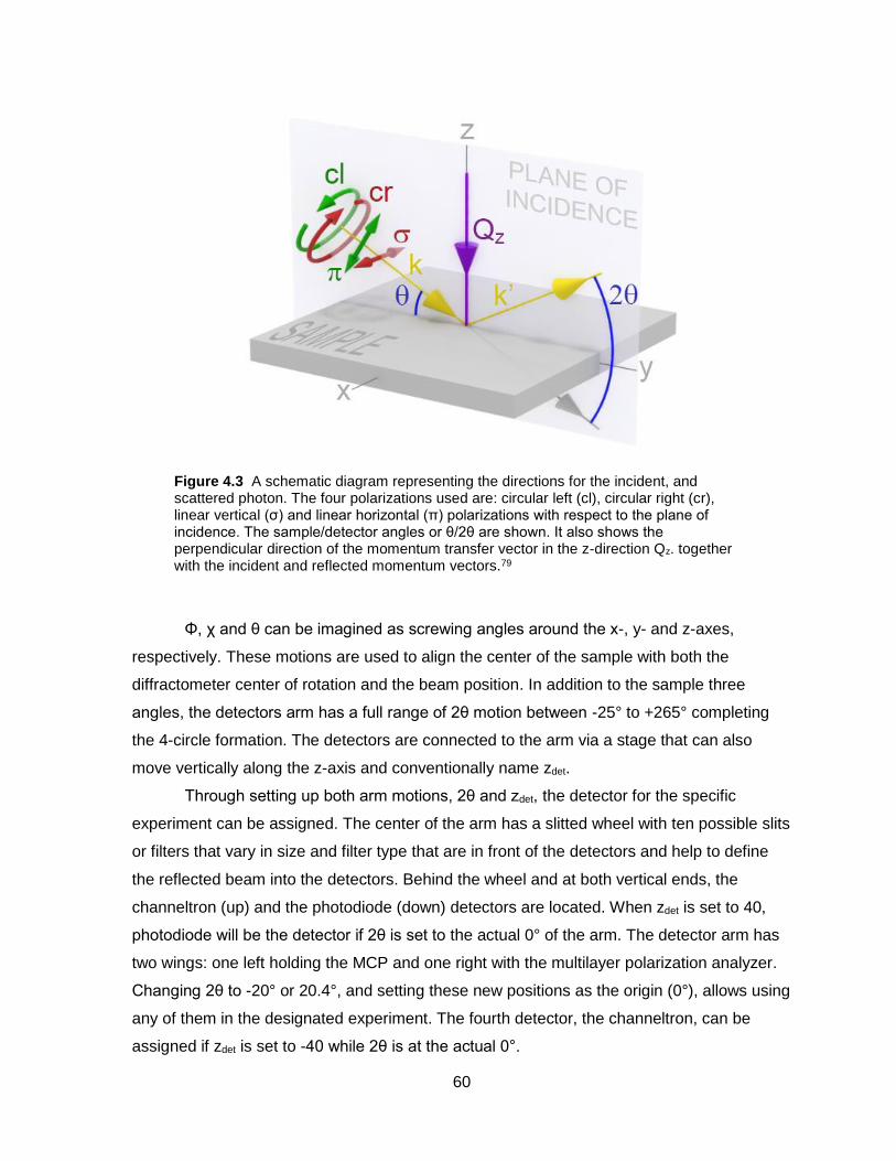
60

Figure 4.3 A schematic diagram representing the directions for the incident, and scattered photon. The four polarizations used are: circular left (cl), circular right (cr), linear vertical (σ) and linear horizontal (π) polarizations with respect to the plane of incidence. The sample/detector angles or θ/2θ are shown. It also shows the perpendicular direction of the momentum transfer vector in the z-direction Qz. together with the incident and reflected momentum vectors.79

Φ, χ and θ can be imagined as screwing angles around the x-, y- and z-axes,

respectively. These motions are used to align the center of the sample with both the

diffractometer center of rotation and the beam position. In addition to the sample three

angles, the detectors arm has a full range of 2θ motion between -25° to +265° completing

the 4-circle formation. The detectors are connected to the arm via a stage that can also

move vertically along the z-axis and conventionally name zdet.

Through setting up both arm motions, 2θ and zdet, the detector for the specific

experiment can be assigned. The center of the arm has a slitted wheel with ten possible slits

or filters that vary in size and filter type that are in front of the detectors and help to define

the reflected beam into the detectors. Behind the wheel and at both vertical ends, the

channeltron (up) and the photodiode (down) detectors are located. When zdet is set to 40,

photodiode will be the detector if 2θ is set to the actual 0° of the arm. The detector arm has

two wings: one left holding the MCP and one right with the multilayer polarization analyzer.

Changing 2θ to -20° or 20.4°, and setting these new positions as the origin (0°), allows using

any of them in the designated experiment. The fourth detector, the channeltron, can be

assigned if zdet is set to -40 while 2θ is at the actual 0°.

61

At the center of the wheel is a ~1 cm2 Yttrium Aluminium Garnet (YAG) crystal that

fluoresces when irradiated with X-rays. The crystal is used in the process of aligning the

diffractometer center of rotation to the beam position inside the SXS endstation. The beam

properties will be presented below. To access the crystal, 2θ should be set to -20° and zdet

down to the -20 position. In addition to the 9 motions, the cryostat rotates with an external

driven motion through a differentially pumped vacuum feed trough. The specific way of

mounting the diffractometer to a sub-frame isolated from the body of the chamber, helps to

modify the position in relation to the incident beam in addition to noise reduction. By using a

special sample holder that accepts the sample over a rotatable cylindrical middle part, Φ

degree of freedom can be extended to the full 360°. This surface of the middle part can also

be at 30° or 45° which adds to the measurement possibilities.

The sample is thermally and electrically isolated from the rest of the sample

manipulator, but it is connected through the sample mount to an electrometer that can

measure the leakage current. The four detectors and the electrometer are running

simultaneously all the time during the experiment. The electrometer and the MCP are used

to measure XAS of the sample in both modes Total Electron Yield (TEY) and Total

Fluorescence Yield (TFY) respectively. TEY is more surface sensitive (~100 Å), and

depends mainly on the conductivity of the samples while the TFY has much more depth

sensitivity and is not affected by the sample conductivity. For example, it was impossible to

acquire any TEY signal for the CoO thin-films at low temperature where the film is extremely

insulating. The photodiode and the polarization analyzer detector are used for SXR

experiments in both modes at constant energy and at Fixed Qz. The channeltron sensitivity

can go down to a single photon, and can be used instead of the photodiode for experiments

in which the signal is expected to be very low.

The chamber is mounted to the REIXS beamline of the Canadian light source (CLS)2

which is a third-generation synchrotron. The beamline starts from the 10ID straight section

of the storage ring with an EPU. The undulator supplies photons with energies ranging

between 80 - 2000 eV, spanning most of the transition metals edges, and with all the

possible polarizations: linear σ/π/45° and circular left/right (Figure 4.3).

The resulting beam passes through a Variable-Line-Spacing Plan Grating

Monochromator (VLS-PGM) with three gratings and associated coated plane mirrors. The

grating and the associated coated mirror are made from various materials including: Au, Ni,

and Cu to cover the whole energy range. The grating-mirror combination helps to optimize

the photon flux. It also allows the selection of the needed harmonic and suppresses other

62

harmonics: 1st harmonic for energies below 900 eV and 3d, 5th harmonics for higher

energies. The beam has an energy resolution of 0.05 eV and a flux of 5x1012 photon/s at

1000 eV and 100 mA ring current with a spot size of 250 and horizontal 150 vertical oval

shaped at the sample position. The incident beam size can be controlled through an orifice

which helps to prevent saturating the detector.

It is important when running an experiment using the RSXS endstation, to make sure

that both the photon shutters and the gate valve connecting the main body to the beamline

are closed. The sample should always be transferred at room temperature and if the run

includes XAS, the cryostat is better turned off if it is not urgently needed since the cryostat

vibration interferes with the TEY signal. In the following section, an actual experimental run

will be introduced with an explanation of the importance for each step.

The first step in running any experiment is to optimize the sample holder position by

finding the centre of rotation. To achieve that, a pin-head sample mount with a telescope are

used through a series of θ rotations between 0° and 180° to optimize the y position,

following that x is optimized at a 90 degree θ angle. The centre of rotation is then aligned

with the beam by direct illumination of the Yttrium Aluminium Garnet (YAG) crystal and

adjusting the z position until the shadow of the tip of the pin-head is in the middle of the

beam spot. The sample is then transferred from the storage in the load lock to the sample

holder in the goniometer. Attached wobble sticks are used to screw the sample to the

manipulator. At 𝜃 = 90°, the telescope is used to confirm the position of the middle of the

sample at the centre of rotation of the diffractometer. The peak of the absorption edge of the

main component is detected and the energy of the monochromator is shifted accordingly.

For the current research, the energy for the samples containing Co has been set as

follows: for the LaCoO3 (LCO) thin-films, the Co3+ L3 edge main peak was set to 779.2 eV

and for the CoO thin-films, the Co2+ first peak is set to 776.3 eV. For the samples that do not

contain Co, the energy was set to the peaks of the major component of the sample including

the La M5 at 833.5 eV and O K at 529.1 eV.

Following that, a set of checking scans have been performed to the assigned peaks

in order to confirm the stability of the undulator, the monochromator and the other beamline

optics. The energy has been moved to a higher or lower value and the polarization has been

changed to linear σ/π or circular left/right as needed. If the experiment requires high energy,

the harmonics are changed among 1, 3 and 5. Each time a small scan has been performed

around the maximum peak to detect and track any unexpected fluctuations in energy. The

resolution of the photon energy is in the range of 0.05 eV, if any energy fluctuation is higher

63

than that, it may affect on-resonant scans located on sharp peaks. This situation requires

more attention and shift of energy before running the intended constant energy

reflectometry.

Running an XAS scan at a fixed energy with changing z and y help to align the

centre of the sample to the beam position inside the RSXS endstation. Using the direct

beam, the centre of the photodiode detector is aligned to the beam and the 2θ position is set

to 0°. It is not required to align the other detectors since they are at fixed horizontal and

vertical positions from the photodiode. The sample is meant to be ready to run XAS

measurements in both modes TEY and TFY. The optimum angles for the Multi-Channeltron

Plate/sample couple are 140.4°/30° which will result in an angle of 69.6° between the

sample surface and the MCP for the TFY measurements.

An absorption long scan was carried out to check all the possible edges of the

components within the range and to check for any contamination signals. To check the

homogeneity of the samples, a matrix of absorption measurements was carried out at

different sample points spanning the whole surface and concentrated closer to the middle

where most of the measurements are performed. To reduce the contamination on the

surface, a thermal cycle was carried out. The sample was gradually heated up to 430 K

allowing the pressure to recover at each temperature, and then it was brought to room

temperature and the test runs were repeated.

The sample is ready for XAS measurements in both TEY and TFY modes. XAS and

X-ray Linear Dichroism (XLD) with σ- and π- polarization were measured for the various

edges. To run the X-ray Magnetic Circular Dichroism (XMCD) measurements, a magnetic

field was applied to the sample. The dipole moments within the sample are expected to align

in a certain direction under the influence of the applied magnetic field. The sample was

silver-paint mounted on the flat surface of a cylindrical magnet especially designed to have

fields in or out of plane. The direction of the magnetic field is set manually by positioning the

magnet with respect to the sample mount using a gauss meter, after which the magnet was

fixed to the mount, and then the sample was pasted to it. The magnets have strength of

slightly less than 0.1 Tesla in the middle of the flat surface, and are assumed to be uniform

in the middle of the sample. XAS is measured with circularly left and right polarized light.

XAS measurements can be conducted at any temperature needed between 430 - 20 K.

Most of the LaCoO3, and CoO thin-films XAS measurements were carried out at room and

20 K temperatures unless stated otherwise. Although the sample manipulator design

ensures maintaining the correct alignment of the sample position at any temperature, the

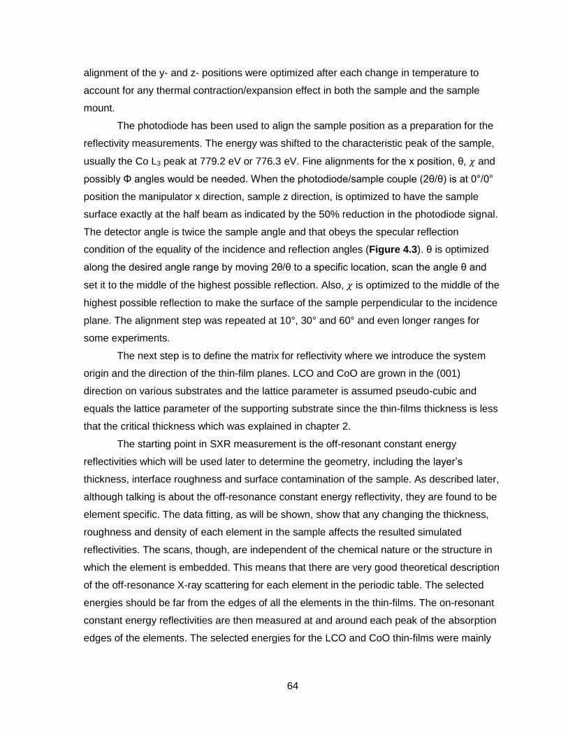
64

alignment of the y- and z- positions were optimized after each change in temperature to

account for any thermal contraction/expansion effect in both the sample and the sample

mount.

The photodiode has been used to align the sample position as a preparation for the

reflectivity measurements. The energy was shifted to the characteristic peak of the sample,

usually the Co L3 peak at 779.2 eV or 776.3 eV. Fine alignments for the x position, θ, 𝜒 and

possibly Φ angles would be needed. When the photodiode/sample couple (2θ/θ) is at 0°/0°

position the manipulator x direction, sample z direction, is optimized to have the sample

surface exactly at the half beam as indicated by the 50% reduction in the photodiode signal.

The detector angle is twice the sample angle and that obeys the specular reflection

condition of the equality of the incidence and reflection angles (Figure 4.3). θ is optimized

along the desired angle range by moving 2θ/θ to a specific location, scan the angle θ and

set it to the middle of the highest possible reflection. Also, 𝜒 is optimized to the middle of the

highest possible reflection to make the surface of the sample perpendicular to the incidence

plane. The alignment step was repeated at 10°, 30° and 60° and even longer ranges for

some experiments.

The next step is to define the matrix for reflectivity where we introduce the system

origin and the direction of the thin-film planes. LCO and CoO are grown in the (001)

direction on various substrates and the lattice parameter is assumed pseudo-cubic and

equals the lattice parameter of the supporting substrate since the thin-films thickness is less

that the critical thickness which was explained in chapter 2.

The starting point in SXR measurement is the off-resonant constant energy

reflectivities which will be used later to determine the geometry, including the layer’s

thickness, interface roughness and surface contamination of the sample. As described later,

although talking is about the off-resonance constant energy reflectivity, they are found to be

element specific. The data fitting, as will be shown, show that any changing the thickness,

roughness and density of each element in the sample affects the resulted simulated

reflectivities. The scans, though, are independent of the chemical nature or the structure in

which the element is embedded. This means that there are very good theoretical description

of the off-resonance X-ray scattering for each element in the periodic table. The selected

energies should be far from the edges of all the elements in the thin-films. The on-resonant

constant energy reflectivities are then measured at and around each peak of the absorption

edges of the elements. The selected energies for the LCO and CoO thin-films were mainly

65

close to the Co L2,3 and O K edges, and around La M4,5, Ti L2,3 and Mn L2,3 edges when the

elements were present in the samples.

The most sensitive SXR measurements to the electronic structure of the thin-film are

those measured at fixed Qz. Fixed Qz scans were taken for the Co L2,3 edges at several Qz

values. The Qz values were selected according to the on-resonant constant energy

reflectivity, mainly the Co L3 edge peaks at 776.3 and 779.2 eV associated with the

characteristic peaks of Co2+ and Co3+ valences. Fixed Qz scans are expected to be more

sensitive to Co2+ which is the “unusual” valence of the ions in the LCO thin-films, that we are

trying to study, where the constant energy reflectivity measured at 776.3 eV has a maximum

(constructive interference) and least sensitive when it has a minimum (destructive

interference), and similar argument is applied for the Co3+ at 779.2 eV. Finding Qz values for

which one of the constant energy scans is at minimum and the other is at maximum helps in

generating contrast between both ions as needed in the experiment. In addition to the

proposed extrema, fixed Qz values were chosen also at points were the interference is not

completely destructive or completely constructive and in some cases, detailed scan maps

for fixed Qz regions at small steps were performed to track specific changes.

The SXR measurements were performed using σ- and π- polarized light to probe

any possible anisotropies that may result from orbital occupation. In the study of the effect of

surface contaminants on the reflectivity, the contamination layer growth, during the sample

cooling, have been tracked and investigated for the CoO on MgO sample.

4.1.3 CoO and LaCoO3 Samples

Depending on the type of the desired study, several samples were readily available.

To develop the understanding of the newly implemented X-ray reflectometry technique, the

highly investigated binary oxide TMO CoO thin-films,44,57 with d7 electronic structures over

various substrates were chosen. Following that, the more complicated perovskite TMO, LCO

thin-films and hetero-structures with their exotic properties, can be better understood and

the data can be further analyzed. CoO thin-films were prepared by the group of L. H. Tjeng

of Max Planck Institute (MPI) in Dresden, whereas the LCO thin-films were grown by the

group of H. N. Lee at Oak Ridge National Lab (ORNL).

Briefly, CoO thin-films were epitaxially grown by Molecular Beam Epitaxy (MBE) on

(001) oriented MnO and MgO substrates with lattice parameters of 4.44 and 4.21 Å,

respectively. The lattice mismatch between CoO, with 4.27 Å lattice parameter, results in

tensile and compressive strains in the CoO thin-films on MnO and MgO, respectively. An

66

ultra-high vacuum chamber, with base pressure better than 310−10 mbar, was used to

grow the samples. Substrates were at ~250 °C and elemental Co of 99.99 % purity was

evaporated at ~1225 ± °C onto the substrate in ~310−7 mbar oxygen purity. Further

specifications about the growth process can be found else where.57,80

LCO thin-films were grown on various substrates at ~700 °C, 100 mTorr of oxygen

with 10 Hz and 58.5 𝑚𝐽 laser energy. The sintered LCO target is ablated by a KrF excimer

laser (𝜆 = 248 nm) with fluence of ~1 𝐽

𝑐𝑚2⁄ . The samples were cooled down to room

temperature in 100 mTorr of oxygen. The supporting substrates were chosen to

demonstrate tensile or compressive strain and polar continuity-discontinuity at the interface

between the LCO thin-films and the supporting substrates. The LCO (3.80 Å) thin-films were

grown on (001) oriented substrates with various lattice parameters and polarity including,

polar NGO (3.86 Å), nonpolar STO (3.90 Å) and polar LAO (3.78 Å) substrates. The film

thickness ranges between 11- 14 nm. Samples were grown in pairs, uncapped and capped

with 1- 2 nm of LAO epitaxial layer. To normalize the measurements, pure LAO, NGO and

STO substrates uncapped and capped with an LAO layer were also obtained.

The structure of the films, and the magnetic properties were measured by the grower

using X-ray Diffraction (XRD) and Super Conducting Quantum Interference Devise (SQUID)

techniques, respectively, and were repeated locally in UBC facilities. XRD and Hard X-ray

Reflectometry were measured for the LCO samples inside a PANalytical X’Pert Pro MRD

diffractometer with Cu Kα at 8050 eV (𝜆 = 1.54 Å) to determine the structural parameters of

the thin-films. The results confirmed the tensile strain of the LCO thin-films on NGO and

STO substrates and the compressive strain of the LCO thin-film on LAO substrates. A

Quantum Design Magnetic Property Measurement System (MPMS-XL7) SQUID

magnetometer has been used to measure the magnetic properties of the un-capped and

capped thin-films on STO and LAO substrates. Due to the magnetic nature of the NGO

substrate, it was not possible to measure the film without the signal from the substrate

interfering in the resulted signal.

The results for the various reflectometry experiments were sorted and analyzed,

using a specially written macro for the commercial Microcal OriginLab software. The newly

developed analysis software, ReMagX,3 is used to simulate and fit the resulted data. XAS

data is used to obtain and calculate the complex refractive index by fitting the TEY signal,

off-resonant, to the complex part of the theoretical refractive index of CoO or LCO generated

from Chantler tables. The real part is then generated via Kramers-Kronig transformation.

67

The resulting complex refractive index is then used in the program’s compound mode to

model the samples, simulate and fit the reflectivity data. For the element specific analysis,

similar method has been used to generate the atomic scattering factor of each element then

they were used to build the models, simulate and fit the data for further determination of the

chemical profile of each element within the sample. Each model is represented by an atomic

density profile that reflects the characteristics of each element in the sample. A detailed

explanation of the software, the modelling and simulation process will be presented in the

following section

4.2 Computer Simulation and Data Fit

The first step in data analysis is to sort and normalize the data. This process was

carried out through a home-built OriginLab 8.1 macro written by the group member Dr.

Macke. XAS signals in both modes taken with σ- or π-polarized light are corrected through

division by the monochromators mesh current: 𝐼𝑚𝑒𝑠ℎ𝑚𝑒𝑎𝑠𝑢𝑟𝑒𝑚𝑒𝑛𝑡. While that is enough for the

measurements taken with σ-polarized light where the electric field vector (𝐄) of the incident

radiation is in-plane parallel to the sample surface, further correction is needed for that taken

with π-polarized light where (𝐄) is at an angle 30° with the surface. The resulting intensity of

the XAS signal out-of-plane perpendicular to the sample surface (𝐼𝑧) is given by a linear

combination of the intensities measured with σ- and π-polarized light 𝐼𝜎 and 𝐼𝜋,

respectively:12

𝐼𝑧 =1

cos2 30° 𝐼𝜋 −

sin2 30°

cos2 30° 𝐼𝜎

𝐼𝑧 =4

3 𝐼𝜋 −

1

3 𝐼𝜎

SXR measurements were corrected with a ratio between the direct current:

𝐼𝑝𝑑𝑑𝑖𝑟𝑒𝑐𝑡

𝐼𝑚𝑒𝑠ℎ𝑑𝑖𝑟𝑒𝑐𝑡⁄ , without the sample and at 0°/0° θ/2θ angles and the photodiode current:

𝐼𝑝𝑑𝑚𝑒𝑎𝑠𝑢𝑟𝑒𝑚𝑒𝑛𝑡

𝐼𝑚𝑒𝑠ℎ𝑚𝑒𝑎𝑠𝑢𝑟𝑒𝑚𝑒𝑛𝑡⁄ , in the actual measurement as follows:

68

𝑅 =

𝐼𝑝𝑑𝑚𝑒𝑎𝑠𝑢𝑟𝑒𝑚𝑒𝑛𝑡

𝐼𝑝𝑑𝑑𝑖𝑟𝑒𝑐𝑡⁄

𝐼𝑚𝑒𝑠ℎ𝑚𝑒𝑎𝑠𝑢𝑟𝑒𝑚𝑒𝑛𝑡

𝐼𝑚𝑒𝑠ℎ𝑑𝑖𝑟𝑒𝑐𝑡⁄

The measurements with π-polarisation were further normalized to compensate for

the angle between the incident photon and samples surface (SXR/cos2θ). The energies

were shifted in such a way that the first peak of the Co2+ is at 776.3 eV or the highest peak

of the Co3+ is at 779.2 eV. Further analysis is made with the use of the simulation and fitting

software ReMagX.3

ReMagX is an “in-house” developed specialized software, developed by Dr.

Sebastian Macke,3 that uses a combination of experimental results and theoretical methods

to build models and simulate the reflectivity data. The software depends on Parratt recursive

formalism77 to generate SXR theoretical curves for various energies. The formalism extends

the result of the reflectivity through a single slab to the case of multilayers thin-films as

explained in chapter 3. The resulting curves will then be fitted to the experimental SXR data,

using a number of fitting algorithms. The software is designed to fit non-magnetic SXR data

with various polarizations in addition to fitting the asymmetric signals in X-ray Magnetic

Reflectivity (XRMR) for the magnetic samples.

The program has two modes: compound and element-specific modes. In the

compound mode, the models are a segregation of layers with each layer represented with a

complex refractive index of the specific compound (Figure 4.4.a). The refractive indices are

generated from the XAS measurements. The generated models start with the supporting

substrate followed by the suggested layers for the model stacking on the top and ends with

a vacuum layer. The program also considers the gradual change of one layer to the other

through the roughness calculations of the interface at the respective lower layer. Thickness

and roughness of each layer are fitting parameters in the compound mode and that

represents the most elaborate capability of the mode.

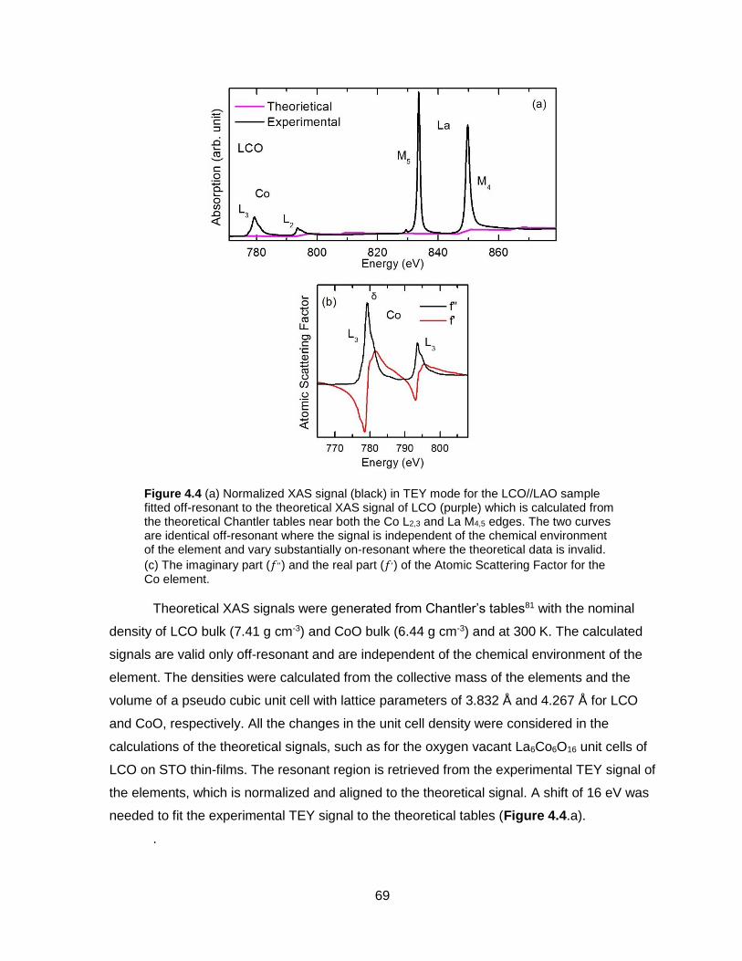
69

Figure 4.4 (a) Normalized XAS signal (black) in TEY mode for the LCO//LAO sample fitted off-resonant to the theoretical XAS signal of LCO (purple) which is calculated from the theoretical Chantler tables near both the Co L2,3 and La M4,5 edges. The two curves are identical off-resonant where the signal is independent of the chemical environment of the element and vary substantially on-resonant where the theoretical data is invalid.

(c) The imaginary part (𝑓,,) and the real part (𝑓,) of the Atomic Scattering Factor for the Co element.

Theoretical XAS signals were generated from Chantler’s tables81 with the nominal

density of LCO bulk (7.41 g cm-3) and CoO bulk (6.44 g cm-3) and at 300 K. The calculated

signals are valid only off-resonant and are independent of the chemical environment of the

element. The densities were calculated from the collective mass of the elements and the

volume of a pseudo cubic unit cell with lattice parameters of 3.832 Å and 4.267 Å for LCO

and CoO, respectively. All the changes in the unit cell density were considered in the

calculations of the theoretical signals, such as for the oxygen vacant La6Co6O16 unit cells of

LCO on STO thin-films. The resonant region is retrieved from the experimental TEY signal of

the elements, which is normalized and aligned to the theoretical signal. A shift of 16 eV was

needed to fit the experimental TEY signal to the theoretical tables (Figure 4.4.a).

.

δ

70

The fitting process starts by subtracting a factor from the TEY signal in such a way

that the background value just below the absorption edge is at zero as can be seen in the

leveled region just below the Co L3 edge of Figure 4.4.a. The resulting curve is then divided

by another factor to make the background signal just above the edge to be unity as can be

seen for the region just above the La M4 edge of Figure 4.4.a. The curve is then aligned and

scaled to replace the resonant regions for both Co and La in the theoretical XAS signal

through a home written macro “FiTEY” which deploys various equations to have a precise fit

and the resulted signal is the imaginary part of the refractive index, β (Figure 4.4.a).3 The

equation which was found to give the best results and was used through the whole thesis is:

𝛽(𝐸) = (𝐼𝑋𝐴𝑆

𝐸 𝑎) + 𝑏 + (𝑐 𝐸)

Where 𝐸 is the energy, 𝐼𝑋𝐴𝑆 is the measured XAS signal, a is the scaling factor, b is

the offset and c is the slope of the linear relation and all are case specific. The real part of

the refractive index, 𝛿, is then calculated through Kramers-Kronig transformation which is a

mathematical method to determine the real part from the imaginary part for the complex

numbers that represents special sets of functions such as the refractive index.4,5,12

Refractive indices were generated from the TEY signals of the all the samples and from

pure reference signals. At this point the compound mode simulation of ReMagX can be

performed for the sample models.3,4,5,12

In the compound mode, the LCO capped samples have been modeled with single

layer on top of the supporting substrates using the refractive index generated from the TEY

signal of the associated sample. The uncapped samples have been then modeled with two

layer models; one layer represented with the refractive index that is generated from the

capped sample TEY signal and a top layer represented using a combination of the refractive

indices generated from the capped sample TEY and what is called the excess TEY signal.

The signal represents the difference between TEY signals of the capped and the uncapped

samples.

The second mode is the element-specific mode, in which the material is treated on

the elemental level rather than the compound level. Similar to the compound mode, in the

element- specific mode, the model is a segregation of layers, but each layer is further

separated into the elemental constituents. The fitting parameters are extended to the

roughness, thickness and density of each individual element with any needed constraint for

71

the parameters. The generated refractive index of each compound is then used to generate

the atomic scattering factors of each element in the compound at any needed valency and

spin-state (Figure 4.4.b). The resulted atomic scattering factors substitute each constituent

in the layer providing more freedom to be individually optimized. Individual elements can

also have more layers than the rest of the constituents, such as the top contamination

oxygen layer. Through the scripting facility, the attributes of the elements can be constrained

in any needed fashion; like connecting the densities of the Co various valences and spin-

states so the collective density equals the nominal value of Co density in LCO unit cell. The

atomic scattering factor can be modified as needed and additional parameters can be added

and fitted; like introducing an extra Lorentzian to correct the intensity of a certain peak. The

oxygen top layer is fitted individually to account for the contamination on the top of the film.

It should be noted that O in this layer is substituted for all the possible surface contaminants

such as CO2, or even the organic molecules that may adsorb to the sample surface. These

light elements have resonances far below the TMOs edges that we are studying, but still can

diffract the radiation and influence the analysis as will be shown in chapter 6 for the analysis

of CoO on MgO substrates.

The atomic scattering factors for all the components were generated by extracting

the imaginary part atomic scattering factor 𝑓 ,, from the refractive index imaginary part 𝛽,

through eliminating 𝑓 ,, of all the other components. The resulted 𝑓 ,, is then Kramers-Kronig

transformed to produce the real part 𝑓 ,. Generally, similar models to the ones produced by

the compound mode have been generated and tested with various fitting parameters on the

elemental level. For both LCO and CoO models, TEY signals of the thin-films were used to

generate the atomic scattering factors to simulate and fit the SXR scans with the one and

two layer models for the capped and uncapped samples. The element specific mode allows

the models to have mixed constituents like the atomic scattering factors of the capped

sample with that of the excess signal at the top layer. The two constituents can exist

together at a specific ratio to be optimized individually or connected as needed. The use of

the element-specific mode was found to improve the simulation in comparison to the

compound mode, especially with the addition of a contamination oxygen layer. The model

was successful for samples like LCO on LAO and NGO uncapped or capped with LAO as

will be discussed in Chapters 7 and 8, and it was acceptable for the LCO on STO sample.

Further analysis of the more complicated LCO on STO sample, requires detailed

representation of the layers not only at elemental level but at various valences, spin-states

and in different symmetries as well. In order to generate the required atomic scattering

72

factors, various pure elements such as Co3+ LS, Co3+ HS, Co2+ HS in Octahedral (Oh)

symmetry (Oh) and Co2+ Tetrahedral symmetry (Td) were generated from previous literature

studies.41,45 Depending on the model suggested, in each layer the densities of the

constituents were connected and constrained to equal the nominal value calculated from the

unit cell density of the respective model. The model was successful for samples like LCO on

STO uncapped or capped with LAO as will be discussed in Chapters 9.

ReMagX has various fitting algorithms which can be used interchangeably: two of

which are intensively used in the current research, Simplex and Evolution.3 In the simplex

algorithm, the software generates one atomic density profile depending on the initial values

of various parameters such as the thickness, roughness and density. The simulated data

with the profile is tested against the experimental measurements. The program then varies

each of the variables and generates a profile and test it one more time. The process is

repeated over and over till the quality of the fit indicated by the least squares is satisfying.3

In the Evolution algorithm, the software generates a population where each member

represents a possible atomic density profile of the model system. The data simulated with

each profile are compared against the experimental measurements and those that pass the

quality criteria (the elite) will form the parents for generating new population members. The

new profiles (the children) will be used to simulate the data and be subject to the quality

check. The process will continue till the change between the parents and the children is very

small.3,4 The simplex algorithm is fast and usually used in the compound mode and for the

refinements of the Evolution algorithm. The Evolution algorithm results in longer simulation

and fitting times, but delivers higher quality results. Usually, a moderate community with

4000 population is used to simulate and fit the SXR results. The quality of the fit is tested by

least square analysis (𝜒2), which is the square of the difference between the simulated and

the experimental data, and the simulation runs on average for 80 iterations. The simulation

should not be terminated without reaching a steady point in which the change in the least

square 𝜒2 is very small or constant, which may take more than 80 iterations. Complete

documentation on the software and some tutorials on preparing the data can be found on

the software website.3

73

5 Element Specific Monolayer Depth Profiling4

The current chapter closely follows the published article entitled “Element Specific

Monolayer Depth Profiling, Adv. Mater. 2014 26 6554” in which I am a coauthor with some

minor changes to follow the general style.

Sub-nanometer atomic layers buried underneath overlayers of different chemical

composition play key roles in many areas of materials science and technology8,9,12,24,82

including as functional units in multilayer device structures,83,84 seed layers for crystallization

of thin-films and nanostructures,85 and buffer layers for strain relief or termination control.37

The distribution of elements in and around buried layers often greatly affects their electronic

phase behaviour and functionality,9,18,21,25 giving rise to rapidly growing demands for

chemical diagnostics with atomic-scale resolution, element sensitivity and probing depths

comparable to the dimensions of the device structures. Existing methods are either

destructive (e.g., cross sectional electron and scanning-probe spectroscopies)86 or limited in

probing depth and resolution (e.g., photoelectron spectroscopy).32 Here we introduce a new

analysis scheme for resonant X-ray reflectometry and demonstrate on the basis of

experiments on two different metal-oxide heterostructures that this technique is capable of

determining complex chemical composition profiles in a non-destructive manner, and with a

probing depth of hundreds of nanometres, sub-nanometre spatial resolution, and an

excellent elemental sensitivity. The technique thus has the potential to serve as an accurate

and versatile characterization tool for nanostructures composed of complex materials.

The necessity for novel chemical diagnostics is particularly visible in the emerging

field of nanostructured transition metal oxides (TMOs),8,9,12,82,83,84,85,37 whose properties are

highly sensitive to chemical composition and stoichiometry.918,21,25 For instance, accurate

information about the dopant-atom distribution is required to optimize the electron mobility in

delta-doped TMO devices.87,88 The current debate about the roles of chemical intermixing in

driving metal-insulator transitions in TMO heterostructures further illustrates the need for

diagnosis tools on the atomic scale.9,21,25

Established chemical profiling techniques satisfy some, but not all the mentioned

requirements. For example, X-ray Absorption Spectroscopy (XAS),31 Hard X-ray

Photoemission Spectroscopy (HAXPES)32 and Ion-beam Analysis89 (SIMS and RBS) are

element-specific but lack atomic-scale resolution. Scanning Transmission Electron

Microscopy in conjunction with Electron Energy Loss Spectroscopy (STEM-EELS)33,86,90

does not have these limitations. However, the preparation procedure of the necessary thin

74

cross-sectional slices is time consuming, and (like SIMS) usually leads to destruction of the

sample.

Here we introduce a new analysis scheme for Resonant X-ray Reflectivity (RXR), a

complementary, non-destructive, element-specific spectroscopic probe of layered

structures.30,72 Despite its large probing depth and sub-nanometer resolution, the

widespread application of RXR as a profiling tool has been hampered by difficulties in

extracting quantitative information from the complex interference patterns obtained in

reflectivity. The scheme we have developed allows us to accurately reconstruct chemical

profiles of layered samples with arbitrary complexity. We validate the method by comparing

RXR results on TMO heterostructures with a-priori information, and with STEM-EELS

measurements on the same samples.

In reflectivity72 the material is described by the dielectric susceptibility 𝜒 (𝑧, 𝜔), which

depends on the concentration 𝑐𝑖(𝑧) and the individual atomic scattering factors 𝑓𝑖 (𝜔), (z is

the distance from the substrate and ω is the photon frequency). The element, its valency

and its electronic properties are characterized by the unique frequency dependence of 𝑓𝑖 (𝜔)

(resonant absorption edge, Figure 5.1 (a). The main problem is that phase information is

lost during the measurement process, which prohibits a direct inversion of the q (wave

vector) resolved data into spatially resolved information.72,91,92,93 Most reflectivity

investigations thus far have focused on measurements at a single, non-resonant energy,

typically in the hard X-ray range, which only provides information about the overall electron

concentration, without referring to individual elements. For this limited case, or for the

related problem in neutron reflectivity, ways to solve or at least circumvent the phase

problem92 have been put forward, for instance by introducing a reference layer into the

heterostructure as will be explained in detail later in the chapter.94

75

Figure 5.1 Schematic representation of the element specific method. (a) Real (light lines) and imaginary (dark lines) part of the scattering factors of three different elements; as a specific example, we use La3+ (red), Ni3+ (blue) and Pr3+ (green). (b) Assumed chemical depth profile, i.e. molar concentration for each element. (c) In a first step, the depth profile of the real and imaginary parts of the susceptibility 𝜒 (𝑧, 𝜔) are calculated. (d) In a second step, a reflectivity map is calculated. Subsequently, it is compared to a measured map, the chemical profile is adjusted and steps 1 and 2 are repeated, until convergence is achieved.

Another approach, first discussed in Ref.26 for the magnetic properties of Fe, is to

take advantage of the strong variation of 𝜒 (𝜔) in the vicinity of resonant absorption edges.

Later endeavours to perform chemical profiling this way were either aiming at one single

element,95,96 or were limited by the small number of measured energies or the restricted

wave vector range.27,97

Here we extend the scope of RXR by exploiting the full potential of this approach,

which not only resolves the inherent element nonspecificity of non-resonant reflectometry:

Also, the particular frequency dependence of 𝜒 (𝜔), the interference character of the

measurements and the Kramers-Kronig relations, which relate the real and imaginary part of

𝜒 (𝑧, 𝜔), preserve phase information in sufficiently large ( q , ω ) maps such as those we

have measured (Figure 5.3). This allows us to reconstruct the detailed chemical profile.

To capture arbitrary intermixing and non-stoichiometry, we start on the elemental

level by describing the sample using atomic scattering factors 𝑓𝑖 (𝜔) and the concentration

depth profiles 𝑐𝑖 (𝑧) of each individual element in each of the valencies present in the

sample (Figure 5.1 (b)). Figure 5.1 (c) exemplifies how the individual scattering factors

shown in Figure 5.1 (a) add up to yield the real and imaginary part of 𝜒 (𝑧, 𝜔). The total

depth-resolved susceptibility is

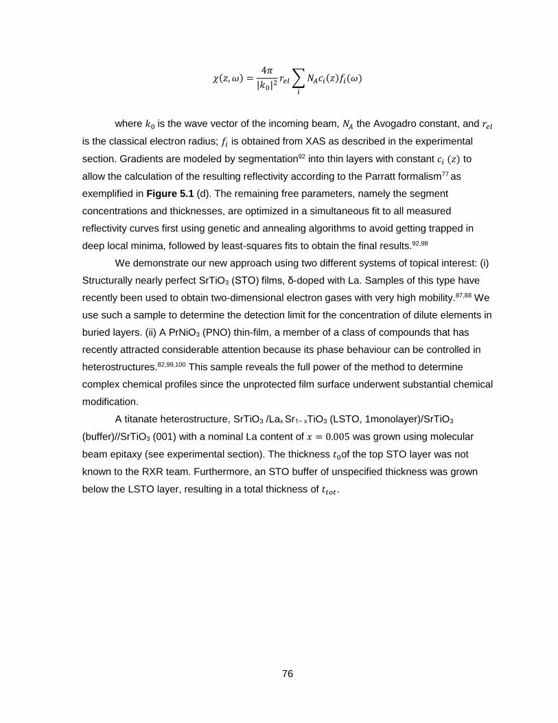
76

𝜒(𝑧, 𝜔) =4𝜋

|𝑘0|2𝑟𝑒𝑙 ∑ 𝑁𝐴𝑐𝑖(𝑧)𝑓𝑖(𝜔)

𝑖

where 𝑘0 is the wave vector of the incoming beam, 𝑁𝐴 the Avogadro constant, and 𝑟𝑒𝑙

is the classical electron radius; 𝑓𝑖 is obtained from XAS as described in the experimental

section. Gradients are modeled by segmentation92 into thin layers with constant 𝑐𝑖 (𝑧) to

allow the calculation of the resulting reflectivity according to the Parratt formalism77 as

exemplified in Figure 5.1 (d). The remaining free parameters, namely the segment

concentrations and thicknesses, are optimized in a simultaneous fit to all measured

reflectivity curves first using genetic and annealing algorithms to avoid getting trapped in

deep local minima, followed by least-squares fits to obtain the final results.92,98

We demonstrate our new approach using two different systems of topical interest: (i)

Structurally nearly perfect SrTiO3 (STO) films, δ-doped with La. Samples of this type have

recently been used to obtain two-dimensional electron gases with very high mobility.87,88 We

use such a sample to determine the detection limit for the concentration of dilute elements in

buried layers. (ii) A PrNiO3 (PNO) thin-film, a member of a class of compounds that has

recently attracted considerable attention because its phase behaviour can be controlled in

heterostructures.82,99,100 This sample reveals the full power of the method to determine

complex chemical profiles since the unprotected film surface underwent substantial chemical

modification.

A titanate heterostructure, SrTiO3 /Lax Sr1− xTiO3 (LSTO, 1monolayer)/SrTiO3

(buffer)//SrTiO3 (001) with a nominal La content of 𝑥 = 0.005 was grown using molecular

beam epitaxy (see experimental section). The thickness 𝑡0of the top STO layer was not

known to the RXR team. Furthermore, an STO buffer of unspecified thickness was grown

below the LSTO layer, resulting in a total thickness of 𝑡𝑡𝑜𝑡.

77

Figure 5.2 SrTiO3 sample 𝛿-doped with Lanthanum. (a) XAS data around the La M5 and M4 edges in total electron yield (TEY) and fluorescence yield (FY) mode. (b) Constant-q reflectivity scans, measured within the same energy range as the data in a), and compared with fitted simulation. (c) Constant energy reflectivity scans, compared with fitted simulation. For clarity, the curves have been multiplied by a factor of 100 with respect to each other. The two vertical lines mark the oscillations stemming from the STO overlayer. The inset shows a magnified view of the curve, exposing thickness fringes stemming from the STO buffer layer, which are marked by vertical lines. (d) Corresponding concentration profile, encompassing the surface and the buried LaxSr1−xTiO3 layer, obtained from the fits to the data. The resulting fitted parameters are:

𝑥 = 0.006 and 𝑡0 = (96 ± 1) Å, and the total thickness of the synthesized

heterostructure, including the buffer layer, is 𝑡0 = (1106 ± 10) Å. The inset schematically shows the structure of the entire sample.

We investigated the sample with XAS and RXR (Figure 5.2). Even in the more bulk-

sensitive FY mode the XAS peaks barely exceed the noise level, and besides, XAS even in

principle does not allow a quantitative assessment of either 𝑥 or 𝑡0. The RXR data, on the

other hand, allow the precise determination of 𝑥 and 𝑡0: A first estimate of 𝑡0 can be

obtained from the large thickness oscillations visible in panel (c). From the comparison of

the various scans taken at and around the La edge with simulation based on the model in

panel (d), which resulted from the fitting procedure described above, we obtain 𝑥 = 0.006

and an STO layer thickness of 𝑡0 = (96 ± 1) Å, in close agreement with the targeted 𝑥 =

0.005 and 100 Å. We remark that, considering the large signal-to-noise ratio of the constant-

q data in Figure 5.2 the method has the potential to detect elemental concentrations

significantly below the concentration of 𝑥 = 0.006 found in our sample.

The total thickness 𝑡𝑡𝑜𝑡of the structure, including the STO buffer layer, was extracted

from the small dense oscillations visible in the inset of panel (c). These results from

additional elemental contrast provided by tiny amounts of organic compounds on the

substrate surface, which cannot be fully removed when preparing it for the film deposition.101

78

The second sample is PrNiO3 deposited by pulsed laser epitaxy on

(LaAlO3)0.3(Sr2AlTaO6)0.7 substrate with (100) termination (see experimental section). While

the targeted thickness was 10 nm, measurements at the Ni L-edge indicate a thickness

closer to ≈9 nm. To resolve this seeming contradiction, we have performed comprehensive

RXR mappings around the Ni L - and Pr M -edges, complemented by individual

measurements close to the O K -edge and at intermediate energies (Figure 5.3).

Figure 5.3 RXR results on the PrNiO3 film. (a) Representative measured (red lines) and fitted (black lines) reflectivity scans. (b) Comparison between the measured and the fitted reflectivity map comprising a total of "31" individual scans, including those shown in a). The energies of the four resonances La M5, La M4, Ni L3 and Ni L2 are marked with arrows.

To obtain the detailed chemical profile, we assumed a model consisting of a

stoichiometric PrNiO3 layer of variable thickness and roughness, beginning at the substrate,

covered by a layer in which the concentrations, thicknesses and roughnesses of the Pr, Ni

and O distributions were all variable and independent from each other. This model allows us

to capture any potential intermixing at the substrate-film interface and non-stoichiometry at

79

the film surface, while at the same timekeeping the number of free parameters manageable

(Figure 5.4).

Figure 5.4 Initial molar concentration profiles, along with the corresponding fitting parameters for the PNO/LSAT sample. The three layers into which the sample was subdivided for the analysis are marked with vertical lines. (D: concentration of the individual element in the layer, t: thickness of the layer, σ: roughness of the interface of the top of the layer).

The fitted individual Pr, Ni and O concentration profiles and the corresponding

parameters are shown in Figure 5.5(b). The simulated RXR results based on these profiles

are in excellent agreement with the measured data (Figure 5.3). The concentration profile in

Figure 5.5 (b) has several remarkable features: First, at the surface of the film there is a

region in which the Ni concentration goes to zero whereas the Pr concentration is still

substantial and only vanishes nearly two unit cells above. The resulting full widths at half

maximum of the Ni and Pr distributions are 91.6 Å and 97.6 Å, respectively, both with a

roughness of about 2 Å. Stoichiometric variations of this kind can drastically affect the

electronic properties of transition metaloxides, and are especially important for the

interpretation of data from surface-sensitive techniques.

80

Figure 5.5 Comparison between EELS and RXR results on the PrNiO3 film. (a), Representative EELS profile around the Pr M4 and Ni L3 edges. The same constant background was subtracted for both profiles. For each panel, the color scale was chosen such that the maximal intensity at the corresponding edge is dark red. (b), Elemental depth profile for the three elements present in the film, Pr, Ni, and O, obtained from fits to the RXR data shown in Figure 5.3. The region at the surface marked with darker red contains other light elements such as carbon and hydrogen, in addition to oxygen. The three layers into which the sample was subdivided for the analysis are marked with vertical lines. The table shows the fitting results for the thickness, roughness and concentration characterizing the profile of each element in the corresponding layer. Roughnesses are valid for the top interface of the corresponding layer. Note that in the element specific method, not all elements are present in all layers, and thicknesses can be different within the same layer.

Second, there is a thick contamination layer consisting of oxygen and lighter

elements on top of the film, which did not desorb in UHV. Taking into account this layer is

crucial to obtain a satisfactory fit even at the relatively distant Ni and Pr edges due to the

additive character and Kramers-Kronig consistency of 𝜒 (𝑧 , 𝜔 ). We refrain from a detailed

determination of its composition, which would require substantial additional mapping at

energies below the oxygen K -edge, without adding new information about the actual film.

Third, the roughness at the substrate interface is below the detection limit, indicating

that PrNiO3 grows well on (LaAlO3)0.3(Sr2AlTaO6)0.7.

81

We tested the robustness and consistency of our results in numerous ways.

Qualitative changes of the model like moving the Ni-depleted region from the surface to the

substrate interface lead to unsolvable inconsistencies in the fit. Also, irrespective of the

assumed initial configuration, the genetic algorithm, which inherently probes a wide range of

possible solutions, including such without a Ni depletion layer, without an organic

contamination layer, and with a Pr/Ni ratio unequal one, always approached our final

solution (Figure 5.5 (b)). We further point out that the influence of the three major

parameters characterizing each layer on the reflectivity profiles is quite different from each

other (Figure 5.6): The thickness is correlated to the thickness fringe periodicity of the

reflectivity profiles but not to the intensity, whereas the concentration affects the intensity at

all wave vectors and the roughness mainly affects the thickness fringe amplitude and

intensity at large wave vector transfers, but both do not affect the fringe periodicity.

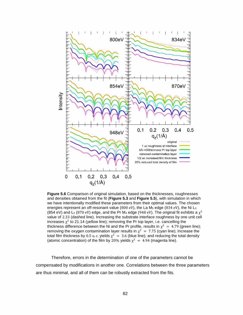
82

Figure 5.6 Comparison of original simulation, based on the thicknesses, roughnesses and densities obtained from the fit (Figure 5.3 and Figure 5.5), with simulation in which we have intentionally modified these parameters from their optimal values. The chosen energies represent an off-resonant value (800 eV), the La M5 edge (834 eV), the Ni L3

(854 eV) and L2 (870 eV) edge, and the Pr M4 edge (948 eV). The original fit exhibits a χ2 value of 2.33 (dashed line). Increasing the substrate interface roughness by one unit cell

increases χ2 to 21.14 (yellow line); removing the Pr top layer, i.e. cancelling the

thickness difference between the Ni and the Pr profile, results in χ2 = 4.79 (green line);

removing the oxygen contamination layer results in χ2 = 7.75 (cyan line); Increase the

total film thickness by 0.5 u. c. yields χ2 = 3.6 (blue line); and reducing the total density

(atomic concentration) of the film by 20% yields χ2 = 4.94 (magenta line).

Therefore, errors in the determination of one of the parameters cannot be

compensated by modifications in another one. Correlations between the three parameters

are thus minimal, and all of them can be robustly extracted from the fits.

83

We completed our study by performing complementary STEM-EELS measurements

on specimens extracted from various locations on the PrNiO3 sample. Representative data

around the Ni and Pr edges is shown in Figure 5.5 (a) and contrasted with the profile

derived from the RXR measurements. It corroborates our finding of a heavily Ni depleted

surface layer and substantial chemical roughness. The atomic-resolution data in Figure 5.7

and Figure 5.8 is also consistent with our RXR finding of a sharp substrate/film interface.

The full width half maximum of the Ni profile, averaged over the different EELS

measurements, is 88.5 Å, in remarkable agreement with the RXR result of 91.6 Å. The same

holds for Pr (97.6 Å vs.103 Å).

Figure 5.7 Atomic resolution STEM-EELS measurements of the substrate-film interface of the PrNiO3 film. The left panel shows an annular dark-field (ADF) STEM measurement, recorded simultaneously during the EELS spectrum image acquisition. The three right panels show atomically resolved EELS maps recorded at the La M5, Ni L3 and Pr M5 edges. The overlap of the Ni L3 and the La M4 edge lead to the false impression of the presence of Ni in the substrate (see also Figure 5.8).

84

Figure 5.8 STEM-EELS projected maps at the different edges of the relevant cations in the PrNiO3 sample. The left panel shows an annular dark-field (ADF) STEM measurement. The right panels show EELS projected spectra, laterally integrated over the four lattice spacings shown in the ADF panel (sum over all pixels on each line) to reduce noise. Results are shown for the La M5 and M4, the Ni L3 and L2, and the Pr M5 and M4 edges.

The two methods are complementary in different aspects: RXR is a non-destructive

scattering technique, whose in-plane resolution is limited by the macroscopic beam size (in

present implementations μm and above). STEM-EELS is destructive, but offers sub-nm

resolution in one in-plane direction. Whereas both exhibit monolayer or close-to monolayer

depth resolution, degraded crystallinity in the Ni-depleted layer might effectively deteriorate

resolution for STEM-EELS, but it does not impact RXR results. The time and effort involved

is comparable: Advance application for measurement time is necessary for both, and STEM

requires an elaborate specimen preparation, whereas RXR depends on a sophisticated data

analysis.

We next compare our approach to further established methods with respect to

destructiveness, the elemental detection limit, depth resolution and everyday availability.

Several methods such as SIMS,102 Rutherford Backscattering (RBS),89 and Sputtering XPS

(SXPS)103 can detect elemental densities of 100 p.p.m. or below, and in contrast to the more

sophisticated STEM-EELS and RXR are frequently available in local laboratories. They are

thus very good tools for quick routine characterization immediately after sample growth or

processing. However, many of them have the disadvantage of being destructive, thus

potentially disturbing the stoichiometry with respect to volatile elements like oxygen. Depth

resolution is a further critical parameter: while several nanometers are readily achievable,

85

sub-nm or monolayer resolution is limited to a few techniques such as RXR and STEM-

EELS. Standing-wave techniques are powerful non-destructive, element specific methods,

which exhibit monolayer resolution, but have a limited scope since they require nearly

perfect interfaces104 or elaborate superlattice samples.35

Consequently, RXR will be typically applied to selected samples which have

undergone preliminary characterization with lab-based techniques. In this work we have

focused our analysis on the determination of the chemical composition profile of

heterostructures. The capability of RXR to extract information about interfacial

electronic,28,105 magnetic,29 and orbital1 reconstruction in structurally and chemically nearly

perfect samples with simple, judiciously chosen layer sequences has been previously

demonstrated. The next step is the extension of our approach to such reconstruction

phenomena in systems of increasing chemical and physical complexity: It is a powerful

method to study the chemical and physical properties of heterostructures comprising

functional materials such as transition-metal oxides, topological insulators or pnictide

superconductors. Technical developments are underway to allow measurements with a

strongly reduced beam spot size in the nanometre range, thus extending its applicability to

laterally structured multilayers, ultimately allowing the spectro microscopic investigation of

novel devices.

5.1 Experiment

The SrTiO3 heterostructures, 𝛿-doped with La, were grown using a hybrid molecular

beam epitaxy (MBE) approach,101 similar to that used for the films investigated in Reference

"88", at a substrate temperature of 900 °𝐶 (measured by thermocouple). Oxygen was

supplied during growth using a RF plasma source operating at 250 𝑊 with an oxygen

background pressure of 410−6 Torr. After growth, these films were annealed in a rapid

thermal annealing furnace in 1 atm of oxygen at 800 °𝐶 for 30 𝑠 to backfill any oxygen

vacancies generated during growth. The PrNiO3 samples were synthesized using pulsed

laser deposition (PLD). Starting materials were ablated using a KrF excimer laser (240 𝑛𝑚)

with 2 𝐻𝑧 pulse rate and 1.6 𝐽/𝑐𝑚2 energy density, and deposited in 0.5 𝑚𝑏𝑎𝑟 oxygen

atmosphere at 730 °𝐶. The resulting films were subsequently annealed in 1 𝑏𝑎𝑟 oxygen

atmosphere at 690 °𝐶 for 30 𝑚𝑖𝑛. The out-of-plane lattice constant of the PrNiO3 film was

determined from X-ray diffraction to be (3.780 ± 0.005) Å. The XAS and X-ray reflectivity

measurements were carried out using a 4-circle in-vacuum diffractometer at the REIXS

86

101D-2 beamline of the Canadian Light Source (CLS) in Saskatoon, Canada.2 The samples

were mounted with their surface normal in the scattering plane. The measurements were

performed using σ-polarized light. The reflectivity scans were performed in specular

geometry, in which the incident angle θ is defined relative to the surface plane. Scans were

recorded and analyzed up to a detector angle of 2 θ ≈ 90°, and where signal-to-noise ratio

permitted up to 110°. The temperature was kept constant at 298 K. A detailed description of

the experimental setup is reported in Ref.1 The off-resonant parts of the atomic scattering

factors of La, Pr, Ni, Ti, and O were taken from Chantler tables.81 The corresponding

resonant parts were retrieved from XAS measurements in total electron yield (TEY) mode,

background corrected, and aligned with the Chantler database as described in Reference.12

To correct the distortion of the La signal due to the significant self-absorption, its scattering

factor was additionally parameterized and fitted to reflectivity data. The resulting imaginary

part of the scattering factors of the above elements (Figure 5.9). The other elements

present in our systems (Sr, Al, Ta) were taken into account by using tabulated values only,

since their absorption edges are sufficiently far away in energy as to not interact appreciably

with the main elements. For all elements, the real part of the scattering factors was obtained

by Kramers-Kronig transformation. The RXR analysis method discussed in this paper is

implemented in the software package ReMagX,3 "www.remagx.org". STEM and EELS

measurements were carried out on a FEI Titan3 microscope at an acceleration voltage of

200 𝑘𝑉. A FIB sample was prepared by cutting the sample vertically and further thinned at

liquid nitrogen temperature until a thickness of around 50 𝑛𝑚 was reached. EELS

acquisitions were performed with an energy resolution of 0.7 𝑒𝑉 at a dispersion of 0.1 𝑒𝑉 per

pixel on a GIF Tridiem ERS. The spectrum images were acquired with a spacing 0.5 Å/𝑝𝑖𝑥𝑒𝑙

and 50 𝑚𝑠/𝑝𝑖𝑥𝑒𝑙 acquisition time. The convergence angle and collection angle used for the

experiment were 20 and 200 𝑚𝑟𝑎𝑑, respectively.

87

Figure 5.9 Imaginary part of the individual scattering factors of the elements present in our films. The scattering factors were obtained from XAS-TEY data, background corrected and fitted to the tabulated off-resonant values from Chantler tables.81

88

6 X-ray Scattering Experiment and Theoretical Modelling of Compressively

Strained CoO Thin-Film on MgO Supporting Substrate as an Example d7 Binary

Oxide Thin-Film

6.1 Introduction

Studying the electronic structure of different materials is still a main goal of many

experiments. With the development of thin-film growing techniques such as PLD and MBE,

and the tendency of creating heterostructured quantum materials, the need for developing

electronic structure measurement techniques for thinn

-films, heterostructures and their interfaces has become a high priority.6 X-ray techniques

are still among the most important for measuring the electronic structure, since the photon

energies are within the range of the transition energies of the electron in various elements.

Although some X-ray techniques such as XPS and X-ray induced Auger Electron

Spectroscopy (AES) are quite advanced and are effectively used to study different

materials, these techniques are not comparable to RSXS for details like the changes in

electronic structure occurring at deeply buried interfaces because of probing depth

limitations and the averaging occurring over a substantial depth range if one uses high

energy XPS to look at buried interface regions.22,32

SXS is an important technique to investigate the geometry and electronic structure of

various materials.4,5,12 XAS, as a part of the technique, is well-developed and has been used

to study the electronic structure of various materials for quite a long time.32,37,38,39,41,43,44,45,57

Although XAS can reveal information about the valence, orbital and spin-states of any

system, it has major limitations; such as the probing depth which prevents the study of

buried interfaces and, particularly, the averaging nature of the signal that limits the detection

of specific spatial part of the sample. On the other hand, soft X-ray reflectometry (SXR) with

better probing depth and spatial resolution, can afford much more information about the

system. It provides more detailed description of the electronic structure of transition metal

oxides in thin-films and heterostructures.4,5,12 SXR is a suitable technique to study the 3d

transition metal elements and other 2p elements such as C and O, since the energies in the

soft X-ray regime are within the absorption edges of these elements. Mostly the 2p - 3d

transitions, known as the L edges, are in the energy range 400 - 950 eV and the 1s - 2p

transition, known as the K edges are in the 300 - 700 eV energy range.72,73 The resulting

spectra provide information about valence, orbital and spin-state of the elements in addition

to the geometry of the sample.1,4,5,12,72,75

89

With all the possibilities that SXR, in principle, has, it is a quite complicated

technique and a systematic way of running a complete experiment in SXS is not well

established to date. In addition, the preliminary experiments with more complicated TMOs

system, such as perovskite LCO, showed that the analysis of the data is quite challenging.

To use this powerful technique to study new quantum systems, such as perovskite

heterostructures, the study should start by investigating a well-known relatively simpler

system to set the rules for both the experiment and the analysis procedures. After

developing a good understanding of the technique, it can be extended to include more

complex structures. The study starts with a well-studied sample, regrow the sample by the

same grower and run a verification XAS study. Following that, a comprehensive SXR study

will be made. To reach the maximum ability of the SXR technique, it is important that the

sample is in the thin-film form. The infinite thickness of the single crystal and the lack of a

well-defined interface will prevent most of the features in the reflectivity curves to be visible.

Still the misfit between the thin-film and the supporting substrate should not be too high to

keep the problem as simple as possible. XAS and SXR results are then compared bringing

out the additional features in SXR.

The system of choice for the current study has been CoO thin-film grown with MBE

on different substrates, with various strains, as a d7 model systems. Detailed XAS studies

for single crystal and thin-film CoO samples have been performed previously,41,44 including

linear dichroism and X-ray magnetic circular dichroism (XMCD) of the CoO sample on

various substrates. The systems also were the subject of many theoretical calculations that

investigated the possible transitions and any possible change in transition energy which may

result from changing the physical and chemical environment of the Co ions.57 Such a system

is an ideal test case to develop our understanding of the new SXR technique. This can then

be extended to systems in which the electronic structure is not known in details like for

example LCO thin-films.

The changes in the electronic structure of the Co2+ ion, as a result of the

compressive strain in the CoO thin-film on a MgO substrate, have been studied, in addition

to the temperature dependence measurements SXR of the CoO thin-film. Previous XAS

measurements reveal the multiplet structure of the Co edge and the differences in the

occupied states as a result of the spin-orbit coupling of the 3d electrons. Orbital anisotropy

appears as a difference in the multiplet structure of the Co edge measured at fixed Qz, for

both vertical and horizontal polarization.57

90

At a quick glance, CoO, as an example of a strongly electron correlated material, has

a rock salt structure and is an antiferromagnetic large band gap insulator with a Neel

temperature of about 291 K.58 Experiments show that the electronic structure of CoO

depends strongly on the temperature. Changing the temperature changes the occupation of

the different d7 multiplet states. Co2+ has 7 electrons in the 3d orbital and the orbital splits

into two lower three-fold degenerate t2g and higher two-fold degenerate eg orbitals. The Co is

in a high spin-state according to Hund’s rules with S=3/2 and an electronic configuration of

t2g 5 eg 2 forming a 3-fold degenerate t2g state. Further splitting occurs due to the spin orbit

coupling of the 3d orbital forming three different states with pseudo total orbital angular

momentum of 1/2, 3/2 and 5/2, with two-, four- and six-fold degeneracy. At very low

temperature the states with 1/2 pseudo angular momentum is occupied and by increasing

the temperature other states with 3/2 and 5/2 start to be filled. The XAS and RXS spectra

are very sensitive to these changes in orbital occupations.

CoO thin-film samples eliminate most of the complexity that is usually associated

with other systems such as LCO. CoO in the (001) direction has successive planes of Co2O2

with zero net charge of each plane. The situation eliminates the polar issue that usually

drives an electronic reconstruction in the polar materials. Heterostructure systems can be

also simplified by growing CoO on other similar nonpolar materials such as MgO and MnO

both with Mn2O2 and Mg2O2.57 Co2+ usually exists in high spin-state HS with (S=3/2) whether

the system is in Oh or Td or even square planar symmetries at low or high temperatures.57

This eliminates any spin-state transitions associated with temperature or strain. The choice

of MgO with a lattice parameter of 4.212 Å, in comparison to the lattice parameter of bulk

CoO single crystal of 4.267 results in a modest compressive strain of about 1% which for

epitaxial growth will result in a further symmetry splitting of the t2g and eg orbitals and further

simplifies the problem but still allows the formation of the interface and strain related

changes. Taking the measurement above the Neel temperature limits the linear dichroism to

the change in crystal field and excludes changes in the spectra due to magnetic ordering

effect.57 The influence of the strain can be calculated as changes in the multiplet structure.

In a similar study of the CoO thin-film grown with MBE on an Ag substrate, Haverkort

et al.57 investigated the effect of compressive strain on the change in the multiplet structure

using XAS and theoretical cluster calculations. The lattice mismatch between thin-film CoO

and the Ag substrate with a lattice parameter of 4.09 Å is higher than that with the MgO

substrate with a lattice parameter of 4.21 Å. They found using X-ray diffraction, that the

lattice parameter of CoO thin-film is reduced to ~ 4.235 Å in plane and elongated to 4.285 Å

91

out of plane as a result of the compressive strain. They explained the difference between

the signal taken at 90° and 20° angle of incidence and clearly showed that the main

difference appeared as a reduction in the intensity of the peak around the 777 eV which

results from the transition of 2p electron to the low t2g 3d orbital.57 In the current study we

expect to find similar results but with slight changes due to the lower lattice mismatch

between CoO and MgO in comparison to that between CoO and Ag in the previous

studies.57 The tetragonal distortion of the strained CoO will be smaller possibly masking any

change in the multiplet structure especially if the resulting t2g splitting is much smaller than

the result of the spin orbit coupling and the signal will be closer to that of bulk CoO.

The current chapter presents a systematic way of running a complete soft X-ray

scattering (SXS) study of transition metal oxide binary systems, such as CoO, constructing a

representative theoretical model using the in-house software ReMagX,3 in addition to

simulating and fitting the theoretical data against the experimental results. The experiment

took with consideration all the challenges faced in previous experiments and went into minor

details to describe the cautions taken to assure that the measurements are valid and reliable

in addition to track changes that usually are overlooked when one runs a more complicated

system. For example, studying the thermal evolution of the sample clarifies any changes

that may occur during heating and cooling processes. Questions regarding the fracturing of

the sample due to the difference in thermal expansion coefficient between the thin-film and

the supporting substrate can be answered to isolate any unusual changes that may appear

in the reflectivity curves after cooling down to 20 K for instance. Also, checking the

homogeneity of the sample can avoid the misinterpretation of XAS results because they

may be structurally related.

Sample surfaces under ambient conditions are usually contaminated with a thin layer

of an absorbed species, such as water or CO2 etc. Although these low mass elements, with

X-ray resonances far from the 2p edges of the transition metals, are not expected to

influence the reflectometry results, experience shows that even very thin layers of adsorbed

species can cause some refraction of the X-ray beam and therefore influence the analysis.

This thin layer can be caused by the condensation of the residual gas inside the UHV

chamber as the temperature of the sample is being reduced. This can be considered

theoretically, in principle, but a systematic way is needed to investigate the phenomena and

to use the finding in improving the model systems and the whole data simulation and fitting

process. In the current study, changes in the XAS and SXR signals have been tracked for

92

the naturally occurring vacuum contaminants, such as O, C and H based, as the CoO//MgO

sample temperature was lowered.

6.2 Experimental Results

In our experiments the 8, and 40 nm thin-films of CoO grown with molecular beam

epitaxy (MBE) technique on MgO as an example of the compressively strained d7 system

are displayed in Figure 6.1. The samples were obtained from the group of L. H. Tjeng of

Max Planck Institute (MPI). The samples were grown as twins, one uncapped and one was

capped with a layer of amorphous Al2O3 to clarify the CoO surface effect and light element

contamination. The methods of growing similar samples by the grower’s group can be found

in ref.57,80,106 It was found that the Al2O3 capping layer imposed new challenging and

unexpected features in the measured curves. To overcome the problem, new set of samples

with a crystalline capping MgO layer were grown but did not receive beamtime to be

measured yet.

Figure 6.1 Schematic draw of the samples used in the current study, it shows the CoO thin-films with 8 and 40 nm thickness grown on MgO sample with and without an Al2O3 Capping layer in addition to one last CoO 8 nm thin-film sandwiched between MgO supporting substrate and crystalline MgO capping layer.

X-ray absorption (XAS) and soft X-ray reflectometry (SXR) have been performed off-

and on-resonant at the Co L2,3 and O K edges. The XAS measurements were carried out in

both the total electron yield (TEY) and total fluorescence yield (TFY) modes. In order to

check the homogeneity of the sample surface, XAS measurements were performed for

multiple surface points starting from the sample center and going outward to the edges. The

reflectometry experiments were carried out at both constant energies and at fixed Qz. In

addition to the single point reflectivity measurements, reflectivity maps with small steps were

taken at constant energy and in fixed Qz modes.

The sample surface was partially cleaned by thermal cycles of gradual annealing up

to 430 K then cooling down to room temperature. It was believed that moisture related

MgO

CoO 40 nm

Al2O3

MgO

CoO 40 nm

MgO

CoO 8 nm

Al2O3

MgO MgO

MgO

CoO 8 nm CoO 8 nm

93

adsorbates such as H2O, or -OH can be removed in addition to some lightly bond

physisorbed adspecies. XAS and SXR measurements were taken at both σ- and π-

polarizations. The uncapped CoO (8 nm)//MgO sample has been measured at 300 K before

cooling, then the sample was cooled immediately to 20 K and measured, that was followed

by heating and measuring at 70, 160 and 300 K .

The results were analyzed, simulated and fitted using the specialized software

ReMagX using Parratt formalism77 in the evolution algorithm and the quality of the fit was

checked with the least square analysis (𝜒2).3

6.2.1 XAS of the Uncapped CoO//MgO Sample

Figure 6.2.a presents the XAS measurements of several regions on the uncapped

CoO (8 nm)//MgO sample surface (Figure 6.2.b). The measurements are almost identical

indicating that the sample is homogeneous and a small shift in the beam position on the

surface will not significantly affects the results. Similar measurements were made for all the

samples and any sample that did not pass the homogeneity test was not considered for

further measurements.

Figure 6.2 (a) XAS scans of several points across the CoO 8 nm thin-film grown on MgO substrate. (b) Sketch of the sample holder with the sample as the square in the middle and the selected points to measure the XAS scans are marked as the red small circles.

In Figure 6.3 and by a careful analysis of the spectra it looks like the Al2O3 non-

crystalline 8 nm capping layer resulted in more damage than helping to protect the surface.

Important major peaks disappeared from the spectra of the capped sample and, by

94

comparing it with literature, the results were not considered valid. Better samples with better

capping layers of MgO were received from the grower and are a work in progress. The

signal from the uncapped sample, on the other hand, is sharp and retains all the major

features and peaks expected from a compressed CoO samples.57 The capped samples were

not characterized any further and new samples with a capping layer of MgO will be grown

and used in future studies.

Figure 6.3 XAS spectra for (a) the capped and (b) the uncapped 8nm CoO thin-film epitaxially grown on MgO supporting substrate. A comparison between the XAS spectra of the capped and the uncapped samples taken with (c) σ-polarized and (d) π-polarized light. All spectra have been taken at room temperature.

The XAS spectra for the 8 nm CoO//MgO in both TEY and TFY mode are shown in

Figure 6.4 for the O K, Co L2,3 with σ- and π-polarized light at 300K. Since the

measurement was done at 300K, which is above the Neel temperature for CoO, the clear

difference between signals taken with σ- and π-polarized light near the Co L3 edge is

attributed to the change in crystal field as a result of the compressive strain for the CoO thin-

film (Figure 6.4.b). The main difference appears near the first sharp peak at 776.3 eV that is

associated with the lowest energy transition from 2p to the 3d t2g orbital. By assuming a

95

single electron picture this peak is associated with the transition of a 2p electron to the lower

t2g shell of the 3d orbitals. The TFY signals near the Co L2,3 edges are identical and look

quite different from the associated TEY signals. The analysis of the signals near the Oxygen

K edge is challenging because of a lot of contributing factors such as the covalent mixing

with the Co 3d states, the O 2p band structure with changes due to the surface, interface

and bulk.

Figure 6.4 The XAS spectra of the uncapped CoO//MgO sample in TEY mode (a, b) and TFY mode (c, d) around the (a, c) O K and (b, d) Co L2,3 edges with σ-polarized light and at 300 K.

The 7 d electrons populate the 5- 3d orbitals leaving one hole in one of the three t2g

orbitals and yields for the total 5 t2g electrons a t2g spin of ½ which is strongly

ferromagnetically coupled by Hund’s rule to the two unpaired eg electrons with a eg spin of 1

yielding a total spin of 3/2 for the ion. The compressive strain in the CoO will lower the

symmetry and further split the orbitals of both t2g and eg shells. In the t2g shell, the dxy orbital

will have a higher energy than that of the dyz and dzx orbitals. This lowers the orbital

degeneracy of the t2g hole from three to one since it will be confined to the xy orbital.

96

Since the π-polarized light in our measurements condition is at 30° to the sample

surface a correction is needed to find the intensity measured with polarization along the z

direction perpendicular to the sample surface as shown in chapter 4.

By applying the selection rule, exciting any electron from the 2p orbitals to the dxy

hole with light that is polarized in the z direction is not permitted. The result will be a

reduction in the intensity of certain peaks in the signal taken with the out-of-plane polarized

light in comparison to that taken with σ-polarized light (in-plane) (Figure 6.4.b), which

confirms the findings of previous studies for the compressed CoO on various substrates

mainly CoO//Ag.106

6.2.2 SXR of the Uncapped CoO//MgO Sample

The most important set of measurements, and by far the most complete, is the SXR

measurements of the 8 nm CoO//MgO sample. The measurements were not only taken for

the sake of the geometry and electronic structure analysis, but they brought out all the minor

details of the technique, the experimental setup and the sample. While the XAS

measurements did not show notable difference, the more sensitive SXR spectra in both

constant energy and fixed Qz value scans clearly provide valuable information about the

sample.

The time evolution of the sample at both 300K and 20K has been tracked using the

constant energy scan at 776.3 eV which is the lowest energy transition peak of the Co L3

edge and are shown in Figure 6.5. The changes in the sample were tracked for three

successive days where they were subjected to gradual cooling and heating multiple times. It

should be noted that the possible minor energy shift that can result from the instability of the

monochromator of the beamline was compensated for by taking constant energy

measurements around the 776.3 eV with an increment or decrement of 0.01 eV.

97

Figure 6.5 SXR measured at constant energy at 776.3 eV and at (a) 300 and (b) 20 K for the CoO (8 nm)//MgO with σ-polarized light. The measurements were taken at various times during the beamtime to track the time evolution of the sample and any possible substantial changes to the sample.

The temperature dependence of the sample was investigated by taking multiple XAS

and SXR measurements at temperature of 20, 70, 160, and 300 K before and after cooling

down. Wide ranges of energies off- and on-resonant near the Co L2,3 edges and with σ- and

π-polarised light were measured, usually the on-resonant energies are chosen at the major

transition peaks and at the continuum shoulder of both L3 and L2 edges.

98

Figure 6.6 (a) TEY signal of the CoO (8 nm)//MgO sample near the O K and Co L2,3 edges at 300K and with σ-polarized light. The vertical red lines are at the selected energies where reflectivities at constant energies have been measured. (b) The reflectivity at constant energy of 776.3 eV taken with σ-polarized light and at 300 K. The red vertical lines represent the Qz values at which the reflectivities at fixed Qz have been measured.

Due to the large number of measurements, only a few scans that show clear

differences will be discussed later. Also, large number of fixed Qz reflectivities have been

measured to track the thermal evolution of the sample.

The constant energy scan at 776.3 eV and at 300 K was used to select the Qz points

to run the measurements (Figure 6.6.b). Reflectivities at fixed Qz values take with both σ-

and π-polarized light and at 20, 70, 160 and 300 K are presented in Figure 6.7 together with

the difference between both. By taking an overall look at the SXR at fixed Qz values, it

clearly shows the increase in details and peak relative height for different Qz values in

comparison to the XAS signals. At lower Qz values, the signal appears to be similar to that of

the TEY, and varies notably when going to higher Qz values.

99

Figure 6.7 X-ray reflectivities near the Co L2,3 absorption edges measured at three fixed Qz values of (a) 0.0751, (b) 0.3815 and (c) 0.3912 Å-1 with both (I) σ-polarization and (II) π-polarization in addition to the difference between the spectra in both polarizations (III). The measurements were taken at temperatures started from 20 K (blue curves) then heated to 70 (red curves), 160 (green curves) and finally 300 K (black curves). The red vertical lines are at 776.3, 776.9, 777.5, 777.7, 778.3, 779.2, 779.8, 781, 792.9 and 793.9 eV from (1) to (10) respectively.

While tracking the thermal evolution of the sample, a changing special feature

appeared in both constant energy reflectivities, between 0.2 and 0.5 Å-1 (Figure 6.11), and

fixed Qz reflectivities maps between 600 to 760 eV in addition to 785 to 794 eV (Figure

6.10) as will be discussed below.

6.2.3 Data Simulation and Fitting

The SXR data of CoO//MgO has been analyzed and simulated using the method

which was explained in chapter 4. The CoO energy-dependent complex refractive index,

𝑛(𝜔) was generated by correction and fitting the TEY spectra of Co L2,3, La M4,5 and O K

edges, of-resonant to the theoretical Chantler database to produce the imaginary part, β.81

100

The real part, δ, is then generated via Kramer-Kronig transformation. The process of

normalizing and fitting the TEY to Chantler tables and the production of the refractive index

is explained in chapter 4. ReMagX has then been used to construct the material model of

the sample to simulate and fit part of the SXR data, specifically the reflectivity scans at

constant energies.3

Figure 6.8 (a) Reference pure spectra of Co2+ HS (black), Co3+ LS (olive) and Co3+ HS (magenta), all in octahedral (Oh) symmetry,41 and the Co2+ HS in tetrahedral (Td) symmetry (cyan).107 The dashed lines are exactly at the energies of 776.3, 776.9, 777.5, 778.1, 778.8, 779.2, 781, 792.9, 793.3, 793.7, 794.4, and 795.0 eV respectively from (1) to (12) and spans both L2 and L3 of the Co edge. (b) The imaginary part of the Co scattering factor generated from the experimental TEY signal (red) of the Co L2,3 edges in CoO//MgO film corrected and aligned of-resonant to the theoretical Chantler database (green).

The material mode of the software gives information about the geometry of the

sample including the thickness and the roughness of each layer. Though, the mode is

limited when it comes to study the electronic structure of the sample for which the powerful

element specific mode is used. The atomic scattering factors of each element which are

sensitive to oxidation states, symmetry of the surroundings, spin and orbital occupations are

required to simulate and fit the data. The scattering factors for Co (Figure 6.8.b), and O for

the uncapped CoO//MgO samples were generated from the refractive indices of the CoO

compound, as described in details earlier in chapter 4. To construct the models in the

element specific mode, the density of each element in the unit cell is required. The density

of each element in the material is calculated from the molar density of the unit cell for both

CoO and MgO. Data were simulated with the Parratt recursive formalism77 using evolution

algorithm to generate the possible solutions and the quality of the fit is checked with 𝜒2 as

101

described in chapter 4. The thickness, roughness and density of each element are then

used as fitting parameters.

The CoO//MgO sample have been represented by a single homogeneous CoO layer

on the supporting MgO substrate. The unit cell density has been set to that of the bulk CoO

since it is expected and, was found in many cases, that for the complex oxides, the unit cell

volume will be conserved.57 The reduction of the lattice parameter for the compressed film in

the xy plane is accompanied by an increase in the parameter in the z axes. The possible

error in calculating the unit cell density will be compensated for by setting the elements

density as a fitting parameter and allow it to change slightly as needed. The TEY signal of

the CoO//MgO sample near the O K and Co L2,3 edges have been used to generate the

needed atomic scattering factors as described above. A light element contamination layer

was assumed at the top of the CoO thin-film and was represented by an O layer.

6.3 Discussion

Figure 6.9 presents a comparison between the TEY signal of CoO//MgO,

CoO//Ag,57,106 and CoO bulk41 all taken with σ-polarized light. As can be seen in Figure

6.9.a, the signals of the CoO//MgO and CoO//Ag are very similar with some difference in the

relative peak intensities and the main difference is in the lowest transition at 776.3 eV. When

the TEY signal is compared with the bulk CoO signal (Figure 6.9.b), it is clearly sharper and

the peaks’ relative intensities are different. The difference can be attributed of course to the

change in the crystal field from the pseudo cubic in the bulk to distorted tetragonal structure

for the compressed CoO thin-film on the MgO substrate. The major difference appears at

the 777.2 eV where a new shoulder appears in the compressed film that is missing for the

bulk signal.

102

Figure 6.9 A comparison between the XAS spectra around the Co L2,3 edges of the uncapped 8 nm thick CoO thin-film on MgO (red) taken at 300K and σ-polarized light with (a) the 9 nm thick CoO//Ag (blue) take at 400 K and 90° angle of incidence,106 and (b) bulk CoO single crystal.41

The TFY signals near the Co L2,3 edges are identical and look quite different from the

associated TEY signals (Figure 6.4.d). The analysis of the signals near the O K edge is

challenging because of the many potential contributions as described above and is beyond

the scope of the current work. For completeness though the TEY and FY signals are shown

in Figure 6.4 a and c, respectively.

Figure 6.5 presents SXR measurements of the time evolution of the sample at 300

and 20 K. Previous studies argued, depending on the TEY measurements, that the sample

was stable no matter how many times it was subjected to thermal cycles between 20 and

400K.57 The measurements at 300K look to be less affected by time than that at 20 K. In

general, the sample is stable in time and within the range of energy fluctuation ~0.05 eV of

the monochromator.

Studying the SXR at constant energy, for thermal evolution of the CoO (8 nm)//MgO

at first glance gives the impression of exactly the opposite of what is expected (Figure 6.11).

By taking only the contraction coefficient of CoO at cold temperature it is expected that the

thickness of the film will slightly reduce with decreasing temperature. The contraction should

appear as an increase in the period of the thickness (Kiessig) fringes on going from 160K to

20K. The data show a general opposite trend. Increasing Kiessig fringe period is associated

with the reduced temperature, Figure 6.11 a,b,c and d for the measurements taken with σ-

polarized light and e,f,g for the measurements taken with π-polarized light. The fringes of

the measurements at 20 K have the smallest period and it increases for measurements at

103

70 K and then increases more for the measurements at 160 K as can be seen in blue, red

and green in Figure 6.11, respectively, for the measurements taken at 776.3, 793.3, 791.4

and 789.7 eV in both polarizations. A similar trend was found for other measurements taken

at other energies but it was less apparent. It should be noted that the trend was violated at

some regions for some measurements if there was a new modulation imposed on the

measurements, such as the ones between 0.3 - 0.4 Å-1 of the measurements taken at 791.4

eV, and 789.7 eV (Figure 6.11 c,d, and g).

To explain the unexpected trend one should start by thinking about the fundamentals

of SXR and how it is different from hard X-ray reflectivity. In hard X-ray, the wave length of

the incident light is very short (~1.5 Å), this makes the system able to detect the crystalline

material only and is not affected by any light contamination material that might adsorb on the

surface especially at low temperatures and even desorb at elevated temperatures. Soft X-

rays with the long wave length are sensitive to the electronic structure of the film and

although the energies used near the absorption edges of Co L2,3 are far from the absorption

edges of the light elements that might contaminate the sample surface, the reflected beam

undergoes further refraction when passing through the top layer and it appears in the final

reflectivity. The surface signature appears as an increase in the film thickness when the

inevitable naturally occurring background contaminants from the ultra-high vacuum system

is attracted to the lower temperature of the sample and adsorbs on the surface as the

temperature decreases. The small reduction in the sample thickness by the thermal

contraction is overcome by the thickened surface contamination layer and the Kiessig

fringes narrows down and the whole film looks to be thicker at low temperatures. It is

believed that the surface contamination layer thickness at low temperature will increase with

time but it will be minor since the sample is in ultra-high vacuum conditions and the residual

gases pressure is very low. In addition to the change in Kiessig fringes width, the new

features in the SXR scans at constant energies are also an indication of surface change as

will be explained below.

104

Figure 6.10 X-ray reflectivity maps of the CoO(8 nm)//MgO sample taken in the fixed Qz region between 0.2 - 0.5 Å-1 and at two energy regions (a) 600 - 750 eV and (b) 786 - 792 eV. Both regions are marked with the blue boxes in (c). The sample was measured with σ-polarized light and at 20 K.

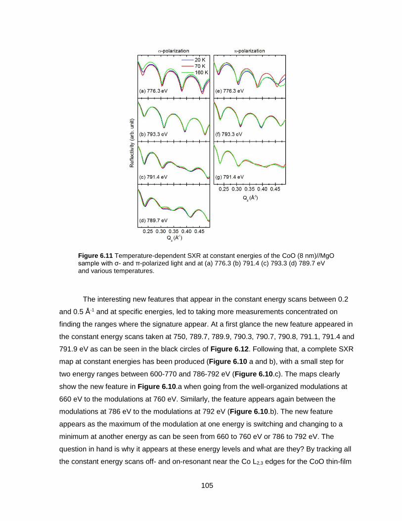
105

Figure 6.11 Temperature-dependent SXR at constant energies of the CoO (8 nm)//MgO sample with σ- and π-polarized light and at (a) 776.3 (b) 791.4 (c) 793.3 (d) 789.7 eV and various temperatures.

The interesting new features that appear in the constant energy scans between 0.2

and 0.5 Å-1 and at specific energies, led to taking more measurements concentrated on

finding the ranges where the signature appear. At a first glance the new feature appeared in

the constant energy scans taken at 750, 789.7, 789.9, 790.3, 790.7, 790.8, 791.1, 791.4 and

791.9 eV as can be seen in the black circles of Figure 6.12. Following that, a complete SXR

map at constant energies has been produced (Figure 6.10 a and b), with a small step for

two energy ranges between 600-770 and 786-792 eV (Figure 6.10.c). The maps clearly

show the new feature in Figure 6.10.a when going from the well-organized modulations at

660 eV to the modulations at 760 eV. Similarly, the feature appears again between the

modulations at 786 eV to the modulations at 792 eV (Figure 6.10.b). The new feature

appears as the maximum of the modulation at one energy is switching and changing to a

minimum at another energy as can be seen from 660 to 760 eV or 786 to 792 eV. The

question in hand is why it appears at these energy levels and what are they? By tracking all

the constant energy scans off- and on-resonant near the Co L2,3 edges for the CoO thin-film

106

on MnO and the LaCoO3 on LaAlO3 and on SrTiO3, which will be shown later in other

chapters, the feature appears but at different temperatures and less pronounced. This

makes us believe that this feature could be attributed to the thin-film surface and its changes

with temperature as thicker surface contaminant layer forms (Figure 6.11 c,d and g). The

clearest evidence that the new feature is surface related comes from the simulation and

fitting software ReMagX. Only by changing the contamination layer and the roughness

between the contamination layer and the CoO thin-film surface, did the features appear in

the simulated curves (Figure 6.12).

Figure 6.12 SXR at constant energies measured at various photon energies off- and on-resonant for the Co L2,3 absorption edges (black circles) together with the simulated curves (red curves) for the uncapped CoO//MgO sample at 300 K with σ-polarized light (a) with an upper O-containing contamination layer or (b) without any contamination layer. The energies on the right side are in (eV) and the curves are shifted vertically for clarity. The vertical purple lines are at fixed Qz values 0.0751, 0.1502, 0.1837, 0.2268, 0.2627, 0.3043, 0.3419, 0.3945 and 0.4598 Å-1, at which the scans in Figure 6.13 are measured.

107

The picture of further interactions and refractions of the photon on its way in or out of

the sample through a light element contamination layer can be also used here. By looking at

the regions where this effect happens we cannot exclude that it may occur everywhere

along the energy range of soft X-ray noting that it happened at the first peak of the O K edge

at 532.1 eV. The region between 786-792 eV is well above the Co L3 edge and slightly

below the L2 high intensity peaks and it includes the continuum step of the L3 edge at 790

eV (Figure 6.10.c).

Figure 6.12 shows some selected experimental SXR scans at constant energies, as

the black circles, and the associated simulated curves, as the red lines, for the uncapped

CoO//MgO sample. The purple vertical lines in Figure 6.12.a represent the position of the

chosen fixed Qz values at which measurements were taken and are shown in Figure 6.13.

The vertical purple lines on Figure 6.13.(1) are at selected peak energies for the Co L3

edges and the associated SXR at constant energies can be found in Figure 6.12 and

marked with red font. The full selected energies and fixed Qz values taken in the current

experiment are shown as the red vertical lines in Figure 6.6.

Figure 6.13 SXR at fixed Qz measured at various values around the Co L2,3 absorption edges (black circles) together with the simulated curves (red curves) for the uncapped CoO//MgO sample at 300 K with σ-polarized light. The vertical purple lines are at 776.3, 777.2, 778.4, 779.2 and 781.4 eV. The associated simulated theoretical model can be seen in Figure 6.14.a.

108

The analysis of SXR at fixed Qz is quite challenging but one can understand possible

changes in two ways. The first way is mostly observational and concentrates on linking the

changes in XAS with the changes is SXR at fixed Qz values. The uncapped sample

CoO//MgO was strongly insulating at low temperature and it was impossible to acquire any

TEY spectra at any temperature lower than 300 K.

Two conditions must be fulfilled to produce an SXR signal at fixed Qz value. The first

is that we must have a photon reflected out of the sample to be detected. At the absorption

edges this is more likely to be intense and appears as a large peak. The 2p5 hole gets filled

with an electron from the 3d shell and a photon is liberated. The second condition is that the

reflected photons from the film surface and the film-substrate interface must be in phase for

the interference to be constructive. If the spectrum is taken at a peak in an absorption edge,

such as the peak at 776.3 eV in the Co L3 edge, and we know that photons are reflected but

no signal is detected, one can infer that the interference at that specific energy with that

angle was completely destructive. This fact makes reflectivity at fixed Qz value very powerful

and by choosing the right energy and the right Qz value, the sensitivity of the measurement

can be manipulated.

To clarify the presented argument, an example will be analyzed for the characteristic

peak at 776.3 eV which in the associated TEY signal represents the lowest energy transition

from the 2p6 (t2g5 eg

2) to the final 2p5 (t2g6 eg

2). When the hole is filled, the liberated photon is

expected to have 776.3 eV. Figure 6.12.a (lowest curve) and Figure 6.13 (line a) clearly

demonstrates the current argument. The Qz values are chosen, from 1 to 9, with the

constant energy scan at 776.3 eV in an alternating way between minima (destructive

interference) and maxima (constructive interference), Figure 6.12.a. Noting the peak at

776.3 eV of the nine curves in Figure 6.13, it is clear that the relative peak intensities

increase at the measurements taken at Qz values at the maxima of the constant energy

curve at 776.3 eV and reduce or even disappear at measurements with Qz value at the

minima. For example, the relative intensity of the 776.3 eV peak is very small for the

measurements taken at 0.0751, 0.1502, 0.2268, and almost disappears for the 0.3043,

0.3845 and 0.4598 Å-1 Qz values (Figure 6.13). All the values are at the minima of the

constant energy scan (Figure 6.12.a), and although we know that the photons are reflected

from the film surface and the film-substrate interface, they are out of phase with respect to

each others and undergo destructive interference Whereas for the same peak in the

measurements taken at 0.1837, 0.2627 and 0.3419 Å-1 Qz values, which are at the maxima

109

of the 776.3 eV constant energy scan, they are very strong. Similar argument applies to the

other peaks and by choosing the right Qz values, one can enhance the sensitivity of the

measurement with respect to a certain transition rather than averaging over the whole

spectrum as in the case of the less sensitive XAS measurements.

The second way depends entirely on constructing a model to represent the sample

and simulate the results with Parratt formalism77 in the specially made software ReMagX.3

Figure 6.14 Atomic density profiles of each element in the model system used to simulate the uncapped CoO//MgO at 300 K taken with σ-polarized light as resulted from the element specific density profile fit after 80 iterations using the evolution algorithm in ReMagX3 (a) with an O-containing contamination layer and (b) without any contamination layer. The dashed lines represent the interfaces between the various layers. The models show the thickness, roughness and density of each element in each layer for both models.

The atomic density profile for the uncapped CoO//MgO sample is presented in

Figure 6.14. The quality of the fit for the constant energy scans looks good, and better than

other samples as will be shown in later chapters, although the model used was a basic

model with a single layer and the Co atomic scattering factor used has been generated from

110

the TEY signal of the uncapped CoO sample. The simplicity of simulating the SXR curves

came in principle from the sample choice where most of the complications have been

eliminated as discussed earlier. The challenging part of simulating and fitting the curves has

been in the fixed Qz range between 0.2 - 0.5 Å-1 for some energies where a new surface

related feature appeared as can be seen for the signals at 789.7, 789.9, 790.3, 790.7,

790.8, 791.1 and 791.4 eV in Figure 6.12. The program preferred not to have any new

feature and all the simulated curves had well organized modulations. Figure 6.15 present a

large reflectivity map produced using the non-contaminated model. It clearly shows that the

new surface related features are not evident. By only allowing the program to fit the

roughness of the CoO surface and the density, thickness and roughness of an added top

contamination O layer, the features were nicely produced and the SXR simulated signals

look very close to that of the experimental curves (Figure 6.12).

Figure 6.15 Theoretical simulated reflectivity map of the CoO (8 nm)//MgO sample produced with ReMagX3 without the top oxygen contamination layer. The inner rectangle marks the region which was measured experimentally and has been shown in Figure 6.10.b.

111

Fitting the more complicated and more detailed reflectivities at fixed Qz values is

more challenging. Using the model with an O-containing contamination layer helped

produced all the features and to certain degree the relative peaks intensities (Figure 6.5).

For example, by comparing the relative intensities of the peak at 776.3 eV of both

measurements at 0.1837 and 0.3043 Å-1, as shown in Figure 6.13 (3) and (6) respectively,

the peak is large notably at 0.1837 Å-1 where the other peaks are supressed and is reduced

where the destructive interference at that energy is expected at 0.3043 Å-1. Fitting the fixed

Qz scans is still a work progress; many variables play vital roles in the simulation process

and are expected to help refining the fitting process such as the small energy shift of the

peaks due to the monochromator fluctuation and the effect of the surface contamination

layer.

6.4 Concluding Remarks

In the current chapter, CoO thin-films grown on MgO substrate along the (001)

direction, capped with an amorphous Al2O3 layer or uncapped have been investigated by

means of soft X-ray Reflectometry (SXR) and X-ray Absorption Spectroscopy (XAS). Both

time and thermal evolution of the sample have been tracked as the temperature was

reduced and elevated during the measurement process. The sample quality evaluation

measurements as well as possible surface contamination removal steps have also been

discussed. XAS signals of the uncapped 8 nm thick CoO thin-film on MgO sample at

multiple surface points show that the sample is homogeneous. The sample surface was

partially cleaned with thermal cycles up to 430 K and down to room temperature before

running the measurements.

The difference in the XAS signal in the TEY mode for the uncapped CoO on MgO

sample, measured with σ- and π-polarized light, especially the lowest energy transition at

the 776.3 eV energy, show the effect of the compressive strain the thin-film undergoes as a

result of the lattice mismatch with the MgO substrate. The strain is believed to confine the

hole of the t2g shell to the dxy orbital which is z-polarized light inaccessible.

SXR measurements at constant energies revealed a special feature in the range 0.2

- 0.5 Å-1 and at specific energy ranges. The features changed with temperature giving the

indication that they are surface related and they correspond to the accumulation of the

surface contaminants. The clear evidence that they are surface related came from the

results of simulating and fitting the SXR data using ReMagX software.3 The simulation

112

shows that by assuming a clear surface, the features were not produced and only when a

light element contamination layer was present, the features were generated. The changes in

the SXR signal with temperature also appears in the measurements taken at fixed Qz scans

and were tracked with a fine reflectivity maps. The study of the surface contamination

helped to better understand the SXS technique and the data analysis process for

applications on more complicated systems as will be shown in later chapters.

A single layer model of CoO with a contamination layer was adopted to simulate and

fit the measured SXR scans and the atomic scattering factor used was generated from the

TEY signal of the uncapped sample. The data simulation helped to determine the geometry

of the sample as well as the electronic structure. One can conclude that the film does not

undergo any vigorous reconstruction and that is expected for neutral type 1 surfaces.63

The CoO on various substrate project is promising, but it is still a work in progress.

The results of the compressed CoO thin-film on MgO substrate is particularly important in

setting up the rules for a systematic surface check, clean and whole SXS experiment. The

results also will help in the analysis of more complicated compressed thin-films such as

LaCoO3 on LaAlO3 systems as will be shown in chapter 7. The surface contamination layer

effect on the SXR signal was valuable and was further studied by an intentional

contamination of the CoO thin-film on MgO substrate with Xe gas (Figure 6.16). In order to

better study the surface effect on the CoO thin-film surface, sample with better crystalline

capping layer of MgO were received and will be measured.

113

Figure 6.16 Reflectivities at constant energies for the CoO on MnO sample before (KBE) and after (KE) the physisorption of Xe gas on the susrface at 20 K and with various exposure time, in addition to measurements at 300 K, before (KBC) and after (CAH) cooling down, all with π-polarized light.

114

7 X-ray Scattering Study and Theoretical Modelling of Compressively Strained

Lanthanum Cobaltate (LaCoO3) Thin-Films on Lanthanum Aluminate (LaAlO3)

Substrates; Uncapped and Capped with a Layer of Lanthanum Aluminate

7.1 Introduction

The next stage in deploying SXS is studying hetero-interfaces between two perovskite

TMOs. When one talks about such interfaces, the most famous example appears in the

work of Ohtomo and Hwang, in which they recognized metallic conductivity and high

electron mobility at the interface between the two band insulators LAO and STO.8

Another well studied example is the hetero-interface between LCO and LAO

perovskite structures,37 which continues the hierarchical study of the Co containing hetero-

interfaces. The choice of LAO as a supporting substrate is expected to simplify the study

since regardless of the terminating substrate surface (𝐿𝑎𝑂+or 𝐴𝑙𝑂2−) the interface will be the

same since the 𝐿𝑎𝑂+ surface is common between the two materials. In the more

complicated systems such as LAO//STO, for example, the termination of the substrate

determines the type of the resulting interface and property. While the (𝐿𝑎𝑂+/𝑇𝑖𝑂20 ) is

conducting, the (𝐴𝑙𝑂2− / 𝑆𝑟𝑂0) is an insulating interface.8

LCO has well studied properties in the bulk form that change when the material is

grown as a thin-film on a LAO supporting substrate.41,42,43,44,45 In a brief review, bulk LCO is

a non-magnetic band insulator below 100 K with most of the Co3+ ions in the LS state with a

total spin value of (S=0) and in Oh symmetry. The system undergoes a spin-state transition

from LS to HS or to the debated IS states with (S = 2) and (S = 1) respectively, when the

temperature rises above 100 K, and changes to paramagnetic. At more elevated

temperature of 500 K the system undergoes a second transition to a metallic state. Strained

LCO shows a significant reduction of the transition temperature from 100 K to 20 K making

the film ferromagnetic between 20 to 84 K. The upper limit is the Curie temperature above

which the system behaves in a manner like that of the bulk.40,42

When the LCO thin-film (a = 3.80 Å) is epitaxially grown on LAO substrate (a = 3.78

Å), the film suffers a compressive strain due to a lattice mismatch of ~0.5% with the

supporting substrate (Figure 7.1). The strain acts as a practical way of generating the

needed pressure which causes substantial changes in the film hence the reduction in the

transition temperature in the thin-film in comparison to the bulk.37,40,42,45

115

Figure 7.1 Models of the perovskite structure unit cells for (a) LaCoO3, and (b) LaAlO3, single crystals. The numbers on the left of each cell represent the charge of each plane in the (001) direction.67

PLD grown LCO thin-film on LAO substrate, in comparison to the bulk, has an

elongated unit cell in the z direction due to the compressive strain. The strain of the film also

results in organized horizontal stripes (Figure 7.2),39 which are still debated. While Mehta et

al.,39 in a recent paper reported the existence of such stripes and supported his findings with

TEM images and XRD study (Figure 7.2.a), Choi et al.,37 in a similar but separate earlier

study, showed that such stripes are not considered a pattern and they are localized and

random inside the film (Figure 7.2.b).

Figure 7.2 TEM image of the LCO thin-film grown on LAO substrate as it appears in (a) Ref.39 (b) Ref.37 The white bright dots are traces of the La metal and the dark horizontal lines with a distance of approximately 3 u.c. are clear and highly organized in (a) and barely visible in (b).

(b)

116

The supporting substrate was found to play an important role in the electronic

structure of the thin-film. Both bulk LCO and bulk LAO have polar (001) planes alternating

between (𝐿𝑎𝑂+) plane with (𝐴𝑙𝑂2−) plane for LAO and with (𝐶𝑜𝑂2

−) plane for LCO with a net

charge of (1+) giving rise to the well-known polar catastrophe issue.5,63 The systems

compensates for that by transferring half a charge from the surface layer. 63

Growing the two polar materials, LCO thin-film on LAO substrate, results in polar

continuity across the interface between LAO and LCO, and the polar catastrophe issue is

transferred to the top of the LCO thin-film. The system is expected to respond to the

problem by a surface electronic reconstruction. Usually for systems containing Co, whether

bulk or thin-film, the system solves the problem by changing the valency at the surface

layers to include both Co2+ and Co3+ which is apparently a more stable form.5

An important model to explain the mechanism of the surface reconstruction of the

LCO thin-film, or any similar film, grown on another polar surface (such as LAO), have been

explained in a mutual publication and reported in chapter 8 below.5 The model suggests that

the (0.5) charge of the top reconstructed layer of the LAO substrate moves upward to

compensate and stabilize the newly grown LCO thin-film surface hence resolves the polar

catastrophy problem.

In the current research, SXS has been used to investigate the geometry and

electronic structure of LCO thin-films grown in the pseudo-cubic (001) direction on a LAO

substrate with and without a LAO capping layer. XAS has been used to determine the

valency of the ions in the system. The geometry of the samples is determined using SXR

scans at constant energies, whereas the electronic structure across the film is investigated

in a depth dependent manner with SXR scans at fixed Qz. The existence of the horizontal

stripes has been also tested by searching for any extra Bragg superlattice peaks in the

reflectivity curves taken at various energies. Such a pattern if present in a large part of the

sample would yield a strong diffraction peak at the Co resonance in resonant SXR.

Crystal structure analysis of the thin-films did not reveal any superlattice peaks that

can be associated with any ordered horizontal stripe pattern resulting from possible oxygen

vacancies. The XAS results show a major difference in the electronic structure between the

capped and uncapped samples which can be attributed to the surface effect of the

uncapped film. While the electronic structure seems to be stoichiometric and homogeneous

throughout the whole LCO thin-film for the capped sample, the surface effect plays a role in

changing the top most part of the film, and introduces a different valency for the expected

Co3+. The surface layer undergoes an electronic reconstruction with a change of the Co3+

117

ions to a mixture of Co2+ and Co3+, to help stabilize the electronic structure. The sensitive

reflectometry measurements in the soft X-ray region helps to model the sample and reveals

the position of the reconstructed layer as well as the element profile along the whole

thickness of the film.

7.2 Experiment and Results

The current research required two LCO thin-films with and without a LAO capping

layer, LAO/LCO//LAO and LCO//LAO along the (001) direction, respectively. Both samples

have been obtained from the group of H. N. Lee at Oak Ridge National Lab (ORNL), Figure

7.3. The samples were grown separately in two various periods and were measured on

various beamtimes directly after growth. The samples are usually stable, and from the

measurement of other LCO thin-films they do not change substantially with time. Sample

growth, SQUID, XRD and TEM characterizations can be found in Ref.37 In a quick glance,

LCO thin-films were grown on top of the (001) surface of LAO substrates at ~700 degree °C,

100 mTorr of oxygen pressure with a repetition frequency of 10 Hz and a laser pulse energy

of 58.5 mJ. The sintered LCO target is ablated by a KrF excimer laser (λ=248 nm) with an

energy fluence of ~1 J cm-2. The samples were cooled down to room temperature in 100

mTorr of oxygen pressure. The sample thickness was determined by the number of laser

shots used to ablate the target which is controlled by many variables and hence explains the

different thicknesses of the samples.

Figure 7.3 Schematic drawing of the samples used in the current study, it shows from left to right the LAO/LCO//LAO, LCO//LAO samples and LAO substrate all with the (001) termination.

The resulting epitaxial films are in the pseudo cubic (001) direction and their

geometries have been confirmed by XRD and TEM measurements as reported by the

grower37. Samples have been transferred and stored in a dry ambient environment. XAS

and SXR experiments have been performed at the RSXS endstation at the REIXS

LaAlO3 LaAlO3 LaAlO3

LaCoO3 LaCoO3

LaAlO3

118

beamline.2 The XAS measurements were carried out in both the total electron yield (TEY)

and total fluorescence yield (TFY) modes. The main experiments were carried out at room

temperature with σ-polarized light. Further experiments were performed at 300, 50 and 20

K, using σ- and π- polarized light. In order to track the debatable horizontal stripes in the

LCO thin-films on LAO, the expected position of the superlattice peaks which may result

from the periodic stripes has been studied with soft X-ray diffraction at various energies up

to 2000 eV.

7.2.1 XAS of the Capped and Uncapped LCO//LAO Samples

Figure 7.4 presents the XAS spectra in TEY and TFY modes of the Co L2,3 and La

M4,5 edges with σ-polarized light at a temperature of 300 K. The TEY signal for the Co L2,3

edges were normalized by subtracting a constant to remove the background and the capped

sample signal was multiplied by a constant in such a way that the L3 peak matches in height

with the uncapped sample signal (Figure 7.4.a). The rest of the TEY and the TFY curves

were shifted vertically without any further normalization (Figure 7.4 b, c and d).

Figure 7.4 The XAS spectra of the capped and uncapped LCO//LAO samples in TEY mode (a, b) and TFY mode (c, d) around the (a, c) Co L2,3 and (b, d) La M4,5 edges with vertical-polarized light and at 300 K. The inset show the major difference in the shape between the capped and uncapped LCO//LAO TEY signals at the energies 776.3 and 777.5 eV.

119

The difference in the probing depth makes some features appear or disappear from

the detected signals of TEY and TFY, like the peak at 776.3 eV of the Co L3 edge which

almost vanishes in the TFY signal for the Co edge. The difference may indicate that the

capped and uncapped samples mainly differ in the surface region where the TEY is more

sensitive in comparison to the more averaging TFY technique. The La M4,5 edge is

dramatically reduced as a result of self-absorption of the TFY signal in comparison to the

TEY signal.

The major difference between the TEY signals of the capped and uncapped samples

appears at the Co edge. While the uncapped sample TEY shows a peak at 776.3 eV and a

shoulder at 777.5, the capped sample signal lacks that (the inset of Figure 7.4.a).

Both signals from the capped and the uncapped samples has the peaks at 779.2 and

794.4 eV in addition to two shoulders at 781.0 and 795.0 eV (Figure 7.5.b), attributed to

electron transitions in the Co3+ LS ions. The signal of the uncapped sample though, has an

extra very clear peak at 776.3 and a shoulder at 777.5 eV, as indicated earlier in the TEY

comparison, which are attributed the low energy electron transitions for the Co2+ ion in Oh

symmetry as can be seen in the cyan reference curve in Figure 7.5.a. Other differences

between the curves of the capped and the uncapped samples can be clarified after the

relative subtraction of the two curves.

In the current chapter, a systematic and automatic way of subtracting the capped

sample signal from the uncapped sample to produce the excess signal has been used, in

comparison with the constrained direct subtraction of the TEY signals used in chapters 8

and 9. The subtraction takes place directly inside ReMagX,3 where a code should be

introduced to drive the subtraction process. The first step will be eliminating the background

completely for the capped and the uncapped sample signals, then subtract them. The next

step will be to fit the newly produced excess signal off-resonant to the theoretical Chantler

tables to produce the imaginary part of the scattering factor and then use Kramers-Kronig

transformation to produce the real part. The ratio between the subtracted curves can be

used as a fitting parameter.

120

Figure 7.5 (a) TEY pure spectra of Co2+ HS (black), Co3+ LS (olive) and Co3+ HS (magenta), all in octahedral (Oh) symmetry,41 in addition to the Co2+ HS in tetrahedral (Td) symmetry (cyan).107 The dashed vertical lines are exactly at the energies of 776.3, 776.9, 777.5, 778.1, 778.8, 779.2, 781.0, 792.9, 793.3, 793.7, 794.4, and 795.0 eV respectively from (1) to (12) and spans both Co L2,3 edges. (b) The normalized and corrected TEY signal of capped (blue) and uncapped (red) LCO//LAO samples for 𝜎-polarization at 300 K. (c) Comparison between the normalized TEY signals of pure Co2+ HS in Oh symmetry (black) and the excess signal (orange). The numbers from (i) to (iv) are assigned at 777.5, 778.1, 778.8 and 780.0 eV respectively.

The resulted excess signal was then compared to the reference signal of the Co2+

HS in Oh symmetry which was digitized from literature (Figure 7.5.c).41 The excess signal

retains all the features of the Co2+ HS in Oh symmetry, the features at 776.3, 777.5, 778.1,

778.8, 781.0 and 794.4 eV. It should be noted that the new shoulder at 780.0 eV for the

excess signal is still under investigation and probably resulted from a splitting one of the

transition peaks because of the surface effect.

Although XAS gives a fast and simple qualitative description of the film, it is merely

an averaging technique over the detected depth and lacks the resolution needed to study

the electronic structure of the film. Further analysis for the electronic structure requires a

more sensitive technique.

121

7.2.2 SXR of the Capped and Uncapped LCO//LAO Samples

SXR is a powerful tool to study the geometry and the electronic properties of thin-

films in addition to the possibility to determine the distribution of each element within the

film. SXR measurements were performed at constant energies with variable Qz vectors, and

at fixed Qz with variable energies.1,4,5,12

The off-resonant constant energy scans enable the geometrical analysis of the

sample; i.e. thickness, roughness and density of the various elements within the film. The

on-resonant energies on the absorption edge of any element within the film reveal any

changes in the electronic structure of the ion throughout the film because of any changes in

the atomic scattering factor across the film layers. The changes include, among others, the

valence, orbital and spin-states of each ion. SXR in both modes, constant energy and fixed

Qz scans, allows to build model systems that simulate the geometry and electronic structure

of each element within the film along the whole thickness of the material or what is known as

Element Specific Depth Profiling.3,4

The measured SXR curves with σ-polarization and at 300 K for the capped and the

uncapped samples are shown below in Figure 7.6 and Figure 7.7 (black circles),

respectively. The selected energies span the whole spectrum of soft X-rays below Co L2,3

edge and above La M4,5. Qz vectors are chosen on the maxima, minima and in between of

the Kiessig fringes taken from the SXR scan at constant energy at 776.3 eV. Fixed Qz at

maxima and minima increase the resolution for specific features within the film and helps to

reveal features that may not appear due to the low intensity of the detected signal. Qz

vectors at these positions gives powerful spatially resolved spectroscopic information about

the electronic structure of the film.

122

7.3 Data Simulation and Fitting

The resulting SXR data has been analyzed using the “in-house” developed

specialized software ReMagX.3 LCO energy-dependent complex refractive index, 𝑛(𝜔) was

generated by fitting the off-resonant part of the TEY spectra near Co L2,3 and La M4,5 edges,

to the theoretical Chantler tables producing the imaginary part of the refractive index, β.81

The real part, 𝛿, is then calculated through Kramers-Kronig transformation as explained in

chapter 4.4,5,12 At this point the refractive index based compound mode of ReMagX can be

used to fit the structure of the samples. Refractive indices were generated for the capped

and the uncapped LCO//LAO samples as well as for the excess signal and were then used

to simulate SXR and fit the results. Usually the compound mode gives a good approximation

of the sample geometry and serves as a starting point for the more powerful Element

Specific Mode.3,4,5

To perform the needed simulation in the element specific mode of ReMagX, the

atomic scattering factors for the capped and the uncapped samples and for the excess

signal from their refractive indices.

Model systems for the capped and the uncapped samples were generated with the

density of the LCO unit cell set to the bulk density of 7.41 g/cm3 assuming that the volume of

the unit cell is conserved. A single homogeneous layer model for the capped sample has

been constructed, whereas for the uncapped sample, and to compensate for the surface

effect, a two layers’ model has been constructed with a lower layer and an upper mixed

layer. The density profile for the capped and the uncapped samples can be found in Figure

7.8.a, and b. It should be noted that the samples have different film thicknesses and were

grown and measured at different times.

The atomic scattering factor of the capped sample has been used to simulate the

SXR signals for the first layer of both models, while it was mixed with the atomic scattering

factor of the excess signal to simulate the upper layer of the uncapped sample. The density

of the Co in the LCO unit cell for the capped sample model and for the lower layer of the

uncapped sample model was set to the LCO bulk value of 0.03014 mol/cm3. The densities

of the two Co species in the LCO unit cell of the surface layer of the uncapped sample were

connected so that the total density equals to the Co density in bulk LCO. Elemental

thickness, roughness and densities were then optimized with the addition of a top layer of

oxygen to represent the contamination on the sample surfaces due to the handling of the

samples in ambient conditions.

123

Due to the strong self-absorption effect of the TEY signal, the signal strength of the

La resonance was reduced and cannot be used directly to fit SXR data. To overcome the

problem, Lorentzians with free amplitude and width substituted each of the La M4,5 edges

and were fitted to the associated SXR curves as described in Chapter 4.

SXR theoretical curves were simulated with Parratt’s formalism77 using the extracted

refractive indices and scattering factors. The curves were fitted simultaneously and the

quality of the fit was tested with the least square analysis (𝜒2) which reflects the difference

between the measured and the simulated curves. A genetic algorithm with a population of

more than 4000 individuals was used, and the fitting was terminated as the result converged

towards a stable solution after 80 iterations.3,4

7.4 Discussion

The simulated (red curves) together with the experimental (black circles) curves for

the LAO/LCO//LAO and LCO//LAO samples are shown in Figure 7.6 and Figure 7.7,

respectively. The constant energy scans on the right with the blue vertical lines indicate the

Qz points chosen and the associated fixed Qz scans on the left side. Figure 7.8 presents the

resulting atomic density profiles for both samples.

Qualitatively and quantitatively, the fit for the constant energy scans is almost perfect

within the Qz range used and retains most of the features for both models (Figure 7.6 and

Figure 7.7), except for a deviation of the curve at 785.0 eV for the capped sample which

shows an extra modulation. This extra modulation can be a surface effect due to the

accumulation of light element contaminants on the top of the sample.

The quality of the fits of the fixed Qz scans is satisfactory since the theoretical

simulation retain most of the features for the experimental scans for both samples (Figure

7.6 and Figure 7.7). The ratio between the energy peaks at the Co edges for the fixed Qz

scans is still not perfect due to the complexity of the perovskite LCO thin-film in general, and

the uncapped thin-film. Probably some features like Co3+ in HS or Co2+ in HS Oh and Td

symmetries exist in a certain localized region within the film and are not visible in the TEY

signal that is used to generate the atomic scattering factors. Such inhomogeneity is

expected due to defects in the crystal structure of the LCO thin-film on LAO where the

compressive strain is not coherent as reported earlier.45 The features then cannot be

simulated without making new combinations of different valencies and spin-states.

124

Figure 7.6 SXR measured at various photon energies off- and on-resonant for the Co L2,3 and La M4,5 absorption edges for the capped LAO/LCO//LAO samples at 300 K with σ-polarized light. Constant energy scans are on the right side and fixed Qz scans on the left. The red lines represent the simulated curves and the black circles are the experimental data. The energies on the right side are in (eV) and the curves are shifted vertically for clarity. The dashed blue lines indicate the Qz values of the associated measurement that can be found on the left side, the curves where scaled individually to show their details. The associated simulated theoretical models can be seen in Figure 7.8.a.

125

Figure 7.7 SXR measured at various photon energies off- and on-resonant for the Co L2,3 and La M4,5 absorption edges for the uncapped LCO//LAO samples at 300 K with σ-polarized light. Constant energy scans are on the right side and fixed Qz scans on the left. The red lines represent the simulated curves and the black circles are the experimental data. The energies on the right side are in (eV) and the curves are shifted vertically for clarity. The dashed blue lines indicate the Qz values of the associated measurement that can be found on the left side, the curves where scaled individually to show their details. The associated simulated theoretical models can be seen in Figure 7.8.b.

The fits for the capped sample are better than the uncapped sample due to the

complexity added by the surface. The fixed Qz at low Qz values fit better than those at high

Qz values and the curves resemble the TEY signal of the sample. The higher the Qz value,

the more features appear in the fixed Qz scans with differences between scans for Qz values

at maxima or minima of the constant energy scan modulations. The atomic density profile

clearly shows the spatial extent of each element along the film depth 𝑧 (Figure 7.8). The

dashed blue lines define the borders of each layer within the model. Figure 7.8.a represents

the atomic density profile for the capped sample. The model starts with the LAO supporting

substrate followed by a large (90.5 Å) LCO thin-film and the (4.0 Å) LAO thin capping layer

in addition to a top most (4.5 Å) contamination layer. The fit suggests that the sample has a

126

majority of Co3+ LS across the whole film with slight mixing with Co2+ HS Oh as indicated by

the literature for the LCO thin-film at room temperature.43 The compressive strain exerted on

the LCO thin-film due to the lattice mismatch is not coherent in two dimensions and does not

exceed the threshold needed for a proper spin-state transition at low temperature.45

Figure 7.8 Atomic density profiles of each element and valence state in the model systems used to simulate (a) capped LAO/LCO//LAO at 300 K, and (b) uncapped LCO//LAO as resulted from the element specific density profile fit using the evolution algorithm in ReMagX.3 The dashed vertical lines represent the interfaces between the various layers. It shows the thickness, roughness and density of each element in each layer including the capped LCO//LAO atomic scattering factor atomic scattering factor and the excess signal, in addition to the contamination layer represented by an oxygen surface layer.

Probably this weakness is the reason for the very weak magnetic moment at low

temperature found in the SQUID measurement of the LCO//LAO thin-film in comparison to

the same film grown on STO or LSAT.37,43,45

The density of Co decreases gradually at both ends as the Al increases with a more

rapid decrease at the top interface. The contamination layer is expected to have an ambient

environment adsorbed species like O- and C-containing molecules among others. Since

they are light elements, their atomic scattering factors have very similar energy dependence;

hence choosing oxygen to represent all light elements is a good approximation.

127

Similarly, the uncapped sample model starts with a LAO substrate then a large

(124.0 Å) LCO lower layer and the mixed (2.0 Å) layer with both atomic scattering factors of

the capped sample and the excess signal. Once more the contamination layer was

represented by a (3.0 Å) layer of oxygen (Figure 7.8). The model shows that the uncapped

thin-film has a majority of Co3+ LS and HS as expected at 300 K, but the upper thin layer has

a vital contribution from the excess signal which is mainly Co2+ HS and in Oh symmetry

(Figure 7.5.c).

The analysis of XAS, the simulation and the fit of the SXR data for both capped and

uncapped LCO//LAO samples revealed a major difference between the samples. While the

sandwich LCO thin-film is homogeneous, the uncapped LCO sample undergoes a major

reconstruction at the surface and a very distinctive top most mixed layer is evident at the

interface.

The position and thickness of the mixed layer for the uncapped sample is crucial in

fitting the SXR spectra, and to demonstrate the possible electron reconstruction scenario

(Figure 7.9). A polar perovskite system, such as LAO, which has charged planes 𝐴𝑙𝑂2− and

𝐿𝑎𝑂+ with a net plane charges of (1-, 1+) respectively, and the unit cell carries a net dipole

moment perpendicular to the sample surface. Surface layers at both ends of the material

should have half the charge of the plane to overcome the polar catastrophe problem as

explained in chapter 2. For example, for LAO, one of the ends should have a charge of (0.5-

) and the other (0.5+) which makes the surface potential converges to a manageable range

rather than diverging. When another polar material, such as LCO with charged planes 𝐶𝑜𝑂2−

and 𝐿𝑎𝑂+ and a net plane charges of (1-, 1+) respectively, is epitaxially grown on LAO

substrate, the terminating charge (0.5-) will travel upward to stabilize the new structure. If

the top two planes of the LCO thin-film, 𝐶𝑜𝑂2− and 𝐿𝑎𝑂+, were considered, the best scenario

to achieve the half charge condition with the least possible surface energy will involve a

valence change of 50% of the Co3+ ions to Co2+ which will change the plane charge 𝐶𝑜𝑂2−

from (1-) to (1.5-). Keeping in mind that the upper 𝐿𝑎𝑂+ plane still has (1+) charge, the net

charge of both planes together will be (0.5-), Figure 7.9. Such reconstruction does not take

place in the LCO thin-film for the capped samples. It is still believed that the stabilizing half

charge is transferred upward to the top of the LAO capping layer and the whole structure is

stable but with a different mechanism from that described for LCO thin-film. At the surface of

the LAO capping layer it is most likely that the top layer will reconstruct to produce the

needed (0.5-) charge and the whole film is fully compensated (Figure 7.9).

128

Figure 7.9 The suggested models for (a) the reconstructed polar LAO crystal (with the surface charge fully compensated through oxygen vacancies or possible adspecies), (b) clean AlO2 terminated LAO crystal at high temperature during the pulsed laser deposition growing of LCO thin-film (assuming the oxygen vacancies were filled back), (c) the reconstructed uncapped LCO thin-film on LAO substrate and the top CoO2 layer shows the change from Co3+ to Co2+ (with the surface fully compensated through the combined charge of the top most two layers as shown) and (d) the reconstructed LCO thin-film on LAO substrate capped with a LAO layer and the surface of the capping layer is full compensated with in a similar fashion as for the single crystal LAO. All models have adspecies and contamination layers that affects the electronic reconstruction process.

129

7.5 Concluding Remarks

In the current chapter, LCO thin-films grown on LAO substrate, capped with a LAO

layer or uncapped, as an example of compressive strain at a polar continuous

heterointerface, have been investigated by means of soft X-ray reflectometry SXR and X-ray

absorption spectroscopy XAS. The difference in the XAS signal in the TEY mode between

the capped and the uncapped sample, sheds light on the way the LCO thin-film responds to

broken symmetry near the surface. While the uncapped sample shows a strong low energy

transition peak at 776.3 eV, which is a trade mark for Co2+ ions in Oh symmetry, the

uncapped sample lacks that; giving a first evidence of possible surface electronic

reconstruction to solve the expected polar catastrophe problem.

A model was used to explain the results of the data simulation and fitting as

explained in a mutual publication and in chapter 8.5 Briefly, in the proposed model, the

uncapped surface of LCO thin-film undergoes an electronic reconstruction to resolve the

polar catastrophe. A valence change from Co3+ to Co2+ HS both in Oh symmetry increases

the charge of the slab from (1-) to (1.5-), with the top most LaO layer at stays at (1+).

Together the two layers give a net charge of (0.5-) which is needed to stabilize the structure

of the thin-film. Such reconstruction does not exist in the top LCO thin-film for the capped

samples in which the polar LAO cap compensates the symmetry breaking and the

reconstruction is moved upward to the surface layer.

SXR measurements revealed once more the surface effect at the top of the

uncapped sample in comparison to the capped one. Using the simulation and fitting

software ReMagX,3 model systems were constructed to represent both samples and the

resulted simulated data was fitted to the experimental ones using atomic scattering factors

generated from the capped sample TEY and the excess signal. The models show that the

uncapped sample must have an upper layer of mixed valencies Co3+, Co2+ to better fit the

experimental findings while such a layer is not required for the LCO film in the capped

sample.

This kind of geometry seems to be common in such systems in which the substrate

and the film are both polar, regardless of the strain type, as it appears in samples grown on

NGO substrates and will be shown later in chapters 8.5 In samples with polar discontinuity

between the film and the substrate, like LCO on STO, the reconstruction is far more

complicated .

130

The LCO thin-films on LAO substrate have been further investigated to precisely

determine any changes in geometry or electronic structure at various temperatures of 20 K,

50 K and 300 K for both - and -polarization. The beamline in CLS contains in addition to

the RSXS endstation, a molecular beam epitaxy MBE chamber that is planned to be

connected to the main endstation and both are under UHV environment. Growing the LCO

films with MBE techniques will improve the quality of the film and reduces some inherited

disadvantages of the PLD technique. The interface roughness is expected to be reduced

and the in-vacuum transfer of the sample will help eliminate some of the naturally occurring

contaminants. To support the experimental finding in the current research ab-initio

calculations are recommended to test the theory against the experimental finding.

131

8 Valence-state Reflectometry of Complex Oxide Heterointerfaces5

The current chapter closely follows the published article entitled “Valence-state

Reflectometry of Complex Oxide Heterointerfaces, npj Quantum Materials 2016 1 16013” in

which I am a coauthor with some minor changes to follow the general style.

Emergent phenomena in transition-metal-oxide heterostructures such

as interface superconductivity and magnetism have been attributed to

electronic reconstruction, which, however, is difficult to detect and characterise.

Here we overcome the associated difficulties to simultaneously address the

electronic degrees of freedom and distinguish interface from bulk effects by

implementing a novel approach to resonant X-ray reflectivity (RXR). Our RXR

study of the chemical and valance profiles along the polar (001) direction of a

LaCoO3 film on NdGaO3 reveals a pronounced valence-state reconstruction

from Co3+ in the bulk to Co2+ at the surface, with an areal density close to 0.5

Co2+ ions per unit cell. An identical film capped with polar (001)

LaAlO3 maintains the Co3+ valence over its entire thickness. We interpret this

as evidence for electronic reconstruction in the uncapped film, involving the

transfer of 0.5e− per unit cell to the subsurface CoO2 layer at its LaO-

terminated polar surface.

8.1 Introduction

Heterostructures comprising transition-metal oxides (TMOs) exhibit a particularly rich

variety of phenomena, including, for instance, superconductivity at interfaces of non-

superconducting copper oxides,9 the coexistence of superconductivity and

ferromagnetism10,11 or orbital reconstruction.12 This is largely due to their structural,

electronic and magnetic degrees of freedom, tuned by heteroepitaxial exposure and

strain.24 A prominent example is the formation of a two-dimensional electron gas at the (001)

interface between the two band insulators SrTiO3 (STO) and LaAlO3 (LAO).8 Various ideas

have been put forward to explain this,8,25,49,50,51,52,53 many of them related to the fact that ionic

and heteropolar films of certain orientations consist of charged planes: this would lead to a

132

sizeable potential along the film normal (polar catastrophe), unless its polar interfaces carry

opposite compensating charge.

This charge can be provided by various reconstruction

mechanisms,8,49,51,52,53,64,65,66 among them structural distortion effects and interface

stoichiometry changes. A different possibility is electronic reconstruction, the pure transfer of

charge between the opposite polar interfaces.8,49,65 It was originally suggested for the polar

(111) surfaces of K3C60 (ref.65) and later on for the (001) interface between the nonpolar

SrTiO3 and the polar LaTiO3 (ref. 49) or LaMnO3.54 Apart from its conceptual appeal,

electronic reconstruction might also form the basis for other interface effects such as

superconductivity in LAO/STO (refs.10,11) and YBa2Cu3O6/STO,55 or ferromagnetism in

LaMnO3/STO and thin LaCoO3 films.46

Recent research has focused on the LAO/STO system, in which the conjectured

electronic reconstruction would entail the transfer of 0.5e− per two-dimensional unit cell

(u.c.) from the LAO surface to the interface, where it would lead to a Ti valence reduction

and to the observed two-dimensional electron gas in the intrinsically nonpolar STO.

LAO/STO and related TMO systems have been extensively studied both

theoretically49,51 and by various experimental techniques,31,32,33,34,35 yielding an accordingly

large body of data, which has provided valuable insight into the physics of polar TMO

interfaces.10,11,16,17,18,25,50,52,53,66 However, different sample preparation and

treatment8,10,16,17,18,25,50 often result in different oxygen stoichiometries.19,20,25,50 In addition,

the variety of the used techniques, probes distinct physical quantities with different depth

resolutions. Therefore, the reported LAO/STO interfacial electron concentrations vary widely

and often deviate by orders of magnitude from values consistent with electronic

reconstruction.19,20,21,22,25,50

Therefore, the origin of the two-dimensional electron gas in LAO/STO remains highly

debated, and microscopic evidence is required, which supports the whole concept of

electronic reconstruction in polar TMO films in general. Here we present such evidence,

which we have collected in a judiciously chosen sample system devoid of several of the

complications encountered in LAO/STO, namely LaCoO3 (LCO) on a polar substrate, and by

using resonant X-ray reflectivity (RXR), an experimental technique with sub-nanometre

resolution and interface sensitivity.

133

8.2 Results

8.2.1 Choice of the Experimental Technique

Various experimental techniques are being routinely used to explore the electronic

properties of TMO heterostructures and interfaces, among them transport and Hall

measurements, X-ray absorption (XAS),31,36 hard X-ray photoemission spectroscopy,32

resonant inelastic X-ray scattering,34 standing-wave excited PES35 or electron energy loss

spectroscopy in scanning transmission-electron geometry.33 These techniques exhibit

different depth resolutions, mostly lacking interface sensitivity, and they probe different

quantities such as the total charge density versus the mobile charge density; this contributes

to the uncertainty regarding the interfacial properties.

Figure 8.1 Schematic composition of the samples and scattering geometry. Both samples consist of LaCoO3 films, about 40 u.c. thick, grown by pulsed laser epitaxy on NdO-terminated (001)-NdGaO3, with or without an additional LAO capping. All three materials are polar along the growth direction. We have chosen the z axis of the coordinate system to point along the surface normal. (a) In the first sample, the polar–nonpolar interface is vacuum/LCO. (b) In the second sample, the LCO surface is covered by two u.c. of LAO, and the polar–nonpolar interface is shifted away from LCO to the LAO surface. (c) Specular scattering geometry with the transferred scattering wave vector q = (0, 0, qz) perpendicularly to the surface.

134

Figure 8.2 XAS spectra in the vicinity of the Co L3 and L2 absorption edges. Data for the uncapped sample are shown in black, and for the LAO-capped sample in red. (a) Spectra measured in TEY mode, scaled with respect to each other as described in the Materials and Methods section. The blue curve shows the difference spectrum, which we attribute to Co2+. The inset shows an enlargement around 776 eV, the energy at which Co2+ shows a characteristic prepeak. (b) Spectra measured in total-fluorescence yield (TFY) mode. (c) Comparison between our measured difference spectrum from (a), shown in blue, and results for Co2+ from ref.41, shown in green.

RXR4,12,26,27,28,29,30,72 is an element- and interface-specific technique, which can

provide evidence for electronic reconstruction by directly probing the valence band

electrons and the valence profile of the transition metal across the interface. It is non-

destructive and does not alter the oxygen stoichiometry. Its full potential has not been

exploited thus far due to difficulties in extracting real-space information from measured

complex interference patterns. To overcome these difficulties, we have developed a novel

approach to RXR to determine valence depth profiles, which is described in later sections.

8.2.2 Sample System

There are several experimental complications associated with the vacuum/LAO/STO

system: first, there is typically some degree of cation intermixing at the interface. Second, it

contains two polar–nonpolar (P/NP) interfaces. Finally, the polar LAO comprises elements

with a rather stable, single valence, making electronic reconstruction within the LAO film

itself prohibitively expensive. Therefore, we have chosen to study a LaCoO3 film37,43,44,56 on

NdGaO3 (NGO) substrate. Both LCO and NGO are polar, and the NdO termination of

NGO108 implies a LaO termination of the LCO film. Co is multivalent, and in LCO it is

octahedrally coordinated with a nominal oxidation of 3+. Our analysis below shows that

135

reconstruction phenomena are confined to the film surface and the LCO//NGO interface

remains unaltered, which simplifies the interpretation. Moreover, we were able to switch off

the P/NP character of the vacuum/LCO interface in a controlled way by depositing a

protective LAO layer on top: this moves the P/NP interface to the LAO surface and provides

us with a second sample containing a reference polar–polar interface (Figure 8.1). The LCO

system is not free from complications itself, which are associated with spin-state degrees of

freedom, and which others43,42,46,56 and we37,44 have studied extensively. However, these do

not interfere with the valence-state study we present here.

The two samples, LCO//NGO and LAO/LCO//NGO, were grown using pulsed laser

epitaxy and characterised as described in the Materials and Methods section. The total film

thickness is about 15 nm, including the 2 u.c. LAO capping in the LAO/LCO sample.

8.2.3 Obtaining the Optical Constants from XAS

XAS and RXR measurements were performed at 300 K with σ-polarised light, using

the four-circle ultra-high vacuum diffractometer at the REIXS 10ID-2 beamline of the

Canadian Light Source in Saskatoon, Canada (see Materials and Methods and ref. 1). The

XAS data of the two samples around the Co L3 and L2 absorption edges, measured in total

electron yield (TEY) mode, which has a shallow probing depth of a few nanometres, are

compared in Figure 8.2.a. The spectrum of the capped sample, XAScap, represents

stoichiometric LaCo3+O3 (high-spin- to low-spin-state ratio ~1/2, see refs. 42,44). The

contribution from Co2+, which is observed in non-stoichiometric films, and which would result

in a shoulder around 777.5 eV and a prepeak around 776 eV, is negligible. In contrast, the

spectrum of the uncapped sample, XASuncap, clearly shows non-Co3+ contributions with

features indicative of Co2+. The fact that a capping of 2 u.c. is sufficient to suppress them,

suggests that this Co with non-3+ valence is localised near the surface. A further indication

for that comes from a comparison with XAS measured in the bulk-averaging fluorescence

yield mode in Figure 8.2.b: here the spectra of the capped and uncapped films are nearly

indistinguishable and very much resemble the Co3+ spectrum shown in Figure 8.2.a.

In order to assess the precise nature of the non-Co3+ contribution, we have

subtracted the LAO/LCO//NGO spectrum from the LCO//NGO spectrum, scaling the spectra

with respect to each other as described in the Materials and Methods section. In Figure

8.2.c, we compare the difference spectrum XASdiff with published experimental data of

Co2+ in octahedral coordination.41 The agreement is excellent, strongly supporting the

hypothesis of a structurally intact LCO surface containing Co2+.

136

8.2.4 RXR Measurements and Fits

In order to substantiate our findings we will next precisely determine the distribution

of Co2+ by analysing RXR data, which were measured at and around the relevant absorption

edges and which are shown in Figure 8.3. The novel analysis scheme we have developed

to determine valence-state profiles is based on our approach in ref.4, and is described in the

Materials and Methods section.

Here the properties to scrutinise are the surfacial and interfacial roughnesses, and

the Co2+ concentration in a surface layer of variable thickness. Therefore, the initial layer

sequence is (O, organic contamination)/LaAlO3/LaCo3+O3/NdGaO3 for the LAO/LCO//NGO

sample and (O, organic contamination)/LaCo1−x2+Cox

3+O3/LaCo3+O3/NdGaO3 for the

LCO//NGO sample (Figure 8.4). We have included the first layer to account for oxygen

adsorption to the surface47 and inevitable contaminations due to air exposure of the sample

before the measurement.4

Figure 8.3 RXR data and fits. Data measured in the constant-energy and constant-qz

modes (black symbols) are shown, along with the best obtained fits (red lines), based on the profiles shown in Figure 8.4. Data points at low qz were corrected for geometry effects111 (see also the Materials and Methods section). (a) Constant-energy scans for the uncapped sample. (b) Constant-qz scans for the uncapped sample. (c) Constant-energy scans for the capped sample. (d) Constant-qz scans for the capped sample. The constant-energy data are shown on a logarithmic scale, the constant-qz on a linear scale. For clarity, the scans have been shifted along the y axis with respect to each other in (a and c). The constant-qz scans in (b and d) were measured at the qzi positions marked with blue numbers i in (a and c).

137

Details about how the implementation of the fitting procedure influences the quality of

the fits are discussed in ref.4 and references therein. In particular, the initial choice of a

suitable layer sequence, and therefore of a reasonable number of parameters is crucial. If

there are too many parameters, the convergence in a finite time is not guaranteed, and the

fitting procedure might get trapped in local minima. For this reason, the substrate and the

bulk of the films have been kept stoichiometric, a restriction that was not enforced at the

surface to be able to track the individual cation profiles in detail. Also, all the elements have

been allowed to converge towards individual roughnesses at the interfaces.

Figure 8.4 Element and valence depth concentration profiles. (a) Profiles of the uncapped sample. (b) Profiles of the capped sample. The region at the surface of the samples marked in lighter red is likely to contain further light elements such as carbon, in addition to oxygen. All results were obtained by the fitting procedure explained in the main text.

Starting with the initial layer sequence, we apply the fitting procedure described in

the Materials and Methods and in ref.4 For both samples, we use constant

energy θ−2θ scans measured up to qz-values of at least 0.58 Å-1 and at various energies

around the La and Co edges (Figure 8.3 a,c), as well as constant-qz scans (Figure 8.3 b,d)

138

at the marked qz-positions. Panels a and b also contain the final fits for the LAO/LCO//NGO

sample, while panels c and d contain those for the LCO//NGO sample. The corresponding

final elemental and valence depth profiles are shown in Figure 8.4.

We will now elaborate on important details of the fit. An important property of the

LAO/LCO//NGO RXR data, which our fit correctly reproduces, is the absence of Co2+-related

structures around 777.5 eV at any wave number qz. This confirms that there is no Co2+ in

this sample in appreciable amounts. In contrast, the RXR data of the uncapped LCO//NGO

sample exhibit prominent features around 777.5 eV at high qz, a qualitative indication of a

Co2+ accumulation localised in depth. Indeed, the quantitative fit reveals a narrow

Co2+ distribution at the film surface with a full width at half maximum of 8.6 Å (~2 u.c.),

concomitant with a decline in Co3+ concentration (Figure 8.4.a). Importantly, the total

amount of Co2+, if it was confined to one monolayer, would correspond to an areal density of

0.55 ± 0.15 ions per u.c., close to half coverage.

The fits demonstrate that both samples exhibit a sharp substrate–film interface and

thus grow with very good quality (Figure 8.3). Our analysis also suggests that the La profile

extends about half a u.c. further than the Co profile, which is consistent with a predominant

LaO termination and is expected from the NdO termination of the substrate. This, and the

fact that we achieve our fits using Co2+ and Co3+ spectra typical for bulk cobaltates, strongly

indicate that both samples maintain their crystallinity up to the LCO surface, and are not

subject to chemical decomposition.

We have confirmed the quality and robustness of our fits in several ways. First, the

successful determination of chemical and valence-state profiles crucially depends on how

different the optical constants of the involved species are. From Figure 8.2 it is clear that

Co3+ and Co2+ have distinctly different resonant absorption edges. Co2+ can be particularly

well identified by the prepeak at 777.5 eV, and we have exploited this to distinguish the

profiles of the two Co valences. The fact that the signatures of Co2+ are stronger at the

Kiessig fringe minima (Figure 8.3.b, right column) than at the maxima (left column), and that

the fits at the maxima are superior to those at the minima fully support our conclusion,

namely that Co2+ is limited to the surface: the maxima reflect the superposition of surface

and interface signal, and are therefore dominated by Co3+. The minima, on the other hand,

reflect the difference between surface (Co2+ and Co3+) and substrate interface signal

(Co3+ only), and are therefore particularly sensitive to Co2+. In addition, the minima are much

sharper than the maxima and thus more prone to even small deviations in the elemental

profiles.

139

Figure 8.5 Crystal structures and schematic charge and valence profiles for both samples. (a) Uncapped sample with the electronically reconstructed surface following from our analysis. (b) Sample capped with LAO. The reconstruction of the LAO surface is not known and beyond the scope of this work. A charge of − 0.5e proximate to the surface follows from the reconstruction.

Figure 8.6 Reconstruction scheme at different stages during the epitaxial sample growth. (a) The reconstructed substrate surface and backside carry effective charges of − e/2 and e/2 per u.c., respectively. (b,c) With each newly deposited film monolayer, the negative charge travels to the sample surface, whereas the charge at the substrate back remains unchanged.

Second, altering the Co2+ concentration from the 0.55 ions per u.c. quickly

deteriorates the fit quality (𝜒2) and distorts the signatures of Co2+ both at minima and

maxima. We use this sensitivity to estimate an error bar of 0.15 ions per u.c., which

indicates the range of Co2+ concentrations within which the 𝜒2 of the fit deviates by <15%

from the best fit. Also, it is qualitatively observed that for concentrations outside this range

the Co2+ features in the RXR simulation strongly under- or overestimate the corresponding

features in the measured RXR data. This also demonstrates that the total

140

Co2+ concentration, which characterises the electronic system, is a sensitive fitting

parameter, as can be also expected on theoretical grounds (cf. references in ref.4).

Third, further simulation showed that there is no accumulation of Co2+ near the

LCO//NGO interface in either of the two samples. This indicates that LCO and NGO are of

comparable polarity and the interface is not involved in the reconstruction.

Finally, we have tried to use Co optical constants based on XAS data from the

LCO//NGO sample only, without subtracting the LAO/LCO//NGO spectrum. Fitting the Co

profile in LCO//NGO reflectivity data with these optical constants did not result in a

satisfactory fit, confirming that the film does not consist of a homogeneous mixture of

Co2+ and Co3+.

8.3 Discussion

How can we interpret the valence-state reconstruction we observe in LCO?

Electrostatic considerations dictate that a polar sample of the given thickness must

reconstruct in some manner.64,65,66 The following facts and findings we have established in

the previous section are important when addressing the associated mechanism: first, the

chemical integrity of the sample surface; second, the NdO termination of the substrate,

which implies an LaO termination of the film; and third, the fact that the amount of charge

necessary to induce the observed Co2+ is close to −0.5e u.c.

The reconstruction scenario, applied to the LCO surface, is outlined in Figure

8.5 and Figure 8.6. Beginning from the surface, the atomic layer sequence is

LaO/CoO2/LaO/CoO2/..., which nominally corresponds to a charge concentration sequence

of +e/−e/+e/−e/... per u.c. over the sample thickness, including the entire substrate (Figure

8.5). The compensation of the associated internal potential occurs successively during

epitaxial growth: the NdO-terminated, polar substrate has undergone a reconstruction by an

unidentified mechanism, resulting in effective charges of −e/2 and e/2 per u.c. at its surface

and backside, respectively (Figure 8.6.a). Upon successively depositing LCO monolayers,

the surface reconstruction heals and the effective negative charge is established at the new

film surface (Figure 8.6 b,c), thereby keeping the internal potential in the now thicker sample

compensated.

La and O have a rather stable single valence and do not exhibit bands near the

chemical potential, whereas calculations, for instance within the framework of LDA+U, have

established that the first electron affinity state is within a Co d-band.48 Therefore, it is

energetically favourable to leave the potential uncompensated over the topmost half u.c.

141

and accommodate the compensating charge in the buried CoO2 layer, leading to the

reconstructed surface configuration LaO (+1)/CoO2 (−1.5). This changes the Co valence to

2.5+, which we spectroscopically observe as a superposition of Co3+ and Co2+ (Figure 8.2).

This electronic reconstruction scenario involving the subsurface layer is very different from

the scenarios discussed for LAO/STO and related materials.

We will next consider different reconstruction scenarios. On the one hand, whereas

chemical reconstruction or the surface deposition of anions such as OH− could

hypothetically prevent the polar catastrophe, these mechanisms do not involve the creation

of Co2+. On the other hand, the deposition of electropositive elements, e.g., in an additional

LaO layer, or the creation of oxygen vacancies could explain the presence of Co2+, but

would not prevent the polar catastrophe, therefore, the energy costs associated with such

disruptions are not justified. These arguments, the close proximity of the observed Co2+

concentration to 0.5 per u.c. and the fact that it is energetically favourable to change the Co

valence in a purely electronical way48 leave electronic reconstruction as the explanation by

far most consistent with our data.

Importantly, based on XAS alone only very qualitative information can be obtained

about the elemental and valence depth distribution by taking advantage of the different

probing depth of the TEY and fluorescence yield mode extraction (see above). Our

investigations indicate that even bulk properties should be better studied by RXR: surface

reconstructions, stoichiometry variations and contaminations are ubiquitous effects. Using

TEY, which typically has a probing depth of a few nanometres, will grossly overemphasise

surface effects. As a case in point consider our TEY results: if interpreted as being

representative of bulk properties, they would falsely indicate a bulk Co2+/Co3+ ratio of 1/4,

whereas the actual bulk Co2+ content is negligible.

Using the more bulk sensitive fluorescence yield mode is not a viable alternative

either, as it does not strictly represent absorption.109,110 The best option whether RXR is not

available is to terminate the sample with a protective layer. However, in many cases it will be

difficult to find a material that does not itself change the film properties: it has to be lattice

matched, of the same polarity, of comparable oxygen affinity and so on.

In summary, we have demonstrated that RXR is an excellent tool to study

reconstruction phenomena in heterostructures comprising complex materials. We have

shown direct microscopic evidence for electronic reconstruction on the polar (001) surface of

LaCoO3. Whereas a RXR analysis of the magnetic structure of LCO has to await future

studies, our results indicate that LCO films are dominated by Co3+ and that Co2+ is limited to

142

the surface: this sets stringent boundary conditions for the interpretation of ferromagnetism

in LCO thin-films37,42 and powders.46 It suggests that Co3+ spin-state transitions in the bulk

drive the ferromagnetism and excludes schemes involving the presence of Co4+ at the

surface.46

Our results stress the necessity to further develop RXR into a tool to routinely extract

optical constants of the bulk and of buried interfaces. This is not only important in the

presence of surface reconstruction but also when the detection of TEY drain current is

technically difficult or not possible, such as in insulators, in the presence of strong magnetic

fields and in femtosecond-resolved pump–probe experiments. Corresponding experimental

endeavours are underway and our approach is ideally suited to analyse the resulting data.

8.4 Material and Methods

8.4.1 Sample Synthesis

We used pulsed laser epitaxy to grow LCO thin-films with (001) orientation on NdO-

terminated single-crystal NGO substrates with (001) orientation (pseudocubic notation). A

KrF excimer laser (λ=248 nm) with a laser fluence of ~1 J/cm2 was used for ablating

sintered LCO and single-crystal LAO targets. The samples were fabricated at 700 °C in

100 mTorr of oxygen partial pressure. We note that the growth at high oxygen partial

pressure was necessary for high-quality, phase-pure LCO thin-films. Lower oxygen partial

pressure resulted in cobalt oxide impurity phases as evidenced by X-ray diffraction.

8.4.2 Optical Constant Determination by XAS

The off-resonant, imaginary parts of the atomic scattering factors of the involved

elements, as well as those parts lying outside of the scrutinised XAS energy window of

~600–900 eV were retrieved from Chantler tables.81 The resonant parts of Co3+ and La were

obtained from XAS measurements in TEY mode. The background was corrected and the

data aligned with the tabulated values as previously described in ref.12 to obtain the

complete imaginary parts of the atomic scattering factors. The real parts were obtained by

Kramers–Kronig transformation.

For the Co2+, intermediate steps were necessary: as described in the main text, a

Co3+ spectrum was subtracted from the data of the uncapped LCO//NGO sample (Figure

8.2). The difference spectrum XASdiff depends on the scaling of the original spectra with

respect to each other. However, the choice of the scaling underlies stringent restrictions:

143

XASdiff may not become negative at any energy, it must reflect the edge jump81 and it should

represent a meaningful Co valence. These restrictions lead to a close to perfect

Co2+ spectrum (Figure 8.2) in octahedral high-spin configuration. Different scaling choices

do not lead to either of the other possible Co valencies (3+ and 4+) in either of the known

spin-states, or mixtures thereof. To further improve the alignment of the cobalt spectra to the

Chantler calculations, which is somewhat complicated by the vicinity of the La resonance,

we have compared the areas below the Co3+ and the Co2+ resonances. For a purely ionic

situation, the ratio is 4/3. We expect covalence effects, which are significantly stronger for

Co3+ than for Co2+, to reduce this ratio to ~1.1. In the aligning process of the two spectra to

the Chantler calculations, we have ensured that this ratio be kept.

8.4.3 Valence-state Profiling Based on RXR Data

Our approach here is based on the chemical profiling scheme we describe in ref.4

The sequence of steps to perform is as follows: first, we set up a model consisting of a

sequence of layers k containing elements (in their respective valence) i, with the parameters

being the thickness tk, atomic concentration ci,k and roughness of the respective upper

interface σi,k. We then simulate the resulting RXR curves, compare them with the measured

curves and optimise the parameters until convergence is achieved. The initial layer

sequence depends on the complexity of the system and reflects preliminary information

about surfactant layers, intermixing regions and so on. For the samples studied here, it is

discussed in the main text.

From the parameters of the individual layers tk, ci,k and σi,k, we obtain the elemental

depth concentration profiles ci(z) of the entire heterostructure, such as those shown

in Figure 8.4. Their properties are described by atomic scattering factors 𝑓𝑖(𝜔) with a unique

photon frequency dependence, which we derive from the XAS spectra as described

above.4,12 The entire heterostructure is then described by the depth-resolved susceptibility

𝜒(𝑧, 𝜔) =4𝜋

|𝑘0|2𝑟𝑒𝑙 ∑ 𝑁𝐴𝑐𝑖(𝑧)𝑓𝑖(𝜔)

𝑖

where 𝑘0 is the wave vector of the incoming beam, 𝑟𝑒𝑙 is the classical electron radius

and 𝑁𝐴 is the Avogadro number. On the basis of 𝜒(𝑧, 𝜔), RXR spectra can be simulated

using the Parratt formalism.77 Finally, a least-squares algorithm is used to optimise 𝜒2, the

deviation between the measured data and the simulated spectra.4,98

144

At low qz-values (below about 0.05 Å-1) the measured intensity is suppressed due to

geometrical shadowing effects and deviates from the expected intensity. We have applied a

corresponding correction factor.111

145

9 Soft X-ray Reflectivity Study of the Valence, Orbital and Spin Reconstruction of

LaCoO3 (LCO) Thin-Film on SrTiO3 (STO) Substrates: The Puzzle of the Vertical

Stripes

9.1 Introduction

Among all the Co containing transition metal oxides (TMOs) thin-films grown on

various substrates, the LCO thin-film epitaxially grown on STO substrate is by far the most

complicated and controversial.37,38 The resemblance between the LCO on STO and LAO on

STO substrates, encouraged the present trial to consider such a system. Both thin-films

suffer tensile strain and both are an example of polar-nonpolar interface. Contrary to the

expectation, capped and uncapped LCO on STO thin-films are insulating and they sustain a

long range ferromagnetic order between 20 and 85K.38

Thin-films of LCO on STO were grown with various methods and studied with various

techniques.37,38,39,41,42,43 Particularly interesting are the latest studies by Choi et al.,37 Biskup

and Mehta et al.38,39 They, separately, used pulsed laser deposition (PLD) to epitaxially

grow samples of LCO on STO and characterized the resulting thin-films with TEM and XAS

among others. TEM images revealed well-organized vertical stripes (Figure 9.1 a and b).

The newly strained thin-film has a conventional unit cell consisting of three primitive LCO

unit cells with one of the cells elongated along the x-axis causing the La-La distance to

increase and that is where the stripes appear.37,38

The new unexpected structure raises many questions about the origin and the

possible consequences of such stripe pattern. Choi et al.37 argued, using XAS around the

Co edge, X-ray diffraction (XRD) and TEM analysis in addition to electron energy loss

spectroscopy (EELS) measurements that these stripes can be thought of as a spin-state

transition of Co3+ in a stoichiometric deformed LCO perovskite structure, and will be referred

to as the SST model. The large tensile strain (~3%) on the film because of the lattice

mismatch between the LCO (3.80 A) and STO (3.90 A) unit cells, produces an in-plane

elongation in the LCO unit cell which in turn results in a spin-state transition of the Co3+ ion

from low-spin (LS, S=0) into high spin (HS, S=2). The rest of the film is Co3+ LS and in both

structures, remain in octahedral (Oh) symmetry and the ratio of the Co3+ LS and Co3+ HS is

2:1, Figure 9.2.a.37

146

Figure 9.1 TEM image of the uncapped LCO//STO sample taken from the work of Choi et al.37 The light circles are for the heavy La atoms. Horizontally, two unit cells look to be normal and retains the lattice parameter of the supporting STO substrate (3.905 Å) and the third is elongated abnormally (4.544 Å) as reported also in a separated study by Biskup et al.38

On the other hand, Biskup et al.38 counter argued, using TEM, EELS and DFT

calculations that the thin-film adapts a structure that combines between Brownmillerite and

perovskite structures and is characterized by oxygen vacancies, and will be called BM+P

model.38 The stripe pattern in their model results from a charge ordering in which the Co3+

ion, in Oh symmetry, in the stripes’ column changes to Co2+ in tetrahedral (Td) symmetry

driven by oxygen deficiencies. Their model suggested a large three columns and two rows

conventional unit cell. In the first two columns, the four unit cells are with the common

LaCoO3 perovskite structure. The cells have Co3+ and Co2+ ions and both are in Oh

symmetry with a checkerboard pattern. The other column, the stripe column, has two unit

cells with the oxygen deficient LaCoO2 Brownmillerite-like structure (an extra half oxygen

vacancy from the common LaCoO2.5 Brownmillerite structure). The resulting unit cell has the

two oxygen vacancies and a chemical formula of La6Co6O16 (Figure 9.2.b) that is merely the

result of adding the formula of the six unit cells. Together the three columns structure gives

rise to all the novel properties that result in both the capped and the uncapped samples

such as insulation and ferromagnetism.38

It is believed that the difference between the capped and the uncapped LCO on STO

samples is in the reconstructed excess layer at the top of the uncapped sample that is

needed to compensate the surface and stabilize the structure as shown in chapters 7 and 8.

Such a layer is not needed for the capped sample in which the reconstruction is shifted

upward to the surface of the LAO cap as has been suggested in the model in chapter 8 for

stabilizing the surface of stacks of polar materials with the upward shift of the reconstruction

and was shown for LCO on LAO and NGO in chapters 7 and 8.5

147

Figure 9.2 Reproduced models of the two conventional unit cells for the LCO thin-film on STO substrates that were suggested to explain the observed stripe pattern noticed in the TEM images. (a) The conventional unit cell La6Co2(HS)Co4(LS)O18, which was suggested in Ref.37 to explain the stripe pattern and was referred to in the text as the SST model. The model has Co3+ in HS in the stripe column and Co3+ LS elsewhere and both are in Oh symmetry. (b) The large conventional unit cell that combines the Brownmillerite-like and the perovskite structures (LaCoO2 + LaCoO3), which was suggested in Ref.38 and referred to in the text as BM-P model. It represents the oxygen vacancies rich state with Co2+ in tetrahedral symmetry (Td) at the stripe column and alternating Co2+ and Co3+ in the other two columns in HS and LS respectively and both are in Oh symmetries. The mesh spheres represent front oxygens.

Since the STO substrate is terminated with TiO2, the interface will have a negative

charge stored in the STO side, and probably achieved by the valence change of the Ti4+ to

Ti3+. The surface of the LCO thin-film will then most probably be CoO2 terminated by

symmetry. The surface must have a net (0.5-) charge rather than the net (1-) charge and

that can be achieved through several possible ways, such as the valence change from Co3+

to Co4+ or some surface positive adsorbed positive ions or through a combination of

changes in two or more atomic planes as shown in the case of the uncapped LCO on LAO

sample in chapter 7.

148

In the current research, soft X-ray Scattering (SXS) has been used to investigate the

geometry and electronic structure of LCO thin-films grown on the TiO2 terminated STO

substrate and in the pseudo-cubic (001) direction, with and without a LAO capping layer. X-

ray absorption will be used to determine the valency of the ions in the system. The geometry

of the substrate will be determined using soft X-ray reflectivity scans at constant energy

whereas the electronic structure, spin-state in a depth dependent manner will be

investigated with SXR scans at fixed Qz.

Three models have were built using ReMagX3 and tested against the experimental

data. A simple capped sample - excess signal model (which I will refer to as C-ES model),

similar to that used for the analysis of the LCO on LAO and NGO, and two models that test

the suggestions of Choi et al.37 and Biskup et al.38 namely the SST model and the BM+P

model as will be explained.

9.2 Experiment and Results

The measurements of the current study have been carried out for two LCO thin-films

on STO substrates; capped with a layer of LAO (LAO/LCO//STO) and uncapped

(LCO//STO), in addition to single crystal STO and an LAO thin-film on STO substrate for

comparison. All the samples have been received from the group of H. N. Lee at Oak Ridge

National Lab (ORNL), Figure 9.3. Both the capped and uncapped samples have been

grown simultaneously and were measured during the same beam time. Sample growth,

SQUID, XRD and TEM characterizations can be found in Ref.37 In a quick glance, LCO thin-

films were grown on the (001) surface of the TiO2 terminated STO substrates at ~700

degree °C, 100 mTorr of oxygen pressure with a repetition frequency of 10 Hz and a laser

pulse energy of 58.5 mJ. The sintered LCO target is ablated by a KrF excimer laser (λ=248

nm) with an energy fluence of ~1 J/cm2. The samples were cooled down to room

temperature in 100 mTorr of oxygen pressure. It should be noted that this large oxygen

pressure has been used after finding that the first set of samples had a high contamination

with Co2+. The sample thickness was determined by the number of laser shots used to

ablate the target after normalizing the thickness after each shot. The resulting epitaxial films

are in the (001) direction and their geometries have been confirmed by XRD and TEM

measurements by the grower and separately by XRD measurement in our group at UBC.

Samples have been transferred and stored in a dry ambient environment at the Canadian

Light Source and UBC. X-ray absorption spectroscopy (XAS) and resonant X-ray

149

reflectometry (SXR) experiments have been performed in the resonant soft X-ray scattering

(RSXS) endstation in the resonant elastic in-elastic X-ray scattering (REIXS) 10ID-2

beamline of the Canadian Light Source (Saskatoon, Canada).2 The XAS measurements

were carried out in both the total electron yield (TEY) and total fluorescence yield (TFY)

modes. The main experiments were carried out at room temperature and σ-polarized light.

Further experiments were performed at 300, and 20 K, using σ- and π- polarized light.

Figure 9.3 Schematic draw of the samples used in the current study, it shows the LCO on STO samples with and without an LAO capping layer in addition to the STO substrate. The exact PLD growing conditions can be found in Ref.37

9.2.1 XAS of the Capped and Uncapped LCO//STO Samples

The resulting XAS spectra in TEY and TFY modes of the capped and the uncapped

samples with σ-polarized light and at 300 K temperature are presented in Figure 9.4. The

measurements were taken near the Co L2,3 (a,c) and La M4,5 (b,d) edges. At first glance the

XAS of both samples look similar, with a slight difference around the 776.3 eV peak and the

777.5 eV peaks associated with Co2+ HS in Oh symmetry (the inset of Figure 9.4.b). The

difference indicates that the uncapped sample differs from the capped samples in the

surface region. XAS scan in TEY mode near the La M4,5 edges are almost identical for both

samples, as expected, and it is dramatically reduced because of self-absorption in the TFY

signal in comparison to the TEY signal for both samples.

Figure 9.5 presents a closer comparison between the capped and the uncapped

samples’ TEY signals. To eliminate the background for both samples, the TEY signal of both

samples where fit to two steps 𝑇𝑎𝑛ℎ(𝐸) function as it appears in Figure 9.5.a and in the

inset of the same figure it shows the two steps to resemble the 2p-3d and 2p-4s transitions.

The normalized TEY signals are shown in Figure 9.5.b and it is clear now that they differ in

the peaks at 776.3, 777.5 and 792.5 eV and less apparent difference at other energies. After

SrTiO3 SrTiO3 SrTiO3

LaCoO3 LaCoO3

LaAlO3

150

subtracting the background for both TEY signals, the resulted normalized capped sample

TEY is subtracted from that of the uncapped sample to produce the excess signal which

then is compared to the pure normalized Co2+ HS in Oh symmetry curve as can be found in

Figure 9.5.c.

Figure 9.4 The XAS spectra of the capped and uncapped LCO//STO samples in TEY mode (a, b) and TFY mode (c, d) around the (a, c) Co L2,3 and (b, d) La M4,5 edges with σ-polarized light and at 300 K. The inset show the major difference in the shape between the capped and uncapped LCO//STO TEY signals at the energies 776.3 and 777.5 eV.

The excess signal, in comparison to the pure Co2+ HS in Oh symmetry curve, shows

the main features at 776.3, 777.5, 778.1, 778.8 and 781.0 eV for the L3, and 792.9 eV at

L2.41 Other peaks at 792.5, 794.4 and 795.0 eV can be attributed to the Co3+ HS and Co2+

HS in Td symmetry with a margin of error due to the subtraction.

In order to test the suggested models of Choi et al.37 and Biskup et al.,38 in light of

the TEM and EELS results and to understand the ability of XAS signal to reveal information

about the spin-state of the system, the normalized pure components from literature, as they

appear in Figure 9.6, were combined together to simulate the experimental TEY scans for

the capped and the uncapped samples (Figure 9.7).41 The curves were normalized and their

backgrounds were subtracted with two-step 𝑡𝑎𝑛ℎ(𝐸) functions.

151

Figure 9.5 (a) Subtracting the background of the XAS spectra of the capped (blue) and uncapped (red) LCO//STO samples in TEY mode near the Co L2,3 edge with two steps 𝑡𝑎𝑛ℎ (𝐸) function (green curves). The inset clearly shows the fit of the function to the 3d and 4s steps of the XAS curve. (b) The normalized TEY signal around the Co L2,3 edges of the capped (blue) and uncapped (red) LCO//STO samples for 𝜎-polarization at 300 K. (c) The excess signal (orange) as resulted from the subtraction of the normalized capped from the uncapped samples. The black curve is the normalized pure Co2+ HS in Oh symmetry with the background subtracted with a two-step 𝑡𝑎𝑛ℎ(𝐸) function. The numbers from (i) to (v) are assigned at 777.5, 778.1, 778.8, 780.0 and 781.0 eV and from (vii) to (x) are assigned at 792.5, 792.9, 794.4 and 795.0 respectively.

Figure 9.6 Reference TEY pure spectra of Co2+ HS (black), Co3+ LS (olive) and Co3+ HS (magenta), all in Oh symmetry,41 in addition to the Co2+ HS in Td symmetry (cyan).107 The dashed vertical lines are exactly at the energies of 776.3, 776.9, 777.5, 778.1, 778.8, 779.2, 781.0, 792.9, 793.3, 793.7, 794.4, and 795.0 eV respectively from (1) to (12) and spans both Co L2,3 edges.

Figure 9.7 a and b presents the suggestions of the SST model by Choi et al.37 for

the capped and the uncapped sample, respectively. The pure components from Figure 9.6

were combined and fitted to the capped sample TEY signal. The fitting results show a ratio

of 60%, 38.5% and 1.5% for the Co3+ LS, Co3+ HS and Co2+ HS in Oh symmetry,

respectively (Figure 9.7.a). By comparing the experimental TEY signal to the fitted

152

envelope, the fitting quality looks to be good with some differences especially in the L2

region. The resulting curve represents, in principle, the components in the hypothesis of the

SST model,37 namely Co3+ LS and Co3+ HS, with almost 2:1 ratio, and some inevitable

contamination of Co2+ in Oh symmetry that is negligible.43 Similarly, trying to simulate and fit

the uncapped sample TEY with the pure components results in a good fit with (64%), (33%)

and (3%) ratio of the Co3+ LS, Co3+ HS and Co2+ HS all in Oh symmetry, respectively (Figure

9.7.b). Again, a ratio of 2:1 for the Co3+ LS to Co3+ HS is observed and it is consistent with

the SST model. The slight increment in the Co2+ HS in Oh symmetry probably is associated

with the unprotected surface of the uncapped sample.

In a similar fashion, the hypothesis from the BM+P model suggested by Biskup et

al.38 and again by Mehta et al.39 were tested. For the BM+P model, a pure Co2+ in Td

symmetry was obtained from the measurements of Co in which substitutes Zn in specific

sites of the ZnO lattice, and it is in Td symmetry.107 The curve was normalized and its

background was subtracted (Figure 9.6). The quality of the fit for the capped and the

uncapped samples TEY is less accurate than that for the SST model (Figure 9.7 c and d).

Ratios of (84%), (10%) and (6%) of Co3+ LS, Co2+ (Oh symmetry), and Co2+ (Td symmetry),

respectively, for the capped sample, and (79%), (13%) and (8%) of Co3+ LS, Co2+ (Oh

symmetry) and Co2+ (Td symmetry), respectively, for the uncapped one. The ratios are very

far from the hypothesis of the BM+P model in which a ratio of 1:1:1 is expected for the Co3+

LS, Co2+ HS in Oh symmetry and Co2+ HS in Td symmetry.38

Although the results of fitting the XAS signal of both samples seems to favour the

hypothesis in the SST model, a conclusion cannot be made at this stage without referring to

the more sensitive and more spatially resolved SXR measurements.

153

Figure 9.7 Combining the pure reference signals to construct a fitted TEY and compare it with the experimental signal measured at 300K with σ-polarized light, for the (a and c) capped sample and the (b and d) uncapped sample. Co3+ LS, Co3+ HS and Co2+ HS in Oh symmetry are used produce the fitted TEY signal depending on the SST model (a and b). Similarly, Co3+ LS, Co2+ in Oh symmetry and Co2+ in Td symmetry are used to test the assumptions of the BM+P model. The curves were normalized by subtracting a two-step 𝑡𝑎𝑛ℎ(𝐸) function for each of them to eliminate the background.

9.2.2 SXR of the Capped and Uncapped LCO//STO Samples

SXR measurements at constant energy and at fixed Qz values were performed with

σ-polarization and at 300 K. The selected energies span the whole spectrum of soft X-ray

below Co L2,3 edge and above La M4,5. Qz vectors have been chosen on the maxima,

minima and in between the Kiessig fringes taken from the constant energy scan at 776.3 eV.

Using the Kiessig fringes, the thickness of the films was confirmed ~14 nm with more

roughness for the uncapped sample. The fixed Qz scans were very complicated and at

certain Qz values differ substantially from the XAS signal.

154

9.2.3 Data Simulation and Fitting

Data analysis for the capped and the uncapped samples have been very challenging

and required testing many models especially since the stripe pattern was explained in two

contradicting ways.37,38

The “in-house” developed specialized software ReMagX was used to build the

density profile models and fit the resulted SXR data.3 Three models were constructed and

the simulated data were tested against the experimental results. The simulation has been

carried out in both compound and element specific modes. The compound mode of

ReMagX helps to get fast approximate results for the samples geometry, though, the power

of ReMagX comes from the element mode,3 in which geometry and electronic structure are

simulated with high accuracy and it gives the possibility of mixing different components in a

very efficient way as shown in chapter 4. Refractive indices and the atomic scattering factors

have been generated from the TEY signals for the capped and the uncapped samples in

addition to a few pure TEY reference signals digitized from the literature,41 (Figure 9.6). To

produce a useful refractive indices and atomic scattering factors from Chantler theoretical

tables, the region of the absorption edge has been retrieved from the associated normalized

TEY signal since Chantler tables are only valid off-resonant. The real part is then generated

via Kramers-Kronig transformation and both parts are ready for further simulation. The

models then were created and the thickness, roughness and density of each component

have been optimized. The data has been simulated and fitted with Parratt recursive

formalism77 with the evolution algorithm and the fit quality was tested with 𝜒2 as discussed

earlier in chapter 4. The larger weight in the fitting process was given to the fixed Qz scans

since they are the most sensitive to the electronic structure.

The models were constructed from the suggested conventional unit cells density of

each element in the unit cell was calculated from the components masses and the volume of

the unit cell which was calculated from the lattice parameters as they were extracted from

the measured or literature values of XRD signals. The models with elements that require

more than one atomic scattering factor in one layer, i.e. Co3+ and Co2+, required the

densities of the components to be connected and the overall density has been set to the

nominal bulk value. A contamination layer of light elements was assumed for all the models

on the top most layer and was represented by an extra oxygen layer. In the next section, we

introduce the three models used in the current study.

155

In general, the difference between the capped and the uncapped sample is in the

existence of a top reconstructed layer for the uncapped sample that is not needed in the

capped sample. As we suggested and the data simulation shows for chapters 7 and 8, the

experimental TEY signals were enough to build a model and clarifies the surface

reconstruction scenario for the uncapped sample and the composition of the top layer. In the

current chapter we start from that and build models for the capped and the uncapped

samples that depend entirely on the measured experimental TEY signal combined from both

samples, as will be shown below. When it comes to testing the other two models that were

suggested to explain the vertical stripes,37,38 only pure reference signals that were obtained

from literature were used to generate the needed refractive indices and atomic scattering

factors.

The first model is the C-ES model in which the refractive indices and the atomic

scattering factors have been generated in the aforementioned method using the TEY signal

of the capped sample and what is known as the excess signal. It is the resulting signal by

subtracting the signal of the capped sample TEY from the uncapped one in the L2,3 regions

of the Co ion. It is therefore clear that the signal is of Co origin and includes the signal that is

coming from the uncapped sample surface which requires surface reconstruction in

comparison to the capped film which is compensated by the capping LAO layer. The excess

signal for the LCO on STO sample is more complicated than that for the LCO on both LAO

and NGO substrates as shown in chapters 7 and 8.

The resulting complex refractive indices were used in ReMagX in the compound

mode to generate the C-ES models for the capped and the uncapped samples. The models

of both samples have a large layer which was represented by the refractive index from the

capped sample. The uncapped sample has a top reconstructed layer that is not needed in

the capped sample. The layer was modeled using an intermixed refractive index of both the

capped sample and the excess signal refractive indices. Following that, the atomic

scattering factors were used in the element specific mode to model the capped and the

uncapped samples using the nominal 7.41 mol cm-1 unit cell density of LCO. This

approximation is valid, since the change in lattice parameters in the xy plane is expected to

be accompanied by a lattice parameter change in z axes and the volume of the unit cell is

conserved. Earlier studies confirmed the validity of such approximation for strained systems

using XRD mapping. The two atomic density profiles of the capped and the uncapped

samples using the C-ES model are presented in Figure 9.8 a and b. The simulated and

fitted curves against the experimental SXR measurements are presented as the green

156

curves in Figure 9.9 a and d, and in Figure 9.10 a and d for the both samples in constant

energy and fixed Qz respectively. The quality of the fit is satisfying given the complexity of

the samples and the large number of possible components that form the atomic scattering

factors. The C-ES model helps to determine the geometry and to a certain degree the

density profile of certain elements within the film. The capped sample starts from the

interface and has a thickness ~ 140 Å with a two-unit cell LAO cap. The small density of the

excess signal contribution in the lower layer of the uncapped sample model is insignificant

proving that all the difference between the two samples is at the interface. In principle

knowing that the excess signal has features that can be attributed to both Co2+ and Co4+

both in HS and in Oh symmetries, will help to clarify the surface reconstruction of the sample

as a response to the broken symmetry as will be shown later in the chapter.

Figure 9.8 Atomic density profiles of each element and valence state in the model systems used to simulate (a,b,c) capped and (d, e, f) uncapped at 300K as resulted from the element specific density profile with 80 iterations in the evolution algorithm in ReMagX.3 The dashed lines represent the interfaces between the various layers. It shows the thickness, roughness and density of each element in each layer. The three possible models are shown as (a,d) C-ES model, here ES is the excess signal and CS stands for the capped sample, (b,e) SST and (e,f) BM+P model. The large contamination layer is represented as O surface layer.

157

The second model is the SST model. In this model the LCO thin-film is stoichiometric

and the transition metal cations are a combination of Co3+ in LS and HS both in Oh

symmetry (Figure 9.2). Figure 9.1 presents TEM image that shows the existence of a

distinct well organized layer of LCO at the interface with the STO substrate after which the

stripes start to dominate. To test the SST model, refractive indices and atomic scattering

factors for the Co3+ LS, Co3+ HS and Co2+ HS in Oh symmetry were generated in a similar

fashion as mentioned earlier and the atomic density profiles are shown in Figure 9.8 b and

e for the capped and the uncapped samples respectively. Various segregated models were

tested by representing the LCO thin-film with 1, 2 and 3 stacks of layers of LCO for the both

samples in addition to the capping LAO layer for the capped sample and an upper most

contamination layer of light elements that can be represented by an oxygen layer. Each of

the LCO layers was set to include all the possible components as suggested by the SST

model,37 with the nominal density of the LCO bulk unit cell set to 7.41 g cm-3. The

component densities were connected using a program code; and their added density was

set to the nominal value of Co density in the LCO unit cell (0.03014 mol cm-3). The

thickness, roughness and relative density of each element were optimized in addition to

thickness, roughness and density of the contamination layers. The results of the fit show a

preference for the two layers’ model for the capped sample and three layers’ model for the

uncapped sample (Figure 9.8 b and e). The existence of a thin layer directly above the

sample followed by a thick layer supports the TEM result in which a uniform stripe-less thin

layer exists followed by the layer with stripes (Figure 9.1).37 The surface effect for the

uncapped sample appears as a thin mixed valency layer on the top of the thick middle layer.

The resulting simulated curves fitted to the constant energy scans and fixed Qz scans of the

capped and the uncapped samples are shown as the blue curves in Figure 9.9 b and e, and

Figure 9.10 b and e respectively. The fitting results appear to be improved from that of the

C-ES model, for the fixed Qz scans where much more detail is revealed.

The BM+P model is more complicated than the other two, due to the substantial

changes in the film composition, especially the oxygen vacancies and the new symmetry in

the stripe region.38 For this model the commonly used unit cell (La1Co1O3) which has been

used in the other two models has been changed to the suggested conventional unit cell

(La6Co6O16) which is a combination of Brownmillerite-like and perovskite structures with unit

cell formula (LaCoO2 + LaCoO3) as shown in the model in Figure 9.2.38 Unfortunately, the

reported measured in-plane lattice parameters were not precise about the conventional unit

cell dimensions, due to the high complexity of the system. It rather reported the dilated unit

158

cell with ~4.54 Å and an average lattice parameter of ~3.92 Å without any measurements for

the out of plane parameter.38 To account for this, a conventional way was adapted to

calculate the density of the unit cell. The average lattice parameter of the thin-film was

equated with the LCO bulk nominal lattice parameter in such a way to conserve the volume

of the unit cell hence the out of-plane lattice parameter (c) was estimated at 3.66 Å and the

density at 7.10 g cm-3 in comparison to 3.80 Å and 7.41 g cm-3 for the bulk LCO. The

expected atomic density reduction in oxygen for the conventional unit cell against the bulk is

[(54 - 44) / 54 ≈ 0.18], and the calculated percentage of oxygen density in the new

conventional cell as calculated with the previous approximation to the bulk is [(0.0943 -

0.0787) / 0.0943 ≈ 0.16]. The earlier prepared refractive indices and atomic scattering

factors for Co3+ LS and Co2+ HS in Oh symmetry were regenerated with the new unit cell and

the newly calculated density. In addition, an extra component, Co2+ HS in Td symmetry, has

been used to generate the needed refractive index and atomic scattering factor. The

conventional unit cells and the new calculated densities were then used to prepare similar

segregated models as for the SST model with 1, 2 and 3 stacks of layers for the capped and

the uncapped samples in addition to the capping LAO layer and an upper most

contamination layer of oxygen-containing species. Each of the LCO layers were set up to

include all the possible components as suggested by the BM+P model.38 The components

density was connected and their added density was set to the nominal value of Co density in

the LCO conventional unit cell of 0.0295 mol cm-3, which was also a fitting parameter to

account for any possible inaccuracy in calculating the density. The data simulation followed

the aforementioned trend as for the SST model. The results of the fit show a preference for

the two layers’ model for the capped and three layers model for the uncapped sample

(Figure 9.8.c and f). A thin layer directly above the interface with the STO substrate is

evident but with less roughness from that of the SST model, more realistically supporting

the TEM result in which an organized stripe less LCO layer exists directly on the supporting

substrate before the stripe pattern begins (Figure 9.1).37 The surface effect for the

uncapped sample appears as a thin layer on the top of the thick middle layer. The resulting

fitted curves for the capped and the uncapped samples are shown in red in Figure 9.9 c and

f, and Figure 9.10 c and f for the constant energy and fixed Qz scans, respectively. The fit

looks to be improved slightly from both previous models, the density of the simulated signal

became closer to that of the experimental values for the fixed Qz scans and some

improvement appears near the L2 peak.

159

9.3 Discussion

Comparing the XAS analysis to the more complicated SXR fitting clearly shows the

power of SXR and how depending solely on the XAS analysis may not be enough to draw a

conclusion about the systems. For example, while the XAS analysis favours the SST model

and did not prove any of the expected results for the BM+P model, the SXR fitting prefers

the BM+P model and to some extent the data fitting improves (Figure 9.9 and Figure 9.10).

Figure 9.9 X-ray reflectivities at constant energies measured at various photon energies off- and on-resonant for the Co L2,3, La M4,5 absorption edges for the capped (a,b,c) and the uncapped (d,e,f) samples at 300 K with σ-polarized light. The green, blue and red coloured lines represent the simulated curves for the samples following the (a,d) C-ES, (b,e) SST, and (c,f) BM+P models while the black circles are the experimental data. The energies on the right side are in (eV) and the curves were shifted vertically for clarity. The simulated theoretical models can be found in Figure 9.8.

160

Figure 9.10 X-ray reflectivities at fixed Qz values for the capped (a,b,c) and uncapped (d,e,f) LCO//STO samples at 300 K with σ-polarized light. The Qz values have been selected at local maximum (completely constructive), minimum (completely destructive) and in between for the constant energy SXR scan at the resonant energy of the L3 Co peak of 776.3 eV. The green, blue and red coloured lines represent the simulated curves for the sample following the (a,d) C-ES, (b,e) SST and (c,f) BM+P models while the black circles are the experimental data. The curves where scaled individually to show their details. The simulated theoretical model can be found in Figure 9.8.

Figure 9.8 show the atomic density profiles of the three models for each of the

capped and the uncapped samples. The green, blue and red curves of Figure 9.9 and

Figure 9.10 represent the resulting simulated curves for the C-ES, SST and BM+P models

161

respectively, while the black circles are the measured experimental data at 300 K with σ-

polarized light.

An overall look at the simulated constant energy scans for the six models reveals a

good fit for all of them with some discrepancies. The best fit appears to be for the C-ES

model as the constant energy scans are more about the geometry of the thin-film such as

the layers’ thickness and roughness. By the analysis of Figure 9.5.c and the comparison of

the excess signal with the pure Co2+ in Oh symmetry,41 they have lots of similarities and they

vary specifically at the energies of 781.0 and 795.0 eV which is believed to be a

characteristic of the signal for Co absorption edges that are strained in-plane. It should be

mentioned also that features at such energies can appear in samples with Co4+ ions in HS,43

a possibility which cannot be ignored without deeper investigation as will be shown below.

The use of the excess signal was proven to be a good choice for modeling the top layer of

the uncapped sample. The results show that the excess signal is coming entirely from the

surface of the uncapped sample and agree with the possible scenarios of surface

reconstruction as will be shown later. The top reconstructed layer in the other two models

has been modeled using pure signals which facilitated the refinement of the reconstruction

scenarios to give more realistic results. The quality of the fits of the fixed Qz scans is

satisfactory since the theoretical simulation retain most of the features for the experimental

scans for both samples (Figure 9.10). The fit improves when moving from the C-ES model

to the other two models that considers spin-state and valence changes within the entire thin-

film. For example, the fixed Qz simulated curve at the 0.3772 Å-1, the (4) scan of Figure

9.10.4, of the C-ES model for the capped sample shows one large peak at the L3 edge with

a small shoulder, it fails to produce the first peak of the lowest transition at 776.3 eV. The

peak starts to appear when considering the BM+P model where a new Co2+ in Td symmetry

contribution was considered. The L3 edge peaks become clear and well resolved in addition

to an overall improvement in the intensity between the experimental and the simulated

curves. This improvement can be attributed in part to the introduction of the Co2+ in Td

symmetry in combination with the Co2+ in Oh symmetry as suggested by the BM+P model.38

Though, the ratio between the different peaks within the fixed Qz scans is still not perfect

due to the complexity of the perovskite LCO thin-film in general, and the uncapped thin-film

in particular. In the following paragraphs, we will introduce the result for each of the models

in details and clarify the major differences between them.

The results for the C-ES model show that the film in the capped sample is entirely

composed of a single (~140 Å) LCO layer that is terminated with a (~ 8 Å) LAO cap and very

162

little roughness (Figure 9.8.a). On the other hand, for the uncapped sample, the model

begins like the caped sample with a large layer (~128 Å), followed by a distinctive extra

upper layer (~12 Å) that emerges because of the surface termination. As shown earlier, the

top layer has been modeled with an intermixing of the Co atomic scattering factors

generated from the capped sample TEY and the excess signal with a 1:1 ratio (Figure

9.8.d). The densities of both, La and Co in the top layer remains at the nominal value for

LCO unit cell.

Depending on the analysis of the C-ES model, three possible scenarios were

suggested to explain the mechanism for the surface electronic reconstruction for the polar

LCO thin-film grown on the nonpolar STO substrate. First, we start by explaining a general

scenario for the growth process of the film on the substrate and the changes in the dipole

moments of the various planes in both materials. Figure 9.11 models the expected route of

growing the LCO film with PLD. By itself the (001) plane of the STO is nonpolar with neutral

type 1 surface, all the planes are charged neutral, and the exposed plane is the TiO2

plane.37 When the LCO thin-film starts to grow, it starts with the LaO/CoO2 bilayer which has

a charge of (1+, 1-) respectively. Although, there is an internal dipole between the planes, it

is still not strong enough for the potential to diverge at the surface. After a certain critical

thickness, the dipole moments perpendicular to the surface adds up and the possible polar

catastrophe problem can happen. Although such a critical thickness is still not investigated

in the case of LCO film on STO substrate, it was proven to exist for the similar system of

LAO on STO, and probably LCO on STO will be similar.8 The LCO system responds by a

surface reconstruction to reduce the surface charge to half the nominal value and stabilize

the structure. Rather than changing the charge of the lower most LaO plane, the top TiO2

plane of the STO substrate undergoes a valence change of 50% of the Ti4+ to Ti3+ ions and

the plane charge changes from 0 to (0.5-) and the interface is fully compensated (Figure

9.11). At the surface of the film, the material undergoes electronic surface reconstruction to

compensate the other side of the film. The simplest reconstruction scenario, in theory,

occurs when the Co ions in the top most CoO2 plane undergoes an energy feasible valence

change of 50% of the Co3+ to Co4+ ions both in Oh symmetries. The charge is reduced from

the nominal charge of (1-) to (0.5-) and the surface is fully compensated (Figure 9.11.c).

163

Figure 9.11 (a) Model of the nonpolar STO crystal in the (001) plane. (b) Clean TiO2 terminated STO crystal at high temperature during the pulsed laser deposition of LCO thin-film. (c) Model of the reconstructed uncapped LCO thin-film on STO substrate, it shows the change in valency in the top CoO2 layer from Co3+ to Co4+ which reduces the plane charge to half the nominal value as the film surface reconstruct to resolve the polar catastrophe problem. (d) Model of the reconstructed LCO thin-film on STO substrate capped with a LAO layer, it shows that the top CoO2 does not reconstruct with the top LAO capping layer compensating for the surface broken symmetry. All models have adspecies and contamination layers that affects the electronic reconstruction process. Detailed models of LCO on STO stripes pattern will be shown in later discussions.

164

When the film is capped with a LAO capping layer, the LCO film does not require a

similar reconstruction, since the LAO layer continues the polar growth and the

reconstruction is shifted to the top of the LAO film which can reconstruct in various ways as

explained in chapter 2 and the fully reconstructed capped sample model is shown in Figure

9.11.d. Although this scenario looks to be the easiest to explain the surface reconstruction,

the analysis of XAS and the simulation and fitting of the SXR data did not support the

existence of Co4+ species with the ratio needed for the reconstruction process. The other

possible scenarios for the reconstruction of the uncapped sample better agree with the XAS

analysis and the density profiles of the simulated models. Both XAS and SXR suggests that

the excess signal has a contribution from Co2+ in HS and in Oh symmetry as indicated by the

characteristic peak at 776.3 eV.41 As can be seen in the density profile in Figure 9.8.d, the

excess signal atomic scattering factor increased by 50% accompanied by a 50% reduction

in that for the capped sample over a 2 unit cell thickness of the film (Figure 9.8.d). If we

claim that the whole excess signals composed of Co2+ in Oh symmetry, like our assumption

in chapter 8, then the scenario of reconstruction will involve a change in valency in the CoO2

plane of 50% Co3+ ions to Co2+ both in Oh symmetries. The charge of CoO2 plane increases

from (1-) to (1.5-) and with the top LaO plane has a (1+) charge, both planes together will

give the needed (0.5-) charge needed to compensate the surface (Figure 9.12.b). Since,

however, the top layer should be a CoO2 layer we can assume the formation of a rock salt

CoO layer which is charge neutral as the top most layer to stabilize the structure. The whole

structure becomes stable and agrees with the model that shows ~2 unit cells thick surface

layer (Figure 9.12.c) and the density profile is shown in Figure 9.8.d. In principle, as will be

shown below, this scenario has been found to be correct even when the measured TEY

signals were substituted with pure reference signals when the SST model was tested but

with a slight difference.

165

Figure 9.12 Three scenarios describing the possible electronic reconstruction mechanisms that the uncapped LCO thin-film on STO substrate can undergo depending on the analysis of both the XAS and the SXR measurements. In the three scenarios, the film starts to grow with a LaO layer with (1+) charge and compensation for the charge occurs with 50% of the Ti4+ change valency to Ti3+ in the underneath TiO2 layer and the charge changes from (0.0) to (0.5-). Depending on the way the top most layer reconstructs to resolve the polar catastrophe problem, the scenarios are: (a) Half the cations in the top CoO2 layer change in valency from Co3+ to Co4+ and the charge is reduced to half the plane nominal value (0.5-) which is needed to fully compensate the surface. (b) Half the cations in the top CoO2 layer change in valency from Co3+ to Co2+ and the charge is increased by half the plane nominal value (1.5-), with the top LaO layer stays at (1.0+), both layers give the needed half charge to compensate the surface and the structure is stable. (c) Similar as in (b), but a top neutral CoO layer caps the film and the structure is even more stable and closer the realistic scenario.

Although using the C-ES model helps in a simple way to find lots of information

about the system including the geometry and to some extent the electronic structure,

particularly the surface reconstruction process, it fails to explain or give a satisfying tool to

test the nature of the stripe pattern. It is important here to introduce the models for the two

suggested explanations of the noted stripe pattern in the TEM images and try to discuss the

possible reconstruction scenarios with their postulates in mind.

The SST model starts with a well-organized (~12 Å) layer entirely of Co3+ LS in Oh

symmetry with high roughness. The layer was added to model the pattern appears in the

TEM image (Figure 9.1). It is worth mentioning that, if the layer was removed and the

thickness was added to the upper layer, the fit did not change notably. Following the first

166

layer, a middle layer then extends up to (~129 Å) and ends with the more roughly shaped

(~8 Å) LAO cap. The uncapped sample has a similar configuration except that the middle

layer extends to (~116 A) then a termination layer (~14 Å) which has a higher density of

Co2+ Oh that compensates for the polar surface (Figure 9.8.e). By looking at the densities of

the Co species in the middle layer of both samples the ratios of ~ 65%:30%:5% for the Co3+

LS, Co3+ HS and Co2+ HS all in Oh symmetry (Figure 9.8.b) with a slight increase in the Co2+

for the uncapped sample which can be explained as a contamination during the PLD

growing process. In the upper layer of the uncapped sample, however, a notable increase in

the Co2+ density a companied by a reduction in the Co3+ LS density is evident which, once

more, indicates a possible surface reconstruction through the indicated valence change. As

mentioned earlier, the third scenario presented for the C-ES model is also suitable to explain

the reconstruction of the uncapped sample in the SST model, since the spin-state of the Co

ions does not affect the planes’ charge. The only important difference is that, in the SST

model we are certain that the surface reconstruction has been carried out through a valence

change of 50% of the Co3+ LS ions to Co2+ HS and both in Oh symmetry (Figure 9.13.a).

The results of simulation for the SST model agree with the ratios found in our XAS analysis

and support the assumptions of the SST model which was suggested by Choi et al.37

Lastly, the BM+P model layers start with a very sharp edged (~8 Å) layer of

combined Co3+ LS Oh and Co2+ Td followed by a (~129 Å) middle layer and terminated with

the rough (~8 A) LAO cap for the capped sample (Figure 9.8.c). Similarly, the uncapped

sample starts with an organized but rougher (~8 Å) layer followed by a middle (~116 Å) layer

and a termination (~14 Å) reconstructed layer Figure 9.8.f. The middle layers for both

samples show a ratio of ~50%:28%:22 for the Co3+ LS in Oh symmetry, Co2+ in Td symmetry

and Co2+ in Oh symmetry, which is different from the 1:1:1 assumption of the BM+P model

but not too far as found in the XAS analysis. In the BM+P model the surface of the

uncapped sample reconstructs with a change in the symmetry of the Co2+ ions from Oh to Td.

The analysis of the possible surface reconstruction scenario for the sample depending on

the BM+P model is quite challenging and here I am presenting a trial. Figure 9.13.b

presents our suggested reconstructed model together with the calculated plane charges

using the large conventional cell, with three columns, which was suggested by the BM-P

model.38 Once more, as for the two other models, the upper TiO2 plane in the STO substrate

reconstructs and the charge changes from (0) to (0.5-). The LCO film starts with an oxygen

vacant La3O2 plane with a net charge of (5.0+) followed by an oxygen vacant

Co𝑂ℎ

3+Co𝑂ℎ

2+Co𝑇𝑑

2+O5.52− with half missing oxygen and a net charge of (4.0-) and will be the charge

167

of the following similar planes. The next plane will be a stoichiometric La3O3 plane with a net

charge of (3+) and the trend of having the LaO planes alternate between (5+) and (3 +)

continues through the whole film. One can think about the LCO film as composed of stacks

of bilayers, with alternating (1+, 1-) charges and separated by twice the inter-planar distance

(d). Since we are dealing with three columns, it is more convenient to divide all the numbers

by (3) to work with an average unit cell rather than a large conventional unit cell (Figure

9.13.b). The bilayer planes will have alternating charges of ( 1

3+,

1

3−) with the bottom TiO2

layer at (1

3−) with the internal dipole moment double in value, since the inter-planar distance

doubled. For the surface to be fully compensated, a charge reduction of ( 1

6 ) is needed in the

upper most oxygen vacant plane which can be achieved through a valence change of ( 1

6 ) of

the Co2+ to change into Co3+ the top layer will have a charge of ( 1

6 ) and the system is fully

compensated. Although this complicated approach looks to be promising, the SXR analysis

did not show any notable increase in the Co3+ signal near the surface.

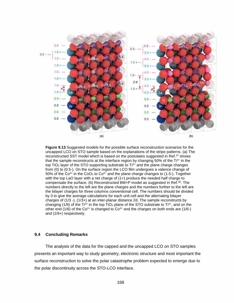
168

Figure 9.13 Suggested models for the possible surface reconstruction scenarios for the uncapped LCO on STO sample based on the explanations of the stripe patterns. (a) The reconstructed SST model which is based on the postulates suggested in Ref.37 shows that the sample reconstructs at the interface region by changing 50% of the Ti4+ in the top TiO2 layer of the STO supporting substrate to Ti3+ and the plane charge changes from (0) to (0.5-). On the surface region the LCO film undergoes a valence change of 50% of the Co3+ in the CoO2 to Co2+ and the plane charge changes to (1.5-). Together with the top LaO layer with a net charge of (1+) produce the needed half charge to compensate the surface. (b) Reconstructed BM+P model as suggested in Ref.38. The numbers directly to the left are the plane charges and the numbers further to the left are the bilayer charges for three columns conventional cell. The numbers should be divided by 3 to give the average calculations for each unit cell and the alternating bilayer charges of (1/3 -), (1/3+) at an inter-planar distance 2d. The sample reconstructs by changing (1/6) of the Ti4+ in the top TiO2 plane of the STO substrate to Ti3+, and on the other end (1/6) of the Co2+ is changed to Co3+ and the charges on both ends are (1/6-) and (1/6+) respectively.

9.4 Concluding Remarks

The analysis of the data for the capped and the uncapped LCO on STO samples

presents an important way to study geometry, electronic structure and most important the

surface reconstruction to solve the polar catastrophe problem expected to emerge due to

the polar discontinuity across the STO-LCO interface.

169

Three models, C-ES, SST and BM+P models were tested to fit the SXR results and

draw a conclusion about their validity in explaining the electronic structure of the samples.

The C-ES model helped to determine the thickness and roughness of the layers and

revealed the probable surface reconstruction of the uncapped sample because of the

broken symmetry. The model is like the suggested ones for the LCO on both LAO and NGO,

and in principle presents a similar explanation to the possible surface reconstruction. The

energy favoured transition from Co3+ to Co2+, both in Oh symmetry, looks to be the most

probable scenario for solving the polar catastrophe problem, transferring the half charge

needed to stabilize the structure. Other scenarios were also introduced including the change

of valency of the Co3+ ions in the surface CoO2 plane to the least unlikely Co4+.

The other two models are in principle widely contradicting and mutually exclusive.

The SST model views the LCO thin-film as a combination of Co3+ LS with the larger unit cell

with Co3+ HS embedded between them and appears as wider than usual columns or stripes.

The model simulates data qualitatively and quantitatively well for the constant energy scans

but deviates notably when the more complicated fixed Qz scans are considered. The atomic

density profiles revealed a ratio of ~ 65%:30%:5% for the Co3+ LS, Co3+ HS and Co2+ HS all

in Oh symmetry, relatively close to the 2:1:0 ratio suggested by the model. The top layer of

the uncapped sample shows a higher concentration of Co2+ HS in Oh symmetry, in

agreement again with the suggested reconstructed model in chapter 8.

The BM+P models fail to have the ratio of 1:1:1 for the Co3+ LS, Co2+ HS in Oh

symmetry, Co2+ in Td symmetry for the capped and uncapped sample, but it again shows the

increase in the Co2+ HS signal. The quality of the fit is not significantly different from the SST

model and again the L3 region seems to take the biggest part in the deviation.

After the analysis of the three models and many others connecting various

components of Co ion together, the data of the capped and the uncapped samples are still

challenging and requires deeper analysis and more measurements. The trial to reduce the

complexity of measurements by changing the samples, for example, growing sandwich LCO

between two STO materials was not a good suggestion. The STO cap layer created a

higher complexity and a new STO-vacuum interface which complicated the measured

signals.

The measurements of constant energy and fixed Qz scans were taken in two

different beamtimes. Although, fitting the data from both beamtimes individually shows very

close similarities, still if we are very particular about our fitting and the various features of the

fixed Qz scans, one should only take measurements from one beamtime only, which is

170

believed to eliminate any changes that might result from the goniometer alignment process

and some shifts in other beamline optics.

The beamline in the Canadian Light Source (CLS)2 contains, in addition to the RSXS

endstation, a molecular beam epitaxy chamber that is planned to be connected to the main

endstation and both are under UHV environment. Growing the LCO films with MBE

techniques will improve the quality of the film and reduce some inherited disadvantages of

the PLD technique. Of special interest is the improvement of the interface roughness. The

ultrahigh vacuum transfer of the sample will help dramatically to control and reduce the

contamination layer.

171

10 General Concluding Remarks

The current state of the project gave some answers and handled some issues that I

found relevant to the study of Co-containing oxides as an example of transition metal oxides

and the application of the SXS technique to study such systems. The results represent good

supporting points for further research. In the current section I would like to present some of

the difficulties and behind the scene challenges that I found in the study which I believe

affected the research. Following that, some modifications and suggestions that might be

helpful in similar future studies will be discussed in details. The suggestions come from

lengthy discussions with group members, my research supervisor and some came from peer

reviews of REIXS beamtime proposals.

We can separate the aspect of the current research into three categories for

explanation purposes. The first and the most important is dealing with the SXS technique in

both modes SXR and XAS. That will also include all the possibilities REIXS beamline and

the RSXS endstation. In this regard, the process of taking the needed measurements

evolved from random into more systematic and comprehensive in such a way that each

block of data will help with a certain analysis level. For example, in the beginning of the

study, LCO on STO sample has been measured over various beamlines due to missing

important blocks of data that were thought to be insignificant, such as SXR at fixed Qz, while

taking other measurements with very long ranges, such as SXR at constant energies when

taken with a very long Qz spans. In addition to that, important measurements at low

temperatures with linear polarized light were not considered and the measurements with

circular polarized light were not effective since the external magnetic fields were not strong

enough, and the development of better accessories to apply effective and uniform fields

came later in the research. The measurements taken for the CoO on MgO sample is more

comprehensive and concise where the samples were measured later in the research. The

measurements were taken with various polarization and temperature steps in addition to

taking the invaluable SXR maps as shown in chapter 6. The experience with the data

analysis shows that the constant energy off-resonant scans are sufficient to study the

geometry of the sample and to some extent reveals information about the contamination

layer. On-resonant and fixed Qz scans are needed to study the electronic structure of the

system. To reveal any irregularities in the measurements due to the surface contamination,

SXR maps are helpful although they are time consuming. Selecting suitable ranges for

taking the effective ranges of each measurement, helped in better time management without

172

affecting the quality of data. The thermal cycles up to 430 K did not show a substantial

change in the signal and probably higher temperatures and better cleaning techniques are

needed if the signal from the contamination layer is sabotaging the measurement. Changing

the polarization is very important in studying the orbital occupation and spin-state of the

system. The system has also sample mounts with various angles that can be helpful in

measuring the vertical stripe pattern that was found for the LCO on STO sample. In addition,

some conventional ways of studying certain aspects of some samples have been deployed.

For example, the study of the adsorption of Xe gas to CoO thin-film surface was conducted

by exposing the Xe gas directly inside the scattering chamber to clarify the effect of the

contamination layer on the resulted reflectometry scans, which is still a work progress and

requires major improvements for the Xe-dosing technique. Unfortunately, the three-chamber

system is still separated and most probably will not be connected in the final configuration

soon due to the lack of space in the fully stacked REIXS beamline. This prevents any use of

the techniques housed in the MBE chamber, or in the multiprobe omicron system, or even in

the linking transfer chamber.

In addition to all the measurements taken and presented in the various chapters, a

huge number of other measurements for various Co-containing systems have been taken

and this is the second aspect of the current study. The samples were chosen only in one

orientation (001) and they included: CoO on MgO uncapped and capped with a layer of

amorphous Al2O3, as presented in chapter 6, CoO sandwiched between two MgO materials,

CoO on MnO uncapped and capped with a layer of non-crystalline Al2O3, as examples of

compressive and tensile strain of a d7 system. The second sets of samples include: LCO on

LAO, NGO and STO all samples are uncapped or capped with a layer of LAO in addition to

sandwiched sample between two STO material. The final sets are superlattice samples of

LCO and LAO, 22, 88 and 1010 unit cells, grown on NGO material. To have

comprehensive measurements and to generate the needed refractive indices of all the

materials, single crystals of LAO, STO, NGO have been also measured. The sample choice

was not the best and the first samples measured were the most complicated systems

namely LCO on STO. The complexity of the measurements not only consumed a long time

in simulating and fitting, but it also did not allow the study of fine isolated part of the sample

such as the effect of the contamination layer. The choice of the samples has been made to

study model d7 and d6 systems in addition to show the effects of compressive or tensile

strain because of the lattice mismatch between the film and the supporting substrate and to

investigate the important polarity problem across the heterointerface and the way the

173

system solves the polar catastrophe problem for some of the materials. The systems ranged

from binary oxide CoO on MgO in the (001) direction with both materials are nonpolar and

their planes are charge neutral to the most complicated system of LCO on STO in the (001)

direction where LCO is polar and has charged planes while STO is nonpolar with a zero-net

charge in the planes.

Since my participation was not significant in the development of the analysis

software ReMagX, I cannot comment or give suggestions to improve the software itself, but I

have some points that maybe helpful in applying the software to build the model systems.

The project tracked and adopted to the development and improvement of the software at its

various stages. Usually the starting point is modelling the data with homogeneous infinite

slabs using the compound refractive index which was a limited process. The system

developed into a well-defined depth profiling ability using the atomic scattering factor of each

element. This development allowed the study of the behaviour of each element in each layer

and revealed details about the valence changes in various layers. The ultimate unique goal

for the current thesis was deploying the modified ReMagX software and the improved

simulation method to study not only the valency of each element within a layer, but its spin-

state also. Models became more specific and testing various combination as reported in the

literature became possible. Although the results were not conclusive, it forms a starting point

for more in-depth analysis in the field. The program also was successful in simulating the

contamination layer effect as presented in chapter 6.

10.1 Suggested Systematic Way to Study Co-containing Materials

In the current section, I am going to present the way with which I may run similar

research depending on the experience accumulated over the past years. This suggestion

maybe simpler than the way the presented research in the thesis was carried out due to

various factors; first it suggests simpler systems of Co-containing materials. One might

argue that probably studying a simpler transition metal than Co could be even a much better

choice, but I am limiting myself to Co. Second, it suggests some measurements that may

improve the quality of the data measured and help in the data analysis specially at low

temperatures. Finally, it gives some more information about possible accessories the REIXS

beamline has and might be helpful.

Similar experiments are expected to dramatically improve if the triple chamber

system which was described in details in chapter 4 was ready and connected. Unfortunately,

this situation may not be possible soon and substantial changes to the beamline space

174

needs to be made for that to happen. In the meantime, the MBE chamber is attached to the

multiprobe omicron chamber via the transfer chamber and all of them are not connected to

the RSXS endstation or the beamline. Though, samples can be transferred in vacuum

between the chambers and the RSXS endstation via a transfer suitcase deferentially

pumped with an ionic pump. Although, this is not a perfect case of transferring the sample

under ultra-high vacuum, but it is way better than storing and transferring the samples in

ambient conditions.

The first suggested step to study Co-containing material is to start with a pure

metallic single crystal system in the (001), (011) and (111) directions. These systems have

been studied before by several well-known surface scientists with whom the resulting RSXS

study can be compared as we showed in chapter 6, for example. The RSXS endstation has

an attached load lock chamber that houses a file which can be used to clean the surface,

but the ideal way to do this kind of study is inside the MBE or the transfer chamber. Both

chambers have the necessary electron guns and leak valves that can be used to sputter

clean the surface with Ar, after which annealing the sample will help the surface to

atomically reconstruct. The cleanliness of the surface can be checked with low energy

electron diffraction LEED in the MBE chamber, as well as X-ray photoemission spectroscopy

in the multiprobe omicron chamber. The clean samples can then be transferred to the RSXS

endstation for the scattering study. It is believed that if the system was ideal and the surface

was clean, the reflectometry scans will reduce to the Fresnel’s reflection case (only single

layer) and the system should be easier to detect and study. The following step is the most

important; in which an intentional oxidation study of the three types of surfaces can be

carried out. The system will start to be complicated and the surface layer will appear in the

reflectometry scans as a clear slow modulation. The study of the oxide layer will give insight

in the transition from Co metal to the Co-containing oxides at the surface. The results of the

study should be very important in determining any kind of surface change, especially with

the ability to control the surface contamination layer that was always a source of error in

samples that were stored in ambient conditions.

The next step would be like what we did in chapter 6 in which we chose a well

studied d7 CoO on various substrate system, but with a substantial change. Rather than

directly grow and study CoO thin-film, one must start with a single crystal CoO grown in

(001), (011) and (111) directions. Again, after cleaning and checking the surface quality, the

reflectometry study will be invaluable to investigate the surface of the single crystal and

clarify the way with which the polar surface in a specific orientation reconstructs to

175

compensate the charge and solve the polar catastrophe problem, as well as giving

reference signals to be used for comparison purposes. Samples grown in the (001) direction

are expected not to substantially reconstruct since the surfaces are type one neutral and the

planes are also charged neutral, whereas samples in the (111) direction will reconstruct by a

valence change of the Co2+ to Co3+ ions and symmetry change of the surface Co2+ ions from

octahedral (Oh) symmetry to tetrahedral (Td) symmetry forming the known spinel structure.

The study of the surface contamination effect in a more controlled manner can be carried

more effectively on the single crystal than the CoO thin-film, as we did in a study of

adsorbing Xe gas on a CoO film on MnO substrate, the study was briefly presented in the

concluding remarks section of chapter 6. The results of our study were challenging to

analyse and the dosing technique was not accurate and efficient. We believe that better

dosing will be achieved in the MBE or even the transfer chambers, and using the single

crystal will simplify the resulting spectra with less features specially in the constant energy

scans. Other gasses can also be used such as oxygen or even carbon containing molecules

such CO or CO2, and again such surface studies do exist and they will be very helpful in the

data analysis.

Having done that, a study like the one presented in chapter 6 can be performed with

the possibility of growing the CoO thin-films onsite in the MBE chamber, in the (001) and

(111) directions on various substrates, and study them with LEED and XPS then move them

to the RSXS endstation. The vacuum transfer is very important at this stage, it will help

eliminate the large surface contamination layer and allow the detection of clear signal that

may answer some questions about oxygen vacancies or increased surface oxygen

densities, both of which were very hard to detect with the samples stored in ambient

conditions. It is expected that the constant energy reflectometry scans will show well defined

modulations without any extra features as shown in the contaminated samples in chapter 6.

The study of thin-films grown on substrates with close lattice parameters will help simplify

the problem and eliminate some unnecessary conditions. For example, the choice of MgO is

good due to the proximity of lattice parameter and structure from that of CoO. In the (001)

direction the material is nonpolar and has zero charges on the planes, but in (111) direction

the material is polar and alternates with Co2+ and O2- planes with 2+ and 2- charges

respectively. Studying the material in the (001) direction will give insight in the changes that

the lattice mismatch imposes, then the results can be used in the analysis of the more

complicated case in the (111) direction where a polar problem exists in addition to the strain

problem. In addition to the aforementioned samples, samples with sandwiched CoO thin-film

176

could also be good candidates due to the double interface rather than one and they are

somewhere between thin-film and superlattice structure.

Our choice of the LCO thin-film grown on LAO substrate fits at this stage very well.

Both materials are polar and have similar plane charges in the three directions in addition to

the closeness of their lattice parameter. The sample is an example of a compressive strain

and the sample grown in the (001) direction was analyzed and presented in chapter 7. In

chapter 7, reflectometry with linearly σ- and π-polarized light was measured at 20 (not

presented) and 300 K. The upper limit is well above the Curie temperature of 85 K, but the

lower limit is just at the spin-state transition temperature at 20 K for thin-film LCO and that

prevents seeing any changes in the reflectometry scans. Probably a better way of running

the experiment will be taking the measurements around the Curie temperature of 85 K (±20

K). At low temperature and different from the bulk LCO, the reflectometry scans will show a

difference between the measurements taken with σ- and π-polarized light, since the

electrons will be populating the two t2g and eg levels and the sixth electron will pair up with

another t2g one and the system will be in higher spin-state (most probably the high spin-state

with S=2). The clearest and most important difference which the current study misses is

going to 20 K as well as ±20 K below and above the Curie temperature of 85 K and running

scattering measurements with circularly polarized light and with an applied magnetic field at

each temperature. The resulting X-ray magnetic circular dichroism and X-ray magnetic

reflectivity (XRMR) measurements should give us insight about the spin-state transition of

the system from completely low spin (S=0) at 20 K to higher spin-states above 20 K. In the

current study, similar measurements were taken for the LCO on STO system but with a

weak 0.1 Tesla non-uniform cylindrical magnet and are still a work in progress. The newly

developed magnets in the RSXS endstation are much better suited now for such

measurements. The LCO on NGO sample is not too far from the LCO on LAO except that it

is tensile rather than compressive strain. All the suggested measurements for the LCO on

LAO sample is also valid here. Growing the samples in other directions such as (011) and

(111) could be very important step up in the study. The samples will still retain the sample

similarity in polarity and plane charges as well as proximity in lattice parameters.

The most important sample and most complicated is LCO thin-film grown on STO

substrate. STO sample is nonpolar with neutral planes when it is grown in the (001) direction

and polar with 𝑇𝑖4+ and 𝑆𝑟2+𝑇𝑖4+𝑂2− in the (011) direction and 𝑇𝑖4+and (𝑆𝑟2+𝑂32−)4− in the

(111) direction as shown in chapter 2. When the sample is grown in the (001), it undergoes

a polar discontinuity across the heterointerface and system is highly tensile strained due to

177

the large difference in lattice parameter between the LCO thin-film and the STO supporting

substrate as shown in chapter 9. The result is a deformed structure with a stripe pattern

whose nature is still debated. Although, I took quite many measurements for the samples,

the measurements were scattered over several beamtimes, and they were not complete and

comprehensive. I would run a similar study as the one suggested for the LCO on LAO for

the (001), (011) and (111) directions. It would be very interesting to see if the stripes are

direction related and if one can use angled sample mounts to detect any possible

superlattice peaks that can be associated with them.

The soft X-ray scattering study of the Co-containing materials is still in the infancy

stage and many modifications will be proposed in the next few years that will improve and

develop the technique and research methodology.

178

References

1 D. G. Hawthorn, F. He, L. Venema, H. Davis, A. J. Achkar, J. Zhang, R. Sutarto, H.

Wadati, A. Radi, T. Wilson, G. Wright, K. M. Shen, J. Geck, H. Zhang, V. Nov´ak, and G.

A. Sawatzky, Rev. Sci. Instrum. 2011 82 073104.

2 Canadian Light Source CLS, Saskatoon, Canada.

3 S. Macke, ReMagX – X-ray magnetic reflectivity tool. Max Planck – UBC centre for

quantum materials (Home-Built Program).

4 S. Macke, A. Radi, J. E. Hamann-Borrero, A. Verna, M. Bluschke, S. Brück , E. Goering,

R. Sutarto , F. He, G. Cristiani, M. Wu, E. Benckiser, H-U. Habermeier, G. Logvenov, N.

Gauquelin, G. A. Botton, A. P. Kajdos, S. Stemmer, G. A. Sawatzky, M. W. Haverkort, B.

Keimer, V. Hinkov Adv. Mater. 2014 26 6554.

5 J. E. Hamann-Borrero, S. Macke, W. S. Choi, R. Sutarto, F. He, A. Radi, I. Elfimov, R. J.

Green, M. W. Haverkort, V. B. Zabolotnyy , H. N. Lee, G. A. Sawatzky, V. Hinkov npj

Quantum Materials 2016 1 16013.

6 D. G. Schlom and M. Zurbuchen, J. Am. Ceram. Soc. 2008 91 [8] 2429.

7 S. Vasala, M. Karppinen, Prog. Solid Stat. Chem. 2015 43 1.

8 A. Ohtomo and H. Hwang, Nature 2004 427 423.

9 A. Gozar, G. Logvenov, L. Fitting Kourkoutis, A. T. Bollinger, L. A. Giannuzzi, D. A.

Muller, I. Bozovic, Nature 2008 455 782.

10 L. Li, C. Richter, J. Mannhart, R. C. Ashoori, Nat. Phys. 2011 7 762.

11 J. A. Bert, B. Kalisky, C. Bell, M. Kim, Y. Hikita, H. Y. Hwang, K. A. Moler Nat. Phys.

2011 7 767.

12 E. Benckiser, M. Haverkort, S. Brück, E. Goering, S. Macke, A. Frañó, X. Yang, O.

Andersen, G. Cristiani, H. Habermeier, et al. Nat. Mat. 2011 10 189

179

13 K. Asai, O. Yokokura, N. Nishimori, H. Chou, Phys. Rev. B 1994 50 3025.

14 M. Losurdo, A. Sacchetti, P. Capezzuto, G. Bruno, L. Armelao, D. Barreca, G. Bottaro,

A. Gasparotto, C. Maragno, E. Tondello, Appl. Phys. Lett. 2005 87 061909/1.

15 M. Daturi, G. Busca, R. Willey, Chem. Mater. 1995 7 2115.

16 S. Thiel, G. Hammerl, A. Schmehl, C. W. Schneider,J. Mannhart, Science 2006 313 1942.

17 A. Brinkman, M. Huijben, M. Van Zaik, J. Huijben, U. Zeitter, J. C. Mann, W. G. Van der

Wiel, G. Rijnders, D. H. A. Blank, H. Hilgenkamp, Nat. Mater. 2007 6 493.

18 M. P. Warusawithana, C. Richter, J. A. Mundy, P. Roy, J. Ludwig, S. Paetel, T. Heeg, A.

A. Pawlicki, L. F. Kourkoutis, M. Zheng, M. Lee, B. Mulcahy, Y. Zander, W. Zhu, J.

Schubert, J. N. Eckstein, D. A. Muller, C. S. Hellberg, J. Mannhart, D. G. Schlom, Nat.

Comm. 2013 4 2351.

19 G. Herranz, M. Basletic, M. Bibes, C. Carretero, E. Tafra, E. Jacquet, K. Bouzehouane,

C. Deranlot, A. Hamzic, J. M. Broto, A. Barthelemy, A. Fert, Phys. Rev. Lett. 2007 98

216803.

20 M. Basletic, J. L. Maurice, C. Carretero, G. Herranz, O. Copie, M. Bibes, E. Jacquet, K.

Bouzehouane, S. Fusil, A. Barthelemy, Nat. Mater. 2008 7 621.

21 N. Nakagawa, H. Y. Hwang, D. A. Muller, Nat. Mat. 2006 5 204.

22 M. Sing, G. Berner, K. Goss, A. Muller, A. Ruff, A. Wetscherek, S. Thiel, J. Mannhart, S. A. Pauli,

C. W. Schneider, P.R Willmott, M. Gorgoi, F. Schafers, R. Claessen Phys. Rev. Lett. 2009 102

176805.

23 C. A. F. Vaz, F. J. Walker, C. H. Ahn and S. Ismail-Beigi, J. Phys.: Condense Matter

2015 27 123(001).

24 H. Y. Hwang, Y. Iwasa, M. Kawasaki, B. Keimer, N. Nagaosa, Y. Tokura, Nat. Mat. 2012

11 103.

25 W. Siemons, G. Koster, H. Yamamoto, W. A. Harrison, G. Lucovsky, T. H. Geballe, D. H.

A. Blank, M. R. Beasley, Phys. Rev. Lett. 2007 98 196802.

180

26 C. Kao, J. B. Hastings, E. D. Johnson, D. P. Siddons, G. C. Smith, G. A. Prinz, Phys.

Rev. Lett. 1990 65 373.

27 D. Kim, H. Lee, S. Kim, H. Kang, D. Noh, H. Kim, S. Sinha, Appl. Phys. Lett. 2004 85

6427.

28 S. Smadici, P. Abbamonte, A. Bhattacharya, X. Zhai, B. Jiang, A. Rusydi, J. N. Eckstein,

S. D. Bader, J.-M. Zuo , Phys. Rev. Lett. 2007 99 196404.

29 J. M. Tonnerre, M. De Santis, S. Grenier, H. Tolentino, V. Langlais, E. Bontempi, M.

Garcia-Fernandez, U. Staub, Phys. Rev. Lett. 2008 100 157202.

30 J. Fink, E. Schierle, E. Weschke, J. Geck, Rep. on Prog. in Phys. 2013 76 056502.

31 J. Stöhr, H. C. Siegmann: “Magnetism: From fundamentals to nanoscale dynamics”

Springer 2006.

32 J. Rubio-Zuazo, G. Castro, J. of Phys.: Conf. Ser. 2008 100 012042.

33 D. A. Muller, Nat. Mat. 2009 8 263.

34 G. Berner, et al. Phys. Rev. B 2010 82 241405.

35 A. X. Gray, C. Papp, B. Balke, S.-H. Yang, M. Huijben, E. Rotenberg, A. Bostwick, S.

Ueda, Y. Yamashita, K. Kobayashi, E. Gullikson, J. B. Kortright, F. M. F. de Groot, G.

Rijnders, D. H. A. Blank, R. Ramesh, C. S. Fadley, Phys. Rev. B 2010 82 205116.

36 F. de Groot, A. Kotani, CRC Press 2008.

37 W. S. Choi, J. H. Kwon, H. Jeen, J. E. Hamann-Borrero, A. Radi, S. Macke, R. Sutarto,

F. He, G. Sawatzky, V. Hinkov, M. Kim, H. N. Lee, Nano Lett. 2012 12, 4966.

38 N. Biškup, J. Salafranca, V. Mehta, Y. Suzuki, S. J. Pennycook, S. T. Pantelides, M.

Varela, PRL, 2014 112. 087202.

39 V. V. Mehta, N. Biskup, C. Jenkins, E. Arenholz, M. Varela, and Y. Suzuki, Phys. Rev.

B 2015 91 144418

181

40 D. Fuchs, C. Pinta, T. Schwarz, P. Schweiss, P. Nagel, S. Schuppler, R. Schneider, M.

Merz, G. Roth, H. v. Löhneysen Phys. Rev. B 2007 75 144402.

41 C. F. Chang, Z. Hu, hua Wu, T. Burnus, N. Hollmann, M. Benomar, T. Lorenz, A.

Tanaka, H. –J. Lin, H. H. Hsieh, C. T. Chen, L. H. Tjeng, Phys. Rev. Lett. 2009 102

116401.

42 C. Pinta, D. Fuchs, M. Merz, M. Wissinger, E. Arac, H. v. Löhneysen, A. Samartsev, P.

Nagel, S. Schuppler1 Phys. Rev. B 2008 78 174402.

43 M. Merz, P. Nagel, C. Pinta, A. Samartsev, H. v. Löhneysen, M. Wissinger, S. Uebe, A.

Assmann, D. Fuchs, S. Schuppler Phys. Rev. B 2010 82 174416.

44 M. W. Haverkort, Z. Hu, J. C. Cezar, T. Burnus, H. Hartmann, M. Reuther, C. Zobel, T.

Lorenz, A. Tanaka, N. B. Brookes, H. H. Hsieh, H. -J. Lin, C. T. Chen, L. H. Tjeng Phys.

Rev. Lett. 2006 97 176405.

45 G. E. Sterbinsky, P. J. Ryan, J. -W. Kim, E. Karapetrova, J. X. Ma, J. Shi, J. C. Woicik,

Phys. Rev. B 2012 85, 020403(R).

46 J.-Q Yan, J.-S. Zhou, J. B. Goodenough, Phys. Rev. B 2004 70, 014402.

47 A. Kushima, S. Yip,B. Yildiz, Phys. Rev. B 2010 82 115435.

48 M. A. Korotin S. Y. Ezhov, I. V. Solovyev, V. I. Anisimov, D. I. Khomskii, G. A. Sawatzky,

Phys. Rev. B 1996 54 5309.

49 S. Okamoto, A. J. Millis, Nature 2004 428 630.

50 A. Kalabukhov, Phys. Rev. B 2007 75 121404.

51 R. Pentcheva, W. E. Pickett, Phys. Rev. Lett. 2009 102 107602.

52 C. L. Jia, S. B. Mi, M. Faley, U. Poppe, J. Schubert, K. Urban, Phys. Rev. B 2009 79

081405.

53 Z. Q. Liu, C. J. Li, W. M. Lu, X. H. Huang, Z. Huang, S. W. Zeng, X. P. Qin, L.S. Huang,

A. Annadi, J. S. Chen, J. M. D. Coey, T. Venkatesan, Ariando, Phys. Rev. X 2013 3

021010.

182

54 X. R. Wang,C. J. Li, W. M. Lu, T. R. Paudel, D. P. Leusink, M. Hoek, N. Poccia, A. Vailionis, T.

Venkatesan, J. M. D. Coey, E. Y. Tsymbal, Ariando, H. Hilgenkamp, Science 2015 349 716.

55 N. Pavlenko, I. Elfimov, T. Kopp, G. A. Sawatzky, Phys. Rev. B 2007 75 140512.

56 J. W. Freeland, J. X. Ma, J. Shi, Appl. Phys. Lett. 2008 93 212501.

57 M. Haverkort, Ph.D. Thesis: “Spin and orbital degrees of freedom in transition metal

oxides and oxide thin-films studied by soft X-ray absorption spectroscopy”, University of

Cologne, Cologne, Germany 2005.

58 J. R. Singer, Phys. Rev. 1956 104 929.

59 G. Miessler, D. Tarr: “Inorganic Chemistry” 3d edition, Printce Hall 2004.

60 C. J. Ballhausen: “Introduction to Ligand Field Theory” McGraw-Hill Book Company Inc.

1962.

61 C. Ballhausen, Introduction to Ligand Field Theory, McGraw-Hill Book Company Inc.

1962.

62 G. A. Somorjai: “Introduction to Surface Chemistry and Analysis” John Wiley & Sons Ltd,

New York 1994.

63 P.W. Tasker, J. Phys. C 1979 12 4977.

64 W. A. Harrison, E. A. Kraut, J. R. Waldrop, R. W. Grant, Phys. Rev. B 1978 18 4402.

65 R. Hesper, L. H. Tjeng, A. Heeres, G. A. Sawatzky, Phys. Rev. B 2000 62 16046.

66 C. Noguera, J. Phys.: Condens. Matter 2000 12 R367.

67 R. D. Shannon, Acta Cryst. 1976 A 32, 751.

68 R. H. Potze, G. A. Sawatzky, M. Abbate, Phys. Rev. B 51, 11501 (1995).

69 P. M. Raccah, J. B. Goodenough, Phys. Rev. 155, 932 (1967).

183

70 R. F. Klie, T. Yuan, M. Tanase, G. Yang, Q. Ramasse APPLIED PHYSICS LETTERS

96, 082510 (2010)

71 A. Wakako, A. Takehiro, A. Yoshio, J. of App. Phys. 2014 116 043513

72 J. Als-Nielsen, D. McMorrow: “Elements of Modern X-ray Physics” John Willy and Sons

Ltd, 2(001).

73 D. Attwood: “Soft X-rays and Extreme Ultraviolet Radiation: Principles and Applications”

Cambridge University Press, 1999.

74 Y. Waseda, E. Matsubara, K. Shinoda: “X-ray Diffraction Crystallography: Introduction,

Examples and Solved Problems”, Springer, 2011.

75 A. Frano, Ph.D. Thesis:”Spin Spirals and Charge Textures in Transition Metal-Oxide

Heterostructure” Springer 2014.

76 J. J. Sakurai, J. Napolitano: “Modern Quantum Mechanics” 2nd edition, Pearson

Education Inc. 2011.

77 L. Parratt, Phys. Rev. 1954 95 359.

78 R. Wicks, Ph.D. Thesis: “Molecular Beam Epitaxy of Magnetic Oxynitride Films,

Construction of a combined growth/analysis system, development of experimental tools

and investigation of two oxynitride systems” University of British Columbia, Vancouver,

Canada 2012.

79 R. Fowles, “Introduction to modern optics”, 2nd Edition, Holts, Rinehart and Winston,

New York 1975.

80 S. Csiszar, Ph.D. Thesis: “X-ray diffraction and X-ray absorption of strained CoO and

MnO thin-films”, University of Groningen, Groningen, Netherlands 2005.

81 C. Chantler, Journal of Physical and Chemical Reference Data 1995 2 71.

82 M. Gibert, P. Zubko, R. Scherwitzl, J. Íñiguez, J.-M. Triscone, Nat. Mat. 2012 11 195.

83 C. Cen, S. Thiel, J. Mannhart, J. Levy, Science 2009 323 1026.

184

84 J. T. Ye, S. Inoue, K. Kobayashi, Y. Kasahara, H. T. Yuan, H. Shimotani, Y. Iwasa, Nat.

Mat. 2010 9 125.

85 M. Li, X. Jiang, G. Samant, C. Felser, S. S. P. Parkin, Appl. Phys. Lett. 2013 103

032410.

86 R. Egerton: “Electron energy-loss spectroscopy in the electron microscope” Springer

2011.

87 Y. Kozuka, M. Kim, C. Bell, B. Kim, Y. Hikita, H. Hwang, Nature 2009 462 487.

88 B. Jalan, S. Stemmer, S. Mack, S. J. Allen, Phys. Rev. B 2010 82 081103.

89 C. Jeynes, R. P. Webb, A. Lohstroh, Rev. Accl. Sci. Tech. 2011 4 41.

90 G. A. Botton, MRS Bull. 2012 37 21.

91 K. Zimmermann, M. Tolan, R. Weber, J. Stettner, A. Doerr, W. Press, Phys. Rev. B 2000

62 10377.

92 A. Van DerLee, F. Salah, B. Harzallah, J. Appl. Cryst. 2007 40 820.

93 T. Hohage, K. Giewekemeyer, T. Salditt, Phys. Rev. E 2008 77 051604.

94 C. F. Majkrzak, N. F. Berk, Phys. Rev. B 1995 52 10827.

95 P. Abbamonte, L. Venema, A. Rusydi, G. A. Sawatzky, G. Logvenov, I. Bozovic, Science

2002 297 581.

96 C. Park, P. Fenter, J. Appl. Cryst. 2007 40 290.

97 J. Bai, M. Tomkiewicz, P. Montano, Z. Phys. B 1995 97 465.

98 W. Press, B. Flannery, S. Teukolsky, W. Vetterling, et al. “Numerical recipes” Cambridge

Univ. Press, 1986.

99 A. Boris, Y. Matiks, E. Benckiser, A. Frano, P. Popovich, V. Hinkov, P. Wochner, M.

Castro-Colin, E. Detemple, V. Malik, et al. Science2011 332 937.

185

100 A. Frano, E. Schierle, M. W. Haverkort, Y. Lu, M. Wu, S. Blanco-Canosa, U. Nwankwo,

A. V. Boris, P. Wochner, G. Cristiani, H. U. Habermeier, G. Logvenov, V. Hinkov, E.

Benckiser, E. Weschke, B. Keimer, Phys. Rev. Lett. 2013 111 106804.

101 B. Jalan, J. Cagnon, T. Mates, S. Stemmer, J. Vac. Sci. Technol. A 2009 27 1365

102 S. Hofmann, Phil. Trans. R. Soc. Lond. A 2004 362 55.

103 D. Briggs, M. P. Seah: “Practical surface analysis by Auger and X-ray photoelectron

spectroscopy” Wiley, New York 1983.

104 N. Nakanishi, H. Hashizume, T. Terashima, Y. Bando, O. Michikami, S. Maeyama, M.

Oshima, Phys. Rev. B 1993 48 10524.

105 H. Wadati , D. G. Hawthorn , J. Geck , T. Higuchi , Y. Hikita , H. Y. Hwang , L. Fitting

Kourkoutis , D. A. Muller , S.-W. Huang , D. J. Huang , H.-J. Lin, C. Schüßler-

Langeheine, H.-H. Wu, E. Schierle, E. Weschke, N. J. C. Ingle, G. A. Sawatzky, J. Appl.

Phys. 2009 106 083705.

106 S. I. Csiszar, M. W. Haverkort, Z. Hu, A. Tanaka, H. H. Hsieh, H.-J. Lin, C. T. Chen, T.

Hibma, L. H. Tjeng, PRL 2005 95, 187205.

107 A. Barla, G. Schmerber, E. Beaurepaire, A. Dinia, H. Bieber, S. Colis, F. Scheurer, J.-P.

Kappler, P. Imperia, F. Nolting, F. Wilhelm, A. Rogalev, D. Müller, J. J. Grob, Phys. Rev.

B 2007 76, 125201.

108 T. Ohnishi, K. Takahashi, M. Nakamura, M. Kawasaki, M. Yoshimoto, H. Koinuma, Appl.

Phys. Lett. 1999 74, 2531.

109 R. Kurian, K. Kunnus, P. Wernet, S. M. Butorin, P. Glatzel, F. M. F. de Groot, J. Phys.:

Condens. Matter 2012 24, 452201.

110 R. J. Green, D. Peak, A. J. Achkar, J. S. Tse, A. Moewes, D. G. Hawthorn, T. Z. Reglier,

Phys. Rev. Lett. 2014 112 129301.

111 A. Gibaud, G. Vignaud, S. K. Sinha, Acta Crystallogr. A Found. Crystallogr. 1993 49,

642.