Ph.D. THESIS ADVANCES IN PARALLEL AND SEQUENTIAL ...

Ph.D. THESIS

ADVANCES IN PARALLEL AND

SEQUENTIAL DYNAMICAL SYSTEMS

OVER GRAPHS

Submitted for the degree of Doctor of Philosophy at the University of Castilla-La Mancha

by

Luis Gabriel Díaz López

January 2020

iii

To my family.

To my friends.

Contents

Preface 1

Abstract 3

1 Introduction 5

2 Preliminaries 17

3 Advances in Parallel Dynamical Systems 29

3.1 Dynamics of periodic orbits . . . . . . . . . . . . . . . . . . . . . . . 29

3.1.1 Existence of periodic orbits . . . . . . . . . . . . . . . . . . . 29

3.1.2 Coexistence of periodic orbits . . . . . . . . . . . . . . . . . . 31

3.1.3 Uniqueness of xed points . . . . . . . . . . . . . . . . . . . . 33

3.1.4 Uniqueness of 2-periodic orbits . . . . . . . . . . . . . . . . . 35

3.1.5 Maximum number of xed points . . . . . . . . . . . . . . . . 39

3.1.6 Maximum number of 2-periodic orbits . . . . . . . . . . . . . 41

3.2 Dynamics of non-periodic orbits . . . . . . . . . . . . . . . . . . . . . 46

3.2.1 Predecessors and GOE congurations . . . . . . . . . . . . . . 46

3.2.2 Convergence to periodic orbits: attractors, global attractors,basins of attraction and transient . . . . . . . . . . . . . . . . 55

4 Advances in Sequential Dynamical Systems 77


4.1.1 Existence of periodic orbits . . . . . . . . . . . . . . . . . . . 77

vi Contents

4.1.2 Coexistence of periodic orbits . . . . . . . . . . . . . . . . . . 81

4.1.3 Uniqueness of xed points . . . . . . . . . . . . . . . . . . . . 86

4.1.4 Uniqueness of periodic orbits . . . . . . . . . . . . . . . . . . . 87

4.1.5 Maximum number of xed points . . . . . . . . . . . . . . . . 97

4.1.6 Maximum number of periodic orbits . . . . . . . . . . . . . . . 98


4.2.1 Predecessors and GOE congurations . . . . . . . . . . . . . . 104

4.2.2 Convergence to periodic orbits: attractors, global attractors,basins of attraction and transient . . . . . . . . . . . . . . . . 117

5 Advances in Parallel and Sequential Directed Dynamical Systems 135


5.1.1 Existence and coexistence of periodic orbits in PDDS . . . . . 137

5.1.2 Existence and coexistence of periodic orbits in SDDS . . . . . 143


5.2.1 Predecessor and GOE congurations in PDDS . . . . . . . . . 146

5.2.2 Predecessor and GOE congurations in SDDS . . . . . . . . . 156

Conclusions and future research directions 171

Bibliography 177

List of Figures

2.1 Graph G = (1, 2, 3, 1, 2, 2, 3). . . . . . . . . . . . . . . . . . . . . . . . . . . . . . . . . . . . 19

2.2 Phase portrait of the system[(1, 2, 3, 1, 2, 2, 3) ,

(x′1 ∨ x′2, x′1 ∨ x′2 ∨ x3, x′2 ∨ x3

)]− PDS. . . 20

2.3 Phase portrait of the system [(1, 2, 3, 1, 2, 2, 3) , F3 F2 F1 (x1, x2, x3) , 1|2|3]− SDS. . . . . 21

2.4 Graph G = (1, . . . , 8, 1, 2, 2, 4, 3, 4, 3, 5, 4, 6, 4, 7, 7, 8). . . . . . . . . . . . . . . . . 26

3.1 Graph G = (1, 2, 3, 1, 2, 2, 3). . . . . . . . . . . . . . . . . . . . . . . . . . . . . . . . . . . . 62

3.2 Phase portrait of the system[(1, 2, 3, 1, 2, 2, 3) , x′1 ∨ x2 ∨ x3

]− PDS. . . . . . . . . . . . . . 63

3.3 Graph G1 = (1, 2, 1, 2). . . . . . . . . . . . . . . . . . . . . . . . . . . . . . . . . . . . . . . . . 63

3.4 Graph G2 = (1, 2, 3, 4, 1, 2, 3, 4, 1, 3). . . . . . . . . . . . . . . . . . . . . . . . . . . . . . . 63

3.5 Graph G3 = (V3, E3) = (1, 2, 3, 4, 5, 6, 1, 2, 3, 4, 1, 3, 5, 6, 1, 5). . . . . . . . . . . . . . . 64

3.6 Graph G4 = (V4, E4) = (1, . . . , 8, E3 ∪ 7, 8, 1, 7, 3, 7). . . . . . . . . . . . . . . . . . . . . . 64

3.7 Graph G5 = (1, . . . , 10, E4 ∪ i, 9 : i ∈ 1, 3, 5, 10). . . . . . . . . . . . . . . . . . . . . . . . . . 65

3.8 Graph G = (1, 2, 3, 4, 1, 2, 2, 3, 1, 4). . . . . . . . . . . . . . . . . . . . . . . . . . . . . . . . 71

3.9 Phase portrait of the system[(1, 2, 3, 4, 1, 2, 2, 3, 1, 4) , x′1 ∨ x2 ∨ x3 ∨ x′4

]− PDS. . . . . . 72

4.1 Patterns for n = 2, n = 3, n = 4 and n = 5. . . . . . . . . . . . . . . . . . . . . . . . . . . . . . . . . 79

4.2 Graph G = (1, 2, 3, 4, 5, 6, 3, 4, 5, 6 ∪ i, j : 1 ≤ i ≤ 2, 3 ≤ j ≤ 6). . . . . . . . . . . . . . . 85

4.3 2-periodic orbit of the system proposed by Theorem 4.11. . . . . . . . . . . . . . . . . . . . . . . . . 86

4.4 3-periodic orbit of the system proposed by Theorem 4.11. . . . . . . . . . . . . . . . . . . . . . . . . 86

4.5 Graph 1, 2, 3, 4, 1, 2, 2, 3, 3, 4, 4, 1. . . . . . . . . . . . . . . . . . . . . . . . . . . . . . 88

4.6 Unique periodic orbit of the [1, 2, 3, 4, 1, 2, 2, 3, 3, 4, 4, 1,NAND, id]− SDS. . . . . . . 88

4.7 Phase portrait of the system[(1, 2, 1, 2) , x′1 ∨ x′2, 1|2

]− SDS. . . . . . . . . . . . . . . . . . . 109

4.8 Phase portrait of the system[(1, 2, 1, 2) , x1 ∨ x′2, 1|2

]− SDS. . . . . . . . . . . . . . . . . . . 110

4.9 Phase portrait of the system [(1, 2, 3, 1, 3, 2, 3) , x1 ∨ x2 ∨ x3, 1|2|3]− SDS. . . . . . . . . . . 115

4.10 Graph G = (1, 2, 3, 4, 5, 6, 7, 1, 2, 2, 3, 3, 4, 3, 5, 4, 6, 5, 7). . . . . . . . . . . . . . . . . 124

4.11 Orbit of x0 = (0, 0, 1, 1, 0, 0, 0). . . . . . . . . . . . . . . . . . . . . . . . . . . . . . . . . . . . . . . . 125

4.12 Graph G = (1, . . . , 9, 1, 2, 2, 3, 3, 4, 4, 5, 3, 6, 6, 7, 3, 8, 8, 9). . . . . . . . . . . . . 132

4.13 Orbit of x0 = (0, 0, 1, 1, 1, 0, 0, 1, 0). . . . . . . . . . . . . . . . . . . . . . . . . . . . . . . . . . . . . . 133

5.1 Graph D = 1, 2, 3, (1, 3) , (2, 3). . . . . . . . . . . . . . . . . . . . . . . . . . . . . . . . . . . . 138

viii List of Figures

5.2 Patterns for n = 3, n = 4, n = 5 and n = 6. . . . . . . . . . . . . . . . . . . . . . . . . . . . . . . . . 139

5.3 Graph D = (V,A). . . . . . . . . . . . . . . . . . . . . . . . . . . . . . . . . . . . . . . . . . . . . . . 142

5.4 2-periodic orbit of the system proposed by Theorem 5.3. . . . . . . . . . . . . . . . . . . . . . . . . . 142

5.5 3-periodic orbit of the system proposed by Theorem 5.3. . . . . . . . . . . . . . . . . . . . . . . . . . 143

5.6 Phase portrait of the system[1, 2, (1, 2), x1 ∨ x′2

]− PDDS. . . . . . . . . . . . . . . . . . . . . . 150

5.7 Phase portrait of the system[(1, 2, (2, 1)) , x′1 ∨ x′2, 1|2

]− SDDS. . . . . . . . . . . . . . . . . . . 160

5.8 Phase portrait of the system[(1, 2, (1, 2)) , x′1 ∨ x′2, 1|2

]− SDDS. . . . . . . . . . . . . . . . . . . 161

5.9 Phase portrait of the system[(1, 2, (1, 2) , (2, 1)) , x1 ∨ x′2, 1|2

]− SDDS. . . . . . . . . . . . . . . 162

5.10 Phase portrait of the system [(1, 2, 3, (1, 2) , (2, 3) , (3, 1)) , x1 ∨ x2 ∨ x3, 1|2|3]− SDDS. . . . . . . 168

Preface

In accordance with the requirements of the procedure established by the Univer-sity of Castilla-La Mancha (UCLM) for the elaboration, defense and examinationof doctoral theses, once I have received the positive examiners' reports and the cor-responding authorizations of the supervisors of the doctoral thesis, Silvia MartínezSanahuja and José Carlos Valverde Fajardo, and the Coordinator of the DoctoralProgramme FISYMAT, Gabriel Fernández Calvo, I submit this work as a disserta-tion for the degree of Doctor of Philosophy at the University of Castilla-La Mancha.

This dissertation, entitled Advances in Parallel and Sequential Dynamical Sys-tems over Graphs, constitutes an own original research work related to the eldsDynamical Systems and Computational Algebra, included in the research linesMath-ematical Models and Methods in Science and Algebraic Models of the Doctoral Pro-gramme FISYMAT.

The scientic contributions of the doctoral thesis have been published or are inprocess of publication by international journals of the JCR (Web of Science) Index:

• Paper [6], On the Periods of Parallel Dynamical Systems, Complexity Volume2017 (2017) Article ID 7209762, 6 pages, corresponds to Subsections 3.1.2 and3.1.3 of Section 3.1 in Chapter 3.

• Paper [7], On periods and equilibria of computational sequential systems, Info.Sci. 409410 (2017) 2734, corresponds to Subsections 4.1.1, 4.1.2 and 4.1.3of Section 4.1 in Chapter 4.

• Paper [8], Maximum number of periodic orbits in parallel dynamical systems,Inf. Sci. 468 (2018) 6371, corresponds to Subsections 3.1.4, 3.1.5 and 3.1.6of Section 3.1 in Chapter 3.

• Paper [9], Predecessors and Garden-of-Eden congurations in parallel dynam-ical systems on maxterm and minterm Boolean functions, J. Comput. Appl.

2 Preface

Math. 348 (2019) 2633, corresponds to Subsection 3.2.1 of Section 3.2 inChapter 3.

• Paper [10], Solution to the predecessors and Gardens-of-Eden problems forsynchronous systems over directed graphs, Appl. Math. Comput. 347 (2019)2228, corresponds to Subsection 5.2.1 of Section 5.2 in Chapter 5.

• Paper [11], Predecessors Existence Problems and Gardens of Eden in SequentialDynamical Systems, Complexity Volume 2019 (2019) Article ID 6280960, 10pages, corresponds to Subsection 4.2.1 of Section 4.2 in Chapter 4.

• Paper [12], Predecessors and Gardens of Eden in sequential dynamical sys-tems over directed graphs, Appl. Math. Nonlinear Sci. 3(2) (2018) 593602,corresponds to Subsection 5.2.2 of Section 5.2 in Chapter 5.

• Paper [13], Dynamical attraction in parallel network models, Appl. Math.Comput. 361 (2019) 874888, corresponds to Subsection 3.2.2 of Section 3.2in Chapter 3.

• Paper [14], Attractors and transient in sequential dynamical systems, Int. J.Comput. Math. (2019), corresponds to Subsection 4.2.2 of Section 4.2 inChapter 4.

• Paper [15], Enumerating periodic orbits in sequential dynamical systems, Underreview, corresponds to Subsections 4.1.4, 4.1.5 and 4.1.6 of Section 4.1 inChapter 4.

• Paper [16], Coexistence of periods in parallel and sequential dynamical systemsover directed graphs, Under review, corresponds to Subsections 5.1.1 and 5.1.2of Section 5.1 in Chapter 5.

The quality indicators of the papers according to the data in Web of Science are:Sum of times cited: 31.Average citations per item: 3.88.H-index: 4.Q1-publications: 6.

Albacete, January 2020

Luis Gabriel Díaz López

Abstract

In this dissertation, the dynamics of homogeneous parallel and sequential dy-namical systems on maxterm and minterm Boolean functions are analyzed.

In particular, for parallel and sequential dynamical systems over undirectedgraphs, the dynamics are described completely, while some advances are providedfor such systems over directed graphs.

Specically, for the case of homogeneous parallel dynamical systems on max-term or minterm Boolean functions over undirected graphs, it is proved that theycan present only two kinds of periodic orbits: xed points and 2-periodic orbits.Furthermore, it is demonstrated that xed points and 2-periodic orbits cannot co-exist. In addition, uniqueness results of such periodic orbits are provided. Finally,the study of the periodic structure of such systems is completed by showing optimalupper bounds for the number of xed points and 2-periodic orbits, and exampleswhere these bounds are attained.

The dynamics of non-periodic orbits are also studied for this kind of systems,by solving the classical predecessor problems (existence, uniqueness, coexistenceand number of predecessors), obtaining a characterization of the Garden-of-Edencongurations and an optimal bound for the number of them. Additionally, it isprovided a characterization of attractors and a method to obtain their basins ofattraction. Finally, optimal upper bounds for the transient in such systems areshown.

In the case of homogeneous sequential dynamical systems on maxterm or mintermBoolean functions over undirected graphs, it is demonstrated that they can presentperiodic orbits of any period. Besides, it is proved that periodic orbits with dierentperiods greater than or equal to 2 can coexist, but when these systems have xedpoints, periodic orbits of other periods cannot appear. Finally, as in the parallelupdate case, the study of the periodic structure of such systems is completed byshowing optimal upper bounds for the number of xed points and periodic orbits ofperiod greater than 1, and examples where these bounds are attained.

4 Abstract

In this case, the dynamics of non-periodic orbits are also studied, by solvingthe same problems as in the case of parallel dynamical systems on maxterm orminterm Boolean functions over undirected graphs. Indeed, the classical predecessorproblems (existence, uniqueness, coexistence and number of predecessors) are solved,providing a characterization of the Garden-of-Eden congurations and an optimalbound for the number of them. A characterization of attractors and a method toobtain their basins of attraction are shown, also providing optimal upper bounds forthe transient in such systems.

Finally, for homogeneous parallel and sequential dynamical systems on maxtermor minterm Boolean functions over directed graphs, it is proved that periodic or-bits of any periods can appear and coexist, even xed points and periodic orbitswith greater periods. Also, a solution to the predecessor problems is provided, soextending the results given for systems over undirected graphs. Consequently, acharacterization of the Garden-of-Eden states is achieved, providing the best boundfor the number of them.

Chapter 1

Introduction

A (mathematical) model is the mathematical formalization of a real phenomenon.Therefore, in its formulation, it is necessary to include, on one hand, the elementsinvolved in the phenomenon and, on the other hand, the relationships among themthat determine their evolution. Thus, the elements (or more precisely their states)are represented in the model using variables, and the relationships among them thatdetermine their evolution are expressed through equations, functions, logical oper-ators, etc., trying to formalize the laws or principles that govern the phenomenonin the reality (technological principles, laws of physics, biological principles, etc.).The evolution of the states of the elements can be inuenced by certain (quanti-able/estimable) conditions that are incorporated into the mathematical model asparameters.

Mathematical models are useful in sciences and engineering, especially in thestudy of the dynamics or evolution of phenomena from the real world in which itis very costly or it is not possible to experiment with real elements. In such cases,the (mathematical) analysis of the model allows to know the asymptotic behaviorof the phenomenon under consideration, providing a very useful tool for evaluatingdecisions in relation to the phenomenon as well as their possible consequences.

Studying the dynamics of a model has as main objectives: the knowledge of theirperiodic and non-periodic states, as well as attractiveness and repellent relationsamong them. These are the objectives that we achieve with this dissertation for

6 Introduction

dierent models coming from electronics or computation, which have also turnedout useful for other sciences as physics, biology, chemistry, mathematics, etc.

Network models are the natural way to formalize any phenomenon involvingcells, gens, entities or any kind of distinct elements which interact among them.In particular, network models where the states of the elements have Boolean states([39]) and the functions determining their evolution are Boolean functions, are calledBoolean network models (BN).

The emergence of the concepts of Cellular Automata (CA) [94] and KaumanNetworks (KN) [78], in the late 1960s, for the formalization of computational pro-cesses and genetic regulation respectively, supposed a rst step in the modelingof evolutionary phenomena through Boolean networks (BN). This type of modelshas proved to be useful not only for computational processes or genetic regulation,but also to solve several problems coming from other sciences, such as chemistry(see [83, 84, 99]), mathematics (see [40, 43, 46, 47, 51, 57, 76, 93]), physics (see[41, 42, 44, 48]), biology (see [1, 5, 53, 78, 79, 61, 86, 90, 105, 106, 113]), ecology (see[54, 72, 73]), or even social sciences such as psychology or sociology (see [2, 70, 82]),among others. Moreover, this new paradigm has served as a basis to establish othernew concepts, as Graph Turing Machines, which can be seen as the innite versionof such models (see [3]).

The rst CA consisted of a grid of cells, where each cell could have a statebelonging to the set 0, 1, which evolved synchronously at (discrete) intervals oftime, giving rise to (discrete) iterations [38]. The update of the state of each cellwas carried out according to a Boolean (local) function, the same for all the cells,depending only on the cell to be updated and the cells surrounding it. That is, in aone-dimensional CA, if xti was the state value of the cell i at time t, its state value atthe instant t+1, xt+1

i , was obtained by applying the local (common) Boolean functionto the state values xti−1, x

ti and x

ti+1. Thus, CA were the rst mathematical model

to capture the essential characteristics of digital systems: synchronicity, regulardistribution and locally dependent iterations.

Although CA were rstly introduced in the works of Ulam and von Neumann[94], they did not arouse a great interest until 1970, when Martin Gardner [59, 60]published in Scientic American an explanation of the so-called Game of Life byJohn Conway [49]. However, it was not until 1983, when Wolfram [117] establishedthe rst results on its complexity, despite its simple construction. In fact, in 1984, asa result of further investigation [118], he suggested that most CA can be classied,according to their dynamic behavior, into four types: the rst three ones, exhibitinga behavior similar to xed-point systems, and the fourth one, with unpredictableasymptotic properties. In later years, Wolfram continued his research (see [119, 120,

Introduction 7

121]), which was nally collected in [122]. During this same period, other workshelped to develop the theory of CA (see [110, 111, 112]) which was well presentedlater, for instance, in [74, 77, 100].

On the other hand, the rst KN of size n and connectivity k, (n, k)-networks,consisted of n interconnected vertices so that each one was connected to another kvertices. In this case, the dependency graph was considered directed, the states ofthe vertices belonged to the set 0, 1 and the local update Boolean functions couldbe dierent for each vertex. It follows that the rst CA could be considered as aparticular case of (n, 2)-networks.

The KN as said above, appeared for the rst time in the work carried out byKauman [78], as models applied to the simulation of genetic networks in whichgenes had an on-o behavior that could be formalized, respectively, as 1 and 0.Kauman's results suggested that, if each gene is aected or inuenced by only 2 or3 genes, then the system seems to behave stably. The most of the results obtained onthis model during the last quarter of the 20th century were published by Kaumanin his book [79].

These rst BN models have evolved in recent years, giving rise to the paradigm of(discrete) dynamical systems on graphs and Boolean functions (GDS), rstly coinedin [28]. Nevertheless, its origins can be situated in a series of papers by Barret,Mortveit and Reydis entitled Elements of a theory of computer simulation I, II,III, IV at the very beginning of this century [33, 34, 35, 36]. This new concept,whose denomination emphasizes its deterministic character, generalizes the previousones in the sense that it contemplates the possibility that the relations among theelements of the system can be arbitrary. Alternatively, this kind of models wasnamed Boolean nite dynamical systems (BFDS) in the recent works [80, 81], whatevoques their principal features of deterministic Boolean models involving a nitenumber of elements. In this dissertation, we focus on the study of the dynamics ofthis kind of models.

For these new models, the relationships among the elements of the system canbe represented by a graph called dependency graph that could be arbitrary. Inthis sense, the smallest aggregation units of the phenomenon are now called nodes(or vertices), in relation to their belonging to the dependency graph, relieving theterm of cells in CA and entities in KN, although we will use all of them along thisdocument. Thus, the relationship between two elements is represented by an edgebetween them or by an arc if the relationship is not bidirectional. In this last case,the dependency graph is directed.

Likewise, each vertex i of the graph has assigned a variable, xi, representing itsstate which is called state variable of the vertex i. In this kind of systems, these

8 Introduction

variables usually take values in the (Boolean) set 0, 1 to indicate the deactivatedor activated state of the corresponding vertex. However, it is possible that they takevalues in a more general Boolean algebra (see [22, 23]).

The evolution of the system is implemented through local (Boolean) functions,which generally come from the restriction of a (global) Boolean function to eachvertex and its adjacent ones in the graph. In this case, the system is said to behomogeneous. Nevertheless, there exists the possibility of considering independentlocal functions to update the state of each vertex (see, for example, [19, 25, 115]).Observe that, once the local functions are dened, they (automatically) determinethe dependency graph of the system and this is why the word graph is usuallyavoided in their denomination. However, in models emerging from experimentalphenomena, it is natural to determine rstly the relationships among the entitiesand, subsequently, how the relations interfere in the evolution of their states.

The evolution of the state of all the nodes of the system can occur synchronouslyor asynchronously. In the rst case, the models are called parallel dynamical systems(PDS) or, alternatively, synchronous dynamical systems (SyDS) ([6, 8, 17, 18, 19,20, 21, 22, 23, 28, 123]). In the second case, they are called sequential dynamicalsystems (SDS) or, alternatively, asynchronous dynamical systems (AsyDS) ([7, 29,30, 33, 34, 35, 36, 50, 51, 91, 92, 95]). In view of them, a mixed situation could becontemplated by considering that some of the nodes update at the same time in aasynchronous scheme of updating. This last models are known as semi-synchronousor mixed dynamical systems (MDS) [62, 65].1

In addition, since the beginning of the present century, another generalizationof BN models is being developed by considering the possibility of non-determinismor stochasticity. This generalization has lead to the concept of stochastic or prob-abilistic Boolean networks [69, 103, 104]. The stochastic character arises when anyof the fundamental elements (dependency graph, Boolean state set, local functions,updating scheme) is chosen randomly, usually from a nite set of them, iterationby iteration. They are often called random Boolean networks (RBN), although thisterm is also used for deterministic ones to indicate that the dependency graph isarbitrary [62, 65].

Regarding the possible generalizations of BN, it is worth mentioning the (pi-oneer) works by Gershenson [62, 65], where classications of the most importantgeneralizations of this kind of models are established. In this line, other interestingworks by the same author on RBN are ([63, 64, 66, 67]).

1The abbreviations GDS, PDS, SyDS, SDS, AsyDS, MDS, CA, BN and GOE will be writtenalong this document for the singular and plural forms of the corresponding terms, since it seemsbetter from an aesthetic point of view.

Introduction 9

Both deterministic an non-deterministic BN can be classied depending on thetype of fundamental elements which constitute them: the dependency graph, the(Boolean) set of states of the entities, the (Boolean) evolution operator and theupdate scheme. That is, they can be classied depending on whether: the depen-dency graph is undirected or directed; the set of states is the basic Boolean algebra0, 1 or a more general one; the local (Boolean) functions are all inferred from ageneral one or they are independent; the updating of all the entities is synchronous,semi-synchronous (mixed) or asynchronous. In this sense, dierent classications ofsystems, which are transversal among them, can be established.

In this dissertation, we focus on deterministic BN over an (arbitrary) undirectedor directed dependency graph (which is not loop-free, although for convenience theloops are not drawn); with the basic Boolean algebra 0, 1 as set of states of theentities; whose evolution operator is homogeneous, induced by a Boolean functionof the type maxterm or minterm; and with parallel or sequential update schemeaccording to a permutation.

The main objective in the study of the dynamics is to get to know the (asymp-totic) behavior of all the orbits of the system [85]. The graphical representationof the dynamics of the system is called its phase portrait. In our context, it is alsonamed phase diagram or transition diagram, since it is a directed graph representingthe transit from each state to its corresponding successor, according to the evolutionof the system.

In the methodology to study the dynamics of a system, a rst step is to studythe structure of its periodic orbits. Specically, as pointed out in [52], it means todetermine the length and number of coexisting periodic orbits. Thus, the method-ology for the study of the periodic structure of these systems consists in solving thefollowing problems:

• Periodic orbits existence (POE): It consists in determining what periods canexist.

• Periodic orbits coexistence (POC): It consists in determining which periodscan coexist and, in this case, if a period determines the existence of others.

• Periodic orbits uniqueness (POU): It consists in determining if a certain peri-odic orbit is the unique one in the system.

• Maximum number of orbits of a certain period (#n-PO): It consists in deter-mining the number of periodic orbits of a certain period.

10 Introduction

In this sense, in [28], the POE and POC problems were solved for homogeneousPDS and SDS when the evolution operator is one of the simplest Boolean functions,that is, for OR (resp. AND) and NAND (resp. NOR). In [34], the authors demon-strated that the xed points of a SDS induced by symmetric Boolean functions asPAR, MAJ, MIN and XOR are independent of the order of updating. Later, the POEproblem was solved, in a more general context, for homogeneous PDS on maxtermand minterm Boolean functions over undirected dependency graphs [17] and overdirected ones [18]. Likewise, the POE problem was also solved for non-homogeneousPDS when the independent local functions belong to AND, OR, NAND, NOR in[19]. Finally, the results were generalized, solving the POE problem for homoge-neous PDS on maxterm an minterm Boolean functions where the state set is anyBoolean algebra [22]. The POE and POC problems for SDS on bi-threshold func-tions over non-uniform networks (where the threshold parameters depend on eachvertex) have been recently studied in [123], proving that the presence of xed pointsexcludes the existence of other periodic orbits.

Regarding the last problem, some recent related works prove that it is com-putationally intractable even in the case of xed points for a certain class of non-homogeneous systems (see [25, 115]). Actually, only upper bounds for the number ofxed points are provided. In the case of SDS, in [29], it was proved that this problemis NP-complete even for some simple cases, although, in the case of SDS on linearor monotone local updating functions, the problem can be solved eciently. Later,in [114] , it was conrmed that the problem of counting xed points is computa-tionally intractable even when the local updating functions are symmetric Booleanfunctions or when every node has a number of adjacent vertices bounded by a smallconstant. Nevertheless, in [50], the problem of enumerating periodic points is solvedfor certain SDS, namely [Cn, parity3, id] and [Cn, (1 + parity)3, id].

Once the periodic structure of a system is known, the next step in the studyof the dynamics is to analyze the asymptotic behavior of non-periodic orbits. Inparticular, in this context, it means to determine which dierent non-periodic statesarrive in the same periodic orbit. In the case of GDS, each non-periodic orbitconverges to a periodic one. In such a case, it is said that the non-periodic orbitis in the basin of attraction of the periodic orbit. The number of iterations neededby the non-periodic point to reach the corresponding periodic orbit is known as itstransient. The maximum of the transients is called the transient or width of thesystem. The methodology for the analysis of the behavior of non-periodic orbits iscarried out through the study of predecessors, which allow us to determine towardswhich periodic orbits they converge and, at the same time, to infer their basinsof attraction, as well as the width or transient of the system. In particular, the

Introduction 11

non-existence of predecessors makes possible to identify the (non-periodic) GOEstates of the system (which are the heads of the branches constituting the basinsof attraction), the width of the system and the attractive periodic orbits can beestablished. Specically, the methodology for the study of predecessors consists insolving several problems similar to the previous ones:

• Predecessors existence (PRE): It consists in determining which states have atleast a predecessor.

• Predecessors coexistence (PREC): It consists in determining when there existsmore than one predecessor for a state.

• Predecessors uniqueness (PREU): It consists in determining when the prede-cessor of a state is unique.

• Maximum number of predecessors of a certain state (#PRE): It consists indetermining the number of predecessors of a certain state.

The study of predecessors, which leads to nd out the corresponding GOE atthe same time, has been treated by several researchers in this eld in dierentenvironments related to Boolean network models [29, 30, 31, 32]. In [33], resultsfor GOE states existence are given in relation to the invertibility of the systems.Specically, the invertibility of a system characterize the non-existence of GOE.

So far, the resolution of these problems has been mainly faced from the point ofview of its computational complexity [29, 30, 31, 32], as previously done in [109] and[68] for CA. In particular, it was shown that the PRE problem is NP-complete forsome restricted classes of SDS. On the other hand, polynomial time algorithms aregiven for the PRE problem for SDS on the simplest maxterm OR (resp. mintermAND) and symmetric Boolean operators, which can be extended to the correspond-ing PDS. In the recent works [80, 81], the authors study the computational com-plexity of generalized t-predecessor problems an t-GOE for some particular cases ofPDS corresponding to a variety of sets of local functions.

The study can be performed computationally, by brute force, when the numberof entities of the system is not excessively large, using computer algorithms such asthose in [20] or [45], or specic software such as [65]: DDLab, http://www.ddlab.com, which allows to simulate the dynamics for synchronous RBN and CA; RBNLab,http://rbn.sourceforge.net, which is able to simulate RBN with dierent updateschemes; or BN/PBN Toolbox for Matlab, https://code.google.com/archive/p/pbn-matlab-toolbox/downloads, which allows to simulate both deterministic andprobabilistic Boolean networks.

12 Introduction

In this dissertation, in contrast with this numerical studies, we have applied alge-braic methods and techniques coming from graph theory, combinatorics and discretemathematics to give analytical proofs of our results. Actually, for an arbitrarily largenumber of entities, the solution needs to involve these methods and techniques. Inthis sense, the results are obtained through the combinatorial analysis of the pos-sibilities of evolution of the states. Likewise, these methods and techniques aredierent from those usually employed in other kinds of dynamical systems, suchas those ones dened over (innite) metric spaces through continuous functions ordierential equations.

As a result of this dissertation, we complete the analysis of the dynamics of PDSand SDS on maxterm and minterm Boolean functions over undirected dependencygraphs, and provide some important advances in the case of directed dependencygraphs, denoted by PDDS and SDDS respectively. Specically, regarding the studyof periodic orbits, we prove that in this kind of PDS only xed points and 2-periodicorbits can appear, while SDS can present periodic orbits of any period. In bothcases, we demonstrate that xed points and periodic orbits of greater periods cannotcoexist. However, periodic orbits of any period greater than 1 can coexist in SDS.Furthermore, we prove that PDDS and SDDS can present periodic orbits of anyperiod which can coexist in any case, even xed points and periodic orbits of greaterperiods.

Additionally, in the case of PDS and SDS, we give results on the uniqueness andmaximum number of periodic orbits, distinguishing the cases of xed points andperiodic orbits of period greater than 1.

Concerning the study of non-periodic orbits, we deal with the classical predeces-sor problems (existence, uniqueness, coexistence and maximum number or predeces-sors) in PDS, SDS, PDDS and SDDS, providing a characterization and upper boundsfor the GOE states of the systems. Moreover, in the case of PDS and SDS, we givea characterization of attractors and a method to obtain their basins of attraction,showing optimal upper bounds for the transient of these systems.

This thesis provides not only several new results in the eld but also some newideas and tools to extend them. Thus, from this approach, a further progress insome future research directions can be expected. The main future research directionscorrespond to extension of these results to other kinds of models, according to theclassications shown before. Specically, generalizations on the set of states ofthe entities, the dependency graph, the local update functions and the evolutionschedule of deterministic BN models can be considered as a natural continuation ofthis research work, as well as the analysis of non-deterministic models. Additionally,from this complete theoretical study, a direct application of these results to models

Introduction 13

coming from sciences, engineering or real-word situations seems to be feasible.

This dissertation is organized as follows. In Chapter 2, we include the mostimportant notation and basic concepts to understand the results in the rest of thechapters.

In Chapter 3, the study of the dynamics in homogeneous PDS on maxterm andminterm Boolean functions over undirected dependency graphs is performed. Therst section of this chapter is dedicated to the analysis of the dynamics of periodic or-bits, showing that these systems can present, as periodic orbits, only xed point and2-periodic orbits. Besides, we prove that periodic orbits with dierent periods can-not coexist, which implies that a kind of Sharkovsky's order is not valid for this classof dynamical systems. Additionally, we provide conditions to obtain a Fixed-PointTheorem and a 2-Periodic-Orbit Theorem in this context, based on the uniquenessof these periodic orbits. Finally, the study of the periodic structure of such systemsis completed by showing upper bounds for the number of xed points and 2-periodicorbits. Actually, we provide examples where these bounds are attained, demonstrat-ing that they are the best possible ones. This section provides a relevant advancein the knowledge of the dynamics of such systems. Moreover, the ideas developedhere help to obtain similar results for other related systems. In the second sectionof this chapter, we study the dynamics of non-periodic orbits. Firstly, we solve theclassical predecessor problems for PDS on maxterm and minterm Boolean functions.Actually, we solve analytically the predecessor existence problem by giving a char-acterization to have a predecessor for any given conguration. As a consequence,we also get a characterization of the Garden-of-Eden (GOE) congurations of thesesystems and an optimal bound for the number of them. Moreover, the structure ofthe predecessors found out allows us to give a solution to the unique predecessorproblem, the coexistence of predecessors problem and the number of predecessorsproblem. Later in this section, we give a characterization of attractors in PDS,which evolve by means of maxterm or minterm Boolean functions, and provide amethod to obtain their basins of attraction. This makes possible to obtain a detaileddescription of their phase diagrams. Furthermore, we state necessary and sucientconditions to know when a xed point or a 2-periodic orbit is globally attractive.Besides, we provide optimal upper bounds for the transient in such systems, i.e., forthe maximum number of iterations required to reach a periodic orbit. In order todo that, we distinguish the two possible cases: attractive xed points and attractive2-periodic orbits. Moreover, we establish patterns that allow us to obtain a PDS ona maxterm or minterm Boolean function for which any given optimal upper boundfor the transient is reached.

In Chapter 4, the study of the dynamics in homogeneous SDS on maxterm

14 Introduction

and minterm Boolean functions over undirected dependency graphs is performed.According with the methodology established, as in the previous chapter, the rstsection is dedicated to the study of periodic orbits in this kind of systems. We showthat sequential systems with (Boolean) maxterms and minterms as global evolutionoperators can present orbits of any period, so breaking the pattern found in theparallel case. Besides, we prove that periodic orbits with dierent periods greaterthan or equal to 2 can coexist. Nevertheless, when an SDS has xed points, wedemonstrate that periodic orbits of other periods cannot appear. Additionally, weprovide conditions to obtain a Fixed-Point Theorem and an m-Periodic-Orbit The-orem (m > 1) in this context, based on the uniqueness of these periodic orbits.Finally, we give an upper bound for the number of xed points and periodic or-bits of period greater than 1, so completing the study of the periodic structure ofsuch systems. We also demonstrate that these bounds are the best possible ones,providing examples where they are attained. In the second section of this chapter,we analyze the dynamics of non-periodic orbits. To do that, we deal with the pre-decessor problems. In particular, we solve algebraically such problems in SDS onmaxterm and minterm Boolean functions. We also provide a description of the GOEcongurations of any system, giving the best upper bound for the number of GOEpoints. On the other hand, we show how to determine attractors in SDS on maxtermand minterm Boolean functions and their corresponding basins of attraction, mak-ing possible to obtain a detailed description of the phase diagrams. Furthermore,we study when an attractor is globally attractive. As another interesting result,upper bounds for the transient in such systems are provided. In order to do that,we distinguish two possible scenarios again: xed points and periodic orbits withperiod greater than 1.

In Chapter 5, the study of the dynamics in homogeneous PDDS and SDDSon maxterm and minterm Boolean functions over directed dependency graphs isintroduced, showing some results obtained directly from the previous ones relatedto PDS and SDS. As in the previous chapters, the rst section is dedicated to theanalysis of periodic orbits. In this case, we study the existence and coexistence ofperiodic orbits in PDDS and SDDS. We prove that periodic orbits of any periods canappear and coexist in such systems, even xed points and periodic orbits with greaterperiods, so breaking the patterns shown in the case of undirected dependency graphs.Thus, in this case of dynamical systems over directed dependency graphs, no order,as the one provided by Sharkovsky, applies. Also, the simplest maxterm and mintermBoolean functions are analyzed, showing that PDDS and SDDS on the maxterm OR(resp. minterm AND) only present xed points as periodic orbits, while PDDS andSDDS on the maxterm NAND (resp. minterm NOR) can present periodic orbits ofany period, except xed points. In the rst case of xed points as periodic orbits,

Introduction 15

the congurations with all the entities activated and all the entities deactivated arealways some of them, but with the possibility of other alternatives, so breakingagain the pattern shown in PDS and SDS. In the second section of this chapter, westudy the dynamics of non-periodic orbits in this kind of systems. We solve all thepredecessor problems in PDDS and SDDS, so extending the results given for systemsover undirected graphs. In this same sense, we provide a characterization to have atleast one predecessor for any given state and, consequently, a characterization of theGOE states. Furthermore, we solve the unique predecessor problem, the coexistenceof predecessors problem and the number of predecessors problem, providing the bestbounds for such a number and for the number of GOE congurations.

Finally, we summarize the most important conclusions of this thesis and showthe future research directions which appear as a natural continuation of this work.

Chapter 3 corresponds to our articles [6, 8, 9, 13]; Chapter 4 corresponds toour papers [7, 11, 14, 15]; and Chapter 5 corresponds to our works [10, 12, 16]. Inparticular, six of these eleven articles were published in Q1-JCR journals.

16 Introduction

Chapter 2

Preliminaries

In our context, a system consists of several entities and each entity has a (Boolean)state at any given time (see [33, 34, 35, 36]). Entities are related and they get in-formation from their associated ones. As done in this dissertation, every entity isusually represented by a vertex of an undirected graph and two vertices are adja-cent if their states inuence each other in the update of the system. Such a graphis said to be the (undirected) dependency graph of the system (see [28]). However,in the last chapter at the end of the thesis, we present some generalizations of theprevious results in which the entities are vertices of a directed dependency graph,representing asymmetrical inuence of the states of the entities.

In the case of symmetrical inuence, we denote the dependency graph by G =(V,E) while, in the asymmetrical situation, by D = (V,A), being V = 1, . . . , nthe vertex set, E the edge set and A the arc set. Along this dissertation, we willassume that G (resp. D) is connected (resp. weekly connected) because, otherwise,the results can be generalized simply by working on each connected component.

For every entity i ∈ V , it is dened its state value, xi ∈ 0, 1, to indicate ifthe entity i is deactivated, xi = 0, or activated, xi = 1. Nevertheless, it is possibleto have state values in a more general Boolean algebra (see [22, 23]). A vectorconstituted by the state values of the entities, x = (x1, . . . , xn), is denominated a(global) state or conguration of the system. There are two special congurations,the one with all the entities activated and the one with all of them deactivated,which will be denoted by I and O respectively.

18 Preliminaries

Since the general situation in this dissertation is the study of systems with sym-metrical inuence of the states of the entities, hereinafter in this chapter, the con-cepts will be dened for undirected dependency graphs. Anyway, all the denitionshere can be easily translated to the case of digraphs. They will be shown explicitlywhere appropriate in the last chapter at the end of the thesis.

For every entity i ∈ V , subset U ⊆ V or subgraph G0 = (V0, E0) of G, in thecase of symmetrical inuence, we consider all the vertices that interfere with themin their updating process:

AG (i) = j ∈ V : i, j ∈ E ∪ i,

AG (U) =⋃i∈U

AG (i).

For our purposes, later on this dissertation, we will also need to consider theseother sets:

AG (i) = j ∈ V : i, j ∈ E,

AG (U) =⋃i∈U

AG (i) ,

AG (G0) = AG (V0) ,

A∗G (U) = AG (U) \ U.

We will denote the complementary set of any of them as usual. That is, forinstance, AG (U)

cwill denote the subset of entities in V which are not in AG (U), or

equivalently the subset of entities which are neither in U nor in A∗G (U).

The update or evolution of the system is performed by local functions. Thereby,to update the state of an entity i, the corresponding local function acts only onAG (i). As the states of the entities are Boolean, the local function are Boolean too.

The state of the entities can be updated in a synchronous way or in an asyn-chronous or sequential manner. In this last case, a permutation on V , π = π1| . . . |πn,which settles the order of updating is usually considered, being π1 the rst entitywhose state updates, π2 the second one, and so on. In each step, the updated statesof the entities are involved in the following evolution of the state of the other vertices.

Denition 2.1. Let G = (V,E) be an undirected graph on V = 1, . . . , n and amap

F : 0, 1n → 0, 1n, F (x1, . . . , xi, . . . , xn) = (y1, . . . , yi, . . . , yn) ,

Preliminaries 19

where yi is the updated state value of the entity i by applying a local function fi overthe state values of the entities in AG (i). They constitute a discrete dynamical systemcalled parallel dynamical system over G, which will be denoted by [G,F ]− PDS orF − PDS when specifying the dependency graph is not necessary.

Accordingly with this denition, in this dissertation, generical PDS with a max-term MAX (resp. minterm MIN) as evolution operator will be denoted by MAX−PDS (resp. MIN− PDS).

Let us illustrate this denition with the following example:

Example 2.1. Let G = (V,E) be the graph dened by V = 1, 2, 3 and E =1, 2, 2, 3 (see Figure 2.1).

1 2 3

Figure 2.1: Graph G = (1, 2, 3, 1, 2, 2, 3).

The adjacency set associated to each vertex i ∈ V , AG (i), is: AG (1) = 1, 2,AG (2) = 1, 2, 3 and AG (3) = 2, 3.

Let us consider the following local functions fi3i=1 dened over the states ofthe entities belonging to each set AG (i):

• f1 (x1, x2) = x′1 ∨ x′2,

• f2 (x1, x2, x3) = x′1 ∨ x′2 ∨ x3,

• f3 (x2, x3) = x′2 ∨ x3.

They constitute the evolution operator F : 0, 1n → 0, 1n,

F (x1, x2, x3) = (f1 (x1, x2) , f2 (x1, x2, x3) , f3 (x2, x3)) = (y1, y2, y3) .

These elements dene a PDS which is denoted by [G,F ]− PDS.

In this case, a state x = (x1, x2, x3) ∈ 0, 13 evolves to other state y =(y1, y2, y3) ∈ 0, 13 if y = F (x). For instance, the state x = (0, 0, 0) evolves toy = F (0, 0, 0) = (1, 1, 1). In Figure 2.2, a phase diagram with the successor of eachconguration can be seen.

20 Preliminaries

010

110

000 001 100 101

111

011

Figure 2.2: Phase portrait of the system [(1, 2, 3, 1, 2, 2, 3) , (x′1 ∨ x′

2, x′1 ∨ x′

2 ∨ x3, x′2 ∨ x3)]−

PDS.

Denition 2.2. Let G = (V,E) be an undirected graph on V = 1, . . . , n, π =π1| . . . |πn a permutation on V and a map

[F, π] = Fπn · · · Fπ1 : 0, 1n → 0, 1n,

[F, π] (x1, . . . , xi, . . . , xn) = (y1, . . . , yi, . . . , yn) ,

where Fπi : 0, 1n → 0, 1n updates the state value of the entity πi ∈ V from xπito yπi considering the state values of the entities belonging to AG (πi) and keepingthe other states unaltered, i.e., Fπi = (id1, . . . , fπi , . . . , idn), being idj the identityfunction over the entity j and fπi : 0, 1n → 0, 1 the local function which performsthe update for the entity πi. They constitute a discrete dynamical system calledsequential dynamical system over G, which will be denoted by [G,F, π] − SDS orF − SDS when specifying the dependency graph is not necessary and the updatingorder can be implicit in this context of sequential evolution.

As in the case of PDS, in this dissertation, generical SDS with a maxterm MAX(resp. minterm MIN) as evolution operator will be denoted by MAX − SDS (resp.MIN− SDS).

Again, let us illustrate this denition with the following example:

Example 2.2. Consider G and fi3i=1 as in Example 2.1 and let π = 1|2|3 be apermutation on V . In terms of Denition 2.2, let us consider:

• F1 (x1, x2, x3) = (x′1 ∨ x′2, x2, x3),

• F2 (y1, x2, x3) = (y1, y′1 ∨ x′2 ∨ x3, x3),

Preliminaries 21

• F3 (y1, y2, x3) = (y1, y2, y′2 ∨ x3).

They constitute the evolution operator [F, π] : 0, 1n → 0, 1n,

[F, π] (x1, x2, x3) = F3 F2 F1 (x1, x2, x3) = (y1, y2, y3) .

These elements dene an SDS which is denoted by [G,F, π]− SDS.

In this case, a state x = (x1, x2, x3) ∈ 0, 13 evolves to other state y =(y1, y2, y3) ∈ 0, 13 if y = [F, π] (x). For instance, the state x = (0, 0, 0) evolves toy = [F, π] (0, 0, 0) = (1, 1, 0). In Figure 2.3, a phase diagram with the successor ofeach conguration can be seen.

000 110 100

010

101

001 111

011

Figure 2.3: Phase portrait of the system [(1, 2, 3, 1, 2, 2, 3) , F3 F2 F1 (x1, x2, x3) , 1|2|3]−SDS.

Every fi is usually the restriction of a global Boolean function1 f : 0, 1n →0, 1 acting only over the states of the entities in AG (i), as we are going to supposein this dissertation. In this case, since the Boolean function f originates F , alongthis thesis we will identify f and F . If all the local functions are the restrictionof a global one, then the system is called homogeneous. Nevertheless, such localfunctions could be independent (see [19]).

In Examples 2.1 and 2.2, each local function fi, i = 1, 2, 3, is originated as therestriction of the global function f : 0, 1n → 0, 1, f (x1, x2, x3) = x′1 ∨ x′2 ∨ x3,over the states of the entities in AG (i).

1A Boolean function on n (Boolean) variables can be understood as a function f : 0, 1n →0, 1, where the evaluation f (x1, . . . , xn) is computed from the values x1, . . . , xn ∈ 0, 1 using thelogical operators AND (∧), OR (∨), NOT (′) as a propositional formula. For further informationabout general Boolean functions and their properties, [89] can be consulted.

22 Preliminaries

As said before, throughout this dissertation, the local functions of the systemsunder study will be given by Boolean functions, which describe how to determine aBoolean output from some Boolean inputs. Special cases of Boolean functions arethe maxterms and the minterms [17]. Recall that a maxterm (resp. minterm) of nvariables x1, . . . , xn is a Boolean function f such that

f (x1, . . . , xn) = z1 ∨ . . . ∨ zn (resp. f (x1, . . . , xn) = z1 ∧ . . . ∧ zn),

where zi = xi or zi = x′i. Minterm is the dual concept of maxterm, changing thedisjunction operator for the conjunction one.

The simplest maxterm is the one where each variable appears once in its directform:

OR (x1, . . . , xn) = x1 ∨ · · · ∨ xn.

Similarly, we have the maxterm NAND, considering all the variables in theircomplemented form:

NAND (x1, . . . , xn) = x′1 ∨ · · · ∨ x′n.

On the other hand, the simplest minterm is the one where each variable appearsonce in its direct form:

AND (x1, . . . , xn) = x1 ∧ · · · ∧ xn.

Similarly, we have the maxterm NOR, considering all the variables in their com-plemented form:

NOR (x1, . . . , xn) = x′1 ∧ · · · ∧ x′n.

The great importance of this special class of Boolean functions is that (see [24,37, 98]) any Boolean function, except F ≡ 1 (resp. F ≡ 0) can be expressed in acanonical form as a conjunction (resp. disjunction) of maxterms (resp. minterms).Thus, it is natural to start with the study of the dynamics for this kind of Booleanfunctions, as we do in this dissertation. For this reason, all the dynamical systemsin this thesis, PDS or SDS (PDDS or SDDS in the context or directed dependencygraphs), will be named dynamical systems over graphs (GDS) on maxterm (resp.minterm) Boolean functions.

Since in this dissertation the evolution operator of each system will be given bya unique maxterm (resp. minterm), each variable of the system will be named director complemented variable, as it appears in the associated maxterm (resp. minterm),

Preliminaries 23

and respectively its associated entity/vertex will be called direct or complementedentity/vertex.

According to [85, 116], understanding a dynamical system means knowing itsorbit structure and, consequently, its phase portrait. That is, the partitioning of thestate space into its orbits, which provides a complete visual idea of the asymptoticbehavior of the whole system. This is the main aim of this thesis, which gives acomplete study of the dynamics in PDS and SDS.

Denition 2.3. The orbit of an F −PDS or F −SDS starting at x = (x1, . . . , xn) ∈0, 1n is the subset of the state space 0, 1n given by

Orb = (x) y = (y1, . . . , yn) ∈ 0, 1n : F t (x) = y, ∀t ∈ N ∪ 0 ⊆ 0, 1n,

being F t = F t)· · · F .

An orbit is said to be a periodic orbit, if each conguration x belonging to itsatises that there exists t ≥ 1 such that F t (x) = x. A state belonging to a periodicorbit is named periodic point. When a periodic orbit consists of a unique state, itis named xed point, while in other case, the orbit is named cycle. In contrast, anorbit is said to be non-periodic, if there is a conguration x of the orbit such thatF t (x) 6= x, ∀t ∈ N. A non-periodic orbit that reaches a periodic point (resp. xedpoint) after a nite number of iterations is said to be an eventually periodic orbit(resp. eventually xed point), and the states of such an orbit are named eventuallyperiodic points (resp. eventually xed points). Since the set of states is nite, in ourcontext, every non-periodic orbit is eventually periodic (or eventually xed).

Example 2.3. In Example 2.1, the phase portrait of the system is described in Fig-ure 2.2. Thus, Orb (1, 1, 1) = Orb (0, 1, 1) = (1, 1, 1) , (0, 1, 1) is the only periodicorbit of the system, while, for instance, Orb (0, 0, 0) = (0, 0, 0) , (1, 1, 1) , (0, 1, 1)and Orb (0, 1, 0) = (0, 1, 0) , (1, 1, 0) , (0, 0, 0) , (1, 1, 1) , (0, 1, 1).

The orbits of PDS, SDS, PDDS and SDDS are ordered sequences of congura-tions that can be enumerated by increasing integers. In this context, it is worthwhileto recall that, given a discrete dynamical system with evolution operator F and aninitial state x, y = F (x) is said to be the successor of the state x. Since a dy-namical system is deterministic, there exists exactly one successor for each state,but a conguration could be the successor of more than one state, which are calledits predecessors. If there is not a state x such that F (x) = y, then y is said tobe a Garden-of-Eden (GOE) point of the system. That is, y is a state withoutpredecessors. The set of GOE states of the system is denoted by GOE [F ].

24 Preliminaries

In our particular case, as the state space of the system is nite, every orbitis either periodic or eventually periodic. This means that the evolution from anyinitial state always reaches a periodic orbit, named an attractor [71]. If the attractorconsists of one state, this periodic orbit is called an attractor point, whereas ifit consists of two or more states, it is said to be an attractor cycle. Each statebelonging to an attractor is a periodic point.

A periodic point x belonging to a cycle satises that there exists an integer p > 1such that F p (x) = x. Also, if for any integer 0 < t < p, F t (x) 6= x, then p is calledthe period of the orbit of x.

At this point, the following concepts related to orbits arise naturally:

Denition 2.4. In a F − PDS or F − SDS, an attractive periodic orbit is an orbitsuch that there exists a state of the system which is not part of the periodic orbit,but reaches it. Contrarily, a repulsive periodic orbit is an isolated periodic orbit,non-reachable from any external state.

Denition 2.5. In a F−PDS or F−SDS, we call basin of attraction of an attractiveperiodic orbit to the set of states that reach such a periodic orbit.

Denition 2.6. The time (number of iterations) that a state needs to reach anattractor is denominated as its transient.

Given a generic [G,F ]−PDS or [G,F, π]−SDS and a conguration y, we denethe following subsets of V and subgraphs of G, which will be useful throughout thisthesis:

Let W ⊆ V (resp. W ′ ⊆ V ) be the set of entities such that the correspondingvariables appear in the maxterm or minterm generating the evolution operator F indirect (resp. complemented) form. These sets W and W ′ are such that W ′ = W c.

Additionally, let us consider the following two subsets of W ′:

W ′D = i ∈ W ′ : AG (i) ∩W 6= ∅,

W ′C = i ∈ W ′ : AG (i) ∩W = ∅.

Each element of W ′D must be subclassied according to the following condition:

if all its adjacent complemented vertices are adjacent to a direct vertex or not.Specically, we consider the following sets:

W ′αD = i ∈ W ′

D : AG (i) ∩W ′ ⊆ W ′D,

W ′βD = i ∈ W ′

D : AG (i) ∩W ′C 6= ∅.

Preliminaries 25

Let G1, . . . , Gp be the connected components which result from G when we re-move all the vertices in W ′ and the edges adjacent to those vertices. On the otherhand, let C1, . . . , Cq be the connected components which result from G when weremove all the vertices in W ∪W ′

D and the edges adjacent to those vertices. Addi-tionally, let G∗ be the graph which results from G when we remove all the verticesin W ′

C and the edges which are incident to those vertices.

For our purposes, sometimes, we will need to consider the subsystem restrictedto one of these subgraphs or restricted to the union of some of them. Let S be asubgraph of G. Then, the subsystem restricted to S will be denoted as

[S, F|S

]−PDS

in the case of parallel update and[S, F|S , π|S

]−SDS in the case of sequential update,

where F|S is the restriction of F to the vertices in S and π|S is the restriction of πto the vertices in S.

It should be pointed out that this subgraph S may not be connected (as is, ingeneral, G∗). Therefore,

[S, F|S

]− PDS and

[S, F|S , π|S

]− SDS may be understood

as a set of independent PDS and SDS, respectively, in the sense that the evolutionin each one only depends on the restriction of F (and π in the case of sequentialupdate) to the connected component of S over which it is dened.

We will say that a vertex i ∈ W ′ and a connected component Gj are adjacent ifi is adjacent to any vertex of Gj. In this context, we dene the subsets W ′

1 and W′2

of W ′:

W ′1 = i ∈ W ′ : there exists a unique j, 1 ≤ j ≤ p, such that i is adjacent to Gj,

W ′2 = W ′ \W ′

1.

For a conguration y = (y1, . . . , yn), we will consider the split of V into thefollowing sets:

V0 = i ∈ V : yi = 0,

V1 = i ∈ V : yi = 1.

Namely, V0 (resp. V1) is the set of deactivated (resp. activated) entities of y.Although, such sets are associated with the conguration y and could be denotedby V0(y) and V1(y), for simplicity, we avoid to include y in the notation.

Additionally, only in the context of SDS, let us consider the following sets con-tained in AG (V0):

P0 = i ∈ V : ∃j ∈ V0 such that i, j ∈ E, i = πr, j = πs and s < r,

Q0 = i ∈ V : ∃j ∈ V0 such that i, j ∈ E, i = πr, j = πs and s > r.

26 Preliminaries

In other words, each element i belonging to P0 (resp. Q0) is adjacent to a vertexj ∈ V0 which is updated, according the order expressed in π, before (resp. after) i.As in the case of V0 (resp. V1, we will avoid to include y in the notation of P0 (resp.Q0).

Similarly for V1, we consider the sets P1 and Q1 contained in AG (V1):

P1 = i ∈ V : ∃j ∈ V1 such that i, j ∈ E, i = πr, j = πs and s < r,

Q1 = i ∈ V : ∃j ∈ V1 such that i, j ∈ E, i = πr, j = πs and s > r.

Once all these subsets of V and subgraphs of G have been dened, for the sakeof clarity, let us illustrate all these denitions with an example:

Example 2.4. Let G = (V,E) be the graph dened by V = 1, . . . , 8 and E =1, 2, 2, 4, 3, 4, 3, 5, 4, 6, 4, 7, 7, 8 (see Figure 2.4).

1

2 3

4

5

6 7

8

Figure 2.4: Graph G = (1, . . . , 8, 1, 2, 2, 4, 3, 4, 3, 5, 4, 6, 4, 7, 7, 8).

Let us consider the identity permutation over 8 elements, π = id, as updatingorder, and the maxterm:

MAX = x1 ∨ x2 ∨ x3 ∨ x′4 ∨ x′5 ∨ x′6 ∨ x′7 ∨ x′8.

Let [G,MAX, π] − SDS be the sequential dynamical system over G associatedwith the maxterm Boolean function MAX.

From MAX, we obtain the sets of entities whose associated variables are direct(W ) or complemented (W ′): W = 1, 2, 3 and W ′ = 4, 5, 6, 7, 8. Inside W ′,the set of entities which are adjacent to a vertex associated to a direct variable isW ′D = 4, 5, while W ′

C = 6, 7, 8 is the set of entities not satisfying this condition.Finally, inside W ′

D, 4 is adjacent to 6, which is adjacent only to complemented

Preliminaries 27

vertices, and 5 do not have adjacent vertices satisfying this condition, so W ′αD = 5

and W ′βD = 4.

In this case, there are p = 2 connected components, subgraphs of G, whichresult when we remove all the vertices in W ′ and the edges adjacent to them: G1 =(1, 2, 1, 2) and G2 = (3, ∅); and q = 2 connected components, subgraphs ofG, which result when we remove all the vertices in W ∪W ′

D and the edges adjacentto them: C1 = (6, ∅) and C2 = (7, 8, 7, 8).

The subsystems restricted to these subgraphs are, respectively:

[(1, 2, 1, 2) , x1 ∨ x2, id]− SDS,

[(3, ∅) , x3, id]− SDS,

[(6, ∅) , x′6, id]− SDS,

[(7, 8, 7, 8) , x′7 ∨ x′8, id]− SDS.

Additionally, the graph G∗ = (1, 2, 3, 4, 5, 1, 2, 2, 4, 3, 4, 3, 5), being[G∗,MAX|G∗ , π|G∗

]− SDS the system dened over this graph G∗ on a maxterm

MAX|G∗ = x1 ∨ x2 ∨ x3 ∨ x′4 ∨ x′5 and order relationship π|G∗ = 1|2|3|4|5.Knowing W ′, G1 and G2, we have that the only vertex belonging to W ′ adjacent

to a unique Gj generates W ′1 = 5, and the others in W ′ form the set W ′

2 =4, 6, 7, 8.

Lastly, let us consider the conguration y = (0, 1, 1, 0, 0, 1, 1, 1). The set ofentities activated is V1 = 2, 3, 6, 7, 8 and deactivated is V0 = 1, 4, 5. Thus,1 ∈ Q1 because 1, 2 ∈ E, 2 ∈ V1 and 2 updates after 1; 2 ∈ P0 because of 1, and2 ∈ Q0 because of 4; 3 ∈ Q0 because of 4 (and 5); 4 ∈ P1 because of 2 (and 3),and 4 ∈ Q1 because of 6 (and 7); 5 ∈ P1 because of 3; 6 ∈ P0 because of 4; 7 ∈ P0

because of 4, and 7 ∈ Q1 because of 8; and 8 ∈ P1 because of 7. So, P0 = 2, 6, 7,Q0 = 2, 3, P1 = 4, 5, 8 and Q1 = 1, 4, 7.

As last appreciations in terms of notation, when a max or∑

expression appearsalong this dissertation acting over an empty set, we will consider 0 as default valuein this situation.

Finally, in this thesis, the results will be expressed (and proved) in terms ofevolution operators generated from general maxterms. That way, the dual resultsin terms of minterms (obtained by interchanging OR (∨) by AND (∧) and theelements 0's (resp. 1's) by 1's (resp. 0's)) become automatically proved by theduality principle in Boolean algebras (see [24, 98]).

28 Preliminaries

Chapter 3

Advances in Parallel Dynamical

Systems

In this chapter, we perform a complete analysis of the dynamics in parallel dy-namical systems on maxterm and minterm Boolean functions over undirected depen-dency graphs. The study is divided into two sections according to the methodologyof research: dynamics of periodic orbits and dynamics of non-periodic orbits.

3.1 Dynamics of periodic orbits

In this section, the dynamics of periodic orbits are analyzed, solving the problemsof existence and coexistence of them in MAX−PDS and MIN−PDS, and obtainingan upper bound for their number. We specially focus on that cases in which thereis a unique periodic orbit, which acts as the unique (global) attractor for the rest oforbits of the system.

3.1.1 Existence of periodic orbits

As a starting point in the study of the dynamics of periodic orbits in PDS, webegin by analyzing the orbital structure of a PDS on a general maxterm or minterm

30 Advances in PDS

as evolution operator. Specically, we study the type of periodic orbits that such asystem can present.

Some previous works (see, for example, [28]) deal with this topic in the case ofthe simplest maxterm or minterm functions. Also, a generalization of these previousstudies is given in [17], where it is shown that the only periodic orbits of a PDS on ageneral maxterm or minterm Boolean function are xed points and periodic orbitsof period 2.

Theorem 3.1 (Periodic structure of MAX−PDS). Let [G,MAX]−PDS be a paralleldynamical system over a dependency graph G = (V,E) associated with the maxtermMAX. Then, all the periodic orbits of this system are xed points or 2-periodic orbits,while the rest of the orbits are eventually xed points or eventually periodic orbits.

Proof. See [17].

Remark 3.1. The proof of Theorem 3.1 provides information about asymptotic be-havior of the entities in a MAX − PDS, which will be essential throughout thisdissertation:

• Each i ∈ W xes its state value after a certain number of iterations.

• When a periodic orbit is reached, each i ∈ W ′D has state value 1.

• The period comes from the evolution of the vertices belonging to W ′C .

Dually, we have the following theorem also proved in [17].

Theorem 3.2 (Periodic structure of MIN−PDS). Let [G,MIN]−PDS be a paralleldynamical system over a dependency graph G = (V,E) associated with the mintermMIN. Then, all the periodic orbits of this system are xed points or 2-periodic orbits,while the rest of the orbits are eventually xed points or eventually periodic orbits.

As a direct consequence of these theorems, the following results for some specialclasses of maxterm and minterm Boolean functions can be established [17].

Corollary 3.1. Let [G,OR]−PDS be a parallel dynamical system over a dependencygraph G = (V,E) associated with the maxterm OR. Then, all the periodic orbits ofthis system are xed points. In fact, there are exactly two xed points, namely, Iand O.

3.1 Dynamics of periodic orbits 31

Corollary 3.2. Let [G,NAND]−PDS be a parallel dynamical system over a depen-dency graph G = (V,E) associated with the maxterm NAND. Then, all the periodicorbits of this system are 2-periodic orbits.

Dually, we have the following results.

Corollary 3.3. Let [G,AND]− PDS be a parallel dynamical system over a depen-dency graph G = (V,E) associated with the minterm AND. Then, all the periodicorbits of this system are xed points. In fact, there are exactly two xed points,namely, O and I.

Corollary 3.4. Let [G,NOR]− PDS be a parallel dynamical system over a depen-dency graph G = (V,E) associated with the minterm NOR. Then, all the periodicorbits of this system are 2-periodic orbits.

3.1.2 Coexistence of periodic orbits

In Theorem 3.1 (resp. Theorem 3.2) of Subsection 3.1.1, it has been shown thatthe periodic orbits of a MAX − PDS (resp. MIN − PDS) are xed points or 2-periodic orbits. Moreover, when the maxterm MAX (resp. minterm MIN) has allthe variables in its direct form, then only (eventually) xed points can appear, whileif it has all the variables in its complemented form, then only (eventually) 2-periodicorbits are possible.

However, some important questions remained open. One of them consists instudying the coexistence of periodic orbits with dierent periods in the same senseof Sharkovsky's Theorem [102, 108] for PDS with general maxterm (resp. minterm)functions as evolution operators. In other words, it consists in guessing whether theexistence of certain periods implies the appearance of other ones in a similar way toSharkovsky's order. Concerning this question, next, we demonstrate that periodicorbits with dierent periods cannot coexist.

In order to do that, we describe the structure that a PDS must have in orderto admit (eventually) xed points. We will outline the reasonings for the case of aMAX− PDS, although all of them can be dually rewritten for a MIN− PDS.

Theorem 3.3. Let [G,MAX] − PDS be a parallel dynamical system over a depen-dency graph G = (V,E) associated with the maxterm MAX. Then, all the periodicorbits of this system are xed points if, and only if, W ′

C = ∅.

32 Advances in PDS

Proof. In the case W ′ = ∅, the system has only two xed points: I and O (seeCorollary 3.1 in Subsection 3.1.1 and [28]). Let us analyze now the general casewhen W ′ 6= ∅:

First, assume that all the periodic orbits of this system are xed points. Takex = (x1, . . . , xn) a xed point, where xi represents the (xed) value of the vertexi ∈ V . Note that, for all i ∈ W ′, it must be xi = 1. Otherwise (i.e., if xi = 0), itwould change to 1 after the following iteration.

Suppose that there exists i ∈ W ′C . In such a case AG (i) ⊆ W ′ and so, for every

j ∈ AG (i), xj = xi = 1. But this is not possible, since in the following iteration thevalue of i would change to 0, which is a contradiction.

To prove the converse implication, let us suppose that for all i ∈ W ′, it isW ∩ AG (i) 6= ∅. We will write xki to indicate the state value of the entity i after kiterations of the evolution operator MAX. Thus, let us consider an arbitrary initialvalue for the variables (x01, . . . , x

0n). Since the dependency graph is nite (and so is

the state space), note that after a certain number of iterations, let us say r ∈ N, thestates of all the vertices belonging toW become xed (see Remark 3.1 in Subsection3.1.1). Let us take i ∈ W ′ and let us prove that xr+1

i = 1. In fact, let us supposethat xr+1

i = 0 and take j ∈ W ∩ AG (i). Then, it would be xr+2j = 1 = xrj (since

we are assuming that the value of j is xed from the iteration r). But then, sincexrj = 1, it must be xr+1

i = 1, which is a contradiction. Thus, xr+1i = 1 for all i ∈ W ′

and these state values do not change, as can be easily inferred from the reasoningabove.

Therefore, all the variables of the system become xed after r+ 1 iterations andthe proof nishes.

Dually, we have the following theorem.

Theorem 3.4. Let [G,MIN]−PDS be a parallel dynamical system over a dependencygraph G = (V,E) associated with the minterm MIN. Then, all the periodic orbits ofthis system are xed points if, and only if, W ′

C = ∅.

In view of Theorems 3.3 and 3.4, we will call xed-point PDS to a PDS whichonly presents xed points as periodic orbits.

Since all the periodic orbits of the system are xed points or 2-periodic orbits(see Theorem 3.1 of Subsection 3.1.1), as a consequence of Theorem 3.3 we have thefollowing result.

Theorem 3.5. Let [G,MAX] − PDS be a parallel dynamical system over a depen-dency graph G = (V,E) associated with the maxterm MAX. Then, all the periodicorbits of this system are 2-periodic orbits if, and only if, W ′

C 6= ∅.


Proof. First, assume that all the periodic orbits of this system are 2-periodicorbits. If the theses were not true, that is, if for all i ∈ W ′ it is W ∩ AG (i) 6= ∅,then from Theorem 3.3 we have that all the periodic orbits of this system are xedpoints, which is a contradiction.

Conversely, let us suppose that there exists i ∈ W ′ such that W ∩ AG (i) = ∅.If the system has a xed point, reasoning as in the proof of Theorem 3.3, we getthat every complemented entity is adjacent to a direct one, which is a contradiction.Hence, all the periodic orbits of the system must be 2-periodic orbits.


Theorem 3.6. Let [G,MIN]−PDS be a parallel dynamical system over a dependencygraph G = (V,E) associated with the minterm MIN. Then, all the periodic orbits ofthis system are 2-periodic orbits if, and only if, W ′

C 6= ∅.

In view of Theorems 3.5 and 3.6, we will call 2-Periodic PDS to a PDS whichonly presents periodic orbits of period 2.Remark 3.2. Note that the cases when the evolution operator of the system is AND,OR, NAND and NOR, studied in [28], can be immediately obtained as particularcases of these theorems.

As a direct consequence of Theorems 3.3 and 3.5, we get the main result of thissubsection.

Corollary 3.5 (Coexistence of periods in MAX−PDS). Let [G,MAX]−PDS be aparallel dynamical system over a dependency graph G = (V,E) associated with themaxterm MAX. Then, (eventually) xed points and (eventually) 2-periodic orbitscannot coexist.

And its dual version.

Corollary 3.6 (Coexistence of periods in MIN − PDS). Let [G,MIN] − PDS bea parallel dynamical system over a dependency graph G = (V,E) associated withthe minterm MIN. Then, (eventually) xed points and (eventually) 2-periodic orbitscannot coexist.

3.1.3 Uniqueness of xed points

Our main objective in this subsection is to obtain a Fixed-Point Theorem for PDSon maxterm and minterm Boolean functions. Observe that, although xed pointsand 2-periodic orbits cannot coexist, there are PDS whose state spaces contain morethan one xed point, as shown in the following example.

34 Advances in PDS

Example 3.1. Let us consider the graph G = (V,E) with V = 1, 2, 3 and E =1, 2, 2, 3, and let us take the evolution operator given by the maxterm

MAX = x1 ∨ x′2 ∨ x3.

The xed points of this PDS are (1, 1, 0), (0, 1, 1), and (1, 1, 1).

Thus, it would be desirable to nd conditions to assure that the system has aunique xed point. In order to do that, assume that the MAX−PDS has at least axed point, that is, W ′

C = ∅ (see Theorems 3.3, 3.5 and Corollary 3.5 in Subsection3.1.2).

Let x = (x1, . . . , xn) be a xed point of the system. As we have commented inRemark 3.1 in Subsection 3.1.1, for all i ∈ W ′, xi = 1.

Furthermore, if j, 1 ≤ j ≤ p, is such that AG (Gj) ∩W ′1 6= ∅, then for all i ∈ W

in Gj, xi = 1. In order to see that, note that in the xed point x all the vertices inGj must be either activated or deactivated. Let us take k ∈ AG (Gj)∩W ′

1. Then, ifxi = 0 for all i ∈ W in Gj, and since xi = 1 for all i ∈ AG (k) ∩W ′, then the stateof k will change to 0 after the next iteration, which is a contradiction.

Therefore, if for every j, 1 ≤ j ≤ p, AG (Gj) ∩W ′1 6= ∅, then the system has a

unique xed point: I.On the other hand, if for a j, 1 ≤ j ≤ p, AG (Gj) ∩W ′

1 = ∅, then in a xedpoint two situations are possible: either all the vertices in Gj are activated or all ofthem are deactivated. Regarding this last comment, we must point out that giveni ∈ W ′

2, if Gi1 , . . . , Gil(i) , 2 ≤ l (i) ≤ p, are the connected components adjacent to i,then not all these components can be deactivated simultaneously in the xed point;otherwise, the value of xi would change from 1 to 0 in the following iteration.

In view of the explanations above, we have proved the following result.

Theorem 3.7 (Fixed-Point Theorem for MAX− PDS). Let [G,MAX]− PDS be aparallel dynamical system over a dependency graph G = (V,E) associated with themaxterm MAX. Assume that W ′

C = ∅. Then, this PDS has a unique xed point if,and only if, for every j, 1 ≤ j ≤ p, AG (Gj) ∩W ′

1 6= ∅. In this situation, the uniquexed point is I, and all the orbits converge to this xed point.


Theorem 3.8 (Fixed-Point Theorem for MIN − PDS). Let [G,MIN] − PDS be aparallel dynamical system over a dependency graph G = (V,E) associated with theminterm MIN. Assume that W ′

C = ∅. Then, this PDS has a unique xed point if,and only if, for every j, 1 ≤ j ≤ p, AG (Gj) ∩W ′

1 6= ∅. In this situation, the uniquexed point is O, and all the orbits converge to this xed point.


3.1.4 Uniqueness of 2-periodic orbits

In Theorems 3.3, 3.5 and Corollary 3.5 of Subsection 3.1.2, it has been shownthat all the periodic orbits of a MAX − PDS are 2-periodic orbits if, and only if,W ′C 6= ∅, i.e., there exists i ∈ W ′ such that W ∩ AG (i) = ∅.Next, we look for conditions to assure the uniqueness of a 2-periodic orbit in a

MAX−PDS. In order to do that, we will use the following result where the particularcase MAX = NAND is analyzed. As usual, we denote by Kn the complete graph ofn vertices.

Proposition 3.1 (2-Periodic-Orbit Theorem for NAND−PDS). Let [G,NAND]−PDS be a parallel dynamical system over a dependency graph G = (V,E) associatedwith the maxterm NAND. Then, there is a unique 2-periodic orbit if, and only if, Gis a complete graph. In this situation, the unique 2-periodic orbit is O, I, and allthe orbits of the system converge to this 2-periodic orbit.

Proof. Firstly, note that according to the results quoted above (and independentlyof the graph G), the only periodic orbits of a NAND − PDS are 2-periodic orbits(see Corollary 3.2 in Subsection 3.1.1). Also, observe that the alternation of thecongurations I/O is always a 2-periodic orbit of the system. We will call thisorbit the activated/deactivated 2-period. Thus, the proof consists in proving thatthe activated/deactivated 2-period is the unique 2-periodic orbit if, and only if, Gis complete.

First, let us assume that G = Kn. We will denote by xki the state value of thevertex i after k iterations of the evolution operator. Let us consider an arbitraryinitial value for the variables (x01, . . . , x

0n).

• If x0i = 1 for all i ∈ V , then x1i = 0 for all i ∈ V and we get the acti-vated/deactivated 2-period.

• Otherwise, if x0j = 0 for any j ∈ V , then x1i = 1 for all i ∈ V and, again, weget the activated/deactivated 2-period.

To prove the converse implication, we will show that if G 6= Kn, then there existsa 2-periodic orbit dierent from the activated/deactivated 2-period. Thus, assumethat G 6= Kn (which in particular implies that n ≥ 3) and choose i ∈ V such thatAG (i) 6= V .

Let us consider the following initial values for the variables:

36 Advances in PDS

x0j = 1 for all j ∈ AG (i), and

x0j = 0 for all j /∈ AG (i).

Then, we have

x1j = 0 for all j ∈ V such that AG (j) ⊆ AG (i), and

x1j = 1 for all j ∈ V such that AG (j) * AG (i).

And nally,

x2j = x0j for all j ∈ V .

Thus, we have found a 2-periodic orbit dierent from the activated/deactivated2-period, which ends the proof.

Dually, we have the following result.

Proposition 3.2 (2-Periodic-Orbit Theorem for NOR−PDS). Let [G,NOR]−PDSbe a parallel dynamical system over a dependency graph G = (V,E) associated withthe minterm NOR. Then, there is a unique 2-periodic orbit if, and only if, G is acomplete graph. In this situation, the unique 2-periodic orbit is I,O, and all theorbits of the system converge to this 2-periodic orbit.

Let us take [G,MAX]−PDS a PDS over a dependency graph G = (V,E) associ-ated with the maxterm MAX, and let us assume W ′

C 6= ∅, which means that all theperiodic orbits of the system are 2-periodic orbits. For a 2-periodic orbit reachedafter r0 iterations (see Remark 3.1 in Subsection 3.1.1):

• If i ∈ W , then xri = xr0i for all r ≥ r0. In other words, the direct vertices donot change their state (activated or deactivated) from the r0-th iteration on.Moreover, in each connected component Gj, 1 ≤ j ≤ p, either all the variablesassociated with the vertices in Gj have state value 1 or all of them have statevalue 0.

• If i ∈ W ′D (note that if MAX 6= NAND and W ′

C 6= ∅, then W ′D 6= ∅), it follows

that xri = 1 for all r ≥ r0. In fact, suppose that there exists i ∈ W ′D such

that (after the r0-th iteration) xi alternates the values 1 and 0, and assume(without loss of generality) that xr0i = 0. Since i ∈ W ′

D, there exists a direct


vertex j adjacent to i. Observe that it must be xr0j = 1. Otherwise (i.e., ifxr0j = 0), it would be xr0+1

j = xr0+1i = 1, which is not possible (we are assuming

that the variables of all the direct vertices do not change their value after ther0-th iteration). Then, being xr0j = 1, we get that xri = 1 for all r > r0, whichcontradicts our initial assumption.

• The restriction of the system to each connected component Cj performs as aNAND− PDS.

In view of this, it should be pointed out that, as commented in Chapter 2 aboutG∗, this graph is not, in general, connected. Therefore, MAX − PDS|G∗ may beunderstood as a set of independent PDS, in the sense that the evolution in eachone only depends on the restriction of MAX to the connected component of G∗ overwhich it is dened. In this setting, by saying that MAX−PDS|G∗ has a unique xedpoint, we mean that all of these independent PDS over the connected componentsof G∗ (if more than one) have a unique xed point.

Then, we have the following theorem.

Theorem 3.9 (2-Periodic-Orbit Theorem for MAX− PDS). Let [G,MAX]− PDSbe a parallel dynamical system over a dependency graph G = (V,E) associated withthe maxterm MAX. Then, this system has a unique 2-periodic orbit if, and only if,the following conditions are simultaneously satised:

i) W ′C 6= ∅.

ii) The subgraph of G generated by W ′C is complete.

iii) Either MAX = NAND or MAX− PDS|G∗ has a unique xed point.

Proof. In Proposition 3.1, we have already demonstrated the result when MAX =NAND. Thus, let us assume that MAX 6= NAND.

Under this assumption, let us suppose that the MAX − PDS has a unique 2-periodic orbit. First, note that, from Theorems 3.3, 3.5 and Corollary 3.5 in Sub-section 3.1.2, there exists i ∈ W ′ such that W ∩ AG (i) = ∅, i.e., W ′

C 6= ∅.Moreover, we know that, once the 2-period has been reached, the restriction of

the system to each connected component Cj, 1 ≤ j ≤ q, performs as a NAND−PDS.Then, as the system has a unique 2-period, it must be q = 1. Consequently, fromProposition 3.1, C1 (which coincides with the subgraph of G generated byW ′

C) mustbe a complete graph.

38 Advances in PDS

Finally, let us see that MAX − PDS|G∗ has a unique xed point. Note that forthe system MAX− PDS|G∗ over G

∗, the subset of direct vertices coincides with theone of MAX − PDS, W . On the other hand, the subset of complemented verticesin MAX − PDS|G∗ is W

′D. In particular, since in G∗ every complemented vertex is

adjacent to a direct vertex, all the periodic orbits of MAX−PDS|G∗ are xed points.

Observe that, given a xed point of MAX−PDS|G∗ , we can construct a 2-periodicorbit of MAX−PDS by xing the values of the variables associated with the verticesinW∪W ′

D as in such xed point, and considering the activated/deactivated 2-periodfor the variables associated with the vertices in W ′

C . Hence, since MAX− PDS hasa unique 2-periodic orbit, it follows that MAX− PDS|G∗ has a unique xed point.

Conversely, assume that W ′C 6= ∅, the subgraph of G generated by W ′

C is com-plete, and MAX− PDS|G∗ has a unique xed point.

Firstly, since W ′C 6= ∅, the only periodic orbits of MAX − PDS are 2-periodic

orbits (see Theorems 3.3, 3.5 and Corollary 3.5 of Subsection 3.1.2). On the otherhand, we know that the restriction of MAX to the subgraph of G generated by W ′

C

performs as a NAND − PDS once the 2-periodic orbit has been reached. Then,since such a subgraph is complete, from Proposition 3.1, we get that the restric-tion of a 2-periodic orbit of the system MAX − PDS to this subgraph is the acti-vated/deactivated 2-period. We also know that in a 2-periodic orbit of MAX−PDS,all the variables associated with the vertices in W ′

D x their values to 1. To nishthe proof, we will see that if MAX − PDS|G∗ has a unique xed point, then in a2-period of the system MAX−PDS all the variables associated to the vertices in Wx their values to 1.

Observe that the connected components which result in G∗ when we remove allits complemented vertices (i.e., the vertices inW ′

D) and the edges which are incidentto those vertices coincide with the ones for G, i.e., they are G1, . . . , Gp.

Since MAX− PDS|G∗ has a unique xed point, from Theorem 3.7 in Subsection3.1.3, we have that, for every j, 1 ≤ j ≤ p, there exists ij ∈ AG∗ (Gj) ∩W ′

D suchthat ij /∈ AG∗ (Gk) for k 6= j.

Reasoning by reduction to the absurd, suppose that for a 2-periodic orbit ofMAX − PDS there exists a vertex i ∈ W whose variable xes its value to 0. LetGj be the connected component containing i, and take ij ∈ AG∗ (Gj) ∩ W ′

D suchthat ij /∈ AG∗ (Gk) for k 6= j. In particular, since ij ∈ W ′

D, its associated variablexes its value to 1 in the 2-periodic orbit. Regarding the variables associated withthe vertices in Gj, all of them x their values to 0 in the 2-periodic orbit. Recallalso that the variables associated with the vertices in W ′

C alternates the states: allof them activated/all of them deactivated. In particular, for an iteration in which


all the variables associated with the vertices in W ′C are activated, we have that

the variables associated with direct vertices adjacent to ij are deactivated, and thevariables associated with complemented vertices adjacent to ij are activated. Butit implies that the value of the variable xij would change from 1 to 0 in the nextiteration, which is a contradiction. Therefore, all the variables associated with thevertices in W x their values to 1 in the 2-periodic orbit and the proof nishes.


Theorem 3.10 (2-Periodic-Orbit Theorem for MIN − PDS). Let [G,MIN] − PDSbe a parallel dynamical system over a dependency graph G = (V,E) associated withthe minterm MIN. Then, this system has a unique 2-periodic orbit if, and only if,the following conditions are simultaneously satised:

i) W ′C 6= ∅.


iii) Either MIN = NOR or MIN− PDS|G∗ has a unique xed point.

3.1.5 Maximum number of xed points

In Theorems 3.3, 3.5 and Corollary 3.5 of Subsection 3.1.2, it has been provedthat all the periodic orbits of a MAX−PDS are xed points if, and only if, W ′

C = ∅,i.e., W ∩AG (i) 6= ∅ for all i ∈ W ′. Moreover, from Theorem 3.7 in Subsection 3.1.3we know that there is a unique xed point if, and only if, AG (Gj) ∩W ′

1 6= ∅ for allj, 1 ≤ j ≤ p.

Throughout this subsection, we will deal with a MAX−PDS over a dependencygraph G such that W ∩ AG (i) 6= ∅ for all i ∈ W ′, i.e., such that its periodic orbitsare only xed points. Our aim is to nd an upper bound for the number of xedpoints, taking into account the adjacency structure of G and the maxterm MAX.

In the simplest case, whenW ′ = ∅ (i.e., MAX = OR), there are two xed points:I and O (see Corollary 3.1 in Subsection 3.1.1 and [28]).

Hence, let us assume that W ′ 6= ∅. Recall that, if x = (x1, . . . , xn) is a xedpoint, where xi represents the (xed) state value of the vertex i ∈ V , then xi = 1 forall i ∈ W ′ (see Remark 3.1 in Subsection 3.1.1 for the details). Moreover, for eachj, 1 ≤ j ≤ p, two situations are possible: either all the vertices in Gj are activatedor all of them are deactivated in the xed point. Regarding this last comment, notethat not all the vertices in W can be deactivated simultaneously; otherwise, the

40 Advances in PDS

values of the variables associated to the vertices in W ′ would change from 1 to 0 inthe following iteration.

At this point, we have the following theorem.

Theorem 3.11. Let [G,MAX]−PDS be a parallel dynamical system over a depen-dency graph G = (V,E) associated with the maxterm MAX. Then:

• If W ′ = ∅ (i.e., MAX = OR), there are exactly two xed points: I and O.

• If W ′ 6= ∅ and W ∩ AG (i) 6= ∅ holds for all i ∈ W ′ (i.e., the periodic orbitsare only xed points), then there are at most 2p − 1 xed points, being p thenumber of connected components which result from G when we remove all thevertices in W ′ and the edges which are incident to those vertices.


Theorem 3.12. Let [G,MIN]− PDS be a parallel dynamical system over a depen-dency graph G = (V,E) associated with the minterm MIN. Then:

• If W ′ = ∅ (i.e., MIN = AND), there are exactly two xed points: O and I.

• If W ′ 6= ∅ and W ∩ AG (i) 6= ∅ holds for all i ∈ W ′ (i.e., the periodic orbitsare only xed points), then there are at most 2p − 1 xed points, being p thenumber of connected components which result from G when we remove all thevertices in W ′ and the edges which are incident to those vertices.

Next, we construct a PDS associated with a particular maxterm MAX where theupper bound obtained in Theorem 3.11 is attained. A dual example of a MIN−PDScan be similarly constructed where the upper bound obtained in Theorem 3.12 isattained.

Example 3.2. Let us consider the star graph G = (V,E) with V = 1, . . . , n,n = p + 1 ≥ 2, and E = 1, i : i = 2, . . . , n, and take the PDS over G whoseevolution operator is the maxterm:

MAX = x′1 ∨ x2 ∨ · · · ∨ xn.

For this system, W ′ = 1 and there are n − 1 = p connected componentsGj = j + 1, ∅, 1 ≤ j ≤ p. It can be easily checked that this system has 2p − 1xed points which result by xing x1 = 1 and taking whichever combination for thevalues of the variables xi, 2 ≤ i ≤ n, except the one with x2 = · · · = xn = 0.


3.1.6 Maximum number of 2-periodic orbits

In this subsection, we establish an upper bound for the number of 2-periodicorbits of a PDS with a Boolean maxterm (resp. minterm) as evolution operator.

To begin with, we analyze the particular case when MAX = NAND (resp. MIN =NOR).

Proposition 3.3. Let [G,NAND] − PDS be a parallel dynamical system over adependency graph G = (V,E) associated with the maxterm NAND. Let P (V ) be thepower set of V and

Θ = AG (Q) : Q ∈ P (V ).

Then, the number of 2-periodic orbits of the system is |Θ|/2.

Proof. Let x0 = (x01, . . . , x0n) be a conguration of state values for the variables

associated with the vertices in V = 1, . . . , n, and consider the sets V0 and V1associated to x0:

V0 = i ∈ V : x0i = 0,

V1 = i ∈ V : x0i = 1.

We will see that x0 is a 2-periodic point of NAND−PDS if, and only if, V1 ∈ Θ(i.e., if, and only if, there exists Q ∈ P (V ) such that AG (Q) = V1).

Firstly, assume that x0 is a 2-periodic point of NAND − PDS. Let x1 be theconguration after an iteration and take Q = i ∈ V : x1i = 0. Then, taking intoaccount that after another iteration x2 = x0, we have that AG (Q) = V1.

Conversely, assume that for the conguration x0 there exists Q ∈ P (V ) suchthat AG (Q) = V1.

If Q = ∅, then V1 = AG (Q) = ∅, i.e., all the entities are deactivated in x0 and soit is a 2-periodic point (part of the activated/deactivated 2-period). If Q 6= ∅, afterone iteration:

• If i ∈ V1 = AG (Q), we distinguish two cases:

If i ∈ Q, then x1i = 0 since x0j = 1 for all j ∈ AG (i).

If i ∈ AG (Q) \Q, then either x1i = 1, provided that i is adjacent to any vertex j ∈ V0 =V \ AG (Q),

42 Advances in PDS

or x1i = 0, provided that AG (i) ∩ V0 = ∅.

• If i ∈ V0, then x1i = 1.

Now, it is straightforward to check that x2i = x0i after another iteration for alli ∈ V , namely, x0 is a 2-periodic point.

The proof nishes by observing that every 2-periodic orbit consists of two (dis-tinct) 2-periodic points.


Proposition 3.4. Let [G,NOR]−PDS be a parallel dynamical system over a depen-dency graph G = (V,E) associated with the minterm NOR. Let P (V ) be the powerset of V and

Θ = AG (Q) : Q ∈ P (V ).

Then, the number of 2-periodic orbits of the system is |Θ|/2.

Thanks to Proposition 3.3 (resp. Proposition 3.4), we can obtain an upper boundfor the number of 2-periodic orbits of a NAND − PDS (resp. NOR − PDS) over adependency graph G = (V,E), which only depends on the number n of vertices ofV .

Proposition 3.5. Let [G,NAND] − PDS be a parallel dynamical system over adependency graph G = (V,E) associated with the maxterm NAND. Then, the numberof 2-periodic orbits of the system is, at most, max1, 2n−2.

Proof. The cases n = 1 and n = 2 follow directly by observing that G is complete(see Proposition 3.1 in Subsection 3.1.4) and therefore there is a unique 2-periodicorbit. Thus, let us assume that n ≥ 3.

Let us take T ∈ Θ, where Θ is the subset of P (V ) dened in Proposition 3.3.Then, there exists Q ∈ P (V ) such that AG (Q) = T .

Let us dene Pi = V \AG (i). Namely, a vertex j ∈ V belongs to Pi if j 6= i andit is not adjacent to i. Then, it can be easily checked that V \T = ∩j∈QPj if T 6= ∅.For our purposes, we will take ∩j∈∅Pj = V \ ∅ = V .

Consequently, if T belongs to Θ, we dene

Ω = ∩j∈QPj : Q ∈ P (V ) 3 V \ T.

Note that |Θ| = |Ω|. Let us see that, for n ≥ 3, |Ω| ≤ 2n−1.


Since G is connected, there exist i1, i2 ∈ V which are adjacent, and so i1 /∈ Pi2and i2 /∈ Pi1 .

Let us take Γ = Q ∈ P (V ) : i1 ∈ Q or i2 ∈ Q. Then, |Γ| = (3/4) 2n. Moreover,for Q ∈ Γ, we have that i1, i2 /∈ ∩j∈QPj, which means that

|∩j∈QPj : Q ∈ Γ| ≤ 1

42n.

Therefore, considering that |P (V ) \ Γ| = (1/4)2n,

|Θ| = |Ω| = |∩j∈QPj : Q ∈ Γ|+ |∩j∈QPj : Q ∈ P (V ) \ Γ| ≤ 1

42n +

1

42n = 2n−1.

This inequality, jointly with Proposition 3.3, allow us to get our thesis.


Proposition 3.6. Let [G,NOR] − PDS be a parallel dynamical system over a de-pendency graph G = (V,E) associated with the minterm NOR. Then, the number of2-periodic orbits of the system is, at most, max1, 2n−2.

Next, we construct a NAND−PDS where the upper bound obtained in Proposi-tion 3.5 is attained. A dual example for a NOR−PDS can be similarly constructedwhere the upper bound obtained in Proposition 3.6 is attained.

Example 3.3. Let us consider the start graph G = (V,E) with V = 1, . . . , n,n ≥ 1, E = 1, i : i = 2, . . . , n, and take the NAND− PDS over V .

This system has max2, 2n−1 2-periodic points:

• If n = 1, the congurations I and O.

• If n ≥ 2:

Whichever conguration of values with x01 = 1, except the one with x0j = 0for all j 6= 1. That is, 2n−1 − 1 congurations.

The conguration with x0j = 0 for all j ∈ V .

Therefore, the system has 2n−2 2-periodic orbits.

44 Advances in PDS

In view of this, we are able to obtain an upper bound for the number of 2-periodicorbits of a PDS over a dependency graph G = (V,E) associated with an arbitrarymaxterm MAX.

Let nj be the number of vertices of Cj, 1 ≤ j ≤ q. In particular, if p = 0 thenMAX = NAND, q = 1, and we are under the assumptions of Proposition 3.5. Thus,the number of 2-periodic orbits of the system is, at most, max1, 2n1−2.

We also know that, if x0 is a 2-periodic point of the system, then for all i ∈ W ′D,

x0i = 1 (and so xri = 1 for all r ∈ N). Moreover, the restriction of the systemto each connected component Gj (resp. Cj) performs as an OR − PDS (resp. aNAND − PDS) once a 2-periodic orbit has been reached. In particular, in eachconnected component Gj, 1 ≤ j ≤ p, either all the vertices in Gj are activated orall of them are deactivated in the 2-periodic point, which leads to 2p combinations.

Finally, observe that the conguration where all the direct vertices are deacti-vated and all the complemented vertices are activated is not a 2-periodic point, sinceunder these assumptions the variables associated with vertices in W ′

D would changetheir values to 0 after an iteration, which is not possible as remarked above.

Therefore, using also Proposition 3.5, we have the following theorem proved.

Theorem 3.13. Let [G,MAX] − PDS be a parallel dynamical system over a de-pendency graph G = (V,E) associated with the maxterm MAX, MAX 6= NAND,such that W ′

C 6= ∅. Then, all the periodic orbits of the system are 2-periods and itsnumber is, at most, (

2p∏q

j=1 max2, 2nj−12

)− 1.

Observe that, in Theorem 3.13, we need that the maxterm is dierent fromNAND, since otherwise p = 0, q = 1 and this upper bound is not available for thenumber of 2-periodic orbits of the system (see Proposition 3.5 and Example 3.3).


Theorem 3.14. Let [G,MIN]− PDS be a parallel dynamical system over a depen-dency graph G = (V,E) associated with the minterm MIN, MIN 6= NOR, such thatW ′C 6= ∅. Then, all the periodic orbits of the system are 2-periods and its number is,

at most, (2p∏q

j=1 max2, 2nj−12

)− 1.


To nish, in the following example, we construct a MAX−PDS where the upperbound obtained in Theorem 3.13 is attained. A dual example of a MIN−PDS can besimilarly constructed where the upper bound obtained in Theorem 3.14 is attained.

Example 3.4. Let us x p > 0, q > 0, n1, . . . , nq > 0, and consider the followingsets of vertices:

• W = d1, . . . , dp.

• W ′D = c1.

• W ′Cj

= cj1, . . . , cjnj for j = 1, . . . , q.

Then, we take as vertex set of the dependency graph V = W ∪W ′D∪(∪qj=1W

′Cj

).

Regarding the adjacencies among these vertices, we take the edges:

• di, c1 for all 1 ≤ i ≤ p.

• cjk, c1 for all 1 ≤ j ≤ q and 1 ≤ k ≤ nj.

• cj1, cjk for all 1 ≤ j ≤ q and 1 ≤ k ≤ nj.

All these edges form the edge set E.

Over this dependency graph G = (V,E), we consider the maxterm MAX whosedirected variables are the ones associated with the vertices in W and whose comple-mented variables are those associated with the vertices in V \W .

In this PDS, we have p connected componentsG1, . . . , Gp, given byGi = di, ∅for each i ∈ 1, . . . , p, and q connected components C1, . . . , Cq, given by Cj =(W ′Cj, cj1, cjk : 1 ≤ k ≤ nj

)for each j ∈ 1, . . . , q.

The system MAX− PDS over G constructed above has exactly(2p∏q

j=1 max2, 2nj−12

)− 1.

2-periodic orbits, as can be reasoned taking into account that every connected com-ponent Cj is a star graph like the one described in Example 3.3, and so the restrictionof the PDS to Cj has max1, 2nj−2 2-periodic orbits.

46 Advances in PDS

3.2 Dynamics of non-periodic orbits

In this last section of the chapter, we study the dynamics of non-periodic orbitsuntil a periodic orbit is reached.

Firstly, we study the existence and uniqueness of predecessor, what naturallyleads us to explore the eld of the Garden-of-Eden congurations of the system.

After that, we expose results about attractiveness of periodic orbits, basins ofattraction, and we analyze the maximum number of iterations needed to ensure thatany non-periodic point reaches a periodic one.

3.2.1 Predecessors and GOE congurations

The study of predecessors in network models is usually divided into four morespecic problems [31, 32]:

• Predecessor existence problem (PRE): Determining whether a predecessor ex-ists for a given state.

• Unique predecessor problem (UPRE): Determining whether a predecessor isthe unique one for a given state.

• Coexistence of predecessors problem (APRE): Determining whether a prede-cessor is not unique for a given state.

• Number of predecessors problem (#PRE): Counting the number of predeces-sors of a given state, in case of non-uniqueness.

In this subsection, we solve the rst one in the context of PDS on maxtermand minterm Boolean functions. This allows us to get also a characterization ofthe GOE of such systems. These results lead us to describe the structure of thepotential predecessors of a given state, what allows us to give results to solve therest of the problems in the mentioned context.

In order to solve the PRE problem, in the next theorem, we provide sucientand necessary conditions to know when a certain conguration y is the successor ofanother conguration x, i.e., when y has at least a predecessor. These conditionsare expressed in simple and direct terms, becoming an agile and fast procedure todetermine whether a specic state of the entities has predecessors in a particularPDS.

3.2 Dynamics of non-periodic orbits 47

Theorem 3.15. Let [G,MAX]−PDS be a parallel dynamical system over a depen-dency graph G = (V,E) associated with the maxterm MAX. Then, a congurationhas a predecessor if, and only if, every activated entity adjacent to a deactivated onein such a conguration is also adjacent to an activated entity which is not adjacentto any deactivated one.

In other words, a conguration y has a predecessor if, and only if, AG (Ac) = V1,being A = AG (V0).

Proof. This constructive proof generates a predecessor state x of a current statey, whenever possible, highlighting those conditions of y under which the existenceof a predecessor x is impossible.

In this case, we can split the set V1 associated to y into two subsets, correspondingto the vertices adjacent to some vertices in V0, A∗G (V0), and the vertices which arenot adjacent to any vertex in V0, AG (V0)

c, that is,

V1 = A∗G (V0) ∪ AG (V0)c.

Suppose, by reduction to the absurd, that there exists a conguration y whichhas a predecessor x, but one of the (activated) entities k such that yk = 1, which isadjacent to one of V0, i.e., k ∈ A∗G (V0) is not adjacent to any entity in AG (V0)

c.

Observe that if i ∈ V0, then for every entity j ∈ AG (i) it must be:

• xj = 0 when j ∈ W , and

• xj = 1 when j ∈ W ′,

since otherwise, yi = 1 and i /∈ V0. In particular, this occurs for every j ∈ AG (V0).

In such a context, since k ∈ A∗G (V0) ⊂ V1 is not adjacent to any entity inAG (V0)

c, it would be yk = 0, what is a contradiction.

Reciprocally, if, in a given conguration y, every activated entity adjacent to adeactivated one, is also adjacent to an activated entity which is not adjacent to anydeactivated one, then, to get a predecessor, x, of the given conguration y, it shouldbe sucient to take x as follows:

• For every entity j ∈ AG (V0)

xj = 0 when j ∈ W , and

48 Advances in PDS

xj = 1 when j ∈ W ′.

• For every entity j ∈ AG (V0)c



Remark 3.3. Observe that, in the conditions of existence of predecessors in Theorem3.15, each activated entity adjacent to a deactivated one acts as an articulation nodebetween deactivated entities and activated entities which are not adjacent to anydeactivated one. That is, in terms of the proof, the vertices in A∗G (V0) act asconnectors between vertices in V0 and vertices in AG (V0)

c.


Theorem 3.16. Let [G,MIN]− PDS be a parallel dynamical system over a depen-dency graph G = (V,E) associated with the minterm MIN. Then, a conguration hasa predecessor if, and only if, every deactivated entity adjacent to an activated onein such a conguration is also adjacent to a deactivated entity which is not adjacentto any activated one.

In other words, a conguration y has a predecessor if, and only if, AG (Ac) = V0,being A = AG (V1).

Remark 3.4. Dually to the case in Theorem 3.15, in the conditions of Theorem3.16, each deactivated entity adjacent to an activated one acts as an articulationnode between activated entities and deactivated entities which are not adjacent toany activated one. That is, in terms of the proof, the vertices in A∗G (V1) act asconnectors between vertices in V1 and vertices in AG (V1)

c.

Theorems 3.15 and 3.16 solve the PRE problem for PDS on maxterm andminterm Boolean functions and allow us to establish a characterization of GOEstates of such systems.

Corollary 3.7 (Characterization of GOE in MAX − PDS). Let [G,MAX] − PDSbe a parallel dynamical system over a dependency graph G = (V,E) associated withthe maxterm MAX. Then, a conguration is a GOE if, and only if, there existsan activated entity adjacent to a deactivated one in such a conguration, but notadjacent to an activated entity which is not adjacent to any deactivated one.

In other words, a conguration y is a GOE if, and only if, AG (Ac) 6= V1, beingA = AG (V0).


Corollary 3.8 (Characterization of GOE in MIN− PDS). Let [G,MIN]− PDS bea parallel dynamical system over a dependency graph G = (V,E) associated withthe minterm MIN. Then, a conguration is a GOE if, and only if, there existsa deactivated entity adjacent to an activated one in such a conguration, but notadjacent to a deactivated entity which is not adjacent to any activated one.

In other words, a conguration y is a GOE if, and only if, AG (Ac) 6= V0, beingA = AG (V1).

In particular, taking this characterization into account, one can discover partic-ular cases of GOE, and bounds for the number of them.

Corollary 3.9. Let [G,MAX] − PDS be a parallel dynamical system over a de-pendency graph G = (V,E), with V = 1, . . . , n and n ≥ 2, associated with themaxterm MAX. A state of the system with only one activated entity has no prede-cessors and, consequently, this conguration is a GOE. Also, the congurations Oand I are never GOE so, the number of GOE points of the system, #GOE, is suchthat

n ≤ #GOE ≤ 2n − 2.

Moreover, these bounds are the best possible because they are reachable.

Proof. The classication as GOE or not GOE of these congurations is directlyobtained from Theorem 3.15 and Corollary 3.7. Thus, we must only prove that thesebounds are reachable, as it happens in the following example:

Let us consider the only PDS with n = 2 entities over the maxterm NAND. Inthis case, there are 4 possible congurations: O and I, which are not GOE points(in fact, they belong to a 2-cycle), and, on the other hand, (0, 1) and (1, 0), whichare GOE points of the system.

And now its dual version.

Corollary 3.10. Let [G,MIN] − PDS be a parallel dynamical system over a de-pendency graph G = (V,E), with V = 1, . . . , n and n ≥ 2, associated with theminterm MIN. A state of the system with only one deactivated entity has no prede-cessors and, consequently, this conguration is a GOE. Also, the congurations Iand O are never GOE so, the number of GOE points of the system, #GOE, is suchthat

n ≤ #GOE ≤ 2n − 2.


50 Advances in PDS

Remark 3.5. In Corollary 3.9 (resp. Corollary 3.10), n ≥ 2 has been imposed. Thisis necessary because a [G,MAX] − PDS (resp. [G,MIN] − PDS) with n = 1 has 2xed points, if W ′ = ∅, or one 2-cycle, if W = ∅. That is, all the orbits are periodicand, consequently, it has not GOE points in any case.

The proof of Theorem 3.15 is constructive and provides information about thestructure of a predecessor of a given state of the system, when it exists. Thisinformation is collected in the following two results.

Corollary 3.11. Let [G,MAX]−PDS be a parallel dynamical system over a depen-dency graph G = (V,E) associated with the maxterm MAX. If a conguration y hasa predecessor state x, such a predecessor has the following structure:

• If yi = 0, then, for every entity j ∈ AG (i):



• If yi = 1, then there exists an entity j ∈ AG (i) such that it accomplishes oneof the following conditions:

xj = 1 with j ∈ W , or

xj = 0 with j ∈ W ′.

Proof. We can see it in the constructive process shown to prove Theorem 3.15.

Remark 3.6. In terms of Corollary 3.11, in the case of existence of predecessor fora state y, there is always a conguration x corresponding to a predecessor, that wewill call fundamental predecessor of y. This conguration, which is proposed in the(second part of the) proof of Theorem 3.15, is as follows:

• If i ∈ AG (V0), then:

xi = 0 when i ∈ W , and

xi = 1 when i ∈ W ′.

• If i ∈ AG (V0)c, then:

xi = 1 with i ∈ W , and

xi = 0 with i ∈ W ′.


Thus, to know if a conguration y has a predecessor, we only need to verify ifthe corresponding conguration x, candidate to be its fundamental predecessor, issuch that MAX (x) = y.

Dually, we have the following corollary.

Corollary 3.12. Let [G,MIN]−PDS be a parallel dynamical system over a depen-dency graph G = (V,E) associated with the minterm MIN. If a conguration y hasa predecessor state x, such a predecessor has the following structure:

• If yi = 1, then, for every entity j ∈ AG (i):



• If yi = 0, then there exists an entity j ∈ AG (i) such that it accomplishes oneof the following conditions:

xj = 0 with j ∈ W , or

xj = 1 with j ∈ W ′.

Remark 3.7. As before, in terms of Corollary 3.12, in the case of existence of prede-cessors for a state y, there is always a conguration x corresponding to a predecessor,that we will call fundamental predecessor of y. This conguration is as follows:

• If i ∈ AG (V1), then:

xi = 1 when i ∈ W , and

xi = 0 when i ∈ W ′.

• If i ∈ AG (V1)c, then:

xi = 0 with i ∈ W , and

xi = 1 with i ∈ W ′.

Thus, to know if a conguration y has a predecessor, as before, we only need toverify if the corresponding conguration x, candidate to be its fundamental prede-cessor, is such that MIN (x) = y.

52 Advances in PDS

Observe that the entities whose state values are 0 (resp. 1) in the congurationy determine univocally their state values and the state values of their adjacent onesin any predecessor x with respect to MAX − PDS (resp. MIN − PDS), when sucha predecessor exits. Nevertheless, for any entity whose state value is 1 (resp. 0) inthe conguration y, it is only necessary the existence of an appropriate adjacent onewhich provides such a value with the MAX−PDS (resp. MIN−PDS) updating. Thispoints out how to look for the solution to the UPRE, APRE and #PRE problemsin our context.

The following results are concerned with the determination of the possible pre-decessors of a given conguration y, once we know that at least one predecessorx exists. As a consequence, we solve the UPRE and APRE problems for PDS onmaxterm and minterm Boolean functions.

Theorem 3.17. Let [G,MAX]−PDS be a parallel dynamical system over a depen-dency graph G = (V,E) associated with the maxterm MAX. Let y be a congurationand suppose that it has a predecessor. Then, the predecessor of y is not unique if,and only if, there exists an activated entity i ∈ AG (V0)

csuch that one of its adjacent

entities also belong to AG (V0)cand the rest of its adjacent ones, if any, are also

adjacent to other entities in AG (V0)c.

In other words, the predecessor of y is not unique if, and only if, there exists andentity i ∈ AG (V0)

csuch that AG (Ac \ i) = V1, being A = AG (V0).

Proof. First of all, suppose that there exists such an activated entity i ∈ AG (V0)c

in the conguration y which is not adjacent to any deactivated one, such that oneof its adjacent entities also belong to AG (V0)

cand the rest of its adjacent ones, if

any, are also adjacent to other entities in AG (V0)c. Remember that, since y has

a predecessor, the entities in AG (V0) at y determine univocally their state valuesin any predecessor with respect to MAX − PDS. On the other hand, we can actsimilarly as in the (second part of the) proof of Theorem 3.15 and for every entityj ∈ AG (V0)

c, j 6= i, to construct a predecessor conguration, we can take as follows:


• xj = 0 when j ∈ W ′.

Now, taking into account that some of the entities which are adjacent to i alsobelong to AG (V0)

cand the rest of its adjacent ones, if any, are also adjacent to other

entities in AG (V0)c, i and its adjacent vertices become activated, independently of


the state value of i. That is, in such a predecessor construction, we can choose eitherxi = 0 or xi = 1, so obtaining two dierent congurations which are predecessors ofy.

Reciprocally, suppose that the conguration y has more than one predecessor.Again, the entities in AG (V0) in the conguration y determine univocally their statevalues in any predecessor with respect to MAX − PDS. Thus, the discrepanciesshould be in the state values of entities belonging to AG (V0)

c, that is, activated

and not adjacent to any deactivated one. Suppose that there is a discrepancy oftwo predecessors in the state values of an entity i ∈ AG (V0)

c. This means that the

entity i and its adjacent ones become activated in y independently of the state valueof i in such predecessors. Therefore, there should exist activated entities belongingto AG (V0)

cwhich are adjacent to i and its adjacent ones in A∗G (V0) to provide that

all of them have state value equal to 1 in the conguration y.

Remark 3.8. In terms of Theorem 3.17, given a state y, if the conguration x denedas in Remark 3.6 is its (fundamental) predecessor, to know if this is its uniquepredecessor, we must only verify if y has a predecessor belonging to the followingset:

P = x ∈ 0, 1n : ∃ i ∈ AG (V0)csuch that xi 6= xi and xj = xj ∀j ∈ V \ i.

This result reduces an initial exponentially-sized problem, that is, the search ofa particular conguration among the 2n possible states of the system, into anotherone in which, at most, n cases must be analyzed. In this case, a short list of possiblecandidates is provided and the evaluation of the evolution operator only over theelements of this set provides the answer to the global problem of existence of aunique predecessor for the state y.


Theorem 3.18. Let [G,MIN]− PDS be a parallel dynamical system over a depen-dency graph G = (V,E) associated with the minterm MIN. Let y be a congurationand suppose that it has a predecessor. Then, the predecessor of y is not unique if,and only if, there exists a deactivated entity i ∈ AG (V1)

csuch that one of its ad-

jacent entities also belong to AG (V1)cand the rest of its adjacent ones, if any, are

also adjacent to other entities in AG (V1)c.

In other words, the predecessor of y is not unique if, and only if, there exists andentity i ∈ AG (V1)

csuch that AG (Ac \ i) = V0, being A = AG (V1).

Remark 3.9. As for the MAX−PDS case, in terms of Theorem 3.18 for MIN−PDS,given a state y, if the conguration x dened as in Remark 3.7 is its (fundamental)

54 Advances in PDS

predecessor, to know if this is its unique predecessor, we must only verify if y has apredecessor belonging to the following set:

P = x ∈ 0, 1n : ∃ i ∈ AG (V1)csuch that xi 6= xi and xj = xj ∀j ∈ V \ i.

As before, this result reduces the search of a particular conguration among the2n possible states of the system to, at most, n cases.

Once the existence of more than one predecessor is known, the following step isto try to obtain the number of them for any given state. In the next two corollaries,we explain how to obtain theoretically the set of all of them and, consequently, itsnumber, in order to solve the classical predecessor problem #PRE.

Corollary 3.13. Let [G,MAX]−PDS be a parallel dynamical system over a depen-dency graph G = (V,E) associated with the maxterm MAX. Let y a congurationand

Pi = x state : x satisfies the conditions in Corollary 3.11 for yi.

Then, P =⋂i∈V Pi is the set of all the predecessor states of y.


Corollary 3.14. Let [G,MIN]−PDS be a parallel dynamical system over a depen-dency graph G = (V,E) associated with the minterm MIN. Let y be a congurationand



In the case of MAX − PDS (resp. MIN − PDS), the conguration O (resp. I)has always a unique predecessor, by Theorems 3.15 and 3.17 (resp. Theorems 3.16and 3.18). However, the calculus of the number of predecessors for a general state ofthe entities dierent from these ones depends on the connections among the entitiesin the particular system. As traditionally done in other contexts, we have been ableto get a bound for the number of predecessors of a general conguration, which isgiven in the following theorem.

Theorem 3.19. Let [G,MAX] − PDS be a parallel dynamical system over a de-pendency graph G = (V,E) associated with the maxterm MAX. Then, the numberof predecessors of a given conguration y dierent from O is upper bounded by

2#AG(V0)c

− 1. In fact, such a bound is reachable.


Proof. From Theorems 3.15 and 3.17, it is clear that the possible discrepanciesbetween predecessors correspond to dierences in state values of entities in AG (V0)

c.

Since the state values of any of these entities are either 0 or 1, a rst bound for thenumber of predecessors is 2#AG(V0)

c

.

However, if AG (V0)c

= ∅, as we are assuming that y 6= O, at least one of theentities has state value 1 and, by Theorem 3.15, y has not predecessors, while ifAG (V0)

c6= ∅, a conguration such that:

• xi = 0 when i ∈ W ∩ AG (V0)c, and

• xi = 1 when i ∈ W ′ ∩ AG (V0)c,

cannot be a predecessor of y. Thus, in any case, one conguration must be discardedfrom the previous bound.

In fact, such a bound 2#AG(V0)c

− 1 is reachable. It is sucient to consider a[G,MAX]−PDS such that the subgraph corresponding to AG (V0)

cis complete and

with the condition that each entity in such a set is adjacent to all the entities inA∗G (V0).


Theorem 3.20. Let [G,MIN]− PDS be a parallel dynamical system over a depen-dency graph G = (V,E) associated with the minterm MIN. Then, the number of pre-

decessors of a given conguration y dierent from I is upper bounded by 2#AG(V1)c

−1.In fact, such a bound is reachable.

3.2.2 Convergence to periodic orbits: attractors, global at-

tractors, basins of attraction and transient

The study performed above helps us to give some results concerning the attrac-tive character of xed points and 2-periodic orbits of any PDS with a maxterm ora minterm Boolean function as global evolution operator, their basins of attractionand the transient (or width) of the system.

Attractive and repulsive periodic orbits

The concepts of attractive and repulsive periodic orbit have already been in-troduced in this thesis in Chapter 2, in Denition 2.4. In this context, for the

56 Advances in PDS

determination of attractors, one can nd some precedents in the literature, wherethe problem is set out from the point of view of constructing a (numerical) algorithmto nd these attractors (see [4, 55, 75]).

It should be noted that, for a periodic orbit, the concept of attractiveness isequivalent to have at least one of the states of the periodic orbit with a predecessordierent from the one that it has in such a periodic orbit. That is, a periodic orbit isattractive if one of the states of the orbit has at least two predecessors. In particular,a xed point with an additional predecessor dierent from itself is an attractive xedpoint, while a xed point without more predecessors than itself is a repulsive one.Note that, in this last case, the repulsive xed point cannot be considered a GOE,although no other dierent state converges to it. Thus, we can state the followingresults that characterize the attractive or repulsive character.

Theorem 3.21. Let [G,MAX]−PDS be a parallel dynamical system over a depen-dency graph G = (V,E) associated with the maxterm MAX. Then, a periodic orbitis attractive if, and only if, for a state y of such a periodic orbit, there exists anactivated entity i ∈ AG (V0)

c, such that one of its adjacent entities also belong to

AG (V0)cand the rest of its adjacent ones, if any, are also adjacent to other entities

in AG (V0)c.

In other words, a periodic orbit is attractive if, and only if, for a state y of sucha periodic orbit, there exists and entity i ∈ AG (V0)

csuch that AG (Ac \ i) = V1,

being A = AG (V0).

Proof. Since a periodic orbit is attractive if one of the states in such an orbit hasat least two predecessors, the result is a consequence of Theorem 3.17 in Subsection3.2.1, where the existence of non-unique predecessors is characterized for this typeof PDS.


Theorem 3.22. Let [G,MIN]− PDS be a parallel dynamical system over a depen-dency graph G = (V,E) associated with the minterm MIN. Then, a periodic orbitis attractive if, and only if, for a state y of such a periodic orbit, there exists adeactivated entity i ∈ AG (V1)

c, such that one of its adjacent entities also belong to

AG (V1)cand the rest of its adjacent ones, if any, are also adjacent to other entities

in AG (V1)c.

In other words, a periodic orbit is attractive if, and only if, for a state y of sucha periodic orbit, there exists and entity i ∈ AG (V1)

csuch that AG (Ac \ i) = V0,

being A = AG (V1).


Observe that, when a PDS presents a unique xed point, this is globally attrac-tive. That is, the rest of the orbits of the system converges to such a xed point.Thus, we can state the conditions that characterize globally attractive xed pointsfor this class of PDS.

Theorem 3.23. Let [G,MAX]−PDS be a parallel dynamical system over a depen-dency graph G = (V,E) associated with the maxterm MAX. Then, this PDS has aglobally attractive xed point if, and only if, W ′

C = ∅ and AG (Gj)∩W ′1 6= ∅ for every

j, 1 ≤ j ≤ p. In this situation, the globally attractive xed point is I.

Proof. Since a xed point of a MAX − PDS is globally attractive if, and only if,it is the unique xed point of such a system, the result is a consequence of Theorem3.7 in Subsection 3.1.3, which is, indeed, a Fixed-Point Theorem for this kind ofPDS.

Dually, we have the following theorem for MIN− PDS.

Theorem 3.24. Let [G,MIN]− PDS be a parallel dynamical system over a depen-dency graph G = (V,E) associated with the minterm MIN. Then, this PDS has aglobally attractive xed point if, and only if, W ′

C = ∅ and AG (Gj)∩W ′1 6= ∅ for every

j, 1 ≤ j ≤ p. In this situation, the globally attractive xed point is O.

A similar situation occurs when a PDS presents a unique 2-periodic orbit, beingsuch an orbit globally attractive. Thus, we can state the conditions that characterizeglobally attractive 2-periodic orbits for this class of PDS.

Theorem 3.25. Let [G,MAX] − PDS be a parallel dynamical system over a de-pendency graph G = (V,E) associated with the maxterm MAX. Then, this systemhas a globally attractive 2-periodic orbit if, and only if, the following conditions aresimultaneously satised:

i) W ′C 6= ∅.


iii) Either MAX = NAND or MAX− PDS|G∗ has a unique xed point.

Proof. Since a 2-periodic orbit of a MAX−PDS is globally attractive if, and onlyif, it is the unique 2-periodic orbit of such a system, the result is a consequence ofTheorem 3.9 in Subsection 3.1.4, where it is proved that the conditions i), ii) andiii) allow us to assure this uniqueness.

58 Advances in PDS

Theorem 3.26. Let [G,MIN] − PDS be a parallel dynamical system over a de-pendency graph G = (V,E) associated with the minterm MIN. Then, this systemhas a globally attractive 2-periodic orbit if, and only if, the following conditions aresimultaneously satised:

i) W ′C 6= ∅.


iii) Either MIN = NOR or MIN− PDS|G∗ has a unique xed point.

Other interesting dynamical situation occurs when a PDS presents more than oneperiodic orbit, but only one of such periodic orbits is attractive. In such a case, everynon-periodic orbit converges to the unique attractive periodic one, which could besaid to be quasi-globally attractive. Quasi-globally attractive equilibria often appearin experimental models as, for example, epidemiological dynamical models, wherethe endemic equilibrium attracts all the states of the systems except the disease freeequilibrium (see, for instance, [26]). In our setting, this situation also occurs. Forinstance, in the case of a PDS on the maxterm OR (resp. minterm AND), there isalways two xed points, namely, I and O. As is well known ([28]), I (resp. O) is aquasi-globally attractive xed point for such OR− PDS (resp. AND− PDS), sinceevery non-periodic orbit converges to it.

Basin of attraction for attractive periodic orbits

Observe that periodic orbits act as organizational kernels of the dynamics of aPDS, since every state nally reaches one of such periodic orbits. In this sense, theirbasins of attraction (see Denition 2.5 in Chapter 2) allow us to describe the phasediagram as much as possible, fractionating it into the dierent trees that reach thecorresponding periodic orbits.

In particular, the basin of attraction of a repulsive periodic orbit is the emptyset. A mechanism for obtaining the basin of attraction of any attractive periodicorbit is to get all the predecessors of such a periodic orbit, proceeding as explainedin Corollaries 3.13 and 3.14 of Subsection 3.2.1.

Dynamical concepts as attractiveness and basins of attraction of periodic orbitshighlight the importance of determining the set of GOE states, whose characteri-zation can be seen in Corollaries 3.7 and 3.8 of Subsection 3.2.1. These states arethe beginning of a branch in the tree constituting a basin of attraction associated


with an attractive periodic orbit. For this reason, they are crucial in order to es-tablish the dierent basins of attraction. Actually, all the orbits are periodic (and,consequently, repulsive), if the PDS does not present GOE states. But, in view ofCorollaries 3.9, 3.10 and Remark 3.5 of Subsection 3.2.1, this is not possible exceptin the trivial case corresponding to only one entity. Thus, we can state the followingcorollary.

Corollary 3.15. Every homogeneous PDS on a maxterm or minterm Boolean func-tion with more than one entity has attractors.

Transient to a xed point in PDS

When studying basins of attraction in general, one of their interesting dynamicfeatures is the width of them, i.e., the maximum number of iterations needed by aneventually periodic orbit to reach its corresponding periodic orbit, as we do hereafter.

As is well known, all the periodic orbits in a PDS on a maxterm or a mintermBoolean function are either xed points or 2-periodic orbits, while the rest of orbitsare eventually xed points or eventually 2-periodic orbits (see Theorems 3.1 and 3.2of Subsection 3.1.1). In particular, the simplest maxterm OR and minterm AND,which present only xed points, are studied in [28], showing that the maximumnumber of iterations needed by an eventually xed point to reach the correspondingxed point is, at most, the diameter of the dependency graph.

Regarding the more general context of PDS on general maxterm and mintermBoolean functions, recall that xed points and 2-periodic orbits cannot coexists (seeCorollaries 3.5 and 3.6 of Subsection 3.1.2). Due to that, we have to distinguishbetween these two cases. Actually, we study now the transient of the non-periodicorbits to xed points.

Lemma 3.1. Let [G,MAX]−PDS be a parallel dynamical system over a dependencygraph G = (V,E) associated with the maxterm MAX. Then, a vertex i ∈ W ′α

D

takes permanent state value 1 at a maximum of mi + 2 iterations, being mi =card (AG (i) ∩W ′).

Proof. Consider a vertex i ∈ W ′ such that AG (i) ∩W 6= ∅ and AG (i) ∩W ′ ⊆AG (W ). Then, we can have only one of the following two possibilities:

• ∀t ≥ 0, xti = 1. Thus, i takes permanent state value 1 at 0 iterations. Since0 < 2 ≤ 2 +mi, the result is proved in this case.

60 Advances in PDS

• ∃T ≥ 0 such that xTi = 0, being the iteration T the rst time that the variablexi takes the value 0. In this situation, after the next iteration T + 1, we havexT+1i = 1 and xT+1

j = 1 ∀j ∈ AG (i) ∩W 6= ∅.Due to that, any j ∈ AG (i) ∩W 6= ∅ makes i take permanent state value 1from this iteration on.

In particular, if T ≤ 1, then i takes permanent state value 1 after, at most, 2iterations. Since 2 ≤ 2 +mi, the result is proved also in this case.

Thus, suppose that T > 1. At this point, it must be ∀t < T , xti = 1 and xtj = 0∀j ∈ AG (i) ∩W .

But, in such a situation, to make i have state value 1 for every 0 < t < T ,∃k ∈ AG (i) ∩W ′ ⊆ AG (W ) such that xt−1k = 0 to provide that xti = 1. Afteriteration t, the vertex k takes permanent state value 1.

Since there are mi vertices in AG (i)∩W ′, the maximum number of iterationsthat xi can maintain its value equal to 1, before changing to 0, is mi. That is,after at most mi iterations, every k ∈ AG (i)∩W ′ takes permanent state value1. This makes i have state value 0 after the next iteration, what means thatT ≤ mi + 1. Consequently, T + 1 ≤ mi + 2, what proves the result in this lastcase.

Theorem 3.27 (Transient in Fixed-Point MAX−PDS). Let [G,MAX]−PDS be aparallel dynamical system over a dependency graph G = (V,E) associated with themaxterm MAX, where the structure of G only allows xed points as periodic orbits.Then, every state of the system reaches a xed point after a maximum of

maxk∈1,...,p

diam (Gk)+ maxi∈W ′mi + 2

iterations, being mi = card (AG (i) ∩W ′), ∀i ∈ W ′.

Proof. First of all, observe that p > 0, because p = 0 implies that MAX = NANDand this system does not allow xed points, as it can be seen in Corollary 3.2 ofSubsection 3.1.1.

In particular, if W ′ = ∅, then MAX = OR and G is the only connected subgraphresulting from the elimination in G of the vertices belonging toW ′ and their incidentedges. Then, as proved in [28], the system converges to a xed point after, at most,diam (Gk) iterations, what ts with the expression of the upper bound.


Thus, suppose that W ′ 6= ∅ (and p > 0). Recall that, as proved in Theorems 3.3,3.5 and Corollary 3.5 of Subsection 3.1.2, a MAX− PDS only presents xed pointsas periodic orbits if, and only if, every complemented vertex is adjacent to a directvertex. For this reason, Lemma 3.1 can be applied to every i ∈ W ′.

Taking this into account, after maxi∈W ′mi + 2 iterations, every i ∈ W ′ haspermanent state value 1. Therefore, after such a number of iterations, the com-plemented vertices neither change their state value nor aect the state of othervertices. Thus, the study of the evolution of the system can be reduced to analyzewhat happens in the restriction to the subgraph induced by V \W ′.

That is, at this point, the behavior of the entire system can be obtained from thestudy of the evolution in each connected subgraph G1, . . . , Gp. Since they only havevertices associated with direct variables, we know that each local system restricted toeach Gk, k ∈ 1, . . . , p, converges to a xed point, and it takes, at most, diam (Gk)iterations to reach it (see [28]). In view of this, in at most maxk∈1,...,pdiam (Gk)iterations, after the maxi∈W ′mi + 2 iterations needed for ensuring that the statevalues of the vertices in W ′ are xed, every vertex in V \W ′ reaches a state valuewhich will not change anymore.

Therefore, after at most

maxk∈1,...,p


iterations, the system reaches a xed point of the MAX− PDS.

Theorem 3.28 (Transient in Fixed-Point MIN − PDS). Let [G,MIN] − PDS be aparallel dynamical system over a dependency graph G = (V,E) associated with theminterm MIN, where the structure of G only allows xed points as periodic orbits.Then, every state of the system reaches a xed point after a maximum of

maxk∈1,...,p


iterations, being mi = card (AG (i) ∩W ′), ∀i ∈ W ′.

Observe that, depending on the conditions of each parallel dynamical system,some max expressions in Theorems 3.27 and 3.28 can be taken over an empty set.Along this dissertation, we consider 0 as default value in these situations.

Theorem 3.27 gives an upper bound for the transient or width of a xed-pointMAX− PDS. Actually, this upper bound is the best possible, since it is reachable,as we show in the example below. A dual example in the case of a minterm MIN asevolution operator can be similarly constructed, where the upper bound obtainedin Theorem 3.28 is reached.

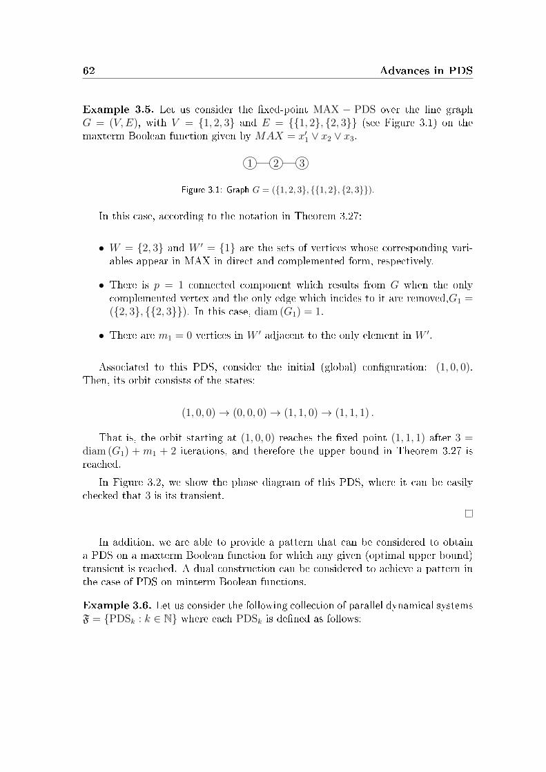
62 Advances in PDS

Example 3.5. Let us consider the xed-point MAX − PDS over the line graphG = (V,E), with V = 1, 2, 3 and E = 1, 2, 2, 3 (see Figure 3.1) on themaxterm Boolean function given by MAX = x′1 ∨ x2 ∨ x3.

1 2 3

Figure 3.1: Graph G = (1, 2, 3, 1, 2, 2, 3).

In this case, according to the notation in Theorem 3.27:

• W = 2, 3 and W ′ = 1 are the sets of vertices whose corresponding vari-ables appear in MAX in direct and complemented form, respectively.

• There is p = 1 connected component which results from G when the onlycomplemented vertex and the only edge which incides to it are removed,G1 =(2, 3, 2, 3). In this case, diam (G1) = 1.

• There are m1 = 0 vertices in W ′ adjacent to the only element in W ′.

Associated to this PDS, consider the initial (global) conguration: (1, 0, 0).Then, its orbit consists of the states:

(1, 0, 0)→ (0, 0, 0)→ (1, 1, 0)→ (1, 1, 1) .

That is, the orbit starting at (1, 0, 0) reaches the xed point (1, 1, 1) after 3 =diam (G1) + m1 + 2 iterations, and therefore the upper bound in Theorem 3.27 isreached.

In Figure 3.2, we show the phase diagram of this PDS, where it can be easilychecked that 3 is its transient.

In addition, we are able to provide a pattern that can be considered to obtaina PDS on a maxterm Boolean function for which any given (optimal upper bound)transient is reached. A dual construction can be considered to achieve a pattern inthe case of PDS on minterm Boolean functions.

Example 3.6. Let us consider the following collection of parallel dynamical systemsF = PDSk : k ∈ N where each PDSk is dened as follows:


100

000

110

111

011

101

010 001

Figure 3.2: Phase portrait of the system [(1, 2, 3, 1, 2, 2, 3) , x′1 ∨ x2 ∨ x3]− PDS.

1 2

Figure 3.3: Graph G1 = (1, 2, 1, 2).

• k = 1: PDS1 is dened as the parallel dynamical system over G1 = (V1, E1)with V1 = 1, 2, E1 = 1, 2 (see Figure 3.3),and whose evolution operator is the maxterm MAX1 = x′1 ∨ x2.In this case, according to the notation in Theorem 3.27:

W1 = 2 and W ′1 = 1 are the sets of vertices whose corresponding

variables appear in MAX1, respectively, in direct and complemented form.

There is p1 = 1 connected component which results from G1 when theonly complemented vertex and the only edge which are incident to it areremoved, G1,1 = (2, ∅). In this case, diam (G1,1) = 0.

There are m1,1 = 0 vertices in W ′1 adjacent to the only element in W ′

1.

• k = 2: PDS2 is dened as the parallel dynamical system over G2 = (V2, E2)with V2 = 1, 2, 3, 4, E2 = 1, 2, 3, 4, 1, 3 (see Figure 3.4),

1 2

3 4

Figure 3.4: Graph G2 = (1, 2, 3, 4, 1, 2, 3, 4, 1, 3).

64 Advances in PDS

and whose evolution operator is the maxterm MAX2 = x′1 ∨ x2 ∨ x′3 ∨ x4.According to the notation in Theorem 3.27:

W2 = 2, 4 and W ′2 = 1, 3 are the sets of vertices whose corresponding

variables appear in MAX2, respectively, in direct and complemented form.

There are p2 = 2 connected components which result from G2 when allthe vertices in W ′

2 and the edges which are incident to them are removed,G2,1 = (2, ∅) and G2,2 = (4, ∅). In this case, diam (G2,i) = 0 fori = 1, 2.

For all i ∈ W ′2, m2,i = card (AG2 (i) ∩W ′

2) = 1.

• k ≥ 3: PDSk is recursively dened as the parallel dynamical system overGk = (Vk, Ek) with Vk = Vk−1 ∪ 2k − 1, 2k, Ek = Ek−1 ∪ 2k − 1, 2k ∪i, 2k−1 : i ∈ W ′

k−2 and whose evolution operator is the maxterm MAXk =MAXk−1 ∨ x′2k−1 ∨ x2k. For example, some particular cases are:

For k = 3, see Figure 3.5,

1 2

3 4

5 6

Figure 3.5: Graph G3 = (V3, E3) = (1, 2, 3, 4, 5, 6, 1, 2, 3, 4, 1, 3, 5, 6, 1, 5).

MAX3 = x′1 ∨ x2 ∨ x′3 ∨ x4 ∨ x′5 ∨ x6.

For k = 4, see Figure 3.6,

1 2

3 4

5 6

78

Figure 3.6: Graph G4 = (V4, E4) = (1, . . . , 8, E3 ∪ 7, 8, 1, 7, 3, 7).

MAX4 = x′1 ∨ x2 ∨ x′3 ∨ x4 ∨ x′5 ∨ x6 ∨ x′7 ∨ x8.


And for k = 5, see Figure 3.7,

1 2

3 4

5 6

78

910

Figure 3.7: Graph G5 = (1, . . . , 10, E4 ∪ i, 9 : i ∈ 1, 3, 5, 10).

MAX5 = x′1 ∨ x2 ∨ x′3 ∨ x4 ∨ x′5 ∨ x6 ∨ x′7 ∨ x8 ∨ x′9 ∨ x10.

According to the notation in Theorem 3.27:

Wk = Wk−1 ∪ 2k and W ′k = W ′

k−1 ∪ 2k − 1 are the sets of verticeswhose corresponding variables appear in MAXk, respectively, in directand complemented form.

There are pk = k connected components which result from Gk when allthe vertices in W ′

k and the edges which are incident to them are removed,Gk,i = (2i, ∅) for i = 1, . . . , k. In this case, diam (Gk,i) = 0 for i =1, . . . , k.

Finally, mk,i = mk−1,i + 1 for each i ∈ W ′k−2, mk,2(k−1)−1 = mk−1,2(k−1)−1

and mk,2k−1 = k − 2.

Associated to these parallel dynamical systems, let us consider the initial statevalues of the variables:

• x01 =(x01,1, x

01,2

)= (1, 0).

• x0k =(x0k,1, . . . , x

0k,2k

)for k ≥ 2, with x0k,i = 1, if i ∈ W ′

k−1, and x0k,i = 0 inother case. For example, some particular cases:

x02 = (1, 0, 0, 0).

x03 = (1, 0, 1, 0, 0, 0).

x04 = (1, 0, 1, 0, 1, 0, 0, 0).

x05 = (1, 0, 1, 0, 1, 0, 1, 0, 0, 0).

Conditions above ensure, for all k ∈ N:

66 Advances in PDS

• mk,2k−1 ≤ k − 1 (initialization condition).

• mk+1,i ≤ mk,i + 1 for all i ∈ W ′k (propagation condition).

which implies that mk,i ≤ k − 1 for all i ∈ W ′k.

On the other hand,

• m1,1 = 0.

• mk+1,1 = mk,1 + 1.

Therefore, mk,1 = k − 1 and then, maxi∈W ′kmk,i = mk,1 = k − 1.

Now, let us see that the valoration x0k in PDSk reaches a xed point in, exactly,k + 1 iterations, value of the upper bound in Theorem 3.27 for this PDS. In fact,note that:

• x01 reaches a xed point in PDS1 after 2 iterations.

• x0k+1 reaches a xed point in PDSk+1 after one iteration more than x0k in PDSk,for all k ∈ N.

The simplest case (k = 1) is direct, since the evolution of x01 in PDS1 is:

(1, 0)→ (0, 0)→ (1, 1) .

Regarding the general case, it follows directly by observing that:

• x1k+1,2(k+1)−1 = x1k+1,2(k+1) = 1, and they continue activated onwards.

• x1k+1,i = x0k,i for all i ∈ Vk, and the restriction of PDSk+1 to Gk evolves asPDSk onwards.

When the component maxk∈1,...,pdiam (Gk) in Theorem 3.27 is greater than 0,the upper bound can be also reached. To see that, let us take the parallel dynamicalsystem PDSk and refurbish it as follows:

• We join a line graph of length l adjacent to vertex 2 in Gk. Thus, diam (Gk,1) =l.


• The new evolution operator is such that its restriction to Gk is MAXk and itsrestriction to the added line graph is the maxterm OR.

Then, if we x the initial state values as above for the vertices in Gk and as 0for the vertices in the added line graph, the system reaches a xed point (the onewith all the vertices activated) in l + k + 1 iterations.

Remark 3.10. Observe that the upper bound for a xed-point PDS on the simplestmaxterm OR (resp. on the simplest minterm AND), which presents only xed points,is given by the diameter of the dependency graph (see [28]). This previous resultis not valid for general maxterm and minterm Boolean functions, as can be seen inExample 3.5 where diam (G) = 2 < 3, being 3 the transient of the system. Thisreveals the relevance of our extended result, given by Theorems 3.27 and 3.28, dueto the breakdown found in the upper bound of the transient for general PDS.

Transient to 2-periodic orbits in PDS

By Theorems 3.3, 3.5 and Corollary 3.5 of Subsection 3.1.2, we know that aMAX − PDS only presents 2-periodic orbits if, and only if, there exists a comple-mented vertex which is not adjacent to a direct vertex. In [28], it is shown that thetransient for PDS on NAND or NOR Boolean functions is 1. Here, we extend theseresults to the case of PDS on a general maxterm or minterm Boolean function.

Lemma 3.2. Let [G,MAX]−PDS be a parallel dynamical system over a dependencygraph G = (V,E) associated with the maxterm MAX, where the structure of G onlyallows 2-periodic orbits. Then, a vertex i ∈ W ′β

D takes permanent state value 1 at amaximum of 2si + 3 iterations, being si = card (AG (i) ∩W ′

D).

Proof. Consider a vertex i ∈ W ′βD . As in the proof of Lemma 3.1, we can have

only one of the following two possibilities:

• ∀t ≥ 0, xti = 1, i.e., i takes permanenet state value 1 after 0 iterations. Since0 < 3 ≤ 3 + 2si, the result is proved in this case.

• ∃T ≥ 0 such that xTi = 0, being the iteration T the rst time that the variablexi takes the value 0. In this situation, after the next iteration T + 1, we havexT+1i = 1 and xT+1

j = 1 ∀j ∈ AG (i) ∩W 6= ∅.Due to that, any j ∈ AG (i) ∩W 6= ∅ makes i take permanent state value 1from this iteration on.

68 Advances in PDS

In particular, if T ≤ 2, then i takes permanent state value 1 after, at most, 3iterations. Since 3 ≤ 3 + 2si, the result is proved also in this case.

Finally, suppose that T > 2. At this point, it must be ∀t < T , xti = 1 andxtj = 0 ∀j ∈ AG (i) ∩W .

But, in this situation, to make i have state value 1 after every iteration t,1 ≤ t < T , ∃k ∈ AG (i) ∩W ′ such that xt−1k = 0, what provides that xti = 1.Now, we have also two possibilities:

If k ∈ W ′D, after the iteration t, x

tk = 1 and xtj = 1 ∀j ∈ AG (k) ∩W .

Due to that, any j ∈ AG (k)∩W 6= ∅ makes k take permanent state value1 from this iteration on. That is, the vertex k does not inuence the statevalue of the vertex i anymore.

If k ∈ W ′C , after the iteration t, x

tk = 1 and xtj = 1 ∀j ∈ AG (k) ⊆ W ′.

Consequently, xt+1k = 0 = xt−1k , repeating this alternation of state values

after every two iterations. In particular, observe that, in such a case, thevertex k does not inuence the state of the vertex i for the intermediateiteration t+ 1.

In view of this, once a vertex k ∈ AG (i) ∩W ′D provides the state value 1 for

the vertex i, it cannot provide it anymore. On the other hand, once a vertexk ∈ AG (i) ∩W ′

C provides state value 1 for the vertex i after the iteration t,in the next iteration t + 1, another vertex l ∈ AG (i) ∩W ′ with state value 0is needed in order to keep it. That is, in the following iteration, without anyother vertex in AG (i) ∩W ′

D with state value equals 0, the state value of xibecomes 0, or 1 denitively if there exists l ∈ AG (i) ∩W ′

C such that xtl = 0while xt−1k = 0.

Therefore, the maximum number of iterations that xi can maintain its valueequal to 1, before changing to 0 for the rst time, can be obtained intercalatingthe inuences of vertices of both sets AG (i) ∩W ′

D and AG (i) ∩W ′C , that is,

vertices with state values equal to 0.

In particular if si = card (AG (i) ∩W ′D) = 0, and we assume (without loos of

generality) that x0i = 1.

If every vertex in AG (i) ∩W ′C = AG (i) ∩W ′ has state value equals 1,

then x1i = 0, being 1 + 1 ≤ 3 + 2 · 0. If there is a vertex k ∈ AG (i)∩W ′

C such that x0k = 0, then, after the rstiteration, we can have:


The state values of the rest of the vertices l ∈ AG (i)∩W ′C become 1

and, consequently, x2i = 0, being 2 + 1 ≤ 3 + 2 · 0. There exists a vertex l ∈ AG (i) ∩ W ′

C dierent from k, such thatx1l = 0, what means that x1i = x2i = 1 and this state does not changeanymore.

For the general case si > 0, observe that, at most, T − 1 ≤ 2si + 1 and,therefore, after T + 1 ≤ 2si + 3 iterations the vertex i has permanent statevalue 1.

Theorem 3.29 (Transient in 2-Periodic MAX − PDS). Let [G,MAX] − PDS be aparallel dynamical system over a dependency graph G = (V,E) associated with themaxterm MAX, where the structure of G only allows 2-periodic orbits. Then, everystate of the system reaches a 2-periodic orbit after a maximum of

max

max

k∈1,...,pdiam (Gk), 1

+ max

maxi∈W ′αD

mi + 2, maxi∈W ′βD

2si + 3

iterations, being mi = card (AG (i) ∩W ′D), ∀i ∈ W ′α

D and si = card (AG (i) ∩W ′D),

∀i ∈ W ′βD .

Proof. In this case, as said above, W ′C 6= ∅.

Firstly, if W ′D = ∅, then p = 0, MAX = NAND and the system reaches a 2-

periodic orbit, at most, after 1 iteration (see [28]). It ts with the expression of theupper bound for this case.

Let us see now the general case when W ′D 6= ∅, which also implies p > 0:

Consider i ∈ W ′D. If i ∈ W ′α

D , it satises the hypotheses of Lemma 3.1, beingmi = card (AG (i) ∩W ′). Thus, at a maximum of mi + 2 iterations, xi will havepermanent state value 1. On the other hand, if i ∈ W ′β

D , it satises the hypothesesof Lemma 3.2. Thus, at a maximum of 2si + 3 iterations, xi will have permanentstate value 1.

Taking this into account, in maxmaxi∈W ′αD mi + 2,maxi∈W ′βD2si + 3 itera-

tions, for all i ∈ W ′D, xi reaches a permanent state value 1. It must be noted that

this calculation is also valid even if W ′αD = ∅ or W ′β

D = ∅, because of the value 0considered by default when a max expression is taken over an empty set.

70 Advances in PDS

After that, for the future evolution of the system, the vertices belonging to W ′D

do not change their state value, and the study of the evolution of the system can bereduced to analyze what happens in the restriction of G to W ∪W ′

C . Given that avertex in W is not adjacent to a vertex in W ′

C , there cannot be interference betweenthese sets and the behavior of the entire system can be obtained from the study ofthe evolution in each connected subgraph G1, . . . , Gp and the connected componentswhich result from G when we remove all the vertices inW ∪W ′

D and the edges whichare incident to them, C1, . . . , Cq.

Regarding G1, . . . , Gp, since they only have vertices associated with direct vari-ables, we know that the restriction of the PDS to each Gk performs as an OR−PDSwhich converges to a xed point in, at most, diam (Gk) iterations (see [28]). Onthe other hand, the restriction of the PDS to each component Ck performs as aNAND − PDS, and so a 2-periodic orbit is reached in, at most, 1 iteration (see[28]). In view of this, after maxmaxk∈1,...,pdiam (Gk), 1 iterations (after themaxmaxi∈W ′αD mi + 2,maxi∈W ′βD

2si + 3 iterations needed for ensuring that thestate values of the vertices in W ′

D are xed) all the vertices in W will reach a statevalue that they will permanently preserve, and all the vertices in W ′

C will repeattheir state value every 2 iterations, alternating values 0 and 1 or preserving statevalue 1 onwards.


max maxk∈1,...,p

diam (Gk), 1+ maxmaxi∈W ′αD


2si + 3

iterations, any (initial) state reaches a 2-periodic orbit.


Theorem 3.30 (Transient in 2-Periodic MIN − PDS). Let [G,MIN] − PDS be aparallel dynamical system over a dependency graph G = (V,E) associated with theminterm MIN, where the structure of G only allows 2-periodic orbits. Then, everystate of the system reaches a 2-periodic orbit after a maximum of

max

max

k∈1,...,pdiam (Gk), 1

+ max

maxi∈W ′αD


2si + 3

iterations, being mi = card (AG (i) ∩W ′

D), ∀i ∈ W ′αD and si = card (AG (i) ∩W ′

D),∀i ∈ W ′β

D .

This new upper bound obtained in Theorem 3.29 is also the best possible onefor this kind of PDS, since it is reachable, as we show in the example below. A


dual example in the case of a minterm MIN as evolution operator can be similarlyconstructed, where the upper bound obtained in Theorem 3.30 is reached.

Example 3.7. Let us consider the PDS over the line graph G = (V,E), withV = 1, 2, 3, 4 and E = 1, 2, 2, 3, 1, 4 (see Figure 3.8) on the maxtermBoolean function given by MAX = x′1 ∨ x2 ∨ x3 ∨ x′4.

1 2 34

Figure 3.8: Graph G = (1, 2, 3, 4, 1, 2, 2, 3, 1, 4).


• W = 2, 3 and W ′ = 1, 4 are the sets of vertices whose corresponding vari-ables appear in MAX in direct and complemented form, respectively. More-over, W ′

D = 1 and W ′C = 4. Finally, W ′α

D = ∅ and W ′βD = 1.

• There is p = 1 connected component which results from G when all the ver-tices in W ′ and the edges which are incident to them are removed, G1 =(2, 3, 2, 3). In this case, diam (G1) = 1.

• There are s1 = 0 vertices in W ′D adjacent to the only element in W ′

D.

The upper bound of Theorem 3.29 for this PDS is 4 iterations. If we consider theinitial conguration x0 = (1, 0, 0, 0), the evolution of x0 until reaching the periodicorbit is:

(1, 0, 0, 0)→ (1, 0, 0, 1)→ (0, 0, 0, 0)→ (1, 1, 0, 1)→ (1, 1, 1, 0) .

In Figure 3.9, we show the phase diagram of this PDS, where it can be easilychecked that 4 is its transient.

As in the case of xed-point PDS, additionally, we are able to provide a patternthat can be considered to obtain a 2-Periodic MAX − PDS for which any given(optimal upper bound) transient is reached. A dual construction can be consideredto achieve a pattern in the case of PDS on minterm Boolean functions.

Example 3.8. Let us consider the following collection of parallel dynamical systemsF2 = PDSk : k ∈ N, where each PDSk is dened as follows:

72 Advances in PDS

1000

1001

0000

1101

1110

1111

0110

1011

1010

0010

0101

0011

0001

0100

1100

0111

Figure 3.9: Phase portrait of the system [(1, 2, 3, 4, 1, 2, 2, 3, 1, 4) , x′1 ∨ x2 ∨ x3 ∨ x′

4] −PDS.

• k = 1: PDS1 is dened as the parallel dynamical system over G1 =(V 1, E1

)with V 1 = 1, 2, 3, 4, E1 = 1, 2, 2, 3, 1, 4 (the same as in Example3.7, which is exposed in Figure 3.8).

The evolution operator is the maxterm MAX1 = x′1 ∨ x2 ∨ x3 ∨ x′4.In this case, the relevant elements in Theorem 3.29 related to this PDS are:

W 1 = 2, 3 andW ′1 = 1, 4 are the sets of vertices whose corresponding

variables appear in MAX1, respectively, in direct and complemented form.Inside W

′1, W

′D,1 = 1 and W ′

C,1 = 4. Finally, W ′αD,1 = ∅ and W ′β

D,1 =1. There is p1 = 1 connected component which results from G1 when all thevertices in W

′1 and the edges which are incident to them are removed,

G1,1 = (2, 3, 2, 3). In this case, diam(G1,1

)= 1.

There are s1,1 = 0 vertices in W′D,1 adjacent to the only element in W

′βD,1.

• k ≥ 2: PDSk is dened from the elements of F shown in Example 3.6. Toavoid duplication in the name of the vertices of each PDSt ∈ F, we will denoteas it to the vertex i in PDSt:


This way, PDSk is recursively dened as the parallel dynamical system overGk =

(V k, Ek

)with V k = V k−1∪V2k−3, Ek = Ek−1∪E2k−3∪1, 12k−3 and

whose evolution operator is the maxterm MAXk = MAXk−1 ∨MAX2k−3.

The relevant elements in Theorem 3.29 related to this PDS are:

W k = W k−1∪W2k−3 =(⋃k−1

t=1 W2t−1

)∪2, 3 andW ′

k = W′k−1∪W ′

2k−3 =(⋃k−1t=1 W

′2t−1

)∪ 1, 4 are the sets of vertices whose corresponding vari-

ables appear in MAXk, respectively, in direct and complemented form.Also, inside W

′k:

W ′D,k = W

′D,k−1 ∪W ′

2k−3 = W′k \ 4.

W ′C,k = W

′C,k−1=4.

Finally, inside W′D,k, W

′αD,k = W

′αD,k−1 ∪ W ′

2k−3 = W′D,k \ 1 and

W′βD,k = W

′βD,k−1 = 1.

There are pk =(∑k−1

t=1 2t− 1)

+ 1 = (k − 1)2 + 1 connected components

which result from Gk when all the vertices in W′k and the edges which

are incident to them are removed, those ones of PDS1, PDS3,. . . ,PDS2k−3and G1,1 dened below. In this case, all these connected components havediameter 0 except G1,1, with diam

(G1,1

)= 1.

Finally, for each i ∈ W′D,k, mk,i if i ∈ W

′αD,k or sk,i if i ∈ W

′βD,k can be

obtained as:

If i ∈ W ′2t−1 \ 12t−1 for t ≤ k − 1, mk,i = m2t−1,i ≤ (2t− 1) − 1 ≤

2k − 4. If i = 12t−1 for t ≤ k − 1, because of the new adjacency 1, 12t−1 ∈Ek, mk,i = m2t−1,i + 1 = (2t− 1)− 1 + 1 ≤ 2k − 3. sk,1 = k − 1.

Therefore, the upper bound in Theorem 3.29 for each PDSk ∈ F2 is 1 + 2(k −1) + 3 = 2k + 2 iterations.

Associated to these parallel dynamical systems, let us consider the initial statevalues of the variables:

• x01 =(x01,1, x

01,2, x

01,3, x

01,4

)= (1, 0, 0, 0).

74 Advances in PDS

• x0k =(x0k,i)i∈V k

for k ≥ 2, with x0k,i = x01,i for i = 1, 2, 3, 4 and x0k,i = x02t−1,i asdened in Example 3.6 if i ∈ V2t−1.

Let us see that the valoration x0k in PDSk reaches a 2-periodic orbit in, exactly,2k + 2 iterations. In fact, note that:

• x01 reaches a 2-periodic orbit in PDS1 after 4 iterations.

• x0k+1 reaches a 2-periodic orbit in PDSk+1 after two iterations more than x0k inPDSk, for all k ∈ N.

The simplest case (k = 1) is direct, since the evolution of x01 in PDS1 is:

(1, 0, 0, 0)→ (1, 0, 0, 1)→ (0, 0, 0, 0)→ (1, 1, 0, 1)→ (1, 1, 1, 0)↔ (1, 1, 1, 1) .

Regarding the general case, it follows directly by observing that:

x0k+1,1 = 1 and, since x0k+1,4 = 0, then x1k+1,1 = 1. Furthermore, the evolution ofthe whole system PDSk+1 during the rst two iterations is the same as the restrictionof PDSk+1 to each connected component which results from Gk+1 when the vertex1 and the edges which are incident to it are removed. Thus:

• x2k+1,2 = 0 = x0k,2.

• x2k+1,3 = 0 = x0k,3.

• x2k+1,4 = 0 = x0k,4.

• x1k+1,11= 0, so x2k+1,1 = 1 = x0k,1.

• x2k+1,i = 1 for all i ∈ V1, and they continue activated onwards.

• If V2t−1 = 12t−1, . . . , 2 (2t− 1)2t−1 and V2t−3 = 12t−3, . . . , 2 (2t− 3)2t−3,with t ∈ 2, . . . , k, then:

x2k+1,j2t−1= 1 for all j ≥ 2 (2t− 1) − 3, and they continue activated

onwards.

x2k+1,j2t−1= x0k,j2t−3

for j ≤ 2 (2t− 1)− 4 = 2 (2t− 3), and the restrictionof PDSk+1 to these G2t−3 evolves as PDSk onwards.


Remark 3.11. Observe that the upper bound for a 2-Periodic PDS on the simplestmaxterm NAND (resp. on the simplest minterm NOR), which presents only periodicorbits of period 2, is 1 (see [28]). This previous result is not valid for general maxtermand minterm Boolean functions, as can be seen in Example 3.7 where the transientof the system is 4. This reveals the relevance of our extended results, given inTheorems 3.29 and 3.30, due to the breakdown found in the upper bound of thetransient for general PDS.

76 Advances in PDS

Chapter 4

Advances in Sequential Dynamical

Systems

In this chapter, we perform a complete analysis of the dynamics in sequentialdynamical systems on maxterm and minterm Boolean functions over undirecteddependency graphs. Following a similar scheme as in the parallel case, the studyis divided into two sections according to the methodology of research: dynamics ofperiodic orbits and dynamics of non-periodic orbits.


In this section, the dynamics of periodic orbits are analyzed, identifying whichof them can exist and coexist, and obtaining an upper bound for their number. Inparticular, as in the parallel case, we are able to give a Fixed-Point Theorem and aPeriodic-Orbit Theorem, so characterizing the uniqueness of them.

4.1.1 Existence of periodic orbits

In Theorem 3.1 (resp. Theorem 3.2) of Subsection 3.1.1, the orbital structureof PDS with general maxterm (resp. minterm) functions as evolution operators has

78 Advances in SDS

been analyzed, proving that the only periodic orbits of such systems are xed pointsand periodic orbits of period 2.

In contrast to these results for PDS, in the case of SDS with general maxterm(resp. minterm) functions as evolution operators, we will see that they can presentorbits of whichever period.

Theorem 4.1 (Periodic structure of MAX − SDS). Let [G,MAX, π] − SDS be asequential dynamical system over a dependency graph G = (V,E) associated withthe maxterm MAX. Then, it can present periodic orbits of any period.

Proof. Given n ∈ N, n ≥ 2, we will give a pattern to construct an SDS with anorbit of period n− 1. Let us take V = 1, . . . , n− 1, n and consider the followingadjacency structure among the vertices:

• Each i ∈ 1, . . . , n − 1 is adjacent to all the vertices in 1, . . . , n − 1 \ i.In other words, we take the complete graph Kn−1 of n− 1 vertices.

• The vertex n is adjacent to the vertex n− 1.

As permutation on V we take π = id, the identity permutation.

Finally, we choose the updating operator

MAX = x′1 ∨ · · · ∨ x′n−1 ∨ xn.

Let us write xki to indicate the state value of the entity i after k iterations ofthe evolution operator MAX. Then, let us consider the initial value for the variablesx0i = 1 for all i ∈ V . It is a straightforward computation to check that the systemevolves in the following way:

• After k iterations, 1 ≤ k ≤ n− 2: xkk = 0, xki = 1 for all i ∈ V \ k.

• After n − 1 iterations, all the state values coincide with the initial ones, i.e.,xn−1i = x0i = 1 for all i ∈ V .

Namely, the SDS so constructed presents a periodic orbit of period n− 1.

To illustrate the designed patterns, in Figure 4.1 the cases for n = 2, n = 3,n = 4 and n = 5 can be seen.


12 123

1

234

1 2

345

Figure 4.1: Patterns for n = 2, n = 3, n = 4 and n = 5.

Remark 4.1. It is direct to perform a similar argument as in the proof of Theorem3.1 of Subsection 3.1.1, but in the context of SDS, to achieve analogous informationto Remark 3.1 about asymptotic behavior of the entities in SDS, essential in thestudy of these systems throughout this thesis:

• Each i ∈ W xes its state value after a certain number of iterations.

• When a periodic orbit is reached, each i ∈ W ′D has state value 1.

• The period comes from the evolution of the vertices belonging to W ′C .

Dually we have the following theorem.

Theorem 4.2 (Periodic structure of MIN − SDS). Let [G,MIN, π] − SDS be asequential dynamical system over a dependency graph G = (V,E) associated withthe minterm MIN. Then, it can present periodic orbits of any period.

It is worth to analyze the particular relevant cases when the evolution operatoris the maxterm OR or NAND (resp. minterm AND or NOR). Recall that the onlyperiodic orbits of PDS over undirected dependency graphs with OR (resp. AND) asupdating operator are xed points and with NAND (resp. NOR), 2-periodic orbits(see Corollaries 3.1, 3.2, 3.3 and 3.4 of Subsection 3.1.1). In this case, when theupdating of the state values is asynchronous and the evolution operator is given by

80 Advances in SDS

OR (resp. AND), the only periodic orbits of the system are xed points, as in PDS.In contrast, when the evolution operator is NAND (resp. NOR), the correspondingSDS could present periodic orbits of any period greater than or equal to 2.

To see that, let us turn to the following well-known lemma (see [35, 91]).

Lemma 4.1. Let [G,F, π]−SDS be a sequential dynamical system over a dependencygraph G = (V,E) associated with the maxterm or minterm F . Then, the systems[G,F, π]− SDS and [G,F ]− PDS have the same xed points.

Firstly, in the case of OR as evolution operator, we have the following result(which is already proved in [28], although an alternative proof is shown here).

Theorem 4.3. Let [G,OR, π] − SDS be a sequential dynamical system over a de-pendency graph G = (V,E) associated with the maxterm OR. Then, all the periodicorbits of this system are xed points. In fact, there are exactly two xed points,namely, I and O.

Proof. By Lemma 4.1 and Corollary 3.1 in Subsection 3.1.1, I and O are the onlyxed points of this SDS.

It only remains to show that there cannot be periodic orbits of greater period:since all the entities belong to W , we can have only one of the following two possi-bilities for each i ∈ V :

• ∀t ≥ 0, xti = 0. In this case, the state value 0 is permanent for this entity fromthe initial conguration.

• ∃T ≥ 0 such that xTi = 1, being the iteration T the rst time that the variablexi takes the value 1. In this situation, the state value 1 is permanent from thisiteration on.

Thus, after a certain number of iterations, all the entities reach a xed valuethat they preserve onwards.

In the case of NAND as evolution operator, we have the following result.

Theorem 4.4. Let [G,NAND, π] − SDS be a sequential dynamical system over adependency graph G = (V,E) associated with the maxterm NAND. Then, this systemcan present periodic orbits of any period, except xed points.


Proof. First, notice that such an SDS cannot present xed points. In fact, we knowthat PDS with NAND as evolution operator cannot present xed points. Then, thisrst assertion follows from Lemma 4.1.

Given n ∈ N, we will provide a pattern to construct an SDS with NAND asevolution operator which has an orbit of period n+ 1.

Let us take V = 1, . . . , n. Assume that the adjacency structure among thevertices is the one of a complete graph Kn of n vertices.

As permutation on V , we take π = id, the identity permutation.

Let us consider the initial state values x0i = 1 for all i ∈ V . Then, the systemevolves as follows:

• After k iterations, 1 ≤ k ≤ n: xkk = 0, xki = 1 for all i ∈ V \ k.

• After n + 1 iterations, all the state values coincide with the initial ones, i.e.,xn+1i = x0i = 1 for all i ∈ V .

Namely, the SDS so constructed presents a periodic orbit of period n+ 1.

Dually, in the case of AND and NOR, we have the following results (the rst oneof them is already proved in [28]).

Theorem 4.5. Let [G,AND, π] − SDS be a sequential dynamical system over adependency graph G = (V,E) associated with the minterm AND. Then, all theperiodic orbits of this system are xed points. In fact, there are exactly two xedpoints, namely, O and I.

Theorem 4.6. Let [G,NOR, π] − SDS be a sequential dynamical system over adependency graph G = (V,E) associated with the minterm NOR. Then, this systemcan present periodic orbits of any period, except xed points.

4.1.2 Coexistence of periodic orbits

In Corollaries 3.5 and 3.6 of Subsection 3.1.2, the orbital structure of PDS withgeneral maxterm (resp. minterm) functions as evolution operators has been ana-lyzed, proving that the coexistence of periodic orbits with dierent periods is notpossible.

In contrast to these results for PDS, in the case of SDS with general maxterm(resp. minterm) functions as evolution operators, we will see that periodic orbits

82 Advances in SDS

with dierent periods greater than or equal to 2 can coexist in an SDS. Nevertheless,when an SDS has xed points, no other periods can appear.

It is well known that, in a PDS over a dependency graph G = (V,E) associatedwith the maxterm MAX (resp. minterm MIN), if there is a xed point, then thereare no periodic orbits of other periods (see Theorems 3.3, 3.5 and Corollary 3.5 inSubsection 3.1.2). This situation remains true for SDS, as we see next. That is,for both PDS and SDS, the existence of xed points excludes the presence of otherperiodic orbits.

Theorem 4.7. Let [G,MAX]−SDS be a sequential dynamical system over a depen-dency graph G = (V,E) associated with the maxterm MAX. Then, all the periodicorbits of this system are xed points if, and only if, W ′

C = ∅.

Proof. In the case W ′ = ∅, the system has only two xed points: I and O (seeTheorem 4.3 of Subsection 4.1.1 and [28]). Let us analyze now the general case whenW ′ 6= ∅:

First, assume that all the periodic orbits of this system are xed points and letus see that W ′

C = ∅.

Take x = (x1, . . . , xn) a xed point, where xi represents the (xed) value of thevertex i ∈ V . Note that, for all i ∈ W ′, it must be xi = 1. Otherwise (i.e., if xi = 0),it would change to 1 after the following iteration.

Suppose that there exists i ∈ W ′ such that W ∩ AG (i) = ∅. In such a case,AG (i) ⊆ W ′ and so, for every j ∈ AG (i), it is xj = xi = 1. Since we are assumingthat x is a xed point, independently of the order in which the state values areupdated (i.e. independently of π), these are the state values of the vertices j ∈ AG (i)when the state value of i is updated. Then, the state value of i would change to 0in the following iteration, which is a contradiction.

To prove the converse implication, let us suppose that for all i ∈ W ′,W∩AG (i) 6=∅. Let us consider an arbitrary initial value for the variables (x01, . . . , x

0n). Since the

dependency graph is nite (and so is the state space), note that after a certainnumber of iterations, let us say r ∈ N, the states of all the vertices belonging to Wbecome xed (see Remark 4.1 in Subsection 4.1.1). Let us take i ∈ W ′ and let usprove that xr+1

i = 1. In fact, let us suppose that xr+1i = 0 and take j ∈ W ∩AG (i).

Then, it would be xr+2j = 1 = xrj (since we are assuming that the state value of j

is xed from the iteration r). Then, since xrj = 1, it must be xr+1i = 1, which is a

contradiction. Thus, xr+1i = 1 for all i ∈ W ′ and these state values do not change.


Therefore, all the variables of the system become xed after r+ 1 iterations andthe proof nishes.

Theorem 4.8. Let [G,MAX]−SDS be a sequential dynamical system over a depen-dency graph G = (V,E) associated with the maxterm MAX. Then, all the periodicorbits of this system have period greater than 1 if, and only if, W ′

C 6= ∅.

Proof. First, assume that all the periodic orbits of this system have period greaterthan 1. If the theses were not true, that is, if for all i ∈ W ′ it is W ∩ AG (i) 6= ∅,then from Theorem 4.7 we have that all the periodic orbits of this system are xedpoints, which is a contradiction.

Conversely, let us suppose that there exists i ∈ W ′ such that W ∩AG (i) = ∅. Ifthere is a xed point, reasoning as in the proof of Theorem 4.7, we have W ′

C = ∅,which is a contradiction. Hence, all the periodic orbits of the system must haveperiod greater than 1.

Corollary 4.1 (Coexistence of periods in MAX − SDS). Let [G,MAX] − SDS bea sequential dynamical system over a dependency graph G = (V,E) associated withthe maxterm MAX. Then, (eventually) xed points and (eventually) periodic orbitsof other periods m ≥ 2 cannot coexist.

Proof. It is a direct consequence of Theorems 4.7 and 4.8.

Remark 4.2. It is important to note that all, the impossibility of coexistence of xedpoints and periodic orbits of other periods m ≥ 2, the condition which implies thatall the periodic orbits of an SDS are xed points and the complementary conditionwhich implied that all the periodic orbits of an SDS have period greater than orequal to 2, are equal to the respective ones in the case of a PDS (see Theorems 3.3,3.5 and Corollary 3.5 in Subsection 3.1.2).


Theorem 4.9. Let [G,MIN]− SDS be a sequential dynamical system over a depen-dency graph G = (V,E) associated with the minterm MIN. Then, all the periodicorbits of this system are xed points if, and only if, W ′

C = ∅.

Theorem 4.10. Let [G,MIN] − SDS be a sequential dynamical system over a de-pendency graph G = (V,E) associated with the minterm MIN. Then, all the periodicorbits of this system have period greater than 1 if, and only if, W ′

C 6= ∅.

84 Advances in SDS

Corollary 4.2 (Coexistence of periods in MIN − SDS). Let [G,MIN] − SDS be asequential dynamical system over a dependency graph G = (V,E) associated withthe minterm MIN. Then, (eventually) xed points and (eventually) periodic orbitsof other periods m ≥ 2 cannot coexist.

In the light of Theorems 4.1 and 4.2 in Subsection 4.1.1, it naturally arises theproblem of determining the possible coexistence of periodic orbits of dierent periodsfor SDS with maxterm or minterm Boolean functions as updating operators. In thissense, in the following theorems, we show that periodic orbits of whichever periodsgreater than or equal to 2 can coexist in such discrete dynamical systems.

Theorem 4.11. Given n1, . . . , nr ⊂ N with ni ≥ 2 for every i = 1, . . . , r, r ≥ 2,there exists an SDS with a maxterm as evolution operator which presents periodicorbits of periods n1, . . . , nr simultaneously.

Proof. Let us construct an SDS with orbits of periods n1, . . . , nr.

For each ni, let us take two complete graphs Kni−1 and Kni−1 of ni− 1 vertices.We will denote by vi,1, . . . , vi,ni−1 and vi,1, . . . , vi,ni−1 the vertices of Kni−1 andKni−1, respectively, for every i ∈ 1, . . . , r. Thus, the dependency graph has2 (n1 + · · ·+ nr − r) vertices.

Apart from the internal adjacencies in each complete graph Kni−1 and Kni−1,we will consider the following adjacency structure among the vertices:

• vi,j is adjacent to vl,m for all j, m and i 6= l. In other words, the vertices inKni−1 are adjacent to all the vertices in Knl−1 for i 6= l.

• vi,j is adjacent to vl,m for all j, m and i 6= l. In other words, the vertices inKni−1 are adjacent to all the vertices in Knl−1 for i 6= l.

• vi,j is adjacent to vl,m for all j, m and i 6= l. In other words, the verticesin Kni−1 are adjacent to all the vertices in Knl−1 for i 6= l (but they are notadjacent to the vertices in Kni−1).

As permutation on the set of vertices, we will consider:

π = v1,1| · · · |v1,n1−1|v1,1| · · · |v1,n1−1| · · · |vr,1| · · · |vr,nr−1|vr,1| · · · |vr,nr−1.

Namely, rst the state values of the vertices in Kn1−1 are updated, then the onesin Kn1−1, next the vertices in Kn2−1 followed by the ones in Kn2−1, and so on untilall the vertices are updated.


As evolution operator, we take MAX = NAND.

As initial state values for the variables, we consider that the vertex vi,1 is deac-tivated and the rest of vertices are activated.

This system evolves as follows:

• After k iterations, 1 ≤ k ≤ ni − 2, vi,k+1 and vi,k are deactivated and the restof vertices are activated.

• After ni − 1 iterations, vi,ni−1 is deactivated and the rest of vertices are acti-vated.

• After ni iterations, all the state values coincide with the initial ones.

Namely, the [G,MAX, π]−SDS so constructed presents a periodic orbit of periodni.

Thus, by considering the dierent r initial state values obtained by varying i in1, . . . , r, r periodic orbits with periods n1, . . . , nr result.

Let us illustrate this result with the following example to clarify the notation.

Example 4.1. The SDS proposed by Theorem 4.11 in which a 2-periodic orbit anda 3-periodic orbit coexist, is dened by

• G = (1, 2, 3, 4, 5, 6, 3, 4, 5, 6 ∪ i, j : 1 ≤ i ≤ 2, 3 ≤ j ≤ 6) (see Fig-ure 4.2),

• MAX = NAND,

• π = id, the identity permutation.

1

2

3

4

5

6

Figure 4.2: Graph G = (1, 2, 3, 4, 5, 6, 3, 4, 5, 6 ∪ i, j : 1 ≤ i ≤ 2, 3 ≤ j ≤ 6).

86 Advances in SDS

According to the notation in Theorem 4.11, 1 is the only vertex in K1, 2 is theonly vertex in K1, 3, 4 are the vertices in K2, and 5, 6 are the vertices in K2.

In this case, the 2-periodic orbit proposed by Theorem 4.11 can be seen in Figure4.3.

011111

101111

Figure 4.3: 2-periodic orbit of the system proposed by Theorem 4.11.

On the other hand, the 3-periodic orbit proposed by Theorem 4.11 can be seenin Figure 4.4.

110111

111001111110


Finally, we can state the dual result.

Theorem 4.12. Given n1, . . . , nr ⊂ N with ni ≥ 2 for every i = 1, . . . , r, r ≥ 2,there exists an SDS with a minterm as evolution operator which presents periodicorbits of periods n1, . . . , nr simultaneously.

4.1.3 Uniqueness of xed points

Our main objective in this subsection is to obtain a Fixed-Point Theorem forSDS. Observe that, although xed points and periodic orbits of greater period can-not coexist, there are SDS whose state spaces contain more than one xed point.Actually, there is a total resemblance regarding the xed points of SDS and PDSwith whichever maxterm or minterm Boolean function as evolution operator, as saidin Lemma 4.1 in Subsection 4.1.1.

In Theorem 3.7 (resp. Theorem 3.8) of Subsection 3.1.3, a Fixed-Point Theoremwas obtained for PDS on maxterm (resp. minterm) Boolean functions as evolutionoperators. Thus, as a direct consequence of this result for PDS, we have the followingtheorem in the context of SDS.


Theorem 4.13 (Fixed-Point Theorem for MAX−SDS). Let [G,MAX, π]−SDS bea sequential dynamical system over a dependency graph G = (V,E) associated withthe maxterm MAX. Assume that, W ′

C = ∅. Then, this SDS has a unique xed pointif, and only if, for every j, 1 ≤ j ≤ p, AG (Gj) ∩W ′

1 6= ∅. In this situation, theunique xed point is I, and all the orbits converge to this xed point.

Proof. It is a direct consequence of Lemma 4.1 in Subsection 4.1.1, Theorems 4.7,4.8 and Corollary 4.1 in Subsection 4.1.2 and Theorem 3.7 in Subsection 3.1.3.


Theorem 4.14 (Fixed-Point Theorem for MIN − SDS). Let [G,MIN, π] − SDS bea sequential dynamical system over a dependency graph G = (V,E) associated withthe minterm MIN. Assume that, W ′

C = ∅. Then, this SDS has a unique xed pointif, and only if, for every j, 1 ≤ j ≤ p, AG (Gj) ∩W ′

1 6= ∅. In this situation, theunique xed point is O, and all the orbits converge to this xed point.

4.1.4 Uniqueness of periodic orbits

By Theorems 4.7, 4.8, 4.9, 4.10 and Corollaries 4.1, 4.2 of Subsection 4.1.2, it iswell known that all the periodic orbits of an SDS have period greater than 1 if, andonly if, W ′

C 6= ∅. Our aim now is to characterize the uniqueness of periodic orbits ofperiod greater than 1 in a MAX− SDS. To achieve this objective, rst, we analyzethe particular case MAX = NAND.

In Proposition 3.1 of Subsection 3.1.4, it is established that, in the case of parallelupdate associated with a NAND Boolean operator, the periodic orbit (order equalto 2 in such a case) is unique if, and only if, the associated dependency graph iscomplete. In this case of sequential update, this pattern is broken, as we show below.

When a sequential update schedule with a maxterm NAND as evolution operatoris considered, as will be seen in Proposition 4.3 of Subsection 4.2.1, we have that theGOE points of the system are the congurations such that there are two adjacentvertices i, j ∈ V with xi = xj = 0. Furthermore, the rest of the congurationsbelong to periodic orbits.

As said above, in a NAND− SDS, the completeness of the dependency graph isnot a necessary condition for the uniqueness of a periodic orbit, breaking the patternfound for the parallel update, shown in Proposition 3.1 of Subsection 3.1.4. We cansee this break down in the following example.

Example 4.2. Let us consider the NAND− SDS dened by

88 Advances in SDS

• G = 1, 2, 3, 4, 1, 2, 2, 3, 3, 4, 4, 1 (see Figure 4.5),

• MAX = x′1 ∨ x′2 ∨ x′3 ∨ x′4,

• π = 1|2|3|4.

1 2

34

Figure 4.5: Graph 1, 2, 3, 4, 1, 2, 2, 3, 3, 4, 4, 1.

The congurations without adjacent complemented entities with state valuesequal to 0 are:

(1, 1, 1, 1) , (0, 1, 1, 1) , (1, 0, 1, 1) , (1, 1, 0, 1) , (1, 1, 1, 0) , (0, 1, 0, 1) , (1, 0, 1, 0) .

In Figure 4.6, it can be seen that all of them belong to the same periodic orbit.

1111 0101 1110 1011

110101111010

Figure 4.6: Unique periodic orbit of the [1, 2, 3, 4, 1, 2, 2, 3, 3, 4, 4, 1,NAND, id]−SDS.

The rest of the congurations are GOE states from which this unique periodicorbit is reached after 1 iteration.

Thus, we can enunciate the following uniqueness result for a periodic orbit in a[G,NAND, π]− SDS.

Lemma 4.2 (m-Periodic-Orbit Theorem for NAND−SDS). Let [G,NAND, π]−SDSbe a sequential dynamical system over a dependency graph G = (V,E) associated withthe maxterm NAND. Then, there is a uniquem-periodic orbit (m > 1) if, and only if,any conguration reaches the state I, being m the number of congurations withoutadjacent (complemented) vertices with state values equal to 0. In this situation, allthe orbits of the system converge to this m-periodic orbit.


Proof. From Theorem 4.4 in Subsection 4.1.1, this kind of SDS only presentsperiodic orbits of period greater than 1. On the other hand, as will be seen inProposition 4.3 of Subsection 4.2.1, the periodic points of the system are thosecongurations without adjacent (complemented) vertices with state values equal to0. In particular, the state I always belongs to a periodic orbit. Thus, the resultfollows from the fact that in an SDS all the congurations belong to or reach aperiodic orbit.

Dually, we have the following lemma.

Lemma 4.3 (m-Periodic-Orbit Theorem for NOR−SDS). Let [G,NOR, π]−SDS bea sequential dynamical system over a dependency graph G = (V,E) associated withthe minterm NOR. Then, there is a unique m-periodic orbit (m > 1) if, and only if,any conguration reaches the state O, being m the number of congurations withoutadjacent (complemented) vertices with state values equal to 1. In this situation, allthe orbits of the system converge to this m-periodic orbit.

Once these results have been established, we provide the following system toshow how they can determine the uniqueness of a periodic orbit in this kind of SDS:

Let us consider a [G,NAND, π]−SDS such that π = 1| . . . |n, the identity permu-tation, and take G the complete graph Kn. Then, the system has a unique periodicorbit because each conguration reaches the state I. In fact, if x ∈ 0, 1n and thereexists i ∈ V such that xi = 0, let j = maxk ∈ V : xk = 0. If j = n, after one itera-tion the conguration I is reached. Otherwise, after one iteration the congurationreached is the one with all the entities activated except j + 1. Similarly, in the nextiteration, the conguration reached is that one with all the entities activated exceptj + 2, and so on. Thus, after n− j + 1 iterations, the conguration I is reached.

As a consequence of Example 4.2 and this last comment, we can enunciate thefollowing corollaries.

Corollary 4.3. In NAND − SDS, the completeness of the dependency graph is asucient (but not necessary) condition for the existence of a unique periodic orbitin the system.

And now the dual result.

Corollary 4.4. In NOR − SDS, the completeness of the dependency graph is asucient (but not necessary) condition for the existence of a unique periodic orbitin the system.

90 Advances in SDS

Finally, once all the results above have been established for the particular casein which the maxterm is NAND (and their dual versions for the minterm NOR),now let us work with a general maxterm MAX as evolution operator.

According to what has been seen for the parallel update case, when a periodicorbit of period greater than 1 is reached after r0 iterations, the system performs asfollows:

• If i ∈ W , then xri = xr0i for all r ≥ r0. In other words, the direct vertices donot change their state (activated or deactivated) from the r0-th iteration on.Moreover, in each connected component Gj, 1 ≤ j ≤ p, either every variableassociated with the vertices in Gj has state value 1 or every variable has statevalue 0.

• If i ∈ W ′D (note that if MAX 6= NAND and W ′

C 6= ∅, then W ′D 6= ∅), it follows

that xri = 1 for all r ≥ r0. In fact, suppose that there exists i ∈ W ′D such that

(after the r0-th iteration) xi takes the value 0 in an innite number of futureupdates of the system, and assume (without loss of generality) that r0 ≥ 1 andxr0i = 0. Since i ∈ W ′

D, there exists a direct vertex j adjacent to i. Observethat it must be xr0+1

j = 1: if j updates before i, xr0i = 0 makes xr0+1j = 1;

while if j updates after i, it is already xr0j = 1 due to xr0i = 0. Then, beingxr0+1j = 1, we get that xri = 1 for all r > r0 + 1, which contradicts our initial

assumption.

• The restriction of the system to each connected component Cj performs as aNAND− SDS. The permutation which determines the updating order in thesystem restricted to Cj is the restriction of π to the vertices in Cj.

In view of this, it should be pointed out that, as commented in Chapter 2 aboutG∗, this graph is not, in general, connected. Thus, the system

[G∗,MAX|G∗ , π|G∗

]−

SDS may be understood as a set of independent SDS, in the sense that the evo-lution in each one only depends on the restriction of MAX and π to the con-nected component of G∗ over which it is dened. In this setting, by saying that[G∗,MAX|G∗ , π|G∗

]−SDS has a unique xed point, we mean that all these indepen-

dent SDS over the connected components of G∗ (if more than one) have a uniquexed point.

Additionally, for every j ∈ 1, . . . , q, let[Cj,MAX|Cj , π|Cj

]−SDS be the sequen-

tial dynamical system over the dependency graph Cj associated with the maxtermMAX|Cj , i.e., the restriction of MAX to the vertices in Cj, and π|Cj , the restrictionof π to the vertices in Cj.


As said before, the restriction of the system to each connected component Cj per-forms as an independent SDS with the maxterm NAND as evolution operator. Thus,we must analyze the periodic orbits of the restricted systems

[Cj,MAX|Cj , π|Cj

]−

SDS, j ∈ 1, . . . , q, and the relationships among them to study the periodic orbitsof the global system.

Let us consider the systems restricted to Cj1 and Cj2 , with j1 6= j2, and respectiveperiodic orbits Orbj1 and Orbj2 . The combination of these orbits in the system[Cj1 ∪ Cj2 ,MAX|Cj1∪Cj2

, π|Cj1∪Cj2

]− SDS is also a periodic orbit.

Observe that, depending on the synchronization of the dierent state vectors ofOrbj1 and Orbj2 in the evolution of the system, dierent periodic orbits can appearin the system restricted to Cj1 ∪ Cj2 , as shown in the following example.

Example 4.3. Let us consider the following SDS:

C1 = [(1, ∅) ,NAND, id]− SDS,

C2 = [(2, ∅) ,NAND, id]− SDS,

being id the identity permutation. For each SDS, let us consider the following setof states belonging to a periodic orbit:

Orb1 = 0, 1,

Orb2 = 0, 1.

From the union of these systems, we obtain the SDS

[(1, 2, ∅) ,NAND, 1|2]− SDS,

in which two periodic orbits are generated from Orb1 and Orb2:

• When x1 = 0 and x2 = 0 update simultaneously, Orbu1 = (0, 0) , (1, 1).

• When x1 = 0 and x2 = 1 update simultaneously, Orbu2 = (0, 1) , (1, 0).

Note that in the union system C1 ∪ C2 also the order 2|1 may be chosen, sinceC1 and C2 update independently.

92 Advances in SDS

Thereby, we dene the product of the periodic orbits Orbj1 and Orbj2 as the setof all the periodic orbits of the restricted system to Cj1 ∪Cj2 generated by the statesbelonging to Orbj1 and Orbj2 .

Finally, let us consider the following lemmas in which, as usual, the functionslcm and gcd return, respectively, the least common multiple and the great commondivisor of a set of integer numbers.

Lemma 4.4. Let[Cj1 ,NAND|Cj1

, π|Cj1

]− SDS and

[Cj2 ,NAND|Cj2

, π|Cj2

]− SDS

be two independent sequential dynamical systems over dependency graphs C1 andC2 respectively, and associated with the maxterm NAND. Given a periodic orbitof the system restricted to Cj1, with period mj1 > 1, and a periodic orbit of thesystem restricted to Cj2, with period mj2 > 1, then the system over Cj1 ∪ Cj2 hasgcd (mj1 ,mj2) dierent periodic orbits of period lcm (mj1 ,mj2) associated with theproduct of such orbits.

Proof. Firstly, by Theorem 4.4 in Subsection 4.1.1, all the periodic orbits of thesesystems have period greater than 1.

In this case, we can give an algebraical structure to the periodic orbits Orbj1and Orbj2 by considering them as cyclic groups generated by a state of each orbit,y and z respectively, as follows:

Orbj1 = 〈y〉 = x ∈ 0, 1nj1 : x = NANDt|Cj1

(y) , for t ∈ N,

Orbj2 = 〈z〉 = x ∈ 0, 1nj2 : x = NANDt|Cj2

(z) , for t ∈ N.

Thus, results about direct product of cyclic groups can be applied in this case.Since card (Orbj1) = mj1 and card (Orbj2) = mj2 , it is known (see [58]) that thedirect product of these cyclic groups is a group with mj1 · mj2 elements of orderlcm (mj1 ,mj2). That is, from the point of view of periodic orbits, this productgenerates

mj1 ·mj2

lcm (mj1 ,mj2)= gcd (mj1 ,mj2)

dierent periodic orbits of period lcm (mj1 ,mj2).

This denition of product of periodic orbits can be easily extended to a productof a nite number of orbits.

Lemma 4.5. Let[Cj,NAND|Cj , π|Cj

]− SDS

qj=1

be a family of independent se-

quential dynamical systems over dependency graphs C1, . . . , Cq respectively, all of


them associated with the maxterm NAND. Given a periodic orbit of each restrictedsystem, with period mj > 1 respectively, then the system over ∪qj=1Cj has∏q

j=1mj

lcm (m1, . . . ,mq)

dierent periodic orbits of period lcm (m1, . . . ,mq) associated with the product ofsuch orbits.

Proof. This result is direct for q = 1 and coincides with Lemma 4.4 when q = 2.For q > 2, it follows from the following recurrence rule: set a xed value t, 2 ≤t < q, if the product of the orbits Orb1, . . . ,Orbt when considering the t systems[Cj,NAND|Cj , π|Cj

]− SDS

tj=1

generates∏tj=1mj

lcm (m1, . . . ,mt)

periodic orbits of period lcm (m1, . . . ,mt) each one, then, by Lemma 4.4, the productof only one of these periodic orbits with the periodic orbit of the following system[Ct+1,NAND|Ct+1

, π|Ct+1

]− SDS generates

gcd (lcm (m1, . . . ,mt) ,mt+1) =lcm (m1, . . . ,mt) ·mt+1

lcm (lcm (m1, . . . ,mt) ,mt+1)

periodic orbits. Therefore, the number of periodic orbits when considering the prod-uct of the t+ 1 orbits Orb1, . . . ,Orbt+1 is∏t

j=1mj

lcm (m1, . . . ,mt)

lcm (m1, . . . ,mt) ·mt+1

lcm (lcm (m1, . . . ,mt) ,mt+1)=

∏t+1j=1mj

lcm (m1, . . . ,mt+1),

and all of them with period lcm (lcm (m1, . . . ,mt) ,mt+1) = lcm (m1, . . . ,mt+1), byLemma 4.4.

Additionally, we establish the following lemma.

Lemma 4.6. Let[Cj,NAND|Cj , π|Cj

]− SDS be a sequential dynamical system and

assume that this system has a unique periodic orbit of period mj. Then, for anyinitial state x0 ∈ 0, 1nj and a vertex i belonging to the graph Cj, exists ri > 1 suchthat in the iteration ri, after the update of the state of the vertex i, all the entitiesare activated. Furthermore, this pattern is periodically repeated onwards every mj

iterations.

94 Advances in SDS

Proof. By Theorem 4.4 in Subsection 4.1.1, all the periodic orbits of this systemhave period greater than 1. Since it has a unique periodic orbit of period mj > 1,as will be seen in Proposition 4.3 of Subsection 4.2.1, there are exactly mj states,x1, . . . , xmj , without adjacent complemented vertices with state values equal to 0,being xk = NAND|Cj

(xk−1

), 1 ≤ k ≤ mj. Note that, one of these congurations is

I.On the other hand, the update of the state of a vertex t from a conguration

without adjacent vertices with state values equal to 0 originates other congurationwithout adjacent vertices with state values equal to 0, because if t has an adjacentvertex with state value 0, the evolution operator NAND updates the state valueof t to 1. Thus, from x1 each update of the state of a unique vertex generates aconguration belonging to x1, . . . , xmj.

Let us analyze the congurations reached after the update of the state of thevertex i in the iterations 2, . . . ,mj + 1, respectively xi,2, . . . , xi,mj+1. Note thatxi,k 6= xi,l for all k, l ∈ 2, . . . ,mj + 1, k 6= l, since otherwise we had a periodicorbit with period smaller than mj. Thereby, x1, . . . , xmj = xi,2, . . . , xi,mj+1 andthere is k ∈ 2, . . . ,mj + 1 such that, in xi,k, every variable has state value 1.

As a consequence of the previous results, we have the following theorem.

Theorem 4.15 (m-Periodic-Orbit Theorem for MAX − SDS). Let [G,MAX, π] −SDS be a sequential dynamical system over a dependency graph G = (V,E) associ-ated with the maxterm MAX. Then, it has a unique periodic orbit of period m, withm > 1, if, and only if, the following conditions are satised simultaneously:

i) W ′C 6= ∅.

ii) Either MAX = NAND or[G∗,MAX|G∗ , π|G∗

]− SDS has a unique xed point

(I).

iii) For every j ∈ 1, . . . , q,[Cj,MAX|Cj , π|Cj

]−SDS has a unique periodic orbit

with period mj > 1 (i.e., in the restricted system every state reaches the sub-conguration with all the entities activated).

iv) For all i, j ∈ 1, . . . , q, i 6= j, mi and mj are coprime integers, being m =∏qj=1mj.

Proof. In Lemma 4.2, we have proved the result for the particular case MAX =NAND. In this case, W ′

C = V , q = 1, C1 = G and the graph G∗ is not dened sincethe set of direct vertices is empty. Thus, let us assume that MAX 6= NAND.


Under this assumption, let us suppose that [G,MAX, π] − SDS has a uniqueperiodic orbit of period m, with m > 1. First, note that from Theorems 4.7, 4.8 andCorollary 4.1 in Subsection 4.1.2, there exists i ∈ W ′ such that W ∩AG (i) = ∅, i.e.,W ′C 6= ∅.Moreover, we know that, once the m-period has been reached, the restriction

of the system to each connected component Cj, 1 ≤ j ≤ q, performs as an SDSwith NAND as evolution operator. Then, since the system has a unique m-period,by Lemma 4.5, each

[Cj,MAX|Cj , π|Cj

]− SDS, 1 ≤ j ≤ q, must have a unique

mj-periodic orbit, and these periods, m1, . . . ,mq, must be pairwise coprime, beingm =

∏qj=1mj.

Finally, let us see that[G∗,MAX|G∗ , π|G∗

]− SDS has a unique xed point. Note

that for this system, the subset of direct vertices coincides with the one in theglobal system [G,MAX, π] − SDS, i.e., W . On the other hand, the subset of com-plemented vertices in


]− SDS is W ′

D. In particular, since in G∗

every complemented vertex is adjacent to a direct vertex, all the periodic orbits of[G∗,MAX|G∗ , π|G∗

]− SDS are xed points (see Theorems 4.7, 4.8 and Corollary 4.1

of Subsection 4.1.2).

Observe that given a xed point of[G∗,MAX|G∗ , π|G∗

]−SDS, we can construct a

periodic orbit for the system [G,MAX, π]−SDS by xing the values of the variablesassociated with the vertices in W ∪W ′

D as in such xed point, and considering theperiodic orbit starting at the conguration with all the vertices in W ′

C activated.Hence, since the initial system [G,MAX, π] − SDS has a unique periodic orbit ofperiod m, it follows that


]− SDS has a unique xed point.

Conversely, let us assume that i), ii), iii) and iv) hold, being MAX 6= NAND.

Firstly, since W ′C 6= ∅, the only periodic orbits of [G,MAX, π] − SDS are peri-

odic orbits with period greater than 1 (see Theorems 4.7, 4.8 and Corollary 4.1 ofSubsection 4.1.2).

On the other hand, we know that the restriction of the system to each Cj, 1 ≤ j ≤q, performs as a NAND− SDS once a periodic orbit has been reached. Then, since[Cj,MAX|Cj , π|Cj

]− SDS has a unique periodic orbit with period mj > 1 for each

j ∈ 1, . . . , q, and mi, mj are coprime integers for i, j ∈ 1, . . . , q with i 6= j, by

Lemma 4.5, the product of the sub-cycles of the subsystems[Cj,MAX|Cj , π|Cj

]−SDS

generates a unique periodic orbit of period m =∏q

j=1mj.

We also know that, in an m-periodic orbit of the system, all the variables as-sociated with vertices in W ′

D x their values to 1. To nish the proof, we will seethat if


]− SDS has a unique xed point, then in a periodic orbit

96 Advances in SDS

of the system [G,MAX, π]−SDS all the variables associated with the direct verticesin [G,MAX, π]− SDS (i.e. the vertices in W ) x their values to 1.

Observe that the connected components which result in G∗ when we remove allits complemented vertices (i.e. the vertices in W ′

D) and the edges which are incidentto those vertices coincide with the ones for G, i.e., they are G1, . . . , Gp.

Since[G∗,MAX|G∗ , π|G∗

]− SDS has a unique xed point, from Theorem 4.13 in

Subsection 4.1.3, we have that for every j, 1 ≤ j ≤ p, there exists ij ∈ AG∗ (Gj)∩W ′D

such that ij /∈ AG∗ (Gk) for k 6= j.

Reasoning by reduction to the absurd, let us suppose that for a periodic orbit of[G,MAX, π] − SDS there exists a vertex i ∈ W whose variable xes its value to 0.Let Gj be the connected component containing i, and take ij ∈ AG∗ (Gj)∩W ′

D suchthat ij /∈ AG∗ (Gk) for k 6= j. In particular, since ij ∈ W ′

D, its associated variablexes its value to 1 in the periodic orbit. Regarding the variables associated with thevertices in Gj, all of them x their values to 0 in the periodic orbit.

On the other hand, once the periodic orbit has been reached, for each k, 1 ≤k ≤ q, there exists rk > 1 such that every vertex in Ck has state value 1 when ijupdates in the rk-th iteration. In fact, this rk can be chosen as

• the one obtained by applying Lemma 4.6 over the last vertex in Ck updatingbefore ij according the order established in π, if any, or, in other case,

• the following iteration to the one obtained by applying Lemma 4.6 over thelast vertex in Ck to update according the order in π.

Also, since this pattern is repeated after mk iterations (see Lemma 4.6) and theintegersm1, . . . ,mq are pairwise coprime, by the Chinese Remainder Theorem, thereexists r > 1 such that every vertex in Ck, for all k ∈ 1, . . . , q, has state value 1when the entity ij updates in the r-th iteration, once the periodic orbit has beenreached.

In particular, for this iteration, when the state of the entity ij updates, allthe variables associated with direct vertices adjacent to ij are deactivated, and thevariables associated with complemented vertices adjacent to ij are activated. Butit implies that the state of the vertex ij would change from 1 to 0 in the iterationr, once the periodic orbit has been reached, which is a contradiction. Therefore, allthe variables associated with the vertices in W x their values to 1 in the periodicorbit and the proof nishes.



Theorem 4.16 (m-Periodic-Orbit Theorem for MIN−SDS). Let [G,MIN, π]−SDSbe a sequential dynamical system over a dependency graph G = (V,E) associated withthe minterm MIN. Then, it has a unique periodic orbit of period m, with m > 1, if,and only if, the following conditions are satised simultaneously:

i) W ′C 6= ∅.

ii) Either MIN = NOR or[G∗,MIN|G∗ , π|G∗

]−SDS has a unique xed point (O).

iii) For every j ∈ 1, . . . , q,[Cj,MIN|Cj , π|Cj

]− SDS has a unique periodic orbit

with period mj > 1 (i.e., in the restricted system every state reaches the sub-conguration with all the entities deactivated).


4.1.5 Maximum number of xed points

By Theorems 4.7, 4.8, 4.9, 4.10 and Corollaries 4.1, 4.2 of Subsection 4.1.2, itis known that all of the periodic orbits of an SDS are xed points if, and only if,W ′C = ∅. Also, by Theorem 4.13 in Subsection 4.1.3, there is a unique xed point

if, and only if, AG (Gj) ∩W ′1 6= ∅ for all j, 1 ≤ j ≤ p.

In this subsection, we consider a MAX− SDS over a dependency graph G suchthat its periodic orbits are only xed points. Our purpose is to nd an upper boundfor the number of xed points, according to the maxterm MAX and the structureof G.

In this case, we have the following theorem.

Theorem 4.17. Let [G,MAX, π] − SDS be a sequential dynamical system over adependency graph G = (V,E) associated with the maxterm MAX such that W ′

C = ∅.Then:

• If W ′ = ∅ (i.e., MAX = OR), there are exactly two xed points: I and O.

• If W ′ 6= ∅, then there are at most 2p − 1 xed points, being p the number ofconnected components, G1, . . . , Gp, which result from G when we remove allthe vertices in W ′ and the edges which are incident to those vertices.

98 Advances in SDS

Proof. This result follows directly from the upper bound obtained in Theorem3.11 of Subsection 3.1.5 for PDS, since the xed points in a [G,MAX, π] − SDScoincide with the xed points of the associated [G,MAX]−PDS (see Lemma 4.1 inSubsection 4.1.1).

Dually, for an SDS associated with a minterm MIN, we have the following result.

Theorem 4.18. Let [G,MIN, π] − SDS be a sequential dynamical system over adependency graph G = (V,E) associated with the minterm MIN such that W ′

C = ∅.Then:

• If W ′ = ∅ (i.e., MIN = AND), there are exactly two xed points: O and I.

• If W ′ 6= ∅, then there are at most 2p − 1 xed points, being p the number ofconnected components, G1, . . . , Gp, which result from G when we remove allthe vertices in W ′ and the edges which are incident to those vertices.

Moreover, the upper bound in Theorem 4.17 is attained in the SDS generatedfrom the PDS shown in Example 3.2 of Subsection 3.1.5 with the identity as updatingpermutation. A dual example of an SDS on a minterm can be constructed wherethe upper bound in Theorem 4.18 is also attained.

4.1.6 Maximum number of periodic orbits

In this subsection, we establish an upper bound for the number of periodic orbitsof period greater than 1 in a MAX− SDS (resp. MIN− SDS).

Firstly, we analyze the particular case when MAX = NAND (resp. MIN =NOR).

Thanks to Proposition 4.3 (resp. Proposition 4.4) in Subsection 4.2.1, we obtainan upper bound for the number of periodic orbits of a [G,NAND, π] − SDS (resp.[G,NOR, π] − SDS) over a dependency graph G = (V,E), which only depends onthe number n of vertices of V .

Proposition 4.1. Let [G,NAND, π] − SDS be a sequential dynamical system overa dependency graph G = (V,E) associated with the maxterm NAND. Then, thenumber of periodic orbits is upper bounded by max1, 2n−2.


Proof. From Proposition 4.3 in Subsection 4.2.1, the periodic points are the con-gurations such that no pair of adjacent vertices have state values equal to 0. Let ussee that the number of such congurations in a connected graph is, at most, 2n−1+1.Then, the result is completed considering that a periodic orbit must have at least 2states.

Reasoning by reduction to the absurd, let us suppose that there exists a graphG with V = 1, . . . , n and more than 2n−1 + 1 periodic points. We can assume,without loss of generality, that n is the minimum with the property that there isa connected graph with n vertices and more than 2n−1 + 1 periodic points. Since,clearly, this is not the case for n = 1 and n = 2 (i.e., G = K2), it must be n ≥ 3.

Since G is a connected nite graph, there is a vertex i such that it is not anarticulation point1. Removing i from G and the edges incident to it, we have aconnected graph G with n−1 ≥ 2 vertices in which the upper bound is valid becauseof the way in which n in taken. Thus, G allows, at most, 2n−2 + 1 congurationswithout adjacent vertices with state value 0.

Therefore, returning to G, there are a maximum of 2n−2 + 1 congurations withxi = 1 and without adjacent vertices with state value 0 (those ones obtained fromG). On the other hand, there are, at most, 2n−2 congurations with xi = 0 andwithout adjacent vertices with state value 0. Observe that, if xi = 0, it must bexj = 1 for all j ∈ AG (i), and card (AG (i)) ≥ 1 since G is connected.

This means that G allows a maximum of 2n−2+1+2n−2 = 2n−1+1 congurationswithout adjacent vertices with state value 0, contradicting the initial assumption,and so the proof nishes.

Dually, we have the following proposition.

Proposition 4.2. Let [G,NOR, π] − SDS be a sequential dynamical system over adependency graph G = (V,E) associated with the minterm NOR. Then, the numberof periodic orbits is upper bounded by max1, 2n−2.

Next, we construct a [G,NAND, π] − SDS where the upper bound obtained inProposition 4.1 is attained. A dual example for a [G,NOR, π]−SDS can be similarlyconstructed where the upper bound obtained in Proposition 4.2 is attained.

Example 4.4. Let us consider the star graph G = (V,E) with V = 1, . . . , n,n > 1, E = 1, i : i = 2, . . . , n, π = 1| . . . |n, the identity permutation, and takethe system [G,NAND, π]− SDS.

1Recall that an articulation point or cut vertex is a vertex that, if removed, disconnects thegraph.

100 Advances in SDS

This system has 2n−1 +1 states without adjacent vertices with state values equalto 0, i.e., from Proposition 4.3 in Subsection 4.2.1, 2n−1 + 1 periodic points:

• Whichever conguration of values with x1 = 1.

• The one with x1 = 0 and xj = 1 for all j ∈ V \ 1.

Specically, there is the 3-periodic orbit:

(0, 1, . . . , 1)→ (1, 0, . . . , 0)→ (1, 1, . . . , 1)→ (0, 1, . . . , 1) ,

and the other periodic points, if any, belong to 2-periodic orbits. In such 2-periodicorbits, x1 always has state value 1 and the other vertices alternate state values 0and 1 after each iteration.

Therefore, the system has 2n−2 periodic orbits.

In view of this, we are able to obtain an upper bound for the number of periodicorbits of a MAX− SDS taking into account Lemma 4.5 of Subsection 4.1.4.

Let nj be the number of vertices of Cj. In particular, if p = 0, then MAX =NAND and q = 1. That is, we are under the assumptions of Proposition 4.1, i.e.,the number of periodic orbits of the system is, at most, max1, 2n1−2.

With all of this, in the case of a general maxterm MAX, we have the followingtheorem.

Theorem 4.19. Let [G,MAX, π] − SDS be a sequential dynamical system over adependency graph G = (V,E) associated with the maxterm MAX, such that W ′

C 6= ∅and MAX 6= NAND. Then, all the periodic orbits of the system have period greaterthan 1, and the number of them is, at most,(

2p∏q

j=1 (2nj−1 + 1)

2

)− 1.

Proof. Since W ′C 6= ∅, from Theorems 4.7, 4.8 and Corollary 4.1 in Subsection

4.1.2, every periodic orbit of this system has period greater than 1. Also, sinceMAX 6= NAND, then W ′

D 6= ∅.We also know that, if x0 is a periodic point of the system, then for all i ∈

W ′D, x

0i = 1 (and so, xmi = 1 for all m ∈ N). Moreover, the restriction of the


system to each connected component Gj (resp. Cj) performs as an OR−SDS (resp.NAND− SDS), once a periodic orbit has been reached.

Thus, in each connected component Gj, 1 ≤ j ≤ p, either all the entities as-sociated with the vertices in Gj are activated or all of them are deactivated in theperiodic point, which leads to 2p combinations.

On the other hand, if in a periodic orbit of the global system the restrictionto each Cj performs as a NAND − SDS, the periodic orbits in the global systemare originated from the product of independent periodic orbits of these restrictedsystems.

Let us assume that, for 1 ≤ j ≤ q, the system restricted to Cj has mj periodicpoints, distributed into sj periodic orbits of respective periods mj,k, for 1 ≤ k ≤ sj.By Lemma 4.5 in Subsection 4.1.4, the number of periodic orbits resulting from theproduct considering in each system restricted to Cj, 1 ≤ j ≤ q, a periodic orbitOrbj,kj of period mj,kj is ∏q

j=1mj,kj

lcm(mj,kj

qj=1

) ≤ ∏qj=1mj,kj

2

since lcm(mj,kj

qj=1

)≥ 2 because each period mj,kj ≥ 2. Therefore, the total

number of periodic orbits is upper bounded by

s1∑k1=1

· · ·sq∑

kq=1

∏qj=1mj,kj

2=

∑s1k1=1 · · ·

∑sqkq=1

∏qj=1mj,kj

2

and, by applying the distributive property,

∑s1k1=1 · · ·

∑sqkq=1

∏qj=1mj,kj

2=

(∑s1k1=1m1,k1

)· · ·(∑sq

kq=1mq,kq

)2

=

∏qj=1mj

2.

Since in a periodic orbit each system restricted to Cj acts as a NAND − SDS,from Proposition 4.1, this total number of periodic orbits is upper bounded by∏q

j=1 (2nj−1 + 1)

2.

Finally, not all these combinations correspond to periodic orbits. Indeed, if i isthe entity in W ′

D which updates in the rst place according to the order π, let usconsider the following conguration:

102 Advances in SDS

• xk = 0 for all k ∈ W .

• xk = 1 for all k ∈ W ′D.

• For each 1 ≤ j ≤ q, the following states of the vertices of the graph Cj:

xk = 1, if k updates after i.

If k1, . . . , ks are the entities which update before i sorted in descendingupdate order (ks updates before ks−1, which updates before ks−2, and soon), let us consider:

xk1 = 0. For 2 ≤ t ≤ s, if kt is adjacent to a deactivated vertex of Cj, kt0 witht0 < t, then xkt = 1. Otherwise, xkt = 0.

Since this state is such that there are no adjacent entities with state values 0in each Cj, 1 ≤ j ≤ q, by Proposition 4.3 in Subsection 4.2.1, this congurationgenerates a periodic point of the system restricted to each Cj, 1 ≤ j ≤ q.

Under these assumptions, in the evolution of this conguration, when i updates,all the direct vertices are deactivated and all the complemented vertices are acti-vated. Thus, the state value of i ∈ W ′

D would become 0 after one iteration, whichis not possible in a periodic point, as remarked above.

Observe that, in Theorem 4.19, we need a maxterm dierent from NAND since,otherwise, p = 0, q = 1 and the upper bound obtained for the number of periodicorbits of the system is not valid (see Proposition 4.1 and Example 4.4).


Theorem 4.20. Let [G,MIN, π] − SDS be a sequential dynamical system over adependency graph G = (V,E) associated with the minterm MIN, such that W ′

C 6= ∅and MIN 6= NOR. Then, all the periodic orbits of the system have period greaterthan 1, and the number of them is, at most,(

2p∏q

j=1 (2nj−1 + 1)

2

)− 1.

To nish, in the following example, we construct a [G,MAX, π] − SDS wherethe upper bound obtained in Theorem 4.19 is attained. A dual example of a[G,MIN, π] − SDS can be similarly constructed where the upper bound obtainedin Theorem 4.20 is attained.


Example 4.5. Let us x p > 0, q > 0, and consider the following sets of vertices:

• W = d1, . . . , dp.

• W ′D = c1.

• W ′Cj

= cj for j = 1, . . . , q.

Then, we take as vertex set of the dependency graph V = W ∪W ′D∪(∪qj=1W

′Cj

).

Regarding the adjacencies among these vertices, we take the edges:

• di, c1 for all 1 ≤ i ≤ p.

• c1, cj for all 1 ≤ j ≤ q.

All these edges constitute the edge set E.

Over this dependency graph G = (V,E), we consider the maxterm MAX whosedirected variables are the ones associated with the vertices in W and whose comple-mented variables are those associated with the vertices in V \W .

Also, we consider the updating order given by π = d1| · · · |dp|c1|c1| · · · |cq.

For this [G,MAX, π]−SDS over G, we have p connected components, G1, . . . , Gp,given byGi = di, ∅, and q connected components, C1, . . . , Cq, with nj = 1 vertex

each one, given by Cj =(W ′Cj, ∅).

The system constructed above has exactly(2p∏q

j=1 (2nj−1 + 1)

2

)− 1

periodic orbits. Certainly, every connected component Cj is a graph with 1 vertexand so, the restriction of the SDS to Cj has one 2-periodic orbit; and the congu-ration with di = 0, 1 ≤ i ≤ p, c1 = 1 and cj = 1, 1 ≤ j ≤ q, does not belong to aperiodic orbit, since after one iteration c1 = 0.

104 Advances in SDS


Following the same scheme as in the parallel case, in this section, we study thedynamics of non-periodic orbits of SDS.

First, we study the existence and uniqueness of predecessor, what naturally leadsus to explore the eld of the Garden-of-Eden congurations of the system.

Finally, we expose results about attractiveness of periodic orbits, basins of at-traction and, specially, we analyze the maximum number of iterations needed toensure that any conguration reaches a periodic orbit.

4.2.1 Predecessors and GOE congurations

As has been already said in Subsection 3.2.1, in [30, 31, 32], the study of prede-cessors is divided into four specic problems:

• Predecessor existence (PRE).

• Predecessor uniqueness (UPRE).

• Predecessors coexistence (APRE).

• Number of predecessors of a given state (#PRE).

We will start solving the rst of these problems in the context of SDS on maxtermand minterm Boolean functions and we will also provide a characterization of GOEpoints. Therefrom, some results will be also reached which will allow us to solve therest of the problems in the previous list.

The next theorem provides a characterization of the existence of predecessors,nding a particular predecessor, named fundamental predecessor, of a specic stateof the system in the context of an SDS, when it exists.

Theorem 4.21. Let [G,MAX, π] − SDS be a sequential dynamical system over adependency graph G = (V,E) associated with the maxterm MAX. Then, a congu-ration y has a predecessor if, and only if, the state x dened as follows is such thatMAX (x) = y:

• For every entity i ∈ V0 ∪ P0,

xi = 0, if i ∈ W ,


xi = 1, if i ∈ W ′.

• For every entity i ∈ (V0 ∪ P0)c,

xi = 1, if i ∈ W ,

xi = 0, if i ∈ W ′.

Proof. It must only be shown that this condition is necessary for the existenceof a predecessor. For this purpose, let us see that if there is a predecessor of y,x = (x1, . . . , xn), then x dened as in this theorem is also a predecessor of y.

Thus, if i ∈ V0 ∪ P0, it must be

• xi = 0 = xi, if i ∈ W ,

• xi = 1 = xi, if i ∈ W ′,

since, otherwise, yi = 1, if i ∈ V0, or yj = 1 for some j ∈ AG (i) ∩ V0 (those onesthat update before i) if i ∈ P0.

Suppose, by reduction to the absurd, that x is not a predecessor of y. Let i ∈ Vbe the rst entity, according to the order established by π, such that xi does notupdate to yi. It must be i ∈ V0 ∪ P0, because the entities in (V0 ∪ P0)

c ⊆ V1 updateto the activated state because of their own state values in x.

If i ∈ P0 \ V0 ⊆ V1, let us analyze the possible states of the entities belonging toAG (i):

• Since i is the rst entity not updating to the state given by yi = 1, then∀j ∈ AG (i) with i = πr, j = πs and s < r, the entity j has updated to thestate given by yj, the same as for x.

• xi = xi.

• ∀j ∈ AG (i) with i = πr, j = πs and s > r:

If j ∈ P0 ∪ V0, then xj = xj.

If j ∈ (P0 ∪ V0)c, then xj = 1, if j ∈ W , or xj = 0, if j ∈ W ′.

Since xi updates to yi = 1, xi must also do it, but this is a contradiction and,consequently, i /∈ P0 \ V0.

Therefore i ∈ V0. In this situation:

106 Advances in SDS


• xi = xi.

• ∀j ∈ AG (i) with i = πr, j = πs and s > r, the entity j ∈ P0, so xj = 0, ifj ∈ W , or xj = 1, if j ∈ W ′.

Since xi updates to yi = 0, xi must also do it, which is a contradiction and,consequently, i /∈ V0.

Therefore, there cannot exist i ∈ V like that and x updates to y.


Theorem 4.22. Let [G,MIN, π] − SDS be a sequential dynamical system over adependency graph G = (V,E) associated with the minterm MIN. Then, a congura-tion y has a predecessor if, and only if, the state x dened as follows is such thatMIN (x) = y:


xi = 1, if i ∈ W ,

xi = 0, if i ∈ W ′.


xi = 0, if i ∈ W ,

xi = 1, if i ∈ W ′.

Theorems 4.21 and 4.22 solve the PRE problem for SDS on maxterm and mintermBoolean functions, respectively, and allow us to establish the following characteri-zation of the GOE points of these systems.

Corollary 4.5 (Characterization of GOE in MAX− SDS). Let [G,MAX, π]− SDSbe a sequential dynamical system over a dependency graph G = (V,E) associatedwith the maxterm MAX. Then, a conguration y is a GOE point of the system if,and only if, the state x dened as in Theorem 4.21 is such that MAX (x) 6= y.

Corollary 4.6 (Characterization of GOE in MIN−SDS). Let [G,MIN, π]−SDS bea sequential dynamical system over a dependency graph G = (V,E) associated withthe minterm MIN. Then, a conguration y is a GOE point of the system if, andonly if, the state x dened as in Theorem 4.22 is such that MIN (x) 6= y.


Next, we provide sucient conditions to determine GOE points.

Corollary 4.7. Let [G,MAX, π] − SDS be a sequential dynamical system over adependency graph G = (V,E) associated with the maxterm MAX. If a state y issuch that (Q0 ∩ V0) ∩W ′ 6= ∅, then y is a GOE point.

Proof. If (Q0 ∩ V0) ∩ W ′ 6= ∅, there is an entity i ∈ V0 whose correspondingvariable in MAX appears in complemented form and with an adjacent entity j ∈ V0updating after it. In this situation, the conguration y cannot be obtained as theupdate of another state x because the evolution of the entity i to the deactivatedstate makes it impossible the posterior update of the entity j to this state.

Corollary 4.8. Let [G,MAX, π] − SDS be a sequential dynamical system over adependency graph G = (V,E) associated with the maxterm MAX. If a state y issuch that (Q0 ∩ V c

0 ) ∩W 6= ∅, then y is a GOE point.

Proof. If (Q0 ∩ V c0 )∩W 6= ∅, there is an entity i ∈ V1 whose corresponding variable

in MAX appears in direct form and with an adjacent entity j ∈ V0 updating afterit. The proof nishes reasoning as in Corollary 4.7.


Corollary 4.9. Let [G,MIN, π] − SDS be a sequential dynamical system over adependency graph G = (V,E) associated with the minterm MIN. If a state y is suchthat (Q1 ∩ V1) ∩W ′ 6= ∅, then y is a GOE point.

Corollary 4.10. Let [G,MIN, π] − SDS be a sequential dynamical system over adependency graph G = (V,E) associated with the minterm MIN. If a state y is suchthat (Q1 ∩ V c


From Corollary 4.7 (resp. Corollary 4.9), it can be deduced that a congurationwith two adjacent complemented vertices with state value 0 (resp. 1) is a GOE pointof a [G,MAX, π]− SDS (resp. [G,MIN, π]− SDS). Actually, when MAX = NAND(resp. MIN = NOR), they are the only GOE points of the system.

Indeed, if a conguration y of [G,NAND, π] − SDS is such that yi = yj = 0implies that i, j /∈ E, then y has a predecessor given by

• xi = 1, if i ∈ V0 ∪ P0,

• xi = 0, if i ∈ (V0 ∪ P0)c.

108 Advances in SDS

Additionally, since in such kinds of systems any conguration reaches a periodicorbit at a maximum of one iteration (see [28]), we have the following result.

Proposition 4.3. Let [G,NAND, π]−SDS be a sequential dynamical system over adependency graph G = (V,E) associated with the maxterm NAND. Then, the GOEpoints of the system are the congurations such that there are two adjacent verticesi, j ∈ V with xi = xj = 0. Furthermore, the other congurations belong to periodicorbits.


Proposition 4.4. Let [G,NOR, π] − SDS be a sequential dynamical system over adependency graph G = (V,E) associated with the minterm NOR. Then, the GOEpoints of the system are the congurations such that there are two adjacent verticesi, j ∈ V with xi = xj = 1. Furthermore, the other congurations belong to periodicorbits.

From Proposition 4.3 (and, dually, from Proposition 4.4), we can see that thepattern of the parallel update case for a MAX − PDS over a dependency graphG = (V,E), with V = 1, . . . , n and n ≥ 2, whereby a conguration with only oneactivated entity has no predecessors, is broken in the case of the sequential update,as shown in the following example.

Example 4.6. In the case of the SDS dened by

• G = (1, 2, 1, 2),

• MAX = x′1 ∨ x′2,

• π = 1|2,

the conguration y = (0, 1) is not a GOE point because x = (1, 1) is its predecessor.

In view of these results, we can state the following corollaries about the numberof GOE points in an SDS.

Corollary 4.11. Let [G,MAX, π]−SDS be a sequential dynamical system over a de-pendency graph G = (V,E) associated with the maxterm MAX, with V = 1, . . . , nand n ≥ 2. Then, the number of GOE points, #GOE, is such that

1 ≤ #GOE ≤ 2n − 2.



Proof. First, we will prove that any SDS with n ≥ 2 has GOE points. Observethat, as n ≥ 2, there exist two adjacent entities i and j with i updating before j. Ifi ∈ W , then a conguration with yi = 1 and yj = 0 has no predecessor; otherwisei ∈ W ′ and the same occurs for a conguration with yi = yj = 0.

In fact, the lower bound is reached, as shown in the example below. Let usconsider the [G,MAX, π]− SDS dened by

• G = (1, 2, 1, 2),

• MAX = x′1 ∨ x′2,

• π = 1|2.

In this case, (0, 0) is a GOE of the system and the rest of states belong to a3-cycle, as can be checked in Figure 4.7.

00

11

0110

Figure 4.7: Phase portrait of the system [(1, 2, 1, 2) , x′1 ∨ x′

2, 1|2]− SDS.

On the other hand, I is never a GOE point of the system, because the state xdened as follows is its predecessor:

• xi = 1, if i ∈ W ,

• xi = 0, if i ∈ W ′.

Also, there is always another conguration with a predecessor, because if x isdened as

• xi = 0, if i ∈ W ,

• xi = 1, if i ∈ W ′,

then x updates to a state y such that y1 = 0.

As shown in the example below, this upper bound is also reached. Let us considerthe following [G,MAX, π]− SDS, determined by

110 Advances in SDS

• G = (1, 2, 1, 2),

• MAX = x1 ∨ x′2,

• π = 1|2.

The phase portrait of this system is shown in Figure 4.8.

01

00 10

11

Figure 4.8: Phase portrait of the system [(1, 2, 1, 2) , x1 ∨ x′2, 1|2]− SDS.

Remark 4.3. In Corollary 4.11, n ≥ 2 has been imposed. This is necessary becausea [G,MAX, π] − SDS with n = 1 has 2 xed points, if W ′ = ∅, or one 2-cycle, ifW = ∅. That is, it has not GOE points in any case.


Corollary 4.12. Let [G,MIN, π] − SDS be a sequential dynamical system over adependency graph G = (V,E) associated with the mintermMIN, with V = 1, . . . , nand n ≥ 2. Then, the number of GOE points, #GOE, is such that

1 ≤ #GOE ≤ 2n − 2.


In Theorem 4.21, a constructive proof about the existence of a fundamental pre-decessor is shown. The conditions regarding a predecessor exposed in that reasoninginspires the following result.

Corollary 4.13. Let [G,MAX, π] − SDS be a sequential dynamical system over adependency graph G = (V,E) associated with the maxterm MAX. If a congurationy has a predecessor x, the following conditions are veried:

• If yi = 0, for every entity j ∈ AG (i), with i = πr and j = πs:


If i = j or r < s:

xj = 0, if j ∈ W , or

xj = 1, if j ∈ W ′.

If r > s:

yj = 0, if j ∈ W , or

yj = 1, if j ∈ W ′.

• If yi = 1, there exists an entity j ∈ AG (i) such that if i = πr and j = πs, atleast one of the following conditions is accomplished:

i = j or r < s, and:

xj = 1, if j ∈ W , or

xj = 0, if j ∈ W ′.

r > s, and:

yj = 1, if j ∈ W , or

yj = 0, if j ∈ W ′.

Proof. On one hand, if yi = 0 and there is j ∈ AG (i) such that the conditionsshown are not satised in this case, the entity i will update to the activated statedue to this adjacent entity j, which is a contradiction. On the other hand, if yi = 1and ∀j ∈ AG (i) these conditions are not satised, the entity i will update to thedeactivated state, which is also a contradiction.


Corollary 4.14. Let [G,MIN, π] − SDS be a sequential dynamical system over adependency graph G = (V,E) associated with the minterm MIN. If a congurationy has a predecessor x, the following conditions are veried:

• If yi = 1, for every entity j ∈ AG (i), with i = πr and j = πs:

If i = j or r < s:

xj = 1, if j ∈ W , or

xj = 0, if j ∈ W ′.

If r > s:

yj = 1, if j ∈ W , or

112 Advances in SDS

yj = 0, if j ∈ W ′.

• If yi = 0, there exists an entity j ∈ AG (i) such that if i = πr and j = πs, atleast one of the following conditions is accomplished:


xj = 0, if j ∈ W , or

xj = 1, if j ∈ W ′.

r > s, and:

yj = 0, if j ∈ W , or

yj = 1, if j ∈ W ′.

In a MAX − SDS (resp. MIN − SDS), the entities whose state is deactivated(resp. activated) in y determine univocally their state and the state of their adjacententities in P0 (resp. P1) in any predecessor x, if such a predecessor exists. However,for any entity whose state value is 1 (resp. 0) in y, it is only necessary the interventionof a timely adjacent entity, or itself, with the appropriate state in the moment ofits update. This point is the key to solve the UPRE, APRE and #PRE problemshereafter.

The following theorems allow us to determine if, given a state y with a predecessorx, there are other congurations dierent from x such that they are also predecessorsof y. Thus, the UPRE and APRE problems in the context of an SDS on maxtermand minterm Bolean functions are solved.

Theorem 4.23. Let [G,MAX, π] − SDS be a sequential dynamical system over adependency graph G = (V,E) associated with the maxterm MAX. Let y be a cong-uration of the system such that it has a predecessor. Then, this predecessor of y isnot unique if, and only if, there is a predecessor of y belonging to the following set:

P = x ∈ 0, 1n : ∃ i ∈ (V0 ∪ P0)c such that xi 6= xi and xj = xj ∀j ∈ V \ i,

being x the fundamental predecessor of y described in Theorem 4.21.

Proof. Since the fundamental predecessor x dened as in Theorem 4.21 is suchthat x /∈ P, it must only be shown that this condition is necessary for the existenceof a predecessor dierent from x. For this purpose, let us see that, if there isa predecessor of y dierent from x, x = (x1, . . . , xn), then there exists a statex = (x1, . . . , xn) ∈ P such that x is also a predecessor of y.


Given that x 6= x, being x a predecessor of y, by Corollary 4.13, there is an entityi0 ∈ (V0 ∪ P0)

c such that xi0 6= xi0 . Let us take x as the only element of P such thatxi0 6= xi0 (consequently, xi0 = xi0), and let us see that this state is a predecessor ofy.

Suppose, by reduction to the absurd, that x is not a predecessor of y. Let i ∈ V bethe rst entity, according to the order established by π, such that xi does not updateto yi. It must be i ∈ V0 ∪ P0 ∪ i0, because the entities in (V0 ∪ P0 ∪ i0)c ⊆ V1update to the activated state because of their own state values in x.

If i ∈ P0 \ (V0 ∪ i0) = P0 \ V0 ⊆ V1, let us analyze the possible states of theentities belonging to AG (i):


• xi = xi.

• ∀j ∈ AG (i) with i = πr, j = πs and s > r:

If j ∈ P0 ∪ V0 ∪ i0, then xj = xj.

If j ∈ (P0 ∪ V0 ∪ i0)c, then either xj = 1, if j ∈ W , or xj = 0, if j ∈ W ′.


If i ∈ V0 \ i0 = V0, we have the following:


• xi = xi.

• ∀j ∈ AG (i) with i = πr, j = πs and s > r, the entity j ∈ P0 = P0 \ i0, soeither xj = 0, if j ∈ W , or xj = 1, if j ∈ W ′.


Therefore i = i0. In this situation, we have the following:

114 Advances in SDS

• Since i is the rst entity not updating to the state given by yi = 1 (i0 ∈(V0 ∪ P0)

c ⊆ V1), then ∀j ∈ AG (i0) with i0 = πr, j = πs and s < r, the entityj has updated to the state given by yj, the same as for x.

• xi0 = xi0 .

• ∀j ∈ AG (i0) with i0 = πr, j = πs and s > r:


If j ∈ (P0 ∪ V0)c, then either xj = 1, if j ∈ W , or xj = 0, if j ∈ W ′.

Since xi updates to yi = 1, xi must also do it, but this is also a contradictionand, consequently, i 6= i0.


Remark 4.4. The previous result reduces an initial exponentially-sized problem, thesearch of a particular conguration among the 2n possible states of the system, intoanother one in which, at most, n cases must be analyzed. In this case, a short list ofpossible candidates is given and the evaluation of the evolution operator only overthe elements of this set provides the answer to the global problem of existence of aunique predecessor for a state y.


Theorem 4.24. Let [G,MIN, π] − SDS be a sequential dynamical system over adependency graph G = (V,E) associated with the minterm MIN. Let y be a cong-uration of the system such that it has a predecessor. Then, this predecessor of y isnot unique if, and only if, there is a predecessor of y belonging to the following set:



These results respond to the question of the existence of more than one predeces-sor for a state y. The next step is to go deeper into this topic, getting the number ofthem. In the following results, we explain a method to obtain all the predecessors ofy and, consequently, this number in order to solve the predecessor problem #PRE.

Corollary 4.15. Let [G,MAX, π] − SDS be a sequential dynamical system overa dependency graph G = (V,E) associated with the maxterm MAX. Let y be aconguration and let us consider the following iterative process:


• Pn+1 = y.

• If i ∈ V , then

Pi = x ∈ 0, 1n : ∃y ∈ Pi+1 / xj = yj if j 6= πi and MAX|AG(πi) (x) = yπi,

being MAX|AG(πi) the restriction of MAX over AG (πi).

Then, P1 is the set of all the predecessors of y.

Example 4.7. Let us illustrate this procedure with a particular example, in orderto clarify the notation. We consider the [G,MAX, π]− SDS dened by

• G = (1, 2, 3, 1, 3, 2, 3),

• MAX = x1 ∨ x2 ∨ x3,

• π = 1|2|3.


100

101

010

011

111001 110000

Figure 4.9: Phase portrait of the system [(1, 2, 3, 1, 3, 2, 3) , x1 ∨ x2 ∨ x3, 1|2|3]− SDS.

The set of predecessors of the conguration y = (1, 1, 1) is

(1, 1, 1) , (1, 1, 0) , (0, 0, 1) , (0, 1, 1) , (1, 0, 1).

Let us see that this set is obtained as P1 at the end of the iterative processstarting with P4 = (1, 1, 1).

116 Advances in SDS

Firstly, P3 is obtained: since π3 = 3, the only congurations that can belong toP3 are (1, 1, 0) and (1, 1, 1). Besides, since MAX|AG(3) (1, 1, 0) = MAX|AG(3) (1, 1, 1) =

1 = y3, then P3 = (1, 1, 0) , (1, 1, 1).Then, to obtain P2, since π2 = 2 and considering the elements in P3, the

only congurations that can belong to this set P2 are (1, 0, 0), (1, 1, 0), (1, 0, 1)and (1, 1, 1). Now, MAX|AG(2) (1, 0, 0) is equal to 0 6= y2, while MAX|AG(2) (1, 1, 0),MAX|AG(2) (1, 0, 1) and MAX|AG(2) (1, 1, 1) are all equal to 1 = y2. Hence, the set P2

is as follows: P2 = (1, 1, 0) , (1, 0, 1) , (1, 1, 1).Finally, since π1 = 1 and knowing the set P2, the only congurations that can

belong to P1 are (0, 1, 0), (1, 1, 0), (0, 0, 1), (1, 0, 1), (0, 1, 1) and (1, 1, 1). Now,MAX|AG(1) (0, 1, 0) is equal to 0 6= y1, while MAX|AG(1) (1, 1, 0), MAX|AG(1) (0, 0, 1),MAX|AG(1) (1, 0, 1), MAX|AG(1) (0, 1, 1) and MAX|AG(1) (1, 1, 1) are all equal to 1 = y1.Thus, P1 = (1, 1, 0) , (0, 0, 1) , (1, 0, 1) , (0, 1, 1) , (1, 1, 1).


Corollary 4.16. Let [G,MIN, π] − SDS be a sequential dynamical system over adependency graph G = (V,E) associated with the minterm MIN. Let y be a congu-ration and let us consider the following iterative process:

• Pn+1 = y.


Pi = x ∈ 0, 1n : ∃y ∈ Pi+1 / xj = yj if j 6= πi and MIN|AG(πi) (x) = yπi,

being MIN|AG(πi) the restriction of MIN over AG (πi).


These last procedures allow us to know all the predecessors of a state y in anSDS and, consequently, the number of them. However, the calculus of the numberof predecessors for a state of the entities depends on the connections among entitiesin the particular graph. In this case, as traditionally done in other contexts, we havebeen able to get a bound for the number of predecessors of a conguration, whichis given in the following theorems.

Theorem 4.25. Let [G,MAX, π] − SDS be a sequential dynamical system over adependency graph G = (V,E) associated with the maxterm MAX. Then, the numberof predecessors of a given state y is upper bounded by 2#(V0∪P0)

c

. Moreover, thisbound is the best possible because it is reachable.


Proof. From Theorem 4.21 and Corollary 4.13, the states of the entities belongingto V0 ∪ P0 in a possible predecessor of y are xed. Since the state values of the restof entities are either 0 or 1, a rst upper bound for the number of predecessors is2#(V0∪P0)

c

.

This upper bound is the best possible because it is reached in the followingexample. Let us consider the [G,MAX, π]− SDS dened by

• G = (V,E), with V = 1, . . . , n, n ≥ 2, and E = 2, i : i ∈ V \ 2,

• MAX = x′1 ∨ x2 ∨ · · · ∨ xn,

• π = 1| . . . |n.

In this context, if y = (0, 1, . . . , 1), then V0 = 1, P0 = 2, Q0 = ∅ andV1 = 2, . . . , n.

For any predecessor, x, it must be x1 = 1 and x2 = 0 but, in this case, all theother choices for the states of the rest of entities generate predecessors of y.


Theorem 4.26. Let [G,MIN, π] − SDS be a sequential dynamical system over adependency graph G = (V,E) associated with the minterm MIN. Then, the numberof predecessors of a given state y is upper bounded by 2#(V1∪P1)

c

. Moreover, thisbound is the best possible because it is reachable.

4.2.2 Convergence to periodic orbits: attractors, global at-

tractors, basins of attraction and transient

The study performed above helps us to give in this subsection some resultsconcerning the attractive character of xed points and periodic orbits of greaterperiod of any SDS with a maxterm or a minterm Boolean function as global evolutionoperator, their basins of attraction and the transient (or width) of the system.

Attractive and repulsive periodic orbits

The concept of attractive or repulsive periodic orbit has already been introducedin this thesis in Chapter 2, in Denition 2.4.

As said before, for a periodic orbit, the concept of attractiveness in our context isequivalent to have at least one of the states of the periodic orbit with a predecessor

118 Advances in SDS

dierent from the one that it has in its periodic orbit. Thus, we can state thefollowing results that characterize the attractive or repulsive character.

Theorem 4.27. Let [G,MAX, π] − SDS be a sequential dynamical system over adependency graph G = (V,E) associated with the maxterm MAX. Then, a periodicorbit is attractive if, and only if, for a state y of such a periodic orbit, there is apredecessor of it belonging to the following set:


being x the fundamental predecessor of y dened as:


xi = 0, if i ∈ W ,

xi = 1, if i ∈ W ′.


xi = 1, if i ∈ W ,

xi = 0, if i ∈ W ′.

Proof. Since a periodic orbit is attractive if one of the states in such an orbit hasat least two predecessors, the result is a consequence of Theorem 4.23 in Subsection4.2.1, where the existence of non-unique predecessors is characterized for this typeof SDS.


Theorem 4.28. Let [G,MIN, π] − SDS be a sequential dynamical system over adependency graph G = (V,E) associated with the minterm MIN. Then, a periodicorbit is attractive if, and only if, for a state y of such a periodic orbit, there is apredecessor of it belonging to the following set:


being x the fundamental predecessor of y dened as:


xi = 1, if i ∈ W ,


xi = 0, if i ∈ W ′.


xi = 0, if i ∈ W ,

xi = 1, if i ∈ W ′.

Observe that, when an SDS presents a unique xed point, this is globally attrac-tive. That is, the rest of the orbits of the system converges to such a xed point.Thus, we can state the conditions that characterize globally attractive xed pointsfor this class of SDS.

Theorem 4.29. Let [G,MAX, π] − SDS be a sequential dynamical system over adependency graph G = (V,E) associated with the maxterm MAX. Then, this SDShas a globally attractive xed point if, and only if, W ′

C = ∅, and AG (Gj) ∩W ′1 6= ∅

for every j, 1 ≤ j ≤ p. In this situation, the globally attractive xed point is I.

Proof. Since a xed point of a MAX − SDS is globally attractive if, and only if,it is the unique xed point of such a system, the result is a consequence of Theorem4.13 in Subsection 4.1.3, which is, indeed, a Fixed-Point Theorem for this kind ofSDS.

Theorem 4.30. Let [G,MIN, π] − SDS be a sequential dynamical system over adependency graph G = (V,E) associated with the minterm MIN. Then, this SDShas a globally attractive xed point if, and only if, W ′

C = ∅, and AG (Gj) ∩W ′1 6= ∅

for every j, 1 ≤ j ≤ p. In this situation, the globally attractive xed point is O.

A similar situation occurs when an SDS presents a unique periodic orbit of periodm, being such an orbit globally attractive. Thus, we can state the conditions thatcharacterize globally attractive m-periodic orbits with m > 1 for this class of SDS.

Theorem 4.31. Let [G,MAX, π] − SDS be a sequential dynamical system over adependency graph G = (V,E) associated with the maxterm MAX. Then, this systemhas a globally attractive m-periodic orbit with m > 1 if, and only if, the followingconditions are simultaneously satised:

i) W ′C 6= ∅.

ii) Either MAX = NAND or[G∗,MAX|G∗ , π|G∗

]− SDS has a unique xed point

(I).

120 Advances in SDS



with period mj > 1 (i.e., in the restricted system every state reaches the sub-conguration with all the entities activated).


Proof. Since an m-periodic orbit, m > 1, of a MAX−SDS is globally attractive if,and only if, it is the unique periodic orbit of period greater than 1 of such a system,the result is a consequence of Theorem 4.15 in Subsection 4.1.4, where it is provedthat the conditions i), ii), iii) and iv) allow to assure this uniqueness.

Theorem 4.32. Let [G,MIN, π] − SDS be a sequential dynamical system over adependency graph G = (V,E) associated with the minterm MIN. Then, this systemhas a globally attractive m-periodic orbit with m > 1 if, and only if, the followingconditions are simultaneously satised:

i) W ′C 6= ∅.

ii) Either MIN = NOR or[G∗,MAX|G∗ , π|G∗

]−SDS has a unique xed point (O).



with period mj > 1 (i.e., in the restricted system every state reaches the sub-conguration with all the entities deactivated).


Basin of attraction for attractive periodic orbits

As in the case of PDS, periodic orbits act as organizational kernels of the dy-namics of an SDS, since every state nally reaches one of such periodic orbits. Theirbasins of attraction (see Denition 2.5 in Chapter 2) allow us to describe the phasediagram as much as possible, fractionating it into the dierent trees that reach thecorresponding periodic orbits.

A mechanism to obtain the basin of attraction of any attractive periodic orbitis to get all the predecessors of such a periodic orbit, proceeding as explained inCorollaries 4.15 and 4.16 of Subsection 4.2.1.


As in the parallel case, the importance of determining the set of GOE states(whose characterization can be seen in Corollaries 4.5 and 4.6 of Subsection 4.2.1) isclear in the light of dynamical concepts as attractiveness and basins of attraction ofperiodic orbits. These states are the beginning of a branch in the tree constitutinga basin of attraction associated with an attractive periodic orbit. Thus, they arecrucial in order to establish the dierent basins of attraction. Actually, all the orbitsare periodic (and, consequently, repulsive), if the SDS does not present GOE states.But, in view of Corollaries 4.11, 4.12 and Remark 4.3 of Subsection 4.2.1, this is notpossible except in the trivial case corresponding to only one entity. Thus, we canstate the following corollary.

Corollary 4.17. Every homogeneous SDS on a maxterm or minterm Boolean func-tion with more than one entity has attractors.

Transient to a xed point in SDS

One of the most interesting dynamic features of the basins of attraction is themaximum number of iterations needed, by an eventually periodic orbit, to reach itscorresponding periodic orbit, which is the width or transient of the system.

As commented in Theorems 4.1 and 4.2 of Subsection 4.1.1, in an SDS on a max-term or minterm Boolean function there can be orbits of any period. In particular,the simplest maxterm OR and minterm AND, which present only xed points, arestudied in [28], showing that the maximum number of iterations needed by an even-tually xed point to reach the corresponding xed point is, at most, the diameterof the dependency graph.

Regarding the more general context of SDS on arbitrary maxterm and mintermBoolean functions, recall that xed points cannot coexist with periodic orbits ofgreater period (see Corollaries 4.1 and 4.2 in Subsection 4.1.2). Due to that, wehave to distinguish between these two cases. In particular, in this subsection, westudy the transient of non-periodic orbits to xed points.

In Subsection 3.2.2, which concerns dynamical attraction in the parallel case,Lemma 3.1 shows an upper bound for the number of iterations needed to ensurethat a vertex i ∈ W ′ such that AG (i) ∩W 6= ∅ and AG (i) ∩W ′ ⊆ AG (W ) (i.e.,i ∈ W ′α

D ) takes permanent state value 1 for a general maxterm.

This proof shows that a vertex i can preserve a non-permanent state value 1 for,at most, as many iterations as the number of elements of AG (i) ∩ W ′. In everyupdate, this non-permanent state 1 can be preserved by the inuence of one of theseadjacent elements in AG (i)∩W ′, each one just for a unique iteration in the optimal

122 Advances in SDS

case. After that, i takes state value 0 and, one iteration later, permanent state value1. For more details, see the proof in Lemma 3.1 of Subsection 3.2.2.

In the case of sequential update, the state value associated to a vertex i ∈ V attime t is involved, in the same iteration t, in the update of the states of the verticesbelonging to AG (i) which are in the updating order after i and, in the iterationt+ 1, in the update of the states of the vertices belonging to AG (i) which are in theupdating order before i. Thus, the initial state value of the vertex i, x0i , does notaect to the update of the state of the vertices belonging to AG (i) which are in theupdating order after i, but x1i does.

For this reason, a vertex i ∈ W ′D with initial state deactivated can recover this

state some iterations later if the entities in AG (i) ∩W update after i, according toπ. Hereafter, i gets permanent state value 1 because all the entities in AG (i) ∩Wbecome activated.

Thus, in the case of SDS, the same reasoning that in the proof of Lemma 3.1in Subsection 3.2.2 can be considered to achieve an upper bound for the numberof iterations needed to ensure that such a vertex i ∈ W ′α

D takes permanent statevalue 1, but starting from the conguration reached after the rst iteration. Thisgives an additional iteration with respect to the upper bound shown in Lemma 3.1of Subsection 3.2.2.

Taking all of this into account, in this case of sequential update, we have thefollowing result:

Lemma 4.7. Let [G,MAX, π] − SDS be a sequential dynamical system over a de-pendency graph G = (V,E) associated with the maxterm MAX. Then, a vertexi ∈ W ′α

D takes permanent state value 1 after a maximum of mi + 3 iterations, beingmi = card (AG (i) ∩W ′).

From Lemma 4.7, we can obtain the following theorem.

Theorem 4.33 (Transient in Fixed-Point MAX− SDS). Let [G,MAX, π]− SDS bea sequential dynamical system over a dependency graph G = (V,E) associated withthe maxterm MAX, where the structure of G only allows xed points as periodicorbits. Then, every orbit of the system reaches a xed point after a maximum of

maxk∈1,...,p


iterations, being mi = card (AG (i) ∩W ′) for each i ∈ W ′.


Proof. First of all, observe that it must be p > 0, because p = 0 implies thatMAX = NAND and the system does not allow xed points, as shown in Theorem4.4 of Subsection 4.1.1.

In particular, if W ′ = ∅, then MAX = OR, p = 1, G1 = G and m1 = 0. Then,as proved in [28], the system converges to a xed point after, at most, diam (G)iterations, what ts with the expression of the upper bound.

Thus, suppose that W ′ 6= ∅ (and so p > 0). Recall that, as proved in Theorems4.7, 4.8 and Corollary 4.1 of Subsection 4.1.2, a [G,MAX, π] − SDS only presentsxed points as periodic orbits if, and only if, every complemented vertex is adjacentto a direct vertex, i.e., W ′

C = ∅. For this reason, Lemma 4.7 can be applied to everyi ∈ W ′.

Taking this into account, after maxi∈W ′mi + 3 iterations, every i ∈ W ′ haspermanent state value 1. Therefore, after such a number of iterations, the com-plemented vertices neither change their state value nor aect the state of othervertices. Thus, the study of the evolution of the system can be reduced to analyzewhat happens in the restriction to the subgraph induced by V \W ′ = W .

That is, at this point, the behavior of the entire system can be obtained from thestudy of the evolution in each connected subgraph G1, . . . , Gp. Since they only havevertices associated with direct variables, we know that each local system restrictedto Gk, k ∈ 1, . . . , p, converges to a xed point, and it takes at most diam (Gk)iterations to reach it (see [28]). In view of this, in at most maxk∈1,...,pdiam (Gk)iterations, after the maxi∈W ′mi + 3 iterations needed for ensuring that the statevalues of the vertices in W ′ are xed, every vertex in W reaches a permanent statevalue.


maxk∈1,...,p


iterations, the system reaches a xed point.


Theorem 4.34 (Transient in Fixed-Point MIN−SDS). Let [G,MIN, π]−SDS be asequential dynamical system over a dependency graph G = (V,E) associated with theminterm MIN, where the structure of G only allows xed points as periodic orbits.Then, every orbit of the system reaches a xed point after a maximum of

maxk∈1,...,p


iterations, being mi = card (AG (i) ∩W ′) for each i ∈ W ′.

124 Advances in SDS

Observe that some max expressions in Theorems 4.33 and 4.34 could be consid-ered over empty sets. In this context, we consider 0 as default value in these casesand also when summations appear over empty sets.

The upper bound provided in Theorem 4.33 is the best possible, since it isreachable as we show in the example below. A dual example can be obtained, inwhich the upper bound in Theorem 4.34 is also reached.

Example 4.8. Let us consider the graph G = (V,E) of Figure 4.10, where

• V = 1, 2, 3, 4, 5, 6, 7, and

• E = 1, 2, 2, 3, 3, 4, 3, 5, 4, 6, 5, 7.

1

2

3

4 5

6 7

Figure 4.10: Graph G = (1, 2, 3, 4, 5, 6, 7, 1, 2, 2, 3, 3, 4, 3, 5, 4, 6, 5, 7).

Now, let us consider the SDS over G on the maxterm Boolean function given by

MAX = x1 ∨ x2 ∨ x′3 ∨ x′4 ∨ x′5 ∨ x6 ∨ x7

and π = id, the identity permutation.


• W = 1, 2, 6, 7 andW ′ = 3, 4, 5 are the sets of vertices whose correspondingvariables appear in MAX in direct and complemented form, respectively.

• There are p = 3 connected components which result from G when the comple-mented vertices and the edges which are incident to them are removed,

G1 = (1, 2, 1, 2) , G2 = (6, ∅) and G3 = (7, ∅) .

In this case, diam (G1) = 1 and diam (G2) = diam (G3) = 0.


• m3 = 2 and m4 = m5 = 1.

Associated with this SDS, let us consider the initial conguration

x0 = (0, 0, 1, 1, 0, 0, 0) .

The transit starting at x0 can be seen in Figure 4.11, being (1, 1, 1, 1, 1, 1, 1) anattractive xed point of the system.

0011000

0010110

0011011

0011111

0001111

0111111

1111111

Figure 4.11: Orbit of x0 = (0, 0, 1, 1, 0, 0, 0).

That is, x0 reaches a xed point after 6 = diam (G1) + m3 + 3 iterations and,therefore, the upper bound in Theorem 4.33 is reached.

Remark 4.5. Observe that the upper bound for the simplest maxterm OR andminterm AND, given by the diameter of the dependency graph in [28], is not validfor general maxterm and minterm Boolean functions when the periodic orbits of thesystem are xed points. This can be seen in Example 4.8, where diam (G) = 4 < 6,being 6 the transient of the system. This reveals the relevance of our more generalresults, given by Theorems 4.33 and 4.34, due to the breakdown found in the upperbound of the transient for general SDS.

Transient to periodic orbits in SDS

From Theorems 4.7, 4.8 and Corollary 4.1 in Subsection 4.1.2, we know that aMAX − SDS only presents periodic orbits of period greater than 1 if, and only if,

126 Advances in SDS

there exists a complemented vertex which is not adjacent to a direct vertex. In [28],it is shown that the transient for SDS on NAND or NOR Boolean functions is 1(except for the simplest system when there is only 1 vertex, in which case all thecongurations are periodic points). Here, we extend these results to the case of SDSon a general maxterm or minterm Boolean function.

Let [G,MAX, π]−SDS be a sequential dynamical system such that it only allowsperiodic orbits of period greater than 1. In this context, W ′

C is not empty (seeTheorems 4.7, 4.8 and Corollary 4.1 of Subsection 4.1.2).

Note that, in such an SDS, W ′D can be empty (see Theorems 4.7, 4.8 and Corol-

lary 4.1 of Subsection 4.1.2) and, therefore, alsoW ′αD andW ′β

D would be empty. Thiscase corresponds to the maxterm NAND, where a periodic orbit is always reachedafter a maximum of 1 iteration ([28]).

Once this particular case has been exposed, we can suppose that W ′D 6= ∅ and,

thus, W ′βD 6= ∅. Lemma 4.7 shows a stability result, which can be also applied in

this case for the vertices belonging to W ′αD , if any. In this context, it is crucial to

analyze the performance of the elements of W ′βD .

As in the case of the elements in W ′αD (see Lemma 4.7), if i ∈ W ′β

D , there existsan iteration such that i has permanent state value 1 after such an iteration. Observethat, if i becomes deactivated after the iteration t ≥ 1, and we take j ∈ W ∩AG (i)(which is not an empty set since i ∈ W ′β

D ⊆ W ′D), then:

• If j updates after i, then j updates to a permanent activated state after theiteration t.

• If j updates before i, then j updates to a permanent activated state after theiteration t+ 1.

As a consequence, i has permanent state value 1 after the iteration t+ 1 in bothcases.

Thus, when a periodic orbit has been reached, all the vertices belonging to W ′D

have permanent state value 1, and the period comes from the evolution of the verticesin W ′

C .

To analyze the number of iterations needed to ensure that a vertex i ∈ W ′βD

reaches a permanent state value 1, we must study its environment within the globalSDS: its adjacent direct vertices; the subsystems restricted to the graphs Cj adjacentto i (i.e., with some vertices adjacent to i); and the adjacent entities belonging toW ′D. Formally, for each i ∈ W ′β

D , the following subsystem arise in a natural way forthe study of its asymptotic stability.


Let us consider the set of vertices

Vi = i ∪ (AG (i) ∩W )∪(AG (i) ∩W ′

D) ∪ (AG (AG (i) ∩W ′D) ∩W )∪

k ∈ V : ∃j ∈ 1, . . . , q/i ∈ AG (Cj) and k is a vertex of the graph Cj

and consider the SDS dened by:

• Si = (Vi, Ei), the subgraph of G where Vi is the vertex set and the edges in Eiare these ones in E between two vertices belonging to Vi.

• MAX|Si , the restriction of MAX to the vertices in the graph Si.

• π|Si , the restriction of π to the vertices in the graph Si.

This SDS,[Si,MAX|Si , π|Si

]− SDS, will be named onwards as the local subsys-

tem associated with i, or SDSi, and i will be called the central vertex of the localsubsystem.

Following with the notation in Lemma 4.7, consider mi = card (AG (i) ∩W ′D).

Since i ∈ W ′βD , by Theorems 4.7, 4.8 and Corollary 4.1 in Subsection 4.1.2, the

local subsystem only presents periodic orbits of period greater than 1. Also, let sibe the maximum period of this system, which can be obtained from the periods ofthe SDS generated by the graphs Cj contained in Si, as studied in Lemma 4.6 ofSubsection 4.1.4.

With this, we have the following lemma.

Lemma 4.8. Let [G,MAX, π] − SDS be a sequential dynamical system over a de-pendency graph G = (V,E) associated with the maxterm MAX, where the structureof G only allows periodic orbits of period greater than 1. Then, any vertex i ∈ W ′β

D

takes permanent state value 1 after a maximum of

1 +∑j∈W ′βD

[1 + sj (mj + 1)]

iterations, being mj = card (AG (j) ∩W ′D) and sj the maximum period of the local

subsystem associated with j.

128 Advances in SDS

Proof. First, the following analysis applies to valuations obtained after an evolu-tion of the system. Hence, an extra iteration must be added to the upper boundwhich will be obtained below. Observe that the initial state can be a congura-tion of the states of the entities impossible to be repeated again after an updateof the system. Consequently, these initial congurations will be excluded from thereasoning. These situations are:

• In the initial conguration, the state of an entity can inuence only to someof its adjacent vertices, those updating before it (as said above in the contex-tualization of Lemma 4.7).

• The initial conguration in the subsystem restricted to a graph Cj may cor-respond to an eventually periodic orbit of this subsystem. However, after anupdate of the global system, the reached conguration will be always a peri-odic point of this subsystem since it will not have two adjacent complementedvertices with state value 0 (see Proposition 4.3 of Subsection 4.2.1). Observethat, after an update of the global system, there cannot be two adjacent com-plemented vertices with state value 0, since the rst of them updating to statevalue 0 would provoke the update of the other one to state value 1.

If we analyze each local subsystem SDSj independently, j ∈ W ′βD , a state value

1 of the central vertex j can be preserved after an update of the system by one ofthese ways:

• If, at the moment of the update of j, there is an adjacent entity k ∈ W whichis activated. Also, this state will be permanently preserved onwards.

• If, at the moment of the update of j, for all k ∈ W ∩ AG (i), k is deactivatedand j has an adjacent entity l ∈ W ′ which is deactivated. In this case, whenj updates again in the following iteration, l is activated, not being able toperform this eect over j.

Since the entities belonging to W ′C which are adjacent to j can show a periodical

evolution, indeed this second option can be permanent even without an adjacentactivated entity.

Thus, if we consider each local subsystem independent from the others, its upperbound is reached by the maximum number of iterations in which the second optionsdoes not become permanent, updating after that the entity j to the deactivated


state and then, to the permanent state activated given by the rst option with anactivated adjacent vertex.

In this case, for this entity j, let us suppose that it takes the maximum numberof iterations, sj− 1, to appear states of the entities belonging to W ′

C which does notpreserve the state value 1 of the entity j in the following iteration. In this case, anadjacent vertex belonging to W ′

D can delay the change of state of this entity, havingto wait again sj − 1 iterations for a valuation of the states of the entities belongingto W ′

C which does not preserve the state value 1 of the entity j in the followingiteration. Again, other adjacent vertex belonging to W ′

D can delay the change ofstate of this entity, and so on until the last adjacent vertex of j belonging to W ′

D

gets permanent state value 1 by means of an adjacent direct vertex with state value1.

When the local subsystem completes sj−1 iterations again, after the next update,j evolves to state value 0, which has taken sj (mj + 1) iterations overall. Next, jevolves to a permanent state value 1 by means of an adjacent direct vertex withstate value 1.

However, since the local subsystems are connected through the graph, the ex-treme case is satised when this situation spreads stepwise from a unique local sub-system to another one, which means to add the individual upper bounds to achievea global upper bound.Remark 4.6. Note that in Lemma 4.7 a dierent upper bound could be obtained foreach vertex verifying the hypothesis, considering the particular conditions of eachone. In this case, the upper bound is the same for all the vertices in W ′β

D , showingthe number of iterations needed to ensure that all the elements of this set havepermanent state value 1 simultaneously. The order in which each element xes itsstate value to 1 depends on the dependency graph and the order of update.

And, nally, we can state the following theorem.

Theorem 4.35 (Transient in m-Periodic MAX−SDS). Let [G,MAX, π]−SDS be asequential dynamical system over a dependency graph G = (V,E) associated with themaxterm MAX, where the structure of G only allows periodic orbits of period greaterthan 1. Then, every orbit of the system reaches a periodic orbit after a maximum of

maxk∈1,...,p

diam (Gk)+ maxmaxi∈W ′αD

mi + 3, (1 +∑j∈W ′βD

[1 + sj (mj + 1)])δW ′βD, 1

iterations, being mi = card (AG (i) ∩W ′D), si the maximum period of the local sub-

system associated with i for each i ∈ W ′βD and δW ′βD

a dummy variable taking value

0, if W ′βD = ∅, and value 1 in other case.

130 Advances in SDS

Proof. In this case, as is well known (see Theorems 4.7, 4.8 and Corollary 4.1 inSubsection 4.1.2), W ′

C 6= ∅.First, if W ′

D = ∅, then p = 0, MAX = NAND and the system reaches a periodicorbit, at most, after 1 iteration (see [28]). It ts with the upper bound for this case.

Now, let us see the general case when W ′D 6= ∅, which also implies p > 0:

Consider i ∈ W ′D.

• If i ∈ W ′αD , the hypotheses of Lemma 4.7 are satised considering mi =

card (AG (i) ∩W ′). So, at a maximum of mi + 3 iterations, xi will have per-manent state value 1.

• On the other hand, if i ∈ W ′βD , then it satises the hypotheses of Lemma 4.8

and so, at a maximum of 1 +∑

j∈W ′βD[1 + sj (mj + 1)] iterations, xi will have

permanent state value 1.

Taking all of this into account, in

maxmaxi∈W ′αD

mi + 3, (1 +∑j∈W ′βD

[1 + sj (mj + 1)])δW ′βD

iterations, for all i ∈ W ′D, xi reaches a permanent state value 1.

It must be noted that this calculation is also valid even if W ′αD = ∅ or W ′β

D = ∅,because of the value 0 considered by default when a max or a

∑expression is taken

over an empty set, besides the use of the dummy variable δW ′βD .

Also, in this case, this number of iterations is always greater than or equal to 1.Thus, it is the same as maxmaxi∈W ′αD mi+3, (1+

∑j∈W ′βD

[1 + sj (mj + 1)])δW ′βD, 1,

to include in the same formula the case W ′D = ∅.

After that, for the future evolution of the system, vertices belonging to W ′D do

not change their state values, and the study of the evolution of the system can bereduced to analyze what happens in the restriction of G to W ∪W ′

C . Since a vertexin W is not adjacent to a vertex in W ′

C , there cannot be interference between thesesets. Hence, the behavior of the entire system can be obtained from the study ofthe evolution in each connected subgraph G1, . . . , Gp and C1, . . . , Cq.

Regarding to G1, . . . , Gp, since they only have vertices associated with directvariables, we know that the restriction of the SDS to each Gk performs as an SDSon a maxterm OR as evolution operator. Therefore, an attractive xed point isattained in, at most, diam (Gk) iterations (see [28]).


On the other hand, the restriction of the SDS to each component Ck performsas an SDS on a maxterm NAND as evolution operator. In this case, let us considerthe following facts:

• The periodic points of the subsystem restricted to a subgraph Ck are thosecongurations without adjacent complemented vertices with state value 0 (seeProposition 4.3 in Subsection 4.2.1). Also, after an update of the global system,there cannot be two adjacent complemented vertices with state value 0, sincethe rst of them updating to state value 0 would provoke the update of theother one to state value 1. Thus:

After one iteration, the system restricted to Ck reaches a periodic pointof this subsystem.

A periodic point of this subsystem over Ck cannot evolve to an eventuallyperiodic orbit of the subsystem due to the interference of the rest of theentities in the global system.

• The number of iterations needed to ensure that all the elements in W ′D have

permanent state value 1 is greater than or equal to 1.

Thus, after the iterations needed to ensure that all the elements in W ′D have

permanent state value 1, all the elements in W ′C already have a state belonging

to a periodic orbit in each subsystem restricted to each subgraph Ck. Finally, thecomposition of these local periodic orbits generates a periodic orbit in the globalsystem, as can be seen in Lemma 4.6 of Subsection 4.1.4.

In view of this, after maxk∈1,...,pdiam (Gk) iterations (following the previousmaxmaxi∈W ′αD mi + 3, (1 +

∑j∈W ′βD

[1 + sj (mj + 1)])δW ′βD, 1 iterations needed for

ensuring that the state value of the vertices in W ′D is xed) all the vertices in W

will reach a state that they will preserve permanently, and all the vertices in W ′C

will have a state that they will repeat simultaneously in a future update.


maxk∈1,...,p


mi + 3, (1 +∑j∈W ′βD

[1 + sj (mj + 1)])δW ′βD, 1

iterations, the system reaches a periodic orbit.


132 Advances in SDS

Theorem 4.36 (Transient in m-Periodic MIN− SDS). Let [G,MIN, π]− SDS be asequential dynamical system over a dependency graph G = (V,E) associated with theminterm MIN, where the structure of G only allows periodic orbits of period greaterthan 1. Then, every orbit of the system reaches a periodic orbit after a maximum of

maxk∈1,...,p


mi + 3, (1 +∑j∈W ′βD

[1 + sj (mj + 1)])δW ′βD, 1

iterations, being mi = card (AG (i) ∩W ′D), si the maximum period of the local sub-

system associated with i for each i ∈ W ′βD and δW ′βD

a dummy variable taking value

0, if W ′βD = ∅, and value 1 in other case.

This new upper bound shown in Theorem 4.35 is also the best possible onefor this kind of SDS, since it is reachable, as shown in the example below. A dualexample can be obtained, in which the upper bound in Theorem 4.36 is also reached.

Example 4.9. Let us consider the graph G = (V,E) (see Figure 4.12), with

• V = 1, 2, 3, 4, 5, 6, 7, 8, 9, and

• E = 1, 2, 2, 3, 3, 4, 4, 5, 3, 6, 6, 7, 3, 8, 8, 9.

1

2

345 6 7

8

9

Figure 4.12: Graph G = (1, . . . , 9, 1, 2, 2, 3, 3, 4, 4, 5, 3, 6, 6, 7, 3, 8, 8, 9).

Now, let us consider the SDS over G on the maxterm Boolean function given by

MAX = x1 ∨ x2 ∨ x′3 ∨ x′4 ∨ x′5 ∨ x′6 ∨ x′7 ∨ x′8 ∨ x′9

and π = id, the identity permutation.



• W = 1, 2 and W ′ = 3, 4, 5, 6, 7, 8, 9 are the sets of vertices whose corre-sponding variables appear in MAX in direct and complemented form, respec-tively. Moreover, W ′

D = 3 and W ′C = 4, 5, 6, 7, 8, 9. Finally, W ′α

D = ∅ andW ′βD = 3.

• There is p = 1 connected component resulting from G when the comple-mented vertices and the edges which are incident to them are removed, G1 =(1, 2, 1, 2). In this case, diam (G1) = 1.

• m3 = 0.

• The local subsystem associated with the only element in W ′βD , SDS3, is the

global system in which the vertex 1 and the edge adjacent to it have beenremoved. In this case, s3 = 3 (see Lemma 4.6 in Subsection 4.1.4).

Associated with this SDS, let us consider the initial conguration

x0 = (0, 0, 1, 1, 1, 0, 0, 1, 0) .

The transit starting at x0 can be seen in Figure 4.13, being (1, 1, 1, 0, 1, 1, 0, 1, 0)a periodic point of the system.

001110010

001011111

001100101

001111010

000101111

011110101

111011010

111101111111110101

Figure 4.13: Orbit of x0 = (0, 0, 1, 1, 1, 0, 0, 1, 0).

134 Advances in SDS

That is, the orbit starting at x0 reaches its attractor after 6 = diam (G1) +(1 + [1 + s3 (m3 + 1)]) iterations. Therefore, the upper bound in Theorem 4.35 isreached.

Remark 4.7. Observe that the upper bound for the simplest maxterm NAND andminterm NOR, which present periodic orbits of period greater than 1, is 1 (see [28]).The theorems above proves that this upper bound is not valid for general maxtermand minterm Boolean functions when the periodic orbits of the system have periodgreater than 1. This can be seen in Example 4.9, where the transient of the systemis 6. Again, this reveals the relevance of our more general results, given in Theorems4.35 and 4.36, due to the breakdown found in the upper bound of the transient forgeneral SDS.

Chapter 5

Advances in Parallel and

Sequential Directed Dynamical

Systems

In Chapters 3 and 4, a complete study of the dynamics in parallel and sequentialdynamical systems on maxterm and minterm Boolean functions over undirecteddependency graphs has been exposed. Some of these results can be immediatelygeneralized for the case of directed dependency graphs. This is the case of the resultson the existence and coexistence of periodic orbits and predecessors and Garden-of-Eden congurations. As a closure of the results exposed in this dissertation andas a sign of continuity in the study of the dynamics of these systems, they will beexposed along this chapter.

As in the last two chapters, the study here is divided into two sections: dynamicsof periodic orbits and dynamics of non-periodic orbits.

The preliminaries in Chapter 2 can be considered also in this chapter, whenappropriate. Anyway, although the generalization of the concepts from undirectedgraphs to directed graphs is immediate, it is worth to devote here some lines todelimit the notation when there are changes regarding what was said in Chapter 2.

First of all, in the case of directed dependency graphs, we consider all the verticesthat inuence i ∈ V or the entities belonging to U ⊆ V in their evolution:

ID (i) = j ∈ V : (j, i) ∈ A ∪ i,

136 Advances in PDDS and SDDS

ID (U) =⋃i∈U

ID (i).

And also, for our purposes, we will need to consider these other sets:

ID (i) = j ∈ V : (j, i) ∈ A,

ID (U) =⋃i∈U

ID (i) ,

I∗D (U) = ID (U) \ U.

Thus, in this case of directed dependency graphs, the formal denition of thea discrete dynamical system in which all the entities update their states in a syn-chronous way is as follows.

Denition 5.1. Let D = (V,A) be a directed graph on V = 1, . . . , n and a map

F : 0, 1n → 0, 1n, F (x1, . . . , xi, . . . , xn) = (y1, . . . , yi, . . . , yn) ,

where yi is the updated state value of the entity i by applying a local function fiover the state values of the entities in ID (i). They constitute a discrete dynamicalsystem called parallel directed dynamical system over D, which will be denotedby [D,F ] − PDDS or F − PDDS when specifying the dependency digraph is notnecessary.

Accordingly with this denition, in this dissertation, generical PDDS with amaxterm MAX (resp. minterm MIN) as evolution operator will be denoted byMAX− PDDS (resp. MIN− PDDS).

On the other hand, in the case of sequential update, the denition is as follows.

Denition 5.2. Let D = (V,A) be a directed graph on V = 1, . . . , n, π =π1| . . . |πn a permutation on V and a map

[F, π] = Fπn · · · Fπ1 : 0, 1n → 0, 1n,

[F, π] (x1, . . . , xi, . . . , xn) = (y1, . . . , yi, . . . , yn) ,

where Fπi : 0, 1n → 0, 1n updates the state value of the entity πi ∈ V from xπito yπi considering the state values of the entities belonging to ID (πi) and keepingthe other states unaltered, i.e., Fπi = (id1, . . . , fπi , . . . , idn), being idj the identityfunction over the entity j and fπi : 0, 1n → 0, 1 the local function which performsthe update for the entity πi. They constitute a discrete dynamical system calledsequential directed dynamical system over D, which will be denoted by [D,F, π] −SDDS or F −SDDS when specifying the dependency graph is not necessary and theupdating order is implicit in this context of sequential evolution.


As in the case of PDDS, in this dissertation, generical SDDS with a maxtermMAX (resp. minterm MIN) as evolution operator will be denoted by MAX− SDDS(resp. MIN− SDDS).

Additionally, we need to redene the sets P0, Q0, P1 and Q1 introduced previ-ously for SDS. Let us consider now, only in the context of SDDS, the following setscontained in ID (V0):

P0 = i ∈ V : ∃j ∈ V0 such that (i, j) ∈ A, i = πr, j = πs and s < r,

Q0 = i ∈ V : ∃j ∈ V0 such that (i, j) ∈ A, i = πr, j = πs and s > r.

In other words, each element i belonging to P0 (resp. Q0) is inuencing to avertex j ∈ V0 which is updated, according the order expressed in π, before (resp.after) i.

Similarly for V1, we consider the sets P1 and Q1 contained in ID (V1):

P1 = i ∈ V : ∃j ∈ V1 such that (i, j) ∈ A, i = πr, j = πs and s < r,

Q1 = i ∈ V : ∃j ∈ V1 such that (i, j) ∈ A, i = πr, j = πs and s > r.


In this section, we solve the problems of existence and coexistence of periodicorbits in MAX − PDDS, MIN − PDDS, MAX − SDDS and MIN − SDDS, in thecontext of the analysis of the dynamics of periodic orbits in this kind of systems.

5.1.1 Existence and coexistence of periodic orbits in PDDS

As a starting point in the study of the dynamics of PDDS, we begin by analyzingthe orbital structure of a PDDS on a general maxterm or minterm as evolutionoperator. Specically, we study the type of periodic orbits that such a system canpresent.

In Sections 3.1 and 4.1, we deal with this topic in the case of general maxtermor minterm functions over undirected graphs, performing a complete analysis of thedynamics in these cases. In this occasion, we propose a generalization of some ofthese previous results by studying the dynamics in the case of dynamical systems


on maxterm and minterm Boolean functions over directed graphs, which also is ofgreat interest from the point of view of circuit theory or computer science.

In the following results, we show that a PDDS on a general maxterm or mintermBoolean function can present periodic orbits of any period, so breaking the patternshown in the case of parallel dynamical systems over undirected dependency graphs,in which only xed points and 2-periodic orbits are available.

Theorem 5.1 (Periodic structure of MAX − PDDS). Let [D,MAX] − PDDS be aparallel directed dynamical system over a dependency digraph D = (V,A) associatedwith the maxterm MAX. Then, it can present periodic orbits of any period.

Proof. The proof can be seen in [18]. Nevertheless, due to its constructive char-acter and its utility in the following, we include it here.

Firstly, the case of period 1 (xed point) is direct since the simplest system withn = 1 and the maxterm OR has two xed points: I and O.

Orbits of period 2 can also appear in this kind of systems. For example, let usconsider the PDDS dened by: D = (1, 2, 3, (1, 3) , (2, 3)) (see Figure 5.1) andMAX = NAND. In this case, the conguration x0 = (0, 1, 1) belongs to a periodicorbit whose elements are: Orb (x0) = (0, 1, 1) , (1, 0, 1).

1 3 2

Figure 5.1: Graph D = 1, 2, 3, (1, 3) , (2, 3).

Finally, given n ∈ N, n ≥ 3, we will give a pattern to construct a PDDS with anorbit of period n. Let us consider the complete digraph Kn = (VKn , EKn) and, fromit, construct the following directed graph D = (V,A):

• V = VKn = 1, . . . , n.

• A = EKn \ ((i, i+ 1) : 1 ≤ i ≤ n− 1 ∪ (n, 1)).

Finally, we choose the updating operator MAX = NAND.

Let us write xki to indicate the state value of the entity i after k iterations ofthe evolution operator MAX. Then, let us consider the initial value for the variablesx01 = 0 and x0i = 1 for all i ∈ V \ 1. It is a straightforward computation to checkthat the system evolves in the following way:


• After k iterations, 1 ≤ k ≤ n− 1: xkk+1 = 0, xki = 1 for all i ∈ V \ k + 1.

• After n iterations, all the state values coincide with the initial ones, i.e., xni =x0i for all i ∈ V .

Namely, the PDDS so constructed presents a periodic orbit of period n.

To illustrate the designed patterns, in Figure 5.2 the cases for n = 3, n = 4,n = 5 and n = 6 can be seen.

1

23

1 2

34

1

2

34

5

1 2

3

45

6

Figure 5.2: Patterns for n = 3, n = 4, n = 5 and n = 6.

Dually, we have the following theorem [18].

Theorem 5.2 (Periodic structure of MIN − PDDS). Let [D,MIN] − PDDS be aparallel directed dynamical system over a dependency digraph D = (V,A) associatedwith the minterm MIN. Then, it can present periodic orbits of any period.

As a direct consequence of these theorems, we can establish the following resultsfor some special classes of maxterm and minterm Boolean functions [18].

Corollary 5.1. Let [D,OR] − PDDS be a parallel directed dynamical system overa dependency digraph D = (V,A) associated with the maxterm OR. Then, all the


periodic orbits of this system are xed points. In fact, I and O are always xedpoints of the system, but other xed points can appear, so breaking the pattern forOR− PDS in the case of undirected dependency graphs.

Corollary 5.2. Let [D,NAND]−PDDS be a parallel directed dynamical system overa dependency digraph D = (V,A) associated with the maxterm NAND. Then, thissystem can present periodic orbits of any period, except xed points.


Corollary 5.3. Let [D,AND]−PDDS be a parallel directed dynamical system overa dependency digraph D = (V,A) associated with the minterm AND. Then, all theperiodic orbits of this system are xed points. In fact, O and I are always xedpoints of the system, but other xed points can appear, so breaking the pattern forAND− PDS in the case of undirected dependency graphs.

Corollary 5.4. Let [D,NOR]−PDDS be a parallel directed dynamical system overa dependency digraph D = (V,A) associated with the minterm NOR. Then, thissystem can present periodic orbits of any period, except xed points.

So far in this subsection, we have recall the results on the existence of periodicorbits in PDDS. However, some important questions still remain open. One of themconsists in analyzing the coexistence of periodic orbits with dierent periods.

In Subsections 3.1.2 and 4.1.2, a complete analysis of the coexistence of periodicorbits in PDS and SDS, respectively, has been performed. This analysis shows thatxed points and periodic orbits of greater period cannot coexist, although all thepossible periodic orbits with periods greater than 1 (only 2-periodic orbits in thecase of PDS and any period greater than 1 in the case of SDS) can coexist.

For PDDS with general maxterm (resp. minterm) functions as evolution opera-tors, we will show that periodic orbits with dierent periods can coexist. Even xedpoints and periodic orbits of period greater than 1 can now coexist, so breaking thepattern observed for PDS and SDS over undirected dependency graphs.

Theorem 5.3 (Coexistence of periods in MAX−PDDS). Given n1, . . . , nr ⊂ N,r ≥ 2, there exists a PDDS with a maxterm as evolution operator which presentsperiodic orbits of periods n1, . . . , nr simultaneously.

Proof. Let us construct a PDDS with orbits of periods n1, . . . , nr.

Firstly, let us consider the case in which ni ≥ 2 for all i ∈ 1, . . . , r.


For each ni, let us take the PDDS in the proof of Theorem 5.1 for which theni-periodic orbit is achieved. To avoid duplication in the name of the vertices of eachPDDS, we will denote by vi,j to the vertex j in the digraph of the PDDS associatedto the ni-periodic orbit.

Let us consider the digraphs associated to these PDDS. Apart from the internalinuences in each case, we will consider the following inuence structure among thevertices: vi,j is adjacent (reciprocal inuence) to vl,m for all j, m and i 6= l. In otherwords, the vertices in two digraphs from dierent PDDS have reciprocal inuenceamong them. This way, we reach a connected digraph D.

As evolutionary operator we take MAX = NAND.

As initial state values for the variables, we consider that the vertex vi,1 is deac-tivated and the rest of vertices are activated.

This system evolves as follows:

• After k iterations, 1 ≤ k ≤ ni− 1, vi,k+1 is deactivated and the rest of verticesare activated.

• After ni iterations, all the state values coincide with the initial ones.

Namely, the [D,MAX]−PDDS so constructed presents a periodic orbit of periodni.

Thus, by considering the dierent r initial state values obtained by varying i in1, . . . , r, r periodic orbits with periods n1, . . . , nr result.

On the other hand, when there exists i ∈ 1, . . . , r such that ni = 1, let[D,MAX] − PDDS be the PDDS constructed above (or in the proof of Theorem5.1 in the case r = 2) in which the other periodic orbits nj ≥ 2, j 6= i, coexist, beingD = (V,A). Based on this systems, let us consider the PDDS dened from theseelements:

• D = (V ∪ d, E ∪ (d, k) : k ∈ V ), the dependency digraph of the PDDS.

• MAX = MAX ∨ d, the maxterm Boolean function of the PDDS.[D,MAX

]−PDDS is as [D,MAX]−PDDS, but with an additional direct entity

inuencing all the other ones but inuenced by none (apart from itself).

In this case, an initial state x0d = 0 will be preserved permanently and the systemwill evolve as [D,MAX]−PDDS, appearing all the periodic orbits of period greaterthan 1; while an initial state x0d = 1 reaches the xed point I after, at most, 1iteration.


Let us illustrate this result with the following example to clarify the notation.

Example 5.1. The PDDS proposed by Theorem 5.3 in which a xed point, a 2-periodic orbit and a 3-periodic orbit coexist, is dened by:

• D = (V,A) (see Figure 5.3), with

V = 1, 2, 3, 4, 5, 6, 7, and A = (2, 4) , (3, 4) ∪ (5, 7) , (6, 5) , (7, 6) ∪ i, j : 2 ≤ i ≤ 4, 5 ≤ j ≤

7 ∪ (1, i) : 2 ≤ i ≤ 7.

1

2

4

3

5

6

7

Figure 5.3: Graph D = (V,A).

• MAX = x1 ∨ x′2 ∨ x′3 ∨ x′4 ∨ x′5 ∨ x′6 ∨ x′7.

According to the notation in Theorem 5.3: 1 is the vertex d in the PDDS ofthe proof of Theorem 5.1 generating the xed point; 2, 3, 4 are the vertices in thePDDS of the proof of Theorem 5.1 generating the 2-periodic orbit; and 5, 6, 7 arethe vertices in the PDDS of the proof of Theorem 5.1 generating the 3-periodic orbit.

In this case, the xed point proposed by Theorem 5.3 is I. The 2-periodic orbitproposed by Theorem 5.3 can be seen in Figure 5.4.

0011111

0101111


And nally, the 3-periodic orbit proposed by Theorem 5.3 can be seen in Figure5.5.


0111011

01111010111110


Finally, we can state the dual result.

Theorem 5.4 (Coexistence of periods in MIN− PDDS). Given n1, . . . , nr ⊂ N,r ≥ 2, there exists a PDDS with a minterm as evolution operator which presentsperiodic orbits of periods n1, . . . , nr simultaneously.

5.1.2 Existence and coexistence of periodic orbits in SDDS

In Theorem 5.1 (resp. Theorem 5.2) of Subsection 5.1.1, some results aboutthe orbital structure of PDDS with general maxterm (resp. minterm) functions asevolution operators have been shown, proving that periodic orbits of any periodcan appear in such systems. In this subsection, we analyze the case of SDDS withgeneral maxterm (resp. minterm) functions as evolution operators, showing thatthis situation remains when considering sequential update in SDDS.

Theorem 5.5 (Periodic structure of MAX − SDDS). Let [D,MAX, π] − SDDSbe a sequential directed dynamical system over a dependency digraph D = (V,A)associated with the maxtermMAX. Then, it can present periodic orbits of any period.

Proof. It is a direct consequence of Theorem 4.1 in Subsection 4.1.1, since an SDSis a particular case of SDDS.


Theorem 5.6 (Periodic structure of MIN−SDDS). Let [D,MIN, π]−SDDS be a se-quential directed dynamical system over a dependency digraph D = (V,A) associatedwith the minterm MIN. Then, it can present periodic orbits of any period.

It worths analyzing the particular relevant cases when the evolution operator ofa discrete dynamical system is the maxterm OR or NAND (resp. minterm ANDor NOR). Recall that the only periodic orbits of PDDS over directed dependencygraphs with OR (resp. AND) as updating operator are xed points while withNAND (resp. NOR), periodic orbits of period greater than 1 (see Corollaries 5.1,


5.2, 5.3 and 5.4 in Subsection 5.1.1). In this case, this situation remains whenconsidering sequential update in SDDS.

To see that, let us establish rst the following lemma.

Lemma 5.1. Let [D,F, π]−SDDS be a sequential directed dynamical system over adependency digraph D = (V,A) associated with the maxterm or minterm F . Then,the systems [D,F, π]− SDDS and [D,F ]− PDDS have the same xed points.

Proof. Let x = (x1, . . . , xn) be a xed point of the [G,F ] − PDDS, where xirepresents the (xed) state value of the vertex i ∈ V . Since the updating of thestate value of each i only depends on the state values of the entities in ID (i) andthe restriction of F to that set, it is straightforward to check that, independently ofthe election of π, x is also a xed point of [G,F, π]− SDDS.

Conversely, let x be a xed point for [G,F, π] − SDDS for a certain updatingpermutation π. Since the state values of all the vertices remain equal in the succes-sive updating steps determined by π, it becomes clear that x is also a xed point of[G,F ]− PDDS.

Firstly, in the case of OR as evolution operator, we have the following result.

Corollary 5.5. Let [D,OR, π] − SDDS be a sequential directed dynamical systemover a dependency digraph D = (V,A) associated with the maxterm OR. Then, allthe periodic orbits of this system are xed points. In fact, I and O are always xedpoints of the system, but other xed points can appear, so breaking the pattern forOR− SDS in the case of undirected dependency graphs.

Proof. This proof is very similar to the one for the analogous result in PDDS.

By Lemma 5.1 and Corollary 5.1 in Subsection 5.1.1, I and O are always xedpoints of this SDDS, but there can appear another ones dierent from them.

It only remains to show that there cannot be periodic orbits of greater period:since all the entities belong to W , we can have only one of the following two possi-bilities for each i ∈ V :

• ∀t ≥ 0, xti = 0. In this case, the state value 0 is permanent for this entity fromthe initial conguration.

• ∃T ≥ 0 such that xTi = 1, being the iteration T the rst time that the variablexi takes the value 1. In this situation, the state value 1 is permanent from thisiteration on.


Thus, after a certain number of iterations, all the entities reach a xed valuethat they preserve onwards.

In the case of NAND as evolution operator, we have the following result.

Corollary 5.6. Let [D,NAND, π]−SDDS be a sequential directed dynamical systemover a dependency digraph D = (V,A) associated with the maxterm NAND. Then,this system can present periodic orbits of any period, except xed points.

Proof. First, notice that such an SDDS cannot present xed points. In fact, weknow that PDDS with NAND as evolution operator cannot present xed points.Then, this rst assertion follows from Lemma 5.1.

On the other hand, this system can present periodic orbits of any period greaterthan 1 is a direct consequence of Theorem 4.4 in Subsection 4.1.1, since an SDS isa particular case of SDDS.


Corollary 5.7. Let [D,AND] − SDDS be a sequential directed dynamical systemover a dependency digraph D = (V,A) associated with the minterm AND. Then, allthe periodic orbits of this system are xed points. In fact, O and I are always xedpoints of the system, but other xed points can appear, so breaking the pattern forAND− SDS in the case of undirected dependency graphs.

Corollary 5.8. Let [D,NOR] − SDDS be a sequential directed dynamical systemover a dependency digraph D = (V,A) associated with the minterm NOR. Then,this system can present periodic orbits of any period, except xed points.

Once studied the existence of periodic orbits in SDDS, we continue analyzingthe possible coexistence of them in this kind of systems. In Theorem 5.1 (resp.Theorem 5.2) of Subsection 5.1.1, some results about the orbital structure of PDDSwith general maxterm (resp. minterm) functions as evolution operators have beenshown, proving that the coexistence of any periodic orbits with dierent periods ispossible, even with xed points.

In line with the results for PDDS, in the context of SDDS with general maxterm(resp. minterm) functions as evolution operators, we will show that periodic orbitswith dierent periods can coexist in an SDDS, even xed points and periodic orbits ofperiod greater than 1, so breaking the pattern observed for systems over undirecteddependency graphs.

Theorem 5.7 (Coexistence of periods in MAX− SDDS). Given n1, . . . , nr ⊂ N,r ≥ 2, there exists an SDDS with a maxterm as evolution operator which presentsperiodic orbits of periods n1, . . . , nr simultaneously.


Proof. If ni ≥ 2 for all i ∈ 1, . . . , r, the result is a direct consequence of Theorem4.11 in Subsection 4.1.2, since an SDS is a particular case of SDDS.

On the other hand, if there exists i ∈ 1, . . . , r with ni = 1, let [G,MAX, π]−SDS be the SDS constructed in Theorem 4.11 in Subsection 4.1.2 (or in Theorem4.4 in Subsection 4.1.1 in the case r = 2) in which the other periodic orbits nj ≥ 2,j 6= i, coexist, being G = (V,E). Based on this SDS, let us consider the SDDSdened from these elements:

• D = (V ∪ d, E ∪ (d, k) : k ∈ V ), the dependency digraph of the SDDS.

• MAX = MAX ∨ d, the maxterm Boolean function of the SDDS.

• π = d|π, the order permutation of the SDDS.

[D,MAX, π

]− SDDS is as [G,MAX, π] − SDS, but with an additional direct

entity inuencing all the other ones but inuenced by none (apart from itself).

In this case, an initial state x0d = 0 will be preserved permanently and the systemwill evolve as [G,MAX, π]−SDS, appearing all the periodic orbits of period greaterthan 1; while an initial state x0d = 1 reaches the xed point I after, at most, 1iteration.


Theorem 5.8 (Coexistence of periods in MIN − SDDS). Given n1, . . . , nr ⊂ N,r ≥ 2, there exists an SDDS with a minterm as evolution operator which presentsperiodic orbits of periods n1, . . . , nr simultaneously.


In this last section, we study the existence and uniqueness of predecessor, whatnaturally leads us to explore the Garden-of-Eden congurations of the system, inthe context of the study of the dynamics of non-periodic orbits in PDDS and SDDS.

5.2.1 Predecessor and GOE congurations in PDDS

As said in Subsection 3.2.1 in the context of PDS, the study of predecessors innetwork models is usually divided into four more specic problems [31, 32]:


• Predecessor existence problem (PRE): Determining whether a predecessor ex-ists for a given state.

• Unique predecessor problem (UPRE): Determining whether a predecessor isthe unique one for a given state.

• Coexistence of predecessors problem (APRE): Determining whether a prede-cessor is not unique for a given state.

• Number of predecessors problem (#PRE): Counting the number of predeces-sors of a given state, in case of non-uniqueness.

In this subsection, to begin with, we solve the rst one in the context of PDDSon maxterm and minterm Boolean functions. This allows us to get also a character-ization of the GOE of such systems. These results lead us to describe the structureof the potential predecessors of a given state, what allows us to give results to solvethe rest of the problems in the mentioned context.

In order to solve the PRE problem, in the next theorem, we provide sucientand necessary conditions to know when a certain conguration y is the successor ofanother conguration x, i.e., when y has at least a predecessor.

Theorem 5.9. Let [D,MAX]−PDDS be a parallel directed dynamical system overa dependency digraph D = (V,A) associated with the maxterm MAX. Then, a con-guration has a predecessor if, and only if, every activated entity inuencing to adeactivated one in such a conguration is also inuenced by an activated entity whichis not inuencing to any deactivated one.

In other words, a conguration has a predecessor if, and only if, ID (Ic) = V1,being I = ID (V0).

Proof. This constructive proof generates a predecessor state x of a current statey, whenever possible, highlighting those conditions of y under which the existenceof a predecessor x is impossible.

In this case, we can split the set V1 associated to y into two subsets, correspondingto the vertices inuencing to some vertices in V0, I∗D (V0), and the vertices which arenot inuencing to any vertex in V0, ID (V0)

c, that is,

V1 = I∗D (V0) ∪ ID (V0)c

Suppose, by reduction to the absurd, that there exists a conguration y whichhas a predecessor x, but one of the (activated) entities k such that yk = 1, which


is inuencing to someone of V0, i.e., k ∈ I∗D (V0), is not inuenced by anyone inID (V0)

c.

Observe that if i ∈ V0, then, for every entity j ∈ ID (i), it must be:


• xj = 1 when j ∈ W ′,

since otherwise, yi = 1 and i /∈ V0. In particular, this occurs for every j ∈ ID (V0).

In such a context, since k ∈ I∗D (V0) ⊂ V1 is not inuenced by any entity inID (V0)

c, it would be yk = 0, what is a contradiction.

Reciprocally, if for a given conguration y every activated entity inuencing to adeactivated one, is also inuenced by an activated entity which is not inuencing toany deactivated one, to get a predecessor, x, of the given conguration y, it shouldbe sucient to take x as follows:

• For every entity j ∈ ID (V0),

xj = 0, if j ∈ W , and

xj = 1, if j ∈ W ′.

• For every entity j ∈ ID (V0)c,


xj = 0, if j ∈ W ′.

Remark 5.1. Observe that, in the conditions of existence of predecessors in Theorem5.9, each activated entity inuencing to a deactivated one acts as an articulationnode between deactivated entities and activated entities which are not inuencingto any deactivated one. That is, in terms of the proof, the vertices in I∗D (V0) act asconnectors between vertices in V0 and vertices in ID (V0)

c.


Theorem 5.10. Let [D,MIN]−PDDS be a parallel directed dynamical system overa dependency digraph D = (V,A) associated with the minterm MIN. Then, a cong-uration has a predecessor if, and only if, every deactivated entity inuencing to an


activated one in such a conguration is also inuenced by a deactivated entity whichis not inuencing to any activated one.

In other words, a conguration has a predecessor if, and only if, ID (Ic) = V0,being I = ID (V1).

Remark 5.2. Dually to the case in Theorem 5.9, in the conditions of Theorem 5.10,each deactivated entity inuencing to an activated one acts as an articulation nodebetween activated entities and deactivated entities which are not inuencing to anyactivated one. That is, in terms of the proof, the vertices in I∗D (V1) act as connectorsbetween vertices in V1 and vertices in ID (V1)

c.

Theorems 5.9 and 5.10 solve the PRE problem for PDDS on maxterm andminterm Boolean functions and allow us to establish a characterization of GOEstates of such systems.

Corollary 5.9 (Characterization of GOE in MAX−PDDS). Let [D,MAX]−PDDSbe a parallel directed dynamical system over a dependency digraph D = (V,A) asso-ciated with the maxterm MAX. Then, a conguration is a GOE if, and only if, thereexists an activated entity inuencing to a deactivated one in such a conguration,but not inuenced by an activated entity which is not inuencing to any deactivatedone.

In other words, a conguration is a GOE if, and only if, ID (Ic) 6= V1, beingI = ID (V0).

Corollary 5.10 (Characterization of GOE in MIN−PDDS). Let [D,MIN]−PDDSbe a parallel directed dynamical system over a dependency digraph D = (V,A) asso-ciated with the minterm MIN. Then, a conguration is a GOE if, and only if, thereexists a deactivated entity inuencing to an activated one in such a conguration,but not inuenced by a deactivated entity which is not inuencing to any activatedone.

In other words, a conguration is a GOE if, and only if, ID (Ic) 6= V0, beingI = ID (V1).

Remark 5.3. Contrarily to the case of MAX − PDS (Corollary 3.9 in Subsection3.2.1), in the case of MAX − PDDS, a state of the system with only one activatedentity could have a predecessor. Specically, if the activated entity has out-degree0, such a state has a predecessor. Dually, in the case of MIN − PDDS, a state ofthe system with only one deactivated entity could have a predecessor. Specically,if the deactivated entity has out-degree 0, such a state has a predecessor.


Actually, we have obtained bounds for the number of GOE points of such systems,as shown below.

Corollary 5.11. Let [D,MAX]−PDDS be a parallel directed dynamical system overa dependency digraph D = (V,A), with V = 1, . . . , n and n ≥ 2, associated withthe maxterm MAX. Then, the number of GOE points, #GOE, is such that

1 ≤ #GOE ≤ 2n − 2.


Proof. Firstly, observe that, as n ≥ 2, there exist a vertex i ∈ V inuencing toother vertex j ∈ V . Then, a conguration such that yi = 1 and yk = 0, if k 6= i, hasno predecessors by Theorem 5.9. This bound is reached in the following example:

Let D = (V,A) be the digraph dened by V = 1, 2 and A = (1, 2). Addi-tionally, let us consider the maxterm MAX = x1 ∨ x′2.

Let [D,MAX]−PDDS be the parallel directed dynamical system over D associ-ated with the maxterm MAX. This system has a unique GOE conguration, as canbe seen in its phase portrait in Figure 5.6.

10

11

00

01

Figure 5.6: Phase portrait of the system [1, 2, (1, 2), x1 ∨ x′2]− PDDS.

On the other hand, in view of the characterization of GOE given in Corollary5.9, it is clear that the states I and O are not GOE points. Moreover, this upperbound is reached for the complete digraph K2, whichever the maxterm MAX, sincethe other two states, (0, 1) and (1, 0), are GOE.

And now its dual version.

Corollary 5.12. Let [D,MIN]−PDDS be a parallel directed dynamical system overa dependency digraph D = (V,A), with V = 1, . . . , n and n ≥ 2, associated withthe minterm MIN. Then, the number of GOE points, #GOE, is such that

1 ≤ #GOE ≤ 2n − 2.



Remark 5.4. In Corollary 5.11 (resp. Corollary 5.12), n ≥ 2 has been imposed. Thisis necessary because a [D,MAX]−PDDS (resp. [D,MIN]−PDDS) with n = 1 has2 xed points, if W ′ = ∅, or one 2-cycle, if W = ∅. That is, it has not GOE pointsin any case.

The proof of Theorem 5.9 is constructive and provides information about thestructure of a predecessor of a given state of the system, when it exists. Thisinformation is collected in the following two results.

Corollary 5.13. Let [D,MAX] − PDDS be a parallel directed dynamical systemover a dependency digraph D = (V,A) associated with the maxterm MAX. If aconguration y has a predecessor state x, such a predecessor veries:

• If yi = 0, for every entity j ∈ ID (i), then


xj = 1, if j ∈ W ′.

• If yi = 1, then there exists an entity j ∈ ID (i) such that it accomplishes oneof the following conditions:

xj = 1 and j ∈ W , or

xj = 0 and j ∈ W ′.

Proof. We can see it in the constructive process shown to prove Theorem 5.9.

Remark 5.5. In terms of Corollary 5.13, in the case of existence of predecessorfor a state y, there is always a structure x corresponding to a predecessor, namedfundamental predecessor of y, as in other contexts. This conguration, which isproposed in the (second part of the) proof of Theorem 5.9, is as follows:

• If i ∈ ID (V0), then

xi = 0, if i ∈ W , and

xi = 1, if i ∈ W ′.

• If i ∈ ID (V0)c, then


xi = 0, if i ∈ W ′.


Thus, to know if a conguration y has a predecessor in a MAX−PDDS, one needsonly to verify if the corresponding conguration x, candidate to be its fundamentalpredecessor, is such that MAX (x) = y.


Corollary 5.14. Let [D,MIN]−PDDS be a parallel directed dynamical system over adependency digraph D = (V,A) associated with the minterm MIN. If a congurationy has a predecessor state x, such a predecessor veries:

• If yi = 1, for every entity j ∈ ID (i), then:


xj = 0, if j ∈ W ′.

• If yi = 0, then there exists an entity j ∈ ID (i) such that it accomplishes oneof the following conditions:

xj = 0 and j ∈ W , or

xj = 1 and j ∈ W ′.

Remark 5.6. As for Corollary 5.13, in terms of Corollary 5.14, in the case of exis-tence of predecessor for a state y, there is always a structure x corresponding to apredecessor, named fundamental predecessor of y. This conguration is as follows:

• If i ∈ ID (V1), then


xi = 0, if i ∈ W ′.

• If i ∈ ID (V1)c, then


xi = 1, if i ∈ W ′.

Thus, as before, to know if a conguration y has a predecessor in a MIN−PDDS,one needs only to verify if the corresponding conguration x, candidate to be itsfundamental predecessor, is such that MIN (x) = y.


As in the case of undirected dependency graphs, observe that the entities whosestate values are 0 (resp. 1) in the conguration y determine univocally their statevalues and the state values of their inuencing ones in any predecessor x with respectto MAX−PDDS (resp. MIN−PDDS), when such a predecessor exits. Nevertheless,for any entity whose state value is 1 (resp. 0) in the conguration y, it is onlynecessary the existence of an appropriate inuencing one which provides such avalue with the MAX− PDDS (resp. MIN− PDDS) updating. This points out howto look for the solution to the UPRE, APRE and #PRE problems in our context.

The following results are concerned with the determination of the possible pre-decessors of a given conguration y, once we know that at least one predecessor xexists. As a consequence, we solve the UPRE and APRE problems for PDDS onmaxterm and minterm Boolean functions.

Theorem 5.11. Let [D,MAX] − PDDS be a parallel directed dynamical systemover a dependency digraph D = (V,A) associated with the maxterm MAX. Let y bea conguration and suppose that it has a predecessor. Then, the predecessor of y isnot unique if, and only if, there exists an activated entity i ∈ ID (V0)

csuch that one

of its inuencing entities also belong to ID (V0)cand its inuenced ones in I∗D (V0),

if any, are also inuenced by other entities in ID (V0)c.

In other words, the predecessor of y is not unique if, and only if, there exists andentity i ∈ ID (V0)

csuch that ID (Ic \ i) = V1, being I = ID (V0).

Proof. First of all, suppose that there exists such an activated entity i ∈ ID (V0)c

in the conguration y which is not inuencing to any deactivated one, such that oneof its inuencing entities also belong to ID (V0)

cand its inuenced ones in I∗D (V0),

if any, are also inuenced by other entities in ID (V0)c. Remember that, since y has

a predecessor, the entities in ID (V0) at y determine univocally their state valuesin any predecessor with respect to MAX − PDDS. On the other hand, we can actsimilarly as in the (second part of the) proof of Theorem 5.9 and for every entityj ∈ ID (V0)

c, j 6= i, to construct a predecessor conguration, we can take as follows:


• xj = 0 when j ∈ W ′.

Now, taking into account that one of the entities which are inuencing to ialso belong to ID (V0)

cand the rest of its inuenced ones in I∗D (V0), if any, are also

inuenced by other entities in ID (V0)c, i and its inuenced vertices in I∗D (V0) become


activated, independently of the state value of i. That is, in such a predecessorconstruction, we can choose either xi = 0 or xi = 1, so obtaining two dierentcongurations which are predecessors of y.

Reciprocally, suppose that the conguration y has more than one predecessor.Again, the entities in ID (V0) in the conguration y determine univocally their statevalues in any predecessor with respect to MAX − PDDS. Thus, the discrepanciesshould be in the state values of entities belonging to ID (V0)

c, that is, activated

and not inuencing to any deactivated one. Suppose that there is a discrepancy oftwo predecessors in the state values of an entity i ∈ ID (V0)

c. This means that the

entity i and its inuenced ones in I∗D (V0) become activated in y independently of thestate value of i in such predecessors. Therefore, there should exist activated entitiesbelonging to ID (V0)

cwhich are inuencing to i and its inuenced ones in I∗D (V0) to

provide that all of them have state value equal to 1 in the conguration y.Remark 5.7. In terms of Theorem 5.11, given a state y, if the conguration x denedas in Remark 5.5 is its (fundamental) predecessor, to know if this is its uniquepredecessor, we must only verify if y has a predecessor belonging to the followingset:

P = x ∈ 0, 1n : ∃ i ∈ ID (V0)csuch that xi 6= xi and xj = xj ∀j ∈ V \ i.

This result reduces an initial exponentially-sized problem, i.e., the search of aparticular conguration among the 2n possible states of the system, into anotherone in which, at most, n cases must be analyzed.


Theorem 5.12. Let [D,MIN]−PDDS be a parallel directed dynamical system overa dependency digraph D = (V,A) associated with the minterm MIN. Let y be aconguration and suppose that it has a predecessor. Then, the predecessor of y isnot unique if, and only if, there exists a deactivated entity i ∈ ID (V1)

csuch that one

of its inuencing entities also belong to ID (V1)cand its inuenced ones in I∗D (V1),

if any, are also inuenced by other entities in ID (V1)c.

In other words, the predecessor of y is not unique if, and only if, there exists andentity i ∈ ID (V1)

csuch that ID (Ic \ i) = V0, being I = ID (V1).

Remark 5.8. Similarly as in Remark 5.7, in terms of Theorem 5.12, given a statey, if the conguration x dened as in Remark 5.6 is its (fundamental) predecessor,to know if this is its unique predecessor, we must only verify if y has a predecessorbelonging to the following set:

P = x ∈ 0, 1n : ∃ i ∈ ID (V1)csuch that xi 6= xi and xj = xj ∀j ∈ V \ i.


As in the case of MAX−PDDS, this result reduces for MIN−PDDS the initialexponentially-sized problem, into another one in which, at most, n cases must beanalyzed.

Once the existence of more than one predecessor is known, the following step isto try to obtain the number of them for any given state. In the next two corollaries,we explain how to obtain theoretically the set of all of them and, consequently, itsnumber, in order to solve the classical predecessor problem #PRE.

Corollary 5.15. Let [D,MAX] − PDDS be a parallel directed dynamical systemover a dependency digraph D = (V,A) associated with the maxterm MAX. Let y aconguration and




Corollary 5.16. Let [D,MIN]−PDDS be a parallel directed dynamical system overa dependency digraph D = (V,A) associated with the minterm MIN. Let y be aconguration and



In the case of MAX − PDDS (resp. MIN − PDDS), the conguration O (resp.I) has always a unique predecessor, by Theorems 5.9 and 5.11 (resp. Theorems 5.10and 5.12). However, the calculus of the number of predecessors for a general state ofthe entities dierent from these ones depends on the connections among the entitiesin each particular system. Nevertheless, as traditionally done, we have been ableto get a bound for the number of predecessors of a general conguration, which isgiven in the following theorem.

Theorem 5.13. Let [D,MAX]−PDDS be a parallel directed dynamical system overa dependency digraph D = (V,A) associated with the maxterm MAX. Then, thenumber of predecessors of a given conguration y dierent from O is upper bounded

by 2#ID(V0)c



Proof. From Theorems 5.9 and 5.11, it is clear that the possible discrepanciesbetween predecessors correspond to dierences in state values of entities in ID (V0)

c.

Since the state values of any of these entities are either 0 or 1, a rst bound for thenumber of predecessors is 2#ID(V0)

c

.

However, if ID (V0)c

= ∅, by Theorem 5.9, y has not predecessors, while ifID (V0)

c6= ∅, a conguration such that:

• xi = 0 when i ∈ W ∩ ID (V0)c, and

• xi = 1 when i ∈ W ′ ∩ ID (V0)c,

cannot be a predecessor of y. Thus, in any case, one conguration must be discardedfrom the previous bound.

In fact, such a bound 2#ID(V0)c

− 1 is reachable. It is sucient to consider a[D,MAX]− PDDS such that the subdigraph corresponding to ID (V0)

cis complete

and with the condition that each entity in such a set is inuencing to all the entitiesin I∗D (V0).


Theorem 5.14. Let [D,MIN]−PDDS be a parallel directed dynamical system overa dependency digraph D = (V,A) associated with the minterm MIN. Then, thenumber of predecessors of a given conguration y dierent from I is upper bounded

by 2#ID(V1)c


5.2.2 Predecessor and GOE congurations in SDDS

As said in Subsection 4.2.1 within the ambit of SDS, in [30, 31, 32], the study ofpredecessors is divided into four specic problems (PRE, UPRE, APRE and #PRE).

Proceeding as in the case of SDS, the next theorem provides us with a character-ization of existence of predecessors in terms of sucient and necessary conditions,nding a particular predecessor, named fundamental predecessor, of a specic stateof the entities in the context of an SDDS, when it exists.

Theorem 5.15. Let [D,MAX, π]−SDDS be a sequential directed dynamical systemover a dependency digraph D = (V,A) associated with the maxterm MAX. Then,a conguration y has a predecessor if, and only if, the state x dened as follows issuch that MAX (x) = y:



xi = 0, if i ∈ W ,

xi = 1, if i ∈ W ′.


xi = 1, if i ∈ W ,

xi = 0, if i ∈ W ′.

Proof. The arguments in this proof are similar to those in the case of SDS. How-ever, for the sake of completeness, we include them here.

It must only be shown that this condition is necessary for the existence of apredecessor. For this purpose, let us see that if there is a predecessor of y, x =(x1, . . . , xn), then x dened as in this theorem is also a predecessor of y.

Thus, if i ∈ V0 ∪ P0, it must be,

• xi = 0 = xi, if i ∈ W ,

• xi = 1 = xi, if i ∈ W ′,

since otherwise, yi = 1, if i ∈ V0, or yj = 1 for some j ∈ V0 inuenced by i (thoseones that update before i) if i ∈ P0.

Suppose, by reduction to the absurd, that x is not a predecessor of y. Let i ∈ Vbe the rst entity, according to the order established by π, such that xi does notupdate to yi. It must be i ∈ V0 ∪ P0, because the entities in (V0 ∪ P0)

c ⊆ V1 updateto the activated state because of their own state values in x.

If i ∈ P0 \ V0 ⊆ V1, let us analyze the possible state of the entities belonging toID (i):

• Since i is the rst entity not updating to the state given by yi = 1, then∀j ∈ ID (i) with i = πr, j = πs and s < r, the entity j has updated to thestate given by yj, the same as for x.

• xi = xi.

• ∀j ∈ ID (i) with i = πr, j = πs and s > r:





Therefore i ∈ V0. In this situation:


• xi = xi.

• ∀j ∈ ID (i) with i = πr, j = πs and s > r, the entity j ∈ P0, so xj = 0, ifj ∈ W , or xj = 1, if j ∈ W ′.




Theorem 5.16. Let [D,MIN, π]− SDDS be a sequential directed dynamical systemover a dependency digraph D = (V,A) associated with the minterm MIN. Then, aconguration y has a predecessor if, and only if, the state x dened as follows issuch that MIN (x) = y:


xi = 1, if i ∈ W ,

xi = 0, if i ∈ W ′.


xi = 0, if i ∈ W ,

xi = 1, if i ∈ W ′.

Theorems 5.15 and 5.16 solve the PRE problem for SDDS on maxterm andminterm Boolean functions, respectively, and allow us to establish the followingcharacterization of the GOE points of these systems.


Corollary 5.17 (Characterization of GOE in MAX − SDDS). Let [D,MAX, π] −SDDS be a sequential directed dynamical system over a dependency digraph D =(V,A) associated with the maxterm MAX. Then, a conguration y is a GOE pointof the system if, and only if, the state x dened as in Theorem 5.15 is such thatMAX (x) 6= y.

Corollary 5.18 (Characterization of GOE in MIN−SDDS). Let [D,MIN, π]−SDDSbe a sequential directed dynamical system over a dependency digraph D = (V,A)associated with the minterm MIN. Then, a conguration y is a GOE point of thesystem if, and only if, the state x dened as in Theorem 5.16 is such that MIN (x) 6=y.

Next, we provide sucient conditions to determine GOE points.

Corollary 5.19. Let [D,MAX, π]−SDDS be a sequential directed dynamical systemover a dependency digraph D = (V,A) associated with the maxterm MAX. If a statey is such that (Q0 ∩ V0) ∩W ′ 6= ∅, then y is a GOE point.

Proof. If (Q0 ∩ V0) ∩ W ′ 6= ∅, there is an entity i ∈ V0 whose correspondingvariable in MAX appears in complemented form and inuencing an entity j ∈ V0which updates after it. In this situation, the conguration y cannot be obtained asthe update of another state x because the evolution of the entity i to the deactivatedstate makes it impossible the posterior update of the entity j to this state.

Corollary 5.20. Let [D,MAX, π]−SDDS be a sequential directed dynamical systemover a dependency digraph D = (V,A) associated with the maxterm MAX. If a statey is such that (Q0 ∩ V c


Proof. If (Q0 ∩ V c0 )∩W 6= ∅, there is an entity i ∈ V1 whose corresponding variable

in MAX appears in direct form and inuencing an entity j ∈ V0 which updates afterit. The proof nishes reasoning as in Corollary 5.19.


Corollary 5.21. Let [D,MIN, π]−SDDS be a sequential directed dynamical systemover a dependency digraph D = (V,A) associated with the minterm MIN. If a statey is such that (Q1 ∩ V1) ∩W ′ 6= ∅, then y is a GOE point.

Corollary 5.22. Let [D,MIN, π]−SDDS be a sequential directed dynamical systemover a dependency digraph D = (V,A) associated with the minterm MIN. If a statey is such that (Q1 ∩ V c



Corollary 5.19 means that a conguration y with a deactivated entity associatedto a complemented variable and inuencing other deactivated one which updatesafter it, is a GOE point. In Subsection 4.2.1, an homologous result is shown for thecase of SDS (see Corollary 4.7). Indeed, when MAX = NAND, they are the onlyGOE points and the other congurations belong to periodic orbits (see Proposition4.3). In NAND − SDDS, these congurations are not the only GOE points of thesystem and there are eventually periodic points dierent from the GOE, as shownin the following example.

Example 5.2. In the case of the NAND− SDDS dened by

• D = (1, 2, (2, 1)),

• MAX = x′1 ∨ x′2,

• π = 1|2,

the conguration (0, 1) is a GOE point and (1, 0) is neither a GOE nor a periodicpoint, as can be seen in the phase portrait of the system in Figure 5.7.

01

10

11 00

Figure 5.7: Phase portrait of the system [(1, 2, (2, 1)) , x′1 ∨ x′

2, 1|2]− SDDS.

Additionally, the pattern of the synchronous update over undirected graphsshown in Corollary 3.9 of Subsection 3.2.1 for a MAX − PDS over a dependencygraph G = (V,E), with V = 1, . . . , n and n ≥ 2, whereby a conguration withonly one activated entity has no predecessors, is broken in this case of SDDS, sinceit is already broken in the case of SDS, as said in Example 4.6 of Subsection 4.2.1,and SDS is a particular case of SDDS.

In view of these results, we can state the following corollaries about the numberof GOE points in an SDDS.


Corollary 5.23. Let [D,MAX, π]−SDDS be a sequential directed dynamical systemover a dependency digraph D = (V,A) associated with the maxterm MAX, withV = 1, . . . , n and n ≥ 2. Then, the number of GOE points, #GOE, is such that

1 ≤ #GOE ≤ 2n − 2.


Proof. First, we will prove that any SDDS with n ≥ 2 has GOE points.

If there is an arc from an entity i towards an entity j with i updating before j, ifi ∈ W then yi = 1 and yj = 0 cannot be obtained after the update of a conguration,and the same if i ∈ W ′ for the values yi = yj = 0.

Otherwise, each arc of D is such that its initial vertex updates after its nalvertex, according to the order π. Thus, the vertex πn is not inuenced by anotherone in its update and, in any predecessor of a state with yπn = 1, πn must beactivated if πn ∈ W or deactivated if πn ∈ W ′. Since D in weakly connected, thereexists k ∈ V such that (πn, k) ∈ A and, therefore, yk = 0 and yπn = 1 cannot beobtained after the update of a conguration.

In fact, the lower bound is reached, as shown in the example below. Let usconsider the [D,MAX, π]− SDDS dened by

• D = (1, 2, (1, 2)),

• MAX = x′1 ∨ x′2,

• π = 1|2.

In this case, (0, 0) is a GOE point, being the phase portrait of the system as canbe checked in Figure 5.8.

00

11

01 10

Figure 5.8: Phase portrait of the system [(1, 2, (1, 2)) , x′1 ∨ x′

2, 1|2]− SDDS.

On the other hand, I is never a GOE point of the system, because the state xdened as follows is its predecessor:


• xi = 1, if i ∈ W ,

• xi = 0, if i ∈ W ′.

Also, there is always another conguration with a predecessor, because if x isdened as

• xi = 0, if i ∈ W ,

• xi = 1, if i ∈ W ′,

then x updates to a state y such that y1 = 0.

As shown in the example below, this upper bound is also reached. Let us considerthe following [D,MAX, π]− SDDS, determined by

• D = (1, 2, (1, 2) , (2, 1)),

• MAX = x1 ∨ x′2,

• π = 1|2.


01

00 10

11

Figure 5.9: Phase portrait of the system [(1, 2, (1, 2) , (2, 1)) , x1 ∨ x′2, 1|2]− SDDS.

Remark 5.9. In Corollary 5.23, n ≥ 2 has been imposed. This is necessary becausea [D,MAX, π] − SDDS with n = 1 has 2 xed points, if W ′ = ∅, or one 2-cycle, ifW = ∅. That is, it has not GOE points in any case.



Corollary 5.24. Let [D,MIN, π]−SDDS be a sequential directed dynamical systemover a dependency digraph D = (V,A) associated with the minterm MIN, with V =1, . . . , n and n ≥ 2. Then, the number of GOE points, #GOE, is such that

1 ≤ #GOE ≤ 2n − 2.


In Theorem 5.15, a constructive proof about the existence of a fundamentalpredecessor is shown. The structure of such a predecessor exposed in that reasoninginspires the following result.

Corollary 5.25. Let [D,MAX, π]−SDDS be a sequential directed dynamical systemover a dependency digraph D = (V,A) associated with the maxterm MAX. If aconguration y has a predecessor x, the following conditions are veried:

• If yi = 0, for every entity j ∈ ID (i), with i = πr and j = πs:

If i = j or r < s:

xj = 0, if j ∈ W , or

xj = 1, if j ∈ W ′.

If r > s:

yj = 0, if j ∈ W , or

yj = 1, if j ∈ W ′.

• If yi = 1, there exists an entity j ∈ ID (i) such that if i = πr and j = πs, atleast one of the following conditions is accomplished:


xj = 1, if j ∈ W , or

xj = 0, if j ∈ W ′.

r > s, and:

yj = 1, if j ∈ W , or

yj = 0, if j ∈ W ′.


Proof. On the one hand, if yi = 0 and there is j ∈ ID (i) such that the conditionsshown are not satised in this case, the entity i will update to the activated statedue to this inuencing entity j, which is a contradiction. On the other hand, ifyi = 1 and ∀j ∈ ID (i) these conditions are not satised, the entity i will update tothe deactivated state, which is also a contradiction.


Corollary 5.26. Let [D,MIN, π] − SDDS be a sequential directed dynamical sys-tem over a dependency digraph D = (V,A) associated with the minterm MIN. If aconguration y has a predecessor x, the following conditions are veried:

• If yi = 1, for every entity j ∈ ID (i), with i = πr and j = πs:

If i = j or r < s:

xj = 1, if j ∈ W , or

xj = 0, if j ∈ W ′.

If r > s:

yj = 1, if j ∈ W , or

yj = 0, if j ∈ W ′.

• If yi = 0, there exists an entity j ∈ ID (i) such that if i = πr and j = πs, atleast one of the following conditions is accomplished:


xj = 0, if j ∈ W , or

xj = 1, if j ∈ W ′.

r > s, and:

yj = 0, if j ∈ W , or

yj = 1, if j ∈ W ′.

In a MAX− SDDS (resp. MIN− SDDS), the entities whose state is deactivated(resp. activated) in y determine univocally their state and the state of their inu-encing entities in P0 (resp. P1) in any predecessor x, if such a predecessor exists.However, for any entity whose state value is 1 (resp. 0) in y, it is only necessarythe intervention of a timely inuencing entity, or itself, with the appropriate statein the moment of its update. This point is the key to solve the UPRE, APRE and#PRE problems hereafter.


The following theorems allow us to determine if, given a state y with a predecessorx, there are other congurations dierent from x such that they are also predecessorsof y. Thus, the UPRE and APRE problems in the context of an SDDS on maxtermand minterm Bolean functions are solved.

Theorem 5.17. Let [D,MAX, π]−SDDS be a sequential directed dynamical systemover a dependency digraph D = (V,A) associated with the maxterm MAX. Let y be aconguration of the system such that it has a predecessor. Then, this predecessor ofy is not unique if, and only if, there is a predecessor of y belonging to the followingset:



Proof. The arguments in this proof are similar to those in the case of SDS. How-ever, to the sake of completeness, we include them here.

Since the fundamental predecessor x dened as in Theorem 5.15 is such thatx /∈ P, it must only be shown that this condition is necessary for the existence of apredecessor dierent from x. For this purpose, let us see that if there is a predecessorof y dierent from x, x = (x1, . . . , xn), then there exists a state x = (x1, . . . , xn) ∈ Psuch that x is also a predecessor of y.

Given that x 6= x and x is a predecessor of y, by Corollary 5.25, there is an entityi0 ∈ (V0 ∪ P0)

c such that xi0 6= xi0 . Let us take x as the only element of P such thatxi0 6= xi0 (consequently, xi0 = xi0), and let us see that this state is a predecessor ofy.

Suppose, by reduction to the absurd, that x is not a predecessor of y. Let i ∈ V bethe rst entity, according to the order established by π, such that xi does not updateto yi. It must be i ∈ V0 ∪ P0 ∪ i0, because the entities in (V0 ∪ P0 ∪ i0)c ⊆ V1update to the activated state because of their own state values in x.

If i ∈ P0 \ (V0 ∪ i0) = P0 \ V0 ⊆ V1, let us analyze the possible state of theentities belonging to ID (i):


• xi = xi.


• ∀j ∈ ID (i) with i = πr, j = πs and s > r:

If j ∈ P0 ∪ V0 ∪ i0, then xj = xj.

If j ∈ (P0 ∪ V0 ∪ i0)c, then xj = 1, if j ∈ W , or xj = 0, if j ∈ W ′.


If i ∈ V0 \ i0 = V0, we have the following:


• xi = xi.

• ∀j ∈ ID (i) with i = πr, j = πs and s > r, the entity j ∈ P0 = P0 \ i0, soxj = 0, if j ∈ W , or xj = 1, if j ∈ W ′.


Therefore i = i0. In this situation, we have the following:

• Since i is the rst entity not updating to the state given by yi = 1 (i0 ∈(V0 ∪ P0)

c ⊆ V1), then ∀j ∈ ID (i0) with i0 = πr, j = πs and s < r, the entityj has updated to the state given by yj, the same as for x.

• xi0 = xi0 .

• ∀j ∈ ID (i0) with i0 = πr, j = πs and s > r:



Since xi updates to yi = 1, xi must also do it, but this is also a contradictionand, consequently, i 6= i0.


Remark 5.10. As in the case of PDDS, this result reduces an initial exponentially-sized problem, into another one in which, at most, n cases must be analyzed.



Theorem 5.18. Let [D,MIN, π]− SDDS be a sequential directed dynamical systemover a dependency digraph D = (V,A) associated with the minterm MIN. Let y be aconguration of the system such that it has a predecessor. Then, this predecessor ofy is not unique if, and only if, there is a predecessor of y belonging to the followingset:



These results respond to the question of the existence of more than one predeces-sor for a state y. The next step is to go deeper into this topic, getting the number ofthem. In the following results we explain a method to obtain all the predecessors ofy and, consequently, this number in order to solve the predecessor problem #PRE.

Corollary 5.27. Let [D,MAX, π]−SDDS be a sequential directed dynamical systemover a dependency digraph D = (V,A) associated with the maxterm MAX. Let y bea conguration and let us consider the following iterative process:

• Pn+1 = y.


Pi = x ∈ 0, 1n : ∃y ∈ Pi+1 / xj = yj if j 6= πi and MAX|ID(πi)(x) = yπi,

being MAX|ID(πi)the restriction of MAX over ID (πi).


Example 5.3. Let us illustrate this procedure with a particular example in orderto clarify the notation. We consider the [D,MAX, π]− SDDS dened by

• D = (1, 2, 3, (1, 2) , (2, 3) , (3, 1)),

• MAX = x1 ∨ x2 ∨ x3,

• π = 1|2|3.


010

011

101

110 100

001111000

Figure 5.10: Phase portrait of the system [(1, 2, 3, (1, 2) , (2, 3) , (3, 1)) , x1 ∨ x2 ∨ x3, 1|2|3] −SDDS.


The set of predecessors of the conguration y = (1, 1, 1) is

(1, 1, 1) , (0, 1, 1) , (1, 0, 1) , (1, 1, 0) , (1, 0, 0) , (0, 0, 1).

Let us see that this set is obtained as P1 at the end of the iterative processstarting with P4 = (1, 1, 1).

Firstly, P3 is obtained: since π3 = 3, the only congurations that can belong toP3 are (1, 1, 0) and (1, 1, 1). Besides, since MAX|ID(3) (1, 1, 0) = MAX|ID(3) (1, 1, 1) =

1 = y3, then P3 = (1, 1, 0) , (1, 1, 1).Then, to obtain P2, since π2 = 2 and considering the elements in P3, the

only congurations that can belong to this set P2 are (1, 0, 0), (1, 1, 0), (1, 0, 1)and (1, 1, 1). Now, MAX|ID(2) (1, 0, 0), MAX|ID(2) (1, 1, 0), MAX|ID(2) (1, 0, 1) andMAX|ID(2) (1, 1, 1) are all equal to 1 = y2. Thus, the set P2 is as follows: P2 =

(1, 0, 0) , (1, 1, 0) , (1, 0, 1) , (1, 1, 1).Finally, since π1 = 1 and knowing the set P2, the only congurations that

can belong to P1 are (0, 0, 0), (1, 0, 0), (0, 1, 0), (1, 1, 0), (0, 0, 1), (1, 0, 1), (0, 1, 1)and (1, 1, 1). Now, MAX|ID(1) (0, 0, 0) and MAX|ID(1) (0, 1, 0) are equal to 0 6= y1,while MAX|ID(1) (1, 0, 0), MAX|ID(1) (1, 1, 0), MAX|ID(1) (0, 0, 1), MAX|ID(1) (1, 0, 1),MAX|ID(1) (0, 1, 1) and MAX|ID(1) (1, 1, 1) are all equal to 1 = y1. Thus, P1 =

(1, 0, 0) , (1, 1, 0) , (0, 0, 1) , (1, 0, 1) , (0, 1, 1) , (1, 1, 1).


Corollary 5.28. Let [D,MIN, π]−SDDS be a sequential directed dynamical systemover a dependency digraph D = (V,A) associated with the minterm MIN. Let y bea conguration and let us consider the following iterative process:


• Pn+1 = y.


Pi = x ∈ 0, 1n : ∃y ∈ Pi+1 / xj = yj if j 6= πi and MIN|ID(πi)(x) = yπi,

being MIN|ID(πi)the restriction of MIN over ID (πi).


As in the case of SDS, these last procedures allow us to know all the predeces-sors of a state y in an SDDS and, consequently, the number of them. However, thecalculus of the number of predecessors for a state of the entities depends on the con-nections among entities in the particular digraph. In this case, as traditionally donein other contexts, we have been able to get a bound for the number of predecessorsof a conguration, which is given in the following theorems.

Theorem 5.19. Let [D,MAX, π]−SDDS be a sequential directed dynamical systemover a dependency digraph D = (V,A) associated with the maxterm MAX. Then, thenumber of predecessors of a given state y is upper bounded by 2#(V0∪P0)

c

. Moreover,this bound is the best possible because it is reachable.

Proof. From Theorem 5.15 and Corollary 5.25, the states of the entities belongingto V0 ∪ P0 in a possible predecessor of y are xed. Since the state values of the restof entities are either 0 or 1, a rst upper bound for the number of predecessors is2#(V0∪P0)

c

.

This upper bound is the best possible because it is reached in the followingexample. Let us consider the [D,MAX, π]− SDDS dened by

• D = (V,A), with V = 1, . . . , n, n ≥ 2, and A = (2, i) : i ∈ V \ 2 ∪(1, 2),

• MAX = x′1 ∨ x2 ∨ · · · ∨ xn,

• π = 1| . . . |n.

In this context, if y = (0, 1, . . . , 1), then V0 = 1, P0 = 2, Q0 = ∅ andV1 = 2, . . . , n.

In any predecessor, x, it must be x1 = 1 and x2 = 0 but, in this case, all theother choices for the states of the rest of entities generate predecessors of y.



Theorem 5.20. Let [D,MIN, π]− SDDS be a sequential directed dynamical systemover a dependency digraph D = (V,A) associated with the minterm MIN. Then, thenumber of predecessors of a given state y is upper bounded by 2#(V1∪P1)

c

. Moreover,this bound is the best possible because it is reachable.

Remark 5.11. As can be checked, these upper bounds coincide with the ones obtainedfor SDS over undirected dependency graphs.

Conclusions and future research

directions

This dissertation supposes a complete description of the dynamics of homoge-neous PDS and SDS on maxterm and minterm Boolean functions over undirectedgraphs.

The results obtained in PDS and SDS have turned out fundamental to identifydierent features of the dynamics in PDDS and SDDS. On the other hand, themethods and techniques developed in this work provide novel ingenious ideas toresearch this theory in the future.

In this sense, this work gives us hope for further progress in some future researchdirections which arise from it. The main future research directions correspond toextensions of the results to other kinds of models. Specically, the study of modelscoming from the generalizations of the basic elements involved in the denitions (i.e.,the set of states of the entities, the dependency graph, the local update functionsand the updating schedule) of deterministic BN models can be considered as a nat-ural continuation of this research work, as well as the analysis of non-deterministicmodels. Additionally, from this complete theoretical study, a direct application ofthese results to models coming from sciences, engineering or real-word situationsseems to be feasible.

More specically, we have:

1. Related to the set of states of the entities:

• Generalization to a (general) Boolean algebra: In [22], a generalizationof PDS over graphs is introduced by considering that the states of theentities can take values in an arbitrary Boolean algebra (B,g,f, ′,O, I)with 2p elements, p ∈ N, p ≥ 1. Note that the results in this dissertationcorrespond to the particular case where B = 0, 1, that is, p = 1. Insuch a paper, a generalization of some results related to PDS is performed

172 Conclusions and future research directions

by using the Stone Representation Theorem for Boolean Algebras in asuitable way to decompose this general dynamical system into p PDS,where the entities take values in 0, 1. Thus, a direct research lineconsists in generalizing the analysis shown in this dissertation for PDSand SDS to the case of general Boolean algebras just following this idea.On the other hand, the states of all the variables usually belong to thesame Boolean algebra, but there exits also the possibility of belongingto dierent Boolean algebras (with dierent number of elements) since,even so, the interaction between two variables with dierent states canbe modeled through a Boolean function.

• Generalization to a (general) nite set of states: The original CA ([117])were dened assuming that each cell can have, not only binary statesactivated and deactivated, but any state value belonging to a nite set.The study in this case is usually performed by considering the binarysituation, although some papers ([88, 107]) explore the general situation,under some physical assumptions of uniformity. Nevertheless, observethat these models are not Boolean network models.

• Generalization to an innite set of entities or states: Although, by com-putational reasons, the study of this kind of dynamical systems is usuallyperformed considering a nite set of entities, already in the original con-ception of CA ([117]), a system can have an innite number of them. Thepossibility of analyzing the dynamics in systems with an innite numberof entities, which can take an innite number of states, can be consideras an interesting future line of research.

• Generalization to fuzzy sets: A direct generalization of our results couldbe obtained by using fuzzy sets and following the ideas in [124].

2. Related to dependency graph:

• Generalization to directed graphs and to special kinds of them: In Chap-ter 5 of this thesis, and in some previous works (see [18] for example),the importance of analyzing the behavior of the system when the entitiesare not inuenced in a symmetrical form is shown. In this Chapter 5,some of the results obtained in the previous chapters of this dissertationare generalized. As a future research direction, we propose a global gen-eralization of all the other previous results, which will lead to a completeunderstanding of the dynamics in PDDS and SDDS.On the other hand, in this thesis, overall results have been obtained forPDS and SDS over general undirected dependency graphs. However,


sometimes, it can be important to know the behavior of a system re-stricted to a particular kind of graph, looking for a specic performance.Some previous works have already dealt with this topic (see, for exam-ple, [21]), being line graphs, star graphs, arborescence structures, acyclicgraphs and circle graphs some special graph classes which are worthwhileto be considered.

• Generalization to free-loop graphs: Structures dierent from the usualare becoming popular because of their appearance in disciplines such asgenetic or biology. This is the case, for example, of the study of thedynamics in systems in which the update of the state of each entity doesnot depend on the state of the own entity (see [97]). This change in thefundamental principles implies a very promising research direction, withmultiple proposals for use in the eld of applied sciences.

• Generalization to mixed-loop graphs: Inspired by the previous proposal,the study can be extended to the most general case of systems whereloops are not in all the nodes, but in some of them, which is the realsituation in some biological systems (see [97]).

3. Related to the local functions:

• Generalization to general Boolean functions: As said in Chapter 2, thegreat importance of the particular class of Boolean functions formed bymaxterms and minterms is that (see [24, 37, 98]) any Boolean function,except F ≡ 1 (resp. F ≡ 0) can be expressed in a canonical form as aconjunction (resp. disjunction) of maxterms (resp. minterms). Thus, itis natural to start with the study of the dynamics for this kind of Booleanfunctions, as done in this thesis. Once this analysis has been done, thefollowing step is to study how the results can be used in order to achievea complete study of the dynamics in parallel and sequential dynamicalsystems over graphs on general Boolean functions as evolution operators.

• Generalization to independent local (Boolean) functions: Along this dis-sertation, we have studied the dynamics of systems in which, the evolutionof the states of the entities is performed by local functions acting overthe adjacency or inuence sets associated with them. All the results inthis thesis are related to the case of homogeneous systems, i.e., thoseones in which the evolution of the states of the entities is performed bylocal functions which are the restriction of a global maxterm or mintermBoolean function.


When generic structures are modeled, the situation could be more com-plex, being able to have independent local functions to update the stateof the entities of the system (see [78]). Some works have already studiedthis situation (see [19, 25, 115]) and, as a line of continuity of the resultsshown in this dissertation, we propose the generalization of them in thiscontext.

4. Related to the updating schedule:

• Generalization to mixed schedule (MDS): Since a complete study of thedynamics has been performed in this thesis in the case of dynamicalsystems with parallel and sequential update of the state of the entities,a direct generalization consists in consider a mixture of both kind ofevolution (see [62, 65]). This schedule is present in some computationalprocesses when the updating task is not performed neither in parallel nora sequential manner, but in a mixed way.In this case, the vertex set V is divided into some subsets, V1, . . . , Vk ⊆ V ,being Vi ∩ Vj = ∅ when i 6= j, such that the update of the states isperformed in a parallel way inside every set Vi, but sequentially amongdierent sets, being the entities belonging to V1 the rst evolving theirstates, after that the entities in V2, and so on.

• Generalization to updating order given by words: In the sequentialupdate case, in this thesis, we have used a permutation among the verticesto specify the sequence in which the states of the entities evolve. Theupdate order is usually formalized this way, but also through nite wordsover the vertex set of the corresponding wiring graph (see [91, 92]). Thatis, in an iteration a node could be updated more than one time. Thispossibility can be considered as a future research line.

In addition, other interesting future research direction could be to use theseresults in the analysis of non-deterministic models. Some recent works (see [91, 92])show the importance of the research in non-deterministic models, which allow moreexibility, adjust to the reality and signicance of the results than in deterministicmodels. The rst steps towards this objective, which would extend greatly theresults, could be the study of the dynamics in systems in which:

• The adjacency relationships change after each iteration.

• The local functions change after each iteration.


• The updating order (in the case of sequential update) changes after each iter-ation.

Along this dissertation, we have mentioned the versatility of CA and KN inapplications to several branches of sciences as biology (see [53, 78, 79, 113]), ecology(see [54, 72, 73]), psychology (see [2, 70]), mathematics (see [41, 43, 47, 57, 76]),physics (see [42, 44, 48]) and chemistry (see [83]), among others. Thus, other futureresearch challenge could be to nd applications to models coming from sciences andengineering (as, for instance, those in [27, 56], where some of our works are takenas a theoretical basis) or to study ad hoc real-word models related with the onestreated here that other researchers can propose us.

Bibliography

[1] W. Abou-Jaoudé, D. Ouattara, M. Kaufman, From structure to dynamics:frequency tuning in the p53-mdm2 network I. logical approach, J. Theor. Biol.258 (2009) 561577.

[2] F.D. Abraham, A beginners guide to the nature and potentialities of dynam-ical and network theory II: A very brief comparison of discrete networks tocontinuous dynamical systems, Chaos Complex. Lett. 9(2) (2015) 118.

[3] N.L. Ackerman, C.E. Freer, Graph Turing Machines, Proceedings of WoLLIC10388 (2017) 113.

[4] T. Akutsu, S. Kosub, A.A. Melkman, T. Tamura, Finding a periodic attractorof a Boolean network, IEEE/ACM Trans. Comput. Biol. Bioinf. 9(5) (2012)14101421.

[5] R. Albert, R.S. Wang, Discrete dynamic modeling of cellular signaling networks,Methods Enzymol 467 (2009) 281306.

[6] J.A. Aledo, L.G. Diaz, S. Martinez, J.C. Valverde, On the Periods of ParallelDynamical Systems, Complexity Volume 2017 (2017) Article ID 7209762, 6pages.

[7] J.A. Aledo, L.G. Diaz, S. Martinez, J.C. Valverde, On periods and equilibriaof computational sequential systems, Info. Sci. 409410 (2017) 2734.

[8] J.A. Aledo, L.G. Diaz, S. Martinez, J.C. Valverde, Maximum number of peri-odic orbits in parallel dynamical systems, Inf. Sci. 468 (2018) 6371.

[9] J.A. Aledo, L.G. Diaz, S. Martinez, J.C. Valverde, Predecessors and Garden-of-Eden congurations in parallel dynamical systems on maxterm and mintermBoolean functions, J. Comput. Appl. Math. 348 (2019) 2633.

178 Bibliography

[10] J.A. Aledo, L.G. Diaz, S. Martinez, J.C. Valverde, Solution to the predecessorsand Gardens-of-Eden problems for synchronous systems over directed graphs,Appl. Math. Comput. 347 (2019) 2228.

[11] J.A. Aledo, L.G. Diaz, S. Martinez, J.C. Valverde, Predecessors Existence Prob-lems and Gardens of Eden in Sequential Dynamical Systems, Complexity Vol-ume 2019 (2019) Article ID 6280960, 10 pages.

[12] J.A. Aledo, L.G. Diaz, S. Martinez, J.C. Valverde, Predecessors and Gardensof Eden in sequential dynamical systems over directed graphs, Appl. Math.Nonlinear Sci. 3(2) (2018) 593602.

[13] J.A. Aledo, L.G. Diaz, S. Martinez, J.C. Valverde, Dynamical attraction inparallel network models, Appl. Math. Comput. 361 (2019) 874888.

[14] J.A. Aledo, L.G. Diaz, S. Martinez, J.C. Valverde, Attractors and transient insequential dynamical systems, Int. J. Comput. Math. (2019).

[15] J.A. Aledo, L.G. Diaz, S. Martinez, J.C. Valverde, Enumerating periodic orbitsin sequential dynamical systems, under review.

[16] J.A. Aledo, L.G. Diaz, S. Martinez, J.C. Valverde, Coexistence of periods inparallel and sequential dynamical systems over directed graphs, under review.

[17] J.A. Aledo, S. Martinez, F.L. Pelayo, J.C. Valverde, Parallel dynamical systemson maxterm and minterm Boolean functions, Math. Comput. Model. 35 (2012)666671.

[18] J.A. Aledo, S. Martinez, J.C. Valverde, Parallel dynamical systems over directeddependency graphs, Appl. Math. Comput. 219 (2012) 11141119.

[19] J.A. Aledo, S. Martinez, J.C. Valverde, Parallel discrete dynamical systems onindependent local functions, J. Comput. Appl. Math. 237 (2013) 335339.

[20] J.A. Aledo, S. Martinez, J.C. Valverde, Updating method for the computationof orbits in parallel and sequential dynamical systems, Int. J. Comput. Math.90(9) (2013) 17961808.

[21] J.A. Aledo, S. Martinez, J.C. Valverde, Parallel dynamical systems over specialdigraph classes, Int. J. Comput. Math. 90 (2013) 20392048.

[22] J.A. Aledo, S. Martinez, J.C. Valverde, Graph Dynamical Systems with GeneralBoolean States, Appl. Math. Inf. Sci. 9 (2015) 18031808.

Bibliography 179

[23] J.A. Aledo, S. Martinez, J.C. Valverde, Parallel dynamical systems over graphsand related topics: a survey, J. Appl. Maths 2015 (2015) Article ID 594294, 14pages.

[24] J.A. Aledo, J. Penabad, J.J. Villaverde, J.C. Valverde, Algebra y MatemáticaDiscreta, Alpeviva, Albacete, 2001.

[25] J. Aracena, A. Richard, L. Salinas, Maximum number of xed points in AND-OR-NOT networks, J. Comput. Syst. Sci. 80 (2014) 11751190.

[26] D.F. Aranda, D.Y. Trejos, J.C. Valverde, A discrete epidemic model for bovineBabesiosis disease and tick populations, Open Phys. 15 (2017) 360369.

[27] S. Asensio-Cuesta, J.M. García-Gómez, J.L. Poza-Luján , J.A. Conejero, Agame-theory method to design job rotation schedules to prevent musculoskeletaldisorders based on workers' preferences and competencies, Int. J. Environ. Res.Public Health 16 (2019) Article ID 4666.

[28] C.L. Barrett, W.Y.C. Chen, M.J. Zheng, Discrete dynamical systems on graphsand Boolean functions, Math. Comput. Simul. 66 (2004) 487497.

[29] C.L. Barrett, H.B. Hunt III, M.V. Marathe, S.S. Ravi, D.J. Rosenkrantz, R.E.Stearns, P.T. Tosic, Gardens of Eden and xed points in sequential dynamicalsystems, Discrete Math. Theor. Comput. Sci. Proceedings (2001) 95110.

[30] C.L. Barrett, H.B. Hunt III, M.V. Marathe, S.S. Ravi, D.J. Rosenkrantz, R.E.Stearns, Predecessor and permutation existence problems for sequential dynam-ical systems, Discrete Math. Theor. Comput. Sci. AB(DMCS) (2003) 6980.

[31] C.L. Barrett, H.B. Hunt III, M.V. Marathe, S.S. Ravi, D.J. Rosenkrantz, R.E.Stearns, M. Thakur, Predecessor existence problems for nite discrete dynam-ical systems, Theoret. Comput. Sci. 386(12) (2007) 337.

[32] C.L. Barrett, H.B. Hunt III, M.V. Marathe, S.S. Ravi, D.J. Rosenkrantz, R.E.Stearns, M. Thakur, Errata for the paper Predecessor existence problems fornite discrete dynamical systems [Theoret. Comput. Sci. 386(12) (2007) 337], Theoret. Comput. Sci. 395 (2008) 132133.

[33] C.L. Barrett, C.M. Reidys, Elements of a theory of computer simulation I,Appl. Math. Comput. 98 (1999) 241259.

[34] C.L. Barrett, H.S. Mortveit, C.M. Reidys, Elements of a theory of computersimulation II, Appl. Math. Comput. 107 (2002) 121136.

180 Bibliography

[35] C.L. Barrett, H.S. Mortveit, C.M. Reidys, Elements of a theory of computersimulation III, Appl. Math. Comput. 122 (2002) 325340.

[36] C.L. Barrett, H.S. Mortveit, C.M. Reidys, Elements of a theory of computersimulation IV: sequential dynamical systems: xed points, invertibility andequivalence, Appl. Math. Comput. 134 (2003) 153171.

[37] E.A. Bender, S.G. Williamson, A Short Course in Discrete Mathematics, DoverPublications, Inc., New York, 2005.

[38] H.J. Blok, B. Bergersen, Synchronous versus asynchronous updating in theGame of Life, Phys. Rev. E 59 (1999) 38763879.

[39] G. Boole, An Investigation of the Laws of Thought, on Which Are Foundedthe Mathematical Theories of Logic and Probabilities, Cambridge UniversityPress, Cambridge, 1854.

[40] S.D. Cardell, A. Fúster-Sabater, Binomial Representation of CryptographicBinary Sequences and Its Relation to Cellular Automata, Complexity 2019(2019) Article ID 2108014, 13 pages.

[41] G. Cattaneo, G. Chiaselotti, A. Dennunzio, E. Formenti, L. Manzoni, NonUniform Cellular Automata Description of Signed Partition Versions of Ice andSand Pile Models, LNCS 8751 (2014) 115124.

[42] G. Cattaneo, G. Chiaselotti, T. Gentile, P.A. Oliverio, The lattice structure ofequally extended signed partitions. A generalization of the Brylawski approachto integer partitions with two possible models: ice piles and semiconductors,Fund. Inform. 141 (2015) 136.

[43] G. Cattaneo, G. Chiaselotti, P.A. Oliverio, F. Stumbo, A new discrete dy-namical system of signed integer partitions, European J. Combin. 55 (2016)119143.

[44] G. Cattaneo, M. Comito, D. Bianucci, Sand piles: from physics to cellularautomata models, Theoret. Comput. Sci. 436 (2012) 3553.

[45] W.Y.C. Chen, X. Li, J. Zheng, Matrix method for linear sequential dynamicalsystems on digraphs, Appl. Math. Comput. 160 (2005) 197212.

[46] G. Chiaselotti, G. Marino, P.A. Oliverio, D. Petrassi, A discrete dynamicalmodel of signed partitions, J. Appl. Math. 1 (2013), Article ID 973501, 10pages.

Bibliography 181

[47] G. Chiaselotti, T. Gentile, P.A. Oliverio, Parallel and sequential dynamics oftwo discrete models of signed integer partitions, Appl. Math. Comput. 232(2014) 12491261.

[48] B. Chopard, M. Droz, Cellular Automata for Modeling Physics, CambridgeUniversity Press, Cambridge, 1998.

[49] J.H. Conway, What is Life?, In Winning ways for your mathematical plays,Academic Press, New York, 1982.

[50] C. Defant, Enumerating periodic points of certain sequential dynamical sys-tems, arXiv:1511.06966v1.

[51] C. Defant, Binary codes and 2-periodic orbits of sequential dynamical system,Discrete Math. Theor. Comput. Sci. 19(3) (2017) 10.

[52] B. Derrida, Y. Pomeau, Random networks of automata: a simple annealedapproximation, Europhysics Letters 1(2) (1986) 4549.

[53] A. Deutsch, S. Dormann, Cellular Automaton Modelling of Biological PatternFormation, Birkhäuser, Boston, 2004.

[54] U. Dieckman, R. Law, J.A.J. Metz, The Geometry of Ecological Interactions.Simplifying Spatial Complexity, Cambridge University Press, Cambridge, 2000.

[55] E. Dubrova, M. Teslenko, A sat-based algorithm for nding attractors in syn-chronous Boolean networks, IEEE/ACM Trans. Comput. Biol. Bioinf. 8(5)(2010) 13931399.

[56] W. Dzwinel, R. Wcislo, D.A. Yuen, S. Miller, PAM: Particle automata in mod-eling of multiscale biological systems, ACM Trans. Model. Comput. Simul. 26(2016).

[57] A. Fuster-Sabater, P. Caballero-Gil, On the use of cellular automata in sym-metric cryptography, Acta Appl. Math. 93 (2006) 215236.

[58] J.A. Gallian, Contemporary Abstract Algebra, seventh ed., Cengage Learning,Boston, 2010.

[59] M. Gardner, The fantastic combination of John Conway's new solitaire gamelife, Scientic American 223 (1970) 120123.

[60] M. Gardner, On cellular automat, self-reproduction, the Garden of Eden andthe game life, Scientic American 224 (1971) 112117.

182 Bibliography

[61] A. Garg, A.D. Cara, I. Xenarios, L. Mendoza, G. Micheli, Synchronous versusasynchronous modeling of gene regulatory networks, Bioinformatics 24 (2008)19171925.

[62] C. Gershenson, Classication of random Boolean networks, In R.K. Standish,M. Bedau, H. Abbass (Eds.) Artifcial Life VIII 18, MIT Press, Massachusets,2002.

[63] C. Gershenson, Phase Transitions in Random Boolean Networks with DierentUpdating Schemes, https://arxiv.org/pdf/nlin/0311008.pdf.

[64] C. Gershenson, Updating Schemes in Random Boolean Networks: Do TheyReally Matter?, In Pollack, J., M. Bedau, P. Husbands, T. Ikegami, R.A. Wat-son (Eds.) Articial Life IX, Proceedings of the Ninth International Conferenceon the Simulation and Synthesis of Living Systems (2004), pp. 238243. MITPress.

[65] C. Gershenson, Introduction to random Boolean networks,http://arxiv.org/pdf/nlin.AO/0408006.pdf.

[66] C. Gershenson, J. Broekaert, D. Aerts, Contextual random Boolean networks,Proceedings of the 7th European Artifcial Life Conference (2003) 615624.

[67] C. Gershenson, S.A. Kauman, I. Shmulevich, The Role of Redundancy inthe Robustness of Random Boolean Networks, In Rocha, L.M., L.S. Yaeger,M.A. Bedau, D. Floreano, R.L. Goldstone, A. Vespignani (Eds.), Articial LifeX, Proceedings of the Tenth International Conference on the Simulation andSynthesis of Living Systems (2006), pp. 3542. MIT Press.

[68] F. Green, NP-complete problems in cellular automata, Complex Systems 1(1987) 453474.

[69] F. Greil, B. Drossel, Dynamics of critical Kauman networks under asyn-chronous stochastic update, Phys. Rev. Lett. 95 (2005) 048701048705.

[70] C. Hardy, Networks of Meaning: A Bridge Between Mind and Matter, Praeger,Michigan, 1998.

[71] R.A. Hernández, Linear nite dynamical systems, Commun. Algebra 33 (2005)29772989.

[72] J. Hofbauer, K. Sigmund, Evolutionary Games and Population Dynamics, Cam-bridge University Press, Cambridge, 2003.

Bibliography 183

[73] P. Hogeweg, Cellular automata as a paradigm for ecological modeling, Appl.Math. Comput. 27(88) 81100.

[74] A. Ilachinski, Cellular Automata. A Discrete Universe, World Scientic, Singa-pore, 2001.

[75] D.J. Irons, Improving the eciency of attractor cycle identication in Booleannetworks, Physica D 217 (2006) 721.

[76] F. Jian, S. Dandan, Complex network theory and its application research onP2P networks, Appl. Math. Nonlinear Sci. 1 (2016) 4552.

[77] J. Kari, Theory of cellular automata: a survey, Theor. Comput. Sci. 334(13)(2005) 333.

[78] S.A. Kauman, Metabolic stability and epigenesis in randomly constructedgenetic nets, J. Theor. Biol. 22 (1969) 437467.

[79] S.A. Kauman, Origins of Order: Self-Organization and Selection in Evolution,Oxford University Press, Oxford, 1993.

[80] A. Kawachi, M. Ogihara, K. Uchizawa, Generalized predecessor existence prob-lems for boolean nite dynamical systems, Paper presented at the Leibniz In-ternational Proceedings in Informatics, LIPIcs (2017) 83.

[81] A. Kawachi, M. Ogihara, K. Uchizawa, Generalized predecessor existence prob-lems for boolean nite dynamical systems on directed graphs, Theor. Comput.Sci. 762 (2019) 2540.

[82] D. Kempe, J. Kleminberg, E. Tardos, Inuential nodes in a diusion modelfor social networks, Proceedings of the 32nd International Colloquium on Au-tomata, Languages and Programming (2005) 11271138.

[83] L.B. Kier, P.G. Seybold, C.K. Cheng, Modeling Chemical Systems Using Cel-lular Automata, Springer, New York, 2005.

[84] L.B. Kier, P.G. Seybold, Cellular automata modeling of complex biochemicalsystems, Springer, New York, 2009.

[85] Y.A. Kuznetsov, Elements of Applied Bifurcation Theory, Springer, New York,2004.

[86] F. Li, T. Long, Y. Lu, Q. Ouyang, C. Tang, The yeast cell-cycle network isrobustly designed, Proc. Natl. Acad. Sci. USA 101 (2004) 47814786.

184 Bibliography

[87] C.L. Liu, Elements of Discrete Mathematics, McGraw-Hill, Inc, New York,1985.

[88] B. Luque, F.J. Ballesteros, Random walk networks, Physica A 342 (2004) 207213.

[89] S. Martinez, Parallel dynamical systems over graphs, Ph.D. Thesis, Universidadde Castilla-La Mancha, 2013.

[90] L. Mendoza, A network model for the control of the dierentiation process inth-cells, BioSystems 84 (2006) 101114.

[91] H.S. Mortveit, C.M. Reidys, Discrete, sequential dynamical systems, DiscreteMath. 226 (2002) 281295.

[92] H.S. Mortveit, C.M. Reidys, An Introduction to Sequential Dynamical Systems,Springer, New York, 2007.

[93] S. Nandi, B. K. Kar, P.P. Chaudhuri, Theory and applications of cellular au-tomata in cryptography, IEEE Transactions on Computers 43(12) (1994) 13461357.

[94] J. von Neumann, Theory of Self-Reproducing Automata, University of IllinoisPress, Chicago, 1966.

[95] C.M. Reidys, On acyclic orientations and sequential dynamical systems, Adv.Appl. Math. 27 (2001) 790804.

[96] A.S. Ribeiro, S.A. Kauman, Noisy attractors and ergodic sets in models ofgene regulatory networks, J. Theoret. Biol. 247 (2007) 743755.

[97] R.S. Robeva, Algebraic and Discrete Mathematical Methods for Modern Biol-ogy, Academic Press, New York, 2015.

[98] K. Rosen, Discrete Mathematics and Its Applications, McGraw-Hill Education,Boca Raton, 2011.

[99] D. Scalise, R. Schulman, Emulating cellular automata in chemical reaction dif-fusion networks, Nat. Comput. 15(2) (2016) 197214.

[100] J. L. Schi, Cellular Automata: A Discrete View of the World, John Wiley &Sons, New York, NY, USA, 2008.

Bibliography 185

[101] R. Serra, M. Villani, A. Barbieri, S.A. Kauman, A. Colacci, On the dynamicsof random Boolean networks subject to noise: attractors, ergodic sets and celltypes, J. Theoret. Biol. 265 (2010) 185193.

[102] A.N. Sharkovsky, Co-existence of cycles of a continuous mapping of a line ontoitself, Ukrainian Mathematical Journal 16 (1964) 6171.

[103] I. Shmulevich, E.R. Dougherty, W. Zhang, From Boolean to probabilisticBoolean networks as models of genetic regulatory networks, Proceedings ofthe IEEE 90 (2002) 17781792.

[104] I. Shmulevich, E.R. Dougherty, Probabilistic Boolean Networks: the Modelingand Control of Gene Regulatory Networks, SIAM, Philadelphia, 2010.

[105] I. Shmulevich, S.A. Kauman, Activities and sensitivities in Boolean networkmodels, Phys. Rev. Lett. 93 (2004) 14.

[106] I. Shmulevich, S.A. Kauman, M. Aldana, Eukaryotic cells are dynamicallyordered or critical but not chaotic, Proc. Nat. Acad. Sci. USA 102(38) (2005)1343913444.

[107] R.V. Sole, B. Luque, S.A. Kauman, Phase transitions in random networkswith multiple states, Technical Report 0002011, Santa Fe Institute, 2000.

[108] P. tefan, A theorem of harkovskii on the existence of periodic orbits ofcontinuous endomorphisms of the real line, Communications in MathematicalPhysics 54(3) (1977) 237248.

[109] K. Sutner, On the computational complexity of nite cellular automata, J.Comput. System Sci. 50 (1995) 8797.

[110] T. Tooli, Cellular automata as an alternative to (rather than an approx-imation of) dierential equations in modeling physics, Physica D 10 (1984)117127.

[111] T. Tooli, N. Margolus, Cellular Automata Machines, MIT Press, Mas-sachusets, 1987.

[112] T. Tooli, N. Margolus, Invertible cellular automata: a review, Physica D 45(1990) 229253.

[113] Z. Toroczkai, H. Guclu, Proximity networks and epidemics, Physica A 378(2007) 68.

186 Bibliography

[114] P.T. Tosic, G.U. Agha, On computational complexity of counting xed pointsin symmetric Boolean graph automata, Lect. Notes Comput. Sci. 3699 (2005)191205.

[115] A. Veliz-Cuba, R. Laubenbacher, On computation of xed points in Booleannetworks, J. Appl. Math. Comput. 39 (2012) 145153.

[116] S. Wiggins, Introduction to Applied Nonlinear Systems and Chaos, Springer,New York, 1990.

[117] S. Wolfram, Statistical mechanics of cellular automata, Rev. Mod. Phys. 55(3)(1983) 601644.

[118] S. Wolfram, Universality and complexity in cellular automata, Physica D 10(1984) 135.

[119] S. Wolfram, Cellular automata as models of complexity, Nature 311(5985)(1984) 419424.

[120] S. Wolfram, Algebraic properties of cellular automata, Physica D 10 (1984)125.

[121] S. Wolfram, Theory and Applications of Cellular Automata, Volume 1 of Ad-vanced Series on Complex Systems, World Scientic, Singapore, 1986.

[122] S. Wolfram, Cellular Automata and Complexity, Addison-Wesley, New York,1994.

[123] S. Wu, A. Adig, H.S. Mortveit, Limit cycle structure for dynamic bi-thresholdsystems, Theor. Comput. Sci. 559 (2014) 3441.

[124] O. Zapata, C. Gershenson, Random Fuzzy Networks, ALIFE 14: Proceedingsof the Fourteenth International Conference on the Synthesis and Simulation ofLiving Systems (2014), 12.

Ph.D. THESIS ADVANCES IN PARALLEL AND SEQUENTIAL ...

Documents

Transcript of Ph.D. THESIS ADVANCES IN PARALLEL AND SEQUENTIAL ...