arX

iv:c

ond-

mat

/980

2255

v1 [

cond

-mat

.sta

t-m

ech]

24

Feb

1998

Phase Separation and Coarsening in One-Dimensional Driven

Diffusive Systems: Local Dynamics Leading to Long-Range

Hamiltonians

M. R. Evans1, Y. Kafri2, H. M. Koduvely2 and D. Mukamel21Department of Physics and Astronomy, University of Edinburgh, Mayfield Road,

Edinburgh EH9 3JZ, U.K.2Department of Physics of Complex Systems, The Weizmann Institute of Science, Rehovot

76100, Israel

(February 24, 1998)

Abstract

A driven system of three species of particle diffusing on a ring is studied

in detail. The dynamics is local and conserves the three densities. A simple

argument suggesting that the model should phase separate and break the

translational symmetry is given. We show that for the special case where the

three densities are equal the model obeys detailed balance and the steady-

state distribution is governed by a Hamiltonian with asymmetric long-range

interactions. This provides an explicit demonstration of a simple mechanism

for breaking of ergodicity in one dimension. The steady state of finite-size

systems is studied using a generalized matrix product ansatz. The coarsening

process leading to phase separation is studied numerically and in a mean-field

model. The system exhibits slow dynamics due to trapping in metastable

states whose number is exponentially large in the system size. The typical

domain size is shown to grow logarithmically in time. Generalizations to a

larger number of species are discussed.

PACS numbers: 02.50.Ey; 05.20.-y; 64.75.+g

Typeset using REVTEX

1

I. INTRODUCTION

Collective phenomena in systems far from thermal equilibrium have been of considerableinterest in recent years [1]. Unlike systems in thermal equilibrium where the Gibbs pictureprovides a theoretical framework within which such phenomena can be studied, here no suchframework exists and one has to resort to studies of specific models in order to gain someunderstanding of the phenomena involved.

One class of such models is driven diffusive systems (DDS) [2,3]. Driven by an externalfield these systems do not generically obey detailed balance so that the steady state hasnon-vanishing currents. Theoretical studies of DDS have revealed basic differences betweensystems in thermal equilibrium and systems far from thermal equilibrium. For example, itis well known that one dimensional (1d) systems in thermal equilibrium with short-rangeinteractions do not exhibit phenomena such as phase transitions, spontaneous symmetrybreaking (SSB) and phase separation (except in the limit of zero temperature or in thecontext of long-range interactions) [4]. In contrast, some examples of noisy 1d DDS withlocal dynamics have been found to exhibit such phenomena.

One example of a noisy system which exhibits SSB in 1d is the asymmetric exclusionmodel of two types of charge studied in [5,6]. In this model, two types of charge are biasedto move in opposite directions on a 1d lattice with open ends. The charges interact via ahard-core interaction, and are injected at one end of the lattice and ejected at the other end.This model is symmetric under the combined operations of charge conjugation and parity(PC symmetry). However, this symmetry is broken in the steady state, where the currentsof the two charges are not equal. The reason for symmetry breaking in this model lies tosome extent in the open boundaries. Other examples of models in which there is SSB in 1dhave also been found in the context of cellular automata [7] and surface growth [8,9]. Inthe latter, SSB was due to the fact that one of the rates for a local dynamical move in themodels is zero. Once this zero rate changes to a non-zero rate SSB disappears.

A closely related problem to spontaneous symmetry breaking, is that of phase separation

in 1d noisy systems. This has been observed in driven diffusive models with inhomogeneities,such as defect sites [10] or particles [11]. In these models it has been found that macroscopicregions of high densities are formed near the defect, much like a high density of cars behinda slow car in a traffic jam [12,13]. Here the phase separation is triggered by the defects.It is of interest to study whether phase separation can occur in 1d noisy homogeneoussystems such as on a ring geometry with no defects, where all possible local transitionrates which are consistent with the symmetry and conservation laws of the model are nonvanishing. Recently, Lahiri and Ramaswamy have introduced a lattice model in the contextof sedimenting colloidal crystals, where phase separation is found to take place without anyinhomogeneities [14]. In this model, there are two rings coupled to each other and particleson each ring undergo an asymmetric exclusion process. The hopping rate between sites iand i+1 on each ring depends on the occupation at the ith site on the other ring. However,this model is studied mainly using Monte Carlo simulations and no analytical results areavailable so far.

In a recent Letter [15] we introduced a simple three-species driven diffusive model ex-hibiting phase separation and spontaneous breaking of the translational symmetry on aring. In the model nearest-neighbor particles exchange with given rates and the numbers

2

of each species are conserved under the dynamics. The rates of all local dynamical movesthat obey the conservation laws are non zero. An argument indicating that generically thesystem phase separates, thus breaking the translational invariance, was given for the casewhen none of the species of particle has zero density. In the special case of equal numberof particles of each type, it was shown that the local dynamics obeys detailed balance withrespect to a long-range asymmetric (chiral) Hamiltonian. In this special case, using theHamiltonian, we have found the steady state of the model exactly and have been able toprove the existence of phase separation analytically.

The existence of a Hamiltonian for this special case is of interest in the light of spec-ulation that non-equilibrium systems exhibiting generic long-range correlations might bedescribed by effective Hamiltonians containing long-range interactions [16,17]. Here we ex-plicitly demonstrate that for the special case where the three densities are equal the modelis exactly described by a long-range asymmetric Hamiltonian. The model not only has long-range correlations but has generic long-range order. The mechanism found in this studysuggests that systems with dynamical rules defined completely locally and a priori with-out respect to any Hamiltonian, may have a steady state where the configuration space issampled according to a measure that is intrinsically global. The Hamiltonian also allowsus to identify the analog of a temperature in the microscopic dynamics as related to thedrive of the system; for zero drive, that is symmetric diffusion of the particles, the effectivetemperature is infinite and phase separation is lost.

We note that a related but distinct three-species model has recently been introduced byArndt et al. This model also exhibits phase separation [18].

In the present work we analyze in detail the M = 3 species model which was introducedin [15] and then generalize it to larger M . We provide the complete proof of phase separationwhich follows from the exact calculation of the partition sum in the thermodynamic limit. Wealso provide numerical evidence of phase separation in the general case where the densitiesof the three particles are not equal.

In order to study the coarsening process Monte-Carlo simulations are performed. How-ever, simulation of the microscopic model is hampered by slow dynamics which makes itdifficult to access the scaling regime. The system becomes trapped in metastable statescomprising several domains of each type of particle. The number of metastable states isexponentially large in the system size. The lifetimes of the metastable states increase ex-ponentially with the average domain size as the fully phase separated state is approached.Thus the model provides an example of slow dynamics in a system without any quencheddisorder [19].

To ameliorate the difficulty of numerically studying such slow dynamics we employ a toymodel wherein it is the domains that are updated rather than the individual particles. Thisallows the long-time scaling behavior of the domain size to be investigated and to confirma logarithmic growth of the average domain size with time. The toy model also affords amean-field solution for the long-time dynamical behavior, that again confirms the scalingbehavior.

Returning to the case of equal numbers of particles of different species it is of interest toinvestigate the steady-state behavior in finite-size systems. We have found it convenient todo this by employing a matrix product technique previously used to solve the steady stateof asymmetric exclusion processes [20]. However, in the case of three species the simplest

3

form of this technique [11,20,12] is applicable only to a limited class of systems [21]. For thepresent model we generalize the matrix product to a product of rank 6 tensors and writethe steady state by taking an appropriate contraction. The partition sum and steady-statecorrelation functions can be conveniently computed numerically using this tensor productansatz.

The paper is organized as follows: in section II we define the model introduced in [15]and we present an argument which indicates that the system should phase separate as longas none of the species of particles has zero density. In section III we study the specialcase where the model satisfies detailed balance and explicitly write down the steady-stateweight for the three-species model. The existence of phase separation in the model for anynon-infinite temperature is proved analytically by calculating some bounds on the two-pointcorrelation functions. Section IV contains numerical evidence for phase separation in thegeneral case where the densities of the three species of particles are not equal. The toymodel, which facilitates efficient Monte Carlo simulations, is used to study the dynamics ofphase separation. A mean-field analysis of this toy model is presented, the details being leftto Appendix A. In Section V we present results for finite systems obtained via the tensorproduct ansatz. Using these results we study finite-size scaling in the system. In section VIwe address phase separation in systems with more than three species of particle and a proofof detailed balance for special cases is given in Appendix B. We conclude in section VII anddiscuss some open questions.

II. DEFINITION OF THE MODEL

We start by defining a three-species model which exhibits phase separation in 1d. Con-sider a one-dimensional, ring-like (periodic) lattice of length N where each site is occupiedby one of the three types of particles, A, B, or C. The model evolves under a randomsequential update procedure which is defined as follows: at each time step two neighboringsites are chosen randomly and the particles at these sites are exchanged according to thefollowing rates

BC←−1−→q

CB

AB←−1−→q

BA

CA←−1−→q

AC.

(1)

The particles thus diffuse asymmetrically around the ring. The dynamics conserves thenumber of particles, NA, NB and NC of the three species.

The q = 1 case is special. Here the diffusion is symmetric and every local exchange ofparticles takes place with the same rate as the reverse move. The system thus obeys detailedbalance reaching a steady state in which all microscopic configurations (compatible with thenumber of particles NA, NB and NC) are equally probable. This state is homogeneous,and no phase separation takes place. We now present a simple argument suggesting thatfor q 6= 1 the steady state of the system is not homogeneous in the thermodynamic limit.For simplicity the case q < 1 is examined. As a result of the bias in the exchange ratesan A particle prefers to move to the left inside a B domain and to the right inside a C

4

domain. Similarly the motion of B and C particles in foreign domains is biased. Considerthe dynamics starting from a random initial configuration. The configuration is composed ofa random sequence of domains of A, B, and C particles. Due to the bias a local configurationin which an A domain is placed to the right of a B domain is unstable and the two domainsexchange places on a relatively short time scale which is linear in the domain size. Similarly,AC and CB domains are unstable too. On the other hand AB, BC and CA configurationsare stable and long lived. Thus after a relatively short time the system reaches a state ofthe type . . . AAABBCCAABBBCCC . . . in which A, B and C domains are located to theright of C, A and B domains, respectively. The evolution of this state takes place via a slowdiffusion process in which, for example, the time scale for an A particle to cross an adjacentB domain is q−l, where l is the size of the B domain. The system therefore coarsens andthe average domain size increases with time as ln t/| ln q| [22]. Eventually the system phaseseparates into three domains of the three species of the form A . . .AB . . . BC . . . C.

In a finite system the phase separated state may further evolve and become disordereddue to fluctuations. However, the time scale for this to happen grows exponentially withthe system size. For example it would take a time of order of q−min{NB ,NC} for the Adomain in the totally phase separated state to break up into smaller domains. Hence inthe thermodynamic limit, this time scale diverges and the phase separated state remainsstable provided the density of each species is non-zero. Note that there are always smallfluctuations about a totally phase separated state. However, these fluctuations affect thedensities only near the domain boundaries. They result in a finite width for the domainwalls. The fact that any phase separated state is stable for a time exponentially long in thesystem size amounts to a breaking of the translational symmetry.

Since the exchange rates are asymmetric, the system generically supports a particlecurrent in the steady state. To see this, consider the A domain in the phase separated state.An A particle near the . . . AB . . . boundary can traverse the entire B domain to the rightwith an effective rate proportional to qNB . Once it crosses the B domain it will move throughthe C domain with rate 1 − q. Similarly an A particle near the . . . CA . . . boundary cantraverse the entire C domain to the left with a rate proportional to qNC . Once the domain iscrossed it moves through the B domain with rate 1− q. Hence the net A particle current isof the order of qNB−qNC . Since this current is exponentially small in system size, it vanishesin the thermodynamic limit. For the case of NA = NB = NC , this argument suggests thatthe current is strictly zero for any N . In sections III and V we study this case in detail.

The arguments presented above suggesting phase separation for q < 1 may be easilyextended to q > 1. In this case, however, the phase separated state is BAC rather than ABC.This may be seen by noting that the dynamical rules are invariant under the transformationq → 1/q together with A↔ B.

III. SPECIAL CASE NA = NB = NC

In this section we show that the dynamics (1), for the special case NA = NB = NC , sat-isfies detailed balance. The corresponding Hamiltonian, which determines the steady-statedistribution, is found to have long-range asymmetric interactions. Using this Hamiltonian,we calculate analytically the partition sum and bounds on the correlation functions in thethermodynamic limit. These are then used to prove the existence of phase separation in the

5

model. Later, in section V we study finite systems for this case and the approach to thethermodynamic limit.

A. Detailed Balance

The general argument presented in the previous section suggests that for the special caseNA = NB = NC , the steady state carries no current for any system size. We demonstratethis explicitly by showing that the local dynamics of the model satisfies detailed balancewith respect to a long-range asymmetric Hamiltonian H.

We define the occupation variables Ai, Bi and Ci as follows:

Ai =

{

1 if site i is occupied by an A particle0 otherwise.

(2)

The variables Bi and Ci are defined similarly. Clearly the relation Ai + Bi + Ci = 1 issatisfied. A microscopic configuration is thus described by a set {Xi} = {Ai, Bi, Ci}. Usingthese variables, we will show that the Hamiltonian H and the steady-state distribution WN

corresponding to the dynamics (1) for the case NA = NB = NC = N/3 are given by

H({Xi}) =N−1∑

i=1

N∑

j=i+1

[CiBj − CiAj + BiAj] , (3)

WN({Xi}) = Z−1N qH({Xi}) . (4)

Here ZN is the partition sum given by∑

qH({Xi}), where the sum is over all configurationsin which NA = NB = NC . Note that the Hamiltonian H does not determine the dynamicsof the system, it just governs the steady-state distribution as given in (3) and (4). Eq.(4) suggests that q serves as a temperature variable with kT = −1/ ln q. Thus, q → 1is the infinite-temperature limit. The Hamiltonian (3) is written in a form which is notmanifestly translationally invariant. However, careful examination reveals that when therelation NA = NB = NC is taken into account, the Hamiltonian as given by (3) is indeedtranslationally invariant (see Appendix B). Therefore site 1 may be chosen arbitrarily. Anexpression for H which is manifestly translationally invariant will be derived at the end ofthis section.

Note that

N−1∑

i=1

N∑

j=i+1

(CiAj + AiCj) = (N/3)2 (5)

since the LHS yields the number of CA (and AC) pairs in the system. Using this relationthe Hamiltonian may also be written in a form where the cyclic symmetry is more apparent:

H({Xi}) =N−1∑

i=1

N∑

j=i+1

[CiBj + AiCj + BiAj ]− (N/3)2 . (6)

6

The proof of Eqs. (3,4) is straightforward. This is done by considering a nearest-neighborparticle exchange and verifying that detailed balance is satisfied with respect to (4). We startby considering nearest-neighbor sites in the interior of the lattice, namely pairs other than(1, N). For example consider the exchange AB → BA taking place at two adjacent sites kand k+1, where k 6= N . This exchange results in the contribution of one more BiAj term inH and hence the energy of the resulting configuration is higher by 1. It is easy to see usingEq. (4) that qWN (. . . AB . . .) = WN(. . . BA . . .), as required by detailed balance. Similarrelations are easily derived for exchange of BC and CA pairs. Now consider an exchangetaking place between sites N and 1, say CA→ AC. According to (3) this exchange costs anenergy of 2NB−NA−NC +1. Therefore the exchange satisfies the detailed balance conditionqWN(A . . . C) = WN(C . . . A) only when 2NB = NA + NC . Similarly, by considering theexchanges AB → BA and BC → CB, one deduces that the detailed balance condition issatisfied for any exchange at sites N and 1 as long as NA = NB = NC . In Appendix Bwe consider the most general nearest-neighbor exchange rates for M species and arbitrarydensities and derive conditions (B7) for exchange rates which satisfy detailed balance.

To write H in a manifestly translationally invariant form we define Hi0({Xi}) as theHamiltonian in which site i0 is the origin. Namely,

Hi0({Xi}) =N+i0−2∑

i=i0

N+i0−1∑

j=i+1

[CiBj − CiAj + BiAj] , (7)

where the summation over i and j is modulo N . Summing (7) over all i0 and dividing byN , one obtains,

H({Xi}) =N∑

i=1

N−1∑

k=1

(1− k

N)(CiBi+k − CiAi+k + BiAi+k) (8)

=N∑

i=1

N−1∑

k=1

(1− k

N)(CiBi+k + AiCi+k + BiAi+k)− (N/3)2 , (9)

where in the summation the value of the site index (i+k) is modulo N . In the Hamiltonian(8) the interaction is linear in the distance between the particles, and thus is long-ranged.The distance is measured in a preferred direction from site i to site i + k. Moreover it isasymmetric in the sense that H is not invariant under the parity operation. It is also relatedto chiral Hamiltonians [23].

B. Ground States and Metastable States

Before proceeding further to evaluate the partition sum and some correlation functionsassociated with the Hamiltonian (3) let us make a few observations. The ground state of theHamiltonian is given by the fully separated state A . . . AB . . . BC . . . C and its translationallyrelated states. The degeneracy of the ground state is thus N and its energy is zero. A simpleway of evaluating the energy of an arbitrary configuration is obtained by noting that nearest-neighbor (nn) exchanges AB → BA, BC → CB and CA→ AC cost one unit of energy eachwhile the reverse exchanges result in an energy gain of one unit. The energy of an arbitraryconfiguration may thus be evaluated by starting with the ground state and performing nn

7

exchanges until the configuration is reached, keeping track of the energy changes at each stepof the way. The highest energy is N2/9 and it corresponds to the totally phase separatedconfiguration A . . . AC . . . CB . . . B and its N translations.

In considering the excited states of the Hamiltonian (3) we note that the model exhibitsa set of metastable states which correspond to local minima of the energy: any exchangeof nn particles results in an increase of the energy. In these states no BA, CB and ACnn pairs exist; only AB, BC and CA nn pairs may be found in addition to AA, BB, andCC. Any metastable state is thus composed of a sequence of domains in which A, B and Cdomains follow C, A and B domains, respectively. Therefore each metastable state has anequal number of domains, s, of each type with s = 1, ..., N/3. The s = 1 case correspondsto the ground state while s = N/3 corresponds to the ABCABC . . . ABC state, composedof a total of N domains each of length 1. (The total number of domains in an s-state is 3s.)

For calculating the free energy and some correlation functions corresponding to theHamiltonian (3) we find it useful to first derive some bounds for the number N (s) of s-states and their energies. In the following such bounds are presented. They are then used,in the next section, to evaluate the free energy and correlation functions of the model.

To obtain a bound for N (s) we note that the number of ways of dividing N/3 A particles

into s domains is(

N/3−1s−1

)

. The number of ways of combining s divisions of each of the three

types of particles is clearly[(

N/3−1s−1

)]3. There are at most N ways of placing this string of

domains on a lattice to obtain a metastable state (the number of ways need not be equal toN since the string may possess some translational symmetry). One therefore has

[(

N/3− 1

s− 1

)]3

≤ N (s) ≤ N

[(

N/3− 1

s− 1

)]3

. (10)

Thus, the total number of metastable states is exponential in N .We now consider the energy of the metastable states. It is easy to convince oneself that

among all s-states, none has energy lower than the following configuration,

A . . . AB . . . BC . . . CABCABC . . . ABC , (11)

where the 3(s − 1) rightmost domains are of size 1 and the three leftmost domains are ofsize (N/3−s+1) each. The energy of this state, Es satisfies the following recursion relation

Es = Es−1 + N/3− s (12)

with E1 = 0. To see this one notes that the s-state may be created from the (s − 1)-stateby first moving a B particle from the leftmost B domain across (N/3 − s) C particles tothe right and then moving an A particle from the leftmost A domain to the right across theadjacent B and C domains. The energy cost of these moves is (N/3− s), yielding (12). Therecursion relation (12), together with E1 = 0, is then readily solved to give

Es = (s− 1)N

3− s(s− 1)

2. (13)

The energy of all metastable s-states is larger or equal to Es as given by Eq.(13). In thefollowing Section we use the bounds (10) and (13) to calculate the partition sum and somecorrelation functions corresponding to the Hamiltonian (3).

8

C. Partition Sum

In this section we prove that, in the large N limit and for all q < 1, the partition sum isgiven by

ZN = N/[(q)∞]3 , (14)

where

(q)∞ = limn→∞

(1− q)(1− q2) . . . (1− qn) . (15)

The partition sum for q > 1 may be obtained by replacing q by 1/q in (14). Note thatthe partition sum is linear and not exponential in N , meaning that the free energy is notextensive. This is a result of the long-range interaction in the Hamiltonian and the fact thatthe energy excitations are localized near the domain boundaries, as will be shown in thefollowing.

For q close to 1, (q)∞ has an essential singularity,

(q)∞ = e−1

ln q [π2/6+O(1−q)] . (16)

This suggests that extensivity of the free energy could be restored in the double limit q → 1and N → ∞ with N ln q finite. This scaling behavior is only suggestive since expression(14) may not be valid in this limit. For q = 1 all configurations with NA = NB = NC are

equally probable, so that the partition sum is given by ZN =(

NN/3

)(

2N/3N/3

)

which goes like

3N for large N .It is instructive to first present the proof of (14) for small values of q. This proof will

then serve as the basis for the proof for any q < 1.We start by noting that in calculating the partition sum (14), configurations with energy

larger then aN (a > 0) may be neglected in the thermodynamic limit. For simplicity we firstdemonstrate this for q < (1/3)1/a, although later we show it for any q < 1. The contributionto the partition sum from these energy states, Zm>aN , is given by

Zm>aN =N2/9∑

m=aN+1

D(m)qm , (17)

where D(m) is the number of configurations of energy m. Clearly, the number of possibleconfigurations in the system is bounded crudely from above by 3N . This bound implies

Zm>aN <N2/9∑

m=aN+1

3Nqm . (18)

Thus, for q < (1/3)1/a, the contribution to the partition sum arising from energies largerthan aN is exponentially small in N and may be neglected in the thermodynamic limit.

The calculation of ZN is thus reduced to calculating a truncated partition sum in whichonly energies up to aN are summed over. To proceed we consider a ≤ 1/3 and takeinto account configurations with energy less than N/3 − 1. This simplifies the calculations

9

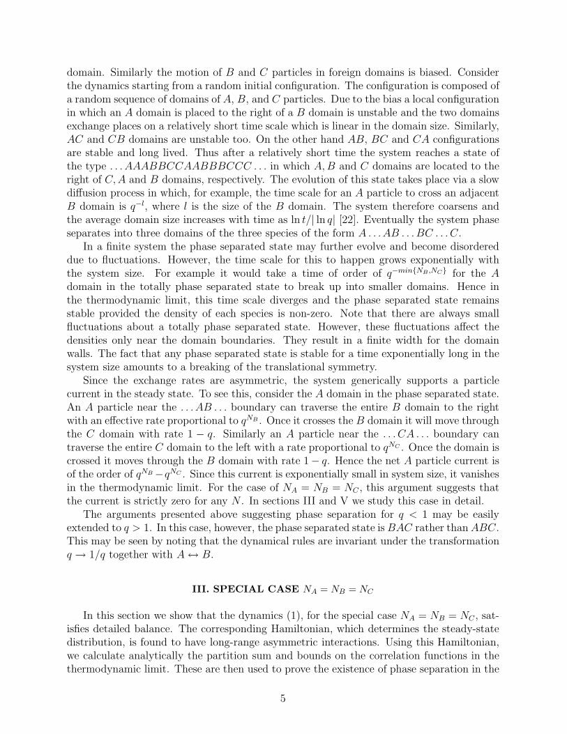
B B A ACCCCCCBBN

BBA A A AA CBA1 l

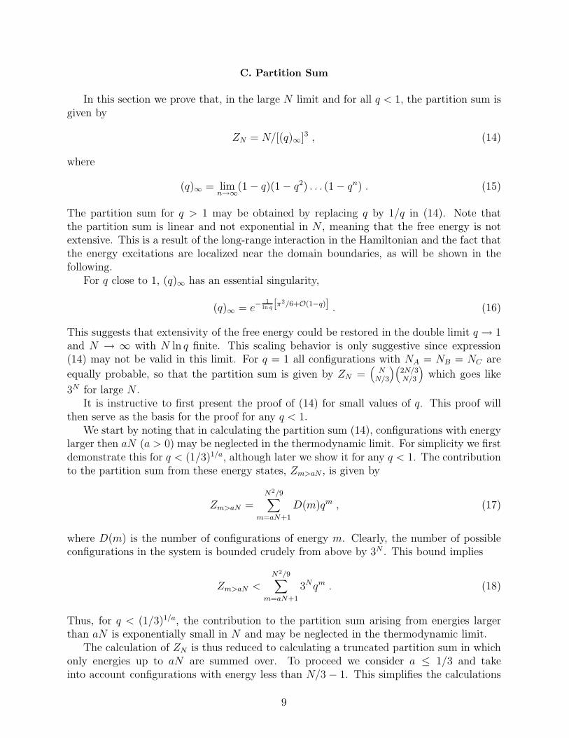
FIG. 1. The l = 5 ground state for an N = 21 system.

considerably since all configurations with energy m < N/3 − 1 may be decomposed intoN disjoint sets of states, each corresponding to a unique ground state (see previous sectionfor a discussion of ground states). We label the sets by l = 1 . . .N , the position of therightmost A particle in the A domain of the ground state belonging to the set (see Fig. 1for an example of an l = 5 ground state). Each state in a specific set can be obtained fromthe corresponding ground state by exchanging nearest neighbors so that the energy alwaysincreases along the intermediate states. Note that this is correct only if excitations of energyless than N/3−1 are considered. This is because not all higher energy states can be reachedby uphill steps from a ground state.

Thus, using translational invariance, the partition sum can be written as

ZN = NZN + e−O(N) , (19)

where ZN is the truncated partition sum of one of the N sets of configurations.We proceed to calculate ZN . This is done by considering all the possible energy exci-

tations with energy less than N/3 − 1 above one ground state. Consider a specific domainboundary, say AB. Excitations of energy m at this boundary can be created by movingone or more A particles into the B domain (this is equivalent to moving B particles intothe A domain). An A particle moving into the B domain is considered as a walker. Theexcitation energy increases linearly with the distance the walker has moved. Thus, in thispicture an excitation of energy m is created by 1 ≤ j ≤ m walkers, traveling a total distancem. The number of excitations of energy m is then given by the number of ways, P (m),of partitioning an integer m into the sum of a sequence of non-increasing positive integers.Taking into account excitations at all three boundaries, an excitation of energy m in thesystem is created by three independent excitations of energy m1, m2 and m3 at the differentdomain boundaries such that m1 + m2 + m3 = m. The number of excitations of this formis just given by P (m1)P (m2)P (m3). Thus, ZN is given by

ZN =N/3−2∑

m=0

qmm∑

mi=0

P (m1)P (m2)P (m3)δm1+m2+m3,m . (20)

Taking the thermodynamic limit we obtain

limN→∞

ZN = (∞∑

m=0

qmP (m))3 . (21)

Using a well known result from number theory, attributed to Euler, for the generatingfunction of P (m) [24],

10

∞∑

m=0

qmP (m) =1

(q)∞(22)

and using (21) and (19), Eq.(14) is obtained.So far we have proved that for q ≤ (1/3)3, Eq.(14) is exact in the thermodynamic limit.

We now extend these results for any q < 1. First we have to show that the states ignored inthe previous calculation for q ≤ (1/3)3 may be ignored for all q < 1. To do this we calculateupper and lower bounds on ZN and show they converge for large enough N .

For this we have to consider the entire energy spectrum of the Hamiltonian. Any config-uration of the system which is neither a ground state nor a metastable state can be obtainedfrom at least one ground state (s = 1) or a metastable state (s > 1) as follows: startingfrom this s-state exchange nearest neighbors such that the energy always increases alongthe path until the configuration is reached. In what follows it is demonstrated that none ofthe configurations which can be obtained from s-states, with s > 1, by the above procedureof particle exchange, contributes to the partition sum in the thermodynamic limit.

An upper bound on the partition sum may be calculated as follows: using the samesteps of derivation used for computing ZN , it is straightforward to show that the con-tribution to the partition sum from an s-state and associated configurations is at most

q(s−1)N/3−s(s−1)/2[(q)∞]−3s. The prefactor q(s−1)N/3−s(s−1)/2 arises from the minimum energy(13) of this metastable state. Therefore by considering the contributions from all the s-statesand using (10) the following bound is found

ZN < N/[(q)∞]3 +N/3∑

s=2

N

(

N/3− 1

s− 1

)

q(s−1)N/3−s(s−1)/2[(q∞)]−3s . (23)

The second term on the RHS represents the contribution from excitations around themetastable states. Replacing q(s−1)N/3−s(s−1)/2 by an upper bound q(s−1)N/6 one can sumthe binomial series. The resulting expression is exponentially small in N for any q < 1.

A lower bound on ZN can be calculated by neglecting configurations with energy greaterthan N/3− 1 as follows,

ZN > NN/3−2∑

m=0

qmm∑

mi=0

P (m1)P (m2)P (m3)δm1+m2+m3,m (24)

= N/[(q)∞]3 −N∞∑

m=N/3−1

qmm∑

mi=0

P (m1)P (m2)P (m3)δm1+m2+m3,m (25)

> N/[(q)∞]3 −N∞∑

m=N/3−1

qm(mP (m))3 . (26)

The asymptotic behavior of P (m) [24] is given by

P (m) ≃ 1

4m√

3exp (π(2/3)1/2 m1/2) . (27)

Thus, for large N the lower bound (26) converges to (14) as does the upper bound (23).

11

D. Correlation Functions

Whether or not a system has long-range order in the steady state can be found bystudying the decay of two-point density correlation functions. For example the probabilityof finding an A particle at site i and a B particle at site j is,

〈AiBj〉 =1

ZN

∑

{Xk}

AiBj qH({Xk}) , (28)

where the summation is over all configurations {Xk} in which NA = NB = NC . Dueto symmetry many of the correlation functions will be the same, for example 〈AiAj〉 =〈BiBj〉 = 〈CiCj〉. A sufficient condition for the existence of phase separation is

limr→∞

limN→∞

(〈A1Ar〉 − 〈A1〉〈Ar〉) > 0. (29)

Since 〈Ai〉 = 1/3 we wish to show that limr→∞ limN→∞〈A1Ar〉 > 1/9. In fact we will showbelow that for any given r and for sufficiently large N ,

〈A1Ar〉 = 1/3−O(r/N) . (30)

This result not only demonstrates that there is phase separation, but also that each of thedomains is pure. Namely the probability of finding a particle a large distance inside a domainof particles of another type is vanishingly small in the thermodynamic limit.

To prove Eq. (30), we use the relation 〈A1Ar〉 = 1/3 − 〈A1Br〉 − 〈A1Cr〉, and showthat the correlation function 〈A1Br〉 is of O(r/N) and 〈A1Cr〉 is of O(1/N). Here we showonly the proof for 〈A1Br〉, since the proof of 〈A1Cr〉 is similar. We also restrict ourselves tor ≤ N/3, which is sufficient for proving Eq. (30).

We have already seen that the contribution to the partition sum from the metastablestates and excitations above them are exponentially small in the system size and hence maybe neglected. Therefore, for calculating the correlation function it is sufficient to considerthe N ground states and excitations above them which may be reached by moves whichonly increase the energy. As we have seen, these states form N disjoint sets of states, eachassociated with one of the ground states. Using this we now show that 〈A1Br〉 = O(r/N).For this purpose we use a restricted partition sum Zs, which is defined as the partition sumZN calculated with the constraint that one of the walkers, say of type A, has traveled atleast distance s. It is given as N →∞ by

Zs =∞∑

m=0

qmm∑

mi=0

P s(m1)P (m2)P (m3)δm1+m2+m3,m . (31)

Here P s(m) is the number of partitions of integer m with the constraint that in all thepartitions the integer s occurs at least once. Noting that P s(m) = P (m − s) it is easy toshow that

Zs = qsZ , (32)

where Z ≡ limN→∞ZN .

12

A A A A A A B B B B B Br

B C C C C C C C A1 l N

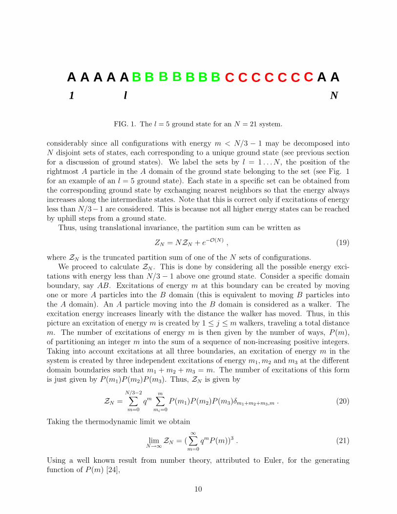
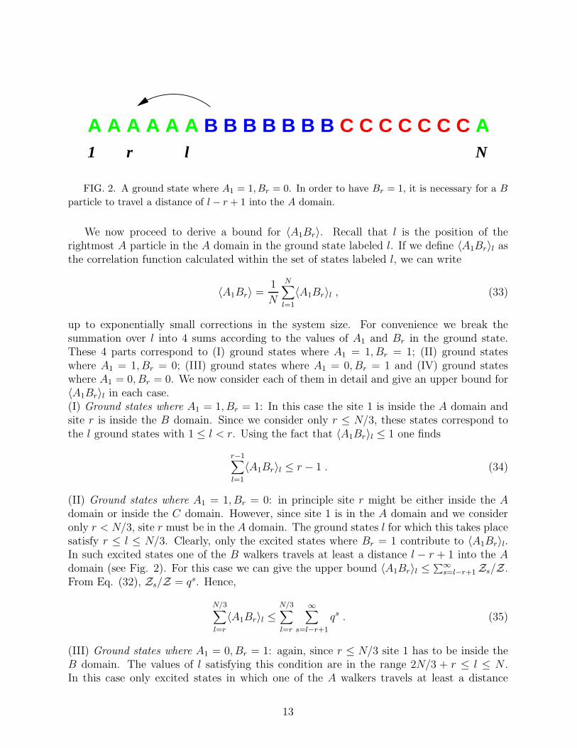
FIG. 2. A ground state where A1 = 1, Br = 0. In order to have Br = 1, it is necessary for a B

particle to travel a distance of l − r + 1 into the A domain.

We now proceed to derive a bound for 〈A1Br〉. Recall that l is the position of therightmost A particle in the A domain in the ground state labeled l. If we define 〈A1Br〉l asthe correlation function calculated within the set of states labeled l, we can write

〈A1Br〉 =1

N

N∑

l=1

〈A1Br〉l , (33)

up to exponentially small corrections in the system size. For convenience we break thesummation over l into 4 sums according to the values of A1 and Br in the ground state.These 4 parts correspond to (I) ground states where A1 = 1, Br = 1; (II) ground stateswhere A1 = 1, Br = 0; (III) ground states where A1 = 0, Br = 1 and (IV) ground stateswhere A1 = 0, Br = 0. We now consider each of them in detail and give an upper bound for〈A1Br〉l in each case.(I) Ground states where A1 = 1, Br = 1: In this case the site 1 is inside the A domain andsite r is inside the B domain. Since we consider only r ≤ N/3, these states correspond tothe l ground states with 1 ≤ l < r. Using the fact that 〈A1Br〉l ≤ 1 one finds

r−1∑

l=1

〈A1Br〉l ≤ r − 1 . (34)

(II) Ground states where A1 = 1, Br = 0: in principle site r might be either inside the Adomain or inside the C domain. However, since site 1 is in the A domain and we consideronly r < N/3, site r must be in the A domain. The ground states l for which this takes placesatisfy r ≤ l ≤ N/3. Clearly, only the excited states where Br = 1 contribute to 〈A1Br〉l.In such excited states one of the B walkers travels at least a distance l − r + 1 into the Adomain (see Fig. 2). For this case we can give the upper bound 〈A1Br〉l ≤

∑∞s=l−r+1Zs/Z.

From Eq. (32), Zs/Z = qs. Hence,

N/3∑

l=r

〈A1Br〉l ≤N/3∑

l=r

∞∑

s=l−r+1

qs . (35)

(III) Ground states where A1 = 0, Br = 1: again, since r ≤ N/3 site 1 has to be inside theB domain. The values of l satisfying this condition are in the range 2N/3 + r ≤ l ≤ N .In this case only excited states in which one of the A walkers travels at least a distance

13

N − l + 1 into the B domain will contribute to 〈A1Br〉l. Hence we can use the upper bound〈A1Br〉l ≤

∑∞s=N−l+1Zs/Z, in this case. Therefore,

N∑

l=2N/3+r

〈A1Br〉l ≤N∑

l=2N/3+r

∞∑

s=N−l+1

qs . (36)

(IV) Ground states where A1 = 0, Br = 0: there are three possibilities here. (a) site 1 isinside the C domain and site r is inside the A domain (N/3 < l < N/3 + r), (b) both thesites 1 and r are inside the C domain (r + N/3 ≤ l ≤ 2N/3), (c) site 1 inside the B domainand site r inside the C domain (2N/3 < l < 2N/3 + r). Since all these are consistent withr ≤ N/3, all these cases can occur. It can be shown that the minimal energy needed tocreate an excited state where A1 = 1 and Br = 1 is ǫa = 2l − r − N/3− 1 for the case (a),ǫb = N/3 + r − 3 for the case (b) and ǫc = 5N/3− 2l + r − 1 for the case (c). The resultingexpression for the bound is

2N/3+r−1∑

l=N/3+1

〈A1Br〉l ≤N/3+r−1∑

l=N/3+1

∞∑

s=ǫa

qs +2N/3∑

l=N/3+r

∞∑

s=ǫb

qs +2N/3+r−1∑

l=2N/3+1

∞∑

s=ǫc

qs . (37)

The summations on the RHS of Eqs. (35-37) can be carried out explicitly. To leading order,the summations gives q/(1−q)2 for each of Eqs. (35) and (36). The summation on the RHSof Eq. (37) vanishes exponentially in the thermodynamic limit. Using Eqs. (33-36), we getthe following expression for the upper bound on 〈A1Br〉

〈A1Br〉 ≤1

N

[

r − 1 +2q

(1− q)2+ e−O(N)

]

. (38)

Therefore 〈A1Br〉 = O(r/N). Similarly one can show that 〈A1Cr〉 = O(1/N). Thus for allq < 1, 〈A1Ar〉 = 1/3−O(r/N), proving the existence of a complete phase separation.

IV. COARSENING

A. Monte Carlo Simulations

We have demonstrated that in the thermodynamic limit the system is phase separatedwhen NA = NB = NC . The general arguments given in section II indicate that when theglobal densities of the three species are non-vanishing and q 6= 1, the system phase separates,even when the three densities are not equal. The argument suggests that the typical time, tf ,in which the system leaves a specific phase separated configuration increases exponentiallywith the system size. Thus, a phase separated state is stable in the thermodynamic limit.In the following we use Monte Carlo simulations to support these arguments.

The time, tf , can be measured using the auto-correlation function defined as,

c(t) =1

N

N∑

i=1

(〈Ai(0)Ai(t)〉+ 〈Bi(0)Bi(t)〉+ 〈Ci(0)Ci(t)〉) , (39)

14

where Ai(t), Bi(t) and Ci(t) are the values of the occupation variables Ai, Bi and Ci attime t, and 〈. . .〉 denotes an average over histories of evolution. Clearly, c(0) = 1 whilec(∞) = (NA/N)2 + (NB/N)2 + (NC/N)2, the value of the autocorrelation between twoindependent configurations. Thus, tf may be defined as the decay time of c(t) to c(∞) whenat t = 0 the system is totally phase separated.

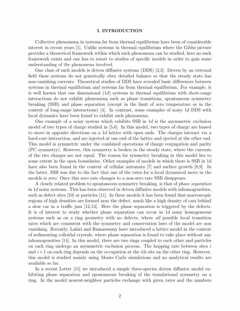
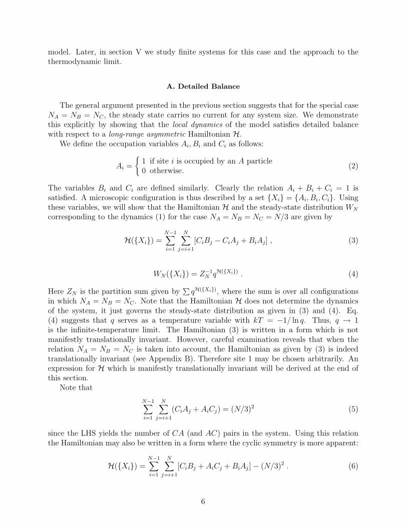
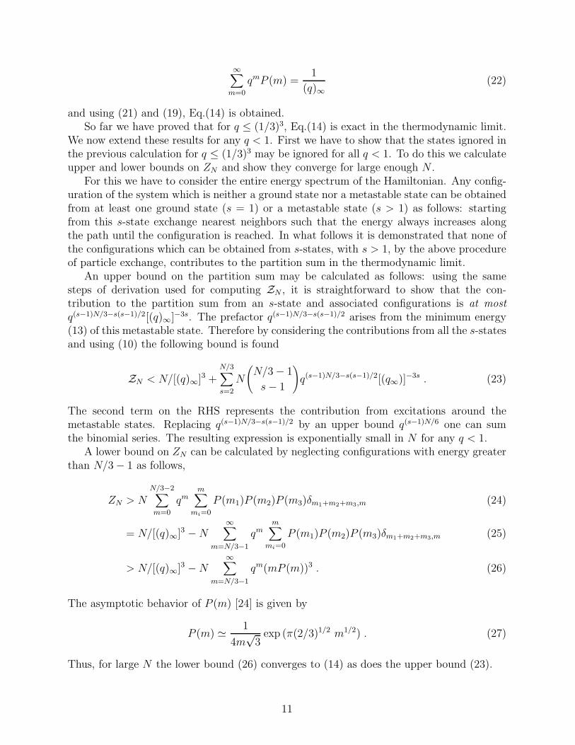
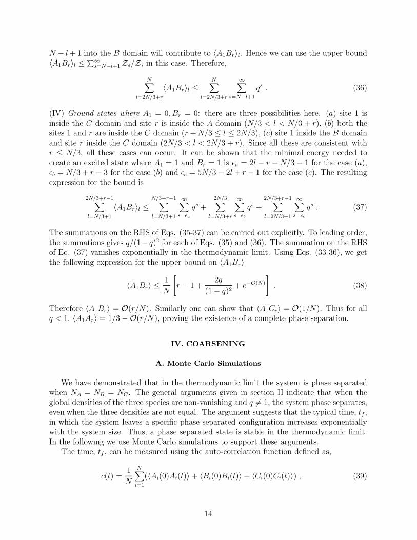
We have measured the time scale tf using Monte Carlo simulations for different systemsizes for NA = NB = NC and for NA 6= NB 6= NC for several q values. An example of suchmeasurements for NA/N = 0.4, NB/N = 0.35 and NC/N = 0.25 is presented in Fig. 3. Inthe plot tf is plotted versus system size for several values of q. It agrees with the exponentialgrowth of tf with the system size suggested by the simple argument of section II. The samebehavior seems to occur for all q 6= 1 and different choices of NA/N , NB/N and NC/N .Therefore we conclude that the Monte Carlo simulations support the claim that for anyq 6= 1 the system will phase separate into three domains in the thermodynamic limit, evenwhen the number of particles of each species is not equal. In the thermodynamic limit thetranslational symmetry is spontaneously broken in this state. Due to the slow dynamics,which reflects escape from metastable states, Monte Carlo simulations could be performedonly for relatively small system size (N ≈ 100). In order to study the coarsening process forlarger systems we employ, in the following, a toy model which mimics the dynamics of themodel (1). The toy model can be conveniently simulated for systems larger by about twoorders of magnitude.

B. Toy Model

We now construct a simple toy model which captures the essential physics of the coarsen-ing process in the model at large times and enables us to simulate systems much larger thanthose accessible by Monte Carlo simulation. Using the toy model we examine another char-acteristic scale of the system. Namely, the average domain size 〈l〉 as a function of the time t.The results support the simple argument leading to a domain growth law 〈l〉 ∼ log t/| log q|.A mean-field version of the toy model is then solved analytically.

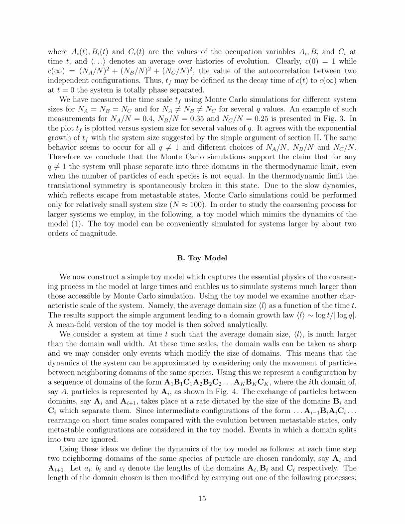
We consider a system at time t such that the average domain size, 〈l〉, is much largerthan the domain wall width. At these time scales, the domain walls can be taken as sharpand we may consider only events which modify the size of domains. This means that thedynamics of the system can be approximated by considering only the movement of particlesbetween neighboring domains of the same species. Using this we represent a configuration bya sequence of domains of the form A1B1C1A2B2C2 . . .AKBKCK , where the ith domain of,say A, particles is represented by Ai, as shown in Fig. 4. The exchange of particles betweendomains, say Ai and Ai+1, takes place at a rate dictated by the size of the domains Bi andCi which separate them. Since intermediate configurations of the form . . .Ai−1BiAiCi . . .rearrange on short time scales compared with the evolution between metastable states, onlymetastable configurations are considered in the toy model. Events in which a domain splitsinto two are ignored.

Using these ideas we define the dynamics of the toy model as follows: at each time steptwo neighboring domains of the same species of particle are chosen randomly, say Ai andAi+1. Let ai, bi and ci denote the lengths of the domains Ai,Bi and Ci respectively. Thelength of the domain chosen is then modified by carrying out one of the following processes:

15

40.0 50.0 60.0 70.0 80.0 90.0 100.0N

103

104

105

106

107

108

tf

q=0.60q=0.65q=0.70q=0.75

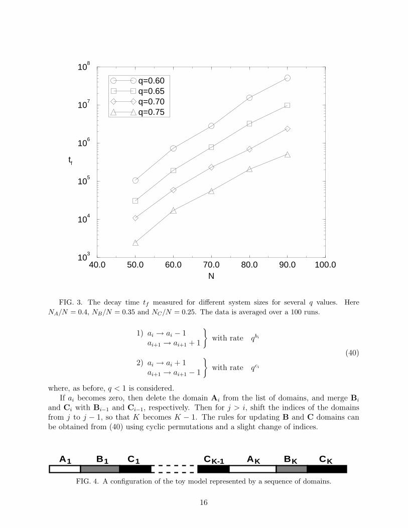
FIG. 3. The decay time tf measured for different system sizes for several q values. Here

NA/N = 0.4, NB/N = 0.35 and NC/N = 0.25. The data is averaged over a 100 runs.

1) ai → ai − 1ai+1 → ai+1 + 1

}

with rate qbi

2) ai → ai + 1ai+1 → ai+1 − 1

}

with rate qci

(40)

where, as before, q < 1 is considered.If ai becomes zero, then delete the domain Ai from the list of domains, and merge Bi

and Ci with Bi−1 and Ci−1, respectively. Then for j > i, shift the indices of the domainsfrom j to j − 1, so that K becomes K − 1. The rules for updating B and C domains canbe obtained from (40) using cyclic permutations and a slight change of indices.

A1 B K1 C1 C A B CK-1 K K

FIG. 4. A configuration of the toy model represented by a sequence of domains.

16

Note that the toy model is only relevant to the description of the coarsening dynamics.This is because here, once the system is left with three domains, it remains in that state.

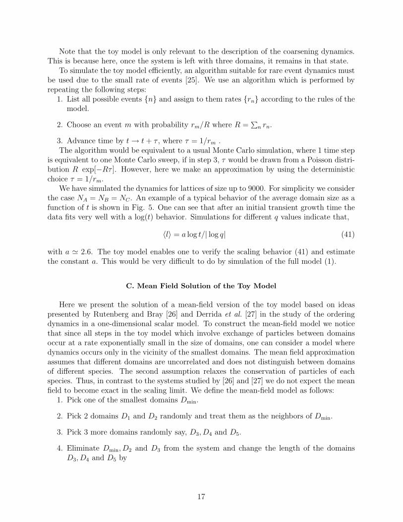
To simulate the toy model efficiently, an algorithm suitable for rare event dynamics mustbe used due to the small rate of events [25]. We use an algorithm which is performed byrepeating the following steps:

1. List all possible events {n} and assign to them rates {rn} according to the rules of themodel.

2. Choose an event m with probability rm/R where R =∑

n rn.

3. Advance time by t→ t + τ , where τ = 1/rm .The algorithm would be equivalent to a usual Monte Carlo simulation, where 1 time step

is equivalent to one Monte Carlo sweep, if in step 3, τ would be drawn from a Poisson distri-bution R exp[−Rτ ]. However, here we make an approximation by using the deterministicchoice τ = 1/rm.

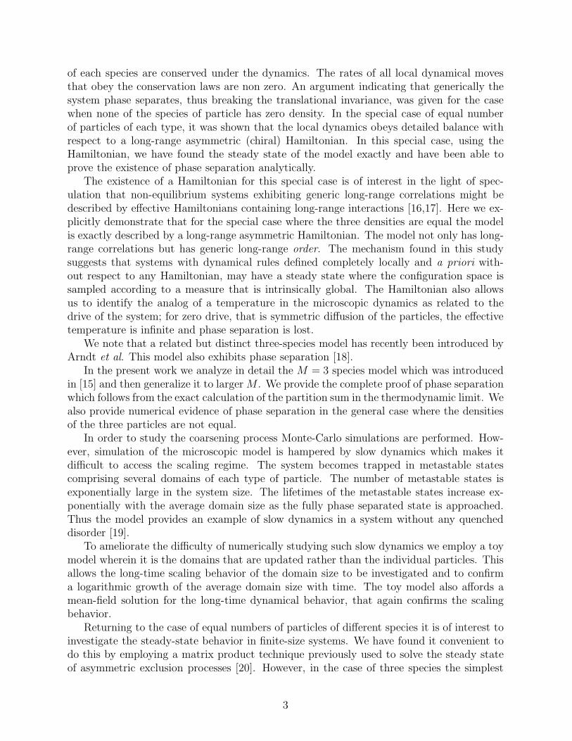
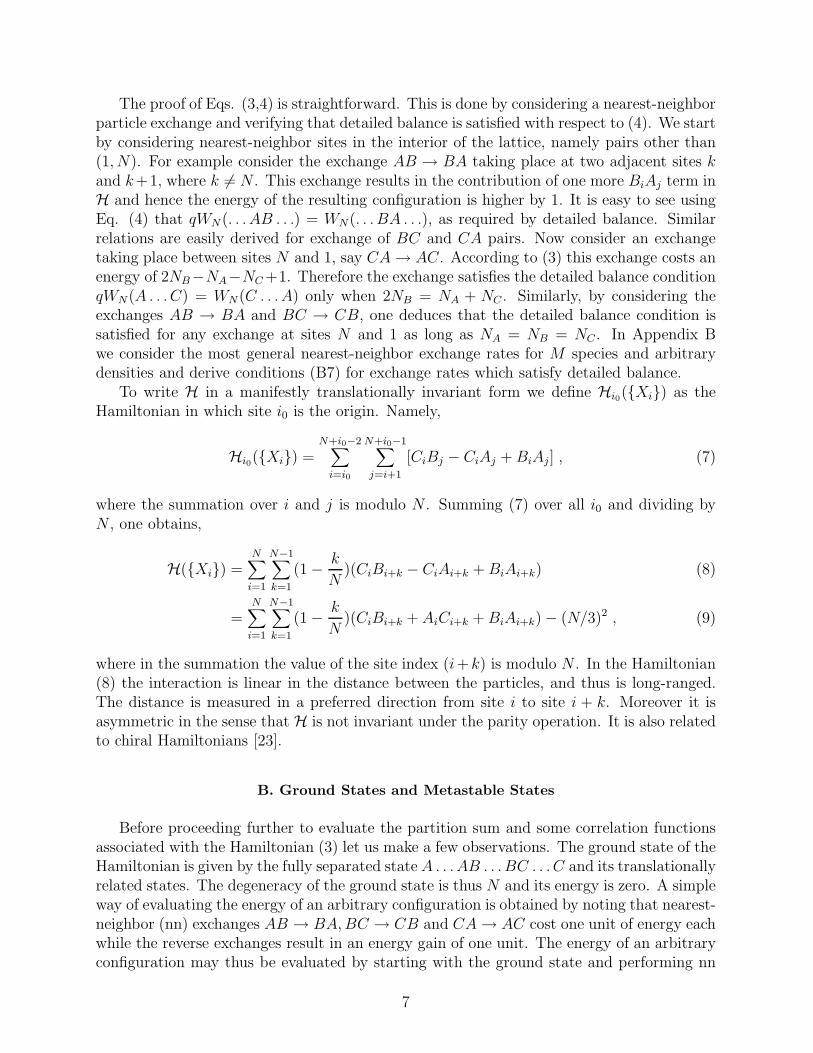
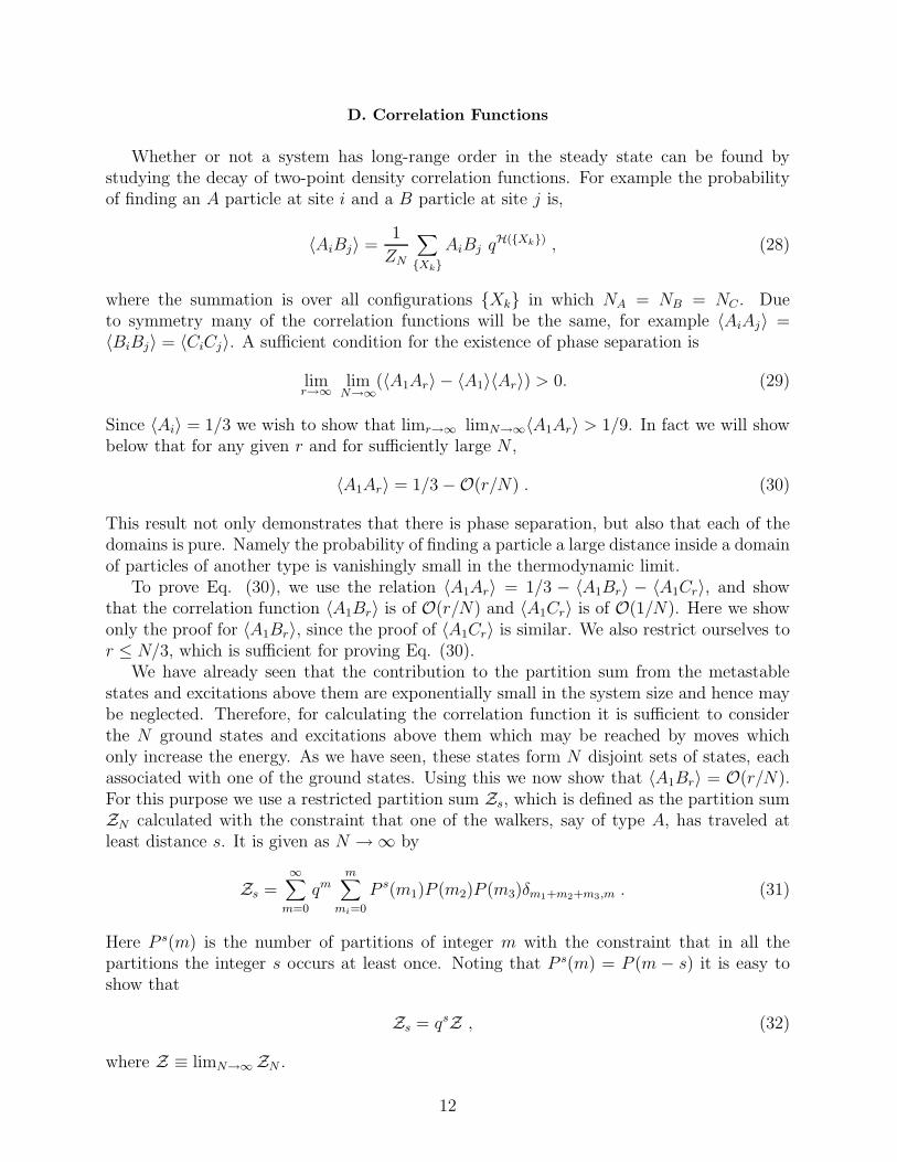
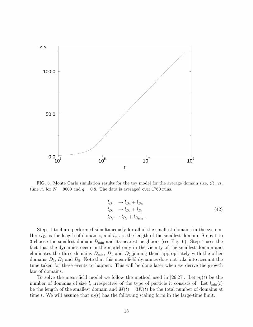
We have simulated the dynamics for lattices of size up to 9000. For simplicity we considerthe case NA = NB = NC . An example of a typical behavior of the average domain size as afunction of t is shown in Fig. 5. One can see that after an initial transient growth time thedata fits very well with a log(t) behavior. Simulations for different q values indicate that,

〈l〉 = a log t/| log q| (41)

with a ≃ 2.6. The toy model enables one to verify the scaling behavior (41) and estimatethe constant a. This would be very difficult to do by simulation of the full model (1).

C. Mean Field Solution of the Toy Model

Here we present the solution of a mean-field version of the toy model based on ideaspresented by Rutenberg and Bray [26] and Derrida et al. [27] in the study of the orderingdynamics in a one-dimensional scalar model. To construct the mean-field model we noticethat since all steps in the toy model which involve exchange of particles between domainsoccur at a rate exponentially small in the size of domains, one can consider a model wheredynamics occurs only in the vicinity of the smallest domains. The mean field approximationassumes that different domains are uncorrelated and does not distinguish between domainsof different species. The second assumption relaxes the conservation of particles of eachspecies. Thus, in contrast to the systems studied by [26] and [27] we do not expect the meanfield to become exact in the scaling limit. We define the mean-field model as follows:

1. Pick one of the smallest domains Dmin.

2. Pick 2 domains D1 and D2 randomly and treat them as the neighbors of Dmin.

3. Pick 3 more domains randomly say, D3, D4 and D5.

4. Eliminate Dmin, D2 and D3 from the system and change the length of the domainsD3, D4 and D5 by

17

103

105

107

109

t

0.0

50.0

100.0

<l>

FIG. 5. Monte Carlo simulation results for the toy model for the average domain size, 〈l〉, vs.

time ,t, for N = 9000 and q = 0.8. The data is averaged over 1760 runs.

lD3→ lD3

+ lD2

lD4→ lD4

+ lD1(42)

lD5→ lD5

+ lDmin.

Steps 1 to 4 are performed simultaneously for all of the smallest domains in the system.Here lDi

is the length of domain i, and lmin is the length of the smallest domain. Steps 1 to3 choose the smallest domain Dmin and its nearest neighbors (see Fig. 6). Step 4 uses thefact that the dynamics occur in the model only in the vicinity of the smallest domain andeliminates the three domains Dmin, D1 and D2 joining them appropriately with the otherdomains D3, D4 and D5. Note that this mean-field dynamics does not take into account thetime taken for these events to happen. This will be done later when we derive the growthlaw of domains.

To solve the mean-field model we follow the method used in [26,27]. Let nl(t) be thenumber of domains of size l, irrespective of the type of particle it consists of. Let lmin(t)be the length of the smallest domain and M(t) = 3K(t) be the total number of domains attime t. We will assume that nl(t) has the following scaling form in the large-time limit.

18

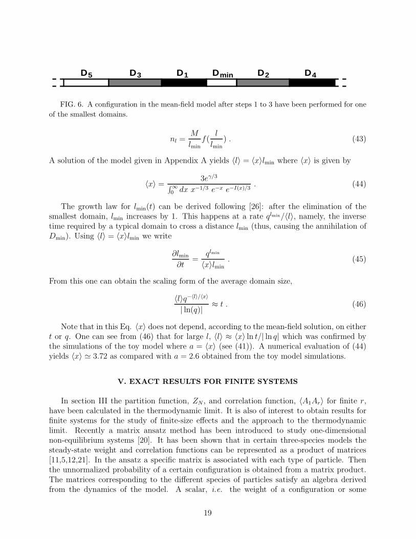
D5 minDDD D D1 23 4

FIG. 6. A configuration in the mean-field model after steps 1 to 3 have been performed for one

of the smallest domains.

nl =M

lminf(

l

lmin) . (43)

A solution of the model given in Appendix A yields 〈l〉 = 〈x〉lmin where 〈x〉 is given by

〈x〉 =3eγ/3

∫∞0 dx x−1/3 e−x e−I(x)/3

. (44)

The growth law for lmin(t) can be derived following [26]: after the elimination of thesmallest domain, lmin increases by 1. This happens at a rate qlmin/〈l〉, namely, the inversetime required by a typical domain to cross a distance lmin (thus, causing the annihilation ofDmin). Using 〈l〉 = 〈x〉lmin we write

∂lmin

∂t=

qlmin

〈x〉lmin. (45)

From this one can obtain the scaling form of the average domain size,

〈l〉q−〈l〉/〈x〉| ln(q)| ≈ t . (46)

Note that in this Eq. 〈x〉 does not depend, according to the mean-field solution, on eithert or q. One can see from (46) that for large l, 〈l〉 ≈ 〈x〉 ln t/| ln q| which was confirmed bythe simulations of the toy model where a = 〈x〉 (see (41)). A numerical evaluation of (44)yields 〈x〉 ≃ 3.72 as compared with a = 2.6 obtained from the toy model simulations.

V. EXACT RESULTS FOR FINITE SYSTEMS

In section III the partition function, ZN , and correlation function, 〈A1Ar〉 for finite r,have been calculated in the thermodynamic limit. It is also of interest to obtain results forfinite systems for the study of finite-size effects and the approach to the thermodynamiclimit. Recently a matrix ansatz method has been introduced to study one-dimensionalnon-equilibrium systems [20]. It has been shown that in certain three-species models thesteady-state weight and correlation functions can be represented as a product of matrices[11,5,12,21]. In the ansatz a specific matrix is associated with each type of particle. Thenthe unnormalized probability of a certain configuration is obtained from a matrix product.The matrices corresponding to the different species of particles satisfy an algebra derivedfrom the dynamics of the model. A scalar, i.e. the weight of a configuration or some

19

correlation function, is usually obtained by performing a trace over the product of matrices,or by multiplying both sides of the product of matrices by vectors. Generalizing this methodto replace matrices by tensors [28], we have been able to obtain recursion relations for thepartition function and correlation function for finite systems for the special case NA = NB =NC . The recursion relations are then used to obtain the partition function and correlationfunction 〈A1Ar〉 for any r in small systems. The results are used to study the scaling of thecorrelation function near the critical point q = 1 (infinite temperature), where the typicaldomain wall width diverges.

A. The Tensor Product Ansatz

It is convenient to consider the unnormalized weights, fN({Xi}), defined through

WN({Xi}) = Z−1N fN ({Xi}) , (47)

where WN({Xi}) is the probability of being in configuration {Xi}. The partition sum ZN

is given by

ZN =∑

{Xi}

fN({Xi}) , (48)

where the sum is over all configurations with NA = NB = NC .We generalize the matrix ansatz and construct the steady-state weight, fN ({Xi}), from a

product of tensors each corresponding to a particle located in a specific place on the lattice.The contraction of the tensors yields a tensor which is then contracted with ‘left’ and ‘right’tensors to generate a scalar. The three tensors which represent the different type of particleare defined as rank 6 tensors through the following tensor products of square matrices

A = E⊗D⊗ 1

B = 1⊗ E⊗D (49)

C = D⊗ 1⊗ E .

Here 1 is a unit matrix. The matrices D and E will be chosen in what follows to satisfy acommutation relation which will be dictated by the detailed balance condition.

To define fN ({Xi}) we introduce the following notation: the contraction of two rank 6tensors O = O1⊗O2⊗O3 and P = P1⊗P2⊗P3, where Oi and Pi are square matrices,according to the rule O1P1⊗O2P2⊗O3P3 is denoted by OP . The contraction of a rank6 tensor O with a ‘left’ rank 3 tensor 〈K| = 〈K1| ⊗ 〈K2| ⊗ 〈K3|, where 〈Ki| are transposedvectors, and a ‘right’ rank 3 tensor, |M〉 = |M1〉 ⊗ |M2〉 ⊗ |M3〉, where |Mi〉 are vectors,defined through 〈K1|O1|M1〉〈K2|O2|M2〉〈K3|O3|M3〉 is denoted by 〈K| O |M〉.

Using these definitions we write the steady-state weight of the system as

fN({Xi}) = 〈U|N∏

i=1

[AiA + BiB + CiC ]|V〉 , (50)

where Ai, Bi and Ci are the occupation variables defined in (2). The expression states thata tensor A is present at place i in the tensor product if site i is occupied by an A particle, a

20

tensor B is present if site i is occupied by a B particle, and a tensor C is present if site i isoccupied by a C particle. The action of the tensor product on 〈U| and |V〉 (to be specifiedlater) produces the scalar fN ({Xi}).

It is straightforward to show using detailed balance that a necessary condition for Eq.(50) to be the steady-state weight is that the following commutation relations are satisfiedbetween A, B, and C :

q AB = BA

q BC = CB (51)

q CA = AC .

Using (49) one can verify that these commutation relations are satisfied provided that qDE =ED. This deformed commutator is of relevance in other stochastic systems [29,30]. Arepresentation of the matrices D and E which satisfies this commutation relation can beobtained as follows: let {〈n|} denote a basis set (n = 0, 1, . . . , N/3) forming a vector space.In this basis we choose the matrices so that,

〈n|E = 〈n|qn for any n〈n|D = 〈n− 1| for n ≥ 1,

(52)

while for n = 0, 〈0|D = 0. An explicit form for E and D is given by the following (N/3 +1)× (N/3 + 1) square matrices

E =N/3∑

n=0

qn|n〉〈n| ; D =N/3∑

n=1

|n〉〈n− 1| . (53)

To obtain fN ({Xi}), 〈U| and |V〉 have to be specified. This should obviously be done sothat fN({Xi}) is non-zero if the ansatz is to give a non-trivial result. We consider a generaltensor product which corresponds to some configuration. The product has N/3 tensors ofeach type A, B and C , which results in a tensor product of three matrix products. Using(49) it can be seen that each matrix product contains N/3 matrices of each type D, E and1. Since E and 1 are diagonal, while D acts to its left as a lowering matrix (see (52)),choosing 〈U| = 〈N/3| ⊗ 〈N/3| ⊗ 〈N/3| ≡ 〈N/3, N/3, N/3|, and |V〉 = |0, 0, 0〉 will give anon-zero fN({Xi}). This makes clear that the minimal size choice for the vector-spaces isN/3+1. Under this choice it is easy to see that in the ground states one has fN = qN2/9 whichcorresponds to a ground state energy N2/9. However, the choice of 〈U| and 〈V| is determinedonly up to some multiplicative factors. These factors may be used to shift the ground stateenergy of the system. For example choosing 〈U| as before with |V〉 = q−N2/9|0, 0, 0〉 willshift the ground state energy to 0. In the following the factors are taken to be 1.

Finally we would like to remark that usually when using the matrix ansatz for systemswith periodic boundary conditions it is often convenient to use a trace of the matrix product[11,21]. In this case this is not possible since the trace of our tensor product is always zero.

B. Partition Sum

In terms of the ansatz (50) the partition function ZN is given by

21

ZN = 〈N3

,N

3,N

3|(A + B + C)N |0, 0, 0〉 . (54)

Note that we are using the canonical ensemble since all tensor products with unequal numberof particles do not contribute to ZN . This is easily seen since in these cases there are alwaysmore than N/3 D matrices acting on one of the vectors 〈N/3|.

To obtain the partition function we derive a recursion relation for

Gli,j,k ≡ 〈i, j, k|(A + B + C)l|0, 0, 0〉 . (55)

One can see that GNN/3,N/3,N/3 = ZN . Rewriting Gl

i,j,k as

Gli,j,k = 〈i, j, k| A(A + B + C)l−1|0, 0, 0〉+ 〈i, j, k| B(A + B + C )l−1|0, 0, 0〉

+〈i, j, k| C(A + B + C )l−1|0, 0, 0〉 , (56)

and using relations (49) and (52) the following recursion relation can be derived

Gli,j,k = qiGl−1

i,j−1,k + qjGl−1i,j,k−1 + qkGl−1

i−1,j,k . (57)

The boundary conditions for this recursion relation is given by the no particle partitionfunction G0

i,j,k = 1 if i = j = k = 0 and is zero otherwise.For small systems (up to N = 21) for which the recursion relation is tractable analytically

on Mathematica, we obtained the partition function ZN = GNN/3,N/3,N/3 as a polynomial in

q. As expected the first N/3− 2 terms of the polynomial match the first N/3− 2 terms ofthe expansion of (14) up to a factor of qN2/9 due to the energy shift in the ground state. Forlarger N we solve the recursion relation numerically.

We note that (57) could have been derived directly from the definition of the partitionfunction without recourse to the tensor ansatz. However, we believe the utility of the ansatzlies in the ease with which correlation functions can be manipulated and relations such asthat of the next subsection derived.

C. Correlation Functions

The correlation function 〈A1Ar〉 is given in terms of the ansatz by

〈A1Ar〉 =〈N

3, N

3, N

3| A(A + B + C) r−2

A(A + B + C) N−r|0, 0, 0〉ZN

. (58)

Using relations (49),(51) and (52) we obtain

〈A1Ar〉 = q2N3

〈N3, N

3− 2, N

3|(A + qB + C /q)r−2(A + B + C )N−r|0, 0, 0〉

ZN(59)

= q2N3

U(r)rN3

, N3−2, N

3

ZN, (60)

where we define the object U(r)si,j,k through,

22

-60 -40 -20 00.00

0.05

0.10

0.0 0.5 1.00.00

0.05

0.10

84

30

q

CC

N lnq

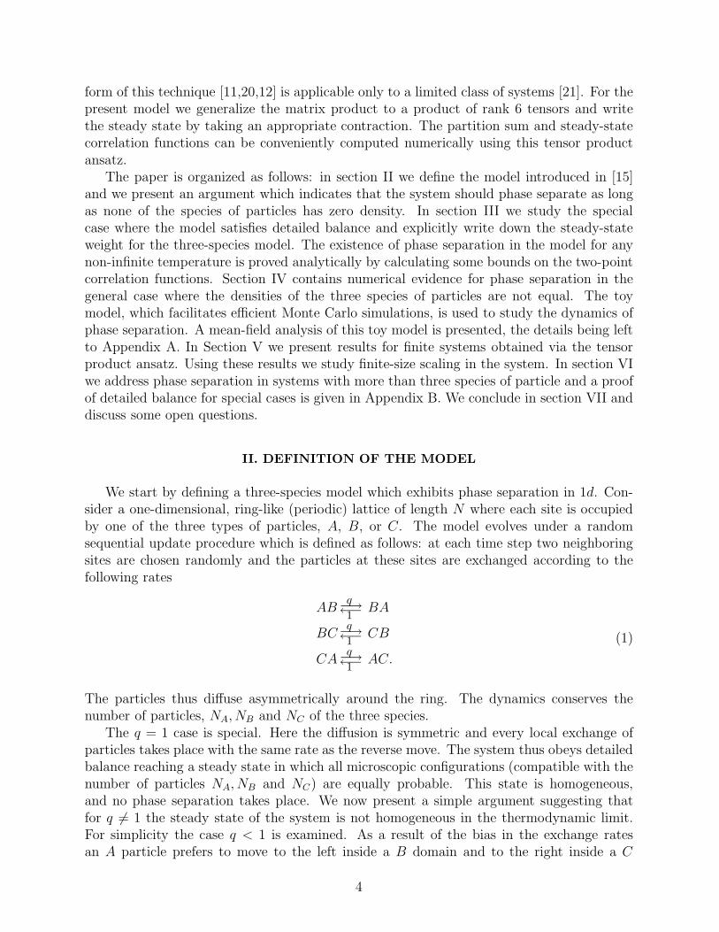
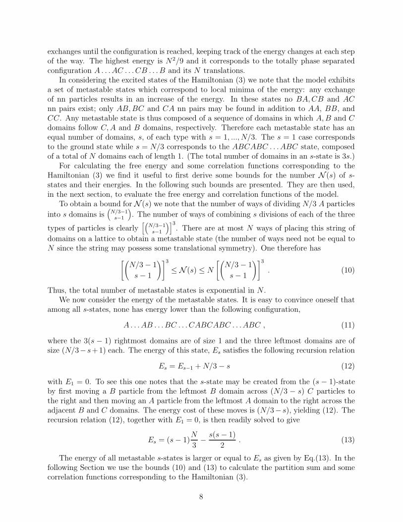
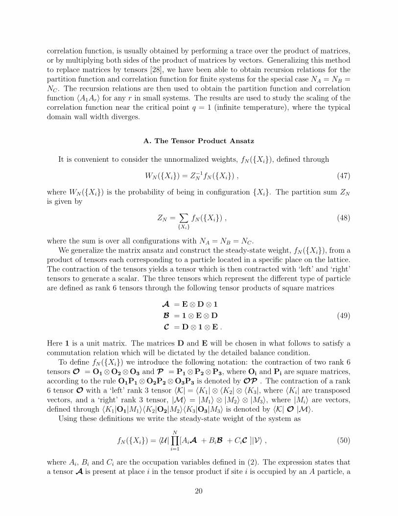
FIG. 7. The correlation function C = 〈A1AN/2〉, obtained from the tensor ansatz, as a function

of the scaled variable N ln q for N = 30, 36, 42, . . . , 84. The inset shows the same data plotted

against q.

U(r)si,j,k = 〈i, j, k|(A + qB + C /q)s−2(A + B + C )N−s|0, 0, 0〉 . (61)

A recursion relation for U(r)si,j,k can be obtained, similarly to the recursion relation for the

partition function (57). Using (49) and (52) gives

U(r)si,j,k = qiU(r)s−1

i,j−1,k + qj+1U(r)s−1i,j,k−1 + qk−1U(r)s−1

i−1,j,k . (62)

The boundary conditions for the recursion relation are obtained by noting that U(r)2i,j,k =

〈i, j, k| (A + B + C)N−r|0, 0, 0〉, i.e., U(r)2i,j,k = GN−r

i,j,k . Using the same methods one canobtain recursion relations for all other correlation functions.

The recursion relations are solved numerically for finite systems. This is done by firstsolving numerically for GN−r

i,j,k , and then using the result as boundary conditions for therecursion relation (62). Owing to (60) we are ultimately interested in U(r)r

N/3,N/3−2,N/3.Using these recursion relations we have calculated the correlation function 〈A1AN/2〉,

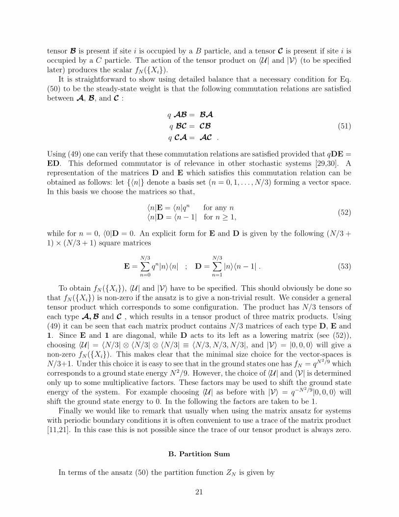
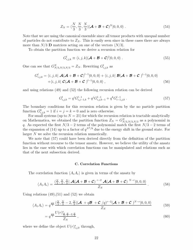
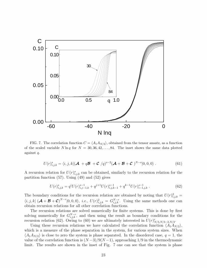
which is a measure of the phase separation in the system, for various system sizes. When〈A1AN/2〉 is close to zero the system is phase separated. In the disordered case, q = 1, thevalue of the correlation function is (N−3)/9(N−1), approaching 1/9 in the thermodynamiclimit. The results are shown in the inset of Fig. 7 one can see that the system is phase

23

separated for small values of q while for q close to 1 the system is disordered. The range ofq values for which the system is phase separated increases as the system size increases. Thenatural scaling variable near the critical point q = 1 is N ln q, the ratio between the domainsize N/3 and the domain wall width

∫

lqldl/∫

qldl = 1/| ln q|. In Fig.(7) the correlationfunction is plotted as a function of the scaling variable. One can see that the data collapseimproves as the system size increases. This scaling variable was also suggested by the formof the partition function (14) in section III C.

VI. GENERALIZATION TO M SPECIES

In the following we discuss possible generalization of the model to M ≥ 3 species. Todemonstrate how this might be done we first discuss the case M = 4. We then commentbriefly on M > 4.

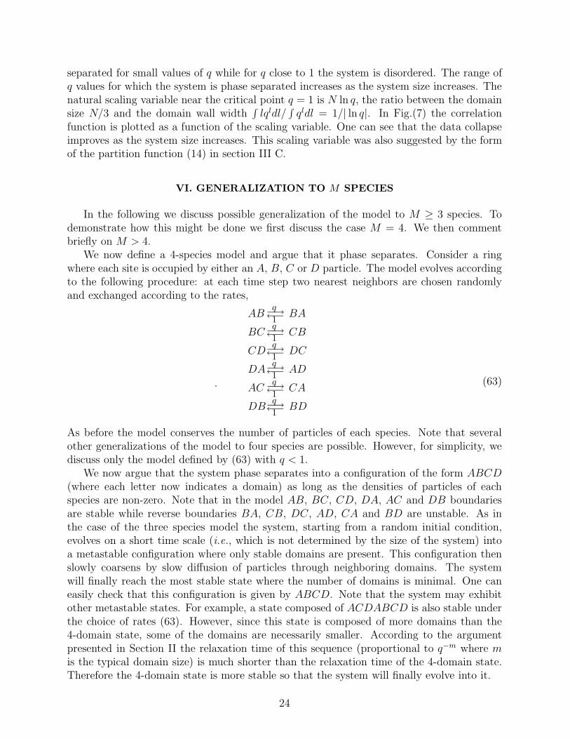
We now define a 4-species model and argue that it phase separates. Consider a ringwhere each site is occupied by either an A, B, C or D particle. The model evolves accordingto the following procedure: at each time step two nearest neighbors are chosen randomlyand exchanged according to the rates,

AB←−1−→q

BA

BC←−1−→q

CB

CD←−1−→q

DC

DA←−1−→q

AD

AC←−1−→q

CA

DB←−1−→q

BD

. (63)

As before the model conserves the number of particles of each species. Note that severalother generalizations of the model to four species are possible. However, for simplicity, wediscuss only the model defined by (63) with q < 1.

We now argue that the system phase separates into a configuration of the form ABCD(where each letter now indicates a domain) as long as the densities of particles of eachspecies are non-zero. Note that in the model AB, BC, CD, DA, AC and DB boundariesare stable while reverse boundaries BA, CB, DC, AD, CA and BD are unstable. As inthe case of the three species model the system, starting from a random initial condition,evolves on a short time scale (i.e., which is not determined by the size of the system) intoa metastable configuration where only stable domains are present. This configuration thenslowly coarsens by slow diffusion of particles through neighboring domains. The systemwill finally reach the most stable state where the number of domains is minimal. One caneasily check that this configuration is given by ABCD. Note that the system may exhibitother metastable states. For example, a state composed of ACDABCD is also stable underthe choice of rates (63). However, since this state is composed of more domains than the4-domain state, some of the domains are necessarily smaller. According to the argumentpresented in Section II the relaxation time of this sequence (proportional to q−m where mis the typical domain size) is much shorter than the relaxation time of the 4-domain state.Therefore the 4-domain state is more stable so that the system will finally evolve into it.

24

In considering M > 4 models one finds that for some choices of transition rates severalstates with the minimum number of domains may become metastable. For example, forM = 5 it is possible to choose transition rates for which both ABCDE and ACEBD arelocally stable. The relative stability (and thus the resulting phase separated state) may befound by determining the relaxation time of these states using simple considerations suchas those presented in Section II.

As is the case of M = 3 detailed balance is found to be satisfied for certain densities andtransition rates for M > 3. The condition for this is derived in Appendix B. In this casethe relative stability of metastable states could be determined by comparing free energies.

VII. CONCLUSION

In this paper a model of three species of particles diffusing on a ring previously introducedin [15] has been studied. The model is governed by local dynamics in which all movescompatible with the conservation of the three densities are allowed. We argue that phaseseparation should occur as long as all densities are non-zero. In the special case of equaldensities we find that the steady state generated by the local stochastic dynamics is exactlygiven by a long-range asymmetric Hamiltonian. Phase separation for this case is explicitlydemonstrated. The model provides an explicit example for the mechanism leading to phaseseparation or breaking of ergodicity in systems with local stochastic dynamics. Although wedid not succeed in solving the steady state in the case of non-equal densities of particles,there is a strong evidence that phase separation still occurs. In order to investigate furtherthe case of equal densities we employed a generalized matrix ansatz to calculate correlationfunction for finite-size systems. The novel structure of the ansatz may give some clue as tohandle other 1d models which have so far resisted solution.

The dynamics of phase separation reduces to a coarsening problem where the typicaldomain size grows logarithmically in time. This results from the elimination of the domainsat a rate exponentially small in their size. The slow dynamics poses a problem of how toaccess the scaling regime numerically. With direct numerical simulations only small systemscan be studied (see Fig. 3). However, by employing a toy model in which domains ratherthan individual sites are updated one can simulate much larger systems and probe the scalingregime (see Fig. 5). Such ideas of updating domains have been used before in the study ofcoarsening [31]. With the aid of the toy model it should be possible to study other aspectsof the scaling regime associated with the slow dynamics and escape from metastable states.

Generalizations are possible to models with M > 3 species. We have discussed somepossibilities and have shown that phase separation may take place, although the structureof the set of metastable states is more complicated. As was the case for M = 3, conditionsfor detailed balance with respect to a long-range Hamiltonian may be determined.

The problem of phase separation and coarsening is of interest also in the broader contextof phase transitions in one dimensional systems. Here the existence of conserved quantitiesresults in certain local transition rates being zero. It would be interesting to generalize thisstudy to models in which no conserved quantity exists and all local rates are non-vanishing.Also, another open problem is to calculate the steady state of the present model in the caseof non-equal densities.

25

Acknowledgments: MRE is a Royal Society University Research Fellow and thanks theWeizmann Institute and the Einstein Center for warm hospitality during several visits. Thesupport of the Minerva Foundation, Munich Germany, the Israeli Science Foundation, andthe Israel Ministry of Science is gratefully acknowledged. Computations were performed onthe SP2 at the Inter-University High Performance Computer Center, Tel Aviv. We thankS. Wiseman for helpful advice on programming and M. J. E. Richardson for careful readingof the manuscript.

APPENDIX A: MEAN-FIELD SOLUTION OF TOY MODEL

To solve the mean-field model we follow the method used in [26,27]. Let nl(t) be thenumber of domains of size l, irrespective of the type of particle it consists of. Let lmin(t)be the length of the smallest domain and M(t) = 3K(t) be the total number of domains attime t. We will assume that nl(t) has the following scaling form in the large-time limit.

nl =M

lminf(

l

lmin) (A1)

After the elimination of the smallest domain as given by (42), nl, lmin and M change accordingto

M ′ = M − 3nlmin(A2)

n′l = nl(1− 5nlmin

M) + nlmin

nl−lmin

Mθ(l − 2lmin) + 2nlmin

l−lmin∑

j=lmin

nj

M

nl−j

M(A3)

l′min = lmin + 1 . (A4)

Using the scaling form (A1) we have,

n′l =M ′

lmin + 1f(

l

lmin + 1) ≈ M

lmin

[f(x)− (3f(1) + 1)f(x)

lmin

− x

lmin

∂xf(x)] (A5)

where x = l/lmin and we have expanded in 1/lmin. Now substituting these in (A3), it isstraightforward to show that

f(x) + x∂xf(x)− 2f(x)f(1) + f(1)f(x− 1)θ(x− 2) + 2θ(x− 2)f(1)∫ ∞

1dy f(y)f(x− y) = 0 .

(A6)

Using the Laplace transform,

φ(p) =∫ ∞

1dx exp[−px] f(x) (A7)

one can show that φ(p) satisfies the differential equation,

p∂pφ(p) = f(1)[φ(p)− 1][2φ(p) + e−p] (A8)

Since φ(p) = 1 − 〈x〉p + . . ., by expanding (A8) to order p one obtains f(1) = 1/3. Thesolution of (A8) with boundary conditions φ(0) = 1 and φ(p) ≈ e−p/3p for p >> 1 is

26

φ(p) =

∫∞p dx x−1/3 e−x e−I(x)/3

3p2/3e−I(p)/3 +∫∞p dx x−1/3 e−x e−I(x)/3

(A9)

where I(x) =∫∞1 dt exp[−xt]/t = − log(x) − γ − ∑∞n=1(−x)n/(n! n) and γ is the Euler

constant. Inverse Laplace transform of (A9) gives the domain size distribution. From (A9)and using the expansion φ(p) = 1 − 〈x〉p + . . ., where the average is with respect to f(x),we get

〈x〉 =3eγ/3

∫∞0 dx x−1/3 e−x e−I(x)/3

. (A10)

APPENDIX B: DETAILED BALANCE CONDITION FOR AN M-SPECIES

MODEL

We now define the most general M species model, where M ≥ 3. Let Xi denote avariable at site i of a ring of size N , which takes values Xi = 1, 2, . . . , M . Xi = m meansthat site i is occupied by a particle of type m. The system evolves by a random sequential,nearest-neighbor exchange dynamics, with the following rates:

mnq(m,n)−→←−

q(n,m)

nm , (B1)

and q(Xi, Xi) = 1. The model conserves Nm, the number of particles of type m, for all m.We now present a condition for the model to satisfy detailed balance with respect to the

steady-state weight given by

W ({Xi}) =N−1∏

i=1

N∏

j=i+1

q(Xj, Xi) , (B2)

where the set {Xi} describes the microscopic configuration.Consider a particle exchange between sites k and k + 1, where Xk = m, Xk+1 = n and

k 6= N (i.e. in the bulk, note that site 1 is chosen arbitrarily). Expanding the product in(B2), it is easy to verify that

W (X1, . . . , m, n, . . . , XN)

W (X1, . . . , n, m, . . . , XN)=

q(n, m)

q(m, n). (B3)

Since this hold for any m, n, and is irrespective of the number of particles of each species,the steady-state weight (B2) satisfies detailed balance for all nearest-neighbor exchanges inthe bulk. If the weights (B2) are translationally invariant then detailed balance will alsohold for exchanges between sites 1 and N .

Thus, to complete the proof of detailed balance it is sufficient to demand that (B2) istranslationally invariant. To do this we relabel sites i→ i + 1. The weight then becomes

W ({Xi}) =N−1∏

i=1

N∏

j=i+1

q(Xj−1, Xi−1) , (B4)

27

where X0 is identical to XN . Rewriting this equation by relabeling the indices we obtain,

W ({Xi}) =

N−1∏

i=1

N∏

j=i+1

q(Xj, Xi)

N−1∏

k=1

q(Xk, XN)

q(XN , Xk). (B5)

Comparing (B5) with (B2) and noting for example that,

N∏

j=1

q(Xj, XN) =M∏

l=1

[q(l, XN)]Nl , (B6)

one can see that (B2) is translational invariant if

M∏

l=1

[

q(m, l)

q(l, m)

]Nl

= 1 , (B7)

for every m = 1, . . . , M . Thus, detailed balance holds if (B7) is satisfied. We note that forgiven densities {Nm} the manifold of solutions for the rates is of M(M − 3)/2 dimensions.

28

REFERENCES[1] see e.g. Scale Invariance, Interfaces and Non-equilibrium Dynamics. (eds. M. Droz, A. J.

Mckane, J. Vannimenus and D. E. Wolf) Plenum, NY, (1995).[2] S. Katz, J. L. Lebowitz and H. Spohn, Phys. Rev. B 28, 1655 (1983); J. Stat. Phys. 34,

497 (1984).[3] B. Schmittmann and R. K. P. Zia Statistical Mechanics of Driven Diffusive Systems in

Phase Transitions and Critical Phenomena (C. Domb and J. L. Lebowitz, eds.) Vol. 17

Academic Press, London, 1995.[4] L. D. Landau and E. M. Lifshitz Statistical Physics 1 (Pergammon, Oxford (1980)).[5] M. R. Evans, D. P. Foster, C. Godreche and D. Mukamel Phys. Rev. Lett. 74, 208 (1995);

J. Stat. Phys 80, 69 (1995).[6] C. Godreche et al, J. Phys. A: Math. Gen. 28, 6039 (1995).[7] P. Gacs, J. Comput. Sys. Sci. 32, 15 (1986).[8] J. Kertesz and D. E. Wolf Phys. Rev. Lett. 62 2571 (1989).[9] U. Alon, M. R. Evans, H. Hinrichsen and D. Mukamel Phys. Rev. Lett. 76 2746 (1996);

cond-mat/9710142[10] S. A. Janowsky and J. L. Lebowitz, Phys. Rev. A 45, 618 (1992); G. Schutz, J. Stat.

Phys. 73, 813 (1993).[11] B. Derrida, S. A. Janowsky, J. L. Lebowitz and E. R. Speer, Europhys. Lett. 22, 651

(1993); K. Mallick, J. Phys. A: Math. Gen. 29, 5375 (1996).[12] M. R. Evans, Europhys. Lett. 36, 13 (1996)[13] J. Krug and P. A. Ferrari, J. Phys. A: Math. Gen 29 L213 (1996)[14] R. Lahiri and S. Ramaswamy Phys. Rev. Lett. 79 1150 (1997).[15] M. R. Evans, Y. Kafri, H. M. Koduvely and D. Mukamel Phys. Rev. Lett. 80, 425, (1998).[16] B. Bergersen and Z. Racz, Phys. Rev. Lett. 67, 3047 (1991).[17] F. J. Alexander and G. L. Eyink, cond-mat/9801258[18] P. F. Arndt, T. Heinzel and V. Rittenberg, J. Phys. A: Math. Gen. 31, L45, (1998).[19] F. Ritort Phys. Rev. Lett. 75, 1190 (1995); W. Krauth and M. Mezard Z. Phys. B 97,

127 (1995).[20] B. Derrida, M. R. Evans, V. Hakim and V. Pasquier J. Phys. A: Math. Gen. 26, 1493

(1993).[21] P. F. Arndt, T. Heinzel and V. Rittenberg, J. Phys. A: Math. Gen. 31, 833 (1998).[22] J. D. Shore, M. Holzer, and J. P. Sethna, Phys. Rev. B 46, 11376 (1992).[23] M. P. M. den Nijs in Phase Transitions and Critical Phenomena (C. Domb and J. L.

Lebowitz, eds.) Vol. 12 Academic Press, London, 1988.[24] G. E. Andrews The Theory of Partitions, Encyclopedia of Mathematics and its Applica-

tions Vol. 2, p. 1–4 (Addison Wesley, MA, 1976).[25] A. B. Bortz, M. H. Kalos and J. L. Lebowitz, J. Comput. Phys. 17, 10 (1975).[26] A. D. Rutenberg and A. J. Bray Phys. Rev. E 50, 1900 (1994).[27] A. J. Bray, B. Derrida and C. Godreche Europhys. Lett. 27, 175 (1994).[28] B. Derrida, M. R. Evans and K. Mallick, J. Stat. Phys. 79, 833 (1995).[29] M. J. E. Richardson J. Stat. Phys. 89, 777 (1997).[30] S. Sandow and G. Schutz Europhys. Lett. 26, 7 (1994).[31] S. J. Cornell and A. J. Bray, Phys. Rev. E 54, 1153 (1996).

29