Transatlantic time and frequency transfer by GPS carrier phase
Upload
khangminh22Category
view
2download
0
Phase Noise in Multi-Carrier Systems
by
Gokul Sridharan
A thesis submitted in conformity with the requirementsfor the degree of Master of Applied Science
Graduate Department of Electrical and Computer EngineeringUniversity of Toronto
Copyright © 2010 by Gokul Sridharan
Abstract
Phase Noise in Multi-Carrier Systems
Gokul Sridharan
Master of Applied Science
Graduate Department of Electrical and Computer Engineering
University of Toronto
2010
This thesis concerns the effect of phase noise (PHN) on multi-carrier systems such as
OFDM and the detection of multi-carrier symbols affected by PHN. It is known that PHN
causes mixing between sub-carriers resulting in inter-carrier interference (ICI) and rotates
symbols on every sub-carrier by a certain angle called the common phase error (CPE).
We explore how these two effects arise and show that these two effects are coupled to
each other. We also note that higher order M-QAM constellations like 64-QAM are more
sensitive to CPE than smaller constellations like 4-QAM. Based on our observations on
CPE, we propose a blind CPE estimation algorithm. The key idea behind this algorithm
is the realization that not all symbols of a constellation are equally prone to errors due to
CPE. We then address the issue of ICI and propose a turbo receiver design to mitigate it.
The turbo receiver is based on a soft-in soft-out detection algorithm that we develop using
the principles of variational inference. The algorithm jointly detects the PHN sequence
and the transmitted bits. The CPE estimation algorithm and the variational inference
based turbo receiver together constitute a complete solution to detection under PHN
for multi-carrier systems. Simulations show that using the proposed algorithms we can
significantly improve the performance. In addition to the analysis for OFDM systems,
we also analyze the effect of PHN on Single-Carrier Frequency Division Multiple Access
(SC-FDMA)– a multiple access scheme proposed recently. We draw parallels to the effect
on OFDM and provide suggestions on detection strategies to alleviate the effects of PHN
on SC-FDMA.
ii

Acknowledgements
This work is a culmination of contributions, sacrifices and support, both directly and
indirectly by many people over the last two years. First and foremost in that long list is
my advisor Prof. Teng Joon Lim. Starting from the weekly group meetings, to nudging
me to take a closer look at the problem that eventually defined my Master’s work, and
in pushing me to adopt a more lucid writing style for this thesis, I have had valuable
inputs from him at every stage. I would like to thank him for his insights and comments
during our weekly meetings and for his patience in editing many of my technical papers.
I greatly appreciate him for accomodating numerous requests for meetings at short notice
and for taking pains to answer e-mail queries promptly and to great depth.
I would also like to thank my thesis examiners, Prof. Frank Kschischang and Prof.
Wei Yu for taking time off to read this thesis and for making some insighful suggestions
and comments on this work.
It was a pleasure working in BA7114, thanks to all my colleagues who made it a very
enjoyable work environment. I have greatly benefited from discussions, both technical
and otherwise, with my colleagues and for this I am very thankful to them. In this
regard, I would like to especially thank Adam Tenenbaum, K.V. Srinivas, Taiwen Teng,
Ali Khanafer, Kianoush Hosseini, Sachin Kadloor, Siddarth Hari, Muhammad Nazmul
Islam, Ehsan Karamad, Hassan Masoon, Willian Chou, Amir Aghaei, Yashar Ghiassi,
Sanam Sadr, Wael Louis and Muhammad Mohanta.
While my wingmates from IITM and friends from India haven’t been around in
Toronto, I thank them for their constant support and reassurance via e-mail. In par-
ticular, I would like to thank my close friend Harini Eavani who has been a key source
of support, comfort and encouragement. Finally, I would like to thank my parents and
my sister for supporting me in all my endeavours all through my life.
iii
Contents
1 Introduction 1
1.1 Introduction . . . . . . . . . . . . . . . . . . . . . . . . . . . . . . . . . . 1
1.2 Thesis Overview . . . . . . . . . . . . . . . . . . . . . . . . . . . . . . . . 3
1.3 Notation . . . . . . . . . . . . . . . . . . . . . . . . . . . . . . . . . . . . 7
2 Phase Noise: Characteristics, Effects and Consequences 9
2.1 Introduction . . . . . . . . . . . . . . . . . . . . . . . . . . . . . . . . . . 10
2.2 Statistical Properties . . . . . . . . . . . . . . . . . . . . . . . . . . . . . 16
2.2.1 Covariance Matrix . . . . . . . . . . . . . . . . . . . . . . . . . . 16
2.2.2 Sample Mean Statistics . . . . . . . . . . . . . . . . . . . . . . . . 16
2.3 Signal Model . . . . . . . . . . . . . . . . . . . . . . . . . . . . . . . . . 17
2.3.1 Receiver Phase Noise . . . . . . . . . . . . . . . . . . . . . . . . . 17
2.3.2 Transmitter Phase Noise . . . . . . . . . . . . . . . . . . . . . . . 20
2.3.3 Multiple Antenna Scenario . . . . . . . . . . . . . . . . . . . . . . 21
2.3.4 Multi-User Scenario : Uplink/Downlink . . . . . . . . . . . . . . . 23
2.4 Relationship Between CPE and ICI . . . . . . . . . . . . . . . . . . . . . 25
2.4.1 Probability of High CPE Events . . . . . . . . . . . . . . . . . . . 29
2.4.2 Energy Split Between CPE and Higher Order Terms . . . . . . . 32
2.5 Phase Noise Estimation and Mitigation: Literature Survey . . . . . . . . 35
2.5.1 Preliminary Analysis : Early Papers . . . . . . . . . . . . . . . . 37
iv
2.5.2 Phase Noise Estimation and Compensation . . . . . . . . . . . . . 39
2.5.3 Key Observations . . . . . . . . . . . . . . . . . . . . . . . . . . . 41
2.5.4 Focus of Our Work . . . . . . . . . . . . . . . . . . . . . . . . . . 42
2.6 Summary . . . . . . . . . . . . . . . . . . . . . . . . . . . . . . . . . . . 43
3 Blind CPE Estimation 45
3.1 Introduction . . . . . . . . . . . . . . . . . . . . . . . . . . . . . . . . . . 45
3.2 Received Signal Model . . . . . . . . . . . . . . . . . . . . . . . . . . . . 46
3.2.1 Existing Pilot-Based Approaches to CPE Estimation . . . . . . . 47
3.3 Blind CPE Estimation Under Detection Uncertainty . . . . . . . . . . . . 49
3.3.1 Key Idea– Auxiliary Variable . . . . . . . . . . . . . . . . . . . . 49
3.3.2 Computing p(uk|dk) . . . . . . . . . . . . . . . . . . . . . . . . . 52
3.4 Simulation Results . . . . . . . . . . . . . . . . . . . . . . . . . . . . . . 57
3.5 Summary . . . . . . . . . . . . . . . . . . . . . . . . . . . . . . . . . . . 60
4 Turbo Receiver Design for ICI Mitigation 63
4.1 Introduction . . . . . . . . . . . . . . . . . . . . . . . . . . . . . . . . . . 64
4.2 Received Signal Model . . . . . . . . . . . . . . . . . . . . . . . . . . . . 67
4.2.1 Gray mapping : bits to M-QAM symbols ( from [6] ) . . . . . . . 67
4.2.2 The Received Signal . . . . . . . . . . . . . . . . . . . . . . . . . 67
4.2.3 Actual and Postulated Posterior Distributions . . . . . . . . . . . 68
4.3 The Bit-Level Variational Inference Algorithm . . . . . . . . . . . . . . . 71
4.3.1 Free Energy Evaluation . . . . . . . . . . . . . . . . . . . . . . . . 71
4.3.2 Free Energy Minimization . . . . . . . . . . . . . . . . . . . . . . 72
4.3.3 The Variational Inference Algorithm . . . . . . . . . . . . . . . . 73
4.3.4 Complexity Analysis . . . . . . . . . . . . . . . . . . . . . . . . . 73
4.4 Simulation Results . . . . . . . . . . . . . . . . . . . . . . . . . . . . . . 74
4.5 Summary . . . . . . . . . . . . . . . . . . . . . . . . . . . . . . . . . . . 80
v
5 Effect of Phase Noise on SC-FDMA 81
5.1 Introduction . . . . . . . . . . . . . . . . . . . . . . . . . . . . . . . . . . 81
5.2 Signal Model . . . . . . . . . . . . . . . . . . . . . . . . . . . . . . . . . 82
5.2.1 ZF Equalization . . . . . . . . . . . . . . . . . . . . . . . . . . . . 83
5.2.2 MMSE Equalization . . . . . . . . . . . . . . . . . . . . . . . . . 84
5.3 Detection in the Presence of Phase Noise . . . . . . . . . . . . . . . . . . 87
5.3.1 Received Signal Model . . . . . . . . . . . . . . . . . . . . . . . . 87
5.3.2 Effect on Linear Receivers . . . . . . . . . . . . . . . . . . . . . . 88
5.3.3 Self Interference vs. Multi-User Interference . . . . . . . . . . . . 93
5.4 Summary . . . . . . . . . . . . . . . . . . . . . . . . . . . . . . . . . . . 96
6 Conclusion 97
Appendices 100
A Evaluating the Free Energy Expression 100
B Computing the Gradient 102
B.1 Gradient w.r.t Sθ . . . . . . . . . . . . . . . . . . . . . . . . . . . . . . . 102
B.2 Gradient w.r.t mθ . . . . . . . . . . . . . . . . . . . . . . . . . . . . . . . 103
B.3 Gradient w.r.t brk and bik . . . . . . . . . . . . . . . . . . . . . . . . . . 104
C Properties of the Permutation Matrix Tk 106
D SC-FDMA Received Signal in the Presence of PHN 110
Bibliography 111
vi
List of Tables
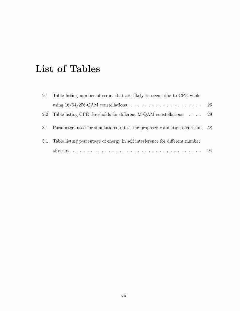
2.1 Table listing number of errors that are likely to occur due to CPE while
using 16/64/256-QAM constellations. . . . . . . . . . . . . . . . . . . . . 26
2.2 Table listing CPE thresholds for different M-QAM constellations. . . . . 29
3.1 Parameters used for simulations to test the proposed estimation algorithm. 58
5.1 Table listing percentage of energy in self interference for different number
of users. . . . . . . . . . . . . . . . . . . . . . . . . . . . . . . . . . . . . 94
vii
List of Figures
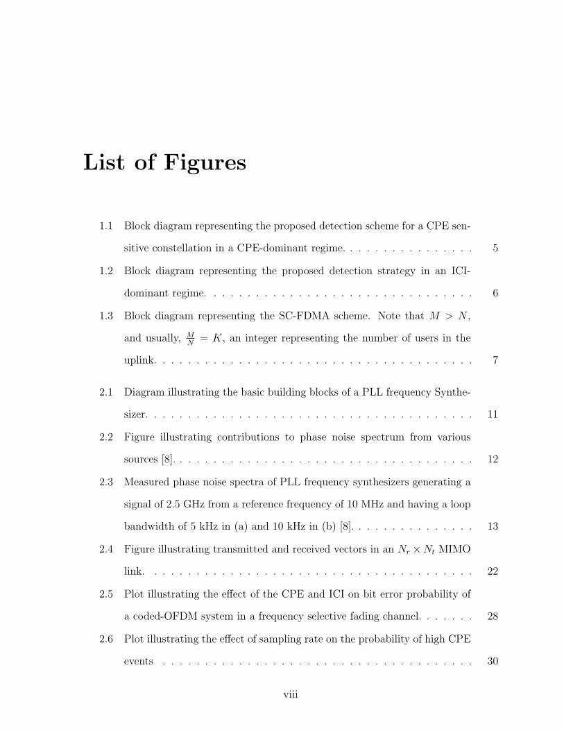
1.1 Block diagram representing the proposed detection scheme for a CPE sen-
sitive constellation in a CPE-dominant regime. . . . . . . . . . . . . . . . 5
1.2 Block diagram representing the proposed detection strategy in an ICI-
dominant regime. . . . . . . . . . . . . . . . . . . . . . . . . . . . . . . . 6
1.3 Block diagram representing the SC-FDMA scheme. Note that M > N ,
and usually, MN
= K, an integer representing the number of users in the
uplink. . . . . . . . . . . . . . . . . . . . . . . . . . . . . . . . . . . . . . 7
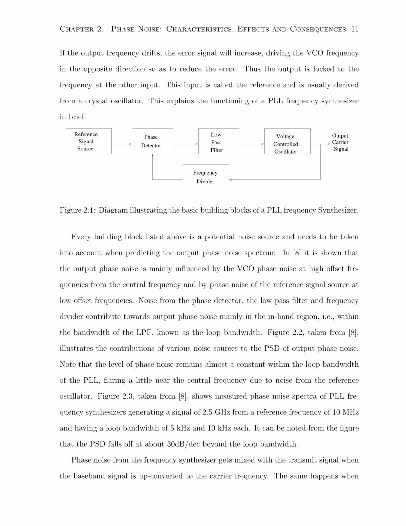
2.1 Diagram illustrating the basic building blocks of a PLL frequency Synthe-
sizer. . . . . . . . . . . . . . . . . . . . . . . . . . . . . . . . . . . . . . . 11
2.2 Figure illustrating contributions to phase noise spectrum from various
sources [8]. . . . . . . . . . . . . . . . . . . . . . . . . . . . . . . . . . . . 12
2.3 Measured phase noise spectra of PLL frequency synthesizers generating a
signal of 2.5 GHz from a reference frequency of 10 MHz and having a loop
bandwidth of 5 kHz in (a) and 10 kHz in (b) [8]. . . . . . . . . . . . . . . 13
2.4 Figure illustrating transmitted and received vectors in an Nr ×Nt MIMO
link. . . . . . . . . . . . . . . . . . . . . . . . . . . . . . . . . . . . . . . 22
2.5 Plot illustrating the effect of the CPE and ICI on bit error probability of
a coded-OFDM system in a frequency selective fading channel. . . . . . . 28
2.6 Plot illustrating the effect of sampling rate on the probability of high CPE
events . . . . . . . . . . . . . . . . . . . . . . . . . . . . . . . . . . . . . 30
viii
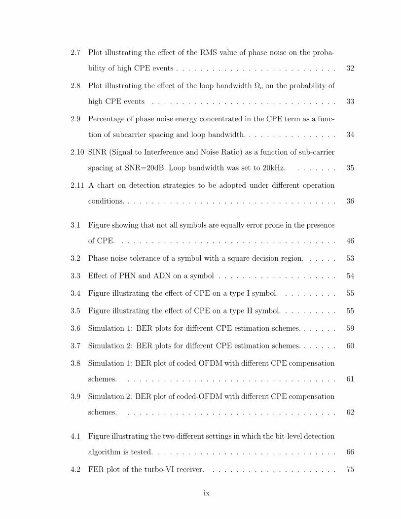
2.7 Plot illustrating the effect of the RMS value of phase noise on the proba-
bility of high CPE events . . . . . . . . . . . . . . . . . . . . . . . . . . . 32
2.8 Plot illustrating the effect of the loop bandwidth Ωo on the probability of
high CPE events . . . . . . . . . . . . . . . . . . . . . . . . . . . . . . . 33
2.9 Percentage of phase noise energy concentrated in the CPE term as a func-
tion of subcarrier spacing and loop bandwidth. . . . . . . . . . . . . . . . 34
2.10 SINR (Signal to Interference and Noise Ratio) as a function of sub-carrier
spacing at SNR=20dB. Loop bandwidth was set to 20kHz. . . . . . . . 35
2.11 A chart on detection strategies to be adopted under different operation
conditions. . . . . . . . . . . . . . . . . . . . . . . . . . . . . . . . . . . . 36
3.1 Figure showing that not all symbols are equally error prone in the presence
of CPE. . . . . . . . . . . . . . . . . . . . . . . . . . . . . . . . . . . . . 46
3.2 Phase noise tolerance of a symbol with a square decision region. . . . . . 53
3.3 Effect of PHN and ADN on a symbol . . . . . . . . . . . . . . . . . . . . 54
3.4 Figure illustrating the effect of CPE on a type I symbol. . . . . . . . . . 55
3.5 Figure illustrating the effect of CPE on a type II symbol. . . . . . . . . . 55
3.6 Simulation 1: BER plots for different CPE estimation schemes. . . . . . . 59
3.7 Simulation 2: BER plots for different CPE estimation schemes. . . . . . . 60
3.8 Simulation 1: BER plot of coded-OFDM with different CPE compensation
schemes. . . . . . . . . . . . . . . . . . . . . . . . . . . . . . . . . . . . 61
3.9 Simulation 2: BER plot of coded-OFDM with different CPE compensation
schemes. . . . . . . . . . . . . . . . . . . . . . . . . . . . . . . . . . . . 62
4.1 Figure illustrating the two different settings in which the bit-level detection
algorithm is tested. . . . . . . . . . . . . . . . . . . . . . . . . . . . . . . 66
4.2 FER plot of the turbo-VI receiver. . . . . . . . . . . . . . . . . . . . . . 75
ix
4.3 Figure illustrating the overall receiver design used to comprehensively sup-
press the effects of phase noise. . . . . . . . . . . . . . . . . . . . . . . . 77
4.4 FER plot of the turbo-VI receiver with CPE compensation. . . . . . . . . 77
4.5 FER plot of the turbo-VI receiver with perfect CPE compensation. . . . 79
4.6 FER plot comparing the performance of turbo-VI and DD-LMMSE re-
ceivers under different settings. . . . . . . . . . . . . . . . . . . . . . . . 80
5.1 Block diagram representing the SC-FDMA scheme and the use of a linear
receiver. Note that N > M , and usually, MN
= K, an integer representing
the number of users in the uplink. . . . . . . . . . . . . . . . . . . . . . . 82
5.2 Plot comparing the performance of interleaved and localized OFDMA/SC-
FDMA while using MMSE channel equalization. . . . . . . . . . . . . . . 86
5.3 Plot illustrating the performance of interleaved and localized SC-FDMA
when all channel coefficients are generated independently and when phase
noise is uncorrelated. . . . . . . . . . . . . . . . . . . . . . . . . . . . . 92
5.4 Plot illustrating the improvement in performance of an SC-FDMA system
affected by phase noise by cancelling self interference alone. . . . . . . . . 95
x
Chapter 1
Introduction
1.1 Introduction
Recent advances in wireless technologies such as multi-antenna multi-carrier systems,
coupled with a spurt in demand for wireless applications have led to significant increases
in data rates and transmission bandwidths. An immediate consequence of operating at
high data rates and high spectral efficiency is that receiver non-idealities such as phase
noise, frequency offset and IQ (In-Phase and Quadrature) imbalance effects, which were
either marginal or could be neglected previously, become significant and need to be
addressed. In this work we focus on the effects of phase noise on multi-carrier systems.
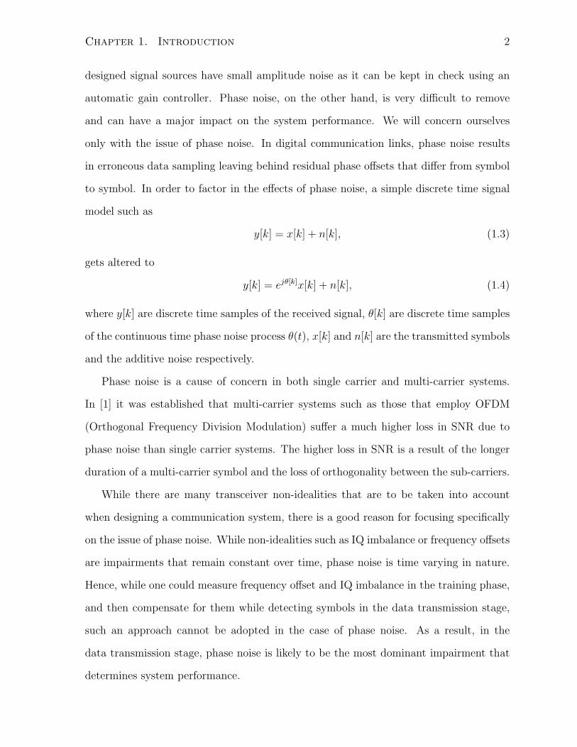
Phase noise (PHN) arises because of imperfections in the carrier frequency synthesizer.
While the output of an ideal frequency generator is given by
s(t) = A sin(ωt), (1.1)
the output of an actual generator is noisy and can be written as
s(t) = (A+ a(t)) sin(ωt+ θ(t)), (1.2)
where a(t) and θ(t) are amplitude and phase fluctuations. Amplitude noise does not
affect the zero crossings while phase noise does not affect the peak amplitude. Well
1
Chapter 1. Introduction 2
designed signal sources have small amplitude noise as it can be kept in check using an
automatic gain controller. Phase noise, on the other hand, is very difficult to remove
and can have a major impact on the system performance. We will concern ourselves
only with the issue of phase noise. In digital communication links, phase noise results
in erroneous data sampling leaving behind residual phase offsets that differ from symbol
to symbol. In order to factor in the effects of phase noise, a simple discrete time signal
model such as
y[k] = x[k] + n[k], (1.3)
gets altered to
y[k] = ejθ[k]x[k] + n[k], (1.4)
where y[k] are discrete time samples of the received signal, θ[k] are discrete time samples
of the continuous time phase noise process θ(t), x[k] and n[k] are the transmitted symbols
and the additive noise respectively.
Phase noise is a cause of concern in both single carrier and multi-carrier systems.
In [1] it was established that multi-carrier systems such as those that employ OFDM
(Orthogonal Frequency Division Modulation) suffer a much higher loss in SNR due to
phase noise than single carrier systems. The higher loss in SNR is a result of the longer
duration of a multi-carrier symbol and the loss of orthogonality between the sub-carriers.
While there are many transceiver non-idealities that are to be taken into account
when designing a communication system, there is a good reason for focusing specifically
on the issue of phase noise. While non-idealities such as IQ imbalance or frequency offsets
are impairments that remain constant over time, phase noise is time varying in nature.
Hence, while one could measure frequency offset and IQ imbalance in the training phase,
and then compensate for them while detecting symbols in the data transmission stage,
such an approach cannot be adopted in the case of phase noise. As a result, in the
data transmission stage, phase noise is likely to be the most dominant impairment that
determines system performance.
Chapter 1. Introduction 3
Characteristics of phase noise depend on the type of frequency generator that is being
used. Prior knowledge of the characteristics can play a vital role in mitigating the effects
of phase noise. Of the many possible ways of generating a reliable carrier signal, phase
locked loop (PLL) based frequency synthesizers are very widely used in most wireless
transceivers. PLL frequency synthesizers offer many advantages over the use of other
forms of local oscillator such as high levels of stability, ease of control through digital
circuitry and higher accuracy. In our work we assume that a PLL based frequency
synthesizer is used to generate the required carrier frequency and will restrict ourselves
to the phase noise characteristics corresponding to such a signal source.
Addressing the practical concerns that arise while designing a transceiver is vital
in ensuring optimal performance of the communication link. While better hardware
designs can alleviate these non-idealities to some extent, it is still important to develop
schemes that can mitigate these effects in the digital domain. Given that phase noise
is an unavoidable phenomenon, it is important to have a thorough understanding of its
effects on the performance of a transceiver. Developing better detection schemes and
computationally efficient algorithms that can estimate and compensate for the effects of
phase noise can have a significant impact on the link performance and can also relax
stringent hardware design constraints.
The next section outlines the various aspects of phase noise, its effects on system
performance and strategies to mitigate these effects that have been addressed in this
thesis.
1.2 Thesis Overview
Phase noise in OFDM/OFDMA systems has received widespread attention over the last
few years. While many researchers have identified the two major consequences of phase
noise as being the rotation of transmitted symbols by a small angle called the common
Chapter 1. Introduction 4
phase error (CPE) and the mixing of signals on adjacent sub-carriers resulting in inter-
carrier interference (ICI), very little attention has been paid to identify which of the two
effects is likely to dominate under different operating conditions. This aspect has a direct
influence on the choice of algorithms to be adopted for symbol detection. This is the
first issue that we address in our work. We identify circumstances under which effects
of CPE may dominate over ICI and vice versa, and provide guidelines with respect to
the choice of parameters and the set of algorithms that one needs to adopt while dealing
with phase noise.
Traditionally, it was common to embed pilot symbols amongst the data symbols
within a single OFDM symbol. This was done so as to aid channel estimation of a time
varying channel. Many works in the past have taken advantage of these pilot symbols to
aid detection of data symbols in the presence of phase noise. But recently, new wireless
standards such as WiMAX (Worldwide Interoperability for Microwave Access, IEEE
802.16) and LTE (3rd Generation Partnership Project Long Term Evolution, put forth
by European Telecommunications Standards Institute) have chosen to adopt a different
distribution of pilot symbols. While WiMAX embeds pilots only in two out of every
three consecutive OFDM symbols, in LTE one full OFDM symbol is devoted to channel
estimation once every seven time slots. Thus, there arise situations where we need to
consider symbol detection without the aid of pilot symbols in each OFDM symbol. In
our work, we exclusively focus on the situation where there are no pilot subcarriers in
an OFDM symbol. Since the case of OFDM symbols with pilots can be very easily
incorporated into algorithms we develop for data detection and phase noise estimation,
the scenario we focus on subsumes all possible distributions of pilots.
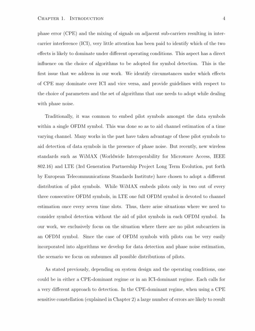
As stated previously, depending on system design and the operating conditions, one
could be in either a CPE-dominant regime or in an ICI-dominant regime. Each calls for
a very different approach to detection. In the CPE-dominant regime, when using a CPE
sensitive constellation (explained in Chapter 2) a large number of errors are likely to result
Chapter 1. Introduction 5
due to uncompensated CPE. Hence, it is very important to estimate and compensate
for CPE before detecting symbols. While estimation of CPE is straightforward in the
presence of pilots, blind estimation poses some challenges. We propose a blind CPE
estimation algorithm whose operating range, i.e., the ability to correctly estimate high
CPEs, is much better than existing algorithms. This algorithm stems from the realization
that not all sub-carrier symbols in an OFDM symbol are equally affected by CPE. In
the CPE-dominant regime, interference is likely to be limited to only a few adjacent
sub-carriers and does not significantly affect performance. It suffices to adopt a simple
ICI mitigation scheme such as that suggested in [2,3]. The proposed detection strategy is
illustrated in Figure 1.1. A detailed analysis on the effects and behaviour of CPE forms
the second part of the thesis.
FEC DecoderSymbol detector
(with ICI cancellation)
Robust CPE estimation
and compensation
(see Chapter 3)
Figure 1.1: Block diagram representing the proposed detection scheme for a CPE sensitive
constellation in a CPE-dominant regime.
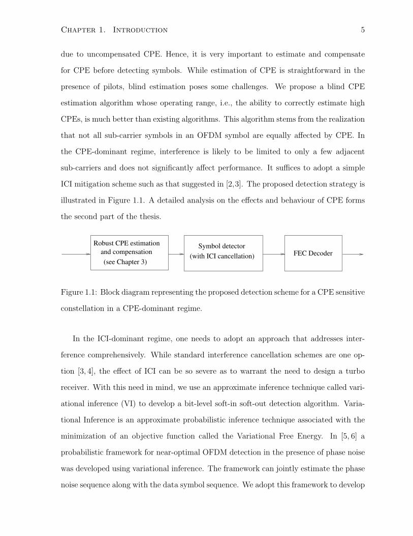
In the ICI-dominant regime, one needs to adopt an approach that addresses inter-
ference comprehensively. While standard interference cancellation schemes are one op-
tion [3, 4], the effect of ICI can be so severe as to warrant the need to design a turbo
receiver. With this need in mind, we use an approximate inference technique called vari-
ational inference (VI) to develop a bit-level soft-in soft-out detection algorithm. Varia-
tional Inference is an approximate probabilistic inference technique associated with the
minimization of an objective function called the Variational Free Energy. In [5, 6] a
probabilistic framework for near-optimal OFDM detection in the presence of phase noise
was developed using variational inference. The framework can jointly estimate the phase
noise sequence along with the data symbol sequence. We adopt this framework to develop
Chapter 1. Introduction 6
a bit-level SISO algorithm and set up a joint iterative detection-decoding procedure that
is very effective in nullifying the interference resulting due to phase noise. The proposed
detection scheme is illustrated in Figure 1.2. Although CPE does not dominate in an ICI-
dominant regime, it cannot be completely neglected and hence, a CPE pre-compensation
block is included in the detection scheme. The choice of CPE compensation algorithm
depends on the symbol constellation being used, this is discussed in Chapter 2. Develop-
ment of the SISO detection algorithm and setting up the turbo receiver forms the third
part of the thesis.
FEC DecoderSignal Vector
ReceivedCPE Estimation
and Compensation
([15]/Chapter 3)
Soft−in Soft−out Symbol
Detector (Chapter 4)
Figure 1.2: Block diagram representing the proposed detection strategy in an ICI-
dominant regime.
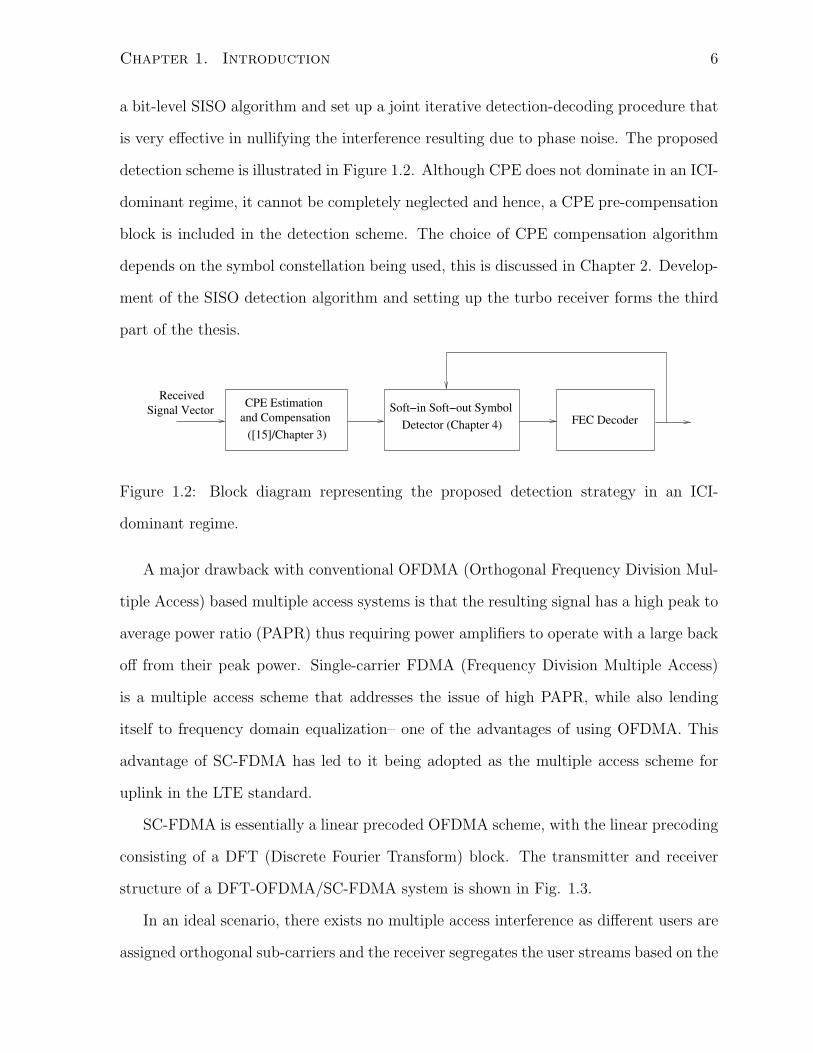
A major drawback with conventional OFDMA (Orthogonal Frequency Division Mul-
tiple Access) based multiple access systems is that the resulting signal has a high peak to
average power ratio (PAPR) thus requiring power amplifiers to operate with a large back
off from their peak power. Single-carrier FDMA (Frequency Division Multiple Access)
is a multiple access scheme that addresses the issue of high PAPR, while also lending
itself to frequency domain equalization– one of the advantages of using OFDMA. This
advantage of SC-FDMA has led to it being adopted as the multiple access scheme for
uplink in the LTE standard.
SC-FDMA is essentially a linear precoded OFDMA scheme, with the linear precoding
consisting of a DFT (Discrete Fourier Transform) block. The transmitter and receiver
structure of a DFT-OFDMA/SC-FDMA system is shown in Fig. 1.3.
In an ideal scenario, there exists no multiple access interference as different users are
assigned orthogonal sub-carriers and the receiver segregates the user streams based on the
Chapter 1. Introduction 7
N point
DFT
DFT
M point
M point ADC/
Mapping
DAC/
RF
RF
P to
S
S to
P
Sub carrier
De−mapping
Symbol
Stream IDFT
Sub carrier
S to
P
CHANNEL
Channel
Equalization
N point
IDFTDETECTOR
Figure 1.3: Block diagram representing the SC-FDMA scheme. Note that M > N , and
usually, MN
= K, an integer representing the number of users in the uplink.
sub-carrier allocation. In the presence of phase noise, the orthogonality between the sub-
carriers is lost, and this leads to multiple access interference. We use the term multiple
access interference to include the inter-symbol interference within a user’s stream as well
as inter-symbol interference across other active users.
While the effect of phase noise on OFDM/OFDMA has received a lot of attention,
its effect on SC-FDMA is not completely understood. In order to better understand the
effect of phase noise on SC-FDMA, we develop a signal model to analyze the effect of
phase noise on SC-FDMA and characterize the effects along with suggestions on strategies
to adopt while dealing with the detection of an SC-FDMA symbol affected by phase noise.
This forms the last part of the thesis.
1.3 Notation
We adopt the following notation all through this thesis:
All vectors and matrices are represented in bold font, e.g. x, M. Vectors are
represented using lower case while matrices are represented using upper case. The
notation x(1:k) is used to represent the length-k vector formed using the first k
Chapter 1. Introduction 8
entries of x. The notation M(1:k, 1:k) represents the submatrix formed using the
first k rows and first k columns of M .
Discrete time processes are represented using the name of the process followed
by the index in square brackets, e.g. x[n], y[n]. Continuous time processes are
represented using the name of the process followed by round parentheses, e.g. x(t),
y(t).
If M is a matrix, MT and MH represent the transpose and the Hermitian transpose
of the matrix, respectively; tr(M) represents the trace of the matrix and diag(M)
represents the diagonal matrix formed using the diagonal entries of M. <(M) and
=(M) represent the matrices formed using the real and imaginary parts of M
respectively.
If x is a vector, <(x) and =(x) represent the vectors formed using the real and imag-
inary parts of x respectively, and diag(x) represents the diagonal matrix formed
using the vector x.
The identity matrix is denoted as I.
The expectation of a random variable x is denoted as E[x].
N (µ, σ2) is used to denote the Gaussian distribution and CN (µ, σ2) is used to
denote the circular symmetrix complex Gaussian distribution. σ2 in the second
case donotes the expectation E[|x-E[x]|2], where x is a circular symmetrix complex
Gaussian distributed random variable.
Chapter 2
Phase Noise: Characteristics, Effects
and Consequences
This chapter deals with various aspects of phase noise. We briefly discuss how phase
noise arises in a frequency synthesizer and characterize its power spectral density (PSD).
Based on the observations made, we introduce a commonly used model for generating
phase noise and contrast it with other models. We then take note of the properties of a
discrete time phase noise sequence, such as, the auto-correlation function, sample mean
statistics etc. We present the signal model of a multi-carrier system affected by phase
noise at the transmitter as well as the receiver. We further investigate the scenario where
the signal is corrupted only by receiver side phase noise and break down the effects of
phase noise into rotation of symbols because of common phase error and inter-carrier
interference resulting from the higher order components of phase noise. Finally, we
proceed to identify scenarios where the effect of CPE dominates over the effect of higher
order components and lay down some guiding principles that aid system design.
New contributions in this chapter include an in-depth analysis of the behaviour of
CPE as a function of various system and hardware parameters, identification of issues
that arise due to high CPE events and computing the frequency of such events. Based on
9
Chapter 2. Phase Noise: Characteristics, Effects and Consequences 10
this analysis certain guidelines for phase noise estimation and mitigation are established.
2.1 Introduction
To cater to demands for higher data rates within a limited bandwidth, many new stan-
dards have adopted higher order modulation schemes such as 64-QAM and also techniques
such as OFDM to transmit effectively over a frequency selective channel. Use of higher-
order constellations along with multi-carrier systems brings to the forefront the issue of
phase noise that can severely limit the system performance. Phase noise is generated
at the frequency signal source which can either be a simple free running oscillator or a
frequency synthesizer. Since the power spectral density of phase noise directly affects the
amount of ICI1, the PSD of phase noise has received a lot of attention. The noise sources
in all building blocks of a signal source contribute towards the PSD of phase noise. In
many works, the phase noise spectrum of a free running oscillator was assumed to fall off
as 1/f 2 from the central frequency, but this assumption was shown to be not accurate
in [7].
In most wireless applications, PLL frequency synthesizers are the preferred form of
signal source primarily because of higher levels of stability and easy control through
digital circuitry. Secondly, it allows one to generate a wide range of very high carrier
frequencies from oscillators tuned to much lower frequencies. The major building blocks
of a PLL frequency synthesizer include a reference signal source, a phase detector, a
low pass filter, a VCO and frequency dividers and multipliers. As shown in Figure 2.1,
the phase detector compares two input signals and produces an error signal which is
proportional to their phase difference. This signal is passed through the low pass filter
(LPF) and used to drive a voltage controlled oscillator which creates the output frequency.
The output frequency is fed through a frequency divider back to the input of the system.
1Larger bandwidth phase noise causes more ICI, as shown later.
Chapter 2. Phase Noise: Characteristics, Effects and Consequences 11
If the output frequency drifts, the error signal will increase, driving the VCO frequency
in the opposite direction so as to reduce the error. Thus the output is locked to the
frequency at the other input. This input is called the reference and is usually derived
from a crystal oscillator. This explains the functioning of a PLL frequency synthesizer
in brief.
Phase
Detector
Voltage
Controlled
Oscillator
Low
Pass
Filter
Frequency
Divider
Reference
Signal
SourceCarrier Output
Signal
Figure 2.1: Diagram illustrating the basic building blocks of a PLL frequency Synthesizer.
Every building block listed above is a potential noise source and needs to be taken
into account when predicting the output phase noise spectrum. In [8] it is shown that
the output phase noise is mainly influenced by the VCO phase noise at high offset fre-
quencies from the central frequency and by phase noise of the reference signal source at
low offset frequencies. Noise from the phase detector, the low pass filter and frequency
divider contribute towards output phase noise mainly in the in-band region, i.e., within
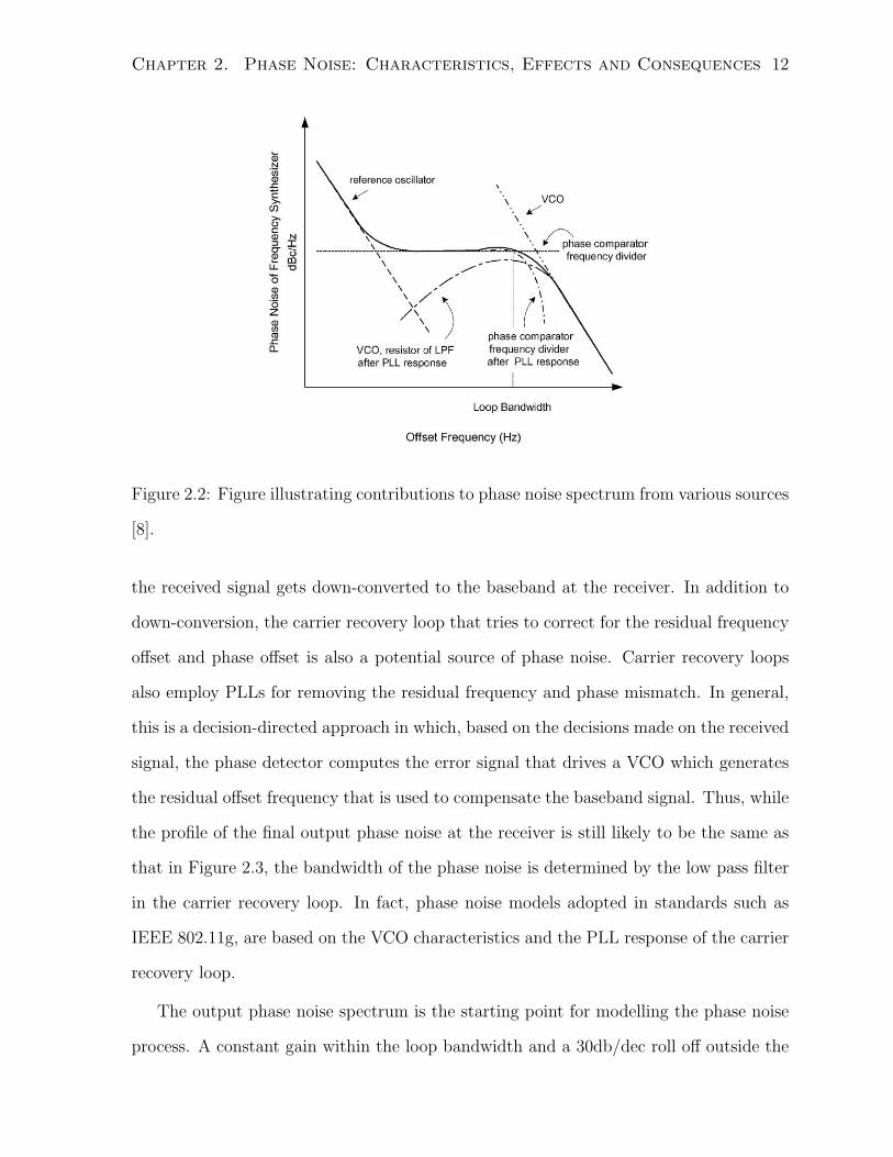
the bandwidth of the LPF, known as the loop bandwidth. Figure 2.2, taken from [8],
illustrates the contributions of various noise sources to the PSD of output phase noise.
Note that the level of phase noise remains almost a constant within the loop bandwidth
of the PLL, flaring a little near the central frequency due to noise from the reference
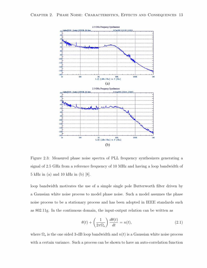
oscillator. Figure 2.3, taken from [8], shows measured phase noise spectra of PLL fre-
quency synthesizers generating a signal of 2.5 GHz from a reference frequency of 10 MHz
and having a loop bandwidth of 5 kHz and 10 kHz each. It can be noted from the figure
that the PSD falls off at about 30dB/dec beyond the loop bandwidth.
Phase noise from the frequency synthesizer gets mixed with the transmit signal when
the baseband signal is up-converted to the carrier frequency. The same happens when
Chapter 2. Phase Noise: Characteristics, Effects and Consequences 12
Figure 2.2: Figure illustrating contributions to phase noise spectrum from various sources
[8].
the received signal gets down-converted to the baseband at the receiver. In addition to
down-conversion, the carrier recovery loop that tries to correct for the residual frequency
offset and phase offset is also a potential source of phase noise. Carrier recovery loops
also employ PLLs for removing the residual frequency and phase mismatch. In general,
this is a decision-directed approach in which, based on the decisions made on the received
signal, the phase detector computes the error signal that drives a VCO which generates
the residual offset frequency that is used to compensate the baseband signal. Thus, while
the profile of the final output phase noise at the receiver is still likely to be the same as
that in Figure 2.3, the bandwidth of the phase noise is determined by the low pass filter
in the carrier recovery loop. In fact, phase noise models adopted in standards such as
IEEE 802.11g, are based on the VCO characteristics and the PLL response of the carrier
recovery loop.
The output phase noise spectrum is the starting point for modelling the phase noise
process. A constant gain within the loop bandwidth and a 30db/dec roll off outside the
Chapter 2. Phase Noise: Characteristics, Effects and Consequences 13
Figure 2.3: Measured phase noise spectra of PLL frequency synthesizers generating a
signal of 2.5 GHz from a reference frequency of 10 MHz and having a loop bandwidth of
5 kHz in (a) and 10 kHz in (b) [8].
loop bandwidth motivates the use of a simple single pole Butterworth filter driven by
a Gaussian white noise process to model phase noise. Such a model assumes the phase
noise process to be a stationary process and has been adopted in IEEE standards such
as 802.11g. In the continuous domain, the input-output relation can be written as
θ(t) +
(1
2πΩo
)dθ(t)
dt= n(t), (2.1)
where Ωo is the one sided 3-dB loop bandwidth and n(t) is a Gaussian white noise process
with a certain variance. Such a process can be shown to have an auto-correlation function
Chapter 2. Phase Noise: Characteristics, Effects and Consequences 14
of the form
Rθ(t) = Rθ(0)e−2πΩo|t|. (2.2)
In the discrete domain, such a model corresponds to a first order auto-regressive
process that can be represented as
θ[k] = (1− a)θ[k − 1] + (a)n[k], (2.3)
which has an an autocorrelation function of the form
Rθ[k −m] = Rθ[0](1− a)|k−m|. (2.4)
The discrete time model and the continuous time model are related through the
equation
1
2πΩoTs=
1− aa
, (2.5)
where we have assumed the sampling rate to be 1/Ts. If we solve for ‘a’ using (2.5) and
substitute in (2.4), we get
Rθ[k −m] = Rθ[0]
(1
1 + 2πΩoTs
)|k−m|. (2.6)
To reconcile the difference in (2.2) and (2.6), note that, in general, the loop bandwidth
tends to be in the range of tens of kHz and the sampling rate Ts in the range of a few MHz.
As a result, we have 2πΩoTs 1, which enables us to write e−2πΩo|t| ≈(
11+2πΩoTs
)t/Ts,
this establishes the equivalence between the two auto-correlation functions.
In [5], the discrete time auto-correlation function of phase noise was assumed to be
of the form
Rθ[k] = Rθ[0]e−2πΩoTs|k|, (2.7)
which is essentially a sampled version of (2.2). Having established the equivalence be-
tween the continuous and the discrete time models, it should make no difference whether
one uses (2.6) or (2.7) to represent the discrete time autocorrelation function. We use
(2.7) as the auto-correlation function of phase noise all through our work. We however
Chapter 2. Phase Noise: Characteristics, Effects and Consequences 15
note that phase noise samples generated through a computer simulation will have an
auto-correlation function that is dependent on the exact type of digital Butterworth fil-
ter used to generate phase noise. While in most designs the auto-correlation function will
very closely resemble (2.7), there is bound to be some difference depending on the exact
digital filter used. The digital Butterworth filter we used had one pole and one zero.
In practice, most PLL frequency synthesizers come with design specifications that
include the root-mean-square (RMS) value of the output phase noise process, this gives
us the value of Rθ[0]. Denoting the RMS value in radians as σθ, we have Rθ[0] = σ2θ .
Even if the RMS value is unknown, simple measurements on the output signal of the
synthesizer can be made to measure the actual RMS value, as outlined in [9]. Typically,
the RMS value is between 1-3.
At this stage, we would like to point out that most of the existing work in addressing
phase noise assumes a Wiener model (Random walk) for phase noise. Such a model is
only appropriate when the carrier signal is generated from a stand alone local oscillator.
Such a design is almost never adopted as a free running oscillator can slowly drift away
from the required phase and frequency. Such a model corresponds to a non-stationary
process whose variance increases linearly with time.
Another assumption made, which was probably necessitated by the use of the Wiener
model, is that perfect phase synchronization exists at the start of every multi-carrier
symbol. Without this assumption there is the possibility of seeing very large drifts in the
phase of the carrier signal, which can make it impossible to detect the transmitted data.
Such an assumption is impractical since frequency and phase matching is done at the
start of the transmission of a payload or packet, and as a result perfect synchronization
at the start of every symbol cannot be guaranteed. The use of a stationary phase noise
model does not force this assumption, thus catering better to the practical scenario. The
next section discusses some statistical properties of a phase noise sequence generated
using the proposed model.
Chapter 2. Phase Noise: Characteristics, Effects and Consequences 16
2.2 Statistical Properties
We are interested in the statistical properties of a discrete time phase noise sequence of
length N , obtained by sampling the continuous time phase noise at the rate of 1/Ts. It
is easy to see from (2.3) that since n[k] is a zero mean Gaussian white noise process, the
resulting phase noise sequence is also zero mean.
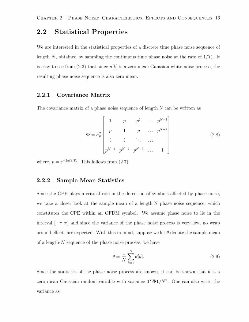
2.2.1 Covariance Matrix
The covariance matrix of a phase noise sequence of length N can be written as
Φ = σ2θ
1 p p2 . . . pN−1
p 1 p . . . pN−2
......
. . . . . .
pN−1 pN−2 pN−3 . . . 1
(2.8)
where, p = e−2πΩoTs . This follows from (2.7).
2.2.2 Sample Mean Statistics
Since the CPE plays a critical role in the detection of symbols affected by phase noise,
we take a closer look at the sample mean of a length-N phase noise sequence, which
constitutes the CPE within an OFDM symbol. We assume phase noise to lie in the
interval [−π π) and since the variance of the phase noise process is very low, no wrap
around effects are expected. With this in mind, suppose we let θ denote the sample mean
of a length-N sequence of the phase noise process, we have
θ =1
N
N∑k=1
θ[k]. (2.9)
Since the statistics of the phase noise process are known, it can be shown that θ is a
zero mean Gaussian random variable with variance 1TΦ1/N2. One can also write the
variance as
Chapter 2. Phase Noise: Characteristics, Effects and Consequences 17
σ2θ = 1TΦ1/N2 =
σ2θ
N2
(1 + p
1− pN −2p(1− pN)
(1− p)2
)(2.10)
2.3 Signal Model
In this section we show how the presence of phase noise affects the signal model of an
OFDM symbol transmitted through a frequency selective channel. We first consider
a single antenna, point to point link with a frequency selective channel between the
transmitter and the receiver. The frequency selective channel is assumed to vary slowly
and remain constant over the duration of an OFDM symbol. We assume no residual
frequency offsets to be present in the received signal. By estimating the residual frequency
offset in the training phase and compensating for it in the data transmission phase, we
can ensure that almost no residual frequency offsets are seen. We also assume that
current channel conditions have been estimated during the training phase and that the
channel state information is available at the receiver. Algorithms that can estimate the
channel in the presence of phase noise and carrier frequency offset have been presented
in [9, 10]. Since phase noise is an impairment at both the transmitter and the receiver,
two immediate cases arise, both of which are discussed in detail below.
2.3.1 Receiver Phase Noise
We first consider the case where there is only receiver phase noise affecting the signal.
Let N be the number of sub-carriers and let the channel have L taps. Let F be the
N × N DFT matrix with the (l,m)th entry given by (1/√N)e−(2πjlm/N), with indices l
and m going from 0 to N − 1. Let d = [d0 d1 . . . dN−1]T be the data vector and let
s = [s0 s1 . . . sN+L−1]T with [s0 s1 . . . sL−1]T = [sN sN+1 . . . sN+L−1]T , be the vector to
be transmitted after appending the cyclic prefix. The vector s without the cyclic prefix
is simply the IDFT of the data vector d i.e., FHd.
Chapter 2. Phase Noise: Characteristics, Effects and Consequences 18
Let θr = [θr0 θr1 . . . θrN+L−1]T be the phase noise sequence affecting the received signal
and let pr = [ejθr0 ejθ
r1 . . . ejθ
rN+L−1 ]T . Let the vector g = [g0 g1 . . . gL−1]T represent the
impulse response of the time domain channel. The received signal in discrete time after
appropriate sampling can be represented as
r = diag(pr)Gs + n, (2.11)
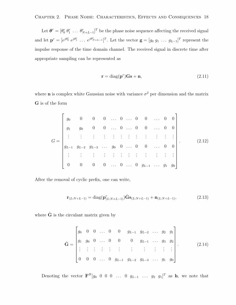
where n is complex white Gaussian noise with variance σ2 per dimension and the matrix
G is of the form
G =
g0 0 0 0 . . . 0 . . . 0 0 . . . 0 0
g1 g0 0 0 . . . 0 . . . 0 0 . . . 0 0
......
......
......
......
......
......
gL−1 gL−2 gL−3 . . . g0 0 . . . 0 0 . . . 0 0
......
......
......
......
......
......
0 0 0 0 . . . 0 . . . 0 gL−1 . . . g1 g0
. (2.12)
After the removal of cyclic prefix, one can write,
r(L:N+L−1) = diag(pr(L:N+L−1))Gs(L:N+L−1) + n(L:N+L−1), (2.13)
where G is the circulant matrix given by
G =
g0 0 0 . . . 0 0 gL−1 gL−2 . . . g2 g1
g1 g0 0 . . . 0 0 0 gL−1 . . . g3 g2
......
......
......
......
......
...
0 0 0 . . . 0 gL−1 gL−2 gL−3 . . . g1 g0
. (2.14)
Denoting the vector FH [g0 0 0 0 . . . 0 gL−1 . . . g2 g1]T as h, we note that
Chapter 2. Phase Noise: Characteristics, Effects and Consequences 19
H=diag(h)= FGFH . Now, the DFT of the received signal is given by
Fr(L:N+L−1) =Fdiag(pr(L:N+L−1))GFHd + Fn(L:N+L−1) (2.15)
=Fdiag(pr(L:N+L−1))FHFGFHd + Fn(L:N+L−1) (2.16)
=Fdiag(pr(L:N+L−1))FHHd + Fn(L:N+L−1) (2.17)
=QrHd + Fn(L:N+L−1) (2.18)
where, Fdiag(pr(L:N+L−1))FH is a circulant matrix and is denoted by Qr. It can be shown
that Fn(L:N+L−1) is an uncorrelated white noise vector distributed as CN (0, 2σ2I). The
rows of Qr are circular shifts of the frequency domain representation of the phase noise
vector given by 1√N
FHpr(L:N+L−1). We define the vector c=[c0 c1 . . . cN−1]T to be
c =1√N
FHpr(L:N+L−1), (2.19)
and note that the lower order frequency components of phase noise are given by c1, cN−1,
c2, cN−2 etc. Using the vector c, the kth component of (2.18) can be written as
(Fr(L:N+L−1)
)k
= c0dkhk +N−1∑
l=0,l 6=k
dlhlc(l−k)mod N +(Fn(L:N+L−1)
)k. (2.20)
Equation (2.20) clearly illustrates how phase noise affects the received signal. Note
that c0 is the common phase error given by
1
N
k=N+L−1∑k=L
ejθk ≈ 1 +1
N
∑θk = 1 + jθ. (2.21)
Its effect is to rotate every received symbol by the average phase angle θ. The other
effect is the inter-carrier interference resulting due to the higher order components of
phase noise. We collectively refer to the components c1, c2, . . . , cN−1 as the higher
order components of phase noise. Another pertinent observation to be made is that the
phase noise sequence affecting the cyclic prefix does not play a role in detection. This is
not the case with transmitter phase noise as we shall see next.
Chapter 2. Phase Noise: Characteristics, Effects and Consequences 20
2.3.2 Transmitter Phase Noise
Let θt = [θt0 θt1 . . . θtN+L−1]T be the phase noise sequence affecting the transmitted
signal and let pt = [ejθt0 ejθ
t1 . . . ejθ
tN+L−1 ]T . Then, the transmitted signal is given by
diag(pt)s, and it can be noted right away that the transmitted signal is no longer cyclic
and as a result the received signal will not be completely ICI free. Defining ptcyc =
[ejθtN ejθ
tN+1 . . . eθ
tN+L−1 eθ
tL eθ
tL+1 . . . eθ
tN+L−1 ]T , where we have replaced the first L
components of pt with its last L components, the received signal can be written as
r =Gdiag(pt)s + n (2.22)
=Gdiag(ptcyc)s + Gdiag(pt − ptcyc)s + n (2.23)
After removing the cyclic prefix and taking the DFT of the received signal, we get
Fr(L:N+L−1) =FGFHFdiag(pt(L:N+L−1))FHd (2.24)
+ FG(L:N+L−1,0:N+L−1)diag(pt − ptcyc)s + Fn(L:N+L−1)
=HQtd + FG(L:N+L−1,0:N+L−1)diag(pt − ptcyc)s + Fn(L:N+L−1) (2.25)
=HQtd + FG(L:N+L−1,0:L−1)diag((pt − ptcyc)(0:L−1))s(0:L−1) + Fn(L:N+L−1),
(2.26)
where Qt is Fdiag(pt(L:N+L−1))FH . As one can see from (2.26), the effect of transmitter
phase noise on the received signal is a little different when compared to that of receiver
phase noise. While the effect of CPE is still the same, ICI results not only from the higher
order components of phase noise but also because of the loss of the cyclic nature of the
transmitted signal, which manifests itself as the second term in (2.26). Further, one can
see that the phase noise affecting the cyclic prefix also contributes towards ICI and hence
any scheme that looks at mitigating ICI needs to consider the whole phase noise sequence
of length N+L as opposed to considering just the length-N phase noise sequence as in
the case of receiver phase noise. The additional ICI term has been erroneously left out
in many papers that try to address the issue of transmitter phase noise.
Chapter 2. Phase Noise: Characteristics, Effects and Consequences 21
Suppose one were to ignore the second term in (2.26), the DFT of the received signal
in the presence of both transmitter and receiver phase noise can be written as
Fr(L:N+L−1) = QrHQtd + Fn(L:N+L−1). (2.27)
Letting ct0 represent the CPE of transmit side phase noise and cr0 represent the receive
side CPE, and denoting (Qr − cr0I) as Qr
and (Qt − ct0I) as Qt, we can write (2.27) as
Fr(L:N+L−1) =(Qr
+ cr0I)H(Qt+ ct0I)d + Fn(L:N+L−1) (2.28)
=(cr0I)H(ct0I)d + QrH(ct0I)d + (cr0I)HQ
td + Fn(L:N+L−1) (2.29)
=(cr0ct0)Hd + ct0Q
rHd + cr0HQ
td + Q
rHQ
td + Fn(L:N+L−1). (2.30)
This equation explicitly shows the combined effect of transmitter and receiver CPE
on the received signal. Since transmitter and receiver CPEs jointly rotate the received
symbols, we can use a single CPE estimation scheme to estimate both the CPEs. While
the algorithm developed in Chapter 3 is used to compensate for receive side CPE, the
same algorithm can be used to jointly estimate the effective CPE by taking into the
account the statistics of both the CPEs.
2.3.3 Multiple Antenna Scenario
In the case of a point to point MIMO scenario, we assume that a single frequency synthe-
sizer generates the carrier signal for all the RF (radio frequency) chains. Thus, signals
transmitted from/received at all the antennas are affected by the same phase noise se-
quence. Suppose a MIMO link consists of Nt transmit antennas and Nr receive antennas
with Nt > Nr, we split an (NNt) length data vector d into Nt vectors of length N each,
as shown in 2.31, where each dk denotes the data vector for the kth antenna. The IDFT
of the data vector is given by
Chapter 2. Phase Noise: Characteristics, Effects and Consequences 22
[d11 d12 . . . d1N ]→[s11 s12 . . . s1N ]
[d21 d22 . . . d2N ]→[s21 s22 . . . s2N ]
[dNt1 dNt2 . . . dNtN ]→[sNt1 sNt2 . . . sNtN ]
[r11 r12 . . . r1N ]
[r21 r22 . . . r2N ]
[rNr1 rNr2 . . . rNrN ]
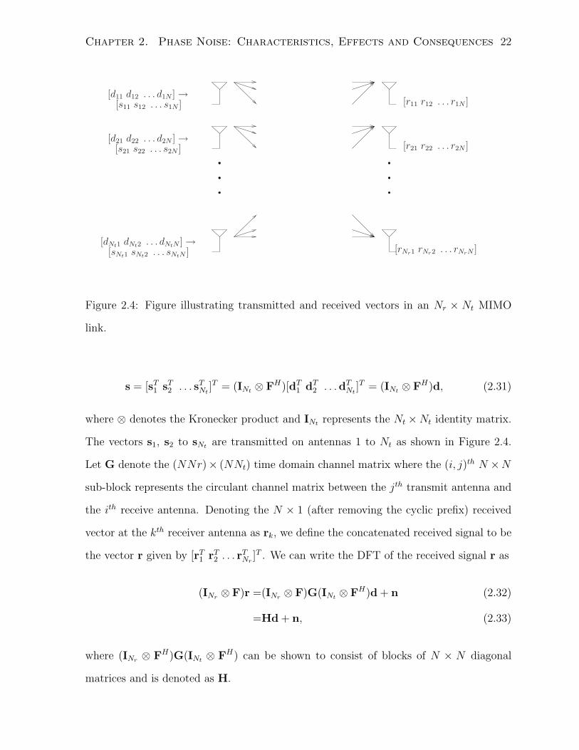
Figure 2.4: Figure illustrating transmitted and received vectors in an Nr × Nt MIMO
link.
s = [sT1 sT2 . . . sTNt ]T = (INt ⊗ FH)[dT1 dT2 . . .dTNt ]
T = (INt ⊗ FH)d, (2.31)
where ⊗ denotes the Kronecker product and INt represents the Nt ×Nt identity matrix.
The vectors s1, s2 to sNt are transmitted on antennas 1 to Nt as shown in Figure 2.4.
Let G denote the (NNr)× (NNt) time domain channel matrix where the (i, j)th N ×Nsub-block represents the circulant channel matrix between the jth transmit antenna and
the ith receive antenna. Denoting the N × 1 (after removing the cyclic prefix) received
vector at the kth receiver antenna as rk, we define the concatenated received signal to be
the vector r given by [rT1 rT2 . . . rTNr
]T . We can write the DFT of the received signal r as
(INr ⊗ F)r =(INr ⊗ F)G(INt ⊗ FH)d + n (2.32)
=Hd + n, (2.33)
where (INr ⊗ FH)G(INt ⊗ FH) can be shown to consist of blocks of N × N diagonal
matrices and is denoted as H.
Chapter 2. Phase Noise: Characteristics, Effects and Consequences 23
In the presence of receiver phase noise pr 2, the expression for the received signal can
be written as
(INr ⊗ F)r =(INr ⊗ F)(INr ⊗ diag(pr))G(INt ⊗ FH)d + n (2.34)
=(INr ⊗ F)(INr ⊗ diag(pr))G(INt ⊗ FH)Hd + n, (2.35)
Using the identity (A⊗B)(C⊗D) = (AC⊗BD), we can write (2.35) as
(INr ⊗ F)r = (INr ⊗Qr)Hd + n, (2.36)
where Qr is as defined before. It is clear that even in the case of multiple antennas,
the effect of phase noise on the received signal is the same. CPE rotates the symbols
of interest by a certain angle while the higher order components of phase noise result in
ICI.
In the case of transmitter phase noise, it can be shown that the received signal can
be written as
(INr ⊗ F)r = H(INr ⊗Qt)d + n, (2.37)
while ignoring the additional interference term that results due to the loss of the cyclic
nature of the transmitted signal. An additional interference term very similar to that in
(2.26) results if one were to take the loss of cyclic nature of the transmitted signal into
account.
2.3.4 Multi-User Scenario : Uplink/Downlink
Since we have established the similarity between the effects phase noise has on SISO and
MIMO scenarios for a point to point link, we only discuss the SISO Multi-User scenario
here. It is easy to see that the cases of uplink and downlink OFDMA with receiver
phase noise, and downlink OFDMA with transmitter phase noise are all equivalent to
2pr is an N × 1 vector, we do not consider the phase noise affecting the cyclic prefix.
Chapter 2. Phase Noise: Characteristics, Effects and Consequences 24
single user scenarios because there is only one phase noise sequence affecting the received
signal. The case of uplink OFDMA with transmitter phase noise is quite different and
needs more attention. We discuss this particular case in more detail.
Let there be K users each of whom has been allocated M sub-carriers out of a total
of N sub-carriers. Denote the M × 1 symbol vector of the kth user as dk and the
concatenated symbol vector [dT1 dT2 . . .dTk ]T as d. The transmit vector (without the cyclic
prefix) corresponding to the kth user is given by
sk = Tkdk, (2.38)
where Tk is a N × M sub-carrier mapping matrix that assigns the M data symbols
to one of the M sub-carriers allocated to the user. Let Hk be the frequency domain
channel matrix corresponding to the channel between the kth user and the base station.
The overall received vector in the frequency domain, after the N -DFT operation can be
written as
Fr =K∑k=1
HkTkdk + n. (2.39)
In the presence of transmitter phase noise, the DFT of the received signal can be written
as
Fr =K∑k=1
HkQtkTkdk + n, (2.40)
where Qtk = Fdiag(ptk)F
H , ptk is the phase noise sequence corrupting the transmitted
signal at the kth user. In (2.40) we have ignored the additional ICI term that results due
to non-cyclic nature of the transmitted signal. It can be observed from (2.40) that symbols
corresponding to different users undergo a rotation corresponding to the CPE affecting
that user. In addition to CPE, ICI results from the mixing of data streams corresponding
to different users. Two immediate questions arise from the signal model. One is to find
out which user is likely to be the most disruptive in terms of the interference caused by
that particular user and two, to find out which user is most affected by a disruptive user.
Chapter 2. Phase Noise: Characteristics, Effects and Consequences 25
The kth user is likely to be disruptive if the off-diagonal terms in Qtk are significant, i.e.,
N−1∑l=1
E[|(ck)l|2] > N−1∑
l=1
E[|(cj)l|2] , for j = 1 to K, j 6= k. (2.41)
If a user is operating in a regime where the CPE term contains most of the energy of
the phase noise, then the higher order terms tend to be small. Since these higher order
components occupy the off-diagonal positions in Qtk, such a user is likely to cause very
little interference. On the other hand, if the higher order components of phase contain
most of the energy, off-diagonal entries in Qtk become significant and cause larger ICI.
Since a higher variance of the phase noise process can also lead to more energy in the
off-diagonal entries, a user suffering from severe phase noise is also likely to cause higher
interference. As to the question of which user suffers most because of the resulting ICI,
since the PSD of phase noise tapers off rapidly beyond the loop bandwidth, most of the
energy in a phase noise sequence is contained in the frequency components corresponding
to the first few orders. Hence, the largest contribution to interference on a particular
sub-carrier is likely to come from users occupying adjacent sub-carriers. As a result, users
occupying sub-carriers adjacent to a disruptive user are likely to suffer the most.
2.4 Relationship Between CPE and ICI
Having drawn attention to the two issues of rotation due to CPE and ICI due to the
higher order components, we now discuss the interplay between these two effects. Recall
that the average power of the phase noise sequence and in turn its frequency domain
representation is given by σ2θ , the square of the RMS value of the process. In the vector
c defined in (2.19), the first term c0 corresponds to CPE while the rest of the terms from
c1 to cN−1 contribute towards ICI. Since the total power is fixed, this means that the
two effects are coupled to each other i.e., if the variance of the CPE term is high, it in
turn means less ICI, and similarly more ICI means lesser variance in CPE. Before we go
any further, we would like to point out that hence forth the signal model that we will
Chapter 2. Phase Noise: Characteristics, Effects and Consequences 26
investigate in detail is the one corresponding to SISO point-to-point link with receiver
phase noise, as given in (2.20).
Having identified that the two effects are coupled to each other, we explore how
different parameters affect the energy split. We also try to define what a CPE-dominant
regime and an ICI-dominant regime are.
16-QAM
CPE % of errors
16 0% (0/16)
17 25% (4/16)
18 25% (4/16)
19 50% (8/16)
20 50% (8/16)
21 75% (12/16)
64-QAM
CPE % of errors
7 0% (0/64)
8 18.8% (12/64)
9 43.8% (28/64)
10 56.3% (36/64)
11 68.8% (44/64)
12 75% (48/64)
13 75% (48/64)
14 75% (48/64)
256-QAM
CPE % of errors
3 0% (0/256)
4 23.4% (60/256)
5 45.3% (116/256)
6 60.9% (156/256)
7 75% (192/256)
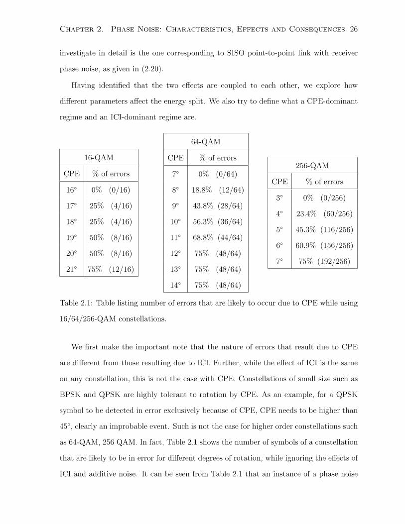
Table 2.1: Table listing number of errors that are likely to occur due to CPE while using
16/64/256-QAM constellations.
We first make the important note that the nature of errors that result due to CPE
are different from those resulting due to ICI. Further, while the effect of ICI is the same
on any constellation, this is not the case with CPE. Constellations of small size such as
BPSK and QPSK are highly tolerant to rotation by CPE. As an example, for a QPSK
symbol to be detected in error exclusively because of CPE, CPE needs to be higher than
45, clearly an improbable event. Such is not the case for higher order constellations such
as 64-QAM, 256 QAM. In fact, Table 2.1 shows the number of symbols of a constellation
that are likely to be in error for different degrees of rotation, while ignoring the effects of
ICI and additive noise. It can be seen from Table 2.1 that an instance of a phase noise
Chapter 2. Phase Noise: Characteristics, Effects and Consequences 27
sequence with CPE greater than 9 will cause a majority of the symbols of the 64-QAM
constellation to be detected in error. Thus, an instance of high CPE can be a potentially
catastrophic event where there could be lots of errors and recovery from such an event,
even with an error correcting code, might not be possible. This is what sets apart the
effect of CPE from that of ICI. While ICI behaves more like additive noise resulting in
a few random errors in every OFDM symbol, certain CPE events tend to cause errors in
bursts that affect the whole OFDM symbol. Since it can happen that the errors resulting
because of a high CPE event cannot be corrected even with an error correcting code,
these events determine the performance at high SNR and the error floor characteristics.
The key takeaway from this is that as far as CPE is concerned, close attention must be
paid to the frequency of high CPE events, where ‘high CPE’ is a constellation dependent
definition.
Another cause of concern is that any blind CPE estimation scheme involves an initial
step where the symbols are estimated while neglecting the presence of phase noise and
it is very important that a good fraction of symbols detected this way are not in error.
This step is key to blind CPE estimation and most existing algorithms are incapable of
reliably estimating CPE when this initial step contains many errors.
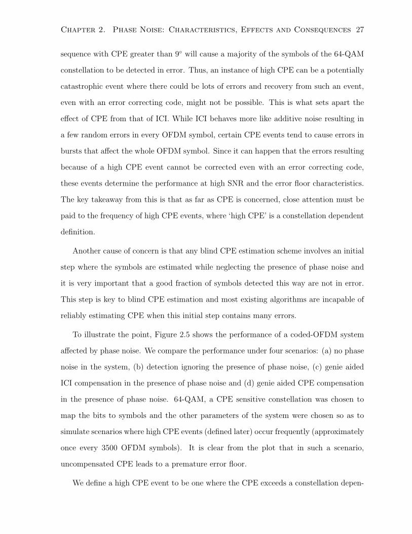
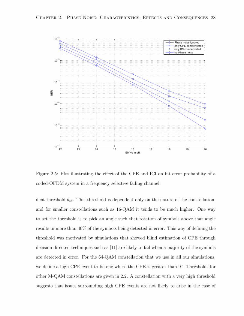
To illustrate the point, Figure 2.5 shows the performance of a coded-OFDM system
affected by phase noise. We compare the performance under four scenarios: (a) no phase
noise in the system, (b) detection ignoring the presence of phase noise, (c) genie aided
ICI compensation in the presence of phase noise and (d) genie aided CPE compensation
in the presence of phase noise. 64-QAM, a CPE sensitive constellation was chosen to
map the bits to symbols and the other parameters of the system were chosen so as to
simulate scenarios where high CPE events (defined later) occur frequently (approximately
once every 3500 OFDM symbols). It is clear from the plot that in such a scenario,
uncompensated CPE leads to a premature error floor.
We define a high CPE event to be one where the CPE exceeds a constellation depen-
Chapter 2. Phase Noise: Characteristics, Effects and Consequences 28
12 13 14 15 16 17 18 19 2010
−7
10−6
10−5
10−4
10−3
10−2
Eb/No in dB
BE
R
Phase noise ignoredonly CPE compensatedonly ICI compensatedno Phase noise
Figure 2.5: Plot illustrating the effect of the CPE and ICI on bit error probability of a
coded-OFDM system in a frequency selective fading channel.
dent threshold θth. This threshold is dependent only on the nature of the constellation,
and for smaller constellations such as 16-QAM it tends to be much higher. One way
to set the threshold is to pick an angle such that rotation of symbols above that angle
results in more than 40% of the symbols being detected in error. This way of defining the
threshold was motivated by simulations that showed blind estimation of CPE through
decision directed techniques such as [11] are likely to fail when a majority of the symbols
are detected in error. For the 64-QAM constellation that we use in all our simulations,
we define a high CPE event to be one where the CPE is greater than 9. Thresholds for
other M-QAM constellations are given in 2.2. A constellation with a very high threshold
suggests that issues surrounding high CPE events are not likely to arise in the case of
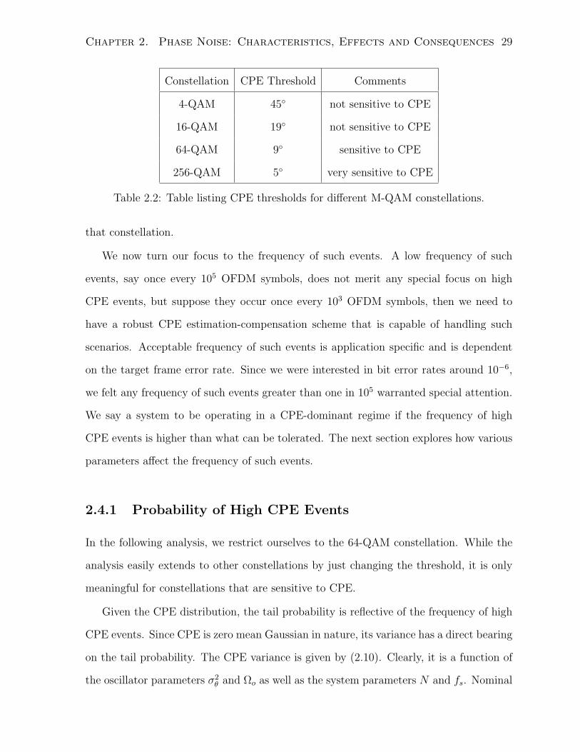
Chapter 2. Phase Noise: Characteristics, Effects and Consequences 29
Constellation CPE Threshold Comments
4-QAM 45 not sensitive to CPE
16-QAM 19 not sensitive to CPE
64-QAM 9 sensitive to CPE
256-QAM 5 very sensitive to CPE
Table 2.2: Table listing CPE thresholds for different M-QAM constellations.
that constellation.
We now turn our focus to the frequency of such events. A low frequency of such
events, say once every 105 OFDM symbols, does not merit any special focus on high
CPE events, but suppose they occur once every 103 OFDM symbols, then we need to
have a robust CPE estimation-compensation scheme that is capable of handling such
scenarios. Acceptable frequency of such events is application specific and is dependent
on the target frame error rate. Since we were interested in bit error rates around 10−6,
we felt any frequency of such events greater than one in 105 warranted special attention.
We say a system to be operating in a CPE-dominant regime if the frequency of high
CPE events is higher than what can be tolerated. The next section explores how various
parameters affect the frequency of such events.
2.4.1 Probability of High CPE Events
In the following analysis, we restrict ourselves to the 64-QAM constellation. While the
analysis easily extends to other constellations by just changing the threshold, it is only
meaningful for constellations that are sensitive to CPE.
Given the CPE distribution, the tail probability is reflective of the frequency of high
CPE events. Since CPE is zero mean Gaussian in nature, its variance has a direct bearing
on the tail probability. The CPE variance is given by (2.10). Clearly, it is a function of
the oscillator parameters σ2θ and Ωo as well as the system parameters N and fs. Nominal
Chapter 2. Phase Noise: Characteristics, Effects and Consequences 30
values for phase noise RMS and loop bandwidth are around 3 and around tens of kHz
respectively; fs/N ratio i.e. the sub-carrier spacing is generally around tens of kHz. Our
parameter of interest here is the log-probability of a high CPE event, which is given by
log(P(high CPE event)) = log(|θ| > θth) = log(2Q(θth/σθ)
), (2.42)
where Q() represents the tail probability of the standard Gaussian distribution. We now
look at the effect of each of the above parameters on the probability of a high CPE event.
0 10 20 30 40 50 60 70 80 90 100−16
−14
−12
−10
−8
−6
−4
−2
Sampling rate in MHz
Log−
Pro
babi
lity
of h
igh
CP
E
N=64 N=128 N=256
N=512
N=1024
N=2048
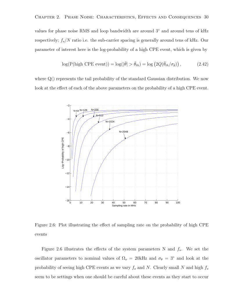
Figure 2.6: Plot illustrating the effect of sampling rate on the probability of high CPE
events
Figure 2.6 illustrates the effects of the system parameters N and fs. We set the
oscillator parameters to nominal values of Ωo = 20kHz and σθ = 3 and look at the
probability of seeing high CPE events as we vary fs and N . Clearly small N and high fs
seem to be settings when one should be careful about these events as they start to occur
Chapter 2. Phase Noise: Characteristics, Effects and Consequences 31
more frequently. A careful observation also points to a dependence on the ratio fs/N ,
which represents sub-carrier spacing, rather than individual dependence on N and fs.
This observation is in fact substantiated by the fact that we can approximate the CPE
variance as
σ2θ =
σ2θ
N2
(1 + p
1− pN −2p(1− pN)
(1− p)2
)(2.43)
=σ2θ
N2
(1 + e−ζ/N
1− e−ζ/NN −2e−ζ/N(1− e−ζ/N)N
(1− e−ζ/N)2
)(2.44)
≈ σ2θ
N2
(1 + (1− ζ/N)
1− (1− ζ/N)N − 2(1− ζ/N)(1− eζ)
(1− (1− ζ/N))2
)(2.45)
σ2θ =σ2
θ
(2− ζ/N
ζ− 2(1− ζ/N)(1− eζ)
(ζ/N)2
)(2.46)
=σ2θ
(2
ζ− 2(1− e−ζ)
ζ2
)+σ2θ
N
(2(1− e−ζ)
ζ− 1
)(2.47)
≈σ2θ
(2
ζ− 2(1− e−ζ)
ζ2
), (2.48)
where ∆fsubc = fs/N and ζ = 2πΩo∆fsubc
. The first approximation is due to the fact that ζ/N
is very small and goes to zero as N increases. The second approximation neglects terms
dependent on N as they are significantly smaller than terms independent of N , for large
N . The plot illustrates the fact that systems with very large sub-carrier bandwidth are
the most susceptible to high CPE events.
In Figure 2.7, we fix the system parameters and look at the effect of RMS value on
the frequency of high CPE events. The loop bandwidth was set to 20 kHz. Since it is
very probable that the RMS value of the oscillator changes with variation in the physical
conditions surrounding the receiver (temperature etc.) changes, it is important for us
to see how sensitive the probability of high CPE events is to the RMS value. In Figure
2.7, we plot the log-probability curves for different settings of N and subcarrier spacing
fsubc. It is clear that the probability is only dependent on fsubc and that it can change
quite rapidly as the RMS value changes by a few degrees. Hence, even though the system
design might suggest a low probability of a high CPE event, it is better to have some
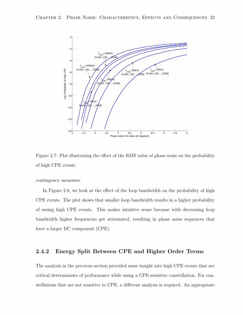
Chapter 2. Phase Noise: Characteristics, Effects and Consequences 32
1 1.5 2 2.5 3 3.5 4 4.5 5 5.5 6−16
−14
−12
−10
−8
−6
−4
−2
0
Phase noise rms value (in degrees)
Log−
Pro
babi
lity
of h
igh
CP
Efsubc
=300kHz
N=(64, 128, ...,2048)
fsubc
=100kHz
N=(64, 128, ...,2048)
fsubc
=75kHz
N=(64, 128, ...,2048)
fsubc
=50kHz
N=(64, 128, ...,2048)
fsubc
=30kHz
N=(64, 128, ...,2048)
fsubc
=15kHz
N=(64, 128, ...,2048)
Figure 2.7: Plot illustrating the effect of the RMS value of phase noise on the probability
of high CPE events
contingency measures.
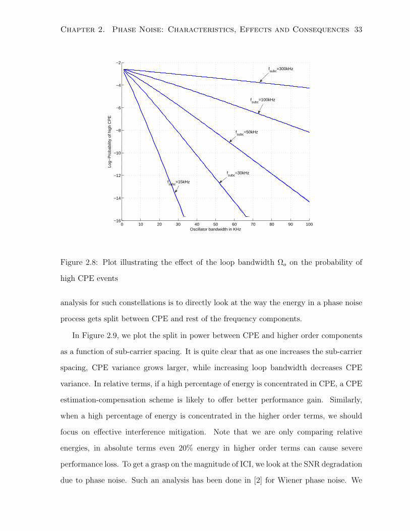
In Figure 2.8, we look at the effect of the loop bandwidth on the probability of high
CPE events. The plot shows that smaller loop bandwidth results in a higher probability
of seeing high CPE events. This makes intuitive sense because with decreasing loop
bandwidth higher frequencies get attenuated, resulting in phase noise sequences that
have a larger DC component (CPE).
2.4.2 Energy Split Between CPE and Higher Order Terms
The analysis in the previous section provided some insight into high CPE events that are
critical determinants of performance while using a CPE-sensitive constellation. For con-
stellations that are not sensitive to CPE, a different analysis is required. An appropriate
Chapter 2. Phase Noise: Characteristics, Effects and Consequences 33
0 10 20 30 40 50 60 70 80 90 100−16
−14
−12
−10
−8
−6
−4
−2
Oscillator bandwidth in KHz
Log−
Pro
babi
lity
of h
igh
CP
E
fsubc
=15kHz
fsubc
=50kHz
fsubc
=100kHz
fsubc
=30kHz
fsubc
=300kHz
Figure 2.8: Plot illustrating the effect of the loop bandwidth Ωo on the probability of
high CPE events
analysis for such constellations is to directly look at the way the energy in a phase noise
process gets split between CPE and rest of the frequency components.
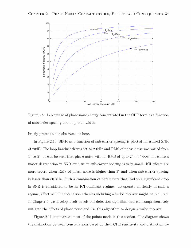
In Figure 2.9, we plot the split in power between CPE and higher order components
as a function of sub-carrier spacing. It is quite clear that as one increases the sub-carrier
spacing, CPE variance grows larger, while increasing loop bandwidth decreases CPE
variance. In relative terms, if a high percentage of energy is concentrated in CPE, a CPE
estimation-compensation scheme is likely to offer better performance gain. Similarly,
when a high percentage of energy is concentrated in the higher order terms, we should
focus on effective interference mitigation. Note that we are only comparing relative
energies, in absolute terms even 20% energy in higher order terms can cause severe
performance loss. To get a grasp on the magnitude of ICI, we look at the SNR degradation
due to phase noise. Such an analysis has been done in [2] for Wiener phase noise. We
Chapter 2. Phase Noise: Characteristics, Effects and Consequences 34
0 50 100 150 200 250 3000
10
20
30
40
50
60
70
80
90
100
sub−carrier spacing in kHz
perc
enta
ge o
f ene
rgy
in C
PE
Ωo=10kHz
Ωo=20kHz
Ωo=50kHz
Ωo=5kHz
Figure 2.9: Percentage of phase noise energy concentrated in the CPE term as a function
of subcarrier spacing and loop bandwidth.
briefly present some observations here.
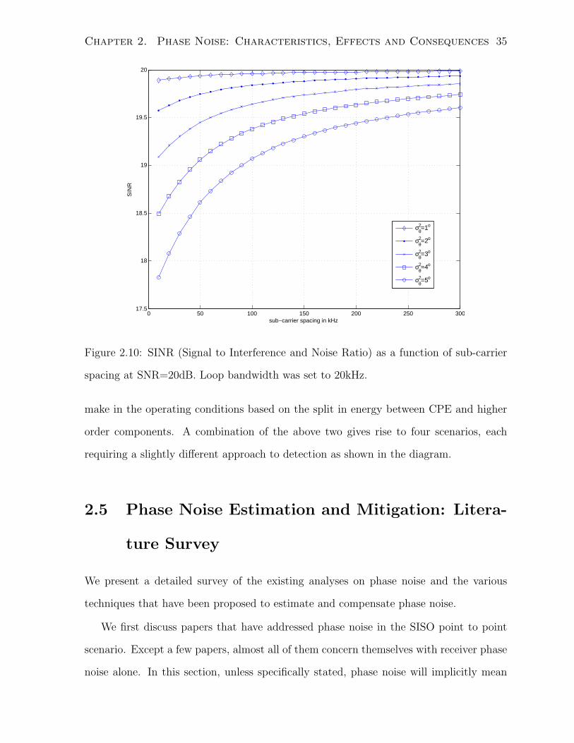
In Figure 2.10, SINR as a function of sub-carrier spacing is plotted for a fixed SNR
of 20dB. The loop bandwidth was set to 20kHz and RMS of phase noise was varied from
1 to 5. It can be seen that phase noise with an RMS of upto 2 − 3 does not cause a
major degradation in SNR even when sub-carrier spacing is very small. ICI effects are
more severe when RMS of phase noise is higher than 3 and when sub-carrier spacing
is lesser than 50 kHz. Such a combination of parameters that lead to a significant drop
in SNR is considered to be an ICI-dominant regime. To operate efficiently in such a
regime, effective ICI cancellation schemes including a turbo receiver might be required.
In Chapter 4, we develop a soft-in soft-out detection algorithm that can comprehensively
mitigate the effects of phase noise and use this algorithm to design a turbo receiver
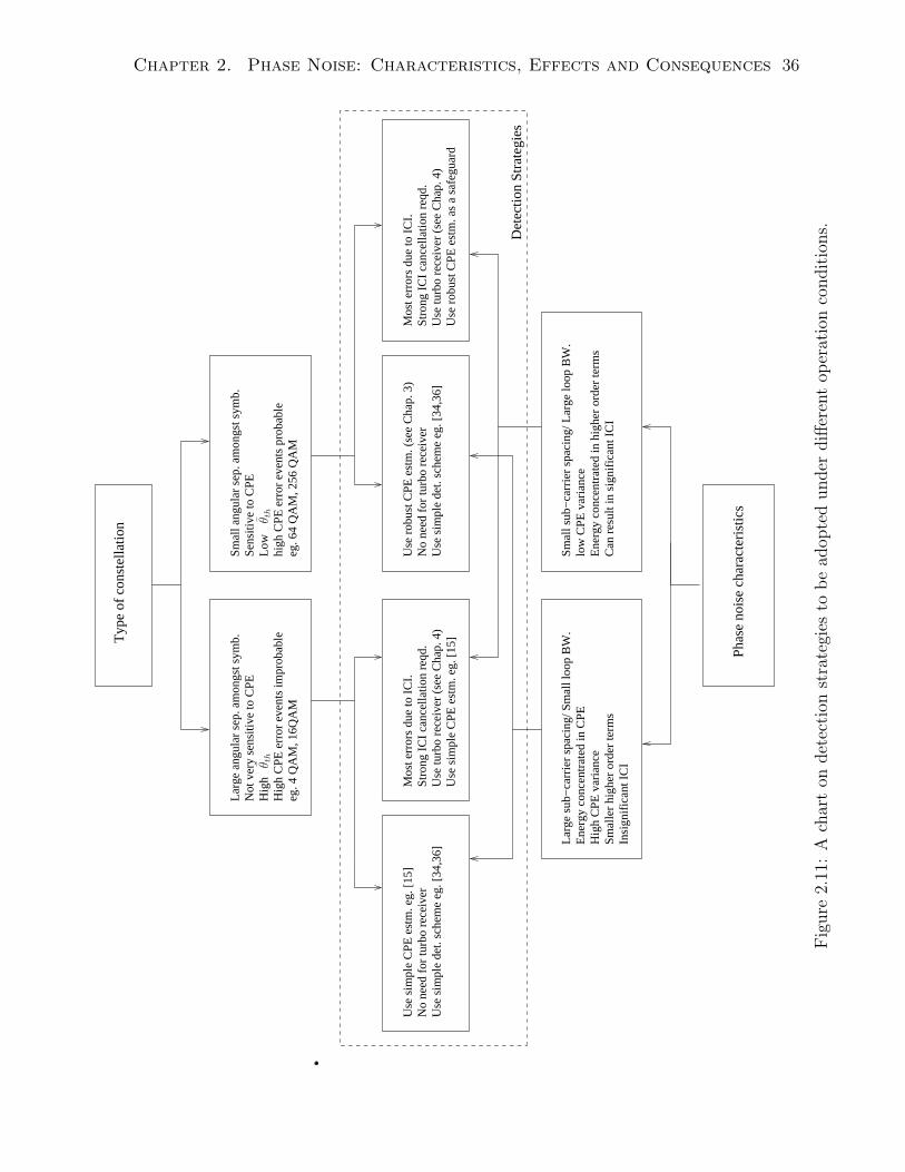
Figure 2.11 summarizes most of the points made in this section. The diagram shows
the distinction between constellations based on their CPE sensitivity and distinction we
Chapter 2. Phase Noise: Characteristics, Effects and Consequences 35
0 50 100 150 200 250 30017.5
18
18.5
19
19.5
20
sub−carrier spacing in kHz
SIN
R
σθ2=1o
σθ2=2o
σθ2=3o
σθ2=4o
σθ2=5o
Figure 2.10: SINR (Signal to Interference and Noise Ratio) as a function of sub-carrier
spacing at SNR=20dB. Loop bandwidth was set to 20kHz.
make in the operating conditions based on the split in energy between CPE and higher
order components. A combination of the above two gives rise to four scenarios, each
requiring a slightly different approach to detection as shown in the diagram.
2.5 Phase Noise Estimation and Mitigation: Litera-
ture Survey
We present a detailed survey of the existing analyses on phase noise and the various
techniques that have been proposed to estimate and compensate phase noise.
We first discuss papers that have addressed phase noise in the SISO point to point
scenario. Except a few papers, almost all of them concern themselves with receiver phase
noise alone. In this section, unless specifically stated, phase noise will implicitly mean
Chapter 2. Phase Noise: Characteristics, Effects and Consequences 36
Typ
e of
con
stel
latio
n
Not
ver
y se
nsiti
ve to
CP
ELa
rge
angu
lar
sep.
am
ongs
t sym
b.S
mal
l ang
ular
sep
. am
ongs
t sym
b.
high
CP
E e
rror
eve
nts
prob
able
Sen
sitiv
e to
CP
E
Hig
h C
PE
err
or e
vent
s im
prob
able
eg. 6
4 Q
AM
, 256
QA
Meg
. 4 Q
AM
, 16Q
AM
Mos
t err
ors
due
to IC
I.S
tron
g IC
I can
cella
tion
reqd
.
Use
sim
ple
CP
E e
stm
. eg.
[15]
Use
rob
ust C
PE
est
m. (
see
Cha
p. 3
)N
o ne
ed fo
r tu
rbo
rece
iver
Use
sim
ple
det.
sche
me
eg. [
34,3
6]
Pha
se n
oise
cha
ract
eris
tics
Sm
all s
ub−
carr
ier
spac
ing/
Lar
ge lo
op B
W.
low
CP
E v
aria
nce
Ene
rgy
conc
entr
ated
in h
ighe
r or
der
term
s C
an r
esul
t in
sign
ifica
nt IC
I
Larg
e su
b−ca
rrie
r sp
acin
g/ S
mal
l loo
p B
W.
Ene
rgy
conc
entr
ated
in C
PE
Hig
h C
PE
var
ianc
eS
mal
ler
high
er o
rder
term
sIn
sign
ifica
nt IC
I
No
need
for
turb
o re
ceiv
erU
se s
impl
e de
t. sc
hem
e eg
. [34
,36]
Use
sim
ple
CP
E e
stm
. eg.
[15]
Mos
t err
ors
due
to IC
I.S
tron
g IC
I can
cella
tion
reqd
.
Use
rob
ust C
PE
est
m. a
s a
safe
guar
dU
se tu
rbo
rece
iver
(se
e C
hap.
4)
Use
turb
o re
ceiv
er (
see
Cha
p. 4
)
Hig
hLo
w
Det
ectio
n S
trat
egie
s
θ th
θ th
Fig
ure
2.11
:A
char
ton
det
ecti
onst
rate
gies
tob
ead
opte
dunder
diff
eren
top
erat
ion
condit
ions.
Chapter 2. Phase Noise: Characteristics, Effects and Consequences 37
receiver phase noise.
2.5.1 Preliminary Analysis : Early Papers
Pollet et al. [1] were one of the very first researchers to investigate the effect of phase
noise on OFDM in which it was established that multi-carrier systems are orders of
magnitude more sensitive to phase noise than single-carrier systems. In [12] a method
to determine the error probability of an OFDM system in the presence of phase noise is
discussed. Both [1] and [12] considered Wiener phase noise i.e. phase noise modelled as a
Wiener (Random Walk) process. Robertson et al. [13] used a model for phase noise that
was suggested in [14], which is based on [15], this model was based on the phase noise
characteristics of PLL systems and very closely resembles the model described in earlier
sections. The behaviour of CPE variance as a function of N and its auto-correlation
across OFDM symbols is studied.
An important observation is that the analysis in [13] fixes the bandwidth of the OFDM
symbol as the number of sub-carriers is varied. As a result, the overall sampling rate
remains the same, the duration of the OFDM symbol grows with N , and the sub-carrier
spacing decreases with increasing N . Since the duration of the OFDM symbol changes
with N , autocorrelation properties of CPE are bound to vary with N . Such is not the
case in our analysis, where we keep the sub-carrier spacing constant as N varies. As a
result, the duration of the OFDM symbol is independent of N , and only the sampling
rate varies. A major consequence of this is that, the statistics of CPE are invariant to N .
In the former case, since CPE is averaged over varying durations, its statistics vary with
N , and one can easily see that CPE related effects are expected to be the most severe
for OFDM symbols of very short duration.
El-Tanany et al. [16] present a generic analysis on phase noise for any given phase
noise mask and provide a phase noise estimation scheme based on an isolated pilot tone in
the OFDM symbol. Armada et al. [17] provide results on SNR degradation due to phase
Chapter 2. Phase Noise: Characteristics, Effects and Consequences 38
noise and presents a CPE estimation scheme based on pilots embedded in the OFDM
symbol. This work also also makes mention of scenarios where CPE can dominate over
the higher order terms, but provides no quantitative results. In [11], non-pilot aided
estimation of CPE is investigated and some decision-directed mechanisms are suggested.
The authors make the observation that not all symbols in a constellation are equally
prone to errors because of CPE. It is this key observation that we exploit in chapter 3.
Before we go any further, we would like to recall the signal model in (2.18), which
can be written as
Fy =QrHd + Fz, (2.49)
where we have denoted r(L:N+L−1) as y and n(L:N+L−1) as z. We also have the equivalent
representation of (2.49) given by
Fy =Dc + Fz, (2.50)
where D is a left circulant matrix, consisting of circular left shifts of the vector Hd. The
vector c is the frequency domain representation of phase noise, as defined before. If one
were to look at just the received signal, one can write
y =PrFHHd + z, (2.51)
where P is a diagonal matrix consisting of the the vector pr(L:N+L−1). Equation (2.51)
can also be written as
y =diag(FHHd)pr(L:N+L−1) + z. (2.52)
These four equations form the basis for most of the algorithms that try to jointly
estimate data symbols and phase noise. Equations (2.51) and (2.52) are the basis for
algorithms that look at estimating the phase noise sequence in time domain, while (2.49)
and (2.50) form the crux of algorithms that look at estimating phase noise in the frequency
Chapter 2. Phase Noise: Characteristics, Effects and Consequences 39
domain. While one can estimate phase noise in either domain, estimation in the frequency
domain has the advantage that it suffices to estimate only the first few components to
compensate for a large percentage of ICI. Due to the small bandwidth and the exponential
decay of the PSD, the first few components account for almost all the energy in the phase
noise process, thus enabling easier ICI mitigation.
2.5.2 Phase Noise Estimation and Compensation
Extensive research has been carried out on the effect of Wiener phase noise on OFDM.
Since CPE shows strong correlation in the case of Wiener phase noise, [18] and [19] use
a Kalman filter to predict and pre-compensate for CPE. In [20], the Kalman filter based
CPE predictor and a decision directed mechanism to evaluate the first few significant
frequency components of phase noise are used to compensate for phase noise. Petrovic et
al. [21] make the case for evaluating all the components in a frequency selective setting
as individual components contributing to ICI get scaled according to the channel gains
corresponding to different sub-carriers. Petrovic et al. [22] point out that certain phase
noise realizations lead to bursts of errors, and suggests interleaving and coding across
multiple OFDM symbols to randomize these errors. The effect of phase noise on coded
OFDM transmission is studied in [23] and an iterative procedure to estimate higher order
frequency components of phase noise using the bit LLRs (log-likelihood ratios) computed
by the decoder is discussed in [4].
Another extensive analysis on Wiener phase noise includes [24], which discusses
MMSE (Minimum Mean Square Error) detection of OFDM symbols affected by phase
noise by considering the ICI term as additional noise. It also discusses MMSE estima-
tion of CPE using pilot symbols. In [2] SINR (Signal to Interference and Noise Ratio)
expression for an OFDM symbol is computed without assuming small phase noise. [3]
discusses a decision directed approach to estimate phase noise and data symbols iter-
atively. Both Maximum Likelihood (ML) and LMMSE (Linear MMSE) techniques of
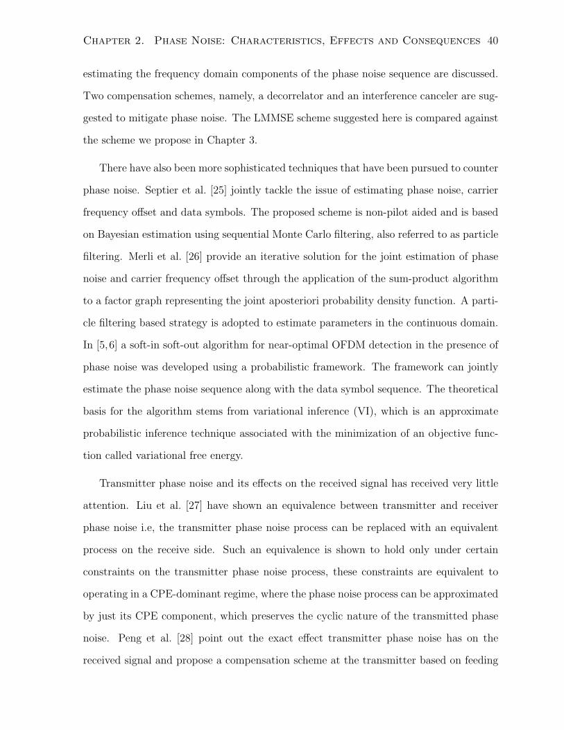
Chapter 2. Phase Noise: Characteristics, Effects and Consequences 40
estimating the frequency domain components of the phase noise sequence are discussed.
Two compensation schemes, namely, a decorrelator and an interference canceler are sug-
gested to mitigate phase noise. The LMMSE scheme suggested here is compared against
the scheme we propose in Chapter 3.
There have also been more sophisticated techniques that have been pursued to counter
phase noise. Septier et al. [25] jointly tackle the issue of estimating phase noise, carrier
frequency offset and data symbols. The proposed scheme is non-pilot aided and is based
on Bayesian estimation using sequential Monte Carlo filtering, also referred to as particle
filtering. Merli et al. [26] provide an iterative solution for the joint estimation of phase
noise and carrier frequency offset through the application of the sum-product algorithm
to a factor graph representing the joint aposteriori probability density function. A parti-
cle filtering based strategy is adopted to estimate parameters in the continuous domain.
In [5,6] a soft-in soft-out algorithm for near-optimal OFDM detection in the presence of
phase noise was developed using a probabilistic framework. The framework can jointly
estimate the phase noise sequence along with the data symbol sequence. The theoretical
basis for the algorithm stems from variational inference (VI), which is an approximate
probabilistic inference technique associated with the minimization of an objective func-
tion called variational free energy.
Transmitter phase noise and its effects on the received signal has received very little
attention. Liu et al. [27] have shown an equivalence between transmitter and receiver
phase noise i.e, the transmitter phase noise process can be replaced with an equivalent
process on the receive side. Such an equivalence is shown to hold only under certain
constraints on the transmitter phase noise process, these constraints are equivalent to
operating in a CPE-dominant regime, where the phase noise process can be approximated
by just its CPE component, which preserves the cyclic nature of the transmitted phase
noise. Peng et al. [28] point out the exact effect transmitter phase noise has on the
received signal and propose a compensation scheme at the transmitter based on feeding
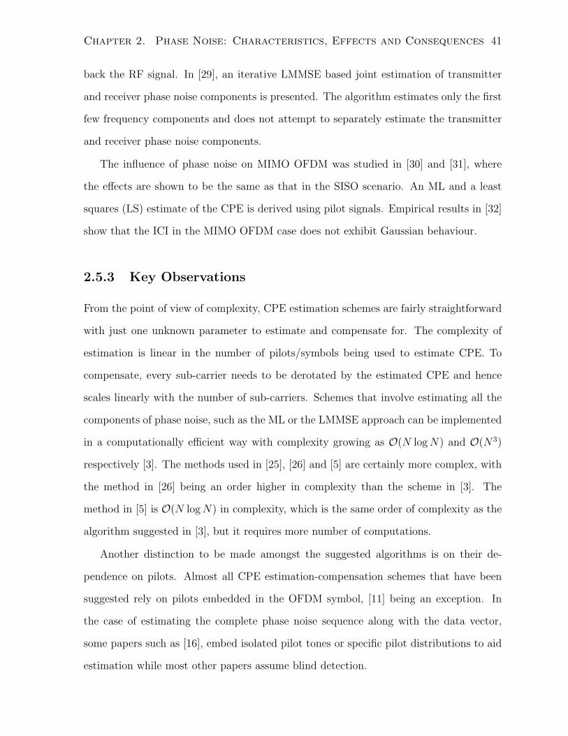
Chapter 2. Phase Noise: Characteristics, Effects and Consequences 41
back the RF signal. In [29], an iterative LMMSE based joint estimation of transmitter
and receiver phase noise components is presented. The algorithm estimates only the first
few frequency components and does not attempt to separately estimate the transmitter
and receiver phase noise components.
The influence of phase noise on MIMO OFDM was studied in [30] and [31], where
the effects are shown to be the same as that in the SISO scenario. An ML and a least
squares (LS) estimate of the CPE is derived using pilot signals. Empirical results in [32]
show that the ICI in the MIMO OFDM case does not exhibit Gaussian behaviour.
2.5.3 Key Observations
From the point of view of complexity, CPE estimation schemes are fairly straightforward
with just one unknown parameter to estimate and compensate for. The complexity of
estimation is linear in the number of pilots/symbols being used to estimate CPE. To
compensate, every sub-carrier needs to be derotated by the estimated CPE and hence
scales linearly with the number of sub-carriers. Schemes that involve estimating all the
components of phase noise, such as the ML or the LMMSE approach can be implemented
in a computationally efficient way with complexity growing as O(N logN) and O(N3)
respectively [3]. The methods used in [25], [26] and [5] are certainly more complex, with
the method in [26] being an order higher in complexity than the scheme in [3]. The
method in [5] is O(N logN) in complexity, which is the same order of complexity as the
algorithm suggested in [3], but it requires more number of computations.
Another distinction to be made amongst the suggested algorithms is on their de-
pendence on pilots. Almost all CPE estimation-compensation schemes that have been
suggested rely on pilots embedded in the OFDM symbol, [11] being an exception. In
the case of estimating the complete phase noise sequence along with the data vector,
some papers such as [16], embed isolated pilot tones or specific pilot distributions to aid
estimation while most other papers assume blind detection.
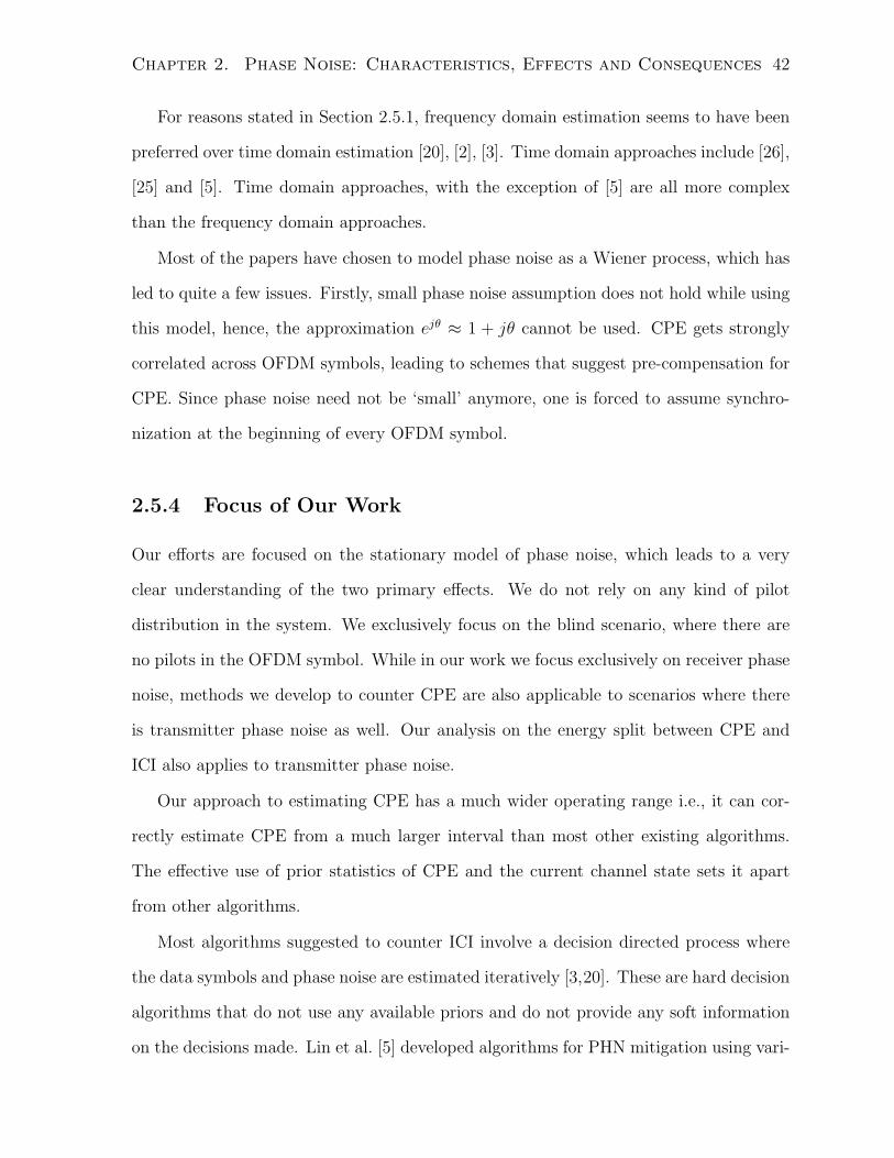
Chapter 2. Phase Noise: Characteristics, Effects and Consequences 42
For reasons stated in Section 2.5.1, frequency domain estimation seems to have been
preferred over time domain estimation [20], [2], [3]. Time domain approaches include [26],
[25] and [5]. Time domain approaches, with the exception of [5] are all more complex
than the frequency domain approaches.
Most of the papers have chosen to model phase noise as a Wiener process, which has
led to quite a few issues. Firstly, small phase noise assumption does not hold while using
this model, hence, the approximation ejθ ≈ 1 + jθ cannot be used. CPE gets strongly
correlated across OFDM symbols, leading to schemes that suggest pre-compensation for
CPE. Since phase noise need not be ‘small’ anymore, one is forced to assume synchro-
nization at the beginning of every OFDM symbol.
2.5.4 Focus of Our Work
Our efforts are focused on the stationary model of phase noise, which leads to a very
clear understanding of the two primary effects. We do not rely on any kind of pilot
distribution in the system. We exclusively focus on the blind scenario, where there are
no pilots in the OFDM symbol. While in our work we focus exclusively on receiver phase
noise, methods we develop to counter CPE are also applicable to scenarios where there
is transmitter phase noise as well. Our analysis on the energy split between CPE and
ICI also applies to transmitter phase noise.
Our approach to estimating CPE has a much wider operating range i.e., it can cor-
rectly estimate CPE from a much larger interval than most other existing algorithms.
The effective use of prior statistics of CPE and the current channel state sets it apart
from other algorithms.
Most algorithms suggested to counter ICI involve a decision directed process where
the data symbols and phase noise are estimated iteratively [3,20]. These are hard decision
algorithms that do not use any available priors and do not provide any soft information
on the decisions made. Lin et al. [5] developed algorithms for PHN mitigation using vari-
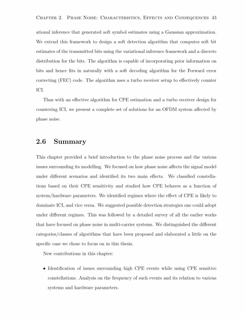
Chapter 2. Phase Noise: Characteristics, Effects and Consequences 43
ational inference that generated soft symbol estimates using a Gaussian approximation.
We extend this framework to design a soft detection algorithm that computes soft bit
estimates of the transmitted bits using the variational inference framework and a discrete
distribution for the bits. The algorithm is capable of incorporating prior information on
bits and hence fits in naturally with a soft decoding algorithm for the Forward error
correcting (FEC) code. The algorithm uses a turbo receiver setup to effectively counter
ICI.
Thus with an effective algorithm for CPE estimation and a turbo receiver design for
countering ICI, we present a complete set of solutions for an OFDM system affected by
phase noise.
2.6 Summary
This chapter provided a brief introduction to the phase noise process and the various
issues surrounding its modelling. We focused on how phase noise affects the signal model
under different scenarios and identified its two main effects. We classified constella-
tions based on their CPE sensitivity and studied how CPE behaves as a function of
system/hardware parameters. We identified regimes where the effect of CPE is likely to
dominate ICI, and vice versa. We suggested possible detection strategies one could adopt
under different regimes. This was followed by a detailed survey of all the earlier works
that have focused on phase noise in multi-carrier systems. We distinguished the different
categories/classes of algorithms that have been proposed and elaborated a little on the
specific case we chose to focus on in this thesis.
New contributions in this chapter:
Identification of issues surrounding high CPE events while using CPE sensitive
constellations. Analysis on the frequency of such events and its relation to various
systems and hardware parameters.
Chapter 2. Phase Noise: Characteristics, Effects and Consequences 44
Analysis on the energy split between CPE and other higher components of phase
noise and the consequences thereof on detection strategies.
Chapter 3
Blind CPE Estimation
This chapter presents a new algorithm for blind CPE estimation. We first describe
common approaches to CPE estimation using pilots embedded in the OFDM symbols
and then discuss techniques that have been proposed to estimate CPE blindly. We
highlight issues that arise while using these techniques to estimate high CPE values.
We then present our approach to blind estimation and show that by sorting detected
symbols according to their reliability we can avoid estimation errors even under high
CPE situations. We finally present simulation results that establish the advantages of
using the new algorithm.
3.1 Introduction
Most algorithms suggested for blind CPE estimation in OFDM systems involve a decision
directed process where the data symbols are first estimated ignoring PHN and these
decisions are fed back to estimate CPE. These algorithms treat all detected symbols as
correct. As a result, crucial to all these algorithms is the success of the initial detection
of symbols. But, in reality, a lot of errors can result in this first step whenever CPE
is beyond a threshold, details of which were dealt with in Chapter 2. This requirement
greatly restricts the ability of these algorithms to correctly estimate high CPE values.
45
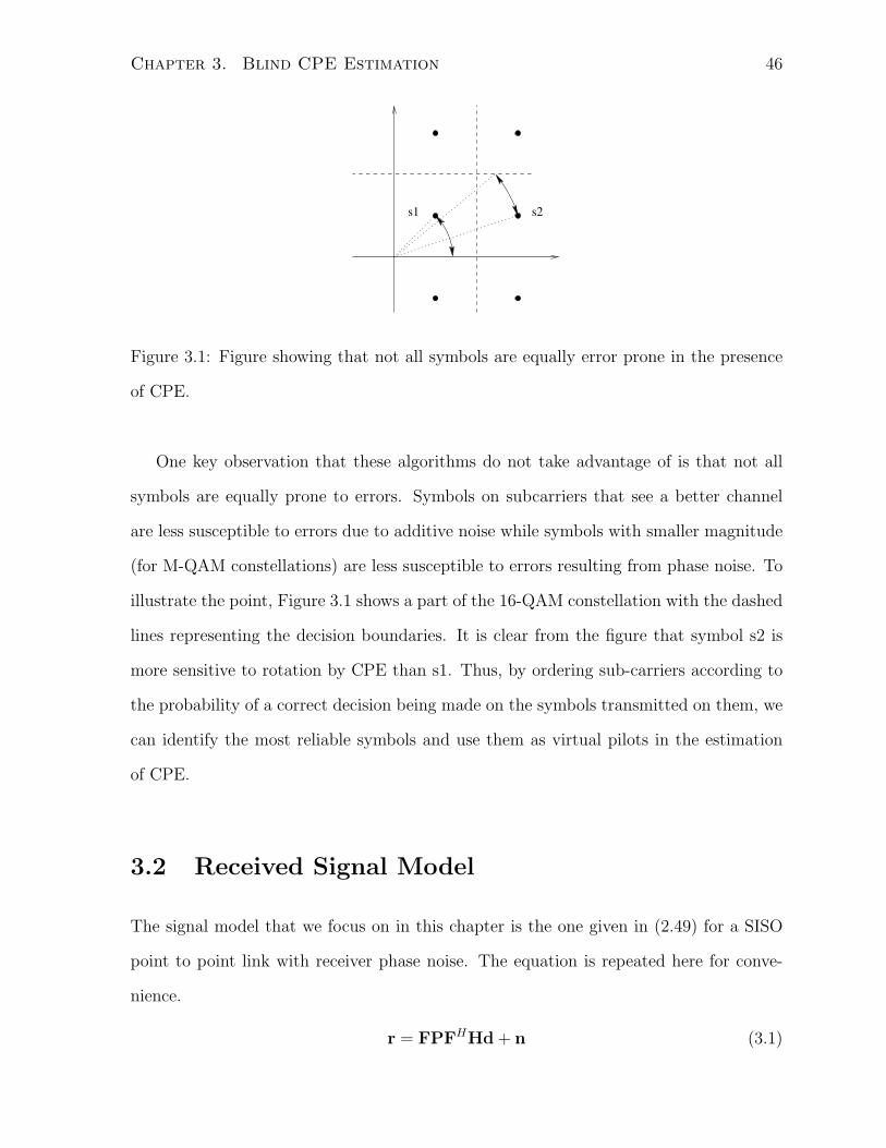
Chapter 3. Blind CPE Estimation 46
s1 s2
Figure 3.1: Figure showing that not all symbols are equally error prone in the presence
of CPE.
One key observation that these algorithms do not take advantage of is that not all
symbols are equally prone to errors. Symbols on subcarriers that see a better channel
are less susceptible to errors due to additive noise while symbols with smaller magnitude
(for M-QAM constellations) are less susceptible to errors resulting from phase noise. To
illustrate the point, Figure 3.1 shows a part of the 16-QAM constellation with the dashed
lines representing the decision boundaries. It is clear from the figure that symbol s2 is
more sensitive to rotation by CPE than s1. Thus, by ordering sub-carriers according to
the probability of a correct decision being made on the symbols transmitted on them, we
can identify the most reliable symbols and use them as virtual pilots in the estimation
of CPE.
3.2 Received Signal Model
The signal model that we focus on in this chapter is the one given in (2.49) for a SISO
point to point link with receiver phase noise. The equation is repeated here for conve-
nience.
r = FPFHHd + n (3.1)
Chapter 3. Blind CPE Estimation 47
The matrix P is a diagonal matrix given by diag(ejθr) ≈ diag(1 + jθ), where θ is the
PHN sequence affecting the signal after removing the cyclic prefix. n is complex white
Gaussian noise with variance σ2 each in the in-phase and quadrature dimensions. The
phase noise is modelled as an AR(1) process, as detailed in Chapter 2.
3.2.1 Existing Pilot-Based Approaches to CPE Estimation
Pilot aided CPE estimation only considers sub-carriers with pilots. Let κ represent the set
of indices corresponding to the pilots in an OFDM symbol. Let rκ denote the frequency
domain representation of the received signal corresponding to the sub-carriers with pilots.
Define Hκ, dκ and nκ analogously. We will treat the ICI resulting from phase noise as
just another noise term with a variance of σ2ICI per dimension. From (2.20) we can write
the variance as
2σ2ICI =E[|d|2]E[|h|2]
N−1∑k=1,
E[|ck|2] (3.2)
≈E[|d|2]E[|h|2](σ2θ − σ2
θ), (3.3)
where E[|d|2] is the average symbol energy and E[|h|2] is the average energy contributed
by the channel per sub-carrier. The approximation holds only when the small angle
approximation is valid. By treating the ICI as additional noise, the received signal
corresponding to the kth sub-carrier can be written as
rk = cohkdk + nICI + n. (3.4)
Using this simplified model, the ML estimate of CPE is given by [11]
Chapter 3. Blind CPE Estimation 48
ˆθML = arg maxθ
p(rκ|θ,dκ) (3.5)
= arg maxθ
∏l∈κ
p(rl|θ,dl) (3.6)
= arg maxθ
∏l∈κ
exp
−|rl − e
jθhldl|22(σ2 + σ2
ICI)
(3.7)
= arg minθ
∑l∈κ
|rl − ejθhldl|22(σ2 + σ2
ICI)(3.8)
≈ arg minθ
∑l∈κ
|rl − (1 + jθ)hldl|2 (3.9)
==(∑
l∈κ rl(hldl)∗∑
l∈κ |hldl|2). (3.10)
Suppose the distribution of CPE is known, then one can compute the MAP estimate
to be
ˆθMAP = arg maxθ
p(rκ|θ,dκ)p(θ) (3.11)
= arg maxθ
p(θ)∏l∈κ
exp
−|rl − e
jθhldl|22(σ2 + σ2
ICI)
. (3.12)
Proceeding as in the case of deriving the ML estimate and assuming that θ is zero
mean Gaussian with variance σ2, the MAP estimate can be written as
ˆθMAP ==(
σ2θ
∑l∈κ rl(hldl)
∗
σ2 + σ2ICI + σ2
θ
∑l∈κ |hldl|2
). (3.13)
Both the estimates are unbiased and mean squared errors for the ML and MAP
estimates are given by
E[(θ − θML)2] =σ2 + σ2
ICI∑l∈κ |hldl|2
(3.14)
E[(θ − θMAP)2] =σ2θ(σ2 + σ2
ICI)
(σ2 + σ2ICI + σ2
θ
∑l∈κ |hldl|2)2
+σ2θ(σ2 + σ2
ICI)∑
l∈κ |hldl|2(σ2 + σ2
ICI + σ2θ
∑l∈κ |hldl|2)2
(3.15)
=σ2θ(σ2 + σ2
ICI)
(σ2 + σ2ICI + σ2
θ
∑l∈κ |hldl|2)
. (3.16)
Chapter 3. Blind CPE Estimation 49
As one would expect, the mean squared errors go down with increasing number of
pilots, but the decrease is dependent on the channel conditions. One drawback of using
pilots to estimate CPE is that the estimates can be unreliable if the pilot signal energy
is too low, due to fading at the pilot tones, an inadequate number of pilot symbols,
or insufficient transmitted pilot energy. This is particularly an issue in coded OFDM
systems as they operate at much lower SNRs.
If there are no pilots embedded in an OFDM symbol, then one can make a preliminary
estimate of the symbols while ignoring the PHN and use these symbol estimates to
compute the CPE. In general, all the symbol decisions are used while estimating CPE.
Denoting the tentative hard decisions on the symbols as d, under the assumption that
no errors have been made, the ML and MAP estimates can be written as
ˆθML ==((Hd)Hr)
|Hd|2 (3.17)
ˆθMAP =σ2θ=((Hd)Hr)
σ2 + σ2ICI + σ2
θ|Hd|2 (3.18)
However, due to the possibility of making errors in the initial symbol decisions the
CPE estimate is not very reliable and hence an iterative procedure must be adopted to
get a better estimate.
3.3 Blind CPE Estimation Under Detection Uncer-
tainty
3.3.1 Key Idea– Auxiliary Variable
Clearly, not all symbols are detected correctly in a practical scenario. Even in the high
SNR regime, if the CPE exceeds a certain threshold, detection errors are very likely to
Chapter 3. Blind CPE Estimation 50
be made. The estimates in the previous subsection do not take this into consideration.
In this section we present a more careful formulation of the CPE estimation problem.
We first introduce an auxiliary binary random vector u. uk, the kth entry of the vector
u is one if the kth symbol has been detected correctly and is zero otherwise. Rather than
looking at estimation of θ in isolation, we look at jointly estimating θ and u as follows:
(ˆθ, u) = arg maxθ,u
p(θ,u|r, d) (3.19)
= arg maxθ,u
p(r|θ, d,u)p(u, θ|d) (3.20)
= arg maxθ,u
p(r|θ, d,u)p(u|θ, d)p(θ) (3.21)
≈ arg maxθ,u
p(r|θ, d,u)p(u|d)p(θ) (3.22)
= arg maxθ,u
p(r|θ, d,u)p(θ)N∏k=1
p(uk|dk) (3.23)
Equation (3.22) follows from (3.21) if we treat θ and u as independent variables.
While this is clearly not true, it simplifies the maximization greatly. For the moment,
we just assume that for any dk, the value of p(uk|dk) is known to us. Now, (3.23) can be
written as
(ˆθ, u) = arg maxθ,u
(− wu ln(2πσ2) +
N∑k=1
ln(p(uk|dk))− 1
2σ2θ
(θ)2
− 1
2σ2
∑k:uk=1
|yk − (1 + jθ)hkdk|2)
(3.24)
= arg maxθ,u
(au(θ)2 + bu(θ) + cu
)(3.25)
Chapter 3. Blind CPE Estimation 51
where,
au =
[− 1
2σ2θ
−N∑k=1
1
2σ2uk|hkdk|2
](3.26)
bu =
[N∑k=1
1
σ2uk=(yk − hkdk)(hkdk)∗
](3.27)
cu =N∑k=1
uk
− ln(2πσ2)− 1
2σ2|yk − hkdk|2+
ln
(P (uk = 1|dk)P (uk = 0|dk)
)+
N∑k=1
ln(P (uk = 0|dk)
). (3.28)
In (3.24), wu is the weight of the vector u. The maximization in (3.25) involves a
search over the continuous parameter θ and all possible N -tuples of the random vector
u. This is an instance of a Mixed Integer Non Linear Problem (MINLP) and solving
for the optimum in such cases is not easy. In this particular case, since the problem
is convex in the continuous parameter θ when the binary vector is held constant, there
are methods which when given enough time and computational resources can find the
optimal solution [33]. But, as pointed out in [33], such methods are computationally
intensive and are not suited for real time applications. With simplicity of optimization
in mind and the fact that it is possible to initialize the optimization at a very good initial
point (shown later), we adopt a likelihood ascent search (LAS) algorithm along the lines
of that suggested in [34]. The algorithm presented here is a sequential likelihood ascent
search (SLAS) with one binary variable being updated at each stage. The algorithm can
be broken down into the following steps.
1. Sort the subcarriers in decreasing order of the tolerance to CPE of the symbols dk.
Computing the CPE tolerance of a symbol is elaborated upon in the next section.
2. Assume that the first l0 subcarriers after sorting have been detected correctly.
Simulations show that l0 can typically be set to a value between 4 to 8. This forces
the first l0 entries in u to be one. Set all other entries in u to zero.
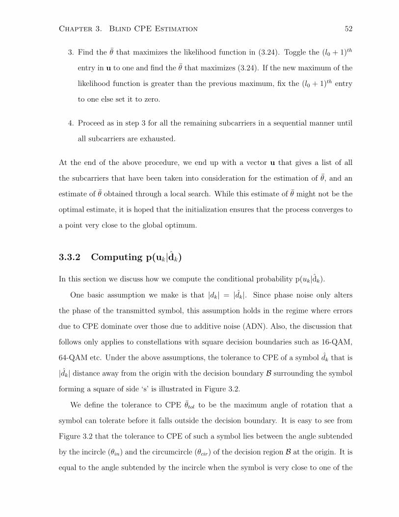
Chapter 3. Blind CPE Estimation 52
3. Find the θ that maximizes the likelihood function in (3.24). Toggle the (l0 + 1)th
entry in u to one and find the θ that maximizes (3.24). If the new maximum of the
likelihood function is greater than the previous maximum, fix the (l0 + 1)th entry
to one else set it to zero.
4. Proceed as in step 3 for all the remaining subcarriers in a sequential manner until
all subcarriers are exhausted.
At the end of the above procedure, we end up with a vector u that gives a list of all
the subcarriers that have been taken into consideration for the estimation of θ, and an
estimate of θ obtained through a local search. While this estimate of θ might not be the
optimal estimate, it is hoped that the initialization ensures that the process converges to
a point very close to the global optimum.
3.3.2 Computing p(uk|dk)
In this section we discuss how we compute the conditional probability p(uk|dk).One basic assumption we make is that |dk| = |dk|. Since phase noise only alters
the phase of the transmitted symbol, this assumption holds in the regime where errors
due to CPE dominate over those due to additive noise (ADN). Also, the discussion that
follows only applies to constellations with square decision boundaries such as 16-QAM,
64-QAM etc. Under the above assumptions, the tolerance to CPE of a symbol dk that is
|dk| distance away from the origin with the decision boundary B surrounding the symbol
forming a square of side ‘s’ is illustrated in Figure 3.2.
We define the tolerance to CPE θtol to be the maximum angle of rotation that a
symbol can tolerate before it falls outside the decision boundary. It is easy to see from
Figure 3.2 that the tolerance to CPE of such a symbol lies between the angle subtended
by the incircle (θin) and the circumcircle (θcir) of the decision region B at the origin. It is
equal to the angle subtended by the incircle when the symbol is very close to one of the
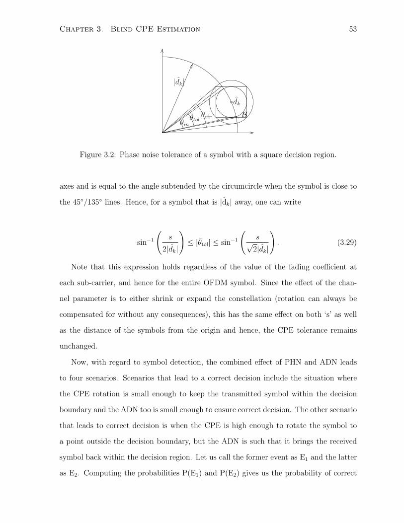
Chapter 3. Blind CPE Estimation 53
θcirθtolθin
dk
B
|dk|
Figure 3.2: Phase noise tolerance of a symbol with a square decision region.
axes and is equal to the angle subtended by the circumcircle when the symbol is close to
the 45/135 lines. Hence, for a symbol that is |dk| away, one can write
sin−1
(s
2|dk|
)≤ |θtol| ≤ sin−1
(s√
2|dk|
). (3.29)
Note that this expression holds regardless of the value of the fading coefficient at
each sub-carrier, and hence for the entire OFDM symbol. Since the effect of the chan-
nel parameter is to either shrink or expand the constellation (rotation can always be
compensated for without any consequences), this has the same effect on both ‘s’ as well
as the distance of the symbols from the origin and hence, the CPE tolerance remains
unchanged.
Now, with regard to symbol detection, the combined effect of PHN and ADN leads
to four scenarios. Scenarios that lead to a correct decision include the situation where
the CPE rotation is small enough to keep the transmitted symbol within the decision
boundary and the ADN too is small enough to ensure correct decision. The other scenario
that leads to correct decision is when the CPE is high enough to rotate the symbol to
a point outside the decision boundary, but the ADN is such that it brings the received
symbol back within the decision region. Let us call the former event as E1 and the latter
as E2. Computing the probabilities P(E1) and P(E2) gives us the probability of correct
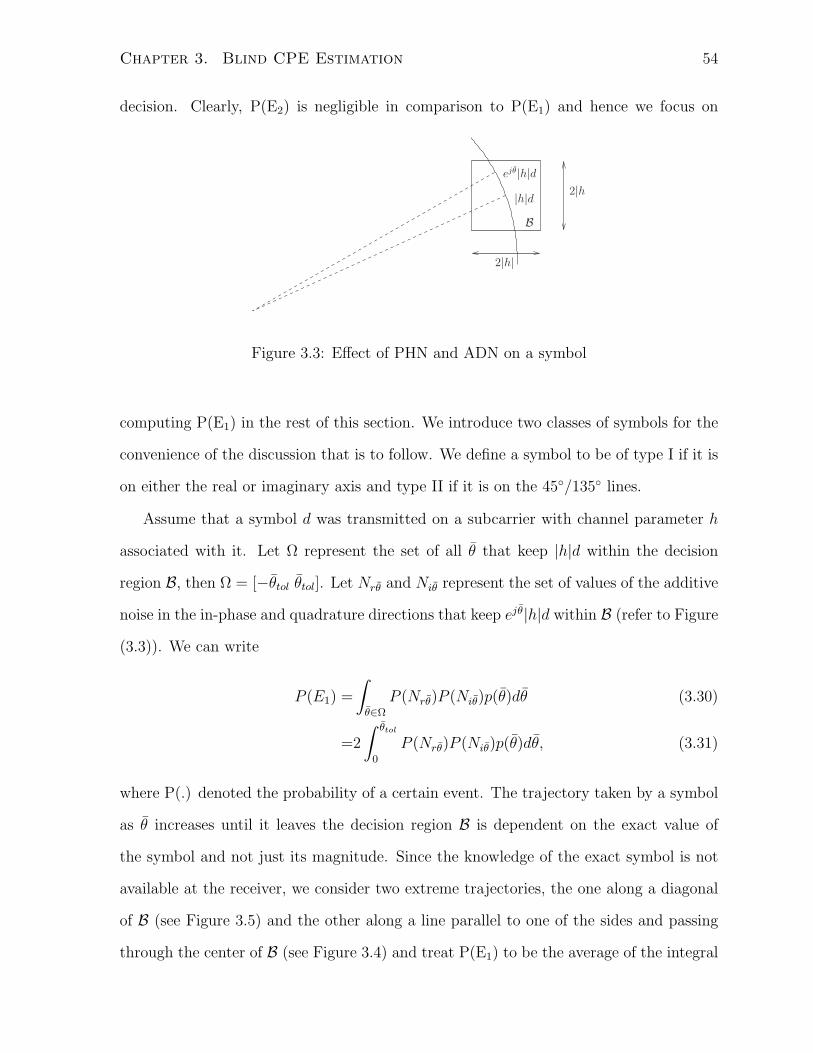
Chapter 3. Blind CPE Estimation 54
decision. Clearly, P(E2) is negligible in comparison to P(E1) and hence we focus on
2|h|
2|h||h|dejθ|h|d
B
Figure 3.3: Effect of PHN and ADN on a symbol
computing P(E1) in the rest of this section. We introduce two classes of symbols for the
convenience of the discussion that is to follow. We define a symbol to be of type I if it is
on either the real or imaginary axis and type II if it is on the 45/135 lines.
Assume that a symbol d was transmitted on a subcarrier with channel parameter h
associated with it. Let Ω represent the set of all θ that keep |h|d within the decision
region B, then Ω = [−θtol θtol]. Let Nrθ and Niθ represent the set of values of the additive
noise in the in-phase and quadrature directions that keep ejθ|h|d within B (refer to Figure
(3.3)). We can write
P (E1) =
∫θ∈Ω
P (Nrθ)P (Niθ)p(θ)dθ (3.30)
=2
∫ θtol
0
P (Nrθ)P (Niθ)p(θ)dθ, (3.31)
where P(.) denoted the probability of a certain event. The trajectory taken by a symbol
as θ increases until it leaves the decision region B is dependent on the exact value of
the symbol and not just its magnitude. Since the knowledge of the exact symbol is not
available at the receiver, we consider two extreme trajectories, the one along a diagonal
of B (see Figure 3.5) and the other along a line parallel to one of the sides and passing
through the center of B (see Figure 3.4) and treat P(E1) to be the average of the integral
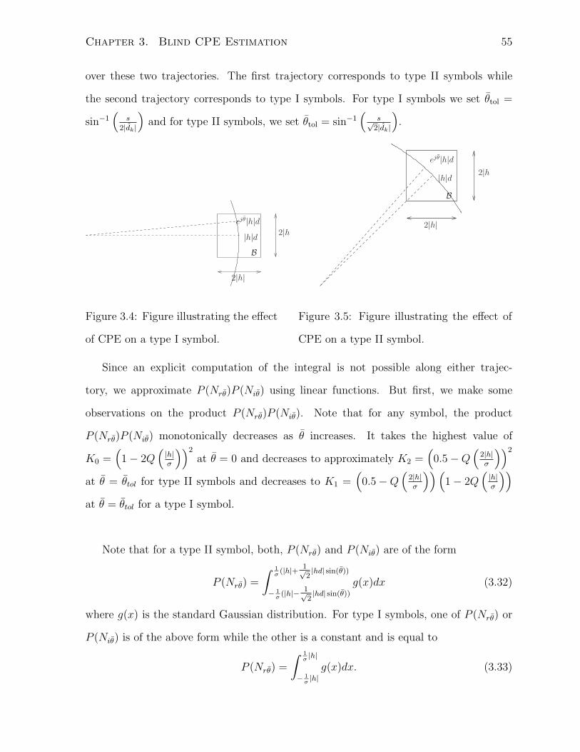
Chapter 3. Blind CPE Estimation 55
over these two trajectories. The first trajectory corresponds to type II symbols while
the second trajectory corresponds to type I symbols. For type I symbols we set θtol =
sin−1(
s
2|dk|
)and for type II symbols, we set θtol = sin−1
(s√
2|dk|
).
2|h|
2|h||h|dejθ|h|d
B
Figure 3.4: Figure illustrating the effect
of CPE on a type I symbol.
2|h|
2|h||h|d
ejθ|h|d
B
Figure 3.5: Figure illustrating the effect of
CPE on a type II symbol.
Since an explicit computation of the integral is not possible along either trajec-
tory, we approximate P (Nrθ)P (Niθ) using linear functions. But first, we make some
observations on the product P (Nrθ)P (Niθ). Note that for any symbol, the product
P (Nrθ)P (Niθ) monotonically decreases as θ increases. It takes the highest value of
K0 =(
1− 2Q(|h|σ
))2
at θ = 0 and decreases to approximately K2 =(
0.5−Q(
2|h|σ
))2
at θ = θtol for type II symbols and decreases to K1 =(
0.5−Q(
2|h|σ
))(1− 2Q
(|h|σ
))at θ = θtol for a type I symbol.
Note that for a type II symbol, both, P (Nrθ) and P (Niθ) are of the form
P (Nrθ) =
∫ 1σ
(|h|+ 1√2|hd| sin(θ))
− 1σ
(|h|− 1√2|hd| sin(θ))
g(x)dx (3.32)
where g(x) is the standard Gaussian distribution. For type I symbols, one of P (Nrθ) or
P (Niθ) is of the above form while the other is a constant and is equal to
P (Nrθ) =
∫ 1σ|h|
− 1σ|h|g(x)dx. (3.33)
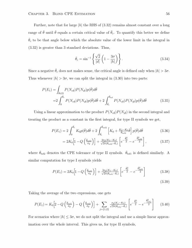
Chapter 3. Blind CPE Estimation 56
Further, note that for large |h| the RHS of (3.32) remains almost constant over a long
range of θ until θ equals a certain critical value of θc. To quantify this better we define
θc to be that angle below which the absolute value of the lower limit in the integral in
(3.32) is greater than 3 standard deviations. Thus,
θc = sin−1
√2
|d|(
1− 3σ
|h|)
. (3.34)
Since a negative θc does not makes sense, the critical angle is defined only when |h| > 3σ.
Thus whenever |h| > 3σ, we can split the integral in (3.30) into two parts:
P (E1) =
∫θ∈Ω
P (Nrθ)P (Niθ)p(θ)dθ
=2
∫ θc
0
P (Nrθ)P (Niθ)p(θ)dθ + 2
∫ θtol
θc
P (Nrθ)P (Niθ)p(θ)dθ (3.35)
Using a linear approximation to the product P (Nrθ)P (Niθ) in the second integral and
treating the product as a constant in the first integral, for type II symbols we get,
P (E1) = 2
∫ θc
0
K0p(θ)dθ + 2
∫ θtol2
θc
[K0 + K2−K0
θtol2θ]p(θ)dθ (3.36)
= 2K0
[1−Q
(θtol2σθ
)]+
2σθ(K2−K0)√2π(θtol2−θc)
[e−
θ2c
2 − e−θ2tol2
2
], (3.37)
where θtol2 denotes the CPE tolerance of type II symbols. θtol1 is defined similarly. A
similar computation for type I symbols yields
P (E1) = 2K0
[1−Q
(θtol1σθ
)]+
2σθ(K1−K0)√2π(θtol1−θc)
[e−
θ2c
2 − e−θ2tol1
2
](3.38)
(3.39)
Taking the average of the two expressions, one gets
P (E1) = K0
[2−Q
(θtol1σθ
)−Q
(θtol2σθ
)]+∑
j=1,2
σθ(Kj−K0)√2π(θtolj−θc)
[e−
θ2c
2 − e−θ2tolj
2
](3.40)
For scenarios where |h| ≤ 3σ, we do not split the integral and use a simple linear approx-
imation over the whole interval. This gives us, for type II symbols,
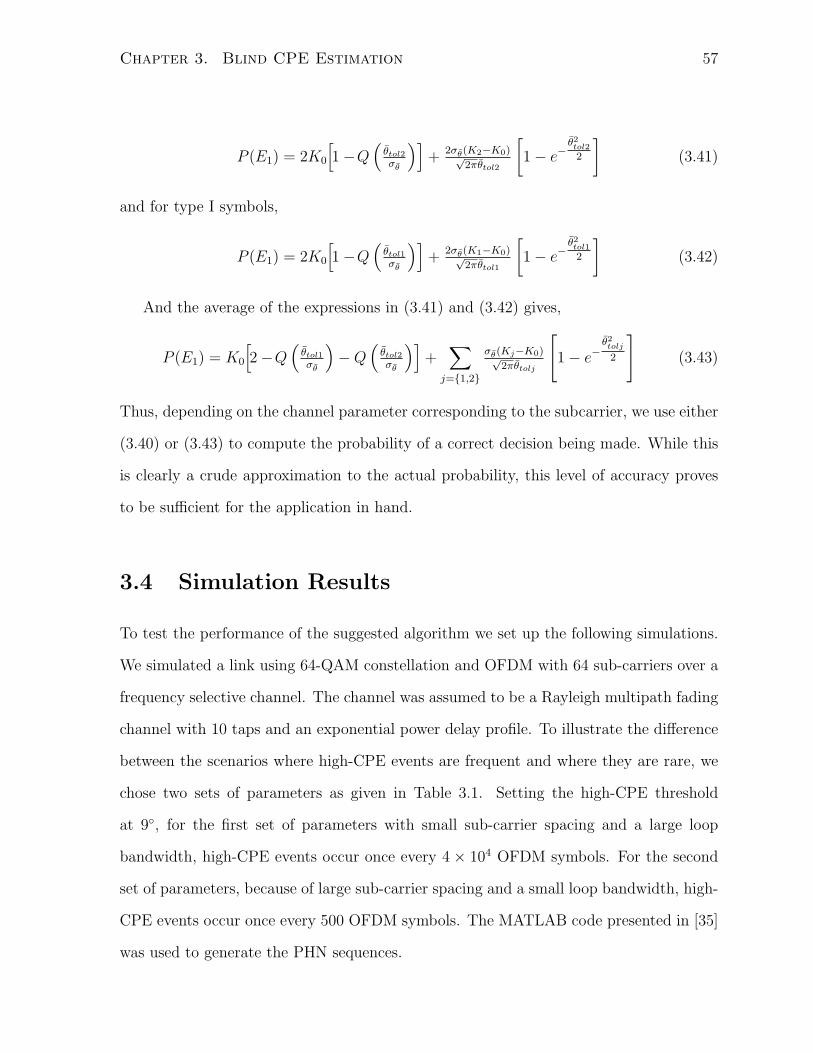
Chapter 3. Blind CPE Estimation 57
P (E1) = 2K0
[1−Q
(θtol2σθ
)]+
2σθ(K2−K0)√2πθtol2
[1− e−
θ2tol2
2
](3.41)
and for type I symbols,
P (E1) = 2K0
[1−Q
(θtol1σθ
)]+
2σθ(K1−K0)√2πθtol1
[1− e−
θ2tol1
2
](3.42)
And the average of the expressions in (3.41) and (3.42) gives,
P (E1) = K0
[2−Q
(θtol1σθ
)−Q
(θtol2σθ
)]+∑
j=1,2
σθ(Kj−K0)√2πθtolj
[1− e−
θ2tolj
2
](3.43)
Thus, depending on the channel parameter corresponding to the subcarrier, we use either
(3.40) or (3.43) to compute the probability of a correct decision being made. While this
is clearly a crude approximation to the actual probability, this level of accuracy proves
to be sufficient for the application in hand.
3.4 Simulation Results
To test the performance of the suggested algorithm we set up the following simulations.
We simulated a link using 64-QAM constellation and OFDM with 64 sub-carriers over a
frequency selective channel. The channel was assumed to be a Rayleigh multipath fading
channel with 10 taps and an exponential power delay profile. To illustrate the difference
between the scenarios where high-CPE events are frequent and where they are rare, we
chose two sets of parameters as given in Table 3.1. Setting the high-CPE threshold
at 9, for the first set of parameters with small sub-carrier spacing and a large loop
bandwidth, high-CPE events occur once every 4 × 10⁴ OFDM symbols. For the second
set of parameters, because of large sub-carrier spacing and a small loop bandwidth, high-
CPE events occur once every 500 OFDM symbols. The MATLAB code presented in [35]
was used to generate the PHN sequences.
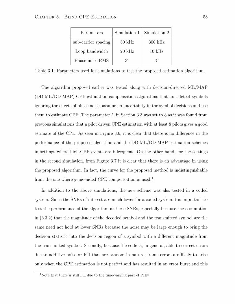
Chapter 3. Blind CPE Estimation 58
Parameters Simulation 1 Simulation 2
sub-carrier spacing 50 kHz 300 kHz
Loop bandwidth 20 kHz 10 kHz
Phase noise RMS 3 3
Table 3.1: Parameters used for simulations to test the proposed estimation algorithm.
The algorithm proposed earlier was tested along with decision-directed ML/MAP
(DD-ML/DD-MAP) CPE estimation-compensation algorithms that first detect symbols
ignoring the effects of phase noise, assume no uncertainty in the symbol decisions and use
them to estimate CPE. The parameter l0 in Section 3.3 was set to 8 as it was found from
previous simulations that a pilot driven CPE estimation with at least 8 pilots gives a good
estimate of the CPE. As seen in Figure 3.6, it is clear that there is no difference in the
performance of the proposed algorithm and the DD-ML/DD-MAP estimation schemes
in settings where high-CPE events are infrequent. On the other hand, for the settings
in the second simulation, from Figure 3.7 it is clear that there is an advantage in using
the proposed algorithm. In fact, the curve for the proposed method is indistinguishable
from the one where genie-aided CPE compensation is used.1.
In addition to the above simulations, the new scheme was also tested in a coded
system. Since the SNRs of interest are much lower for a coded system it is important to
test the performance of the algorithm at these SNRs, especially because the assumption
in (3.3.2) that the magnitude of the decoded symbol and the transmitted symbol are the
same need not hold at lower SNRs because the noise may be large enough to bring the
decision statistic into the decision region of a symbol with a different magnitude from
the transmitted symbol. Secondly, because the code is, in general, able to correct errors
due to additive noise or ICI that are random in nature, frame errors are likely to arise
only when the CPE estimation is not perfect and has resulted in an error burst and this
1Note that there is still ICI due to the time-varying part of PHN.
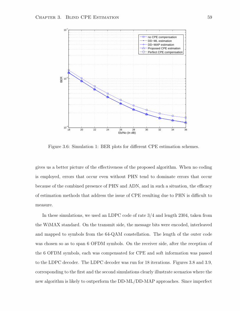
Chapter 3. Blind CPE Estimation 59
18 20 22 24 26 28 30 32 34 3610
−3
10−2
10−1
Eb/No (in dB)
BE
R
no CPE compensationDD−ML estimationDD−MAP estimationProposed CPE estmationPerfect CPE compensation
Figure 3.6: Simulation 1: BER plots for different CPE estimation schemes.
gives us a better picture of the effectiveness of the proposed algorithm. When no coding
is employed, errors that occur even without PHN tend to dominate errors that occur
because of the combined presence of PHN and ADN, and in such a situation, the efficacy
of estimation methods that address the issue of CPE resulting due to PHN is difficult to
measure.
In these simulations, we used an LDPC code of rate 3/4 and length 2304, taken from
the WiMAX standard. On the transmit side, the message bits were encoded, interleaved
and mapped to symbols from the 64-QAM constellation. The length of the outer code
was chosen so as to span 6 OFDM symbols. On the receiver side, after the reception of
the 6 OFDM symbols, each was compensated for CPE and soft information was passed
to the LDPC decoder. The LDPC decoder was run for 18 iterations. Figures 3.8 and 3.9,
corresponding to the first and the second simulations clearly illustrate scenarios where the
new algorithm is likely to outperform the DD-ML/DD-MAP approaches. Since imperfect
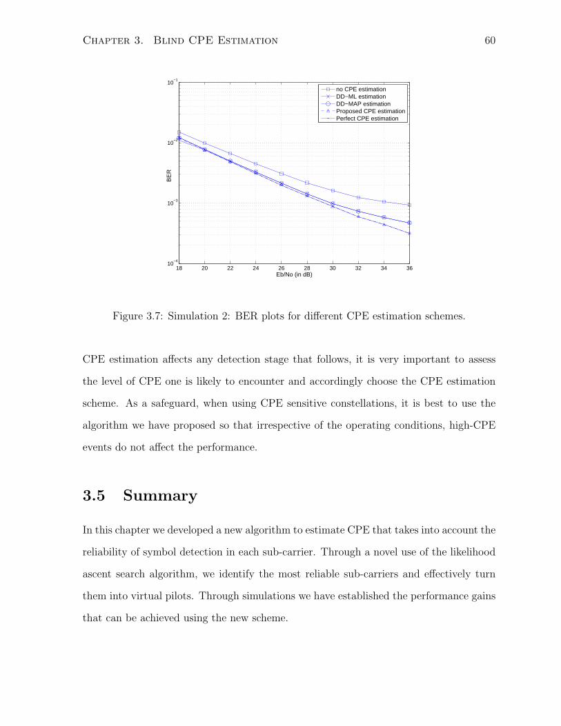
Chapter 3. Blind CPE Estimation 60
18 20 22 24 26 28 30 32 34 3610
−4
10−3
10−2
10−1
Eb/No (in dB)
BE
R
no CPE estimationDD−ML estimationDD−MAP estimationProposed CPE estimationPerfect CPE estimation
Figure 3.7: Simulation 2: BER plots for different CPE estimation schemes.
CPE estimation affects any detection stage that follows, it is very important to assess
the level of CPE one is likely to encounter and accordingly choose the CPE estimation
scheme. As a safeguard, when using CPE sensitive constellations, it is best to use the
algorithm we have proposed so that irrespective of the operating conditions, high-CPE
events do not affect the performance.
3.5 Summary
In this chapter we developed a new algorithm to estimate CPE that takes into account the
reliability of symbol detection in each sub-carrier. Through a novel use of the likelihood
ascent search algorithm, we identify the most reliable sub-carriers and effectively turn
them into virtual pilots. Through simulations we have established the performance gains
that can be achieved using the new scheme.
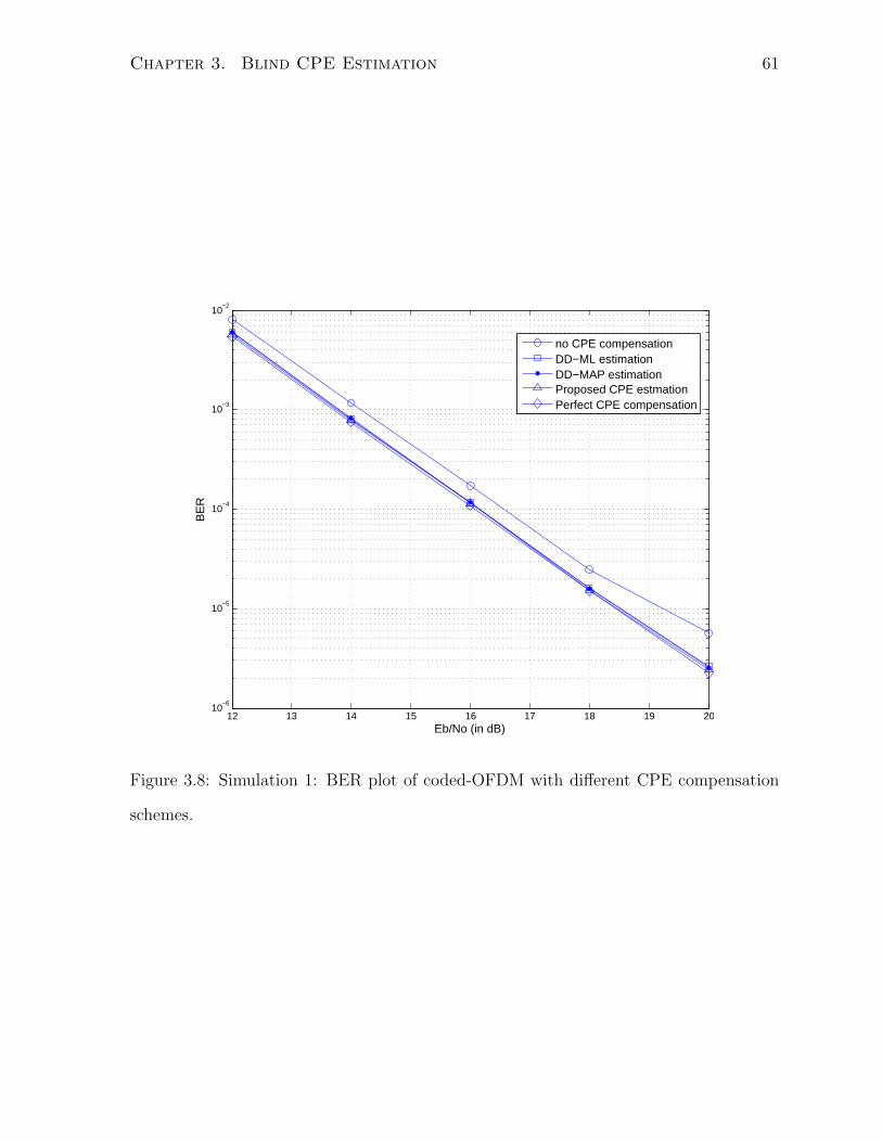
Chapter 3. Blind CPE Estimation 61
12 13 14 15 16 17 18 19 2010
−6
10−5
10−4
10−3
10−2
Eb/No (in dB)
BE
R
no CPE compensationDD−ML estimationDD−MAP estimationProposed CPE estmationPerfect CPE compensation
Figure 3.8: Simulation 1: BER plot of coded-OFDM with different CPE compensation
schemes.
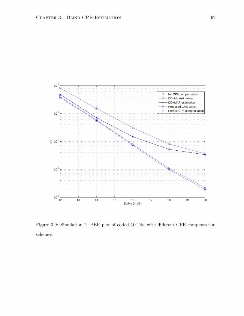
Chapter 3. Blind CPE Estimation 62
12 13 14 15 16 17 18 19 2010
−6
10−5
10−4
10−3
10−2
Eb/No (in dB)
BE
R
No CPE compensationDD−ML estimationDD−MAP estimationProposed CPE estm.Perfect CPE compensation
Figure 3.9: Simulation 2: BER plot of coded-OFDM with different CPE compensation
schemes.
Chapter 4
Turbo Receiver Design for ICI
Mitigation
This chapter addresses the issue of inter-carrier interference (ICI) due to phase noise.
Rather than adopting a standard ICI cancellation scheme, we adopt a more sophisticated
approach that jointly estimates the transmitted symbols and the phase noise sequence
corrupting the received signal. We use an approximate probabilistic framework called
variational inference (VI), using which we develop a soft-in soft-out (SISO) algorithm
that generates posterior bit-level soft estimates while taking into account the effect of
phase noise. The algorithm also provides an estimate of the phase noise sequence. Using
this SISO algorithm, a turbo receiver is designed by passing soft information between
the SISO detector and an outer forward error correcting (FEC) decoder that uses a
soft decoding algorithm. We compare the performance of the turbo receiver against a
single-pass detection-decoding setup, both with and without the algorithm presented in
Chapter 3 is used to estimate and compensate for CPE.
63
Chapter 4. Turbo Receiver Design for ICI Mitigation 64
4.1 Introduction
As outlined in Chapter 2, certain operating conditions such as large loop bandwidth
and small sub-carrier spacing along with high phase noise RMS give rise to situations
with severe interference, resulting is significant degradation in SNR and consequently,
a much higher bit error rate. Under such circumstances, a comprehensive approach to
phase noise induced ICI mitigation is necessary. In this chapter, we develop a detection
algorithm that jointly detects the transmitted bits and the phase noise sequence affecting
the OFDM symbol. So as to completely alleviate the effects of phase noise, we use this
algorithm to set up a turbo receiver that iterates soft information between the detector
and the decoder.
Joint data and phase noise estimation for single carrier systems and multi carrier
systems such as OFDM has been studied extensively [24], [5,10,36–38]. While for single
carrier systems it is possible to construct the factor graph and adopt a message passing
algorithm [38] such an approach becomes prohibitively complicated for OFDM systems
due to inter-connections between all the transmitted bits. Hence, there is a need to
adopt approximate inference techniques that can make the best use of the available
priors in computing the joint estimate. One such technique that lets us compute soft
estimates in such a scenario is variational inference. For the single carrier case, Nissila [39]
considered the use of variational inference for detection of symbols transmitted over
an AWGN channel in the presence of phase uncertainty. In the case of multi-carrier
systems, Lin and Lim [5] developed algorithms for PHN mitigation using variational
inference that generated soft symbol and phase noise estimates. Variational inference
is an approximate probabilistic inference technique associated with the minimization
of an objective function called variational free energy. Variational inference in essence
computes an approximation to the joint posterior distribution of all unknown variables.
In the case of detection in phase noise, these are the transmitted symbols and the phase
noise sequence. The input to the algorithm are the received signal and priors on the
Chapter 4. Turbo Receiver Design for ICI Mitigation 65
transmitted symbols and the phase noise sequence. In [5], Gaussian priors were used for
both the unknown vectors. The algorithm outputs a Gaussian posterior distribution for
the transmitted symbols as well as the phase noise sequence.
With the design of a turbo receiver in mind, we note that, typically, an FEC decoder
employs a bit level soft decoding algorithm such as the sum-product algorithm for de-
coding LDPC codes. An FEC decoder working at a bit level and a detection algorithm
working at a symbol level pose a mismatch that needs to be bridged. While one can com-
pute the individual bit priors (log likelihood ratios) using the mean and variance of the
posterior distribution of a symbol, computing the prior mean and variance of the sym-
bols using the extrinsic bit LLRs computed by the FEC decoder is not straightforward.
Hence, keeping the compatibility of the detection and decoding algorithms in mind, we
develop a bit level detection algorithm, using variational inference. The algorithm is
capable of accepting prior information on the transmitted bits and outputs the posterior
distribution of the bits after transmission, while taking the current channel state, phase
noise and additive noise into consideration.
Two advantages arise in developing a bit level detection algorithm. One, there is no
need to impose an artificial Gaussian prior on the symbols. We adopt a more natural
Bernoulli distribution, with zero mean as the prior for transmitted bits. Second, the
symbol level detection algorithm requires an initialization step that necessitates hard
decisions on symbols while ignoring phase noise. In the algorithm that we develop, the
algorithm is initialized to uniform priors on all the bits.
The rest of the chapter is organized as follows. We first introduce the function used to
map bits to symbols, this is a multi-linear function and plays a key role in our derivation.
We then introduce the signal model that we will focus on. Next, we discuss the actual
posterior distribution of the symbols and phase noise, and introduce the concept of
variational inference. We then present the algorithm that uses variational inference to
compute an approximation of the posterior distribution. This approximate posterior
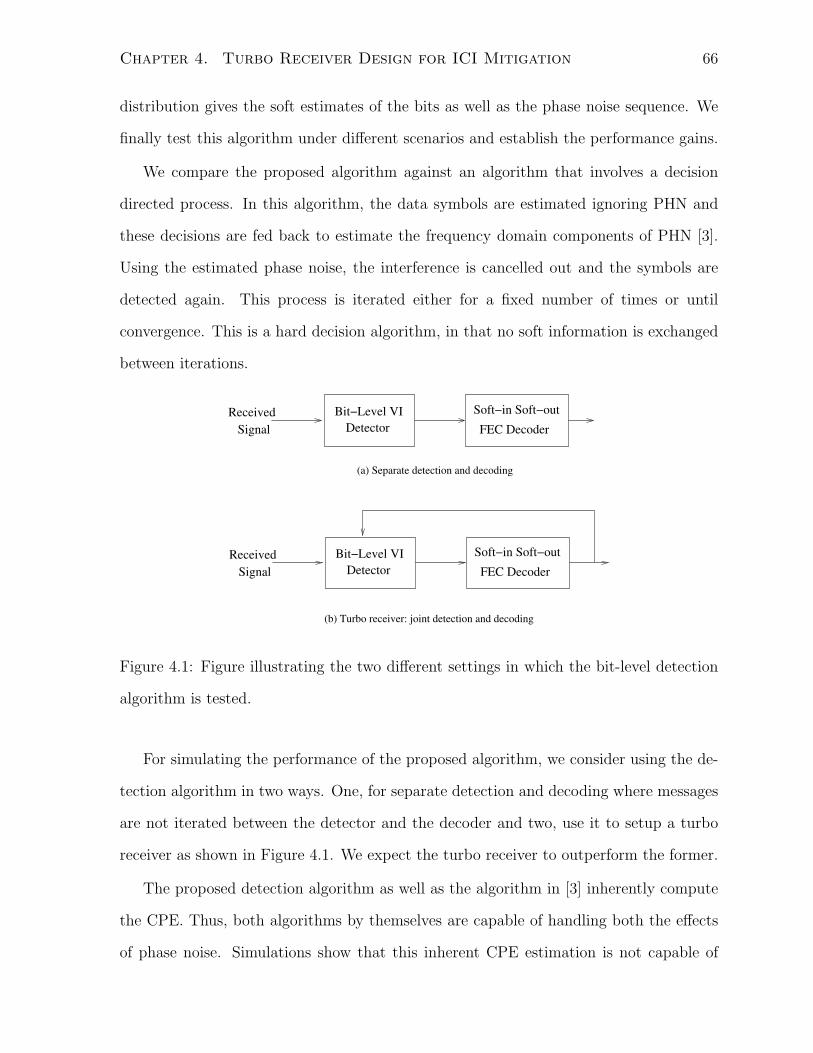
Chapter 4. Turbo Receiver Design for ICI Mitigation 66
distribution gives the soft estimates of the bits as well as the phase noise sequence. We
finally test this algorithm under different scenarios and establish the performance gains.
We compare the proposed algorithm against an algorithm that involves a decision
directed process. In this algorithm, the data symbols are estimated ignoring PHN and
these decisions are fed back to estimate the frequency domain components of PHN [3].
Using the estimated phase noise, the interference is cancelled out and the symbols are
detected again. This process is iterated either for a fixed number of times or until
convergence. This is a hard decision algorithm, in that no soft information is exchanged
between iterations.
FEC Decoder
Soft−in Soft−outBit−Level VI
DetectorSignal
Received
FEC Decoder
Soft−in Soft−outBit−Level VI
DetectorSignal
Received
(a) Separate detection and decoding
(b) Turbo receiver: joint detection and decoding
Figure 4.1: Figure illustrating the two different settings in which the bit-level detection
algorithm is tested.
For simulating the performance of the proposed algorithm, we consider using the de-
tection algorithm in two ways. One, for separate detection and decoding where messages
are not iterated between the detector and the decoder and two, use it to setup a turbo
receiver as shown in Figure 4.1. We expect the turbo receiver to outperform the former.
The proposed detection algorithm as well as the algorithm in [3] inherently compute
the CPE. Thus, both algorithms by themselves are capable of handling both the effects
of phase noise. Simulations show that this inherent CPE estimation is not capable of
Chapter 4. Turbo Receiver Design for ICI Mitigation 67
handling high-CPE events and necessitates an explicit CPE estimation-compensation
scheme as a pre-processing step. This aspect is elaborated further in Section (4.4).
4.2 Received Signal Model
4.2.1 Gray mapping : bits to M-QAM symbols ( from [6] )
We assume M to be an integer of the form 22k, where k is a positive integer. Let L
denote log2M and let B ∈ −1, 1N×L represent a matrix of N × L bits that need to be
mapped to N M-QAM symbols. Denote the columns of B as br1, br2, . . . brL/2, bi1, bi2
. . . biL/2. If the resulting vector of M-QAM symbols is represented as d, then, from [6],
we have the following relation :
d =
L/2∑l=1
2l−1
p=L/2
6∏p=1
brp + jL∑
l=L/2+1
2l−1
p=L/2
6∏p=1
bip (4.1)
Here, 6∏
represents element wise product of the vectors. Let the function f denote
the mapping from bits to symbols, so that d = f (B). Further, denote the matrix [br1
br2 . . . brL/2] as Br, and the matrix [bi1 bi2 . . . biL/2] as Bi and define the functions f r
and f i as :
f i(Bi) = j.=(f (B)) (4.2)
f r(Br) = <(f (B)) (4.3)
Hence, d = f (B) = f r(Br) + f i(Bi).
4.2.2 The Received Signal
The signal model that we focus on in this chapter is the one given in (2.49) for a SISO
point to point link with receiver phase noise. Using the representation in Section 4.2.1,
Chapter 4. Turbo Receiver Design for ICI Mitigation 68
the received signal in the frequency domain can be written as
r = PFHHd + n = PFHHf (B) + n (4.4)
The matrix P is a diagonal matrix given by diag(ejθr) ≈ diag(1 + jθ), where θ is the
PHN sequence affecting the signal after removing the cyclic prefix. The phase noise is
modelled as an AR(1) process, as detailed in Chapter 2. H = diag(h) is the channel
matrix in the frequency domain and the N×L binary matrix B contains the transmitted
bit sequence (d is the corresponding symbol sequence). n is complex white Gaussian
noise with variance σ2 per dimension.
4.2.3 Actual and Postulated Posterior Distributions
From [5], we note that by approximating ejθ to 1+ jθ under the small angle assumption,
one can write the conditional distribution of r given B and θ to be :
p(r|B,θ) = CN (diag(1 + jθ)FHHf (B), 2σ2I)
(4.5)
Further, in [5] it was shown that the optimal detector (i.e. ML estimate of d) for
such a signal model, given the prior distribution of the phase noise sequence θ, has an
exponential complexity in N . Given that the distribution p(r|B) and consequently the
posterior distribution p(B|r) do not lend themselves to efficient optimal detection, we look
at an approximation to p(B|r), such that, computing the optimal estimate corresponding
to the approximated distribution is straightforward. To this end, we note that p(B|r) is
computed by marginalizing p(B,θ|r) with respect to θ, i.e.
p(B|r) =
∫p(B,θ|r)dθ (4.6)
The variational inference approach approximates p(B,θ|r) with a function Q(B,θ) of the
form QB(B)Qθ(θ) such that
QB(B)Qθ(θ) ≈ p(B,θ|r) (4.7)
Chapter 4. Turbo Receiver Design for ICI Mitigation 69
This kind of an approximation is equivalent to assuming that B and θ are independent
conditioned on r and this in turn implies the maximizer of the distribution QB(B) is the
optimal estimate of B. We further assume that the distribution QB(B) can be factorized
into∏N
n=1
∏Ll=1 Qb(bnl). Such a factorization for the postulated posterior distribution of
the bits, where the distribution is assumed to be independent over n and l, is commonly
known as the mean field approximation. In this paper, we assume Qb(bnl) to be a Bernoulli
distribution with parameter λnl. We postulate the posterior conditional distribution of
phase noise to be a multi-variate Gaussian distribution with mean mθ and covariance
Sθ. Thus, we have
Q(B,θ) = QB(B)Qθ(θ)
=
[N∏n=1
L∏l=1
(λnl)1+bnl
2 (1− λnl)1−bnl
2
]N (mθ,Sθ) (4.8)
=
[N∏n=1
L∏l=1
(1+bnl
2
) 1+bnl2(
1−bnl2
)1−bnl2
]N (mθ,Sθ) (4.9)
where, bnl = 2λnl − 1, is the mean of the postulated posterior distribution Qb(bnl). Note
that inspite of prior knowledge that the phase noise is generated from an AR(1) process,
we do not include this aspect in the postulated posterior distribution of phase noise. We
need the distibution Qθ(θ) to closely resemble the distribution p(θ|r), which is given by
p(θ|r) =
∫p(B,θ|r)dB. (4.10)
It is clear from the above equation that the marginal posterior distribution for θ need
not have the AR(1) property and hence such a structure must not be imposed on the
postulated distribution.
Having fixed the structure of the postulated posterior distribution, it remains now
to compute the parameters of this distribution such that it closely approximates the
actual posterior distribution. The variational inference approach introduces the concept
of variational free energy as a measure of similarity between two distributions. The
Chapter 4. Turbo Receiver Design for ICI Mitigation 70
variational free energy between the two distributions of interest here is given by
F (Q, p) =
∫B,θ
Q(B,θ) logQ(B,θ)
p(B,θ, r)dBdθ. (4.11)
We use the distribution p(B,θ, r) instead of p(B,θ|r) as they are related simply
through a constant of proportionality. It is to be noted that the free energy expression is
exactly equal to the Kullback-Leibler divergence between Q(B,θ) and p(B,θ|r) to within
an additive constant. The variational inference approach involves the minimization of
the free energy over the parameters of Q(B,θ) so that the resulting distribution closely
approximates the actual posterior distribution.
The actual posterior distribution can be computed by conditioning over the unknowns
as follows:
p(B,θ, r) =p(r|B,θ)p(B)p(θ) (4.12)
Using (4.5), and assuming independent Bernoulli distributed priors on bits, with the lth
bit of the nth symbol having mean µnl (set µnl to 0 if no prior information is available)
and assuming the prior distribution of PHN to be a multi-variate Gaussian distribution
with mean µθ and covariance matrix φθ (if no prior information is available, set mean to
0 and covariance to Φ as given in (2.8)), we can write the posterior distribution as
p(B,θ, r) =CN (diag(1 + jθ)FHHf (B), 2σ2I)×[
N∏n=1
L∏l=1
(1+µnl
2
)1+bnl2(
1−µnl2
)1−bnl2
]N (µθ,φθ). (4.13)
The next section discusses the computation and minimization of the free energy ex-
pression.
Chapter 4. Turbo Receiver Design for ICI Mitigation 71
4.3 The Bit-Level Variational Inference Algorithm
4.3.1 Free Energy Evaluation
The free energy expression given in (4.11) can be written as the summation of five terms
as shown in (4.14).
F (Q, p) =−∫
B
Q(θ) log p(B)dB︸ ︷︷ ︸i
−∫
θ
Q(θ) log p(θ)dθ︸ ︷︷ ︸ii
+
∫B
Q(B) log p(B)dB︸ ︷︷ ︸iii
+
∫θ
Q(θ) logQ(θ)dθ︸ ︷︷ ︸iv
−∫
B,θ
Q(B)Q(θ) log(p(r|B,θ))dBdθ︸ ︷︷ ︸v
(4.14)
The exact computation of the free energy expression is given in Appendix A and the
final expression is presented here. Note that the free energy expression is parameterized
by the mean and the covariance matrix of the PHN sequence and the mean value of
the posterior distribution of the bits. Note that when treating the unknown B as a
matrix of Bernoulli random variables, we denote B as the matrix of the means (bnl) of
the corresponding random variables in B. We define Br, Bi, brj and brk in a similar
fashion.
F (mθ,Sθ, B) =
−N∑n=1
L∑l=1
[(1+bnl
2
)log(
1+µnl2
)+(
1−bnl2
)log(
1−µnl2
)]+
1
2tr(φ−1
θ Sθ) +1
2mT
θ φ−1θ mθ
− µTθ φ−1
θ mθ +N∑n=1
L∑l=1
[(1+bnl
2
)log(
1+bnl2
)+(
1−bnl2
)log(
1−bnl2
)]− 1
2log |Sθ|
+1
2σ2
[− rHZf (B)− f (B)
HZHr + f r(Br)
HM0f i(Bi) + f i(Bi)
HM0f r(Br)
+ f r(Br)H
M1f r(Br) + f i(Bi)H
M1f i(Bi) + 1HM2νr + 1HM2νi
](4.15)
Chapter 4. Turbo Receiver Design for ICI Mitigation 72
4.3.2 Free Energy Minimization
Clearly, closed form expressions for the optimal parameters that minimize the free energy
expression cannot be computed. Hence, we adopt a coordinate-descent approach to
minimization, wherein one parameter is updated while keeping the others constant. Such
an approach will converge to a local minimum. The update to each parameter is obtained
by computing the gradient of the free energy expression given in (4.15) w.r.t the parameter
and setting it to zero. This leads to three update equations, one each for the mean and
covariance matrix of the phase noise and one for updating the mean corresponding to
the bits. The update equations are :
STθ =
[φ−1θ +
1
σ2XmXH
m +1
σ2
(diag
(FHHdiag(νr + νi − |f (B)|2)HHF
))]−1
(4.16)
mθ =Sθ
[− 1
σ2Im(rHXm)T + φ−1
θ µθ
](4.17)
tbrk =tµrk +1
σ2
[diag(αk)<ZHr − diag(δk)M
T1 1
+ diag(αk)(j=M0f i(Bi)−<MT
2 f r(Br))]
(4.18)
tbik =tµik +1
σ2
[diag(βk)=ZHr − diag(Ωk)M
T1 1
+ diag(βk)(=M0f r(Br) + j<MT
2 f i(Bi))]
(4.19)
In the above equations, tbrk and tbik represent tanh−1(brk) and tanh−1(bik) (computed
element wise) respectively, while tµrk and tµik represent tanh−1(µrk) and tanh−1(µik)
respectively, with µrk and µik defined analogous to brk and bik but with prior means.
Further, the derivatives ∂f r(Br)
∂brkand ∂f i(Bi)
∂bikare denoted as diag(αk) and diag(βk). The
derivatives ∂νr∂brk
and ∂νi∂bik
are denoted as diag(δk) and diag(Ωk). Detailed derivation of
the update equations is given in Appendix B.
Chapter 4. Turbo Receiver Design for ICI Mitigation 73
4.3.3 The Variational Inference Algorithm
Algorithm 1 gives the pseudo code for the steps involved in the VI based soft bit detec-
tion algorithm. We note that because of the coordinate descent approach to free energy
minimization, the algorithm converges to a local minimum and not the global minimum.
Simulations indicated a quick convergence within 3-5 iterations. However, since conver-
gence is only to the local minimum, this is likely to be an issue in high-CPE events and is
actually seen as an error floor in the performance of the stand alone turbo receiver shown
in (4.1). The bit LLRs given by 2(tbrk − tµrk) and 2(tbik − tµik) are the soft messages
passed to the FEC decoder. The SISO FEC decoder is standard for many codes such
as LDPC and turbo and is not described here. For the turbo receiver setup, the phase
noise mean and covariance are re-initialized to 0 and Φ after every iteration between the
detector and the decoder.
4.3.4 Complexity Analysis
In this section we analyze the order of complexity of each step in the pseudocode presented
in Algorithm 1. The first step involves the computation of the vectors νr, νi, αk, δk,
Xm, each of which involve only element wise products of vectors and can be computed in
O(N) time. Next, the update equation of the covariance matrix Sθ involves computing
the inverse of a tridiagonal matrix, with each of the off-diagonal vectors having constant
entries. There exist algorithms that can invert such a matrix in O(N logN) time [40].
Updating mθ is equivalent to solving a tridiagonal system of equations, which is of O(N)
complexity [40]. The bit update equations involve computing four terms. Since the
only dense matrix involved in any of the terms is the DFT matrix, each of the terms
can be computed in O(N logN) time. Thus the overall complexity of the algorithm is
O(N logN).
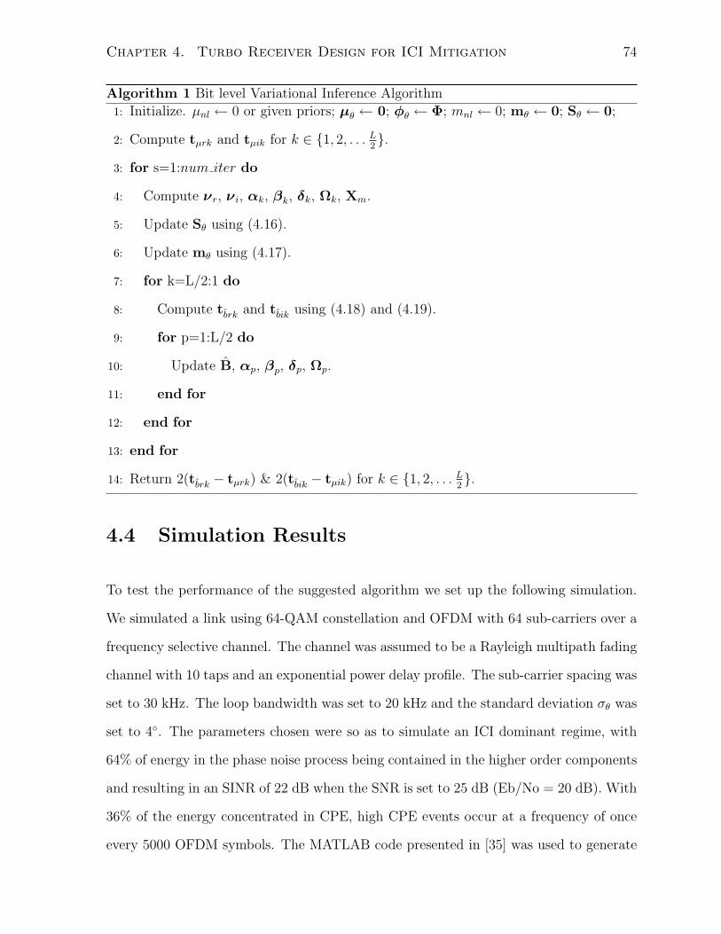
Chapter 4. Turbo Receiver Design for ICI Mitigation 74
Algorithm 1 Bit level Variational Inference Algorithm
1: Initialize. µnl ← 0 or given priors; µθ ← 0; φθ ← Φ; mnl ← 0; mθ ← 0; Sθ ← 0;
2: Compute tµrk and tµik for k ∈ 1, 2, . . . L2.
3: for s=1:num iter do
4: Compute νr, νi, αk, βk, δk, Ωk, Xm.
5: Update Sθ using (4.16).
6: Update mθ using (4.17).
7: for k=L/2:1 do
8: Compute tbrk and tbik using (4.18) and (4.19).
9: for p=1:L/2 do
10: Update B, αp, βp, δp, Ωp.
11: end for
12: end for
13: end for
14: Return 2(tbrk − tµrk) & 2(tbik − tµik) for k ∈ 1, 2, . . . L2.
4.4 Simulation Results
To test the performance of the suggested algorithm we set up the following simulation.
We simulated a link using 64-QAM constellation and OFDM with 64 sub-carriers over a
frequency selective channel. The channel was assumed to be a Rayleigh multipath fading
channel with 10 taps and an exponential power delay profile. The sub-carrier spacing was
set to 30 kHz. The loop bandwidth was set to 20 kHz and the standard deviation σθ was
set to 4. The parameters chosen were so as to simulate an ICI dominant regime, with
64% of energy in the phase noise process being contained in the higher order components
and resulting in an SINR of 22 dB when the SNR is set to 25 dB (Eb/No = 20 dB). With
36% of the energy concentrated in CPE, high CPE events occur at a frequency of once
every 5000 OFDM symbols. The MATLAB code presented in [35] was used to generate
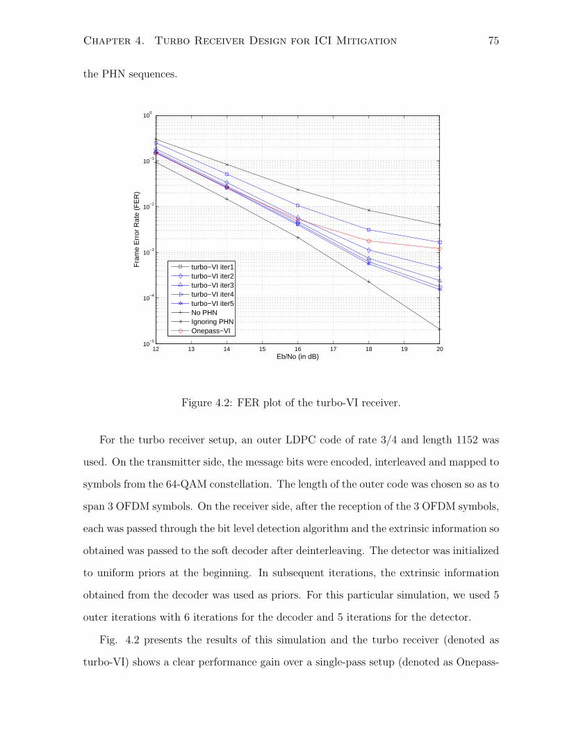
Chapter 4. Turbo Receiver Design for ICI Mitigation 75
the PHN sequences.
12 13 14 15 16 17 18 19 2010
−5
10−4
10−3
10−2
10−1
100
Eb/No (in dB)
Fra
me
Err
or R
ate
(FE
R)
turbo−VI iter1turbo−VI iter2turbo−VI iter3turbo−VI iter4turbo−VI iter5No PHNIgnoring PHNOnepass−VI
Figure 4.2: FER plot of the turbo-VI receiver.
For the turbo receiver setup, an outer LDPC code of rate 3/4 and length 1152 was
used. On the transmitter side, the message bits were encoded, interleaved and mapped to
symbols from the 64-QAM constellation. The length of the outer code was chosen so as to
span 3 OFDM symbols. On the receiver side, after the reception of the 3 OFDM symbols,
each was passed through the bit level detection algorithm and the extrinsic information so
obtained was passed to the soft decoder after deinterleaving. The detector was initialized
to uniform priors at the beginning. In subsequent iterations, the extrinsic information
obtained from the decoder was used as priors. For this particular simulation, we used 5
outer iterations with 6 iterations for the decoder and 5 iterations for the detector.
Fig. 4.2 presents the results of this simulation and the turbo receiver (denoted as
turbo-VI) shows a clear performance gain over a single-pass setup (denoted as Onepass-
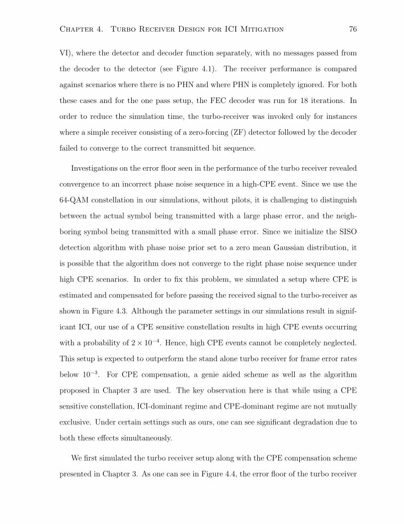
Chapter 4. Turbo Receiver Design for ICI Mitigation 76
VI), where the detector and decoder function separately, with no messages passed from
the decoder to the detector (see Figure 4.1). The receiver performance is compared
against scenarios where there is no PHN and where PHN is completely ignored. For both
these cases and for the one pass setup, the FEC decoder was run for 18 iterations. In
order to reduce the simulation time, the turbo-receiver was invoked only for instances
where a simple receiver consisting of a zero-forcing (ZF) detector followed by the decoder
failed to converge to the correct transmitted bit sequence.
Investigations on the error floor seen in the performance of the turbo receiver revealed
convergence to an incorrect phase noise sequence in a high-CPE event. Since we use the
64-QAM constellation in our simulations, without pilots, it is challenging to distinguish
between the actual symbol being transmitted with a large phase error, and the neigh-
boring symbol being transmitted with a small phase error. Since we initialize the SISO
detection algorithm with phase noise prior set to a zero mean Gaussian distribution, it
is possible that the algorithm does not converge to the right phase noise sequence under
high CPE scenarios. In order to fix this problem, we simulated a setup where CPE is
estimated and compensated for before passing the received signal to the turbo-receiver as
shown in Figure 4.3. Although the parameter settings in our simulations result in signif-
icant ICI, our use of a CPE sensitive constellation results in high CPE events occurring
with a probability of 2× 10⁻⁴. Hence, high CPE events cannot be completely neglected.
This setup is expected to outperform the stand alone turbo receiver for frame error rates
below 10−3. For CPE compensation, a genie aided scheme as well as the algorithm
proposed in Chapter 3 are used. The key observation here is that while using a CPE
sensitive constellation, ICI-dominant regime and CPE-dominant regime are not mutually
exclusive. Under certain settings such as ours, one can see significant degradation due to
both these effects simultaneously.
We first simulated the turbo receiver setup along with the CPE compensation scheme
presented in Chapter 3. As one can see in Figure 4.4, the error floor of the turbo receiver
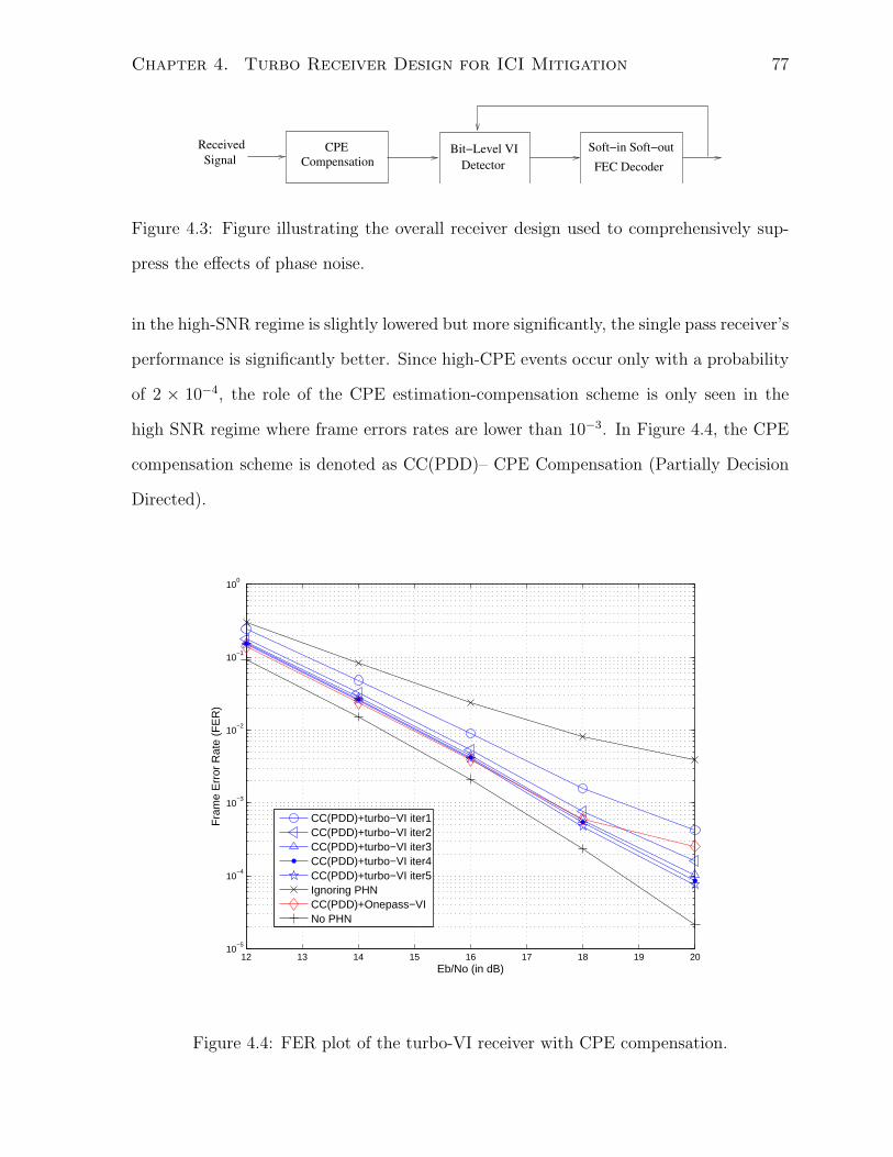
Chapter 4. Turbo Receiver Design for ICI Mitigation 77
FEC Decoder
Soft−in Soft−outBit−Level VI
Detector
CPE
Compensation
Received
Signal
Figure 4.3: Figure illustrating the overall receiver design used to comprehensively sup-
press the effects of phase noise.
in the high-SNR regime is slightly lowered but more significantly, the single pass receiver’s
performance is significantly better. Since high-CPE events occur only with a probability
of 2 × 10⁻⁴, the role of the CPE estimation-compensation scheme is only seen in the
high SNR regime where frame errors rates are lower than 10−3. In Figure 4.4, the CPE
compensation scheme is denoted as CC(PDD)– CPE Compensation (Partially Decision
Directed).
12 13 14 15 16 17 18 19 2010
−5
10−4
10−3
10−2
10−1
100
Eb/No (in dB)
Fra
me
Err
or R
ate
(FE
R)
CC(PDD)+turbo−VI iter1CC(PDD)+turbo−VI iter2CC(PDD)+turbo−VI iter3CC(PDD)+turbo−VI iter4CC(PDD)+turbo−VI iter5Ignoring PHNCC(PDD)+Onepass−VINo PHN
Figure 4.4: FER plot of the turbo-VI receiver with CPE compensation.
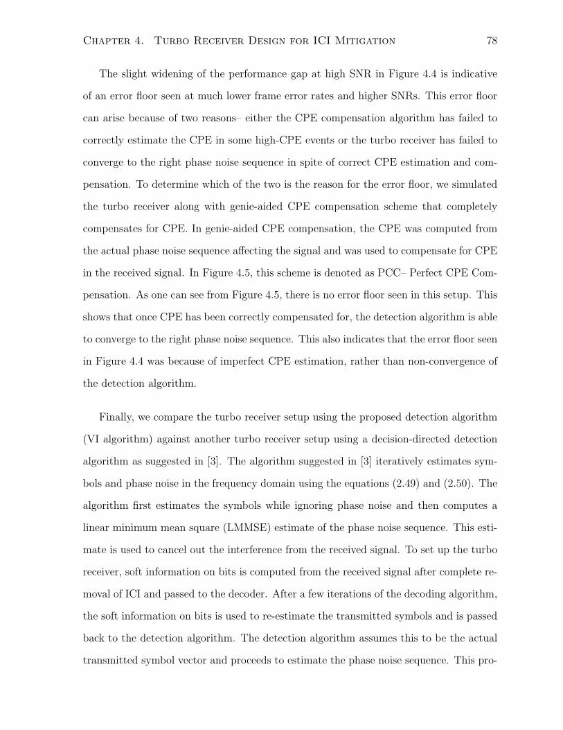
Chapter 4. Turbo Receiver Design for ICI Mitigation 78
The slight widening of the performance gap at high SNR in Figure 4.4 is indicative
of an error floor seen at much lower frame error rates and higher SNRs. This error floor
can arise because of two reasons– either the CPE compensation algorithm has failed to
correctly estimate the CPE in some high-CPE events or the turbo receiver has failed to
converge to the right phase noise sequence in spite of correct CPE estimation and com-
pensation. To determine which of the two is the reason for the error floor, we simulated
the turbo receiver along with genie-aided CPE compensation scheme that completely
compensates for CPE. In genie-aided CPE compensation, the CPE was computed from
the actual phase noise sequence affecting the signal and was used to compensate for CPE
in the received signal. In Figure 4.5, this scheme is denoted as PCC– Perfect CPE Com-
pensation. As one can see from Figure 4.5, there is no error floor seen in this setup. This
shows that once CPE has been correctly compensated for, the detection algorithm is able
to converge to the right phase noise sequence. This also indicates that the error floor seen
in Figure 4.4 was because of imperfect CPE estimation, rather than non-convergence of
the detection algorithm.
Finally, we compare the turbo receiver setup using the proposed detection algorithm
(VI algorithm) against another turbo receiver setup using a decision-directed detection
algorithm as suggested in [3]. The algorithm suggested in [3] iteratively estimates sym-
bols and phase noise in the frequency domain using the equations (2.49) and (2.50). The
algorithm first estimates the symbols while ignoring phase noise and then computes a
linear minimum mean square (LMMSE) estimate of the phase noise sequence. This esti-
mate is used to cancel out the interference from the received signal. To set up the turbo
receiver, soft information on bits is computed from the received signal after complete re-
moval of ICI and passed to the decoder. After a few iterations of the decoding algorithm,
the soft information on bits is used to re-estimate the transmitted symbols and is passed
back to the detection algorithm. The detection algorithm assumes this to be the actual
transmitted symbol vector and proceeds to estimate the phase noise sequence. This pro-
Chapter 4. Turbo Receiver Design for ICI Mitigation 79
12 13 14 15 16 17 18 19 2010
−5
10−4
10−3
10−2
10−1
100
Eb/No (in dB)
Fra
me
Err
or R
ate
PCC+turbo−VI iter1PCC+turbo−VI iter2PCC+turbo−VI iter3PCC+turbo−VI iter4PCC+turbo−VI iter5No PHNIgnoring PHNPCC+Onepass−VI
Figure 4.5: FER plot of the turbo-VI receiver with perfect CPE compensation.
cess is repeated several times. All simulation parameters for this setup are identical to
the turbo receiver discussed previously.
Just as in the the previous scenario, the algorithm was tested under three scenarios:
no CPE compensation, perfect CPE compensation and CPE compensation using the
algorithm in Chapter 3. The results are compared against the turbo receiver set up using
the VI algorithm and the comparative plot is presented in Figure 4.6. The plot shows
performance curves after 5 outer iterations of the turbo receiver. The plot establishes a
clear gain in performance using the VI algorithm. But it must be pointed out that this
improvement in performance comes at the expense of complexity.
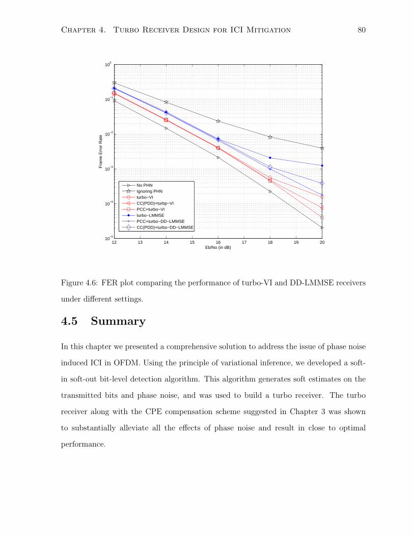
Chapter 4. Turbo Receiver Design for ICI Mitigation 80
12 13 14 15 16 17 18 19 2010
−5
10−4
10−3
10−2
10−1
100
Eb/No (in dB)
Fra
me
Err
or R
ate
No PHNIgnoring PHNturbo−VICC(PDD)+turbp−VIPCC+turbo−VIturbo−LMMSEPCC+turbo−DD−LMMSECC(PDD)+turbo−DD−LMMSE
Figure 4.6: FER plot comparing the performance of turbo-VI and DD-LMMSE receivers
under different settings.
4.5 Summary
In this chapter we presented a comprehensive solution to address the issue of phase noise
induced ICI in OFDM. Using the principle of variational inference, we developed a soft-
in soft-out bit-level detection algorithm. This algorithm generates soft estimates on the
transmitted bits and phase noise, and was used to build a turbo receiver. The turbo
receiver along with the CPE compensation scheme suggested in Chapter 3 was shown
to substantially alleviate all the effects of phase noise and result in close to optimal
performance.
Chapter 5
Effect of Phase Noise on SC-FDMA
In this chapter we study the effect of receiver phase noise on SC-FDMA, which has been
adopted as the uplink modulation technique in LTE. In particular, we study the effect of
phase noise on the performance of linear receivers adopted in the detection of SC-FDMA
symbols. It is shown that CPE affects SC-FDMA symbols in the same manner as OFDM
symbols. While the higher order components result in ICI, the nature of ICI affecting the
sub-carriers depends on whether an interleaved or a localized allocation of sub-carriers
has been adopted. Its effect on both localized and interleaved SC-FDMA is discussed
along with some suggestions for mitigating the ICI from phase noise.
5.1 Introduction
In order to address the issue of peak-to-average power ratio (PAPR) encountered in uplink
OFDMA, SC-FDMA has been adopted for uplink transmission in the LTE standard. SC-
FDMA can be viewed as a DFT precoded OFDMA scheme. Two common approaches to
allocating sub-carriers to users include localized SC-FDMA and interleaved SC-FDMA.
In localized SC-FDMA each user is allocated a set of contiguous sub-carriers for uplink
transmission. In interleaved SC-FDMA, the users are allocated sub-carriers spread evenly
over the transmission bandwidth. Interleaved SC-FDMA offers some diversity benefits
81
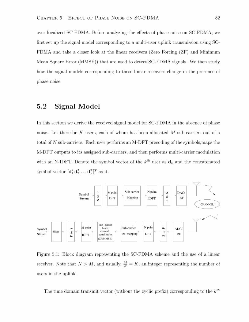
Chapter 5. Effect of Phase Noise on SC-FDMA 82
over localized SC-FDMA. Before analyzing the effects of phase noise on SC-FDMA, we
first set up the signal model corresponding to a multi-user uplink transmission using SC-
FDMA and take a closer look at the linear receivers (Zero Forcing (ZF) and Minimum
Mean Square Error (MMSE)) that are used to detect SC-FDMA signals. We then study
how the signal models corresponding to these linear receivers change in the presence of
phase noise.
5.2 Signal Model
In this section we derive the received signal model for SC-FDMA in the absence of phase
noise. Let there be K users, each of whom has been allocated M sub-carriers out of a
total of N sub-carriers. Each user performs an M-DFT precoding of the symbols,maps the
M-DFT outputs to its assigned sub-carriers, and then performs multi-carrier modulation
with an N-IDFT. Denote the symbol vector of the kth user as dk and the concatenated
symbol vector [dT1 dT2 . . .dTk ]T as d.
ADC/
RF
DAC/
RF
P to
SN point
IDFT
Sub carrier
Mapping
M point
DFT
S to
P
Symbol
Stream
CHANNEL
N point
DFT
Sub carrier
De−mapping
sub−carrier
equalization
channel based
(ZF/MMSE)
M point
IDFT S to
P
P to
S
StreamSlicer
Symbol
Figure 5.1: Block diagram representing the SC-FDMA scheme and the use of a linear
receiver. Note that N > M , and usually, MN
= K, an integer representing the number of
users in the uplink.
The time domain transmit vector (without the cyclic prefix) corresponding to the kth
Chapter 5. Effect of Phase Noise on SC-FDMA 83
user is given by
xk = FNTkFMdk (5.1)
where, Tk is a N ×M sub-carrier mapping/permutation matrix and FM is the M ×MDFT matrix. The structure of Tk and some properties associated with operations that
involve these permutation matrices are discussed in Appendix C. Let the channel between
the kth user and the base station be represented as hk in the frequency domain and let
Hk = diag(hk). Then the received signal corresponding to the kth user at the output of
the N-DFT front end is given by (ignoring noise)
yk = HkTkFMdk (5.2)
The overall received vector corresponding to the signals received from all the K users is
given by
y =K∑k=1
HkTkFMdk + n (5.3)
Figure 5.1 shows the basic operations involved in the transmission and reception of
an SC-FDMA symbol. The figure corresponds in particular to a linear receiver, where
frequency domain channel equalization is carried out on a sub-carrier basis. In this
chapter we discuss in detail the effect of phase noise on linear receivers used to detect
SC-FDMA symbols. In Figure 5.1, ‘P to S’ denotes parallel to serial conversion, ‘S to P’
denotes serial to parallel conversion. DAC and ADC refer to digital to analog conversion
and analog to digital conversion respectively. RF represents all radio frequency circuitry
required for up-conversion to carrier frequency.
5.2.1 ZF Equalization
Assuming we have a frequency domain ZF equalizer at the receiver, we extract the infor-
mation corresponding to the kth user from the vector y by first forming an M × 1 vector
consisting of all the sub-carriers corresponding to the kth user and then compensating
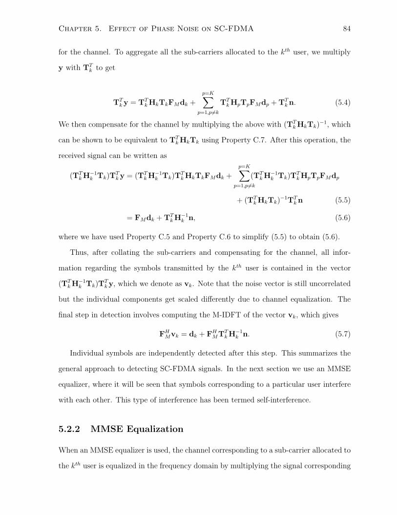
Chapter 5. Effect of Phase Noise on SC-FDMA 84
for the channel. To aggregate all the sub-carriers allocated to the kth user, we multiply
y with TTk to get
TTk y = TT
kHkTkFMdk +
p=K∑p=1,p 6=k
TTkHpTpFMdp + TT
kn. (5.4)
We then compensate for the channel by multiplying the above with (TTkHkTk)
−1, which
can be shown to be equivalent to TTkHkTk using Property C.7. After this operation, the
received signal can be written as
(TTkH−1
k Tk)TTk y = (TT
kH−1k Tk)T
TkHkTkFMdk +
p=K∑p=1,p 6=k
(TTkH−1
k Tk)TTkHpTpFMdp
+ (TTkHkTk)
−1TTkn (5.5)
= FMdk + TTkH−1
k n, (5.6)
where we have used Property C.5 and Property C.6 to simplify (5.5) to obtain (5.6).
Thus, after collating the sub-carriers and compensating for the channel, all infor-
mation regarding the symbols transmitted by the kth user is contained in the vector
(TTkH−1
k Tk)TTk y, which we denote as vk. Note that the noise vector is still uncorrelated
but the individual components get scaled differently due to channel equalization. The
final step in detection involves computing the M-IDFT of the vector vk, which gives
FHMvk = dk + FH
MTTkH−1
k n. (5.7)
Individual symbols are independently detected after this step. This summarizes the
general approach to detecting SC-FDMA signals. In the next section we use an MMSE
equalizer, where it will be seen that symbols corresponding to a particular user interfere
with each other. This type of interference has been termed self-interference.
5.2.2 MMSE Equalization
When an MMSE equalizer is used, the channel corresponding to a sub-carrier allocated to
the kth user is equalized in the frequency domain by multiplying the signal corresponding
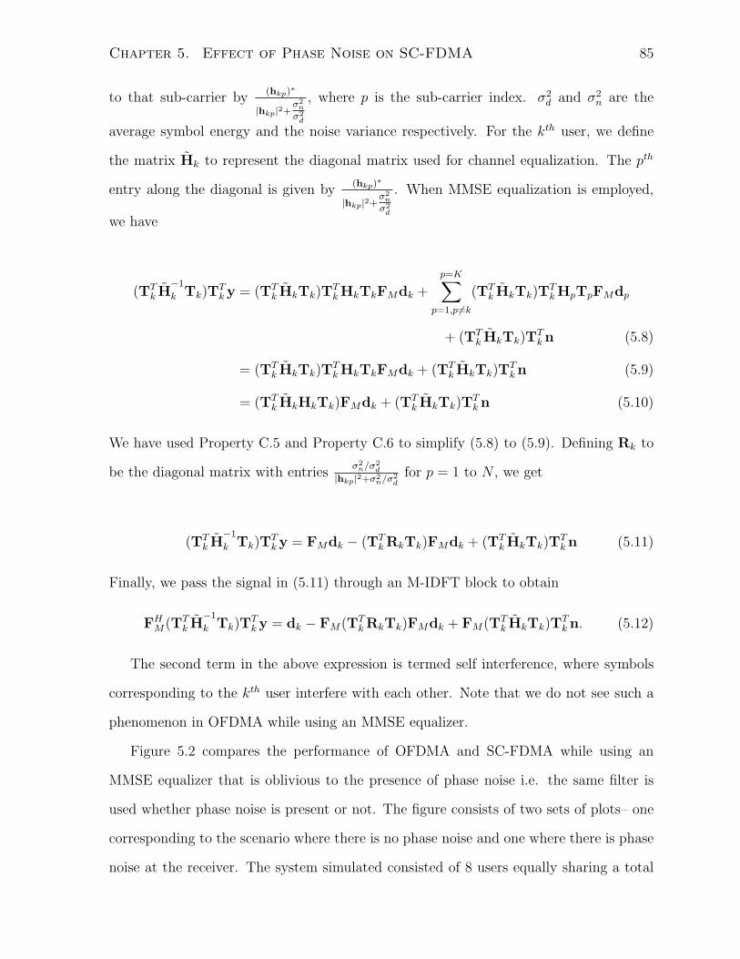
Chapter 5. Effect of Phase Noise on SC-FDMA 85
to that sub-carrier by(hkp)∗
|hkp|2+σ2n
σ2d
, where p is the sub-carrier index. σ2d and σ2
n are the
average symbol energy and the noise variance respectively. For the kth user, we define
the matrix Hk to represent the diagonal matrix used for channel equalization. The pth
entry along the diagonal is given by(hkp)∗
|hkp|2+σ2n
σ2d
. When MMSE equalization is employed,
we have
(TTk H
−1
k Tk)TTk y = (TT
k HkTk)TTkHkTkFMdk +
p=K∑p=1,p 6=k
(TTk HkTk)T
TkHpTpFMdp
+ (TTk HkTk)T
Tkn (5.8)
= (TTk HkTk)T
TkHkTkFMdk + (TT
k HkTk)TTkn (5.9)
= (TTk HkHkTk)FMdk + (TT
k HkTk)TTkn (5.10)
We have used Property C.5 and Property C.6 to simplify (5.8) to (5.9). Defining Rk to
be the diagonal matrix with entriesσ2n/σ
2d
|hkp|2+σ2n/σ
2d
for p = 1 to N , we get
(TTk H
−1
k Tk)TTk y = FMdk − (TT
kRkTk)FMdk + (TTk HkTk)T
Tkn (5.11)
Finally, we pass the signal in (5.11) through an M-IDFT block to obtain
FHM(TT
k H−1
k Tk)TTk y = dk − FM(TT
kRkTk)FMdk + FM(TTk HkTk)T
Tkn. (5.12)
The second term in the above expression is termed self interference, where symbols
corresponding to the kth user interfere with each other. Note that we do not see such a
phenomenon in OFDMA while using an MMSE equalizer.
Figure 5.2 compares the performance of OFDMA and SC-FDMA while using an
MMSE equalizer that is oblivious to the presence of phase noise i.e. the same filter is
used whether phase noise is present or not. The figure consists of two sets of plots– one
corresponding to the scenario where there is no phase noise and one where there is phase
noise at the receiver. The system simulated consisted of 8 users equally sharing a total
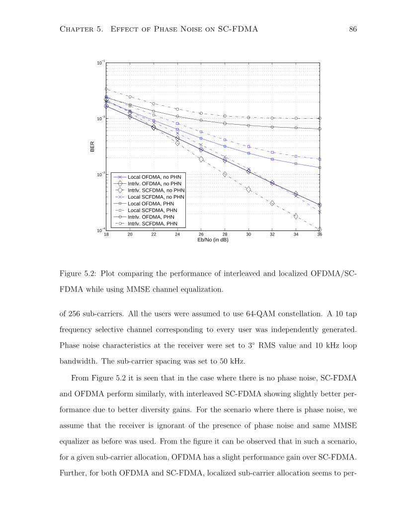
Chapter 5. Effect of Phase Noise on SC-FDMA 86
18 20 22 24 26 28 30 32 34 3610
−4
10−3
10−2
10−1
Eb/No (in dB)
BE
R
Local OFDMA, no PHNIntrlv. OFDMA, no PHNIntrlv. SCFDMA, no PHNLocal SCFDMA, no PHNLocal OFDMA, PHNLocal SCFDMA, PHNIntrlv. OFDMA, PHNIntrlv. SCFDMA, PHN
Figure 5.2: Plot comparing the performance of interleaved and localized OFDMA/SC-
FDMA while using MMSE channel equalization.
of 256 sub-carriers. All the users were assumed to use 64-QAM constellation. A 10 tap
frequency selective channel corresponding to every user was independently generated.
Phase noise characteristics at the receiver were set to 3 RMS value and 10 kHz loop
bandwidth. The sub-carrier spacing was set to 50 kHz.
From Figure 5.2 it is seen that in the case where there is no phase noise, SC-FDMA
and OFDMA perform similarly, with interleaved SC-FDMA showing slightly better per-
formance due to better diversity gains. For the scenario where there is phase noise, we
assume that the receiver is ignorant of the presence of phase noise and same MMSE
equalizer as before was used. From the figure it can be observed that in such a scenario,
for a given sub-carrier allocation, OFDMA has a slight performance gain over SC-FDMA.
Further, for both OFDMA and SC-FDMA, localized sub-carrier allocation seems to per-
Chapter 5. Effect of Phase Noise on SC-FDMA 87
form much better than the corresponding interleaved sub-carrier allocation. This is a
surprising result since interleaved SC-FDMA performs better than localized SC-FDMA
in the absence of phase noise. We explore the reasons behind such behaviour in the next
few sections. The next section analyzes effect of phase noise on the received signal model.
5.3 Detection in the Presence of Phase Noise
5.3.1 Received Signal Model
As defined in Chapter 2, let θr be the phase noise sequence affecting an SC-FDMA
symbol, let pr = ejθr
and let Q be the circulant matrix given by FNdiag(pr)FHN . The
rows of Q are circular shifts of the frequency domain components of phase noise given
by 1√N
FHNpr = [c0 c1 c2 . . . cN−1]T . In the presence of receiver phase noise, the received
signal after the N-DFT front end can be written as
y = QK∑k=1
HkTkFMdk + n. (5.13)
Aggregating the sub-carriers corresponding to the kth user by multiplying with TTk
gives
TTk y = TT
kQK∑p=1
HpTpFMdp + TTkn. (5.14)
In Appendix D, we further manipulate this expression to obtain
TTk y =c0(TT
kHkTk)FMdk + (TTk (Q− c0I)Tk)(T
TkHkTk)FMdk
+
p=K∑p=1,p 6=k
(TTkQTp)(T
Tp HpTp)FMdp + TT
kn (5.15)
In (5.15), the first term is the same as the received signal in the absence of phase
noise except for the rotation by CPE. Its seen that the effect of CPE on an SC-FDMA
symbol is the same as that on an OFDM/OFDMA symbol. The second term repre-
sents the self-interference (interference within a users data stream) that results due to
Chapter 5. Effect of Phase Noise on SC-FDMA 88
phase noise. The third term represents the multi-user interference that results from
data streams corresponding to other users. Further discussion on self interference and
multi-user interference is presented in Section 5.3.3.
5.3.2 Effect on Linear Receivers
Our analysis so far has been focused on the basic received signal model and is independent
of the type of receiver being used. We now turn our attention to the effect phase noise has
on linear receivers (ZF/MMSE). In the absence of impairments such as phase noise, it is
optimal to treat every sub-carrier to be independent of each other and adopt frequency
domain equalization as shown in Section 5.2.2. Due to their low complexity and ease
of implementation, such receivers are very commonly used in practice and hence it is
important for us to assess the impact phase noise is likely to have on such receivers.
Through this analysis we also try to explain why the impact of phase noise on interleaved
and localized SC-FDMA is different while using a linear receiver as seen in Figure 5.2.
To keep the analysis simple, we consider a ZF equalizer here. Arguments made here also
hold for MMSE equalizers at high SNR.
Given a ZF equalizer at the receiver, from (5.15), the signal after channel equalization
can be written as
(TTkH−1
k Tk)TTk y =c0(TT
kH−1k Tk)(T
TkHkTk)FMdk
+ (TTkH−1
k Tk)(TTk (Q− c0I)Tk)(T
TkHkTk)FMdk
+
p=K∑p=1,p 6=k
(TTkH−1
k Tk)(TTkQTp)(T
Tp HpTp)FMdp + (TT
kH−1k Tk)T
Tkn
(5.16)
Chapter 5. Effect of Phase Noise on SC-FDMA 89
(TTkH−1
k Tk)TTk y =c0FMdk + (TT
kH−1k Tk)(T
Tk (Q− c0I)Tk)(T
TkHkTk)FMdk
+
p=K∑p=1,p 6=k
(TTkH−1
k Tk)(TTkQTp)(T
Tp HpTp)FMdp + (TT
kH−1k Tk)T
Tkn.
(5.17)
After the final M-IDFT operation, we can write
FHM(TT
kH−1k Tk)T
Tk y =c0dk + FH
M(TTkH−1
k Tk)(TTk (Q− c0I)Tk)(T
TkHkTk)FMdk
+
p=K∑p=1,p 6=k
FHM(TT
kH−1k Tk)(T
TkQTp)(T
Tp HpTp)FMdp
+ FHM(TT
kH−1k Tk)T
Tkn. (5.18)
While CPE has the same effect as before, quantifying the resulting ICI is not straight-
forward. We first take a closer look at the second term in (5.18). The second term in
(5.18) representing self interference is an M × 1 vector that is essentially the product of
five matrices – FHM , (TT
kH−1k Tk), (TT
k (Q − c0I)Tk), (TTkHkTk), FM and the vector dk.
Any entry in the resulting M × 1 vector is a summation of many terms having a generic
representation given by
e1 = αh−1i cxhjβdl, (5.19)
where α and β are any two entries from FHM and FM respectively 1, h−1
i and hj are entries
from the matrix (TTkH−1
k Tk) and (TTkHkTk) respectively, and cx is an entry from the
matrix TTk (Q − c0I)Tk
2. Similarly, any entry in the resulting M × 1 vector from the
third term in (5.18) representing multi-user interference, is a summation of many terms
having a generic representation given by
e2 = αh−1i czhjβdl, (5.20)
1Note that |α| = |β| = 12By Properties C.8 and C.9, this matrix is independent of k, hence the argument is valid for any user
Chapter 5. Effect of Phase Noise on SC-FDMA 90
where α and β are as defined before, while h−1i and hj are entries from the matrix
(TTkH−1
k Tk) and (TTp HpTp) respectively, with k 6= p, and cz is an entry from the matrix
(TTkQTp).
While e1 and e2 look similar, the key difference arises from the fact that hi and hj
can be strongly correlated in the case of e1, while this is never the case with e2, where
hi and hj come from two different users. When hi and hj are either identical or strongly
correlated, the variance of e1 can be written as
V ar(e1) ≈ E[|dl|2]E[|cx|2], (5.21)
and in the case of e2, since hi and hj are independent of each other, the variance of e2
can be written as
V ar(e2) = E[|dl|2]E[|cz|2]E
[( |hj||hi|)2]. (5.22)
The variance of e2 contains a term involving the second moment of the ratio of two
Rayleigh random variables (or the mean of the ratio of two Chi-square random variables
with two degrees of freedom). The distribution of the ratio of two Rayleigh random
variables is called the Fisher-Snedecor distribution and it is known that the variance of
such a ratio diverges [41], suggesting that the interference resulting from the third term
in (5.18) can be significant provided E[|cz|2] does not go to zero. This difference between
e1 and e2 differentiates localized and interleaved SC-FDMA, but the argument is not yet
complete.
In the case of localized SC-FDMA, the significant frequency components of phase
noise that contain most of the energy of the phase noise process are contained in the sub-
matrix (TTk (Q−c0I)Tk) and contribute towards self interference. As a result, the terms in
multi-user interference, of the form e2, have very small phase noise frequency components
associated with them, rendering terms resembling e2 insignificant. The coming together
of this fact and the high correlation amongst the channel coefficients corresponding to
Chapter 5. Effect of Phase Noise on SC-FDMA 91
a user as a result of contiguous sub-carrier allocation, that most interference terms in
localized SC-FDMA comes from terms resembling e1, whose variance remains bounded.
On the other hand, in the case of interleaved SC-FDMA, not all significant frequency
components are contained in (TTk (Q− c0I)Tk). As a result, among the terms that con-
tribute towards multi-user interference, there are terms where E[|cz|2] can be significant.
Since the channel coefficients of such terms, with the generic representation given by e2,
are completely independent of each other, the variance of these terms becomes unbounded
and can cause significant interference. We believe this to be reason behind interleaved
SC-FDMA being affected by phase noise much more than localized SC-FDMA while
using a linear receiver.
In order to test our hypothesis, we ran two sets of simulations. Our hypothesis hinges
on two things: channel coefficient correlation in the case of localized SC-FDMA and phase
noise energy concentration in the lower order frequency components. Removal of either
property must render the effects on interleaved and localized SC-FDMA equivalent. This
is what we intended to check.
In the first set of simulations, rather than generating the frequency selective channel
in the time domain and then computing its frequency domain coefficients, we directly
generated independent channel coefficients corresponding to different sub-carriers in the
frequency domain. As a consequence of this, if our hypothesis is right, localized SC-
FDMA will now not have the advantage of correlated channel coefficients being associated
with dominant phase noise frequency components and we expect interleaved and localized
SC-FDMA to be equally affected by phase noise. This is verified through simulations in
Figure 5.3, where it is seen that interleaved and localized SC-FDMA have very similar
performance curves in the presence of phase noise.
In the second test, rather than modelling phase noise as a correlated process, we
modelled it as an uncorrelated process. As a result, the energy in the phase noise process
is equally spread amongst all the frequency components. As a consequence of this, local-
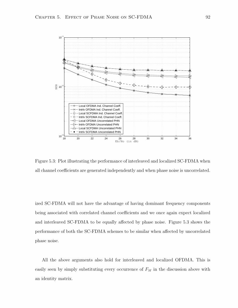
Chapter 5. Effect of Phase Noise on SC-FDMA 92
18 20 22 24 26 28 30 32 34 3610
−3
10−2
10−1
Eb/No (in dB)
BER
Local OFDMA Ind. Channel Coeff.Intrlv OFDMA Ind. Channel Coeff.Local SCFDMA Ind. Channel Coeff.Intrlv SCFDMA Ind. Channel Coeff.Local OFDMA Uncorrelated PHNIntrlv OFDMA Uncorrelated PHNLocal SCFDMA Uncorrelated PHNIntrlv SCFDMA Uncorrelated PHN
Figure 5.3: Plot illustrating the performance of interleaved and localized SC-FDMA when
all channel coefficients are generated independently and when phase noise is uncorrelated.
ized SC-FDMA will not have the advantage of having dominant frequency components
being associated with correlated channel coefficients and we once again expect localized
and interleaved SC-FDMA to be equally affected by phase noise. Figure 5.3 shows the
performance of both the SC-FDMA schemes to be similar when affected by uncorrelated
phase noise.
All the above arguments also hold for interleaved and localized OFDMA. This is
easily seen by simply substituting every occurrence of FM in the discussion above with
an identity matrix.
Chapter 5. Effect of Phase Noise on SC-FDMA 93
5.3.3 Self Interference vs. Multi-User Interference
In Section 5.3.1 we studied the SC-FDMA received signal model immediately after the
N-DFT operation at the receiver and noted in (5.15) that the total interference consists
of two terms – self interference and multi-user interference.
A point of interest here is to find out which of the two interferences is likely to
dominate and under what circumstances. Suppose one finds self-interference to be dom-
inant, then interference cancellation schemes that work exclusively on individual user
data streams will suffice to substantially reduce the effects of phase noise. This is of
particular advantage when different users use different constellations for modulation. In
such a scenario, we can pick a user using a smaller constellation (4-QAM/16-QAM) that
is not CPE sensitive and more robust to ICI and additive noise to estimate the significant
frequency components of phase noise that contribute towards ICI and use these estimates
to cancel ICI in other users’ data streams. On the other hand, if multi-user interference
is likely to dominate, then we cannot take recourse to interference cancellers that work
on individual user data streams, and we have to look at joint interference cancellation
across all the data streams. This is clearly much more complicated than the case where
self-interference tends to dominate.
From (5.15), it is seen that the amount of self-interference is directly related to
the amount of energy contained in TTk (Q − c0I)Tk, which is given by E[tr(TT
k (Q −c0I)Tk)(T
Tk (Q− c0I)Tk)
H]. Note that we are essentially comparing the average energy
contained in the vector given by the second term in (5.15) to the average energy con-
tained in the vector given by the third term in (5.15) which consists of a summation
of contributions from (K-1) other users. Denoting the two average energies as ESI and
EMUI , and assuming all channel gains to be independent with variance Eh and average
symbol energy to be Ed, we get
ESI = EhEdE[tr
(TTk (Q− c0I)Tk)(T
Tk (Q− c0I)Tk)
H]. (5.23)
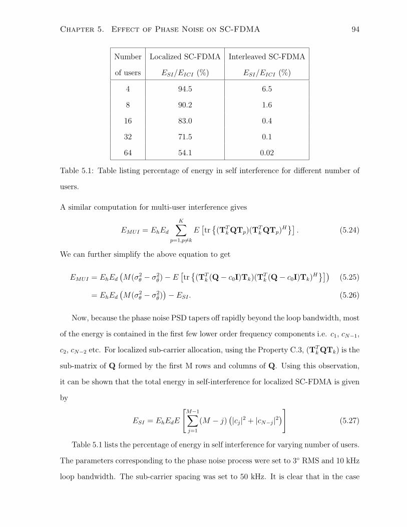
Chapter 5. Effect of Phase Noise on SC-FDMA 94
Number Localized SC-FDMA Interleaved SC-FDMA
of users ESI/EICI (%) ESI/EICI (%)
4 94.5 6.5
8 90.2 1.6
16 83.0 0.4
32 71.5 0.1
64 54.1 0.02
Table 5.1: Table listing percentage of energy in self interference for different number of
users.
A similar computation for multi-user interference gives
EMUI = EhEd
K∑p=1,p 6=k
E[tr
(TTkQTp)(T
TkQTp)
H]. (5.24)
We can further simplify the above equation to get
EMUI = EhEd(M(σ2
θ − σ2θ)− E
[tr
(TTk (Q− c0I)Tk)(T
Tk (Q− c0I)Tk)
H])
(5.25)
= EhEd(M(σ2
θ − σ2θ))− ESI . (5.26)
Now, because the phase noise PSD tapers off rapidly beyond the loop bandwidth, most
of the energy is contained in the first few lower order frequency components i.e. c1, cN−1,
c2, cN−2 etc. For localized sub-carrier allocation, using the Property C.3, (TTkQTk) is the
sub-matrix of Q formed by the first M rows and columns of Q. Using this observation,
it can be shown that the total energy in self-interference for localized SC-FDMA is given
by
ESI = EhEdE
[M−1∑j=1
(M − j) (|cj|2 + |cN−j|2)]
(5.27)
Table 5.1 lists the percentage of energy in self interference for varying number of users.
The parameters corresponding to the phase noise process were set to 3 RMS and 10 kHz
loop bandwidth. The sub-carrier spacing was set to 50 kHz. It is clear that in the case
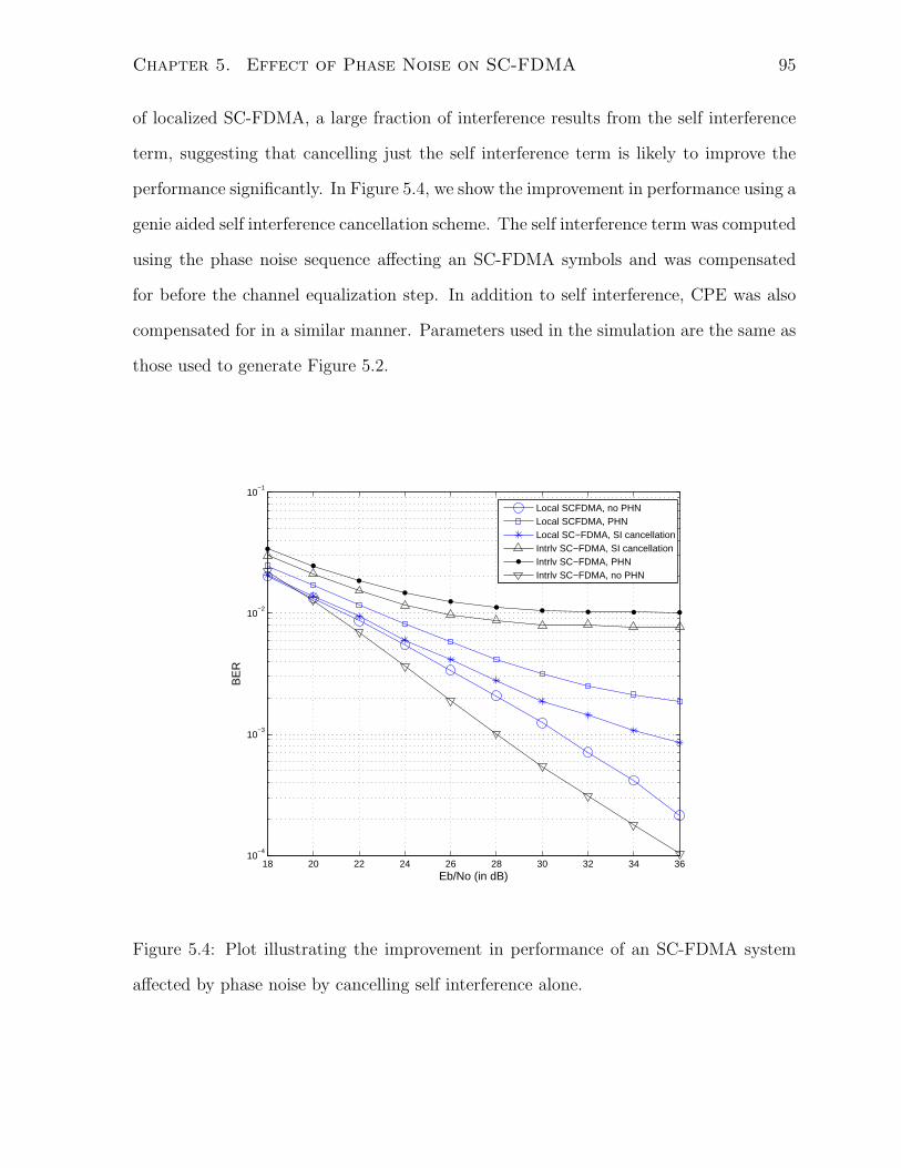
Chapter 5. Effect of Phase Noise on SC-FDMA 95
of localized SC-FDMA, a large fraction of interference results from the self interference
term, suggesting that cancelling just the self interference term is likely to improve the
performance significantly. In Figure 5.4, we show the improvement in performance using a
genie aided self interference cancellation scheme. The self interference term was computed
using the phase noise sequence affecting an SC-FDMA symbols and was compensated
for before the channel equalization step. In addition to self interference, CPE was also
compensated for in a similar manner. Parameters used in the simulation are the same as
those used to generate Figure 5.2.
18 20 22 24 26 28 30 32 34 3610
−4
10−3
10−2
10−1
Eb/No (in dB)
BE
R
Local SCFDMA, no PHNLocal SCFDMA, PHNLocal SC−FDMA, SI cancellationIntrlv SC−FDMA, SI cancellationIntrlv SC−FDMA, PHNIntrlv SC−FDMA, no PHN
Figure 5.4: Plot illustrating the improvement in performance of an SC-FDMA system
affected by phase noise by cancelling self interference alone.
Chapter 5. Effect of Phase Noise on SC-FDMA 96
5.4 Summary
In this chapter we analyzed the effect of phase noise on SC-FDMA. We noted that
when linear receivers are used, the effect of phase noise on interleaved and localized SC-
FDMA can be quite different. We provided a qualitative argument for the difference in
performance of the two SC-FDMA schemes and tested our hypothesis under two different
scenarios. We also studied the general received signal model of a system employing SC-
FDMA and suggested some detection strategies that one could adopt while detecting
SC-FDMA symbols affected by phase noise.
Chapter 6
Conclusion
In the first part of this thesis we focused on the effect phase noise has on OFDM/OFDMA
systems. We focused on how phase noise affects the signal model under different scenarios
and identified its two main effects. We separately studied the behaviour of CPE and the
higher order components and identified the main issues surrounding each of them. To be
specific, we classified constellations based on their CPE sensitivity and highlighted the
effect high CPE can have on blind/decision-directed algorithms.
We then developed an algorithm to blindly estimate CPE that is robust to decision-
directed errors. The algorithm is able to side step the issues surrounding erroneous
detection by taking into account the reliability of symbol detection in each sub-carrier.
Through a novel use of the likelihood ascent search algorithm, we identify the most
reliable sub-carriers and effectively turn them into virtual pilots. The algorithm was
shown to provide accurate CPE estimates even in a high CPE scenario.
We then turned our attention to the issue of ICI mitigation in OFDM systems affected
by phase noise. Using the principle of variational inference, we developed a soft-in soft-
out bit-level detection algorithm. This algorithm jointly estimates the transmitted bits
and the phase noise sequence and generates soft estimates on the transmitted bits and
phase noise. This algorithm was used in three different receiver setups including its use in
97
Chapter 6. Conclusion 98
building a turbo receiver. The turbo receiver along with the CPE compensation scheme
suggested in Chapter 3 was shown to substantially alleviate all the effects of phase noise
and result in close to optimal performance.
Our focus in this thesis was exclusively on receiver phase noise. Future work in this
area must first separately account for the effect of transmitter phase noise and then
consider the joint effects of transmitter and receiver phase noise. Not all phase noise
parameters can be individually estimated in such a scenario and one will have to consider
estimating the effective components that contribute towards interference. In our work
we assumed the channel coefficients to be perfectly known. This is not case in a practical
scenario and there is a need to investigate the performance of the suggested algorithms
under channel uncertainty.
Finally, we analyzed the effect of phase noise on SC-FDMA. We took note of the
surprising result that sub-carrier mapping plays a crucial role in determining the perfor-
mance of the system while using a linear receiver. In particular, we observed that in-
terleaved SC-FDMA was much more sensitive to phase noise than localized SC-FDMA.
We provided a qualitative argument to explain the difference in performance between
the two sub-carrier allocation schemes and substantiated our argument by testing the
proposed hypothesis under two different scenarios. We also studied the general received
signal model of a system employing SC-FDMA and suggested some detection strategies
that one could adopt while detecting SC-FDMA symbols affected by phase noise.
Future work in this area could include providing a clear quantitative explanation
for the difference in performance between interleaved and localized SC-FDMA. Interfer-
ence mitigation in a phase noise affected SC-FDMA system by estimating the dominant
frequency components of phase noise from the received signal corresponding to the sub-
carriers allocated to a user using a constellation robust to CPE can also be explored.

Appendices
99
Appendix A
Evaluating the Free Energy
Expression
As shown in (4.14), the free energy expression can be written as the sum of five terms.
Since we have adopted a discrete distribution for QB(B), it is straightforward to compute
the first and third terms. The second term is the Kullback-Liebler divergence between
two multi-variate Gaussian distributions and can be computed easily. The fourth term is
simply the differential entropy of a multi-variate Gaussian distribution. We discuss the
computation of the fifth term (v) here. Now,
−2σ2(v) =const+
∫B,θ
[Q(B)Q(θ)(r−PFHHf (B))H(r−PFHHf (B))
]dBdθ (A.1)
Proceeding exactly as in [5], we can simplify (A.1) to
−2σ2(v) =const+
∫B
Q(B)[f (B)HZHZf (B)− rHZf (B)
− f (B)HZHr + f (B)HΨf (B)]dB, (A.2)
100
Appendix A. Evaluating the Free Energy Expression 101
where, we have defined Z = diag(1 + jmθ)FHH and Ψ = HHFdiag(Sθ)F
HH). Using
Lemmas 5 and 6 from [6], we can simplify (A.2) to
−2σ2(v) =const− rHZf (B)− f (B)H
ZHr + 1H(M1)(νr + νr)
+ f r(Br)H
(M0)f i(Bi) + f i(Bi)H
(M0)f r(Br)
+ f r(Br)H
(M2)f r(Br) + f i(Bi)H
(M2)f i(Bi) (A.3)
where, M0 =(Ψ + ZHZ) (A.4)
M1 =Ψ + ZHZ− diag(Ψ + ZHZ) (A.5)
M2 = diag(Ψ + ZHZ) (A.6)
νr =∑
0<i≤j<(L/2)
2i+jp=j
6∏p=i
bp +
L/2∑i=1
22(i−1) (A.7)
νi =∑
0<i≤j<(L/2)
2i+jp=j
6∏p=i
bp+(L/2) +
L/2∑i=1
22(i−1). (A.8)
Appendix B
Computing the Gradient
B.1 Gradient w.r.t Sθ
Using (4.11) and (4.15), we can write
∂F
∂ S−1θ
=∂(−i− ii+ iii+ iv − v)
∂S−1θ
(B.1)
One can compute the terms above to be :
∂(i)
∂S−1θ
= 0;∂(ii)
∂S−1θ
=1
2STθ φ−1
θ STθ ;∂(iii)
∂S−1θ
= 0;∂(iv)
∂S−1θ
=1
2STθ (B.2)
To compute ∂(v)
∂S−1θ
, note the following two results.
(a)∂(xHdiag(Sθ)y)
∂S−1θ
=∂(tr(diag(xH)Sθdiag(y))
)∂S−1
θ
=∂(tr(diag(y)diag(xH)Sθ)
)∂S−1
θ
=− STθ(diag(y)diag(xH)
)Sθ (B.3)
(b)∂ (tr(Xdiag(Sθ)))
∂S−1θ
=∂ (tr(diag(X)Sθ))
∂S−1θ
=− STθ (diag(X)) STθ (B.4)
102
Appendix B. Computing the Gradient 103
Using (B.3) and (B.4) we can compute ∂(v)
∂S−1θ
to be
∂(v)
∂S−1θ
=−1
2σ2
[− STθ (XmXH
m)STθ
− STθ diag(FHHdiag(νr + νi − |f (B)|2)HHF)STθ
], (B.5)
where Xm = diag(FHHf(B)). Using (B.2) and (B.5) it is straightforward to compute
(4.16).
B.2 Gradient w.r.t mθ
Using (4.14) and (4.15), we can write
∂F
∂ mθ
=∂(−i− ii+ iii+ iv − v)
∂mθ
. (B.6)
One can compute the terms above to be :
∂(i)
∂mθ
= 0;∂(ii)
∂mθ
= φ−Tθ µθ − φ−1θ mθ;
∂(iii)
∂mθ
= 0;∂(iv)
∂mθ
= 0; (B.7)
To compute ∂(v)∂mθ
, note the following two results.
(a)∂(xH(I+jdiag(mθ))
H(I+jdiag(mθ))y)
∂mθ
=∂((1+jmθ)
Hdiag(xH)diag(y)(1+jmθ))
∂mθ
=− 2diag(xH)diag(y)mθ (B.8)
(b)∂(xHdiag(ZHZ)y
)∂mθ
=∂(tr(diag(xH)ZHZdiag(y))
)∂mθ
=∂((1 + jmθ)
TM(1− jmθ))
∂mθ(where M = diag(FHHdiag(y)diag(xH)HHF)
)= 2diag(FHHdiag(y)diag(xH)HHF)mθ (B.9)
Using (B.8) and (B.9), we can compute ∂(v)∂mθ
to be :
∂(v)
∂mθ
=−1
σ2
[XHmXmmθ + =(rHXm)T
+ diag(FHHdiag(νr + νi − |f (B)|2)
)mθ
](B.10)
Appendix B. Computing the Gradient 104
Using (B.7), (B.10) and the update equation for Sθ given in (4.16), we can compute the
update equation for mθ to be as given in (4.17).
B.3 Gradient w.r.t brk and bik
To compute∂F
∂brk, consider the term (i) from (4.11):
(i) =N∑n=1
L∑l=1
[(1 +mnl
2
)log
(1 + µnl
2
)+
(1−mnl
2
)log
(1− µnl
2
)](B.11)
(ii) =N∑n=1
L∑l=1
[(1 +mnl
2
)log
(1 +mnl
2
)+
(1−mnl
2
)log
(1−mnl
2
)](B.12)
Differentiating (B.11) w.r.t to mnl gives tanh−1(µnl). Denote ∂(i)
∂blkas tµlk for l ∈ r, i
and k = 1, 2, . . . , L/2. Similarly, differentiating term (ii) (given in (B.12)) w.r.t to mnl
gives tanh−1(mnl). Denote ∂(ii)
∂blkas tmlk for l ∈ r, i and k = 1, 2, . . . , L/2.
Further, note the following :
(a)∂f r(Br)
∂brk= diag(αk), where αk = I
(k = L/2
)2k−1.1 +
k∑l=1
2l−1
L/2
6∏
p=l,p6=k
brp (B.13)
(b)∂f i(Bi)
∂bik= diag(βk), where βk = j.
(I(k = L/2
)2k−1.1 +
k∑l=1
2l−1
L/2
6∏
p=l,p 6=k
bip
)(B.14)
(c)∂f r(Br)
HMf r(Br)
∂brk=∂f r(Br)
HMf r(Br)
∂f r(Br)
∂f r(Br)
∂brk= 2[<f r(Br)
HMdiag(αrk)]T
(B.15)
(d)∂f i(Bi)
HMf i(Bi)
∂bik=∂f i(Bi)
HMf i(Bi)
∂f i(Bi)
∂f i(Bi)
∂bik= 2[=f i(Bi)
HMdiag(βik)]T(B.16)
Appendix B. Computing the Gradient 105
(e)∂νr
∂brk=diag
(I(0 < k < L/2
).22k1 +
∑0<i≤k≤j<L/2
i 6=j
j
6∏p=ip 6=k
brp
), diag(δk) (B.17)
(f)∂νi
∂bik=diag
(I(0 < k < L/2
).22k1 +
∑0<i≤k≤j<L/2
i 6=j
j
6∏p=ip 6=k
bip
), diag(Ωk) (B.18)
(g)∂(1TMνr)
∂brk=MT1diag(δk) (B.19)
(h)∂(1TMνi)
∂bik=MT1diag(Ωk) (B.20)
In (B.17) and (B.18), I(·) represents the indicator function. Using all of the results from
equations (B.13) to (B.20), we can compute the gradient to be :
∂F
∂brk= tµrk − tmrk +
1
σ2
[diag(αk)
(<ZHr − <MT
2 f r(Br))
+ jdiag(αk)=M0f i(Bi)− diag(δk)MT1 1
](B.21)
∂F
∂bik= tµik − tmik +
1
σ2
[diag(βk)
(=ZHr+ =M0f r(Br))
+ j.diag(βk)<MT2 f i(Bi)− diag(Ωk)M
T1 1
](B.22)
Appendix C
Properties of the Permutation
Matrix Tk
The matrix Tk maps M data symbols of the kth user to M out of the N available sub-
carriers. Assuming the number of users to be K, we have MK = N . Let Uk represent the
set of indices of the sub-carriers allocated to the kth user. Suppose the ith symbol in the
data vector dk is mapped to the jth sub-carrier then, Tk(i,j) = 1, and is zero otherwise.
Of the N rows of Tk, N −M rows are all zeros and the remaining M rows consist of
the M unit vectors of the standard basis of an M-dimensional space. As a result, TkTTk
is an N × N diagonal matrix with the jth entry along the diagonal being one if the jth
row of Tk is non-zero and is zero otherwise. Further, the columns of Tk form a size-M
subset of the unit vectors of the standard basis of an N -dimensional space. As a result,
TTkTk is the M ×M identity matrix. We denote the concatenated matrix [T1T2 . . .TK ]
as T. Since a sub-carrier is assigned exclusively to a user, T is a permutation of the
identity matrix and is orthogonal i.e. TTT = I. We observe the following properties of
a permutation matrix Tk.
Property C.1. Given an N × N matrix R, TTkR is an M × N matrix consisting of a
subset of M rows from R whose indices are in Uk.
106
Appendix C. Properties of the Permutation Matrix Tk 107
Proof. Since every row of TTk is a unit vector from the standard basis of an N -dimensional
space and no two rows are identical, every row in TTk picks a row from R. Specifically, if
the ith row in TTk has a non-zero entry in the jth location, then the ith row in the resulting
matrix is simply the jth row of R.
Property C.2. Given an N × N matrix R, RTk is an N ×M matrix consisting of a
subset of M columns from R whose indices are in Uk.
Proof. This immediately follows from Property C.1, once we note that RTk is (TTkRT )T .
Property C.3. Given an N × N matrix R, TTkRTk is an M × M sub-matrix of R
formed by M columns and M rows of R, sharing the same set of indices Uk.
Proof. This property follows immediately from the Property C.1 and Property C.2.
Property C.4. Suppose R is an N × N diagonal matrix then TTkRTk is a M × M
diagonal matrix with entries picked from diag(R) such that the indices of the chosen
entries belong to Uk.
Proof. This property follows from Property C.3.
Property C.5. If R and S are two N × N diagonal matrices, then TTkRTkT
TkSTk is
equal to TTkRSTk.
Proof. We first note that TkTTk is a diagonal matrix. Since R and S are also diagonal
matrices, we can change the order of the product. Hence, we have,
(TTkRTk)(T
TkSTk) = TT
k (TkTTk )RSTk (C.1)
= (TTkTk)(T
TkRSTk) (C.2)
= TTkRSTk, (C.3)
where the last equality follows from the fact that (TTkTk) is the M ×M identity matrix.
Appendix C. Properties of the Permutation Matrix Tk 108
Property C.6. If R is an N ×N diagonal matrix, then, TTkRTp = 0 for p 6= k.
Proof. Using Property C.1 and Property C.2, we note that the set of indices of the rows
and columns that form the resulting matrix belong to the sets Uk and Up respectively.
Since users do not share sub-carriers, Uk ∩ Up = ∅ and hence no chosen row and chosen
column share the same index. Since all the non-zero entries in R lie along the diagonal,
the result follows.
Property C.7. If R is an N × N invertible diagonal matrix, then, (TTkRTk)
−1 =
TTkR−1Tk.
Proof. We first note that TTkRTk is an M ×M diagonal matrix. Specifically, if the ith
row in TTk has a non-zero entry in the jth location, then the (i, i)th element in TT
kRTk
is given by R(j,j). Since the resulting matrix is a diagonal matrix, inverting TTkRTk
is equivalent to inverting the individual components along the diagonal of the resulting
matrix. Since these individual components are entries along the diagonal in R, to get
the required inverse, we first invert R and then compute the product TTkR−1Tk.
All the above properties are true for any general sub-carrier allocation. We now focus
on properties of permutation matrices specific to localized and interleaved sub-carrier
mapping. In the case of localized SC-FDMA, the first user is allocated the first M sub-
carriers, thus T1 (1:M, 1:M) = I. Similarly, for the kth user, Tk (1+(kM):(k+1)M, 1:M) = I.
Property C.8. For the case of localized sub-carrier allocation, if R is an N×N circulant
matrix, then TTkRTk = R(1+(kM):(k+1)M, 1+(kM):(k+1)M) = R(1:M, 1:M) and is independent
of k.
Proof. This property follows from Property C.3 and the observation that all M × M
submatrices of R formed from a set of M contiguous rows and columns that share the
same set of indices are equivalent.
Appendix C. Properties of the Permutation Matrix Tk 109
For interleaved sub-carrier mapping, the data symbols corresponding to the kth user
are mapped to sub-carriers with indices k,M + k, 2M + k, . . .KM + k. As a result,
the matrices Tk are row shifted copies of each other.
Property C.9. For the case of localized sub-carrier allocation, if R is an N×N circulant
matrix, then TTkRTk is independent of k.
Proof. Let the first row of R be denoted as r. Then R(i,j) = v((j−i) mod N)+1. Now, any
entry in the sub-matrix TTkRTk belong to a row in R whose index is given by pM + k
for some p ∈ 0, 1, . . . (N − 1) and a column in R whose index is given by qM + k
for some q ∈ 0, 1, . . . (N − 1). We now note that such an element in R is given by
R(pM+k,qM+k) = v((qM+k−pM−k) mod N)+1 = v((qM−pM) mod N)+1, which is independent of
k.
Appendix D
SC-FDMA Received Signal in the
Presence of PHN
In this Appendix we show how we manipulate (5.14) to get (5.15). From (5.14), we have
TTk y =TT
kQK∑p=1
HpTpFMdp + TTkn (D.1)
=TTkQTTT
K∑p=1
HpTpFMdp + TTkn (D.2)
=TTkQT
K∑p=1
TTHpTpFMdp + TTkn (D.3)
=[TTkQT1 TT
kQT2 . . .TTkQTK
] K∑p=1
TTHpTpFMdp + TTkn (D.4)
=[TTkQT1 TT
kQT2 . . .TTkQTK
]×K∑p=1
[(TT
1 HpTpFMdp)T (TT
2 HpTpFMdp)T . . . (TT
KHpTpFMdp)T]T
+ TTkn (D.5)
=i=K∑i=1
p=K∑p=1
(TTkQTi)(T
Ti HpTp)FMdp + TT
kn (D.6)
110
Appendix D. SC-FDMA Received Signal in the Presence of PHN 111
Now, we use Property C.6 to simplify the previous equation to
TTk y =(TT
kQTk)(TTkHkTk)FMdk +
p=K∑p=1,p 6=k
(TTkQTp)(T
Tp HpTp)FMdp + TT
kn (D.7)
=c0(TTkHkTk)FMdk + (TT
k (Q− c0I)Tk)(TTkHkTk)FMdk
+
p=K∑p=1,p 6=k
(TTkQTp)(T
Tp HpTp)FMdp + TT
kn (D.8)
Bibliography
[1] T. Pollet, M. Van Bladel, and M. Moeneclaey, “BER sensitivity of OFDM systems
to carrier frequency offset and Wiener phase noise,” IEEE Transactions on Com-
munications, vol. 43, no. 234, pp. 191–193, 1995.
[2] S. Wu and Y. Bar-Ness, “OFDM systems in the presence of phase noise: conse-
quences and solutions,” IEEE Transactions on Communications, vol. 52, no. 11, pp.
1988–1996, November 2004.
[3] S. Wu, P. Liu, and Y. Bar-Ness, “Phase noise estimation and mitigation for OFDM
systems,” IEEE Transactions on Wireless Communications, vol. 5, no. 12, pp. 3616
–3625, December 2006.
[4] W. Rave, D. Petrovic, and G. Fettweis, “Iterative correction of phase noise in multi-
carrier modulation,” in Proceedings of the 9th International OFDM Workshop (In-
OWo), 2004.
[5] D. D. Lin and T. J. Lim, “The variational inference approach to joint data detection
and phase noise estimation in OFDM,” IEEE Transactions on Signal Processing,
vol. 55, no. 5, pp. 1862–1874, May 2007.
[6] ——, “Bit-level equalization and soft detection for Gray-coded multilevel modula-
tion,” IEEE Transactions on Information Theory, vol. 54, no. 10, pp. 4731–4742,
October 2008.
112
Bibliography 113
[7] A. Demir, A. Mehrotra, and J. Roychowdhury, “Phase noise in oscillators: a unifying
theory and numerical methods for characterization,” IEEE Transactions on Circuits
and Systems I: Fundamental Theory and Applications, vol. 47, no. 5, pp. 655 –674,
May 2000.
[8] Y. W. Kim and J. D. Yu, “Phase noise model of single loop frequency synthesizer,”
IEEE Transactions on Broadcasting, vol. 54, no. 1, pp. 112 –119, March 2008.
[9] D. D. Lin, R. Pacheco, T. J. Lim, and D. Hatzinakos, “Joint estimation of channel
response, frequency offset, and phase noise in OFDM,” IEEE Transactions on Signal
Processing, vol. 54, no. 9, pp. 3542–3554, September 2006.
[10] F. Septier, Y. Delignon, A. Menhaj-Rivenq, and C. Garnier, “Monte Carlo methods
for channel, phase noise, and frequency offset estimation with unknown noise vari-
ances in OFDM systems,” IEEE Transactions on Signal Processing, vol. 56, no. 8,
pp. 3613–3626, August 2008.
[11] K. Nikitopoulos and A. Polydoros, “Phase-impairment effects and compensation
algorithms for OFDM systems,” IEEE Transactions on Communications, vol. 53,
no. 4, pp. 698 –707, April 2005.
[12] L. Tomba, “On the effect of Wiener phase noise in OFDM systems,” IEEE Trans-
actions on Communications, vol. 46, no. 5, pp. 580–583, May 1998.
[13] P. Robertson and S. Kaiser, “Analysis of the effects of phase-noise in orthogonal
frequency division multiplex (OFDM) systems,” vol. 3, June 1995, pp. 1652 –1657.
[14] “Reducing the effects of phase noise,” Deliverable, Race-dTTb/WP3.33, October
1994.
[15] V. Kroupa, “Noise properties of PLL systems,” IEEE Transactions on Communica-
tions, vol. 30, no. 10, pp. 2244 – 2252, October 1982.
Bibliography 114
[16] M. El-Tanany, Y. Wu, and L. Hazy, “Analytical modeling and simulation of phase
noise interference in OFDM-based digital television terrestrial broadcasting sys-
tems,” IEEE Transactions on Broadcasting, vol. 47, no. 1, pp. 20 –31, March 2001.
[17] A. Garcia Armada, “Understanding the effects of phase noise in orthogonal frequency
division multiplexing (OFDM),” IEEE Transactions on Broadcasting, vol. 47, no. 2,
pp. 153 –159, June 2001.
[18] D. Petrovic, W. Rave, and G. Fettweis, “Phase noise suppression in OFDM using
a Kalman filter,” in The 6th International Symposium on Wireless Personal Multi-
media Communications (WPMC), 2003.
[19] ——, “Common phase error due to phase noise in OFDM-estimation and suppres-
sion,” in 15th IEEE International Symposium on Personal, Indoor and Mobile Radio
Communications (PIMRC), vol. 3, 2004, pp. 1901 – 1905 Vol.3.
[20] ——, “Phase noise suppression in OFDM including intercarrier interference,” in
Proceedings of the 8th International OFDM Workshop (InOWo), 2003, pp. 219–224.
[21] ——, “Intercarrier interference due to phase noise in OFDM - estimation and sup-
pression,” in IEEE 60th Vehicular Technology Conference (VTC), vol. 3, 2004, pp.
2191 – 2195.
[22] ——, “Limits of phase noise suppression in OFDM,” in Proceedings of the 11th
European Wireless Conference, vol. 1, April 2005, pp. 68 –73.
[23] ——, “Performance degradation of coded-OFDM due to phase noise,” in The 57th
IEEE Semiannual Vehicular Technology Conference (VTC 2003-Spring), vol. 2,
2003, pp. 1168 – 1172.
Bibliography 115
[24] S. Wu and Y. Bar-Ness, “A phase noise suppression algorithm for OFDM-based
WLANs,” IEEE Communications Letters, vol. 6, no. 12, pp. 535 – 537, December
2002.
[25] F. Septier, Y. Delignon, A. Menhaj-Rivenq, and C. Garnier, “Non-pilot-aided se-
quential Monte Carlo method to joint signal, phase noise, and frequency offset esti-
mation in multicarrier systems,” EURASIP Journal on Advances in Signal Process-
ing, 2008.
[26] F. Merli and G. Vitetta, “A factor graph approach to the iterative detection of
OFDM signals in the presence of carrier frequency offset and phase noise,” in IEEE
International Conference on Communications (ICC), 2007, pp. 2865 –2870.
[27] P. Liu, Y. Bar-Ness, and J. Zhu, “Effects of phase noise at both transmitter and
receiver on the performance of OFDM systems,” in 40th Annual Conference on
Information Sciences and Systems, 2006, pp. 312 –316.
[28] W. Peng, Q. Gao, X. Zhang, S. Zhou, and X. Xu, “Analysis of transmitter phase
noise in OFDM system and its mitigation,” in IEEE 69th Vehicular Technology
Conference (VTC), 2009, pp. 1 –5.
[29] S. Bittner, W. Rave, and G. Fettweis, “Joint iterative transmitter and receiver phase
noise correction using soft information,” in IEEE International Conference on Com-
munications (ICC), 2007, pp. 2847 –2852.
[30] T. C. W. Schenk and P. Mattheijssen, “Analysis of the influence of phase noise in
MIMO-OFDM based WLAN systems,” in IEEE Symposium on Communications
and Vehicular Technology (SCVT), November 2003.
[31] T. Schenk, X.-J. Tao, P. Smulders, and E. Fledderus, “Influence and suppression of
phase noise in multi-antenna OFDM,” in IEEE 60th Vehicular Technology Confer-
ence (VTC), vol. 2, 2004, pp. 1443 – 1447.
Bibliography 116
[32] S. Bittner, E. Zimmermann, W. Rave, and G. Fettweis, “Performance analysis of
iterative MIMO-OFDM receiver under the presence of phase noise,” in Proceedings
of the ITG/IEEE Workshop on Smart Antennas (WSA), February 2007.
[33] S. Leyffer, “Deterministic methods for mixed integer nonlinear programming,” Ph.D.
dissertation, University of Dundee, Dundee, December 1993.
[34] Y. Sun, “A family of likelihood ascent search multiuser detectors: an upper bound
of bit error rate and a lower bound of asymptotic multiuser efficiency,” IEEE Trans-
actions on Communications, vol. 57, no. 6, pp. 1743 –1752, June 2009.
[35] M. Webster and M. Seals. Suggested phase noise model for
802.11hrb. [Online]. Available: https://mentor.ieee.org/802.11/dcn/00/
11-00-0296-01-00sb-suggested-phase-noise-model-for-802-11-hrb.ppt
[36] Y. Gong and X. Hong, “A new algorithm for OFDM joint data detection and phase
noise cancellation,” in IEEE International Conference on Communications (ICC),
May 2008, pp. 636–640.
[37] W. Rave, D. Petrovic, and G. Fettweis, “Iterative correction of phase noise in multi-
carrier modulation,” in Proceedings of the 9th International OFDM Workshop (In-
OWo), 2004.
[38] A. Barbieri, G. Colavolpe, and G. Caire, “Joint iterative detection and decoding in
the presence of phase noise and frequency offset,” IEEE Transactions on Commu-
nications, vol. 55, no. 1, pp. 171–179, January 2007.
[39] M. Nissila, “Iterative receivers for digital communications via variational inference
and estimation,” Ph.D. dissertation, University of Oulu, Oulu, Finland, January
2008.
Bibliography 117
[40] S. Cei, M. Galli, M. Soccio, and P. Zellini, “On some parallel algorithms for inverting
tridiagonal and pentadiagonal matrices,” Calcolo Journal, vol. 18, no. 4, pp. 303–
319, December 1981.
[41] M. Abramowitz and I. A. Stegun, Handbook of Mathematical Functions with
Formulas, Graphs, and Mathematical Tables. New York, New York: Dover, 1965.
[Online]. Available: http://www.math.sfu.ca/∼cbm/aands/page 946.htm
Copyright © 2022 FDOKUMEN