Phase-field modeling of fracture in liquid

Valery I. Levitas,1,a) Alexander V. Idesman,2 and Ameeth K. Palakala2

1Departments of Mechanical Engineering, Aerospace Engineering, and Material Science and Engineering,Iowa State University, Ames, Iowa 50011, USA2Department of Mechanical Engineering, Texas Tech University, Lubbock, Texas 79409, USA

(Received 31 March 2011; accepted 27 June 2011; published online 11 August 2011)

Phase-field theory for the description of the overdriven fracture in liquid (cavitation) in tensile

pressure wave is developed. Various results from solid mechanics are transferred into mechanics of

fluids. Thermodynamic potential is formulated that describes the desired tensile pressure–volumetric

strain curve and for which the infinitesimal damage produces infinitesimal change in the equilibrium

bulk modulus. It is shown that the gradient of the order parameter should not be included in the

energy, in contrast to all known phase-field approaches for any material instability. Analytical

analysis of the equations is performed. Problems relevant to the melt-dispersion mechanism of the

reaction of nanoparticles on cavitation in spherical and ellipsoidal nanoparticles with different aspect

ratios, after compressive pressure at its surface sharply dropped, are solved using finite element

method. Some nontrivial features (lack of fracture at dynamic pressure much larger than the liquid

strength and lack of localized damage for some cases) are obtained analytically and numerically.

Equations are formulated for fracture in viscous liquid. A similar approach can be applied to fracture

in amorphous and crystalline solids. VC 2011 American Institute of Physics. [doi:10.1063/1.3619807]

I. INTRODUCTION

Liquid can withstand a high tensile pressure for a short

time after which it fractures with appearance of bubbles filled

with gas at phase equilibrium pressure. In contrast to boiling,

bubbles appear not due to liquid–gas transformation but due

to bonds breaking between atoms, i.e., their separation at the

distance when molecules stop interacting. Cavitation was

studied in classical works by Zeldovitch1 and Fisher2 as a

nucleation problem and the rate of bubble appearance versus

tensile pressure and temperature was determined. More recent

studies are presented, for example., in Refs. 3–9. In various

applications at the nanoscale (e.g., for cavitation in rarefaction

waves during laser ablation10 or in Al nanoparticles after

dynamic oxide shell fracture11–13), it is desirable to model

nucleation and growth of individual bubbles without any

assumptions about nucleation places, bubble shapes, and their

evolution. Note that metallic nanoparticles (e.g., nickel and

aluminum) can withstand tensile pressure of several GPa dur-

ing tens of picoseconds.8,10,12 Molecular dynamics simulation

can solve this problem (see, e.g., Refs. 8 and 10), but it has

well-known limitations on size of the system and process

duration. Phase-field theory has much weaker limitations on

the system size and process time but it requires development

of the proper thermodynamic potential and kinetics. There are

two main items in any phase-field approach. (1) An order

parameter g is introduced that describes two (meta) stable

states of material and material instability that leads to transfor-

mation from one state to another. (2) The evolution of the sys-

tem is described by the phase-field equation for g that leads to

formation of finite-width (diffuse) interfaces between regions

with different (meta) stable states, in contrast to discontinuity

surfaces in a sharp-interface approach. While for evolution of

cracks in solids phase-field theory was recently intensively

developed and applied to various problems,14–18 and in more

advanced form (but for quasistatic deformation) in Refs. 19

and 20, we are not aware of any similar work for fracture of

liquid. The goal of this paper is to develop phase-field theory

and finite element method (FEM) simulation for overdriven

fracture of liquid in tensile pressure wave. By overdriven we

mean that applied tensile pressure exceeds the ultimate

strength of liquid, and thermal fluctuations are not necessary

for nucleation. At the same time, if a traditional stochastic

term that mimics fluctuations is introduced in our phase-field

equation, this equation will be applicable for the description

of thermally activated fracture well below the ultimate

strength of the liquid. While we are inspired by the above-

mentioned papers for solids, our approach for liquid has sev-

eral basic distinguishing points:

(a) Thermodynamic potential is developed that describes the

desired tensile pressure p > 0–volumetric strain e0 curve

(Fig. 1) and for which the infinitesimal damage produces

infinitesimal change in the equilibrium bulk modulus (in

contrast to Refs. 19 and 20). Note that the tensile pressure

p is considered as a positive one, which is opposite to the

usual convention but convenient for study of cavitation.

(b) The gradient of the order parameter does not contribute

to the energy, in contrast to all known phase-field

approaches for any material instability, like phase trans-

formations, twinning, and dislocation evolution. Lack of

the term with gradient of the order parameter does not

prevent our theory from being a phase-field theory

because it still possesses the two main features of any

phase-field theory mentioned earlier.

(c) Bubble nucleation was treated here while pre-existing

cracks or fixed void were studied in Refs. 14, 15, and

17–20.a)Electronic mail: vlevitas@iastate.edu.

0021-8979/2011/110(3)/033531/9/$30.00 VC 2011 American Institute of Physics110, 033531-1

JOURNAL OF APPLIED PHYSICS 110, 033531 (2011)

Author complimentary copy. Redistribution subject to AIP license or copyright, see http://jap.aip.org/jap/copyright.jsp

The obtained results have implications on the develop-

ment of phase-field theory of fracture (void and crack nucle-

ation and growth) in crystalline and amorphous solids and on

general phase-field theory as well. In addition, the dynamic

equations of motion are used instead of static equations,

which are used in most similar papers.19,20 Static equations

allow one to consider fracture of solids but they are com-

pletely unrealistic for fracture of liquid. FEM was used for

problem solution (in contrast to Refs. 14–20), which allows

one to easily include arbitrary boundary conditions, large

displacement and strains, dynamic formulation, and more

sophisticated constitutive equations (when required). Prob-

lems on cavitation in spherical and ellipsoidal particles with

different aspect ratios after compressive pressure at its sur-

face sharply dropped are solved. They are important for the

development and understanding of the melt-dispersion mech-

anism of reaction of aluminum nanoparticles.11–13 Our ana-

lytical study revealed that liquid can withstand, without

fracture, dynamic pressure that significantly exceeds the liq-

uid strength and that damage does not localize in some cases;

numerical results confirm these findings.

The paper is organized as follows. Phase-field model

for fracture in ideal liquid is developed in Sec. II. The total

system of equations is presented in Sec. III. Section IV con-

tains analytical estimates for fracture in liquid. FEM solu-

tions for cavitation within spherical and ellipsoidal

particles are obtained and analyzed in Sec. V. Comparison

with alternative phase-field approaches to fracture in solids

is presented in Sec. VI. Generalization for fracture in vis-

cous liquid is given in Sec. VII. Section VIII contains con-

cluding remarks.

II. PHASE-FIELD MODEL FOR FRACTURE IN LIQUID

Thermodynamic derivations. The equilibrium tensile

pressure p–volumetric strain e0 curve for an elemental vol-

ume of liquid has stable increasing and unstable decreasing

branches and p¼ 0 for e0 � et (Fig. 1), where et is the stress-

free volumetric strain corresponding to completely broken

liquid and zero pressure. Let us introduce the order parame-

ter g (internal variable) characterizing the bond breaking pro-

cess, namely, g ¼ 0 corresponds to “undamaged” liquid and

g � 1 corresponds to completely broken bonds and zero ther-

modynamically equilibrium pressure. The nonequilibrium,

nonlinear equation of state,

pðe0; gÞ ¼ K e0 � etuðgÞ½ �; (1)

describes relaxation of pressure for undamaged liquid

p ¼ Ke0 due to evolution of the order parameter g (bond

breaking), where K is the bulk modulus and uðgÞ is a mono-

tonic function to be determined. Since for undamaged liquid

(g ¼ 0) p ¼ Ke0, then uð0Þ ¼ 0. Without loss of generality

we put uð1Þ ¼ 1. Since nothing changes after complete frac-

ture (g � 1), then one has to accept that u ¼ 1 for g � 1.

Note that for solids, the term etuðgÞ is called eigen (transfor-

mation) strain and it is used in Refs. 19 and 20 to describe

cracks; the difference e0 � etuðgÞ is the elastic volumetric

strain.

To obtain an equilibrium tensile pressure p–volumetric

strain e0 curve shown in Fig. 1, we will start with the sim-

plest expression for the internal energy,

U ¼ 0:5K e0 � etuðgÞ½ �2þQf ðgÞ; (2)

where the first term represents the elastic energy and Qf ðgÞis the cohesion energy. Here Q is the maximum cohesion

energy and f ðgÞ is a function to be determined. For function

f, f ð0Þ ¼ 0 (i.e., for g ¼ 0 there is no energy associated with

the damage) and f ðgÞ ¼ 1 for g � 1, i.e., the cohesion energy

reaches maximum value Q at g ¼ 1 corresponding to com-

plete fracture and then it is independent of g for g � 1 (since

fluid is already completely damaged). To provide a smooth

conjugation of two branches of U function at g ¼ 1, we put

df ð1Þ=dg ¼ 0.

To be able to use pressure p as an independent variable,

it is convenient to introduce the Gibbs energy,

U ¼ U � pe0 ¼ �0:5p2=K � petuðgÞ þ Qf ðgÞ; (3)

where Eq. (1) was used. Conditions of thermodynamic

equilibrium,

e0 ¼ �@U@p

;@U@g¼ 0; (4)

result in, for 0 � g � 1,

e0 ¼p

Kþ etuðgÞ; (5)

p ¼ Q

et

df

dg=

dudg: (6)

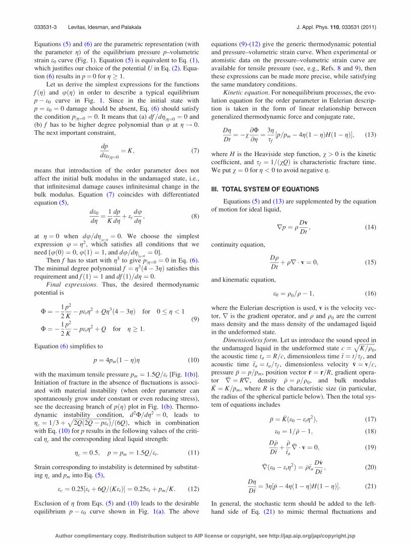
FIG. 1. (Color online) (a) Equilibrium

tensile pressure–volumetric strain curve

[Eqs. (5) and (10)] and (b) pressure–

order parameter curve [Eq. (10)].

033531-2 Levitas, Idesman, and Palakala J. Appl. Phys. 110, 033531 (2011)

Author complimentary copy. Redistribution subject to AIP license or copyright, see http://jap.aip.org/jap/copyright.jsp

Equations (5) and (6) are the parametric representation (with

the parameter g) of the equilibrium pressure p–volumetric

strain e0 curve (Fig. 1). Equation (5) is equivalent to Eq. (1),

which justifies our choice of the potential U in Eq. (2). Equa-

tion (6) results in p¼ 0 for g � 1.

Let us derive the simplest expressions for the functions

f ðgÞ and uðgÞ in order to describe a typical equilibrium

p� e0 curve in Fig. 1. Since in the initial state with

p ¼ e0 ¼ 0 damage should be absent, Eq. (6) should satisfy

the condition pjg¼0 ¼ 0. It means that (a) df=dgjg¼0 ¼ 0 and

(b) f has to be higher degree polynomial than u at g! 0.

The next important constraint,

dp

de0jg¼0

¼ K; (7)

means that introduction of the order parameter does not

affect the initial bulk modulus in the undamaged state, i.e.,

that infinitesimal damage causes infinitesimal change in the

bulk modulus. Equation (7) coincides with differentiated

equation (5),

de0

dg¼ 1

K

dp

dgþ et

dudg; (8)

at g ¼ 0 when du=dgjg¼0¼ 0. We choose the simplest

expression u ¼ g2, which satisfies all conditions that we

need [uð0Þ ¼ 0, uð1Þ ¼ 1, and du=dgjg¼0¼ 0].

Then f has to start with g3 to give pjg¼0 ¼ 0 in Eq. (6).

The minimal degree polynomial f ¼ g3ð4� 3gÞ satisfies this

requirement and f ð1Þ ¼ 1 and df ð1Þ=dg ¼ 0.

Final expressions. Thus, the desired thermodynamic

potential is

U ¼ � 1

2

p2

K� petg

2 þ Qg3ð4� 3gÞ for 0 � g < 1

U ¼ � 1

2

p2

K� petg

2 þ Q for g � 1:

(9)

Equation (6) simplifies to

p ¼ 4pmð1� gÞg (10)

with the maximum tensile pressure pm ¼ 1:5Q=et [Fig. 1(b)].

Initiation of fracture in the absence of fluctuations is associ-

ated with material instability (when order parameter can

spontaneously grow under constant or even reducing stress),

see the decreasing branch of pðgÞ plot in Fig. 1(b). Thermo-

dynamic instability condition, d2U=dg2 ¼ 0, leads to

gc ¼ 1=3þffiffiffiffiffiffiffiffiffiffiffiffiffiffiffiffiffiffiffiffiffiffiffiffiffiffiffi2Qð2Q� petÞ

p=ð6QÞ, which in combination

with Eq. (10) for p results in the following values of the criti-

cal gc and the corresponding ideal liquid strength:

gc ¼ 0:5; p ¼ pm ¼ 1:5Q=et: (11)

Strain corresponding to instability is determined by substitut-

ing gc and pm into Eq. (5),

ec ¼ 0:25 et þ 6Q=ðKetÞ½ � ¼ 0:25et þ pm=K: (12)

Exclusion of g from Eqs. (5) and (10) leads to the desirable

equilibrium p� e0 curve shown in Fig. 1(a). The above

equations (9)-(12) give the generic thermodynamic potential

and pressure–volumetric strain curve. When experimental or

atomistic data on the pressure–volumetric strain curve are

available for tensile pressure (see, e.g., Refs. 8 and 9), then

these expressions can be made more precise, while satisfying

the same mandatory conditions.

Kinetic equation. For nonequilibrium processes, the evo-

lution equation for the order parameter in Eulerian descrip-

tion is taken in the form of linear relationship between

generalized thermodynamic force and conjugate rate,

DgDt¼ �v

@U@g¼ 3g

sfp=pm � 4gð1� gÞHð1� gÞ½ �; (13)

where H is the Heaviside step function, v > 0 is the kinetic

coefficient, and sf ¼ 1=ðvQÞ is characteristic fracture time.

We put v ¼ 0 for g < 0 to avoid negative g.

III. TOTAL SYSTEM OF EQUATIONS

Equations (5) and (13) are supplemented by the equation

of motion for ideal liquid,

rp ¼ qDv

Dt; (14)

continuity equation,

DqDtþ qr � v ¼ 0; (15)

and kinematic equation,

e0 ¼ q0=q� 1; (16)

where the Eulerian description is used, v is the velocity vec-

tor, r is the gradient operator, and q and q0 are the current

mass density and the mass density of the undamaged liquid

in the undeformed state.

Dimensionless form. Let us introduce the sound speed in

the undamaged liquid in the undeformed state c ¼ffiffiffiffiffiffiffiffiffiffiffiK=q0

p,

the acoustic time ta ¼ R=c, dimensionless time �t ¼ t=sf , and

acoustic time �ta ¼ ta=sf , dimensionless velocity �v ¼ v=c,

pressure �p ¼ p=pm, position vector �r ¼ r=R, gradient opera-

tor �r ¼ Rr, density �q ¼ q=q0, and bulk modulus�K ¼ K=pm, where R is the characteristic size (in particular,

the radius of the spherical particle below). Then the total sys-

tem of equations includes

�p ¼ �Kðe0 � etg2Þ; (17)

e0 ¼ 1=�q� 1; (18)

D�qD�tþ �q

�ta

�r � v ¼ 0; (19)

�rðe0 � etg2Þ ¼ �q�ta

D�v

D�t; (20)

DgD�t¼ 3g �p� 4gð1� gÞHð1� gÞ½ �: (21)

In general, the stochastic term should be added to the left-

hand side of Eq. (21) to mimic thermal fluctuations and

033531-3 Levitas, Idesman, and Palakala J. Appl. Phys. 110, 033531 (2011)

Author complimentary copy. Redistribution subject to AIP license or copyright, see http://jap.aip.org/jap/copyright.jsp

cause appearance of the critical nucleus. In the paper, we

focus on the overdriven fracture, i.e., when p > pm and any

perturbation will result in nucleation. It can be introduced

through initial condition g0 > 0, because for g0 ¼ 0 one

obtains _g ¼ 0 in Eq. (21).

Geometrically linear case. For the case when displace-

ment and volumetric strain are relatively small (for example,

for et � 0:1 and initial stage of flow with the bubbles), the

difference between Lagrangian and Eulerian approaches is

negligible, differentiation with respect to time and space

variable is commutative, and one can reformulate the prob-

lem in terms of particles displacements u. Thus, introducing

dimensionless displacements �u ¼ u=R, instead of three equa-

tions, Eqs. (18)–(20), one obtains two equations,

e0 ¼ �r � �u; (22)

�rðe0 � etg2Þ ¼ �t 2

a

d2�u

d�t 2; (23)

and �q ’ 1. Equations (17), (21)–(23) look like phase-field

theory of fracture of elastic solids with zero shear moduli

and small displacements and volumetric strains. However,

our phase-field equation (21) differs from that used for solids

in Refs. 14–20.

IV. ANALYTICAL ESTIMATES

A. Fracture at constant pressure

First, let us focus on the solution to Eq. (21) in a local

material point for constant pressure �p and its interpretation

with the help of Fig. 1. After nucleation, for any constant

�p � 1, solution of Eq. (21) for g tends to the stationary solu-

tion �p ¼ 4gð1� gÞ [which coincides with Eq. (10)] shown in

Fig. 1(b). For g � 0:5, liquid exhibits stable equilibrium

behavior with �p � 1, for g > 0:5 the stationary solution is

unstable, i.e., g grows with decrease in �p.

For �p > 1, there is no stationary solution for g and

unstable fracture starts. Growth in g in turn leads to pressure

relaxation [see Eq. (17)] to unstable branch of stationary so-

lution for g, �p ¼ 4gð1� gÞ, or to g � 1 and �p ¼ 0. For

g � 1, Eq. (21) simplifies to

dgd�t¼ 3g�p; (24)

i.e., g will evolve until the stationary value corresponding to

�p ¼ 0. If further evolution of g occurs at �p ¼ 0, then evolu-

tion of g is not determined by Eq. (21) (since fracture is com-

pleted) but by condition �p ¼ 0 in Eq. (17), i.e., by

g ¼ffiffiffiffie0

et

r: (25)

This process does not represent fracture but hydrodynamic

expansion of cavity.

Healing. Note that if pressure instantaneously drops to

zero, elastic unloading occurs with bulk modulus K, like for

elastoplastic material. Then for 0 < g < 1 material will heal

[ _g < 0 in Eq. (21)] and for g � 1 will not [see Eq. (24)].

Healing of completely fractured liquid can start when

�e0 < 1, which leads to g < 1 [Eq. (25)] and _g < 0 according

to Eq. (21). Integral of Eq. (21) at p ¼ 0 leads to the follow-

ing equation for healing:

�t ¼ 4½FðgÞ � Fðg0Þ� with F ¼ 1

gþ ln

1� gg

; �e0 ¼ g2:

(26)

Healing at constant �e0 is described by Eq. (28), see the

following.

B. Very fast fracture, �ta � 1

We will focus on the case �ta � 1 (i.e., when fracture

time is much shorter than the acoustic time) and when the

equation of motion, Eq. (20), can be simplified to d�v=d�t ’ 0

and Eq. (19) simplifies to �q ’ const. Thus, fracture can be

considered as a quasistatic process at e0 ¼ const. Then sub-

stitution of Eq. (17) into Eq. (21) results in

dgd�t¼ 3g Ktð�e0 � g2Þ � 4gð1� gÞHð1� gÞ

� �; (27)

with Kt ¼ �Ket and �e0 ¼ e0=et, i.e., �p ¼ Ktð�e0 � g2Þ.

(a) For g � 1, Hð1� gÞ ¼ 1 and Eq. (27) allows the closed

form solution

�t ¼ ðKt � 4Þ3

2Kt�e0B½NðgÞ � Nðg0Þ�;

N ¼ ln½ga�bjg� ajbjb� gj�a�(28)

with

B¼ffiffiffiffiffiffiffiffiffiffiffiffiffiffiffiffiffiffiffiffiffiffiffiffiffiffiffiffiffiffiffiffiffi4� 4Kt�e0þK2

t �e0

q; a¼�2�B

Kt� 4; b¼�2þB

Kt� 4;

(29)

where a and b are the roots of square equation

�p ¼ Ktð�e0 � g2Þ ¼ 4gð1� gÞ; (30)

corresponding to stationary g. The condition that B is a

real number is automatically satisfied for Kt > 4 and

leads to �e0 � 4= Ktð4� KtÞ½ � for Kt < 4. Since

4= Ktð4� KtÞ½ � � 1, then the limitation for the case with

Kt < 4, �e0 � 1 is not restrictive, because we consider the

case g � 1. For Kt > 4, a < 0, and the root g ¼ b,

0 � b � 1, represents the only realistic stationary solu-

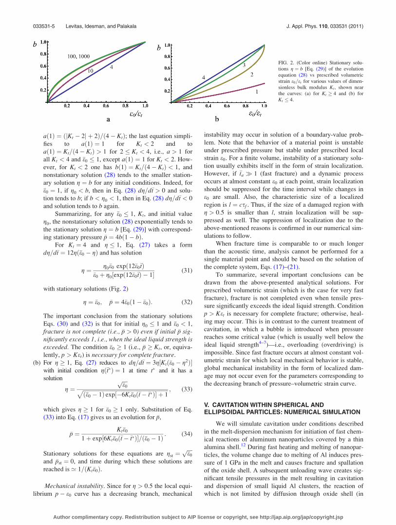
tion, which is shown in Fig. 2 versus �e0 for various

Kt > 4. For Kt ! 4, the relationship bð�e0Þ ¼ �e0 is linear;

for any Kt > 4, one has bð0Þ ¼ 0 and bð1Þ ¼ 1. The sta-

tionary solution b weakly depends on Kt and, for exam-

ple, for Kt ¼ 100 and Kt ¼ 1000, the difference in bð�e0Þis invisible. For Kt < 4, one has bð0Þ ¼ 0 and

bð1Þ ¼ jKt � 2j � 2ð Þ= Kt � 4ð Þ; the last equation simpli-

fies to bð1Þ ¼ 1 for 2 � Kt < 4 and to

bð1Þ ¼ Kt= 4� Ktð Þ for Kt < 2.

The first root að�e0Þ does not give realistic stationary

solutions 0 � a � 1 for Kt < 4 as well. Indeed, að�e0Þdecreases with the growth of �e0; að0Þ ¼ 4= 4� Ktð Þ > 1;

033531-4 Levitas, Idesman, and Palakala J. Appl. Phys. 110, 033531 (2011)

Author complimentary copy. Redistribution subject to AIP license or copyright, see http://jap.aip.org/jap/copyright.jsp

að1Þ ¼ jKt � 2j þ 2ð Þ= 4� Ktð Þ; the last equation simpli-

fies to að1Þ ¼ 1 for Kt < 2 and to

að1Þ ¼ Kt= 4� Ktð Þ > 1 for 2 � Kt < 4, i.e., a > 1 for

all Kt < 4 and �e0 � 1, except að1Þ ¼ 1 for Kt < 2. How-

ever, for Kt < 2 one has bð1Þ ¼ Kt= 4� Ktð Þ < 1, and

nonstationary solution (28) tends to the smaller station-

ary solution g ¼ b for any initial conditions. Indeed, for

�e0 ¼ 1, if g0 < b, then in Eq. (28) dg=d�t > 0 and solu-

tion tends to b; if b < g0 < 1, then in Eq. (28) dg=d�t < 0

and solution tends to b again.

Summarizing, for any �e0 � 1, Kt, and initial value

g0, the nonstationary solution (28) exponentially tends to

the stationary solution g ¼ b [Eq. (29)] with correspond-

ing stationary pressure �p ¼ 4bð1� bÞ.For Kt ¼ 4 and g � 1, Eq. (27) takes a form

dg=d�t ¼ 12g �e0 � gð Þ and has solution

g ¼ g0�e0 expð12�e0�tÞ�e0 þ g0½expð12�e0�tÞ � 1� (31)

with stationary solutions (Fig. 2)

g ¼ �e0; �p ¼ 4�e0ð1� �e0Þ: (32)

The important conclusion from the stationary solutions

Eqs. (30) and (32) is that for initial g0 � 1 and �e0 < 1,

fracture is not complete (i.e., �p > 0) even if initial �p sig-nificantly exceeds 1, i.e., when the ideal liquid strength isexceeded. The condition �e0 � 1 (i.e., �p � Kt, or, equiva-

lently, p > Ket) is necessary for complete fracture.

(b) For g � 1, Eq. (27) reduces to dg=d�t ¼ 3g Ktð�e0 � g2Þ½ �with initial condition gð�t�Þ ¼ 1 at time t� and it has a

solution

g ¼ffiffiffiffi�e0

pffiffiffiffiffiffiffiffiffiffiffiffiffiffiffiffiffiffiffiffiffiffiffiffiffiffiffiffiffiffiffiffiffiffiffiffiffiffiffiffiffiffiffiffiffiffiffiffiffiffiffiffiffiffiffiffiffiffiffiffiffiffiffið�e0 � 1Þ exp½�6Kt�e0ð�t� �t�Þ� þ 1

p ; (33)

which gives g � 1 for �e0 � 1 only. Substitution of Eq.

(33) into Eq. (17) gives us an evolution for �p,

�p ¼ Kt�e0

1þ exp½6Kt�e0ð�t� �t�Þ�=ð�e0 � 1Þ : (34)

Stationary solutions for these equations are gst ¼ffiffiffiffi�e0

p

and �pst ¼ 0, and time during which these solutions are

reached is ’ 1=ðKt�e0Þ.

Mechanical instability. Since for g > 0:5 the local equi-

librium p� e0 curve has a decreasing branch, mechanical

instability may occur in solution of a boundary-value prob-

lem. Note that the behavior of a material point is unstable

under prescribed pressure but stable under prescribed local

strain e0. For a finite volume, instability of a stationary solu-

tion usually exhibits itself in the form of strain localization.

However, if �ta � 1 (fast fracture) and a dynamic process

occurs at almost constant e0 at each point, strain localization

should be suppressed for the time interval while changes in

e0 are small. Also, the characteristic size of a localized

region is l ¼ csf . Thus, if the size of a damaged region with

g > 0:5 is smaller than l, strain localization will be sup-

pressed as well. The suppression of localization due to the

above-mentioned reasons is confirmed in our numerical sim-

ulations to follow.

When fracture time is comparable to or much longer

than the acoustic time, analysis cannot be performed for a

single material point and should be based on the solution of

the complete system, Eqs. (17)–(21).

To summarize, several important conclusions can be

drawn from the above-presented analytical solutions. For

prescribed volumetric strain (which is the case for very fast

fracture), fracture is not completed even when tensile pres-

sure significantly exceeds the ideal liquid strength. Condition

p > Ket is necessary for complete fracture; otherwise, heal-

ing may occur. This is in contrast to the current treatment of

cavitation, in which a bubble is introduced when pressure

reaches some critical value (which is usually well below the

ideal liquid strength4–7)—i.e., overloading (overdriving) is

impossible. Since fast fracture occurs at almost constant vol-

umetric strain for which local mechanical behavior is stable,

global mechanical instability in the form of localized dam-

age may not occur even for the parameters corresponding to

the decreasing branch of pressure–volumetric strain curve.

V. CAVITATION WITHIN SPHERICAL ANDELLIPSOIDAL PARTICLES: NUMERICAL SIMULATION

We will simulate cavitation under conditions described

in the melt-dispersion mechanism for initiation of fast chem-

ical reactions of aluminum nanoparticles covered by a thin

alumina shell.12 During fast heating and melting of nanopar-

ticles, the volume change due to melting of Al induces pres-

sure of 1 GPa in the melt and causes fracture and spallation

of the oxide shell. A subsequent unloading wave creates sig-

nificant tensile pressures in the melt resulting in cavitation

and dispersion of small liquid Al clusters, the reaction of

which is not limited by diffusion through oxide shell (in

FIG. 2. (Color online) Stationary solu-

tions g ¼ b [Eq. (29)] of the evolution

equation (28) vs prescribed volumetric

strain e0=et for various values of dimen-

sionless bulk modulus Kt, shown near

the curves: (a) for Kt � 4 and (b) for

Kt � 4.

033531-5 Levitas, Idesman, and Palakala J. Appl. Phys. 110, 033531 (2011)

Author complimentary copy. Redistribution subject to AIP license or copyright, see http://jap.aip.org/jap/copyright.jsp

contrast to traditional mechanisms). Here we consider the

appearance of the first void in the melt. Solution to the sys-

tem of equations (17)–(21) was found using FEM and code

COMSOL.

We consider a liquid sphere of radius R that is initially

in mechanical equilibrium under applied external compres-

sive pressure �p0 (p0 > 0), i.e., initial velocity is zero. Initial

value g0 ¼ 0:03 is distributed everywhere to start evolution

of g. Let the magnitude of the compressive pressure at the

boundary �r ¼ 1 reduce linearly in time from p0 to the final

value pf during the time ts (e.g., during the time of oxide

shell fracture12), after which it remains constant. During this

process, the unloading wave propagates to the center and

creates large tensile pressure, which causes cavitation. For

spherical particle, cavitation starts at the center where the

reflected wave causes the highest pressure. The effect of the

heterogeneity of distribution and the magnitude of g0 on the

solution will be studied elsewhere. Some estimates of the

effect of the magnitude of g0 can be obtained from analytical

solutions in Sec. IV.

Before fracture starts and evolution of the order parame-

ter is negligible, we arrive at classical fluid dynamics equa-

tions. Then, solution depends on the different dimensionless

time ~t ¼ t=ta ¼ �t=�ta and pressure ~p ¼ p=p0 ¼ �p=�p0.

The following parameters have been used in calcula-

tions12: ~pf ¼ 0:05, ~ts ¼ 0:2, �p0 ¼ 1, �ta ¼ 0:944, et ¼ 0:1, and�K ¼ 71:1. This leads to Kt ¼ 7:11, the maximum tensile

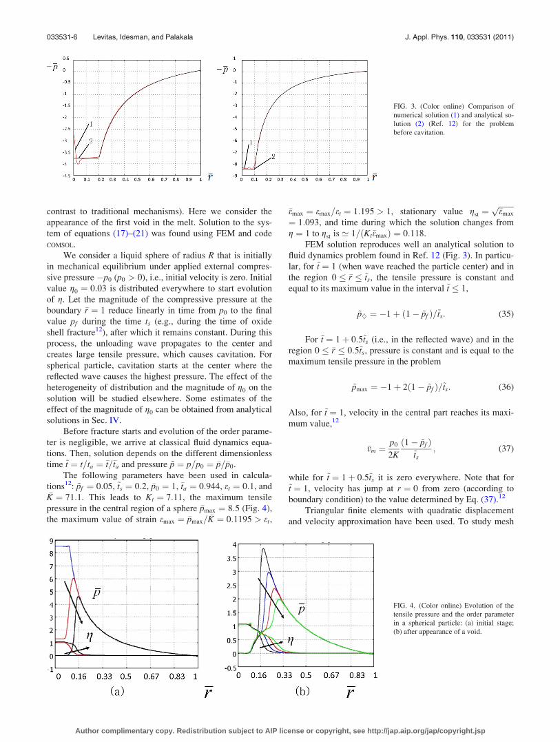
pressure in the central region of a sphere �pmax ¼ 8:5 (Fig. 4),

the maximum value of strain emax ¼ �pmax= �K ¼ 0:1195 > et,

�emax ¼ emax=et ¼ 1:195 > 1, stationary value gst ¼ffiffiffiffiffiffiffiffi�emax

p

¼ 1:093, and time during which the solution changes from

g ¼ 1 to gst is ’ 1=ðKt�emaxÞ ¼ 0:118.

FEM solution reproduces well an analytical solution to

fluid dynamics problem found in Ref. 12 (Fig. 3). In particu-

lar, for ~t ¼ 1 (when wave reached the particle center) and in

the region 0 � �r � ~ts, the tensile pressure is constant and

equal to its maximum value in the interval ~t � 1,

~p} ¼ �1þ ð1� ~pf Þ=~ts: (35)

For ~t ¼ 1þ 0:5~ts (i.e., in the reflected wave) and in the

region 0 � �r � 0:5~ts, pressure is constant and is equal to the

maximum tensile pressure in the problem

~pmax ¼ �1þ 2ð1� ~pf Þ=~ts: (36)

Also, for ~t ¼ 1, velocity in the central part reaches its maxi-

mum value,12

�vm ¼p0

2K

ð1� ~pf Þ~ts

; (37)

while for ~t ¼ 1þ 0:5~ts it is zero everywhere. Note that for~t ¼ 1, velocity has jump at r ¼ 0 from zero (according to

boundary condition) to the value determined by Eq. (37).12

Triangular finite elements with quadratic displacement

and velocity approximation have been used. To study mesh

FIG. 4. (Color online) Evolution of the

tensile pressure and the order parameter

in a spherical particle: (a) initial stage;

(b) after appearance of a void.

FIG. 3. (Color online) Comparison of

numerical solution (1) and analytical so-

lution (2) (Ref. 12) for the problem

before cavitation.

033531-6 Levitas, Idesman, and Palakala J. Appl. Phys. 110, 033531 (2011)

Author complimentary copy. Redistribution subject to AIP license or copyright, see http://jap.aip.org/jap/copyright.jsp

dependence of the solution, two meshes consisting of 7936

finite elements with 48 147 mechanical degrees of freedom

and 31 744 elements with 191 523 mechanical degrees of

freedom were used for a quarter of axisymmetric cross sec-

tion. The solutions for the order parameter for the two

meshes practically coincided, especially when g exceeded 1

at the center of the sphere.

Evolution of the pressure distribution and the order

parameter is shown in Fig. 4. At time ~t ¼ 1þ 0:5~ts ¼ 1:1(when tensile pressure �p ¼ 8:5 is maximal and particles

velocity is zero), there is still no visible change in the order

parameter, despite very high tensile pressures. However, at~t ¼ 1:136, g ¼ 1 at the center of particle and pressure in this

region dropped homogeneously to 1.3. At ~t ¼ 1:154, while ghas grown very little to gst ¼ 1:093, pressure in this region

reached its thermodynamically equilibrium value 0, which is

equivalent to the appearance of a hole. Pressure drop gener-

ates an additional unloading wave. Diameter of the hole does

not change during calculation time ~t ¼ 1:21. Near the hole,

pressure reduces and the order parameter grows until both of

them reached thermodynamically equilibrium values

�p ¼ 4gð1� gÞ determined by Eq. (10). While the local equi-

librium is thermodynamically unstable under prescribed

pressure, there is not any instability and strain localization.

According to our discussions in Sec. IV.B, there are two

reasons for the lack of strain localization:

(1) Actual time during which damage evolution has occurred

is ten times smaller than the acoustic time, i.e., damage

occurred under almost constant e0 at each point. Local

solution is stable under prescribed e0.

(2) The size of the potential localization zone is

l ¼ csf ¼ Rsf=ta ¼ R=�ta ¼ 1:06R and is much larger

than the actual damaged zone with g > 0:5 in Fig. 4.

The solution to the same problem but for ellipsoidal par-

ticles with aspect ratio a ¼ 1:2 is presented in Fig. 5. Maxi-

mum tensile pressure reduces with growing aspect ratio

(�p ¼ 7:55 > Kt for a ¼ 1:2 and �p ¼ 2:98 < Kt for a ¼ 2),

which slows the growth of the order parameter. While for

a ¼ 1:2 a noncircular hole appeared at the center of particle

(i.e., g reached 1 and pressure dropped to zero), for a ¼ 2 the

order parameter did not exceed 0.7 and pressure did not

reach zero, i.e,. the hole did not appear. Concerning the

melt-dispersion mechanism,12 small deviation from spherical

shape does not prevent cavitation but for large aspect ratios

this mechanism cannot be initiated.

The typical order of magnitude of ideal strength of

liquid metals is pm ¼ 1GPa, while complete fracture does

not occur for p < Ket ¼ 7:11GPa on the time scale of 1ps.

Indeed, dynamic tensile pressure can significantly exceed the

liquid strength without causing complete fracture. For Ni,

fracture of melt starts at 6 GPa.10 Note that in Refs. 8 and 9

pressure was below theoretical strength (spinodal) of liquid,

causing thermal fluctuations to be required for the bubble

nucleation, as well as greatly increasing the fracture time.

VI. COMPARISON WITH ALTERNATIVE PHASE-FIELDAPPROACHES

A. Comparison with the alternative potential

The potential in Refs. 19 and 20 for a crack in solid

(adapted for p� e0 variables) is

U ¼ �0:5p2=K � pg=d þ Q sin2ð0:5pg=gcÞ (38)

with Q ¼ 2g2cK=ðp2d2Þ, non-normalized g and gc and d as

parameters. Comparison with Eq. (9) shows that

etuðgÞ ¼ g=d, i.e., uðgÞ ¼ g, which contradicts our require-

ments du=dgjg¼0 ¼ 0, derived from condition equation (7).

Indeed, thermodynamic equilibrium conditions @U=@g ¼ 0

and e0 ¼ �@U=@p result in

p ¼ 0:5Qdpgc

sinpggc

� �(39)

or for small g in

p ’ 0:5gQdp2

g2c

¼ Kgd; e0 ¼

p

Kþ g

d: (40)

FIG. 5. (Color online) Evolution of the

order parameter (a)–(c) and the tensile

pressure (d)–(f) in an ellipsoidal particle

with a ¼ 1:2.

033531-7 Levitas, Idesman, and Palakala J. Appl. Phys. 110, 033531 (2011)

Author complimentary copy. Redistribution subject to AIP license or copyright, see http://jap.aip.org/jap/copyright.jsp

Excluding g from these two equations, we obtain e0 ¼ 2p=K.

At the same time for nonequilibrium (fast) loading when

_g ¼ 0, e0 ¼ p=K, i.e., the equilibrium bulk modulus in Refs.

19 and 20 is two times smaller than the bulk modulus with-

out initiation of fracture, which is contradictory.

Note that the nonlinear equilibrium pðe0Þ curve for

cracks in Refs. 14–18 was described in terms of variable

elastic modulus rather than in terms of eigen strain.

B. Lack of the gradient energy

Usually, in all phase-field approaches (for example, for

fracture, phase transformations, and twinning), an additional

gradient energy term, 0:5brg � rg with b > 0 as the coeffi-

cient, is added to U, which results in Ginzburg–Landau equa-

tion [i.e., in the additional Laplacian term bDg in Eq. (13),

see Refs. 14–18]. Gradient energy is concentrated near the

newly formed free surface and reproduces interface energy.

However, in our approach, the introduction of gradient

energy will lead to a double count of cohesive energy and,

consequently, to violation of the energy balance. Indeed,

when crack appears in solid, stress work is equal to the cohe-

sion energy which is stored in the interplanar volume.19,20

Surface energy is defined in terms of cohesion energy but it

is not added to the energy balance.19,20 Similarly, here cohe-

sion energy QV is stored in a hole of the volume V, so gradi-

ent (surface) energy cannot be added.

Also, while without gradient energy material instability

starts at each material point independently when p > pm, gra-

dient energy promotes interface propagation for any pressure

not equal to thermodynamic equilibrium (Maxwell) pressure.

That is why the propagating crack in Refs. 14–18 increases

its width due to phase transformation between solid phase

and gas (or vacuum, or soft phase) inside the crack, which is

not physical for actual cracks. In Refs. 19 and 20, gradient

energy is formulated in a way that it appears at the crack tip

only but not at crack faces. This contribution determines the

line tension energy (rather than surface energy) and the crack

core radius, similar to those for dislocations.21 It is found in

Refs. 19 and 20 that the gradient energy produces a weak

effect on the solution of the problems under study. Note that

in the cohesive zone models for crack,22,23 gradient energy is

absent.

We are not aware of phase-field modeling of any mate-

rial instability (like phase transformations, twinning, and dis-

location evolution) at the nanoscale that did not use gradient

energy and the corresponding term in kinetic equation for

order parameter. At the macroscale, we dropped gradient

energy in phase-field modeling phase transformations,24,25

because surface energy is not important for large volumes

and interface width is negligible. For problems on damage

and shear band localization in solids, strain gradient energy

is added to avoid an ill-posed boundary-value problem.26

Indeed, otherwise, due to the lack of characteristic size in the

problem formulation, thickness of a shear band is zero and

drastic mesh dependence of the solution is observed. Adding

strain gradient contribution to the energy introduces a char-

acteristic size in the problem formulation and leads to the

strain gradient regularization.

Despite the lack of gradient energy and corresponding

regularization in our problem formulation, this does not lead

to an ill-posed problem and sharp (zero thickness) interface;

the problem is well posed due to the rate-type regularization

in Eq. (13) and momentum equation (14), which introduces a

characteristic length lf ¼ csf . This regularization is similar

to strain-rate regularization in viscoplasticity.27

Lack of the term with the gradient of the order parame-

ter does not prevent our theory from being a phase-field

(Ginzburg–Landau) theory, because it still possesses the two

main features of any phase-field theory mentioned in Sec. I.

In fact, the Landau theory of the second-order phase transfor-

mations did not contain the gradient of the order parame-

ter,28,29 which was later introduced by Ginzburg. Our theory,

based on potential (2), can be formally considered as a

mixture-type theory with a volume fraction of broken phase

g2 (because volumetric transformation strain is proportional

to g2) and interaction (surface) energy Qf ðgÞ. Then, omitting

the gradient-type energy would be natural. However, the

phase-field theory of fracture in Refs. 14,18 also was formu-

lated as a mixture-type theory with the order parameters as

concentration of soft phase or point defects. Still, in these

works the gradient-type energy has been used, and we would

need to justify why we do not use it in our mixture theory.

Also, change in concentration in mixture theory corresponds

to transformations between phases, which corresponds more

to sublimation or vacancy diffusion to the free surface

than to fracture. Instead, we would like to describe bond

breaking in each material point independent of other points,

and this was one more reason to remove the gradient term;

see our earlier discussion.

VII. CAVITATION IN VISCOUS LIQUID

For viscous liquid, the nonhydrostatic stresses should be

taken into account in the description of cavitation. At the

macroscale, the cavitation criterion suggested by Joseph4–7

is based on maximum tensile stress. The simplest way to do

this within a phase-field approach is to substitute pressure in

the transformation work term with the maximum tensile

stress r1,

U ¼ �0:5p2=K � r1etg2 þ Qg3ð4� 3gÞ: (41)

Then, the principle strains are ei ¼ �@U=@ri, i.e.,

e1 ¼ p=3Kþ etg2; e2 ¼ e3 ¼ p=3K; e0 ¼ p=Kþ etg

2: (42)

The evolution equation for the order parameter is similar to

Eq. (13),

dgdt¼ �v

@U@g¼ 3g

sf

r1

pm� 4gð1� gÞHð1� gÞ

� �; (43)

but with r1 instead of p. Equation for stress tensor in liquid

is

rij ¼ Kðe0 � etg2Þdij

þ �a1ðgÞ@vk

@xkdij þ

1

2la2ðgÞ

@vi

@xjþ @vj

@xi

� �� �; (44)

033531-8 Levitas, Idesman, and Palakala J. Appl. Phys. 110, 033531 (2011)

Author complimentary copy. Redistribution subject to AIP license or copyright, see http://jap.aip.org/jap/copyright.jsp

where dij is the Kronecker delta symbol, � and l are volu-

metric and shear viscosities, and aiðgÞ are the functions with

the following properties: aið0Þ ¼ 1 and ai ¼ 0 for g � 1.

Thus, cavitation is governed by the maximum principal

stress, which is consistent with macroscopic cavitation crite-

rion in Refs. 4 and 5. Note that in Refs. 4 and 5, r1 is the

stress before fracture while in our approach it is variable

stress in the fracture zone during the fracture process. Poten-

tial interpretation problem is that the direction of the largest

principal stress may vary during the fracture process, i.e., it

may stretch different bonds. It may change by 90 when the

middle principle stress became the largest one. However,

according to the above-mentioned properties of the functions

aiðgÞ, the viscosities and nonhydrostaticity reduce during the

fracture. Note that in similar way, one can generalize the

above-presented phase-field approach for liquid with more

complex constitutive equations.

VIII. CONCLUDING REMARKS

To summarize, phase-field theory for the description of

the fracture in liquid is developed. Various results from solid

mechanics are transferred into mechanics of fluids. Note that

the same thermodynamic potential as for viscous liquid can be

used to model fracture of disordered solids (glasses), if we

add energy of deviatoric stresses. It also can be used for each

cleavage plane in theory19,20 for fracture of single crystals to

avoid jump-like reduction in elastic moduli when damage

starts. In particular, quadratic, rather than linear dependence

of the eigen (transformation) strain is crucial for this purpose.

Stochastic contribution (the noise due to thermal fluctuations,

which satisfies the dissipation-fluctuation theorem) can be

trivially added. Large-strain formulation30,31 and surface ten-

sion32,33 can be incorporated as well. This work also stresses

the importance of analyzing pressure (stress)–strain curve in

any stress-related phase-field theory. Earlier,34,35 we demon-

strated this for martensitic phase transformations. One more

general contribution to the phase-field theories is the demon-

stration that for some cases, the gradient energy term has to be

omitted, since it double counts cohesive energy and causes

unrealistic diffusive expansion of the fractured region. The

only example that we aware of neglected gradient term is in

our microscale phase-field theory of martensitic phase trans-

formation,24,25 because at the microscale surface energy and

corresponding width of the diffuse interface are negligible.

Note that as result of solution of dynamic nucleation problem

an unexpected metastable phase of material was obtained.

This is a gas-like state of a matter under zero pressure in

which distance between molecules is greater than atomic

interaction distance. However, its free energy is equal to Qand is greater than free energy of gas and liquid. As the next

step, this phase will transform into a stable mixture of liquid

and gas. This phase transformation should be described with a

different order parameter and gradient (liquid–gas interface)

energy should be included. This problem will be treated

elsewhere. The effect of impurities, interfaces, and other

nucleation sites for fracture can be easily introduced by reduc-

ing pm and et at their surface.

ACKNOWLEDGMENTS

V.I.L. wishes to thank B. Ganapathysubramanian for

helpful discussions on this paper. The support of the NSF

(CBET-0755236 and CMMI-0969143), ONR (N00014-08-1-

1262), Air Force (FA9300-11-M-2008), ISU, and TTU for

this research is gratefully acknowledged.

1Ya. B. Zeldovitch, Acta Physicochim. URSS 18, 1 (1943).2J. C. Fisher, J. Appl. Phys. 19, 1062 (1948).3C. E. Brennen, Cavitation and Bubble Dynamics (Oxford University Press,

New York, 1995).4D. D. Joseph, Phys. Rev. Lett. 51, 1649 (1995).5D. D. Joseph, J. Fluid Mech. 366, 367 (1998).6J. C. Padrino, D. D. Joseph, T. Funda, J. Wang, and W. A. Sirignano, J.

Fluid Mech. 578, 381 (2007).7S. Dabiri, W. A. Sirignano, and D. D. Joseph, Phys. Fluids 19, 072112

(2007).8T. T. Bazhirov, G. E. Norman, and V. V. Stegailov, J. Phys.: Condens.

Matter 20, 114113 (2008).9K. Davitt, A. Arvengas, and F. Caupin, EPL 90, 16002 (2010).

10D. S. Ivanov and L. V. Zhigilei, Phys. Rev. B 68, 064114 (2003).11V. I. Levitas, B. Dikici, and M. L. Pantoya, Combust. Flame 158, 1413

(2011).12V. I. Levitas, B. W. Asay, S. F. Son, and M. L. Pantoya, J. Appl. Phys.

101, 083524 (2007).13V. I. Levitas, Combust. Flame 156, 543 (2009).14I. S. Aranson, V. A. Kalatsky, and V. M. Vinokur, Phys. Rev. Lett. 85, 118

(2000).15A. Karma, D. A. Kessler, and H. Levine, Phys. Rev. Lett. 87, 45501

(2001).16A. Karma and A. E. Lobkovsky, Phys. Rev. Lett. 92, 245510 (2004).17H. Henry and H. Levine, Phys. Rev. Lett. 93, 105504 (2004).18R. Spatschek, M. Hartmann, E. Brener, H. Mueller-Krumbhaar, and K.

Kassner, Phys. Rev. Lett. 96, 015502 (2006).19Y. M. Jin, Y. U. Wang, and A. G. Khachaturyan, Appl. Phys. Lett. 79,

3071 (2001).20Y. U. Wang, Y. M. Jin, and A. G. Khachaturyan, J. Appl. Phys. 91, 6435

(2002).21Y. U. Wang, Y. M. Jin, A. M. Cuitino, and A. G. Khachaturyan, Acta

Mater. 49, 1847 (2001).22X. P. Xu and A. Needleman, J. Mech. Phys. Solids 42, 1397 (1994).23K. Park, G. H. Paulino, and J. R. Roesler, J. Mech. Phys. Solids 57, 891

(2009).24V. I. Levitas, A. V. Idesman, and D. L. Preston, Phys. Rev. Lett. 93,

105701 (2004).25A. V. Idesman, V. I. Levitas, D. L. Preston, and J. Y. Cho, J. Mech. Phys.

Solids 53, 495 (2005).26H. M. Zbib and E. C. Aifantis, Acta Mech. 92, 209 (1992).27P. Perzyna and K. Korbel, Acta Mech. 129, 31 (1998).28L. D. Landau and E. M. Lifshitz, Statistical Physics (Butterworth Heine-

mann, Oxford, 1980).29L. D. Landau, Collected Papers of L. D. Landau, edited by D. Haar (Gor-

don and Breach, New York, 1965).30V. I. Levitas, V. A. Levin, K. M. Zingerman, and E.I. Freiman, Phys. Rev.

Lett. 103, 025702 (2009).31V. I. Levitas and D. L. Preston, Phys. Lett. A 343, 32 (2005).32V. I. Levitas and M. Javanbakht, Phys. Rev. Lett. 105, 165701 (2010).33V. I. Levitas and K. Samani, Nat. Commun. 2, 284 (2011).34V. I. Levitas and D. L. Preston, Phys. Rev. B 66, 134206 (2002).35V. I. Levitas and D. L. Preston, Phys. Rev. B 66, 134207 (2002).

033531-9 Levitas, Idesman, and Palakala J. Appl. Phys. 110, 033531 (2011)

Author complimentary copy. Redistribution subject to AIP license or copyright, see http://jap.aip.org/jap/copyright.jsp