HAL Id: tel-01958391https://pastel.archives-ouvertes.fr/tel-01958391

Submitted on 18 Dec 2018

HAL is a multi-disciplinary open accessarchive for the deposit and dissemination of sci-entific research documents, whether they are pub-lished or not. The documents may come fromteaching and research institutions in France orabroad, or from public or private research centers.

L’archive ouverte pluridisciplinaire HAL, estdestinée au dépôt et à la diffusion de documentsscientifiques de niveau recherche, publiés ou non,émanant des établissements d’enseignement et derecherche français ou étrangers, des laboratoirespublics ou privés.

Oxidation stability of fuels in liquid phaseKarl Chatelain

To cite this version:Karl Chatelain. Oxidation stability of fuels in liquid phase. Chemical engineering. Université Paris-Saclay, 2016. English. �NNT : 2016SACLY020�. �tel-01958391�

NNT : 2016SACLY020

THÈSE DE DOCTORATDE L’UNIVERSITE PARIS-SACLAY

préparée à

L’ENSTA ParisTech

ÉCOLE DOCTORALE N◦579Sciences Mécaniques et Énergétiques, Matériaux et Géosciences (SMEMAG)

Spécialité de doctorat : Génie des procédés

par

Karl CHATELAIN

Etude de la stabilité à l’oxydation des carburantsen phase liquide

Thèse présentée et soutenue à Rueil-Malmaison, le 15 décembre 2016

Composition du jury :

Dr. André NICOLLE Président IFP Energies nouvelles, R102Pr. Richard WEST Rapporteur Northeastern University, Boston, CoMoChEngPr. Pierre-Alexandre GLAUDE Rapporteur CNRS Nancy, LRGPDr. Mickael SICARD Examinateur ONERA, DEFADr. Thomas DUBOIS Examinateur TOTAL ACSDr. Laurie STARCK Examinateur IFP Energies nouvelles, R104Mme. Arij BEN AMARA Examinateur IFP Energies nouvelles, R104Pr. Laurent CATOIRE Directeur de Thèse ENSTA ParisTech, Université Paris-Saclay, UCP

ii

Acknowledgements

This work was made possible thanks to the support of the IFP Energies nouvelles (IFPEN) and the chemicalengineering laboratory (UCP) of the ENSTA ParisTech, Université Paris-Saclay. It was mainly performedat IFPEN in partnership with several divisions: powertrain and vehicule (R10) mostly, physics and analysis(R05) and process experiments (R15). It also includes several months spent in the Massachusetts Instituteof Technology (MIT) in Cambridge (MA,USA) as a visiting researcher.

First, I would like to thank the committee for accepting to evaluate this work. In particular, ProfessorRichard West from Northeastern University in Boston and Professor Pierre-Alexandre Glaude from theCNRS Nancy for accepting to review my thesis.I also thank all others committee members, notably Doctor Mickael Sicard from ONERA and Doctor ThomasDubois from Total ACS, for their interest in this topic and our fruitful discussions during and after thedefence.

I would like to thank Profesor Laurent Catoire, as the laboratory head of UCP and my PhD advisor,for his scientific contribution, his time and the trust he placed in me to accomplish this research. Inaddition, I thank Doctor Laurie Starck for promoting this stimulating research topic at IFPEN involvingboth experimental and modeling work on fuel autoxidation. In addition, I am grateful for the opportunityshe gave me to accomplish part of this work in MIT. Thus, I am also thankful to Professor William Greenand his group for welcoming me as a visiting researcher.I appreciated the regular discussions and meetings on this research topic with Doctor André Nicolle andArij Ben Amara, thank you very much for your investment.I would like to thank all people who contributed to the success of this experimental work, Doctor MairaAlves-Fortunato, Pascal Hayrault, Michel Chardin, Benjamin Veyrat and also the students who contributedto part of the data acquisition Skander and Clara.

Now I would like to thank all colleagues and friends who contributed indirectly to the success of thiswork with our discussions or just by sharing common hobbies. The IFPEN runners: Mickael, Lama, Jan,Guillaume, Pascal and Patricia. My office mates: Betty, Elias, Benjamin, Edouard and Eleftherios. Allothers IFPEN colleagues: Sophie, Federico, Valerio, Gorka, Antoine and Detlev. My ENSTA colleagues:Aurélien, Julien, Amir, Zhewei and Johnny. And the others friends not mentioned earlier: Olivier, Larysa,Audrey, Sébastien, Amélie and Romain.

Before to conclude, I especially thank my previous advisors, Pr. Rémy Mével and Pr. Joseph Shepherdwith whom my interest in Research started, thanks to their stimulating research topics in the ExplosionDynamics Laboratory (EDL) in the California Institute of Technology (Caltech).

Finally, and most importantly, I would like to thank my parents, my family and especially my wifeTiphaine for their understanding, their care and patience during the last three years.

i

ii

List of Figures

1.1 CO2 concentration evolution in the atmosphere over the last ten thousand years [1] . . . . . . 2

1.2 Illustration of a local pollution episode which occurred during Spring 2014 in Paris [2] . . . . . 2

1.3 Simplified representation of a common rail injection system in a 4-cylinder engine from [3].Text in purple represents issues caused by fuel autoxidation. Red dashed blocks representareas with fuel stresses. Black and grey arrows stand for the fuel flow. Fouling induced byheterogeneous catalysis are not represented but should be considered in every lines. . . . . . . 2

1.4 Injector deposit formation after 1016 hours of operation with Rapeseed Biodiesel observed bySem [4] . . . . . . . . . . . . . . . . . . . . . . . . . . . . . . . . . . . . . . . . . . . . . . . . . . . . . 3

1.5 Effect of water on the decomposition of urea [5] . . . . . . . . . . . . . . . . . . . . . . . . . . . . 3

2.1 Examples of experimental apparatus used in liquid phase autoxidation studies . . . . . . . . . 6

2.2 Fuel composition impact on autoxidation rate . . . . . . . . . . . . . . . . . . . . . . . . . . . . . 7

2.3 Impact of oxygen on autoxidation . . . . . . . . . . . . . . . . . . . . . . . . . . . . . . . . . . . . . 7

2.4 Typical molecule from each antioxidant family. a), b) and c) are respectively H donor, peroxyinhibitor and complexing agent . . . . . . . . . . . . . . . . . . . . . . . . . . . . . . . . . . . . . . 8

2.5 Antioxidant types and concentration effects on autoxidation kinetics. . . . . . . . . . . . . . . . 8

2.6 Chain length impact on the autoxidation kinetics . . . . . . . . . . . . . . . . . . . . . . . . . . . 9

2.7 Uncertainties on the branching impact on autoxidation kinetics . . . . . . . . . . . . . . . . . . 9

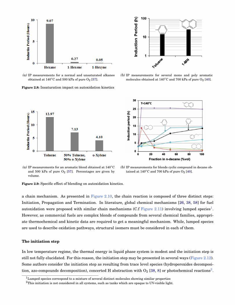
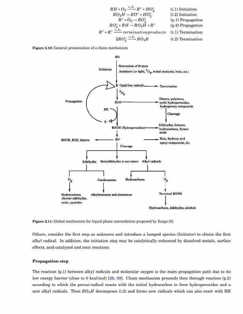
2.8 Insaturation impact on autoxidation kinetics . . . . . . . . . . . . . . . . . . . . . . . . . . . . . . 10

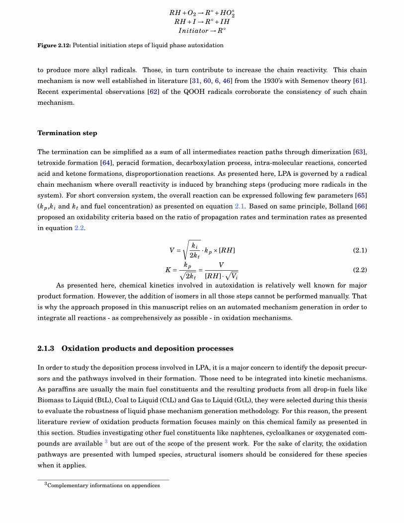
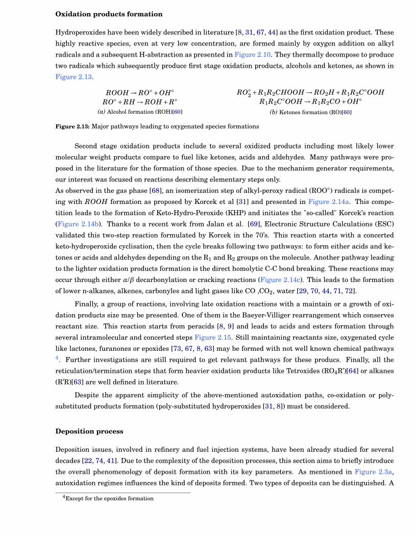
2.9 Specific effect of blending on autoxidation kinetics. . . . . . . . . . . . . . . . . . . . . . . . . . . 10

2.10 General presentation of a chain mechanism . . . . . . . . . . . . . . . . . . . . . . . . . . . . . . . 11

2.11 Global mechanism for liquid phase autoxidation proposed by Zongo [6] . . . . . . . . . . . . . . 11

2.12 Potential initiation steps of liquid phase autoxidation . . . . . . . . . . . . . . . . . . . . . . . . . 12

2.13 Major pathways leading to oxygenated species formations . . . . . . . . . . . . . . . . . . . . . . 13

2.14 Major pathways leading to lighter oxidation products formation . . . . . . . . . . . . . . . . . . 14

2.15 Major reaction steps from the Bayer-Villiger reaction [7, 8, 9] . . . . . . . . . . . . . . . . . . . . 15

2.16 Illustration of the close relation between chemical and physical processes on deposition mech-anism. Modified scheme from Beaver et al. [10] . . . . . . . . . . . . . . . . . . . . . . . . . . . . 15

2.17 Global process for the deposit formation. The bulk reactivity path (i) is represented with blackarrows. The catalytic oxidation path (ii) is represented with purple arrows. The solubility ofdeposit into fresh solvent (iii) is represented with grey arrows. . . . . . . . . . . . . . . . . . . . 16

2.18 Temperature profile during the autoxidation of several compounds [11] . . . . . . . . . . . . . . 16

2.19 Illustration of Reverse Micelle formation and its implication in the chain mechanism of au-toxidation . . . . . . . . . . . . . . . . . . . . . . . . . . . . . . . . . . . . . . . . . . . . . . . . . . . 17

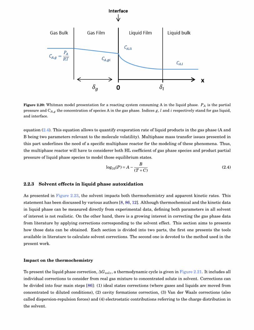
2.20 Whitman model presentation for a reacting system consuming A in the liquid phase. PA isthe partial pressure and CA,g the concentration of species A in the gas phase. Indices g, l andi respectively stand for gas liquid, and interface. . . . . . . . . . . . . . . . . . . . . . . . . . . . . 18

iii

LIST OF FIGURES LIST OF FIGURES

2.21 Thermodynamic cycle presenting solvation process. Grey arrow represents the Free energychange between ideal gas to diluted solute in solvent. Diagram is from Jalan et al. [12] . . . . 19

2.22 Solvent model illustration from discrete (a) to continuum model (f). Illustration is from Jalanet al. [12] . . . . . . . . . . . . . . . . . . . . . . . . . . . . . . . . . . . . . . . . . . . . . . . . . . . . 19

2.23 Solvation effects on activation energies . . . . . . . . . . . . . . . . . . . . . . . . . . . . . . . . . 21

2.24 Typical size of detailed and skeletal mechanisms for hydrocarbon fuels.The figure is fromLu and Law [13]. As presented with the mechanism selected, mechanism size is linearlycorrelated with the number of species, NumberRxn = 5×NumberSpc. . . . . . . . . . . . . . . . 23

3.1 PetroOxy device representation and its typical experimental result . . . . . . . . . . . . . . . . 26

3.2 Autoclave scheme and typical experimental signal . . . . . . . . . . . . . . . . . . . . . . . . . . . 27

3.3 Gas chromatograph presentation and a scheme presenting Mass Spectrometer (MS) workingprinciple. . . . . . . . . . . . . . . . . . . . . . . . . . . . . . . . . . . . . . . . . . . . . . . . . . . . . 29

3.4 Fourier Transform InfraRed (FTIR)-Attenuated Total Reflectance (ATR) working principleand typical signal presentation . . . . . . . . . . . . . . . . . . . . . . . . . . . . . . . . . . . . . . 30

3.5 Comparison of HP-5 and DB-FFAP separation capability on an oxidation residual sample. . . 31

3.6 Illustration of valve timing with the Gas Chromatograph (GC)-Thermal Conductivity Detec-tor (TCD). Area (a) represents the injection loop loading. Area (b) stands for all productselution. At the beginning of the (c) area, the valve V2 switches and traps all light products,and during this period, heavier ones are eluted. In (d), the valve V2 switches back and re-leases light products trapped in step (b). . . . . . . . . . . . . . . . . . . . . . . . . . . . . . . . . . 33

3.7 Example of Detector Response calculation using the Equivalent Carbon Number (ECN)model. a.u stands for area units. HMF stands for 5-Hydroxymethyl-2-furaldehyde. . . . . . . . 34

3.8 Relative Errors (RelativeError(RE) = ∆(D.R.ECN,i −D.R.Exp,i)/D.R.Exp,i))on Detector Re-sponse (DR) prediction over the 6 molecules tested for a given ECN reference compound."Ref. C8" means octane is selected as a reference compound (DRre f ) in the ECN model . . . . 35

3.9 Final predictions on the detector response according to typical chemical families of oxidationproducts. C8 and C12 predictions are obtained according to FID linearity rule and oxygenatedmolecules predictions are obtained according to the ECN models. . . . . . . . . . . . . . . . . . . 36

3.10 Techniques used to extract Induction Period (IP) from experimental data containing differenttype of data: Species profiles, macroscopic measurements. . . . . . . . . . . . . . . . . . . . . . . 37

3.11 General modeling chain from fuel to reactor . . . . . . . . . . . . . . . . . . . . . . . . . . . . . . . 38

3.12 Multi-Scale Approach (MSA) presentation. . . . . . . . . . . . . . . . . . . . . . . . . . . . . . . . 38

3.13 Decision diagram presentation . . . . . . . . . . . . . . . . . . . . . . . . . . . . . . . . . . . . . . . 39

3.14 RMG generation process illustration. Species A, B, C and D are reactants. During the initial-ization step, the algorithm is finding reactions matching those species. After a given reactiontime, Species E is passing the tolerance threshold and is added to the core mechanisms. Thennew paths are investigated with species E in the core mechanism. Illustration was extractedfrom a RMG study group presentation [14]. . . . . . . . . . . . . . . . . . . . . . . . . . . . . . . . 40

3.15 Geometry optimisation process . . . . . . . . . . . . . . . . . . . . . . . . . . . . . . . . . . . . . . 42

3.16 Potential Energy Surface (PES) with low energy barrier (D step) obtained by Jalan et al.[15]for the Korcek’s reaction . . . . . . . . . . . . . . . . . . . . . . . . . . . . . . . . . . . . . . . . 42

3.17 Impact of the Absolute TOLerance (ATOL) and Relative TOLerance (RTOL) parameters onthe mechanism size. . . . . . . . . . . . . . . . . . . . . . . . . . . . . . . . . . . . . . . . . . . . . . 44

3.18 Adjacency lists illustration. * means this adjacency list contains explanatory H atoms,whereas they are not mandatory. The very first number represents the position of atoms.Then, C and O represent the atoms, then the number stand for the number of radical on theatom, then the list of connection of this atoms are presented between brackets: first numberis referring to the atom number and then the letter to the bound type (S: single, D:double) . . 45

iv

LIST OF FIGURES LIST OF FIGURES

4.1 Typical experimental results and initial oxygen pressure effect on IP measurements . . . . . . 48

4.2 Measurements uncertainties induced by purity levels . . . . . . . . . . . . . . . . . . . . . . . . . 49

4.3 Impact of the chain length on n-alkanes autoxidation within the 393-433 K temperature range. 50

4.4 Impact of the blending on n-paraffins autoxidation using two blends . . . . . . . . . . . . . . . . 50

4.5 Model validation with current and literature data. Blue and black symbols respectively standfor present study and literature data results. Red dashed and black solid lines respectivelystand for fit of experimental data and model predictions. Data are available as a supplemen-tary material. . . . . . . . . . . . . . . . . . . . . . . . . . . . . . . . . . . . . . . . . . . . . . . . . . 53

4.6 Species profile validation of n-decane and n-dodecane mechanisms with literature data. . . . . 54

4.7 Comparison of predicted and experimental IPs for the n-alkanes range. Symbols representvalues from the above-mentioned fit of our experimental data. Solid lines correspond to modelpredictions. . . . . . . . . . . . . . . . . . . . . . . . . . . . . . . . . . . . . . . . . . . . . . . . . . . 55

4.8 Fuel RoC analysis performed on C8 and C12 mechanisms. IPs are respectively reached at t =6890 s and t = 4460 s for C8 and C12 models. . . . . . . . . . . . . . . . . . . . . . . . . . . . . . . 55

4.9 RoC analysis of both HO and HO2 radicals between C8 and C12 mechanisms . . . . . . . . . . . 55

4.10 Reaction families involved in the fuel rate of consumption between C8 and C12 mechanisms.Solid and dashed lines, respectively, represent C8 and C12 models. . . . . . . . . . . . . . . . . . 56

4.11 Macroscopic results for n-octane (n-C8) oxidation at 383 K and 1000 kPa in autoclave . . . . . 58

4.12 Total Ions Current (TIC) MS spectrum for oxidized n-C8 sample filtered with specific m/z ions. 59

4.13 FTIR-ATR analysis of n-C8 sample after 94 h oxidation. Absorption bands 1 and 3 are rele-vant to C-H bond stretch respectively from CH3 and CH2 groups. The absorption band 2 isrelevant to C=O bond stretch from n-C8 ketones isomers formed during autoxidation . . . . . 59

4.14 Species profiles of major species identified during n-C8 oxidation at 383 K. . . . . . . . . . . . . 60

4.15 Species profiles of minor species identified during n-C8 oxidation at 383 K. . . . . . . . . . . . . 60

4.16 Example of an esterification reaction [16] . . . . . . . . . . . . . . . . . . . . . . . . . . . . . . . . 61

4.17 IP=f(1/T) for the four molecules investigated. . . . . . . . . . . . . . . . . . . . . . . . . . . . . . . 63

4.18 IP evolution with the number of ramification on C8 alkanes at several temperature . . . . . . 64

4.19 Assessment of regressions performance with the ratio of the regression error (∆(IPReg. −IPExp)) over experimental errors (∆(IPexp)). When |Ratio| < 1, the error from the regres-sion (∆(IPReg. − IPExp)) is lower than experimental uncertainties. . . . . . . . . . . . . . . . . . 65

4.20 Models prediction on IP against present study (blue symbols) and literature data (black sym-bols). For clarity sake, a regression on present study data (dashed blue line) is performed toassess models (solid black lines) performance. Uncertainties on models prediction correspondto IPs variations between 50-20000 ppm initial Oxygen concentration. . . . . . . . . . . . . . . 67

4.21 Model prediction of the branching impact on paraffins oxidation kinetics . . . . . . . . . . . . . 68

4.22 RE calculations on both present and literature data models to predict IP at several tempera-tures. . . . . . . . . . . . . . . . . . . . . . . . . . . . . . . . . . . . . . . . . . . . . . . . . . . . . . 68

4.23 Effect of both oxygen concentration and temperature on the sum of fuel Rate of Production(RoP) and Rate of Consumption (RoC) respectively presented on the upper and lower partsof each chart. Analysis was conducted at 423 K with 20000 ppm and 1000 ppm of oxygenrespectively in solid and dashed lines. . . . . . . . . . . . . . . . . . . . . . . . . . . . . . . . . . . 70

4.24 Effect of oxygen concentration on fuel RoC distribution. Analysis was conducted at 423 Kwith 20000 ppm and 1000 ppm of oxygen respectively in solid and dashed lines. rOO◦ standsfor the sum of light hydroperoxides from C1 to C7 . . . . . . . . . . . . . . . . . . . . . . . . . . . 71

4.25 Effect of oxygen concentration on major species formation. Analysis was conducted at 423 Kwith 20000 ppm and 1000 ppm of oxygen respectively in solid and dashed lines. . . . . . . . . . 72

4.26 Temporal evolution of the sum of RoC and RoP with two different pairs of mechanisms. . . . . 74

4.27 Temporal evolution of the RoC distribution with different pairs of mechanisms. . . . . . . . . . 75

v

LIST OF FIGURES LIST OF FIGURES

4.28 Macroscopic results for 2-methylheptane (MH) oxidation at 383 K and 1000 kPa in autoclave . 77

4.29 TIC MH spectrum for oxidized octane sample filtered with specific m/z ions. . . . . . . . . . . . 78

4.30 FTIR-ATR analysis of MH sample after 24 h oxidation. Absorption bands 1 and 3 are relevantto C-H bond stretch respectively from CH3 and CH2 groups. The absorption band 2 is relevantto C=O bond stretch from MH ketones isomers formed during autoxidation. . . . . . . . . . . . 78

4.31 Species profiles of major species identified during MH oxidation at 383 K. . . . . . . . . . . . . 79

4.32 Species profiles of minors species identified during MH oxidation at 383 K. . . . . . . . . . . . . 80

4.33 Evolution of both IPs and regression parameters as function of the number of carbons of alln-paraffins studied. . . . . . . . . . . . . . . . . . . . . . . . . . . . . . . . . . . . . . . . . . . . . . 81

4.34 Evolution of both IPs and regression parameters as function of the number of carbons of alliso-paraffins studied. . . . . . . . . . . . . . . . . . . . . . . . . . . . . . . . . . . . . . . . . . . . . 81

4.35 Validation of the extended model for n-paraffins chemical families . . . . . . . . . . . . . . . . . 82

4.36 Validation of the extended model for iso-paraffins chemical families . . . . . . . . . . . . . . . . 82

4.37 Measured IPs for MH according to both experiments . . . . . . . . . . . . . . . . . . . . . . . . . 83

4.38 Pictures of samples and autoclave content for both n-C8 and MH . . . . . . . . . . . . . . . . . . 85

4.39 Two phases analysis on the most oxidized sample of n-C8 experiment . . . . . . . . . . . . . . . 86

4.40 Two phases analysis on the most oxidized sample of MH experiment . . . . . . . . . . . . . . . 86

4.41 Two phases analysis on the most oxidized sample of n-C8 experiment and theorical IR spec-trum of water from NIST. The area 1 represents the water signal contribution. The area 2represents the C-H bonds vibrations. The area 3 represents contribution of the C=O bands. . . 87

4.42 Example of an esterification reaction [16] . . . . . . . . . . . . . . . . . . . . . . . . . . . . . . . . 87

4.43 Species profiles agreement between experimental results and model predictions on n-C8 at383K and 10 bars. . . . . . . . . . . . . . . . . . . . . . . . . . . . . . . . . . . . . . . . . . . . . . . 88

4.44 Species profiles agreement between experimental results and model predictions on MH at383K and 10 bars. . . . . . . . . . . . . . . . . . . . . . . . . . . . . . . . . . . . . . . . . . . . . . . 88

4.45 Species profiles agreement between experimental results and model predictions on n-C8 at383K and 10 bars with an hypothetical new reactor model. . . . . . . . . . . . . . . . . . . . . . 90

4.46 Species profiles agreement between experimental results and model predictions on MH at383K and 10 bars with an hypothetical new reactor model. . . . . . . . . . . . . . . . . . . . . . 90

4.47 Representation of the sum of products remained in the liquid phase from both n-C8 and MHmodels predictions at 383 K. . . . . . . . . . . . . . . . . . . . . . . . . . . . . . . . . . . . . . . . . 91

5.1 Schematic presenting the overall methodology used here. The framed block and arrow ingreen aim to emphasize the current modeling limitation pointed during this work. . . . . . . . 94

6.1 Current liquid phase reactor model representing an homogeneous liquid phase with a set ofspecies (SPC) and its associated mechanism. . . . . . . . . . . . . . . . . . . . . . . . . . . . . . . 96

6.2 Hypothetical new reactor model with four distinct phases: gas, liquid1, liquid2 and solid.Every phase has its own set of species with its own mechanism. Three distincts interfaces arerepresented in purple to represent the species transport from one phase to another. . . . . . . 96

6.3 Global process for the deposit formation. The bulk reactivity path (i) is represented with blackarrows. The catalytic oxidation path (ii) is represented with purple arrows. The solubility ofdeposit into fresh solvent (iii) is represented with grey arrows. . . . . . . . . . . . . . . . . . . . 96

4 Thermodynamic cycle to determine formation enthalpy at 298 K for a given hydrocarbonCxHy . Atom.Energ. correspond to atomization energy. . . . . . . . . . . . . . . . . . . . . . . . 107

5 General presentation of each hierarchy defined by Wheeler et al [17]. . . . . . . . . . . . . . . . 107

vi

LIST OF FIGURES LIST OF FIGURES

6 Comparison of average errors using atomization energies and the new homodesmotic hier-archy presented by Wheeler et al. [17] obtained for conjugated hydrocarbons or not againstcommon theory levels. The two cut off values are respectively from left to right 342 and 36kcal/mol. . . . . . . . . . . . . . . . . . . . . . . . . . . . . . . . . . . . . . . . . . . . . . . . . . . . . 108

7 Free rotors examples . . . . . . . . . . . . . . . . . . . . . . . . . . . . . . . . . . . . . . . . . . . . 110

8 IP validation with both RMG Java version: 3.2.1 and 4.0.1 . . . . . . . . . . . . . . . . . . . . . . 112

9 Accuracy of thermochemistry calculations of RMG 3.2.1 and RMG 4.0.1. . . . . . . . . . . . . . 113

10 Illustration of the group representation used in RMG . . . . . . . . . . . . . . . . . . . . . . . . . 113

11 Presentation of the Evans-Polanyi expression to obtain Ea from the empirical law (4). . . . . . 114

12 Impact of both temperature and oxygen concentration on the sum of HO◦2 radical RoP and

RoC respectively presented on upper and lower part of each chart. . . . . . . . . . . . . . . . . . 115

13 Impact of both temperature and oxygen concentration on the sum of OH◦ radical RoP andRoC respectively presented on upper and lower part of each chart. . . . . . . . . . . . . . . . . . 116

14 Species profiles agreement between experimental results and model predictions on n-C8 at383K and 10 bars. . . . . . . . . . . . . . . . . . . . . . . . . . . . . . . . . . . . . . . . . . . . . . . 117

15 Species profiles agreement between experimental results and model predictions on MH at383K and 10 bars. . . . . . . . . . . . . . . . . . . . . . . . . . . . . . . . . . . . . . . . . . . . . . . 117

vii

LIST OF FIGURES LIST OF FIGURES

viii

List of Tables

3.1 Typical InfraRed (IR) absorption bands for oxidized paraffins with vibrational mode informa-tions in bracket. . . . . . . . . . . . . . . . . . . . . . . . . . . . . . . . . . . . . . . . . . . . . . . . 30

3.2 List of all analytical devices. ? sign means those analyses were set for autoclave study andwas not available for previous studies. If no holding time are provided in oven programs itmeans this value equals 0. . . . . . . . . . . . . . . . . . . . . . . . . . . . . . . . . . . . . . . . . . 32

3.3 The value of carbons and chemical functions penalties used in the ECN model. . . . . . . . . . 34

3.4 Summary of ECN model deviation on predicting D.R.comp from a given reference compound.S1 corresponds to the sum of the absolute relative errors obtained over the 6 molecules testedfor a given reference compound, with RE =∆(D.R.ECN,i−D.R.Exp,i)/D.R.Exp,i. S2 representsthe sum of the absolute relative errors for oxygenated molecules only. . . . . . . . . . . . . . . . 35

4.1 Identified products in n-alkanes autoxidation in the present study and literature. Lines start-ing with asterisks correspond to chemical families for which previous studies may not presentthe full isomer distinction. . . . . . . . . . . . . . . . . . . . . . . . . . . . . . . . . . . . . . . . . . 51

4.2 Mechanisms obtained with four n-alkanes . . . . . . . . . . . . . . . . . . . . . . . . . . . . . . . . 52

4.3 Summary of Literature Data Used for Validation. Operating conditions and reconstructiontechniques are given to make comparison easier between experimental data. "5% sum of prod-ucts" means that IP is obtained when the products concentrations sum reaches 5% of initialfuel concentration. PMC stands for Partially Mixed and Closed. "?" means the experimentaldevice has a bubbling system. . . . . . . . . . . . . . . . . . . . . . . . . . . . . . . . . . . . . . . . 52

4.4 Summary of reactions involved in the RoC analysis of fuel with reaction examples for theoctane model with typical kinetic parameters . . . . . . . . . . . . . . . . . . . . . . . . . . . . . . 56

4.5 Summary of experimental conditions tested in the present work. . . . . . . . . . . . . . . . . . . 61

4.6 Mechanisms obtained with the four C8-alkanes. . . . . . . . . . . . . . . . . . . . . . . . . . . . . 62

4.7 Coefficients of both linear and exponential regressions . . . . . . . . . . . . . . . . . . . . . . . . 64

4.8 Similarities and differences of oxidation products formed between the tested isomers of C8.X, - and ∼ signs respectively mean compounds identified, not identified and traces suspected. 65

4.9 Literature data used for validation with their associated detection technique.* Due to the pos-sible existence of two oxidation regimes, data below 393 K are not conserved for the validationof 2,2,4-trimethylpentane (TMP) . . . . . . . . . . . . . . . . . . . . . . . . . . . . . . . . . . . . . . 66

4.10 Summary of reactions involved in the RoC analysis of fuel with corresponding kinetic pa-rameters within each label. * Means parameters are identical on each mechanisms. I, IIand III mean there is no rate constant distinction if the radical is respectively on a primary,secondary and tertiary carbon. . . . . . . . . . . . . . . . . . . . . . . . . . . . . . . . . . . . . . . . 69

4.11 Performance of the extended empirical model according to both chemical families and IPsvalues . . . . . . . . . . . . . . . . . . . . . . . . . . . . . . . . . . . . . . . . . . . . . . . . . . . . . 83

1 Gaussian input file example. The effective input file is within the section filled in grey andcomments on each line are in parenthesis. . . . . . . . . . . . . . . . . . . . . . . . . . . . . . . . . 109

ix

LIST OF TABLES LIST OF TABLES

2 Number of conformers obtained for C2-C16 paraffins with 2 and 3 rotations per rotor followingthe expression: RotNumberdihedrals . With Rot corresponding to the number of twist per rotorsand Numberdihedrals = Ncarbons−1 for n-paraffins . . . . . . . . . . . . . . . . . . . . . . . . . . . 109

3 RMG input file example. The effective input file is within the section filled in grey and com-ments on each line are in parenthesis. . . . . . . . . . . . . . . . . . . . . . . . . . . . . . . . . . . 110

4 Elements used in the group definition . . . . . . . . . . . . . . . . . . . . . . . . . . . . . . . . . . 114

x

Abbreviations

A Preexponential factor.AE Absolute Error.AH Antioxidant.ASTM American Society for Testing and Materials.ATOL Absolute TOLerance.ATR Attenuated Total Reflectance.

BDE Bond Energy Dissociation.BtL Biomass to Liquid.

CtL Coal to Liquid.

DMH 2,5-dimethylheptane.DR Detector Response.

Ea Activation Energy.ECN Equivalent Carbon Number.ESC Electronic Structure Calculation.

FID Flame Ionization Detector.FTIR Fourier Transform InfraRed.

GC Gas Chromatograph.GtL Gas to Liquid.

HC Hydrocarbon.HL Henry’s Law.HOOQOO◦ γ-peroxy-alkyhydroperoxi radical.HOOQOOH alkyl-di-hydroperoxide.

IP Induction Period.IR InfraRed.

KHP Keto-Hydro-Peroxide.KSE Kinetic Solvent Effect.

LPA Liquid Phase Autoxidation.LSER Linear Solvation Energy Relation.

MH 2-methylheptane.MS Mass Spectrometer.MSA Multi-Scale Approach.

n-C8 n-octane.NPD Nitrogen-Phosphorus Detector.

PES Potential Energy Surface.

RE Relative Error.RF Response Factor.RM Reversed Micelles.RMG Reaction Mechanism Generator.RoC Rate of Consumption.ROO◦ alkyl-peroxy radical.ROOH alkyl-mono-hydroperoxide.RoP Rate of Production.RSSOT Rapid Small Scale Oxidation Test.RTOL Relative TOLerance.

SATP Standard Ambient Temperature and Pres-sure.

SCRF Henry’s Law.

TCD Thermal Conductivity Detector.THF TetraHydroFuran.TIC Total Ions Current.TMP 2,2,4-trimethylpentane.TST Transition State Theory.

UV Ultra-Violet.

xi

xii

Contents

1 Context of the study 1

2 Literature review 52.1 Liquid phase autoxidation . . . . . . . . . . . . . . . . . . . . . . . . . . . . . . . . . . . . . . . . . 5

2.1.1 Experimental results of autoxidation studies . . . . . . . . . . . . . . . . . . . . . . . . . . 5

2.1.2 Chemical kinetics of autoxidation . . . . . . . . . . . . . . . . . . . . . . . . . . . . . . . . . 9

2.1.3 Oxidation products and deposition processes . . . . . . . . . . . . . . . . . . . . . . . . . . 12

2.2 Solvent modeling . . . . . . . . . . . . . . . . . . . . . . . . . . . . . . . . . . . . . . . . . . . . . . . 15

2.2.1 Heterogeneity inside the liquid bulk . . . . . . . . . . . . . . . . . . . . . . . . . . . . . . . 15

2.2.2 Phase equilibrium in liquid phase autoxidation . . . . . . . . . . . . . . . . . . . . . . . . 17

2.2.3 Solvent effects in liquid phase autoxidation . . . . . . . . . . . . . . . . . . . . . . . . . . . 18

2.3 Modeling tools . . . . . . . . . . . . . . . . . . . . . . . . . . . . . . . . . . . . . . . . . . . . . . . . 22

2.3.1 Mechanism generators . . . . . . . . . . . . . . . . . . . . . . . . . . . . . . . . . . . . . . . 22

2.3.2 Electronic structure calculations . . . . . . . . . . . . . . . . . . . . . . . . . . . . . . . . . 23

2.4 Conclusions . . . . . . . . . . . . . . . . . . . . . . . . . . . . . . . . . . . . . . . . . . . . . . . . . . 24

3 Material and Methods 253.1 Experimental devices . . . . . . . . . . . . . . . . . . . . . . . . . . . . . . . . . . . . . . . . . . . . 25

3.1.1 PetroOxy experiment . . . . . . . . . . . . . . . . . . . . . . . . . . . . . . . . . . . . . . . . 25

3.1.2 Autoclave experiment . . . . . . . . . . . . . . . . . . . . . . . . . . . . . . . . . . . . . . . . 26

3.1.3 Analytical devices . . . . . . . . . . . . . . . . . . . . . . . . . . . . . . . . . . . . . . . . . . 28

3.1.4 Calibration coefficient estimation . . . . . . . . . . . . . . . . . . . . . . . . . . . . . . . . . 32

3.1.5 Induction Period definitions . . . . . . . . . . . . . . . . . . . . . . . . . . . . . . . . . . . . 36

3.2 Molecular modeling approach . . . . . . . . . . . . . . . . . . . . . . . . . . . . . . . . . . . . . . . 37

3.2.1 Description of the methodology . . . . . . . . . . . . . . . . . . . . . . . . . . . . . . . . . . 38

3.2.2 Models coupling . . . . . . . . . . . . . . . . . . . . . . . . . . . . . . . . . . . . . . . . . . . 39

3.2.3 Key steps of the multi-scale approach . . . . . . . . . . . . . . . . . . . . . . . . . . . . . . 43

3.3 Conclusion . . . . . . . . . . . . . . . . . . . . . . . . . . . . . . . . . . . . . . . . . . . . . . . . . . . 44

4 Results and Discussions 474.1 N-paraffins studies . . . . . . . . . . . . . . . . . . . . . . . . . . . . . . . . . . . . . . . . . . . . . . 47

4.1.1 Preliminary study with PetroOxy . . . . . . . . . . . . . . . . . . . . . . . . . . . . . . . . . 47

4.1.2 Detailed results with autoclave . . . . . . . . . . . . . . . . . . . . . . . . . . . . . . . . . . 57

4.2 Iso-paraffins studies . . . . . . . . . . . . . . . . . . . . . . . . . . . . . . . . . . . . . . . . . . . . . 61

4.2.1 Preliminary study with PetroOxy . . . . . . . . . . . . . . . . . . . . . . . . . . . . . . . . . 61

4.2.2 Detailed results with autoclave . . . . . . . . . . . . . . . . . . . . . . . . . . . . . . . . . . 76

xiii

xiv

4.3 Discussions . . . . . . . . . . . . . . . . . . . . . . . . . . . . . . . . . . . . . . . . . . . . . . . . . . 79

4.3.1 Structure reactivity impact on paraffins autoxidation . . . . . . . . . . . . . . . . . . . . 79

4.3.2 Experimental results discussions . . . . . . . . . . . . . . . . . . . . . . . . . . . . . . . . . 83

4.3.3 Modeling results discussions . . . . . . . . . . . . . . . . . . . . . . . . . . . . . . . . . . . . 85

4.4 Conclusion . . . . . . . . . . . . . . . . . . . . . . . . . . . . . . . . . . . . . . . . . . . . . . . . . . . 91

5 General conclusions 93

6 Perspectives 956.1 New chemical systems . . . . . . . . . . . . . . . . . . . . . . . . . . . . . . . . . . . . . . . . . . . . 95

6.2 New reactor model . . . . . . . . . . . . . . . . . . . . . . . . . . . . . . . . . . . . . . . . . . . . . . 95

6.3 Reaction Mechanism Generator (RMG) upgrades . . . . . . . . . . . . . . . . . . . . . . . . . . . 97

6.3.1 Solvent database upgrade . . . . . . . . . . . . . . . . . . . . . . . . . . . . . . . . . . . . . 97

6.3.2 Solvent effects on the thermokinetics . . . . . . . . . . . . . . . . . . . . . . . . . . . . . . 97

Bibliography 99

Appendices 107.1 Electronic Structure Calculation (ESC) supplementaries . . . . . . . . . . . . . . . . . . . . . . . 107

.2 RMG supplementaries . . . . . . . . . . . . . . . . . . . . . . . . . . . . . . . . . . . . . . . . . . . . 110

.2.1 Reactivity difference between RMG3 and RMG4 mechanisms . . . . . . . . . . . . . . . . 110

.2.2 Correction on the Free energy of solvation calculation implemented since RMG4 . . . . 110

.2.3 RMG input file . . . . . . . . . . . . . . . . . . . . . . . . . . . . . . . . . . . . . . . . . . . . 110

.2.4 Molecule identification and thermo-kinetic calculations . . . . . . . . . . . . . . . . . . . 111

.2.5 RMG thermochemistry calculation . . . . . . . . . . . . . . . . . . . . . . . . . . . . . . . . 112

.2.6 RMG kinetic rate estimation . . . . . . . . . . . . . . . . . . . . . . . . . . . . . . . . . . . . 113

.3 Complementary iso-paraffins mechanisms analyses . . . . . . . . . . . . . . . . . . . . . . . . . . 115

.4 Additionnal figures for species profiles agreements . . . . . . . . . . . . . . . . . . . . . . . . . . 117

Chapter 1

Context of the study

Liquid phase stability is a major concern in the transportation and the energy field. Relevant examples

are fuels, lubricants and additives which have to be stable from the refinery to their application (engine,

combustors). However, liquid phase reactivity can occur even at low or high temperature under many differ-

ent conditions such as pyrolytic/oxidative, photo-chemically activated, microbiological (aerobic or anaerobic

conditions), under atmospheric or pressurized conditions. Different applications can be cited from fuel sta-

bility under storage [18] or operating conditions [4] to production industries or health sector such as food,

comestics and fragrances. In this thesis, fuel stability under both storage and operating conditions are

considered where degradations are more likely occurring under the low temperature regime also defined as

autoxidation [19].

The fuel and transport field is constantly changing due to recent environmental considerations

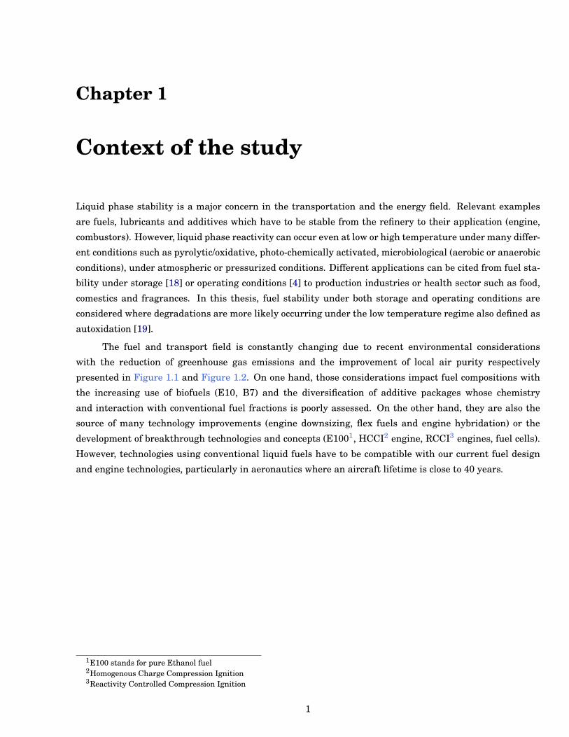
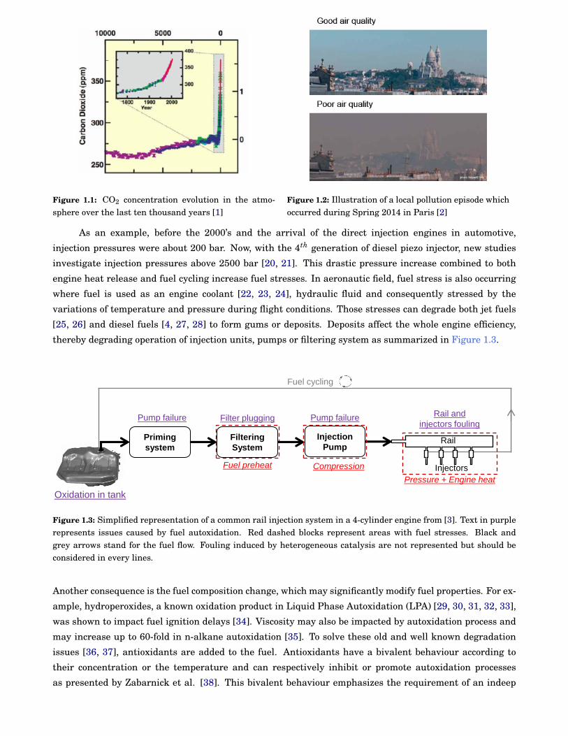
with the reduction of greenhouse gas emissions and the improvement of local air purity respectively

presented in Figure 1.1 and Figure 1.2. On one hand, those considerations impact fuel compositions with

the increasing use of biofuels (E10, B7) and the diversification of additive packages whose chemistry

and interaction with conventional fuel fractions is poorly assessed. On the other hand, they are also the

source of many technology improvements (engine downsizing, flex fuels and engine hybridation) or the

development of breakthrough technologies and concepts (E1001, HCCI2 engine, RCCI3 engines, fuel cells).

However, technologies using conventional liquid fuels have to be compatible with our current fuel design

and engine technologies, particularly in aeronautics where an aircraft lifetime is close to 40 years.

1E100 stands for pure Ethanol fuel2Homogenous Charge Compression Ignition3Reactivity Controlled Compression Ignition

1

2 Chapter 1

Figure 1.1: CO2 concentration evolution in the atmo-sphere over the last ten thousand years [1]

Figure 1.2: Illustration of a local pollution episode whichoccurred during Spring 2014 in Paris [2]

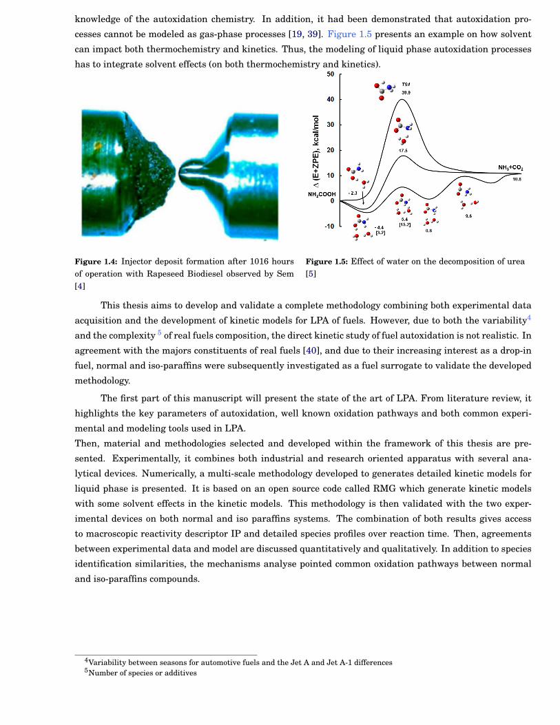
As an example, before the 2000’s and the arrival of the direct injection engines in automotive,

injection pressures were about 200 bar. Now, with the 4th generation of diesel piezo injector, new studies

investigate injection pressures above 2500 bar [20, 21]. This drastic pressure increase combined to both

engine heat release and fuel cycling increase fuel stresses. In aeronautic field, fuel stress is also occurring

where fuel is used as an engine coolant [22, 23, 24], hydraulic fluid and consequently stressed by the

variations of temperature and pressure during flight conditions. Those stresses can degrade both jet fuels

[25, 26] and diesel fuels [4, 27, 28] to form gums or deposits. Deposits affect the whole engine efficiency,

thereby degrading operation of injection units, pumps or filtering system as summarized in Figure 1.3.

Priming

system

Filtering

System

Injection

Pump

Pressure + Engine heat

CompressionFuel preheat

Fuel cycling

Rail

Injectors

Oxidation in tank

Filter plugging Pump failurePump failure Rail and

injectors fouling

Figure 1.3: Simplified representation of a common rail injection system in a 4-cylinder engine from [3]. Text in purplerepresents issues caused by fuel autoxidation. Red dashed blocks represent areas with fuel stresses. Black andgrey arrows stand for the fuel flow. Fouling induced by heterogeneous catalysis are not represented but should beconsidered in every lines.

Another consequence is the fuel composition change, which may significantly modify fuel properties. For ex-

ample, hydroperoxides, a known oxidation product in Liquid Phase Autoxidation (LPA) [29, 30, 31, 32, 33],

was shown to impact fuel ignition delays [34]. Viscosity may also be impacted by autoxidation process and

may increase up to 60-fold in n-alkane autoxidation [35]. To solve these old and well known degradation

issues [36, 37], antioxidants are added to the fuel. Antioxidants have a bivalent behaviour according to

their concentration or the temperature and can respectively inhibit or promote autoxidation processes

as presented by Zabarnick et al. [38]. This bivalent behaviour emphasizes the requirement of an indeep

Chapter 1 3

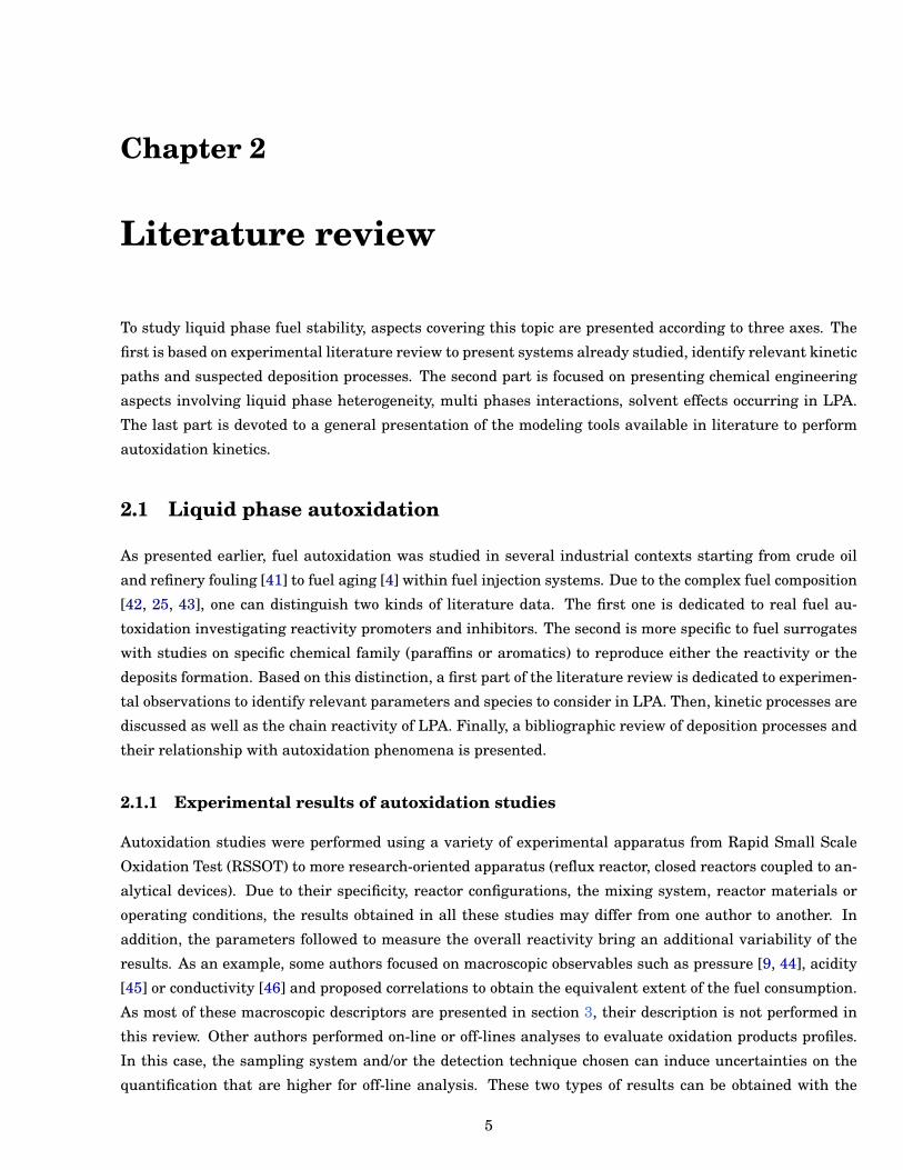
knowledge of the autoxidation chemistry. In addition, it had been demonstrated that autoxidation pro-

cesses cannot be modeled as gas-phase processes [19, 39]. Figure 1.5 presents an example on how solvent

can impact both thermochemistry and kinetics. Thus, the modeling of liquid phase autoxidation processes

has to integrate solvent effects (on both thermochemistry and kinetics).

Figure 1.4: Injector deposit formation after 1016 hoursof operation with Rapeseed Biodiesel observed by Sem[4]

Figure 1.5: Effect of water on the decomposition of urea[5]

This thesis aims to develop and validate a complete methodology combining both experimental data

acquisition and the development of kinetic models for LPA of fuels. However, due to both the variability4

and the complexity 5 of real fuels composition, the direct kinetic study of fuel autoxidation is not realistic. In

agreement with the majors constituents of real fuels [40], and due to their increasing interest as a drop-in

fuel, normal and iso-paraffins were subsequently investigated as a fuel surrogate to validate the developed

methodology.

The first part of this manuscript will present the state of the art of LPA. From literature review, it

highlights the key parameters of autoxidation, well known oxidation pathways and both common experi-

mental and modeling tools used in LPA.

Then, material and methodologies selected and developed within the framework of this thesis are pre-

sented. Experimentally, it combines both industrial and research oriented apparatus with several ana-

lytical devices. Numerically, a multi-scale methodology developed to generates detailed kinetic models for

liquid phase is presented. It is based on an open source code called RMG which generate kinetic models

with some solvent effects in the kinetic models. This methodology is then validated with the two exper-

imental devices on both normal and iso paraffins systems. The combination of both results gives access

to macroscopic reactivity descriptor IP and detailed species profiles over reaction time. Then, agreements

between experimental data and model are discussed quantitatively and qualitatively. In addition to species

identification similarities, the mechanisms analyse pointed common oxidation pathways between normal

and iso-paraffins compounds.

4Variability between seasons for automotive fuels and the Jet A and Jet A-1 differences5Number of species or additives

4 Chapter 1

Chapter 2

Literature review

To study liquid phase fuel stability, aspects covering this topic are presented according to three axes. The

first is based on experimental literature review to present systems already studied, identify relevant kinetic

paths and suspected deposition processes. The second part is focused on presenting chemical engineering

aspects involving liquid phase heterogeneity, multi phases interactions, solvent effects occurring in LPA.

The last part is devoted to a general presentation of the modeling tools available in literature to perform

autoxidation kinetics.

2.1 Liquid phase autoxidation

As presented earlier, fuel autoxidation was studied in several industrial contexts starting from crude oil

and refinery fouling [41] to fuel aging [4] within fuel injection systems. Due to the complex fuel composition

[42, 25, 43], one can distinguish two kinds of literature data. The first one is dedicated to real fuel au-

toxidation investigating reactivity promoters and inhibitors. The second is more specific to fuel surrogates

with studies on specific chemical family (paraffins or aromatics) to reproduce either the reactivity or the

deposits formation. Based on this distinction, a first part of the literature review is dedicated to experimen-

tal observations to identify relevant parameters and species to consider in LPA. Then, kinetic processes are

discussed as well as the chain reactivity of LPA. Finally, a bibliographic review of deposition processes and

their relationship with autoxidation phenomena is presented.

2.1.1 Experimental results of autoxidation studies

Autoxidation studies were performed using a variety of experimental apparatus from Rapid Small Scale

Oxidation Test (RSSOT) to more research-oriented apparatus (reflux reactor, closed reactors coupled to an-

alytical devices). Due to their specificity, reactor configurations, the mixing system, reactor materials or

operating conditions, the results obtained in all these studies may differ from one author to another. In

addition, the parameters followed to measure the overall reactivity bring an additional variability of the

results. As an example, some authors focused on macroscopic observables such as pressure [9, 44], acidity

[45] or conductivity [46] and proposed correlations to obtain the equivalent extent of the fuel consumption.

As most of these macroscopic descriptors are presented in section 3, their description is not performed in

this review. Other authors performed on-line or off-lines analyses to evaluate oxidation products profiles.

In this case, the sampling system and/or the detection technique chosen can induce uncertainties on the

quantification that are higher for off-line analysis. These two types of results can be obtained with the

5

6 Chapter 2

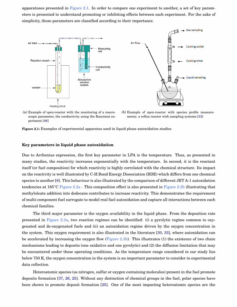
apparatuses presented in Figure 2.1. In order to compare one experiment to another, a set of key param-

eters is presented to understand promoting or inhibiting effects between each experiment. For the sake of

simplicity, those parameters are classified according to their importance.

(a) Example of open-reactor with the monitoring of a macro-scopic parameter, the conductivity using the Rancimat ex-periment [46]

(b) Example of open-reactor with species profile measure-ments: a reflux reactor with sampling systems [33]

Figure 2.1: Examples of experimental apparatus used in liquid phase autoxidation studies

Key parameters in liquid phase autoxidation

Due to Arrhenius expression, the first key parameter in LPA is the temperature. Thus, as presented in

many studies, the reactivity increases exponentially with the temperature. In second, it is the reactant

itself (or fuel composition) for which reactivity is highly correlated with the chemical structure. Its impact

on the reactivity is well illustrated by C-H Bond Energy Dissociation (BDE) which differs from one chemical

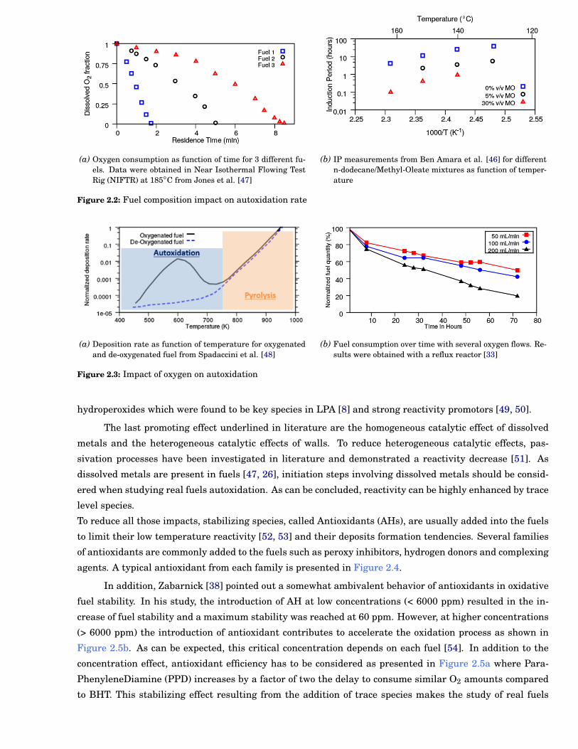
species to another [8]. This behaviour is also illustrated by the comparison of different JET A-1 autoxidation

tendencies at 185◦C Figure 2.2a . This composition effect is also presented in Figure 2.2b illustrating that

methyloleate addition into dodecane contributes to increase reactivity. This demonstrates the requirement

of multi-component fuel surrogate to model real fuel autoxidation and capture all interactions between each

chemical families.

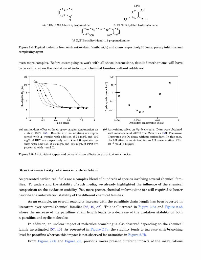
The third major parameter is the oxygen availability in the liquid phase. From the deposition rate

presented in Figure 2.3a, two reaction regimes can be identified: (i) a pyrolytic regime common to oxy-

genated and de-oxygenated fuels and (ii) an autoxidation regime driven by the oxygen concentration in

the system. This oxygen requirement is also illustrated in the literature [30, 33], where autoxidation can

be accelerated by increasing the oxygen flow (Figure 2.3b). This illustrates (1) the existence of two chain

mechanisms leading to deposits (one oxidative and one pyrolytic) and (2) the diffusion limitation that may

be encountered under these operating conditions. As the temperature range considered in our study lies

below 750 K, the oxygen concentration in the system is an important parameter to consider in experimental

data collection.

Heteroatomic species (as nitrogen, sulfur or oxygen containing molecules) present in the fuel promote

deposits formation [37, 26, 25]. Without any distinction of chemical groups in the fuel, polar species have

been shown to promote deposit formation [25]. One of the most impacting heteroatomic species are the

Chapter 2 7

(a) Oxygen consumption as function of time for 3 different fu-els. Data were obtained in Near Isothermal Flowing TestRig (NIFTR) at 185◦C from Jones et al. [47]

(b) IP measurements from Ben Amara et al. [46] for differentn-dodecane/Methyl-Oleate mixtures as function of temper-ature

Figure 2.2: Fuel composition impact on autoxidation rate

(a) Deposition rate as function of temperature for oxygenatedand de-oxygenated fuel from Spadaccini et al. [48]

(b) Fuel consumption over time with several oxygen flows. Re-sults were obtained with a reflux reactor [33]

Figure 2.3: Impact of oxygen on autoxidation

hydroperoxides which were found to be key species in LPA [8] and strong reactivity promotors [49, 50].

The last promoting effect underlined in literature are the homogeneous catalytic effect of dissolved

metals and the heterogeneous catalytic effects of walls. To reduce heterogeneous catalytic effects, pas-

sivation processes have been investigated in literature and demonstrated a reactivity decrease [51]. As

dissolved metals are present in fuels [47, 26], initiation steps involving dissolved metals should be consid-

ered when studying real fuels autoxidation. As can be concluded, reactivity can be highly enhanced by trace

level species.

To reduce all those impacts, stabilizing species, called Antioxidants (AHs), are usually added into the fuels

to limit their low temperature reactivity [52, 53] and their deposits formation tendencies. Several families

of antioxidants are commonly added to the fuels such as peroxy inhibitors, hydrogen donors and complexing

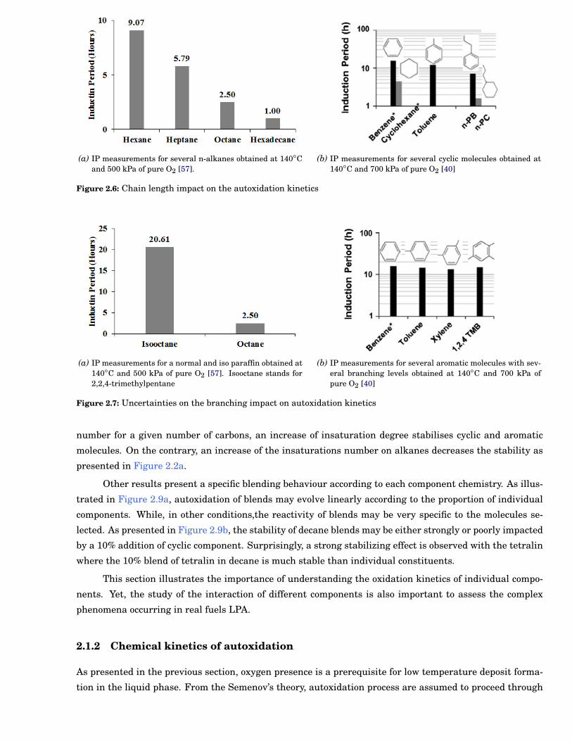
agents. A typical antioxidant from each family is presented in Figure 2.4.

In addition, Zabarnick [38] pointed out a somewhat ambivalent behavior of antioxidants in oxidative

fuel stability. In his study, the introduction of AH at low concentrations (< 6000 ppm) resulted in the in-

crease of fuel stability and a maximum stability was reached at 60 ppm. However, at higher concentrations

(> 6000 ppm) the introduction of antioxidant contributes to accelerate the oxidation process as shown in

Figure 2.5b. As can be expected, this critical concentration depends on each fuel [54]. In addition to the

concentration effect, antioxidant efficiency has to be considered as presented in Figure 2.5a where Para-

PhenyleneDiamine (PPD) increases by a factor of two the delay to consume similar O2 amounts compared

to BHT. This stabilizing effect resulting from the addition of trace species makes the study of real fuels

8 Chapter 2

(a) THQ: 1,2,3,4-tetrahydroquinoline (b) BHT: Butylated hydroxytoluene

(c) N,N’-Bis(salicylidene)-1,3-propanediamine

Figure 2.4: Typical molecule from each antioxidant family. a), b) and c) are respectively H donor, peroxy inhibitor andcomplexing agent

even more complex. Before attempting to work with all those interactions, detailed mechanisms will have

to be validated on the oxidation of individual chemical families without additives.

(a) Antioxidant effect on head space oxygen consumption onJP-5 at 180◦C [55]. Results with no additives are repre-sented with N, results with addition of 25 mg/L and 100mg/L of BHT are respectively with • and ■ symbols, re-sults with addition of 25 mg/L and 100 mg/L of PPD arepresented with ◦ and ä.

(b) Antioxidant effect on O2 decay rate. Data were obtainedwith n-dodecane at 200◦C from Zabarnick [38]. The arrowillustrates the O2 decay without antioxidant. In this case,the AH effect is maximized for an AH concentration of 2×10−4 mol/l (≈ 60ppm)

Figure 2.5: Antioxidant types and concentration effects on autoxidation kinetics.

Structure-reactivity relations in autoxidation

As presented earlier, real fuels are a complex blend of hundreds of species involving several chemical fam-

ilies. To understand the stability of such media, we already highlighted the influence of the chemical

composition on the oxidation stability. Yet, more precise chemical informations are still required to better

describe the autoxidation stability of the different chemical families.

As an example, an overall reactivity increase with the paraffinic chain length has been reported in

literature over several chemical families [56, 40, 57]. This is illustrated in Figure 2.6a and Figure 2.6b

where the increase of the paraffinic chain length leads to a decrease of the oxidation stability on both

n-paraffins and cyclic molecules.

In addition, an unclear impact of molecules branching is also observed depending on the chemical

family investigated [57, 40]. As presented in Figure 2.7a, the stability tends to increase with branching

level for paraffins whereas this impact is not observed for aromatics in Figure 2.7b.

From Figure 2.6b and Figure 2.8, previous works present different impacts of the insaturations

Chapter 2 9

(a) IP measurements for several n-alkanes obtained at 140◦Cand 500 kPa of pure O2 [57].

(b) IP measurements for several cyclic molecules obtained at140◦C and 700 kPa of pure O2 [40]

Figure 2.6: Chain length impact on the autoxidation kinetics

(a) IP measurements for a normal and iso paraffin obtained at140◦C and 500 kPa of pure O2 [57]. Isooctane stands for2,2,4-trimethylpentane

(b) IP measurements for several aromatic molecules with sev-eral branching levels obtained at 140◦C and 700 kPa ofpure O2 [40]

Figure 2.7: Uncertainties on the branching impact on autoxidation kinetics

number for a given number of carbons, an increase of insaturation degree stabilises cyclic and aromatic

molecules. On the contrary, an increase of the insaturations number on alkanes decreases the stability as

presented in Figure 2.2a.

Other results present a specific blending behaviour according to each component chemistry. As illus-

trated in Figure 2.9a, autoxidation of blends may evolve linearly according to the proportion of individual

components. While, in other conditions,the reactivity of blends may be very specific to the molecules se-

lected. As presented in Figure 2.9b, the stability of decane blends may be either strongly or poorly impacted

by a 10% addition of cyclic component. Surprisingly, a strong stabilizing effect is observed with the tetralin

where the 10% blend of tetralin in decane is much stable than individual constituents.

This section illustrates the importance of understanding the oxidation kinetics of individual compo-

nents. Yet, the study of the interaction of different components is also important to assess the complex

phenomena occurring in real fuels LPA.

2.1.2 Chemical kinetics of autoxidation

As presented in the previous section, oxygen presence is a prerequisite for low temperature deposit forma-

tion in the liquid phase. From the Semenov’s theory, autoxidation process are assumed to proceed through

10 Chapter 2

(a) IP measurements for a normal and unsaturated alkanesobtained at 140◦C and 500 kPa of pure O2 [57].

(b) IP measurements for several mono and poly aromaticmolecules obtained at 140◦C and 700 kPa of pure O2 [40].

Figure 2.8: Insaturation impact on autoxidation kinetics

(a) IP measurements for an aromatic blend obtained at 140◦Cand 500 kPa of pure O2 [57]. Percentages are given byvolume.

(b) IP measurements for blends cyclic compound in decane ob-tained at 140◦C and 700 kPa of pure O2 [40].

Figure 2.9: Specific effect of blending on autoxidation kinetics.

a chain mechanism. As presented in Figure 2.10, the chain reaction is composed of three distinct steps:

Initiation, Propagation and Termination. In literature, global chemical mechanisms [26, 38, 58] for fuel

autoxidation were proposed with similar chain mechanisms (C.f Figure 2.11) involving lumped species1.

However, as commercial fuels are complex blends of compounds from several chemical families, appropri-

ate thermochemical and kinetic data are required to get a meaningful mechanism. While, lumped species

are used to describe oxidation pathways, structural isomers must be considered in each of them.

The initiation step

In low temperature regime, the thermal energy in liquid phase system is modest and the initiation step is

still not fully elucidated. For this reason, the initiation step may be presented in several ways (Figure 2.12).

Some authors consider the initiation step as resulting from trace level species (hydroperoxides decomposi-

tion, azo-compounds decomposition), concerted H abstraction with O2 [38, 8] or photochemical reactions2.

1Lumped species correspond to a mixture of several distinct molecules showing similar properties2This initiation is not considered in all systems, such as tanks which are opaque to UV-visible light.

Chapter 2 11

RH+O2νi ,ki−−−→ R◦+HO◦

2 (i.1) InitiationRO2H → RO◦+HO◦

2 (i.2) InitiationR◦+O2 → RO◦

2 (p.1) PropagationRO◦

2 +RH → RO2H+R◦ (p.2) Propagation

R◦+R◦ νt,kt−−−→ terminationproducts (t.1) Termination

2RO◦2νt,kt−−−→ RO4R (t.2) Termination

Figure 2.10: General presentation of a chain mechanism

Figure 2.11: Global mechanism for liquid phase autoxidation proposed by Zongo [6]

Others, consider the first step as unknown and introduce a lumped species (Initiator) to obtain the first

alkyl radical. In addition, the initiation step may be catalytically enhanced by dissolved metals, surface

effects, acid catalyzed and ionic reactions.

Propagation step

The reaction (p.1) between alkyl radicals and molecular oxygen is the main propagation path due to its

low energy barrier (close to 0 kcal/mol) [26, 59]. Chain mechanism proceeds then through reaction (p.2)

according to which the peroxi-radical reacts with the initial hydrocarbon to form hydroperoxides and a

new alkyl radicals. Then RO2H decomposes (i.2) and forms new radicals which can also react with RH

12 Chapter 2

RH+O2 → R◦+HO◦2

RH+ I → R◦+ IHInitiator → R◦

Figure 2.12: Potential initiation steps of liquid phase autoxidation

to produce more alkyl radicals. Those, in turn contribute to increase the chain reactivity. This chain

mechanism is now well established in literature [31, 60, 6, 46] from the 1930’s with Semenov theory [61].

Recent experimental observations [62] of the QOOH radicals corroborate the consistency of such chain

mechanism.

Termination step

The termination can be simplified as a sum of all intermediates reaction paths through dimerization [63],

tetroxide formation [64], peracid formation, decarboxylation process, intra-molecular reactions, concerted

acid and ketone formations, disproportionation reactions. As presented here, LPA is governed by a radical

chain mechanism where overall reactivity is induced by branching steps (producing more radicals in the

system). For short conversion system, the overall reaction can be expressed following few parameters [65]

(kp,ki and kt and fuel concentration) as presented on equation 2.1. Based on same principle, Bolland [66]

proposed an oxidability criteria based on the ratio of propagation rates and termination rates as presented

in equation 2.2.

V =√

ki

2kt·kp × [RH] (2.1)

K = kp√2kt

= V

[RH] ·√Vi(2.2)

As presented here, chemical kinetics involved in autoxidation is relatively well known for major

product formation. However, the addition of isomers in all those steps cannot be performed manually. That

is why the approach proposed in this manuscript relies on an automated mechanism generation in order to

integrate all reactions - as comprehensively as possible - in oxidation mechanisms.

2.1.3 Oxidation products and deposition processes

In order to study the deposition process involved in LPA, it is a major concern to identify the deposit precur-

sors and the pathways involved in their formation. Those need to be integrated into kinetic mechanisms.

As paraffins are usually the main fuel constituents and the resulting products from all drop-in fuels like

Biomass to Liquid (BtL), Coal to Liquid (CtL) and Gas to Liquid (GtL), they were selected during this thesis

to evaluate the robustness of liquid phase mechanism generation methodology. For this reason, the present

literature review of oxidation products formation focuses mainly on this chemical family as presented in

this section. Studies investigating other fuel constituents like naphtenes, cycloalkanes or oxygenated com-

pounds are available 3 but are out of the scope of the present work. For the sake of clarity, the oxidation

pathways are presented with lumped species, structural isomers should be considered for these species

when it applies.

3Complementary informations on appendices

Chapter 2 13

Oxidation products formation

Hydroperoxides have been widely described in literature [8, 31, 67, 44] as the first oxidation product. These

highly reactive species, even at very low concentration, are formed mainly by oxygen addition on alkyl

radicals and a subsequent H-abstraction as presented in Figure 2.10. They thermally decompose to produce

two radicals which subsequently produce first stage oxidation products, alcohols and ketones, as shown in

Figure 2.13.

ROOH → RO◦+OH◦

RO◦+RH → ROH+R◦

(a) Alcohol formation (ROH)[60]

RO◦2 +R1R2CHOOH → RO2H+R1R2C◦OOH

R1R2C◦OOH → R1R2CO+OH◦

(b) Ketones formation (RO)[60]

Figure 2.13: Major pathways leading to oxygenated species formations

Second stage oxidation products include to several oxidized products including most likely lower

molecular weight products compare to fuel like ketones, acids and aldehydes. Many pathways were pro-

posed in the literature for the formation of those species. Due to the mechanism generator requirements,

our interest was focused on reactions describing elementary steps only.

As observed in the gas phase [68], an isomerization step of alkyl-peroxy radical (ROO◦) radicals is compet-

ing with ROOH formation as proposed by Korcek et al [31] and presented in Figure 2.14a. This compe-

tition leads to the formation of Keto-Hydro-Peroxide (KHP) and initiates the "so-called" Korcek’s reaction

(Figure 2.14b). Thanks to a recent work from Jalan et al. [69], Electronic Structure Calculations (ESC)

validated this two-step reaction formulated by Korcek in the 70’s. This reaction starts with a concerted

keto-hydroperoxide cyclisation, then the cycle breaks following two pathways: to form either acids and ke-

tones or acids and aldehydes depending on the R1 and R2 groups on the molecule. Another pathway leading

to the lighter oxidation products formation is the direct homolytic C-C bond breaking. These reactions may

occur through either α/β decarbonylation or cracking reactions (Figure 2.14c). This leads to the formation

of lower n-alkanes, alkenes, carbonyles and light gases like CO ,CO2, water [29, 70, 44, 71, 72].

Finally, a group of reactions, involving late oxidation reactions with a maintain or a growth of oxi-

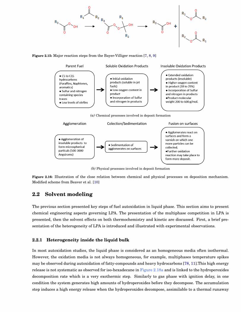
dation products size may be presented. One of them is the Baeyer-Villiger rearrangement which conserves

reactant size. This reaction starts from peracids [8, 9] and leads to acids and esters formation through

several intramolecular and concerted steps Figure 2.15. Still maintaining reactants size, oxygenated cycle

like lactones, furanones or epoxides [73, 67, 8, 63] may be formed with not well known chemical pathways4. Further investigations are still required to get relevant pathways for these producs. Finally, all the

reticulation/termination steps that form heavier oxidation products like Tetroxides (RO4R’)[64] or alkanes

(R’R)[63] are well defined in literature.

Despite the apparent simplicity of the above-mentioned autoxidation paths, co-oxidation or poly-

substituted products formation (poly-substituted hydroperoxides [31, 8]) must be considered.

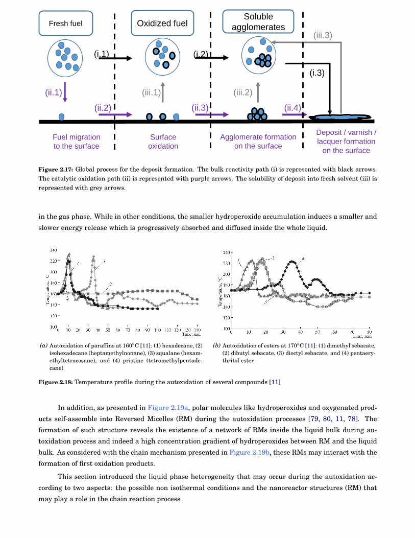
Deposition process

Deposition issues, involved in refinery and fuel injection systems, have been already studied for several

decades [22, 74, 41]. Due to the complexity of the deposition processes, this section aims to briefly introduce

the overall phenomenology of deposit formation with its key parameters. As mentioned in Figure 2.3a,

autoxidation regimes influences the kind of deposits formed. Two types of deposits can be distinguished. A

4Except for the epoxides formation

14 Chapter 2

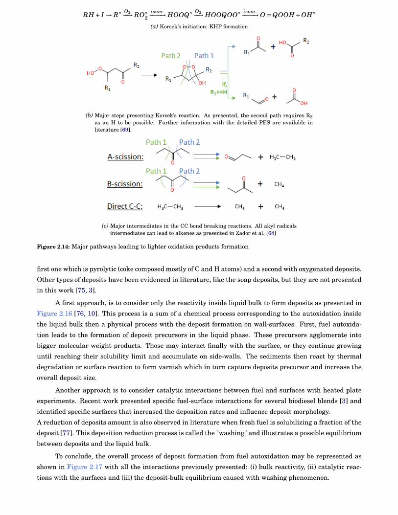
RH+ I → R◦ O2−−→ RO◦2

isom.−−−−→ HOOQ◦ O2−−→ HOOQOO◦ isom.−−−−→O =QOOH+OH◦

(a) Korcek’s initiation: KHP formation

(b) Major steps presenting Korcek’s reaction. As presented, the second path requires R2as an H to be possible. Further information with the detailed PES are available inliterature [69].

(c) Major intermediates in the CC bond breaking reactions. All akyl radicalsintermediates can lead to alkenes as presented in Zador et al. [68]

Figure 2.14: Major pathways leading to lighter oxidation products formation

first one which is pyrolytic (coke composed mostly of C and H atoms) and a second with oxygenated deposits.

Other types of deposits have been evidenced in literature, like the soap deposits, but they are not presented

in this work [75, 3].

A first approach, is to consider only the reactivity inside liquid bulk to form deposits as presented in

Figure 2.16 [76, 10]. This process is a sum of a chemical process corresponding to the autoxidation inside

the liquid bulk then a physical process with the deposit formation on wall-surfaces. First, fuel autoxida-

tion leads to the formation of deposit precursors in the liquid phase. These precursors agglomerate into

bigger molecular weight products. Those may interact finally with the surface, or they continue growing

until reaching their solubility limit and accumulate on side-walls. The sediments then react by thermal

degradation or surface reaction to form varnish which in turn capture deposits precursor and increase the

overall deposit size.

Another approach is to consider catalytic interactions between fuel and surfaces with heated plate

experiments. Recent work presented specific fuel-surface interactions for several biodiesel blends [3] and

identified specific surfaces that increased the deposition rates and influence deposit morphology.

A reduction of deposits amount is also observed in literature when fresh fuel is solubilizing a fraction of the

deposit [77]. This deposition reduction process is called the "washing" and illustrates a possible equilibrium

between deposits and the liquid bulk.

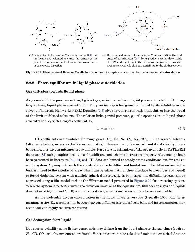
To conclude, the overall process of deposit formation from fuel autoxidation may be represented as

shown in Figure 2.17 with all the interactions previously presented: (i) bulk reactivity, (ii) catalytic reac-

tions with the surfaces and (iii) the deposit-bulk equilibrium caused with washing phenomenon.

Chapter 2 15

Figure 2.15: Major reaction steps from the Bayer-Villiger reaction [7, 8, 9]

(a) Chemical processes involved in deposit formation

(b) Physical processes involved in deposit formation

Figure 2.16: Illustration of the close relation between chemical and physical processes on deposition mechanism.Modified scheme from Beaver et al. [10]

2.2 Solvent modeling

The previous section presented key steps of fuel autoxidation in liquid phase. This section aims to present

chemical engineering aspects governing LPA. The presentation of the multiphase competition in LPA is

presented, then the solvent effects on both thermochemistry and kinetic are discussed. First, a brief pre-

sentation of the heterogeneity of LPA is introduced and illustrated with experimental observations.

2.2.1 Heterogeneity inside the liquid bulk

In most autoxidation studies, the liquid phase is considered as an homogeneous media often isothermal.

However, the oxidation media is not always homogeneous, for example, multiphases temperature spikes

may be observed during autoxidation of fatty-compounds and heavy hydrocarbons [78, 11].This high energy

release is not systematic as observed for iso-hexadecane in Figure 2.18a and is linked to the hydroperoxides

decomposition rate which is a very exothermic step. Similarly to gas phase with ignition delay, in one

condition the system generates high amounts of hydroperoxides before they decompose. The accumulation

step induces a high energy release when the hydroperoxides decompose, assimilable to a thermal runaway

16 Chapter 2

Fresh fuel

(ii.1)

(i.1)

Soluble

agglomerates

(i.2)

(iii.1)

(ii.3)

(i.3)

(iii.2)

(ii.2) (ii.4)

(iii.3)

Oxidized fuel

Surface

oxidation

Agglomerate formation

on the surface

Deposit / varnish /

lacquer formation

on the surface

Fuel migration

to the surface

Figure 2.17: Global process for the deposit formation. The bulk reactivity path (i) is represented with black arrows.The catalytic oxidation path (ii) is represented with purple arrows. The solubility of deposit into fresh solvent (iii) isrepresented with grey arrows.

in the gas phase. While in other conditions, the smaller hydroperoxide accumulation induces a smaller and

slower energy release which is progressively absorbed and diffused inside the whole liquid.

(a) Autoxidation of paraffins at 160◦C [11]: (1) hexadecane, (2)isohexadecane (heptamethylnonane), (3) squalane (hexam-ethyltetracosane), and (4) pristine (tetramethylpentade-cane)

(b) Autoxidation of esters at 170◦C [11]: (1) dimethyl sebacate,(2) dibutyl sebacate, (3) dioctyl sebacate, and (4) pentaery-thritol ester

Figure 2.18: Temperature profile during the autoxidation of several compounds [11]

In addition, as presented in Figure 2.19a, polar molecules like hydroperoxides and oxygenated prod-

ucts self-assemble into Reversed Micelles (RM) during the autoxidation processes [79, 80, 11, 78]. The

formation of such structure reveals the existence of a network of RMs inside the liquid bulk during au-

toxidation process and indeed a high concentration gradient of hydroperoxides between RM and the liquid

bulk. As considered with the chain mechanism presented in Figure 2.19b, these RMs may interact with the

formation of first oxidation products.

This section introduced the liquid phase heterogeneity that may occur during the autoxidation ac-

cording to two aspects: the possible non isothermal conditions and the nanoreactor structures (RM) that

may play a role in the chain reaction process.

Chapter 2 17

(a) Schematic of the Reverse Micelle formation [81]. Po-lar heads are oriented towards the center of thestructure and apolar parts of molecules are orientedin the oposite direction.

(b) Hypothetical impact of the Reverse Micelles (RM) on the firststage of autoxidation [78]. Polar products accumulate insidethe RM and react inside the structure to give either volatileproducts or radicals that can contribute to the chain reaction.

Figure 2.19: Illustration of Reverse Micelle formation and its implication in the chain mechanism of autoxidation

2.2.2 Phase equilibrium in liquid phase autoxidation

Gas diffusion towards liquid phase

As presented in the previous section, O2 is a key species to consider in liquid phase autoxidation. Contrary

to gas phase, liquid phase concentration of oxygen (or any other gases) is limited by its solubility in the

solvent of interest. Henry’s Law (HL) Equation (2.3) gives oxygen concentration calculation into the liquid

at the limit of diluted solutions. The relation links partial pressure, pi, of a species i to its liquid phase

concentration, ci with Henry’s coefficient, kh.

pi = kh × ci (2.3)

HL coefficients are available for many gases (H2, He, Ne, O2, N2, CO2, ...) in several solvents

(alkanes, alcohols, esters, cycloalkanes, aromatics). However, only few experimental data for hydrocar-

bons/molecular oxygen mixtures are available. Pure solvent estimation of HL are available in DETHERM

database [82] using empirical relations. In addition, some chemical structure-property relationships have

been presented in literature [83, 84, 85]. HL data are limited to steady states conditions but for real re-

acting system, O2 may not reach the steady state due to diffusional limitations. The diffusion inside the

bulk is linked to the interfacial areas which can be either natural (free interface between gas and liquid)

or forced (bubbling system with multiple spherical interfaces). In both cases, the diffusion process can be

expressed using a film model such as the Whitman model presented in Figure 2.20 for a reacting system.

When the system is perfectly mixed (no diffusion limit) or at the equilibrium, film sections (gas and liquid)

does not exist (δg = 0 and δl = 0) and concentration gradients inside each phase become negligible.

As the molecular oxygen concentration in the liquid phase is very low (typically 1000 ppm for n-

paraffins at 298 K), a competition between oxygen diffusion into the solvent bulk and its consumption may

occur easily in highly reactive conditions.

Gas desorption from liquid

Due species volatility, some lighter compounds may diffuse from the liquid phase to the gas phase (such as

H2, CO, CO2 or light oxygenated products). Vapor pressure can be calculated using the empirical Antoine

18 Chapter 2

Figure 2.20: Whitman model presentation for a reacting system consuming A in the liquid phase. PA is the partialpressure and CA,g the concentration of species A in the gas phase. Indices g, l and i respectively stand for gas liquid,and interface.

equation (2.4). This equation allows to quantify evaporation rate of liquid products in the gas phase (A and

B being two parameters relevant to the molecule volatility). Multiphase mass transfer issues presented in

this part underlines the need of a specific multiphase reactor for the modeling of these phenomena. Thus,

the multiphase reactor will have to considerer both HL coefficient of gas phase species and product partial

pressure of liquid phase species to model those equilibrium states.

log10(P)= A− B(T +C)

(2.4)

2.2.3 Solvent effects in liquid phase autoxidation

As presented in Figure 2.23, the solvent impacts both thermochemistry and apparent kinetic rates. This

statement has been discussed by various authors [8, 86, 12]. Although thermochemical and the kinetic data

in liquid phase can be measured directly from experimental data, defining both parameters in all solvent

of interest is not realistic. On the other hand, there is a growing interest in correcting the gas phase data

from literature by applying corrections corresponding to the solvent effect. This section aims to presents

how those data can be obtained. Each section is divided into two parts, the first one presents the tools

available in literature to calculate solvent corrections. The second one is devoted to the method used in the

present work.

Impact on the thermochemistry

To present the liquid phase correction, ∆Gsolv, a thermodynamic cycle is given in Figure 2.21. It includes all

individual corrections to consider from real gas mixture to concentrated solute in solvent. Corrections can

be divided into four main steps [86]: (1) ideal states corrections (where gases and liquids are moved from

concentrated to diluted conditions), (2) cavity formations correction, (3) Van der Waals corrections (also

called dispersion-repulsion forces) and (4) electrostatic contributions referring to the charge distribution in

the solvent.

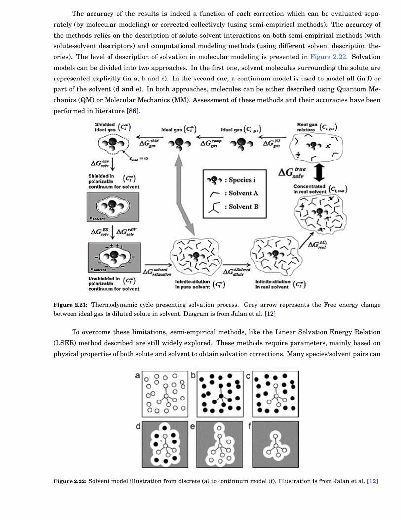
Chapter 2 19

The accuracy of the results is indeed a function of each correction which can be evaluated sepa-

rately (by molecular modeling) or corrected collectively (using semi-empirical methods). The accuracy of

the methods relies on the description of solute-solvent interactions on both semi-empirical methods (with

solute-solvent descriptors) and computational modeling methods (using different solvent description the-

ories). The level of description of solvation in molecular modeling is presented in Figure 2.22. Solvation

models can be divided into two approaches. In the first one, solvent molecules surrounding the solute are

represented explicitly (in a, b and c). In the second one, a continuum model is used to model all (in f) or

part of the solvent (d and e). In both approaches, molecules can be either described using Quantum Me-

chanics (QM) or Molecular Mechanics (MM). Assessment of these methods and their accuracies have been

performed in literature [86].

Figure 2.21: Thermodynamic cycle presenting solvation process. Grey arrow represents the Free energy changebetween ideal gas to diluted solute in solvent. Diagram is from Jalan et al. [12]

To overcome these limitations, semi-empirical methods, like the Linear Solvation Energy Relation

(LSER) method described are still widely explored. These methods require parameters, mainly based on

physical properties of both solute and solvent to obtain solvation corrections. Many species/solvent pairs can

Figure 2.22: Solvent model illustration from discrete (a) to continuum model (f). Illustration is from Jalan et al. [12]

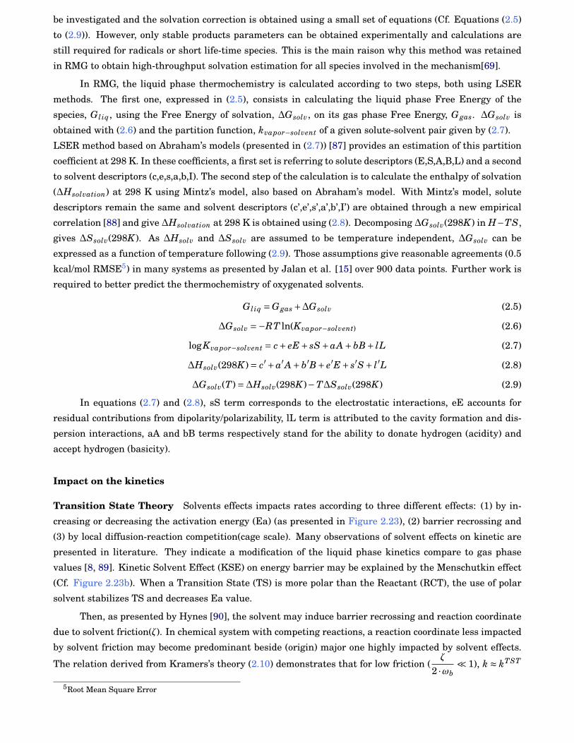
20 Chapter 2

be investigated and the solvation correction is obtained using a small set of equations (Cf. Equations (2.5)

to (2.9)). However, only stable products parameters can be obtained experimentally and calculations are

still required for radicals or short life-time species. This is the main raison why this method was retained

in RMG to obtain high-throughput solvation estimation for all species involved in the mechanism[69].

In RMG, the liquid phase thermochemistry is calculated according to two steps, both using LSER

methods. The first one, expressed in (2.5), consists in calculating the liquid phase Free Energy of the

species, G l iq, using the Free Energy of solvation, ∆Gsolv, on its gas phase Free Energy, Ggas. ∆Gsolv is

obtained with (2.6) and the partition function, kvapor−solvent of a given solute-solvent pair given by (2.7).

LSER method based on Abraham’s models (presented in (2.7)) [87] provides an estimation of this partition

coefficient at 298 K. In these coefficients, a first set is referring to solute descriptors (E,S,A,B,L) and a second

to solvent descriptors (c,e,s,a,b,I). The second step of the calculation is to calculate the enthalpy of solvation

(∆Hsolvation) at 298 K using Mintz’s model, also based on Abraham’s model. With Mintz’s model, solute

descriptors remain the same and solvent descriptors (c’,e’,s’,a’,b’,I’) are obtained through a new empirical

correlation [88] and give ∆Hsolvation at 298 K is obtained using (2.8). Decomposing ∆Gsolv(298K) in H−TS,

gives ∆Ssolv(298K). As ∆Hsolv and ∆Ssolv are assumed to be temperature independent, ∆Gsolv can be

expressed as a function of temperature following (2.9). Those assumptions give reasonable agreements (0.5

kcal/mol RMSE5) in many systems as presented by Jalan et al. [15] over 900 data points. Further work is

required to better predict the thermochemistry of oxygenated solvents.

G l iq =Ggas +∆Gsolv (2.5)

∆Gsolv =−RT ln(Kvapor−solvent) (2.6)

logKvapor−solvent = c+ eE+ sS+aA+bB+ lL (2.7)

∆Hsolv(298K)= c′+a′A+b′B+ e′E+ s′S+ l′L (2.8)

∆Gsolv(T)=∆Hsolv(298K)−T∆Ssolv(298K) (2.9)

In equations (2.7) and (2.8), sS term corresponds to the electrostatic interactions, eE accounts for

residual contributions from dipolarity/polarizability, lL term is attributed to the cavity formation and dis-

persion interactions, aA and bB terms respectively stand for the ability to donate hydrogen (acidity) and

accept hydrogen (basicity).

Impact on the kinetics

Transition State Theory Solvents effects impacts rates according to three different effects: (1) by in-

creasing or decreasing the activation energy (Ea) (as presented in Figure 2.23), (2) barrier recrossing and

(3) by local diffusion-reaction competition(cage scale). Many observations of solvent effects on kinetic are

presented in literature. They indicate a modification of the liquid phase kinetics compare to gas phase

values [8, 89]. Kinetic Solvent Effect (KSE) on energy barrier may be explained by the Menschutkin effect

(Cf. Figure 2.23b). When a Transition State (TS) is more polar than the Reactant (RCT), the use of polar

solvent stabilizes TS and decreases Ea value.

Then, as presented by Hynes [90], the solvent may induce barrier recrossing and reaction coordinate

due to solvent friction(ζ). In chemical system with competing reactions, a reaction coordinate less impacted

by solvent friction may become predominant beside (origin) major one highly impacted by solvent effects.

The relation derived from Kramers’s theory (2.10) demonstrates that for low friction (ζ

2 ·ωb¿ 1), k ≈ kTST

5Root Mean Square Error

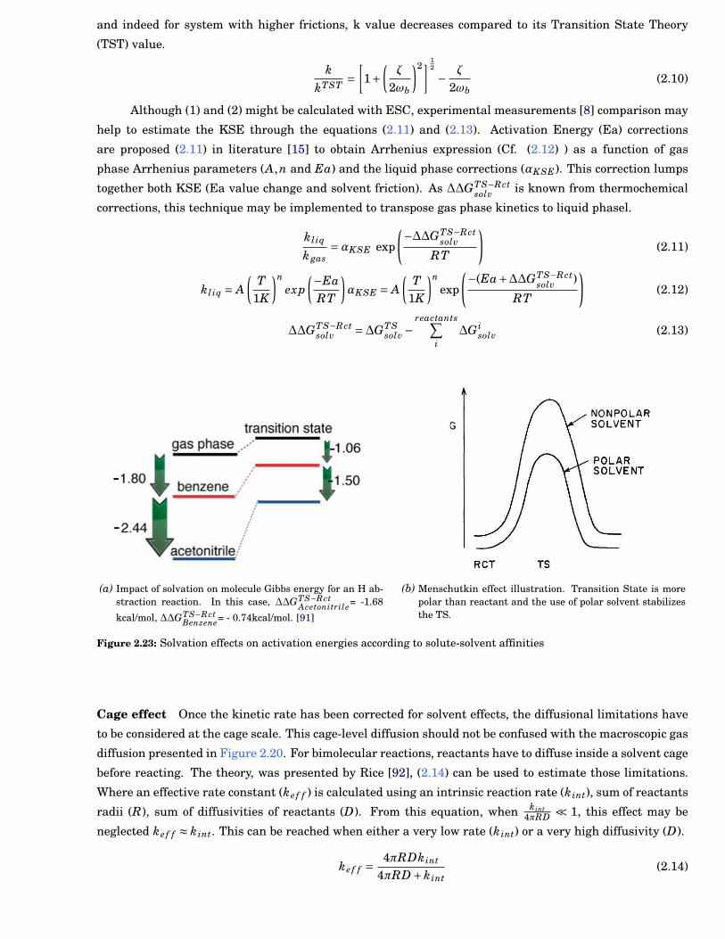
Chapter 2 21

and indeed for system with higher frictions, k value decreases compared to its Transition State Theory

(TST) value.

kkTST =

[1+

(ζ

2ωb

)2] 12

− ζ

2ωb(2.10)

Although (1) and (2) might be calculated with ESC, experimental measurements [8] comparison may

help to estimate the KSE through the equations (2.11) and (2.13). Activation Energy (Ea) corrections

are proposed (2.11) in literature [15] to obtain Arrhenius expression (Cf. (2.12) ) as a function of gas

phase Arrhenius parameters (A,n and Ea) and the liquid phase corrections (αKSE). This correction lumps

together both KSE (Ea value change and solvent friction). As ∆∆GTS−Rctsolv is known from thermochemical

corrections, this technique may be implemented to transpose gas phase kinetics to liquid phasel.

kl iq

kgas=αKSE exp

(−∆∆GTS−Rctsolv

RT

)(2.11)

kl iq = A(

T1K

)nexp

(−EaRT

)αKSE = A

(T

1K

)nexp

(−(Ea+∆∆GTS−Rctsolv )

RT

)(2.12)

∆∆GTS−Rctsolv =∆GTS

solv −reactants∑

i∆G i

solv (2.13)

(a) Impact of solvation on molecule Gibbs energy for an H ab-straction reaction. In this case, ∆∆GTS−Rct

Acetonitrile= -1.68

kcal/mol, ∆∆GTS−RctBenzene= - 0.74kcal/mol. [91]

(b) Menschutkin effect illustration. Transition State is morepolar than reactant and the use of polar solvent stabilizesthe TS.

Figure 2.23: Solvation effects on activation energies according to solute-solvent affinities

Cage effect Once the kinetic rate has been corrected for solvent effects, the diffusional limitations have

to be considered at the cage scale. This cage-level diffusion should not be confused with the macroscopic gas

diffusion presented in Figure 2.20. For bimolecular reactions, reactants have to diffuse inside a solvent cage

before reacting. The theory, was presented by Rice [92], (2.14) can be used to estimate those limitations.

Where an effective rate constant (ke f f ) is calculated using an intrinsic reaction rate (kint), sum of reactants

radii (R), sum of diffusivities of reactants (D). From this equation, when kint4πRD ¿ 1, this effect may be

neglected ke f f ≈ kint. This can be reached when either a very low rate (kint) or a very high diffusivity (D).

ke f f =4πRDkint

4πRD+kint(2.14)

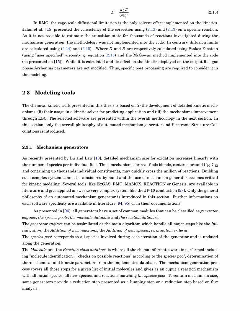
22 Chapter 2

D = kbT6πηr

(2.15)

In RMG, the cage-scale diffusional limitation is the only solvent effect implemented on the kinetics.

Jalan et al. [15] presented the consistency of the correction using (2.12) and (2.13) on a specific reaction.

As it is not possible to estimate the transition state for thousands of reactions investigated during the

mechanism generation, the methodology was not implemented into the code. In contrary, diffusion limits

are calculated using (2.14) and (2.15) . Where D and R are respectively calculated using Stokes-Einstein

(using "user specified" viscosity, η, equation (2.15) and the McGowan method implemented into the code

(as presented on [15]). While it is calculated and its effect on the kinetic displayed on the output file, gas

phase Arrhenius parameters are not modified. Thus, specific post processing are required to consider it in

the modeling.

2.3 Modeling tools

The chemical kinetic work presented in this thesis is based on (i) the development of detailed kinetic mech-

anisms, (ii) their usage in a kinetic solver for predicting application and (iii) the mechanisms improvement

through ESC. The selected software are presented within the overall methodology in the next section. In

this section, only the overall philosophy of automated mechanism generator and Electronic Structure Cal-

culations is introduced.

2.3.1 Mechanism generators

As recently presented by Lu and Law [13], detailed mechanism size for oxidation increases linearly with

the number of species per individual fuel. Thus, mechanisms for real-fuels blends, centered around C10-C12

and containing up thousands individual constituents, may quickly cross the million of reactions. Building

such complex system cannot be considered by hand and the use of mechanism generator becomes critical

for kinetic modeling. Several tools, like ExGAS, RMG, MAMOX, REACTION or Genesis, are available in

literature and give applied answer to very complex system like the JP-10 combustion [93]. Only the general

philosophy of an automated mechanism generator is introduced in this section. Further informations on

each software specificity are available in literature [94, 95] or in their documentations.

As presented in [94], all generators have a set of common modules that can be classified as generator

engines, the species pools, the molecule database and the reaction database.

The generator engines can be assimilated as the main algorithm which handle all major steps like the Ini-

tialization, the Addition of new reactions, the Addition of new species, termination criteria.

The species pool correponds to all species involved during each iteration of the generator and is updated

along the generation.

The Molecule and the Reaction class database is where all the chemo-informatic work is performed includ-

ing "molecule identification", "checks on possible reactions" according to the species pool, determination of

thermochemical and kinetic parameters from the implemented database. The mechanism generation pro-

cess covers all those steps for a given list of initial molecules and gives as an ouput a reaction mechanism

with all initial species, all new species, and reactions matching the species pool. To contain mechanism size,

some generators provide a reduction step presented as a lumping step or a reduction step based on flux

analysis.

Chapter 2 23

Figure 2.24: Typical size of detailed and skeletal mechanisms for hydrocarbon fuels.The figure is from Lu and Law[13]. As presented with the mechanism selected, mechanism size is linearly correlated with the number of species,NumberRxn = 5×NumberSpc.

Finally once the generation is completed, the mechanism can be coupled to a kinetic solver like Can-

tera or Chemkin suite softwares to model specific conditions. In the case of a rate based generator, like

RMG, the reactor model already influence the generation process. Thus, the implementation of new reactor

model may become critical to increase mechanism generator capability.

2.3.2 Electronic structure calculations

ESC They are all based on the laws of Quantum Mechanics (QM) and predict molecules structures, energies,

vibrational frequencies and reactions pathways of a variety of chemical compounds (stable or transition

structures).

To perform these calculations, the algorithm is solving the Schrödinger equation (Cf. (2.16)) to find the

different stationary states of the species considered. In equation (2.16), ψ is the wave function (whose

squared norm represents the probability of presence), H is the Hamiltonian operator and E the energy of

the particle. However, this equation is analytically not solvable for polyelectronic systems.

Hψ= Eψ (2.16)

According to the electronic structure method selected, modeling approaches are required to solve

(2.16). There are two main classes of methods. Semi-empirical methods such as AM1, PM3, PM6 that

use parameters extracted from experimental data to simplify the equations. There are many different

semi-empirical methods available and their accuracy depends on each system. Ab initio methods rely on

a small number of physical constants for the basis of their computations. In Hartree-Fock (HF) approach,

24 Chapter 2

the solution of Schrödinger equation assumes the wave function to be an antisymmetrized product of one-

electron spin-orbitals. Hence, each electron is treated separately and the effect of all the other electrons is

globalized through an effective potential (central-field approximation) determined in a self-consistent way.

The difference between the exact nonrelativistic energy and the HF energy is the correlation energy of the

molecule. Electron correlation is not accounted in HF approach, it is addressed by post-HF methods, such

as coupled cluster theory. However, post-HF methods can become computationally prohibitive for geometry

searches if more than 10 heavy atoms are involved, DFT becoming then the method of choice. DFT methods

are based on the Hohenberg-Kohn theorems which state that the ground state properties of a many-electron

system are uniquely determined by an electron density that depends on only 3 spatial coordinates (instead

of 3N dimensions) and that minimizes an energy functional. The accuracy of DFT depends on the quality

of the exchange-correlation functional.

As presented earlier (subsection 2.2.3), calculations can be performed with the solvent to calculate liquid

phase interactions . To model those interactions, calculations are performed placing a solute in a solvent

cavity. Those methods are called Henry’s Law (SCRF). Several levels of solvent description can be selected

from the simplest one (Dipole & Sphere model, also called Onsager’s model) to the most realistic one (Self

Consistent Isodensity Polarized Continuum Model) (C.f Figure 2.22 for solvent model presentation). Due

to computational limitations, the SCRF model selection depends on each system (number of atoms and

electrons of the molecules).

2.4 Conclusions

In this part, the state of the art of liquid phase autoxidation has been presented. First, a review of autoxi-

dation literature study was performed highlighting the key parameters of oxidation kinetics and introduced

the principle of structure-reactivity relations. Then, the theory behind the chain reaction in liquid phase

have been presented with most relevant oxidation pathways and the expected products in the conditions

investigated in this manuscript.

Second, chemical engineering aspects identified in LPA were presented including the liquid bulk hetero-

geneity, phase equilibrium phenomena and solvent effects on both thermochemistry and kinetics. Finally,

a review of the main modeling tools employed in this work are presented.

In the next chapter, the experimental and modeling methodologies are presented in details. A presen-

tation of both experimental apparatus with analytical devices is performed. Then the proposed MultiScale

Aprroach used to build relevant liquid phase kinetic models for fuel surrogate autoxidation is presented.

Chapter 3

Material and Methods

The study of liquid phase oxidation of fuels involves long time scales phenomena. To reduce experimental

cost and operating time, a set of experimental apparatuses. The RSSOTs, aims to reproduce real oxidative

conditions in shorter amount of time. Coupled to liquid residual analysis, they give interesting results for

models validation. A complementary approach is to use more research oriented devices with complex sam-

pling systems to analyse in-line or off-line the reacting mixture at several time steps. These two approaches

are conducted within this work with a PetroOxy and an autoclave associated to qualitative and quantitative

analyses.

To model such long time scales phenomena, it is a major concern to develop associated detailed kinetic

models for the liquid phase. This chapter introduces both the experimental and modeling methodology

employed in this work to study the liquid phase oxidation kinetics.

3.1 Experimental devices

In this section, the PetroOxy and autoclave experiments with their analytical devices are presented in

details with their operating methods. For a sake of clarity, the macroscopic parameter, IP, widely used in

models validation is defined with its majors experimental observations.

3.1.1 PetroOxy experiment

Experiments were performed with a PetroOxy apparatus from Petrotest Instruments GmbH & Co. KG. It

is one of the existing reference instruments to perform RSSOT of fuels and fuel surrogates as described

in American Society for Testing and Materials (ASTM) 7545 methods [96]. This equipment, presented in

Figure 3.1a, offers convenient features such as a small volume of samples, gold plated test cell (7) and a

high pressure cell with typical operating ranges up to 700 kPa of initial oxygen and 160◦ C. Previous works

[44, 97] have successfully employed this device to study liquid phase autoxidation kinetics. In addition,

PetroOxy measurements obtained over a large data set present a high reproducibility, the absolute average

deviation of results may be expressed as function of the measured IP according to ∆IP(hours) = 0.018×IP(hours). A higher deviation (around 6 % in average) was previously obtained [98] with a smaller data

set of bio-diesel experimental results only with very low IP measurements.

25

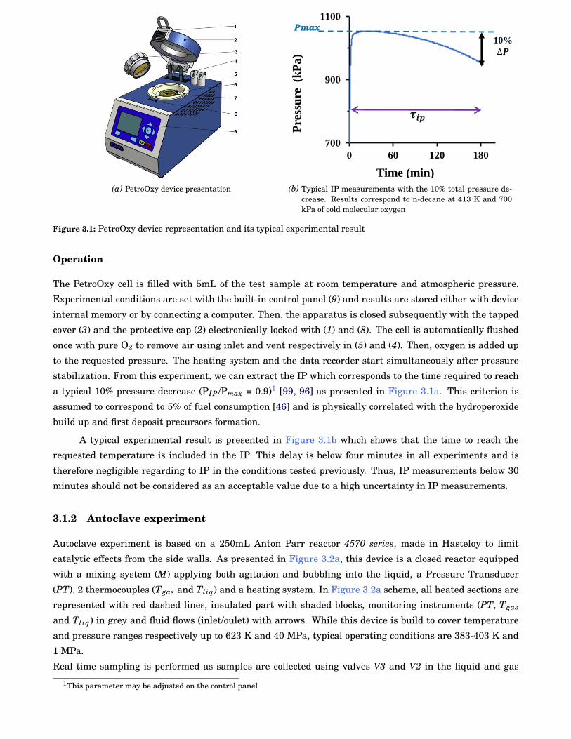
26 Chapter 3

(a) PetroOxy device presentation

700

900

1100

0 60 120 180

Pre

ssu

re (k

Pa

)

Time (min)

𝑷𝒎𝒂𝒙

𝝉𝒊𝒑

10%

∆𝑷

(b) Typical IP measurements with the 10% total pressure de-crease. Results correspond to n-decane at 413 K and 700kPa of cold molecular oxygen

Figure 3.1: PetroOxy device representation and its typical experimental result

Operation

The PetroOxy cell is filled with 5mL of the test sample at room temperature and atmospheric pressure.

Experimental conditions are set with the built-in control panel (9) and results are stored either with device

internal memory or by connecting a computer. Then, the apparatus is closed subsequently with the tapped

cover (3) and the protective cap (2) electronically locked with (1) and (8). The cell is automatically flushed

once with pure O2 to remove air using inlet and vent respectively in (5) and (4). Then, oxygen is added up

to the requested pressure. The heating system and the data recorder start simultaneously after pressure

stabilization. From this experiment, we can extract the IP which corresponds to the time required to reach

a typical 10% pressure decrease (PIP /Pmax = 0.9)1 [99, 96] as presented in Figure 3.1a. This criterion is

assumed to correspond to 5% of fuel consumption [46] and is physically correlated with the hydroperoxide

build up and first deposit precursors formation.

A typical experimental result is presented in Figure 3.1b which shows that the time to reach the

requested temperature is included in the IP. This delay is below four minutes in all experiments and is

therefore negligible regarding to IP in the conditions tested previously. Thus, IP measurements below 30

minutes should not be considered as an acceptable value due to a high uncertainty in IP measurements.

3.1.2 Autoclave experiment

Autoclave experiment is based on a 250mL Anton Parr reactor 4570 series, made in Hasteloy to limit

catalytic effects from the side walls. As presented in Figure 3.2a, this device is a closed reactor equipped

with a mixing system (M) applying both agitation and bubbling into the liquid, a Pressure Transducer

(PT), 2 thermocouples (Tgas and Tl iq) and a heating system. In Figure 3.2a scheme, all heated sections are

represented with red dashed lines, insulated part with shaded blocks, monitoring instruments (PT, Tgas

and Tl iq) in grey and fluid flows (inlet/oulet) with arrows. While this device is build to cover temperature

and pressure ranges respectively up to 623 K and 40 MPa, typical operating conditions are 383-403 K and

1 MPa.

Real time sampling is performed as samples are collected using valves V3 and V2 in the liquid and gas

1This parameter may be adjusted on the control panel

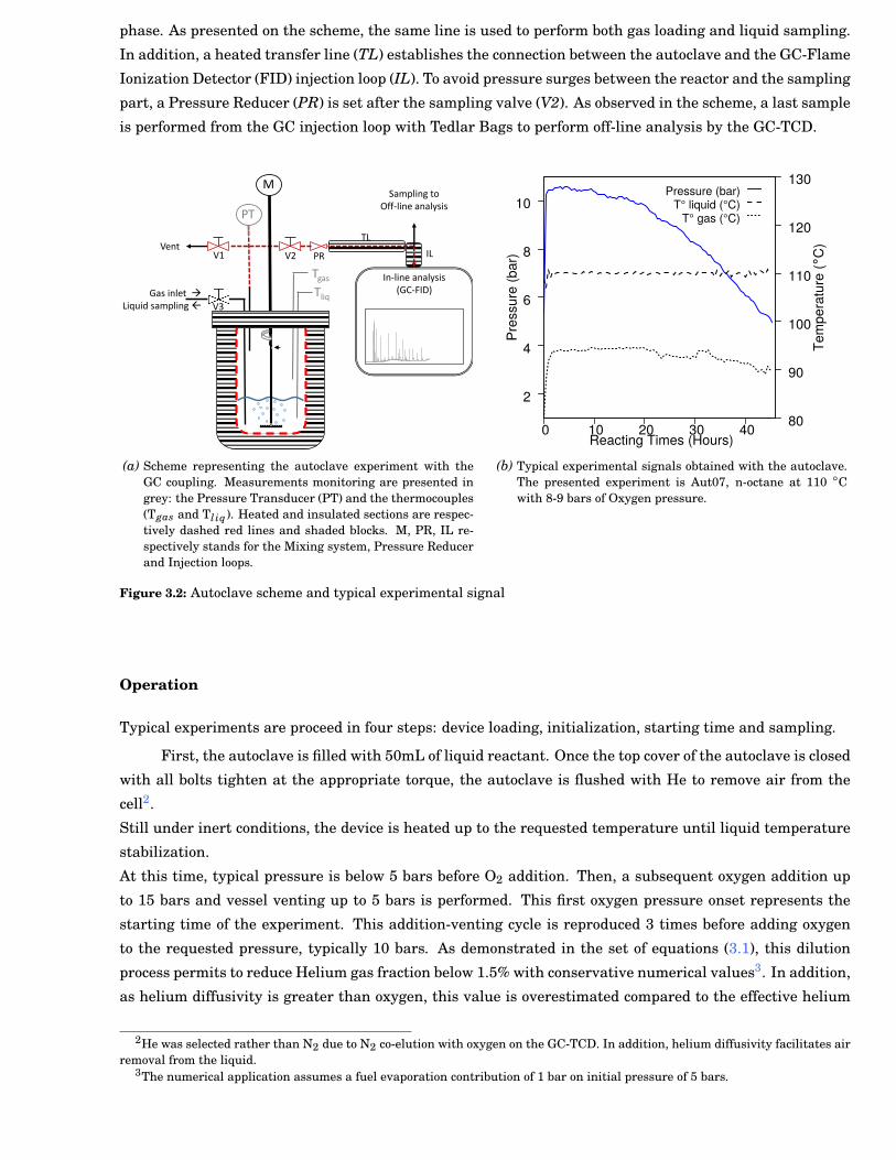
Chapter 3 27

phase. As presented on the scheme, the same line is used to perform both gas loading and liquid sampling.

In addition, a heated transfer line (TL) establishes the connection between the autoclave and the GC-Flame

Ionization Detector (FID) injection loop (IL). To avoid pressure surges between the reactor and the sampling

part, a Pressure Reducer (PR) is set after the sampling valve (V2). As observed in the scheme, a last sample

is performed from the GC injection loop with Tedlar Bags to perform off-line analysis by the GC-TCD.

M

Tgas

TliqGas inlet Liquid sampling

Vent

PT

V1 V2

Sampling toOff-line analysis

In-line analysis(GC-FID)

PR

TL

IL

V3

(a) Scheme representing the autoclave experiment with theGC coupling. Measurements monitoring are presented ingrey: the Pressure Transducer (PT) and the thermocouples(Tgas and Tl iq). Heated and insulated sections are respec-tively dashed red lines and shaded blocks. M, PR, IL re-spectively stands for the Mixing system, Pressure Reducerand Injection loops.

2

4

6

8

10

0 10 20 30 40 80

90

100

110

120

130

Pres

sure

(bar

)

Tem

pera

ture

(°C

)

Reacting Times (Hours)

Pressure (bar)T° liquid (°C)

T° gas (°C)

(b) Typical experimental signals obtained with the autoclave.The presented experiment is Aut07, n-octane at 110 ◦Cwith 8-9 bars of Oxygen pressure.

Figure 3.2: Autoclave scheme and typical experimental signal

Operation

Typical experiments are proceed in four steps: device loading, initialization, starting time and sampling.

First, the autoclave is filled with 50mL of liquid reactant. Once the top cover of the autoclave is closed

with all bolts tighten at the appropriate torque, the autoclave is flushed with He to remove air from the

cell2.

Still under inert conditions, the device is heated up to the requested temperature until liquid temperature

stabilization.

At this time, typical pressure is below 5 bars before O2 addition. Then, a subsequent oxygen addition up

to 15 bars and vessel venting up to 5 bars is performed. This first oxygen pressure onset represents the

starting time of the experiment. This addition-venting cycle is reproduced 3 times before adding oxygen

to the requested pressure, typically 10 bars. As demonstrated in the set of equations (3.1), this dilution

process permits to reduce Helium gas fraction below 1.5% with conservative numerical values3. In addition,

as helium diffusivity is greater than oxygen, this value is overestimated compared to the effective helium

2He was selected rather than N2 due to N2 co-elution with oxygen on the GC-TCD. In addition, helium diffusivity facilitates airremoval from the liquid.

3The numerical application assumes a fuel evaporation contribution of 1 bar on initial pressure of 5 bars.

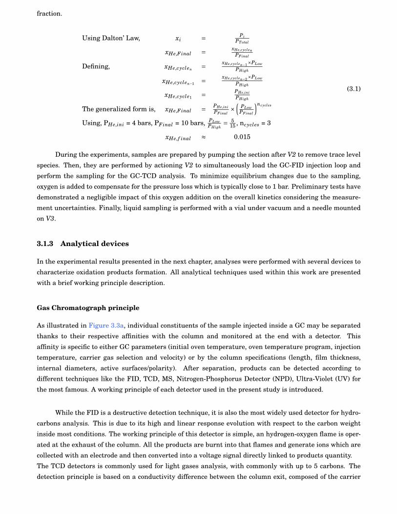
28 Chapter 3

fraction.

Using Dalton’ Law, xi = PiPTotal

xHe,Final = xHe,cyclenPFinal

Defining, xHe,cyclen = xHe,cyclen−1×PLow

PHigh

xHe,cyclen−1 = xHe,cyclen−2×PLow

PHigh

xHe,cycle1 = PHe,iniPHigh

The generalized form is, xHe,Final = PHe,iniPFinal

×(

PLowPFinal

)ncycles

Using, PHe,ini = 4 bars, PFinal = 10 bars, PLowPHigh

= 515 , ncycles = 3

xHe, f inal ≈ 0.015

(3.1)

During the experiments, samples are prepared by pumping the section after V2 to remove trace level

species. Then, they are performed by actioning V2 to simultaneously load the GC-FID injection loop and

perform the sampling for the GC-TCD analysis. To minimize equilibrium changes due to the sampling,

oxygen is added to compensate for the pressure loss which is typically close to 1 bar. Preliminary tests have

demonstrated a negligible impact of this oxygen addition on the overall kinetics considering the measure-

ment uncertainties. Finally, liquid sampling is performed with a vial under vacuum and a needle mounted

on V3.

3.1.3 Analytical devices

In the experimental results presented in the next chapter, analyses were performed with several devices to

characterize oxidation products formation. All analytical techniques used within this work are presented

with a brief working principle description.

Gas Chromatograph principle

As illustrated in Figure 3.3a, individual constituents of the sample injected inside a GC may be separated

thanks to their respective affinities with the column and monitored at the end with a detector. This

affinity is specific to either GC parameters (initial oven temperature, oven temperature program, injection

temperature, carrier gas selection and velocity) or by the column specifications (length, film thickness,

internal diameters, active surfaces/polarity). After separation, products can be detected according to

different techniques like the FID, TCD, MS, Nitrogen-Phosphorus Detector (NPD), Ultra-Violet (UV) for

the most famous. A working principle of each detector used in the present study is introduced.

While the FID is a destructive detection technique, it is also the most widely used detector for hydro-

carbons analysis. This is due to its high and linear response evolution with respect to the carbon weight

inside most conditions. The working principle of this detector is simple, an hydrogen-oxygen flame is oper-

ated at the exhaust of the column. All the products are burnt into that flames and generate ions which are

collected with an electrode and then converted into a voltage signal directly linked to products quantity.

The TCD detectors is commonly used for light gases analysis, with commonly with up to 5 carbons. The

detection principle is based on a conductivity difference between the column exit, composed of the carrier

Chapter 3 29

(a) GC presentation with its major elements: injector, column,oven, detector, gas supply part and the acquisition section.

Ion generation

Mass selection

Ion detection

Sample injection/GC coupling

Data acquisition

(b) Scheme presenting the main section of a MS

Figure 3.3: Gas chromatograph presentation and a scheme presenting MS working principle.

gas and eluted products, and the carrier gas used as a reference. Thus, due to similar thermal conductivity,

H2 detection sensibility is not satisfactory when Helium is selected as carrier gas.

The MS is an analytical technique by itself and can be used without a GC. When it is used as a detector,

it simplifies mass spectrum analysis thanks to the GC separation. As illustrated in Figure 3.3b, the MS is

composed of three parts: Ion generation, Mass selection and Ions detection. For each part of the MS several

techniques exist, our interest is focused on the one in use with our MS. In the conditions of the present

study, ions fragments are generated by electron impact generated itself with a high temperature filament.

Then, mass are sorted specifically according to their mass over a charge ratio (m/z) with a quadrupole

generating an oscillating magnetic field. Finally, ions are monitored with an ion multiplier detector.

FTIR-ATR principle

Although this technique is less accurate and selective than GCs , the FTIR analysis is a non destructive

technique allowing structural information without applying any thermal stress on the samples. For this

reason, it is used to complete and confirm specific GC conclusions but not as a standard procedure.

Signal acquisition from FTIR-ATR is similar to transmission FTIR and based on the Beer-Lambert’s

law (3.2). With, the Absorbance (A) defined as the logarithm of incoming over outgoing lights ratio ( I0I ). The

IR light is absorbed and excites the molecules according to vibrational, rotational and translational modes

as presented in Table 3.1. Thus, absorption signal of a given molecule is function of its extinction coefficient

(ε in cm3 ·mol−1 · cm−1), the optical path (l in cm) and its concentration (c in mol · cm−3) and is expressed

as a sum of individual absorption in case of blends (3.2).

In the case of the FTIR-ATR, the incident beam crosses an ATR crystal, then totally reflects on the sample-

crystal interface and finally crosses out the crystal to the detector. This Total Reflection is obtained when

a IR beam, with a high incident angle (θ), crosses an optically thinner material (n2 < n1). In such con-

figuration, only sample-crystal interface (few µm) contributes to the IR signal attenuation as presented

Figure 3.4a. Further informations on this specific techniques are available in literature [100].

From Beer’s Law A =− log I0I = ε× l× c

With a blend of n compounds, A =n∑

i=1εi × l× ci

(3.2)

The FTIR-ATR (Vertex 70 from Bruker) is operated placing few drops of the sample on the mono

reflection horizontal diamond. The final spectrum is obtained averaging 8 scans over wave number range

30 Chapter 3

from 500 to 4000 cm−1 with a resolution of 0.2 cm−1.

n2

Sample

n1

ATR

Crystal

Penetration

depth (<1µm)

Reflected wave

(to the detector)

Incident wave

(from IR source)

θ

(a) Scheme presenting the beam path from the light sourceto the detector in the FTIR-ATR.

0

0.1

0.2

500150025003500

Ab

so

rba

nc

e

Wave Number (cm-1)

(b) Typical FTIR-ATR signal obtained with octane oxi-dized during 21.3 hours at 110 ◦C in the autoclave.

Figure 3.4: FTIR-ATR working principle and typical signal presentation

Table 3.1: Typical IR absorption bands for oxidized paraffins with vibrational mode informations in bracket.

Chemical family Wave number (cm−1) Bonds involved

Alkanes3000-2850 C-H (streching)1470-1450 C-H (bending)1380-1370 C-H (bending)

Carbonylesketones/aldehydes 1740-1650 C=O (streching)

Acids3400-2500 O-H (streching)1740-1660 C=O (streching)1320-1210 C-O (streching)

Esters1750-1730 C=O (streching)1300-1000 C-O (streching)

Alcohols3600-3200 O-H (streching)

Primary 1080-1000 C-O (streching)Secondary 1160-1050 C-O (streching)

GC preliminary study

Due to the large amounts of potential oxidation products. A preliminary study was performed in order to

identify appropriate GC settings and more specifically the column itself. In this preliminary study three

columns were tested: a DB-1, a HP-5 and DB-FFAP, with several GC settings to identify which one allows

high peaks resolution for most of the oxidation products. An oxidized residual of decane obtained at 160 ◦Cfrom PetroOxy experiment was selected to assess columns capability.

As observed in literature [56], peak resolution with the DB-1 column is not satisfactory, with many co-

elution phenomena behind the solvent peak. As all those co-eluted peaks contain most of the first oxidation

products like ketones, alcohols, acids, the separation capability of the DB-1 is not satisfactory for semi-

quantitative applications.

As observed in Figure 3.5, typical elution from DB-1 and DB-FFAP columns is presented with which com-

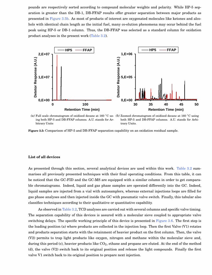
Chapter 3 31

pounds are respectively sorted according to compound molecular weights and polarity. While HP-5 sep-

aration is greater than the DB-1, DB-FFAP results offer greater separation between major products as

presented in Figure 3.5b. As most of products of interest are oxygenated molecules like ketones and alco-

hols with identical chain length as the initial fuel, many co-elution phenomena may occur behind the fuel

peak using HP-5 or DB-1 column. Thus, the DB-FFAP was selected as a standard column for oxidation

product analyses in the present work (Table 3.2).

0,E+00

1,E+07

2,E+07

0 100

De

teto

r R

es

po

ns

e (

A.U

.)

Retention Time (min)

HP5 FFAP

(a) Full scale chromatogram of oxidized decane at 160 ◦C us-ing both HP-5 and DB-FFAP columns. A.U. stands for Ar-bitrary Units

0,E+00

5,E+05

1,E+06

30 35 40 45 50

De

teto

r R

es

po

nse (

A.U

.)

Retention Time (min)

HP5 FFAP

(b) Zoomed chromatogram of oxidized decane at 160 ◦C usingboth HP-5 and DB-FFAP columns. A.U. stands for Arbi-trary Units.

Figure 3.5: Comparison of HP-5 and DB-FFAP separation capability on an oxidation residual sample.

List of all devices

As presented through this section, several analytical devices are used within this work. Table 3.2 sum-

marises all previously presented techniques with their final operating conditions. From this table, it can

be noticed that the GC-FID and the GC-MS are equipped with a similar column in order to get compara-

ble chromatograms. Indeed, liquid and gas phase samples are operated differently into the GC. Indeed,

liquid samples are injected from a vial with autosamplers, whereas external injections loops are filled for

gas phase analyses and then injected inside the GC with pneumatic valve switch. Finally, this tabular also

classifies techniques according to their qualitative or quantitative capability.

As observed in Table 3.2, TCD analyses are carried out with several columns and specific valve timing.

The separation capability of this devices is assured with a molecular sieve coupled to appropriate valve

switching delays. The specific working principle of this device is presented in Figure 3.6. The first step is

the loading position (a) where products are collected in the injection loop. Then the first Valve (V1) rotates

and products separation starts with the retainment of heavier product on the first column. Then, the valve

(V2) permits to trap light products like oxygen, nitrogen and methane within the molecular sieve and,

during this period (c), heavier products like CO2, ethane and propane are eluted. At the end of the method

(d), the valve (V2) switch back to its original position and release the light compounds. Finally the first

valve V1 switch back to its original position to prepare next injection.

32 Chapter 3

Table 3.2: List of all analytical devices. ? sign means those analyses were set for autoclave study and was not availablefor previous studies. If no holding time are provided in oven programs it means this value equals 0.

Techniques Phase analysed In experiments

Qualitative AnalysesGC-MS Liquid and Gas Petroxy and Autoclave

Specifications: GC 6890N coupled to a MS 5973 both from Agilent. The GC is equipped with anautosampler G4513A and a DB-FFAP column (30 m × 0.25 mm × 0.25 µm); GC settings are:carrier gas: He with constant flow 0.5 mL/min; Split/splitless injector 275◦C, 1 µL sample witha 150:1 split ratio; Oven program: Tinit=40◦C for 10min, then 5◦C/min up to 100◦C, 1◦C/minup to 150◦C and 20◦C/min up to 250◦C held 13 min. MS settings (electron impact (70 eV);quadrupole detector in full scan mod, m/z range from 10 to 600)

FTIR-ATR Liquid Petroxy and AutoclaveSpecifications: The FTIR-ATR involve a mono-refexion ATR cell equipped with an horizontalcrystal in diamond. Spectra are obtained in atmospheric conditions averaging 8 scans overthe wave numbers range 500-4000 cm−1 with a resolution of 0.2 cm−1.

Semi-quantative AnalysesGC-FID Liquid Autoclave?

Specifications: GC 6890N from Agilent with an auto-sampler 7683 series and a DB-FFAP (60m×0.25 mm× 0.25 µm). GC settings are: carrier gas: He with constant flow: 0.7mL/min;Split/splitless injector 200◦C, 1 µL sample with a 500:1 split ratio; Oven program: Tinit=40◦Cfor 10min, then 5◦C/min up to 100◦C, then 1◦C/min up to 150◦C and 20◦C/min up to 250◦Cheld 13 minutes. Detector settings: 200 ◦C, flows: H2 30 mL/min, air 350 mL/min, makeup25 mL/min.

GC-TCD Gas Autoclave?

Specifications: GC 6890N from Agilent equipped with a 250 µL heated injection loop (150◦C), aPorapak Q (packed column: OD=1/8", ID=2.5 mm and l=4.5m) and 5 Å molecular sieve (packedcolumn: OD=1/8", ID=2.5 mm and l=7.6m). GC settings are: Carrier gas: He, constant flow30mL/min; injection loop is the injector; Valve timing: 0.00 min V1 et V2 OFF, 0.10 min V1ON, 5.40 min V2 ON, 46.0 min V2 OFF, 60.0 V1 OFF; Oven program: Tinit=50◦C during 5min, then 5◦C/min up to 55◦C and 55◦C/min up to 245◦C) held 32 min, cooling up to 70◦C at40◦C/min held 14 min; Detector settings: Temperature:250 ◦ C, reference flow: 40 mL/min.

GC-FID Gas Autoclave?

Specifications: Varian GC/450 equipped with a 20 mL heated injection loop (180◦C) and DB-FFAP column (30 m × 0.25 mm × 0.25 µm). GC settings are: Carrier gas: He, constant flow1mL/min; Split/splitless injector (1177): 275◦C, split ratio: 250:1; Oven program: Tinit=30◦Cduring 5 min, then 5◦C/min up to 150◦C and 15◦C/min up to 245◦C) held 10 min; Detectorsettings: 275 ◦C, flows: H2 30 mL/min, air 300 mL/min, makeup 20 mL/min.

3.1.4 Calibration coefficient estimation

As introduced in the section 2 and presented in the preliminary study, numerous oxidation products are

formed during autoxidation. For kinetic modeling validation, most of them have to be quantified or semi-

quantified. Due to the size of the experimental matrix (Cf. chapter 4), the establishment of an external

calibration for individual constituents is not realistic. This section introduces the methodology used to

estimate FIDs DRs for liquid and gas phase species quantified with the GC-FID. In contrary, due to the

limited number of species of interest in the GC-TCD analyses, their quantification is performed with an

external calibration using a single gas calibration standard.

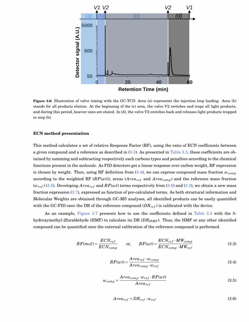
Chapter 3 33

(b)

50

500

5000

0 20 40 60D

ete

cto

r s

ign

al (A

.U.)

Retention Time (min)

V1 V2 V2 V1

(a) (c) (d)

Figure 3.6: Illustration of valve timing with the GC-TCD. Area (a) represents the injection loop loading. Area (b)stands for all products elution. At the beginning of the (c) area, the valve V2 switches and traps all light products,and during this period, heavier ones are eluted. In (d), the valve V2 switches back and releases light products trappedin step (b).

ECN method presentation

This method calculates a set of relative Response Factor (RF), using the ratio of ECN coefficients between

a given compound and a reference as described in (3.3). As presented in Table 3.3, these coefficients are ob-

tained by summing and subtracting respectively each carbons types and penalties according to the chemical

functions present in the molecule. As FID detectors get a linear response over carbon weight, RF expression

is chosen by weight. Then, using RF definition from (3.4), we can express compound mass fraction wcomp

according to the weighted RF (RF(wt)), areas (Areare f and Areacomp) and the reference mass fraction

(wre f ) (3.5). Developing Areare f and RF(wt) terms respectively from (3.6) and (3.3), we obtain a new mass

fraction expression (3.7), expressed as function of pre-calculated terms. As both structural information and

Molecular Weights are obtained through GC-MS analyses, all identified products can be easily quantified

with the GC-FID once the DR of the reference compound (DRre f ) is calibrated with the device.

As an example, Figure 3.7 presents how to use the coefficients defined in Table 3.3 with the 5-

hydroxymethyl-2furaldehyde (HMF) to calculate its DR (DRHMF ). Thus, the HMF or any other identified

compound can be quantified once the external calibration of the reference compound is performed.

RF(mol)= ECNre f

ECNcompor, RF(wt)= ECNre f ·MWcomp

ECNcomp ·MWre f(3.3)

RF(wt)= Areare f ·wcomp

Areacomp ·wre f(3.4)

wcomp = Areacomp ·wre f ·RF(wt)Areare f

(3.5)

Areare f = DRre f ·wre f (3.6)

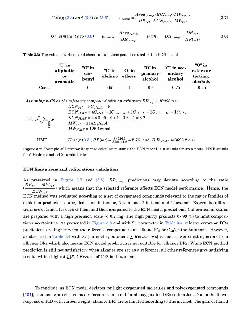
34 Chapter 3

Using (3.3) and (3.6) in (3.5), wcomp = Areacomp ·ECNre f ·MWcomp

DRre f ·ECNcomp ·MWre f(3.7)

Or, similarl y to (3.6) wcomp = Areacomp

DRcompwith DRcomp = DRre f

RF(wt)(3.8)

Table 3.3: The value of carbons and chemical functions penalties used in the ECN model.

"C" inaliphatic

oraromatic

"C" incar-

bonyl

"C" inolefinic

"O" inethers

"O" inprimaryalcohol

"O" in sec-ondaryalcohol

"O" inesters ortertiaryalcohols

Coeff. 1 0 0.95 -1 -0.6 -0.75 -0.25

Assuming n-C8 as the reference compound with an arbitrary DRre f = 10000 a.u.ECNre f = 8Caliph. = 8ECNHMF = 4Cole f . +1Ccarbon. +1Caliph. +1Oprim.OH +1OetherECNHMF = 4×0.95+0+1−0.6−1= 3.2MWre f = 114.2g/molMWHMF = 126.1g/mol

HMF Using (3.3), RF(wt)= 8×126.13.2×114.2 = 2.76 and D.R.HMF ' 3623.2 a.u.

Figure 3.7: Example of Detector Response calculation using the ECN model. a.u stands for area units. HMF standsfor 5-Hydroxymethyl-2-furaldehyde.

ECN limitations and calibrations validation

As presented in Figure 3.7 and (3.8), DRcomp predictions may deviate according to the ratio

(DRre f ×MWre f

ECNre f) which means that the selected reference affects ECN model performance. Hence, the

ECN method was evaluated according to a set of oxygenated compounds relevant to the major families of

oxidation products: octane, dodecane, butanone, 2-octanone, 2-butanol and 1-hexanol. Externals calibra-

tions are obtained for each of them and then compared to the ECN model predictions. Calibration mixtures

are prepared with a high precision scale (< 0.2 mg) and high purity products (> 99 %) to limit composi-

tion uncertainties. As presented in Figure 3.8 and with S1 parameter in Table 3.4, relative errors on DRs

predictions are higher when the reference compound is an alkane (C8 or C12)or the butanone. However,

as observed in Table 3.4 with S2 parameter, butanone∑|Rel.Errors| is much lower omitting errors from

alkanes DRs which also means ECN model prediction is not suitable for alkanes DRs. While ECN method

prediction is still not satisfactory when alkanes are set as a reference, all other references give satisfying

results with a highest∑|Rel.Errors| of 11% for butanone.

To conclude, as ECN model deviates for light oxygenated molecules and polyoxygenated compounds

[101], octanone was selected as a reference compound for all oxygenated DRs estimation. Due to the linear

response of FID with carbon weight, alkanes DRs are estimated according to this method. The gain obtained

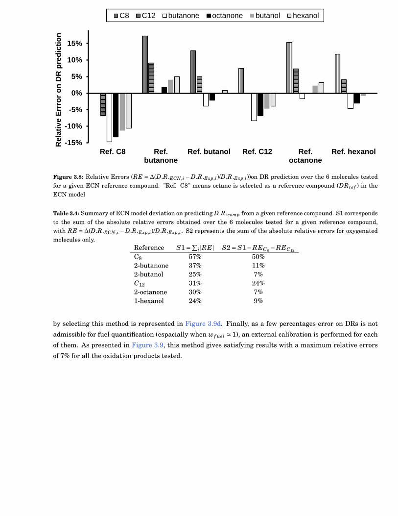
Chapter 3 35

-15%

-10%

-5%

0%

5%

10%

15%

Ref. C8 Ref.butanone

Ref. butanol Ref. C12 Ref.octanone

Ref. hexanol

Re

lati

ve

Err

ror

on

DR

pre

dic

tio

n

C8 C12 butanone octanone butanol hexanol

Figure 3.8: Relative Errors (RE = ∆(D.R.ECN,i −D.R.Exp,i)/D.R.Exp,i))on DR prediction over the 6 molecules testedfor a given ECN reference compound. "Ref. C8" means octane is selected as a reference compound (DRre f ) in theECN model

Table 3.4: Summary of ECN model deviation on predicting D.R.comp from a given reference compound. S1 correspondsto the sum of the absolute relative errors obtained over the 6 molecules tested for a given reference compound,with RE =∆(D.R.ECN,i −D.R.Exp,i)/D.R.Exp,i. S2 represents the sum of the absolute relative errors for oxygenatedmolecules only.

Reference S1=∑i|RE| S2= S1−REC8 −REC12

C8 57% 50%2-butanone 37% 11%2-butanol 25% 7%C12 31% 24%2-octanone 30% 7%1-hexanol 24% 9%

by selecting this method is represented in Figure 3.9d. Finally, as a few percentages error on DRs is not

admissible for fuel quantification (espacially when w f uel ≈ 1), an external calibration is performed for each

of them. As presented in Figure 3.9, this method gives satisfying results with a maximum relative errors

of 7% for all the oxidation products tested.

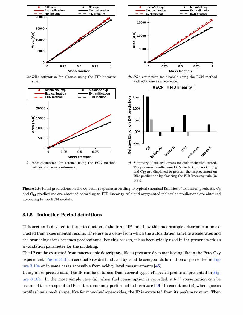
36 Chapter 3

0

5000

10000

15000

20000

0 0.25 0.5 0.75 1

Are

a (

A.u

)

Mass fraction

C12 exp. C8 exp.Ext. calibration Ext. calibrationFID linearity FID linearity

(a) DRs estimation for alkanes using the FID linearityrule.

0

5000

10000

15000

0 0.25 0.5 0.75 1

Are

a (

A.u

)

Mass fraction

hexan1ol exp. butan2ol exp.Ext. calibration Ext. calibrationECN method ECN method

(b) DRs estimation for alcohols using the ECN methodwith octanone as a reference.

1 1.2

0

5000

10000

15000

20000

0 0.25 0.5 0.75 1

Are

a (

A.u

)

Mass fraction

octan2one exp. butanone exp.Ext. calibration Ext. calibrationECN method ECN method

(c) DRs estimation for ketones using the ECN methodwith octanone as a reference.

-5%

0%

5%

10%

15%

Rela

tiv

e E

rrro

r o

n D

R p

red

icti

on

ECN FID linearity

(d) Summary of relative errors for each molecules tested.The previous results from ECN model (in black) for C8and C12 are displayed to present the improvement onDRs predictions by choosing the FID linearity rule (ingrey).

Figure 3.9: Final predictions on the detector response according to typical chemical families of oxidation products. C8

and C12 predictions are obtained according to FID linearity rule and oxygenated molecules predictions are obtainedaccording to the ECN models.

3.1.5 Induction Period definitions

This section is devoted to the introduction of the term "IP" and how this macroscopic criterion can be ex-

tracted from experimental results. IP refers to a delay from which the autoxidation kinetics accelerates and

the branching steps becomes predominant. For this reason, it has been widely used in the present work as

a validation parameter for the modeling.

The IP can be extracted from macroscopic descriptors, like a pressure drop monitoring like in the PetroOxy

experiment (Figure 3.1b), a conductivity drift induced by volatile compounds formation as presented in Fig-

ure 3.10a or in some cases accessible from acidity level measurements [45].

Using more precise data, the IP can be obtained from several types of species profile as presented in Fig-

ure 3.10b. In the most simple case (a), when fuel consumption is recorded, a 5 % consumption can be

assumed to correspond to IP as it is commonly performed in literature [46]. In conditions (b), when species

profiles has a peak shape, like for mono-hydroperoxides, the IP is extracted from its peak maximum. Then

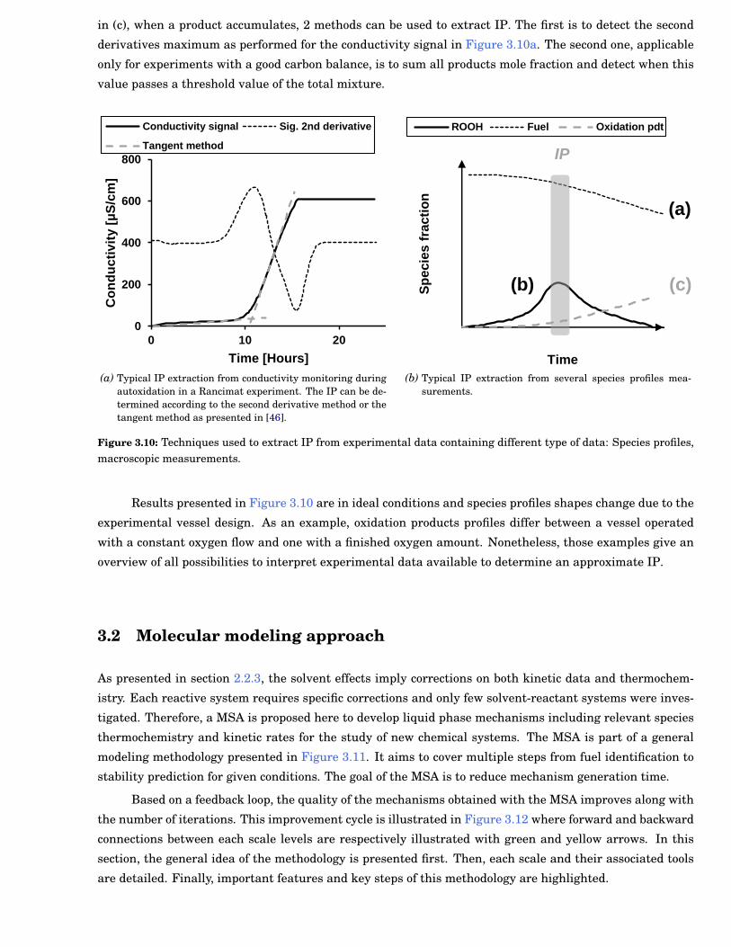
Chapter 3 37

in (c), when a product accumulates, 2 methods can be used to extract IP. The first is to detect the second

derivatives maximum as performed for the conductivity signal in Figure 3.10a. The second one, applicable

only for experiments with a good carbon balance, is to sum all products mole fraction and detect when this

value passes a threshold value of the total mixture.

0

200

400

600

800

0 10 20

Co

nd

uc

tiv

ity [

µS

/cm

]

Time [Hours]

Conductivity signal Sig. 2nd derivative

Tangent method

(a) Typical IP extraction from conductivity monitoring duringautoxidation in a Rancimat experiment. The IP can be de-termined according to the second derivative method or thetangent method as presented in [46].

Sp

ecie

s f

racti

on

Time

ROOH Fuel Oxidation pdt

IP

(a)

(c)(b)

(b) Typical IP extraction from several species profiles mea-surements.

Figure 3.10: Techniques used to extract IP from experimental data containing different type of data: Species profiles,macroscopic measurements.

Results presented in Figure 3.10 are in ideal conditions and species profiles shapes change due to the

experimental vessel design. As an example, oxidation products profiles differ between a vessel operated

with a constant oxygen flow and one with a finished oxygen amount. Nonetheless, those examples give an

overview of all possibilities to interpret experimental data available to determine an approximate IP.

3.2 Molecular modeling approach

As presented in section 2.2.3, the solvent effects imply corrections on both kinetic data and thermochem-

istry. Each reactive system requires specific corrections and only few solvent-reactant systems were inves-

tigated. Therefore, a MSA is proposed here to develop liquid phase mechanisms including relevant species

thermochemistry and kinetic rates for the study of new chemical systems. The MSA is part of a general

modeling methodology presented in Figure 3.11. It aims to cover multiple steps from fuel identification to

stability prediction for given conditions. The goal of the MSA is to reduce mechanism generation time.

Based on a feedback loop, the quality of the mechanisms obtained with the MSA improves along with

the number of iterations. This improvement cycle is illustrated in Figure 3.12 where forward and backward

connections between each scale levels are respectively illustrated with green and yellow arrows. In this

section, the general idea of the methodology is presented first. Then, each scale and their associated tools

are detailed. Finally, important features and key steps of this methodology are highlighted.

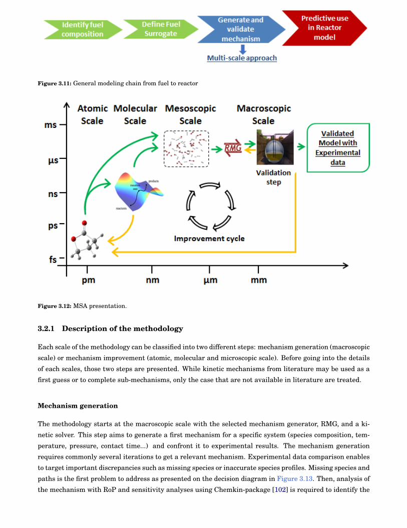
38 Chapter 3

Figure 3.11: General modeling chain from fuel to reactor

Figure 3.12: MSA presentation.

3.2.1 Description of the methodology

Each scale of the methodology can be classified into two different steps: mechanism generation (macroscopic

scale) or mechanism improvement (atomic, molecular and microscopic scale). Before going into the details

of each scales, those two steps are presented. While kinetic mechanisms from literature may be used as a

first guess or to complete sub-mechanisms, only the case that are not available in literature are treated.

Mechanism generation

The methodology starts at the macroscopic scale with the selected mechanism generator, RMG, and a ki-

netic solver. This step aims to generate a first mechanism for a specific system (species composition, tem-

perature, pressure, contact time...) and confront it to experimental results. The mechanism generation

requires commonly several iterations to get a relevant mechanism. Experimental data comparison enables

to target important discrepancies such as missing species or inaccurate species profiles. Missing species and

paths is the first problem to address as presented on the decision diagram in Figure 3.13. Then, analysis of

the mechanism with RoP and sensitivity analyses using Chemkin-package [102] is required to identify the

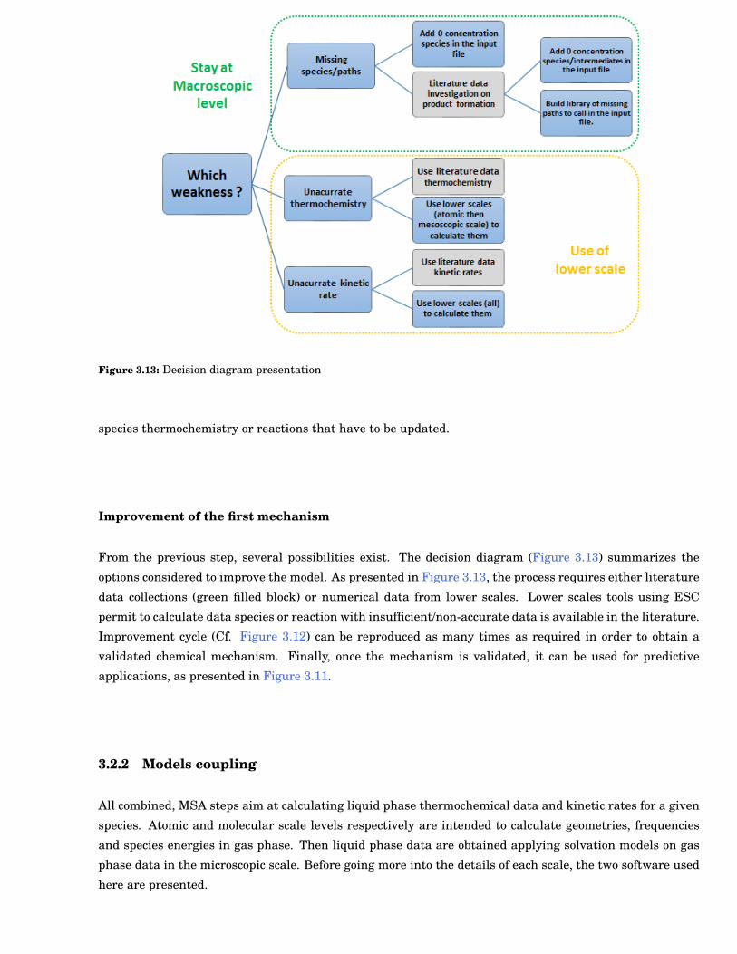
Chapter 3 39

Figure 3.13: Decision diagram presentation

species thermochemistry or reactions that have to be updated.

Improvement of the first mechanism

From the previous step, several possibilities exist. The decision diagram (Figure 3.13) summarizes the

options considered to improve the model. As presented in Figure 3.13, the process requires either literature

data collections (green filled block) or numerical data from lower scales. Lower scales tools using ESC

permit to calculate data species or reaction with insufficient/non-accurate data is available in the literature.

Improvement cycle (Cf. Figure 3.12) can be reproduced as many times as required in order to obtain a

validated chemical mechanism. Finally, once the mechanism is validated, it can be used for predictive

applications, as presented in Figure 3.11.

3.2.2 Models coupling

All combined, MSA steps aim at calculating liquid phase thermochemical data and kinetic rates for a given

species. Atomic and molecular scale levels respectively are intended to calculate geometries, frequencies

and species energies in gas phase. Then liquid phase data are obtained applying solvation models on gas

phase data in the microscopic scale. Before going more into the details of each scale, the two software used

here are presented.

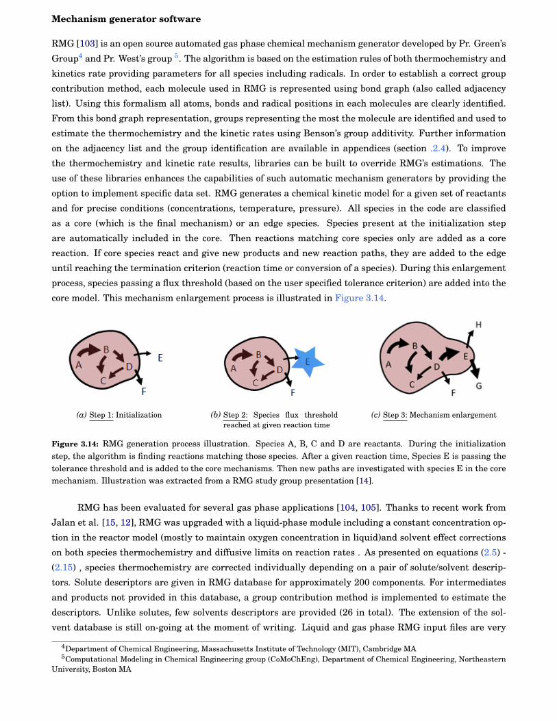
40 Chapter 3

Mechanism generator software

RMG [103] is an open source automated gas phase chemical mechanism generator developed by Pr. Green’s

Group4 and Pr. West’s group 5. The algorithm is based on the estimation rules of both thermochemistry and

kinetics rate providing parameters for all species including radicals. In order to establish a correct group

contribution method, each molecule used in RMG is represented using bond graph (also called adjacency

list). Using this formalism all atoms, bonds and radical positions in each molecules are clearly identified.

From this bond graph representation, groups representing the most the molecule are identified and used to

estimate the thermochemistry and the kinetic rates using Benson’s group additivity. Further information

on the adjacency list and the group identification are available in appendices (section .2.4). To improve

the thermochemistry and kinetic rate results, libraries can be built to override RMG’s estimations. The

use of these libraries enhances the capabilities of such automatic mechanism generators by providing the

option to implement specific data set. RMG generates a chemical kinetic model for a given set of reactants

and for precise conditions (concentrations, temperature, pressure). All species in the code are classified

as a core (which is the final mechanism) or an edge species. Species present at the initialization step

are automatically included in the core. Then reactions matching core species only are added as a core

reaction. If core species react and give new products and new reaction paths, they are added to the edge

until reaching the termination criterion (reaction time or conversion of a species). During this enlargement

process, species passing a flux threshold (based on the user specified tolerance criterion) are added into the

core model. This mechanism enlargement process is illustrated in Figure 3.14.

(a) Step 1: Initialization (b) Step 2: Species flux thresholdreached at given reaction time

(c) Step 3: Mechanism enlargement

Figure 3.14: RMG generation process illustration. Species A, B, C and D are reactants. During the initializationstep, the algorithm is finding reactions matching those species. After a given reaction time, Species E is passing thetolerance threshold and is added to the core mechanisms. Then new paths are investigated with species E in the coremechanism. Illustration was extracted from a RMG study group presentation [14].

RMG has been evaluated for several gas phase applications [104, 105]. Thanks to recent work from

Jalan et al. [15, 12], RMG was upgraded with a liquid-phase module including a constant concentration op-

tion in the reactor model (mostly to maintain oxygen concentration in liquid)and solvent effect corrections

on both species thermochemistry and diffusive limits on reaction rates . As presented on equations (2.5) -

(2.15) , species thermochemistry are corrected individually depending on a pair of solute/solvent descrip-

tors. Solute descriptors are given in RMG database for approximately 200 components. For intermediates

and products not provided in this database, a group contribution method is implemented to estimate the

descriptors. Unlike solutes, few solvents descriptors are provided (26 in total). The extension of the sol-

vent database is still on-going at the moment of writing. Liquid and gas phase RMG input files are very

4Department of Chemical Engineering, Massachusetts Institute of Technology (MIT), Cambridge MA5Computational Modeling in Chemical Engineering group (CoMoChEng), Department of Chemical Engineering, Northeastern

University, Boston MA

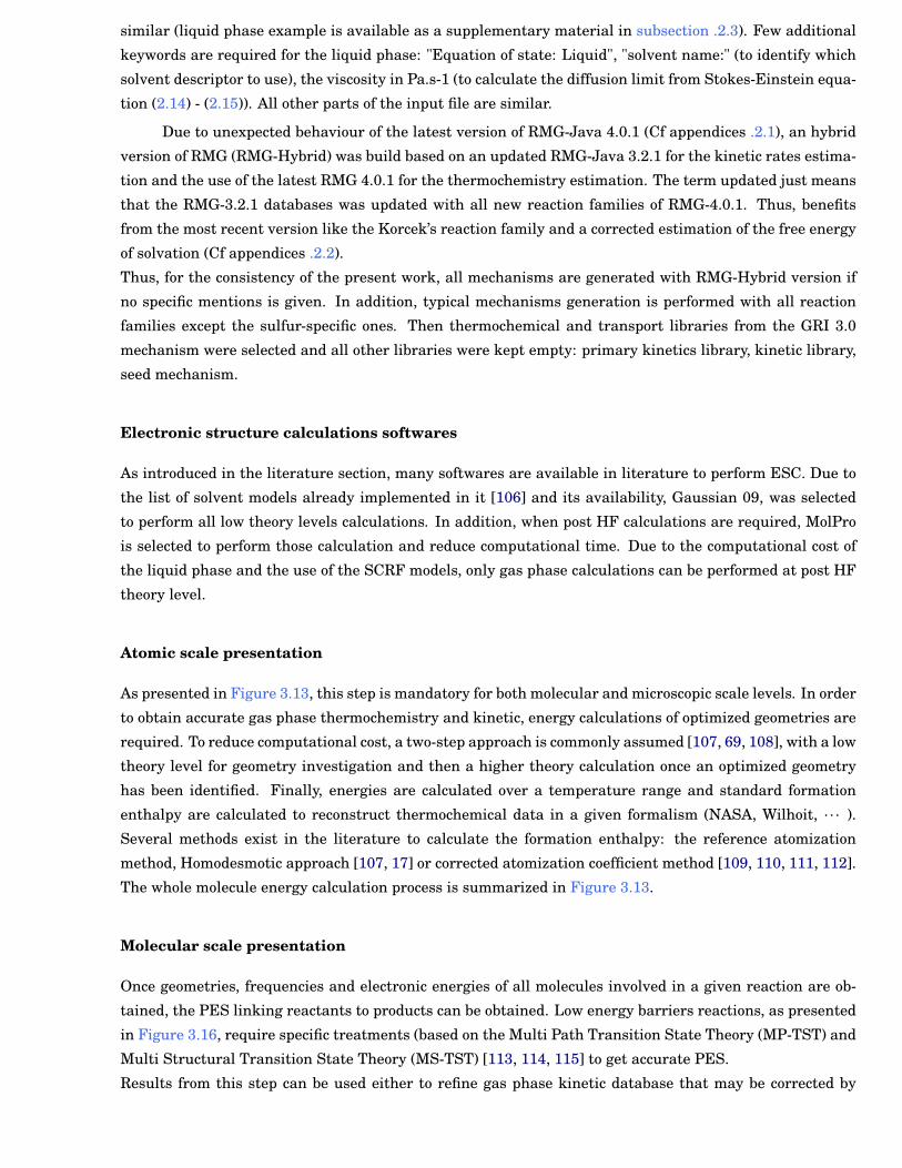
Chapter 3 41

similar (liquid phase example is available as a supplementary material in subsection .2.3). Few additional

keywords are required for the liquid phase: "Equation of state: Liquid", "solvent name:" (to identify which

solvent descriptor to use), the viscosity in Pa.s-1 (to calculate the diffusion limit from Stokes-Einstein equa-

tion (2.14) - (2.15)). All other parts of the input file are similar.

Due to unexpected behaviour of the latest version of RMG-Java 4.0.1 (Cf appendices .2.1), an hybrid

version of RMG (RMG-Hybrid) was build based on an updated RMG-Java 3.2.1 for the kinetic rates estima-

tion and the use of the latest RMG 4.0.1 for the thermochemistry estimation. The term updated just means

that the RMG-3.2.1 databases was updated with all new reaction families of RMG-4.0.1. Thus, benefits

from the most recent version like the Korcek’s reaction family and a corrected estimation of the free energy

of solvation (Cf appendices .2.2).

Thus, for the consistency of the present work, all mechanisms are generated with RMG-Hybrid version if

no specific mentions is given. In addition, typical mechanisms generation is performed with all reaction

families except the sulfur-specific ones. Then thermochemical and transport libraries from the GRI 3.0

mechanism were selected and all other libraries were kept empty: primary kinetics library, kinetic library,

seed mechanism.

Electronic structure calculations softwares

As introduced in the literature section, many softwares are available in literature to perform ESC. Due to

the list of solvent models already implemented in it [106] and its availability, Gaussian 09, was selected

to perform all low theory levels calculations. In addition, when post HF calculations are required, MolPro

is selected to perform those calculation and reduce computational time. Due to the computational cost of

the liquid phase and the use of the SCRF models, only gas phase calculations can be performed at post HF

theory level.

Atomic scale presentation

As presented in Figure 3.13, this step is mandatory for both molecular and microscopic scale levels. In order

to obtain accurate gas phase thermochemistry and kinetic, energy calculations of optimized geometries are

required. To reduce computational cost, a two-step approach is commonly assumed [107, 69, 108], with a low

theory level for geometry investigation and then a higher theory calculation once an optimized geometry

has been identified. Finally, energies are calculated over a temperature range and standard formation

enthalpy are calculated to reconstruct thermochemical data in a given formalism (NASA, Wilhoit, · · · ).

Several methods exist in the literature to calculate the formation enthalpy: the reference atomization

method, Homodesmotic approach [107, 17] or corrected atomization coefficient method [109, 110, 111, 112].

The whole molecule energy calculation process is summarized in Figure 3.13.

Molecular scale presentation

Once geometries, frequencies and electronic energies of all molecules involved in a given reaction are ob-

tained, the PES linking reactants to products can be obtained. Low energy barriers reactions, as presented

in Figure 3.16, require specific treatments (based on the Multi Path Transition State Theory (MP-TST) and

Multi Structural Transition State Theory (MS-TST) [113, 114, 115] to get accurate PES.

Results from this step can be used either to refine gas phase kinetic database that may be corrected by

42 Chapter 3

Figure 3.15: Geometry optimisation process

RMG code or can be used directly as a liquid phase kinetic database after the solvent effect treatment from

the mesoscopic scale.

Figure 3.16: PES with low energy barrier (D step) obtained by Jalan et al. [15]for the Korcek’s reaction

Mesoscopic scale presentation

Mesoscopic scale calculations can be used in: thermochemical and kinetic rate calculations in liquid phase.

In those calculations, gas phase data are corrected applying a given SCRF model ( Figure 2.22 in section

subsection 2.2.3) to include solute-solvent interactions.

While in some conditions, the gas phase geometries may correspond to the lowest energy geometry, in some

other conditions, the stabilizing effect of solvent may change the energy level order of the geometries. For

this reason, a consistent approach is to reconsider all initial geometries of the gas phase step to identify

a possible lower energy conformer. This was presented with Figure 2.23 and Figure 2.23b, where energy

barrier height may be affected specifically according to solute-solvent interactions. As a results, a higher

energy barrier trajectory may become more relevant in liquid phase due to the stabilising effects of the

solvent. In addition to the barrier energy height changes, the partition function may also be affected by the

solvent effect, as presented in literature review chapter.

Results from this step is either used as an input of RMG generation or used to correct the generated

mechanism (without re-generation).

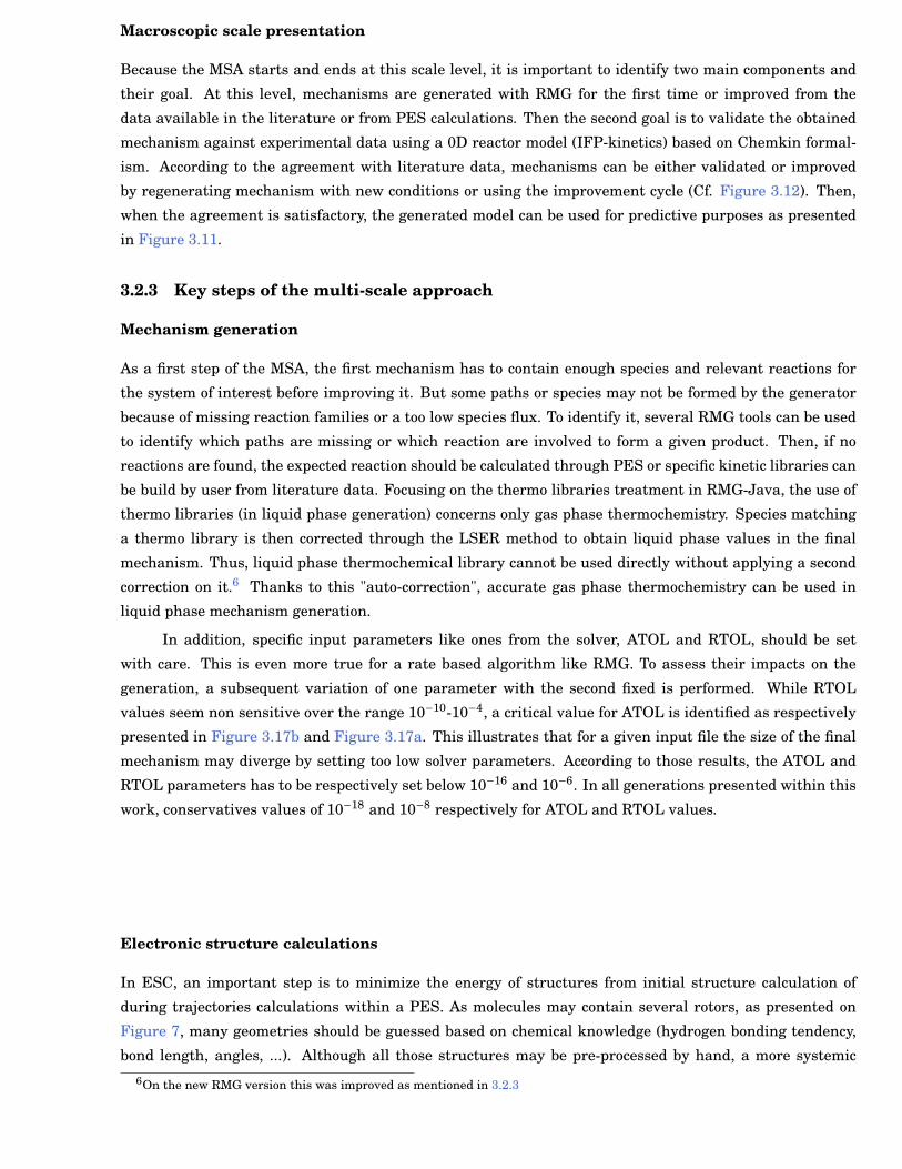
Chapter 3 43

Macroscopic scale presentation

Because the MSA starts and ends at this scale level, it is important to identify two main components and

their goal. At this level, mechanisms are generated with RMG for the first time or improved from the

data available in the literature or from PES calculations. Then the second goal is to validate the obtained

mechanism against experimental data using a 0D reactor model (IFP-kinetics) based on Chemkin formal-

ism. According to the agreement with literature data, mechanisms can be either validated or improved

by regenerating mechanism with new conditions or using the improvement cycle (Cf. Figure 3.12). Then,

when the agreement is satisfactory, the generated model can be used for predictive purposes as presented

in Figure 3.11.

3.2.3 Key steps of the multi-scale approach

Mechanism generation

As a first step of the MSA, the first mechanism has to contain enough species and relevant reactions for

the system of interest before improving it. But some paths or species may not be formed by the generator

because of missing reaction families or a too low species flux. To identify it, several RMG tools can be used

to identify which paths are missing or which reaction are involved to form a given product. Then, if no

reactions are found, the expected reaction should be calculated through PES or specific kinetic libraries can

be build by user from literature data. Focusing on the thermo libraries treatment in RMG-Java, the use of

thermo libraries (in liquid phase generation) concerns only gas phase thermochemistry. Species matching

a thermo library is then corrected through the LSER method to obtain liquid phase values in the final

mechanism. Thus, liquid phase thermochemical library cannot be used directly without applying a second

correction on it.6 Thanks to this "auto-correction", accurate gas phase thermochemistry can be used in

liquid phase mechanism generation.

In addition, specific input parameters like ones from the solver, ATOL and RTOL, should be set

with care. This is even more true for a rate based algorithm like RMG. To assess their impacts on the

generation, a subsequent variation of one parameter with the second fixed is performed. While RTOL

values seem non sensitive over the range 10−10-10−4, a critical value for ATOL is identified as respectively

presented in Figure 3.17b and Figure 3.17a. This illustrates that for a given input file the size of the final

mechanism may diverge by setting too low solver parameters. According to those results, the ATOL and

RTOL parameters has to be respectively set below 10−16 and 10−6. In all generations presented within this

work, conservatives values of 10−18 and 10−8 respectively for ATOL and RTOL values.

Electronic structure calculations

In ESC, an important step is to minimize the energy of structures from initial structure calculation of

during trajectories calculations within a PES. As molecules may contain several rotors, as presented on

Figure 7, many geometries should be guessed based on chemical knowledge (hydrogen bonding tendency,

bond length, angles, ...). Although all those structures may be pre-processed by hand, a more systemic6On the new RMG version this was improved as mentioned in 3.2.3

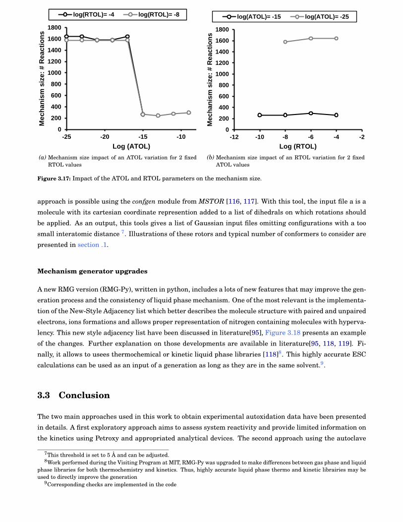
44 Chapter 3

0

200

400

600

800

1000

1200

1400

1600

1800

-25 -20 -15 -10

Mech

an

ism

siz

e:

# R

eacti

on

s

Log (ATOL)

log(RTOL)= -4 log(RTOL)= -8

(a) Mechanism size impact of an ATOL variation for 2 fixedRTOL values

0

200

400

600

800

1000

1200

1400

1600

1800

-12 -10 -8 -6 -4 -2

Mech

an

ism

siz

e:

# R

eacti

on

s

Log (RTOL)

log(ATOL)= -15 log(ATOL)= -25

(b) Mechanism size impact of an RTOL variation for 2 fixedATOL values

Figure 3.17: Impact of the ATOL and RTOL parameters on the mechanism size.

approach is possible using the confgen module from MSTOR [116, 117]. With this tool, the input file a is a

molecule with its cartesian coordinate represention added to a list of dihedrals on which rotations should

be applied. As an output, this tools gives a list of Gaussian input files omitting configurations with a too

small interatomic distance 7. Illustrations of these rotors and typical number of conformers to consider are

presented in section .1.

Mechanism generator upgrades

A new RMG version (RMG-Py), written in python, includes a lots of new features that may improve the gen-

eration process and the consistency of liquid phase mechanism. One of the most relevant is the implementa-

tion of the New-Style Adjacency list which better describes the molecule structure with paired and unpaired

electrons, ions formations and allows proper representation of nitrogen containing molecules with hyperva-

lency. This new style adjacency list have been discussed in literature[95], Figure 3.18 presents an example

of the changes. Further explanation on those developments are available in literature[95, 118, 119]. Fi-

nally, it allows to usees thermochemical or kinetic liquid phase libraries [118]8. This highly accurate ESC

calculations can be used as an input of a generation as long as they are in the same solvent.9.

3.3 Conclusion

The two main approaches used in this work to obtain experimental autoxidation data have been presented

in details. A first exploratory approach aims to assess system reactivity and provide limited information on

the kinetics using Petroxy and appropriated analytical devices. The second approach using the autoclave

7This threshold is set to 5 Å and can be adjusted.8Work performed during the Visiting Program at MIT, RMG-Py was upgraded to make differences between gas phase and liquid

phase libraries for both thermochemistry and kinetics. Thus, highly accurate liquid phase thermo and kinetic librairies may beused to directly improve the generation

9Corresponding checks are implemented in the code

Chapter 3 45

1 C 0 {2,S} {6,S} {7,S} {8,S} 1 C u0 p0 c0 {2,S} {6,S} {7,S} {8,S}

O

2 C 0 {1,S} {3,S} {5,D} 2 C u0 p0 c0 {1,S} {3,S} {9,S} {10,S}3 C 0 {2,S} {4,S} {9,S} {10,S} 3 C u0 p0 c0 {2,S} {4,S} {5,D}4 C 0 {3,S} {11,S} {12,S} {13,S} 4 C u0 p0 c0 {3,S} {11,S} {12,S} {13,S}5 O 0 {2,D} 5 O u0 p2 c0 {3,D}6 H 0 {1,S} 6 H u0 p0 c0 {1,S}7 H 0 {1,S} 7 H u0 p0 c0 {1,S}8 H 0 {1,S} 8 H u0 p0 c0 {1,S}9 H 0 {3,S} 9 H u0 p0 c0 {2,S}10 H 0 {3,S} 10 H u0 p0 c0 {2,S}11 H 0 {4,S} 11 H u0 p0 c0 {4,S}12 H 0 {4,S} 12 H u0 p0 c0 {4,S}13 H 0 {4,S} 13 H u0 p0 c0 {4,S}Old adjacency list* New style adjacency list chemical formula

Figure 3.18: Adjacency lists illustration. * means this adjacency list contains explanatory H atoms, whereas they arenot mandatory. The very first number represents the position of atoms. Then, C and O represent the atoms, then thenumber stand for the number of radical on the atom, then the list of connection of this atoms are presented betweenbrackets: first number is referring to the atom number and then the letter to the bound type (S: single, D:double)

and its associated analytical devices, is complementary to the Petroxy studies and gives detailed informa-

tion with both gas and liquid phase species profiles.

From the modeling side, the molecular modeling approach is presented in details with the MSA. It

involves a hybrid version of RMG-Java to generate a first mechanism that may be improved by either user

knowledge or literature data, ESC or a combination of both. As ESC steps are very long and complex, they

were not evaluated during the framework of this thesis.

46 Chapter 3

Chapter 4

Results and Discussions

Studies conducted within the framework of this thesis aims to reduce the gap between chemical knowledge

and autoxidation phenomenon. To do so, the autoxidation of two chemical systems, the n-paraffins and

the iso-parrafins, are subsequently investivated with the PetroOxy and the autoclave device. With the first

device, preliminary study is performed in order (i) to assess the overall reactivity of the system, (ii) to

identify major oxidation products and (iii) to build and analyse the chemical mechanisms obtained with the

MSA. With the second device, detailed species profile of both gas and liquid phase are obtained in order to

complete the first study with the dynamics of autoxidation.

Finally the discussion section presents three axis, the structure reactivity relation, experimental results

consistency and finally models validation with improvements perspectives.

4.1 N-paraffins studies

4.1.1 Preliminary study with PetroOxy

In the bulk of a homogeneous liquid phase, autoxidation kinetics of pure n-alkane or their blends depends on

both oxygen pressure and temperature. The influence of those parameters on autoxidation is investigated

hereafter for C8-C16 n-alkanes.

Material and methods

Experimental devices High purity liquid n-alkanes 99% and 99.8% and dioxygen 99.9% were selected

to reduce the catalytic effect of trace species during experiments which may influence initiation reaction.

Thus, pure liquid reactants were analyzed with a Gas Chromatograph coupled to a mass spectrometer

(GC-MS) fully described in chapter 3. N-Alkanes and iso-alkanes with close numbers of carbon and no

oxygenates were identified among the 1% impurities, which may suggest a limited influence on IP mea-

surements. Experiments were performed with a PetroOxy apparatus presented in the previous chapter

chapter 3.

From this experiment, we can extract the IP, which corresponds to the time required to reach a 10%

pressure decrease(

PIP

Pmax= 0.9

),[99, 96] as presented in Figure 4.1a.This criterion commonly corresponds

to 5% of fuel consumption [46] and corresponds to the hydroperoxide build up and first deposit precursors

formation. A typical experimental result is presented in Figure 4.1a, which shows that the time to reach the

requested temperature is included in the IP. This delay is below 4 min in all experiments and is therefore

47

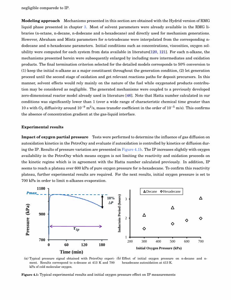
48 Chapter 4

negligible comparede to IP.

Modeling approach Mechanisms presented in this section are obtained with the Hydrid version of RMG

liquid phase presented in chapter 3. Most of solvent parameters were already available in the RMG li-

braries (n-octane, n-decane, n-dodecane and n-hexadecane) and directly used for mechanism generations.

However, Abraham and Mintz parameters for n-tetradecane were interpolated from the corresponding n-

dodecane and n-hexadecane parameters. Initial conditions such as concentrations, viscosities, oxygen sol-

ubility were computed for each system from data available in literature[120, 121]. For each n-alkane, the

mechanisms presented herein were subsequently enlarged by including more intermediates and oxidation

products. The final termination criterion selected for the detailed models corresponds to 50% conversion to

(1) keep the initial n-alkane as a major constituent throughout the generation condition, (2) let generation

proceed until the second stage of oxidation and get relevant reactions paths for deposit precursors. In this

manner, solvent effects would rely mainly on the nature of the fuel while oxygenated products contribu-

tion may be considered as negligible. The generated mechanisms were coupled to a previously developed

zero-dimensional reactor model already used in literature [46]. Note that Hatta number calculated in our

conditions was significantly lower than 1 (over a wide range of characteristic chemical time greater than

10 s with O2 diffusivity around 10−9 m2/s, mass transfer coefficient in the order of 10−5 m/s). This confirms

the absence of concentration gradient at the gas-liquid interface.

Experimental results

Impact of oxygen partial pressure Tests were performed to determine the influence of gas diffusion on

autoxidation kinetics in the PetroOxy and evaluate if autoxidation is controlled by kinetics or diffusion dur-

ing the IP. Results of pressure variation are presented in Figure 4.1b. The IP increases slightly with oxygen

availability in the PetroOxy which means oxygen is not limiting the reactivity and oxidation proceeds on

the kinetic regime which is in agreement with the Hatta number calculated previously. In addition, IP

seems to reach a plateau over 600 kPa of pure oxygen pressure for n-hexadecane. To confirm this reactivity

plateau, further experimental results are required. For the next results, initial oxygen pressure is set to

700 kPa in order to limit n-alkanes evaporation.

700

900

1100

0 60 120 180

Pre

ssu

re (k

Pa

)

Time (min)

𝑷𝒎𝒂𝒙

𝝉𝒊𝒑

10%

∆𝑷

(a) Typical pressure signal obtained with PetroOxy experi-ment. Results correspond to n-decane at 413 K and 700kPa of cold molecular oxygen.

1

2

3

200 300 400 500 600 700

Ind

uct

oin

Per

iod

(h

ou

rs)

Initial Oxygen Pressure (kPa)

Decane Hexadecane

(b) Effect of initial oxygen pressure on n-decane and n-hexadecane autoxidation at 413 K.

Figure 4.1: Typical experimental results and initial oxygen pressure effect on IP measurements

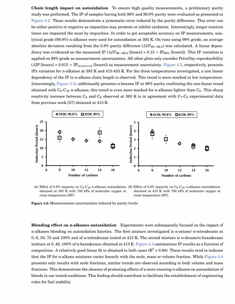
Chapter 4 49

Chain length impact on autoxidation To ensure high quality measurements, a preliminary purity

study was performed. The IP of samples having both 99% and 99.8% purity were evaluated as presented in

Figure 4.2. Those results demonstrate a systematic error induced by the purity difference. This error can

be either positive or negative as impurities may promote or inhibit oxidation. Interestingly, longer reaction

times are impacted the most by impurities. In order to get acceptable accuracy on IP measurements, ana-

lytical grade (99.8%) n-alkanes were used for autoxidation at 393 K. On runs using 99% grade, an average

absolute deviation resulting from the 0.8% purity difference (∆IP99→99.8) was calculated. A linear depen-

dency was evidenced on the measured IP (∆IP99→99.8 [hours] = 0.13 × IP99% [hours]). This IP variation is

applied on 99% grade as measurement uncertainties. All other plots only consider PetroOxy reproducibility

(∆IP [hours] = 0.015 × IPmeasured [hours]) as measurement uncertainty. Figure 4.3, respectively, presents

IPs variation for n-alkanes at 393 K and 413-433 K. For the three temperatures investigated, a non linear

dependency of the IP to n-alkane chain length is observed. This trend is more marked at low temperature.

Interestingly, Figure 4.3a additionally presents n-hexane IP at 99% purity confirming the non-linear trend

obtained with C8-C16 n-alkanes, this trend is even more marked for n-alkanes lighter than C8. This sharp

reactivity increase between C6 and C8 observed at 393 K is in agreement with C7-C8 experimental data

from previous work [57] obtained at 413 K.

0

5

10

15

20

25

6 8 10 12 14 16

Ind

uct

ion

Per

iod

(h

ou

rs)

Number of carbons

393K 99.8% 393K 99%

(a) Effect of 0.8% impurity on C8-C16 n-alkanes autoxidationobtained at 393 K with 700 kPa of molecular oxygen atroom temperature (RT).

0

1

2

3

4

5

6 8 10 12 14 16

Ind

uct

ion

Per

iod

(h

ou

rs)

Number of carbons

413K 99.8% 413K 99%

(b) Effect of 0.8% impurity on C8-C16 n-alkanes autoxidationobtained at 413 K with 700 kPa of molecular oxygen atroom temperature (RT).

Figure 4.2: Measurements uncertainties induced by purity levels

Blending effect on n-alkanes autoxidation Experiments were subsequently focused on the impact of

n-alkanes blending on autoxidation kinetics. The first mixture investigated is n-octane/ n-tetradecane at

0, 6, 50, 75 and 100% mol of n-tetradecane tested at 413 K. The second mixture is n-decane/n-hexadecane

mixture at 0, 40, 100% of n-hexadecane obtained at 413 K. Figure 4.4 summarizes IP results as a function of

composition. A relatively good linear fit is obtained in both cases (R2 > 0.98). These results tend to indicate

that the IP for n-alkane mixtures varies linearly with the mole, mass or volume fraction. While Figure 4.4

presents only results with mole fractions, similar trends are observed according to both volume and mass

fractions. This demonstrate the absence of promoting effects of a more reacting n-alkanes on autoxidation of

blends in our tested conditions. This finding should contribute to facilitate the establishment of engineering

rules for fuel stability.

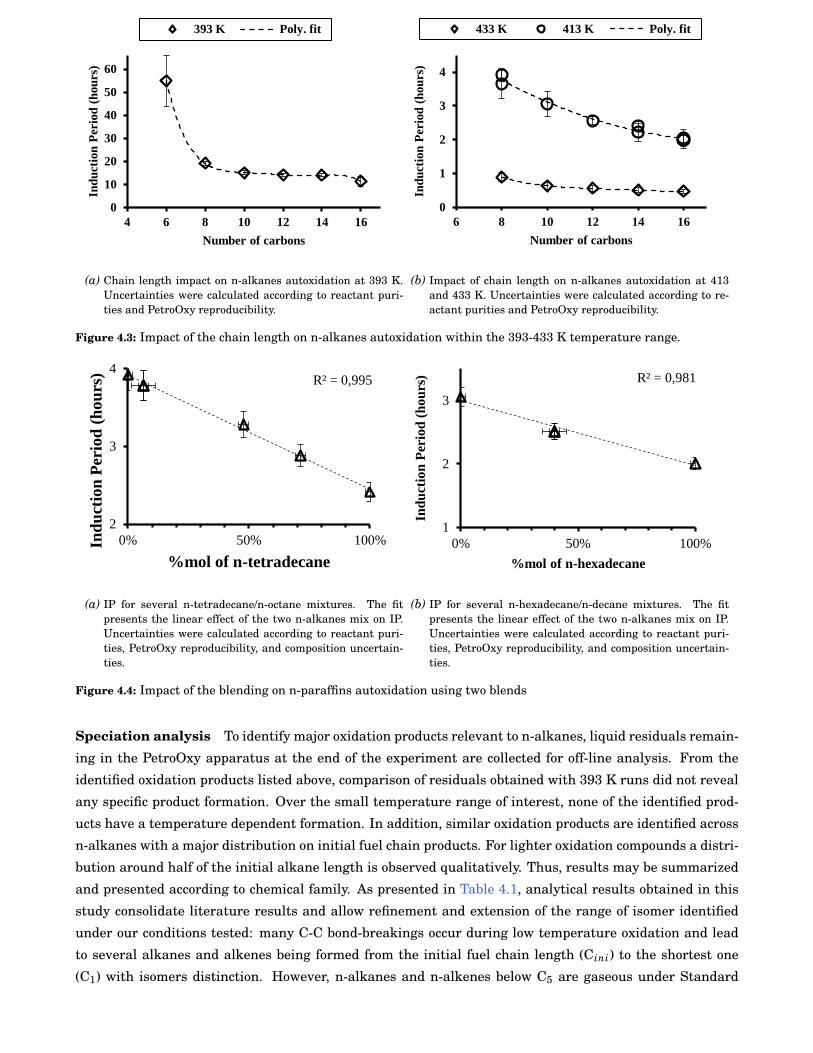
50 Chapter 4

0

10

20

30

40

50

60

4 6 8 10 12 14 16

Ind

uct

ion

Per

iod

(h

ou

rs)

Number of carbons

393 K Poly. fit

(a) Chain length impact on n-alkanes autoxidation at 393 K.Uncertainties were calculated according to reactant puri-ties and PetroOxy reproducibility.

0

1

2

3

4

6 8 10 12 14 16

Ind

uct

ion

Per

iod

(h

ou

rs)

Number of carbons

433 K 413 K Poly. fit

(b) Impact of chain length on n-alkanes autoxidation at 413and 433 K. Uncertainties were calculated according to re-actant purities and PetroOxy reproducibility.

Figure 4.3: Impact of the chain length on n-alkanes autoxidation within the 393-433 K temperature range.

R² = 0,995

2

3

4

0% 50% 100%Ind

uct

ion

Per

iod

(h

ou

rs)

%mol of n-tetradecane

(a) IP for several n-tetradecane/n-octane mixtures. The fitpresents the linear effect of the two n-alkanes mix on IP.Uncertainties were calculated according to reactant puri-ties, PetroOxy reproducibility, and composition uncertain-ties.

R² = 0,981

1

2

3

0% 50% 100%

Ind

uct

ion

Per

iod

(h

ou

rs)

%mol of n-hexadecane

(b) IP for several n-hexadecane/n-decane mixtures. The fitpresents the linear effect of the two n-alkanes mix on IP.Uncertainties were calculated according to reactant puri-ties, PetroOxy reproducibility, and composition uncertain-ties.

Figure 4.4: Impact of the blending on n-paraffins autoxidation using two blends

Speciation analysis To identify major oxidation products relevant to n-alkanes, liquid residuals remain-

ing in the PetroOxy apparatus at the end of the experiment are collected for off-line analysis. From the

identified oxidation products listed above, comparison of residuals obtained with 393 K runs did not reveal

any specific product formation. Over the small temperature range of interest, none of the identified prod-

ucts have a temperature dependent formation. In addition, similar oxidation products are identified across

n-alkanes with a major distribution on initial fuel chain products. For lighter oxidation compounds a distri-

bution around half of the initial alkane length is observed qualitatively. Thus, results may be summarized

and presented according to chemical family. As presented in Table 4.1, analytical results obtained in this

study consolidate literature results and allow refinement and extension of the range of isomer identified

under our conditions tested: many C-C bond-breakings occur during low temperature oxidation and lead

to several alkanes and alkenes being formed from the initial fuel chain length (Cini) to the shortest one

(C1) with isomers distinction. However, n-alkanes and n-alkenes below C5 are gaseous under Standard

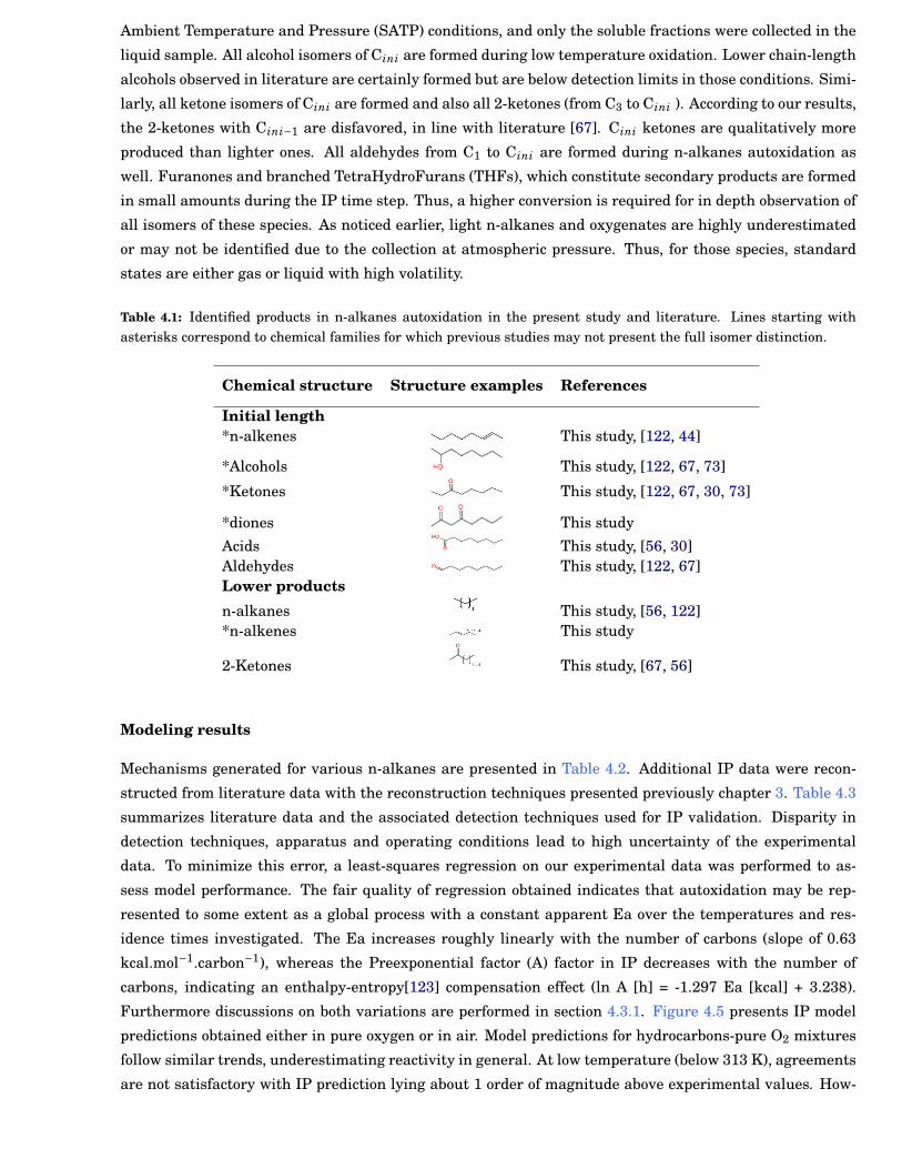
Chapter 4 51

Ambient Temperature and Pressure (SATP) conditions, and only the soluble fractions were collected in the

liquid sample. All alcohol isomers of Cini are formed during low temperature oxidation. Lower chain-length

alcohols observed in literature are certainly formed but are below detection limits in those conditions. Simi-

larly, all ketone isomers of Cini are formed and also all 2-ketones (from C3 to Cini ). According to our results,

the 2-ketones with Cini−1 are disfavored, in line with literature [67]. Cini ketones are qualitatively more

produced than lighter ones. All aldehydes from C1 to Cini are formed during n-alkanes autoxidation as

well. Furanones and branched TetraHydroFurans (THFs), which constitute secondary products are formed

in small amounts during the IP time step. Thus, a higher conversion is required for in depth observation of

all isomers of these species. As noticed earlier, light n-alkanes and oxygenates are highly underestimated

or may not be identified due to the collection at atmospheric pressure. Thus, for those species, standard

states are either gas or liquid with high volatility.

Table 4.1: Identified products in n-alkanes autoxidation in the present study and literature. Lines starting withasterisks correspond to chemical families for which previous studies may not present the full isomer distinction.

Chemical structure Structure examples References

Initial length*n-alkenes This study, [122, 44]

*Alcohols This study, [122, 67, 73]

*Ketones This study, [122, 67, 30, 73]

*diones This studyAcids This study, [56, 30]Aldehydes This study, [122, 67]Lower productsn-alkanes This study, [56, 122]*n-alkenes This study

2-Ketones This study, [67, 56]

Modeling results

Mechanisms generated for various n-alkanes are presented in Table 4.2. Additional IP data were recon-

structed from literature data with the reconstruction techniques presented previously chapter 3. Table 4.3

summarizes literature data and the associated detection techniques used for IP validation. Disparity in

detection techniques, apparatus and operating conditions lead to high uncertainty of the experimental

data. To minimize this error, a least-squares regression on our experimental data was performed to as-

sess model performance. The fair quality of regression obtained indicates that autoxidation may be rep-

resented to some extent as a global process with a constant apparent Ea over the temperatures and res-

idence times investigated. The Ea increases roughly linearly with the number of carbons (slope of 0.63

kcal.mol−1.carbon−1), whereas the Preexponential factor (A) factor in IP decreases with the number of

carbons, indicating an enthalpy-entropy[123] compensation effect (ln A [h] = -1.297 Ea [kcal] + 3.238).

Furthermore discussions on both variations are performed in section 4.3.1. Figure 4.5 presents IP model

predictions obtained either in pure oxygen or in air. Model predictions for hydrocarbons-pure O2 mixtures

follow similar trends, underestimating reactivity in general. At low temperature (below 313 K), agreements

are not satisfactory with IP prediction lying about 1 order of magnitude above experimental values. How-

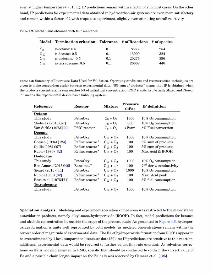
52 Chapter 4

ever, at higher temperature (> 313 K), IP predictions remain within a factor of 2 in most cases. On the other

hand, IP predictions for experimental data obtained in hydrocarbon-air systems are even more satisfactory

and remain within a factor of 2 with respect to experiment, slightly overestimating overall reactivity.

Table 4.2: Mechanisms obtained with four n-alkanes

Model Termination criterion Tolerance # of Reactions # of species

C8 n-octane: 0.5 0.1 8566 254C10 n-decane: 0.5 0.1 13909 324C12 n-dodecane: 0.5 0.1 20276 396C14 n-tetradecane: 0.5 0.1 26669 440

Table 4.3: Summary of Literature Data Used for Validation. Operating conditions and reconstruction techniques aregiven to make comparison easier between experimental data. "5% sum of products" means that IP is obtained whenthe products concentrations sum reaches 5% of initial fuel concentration. PMC stands for Partially Mixed and Closed."?" means the experimental device has a bubbling system.

Reference Reactor Mixture Pressure(kPa) IP definition

OctaneThis study PetroOxy C8 + O2 1000 10% O2 consumptionSkolniak (2015)[57] PetroOxy C8 + O2 800 10% O2 consumptionVan Sickle (1973)[29] PMC reactor C8 + O2 >Patm 5% Fuel conversionDecaneThis study PetroOxy C10 + O2 1000 10% O2 consumptionGoosen (1994) [124] Reflux reactor? C10 + O2 100 5% sum of productsCullis (1981)[67] Reflux reactor? C10 + O2 100 5% sum of productsRubio (1980) [32] Reflux reactor? C10 + O2 100 Max Acid & ROOHDodecaneThis study PetroOxy C12 + O2 1000 10% O2 consumptionBen Amara (2013)[46] Rancimat? C12 + air 100 2nd deriv. conductivitySicard (2013) [44] PetroOxy C12 + O2 1000 10% O2 consumptionRubio (1980) [32] Reflux reactor? C12 + O2 100 Max. Acid peakBoss et al. (1975)[71] Reflux reactor? C12 + O2 100 5% fuel consumptionTetradecaneThis study PetroOxy C14 + O2 1000 10% O2 consumption

Speciation analysis Modeling and experiment speciation comparison was restricted to the major stable

autoxidation products, namely alkyl-mono-hydroperoxide (ROOH). In fact, model predictions for ketones

and alcohols concentration lie outside the scope of the present study. As presented in Figure 4.6, hydroper-

oxides formation is quite well reproduced by both models, as modeled concentrations remain within the

correct order of magnitude of experimental data. The Ea of hydroperoxide formation from ROO◦s appear to

be overestimated by 1 kcal compared to literature data [59]. As IP predictions are sensitive to this reaction,

additional experimental data would be required to further adjust this rate constant. As solvation correc-

tions on Ea is not implemented in RMG, specific ESC should be conducted to confirm the correct value of

Ea and a possible chain length impact on the Ea as it was observed by Câmara et al. [125].

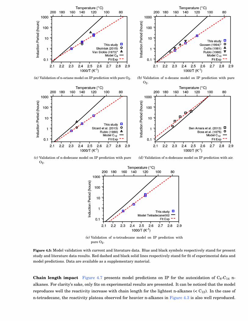
Chapter 4 53

(a) Validation of n-octane model on IP prediction with pure O2.

(b) Validation of n-decane model on IP prediction with pureO2.

(c) Validation of n-dodecane model on IP prediction with pureO2.

(d) Validation of n-dodecane model on IP prediction with air.

(e) Validation of n-tetradecane model on IP prediction withpure O2.

Figure 4.5: Model validation with current and literature data. Blue and black symbols respectively stand for presentstudy and literature data results. Red dashed and black solid lines respectively stand for fit of experimental data andmodel predictions. Data are available as a supplementary material.

Chain length impact Figure 4.7 presents model predictions on IP for the autoxidation of C8-C14 n-

alkanes. For clarity’s sake, only fits on experimental results are presented. It can be noticed that the model

reproduces well the reactivity increase with chain length for the lightest n-alkanes (< C12). In the case of

n-tetradecane, the reactivity plateau observed for heavier n-alkanes in Figure 4.3 is also well reproduced.

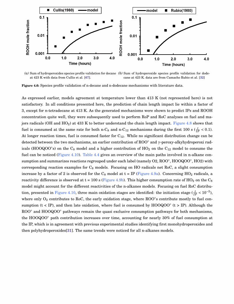
54 Chapter 4

(a) Sum of hydroperoxides species profile validation for decaneat 423 K with data from Cullis et al. [67].

(b) Sum of hydroperoxide species profile validation for dode-cane at 423 K. data are from Camacho Rubio et al. [32]

Figure 4.6: Species profile validation of n-decane and n-dodecane mechanisms with literature data.

As expressed earlier, models agreement at temperature lower than 413 K (not represented here) is not

satisfactory. In all conditions presented here, the prediction of chain length impact lie within a factor of

3, except for n-tetradecane at 413 K. As the generated mechanisms were shown to predict IPs and ROOH

concentration quite well, they were subsequently used to perform RoP and RoC analyses on fuel and ma-

jors radicals (OH and HO2) at 433 K to better understand the chain length impact. Figure 4.8 shows that

fuel is consumed at the same rate for both n-C8 and n-C12 mechanisms during the first 100 s ( tIP < 0.1).

At longer reaction times, fuel is consumed faster for C12. While no significant distribution change can be

detected between the two mechanisms, an earlier contribution of ROO◦ and γ-peroxy-alkyhydroperoxi rad-

icals (HOOQOO◦s) on the C8 model and a higher contribution of HO2 on the C12 model to consume the

fuel can be noticed (Figure 4.10). Table 4.4 gives an overview of the main paths involved in n-alkane con-

sumption and summarizes reactions regrouped under each label (namely O2, ROO◦, HOOQOO◦, HO2) with

corresponding reaction examples for C8 models. Focusing on HO radicals net RoC, a slight consumption

increase by a factor of 2 is observed for the C8 model at t = IP (Figure 4.9a). Concerning HO2 radicals, a

reactivity difference is observed at t = 100 s (Figure 4.9b). This higher consumption rate of HO2 on the C8

model might account for the different reactivities of the n-alkanes models. Focusing on fuel RoC distribu-

tion, presented in Figure 4.10, three main oxidation stages are identified: the initiation stage ( tIP < 10−5),

where only O2 contributes to RoC, the early oxidation stage, where ROO◦s contribute mostly to fuel con-

sumption (t < IP), and then late oxidation, where fuel is consumed by HOOQOO◦ (t > IP). Although the

ROO◦ and HOOQOO◦ pathways remain the quasi exclusive consumption pathways for both mechanisms,

the HOOQOO◦ path contribution increases over time, accounting for nearly 30% of fuel consumption at

the IP, which is in agreement with previous experimental studies identifying first monohydroperoxides and

then polyhydroperoxides[31]. The same trends were noticed for all n-alkanes models.

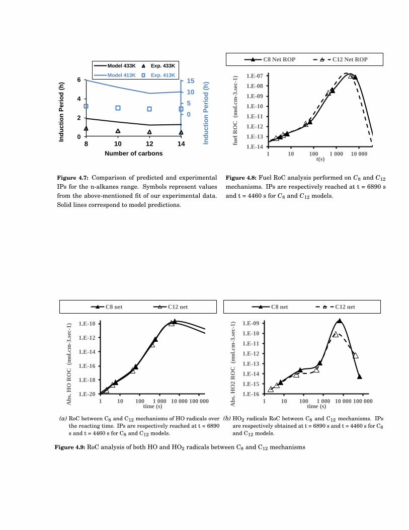
Chapter 4 55

-10

-5

0

5

10

15

0

2

4

6

8 10 12 14 Ind

uc

tio

n P

eri

od

(h)

Ind

ucti

on

Peri

od

(h

)

Number of carbons

Model 433K Exp. 433K

Model 413K Exp. 413K

Figure 4.7: Comparison of predicted and experimentalIPs for the n-alkanes range. Symbols represent valuesfrom the above-mentioned fit of our experimental data.Solid lines correspond to model predictions.

1.E-14

1.E-13

1.E-12

1.E-11

1.E-10

1.E-09

1.E-08

1.E-07

1 10 100 1 000 10 000

fuel

RO

C

(mol.

cm

-3.s

ec-1

)

t(s)

C8 Net ROP C12 Net ROP

Figure 4.8: Fuel RoC analysis performed on C8 and C12

mechanisms. IPs are respectively reached at t = 6890 sand t = 4460 s for C8 and C12 models.

1.E-20

1.E-18

1.E-16

1.E-14

1.E-12

1.E-10

1 10 100 1 000 10 000 100 000Ab

s. H

O R

OC

(m

ol.

cm-3

.sec

-1)

time (s)

C8 net C12 net

(a) RoC between C8 and C12 mechanisms of HO radicals overthe reacting time. IPs are respectively reached at t = 6890s and t = 4460 s for C8 and C12 models.

1.E-16

1.E-15

1.E-14

1.E-13

1.E-12

1.E-11

1.E-10

1.E-09

1 10 100 1 000 10 000 100 000

Ab

s. H

O2

RO

C

(mol.

cm

-3.s

ec-1

)

time (s)

C8 net C12 net

(b) HO2 radicals RoC between C8 and C12 mechanisms. IPsare respectively obtained at t = 6890 s and t = 4460 s for C8and C12 models.

Figure 4.9: RoC analysis of both HO and HO2 radicals between C8 and C12 mechanisms

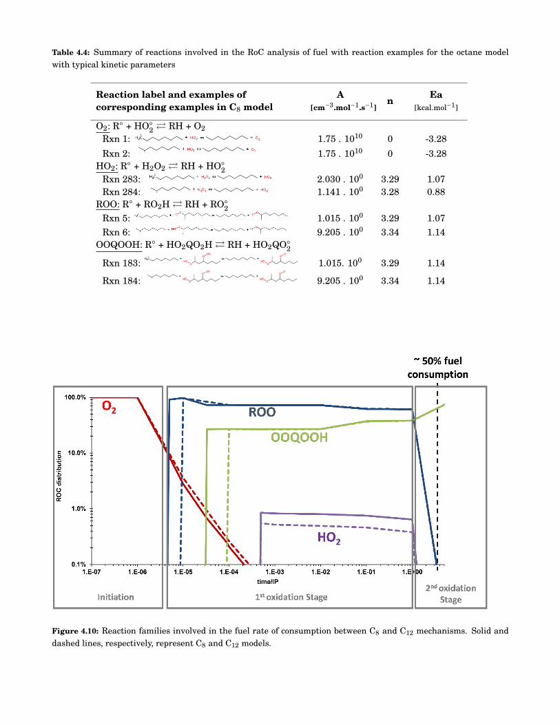
56 Chapter 4

Table 4.4: Summary of reactions involved in the RoC analysis of fuel with reaction examples for the octane modelwith typical kinetic parameters

Reaction label and examples ofcorresponding examples in C8 model

A[cm−3.mol−1.s−1]

n Ea[kcal.mol−1]

O2: R◦ + HO◦2 � RH + O2

Rxn 1: 1.75 . 1010 0 -3.28Rxn 2: 1.75 . 1010 0 -3.28

HO2: R◦ + H2O2 � RH + HO◦2

Rxn 283: 2.030 . 100 3.29 1.07Rxn 284: 1.141 . 100 3.28 0.88

ROO: R◦ + RO2H� RH + RO◦2

Rxn 5: 1.015 . 100 3.29 1.07Rxn 6: 9.205 . 100 3.34 1.14

OOQOOH: R◦ + HO2QO2H� RH + HO2QO◦2

Rxn 183: 1.015. 100 3.29 1.14

Rxn 184: 9.205 . 100 3.34 1.14

Figure 4.10: Reaction families involved in the fuel rate of consumption between C8 and C12 mechanisms. Solid anddashed lines, respectively, represent C8 and C12 models.

Chapter 4 57

4.1.2 Detailed results with autoclave

In order to get more information of n-octane oxidation, experiments are now conducted in the autoclave to

obtain products formation in both liquid and gas phase over time. In order to obtain results as PetroOxy

ones, experiments are conducted with both similar amount of oxygen and sample to reactor volume ratio

(Vsample

Vreactor= 0.2)

Material and methods

As autoclave experiments and its associated analytical devices were already presented(chapter 3), no fur-

ther description is performed here.

Experiments are conducted twice at 383 K and 1000 kPa of total pressure with 50mL of reactant. This

repeatability point aims to to cover most of the oxidation regime and to validate oxidation rates. As the

sampling technique presented in (chapter 3) modifies gas phase composition, one of the two experiment is

limited to one intermediate sample. Thus, the repeatability point aims to confirm the absence of sampling

effect on the oxidation rate. Each intermediate sample is about 1mL and final content of the autoclave is

also collected for visual inspections.

Experimental results

Macroscopic reactivity Results summarizing n-C8 oxidation over time are presented in Figure 4.11.

Figure 4.11a presents pressure and temperature evolution over the reaction time of the two experiments.

Surprisingly, a high temperature gradient is observed between gas and liquid phase, around 15-20◦Cand reproduced on both experiments. Pressure uncertainties are calculated according to this equation

∆(P)t = PUncert.×(1+nspl.,t)+(Pspl.,t+ε−Pspl.,t−ε) to consider both measurements errors and potential pres-

sure addition after the sampling. Considering this uncertainty, the fair reproducibility of pressure and tem-

perature profiles demonstrates the absence of any sampling effect on the autoxidation. Sampling times are

represented in Figure 4.11a with arrows and their corresponding pictures is presented in Figure 4.11b over

reaction time. As observed on those pictures, the starting fuel which was colourless turns into a coloured

two phases system at the end of the experiment. From the second reactor content picture, the formation

of such two phases system seems to occur below 45 hours. The absence of such two phases system in the

corresponding vial tends to prove slight inhomogeneities in the sampling process. The composition of the

two phases is discussed later (section 4.3.2). Finally, Figure 4.11c and Figure 4.11d respectively illustrate

the formation of liquid and gas phase products over time. Liquid and gas phase results are respectively

from a GC-FID and from both a GC-FID and a GC-TCD. For clarity sake, only n-C8 and O2 signals are cut

off to observe oxidation products formation.

Products identification Figure 4.12 summarizes the identification of both ketones and acids chemical

families with the GC-MS. In both figures, the full scan spectrum was filtered with majors ions of the pre-

sented chemical families. As concluded with petroxy residual analyses, C7 acids and ketones formation are

disfavoured compared to all others possible lengths. In order to confirm major products formation, the most

oxidized samples were analysed with FTIR and the resulting spectrum is presented in Figure 4.13. Absorp-

tion bands 1 and 3 are relevant to C-H bond stretch respectively from CH3 and CH2 groups. In addition the

absorption band 2 is relevant to C=O bond stretch n-C8 spectrum from species containing ketones. Those

results validated GCs conclusions with majors species identification as n-C8 and octanone isomers.

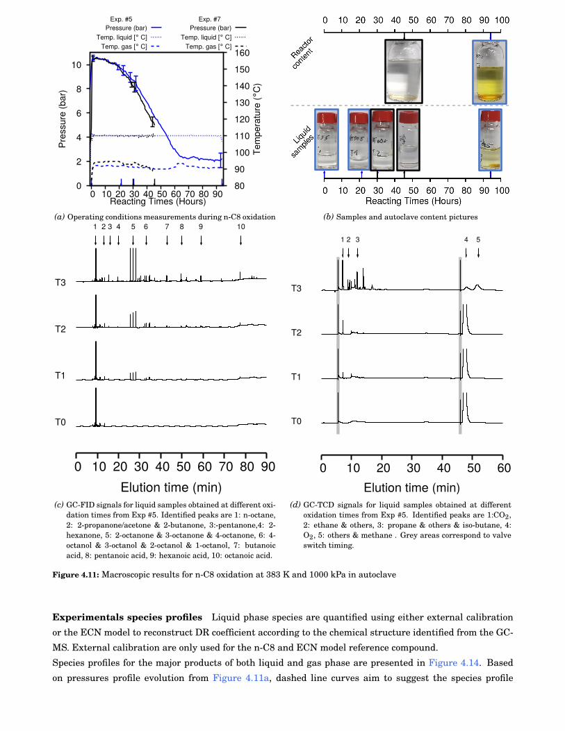
58 Chapter 4

0

2

4

6

8

10

0 10 20 30 40 50 60 70 80 90 80

90

100

110

120

130

140

150

160

Exp. #5 Exp. #7

Pres

sure

(bar

)

Tem

pera

ture

(°C

)

Reacting Times (Hours)

Pressure (bar)Temp. liquid [° C]

Temp. gas [° C]

Pressure (bar)Temp. liquid [° C]

Temp. gas [° C]

(a) Operating conditions measurements during n-C8 oxidation (b) Samples and autoclave content pictures

0 10 20 30 40 50 60 70 80 90

T0

T1

T2

T3

1 2 3 4 5 6 7 8 9 10

Elution time (min)(c) GC-FID signals for liquid samples obtained at different oxi-

dation times from Exp #5. Identified peaks are 1: n-octane,2: 2-propanone/acetone & 2-butanone, 3:-pentanone,4: 2-hexanone, 5: 2-octanone & 3-octanone & 4-octanone, 6: 4-octanol & 3-octanol & 2-octanol & 1-octanol, 7: butanoicacid, 8: pentanoic acid, 9: hexanoic acid, 10: octanoic acid.

0 10 20 30 40 50 60

T0

T1

T2

T3

1 2 3 4 5

Elution time (min)(d) GC-TCD signals for liquid samples obtained at different

oxidation times from Exp #5. Identified peaks are 1:CO2,2: ethane & others, 3: propane & others & iso-butane, 4:O2, 5: others & methane . Grey areas correspond to valveswitch timing.

Figure 4.11: Macroscopic results for n-C8 oxidation at 383 K and 1000 kPa in autoclave

Experimentals species profiles Liquid phase species are quantified using either external calibration

or the ECN model to reconstruct DR coefficient according to the chemical structure identified from the GC-

MS. External calibration are only used for the n-C8 and ECN model reference compound.

Species profiles for the major products of both liquid and gas phase are presented in Figure 4.14. Based

on pressures profile evolution from Figure 4.11a, dashed line curves aim to suggest the species profile

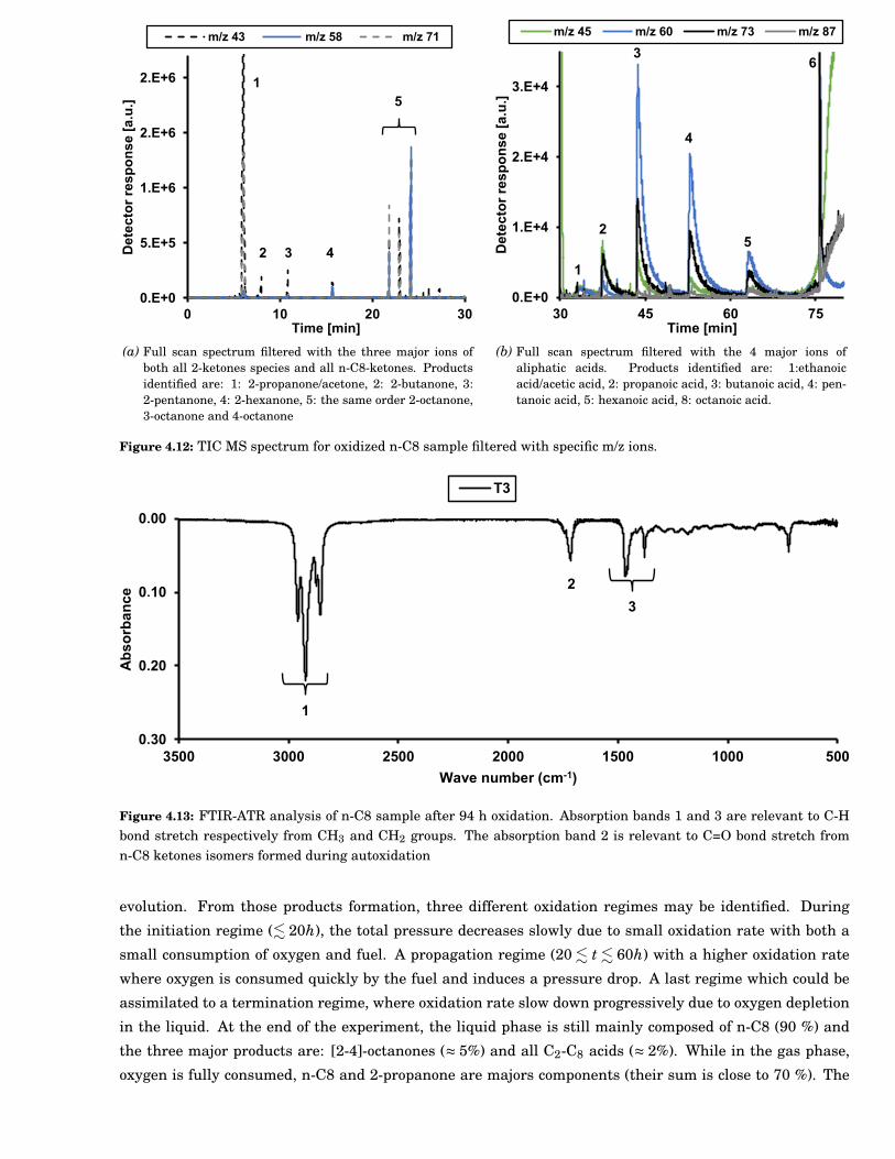
Chapter 4 59

0.E+0

5.E+5

1.E+6

2.E+6

2.E+6

0 10 20 30

De

tec

tor

res

po

ns

e [

a.u

.]

Time [min]

m/z 43 m/z 58 m/z 71

1

2 3 4

5

(a) Full scan spectrum filtered with the three major ions ofboth all 2-ketones species and all n-C8-ketones. Productsidentified are: 1: 2-propanone/acetone, 2: 2-butanone, 3:2-pentanone, 4: 2-hexanone, 5: the same order 2-octanone,3-octanone and 4-octanone

0.E+0

1.E+4

2.E+4

3.E+4

30 45 60 75

Dete

cto

r re

sp

on

se

[a

.u.]

Time [min]

m/z 45 m/z 60 m/z 73 m/z 87

1

2

3

4

5

6

(b) Full scan spectrum filtered with the 4 major ions ofaliphatic acids. Products identified are: 1:ethanoicacid/acetic acid, 2: propanoic acid, 3: butanoic acid, 4: pen-tanoic acid, 5: hexanoic acid, 8: octanoic acid.

Figure 4.12: TIC MS spectrum for oxidized n-C8 sample filtered with specific m/z ions.

0,00

0,10

0,20

0,30

500100015002000250030003500

Ab

so

rba

nc

e

Wave number (cm-1)

T3

1

2

3

Figure 4.13: FTIR-ATR analysis of n-C8 sample after 94 h oxidation. Absorption bands 1 and 3 are relevant to C-Hbond stretch respectively from CH3 and CH2 groups. The absorption band 2 is relevant to C=O bond stretch fromn-C8 ketones isomers formed during autoxidation

evolution. From those products formation, three different oxidation regimes may be identified. During

the initiation regime (. 20h), the total pressure decreases slowly due to small oxidation rate with both a

small consumption of oxygen and fuel. A propagation regime (20. t. 60h) with a higher oxidation rate

where oxygen is consumed quickly by the fuel and induces a pressure drop. A last regime which could be

assimilated to a termination regime, where oxidation rate slow down progressively due to oxygen depletion

in the liquid. At the end of the experiment, the liquid phase is still mainly composed of n-C8 (90 %) and

the three major products are: [2-4]-octanones (≈ 5%) and all C2-C8 acids (≈ 2%). While in the gas phase,

oxygen is fully consumed, n-C8 and 2-propanone are majors components (their sum is close to 70 %). The

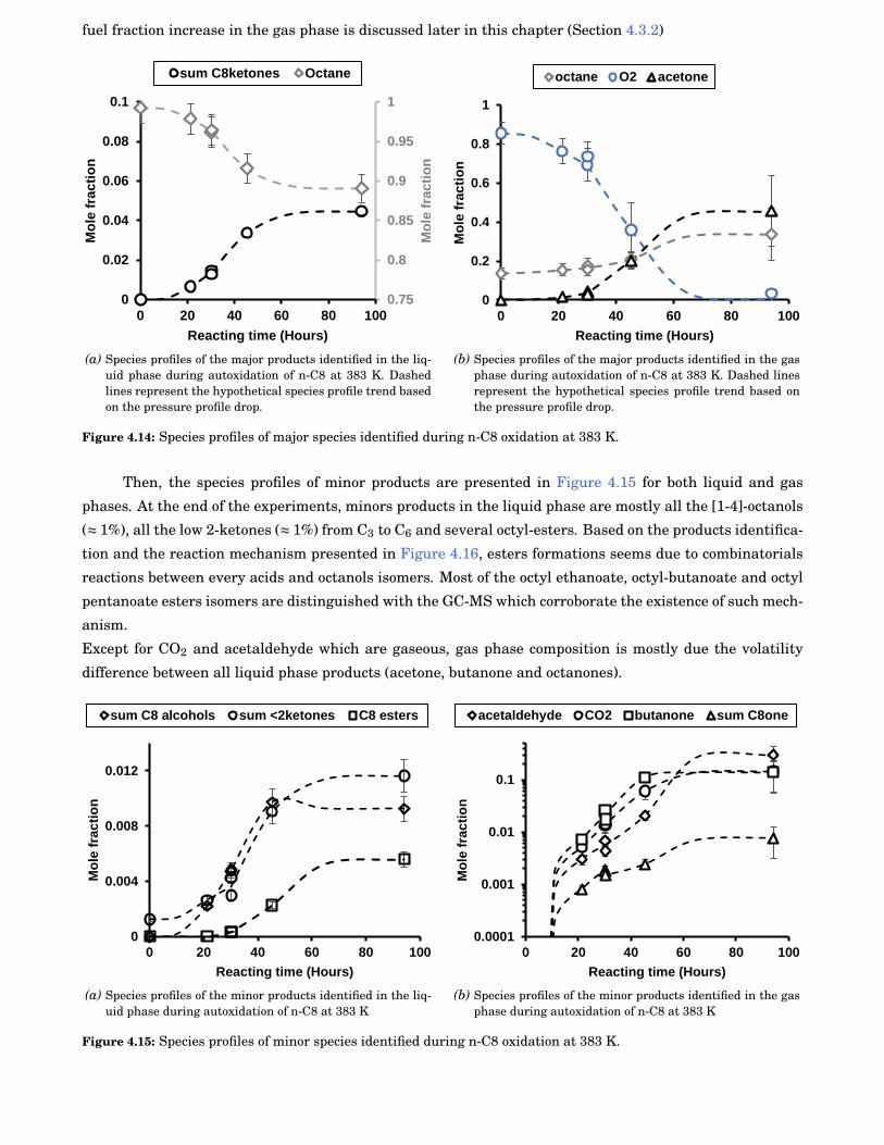
60 Chapter 4

fuel fraction increase in the gas phase is discussed later in this chapter (Section 4.3.2)

0.75

0.8

0.85

0.9

0.95

1

0

0.02

0.04

0.06

0.08

0.1

0 20 40 60 80 100

Mo

le f

rac

tio

n

Mo

le f

rac

tio

n

Reacting time (Hours)

sum C8ketones Octane

(a) Species profiles of the major products identified in the liq-uid phase during autoxidation of n-C8 at 383 K. Dashedlines represent the hypothetical species profile trend basedon the pressure profile drop.

0

0.2

0.4

0.6

0.8

1

0 20 40 60 80 100

Mo

le f

rac

tio

n

Reacting time (Hours)

octane O2 acetone

(b) Species profiles of the major products identified in the gasphase during autoxidation of n-C8 at 383 K. Dashed linesrepresent the hypothetical species profile trend based onthe pressure profile drop.

Figure 4.14: Species profiles of major species identified during n-C8 oxidation at 383 K.

Then, the species profiles of minor products are presented in Figure 4.15 for both liquid and gas

phases. At the end of the experiments, minors products in the liquid phase are mostly all the [1-4]-octanols

(≈ 1%), all the low 2-ketones (≈ 1%) from C3 to C6 and several octyl-esters. Based on the products identifica-

tion and the reaction mechanism presented in Figure 4.16, esters formations seems due to combinatorials

reactions between every acids and octanols isomers. Most of the octyl ethanoate, octyl-butanoate and octyl

pentanoate esters isomers are distinguished with the GC-MS which corroborate the existence of such mech-

anism.

Except for CO2 and acetaldehyde which are gaseous, gas phase composition is mostly due the volatility

difference between all liquid phase products (acetone, butanone and octanones).

0

0.004

0.008

0.012

0 20 40 60 80 100

Mo

le f

rac

tio

n

Reacting time (Hours)

sum C8 alcohols sum <2ketones C8 esters

(a) Species profiles of the minor products identified in the liq-uid phase during autoxidation of n-C8 at 383 K

0.0001

0.001

0.01

0.1

0 20 40 60 80 100

Mo

le f

rac

tio

n

Reacting time (Hours)

acetaldehyde CO2 butanone sum C8one

(b) Species profiles of the minor products identified in the gasphase during autoxidation of n-C8 at 383 K

Figure 4.15: Species profiles of minor species identified during n-C8 oxidation at 383 K.

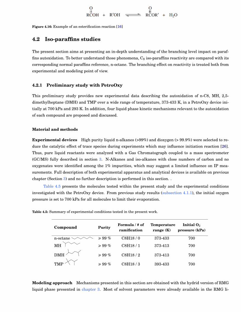
Chapter 4 61

Figure 4.16: Example of an esterification reaction [16]

4.2 Iso-paraffins studies

The present section aims at presenting an in-depth understanding of the branching level impact on paraf-

fins autoxidation. To better understand those phenomena, C8 iso-paraffins reactivity are compared with its

corresponding normal paraffins reference, n-octane. The branching effect on reactivity is treated both from

experimental and modeling point of view.

4.2.1 Preliminary study with PetroOxy

This preliminary study provides new experimental data describing the autoxidation of n-C8, MH, 2,5-

dimethylheptane (DMH) and TMP over a wide range of temperature, 373-433 K, in a PetroOxy device ini-

tially at 700 kPa and 293 K. In addition, four liquid phase kinetic mechanisms relevant to the autoxidation

of each compound are proposed and discussed.

Material and methods

Experimental devices High purity liquid n-alkanes (>99%) and dioxygen (> 99.9%) were selected to re-

duce the catalytic effect of trace species during experiments which may influence initiation reaction [26].

Thus, pure liquid reactants were analyzed with a Gas Chromatograph coupled to a mass spectrometer

(GC/MS) fully described in section 3. N-Alkanes and iso-alkanes with close numbers of carbon and no

oxygenates were identified among the 1% impurities, which may suggest a limited influence on IP mea-

surements. Full description of both experimental apparatus and analytical devices is available on previous

chapter (Section 3) and no further description is performed in this section. .

Table 4.5 presents the molecules tested within the present study and the experimental conditions

investigated with the PetroOxy device. From previous study results (subsection 4.1.1), the initial oxygen

pressure is set to 700 kPa for all molecules to limit their evaporation.

Table 4.5: Summary of experimental conditions tested in the present work.

Compound PurityFormula / # oframification

Temperaturerange (K)

Initial O2

pressure (kPa)

n-octane Ê 99 % C8H18 / 0 373-433 700

MH Ê 99 % C8H18 / 1 373-413 700

DMH Ê 99 % C8H18 / 2 373-413 700

TMP Ê 99 % C8H18 / 3 393-433 700

Modeling approach Mechanisms presented in this section are obtained with the hydrid version of RMG

liquid phase presented in chapter 3. Most of solvent parameters were already available in the RMG li-

62 Chapter 4

braries (n-octane, iso-octane). As MH, DMH and TMP are all iso-octane, isooctane solvation parameter was

applied on them. Initial conditions such as concentrations, viscosities, oxygen solubility were computed

for each system from data available in literature [120, 121]. Table 4.6 summarizes the four mechanisms

obtained with RMG-Hybrid in best agreement with IPs. Mechanisms generation was established based on

the oxidation pathways comprehension from Section 4.1. Thus, all mechanisms are constructed to involve

specific products formation: ROOH, C8-ketones, C8-alcohols, alkyl-di-hydroperoxide (HOOQOOH), KHP,

cyclic Korcek intermediates, lighter acids and carbonyls either from Korcek’s reactions or α/β-scissions,

lighter Hydrocarbon (HC) from either direct C-C bond breaking or α/β-scissions. In agreement with experi-

mental observations from section 4.1, the formation of both lighter alcohols and peracids is removed to limit

mechanisms size increase. The n-C8-v2 mechanism presented in Table 4.6 is an upgraded version of the

n-C8 mechanisms from section 4.1. Thus, the remove of all negligeable pathways explain why it is smaller

than its original version from section 4.1. For a sake of clarity, in the next figures the mechanism n-C8-v2

is called n-C8.The high tolerance value used for both MH and DMH generations, means those mechanism

are closely linked to the user specified reaction paths. While in the case of TMP, this criteria was not self

consistent and a lower tolerance value was required to add more termination paths (RO4R, RO3R) and more

stable species formation with mostly β-alkene formation.

The generated mechanisms were coupled to a previously developed zero-dimensional reactor model already

used in literature [46].

Table 4.6: Mechanisms obtained with the four C8-alkanes.

Model Terminationcriterion

Solventselected Tolerance # of Re-

actions# of

species

n-C8-v2: n-octane: 0.5 octane 0.1 201 7324MH: 2-methylheptane: 0.5 iso-octane 0.9 191 7004DMH: 2,5-dimethylhexane: 0.5 iso-octane 0.9 91 1436TMP: 2,2,4-trimethylpentane: 0.5 iso-octane 0.1 193 5556

Experimental results

To identify the effect of the branching on alkanes reactivity, wide temperature range (373-433 K) exper-

iments were conducted on the four C8 alkanes at 700 kPa of initial oxygen. To obtain meaningful data,

acquisition of IP below 0.5 hours is not considered due to the heatingtimeIP ratio. As purity impact was not

studied within this work, previous results (Section 4.1.1) obtained in similar conditions (99% compound

purity, similar temperature range, oxygen pressure) with n-alkanes are considered (∆IP99→99.8 (hrs) = 0.13

× IP99% (hrs)).

Temperature impact Figure 4.17 presents the evolution of IP with temperature reciprocal for all

molecules tested. Whereas additional data would be required for temperature below 393 K, IP seems to

decrease exponentially with the temperature reciprocal for n-C8, MH, DMH and TMP. The fair quality of

the regression for n-C8, MH, DMH indicates that their autoxidation may be assimilated to a global pro-

cess with an apparent A’ and Ea’ presented in Figure 4.17b. While a fair regression is presented for TMP,

two distinct oxidation regime are observable for temperature above and lower 403 K. In addition, the com-

parison of apparent Ea’ emphasizes a specific oxidation behaviour of the TMP which has a much smaller

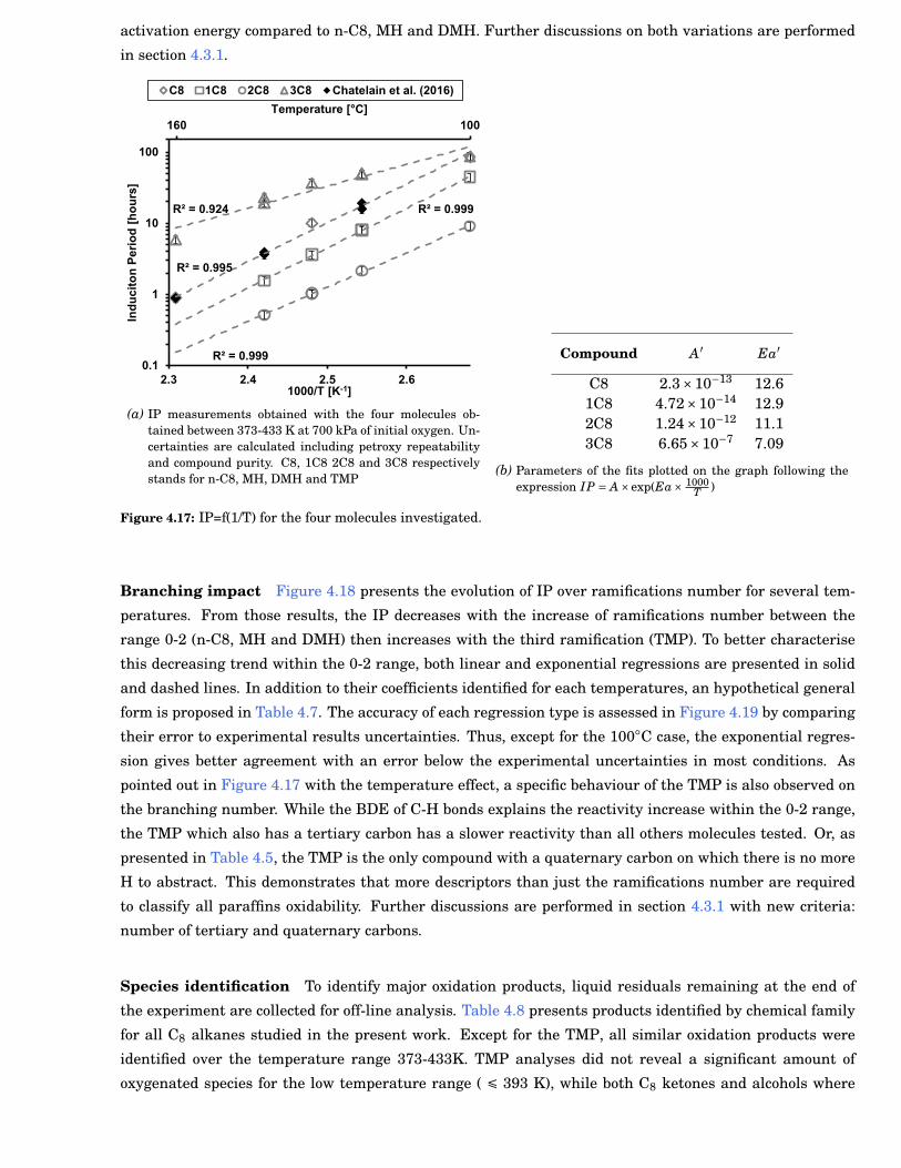
Chapter 4 63

activation energy compared to n-C8, MH and DMH. Further discussions on both variations are performed

in section 4.3.1.

R² = 0.999

R² = 0.999

R² = 0.924

R² = 0.995

100160

0.1

1

10

100

2.3 2.4 2.5 2.6

Temperature [°C]

Ind

uc

ito

n P

eri

od

[h

ou

rs]

1000/T [K-1]

C8 1C8 2C8 3C8 Chatelain et al. (2016)

(a) IP measurements obtained with the four molecules ob-tained between 373-433 K at 700 kPa of initial oxygen. Un-certainties are calculated including petroxy repeatabilityand compound purity. C8, 1C8 2C8 and 3C8 respectivelystands for n-C8, MH, DMH and TMP

Compound A′ Ea′

C8 2.3×10−13 12.61C8 4.72×10−14 12.92C8 1.24×10−12 11.13C8 6.65×10−7 7.09

(b) Parameters of the fits plotted on the graph following theexpression IP = A×exp(Ea× 1000

T )

Figure 4.17: IP=f(1/T) for the four molecules investigated.

Branching impact Figure 4.18 presents the evolution of IP over ramifications number for several tem-

peratures. From those results, the IP decreases with the increase of ramifications number between the

range 0-2 (n-C8, MH and DMH) then increases with the third ramification (TMP). To better characterise

this decreasing trend within the 0-2 range, both linear and exponential regressions are presented in solid

and dashed lines. In addition to their coefficients identified for each temperatures, an hypothetical general

form is proposed in Table 4.7. The accuracy of each regression type is assessed in Figure 4.19 by comparing

their error to experimental results uncertainties. Thus, except for the 100◦C case, the exponential regres-

sion gives better agreement with an error below the experimental uncertainties in most conditions. As

pointed out in Figure 4.17 with the temperature effect, a specific behaviour of the TMP is also observed on

the branching number. While the BDE of C-H bonds explains the reactivity increase within the 0-2 range,

the TMP which also has a tertiary carbon has a slower reactivity than all others molecules tested. Or, as

presented in Table 4.5, the TMP is the only compound with a quaternary carbon on which there is no more

H to abstract. This demonstrates that more descriptors than just the ramifications number are required

to classify all paraffins oxidability. Further discussions are performed in section 4.3.1 with new criteria:

number of tertiary and quaternary carbons.

Species identification To identify major oxidation products, liquid residuals remaining at the end of

the experiment are collected for off-line analysis. Table 4.8 presents products identified by chemical family

for all C8 alkanes studied in the present work. Except for the TMP, all similar oxidation products were

identified over the temperature range 373-433K. TMP analyses did not reveal a significant amount of

oxygenated species for the low temperature range ( É 393 K), while both C8 ketones and alcohols where

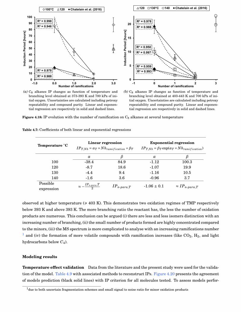
64 Chapter 4

R² = 0.998

R² = 0.946

R² = 0.978

R² = 0.9880

10

20

30

40

50

60

70

80

90

100

-1.0 0.0 1.0 2.0 3.0

Ind

ucit

on

Peri

od

[h

ou

rs]

Number of ramifications

100°C 120 Chatelain et al. (2016)

(a) C8 alkanes IP changes as function of temperature andbranching level obtained at 373-393 K and 700 kPa of ini-tial oxygen. Uncertainties are calculated including petroxyrepeatability and compound purity. Linear and exponen-tial regression are respectively in solid and dashed lines.

R² = 0.978

R² = 0.950

R² = 0.997

R² = 0.959

R² = 0.993

R² = 0.988

0

5

10

15

20

-1 0 1 2 3

Ind

ucit

on

Peri

od

[h

ou

rs]

Number of ramifications

120 130°C 140 Chatelain et al. (2016)

(b) C8 alkanes IP changes as function of temperature andbranching level obtained at 403-443 K and 700 kPa of ini-tial oxygen. Uncertainties are calculated including petroxyrepeatability and compound purity. Linear and exponen-tial regression are respectively in solid and dashed lines.

Figure 4.18: IP evolution with the number of ramification on C8 alkanes at several temperature

Table 4.7: Coefficients of both linear and exponential regressions

Temperature ◦CLinear regression

IPT,Nb =αT ×Nbrami f ication +βT

Exponential regressionIPT,Nb =βT exp(αT ×Nbrami f ication)

α β α β

100 -38.4 84.9 -1.12 100.3120 -8.7 18.6 -1.07 19.9130 -4.4 9.4 -1.16 10.5140 -1.6 3.6 -0.96 3.7

Possibleexpression ≈− IPn-para,T

2 IPn-para,T -1.06 ± 0.1 ≈ IPn-para,T

observed at higher temperature (Ê 403 K). This demonstrates two oxidation regimes of TMP respectively

below 393 K and above 393 K. The more branching ratio the reactant has, the less the number of oxidation

products are numerous. This conclusion can be argued (i) there are less and less isomers distinction with an

increasing number of branching, (ii) the small number of products formed are highly concentrated compared

to the minors, (iii) the MS spectrum is more complicated to analyse with an increasing ramifications number1 and (iv) the formation of more volatile compounds with ramification increases (like CO2, H2, and light

hydrocarbons below C4).

Modeling results

Temperature effect validation Data from the literature and the present study were used for the valida-

tion of the model. Table 4.9 with associated methods to reconstruct IPs. Figure 4.20 presents the agreement

of models prediction (black solid lines) with IP criterion for all molecules tested. To assess models perfor-

1due to both uncertain fragmentation schemes and small signal to noise ratio for minor oxidation products

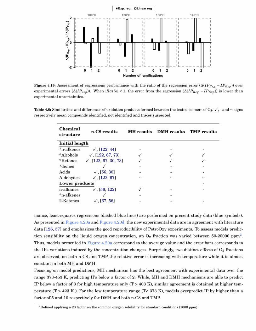
Chapter 4 65

100°C 120°C 130°C 140°C

-2

0

2

0 1 2 0 1 2 0 1 2 0 1 2D(I

PR

eg

.-

IPE

xp

.) / D

(IP

Ex

p.)

Number of ramifications

Exp. reg. Linear reg

Figure 4.19: Assessment of regressions performance with the ratio of the regression error (∆(IPReg. − IPExp)) overexperimental errors (∆(IPexp)). When |Ratio| < 1, the error from the regression (∆(IPReg. − IPExp)) is lower thanexperimental uncertainties.

Table 4.8: Similarities and differences of oxidation products formed between the tested isomers of C8. X, - and ∼ signsrespectively mean compounds identified, not identified and traces suspected.

Chemicalstructure n-C8 results MH results DMH results TMP results

Initial length*n-alkenes X, [122, 44] - - -*Alcohols X, [122, 67, 73] X X X*Ketones X, [122, 67, 30, 73] X X X*diones X - - -Acids X, [56, 30] - - -Aldehydes X, [122, 67] ∼ ∼ ∼Lower products -n-alkanes X, [56, 122] X - -*n-alkenes X - -2-Ketones X, [67, 56] - - -

mance, least-squares regressions (dashed blue lines) are performed on present study data (blue symbols).

As presented in Figure 4.20a and Figure 4.20d, the new experimental data are in agreement with literature

data [126, 57] and emphasizes the good reproducibility of PetroOxy experiments. To assess models predic-

tion sensibility on the liquid oxygen concentration, an O2 fraction was varied between 50-20000 ppm2.

Thus, models presented in Figure 4.20a correspond to the average value and the error bars corresponds to

the IPs variations induced by the concentration changes. Surprisingly, two distinct effects of O2 fractions

are observed, on both n-C8 and TMP the relative error is increasing with temperature while it is almost

constant in both MH and DMH.

Focusing on model predictions, MH mechanism has the best agreement with experimental data over the

range 373-453 K, predicting IPs below a factor of 2. While, MH and DMH mechanisms are able to predict

IP below a factor of 3 for high temperature only (T > 403 K), similar agreement is obtained at higher tem-

perature (T > 423 K ). For the low temperature range (T< 373 K), models overpredict IP by higher than a

factor of 5 and 10 respectively for DMH and both n-C8 and TMP.

2Defined applying a 20 factor on the common oxygen solubility for standard conditions (1000 ppm)

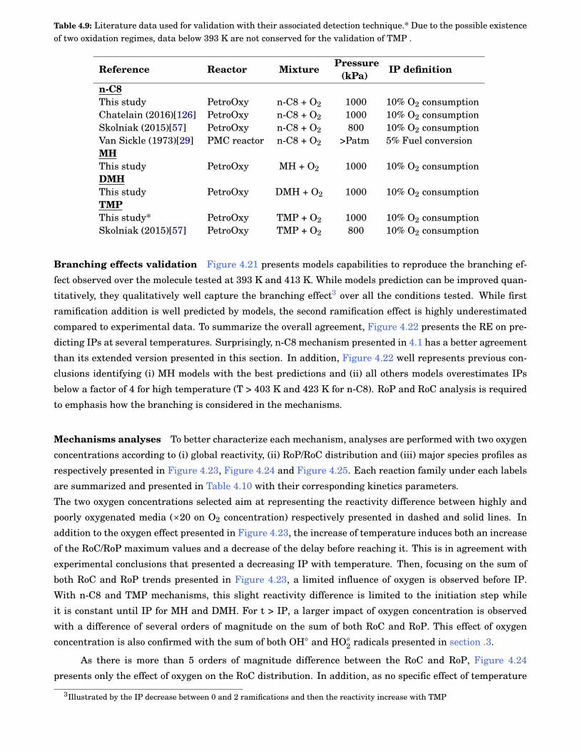
66 Chapter 4

Table 4.9: Literature data used for validation with their associated detection technique.* Due to the possible existenceof two oxidation regimes, data below 393 K are not conserved for the validation of TMP .

Reference Reactor Mixture Pressure(kPa) IP definition

n-C8This study PetroOxy n-C8 + O2 1000 10% O2 consumptionChatelain (2016)[126] PetroOxy n-C8 + O2 1000 10% O2 consumptionSkolniak (2015)[57] PetroOxy n-C8 + O2 800 10% O2 consumptionVan Sickle (1973)[29] PMC reactor n-C8 + O2 >Patm 5% Fuel conversionMHThis study PetroOxy MH + O2 1000 10% O2 consumptionDMHThis study PetroOxy DMH + O2 1000 10% O2 consumptionTMPThis study* PetroOxy TMP + O2 1000 10% O2 consumptionSkolniak (2015)[57] PetroOxy TMP + O2 800 10% O2 consumption

Branching effects validation Figure 4.21 presents models capabilities to reproduce the branching ef-

fect observed over the molecule tested at 393 K and 413 K. While models prediction can be improved quan-

titatively, they qualitatively well capture the branching effect3 over all the conditions tested. While first

ramification addition is well predicted by models, the second ramification effect is highly underestimated

compared to experimental data. To summarize the overall agreement, Figure 4.22 presents the RE on pre-

dicting IPs at several temperatures. Surprisingly, n-C8 mechanism presented in 4.1 has a better agreement

than its extended version presented in this section. In addition, Figure 4.22 well represents previous con-

clusions identifying (i) MH models with the best predictions and (ii) all others models overestimates IPs

below a factor of 4 for high temperature (T > 403 K and 423 K for n-C8). RoP and RoC analysis is required

to emphasis how the branching is considered in the mechanisms.

Mechanisms analyses To better characterize each mechanism, analyses are performed with two oxygen

concentrations according to (i) global reactivity, (ii) RoP/RoC distribution and (iii) major species profiles as

respectively presented in Figure 4.23, Figure 4.24 and Figure 4.25. Each reaction family under each labels

are summarized and presented in Table 4.10 with their corresponding kinetics parameters.

The two oxygen concentrations selected aim at representing the reactivity difference between highly and

poorly oxygenated media (×20 on O2 concentration) respectively presented in dashed and solid lines. In

addition to the oxygen effect presented in Figure 4.23, the increase of temperature induces both an increase

of the RoC/RoP maximum values and a decrease of the delay before reaching it. This is in agreement with

experimental conclusions that presented a decreasing IP with temperature. Then, focusing on the sum of

both RoC and RoP trends presented in Figure 4.23, a limited influence of oxygen is observed before IP.

With n-C8 and TMP mechanisms, this slight reactivity difference is limited to the initiation step while

it is constant until IP for MH and DMH. For t > IP, a larger impact of oxygen concentration is observed

with a difference of several orders of magnitude on the sum of both RoC and RoP. This effect of oxygen

concentration is also confirmed with the sum of both OH◦ and HO◦2 radicals presented in section .3.

As there is more than 5 orders of magnitude difference between the RoC and RoP, Figure 4.24

presents only the effect of oxygen on the RoC distribution. In addition, as no specific effect of temperature

3Illustrated by the IP decrease between 0 and 2 ramifications and then the reactivity increase with TMP

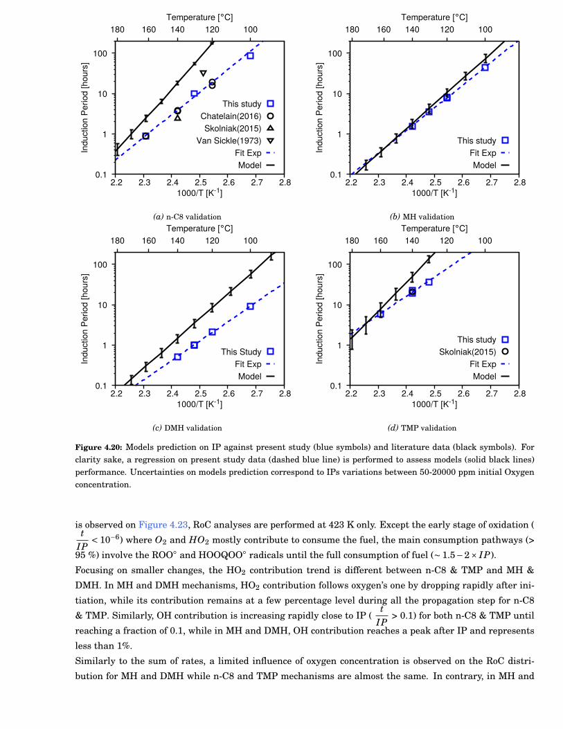
Chapter 4 67

0.1

1

10

100

2.2 2.3 2.4 2.5 2.6 2.7 2.8

180 160 140 120 100

Indu

ctio

n Pe

riod

[hou

rs]

1000/T [K-1]

Temperature [°C]

This studyChatelain(2016)Skolniak(2015)

Van Sickle(1973)Fit ExpModel

(a) n-C8 validation

0.1

1

10

100

2.2 2.3 2.4 2.5 2.6 2.7 2.8

180 160 140 120 100

Indu

ctio

n Pe

riod

[hou

rs]

1000/T [K-1]

Temperature [°C]

This studyFit ExpModel

(b) MH validation

0.1

1

10

100

2.2 2.3 2.4 2.5 2.6 2.7 2.8

180 160 140 120 100

Indu

ctio

n Pe

riod

[hou

rs]

1000/T [K-1]

Temperature [°C]

This StudyFit ExpModel

(c) DMH validation

0.1

1

10

100

2.2 2.3 2.4 2.5 2.6 2.7 2.8

180 160 140 120 100

Indu

ctio

n Pe

riod

[hou

rs]

1000/T [K-1]

Temperature [°C]

This studySkolniak(2015)

Fit ExpModel

(d) TMP validation

Figure 4.20: Models prediction on IP against present study (blue symbols) and literature data (black symbols). Forclarity sake, a regression on present study data (dashed blue line) is performed to assess models (solid black lines)performance. Uncertainties on models prediction correspond to IPs variations between 50-20000 ppm initial Oxygenconcentration.

is observed on Figure 4.23, RoC analyses are performed at 423 K only. Except the early stage of oxidation (t

IP< 10−6) where O2 and HO2 mostly contribute to consume the fuel, the main consumption pathways (>

95 %) involve the ROO◦ and HOOQOO◦ radicals until the full consumption of fuel (∼ 1.5−2× IP).

Focusing on smaller changes, the HO2 contribution trend is different between n-C8 & TMP and MH &

DMH. In MH and DMH mechanisms, HO2 contribution follows oxygen’s one by dropping rapidly after ini-

tiation, while its contribution remains at a few percentage level during all the propagation step for n-C8

& TMP. Similarly, OH contribution is increasing rapidly close to IP (t

IP> 0.1) for both n-C8 & TMP until

reaching a fraction of 0.1, while in MH and DMH, OH contribution reaches a peak after IP and represents

less than 1%.

Similarly to the sum of rates, a limited influence of oxygen concentration is observed on the RoC distri-

bution for MH and DMH while n-C8 and TMP mechanisms are almost the same. In contrary, in MH and

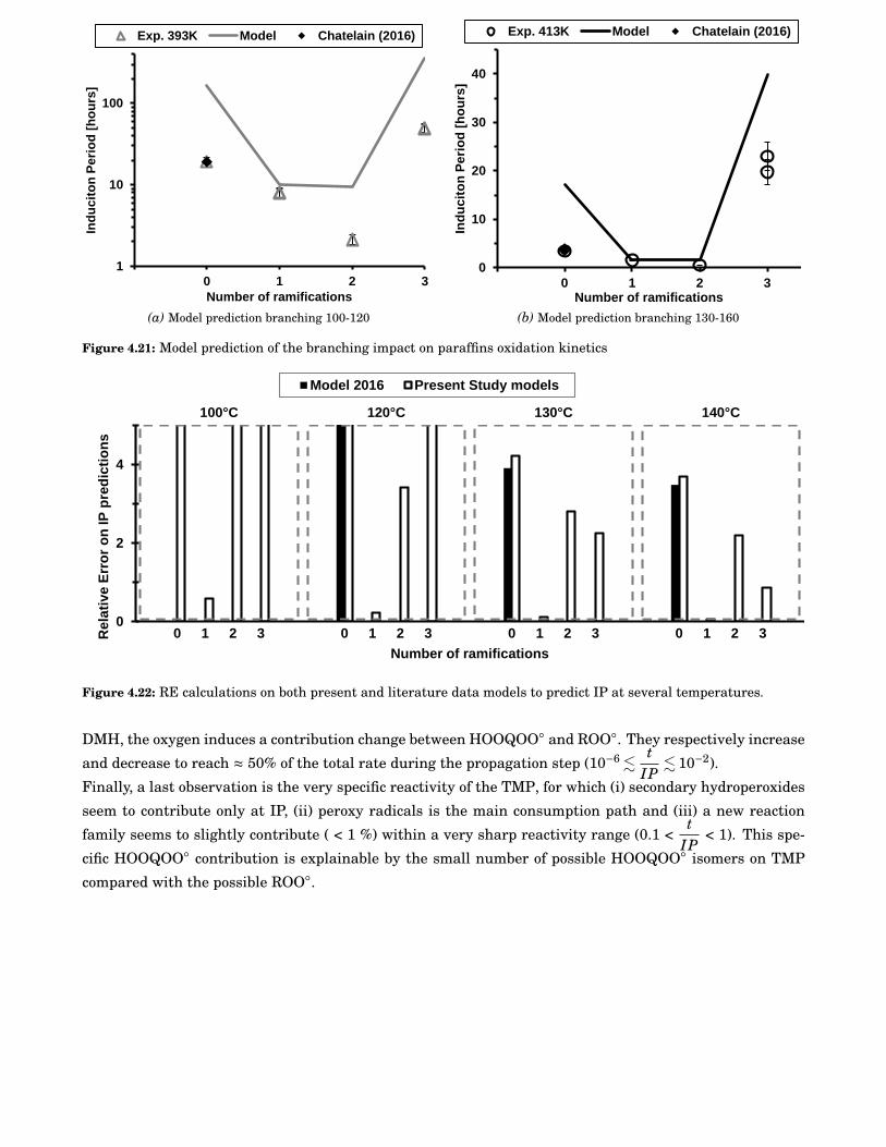
68 Chapter 4

1

10

100

-1 0 1 2 3

Ind

uc

ito

n P

eri

od

[h

ou

rs]

Number of ramifications

Exp. 393K Model Chatelain (2016)

(a) Model prediction branching 100-120

0

10

20

30

40

-1 0 1 2 3

Ind

uc

ito

n P

eri

od

[h

ou

rs]

Number of ramifications

Exp. 413K Model Chatelain (2016)

(b) Model prediction branching 130-160

Figure 4.21: Model prediction of the branching impact on paraffins oxidation kinetics

100°C 120°C 130°C 140°C

0.9

1.9

2.9

3.9

4.9

5.9

6.9

7.9

8.9

9.9

0

2

4

0 1 2 3 0 1 2 3 0 1 2 3 0 1 2 3Re

lati

ve

Err

or

on

IP

pre

dic

tio

ns

Number of ramifications

Model 2016 Present Study models

Figure 4.22: RE calculations on both present and literature data models to predict IP at several temperatures.

DMH, the oxygen induces a contribution change between HOOQOO◦ and ROO◦. They respectively increase

and decrease to reach ≈ 50% of the total rate during the propagation step (10−6.t

IP. 10−2).

Finally, a last observation is the very specific reactivity of the TMP, for which (i) secondary hydroperoxides

seem to contribute only at IP, (ii) peroxy radicals is the main consumption path and (iii) a new reaction

family seems to slightly contribute ( < 1 %) within a very sharp reactivity range (0.1 <t

IP< 1). This spe-

cific HOOQOO◦ contribution is explainable by the small number of possible HOOQOO◦ isomers on TMP

compared with the possible ROO◦.

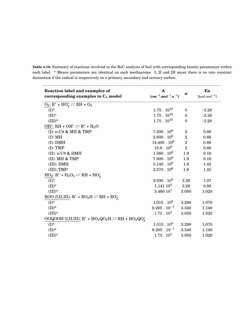
Chapter 4 69

Table 4.10: Summary of reactions involved in the RoC analysis of fuel with corresponding kinetic parameters withineach label. * Means parameters are identical on each mechanisms. I, II and III mean there is no rate constantdistinction if the radical is respectively on a primary, secondary and tertiary carbon.

Reaction label and examples ofcorresponding examples in C8 model

A[cm−3.mol−1.s−1]

n Ea[kcal.mol−1]

O2: R◦ + HO◦2 � RH + O2

(I)* 1.75 . 1010 0 -3.28(II)* 1.75 . 1010 0 -3.28(III)* 1.75 . 1010 0 -3.28

OH◦: RH + OH◦ � R◦ + H2O(I): n-C8 & MH & TMP 7.200 . 106 2 0.86(I): MH 3.600 . 106 2 0.86(I): DMH 14.400 . 106 2 0.86(I): TMP 10.8 . 106 2 0.86(II): n-C8 & DMH 1.580 . 106 1.9 0.16(II): MH & TMP 7.900 . 106 1.9 0.16(III): DMH 5.140 . 106 1.9 1.45(III): TMP 2.570 . 106 1.9 1.45

HO2: R◦ + H2O2 � RH + HO◦2

(I)* 2.030 . 100 3.29 1.07(II)* 1.141 100 3.28 0.88(III)* 3.460 101 3.050 1.020

ROO (I,II,III): R◦ + RO2H� RH + RO◦2

(I)* 1.015 . 100 3.290 1.070(II)* 9.205 . 10−1 3.340 1.140(III)* 1.73 . 101 3.050 1.020

OOQOOH (I,II,III): R◦ + HO2QO2H� RH + HO2QO◦2

(I)* 1.015 . 100 3.290 1.070(II)* 9.205 . 10−1 3.340 1.140(III)* 1.73 . 101 3.050 1.020

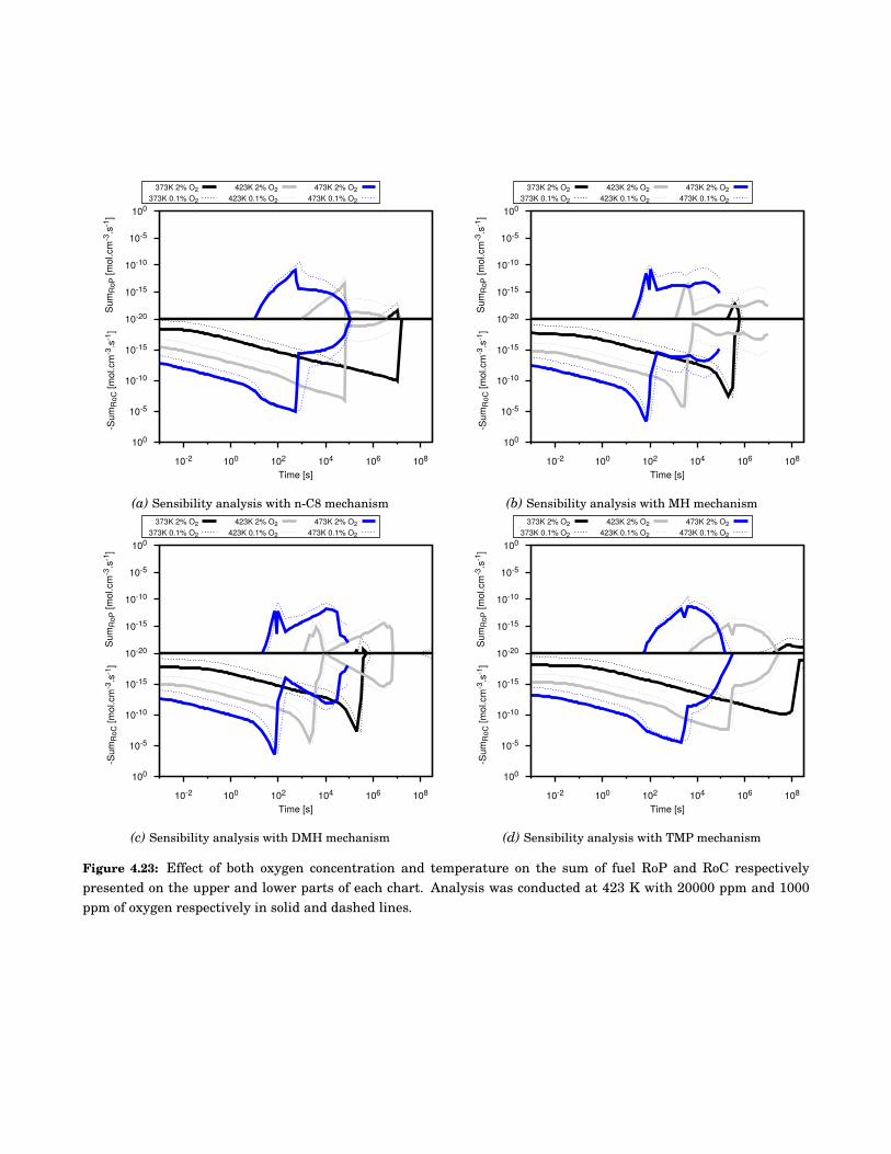
70 Chapter 4

10-20

10-15

10-10

10-5

100

10-2 100 102 104 106 108

-Sum

RoC

[mol

.cm

-3.s

-1]

Time [s]

10-15

10-10

10-5

100

Sum

RoP

[mol

.cm

-3.s

-1]

373K 2% O2373K 0.1% O2

423K 2% O2423K 0.1% O2

473K 2% O2473K 0.1% O2

(a) Sensibility analysis with n-C8 mechanism

10-20

10-15

10-10

10-5

100

10-2 100 102 104 106 108

-Sum

RoC

[mol

.cm

-3.s

-1]

Time [s]

10-15

10-10

10-5

100

Sum

RoP

[mol

.cm

-3.s

-1]

373K 2% O2373K 0.1% O2

423K 2% O2423K 0.1% O2

473K 2% O2473K 0.1% O2

(b) Sensibility analysis with MH mechanism

10-20

10-15

10-10

10-5

100

10-2 100 102 104 106 108

-Sum

RoC

[mol

.cm

-3.s

-1]

Time [s]

10-15

10-10

10-5

100

Sum

RoP

[mol

.cm

-3.s

-1]

373K 2% O2373K 0.1% O2

423K 2% O2423K 0.1% O2

473K 2% O2473K 0.1% O2

(c) Sensibility analysis with DMH mechanism

10-20

10-15

10-10

10-5

100

10-2 100 102 104 106 108

-Sum

RoC

[mol

.cm

-3.s

-1]

Time [s]

10-15

10-10

10-5

100

Sum

RoP

[mol

.cm

-3.s

-1]

373K 2% O2373K 0.1% O2

423K 2% O2423K 0.1% O2

473K 2% O2473K 0.1% O2

(d) Sensibility analysis with TMP mechanism

Figure 4.23: Effect of both oxygen concentration and temperature on the sum of fuel RoP and RoC respectivelypresented on the upper and lower parts of each chart. Analysis was conducted at 423 K with 20000 ppm and 1000ppm of oxygen respectively in solid and dashed lines.

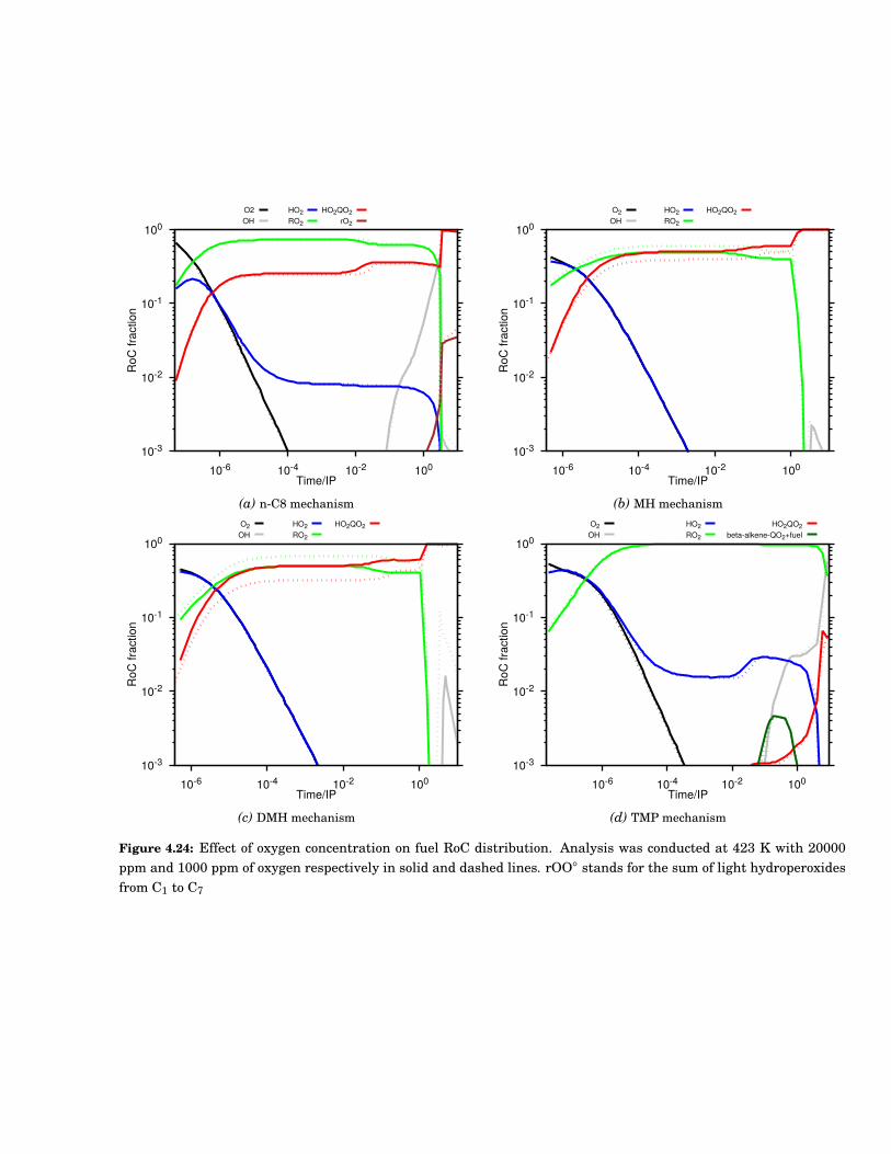
Chapter 4 71

10-3

10-2

10-1

100

10-6 10-4 10-2 100

RoC

frac

tion

Time/IP

O2OH

HO2 RO2

HO2QO2 rO2

(a) n-C8 mechanism

10-3

10-2

10-1

100

10-6 10-4 10-2 100

RoC

frac

tion

Time/IP

O2OH

HO2RO2

HO2QO2

(b) MH mechanism

10-3

10-2

10-1

100

10-6 10-4 10-2 100

RoC

frac

tion

Time/IP

O2OH

HO2RO2

HO2QO2

(c) DMH mechanism

10-3

10-2

10-1

100

10-6 10-4 10-2 100

RoC

frac

tion

Time/IP

O2OH

HO2RO2

HO2QO2beta-alkene-QO2+fuel

(d) TMP mechanism

Figure 4.24: Effect of oxygen concentration on fuel RoC distribution. Analysis was conducted at 423 K with 20000ppm and 1000 ppm of oxygen respectively in solid and dashed lines. rOO◦ stands for the sum of light hydroperoxidesfrom C1 to C7

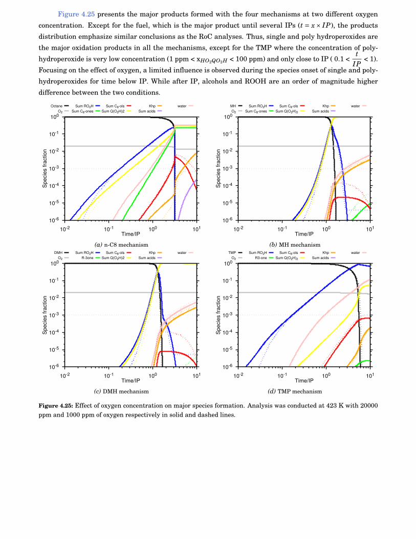
72 Chapter 4

Figure 4.25 presents the major products formed with the four mechanisms at two different oxygen

concentration. Except for the fuel, which is the major product until several IPs (t = x× IP), the products

distribution emphasize similar conclusions as the RoC analyses. Thus, single and poly hydroperoxides are

the major oxidation products in all the mechanisms, except for the TMP where the concentration of poly-

hydroperoxide is very low concentration (1 ppm < xHO2QO2H < 100 ppm) and only close to IP ( 0.1 <t

IP< 1).

Focusing on the effect of oxygen, a limited influence is observed during the species onset of single and poly-

hydroperoxides for time below IP. While after IP, alcohols and ROOH are an order of magnitude higher

difference between the two conditions.

10-6

10-5

10-4

10-3

10-2

10-1

100

10-2 10-1 100 101

Spec

ies

fract

ion

Time/IP

OctaneO2

Sum RO2HSum C8-ones

Sum C8-olsSum Q(O2H)2

KhpSum acids

water

(a) n-C8 mechanism

10-6

10-5

10-4

10-3

10-2

10-1

100

10-2 10-1 100 101

Spec

ies

fract

ion

Time/IP

MHO2

Sum RO2HSum C8-ones

Sum C8-olsSum Q(O2H)2

KhpSum acids

water

(b) MH mechanism

10-6

10-5

10-4

10-3

10-2

10-1

100

10-2 10-1 100 101

Spec

ies

fract

ion

Time/IP

DMHO2

Sum RO2HR-3one

Sum C8-olsSum Q(O2H)2

KhpSum acids

water

(c) DMH mechanism

10-6

10-5

10-4

10-3

10-2

10-1

100

10-2 10-1 100 101

Spec

ies

fract

ion

Time/IP

TMPO2

Sum RO2HR3-one

Sum C8-olsSum Q(O2H)2

KhpSum acids

water

(d) TMP mechanism

Figure 4.25: Effect of oxygen concentration on major species formation. Analysis was conducted at 423 K with 20000ppm and 1000 ppm of oxygen respectively in solid and dashed lines.

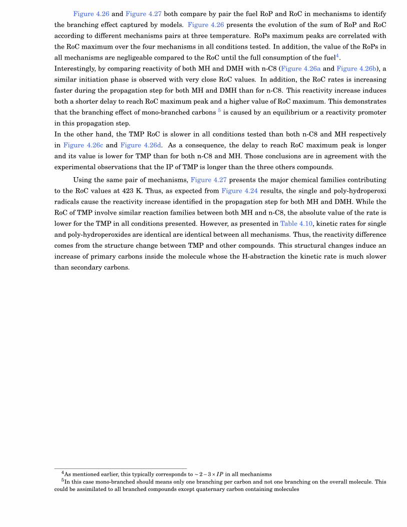
Chapter 4 73

Figure 4.26 and Figure 4.27 both compare by pair the fuel RoP and RoC in mechanisms to identify

the branching effect captured by models. Figure 4.26 presents the evolution of the sum of RoP and RoC

according to different mechanisms pairs at three temperature. RoPs maximum peaks are correlated with

the RoC maximum over the four mechanisms in all conditions tested. In addition, the value of the RoPs in

all mechanisms are negligeable compared to the RoC until the full consumption of the fuel4.

Interestingly, by comparing reactivity of both MH and DMH with n-C8 (Figure 4.26a and Figure 4.26b), a

similar initiation phase is observed with very close RoC values. In addition, the RoC rates is increasing

faster during the propagation step for both MH and DMH than for n-C8. This reactivity increase induces

both a shorter delay to reach RoC maximum peak and a higher value of RoC maximum. This demonstrates

that the branching effect of mono-branched carbons 5 is caused by an equilibrium or a reactivity promoter

in this propagation step.

In the other hand, the TMP RoC is slower in all conditions tested than both n-C8 and MH respectively

in Figure 4.26c and Figure 4.26d. As a consequence, the delay to reach RoC maximum peak is longer

and its value is lower for TMP than for both n-C8 and MH. Those conclusions are in agreement with the

experimental observations that the IP of TMP is longer than the three others compounds.

Using the same pair of mechanisms, Figure 4.27 presents the major chemical families contributing

to the RoC values at 423 K. Thus, as expected from Figure 4.24 results, the single and poly-hydroperoxi

radicals cause the reactivity increase identified in the propagation step for both MH and DMH. While the

RoC of TMP involve similar reaction families between both MH and n-C8, the absolute value of the rate is

lower for the TMP in all conditions presented. However, as presented in Table 4.10, kinetic rates for single

and poly-hydroperoxides are identical are identical between all mechanisms. Thus, the reactivity difference

comes from the structure change between TMP and other compounds. This structural changes induce an

increase of primary carbons inside the molecule whose the H-abstraction the kinetic rate is much slower

than secondary carbons.

4As mentioned earlier, this typically corresponds to ∼ 2−3× IP in all mechanisms5In this case mono-branched should means only one branching per carbon and not one branching on the overall molecule. This

could be assimilated to all branched compounds except quaternary carbon containing molecules

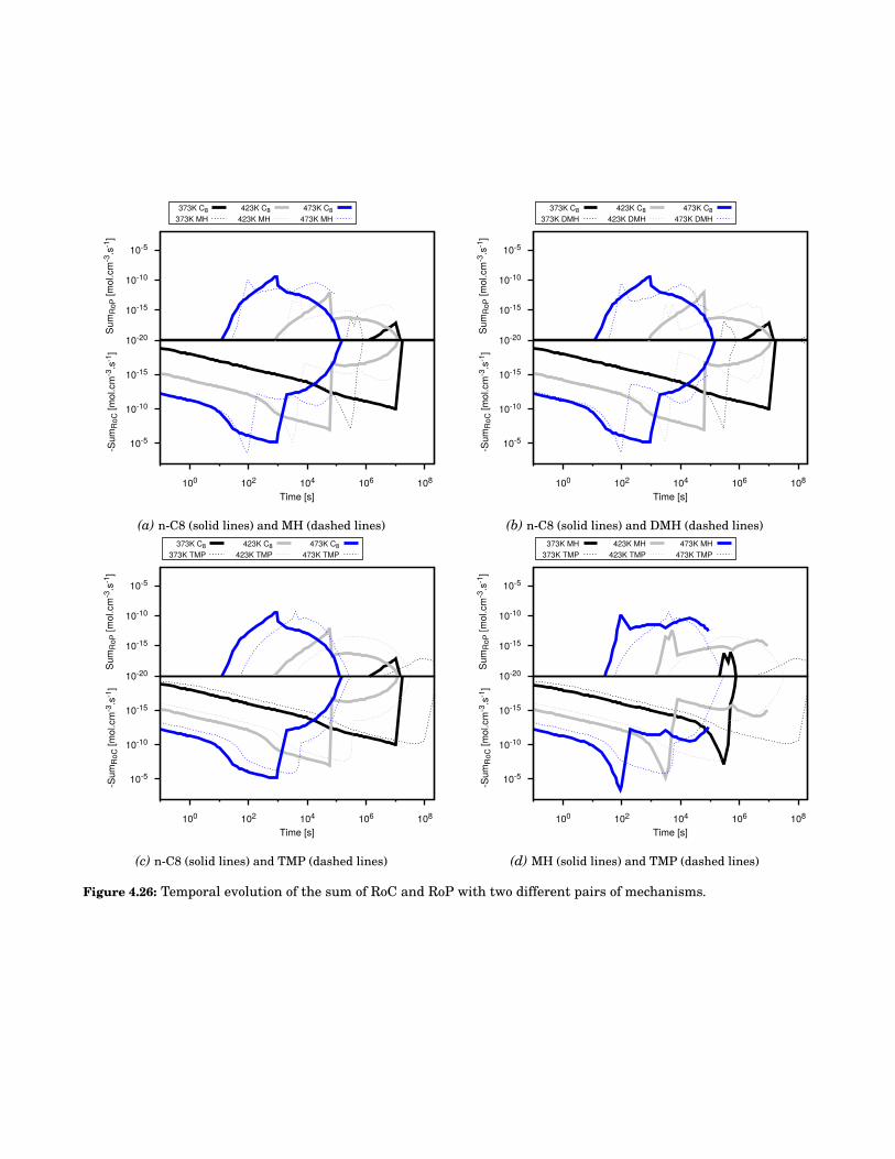
74 Chapter 4

10-20

10-15

10-10

10-5

100 102 104 106 108

-Sum

RoC

[mol

.cm

-3.s

-1]

Time [s]

10-15

10-10

10-5

Sum

RoP

[mol

.cm

-3.s

-1]

373K C8373K MH

423K C8423K MH

473K C8473K MH

(a) n-C8 (solid lines) and MH (dashed lines)

10-20

10-15

10-10

10-5

100 102 104 106 108-S

umR

oC [m

ol.c

m-3

.s-1

]Time [s]

10-15

10-10

10-5

Sum

RoP

[mol

.cm

-3.s

-1]

373K C8373K DMH

423K C8423K DMH

473K C8473K DMH

(b) n-C8 (solid lines) and DMH (dashed lines)

10-20

10-15

10-10

10-5

100 102 104 106 108

-Sum

RoC

[mol

.cm

-3.s

-1]

Time [s]

10-15

10-10

10-5

Sum

RoP

[mol

.cm

-3.s

-1]

373K C8373K TMP

423K C8423K TMP

473K C8473K TMP

(c) n-C8 (solid lines) and TMP (dashed lines)

10-20

10-15

10-10

10-5

100 102 104 106 108

-Sum

RoC

[mol

.cm

-3.s

-1]

Time [s]

10-15

10-10

10-5

Sum

RoP

[mol

.cm

-3.s

-1]

373K MH373K TMP

423K MH423K TMP

473K MH473K TMP

(d) MH (solid lines) and TMP (dashed lines)

Figure 4.26: Temporal evolution of the sum of RoC and RoP with two different pairs of mechanisms.

Chapter 4 75

10-18

10-15

10-12

10-9

10-6

10-2 100 102 104

-Sum

RoC

[mol

.cm

-3.s

-1]

Time [s]

O2OH

HO2 ROO

OOQOOH

(a) n-C8 (solid lines) and MH (dashed lines)

10-18

10-15

10-12

10-9

10-6

10-2 100 102 104-S

umR

oC [m

ol.c

m-3

.s-1

]Time [s]

O2OH

HO2 ROO

OOQOOH

(b) n-C8 (solid lines) and DMH (dashed lines)

10-18

10-15

10-12

10-9

10-6

10-2 100 102 104

-Sum

RoC

[mol

.cm

-3.s

-1]

Time [s]

O2OH

HO2 ROO

OOQOOH

(c) n-C8 (solid lines) and TMP (dashed lines)

10-18

10-15

10-12

10-9

10-6

10-2 100 102 104

-Sum

RoC

[mol

.cm

-3.s

-1]

Time [s]

O2OH

HO2 ROO

OOQOOH

(d) MH (solid lines) and TMP (dashed lines)

Figure 4.27: Temporal evolution of the RoC distribution with different pairs of mechanisms.

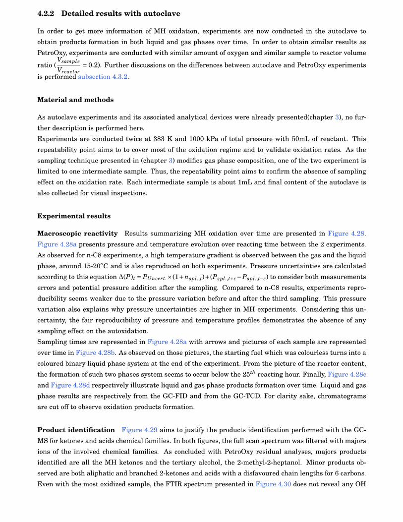
76 Chapter 4

4.2.2 Detailed results with autoclave

In order to get more information of MH oxidation, experiments are now conducted in the autoclave to

obtain products formation in both liquid and gas phases over time. In order to obtain similar results as

PetroOxy, experiments are conducted with similar amount of oxygen and similar sample to reactor volume

ratio (Vsample

Vreactor= 0.2). Further discussions on the differences between autoclave and PetroOxy experiments

is performed subsection 4.3.2.

Material and methods

As autoclave experiments and its associated analytical devices were already presented(chapter 3), no fur-

ther description is performed here.

Experiments are conducted twice at 383 K and 1000 kPa of total pressure with 50mL of reactant. This

repeatability point aims to to cover most of the oxidation regime and to validate oxidation rates. As the

sampling technique presented in (chapter 3) modifies gas phase composition, one of the two experiment is

limited to one intermediate sample. Thus, the repeatability point aims to confirm the absence of sampling

effect on the oxidation rate. Each intermediate sample is about 1mL and final content of the autoclave is

also collected for visual inspections.

Experimental results

Macroscopic reactivity Results summarizing MH oxidation over time are presented in Figure 4.28.

Figure 4.28a presents pressure and temperature evolution over reacting time between the 2 experiments.

As observed for n-C8 experiments, a high temperature gradient is observed between the gas and the liquid

phase, around 15-20◦C and is also reproduced on both experiments. Pressure uncertainties are calculated

according to this equation ∆(P)t = PUncert.×(1+nspl.,t)+(Pspl.,t+ε−Pspl.,t−ε) to consider both measurements

errors and potential pressure addition after the sampling. Compared to n-C8 results, experiments repro-

ducibility seems weaker due to the pressure variation before and after the third sampling. This pressure

variation also explains why pressure uncertainties are higher in MH experiments. Considering this un-

certainty, the fair reproducibility of pressure and temperature profiles demonstrates the absence of any

sampling effect on the autoxidation.

Sampling times are represented in Figure 4.28a with arrows and pictures of each sample are represented

over time in Figure 4.28b. As observed on those pictures, the starting fuel which was colourless turns into a

coloured binary liquid phase system at the end of the experiment. From the picture of the reactor content,

the formation of such two phases system seems to occur below the 25th reacting hour. Finally, Figure 4.28c

and Figure 4.28d respectively illustrate liquid and gas phase products formation over time. Liquid and gas

phase results are respectively from the GC-FID and from the GC-TCD. For clarity sake, chromatograms

are cut off to observe oxidation products formation.

Product identification Figure 4.29 aims to justify the products identification performed with the GC-

MS for ketones and acids chemical families. In both figures, the full scan spectrum was filtered with majors

ions of the involved chemical families. As concluded with PetroOxy residual analyses, majors products

identified are all the MH ketones and the tertiary alcohol, the 2-methyl-2-heptanol. Minor products ob-

served are both aliphatic and branched 2-ketones and acids with a disfavoured chain lengths for 6 carbons.

Even with the most oxidized sample, the FTIR spectrum presented in Figure 4.30 does not reveal any OH

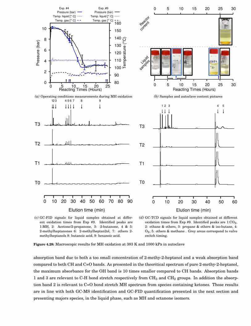
Chapter 4 77

0

2

4

6

8

10

0 5 10 15 20 25 80

90

100

110

120

130

140

150

160

Exp. #4 Exp. #9

Pres

sure

(bar

)

Tem

pera

ture

(°C

)

Reacting Times (Hours)

Pressure (bar)Temp. liquid [° C]

Temp. gas [° C]

Pressure (bar)Temp. liquid [° C]

Temp. gas [° C]

(a) Operating conditions measurements during MH oxidation (b) Samples and autoclave content pictures

0 10 20 30 40 50 60 70 80 90

T0

T1

T2

T3

123 4 5 6 7 8 9

Elution time (min)(c) GC-FID signals for liquid samples obtained at differ-

ent oxidation times from Exp #9. Identified peaks are1:MH, 2: Acetone/2-propanone, 3: 2-butanone, 4 & 5:2-methylheptanones 6: 2-methylheptan2ol, 7: others 2-methylheptanols 8: butanoic acid, 9: hexanoic acid.

0 10 20 30 40 50 60

T0

T1

T2

T3

1 2 3 4 5

Elution time (min)(d) GC-TCD signals for liquid samples obtained at different

oxidation times from Exp #9. Identified peaks are 1:CO2,2: ethane & others, 3: propane & others & iso-butane, 4:O2, 5: others & methane . Grey areas correspond to valveswitch timing.

Figure 4.28: Macroscopic results for MH oxidation at 383 K and 1000 kPa in autoclave

absorption band due to both a too small concentration of 2-methy-2-heptanol and a weak absorption band

compared to both CH and C=O bands. As presented in the theoritical spectrum of pure 2-methy-2-heptanol,

the maximum absorbance for the OH band is 10 times smaller compared to CH bands. Absorption bands

1 and 3 are relevant to C-H bond stretch respectively from CH3 and CH2 groups. In addition the absorp-

tion band 2 is relevant to C=O bond stretch MH spectrum from species containing ketones. Those results

are in line with both GC-MS identification and GC-FID quantification presented in the next section and

presenting majors species, in the liquid phase, such as MH and octanone isomers.

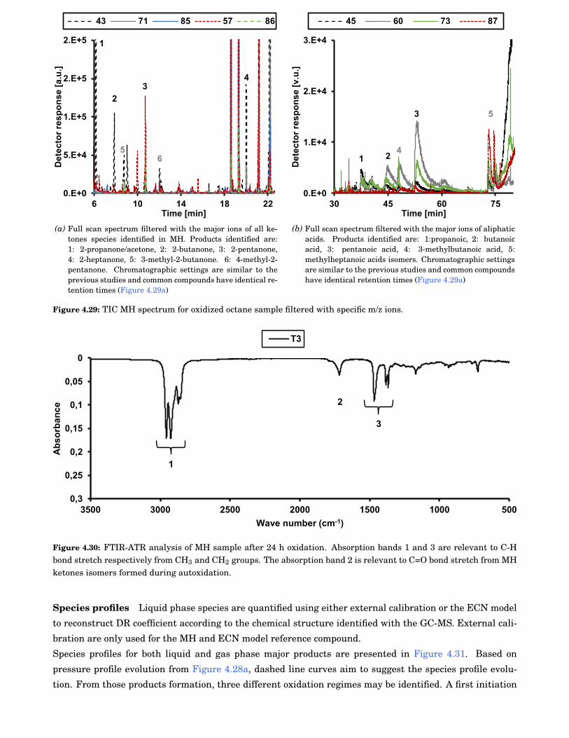
78 Chapter 4

0.E+0

5.E+4

1.E+5

2.E+5

2.E+5

6 10 14 18 22

De

tec

tor

res

po

ns

e [

a.u

.]

Time [min]

43 71 85 57 86

1

2

34

56

(a) Full scan spectrum filtered with the major ions of all ke-tones species identified in MH. Products identified are:1: 2-propanone/acetone, 2: 2-butanone, 3: 2-pentanone,4: 2-heptanone, 5: 3-methyl-2-butanone. 6: 4-methyl-2-pentanone. Chromatographic settings are similar to theprevious studies and common compounds have identical re-tention times (Figure 4.29a)

0.E+0

1.E+4

2.E+4

3.E+4

30 45 60 75

De

tec

tor

res

po

ns

e[v

.u.]

Time [min]

45 60 73 87

1 2

3 5

4

(b) Full scan spectrum filtered with the major ions of aliphaticacids. Products identified are: 1:propanoic, 2: butanoicacid, 3: pentanoic acid, 4: 3-methylbutanoic acid, 5:methylheptanoic acids isomers. Chromatographic settingsare similar to the previous studies and common compoundshave identical retention times (Figure 4.29a)

Figure 4.29: TIC MH spectrum for oxidized octane sample filtered with specific m/z ions.

0

0,05

0,1

0,15

0,2

0,25

0,3

500100015002000250030003500

Ab

so

rba

nc

e

Wave number (cm-1)

T3

1

2

3

Figure 4.30: FTIR-ATR analysis of MH sample after 24 h oxidation. Absorption bands 1 and 3 are relevant to C-Hbond stretch respectively from CH3 and CH2 groups. The absorption band 2 is relevant to C=O bond stretch from MHketones isomers formed during autoxidation.

Species profiles Liquid phase species are quantified using either external calibration or the ECN model

to reconstruct DR coefficient according to the chemical structure identified with the GC-MS. External cali-

bration are only used for the MH and ECN model reference compound.

Species profiles for both liquid and gas phase major products are presented in Figure 4.31. Based on

pressure profile evolution from Figure 4.28a, dashed line curves aim to suggest the species profile evolu-

tion. From those products formation, three different oxidation regimes may be identified. A first initiation

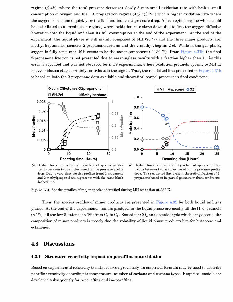
Chapter 4 79

regime (. 4h), where the total pressure decreases slowly due to small oxidation rate with both a small

consumption of oxygen and fuel. A propagation regime (4. t . 12h) with a higher oxidation rate where

the oxygen is consumed quickly by the fuel and induces a pressure drop. A last regime regime which could

be assimilated to a termination regime, where oxidation rate slows down due to first the oxygen diffusive

limitation into the liquid and then its full consumption at the end of the experiment. At the end of the

experiment, the liquid phase is still mainly composed of MH (90 %) and the three major products are:

methyl-heptanones isomers, 2-propanone/acetone and the 2-methy-2heptan-2-ol. While in the gas phase,

oxygen is fully consumed, MH seems to be the major component ( u 30 %). From Figure 4.31b, the final

2-propanone fraction is not presented due to meaningless results with a fraction higher than 1. As this

error is repeated and was not observed for n-C8 experiments, others oxidation products specific to MH at

heavy oxidation stage certainly contribute to the signal. Thus, the red dotted line presented in Figure 4.31b

is based on both the 2-propanone data available and theoretical partial pressure in final conditions.

0.8

0.85

0.9

0.95

1

0

0.005

0.01

0.015

0.02

0.025

0 10 20 30

Mo

le f

rac

tio

n

Mo

le f

rac

tio

n

Reacting time (Hours)

sum C8ketones 2propanone

MH-2ol Methylheptane

(a) Dashed lines represent the hypothetical species profilestrends between two samples based on the pressure profiledrop. Due to very close species profiles trend 2-propanoneand 2-methylpropanol are represents with the same blackdashed line.

0.0

0.2

0.4

0.6

0.8

1.0

0 5 10 15 20 25

Mo

le f

rac

tio

n

Reacting time (Hours)

MH acetone O2

(b) Dashed lines represent the hypothetical species profilestrends between two samples based on the pressure profiledrop. The red dotted line present theoretical fraction of 2-propanone based on its partial pressure in those conditions.

Figure 4.31: Species profiles of major species identified during MH oxidation at 383 K.

Then, the species profiles of minor products are presented in Figure 4.32 for both liquid and gas

phases. At the end of the experiments, minors products in the liquid phase are mostly all the [1-4]-octanols

(≈ 1%), all the low 2-ketones (≈ 1%) from C3 to C6. Except for CO2 and acetaldehyde which are gaseous, the

composition of minor products is mostly due the volatility of liquid phase products like for butanone and

octanones.

4.3 Discussions

4.3.1 Structure reactivity impact on paraffins autoxidation

Based on experimental reactivity trends observed previously, an empirical formula may be used to describe

paraffins reactivity according to temperature, number of carbons and carbons types. Empirical models are

developed subsequently for n-paraffins and iso-paraffins.

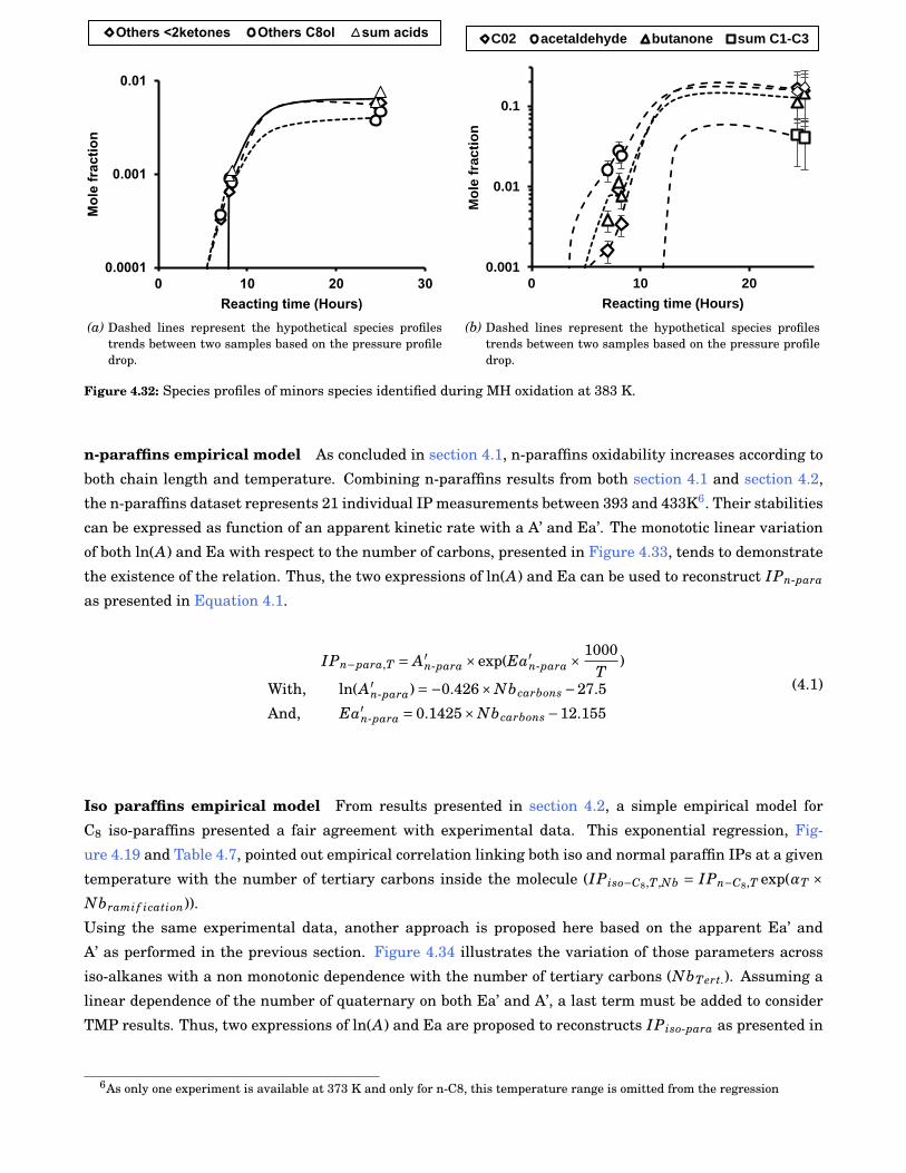
80 Chapter 4

0.0001

0.001

0.01

0 10 20 30

Mo

le f

rac

tio

n

Reacting time (Hours)

Others <2ketones Others C8ol sum acids

(a) Dashed lines represent the hypothetical species profilestrends between two samples based on the pressure profiledrop.

0.001

0.01

0.1

0 10 20

Mo

le f

rac

tio

n

Reacting time (Hours)

C02 acetaldehyde butanone sum C1-C3

(b) Dashed lines represent the hypothetical species profilestrends between two samples based on the pressure profiledrop.

Figure 4.32: Species profiles of minors species identified during MH oxidation at 383 K.

n-paraffins empirical model As concluded in section 4.1, n-paraffins oxidability increases according to

both chain length and temperature. Combining n-paraffins results from both section 4.1 and section 4.2,

the n-paraffins dataset represents 21 individual IP measurements between 393 and 433K6. Their stabilities

can be expressed as function of an apparent kinetic rate with a A’ and Ea’. The monototic linear variation

of both ln(A) and Ea with respect to the number of carbons, presented in Figure 4.33, tends to demonstrate

the existence of the relation. Thus, the two expressions of ln(A) and Ea can be used to reconstruct IPn-para

as presented in Equation 4.1.

IPn−para,T = A′n-para ×exp(Ea′

n-para ×1000

T)

With, ln(A′n-para)=−0.426×Nbcarbons −27.5

And, Ea′n-para = 0.1425×Nbcarbons −12.155

(4.1)

Iso paraffins empirical model From results presented in section 4.2, a simple empirical model for

C8 iso-paraffins presented a fair agreement with experimental data. This exponential regression, Fig-

ure 4.19 and Table 4.7, pointed out empirical correlation linking both iso and normal paraffin IPs at a given

temperature with the number of tertiary carbons inside the molecule (IPiso−C8,T,Nb = IPn−C8,T exp(αT ×Nbrami f ication)).

Using the same experimental data, another approach is proposed here based on the apparent Ea’ and

A’ as performed in the previous section. Figure 4.34 illustrates the variation of those parameters across

iso-alkanes with a non monotonic dependence with the number of tertiary carbons (NbTert.). Assuming a

linear dependence of the number of quaternary on both Ea’ and A’, a last term must be added to consider

TMP results. Thus, two expressions of ln(A) and Ea are proposed to reconstructs IPiso-para as presented in

6As only one experiment is available at 373 K and only for n-C8, this temperature range is omitted from the regression

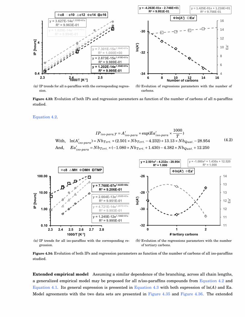
Chapter 4 81

y = 3.627E-14e1.335E+01x

R² = 9.963E-01

y = 1.829E-14e1.351E+01x

R² = 9.994E-01

y = 7.301E-15e1.384E+01x

R² = 1.000E+00

y = 2.873E-15e1.419E+01x

R² = 9.989E-01

y = 1.202E-14e1.354E+01x

R² = 9.995E-010.4

4

2.3 2.4 2.5

IP [

ho

urs

]

1000/T [K-1]

c8 c10 c12 c14 c16

(a) IP trends for all n-paraffins with the corresponding regres-sion.

y = -4.263E-01x - 2.746E+01R² = 9.951E-01

y = 1.425E-01x + 1.216E+01R² = 9.756E-01

4

6

8

10

12

14

16

-34

-32

-30

6 8 10 12 14 16

Ea'

ln(A

')

Number of carbons

ln(A') Ea'

(b) Evolution of regressions parameters with the number ofcarbons.

Figure 4.33: Evolution of both IPs and regression parameters as function of the number of carbons of all n-paraffinsstudied.

Equation 4.2.

IPiso-para,T = A′iso-para ×exp(Ea′

iso-para ×1000

T)

With, ln(A′iso-para)= NbTert. × (2.501×NbTert. −4.232)+13.13×NbQuat. −28.954

And, Ea′iso-para = NbTert. × (−1.080×NbTert. +1.430)−4.382×NbQuat. +12.250

(4.2)

y = 2.664E-13e1.252E+01x

R² = 9.951E-01

y = 4.721E-14e1.287E+01x

R² = 9.993E-01

y = 1.245E-12e1.106E+01x

R² = 9.995E-01

y = 7.760E-07e7.022E+00x

R² = 9.206E-01

0.10

1.00

10.00

100.00

2.3 2.4 2.5 2.6 2.7 2.8

IP [

ho

urs

]

1000/T [K-1]

c8 MH DMH TMP

(a) IP trends for all iso-paraffins with the corresponding re-gression.

y = 2.501x2 - 4.232x - 28.954R² = 1.000

y = -1.080x2 + 1.430x + 12.520R² = 1.000

11

11

12

12

13

13

14

-32

-30

-28

-26

0 1 2E

a'

ln(A

')

# tertiary carbons

ln(A') Ea'

(b) Evolution of the regressions parameters with the numberof tertiary carbons.

Figure 4.34: Evolution of both IPs and regression parameters as function of the number of carbons of all iso-paraffinsstudied.

Extended empirical model Assuming a similar dependence of the branching, across all chain lengths,

a generalized empirical model may be proposed for all n/iso-paraffins compounds from Equation 4.2 and

Equation 4.1. Its general expression is presented in Equation 4.3 with both expression of ln(A) and Ea.

Model agreements with the two data sets are presented in Figure 4.35 and Figure 4.36. The extended

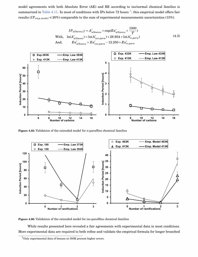
82 Chapter 4

model agreements with both Absolute Error (AE) and RE according to iso/normal chemical families is

summarized in Table 4.11. In most of conditions with IPs below 72 hours 7: this empirical model offers fair

results (IPemp.model É 20%) comparable to the sum of experimental measurements uncertainties (15%).

IPalkanes,T = A′alkanes ×exp(Ea′

alkanes ×1000

T)

With, ln(A′alkanes)= ln(A′

iso-para)+28.954+ ln(A′n-para)

And, Ea′alkanes = Ea′

iso-para −12.250+Ea′n-para

(4.3)

0

10

20

30

40

50

60

4 6 8 10 12 14 16

Ind

ucit

on

Peri

od

[h

ou

rs]

Number of carbons

Exp.393K Emp. Law 393K

Exp. 413K Emp. Law 413K

0

1

2

3

4

5

4 6 8 10 12 14 16

Ind

uc

ito

n P

eri

od

[h

ou

rs]

Number of carbons

Exp. 433K Emp. Law 433K

Exp. 413K Emp. Law 413K

Figure 4.35: Validation of the extended model for n-paraffins chemical families

0

20

40

60

80

100

120

-1 0 1 2 3

Ind

uc

ito

n P

eri

od

[h

ou

rs]

Number of ramifications

Exp. 100 Emp. Law 373K

Exp. 120 Emp. Law 393K

0

5

10

15

20

25

30

35

40

-1 0 1 2 3

Ind

uc

ito

n P

eri

od

[h

ou

rs]

Number of ramifications

Exp. 403K Emp. Model 403K

Exp. 413K Emp. Model 413K

Figure 4.36: Validation of the extended model for iso-paraffins chemical families

While results presented here revealed a fair agreements with experimental data in most conditions.

More experimental data are required to both refine and validate the empirical formula for longer branched

7Only experimental data of hexane at 393K present higher errors.

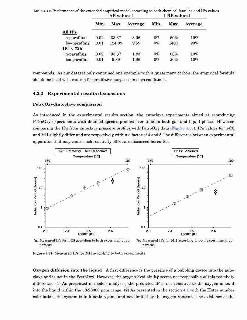
Chapter 4 83

Table 4.11: Performance of the extended empirical model according to both chemical families and IPs values| AE values | | RE values|

Min. Max. Average Min. Max. Average

All IPsn-paraffins 0.02 33.37 3.06 0% 60% 10%Iso-paraffins 0.01 124.09 9.59 0% 140% 20%

IPs < 72hn-paraffins 0.02 33.37 1.83 0% 60% 10%Iso-paraffins 0.01 9.89 1.96 0% 20% 10%

compounds. As our dataset only contained one example with a quaternary carbon, the empirical formula

should be used with caution for predictive purposes in such conditions.

4.3.2 Experimental results discussions

PetroOxy-Autoclave comparison

As introduced in the experimental results section, the autoclave experiments aimed at reproducing

PetroOxy experiments with detailed species profiles over time on both gas and liquid phase. However,

comparing the IPs from autoclave pressure profiles with PetroOxy data (Figure 4.37), IPs values for n-C8

and MH slightly differ and are respectively within a factor of 4 and 5.The differences between experimental

apparatus that may cause such reactivity offset are discussed hereafter.

100160

0.1

1

10

100

2.3 2.4 2.5 2.6

Temperature [°C]

Ind

ucit

on

Peri

od

[h

ou

rs]

1000/T [K-1]

C8 PetroOxy C8 autoclave

(a) Measured IPs for n-C8 according to both experimental ap-paratus

100160

0.1

1

10

100

2.3 2.4 2.5 2.6

Temperature [°C]

Ind

ucit

on

Peri

od

[h

ou

rs]

1000/T [K-1]

1C8 Série3

(b) Measured IPs for MH according to both experimental ap-paratus

Figure 4.37: Measured IPs for MH according to both experiments

Oxygen diffusion into the liquid A first difference is the presence of a bubbling device into the auto-

clave and is not in the PetroOxy. However, the oxygen availability seems not responsible of this reactivity

difference. (1) As presented in models analyses, the predicted IP is not sensitive to the oxygen amount

into the liquid within the 50-20000 ppm range. (2) As presented in the section 4.1 with the Hatta number

calculation, the system is in kinetic regime and not limited by the oxygen content. The existence of the

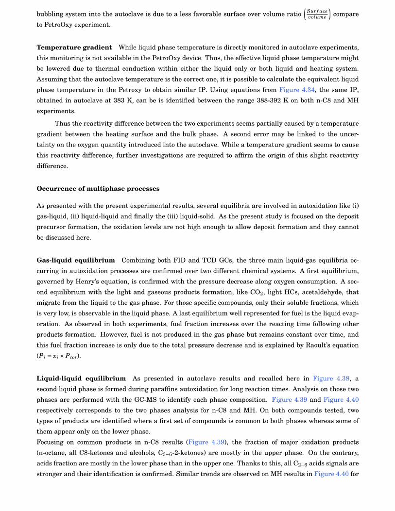
84 Chapter 4

bubbling system into the autoclave is due to a less favorable surface over volume ratio(

Sur f acevolume

)compare

to PetroOxy experiment.

Temperature gradient While liquid phase temperature is directly monitored in autoclave experiments,

this monitoring is not available in the PetroOxy device. Thus, the effective liquid phase temperature might

be lowered due to thermal conduction within either the liquid only or both liquid and heating system.

Assuming that the autoclave temperature is the correct one, it is possible to calculate the equivalent liquid

phase temperature in the Petroxy to obtain similar IP. Using equations from Figure 4.34, the same IP,

obtained in autoclave at 383 K, can be is identified between the range 388-392 K on both n-C8 and MH

experiments.

Thus the reactivity difference between the two experiments seems partially caused by a temperature

gradient between the heating surface and the bulk phase. A second error may be linked to the uncer-

tainty on the oxygen quantity introduced into the autoclave. While a temperature gradient seems to cause

this reactivity difference, further investigations are required to affirm the origin of this slight reactivity

difference.

Occurrence of multiphase processes

As presented with the present experimental results, several equilibria are involved in autoxidation like (i)

gas-liquid, (ii) liquid-liquid and finally the (iii) liquid-solid. As the present study is focused on the deposit

precursor formation, the oxidation levels are not high enough to allow deposit formation and they cannot

be discussed here.

Gas-liquid equilibrium Combining both FID and TCD GCs, the three main liquid-gas equilibria oc-

curring in autoxidation processes are confirmed over two different chemical systems. A first equilibrium,

governed by Henry’s equation, is confirmed with the pressure decrease along oxygen consumption. A sec-

ond equilibrium with the light and gaseous products formation, like CO2, light HCs, acetaldehyde, that

migrate from the liquid to the gas phase. For those specific compounds, only their soluble fractions, which

is very low, is observable in the liquid phase. A last equilibrium well represented for fuel is the liquid evap-

oration. As observed in both experiments, fuel fraction increases over the reacting time following other

products formation. However, fuel is not produced in the gas phase but remains constant over time, and

this fuel fraction increase is only due to the total pressure decrease and is explained by Raoult’s equation

(Pi = xi ×Ptot).

Liquid-liquid equilibrium As presented in autoclave results and recalled here in Figure 4.38, a

second liquid phase is formed during paraffins autoxidation for long reaction times. Analysis on those two

phases are performed with the GC-MS to identify each phase composition. Figure 4.39 and Figure 4.40

respectively corresponds to the two phases analysis for n-C8 and MH. On both compounds tested, two

types of products are identified where a first set of compounds is common to both phases whereas some of

them appear only on the lower phase.

Focusing on common products in n-C8 results (Figure 4.39), the fraction of major oxidation products

(n-octane, all C8-ketones and alcohols, C3−6-2-ketones) are mostly in the upper phase. On the contrary,

acids fraction are mostly in the lower phase than in the upper one. Thanks to this, all C2−6 acids signals are

stronger and their identification is confirmed. Similar trends are observed on MH results in Figure 4.40 for

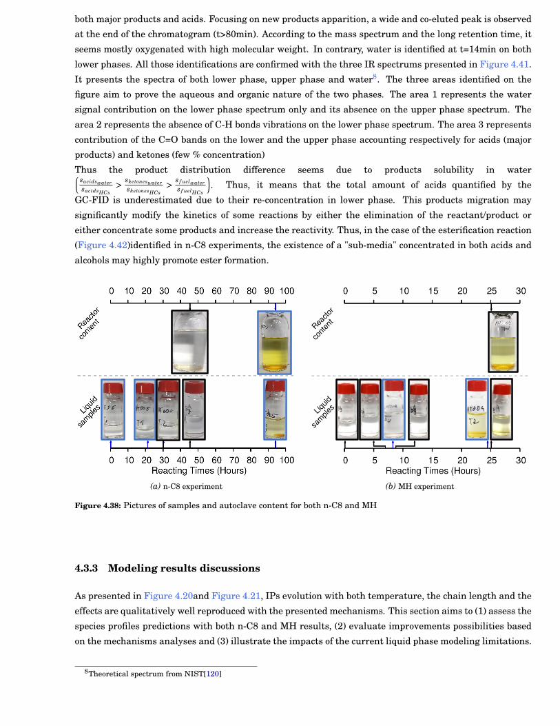
Chapter 4 85

both major products and acids. Focusing on new products apparition, a wide and co-eluted peak is observed

at the end of the chromatogram (t>80min). According to the mass spectrum and the long retention time, it

seems mostly oxygenated with high molecular weight. In contrary, water is identified at t=14min on both

lower phases. All those identifications are confirmed with the three IR spectrums presented in Figure 4.41.

It presents the spectra of both lower phase, upper phase and water8. The three areas identified on the

figure aim to prove the aqueous and organic nature of the two phases. The area 1 represents the water

signal contribution on the lower phase spectrum only and its absence on the upper phase spectrum. The

area 2 represents the absence of C-H bonds vibrations on the lower phase spectrum. The area 3 represents

contribution of the C=O bands on the lower and the upper phase accounting respectively for acids (major

products) and ketones (few % concentration)

Thus the product distribution difference seems due to products solubility in water(sacidswatersacidsHCs

> sketoneswatersketonesHCs

> s f uelwaters f uelHCs

). Thus, it means that the total amount of acids quantified by the

GC-FID is underestimated due to their re-concentration in lower phase. This products migration may

significantly modify the kinetics of some reactions by either the elimination of the reactant/product or

either concentrate some products and increase the reactivity. Thus, in the case of the esterification reaction

(Figure 4.42)identified in n-C8 experiments, the existence of a "sub-media" concentrated in both acids and

alcohols may highly promote ester formation.

(a) n-C8 experiment (b) MH experiment

Figure 4.38: Pictures of samples and autoclave content for both n-C8 and MH

4.3.3 Modeling results discussions

As presented in Figure 4.20and Figure 4.21, IPs evolution with both temperature, the chain length and the

effects are qualitatively well reproduced with the presented mechanisms. This section aims to (1) assess the

species profiles predictions with both n-C8 and MH results, (2) evaluate improvements possibilities based

on the mechanisms analyses and (3) illustrate the impacts of the current liquid phase modeling limitations.

8Theoretical spectrum from NIST[120]

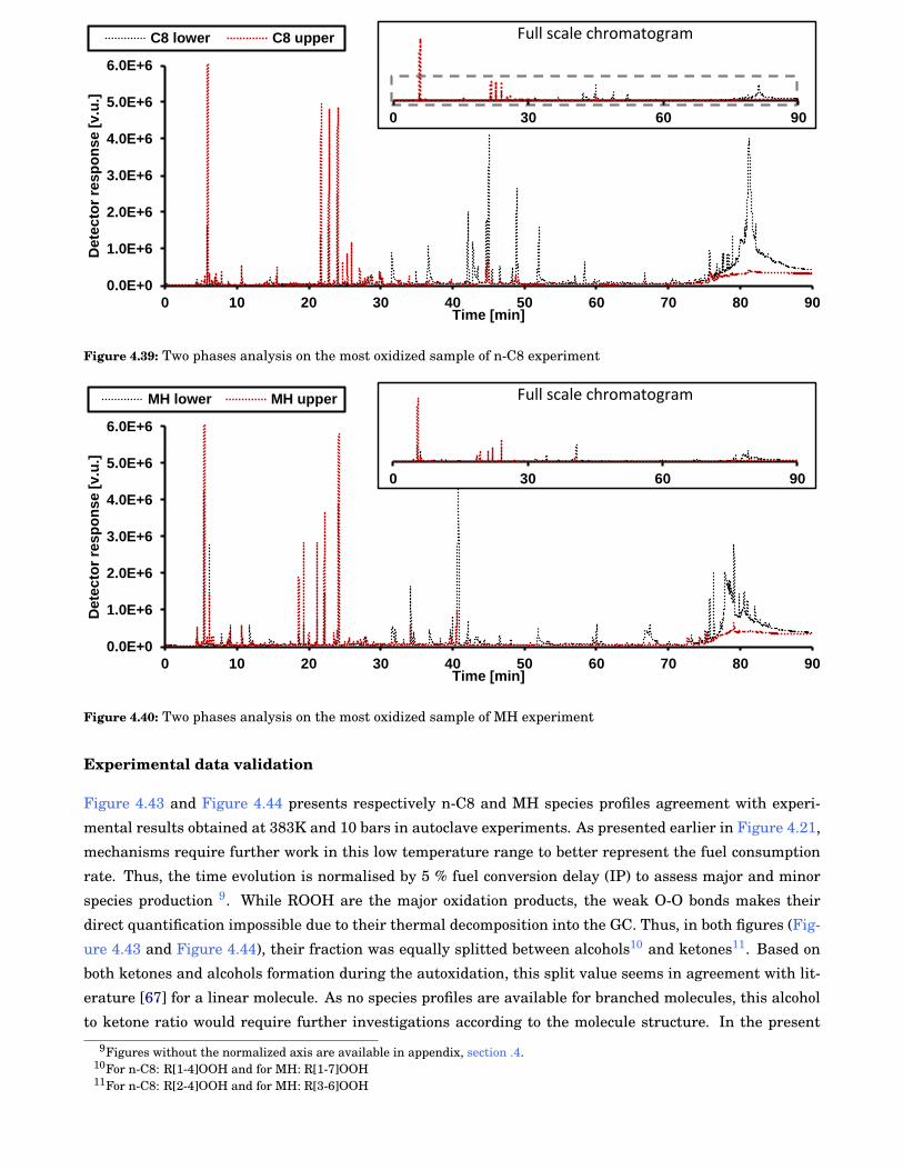
86 Chapter 4

0.0E+0

1.0E+6

2.0E+6

3.0E+6

4.0E+6

5.0E+6

6.0E+6

0 10 20 30 40 50 60 70 80 90

De

tec

tor

resp

on

se

[v.u

.]

Time [min]

C8 lower C8 upper

0 30 60 90

Full scale chromatogram

Figure 4.39: Two phases analysis on the most oxidized sample of n-C8 experiment

0.0E+0

1.0E+6

2.0E+6

3.0E+6

4.0E+6

5.0E+6

6.0E+6

0 10 20 30 40 50 60 70 80 90

Dete

cto

r re

sp

on

se

[v.u

.]

Time [min]

MH lower MH upper

0 30 60 90

Full scale chromatogram

Figure 4.40: Two phases analysis on the most oxidized sample of MH experiment

Experimental data validation

Figure 4.43 and Figure 4.44 presents respectively n-C8 and MH species profiles agreement with experi-

mental results obtained at 383K and 10 bars in autoclave experiments. As presented earlier in Figure 4.21,

mechanisms require further work in this low temperature range to better represent the fuel consumption

rate. Thus, the time evolution is normalised by 5 % fuel conversion delay (IP) to assess major and minor

species production 9. While ROOH are the major oxidation products, the weak O-O bonds makes their

direct quantification impossible due to their thermal decomposition into the GC. Thus, in both figures (Fig-

ure 4.43 and Figure 4.44), their fraction was equally splitted between alcohols10 and ketones11. Based on

both ketones and alcohols formation during the autoxidation, this split value seems in agreement with lit-

erature [67] for a linear molecule. As no species profiles are available for branched molecules, this alcohol

to ketone ratio would require further investigations according to the molecule structure. In the present

9Figures without the normalized axis are available in appendix, section .4.10For n-C8: R[1-4]OOH and for MH: R[1-7]OOH11For n-C8: R[2-4]OOH and for MH: R[3-6]OOH

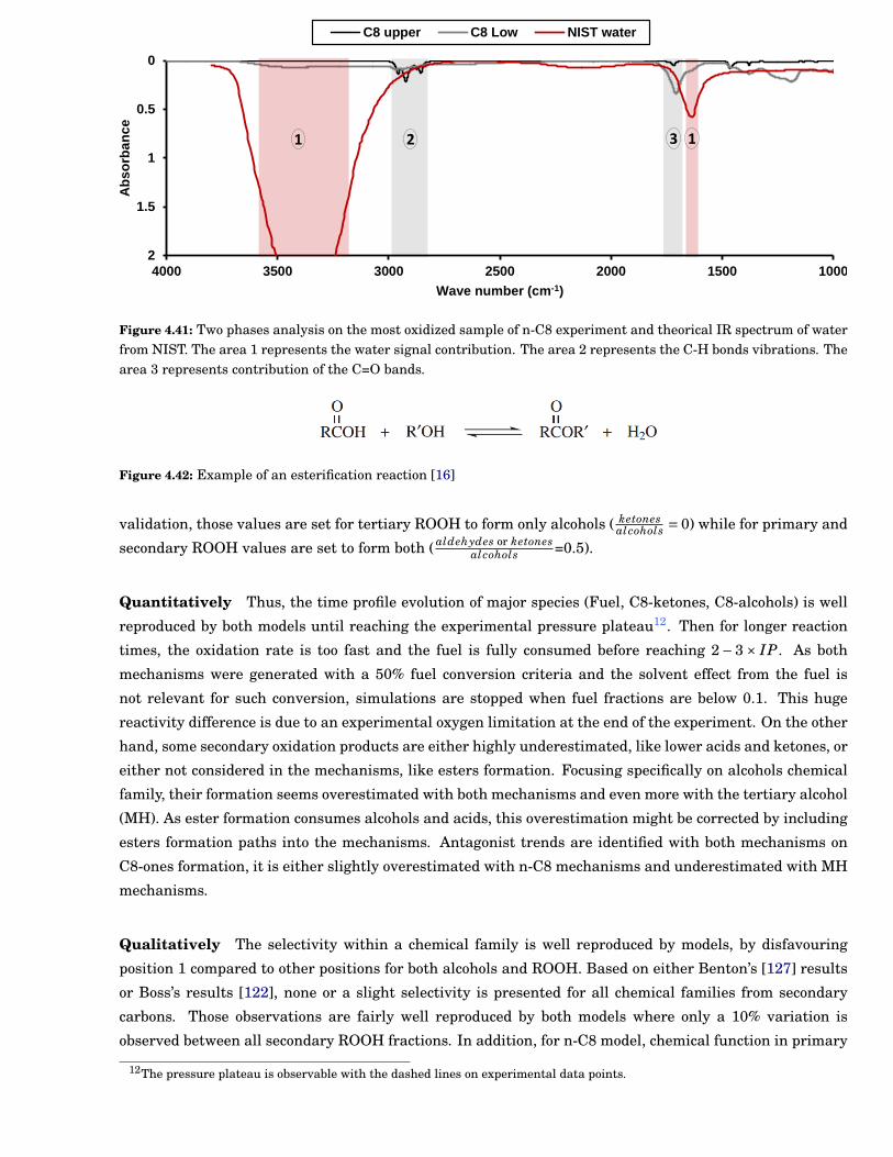
Chapter 4 87

0

0.5

1

1.5

2

1000150020002500300035004000

Ab

so

rba

nc

e

Wave number (cm-1)

C8 upper C8 Low NIST water

12 31

Figure 4.41: Two phases analysis on the most oxidized sample of n-C8 experiment and theorical IR spectrum of waterfrom NIST. The area 1 represents the water signal contribution. The area 2 represents the C-H bonds vibrations. Thearea 3 represents contribution of the C=O bands.

Figure 4.42: Example of an esterification reaction [16]

validation, those values are set for tertiary ROOH to form only alcohols ( ketonesalcohols = 0) while for primary and

secondary ROOH values are set to form both ( aldehydes or ketonesalcohols =0.5).

Quantitatively Thus, the time profile evolution of major species (Fuel, C8-ketones, C8-alcohols) is well

reproduced by both models until reaching the experimental pressure plateau12. Then for longer reaction

times, the oxidation rate is too fast and the fuel is fully consumed before reaching 2− 3× IP. As both

mechanisms were generated with a 50% fuel conversion criteria and the solvent effect from the fuel is

not relevant for such conversion, simulations are stopped when fuel fractions are below 0.1. This huge

reactivity difference is due to an experimental oxygen limitation at the end of the experiment. On the other

hand, some secondary oxidation products are either highly underestimated, like lower acids and ketones, or

either not considered in the mechanisms, like esters formation. Focusing specifically on alcohols chemical

family, their formation seems overestimated with both mechanisms and even more with the tertiary alcohol

(MH). As ester formation consumes alcohols and acids, this overestimation might be corrected by including

esters formation paths into the mechanisms. Antagonist trends are identified with both mechanisms on

C8-ones formation, it is either slightly overestimated with n-C8 mechanisms and underestimated with MH

mechanisms.

Qualitatively The selectivity within a chemical family is well reproduced by models, by disfavouring

position 1 compared to other positions for both alcohols and ROOH. Based on either Benton’s [127] results

or Boss’s results [122], none or a slight selectivity is presented for all chemical families from secondary

carbons. Those observations are fairly well reproduced by both models where only a 10% variation is

observed between all secondary ROOH fractions. In addition, for n-C8 model, chemical function in primary

12The pressure plateau is observable with the dashed lines on experimental data points.

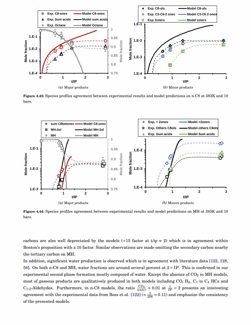
88 Chapter 4

0.75

0.8

0.85

0.9

0.95

1

1.E-4

1.E-3

1.E-2

1.E-1

0 1 2 3

Mo

le f

rac

tio

n

Mo

le f

rac

tio

n

t/IP

Exp. C8-ones Model C8-ones

Exp. Sum acids Model sum acids

Exp. Octane Model Octane

(a) Major products

1.E-4

1.E-3

1.E-2

1.E-1

0 1 2 3

Mo

le f

rac

tio

n

t/IP

Exp. C8-ols Model C8-ols

Exp. C3-C6-2 ones Model C3-C6 2-ones

Exp. Esters Model esters

(b) Minor products

Figure 4.43: Species profiles agreement between experimental results and model predictions on n-C8 at 383K and 10bars.

0.75

0.8

0.85

0.9

0.95

1

1.E-3

1.E-2

1.E-1

0 1 2 3

Mo

le f

rac

tio

n

Mo

le f

rac

tio

n

t/IP

sum C8ketones Model C8-ones

MH-2ol Model MH-2ol

MH Model MH

(a) Major products

1.E-4

1.E-3

1.E-2

0 1 2 3

Mo

le f

rac

tio

n

t/IP

Exp. < 2ones Model <2ones

Exp. Others C8ols Model others C8ols

Exp. Sum acids Model Sum acids

(b) Minors products

Figure 4.44: Species profiles agreement between experimental results and model predictions on MH at 383K and 10bars.

carbons are also well depreciated by the models (×15 factor at t/ip = 2) which is in agreement within

Benton’s proposition with a 10 factor. Similar observations are made omitting the secondary carbon nearby

the tertiary carbon on MH.

In addition, significant water production is observed which is in agreement with literature data [122, 128,

56]. On both n-C8 and MH, water fractions are around several percent at 2× IP. This is confirmed in our

experimental second phase formation mostly composed of water. Except the absence of CO2 in MH models,

most of gaseous products are qualitatively produced in both models including CO, H2, C1 to C4 HCs and

C1-2-Aldehydes. Furthermore, in n-C8 models, the ratio CO2water ≈ 0.01 at t

IP = 2 presents an interesting

agreement with the experimental data from Boss et al. [122] (≈ 3256 ≈ 0.11) and emphasize the consistency

of the presented models.

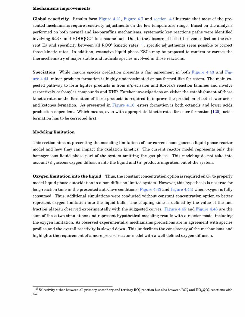
Chapter 4 89

Mechanisms improvements

Global reactivity Results form Figure 4.21, Figure 4.7 and section .4 illustrate that most of the pre-

sented mechanisms require reactivity adjustments on the low temperature range. Based on the analysis

performed on both normal and iso-paraffins mechanisms, systematic key reactions paths were identified

involving ROO◦ and HOOQOO◦ to consume fuel. Due to the absence of both (i) solvent effect on the cur-

rent Ea and specificity between all ROO◦ kinetic rates 13, specific adjustments seem possible to correct

those kinetic rates. In addition, extensive liquid phase ESCs may be proposed to confirm or correct the

thermochemistry of major stable and radicals species involved in those reactions.

Speciation While majors species prediction presents a fair agreement in both Figure 4.43 and Fig-

ure 4.44, minor products formation is highly underestimated or not formed like for esters. The main ex-

pected pathway to form lighter products is from α/β-scission and Korcek’s reaction families and involve

respectively carbonyles compounds and KHP. Further investigations on either the establishment of those

kinetic rates or the formation of those products is required to improve the prediction of both lower acids

and ketones formation. As presented in Figure 4.16, esters formation is both octanols and lower acids

production dependent. Which means, even with appropriate kinetic rates for ester formation [120], acids

formation has to be corrected first.

Modeling limitation

This section aims at presenting the modeling limitations of our current homogeneous liquid phase reactor

model and how they can impact the oxidation kinetics. The current reactor model represents only the

homogeneous liquid phase part of the system omitting the gas phase. This modeling do not take into

account (i) gaseous oxygen diffusion into the liquid and (ii) products migration out of the system.

Oxygen limitation into the liquid Thus, the constant concentration option is required on O2 to properly

model liquid phase autoxidation in a non diffusion limited system. However, this hypothesis is not true for

long reaction time in the presented autoclave conditions (Figure 4.43 and Figure 4.44) when oxygen is fully

consumed. Thus, additional simulations were conducted without constant concentration option to better

represent oxygen limitation into the liquid bulk. The coupling time is defined by the value of the fuel

fraction plateau observed experimentally with the suggested curves. Figure 4.45 and Figure 4.46 are the

sum of those two simulations and represent hypothetical modeling results with a reactor model including

the oxygen limitation. As observed experimentally, mechanisms predictions are in agreement with species

profiles and the overall reactivity is slowed down. This underlines the consistency of the mechanisms and

highlights the requirement of a more precise reactor model with a well defined oxygen diffusion.

13Selectivity either between all primary, secondary and tertiary RO◦2 reaction but also between RO◦

2 and HO2QO◦2 reactions with

fuel

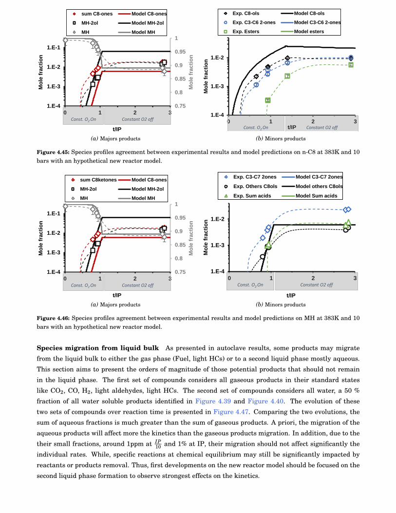
90 Chapter 4

0.75

0.8

0.85

0.9

0.95

1

1.E-4

1.E-3

1.E-2

1.E-1

0 1 2 3

Mo

le f

rac

tio

n

Mo

le f

rac

tio

n

t/IP

sum C8-ones Model C8-ones

MH-2ol Model MH-2ol

MH Model MH

Constant O2 offConst. O2 On

(a) Majors products

1.E-4

1.E-3

1.E-2

0 1 2 3

Mo

le f

rac

tio

n

t/IP

Exp. C8-ols Model C8-ols

Exp. C3-C6 2-ones Model C3-C6 2-ones

Exp. Esters Model esters

Constant O2 offConst. O2 On

(b) Minors products

Figure 4.45: Species profiles agreement between experimental results and model predictions on n-C8 at 383K and 10bars with an hypothetical new reactor model.

0.75

0.8

0.85

0.9

0.95

1

1.E-4

1.E-3

1.E-2

1.E-1

0 1 2 3

Mo

le f

rac

tio

n

Mo

le f

rac

tio

n

t/IP

sum C8ketones Model C8-ones

MH-2ol Model MH-2ol

MH Model MH

Constant O2 offConst. O2 On

(a) Majors products

1.E-4

1.E-3

1.E-2

0 1 2 3

Mo

le f

rac

tio

n

t/IP

Exp. C3-C7 2ones Model C3-C7 2ones

Exp. Others C8ols Model others C8ols

Exp. Sum acids Model Sum acids

Constant O2 offConst. O2 On

(b) Minors products

Figure 4.46: Species profiles agreement between experimental results and model predictions on MH at 383K and 10bars with an hypothetical new reactor model.

Species migration from liquid bulk As presented in autoclave results, some products may migrate

from the liquid bulk to either the gas phase (Fuel, light HCs) or to a second liquid phase mostly aqueous.

This section aims to present the orders of magnitude of those potential products that should not remain

in the liquid phase. The first set of compounds considers all gaseous products in their standard states

like CO2, CO, H2, light aldehydes, light HCs. The second set of compounds considers all water, a 50 %

fraction of all water soluble products identified in Figure 4.39 and Figure 4.40. The evolution of these

two sets of compounds over reaction time is presented in Figure 4.47. Comparing the two evolutions, the

sum of aqueous fractions is much greater than the sum of gaseous products. A priori, the migration of the

aqueous products will affect more the kinetics than the gaseous products migration. In addition, due to the

their small fractions, around 1ppm at IP10 and 1% at IP, their migration should not affect significantly the

individual rates. While, specific reactions at chemical equilibrium may still be significantly impacted by

reactants or products removal. Thus, first developments on the new reactor model should be focused on the

second liquid phase formation to observe strongest effects on the kinetics.

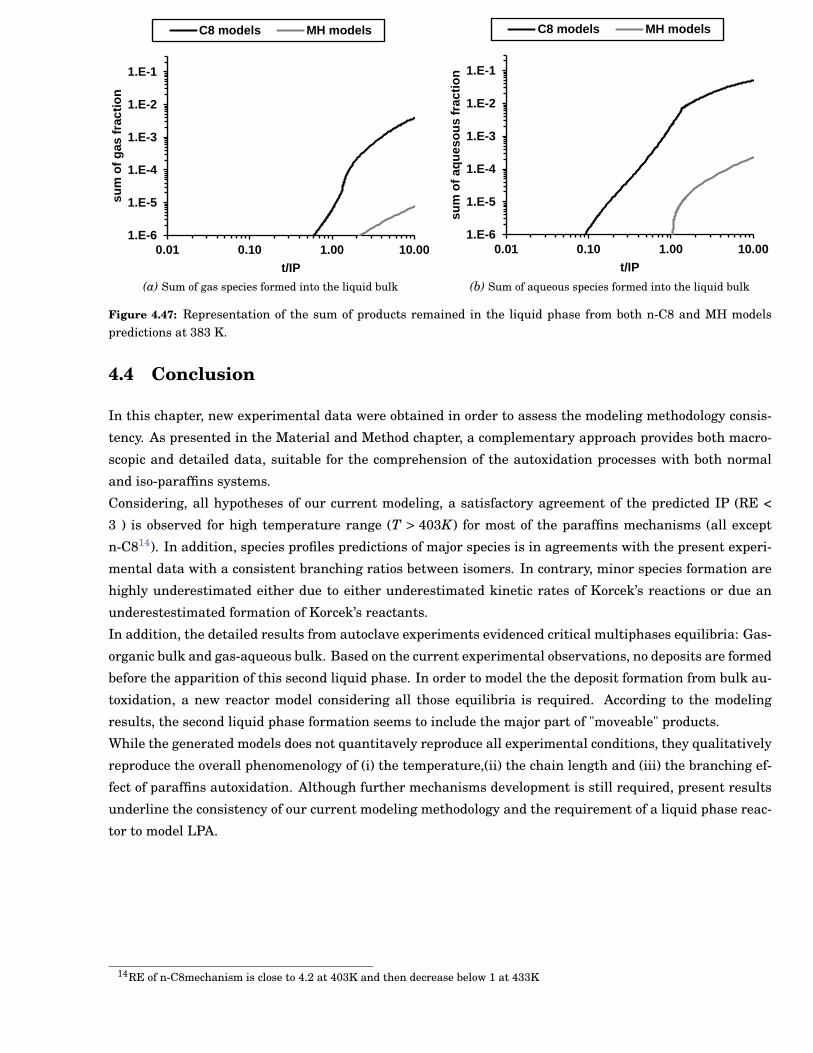
Chapter 4 91

1.E-6

1.E-5

1.E-4

1.E-3

1.E-2

1.E-1

0.01 0.10 1.00 10.00

su

m o

f g

as

fra

cti

on

t/IP

C8 models MH models

(a) Sum of gas species formed into the liquid bulk

1.E-6

1.E-5

1.E-4

1.E-3

1.E-2

1.E-1

0.01 0.10 1.00 10.00

su

m o

f a

qu

es

ou

s f

rac

tio

n

t/IP

C8 models MH models

(b) Sum of aqueous species formed into the liquid bulk

Figure 4.47: Representation of the sum of products remained in the liquid phase from both n-C8 and MH modelspredictions at 383 K.

4.4 Conclusion

In this chapter, new experimental data were obtained in order to assess the modeling methodology consis-

tency. As presented in the Material and Method chapter, a complementary approach provides both macro-

scopic and detailed data, suitable for the comprehension of the autoxidation processes with both normal

and iso-paraffins systems.

Considering, all hypotheses of our current modeling, a satisfactory agreement of the predicted IP (RE <

3 ) is observed for high temperature range (T > 403K) for most of the paraffins mechanisms (all except

n-C814). In addition, species profiles predictions of major species is in agreements with the present experi-

mental data with a consistent branching ratios between isomers. In contrary, minor species formation are

highly underestimated either due to either underestimated kinetic rates of Korcek’s reactions or due an

underestestimated formation of Korcek’s reactants.

In addition, the detailed results from autoclave experiments evidenced critical multiphases equilibria: Gas-

organic bulk and gas-aqueous bulk. Based on the current experimental observations, no deposits are formed

before the apparition of this second liquid phase. In order to model the the deposit formation from bulk au-

toxidation, a new reactor model considering all those equilibria is required. According to the modeling

results, the second liquid phase formation seems to include the major part of "moveable" products.

While the generated models does not quantitavely reproduce all experimental conditions, they qualitatively

reproduce the overall phenomenology of (i) the temperature,(ii) the chain length and (iii) the branching ef-

fect of paraffins autoxidation. Although further mechanisms development is still required, present results

underline the consistency of our current modeling methodology and the requirement of a liquid phase reac-

tor to model LPA.

14RE of n-C8mechanism is close to 4.2 at 403K and then decrease below 1 at 433K

92 Chapter 4

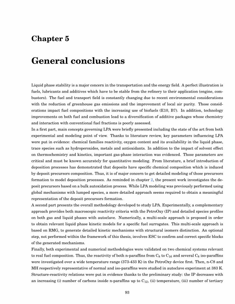
Chapter 5

General conclusions

Liquid phase stability is a major concern in the transportation and the energy field. A perfect illustration is

fuels, lubricants and additives which have to be stable from the refinery to their application (engine, com-

bustors). The fuel and transport field is constantly changing due to recent environmental considerations

with the reduction of greenhouse gas emissions and the improvement of local air purity. Those consid-

erations impact fuel compositions with the increasing use of biofuels (E10, B7). In addition, technology

improvements on both fuel and combustion lead to a diversification of additive packages whose chemistry

and interaction with conventional fuel fractions is poorly assessed.

In a first part, main concepts governing LPA were briefly presented including the state of the art from both

experimental and modeling point of view. Thanks to literature review, key parameters influencing LPA

were put in evidence: chemical families reactivity, oxygen content and its availability in the liquid phase,

trace species such as hydroperoxides, metals and antioxidants. In addition to the impact of solvent effect

on thermochemistry and kinetics, important gas-phase interaction was evidenced. Those parameters are

critical and must be known accurately for quantitative modeling. From literature, a brief introduction of

deposition processes has demonstrated that deposits have specific chemical composition which is induced

by deposit precursors composition. Thus, it is of major concern to get detailed modeling of those precursors

formation to model deposition processes. As reminded in chapter 2, the present work investigates the de-

posit precursors based on a bulk autoxidation process. While LPA modeling was previously performed using

global mechanisms with lumped species, a more detailed approach seems required to obtain a meaningful

representation of the deposit precursors formation.

A second part presents the overall methodology developed to study LPA. Experimentally, a complementary

approach provides both macroscopic reactivity criteria with the PetroOxy (IP) and detailed species profiles

on both gas and liquid phases with autoclave. Numerically, a multi-scale approach is proposed in order

to obtain relevant liquid phase kinetic models for a specific fuel surrogates. This multi-scale approach is

based on RMG, to generate detailed kinetic mechanisms with structural isomers distinction. An optional

step, not performed within the framework of this thesis, involves ESC to confirm and correct specific blocks

of the generated mechanisms.

Finally, both experimental and numerical methodologies were validated on two chemical systems relevant

to real fuel composition. Thus, the reactivity of both n-paraffins from C8 to C16 and several C8 iso-paraffins

were investigated over a wide temperature range (373-433 K) in the PetroOxy device first. Then, n-C8 and

MH respectively representative of normal and iso-paraffins were studied in autoclave experiment at 383 K.

Structure-reactivity relations were put in evidence thanks to the preliminary study: the IP decreases with

an increasing (i) number of carbons inside n-paraffins up to C12, (ii) temperature, (iii) number of tertiary

93

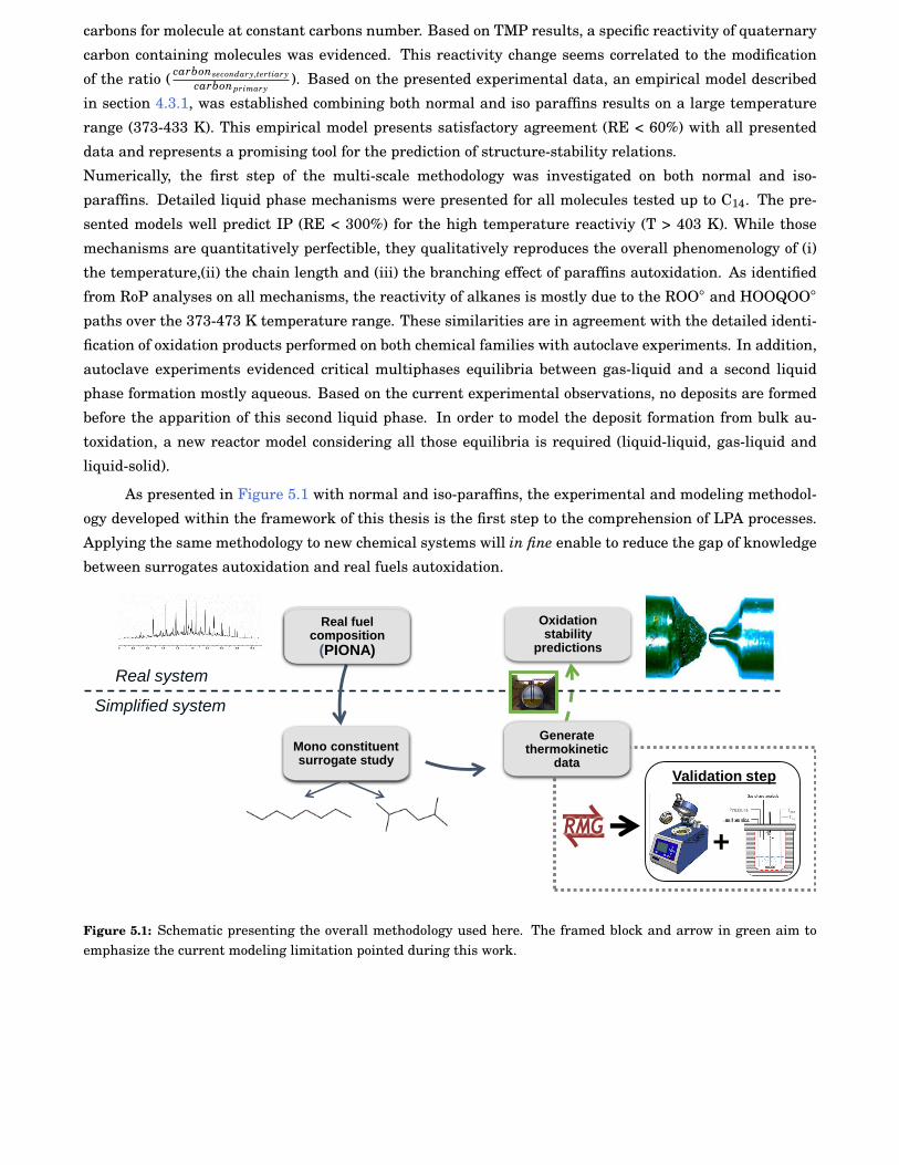
94 Chapter 5

carbons for molecule at constant carbons number. Based on TMP results, a specific reactivity of quaternary

carbon containing molecules was evidenced. This reactivity change seems correlated to the modification

of the ratio ( carbonsecondary,tertiarycarbonprimary

). Based on the presented experimental data, an empirical model described

in section 4.3.1, was established combining both normal and iso paraffins results on a large temperature

range (373-433 K). This empirical model presents satisfactory agreement (RE < 60%) with all presented

data and represents a promising tool for the prediction of structure-stability relations.

Numerically, the first step of the multi-scale methodology was investigated on both normal and iso-

paraffins. Detailed liquid phase mechanisms were presented for all molecules tested up to C14. The pre-

sented models well predict IP (RE < 300%) for the high temperature reactiviy (T > 403 K). While those

mechanisms are quantitatively perfectible, they qualitatively reproduces the overall phenomenology of (i)

the temperature,(ii) the chain length and (iii) the branching effect of paraffins autoxidation. As identified

from RoP analyses on all mechanisms, the reactivity of alkanes is mostly due to the ROO◦ and HOOQOO◦

paths over the 373-473 K temperature range. These similarities are in agreement with the detailed identi-

fication of oxidation products performed on both chemical families with autoclave experiments. In addition,

autoclave experiments evidenced critical multiphases equilibria between gas-liquid and a second liquid

phase formation mostly aqueous. Based on the current experimental observations, no deposits are formed

before the apparition of this second liquid phase. In order to model the deposit formation from bulk au-

toxidation, a new reactor model considering all those equilibria is required (liquid-liquid, gas-liquid and

liquid-solid).

As presented in Figure 5.1 with normal and iso-paraffins, the experimental and modeling methodol-

ogy developed within the framework of this thesis is the first step to the comprehension of LPA processes.

Applying the same methodology to new chemical systems will in fine enable to reduce the gap of knowledge

between surrogates autoxidation and real fuels autoxidation.

Real fuel composition

(PIONA)

Oxidationstability

predictions

Surrogateestablishment

Real system

Simplified system

Generatethermokinetic

data

Real fuel composition

(PIONA)

Mono constituent surrogate study

Generatethermokinetic

data

Real fuel composition

(PIONA)

Validation step

+0000

Figure 5.1: Schematic presenting the overall methodology used here. The framed block and arrow in green aim toemphasize the current modeling limitation pointed during this work.

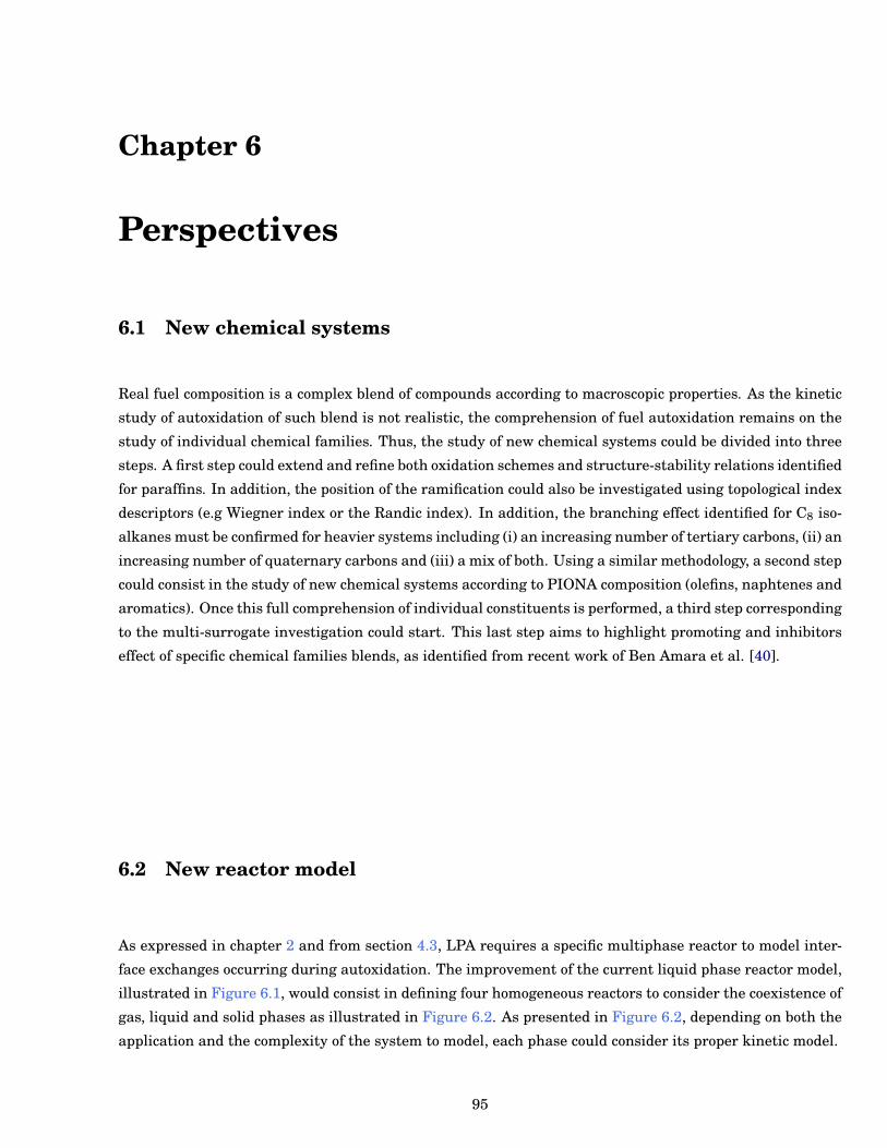
Chapter 6

Perspectives

6.1 New chemical systems

Real fuel composition is a complex blend of compounds according to macroscopic properties. As the kinetic

study of autoxidation of such blend is not realistic, the comprehension of fuel autoxidation remains on the

study of individual chemical families. Thus, the study of new chemical systems could be divided into three

steps. A first step could extend and refine both oxidation schemes and structure-stability relations identified

for paraffins. In addition, the position of the ramification could also be investigated using topological index

descriptors (e.g Wiegner index or the Randic index). In addition, the branching effect identified for C8 iso-

alkanes must be confirmed for heavier systems including (i) an increasing number of tertiary carbons, (ii) an

increasing number of quaternary carbons and (iii) a mix of both. Using a similar methodology, a second step

could consist in the study of new chemical systems according to PIONA composition (olefins, naphtenes and

aromatics). Once this full comprehension of individual constituents is performed, a third step corresponding

to the multi-surrogate investigation could start. This last step aims to highlight promoting and inhibitors

effect of specific chemical families blends, as identified from recent work of Ben Amara et al. [40].

6.2 New reactor model

As expressed in chapter 2 and from section 4.3, LPA requires a specific multiphase reactor to model inter-

face exchanges occurring during autoxidation. The improvement of the current liquid phase reactor model,

illustrated in Figure 6.1, would consist in defining four homogeneous reactors to consider the coexistence of

gas, liquid and solid phases as illustrated in Figure 6.2. As presented in Figure 6.2, depending on both the

application and the complexity of the system to model, each phase could consider its proper kinetic model.

95

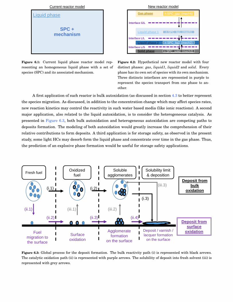
96 Chapter 6

Current reactor model

SPC + mechanism

Liquid phase

Figure 6.1: Current liquid phase reactor model rep-resenting an homogeneous liquid phase with a set ofspecies (SPC) and its associated mechanism.

Liquid phase 2 n SPC_liq2, (mech2)

Gas phase n SPC_gaz, (mech4)

Liquid phase 1 n SPC_liq1, (mech)

Solid phase n SPC_solid, (mech3)

Interface L/L

Interface L/S

Interface G/L

New reactor model

Figure 6.2: Hypothetical new reactor model with fourdistinct phases: gas, liquid1, liquid2 and solid. Everyphase has its own set of species with its own mechanism.Three distincts interfaces are represented in purple torepresent the species transport from one phase to an-other.

A first application of such reactor is bulk autoxidation (as discussed in section 4.3 to better represent

the species migration. As discussed, in addition to the concentration change which may affect species rates,

new reaction kinetics may control the reactivity in such water based media (like ionic reactions). A second

major application, also related to the liquid autoxidation, is to consider the heterogeneous catalysis. As

presented in Figure 6.3, both bulk autoxidation and heterogeneous autoxidation are competing paths to

deposits formation. The modeling of both autoxidation would greatly increase the comprehension of their

relative contributions to form deposits. A third application is for storage safety, as observed in the present

study, some light HCs may desorb form the liquid phase and concentrate over time in the gas phase. Thus,

the prediction of an explosive phase formation would be useful for storage safety applications.

Fresh fuel

(ii.1)

(i.1)

Soluble

agglomerates

(i.2)

(iii.1)

(ii.3)

(i.3)

(iii.2)

(ii.2) (ii.4)

(iii.3)

Oxidized

fuel

Surface

oxidation

Agglomerate

formation

on the surface

Deposit / varnish /

lacquer formation

on the surface

Fuel

migration to

the surface

Solubility limit

& deposition

Deposit from

surface

oxidation

Deposit from

bulk

oxidation

Figure 6.3: Global process for the deposit formation. The bulk reactivity path (i) is represented with black arrows.The catalytic oxidation path (ii) is represented with purple arrows. The solubility of deposit into fresh solvent (iii) isrepresented with grey arrows.

Chapter 6 97

6.3 RMG upgrades

6.3.1 Solvent database upgrade

One current limitation of RMG, is the limited number of solvents available to calculate the solvent ef-

fect corrections. Beside solvent effects, solvent properties are also of interest1. However, the evolution of

the mixture composition during autoxidation implies to reconsider the solvation corrections for high fuel

conversion values (due to high conversion of the initial fuel sample, formation of wide variety of carbonyl

compounds and water). Currently, solvation corrections are not taking into account this composition change

and is still using the initial fuel for the solvation correction. For the modeling of systems at low conversion,

this assumption is realistic. As the solvent database contains only 26 solvents, an update is required before

implementing reacting system calculations

6.3.2 Solvent effects on the thermokinetics

In addition to the database upgrade, current RMG calculations are based on some assumptions like the lin-

ear temperature dependence on the free energy of solvation (pointed out in Jalan’s work). In addition, new

developments are in progress in RMG codes to better represent solvation in autoxidation conditions (highly

concentrated system and not in SATP). To complete the thermochemistry improvements, new studies [129]

are currently in progress to consider on the fly solvent effect correction on the Ea. Recent discussions

with RMG members indicated that both corrections (cage diffusion effect and EA corrections) will be di-

rectly integrated into the rate constant in the next developments. Thus, the consistency of the generated

mechanisms will be improved.

1Solvent properties do not evolve during the oxidation and is fixed by the input file.

98 Chapter 6

Bibliography

[1] L. Russier, “Documents from ifp training course "moteurs - carburants". originally from université deberne.”.

[2] L. Russier, “Documents from ifp training course "moteurs - carburants". originally from "air parif".”.

[3] K. Bacha, Etude de l’intéraction entre le carburant diesel et les composants du système d’injectiondiesel. PhD thesis, Université Haute-Alsace, IS2M, 2016.

[4] T. R. Sem, “Investigation of injector tip deposits on transport refrigeration units running on biodieselfuel,” tech. rep., SAE Technical Paper, 2004.

[5] A. Nicolle, S. Cagnina, and T. de Bruin, “First-principle based modeling of urea decomposition kineticsin aqueous solutions,” Chemical Physics Letters, pp. –, 2016.

[6] W. M. Zongo, Etudes de l’oxydation des huiles de poisson microencapsulées par DSC sous pression.PhD thesis, HES-SO Valais, 2009.

[7] B. M. Trost and I. Fleming, Comprehensive Organic Synthesis, Selectivity, Strategy and Efficiencyin Modern Organic Chemistry, Volume7, ch. 5.1: The Baeyer-villiger Reaction, pp. 671–689. Elsevier,1991.

[8] E. T. Denisov and I. B. Afanas’ ev, Oxidation and antioxidants in organic chemistry and biology. CRCpress, 2005.

[9] C. Marteau, F. Ruyffelaere, J.-M. Aubry, C. Penverne, D. Favier, and V. Nardello-Rataj, “Oxidativedegradation of fragrant aldehydes. autoxidation by molecular oxygen,” Tetrahedron, vol. 69, no. 10,pp. 2268–2275, 2013.

[10] B. Beaver, L. Gao, C. Burgess-Clifford, and M. Sobkowiak, “On the mechanisms of formation of ther-mal oxidative deposits in jet fuels. are unified mechanisms possible for both storage and thermaloxidative deposit formation for middle distillate fuels?,” Energy & Fuels, vol. 19, no. 4, pp. 1574–1579, 2005.

[11] E. Oganesova, E. Bordubanova, G. Kuz’mina, V. Bakunin, and O. Parenago, “Influence of the struc-ture of higher paraffin hydrocarbons and their derivatives on the mechanism of high-temperatureliquid-phase oxidation,” Petroleum Chemistry, vol. 49, no. 4, pp. 311–316, 2009.

[12] A. Jalan, R. W. Ashcraft, R. H. West, and W. H. Green, “Predicting solvation energies for kineticmodeling,” Annual Reports Section" C"(Physical Chemistry), vol. 106, pp. 211–258, 2010.

[13] T. Lu and C. K. Law, “Toward accommodating realistic fuel chemistry in large-scale computations,”Progress in Energy and Combustion Science, vol. 35, no. 2, pp. 192 – 215, 2009.

[14] Pr. Green’s group website: cheme.scripts.mit.edu/green-group/rmg.

[15] A. Jalan, I. M. Alecu, R. Meana-Pañeda, J. Aguilera-Iparraguirre, K. R. Yang, S. S. Merchant, D. G.Truhlar, and W. H. Green, “New pathways for formation of acids and carbonyl products in low-temperature oxidation: the korcek decomposition of γ-ketohydroperoxides,” Journal of the AmericanChemical Society, vol. 135, no. 30, pp. 11100–11114, 2013.

99

100 Bibliography

[16] M. Aslam, G. P. Torrence, and E. G. Zey, “Esterification,” Kirk-Othmer Encyclopedia of ChemicalTechnology, 2000.

[17] S. E. Wheeler, K. N. Houk, P. v. R. Schleyer, and W. D. Allen, “A hierarchy of homodesmotic reactionsfor thermochemistry,” Journal of the American Chemical Society, vol. 131, no. 7, pp. 2547–2560, 2009.

[18] Z. Yang, B. P. Hollebone, Z. Wang, C. Yang, C. Brown, and M. Landriault, “Storage stability of com-mercially available biodiesels and their blends under different storage conditions,” Fuel, vol. 115,pp. 366–377, 2014.

[19] G. A. Olah et al., Hydrocarbon chemistry. John Wiley & Sons, 2003.

[20] S. Matsumoto, K. Date, T. Taguchi, and O. E. Herrmann, “The new denso common rail diesel solenoidinjector,” MTZ worldwide, vol. 74, no. 2, pp. 44–48, 2013.

[21] D. Ueda, H. Tanada, A. Utsunomiya, J. Kawamura, and J. Weber, “4th generation diesel piezo injector(realizing enhanced high response injector),” tech. rep., SAE Technical Paper, 2016.

[22] T. Doungthip, J. Ervin, S. Zabarnick, and T. Williams, “Simulation of the effect of metal-surfacecatalysis on the thermal oxidation of jet fuel,” Energy & fuels, vol. 18, no. 2, pp. 425–437, 2004.

[23] J. Ervin and S. Zabarnick, “Computational fluid dynamics simulations of jet fuel oxidation incorpo-rating pseudo-detailed chemical kinetics,” Energy & fuels, vol. 12, no. 2, pp. 344–352, 1998.

[24] L. M. Balster, E. Corporan, M. J. DeWitt, J. T. Edwards, J. S. Ervin, J. L. Graham, S.-Y. Lee, S. Pal,D. K. Phelps, L. R. Rudnick, et al., “Development of an advanced, thermally stable, coal-based jetfuel,” Fuel Processing Technology, vol. 89, no. 4, pp. 364–378, 2008.

[25] L. M. Balster, S. Zabarnick, R. C. Striebich, L. M. Shafer, and Z. J. West, “Analysis of polar speciesin jet fuel and determination of their role in autoxidative deposit formation,” Energy & fuels, vol. 20,no. 6, pp. 2564–2571, 2006.

[26] N. J. Kuprowicz, S. Zabarnick, Z. J. West, and J. S. Ervin, “Use of Measured Species Class Concentra-tions with Chemical Kinetic Modeling for the Prediction of Autoxidation and Deposition of Jet Fuels,”Energy & Fuels, vol. 21, no. 2, pp. 530–544, 2007.

[27] S. Jain and M. Sharma, “Stability of biodiesel and its blends: a review,” Renewable and SustainableEnergy Reviews, vol. 14, no. 2, pp. 667–678, 2010.

[28] B. D. Batts and A. Z. Fathoni, “A literature review on fuel stability studies with particular emphasison diesel oil,” Energy & Fuels, vol. 5, no. 1, pp. 2–21, 1991.

[29] D. E. Van Sickle, T. Mill, F. R. Mayo, H. Richardson, and C. W. Gould, “Intramolecular propaga-tion in the oxidation of n-alkanes. autoxidation of n-pentane and n-octane,” The Journal of OrganicChemistry, vol. 38, no. 26, pp. 4435–4440, 1973.

[30] F. Garcia-Ochoa, A. Romero, and J. Querol, “Modeling of the thermal n-octane oxidation in the liquidphase,” Industrial & engineering chemistry research, vol. 28, no. 1, pp. 43–48, 1989.

[31] R. Jensen, S. Korcek, L. Mahoney, and M. Zinbo, “Liquid-phase autoxidation of organic compounds atelevated temperatures. 1. the stirred flow reactor technique and analysis of primary products from n-hexadecane autoxidation at 120-180. degree. c,” Journal of the American Chemical Society, vol. 101,no. 25, pp. 7574–7584, 1979.

[32] F. Camacho Rubio, F. Diaz-Rodriguez, and J. Fernandez-Gonzalez, “Oxidacion de n-parafinas in faseliquida,” Anales de Quimica, vol. 76, p. 375, 1980.

[33] S. Gernigon, Etude de la stabilité à l’oxydation des carburants liquides hydrocarbonés: Influence etcomportement des antioxydants. PhD thesis, Paris 7, 2010.

Bibliography 101

[34] N. Blin-Simiand, F. Jorand, K. Keller, M. Fiderer, and K. Sahetchian, “Ketohydroperoxides and ig-nition delay in internal combustion engines,” Combustion and Flame, vol. 112, no. 1-2, pp. 278–282,1998.

[35] S. Blaine and P. E. Savage, “Reaction pathways in lubricant degradation. 2. n-Hexadecane autoxida-tion,” Industrial & engineering chemistry research, vol. 30, no. 9, pp. 2185–2191, 1991.

[36] R. Thompson, L. Druge, and J. Chenicek, “Stability of fuel oils in storage: Effect of sulfur compounds,”Industrial & Engineering Chemistry, vol. 41, no. 12, pp. 2715–2721, 1949.

[37] S. Zabarnick, “Studies of jet fuel thermal stability and oxidation using a quartz crystal microbalanceand pressure measurements,” Industrial & engineering chemistry research, vol. 33, no. 5, pp. 1348–1354, 1994.

[38] S. Zabarnick, “Chemical kinetic modeling of jet fuel autoxidation and antioxidant chemistry,”Industrial & engineering chemistry research, vol. 32, no. 6, pp. 1012–1017, 1993.

[39] R. I. Masel, “Chemical Kinetics and Catalysis (Masel, Richard I.),” J. Chem. Educ., vol. 79, pp. 313–,Mar. 2002.

[40] A. Ben Amara, S. Kaoubi, and L. Starck, “Toward an optimal formulation of alternative jet fuels:Enhanced oxidation and thermal stability by the addition of cyclic molecules,” Fuel, 2016.

[41] B. N. Sundaram, The effects of oxygen on synthetic crude oil fouling. PhD thesis, University of BritishColumbia, 1998.

[42] J. Shepherd, C. Nuyt, J. Lee, and J. Woodrow, “Flash point and chemical composition of aviationkerosene (jet a),” 2000.

[43] F. Adam, F. Bertoncini, V. Coupard, N. Charon, D. Thiébaut, D. Espinat, and M.-C. Hennion, “Usingcomprehensive two-dimensional gas chromatography for the analysis of oxygenates in middle distil-lates: I. determination of the nature of biodiesels blend in diesel fuel,” Journal of Chromatography A,vol. 1186, no. 1, pp. 236–244, 2008.

[44] M. Sicard, J. Boulicault, K. Coulon, C. Thomasset, J. Ancelle, B. Raepsaet, and F. Ser, “Oxidationstability of jet fuel model molecules evaluated by rapid small scale oxidation tests.,” in The 13thInternational Conference on Stability, Handling and Use of Liquid Fuels 2013 IASH 2013, 2013.

[45] A. Ben Amara, B. Lecointe, N. Jeuland, T. Takahashi, Y. IIda, H. Hashimoto, and J. Bouilly, “Exper-imental study of the impact of diesel/biodiesel blends oxidation on the fuel injection system,” tech.rep., SAE Technical Paper, 2014.

[46] A. Ben Amara, A. Nicolle, M. Alves-Fortunato, and N. Jeuland, “Toward predictive modeling ofpetroleum and biobased fuel stability: Kinetics of methyl oleate/n-dodecane autoxidation,” Energy& Fuels, vol. 27, no. 10, pp. 6125–6133, 2013.

[47] E. G. Jones and L. M. Balster, “Autoxidation of dilute jet-fuel blends,” Energy & Fuels, vol. 13, no. 4,pp. 796–802, 1999.

[48] L. J. Spadaccini, R. A. Meinzer, and H. Huang, “For removing dissolved oxygen from a liquid fuel inthe fuel system of an energy conversion device.,” Nov. 13 2001. US Patent 6,315,815.

[49] S. W. Benson and P. S. Nangia, “Some unresolved problems in oxidation and combustion,” Accountsof Chemical Research, vol. 12, no. 7, pp. 223–228, 1979.

[50] N. Semenov, Some Problems of Chemical Kinetics. Vol. 1 & 2. Pergamon, 1958.

[51] E. G. Jones, L. M. Balster, and W. J. Balster, “Autoxidation of aviation fuels in heated tubes: Surfaceeffects,” Energy & fuels, vol. 10, no. 3, pp. 831–836, 1996.

102 Bibliography

[52] S. Zabarnick, “Pseudo-detailed chemical kinetic modeling of antioxidant chemistry for jet fuel appli-cations,” Energy & Fuels, vol. 12, no. 3, pp. 547–553, 1998.

[53] E. G. Jones and L. M. Balster, “Interaction of a synthetic hindered-phenol with natural fuel antioxi-dants in the autoxidation of paraffins,” Energy & fuels, vol. 14, no. 3, pp. 640–645, 2000.

[54] I. Oil, “Thermal/oxidation storage stability of bio-diesel fuels,” 2009.

[55] B. Grinstead and S. Zabarnick, “Studies of jet fuel thermal stability, oxidation, and additives usingan isothermal oxidation apparatus equipped with an oxygen sensor,” Energy & Fuels, vol. 13, no. 3,pp. 756–760, 1999.

[56] L. D. T. Câmara, R. S. Monteiro, A. M. Constantino, D. A. Aranda, and J. C. Afonso, “Oxidative crack-ing of linear hydrocarbons at low temperatures,” Chemical Engineering Communications, vol. 198,no. 3, pp. 416–424, 2010.

[57] M. Skolniak, P. Bukrejewski, and J. Frydrych, “Analysis of changes in the properties of selectedchemical compounds and motor fuels taking place during oxidation processes,” Intech, 2015.

[58] J. Pfaendtner and L. J. Broadbelt, “Mechanistic Modeling of Lubricant Degradation. 2. The Autoxi-dation of Decane and Octane,” Industrial & Engineering Chemistry Research, vol. 47, pp. 2897–2904,Mar. 2008.

[59] J. Pfaendtner and L. J. Broadbelt, “Mechanistic Modeling of Lubricant Degradation. 1. Structure-Reactivity Relationships for Free-Radical Oxidation,” Industrial & Engineering Chemistry Research,vol. 47, pp. 2886–2896, Mar. 2008.

[60] J. Pfaendtner and L. J. Broadbelt, “Elucidation of structure–reactivity relationships in hindered phe-nols via quantum chemistry and transition state theory,” Chemical Engineering Science, vol. 62,no. 18, pp. 5232–5239, 2007.

[61] N. Semenov, “Z. physik, 48, 571 (1928),” Z. phys. Chem.,(B), vol. 11, p. 464, 1930.

[62] J. D. Savee, E. Papajak, B. Rotavera, H. Huang, A. J. Eskola, O. Welz, L. Sheps, C. A. Taatjes,J. Zádor, and D. L. Osborn, “Direct observation and kinetics of a hydroperoxyalkyl radical (qooh),”Science, vol. 347, no. 6222, pp. 643–646, 2015.

[63] K. T. Reddy, N. P. Cernansky, and R. S. Cohen, “Modified reaction mechanism of aerated n-dodecaneliquid flowing over heated metal tubes,” Energy & Fuels, vol. 2, no. 2, pp. 205–213, 1988.

[64] S. Korcek, J. Chenier, J. Howard, and K. Ingold, “Absolute rate constants for hydrocarbon autoxida-tion. xxi. activation energies for propagation and the correlation of propagation rate constants withcarbon-hydrogen bond strengths,” Canadian Journal of Chemistry, vol. 50, no. 14, pp. 2285–2297,1972.

[65] A. Van Tiggelen, Oxydations et combustions, vol. 2. Editions Technip, 1968.

[66] J. Bolland, “Kinetic studies in the chemistry of rubber and related materials. i. the thermal oxidationof ethyl linoleate,” Proceedings of the Royal Society of London. Series A. Mathematical and PhysicalSciences, vol. 186, no. 1005, pp. 218–236, 1946.

[67] C. Cullis, M. Hirschler, and R. Rogers, “The oxidation of decane in the liquid and gaseous phases,”Proceedings of the Royal Society of London. A. Mathematical and Physical Sciences, vol. 375,no. 1763, pp. 543–563, 1981.

[68] J. Zádor, C. A. Taatjes, and R. X. Fernandes, “Kinetics of elementary reactions in low-temperatureautoignition chemistry,” Progress in energy and combustion science, vol. 37, no. 4, pp. 371–421, 2011.

[69] A. Jalan, R. H. West, and W. H. Green, “An Extensible Framework for Capturing Solvent Effects inComputer Generated Kinetic Models,” J. Phys. Chem. B, vol. 117, pp. 2955–2970, Jan. 2013.

Bibliography 103

[70] R. Larsen, R. Thorpe, and F. Armfield, “Oxidation characteristics of pure hydrocarbons,” Industrial& Engineering Chemistry, vol. 34, no. 2, pp. 183–193, 1942.

[71] B. Boss and R. Hazlett, “n-dodecane oxidation-elucidation by internal reference techniques,” ProductR&amp;D, vol. 14, no. 2, pp. 135–138, 1975.

[72] E. Booser and M. Fenske, “Liquid phase hydrocarbon oxidation,” Industrial & EngineeringChemistry, vol. 44, no. 8, pp. 1850–1856, 1952.

[73] A. M. Syroezhko, V. M. Potekhin, and V. A. Proskuryakov, “Composition of the products of the liquidphase oxidation of n-decane,” Zhurnal Prikladnoi Khimii, vol. 43, pp. 1791 – 1798, 1970.

[74] A. Watkinson and D. Wilson, “Chemical reaction fouling: A review,” EXPERIMENTAL THERMALAND FLUID SCIENCE, vol. 14, pp. 361–374, MAY 1997.

[75] P. Lacey, S. Gail, J. M. Kientz, N. Milovanovic, and C. Gris, “Internal fuel injector deposits,” SAEInternational Journal of Fuels and Lubricants, vol. 5, no. 1, pp. 132–145, 2012.

[76] O. K. Bhan, D. W. Brinkman, J. B. Green, and B. Carley, “Storage stability of marine diesel fuels,”Fuel, vol. 66, no. 9, pp. 1200 – 1214, 1987.

[77] A. Jalan, Predictive kinetic modeling of low-temperature hydrocarbon oxidation. PhD thesis, Mas-sachusetts Institute of Technology, 2014.

[78] O. Parenago, G. Kuz´mina, V. Bakunin, and E. Y. Oganesova, “Nanosized structures in high-temperature oxidation of lubricating oil hydrocarbons,” Russian Journal of General Chemistry,vol. 79, no. 6, pp. 1390–1399, 2009.

[79] O. Kasaikina, Z. Kartasheva, and L. Pisarenko, “Effect of surfactants on liquid-phase oxidation ofhydrocarbons and lipids,” Russian Journal of General Chemistry, vol. 78, no. 8, pp. 1533–1544, 2008.

[80] O. Kasaikina, A. Golyavin, D. Krugovov, Z. Kartasheva, and L. Pisarenko, “Micellar catalysis in theoxidation of lipids,” Moscow University Chemistry Bulletin, vol. 65, no. 3, pp. 206–209, 2010.

[81] E. Y. Oganesova, E. Bordubanova, Z. Popova, V. Bakunin, G. Kuz’Mina, and O. Parenago, “Influenceof the conditions of the liquid-phase oxidation of hexadecane on the reaction mechanism,” PetroleumChemistry, vol. 44, no. 2, pp. 99–105, 2004.

[82] “Detherm database 2015.”

[83] R. Battino, T. R. Rettich, and T. Tominaga, “The solubility of oxygen and ozone in liquids,” Journal ofphysical and chemical reference data, vol. 12, no. 2, pp. 163–178, 1983.

[84] J. Makranczy, K. Megyery-Balog, L. Rusz, and L. Patyi, “Solubility of gases in normal-alkanes,” Hung.J. Ind. Chem, vol. 4, no. 2, pp. 269–280, 1976.

[85] C. Blanc and M. Batiste, “Solubility coefficient of oxygen in parraffins,” Bulletin du Centre deRecherches de Pau, vol. 4, no. 1, pp. 235–241, 1970.

[86] M. Orozco and F. J. Luque, “Theoretical methods for the description of the solvent effect in biomolec-ular systems,” Chemical reviews, vol. 100, no. 11, pp. 4187–4226, 2000.

[87] M. H. Abraham, R. E. Smith, R. Luchtefeld, A. J. Boorem, R. Luo, and W. E. Acree, “Prediction ofsolubility of drugs and other compounds in organic solvents,” Journal of pharmaceutical sciences,vol. 99, no. 3, pp. 1500–1515, 2010.

[88] C. Mintz, J. Gibbs, W. E. Acree, and M. H. Abraham, “Enthalpy of solvation correlations for organicsolutes and gases dissolved in acetonitrile and acetone,” Thermochimica Acta, vol. 484, no. 1, pp. 65–69, 2009.

104 Bibliography

[89] H. Struebing, Z. Ganase, P. G. Karamertzanis, E. Siougkrou, P. Haycock, P. M. Piccione, A. Armstrong,A. Galindo, and C. S. Adjiman, “Computer-aided molecular design of solvents for accelerated reactionkinetics,” Nature Chemistry, vol. 5, pp. 952–957, 2013.

[90] J. T. Hynes, “Chemical reaction rates and solvent friction,” Journal of Statistical Physics, vol. 42,no. 1-2, pp. 149–168, 1986.

[91] H. S. El-Sheshtawy, U. Pischel, and W. M. Nau, “Solvent polarity affects h atom abstractions fromc–h donors,” Organic letters, vol. 13, no. 10, pp. 2694–2697, 2011.

[92] S. A. Rice, Diffusion-limited reactions, ch. 2, pp. 3–45. Elsevier, 1985.

[93] N. M. Vandewiele, G. R. Magoon, K. M. Van Geem, M.-F. Reyniers, W. H. Green, and G. B. Marin,“Kinetic modeling of jet propellant-10 pyrolysis,” Energy & Fuels, vol. 29, no. 1, pp. 413–427, 2014.

[94] E. Blurock, F. Battin-Leclerc, T. Faravelli, and W. H. Green, “Automatic generation of detailed mech-anisms,” in Cleaner Combustion, pp. 59–92, Springer, 2013.

[95] C. W. Gao, J. W. Allen, W. H. Green, and R. H. West, “Reaction mechanism generator: Automaticconstruction of chemical kinetic mechanisms,” Computer Physics Communications, 2016.

[96] “Astm d7545 - 09 standard test method for oxidation stability of middle distillate fuels-rapid smallscale oxidation test (rssot).”

[97] K. Bacha, A. Ben-Amara, A. Vannier, M. Alves-Fortunato, and M. Nardin, “Oxidation stability ofdiesel/biodiesel fuels measured by a petrooxy device and characterization of oxidation products,”Energy & Fuels, vol. 29, no. 7, pp. 4345–4355, 2015.

[98] Y. Machado, U. Teles, A. D. Neto, T. Dantas, and J. Fonseca, “Determination of antioxidant depletionkinetics using {ASTMD} 7545 as the accelerated oxidation method,” Fuel, vol. 112, no. 0, pp. 172 –177, 2013.

[99] “En pren 16091-2010 liquid petroleum products. middle distillates and fatty acid methyl ester famefuels and blends. determination of oxidation stability by rapid small scale oxidation method,” 2010.

[100] G. Sarau, A. Bochmann, R. Lewandowska, and S. Christiansen, From Micro- to Macro-RamanSpectroscopy: Solar Silicon for a Case Study, Advanced Aspects of Spectroscopy, ch. 3. InTech, 2012.

[101] S. Drevet, M. Ménard, and S. Souchon, “Internal report ifpen: R0520s vs/sb 074-15,” tech. rep., IF-PEn, 2015.

[102] “Chemkin-pro, 15131, reaction design: San diego, 2013.”

[103] W. H. Green, J. W. Allen, B. A. Buesser, R. W. Ashcraft, G. J. Beran, C. A. Class, C. Gao, C. F.Goldsmith, M. R. Harper, A. Jalan, M. Keceli, G. Magoon, D. M. Matheu, S. S. Merchant, J. A. D.Mo, S. Petway, S. Raman, S. S. J. Song, Y. Suleymanov, K. M. V. Geem, J. Wen, R. H. West, A. Wong,H. Wong, P. Yelvington, N. Yee, and J. Yu, “Rmg - reaction mechanism generator v4.0.1,” tech. rep.,http://rmg.sourceforge.net/, 2013.

[104] K. M. Van Geem, M.-F. Reyniers, G. B. Marin, J. Song, W. H. Green, and D. M. Matheu, “Automaticreaction network generation using rmg for steam cracking of n-hexane,” AIChE journal, vol. 52, no. 2,pp. 718–730, 2006.

[105] M. R. Harper, K. M. Van Geem, S. P. Pyl, G. B. Marin, and W. H. Green, “Comprehensive reactionmechanism for n-butanol pyrolysis and combustion,” Combustion and Flame, vol. 158, no. 1, pp. 16–41, 2011.

Bibliography 105

[106] M. J. Frisch, G. W. Trucks, H. B. Schlegel, G. E. Scuseria, M. A. Robb, J. R. Cheeseman, G. Scal-mani, V. Barone, B. Mennucci, G. A. Petersson, H. Nakatsuji, M. Caricato, X. Li, H. P. Hratchian,A. F. Izmaylov, J. Bloino, G. Zheng, J. L. Sonnenberg, M. Hada, M. Ehara, K. Toyota, R. Fukuda,J. Hasegawa, M. Ishida, T. Nakajima, Y. Honda, O. Kitao, H. Nakai, T. Vreven, J. A. Montgomery,Jr., J. E. Peralta, F. Ogliaro, M. Bearpark, J. J. Heyd, E. Brothers, K. N. Kudin, V. N. Staroverov,R. Kobayashi, J. Normand, K. Raghavachari, A. Rendell, J. C. Burant, S. S. Iyengar, J. Tomasi,M. Cossi, N. Rega, J. M. Millam, M. Klene, J. E. Knox, J. B. Cross, V. Bakken, C. Adamo, J. Jaramillo,R. Gomperts, R. E. Stratmann, O. Yazyev, A. J. Austin, R. Cammi, C. Pomelli, J. W. Ochterski, R. L.Martin, K. Morokuma, V. G. Zakrzewski, G. A. Voth, P. Salvador, J. J. Dannenberg, S. Dapprich, A. D.Daniels, Ã. Farkas, J. B. Foresman, J. V. Ortiz, J. Cioslowski, and D. J. Fox, “Gaussian 09 RevisionD.01.” Gaussian Inc. Wallingford CT 2009.

[107] M. S. Contreras, T. De Bruin, P. Mougin, and H. Toulhoat, “Thermochemistry of 1-methylnaphthalenehydroconversion: Comparison of group contribution and ab initio models,” Energy & fuels, vol. 27,no. 9, pp. 5475–5482, 2013.

[108] M. H. Keshavarz, M. Zamani, F. Atabaki, and K. Hosseini Monjezi, “Reliable approach for predictionof heats of formation of polycyclic saturated hydrocarbons using recently developed density function-als,” Computational and Theoretical Chemistry, vol. 1011, pp. 30–36, 2013.

[109] A. Osmont, L. Catoire, I. Gökalp, and M. T. Swihart, “Thermochemistry of cc and ch bond breakingin fatty acid methyl esters,” Energy & fuels, vol. 21, no. 4, pp. 2027–2032, 2007.

[110] L. Catoire, M. Yahyaoui, A. Osmont, I. Gökalp, M. Brothier, H. Lorcet, and D. Guénadou, “Thermo-chemistry of compounds formed during fast pyrolysis of lignocellulosic biomass,” Energy & Fuels,vol. 22, no. 6, pp. 4265–4273, 2008.

[111] A. Osmont, L. Catoire, T. M. Klapötke, G. L. Vaghjiani, and M. T. Swihart, “Thermochem-istry of species potentially formed during nto/mmh hypergolic ignition,” Propellants, Explosives,Pyrotechnics, vol. 33, no. 3, pp. 209–212, 2008.

[112] A. Osmont, M. Yahyaoui, L. Catoire, I. Gökalp, and M. T. Swihart, “Thermochemistry of co,(co) o, and(co) c bond breaking in fatty acid methyl esters,” Combustion and Flame, vol. 155, no. 1, pp. 334–342,2008.

[113] I. Alecu and D. G. Truhlar, “Computational study of the reactions of methanol with the hydroper-oxyl and methyl radicals. 1. accurate thermochemistry and barrier heights,” The Journal of PhysicalChemistry A, vol. 115, no. 13, pp. 2811–2829, 2011.

[114] I. Alecu and D. G. Truhlar, “Computational study of the reactions of methanol with the hydroper-oxyl and methyl radicals. 2. accurate thermal rate constants,” The Journal of Physical Chemistry A,vol. 115, no. 51, pp. 14599–14611, 2011.

[115] X. Xu, I. Alecu, and D. G. Truhlar, “How well can modern density functionals predict internucleardistances at transition states?,” Journal of Chemical Theory and Computation, vol. 7, no. 6, pp. 1667–1676, 2011.

[116] J. Zheng, R. Meana-Pañeda, and D. G. Truhlar, “Mstor version 2013: A new version of the com-puter code for the multi-structural torsional anharmonicity, now with a coupled torsional potential,”Computer Physics Communications, vol. 184, no. 8, pp. 2032–2033, 2013.

[117] J. Zheng, S. L. Mielke, K. L. Clarkson, and D. G. Truhlar, “Mstor: A program for calculating partitionfunctions, free energies, enthalpies, entropies, and heat capacities of complex molecules includingtorsional anharmonicity,” Computer Physics Communications, vol. 183, no. 8, pp. 1803–1812, 2012.

[118] Online manual of RMG-Py: http://reactionmechanismgenerator.github.io/RMG-Py/users/rmg/index.html.

[119] s. g. RMG, “21- introduction to rmg-py,” tech. rep., RMG study group, 2015.

106 Bibliography

[120] P. Linstrom and E. W.G. Mallard, “Nist chemistry webbook,” NIST Standard Reference DatabaseNumber 69, National Institute of Standards and Technology, 2001.

[121] J. Rowley, W. V. Wilding, J. L. Oscarson, Y. Yang, and N. Giles, “Design institute for physical proper-ties data,” (DIPPR-AIChE), 2011.

[122] B. Boss and R. Hazlett, “Oxidation of hydrocarbons in the liquid phase: n-dodecane in a borosilicateglass chamber at 200c,” Canadian Journal of Chemistry, vol. 47, no. 22, pp. 4175–4182, 1969.

[123] L. Liu and Q.-X. Guo, “Isokinetic relationship, isoequilibrium relationship, and enthlapy-entropycompensation,” Chemical reviews, vol. 101, no. 3, pp. 673–696, 2001.

[124] A. Goosen and D. H. Morgan, “Autoxidation of nonane and decane: a product study,” Journal ChemicalSociety , Perkin Trans. 2, pp. 557–562, 1994.

[125] L. D. T. Câmara, N. C. Furtado, R. S. Monteiro, D. A. Aranda, and C. Taft, “Molecular orbital ap-proach for investigating the kinetics of cracking hydroperoxides,” Journal of Molecular Structure:THEOCHEM, vol. 776, no. 1-3, pp. 41–45, 2006.

[126] K. Chatelain, A. Nicolle, A. Ben Amara, L. Catoire, and L. Starck, “Wide range experimental andkinetic modeling study of chain length impact on n-alkanes autoxidation,” Energy & Fuels, vol. 30,no. 2, pp. 1294–1303, 2016.

[127] J. Benton and M. Wirth, “Position of radical attack during oxidation of long-chain paraffins,” Nature,1953.

[128] B. D. Boss, R. N. Hazlett, and R. L. Shepard, “Analysis of normal paraffin oxidation products in thepresence of hydroperoxides,” Analytical Chemistry, vol. 45, no. 14, pp. 2388–2392, 1973.

[129] B. Slakman, K. Chatelain, A. B. Amara, L. Starck, M. Matrat, L. Catoire, A. Nicolle, and R. West,“Liquid-phase mechanism generation for application to fuel oxidation,” in ISCRE, 2016.

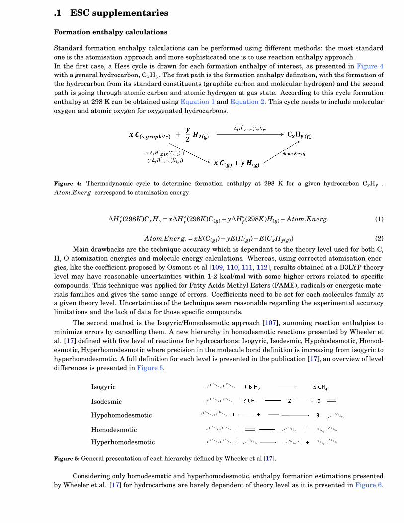
Appendix 107

.1 ESC supplementaries

Formation enthalpy calculations

Standard formation enthalpy calculations can be performed using different methods: the most standardone is the atomisation approach and more sophisticated one is to use reaction enthalpy approach.In the first case, a Hess cycle is drawn for each formation enthalpy of interest, as presented in Figure 4with a general hydrocarbon, CxHy. The first path is the formation enthalpy definition, with the formation ofthe hydrocarbon from its standard constituents (graphite carbon and molecular hydrogen) and the secondpath is going through atomic carbon and atomic hydrogen at gas state. According to this cycle formationenthalpy at 298 K can be obtained using Equation 1 and Equation 2. This cycle needs to include molecularoxygen and atomic oxygen for oxygenated hydrocarbons.

Figure 4: Thermodynamic cycle to determine formation enthalpy at 298 K for a given hydrocarbon CxHy .Atom.Energ. correspond to atomization energy.

∆H◦f (298K)CxHy = x∆H◦

f (298K)C(g) + y∆H◦f (298K)H(g) − Atom.Energ. (1)

Atom.Energ.= xE(C(g))+ yE(H(g))−E(CxHy(g)) (2)

Main drawbacks are the technique accuracy which is dependant to the theory level used for both C,H, O atomization energies and molecule energy calculations. Whereas, using corrected atomisation ener-gies, like the coefficient proposed by Osmont et al [109, 110, 111, 112], results obtained at a B3LYP theorylevel may have reasonable uncertainties within 1-2 kcal/mol with some higher errors related to specificcompounds. This technique was applied for Fatty Acids Methyl Esters (FAME), radicals or energetic mate-rials families and gives the same range of errors. Coefficients need to be set for each molecules family ata given theory level. Uncertainties of the technique seem reasonable regarding the experimental accuracylimitations and the lack of data for those specific compounds.

The second method is the Isogyric/Homodesmotic approach [107], summing reaction enthalpies tominimize errors by cancelling them. A new hierarchy in homodesmotic reactions presented by Wheeler etal. [17] defined with five level of reactions for hydrocarbons: Isogyric, Isodesmic, Hypohodesmotic, Homod-esmotic, Hyperhomodesmotic where precision in the molecule bond definition is increasing from isogyric tohyperhomodesmotic. A full definition for each level is presented in the publication [17], an overview of leveldifferences is presented in Figure 5.

Isogyric

Isodesmic

Hypohomodesmotic

Homodesmotic

Hyperhomodesmotic

Figure 5: General presentation of each hierarchy defined by Wheeler et al [17].

Considering only homodesmotic and hyperhomodesmotic, enthalpy formation estimations presentedby Wheeler et al. [17] for hydrocarbons are barely dependent of theory level as it is presented in Figure 6.

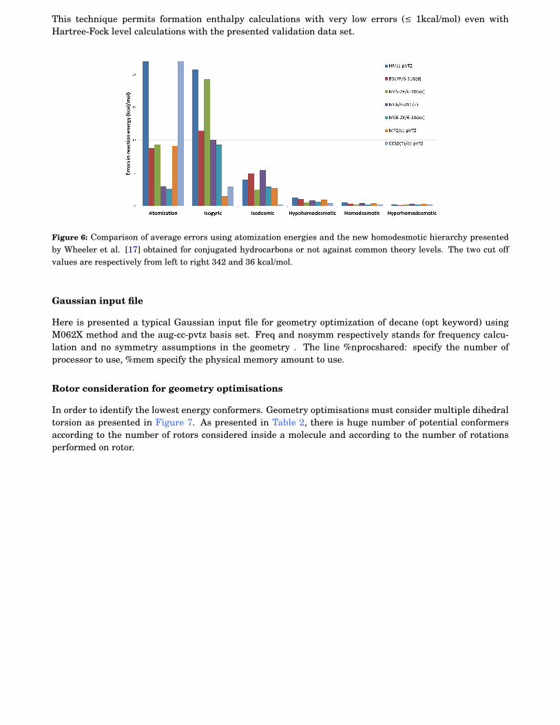
108 Appendix

This technique permits formation enthalpy calculations with very low errors (≤ 1kcal/mol) even withHartree-Fock level calculations with the presented validation data set.

Figure 6: Comparison of average errors using atomization energies and the new homodesmotic hierarchy presentedby Wheeler et al. [17] obtained for conjugated hydrocarbons or not against common theory levels. The two cut offvalues are respectively from left to right 342 and 36 kcal/mol.

Gaussian input file

Here is presented a typical Gaussian input file for geometry optimization of decane (opt keyword) usingM062X method and the aug-cc-pvtz basis set. Freq and nosymm respectively stands for frequency calcu-lation and no symmetry assumptions in the geometry . The line %nprocshared: specify the number ofprocessor to use, %mem specify the physical memory amount to use.

Rotor consideration for geometry optimisations

In order to identify the lowest energy conformers. Geometry optimisations must consider multiple dihedraltorsion as presented in Figure 7. As presented in Table 2, there is huge number of potential conformersaccording to the number of rotors considered inside a molecule and according to the number of rotationsperformed on rotor.

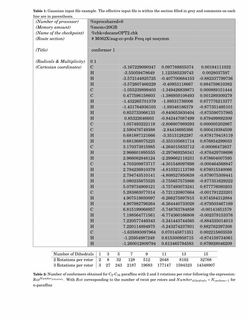
Appendix 109

Table 1: Gaussian input file example. The effective input file is within the section filled in grey and comments on eachline are in parenthesis.

(Number of processor) %nprocshared=8(Memory amount) %mem=20GB(Name of the checkpoint) %chk=decaneOPT2.chk(Route section) # M062X/aug-cc-pvdz Freq opt nosymm

(Title) conformer 1

(Radicals & Multiplicity) 0 1(Cartesian coordinates) C -3.167229090347 0.097788855374 0.00184111032

H -3.55059478649 1.123385239743 0.0028037597H -3.572144925725 -0.407700684153 -0.882337799736H -3.572607466229 -0.40953118667 0.884759610382C -1.055239899403 -1.349426839871 0.000889151444C 0.477596158603 -1.386959108493 0.001289309279H -1.432265701379 -1.89531736006 0.877776213377H -1.431764936103 -1.89348186379 -0.877351495101H 0.853733066133 -0.840653830404 -0.875590757985H 0.85322646603 -0.842447087499 0.879499892309C 1.057493222119 -2.806807989293 0.000005202967C 2.590476749388 -2.84416695366 0.000419384509H 0.681887121666 -3.35131282287 -0.878179418119H 0.681368075225 -3.353105681714 0.876854299033C 3.170373815985 -4.264015832712 -0.00086472637H 2.966601895555 -2.297869256341 -0.876429708696H 2.966082848124 -2.299662118231 0.878604007595C 4.703209873717 -4.301548097698 -0.000464568847H 2.794236910379 -4.810321113789 0.876015340066H 2.794743510141 -4.808527850638 -0.879075309441H 5.080235675525 -3.755657575866 -0.877351629222H 5.079734909121 -3.757493073241 0.877776080203C 5.283863077014 -5.721120807664 -0.001791223201H 4.907519850097 -6.266275897915 0.874584312884H 4.907982796264 -6.264440733028 -0.879503467189C 6.815199068957 -5.748763784858 -0.00141651579H 7.198564771561 -6.774360166808 -0.002379153376H 7.220577449343 -5.241443744565 -0.884335014013H 7.220114894975 -5.243274237931 0.882762397308C -1.635893097964 0.070145871351 0.002215803559H -1.25954987249 0.615300958715 -0.874159734061H -1.260012809794 0.613465794583 0.879928046209

Number of Dihedrals 1 3 5 7 9 11 13 152 Rotations per rotor 2 8 32 128 512 2048 8192 327683 Rotations per rotor 3 27 243 2187 19683 177147 1594323 14348907

Table 2: Number of conformers obtained for C2-C16 paraffins with 2 and 3 rotations per rotor following the expression:RotNumberdihedrals . With Rot corresponding to the number of twist per rotors and Numberdihedrals = Ncarbons−1 forn-paraffins

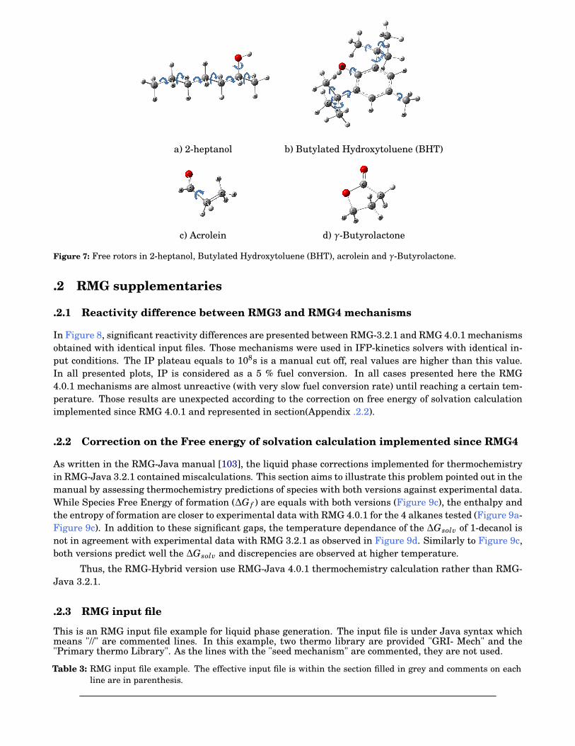
110 Appendix

a) 2-heptanol b) Butylated Hydroxytoluene (BHT)

c) Acrolein d) γ-Butyrolactone

Figure 7: Free rotors in 2-heptanol, Butylated Hydroxytoluene (BHT), acrolein and γ-Butyrolactone.

.2 RMG supplementaries

.2.1 Reactivity difference between RMG3 and RMG4 mechanisms

In Figure 8, significant reactivity differences are presented between RMG-3.2.1 and RMG 4.0.1 mechanismsobtained with identical input files. Those mechanisms were used in IFP-kinetics solvers with identical in-put conditions. The IP plateau equals to 108s is a manual cut off, real values are higher than this value.In all presented plots, IP is considered as a 5 % fuel conversion. In all cases presented here the RMG4.0.1 mechanisms are almost unreactive (with very slow fuel conversion rate) until reaching a certain tem-perature. Those results are unexpected according to the correction on free energy of solvation calculationimplemented since RMG 4.0.1 and represented in section(Appendix .2.2).

.2.2 Correction on the Free energy of solvation calculation implemented since RMG4

As written in the RMG-Java manual [103], the liquid phase corrections implemented for thermochemistryin RMG-Java 3.2.1 contained miscalculations. This section aims to illustrate this problem pointed out in themanual by assessing thermochemistry predictions of species with both versions against experimental data.While Species Free Energy of formation (∆G f ) are equals with both versions (Figure 9c), the enthalpy andthe entropy of formation are closer to experimental data with RMG 4.0.1 for the 4 alkanes tested (Figure 9a-Figure 9c). In addition to these significant gaps, the temperature dependance of the ∆Gsolv of 1-decanol isnot in agreement with experimental data with RMG 3.2.1 as observed in Figure 9d. Similarly to Figure 9c,both versions predict well the ∆Gsolv and discrepencies are observed at higher temperature.

Thus, the RMG-Hybrid version use RMG-Java 4.0.1 thermochemistry calculation rather than RMG-Java 3.2.1.

.2.3 RMG input file

This is an RMG input file example for liquid phase generation. The input file is under Java syntax whichmeans "//" are commented lines. In this example, two thermo library are provided "GRI- Mech" and the"Primary thermo Library". As the lines with the "seed mechanism" are commented, they are not used.

Table 3: RMG input file example. The effective input file is within the section filled in grey and comments on eachline are in parenthesis.

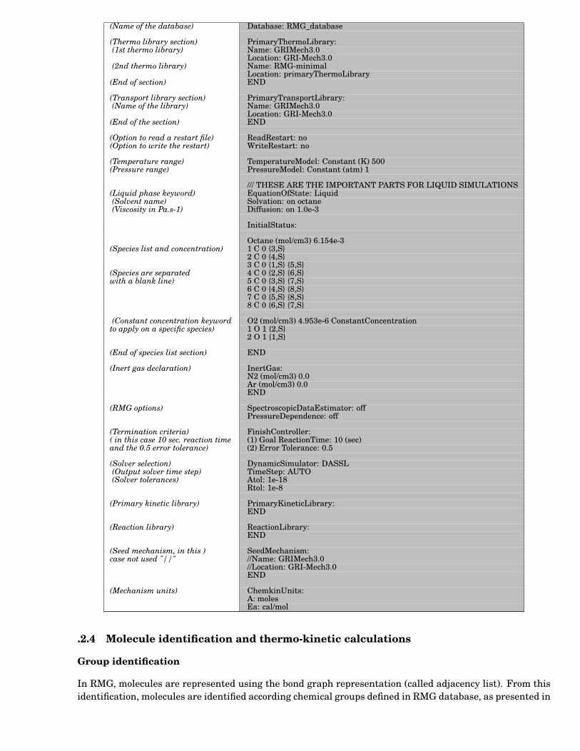
Appendix 111

(Name of the database) Database: RMG_database

(Thermo library section) PrimaryThermoLibrary:(1st thermo library) Name: GRIMech3.0

Location: GRI-Mech3.0(2nd thermo library) Name: RMG-minimal

Location: primaryThermoLibrary(End of section) END

(Transport library section) PrimaryTransportLibrary:(Name of the library) Name: GRIMech3.0

Location: GRI-Mech3.0(End of the section) END

(Option to read a restart file) ReadRestart: no(Option to write the restart) WriteRestart: no

(Temperature range) TemperatureModel: Constant (K) 500(Pressure range) PressureModel: Constant (atm) 1

/// THESE ARE THE IMPORTANT PARTS FOR LIQUID SIMULATIONS(Liquid phase keyword) EquationOfState: Liquid(Solvent name) Solvation: on octane(Viscosity in Pa.s-1) Diffusion: on 1.0e-3

InitialStatus:

Octane (mol/cm3) 6.154e-3(Species list and concentration) 1 C 0 {3,S}

2 C 0 {4,S}3 C 0 {1,S} {5,S}

(Species are separated 4 C 0 {2,S} {6,S}with a blank line) 5 C 0 {3,S} {7,S}

6 C 0 {4,S} {8,S}7 C 0 {5,S} {8,S}8 C 0 {6,S} {7,S}

(Constant concentration keyword O2 (mol/cm3) 4.953e-6 ConstantConcentrationto apply on a specific species) 1 O 1 {2,S}

2 O 1 {1,S}

(End of species list section) END

(Inert gas declaration) InertGas:N2 (mol/cm3) 0.0Ar (mol/cm3) 0.0END

(RMG options) SpectroscopicDataEstimator: offPressureDependence: off

(Termination criteria) FinishController:( in this case 10 sec. reaction time (1) Goal ReactionTime: 10 (sec)and the 0.5 error tolerance) (2) Error Tolerance: 0.5

(Solver selection) DynamicSimulator: DASSL(Output solver time step) TimeStep: AUTO(Solver tolerances) Atol: 1e-18

Rtol: 1e-8

(Primary kinetic library) PrimaryKineticLibrary:END

(Reaction library) ReactionLibrary:END

(Seed mechanism, in this ) SeedMechanism:case not used "//" //Name: GRIMech3.0

//Location: GRI-Mech3.0END

(Mechanism units) ChemkinUnits:A: molesEa: cal/mol

.2.4 Molecule identification and thermo-kinetic calculations

Group identification

In RMG, molecules are represented using the bond graph representation (called adjacency list). From thisidentification, molecules are identified according chemical groups defined in RMG database, as presented in

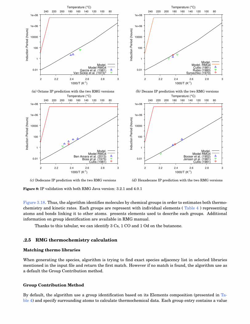
112 Appendix

0.01

1

100

10000

1e+06

1e+08

2 2.2 2.4 2.6 2.8 3

80 100 120 140 160 180 200 220 240

Indu

ctio

n Pe

riod

(hou

rs)

1000/T (K-1)

Temperature (°C)

Model.Model RMG4

Garcia et al. (1981)Van Sickle et al. (1973)*

(a) Octane IP prediction with the two RMG versions

0.01

1

100

10000

1e+06

1e+08

2 2.2 2.4 2.6 2.8 3

80 100 120 140 160 180 200 220 240

Indu

ctio

n Pe

riod

(hou

rs)

1000/T (K-1)

Temperature (°C)

Model.Model. RMG4

Cullis (1981)Rubio (1980)

Syroezhko (1970)

(b) Decane IP prediction with the two RMG versions

0.01

1

100

10000

1e+06

1e+08

2 2.2 2.4 2.6 2.8 3

80 100 120 140 160 180 200 220 240

Indu

ctio

n Pe

riod

(hou

rs)

1000/T (K-1)

Temperature (°C)

Model.Model RMG4

Ben Amara et al. (2013)Boss et al. (1975)

Cullis (1981)

(c) Dodecane IP prediction with the two RMG versions

0.01

1

100

10000

1e+06

1e+08

2 2.2 2.4 2.6 2.8 3

80 100 120 140 160 180 200 220 240

Indu

ctio

n Pe

riod

(hou

rs)

1000/T (K-1)

Temperature (°C)

Model.Model RMG4

Booser et al. (1952)Jensen et al. (1981)

Cullis (1981)

(d) Hexadecane IP prediction with the two RMG versions

Figure 8: IP validation with both RMG Java version: 3.2.1 and 4.0.1

Figure 3.18. Thus, the algorithm identifies molecules by chemical groups in order to estimates both thermo-chemistry and kinetic rates. Each groups are represent with individual elements ( Table 4 ) representingatoms and bonds linking it to other atoms. presents elements used to describe each groups. Additionalinformation on group identification are available in RMG manual.

Thanks to this tabular, we can identify 3 Cs, 1 CO and 1 Od on the butanone.

.2.5 RMG thermochemistry calculation

Matching thermo libraries

When generating the species, algorithm is trying to find exact species adjacency list in selected librariesmentioned in the input file and return the first match. However if no match is found, the algorithm use asa default the Group Contribution method.

Group Contribution Method

By default, the algorithm use a group identification based on its Elements composition (presented in Ta-ble 4) and specify surrounding atoms to calculate thermochemical data. Each group entry contains a value

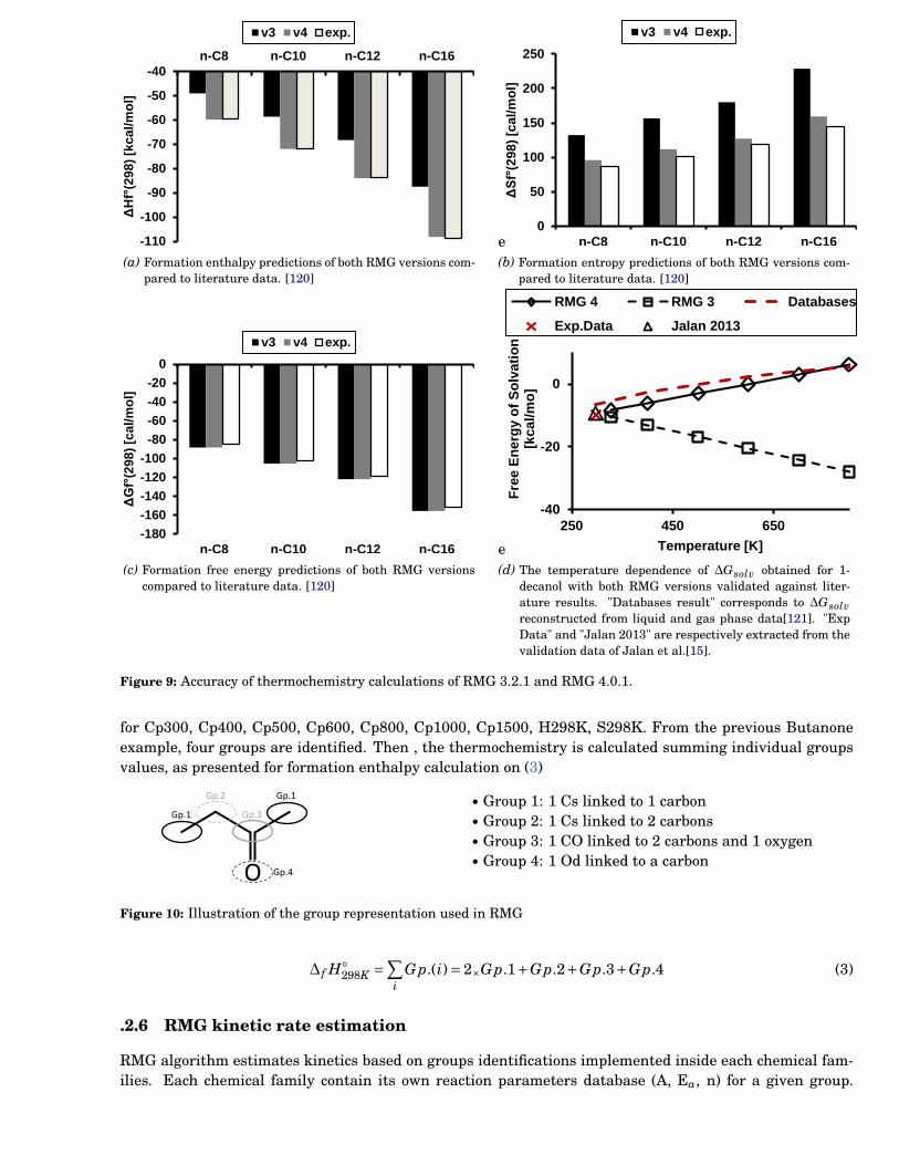
Appendix 113

-110

-100

-90

-80

-70

-60

-50

-40

n-C8 n-C10 n-C12 n-C16

ΔHf°

(29

8)

[kc

al/

mo

l]

v3 v4 exp.

(a) Formation enthalpy predictions of both RMG versions com-pared to literature data. [120]

e0

50

100

150

200

250

n-C8 n-C10 n-C12 n-C16

ΔSf°

(29

8)

[ca

l/m

ol]

v3 v4 exp.

(b) Formation entropy predictions of both RMG versions com-pared to literature data. [120]

-180

-160

-140

-120

-100

-80

-60

-40

-20

0

n-C8 n-C10 n-C12 n-C16

ΔGf°

(29

8)

[ca

l/m

ol]

v3 v4 exp.

(c) Formation free energy predictions of both RMG versionscompared to literature data. [120]

e

-40

-20

0

250 450 650F

ree

En

erg

y o

f S

olv

ati

on

[k

ca

l/m

o]

Temperature [K]

RMG 4 RMG 3 Databases

Exp.Data Jalan 2013

(d) The temperature dependence of ∆Gsolv obtained for 1-decanol with both RMG versions validated against liter-ature results. "Databases result" corresponds to ∆Gsolvreconstructed from liquid and gas phase data[121]. "ExpData" and "Jalan 2013" are respectively extracted from thevalidation data of Jalan et al.[15].

Figure 9: Accuracy of thermochemistry calculations of RMG 3.2.1 and RMG 4.0.1.

for Cp300, Cp400, Cp500, Cp600, Cp800, Cp1000, Cp1500, H298K, S298K. From the previous Butanoneexample, four groups are identified. Then , the thermochemistry is calculated summing individual groupsvalues, as presented for formation enthalpy calculation on (3)

O

Gp.2

Gp.1

Gp.1

Gp.3

Gp.4

• Group 1: 1 Cs linked to 1 carbon• Group 2: 1 Cs linked to 2 carbons• Group 3: 1 CO linked to 2 carbons and 1 oxygen• Group 4: 1 Od linked to a carbon

Figure 10: Illustration of the group representation used in RMG

∆ f H◦298K =∑

iG p.(i)= 2×G p.1+G p.2+G p.3+G p.4 (3)

.2.6 RMG kinetic rate estimation

RMG algorithm estimates kinetics based on groups identifications implemented inside each chemical fam-ilies. Each chemical family contain its own reaction parameters database (A, Ea, n) for a given group.

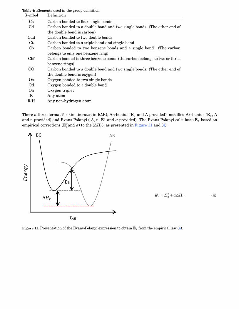
114 Appendix

Table 4: Elements used in the group definitionSymbol Definition

Cs Carbon bonded to four single bondsCd Carbon bonded to a double bond and two single bonds. (The other end of

the double bond is carbon)Cdd Carbon bonded to two double bondsCt Carbon bonded to a triple bond and single bondCb Carbon bonded to two benzene bonds and a single bond. (The carbon

belongs to only one benzene ring)Cbf Carbon bonded to three benzene bonds (the carbon belongs to two or three

benzene rings)CO Carbon bonded to a double bond and two single bonds. (The other end of

the double bond is oxygen)Os Oxygen bonded to two single bondsOd Oxygen bonded to a double bondOa Oxygen tripletR Any atom

R!H Any non-hydrogen atom

There a three format for kinetic rates in RMG, Arrhenius (Ea and A provided), modified Arrhenius (Ea, Aand n provided) and Evans Polanyi ( A, n, E◦

a and α provided). The Evans Polanyi calculates Ea based onempirical corrections (E0

aand α) to the (∆Hr), as presented in Figure 11 and (4).

BC AB

Ea

∆𝐻𝑟

𝑟𝐴𝐵

𝐸𝑛𝑒𝑟𝑔𝑦

Ea = E◦a +α∆Hr (4)

Figure 11: Presentation of the Evans-Polanyi expression to obtain Ea from the empirical law (4).

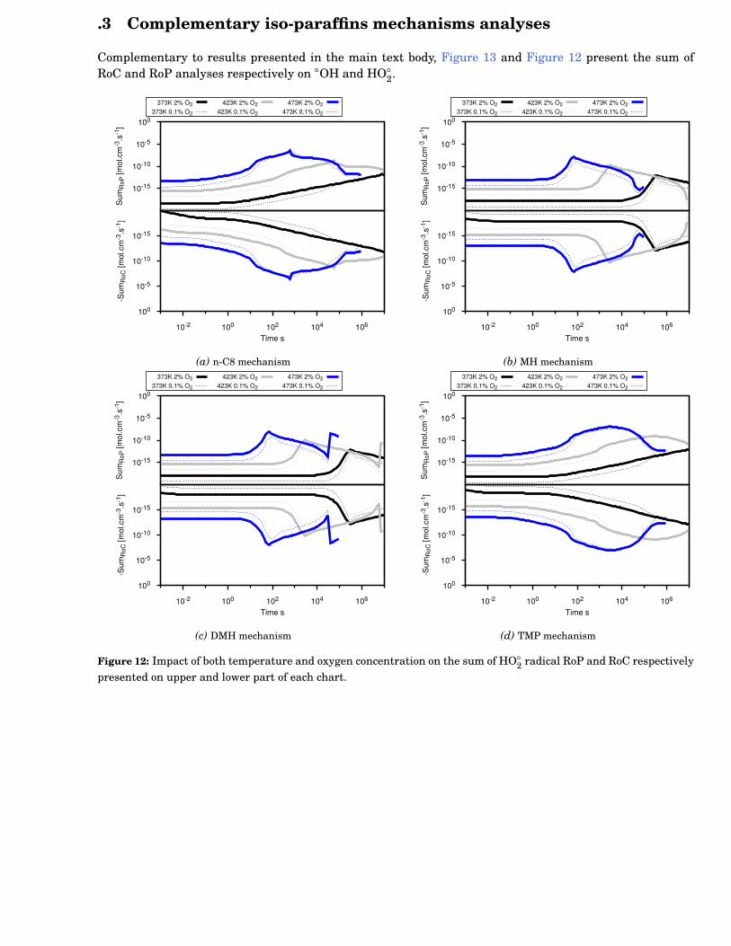
Appendix 115

.3 Complementary iso-paraffins mechanisms analyses

Complementary to results presented in the main text body, Figure 13 and Figure 12 present the sum ofRoC and RoP analyses respectively on ◦OH and HO◦

2.

10-15

10-10

10-5

100

10-2 100 102 104 106

-Sum

RoC

[mol

.cm

-3.s

-1]

Time s

10-15

10-10

10-5

100Su

mR

oP [m

ol.c

m-3

.s-1

]

373K 2% O2373K 0.1% O2

423K 2% O2423K 0.1% O2

473K 2% O2473K 0.1% O2

(a) n-C8 mechanism

10-15

10-10

10-5

100

10-2 100 102 104 106

-Sum

RoC

[mol

.cm

-3.s

-1]

Time s

10-15

10-10

10-5

100

Sum

RoP

[mol

.cm

-3.s

-1]

373K 2% O2373K 0.1% O2

423K 2% O2423K 0.1% O2

473K 2% O2473K 0.1% O2

(b) MH mechanism

10-15

10-10

10-5

100

10-2 100 102 104 106

-Sum

RoC

[mol

.cm

-3.s

-1]

Time s

10-15

10-10

10-5

100

Sum

RoP

[mol

.cm

-3.s

-1]

373K 2% O2373K 0.1% O2

423K 2% O2423K 0.1% O2

473K 2% O2473K 0.1% O2

(c) DMH mechanism

10-15

10-10

10-5

100

10-2 100 102 104 106

-Sum

RoC

[mol

.cm

-3.s

-1]

Time s

10-15

10-10

10-5

100

Sum

RoP

[mol

.cm

-3.s

-1]

373K 2% O2373K 0.1% O2

423K 2% O2423K 0.1% O2

473K 2% O2473K 0.1% O2

(d) TMP mechanism

Figure 12: Impact of both temperature and oxygen concentration on the sum of HO◦2 radical RoP and RoC respectively

presented on upper and lower part of each chart.

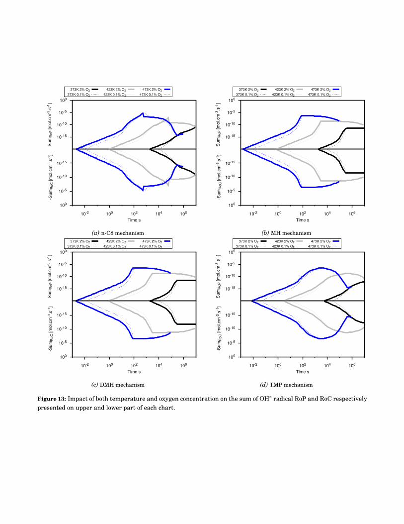
116 Appendix

10-15

10-10

10-5

100

10-2 100 102 104 106

-Sum

RoC

[mol

.cm

-3.s

-1]

Time s

10-15

10-10

10-5

100

Sum

RoP

[mol

.cm

-3.s

-1]

373K 2% O2373K 0.1% O2

423K 2% O2423K 0.1% O2

473K 2% O2473K 0.1% O2

(a) n-C8 mechanism

10-15

10-10

10-5

100

10-2 100 102 104 106

-Sum

RoC

[mol

.cm

-3.s

-1]

Time s

10-15

10-10

10-5

100

Sum

RoP

[mol

.cm

-3.s

-1]

373K 2% O2373K 0.1% O2

423K 2% O2423K 0.1% O2

473K 2% O2473K 0.1% O2

(b) MH mechanism

10-15

10-10

10-5

100

10-2 100 102 104 106

-Sum

RoC

[mol

.cm

-3.s

-1]

Time s

10-15

10-10

10-5

100

Sum

RoP

[mol

.cm

-3.s

-1]

373K 2% O2373K 0.1% O2

423K 2% O2423K 0.1% O2

473K 2% O2473K 0.1% O2

(c) DMH mechanism

10-15

10-10

10-5

100

10-2 100 102 104 106

-Sum

RoC

[mol

.cm

-3.s

-1]

Time s

10-15

10-10

10-5

100

Sum

RoP

[mol

.cm

-3.s

-1]

373K 2% O2373K 0.1% O2

423K 2% O2423K 0.1% O2

473K 2% O2473K 0.1% O2

(d) TMP mechanism

Figure 13: Impact of both temperature and oxygen concentration on the sum of OH◦ radical RoP and RoC respectivelypresented on upper and lower part of each chart.

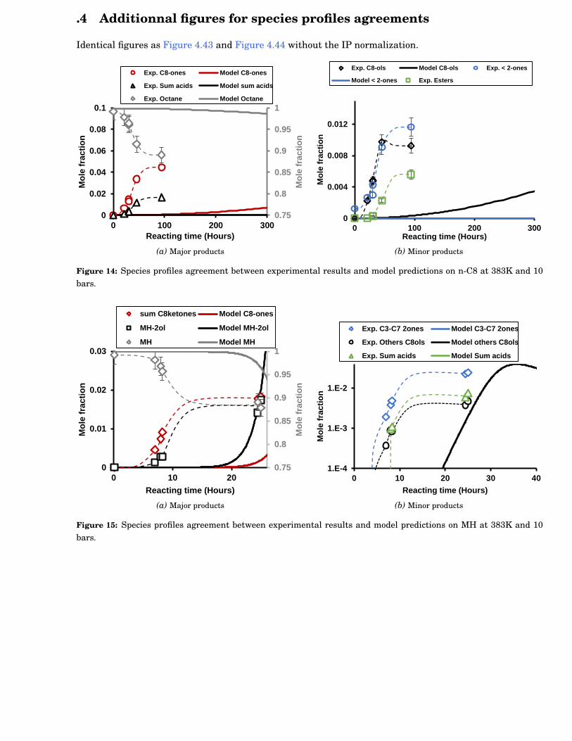
Appendix 117

.4 Additionnal figures for species profiles agreements

Identical figures as Figure 4.43 and Figure 4.44 without the IP normalization.

0.75

0.8

0.85

0.9

0.95

1

0

0.02

0.04

0.06

0.08

0.1

0 100 200 300

Mo

le f

rac

tio

n

Mo

le f

rac

tio

n

Reacting time (Hours)

Exp. C8-ones Model C8-ones

Exp. Sum acids Model sum acids

Exp. Octane Model Octane

(a) Major products

0

0.004

0.008

0.012

0 100 200 300

Mo

le f

rac

tio

n

Reacting time (Hours)

Exp. C8-ols Model C8-ols Exp. < 2-ones

Model < 2-ones Exp. Esters

(b) Minor products

Figure 14: Species profiles agreement between experimental results and model predictions on n-C8 at 383K and 10bars.

0.75

0.8

0.85

0.9

0.95

1

0

0.01

0.02

0.03

0 10 20

Mo

le f

rac

tio

n

Mo

le f

rac

tio

n

Reacting time (Hours)

sum C8ketones Model C8-ones

MH-2ol Model MH-2ol

MH Model MH

(a) Major products

1.E-4

1.E-3

1.E-2

0 10 20 30 40

Mo

le f

rac

tio

n

Reacting time (Hours)

Exp. C3-C7 2ones Model C3-C7 2ones

Exp. Others C8ols Model others C8ols

Exp. Sum acids Model Sum acids

(b) Minor products

Figure 15: Species profiles agreement between experimental results and model predictions on MH at 383K and 10bars.

118 Appendix

Titre : Stabilité à l’oxydation des carburants en phase liquideMots clés : Autoxydation, phase liquide, carburant modèle, n-paraffines, iso-paraffines, mécanismes cinétiquesdétaillésRésumé : La stabilité des carburants en phase liquide est de premier ordre dans le domaine du transport. Parexemple, les carburants, les lubrifiants ou les additifs doivent être stables de leur production jusqu’à leurutilisation. Cette thèse a pour but de développer et de valider une méthodologie alliant l’acquisition dedonnées expérimentales et le développement de modèles cinétiques pour l’autoxydation en phase liquide.Expérimentalement, une approche complémentaire a été mise en place pour obtenir à la fois des données deréactivité globales via un appareil PetroOxy et des profils d’espèces via un autoclave instrumenté.Numériquement, une méthodologie basée sur un générateur de mécanismes est proposée pour obtenir unechimie détaillée en phase liquide. Les paraffines linéaires et branchées sont étudiées comme des carburantsmodèles représentatifs de l’autoxidation de carburants réels afin de valider l’approche proposée. Ces familleschimiques sont représentatives de la composition des carburants réels et alternatifs.La réactivité des n-paraffines de C8 à C16 ainsi que d’isomères de l’octane a été étudiée en PetroOxy sur lagamme de température 373-433 K. Puis, des profils d’espèces détaillés de la phase gaz et de la phase liquide ontété obtenus durant l’étude de l’oxydation du n-C8 et du 2-methylheptane dans un autoclave à 383 K et 10 bars.Des mécanismes cinétiques détaillés ont été développé pour toutes les molécules jusqu’à C14. Les mécanismesreproduisent qualitativement la formation des espèces majoritaires lors de l’autoxidation des alcanes ainsi queles tendances observées liées à la longueur de chaîne et la ramification. L’analyse des mécanismes cinétiques amis en avant le rôle prédominant des radicaux peroxy (ROO) et peroxy-hydroperoxyde (HOOQOO) dans laconsommation de carburants modèles.Cette étude a permis d’améliorer la compréhension des processus d’autoxidation des alcanes linéaires etbranchés. L’étude de nouveaux systèmes permettra d’améliorer la compréhension globale des processusd’autoxidation et, de réduire l’écart de compréhension existant entre l’autoxidation des carburants réels et descarburants modèles.

Title : Oxidation stability of fuel in liquid phaseKeywords : Autoxidation, liquid phase, fuel, surrogates, n-paraffins, iso-paraffins, detailed chemical kineticmodelAbstract : Liquid phase stability is a major concern in the transportation and the energy fields. Relevantexamples are fuels, lubricants and additives which have to be stable from their production to their application(engine, combustors). This thesis aims to develop and validate a complete methodology combining bothexperimental data acquisition and the development of kinetic models for liquid phase autoxidation.The experimental methodology is based on a complementary approach to obtain (i) a global reactivitydescriptor (Induction Periods) and (ii) detailed species profiles respectively using a PetroOxy device and aninstrumented autoclave. Numerically, the presented methodology includes detailed liquid phase mechanismsgeneration with an automatic mechanism generator (RMG). Normal and iso-paraffins were selected as fuelsurrogates for autoxidation to validate the developed methodology. They were selected regarding their largecontribution in fuel composition and their growing interest as drop-in fuels.The reactivity of both n-paraffins from C8 to C16 and several C8 iso-paraffins was investigated over a widetemperature range (373-433 K) in the PetroOxy with liquid phase analyses. Then, detailed species profiles fromthe autoxidation of both n-octane and 2-methylheptane in autoclave were obtained at 383 K and 10 bars.Detailed liquid phase mechanisms were developed for all molecules tested up to C14. Mechanisms qualitativelyreproduce the overall phenomenology of the chain length, the branching and the major species profilesobserved experimentally. Mechanisms analysis allow to identify the main consumption pathways of alkanesthrough peroxy (ROO) and peroxy-hydroperoxide radicals (HOOQOO) over the temperature rangeinvestigated (373-473 K).This study permitted to increase the comprehension of autoxidation processes involved in normal andbranched alkanes. The study of new chemical systems will increase the global comprehension of autoxidationprocesses and in fine it will reduce the gap between the current autoxidation knowledge and the real fuelautoxidation.

Université Paris-SaclayEspace Technologique / Immeuble DiscoveryRoute de l’Orme aux Merisiers RD 128 / 91190 Saint-Aubin, France