PH 211 Labs - Physics | | Oregon State University

Oregon State University Fall Term, 2018

PH 211 Labs Lab Policies and General Information ............................................................................................................................................2 The purposes of these labs ............................................................................................................................................................2 Attendance ....................................................................................................................................................................................2 Your lab grade ..............................................................................................................................................................................2

Lab Types, Reports and Scoring ......................................................................................................................................................3 Lab types .......................................................................................................................................................................................3 The lab write-up ...........................................................................................................................................................................3 Grading the lab write-up ..............................................................................................................................................................3 Rubric O (Observation experiment) ......................................................................................................................................4 Rubric T (Testing experiment) ...............................................................................................................................................5 Rubric A (Application experiment) ........................................................................................................................................6

Experimental Uncertainty .................................................................................................................................................................7

LAB 0: Introduction to the Course (5 points)...............................................................................................................................11 A take-home exercise set due from every student by 6:00 p.m. on Tues., 9/25

LAB 1: Linear Motion (15 points) .................................................................................................................................................19 I. General physics knowledge “pre”-survey (5 points for full participation) ...........................................................................19 II. Background: Drawing motion diagrams .............................................................................................................................19 III. Investigating and representing linear motion (an Observation experiment) ......................................................................20 IV. Playing with motion .............................................................................................................................................................21 V. Determining a relationship between ramp angle and acceleration (an Observation experiment) .......................................22 VI. Math Review: A take-home exercise set due from every student by 6:00 p.m. on Tues., 10/2 ............................................23

LAB 2: Linear Kinematics (10 points) ..........................................................................................................................................24 I. Background: Experimental uncertainties and the weakest link rule .....................................................................................24 II. (STATION A) Angle and acceleration for a wooden block sliding down a wooden ramp (an Observation Experiment) ....25 III. (STATION B) Predicting where two carts will meet (a Testing experiment) ......................................................................26 IV. “Spot the Physics:” Motion A take-home exercise set due from every student by 6:00 p.m. on Tues., 10/9 ...............27

LAB 3: Applying Linear Kinematics (10 points) ..........................................................................................................................28 I. Rolling rocks (a Testing experiment) .......................................................................................................................................28 II. Falling cotton balls (a Testing experiment) ..........................................................................................................................29

LAB 4: Linear Momentum (What Changes It?) (15 points) .......................................................................................................30 I. Force and the resulting change in motion (a Testing experiment) .........................................................................................30 II. “Spot the Physics:” Linear Momentum – A take-home exercise due from every student by 6:00 p.m. on Tues., 10/24 .....31

LAB 5: Analyzing Force and Motion (10 points) .........................................................................................................................32 I. How is an object’s motion related to the net force on it? (an Observation experiment) .......................................................32 II. Does an object always move in the direction of the net force acting on it? (a Testing experiment) ....................................33 III. Free-Body Diagrams part A: A take-home exercise (5 points), due from every student by 6:00 p.m. on Tues., 10/31 ......34

LAB 6: Analyzing Force Systems (10 points)................................................................................................................................35 I. Newton’s second law (a Testing experiment) .........................................................................................................................35 II. Static friction (an Application experiment) ...........................................................................................................................36 III. Free-Body Diagrams part B: A take-home exercise (5 points), due from every student by 6:00 p.m. on Tues., 11/7 ........37

(no LAB 7)—Open-Lab Make-ups .................................................................................................................................................38 OPEN LABS (“drop in” anytime, any day)—for making up Labs 1-6 (two such makeups maximum)

LAB 8: Mechanical Energy Accounting (10 points) .....................................................................................................................39 I. Background Reading ..............................................................................................................................................................39 II. The Energy(s) in a Pendulum................................................................................................................................................39 III. Mech. Energy Accounting: A take-home exercise set (5 points), due from every student by 6:00 p.m. on Tues., 11/28 ....40

LAB 10: Putting It All Together (15 points) .................................................................................................................................41 I. General physics knowledge “post”-survey (5 points for full participation) ..........................................................................41 II. Pendulum box-bash (an Application experiment) .................................................................................................................41 Attend ONLY your own lab session for Lab 10; Week 10 is NOT an open lab week.

http://www.physics.oregonstate.edu/~coffinc/COURSES/ph211/Labs/Lab5-III.pdf

Oregon State University PH 211 Lab Manual Fall 2018

^^^^

^^^^

Lab Policies and General Information

The purpose(s) of these labs: The lab portion of this course is not to test what you (may) already know about physics. Rather, it’s to help you develop and sharpen that knowledge—more fully and clearly than ever before. In particular, lab is where you encounter first-hand the fundamental “testing” nature of science. As you will see, these labs are not “cookbook” recipes of procedures that you just plod through. Your TA is there to act as your guide only in a minimal sense—as a resource or a sounding board, not to demonstrate or explain exactly what to do. To a large extent, you will design your own experiments—so you will need to come to lab fully prepared: Bring the relevant lab pages printed out and already read (but you need not print out this general lab info).

Also in lab—like the rest of this course—you must continually hone the all-important skill of putting into words what you think and what you discover; you must be able to explain, reconcile and summarize your reasoning. So resolve right now to take full advantage of lab: to (i) explore physics principles to your own satisfaction; and (ii) make sure that your work makes sense to you—and that you can, likewise, convey that sense to others.

Attendance: Lab is a team effort; you will work each week as part of a group. Usually, you will be allowed to form your own groups—of three persons—but note that your TA has full discretion in this matter. And he/she may allow the same groups to form each week or ask you to form new ones.

Your participation is required throughout every lab session. In order to be counted as present for the lab (i.e. con-tributing to your group and receiving a non-zero score for that lab), you must arrive no more than “a few minutes” late (and you must stay until your group has turned in its lab write-up). What does “a few minutes” mean? That is up to your TA—he/she will tell you this in Lab 1 (either in person or via the Lab Syllabus, or both). Whatever rule he/she sets for that late “cutoff” is what you go by. And then note: Lab credit is not given just for “warming the chair.” To earn a share of the points each week, you must participate actively and contribute genuinely to your group. Your TA has full discretion to deduct points from your lab credit for marginal (or non-) participation.

Your lab grade: Your lab is worth 10% of your overall course grade (100 points out of 1000 total possible for the course). There are nine labs (named for the weeks during the term when you do them: 0-6, 8 and 10). Each lab is worth either 5, 10 or 15 points. Most labs have a portion that you do while in the lab room—for which you turn in a report (Lab 0 being the exception)—and then many labs have a follow-up “take-home” portion (and Lab 0 is all “take-home”). NOTE: For any lab in which your lab report score is zero OR your take-home score is zero, , 5% will be deducted from) your total course score (not just your lab score). This is a serious penalty—DO NOT EARN ANY LAB ZEROES!As part of Labs 1 and 10, you’ll take an assessment test, where credit is given simply for your complete participa-tion and effort, not for your specific responses. These tests are required but are used only to assess how the whole class has progressed. Your responses do not factor into your course grade; in fact, they are not even scored until after your final course grade has been posted. See the online Course Syllabus for more about lab grading policy.

There is one lab report per group—done entirely and handed in during the 3-hour lab period. Each group member must clearly put his/her name and student ID at the top of the write-up in order to obtain credit. You will usually need to supply your own paper for the write-up—do not plan to write on the pages of this lab packet unless it specifically gives you space and directions to do so. When using your own paper, you should use whatever format your TA may prefer/specify, if any. (See the next page for more specifics about the content of the lab write-ups.)

Any take-home portion of the lab is individual work—and that due date is typically the Tuesday of the week fol-lowing your in-lab work. (Those due dates are noted here and in the Course Calendar.) Best time to work on the take-home lab portion: Right in the lab, after you and your group have handed in your report. The lab TA is there to help for both portions.


^^^^

^^^^

Lab Types, Reports and Scoring

Lab Types: You will conduct 3 different types of lab experiments in the lab room this term.

A. Observation experiments. These are intended for students to learn skills such as changing one variable at a time, clearly recording and representing observations, and making accurate observations without mixing them with explanations. This is the first step of the experimental cycle, and allows you to observe phenomena, look for patterns in data, and start to devise explanations (once observations are carefully completed).

B. Testing experiments. Once explanations have been devised, the next step is to conduct an independent test students design that will test a hypothesis based on a specific explanation or rule. This helps you practice the skill of making predictions about the outcome of an experiment based on an explanation/rule/relationship. For a testing experiment, you can’t just do the experiment and record what happens – they must have a predicted outcome based on some explanation – and if the outcome of the experiment agrees with the prediction it gives confidence that the explanation may be correct, but if it disagrees, then you know the explanation is incorrect. In order to make this judgment, you also need to apply basic uncertainty calculations. (A guide for under-standing uncertainty is included in this packet.)

C. Application experiments. The third type of experiment is the application experiment, where you apply some explanation/rule/relationship that you have tested enough that you think it is ‘good’, and you apply it to un-derstand a new situation. Some application experiments require that you determine some unknown quantity multiple ways – in order to determine if the methods are consistent, it is necessary to apply basic uncertainty analysis. By performing this sequence of experiments, it is possible to explore and devise a physics relation-ship, test it, and when you are convinced it is good, apply it to understand a new situation – providing you with a complete understanding of the basic physics relationships (equations). By designing your own experiments, it gives you creative control, and assures that you understand the steps that you perform, as they are done by your conscious choice, and not by following instructions or ‘playing around.’

Your group lab write-up is not a formal report, but it does need to be clear. The lab will often include a reminder of the general items that must always be included within your write-up (related to the type of experiment: obser-vation, testing, or application). It may also have specific questions for you to answer and/or tasks to complete (answer and document) in your write-up. Your information does not need to be presented in paragraph form; use short, clear and complete sentences to address the required points succinctly. You may use equations and/or dia-grams instead of trying to write the math out in words.

Your TA will score each write-up by evaluating a selected subset (usually 5-10) of the items required in the lab. Each item will be scored out of a possible of 3 points, according to a rubric—a scoring guide. For each of these three types of experiments, there is rubric for you and the TA to use to evaluate your work—see the next three pages. Plan to bring these rubrics (and also the section covering experimental uncertainty) to lab with you, so that you can check your write-up as you work on it.

Your TA will take your total lab score that week (which will include any take-home portion) and convert it to a scale out of 5, 10 or 15 points, depending on the lab. Your TA will return your lab report during the next lab ses-sion; he/she will also have your take-home lab portion scored and ready to return within a week of its due date.


^^^^

^^^^

Rubric O: Observational experiment

Scientific Ability

1. Clearly identify the phenomenon to be investigated.

2. Design a reliable experiment that investigates the phenomenon.

3. Decide what to measure; identify the independent and dependent variables.

4. Use the available equipment to make measurements.

5. Describe observations without explaining them, using words and a picture of the experimental set-up.

6. Identify the shortcomings in the experimental design—and suggest improvements.

7. Construct a mathematical relationship (if applicable) that represents a trend in the data.

––––––––––––––––––––––8. Devise an explanation for an observed relationship.

9. Identify the assumptions made in devising the explanation.

Missing(0 points)

No mention is made of thephenomenon to beinvestigated.

The experiment does notinvestigate the phenom-enon.

The chosen measurements will not produce data that can be used to achieve the goals of the experiment.

At least one of the chosenmeasurements cannot be made with the available equipment.

No description ismentioned.

No attempt is made to identify any shortcomings of the experimental design.

No attempt is made (if applicable) to construct a relationship that represents a trend in the data.

No attempt is made to explain the observed rela-tionship.

No attempt is made to identify any assumptions.

Inadequate(1 point)

An attempt is made to identify the phenomenon to be investigated, but it is described in a confusing manner.

The experiment involves the phenomenon but its design is unlikely toproduce data containing any interesting patterns.

The chosen measurements will produce only data that is useful (at best) to partially achieve the goals of the experiment.

All chosen measurements can be made, but no details are given about how they are done.

A description is offered but it is incomplete. No picture is present. Or, most of the observations are mentioned in the context of prior knowledge.

Some shortcomings are described—but vaguely— with no suggestions for improvements.

An attempt is made (if ap-plicable), but the relation-ship suggested does not represent the trend in the data.

An explanation is offered, but it is vague, or not test-able, or it contradictsthe observations.

An attempt is made to identify assumptions, but most are missing, described vaguely, or incorrect.

Still needs improvement(2 points)

The phenomenon to beinvestigated is described, but there are minoromissions or vague details.

The experiment inves-tigates the phenomenon and the data will probably show interesting patterns, but its design will miss some features or patterns.

The chosen measurements will produce data useful in achieving the experiment’s goals, but independent and dependent variables aren’t clearly distinguished.

All chosen measurements can be made, but the de-tails of how they are done are vague or incomplete.

The description (with a la-beled picture) is given but mixed with explanations/ other material. Or, someobservations are given in terms of prior knowledge.

Some shortcomings are identified and some im-provements are offered,but not all aspects of the design are considered.

The relationship (if appli-cable) represents the trend, but there is no analysis of how well it fits the data. Or, some features of the relationship are missing.

An explanation is made and is based on simplifying the phenomenon, butit uses flawed reasoning.

Most assumptions are cor-rectly identified.

Adequate(3 points)

The phenomenon to beinvestigated is clearly stated.

The experiment investi-gates the phenomenon; it is highly likely the data will contain interesting patterns with all their features observable.

The chosen measurements will produce data useful for achieving the experi-ment’s goals. Independent and dependent variables are clearly distinguished.

All chosen measurements can be made and all details of how they are done are clearly provided.

Clear descriptions are given of what happens in the experiments—both verbally and via a labeled picture.

All major shortcomings of the experiment are identi-fied and specific sugges-tions for improvement are made.

The relationship (if appli-cable) represents the trend accurately and completely;and an analysis of how well it agrees with the data is included.

A reasonable explanation is made and is based onsimplifying the phenom-enon.

All assumptions are cor-rectly identified.


^^^^

^^^^

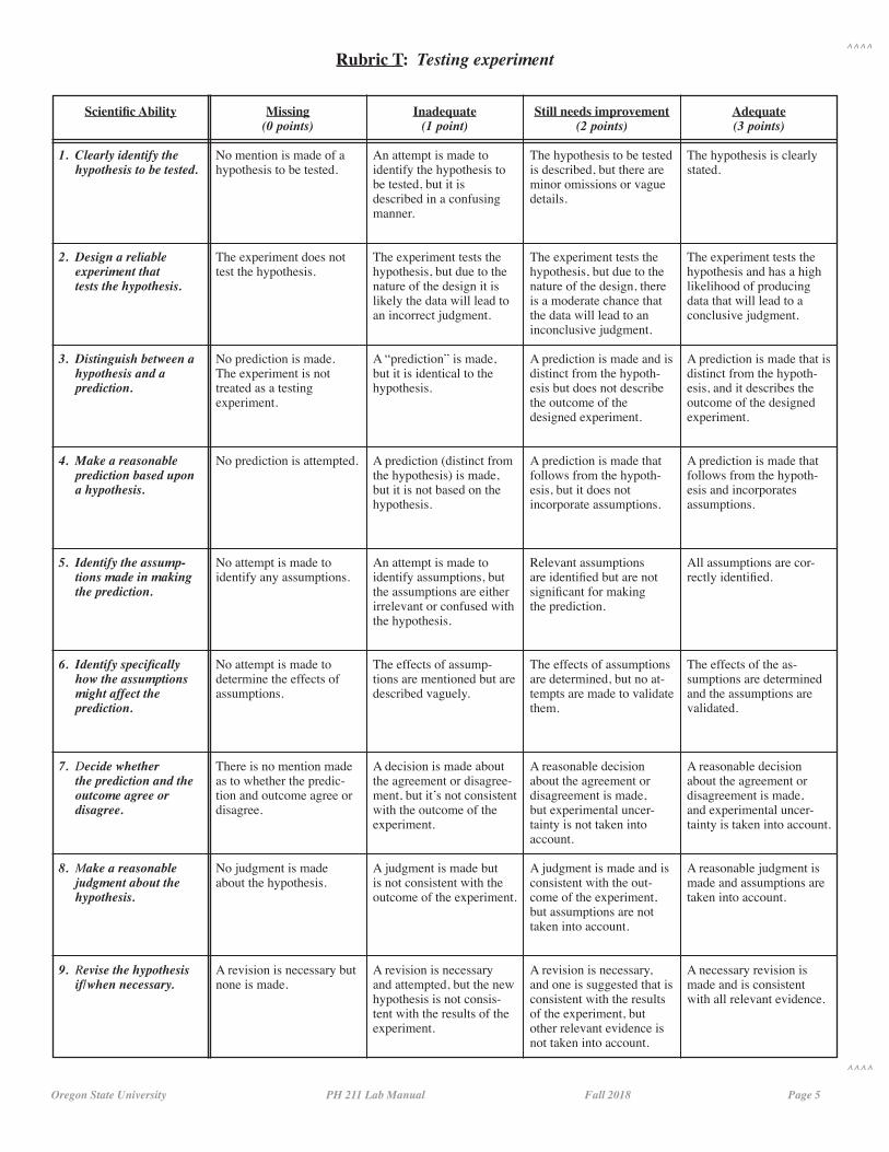
Rubric T: Testing experiment

Scientific Ability

1. Clearly identify the hypothesis to be tested.

2. Design a reliable experiment that tests the hypothesis.

3. Distinguish between a hypothesis and a prediction.

4. Make a reasonable prediction based upon a hypothesis.

5. Identify the assumptions made in making the prediction.

6. Identify specifically how the assumptions might affect the prediction.

7. Decide whether the prediction and the outcome agree or disagree.

8. Make a reasonable judgment about the hypothesis.

9. Revise the hypothesis if/when necessary.

Missing(0 points)

No mention is made of ahypothesis to be tested.

The experiment does not test the hypothesis.

No prediction is made. The experiment is not treated as a testingexperiment.

No prediction is attempted.

No attempt is made to identify any assumptions.

No attempt is made todetermine the effects ofassumptions.

There is no mention made as to whether the predic-tion and outcome agree or disagree.

No judgment is made about the hypothesis.

A revision is necessary butnone is made.

Inadequate(1 point)

An attempt is made to identify the hypothesis to be tested, but it isdescribed in a confusing manner.

The experiment tests the hypothesis, but due to the nature of the design it islikely the data will lead to an incorrect judgment.

A “prediction” is made, but it is identical to the hypothesis.

A prediction (distinct from the hypothesis) is made, but it is not based on the hypothesis.

An attempt is made to identify assumptions, but the assumptions are eitherirrelevant or confused with the hypothesis.

The effects of assump-tions are mentioned but are described vaguely.

A decision is made about the agreement or disagree-ment, but it’s not consistent with the outcome of theexperiment.

A judgment is made but is not consistent with the outcome of the experiment.

A revision is necessary and attempted, but the new hypothesis is not consis-tent with the results of the experiment.


The hypothesis to be tested is described, but there are minor omissions or vague details.

The experiment tests the hypothesis, but due to the nature of the design, there is a moderate chance that the data will lead to an inconclusive judgment.

A prediction is made and is distinct from the hypoth-esis but does not describe the outcome of thedesigned experiment.

A prediction is made that follows from the hypoth-esis, but it does notincorporate assumptions.

Relevant assumptions are identified but are not significant for makingthe prediction.

The effects of assumptions are determined, but no at-tempts are made to validate them.

A reasonable decision about the agreement or disagreement is made,but experimental uncer-tainty is not taken into account.

A judgment is made and isconsistent with the out-come of the experiment, but assumptions are nottaken into account.

A revision is necessary, and one is suggested that is consistent with the results of the experiment, but other relevant evidence is not taken into account.

Adequate(3 points)

The hypothesis is clearly stated.

The experiment tests thehypothesis and has a highlikelihood of producing data that will lead to a conclusive judgment.

A prediction is made that is distinct from the hypoth-esis, and it describes the outcome of the designed experiment.

A prediction is made that follows from the hypoth-esis and incorporates assumptions.


The effects of the as-sumptions are determined and the assumptions are validated.

A reasonable decision about the agreement or disagreement is made,and experimental uncer-tainty is taken into account.

A reasonable judgment is made and assumptions are taken into account.

A necessary revision is made and is consistent with all relevant evidence.


^^^^

^^^^

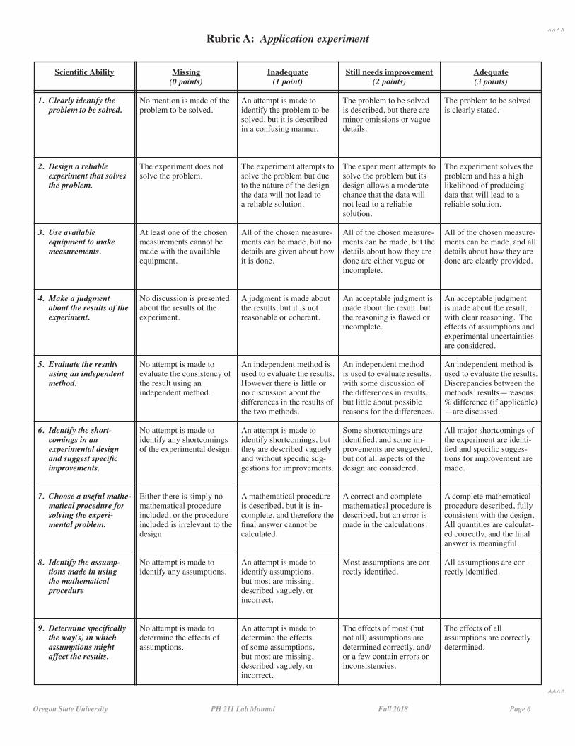
Rubric A: Application experiment

Scientific Ability

1. Clearly identify the problem to be solved.

2. Design a reliable experiment that solves the problem.

3. Use available equipment to make measurements.

4. Make a judgment about the results of the experiment.

5. Evaluate the results using an independent method.

6. Identify the shortcomings in an experimental design and suggest specific improvements.

7. Choose a useful mathematical procedure for solving the experimental problem.

8. Identify the assumptions made in using the mathematical procedure

9. Determine specifically the way(s) in which assumptions might affect the results.

Missing(0 points)

No mention is made of theproblem to be solved.

The experiment does notsolve the problem.

At least one of the chosenmeasurements cannot bemade with the availableequipment.

No discussion is presentedabout the results of theexperiment.

No attempt is made toevaluate the consistency ofthe result using anindependent method.

No attempt is made toidentify any shortcomingsof the experimental design.

Either there is simply no mathematical procedure included, or the procedure included is irrelevant to the design.

No attempt is made toidentify any assumptions.

No attempt is made todetermine the effects ofassumptions.

Inadequate(1 point)

An attempt is made to identify the problem to be solved, but it is described in a confusing manner.

The experiment attempts to solve the problem but due to the nature of the design the data will not lead toa reliable solution.

All of the chosen measure-ments can be made, but no details are given about how it is done.

A judgment is made about the results, but it is not reasonable or coherent.

An independent method isused to evaluate the results.However there is little or no discussion about the differences in the results of the two methods.

An attempt is made to identify shortcomings, but they are described vaguely and without specific sug-gestions for improvements.

A mathematical procedure is described, but it is in-complete, and therefore the final answer cannot becalculated.

An attempt is made to identify assumptions, but most are missing, described vaguely, or incorrect.

An attempt is made todetermine the effects of some assumptions, but most are missing, described vaguely, or incorrect.


The problem to be solved is described, but there are minor omissions or vague details.

The experiment attempts tosolve the problem but its design allows a moderate chance that the data willnot lead to a reliablesolution.

All of the chosen measure-ments can be made, but the details about how they are done are either vague or incomplete.

An acceptable judgment ismade about the result, but the reasoning is flawed orincomplete.

An independent method is used to evaluate results, with some discussion of the differences in results, but little about possible reasons for the differences.

Some shortcomings areidentified, and some im-provements are suggested, but not all aspects of the design are considered.

A correct and completemathematical procedure isdescribed, but an error is made in the calculations.

Most assumptions are cor-rectly identified.

The effects of most (but not all) assumptions are determined correctly, and/or a few contain errors or inconsistencies.

Adequate(3 points)

The problem to be solved is clearly stated.

The experiment solves the problem and has a high likelihood of producing data that will lead to areliable solution.

All of the chosen measure-ments can be made, and all details about how they are done are clearly provided.

An acceptable judgment is made about the result, with clear reasoning. The effects of assumptions and experimental uncertainties are considered.

An independent method is used to evaluate the results. Discrepancies between the methods’ results—reasons, % difference (if applicable) —are discussed.

All major shortcomings of the experiment are identi-fied and specific sugges-tions for improvement are made.

A complete mathematical procedure described, fully consistent with the design. All quantities are calculat-ed correctly, and the final answer is meaningful.


The effects of allassumptions are correctly determined.


^^^^

^^^^

Experimental Uncertainty

You can’t measure any physical quantity exactly. You can say only that its value lies within a certain range of uncertainty. Therefore, as an experimenter measuring any value, X, you must make a judgment that the “true” value of X lies somewhere between X – ΔX and X + ΔX (usually expressed in the standard form, X ± ΔX).

Why is this important? Why do you need to know about uncertainty—and how to estimate it? Because otherwise you can’t answer even the simplest questions in scientific experimentation. For example:

“Is the measured value in agreement with the prediction?”

“Do the data fit the physical model?”

To answer either of these questions, you need to use numbers—the data you’ve measured. But what value(s) should you use, when all of them contain uncertainties?

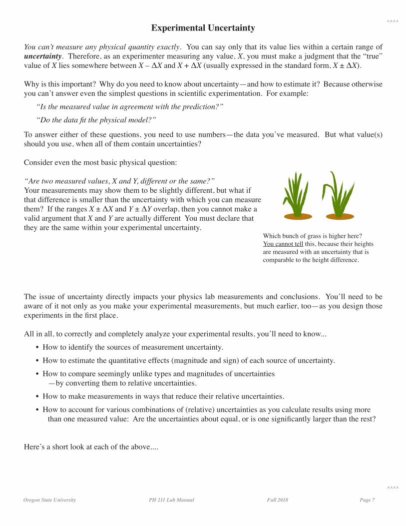
Consider even the most basic physical question:

“Are two measured values, X and Y, different or the same?”Your measurements may show them to be slightly different, but what ifthat difference is smaller than the uncertainty with which you can measurethem? If the ranges X ± ΔX and Y ± ΔY overlap, then you cannot make avalid argument that X and Y are actually different You must declare thatthey are the same within your experimental uncertainty. Which bunch of grass is higher here? You cannot tell this, because their heights are measured with an uncertainty that is comparable to the height difference.

The issue of uncertainty directly impacts your physics lab measurements and conclusions. You’ll need to be aware of it not only as you make your experimental measurements, but much earlier, too—as you design those experiments in the first place.

All in all, to correctly and completely analyze your experimental results, you’ll need to know...

• How to identify the sources of measurement uncertainty.

• How to estimate the quantitative effects (magnitude and sign) of each source of uncertainty.

• How to compare seemingly unlike types and magnitudes of uncertainties —by converting them to relative uncertainties.

• How to make measurements in ways that reduce their relative uncertainties.

• How to account for various combinations of (relative) uncertainties as you calculate results using more than one measured value: Are the uncertainties about equal, or is one significantly larger than the rest?

Here’s a short look at each of the above....


^^^^

^^^^

Sources of Uncertainty in Measurements

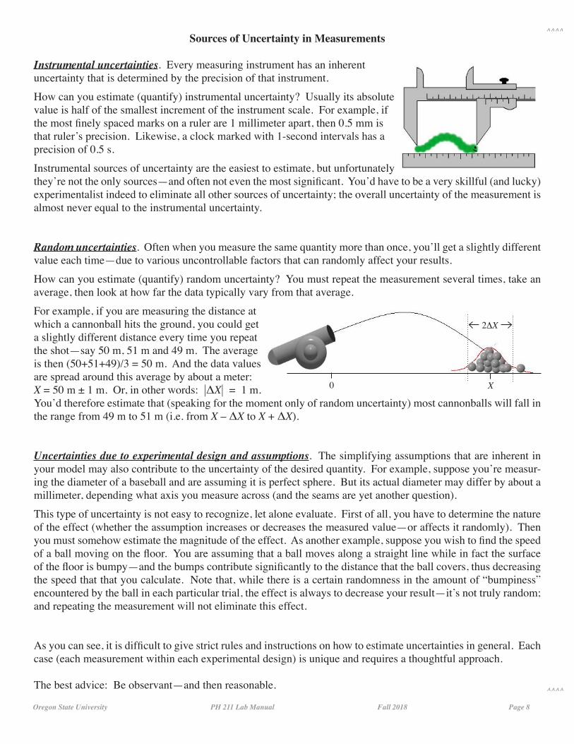
Instrumental uncertainties. Every measuring instrument has an inherentuncertainty that is determined by the precision of that instrument.

How can you estimate (quantify) instrumental uncertainty? Usually its absolutevalue is half of the smallest increment of the instrument scale. For example, ifthe most finely spaced marks on a ruler are 1 millimeter apart, then 0.5 mm isthat ruler’s precision. Likewise, a clock marked with 1-second intervals has aprecision of 0.5 s.

Instrumental sources of uncertainty are the easiest to estimate, but unfortunatelythey’re not the only sources—and often not even the most significant. You’d have to be a very skillful (and lucky) experimentalist indeed to eliminate all other sources of uncertainty; the overall uncertainty of the measurement is almost never equal to the instrumental uncertainty.

Random uncertainties. Often when you measure the same quantity more than once, you’ll get a slightly different value each time—due to various uncontrollable factors that can randomly affect your results.

How can you estimate (quantify) random uncertainty? You must repeat the measurement several times, take an average, then look at how far the data typically vary from that average.

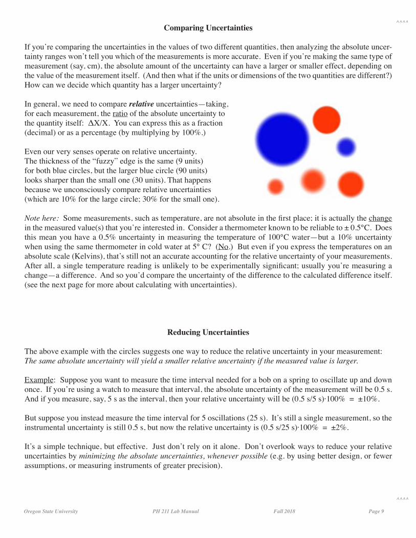
For example, if you are measuring the distance atwhich a cannonball hits the ground, you could geta slightly different distance every time you repeatthe shot—say 50 m, 51 m and 49 m. The averageis then (50+51+49)/3 = 50 m. And the data valuesare spread around this average by about a meter:X = 50 m ± 1 m. Or, in other words: |ΔX| = 1 m.You’d therefore estimate that (speaking for the moment only of random uncertainty) most cannonballs will fall in the range from 49 m to 51 m (i.e. from X – ΔX to X + ΔX).

Uncertainties due to experimental design and assumptions. The simplifying assumptions that are inherent in your model may also contribute to the uncertainty of the desired quantity. For example, suppose you’re measur-ing the diameter of a baseball and are assuming it is perfect sphere. But its actual diameter may differ by about a millimeter, depending what axis you measure across (and the seams are yet another question).

This type of uncertainty is not easy to recognize, let alone evaluate. First of all, you have to determine the nature of the effect (whether the assumption increases or decreases the measured value—or affects it randomly). Then you must somehow estimate the magnitude of the effect. As another example, suppose you wish to find the speed of a ball moving on the floor. You are assuming that a ball moves along a straight line while in fact the surface of the floor is bumpy—and the bumps contribute significantly to the distance that the ball covers, thus decreasing the speed that that you calculate. Note that, while there is a certain randomness in the amount of “bumpiness” encountered by the ball in each particular trial, the effect is always to decrease your result—it’s not truly random; and repeating the measurement will not eliminate this effect.

As you can see, it is difficult to give strict rules and instructions on how to estimate uncertainties in general. Each case (each measurement within each experimental design) is unique and requires a thoughtful approach.

The best advice: Be observant—and then reasonable.

0 X

2DX


^^^^

^^^^

Comparing Uncertainties

If you’re comparing the uncertainties in the values of two different quantities, then analyzing the absolute uncer-tainty ranges won’t tell you which of the measurements is more accurate. Even if you’re making the same type of measurement (say, cm), the absolute amount of the uncertainty can have a larger or smaller effect, depending on the value of the measurement itself. (And then what if the units or dimensions of the two quantities are different?) How can we decide which quantity has a larger uncertainty?

In general, we need to compare relative uncertainties—taking,for each measurement, the ratio of the absolute uncertainty tothe quantity itself: ΔX/X. You can express this as a fraction(decimal) or as a percentage (by multiplying by 100%.)

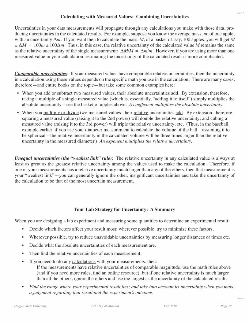
Even our very senses operate on relative uncertainty.The thickness of the “fuzzy” edge is the same (9 units)for both blue circles, but the larger blue circle (90 units)looks sharper than the small one (30 units). That happensbecause we unconsciously compare relative uncertainties(which are 10% for the large circle; 30% for the small one).

Note here: Some measurements, such as temperature, are not absolute in the first place; it is actually the change in the measured value(s) that you’re interested in. Consider a thermometer known to be reliable to ± 0.5°C. Does this mean you have a 0.5% uncertainty in measuring the temperature of 100°C water—but a 10% uncertainty when using the same thermometer in cold water at 5° C? (No.) But even if you express the temperatures on an absolute scale (Kelvins), that’s still not an accurate accounting for the relative uncertainty of your measurements. After all, a single temperature reading is unlikely to be experimentally significant; usually you’re measuring a change—a difference. And so you’d compare the uncertainty of the difference to the calculated difference itself. (see the next page for more about calculating with uncertainties).

Reducing Uncertainties

The above example with the circles suggests one way to reduce the relative uncertainty in your measurement: The same absolute uncertainty will yield a smaller relative uncertainty if the measured value is larger.

Example: Suppose you want to measure the time interval needed for a bob on a spring to oscillate up and down once. If you’re using a watch to measure that interval, the absolute uncertainty of the measurement will be 0.5 s. And if you measure, say, 5 s as the interval, then your relative uncertainty will be (0.5 s/5 s)·100% = ±10%.

But suppose you instead measure the time interval for 5 oscillations (25 s). It’s still a single measurement, so the instrumental uncertainty is still 0.5 s, but now the relative uncertainty is (0.5 s/25 s)·100% = ±2%.

It’s a simple technique, but effective. Just don’t rely on it alone. Don’t overlook ways to reduce your relative uncertainties by minimizing the absolute uncertainties, whenever possible (e.g. by using better design, or fewer assumptions, or measuring instruments of greater precision).


^^^^

^^^^

Calculating with Measured Values: Combining Uncertainties

Uncertainties in your data measurements will propagate through any calculations you make with those data, producing uncertainties in the calculated results. For example, suppose you know the average mass, m, of one apple, with an uncertainty Δm. If you want then to calculate the mass, M, of a basket of, say, 100 apples, you will get M ± ΔM = 100m ± 100Δm. Thus, in this case, the relative uncertainty of the calculated value M remains the same as the relative uncertainty of the single measurement: ΔM/M = Δm/m. However, if you are using more than one measured value in your calculation, estimating the uncertainty of the calculated result is more complicated.

Comparable uncertainties: If your measured values have comparable relative uncertainties, then the uncertainty in a calculation using those values depends on the specific math you use in the calculation. There are many cases, therefore—and entire books on the topic—but take some common examples here:

• When you add or subtract two measured values, their absolute uncertainties add. By extension, therefore, taking a multiple of a single measured value (which is, essentially, “adding it to itself”) simply multiplies the absolute uncertainty—see the basket of apples above. A coefficient multiplies the absolute uncertainty.

• When you multiply or divide two measured values, their relative uncertainties add. By extension, therefore, squaring a measured value (raising it to the 2nd power) will double the relative uncertainty; and cubing a measured value (raising it to the 3rd power) will triple the relative uncertainty; etc. (Thus, in the baseball example earlier, if you use your diameter measurement to calculate the volume of the ball—assuming it to be spherical—the relative uncertainty in the calculated volume will be three times larger than the relative uncertainty in the measured diameter.) An exponent multiplies the relative uncertainty.

Unequal uncertainties (the “weakest link” rule): The relative uncertainty in any calculated value is always at least as great as the greatest relative uncertainty among the values used to make the calculation. Therefore, if one of your measurements has a relative uncertainty much larger than any of the others, then that measurement is your “weakest link”—you can generally ignore the other, insignificant uncertainties and take the uncertainty of the calculation to be that of the most uncertain measurement.

Your Lab Strategy for Uncertainty: A Summary

When you are designing a lab experiment and measuring some quantities to determine an experimental result:

• Decide which factors affect your result most; wherever possible, try to minimize these factors.

• Wherever possible, try to reduce unavoidable uncertainties by measuring longer distances or times etc.

• Decide what the absolute uncertainties of each measurement are.

• Then find the relative uncertainties of each measurement.

• If you need to do any calculations with your measurements, then: If the measurements have relative uncertainties of comparable magnitude, use the math rules above (and if you need more rules, find an online resource); but if one relative uncertainty is much larger than all the others, ignore the others and use the largest as the uncertainty of the calculated result.

• Find the range where your experimental result lies; and take into account its uncertainty when you make a judgment regarding that result and the experiment’s outcome.

Oregon State University PH 211 Fall Term 2018

Lab 0Due: Tuesday, September 25, at 6:00 p.m.

Print your full LAST name: ______________________________________________

Print your full first name: _______________________________________________

Print your Lab TA’s name: _________________________________________

What is your Lab TA’s box # (located outside of Wngr 234)? _________

Print your Lab SECTION # here: ----------------->

“I affirm and attest that this Lab take-home excercise is my own work.While I may have had help from (and/or worked with) others,all the reasoning, solutions and results presented in final formhere are my own doing—and expressed in my own words.”

Sign your name (full signature): __________________________________________

Print today’s date: ____________________________________________________

Oregon State University Physics 211 Fall Term, 2018

Lab 0PH 211 Course Introduction

Purpose: To familiarize yourself with the purposes and policies of PH 211.

Directions: The answer to items here can be found either on the OSU web site or the PH 211 web site: http://www.physics.oregonstate.edu/~coffinc/COURSES/ph211. You’ll save a lot of time by first thoroughly reading all parts of the PH 211 web site (starting with the Syllabus and Frequently Asked Questions), rather than just skimming for answers. And note that some answers regarding lab will be found in the first portion of this lab file.

You may either use the space provided here, or you may supplement as needed with your own paper. (If you use your own paper, there is no need to re-state the questions.) But you’ll always need to provide (and complete) the cover sheet (first page) of this file.

1. a. Where will you find the written materials for each lab?

b. What information about each lab will your lab TA provide?

c. A lab group consists of how many students?

d. Why is it important to read each lab and prepare for it prior to arriving in lab?

e. What is the purpose of the labs in PH 211?

f. What portions of lab are covered on the exams?

http://www.physics.oregonstate.edu/~coffinc/COURSES/ph211/index.html


^^^^

^^^^

2. a. If you have to miss a lab (or want to repeat it for a better score), what are your options?

b. What are the consequences of not making up a missed lab or not turning in a take-home lab part?

c. What is your lab section #? What is your TA’s box #? Why are both numbers important enough to put on the front of any take-home lab assignment? Why is it important not to confuse the two numbers?

d. How will you know your lab percentage during the term? Does Chris keep a running total?

3. a. When are the PH 211 exams this term? Give the day of the week, the date, and the starting time for each:

Midterm 1: Midterm 2: Final:

SIGN HERE to confirm that you are aware of the above exam dates and times AND that you will notify Chris no later than ____________________________________________________ than Monday, October 1 about ANY time (your signature) conflicts you have for ANY of these exams.

b. What are you allowed to bring to the exams? Give a complete and detailed list.

c. When and how will you learn full details about the exam locations, rules and topics?

d. What should you do if you disagree with the scoring on your exam? Where is the form and specific information about this?


^^^^

^^^^

4. a. What portion of your total grade are the clicker questions?

Can any other portion of the course be substituted for your clicker score?

b. How do you register so that your clicker responses are credited?

c. Does your clicker app work in all three sections of lecture?

d. How does the clicker scoring work? (And what if you’re absent, late, you forget your app, or it doesn’t work?)

e. Where are clicker questions posted? How about the answers?

f. How will you know your clicker % during the term? Does Chris keep your running total?

5. a. Where do you find the Prep problem sets? How about the Prep problem solutions?

b. How closely do Prep problems represent typical exam or HW problems?

c. What portion of your grade do you earn with Prep problems?


^^^^

^^^^

6. a. Where do you find the HW (homework) assignments? How about the HW solutions?

b. How many HW assignments are there?

c. What are those other links (e.g. Lab 1-VI, Lab 2-IV, Prep 1-2, etc.)? What sorts of assignments are they?

d. Where do you get full details on what are the HW sets like—and when/where they are due?

e. How will you know how you did on your HW assignments?

f. What portion of your total grade are the HW assignments?

Can any other portion of the course be substituted for your HW score?


^^^^

^^^^

7. a. What are Chris’ office hours this term—and where is his office?

b. Do you need to make an appointment with Chris in order to visit during office hours?

c. If you need to make an appointment with Chris for any other time, how should you do this?

d. What number of hours does Chris recommend as a rough “time budget” for you to spend per week— outside of class and lab time—studying in this course?

What number of hours per credit hour does OSU (via its Academic Success Center) recommend that you budget for study in any course?

e. What are the key factors Chris recommends for more effective learning and better success in this course?

f. Where do the Prep problems come from? What is the real purpose of the Prep problem sets and how should you use them?

g. According to OSU’s Academic Regulations, what does a grade of C represent?

h. What portion of all students who enrolled in PH 211 last Fall here at OSU earned a course grade of C or better?


^^^^

^^^^

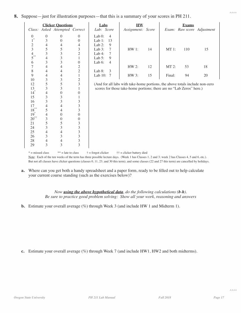
8. Suppose—just for illustration purposes—that this is a summary of your scores in PH 211.

Clicker Questions Labs HW Exams Class: Asked Attempted Correct Lab: Score Assignment: Score Exam: Raw score Adjustment

0 0 0 0 Lab 0: 4 1† 3 0 0 Lab 1: 13 2 4 4 4 Lab 2: 9 3 5 5 3 Lab 3: 7 HW 1: 14 MT 1: 110 15 4 3 3 2 Lab 4: 7 5** 4 3 1 Lab 5: 9 6 3 3 0 Lab 6: 4 7 4 4 2 HW 2: 12 MT 2: 53 18 8 4 4 2 Lab 8: 3 9 4 4 1 Lab 10: 7 HW 3: 15 Final: 94 20 10 3 3 2 12 5 5 3 (And for all labs with take-home portions, the above totals include non-zero 13 3 3 1 scores for those take-home portions; there are no “Lab Zeros” here.) 14* 4 0 0 15 3 3 1 16 3 3 3 17 4 4 3 18** 5 4 3 19* 4 0 0 20†† 3 0 0 21 5 5 3 24 3 3 3 25 4 4 3 26 3 3 3 28 4 4 3 29 3 3 3

* = missed class ** = late to class † = forgot clicker †† = clicker battery died Note: Each of the ten weeks of the term has three possible lecture days. (Week 1 has Classes 1, 2 and 3; week 2 has Classes 4, 5 and 6, etc.). But not all classes have clicker questions (classes 0, 11, 23, and 30 this term), and some classes (22 and 27 this term) are cancelled by holidays.

a. Where can you get both a handy spreadsheet and a paper form, ready to be filled out to help calculate your current course standing (such as the exercises below)?

Now using the above hypothetical data, do the following calculations (b-h).Be sure to practice good problem solving: Show all your work, reasoning and answers

b. Estimate your overall average (%) through Week 3 (and include HW 1 and Midterm 1).

c. Estimate your overall average (%) through Week 7 (and include HW1, HW2 and both midterms).


^^^^

^^^^

d. Estimate your overall course average (%) going into the final exam (including all work except the final).

e. Estimate the net score (i.e. after adjustment) that you needed on the final exam to get a C for the course.

f. Estimate your final course average (%) and course grade.

g. What if you had missed Classes 18 and 26 (but all other data given on the previous page were as given)? Re-estimate your final course % and grade in this case.

h. What if you had turned in Lab 5-III (scoring 4 points) but you never did the 5-point in-lab portion of Lab 5 (that is, parts 5-I and 5-II)—and neglected to make those up? Assuming that all other data given on the previous page were as given, re-estimate your final course % and grade in this case.

i. Why are all these calculations (b-h) only estimates (not exact)? And are the estimates probably conservative (too low) or optimistic (too high)?


^^^^

^^^^

LAB 1: Linear Motion

I. General Physics Knowledge “Pre-” Survey

Your lab TA will soon be introducing him/herself and how lab works—before you start doing any lab activities. But first, there is a 30-minute “pre-test” survey of where you’re starting with your physics knowledge. The Physics Department uses this data only internally—to try to improve these courses. This item is required (and worth 5 points to you)—please answer all items to the best of your current knowledge. But please note: The 5 points will be awarded not according to whether your answers are right or wrong, but only whether you participated fully and did your best. Your lab TA will explain the details of the survey and give you all materials necessary (write only on the answer form—not on the questions sheets).

IMPORTANT: If you have absolutely no idea what the question is talking about—or no idea about how to answer it—just leave the answer blank, rather than guessing randomly. But if you have at least some idea about the item, go ahead and give it your best try.

II. Background: Drawing Motion Diagrams

Study this section. Then your TA will work an example and show how to translate between motion diagrams and graphs.

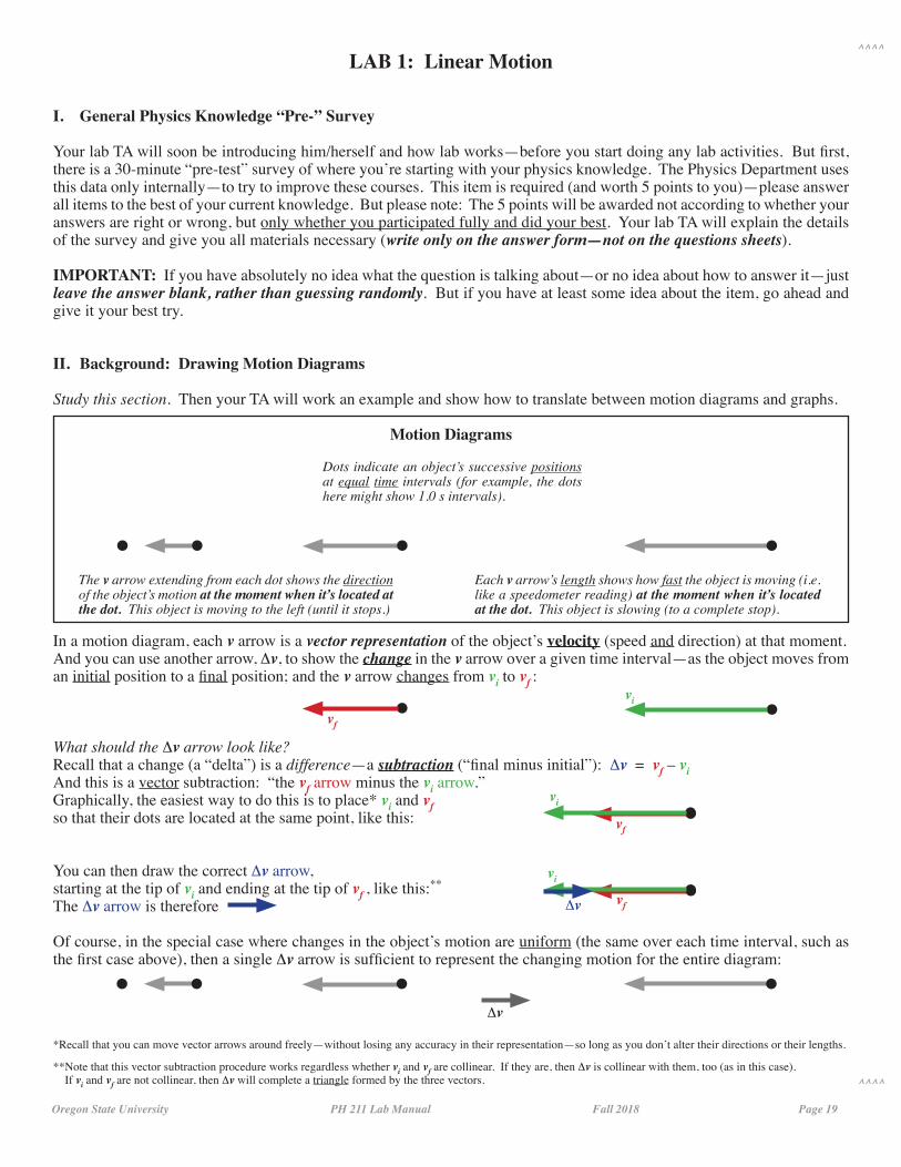
Motion Diagrams

In a motion diagram, each v arrow is a vector representation of the object’s velocity (speed and direction) at that moment. And you can use another arrow, Dv, to show the change in the v arrow over a given time interval—as the object moves from an initial position to a final position; and the v arrow changes from vi to vf :

What should the Dv arrow look like?Recall that a change (a “delta”) is a difference—a subtraction (“final minus initial”): Dv = vf – viAnd this is a vector subtraction: “the vf arrow minus the vi arrow.”Graphically, the easiest way to do this is to place* vi and vfso that their dots are located at the same point, like this:

You can then draw the correct Dv arrow,starting at the tip of vi and ending at the tip of vf , like this:**

The Dv arrow is therefore

Of course, in the special case where changes in the object’s motion are uniform (the same over each time interval, such as the first case above), then a single Dv arrow is sufficient to represent the changing motion for the entire diagram:

*Recall that you can move vector arrows around freely—without losing any accuracy in their representation—so long as you don’t alter their directions or their lengths.

**Note that this vector subtraction procedure works regardless whether vi and vf are collinear. If they are, then Dv is collinear with them, too (as in this case). If vi and vf are not collinear, then Dv will complete a triangle formed by the three vectors.

Dots indicate an object’s successive positions at equal time intervals (for example, the dots here might show 1.0 s intervals).

The v arrow extending from each dot shows the direction of the object’s motion at the moment when it’s located at the dot. This object is moving to the left (until it stops.)

Each v arrow’s length shows how fast the object is moving (i.e. like a speedometer reading) at the moment when it’s located at the dot. This object is slowing (to a complete stop).

vf

vi

vf

vi

vf

vi

Dv

Dv


^^^^

^^^^

III. Investigating and Representing Linear Motion (an Observation experiment)

Purposes:

• Design an experiment to observe motion;

• Practice making clear observations and distinguishing them from explanations;

• Practice taking data in a scientific fashion;

• Represent motion in multiple ways and understand the relationships between those representations.

Description:

You have a cart and a metal ramp, meter sticks, a stopwatch, and pieces of sticky-tape for marking locations on the ramp. The task for your group is to describe the motion of the cart under at least two different conditions, and to represent each condition two different ways.

Notes and Suggestions:

First do a few trial runs so that you get used to calling out the time at equal intervals and marking the locations. (It may take all of your group members working together to mark the cart accurately and frequently!)

Then use the following as an experimental guide. All lettered steps must be addressed in your lab write-up—a random sub-set of those steps will be graded. (Not all labs this term will prompt you so explicitly on the steps you should take, but for these first few times, you’ll get a little more guidance.) Note: Any step followed by a code refers to a specific skill in one of the rubrics. For example, (O3) would refer to ability 3 in the Observation experiment rubric.

a. Design two reliable experiments that will investigate the phenomenon. (O2)

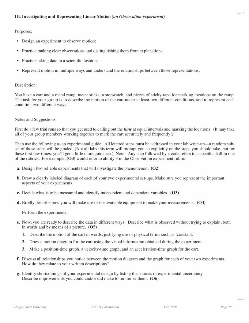
b. Draw a clearly labeled diagram of each of your two experimental set-ups. Make sure you represent the important aspects of your experiments.

c. Decide what is to be measured and identify independent and dependent variables. (O3)

d. Briefly describe how you will make use of the available equipment to make your measurements. (O4)

Perform the experiments.

e. Now, you are ready to describe the data in different ways: Describe what is observed without trying to explain, both in words and by means of a picture. (O5) 1. Describe the motion of the cart in words, justifying use of physical terms such as ‘constant.’ 2. Draw a motion diagram for the cart using the visual information obtained during the experiment. 3. Make a position-time graph, a velocity-time graph, and an acceleration-time graph for the cart.

f. Discuss all relationships you notice between the motion diagram and the graph for each of your two experiments. How do they relate to your written descriptions?

g. Identify shortcomings of your experimental design by listing the sources of experimental uncertainty. Describe improvements you could and/or did make to minimize them. (O6)


^^^^

^^^^

IV. Playing with Motion

Purposes:

• Practice with the motion sensors and Logger Pro software.

• Connect your kinesthetic experience with the graphs.

• Practice interpreting data and graphs

Description:

You’ll be using motion detectors to determine the locations of objects at various times—without saving data this time.


The detector emits ultrasonic (high-frequency sound) waves in a cone about 20 degrees. The waves reflect off objects and are recaptured by the sensor; based on the speed of sound the sensor then knows how far away the object is. These waves measure the position of the object—accurate to within about 1 mm. Sequential position measurements are used to calcu-late the velocity and acceleration of the object.

a. Connect the Motion Detector to DIG/SONIC 2 of the LabPro. If the Motion Detector won’t connect to LoggerPro, unplug it from the USB port and plug it back in. Check other wired connections, also.

b. Place the Motion Detector so that it points toward an open space at least 4 m long. Anything within the cone can reflect the waves and possibly cause an accidental measurement, so watch for chairs, desks, other people, etc. Objects closer than 0.5 m or further than 7 m will not be detected properly. Some targets (e.g. a bulky sweater) may not give a strong reflection, giving inconsistent results. If this happens, hold a book in front of you. In a crowded room, it may be hard to find 3-4 meters with no interference. Be alert for this—cooperate with other groups, taking turns as needed.

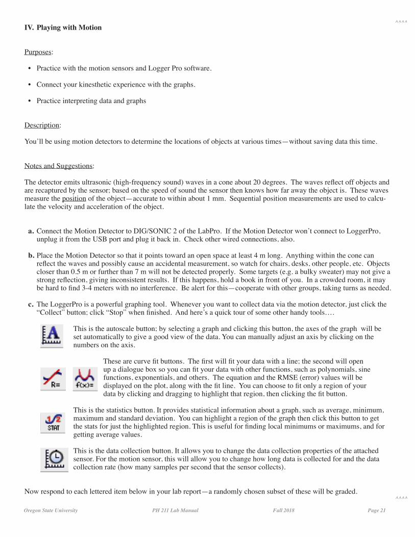
c. The LoggerPro is a powerful graphing tool. Whenever you want to collect data via the motion detector, just click the “Collect” button; click “Stop” when finished. And here’s a quick tour of some other handy tools….

This is the autoscale button; by selecting a graph and clicking this button, the axes of the graph will be set automatically to give a good view of the data. You can manually adjust an axis by clicking on the numbers on the axis.

These are curve fit buttons. The first will fit your data with a line; the second will open up a dialogue box so you can fit your data with other functions, such as polynomials, sine functions, exponentials, and others. The equation and the RMSE (error) values will be displayed on the plot, along with the fit line. You can choose to fit only a region of your data by clicking and dragging to highlight that region, then clicking the fit button.

This is the statistics button. It provides statistical information about a graph, such as average, minimum, maximum and standard deviation. You can highlight a region of the graph then click this button to get the stats for just the highlighted region. This is useful for finding local minimums or maximums, and for getting average values.

This is the data collection button. It allows you to change the data collection properties of the attached sensor. For the motion sensor, this will allow you to change how long data is collected for and the data collection rate (how many samples per second that the sensor collects).

Now respond to each lettered item below in your lab report—a randomly chosen subset of these will be graded.


^^^^

^^^^

(This activity is not a traditional experiment; none of the steps below corresponds to any of the rubrics.)

d. Use the Logger Pro software to make graphs of position and velocity vs. time. Compare the graphs you get for someone moving toward the motion detector to someone moving away from it; and for someone moving at various speeds (fast and slow). Explain your findings in your lab report.

e. Open the experiment file (located in the lab 1 motion folder, which you’ll find after you’ve logged in as PH211). The file is called Exp 01b Distance Match One. The position vs. time graph shown will appear. Describe how you would walk to produce this target graph.

f. Perform the necessary experiment to match the position graph as well as you reasonably can.

g. Sketch the graph from the file and from your data in your lab report, and discuss in your lab report any differences between the two graphs.

h. Open the experiment file Exp 01c Distance Match Two. Describe how you would walk to produce this target graph.

i. Perform the necessary experiment to match position the graph as well as you reasonably can.

j. In your lab report, sketch the graphs from the file and your data, then discuss any differences between the two graphs.

V. Determining a Relationship Between Ramp Angle and Acceleration (an Observation experiment)

Purposes:

• Design an experiment to determine a mathematical relationship.

• Construct a mathematical relationship from data.

Description:

You have a cart and a metal ramp, meter sticks, and a motion detector. The task for your group is to determine a mathemati-cal relationship between the angle of the ramp and the acceleration of the cart, based on your experimental data.


The software will graph the velocity of the cart (vs. time). Then there is a ‘Fit’ button on the toolbar in Logger Pro—take a moment to compare how the different mathematical fit models look with your data. They may look similar, or one may look like a better fit than the others—but for this experiment, look for a linear fit for velocity to determine the acceleration.

Use the following guide—again (as in Lab 1, part III above), with these reminders: All lettered steps must be addressed in your lab write-up; a random subset of those steps will be graded. (Not all labs this term will prompt you so explicitly on the steps you should take, but for these first few times, you’ll get a little more guidance.) Note: Any step followed by a code refers to a specific skill in one of the rubrics. Thus, (O3) would refer to ability 3 in the Observation experiment rubric.

a. Design a reliable experiment that will investigate the phenomenon. (O2)

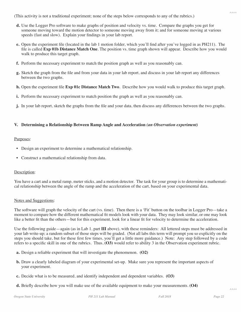
b. Draw a clearly labeled diagram of your experimental set-up. Make sure you represent the important aspects of your experiment.

c. Decide what is to be measured, and identify independent and dependent variables. (O3)

d. Briefly describe how you will make use of the available equipment to make your measurements. (O4)


^^^^

^^^^

Perform the experiments.

e. Describe what is observed without trying to explain, both in words and by means of a data table. (O5)

f. Explain specifically how you are finding the acceleration from your data and why you’re being asked to do a fit from the velocity graph.

g. Using your data, construct a mathematical relationship that represents a trend in the data (the relationship between the ramp angle and the acceleration of the cart). (O7)

h. Devise an explanation for your observed relationship between the ramp angle and the cart’s acceleration. (O8)

i. Identify any assumptions made in devising the explanation. (O9)

j. How could you test the relationship you found? In your lab report, give a brief description of an experiment that will test that relationship. (You do not need to conduct the test.)

k. Identify shortcomings of your experimental design by listing the sources of experimental uncertainty. Describe improvements you could and/or did make to minimize them. (O6)

VI. Math Review

Purpose:

To practice with the math tools you will need this term in PH 211.

Description:

This last part of Lab 1 is a take-home set of exercises. Click here to download the .pdf file containing all instructions, examples and items for this set of practice exercises.


Lab 1 is worth 15 points total. This (part VI) exercise set is worth 5 points all by itself—but unlike the other parts (I - V), this part is a take-home item, due from every student (not a group assignment) by Tuesday, October 2, at 6:00 p.m.

When you are ready to turn in this take-home assignment, you do not need to include the pages that contained explana-tions—only pages where you worked the various exercises (and space has been provided for most, although you may want to use additional sheets of your own—and you will definitely need to provide 2 sheets of graph paper). Be sure to label each secton and item of the exercises so that the grader can easily find and follow your work.

Turn in your completed work, including diagrams and accompanying equations—with the completed cover sheet stapled on top—to your Lab TA’s box (located outside Wngr 234).

http://www.physics.oregonstate.edu/~coffinc/COURSES/ph211/Labs/Lab1-VI.pdf


^^^^

^^^^

LAB 2: Linear Kinematics

I. Background: Experimental Uncertainties and the Weakest Link Rule

Carefully read (or re-read) pages 7-10 of the general information accompanying these labs—the material about experimental uncertainty.

This reminder of the “Weakest Link” rule: The relative (percent) uncertainty in the calculated value of an experimental quantity is at least as great as the most uncertain (i.e. greatest relative uncertainty) value used to make the calculation. So first you must estimate the relative uncertainty in each measured quantity used to make the calculation. If the uncertainty of one of those measurements is significantly greater than any of the others, then (as a rough estimate) the final calculation is assigned the same percent uncertainty as that most uncertain measurement.

Example: Suppose that after a hike in the mountains, a friend asks how fast you walked. You recall only that the trailhead sign said the trail (the round-trip loop) was 6.1 miles long and that it took you somewhere between two and three hours. So you use an estimated time of 2.5 h and then calculate your average speed: Average speed = 6 miles/2.5 h = 2.4 miles/h.

You report this to your friend. How confident should he be of your estimate?

Notice that you didn’t report any specific uncertainty, so your friend will assume the absolute uncertainty implied by the significant figures of your answer (half the value of the least significant digit): ± 0.05 miles/h

Thus, you have implied this relative uncertainty: [(± 0.05 miles/h)/(2.4 miles/h)]·100% = ±2%

Is this justified? Are you really that sure—to within 2%—how fast your average walking speed was? No way.Look at your two measurements and their relative uncertainties:

The distance (6.1 ± 0.05 miles, implied by the trailhead sign) had a relative uncertainty of [(± 0.05 mi)/(6.1 mi)]·100% = ±0.8%.

But the time interval for the trip (2.5 ± 0.5 hours) had a relative uncertainty of [(± 0.5 h)/(2.5 h)]·100% = ±20%.

This is a case where the “Weakest Link” rule clearly applies: Since the two measurements had drastically different rela-tive uncertainties, a good rough estimate of the relative uncertainty in your reported calculation (your speed) is the relative uncertainty of the most uncertain measurement (your time): ±20%. And 20% of 2.4 is about 0.5.

Conclusion: You should have told your friend that on your hike you walked at about 2.4 miles/h ± 0.5 miles/h.


^^^^

^^^^

II. (STATION A) Angle and Acceleration for a Wooden Block Sliding Down a Wooden Ramp (an Observation Experiment)

Purposes:

• Design an experiment to take appropriate data to find a relationship.

• Construct a mathematical relationship from data.

• Interpret the relationship and data to understand the differences between this relationship and the one you found with a cart on a track

Description:

You have a wooden block, a wood ramp, meter sticks, and a motion detector. The task for your group is to determine a math-ematical relationship between the angle of the ramp and the acceleration of the block, based on your experimental data.


The software will graph the position and velocity of the block (vs. time). Then you will use the ‘Fit’ button on the toolbar in Logger Pro to try a Linear fit for velocity and acceleration, then a Quadratic fit for position and acceleration. (The issue: Which is a better fit?) Use the following guide—with these reminders: All lettered steps must be addressed in your lab write-up; a random subset of those steps will be graded. Note: Any step followed by a code refers to a specific skill in one of the rubrics. Thus, (O3) would refer to ability 3 in the Observation experiment rubric. a. Design a reliable experiment that will investigate the phenomenon. (O2) b. Draw a clearly labeled diagram of your experimental set-up. Be sure to represent the important aspects of your experiment. c. Decide what is to be measured, and identify independent and dependent variables. (O3) d. Briefly describe how you will make use of the available equipment to make your measurements. (O4)Perform the experiment. e. Describe what is observed without trying to explain, both in words and by using a data table. (O5) f. Explain specifically how you are finding the acceleration from your data and why you are being asked to do a fit from the velocity graph. g. Using your data, construct a mathematical relationship that represents a trend in the data (the relationship between the ramp angle and the acceleration of the block). Use Logger Pro to help you graph and fit the data. (Your relationship should span the range of angles between 0 and 90 degrees and won’t necessarily be a simple relationship.) (O7) h. Devise an explanation for your observed relationship. (O8) i. Identify any assumptions made in devising the explanation (relationship between the ramp angle and the acceleration of the block). (O9) j. How could you test the relationship you found? Give a brief description in your lab report of an experiment that would test the relationship in your lab report. (You do not need to conduct the test.) k. Identify shortcomings of your experimental design by listing the sources of experimental uncertainty. Describe improvements you could and/or did make to minimize them. (O6) l. Use of the weakest link rule to estimate the uncertainty in your relationship. m. Contrast the mathematical relationship you found here with the one you found in Lab 1, part III, between a cart and a metal track. What is similar between the two relationships? What is different? What about the experiments might contribute to a different relationship?


^^^^

^^^^

III. (STATION B) Predicting where two carts will meet (a Testing Experiment)

Purposes:

• Combining experimental data with problem solving to make predictions for the outcome of a new situation.

• Considering factors that will impact the outcome of the situation.

• Having fun smashing things together.

Description:

Your task is to place two carts in the appropriate initial positions so that they meet at the center point when released from rest (at the same moment), rolling down their respective ramps—whose incline angles differ by at least 15 degrees.

You may use the equipment to take any necessary data, but you are not allowed to use ‘trial and error’ to solve this. You must calculate and predict the right locations—then test those predictions in front of your TA. You are not allowed to do the final ‘test’ of your calculations until you have approval from your TA—and he/she must be present to observe the test.


Make sure the foam pad is between the two ramps at the base, so the carts don’t actually collide in the center, but hit each side of the foam pad simultaneously. Then use the following guide—with these reminders: All lettered steps must be ad-dressed in your lab write-up; a random subset of those steps will be graded. Note: Any step followed by a code refers to a specific skill in one of the rubrics. Thus, (T3) would refer to ability 3 in the Testing experiment rubric. a. Make a sketch of your experiment, including labels for all important aspects. b. What quantities will you need to find in order to predict the appropriate starting locations? c. Do any necessary experiments, measurements, or calculations to determine the values of those quantities. (You may also refer to your results from lab 1.) d. Make a reasonable prediction based on your hypothesis (the model developed in lab 1 and the kinematics model developed in class) to predict where to initially place the carts such that they meet in the center. (T4) e. Use the weakest link rule to estimate the uncertainty in your calculations. f. Identify the assumptions made in making the prediction. (T5) g. Determine specifically the way in which assumptions might affect the prediction (for example, will ignoring a certain effect mean you should actually place the cart a little higher or a little lower—and why?) (T6)When your calculations are completed, show the results to your lab instructor and then try the experiment. h. Record the outcome of your experiment. i. Decide whether or not the prediction and the outcome agree/disagree. (T6) j. Reconcile any difference in your prediction and the outcome of the experiment. Be specific. For example, you can discuss how experimental uncertainties affected the outcome; or how you can improve your calculations.


^^^^

^^^^

IV. “Spot the Physics” – Motion

Purpose:

To practice identifying the type(s) of motion—and related issues—that you will commonly encounter .

Description:

This last part of Lab 2 is a take-home set of exercises. Click here to download the .pdf file containing all instructions, examples and items for this set of practice exercises. (The link may not yet be ready at the start of Week 2.)


Lab 2 is worth 10 points total. This (part IV) exercise set is worth 5 points all by itself—but unlike the other parts (I - III), this part is a take-home item, due from every student (not a group assignment) by Tuesday, October 9, at 6:00 p.m.

When you are ready to turn in this take-home assignment, you do not need to include the pages that contained only explana-tions—only pages where you worked the various exercises (and space has been provided for most, although you may want to use additional sheets of your own). Be sure to label each secton and item of the exercises so that the grader can easily find and follow your work.

Turn in your completed work, including diagrams and accompanying equations—with the completed cover sheet stapled on top—to your Lab TA’s box (located outside Wngr 234).

http://www.physics.oregonstate.edu/~coffinc/COURSES/ph211/Labs/Lab2-IV.pdf


^^^^

^^^^

LAB 3: Applying Linear Kinematics

I. Rolling Rocks (a Testing Experiment)

Purpose:

To design, implement and report on a testing experiment with a minimum of guidance (i.e, to conduct a reasonably authentic scientific investigation).

Description:

A heated (and high-stakes) controversy has recently erupted between the residents of a new housing estate and the local Town Council. The estate is situated by the shore of a small lake, and the issue is the possible danger posed by a number of large rocks perched on the slope above a high cliff on the opposite shore of the lake.

At the heart of the dispute is the relationship between the rocks’ height (h) above the edge of the cliff and the horizontal dis-tance (d) which the rocks will travel as projectiles should they break loose, roll down the hill and go off the edge of the cliff. Two groups of ‘experts’ (engineers and geologists) have already investigated. Each group used an apparatus consisting of a slope and a steel ball. In both studies, the steel ball was rolled down the slope and off the edge from various heights, and h and d were measured.

The engineers concluded that h is proportional to d, but the geologists concluded that h is proportional to d2. If one group is correct, the rocks will land in the lake, but if the other group is correct, the rocks will shoot over the lake and smash into the houses.

The Chair of the OSU Physics Department has been approached to resolve the controversy and now asks you to investigate the situation urgently (using the same apparatus). She wants a full report detailing all aspects of the experiments, measure-ments, calculations, and graphs—and your group’s conclusions as to which (if either) of the other groups is correct. In par-ticular, she needs careful attention paid to your graphs of d vs. h and d2 vs. h—and the explanations as to how these graphs were used to determine the proportionality: She will be showing them to reporters at a press conference later this week.


Use the Testing experiment rubric and its various parts to guide what you include in your lab report (recall, for example how you carried out and reported on the testing experiment from Lab 2—but keep in mind that you may need more parts of the rubric than you did in Lab 2).

Be sure to incorporate error analysis using the weakest link rule detailed in the first part of this lab packet.

A randomly chosen subset of the rubrics will be used for grading.


^^^^

^^^^

II. Testing Experiment: Falling Cotton Balls

Purpose:

To design, implement and report on a testing experiment with a minimum of guidance (i.e, to conduct a reasonably authentic scientific investigation).

Description:

Design, implement and report on an experiment that tests the following theory.

On the Descent of Cotton Balls: a Theoretical Perspective

J. K. FINKLEBOTTOM & P. R. PRIEST

Abstract: Cotton balls fall more slowly than rocks in most situations. We present an extension to the traditional Newtonian view of objects to include free-falling cotton balls.

Cotton balls (which are sometimes made of Rayon) are puffs of fluff, roughly spherical, with a diameter of about 3 cm and a mass between 0.5g and 1.0g. If you drop them, they fall. It has been observed, however (Galileo and Snerd, 1998) that if you drop a rock and a cotton ball simultaneously from the top of a tower, the rock hits first. Evidently, air resistance slows the cotton ball more than the rock. We suggest that its effect is greater because the cotton ball is lighter. Our reasoning is this: Each air molecule, on impact, imparts a small force to a falling object. Using the traditional force formula, F = ma (Newton, 1687), we see that each collision effectively reduces the gravitational acceleration of any object falling through air by an amount that is inversely proportional to that object’s mass (i.e., a = F⁄m). Thus the light cotton ball is slowed more than a comparably-sized (and heavier) rock.

Therefore we should modify the formula for the distance, s, fallen in time t.

Instead of the traditional formula, s = (1/2)gt2 (where g is the acceleration of gravity), we suggest that the

correct model for falling cotton balls is s = (1/2)kt2, where k is an acceleration value smaller than g.

Though the truth of our theory seems self-evident, we await confirmation from experiment.

eeps media © 2004 – Annals of Plausibility


Use the Testing experiment rubric and its various parts to guide what you include in your lab report (recall, for example how you carried out and reported on the testing experiment from lab 2—but keep in mind that you may need more parts of the rubric than you did in lab 2).

Be sure to incorporate error analysis using the weakest link rule detailed in the first part of this lab packet.

A randomly chosen subset of the rubrics will be used for grading.

PH 211 Labs - Physics | | Oregon State University

Documents

Transcript of PH 211 Labs - Physics | | Oregon State University