Peristaltic flow of a Maxwell fluid in a channel with compliant walls

Chaos, Solitons and Fractals 39 (2009) 407–416

www.elsevier.com/locate/chaos

Peristaltic flow of a Maxwell fluid in a channelwith compliant walls

Nasir Ali a,*, Tasawar Hayat a, Saleem Asghar b

a Department of Mathematics, Quaid-i-Azam University 45320, Islamabad 44000, Pakistanb Department of Mathematical Sciences, COMSATS Institute of Information Technology, Islamabad, Pakistan

Abstract

This paper describes the peristaltic motion of a non-Newtonian fluid in a channel having compliant boundaries.Constitutive equations for a Maxwell fluid have been used. Perturbation method has been used for the analytic solution.The influence of pertinent parameters is analyzed. Comparison of the present analysis of Maxwell fluid is made with theexisting results of viscous fluid.� 2007 Elsevier Ltd. All rights reserved.

1. Introduction

The study of peristaltic flow has been generated a lot of interest and hence the huge amount of literature on the topicis available for the viscous fluids. Such study has a host of well established applications in the applied sciences. Thisincludes the urine transport from kidney to bladder, the movement of chyme in the gastrointestinal tract, transportof spermatozoa in the ductus efferentes of the male reproductive tract, movement of ovum in the female fallopian tube,swallowing of food through the esophagus, transport of lymph in the lymphatic vessels and the vasomotion of smallblood vessels such as arterioles, venules and capillaries. In addition, technical roller and finger pumps also operateaccording to the mechanism of peristalsis.

Recently, the motion of non-Newtonian fluids has been an important subject in the field of chemical, biomedical andenvironmental engineering and science. Undoubtedly the mechanics of non-Newtonian fluids presents special chal-lenges to engineers, physicists, modellers, numerical simulists and mathematicians. This is due to the fact that nonlin-earity manifest itself in a variety of ways. The flows of non-Newtonian fluids are not only important because of theirtechnological significance but also in the interesting mathematical features presented by the equations governing theflow. Moreover, the elastic properties of real fluids can be determined and measured. Extensive literature on the subjectis now available. Some recent contributions in this direction may be given in Refs. [1–10]. There are also few studiesavailable about peristaltic flow of non-Newtonian fluids. Mention may be made to some recent interesting studies[11–21]. Very recently, Abd Elnaby and Haroun [22] discussed the peristaltic flow of a viscous fluid in a channel havingcompliant walls.

0960-0779/$ - see front matter � 2007 Elsevier Ltd. All rights reserved.doi:10.1016/j.chaos.2007.04.010

* Corresponding author.E-mail address: [email protected] (N. Ali).

mailto:[email protected]

408 N. Ali et al. / Chaos, Solitons and Fractals 39 (2009) 407–416

To date peristaltic flow of non-Newtonian fluid between compliant walls has not been analyzed. The main goal hereis to present such a study. For that we select a subclass of rate type fluids namely the Maxwell fluid which can predictthe stress relaxation effects. The two-dimensional channel flow has been first modelled and than solved under smallwave amplitude assumption. Expression for the mean velocity has been determined by employing perturbation method.Graphs are plotted just to analyze the novel features of various sundry parameters.

2. Flow analysis

Let ðx; y; zÞ be the Cartesian coordinate system. Consider the two-dimensional flow of an incompressible Maxwellfluid in a channel of uniform thickness 2h. The channel walls are flexible, considered as compliant wall on which smallamplitude travelling waves are imposed. If u and m are the velocities in x- and y-directions, respectively then the velocityvector is defined by

V ¼ ðu; v; 0Þ: ð1Þ

The equations which govern the flow are

div V ¼ 0; ð2Þ

qdV

dt¼ �$p þ divS; ð3Þ

in which q is the fluid density, d/dt is the material derivative, p is the pressure and S is the extra stress tensor.For a linear Maxwell fluid S satisfies the following expression:

1þ so

ot

� �S ¼ lðLþ LTÞ; ð4Þ

where l is the dynamic viscosity, s is the relaxation time and L = gradV.From Eqs. (1)–(4) we can write

ouoxþ ov

oy¼ 0; ð5Þ

1þ so

ot

� �ouotþ u

ouoxþ v

ouoy

� �¼ � 1þ s

o

ot

� �1

qopoxþ mr2u; ð6Þ

1þ so

ot

� �ovotþ u

ovoxþ v

ovoy

� �¼ � 1þ s

o

ot

� �1

qopoyþ mr2v: ð7Þ

Defining the velocity components in terms of the stream function w by

u ¼ owoy; v ¼ � ow

ox; ð8Þ

the continuity equation (5) is identically satisfied and Eqs. (6) and (7) reduce to

1þ so

ot

� �o

otr2wþ wyr2wx � wxr2wy

� �¼ mr4w; ð9Þ

where r2 ¼ o2

ox2 þ o2

oy2.

3. Wall model and boundary conditions

The compliant walls of the channel are modelled as spring-backed plates and are constrained to move only in thevertical direction. Here we consider

g ¼ a cos2pkðx� ctÞ; ð10Þ

where ±g indicate the vertical displacement of the upper and lower walls from their equilibrium positions, k is the wave-length, c is the wave speed, t is the time and a is the amplitude. The equation describing the motion of compliant wall is[22]

N. Ali et al. / Chaos, Solitons and Fractals 39 (2009) 407–416 409

mo2

ot2þ d

o

otþ B

o4

ox4� T

o2

ox2þ K

� �g ¼ p � p0:

In above equation m is the plate mass per unit area, d is the wall damping coefficient, B is the flexural rigidity of theplate, T is the longitudinal tension per unit width, K is spring stiffness and p0 is the pressure on the outside surface of thewall due to tension in the muscle. It is assumed here that p0 = 0 and channel walls are inextensible so that only theirlateral motion normal to the undeformed positions occur. The horizontal displacement is assumed zero. The boundarycondition for the fluid are

wy ¼ 0 and wx ¼ �ogot

at y ¼ �h� g: ð11Þ

The continuity of stresses requires that at the interface of the walls and the fluid, p must be same as that which acts onthe fluid at y = ±h ± g . Thus use of x-momentum equation yields

o

ox1þ s

o

ot

� �m

o2got2þ d

ogotþ B

o4gox4� T

o2gox2þ Kg

� �¼ qmr2wy � q 1þ s

o

ot

� �ðwyt þ wywyx � wxwyyÞ:

For the non-dimensional problem, the following dimensionless quantities are introduced:

�x ¼ xh; �y ¼ y

h; �u ¼ u

c; �v ¼ v

c; �t ¼ ct

h; �p ¼ p

qc2; �g ¼ g

h; �s ¼ sc

h; �w ¼ w

ch; �m ¼ m

qh�d ¼ dh

qm;

�g ¼ gd; B ¼ B

qhm2; T ¼ Th

qm2; K ¼ Kh3

qm2:

In terms of above equation the dimensionless problem becomes

1þ so

ot

� �o

otr2wþ wyr2wx � wxr2wy

� �¼ 1

Rr4w; ð13Þ

g ¼ e cos aðx� tÞ; ð14Þwy ¼ 0 and wx ¼ �ae sin aðx� tÞ at y ¼ �1� g; ð15Þo

ox1þ s

o

ot

� �m

o2

ot2þ d

o

otþ B

o4

ox4� T

o2

ox2þ K

� �g

¼ 1

Rr2wy þ 1þ s

o

ot

� �ð�wyt � wywyx þ wxwyyÞ at y ¼ �1� g; ð16Þ

where the bars have been suppressed for simplicity and the amplitude ratio e, the wave number a, Reynolds number R

are, respectively, defined by e = a/h, a = 2ph/k and R = ch/m.

4. Methodology of solution

We write [23]

w ¼ w0 þ ew1 þ e2w2 þ � � � ; ð17Þopox¼ op

ox

� �0

þ eopox

� �1

þ e2 opox

� �2

þ � � � ; ð18Þ

in which opox

� �0

corresponds to the imposed pressure gradient and the other terms represent the peristaltic motion. Insert-ing Eq. (17) into Eq. (13) and then equating like powers of e we can write

1þ so

ot

� �o

otr2w0 þ w0yr2w0x � w0xr2w0y

� �¼ 1

Rr4w0; ð19Þ

1þ so

ot

� �o

otr2w1 þ w0yr2w1x þ w1yr2w0x � w0xr2w1y � w1xr2w0y

� �¼ 1

Rr4w1; ð20Þ

1þ so

ot

� �o

otr2w2 þ w0yr2w2x þ w1yr2w1x þ w2yr2w0x � w0xr2w2y � w1xr2w1y � w2xr2w0y

� �¼ 1

Rr4w2: ð21Þ


The boundary conditions can also be found by substituting Eq. (17) into Eqs. (15) and (16). However, since e appearsboth explicitly and implicitly. They must first be expanded in a Taylor series about the mean position. Carrying out thisanalysis (as discussed by Fung and Yih [23]) yields the following conditions:

w0yð�1Þ ¼ 0; ð22Þw0xð�1Þ ¼ 0; ð23Þw1yð�1Þ � w0yyð�1Þ cos aðx� tÞ ¼ 0; ð24Þw1xð�1Þ þ w0xyð�1Þ cos aðx� tÞ ¼ �a sin aðx� tÞ; ð25Þ1

Rr2 w1yð�1Þ � cos aðx� tÞw0yyð�1Þ�

� 1þ so

ot

� �½w1ytð�1Þ � cos aðx� tÞw0yytð�1Þ�

� 1þ so

ot

� �w0yð�1Þw1yxð�1Þ � cos aðx� tÞw0yð�1Þw0yyxð�1Þ þ w1yð�1Þw0yxð�1Þ�

� cos aðx� tÞw0yyð�1Þw0yxð�1Þþ 1þ s

o

ot

� �w0xð�1Þw1yyð�1Þ þ w1xð�1Þw0yyð�1Þ�

� cos aðx� tÞw0xð�1Þw0yyyð�1Þ � cos aðx� tÞw0xyð�1Þw0yyð�1Þ

¼ 1þ so

ot

� �m

o3

oxot2þ d

Ro2

oxotþ B

R2

o5

ox5� T

R2

o3

ox3þ K

R2

o

ox

� �cos aðx� tÞ; ð26Þ

w2yð�1Þ � w1yyð�1Þ cos aðx� tÞ þ 1

2w0yyyð�1Þ cos2 aðx� tÞ ¼ 0; ð27Þ

w2xð�1Þ � w1xyð�1Þ cos aðx� tÞ þ 1

2w0xyyð�1Þ cos2 aðx� tÞ ¼ 0; ð28Þ

1

Rr2 w2yð�1Þ � cos aðx� tÞw1yyð�1Þ þ cos2 aðx� tÞ

2w0yyyð�1Þ

� �� 1þ s

o

ot

� �w2ytð�1Þ�

� cos aðx� tÞw1yytð�1Þ þ cos2 aðx� tÞ2

w0yyytð�1Þ � 1þ so

ot

� �w2yxð�1Þw0yð�1Þ�

� cos aðx� tÞw0yð�1Þw1yyxð�1Þ þ cos2 aðx� tÞ2

w0yð�1Þw0yyyxð�1Þ þ w1yð�1Þw1yxð�1Þ

� cos aðx� tÞw1yð�1Þw0yyxð�1Þ þ w2yð�1Þw0yxð�1Þ � cos aðx� tÞw0yyð�Þw1yxð�1Þ

þ cos2 aðx� tÞw0yyð�1Þw0yyxð�1Þ þ cos2 aðx� tÞ2

w0yxð�1Þw0yyyð�1Þ

� cos aðx� tÞw1yyð�1Þw0yxð�1Þþ 1þ s

o

ot

� �w0xð�1Þw2yyð�1Þ þ w1xð�1Þw1yyð�1Þ�

� cos aðx� tÞw0xð�1Þw1yyyð�1Þ þ cos2 aðx� tÞ2

w0xð�1Þw0yyyyð�1Þ

� cos aðx� tÞw1xð�1Þw0yyyð�1Þ þ w2xð�1Þw0yyð�1Þ � cos aðx� tÞw0xyð�1Þw1yyð�1Þþ cos2 aðx� tÞw0xyð�1Þw0yyyð�1Þ � cos aðx� tÞw1xyð�1Þw0yyð�1Þ

þ cos2 aðx� tÞ2

w0yyð�1Þw0xyyð�1Þ� ¼ 0: ð29Þ

The system consisting of Eqs. (19), (22) and (23) which describe the steady flow has a solution in the following form:

w0 ¼ K0 y � y3

3

� �;

in which K0 ¼ � R2ðopox Þ0 is the Poiseuille parameter.

Eqs. (20), (24)–(26) can be satisfied by a solution of the form

w1 ¼1

2/1ðyÞeiaðx�tÞ þ /�1ðyÞe�iaðx�tÞ�

; ð31Þ

in which asterisk denotes the complex conjugate. Substitution of Eq. (31) in Eqs. (20), (24)–(26) results the followingequation and boundary conditions:


d2

dy2� a2

� �d2

dy2� a2

� �/1ðyÞ ¼ iad1R w00 � 1

� � d2

dy2� a2

� �/1ðyÞ � 2iad1w

0000 /1ðyÞ; ð32Þ

/01ð�1Þ ¼ �w000ð�1Þ;/1ð�1Þ ¼ �1; ð33Þ/0001 ð�1Þ � a2/01ð�1Þ � 2K0a

2 þ iad1R/01ð�1Þ � 2iad1K0/1ð�1Þ ¼ Rv; ð34Þ

where d1 ¼ 1� ias and

v ¼ � ia

R2ðiaRd þ a2R2m� a4B� a2T � KÞ:

Similarly, Eqs. (21), (27)–(29) can be satisfied by the following solution:

w2 ¼1

2/20ðyÞ þ /22ðyÞe2iaðx�tÞ þ /�22ðyÞe�2iaðx�tÞ�

: ð35Þ

Invoking Eq. (35) into Eqs. (21), (27)–(29) and equating harmonic and non-harmonic parts we obtain

/0000

20ðyÞ ¼ �iaR2

/1ðyÞ/�001 ðyÞ � /�1ðyÞ/001ðyÞ

� �0; ð36Þ

2/020ð�1Þ � /001ð�1Þ þ /�001 ð�1Þ� �

þ w0000 ð�1Þ ¼ 0; ð37Þ

/00020ð�1Þ ¼ � 1

2/0000

1 ð�1Þ þ /�0000

1 ð�1Þ �

� iaR2

/�001 ð�1Þ � /001ð�1Þ� �

� iaRK0 /�1ð�1Þ � /1ð�1Þ� �

� iaR2

/1ð�1Þ/�001 ð�1Þ � /�1ð�1Þ/001ð�1Þ� �

; ð38Þ

d2

dy2� 4a2

� �d2

dy2� 4a2 þ 2iad2R

� �/22ðyÞ ¼

iad2R2

/01ðyÞ/001ðyÞ � /1ðyÞ/0001 ðyÞ

� �þ 2iad2R

d2

dy2� 4a2

� �/22ðyÞ � 2iad2Rw0000 /22ðyÞ; ð39Þ

4/022ð�1Þ � 2/001ð�1Þ þ w0000 ð�1Þ ¼ 0;

/22ð�1Þ � 1

4/01ð�1Þ ¼ 0; ð40Þ

/00022ð�1Þ ¼ 4að2a� iRd2Þ/022ð�1Þ � 8iaK0d2R/22ð�1Þ þ iaRd2/01ð�1Þ/01ð�1Þ

� iaRd2/1ð�1Þ/001ð�1Þ � /0000

1 ð�1Þ � aðiRd2 � aÞ/001ð�1Þ � 4K0a2 � 2iaK0d2R/1ð�1Þ; ð41Þ

where d2 = 1 � 2ias.Eqs. (32)–(34), (36)–(41) are sufficient to obtain the solution up to O(e2). Although Eq. (32) is linear ordinary dif-

ferential equation, its solution is not straightforward. Since the coefficients are function of y and problem is not an eigenvalue problem. Thus, we give the solution for the case of free pumping.

5. Solution for the case of free pumping

Foe free pumping the imposed pressure gradient ðopox Þ0 ¼ 0 and the motion is produced by peristaltic waves. There-

fore Eqs. (32)–(34) have the following solution:

/1ðyÞ ¼ A1 sinh ay þ A2 sinh by; ð42Þ

where

A1 ¼�b cosh b

a cosh a sinh b� b cosh b sinh a; ð43Þ

A2 ¼a cosh a

a cosh a sinh b� b cosh b sinh a; ð44Þ

b2 ¼ a2 � iad1R:

As far as the mean velocity is concerned, only the function /20 contributes in the solution when the terms up to O(e2) areretained. Thus, the functions /22 and /�22 do not contribute to mean time velocity, and therefore we shall not calculate


these. We shall continue with the solution for /20. The solution of differential equation (36) satisfying conditions (37)and (38) is

/020ðyÞ ¼ F ðyÞ � F ð1Þ þ D� C1ð1� y2Þ; ð45Þ

D ¼ � 1

2a2 A1 þ A�1� �

sinh aþ b2A2 sinh bþ b�2A�2 sinh b��

; ð46Þ

C1 ¼ A11 sinh aþ A22 sinh bþ A33 sinh b�; ð47Þ

F ðyÞ ¼ a2R4

A�1A2

coshðbþ aÞyðbþ aÞ2

� coshðb� aÞyðb� aÞ2

" #þ 2A2A�2

coshðbþ b�Þyðbþ bÞ2

� coshðb� b�Þyðb� b�Þ2

" #(

þ A1A�2coshðaþ b�Þyðaþ b�Þ2

� coshða� b�Þyða� b�Þ2

" #); ð48Þ

whence

A11 ¼ �1

4a3 A1ðaþ iRÞ þ A�1ða� iRÞ� �

; A22 ¼ �1

4b2A2ðb2 þ iaRÞ; A33 ¼ �

1

4b�2A�2ðb

�2 � iaRÞ;

and the mean time–average velocity is

�uðyÞ ¼ e2

2/020ðyÞ ¼

e2

2½F ðyÞ � F ð1Þ þ D� C1ð1� y2Þ�: ð49Þ

Now the critical reflux condition is defined as one for which the mean velocity �uðyÞ is zero at the center line y = 0 [23].Therefore according to Eq. (49) critical reflux condition here is given by

T critical reflux ¼M17 þ

ffiffiffiffiffiffiffiffiffiffiffiffiffiffiffiffiffiffiffiffiffiffiffiffiM2

17 � 4M28

q2M7

; ð50Þ

where

M1 ¼a5

4bR2ða� bÞ2; M2 ¼

�a5

4bR2ðaþ bÞ2; M3 ¼

a5

4b�R2ða� b�Þ2;

M4 ¼�a5

4b�R2ðaþ b�Þ2; M5 ¼

�a6

2bb�R2ðb� b�Þ2; M6 ¼

a6

2bb�R2ðbþ b�Þ2;

M7 ¼ ðM1 þM2Þ secha sechb�M2 secha sechb coshðaþ bÞ �M1 secha sechb coshða� bÞþ ðM3 þM4Þ secha sechb� �M3 secha sechb� coshða� b�Þ �M4 secha sechb� coshðaþ b�Þþ ðM5 þM6Þ sechb sechb� �M5 sechb sechb� coshðb� b�Þ �M6 sechb sechb� coshðbþ b�Þ;

M8 ¼1

2bða� bÞ2Ka3

R2� ma5 þ Ba7

R2

� �; M9 ¼ �

a� baþ b

� �2

M8; M10 ¼bb�

a� ba� b�

� �2

M8;

M11 ¼ �bb�

a� baþ b�

� �2

M8; M12 ¼ �2ab�

a� bb� b�

� �2

M8; M13 ¼2ab�

a� bbþ b�

� �2

M8;

M14 ¼ �a3

R3þ a5

2R2; M15 ¼

a2b

2R2� ia3b

4R� a2b3

4R2; M16 ¼ M�

15;

M17 ¼ ðM8 þM9Þ secha sechb�M8 secha sechb coshða� bÞ�M9 secha sechb coshðaþ bÞ þ ðM10 þM11Þ secha sechb�

�M10 secha sechb� coshða� b�Þ �M11 secha sechb� coshðaþ b�Þþ ðM12 þM13Þ sechb sechb� �M12 sechb sechb� coshðb� b�Þ�M13 sechb sechb� coshðbþ b�Þ þM14 tanh aþM15 tanh bþM16 tanh b�;

M18 ¼1

2bða� bÞ2K2a

2R2þ d2a3

2� Kma3 þ BKa5

R2þ ma5R2

2� Bma7 þ B2a9

2R2

� �;

M19 ¼ �a� baþ b

� �2

M18; M20 ¼bb�

a� ba� b�

� �2

M18; M21 ¼ �bb�

a� baþ b�

� �2

M18;

M22 ¼ �2ab�

a� bb� b�

� �2

M18; M23 ¼2ab�

a� bbþ b�

� �2

M18;

Fig. 1.elastans = 0.5(panel


M24 ¼ �Ka

R2þ da3

2þ ma3 þ Ka3

2R2� ma5

2� Ba5

R2� Ba5

R2;

M25 ¼Kb

2R2� idab

2R� ma2b

2þ imRa3b

4� iKab

4R� da2b

4

þ Bba4

2R2� iBa5b

4R� Kb3

4R2þ idab3

4Rþ ma2b3

4� Ba4b3

4R2;

M26 ¼ M�25;

M27 ¼ ðM18 þM19Þsecha sechb�M18 secha sechb coshða� bÞ�M19 secha sechb coshðaþ bÞ þ ðM20 þM21Þsecha sechb�

�M20 secha sechb� coshða� b�Þ �M21 secha sechb� coshðaþ b�Þþ ðM22 þM23Þ sechb sechb� �M22 sechb sechb� coshðb� b�Þ�M23 sechb sechb� coshðbþ b�ÞM24 tanh aþM25 tanh bþM26 tanh b�;

M28 ¼ M7M27:

6. Discussion

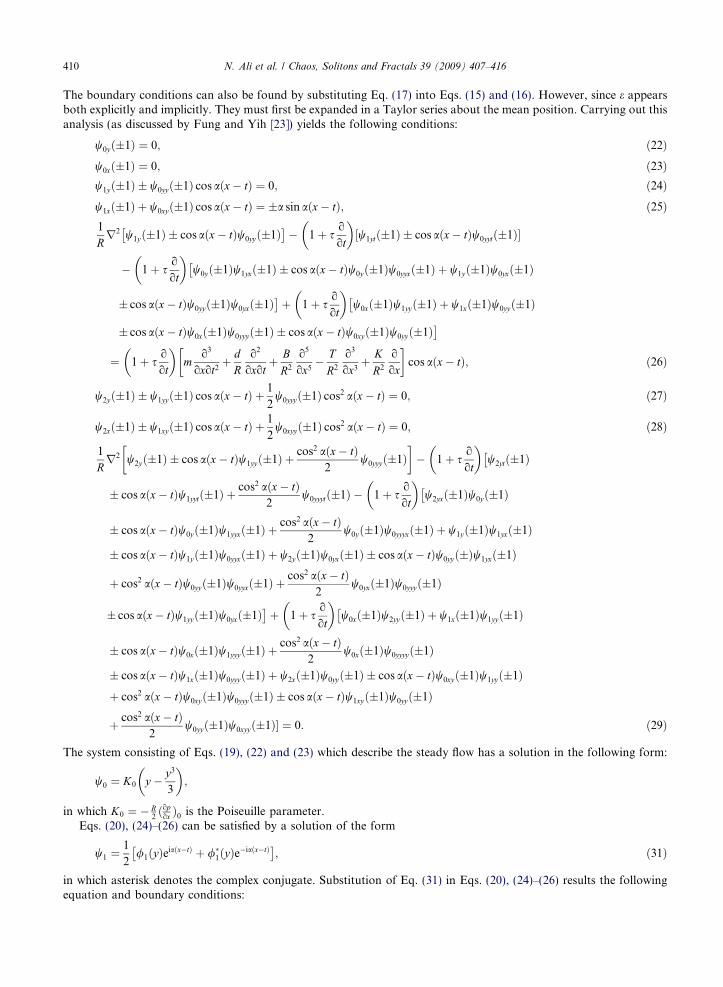
In this section graphical results are displayed just to see the effects of various pertinent parameter on the mean veloc-ity at the boundaries, the mean velocity perturbation function, the time-averaged mean axial velocity distribution andreversal flow. In Fig. 1a the effects of wall damping d on the mean velocity at boundaries D are noted. It is seen that D

decreases by increasing d. Fig. 1b depicts the effects of wall tension T on D. Here D increases with an increase in T. Also

The variation of D with wave number a for four different values of wall damping d (panel (a)), wall tension T (panel (b)), wallce K (panel (c)) and relaxation time s (panel (d)). The other parameters chosen are m = 0.01, B = 2, T = 1, K = 1, R = 10 and(panel (a)); m = 0.01, B = 2, d = 0.5, K = 1, R = 10 and s = 0.5 (panel (b)); m = 0.01, B = 2, T = 1, d = 0.5, R = 10 and s = 0.5(c)) and m = 0.01, B = 2, T = 1, K = 1, R = 10 and d = 0.5 (panel (d)).


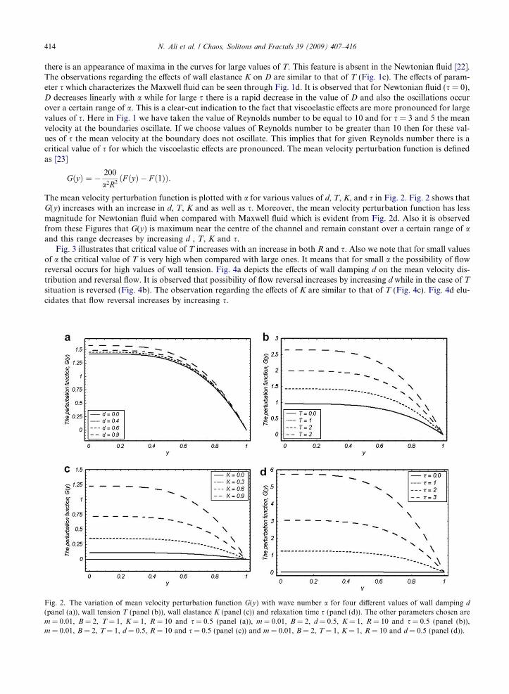
there is an appearance of maxima in the curves for large values of T. This feature is absent in the Newtonian fluid [22].The observations regarding the effects of wall elastance K on D are similar to that of T (Fig. 1c). The effects of param-eter s which characterizes the Maxwell fluid can be seen through Fig. 1d. It is observed that for Newtonian fluid (s = 0),D decreases linearly with a while for large s there is a rapid decrease in the value of D and also the oscillations occurover a certain range of a. This is a clear-cut indication to the fact that viscoelastic effects are more pronounced for largevalues of s. Here in Fig. 1 we have taken the value of Reynolds number to be equal to 10 and for s = 3 and 5 the meanvelocity at the boundaries oscillate. If we choose values of Reynolds number to be greater than 10 then for these val-ues of s the mean velocity at the boundary does not oscillate. This implies that for given Reynolds number there is acritical value of s for which the viscoelastic effects are pronounced. The mean velocity perturbation function is definedas [23]

Fig. 2.(panelm = 0.m = 0.

GðyÞ ¼ � 200

a2R2ðF ðyÞ � F ð1ÞÞ:

The mean velocity perturbation function is plotted with a for various values of d, T, K, and s in Fig. 2. Fig. 2 shows thatG(y) increases with an increase in d, T, K and as well as s. Moreover, the mean velocity perturbation function has lessmagnitude for Newtonian fluid when compared with Maxwell fluid which is evident from Fig. 2d. Also it is observedfrom these Figures that G(y) is maximum near the centre of the channel and remain constant over a certain range of aand this range decreases by increasing d , T, K and s.

Fig. 3 illustrates that critical value of T increases with an increase in both R and s. Also we note that for small valuesof a the critical value of T is very high when compared with large ones. It means that for small a the possibility of flowreversal occurs for high values of wall tension. Fig. 4a depicts the effects of wall damping d on the mean velocity dis-tribution and reversal flow. It is observed that possibility of flow reversal increases by increasing d while in the case of T

situation is reversed (Fig. 4b). The observation regarding the effects of K are similar to that of T (Fig. 4c). Fig. 4d elu-cidates that flow reversal increases by increasing s.

The variation of mean velocity perturbation function G(y) with wave number a for four different values of wall damping d

(a)), wall tension T (panel (b)), wall elastance K (panel (c)) and relaxation time s (panel (d)). The other parameters chosen are01, B = 2, T = 1, K = 1, R = 10 and s = 0.5 (panel (a)), m = 0.01, B = 2, d = 0.5, K = 1, R = 10 and s = 0.5 (panel (b)),01, B = 2, T = 1, d = 0.5, R = 10 and s = 0.5 (panel (c)) and m = 0.01, B = 2, T = 1, K = 1, R = 10 and d = 0.5 (panel (d)).

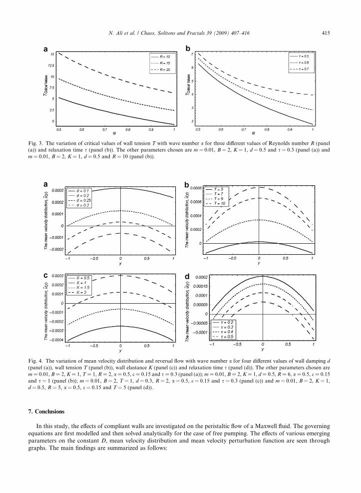
Fig. 3. The variation of critical values of wall tension T with wave number a for three different values of Reynolds number R (panel(a)) and relaxation time s (panel (b)). The other parameters chosen are m = 0.01, B = 2, K = 1, d = 0.5 and s = 0.3 (panel (a)) andm = 0.01, B = 2, K = 1, d = 0.5 and R = 10 (panel (b)).

Fig. 4. The variation of mean velocity distribution and reversal flow with wave number a for four different values of wall damping d

(panel (a)), wall tension T (panel (b)), wall elastance K (panel (c)) and relaxation time s (panel (d)). The other parameters chosen arem = 0.01, B = 2, K = 1, T = 1, R = 2, a = 0.5, e = 0.15 and s = 0.3 (panel (a)); m = 0.01, B = 2, K = 1, d = 0.5, R = 6, a = 0.5, e = 0.15and s = 1 (panel (b)); m = 0.01, B = 2, T = 1, d = 0.3, R = 2, a = 0.5, e = 0.15 and s = 0.3 (panel (c)) and m = 0.01, B = 2, K = 1,d = 0.5, R = 5, a = 0.5, e = 0.15 and T = 5 (panel (d)).


7. Conclusions

In this study, the effects of compliant walls are investigated on the peristaltic flow of a Maxwell fluid. The governingequations are first modelled and then solved analytically for the case of free pumping. The effects of various emergingparameters on the constant D, mean velocity distribution and mean velocity perturbation function are seen throughgraphs. The main findings are summarized as follows:


• The constant D decreases with an increase in d and s. However it increases by increasing T and K.• The mean velocity perturbation function G(y) increases when d, T, K and s are increased.• The flow reversal decreases by increasing K and T while it increases for large values of d and s.• The results of Newtonian fluid [22] can be recovered as a limiting case by taking s! 0.

Acknowledgements

We are grateful to a reviewer for his valuable suggestions which undoubtedly improved the quality of the manu-script. We are further grateful to Higher Education Commission of Pakistan, for the financial support.

References

[1] Hayat T, Khan M, Ayub M. Some analytical solutions for second grade fluid flows for cylindrical geometries. Math ComputModell 2006;43:16–29.

[2] Sajid M, Hayat T, Asghar S. On analytic solution of the steady flow of a fourth grade fluid. Phys Lett A 2006;355:18–26.[3] Khan M, Hayat T, Asghar S. Exact solution for MHD flow of a generalized Oldroyd-B fluid with modified Darcy’s law. Int J Eng

Sci 2006;44:333–9.[4] Khan M, Maqbool K, Hayat T. Influence of Hall current on the flows of generalized Oldroyd-B fluid in a porous space. Acta

Mech 2006;184:1–13.[5] Chen CI, Hayat T, Chen JL. Exact solutions for the unsteady flow of a Burgers’ fluid in a duct induced by time-dependent

prescribed volume flow rate. Heat Mass Transfer 2006;43:85–90.[6] Tan WC, Masuoka T. Stokes first problem for an Oldroyd-B fluid in a porous half space. Phys Fluid 2005;17:0231017.[7] Fetecau C, Fetecau C. Starting solutions for some unsteady unidirectional flows of a second grade fluid. Int J Eng Sci

2005;43:781–9.[8] Fetecau C, Fetecau C. Decay of a potential vortex in an Oldroyd-B fluid. Int J Eng Sci 2005;43:340–51.[9] Fetecau C, Fetecau C. On some axial Couette flows of non-Newtonian fluids. Z Angew Math Phys 2005;56:1098–106.

[10] Baris S, Dokuz MS. Three-dimensional stagnation point flow of a second grade fluid towards a moving plate. Int J Eng Sci2006;44:49–58.

[11] Mekheimer KhS. Peristaltic flow of blood under effect of a magnetic field in a non-uniform channels. Appl Math Comput2004;153:763–77.

[12] Mekheimer KhS. Peristaltic transport of a couple-stress fluid in a uniform and non-uniform channels. Biorheology2002;39:755–65.

[13] Hayat T, Mahomed FM, Asghar S. Peristaltic flow of magnetohydrodynamic Johnson–Segalman fluid. Nonlinear Dyn2005;40:375–85.

[14] Hayat T, Ali N. On mechanism of peristaltic flows for power-law fluids. Physica A 2006;371:188–94.[15] Hayat T, Ali N. Peristaltically induced motion of a MHD third grade fluid in a deformable tube. Physica A 2006;370:225–39.[16] Hayat T, Khan M, Asghar S, Siddiqui AM. A mathematical model of peristalsis in tubes through a porous medium. J Porous

Media 2006;9:55–67.[17] Hayat T, Ali N, Asghar S, Siddiqui AM. Exact peristaltic flow in tubes with an endoscope. Appl Math Comput 2006;182:359–68.[18] Hayat T, Ali N. A mathematical description for peristaltic hydromagnetic flow in a tube. Appl Math Comput, in press.[19] Hayat T, Ali N, Asghar S. Peristaltic motion of Burgers’ fluid in a planar channel. Appl Math Comput 2007;1:309–29.[20] Elshahed M, Haroun MH. Peristaltic transport of Johnson–Segalman fluid under effect of a magnetic field. Math Problems Eng

2005;6:663–77.[21] Haroun MH. Effect of Deborah number and phase difference on peristaltic transport of a third-order fluid in an asymmetric

channel. Comm Non-linear Sci Numer Simm, in press.[22] Abd Elnaby MA, Haroun MH. A new model for study the effect of wall properties on peristaltic transport of a viscous fluid.

Comm Non-linear Sci Numer Simm, in press.[23] Fung YC, Yih CS. Peristaltic transport. Trans ASME J Appl Mech 1968;33:669–75.

Peristaltic flow of a Maxwell fluid in a channel with compliant walls

Documents

Transcript of Peristaltic flow of a Maxwell fluid in a channel with compliant walls