Performing Real-Time Interactive Fiber Tracking

Adiel Mittmann,1 Tiago H. C. Nobrega,1 Eros Comunello,1 Juliano P. O. Pinto,2 Paulo R. Dellani,3

Peter Stoeter,4 and Aldo von Wangenheim1

Fiber tracking is a technique that, based on a diffusiontensor magnetic resonance imaging dataset, locates thefiber bundles in the human brain. Because it is acomputationally expensive process, the interactivity ofcurrent fiber tracking tools is limited. We propose a newapproach, which we termed real-time interactive fibertracking, which aims at providing a rich and intuitiveenvironment for the neuroradiologist. In this approach,fiber tracking is executed automatically every time theuser acts upon the application. Particularly, when thevolume of interest from which fiber trajectories arecalculated is moved on the screen, fiber tracking isexecuted, even while it is being moved. We present ourfiber tracking tool, which implements the real-time fibertracking concept by using the video card’s graphicsprocessing units to execute the fiber tracking algorithm.Results show that real-time interactive fiber tracking isfeasible on computers equipped with common, low-costvideo cards.

KEY WORDS: Fiber tracking, diffusion tensor imaging,graphics processing units, real-time applications

INTRODUCTION

D iffusion tensor magnetic resonance imaging(DT-MRI) is a technique that, given a set of

magnetic resonance scans acquired with a specificprotocol, allows the estimation of diffusion tensorsat all voxels of the volume.1,2 Most commonly, thehuman brain is imaged,3 although other structures,like the spinal cord, have been imaged as well.4

The diffusion tensor is a mathematical model thatbears information on both the direction and theintensity of diffusion. In the context of DT-MRI, itcharacterizes the diffusion of water moleculesalong myelinated neuronal fibers.5

The post-processing of DT-MRI volumes typi-cally consists of the fiber tracking process, whichtakes advantage of the information on water diffu-sion to determine the locations of fiber bundles.6,7

There are several fiber tracking techniques,8–10 oneof them being the streamline method,11 which finds

fiber trajectories by following the main diffusiondirection of water. Heuristics may be used to furtherimprove the quality of results and to solve problemsrelated to partial volume effects,12 such as fibercrossing or fiber kissing. Streamline fiber tracking,with which this article is concerned, is typicallyexecuted for a given volume of interest (VOI), whereseed points are evenly spread and each of whichgenerates a fiber trajectory. This method of fibertracking relies on mathematical operations likevector integration and interpolation.13

The large number of complex mathematicaloperations that the fiber tracking process requireshinders the interactivity provided by applications,since a significant amount of time is spent on thoseoperations. To the best of our knowledge, currentcommercial systems cope with the processing timeissues either by not allowing interactive fiber

1From the Universidade Federal de Santa Catarina,Departamento de Informática e Estatística, 88040-970, Floria-nópolis, SC, Brazil.

2From the University Hospital, Federal University of SantaCatarina, 88040-970, Florianópolis, SC, Brazil.

3From the Department of Neurology, Johannes GutenbergUniversity of Mainz, Langenbeckstrasse 1, 55131, Mainz,Germany.

4From the Institute for Neuroradiology, Johannes GutenbergUniversity of Mainz, Langenbeckstrasse 1, 55131, Mainz,Germany.Electronic supplementary material The online version of thisarticle (doi:10.1007/s10278-009-9266-9) contains supple-mentary material, which is available to authorized users.

Correspondence to: Adiel Mittmann, Universidade Federalde Santa Catarina, Departamento de Informática e Estatística,88040-970, Florianópolis, SC, Brazil; tel: +55-48-37219516;e-mail: adiel@inf.ufsc.br

Copyright * 2010 by Society for Imaging Informatics inMedicine

Online publication 13 February 2010doi: 10.1007/s10278-009-9266-9

Journal of Digital Imaging, Vol 24, No 2 (April), 2011: pp 339Y351 339

tracking at all or by requiring the result of a full-brain fiber tracking process to be loaded prior tobeing explored. One commercial product, the iPlanBOLD MRI Mapping software from BrainLAB,14

provides interactive fiber tracking, but sets ofprecomputed trajectories are required to be loadedbeforehand into the program for exploratoryactions to be taken. Another commercial product,the BrainVoyager QX,15–17 on the other hand,does not need precalculated trajectories to beloaded before exploration, but the interactivityexperienced by the user is not as rich as thatprovided by iPlan BOLD MRI Mapping.In order to speed up the process of fiber

tracking, the use of graphics processing units(GPUs) has been proposed. Jeong et al.18 haveproposed the use of GPUs to compute and visual-ize white matter connectivity by means of a voxel-based approach. Petrovic et al.19 have used GPUsin order to visualize fiber tracking results, whichare not generated by the GPU in their approach.McGraw and Nadar20 have shown how stochasticfiber tracking can be executed on the GPU,allowing the user to observe results being gener-ated on the screen. We have previously proposedthe use of GPUs for the execution of streamlinefiber tracking21 and have also compared them withcomputer clusters in this context22. An optimizedstrategy for performing fiber tracking on GPUswas later proposed by Köhn et al.,23 whoemployed geometry shaders to calculate results.Kwatra et al.24 have proposed the use of program-mable hardware for fiber tracking, but thisapproach has the inconvenience of using non-standard hardware, whereas the GPU approachesrequire only a consumer-grade graphics card.In this article, we present a novel approach to

interactivity in the context of fiber tracking, whichwe have termed real-time interactive fiber tracking.In this approach, the user can interactively defineVOIs, move them around the DT-MRI volume,change the fiber tracking algorithm’s parameters,and have all results calculated in real time, whileinteraction occurs. When the user moves the VOIto a new position, for instance, new fibers arecalculated automatically and quickly, even whilethe VOI is being dragged, thus producing ananimation-like effect. This approach introduces awhole new level of interactivity, in which the userneither has to preload previous fiber trackingresults nor has to wait long for results to be

updated on the screen. We also introduce a fibertracking tool which implements real-time interac-tive fiber tracking. This tool provides two imple-mentations of fiber tracking, one which is executedon the CPU and another which is executed on theGPU. The remarks of a neuroradiologist and aradiologist who evaluated the GPU implementa-tion have been collected in the concluding section.We propose an automatic procedure for the

measurement of the frames per second (FPS) rateachieved by real-time interactive fiber trackingapplications. This is desirable since it establishes astandard way to quantify the speed achieved whendifferent hardware setups or different datasets areused. This might also prove useful when othertools adopt the approach described in this paper,since it would allow the comparison of differentfiber tracking tools. By using this index, we showthat the GPU implementation provides a betterinteractive experience than the CPU one bymeasuring the number of FPS each implementa-tion achieved. Detailed results are given for bothcases. A video containing additional explanationson our approach and unedited footage of anexploratory fiber tracking session is included inthis article’s electronic supplementary material.This article is organized as follows: sec-

tion Materials and Methods provides a definition ofthe real-time interactive approach to fiber tracking,presents our tool, which implements that approach,and describes the materials and the methodology usedin the experiments; the section Results presents theresults obtained by our fiber tracking tool; finally, inthe section Discussion and Conclusions, we discussthe results obtained and give our conclusions.

MATERIALS AND METHODS

In this section, the definition of real-time inter-active fiber tracking is presented, followed by adescription of the fiber tracking tool developed tomeet that definition. The characteristics of the DT-MRI datasets and the computer hardware used inthe experiments are also given in this section.

Definition of Real-Time Interactive FiberTracking

In order to make precise what is meant by theterm “real-time interactive fiber tracking”, a

340 MITTMANN ET AL.

definition is needed. This is especially necessarybecause any tool that interacts with the user mayclaim it is interactive whatever the level of inter-activity it achieves, e.g., an application that allowsthe user to define a volume of interest by using themouse may state that it supports interactive fibertracking, even though that is arguably a poor level ofinteractivity. Furthermore, while any kind of inter-activity imposes a constraint on how long thesoftware takes to respond, “real-time” interactivitypushes that constraint even further.An application is said to provide real-time

interactive fiber tracking if:

1. Interactivity requirements(a) The VOI containing the seed points can be

dragged to all parts of the imaged volume byusing a pointing device, such as a mouse.

(b) The parameters of the fiber tracking algorithmused to find trajectories for the VOI’s seedpoints, like minimum fractional anisotropy(FA) and minimum mean diffusivity (MD),can be changed.

(c) Whenever the VOI is moved or the algorithm’sparameters are changed, trajectories are recom-puted automatically, that is, the user is notrequired to request results to be updated. Inparticular, resulting trajectories are updatedeven while the VOI is being moved and notonly after the user has already selected a newlocus for the VOI.

(d) No trajectories are preloaded in memory, thatis, no previous fiber tracking results are usedwhen computing the new ones.

2. Time constraint

Whenever new trajectories have to be computed(as per point 1.c above), the application mustboth calculate and display new results in real-time, with a mean FPS rate greater than 10 withthe application’s default parameters, whichimplies a time limit of 100 ms per frame. Theapplication behaves as a soft real-time system: asthe number of seed points within the VOIincreases and the algorithm’s parameters becomemore permissive, the FPS rate decreases.Item 2 is admittedly vague regarding the default

parameters, but those are application-specific andcannot all be considered here. However, defaultparameters should provide a user with a usefulenvironment, since there is no point in stating that atool supports real-time interactive fiber tracking if the

time constraint can only be met with a parameter setthat cripples the quality of results produced by the tool.

The Fiber Tracking Tool

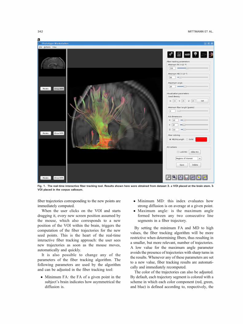
A fiber tracking tool was developed with the aimof empowering the user with a real-time, interactiveenvironment so that the requirements set out in theprevious section could be met. The tool wasimplemented as an extension to a radiology work-station being developed by our group. Figure 1shows two screen shots of the fiber tracking tool.The fiber tracking tool employs, at any given time,

one of two platforms to execute the fiber trackingalgorithm: the CPU, which is the standard way ofexecuting programs on a computer, or the computer’sGPU. Under either platform, however, the com-puter’s CPU is used for volume loading and userinteraction. The use of GPUs as general-purposeprocessors is a recent approach to parallel computingthat is finding wide acceptance25 because it providesa low-cost, single-computer parallel environment.Today’s GPUs are an evolution of the graphicsaccelerator cards of the past, which could performonly graphics-related computing. They are nowprogrammable, massively parallel processors able toperform any kind of computation. Newer-generationGPUs offer, under some circumstances, processingcapabilities of up to 1 teraflop (1 trillion floating-point operations per second) as well as high-levelprogramming interfaces that ease the development ofGPU programs.26 The details of the GPU implemen-tation of fiber tracking are given in the section FiberTracking on the GPU.The first step for the use of the fiber tracking tool is

the loading of the DT-MRI volumes. These volumesconvey information on the diffusion of water in thesubject’s brain and are the base for all furtherprocessing. Once the DT-MRI volumes are loaded,a click on the fiber tracking button places a VOI inthe middle of the volume and the corresponding fibertrajectories are computed and shown.The VOI is the region in which seed points, each of

which spawns a single trajectory, are placed. Thenumber of seed points within the VOI is changed byadjusting three gauge widgets that control the numberof points in the x, y, and z directions. Initially, thenumber of points along the three directions is set to10, thus yielding a total of 1,000 possible trajectories.When the user changes the density of seed points, the

PERFORMING REAL-TIME INTERACTIVE FIBER TRACKING 341

fiber trajectories corresponding to the new points areimmediately computed.When the user clicks on the VOI and starts

dragging it, every new screen position assumed bythe mouse, which also corresponds to a newposition of the VOI within the brain, triggers thecomputation of the fiber trajectories for the newseed points. This is the heart of the real-timeinteractive fiber tracking approach: the user seesnew trajectories as soon as the mouse moves,automatically and quickly.It is also possible to change any of the

parameters of the fiber tracking algorithm. Thefollowing parameters are used by the algorithmand can be adjusted in the fiber tracking tool:

� Minimum FA: the FA of a given point in thesubject’s brain indicates how asymmetrical thediffusion is.

� Minimum MD: this index evaluates howstrong diffusion is on average at a given point.

� Maximum angle: is the maximum angleformed between any two consecutive linesegments in a fiber trajectory.

By setting the minimum FA and MD to highvalues, the fiber tracking algorithm will be morerestrictive when determining fibers, thus resulting ina smaller, but more relevant, number of trajectories.A low value for the maximum angle parameteravoids the presence of trajectories with sharp turns inthe results. Whenever any of these parameters are setto a new value, fiber tracking results are automati-cally and immediately recomputed.The color of the trajectories can also be adjusted.

By default, each trajectory segment is colored with ascheme in which each color component (red, green,and blue) is defined according to, respectively, the

Fig. 1. The real-time interactive fiber tracking tool. Results shown here were obtained from dataset 3. a VOI placed at the brain stem. bVOI placed in the corpus callosum.

342 MITTMANN ET AL.

FA of that region, the MD, and the distance to thecorresponding seed point. The user may also pick acolor with which the tool colors all fiber trajectoriesof the current VOI. The changing of the coloringscheme does not require fiber trajectories to berecomputed, since this is only a drawing feature,which is taken care of by the CPU.Another feature that aids the exploration of a

subject’s brain is the possibility to place an arbitrarynumber of VOIs. This, coupled with the ability ofchanging the fiber tracking parameters and the colorof each VOI’s trajectories, allows for the creation ofcomplex, meaningful visualizations. Figure 2 showsa screen shot of one such visualization.

Fiber Tracking on the GPU

GPUs offer two main features that render them agood platform for the implementation of fiber

tracking: parallelism and fast floating-point oper-ations. Parallelism is useful because each trajectorycan be computed independently from the others, sothat, when fiber tracking is executed on GPUs,many fiber trajectories are being computed simul-taneously at any given time. The fact that GPUsare capable of performing floating-point operationsat a significant rate also benefits fiber tracking,which requires interpolation of tensors and inte-gration of vector fields, all of which are complexmathematical operations.The fiber tracking implementation for the GPU

makes use of the compute unified device architecture(CUDA),27 which is a recent technology introducedby vendor NVIDIA28 with the aim of making generalcomputation on GPUs more developer-friendly.Previous technologies, despite enabling computa-tions of any kind, required a greater effort whenwriting programs with little or no relation to graphics

Fig. 1. (continued).

PERFORMING REAL-TIME INTERACTIVE FIBER TRACKING 343

or image processing. We have already shown21 howfiber tracking can be executed on GPUs by using onesuch older technology, the language Cg, short for Cfor Graphics.29

Fiber tracking is able to take advantage of GPUsbecause fiber trajectories are computed from a setof seed points, and each of those seed points canbe individually examined for trajectories, inde-pendently of the others. Thus, each processor inthe GPU is assigned a different seed point, which itthen uses as a starting point for calculating fibertrajectories. A common GPU, like the GeForce9600 GT, possesses 64 stream processors; whenfiber tracking is executed on that GPU, 64 fibertrajectories are being calculated simultaneously.Prior to executing fiber tracking itself, the GPU

must be sent the discrete tensor field, which iscalculated by the CPU from the DT-MRI volumesselected by the user. The discrete tensor field is a

three-dimensional grid containing tensors at thecenter of all voxels originally imaged; because eachtensor conveys information on the diffusion of aparticular point, the tensor field can be seen as a mapof water diffusion for the whole imaged volume.After the GPU has received the discrete tensor

field, fiber tracking can be executed. In order to takefull advantage of the parallelism offered by the GPU,as many threads are created as there are availableprocessors, each thread being responsible for calcu-lating one trajectory. Threads are managed automati-cally by CUDA, and as soon as a thread finishes atrajectory, a new one can be started. Typically, thenumber of seeds is greater than the number ofavailable processors (the fiber tracking tool’s defaultis 1,000 seeds), which ensures that the GPU is usedto its maximum. The resulting fiber trajectories foundby the GPU are then read back by the fiber trackingtool, which shows them immediately.

Fig. 2. Combination of results from two VOIs, one at the corpus callosum and another at the brain stem. The active VOI has its edgeshighlighted.

344 MITTMANN ET AL.

It is important to notice that, under normal userinteraction, the GPU is called several times a second(usually more than ten) to find new fiber trajectories.This happens because, as the mouse pointer moveson the screen, the VOI’s position changes and fibertracking is automatically triggered for every pixel themouse pointer is moved to.

Rendering of Fiber Trajectories

One important aspect of a fiber tracking appli-cation is the presentation of results to the user. Aninteractive application must show fiber trajectoriesin a graphical, three-dimensional way, but render-ing a potentially large number of trajectory seg-ments easily becomes a performance bottleneck. Inorder to meet the requirements established in thesection Definition of Real-Time Interactive FiberTracking, a compromise between speed andappealing visualizations must be found.The simplest and fastest way to render trajecto-

ries is to draw a series of line segments. Therendering of lines stored in memory as large arraysof vertices is a relatively fast operation for videocards, and since the results of the GPU fibertracking program are stored precisely as arrays ofvertices, no modifications are needed on the dataread from the GPU in order to draw fibertrajectories as line segments.Another way of rendering trajectories is to place

a cylinder between each consecutive pair oftrajectory points, so that each trajectory looks likea series of cylinders, instead of a series of linesegments. Cylinders provide an enhanced percep-tion of depth and spatial placement, since theyrespond realistically to light sources, presentingshades and reflexes. The final result is a morerepresentative display of the fiber trajectoriesoriginating in the VOI.The fiber tracking tool uses a hybrid approach for

the rendering of fibers: they are normally drawn ascylinders, but they are drawn as lines while the useris dragging the VOI. This way, interactivity is notcompromised when frames need to be renderedquickly, and a high-quality result is presented whenthe user has finished moving the VOI.

Performance Measurement

The FPS rate is the standard index for perform-ance measurements in interactive graphic applica-

tions. It measures the number of frames theapplication renders on the screen per second. Onepossible approach for the measurement of the FPSrate in a fiber tracking tool would be to ask one ormore users to explore the fiber trajectories of abrain for some time, while the application keepstrack of the time taken for each frame to becomputed and drawn on the screen. Afterwards (oreven during the execution of the application), theFPS rates can be calculated and processed accord-ingly. However, such an approach has a crucialdrawback: it is not reproducible, since one cannotreasonably expect the user to take the exact sameactions more than once. Because a comparisonbetween different hardware setups and differentdatasets is desired, an automatic procedure isneeded for the measurement of the FPS rate in afiber tracking application.One way to mimic the user’s behavior is to

move the VOI along one direction in small steps,as if it were the user who was moving the VOI. Inthis strategy, each one of those steps correspondsto one frame drawn on the screen. By keepingtrack of the time spent in each step, the applicationcan then calculate the FPS rate. Based on this idea,we propose the following objective, automaticprocedure for measuring the FPS rate of a fibertracking application:

1. The VOI is resized so that its dimensions equal10% of those of the full volume. This way, theVOI has the same shape as the entire DT-MRIdataset, but a fraction (0.1%) of its physicalvolume. The VOI is placed at the bottom (alongthe z axis) of the volume and centered along thex and y directions.

2. Fiber tracking is executed according to theparameters currently set and results are shownon the screen.

3. The VOI is moved upwards a distance of 0.9%of the volume height.

4. Steps 2–3 are repeated other 99 times, for atotal of 100 iterations that take the VOI fromthe very bottom to the very top of the volume.

This procedure places the VOI at the bottom ofthe volume and then sweeps it along the zdirection, as if the user was moving the VOI. Step4 moves it upwards by 0.9% of the volume heightbecause the procedure must cover 90% of itsheight (since the other 10% are occupied by theVOI itself) in 100 steps. In order to calculate the

PERFORMING REAL-TIME INTERACTIVE FIBER TRACKING 345

FPS rate achieved during the procedure, onesimply divides its execution time by the numberof iterations, which is fixed at 100.

DT-MRI Datasets

Three DT-MRI datasets (henceforth referred toas dataset 1, dataset 2, and dataset 3) were acquiredfor the experiments described in this article. Dataset2 was acquired on a 3-T MAGNETOM Trio(Siemens Medical Solutions, Erlangen, Germany),and datasets 1 and 3 were acquired on a 1.5-TMAGNETOM Sonata scanner (Siemens MedicalSolutions, Erlangen, Germany). The MR scannerswere equipped with iPAT head-cage coils of eightchannels (Sonata scanner) and 12 channels (Trioscanner). The gradient systems had a strength of upto 40 mT/m (effective 69 mT/m) and a slew rate ofup to 200 T/m/s (effective 346 T/m/s). On bothsystems, parallel imaging techniques were applied,and the images so acquired were reconstructedusing the generalized autocalibrating partiallyparallel acquisition (GRAPPA) algorithm, withan accelerating factor of 2. The datasets wereacquired with a single-shot spin-echo echo-planarimaging sequence, being composed of a baselineimage acquired without diffusion weighting (withb=0 s/mm2) and a set of diffusion-weightedimages (with b=1.000 s/mm2) applied along sixdirections (Sonata scanner) and 20 directions (Trioscanner). All images composing the datasetswere measured six times and stored separately.Sequences were parameterized with TE/TR=105/8,000 ms (Sonata scanner) and TE/TR=118/11,800 ms (Trio scanner).Dataset 1 is composed of 40 slices, each of

which 3.00 mm thick, with a field of view (FOV)of 230 mm and an in-plane resolution of 128×128pixels, yielding a voxel size of 1.8×1.8×3.0 mm.Dataset 2 is composed of 70 slices, 1.9 mm thick,FOV of 243 mm, and an in-plane resolution of128×128 pixels, thus producing isotropic voxelsof 1.9 mm3. Dataset 3 is composed of 33 slices,3.0 mm thick, FOV of 230 mm, and an in-plane

resolution of 128×128 pixels, resulting in a voxelsize of 1.8×1.8×3.0 mm.All datasets underwent correction for distor-

tions induced by eddy currents (ECs) andmotion artifacts.30,31 For that purpose, FLIRT(Oxford Centre for Functional MRI of theBrain, Oxford, UK), which implements a coreg-istration that employs a measure of mutualinformation, was used to realign all images ofthe individual DT-MRI datasets. The imagesthus corrected were visually inspected forpossible false alignment resulting from wrongcoregistrations. All diffusion-weighted imageshad their diffusion-sensitizing gradient directiontransformed in order to compensate for therotational component of the affine transforma-tion computed in the procedure for correctingmotion artifacts and EC distortions.

Computer Hardware

Two hardware setups were used in the experi-ments, and their characteristics are described inTable 1. Both computers are made up of low-costcomponents and are by no means high-end equip-

0 2,000 4,000 6,000 8,000

050

,000

100,

000

150,

000

Fig. 3. Mean number of trajectory points against number ofseed points for all three datasets. The number of seed trajectorypoints grows linearly with the number of seed points. Here, filleddiamond, dataset 1; inverted filled triangle, dataset 2; filledsquare, dataset 3.

Table 1. Description of Computer Hardware Used in the Experiments

CPU Video card Driver version OS Mode

Setup 1 Athlon 64 X2 4400+, 2GB RAM GeForce 8600 GT, 256MB RAM 173.08 64-bitSetup 2 Athlon 64 X2 4400+, 2GB RAM GeForce 9600 GT, 512MB RAM 173.08 64-bit

346 MITTMANN ET AL.

ments. Although the CPUs of both computers areidentical, they are individually considered in thisarticle because they depend indirectly on the GPUfor the drawing of graphics. The same CPU,therefore, could achieve a better performance whencoupled with a superior GPU.The performance of applications which use the

GPU as a means to accelerate the computation ofspecific tasks depends not only on the video cardof a computer, but also on the other hardware andsoftware components. We have shown in aprevious work,21 however, that performance

improvements are achieved by GPU applicationseven when the other components are not optimal.In particular, even 32-bit systems with datedhardware were able to attain significant speed upsin their experiments.

RESULTS

The VOI-sweeping procedure described in thesection Performance Measurement was executed forall combinations of hardware setups, datasets, and

GPU CPU

Set

up 1

Set

up 2

0 100,000 200,000 300,000 0 100,000 200,000 300,000

0 100,000 200,000 300,000

08

10

0 100,000 200,000 300,000

24

6

08

102

46

08

102

46

08

102

46

Fig. 4. Scatterplots showing the number of trajectory points and the time taken to process them. Here, filled diamond, dataset 1;inverted filled triangle, dataset 2; filled square, dataset 3.

PERFORMING REAL-TIME INTERACTIVE FIBER TRACKING 347

platforms (CPU and GPU). The procedure wasreplicated eight times in order to provide moreaccurate timings. The fiber tracking tool’s defaultparameters were used, so that the stop criteria were:FAG0.15, MDG50×10-6 mm2 s-1 and an anglebetween successive trajectories greater than 20°.In order to assess how platforms scale when the

number of trajectory points in the results increase,the procedure was applied multiple times with avarying number of seed points. For each setup–dataset–platform combination, the density of seedpoints within the VOI was increased each time theprocedure was applied by adding 1 seed to eachdimension, so that, for instance, in the firstexecution, the density was 1×1×1, for a total of1 seed point; in the second execution, the densitywas 2×2×2, for a total of 8 seed points. Thenumber of seed points, therefore, grows exponen-tially over time and is given by the function f(x)=x³. The procedure was applied up to a limit of20� 20� 20 ¼ 8; 000 seeds. When runningexperiments, not only the total execution timewas recorded, but also the time each iteration ofthe VOI-sweeping procedure took to be completedand the total number of trajectory points it found.Figure 3 shows, for all three datasets, the mean

number of trajectory points generated by theiterations of the VOI-sweeping procedure. Thereis no need for a separate graph for each hardware–platform combination because there is very littlevariation in the actual results generated by them.These differences are a natural product of different

floating-point environments, and a broader discus-sion of the effects of floating-point operations onfiber tracking is given by a previous work.21

Dataset 1 generates a greater number of trajec-tory points than datasets 2 and 3 for the samenumber of seeds, which implies that the fibertrajectories for that dataset are longer. As anexample, when fiber tracking is executed withalmost 5,000 seeds, the mean number of trajectorypoints found in dataset 1 is close to 100,000,whereas, in dataset 2, a little more than 60,000trajectory points were found on average. Thissimply reflects differences inherent to each dataset,and determining the exact cause (be it the signal-to-noise ratio, the actual brain volume, or someother factor) is beyond the scope of this paper.The number of trajectory points a fiber tracking

algorithm finds is the main factor that influencesexecution time. Figure 4 contains scatterplots forall hardware–platform combinations, showing, forall three datasets, how much time each one of the20� 100 ¼ 2; 000 iterations of the VOI-sweepingprocedure took to complete and the number oftrajectory points it found. In all cases, there is aclear linear trend; but for GPUs, the execution timegrows more slowly as the number of trajectorypoints increase, indicating that they achieved ahigher performance than that achieved by theCPUs.The actual FPS rate achieved by the CPUs and

GPUs of both setups is given by the graph inFigure 5. When the number of seeds is very small

0 2,000 4,000 6,000 8,000

110

100

1000

0 2,000 4,000 6,000 8,000

110

100

1000

a b

Fig. 5. FPS rate against number of seeds for both setups. Red lines indicate GPU and green lines CPU. a Setup 1. b Setup 2.

348 MITTMANN ET AL.

(less than 30), CPUs perform better than GPUs,because the latter has a fixed minimum cost for theexecution of any amount of fiber tracking. For alarger, and therefore more useful, number of seeds,the FPS rate achieved by GPUs is consistentlyhigher. The line that crosses horizontally the graphat 10 FPS indicates the interactivity limit, asestablished in the section Definition of Real-TimeInteractive Fiber Tracking. The highest seeddensity at which each setup–platform–datasetcombination could still keep an interactive FPSrate is given by Table 2. While the CPU could notsustain a mean 10 FPS rate with more than 125seeds, all GPUs were able to keep that rate with atleast 1,728 seeds. In particular, for all threedatasets, the GPU of setup 2 was able to maintainthe interactive FPS rate with at least 3,375 seeds,which corresponds to a density of 15×15×15seeds within the VOI.The results shown by Table 2 imply that, for the

hardware configurations used in our experiments,only the GPU was able to fully comply with thedefinition of real-time interactive fiber trackinggiven in Definition of Real-Time Interactive FiberTracking, since the tool’s default seed density is10×10×10, and for no dataset any of the CPUswas able to sustain an interactive rate with thatseed density.The quality of results presented to the user

depends heavily on the number of seeds. A lowseed density causes the visualization to seemincomplete and conveys less information than ahigh seed density. This difference in quality can beseen in Figure 6, which shows two results of fibertracking executed for dataset 3 with a VOI locatedat the brain stem, one with a density of15� 15� 15 ¼ 3; 375 seeds and the other with adensity of 5� 5� 5 ¼ 125 seeds, which are themaximum density at which the GPU and the CPUof setup 1, respectively, are able to keep aninteractive FPS rate for dataset 3. The resultsobtained with 3,375 seeds (Fig. 6a) are rich indetail and large in size, while those obtained with125 seeds (Fig. 6b) are poorer and less meaningful.

Thus, while our CPU implementation of fibertracking could be said to be real-time interactive,it would only be so for a very low number ofseeds.The best way to appreciate the interactivity

provided by the GPU is by seeing it working. Avideo showing an interactive real-time fiber track-ing exploratory session is available in this article’selectronic supplementary material. The FPS rate inthe video is, however, considerably lower than thatactually achieved by the application (especiallywhen a large number of trajectory points are beingshown) because of limitations in the video captur-ing tool.

Fig. 6. Results obtained from dataset 3 with the highestseed density supported by the GPU (a) and the CPU (b) whilestill being able to sustain an interactive FPS rate. a15� 15� 15 ¼ 3; 375 seeds. b 5� 5� 5 ¼ 125 seeds.

Table 2. Maximum Seed Density at which each Setup and Platform Was Able to Maintain an Interactive Rate

Setup 1/GPU Setup 2/GPU Setup 1/CPU Setup 2/CPU

Dataset 1 1; 728 ¼ 12� 12� 12 3; 375 ¼ 15� 15� 15 125 ¼ 5� 5� 5 125 ¼ 5� 5� 5Dataset 2 2; 197 ¼ 13� 13� 13 4; 096 ¼ 16� 16� 16 216 ¼ 6� 6� 6 216 ¼ 6� 6� 6Dataset 3 2; 197 ¼ 13� 13� 13 3; 375 ¼ 15� 15� 15 125 ¼ 5� 5� 5 125 ¼ 5� 5� 5

PERFORMING REAL-TIME INTERACTIVE FIBER TRACKING 349

DISCUSSION AND CONCLUSIONS

In this paper, we have introduced the concept ofreal-time interactive fiber tracking, which applica-tions can use to provide users with a rich interactiveexperience, producing a more comfortable andintuitive environment. The main idea behind thisconcept is that applications should update resultsimmediately after any action taken by the user,however simple it might be. Because real-timeinteractive fiber tracking depends heavily on the timetaken for the application to respond to user actions,we have also defined a method that calculates the FPSrate in an application-independent manner, so thatdifferent implementations or even different platformsor subjects can be compared with each other.We have presented our fiber tracking tool,

which implements the concept of real-time inter-active fiber tracking. This tool can execute fibertracking on the GPU or on the CPU, and we haveevaluated the performance of both platforms forthree datasets. This evaluation has shown that theGPU implementation is able to sustain a renderingrate above 10 FPS for the tool’s default parameters,and the best GPU used in the experiments sustains arate of 10 FPS for all datasets in a density of 3,375seed points. Although the hardware setups had aCPU with two cores, only one core was used by thefiber tracking process. However, even if both coreshad been used and the performance had beendoubled, that setup’s GPU would still have faredbetter.Our GPU implementation of fiber tracking was

built on top of an extensible multi-purpose proto-type workstation, which has been developed byour research group. We adopted the strategy ofextending a regular, CPU-oriented radiologicalworkstation with a GPU plug-in that executes aspecific procedure, fiber tracking in this case, sothat the processing power offered by the com-puter’s GPU can be fully taken advantage of. Webelieve that this simple development strategy canbe used for other purposes in the context ofradiological workstations.The GPU implementation was evaluated by a

neuroradiologist and a radiologist, both users of otherfiber tracking tools. The former stated that the fibertracking tool presented in this paper is faster, moreintuitive, and provides a richer interactive experiencethan the other tools he is acquainted with. The latterstated that our tool not only is faster, but alsomakes it

easier for the fiber tracking results to be manipulatedon the screen, which he considers an advantage overthe other fiber tracking tools he uses.The radiologist also remarked that every tool

which allows results to be obtained more quicklyalways impacts the daily medical practice. Hesummarized his opinion adding that “by making itboth faster for images to be obtained and easier forthe radiologist to elaborate reports, and by improvingthe visualization of medical data for physicians, onealways causes a positive impact on the daily routine.”The hardware setups used in our experiments

are already outdated, which means that currentCPUs and GPUs will achieve an even betterperformance; in particular, the video cards of bothsetups, as of early 2009, can be purchased for lessthan US$100,00.32 The GeForce series, manufac-tured by NVIDIA,33 is constantly updated withnew video cards, with an ever-increasing floating-point performance. Future experiments with newerGPUs will likely yield a significantly betterperformance.GPUs are a promising tool for medical applica-

tions in general and fiber tracking in particular. Bymaking it possible to execute existing methodsmuch faster, GPUs provide the user with a morecomfortable tool and enables interactivity techni-ques that previously were not possible with low-cost equipments.

ACKNOWLEDGMENTS

The authors would like to thank Dr. Antonio Carlos dosSantos, from the Faculty of Medicine at Ribeirão Preto, for hishelp evaluating the fiber tracking tool.

REFERENCES

1. Basser PJ, Mattiello J, Le Bihan D: MR diffusion tensorspectroscopy and imaging. Biophys J 66:259–267, 1994

2. Basser PJ, Mattiello J, Le Bihan, D: Estimation of theeffective self-diffusion tensor from the NMR spin echo. J MagnReson B 103:247–254, 1994.

3. Le Bihan D, Mangin JF, Poupon C, Clark CA, Pappata S,Molko N, Chabriat H: Diffusion tensor imaging: concepts andapplications. J Magn Reson Imaging 13:534–546, 2001.

4. Yamada K, Shiga K, Kizu O, Ito H, Akiyama K, NakagawaM, Nishimura T: Oculomotor nerve palsy evaluated by diffusion-tensor tractography. Neuroradiology 48:434–437, 2006.

5. Beaulieu C: The basis of anisotropic water diffusion in thenervous system—a technical review. NMR Biomed, 15:435–455, 2002.

6. Conturo TE, Lori NF, Cull TS, Akbudak E, Snyder AZ,Shimony JS, McKinstry RC, Burton H, Raichle ME: Tracking

350 MITTMANN ET AL.

neuronal fiber pathways in the living human brain. Proc. Natl.Acad. Sci. USA 96, 10422–10427, 1999.

7. Basser PJ, Pajevic S, Pierpaoli C, Aldroubi A: Fiber tractfollowing in the human brain using DT-MRI data. IEICE TransInf & Syst E85-D:15–21, 2002.

8. Hagmann P, Jonasson L, Deffieux T, Meuli R, Thiran J,Wedeen VJ: Fibertract segmentation in position orientationspace from high angular resolution diffusion MRI. NeuroImage32:665–675, 2006.

9. Friman O, Farnebäck G, Westin C: A Bayesian approachfor stochastic white matter tractography. IEEE Trans MedImaging 25:965–978, 2006.

10. Staempfli P, Jaermann T, Crelier GR, Kollias S,Valavanis A, Boesiger P: Resolving fiber crossing usingadvanced fast marching tractography based on diffusion tensorimaging. NeuroImage 30:110–120, 2006.

11. Mori S, van Zijl PCM: Fiber tracking: principles andstrategies—a technical review. NMR Biomed 15:468–480,2002.

12. Dellani PR, Glaser M, Wille PR, Vucurevic G, Stadie A,Bauermann T, Tropine A, Perneczky A, von Wangenheim, A,Stoeter P: White matter fiber tracking computation based ondiffusion tensor imaging for clinical applications. J DigitImaging 20:88–97, 2007.

13. Pajevic S, Aldroubi A, Basser PJ: A continuous tensorfield approximation of discrete DT-MRI data for extractingmicrostructural and architectural features of tissue. J MagnReson 154:85–100, 2002.

14. BrainLAB. iPlan BOLD MRI Mapping. Available athttp://www.brainlab.com/. Visited on 18 March 2009.

15. Brain Innovation B.V. BrainVoyager QX. Available athttp://www.brainvoyager.com/. Visited on 18 March 2009.

16. Goebel R, Esposito F, Formisano E: Analysis offunctional image analysis contest (FIAC) data with BrainvoyagerQX: From single-subject to cortically aligned group generallinear model analysis and self-organizing group independentcomponent analysis. Human Brain Mapping 27:392–401,2001.

17. Roebroeck A, Galuske R, Formisano E, Chiry O,Bratzke H, Ronen I, Kim DS, Goebel R: High-resolutiondiffusion tensor imaging and tractography of the human opticchiasm at 9.4 T. NeuroImage 39:157–186, 2008.

18. Jeong W, Fletcher P, Tao R, Whitaker R: InteractiveVisualization of Volumetric White Matter Connectivity in DT-MRI Using a Parallel-Hardware Hamilton-Jacobi Solver. IEEETrans Vis Comp Graph 13:1480–1487, 2007.

19. Petrovic V, Fallon J, Kuester F: Visualizing Whole-Brain DTI Tractography with GPU-based Tuboids and LoD

Management. IEEE Trans Vis Comp Graph 13:1488–1495,2007.20. McGraw T, Nadar M: Stochastic DT-MRI Connectivity

Mapping on the GPU. IEEE Trans Vis Comp Graph. 13:1504–1511, 2007.21. Mittmann A, Comunello E, von Wangenheim A:

Diffusion tensor fiber tracking on graphics processing units.Comput Med Imaging Graph 32:521–530, 2008.22. Mittmann A, Dantas MAR, von Wangenheim A: Design

and Implementation of Brain Fiber Tracking for GPUs and PCClusters. Proc. 21st International Symposium on ComputerArchitecture and High Performance Computing SBAC-PAD,São Paulo, 101–108, 2009.23. Köhn A, Klein J, Weiler F, Peitgen H-O: A GPU-based

fiber tracking framework using geometry shaders. Proc. of SPIEMedical Imaging, Orlando, 72611J–72611J10, 2009.24. Kwatra A, Prasanna V, Singh M: Accelerating DTI

tractography using FPGAs. Proc. 20th International Paral-lel and Distributed Processing Symposium IPDPS, 1–8,2006.25. Owens JD, Luebke D, Govindaraju N, Harris M, Krüger

J, Lefohn AE, Purcell TJ: A Survey of General-PurposeComputation on Graphics Hardware. Eurographics 2005, Stateof the Art Reports, 21–51, 2005.26. PC Perspective. NVIDIA Tesla High Performance

Computing—GPUs Take a New Life. Available at http://www.pcper.com/article.php?aid=424. Accessed 18 March 2009.27. Buck I: GPU computing with NVIDIA CUDA. ACM

SIGGRAPH 2007 courses.28. NVIDIA. NVIDIA website. Available at http://www.

nvidia.com/. Accessed 14 November 2008.29. Mark WR, Glanville RS, Akeley K, Kilgard MJ: Cg: a

system for programming graphics hardware in a C-likelanguage. Proceedings of the ACM SIGGRAPH conference,San Diego, 896–907, 2003.30. Bammer R, Auer M: Correction of eddy-current induced

image warping in diffusion-weighted single-shot EPI usingconstrained non-rigid mutual information image registration.Proc. 9th ISMRM, Glasgow, 2001.31. Skare S, Anderson JLR: Simultaneous correction of eddy

currents and motion in DTI using the residual error of thediffusion tensor: comparisons with mutual information. Proc.10th ISMRM, Hawaii, 2002.32. Newegg. Available at http://www.newegg.com/.

Accessed 18 March 2008.33. NVIDIA. NVIDIA GeForce family. Available at http://

www.nvidia.com/object/geforce_family.html. AccessedNovember 14, 2008.

PERFORMING REAL-TIME INTERACTIVE FIBER TRACKING 351