This article appeared in a journal published by Elsevier. The attachedcopy is furnished to the author for internal non-commercial researchand education use, including for instruction at the authors institution

and sharing with colleagues.

Other uses, including reproduction and distribution, or selling orlicensing copies, or posting to personal, institutional or third party

websites are prohibited.

In most cases authors are permitted to post their version of thearticle (e.g. in Word or Tex form) to their personal website orinstitutional repository. Authors requiring further information

regarding Elsevier’s archiving and manuscript policies areencouraged to visit:

http://www.elsevier.com/authorsrights

Author's personal copy

Performance prediction of a multi-MW wind turbine adopting anadvanced hydrostatic transmission

Paolo Silva a, Antonio Giuffrida a,*, Nicola Fergnani a, Ennio Macchi a, Matteo Cantù b,Roberto Suffredini b, Massimo Schiavetti b, Gianluca Gigliucci b

a Politecnico di Milano, Dipartimento di Energia, Via Lambruschini 4, 20156 Milano, Italyb Enel Ingegneria e Ricerca SpA, Via Andrea Pisano 120, 56122 Pisa, Italy

a r t i c l e i n f o

Article history:Received 2 May 2013Received in revised form13 September 2013Accepted 9 November 2013Available online 12 December 2013

Keywords:Wind turbineHydrostatic transmissionEnergy modelEnergy productionDrive-train layout

a b s t r a c t

This paper analyzes the performance of multi-MW wind turbines by means of a specific numericalmodel, with the aim of evaluating the application of an advanced hydrostatic transmission in a con-ventional state-of-the-art machine. The interest for such a solution is mainly related to the potentialincrease of reliability and reduction of maintenance costs in spite of an expected reduction of perfor-mance. The implemented numerical algorithm considers the energy model of single components of thewhole turbine drive-train, from the blades to the electric grid. The model is firstly applied to a con-ventional turbine and validated according to available yearly data from a wind farm. Then, it is used tocalculate the annual energy production for different drive-train configurations applied to the same rotor,including the widespread solution with induction generator and inverter connected to the rotor, per-manent magnet generator with direct drive connection or the proposed advanced hydrostatic trans-mission. The differences in yearly electricity output among the investigated configurations are within fewpercentage points.

� 2013 Elsevier Ltd. All rights reserved.

1. Introduction

The worldwide request for alternatives to fossil fuels has beengrowing considerably during the last decades, driving a rapidimprovement of technologies exploiting renewable energies.Among them, there are wind energy conversion systems, mainlybased on large-scale wind turbines using either a mechanicalgearbox or a low-speed generator [1,2]. Both DFIG (doubly fed in-duction generator) wind turbines and direct-drive PMG (perma-nent magnet generator) wind turbines are widely used, nowadays.Low-speed PMG machines have higher reliability, compared toDFIG ones, owing to the elimination of the high-speed rotatingcomponents. As a matter of fact, the frequency converters for rotorspeed variation and, in most cases, the mechanical gearbox arecomponents that allow to obtain high overall efficiency in state-of-the-art multi-MW wind turbines, but are the main responsible forfaults and out-of-service [3], causing high maintenance costs,especially in off-shore applications [4].

High-pressure fluid power systems, actually present in variousapplications such as fuel injection equipment [5], construction

machinery [6], hybrid propulsion [7] and lubrication systems [8],could be used to replace some critical components of awind energyconversion system. In particular, a hydrostatic transmission can linkthe rotor to the electric generator, combining good efficiency andgrid stability with high reliability and relatively low costs. Recently,attention has been paid to solutions of hydrostatic transmissionsintegrated inwind turbine drive-trains, ranging from 100 kW [9] upto 1 MW [10] machines. Techno-economic feasibility studies for aproposed 1.5 MW wind turbine utilizing a continuously variableratio hydrostatic drive-train were presented as well [11]. However,no matter how compact and robust they may be, state-of-the-artpositive-displacement units currently present in hydrostatictransmissions really suffer from reduced efficiency at partial loadand displacement volume different from the maximum, so energytransfer from the rotor to the electric generator could be seriouslypenalized. Digital fluid power is a recent branch that offers highpotential for innovative solutions. A successful application requiresnew components, a sound understanding of the system andnew control principles. Specific details about the state of the artcan be found elsewhere [12], but in all cases, control is effected byswitching valves. Digital fluid power offers several advant-ages compared with analog technologies, i.e. higher efficiency,precision, redundancy, robustness, as well as higher component

* Corresponding author.E-mail address: antonio.giuffrida@polimi.it (A. Giuffrida).

Contents lists available at ScienceDirect

Energy

journal homepage: www.elsevier .com/locate/energy

0360-5442/$ e see front matter � 2013 Elsevier Ltd. All rights reserved.http://dx.doi.org/10.1016/j.energy.2013.11.034

Energy 64 (2014) 450e461

Author's personal copy

standardization potential [13]. As far as this study is concerned,digital-displacement pumps and motors [14] are selected as com-ponents of a high-efficiency hydrostatic transmission to be used ina wind energy conversion system in order to enhance its overallefficiency [15,16].

In the next sections, after presenting the basic principle of ahydrostatic transmission and its integration in a wind energyconversion system, details of wind turbine drive-train modelingand drive-train schemes are reported. Eventually, the results of thestudy are presented and discussed.

2. Hydrostatic transmission in a wind turbine drive-train

Hydrostatic transmissions are widely recognized as excellentsystems for power transmission when variable output velocity isrequired in engineering applications, such as the fields ofmanufacturing, automation and heavy-duty vehicles. A hydrostatictransmission offers fast response, maintains precise velocity undervarying loads and allows to control speed, torque, power or, in somecases, direction of rotation when required [17,18].

The operating principle of a hydrostatic transmission is simple:a positive-displacement pump, connected to the prime mover,generates a flow rate to drive a positive-displacement motor, whichis connected to the load. If the displacement volumes of pump andmotor are fixed, the hydrostatic transmission simply acts as a me-chanical gearbox with fixed gear ratio that transmits power fromthe prime mover to the load. When using a variable-displacementpump or motor, or both, a continuous control of speed, torqueand power is possible. Paying here attention to speed control, it ispossible to formulate the theoretical flow rate generated by thepump, along with the theoretical rotational speed of the motor, byneglecting, for the sake of simplicity, leakage flows inside the ma-chines [19]:

Qp;th ¼ ap,Vp,np (1)

nm;th ¼ Qm

am,Vm(2)

If no fluid loss occurs in the hydraulic circuit, thewhole flow rategenerated by the pump enters themotor, so the rotational speeds ofboth pump and motor can be related:

nm;th ¼ ap,Vp

am,Vm,np (3)

According to the last formula, a proper setting of pump andmotor displacement volumes (by means of the factors ap and am,variable from a minimum close to 0 up to 1) allows to control therotational speed of the motor. This feature is interesting if a hy-drostatic transmission has to be integrated in a wind turbinedrive-train. Moreover, if advanced hydrostatic units based on thedigital-displacement concept [14e16] are used, thanks to theirhigh efficiency at both full- and partial-load conditions, it ispossible to improve the overall energy conversion efficiency of thewind turbine drive-train.

As schematically shown in Fig. 1, the rotor transmits mechanicalpower to the pump that generates a high-pressure flow ratenecessary to drive the motor, connected to the electric generator.Both pump and motor are digital-displacement machines. Othercomponents of the hydrostatic transmission are valves, a hydraulicaccumulator, filters, oil coolers, a small system necessary to set theminimum pressure in the hydraulic circuit, along with a controlunit of the complex system.

Fig. 2 shows a schematic cross-section of a radial piston unit,whose displacement volume can be increased just by adoptingmore banks in parallel [15]. Two digital solenoid-driven poppetvalves, the first arranged along the piston axis and the second

Acronyms

DD digital-displacementDFIG doubly fed induction generatorFSC full scale converterHT hydrostatic transmissionIGBT insulated-gate bipolar transistorPMG permanent magnet generatorRMS root mean squareSCIG squirrel cage induction generatorSG synchronous generatorVCE collectoreemitter voltage

NomenclatureCp power coefficientDp pressure difference (MPa)a factor determining the current displacement volumeb pitch angle (deg)h efficiencyl tip speed ratiom fluid dynamic viscosity (cP)x dead volume ratio4 phase of voltage relative to currentJ dimensionless loss coefficientB fluid bulk modulus (MPa)i number of gearing stagesn rotational speed (rpm)

Q volumetric flow rate (dm3/s)V maximum displacement volume (dm3/rev)z number of cylinders or pumping elements

Subscripts1 single-cylinderAC alternating currentb bearingsDC direct currentf frictionfl flank (of the teeth)hm hydraulic-mechanicalk constantL fluid leakagel lossm motornom nominalo oilp pumppa parallelpl planetaryREF references sealsth theoreticaltr transformerv volumetricvf viscous friction

P. Silva et al. / Energy 64 (2014) 450e461 451

Author's personal copy

laterally, control the flow rates entering and exiting each variablevolume chamber. Although it is unusual to use a radialeccentric geometry with fast machines, digital valves make thisarrangement possible. However, solutions with a two-lobe [20] ora multi-lobe [16] cam ring, rather than an eccentric, are possible aswell.

3. Wind turbine drive train modeling

The numerical algorithm implemented to investigate the drive-train performance takes the energy model of each component ofthe turbine drive-train into account. Once the efficiency of eachcomponent has been modeled in terms of performance, it ispossible to evaluate the amount of power loss in each componentand to calculate the electrical power production for a specific wind

condition. The model used to simulate different turbine drive-trainconfigurations is based on the schematic in Fig. 3, where the idealpower of the wind stream (on the left) is converted into the elec-trical power output (on the right) through sequential powerconversions.

Since the operating conditions of the wind turbine compo-nents vary significantly depending on the actual wind speed, amodel for each component present in the drive-train wasimplemented as a function of the variables that affect its perfor-mance. Such variables are reported at the top of Fig. 3. As for thebearings and the transformer, the performance only depends onone variable, i.e. angular velocity and power respectively, whereasthe performance of the other components is more complex toevaluate, e.g. for the generator at least two variables must beconsidered.

A delicate task lies in evaluating the performance of the rotor forvariable wind speeds, since each turbine has a rotor with specificgeometry and characteristics. Moreover, the performance of therotor depends considerably on the control strategies adopted (pitchangle and rotational speed). In order to solve this problem, amathematical model was finely tuned to fit the experimental dataavailable from a state-of-the-art 2.0 MW DFIG wind turbine, char-acterized with a rotor diameter equal to 90 m, present in an Enelwind farm. The experimental data include wind speed, electricalpower output, rotational speed and pitch angle over a significanttime period, with a 10-min sampling interval. This great deal ofdata was filtered and processed according to the bin method, asoutlined in the IEC (International Electrotechnical Commission)61400-12-1 international standard [21] and applied in Refs. [22,23],in order (i) to eliminate acquisition errors and (ii) to obtain thepower curve of the real turbine along with the rotational speed andpitch angle characterization. The dispersion of the experimentalpower data for a given wind speed was evaluated by means of thestandard deviation that resulted in an average value of 58.7 kW. Themost probable reason for such a result is related to the dataacquisition system whose averaging method over the 10-minsampling interval could be affected by quick variations of windspeed along with wind blasts. Moreover, the wind speed ismeasured over the turbine nacelle, so the undisturbed wind speed

Fig. 1. Schematic of a hydrostatic transmission integrated in a wind energy conversion system.

Fig. 2. Cross-section of a digital displacement machine [15].

P. Silva et al. / Energy 64 (2014) 450e461452

Author's personal copy

calculated by the acquisition system provided by the turbinemanufacturer could differ from the real one.

In order to finely tune the mathematical model of the rotor, themechanical power transmitted from the rotor to the shaft (“Rotorpower out” in Fig. 3) was determined for each data point, startingfrom the electricity production registered by the data logger. Such atask was performed by means of the “inverse” drive-trainmodeling, which is similar to the “direct” modeling schematizedin Fig. 3. In this case, the power loss of each component was addedto the electrical power output, allowing for the assessment of therotor power output.

In the next paragraphs, the model simulating the performanceof each component is presented: the model of the rotor is ob-tained by the inverse drive-train model. Later, the direct drive-train model is validated by a comparison with the experimentaldata.

3.1. Rotor

The power coefficient of the rotor (Cp) is the ratio between themechanical power transmitted from the rotor to the shaft and theideal power that could be exploited from the wind stream. Refer-ring to a specific rotor, such a coefficient depends mainly on boththe tip speed ratio (l) and the pitch angle (b), as shown in Fig. 4[24]. The tip speed ratio accounts for the velocity at the rotorblade tip divided by the actual velocity of the wind, while the pitchangle is measured between the rotation plane of the rotor and thechord of the wing.

In order to evaluate rotor performance for different operatingconditions, several mathematical expressions were preliminarily

examined in this study [1,2,25]. For each expression, a number ofcoefficients were adjusted to closely fit the experimental data andthe mean square error was calculated. The best fit was obtainedwith the following equation:

Cp ¼ a1,�a2l� a3,b� a4,b

a5 � a6�,e

a7s (4)

where

s ¼"

1l� a8,b

� a9b3 þ 1

#�1

(5)

The nine coefficients a1 to a9 obtained with a regression for thebest fit are detailed in the Appendix.

Fig. 5 shows an appreciable agreement between the equationmodeling rotor performance and the experimental data: the pitchangle corresponding to each value of tip speed ratio is assumed tobe equal to the experimental one. The maximum efficiency of therotor is equal to 0.418, evidently less than the ideal limit (0.593)coming from Betz’s theory [1,2].

3.2. Gearbox

The model used to simulate the gearbox takes into accountvariable losses, proportional to the power flow (i.e. friction amongthe teeth that varies with load), and fixed losses, independent of thepower flow. Both losses are evaluated as a function of the number ofplanetary and parallel stages:

Jfixed ¼ Js þ b þJfl,ipl þ pa (6)

Fig. 3. Drive-train components and power conversions.

Fig. 4. Power coefficient as a function of tip speed ratio and pitch angle [24]. Fig. 5. Comparison between Eq. (4) and experimental data (dots).

P. Silva et al. / Energy 64 (2014) 450e461 453

Author's personal copy

Jvariable ¼ Jo þ b þJpa,ipa þJpl,ipl (7)

hgearbox ¼ 1��Jvariable þJfixed,

PnomP

�(8)

where Pnom and P are the nominal and the actual power input to thegearbox, respectively. The values of the five parameters in Eqs. (6)and (7) are reported in the Appendix. Bearing losses are takeninto account as well, according to the schematic in Fig. 3.

Referring to a common gearbox layout, with two planetarystages and one parallel stage, the efficiency resulting from Eq. (8) isclose to 0.96, for power input greater than 50% of the nominalpower, and decreases rapidly for power input less than 20%.

3.3. Electrical generator and inverter

The combination of mechanical, electrical and magnetic phe-nomena occurring inside the generator brings about different lossesthat are anything but easy to be evaluated. In particular, the modelfor evaluating losses in DFIG, PMG and SCIG (squirrel cage inductiongenerator) units reported in Ref. [26]was implemented in thiswork,along with a model of the rotor inverter associated to the DFIG unitand the full-scale converter associated to both PMG and SCIG.

Power input and rotational speed are the main variables thataffect the performance of generator and inverter: the maximumefficiency for both components is obtained with a power inputclose to the nominal value and a rotational speed ranging from thenominal to the maximum value.

Several losses occurring in a generator were considered andmodeled: mechanical losses, core losses (hysteresis and eddy cur-rents), stator and rotor Joule losses, rotor windage losses (due to thepresence of air in the gaps between rotor and stator). On the otherhand, the model of the inverter considers conduction losses, switchlosses, diode conduction losses, diode switch losses and filter losses.

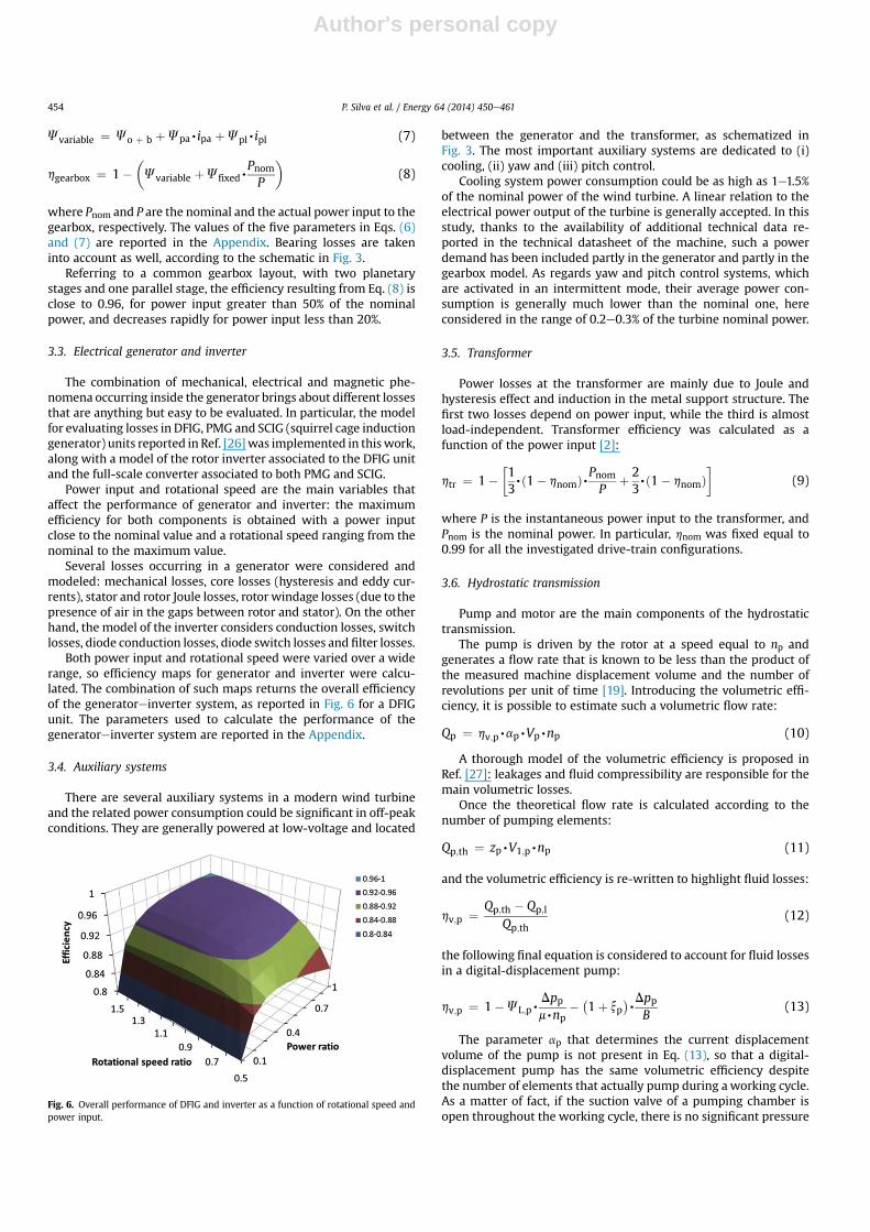
Both power input and rotational speed were varied over a widerange, so efficiency maps for generator and inverter were calcu-lated. The combination of such maps returns the overall efficiencyof the generatoreinverter system, as reported in Fig. 6 for a DFIGunit. The parameters used to calculate the performance of thegeneratoreinverter system are reported in the Appendix.

3.4. Auxiliary systems

There are several auxiliary systems in a modern wind turbineand the related power consumption could be significant in off-peakconditions. They are generally powered at low-voltage and located

between the generator and the transformer, as schematized inFig. 3. The most important auxiliary systems are dedicated to (i)cooling, (ii) yaw and (iii) pitch control.

Cooling system power consumption could be as high as 1e1.5%of the nominal power of the wind turbine. A linear relation to theelectrical power output of the turbine is generally accepted. In thisstudy, thanks to the availability of additional technical data re-ported in the technical datasheet of the machine, such a powerdemand has been included partly in the generator and partly in thegearbox model. As regards yaw and pitch control systems, whichare activated in an intermittent mode, their average power con-sumption is generally much lower than the nominal one, hereconsidered in the range of 0.2e0.3% of the turbine nominal power.

3.5. Transformer

Power losses at the transformer are mainly due to Joule andhysteresis effect and induction in the metal support structure. Thefirst two losses depend on power input, while the third is almostload-independent. Transformer efficiency was calculated as afunction of the power input [2]:

htr ¼ 1��13,ð1� hnomÞ,Pnom

Pþ 23,ð1� hnomÞ

�(9)

where P is the instantaneous power input to the transformer, andPnom is the nominal power. In particular, hnom was fixed equal to0.99 for all the investigated drive-train configurations.

3.6. Hydrostatic transmission

Pump and motor are the main components of the hydrostatictransmission.

The pump is driven by the rotor at a speed equal to np andgenerates a flow rate that is known to be less than the product ofthe measured machine displacement volume and the number ofrevolutions per unit of time [19]. Introducing the volumetric effi-ciency, it is possible to estimate such a volumetric flow rate:

Qp ¼ hv;p,ap,Vp,np (10)

A thorough model of the volumetric efficiency is proposed inRef. [27]: leakages and fluid compressibility are responsible for themain volumetric losses.

Once the theoretical flow rate is calculated according to thenumber of pumping elements:

Qp;th ¼ zp,V1;p,np (11)

and the volumetric efficiency is re-written to highlight fluid losses:

hv;p ¼ Qp;th � Qp;l

Qp;th(12)

the following final equation is considered to account for fluid lossesin a digital-displacement pump:

hv;p ¼ 1�JL;p,Dppm,np

� �1þ xp

,DppB

(13)

The parameter ap that determines the current displacementvolume of the pump is not present in Eq. (13), so that a digital-displacement pump has the same volumetric efficiency despitethe number of elements that actually pump during aworking cycle.As a matter of fact, if the suction valve of a pumping chamber isopen throughout the working cycle, there is no significant pressure

Fig. 6. Overall performance of DFIG and inverter as a function of rotational speed andpower input.

P. Silva et al. / Energy 64 (2014) 450e461454

Author's personal copy

drop between the suction volume and the chamber and, conse-quently, leakage and fluid compressibility are really negligible andnot comparable to the tens of MPa as pressure difference betweenoutlet and inlet of the pump. Different considerations concern thepumping elements of a state-of-the-art positive-displacementpump, e.g. a swash-plate-type piston unit with port plate [28],where all the pistons work, even at intermediate displacement, justreducing the stroke of each piston.

Eq. (13) proposed for the pump can be revised for the motor. Inthis case, the volumetric efficiency is similarly determined as:

hv;m ¼ Qm;th

Qm;th þ Qm;l¼ 1

1þJL;m, Dpmm,nm

þ ð1þ xmÞ,DpmB

(14)

On the other hand, a model considering only volumetric losses isnot sufficient: hydraulic-mechanical losses in both the pump andthe motor must be taken into account.

The actual torque required by the pump is calculated as

Tp ¼ ap,Vp,Dpphhm;p

(15)

and differs from the theoretical one just for the presence of thehydraulic-mechanical efficiency at the denominator. Similarly, theoutput torque at the motor shaft is calculated as

Tm ¼ hhm;m,am,Vm,Dpm (16)

Torque losses in hydrostatic units are mainly due to frictionforces in lubricated gaps present inside the machine elements inrelative motion [29]. Dealing with a hydraulic motor, they must bededucted from the theoretical output torque:

Tm ¼ Tm;th � Tm;l ¼ am,Vm,Dpm � Tm;l (17)

In particular, the torque loss is the sum of:

� the friction torque, which is proportional to the load, i.e. to thepressure difference between inlet and outlet of the motor, bymeans of a friction coefficient that is maximum when therotational speed is zero and decreases as speed increases;

� the viscous friction torque, which is proportional to fluid vis-cosity, rotational speed and characteristic dimensions of themachine that can be similarly quantified as proportional to thedisplacement volume of the machine;

� the constant friction torque, independent of operating conditions.

No turbulent friction component is here considered for the sakeof simplicity.

Thus, the hydraulic-mechanical efficiency of the motor isformulated as:

hhm;m ¼ 1�Jf ;m,1

am,nm�Jvf ;m,

m,nmam,Dpm

�Jk;m,1

am,Dpm(18)

Similarly, the hydraulic-mechanical efficiency of the pump is:

hhm;p ¼ 11þJf ;p,

1ap,np

þJvf ;p,m,np

ap,DppþJk;p,

1ap,Dpp

(19)

Looking at the equations returning both volumetric andhydraulic-mechanical efficiencies, it is possible to realize that in-termediate displacement volumes affect only the latter. As a matterof fact, if partial displacement mode does not affect volumetriclosses as previously highlighted, piston motion inside the cylinderis always subject to friction, resulting in a torque loss.

Referring to the volumetric and hydraulic-mechanical effi-ciencies for both pump andmotor, and neglecting pressure drops inthe lines connecting the two digital-displacement units, it ispossible to model the efficiency of the hydrostatic transmission bysetting the coefficients present in the equations above. These co-efficients are detailed in the Appendix, and were determined inorder to fit the results of the digital-displacement unit investigatedin Ref. [30], once fixed fluid properties in terms of bulk modulus(1400 MPa) and viscosity (32 cP).

As an example, according to Eqs. (14) and (18), Fig. 7 shows bothvolumetric and hydraulic-mechanical efficiency depending on thepressure difference between inlet and outlet of the motor rotatingat 1500 rpm. Three normalized values of displacement volume arereported, showing that efficiency values remain high even at lowerloads and displacement volumes.

Finally, both pump and motor models were integrated and usedto assess the overall efficiency of an advanced hydrostatic trans-mission with one pump, directly driven by the rotor, deliveringhigh-pressure fluid to two motors in a parallel configuration,driving two separate generators. Thus, for each input to the systemin terms of power and rotor speed, a routinewas created in order tocalculate the displacement volumes of the machines and themaximum pressure of the hydraulic circuit determining themaximum efficiency of the system. The result of such a controlprocedure is the overall efficiency of the hydrostatic transmission,as shown in Fig. 8. In particular, it can be seen that only onemotor isused when input power is less than 16% of the nominal power,whereas both motors run for higher inputs, with an overall

Fig. 7. Volumetric and hydraulic-mechanical efficiencies of the simulated digital-displacement motor rotating at 1500 rpm (in dashed and continuous lines,respectively).

Fig. 8. Efficiency comparison for the advanced hydrostatic transmission and theconventional HT system as in Ref. [10].

P. Silva et al. / Energy 64 (2014) 450e461 455

Author's personal copy

efficiency sensibly higher than the one of the system adopted in Ref.[10], where state-of-the-art positive-displacement units were used.

4. Model validation

In order to test the accuracy of the drive-train model, the per-formance of the turbine whose experimental data were availablewas simulated. Experimental pitch angle and tip speed ratio wereused for each wind speed.

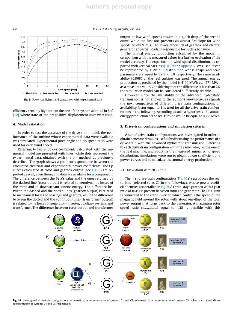
Referring to Fig. 9, power coefficients calculated with the nu-merical model are presented with lines, while dots represent theexperimental data, obtained with the bin method, as previouslydescribed. The graph shows a good correspondence between thecalculated electrical and experimental power coefficients. The Cpcurves calculated at rotor and gearbox output (see Fig. 3) are re-ported as well, even though no data are available for a comparison.The difference between the Betz’s value and the ones returned bythe dashed line (rotor output) is related to aerodynamic losses ofthe rotor and to downstream kinetic energy. The difference be-tween the dashed and the dotted lines (gearbox output) is relatedto mechanical losses of bearings and gearbox, while the differencebetween the dotted and the continuous lines (transformer output)is related to the losses of generatoreinverter, auxiliary systems andtransformer. The difference between rotor output and transformer

output at low wind speeds results in a quick drop of the secondcurve, while the first one presents an almost flat slope for windspeeds below 9 m/s. The lower efficiency of gearbox and electricgenerator at partial loads is responsible for such a behavior.

The annual energy production calculated by the model incomparisonwith the measured values is a further evaluation of themodel accuracy. The experimental wind speed distribution, as re-portedwith vertical bars in Fig. A1 in the Appendix, was used: it canbe represented by a Weibull distribution whose shape and scaleparameters are equal to 1.9 and 6.8 respectively. The same avail-ability (0.968) of the real turbine was used. The annual energyproduction as predicted by the model is 4199 MWh vs. 4271 MWhas a measured value. Considering that the difference is less than 2%,the simulation model can be considered sufficiently reliable.

However, since the availability of the advanced hydrostatictransmission is not known to the author’s knowledge, as regardsthe next comparison of different drive-train configurations, anavailability factor equal to 1 is used for all the drive-train configu-rations in the following. According to such a hypothesis, the annualenergy production of the real turbinewould be equal to 4338MWh.

5. Drive-train configurations and simulation criteria

A set of drive-train configurations was investigated in order toobtain benchmark values useful for discussing the performance of adrive-train with the advanced hydrostatic transmission. Referringto each drive-train configurationwith the same rotor, i.e. the one ofthe real machine, and adopting the measured annual wind speeddistribution, simulations were run to obtain power coefficient andpower curves and to calculate the annual energy production.

5.1. Drive-train with DFIG unit

The first drive-train configuration (Fig. 10a) reproduces the realturbine (referred to as C1 in the following), whose power coeffi-cient curves are detailed in Fig. 9. A three-stage gearbox with a gearratio of 104:1 is present between rotor and generator. The DFIG unitis connected to the rotor inverter, which controls the speed of themagnetic field around the rotor, with about one-third of the totalpower output that turns back to the generator. A maximum rotorspeed ratio (nmax/nmin) equal to 1.35 is possible with this

Fig. 9. Power coefficients and comparison with experimental data.

Fig. 10. Investigated drive-train configurations: schematic a) is representative of systems C1 and C2; schematic b) is representative of systems C3; schematics c) and d) arerepresentative of systems C4 and C5 respectively.

P. Silva et al. / Energy 64 (2014) 450e461456

Author's personal copy

configuration, due to the limitation of the generator itself, so thewind speed interval where the tip speed ratio is constant isreduced. The main advantage of this configuration consists in thesmall size of the inverter: a low amount of energy is converted withreduced energy losses. On the other hand, a frequent maintenanceis required to change the slip rings used to power up the rotor andthe reactive power supplied by the turbine can be controlled withina limited range (generally cos 4 ¼ 0.96e0.98). Until a few years agothis drive-train configuration was the most flexible and efficientamong the commercially available solutions: as a consequence, alarge number of such turbines has been installed. The drive-trainconfiguration schematized in Fig. 10a is also adopted for the sys-tem C2, as detailed in the following.

5.2. Drive-train with direct-drive PMG unit

According to the direct-drive configuration presented in Fig. 10b(in the following as systemC3), the rotor is directly connected to thegenerator with no gearbox. A large diameter and multi-pole gener-ator is necessary to provide the required torque. This type ofgenerator is usually made with permanent magnets in order toeliminate the Joule lossespresent in the rotorof anexcitedgenerator,due to the very high currents required for a high resistant torque.Such a drive-train configuration allows a high rotor speed ratio(about 2.25, as deduced from technical datasheets of several com-mercial turbines) with a high average efficiency of the rotor. The fullscale converter allows to regulate the power factor of the turbineoverawide range, and tocontrol theoutput voltage. Themain sourceof breakdown is also eliminated, alongwith the losses related to thegearbox. On the other hand, a large-size converter is required and allthe power generated is affected by the inverter losses. This compo-nent requires a periodicmaintenance and needs a replacement afterseveral years, even though this problem is mitigated by the pro-gressive inverter cost reductions of the last decade.

5.3. Drive-trains with the advanced hydrostatic transmission

Two schematic drive-train configurations with an advanced hy-drostatic transmission are presented in Fig. 10c and d. As comparedto systemC1, thegearbox is replacedby thehydrostatic transmissionand no inverter is present, since the generator runs at constantspeed. The control of the displacement volumes of both pump andmotor allows to obtain a rotor speed ratio as high as necessary. Aspreviously highlighted, themain advantages of such a configurationare (i) the limitless range of the rotor speed, (ii) the potentially highreliability and low maintenance requirements of the hydrostaticdrive, against a conventional gearbox, and (iii) the possibility toreduce the weight of the nacelle. On the other hand, a reduction ofthe nominal Cp value is expected, as a consequence of the loweroverall efficiency of the hydrostatic transmission (see Fig. 8).

The best performance of the hydrostatic transmission, in termsof turbine cost and Cp curve, can be achieved by means of a fastgenerator, typically running at 1500 rpm. In order to allow a reac-tive power regulation (with typical cos 4 in the range from 0.8 to 1),a synchronous and externally excited generator can be used: thisconfiguration is referred to as C4. However, due to the presence ofslip rings, this solution reduces the reliability of the drive-train,which is one of the most interesting potential advantages of thehydrostatic transmission. Moreover, the efficiency of this generatorat partial loads decreases, owing to Joule losses in the rotor, whosecurrent must be high to achieve the desired resistant torque. Thus,two configurations with hydrostatic transmission were simulated:the first (Fig. 10c) includes the above-mentioned synchronousgenerator, while the second (Fig. 10d) uses a fast PMG unit, referredto as C5. The latter has a high efficiency over all theworking range, a

high reliability and requires fewmaintenance. On the other hand, itdoes not allow a reactive power control and requires a bank ofcapacitors to compensate the inductive power generation.

Asdetailed in Fig.10, the rotor speed rationmax/nminpossiblewiththe hydrostatic transmission has been set equal to 3,which allows toguarantee constant tip speed ratio, reflecting on a maximum effi-ciency of the rotor, for wind speeds lower than the nominal value.

5.4. Simulation criteria

Pitch angle and rotational speed are adjusted by the controlsystem of the turbine as a function of wind speed. They are themostimportant parameters affecting rotor performance and have to becontrolled with specific strategies.

Fig.11 shows a typical power curveof awind turbine. Ifwind speedis less than vcut-in, it is neither possible nor convenient to run theturbine. When wind speed increases, up to vuN, the electrical powerproduction has to be maximized by means of a pitch angle and a tipspeed ratio close to the optimumvalues. The rotational speed is con-stant and equal to its maximum value for wind speeds ranging fromvrated and vcut-off, while the pitch angle is varied in order to limit thepower to its nominal value. Fig. 11 also shows an interval of windspeeds, between vuN and vrated, where the pitch angle is varied toachieve a progressive transition from the two contiguous regions.Finally,whenwindspeed is greater thanvcut-out, rotor bladeswouldbesubject to overloads, so the turbine is stopped to avoid damages.

In order to allow a consistent comparison of the different drive-train configurations reported in Fig. 10, fixed control strategies wereconsidered for wind speeds ranging from vcut-in to vuN (as detailed inFig. 11):

� rotor speed variation oriented to maintain the tip speed ratioconstant over an as wide as possible range, according to thespeed limitations imposed by the generator;

� pitch angle variation in order to achieve the maximum effi-ciency of the rotor, in case of generator speed limitations.

Moreover, the following parameters were determined:

� vcut-in corresponding to an electrical power output equal to 1.5%of the nominal power;

� vrated corresponding to an electric power output equal to thenominal value, i.e. 2.0 MW.

Since the control strategies of the real turbine do not alwaysmatch these three modes, a simulation of a DFIG turbine (referredto as C2), here revised to comply with the above-mentionedspecifications, was run. An annual energy production 4% higherthan the experimental one and a Cp curve closer to the one declaredby the manufacturer were achieved.

Fig. 11. Schematic of the regions for a pitch- and speed-controlled multi-MW windturbine [31].

P. Silva et al. / Energy 64 (2014) 450e461 457

Author's personal copy

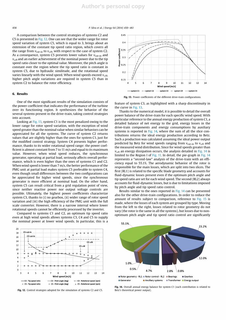
A comparison between the control strategies of systems C2 andC5 is presented in Fig. 12. One can see that the wider range for rotorspeed variation of system C5, which is equal to 3, brings about anextension of the constant tip speed ratio region, which covers allthe range from vcut-in to vuN, with respect to the case of system C2.As a consequence, system C5 presents lower values for vcut-in andvuN and an earlier achievement of the nominal power due to the tipspeed ratio closer to the optimal value. Moreover, the pitch angle isconstant over the region where the tip speed ratio is constant insystem C5, due to hydraulic similitude, and the rotational speedvaries linearly with the wind speed. Whenwind speeds exceed vuN,higher pitch angle variations are required in system C5 than insystem C2 to balance the rotor efficiency.

6. Results

One of the most significant results of the simulation consists ofthe power coefficient that indicates the performance of the turbineover its functioning region. It synthesizes the behavior of theseveral systems present in the drive-train, taking control strategiesinto account.

Looking at Fig. 13, system C1 is the most penalized owing to thelower range for rotor speed variation, with the exception of windspeed greater than the nominal valuewhen similar behaviors can beappreciated for all the systems. The curve of system C2 returnsvalues that are slightly higher than the ones for system C1, just forthe modified control strategy. System C4 presents higher perfor-mance, thanks to its wider rotational speed range: the power coef-ficient is almost constant from7 to 11m/s and equal to itsmaximumvalue. However, when wind speed reduces, the synchronousgenerator, operating at partial load, seriously affects overall perfor-mance, which is even higher than the ones of systems C1 and C2.Whenwind speed is lower than 7m/s, the better performance of thePMG unit at partial load makes system C5 preferable to system C4,even though small differences between the two configurations canbe appreciated for higher wind speeds, since the synchronousgenerator is more efficient at nominal load. On the other hand,system C5 can result critical from a grid regulation point of view,since neither reactive power nor output voltage controls arepossible. Ultimately, the highest power coefficients characterizesystem C3, thanks to (i) no gearbox, (ii) wider range of rotor speedvariation and (iii) the high efficiency of the PMG unit with the fullscale converter. However, there is a narrow interval where lowerrotational speeds cannot be efficiently processed by the inverter.

Compared to systems C1 and C2, an optimum tip speed ratioeven at high wind speeds allows systems C3, C4 and C5 to supplythe nominal power at lower wind speeds. In particular, this is a

feature of system C3, as highlighted with a sharp discontinuity inthe curve in Fig. 13.

Thanks to the numerical model, it is possible to detail the overallpower balance of the drive-train for each specific wind speed. Withparticular reference to the annual energy production of system C1, adetailed balance of net energy to the grid, energy losses in thedrive-train components and energy consumptions by auxiliarysystems is reported in Fig. 14, where the sum of all the slice con-tributions returns the ideal energy production according to Betz.Such a production was calculated assuming the ideal power outputpredicted by Betz for wind speeds ranging from vcut-in to vuN andthemeasured wind distribution. Since for wind speeds greater thanvuN an energy dissipation occurs, the analysis detailed in Fig. 14 islimited to the Region I of Fig. 11. In detail, the pie-graph in Fig. 14represents a “second-law” analysis of the drive-train with an effi-ciency equal to 55.1%. The aerodynamic behavior of the rotor isresponsible for the main losses, which are split into two slices. Thefirst (RL1) is related to the specific blade geometry and accounts forfluid-dynamic losses present even if the optimum pitch angle andtip speed ratio are set for each wind speed. The second (RL2) alwaysaccounts for fluid-dynamic losses, but is due to limitations imposedby pitch angle and tip speed ratio control.

Results similar to the ones reported in Fig. 14 can be presentedalso for the other drive-train configurations. In order to reduce theamount of results subject to comparison, reference to Fig. 15 ismade, where the losses of each system are grouped by type. Movingfrom the left to the right, losses related to rotor geometry do notvary (the rotor is the same in all the systems), but losses due to non-optimum pitch angle and tip speed ratio control are significantly

Fig. 12. Control strategies adopted for the simulation of systems C2 and C5.

Fig. 13. Power coefficients of the different drive-train configurations.

Fig. 14. Overall annual energy balance for system C1 (each contribution is related toBetz’s theoretical power output).

P. Silva et al. / Energy 64 (2014) 450e461458

Author's personal copy

reduced in systems C3 to C5. System C3 has neither gearbox norhydrostatic transmission, whose losses are almost twice thegearbox losses in systems C1 and C2. As regards the losses at theelectric generator, higher values characterize systems C1 to C3, dueto the presence of the inverter. Losses at bearings, auxiliary systemsand transformer are almost equal for each system.

The data reported in Fig. 15 are based on the measured windspeed density distribution. As for lower scale parameters (narrowdistribution curves), simulations also showed that RL2 losses ofsystems C1 to C3 are reduced if the drive-train configuration isadjusted in order to match the optimum working point with themost frequent wind speed.

Finally, annual energy productions of the five investigated sys-tems are reported in Table 1. Considering system C2 as a reference,systems C4 and C5 seem to be interesting at a glance, since energyproduction increases. Moreover, the drive-train with the hydro-static transmission should bemore reliable than the DFIG one, sinceboth gearbox and slip rings are eliminated. Nevertheless, Table 1highlights the superiority of system C3, which seems to be thepreferable solution from an energy production point of view, even

though issues related to component cost and reliability should beconsidered in order to choose the best configuration for the windenergy conversion system.

7. Conclusions

Starting fromdesign and experimental data available for a state-of-the-art2MWDFIGwindturbine, anumericalmodelwas implementedto investigate the performance of wind energy conversion systemswith drive-train configurations different from the original one.

The first analysis focusing on the original system highlighted theimportance of a proper control system, oriented to increase theannual energy production. In fact, experimental data showed anon-optimized control of the examined wind turbine, so an in-crease in annual energy production seems to be possible throughan improvement of the rotor control strategy.

A direct-drive layout was considered as well, and the mostfavorable energy production was calculated. The absence of com-ponents, in contrast with the original configuration, should in-crease system reliability, being the inverter the only cause of fault inthis case. However, full voltage, frequency and reactive powercontrols are not feasible without an FSC (full scale converter) unit.

The use of an advanced hydrostatic transmission in the drive-train was finally studied, as the scope of the work. Compared tothe direct-drive layout, from an energetic point of view, this solu-tion could be interesting when the wind speed is near the cut-invalue. On the other hand, reductions of the hydrostatic trans-mission efficiency occurring at higher wind speeds, significantlypenalize the performance of the whole drive-train. Regarding thegenerator, two different solutions were considered: with a PMGunit it is possible to reach great reliability as well as high part loadefficiency, whereas with a synchronous generator the reactive po-wer output can be adjusted. Both evaluated hydrostatic configu-rations return about 8e9% more in terms of yearly electricityproduction with respect to a DFIG turbine and approximately 3%less compared to a direct-drive PMG configuration. In any case, ahydrostatic transmission could be useful to (i) lower the drive-traincost, (ii) improve system reliability and (iii) reduce the weight ofthe nacelle. The last two features could be key points for off-shoreapplications, although the higher average wind speed in open seacould increase the energy balance difference with respect to thePMG system, due to the lower efficiency of the hydrostatic trans-mission at full load. Further evaluations concerning costs, as well asconsiderations about the scenario in which the wind farm will beoperated, should drive the choice of the proper drive-train layout.

Appendix

Fig. 15. Comparison of annual energy losses characteristic of the investigated drive-trains.

Table 1Calculated annual energy productions.

System Energy production[MWh/year]

Variation

C1: current drive-train with DFIG unit 4338 �4%C2: optimized drive-train with DFIG unit 4520 e

C3: drive-train with direct-drive PMG unit 5045 11.6%C4: drive-train with HT and SG unit 4895 8.3%C5: drive-train with HT and PMG unit 4920 8.8%

Fig. A1. Density distribution of the measured wind speed (bars indicate the wind speed distribution, along with the Weibull curve withshape and scale parameters equal to 1.9 and 6.8 respectively).

P. Silva et al. / Energy 64 (2014) 450e461 459

Author's personal copy

References

[1] Burton T, Sharpe D, Jenkins N, Bossanyi E. Wind energy handbook. John Wiley& Sons; 2001.

[2] Ackermann T. Wind power in power systems. John Wiley & Sons; 2005.[3] Ribrant J, Bertling ML. Survey of failures in wind power systems with focus on

Swedish wind power plants during 1997e2005. IEEE Trans Energy Convers2007;22(1):167e73. http://dx.doi.org/10.1109/TEC.2006.889614.

[4] Sun X, Huang D, Wu G. The current state of offshore wind energy technologydevelopment. Energy 2012;41:298e312. http://dx.doi.org/10.1016/j.energy.2012.02.054.

[5] Ficarella A, Giuffrida A, Lanzafame R. Common rail injector modified toachieve a modulation of the injection rate. Int J Automot Technol 2005;6(4):305e14.

[6] Giuffrida A, Laforgia D. Modelling and simulation of a hydraulic breaker. Int JFluid Power 2005;6(2):47e56.

[7] Filipi Z, Louca L, Daran B, Lin CC, Yildir U, Wu B, et al. Combined opti-misation of design and power management of the hydraulic hybridpropulsion system for the 6 � 6 medium truck. Int J Heavy Vehicle Syst2004;11(3e4):372e402. http://dx.doi.org/10.1504/IJHVS.2004.005458.

[8] Giuffrida A, Lanzafame R. On the pressure relief valve for the lubricationsystem of an internal combustion engine. In: Proceedings of the 2007 falltechnical conference of the ASME internal combustion engine division,October 14e17, 2007, Charleston, South Carolina, USA. http://dx.doi.org/10.1115/ICEF2007-1716.

[9] Tita I, Cǎlǎrasu D. Wind power systems with hydrostatic transmission forclean energy. Environ Eng Manag J 2009;8(2):327e34.

[10] Schmitz J, Vatheuer N, Murrenhoff H. Development of a hydrostatic trans-mission for wind turbines. In: Proceedings of 7th international fluid powerconference, March 22e24, 2010, Aachen, Germany.

[11] Browning JR, Manwell JF, McGowan JG. A techno-economic analysis of aproposed 1.5 MW wind turbine with a hydrostatic drive train. Wind Eng2009;33(6):571e85. http://dx.doi.org/10.1260/0309-524X.33.6.571.

[12] Linjama M. Digital fluid power e state of the art. In: Proceedings of the 12thScandinavian international conference on fluid power, May 18e20, 2011,Tampere, Finland.

[13] Scheidl R, Linjama M, Schmidt S. Is the future of fluid power digital? Proc InstMech Eng Part I J Syst Control Eng 2012;226(6):721e3. http://dx.doi.org/10.1177/0959651811435628.

[14] Ehsan M, RampenW, Salter S. Modeling of digital-displacement pump-motorsand their application as hydraulic drives for nonuniform loads. ASME J DynSyst Meas Control 2000;122(1):210e5. http://dx.doi.org/10.1115/1.482444.

[15] Salter SH, Taylor JRM, Caldwell NJ. Power conversion mechanisms for waveenergy. Proc Inst Mech Eng Part M J Eng Marit Environ 2002;216(1):1e27.http://dx.doi.org/10.1243/147509002320382103.

[16] Payne GS, Kiprakis AE, Ehsan M, Rampen WHS, Chick JP, Wallace AR. Effi-ciency and dynamic performance of Digital Displacement� hydraulictransmission in tidal current energy converters. Proc Inst Mech Eng Part A JPower Energy 2007;221(2):207e18. http://dx.doi.org/10.1243/09576509JPE298.

[17] Manring ND, Luecke G. Modeling and designing a hydrostatic transmissionwith a fixed displacement motor. ASME J Dyn Syst Meas Control 1998;120(1):45e9. http://dx.doi.org/10.1115/1.2801320.

[18] Kugi A, Schlacher K, Aitzetmüller H, Hirmann G. Modelling and simulation of ahydrostatic transmission with variable-displacement pump. Math ComputSimul 2000;53(4e6):409e14. http://dx.doi.org/10.1016/S0378-4754(00)00234-2.

[19] Ivantysyn J, Ivantysynova M. Hydrostatic pumps and motors. Academia BooksInternational; 2000.

[20] Giuffrida A, Lanzafame R. Cam shape and theoretical flow rate in balancedvane pumps. Mech Mach Theory 2005;40(3):353e69. http://dx.doi.org/10.1016/j.mechmachtheory.2004.07.008.

[21] IEC. Wind turbines e part 12-1: power performance measurements ofelectricity producing wind turbines. IEC 61400-12-1 international standard;2005.

[22] Llombart A, Watson SJ, Llombart D, Fandos JM. Power curve characterization I:improving the bin method. In: International conference on renewable en-ergies and power quality, March 16e18, 2005, Zaragoza, Spain.

[23] Llombart A, Watson SJ, Fandos JM, Llombart D. Power curve characteriza-tion II: modelling using polynomial regression. In: International conferenceon renewable energies and power quality, March 16e18, 2005, Zaragoza,Spain.

[24] Kulka A. Pitch and torque control of variable speed wind turbines. MSc Thesis.Göteborg, Sweden: Chalmers University of Technology; 2004.

[25] Takahashi R, Ichita H, Tamura J, Kimura M, Ichinose M, Futami M-O, et al.Efficiency calculation of wind turbine generation system with doubly fedinduction generator. In: Proceedings of the 19th international conference onelectrical machines, September 6e8, 2010, Rome, Italy.

[26] Poore R, Lettenmaier T. Alternative design study report: windPACT advancedwind turbine drive train designs study. Golden, Colorado: NREL; August 2003.Report no. NREL/SR-500-33196.

[27] Giuffrida A, Ficarella A, Laforgia D. Study of the delivery behaviour of a pump forcommon rail fuel injection equipment. Proc Inst Mech Eng Part I J Syst ControlEng 2009;223(4):521e35. http://dx.doi.org/10.1243/09596518JSCE612.

Table A1Best fit coefficients in Eqs. (4) and (5).

a1 1.53a2 67.87a3 �0.09a4 0a5 4.90a6 5.09a7 20.21a8 �0.02a9 0

Table A2Coefficients in Eqs. (6) and (7).

Jsþb 2$10�3

Jfl 1$10�3

Joþb 1.8$10�3

Jpa 1.1$10�2

Jpl 8$10�3

Table A3Coefficients of the DFIG model [26].

Generator nominal speed [rpm] 1620Line out voltage [V] 690Rotor resistance [U] 3.65$10�3

Stator resistance [U] 1.35$10�2

Iron resistance [U] 6.2$10�2

Magnetic reactance [U] 1.776Rotor/stator windage ratio 3Windage loss factor [kW/rpm] 1$10�3

Table A4Coefficients of the rotor inverter model [26].

DC bus voltage [V] 1100Switching frequency [Hz] 3000IGBT fixed portion VCE [V] 1.5IGBT dynamic resistance [U] 1.36$10�3

Diode fixed portion [V] 1.25Diode dynamic resistance [U] 5$10�4

IGBT turn-on energy loss [J] 0.45IGBT turn-off energy loss [J] 0.60Current for oneoff switching [A] 1200Voltage for oneoff switching [V] 900Diode recovery energy loss [J] 3$10�2

Fixed loss per bridge [kW] 2Grid RMS lineeline voltage [V] 690Modulation index [VAC/VDC] 0.887

Table A5Coefficients in Eqs. (13), (14), (18) and (19).

Coefficient Pump Motor

x 0.55 0.55JL 1.47$10�3 1.81$10�3

Jf 8.75$10�2 7.39$10�2

Jvf 2.52$10�2 2.33$10�3

Jk 0.118 0.391

P. Silva et al. / Energy 64 (2014) 450e461460

Author's personal copy

[28] Manring ND. The discharge flow ripple of an axial-piston swash-plate typehydrostatic pump. ASME J Dyn Syst Meas Control 2000;122(2):263e8. http://dx.doi.org/10.1115/1.482452.

[29] Hibi A, Ichikawa T. Mathematical model of the torque characteristics for hy-draulic motors. Bull JSME 1977;20(143):616e21.

[30] Merrill KJ, Holland MA, Lumkes JH. Efficiency analysis of a digital pump/motoras compared to a valve plate design. In: Proceedings of 7th international fluidpower conference, March 22e24, 2010, Aachen, Germany.

[31] Muyeen SM. Wind power. Intech; 2010.

P. Silva et al. / Energy 64 (2014) 450e461 461