Western University Western University

Scholarship@Western Scholarship@Western

Electronic Thesis and Dissertation Repository

9-9-2020 11:30 AM

Hydrostatic Performance Of Reinforced Concrete Pipe For Hydrostatic Performance Of Reinforced Concrete Pipe For

Infiltration Infiltration

Lui Sammy Wong, The University of Western Ontario

Supervisor: Nehdi, Moncef L., The University of Western Ontario

A thesis submitted in partial fulfillment of the requirements for the Doctor of Philosophy degree

in Civil and Environmental Engineering

© Lui Sammy Wong 2020

Follow this and additional works at: https://ir.lib.uwo.ca/etd

Part of the Civil Engineering Commons

Recommended Citation Recommended Citation Wong, Lui Sammy, "Hydrostatic Performance Of Reinforced Concrete Pipe For Infiltration" (2020). Electronic Thesis and Dissertation Repository. 7397. https://ir.lib.uwo.ca/etd/7397

This Dissertation/Thesis is brought to you for free and open access by Scholarship@Western. It has been accepted for inclusion in Electronic Thesis and Dissertation Repository by an authorized administrator of Scholarship@Western. For more information, please contact wlswadmin@uwo.ca.

ii

ABSTRACT

Groundwater infiltration into underground sewer systems has long been a costly issue for

municipalities. With reinforced concrete pipe (RCP) being a primary option for sewer systems,

existing hydrostatic testing methods conducted by manufacturers to measure internal pipe pressure,

as required by specifications, do not reflect in-situ external hydrostatic conditions. This thesis

records the development of a novel testing method to evaluate the RCP joint performance for

infiltration. The test is safe and easy to conduct by RCP producers at the factory. The test method

mimics field conditions of possible RCP joint gap and joint offset. Over 100 tests were conducted,

including 600 mm, 900 mm and 1200 mm RCP with conventional single offset self-lubricated

gaskets. This study also evaluates the gasket performance for infiltration. Pipe joint performance

curves were developed based on the test results. Comparison to laboratory load-deformation tests

on gaskets was conducted, indicating that predictions of the sealing potential derived using gasket

geometry agreed well with the results of infiltration tests. The study shows that the joint gap plays

an important role in the sealing potential. The developed apparatus allows the observation of gasket

movement under infiltration pressure against the gasket leading to failure. The performance curves

also allow the prediction of an infiltration potential leading to a practical applicational procedure

to guide RCP installation. A case study of deep RCP pipe subjected to groundwater pressure

illustrated the usefulness of the performance curves to derive maximum allowable joint gaps, which

contractors could rely on during RCP installation. The findings should allow deducing technical

guidance on how water tightness of RCP can be achieved at installation below the prevailing

groundwater level. Two oversampling methods: Synthetic Minority Over-sampling Technique

(SMOTE) and Density-Based SMOTE, were employed to address the unbalanced dataset.

Accordingly, applying advanced machine learning techniques, the scale of variation in the test data

can be analyzed and accurately predicted using tree-based supervised classification methods:

random forest, extra trees and gradient boosting.

iii

Keywords

Concrete pipe; Infiltration; Joint; Performance; Hydrostatic Pressure; Test; Machine Learning;

Supervised Learning; Gradient Boosting; SMOTE, DBSMOTE.

iv

SUMMARY FOR THE LAY AUDIENCE

Groundwater infiltration into sewer systems is a costly problem for many municipalities. With

reinforced concrete pipe (RCP) being one of the most commonly used pipe options for sewer

systems, existing hydrostatic testing methods conducted by manufacturers measuring internal

pressure do not reflect in-situ external hydrostatic conditions. This thesis presents the development

of a novel testing method to evaluate the RCP joint performance for infiltration. The test is safe

and easy to conduct by RCP producers at the factory. The test also mimics the field conditions of

possible joint gaps and joint offsets. The test procedure was repeated many times for 600 mm, 900

mm and 1200 mm RCP. The performance of commonly used single offset self-lubricated gaskets

and various alignments were evaluated. Performance curves were developed based on the testing

results. Comparisons to the laboratory load-deformation tests on gaskets were also conducted,

indicating that predictions of the sealing potential derived using gasket geometry agreed with the

results of the infiltration tests. The study shows that the joint gap plays an important role in the

sealing potential. The apparatus developed allows the observation of gasket movements under

infiltration pressures against the gasket leading to failure. The performance curves also allow the

prediction of an infiltration potential leading to a practical applicational procedure to guide the

installation of the pipe. A case study of deep RCP pipe subjected to groundwater pressure

illustrated the usefulness of the performance curves to derive maximum allowable joint gap, which

contractors could rely on during RCP installation. The findings should allow deducing technical

guidance on how water tightness of RCP can be achieved at installations below the prevailing

groundwater level. Lastly, with the application of advanced machine learning techniques, the scale

of the variation in the test data can be analyzed and predicted using classification methods. The

modeling technique, procedure and accuracy evaluation are presented.

v

CO-AUTHORSHIP STATEMENT

This thesis was prepared according to the integrated-article layout designated by the Faculty

of Graduate Studies at Western University, London, Ontario, Canada. All the work stated in

this thesis, including experimental testing, data analysis, machine learning models, and writing

of draft manuscripts for publication, was carried out by the candidate under the supervision

and guidance of Professor M.L. Nehdi. Any other co-authors assisted in conducting the

experimental program and/or revision of the initial draft of the manuscript. The following

publications have been either published, accepted or submitted to peer-reviewed technical

journals and international conferences:

Wong, L. and Nehdi, M.L. (2018) Critical Analysis of Precast Concrete Pipe Standards,

Infrastructures, 3(3), 18 p. ; https://doi.org/10.3390/infrastructures3030018

Wong, L. and Nehdi, M.L. (2018) New Test Method for RCP Joint Hydrostatic Infiltration,

CSCE Conference 2018, Fredericton, New Brunswick, Canada.

Wong, L. and Nehdi, M.L. (2020, In Press) Quantifying Resistance of Reinforced Concrete

Pipe Joints to Water Infiltration, ASCE Journal of Pipeline Systems - Engineering and

Practice.

Wong, L. and Nehdi, M.L. (2020, Submitted) Predicting Hydrostatic Infiltration in Reinforced

Concrete Sewer Pipes Considering Joint Gap and Joint Offset, ASCE Journal of Pipeline

Systems - Engineering and Practice.

Wong, L., Marani, A. and Nehdi, M.L. (2020, Submitted) Coupled Gradient Boosting –

Ensemble Oversampling Hybrid Model for Prediction of Concrete Pipe Joint Infiltration,

ASCE Journal of Pipeline Systems - Engineering and Practice.

vi

DEDICATION

To: My Wife: Grace Tsoi

My Children: Kalos Wong and Charis Wong

My Parents: Wa Chan, Kan Chuen Wong

vii

ACKNOWLEDGMENTS

Professor M. L. Nehdi – supervisor and mentor, his encouragement, vision and guidance,

allowed me to open doors to the new field of machine learning in Con Civil Engineering.

Brian Wood – President at Con Cast Pipe, my former employer, for his financial support and

his vision in the industry and pursuing innovation.

Con Cast Pipe – Support in the space and technical staff (Andrew Cleland, James Cameron,

Tien Nguyen) at different stages of the experimental program.

Press Seal Corporation and Hamilton Kent – supplies of gasket samples, and their technical

inputs, laboratory for material testing.

James Malpass, P.Eng. – technical mentor, his practical experience and guidance provided

great help. Being a distant student, he welcomed me to stay at his place for certain occasions

such as inclement weather or examinations.

viii

TABLE OF CONTENTS

ABSTRACT ....................................................................................................................... ii

CO-AUTHORSHIP STATEMENT ................................................................................ v

ACKNOWLEDGMENTS .............................................................................................. vii

TABLE OF CONTENTS .............................................................................................. viii

LIST OF TABLES ......................................................................................................... xiii

LIST OF FIGURES ........................................................................................................ xv

LIST OF NOMENCLATURE ...................................................................................... xix

LIST OF ABBREVIATION.......................................................................................... xxi

LIST OF APPENDICES ............................................................................................. xxiii

PREFACE ..................................................................................................................... xxiv

CHAPTER 1 ....................................................................................................................... 1

1 Introduction .................................................................................................................... 1

1.1 Research Needs and Motivation ............................................................................. 2

1.2 Research Objectives ................................................................................................ 2

1.3 Thesis Outline and Format ...................................................................................... 2

1.4 Original Contribution .............................................................................................. 4

1.5 References ............................................................................................................... 5

CHAPTER 2 ....................................................................................................................... 6

2 Literature Review ........................................................................................................... 6

2.1 Inflow and Infiltration ............................................................................................. 6

2.2 Reinforced Concrete Pipe Development ................................................................. 9

2.2.1 History of RCP ............................................................................................ 9

2.2.2 Industry Challenges .................................................................................. 10

2.3 Specification Review ............................................................................................ 13

ix

2.4 Specifications Review for Hydrostatic Performance ............................................ 16

2.4.1 General ...................................................................................................... 16

2.4.2 Internal Pressure Tests for Joint Quality ................................................... 17

2.4.3 Internal Pressure Tests for Pressure Rating .............................................. 17

2.4.4 In-field Tests for Infiltration ..................................................................... 18

2.5 Gaps in Standard Specifications ........................................................................... 20

2.6 Recent Development for Infiltration Test ............................................................. 22

2.7 Summary ............................................................................................................... 24

2.8 References ............................................................................................................. 26

CHAPTER 3 ..................................................................................................................... 30

3 Experiment Development ............................................................................................ 30

3.1 Testing Concept .................................................................................................... 30

3.2 Mechanical Apparatus .......................................................................................... 32

3.3 Testing Setup ........................................................................................................ 34

3.4 Setup with Joint Gaps ........................................................................................... 36

3.5 Setup with Joint Offset.......................................................................................... 37

3.6 Testing Procedure ................................................................................................. 39

3.6.1 Measurements ........................................................................................... 39

3.6.2 Ultimate Capacity ..................................................................................... 39

3.6.3 Operating Capacity ................................................................................... 41

3.7 Test Results for Condition Classification ............................................................. 41

3.8 Sample Selection ................................................................................................... 43

3.8.1 Pipe ........................................................................................................... 43

3.8.2 Gasket ....................................................................................................... 44

3.9 Summary ............................................................................................................... 45

x

3.10 References ............................................................................................................. 46

CHAPTER 4 ..................................................................................................................... 47

4 Pipe Joint Design ......................................................................................................... 47

4.1 Rubber Gasket ....................................................................................................... 47

4.2 Joint Design .......................................................................................................... 49

4.3 Gasket Specimens ................................................................................................. 52

4.4 Sealing Potential Calculation ................................................................................ 56

4.5 Sealing Pressure and Joint Gap ............................................................................. 56

4.6 Sealing Pressure and Geometrical Variations ....................................................... 57

4.7 Sealing Pressure and Joint Alignment .................................................................. 57

4.8 Summary ............................................................................................................... 58

4.9 References ............................................................................................................. 58

CHAPTER 5 ..................................................................................................................... 59

5 Testing Results ............................................................................................................. 59

5.1 Ultimate Hydrostatic Capacity .............................................................................. 59

5.2 Operating Hydrostatic Capacity ............................................................................ 61

5.3 Joint Gap Monitoring ............................................................................................ 63

5.4 Leakage Monitoring .............................................................................................. 66

5.5 Additional Tests .................................................................................................... 68

5.6 Preliminary Findings ............................................................................................. 69

5.7 Ultimate Pressure Capacity Varying by Pipe Size ................................................ 70

5.8 Water Level Reduction in Ultimate Pressure Evaluation ..................................... 71

5.9 Water Level Reduction in 20-hour Operation Test............................................... 76

5.10 Summary ............................................................................................................... 77

5.11 References ............................................................................................................. 78

xi

CHAPTER 6 ..................................................................................................................... 79

6 Joint Hydrostatic Performance Curves and Application .............................................. 79

6.1 Hydrostatic Performance Implications ................................................................. 79

6.2 Reality Challenges in Maintaining Minimum Joint Gap ...................................... 80

6.3 Performance Curve Development ......................................................................... 81

6.4 Test Results ........................................................................................................... 83

6.5 Prediction Using Gasket Load-deformation Tests ................................................ 84

6.6 Discussion on Uncertainty of Data ....................................................................... 85

6.7 Application of Performance Curves...................................................................... 86

6.7.1 Process ...................................................................................................... 86

6.7.2 Infiltration Potential Factor ....................................................................... 87

6.7.3 Illustrative Case Study .............................................................................. 89

6.8 Summary ............................................................................................................... 91

6.9 References ............................................................................................................. 91

CHAPTER 7 ..................................................................................................................... 92

7 Hydrostatic Performance for Infiltration Prediction using Machine Learning Techniques

...................................................................................................................................... 92

7.1 Recent AI Applications ......................................................................................... 92

7.2 Machine Learning Literature Review ................................................................... 94

7.2.1 Tree-based classifiers ................................................................................ 94

7.2.2 Oversampling ............................................................................................ 96

2.4.1 K-Nearest Neighbours (KNN) .................................................................. 97

7.3 Model Development.............................................................................................. 98

7.3.1 Data Preparation........................................................................................ 98

7.3.2 Data Statistical Distribution ...................................................................... 99

7.3.3 Machine Learning Model ........................................................................ 104

xii

7.3.4 Classification Performance ..................................................................... 105

7.4 Results and Discussions ...................................................................................... 108

7.4.1 General .................................................................................................... 108

7.4.2 Performance of Tree-based Models Before Oversampling .................... 108

7.4.3 Oversampling Methods ........................................................................... 112

7.4.4 SMOTE ................................................................................................... 113

7.4.5 DBSMOTE ............................................................................................. 115

7.4.6 Comparison between different models ................................................... 117

7.4.7 Feature Importance ................................................................................. 119

7.4.8 Design Approach: Recommendations for Future Work ......................... 120

7.5 Summary ............................................................................................................. 120

7.6 References ........................................................................................................... 121

CHAPTER 8 ................................................................................................................... 125

8 Summary, Conclusions and Recommendations ......................................................... 125

8.1 Conclusions ......................................................................................................... 126

8.1.1 Existing Standards and Literature ........................................................... 126

8.1.2 Experimental Development .................................................................... 127

8.1.3 Machine Learning Modeling................................................................... 130

8.2 Recommendations ............................................................................................... 131

8.3 References ........................................................................................................... 132

Bibliography ................................................................................................................... 133

Appendix A – Design of the Testing Apparatus ................................................................. 1

Appendix B – Testing Results ............................................................................................ 1

Appendix C – Machine Learning Source Code and Output ............................................... 1

Curriculum Vitae ................................................................................................................ 1

xiii

LIST OF TABLES

Table 1: List of flexible pipe products. ................................................................................... 10

Table 2: List of RCP standards. .............................................................................................. 14

Table 3: Acceptance criteria for RCP. .................................................................................... 14

Table 4: Population of studied area (Population Reference Bureau 2013). ............................ 15

Table 5: Summary of Joint Performance Standards ............................................................... 16

Table 6: Hydrostatic performance test summary .................................................................... 18

Table 7: Infiltration Allowance for Sanitary Sewer ................................................................ 21

Table 8: Comparison between Infiltration Test and Conventional Hydrostatic Test ............. 25

Table 9: Infiltration Test Result Conditions ........................................................................... 42

Table 10: Infiltration Test Count Summary ............................................................................ 42

Table 11: Pipe Joint Geometry ............................................................................................... 43

Table 12: List of Gaskets Used in the Research ..................................................................... 45

Table 13: RCP Single Offset Joint Detail ............................................................................... 51

Table 14: Gasket Properties .................................................................................................... 53

Table 15: Summary of Test Result for Ultimate Capacity with Aligned Position ................. 60

Table 16: Summary of Test Result for Ultimate Capacity with Offset Position .................... 61

Table 17: Summary of Test Result for Operating Capacity with Aligned Position ............... 62

Table 18: Summary of Test Result for Operating Capacity with Offset Position .................. 63

Table 19: Summary of Test Result for Other Pipes and Gaskets ........................................... 69

xiv

Table 20: Gasket Mass to Annular Space Influence Ratio, Ig ................................................. 70

Table 21: Estimated Volumetric Change in Annular Space ................................................... 72

Table 22: Recent Applications of Machine Learning in Civil Engineering ........................... 93

Table 23: Data Parameters for ML ......................................................................................... 99

Table 24: The Summary of Coefficient of Determination from the Regression Analysis ... 103

Table 25: Hyperparameters for Tuning ML Learning Models ............................................. 112

Table 26: Hyperparameters for Tuning SMOTE and DBSMOTE Models .......................... 117

Table 27: The Confusion Matrix, Accuracy, And AUC using Various Splits of the Original

Dataset................................................................................................................................... 119

xv

LIST OF FIGURES

Figure 1: CCTV showing Type 3 Infiltration as per ASTM C1840 (2017). ............................ 7

Figure 2: A 40-year-old concrete pipe showing the level of sewage. ..................................... 13

Figure 3: Illustration of various hydrostatic test setup standard configurations. .................... 19

Figure 4: Test setup for infiltration by Fenner (After Fenner, 1990)...................................... 22

Figure 5: Test setup for joint alignment (top), offset (centre) and joint deflection (bottom)

proposed by Moore and Garcia (2015). .................................................................................. 23

Figure 6: Test Setup. ............................................................................................................... 31

Figure 7: RCP Joint Test Detail. ............................................................................................. 32

Figure 8: Pressurization Apparatus. ........................................................................................ 33

Figure 9: Pressurization Mechanical System Scheme. ........................................................... 34

Figure 10: Test Pipe Section (left) Bell End (right) Spigot End. ............................................ 35

Figure 11: Interior of Test Pipe Section. ................................................................................. 35

Figure 12: (a) A spacer ring is placed in between the pipe sample to create the desired joint

gap. (b) The gap spacer ring is placed below the secondary gasket to open the gap of the pipe

joint. ........................................................................................................................................ 36

Figure 13: Illustration for offset joint. .................................................................................... 37

Figure 14: Hydrostatic test setup for infiltration with joint offset. ......................................... 38

Figure 15 Moment of Failure. ................................................................................................. 40

Figure 16: RCP Joint Profile and Annular Space ................................................................... 44

Figure 17: Typical load-deformation curve for rubber gasket (After Czernik, 1996). ........... 48

xvi

Figure 18: Gasket deformation test. ........................................................................................ 49

Figure 19: Illustration of gasket geometry withstands internal pressure. ............................... 50

Figure 20: RCP Single Offset Joint Detail. ............................................................................. 51

Figure 21: Typical cross-section of self-lubricated single offset gasket. ................................ 54

Figure 22: Gasket Geometric Properties. ................................................................................ 55

Figure 23: Offset joint. ............................................................................................................ 58

Figure 24: Hydrostatic Infiltration Performance for 600 mm RCP. ....................................... 64

Figure 25: Hydrostatic Infiltration Performance for 900 mm RCP. ....................................... 65

Figure 26: Hydrostatic Infiltration Performance for 1200 mm RCP. ..................................... 65

Figure 27: Water Level Monitoring from WSCC. .................................................................. 66

Figure 28: Minor External Leak During Test (1200 mm RCP, 375 kPa). .............................. 67

Figure 29: Leakage from Outside. .......................................................................................... 67

Figure 30: Leakage from Inlet Tube Caulking (600mm at 300 kPa). ..................................... 68

Figure 31: Hydrostatic Infiltration Performance for Self-lubricated Single Offset Gasket

Profile (T06)............................................................................................................................ 71

Figure 32: Water Reduction Chart for 600 mm RCP. ............................................................ 74

Figure 33: Water Reduction Chart for 900 mm RCP. ............................................................ 74

Figure 34: Water Reduction Chart for 1200 mm RCP. .......................................................... 75

Figure 35: Primary Gasket Displacement at Failure. .............................................................. 76

Figure 36: Water Level Reduction for 20-hour Operation Test (T06). .................................. 77

xvii

Figure 37: (a) Left: Displaced gasket captured by CCTV and (b) Right: observed in the

infiltration test. ........................................................................................................................ 80

Figure 38: Joint gap on the (a) left, and (b) right side of the pipe created in the job site to

account for the manufacturing tolerance to maintain sewer alignment. ................................. 82

Figure 39: 600 mm RCP infiltration Joint Test Performance Curves. .................................... 82

Figure 40: 900 mm RCP infiltration Joint Test Performance Curves. .................................... 83

Figure 41: 1200 mm RCP infiltration Joint Test Performance Curves. .................................. 83

Figure 42: Infiltration Potential Assessment Model. .............................................................. 87

Figure 43: Infiltration Potential Assessment Illustration. ....................................................... 89

Figure 44: Profile View of a Potential Infiltration Case. ........................................................ 90

Figure 45: Decision Tree Scheme. .......................................................................................... 95

Figure 46: Behaviour of Rubber used as RCP Joint Sealant. ............................................... 101

Figure 47: Statistical Distribution and Trends of RCP Infiltration Test Results. ................. 102

Figure 48: Regression Analysis. ........................................................................................... 103

Figure 49: Classification ML Model Framework for RCP Joint Performance Data. ........... 105

Figure 50: Confusion Matrix. ............................................................................................... 106

Figure 51: Scheme ROC Curve. ........................................................................................... 108

Figure 52: Classification Report and Confusion Matrix from: (a), (b) and (c) Original Training

Data; (d) SMOTE Training Data; and (e) DBSMOTE Training Data .................................. 110

Figure 53: Classification Report and Confusion Matrix from the Original Testing Data .... 111

Figure 54: Performance Comparison Among Tree-based Classifiers on Testing Data ........ 112

xviii

Figure 55: Comparison of data counts between oversampling techniques ........................... 113

Figure 56: Accuracy and AUC Comparison between Original Testing Data and Oversampled

Data using SMOTE. .............................................................................................................. 115

Figure 57: Accuracy Measurements Against eps Using DBSMOTE. .................................. 116

Figure 58: Accuracy Measurements Against min_samples Using DBSMOTE. .................. 117

Figure 59: Comparison of performance using gradient boosting classifiers trained by the

original, SMOTE and DBSMOTE training data................................................................... 118

Figure 60: Feature Importance Using DBSMOTE ............................................................... 119

xix

LIST OF NOMENCLATURE

As mm2 Annular space

ASc mm Circumference of the annular space

B mm Single offset distance of the joint

b Constant in regression analysis

Ds mm Diameter of the single offset step at the pipe spigot

f mm Spigot width

F1 Score measuring the accuracy of ML model

G mm Joining gap

Hc mm Compressed height of the gasket

Hg mm height of unstretched gasket

Hs mm height of stretched gasket

Ig g / mm2 influence ratio

ID mm Pipe inner diameter

J mm Joint depth

jS mm Joint depth of the larger gap

jT mm Joint depth of the smaller gap

m Slope in regression analysis

n Number of samples

P N or lb Applied force in gasket load-performance test

xx

Pf N or lb Factored applied force in gasket load-deformation test

R The square root of coefficient of determination

rs ratio of stretched length to unstretched length

S mm Larger gap between the bell and spigot of the single offset joint

S’ mm Larger gap between the bell and spigot of the single offset joint with open

joint gap

T mm Smaller gap between the bell and spigot of the single offset joint

T’ mm Smaller gap between the bell and spigot of the single offset joint with open

joint gap

W mm Base width of the gasket

x Input variable

y Output value

yi Output value, i

�̂� Fitted or predicted output value

�̅� Mean of output value

S mm Change in larger gap between the bell and spigot of the single offset joint

due to the opening of the joint gap

Taper angle of the joint

xxi

LIST OF ABBREVIATION

AUC area under curve

AI artificial intelligence

ANN artificial neural network

CCTV closed-circuit television

CSP corrugated steel pipe

DBSMOTE density-based synthetic minority over-sampling technique

ET extra trees

ETC extra trees classifier

FN false negative

FP false positive

FPR false-positive rate

GBC gradient boosted classifier

GB gradient boosting

HDPE high-density polyethylene

InI Inflow and infiltration

KNN K-nearest neighbours

ML machine learning

MICC microbiologically induced concrete corrosion

min Minute

xxii

MTO Ministry of Transportation Ontario

PE polyethylene

PVC polyvinyl chloride

RF random forest

RFC random forest classifiers

ROC receiver operating characteristic

RCP reinforced concrete pipe

SRHDPE steel reinforced high-density polyethylene

SMOSTE synthetic minority over-sampling technique

TN true negative

TP true positive

TPR true positive rate

WSCC water supply connecting cylinder

xxiii

LIST OF APPENDICES

Appendix A – Design of the Testing Apparatus

Appendix B – Test Results

Appendix C – Machine Learning Source Code and Output

xxiv

PREFACE

I spent the first half of my career in the precast concrete industry after graduating from my

master’s degree, specifically, with a reinforced concrete pipe manufacturer. When hearing

about the superior performance of concrete pipe and many marketing articles on the

embarrassing news of its counterparts, the industry was very slow in developing effective

solutions to tackle two of its main challenges: leaky joints and hydrogen sulphide corrosion.

These challenges led to a decline in the sanitary market in many places across the United States

and Canada. In some parts of the United States, the market had vanished and was replaced with

flexible pipes. As an engineer, we are trained to solve technical problems by applying sound

engineering principles. Our solutions are built on a concrete research foundation. With great

encouragement from my supervisor Prof. Moncef L. Nehdi, and the financial support from the

president of my ex-employer, Brian Wood, I enrolled in the Ph.D. program at Western in 2017.

Being a full-time student with a full-time job, these years were not easy. My experience in the

industry allowed me to fast track the research making this possible. Despite the challenges in

machine learning, which put me out of my comfort zone, the outcome was enjoyable. The

knowledge of machine learning creates unlimited possibilities in this field because the industry

is so behind in adopting the advantages of emerging technologies. This degree started another

new chapter of my career.

1

CHAPTER 1

1 Introduction

The ingression of groundwater into sewage pipeline systems, known as infiltration, has

been a challenge for municipalities as early as the 1970s. Part of the issue was due to ageing

infrastructure. However, many newly constructed pipe joints have exacerbated the

problem. Research and development in the joint performance of reinforced concrete pipe

(RCP) have been overlooked. Over the past century, the RCP industry has rather focused

on material structural strength and design theory. Yet, the century-old RCP faced

tremendous threats from emerging flexible synthetic pipe materials. Among many

technical challenges, leaky joints and microbial induced concrete corrosion have been the

most problematic. When dealing with hydrostatic joint performance, the industry does not

have a standardized test to validate the capacity of the existing joint designs and joint

materials against external pressure. The current hydrostatic test required by the standard is

for quality control purposes; and is limited in measuring the ability of the joint to withstand

the internal pressure for 10 minutes. The measurement is binary and is incorrectly

interpreted by the end-user.

This thesis records the development of a new method to evaluate the RCP joint hydrostatic

performance for infiltration. It offers a standard testing method, not only as quality control

for concrete pipe manufacturers but also provides a channel of further development for

better hydrostatic performance. The second part of the study takes the data collected from

the experiment further into the artificial intelligence world. Advanced machine learning

(ML) techniques are explored to allow predictions of leakage given predefined conditions.

2

Using supervised tree-based ML models and methods to account for the imbalanced data

results in the best predictive accuracy of experimental results.

1.1 Research Needs and Motivation

Technological breakthroughs are needed to rejuvenate the RCP industry. In order to preserve

the value of RCP, the foremost step is to mitigate the shortcomings of the existing aged

specifications that fail to tackle leaky joints, deficient load tests, and microbiologically

induced concrete corrosion (MICC) by hydrogen sulphate attack. In 2017, a university-

industry research program via synergy between Western University and Con Cast Pipe was

initiated to enhance the mechanical, hydrostatic, and durability performance of RCP. As an

overall research scope, it aims at RCP production cost reduction, developing robust and

unbiased specifications, mitigating biogenic corrosion problems, and better meeting end-user

expectations. This thesis focuses on the specific issue of joint infiltration for newly installed

RCP sewers.

1.2 Research Objectives

The research objectives are to provide a groundwork to the RCP industry so that the RCP

infiltration potential can be better understood, evaluated and mitigated. These objectives

can be achieved by pioneering a testing standard that can adequately evaluate the capacity

of the RCP joint against infiltration in the factory setting, easy enough to be conducted as

a satisfactory quality test, and reliable enough to reflect the in-situ hydrostatic conditions.

1.3 Thesis Outline and Format

This thesis has been prepared in accordance with the integrated-article format predefined

by the Faculty of Graduate Studies at Western University, London, Ontario, Canada. The

contents are presented in eight chapters. Substantial parts of the thesis have either published

or submitted for publication in peer-reviewed technical journals (Wong and Nehdi, 2018,

Wong and Nehdi, 2020, Wong et al., 2020). The outline of the chapters is as follows:

3

Chapter 1 provides an introduction, along with the research background and objectives of

the study.

Chapter 2 provides a comprehensive literature review on RCP development history, the

challenges on inflow and infiltration, specifications for RCP hydrostatic performance and

the knowledge gap between the standards and the practical challenges. Chapter 2 also

reviews the recent experimental developments on similar topics conducted by other

researchers.

Chapter 3 details the experimental concept, physical setup, testing procedures and the

anticipated results. Chapter 3 also provides descriptions of the pipe samples and gasket

sample selections.

Chapter 4 provides information on pipe joint design and mechanical properties of rubber

gaskets. The sealing potential created by both the gaskets and the pipe joints, and influence

factors are covered in this chapter.

Chapter 5 reports the testing results and evaluates the ultimate and operating capacity.

Other results obtained in the experimental program, such as joint gap monitoring, are also

reported. This chapter also provides preliminary findings and experimental observations.

Chapter 6 presents joint the performance curves of three selected RCP sizes developed

using the data collected from the experimental program. This chapter links the

experimental and practical construction challenges in jointing RCP with respect to the

hydrostatic performance for infiltration. An illustrative case study is presented to support

the application of the performance curves developed from the experiment.

Chapter 7 presents the use of machine learning techniques to predict the experimental

outcomes based on the data collected from the experiment. Several classification

algorithms are reviewed. The ML model is developed to select the best algorithms for this

application.

The entire study is summarized in Chapter 8. The main conclusions and recommendations

that emanate from this work are outlined in this Chapter.

4

1.4 Original Contribution

This research bridges a major knowledge gap between existing industry standards in

evaluating the hydrostatic performance of the RCP joint and the misunderstanding of the

actual performance when the pipe is subjected to infiltration conditions from high

groundwater tables in the job site. The reported research describes the development of a

novel experimental set-up and an original database supporting the method of evaluation.

The key influential parameters on joint performance, including joint gap, joint offset,

gasket type, pipe size, and test duration, are revealed. The outcomes were further modelled

using machine learning techniques to provide adequate predictions.

The study is divided into five phases with the following original contributions:

1. Providing critical analysis of pertinent existing codes and standards for RCP

outlining the gap between standards and end-user expectations.

2. Developing a novel testing method including the mechanical apparatus, varied

alignment setups, and procedures to evaluate the suitability of existing RCP joint

designs and jointing materials.

3. Collecting a unique and versatile, capturing the key influential parameters to

produce RCP joint infiltration performance curves.

4. Developing application procedures to quantify the RCP installation quality against

site-specific groundwater conditions in order to mitigate the infiltration potential.

5. Developing, for the first time in the open literature, RCP infiltration prediction

models based on machine learning methodologies in order to open the doors for the

use of ML in such applications.

5

1.5 References

Wong, L. and Nehdi, M.L. (2018) Critical Analysis of Precast Concrete Pipe Standards,

Infrastructures 2018, 3(3), 18;

Wong, L.; Nehdi, M. L. (2018). New Test Method for RCP Joint Hydrostatic Infiltration,

CSCE Conference 2018, Fredericton, New Brunswick, Canada

Wong, L. and Nehdi, M.L. (2020) Quantifying Resistance of Reinforced Concrete Pipe

Joints to Water Infiltration, ASCE Journal of Pipeline Systems - Engineering and Practice,

Reston, Virginia, United States.

Wong, L. and Nehdi, M.L. (2020) Predicting Hydrostatic Infiltration in Reinforced

Concrete Sewer Pipes Considering Joint Gap and Joint Offset, ASCE Journal of Pipeline

Systems - Engineering and Practice, Reston, Virginia, United States.

Wong, L., Marani, A. and Nehdi, M.L. (2020, In peer-review) Hybrid Tree-Based

Ensemble-Oversampling Prediction of RCP Joint Performance for Infiltration, ASCE

Journal of Pipeline Systems - Engineering and Practice, Reston, Virginia, United States.

6

CHAPTER 2

2 Literature Review

This chapter provides a brief history of RCP development and critical analysis of existing

RCP standards worldwide, focusing on the challenges faced by the RCP industry in joint

performance and concrete corrosion. Greater concerns regarding inflow and infiltration

demand the need for this research. A review of several existing specifications and RCP

infiltration research provides a background understanding of the research. Substantial parts

of this chapter have been published in the journal Infrastructures (Wong and Nehdi,

2018).

2.1 Inflow and Infiltration

In-situ joint performance has routinely become a focal point for RCP performance and a

source of concern for infiltration (Pipeline, 1999). Given that the pipe materials are sound,

and pipe structural design is adequate, two conditions must be met for infiltration to take

place: (a) presence of groundwater, and (b) path where the groundwater can ingress

through. Gapped, defected and displaced joints in newly installed pipes commonly

contribute to the occurrence of infiltration (Fenner, 1990). In a recent report (Norton

Engineering Inc. 2017), poor pipe jointing was claimed to be the main reason for

infiltration. Leaky pipe joints are not an acceptable outcome for the owner. Singh and

Adachi (2013) presented a theoretical bathtub curve of buried pipe indicating that the

failure rate was relatively high, not only in aged pipelines but also in its earlier stage before

entering the prime service period. Failure occurring right after installation is common,

7

considering possible infiltration caused by deficient and displaced joints during

construction. Visual inspection sometimes may not be completely reliable because the

evidence of InI varies based on the time of the year (Robinson et al., 2019). Yet, it is often

too late to make appropriate accommodations at the time of the pipe project closing

inspection. When leaks occur, fine particle migration is likely to follow. According to the

industry mandate, a leak should not be accepted by the owner and should be sealed. The

role of the RCP joints was reported in a 40 km sample of the pipe network, which showed

that it had a major influence on the hydrostatic performance (Buco et al. 2008).

Figure 1 shows a typical case of a severe infiltration (Type 3 as per ASTM C1840) through

an RCP joint in a newly constructed sewer line observed in closed-circuit television

(CCTV) inspection. To repair this type of problem, trenchless technologies such as

injection grouting can be deployed (Collection Systems Committee, 2017). The repair

cost can be extremely high in comparison to the cost of the pipe material and construction,

especially in smaller diameter pipes, e.g. 1200 mm or smaller, where human access is

restricted. The repair will often cause construction delays, increased cost and prolonged

social impacts. Any field repairs, such as chemical grouting or structural lining, could fix

the problem, but generally, make RCP less attractive to the designer.

Figure 1: CCTV showing Type 3 Infiltration as per ASTM C1840 (2017).

8

A typical concrete pipe joint is considered as a moment-release joint, where no moment

transfer takes place (Moore and Sheldon, 2012). The joint can rotate and cause separation

of one side with respect to the opposite side of the pipe. RCP sections can respond to

external loading and ground movement, which may cause joint rotation and/or

displacement. Changing construction practice from one pipe section to another and non-

uniform bedding conditions can lead to earth load effects with shear force and moment

rotation across the joint. Current RCP design codes only consider in-plane stresses and

strains, ignoring the longitudinal effects due to the condition of the surrounding soil.

Under-performing RCP joints may cause infiltration and subsequent loss of surrounding

soil support. Sewer pipe allowing ingress of water can affect the soil-structure under

roadways. In the case of corroded steel pipes, sinkholes can be created, causing economic

loss, possible injury and even life loss (CBC, 2012).

The RCP industry has often focused on promoting the superior mechanical strength of RCP

over that of emerging pipe materials. Indeed, the support of the surrounding soil usually

plays a less important role in RCP than that in the flexible pipe installations due to the

higher pipe stiffness than that of the surrounding soil. The field joint performance is

generally perceived as the responsibility of the contractor, not the manufacturer or sealing

material supplier. This is reflected in the existing method of joint evaluation using a

factory-performed test. This common test, required by the standards to evaluate hydrostatic

performance, only examines exfiltration over a very short time period (Wong and Nehdi,

2018), while infiltration is not assessed (CSA A257, 2014). Hence, it does not evaluate

true performance but is rather a go-or-no-go quality assurance check. This test does not

capture actual in-situ performance when the pipe incurs infiltration of groundwater. The

hydrostatic performance requirements of the joint are usually stated in regional or

municipal standards (ASSHTO 2009, MTO 2014, York Region 2011). Owners also

commonly require the RCP to be watertight, resisting infiltration and exfiltration, zero

leakage, or any other means of protecting groundwater from entering the sewage system.

Engineers are responsible for explaining how water tightness of the underground pipes and

structures are to be achieved at elevations below the prevailing groundwater level, or at

least how the risk of infiltration leakage due to groundwater is to be mitigated.

9

2.2 Reinforced Concrete Pipe Development

2.2.1 History of RCP

Archeological evidence shows that sewer type construction has existed for thousands of

years (OCPA, nd.). The documented history of gravity sewer pipe using rigid materials

such as concrete, clay and bricks in North America can be traced back to the late 19th

century (Schladweiler, 2017). Through scientific research, engineers have continuously

evolved the pipe’s strength, durability, and joint performance. For instance, Marston and

Anderson (1931) were the first to develop a rational design approach for a rigid pipe. They

discovered that the installation conditions influenced the load acting on the pipe. Orlander

(1950) and Spanglar (1960) further enhanced Marston’s theory by better describing the

stress distribution around the pipe.

In the mid-1960s, Frank Heger (1963) studied the structural behaviour of reinforced

concrete pipe (RCP) under the three-edge bearing test. This test is still being used today as

a primary structural testing method for rigid concrete pipes. The use of welded deformed

wire fabric as pipe reinforcement was also reported by Frank Heger. It enhanced crack

control and offered better bonding between the concrete and reinforcing steel, resulting in

a substantial reduction of the needed reinforcing steel (Heger 1967). With advancements

in computational technology, finite element modelling was used to simulate the pipe-soil

interaction, which provided a better approximation of the earth pressure envelope around

the pipe. In the 1970s and 1980s, Heger developed earth pressure distribution based on four

standard installation methods. This was later published by the American Society of Civil

Engineering (ASCE) (1993), AASHTO LRFD (2009) and the Canadian Highway Bridge

Design Code (2014). Going into the new millennium, fibre-reinforced concrete pipe was

investigated by the industry. Steel fibre for pipe reinforcement was adopted in European

Standard BS EN 1916 in 2002. The use of steel fibre as primary pipe reinforcement was

first published in ASTM C1765 in 2013, followed by using synthetic fibre-reinforced

concrete pipe (FRCP) (ASTM C1818) in 2015. Several studies of fibre-reinforced concrete

in Canada were published between 2012 and 2016 (Mohamed et. al. 2012).

10

2.2.2 Industry Challenges

Competition from Flexible Pipe Industry

Since the commercialization of polyvinyl chloride (PVC) pipe in the 1950s, its lightweight,

longer lay length, chemical resistance and leak-free features made a significant impact on

the concrete pipe industry. Subsequent developments of other flexible pipe materials, such

as corrugated steel pipe (CSP), high-density polyethylene (HDPE), polypropylene (PP),

fibreglass pipe, and steel-reinforced high-density polyethylene (SRHDPE) offered a

multitude of options to engineers when selecting pipe materials to suit design criteria. CSP

and SRHDPE can be designed to 3600 mm and 2400 mm, respectively (Table 1).

Table 1: List of flexible pipe products.

Pipe Materials Size Range

(mm)

Length

(m) Introduced Joint Source

Polypropylene

Pipe 300–1500 4–6 NA 10.8 psi @ 1000 h ADS SaniTite HP

Corrugated

Polyethylene 100–1500 1987 Watertight ADS N-12WT

HDPE

100–900 6–10 1960s

(Lester, 2017) Soil-tight Armtec BOSS 1000, 2000

600–1500 6 NA Pressure rated at 5 psi

with 10 psi surge ADS N12 Low Head

Steel Reinforced

PE 600–2400

4.2 or

6.6 NA

Welded joint leak-free

Test to 15 psi–3 psi load

head, soil-tight

Armtec DuroMax

Fiber Glass

Reinforced 450–3150 0.75–6

1960s

(Curran, 2013)

Pressure classes

0–250 psi Hobas

PVC 100–1500 -- 1950s

(Walker 1990) Pressure rated at 50 psi Ipex Ring Tite PVC DR35

Corrugated Steel

Pipe 150–3600 --

1896

(Rinker Materials

1994)

Soil-tight Armtec—HelCor

RCP 300–3600 2.4 >100 year

(OCPA, nd)

Watertight, test to 15

psi OCPA

The difference between flexible pipes and concrete pipes is that the flexible pipe relies on

the soil as part of the structural support. Flexible materials interact with the surrounding

soil under overburden load by deformation. The stiffness of the surrounding soil resulting

from the level of compaction provides resistance to the deformation of the pipe. This is

also known as the positive arching effect. Consequently, the installation of flexible pipes

is more stringent than that for concrete pipe in terms of the geometry of the trench and

11

compaction effort of the backfill materials. However, the common misunderstanding of the

differences in installation requirements between flexible and rigid pipes often puts concrete

pipe at a disadvantage.

Going into the 21st century, many flexible pipe companies introduced various innovative

wall profiles to improve the pipe stiffness and reduce its deformation. With improved

technology, hybrid materials, stronger mechanical properties and effective marketing, the

flexible pipe increased its size range significantly, reaching 2400 to 3000 mm in diameter.

Table 1 provides a list of the flexible pipe materials currently available in the North

American market, showing their advantages over the rigid concrete pipe. With strong

marketing, flexible pipe materials pose a real challenge for concrete pipe, despite that the

durability of such pipes is yet to be proven considering that, other than PVC, these products

have been on the market for less than 25 years.

Hydrostatic Performance Challenges

There is a need to preserve the advantages of reinforced concrete pipe through

understanding the expectations of the end-user and the advent of technological

advancements and innovations that can propel its performance and bridge the gap between

the market needs and current standards. A pipeline is expected to resist the infiltration of

groundwater or soil and resist the exfiltration of the flow (MTO, 2014). The pipe joint is

expected to withstand movements of the pipe, such as deflections, without causing leakage.

Profiled gaskets, O-ring gaskets or welded joints are needed where the groundwater level

is above invert, and infiltration cannot be tolerated, especially in sanitary applications. The

term “water-tightness” is commonly used by specifiers to describe this condition, but this

is usually misinterpreted by the pipe manufacturers. Pipe manufacturers usually perform

limited routine hydrostatic tests internally and assume that the joint performs equally to the

corresponding external pressure. The watertightness of a joint is interpreted based on

laboratory results from the gasket supplier. Hydrostatic pressure was quantified, for

instance, by the Ministry of Transportation Ontario (MTO) Gravity Pipe Design Guideline

(MTO 2014) at 10.5-m head for RCP and 7.5-m for HDPE and PVC without a leak. This

12

quantifies the hydrostatic performance expectations and conditions of any gravity sewer,

including RCP. The joint performance of RCP was mentioned in several reports and

publications (MTO 2014, Pratt et al. 2011). Joint failures were reported due to ground

movement (e.g., soil settlement), infiltration and exfiltration caused by installation and

joint sealant materials, and inadequate design and application.

Bio-Corrosion Challenges

The challenges of microbiologically induced concrete corrosion (MICC) pose a significant

threat to RCP used to carry sewage. Concrete corrosion due to the exposure to hydrogen

sulphide in the sewerage environment was first reported by Parker (1945) in 1945.

Hydrogen sulphide gas induced by bacteria growth on the interface between the sewage

and the pipe forms sulfuric acid. The acidic environment rich in sulphate corrodes the upper

part of the concrete pipe, causing peeling and reduction in wall thickness and subsequent

reinforcing steel corrosion. Figure 2 exhibits a 40-year old pipe removed from its service,

showing the level of the sewerage. The deterioration results in mechanical strength

reduction and hence, service life reduction. Wu et al. (2018) recently reported a reduction

in service life from 75 and 100 years to less than 20 years for a concrete tunnel segment in

Edmonton, constructed in 2001. 50% reduction in the service life of concrete truck sewers

were reported in their findings, indicating various deterioration due to the biogenic

corrosion of concrete. In recent years, various researchers have explored developing

prediction models for the concrete pipe wall reduction rate and service life span

(Vollertsen et al. 2011, Sulikowski et al. 2016, Bielefeldt et al. 2017) by considering

factors that influence MICC. New findings, however, still require implementation in

concrete pipe standards so that innovative improvements can be introduced in full-scale

RCP production.

13

Figure 2: A 40-year-old concrete pipe showing the level of sewage.

2.3 Specification Review

In order to develop technical solutions for the abovementioned challenges, the critical

analysis was performed in the selected area by comparing existing RCP specifications. The

manufacturing standards of RCP used in five concrete pipe consumption countries

representing a quarter of the world’s population were compared. These include Canada,

the United States of America (US), the United Kingdom (UK), Australia and New Zealand,

and the People’s Republic of China (China). These countries are hereafter called the study

area. The governing RCP standards in the study area are listed in Table 2. In addition to

the geometry and tolerance requirements, the RCP acceptance criteria in the study area

consist of structural strength, hydrostatic performance, and concrete quality. Table 3

exhibits the similarities and differences between the various acceptance criteria.

14

Table 2: List of RCP standards.

Study Area

Design

Standard and

Reference

Materials and

Manufacturing

Specification

Structural

Strength Testing

Standard

Hydrostatic

Performance

Testing Standard

Canada

CSA S6

OCPA Concrete

Pipe Design

Manual

CSA A257.2 (RCP) CSA A257.0 CSA A257.0

USA

ASCE15

ACPA Concrete

Pipe Design

Manual

ASTM C76 (RCP)

ASTM C1765 (SFRCP)

ASTM C1818 (SynFRCP)

ASTM C497 ASTM C443

ASTM C1628

United

Kingdom BS EN 1295

BS EN 1916

(RCP, SFRCP) BS EN 1916 BS EN 1916

Australia &

New

Zealand

AS/NZS 3725 AS/NZS 4058 (RCP)

AS4139 (FRCP) AS/NZS 4058 AS/NZS 4058

China CECS 143 GB/T11836 (RCP) GB/T16752 GB/T16752

Table 3: Acceptance criteria for RCP.

Study

Area Materials

Durability

Test

Visual

Inspection

Concrete

Strength

Reinforcement

Placement and

Amount

Load

Test

Hydrostatic

Test

Canada Absorption Yes Yes Yes Note 1

USA 1 Yes Absorption Yes Yes Note 2

USA 2 Yes Absorption Yes Yes Cover and

amount Note 2

UK Yes Yes Cover only Yes Yes

Australia

& New

Zealand

Absorption Yes Cover only Yes Yes

China Yes Yes Cover only Yes Yes

Note 1—owner required; Note 2—joint conform to ASTM C443, C990, C1628 or other specifications.

15

The study area was selected to cover countries having well-established concrete pipe

associations and/or related industrial, non-profit regulatory bodies. The US and Canada are

selected as a representation of North American standards. The American Standards of

Testing and Materials (ASTM) are widely adopted and referenced around the world. British

Standards were selected as a representation for European countries and many

Commonwealth Nations. Countries such as Malaysia also adopt British Standards for

reinforced concrete pipe. Hong Kong, a former British oversea colony, also adopts British

Standards for drainage design guides. Australia and New Zealand are part of the front end

of pipe technology advancement and were also selected. China, with about 19% of the

world’s population, is one of the fastest-growing economies in the world, was also selected.

Its densely populated metropolises experience rapid urbanization along with high demand

for infrastructure development, including drainage systems, and thus the rationale for

including it in this study. Table 4 showed the total population in 2013 covered by the

standards studied in this Chapter.

Table 4: Population of studied area (Population Reference Bureau 2013).

Study Area Population (Million) %

Canada 35 0.5

USA 316 4.4

United Kingdom 64 (700) 0.9 (9.8) *

Australia & New Zealand 27 0.4

China 1357 19.0

Total (Study Area) 1799 25.2 (34.1) *

Total Population 7137

* () population of Europe.

The study endeavours to reveal the shortcomings of current standards and the discrepancy

between them and the owners’ expectations, aiming at supporting the need for change and

the potential development of standards that capture recent technological RCP

advancements. In particular, hydrostatic pressure performance evaluation from those

specifications is presented in subsequent sections. Full study focussing on comparing

structural strength examination and concrete durability measurement provisions in current

RCP standards was published by Wong and Nehdi (2018).

16

2.4 Specifications Review for Hydrostatic Performance

2.4.1 General

Three approaches were categorized in the specifications reviewed from the study areas

(Table 5): joint quality tests, pressure rating evaluations, and commissioning tests. The

first two methods are performed by pipe suppliers in the factory, while the latter method is

completed by contractors in the field after installation of the pipeline.

Table 5: Summary of Joint Performance Standards

Standard Ori.

*

No.

of

Pipe

No.

of

Jt.

Med.

**

Dir.

*** Pressure Limit (kPa)#

Test

Duration

Accept.

Criteria

Leak

Exam.

Joint Quality

CSA A257 H 3 2 W I 103(A),90(D),35(O) 10 min No leak Visual

ASTM C443 X 2 1 W I 90 (A), 70 (D) 10 min No leak Visual

ASTM C990 V 2 1 W I 90 (A) 10 min No leak Visual

ASTM C1628 X 2 1 W I 90 (A), 70 (D) 10 min No leak Visual

ASTM C497 H 2 1 W E Owner spec. Owner spec. No leak Visual

AS/NZS 4058

H 4 3 W I

90 (A) 60 min Limit

Leakage Measure

V/H 1 0 W

I 90 90 sec/10

mm wall

Limit

Leakage

Measure

I 50, +20% of Operating Visual

BS EN 1916 H 2 1 W I 50 (A), 50 (D), 50 (O) 15 min Visual

GB/T 16752 V/H 1 0 W I 60 CL1, 100 CL2,3 10 min No leak Visual

Pressure Rated

AWWA C302 H 2

+ 1+ W

I Operating 48 hours No leak Visual

I 120 % of operating 20 min No leak Visual

ASTM C361 X 2 1 W I 120% of spec 75-300

375 (A), 375 (O)

Not

specified No leak Visual

In-field Quality

ASTM

C1214 H

V

ar

Va

r. A E Initiate at 23.7 (B)

0.3 – 6

min/100ft

based on

size

Limit

Leakage Measure

ASTM C969 H

<

70

0ft

Va

r. W I/E

Min. 6 (B)

(2ft or 0.6m head)

Limit

Leakage Measure

ASTM

C1103 H 2 1

A /

W E 24 > GWT (B) 5 sec

Limit

Leakage Measure

*Orientation: H – Horizontal, V – Vertical, X – Not specified,

**Testing Media: W – Water, A- Air,

***Pressure Direction: I – Internal pressure, E – External Pressure,

# Testing Position: A – Aligned, D – Deflected, O – Offset, B – as built

17

2.4.2 Internal Pressure Tests for Joint Quality

Standard practices such as CSA A257.2 (2019), ASTM C443 (2012), ASTM C1628

(2017) and BS EN 1916 (2002), AS/NZ 4058 (2007) and GB/T 16752 (2006) evaluate

the joint performance by internal hydrostatic pressure. Pipes are horizontally or vertically

connected and plugged using bulkheads at each end. One to four test pipes are required in

the setup. Figure 3 illustrates various hydrostatic test setups adopted in the study areas,

and Table 6 summarized the internal hydrostatic performance requirements of each study

area. This is a common method and is widely adopted by pipe manufacturers. The duration

of the test varies from 2 min to 10 min, depending on the standard. The target pressure is

maintained, and the technician is required to observe whether leakage occurs. This test also

evaluates the performance with open joint, i.e. while deflecting the pipe alignment to force

an open joint. CSA A257.2 and BS EN 1916 also evaluate the performance when the joint

is subject to a shear force creating a joint offset. In the joint offset, the annular space (space

in the joint), when maximized at one side, creates minimum compression in the rubber

material, hence the worst hydrostatic performance. However, the main purpose of these

tests conducted by the pipe manufacturer is mere quality assurance of the product. Most of

these tests have a target pressure, e.g. 103 kPa for CSA A257.2 and 90 kPa for ASTM

C443. The test results are binary: pass or fail, and rarely evaluate the true capacity of the

joint. The tests also evaluate the ability of the joint to withstand internal pressure and do

not correlate to external pressure. In addition, the duration of tests is short, and the pipe

sizes are limited to smaller diameters in the interest of safety. No working pressure is

determined from this group of testing methods, leading to some misinterpretation or misuse

of the standards.

2.4.3 Internal Pressure Tests for Pressure Rating

Similar to the test methods described above, AS/NZS 4058 (2007), AWWA C302 (2016)

and ASTM C361 (2014) adopt the same testing methodology and provide pressure ratings.

Among these standards, AWWA C302 and ASTM C361 are technically considered to be

used for examining pressure pipe. The pressure rating is determined by testing the pipe

18

assembly to a pressure higher than the specified level, usually 20%. These standards are

more stringent and are sometimes being specified in gravity sewer applications that require

an elevated joint performance. ASTM C361 requires evaluating the pressure rating under

both aligned and offset positions. However, like those tests performed by the manufacturer

described in the previous section, these tests only examine the internal pressure rating and

do not correlate to field performance.

Table 6: Hydrostatic performance test summary

Study Area

# of

Test

Pipes

Test Ori. Straight Alignment Deflection Differential

(Shear) Load

Joint

Shear Test

Other

Requirements

Canada

(CSA A257) 3 Horizontal

103 kPa

(10 min)

90 kPa

(10 min)

35 kPa at

10 min

45 kN shear

load

Shear load

during

hydro

Owner’s

requirement

Not required if size

larger than 1200

mm

US

(ASTM) 2

Horizontal

or Vertical

90 kPa

(10 min)

69 kPa

(10 min) Not required

Shear load

without

hydro

Owner’s

requirement

UK

(BS EN 1916) 2 Horizontal

50 kPa

(15 min)

50 kPa

(15 min)

50 kPa for 15

min

50 kPa for

15 min

Not required if wall

is thicker than 125

mm

China

(GB/T 16752) 1

Horizontal

or Vertical

60 kPa CL1 (10 min)

100 kPa CL2 & 3 (10

min)

Not

specified Not specified --

Not required if wall

is thicker than 150

mm

Australia/New

Zealand

(AS/NZ 4058)

1 Horizontal

Vertical

90 kPa

(90 s/10 mm wall

thickness)

Not

specified Not specified -- --

Australia/New

Zealand

(AS/NZ 4058)

4 Horizontal

90 kPa ≤ 0.6

mL/mm/m

loss rate in 1 h

Not

specified Not specified -- --

Australia/New

Zealand

(AS/NZ 4058)

4 Horizontal

Pspec = pressure rating

Ptest = 1.2 Pspec

Pult = 1.5 Pspec for 30 s

Not

specified Not specified Yes

Contract

requirement

2.4.4 In-field Tests for Infiltration

In-field tests are far more effective in detecting leaks under service conditions. They allow

the contractor to measure the amount of leakage using air or water after installation of the

pipeline. These tests are part of sewer pipe acceptance requirements against infiltration.

However, some of these tests can be cumbersome and time-consuming to perform. About

69% of municipalities in Canada do not require these tests (Norton Engineering Inc.,

2017). For an infiltration test such as ASTM C1103 (2014), a certain level of groundwater

is needed, which may not be available at the time of the test. Other standard tests, such as

19

ASTM C969 (2017) and ASTM C1214 (2013), allow pressure reduction over a long

section of pipe. If the total leakage exceeds the limit, it is difficult to identify which joints

are the source of the problem. In addition, these tests are usually difficult to execute during

construction and only examine the pressure resistance for a short period. These tests are

the only way to examine the quality of pipe installation, and many municipalities and

regions adopt them for commissioning infiltration acceptance criteria. Criterial limits vary

from location to another, as shown in Table 5.

Figure 3: Illustration of various hydrostatic test setup standard configurations.

20

2.5 Gaps in Standard Specifications

In the case of sanitary sewer applications, watertight joints are expected to provide flow

continuity. A watertight joint is defined as one that provides zero leakage against water

infiltration and exfiltration for a specific head or pressure (ASSHTO, 2009). The Ontario

Ministry of Transportation (2007) specifies that all pipe joints shall provide resistance to

infiltration of groundwater with specified pressure to match the typical exfiltration

performance of 103 kPa (10.5 m of hydraulic head). In most municipalities, infiltration

criteria are considered in designing pipelines, as shown in Table 7. For example,

infiltration criteria in the York Region, Ontario, Canada (2011) and OPSS 410 (2012) are

limited to 0.075 litres per millimetre of pipe diameter per 100 metres per hour. In the case

of a 600 mm diameter pipe, the maximum permissible leakage due to infiltration is

calculated to be 45 litres per 100 metres length per hour. Other municipalities have specific

pipe joint requirements against infiltration. For instance, the City of Surrey, British

Columbia, Canada (2016) requires an appropriate design of pipe joints for infiltration if the

high groundwater table rises above the pipe obvert.

To validate the performance of RCP against infiltration, in-situ testing after pipe

installation is required to demonstrate the limit of infiltration and exfiltration. ASTM C969

(2017) limits infiltration to 200 gallons per inch pipe diameter per mile in 24 hours (0.0927

litres per millimetre diameter per 100 metres per hour). OPSS 410 (2012) limits leakage to

0.075 litres/millimetre diameter per 100 metres of pipe per hour, which is less than the

ASTM C969 requirement. Such performance requirements are referenced in designing the

hydraulic capacity but usually have no relationship to the groundwater conditions, joint

design, and installation quality. Moreover, the Region of Peel, Ontario, has recently

updated its manhole design standards for new sanitary sewers to completely restrict the

ingression of water by specifying multiple levels of joint protection and adopting the use

of pressure pipes (Region of Peel, 2019). However, there is neither routine evaluation nor

validation against infiltration being conducted by pipe manufacturers.

The presence of groundwater is one of the performance criteria that should be adequately

considered for RCP joints. Presently, design requirements generally neither consider nor

21

require validating infiltration performance by the pipe manufacturer. If the pipe is buried

5 m, 9 m or 12 m below the groundwater level, the joint infiltration resistance shall be

designed to withstand at least 50 kPa, 90 kPa, and 120 kPa, respectively. The groundwater

level is maintained stable for a long duration, which puts the pipe under sustained pressure.

Most existing hydrostatic tests and in-situ infiltration tests for system commissioning

conduct measurements over a very short period. Existing practices do not warrant the long-

term hydrostatic performance of RCP under sustained pressure. This reveals a gap between

end-user expectations and industry practices. Without proper standard validation of RCP

infiltration prior to installation, the manufacturer and contractor are exposed to high risk,

including litigation and financial obligations.

Table 7: Infiltration Allowance for Sanitary Sewer

Municipalities Location Reference

Year

Reference

Section

Infiltration Criteria

Region of Peel Ontario,

Canada

July 2009 Section 2.3 0.0002 m3/s/ha

(0.2 L/s/ha)

City of

Edmonton

Alberta,

Canada

December 2014 Section 8.7.1 0.28 L/s/ha

City of Toronto Ontario,

Canada

November 2009 Chapter 2 0.26 L/s/ha

Region of York Ontario,

Canada

March 2017 Section 26.12.2 0.075 L/mm/100m/hr

City of Surrey BC,

Canada

March 2008

Kerr Wood Leidal

Associated

Engineering

(2008)

Section 4.1.4

Section 4.3.2

11200 L/day/ha

(0.13 L/s/ha)

OPSS 410 Ontario,

Canada

November 2012 Clause 07.16.03 0.075 L/mm/100m/hr

ASTM C969 US 2017

200

Galloon/inch/mile/day

(0.0927

L/mm/100m/hr)

22

2.6 Recent Development for Infiltration Test

A few non-standard methods for evaluating infiltration were developed by gasket suppliers.

The concept was to use a secondary gasket to create a space in the joint for pressurization.

These tests require horizontal alignment with visual examination during the test (Hamilton

Kent, Ltd.). This test method was recently included in ASTM C497 (2019) as part of the

standard test for infiltration. The test duration and pressure level are owners specific, and the

test result is usually binary: “leak” or “no-leak”. Unlike exfiltration, where visual inspection is

conducted from the outside of the pipe, it is nearly impossible to conduct visual inspection

effectively on the inside of the pipe if the pipe is less than 1200 mm.

Fenner (1990) developed a method to test a 300 mm clay pipe joint for infiltration by clamping

the joint with the surrounding rubber sleeve (Figure 4). The maximum pressure exerted on the

rubber seal was a 5-meter hydraulic head (50 kPa) equaling to the height of the water level in

the standpipe. The leakage was monitored through the piezometer tube. Fenner also examined

the joint performance under a vertical angular deflection between two pipes, similar to the

deflected alignment and with the damaged joint. Despite the sample only limited to 300 mm,

and the material was not reinforced concrete, this method was the earliest reported testing

method for infiltration.

Figure 4: Test setup for infiltration by Fenner (After Fenner, 1990).

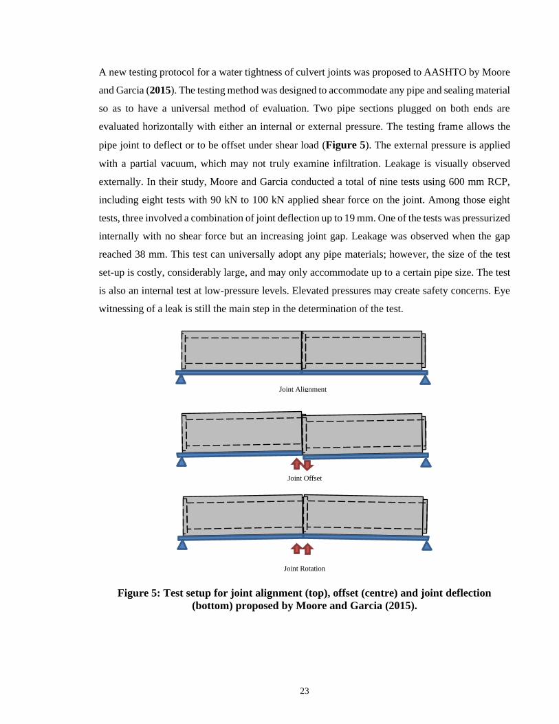
23

A new testing protocol for a water tightness of culvert joints was proposed to AASHTO by Moore

and Garcia (2015). The testing method was designed to accommodate any pipe and sealing material

so as to have a universal method of evaluation. Two pipe sections plugged on both ends are

evaluated horizontally with either an internal or external pressure. The testing frame allows the

pipe joint to deflect or to be offset under shear load (Figure 5). The external pressure is applied

with a partial vacuum, which may not truly examine infiltration. Leakage is visually observed

externally. In their study, Moore and Garcia conducted a total of nine tests using 600 mm RCP,

including eight tests with 90 kN to 100 kN applied shear force on the joint. Among those eight

tests, three involved a combination of joint deflection up to 19 mm. One of the tests was pressurized

internally with no shear force but an increasing joint gap. Leakage was observed when the gap

reached 38 mm. This test can universally adopt any pipe materials; however, the size of the test

set-up is costly, considerably large, and may only accommodate up to a certain pipe size. The test

is also an internal test at low-pressure levels. Elevated pressures may create safety concerns. Eye

witnessing of a leak is still the main step in the determination of the test.

Figure 5: Test setup for joint alignment (top), offset (centre) and joint deflection

(bottom) proposed by Moore and Garcia (2015).

Joint Alignment

Joint Offset

Joint Rotation

24

A novel RCP joint infiltration test was developed and reported in this thesis based on a vertical

setup of two pipe sample sections (spigot and bell). This simple test can easily be performed by

RCP manufacturers in their production facilities. The detailed test setup and procedure will be

described in Chapter 3. Table 8 compares the tests reported by Wong and Nehdi (2018), Moore

and Garcia (2015), Fenner (1990) and the conventional CSA A257 exfiltration test.

2.7 Summary

In summary, this chapter provides a background understanding of RCP joints, industry

standards related to hydrostatic performance, and the divide between existing standards and

the water-tightness requirements set by the end-users. It concludes that:

1. The standard tests do not effectively evaluate the external pressure induced by

groundwater through infiltration.

2. The standard tests do not meet the owner’s watertight requirement against infiltration.

3. Infiltration is currently a major issue faced by most of the municipalities.

4. An effective, reliable and robust RCP standard infiltration testing method is yet to be

developed, standardized and adopted by RCP manufacturers.

5. No literature was found that reports the hydrostatic performance of the RCP joint

against infiltration.

In order to preserve RCP products as a major drainage material, further research is needed to

mitigate the weaknesses of the RCP joint performance against infiltration. It is important to

develop a simple, user-friendly and reliable test for the industry to adopt.

25

Tab

le 8

: C

om

pari

son

bet

ween

In

filt

rati

on

Tes

t an

d C

on

ven

tion

al

Hyd

rost

ati

c T

est

Fa

nn

er (

19

90)

Infi

ltra

tio

n a

nd

exfi

ltra

tio

n

of

Pip

e Jo

int

30

0 m

m c

lay

pip

e

Ho

rizo

nta

l st

raig

ht

Ho

rizo

nta

l d

efle

cted

Cir

cum

fere

nti

al c

oll

ar

aro

und

th

e jo

int

50

Mea

sure

men

t o

f le

ak r

ate

No

t re

po

rted

Bas

ed o

n t

wo

pip

es

ho

rizo

nta

lly

po

siti

on

ed

Fu

ll p

ipe

Sp

ecia

l d

esig

ned

rub

ber

slee

ve

and

rig

id G

RP

tu

be

setu

p

CS

A A

25

7.2

(20

14)

Qu

alit

y c

on

tro

l o

f R

CP

join

t fo

r ex

filt

rati

on

in t

he

fact

ory

30

0 m

m t

o 1

20

0 m

m

(3)

2.4

m f

ull

-len

gth

pip

e

Ho

rizo

nta

l st

raig

ht

Ho

rizo

nta

l d

efle

cted

Ho

rizo

nta

l o

ffse

t

Inte

rnal

vo

lum

e o

f p

ipes

10

5

Pas

s o

r fa

il o

f ta

rget

pre

ssu

re

10

min

ute

s

Bas

ed o

n t

hre

e p

ipes

ho

rizo

nta

lly

po

siti

on

ed

Fu

ll p

ipe

Min

imu

m 1

-ho

ur

fill

ing

dep

end

s on

pip

e si

ze

Mo

ore

an

d G

arc

ia (

20

15)

Sta

nd

ard

ized

tes

t fo

r in

filt

rati

on

an

d

exfi

ltra

tio

n f

or

all

pip

e m

ater

ials

60

0 m

m d

iam

eter

(2)

2.4

4 m

lo

ng

Ho

rizo

nta

l st

raig

ht

Ho

rizo

nta

l d

efle

cted

Inte

rnal

vo

lum

e o

f p

ipes

55

Ob

serv

atio

n o

f le

akag

e

Up

to

96

ho

urs

Bas

ed o

n t

wo

pip

es h

ori

zon

tall

y

po

siti

on

ed

Fu

ll p

ipe

Min

imu

m 1

-ho

ur

fill

ing

dep

end

s o

n

pip

e si

ze

Wo

ng

an

d N

ehd

i (2

01

8,

20

20

)

Ev

alu

atio

n o

f jo

int

hy

dro

stat

ic

per

form

ance

fo

r in

filt

rati

on

60

0 m

m t

o 1

20

0 m

m d

iam

eter

RC

P

0.4

5 m

lo

ng p

ipe

spig

ot

end

0.4

5 m

lo

ng p

ipe

bel

l en

d

Ver

tica

l al

ign

ed

Ver

tica

l g

app

ed

Ver

tica

l o

ffse

t an

d g

app

ed

An

nu

lar

spac

e an

d v

olu

me

of

cyli

nd

er

68

5

Ult

imat

e p

ress

ure

, w

ork

ing

pre

ssu

re (

80

%),

gas

ket

mov

emen

t

Ult

imat

e (3

0 –

45

min

s)

Op

erat

ing

(2

0 h

ou

rs)

Bas

ed o

n c

ross

-sec

tio

n o

f th

e p

ipe

Cu

t p

ipe

sam

ple

s

Les

s th

an 1

0 m

in f

illi

ng

Ref

eren

ce

Sco

pe

of

the

test

Sa

mp

les

Ori

.

Am

ou

nt

of

wa

ter

Ma

x.

Ta

rget

(k

Pa

)

Res

ult

s

Du

rati

on

of

test

(ex

clu

din

g s

etu

p)

Tes

tin

g f

oo

tpri

nt

Pre

pa

rati

on

26

2.8 References

American Association of State Highway and Transportation Officials (AASHTO), “LRFD

Bridge Design Specification”, Washington, D.C., USA, 2014.

American Association of State Highway and Transportation Officials (AASHTO), “Pipe

Joint Selection for Highway Culvert and Storm Drains”, Washington D.C., USA,

2009, pp. 63-09.

ASCE 15, “Standard Practice for Direct Design of Buried Precast Concrete Pipe Using

Standard Installation”, American Society of Civil Engineers, Reston, VA, USA, 1993,

48 p.

ASTM C1103-14, “Standard Practice for Joint Acceptance Testing of Installed Precast

Concrete Pipe Sewer Lines” ASTM International, West Conshohocken, PA, USA, 2

p.

ASTM C1214-13, “Standard Test Method for Concrete Pipe Sewerlines by Negative Air

Pressure (Vacuum) Test Method”, ASTM International, West Conshohocken, PA,

USA, 4 p.

ASTM C1628-17 “Standard Specification for Joints for Concrete Gravity Flow Sewer Pipe,

Using Rubber Gaskets”, ASTM International, West Conshohocken, PA, USA, 2017,

7 p.

ASTM C1765-13, “Standard Specification for Steel Fiber Reinforced Concrete Culvert,

Storm Drain, and Sewer Pipe”, ASTM International, West Conshohocken, PA, USA,

2013, 6 p.

ASTM C1818-15, “Standard Specification for Synthetic Fiber Reinforced Concrete Culvert,

Storm Drain, and Sewer Pipe” ASTM International, West Conshohocken, PA, USA,

2015, 8 p.

ASTM C1840-17, “Standard Practice for Inspection and Acceptance of Installed Reinforced

Concrete Culvert, Storm Drain, and Storm Sewer Pipe” ASTM International, West

Conshohocken, PA, USA, 2017, 9 p.

ASTM C361M-14, “Standard Specification for Reinforced Concrete Low-Head Pressure

Pipe”, ASTM International, West Conshohocken, PA, USA, 26 p.

ASTM C443-12, “Standard Specification for Joints for Concrete Pipe and Manholes, Using

Rubber Gasket” ASTM International, West Conshohocken, PA, USA, 2012, 3 p.

ASTM C497-19, Standard Testing Methods for Concrete Pipe, Concrete Box Sections, or

Tile; ASTM C497, ASTM International: West Conshohocken, PA, USA, 17 p.

ASTM C969-17, “Standard Practice for Infiltration and Exfiltration Acceptance Testing of

Installed Precast Concrete Pipe Sewer Lines” ASTM International: West

Conshohocken, PA, USA, 2017, 3 p.

AS/NZS 4058, “Precast Concrete Pipes (Pressure and Non-Pressure)”, Australian Standard:

Environmental Health Directorate, East Perth, Australia, 2007, 65 p.

AWWA C302, “Reinforced Concrete Pressure Pipe, Non-cylinder Type, American Water

Works Association, Denver, CO, USA, 2016, 40 p.

27

Bielefeldt, Gutierrez-Padilla, Ovtchinnikov, Silverstein, Hernandez. Backterial, “Kinetics of

Sulfur Oxidizing Bacteria and Their Biodeterioration Rates of Concrete Sewer Pipe

Samples”, Journal of Environmental Engineering, Vol. 136 Issue 7, 2017.

BS EN 1916:2002, “Concrete Pipes and Fittings, Unreinforced, Steel Fibre and Reinforced”,

British Standards Institution (BSI), London, UK, 2002, 94 p.

Buco, J., Emeriault, F., Kastner, R., “Full-Scale Experimental Determination of Concrete

Pipe Joint Behavior and Its Modeling”, Journal of Infrastructure Systems, Vol .14,

Issue 3, 2008, pp. 230-240.

CBC News, “2011 video shows 'very serious' storm sewer damage”, Canadian Broadcasting

Corporation, Toronto, Ontario: https://www.cbc.ca/news/canada/ottawa/2011-video-

shows-very-serious-storm-sewer-damage-1.1139040, Assessed, Feb 10, 2020, 2012.

City of Surrey, “Design Criteria Manual”, Engineering Department., British Columbia,

Canada, 2016, 193 p.

Collection Systems Committee, “Sanitary Sewer Rehabilitation Fact Sheet”, Water

Environment Federation: Alexandria, VA: https://www.wef.org/globalassets/assets-

wef/direct-download-library/public/03---resources/wsec-2017-fs-009---csc---sewer-

rehabilitation---final---9.27.17.pdf. Assessed, Feb 10, 2020, 2017.

CSA A257, “Standards for Concrete Pipe and Manhole Sections”, CSA Group, Mississauga,

ON, Canada, 2019, 40 p.

CSA S6, “Canadian Highway Bridge Design Code”, CSA Group: Mississauga, ON, Canada,

2014, 894 p.

Curran, S.D. “Fiberglass Pipe Past, Present and Future”, Fiber Glass Tank and Pipe Institute:

Houston, TX, USA, 2013, p 5.

Fenner, R. A. “Excluding Groundwater Infiltration into New Sewers”, Water and

Environment Journal, Vol. 4, Issue 6, 1990, pp. 544-551.

GB/T 16752, “Test Methods of Concrete and Reinforced Concrete Drainage and Sewer

Pipe”, China, 2006.

Heger, F. “Structural Behaviour of Circular Reinforced Concrete Pipe – Development of

Theory”, Journal of the American concrete Institute, 1963, p 48.

Heger, F.; Gillespie, “J. Design of Circular Concrete Pipe Reinforced with Welded Deformed

Wire Fabric”, Transportation Research Board: 1967, p 34.

Lester, H.G. “Corrugated Polyethylene Pipe Design Manual & Installation Guide”, Plastic

Pipe Institute: Irving, TX, USA, 2017.

Marston, A.; Anderson, A.O. “The Theory of Loads on Pipes in Ditches and Test of Cement

and Clay Drain Tile and Sewer Pipe”, Iowa State College of Agriculture and

Mechanic Arts: Ames, IA, USA, 1913.

Ministry of Transportation Ontario. “MTO Gravity Pipe Design Guideline”; Ministry of

Transportation Ontario: St. Catharines, ON, Canada, 2014, p 233.

Mohamed, N.; Soliman, A.M.; Nehdi, M.L. “Utilization of steel fibres in precast concrete

pipes”, In Proceedings of TAC 2012, Tunnel and Underground Space: Sustainability

and Innovations, Montreal, Canada, 2012-10-17 (TAC Paper 158), 2012.

28

Mohamed, N.; Soliman, A.M.; Nehdi, M.L. “Full-scale pipes using dry-cast steel fibre-

reinforced concrete”, Construction Building Materials, 2012, 72, pp. 411–422.

Mohamed, N.; Soliman, A.M.; Nehdi, M.L. “Mechanical performance of full-scale precast

steel fibre-reinforced concrete pipes”, Engineering Structures, 2012, 84, pp. 287–299.

Mohamed, N.; Nehdi, M.L. “Rational finite element assisted design of precast steel fibre-

reinforced concrete pipes”, Engineering Structures, 2012, 124, pp. 196–206.

Moore and Garcia “Test Methods for Watertightness of Culvert Joints”, National

Cooperative Highway Research Program Project 20-07, Task 347. Transportation

Research Board: USA, 2015.

Moore, I., Sezen, H., Sheldon, T. “Structural Design of Culvert Joint”, NCHRP

Transportation Research Board of the National Academies, Web-only Document 190,

http://www.trb.org/Publications/Blurbs/167506.aspx, 2012, 388 p.

Norton Engineering Inc, “Unacceptable Inflow and Infiltration in New Subdivisions Phase 1

Final Report. Phase 1 Final Report, 59 p., available at:

http://web.archive.org/web/20190403210735/https://www.nortonengineeringinc.ca/I

&I%20in%20NS%20Final%20Report%202017_Oct%2016%202017.pdf, 2017.

OCPA, “Concrete Pipe Design Manual”, Ontario Concrete Pipe Association, Kitchener, ON,

Canada, nd.,145 p.

OPSS 410 “Construction Specification for Pipe Sewer Installation in Open Cut”, Ontario

Municipal Provincial Standards, 2012.

Orlander, H.C. “Stress Analysis of Concrete Pipe”, Engineering Monograph No. 6; US

Bureau of Reclamation, Washington, DC, USA, 1950.

Parker, C.D. “The Corrosion of Concrete”, The Sewage Branch of the Melbourne and

Metropolitan Board of Works, Aust. J. Exp. Biol. Med. Sci. 1945, 23, pp 81–90.

Pipeline “Infiltration and Inflow Can be Costly for Communities”, National Environmental

Service Center, Vol. 10, Issue No. 2, 1999, 8 p.

Population Reference Bureau “2013 World Population Data Sheet”, Population Reference

Bureau: Washington, DC, USA, 2013.

Pratt, C.; Yang, H. “Hodkiewicz, M. Factors Influencing Pipe Failures in the West Australia

Environment”, CEED Proceeding: 2011.

Region of Peel Standard Drawing 2-5-2, “New Sanitary Sewer Construction, Typical Precast

Circular Maintenance Hole Details (1200 mm – 3000 mm)”, Region of Peel Public

Works Standard Drawing, Brampton, Ontario, Canada, 2019.

Rinker Materials, “Corrugated Steel Pipe”, Info Series, Rinker Materials, 1994.

Robinson, B, Sandink, D, Lapp, D. “Reducing the Risk of Inflow and Infiltration (I/I) in New

Sewer Construction”, Institute for Catastrophic Loss Reduction: Toronto, Ont.,

Canada, No. 64, Nov. 2019, 72p.

Schladweiler, J.C. “The History of Sanitary Sewer”. 2017. Available online:

http://www.sewerhistory.org/ (accessed on June 14, 2018).

29

Singh, A. and Adachi, S. “Bathtub curves and pipe prioritization based on failure rate”, Built

Environment Project and Asset Management, Vol. 3 (1), 2013, pp.105-122.

Spangler, M. “Soil Engineering”; International Textbook Company: Scranton, PA, USA,

1960.

Sulikowski, J.; Kozubal, J. “The Durability of a Concrete Sewer Pipeline Under

Deterioration by Sulphate and Chloride Corrosion”, Procedia Eng. 2016, 153, pp

698–705.

Walker, R. “The Early History of PVC Pipe”, thePlumber.com,

https://theplumber.com/early-history-of-pvc-pipe/, assessed on Feb 20, 2020, 1990.

Wong, L. and Nehdi, M.L, “Critical Analysis of Precast Concrete Pipe Standards”,

Infrastructures, 3(3), 18, 2018, 18p.

Wong, L. and Nehdi, M.L. “New Test Method for RCP Joint Hydrostatic Infiltration”, CSCE

Conference 2018, Fredericton, New Brunswick, Canada, 2018.

Wu, L.; Hu, C.; Liu, W. “The sustainability of Concrete in Sewer Tunnel—A Narrative

Review of Acid Corrosion in the City of Edmonton Canada”, Sustainability 2018,

2018, 10, pp 517.

Vollertsen, J.; Nielsen, A.H.; Jensen, H.S.; Rudelle, E.A.; Hvitved-Jacobsen, T. “Modeling

the Corrosion of Concrete Sewer”, In Proceedings of the 12th International

Conference on Urban Drainage, Porto Alegre, Brazil, 11–16 September 2011.

York Region “Sanitary Sewer System Inspection, Testing and Acceptance Guideline”,

Section 2.4: Ontario, Canada, 2011.

30

CHAPTER 3

3 Experimental Development

This chapter provides details of the experimental developments, including the concept of the

tests, the experimental apparatus, and the testing setup. Two testing procedures, for ultimate

and operating joint capacities, and the results classifications are also detailed in this chapter.

Later in the chapter, the selection of the pipe samples and gasket samples are provided.

Substantial parts of this chapter have been published in Wong and Nehdi (2018).

3.1 Testing Concept

The tests developed in this study were to provide easy setup, safe operation and quantitative

measurements of RCP joint leakage, to quantify the RCP short-term ultimate pressure and to

evaluate its long-term performance during operation. Figure 6 shows the unique vertical setup

with a section of the bell and spigot of a pipe that provides ease of access to the inside face of

the pipe sample. Figure 7, an enlarged cut face of the test joint illustration, shows a small

annular space between the primary and secondary gaskets to be pressurized. The pressure is

created using compressed air to push the water into the annular space through a small inlet

tube. The hydrostatic pressure variation inside the annular space is constant in the vertical setup

because the joint gap is on the horizontal plane. Conversely, in the horizontal setup described

in ASTM C497 (2019), the pressure varies inside the annular space due to the elevation

differential. The primary gasket is used to seal the RCP after the pipe is placed in service. The

purpose of the secondary gasket is to force failure in the primary gasket during the test;

therefore, those gaskets are carefully selected based on the joint detail of the test RCP.

Suppliers are consulted for the adequate gasket based on the target testing pressure, material

31

properties, and available space. Small inlet and outlet holes are drilled at 180 degrees through

the pipe and in between the primary and secondary gaskets. Plastic tubes are sealed with epoxy

before conducting the test to allow water to be introduced into the space. To ensure a safe

testing process, the equipment was designed to handle a maximum pressure of 685 kPa,

equivalent to 68.5-m of hydraulic head. Unlike traditional hydrostatic tests, only a very small

amount of water is used in the confined annular space and the testing system. Hence, the filling

time is much shorter during the setup. In addition, the new test has no flooding hazard of the

testing area when a failure occurs because the maximum amount of water that is possible to

leak out is in the water supply connecting cylinder. The operator is expected to monitor and

quantify leakage during the test in addition to visual inspection.

Figure 6: Test Setup.

32

Figure 7: RCP Joint Test Detail.

3.2 Mechanical Apparatus

The mechanical apparatus shown in Figure 8 is used to control the compressed air pressure

introduced into the annular space of the RCP joint. The pressurization scheme is shown in

Figure 9. The apparatus includes an air inlet valve, pressure regulator, pressure gauge, water

supply connecting cylinder (WSCC), connecting hoses, and a water outlet valve. The pressure

regulator allows the operator to control the incoming pressure and maintain the required target

testing pressure, which is displayed in the pressure gauge. The WSCC made of a 4-inch

diameter semi-transparent fibreglass pressure cylindrical chamber contains enough water at

the time of the test to supply the water demand in the annular space. The cylinder allows the

water loss during the test to be monitored and measured if a system leakage and/or joint leakage

occur. The water outlet valve is used to introduce water to the system during the setup process.

When filling the annular space using the inlet valve, the space is considered filled when water

escapes from the outlet valve. The outlet valve is then kept closed during the entire test. The

design of the apparatus is included in Appendix A.

Pipe Bell

Pipe Spigot

Pressurized zone

Primary gasket

space

Secondary gasket

Spacer ring (optional)

Pressure

Inlet or

Outlet

Joint gap

INS

IDE

OU

TS

IDE

33

Figure 8: Pressurization Apparatus.

Water

Supply

Connecting

Cylinder

Pressure

Gauge

Regulator

Valve

Air-in

Water-out

34

Figure 9: Pressurization Mechanical System Scheme.

3.3 Testing Setup

Two pipe sections consisting of a bell end and spigot end, as shown in Figure 10, are aligned

and stacked vertically (Figure 6). These sections are saw-cut from the same random pipe

sample. The total height of the combined pipe sections is between 700 and 1000 mm for ease

of assessment and monitoring of the interior pipe face during the test. Figure 11 shows the

interior of the test assembly setup. Shorter test pipe sections allow the operator to safely

monitor the inside of the pipe during the test. The test joint is created by carefully joining two

pipe sections sealed with a primary gasket and a secondary gasket. The primary gasket is seated

in its design location, and the secondary gasket is placed between the shoulder of the pipe

spigot, and the bell end face to create the confined space for pressurization. When a larger gap

is required, a plastic spacer ring is sandwiched in between the pipe samples below the annular

space. Both joined pipe sections are strapped down to the supporting steel base frame to create

restraint from separation during the test. Due to the internal pressure generated, a large uplift

force is expected. The number of tie-down straps and the strap rating are calculated based on

the target testing pressure and the geometry of the annular space. The base frame is specially

designed to carry the expected forces from the strap. In comparison to the field condition, the

35

restraints of the pipe joints are generated by groundwater pressure all around and in between

the joint and any adjacent joints.

Before the start of the test, water is introduced from the outlet of the system to the inlet and

fills up the WSCC. This process is to ensure that the entire annular space is filled with water,

and all air is expelled. It is suggested to pressurize the setup to a minimum of 50 kPa to detect

any leaks associated with the setup before the formal start of the test. The frame used in this

research was designed for a maximum pipe size of 1829 mm outer diameter tested up to 685

kPa. However, the size of the frame does not limit the pipe size as it can be expanded to

accommodate a larger pipe.

Figure 10: Test Pipe Section (left) Bell End (right) Spigot End.

Figure 11: Interior of Test Pipe Section.

36

3.4 Setup with Joint Gaps

In the conventional test, the pipe alignment is deflected to examine the opened joint's hydrostatic

performance. The deflected alignment is difficult to achieve because it creates a non-uniform

annular space for the secondary gasket to work. Producing a non-uniform gasket is not cost-

effective. In order to examine the joint with open gaps under the infiltration condition, a plastic

spacer ring is introduced in between the joint. The purpose of this additional ring spacer is to

increase the annular space and provide a larger area for the gasket to move during the test. This

simulates the joint gap described in the earlier section of this Chapter. Following the same testing

procedure, different thicknesses of rings from 6 mm to 13 mm are used in the study to monitor the

effect on the hydrostatic performance with respect to the joint gap. Figure 12(a) shows a white

plastic spacer ring below the secondary gasket that is sandwiched between the pipe samples in the

joint. Figure 12(b) shows the placement of the spacer ring during the test setup.

Figure 12: (a) A spacer ring is placed in between the pipe sample to create the desired

joint gap. (b) The gap spacer ring is placed below the secondary gasket to open the gap

of the pipe joint.

Plastic spacer ring

37

3.5 Setup with Joint Offset

RCP joints can be offset by external factors such as the differential settlement of bedding materials,

differential loads from the backfill or other construction loads. When the joint is offset, the annular

space is reduced on one side and increased on the opposite side. This leads to a reduction in

hydrostatic performance on the side, having increased joint gap. The joint detail used in this

research allows the joint to be offset by 3 mm. To simulate the joint offset, a lateral load is applied

using a hydraulic jack on the upper test section with two reaction back supports on the lower test

section. Figure 13 illustrates the test setup for offset joints. To provide a safe operating condition

and maintain the offset during the test, a jacking post with a hydraulic pump is mounted on the

base frame in addition to the typical setup described earlier. Two back support posts are mounted

on the opposite side at about 30 degrees apart. The pump is then connected to a jacking device.

Before offsetting the joint, the distance between the pump and the post is measured as a reference.

Figure 14 shows the complete test setup with joint offset and the measurement of the offset joint.

Figure 13: Illustration for offset joint.

Applied

load

Back

supports

Minimum

Annular

Space

Maximum

Annular

Space

38

Fig

ure

14:

Hyd

rost

ati

c te

st s

etu

p f

or

infi

ltra

tio

n w

ith

join

t off

set.

Jack

ing

Po

st

Bac

k s

up

po

rt(s

)

Jack

ing

Dev

ice

Bas

e F

ram

e

Tie

Do

wn

Str

aps

Wat

er S

up

ply

Co

nn

ecti

ng

Cy

lin

der

Pip

e S

amp

les

Pre

ssu

re G

aug

e an

d

Val

ves

39

3.6 Testing Procedure

3.6.1 Measurements

During the test, the following parameters are monitored and recorded: pressure, time, water

level in the WSCC, and joint gap movement. The testing pressure is measured in kilopascal

(kPa) at a minimum of 25 kPa intervals. Time measurements are conducted using a digital

stopwatch displayed near the pressure gauge. The water level in the WSCC with respect to the

starting point is measured in millimetres at each pressure interval using callipers. The change

in water level is recorded and converted to litres based on the calculation of cylinder volumetric

change, which indicates the loss of water in the WSCC, as discussed below. Joint gap and its

movement are critical in the joint hydrostatic performance; therefore, the initial joint gap and

its change are measured in millimetres using a ruler at a minimum of two points around the

pipe. The change of the joint gap during the pressure test should be minimal.

3.6.2 Ultimate Capacity

The first target of the test is determining a short-term ultimate hydrostatic capacity of the RCP

joint, which is when the joint can no longer hold the test pressure for 10 minutes. The test

begins with a selected starting pressure based on the CSA A257 requirement of 105 kPa, the

recommendation of the gasket supplier, or previous test experience, whichever is greater. As

more test results are collected, higher starting pressure can be selected to reduce the duration

of the test. The pressure is then gradually increased at intervals of 25 kPa or 50 kPa and held

for a minimum of 10 minutes at each increment, followed by visual inspection for leaks. The

measurement of the water level in the WSCC is also recorded. The duration of 10 minutes is

selected based on similar evaluations from most hydrostatic standard tests. Any leakage

observed at the inside of the pipe joint is considered a failure. The ultimate capacity is rated at

the previous pressure level. All other leakage observed, such as outside the joint, inlet and/or

outlet pipes or other locations, will not be considered as failure. If those leakages can be

controlled and do not impact the test, the test can be continued. Adjustment of the straps can

40

also be made to mitigate exterior leakage during the test. The time for each incremental attempt

is recorded by the operator using a stopwatch. Figure 15 (a) and (b) show two typical failures

of primary gaskets. A test using 600 mm RCP failed at 250 kPa when water seeped down the

inner face of the joint. A test using 900 mm RCP failed at 475 kPa when water suddenly shot

out.

(a) 600 mm RCP, 250 kPa,

(b) 900 mm RCP, 475 kPa.

Figure 15 Moment of Failure.

41

3.6.3 Operating Capacity

The hydrostatic performance of the RCP joint is affected by the exposure to sustained

groundwater pressure. Hence, to evaluate the RCP operating capacity, the annular space is

subjected to sustained pressure for a minimum of 20 hours to allow the gasket and joint to be

stabilized. The target operating pressure is set to 80% of the ultimate capacity; therefore, the

test is usually completed after the ultimate capacity is determined. A new set of gaskets from

the same lot are used in this test to avoid damage caused during the previous establishment of

the ultimate pressure. It is recommended to begin the test by holding the pressure at 100 kPa,

followed by 10 minutes at 70% of the ultimate pressure. This is to ensure that the test setup is

performing as expected. If no leakage is observed, the pressure is then held at 80% of the

ultimate capacity for the next 20 hours. Visual examination for leakage shall be made within

10 minutes after reaching the 80% mark, followed by periodic inspection at 4-hour intervals.

The water level in the WSCC versus time shall be recorded at each inspection. After 20 hours,

full inspection for leakage is conducted, and the water level in the final WSCC is recorded. If

no leak is observed from the inside of the pipe, the test is successful, and the operating capacity

of the pipe joint is determined at 80% of the ultimate capacity.

3.7 Test Results for Condition Classification

More than 100 tests were conducted. For both the ultimate and operating performance

conditions, the result of the test has four unique success conditions, as outlined in Table 9. The

summary of the infiltration test count is provided in Table 10. For the ultimate capacity, a

successful test terminated based on the failure of the primary gasket with minor or no external

leak is categorized into Condition 1. The test is considered as Condition 2 when an external

leak is observed during the test without a complete failure of the secondary gasket. In this case,

the ultimate capacity of the primary gasket is considered when an interior leak occurs. The test

is considered as Condition 3 when the secondary gasket is unable to hold the pressure in the

annular space during the test. Here, the ultimate capacity of the primary gasket is not reached.

For the operating capacity, Condition 1 considers a successful test with minor or no external

leak, and the target duration is reached or exceeded. Condition 2 considers that external leak

42

is observed, the target pressure is maintained, and the target duration is reached. The test is

considered as Condition 3 when the target duration is not reached due to external leak or other

types of leakage. The test is considered unsuccessful, i.e. Condition 4, when the setup was

unable to hold any pressure, or major leakage occurs at the early stage of the test setup. The

tests categorized as Condition 4 are not included in this Chapter.

Table 9: Infiltration Test Result Conditions

Condition Description

Ultimate Test

1 • No significant external leak was observed during the test. A minor external leak

can be eliminated by adjusting the tension of the straps.

• The test is terminated based on the leakage or failure of the testing gasket.

• The ultimate capacity of the test gasket is determined based on the failure of

testing gasket or equipment capacity.

2 • The external leak is substantial during the test, but the water tank is not fully

drained at the end of the test. The test is terminated based on the leakage or failure

of the testing gasket.

• The Target pressure level can be maintained during the test.

• The test is terminated based on the leakage or failure of the testing gasket.

• The ultimate capacity of the testing gasket is determined based on the failure of

testing gasket or equipment capacity.

3 • External leak substantial during the test.

• The test is terminated based on the leakage or failure of the secondary gasket.

• The ultimate capacity of the test gasket is determined based on the pressure level

prior to the termination of the test.

4 • The test is not completed due to the setup issue.

• No pressure data is collected.

Operating Test

1 Target pressure and duration are both reached with no external leak. A minor

external leak, when observed during the test, is corrected.

2 Target pressure and duration are reached despite the external leak.

3 The test is terminated before the target duration is reached due to an external leak

or testing gasket failure.

Table 10: Infiltration Test Count Summary

43

Results Ultimate Operating Grand Total

Condition 1 38 30 68

Condition 2 19 12 31

Condition 3 13 2 15

Grand Total 68 44 114

3.8 Sample Selection

3.8.1 Pipe

In the initial phase of developing this test method, conventional RCP sizes of 600 mm, 900

mm and 1200 mm in diameter were selected. These three sizes were selected for this research

partly because the cost of repair is relatively higher than that for the larger size pipes due to

the restriction of operator entry, and partly because they are easier to handle compared to a

larger size. In addition, the industry claims that these sizes have a higher competition from

other emergent pipe materials. The pipe samples were made by the sponsor plant in Oakville,

Ontario, Canada in compliance with CSA A257.2 using a vibration and pressing process, with

a conventional dry cast concrete mixture that exceeded a compressive strength of 40 MPa at

28 days and reinforced with a spiral cold drawn wire cage(s). The joint was comprised of a

single offset spigot end jointing into a groove bell end, as shown in Figure 10. A detail of the

joint cross-section is shown in Figure 16, and the geometry is listed in Table 11.

Table 11: Pipe Joint Geometry

Size 600 900 1200

ID 610 914 1219

S mm 8.3 8.3 7.6

T mm 3.2 3.2 3.7

jS mm 48.8 48.8 63.5

jT mm 49.6 49.6 44.5

J mm 98.4 98.4 108

f mm 61.5 61.5 53

As Annular Space mm2 564 564 882

Spigot Diameter

ID + 2f

mm 733 1037 1325

Spigot Circumference mm 2303 3258 4163

44

Figure 16: RCP Joint Profile and Annular Space

3.8.2 Gasket

The various models of primary gaskets tested are commonly used by the industry and were

pre-lubricated and made of synthetic rubber, meeting requirements of ASTM C443, ASTM

C425, ASTM C1619, and CSA A257. The secondary gaskets having profiles recommended

by industry suppliers were used to provide sealing to contain the annular space for

pressurization. The purpose of the study was to develop and validate the new test method and

not to compare the performance of commercial gasket brands. Therefore, the actual gasket

brands in Table 12 were not disclosed and are rather represented by a prefix letter “T” for

primary testing gasket and “S” for the secondary gasket. For those primary testing gaskets, the

mass and the unstretched cut length were measured prior to the test. When installing the gasket

on to the pipe spigot, the gasket is stretched from its original cut length because the

circumference of the pipe spigot is larger than the unstretched cut length. The increase in the

stretched length varies between 10 % and 16%. The average stretched unit mass is calculated

S T

BELL

SPIGOT

J

jS jT

f

ID

45

by dividing the average mass measured by the spigot circumference or stretched length. The

influence ratio, Ig, is defined in Eq. 1 as the ratio of the mass of the gasket to the effective

annular space that confines the gasket, which provides an important explanation of the ultimate

capacity of the gasket against the infiltration pressure. The effective annular space is shaded in

Figure 16. In the case of the single offset joint of the test pipe, the annular space, As, is

estimated using Eq. 2.

Eq. 1 𝑰𝒈 =average gasket mass (g)

effective annular space (mm2)

Eq. 2 𝐴𝑠 = 𝑆 × 𝑗𝑆 + 𝑇 × 𝑗𝑇

Table 12: List of Gaskets Used in the Research

Profile

ID

Type Supplier Design

Capacity

Remark

S01 Wedge 1 Secondary

S03 Wedge 2 Secondary

S04 Wedge 2 Secondary

T02 Self-lubricated 135 1 105 Primary

T03 Self-lubricated 165 2 105 Primary

T04 Self-lubricated 185 2 105 Primary

T05 Double Tilting Gasket

with PP coupler

3 250 Primary

T06 Self-lubricated 135 2 105 Primary

T07 Self-lubricated 185 1 105 Primary

T08 Wedge Profiled 1 140 Primary

3.9 Summary

This chapter provides a detailed description of a novel infiltration testing method that RCP

manufacturers can easily set up and conduct in a factory setting. The test is much safer to

conduct owing to the much lower water consumption needed to achieve a much higher-

pressure target in comparison to conventional exfiltration tests. Although the pipe sizes and

gaskets were listed, larger pipe sizes and other types of gaskets can be easily accommodated

using the same setup and procedure. The test has been proven reliable based on the repeatability

of the results in this research.

46

3.10 References

ASTM C497 “Standard Testing Methods for Concrete Pipe, Concrete Box Sections, or Tile”,

ASTM International: West Conshohocken, PA, USA, 2019, 17 p.

ASTM C443-12, “Standard Specification for Joints for Concrete Pipe and Manholes, Using

Rubber Gasket” ASTM International, West Conshohocken, PA, USA, 2012, 3 p.

ASTM C425-04, “Standard Specification for Compression Joints for Vitrified Clay Pipe and

Fittings” ASTM International, West Conshohocken, PA, USA, 2004, 3 p.

ASTM C1619-19, “Standard Specification for Elastomeric Seals for Joining Concrete

Structures” ASTM International, West Conshohocken, PA, USA, 2019, 3 p.

CSA A257, “Standards for Concrete Pipe and Manhole Sections”, CSA Group, Mississauga,

ON, Canada, 2019, 40 p.

47

CHAPTER 4

4 Pipe Joint Design

This chapter discusses the properties of the rubber, the design of gaskets, and the properties of

the gasket specimens in greater detail. Theoretic calculation of sealing pressure based on the

load-deformation curve of the gasket sample is presented. The sealing potential based on the

calculation is subsequently used to compare the results obtained by the infiltration test.

4.1 Rubber Gasket

The hydrostatic capacity of RCP depends on the properties of rubber gaskets, a primary material

used in sealing RCP joints. Its mechanical properties, geometric dimensions, and the pipe joint

design also contribute to the sealing potential. Rubber maintains its volume under applied load by

deformation. The cross-section of the rubber increases when it is compressed and reduces when it

is stretched. The mechanical properties in compression can be derived using ASTM D575 (2001).

The ability to deform under applied load can be described in three phases: elastic, viscoelastic, and

viscous phase (Czernik 1996). Figure 17 illustrates the relationship between the applied load and

deformation due to the compression of a typical rubber. In the early stage of loading or elastic

response, the deformation of a rubber specimen due to compression forces increases linearly and

returns to its initial shape when the applied force is removed. When the applied load reaches the

viscoelastic response phase, the change in deformation diminishes at the same load increment. The

change in performance is time-dependent but is totally recoverable. However, if the load causes

the rubber to deform into the viscous response phase, the deformation is no longer recoverable. In

this Chapter, the rubber gasket samples were tested to the viscoelastic phase assuming that the

rubber gasket is intended not to exceed the viscoelastic properties in its service life.

48

Figure 17: Typical load-deformation curve for rubber gasket (After Czernik, 1996).

Rubber also relaxes under load over time, incurring stress relaxation or creep. The load-

deformation curve is empirically developed by measuring the actual deformation of the gasket

sample in accordance with ASTM D575 (2001). Figure 18 displays a typical test conducted

by gasket manufacturers to determine the load-deformation curve. The curve describes the

material behaviour for a specific rubber compound and gasket design. However, the surface

boundary and the actual media of the pressure are ignored in the test. The load-deformation

behaviour of rubber also depends on the durometer, hardness of the material, in accordance

with ASTM D2240 (2015). These properties also impact the sealing potential of the gasket.

d, Deformation (mm) 0 0

P,

Lo

ad (

kN

) o

r

, S

tres

s (k

Pa)

49

Figure 18: Gasket deformation test.

4.2 Joint Design

In addition to the aforesaid material mechanical properties, the sealing potential of a rubber gasket

also depends on its cross-sectional geometry. The face of the gasket in contact with the applied

hydrostatic pressure determines the amount of frictional force required to keep the gasket in

equilibrium. Figure 19 illustrates that the orientation of the gasket dictates the amount of contact

area; and thus, affects the amount of frictional resistance provided.

Gasket

Applied Force

50

Figure 19: Illustration of gasket geometry withstands internal pressure.

The amount of stretch at the time of loading and the ratio of the cross-sectional area to the confined

space also determines the sealing potential. The confined space, also known as annular space,

generates compression of the rubber, creating the sealing potential (ACPA, 2019). The joint design

defined in the plant certification published by the American Concrete Pipe Association (APCA)

provides a mathematical calculation for the minimum and maximum compression of two common

RCP joints for confined circular gaskets and single offset profiled gaskets. These values can be

used to calculate the maximum and minimum sealing potential based on the load-performance

curve of the rubber.

The joint design of the RCP in this experimental program is shown in Figure 20 (a) and Table

13. This design has been commonly used by the RCP industry to offer self-balancing ability during

pipe installation without manually equalizing the tension such as in traditional wedge or O-ring

gasket. The female end of the pipe, known as the bell, receives the male end, known as the spigot,

with a 2-degree taper in the wall of the slot. The spigot of the pipe has an offset, B, of 6.7 mm, 6.7

mm and 7.6 mm for 600 mm, 900 mm, and 1200 mm pipes, respectively. This offset creates two

sizes of annular space, S and T. The tapered face reduces the annular space, S, when the pipe is

being jointed together, inducing compression in the sealing material. This is a common design for

all concrete pipes. The tube section of the sample gasket is rolled into the annular space, denoted

“T,” for its final resting position. The joint design has a taper angle, , for an easier homing process

as illustrated in Figure 20. The effect of the taper angle on the sealing potential will be discussed

later. The 600 mm and 900 mm pipes share the same gasket profile, while the 1200 mm pipe sample

uses a different gasket profile due to its larger annular space.

applied

pressure

Sealing

pressure

Sealing

pressure

friction

friction

applied

pressure

Sealing

pressure

Sealing

pressure

friction

friction

51

(a) Ideal position by design

(b) With joint gap

Figure 20: RCP Single Offset Joint Detail.

Table 13: RCP Single Offset Joint Detail

Read this table in conjunction with Figure 20

Unit of Measure: millimetre

ASc – Circumference of annular space

Size 600 900 1200

jS 48.8 48.8 63.5

B 6.7 6.7 7.6

(°) 2 2 2

S 8.3 8.3 11.3

T 3.2 3.2 3.7

Ds 733 1037 1325

ASc 2303 3258 4163

jS

S

G

B

T

Ds

Bell

Spigot

jS

S’

G

T’

Bell

Spigot

52

4.3 Gasket Specimens

The gaskets used in this study are the self-lubricating, profiled type, that is designed for the single

offset joint described above. The typical cross-section of an unstretched gasket, illustrated in

Figure 21(a), consists of two sections: the deformation section and the rolling tube section. Figure

21(b) shows the stretched cross-section after the gasket is placed onto the pipe spigot. There was

a reduction in gasket height due to the increase in gasket length. The maximum stretch limit was

20% in addition to the unstretched length (ACPA, 2019). The stretched height can be calculated

using Eq. 3.

Eq. 3 𝑯𝒔 =𝑯𝒈

√𝒓𝒔

Where 𝐻𝑔: height of unstretched gasket; 𝐻𝑠: height of stretched gasket; 𝐻𝑐: Height of

compressed gasket; 𝑟𝑠: a ratio of stretched length to unstretched length.

Figure 21(c) shows the cross-section of the gasket after being compressed when two pipe sections

were jointed. The rolling tube section was lubricated inside by silicone during gasket

manufacturing to assist the jointing process of the concrete pipe. The rolling action during the

homing process self equalizes the gasket tension along the entire length. Thus, additional

equalization was not necessary compared to conventional profiled wedges or O-ring gaskets. The

gasket height in the compressed state was limited to the available annular space shown in Figure

21(c). The force required to compress the gasket from the stretched state into the compressed state

creates the sealing potential, which is discussed in the next section. Gasket samples were also

randomly selected in terms of dimension and weight. The number of samples, minimum, average

and maximum values listed in Table 14 exhibit a certain degree of variations. The unstretched

length and mass were plotted against each other, as shown in Figure 22(a)-(c), as well as the height

and base width in Figure 22(d)-(f). The scale of the x-axis and y-axis were maintained similarly

in the figures for ease of comparison. The degree of variation is believed to explain the variation

of sealing potential. This will be discussed further in the later section.

53

Table 14: Gasket Properties

Pipe Size 600 900 1200 600 900 1200

Gasket Ref ID T02 T02 T07 T06 T06 T03

Supplier3 A A A B B B

Spigot Dia. (mm) 733 1037 1325 733 1037 1325

Spigot Cirf.2, Ls (mm) 2303 3258 4163 2303 3258 4163

Annular Space, A (mm) 8.3 8.3 11.3 8.3 8.3 11.3

Max limit of Annular Space (mm) 1.1 A 9.13 9.13 12.43 9.13 9.13 12.43

Unstretched Length1, Lu

(mm)

Count 20 19 21 14 17 21

Min 2088 2957 3591 1994 2854 3678

Avg 2103 2971 3623 2030 2882 3707

Max 2119 2987 3674 2056 2930 3749

Max %

Stretch 10.3% 10.2% 15.9% 15.5% 14.1% 13.2%

Min %

Stretch 8.7% 9.1% 13.3% 12.0% 11.2% 11.0%

Mass1

(g)

Count 20 19 21 14 17 21

Min 566 764 1456 590 852 1366

Avg 577 805 1501 617 914 1442

Max 590 826 1537 636 949 1472

Var 24 63 81 46 97 106

Unit Mass

(g/m)

Count 20 19 21 14 17 21

Min 246 234 350 256 261 328

Avg 251 247 361 268 280 347

Max 256 254 369 276 291 354

Var 11 19 19 20 30 26

Unstretched Height, Hg*

(mm)

Count 7 6 17 3 11 16

Min 15.3 15.8 18.5 16.1 16.2 18.9

Avg 15.8 16.6 19.4 16.1 16.7 19.6

Max 16.0 17.3 20.3 16.3 17.4 20.5

Var 0.7 1.5 1.9 0.2 1.3 1.6

Base Width, W1

(mm)

Count 7 6 17 3 11 16

Min 17.1 17.2 21.0 16.8 16.5 18.9

Avg 17.3 17.5 21.9 17.1 16.8 20.1

Max 17.5 17.8 22.4 17.3 17.2 21.1

Stretched Height, Hs

(mm)

Min 14.6 15.1 17.2 14.9 15.2 17.8

Avg 15.2 15.9 18.1 15.1 15.7 18.5

Max 15.3 16.5 19.0 15.4 16.5 19.4

Var 0.7 1.4 1.7 0.5 1.3 1.6

%Min 4.4% 4.7% 6.6% 7.0% 5.8% 5.8%

%Max 4.3% 4.4% 6.6% 5.5% 5.2% 5.2%

Reduction in Gasket Height

or Compressed Height, Hc

(mm)

Hs-1.1S

Min 5.50 5.95 4.81 5.81 6.08 5.37

Avg 6.03 6.73 5.64 5.97 6.57 6.10

Max 6.21 7.39 6.53 6.27 7.38 6.95

% Min 37.6% 39.5% 27.9% 38.9% 40.0% 30.2%

% Max 40.5% 44.7% 34.4% 40.7% 44.7% 35.9% 1Value obtained by measurement; 2Also known as gasket stretched length; 3Durometer for Gasket A is 40D, and Gasket B is 45D

54

(a) Original unstretched shape

(b) Stretched shape

(c) Compressed shape

Figure 21: Typical cross-section of self-lubricated single offset gasket.

Hg

W

Deformation Section

Rolling Tube Section

Hg

W

Hs

Original Shape

Stretched Shape

Hg

W

S

Hc

Original Shape

Compressed Shape

55

(a) 600 mm RCP

(d) 600 mm RCP

(b) 900 mm RCP

(e) 900 mm RCP

(c) 1200 mm RCP

(f) 1200 mm RCP

Legend:

Figure 22: Gasket Geometric Properties.

56

4.4 Sealing Potential Calculation

The sealing potential was estimated based on the deformation properties of the rubber under

the load, i.e. load-deformation behaviour obtained from ASTM D575. The compensation was

made to account for the reduction in the cross-section area during the stretch, i.e. increase in

length when installing the gasket on the spigot of the pipe. In the final compressed condition

(Figure 20(c)), the reduction of the gasket height, Hc, was computed by subtracting the annual

space, S, from the stretched height, Hs. The required force, Pf, to compress the gasket to have

a reduction, Hc, can be empirically determined based on its load-deformation behaviour

obtained from the load-deformation curve using Eq. 4. 20% factor was applied to the force in

the load-deformation test to account for relaxation. In this study, when comparing to the short-

term ultimate test, the relaxation factor was omitted. The sealing pressure was computed by

dividing the applied force by the sample contact area.

Eq. 4 𝑷𝒇 =𝑷

(𝟏−𝟐𝟎%)

4.5 Sealing Pressure and Joint Gap

The sealing pressure is also impacted by the change in annular space due to the joint gap and the

geometrical variation of the gasket itself. The spigot of the pipe sample has 2% taper angle on the

conic surfaces of the bell and the outer surface of the spigot by design. This is typical as per ASTM

C443, which limits the angle to be 3.5% measured from the pipe axis. As shown in Figure 20 (b),

the 2% taper angle increases the annular space as the joint gap increases at the rate of the joint gap,

G, multiplying the tangent of the taper angle, (Eq. 5).

Eq. 5 ∆𝑺 = 𝑮. 𝒕𝒂𝒏

With 2% taper angle, the annular space increases by 0.87 mm when the joint gap increases to 25

mm. For 600mm and 900 mm pipe sample, the increase is 10.5%; and for 1200 mm pipe sample,

the annular space increases by 7.7%. This increase reduces the force required to compress the

gasket; hence, reduce the sealing pressure. For the gasket samples used in this study, the reductions

are ranged between 30% to 36% when the joint gap increases to 25 mm.

57

4.6 Sealing Pressure and Geometrical Variations

The sealing pressure is also impacted by the geometrical variation of the gasket itself. Figure 22

shows the mass of the gasket varies against the unstretched length, and the unstretched height varies

against the base width. The variation of unstretched length for Gasket A in 1200 mm diameter pipe

seems to be higher and that in 600 mm. So does Gasket B in 1200 mm pipe, when comparing to

600 mm pipe and 900 mm pipe, the variation in unstretched length is higher. The amount of the

gasket stretched, increase in length, after being positioned at the pipe spigot are ranged between

8.7% and 15.9% (Table 14), smaller than the maximum stretch limit of 20% as per ACPA (2019).

This increase results in a reduction in the gasket height by 4.3% to 6.6%. This variation of the

compressed height varies between 27.9% and 44.7% of the stretched height. For non-circular

gasket (i.e. single offset gaskets), the minimum and maximum compression should be within 15%

and 40%. This large variation impacts the force required to compress the gasket in the annular

space, which indicates that the sealing pressure is very sensitive to the geometric variation of the

gasket.

4.7 Sealing Pressure and Joint Alignment

Practically speaking, the straight alignment describing the ideal installation does not usually govern

the sealing capacity. The maximum predicted sealing potential depends on the joint gap, G, or joint

offset, or a combination of both, as illustrated in Figure 23. The maximum allowable joint offset

is the secondary annular space T. In this study, the maximum allowable joint offset is 3.2 mm, 3.2

mm, and 3.7 mm for 600 mm, 900 mm, and 1200 mm pipes, respectively. By offsetting the joint,

the annual space increases on one side and decreases on the other side (Figure 23 (a)). In other

words, the sealing potential at the side with larger annular space is reduced. The minimum sealing

potential at the location of maximum annular space is calculated using Error! Reference source not f

ound.. Figure 23 (b) illustrates a more extreme condition where the joint is offset with a joint gap.

The maximum annual space, S’max, can be calculated using Eq. 7, which is rewritten from Eq. 6

to account for both joint offset, T, and joint gap, G.

Eq. 6 𝑺𝒎𝒂𝒙 = 𝑺 + 𝑻

where 𝑇𝑚𝑎𝑥 = 2𝑇 when 𝑇𝑚𝑖𝑛 = 0

Eq. 7 𝑺′𝒎𝒂𝒙 = 𝑮𝒕𝒂𝒏 + 𝑺𝒎𝒂𝒙 = 𝑮. 𝒕𝒂𝒏 + 𝑺 + 𝑻

58

(a) With no gap (b) With joint gap

Figure 23: Offset joint.

4.8 Summary

This chapter provides a basic understanding of the behaviour of rubber gaskets in preparation

for explaining the experimental observations. The theoretic calculation of the sealing potential

further provides a baseline for experimental comparison. The influential parameters, such as

geometric variation and joint alignment, are to be further studied based on the experimental

measurements reported in the next chapter.

4.9 References

ACPA “2019a ACPA QCast Plant Certification Manual”, American Concrete Pipe

Association, Irving, Taxes, US

ASTM D575 “Standard Test Methods for Rubber Properties in Compression”, ASTM

International: West Conshohocken, PA, USA, 2001, 4 p.

ASTM D2240 “Standard Testing Method for Rubber Property – Durometer Test”, ASTM

International: West Conshohocken, PA, USA, 2015.

Czernik, D. “Gaskets Design, Selection, and Testing”, McGraw-Hill, New York, USA, 1996.

A

S’min G

Tmin

Bell

Spigot

S’max’

Tmax

Bell

Spigot

A

Smin G

Tmin

Bell

Spigot

Smax

Tmax

Bell

Spigot

59

CHAPTER 5

5 Testing Results

This chapter reports results from a total of 122 infiltration tests, in which 114 tests were

conducted at an industry scale manufacturing facility on standard pipe sizes of 600 mm, 900

mm, and 1200 mm made at the same location. Eight tests were conducted using other pipe

sizes and gaskets. The results exhibit the influence of the joint gap and other input variables.

The observations of gasket movement under pressure and at failure are also reported.

Preliminary findings provide insights into key parameters that influence the results. Substantial

parts of this Chapter will be published in Wong and Nehdi (2020).

5.1 Ultimate Hydrostatic Capacity

A total of 68 tests were conducted to examine the ultimate hydrostatic capacity of the RCP

joint against infiltration. The test results for the aligned position and offset position were

presented in Table 15 and Table 16, respectively. Among these tests, 55 of those tests

(Condition 1 and 2) were terminated due to the failure state of the primary gasket when water

seeped through the joint from inside of the pipe (Figure 15a) or shot out from the testing

pressure due to gasket displacement (Figure 15b). Twelve tests had a failure of the secondary

gasket before the primary gasket, leading to termination of the test (Condition 3). A parallel

objective of the testing was to examine the performance of the test apparatus. Accordingly,

two tests were terminated without showing a failure state at 86% and 95% of the test set-up

design capacity. The test of 600 mm diameter RCP reached 650 kPa (Test #9) for 10 minutes,

followed by 20-hour at an operating pressure of 525 kPa with no sign of leakage for both tests.

60

Table 15: Summary of Test Result for Ultimate Capacity with Aligned Position

Gasket Size Gasket

ID

Test ID Pressure

(kPa)

Gap

(mm) Terminated Reason

Data

Points

Result

Condition

A 600 T02 21 300 5.6 Failure of primary gasket 11 1

47* 105 6.0 Failure of primary gasket 5 1

46 150 6.3 Failure of primary gasket 5 1

1 225 8.6 Failure of test gasket 9 1

37 50 9.5 Failure of primary gasket 4 1

13 250 9.8 Failure of test gasket 11 1

48 50 12.9 Small leak at inside 6 1

900 T02 23 600 4.8 86% of equip. cap. 21 1

11 425 9.0 Failure of test gasket 11 1

71 175 10.1 Leak from primary gasket 15 1

66* 175 10.6 Leak from primary gasket 6 1

65 250 11.3 Leak from primary gasket 9 1

70 100 11.4 Leak from primary gasket 5 1

73 150 15.9 Leak from primary gasket 15 1

1200 T07 91 350 3.6 Leak from primary gasket 11 1

94 375 6.5 Leak from primary gasket 13 2

15 350 10.8 Leak from primary gasket 15 1

59 300 11.0 Failure of primary gasket 7 2

124 225 11.1 Leak from primary gasket 7 2

60 300 11.4 Leak from secondary 11 3

132 250 14.0 Leak from primary gasket 12 2

B 600 T06 9 650 5.5 95% of equip. cap. 15 3

41 400 6.6 Failure of test gasket 11 1

31 450 6.9 Failure of primary gasket 13 1

40 350 10.0 Failure of test gasket 13 1

45 200 13.3 Failure of primary gasket 9 1

126 450 14.5 Leak from primary gasket 17 2

900 T06 7 550 8.1 2nd gasket displaced 10 3

62 550 9.7 Leak from secondary 18 3

69 250 11.0 Leak from primary gasket 9 1

75 325 14.3 Leak from primary gasket 24 1

1200 T03 89 450 4.3 Leak from secondary 16 3

3 480 7.3 Failure of Secondary 16 1

105 275 8.1 Leak from primary 15 2

98 9.03 175 Leak from secondary 6 3

92 475 9.8 Leak from primary gasket 19 2

125 275 9.8 Leak due to concrete's quality 7 3

131 400 11.2 Leak from primary gasket 15 2

61 350 11.3 Leak from secondary 7 3

58 350 12.4 Leak from secondary 13 3

103 225 13.0 Leak from primary gasket 7 1

133 450 14.1 Leak from primary gasket 14 2

99 325 14.4 Leak from secondary 13 3

1200 T04 5 500 8.0 Failure of Secondary 11 3

* Tests were conducted under operating pressure. Leaks were discovered before the target duration was achieved

but still meeting the ultimate test duration requirement. These two tests were considered an ultimate test.

61

Table 16: Summary of Test Result for Ultimate Capacity with Offset Position

Gasket Size Gasket

ID

Test

No.

Gap

(mm)

Pressure

(kPa) Terminated Reason

Data

Points

Result

Condition

A 600 T02 35 4.72 150 Failure of primary gasket 6 1

117 8.83 350 Leak from primary gasket 17 2

119 10 250 Leak from primary gasket 13 2

121 13.63 250 Leak from primary gasket 12 1

55 16.41 150 Failure of primary gasket 11 2

900 T02 38 3.82 275 Failure of primary gasket 11 1

79 9 350 Leak from primary gasket 17 1

74 10.02 150 Leak from primary gasket 11 1

77 12.98 150 Leak from primary gasket 12 1

1200 T07 100 2.99 450 Leak from primary gasket 17 1

108 6.04 300 Leak from primary gasket 11 2

136 11.88 250 Leak from primary gasket 9 2

134 13.6 300 Leak from primary gasket 11 2

B 600 T06 43 4.2 650 Equipment capacity 19 1

127 7.96 650 Leak from primary gasket 16 2

56 12.9 500 No Failure 21 1

900 T06 50 5.23 550 Failure of Secondary 13 3

83 5.53 300 Leak from primary gasket 10 1

82 6.63 200 Leak from primary gasket 5 1

84 8.61 400 Leak from primary gasket 15 1

87 11.53 225 Leak from primary gasket 9 1

110 16.62 500 Leak from primary gasket 23 2

1200 T03 107 3.38 500 Leak from primary gasket 20 2

54 7.3 375 Failure of secondary gasket 15 3

129 7.95 600 Leak from primary gasket 17 2

140 16.06 450 Leak from primary gasket 11 1

5.2 Operating Hydrostatic Capacity

A total of 44 tests were conducted for evaluating the operating hydrostatic capacity of the joint.

Among those, 24 and 20 tests were examined under aligned and offset positions presented in

Table 17 and Table 18, respectively. In the case of determining the hydrostatic capacity under

sustained operating pressure, pressure from the previous test was first removed. The pipe

sections were then taken apart for gasket inspection. Replacements were made to ensure that

the subsequent operation pressure test was not conducted using damaged gaskets or pipe

sections. A total of 30 tests (Condition 1) were completed for at least 20 hours of maintaining

62

80% of the established ultimate capacity. Twelve tests were completed for 20 hours with an

external leak observed during the test (Condition 2). Two tests were terminated within the first

10 min due to the failure of the primary gasket (Condition 3).

Table 17: Summary of Test Result for Operating Capacity with Aligned Position

Gasket Size Gasket

ID Test No.

Gap

(mm)

Pressure

(kPa)

Terminated

Reason

Data

Points

Result

Condition

Duration

(min)

A 600 T02 22 5.58 280 Completed 4 2 1200

2 8.6 180 Completed 4 1 1200

123 9.65 50 Completed 14 2 1200

14 9.8 175 Test gasket

displaced 2 3 8

900 T02 24 4.8 480 Completed 2 1 1200

67 7.73 200 Completed 7 1 1200

72 11.8 140 Completed 10 1 1200

81 13.61 120 Completed 10 1 1200

1200 T07 93 3.12 320 Completed 13 1 1200

96 6.27 300 Completed 11 2 1200

147 9.97 180 Completed 12 2 1200

16 10.8 280 Leak from

primary gasket 4 3 2

139 14.82 200 Completed 13 2 1200

B 600 T06 10 5.5 525 Completed 4 1 1200

42 6.61 320 Completed 5 1 1200

128 14.11 360 Completed 8 1 1200

900 T06 64 9.8 480 Completed 19 1 1200

114 11.81 225 Completed 14 1 1200

116 16.32 295 Completed 11 1 1200

1200 T03 90 3.45 400 Completed 11 1 1200

4 7.34 414 Completed 2 1 1320*

95 7.48 420 Leak from

primary gasket 12 3 120

138 16.51 360 Completed 11 1 1200

T04 6 7.8 414 Completed 2 1 1200

* The duration exceeded 20 hour because the 20-hour target was reached before the office

hour.

63

Table 18: Summary of Test Result for Operating Capacity with Offset Position

Gasket Size Gasket

ID

Test

No.

Gap

(mm)

Pressure

(kPa) Terminated Reason

Data

Points

Result

Condition

Duration

(min)

A 600 T02 36 4.42 125 Completed 6 1 1200

T02 118 7.25 280 Leak from primary

gasket 10 3 960

T02 120 9.21 200 Leak from primary

gasket 11 3 1080

T02 122 13.26 160 Leak from primary

gasket 9 1 30

900 T02 39 3.82 220 Completed 5 1 1200

T02 80 8.51 280 Leak from primary

gasket 13 2 1200

T02 76 10.5 120 Completed 8 1 1200

T02 78 14.76 120 Completed 7 2 1200

1200 T07 146 3.29 240 Completed 12 1 1200

T07 101 3.3 360 Leak from primary

gasket 7 1 1200

T07 106 3.38 360 Completed 10 2 1200

T07 148 9.71 200 Completed 11 2 1200

T07 144 13.34 240 Completed 12 2 1200

B 600 T06 44 4.2 520 Completed 2 1 1200

T06 57 13.1 400 Completed 2 1 1200

900 T06 113 5.75 270 Completed 13 1 1200

T06 85 8.99 320 Completed 9 1 1200

T06 115 11.53 205 Completed 12 1 1200

T06 111 15.5 400 Completed 15 1 1200

1200 T03 142 3.77 400 Completed 10 2 1200

5.3 Joint Gap Monitoring

The joint gap is achieved by placing the wedge style secondary gasket in between the shoulder

of the pipe and the end face of the spigot (Figure 7). The gasket was compressed, but complete

jointing of the pipe sections was avoided. The maximum gaps achieved in the tests ranged

between 3.9 mm and 10.8 mm. With an additional plastic spacer ring having a thickness of 6

mm, 9 mm or 13 mm to be sandwiched in the joint, a maximum joint gap of 16.5 mm can be

achieved (Test #138). This can simulate a large spectrum of in-field construction conditions of

the resulting joint gap. Joint gaps at a minimum of three locations around the pipe were

measured and monitored throughout the test. Variations and fluctuations of the joint gap

64

measurement observed during the test were minor and considered insignificant. These

observed results were attributed to the flexible straps and degree of compression of the

secondary gasket. If larger variations were observed during the test, or minor leakage was

observed on the secondary gasket, adjustments of the straps were made to ensure proper

restraint was provided to prevent further joint separation. The largest gap for each test is

reported in Table 15. The ultimate hydrostatic pressure from each test is plotted against the

maximum joint gap in Figure 24, Figure 25, and Figure 26 for 600 mm, 900 mm and 1200

mm diameter RCP, respectively. The findings are further discussed below.

Figure 24: Hydrostatic Infiltration Performance for 600 mm RCP.

Ig = 0.42

Ig = 0.45

65

Figure 25: Hydrostatic Infiltration Performance for 900 mm RCP.

Figure 26: Hydrostatic Infiltration Performance for 1200 mm RCP.

Ig = 0.48

Ig = 0.44

Ig = 0.40

Ig = 0.41

66

5.4 Leakage Monitoring

In addition to visual inspection for leakage, the use of the WSCC allows monitoring the amount

of water leaving the system (Figure 27). The water level in the WSCC was marked as a datum

before pressurization. At each pressure increment, the water level was measured at the

beginning and at the end of the 10-minute holding period. Figure 28 shows minor leakage

from outside of the pipe joint. Figure 29 exhibits typical leakage through the secondary gasket

from the outside face of the pipe sections, while Figure 15 shows typical leakage through the

primary gasket from the inside face of the pipe sections. Leakage usually starts when a

watermark appears in between the joint gap and through the gasket. The intensity of water

seepage increases until significant water is lost in the WSCC. Adjustment of the straps is made

in some cases to reduce and/or stop the leakage from the secondary gasket, as long as the

required pressure for the corresponding increment was not compromised. Other minor leaks

from the inlet pipe connecting the WSCC and the joint can also be observed (Figure 30). The

recorded water levels throughout the test at each pressure level are then plotted versus time.

The rate of change in the water level is discussed below.

Figure 27: Water Level Monitoring from WSCC.

Mark for the

initial water

level

Current water level

67

Figure 28: Minor External Leak During Test (1200 mm RCP, 375 kPa).

Figure 29: Leakage from Outside.

68

Figure 30: Leakage from Inlet Tube Caulking (600mm at 300 kPa).

5.5 Additional Tests

To demonstrate the validity of the testing method, eight additional tests were conducted, and

the results are reported in Table 19. These tests use 675 mm and 750 RCP with self-lubricated

gasket, 675 mm RCP with profiled wedge gasket, 1800 mm lined RCP with single offset joint,

600 mm lined pipe with joint coupler and double tilting gaskets. Although the tests did not take

the primary gasket to failure, the results show the infiltration pressure level reached,

representing the target ultimate capacity of the joint and gasket combination. The purpose of

these tests was to demonstrate that the developed test method could be used to test a variety of

pipe joint profile and gasket combinations. These tests were outside the original scope of the

research. Thus, the results were not included in developing the performance charts. The effects

69

of the added variation, including the liner, joint coupler, and new wedged profile may influence

the performance. More control may be introduced for complete performance evaluation.

Table 19: Summary of Test Result for Other Pipes and Gaskets

Gasket Size Gasket

Ref. ID Test

ID Pressure

(kPa)

Joint

Gap

(mm) Term. Reason

Duration

(min)

C 600* T05 18 250 NA Coupler drop (upper gasket) 10

C 600* T05 19 200 NA Completed 1200

B 750 T06 25 600 3.9

Tube leak at 500kPa, reset

the water level, 86% of

equipment capacity

10

B 750 T06 26 480 3.9 Completed 1200

B 675 T06 27 600 4.1 86% of equip. cap. 10

B 675 T06 28 480 4.1 Completed 1200

B 675 T08 29 500 4.4 Ball valve blew off 10

B 1800! T04 104 200 7.7 Leaks from secondary 10

* Lined concrete pipe with double tilting gasket and plastic coupler joint

! Lined concrete pipe with single offset joint

5.6 Preliminary Findings

Figure 24, Figure 25, and Figure 26 exhibit the ultimate pressure reached during the tests

versus the maximum joint gap for 600 mm, 900 mm and 1200 mm diameter pipes. Each figure

contains two sets of data, i.e. two gasket sources with two different influence ratios, Ig, derived

in Table 20. The scatter of data points indicates a moderate negative relationship, as shown

via the best fit logarithmic curve. For 600 mm pipes (Figure 24), a capacity reduction of 200

kPa was observed between a joint gap of 6 mm to 14 mm in Gasket Profile T06, while 140 kPa

reduction between 6 mm and 12 mm was measured for Gasket Profile T02. For 900 mm pipes

(Figure 25), 200 kPa capacity reduction was found between 9 mm and 13.5 mm joint gap for

Gasket Profile T06, while 180 kPa capacity reduction was registered for Gasket Profile T02.

For gasket profile T02, the capacity was estimated at 100 kPa when the gap exceeded 15 mm.

For 1200 mm pipes (Figure 26), the data for both gasket profiles seemed to be overlap. The

capacity reduction trends between 5 mm and 14 mm joint gap at 80 kPa were somewhat

parallel.

The larger the joint gap, the lower will be the ultimate hydrostatic infiltration pressure. Larger

gasket profile (heavier average stretched unit mass) results in a larger difference in influence

70

ratios; hence higher ultimate pressure can be achieved with a given joint gap. The high

variation observed is likely due to the gasket’s mechanical properties that are sensitive to the

applied pressure and the condition of the concrete surface at the pipe joint. In addition, the

lesser capacity reduction for 1200 mm pipes compared to its 600 mm and 900 mm counterparts

is caused by bigger joint height, J. The pipe joint height for 1200 mm RCP was 108 mm, while

it was 98 mm for 900 mm and 600 mm RCP. Longer single offset joint offers a longer distance

for the gasket to travel before failure. The gasket movement under pressure during the test can

be observed through monitoring the water level, as discussed later in this text.

Table 20: Gasket Mass to Annular Space Influence Ratio, Ig

Size

Gasket

Profile

ID

Spigot

Dia.

(mm)

Spigot

Circumf.

(mm)

Average

unstretched

length

(mm)

Average

mass

(g)

Estimate

Stretch %

Average

stretched

unit mass

(g/m)

Annular

space

(mm2)

Ig

(g/mm2/m)

600 T02 733 2303 2074 550 11% 239 564 0.42

900 T02 1037 3258 2967 803 10% 247 564 0.44

1200 T07 1325 4163 3616 1496 15% 359 882 0.41

600 T06 733 2303 1994 590 16% 256 564 0.45

900 T06 1037 3258 2885 885 13% 272 564 0.48

1200 T03 1325 4163 3703 1452 12% 349 882 0.40

5.7 Ultimate Pressure Capacity Varying by Pipe Size

Figure 31 shows the ultimate pressure capacity against infiltration from the data collected on

600, 675, 750, and 900 mm RCP using the same self-lubricated gasket profile 135 (T06). All

pipe sizes had an identical joint profile with a joint height (J) of 98.4 mm, a joint step (jS) of

48.8 mm by 8.3 mm (S) and 49.6 mm (jT) by 3.2 mm (T) (Figure 16). The data show a similar

moderately negative relationship discussed earlier, as illustrated by the best fit logarithmic

curve. The logarithmic trendline is used instead of the linear trendline because of the non-linear

relationship between the gasket movement and joint gap under various pressure. When the

joint gap is small, the gasket tends to be confined, resulting in higher sealing pressure. When

the joint gap increases, the gasket relies on the friction between the concrete and rubber to

maintain stationary position. This relationship between the ultimate pressure capacity and the

joint gap is not believed to be linear. In addition, the reduction in capacity changed from 600

71

kPa at a 4 mm joint gap to 320 kPa at a 14 mm joint gap, indicating that it is more sensitive to

the joint gap but less sensitive to the pipe size.

Figure 31: Hydrostatic Infiltration Performance for Self-lubricated Single Offset

Gasket Profile (T06).

5.8 Water Level Reduction in Ultimate Pressure Evaluation

Measurement of the water level reduction with respect to the datum was converted into volume

(litres) and plotted against the progress of the applied pressure in Figure 32, Figure 33, and

Figure 34 for 600 mm, 900 mm and 1200 mm diameter pipes, respectively. The trend was

somewhat linear with a different rate, depending on the size of the pipe, pressure capacity and

joint gap. The linear volumetric reduction rates in millilitres per 100 kilopascals of joint

annular space from each test are listed in Table 21 for selected tests. In 600 mm diameter RCP

(Figure 32), the volumetric loss from three tests was plotted against the hydrostatic pressure.

A linear reduction rate of 20 mL per 100 kPa was observed for the test with a 5.5 mm joint

gap. A higher rate of 33 mL per 100 kPa was observed for the test with a 9.8 mm joint gap due

to the larger annular space. For the test with a 5.6 mm joint gap, the reduction should be

comparable to that with a 5.5 mm gap. However, due to the leakage observed at the inlet tube

caulking, the reduction rate was 33 mL per 100 kPa, higher than that with a 5.5 mm joint gap.

In 900 mm diameter RCP (Figure 33), both tests with 8.1 mm and a 9.0 mm joint gap exhibited

72

a volumetric reduction rate of 40 mL per 100 kPa. The test with a 4.8 mm joint gap had a

reduction rate of 28 mL per 100 kPa until 500 kPa, followed by an escalated reduction rate of

260 mL per 100 kPa due to severe leak at the inlet tube. In the 1200 mm diameter RCP (Figure

34), the test with an 8.0 mm joint gap exhibited a reduction rate of 30 mL per 100 kPa until

350 kPa, where an exterior leak was observed. The test with a 7.3 mm joint gap showed a

somewhat linear trend until 200 kPa, followed by a severe escalation in the reduction rate due

to exterior leak. Similarly, the test with a 10.8 mm joint gap exhibited a reduced rate of 100

mL until 350 kPa, followed by a higher rate caused by an exterior leak.

Table 21: Estimated Volumetric Change in Annular Space

Pipe

Size

(mm)

Primary

Gasket 2nd

Gasket Gap

(mm) kPa Vol. Chg. mL/ 100 kPa!

Test

ID

600 T02 S01 8.6 225 33 21

600 T02 S01 10.0 250 27 13

600 T06 S03 5.5 650 20 9

750 T06 S03 3.9 600 16 25

675 T06 S03 4.1 600 33 27

900 T02 S01 9.0 425 43 11

900 T06 S03 8.5 550 40 7

1200 T07 S01 11.0 350 30 23

1200 T04 S04 7.3 500 56 17

1200 T03 S03 8.0 480 33 5 ! Volumetric change in mL / 100 kPa at the initial linear behaviour of the gasket movement

Reduction of the water volume is attributed to various reasons: (a) volume reduction of water

under pressure, (b) absorption of concrete, (c) increase in joint gap causing an increase in

annular space, (d) compression of rubber causing an increase in annular space, (e) displacement

of the primary gasket, and (f) leakage. The reduction of water volume under pressure between

0 kPa and 685 kPa at room temperature is trivial. The change in the joint gap was found to be

within 1 mm in most cases. The change in water level in the WSCC due to (a), (b) and (c) was

not found to be a primary cause of the measured water loss.

The observed differences in water reduction rates are likely related to compression of rubber

followed by displacement of the primary test gasket in its annular space. Figure 31 shows the

water reduction rate impacted by the joint gap. Other than one outlier, there is a linear trend

indicating that the reduction rate increased when the joint gap increased. Figure 35 indicates

that the gasket was visible at the failure state in between the joint gap for the 900-mm diameter

73

pipe tested to (a) 475 kPa and (b) 525 kPa, indicating that significant movement has taken

place during the test. The single offset pre-lubricated gasket is designed to roll into the

narrower gap from the step of the spigot during the jointing process of the pipe. This leaves

space behind the gasket from the inside of the pipe bell. The existing design of the joint is more

favourable to withstand internal pressure when it pushes the gasket outward into the narrower

annular space. However, it is not favourable in resisting external pressure since it pushes the

gasket towards the wider part of the annular space to the bell. Therefore, the primary cause of

the reduction in the water level is the gasket displacement into the volumetric increase of the

annular space.

It was also observed in the case of the 900 mm RCP with T02 and T03 gaskets that the joint

failed when the joint gap was greater than 9 mm and 9.8 mm, respectively. At the time of

failure, the gasket in both cases had left the annular space. The amount of displacement is

related to the mechanical properties and size of the rubber, the friction between the gasket and

the concrete, the degree of compression resulting from the joint gap, the joint and concrete

conditions. However, a more quantitative assessment needs a dedicated investigation. Leakage

observed during the tests is often progressive at the beginning, but sudden at the time of

imminent failure. This behaviour can easily be observed and measured using the test method

proposed herein, indicating its potential value for consideration into relevant standard

guidelines.

74

Figure 32: Water Reduction Chart for 600 mm RCP.

Figure 33: Water Reduction Chart for 900 mm RCP.

75

Figure 34: Water Reduction Chart for 1200 mm RCP.

(a) Test #11 900 mm RCP, 475 kPa, Gasket Profile T02, 9 mm gap

76

(b) Test #92 900 mm RCP, 525 kPa, Gasket Profile T03, 9.8 mm gap

Figure 35: Primary Gasket Displacement at Failure.

5.9 Water Level Reduction in 20-hour Operation Test

The water level was monitored for a total of 20 hours duration for three tests using 900 mm

RCP (Test # 67, 81, and 114). The results are plotted in Figure 36. The rate of reduction in

water level reached up to 2.5 mL in the first 10 minutes, but diminished thereafter, indicating

that the movement of the gasket slows down with time. The measurement taken at the end of

the 20-hour duration for Tests #67 and #81 were 2.8 mL and 3.1 mL, respectively. For test

#114, the final reading was 4.4 mL, higher than tests #67 and #81. This was attributed to the

method of measurement using a calliper on the marked water level. The accuracy of this

method is rather modest when the water level remains unchanged over a long period. In

general, the position of the gasket under pressure over time stabilized, based on the trend

observed over 20 hours.

Based on the observation of the gasket movement reported earlier, one would question the

behaviour over a longer period. Few operation tests for 900 mm pipe with various joint gaps

were selected to include additional measurement of the water level from the WSCC. No

apparent leakage from neither inside nor outside of the pipe joint was observed. The

measurement was reported in Figure 36. The reduction in water level has a logarithmic

relationship with the duration under sustained pressure. The water reduction was reported as

1.1 mm, 3 mm, and 7.2 mm for the joint gaps 7.7 mm, 9.3 mm and 11.8 mm, respectively,

77

indicating that the larger the gap, the more severe is the movement. The level of the movement

reduced over time. Gasket movement tended to stabilize in a longer duration compared to the

conventional 10-minute test. If the joint gap was relatively large at the beginning, under

sustained high pressure, the leakage was expected to eventually occur.

Figure 36: Water Level Reduction for 20-hour Operation Test (T06).

5.10 Summary

This chapter reports the testing results based on the ultimate and operating hydrostatic

capacities and their failure modes. It was observed that the capacity decreased as the joint gap

increased. During the test, the leakage could be visualized and monitored through the water

level in the WSCC. Additional tests also showed that the test could be used for a larger diameter

pipe, e.g. 1800 mm. The water level reduction charts could signify the severity of leakage

during the tests. The gasket monitoring over 20 hours also revealed the behaviour of the gasket

movement with respect to the joint gap.

78

5.11 References

Wong, L. and Nehdi, M.L “Quantifying Resistance of Reinforced Concrete Pipe Joints to

Water Infiltration”, ASCE Journal of Pipeline Systems - Engineering and Practice, Reston,

Virginia, United States, 2020.

79

CHAPTER 6

6 Joint Hydrostatic Performance Curves and Application

This chapter presents the real-world challenges in maintaining minimum RCP joint gaps during

in-situ installation. Performance curves were developed using the data collected from the

infiltration tests to provide quantified guidance to mitigate the risk of leakage due to the

infiltration of groundwater.

6.1 Hydrostatic Performance Implications

An ideal installation of RCP requires the contractor to minimize the joint gap during

installation. The minimum joint gap, by design, is when the end face of the pipe is completely

in contact with the adjacent pipe. In this position, the annular space created by the joint is

minimized, implying that maximum compression of the rubber gasket can be achieved, and

hence maximum sealing potential. Based on experimental testing completed thus far in this

research, the conventional RCP and single offset gaskets can reach up to 600 kPa and 360 kPa

for Gasket A in the aligned and offset positions, respectively. For Gasket B, the ultimate

capacity can reach 650 kPa regardless of the alignment. CSA A257.2 reduced the target

hydrostatic test pressure from 105 kPa under straight alignment to 35 kPa under offset

alignment (67% reduction) to account for the potential influence of offset joints. In the

infiltration test, the offset did influence the capacity, but not in a systematic manner. The joint

gap seemed to be more influential on the sealing potential. Minimizing the joint gap also

prevents the gasket from displacing and escaping from the annular space. Figure 37 (a) shows

a typical gasket displacement captured by closed-circuit television (CCTV), which is

comparable to the observation in the infiltration test of Figure 37 (b).

80

Figure 37: (a) Left: Displaced gasket captured by CCTV and (b) Right: observed in the

infiltration test.

6.2 Reality Challenges in Maintaining Minimum Joint Gap

The main reasons that RCP joint gaps cannot be minimized include site conditions, pipe alignment,

gasket position, and manufacturing tolerances. Jointing the pipe is an important step in the

installation process. FDOT (2019) specifies 16 mm (5/8”), 22 mm (7/8”) and 25 mm (1”) for 300

mm to 525 mm, 600 mm to 1650 mm, and 1800 mm or larger RCP with a minimum hydrostatic

pressure resistance expectation of 35 kPa (5 psi) to be considered as a watertight joint. In Canada,

CSA A257.1 requires a 13 mm deflection in the horizontal setup for RCP hydrostatic test to 90 kPa

(CSA, 2019). This implies that the maximum permissible gap is 13 mm. In addition, the installation

guide (OCPA, 2012) requires proper equipment and methods to create an acceptable RCP joint.

The maximum sealing potential requires a resultant compression of the sealing material to be

developed during the jointing process. Proper positioning of the gasket, as per its original design,

implies proper development of such compression. Failure to follow the original design intent will

result in inadequate jointing.

Also, the preparation of the bedding material, including levelling and compaction, is important to

create conditions that mitigate potential differential settlements. For smaller diameter RCP with

flared bells, a void must be created to house the larger bell section. This prevents a potential bridge

effect that may cause longitudinal bending and joint rotation. Moreover, pipe alignment is one of

the main causes of opened joints. Many contractors use joint gaps as their allowable deviations in

installations without considering the potential implication to the hydrostatic performance. Inquiries

81

from contractors about how large a joint they can leave open are common. Figure 38 shows a

joint gap that was purposely created by inserting a piece of wood to maintain alignment of the pipe

run. The offset of the joints is also common, but it is hard to determine because its main causes are

the differential settlement of bedding materials, uneven backfill, surcharge loading from

construction equipment, and possible live loads from traffic in shallow buried depths.

Furthermore, the permissible manufacturing tolerances can affect the joint quality, in addition to

the construction alignment tolerances. Figure 37(a) and (b) show the lay length measurements of

2425 mm and 2445 mm from the inside of the pipe on the left and right sides of an installed pipe,

respectively. The design lay length of this pipe is 2438 mm. The measurement reaches the

maximum variation of lay length on the opposite side that is permitted by CSA A257.2. Wong and

Nehdi (2018) synthesized the maximum variation permitted by several standards around the world.

CSA A257 (2014) and ASTM C76 (2016) allow a 6 mm to 20 mm difference between opposite

sides for various pipe sizes, while AS/NZ 4058 (2007) allows 2 to 10 mm for corresponding pipe

sizes. This tolerance may be too large, considering the risk of infiltration. Nonetheless, the lack of

understanding of the importance of joint gaps in relation to the hydrostatic performance and its risk

implications cannot be overstated.

6.3 Performance Curve Development

Figure 39, Figure 40, and Figure 41 illustrate the gasket performance against infiltration for

600 mm, 900 mm and 1200 mm RCP joints, respectively. Three groups of information for the

data collected from the hydrostatic infiltration tests for 600 mm, 900 mm and 1200 mm

diameter RCP were plotted against the joint gap. The ultimate pressure data points, their

logarithmic trend lines, and the sealing potential based on the load-deformation performance

for each gasket material were presented in the graphs. The ultimate pressure data were

determined from each hydrostatic test setup. The sealing potential curves were derived based

on the calculation described in the previous section. This figure is intended to compare the

sealing potential derived from the gasket geometric calculation to the actual hydrostatic

performance from the RCP joint infiltration test with respect to the various joint gaps.

82

Figure 38: Joint gap on the (a) left, and (b) right side of the pipe created in the job site to

account for the manufacturing tolerance to maintain sewer alignment.

Figure 39: 600 mm RCP infiltration Joint Test Performance Curves.

83

Figure 40: 900 mm RCP infiltration Joint Test Performance Curves.

Figure 41: 1200 mm RCP infiltration Joint Test Performance Curves.

6.4 Test Results

Figure 39 shows the joint performance versus infiltration for the 600 mm pipe specimens. The

actual capacity indicated a downward trend for both gasket specimens. Gasket B generally had

approximately twice the capacity of Gasket A. In the aligned condition, Gaskets A and B had

70% and 30% reduced sealing potential at a 12 mm gap in comparison to that at a 6 mm gap,

respectively. Although results from the offset condition showed a similar downward trend, the

gasket specimens seem to have been less affected by the offset orientation. Moreover,

84

according to CSA A257.2, the target for the hydrostatic test with a deflected joint, i.e. joint

with a 13 mm opening, is 90 kPa. Based on the infiltration test results, Gasket A had a sealing

capacity for infiltration below 90 kPa when the joint gap exceeded 11 mm; hence, it failed to

meet this requirement.

Figure 40 shows the joint performance against infiltration for the 900 mm pipe specimens.

Results for Gasket A were more consistent comparing to Gasket B, following a downward

logarithmic trendline. The sealing capacity for infiltration decreased by 230 kPa between the

joint gap of 6 mm and 12 mm. Gasket B had larger fluctuation resulting from a larger variance

of the influence of the ratio of stretched unit mass to annular space. For gasket A, the offset

alignment seemed to affect the infiltration performance, while Gasket B was more substantially

affected by the offset alignment.

Figure 41 shows the joint performance versus infiltration for the 1200 mm pipe specimens.

Gasket A had better consistency following a downward trend. An 80 kPa reduction in sealing

potential for infiltration was observed between the joint gap of 6 mm and 12 mm. Gasket B

exhibited a higher reduction of 160 kPa between a joint gap of 6 mm and 12 mm. In addition,

a larger variance was observed for Gasket B, resulting from a larger variance of the influence

ratio in comparison to Gasket A. The offset alignment influenced the results for Gasket A more

than for Gasket B.

In conclusion, the infiltration performance of the gasket is in agreement with the prediction derived

from the gasket geometry. However, the prediction of the sealing potential decreased less

drastically with increasing joint gap than in the case of the hydrostatic performance in the

infiltration test.

6.5 Prediction Using Gasket Load-deformation Tests

Laboratory predictions are obtained through a theoretical estimate based on the material load-

deformation tests described in the earlier section of this Chapter. The curves show a somewhat

linear reflection in its elastic response in the load-deformation behaviour. The sealing potentials

from the load-deformation test are plotted in Figure 39, Figure 40, and Figure 41 using solid

lines for 600 mm, 900 mm and 1200 mm, respectively.

85

For 600 mm gasket specimens, predictions with zero gap were 335 kPa and 334 kPa,

decreasing linearly to 267 kPa and 281 kPa, with a 13 mm gap for Gaskets A and B,

respectively. This indicates that Gasket B had slightly higher sealing potential under laboratory

conditions with a larger gap than Gasket A. In addition, increasing the joint gap from 6 mm to

12 mm decreased the sealing potential in laboratory tests by 34 kPa and 26 kPa for Gaskets A

and B, respectively, which is substantially less than that in the hydrostatic infiltration

experiments. This is because the rubber gasket sample does not experience a frictional force

perpendicular to the applied load in the load performance test, whilst the pressure

perpendicular to the joint face can be substantial in the infiltration test. For the 900 mm gasket

samples, laboratory predictions were somewhat similar because the gasket profiles were

identical to that of the 600 mm samples. With a slight difference in strength length, a similar

reduction in sealing potential comparisons would be expected.

For the 1200 mm gasket samples, the average widths of the gasket were 21.9 mm and 20.1

mm, 4.4 mm and 3.0 mm larger than that in the 600 mm for Gaskets A and B, respectively.

Larger base areas resulted in higher frictional resistance when subjected to similar infiltration

force. Gasket B had less profile size than that of Gasket A, resulting in a lower sealing potential

in the laboratory test given the same annular space. Compared to the infiltration test, the

laboratory results seemed to overestimate the results for Gasket A and underestimate it for

Gasket B.

In conclusion, as illustrated in Figure 19, the load-deformation test does not account for the

slippage of the gasket, does neither consider the actual boundary (i.e. concrete and rubber), nor the

load that is applied normally to the contact surface. The actual infiltration pressure was exerted on

the gasket parallel to the boundary surface. The gasket tended to slip when the frictional resistance

was exceeded. The actual sealing potential needs to consider the frictional resistance caused by

the gasket movement. This also indicates that the hydrostatic performance curves for infiltration

may not be linear.

6.6 Discussion on Uncertainty of Data

The general overview of the test data shows significant scatter and spread larger than what was

expected despite the downward trends, e.g. Figure 26. The scatter may result from other

86

hidden or exogenous variables, which will be addressed in the machine learning modelling

approach in Section 7. It may also be attributed to the non-quantifiable assumptions. The gasket

sample was lubricated inside the tube section to allow self-equalization during the installation.

However, it is not certain whether the gasket is completely equalized. It is also not certain that

the lubrication was applied evenly covering the entire gasket. Moreover, during the jointing

process, the top bell end of the pipe sample was lowered and inserted into the spigot end of the

pipe by a forklift. It was assumed to be level, and the joint was evenly closed. It was, in fact,

impossible to make it perfectly level. These may contribute to the spread of the test results. To

obtain the actual infiltration performance data for the RCP joint, the results are a first attempt

in this research to reach rational behavior. Despite the scatter and data spread, it provides a

starting point for future research. The results can also provide a support to the future

development of guidelines and acceptance criteria after conducting a wider scope of

experiments that resolve the limitations of this study, the uncertainty of the assumptions, and

more robust control of the experimental setup to reduce data scatter.

6.7 Application of Performance Curves

6.7.1 Process

The extent of pipe infiltration is usually site-specific. For new sewers, the quantifiable factors

include the pipe material standards and methods, quality of workmanship (i.e. installation),

ground conditions, and, more importantly, the height of the groundwater level and its seasonal

variation (Butler and Davies, 2004). Part of the quantifiable measures to associate the quality

of installation and expected performance against infiltration is to associate the RCP joint

hydrostatic performance test for infiltration through the performance curves developed earlier.

This should provide a practical tool to mitigate potential infiltration into new sewer pipes that

could result from a specific site condition. Such an assessment could further provide

installation guidance based on the selected gasket and pipe material to minimize leakage after

installation. Figure 42 presents an assessment flow chart to relate field conditions to testing

results. This model consists of three components: inputs, analysis and outputs. The process

takes the hydrostatic pressure from the high groundwater level compared to the hydrostatic

performance curves for infiltration and the gasket load-deformation curves of the gasket

87

materials. An infiltration potential factor is introduced to relate the field condition and the

experimental results. The maximum allowable joint gap can be derived for the hydrostatic

performance curve from the infiltration test. The information can be used for quality control

when jointing the RCP during installation. The assessment procedure should: (i) determine the

maximum pressure head from the high groundwater condition; (ii) apply infiltration potential

factor to account for the statistical variance of the gasket and pipe materials; and (iii) Obtain

the maximum allowable joint gap from the hydrostatic performance curve.

Figure 42: Infiltration Potential Assessment Model.

6.7.2 Infiltration Potential Factor

Similar pressure predictions with different reduction scale with respect to the joint gap based

on material tests and infiltration tests were observed. This is due to the different loading models

used in the tests. The pressure reduction was faster when increasing the joint gap than that

predicted using material testing. This is because the gasket was forced to slip under the

infiltration pressure pushing towards the inside joint face. The direction of movement is

parallel to the face of the concrete. The frictional coefficient between rubber and wet concrete

ranges between 0.45 and 0.75; and between 0.6 and 0.85 for dry concrete (The Engineering

Toolbox, 2004). This also explains why the pressure reduction was faster when the joint gap

increased. The contact face was wetter due to less pressure between concrete and rubber,

resulting in lower pressure. The surface roughness may also contribute to the frictional

resistance (El-Sherbiny et al. 2012).

Ground Water Level

Inputs

Hydrostatic Performance

Curve for Infiltration

Gasket Load Deformation

Curve

Infiltration

Potential

Evaluation

Maximum

Allowable

Joint Gap

Analysis Outputs

88

A potential infiltration factor is recommended to be introduced to relate the findings from the

test and the field expectations. For example, the Ontario Ministry of Transportation requires

the pipe to withstand 10.5 m pressure head equivalent to 105 kPa (MTO, 2014). The

performance from the gasket material tests reported herein ranged between 250 kPa to 350

kPa. It is suggested that a factor of 3:1 can be used related to the experimental results to the

field expectation. The factor may further increase to account for the omission of the slippage

between the bearing surface and the gasket sample in the material test.

In addition, long term performance factor should also be considered. In the 20-hour hydrostatic

test for operation conditions, 80% of the ultimate capacity is used as the test target. Therefore,

in interpreting the infiltration potential factor, an additional 20% should be reduced from the

performance curves.

Figure 43 exhibits the infiltration potential factor in a performance model of the RCP joint.

The tested ultimate performance is represented by the upper curve, followed by a reduction

trend reflecting the reduction potential in long-term performance due to the rubber relaxation

and gasket movement. The final in-field capacity is illustrated by an offset curve accounting

for the specification deficiency, manufacturing tolerances, construction tolerances and the

design of the joint and gasket. The actual design requirements ought to be based on the

maximum groundwater table obtained by a geotechnical investigation. The difference between

the ultimate test capacity and the design requirement is considered to be the infiltration

potential factor. As the long-term performance is progressively reduced, the difference

between the ideal long-term factor of safety and the design requirement is considered to be the

required factor of safety. However, the actual performance is lower than the design

requirement, leading to infiltration potential.

89

Figure 43: Infiltration Potential Assessment Illustration.

6.7.3 Illustrative Case Study

A sample pipe installation project located in West Gwillimbury in the Region of York, Ontario,

Canada, included a 600 mm concrete sanitary sewer with an average buried depth of 12 to 13

m from the finished grade to the underside of the pipe. The 100-year high groundwater level

was found at 235 m to 236 m above sea level. The stormwater pipe was designed to match its

crown to the high groundwater level, whilst the 600 m sanitary trunk line was designed to be

deeper at about 228 m. The sanitary sewer was submerged in the groundwater after installation

and exposed to potential infiltration. Figure 44 shows a simplified illustration of the profile

view of the ground condition and pipe design. The high groundwater table located at 235 m to

236 m measured above sea level was expected to exert approximately 8.0 m (80 kPa) to 8.5 m

(85 kPa) of hydrostatic pressure against the RCP. To apply a 3:1 infiltration potential factor,

the 600 mm concrete pipe supplier needed to demonstrate that the joint can withstand

infiltration pressure of 255 kPa under operating condition. Considering that 255 kPa was 80%

of the ultimate capacity requirement, the maximum permissible joint gaps that can withstand

90

320 kPa (255 kPa divided by 0.8) of infiltration pressure based on the performance curves are

4 mm and 13 mm for Gaskets A and B, respectively.

Gasket B was recommended for use in this project partly because the testing results showed

high variation for Gasket A, and partly because the 4-millimetre allowable joint gap is difficult

to achieve in the field. In addition, the maximum allowable joint gap of 13 mm when using

Gasket B can be controlled by the contractor during the installation. It is critical to validate the

joint gap during the installation process and correct the gap if, for any reason, the maximum

joint gap cannot be maintained. It would be much less costly to repair the joint during

installation than afterwards.

Figure 44: Profile View of a Potential Infiltration Case.

47.3m 600 CONC SAN

200 PVC WM

EX. GRADE

PROP. GRADE

0+

840

0+

800

230

235

240

Elev. MASL

91

6.8 Summary

The actual challenges in maintaining minimum RCP joint gaps include construction conditions

and manufacturing tolerances, indicating that the ideal joint is difficult to achieve. Performance

curves developed based on the test results quantify the influence of the joint gap. The

infiltration potential requires consideration of not only the joint itself but also the groundwater

conditions. An illustrative case study was presented to assess the infiltration potential based on

a suggested infiltration potential factor to mitigate the risk of infiltration using the performance

curves developed.

6.9 References

ASTM C76 “Standard Specification for Reinforced Concrete Culvert, Storm Drain and

Sewer Pipe”, ASTM International: West Conshohocken, PA, USA, 2016, 11 p.

AS/NZS 4058, “Precast Concrete Pipes (Pressure and Non-Pressure)”, Australian Standard:

Environmental Health Directorate, East Perth, Australia, 2007, 65 p.

CSA A257, “Standards for Concrete Pipe and Manhole Sections”, CSA Group, Mississauga,

ON, Canada, 2019, 40 p.

El-Sherbiny Y.M., Hasouna A. T. and Ali W. T. “Friction Coefficient of Rubber Sliding

Against Flooring Materials”, ARPN Journal of engineering and Applied Sciences,

Vol. 7, No. 1, January 2012: Islamabad, Pakistan, 2012

Engineering Toolbox, “Friction and Friction Coefficients”, online available at

https://www.engineeringtoolbox.com/friction-coefficients-d_778.html, Assessed Feb

25, 2020, 2004.

Ministry of Transportation Ontario. “MTO Gravity Pipe Design Guideline”; Ministry of

Transportation Ontario: St. Catharines, ON, Canada, 2007, p 183.

OCPA, “Concrete Pipe Installation Pocket Guide”, Ontario Concrete Pipe Association,

Kitchener, ON, Canada, 2012.

Wong, L. and Nehdi, M.L. “Critical Analysis of Precast Concrete Pipe Standards”,

Infrastructures 2018, 3(3), 18; https://doi.org/10.3390/infrastructures3030018, 2018.

92

CHAPTER 7

7 Hydrostatic Performance for Infiltration Prediction Using Machine Learning Techniques

Concrete Pipe, the most commonly used product in sewage systems, faces a challenge in

dealing with inflow and infiltration (InI) since the quality of the pipe joint relies not just on the

joint materials and design, but also on the installation quality. Existing testing methods

generally do not proactively capture the infiltration risk. Thus, a novel, simple and robust

hydrostatic test for RCP infiltration was developed and presented in the previous chapters. A

comprehensive testing program using the new test has collected hundreds of data points on the

infiltration performance of RCP joints using existing joint designs and sealing materials.

The experimental procedure and dataset were aimed to capture multiple influential parameters

in the design of RCP joints. Due to the nonlinear relationship between such design parameters,

conventional statistical models failed to provide a comprehensive and reliable predictive tool

to propose design guidelines. Therefore, advanced modelling techniques are required to

capture all the underlying effects of different parameters. Substantial parts of this Chapter have

been submitted for publication to the ASCE Journal of Pipeline Systems Engineering and

Practice.

7.1 Recent AI Applications

The evolution of artificial intelligence (AI) algorithms and soft computing techniques allowed

solving diverse, complex engineering problems (Reich, 1997, Reich and Barai, 1999, Koch

et al., 2015). Accordingly, supervised learning methods, namely regression and classification,

demonstrated the potential to predict the behaviour of various engineering materials and

93

systems. A significant number of research studies have deployed robust supervised algorithms

to model different civil engineering problems. Table 22 presents some studies regarding the

application of machine learning (ML) algorithms in various civil engineering areas. Regression

tools, which are widely used in civil engineering, can be effectively applied to predicting the

mechanical properties of concrete. (Nehdi et al., 2001, Yaseen, et al., 2018).

Table 22: Recent Applications of Machine Learning in Civil Engineering

Topic Method Ref.

The failure mode of concrete bridge

columns

KNN, ANN,

Tree-based methods, etc. Mangalathu, 2019

Self-compacting concrete ANN Nehdi et al., 2001

Lightweight foamed concrete Extreme learning machine Yaseen, et al., 2018

Failure of beam-column joints KNN, ANN,

Tree-based methods, etc. Mangalathu, 2018

Pavement crack detection Deep learning Zhang et al., 2017

High-rise building structures Hybrid machine learning

model Rafiei and Adeli, 2017

Crack classification in concrete SURF, CNN Kim et al., 2019

Streamflow forecasting ANN Zealand, 1999

Classification techniques can also be used to investigate the complex behaviour of civil

engineering systems. Prediction of the failure mode of structures, as well as defect detection

in civil engineering infrastructure using classification problems, have been extensively

investigated. For instance, Melhem and Cheng (2019) used the K-nearest neighbours (KNN)

algorithm to predict the remaining service life of bridge decks and reported that larger datasets

could result in higher predictive accuracy. Mangalathu and Jeon (2019) explored the failure

mode of bridge columns using various ML algorithms such as KNN, decision trees, random

forests, quadratic discriminant analysis, and artificial neural network (ANN). They reported

that ANN achieved 11% higher accuracy in predicting the failure mode compared to existing

models in the literature. They predicted the failure mode of beam-column joints using a dataset

containing 536 examples of experimental tests (Mangalathu and Jeon, 2019). Similar studies

in the literature exhibit how developing predictive ML models can help engineers propose

rational guidelines for the design of complicated infrastructures.

94

Therefore, the present study explores several ML techniques, including gradient boosting, random

forest, extra trees coupled with data oversampling methods to develop intelligent models for

prediction of hydrostatic pipe infiltration. The proposed models demonstrated high accuracy in the

prediction of joint performance, considering the design parameters included in the experimental

data collection process. It is anticipated that robust predictive models could allow developing

design charts that aid municipalities in proactively averting sewage system infiltration problems at

low cost, instead of the current costly reactive approach to this problem.

7.2 Machine Learning Literature Review

This section captures the state-of-the-art classification techniques used in model development.

Among all major types of classifiers, tree-based ensembles, including Random Forest, Extra

trees, and Gradient Boosting, achieved higher performance, and thus are outlined below. The

sampling techniques for handling imbalanced data, such as the Synthetic Minority Over-

sampling Technique (SMOTE) and Density-Based SMOTE, are also discussed in this section.

K-nearest neighbors (KNN), which is also deployed in the process of generating synthetic data,

is elaborated on herein.

7.2.1 Tree-based classifiers

Supervised learning methods have been widely implemented in various engineering fields in

the form of regression and classification algorithms, as mentioned earlier. Many classification

algorithms can be employed to predict either binary-class or multi-class outputs. Decision trees

are one of the algorithms that have been employed for various classification problems in recent

decades (Mangalathu and Jeon, 2018, Mangalathu and Jeon, 2019). The decision tree

recursively splits the dataset into several smaller subsets. Each decision tree is composed of a

root node that contains all the data, a group of internal nodes called splits for decision making

in feature space, and a group of terminal nodes called leaves for the final decision (Figure 45).

Using a decision tree classification algorithm, a dataset is classified by subdividing it in a

sequential manner based on the decision criteria defined by the tree. Consequently, each

observation in the dataset is assigned with a class label according to the corresponding leaf

node (Friedl and Brodley, 1997). Furthermore, the capability of the decision tree algorithm

95

in modelling complex problems is improved by the emergence of tree-based ensemble methods

(Quinlan, 2006, Breiman, 1996, Breiman et al., 1984, Liaw and Wiener, 2002). Boosting

and bagging are the major ensemble methods used for classification and regression problems.

Each ensemble method is composed of several single decision trees as multiple predictors that

are aggregated to obtain the final output. More details on the bagging and boosting ensembles

can be found in (Breiman, 1996, Breiman et al., 1984, Liaw and Wiener, 2002). Various

well-known ensembled algorithms, such as random forest (RF), extra trees (ET), and gradient

boosting (GB) have been utilized in different engineering problems. In this study, RF, ET, and

GB classifiers are used to model the RCP joint performance for infiltration.

Figure 45: Decision Tree Scheme.

Random Forest Classifiers (RFC)

RFC is among the most promising and powerful ensemble models even for high-dimensional

or skewed classification problems. Random forest is an ensemble of decision trees considered

as a robust classifier having several weaker classifiers (Rodriguez-Galiano et al., 2012). In

other words, RFC is a combination of several single decision tree classifiers with one vote to

predict the class of each input observation. Accordingly, every single classifier is created

considering a random vector that is independently driven from the input vector. Bootstrap

aggregation, i.e. bagging, is employed to enhance the performance of the weak learners by

means of generating a group of classifiers. Using RFC, the training of each estimator is

performed using a training subset sampled from the original training set in a random manner.

Consequently, each estimator assigns a vote to classify the input vector (Breiman, 1996,

Breiman et al., 1984, Liaw and Wiener, 2002, Rodriguez-Galiano et al., 2012, Azar et al.,

2014).

96

Extra Trees Classifier (ETC)

The extra trees algorithm is a tree-based ensemble model that has recently been used for many

classification and regression problems. The algorithm was proposed by Geurts et al. (2006)

as a modified version of the random forest algorithm in which any single decision tree is trained

based on a randomly selected subset of the data (Geurts, 2006, John et al., 2015). In contrast

to the random forest, the training subset for each decision tree in the extra trees algorithm is

not selected using the tree bagging method, and thus, all the decision trees in the ensemble are

trained using the entire training dataset. Moreover, ETC selects the best feature and its

associated value in a random manner to split the node. Therefore, the extra tree algorithm has

a more robust performance in terms of avoiding overfitting (Ahmad et al., 2018, Geurts,

2006). More details on the algorithm and its performance can be found in Ahmad et al. (2018),

Geurts (2006), and John et al. (2015).

Gradient Boosted Classifier (GBC)

Gradient boosting (GB) is a tree-based machine learning algorithm that has demonstrated high

efficiency and accuracy in many prediction problems such as binary and multi-class

classification (Ke et al., 2017, Torres-Barran, 2019, Liu et al., 2017). GB is a boosting

ensemble method in which weak predictors are combined iteratively. The boosting iterations

are optimized according to the gradient descent method to result in a robust predictor (Torres-

Barran, 2019, Mason, 2000).

7.2.2 Oversampling

Imbalanced datasets are often inevitable in real-world problems. Consequently, imbalanced

classification problems have been emphatically addressed by data scientists in recent years.

From a technical point of view, an imbalanced classification problem is formed based on a

binary or multiclass dataset in which the size (i.e. number of observations) of one of the classes

is significantly lower compared to the others. Yet, the minority class in the imbalanced dataset

represents the desirable concept to predict in nearly all cases. In this study, the observation of

leakage in the conducted tests is considered a minority class, leading to the collection of an

97

imbalanced dataset. The crucial issue associated with such classification problems is the likely

biased prediction performance of the learning algorithm toward the majority class.

One prevalent approach to overcome the imbalanced nature of biased datasets is to resample

them in the preprocessing stage (Cordon et al., 2018). The resampling can be conducted using

either under-sampling, which is the elimination of some majority class observations, or

oversampling in which new instances of the minority class are appended to the training dataset

using oversampling methods. Oversampling is preferred for rebalancing data considering that

no relevant example in the dataset is eliminated. Moreover, the concept represented by the

minority class is reinforced after oversampling such that the trained model would not

misclassify the minority observations. There have been a great number of oversampling

methods proposed to mitigate imbalanced datasets. The basics of two popular methods are

briefly discussed herein.

2.4.1 K-Nearest Neighbours (KNN)

KNN is a non-linear technique that has been widely used for binary and multi-class

classification problems owing to its simplicity and efficiency (Melhem and Cheng 2019). The

number of observations to be considered for decision making, i.e. the number of neighbours is

the most influential parameter in the algorithm that needs to be tuned. Indeed, the number of

neighbours, k, demonstrates the complexity of the decision boundary between the classes

(Varmuza 2014). The optimal number of neighbours is greatly dependent on the dataset;

however, a large value of k mitigates the noise effect while making the classification

boundaries more complicated.

Synthetic Minority Over-sampling Technique (SMOTE)

SMOTE was first proposed by Chawla et al. (2002) as a state-of-the-art oversampling

technique to mitigate the imbalanced nature of real-world datasets in classification problems.

The key idea of this method was to oversample the minority class by means of generative data

examples called “synthetic” rather than using the replacement method. They created the

synthetic examples over the manner of operating in “feature space” instead of in “data space,”

98

which is referred to as an application-specific manner. In this procedure, each minority class

observation is taken into account, and the synthetic samples are introduced over the line

segments considering either any or all the k minority class nearest neighbours (Chawla et al.

2002). The number of k nearest neighbours are selected in a random manner based on the

amount of the required oversampling, i.e. proportion (Chawla et al. 2002). Therefore, the

proportion of the required synthetic data and the number of nearest neighbours are key

parameters in the performance of the SMOTE method. More details on this method can be

found in (Chawla et al. 2002).

Density-Based SMOTE (DBSMOTE)

Bunkhumpornpat et al. (2012) introduced DBSMOTE to improve the performance of the

SMOTE method. Over-generalization harmfully influence the SMOTE method since it blindly

generalizes the oversampling over the minority class while the majority class is not considered.

This is more highlighted in overlapping regions (Bunkhumpornpat et al., 2012). Using

DBSMOTE, the new data are synthesized within a distance of the center of the cluster called

eps (Bunkhumpornpat et al., 2012, Wong et al., 2016). Therefore, synthetic samples do not

fall into the majority class. Bunkhumpornpat et al. (2012) reported that the DBSMOTE

algorithm had better performance results compared to the SMOTE method.

7.3 Model Development

7.3.1 Data Preparation

The dataset used for the modelling purpose is an exclusive comprehensive design-wise data

collected by the author of this thesis from a real novel test facility, as mentioned earlier. The

testing program included nine input parameters: pipe size, gasket model, gasket length, gasket

mass, pressure, pressure duration, joint gap, and setup alignment. In total, 1338 pressure data

points were collected. Therefore, the dataset used for ML models has nine input features along

with a binary-class output. Table 23 summarizes the data parameters used in this analysis. The

pipe size captures a discrete value of the nominal pipe diameter size in millimetre. The gasket

models capture five unique profiles of single offset gaskets commonly used by the industry.

99

Gasket length is the unstretched length being measured before the test. Gasket mass is a unit

mass in gram per metre. The pressure is recorded in kilopascal. Duration is measured in a

minute during which the pressure was maintained. For the 20-hour operational pressure test,

the duration is recorded as 1200 minutes. The water level was measured in millimetre with

respect to a datum. The internal diameter of the water supply connecting cylinder is 100 mm;

hence, each millimetre reduction in the cylinder corresponds to 7853 mm3 or 7.853 mL

reduction. The joint gap is measured in millimetre and is taken as maximum during each test,

where it usually occurs at maximum applied pressure. The data containing pressure at zero kPa

when time is zero was removed from the dataset. In addition, the gasket model is identified by

separating into fields with a Boolean option of 0 and 1 to identify its model.

Table 23: Data Parameters for ML

Parameters Input / Output Type Unit

Pipe Nominal Size Input Value mm

Gasket Model Input Boolean 1 / 0

Gasket Length Input Value mm

Gasket Mass Input Value gram / metre

Pressure Input Value kPa

Duration Input Value Minute

Water level Input Value mm

Joint Gap Input Value mm

Setup Input Option 1 / 2

Leakage Output Boolean Yes / No

7.3.2 Data Statistical Distribution

Based on the known behaviour of rubber used as a jointing sealant illustrated in Figure 46, a

smaller joint gap minimizes the annular space; thus, it maximizes the sealing potential.

Conversely, a larger joint gap maximizes the annular space; thus, minimizes the sealing

potential. The testing program consisted of 123 successful tests that collected a total of 1338

data points. The pressure level at ultimate capacity and the corresponding operating capacity

is plotted in Figure 47. Using conventional regression analysis, the distribution showed

significantly large variation with a coefficient of determinations, R2, equal to 0.072 and 0.081

from the linear (Eq. 8) and logarithmic regression (Eq. 9), respectively. The reason for using

logarithmic regression is that when the rubber is under a completely confined condition, the

sealing pressure is way beyond the testing range. This is due to the fact that the confined space

100

allows the rubber to develop viscoelastic behaviour where the same amount of deformation

requires an incremental amount of applied pressure. The linear regression is also being used

for comparison purposes. R2 is calculated by subtracting from a value of one the ratio between

the sum of the square of regression error and the sum of the square of total error (Eq. 10).

These coefficients indicate that two variables: pressure and joint gap, were poorly related and

close to independence. The upper and lower 95% confidence level presented a gradual decline

at a rate of 25 kPa and 10 kPa per millimetre joint gap increase. The linear and logarithmic

trendlines, and the 95% upper and lower confidence levels are plotted in Figure 47.

Eq. 8 𝒚 = 𝒎𝒙 + 𝒃

Eq. 9 𝒚 = 𝒎𝒍𝒏(𝒙) + 𝒃

where y – output value, x – input value, m – slope, b – constant

Eq. 10 𝑹𝟐 = 𝟏 −∑(𝒚𝒊−�̂�)𝟐

∑(𝒚𝒊−�̅�)𝟐

where R2 – the coefficient of determination, yi – output value, �̂� = f(xi) fitted output value, �̅� =∑ 𝑦𝑖

𝑛 – mean output value

The coefficients of determination for linear and logarithmic regression were very small,

indicating that the joint pressure capacity and joint gap do not have a clear relationship. By

grouping and categorizing the data based on data parameters, the coefficients of determination

were substantially increased. In the case of the dataset with various joint gaps under offset

alignment for Gasket Model T07, the coefficient of determinations was higher = 0.77,

indicating that the hydrostatic performance of the gasket profile under that setup and duration

was predictable.

101

Table 24 summarizes the coefficients of determination for linear and logarithmic regression

analysis. The order of variables introduced is based on the parameters known to be most

impactful on the outcome. Figure 48 plots the coefficients against the number of variables,

which shows an increase in predictability with an increase in the number of variables. In

conclusion, traditional regression models were unable to predict the performance boundary due

to multi-variables that influence the output. Machine learning could yield a better method of

analysis by utilizing all the data, including both success and failure conditions. The

classification models were thus more suitable to determine the performance boundary.

Figure 46: Behaviour of Rubber used as RCP Joint Sealant.

Joint gap

Sealin

g P

oten

tial

Th

resho

ld

102

Figure 47: Statistical Distribution and Trends of RCP Infiltration Test Results.

103

Table 24: The Summary of Coefficient of Determination from the Regression Analysis

No. of

Variables Variables

Number

of Data

Point

Linear

Regression

Logarithmic

Regression

1 Joint Gap 113 0.0723 0.0805

2 Joint Gap, Aligned 67 0.107 0.0799

0.118 0.0905 Joint Gap, Offset 46 0.041 0.050

3

Joint Gap, Aligned, Ultimate 41 0.148

0.100

0.156

0.117 Joint Gap, Aligned, Operating 26 0.092 0.124

Joint Gap, Offset, Ultimate 26 0.055 0.067

Joint Gap, Offset, Operating 20 0.071 0.095

4

Joint Gap, Aligned, Ultimate, T06 10 0.367

0.266

0.402

0.249

Joint Gap, Aligned, Ultimate, T07 7 0.482 0.400

Joint Gap, Aligned, Ultimate, T02 12 0.339 0.401

Joint Gap, Aligned, Ultimate, T03 12 0.037 0.062

Joint Gap, Aligned, Operating, T06 6 0.298 0.321

Joint Gap, Aligned, Operating, T07 5 0.585 0.582

Joint Gap, Aligned, Operating, T02 10 0.376 0.456

Joint Gap, Aligned, Operating, T03 4 0.630 0.380

Joint Gap, Offset, Ultimate, T06 9 0.006 0.023

Joint Gap, Offset, Ultimate, T07 4 0.612 0.771

Joint Gap, Offset, Ultimate, T02 8 0.084 0.040

Joint Gap, Offset, Ultimate, T03 4 0.032 0.026

Joint Gap, Offset, Operating, T06 6 0.028 0.088

Joint Gap, Offset, Operating, T07 5 0.421 0.469

Joint Gap, Offset, Operating, T02 8 0.143 0.074

Figure 48: Regression Analysis.

104

7.3.3 Machine Learning Model

A classification model framework (Figure 49) was developed to predict leakage of the pipe

setup using the dataset explained earlier. For this purpose, three different ML algorithms were

initially applied to the imbalanced original dataset, including random forest classifiers (RFC),

extra trees classifier (ETC), and gradient boosting classifier (GBC). Each model was tuned to

acquire the best performance while avoiding potential overfitting. 80% of the dataset was used

for model training, known as original training data; and 20% was used for model testing,

known as original testing data. The performance of each model on the original testing data was

evaluated using well-known classification metrics introduced below.

RandomizedSearchCV from scikit-learn in Python, along with 5-Fold cross-

validation, were implemented to tune the most influential hyperparameters of the

aforementioned algorithms (Pedregosa et al., 2011). Subsequently, oversampling methods

were implemented to mitigate the biased trend in the dataset and avert overfitting in the

classifiers.

Among the tuned models, the best model achieved using the original testing data was selected

for the oversampling step. Due to the imbalanced number of classes in the dataset, two

oversampling methods: SMOTE and DBSMOTE, were applied to the training dataset to avoid

misclassification of the minority class. The oversampled datasets are called SMOTE data and

DBSMOTE data, respectively. These data were randomly split into 80% for training and 20%

for testing, known as SMOTE training and testing data, as well as DBSMOTE training and

testing data, respectively. For this purpose, the smote-variants package in Python was

implemented. Kovács (2019) developed the smote-variants package using 85 different

minority oversampling methods proposed in the literature. In this study, SMOTE and

DBSMOTE were utilized, as explained earlier. Furthermore, to prevent the biased performance

of the model toward any classes after oversampling, the parameters of each method were tuned

so as to maintain the most desirable accuracy of prediction using the original testing data. The

prediction accuracy of the models after implementing each oversampling algorithm on the

original testing data was evaluated using different classification metrics further explained

below.

105

Figure 49: Classification ML Model Framework for RCP Joint Performance Data.

7.3.4 Classification Performance

The evaluation of classification algorithms is a crucial stage in the development of predictive

models using different classifiers. The purpose of an ML classifier model is to learn using

training data so that it can predict the class label for new unseen data, called testing data

(Tharwat, 2018). A confusion matrix is a preliminary metric to evaluate the predictive

performance of a predictive classifier. In a binary classification model, assume P for positive

class and N for negative class. The confusion matrix presents the four possible outputs after

the prediction, as shown in Figure 50. The blue cells in the matrix indicate correct predictions

for both classes, i.e. True Positive and True Negative, while the red cells represent false

106

predictions. If the output of the observation is positive, and it is predicted as positive (correctly

classified observation), it is considered as a true positive (TP). If it is misclassified as negative,

it is counted as false negative (FN). By the same token, if the example is negative and correctly

predicted as negative, it is true negative (TN); if it is negative and misclassified as positive, it

is regarded as false positive (FP). The confusion matrix is the basis for the calculation of many

classification metrics (Tharwat, 2018). Accuracy, precision, and recall are among the most

widely used measures to assess the performance of classification models. These three metrics

can be calculated using the following equations (Tharwat, 2018, Sokolova et al., 2006):

Figure 50: Confusion Matrix.

Eq. 11: 𝐴𝑐𝑐𝑢𝑟𝑎𝑐𝑦 =𝑇𝑃+𝑇𝑁

𝑇𝑃+𝑇𝑁+𝐹𝑃+𝐹𝑁

Eq. 12: 𝑃𝑟𝑒𝑐𝑖𝑠𝑖𝑜𝑛 =𝑇𝑃

𝑇𝑃+𝐹𝑃

Eq. 13: 𝑅𝑒𝑐𝑎𝑙𝑙 =𝑇𝑃

𝑇𝑃+𝐹𝑁

According to Tharwat (2018), all of the aforementioned metrics can be used to evaluate the

performance of imbalanced classification problems. However, some other measures have

proven to be beneficial in assessing classifiers. 𝐹1 − 𝑠𝑐𝑜𝑟𝑒 is a metric that demonstrates the

harmonic mean of precision and recall (Tharwat, 2018, Sokolova et. al., 2006). 𝐹1 − 𝑠𝑐𝑜𝑟𝑒

can be calculated using Eq. 14. The score can vary from zero to one, with one indicating the

supreme performance.

107

Eq. 14 𝐹1 = 2 ×𝑃𝑟𝑒𝑐𝑖𝑠𝑖𝑜𝑛×𝑅𝑒𝑐𝑎𝑙𝑙

𝑃𝑟𝑒𝑐𝑖𝑠𝑖𝑜𝑛+𝑅𝑒𝑐𝑎𝑙𝑙=

𝑇𝑃

𝑇𝑃+0.5𝐹𝑁+0.5𝐹𝑃

Two other important metrics for evaluating classification models are sensitivity metrics, i.e.

true-positive rate (TPR) and false-positive rate (FPR). TPR indicates the ratio of the positive

samples that are classified correctly to the total number of positive examples. Similarly, FPR

denotes the ratio of negative examples classified incorrectly to the total negative observations

(Tharwat, 2018). Accordingly, they can be calculated using Eq. 15 and Eq. 16.

Eq. 15 𝑇𝑃𝑅 =𝑇𝑃

𝑇𝑃+𝐹𝑁

Eq. 16 𝐹𝑃𝑅 =𝐹𝑃

𝐹𝑃+𝑇𝑁

TPR and FPR are generally used to create a useful graphical metric called receiver operating

characteristic (ROC) curve (Figure 51). This graph plots the TPR (y-axis) versus FPR (x-axis)

by changing the prediction thresholds in the feature spaces. It correspondingly has four important

points. Point 1 (0,0) in the lower-left corner of the curve shows that there is no positive

classification in the classifier, while all negative examples are predicted correctly. In other

words, both TPR and FPR are zero at point 1. Similarly, Point 2 (0,1) in the top left corner of

the graph indicates the best performance of the classifier, where all positive and negative

observations are classified correctly. Point 3 (1, 0) in the bottom right corner indicates the

worst performance of the classifier, where all positive and negative observations are classified

incorrectly. Lastly, Point 4 (1,1) in the top right corner indicates that there is no negative

classification in the classifier, while all positive examples are predicted correctly. Using the

ROC curve, any classifier that lies within the upper left space of the graph has a better

performance compared to those located at the lower right domain of the graph (Tharwat,

2018). A very important metric to quantify the ROC curve for a better understanding of the

classifiers’ performance is the area under the ROC curve, known as AUC. This score is always

between 0 and 1, while the ideal performance occurs at AUC=1. Figure 51 illustrates a

schematic ROC curve along with its important points. Curve B has a higher AUC than Curve

A, thus has better performance. More details on the evaluation criteria for classification

algorithms can be found in (Tharwat, 2018). YellowBrick package in python was

employed to plot the results reported herein (Bengfort, 2019).

108

Figure 51: Scheme ROC Curve.

7.4 Results and Discussions

7.4.1 General

The prediction performance of different classification models explained earlier was first

evaluated. The best classification algorithm was distinguished using the original dataset.

Subsequently, the oversampling techniques were applied to the original training dataset based

on the framework presented in Figure 49, and the performance of the best classification model

was measured to achieve the best model for further studies using the original testing data.

7.4.2 Performance of Tree-based Models Before Oversampling

To evaluate the predictive performance of the three tree-based ensemble models, different

classification metrics discussed earlier were used to assess the performance of each model

applied to the original dataset. Figure 52 (a), (b) and (c) show the classification reports for the

RFC, ETC, and GBC models, respectively, using original training data without resampling,

109

including precision, recall and F1-score for both classes of “Leakage” and “No Leakage.”

These classifiers reported excellent performance in learning the “No leakage” cases. In the

case of ETC, the false positive was zero, indicating that no error was made in predicting the

“No leakage” cases, leading to 100% precision. However, the recall shows the lowest value

among all classifiers, indicating that the ability to detect “Leakage” was only 42.9%. It is

important to accurately detect leakage, therefore among the classifiers, GBC performed the

best and was thus used for further development.

In evaluating the classifiers using the original testing data, as shown in Figure 53 (a), (b), and

(c) for RFC, ETC, and GBC respectively, all models demonstrated robust performance in

predicting the “No Leakage” class, whilst they had a poor performance in predicting the

“Leakage” class. This can also be visualized in Figure 54. This performance was due to the

imbalanced nature of the dataset. Indeed, the original dataset was biased towards the “No

Leakage” class, and thus, the models were overfitted in predicting the “No Leakage” class.

This trend is better distinguishable in confusion matrices of the models. As mentioned earlier,

20% of the dataset, i.e. 146 instances, was allocated for testing, which was called original

testing data. Among these, only ten observations were labelled with the “Leakage” class.

According to the confusion matrices, the RFC and ETC models predicted only 3 and 1

examples correctly, respectively, while and GBC predicted 5 data observations correctly.

Therefore, the models were not capable of predicting the leakage of the pipelines accurately.

However, the GBC model exhibited better performance compared to the RFC and ETC models.

It should be noted that the confusion matrix is more rationale for evaluating the performance

of classifiers due to the imbalanced dataset. Moreover, the results reported in Figure 53 (a),

(b), and (c) are from tuned models. Tuning was carried out using the RandomizedSearchCV

package with 5-fold cross-validation, as mentioned earlier. The AUC was monitored as the

evaluation metric. Table 25 presents the best values for each model after tuning.

110

Figure 52: Classification Report and Confusion Matrix from: (a), (b) and (c) Original

Training Data; (d) SMOTE Training Data; and (e) DBSMOTE Training Data

111

Figure 53: Classification Report and Confusion Matrix from the Original Testing Data

112

Figure 54: Performance Comparison Among Tree-based Classifiers on Testing Data

Table 25: Hyperparameters for Tuning ML Learning Models

Model RFC ETC GBC n_estimator 100 100 245 learning_rate 0.35 max_depth 6 8 1

min_samples_split 9 10 27 min_samples_leaf 1 1 19

subsample 0.37 max_features 8 9 9

7.4.3 Oversampling Methods

To overcome the imbalanced feature of the dataset, oversampling techniques were employed

to generate synthetic data points belonging to the minority class, i.e. “Leakage.” For this

purpose, the SMOTE and DBSMOTE oversampling methods were applied to mitigate the

biased distribution of the data. Figure 55 shows a comparison of the synthetic data created for

the minority class between SMOTE and DBSMOTE. The percentage of the minority class was

increased from 8.4% to 21% and 45% of total data using the SMOTE and DBSMOTE

approaches, respectively. GBC found earlier to have better prediction accuracy was used for

modelling using the oversampled training dataset. Purposefully, the parameters of each

Precision Recall F1

RFC 0.75 0.3 0.429

ETC 0.5 0.1 0.167

GBC 0.71 0.50 0.59

00.10.20.30.40.50.60.70.80.9

1

Leakage Class

Precision Recall F1

RFC 0.951 0.993 0.971

ETC 0.938 0.993 0.964

GBC 0.96 0.97 0.98

00.10.20.30.40.50.60.70.80.9

1

No Leakage Class

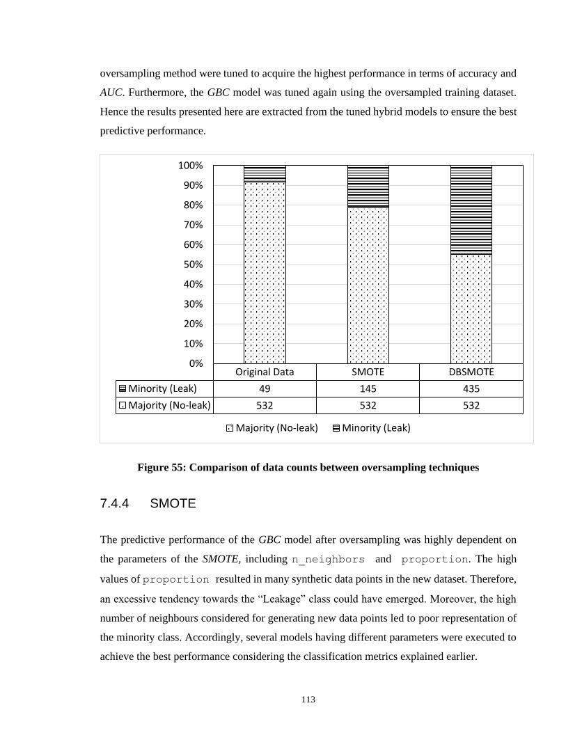
113

oversampling method were tuned to acquire the highest performance in terms of accuracy and

AUC. Furthermore, the GBC model was tuned again using the oversampled training dataset.

Hence the results presented here are extracted from the tuned hybrid models to ensure the best

predictive performance.

Figure 55: Comparison of data counts between oversampling techniques

7.4.4 SMOTE

The predictive performance of the GBC model after oversampling was highly dependent on

the parameters of the SMOTE, including n_neighbors and proportion. The high

values of proportion resulted in many synthetic data points in the new dataset. Therefore,

an excessive tendency towards the “Leakage” class could have emerged. Moreover, the high

number of neighbours considered for generating new data points led to poor representation of

the minority class. Accordingly, several models having different parameters were executed to

achieve the best performance considering the classification metrics explained earlier.

Original Data SMOTE DBSMOTE

Minority (Leak) 49 145 435

Majority (No-leak) 532 532 532

0%

10%

20%

30%

40%

50%

60%

70%

80%

90%

100%

Majority (No-leak) Minority (Leak)

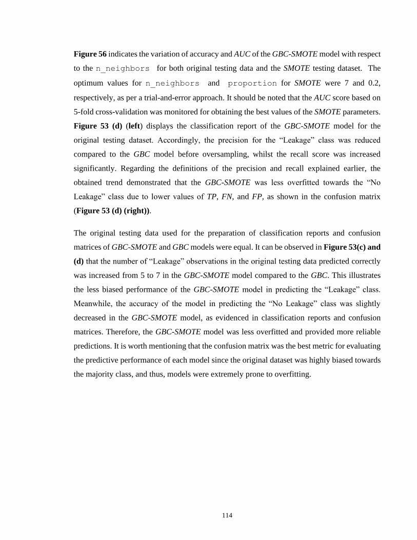
114

Figure 56 indicates the variation of accuracy and AUC of the GBC-SMOTE model with respect

to the n_neighbors for both original testing data and the SMOTE testing dataset. The

optimum values for n_neighbors and proportion for SMOTE were 7 and 0.2,

respectively, as per a trial-and-error approach. It should be noted that the AUC score based on

5-fold cross-validation was monitored for obtaining the best values of the SMOTE parameters.

Figure 53 (d) (left) displays the classification report of the GBC-SMOTE model for the

original testing dataset. Accordingly, the precision for the “Leakage” class was reduced

compared to the GBC model before oversampling, whilst the recall score was increased

significantly. Regarding the definitions of the precision and recall explained earlier, the

obtained trend demonstrated that the GBC-SMOTE was less overfitted towards the “No

Leakage” class due to lower values of TP, FN, and FP, as shown in the confusion matrix

(Figure 53 (d) (right)).

The original testing data used for the preparation of classification reports and confusion

matrices of GBC-SMOTE and GBC models were equal. It can be observed in Figure 53(c) and

(d) that the number of “Leakage” observations in the original testing data predicted correctly

was increased from 5 to 7 in the GBC-SMOTE model compared to the GBC. This illustrates

the less biased performance of the GBC-SMOTE model in predicting the “Leakage” class.

Meanwhile, the accuracy of the model in predicting the “No Leakage” class was slightly

decreased in the GBC-SMOTE model, as evidenced in classification reports and confusion

matrices. Therefore, the GBC-SMOTE model was less overfitted and provided more reliable

predictions. It is worth mentioning that the confusion matrix was the best metric for evaluating

the predictive performance of each model since the original dataset was highly biased towards

the majority class, and thus, models were extremely prone to overfitting.

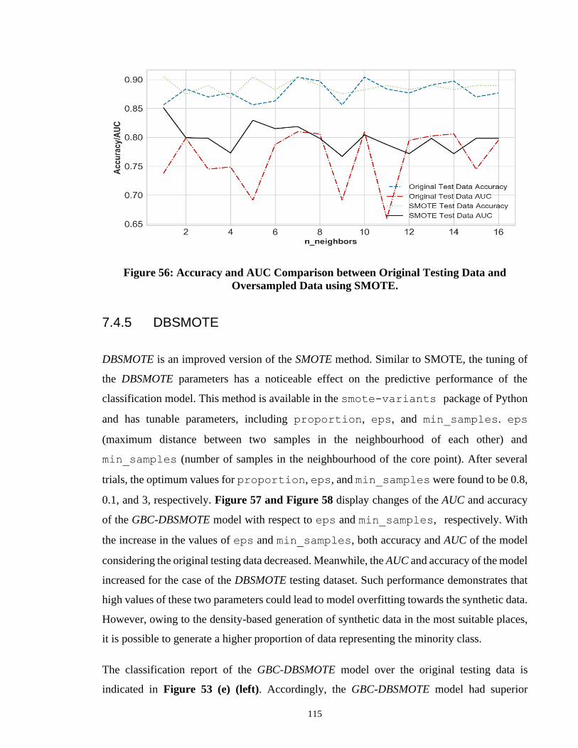
115

Figure 56: Accuracy and AUC Comparison between Original Testing Data and

Oversampled Data using SMOTE.

7.4.5 DBSMOTE

DBSMOTE is an improved version of the SMOTE method. Similar to SMOTE, the tuning of

the DBSMOTE parameters has a noticeable effect on the predictive performance of the

classification model. This method is available in the smote-variants package of Python

and has tunable parameters, including proportion, eps, and min_samples. eps

(maximum distance between two samples in the neighbourhood of each other) and

min_samples (number of samples in the neighbourhood of the core point). After several

trials, the optimum values for proportion, eps, and min_samples were found to be 0.8,

0.1, and 3, respectively. Figure 57 and Figure 58 display changes of the AUC and accuracy

of the GBC-DBSMOTE model with respect to eps and min_samples, respectively. With

the increase in the values of eps and min_samples, both accuracy and AUC of the model

considering the original testing data decreased. Meanwhile, the AUC and accuracy of the model

increased for the case of the DBSMOTE testing dataset. Such performance demonstrates that

high values of these two parameters could lead to model overfitting towards the synthetic data.

However, owing to the density-based generation of synthetic data in the most suitable places,

it is possible to generate a higher proportion of data representing the minority class.

The classification report of the GBC-DBSMOTE model over the original testing data is

indicated in Figure 53 (e) (left). Accordingly, the GBC-DBSMOTE model had superior

116

prediction performance compared to that of GBC and GBC-SMOTE considering precision,

recall, and F1-score metrics. Moreover, among 136 and 10 “No Leakage” and “Leakage”

observations in the original testing data, 129 and 9 were predicted correctly by the GBC-

DBSMOTE model, respectively, as shown in the confusion matrix (Figure 53 (e) (right)).

Therefore, the GBC-DBSMOTE model achieved less biased predictions using the original

testing dataset. As mentioned earlier, the developed models were tuned again after

oversampling, and Table 26 presents the tuned hyperparameters of the GBC-SMOTE and

GBC-DBSMOTE models using the oversampled training dataset.

Figure 57: Accuracy Measurements Against eps Using DBSMOTE.

117

Figure 58: Accuracy Measurements Against min_samples Using DBSMOTE.

Table 26: Hyperparameters for Tuning SMOTE and DBSMOTE Models

Model GBC-SMOTE

GBC-DBSMOTE

n_estimator 190 190 learning_rate 0.21 0.215 max_depth 1 1

min_samples_split 2 2 min_samples_leaf 1 10

subsample 0.68 0.74

7.4.6 Comparison between different models

Figure 59 shows the precision, recall, and F1-score comparison for the minority class along

with the accuracy and AUC using gradient boosting classifiers trained by the original, SMOTE

and DBSMOTE training data. Precision is not a good measure of imbalanced data because it

is affected by the incorrectly predicted negative class, i.e. majority class. Recall, on the other

hand, reflects the reality of the positive class because it only considers the positive class, i.e.

minority class. Among these three models, GBC-DBSMOTE had a recall value of 0.9, and

AUC had 0.92 and was the best performer in handling the leakage class.

118

Figure 59: Comparison of performance using gradient boosting classifiers trained by

the original, SMOTE and DBSMOTE training data.

To have a rational comparison between the predictive performance of the GBC, GBC-SMOTE,

and GBC-DBSMOTE models considering various splits of the original dataset, the performance

of each model was assessed using three different seeds of data split. Table 27 presents the

confusion matrix, accuracy, and AUC of each seed (i.e. data split) for all models developed

herein. GBC-DBSMOTE demonstrated better performance in predicting the class of

observations in the original testing data compared to GBC and GBC-DBSMOTE. Accordingly,

the GBC-DBSMOTE was less overfitted towards any class of the dataset, whereas GBC was

extremely overfitted towards the majority class, and GBC-SMOTE was slightly biased towards

the synthetic minority class. It is noted that the accuracy of the models after oversampling is

slightly lower compared to the GBC model, which indicates that it was overfitted. Thus,

accuracy alone is not adequate to assess the predictive performance of the model. Nonetheless,

the AUC of the models after oversampling was significantly improved in all cases of data split.

Moreover, the superior performance of GBC-DBSMOTE was evident from the confusion

matrices so that a high portion of the testing data examples were predicted correctly in all split

cases.

Precision Recall F1 Accuracy AUC

GBC 0.71 0.50 0.59 0.95 0.74

GBC-SMOTE 0.39 0.70 0.50 0.90 0.81

GBC-DBSMOTE 0.56 0.90 0.69 0.95 0.92

0.00

0.10

0.20

0.30

0.40

0.50

0.60

0.70

0.80

0.90

1.00

119

Table 27: The Confusion Matrix, Accuracy, And AUC using Various Splits of the

Original Dataset

Model Case 1 Case 2 Case 3

Confusion matrix

Accuracy AUC Confusion

matrix Accuracy AUC

Confusion matrix

Accuracy AUC

GBC 134 2

5 5

95.21 0.74

135 5

6 3 92.47 0.65

132 1

9 4 93.15 0.65

GBC-SMOTE

125 11

3 7

90.41 0.81

118 19

2 7 85.62 0.82

81 52

1 12 63.7 0.77

GBC-DBSMOTE

129 7

1 9 94.52 0.92

125 12

2 7 90.41 0.85

122 11

3 10 90.41 0.84

7.4.7 Feature Importance

Figure 60 exhibits the feature importance based on DBSMOTE. The feature importance

evaluation is a technique to examine how useful the input features are impacting the output.

The feature importance score plays an important role in providing insight on what to further

investigate, feature selection and providing the basis for dimensional reduction. In the case of

this research, joint gap, applied pressure, and gasket length are the three most impactful

features, followed by pipe size and gasket mass. The water level and duration exhibit a lower

impact on the output.

Figure 60: Feature Importance Using DBSMOTE

120

7.4.8 Design Approach: Recommendations for Future Work

The exclusive and comprehensive data collected from the novel experimental procedure

developed in this thesis captures the influential parameters in the design of RCP joints. The

nonlinear relationship between different attributes of the data resulted in poor performance of

conventional statistical methods for predicting the performance of various RCP joint

configurations. Nevertheless, the proposed intelligent data-driven GBC-DBSMOTE model

achieved high accuracy in predicting the failure of RCP joints. The model distinguished the

most influential parameters in the design of joints in great agreement with experimental

findings. As observed in real-world practice, the proposed intelligent model recognized the

“pressure” and “joint gap” as the attributes having higher feature importance. This predictive

tool is aimed to serve as a new guideline for deigning durable RCP joints under InI condition.

Using the hybrid model developed in this study, comprehensive design charts respecting

various configurations, i.e. pipe size, gasket type, joint gap, etc., can be proposed. Moreover,

design failure thresholds for different RCP configurations could be identified in future work.

InI performance-based optimization of RCP joint configurations using the ML framework

introduced here is a vital design step to be pursued in future work.

7.5 Summary

This chapter demonstrates the successful application of machine learning to model hydrostatic

infiltration in reinforced concrete pipe joints where conventional regression analysis

techniques have failed to produce reliable predictions given the complex inter-relationships of

a multitude of input parameters. An exclusive experimental dataset was collected from a

comprehensive test procedure containing 9 design-wise input features. Tree-based supervised

machine learning techniques: RFC, ETC and GBC were deployed in this study. Considering

that the experimental dataset was extremely imbalanced, two oversampling techniques,

SMOTE and DBSMOTE, were adopted to mitigate the biased performance of classifiers.

Accordingly, the conclusions below can be drawn from this study:

121

1. Among the different classifiers considered, GBC had the best predictive performance

according to several classification metrics, including accuracy, recall, F1-score, and

AUC.

2. After being turned, all the basic classifiers indicated overfitted performance towards

the majority class in the dataset, i.e. “No Leakage,” due to the imbalanced dataset

3. The oversampling techniques mitigated the bias in the dataset and thus, improved the

prediction performance.

4. DBSMOTE demonstrated better predictive performance compared to SMOTE

according to various classification metrics, such as confusion matrix and AUC.

5. The tuning of the oversampling algorithms resulted in considerable improvement in

their predictive performance.

6. Using DBSMOTE, more synthetic data could be appended to the dataset for training,

i.e. higher values of proportion, without overfitting the dataset towards synthetic data

compared to SMOTE.

7. The GBC-DBSMOTE hybrid model provided the most promising and reliable results

over different splits of the original datasets compared to GBC and GBC-SMOTE.

8. The proposed hybrid model proved to be a reliable predictive tool for providing design

guidelines for different pipe joint configurations.

In conclusion, this ML model framework developed in this Chapter could provide a foundation

for developing design RCP joint hydrostatic performance charts against infiltration for various

models of sealing gaskets, duration and level of pressure, pipe size and other influential input

parameters, which should be pursued in further study.

7.6 References

Ahmad, M. W., Reynolds, J., Rezgui, Y. “Predictive modelling for solar thermal energy

systems: A comparison of support vector regression, random forest, extra trees and

regression tree”, Journal of Cleaner Production Vol. 203, 2018, pp. 810-821.

Azar, A. T., Elshazly, H. I., Hassanien, A. E., Elkorany, A. M. “A random forest classifier

for lymph diseases”, Computer Methods and Programs in Biomedicine, Vol. 113,

2014, pp. 465-473.

122

Bengfort, B., Billbro, R. “Yellowbrick: Visualizing the Scikit-Learn Model Selection

Process”, The Journal of Open Source Software, Vol. 4, 2019, pp. 1075

Breiman, L., “Bagging Predictors”, Machine Learning, Vol. 24, 1996, pp. 123-140.

Breiman, L., Friedman, J. H., Olshen, R. A., Stone, C. J. ”Classification and Regression

Trees”, Chapman & Hall/CRC, New York, NY, United State, 1984.

Bunkhumpornpat, C., Sinapiromsaran, K., Lursinsap, C. “DBSMOTE: Density-Based

Synthetic Minority Over-sampling Technique”, Applied Intelligence, Vol. 36, 2012,

pp. 664-684.

Cordon, I., Garcia, S., Fernandez, A., Herrera, F., “Imbalance: Oversampling algorithms for

imbalanced classification in R”, Knowledge-Based Systems, Vol. 161, 2018, pp. 329-

341.

Chawla, N. V., Bowyer, K. W., Hall, L. O., Kegelmeyer, W. P., “Journal of Artificial

Intelligence Research, Vol. 16 pp. 321-357, 2002.

Friedl, M. A., Brodley, C. E., “Decision Tree Classification of Land Cover from Remotely

Sensed Data”, Elsevier Science Inc., New York, NY, United State, 1997.

Geurts, P., Ernst, D., Wehenkel, L., “Extremely randomized trees, Machine Learning, Vol.

63, 2006, pp. 3-42.

John, V., Lui, Z., Guo, C., Mita, S., Kidono, K. “Real-time Lane Estimation Using Deep

Features and Extra Trees Regression”, Pacific-Rim Symposium 2015, Auckland,

New Zealand, November 25-27, 2015, pp. 721 – 733.

Ke, G., Meng, Q., Finley, T., Wang, T., Chen, W., Ma, W., Te, Q., Liu, T. “LightGBM: A

Highly Efficient Gradient Boosting Decision Tree”, 31st Conference on Neural

Information Processing Systems, Long Beach, CA, United State, 2017.

Kim, H., Ahn, E., Shin, M., Sim, S. H. “Crack and Noncrack Classification from Concrete

Surface Images Using Machine Learning”, Structural Health Monitoring, Vol. 18,

Issue 3, 2019, pp 725-738.

Koch, C., Georgieva, K., Kasireddy, V., Akinci, B., Fieguth, Paul., “A review on computer

vision based defect detection and condition assessment of concrete and asphalt civil

infrastructure”, Advanced Engineering Informatics, Vol. 29, 2015, pp. 196-210.

Kovacs, G. “Somte-variants: A python implementation of 85 minority oversampling

techniques”, Neurocomputing, Vol. 366, 2019, pp. 352-354.

Liaw A., Wiener, M. “Classification and Regression by randomForest”, R News, Vol. 2/3,

2002, pp. 18-22.

Liu, Y., Gu, Y., Nguyen, J. C., Li, H., Zhang, J., Gao, Y., Huang, Y., “Symptom severity

classification with gradient tree boosting”, Journal of Biomedical Informatics, Vol.

75, 2017, pp. S105-S111.

123

Mangalathu, S., Jeon, J. S. “Classification of failure mode and prediction of shear strength

for reinforced concrete beam-column joints using machine learning techniques”,

Engineering Structures, Vol. 160, 2018, pp. 85-94.

Mangalathu, S., Jeon, J. S. “Machine Learning-Based Failure Mode Recognition of Circular

Reinforced Concrete Bridge Columns: Comparative Study”, American Society of

Civil Engineering – Journal of Structural Engineering, Reston, Virginia, United

States, 2019.

Mason, L., Baxter, J., Bartlett, P., Frean, M. “Boosting algorithms as gradient descent”,

Advances in Neural Information Processing Systems, 12 512–518. MIT Press,

Cambridge, MA. 2000, pp. 512- 518.

Melhem, H. G., Cheng, Y. “Prediction of Remaining Service Life of Bridge Decks Using

Machine Learning”, American Society of Civil Engineering – Journal of Computing

in Civil Engineering, Reston, Virginia, United States, 2019.

Nehdi, M., Chabib, H. E., Naggar, M. H. “Predicting Performance of Self-Compacting

Concrete Mixtures Using Artificial Neural Networks”, ACI Materials Journal,

September – October 2001 Issue, 2001, pp. 394 – 401.

Pedregosa, F., Varoquaux, G., Gramfort, A., Michel, V., Thirion, B., Grisel, O., Blondel, M.,

Prettenhofer, P., Weiss, R., Dubourg, V., Vanderplas, J., Passos, A., Cournapeau, D.,

Brucher, M., Perrot, M., Duchesnay, E. “Scikit-learn: Machine Learning in Python”,

Journal of Machine Learning Research, Vol. 12, 2011, pp. 2825-2830.

Quinlan, J. R., “Bagging, Boosting, and C4.5”, University of Sydney, Australia, 2006.

Rafiei, M. H., Adeli, H. “A novel machine learning-based algorithm to detect damage in

high-rise building structures”, Structural Design of Tall and Special Buildings, Vol.

26, Issue 18, e1400, 2017.

Reich, Y., “Machine Learning Techniques for Civil Engineering Problems”, Microcomputers

in Civil Engineering, Vol. 12, Malden, MA, United States, 1997, pp. 295 – 310.

Reich, Y., Barai, S. V. “Evaluating machine learning models for engineering problems”,

Artificial Intelligence in Engineering, Vol. 13, 1999, pp. 257-272.

Rodriguez-Galiano, V. F., Ghimire, B., Rogan, J., Chica-Olmo, M., Rigol-Sanchez, J. P. “An

assessment of the effectivenes s of a random forest classifier for land-cover

classification, ISPRS Journal of Photogrammetry and Remote Sensing, Vol. 67, 2012,

pp. 63-104.

Sattar, A.M.A., Ertuğrul, Ö., Gharabaghi, B. et al. Extreme learning machine model for water

network management. Neural Comput & Applic 31, 2019, pp. 157–169.

Sokolova, M., Japkowicz, N., Szpakowicz, S. “Beyond Accuracy, F-Score and ROC: A

Family of Discriminant Measures for Performance Evaluation”, LNAI Vol. 4304,

2006, pp. 1015-1021.

124

Tharwat, A. “Classification assessment methods”, Applied Computing and Informatics,

2018, (In press).

Torres-Barran, A., Alonso, A., Dorronsoro, J. R. “Regression tree ensembles for wind energy

and solar radiation prediction”, Neurocomputing, Vol. 326–327, 2019, pp. 151-160.

Varmuza, K., Filzmoser, P., Hilchenbach, M., Kruger, H., Silen, J. “KNN classification –

evaluated by repeated double cross validation: Recognition of minerals relevant for

comet dust”, Chemometrics and Intelligent Laboratory Systems, Vol. 138, 2014, pp.

67-71.

Wong, S. C., Gatt, A., Stamatescu, V., McDonnell, M. D., “Understanding data augmentation

for classification: when to wrap?”, 2016 International Conference on Digital Image

Computing: Techniques and Applications (DICTA), Institute of Electrical and

Electronic Engineers, Gold Coast, QLD, Australia, 2016.

Yaseen, Z. M., Deo, R. C., Hilal, A., Abd, A. M., Bueno, L. C., Salcedo-Sanz, S., Nehdi, M.

L., “Predicting compressive strength of lightweight foamed concrete using extreme

learning machine model”, Advances in Engineering Software, Vol. 115, 2018, pp.

112-125.

Zealand, C. M., Burn, D. H., Simonovic, S. P., “Short term streamflow forecasting using

artificial neural networks”, Journal of Hydrology, Vol. 214, 1999, pp. 32-48.

Zhang, A., Wang, C. P., Li, B., Yang, E., Dai, X., Peng, Y., Fei, Y., Liu, Y., Li, J. Q., Chen,

C., “Automated Pixel-level Pavement Crack Detection on 3D Asphalt Surfaces Using

a Deep-Learning Network”, Computer-aided Civil and Infrastructure Engineering,

Vol. 32, 2017, pp. 805-819.

125

CHAPTER 8

8 Summary, Conclusions and Recommendations

Sanitary sewage networks are key infrastructure assets in today’s civilization. Undesirable

inflow and infiltration (InI) into piped drinking and/or sewage flows mixed with flows from

the natural environment can cause a huge financial burden to municipalities. InI is among the

top challenges for municipalities and results primarily from stormwater percolating into the

ground and finding its way into sanitary sewer systems. This tremendously escalates the

operating costs of water treatment facilities. RCP, the most commonly used product in sewage

systems, faces a challenge in dealing with InI since the quality of the pipe joint relies not just

on the joint materials and design, but also on the installation quality.

Chapter 2 reviewed the deficiencies of existing standards in many places around the world,

which generally do not proactively capture the infiltration risks. The state-of-the-art practice

of manufacturers for testing the water tightness of reinforced concrete pipe does not provide

useful results regarding performance under in-situ groundwater pressures. The true

performance requirements for RCP joints are to resist the external hydrostatic pressures

resulting from high groundwater tables. Combined with previous research efforts, the situation

demands a simple method to evaluate the capacity of the RCP joint performance for infiltration.

Accordingly, a novel testing method was introduced in Chapter 3 to allow RCP manufacturers

to conduct an in-factory test in a safe and efficient way. The testing apparatus, setup, and

procedures were described in detail. A comprehensive testing program, presented in Chapter

4, using the new test, has collected hundreds of data points on the infiltration performance of

RCP joints using existing joint designs and gasket materials.

126

Chapter 5 provided a comprehensive analysis of the testing data and reviewed the influence

factors. Performance charts for those gaskets were developed in Chapter 6 from these data

points. An illustrative case was used to connect the experimental data to a real-life case where

a high groundwater table above the obvert of the pipe posed an infiltration potential. A safety

factor can be derived from the performance chart providing quantified guidance in permissible

joint gaps in the construction quality.

Furthermore, the novel experimental dataset is influenced by multiple nonlinear factors. Thus,

several advanced machine learning (ML) techniques were used to create a rational predictive

model. Those techniques, presented in Chapter 7, consist of Gradient Boosting with

DBSMOTE, addressed the imbalanced data challenges and provided the best accuracy model.

8.1 Conclusions

Based on the research work reported in this thesis, the main emanating conclusions can be

categorized into three parts: existing standards and literature, experimental developments, and

ML modelling techniques as follows.

8.1.1 Existing Standards and Literature

Standard provisions for precast concrete pipe around the world regarding RCP hydrostatic

performance evaluation do not provide a true evaluation of the joint performance against

infiltration. There has been little effort to critically analyze the international experience gained

in this field, to compare performance criteria, and to derive the best international practice

guidelines. This effort has exposed various knowledge deficiencies along with deviations

between the standards and the end-user expectations in terms of infiltration. There is a clear

need for improvement to bridge the gap between true hydrostatic performance requirements

and current testing procedures.

127

8.1.2 Experimental Development

This study developed a simple and safe method to examine the capacity of RCP joints for

infiltration. Over 100 tests were conducted, and the test procedure was successfully repeated.

The proposed test methodology is concluded to be able to provide consistent and reliable

measurements, controls and outputs. Eight additional special tests were conducted with gasket

and pipe samples beyond the ones selected for the research program. The results demonstrated

that the procedure is able to accommodate a larger variation of the samples. These include

precise pressure measurements, joint gap monitoring, and capture of water consumption values

in the system during the test. Based on the experimental observations and findings, the

following conclusions can be drawn:

1. Current pipe joint designs and gaskets used by industry can withstand significantly

higher pressure than the commonly accepted pressure rating of 105 kPa (13 psi) as per

CSA A257. With tighter and restrained joint gaps, experiments demonstrated the

possibility of achieving 480 to 680 kPa against infiltration. The results of the current

study indicated that, with better control of the joint gap during pipe installation, the

joint would not be the weakest link of a drainage network.

2. Traditional pipe hydrostatic performance tests generally rely on visual inspection for

leakage. In the current proposed test, a more rational approach is used where WSCC

measures the volumetric water loss during the test. During testing, leakage was first

detected by observing an increase in the water reduction rate. This eliminates

guesswork and helps the operator focus on the quantitative aspects of the test.

3. The test results provided a relationship between the pressure and movement of the

gasket. This revealed that the current design of the pipe joint is driven by providing

better performance under existing standards. Such designs can be perceived as a reverse

of what is actually needed to withstand the infiltration of groundwater. It also reflects

a misunderstanding of the end-user expectations and incorrect assumption that the pipe

joint design and gasket would perform equally regarding both exfiltration and

infiltration.

4. The hydrostatic capacity of the RCP joint is predominantly influenced by the joint gap.

In conventional hydrostatic testing, CSA A257, ASTM C443, ASTM C1628, and BS

128

EN 1916 require the joint to remain watertight with a 13-mm deflection on one side.

There is no maximum acceptable joint gap defined in these specifications. Accordingly,

engineers expect similar performance under a 13-mm joint gap in the field. ACPA

(2009) states that the manufacturer shall define the maximum allowable joint gap.

However, there is no research in the open literature that relates actual hydrostatic

performance to the joint gap. Hence, the results obtained in this research provide a trend

showing that the capacity of the pipe joint to withstand infiltration pressure decreases

as the joint gap increases.

5. Based on the findings, the maximum allowable joint gap should be a variable based on

the type of the gasket, applied pressure, and the joint type. However, 13 mm can be an

acceptance criterion for a target pressure defined in the specifications given that the

pipe producers can demonstrate it using the infiltration test.

6. The ultimate infiltration pressure is a function of the influence ratio, Ig, the ratio of the

mass of the gasket, to the effective annular space. The higher the influence ratio, the

higher the infiltration pressure capacity the gasket can achieve.

7. High variations in the pressure-joint gap curve likely result from other factors such as

the mechanical properties of the rubber gasket. Further studies on these factors are

recommended.

8. The ultimate infiltration pressure is not sensitive to the pipe size given the same gasket

profile and joint profile. However, larger size of the pipe will require different joint

height and thickness for providing shear transfer, thus the gasket profile design varies

based on the size of the pipe. The ultimate infiltration pressure may be affected with

different gasket and joint profile.

9. The proposed 20-hour test provides evidence of the essential steps for evaluating the

operating pressure when the pipe is placed in service. Gasket movement tends to

stabilize in a longer duration compared to the conventional 10-minute test. The larger

the joint gap, the more severe is the movement.

10. The new test method introduced in the current study demonstrated operational

advantages, including a much higher level of safety compared to conventional pressure

tests such as ASTM C361 and AWWA C302 since only a limited amount of water is

needed in the test. The minimum water volume required also shortens the filling time

compared to conventional pressure tests.

129

11. In the new test, unlike existing exfiltration tests, failure does not pose safety hazards to

the operator nor to anyone near the testing area. Moreover, the height of the pipe allows

the operator to easily access the inside of the pipe for visual examination. Water level

monitoring in the WSCC can be used to quantify the leak, unlike current tests that rely

on qualitative assessment.

12. The hydrostatic behaviour of the RCP joint serves a critical function in drainage

networks. By providing a method to evaluate the ability of the joint to withstand

infiltration, the present study opens many possibilities for innovation and improvement

to add value to RCP advantages, including strength, durability, sustainability, and

resiliency.

13. The preliminary results benchmarked the hydrostatic performance of existing RCP

joints and gasket designs. Hence, the proposed testing method can allow a better

understanding of the relationship between joint hydrostatic performance and joint gap,

with the potential to develop enhanced RCP installation guidelines. This would

empower contractors to mitigate infiltration risks and make sounder decisions based on

actual field conditions.

14. The discovery of the time-dependent gasket movement in the annular space can lead to

improvements in existing single offset joints. In the subsequent phase of this research,

additional parameters, including joint gap, joint offset, and various gasket and pipe

materials, will be considered to make a more reliable evaluation.

15. The eight additional tests conducted beyond the original scope evaluated 675 mm, 750

mm and 1800 mm RCP, wedged profile gasket, and lined pipes. The test method was

found suitable to cover a wide variety of different pipe joints, pipe types, and gasket

types.

16. The spacer ring and lateral hydraulic jack added to the originally developed test method

can reasonably simulate field conditions and installation quality. The hydrostatic

performance under various joint gaps and joint offsets can be quantified using this

method.

17. The study effectively relates the material behaviour of RCP joint and field conditions,

such that an assessment factor can be suggested for a rational engineering decision

process.

130

18. There are some differences in the sealing potential predictions between material tests

and infiltration tests. The material tests do not reflect the real sealing potential scale;

indeed, comparison tests indicated that their results might be biased. The pressure

reduction was faster in the infiltration test with an increased joint gap than that in the

material testing. This is due to the different loading schemes in those tests.

19. The gasket height influences the hydrostatic performance. It affects the infiltration test

more than it does for the material load test. The effect was more severe when the joint

gap increased.

20. The infiltration performance of the gasket agrees with the prediction derived from the

gasket geometry. However, the prediction of the sealing potential decreased less

drastically with increasing joint gap than in the case of the hydrostatic performance in

the infiltration test.

8.1.3 Machine Learning Modeling

The following conclusions can be drawn from ML modelling using the experimental data:

1. ML models can be used to provide reasonable predictions of RCP infiltration.

2. Among the different ML classifiers considered, GBC had the best predictive

performance according to several classification metrics, including accuracy, recall, F1-

score, and AUC.

3. The modelling procedure requires tuning of the model to avoid overfitting performance

towards majority class in the dataset, i.e. “No Leakage,” due to the imbalanced dataset

4. The oversampling techniques used mitigated the bias in the dataset and thus, improved

the prediction performance. DBSMOTE demonstrated better predictive performance

compared to SMOTE according to various classification metrics, such as confusion

matrix and AUC.

5. The tuning of the oversampling algorithms resulted in considerable improvement in

their predictive performance. Using DBSMOTE, more synthetic data could be

appended to the dataset for training, i.e. higher values of proportion, without overfitting

the dataset towards synthetic data compared to SMOTE.

131

6. The GBC-DBSMOTE hybrid model provided the most promising and reliable results

over different splits of the original datasets compared to GBC and GBC-SMOTE.

8.2 Recommendations

This research has emphasized the critical analysis of existing standards, including the necessity

to review and update concrete pipe standards in order to capture modern developments in

concrete technology and to bridge the performance evaluation gap in the context of joint

performance for infiltration. The testing method proved to be simple, robust, and repeatable

for measuring the infiltration capacity of RCP joints. One observation related to the uncertainty

may require further investigation where under higher level of applied infiltration pressure, the

result seemed to have larger spread with respect to the joint gap. In addition, further, increase

of the joint gap beyond the threshold will allow the data to reveal the complete performance

spectrum. One of the limitations at the beginning of the research was to select the parameters

that influence the output. With assistance from machine learning, the feature importance was

revealed providing insight into those parameters that may require further investigation. The

actual material properties being tested, such as rubber hardness to the infiltration test, may be

considered. These allow the acceptance criteria for routine quality control tests to be

established. Lastly, the testing method can also be used in RCP joint and gasket profile

development for better sealing potential.

Further study is recommended to evaluate the factors that influence the long-term performance,

i.e. 20 hours or longer, such as gasket relaxation and movement under sustained infiltration

pressures. A joint effort between the gasket and precast RCP manufacturers to develop

performance curves for their products and combinations thereof is needed. These curves can

then be used to evaluate the risks associated with actual field conditions.

The improvement of secondary gaskets can increase the efficiency of the test. The effect of the

secondary gasket type, properties and profile were not detailed and investigated. In some tests,

it caused certain challenges in holding the pressure. The use of external steel bands to create

the space for pressurization could be an option. More advanced instrumentation, such as water

levels and joint gap measurements, as well as linking to an applied pressure using datalogger,

can be an option to increase accuracy.

132

The machine learning model framework developed in this Chapter could provide a foundation

for developing design RCP joint hydrostatic performance charts against infiltration. These

could include various models of sealing gaskets, duration and level of pressures, pipe sizes and

other influential input parameters, which should be pursued in further study.

8.3 References

American Concrete Pipe Association “Concrete Pipe Joints Your Best Choice”, ePipe. Resource

#e-07-124 08/09, 2009.

ASTM C361M-14, “Standard Specification for Reinforced Concrete Low-Head Pressure

Pipe”, ASTM International, West Conshohocken, PA, USA, 26 p.

ASTM C443-12, “Standard Specification for Joints for Concrete Pipe and Manholes, Using

Rubber Gasket” ASTM International, West Conshohocken, PA, USA, 2012, 3 p.

ASTM C1628-17 “Standard Specification for Joints for Concrete Gravity Flow Sewer Pipe,

Using Rubber Gaskets”, ASTM International, West Conshohocken, PA, USA, 2017,

7 p.

AWWA C302, “Reinforced Concrete Pressure Pipe, Non-cylinder Type, American Water

Works Association, Denver, CO, USA, 2016, 40 p.

BS EN 1916:2002, “Concrete Pipes and Fittings, Unreinforced, Steel Fibre and Reinforced”,

British Standards Institution (BSI), London, UK, 2002, 94 p.

CSA A257, “Standards for Concrete Pipe and Manhole Sections”, CSA Group, Mississauga,

ON, Canada, 2019, 40 p.

133

Bibliography

Lui Sammy Wong was the VP of Engineering and Quality at Con Cast Pipe. He holds a Master

of Engineering Science in civil engineering from the University of Western Ontario. Sammy

is a professional engineer and designated consulting engineer in Ontario, Canada, interested in

the precast infrastructure design, manufacturing, quality and installation. Projects that he was

involved with as a technical director include bridge elements for Hwy 407 East Extension,

precast tunnels sections for Eglinton Crosstown LRT Kennedy Station and Mount Dennis

Station, precast bridge elements for several bridge replacement projects along the Richmond

Hill GO train line and Stouffville GO train line, and many other large span culverts and bridges

for MTO, etc. With more than 15 years of experience in the precast industry, he is currently

taking an active role in several technical committees such as the Ontario Concrete Pipe

Association, Canadian Concrete Pipe and Precast Association, CSA A257 Standards of

Concrete Pipe and Manhole Sections, Canadian Precast and Prestressed Concrete Institute

(CPCI), and Quality Assurance Council at Canadian Precast Concrete Quality Assurance

(CPCQA) Certification Program. He also volunteers in CSA S6 Canadian Highway Bridge

Design Code – Section 7 Buried Structure sub-committee since 2016. With his passion in the

concrete pipe industry, Sammy enrolled in the Ph.D. program at Western University, London,

Ontario, to develop better testing and evaluation methodologies over the reinforced concrete

pipe application.

Appendix A – Page A1

Appendix A – Design of the Testing Apparatus

Appendix A – Page A2

Base Frame Assembly

Appendix A – Page A3

Pressure System and Stand Assembly

Appendix A – Page A4

Jacking Post Assembly

Appendix A – Page A5

Back-stop Post Assembly

Appendix A – Page A6

Complete Setup Assembly

Appendix B – Page B1

Appendix B – Testing Results

The content of Appendix B can be found in Supplemental Content.

Appendix C – Page C1

Appendix C – Machine Learning Source Code and Output

The content of Appendix C can be found in Supplemental Content.

Vitae – Page V1

Curriculum Vitae

Name: Lui (Sammy) Wong

Post-secondary University of Western Ontario

Education and London, Ontario, Canada

Degrees: 1997-2001 B.E.Sc.

The University of Western Ontario

London, Ontario, Canada

2001-2002 M.E.Sc.

The University of Western Ontario

London, Ontario, Canada

2017-2020 Ph.D.

Honours and The Milos Novak Memorial Award 2002

Awards:

Winner of the Peter S. Higgins Structural Analysis Competition 2001

Awarded Certificate of Merit for the Final Year Project 2001

Related Work Precast Concrete Engineer 2006 - 2020

Experience

Publications:

Wong, L.S. (2020). Are Reinforced Concrete Pipe Joint Infiltration Proof?, Environmental

Science & Engineering Magazine, June/July 2020 Issue, pp. 30-33.

Wong, L.S., Marani, A. and Nehdi, M.L. (2020, Submitted). Hybrid Tree-Based Ensemble-

Oversampling Prediction of RCP Joint Performance for Infiltration, ASCE Journal of

Pipeline Systems - Engineering and Practice, Reston, Virginia, United States.

Younis, A., Ramadan, A., Wong, L.S., Nehdi, M. L. (2020 submitted). Modified Three-Edge

Bearing Test for Reinforced-Concrete Pipe Eliminating Crack-Width Criteria,

Structures.

Younis, A., Shehata, A., Ramadan, A., Wong, L.S., Nehdi, M. L. (2020 submitted).

Numerical Modeling of Reinforced-Concrete Pipe with Single, Double and Triple

Cage Reinforcement, Engineering Structures.

Ramadan, A., Younis, A., Wong, L.S., Nehdi, M. L. (2020). Investigation of Structural

Behavior of Precast Concrete Pipe with Single Elliptical Steel Cage Reinforcement,

Engineering Structures.

Vitae – Page V2

Ramadan, A., Shehata, A., Younis, A., Wong, L.S., Nehdi, M. L. (2020 submitted). Modeling

Structural Behavior of Precast Concrete Pipe with Single Elliptical Steel Cage

Reinforcement, Structures.

Wong, L.S. and Nehdi, M.L. (2020). Predicting Hydrostatic Infiltration in Reinforced

Concrete Sewer Pipes Considering Joint Gap and Joint Offset, ASCE Journal of

Pipeline Systems - Engineering and Practice, Reston, Virginia, United States.

Wong, L.S. and Nehdi, M.L. (2020). Quantifying Resistance of Reinforced Concrete Pipe

Joints to Water Infiltration, ASCE Journal of Pipeline Systems - Engineering and

Practice, Reston, Virginia, United States.

Wong, L.S., Cameron, J., Nehdi, M.L. (2019). Study of Precast Concrete Crazing Due To

Moist Curing, CSCE June 12-15, 2019, Montreal.

Ramadan, A., Younis, A., Wong, L.S., Nehdi, M.L. (2019). Reinforced Concrete Pipe

Design With Single Elliptical Cage Reinforcement, CSCE June 12-15, 2019,

Montreal.

Wong, L.S. (2019). Precast Concrete Tunnel Segments - Go Beyond The Limit!, Concrete

Pipe Journal, Spring Issue 2019

Wong, L.S. (2019). Self-compacting Bedding, Concrete Pipe Journal, Spring Issue 2019

Wong, L.S., Nehdi, M.L. (2018). New Test Method For Reinforced Concrete Pipe Joint

Hydrostatic Infiltration, CSCE June 13 – June 16, 2018, Fredericton

Vuk, F., Campbell, P., Wong, L.S., (2018). Hidden Valley Road Bridge Replacement,

Concrete Pipe Journal, 2018 Spring Issue

Wong, L.S., Nehdi, M.L. (2018). Critical Analysis of International Precast Concrete Pipe

Standards, Infrastructures

Wong, L.S. (2016). Full Scale Manufacturing of Steel Fibre Reinforced Concrete Pipe,

CSCE Conference, Jun 1-3, 2016, London Ontario Canada.

Wong, L.S., Allouche, E.N., Dhar., A.S., Baumert,. M., Moore, I.D. (2006). Long-term

Monitoring of SIDD Type VI Installation, Canadian Geotechnical Journal, pp. 394-

408.

Wong, L.S. and Allouche, E. N. (2002). SimSEWER – Interactive Educational Simulation

Software for Buried Infrastructure Management, Pipeline Engineering and

Construction International Conference 2003, American Society of Civil Engineering

Wong, L.S., Allouche, E.N. and Moore, I.D. (2002). Long-Term Monitoring And Analysis of

Full Scale Concrete Pipe Test Beds, ASCE Pipelines 2002, August 4-7, Cleveland,

OH, USA.

Vitae – Page V3

Allouche, E.N., Wong, L. S. and Baumert, M.E. (2001). Full Scale Testing of Concrete

Pipe Bedding Design, 2001 International conference on underground infrastructure,

June 10-13, Waterloo, Ontario, Canada, pp. 117-124.