Improving Cryptographic Architectures by Adopting Efficient

Adders in their Modular Multiplication Hardware

Adnan A. Gutub and Hassan A. Tahhan

Computer Engineering Department King Fahd University of Petroleum and Minerals

Dhahran 31261, SAUDI ARABIA Email: gutub@ccse.kfupm.edu.sa

Abstract

This work studies and compares different modular multiplication algorithms with emphases on the underlying binary adders. The method of interleaving multiplication and reduction, Montgomery’s method, and high-radix method were studied using the carry-save adder, carry-lookahead adder and carry-skip adder. Two recent implementations of the first two methods were modeled and synthesized for practical analysis. A modular multiplier following Koc’s implementation [6] based on carry-save adders and the use of carry-skip adders in the final addition step is expected to be of a fast speed with fair area requirement and reduced power consumption.

1. Introduction Modular multiplication is the basic arithmetic operation in many encryption systems that provide key

distribution and authentication. This operation is defined as C = A * B mod M. Since the size of the operands required to achieve secured systems is usually very large, the modular multiplication operation is going to be too expensive. Several modular multiplication algorithms have been proposed to solve this problem based on various computer arithmetic principles. This work discuses and compares some of these algorithms. Mainly, the classical method of interleaving multiplication and reduction, and Montgomery’s algorithm are presented here.

Binary adders are the basic building blocks in modular multipliers as any other kind of multipliers. They perform the multiplication operation through repeated number of additions. Hence, this work discusses different types of adders and compares between them. Hardware components studied in this work were modeled using VHDL and synthesized. ModelSim Se 5.6a was used to design and test the VHDL code. The Xilinx ISE 5.2i tool was used for synthesis.

2. Modular Multiplication Algorithms

The modular multiplication operation is defined as the computation of P = A * B mod M given the integers A, B and M. Usually, A and B are assumed to be positive integers that are less than the modulus M which are represented using n bits.

In the literature, various algorithms for modular multiplication have been proposed with different hardware implementations. A straightforward way to perform the modular multiplication operation is to do the multiplication first and then divide the result by the modulus. As someone might expect, this method is too expensive in terms of time and area requirements. An N×N bit multiplier is required followed by a 2N×N bit divider used to computer the remainder of the division process. Since the multiplication result of A * B is not important to the result of the modular multiplication, doing the reduction during the multiplication step is more suitable and also more efficient for the modular multiplication problem [19]. Hence, this survey does not seek to cover every technique and research in the area of modular multiplication computing. Instead, It discuses the basic common algorithms for modular multiplication of good performance so it might serve as an introduction to this widely evolving field.

The algorithms are described using the binary representation so that direct mapping with the hardware can be induced from it. Some architectural implementations of the presented algorithms shall be discussed.

1

The upper case letters denote the words and the lower case ones denote the bits. The algorithms to be studied are: the method of interleaving multiplication and reduction, Montgomery’s method and high-radix method.

2.1 Interleaving multiplication and reduction

This algorithm of computing the modular multiplication was first proposed by Blakley [1, 2]. It embeds the subtraction steps of the division in the shift-addition iterations of the multiplication. One traditional version of the algorithm is as follows:

1 2 3 4 5 6 7 8 9 10 11

P = 0 for i = n-1 to 0 P = 2 * P if ( P ≥ M ) P = P – M if ( bi = 1 ) P = P + A if ( P ≥ M ) P = P – M

Left Shift Magnitude Comparison Addition Magnitude Comparison

The algorithm computes the product in n steps for the n-bit modulus by scanning the bits from left to right. At each step, one left shift, one addition, and two magnitude comparisons are performed. The magnitude comparison can be done by first subtracting the modulus from the partial product and then the produced carry determines the correct value of the partial product [3].

In terms of hardware, the most crucial operations are the addition and subtraction operations. They slow down as the operands size increases. Reducing the complexity of the addition and subtraction operations will have significant impact on the overall performance of the algorithm.

The algorithm requires 2n subtractions and n additions. If the addition and subtraction operations are summed to have similar time complexity [5], the algorithm needs 3n full-magnitude additions (3n2 single-bit additions). This analysis looks for the algorithm on its worst case to reflect the hardware longest path delay.

By scanning the bits from right to left, the above algorithm can be parallelized and thus speeded up with exactly the same amount of hardware. On the worst case, the algorithm will required 2n full-magnitude additions as follows:

1 2 3 4 5 6 7 8 9 10 11

P = 0 for i = 0 to n-1 if ( bi = 1 ) P = P + A if ( P ≥ M ) P = P – M A = 2 * A if ( A ≥ M ) A = A – M

in parallel with steps 9 and 10

Chiou and Yang [4] proposed an algorithm with a speedup ratio of 2 by removing the magnitude comparison needed by the traditional Blakley’s algorithm. Unfortunately, the algorithm needs non-trivial pre-calculations (for example, 2n mod M) that make it unsuitable for single modular multiplication.

Many modified implementations of the Blakley’s algorithms are based on the use of carry save adders [6, 15, 3, 17, 19]. Carry-save adders (discussed later in section 3.2) will speedup the addition operation since they have constant time complexity. They take three operands as input and produce a sum-carry pair that represents the result. Carry-save adders are used to compute the partial products while a carry-propagation stage is needed at the last iteration. In order to decide if the partial product needs to be reduced without performing the full-magnitude addition, fast sign detection technique is needed to determine the sign of the sum-carry pair.

2

In reference [6], Koc proposed fast sign estimation technique that has constant time complexity based on the use of 5-bit carry-lookahead logic. The bits were scanned from left to right with overall time complexity of Ο(n + log m).

In reference [16], based on Koc’s technique, the bits were scanned from right to left, but the amount of hardware required was doubled and the time increased too. Such a result is unexpected specially if we recall that scanning bits from right to left introduces parallelism by which the speed of the traditional version of the algorithm was improved. However, science the two reduction steps, in lines 7 and 10, are done on two separate numbers which can not be combined in one step, the result of reference [16] is reasonable.

2.2 Montgomery’s method

In 1985, Montgomery [7] proposed a method for modular multiplication that replaces the costly division operation needed to perform modular reduction by simple shift operations, at the cost of having to transform the operands into a new domain representation before the operation and retransforming the result thereafter.

The Montgomery’s algorithm computes A * B * R-1 mode M given that A, B < M. In addition, R should be larger than M such that they are relatively prime. It is more useful to take R as a power of two because of today’s digital computers [5]. If R is assumed to be equal to 2n, then a modified binary-based version [10] of the algorithm is as follows:

Initialization Step: 1 Transform A and B to A’ and B’, such that A’ = A * R mod M and B’ = B * R mod M Multiplication Step ( P’ = A’ * B’ * R-1 mod M ): 2 P’ = 0 3 for i= 0 to n-1 4 5 P’ = P’ + a’i * B’ 6 if ( p’0 = 1 ) P’ = P’ + M 7 P’ = P’ / 2 8 9 if ( P’ ≥ M ) P’ = P’ - M Finalization Step: 10. Transform P’ to P, such that P = P’ * 1 * R-1 mod M

The basic idea of Montgomery’s algorithm is the following: adding multiple of M to the intermediate

results does not change the value of the final result, because the result is computed modulo M. After the addition in step 5 of the loop, the least significant bit of the intermediate result is inspected. If it is odd, the modulus M, which is an odd number, is added to the intermediate result to make it even. This even number can be divided by 2 without a remainder. After n steps these divisions add up to one division by 2n.

Step 9 of the algorithm is an additional operation to limit the temporary result, but it increases the algorithm complexity which may cause the hardware cost to increase, too. Fortunately, this step can be removed without changing other steps by taking R to be 2n+2 [11, 18]. Thus the algorithm requires n+2 iteration steps where a’

n and a’n+1 are defined to be zeros. However, this survey will discus the traditional

binary version of Montgomery’s algorithm described above. The hardware design for doing Montgomery’s multiplication can be used for transforming back the

result of the Montgomery’s product into the ordinary integer form (step 10) by having P’ and 1 as the operands of the multiplication operation. In contrast, direct use of Montgomery’s multiplication to do the initialization step is not possible without some preparation of the operands. More details can be found in reference [9].

The algorithm computes the Montgomery’s product in n steps for the n-bit modulus, where at each step one left shift, two additions, and one bit-by-word multiplication are performed. The subtraction operation after the loop can be ignored since it is done once.

The most important property of Montgomery’s algorithm is that no full magnitude comparison is required for the modular reduction [5, 8]. XORing P’

0, a’i and b’

0 will determine the need of a reduction step

3

prior to the addition operation in step 6. In contrast, the traditional method of interleaving as described before, computes the entire sum in order to decide whether a reduction needs to be performed [5].

In terms of hardware, the most crucial operation is the addition operation. The shift left operation might be done easily using wiring. AND gates can generate the bit-by-word multiplication in step 5 of the presented Montgomery’s algorithm.

On the worst case, the algorithm requires 2n full-magnitude additions for one go by the multiplication step. Since the algorithm needs two passes to compute the desired result, 4n full-magnitude additions are required by the algorithm. Moreover, doing the pre-calculations of the two operands, A and B, in hardware will cost 4n full-magnitude additions, too. Thus, the total cost of Montgomery’s algorithm for single modular multiplication is 8n full-magnitude additions.

The pre-calculations and post-calculations needed by Montgomery’s algorithm make it unsuitable for single modular multiplication. In multiple modular multiplication such as modular expatiation (P = DE mod M), the ratio between the transformation overhead and the actual modular multiplication arithmetic is much lower. Thus, it is more appropriate when several multiplications with respect to the same modulus are to be performed [9, 10].

Since the time Montgomery’s algorithm has been proposed, many researchers have worked on improving it. Several sequential and parallel architectures have been proposed [9, 10, 11, 12, 18]. Architectures based on carry save adders with redundant representation of the intermediate results seem to be the most effective solutions since they have constant time complexity with minimum area requirement.

2.3 High-Radix Methods

Numbers can be represented in various ways. The power-of-two base is preferable for machine computations. The base here is also called the radix. For example, radix 2 representation of a = (123)10 is (1111011)2. Radix 4 representation of a can be easily obtained by grouping the digits of base 2 representation of a in pairs of two digits. In this case, a = (1323)4.

Since the speed of radix-2 multipliers is approaching limits, the use of higher radices is investigated [5]. High-radix operations require fewer clock cycles, but the cycle time will increase as well as required area. The cycle time will increase significantly due to the increase in the required time for the reduction step [5]. The reduction step will consume more time because it involves a 2radix-length division.

Walter [13] shows that by increasing the radix of algorithms performing the multiplication via repeated addition, there is a direct trade-off between the required space and the overall computation time. As the radix goes higher, the time decreases but the required area increases. This will make the Time×Area factor constant and independent of the choice of the radix. However, this factor is expected to improve for radices that are not much larger that radix 2. In reference [19], radix-2 and radix-4 modular multipliers were proposed with about the same area requirement which seems to be a contradiction with Walter’s law.

The high-radix method can be applied to the method of interleaving multiplication and reduction as well as Montgomery’s method [5]. Other modular multiplication algorithms [19, 20] that are not discussed here might apply the high-radix method, too.

All the three modular multiplication algorithms described here have linear area complexity. However, Walter [14] proposed an optimum-speed modular multiplication algorithm that has a logarithmic time complexity, but it requires a space in the order of Ο(n2). As Walter suggested, this algorithm can be used to speedup the reduction step in the high-radix modular multiplication methods.

2.4 Comparison

This section compares two algorithms presented in section 1.1 and 1.2. The method presented in section 1.1 will be referred to as the classical method of interleaving multiplication with reduction while the other one as Montgomery’s method.

By comparing Koc’s implementation [6] with other implementations of the classical algorithm, it seems to have the least time and area complexity within its category.

In contrast with the classical method, there exist many different implementations for Montgomery’s algorithm. Researchers found it more attractive to improve than the classical method. However, this study shows that Koc’s implementation of the classical method is very comparable with recent proposed implementations of Montgomery’s algorithm [18]. Moreover, improvements done to Montgomery’s method [11, 12, 18] can be extended to Koc’s implementation.

4

Hence, the proposed implementations in references [6] and [18] are chosen for comparison since they have comparable hardware structure. Details of both algorithms can be found in the mentioned references. The two implementations were modeled using VHDL and synthesized using the Xilinx synthesis tool (ISE Series 5.2i). The following tables summarize the differences between the two algorithms.

Description Koc [6] Montgomery [18]

Algorithm

M = 8Minput , S = 0, C = 0, and t = n-1 for i = n-1 to -3 (S,C) = 2S + 2C + aiB if ES (S,C) = + (S,C) = S + C – M else if ES (S,C) = – (S,C) = S + C + M else if ES (S,C) = ± (S,C) = S + C P = S + C if P < 0 P = P + M return P/8

S = 0 and C = 0 for i = 0 to n+1 (S,C) = S + C + aiB if s0 = 1 (S,C) = S + C + M (S,C) = S / 2 + C / 2 P = S + C return P

Hardware

Table 1: Description of algorithms in [6] and [18].

Algorithmic Analysis Koc [6] Montgomery [18]

Pre-calculations The two’s complement of the modulus needs to be computed

Transformation of operands into Montgomery’s domain

Inter-calculations n + 3 iterations n + 2 iterations

Post-calculations There is a correction step in addition to the final summation of the sum-carry pair

Summation of the sum-carry pair needs to be transformed back to the ordinary domain

Restrictions If M is represented using n bits, then |M| ≥ 2n-1 GCD (M, 2) = 1

Table 2: Algorithmic analysis of algorithms in [6] and [18].

5

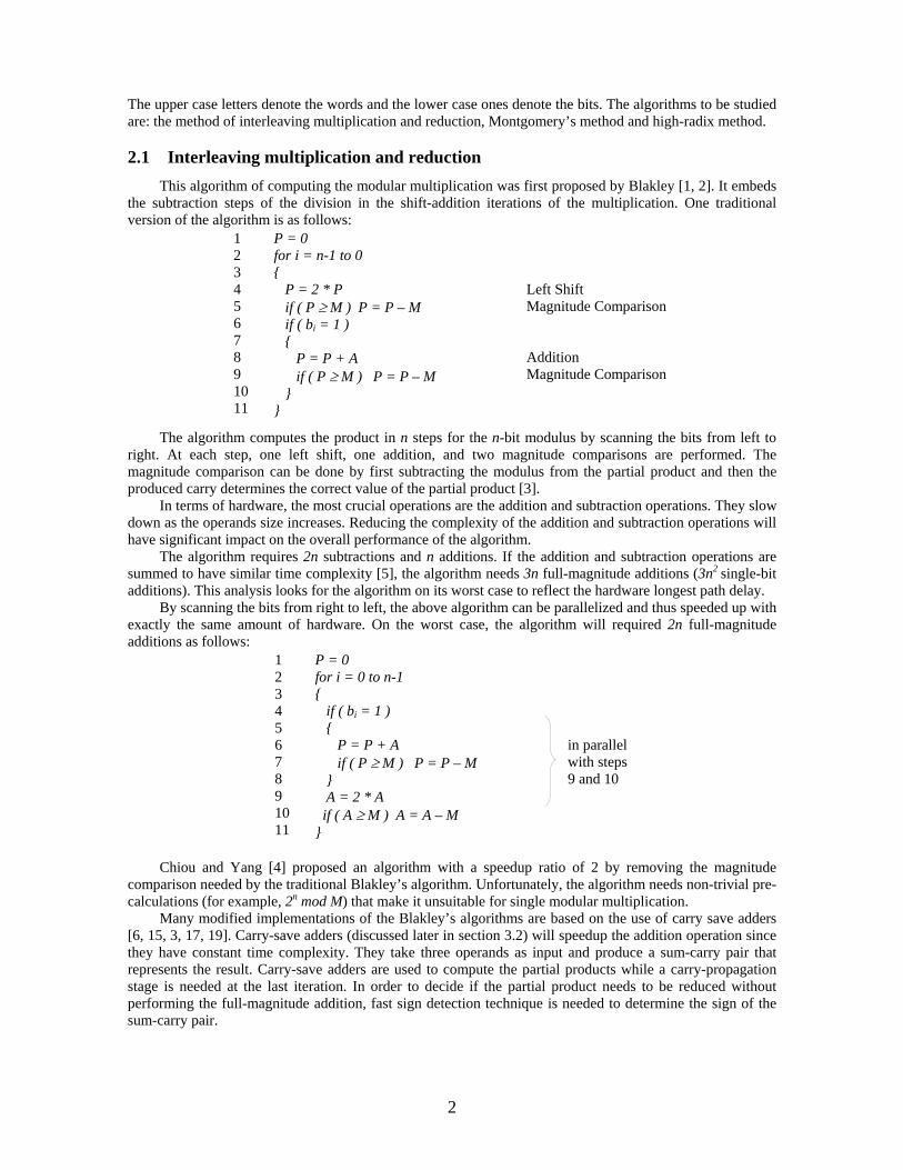
Hardware Analysis of Multiplication Step Koc [6] Montgomery [18]

Logic Two (n+4)-bit carry save adders plus 5-bit carry lookahead logic Two n-bit carry save adders

Registers 6 5 Table 3: Hardware analysis of the multiplication steps of algorithms in [6] and [18].

Synthesis Analysis of Multiplication Step Koc [6] Montgomery [18]

Clock period 6.468 ns 6.342 ns Table 4: Synthesis analysis of the multiplication steps of algorithms in [6] and [18].

The above figures show that the classical method in reference [6] takes slightly larger amount of hardware than the Montgomery’s method in reference [18]. In addition, the multiplication step of the classical method takes slightly more time than Montgomery’s method. Moreover, it has a correction step at the end of the algorithm that will complicate the hardware for the final summation circuit.

However, a full-custom design of the sign-estimation logic needed by the classical method will reduce the latency to its minimum. The carry-save logic and the sign-estimation logic are both of three logic levels. This means that parallel execution of the two logics will take about the same time as one individual carry-save stage. Hence, the multiplication steps of two algorithms are expected to have the same latency.

By considering the pre and post-calculations needed by both algorithms, we see that Montgomery’s method needs much more expensive calculations. Reference [12] shows how practically pre and post-calculations of Montgomery’s method take very long time over the multiplication step. These calculations doubled the amount of time required by Montgomery’s method by more than 20 times. In addition, the hardware was complicated.

Thus, carry save implementations of the classical method of interleaving multiplication and reduction has the potential to be one of the most effective solutions in terms of time and hardware requirements. Further improvements by researchers on the classical method would lead to a high speed modular multiplier which is scalable and regular by its nature.

2.5 Remarks

This section discusses some aspects of Koc’s implementation [6]. The algorithm restricts the magnitude of M to be larger than 2n-1 which reduces the valid range of numbers that M can have. However, this restriction can be relaxed by including more bits in the sign-estimation logic at the cost of increasing the complexity of this logic [6]. However, since A and B should be generally less than M, the desired precision of the sign-estimation logic is not expected to be much apart from 2n-1. This keeps the sign-estimation logic fast and does not add much complexity to it.

The sign-estimation logic produces qM where q could be 1, -1 or 0. Similarly, aiB might produce a zero if ai equals 0. In both cases, when a zero is produced, the carry-save stage can be omitted. However, in the case of aiB, omitting the carry-save logic is not straightforward because of the left shift applied on the sum-carry pair. A small experiment was run to test the frequency of q being equal to 0. Unfortunately, q equals to 1 or -1 most of the time and it equals to 0 only very few times. Thus, time and space overheads introduced by the hardware used to skip the carry-save stage, when it is possible, will most probably overcome the time gained from omitting the carry-save stage. Hence, the modular multiplier is kept in its simplest structure as it was proposed.

2.6 Proposed Improvements This section studies some aspects of Koc’s implementation [6] and suggests improvements on the

original version of the algorithm.

6

2.6.1 Pipelining If each carry-save adder is considered to represent one stage, then this modular multiplier can be

pipelined in two stages. However, due to data dependency, the pipelining will not improve the throughput if not increasing the latency because of the needed latches. However, the pipeline can be used to compute two separate operations simultaneously as follows:

CSA-1

operation: 1

addition: 1

iteration: 1

operation: 2

addition: 1

iteration: 1

operation: 1

addition: 1

iteration: 2

operation: 2

addition: 1

iteration: 2

operation: 1

addition: 1

iteration: 3

CSA-2

operation: 1

addition: 2

iteration: 1

operation: 2

addition: 2

iteration: 1

operation: 1

addition: 2

iteration: 2

operation: 2

addition: 2

iteration: 2

Figure 1: Pipelining two separate multiplication operations.

Figure 2: The core of the multiplier after pipelining.

2.6.2 Parallelizing the correction step

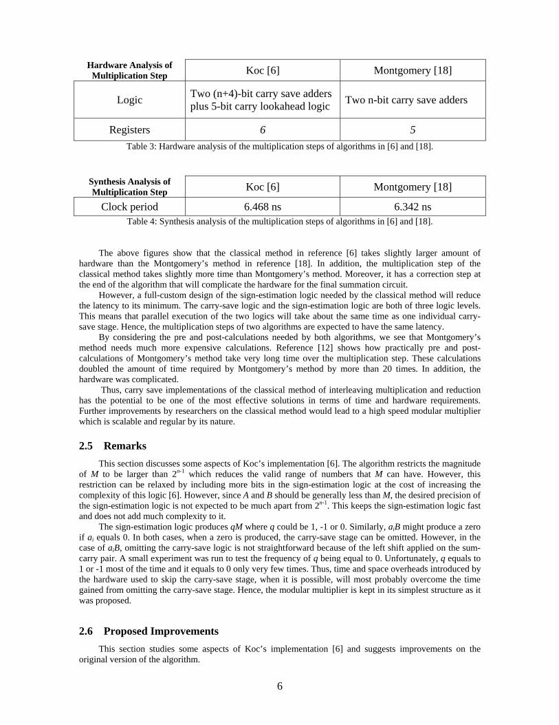
The correction step at the end of the algorithm increases the algorithm complexity. It can be implemented at the software level as well as the hardware level. At the hardware level, the correction step can be done in the last stage of the algorithm through a dedicated logic. The sum-carry pair can be added and if the result is negative, then the result is fed to the adder again with the modulus. The correction step in this case will take 2 log n times. However, the factor can be reduced by computing the two possible results in parallel at the cost of increasing the hardware complexity as shown in Figure 3.

2.6.3 Speedup with high-radix

The total number of clock cycles needed by Koc’s implementation of the classical method of interleaving multiplication with reduction can be reduced using the high-radix method. In a straightforward way, radix-4 modular multiplier may be implemented as shown in Figure 4. (for VHDL coding details, refer to Appendix-B):

7

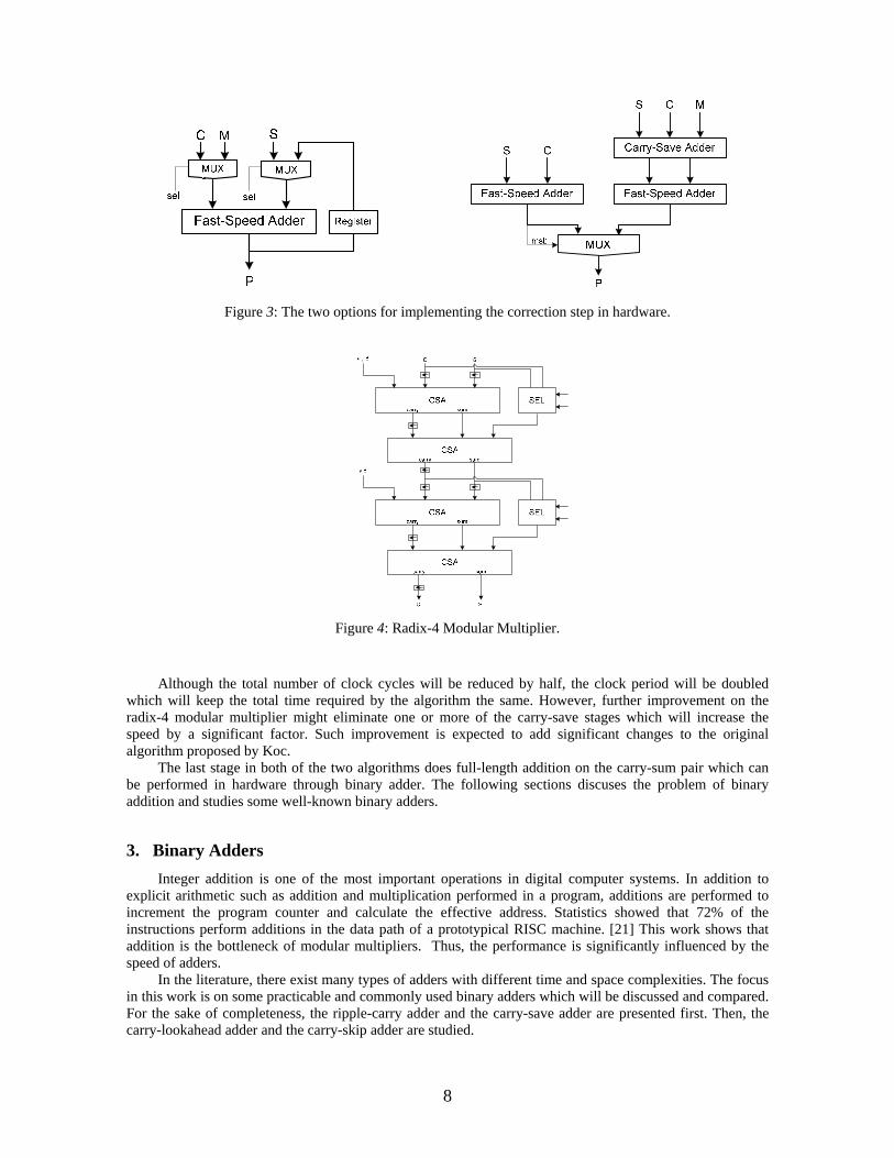
Figure 3: The two options for implementing the correction step in hardware.

Figure 4: Radix-4 Modular Multiplier.

Although the total number of clock cycles will be reduced by half, the clock period will be doubled

which will keep the total time required by the algorithm the same. However, further improvement on the radix-4 modular multiplier might eliminate one or more of the carry-save stages which will increase the speed by a significant factor. Such improvement is expected to add significant changes to the original algorithm proposed by Koc.

The last stage in both of the two algorithms does full-length addition on the carry-sum pair which can be performed in hardware through binary adder. The following sections discuses the problem of binary addition and studies some well-known binary adders.

3. Binary Adders Integer addition is one of the most important operations in digital computer systems. In addition to

explicit arithmetic such as addition and multiplication performed in a program, additions are performed to increment the program counter and calculate the effective address. Statistics showed that 72% of the instructions perform additions in the data path of a prototypical RISC machine. [21] This work shows that addition is the bottleneck of modular multipliers. Thus, the performance is significantly influenced by the speed of adders.

In the literature, there exist many types of adders with different time and space complexities. The focus in this work is on some practicable and commonly used binary adders which will be discussed and compared. For the sake of completeness, the ripple-carry adder and the carry-save adder are presented first. Then, the carry-lookahead adder and the carry-skip adder are studied.

8

3.1 Ripple-Carry Adder (RCA) The ripple-carry adder consists of a sequence of cascaded Full Adders (FA) by which each FA

computes the ith bit of the result according to the following logical relations: si = ai ⊕ bi ⊕ ci , ci+1 = ai bi + (ai + bi) ci , where i = 0, 1, …, n-1

Figure 5: Ripple-Carry Adder Obviously, both the logic complexity and the worst case computation time are Ο(n). The ripple-carry

adder required the optimum space and has the worst computation time among it category of parallel adders. However, the carry propagation process takes on average Ο(log n) time to be completed [5, 22]. The carry-completion sensing adder is an asynchronous adder designed based on this fact.

3.2 Carry-Save Adder (CSA) A carry-save adder adds three n-bit numbers and produces the result without performing carry

propagation by saving the carry. The result will be in an n-bit redundant format represented using two bit vectors, sum and carry. The total delay of a carry-save adder equals to the delay of a single full adder cell. In addition, the carry save adder requires n times the area of a full adder cell. Thus, the carry-save adder takes Ο(1) time and Ο(n) space. A carry-save adder will look as follows:

Figure 6: Carry-Save Adder

According to reference [5], there are basically two disadvantages of the carry-save adders. The carry-save adders do not add two numbers and produce a single output; instead, they add three inputs and produce two outputs such that the sum of the outputs equals to the sum of the inputs. Moreover, the sign-detection is hard. Unless the addition on the outputs is performed in full length, the correct sign of the sum-carry pair may never be determined.

3.3 Carry-Lookahead Adder (CLA) The carry-lookahead scheme computes the sum as follows:

si = ai ⊕ bi ⊕ ci , pi = ai ⊕ bi , gi = ai bi , ci+1 = gi + pi ciBy expanding further the equation of the carry we get:

ci+1 = gi + pi gi-1 + pi pi-1 gi-2 + pi pi-1 … p1 g0 + pi pi-1 … p1 p0 c0 A carry-lookahead adder may look like this:

9

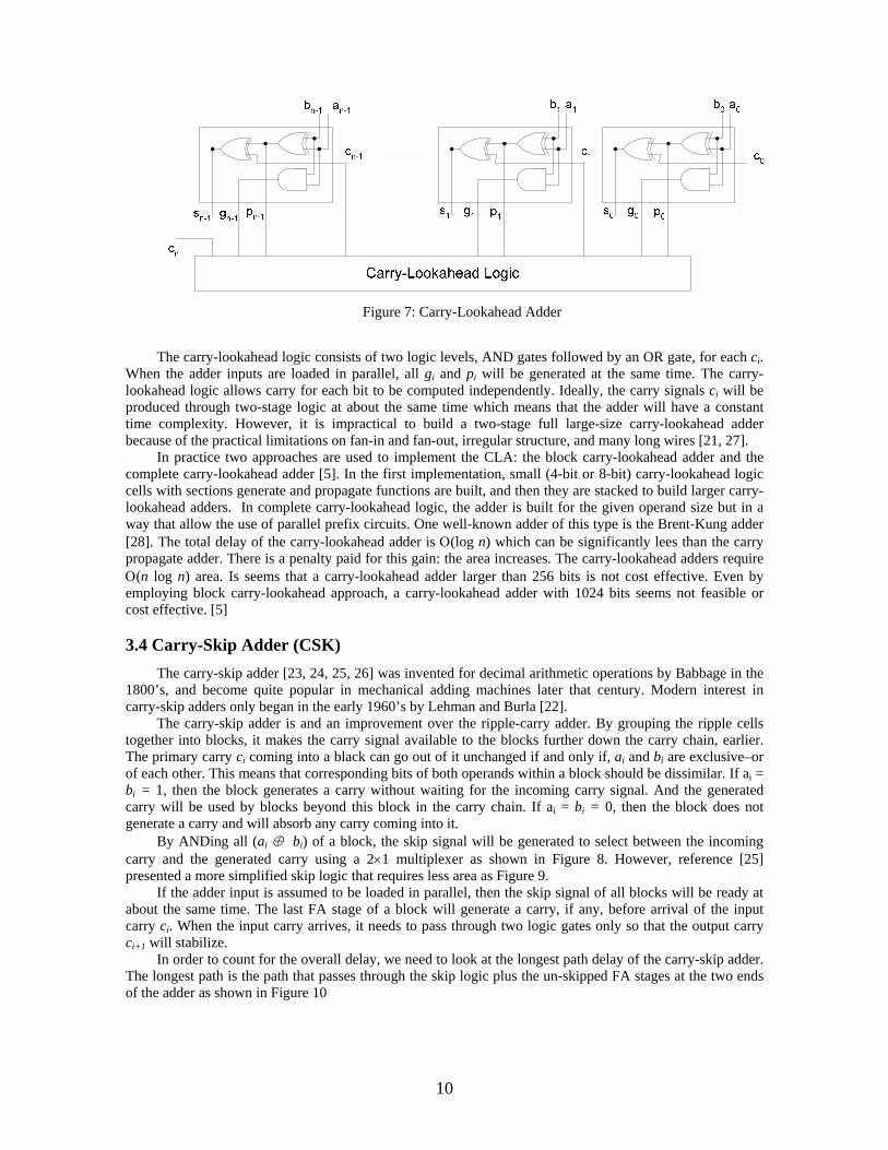
Figure 7: Carry-Lookahead Adder

The carry-lookahead logic consists of two logic levels, AND gates followed by an OR gate, for each ci.

When the adder inputs are loaded in parallel, all gi and pi will be generated at the same time. The carry-lookahead logic allows carry for each bit to be computed independently. Ideally, the carry signals ci will be produced through two-stage logic at about the same time which means that the adder will have a constant time complexity. However, it is impractical to build a two-stage full large-size carry-lookahead adder because of the practical limitations on fan-in and fan-out, irregular structure, and many long wires [21, 27].

In practice two approaches are used to implement the CLA: the block carry-lookahead adder and the complete carry-lookahead adder [5]. In the first implementation, small (4-bit or 8-bit) carry-lookahead logic cells with sections generate and propagate functions are built, and then they are stacked to build larger carry-lookahead adders. In complete carry-lookahead logic, the adder is built for the given operand size but in a way that allow the use of parallel prefix circuits. One well-known adder of this type is the Brent-Kung adder [28]. The total delay of the carry-lookahead adder is Ο(log n) which can be significantly lees than the carry propagate adder. There is a penalty paid for this gain: the area increases. The carry-lookahead adders require Ο(n log n) area. Is seems that a carry-lookahead adder larger than 256 bits is not cost effective. Even by employing block carry-lookahead approach, a carry-lookahead adder with 1024 bits seems not feasible or cost effective. [5]

3.4 Carry-Skip Adder (CSK)

The carry-skip adder [23, 24, 25, 26] was invented for decimal arithmetic operations by Babbage in the 1800’s, and become quite popular in mechanical adding machines later that century. Modern interest in carry-skip adders only began in the early 1960’s by Lehman and Burla [22].

The carry-skip adder is and an improvement over the ripple-carry adder. By grouping the ripple cells together into blocks, it makes the carry signal available to the blocks further down the carry chain, earlier. The primary carry ci coming into a black can go out of it unchanged if and only if, ai and bi are exclusive–or of each other. This means that corresponding bits of both operands within a block should be dissimilar. If ai = bi = 1, then the block generates a carry without waiting for the incoming carry signal. And the generated carry will be used by blocks beyond this block in the carry chain. If ai = bi = 0, then the block does not generate a carry and will absorb any carry coming into it.

By ANDing all (ai ⊕ bi) of a block, the skip signal will be generated to select between the incoming carry and the generated carry using a 2×1 multiplexer as shown in Figure 8. However, reference [25] presented a more simplified skip logic that requires less area as Figure 9.

If the adder input is assumed to be loaded in parallel, then the skip signal of all blocks will be ready at about the same time. The last FA stage of a block will generate a carry, if any, before arrival of the input carry ci. When the input carry arrives, it needs to pass through two logic gates only so that the output carry ci+1 will stabilize.

In order to count for the overall delay, we need to look at the longest path delay of the carry-skip adder. The longest path is the path that passes through the skip logic plus the un-skipped FA stages at the two ends of the adder as shown in Figure 10

10

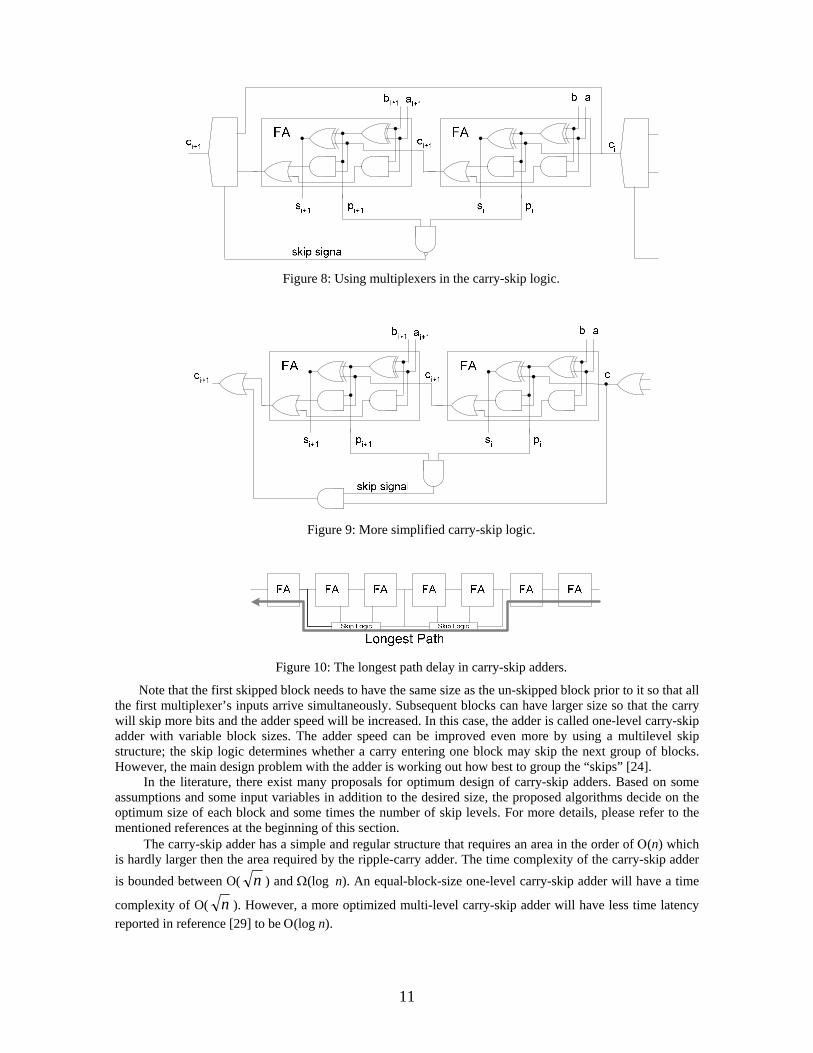
Figure 8: Using multiplexers in the carry-skip logic.

Figure 9: More simplified carry-skip logic.

Figure 10: The longest path delay in carry-skip adders.

Note that the first skipped block needs to have the same size as the un-skipped block prior to it so that all the first multiplexer’s inputs arrive simultaneously. Subsequent blocks can have larger size so that the carry will skip more bits and the adder speed will be increased. In this case, the adder is called one-level carry-skip adder with variable block sizes. The adder speed can be improved even more by using a multilevel skip structure; the skip logic determines whether a carry entering one block may skip the next group of blocks. However, the main design problem with the adder is working out how best to group the “skips” [24].

In the literature, there exist many proposals for optimum design of carry-skip adders. Based on some assumptions and some input variables in addition to the desired size, the proposed algorithms decide on the optimum size of each block and some times the number of skip levels. For more details, please refer to the mentioned references at the beginning of this section.

The carry-skip adder has a simple and regular structure that requires an area in the order of Ο(n) which is hardly larger then the area required by the ripple-carry adder. The time complexity of the carry-skip adder is bounded between O( n ) and Ω(log_n). An equal-block-size one-level carry-skip adder will have a time

complexity of O( n ). However, a more optimized multi-level carry-skip adder will have less time latency reported in reference [29] to be Ο(log n).

11

3.5 Comparison This section compares two fast speed adders described above: the carry-skip adder and carry-lookahead

adder. By relaying on some recently published research, the two adders will be compared in terms of time, area and power.

In order to have a fair comparison, we claim that the adders need to be design at the VLSI level. Using FPGAs to implement and compare both adders will give results that are most probably inconsistent with results obtained from a practical implementation. In addition, it has been shown that optimizing the carry-skip adder is highly dependent on the time delay deference between the skip logic and the propagate logic. Thus, optimizing the carry-skip adder on FPGAs is difficult and may not lead to an optimum time delay. This explains why implementing the carry-skip adder on FPGAs as in reference [30] results in a time delay that is not much better that the delay of the ripple-carry adder.

In reference [29], the two adders were designed using the CMOS technology and compared. A 32-bit carry-skip adder was better than a 32-bit carry-lookahead adder in terms of time, area and power. A carry-skip adder, that has multi-level skip logic, was compared with a conventional carry-lookahead adder. The carry-skip adder was 14 % faster. However, if the adder size is increased to 64 bits, the carry-lookahead adder starts to have slight improvement in time over the carry-skip adder.

The carry-skip adders have the potential for reduced power dissipation because they requires only propagate signals, in contrast with the carry-lookahead adders that require both propagate and generate signals [29]. Moreover, the carry-skip adders require a linear area that is hardly larger then the area required by the ripple-carry adder. This means much lower power consumption than the carry-lookahead adders. Reference [29] reports that the carry-skip adder’s power dissipation was 58 % of that of the carry-lookahead adder.

If one-level carry-skip adder is used, as in reference [27], then 64-bit carry-skip adder is 38% slower than 64-bit carry-lookahead adder. However, the carry-skip adder is still better than the carry-lookahead adder in the average power consumption by 33% and in chip area by 32%.

The results presented here matches with the theoretical analysis presented before. A full-optimized carry-skip adder is comparable in speed with a conventional carry-lookahead adder since they are of the same complexity class, Ο(log n). However, the carry-skip adder is much better than the carry-lookahead adder in terms of area and power consumption.

4. Conclusion This work studied the modular multiplication problem over large operand sizes. Various types of

modular multiplication algorithms have been presented and the time complexities of these algorithms were compared. Two implementations for Montgomery’s method and the method of interleaving multiplication and reduction were modeled using VHDL and synthesized. A time-area analysis of both implementations showed that Koc’s implementation [6] based on carry-save adders of the interleaving method has the potential to be one of the most effective solutions in terms of time and hardware requirements. This implementation was improved further by parallelizing the final correction step of the algorithm. In addition, pipelining was used to compute two separate modular multiplication operations simultaneously. A radix-4 modular multiplier based on Koc’ implementation was proposed, too.

Carry-save adders give the maximum speedup in computing the partial products since they have constant time complexity. However, full-length addition on the sum-carry pair needs to be carried out at the last iteration. This final addition is done through dedicated binary adder. Two binary adders were studied: the carry-lookahead adder and the carry-skip adder. It has been shown that the two adders can be of a comparable speed. However, the carry-skip adders require smaller area and consume much less power than the carry-lookahead adders.

References

[1] Blakley, G. R.: ‘A Computer Algorithm for Calculating the Product A*B modulo M’, IEEE Transactions on Computers, 32(5): 497-500, May 1983. [2] Sloan, K. R.: ‘Comments on: ‘A Computer Algorithm for Calculating the Product A*B modulo M”, IEEE Transactions on Computers, 34(3), 1985. [3] C. K. Koc and C. Y. Hung: ‘Multi-operand modulo addition using carry save adders’, Electronics Letters, 26(6): 361-363, 1990.

12

[4] Chiou, C. W. and T. C. Yang, ‘Iterative Modular Multiplication Without Magnitude Comparison’, Electronics Letters 30(24): 2017-2018, 1994. [5] Koc, C. K.: ‘RSA Hardware Implementation’, RSA Laboratories, RSA Data Security, Inc. 1996. [6] Koc, C. K. and C. Y. Hung, ‘Fast Algorithm For Modular Rreduction’, IEE Proceedings: Computers and Digital Techniques, 145(4): 265-271, 1998. [7] Montgomery, P. L.: ‘Modular Multiplication Without Trial Division’, Mathematical Computation, 44: 519-521, 1985. [8] Walter, C. D.: ‘Montgomery Exponentiation Needs no Final Subtractions’, Electronics Letters, 35(21): 1831-1832, 1999. [9] Daly , Alan and William Marnane: ‘Efficient Architectures for implementing Montgomery Modular Multiplication and RSA Modular Exponentiation on Reconfigurable Logic’, International Symposium on Field Programmable Gate Arrays, 2002. [10] Nedjah Nadia and Luiza Mourelle: ‘Two Hardware Implementations for the Montgomery Modular Multiplication: Sequential versus Parallel’, 15th Symposium on Integrated Circuits and Systems Design, 2002. [11] Wang, Jhing-Fa, Po-Chuan Lin and Ping-Kun Chiu: ‘A Staged Carry-Save-Adder Array for Montgomery Modular Multiplication’, AP-ASIC 2002, 2002. [12] Satoh, Akashi and Kohji Takano: ‘A Scalable Dual-Field Elliptic Curve Cryptographic Processor’, IEEE Transactions on Computers, 52(4): 449-460, 2003. [13] Walter, C. D.: ‘Space/Time Trade-Offs for Higher Radix Modular Multiplication Using Repeated Addition’, IEEE Transactions on Computers, 46(2): pp. 139-141, 1997. [14] Walter, C. D.: ‘Logarithmic Speed Modular Multiplication’, Electronics Letters 30(17): pp. 1397-8, 1994. [15] Koc, C. K. and C. Y. Hung: ’ Carry save adders for computing the product AB modulo N’, Electronics Letters, 26(13): pp. 899-900, 1990. [16] Shuguo, Li and others: ‘Fast modular multiplication with carry save adder’, Proceedings of 4th International Conference on ASIC, pp. 360 –363, 2001. [17] Zhang, C. N., Shirazi, B.and Yun, D. Y.: ‘Parallel designs for Chinese remainder conversion’, Proceedings of the International Conference on Parallel Processing, pp. 557-559, 1987. [18] Kwon, Taek-Won and others: ‘Two Implementation Methods of a 1024-bit RSA Cryptoprocessor Based on Modified Montgomery Algorithm’. IEEE International Symposium On Circuits and Systems (ISCAS), pp. 650–653,2001. [19] Mekhallalati, M. C., M. K. Ibrahim and A. S. Ashur: ‘Radix Modular Multiplication Algorithm’, Journal of Circuits and Systems, and Computers, .6(5): pp. 547-567, 1996. [20] Bajard, J. C., L. S. Didier and Peter Kornerup: ‘Modular Multiplication and Base Extensions in Residue Number System’, Proceedings of the 15th IEEE Symposium on Computer Arithmetic, pp. 59 –65, 2001. [21] Cheng, Fu-Chiung, Stephen H. Unger and Michael Theobald: ‘Self-Timed Carry-Lookahead Adders’, IEEE Transactions on Computers, 49(7):. 659-672, 2000. [22] Lehman, M. and N. Burla: ‘Skip Technique for High Speed Carry Propagation in Binary Arithmetic Unites’, IRE Transactions on Electronic Computers, 10: 691-698, 1961. [23] Kantabutra, Vitit: ‘Designing Optimum One-LevelCarry-Skip Adders’, IEEE Transactions on Computers, 42(6):759--764, June 1993. [24] Burges, Neil: ‘Accelerated Carry-Skip Adders with Low Hardware Cost’, Conference on Signals, Systems and Computers, 1: 852 -856, 2001. Goel, A. K. and P. S. Bapat: ‘A New Time-Position Algorithm for the Modeling of Multilevel Carry Skip Adders in VHDL’, Proceedings: 1996 Canadian Conference on Electrical and Computer Engineering, pp. 158-61, 1996. [25] Turrini, Silvio: ‘Optimal Group Distribution in Carry-Skip Adders’, WRL Research Report 89/2, February 1989. [26] Nagendra, C., M. J. Irwin and R. M. Owens: ‘Area Time Power Tradeoffs in Parallel Adders’, IEEE Transactions on Circuits and Systems 43(10):689-702, 1996. [27] Brent R. P. and H. T. Kung: ‘A Regular Layout for Parallel Adders’, IEEE Transactions on Computers, C-31:260—264, 1982. [28] Gayles, Eric S., R. M. Owens and M. J. Irwin: ‘Low Power Circuit Techniques for Fast Carry Skip Adders’ Proceedings of 1996 Midwest Symposium. On Circuits and Systems, pp. 87-90, Aug. 1996. [29] Xing , Shanzhen and Willlam W. Yu: ‘FPGA Adders: Performance Evaluation and Optimal Design’, IEEE Design & Test OF Computers, pp. 24-29, Jan–March 1998.

13