
State feedback stabilization of linear time-varying systems on time scales

Chapter 3Performance-Information Analysisand Distributed Feedback Stabilizationin Large-Scale Interconnected Systems
Khanh D. Pham
Summary Large-scale interconnected systems are characterized as large and com-plex systems divided into several smaller autonomous systems that have certain au-tonomy in local optimization and decision-making. As an example, a class of in-terconnected linear stochastic systems, where no constituent systems need to haveglobal information and distributed decision making enables autonomous systems todynamically reconfigure risk-value aware performance indices for uncertain envi-ronmental conditions, is considered in the subject research. Among the many chal-lenges in distributed and intelligent control of interconnected autonomous systemsis performance uncertainty analysis and decentralized feedback stabilization. Thetheme of the proposed research is the interplay between performance-informationdynamics and decentralized feedback stabilization, both providing the foundationsfor distributed and autonomous decision making. First, recent work by the author inwhich performance information availability was used to assess limits of achievableperformance will be extended to give insight into how different aggregation struc-tures and probabilistic knowledge of random decision processes between networksof autonomous systems are exploited to derive a distributed computation of com-plete distributions of performance for interconnected autonomous systems. Second,the resulting information statistics on performance of interconnected autonomoussystems will be leveraged in the design of decentralized output-feedback stabiliza-tion, thus enabling distributed autonomous systems to operate resiliently in uncer-tain environments with performance guarantees that are now more robust than thetraditional performance average.
3.1 Introduction
The research under investigation is adaptive control decisions of interconnected sys-tems in stochastic and dynamic environments. The central subject matter of the
K.D. Pham (�)Space Vehicles Directorate, Air Force Research Laboratory, Kirtland Air Force Base, NM 87117,USAe-mail: [email protected]
M.J. Hirsch et al. (eds.), Dynamics of Information Systems,Springer Optimization and Its Applications 40, DOI 10.1007/978-1-4419-5689-7_3,© Springer Science+Business Media, LLC 2010
45

46 K.D. Pham
Fig. 3.1 An architecture forrisk-averse based large-scaleinterconnected systems
chapter is focused on two related perspectives: the performance-information analy-sis perspective and the distributed feedback stabilization perspective. These seem tobe the two dominant perspectives in stochastic control of large-scale interconnectedsystems. Specifically, the following two problems are associated with adaptive con-trol decision. The first is the problem of designing a performance-information sys-tem that can motivate and screen appropriate adaptive control decision by an inter-connected system in charge of local operation in a stochastic and dynamic environ-ment. The second is the problem of emphasizing the importance of adaptive controldecision in stochastic control under environmental uncertainty and exploring thecharacteristics of an interconnected system conducive to adaptive control decisionby the autonomous system to whom operating authority is delegated.
What framework can be used to view that process in distributed stabilization forlarge-scale interconnected systems? To be useful, perhaps, such a framework mustbe simple, but at the same time it must be comprehensive enough that most of theessential elements of a distributed control process can be discussed. The controlprocess envisaged here is a dynamic process surrounding performance assessment,feedback and corrective action. Diagrammatically, the entire relationship may bedepicted as shown in Fig. 3.1. Each autonomous system has some goal in termsof the performance riskiness of the operating process it has to control. The perfor-mance uncertainty is affected not only by the control decision or action but alsoby the environment in which the system (the local control decision and the localoperating process) must operate. The basic reason for the existence of control deci-sion is uncertainty or incomplete knowledge on the part of the decision policy about(1) the mechanism of the operating process and (2) the environmental conditions

3 Performance-Information Analysis and Distributed Feedback Stabilization 47
that should prevail at any point in time. In this diagram, each interconnected systemrecognizes the need for action in congruence with the expected standard of per-formance, e.g., risk aversion for performance against all random realizations fromenvironmental disturbances is considered herein. The autonomous system will usethe standard as a guideline to determine whether its action is called for or not. Itsrecognition comes as a result of filtering feedback information through some criteriasuch as risk modeling and risk measures for making judgment.
From this point of view, all respective measures of performance for intercon-nected systems are viewed as random variables with mixed random realizationsfrom their own uncertain environments. Information about the states of environ-ments is assumed to be common knowledge. Furthermore, it is assumed here thateach interconnected system will choose control decisions which will be best forits own utility, whether it is an internalized goal of either (1) performance prob-ing via an effective knowledge construct that can be able to extract the knowledgeof higher-order characteristics of performance distribution; (2) performance cautionthat mitigates performance riskiness with multiple attributes beyond performanceaveraging as such variance, skewness, flatness, etc., just to name a few; or (3) both.The final process execution has only one category of factors. It is the implementationof a risk-averse decision strategy where explicit recognition of performance uncer-tainty brings to what constitutes a “good” decision by the interconnected system.To the best of the author’s knowledge, the problem of performance risk congruencehas not attracted much academic or practical attention in stochastic multi-agent sys-tems until very recently [8, 9] and [10]. Failure to recognize the problem may notbe harmful in many operating decision situations when alternative courses of ac-tion may not differ very much in their risk characteristics. But in cases of importantand indispensable consideration in reliability-based design [3] and incorporation ofaversion to specification uncertainty [5], which may involve much uncertainty andalternatives whose risk characteristics are wide ranged, consideration of the inter-connected system’s goal toward risk may be a crucial factor in designing a highperformance system.
The chapter is organized as follows. Section 3.2 puts the distributed controlof adaptive control decisions for interconnected systems in uncertain environ-ments into a consistent mathematical framework. In Sect. 3.3, the performance-information analysis is a focal point for adaptive control decisions of interconnectedsystems. The methodological characteristics of moment and cumulant generatingmodels are used to characterize the uncertainty of performance information withrespect to uncertain environments. Some interesting insights into how the value ofperformance information are affected by changes in the attributes of a performance-information system. Section 3.4 will develop a distributed feedback stabilization fora large-scale interconnected system with adaptive control decision using the recentstatistical control development. Another main feature of this section is the explo-ration of risk and preference for a stochastic control system. A generalization ofperformance evaluation is suggested. The risk of a performance measure is express-ible as a linear combination of the associated higher-order statistics. From Sect. 3.5,construction of a candidate function for the value function and the calculation of
48 K.D. Pham
decentralized efficient risk-averse decision strategies accounting for multiple at-tributes of performance robustness are discussed. Finally, some concluding remarksare drawn in Sect. 3.6. These final remarks will help put the novelty of this researchin perspectives of distributed control and performance-information analysis.
3.2 Problem Formulation
Before going into a formal presentation, it is necessary to consider some conceptualnotations. To be specific, for a given Hilbert space X with norm ‖ · ‖X , 1 ≤ p ≤ ∞and a, b ∈ R such that a ≤ b, a Banach space is defined as follows
Lp
F (a, b;X)
�{
φ(·) = {φ(t,ω) : a ≤ t ≤ b
}such that φ(·) is an X-valued
Ft -measurable process on [a, b] with E
{∫ b
a
∥∥φ(t,ω)∥∥p
Xdt
}< ∞
}(3.1)
with norm
∥∥φ(·)∥∥F ,p�
(E
{∫ b
a
∥∥φ(t,ω)∥∥p
Xdt
})1/p
(3.2)
where the elements ω of the filtered sigma field Ft of a sample description spaceΩ that is adapted for the time horizon [a, b] are random outcomes or events. Also,the Banach space of X-valued continuous functionals on [a, b] with the max-norminduced by ‖ · ‖X is denoted by C(a, b;X). The deterministic version of (3.1) andits associated norm (3.2) is written as Lp(a, b;X) and ‖ · ‖p .
More specifically, consider a network of N interconnected systems, or equiva-lently, agents numbered from 1 through N . Each agent i, for i ∈ N � {1,2, . . . ,N}operates within its local environment modeled by the corresponding filtered proba-bility space (Ωi, Fi , {Fi}t≥t0>0, Pi ) that is defined with a stationary pi -dimensionalWiener process wi(t) � wi(t,ωi) : [t0, tf ] × Ωi �→ R
pi on a finite horizon [t0, tf ]and the correlation of independent increments
E{[
wi(τ) − wi(ξ)][
wi(τ) − wi(ξ)]T } = Wi |τ − ξ |, Wi > 0
Assume that agent i generates and maintains its own states based on informationconcerning its neighboring agents and local environment. The update rule of agenti evolves according to a simple nearest-neighbor model
dxi(t) = (Ai(t)xi(t) + Bi(t)ui(t) + Ci(t)zi(t) + Ei(t)di(t)
)dt
+ Gi(t) dwi(t)
xi(t0) = x0i
(3.3)

3 Performance-Information Analysis and Distributed Feedback Stabilization 49
where all the coefficients Ai ∈ C(t0, tf ;Rni×ni ), Bi ∈ C(t0, tf ;R
ni×mi ), Ci ∈C(t0, tf ;R
ni×qi ), Ei ∈ C(t0, tf ;Rni×ri ), and Gi ∈ C(t0, tf ;R
ni×pi ) are deter-ministic matrix-valued functions. Furthermore, it should be noted that xi ∈L2
Fi(t0, tf ;R
ni ) is the ni -dimensional state of agent i with the initial state x0i ∈ R
ni
fixed, ui ∈ L2Fi
(t0, tf ;Rmi ) is the mi -dimensional control decision, and di ∈
L2(t0, tf ;Rri ) is the ri -dimensional known disturbance.
In the formulation the actual interaction, zi ∈ L2Fi
(t0, tf ;Rqi ) represented by the
qi -dimensional process is of interest to agent i where Lij represent time-varyinginteraction gains associated with its neighboring agents
zi(t) =N∑
j=1,j =i
Lij (t)xij (t), i ∈ N (3.4)
For practical purposes, the process zi is however not available at the level of agent i.It is then desired to have decentralized decision making without intensive commu-nication exchanges. An approach of interaction prediction is therefore proposed toresolve the communication difficulty by means of a crude model of reduced orderfor the interactions among the neighboring agents that can exchange informationwith agent i. In this work, the actual interaction zi(·) is now approximated by anexplicit model of the type
dzmi(t) = (Azi(t)zmi(t) + Ezi(t)dmi(t)
)dt + Gzi(t) dwmi(t), zmi(t0) = 0
(3.5)
where Azi ∈ C(t0, tf ;Rqi×qi ) is an arbitrary deterministic matrix-valued function
which describes a crude model for the actual interaction zi(·). In particular, Azi
can be chosen to be the off-diagonal block of the global matrix coefficient A corre-sponding the partition vector zi(·). Other coefficients Ezi ∈ C(t0, tf ;R
qi×rmi ) andGzi ∈ C(t0, tf ;R
qi×pmi ) are deterministic matrix-valued functions of the stochas-tic differential equation (3.5). The approximate interaction zmi(·) produced by themodel is affected not only by the known disturbance dmi ∈ L2(t0, tf ;R
rmi ) but alsoby another local uncertainty wmi(t) � wmi(t,ωmi) : [t0, tf ]×Ωmi �→ R
pmi which isan pmi -dimensional stationary Wiener process defined on a complete filtered prob-ability space (Ωmi, Fmi, {Fmi}t≥t0>0, Pmi) over [t0, tf ] with the correlation of in-dependent increments
E{[
wmi(τ ) − wmi(ξ)][
wmi(τ ) − wmi(ξ)]T }
= Wmi|τ − ξ |, Wmi > 0
With the approach considered here, there is a need to treat the actual interaction zi(·)as a control process that is supposed to follow the approximate interaction processzmi(·). Thus, this requirement leads to certain classes of admissible control laws as-sociated with (3.3) to be denoted by Ui ×Zi ⊂ L2
Fi(t0, tf ;R
mi )×L2Fmi
(t0, tf ;Rqi ),
e.g., given (ui(·), zi(·)) ∈ Ui × Zi , the 3-tuple (xi(·), ui(·), zi(·)) shall be referredto as an admissible 3-tuple if xi(·) ∈ L2
Fi(t0, tf ;R
ni ) is a solution of the stochastic

50 K.D. Pham
differential equation (3.3) associated with ui(·) ∈ Ui and zi(·) ∈ Zi . Furthermore,the nearest neighbor model of local dynamics (3.3) in the absence of its known dis-turbances and local environment is assumed to be uniformly exponentially stable.That is, there exist positive constants η1 and η2 such that the pointwise matrix normof the closed-loop state transition matrix associated with the local dynamical model(3.3) satisfies the inequality
∥∥Φi(t, τ )∥∥ ≤ η1e
−η2(t−τ) ∀t ≥ τ ≥ t0
The pair (Ai(t), [Bi(t),Ci(t)]) is pointwise stabilizable if there exist boundedmatrix-valued functions Ki(t) and Kzi(t) so that the closed-loop system dx(t) =(Ai(t) + Bi(t)Ki(t) + Ci(t)Kzi(t))xi(t) dt is uniformly exponentially stable.
Under the assumptions of xi(t0) ∈ Rni , zmi(t0) ∈ R
qi , ui(·) ∈ Ui , and zi(·) ∈Zi , there are tradeoffs among the closeness of the local states from desired states,the size of the local control levels, and the size of local interaction approximates.Therefore, agent i has to carefully balance the three to achieve its local performance.Stated mathematically, there exists an integral-quadratic form (IQF) performancemeasure Ji : R
ni × Rqi × Ui × Zi �→ R
Ji
(x0i , z0
mi;ui(·), zi(·))
= xTi (tf )Q
fi xi(tf ) +
∫ tf
t0
[xTi (τ )Qi(τ )xi(τ ) + uT
i (τ )Ri(τ )ui(τ )
+ (zi(τ ) − zmi(τ )
)TRzi(τ )
(zi(τ ) − zmi(τ )
)]dτ (3.6)
associated with agent i wherein Qfi ∈ R
ni×ni , Qi ∈ C(t0, tf ;Rni×ni ), Ri ∈
C(t0, tf ;Rmi×mi ), and Rzi ∈ C(t0, tf ;R
qi×qi ) representing relative weightings forterminal states, transient states, decision levels, and interaction mismatches are de-terministic and positive semidefinite with Ri(t) and Rzi(t) invertible.
The description of the framework continues with yet another collection of ran-dom processes {yi(t)}Ni=1 that carry critical information about, for instance, theagents’ states and their underlying dynamic structures, e.g.,
dyi(t) = Hi(t)xi(t) dt + dvi(t), i ∈ N (3.7)
which is a causal function of the local process xi(t) corrupted by another stationarysi -dimensional Wiener process vi(t) � vi(t,ωi) : [t0, tf ] × Ωi �→ R
si on a finitehorizon [t0, tf ] and the correlation of independent increments
E{[
vi(τ ) − vi(ξ)][
vi(τ ) − vi(ξ)]T } = Vi |τ − ξ |, Vi > 0
Within the chosen framework for decentralized decision making, each agent is fur-ther supposed to estimate its evolving process that depends on both its own localmeasurements and interaction approximates from other agents. Given observationsyi(τ ), t0 ≤ τ ≤ t , the state estimate at agent i is denoted by xi (t). Further, the stateestimate error covariance matrix of the state estimation error xi (t) � xi(t) − xi(t)
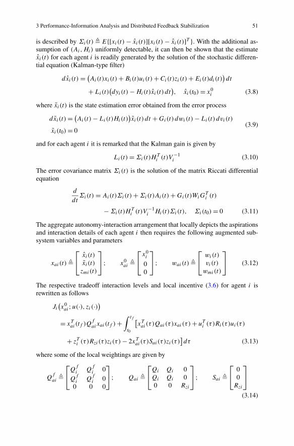
3 Performance-Information Analysis and Distributed Feedback Stabilization 51
is described by Σi(t) � E{[xi(t) − xi (t)][xi(t) − xi (t)]T }. With the additional as-sumption of (Ai,Hi) uniformly detectable, it can then be shown that the estimatexi (t) for each agent i is readily generated by the solution of the stochastic differen-tial equation (Kalman-type filter)
dxi(t) = (Ai(t)xi(t) + Bi(t)ui(t) + Ci(t)zi(t) + Ei(t)di(t)
)dt
+ Li(t)(dyi(t) − Hi(t)xi (t) dt
), xi (t0) = x0
i (3.8)
where xi (t) is the state estimation error obtained from the error process
dxi(t) = (Ai(t) − Li(t)Hi(t)
)xi (t) dt + Gi(t) dwi(t) − Li(t) dvi(t)
xi(t0) = 0(3.9)
and for each agent i it is remarked that the Kalman gain is given by
Li(t) = Σi(t)HTi (t)V −1
i (3.10)
The error covariance matrix Σi(t) is the solution of the matrix Riccati differentialequation
d
dtΣi(t) = Ai(t)Σi(t) + Σi(t)Ai(t) + Gi(t)WiG
Ti (t)
− Σi(t)HTi (t)V −1
i Hi(t)Σi(t), Σi(t0) = 0 (3.11)
The aggregate autonomy-interaction arrangement that locally depicts the aspirationsand interaction details of each agent i then requires the following augmented sub-system variables and parameters
xai(t) �
⎡⎣
xi(t)
xi(t)
zmi(t)
⎤⎦ ; x0
ai �
⎡⎣
x0i
00
⎤⎦ ; wai(t) �
⎡⎣
wi(t)
vi(t)
wmi(t)
⎤⎦ (3.12)
The respective tradeoff interaction levels and local incentive (3.6) for agent i isrewritten as follows
Ji
(x0ai;u(·), zi(·)
)
= xTai(tf )Q
faixai(tf ) +
∫ tf
t0
[xTai(τ )Qai(τ )xai(τ ) + uT
i (τ )Ri(τ )ui(τ )
+ zTi (τ )Rzi(τ )zi(τ ) − 2xT
ai(τ )Sai(τ )zi(τ )]dτ (3.13)
where some of the local weightings are given by
Qfai �
⎡⎣
Qfi Q
fi 0
Qfi Q
fi 0
0 0 0
⎤⎦ ; Qai �
⎡⎣
Qi Qi 0Qi Qi 00 0 Rzi
⎤⎦ ; Sai �
⎡⎣
00
Rzi
⎤⎦
(3.14)

52 K.D. Pham
Fig. 3.2 Risk-averse controlprocess: performance-information analysis andrisk-averse decision policies
subject to the local dynamics for strategic relations
dxai(t) = (Aai(t)xai(t) + Bai(t)ui(t) + Cai(t)zi(t) + Dai(t)
)dt
+ Gai(t)dwai(t)
xai(t0) = x0ai
(3.15)
with the corresponding system parameters
Aai �
⎡⎣
Ai LiHi 00 Ai − LiHi 00 0 Azi
⎤⎦ ; Bai �
⎡⎣
Bi
00
⎤⎦ ; Cai �
⎡⎣
Ci
00
⎤⎦ (3.16)
Dai �
⎡⎣
Eidi
0Ezidmi
⎤⎦ ; Gai �
⎡⎣
0 Li 0Gi −Li 00 0 Gzi
⎤⎦ ; Wai �
⎡⎣
Wi 0 00 Vi 00 0 Wmi
⎤⎦
(3.17)
Thus, far only the structure and the circumstantial setting of a large-scale intercon-nected system have been made clear. The next task is a discussion of a risk-aversecontrol process which can be divided into two phases: (1) performance-informationanalysis and (2) risk-averse decision policy. The essence of these phases is, in asense, the setting of a standard. Standards in performance-information analysis pro-vide a yardstick of performance evaluation and standards in risk-averse decisionpolicy phase communicate and coordinate acceptable levels of risk aversion effortsto the interconnected systems. Essentially, Fig. 3.2 shows a model of the standardsin a risk-averse control system serving two purposes: (1) as targets for the intercon-nected systems to strive for and (2) as an evaluation yardstick.
3.3 Performance-Information Analysis
Performance-information analysis affects the consequence factor to agent i at twolevels. First, it specifies the variable of performance measure to be looked at and thusdetermines an important element in the consequence of control decision at agent i.Second, performance risk analysis implies the existence of standards of compari-son for the performance variables specified. This implies that some notions of riskmodeling and measures for which standards have great significance may be in need.

3 Performance-Information Analysis and Distributed Feedback Stabilization 53
As a basic analytical construct, it is important to recognize that, within the viewof the linear-quadratic structure (3.15) and (3.13), the performance measure (3.13)for agent i is clearly a random variable with Chi-squared type. Hence, the degreeof uncertainty of (3.13) must be assessed via a complete set of higher-order perfor-mance statistics beyond the statistical averaging. The essence of information aboutthe states of performance uncertainty regards as a source of information flow whichwill affect agent i’s perception of the problem and the environment. More specifi-cally, for agent i, first and second characteristic functions of the Chi-squared randomvariable (3.13), denoted respectively, by ϕi(s, x
sai ) and ψi(s, x
sai ) which are utilized
to provide a conceptual framework for evaluation of performance information, aregiven by
ϕi
(s, xs
ai; θi
)� E
{eθiJi (s,x
sai
)}
(3.18)
ψi
(s, xs
ai; θi
)� ln
{ϕi
(s, xs
ai; θi
)}(3.19)
where small parameter θi is in an open interval about 0 for the information sys-tems ϕi(s, x
sai) and ψi(s, x
sai) whereas the initial condition, (t0, x
0ai) is now param-
eterized as the running condition, (s, xsai ) with s ∈ [t0, tf ] and xs
ai � xai(s). Fromthe definition, there are three factors as the determinants of the value of perfor-mance information: (i) the characteristics of the set of actions; (ii) the characteris-tics of consequence of alternatives; and (iii) the characteristics of the utility func-tion.
The first factor relates to the action set, denoted by Ui via state-estimate feed-back strategies to maintain a fair degree of accuracy on each agent behaviors andthe corresponding utility. Since the significance of (3.15) and (3.13) is the linear-quadratic nature, the actions of agent i should therefore be causal functions ofthe local process xi (t). The restriction of decision strategy spaces can be justi-fied by the assumption that agent i participates in the large-scale decision mak-ing where it only has access to the current time and local state estimates of theinteraction. Thus, it amounts to considering only those feedback strategies whichpermit linear feedback syntheses γi : [t0, tf ] × L2
Fi(t0, tf ;R
ni ) �→ L2Fi
(t0, tf ;Rmi )
and γ zi : [t0, tf ] × L2
Fi(t0, tf ;R
ni ) �→ L2Fi
(t0, tf ;Rqi )
ui(t) = γi
(t, xi (t)
)� Ki(t)xi (t) + pi(t) (3.20)
zi(t) = γ zi
(t, xi(t)
)� Kzi(t)xi (t) + pzi(t) (3.21)
where matrix-valued gains Ki ∈ C(t0, tf ;Rmi×ni ) and Kzi ∈ C(t0, tf ;R
qi×ni ) to-gether with vector-valued affine pi ∈ C(t0, tf ;R
mi ) and pzi ∈ C(t0, tf ;Rqi ) will be
appropriately defined, respectively.The importance of the second factor comes from the consequence of actions,
denoted by the outcome function which maps the triplets of outcomes, actions and
54 K.D. Pham
random realizations of the underlying stochastic process into outcomes, e.g.,
dxai(t) = (Fai(t)xai(t) + Bai(t)pi(t) + Cai(t)pzi(t) + Dai(t)
)dt
+ Gai(t) dwai(t)
xai(s) = xsai
(3.22)
where the time-continuous composite state matrix, Fai is given by
Fai �
⎡⎣
Ai + BiKi + CiKzi LiHi 00 Ai − LiHi 00 0 Azi
⎤⎦
The characteristics of the utility function Ji(s, xsai) which maps outcomes into utility
levels can be influenced the value of performance information in various ways, e.g.,
Ji(s, xsai) = xT
ai(tf )Qfaixai(tf ) +
∫ tf
s
[xTai(τ )Nai(τ )xai(τ ) + 2xT
ai(τ )Oai(τ )]dτ
+∫ tf
s
[pT
i (τ )Ri(τ )pi(τ ) + pTzi(τ )Rzi(τ )pzi(τ )
]dτ (3.23)
where
Nai �
⎡⎣
Qi + KTi RiKi + KT
ziRziKzi Qi 0Qi Qi 0
−2RziKzi 0 Rzi
⎤⎦
Oai �
⎡⎣
KTi Ripi + KT
ziRzipzi
0−Rzipzi
⎤⎦
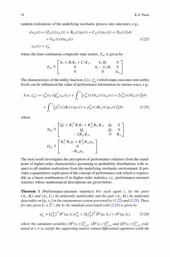
The next result investigates the perception of performance riskiness from the stand-point of higher-order characteristics pertaining to probability distributions with re-spect to all random realizations from the underlying stochastic environment. It pro-vides a quantitative explication of the concept of performance risk which is express-ible as a linear combination of its higher-order statistics, i.e., performance-measurestatistics whose mathematical descriptions are given below.
Theorem 1 (Performance-measure statistics) For each agent i, let the pairs(Ai,Bi) and (Ai,Ci) be uniformly stabilizable and the pair (Ai,Hi) be uniformlydetectable on [t0, tf ] in the autonomous system governed by (3.22) and (3.23). Then,for any given ki ∈ Z
+, the ki -th cumulant associated with (3.23) is given by
κiki
= (x0
ai
)TH i(t0, ki)x
0ai + 2
(x0ai
)TDi(t0, ki) + Di(t0, ki) (3.24)
where the cumulant variables {Hi(s, r)}ki
r=1, {Di(s, r)}ki
r=1 and {Di(s, r)}ki
r=1 eval-uated at s = t0 satisfy the supporting matrix-valued differential equations (with the
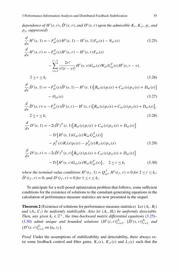
3 Performance-Information Analysis and Distributed Feedback Stabilization 55
dependence of Hi(s, r), Di(s, r), and Di(s, r) upon the admissible Ki , Kzi , pi , andpzi suppressed)
d
dsH i(s,1) = −FT
ai(s)Hi(s,1) − Hi(s,1)Fai(s) − Nai(s) (3.25)
d
dsH i(s, r) = −FT
ai(s)Hi(s, r) − Hi(s, r)Fai(s)
−r−1∑v=1
2r!v!(r − v)!H
i(s, v)Gai(s)WaiGTai(s)H
i(s, r − v),
2 ≤ r ≤ ki (3.26)
d
dsDi(s,1) = −FT
ai(s)Di (s,1) − Hi(s,1)
[Bai(s)pi(s) + Cai(s)pzi(s) + Dai(s)
]
− Oai(s) (3.27)
d
dsDi(s, r) = −FT
ai(s)Di(s, r)−Hi(s, r)
[Bai(s)pi(s)+Cai(s)pzi(s)+Dai(s)
],
2 ≤ r ≤ ki (3.28)
d
dsDi(s,1) = −2(Di)T (s,1)
[Bai(s)pi(s) + Cai(s)pzi(s) + Dai(s)
]
− Tr{Hi(s,1)Gai(s)WaiG
Tai(s)
}
− pTi (s)Ri(s)pi(s) − pT
zi(s)Rzi(s)pzi(s) (3.29)
d
dsDi(s, r) = −2(Di)T (s, r)
[Bai(s)pi(s) + Cai(s)pzi(s) + Dai(s)
]
− Tr{Hi(s, r)Gai(s)WaiG
Tai(s)
}, 2 ≤ r ≤ ki (3.30)
where the terminal-value conditions Hi(tf ,1) = Qfai , Hi(tf , r) = 0 for 2 ≤ r ≤ ki ;
Di(tf , r) = 0; and Di(tf , r) = 0 for 1 ≤ r ≤ ki .
To anticipate for a well-posed optimization problem that follows, some sufficientconditions for the existence of solutions to the cumulant-generating equations in thecalculation of performance-measure statistics are now presented in the sequel.
Theorem 2 (Existence of solutions for performance-measure statistics) Let (Ai,Bi)
and (Ai,Ci) be uniformly stabilizable. Also let (Ai,Hi) be uniformly detectable.Then, any given ki ∈ Z
+, the time-backward matrix differential equations (3.25)–(3.30) admit unique and bounded solutions {Hi(s, r)}ki
r=1, {Di(s, r)}ki
r=1 and
{Di(s, r)}ki
r=1 on [t0, tf ].
Proof Under the assumptions of stabilizability and detectability, there always ex-ist some feedback control and filter gains, Ki(s), Kzi(s) and Li(s) such that the

56 K.D. Pham
continuous-time composite state matrix Fai(s) is exponentially stable on [t0, tf ].According to the results in [1], the state transition matrix, Φai(s, t0) associated withthe continuous-time composite state matrix Fai(s) has the following properties
d
dsΦai(s, t0) = Fai(s)Φai(s, t0); Φai(t0, t0) = I
limtf →∞
∥∥Φai(tf , σ )∥∥ = 0; lim
tf →∞
∫ tf
t0
∥∥Φai(tf , σ )∥∥2
dσ < ∞.
By the matrix variation of constant formula, the unique and time-continuous solu-tions to the time-backward matrix differential equations (3.25)–(3.26) together withthe terminal-value conditions are then written as follows
Hi(s,1) = ΦTai(tf , s)Q
faiΦai(tf , s) +
∫ tf
s
ΦTai(σ, s)Nai(σ )Φai(σ, s) dσ
H i(s, r) =∫ tf
s
ΦTai(σ, s)
r−1∑v=1
2r!v!(r − v)!H
i(σ, v)Gai(σ )WaiGTai(σ )
× Hi(σ, r − v)Φai(σ, s) dσ
for any s ∈ [t0, tf ] and 2 ≤ r ≤ ki . It is observed that as long as the growth rate ofthe integrals is not faster than the exponentially decreasing rate of two factors ofΦai(·, ·), it is therefore concluded that there exist upper bounds on the unique andtime-continuous solutions {Hi(s, r)}ki
r=1 for any time interval [t0, tf ]. With the exis-tence and boundedness of the solutions of the equations (3.25) and (3.26), it is rea-sonable to conclude that the unique and time-continuous solutions {Di(s, r)}ki
r=1 and
{Di(s, r)}ki
r=1 of the remaining linear vector- and scalar-valued equations (3.28)–(3.30) also exist and are bounded on the time interval [t0, tf ]. �
As for the problem statements of the control decision optimization, the results(3.25)–(3.30) are now interpreted in terms of variables and matrices of the localdynamical system by letting Hi(s, r), Di(s, r) and Gai(s)WaiG
Tai(s) be partitioned
as follows
Hi(s, r) �
⎡⎢⎣
Hi00(s, r) H i
01(s, r) H i02(s, r)
H i10(s, r) H i
11(s, r) H i12(s, r)
H i20(s, r) H i
21(s, r) H i22(s, r)
⎤⎥⎦ ; Di(s, r) �
⎡⎢⎣
Di0(s, r)
Di1(s, r)
Di2(s, r)
⎤⎥⎦
Gai(s)WaiGTai(s)
�
⎡⎢⎣
Πi00(s) Πi
01(s) Πi02(s)
Πi10(s) Πi
11(s) Πi12(s)
Πi20(s) Πi
21(s) Πi22(s)
⎤⎥⎦
3 Performance-Information Analysis and Distributed Feedback Stabilization 57
=⎡⎢⎣
Li(s)ViLTi (s) −Li(s)ViL
Ti (s) 0
−Li(s)ViLTi (s) Li(s)ViL
Ti (s) + Gi(s)WiG
Ti (s) 0
0 0 Gzi(s)WmiGTzi(s)
⎤⎥⎦
Hi(s, r)Gai(s)WaiGTai(s) �
⎡⎢⎣
P i00(s) P i
01(s) P i02(s)
P i10(s) P i
11(s) P i12(s)
P i20(s) P i
21(s) P i22(s)
⎤⎥⎦
whose the matrix components for agent i are defined by
P i00(s) � Hi
00(s, r)Πi00(s) + Hi
01(s, r)Πi10(s) + Hi
02(s, r)Πi20(s)
P i01(s) � Hi
00(s, r)Πi01(s) + Hi
01(s, r)Πi11(s) + Hi
02(s, r)Πi21(s)
P i02(s) � Hi
00(s, r)Πi02(s) + Hi
01(s, r)Πi12(s) + Hi
02(s, r)Πi22(s)
P i10(s) � Hi
10(s, r)Πi00(s) + Hi
11(s, r)Πi10(s) + Hi
12(s, r)Πi20(s)
P i11(s) � Hi
10(s, r)Πi01(s) + Hi
11(s, r)Πi11(s) + Hi
12(s, r)Πi21(s)
P i12(s) � Hi
10(s, r)Πi02(s) + Hi
11(s, r)Πi12(s) + Hi
12(s, r)Πi22(s)
P i20(s) � Hi
20(s, r)Πi00(s) + Hi
21(s, r)Πi10(s) + Hi
22(s, r)Πi20(s)
P i21(s) � Hi
20(s, r)Πi01(s) + Hi
21(s, r)Πi11(s) + Hi
22(s, r)Πi21(s)
P i22(s) � Hi
20(s, r)Πi02(s) + Hi
21(s, r)Πi12(s) + Hi
22(s, r)Πi22(s)
Then the previous result can be expanded as follows.
Theorem 3 (Performance-measure statistics) For each agent i, let the pairs(Ai,Bi) and (Ai,Ci) be uniformly stabilizable and the pair (Ai,Hi) be uniformlydetectable on [t0, tf ] in the autonomous system governed by (3.3) through (3.7).Then, for any given ki ∈ Z
+, the ki-th cumulant associated with (3.23) is given by
κiki
= (x0i
)TH i
00(t0, ki)x0i + 2
(x0i
)TDi
0(t0, ki) + Di(t0, ki) (3.31)
where the cumulant components {Hi00(s, r)}ki
r=1, {Hi01(s, r)}ki
r=1, {Hi02(s, r)}ki
r=1,
{Hi10(s, r)}ki
r=1, {Hi11(s, r)}ki
r=1, {Hi12(s, r)}ki
r=1, {Hi20(s, r)}ki
r=1, {Hi21(s, r)}ki
r=1,
{Hi22(s, r)}ki
r=1, {Di0(s, r)}ki
r=1, {Di1(s, r)}ki
r=1, {Di2(s, r)}ki
r=1 and {Di(s, r)}ki
r=1 eval-uated at s = t0 satisfy the supporting matrix-valued differential equations
d
dsH i
00(s,1) = −[Ai(s) + Bi(s)Ki(s) + Ci(s)Kzi(s)
]TH i
00(s,1)
− Hi00(s,1)
[Ai(s) + Bi(s)Ki(s) + Ci(s)Kzi(s)
]
− KTi (s)Ri(s)Ki(s) − Qi(s) − KT
zi(s)Rzi(s)Kzi(s),
58 K.D. Pham
Hi00(tf ,1) = Q
fi (3.32)
d
dsH i
01(s,1) = −[Ai(s) + Bi(s)Ki(s) + Ci(s)Kzi(s)
]TH i
01(s,1) − Qi(s)
− Hi00(s,1)Li(s)Hi(s) − Hi
01(s,1)[Ai(s) − Li(s)Hi(s)
],
H i01(tf ,1) = Q
fi (3.33)
d
dsH i
02(s,1) = −[Ai(s) + Bi(s)Ki(s) + Ci(s)Kzi(s)
]TH i
02(s,1)
− Hi02(s,1)Azi(s), H i
02(tf ,1) = 0 (3.34)
d
dsH i
10(s,1) = −[Li(s)Hi(s)
]TH i
00(s,1) − [Ai(s) − Li(s)Hi(s)
]TH i
10(s,1)
− Hi10(s,1)
[Ai(s) + Bi(s)Ki(s) + Ci(s)Kzi(s)
] − Qi(s),
H i10(tf ,1) = Q
fi (3.35)
d
dsH i
11(s,1) = −[Li(s)Hi(s)
]TH i
01(s,1) − [Ai(s) − Li(s)Hi(s)
]TH i
11(s,1)
− Hi10(s,1)Li(s)Hi(s) − Hi
11(s,1)[Ai(s) − Li(s)Hi(s)
],
H i11(tf ,1) = Q
fi (3.36)
d
dsH i
12(s,1) = −[Li(s)Hi(s)
]TH i
02(s,1) − [Ai(s) − Li(s)Hi(s)
]TH i
12(s,1)
− Hi12(s,1)Azi(s), H i
12(tf ,1) = 0 (3.37)
d
dsH i
20(s,1) = −Hi20(s,1)
[Ai(s) + Bi(s)Ki(s) + Ci(s)Kzi(s)
]
− ATzi(s)H
i20(s,1) + 2Rzi(s)Kzi(s), H i
20(tf ,1) = 0 (3.38)
d
dsH i
21(s,1) = −ATzi(s)H
i21(s,1) − Hi
20(s,1)[Li(s)Hi(s)
]
− Hi21(s,1)
[Ai(s) − Li(s)Hi(s)
], H i
21(tf ,1) = 0 (3.39)
d
dsH i
22(s,1) = −ATzi(s)H
i22(s,1) − Hi
22(s,1)Azi(s) − Rzi(s), H i22(tf ,1) = 0
(3.40)
d
dsH i
00(s, r) = −[Ai(s) + Bi(s)Ki(s) + Ci(s)Kzi(s)
]TH i
00(s, r)
− Hi00(s, r)
[Ai(s) + Bi(s)Ki(s) + Ci(s)Kzi(s)
]
−r−1∑v=1
2r!v!(r − v)!
[P i
00(s)Hi00(s, r − v) + P i
01(s)Hi01(s, r − v)

3 Performance-Information Analysis and Distributed Feedback Stabilization 59
+ P i02(s)H
i20(s, r − v)
], H i
00(tf , r) = 0, 2 ≤ r ≤ ki (3.41)
d
dsH i
01(s, r) = −[Ai(s) + Bi(s)Ki(s) + Ci(s)Kzi(s)
]TH i
01(s, r)
− Hi00(s, r)
[Li(s)Hi(s)
] − Hi01(s, r)
[Ai(s) − Li(s)Hi(s)
]
−r−1∑v=1
2r!v!(r − v)!
[P i
00(s)Hi01(s, r − v) + P i
01(s)Hi11(s, r − v)
+ P i02(s)H
i21(s, r − v)
], H i
01(tf , r) = 0, 2 ≤ r ≤ ki (3.42)
d
dsH i
02(s, r) = −[Ai(s) + Bi(s)Ki(s) + Ci(s)Kzi(s)
]TH i
02(s, r)
−r−1∑r=1
2r!v!(r − v)!
[P i
00(s)Hi02(s, r − v) + P i
01(s)Hi12(s, r − v)
+ P i02(s)H
i22(s, r − v)
] − Hi02(s, r)Azi(s), H i
02(tf , r) = 0,
2 ≤ r ≤ ki (3.43)
d
dsH i
10(s, r) = −[Li(s)Hi(s)
]TH i
00(s, r) − [Ai(s) − Li(s)Hi(s)
]TH i
10(s, r)
− Hi10(s, r)
[Ai(s) + Bi(s)Ki(s) + Ci(s)Kzi(s)
]
−r−1∑v=1
2r!v!(r − v)!
[P i
10(s)Hi00(s, r − v) + P i
11(s)Hi10(s, r − v)
+ P i12(s)H
i20(s, r − v)
], H i
10(tf , r) = 0, 2 ≤ r ≤ ki (3.44)
d
dsH i
11(s, r) = −[Li(s)Hi(s)
]TH i
01(s, r) − [Ai(s) − Li(s)Hi(s)
]TH i
11(s, r)
− Hi10(s, r)
[Li(s)Hi(s)
] − Hi11(s, r)
[Ai(s) − Li(s)Hi(s)
]
−r−1∑v=1
2r!v!(r − v)!
[P i
10(s)Hi01(s, r − v) + P i
11(s)Hi11(s, r − v)
+ P i12(s)H
i21(s, r − v)
], H i
11(tf , r) = 0, 2 ≤ r ≤ ki (3.45)
d
dsH i
12(s, r) = −[Li(s)Hi(s)
]TH i
02(s, r) − [Ai(s) − Li(s)Hi(s)
]TH i
12(s, r)
−r−1∑v=1
2r!v!(r − v)!
[P i
10(s)Hi02(s, r − v) + P i
11(s)Hi12(s, r − v)
+ P i12(s)H
i22(s, r − v)
] − Hi12(s, r)Azi(s), H i
12(tf , r) = 0,
2 ≤ r ≤ ki (3.46)

60 K.D. Pham
d
dsH i
20(s, r) = −ATzi(s)H
i20(s, r) − Hi
20(s, r)[Ai(s) + Bi(s)Ki(s) + Ci(s)Kzi(s)
]
−r−1∑v=1
2r!v!(r − v)!
[P i
20(s)Hi00(s, r − v) + P i
21(s)Hi10(s, r − v)
+ P i22(s)H
i20(s, r − v)
], H i
20(tf , r) = 0, 2 ≤ r ≤ ki (3.47)
d
dsH i
21(s, r) = −ATzi(s)H
i21(s, r) − Hi
20(s, r)[Li(s)Hi(s)
]
−r−1∑v=1
2r!v!(r − v)!
[P i
20(s)Hi01(s, r − v) + P i
21(s)Hi11(s, r − v)
+ P i22(s)H
i21(s, r − v)
] − Hi21(s, r)
[Ai(s) − Li(s)Hi(s)
],
H i21(tf , r) = 0, 2 ≤ r ≤ ki (3.48)
d
dsH i
22(s, r) = −ATzi(s)H
i22(s, r) − Hi
22(s, r)Azi(s)
−r−1∑v=1
2r!v!(r − v)!
[P i
20(s)Hi02(s, r − v) + P i
21(s)Hi12(s, r − v)
+ P i22(s)H
i22(s, r − v)
], H i
22(tf , r) = 0, 2 ≤ r ≤ ki (3.49)
d
dsDi
0(s,1) = −[Ai(s) + Bi(s)Ki(s) + Ci(s)Kzi(s)
]TDi
0(s,1)
− Hi00(s,1)
[Bi(s)pi(s) + Ci(s)pzi(s) + Ei(s)di(s)
]
− Hi02(s,1)Ezi(s)dmi(s) − KT
i (s)Ri(s)pi(s)
− KTzi (s)Rzi(s)pzi(s), Di
0(tf ,1) = 0 (3.50)
d
dsDi
1(s,1) = −[Li(s)Hi(s)
]TDi
0(s,1) − [Ai(s) − Li(s)Hi(s)
]TDi
1(s,1)
− Hi10(s,1)
[Bi(s)pi(s) + Ci(s)pzi(s) + Ei(s)di(s)
]
− Hi12(s,1)Ezi(s)dmi(s), Di
1(tf ,1) = 0 (3.51)
d
dsDi
2(s,1) = −Hi20(s,1)
[Bi(s)pi(s) + Ci(s)pzi(s) + Ei(s)di(s)
]
− ATzi(s)D
i2(s,1) − Hi
22(s,1)Ezi(s)dmi(s) + Rzi(s)pzi(s),
Di2(tf ,1) = 0 (3.52)
d
dsDi
0(s, r) = −[Ai(s) + Bi(s)Ki(s) + Ci(s)Kzi(s)
]TDi
0(s, r)

3 Performance-Information Analysis and Distributed Feedback Stabilization 61
− Hi00(s, r)
[Bi(s)pi(s) + Ci(s)pzi(s) + Ei(s)di(s)
]
− Hi02(s, r)Ezi(s)dmi(s), Di
0(tf , r) = 0, 2 ≤ r ≤ ki (3.53)
d
dsDi
1(s, r) = −[Li(s)Hi(s)
]TDi
0(s, r) − [Ai(s) − Li(s)Hi(s)
]TDi
1(s, r)
− Hi10(s, r)
[Bi(s)pi(s) + Ci(s)pzi(s) + Ei(s)di(s)
]
− Hi12(s, r)Ezi(s)dmi(s), Di
1(tf , r) = 0, 2 ≤ r ≤ ki (3.54)
d
dsDi
2(s, r) = −Hi20(s, r)
[Bi(s)pi(s) + Ci(s)pzi(s) + Ei(s)di(s)
]
− ATzi(s)D
i2(s, r) − Hi
22(s, r)Ezi(s)dmi(s), Di2(tf , r) = 0,
2 ≤ r ≤ ki (3.55)
d
dsDi(s,1) = −2
(Di
0
)T(s,1)
[Bi(s)pi(s) + Ci(s)pzi(s) + Ei(s)di(s)
]
− 2(Di
2
)T(s,1)Ezi(s)dmi(s)
− Tr{Hi
00(s,1)Πi00(s) + Hi
01(s,1)Πi10(s) + Hi
02(s,1)Πi20(s)
}
− Tr{Hi
10(s,1)Πi01(s) + Hi
11(s,1)Πi11(s) + Hi
12(s,1)Πi21(s)
}
− Tr{Hi
20(s,1)Πi02(s) + Hi
21(s,1)Πi12(s) + Hi
22(s,1)Πi22(s)
}
− pTi (s)Ri(s)pi(s) − pT
zi(s)Rzi(s)pzi(s), Di(tf ,1) = 0 (3.56)
d
dsDi(s, r) = −2
(Di
0
)T(s, r)
[Bi(s)pi(s) + Ci(s)pzi(s) + Ei(s)di(s)
]
− 2(Di
2
)T(s, r)Ezi(s)dmi(s)
− Tr{Hi
00(s, r)Πi00(s) + Hi
01(s, r)Πi10(s)
}
− Tr{Hi
02(s, r)Πi20(s)
} − Tr{Hi
10(s, r)Πi01(s) + Hi
11(s, r)Πi11(s)
}
− Tr{Hi
12(s, r)Πi21(s)
} − Tr{Hi
20(s, r)Πi02(s) + Hi
21(s, r)Πi12(s)
}
− Tr{Hi
22(s, r)Πi22(s)
}, Di(tf , r) = 0, 2 ≤ r ≤ ki (3.57)
Clearly, then, the compactness offered by logic from the state-space model de-scription (3.3) through (3.7) has been successfully combined with the quantitativityfrom the a priori knowledge about probabilistic descriptions of uncertain environ-ments. Thus, the uncertainty of performance (3.23) at agent i can now be repre-sented in a compact and robust way. Subsequently, the time-backward differentialequations (3.32)–(3.57) not only offer a tractable procedure for the calculation of(3.31) but also allow the incorporation of a class of linear feedback syntheses sothat agent i is actively mitigating its performance uncertainty. Such performance-
62 K.D. Pham
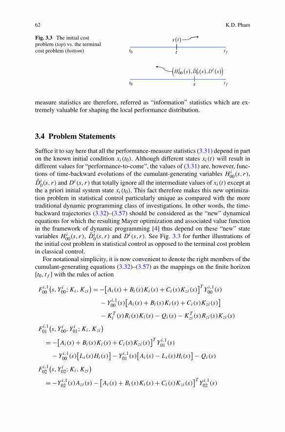
Fig. 3.3 The initial costproblem (top) vs. the terminalcost problem (bottom)
measure statistics are therefore, referred as “information” statistics which are ex-tremely valuable for shaping the local performance distribution.
3.4 Problem Statements
Suffice it to say here that all the performance-measure statistics (3.31) depend in parton the known initial condition xi(t0). Although different states xi(t) will result indifferent values for “performance-to-come”, the values of (3.31) are, however, func-tions of time-backward evolutions of the cumulant-generating variables Hi
00(s, r),Di
0(s, r) and Di(s, r) that totally ignore all the intermediate values of xi(t) except atthe a priori initial system state xi(t0). This fact therefore makes this new optimiza-tion problem in statistical control particularly unique as compared with the moretraditional dynamic programming class of investigations. In other words, the time-backward trajectories (3.32)–(3.57) should be considered as the “new” dynamicalequations for which the resulting Mayer optimization and associated value functionin the framework of dynamic programming [4] thus depend on these “new” statevariables Hi
00(s, r), Di0(s, r) and Di(s, r). See Fig. 3.3 for further illustrations of
the initial cost problem in statistical control as opposed to the terminal cost problemin classical control.
For notational simplicity, it is now convenient to denote the right members of thecumulant-generating equations (3.32)–(3.57) as the mappings on the finite horizon[t0, tf ] with the rules of action
Fi,100
(s, Y i
00;Ki,Kzi
) = −[Ai(s) + Bi(s)Ki(s) + Ci(s)Kzi(s)
]TY
i,100 (s)
− Yi,100 (s)
[Ai(s) + Bi(s)Ki(s) + Ci(s)Kzi(s)
]
− KTi (s)Ri(s)Ki(s) − Qi(s) − KT
zi (s)Rzi(s)Kzi(s)
Fi,101
(s, Y i
00, Yi01;Ki,Kzi
)
= −[Ai(s) + Bi(s)Ki(s) + Ci(s)Kzi(s)
]TY
i,101 (s)
− Yi,100 (s)
[Li(s)Hi(s)
] − Yi,101 (s)
[Ai(s) − Li(s)Hi(s)
] − Qi(s)
Fi,102
(s, Y i
02;Ki,Kzi
)
= −Yi,102 (s)Azi(s) − [
Ai(s) + Bi(s)Ki(s) + Ci(s)Kzi(s)]T
Yi,102 (s)

3 Performance-Information Analysis and Distributed Feedback Stabilization 63
Fi,110
(s, Y i
00, Yi10;Ki,Kzi
)
= −[Ai(s) − Li(s)Hi(s)
]TY
i,110 (s) − [
Li(s)Hi(s)]T
Yi,100 (s)
− Yi,110 (s)
[Ai(s) + Bi(s)Ki(s) + Ci(s)Kzi(s)
] − Qi(s)
Fi,111
(s, Y i
01, Yi10, Y
i11
) = −Yi,110 (s)
[Li(s)Hi(s)
] − Yi,111 (s)
[Ai(s) − Li(s)Hi(s)
]
− [Li(s)Hi(s)
]TY
i,101 (s) − [
Ai(s) − Li(s)Hi(s)]T
Yi,111 (s)
Fi,112
(s, Y i
02, Yi12
) = −Yi,112 (s)Azi(s) − [
Li(s)Hi(s)]T
Yi,102 (s)
− [Ai(s) − Li(s)Hi(s)
]TY
i,112 (s)
Fi,120
(s, Y i
20;Ki,Kzi
) = −Yi,120 (s)
[Ai(s) + Bi(s)Ki(s) + Ci(s)Kzi(s)
]
− ATzi(s)Y
i,120 (s) + 2Rzi(s)Kzi(s)
Fi,121
(s, Y i
20, Yi21
) = −ATzi(s)Y
i,121 (s) − Y
i,120 (s)
[Li(s)Hi(s)
]
− Yi,121 (s)
[Ai(s) − Li(s)Hi(s)
]
Fi,122
(s, Y i
22
) = −ATzi(s)Y
i,122 (s) − Y
i,122 (s)Azi(s) − Rzi(s)
Fi,r00
(s, Y i
00, Yi01, Y
i20;Ki,Kzi
)
= −[Ai(s) + Bi(s)Ki(s) + Ci(s)Kzi(s)
]TY
i,r00 (s)
− Yi,r00 (s)
[Ai(s) + Bi(s)Ki(s) + Ci(s)Kzi(s)
]
−r−1∑v=1
2r!v!(r − v)!
[P i
00(s)Yi,r−v00 (s) + P i
01(s)Yi,r−v01 (s) + P i
02(s)Yi,r−v20 (s)
]
Fi,r01
(s, Y i
00, Yi01, Y
i11, Y
i21;Ki,Kzi
)
= −Yi,r01 (s)
[Ai(s) − Li(s)Hi(s)
]
− Yi,r00 (s)
[Li(s)Hi(s)
] − [Ai(s) + Bi(s)Ki(s) + Ci(s)Kzi(s)
]TY
i,r01 (s)
−r−1∑v=1
2r!v!(r − v)!
[P i
00(s)Yi,r−v01 (s) + P i
01(s)Yi,r−v11 (s) + P i
02(s)Yi,r−v21 (s)
]
Fi,r02
(s, Y i
02, Yi12, Y
i22;Ki,Kzi
)
= −Yi,r02 (s)Azi(s) − [
Ai(s) + Bi(s)Ki(s) + Ci(s)Kzi(s)]T
Yi,r02 (s)
−r−1∑r=1
2r!v!(r − v)!
[P i
00(s)Yi,r−v02 (s) + P i
01(s)Yi,r−v12 (s) + P i
02(s)Yi,r−v22 (s)
]

64 K.D. Pham
Fi,r10
(s, Y i
00, Yi10, Y
i20;Ki,Kzi
)
= −[Ai(s) − Li(s)Hi(s)
]TY
i,r10 (s)
− [Li(s)Hi(s)
]TY
i,r00 (s) − Y
i,r10 (s)
[Ai(s) + Bi(s)Ki(s) + Ci(s)Kzi(s)
]
−r−1∑v=1
2r!v!(r − v)!
[P i
10(s)Yi,r−v00 (s) + P i
11(s)Yi,r−v10 (s) + P i
12(s)Yi,r−v20 (s)
]
Fi,r11
(s, Y i
01, Yi10, Y
i11, Y
i21
)
= −[Ai(s) − Li(s)Hi(s)
]TY
i,r11 (s) − [
Li(s)Hi(s)]T
Yi,r01 (s)
− Yi,r10 (s)
[Li(s)Hi(s)
] − Yi,r11 (s)
[Ai(s) − Li(s)Hi(s)
]
−r−1∑v=1
2r!v!(r − v)!
[P i
10(s)Yi,r−v01 (s) + P i
11(s)Yi,r−v11 (s) + P i
12(s)Yi,r−v21 (s)
]
Fi,r12
(s, Y i
02, Yi12, Y
i22
)
= −Yi,r12 (s)Azi(s) − [
Li(s)Hi(s)]T
Yi,r02 (s) − [
Ai(s) − Li(s)Hi(s)]T
Yi,r12 (s)
−r−1∑v=1
2r!v!(r − v)!
[P i
10(s)Yi,r−v02 (s) + P i
11(s)Yi,r−v12 (s) + P i
12(s)Yi,r−v22 (s)
]
Fi,r20 (s) = −AT
zi(s)Yi,r20 (s) − Y
i,r20 (s)
[Ai(s) + Bi(s)Ki(s) + Ci(s)Kzi(s)
]
−r−1∑v=1
2r!v!(r − v)!
[P i
20(s)Yi,r−v00 (s) + P i
21(s)Yi,r−v10 (s)
+ P i22(s)Y
i,r−v20 (s)
]
Fi,r21
(s, Y i
01, Yi11, Y
i20, Y
i21
)
= −ATzi(s)Y
i,r21 (s) − Y
i,r20 (s)
[Li(s)Hi(s)
]
−r−1∑v=1
2r!v!(r − v)!
[P i
20(s)Yi,r−v01 (s) + P i
21(s)Yi,r−v11 (s) + P i
22(s)Yi,r−v21 (s)
]
− Yi,r21 (s)
[Ai(s) − Li(s)Hi(s)
]
Fi,r22
(s, Y i
02, Yi12, Y
i22
)
= −ATzi(s)Y
i,r22 (s) − Y
i,r22 (s)Azi(s) −
r−1∑v=1
2r!v!(r − v)!
[P i
20(s)Yi,r−v02 (s)
+ P i21(s)Y
i,r−v12 (s) + P i
22(s)Yi,r−v22 (s)
]
3 Performance-Information Analysis and Distributed Feedback Stabilization 65
Gi,10
(s, Zi
0, Yi00, Y
i02;Ki,Kzi;pi,pzi
)
= −Yi,102 (s)Ezi(s)dmi(s) − Y
i,100 (s)
[Bi(s)pi(s) + Ci(s)pzi(s) + Ei(s)di(s)
]
− KTzi(s)Rzi(s)pzi(s) − [
Ai(s) + Bi(s)Ki(s) + Ci(s)Kzi(s)]T
Zi,10 (s)
− KTi (s)Ri(s)pi(s)
Gi,11
(s, Y i
10, Yi12, Z
i0, Z
i1;pi,pzi
)
= −[Ai(s) − Li(s)Hi(s)
]TZ
i,11 (s)
− Yi,110 (s)
[Bi(s)pi(s) + Ci(s)pzi(s) + Ei(s)di(s)
]
− [Li(s)Hi(s)
]TZ
i,10 (s) − Y
i,112 (s)Ezi(s)dmi(s)
Gi,12
(s, Y i
20, Yi22, Z
i2;pi,pzi
)
= −Yi,120 (s)
[Bi(s)pi(s) + Ci(s)pzi(s) + Ei(s)di(s)
]
− ATzi(s)Z
i,12 (s) − Y
i,122 (s)Ezi(s)dmi(s) + Rzi(s)pzi(s)
Gi,r0
(s, Y i
00, Yi02, Z
i0;Ki,Kzi;pi,pzi
)
= −Yi,r02 (s)Ezi(s)dmi(s) − Y
i,r00 (s)
[Bi(s)pi(s) + Ci(s)pzi(s) + Ei(s)di(s)
]
− [Ai(s) + Bi(s)Ki(s) + Ci(s)Kzi(s)
]TZ
i,r0 (s)
Gi,r1
(s, Y i
10, Yi12, Z
i0, Z
i1;pi,pzi
)
= −[Ai(s) − Li(s)Hi(s)
]TZ
i,r1 (s)
− Yi,r10 (s)
[Bi(s)pi(s) + Ci(s)pzi(s) + Ei(s)di(s)
]
− [Li(s)Hi(s)
]TZ
i,r0 (s) − Y
i,r12 (s)Ezi(s)dmi(s)
Gi,r2
(s, Y i
20, Yi22, Z
i2;pi,pzi
)
= −ATzi(s)Z
i,r2 (s) − Y
i,r22 (s)Ezi(s)dmi(s)
− Yi,r20 (s)
[Bi(s)pi(s) + Ci(s)pzi(s) + Ei(s)di(s)
]
Gi,1(s, Y i00, Y
i01, Y
i02, Y
i10, Y
i11, Y
i12, Y
i20, Y
i21, Y
i22, Z
i0, Z
i2;pi,pzi
)
= −2(Z
i,10
)T(s)
[Bi(s)pi(s) + Ci(s)pzi(s) + Ei(s)di(s)
]
− 2(Z
i,12
)T(s)Ezi(s)dmi(s)
− Tr{Y
i,100 (s)Πi
00(s) + Yi,101 (s)Πi
10(s) + Yi,102 (s)Πi
20(s)}
− Tr{Y
i,110 (s)Πi
01(s) + Yi,111 (s)Πi
11(s) + Yi,112 (s)Πi
21(s)}

66 K.D. Pham
− Tr{Y
i,120 (s)Πi
02(s) + Yi,121 (s)Πi
12(s) + Yi,122 (s)Πi
22(s)}
− pTi (s)Ri(s)pi(s) − pT
zi(s)Rzi(s)pzi(s)
Gi,r(s, Y i
00, Yi01, Y
i02, Y
i10, Y
i11, Y
i12, Y
i20, Y
i21, Y
i22, Z
i0, Z
i2;pi,pzi
)
= −2(Z
i,r0
)T(s)
[Bi(s)pi(s) + Ci(s)pzi(s) + Ei(s)di(s)
]
− 2(Z
i,r2
)T(s)Ezi(s)dmi(s)
− Tr{Y
i,r00 (s)Πi
00(s) + Yi,r01 (s)Πi
10(s) + Yi,r02 (s)Πi
20(s)}
− Tr{Y
i,r10 (s)Πi
01(s) + Yi,r11 (s)Πi
11(s) + Yi,r12 (s)Πi
21(s)}
− Tr{Y
i,r20 (s)Πi
02(s) + Yi,r21 (s)Πi
12(s) + Yi,r22 (s)Πi
22(s)}
provided that all the ki -tuple variables are given by
Y i00(·) �
(Y
i,100 (·), . . . , Y i,ki
00 (·)) ≡ (Hi
00(·,1), . . . ,H i00(·, ki)
)
Y i01(·) �
(Y
i,101 (·), . . . , Y i,ki
01 (·)) ≡ (Hi
01(·,1), . . . ,H i01(·, ki)
)
Y i02(·) �
(Y
i,102 (·), . . . , Y i,ki
02 (·)) ≡ (Hi
02(·,1), . . . ,H i02(·, ki)
)
Y i10(·) �
(Y
i,110 (·), . . . , Y i,ki
10 (·)) ≡ (Hi
10(·,1), . . . ,H i10(·, ki)
)
Y i11(·) �
(Y
i,111 (·), . . . , Y i,ki
11 (·)) ≡ (Hi
11(·,1), . . . ,H i11(·, ki)
)
Y i12(·) �
(Y
i,112 (·), . . . , Y i,ki
12 (·)) ≡ (Hi
12(·,1), . . . ,H i12(·, ki)
)
Y i20(·) �
(Y
i,120 (·), . . . , Y i,ki
20 (·)) ≡ (Hi
20(·,1), . . . ,H i20(·, ki)
)
Y i21(·) �
(Y
i,121 (·), . . . , Y i,ki
21 (·)) ≡ (Hi
21(·,1), . . . ,H i21(·, ki)
)
Y i22(·) �
(Y
i,122 (·), . . . , Y i,ki
22 (·)) ≡ (Hi
22(·,1), . . . ,H i22(·, ki)
)
Zi0(·) �
(Z
i,10 (·), . . . , Zi,ki
0 (·)) ≡ (Di
0(·,1), . . . , Di0(·, ki)
)
Zi1(·) �
(Z
i,11 (·), . . . , Zi,ki
1 (·)) ≡ (Di
1(·,1), . . . , Di1(·, ki)
)
Zi2(·) �
(Z
i,12 (·), . . . , Zi,ki
2 (·)) ≡ (Di
2(·,1), . . . , Di2(·, ki)
)
Zi0(·) �
(Z
i,10 (·), . . . ,Zi,ki
0 (·)) ≡ (Di
0(·,1), . . . ,Di0(·, ki)
)
Now it is straightforward to establish the product mappings
F i00 � F
i,100 × · · · × F
i,ki
00 F i01 � F
i,101 × · · · × F
i,ki
01
F i02 � F
i,102 × · · · × F
i,ki
02 F i10 � F
i,110 × · · · × F
i,ki
10
F i11 � F
i,111 × · · · × F
i,ki
11 F i12 � F
i,112 × · · · × F
i,ki
12

3 Performance-Information Analysis and Distributed Feedback Stabilization 67
F i20 � F
i,120 × · · · × F
i,ki
20 F i21 � F
i,121 × · · · × F
i,ki
21
F i22 � F
i,122 × · · · × F
i,ki
22 Gi0 � G
i,10 × · · · × G
i,ki
0
Gi1 � G
i,11 × · · · × G
i,ki
1 Gi2 � G
i,12 × · · · × G
i,ki
2
Gi � Gi,1 × · · · × Gi,ki
Thus, the dynamic equations (3.32)–(3.57) can be rewritten compactly as follows
d
dsY i
00(s) = F i00
(s, Y i
00(s), Yi01(s), Y
i20(s);Ki(s),Kzi(s)
), Y i
00(tf ) (3.58)
d
dsY i
01(s) = F i01
(s, Y i
00(s), Yi01, Y
i11(s), Y
i21(s);Ki(s),Kzi(s)
), Y i
01(tf ) (3.59)
d
dsY i
02(s) = F i02
(s, Y i
02, Yi12(s), Y
i22(s);Ki(s),Kzi(s)
), Y i
02(tf ) (3.60)
d
dsY i
10(s) = F i10
(s, Y i
00(s), Yi10(s), Y
i20(s);Ki(s),Kzi(s)
), Y i
10(tf ) (3.61)
d
dsY i
11(s) = F i11
(s, Y i
01(s), Yi10(s), Y
i11(s), Y
i21(s)
), Y i
11(tf ) (3.62)
d
dsY i
12(s) = F i12
(s, Y i
02(s), Yi12(s), Y
i22(s)
), Y i
12(tf ) (3.63)
d
dsY i
20(s) = F i20
(s, Y i
00(s), Yi10(s), Y
i20(s);Ki(s),Kzi(s)
), Y i
20(tf ) (3.64)
d
dsY i
21(s) = F i21
(s, Y i
01(s), Yi11(s), Y
i20(s), Y
i21(s)
), Y i
21(tf ) (3.65)
d
dsY i
22(s) = F i22
(s, Y i
02(s), Yi12(s), Y
i22(s)
), Y i
22(tf ) (3.66)
d
dsZi
0(s) = Gi0
(s, Y i
00(s), Yi02(s), Z
i0(s);Ki(s),Kzi(s);pi(s),pzi(s)
),
Zi0(tf ) (3.67)
d
dsZi
1(s) = Gi1
(s, Y i
10(s), Yi12(s), Z
i0(s), Z
i1(s);pi(s),pzi(s)
), Zi
1(tf ) (3.68)
d
dsZi
2(s) = Gi2
(s, Y i
20, Yi22(s), Z
i2(s);pi(s),pzi(s)
), Zi
2(tf ) (3.69)
d
dsZi(s) = Gi
(s, Y i
00(s), Yi01(s), Y
i02(s), Y
i10(s), Y
i11(s), Y
i12(s), Y
i20(s), . . .
Y i21(s), Y
i22(s), Z
i0(s), Z
i2(s);pi(s),pzi(s)
), Zi(tf ) (3.70)
where the terminal-value conditions are defined by
Y i00(tf ) � Q
fi × 0 × · · · × 0 Y i
01(tf ) � Qfi × 0 × · · · × 0

68 K.D. Pham
Y i02(tf ) � 0 × 0 × · · · × 0 Y i
10(tf ) � Qfi × 0 × · · · × 0
Y i11(tf ) � Q
fi × 0 × · · · × 0 Y i
12(tf ) � 0 × 0 × · · · × 0
Y i20(tf ) � 0 × 0 × · · · × 0 Y i
21(tf ) � 0 × 0 × · · · × 0
Y i22(tf ) � 0 × 0 × · · · × 0 Zi
0(tf ) � 0 × 0 × · · · × 0
Zi1(tf ) � 0 × 0 × · · · × 0 Zi
2(tf ) � 0 × 0 × · · · × 0
Zi(tf ) � 0 × 0 × · · · × 0
Note that for each agent i the product system (3.58)–(3.70) uniquely determinesY i
00, Y i01, Y i
02, Y i10, Y i
11, Y i12, Y i
20, Y i21, Y i
22, Zi0, Zi
1, Zi2, and Zi once the admissible
4-tuple (Ki,Kzi,pi,pzi) is specified. Thus, Y i00, Y i
01, Y i02, Y i
10, Y i11, Y i
12, Y i20, Y i
21,Y i
22, Zi0, Zi
1, Zi2, and Zi are considered as the functions of Ki , Kzi , pi , and pzi .
The performance index for the interconnected system can therefore be formulatedin terms of Ki , Kzi , pi , and pzi for agent i.
The subject of risk taking has been of great interest not only to control system de-signers of engineered systems but also to decision makers of financial systems. Oneapproach to study risk in stochastic control system is exemplified in the ubiquitoustheory of linear-quadratic Gaussian (LQG) control whose preference of expectedvalue of performance measure associated with a class of stochastic systems is min-imized against all random realizations of the uncertain environment. Other aspectsof performance distributions that do not appear in the classical theory of LQG arevariance, skewness, kurtosis, etc. For instance, it may nevertheless be true that someperformance with negative skewness appears riskier than performance with positiveskewness when expectation and variance are held constant. If skewness does, in-deed, play an essential role in determining the perception of risk, then the range ofapplicability of the present theory should be restricted, for example, to symmetricor equally skewed performance measures.
There have been several studies that attempt to generalize the present LQG the-ory to account for the effects of variance [11] and [6] or of other description ofprobability density [12] on the perceived riskiness of performance measures. Thecontribution of this research is to directly address the perception of risk via a selec-tive set of performance distribution characteristics of its outcomes governed by ei-ther dispersion, skewness, flatness, etc. or a combination thereof. Figure 3.4 depictssome possible interpretations on measures of performance risk for control decisionunder uncertainty.
Definition 1 (Risk-value aware performance index) Associate with agent i theki ∈ Z
+ and the sequence μi = {μir ≥ 0}ki
r=1 with μi1 > 0. Then, for (t0, x
0i ) given,
the risk-value aware performance index
φi0 : {t0} × (
Rni×ni
)ki × (R
ni)ki × R
ki �→ R+
over a finite optimization horizon is defined by a risk-value model to reflect thetradeoff between value and riskiness of the Chi-squared type performance mea-

3 Performance-Information Analysis and Distributed Feedback Stabilization 69
Fig. 3.4 Measures of performance risk for control decision under uncertainty
sure (3.31)
φi0
(t0, Y
i00(·,Ki,Kzi,pi,pzi), Z
i0(·,Ki,Kzi,pi,pzi),Z
i(·,Ki,Kzi,pi,pzi))
� μi1κ
i1(Ki,Kzi ,pi,pzi)︸ ︷︷ ︸
Value Measure
+ μi2κ
i2(Ki,Kzi ,pi,pzi) + · · · + μi
kiκiki
(Ki,Kzi,pi,pzi)︸ ︷︷ ︸Risk Measure
= μi1
[(x0i
)TY
i,100 (t0,Ki,Kzi ,pi,pzi)x
0i + 2
(x0i
)TZ
i,10 (t0,Ki,Kzi,pi,pzi)
+ Zi,10 (t0,Ki,Kzi ,pi,pzi)
] + μi2
[(x0
i
)TY
i,200 (t0,Ki,Kzi ,pi,pzi)x
0i
+ 2(x0i
)TZ
i,20 (t0,Ki,Kzi ,pi,pzi) + Z
i,20 (t0,Ki,Kzi,pi,pzi)
]
+ · · · + μiki
[(x0i
)TY
i,ki
00 (t0,Ki,Kzi,pi,pzi)x0i
+ 2(x0i
)TZ
i,ki
0 (t0,Ki,Kzi,pi,pzi) + Zi,ki
0 (t0,Ki,Kzi,pi,pzi)]
(3.71)
where all the parametric design measures μir considered here by agent i, repre-
sent for different emphases on higher-order statistics and agent prioritization towardperformance robustness. Solutions {Y i,r
00 (s,Ki,Kzi,pi,pzi)}ki
r=1, {Zi,r0 (s,Ki,Kzi ,
pi,pzi)}ki
r=1 and {Zi,r (s,Ki,Kzi,pi,pzi)}ki
r=1 when evaluated at s = t0 satisfy thetime-backward differential equations (3.32)–(3.57) together with the terminal-valueconditions as aforementioned.
From the above definition, the statistical problem is shown to be an initial costproblem, in contrast with the more traditional terminal cost class of investigations.One may address an initial cost problem by introducing changes of variables whichconvert it to a terminal cost problem. However, this modifies the natural contextof statistical control, which it is preferable to retain. Instead, one may take a moredirect dynamic programming approach to the initial cost problem. Such an approachis illustrative of the more general concept of the principle of optimality, an ideatracing its roots back to the 17th century and depicted in Fig. 3.5.

70 K.D. Pham
Fig. 3.5 Value functions inthe terminal cost problem(top) and the initial costproblem (bottom)
Fig. 3.6 Admissible feedback gains and interaction recovery inputs
For the given (tf , Y i00(tf ), Zi
0(tf ),Zi(tf )), classes of Ki
tf ,Y i00(tf ),Zi
0(tf ),Zi(tf );μi,
Kzi
tf ,Y i00(tf ),Zi
0(tf ),Zi(tf );μi, P i
tf ,Y i00(tf ),Zi
0(tf ),Zi(tf );μiand P zi
tf ,Y i00(tf ),Zi
0(tf ),Zi(tf );μiof
admissible 4-tuple (Ki,Kzi ,pi,pzi) are then defined.
Definition 2 (Admissible feedback gains and affine inputs) For agent i, the compactsubsets Ki ⊂ R
ni×ni , Kzi , P i ⊂ Rmi , and P zi ⊂ R
mzi be denoted by the sets ofallowable matrices and vectors as in Fig. 3.6.
Then, for ki ∈ Z+, μi = {μi
r ≥ 0}ki
r=1 with μi1 > 0, the matrix-valued sets
of Ki
tf ,Y i00(tf ),Zi
0(tf ),Zi(tf );μi∈ C(t0, tf ;R
mi×ni ) and Kzi
tf ,Y i00(tf ),Zi
0(tf ),Zi(tf );μi∈
C(t0, tf ;Rmzi×ni ) and the vector-valued sets of P i
tf ,Y i00(tf ),Zi
0(tf ),Zi(tf );μi∈ C(t0, tf ;

3 Performance-Information Analysis and Distributed Feedback Stabilization 71
Rmi ) and P zi
tf ,Y i00(tf ),Zi
0(tf ),Zi(tf );μi∈ C(t0, tf ;R
mzi ) with respective values Ki(·) ∈Ki , Kzi(·) ∈ Kzi , pi(·) ∈ P i , and pzi(·) ∈ P zi are admissible if the resulting so-lutions to the time-backward differential equations (3.32)–(3.57) exist on the finitehorizon [t0, tf ].
The optimization problem for agent i, where instantiations are aimed at reducingperformance robustness and constituent strategies are robust to uncertain environ-ment’s stochastic variations, is subsequently stated.
Definition 3 (Optimization of Mayer problem) Suppose that ki ∈ Z+ and the se-
quence μi = {μir ≥ 0}ki
r=1 with μi1 > 0 are fixed. Then, the optimization prob-
lem over [t0, tf ] is given by the minimization of agent i’s performance index(3.71) over all Ki(·) ∈ Ki
tf ,Y i00(tf ),Zi
0(tf ),Zi(tf );μi, Kzi(·) ∈ Kzi
tf ,Y i00(tf ),Zi
0(tf ),Zi(tf );μi,
pi(·) ∈ P i
tf ,Y i00(tf ),Zi
0(tf ),Zi(tf );μiand pzi(·) ∈ P zi
tf ,Y i00(tf ),Zi
0(tf ),Zi(tf );μisubject to the
time-backward dynamical constraints (3.58)–(3.70) for s ∈ [t0, tf ].
It is important to recognize that the optimization considered here is in “Mayerform” and can be solved by applying an adaptation of the Mayer form verifi-cation theorem of dynamic programming given in [4]. In the framework of dy-namic programming where the subject optimization is embedded into a fam-ily of optimization based on different starting points, there is therefore a needto parameterize the terminal time and new states by (ε,Y i
00, Zi0,Z
i) rather than(tf , Y i
00(tf ), Zi0(tf ),Zi(tf )). Thus, the values of the corresponding optimization
problems depend on the terminal-value conditions which lead to the definition of avalue function.
Definition 4 (Value function) The value function V i : [t0, tf ] × (Rni×ni )ki ×(Rni )ki × R
ki �→ R+ associated with the Mayer problem defined as V i (ε, Y i
00,
Zi0,Z
i) is the minimization of φi0(t0, Y
i00(·,Ki,Kzi,pi,pzi), Z
i0(·,Ki,Kzi,pi,
pzi),Zi(·,Ki,Kzi ,pi,pzi)) over all Ki(·) ∈ Ki
tf ,Y i00(tf ),Zi
0(tf ),Zi(tf );μi, Kzi(·) ∈
Kzi
tf ,Y i00(tf ),Zi
0(tf ),Zi(tf );μi, pi(·) ∈ P i
tf ,Y i00(tf ),Zi
0(tf ),Zi(tf );μi, and pzi(·) ∈
P zi
tf ,Y i00(tf ),Zi
0(tf ),Zi(tf );μisubject to some (ε,Y i
00, Zi0,Z
i) ∈ [t0, tf ] × (Rni×ni )ki ×(Rni )ki × R
ki .
It is conventional to let V i (ε, Y i00, Z
i0,Z
i) = ∞ when Ki
tf ,Y i00(tf ),Zi
0(tf ),Zi(tf );μi,
Kzi
tf ,Y i00(tf ),Zi
0(tf ),Zi(tf );μi, P i
tf ,Y i00(tf ),Zi
0(tf ),Zi(tf );μiand P zi
tf ,Y i00(tf ),Zi
0(tf ),Zi(tf );μiare
empty. To avoid cumbersome notation, the dependence of trajectory solutions onKi , Kzi , pi and pzi is now suppressed. Next, some candidates for the value functioncan be constructed with the help of a reachable set.

72 K.D. Pham
Definition 5 (Reachable set) At agent i, let the reachable set Qi be defined as fol-lows
Qi �{(
ε,Y i00, Z
i0,Z
i) ∈ [t0, tf ] × (
Rni×ni
)ki × (R
ni)ki × R
ki such that
Ki
tf ,Y i00(tf ),Zi
0(tf ),Zi(tf );μi× Kzi
tf ,Y i00(tf ),Zi
0(tf ),Zi(tf );μi×
P i
tf ,Y i00(tf ),Zi
0(tf ),Zi(tf );μi× P zi
tf ,Y i00(tf ),Zi
0(tf ),Zi(tf );μinot empty
}
Moreover, it can be shown that the value function is satisfying a partial differen-tial equation at each interior point of Qi at which it is differentiable.
Theorem 4 (Hamilton–Jacobi–Bellman (HJB) equation for Mayer problem) Foragent i, let (ε,Y i
00, Zi0,Z
i) be any interior point of the reachable set Qi at
which the value function V i(ε, Y i00, Z
i0,Z
i) is differentiable. If there exists anoptimal 4-tuple control strategy (K∗
i ,K∗zi , p
∗i , p
∗zi) ∈ Ki
tf ,Y i00(tf ),Zi
0(tf ),Zi(tf );μi×
Kzi
tf ,Y i00(tf ),Zi
0(tf ),Zi(tf );μi× P i
tf ,Y i00(tf ),Zi
0(tf ),Zi(tf );μi× P zi
tf ,Y i00(tf ),Zi
0(tf ),Zi(tf );μi, the
partial differential equation associated with agent i
0 = minKi∈Ki,Kzi∈Kzi ,pi∈P i,pzi∈P zi
{∂
∂εV i
(ε,Y i
00, Zi0,Z
i)
+ ∂
∂ vec(Y i00)
V i(ε,Y i
00, Zi0,Z
i) · vec
(F i
00
(ε;Y i
00, Yi01, Y
i20;Ki,Kzi
))
+ ∂
∂ vec(Zi0)
V i(ε,Y i
00, Zi0,Z
i) · vec
(Gi
0
(ε;Y i
00, Yi02, Z
i0;Ki,Kzi;pi,pzi
))
+ ∂
∂ vec(Zi)V i
(ε,Y i
00, Zi0,Z
i)
· vec(Gi
(ε;Y i
00, Yi00, Y
i01, Y
i02, Y
i10, Y
i11, Y
i12, Y
i20, Y
i21, Y
i22, Z
i0, Z
i2;pi,pzi
))}
(3.72)
is satisfied together with V i (t0, Yi00, Z
i0,Z
i) = φi0(t0, Y
i00, Z
i0,Z
i) and vec(·) thevectorizing operator of enclosed entities. The optimum in (3.72) is achieved by the4-tuple control decision strategy (K∗
i (ε),K∗zi (ε),p
∗i (ε),p
∗zi (ε)) of the optimal deci-
sion strategy at ε.
Proof Detail discussions are in [4] and the modification of the original proofsadapted to the framework of statistical control together with other formal analysiscan be found in [7] which is available via http://etd.nd.edu/ETD-db/theses/available/etd-04152004-121926/unrestricted/PhamKD052004.pdf. �
Finally, the next theorem gives the sufficient condition used to verify optimaldecisions for the interconnected system or agent i.
3 Performance-Information Analysis and Distributed Feedback Stabilization 73
Theorem 5 (Verification theorem) Fix ki ∈ Z+. Let W i (ε, Y i
00, Zi0,Z
i) be a contin-uously differentiable solution of the HJB equation (3.72) and satisfy the boundarycondition
W i(t0, Y
i00, Z
i0,Z
i) = φi
0
(t0, Y
i00, Z
i0,Z
i)
(3.73)
Let (tf , Y i00(tf ), Zi
0(tf ),Zi(tf )) be a point of Qi ; 4-tuple (Ki,Kzi,pi,pzi) in
Ki
tf ,Y i00(tf ),Zi
0(tf ),Zi(tf );μi× Kzi
tf ,Y i00(tf ),Zi
0(tf ),Zi(tf );μi× P i
tf ,Y i00(tf ),Zi
0(tf ),Zi(tf );μi×
P zi
tf ,Y i00(tf ),Zi
0(tf ),Zi(tf );μi; and Y i
00, Zi0, and Zi the corresponding solutions of (3.58)–
(3.70). Then, W i(s, Y i00(s), Z
i0(s),Z
i(s)) is time-backward increasing in s. If
(K∗i ,K∗
zi , p∗i , p∗
zi) is a 4-tuple in Ki
tf ,Y i00(tf ),Zi
0(tf ),Zi(tf );μi×Kzi
tf ,Y i00(tf ),Zi
0(tf ),Zi(tf );μi
× P i
tf ,Y i00(tf ),Zi
0(tf ),Zi(tf );μi× P zi
tf ,Y i00(tf ),Zi
0(tf ),Zi(tf );μidefined on [t0, tf ] with cor-
responding solutions, Y i∗00 , Zi∗
0 and Zi∗ of the dynamical equations such that
0 = ∂
∂εW i
(s, Y i∗
00(s), Zi∗0 (s),Zi∗(s)
) + ∂
∂ vec(Y i00)
W i(s, Y i∗
00(s), Zi∗0 (s),Zi∗(s)
)
· vec(F i
00
(s;Y i∗
00(s), Y i∗01 (s), Y i∗
20 (s);K∗i (s),K∗
zi (s)))
+ ∂
∂ vec(Zi0)
W i(s, Y i∗
00 (s), Zi∗0 (s),Zi∗(s)
)
· vec(Gi
0
(s;Y i∗
00 (s), Y i∗02 (s), Zi∗
0 (s);K∗i (s),K∗
zi (s);p∗i (s),p
∗zi (s)
))
+ ∂
∂ vec(Zi)W i
(s, Y i∗
00 (s), Zi∗0 (s),Zi∗(s)
)
· vec(Gi
(ε;Y i∗
00(s), Y i∗00(s), Y i∗
01 (s), Y i∗02 (s), Y i∗
10 (s), Y i∗11 (s), Y i∗
12(s),
Y i∗20(s), Y i∗
21 (s), Y i∗22(s), Zi∗
0 (s), Zi∗2 (s);p∗
i (s),p∗zi (s)
))(3.74)
then (K∗i ,K∗
zi , p∗i , p
∗zi ) in Ki
tf ,Y i00(tf ),Zi
0(tf ),Zi(tf );μi× Kzi
tf ,Y i00(tf ),Zi
0(tf ),Zi(tf );μi×
P i
tf ,Y i00(tf ),Zi
0(tf ),Zi(tf );μi× P zi
tf ,Y i00(tf ),Zi
0(tf ),Zi(tf );μiis optimal and
W i(ε,Y i
00, Zi0,Z
i) = V i
(ε,Y i
00, Zi0,Z
i)
(3.75)
where V i (ε, Y i00, Z
i0,Z
i) is the value function.
Proof Due to the length limitation, the interested reader is referred to the work bythe author [7] which can be found via http://etd.nd.edu/ETD-db/theses/available/etd-04152004-121926/unrestricted/PhamKD052004.pdf for the detail proof andother relevant analysis. �
Note that, to have a solution (K∗i ,K∗
zi , p∗i , p∗
zi) ∈ Ki
tf ,Y i00(tf ),Zi
0(tf ),Zi(tf );μi×
Kzi
tf ,Y i00(tf ),Zi
0(tf ),Zi(tf );μi× P i
tf ,Y i00(tf ),Zi
0(tf ),Zi(tf );μi× P zi
tf ,Y i00(tf ),Zi
0(tf ),Zi(tf );μiwell

74 K.D. Pham
Fig. 3.7 Cost-to-go in thesufficient condition toHamilton–Jacobi–Bellmanequation
defined and continuous for all s ∈ [t0, tf ], the trajectory solutions Y i00(s), Zi
0(s)
and Zi(s) to the dynamical equations (3.58)–(3.70) when evaluated at s = t0 mustthen exist. Therefore, it is necessary that Y i
00(s), Zi0(s) and Zi(s) are finite for all
s ∈ [t0, tf ). Moreover, the solutions of the dynamical equations (3.58)–(3.70) ex-ist and are continuously differentiable in a neighborhood of tf . Applying the resultsfrom [2], these trajectory solutions can further be extended to the left of tf as long asY i
00(s), Zi0(s) and Zi(s) remain finite. Hence, the existence of unique and continu-
ously differentiable solution Y i00(s), Z
i0(s) and Zi(s) are bounded for all s ∈ [t0, tf ).
As a result, the candidate value function W i (s, Y i00, Z
i0,Z
i) is continuously differ-entiable as well.
3.5 Distributed Risk-Averse Feedback Stabilization
Note that the optimization problem is in “Mayer form” and can be solved by apply-ing an adaptation of the Mayer form verification theorem of dynamic programmingas described in the previous section. In particular, the terminal time and states ofa family of optimization problems are now parameterized as (ε,Y i
00, Zi0,Z
i) ratherthan (tf ,H i
00(tf ), Di0(tf ),Di(tf )). Precisely stated, for ε ∈ [t0, tf ] and 1 ≤ r ≤ ki ,
the states of the performance robustness (3.58)–(3.70) defined on the interval [t0, ε]have the terminal values denoted by Hi
00(ε) ≡ Y i00, Di
0(ε) ≡ Zi0 and Di(ε) ≡ Zi .
Figure 3.7 further illustrates the cost-to-go and cost-to-come functions in statisticalcontrol.
Since the performance index (3.71) is quadratic affine in terms of arbitrarily fixedx0i , this observation suggests a candidate solution to the HJB equation (3.72) may be
of the form as follows. For instance, it is assumed that (ε,Y i00, Z
i0,Z
i) is an interiorpoint of the reachable set Qi at which the real-valued function
W i(ε,Y i
00, Zi0,Z
i) = (
x0i
)Tki∑
r=1
μir
(Y
i,r00 + Ei
r(ε))x0i
+ 2(x0i
)Tki∑
r=1
μir
(Z
i,r0 + T i
r (ε))
+ki∑
r=1
μir
(Zi,r + T i
r (ε))
(3.76)

3 Performance-Information Analysis and Distributed Feedback Stabilization 75
is differentiable. The parametric functions of time Eir ∈ C1(t0, tf ;R
ni×ni ), T ir ∈
C1(t0, tf ;Rni ) and T i
r ∈ C1(t0, tf ;R) are yet to be determined. Furthermore, thetime derivative of W i (ε, Y i
00, Zi0,Z
i) can be shown as below
d
dεW i
(ε,Y i
00, Zi0,Z
i)
= (x0i
)Tki∑
r=1
μir
[F
i,r00
(ε;Y i
00, Yi01, Y
i20;Ki,Kzi
) + d
dεEi
r(ε)
]x0
i
+ 2(x0i
)Tki∑
r=1
μir
[G
i,r0 (ε;Y i
00, Yi02, Z
i0;Ki,Kzi;pi,pzi) + d
dεT i
r (ε)
]
+ki∑
r=1
μir
[Gi,r
(ε;Y i
00, Yi00, Y
i01, Y
i02, Y
i10, Y
i11, Y
i12, Y
i20, Y
i21, Y
i22, Z
i0, Z
i2;
pi,pzi
)
+ d
dεT i
r (ε)
](3.77)
The substitution of this hypothesized solution (3.76) into the HJB equation (3.72)and making use of (3.77) results in
0 ≡ minKi∈Ki,Kzi∈Kzi ,pi∈P i,pzi∈P zi
{(x0i
)Tki∑
r=1
μir
d
dεEi
r (ε)x0i +
ki∑r=1
μir
d
dεT i
r (ε)
+ 2(x0i
)Tki∑
r=1
μir
d
dεT i
r (ε) + (x0i
)Tki∑
r=1
μirF
i,r00
(ε;Y i
00, Yi01, Y
i20;Ki,Kzi
)x0i
+ 2(x0i
)Tki∑
r=1
μirG
i,r0
(ε;Y i
00, Yi02, Z
i0;Ki,Kzi;pi,pzi
)
+ki∑
r=1
μirG
i,r(ε;Y i
00, Yi00, . . . , Y
i01, Y
i02, Y
i10, Y
i11, Y
i12, Y
i20, Y
i21, Y
i22, Z
i0, Z
i2;
pi,pzi
)}(3.78)
In the light of arbitrary x0i with the rank of one, the differentiation of the expression
within the bracket of (3.78) with respect to Ki , Kzi , pi , and pzi yields the necessaryconditions for an extremum of (3.71) on [t0, ε]
Ki = −(μi
1Ri(ε))−1
BTi (ε)
ki∑r=1
μirY
i,r00 (3.79)

76 K.D. Pham
Kzi = −(μi
1Rzi(ε))−1
CTi (ε)
ki∑r=1
μirY
i,r00 (3.80)
pi = −(μi
1Ri(ε))−1
BTi (ε)
ki∑r=1
μir Z
i,r0 (3.81)
pzi = −(μi
1Rzi(ε))−1
CTi (ε)
ki∑r=1
μirZ
i,r0 (3.82)
Replacing these results (3.79)–(3.82) into the right member of the HJB equation(3.72) yields the value of the minimum. It is now necessary to exhibit {Ei
r(·)}ki
r=1,
{T ir (·)}ki
r=1, and {T ir (·)}ki
r=1 which render the left side of the HJB equation (3.72)
equal to zero for ε ∈ [t0, tf ], when {Y i,r00 }ki
r=1, {Zi,r0 }ki
r=1, and {Zi,r}ki
r=1 are evaluatedalong the solution trajectories of the dynamical equations (3.58) through (3.70). Dueto the space limitation, the closed forms for {Ei
r(·)}ki
r=1, {T ir (·)}ki
r=1, and {T ir (·)}ki
r=1are however, omitted here. Furthermore, the boundary condition (3.73) requires that
(x0i
)Tki∑
r=1
μir
(Y
i,r00 (t0) + Ei
r(t0))x0i + 2
(x0i
)Tki∑
r=1
μir
(Z
i,r0 (t0) + T i
r (t0))
+ki∑
r=1
μir
(Zi,r (t0) + T i
r (t0))
= (x0i
)Tki∑
r=1
μirY
i00(t0) x0
i + 2(x0i
)Tki∑
r=1
μirZ
i,r0 (t0) +
ki∑r=1
μirZ
i,r (t0)
Thus, matching the boundary condition yields the initial value conditions Eir(t0) =
0, T ir (t0) = 0 and T i
r (t0) = 0.Applying the 4-tuple decision strategy specified in (3.79)–(3.82) along the so-
lution trajectories of the time-backward differential equations (3.58)–(3.70), theseequations become the time-backward Riccati-type differential equations. Enforc-ing the initial value conditions of Ei
r(t0) = 0, T ir (t0) = 0 and T i
r (t0) = 0 uniquelyimplies that Ei
r (ε) = Yi,r00 (t0) − Y
i,r00 (ε), T i
r (ε) = Zi,r0 (t0) − Z
i,r0 (ε), and T i
r (ε) =Zi,r (t0) − Zi,r (ε) for all ε ∈ [t0, tf ] and yields a value function
W i(ε,Y i
00, Zi0,Z
i)
= (x0i
)Tki∑
r=1
μirY
i,r00 (t0) x0
i + 2(x0i
)Tki∑
r=1
μirZ
i,r0 (t0) +
ki∑r=1
μirZ
i,r (t0)
for which the sufficient condition (3.74) of the verification theorem is satisfied.Therefore, the extremal risk-averse control laws (3.79)–(3.82) minimizing (3.71)

3 Performance-Information Analysis and Distributed Feedback Stabilization 77
become optimal
K∗i (ε) = −(
μ1Ri(ε))−1
BTi (ε)
ki∑r=1
μirY
i,r∗00 (ε) (3.83)
K∗zi(ε) = −(
μ1Rzi(ε))−1
CTi (ε)
ki∑r=1
μirY
i,r∗00 (ε) (3.84)
p∗i (ε) = −(
μ1Ri(ε))−1
BTi (ε)
ki∑r=1
μirZ
i,r∗0 (ε) (3.85)
p∗zi(ε) = −(
μ1Rzi(ε))−1
CTi (ε)
ki∑r=1
μirZ
i,r∗0 (ε) (3.86)
In closing the chapter, it is beneficial to summarize the methodological character-istics of the performance robustness analysis and distributed feedback stabilizationand reflect on them from a larger perspective, e.g., management control of a large-scale interconnected system.
Theorem 6 (Decentralized and risk-averse control decisions) Let the pairs (Ai,Bi)
and (Ai,Ci) be uniformly stabilizable and the pair (Ai,Hi) be uniformly detectableon [t0, tf ]. The corresponding interconnected system controlled by agent i is thenconsidered with the initial condition x∗(t0)
dx∗i (t) = (
Ai(t)x∗i (t) + Bi(t)u
∗i (t) + Ci(t)z
∗i (t) + Ei(t)di(t)
)dt + Gi(t) dwi(t)
dy∗i (t) = Hi(t)x
∗i (t) dt + dvi(t),
i ∈ N
whose local interactions with the nearest neighbors are given by
z∗i (t) =
N∑j=1,j =i
Lij (t)x∗ij (t), i ∈ N
which is then approximated by an explicit model-following of the type
dzmi(t) = (Azi(t)zmi(t) + Ezi(t)dmi(t)
)dt + Gzi(t) dwmi(t), zmi(t0) = 0.
Then, the local state estimate x∗i (t) for each agent i is generated by
dx∗i (t) = (
Ai(t)x∗i (t) + Bi(t)u
∗i (t) + Ci(t)z
∗i (t) + Ei(t)di(t)
)dt
+ Li(t)(dy∗
i (t) − Hi(t)x∗i (t) dt
), x∗
i (t0) = x0i

78 K.D. Pham
and the Kalman-type gain is given by
Li(t) = Σi(t)HTi (t)V −1
i
The covariance for estimation error, Σi(t) is the solution of the time-forward matrixdifferential equation
d
dtΣi(t) = Ai(t)Σi(t) + Σi(t)Ai(t) + Gi(t)WiG
Ti (t)
− Σi(t)HTi (t)V −1
i Hi(t)Σi(t), Σi(t0) = 0
Further, let ki ∈ Z+ and the sequence μi = {μi
r ≥ 0}ki
r=1 with μi1 > 0. The optimal
decentralized and risk-averse control decision for agent i is given by
u∗i (t) = K∗
i (t)x∗i (t) + p∗
i (t); z∗i (t) = K∗
zi (t)x∗i (t) + p∗
zi(t)
provided that
K∗i (s) = −R−1
i (s)BTi (s)
ki∑r=1
μirY
i,r∗00 (s) (3.87)
K∗zi(s) = −R−1
zi (s)CTi (s)
ki∑r=1
μirY
i,r∗00 (s) (3.88)
p∗i (s) = −R−1
i (s)BTi (s)
ki∑r=1
μir Z
i,r∗0 (s) (3.89)
p∗zi(s) = −R−1
zi (s)CTi (s)
ki∑r=1
μir Z
i,r∗0 (s) (3.90)
where normalized weighting preferences μir � μi
r/μi1’s are chosen by agent i
toward strategic design of its performance robustness. The supporting solutions{Y i,r∗
00 (s)}ki
r=1, {Zi,r∗0 (s)}ki
r=1, {Zi,r∗(s)}ki
r=1 optimally satisfy the time-backwardmatrix-valued and vector-valued differential equations
d
dsY i∗
00(s) = F i∗00
(s, Y i∗
00(s), Y i∗01 (s), Y i∗
20(s);K∗i (s),K∗
zi (s)), Y i∗
00(tf ) (3.91)
d
dsY i∗
01(s) = F i∗01
(s, Y i∗
00(s), Y i∗01 , Y i∗
11(s), Y i∗21 (s);K∗
i (s),K∗zi(s)
), Y i∗
01 (tf )
(3.92)
d
dsY i∗
02(s) = F i∗02
(s, Y i∗
02 , Y i∗12 (s), Y i∗
22(s);K∗i (s),K∗
zi (s)), Y i∗
02(tf ) (3.93)
d
dsY i∗
10(s) = F i∗10
(s, Y i∗
00(s), Y i∗10 (s), Y i∗
20(s);K∗i (s),K∗
zi (s)), Y i∗
10(tf ) (3.94)

3 Performance-Information Analysis and Distributed Feedback Stabilization 79
d
dsY i∗
11(s) = F i∗11
(s, Y i∗
01(s), Y i∗10 (s), Y i∗
11(s), Y i∗21 (s)
), Y i∗
11(tf ) (3.95)
d
dsY i∗
12(s) = F i∗12
(s, Y i∗
02(s), Y i∗12 (s), Y i∗
22(s)), Y i∗
12 (tf ) (3.96)
d
dsY i∗
20(s) = F i∗20
(s, Y i∗
00(s), Y i∗10 (s), Y i∗
20(s);K∗i (s),K∗
zi (s)), Y i∗
20(tf ) (3.97)
d
dsY i∗
21(s) = F i∗21
(s, Y i
01(s), Yi11(s), Y
i20(s), Y
i21(s)
), Y i∗
21(tf ) (3.98)
d
dsY i∗
22(s) = F i∗22
(s, Y i∗
02(s), Y i∗12 (s), Y i∗
22(s)), Y i∗
22 (tf ) (3.99)
d
dsZi∗
0 (s) = Gi∗0
(s, Y i∗
00(s), Y i∗02 (s), Zi∗
0 (s);K∗i (s),K∗
zi (s); . . . p∗i (s),p∗
zi(s)),
Zi∗0 (tf ) (3.100)
d
dsZi∗
1 (s) = Gi∗1
(s, Y i∗
10(s), Y i∗12 (s), Zi∗
0 (s), Zi∗1 (s);p∗
i (s),p∗zi (s)
),
Zi∗1 (tf ) (3.101)
d
dsZi∗
2 (s) = Gi∗2
(s, Y i∗
20 , Y i∗22(s), Zi∗
2 (s);p∗i (s),p∗
zi(s)), Zi∗
2 (tf ) (3.102)
d
dsZi∗(s) = Gi∗(s, Y i∗
00(s), Y i∗01 (s), Y i∗
02 (s), Y i∗10(s), Y i∗
11 (s), Y i∗12 (s), Y i∗
20(s),
Y i∗21 (s), Y i∗
22(s), Zi∗0 (s), Zi∗
2 (s);p∗i (s),p
∗zi (s)
),
Zi∗(tf ) (3.103)
where the terminal-value conditions are defined by
Y i∗00(tf ) � Q
fi × 0 × · · · × 0 Y i∗
01 (tf ) � Qfi × 0 × · · · × 0
Y i∗02(tf ) � 0 × 0 × · · · × 0 Y i∗
10 (tf ) � Qfi × 0 × · · · × 0
Y i∗11(tf ) � Q
fi × 0 × · · · × 0 Y i∗
12 (tf ) � 0 × 0 × · · · × 0
Y i∗20(tf ) � 0 × 0 × · · · × 0 Y i∗
21 (tf ) � 0 × 0 × · · · × 0
Y i∗22(tf ) � 0 × 0 × · · · × 0 Zi∗
0 (tf ) � 0 × 0 × · · · × 0
Zi∗1 (tf ) � 0 × 0 × · · · × 0 Zi∗
2 (tf ) � 0 × 0 × · · · × 0
Zi∗(tf ) � 0 × 0 × · · · × 0
As pictorial illustrations, Fig. 3.8 shows how local interaction predictions be-tween agent i and its neighbor agents as well as local perceptions of performancerisk associated with the Chi-squared performance random variable are integrated
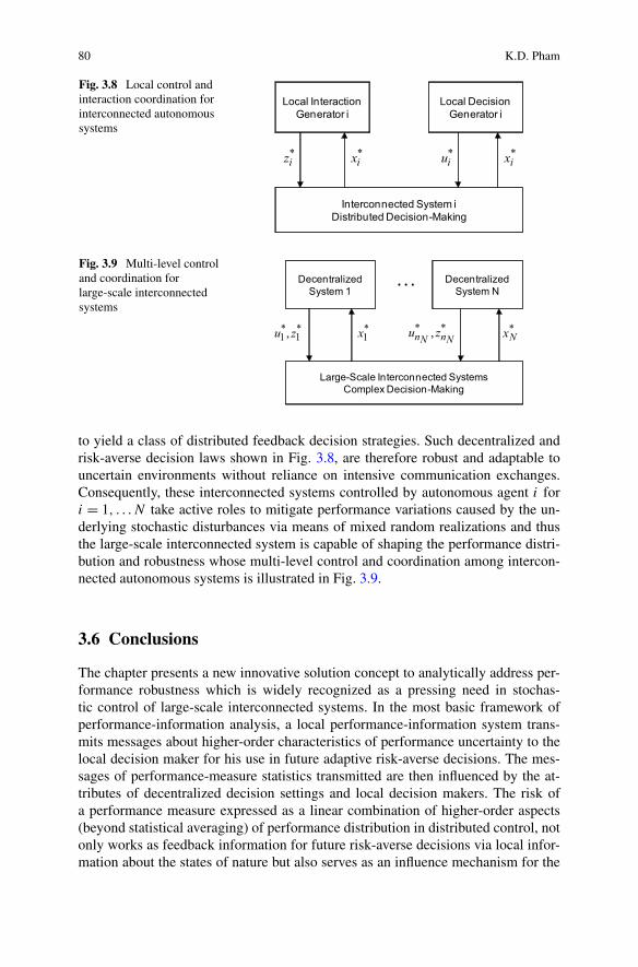
80 K.D. Pham
Fig. 3.8 Local control andinteraction coordination forinterconnected autonomoussystems
Fig. 3.9 Multi-level controland coordination forlarge-scale interconnectedsystems
to yield a class of distributed feedback decision strategies. Such decentralized andrisk-averse decision laws shown in Fig. 3.8, are therefore robust and adaptable touncertain environments without reliance on intensive communication exchanges.Consequently, these interconnected systems controlled by autonomous agent i fori = 1, . . .N take active roles to mitigate performance variations caused by the un-derlying stochastic disturbances via means of mixed random realizations and thusthe large-scale interconnected system is capable of shaping the performance distri-bution and robustness whose multi-level control and coordination among intercon-nected autonomous systems is illustrated in Fig. 3.9.
3.6 Conclusions
The chapter presents a new innovative solution concept to analytically address per-formance robustness which is widely recognized as a pressing need in stochas-tic control of large-scale interconnected systems. In the most basic framework ofperformance-information analysis, a local performance-information system trans-mits messages about higher-order characteristics of performance uncertainty to thelocal decision maker for his use in future adaptive risk-averse decisions. The mes-sages of performance-measure statistics transmitted are then influenced by the at-tributes of decentralized decision settings and local decision makers. The risk ofa performance measure expressed as a linear combination of higher-order aspects(beyond statistical averaging) of performance distribution in distributed control, notonly works as feedback information for future risk-averse decisions via local infor-mation about the states of nature but also serves as an influence mechanism for the

3 Performance-Information Analysis and Distributed Feedback Stabilization 81
local decision maker’s current control behavior. This work contributes toward theconstruction of a theory of performance robustness for stochastic control of a classof large-scale systems in terms of both substantial results and research methodology.
References
1. Brockett, R.W.: Finite Dimensional Linear Systems. Wiley, New York (1970)2. Dieudonne, J.: Foundations of Modern Analysis. Academic Press, New York (1960)3. Field, R.V., Bergman, L.A.: Reliability based approach to linear covariance control design.
J. Eng. Mech. 124, 193–199 (1998)4. Fleming, W.H., Rishel, R.W.: Deterministic and Stochastic Optimal Control. Springer, New
York (1975)5. Hansen, L.P., Sargent, T.J., Tallarini, T.D. Jr.: Robust permanent income and pricing. Rev.
Econ. Stud. 66, 873–907 (1999)6. Liberty, S.R.: Performance analysis of stochastic linear control systems: a new viewpoint. In:
Proceedings International Forum on Alternatives for Linear Multivariable Control, pp. 79–86(1977)
7. Pham, K.D.: Statistical control paradigms for structural vibration suppression. In: PhD Disser-tation (2004). Available via http://etd.nd.edu/ETD-db/theses/available/etd-04152004-121926/unrestricted/PhamKD052004.pdf. Cited 13 August 2009
8. Pham, K.D.: Cooperative solutions in multi-person quadratic decision problems: performance-measure statistics and cost-cumulant control paradigm. In: The 46th Conference on Decisionsand Control, pp. 2484–2490 (2007)
9. Pham, K.D.: Non-cooperative outcomes for stochastic Nash games: decision strategies to-wards multi-attribute performance robustness. In: The 17th World Congress International Fed-eration on Automatic Control, pp. 11750–11756 (2008)
10. Pham, K.D.: New results in stochastic cooperative games: strategic coordination for multi-resolution performance robustness. In: Hirsch, M.J., Pardalos, P.M., Murphey, R., Grundel, D.(eds.) Optimization and Cooperative Control Strategies. Lecture Notes in Control and Infor-mation Sciences, vol. 381, pp. 257–285. Springer, Berlin (2008)
11. Sain, M.K.: Control of linear systems according to the minimal variance criterion-a new ap-proach to the disturbance problem. IEEE Trans. Autom. Control 11, 118–122 (1966)
12. Whittle, P.: Risk Sensitive Optimal Control. Wiley, New York (1990)
Copyright © 2022 FDOKUMEN