Performance Evaluation of a Routing Protocol for Wireless Sensor Networks

NAVAL

POSTGRADUATE SCHOOL

MONTEREY, CALIFORNIA

THESIS

Approved for public release; distribution is unlimited

PERFORMANCE EVALUATION OF A ROUTING PROTOCOL IN WIRELESS SENSOR NETWORKS

by

Cheng Kiat Amos, Teo

December 2005

Thesis Advisors: Gurminder Singh John C. McEachen Second Reader: Michael A. Morgan

THIS PAGE INTENTIONALLY LEFT BLANK

i

REPORT DOCUMENTATION PAGE Form Approved OMB No. 0704-0188 Public reporting burden for this collection of information is estimated to average 1 hour per response, including the time for reviewing instruction, searching existing data sources, gathering and maintaining the data needed, and completing and reviewing the collection of information. Send comments regarding this burden estimate or any other aspect of this collection of information, including suggestions for reducing this burden, to Washington headquarters Services, Directorate for Information Operations and Reports, 1215 Jefferson Davis Highway, Suite 1204, Arlington, VA 22202-4302, and to the Office of Management and Budget, Paperwork Reduction Project (0704-0188) Washington DC 20503. 1. AGENCY USE ONLY (Leave blank)

2. REPORT DATE December 2005

3. REPORT TYPE AND DATES COVERED Master’s Thesis

4. TITLE AND SUBTITLE: Performance Evaluation of a Routing Protocol in Wireless Sensor Network 6. AUTHOR(S) Cheng Kiat Amos, Teo

5. FUNDING NUMBERS

7. PERFORMING ORGANIZATION NAME(S) AND ADDRESS(ES) Naval Postgraduate School Monterey, CA 93943-5000

8. PERFORMING ORGANIZATION REPORT NUMBER

9. SPONSORING /MONITORING AGENCY NAME(S) AND ADDRESS(ES) N/A

10. SPONSORING/MONITORING AGENCY REPORT NUMBER

11. SUPPLEMENTARY NOTES. The views expressed in this thesis are those of the author and do not reflect the official policy or position of the Department of Defense or the U.S. Government. 12a. DISTRIBUTION / AVAILABILITY STATEMENT Approved for public release; distribution is unlimited

12b. DISTRIBUTION CODE

13. ABSTRACT (maximum 200 words) The ability to sense and monitor a variety of environmental conditions using un-tethered sensors offers a significant

change over traditional sensing systems that need to be strategically positioned and have topologies engineered. As such, recent research into wireless sensor networks has attracted great interest due to its diversity of applications, ranging in areas such as home, health, environmental and military applications. In this thesis, the evaluation of a routing protocol developed by Crossbow Technologies called XMesh, is presented. The main components of the routing protocol are described and the routing algorithm explained. Experiments were conducted to determine the connectivity ranges of motes in different transmission power settings. The relationship of mote transmission power and network connectivity is presented. An energy efficiency study looked at the means of extending the lifespan of the network. Although, packet losses during the period of a node failure were significant, the routing protocol showed that it was able to adapt and reorganize to provide reliable and stable routing in a network.

15. NUMBER OF PAGES

81

14. SUBJECT TERMS Wireless Sensor Network, XMesh Routing Protocol, Network Stability, Link Connectivity, Energy Efficiency Study.

16. PRICE CODE

17. SECURITY CLASSIFICATION OF REPORT

Unclassified

18. SECURITY CLASSIFICATION OF THIS PAGE

Unclassified

19. SECURITY CLASSIFICATION OF ABSTRACT

Unclassified

20. LIMITATION OF ABSTRACT

UL

NSN 7540-01-280-5500 Standard Form 298 (Rev. 2-89) Prescribed by ANSI Std. 239-18

ii


iii

Approved for public release; distribution is unlimited

PERFORMANCE EVALUATION OF A ROUTING PROTOCOL IN WIRELESS SENSOR NETWORKS

Cheng Kiat Amos, TEO

Major, Republic of Singapore Navy B.Engg (Hons), University of Tasmania, 1999

Submitted in partial fulfillment of the

requirements for the degree of

MASTER OF SCIENCE IN ELECTRICAL ENGINEERING

from the

NAVAL POSTGRADUATE SCHOOL December 2005

Author: Cheng Kiat Amos, TEO

Approved by: Gurminder Singh

Thesis Advisor John C. McEachen

Co-Advisor Michael A. Morgan

Second Reader

Jeffrey B. Knorr

Chairman, Department of Electrical and Computer Engineering

iv


v

ABSTRACT The ability to sense and monitor a variety of environmental conditions using un-

tethered sensors offers a significant change over traditional sensing systems that need to

be strategically positioned and have topologies engineered. Recent research into wireless

sensor networks has attracted great interest due to its diversity of applications, ranging in

areas such as home, health, environmental and military applications.

In this thesis, the evaluation of a routing protocol developed by Crossbow

Technologies called XMesh, is presented. The main components of the routing protocol

are described and the routing algorithm explained. Experiments were conducted to

determine the connectivity ranges of motes in different transmission power settings. The

relationship of mote transmission power and network connectivity is presented. An

energy efficiency study looked at the means of extending the lifespan of the network.

Although, packet losses during the period of a node failure were significant, the routing

protocol showed that it was able to adapt and reorganize to provide reliable and stable

routing in a network.

vi


vii

TABLE OF CONTENTS

I. INTRODUCTION........................................................................................................1 A. MOTIVATION ................................................................................................1 B. THESIS OBJECTIVE.....................................................................................2 C. THESIS ORGANIZATION............................................................................2

II. WIRELESS SENSOR NETWORKS .........................................................................3 A. CHAPTER OVERVIEW ................................................................................3 B. INTRODUCTION TO WIRELESS SENSOR NETWORKS .....................3

1. Node Hardware Components..............................................................3 a. Processor ...................................................................................4 b. Memory......................................................................................4 c. Communications Device ...........................................................4 d. Sensors.......................................................................................5 e. Power Supply.............................................................................5

2. Node Operating System.......................................................................5 3. Network Topology................................................................................6

C. WIRELESS SENSOR NETWORKS AND OTHER WIRELESS NETWORKS....................................................................................................6

D. APPLICATIONS OF WIRELESS SENSOR NETWORKS .......................7 1. Commercial and Industrial Applications ..........................................8

a. Monitoring an Industrial Plant ................................................8 b. Environmental Control in Buildings........................................8 c. Inventory Control......................................................................9

2. Health Applications .............................................................................9 a. Gym Workout Performance Monitoring..................................9 b. Monitoring of Human Physiological Data ..............................9

3. Environmental Applications ...............................................................9 a. Soil Condition Monitoring........................................................9 b. Seismic Activity Detection.........................................................9

4. Security and Military Applications ..................................................10 a. Monitoring of Force Movement and Inventory .....................10 b. Battlefield Reconnaissance and Surveillance........................10

E. PRIOR WORK...............................................................................................10 F. SUMMARY ....................................................................................................11

III. ROUTING PROTOCOLS IN WIRELESS SENSOR NETWORKS ...................13 A. CHAPTER OVERVIEW ..............................................................................13 B. ROUTING CHALLENGES IN WIRELESS SENSOR NETWORKS.....13

1. Transmission Medium.......................................................................13 2. Coverage and Connectivity ...............................................................14 3. Node Deployment ...............................................................................14 4. Power Consumption...........................................................................14 5. Scalability............................................................................................15

viii

6. Fault Tolerance ..................................................................................15 7. Data Aggregation ...............................................................................15

C. FLAT BASED ROUTING ............................................................................16 1. Sensor Protocols for Information via Negotiation (SPIN) .............16 2. Directed Diffusion ..............................................................................18 3. Energy Aware Routing (EAR)..........................................................20 4. Direct Sequence Distance Vector (DSDV) .......................................21

D. HIERARCHICAL BASED ROUTING .......................................................21 1. Low Energy Adaptive Clustering Hierarchy (LEACH).................22 2. Threshold Sensitive Energy Efficient Protocol (TEEN).................23 3. Two-Tier Data Dissemination (TTDD) ............................................25

E. LOCATION BASED ROUTING .................................................................26 1. Geographic and Energy Aware Routing (GEAR) ..........................26 2. Geographic Adaptive Fidelity (GAF)...............................................28

F. SUMMARY ....................................................................................................30

IV. XMESH ROUTING PROTOCOL...........................................................................31 A. CHAPTER OVERVIEW ..............................................................................31 B. PROTOCOL COMPONENTS.....................................................................31

1. Routing Table .....................................................................................32 2. Estimator ............................................................................................32 3. Table Management ............................................................................32 4. Parent Selection..................................................................................33 5. Cycle Detection...................................................................................33 6. Filter ....................................................................................................33 7. Timer...................................................................................................33

C. ROUTING ALGORITHM............................................................................34 D. XMESH PACKET FORMAT ......................................................................37 E. SUMMARY ....................................................................................................39

V. EXPERIMENTAL STUDY ......................................................................................41 A. CHAPTER OVERVIEW ..............................................................................41 B. HARDWARE PLATFORM .........................................................................41 C. CONNECTIVITY ANALYSIS.....................................................................42

1. Node Connectivity..............................................................................42 2. Network Connectivity........................................................................45

D. ENERGY EFFICIENCY STUDY................................................................45 E. EVALUATION OF XMESH ........................................................................48

1. Experiment Setup...............................................................................48 2. Evaluation Metrics.............................................................................51

a. Packet Delivery Ratio..............................................................51 b. Stability ....................................................................................51

3. Results .................................................................................................51 a. Observations on Packet Delivery Ratio ..................................52 b. Observation on Stability..........................................................53

F. SUMMARY ....................................................................................................53

ix

VI. CONCLUSION AND FUTURE WORK .................................................................55 A. CONCLUSION ..............................................................................................55 B. FUTURE WORK...........................................................................................56

LIST OF REFERENCES......................................................................................................57

INITIAL DISTRIBUTION LIST .........................................................................................61

x


xi

LIST OF FIGURES

Figure 1. Components of a Sensor Node...........................................................................4 Figure 2. Basic Network Topologies (From Ref [10])......................................................6 Figure 3. Problems with Flooding: (a) Implosion (b) Overlap (From Ref [23]).............17 Figure 4. SPIN Protocol (From Ref [23])........................................................................18 Figure 5. Simplified Schematic for Directed Diffusion (From Ref [25]) .......................19 Figure 6. Hierarchical Clustering in TEEN and APTEEN (from Ref [30])....................24 Figure 7. GEAR: Learning Route around Holes (From Ref [33]) ..................................26 Figure 8. Recursive Geographic Forwarding in GEAR (From Ref [33]) .......................27 Figure 9. Example of Virtual Grid in GAF (From Ref [34]) ..........................................28 Figure 10. State Transitions in GAF (From Ref [34]).......................................................29 Figure 11. XMesh Routing Components. (From Ref [7]) .................................................31 Figure 12. Broadcasting Beacon Messages and Health Packets (After Ref [36]).............34 Figure 13. Network Status during Initial Configuration (After Ref [36]).........................36 Figure 14. Network Status with Cost Values (After Ref [36])..........................................37 Figure 15. TinyOS Message Structure (From Ref [37]) ...................................................38 Figure 16. TinyOS Message Packet Transmission Sequence (From Ref [37]).................38 Figure 17. Photo and Block Diagram of MICA2 (from Ref [7]) ......................................41 Figure 18. Node Connectivity Experiment Setup .............................................................42 Figure 19. Reception Probability of Links in a Line Topology ........................................43 Figure 20. Transmission Power versus Transmission Distances ......................................44 Figure 21. Battery Discharge Characteristic, Energizer e91 (www.energizer.com).........46 Figure 22. MICA2 Battery Pack Service Life Test Data (From Ref [7]).........................47 Figure 23. Duty Cycle and their Corresponding Mote Lifetimes......................................48 Figure 24. Motes Deployed in Bullard Hall Study Space .................................................48 Figure 25. Snapshot from Surge GUI of the sensor network after links were

established........................................................................................................49 Figure 26. Network with Simulated Node Failure and Rerouting via Node 7. .................50 Figure 27. Packet Delivery Ratio ......................................................................................52 Figure 28. Stability of the Network...................................................................................53

xii


xiii

LIST OF TABLES

Table 1. Classification and Comparison of Routing Protocols in Wireless Sensor Networks ..........................................................................................................30

Table 2. Transmission Power versus Operating Distances ............................................44 Table 3. Mote Density Required for Connectivity.........................................................45 Table 4. Definition of Surge-View Statistics..................................................................51 Table 5. Output from Stats Program in Surge-View ......................................................52

xiv


xv

ACKNOWLEDGMENTS

I would like to thank my thesis advisor, Professor Gurminder Singh for providing

guidance, direction and the research support to embark on this journey.

I would also like to express my thanks to Professor John McEachen for his

research advice on how to approach the thesis problem and his patience.

My thanks to Professor Michael Morgan for his time and effort in reviewing my

thesis; and to Mr. Bob Broadston for his technical expertise.

I would like to extend my appreciation to all the professors in the Electrical

Engineering Department who have taught me and made my learning experience a

memorable one.

Last but not least, to my wife, Sharona, for her constant support and

encouragement.

xvi


xvii

EXECUTIVE SUMMARY

Wireless sensor networks consist of small nodes with sensing, computational and

wireless communications capabilities that can be deployed randomly or deterministically

in an area from which the users wish to collect data. Typically, wireless sensor networks

contain hundreds or thousands of these sensor nodes that are generally identical. These

sensor nodes have the ability to communicate either among each other or directly to a

base station (BS). The network is highly distributed and the nodes are lightweight.

Intuitively, a greater number of sensors will enable sensing over a larger area. As the

manufacturing of small, low-cost sensors become increasingly technically and

economically feasible, a large number of these sensors can be networked to operate

cooperatively unattended for a variety of applications. Such applications include military

and civil applications like intrusion detection, target field imaging, tactical surveillance

and inventory control.

This study evaluates a routing protocol developed by Crossbow Technologies

called XMesh. The routing problem for sensor networks differs from that of traditional

ad-hoc wireless networks because sensor nets can be constrained by limited battery

power, communication bandwidth, processing power and on-board memory. The nodes

are connected by low power radios and operate in aggregate over multi hops to achieve

some application-specific communication. The hardware platform used in this study was

the MICA2 motes running TinyOS. The RF transmission power was adjusted through

software.

The main components of the XMesh routing protocol are described and the

routing algorithm explained. Before studying the routing protocol, experiments were

conducted to characterize mote connectivity ranges in different transmission power

settings. These experiments provided a better understanding of the loss behavior of a link

that enabled a practical network topology to be designed. It was observed that for any

given power setting, there were three regions of communications, the effective,

transitional and unreliable regions; and the number of motes required for connectivity in

a given area is proportional to the amount of transmitted power of the motes.

xviii

An energy efficiency study looked at the means of extending the lifespan of the

network. It was determined that to prolong the network lifetime, a duty cycle must be

implemented so that the motes can conserve power by staying asleep. For a 1% duty

cycle, the lifetime of a network is approximately 1.1 years.

To observe the XMesh routing protocol, eight MICA2 motes were deployed in a

cluttered indoor environment. It was observed that the average time taken for the motes

to establish connectivity when placed close to the base station was approximately five to

seven minutes while the average time taken to establish connectivity if the motes were

deployed before being switched on was between twelve and eighteen minutes. It was also

observed that the packet delivery ratio drops significantly when a node is switched off to

simulate node failure but returned to prior levels when the routing paths were

reestablished. Although, packet losses during the period of a node failure were

significant, the routing protocol demonstrated that it was able to adapt and reorganize to

provide reliable and stable routing in a network.

The characteristics and performance of the XMesh routing protocol demonstrated

its ability to maintain the network functionalities when sensor nodes fail. The routing

protocol was able to establish new links and routes to the data collection base station.

1

I. INTRODUCTION

A. MOTIVATION The ability to sense and monitor a variety of environmental conditions using un-

tethered sensors offers a significant change over traditional sensing systems that need to

be strategically positioned and have topologies engineered. Recent research into Wireless

Sensor Networks (WSN) has attracted great interest due to its diversity of applications,

ranging in areas such as home, health, environmental and military applications [1].

Wireless sensor networks consist of a large number of small, low-powered and

multi-function sensors nodes that are able to sense, process and communicate through

collaborative efforts. Their desired characteristics include: ease of installation; self-

identification; self diagnostics; reliability, time awareness for co-ordination with other

nodes; signal processing and standard control protocol and network interfaces [2]. The

advantage of wireless sensor networks is their ability to gather useful information from

the physical world and communicate that information to more powerful logical devices

that can process it. From a military perspective, such priori information acquired through

stealthy unmanned surveillance of enemy capabilities and positions would reduce the risk

to human personnel in certain missions. In the near future, sensor devices will be

produced in large qualities at a low cost and densely deployed to improve robustness and

reliability. However, the characteristics of the wireless environment pose several

challenges in wireless sensor networks; the most distinct being the random time-varying

fading nature of the wireless channels. Additional difficulties and considerations include

arbitrary network topology, resource contention (limited frequency allocation and multi-

access), multi-path, co-channel interference, and hostile jamming issues. As such,

wireless sensor networking protocols and algorithms must possess an inherent self-

organizing ability.

The routing problem for sensor networks differs from that of traditional ad-hoc

wireless networks because sensor nets typically involve resource1 constrained nodes

connected by low power radios and operate in aggregate over multi hops to achieve some

1 Battery Power, Communication Bandwidth, Processing Power, On-board Memory

2

application-specific communication. Although there are several papers that model the

networking performance of wireless sensor networks [3, 4, 5, 6], the practical evaluation

of networking in wireless sensor networks are limited. This research will evaluate the

performance of the XMesh routing protocol in wireless sensor networks using several

MICA2 motes. The motes were developed by Crossbow Technology and offer low

latency, low energy consumption with a low data rate. The Crossbow network claims to

be scalable and reliable through multi hop and dynamic routing algorithms and possesses

the ability to self-configure [7].

B. THESIS OBJECTIVE The purpose of this research is to evaluate a sensor network made up of a group of

MICA2 motes equipped with acoustic, infrared and magnetic sensors. Specifically, it will

• Evaluate the communications characteristics of the MICA2 radio. It will also determine the optimal connectivity of the motes.

• Evaluate the trade-off between energy efficiency and surveillance capability of the MICA2 motes; estimate the lifetime of the sensor network to determine the time to mote replenishment.

• Study the effect of mote failures on the wireless sensor network.

• Study the MICA2 routing infrastructure and determine if it can survive under adverse environments.

C. THESIS ORGANIZATION This chapter has presented the motivation for this study and the thesis objectives.

Chapter II provides an overview of wireless sensor networks and presents the basic

components of a sensor node and some sensor network applications. Prior related work is

also discussed. Chapter III presents the routing challenges in wireless sensor networks

and surveys the various networking algorithms found in wireless sensor networks.

Chapter IV will specifically focus on the XMesh routing protocol, its components and

algorithm. Chapter V presents an empirical characterization of the communications link

in terms of the loss behavior at various levels of transmission power and also discusses

the motes energy efficiency versus transmission power desired, and the connectivity

ranges of the sensor network. This chapter also discusses the results and findings of the

study of the routing algorithm’s ability to handle node failures. Chapter VI summaries the

research work and includes some proposals for future work.

3

II. WIRELESS SENSOR NETWORKS

A. CHAPTER OVERVIEW This chapter introduces wireless sensor networks and the components that

constitute a sensor network. The possible use of wireless sensor networks in industrial,

commercial, health, environmental and military applications is presented. This chapter

also compares wireless sensor networks with other wireless networks.

B. INTRODUCTION TO WIRELESS SENSOR NETWORKS Wireless sensor networks consist of small nodes with sensing, computational and

wireless communications capabilities that can be deployed randomly or deterministically

in an area from which the users wish to collect data. Typically, wireless sensor networks

contain hundreds or thousands of these sensor nodes that are generally identical. These

sensor nodes have the ability to communicate either among each other or directly to a

base station (BS). The network is highly distributed and the nodes are lightweight.

Intuitively, a greater number of sensors will enable sensing over a larger area. As the

manufacturing of small, low-cost sensors become increasingly technically and

economically feasible, a large number of these sensors can be networked to operate

cooperatively unattended for a variety of applications. Such applications include military

and civil applications like intrusion detection, target field imaging, tactical surveillance

and inventory control. This section introduces the general components in a single node,

its operating system and the wireless sensor network topology.

1. Node Hardware Components A basic sensor node consists of five main hardware components [8] namely: the

processor; memory; sensor; communication device and power supply. Figure 1 shows the

schematic diagram of the sensor node components. The figure also shows the

communication architecture of a wireless sensor network.

4

Figure 1. Components of a Sensor Node

a. Processor The processor is the core of the wireless sensor node. It collects data from

the sensor, processes the data, decides when and where to send it, receives data from

other sensor nodes, and decides on the actuator’s behavior. It has to execute various

programs, ranging from time critical signal processing to communications protocols to

application programs. Essentially, it is the heart of the node.

b. Memory The memory component consists of Random Access Memory (RAM) to

store intermediate sensor readings, packets from other nodes; and an Electrical Erasable

Programmable Read-Only Memory (EEPROM) to store program code as RAM that loses

its contents once the power supply is interrupted. Flash memory is EEPROM-like but

enables data to be erased and written in blocks instead of bytes. It can also be used as

intermediate storage if the RAM is insufficient but the long read/write access delays of

flash memory and the high energy required must be accounted for when doing so.

c. Communications Device The communications device is used to exchange data between individual

nodes. The transmission medium of choice for sensor networks is Radio Frequency (RF)

based communications. Although RF communications require modulation, filtering, and

multiplexing circuitry, which make them more complex and expensive, it is preferred

because it does not require visual line of sight between sender and receiver. Packets

Memory

Processor

Communication device

Sensors

Power Supply

Internet BS Target

Sensor node

5

conveyed in the sensor network are small, data rates are low and frequency reuse is high

due to the short communications distances. Typically, communications frequencies range

between 433 MHz and 2.4 GHz.

d. Sensors Sensors used in WSN can be categorized into three categories. The first is

passive, omni-directional sensors that measure the quality at the point of the sensor nodes

without actually manipulating the environment by active probing such as light sensors,

microphones, thermometers, and vibration sensors. The second is passive, narrow beam

sensors that have a well defined direction of measurement as in the case of cameras. The

third is active sensors that actively probe the environment such as laser or sonar systems.

e. Power Supply Once deployed, sensor nodes are usually inaccessible. As such, the

lifetime of a sensor network is dependent on the power resources of the nodes. Hence, the

nodes power supply is a crucial system component. The typical form of energy source are

the traditional batteries which have a fixed lifespan. One way to extend the life of a node

is by recharging the battery from the environment, i.e., energy scavenging [9]. Solar cells

are an example of techniques used for energy scavenging.

2. Node Operating System The task of an operating environment is to control and protect access to resources

and manage their allocation to different users. It also supports the concurrent execution of

several processes and communication between these processes [8]. These tasks are only

partially required for wireless sensor networks as its executing code is more restricted.

The execution environment for wireless sensor networks should support the specific

needs of the system, in particular, the need for energy efficiency. There are several

programming models such as concurrent programming, process based programming and

events based programming. It was concluded in [8] that events based programming most

suited the reactive nature of wireless sensor networks. It was also concluded that the

operating system TinyOS, and the programming language nesC, are able to support the

concurrency required for sensor node software while staying within the confined

resources and running on top of the simple hardware provided by these nodes [7].

6

3. Network Topology The basic network topologies are shown in Figure 2. They include star, ring, tree,

bus, fully connected and mesh. A wireless sensor network employs a mesh topology.

Mesh networks are regularly distributed networks that allow transmission only to the

node’s nearest neighbor [10]. They are good for large-scale networks of wireless sensors

that are distributed over a geographic region. The regular structure for mesh topology

reflects the communication topology; the actual geographic distribution of the node need

not be a regular mesh.

Figure 2. Basic Network Topologies (From Ref [10])

C. WIRELESS SENSOR NETWORKS AND OTHER WIRELESS

NETWORKS The characteristics of a sensor node can be categorized as low power

consumption, small physical size, concurrency of operations and diversity in design and

usage [11]. As such, wireless sensor networks differ from other wireless networks like

mobile ad-hoc networks and cellular networks in the following areas.

First, the number of sensor nodes in a sensor network can be several orders of

magnitude higher than in a traditional ad-hoc network. As such, it is not possible to build

7

a global addressing scheme as the overhead of ID maintenance would be high given the

large number of sensor nodes. Thus, traditional IP-based protocols may not be applied to

wireless sensor networks.

Second, sensor nodes are constrained by limitations in energy, computational

resources and storage capacities. As such, careful resource management is vital to extend

the lifespan and optimize the efficiency of processing and memory in the sensor node.

Third, the nodes in wireless sensor networks are generally static after deployment

except for a few mobile nodes. Nodes in other traditional wireless modes are free to

move, which results in unpredictable and frequent topological changes.

Fourth, sensor nodes operate in a hazardous environment and are thus prone to

failures. Hence, the topology of the network may require reconfiguration as nodes fail.

Fifth, wireless sensor networks require the flow of sensed data from multiple

sources to a particular base station. This, however, does not prevent the flow of data in

other forms such as peer-to-peer or multicast.

Sixth, position awareness of sensor nodes is important, whether the nodes are

deployed deterministically or randomly, since data collection is normally based on

location. Currently, it is not feasible to use the Global Position System (GPS) due to the

power requirements and cost. Methods based on triangulation [12] allow the sensor to

approximate their position using the radio strengths for a few known points.

Finally, data collected are from many sensors that are in close proximity. Hence,

there is a good probability that the sensed phenomenon is the same and that there will be

some redundancy in the data collected. Such redundancy needs to be exploited to

improve bandwidth and energy utilization.

D. APPLICATIONS OF WIRELESS SENSOR NETWORKS Sensor networks may consist of different types of sensors such as thermal,

infrared, acoustic, magnetic, visual and seismic, to monitor a wide variety of conditions

such as temperature, lighting conditions, noise levels, vehicle movement, presence or

absence of objects and soil movement. The range of use of sensor nodes vary from event

8

detection to continuous sensing to local control of actuators. This section provides an

overview of some applications of wireless sensor networks.

1. Commercial and Industrial Applications

a. Monitoring an Industrial Plant The control room in a large industrial plant has indicators that display the

state of the plant (temperature, pressure of storage tanks, condition of equipment, state of

values, etc.) as well as input devices that control actuators that affect the observed state of

the plant. The sensors used to monitor the state of the physical plant, the control device

and the actuators are relatively cheap when compared to the cost of shielding required in

a wired environment. Cost savings can be achieved through inexpensive wireless means.

The states of the plant often change slowly, and as such, the required data throughput of

the network can be relatively low but the required reliability is high. Wireless sensor

networks providing multi message routing paths can meet these requirements.

b. Environmental Control in Buildings The heating ventilation and air-conditioning (HVAC) of buildings are

centrally controlled, typically by a small number of thermostats and humidistats. The

number of humidistats and thermostats are limited by the cost of their wired connection

to the rest of the HVAC system. The result may be that a room could be warmer than

another because there are only one or two controls in that section of the building. The

cause of such unsatisfactory HVAC is that the control systems lack information about the

environment in the building to maintain a suitable environment for everyone. A

distributed wireless sensor network, not requiring the expense of wired sensors and

actuators, can be used to monitor the temperature in different parts of a room through

several thermostats and humidistats placed around each room. Air flow to each room can

be regulated through wireless control of the vents. Also, such sensors can be placed in air

ducts to determine the quality of air or performance of heat exchangers without requiring

maintenance personnel to make manual measurements. Such a system will enable close

monitoring of the system performance that may lead to cost savings, which may amount

to $55 billion a year and reducing 35 million tons of carbon emissions [9].

9

c. Inventory Control Each item in a warehouse can be tagged with a sensor node. This will

enable the users to track the exact location of the items as well as inventory the stock on

hand. Inserting new items can be achieved by attaching the appropriate sensor nodes to

the item. If the items are perishable, the senor node can also report the state of the items

such as days in storage or temperature.

2. Health Applications

a. Gym Workout Performance Monitoring A gym member enters the club and registers with his/her trainer at the

kiosk or desk. The relevant cardio and weights machines are reserved and programmed in

accordance to the users exercise plan. The users pulse and respiratory rate can be

monitored via wearable sensor nodes and transmitted to a personal computer for analysis.

The club can monitor the members exercise behavior and intervene when members need

help reaching their goals.

b. Monitoring of Human Physiological Data Physiological data collected can be stored over a period of time to study

human habits and behavior. Sensor nodes allow greater freedom of movement and allow

physicians to either monitor an existing condition or pre-empt a possible condition.

3. Environmental Applications

a. Soil Condition Monitoring Sensor nodes can monitor soil temperature and moisture for a given area.

If the moisture of the soil falls below a threshold, the irrigation system turns on to

provide the necessary moisture for optimal crop growth. The sensor nodes can also be

fitted with a variety of chemical and biological sensors so as to enable the farmer to

determine the level of fertilizer or herbicide required. This application is most suited for

vineyards as minor changes in the environment can greatly affect the value of the crop

and how it is subsequently processed.

b. Seismic Activity Detection The detection of seismic activity may mark the onset of earthquakes,

volcanic eruptions or a tsunami. Timely analysis of such information will enable cities to

10

be evacuated. Sensor nodes placed in regions of seismic activity (such as the San Andreas

fault-line) will enable geologists to monitor and predict the onset of an earthquake,

volcanic eruption or a tsunami.

4. Security and Military Applications A wireless sensor network can be an integral part of military command, control,

communications, computing, intelligence, surveillance, reconnaissance and targeting

(C4ISRT) systems. They can be quickly deployed and are fault tolerant, which makes

them an ideal sensing technique for reconnaissance and surveillance.

a. Monitoring of Force Movement and Inventory The location and status of friendly forces and the condition and

availability of equipment and ammunition can be monitored by the use of wireless sensor

networks. This will enable the military commander to maneuver his forces or equipment

to where it is needed most.

b. Battlefield Reconnaissance and Surveillance A wireless sensor network can be small, unobtrusive and camouflaged to

resemble rocks trees or even litter. These networks have distributed control and routing

algorithms, which make them difficult to destroy in battle. As such, critical terrain and

approaches routes can be covered with sensor nodes to monitor enemy activity. Deployed

wireless networks can be used in place of guards or sentries; and can also be used to

locate and identify targets for potential attacks or to support an attack by friendly forces.

E. PRIOR WORK In a recent study by Tingle [13], communication and sensor ranges of the MICA2

with fixed radio transmission power were evaluated over four types of terrain, namely

open terrain, outdoor wooded, urban outdoor and indoor and two heights, namely six and

12 inches. The study found that the radio ranges varied between five to 19 meters. It was

noted that communication at ground level was never greater than six meters and the

longest connectivity recorded was 19 meters with the mote at 12” off the ground in the

indoor environment. The study also gave an account of the protocol stack (physical-

datalink-network-application) used in sensor networks, layered and clustered network

architectures; and the characteristics of the different types of sensors that can be used in

wireless sensor networks.

11

A concurrent study by Koh [14] provides a detailed study on the mote antenna

performance and the antenna radiation characteristics.

F. SUMMARY This chapter presented the components of a generic sensor node and its operating

system. It discussed the difference between wireless sensor networks and other wireless

networks such as mobile ad-hoc networks and cellular networks. Some possible

applications were introduced. As MEM technologies mature, it can be precluded that

wireless sensor networks will be employed in a large number of situations.

12


13

III. ROUTING PROTOCOLS IN WIRELESS SENSOR NETWORKS

A. CHAPTER OVERVIEW The basic issue in communication networks is the transmission of data with a

prescribed throughput and Quality of Service (QoS) such as the cost of transmission over

a link, packet loss, congestion over a link, message delay, network lifetime, etc. Since

wireless sensor networks consist of multiple nodes and may require multiple services,

routing methods in wireless sensor networks must be able to adapt to the dynamic nature

of the network. This chapter describes the challenges in the design of a routing protocol

in wireless sensor networks. This chapter also presents some of the routing protocols that

are used in wireless sensor networks. They are classified into three categories: flat-based

routing, hierarchical based routing and location based routing [15]. In flat-based routing,

all nodes are assigned equal roles and functions. In hierarchical-based routing, nodes are

assigned different roles, such as cluster heads, in the network. In location based routing,

the node locations are used in routing the data in the network. These schemes are

described in greater detail in the following sections

B. ROUTING CHALLENGES IN WIRELESS SENSOR NETWORKS Wireless sensor networks are usually deployed in inaccessible or remote locations

and are often unattended. Despite the numerous applications of wireless sensor networks,

these networks have several limitations such as limited energy supply, limited bandwidth

of the wireless link and limited processing power. The ability to execute data

communications while trying to prolong the lifetime of the network and also prevent

connectivity degradation is a difficult task. The design of routing in wireless sensor

networks has to overcome many factors before efficient communications can be

achieved. Some of the routing challenges are presented in this section.

1. Transmission Medium In a sensor network, communicating nodes are linked by a wireless medium.

These links can be formed through radio, infrared or optical methods. Each method has

its own advantages and disadvantages. For example, infrared and optical communications

require line-of-sight whereas radio communications do not. As such, infrared and optical

14

communications methods are not ideal choices for a sensor network. However, in radio

communications, problems associated with a wireless channel such as fading and high

error rates, affect the routing operation of the sensor network. The choice of frequency is

an important factor in the system design as well. According to [16], certain hardware

constraints and the trades-offs between antenna efficiency and power consumption limit

the choice of carrier frequencies to the UHF range. [8] provides an in-depth discussion of

wireless channel and communication fundamentals.

2. Coverage and Connectivity A sensor’s view of the environment is limited by its sensing range; it can only

cover a limited physical area of the environment. According to [17], the node has

coverage of an area when the area can be monitored by its sensors. When the sensor

network is connected so that information collected by the nodes can be relayed back to

the base station, it is said to have connectivity. It is proven that if the radio range is at

least twice that of the sensing range, complete coverage of an area implies connectivity

among a set of working nodes. As such, sensor networks should be deployed in high

density to preclude them from being isolated and also to prolong network lifetime.

However, it cannot be assumed that the network topology and size will be static as node

failures will inevitably cause the network to shrink and the network topology to change.

3. Node Deployment Node deployments in wireless sensor networks are application dependent [1] and

are either randomized or deterministic. Whether deployed deterministically or randomly,

sensor nodes are deployed in large numbers in high density. As such, transmissions

ranges are usually short and routing would consist of multi-hops. In deterministic

deployment, nodes are manually placed and data is routed along a pre-determined path.

In random deployment, the nodes are scattered randomly creating a distribution that may

not be uniform and an ad-hoc infrastructure [18]. In this situation, clustering will be

necessary to allow connectivity and enable energy-efficient network operations.

4. Power Consumption

Sensor nodes are generally of a small form factor, implying that they are equipped

with a limited power supply. In a multi-hop sensor network, nodes have a dual role of

data originator and data router. Sensor nodes can use up their limited energy performing

15

computations and transmitting information in a wireless environment. The sensor node

lifetime greatly depends on battery lifespan [19]. Power consumption in the nodes can be

attributed to three main areas: sensing, data processing and communication [1]. Of the

three domains, data communications expends the most energy. This has led to the use of

power efficient modulation schemes such as M-ary Frequency Shift Keying (MFSK) and

energy efficient routing protocols such as energy-aware routing [20, 21].

5. Scalability A sensor network can comprise several to several hundred nodes, each of which

has its own computing power and can transmit and receive data over wireless

communication links. Routing algorithms must be able to work with such a large number

of nodes. In normal operations, most nodes are usually dormant, less a few that provide a

coarse sensing quality, until an event occurs. The routing algorithm must be scalable

enough to respond when multiple events are triggered from the environment.

6. Fault Tolerance Nodes may fail due to a lack of power, physical damage, environmental

interference such as rain or man-made interference such as electronic jamming. The

failure of sensor nodes should not affect the overall task of the sensor network. Fault

tolerance is the ability to sustain sensor network functionalities without interruption when

sensor nodes fail [22]. If many nodes fail, the routing protocols must be able to establish

new links and routes to the data collection base station. This may require varying signal

rates and transmit powers on existing links to reduce energy consumption, or rerouting

packets through areas in the network where more nodes are available. This means that

several layers of redundancy may be required in a fault tolerant sensor network.

7. Data Aggregation Due to the close proximity of deployment, several sensor nodes are likely to sense

the same event which results in redundant data. These packets from multiple nodes can

be aggregated to reduce the number of transmissions. Data aggregation is the

combination of data from different sources according to a certain aggregation function

(e.g., minima, maxima, average) [4]. Recognizing that data processing would require less

energy than communications, substantial energy savings can be obtained through data

aggregation. This technique has been used to achieve energy efficiency and data transfer

16

optimizations in several routing protocols. Data aggregation can also be employed

through signal processing techniques. Referred to as data fusion, a node is capable of

producing a more accurate output signal by using techniques such as beamforming to

combine the incoming signals and reduce the noise in the signals [19].

C. FLAT BASED ROUTING In flat based routing, all nodes are assigned the same roles and nodes collaborate

to perform the sensing task. Due to the large number of nodes in sensor networks,

assigning global identifiers to each node will not be feasible. With such a lack of global

identification, data is usually transmitted from every sensor node in the region with much

redundancy. This is very inefficient in terms of energy consumption. As such, routing

protocols need to be able to select and query a set of nodes and utilize data aggregation

during the relay of data. This has led to data-centric routing where the base station sends

queries to certain regions and waits for data from sensors located in the selected region.

This has necessitated the use of attribute-based naming to specify the properties of the

data. This section introduces some of these protocols and highlights their advantages and

key concepts.

1. Sensor Protocols for Information via Negotiation (SPIN) SPIN [23, 24] is a family of adaptive protocols that disseminate the information at

each node to every node in the network assuming that all nodes in the network are

potential base stations. These nodes use the assumption that nodes in close proximity of

each other have similar data and as such, only data that other nodes do not posses need to

be distributed. Nodes assign a high level name to describe their data completely (called

meta-data) and perform metadata negotiation before any data is transmitted. This ensures

that no redundant data are sent throughout the network. The semantics of the meta-data

format is application specific and not specified in SPIN. In addition, SPIN has access to

current energy levels of the node and adapts the protocol it is running based on how much

energy is remaining.

The SPIN family of protocols is based on two basic ideas. First, to operate

efficiently and conserve energy, sensor applications need to communicate with each other

about the data that they already have and the data they still need to obtain. Exchanging

data about the sensor data requires less energy than exchanging all the sensor data.

17

Secondly, nodes in the network monitor and adapt to the changes in their own energy

sources to extend the operating life of the network.

Conventional protocols like flooding and gossiping waste energy by sending

unnecessary data by sensors covering overlapping areas. Drawbacks of flooding include

implosion which is caused by duplicate messages sent to the same node (as illustrated in

Figure 3a), overlap when two nodes sensing the same region send similar packets to the

same neighbor (as illustrated in Figure 3b), and resources consuming large amounts of

energy without considering energy constraints. Gossiping avoids the problem of

implosion by selecting a random node to send the packet rather than broadcasting the

packet blindly. This, however, causes delays in the propagation of data in the network.

Figure 3. Problems with Flooding: (a) Implosion (b) Overlap (From Ref [23])

The problem of flooding is resolved by SPIN’s meta-data negotiation, which also

achieves significant energy efficiency. SPIN uses a three stage protocol as sensor nodes

use three types of messages: ADV, REQ and DATA. The ADV message allows the

sensor to advertise a particular meta-data, REQ to request a specific data and DATA to

carry the message itself. As illustrated in the figure below, the protocol starts when a

node obtains new data that it is willing to share. It starts by advertising (a) this to its

neighbors. If a neighbor is interested in the data, it responds by sending a request (b) for

the data and the data (c) is sent to the neighbor node. This process repeats with other

nodes (d,e,f), which results in the entire sensor area receiving a copy of the data.

A

D

C B

m m

m m

A B

C

q s r

(r,s) (q,r)

(a) (b)

18

Figure 4. SPIN Protocol (From Ref [23])

One advantage of SPIN is that topological changes are localized since each node

only requires knowledge of its single-hop neighbors. SPIN provides more energy savings

than flooding and meta-data negotiation almost halves the redundant data. SPIN’s

advertising mechanism does not provide guaranteed data delivery. Consider that if the

nodes are interested in data located far away from the source nodes and the nodes

between the source and destination nodes are not interested in that data, such data will not

be delivered to the destination at all. Hence, SPIN may not be a good choice for

applications such as intrusion detection where reliable data delivery over periodic

intervals is required.

2. Directed Diffusion A data aggregation model for a wireless sensor network called directed diffusion

was proposed in [25, 26]. The main idea of this model is to dispose of unnecessary

network operations through combining the data coming from different sources en route,

eliminating redundancy, minimizing the number of transmissions, thereby saving energy

and prolonging the network lifespan. Directed diffusion is a data-centric and application

aware model in the sense that all data generated by sensor nodes is named by attribute-

value pairs such as name of objects, interval, duration, geographic location etc. (e.g., ID =

19

12, type = seismic, location = NE, footprint = vehicle/wheeled/>40 tones). A base station

(i.e., sink) may request data by broadcasting interests (e.g., type = seismic, location =

NE). Each node receiving the interest can cache the interest for later in-network data

aggregation. The interests in the caches are compared with the received data with the

values of the interest. This enables diffusion to achieve energy savings later by selecting

empirically good paths. As the interest propagates through intermediate nodes in the

network, gradients2 are set up to draw data satisfying the query toward the requesting

node (e.g., NE). Each sensor node that receives the interest establishes a gradient toward

the sensor node from which it received the interest. This process continues until gradients

are built from the source back to the base station. Figure 5 shows an example of the

workings of directed diffusion (sending interest, building gradients, and data

dissemination). When the interest fits gradients, paths of information flow are formed

from multiple paths and then the best paths are reinforced to prevent further flooding. To

reduce communication costs, data is aggregated on the way back to the base station. The

base station may periodically resend interest when it receives data from the source(s) as

interests may not be reliably transmitted through the network.

Figure 5. Simplified Schematic for Directed Diffusion (From Ref [25])

Directed diffusion differs from SPIN in two aspects. The first being that directed

diffusion issues data queries on demand as the BS sends queries to the sensor nodes. In

SPIN, nodes advertise the presence of data allowing the interested node to query that

data. The second is that all communication in directed diffusion is neighbor to neighbor

2 A gradient is a reply link to a neighbor from which the interest was received. The strength of the gradient may be different towards different neighbors resulting in different amounts of information flow.

20

with each node having the capability to perform data aggregation and caching. There is

no need to maintain a global network topology, unlike SPIN. However, directed diffusion

may not be applied to applications that require continuous data delivery such as habitat

monitoring since it is a query driven system. The naming schemes are application

dependent and need to be defined a priori. It may also require some additional overhead

at the sensor nodes when matching data to queries.

3. Energy Aware Routing (EAR) Energy aware routing [27] is a variant of directed diffusion and is intended to

increase the lifetime of the network. It differs from directed diffusion in that it maintains

a set of sub-optimal paths instead of maintaining or enforcing one optimal path at a

higher rate. These paths are maintained and chosen by a certain probability. The value of

this probability is determined by how low an energy consumption each path can achieve.

Always using the minimum energy path all the time will deplete the energy of the nodes

on that path. Hence, by having multiple paths that are chosen at different times, the

energy of any single path will not be depleted quickly. This can achieve longer network

lifetime as energy is dissipated equally among the nodes. The protocol assumes that each

node is addressable through class-based addressing that includes locations and types of

the nodes.

The protocol initiates a connection through localized flooding, which is used to

discover all routes between source and destination pairs and their costs, building routing

tables. High cost paths are discarded and a forwarding table is built by choosing

neighboring nodes in a manner proportional to their cost. Node selection is done

according to the closeness to the destination and each node assigns a probability to each

of its neighbors in the forwarding table which corresponds to the formed paths. Each

node randomly selects a neighbor node from its forwarding table to send data to the

destination with the probability inversely proportional to the node cost. Route

maintenance is achieved through periodic localized flooding to keep the paths alive. This

approach provides an overall improvement in energy saving, and thus, increasing

network lifetime. However, this approach requires the gathering of location information

and setting up the addressing mechanism for the nodes, which complicates route set up

compared to directed diffusion.

21

4. Direct Sequence Distance Vector (DSDV) DSDV [28] is an adaptation of the classical Bellman-Ford routing protocol for use

in ad-hoc networks. Routing is achieved by using routing tables maintained by each node.

The bulk of complexity in DSDV is in generating and maintaining these routing tables.

In DSDV, packets are routed between nodes of an ad-hoc network using routing

tables stored at each node. Each routing table, at each node, contains a list of the

addresses of every other node in the network. Along with each node’s address, the table

contains the address of the next hop for a packet to take place in order to reach the node.

In addition to the destination address and the next hop address, routing tables maintain

the rout metric and the route sequence number.

When network topology changes are detected or when there are no changes over a

time period, each node will broadcast a routing table update packet. The update packet

starts out with a metric of one. This signifies to each receiving neighbor they are one hop

away from the node. The neighbors will increment this metric and then retransmit the

update packet. This process repeats itself until everyone in the network has received a

copy of the update packet with a corresponding metric. If the node receives duplicate

update packets, it will only pay attention to the update packet with the smallest metric

and ignore the rest.

DSDV requires nodes to transmit routing table packets periodically, regardless of

network traffic. These update packets broadcast throughout the network so every node in

the network knows how to reach every other node. As the number of nodes grows, the

size of the routing table and the bandwidth required to update them also grows. This is

the main weakness of DSDV.

D. HIERARCHICAL BASED ROUTING Hierarchical or cluster based routing methods are well known routing methods

with a special advantage related to scalability and efficient communications. Hence, they

are used for energy efficient routing in wireless sensor networks. In hierarchical routing,

higher-energy nodes can be used to process and send the information, while low-energy

nodes can be used to perform the sensing in the vicinity of the target. The creation of

clusters and the assignment of special tasks to cluster heads contribute to the overall

22

systems scalability. Nodes within a cluster lower the energy consumption by performing

data aggregation and fusion, lowering the number of transmitted messages to the base

station, thus prolonging network lifetime. Hierarchical routing is mainly comprised of

two levels: one for the selection of cluster heads and the other for routing.

1. Low Energy Adaptive Clustering Hierarchy (LEACH) LEACH [19] is a cluster based routing algorithm in which self-elected cluster

heads collect data from all the sensor nodes in their cluster, aggregate the collected data

by data fusion methods and transmit the data directly to the base station. These self-

elected cluster heads continue to be cluster heads for a period referred to as a round. At

the beginning of each round, every node determines if it can be a cluster head during the

current round by the energy left at the node. In this manner, a uniform energy dissipation

of the sensor network is obtained. If a node decides to be a cluster head for the current

round, it announces its decision to its neighbors. Other nodes which choose not to be

cluster heads determine to which cluster they want to belong by choosing the cluster head

that requires the minimum communication energy. LEACH was proposed for routing

data in wireless sensor networks which have a fixed based station to which recorded data

needs to be routed. All the sensor nodes are considered static, homogenous and energy

constrained. The sensor nodes are expected to sense the environment continuously and

thus have data sent at a fixed rate. These assumptions make it unsuitable for sensor

networks where a moving source needs to be monitored.

The operation of LEACH is separated into two phases: the setup phase and the

steady state data transfer phase. In the set up phase, the clusters are organized and cluster

heads selected. The means of selection ensure that every node that advertises to be a

cluster head chooses a random number between 0 and 1. If the generated number is less

than a threshold, the node will be the cluster head for the current round. After receiving

all the messages from the nodes that would like to be included into the cluster and based

on the number of nodes in the cluster, the cluster head creates and announces a TDMA

schedule, assigning each node a time slot when it can transmit. Each cluster

communicates using different CDMA codes to reduce interference from nodes belonging

to other clusters The CDMA code to be used in the current round is transmitted along

with the TDMA schedule. In the steady state phase, the actual data transfer to the base

23

station takes place. The cluster head node upon receiving all the data, aggregates it before

sending it to the base station. After a certain time, determined a priori, the network goes

back to the set up phase and enters another round of selecting new cluster heads.

LEACH uses single hop routing and assumes that all nodes can transmit with

enough power to reach the base station and that each node has the computational power

to support a different MAC. It is, therefore, not applicable to networks deployed in large

regions. It is also assumed that the cluster heads will be evenly distributed throughout the

network. This may not be the case and there is a possibility that cluster head may be

concentrated in one part of the network. Lastly, it assumes that being a cluster head

consumes approximately the same amount of energy for each node. As such, it assumes

that all nodes have the same amount of energy at the beginning of each election round.

2. Threshold Sensitive Energy Efficient Protocol (TEEN) TEEN [29] and Adaptive Periodic TEEN (APTEEN) [30] was proposed for time

critical applications. Responsiveness is important for time critical applications, in which

the network operates in a reactive mode.

TEEN pursues a hierarchical approach along with the use of a data centric

mechanism. The sensor network architecture is based on a hierarchical grouping where

closer nodes form clusters and this process continues to a second level until the base

station is reached as illustrated in Figure 6. In TEEN, the sensor nodes sense the medium

continuously but data transmissions are done less frequently. After the clusters are

formed, the cluster heads broadcasts two thresholds to the nodes, a hard and soft

threshold for sensed attributes. The hard threshold is the minimum possible value of an

attribute that will trigger a node to switch on its transmitter and transmit to the cluster

head. Hence, only when the sensed attribute is in the range of interest, does the hard

threshold allow the nodes to transmit, which reduces the number of transmissions

significantly. Once a node senses a value greater or equal to the hard threshold, it

transmits data only when the value of that attribute changes by an amount equal or

greater than the soft threshold, reducing the number of transmission further if there is no

or little change in the value of the sensed attribute. A smaller value of the soft threshold

will provide a more accurate picture of the network at the expense of increased energy

consumption. Hence, the soft and hard threshold can be adjusted to control the number of

24

packet transmission, thereby controlling the trade off between energy efficiency and data

accuracy. The disadvantage of TEEN is that the user may not get any data if the

thresholds are not reached. As such, TEEN is not good for applications requiring periodic

reports.

Figure 6. Hierarchical Clustering in TEEN and APTEEN (from Ref [30])

APTEEN is an extension of TEEN and aims to react to time critical events as well

as capture periodic data collections. When the clusters are formed, the cluster head

broadcasts the interest attributes (physical parameters of information of interest), soft and

hard threshold values, the TDMA transmission schedule and a count value (maximum

value between two successive report sent by a node) to all the nodes. Cluster heads also

perform data aggregation in order to save energy. It shares the same architecture as

TEEN. However, if a node does not send data for a time period equal to the count value,

it is forced to sense and retransmit the data. The TDMA schedule assigns a transmission

clot to each of the nodes in the cluster. As such, APTEEN combines both proactive and

reactive policies enabling greater flexibility through the setting of count and threshold

values by which energy consumption is controlled. APTEEN supports three different

25

query types: historical – to analyze past data; one-time – to take a snapshot of the

network; and persistent – to monitor an event over a period of time.

The main drawback of the two schemes is the added overhead and complexity

associated with forming clusters at multiple levels, implanting threshold-based functions

and dealing with attribute-based naming of queries.

3. Two-Tier Data Dissemination (TTDD) TTDD [31] provides data delivery to multiple mobile base stations. In TTDD,

each data source proactively builds a grid structure that is used to disseminate data to the

mobile sinks by assuming that sensor nodes are stationary and location aware. Since

sensors are assumed to know their location in order to tag sensing data and because a

sensor’s location is static, TTDD can use a greedy geographic forwarding to construct

and maintain the grid structure with low overhead. Once an event occurs, sensors

surrounding it process the signal and one of them becomes the source to generate data

reports. To build the grid structure, a data source chooses itself as the start crossing point

of the grid, and sends an announcement to each of its four adjacent crossing points. When

the message reaches the node closest to the crossing point specified in the message, it will

stop. During the process, each intermediate node stores the source information and

further forwards the message to its adjacent crossing points except for the one from

which it received the message. This recursive propagation of data announcement

messages notifies those sensors that are closest to the crossing locations to become the

dissemination node of the given source. After this process, the grid structure is obtained.

Using the grid, a base station can use a flood query, which will be forwarded to the

nearest dissemination point in the local cell to receive data. The query is then forwarded

along other dissemination points upstream to the source. The requested data then flows

down in the reverse path to the base station. TTDD does not specify how the algorithm

obtains the nodes location information, which is required to set up the grid and may

imply that the nodes are deployed deterministically. The overhead associated with

maintaining and recalculating the grid as the network topology changes may be high. The

length of the forwarding path is longer than the shortest path but the authors believe that

the sub-optimality in the path length is gained in scalability.

26

E. LOCATION BASED ROUTING In location based routing, sensor nodes are addressed by means of their locations.

The distance between neighbors can be estimated through their signal strengths [32] and

relative coordinates of neighboring nodes can be obtained by exchanging such

information between neighbors. Alternatively, the locations may be available using GPS

by communicating directly with nodes equipped with low-power GPS receivers. To save

energy, some location based schemes demand that the nodes sleep when there is no

activity.

1. Geographic and Energy Aware Routing (GEAR) Since data queries often include geographic attributes, this geographic

information can be used while disseminating these queries to appropriate regions. GEAR

[33] uses energy-aware and geographically informed neighbor selection heuristics to

route a packet toward the destination region. The idea is to restrict the number of interest

messages in directed diffusion by only considering the target region rather than sending

the interests to the whole network. GEAR compliments directed diffusion in this way to

conserve more energy.

Figure 7. GEAR: Learning Route around Holes (From Ref [33])

Each node in GEAR keeps an estimated cost and a learning cost of reaching the

destination through its neighbors. The estimated cost is a combination of residual energy

and distance to destination. The learned cost is a refinement of the estimated cost that

accounts for routing around holes in the network. A hole occurs when a node does not

have any closer neighbor to the target region than itself. In Figure 7, nodes G,H and I are

27

energy deleted nodes and therefore cannot relay packets. If node S wants to send a packet

to node T, it would forward to its lowest cost neighbor, node C. At node C, it will have

encounter a hole as all of node C’s neighbors are further away from T that itself. Ties are

broken by a pre-defined order (e.g. node ID). In this example in Figure 7, node B is

chosen and the learned cost is updated. If there were no holes, the estimated cost would

equal the learned cost. The learned cost is propagated one hop back every time a packet

reaches the destination so that route set up for the next packet will be adjusted.

There are two phases in the algorithm. The first is forwarding packets towards the

target region. Upon receiving a packet, a node checks its neighbors to see if there is one

neighbor which is closer to the target than itself. If there is more than one, it selects the

nearest neighbor to the target as the next hop. If they are all further than the node itself,

implying a hole, one of the neighbors is picked to forward the packet based on the

learning cost function. The choice can be updated according to the convergence of the

learned cost during the delivery of the packet. The second is forwarding packets within

the region. If the packet has reached the region, it can be diffused in that region by either

recursive geographic forwarding or restricted flooding. Restricted flooding is only good

when the nodes are not densely deployed. In high-density networks, recursive geographic

forwarding is more energy-efficient than restricted flooding. As illustrated in Figure 8,

the region is divided into four sub regions and four copies of the packet are created. This

splitting and forwarding process is repeated until only one node is left. When no nodes

are inside a sub region, the packet is dropped.

Figure 8. Recursive Geographic Forwarding in GEAR (From Ref [33])

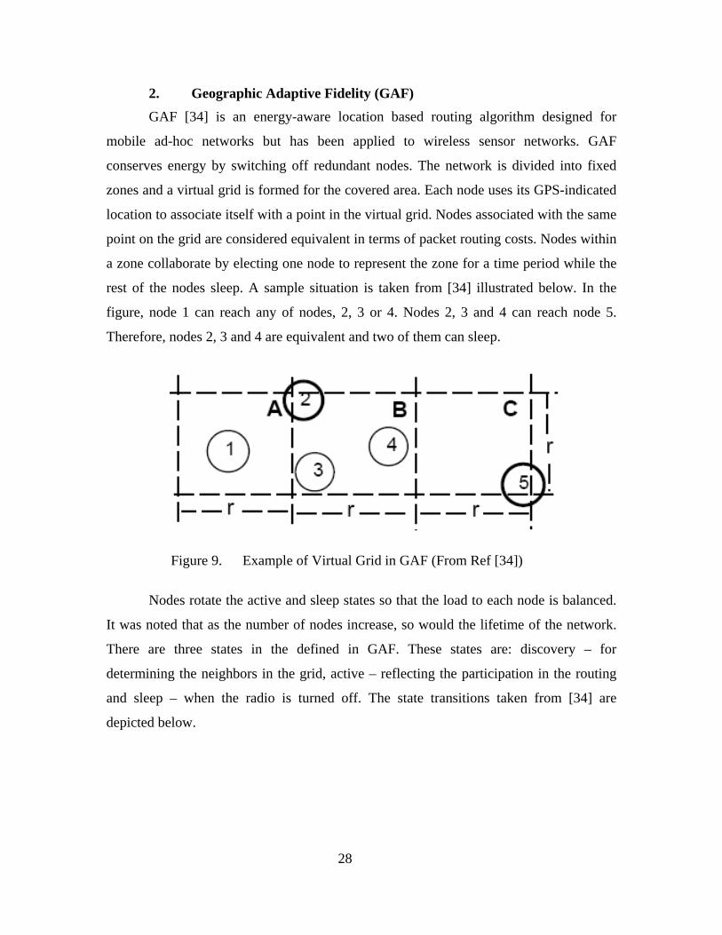
28

2. Geographic Adaptive Fidelity (GAF) GAF [34] is an energy-aware location based routing algorithm designed for

mobile ad-hoc networks but has been applied to wireless sensor networks. GAF

conserves energy by switching off redundant nodes. The network is divided into fixed

zones and a virtual grid is formed for the covered area. Each node uses its GPS-indicated

location to associate itself with a point in the virtual grid. Nodes associated with the same

point on the grid are considered equivalent in terms of packet routing costs. Nodes within

a zone collaborate by electing one node to represent the zone for a time period while the

rest of the nodes sleep. A sample situation is taken from [34] illustrated below. In the

figure, node 1 can reach any of nodes, 2, 3 or 4. Nodes 2, 3 and 4 can reach node 5.

Therefore, nodes 2, 3 and 4 are equivalent and two of them can sleep.

Figure 9. Example of Virtual Grid in GAF (From Ref [34])

Nodes rotate the active and sleep states so that the load to each node is balanced.

It was noted that as the number of nodes increase, so would the lifetime of the network.

There are three states in the defined in GAF. These states are: discovery – for

determining the neighbors in the grid, active – reflecting the participation in the routing

and sleep – when the radio is turned off. The state transitions taken from [34] are

depicted below.

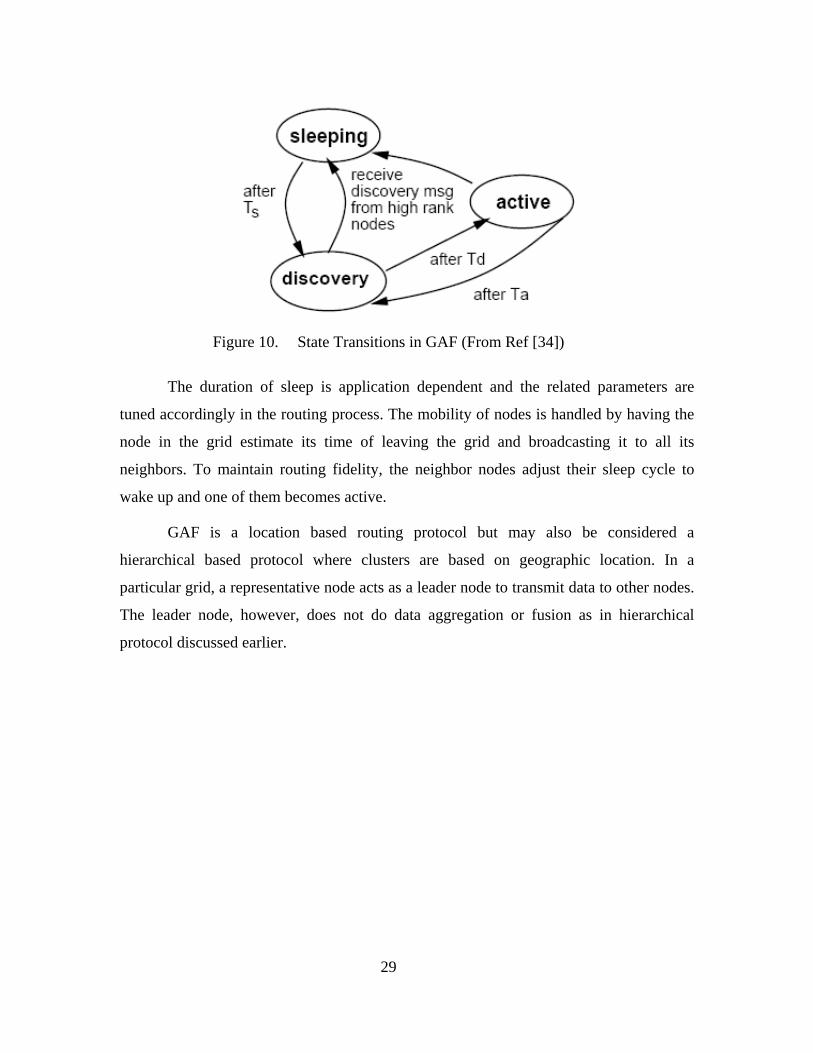
29

Figure 10. State Transitions in GAF (From Ref [34])

The duration of sleep is application dependent and the related parameters are

tuned accordingly in the routing process. The mobility of nodes is handled by having the

node in the grid estimate its time of leaving the grid and broadcasting it to all its

neighbors. To maintain routing fidelity, the neighbor nodes adjust their sleep cycle to

wake up and one of them becomes active.

GAF is a location based routing protocol but may also be considered a

hierarchical based protocol where clusters are based on geographic location. In a

particular grid, a representative node acts as a leader node to transmit data to other nodes.

The leader node, however, does not do data aggregation or fusion as in hierarchical

protocol discussed earlier.

30

F. SUMMARY This chapter described the challenges in the design of routing protocol in wireless

sensor networks and presented some of the routing protocols used in wireless sensor

networks. The table below compares the three classifications: flat-based routing,

hierarchical based routing and location based routing. The next chapter focuses on a

specific flat-based routing protocol designed for wireless sensor networks called XMesh.

Protocol Classification Data

Aggregation

Mobility Position

Awareness

Local-

lisation

Scalability Negotiation

based

Multi-

path

Query -

based

SPIN Flat Yes Possible No No Limited Yes Yes Yes

Directed

Diffusion

Flat Yes Limited No Yes Limited Yes Yes Yes

EAR Flat No Limited No No Limited No No Yes

DSDV Flat No Yes No No Limited No No No

LEACH Hierarchical Yes Fixed

BS

No Yes Good No No No

TEEN &

APTEEN

Hierarchical Yes Fixed

BS

No Yes Good No No No

TTDD Hierarchical No Yes Yes No Low No Possible Possible

GEAR Location No Limited No No Limited No No No

GAF Location No Limited Yes No Good No No No

Table 1. Classification and Comparison of Routing Protocols in Wireless Sensor

Networks

31

IV. XMESH ROUTING PROTOCOL

A. CHAPTER OVERVIEW XMesh is a multi-hop routing protocol developed by Crossbow to run on the

MICA family of motes using the TinyOS environment [35]. It is an ad-hoc mesh

networking protocol capable of network formation without the need for human

intervention. It is also capable of adding and removing network nodes automatically

without having to reset the network. It uses a routing beacon from the base station to

establish route paths back. Given the general acceptance of Crossbow motes for research

purposes, this chapter has been dedicated to a greater understanding of the XMesh multi-

hop routing protocol which was evaluated.

B. PROTOCOL COMPONENTS The high level interactions of all the components implementing the routing

protocol are shown in the figure below. A routing beacon from the base station is used to

establish paths back to it. Each node maintains estimates of the inbound link quality (i.e.,

reception) that is propagated back to its neighbors as the routing protocol is based on the

outbound (i.e., transmission) link.

Figure 11. XMesh Routing Components. (From Ref [7])

32

1. Routing Table The routing table contains the status and routing entries for neighbors. Its fields

include the MAC address, an estimate routing cost to sink, parent address, a child flag, a

list of reception (inbound) link quality, a send (outbound) link quality and link estimator

data structures. The routing table can hold up to 16 entries.

2. Estimator The estimator computes the link quality of its neighbor nodes. Link quality is the

measure of the percent of packets that arrive undamaged on a link and is determined by

the ratio of received to expected packets (i.e., the packet delivery success rate). Other

measures include hop count and route stability.

The estimator snoops on packets in the channel and link quality is estimated by

observing packet success and loss events. Higher level protocols use these estimations to

build routing structures. The estimator is required to react quickly to large changes in link

quality and yet be stable when the link is affected by short term fluctuations. It should not

require significant storage and processing because of limited memory and computational

ability. The ability to react quickly enables higher-level protocols to adapt to

environmental changes and mobility. In XMesh, a window mean with an exponentially

weighted moving average (WMEWMA) is used to estimate the link quality. It computes

the success rate over a fixed time period and smoothes the average with an exponentially

weighted moving average (EWMA).

3. Table Management The eviction, insertion and reinforcement of nodes in the routing table are

determined by the table management policy. A node performs neighbor discovery by

recording information about nodes from which it receives packets either as a result of

passive monitoring or active probing. Link estimation is used to determine which nodes

should be considered neighbors. For each incoming packet upon which neighbor analysis

is performed, the source is considered for insertion or reinforcement. Insertions are

performed if the table is not full. If the source is represented in the table, a reinforcement

operation may be performed to keep it there. If the source is not present and the table is

full, the node must decide whether to discard the information associated with the source

or to evict another node from the table.

33

4. Parent Selection Parent selection is run periodically to identify one of the neighbors for routing.

The cost of a node is an abstract measure of distance, based on various metrics such as

hop count; number of transmissions or reconfiguration over time. A neighbor is selected

as a potential parent only if its cost is less than a current cost of the node. It may also

change to a new parent if the link quality of the current parent drops below a threshold, if

the sink is unreachable through the current parent or if a cycle is detected. When

connectivity to the current parent worsens, its link estimation will degrade over time,

allowing the selection of a new parent. If the connectivity to the current parent is lost and

no potential parents are available, the node declares it to have no parent and sets its cost

to infinity. If the rate of parent change is high, fluctuations in routing will cause the

network to be unstable, hence, routes are evaluated on a periodic basis rather than upon

receiving a route update.

5. Cycle Detection When a node originates a message and sees it returning, a loop has occurred (i.e.,

forwarding message to child instead of parent). By monitoring the forwarding traffic and

snooping on the parents address in each neighbor’s messages, neighboring child nodes

can be identified and will not be considered as potential parents. Since each node is a

router and a data source, cycles can be detected quickly. Once cycle is detected, it is

broken by discarding the current parent by choosing a new one or by becoming disjoint

from the tree.

6. Filter The filter discards non-data packets and duplicate packets. Duplicate packets can

be created upon retransmission when the ACK is lost. Without the filter, these will be

forwarded and possibly causing more retransmissions and more contention, wasting

energy. To avoid duplicate packets, the routing layer at the originating node appends the

sender ID and originating sequence number to the routing header. To suppress

forwarding duplicate messages, each parent retains the most recent originator ID and

originating sequence number in child entries in the routing table.

7. Timer

The timer triggers the periodic update of routing tables, messaging etc.

34

C. ROUTING ALGORITHM In the XMesh routing algorithm [36], the cost metric is one that minimizes the

total number of transmissions in delivering a packet over multiple hops to a destination

and is termed the Minimum Transmission (MT) cost metric. This differs from the

traditional cost metric of distance vector routing which is hop count. In highly reliable

links, retransmissions are infrequent and hop count would suffice in capturing the cost of

packet delivery. However, with links of varying quality, a longer path with fewer

retransmissions may be better than a shorter path with many retransmissions. That is, the

energy required to transmit a packet over a distance with a single hop will be far greater

that the energy required transmitting a packet over that distance with multiple hops.

Figure 12. Broadcasting Beacon Messages and Health Packets (After Ref [36])

The multi-hop network is initially formed when motes broadcast periodic beacon

messages to all other motes within radio range. In Figure 12, nodes one, two, three and

four are within radio range of each other and only nodes one and two are inside the radio

range of the base station mote, node zero. Health and/or data packets are also periodically

transmitted to the base station. The health packets contain information about how well the

Beacon Message and Health Packets being broadcasted

PC

1

0

2

3

4

35

mote is performing in the mesh network, specifically radio traffic. Other health packet

information includes battery voltage and the parent’s received signal strength indicator

(RSSI) data. In Figure 12, node 3 is depicted sending health packets to the base station

through node 2.

When the beacon messages are sent, they contain a cost value, which indicate to

other motes the energy required to transmit a message to the base station. Higher cost

indicates more energy required to make the transmission. The purpose of the cost metric

is to minimize the total cost it takes to transmit to the base station mote (i.e. node zero).

Each node in the mesh network will broadcast its cost value [36] which is derived later in

this section. The beacon message includes the number of hops to send a message to the

base station mote and a packet sequence number. The packet sequence number is a 16 bit

integer and is incremented every time a message is transmitted from the base station mote

or other motes. The beacon message also contains a neighborhood list (NL). The NL

contains information about all other motes in the vicinity that the mote or base station

mote can hear. The NL information has two parts:

• The ID of the neighborhood mote (NM).

• A received estimate on how well the mote can hear neighbor motes. The

received estimate value is based on monitoring the sequence numbers of

the received messages from the NM. The mote can then compute the

percentage of lost packets which determines the link quality between

nodes.

Since losing an acknowledgement would lead to a retransmission that wastes

energy, the link qualities between motes in both directions are important. For each link,

the MT cost is estimated by the inverse of the product of link qualities in the forward

(SendQuality) and backward (RecieveQuality) directions. The link’s cost to its parent or

the Minimum Transmission cost is written as

1 1 1 1ToParent

forward backward

MTlinkquality linkquality SendQuality RecieveQuality

= × = × (4.1)

36

For example, if the SendQuality between node one and node zero is 23% and the

RecieveQuality is 29%, the link cost to node zero is 15.

The parent’s cost would be the total cost of all hops to the base station.

Parent’s cost ( )MT=∑ (4.2)

Hence, the node’s cost value is calculated as:

Node cost = Parent’s cost + Link cost to Parent = ( ) ToParentMT MT= +∑ (4.3)

Figure 13 shows the network status during initial configuration. The base station

beacon message has a cost equal to zero and all other motes have an infinite cost as they

do not know how to route messages back to the base station. There are no routing entries

in the beacon message. Any data messages from the motes are sent with a broadcast

address since no parents have been selected.

Figure 13. Network Status during Initial Configuration (After Ref [36])

After some time, all the motes within the network will be able to hear the beacon

messages from the base station. The motes can then forward messages to the base station.

PC Cost: ∞Cost:0 Parent: PC

Cost: ∞

Cost: ∞

Cost: ∞

1

0

2

3

4

37

As the base station begins to receive messages from other motes, it will include them in

its neighborhood list for broadcasting beacon message. In turn, the motes will include the

base station and other neighbor motes for their beacon message broadcast. Once a parent

is selected, the data message will change from a broadcast address to the parent address.

The mesh network formation will then propagate to the motes that are further away and

cannot hear the base station beacon messages. Figure 14 shows the network status with

cost values established and illustrates the MT path from node three is the one taken

through nodes four and one to node zero.

Figure 14. Network Status with Cost Values (After Ref [36])

D. XMESH PACKET FORMAT

The TinyOS message structure, shown below, consists of a five byte header, a 29

byte payload and a two byte CRC, which is used to determine successful packet

reception.

15

Cost:0 Parent: PC

P20

15

15

10

18

15

28

20

30

40

25

Parent cost

Link cost

Node cost

1

02

3

4

38

Figure 15. TinyOS Message Structure (From Ref [37])

The fields in the TinyOS message header are:

• Address (2 bytes)

• Active Message type (1 byte). The field identifies the type of message being sent: Data, routing or broadcast.

• Group ID (1 byte)

• Payload length (1 byte). This field tells how much actual data is present as the payload size is variable.

Figure 16. TinyOS Message Packet Transmission Sequence (From Ref [37])

The TinyOS message packet transmission sequence is depicted above. Prior to

message transmission, a simple CSMA-based MAC is employed. A random delay is

generated before listening for an idle channel. If the channel is busy, it backs off with a

random delay over a predefined window. When the medium is clear the transmitter is

turned on and the preamble and frame sync bytes are sent to synchronize the motes in the

network. There are three types of preamble,

• Full Extended preamble – used in routing discovery and link monitoring. All route update messages are transmitted using the extended preamble message so that the nodes can discover new links and become synchronized into the network. In addition, all nodes also transmit their locally generated data messages using extended preamble packets.

Header (5) Payload (29) CRC (2)

39

• Short Extended Preamble – used for all routed traffic not originating from the local node. Therefore, all data being forwarded through a node is transmitted with the short extended messages. This applies to all forwarded messages except for those messages traveling to the base station.

• Standard Preamble – used for routed data traveling to the base station for the last hop. The base station has significantly higher network traffic than the rest of the network. Therefore, the use of the standard preamble packet lowers the power consumption of the nodes surrounding the base station.

After the message is sent over the SPI (SCSI Parallel Interface) port, the

transmitter is turned off and the event that the transmission has been completed is

signaled to the application.

At the receiving mote, the TOS packet is assembled. The CRC and group ID are

checked. If the CRC is bad or the group ID does not match, the packet is rejected.

Otherwise, it is accepted and the application signals that a packet has been received.

E. SUMMARY This chapter described the routing components and algorithm of XMesh and

presented the XMesh packet format. The next chapter presents the findings of the

experimental study.

40


41

V. EXPERIMENTAL STUDY

A. CHAPTER OVERVIEW This chapter provides an overview of the hardware platform used in the

experiments. It presents the empirical observations that characterize the network links.

The energy requirements for motes and the network lifespan are discussed. With an

understanding of the character of the network links, the XMesh routing protocol was

observed and the experimental findings presented.

B. HARDWARE PLATFORM

Figure 17. Photo and Block Diagram of MICA2 (from Ref [7])

The diagram above illustrates the hardware platform used in this study, the

Crossbow Technology MICA2 motes running TinyOS. Each sensor node consists of a

7.37 MHz ATmega Microcontroller with 128 kB of Flash for program memory and 4 kB

of SDRAM for data and variables. The network device is Chipcon’s CC1000 radio at 916

MHz (MPR4003), frequency shift keying (FSK) RF transceiver with a max data rate of

38.4 kbps. The RF transmission power can be adjusted through software. The

connectivity experiments used four power levels, -20 dBm (0.01 mW), -10 dBm (0.1

mW), 0 dBm (1 mW) and 5 dBm (3.16 mW). A node can be configured as a base station

3 The MPR400 can operate in two frequency regions: 868 – 870 MHz (up to 4 channels) and 902 – 928 MHz (up to 54 channels). The actual number of possible channels is higher for all MICA2 motes but an adjacent channel spacing of 500 kHz is recommended to avoid adjacent channel interference.

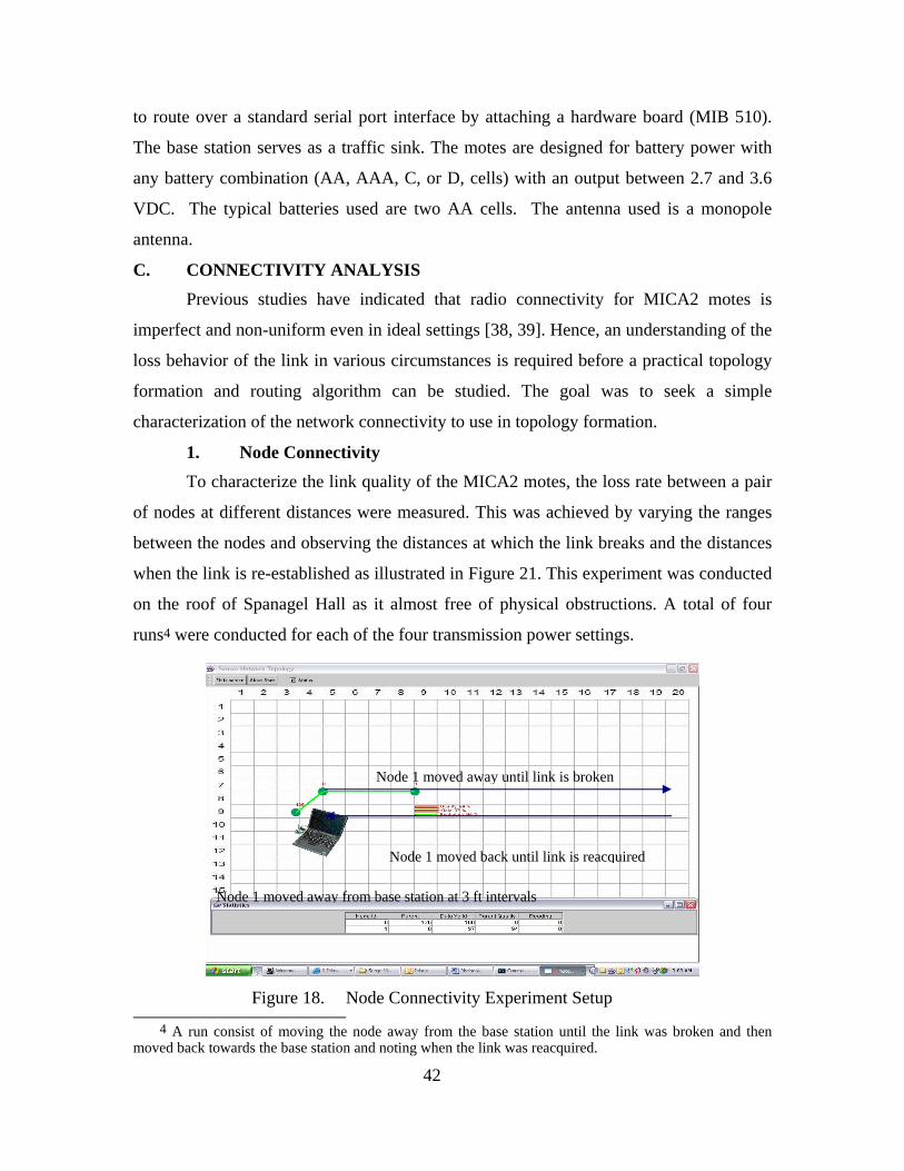
42

to route over a standard serial port interface by attaching a hardware board (MIB 510).

The base station serves as a traffic sink. The motes are designed for battery power with

any battery combination (AA, AAA, C, or D, cells) with an output between 2.7 and 3.6

VDC. The typical batteries used are two AA cells. The antenna used is a monopole

antenna.

C. CONNECTIVITY ANALYSIS Previous studies have indicated that radio connectivity for MICA2 motes is

imperfect and non-uniform even in ideal settings [38, 39]. Hence, an understanding of the

loss behavior of the link in various circumstances is required before a practical topology

formation and routing algorithm can be studied. The goal was to seek a simple

characterization of the network connectivity to use in topology formation.

1. Node Connectivity To characterize the link quality of the MICA2 motes, the loss rate between a pair

of nodes at different distances were measured. This was achieved by varying the ranges

between the nodes and observing the distances at which the link breaks and the distances

when the link is re-established as illustrated in Figure 21. This experiment was conducted

on the roof of Spanagel Hall as it almost free of physical obstructions. A total of four

runs4 were conducted for each of the four transmission power settings.

Figure 18. Node Connectivity Experiment Setup

4 A run consist of moving the node away from the base station until the link was broken and then

moved back towards the base station and noting when the link was reacquired.

Node 1 moved away from base station at 3 ft intervals

Node 1 moved away until link is broken

Node 1 moved back until link is reacquired

43

Figure 22 shows data collected in a scatter plot. It shows how link quality varies

over distance with the motes at the height of 2.5 feet (0.76 m) for a transmission power of

-10 dBm (0.1 mW). It was also observed that the link quality can vary at a same

distance. For example, the link quality at four feet varied between 100% and 98%.

0.0

0.1

0.2

0.3

0.4

0.5

0.6

0.7

0.8

0.9

1.0

0 10 20 30 40 50 60 70 80Distance (feet)

Link

Qua

lity

Transitional regionEffective region

Unreliable region

Figure 19. Reception Probability of Links in a Line Topology

For a given power setting, there is a distance within which the node pairs

basically have good connectivity5. The size of this “effective region” increases with

transmit power. There is also a point beyond which the nodes essentially have no

connectivity, termed the “unreliable region”. In the “transitional region” between these

two points, the average link quality falls off fairly smoothly with some variation. The

other transmission power settings show a similar structure. The results for the four

transmission power levels were tabulated in Table 3 and plotted in Figure 23. It

quantified that more transmission power was required to maintain good connectivity over

larger distances. It was noted that the link between the base station and the node was

5 Good connectivity is defined as link quality greater than 80%

44

established within a minute for each transmission power setting. This was attributed to

the proximity of the mote to the base station (approximately one foot) at the start of each

run.

Transmission Power (mW)

Effective Distance Unreliable Distance

0.01 (-20 dBm) 4 feet (1.22 m) 7.5 feet (2.28 m) 0.1 (-10 dBm) 25 feet (7.62 m) 55 feet (16.76 m) 1 (0 dBm) 80 feet (24.38 m) 110 feet (33.53 m) 3.16 (5 dBm) 145 feet (44.20 m) 170 feet (51.82 m)

Table 2. Transmission Power versus Operating Distances

Link Break-off and Reaquire Distances vs Transmission Power

0

20

40

60

80

100

120

140

160

180

0.01 0.1 1 10Transmission Power (dBm)

Dis

tanc

e (fe

et)

Re-estbBrkoff

Figure 20. Transmission Power versus Transmission Distances

These readings differ from what was advertised in the Crossbow MICA2

datasheet [40]. Also, the Crossbow Technologies technical support (FAQ website) states

“916 MHz band MICA2s have been tested to transmit up to ~500 feet (~165m) outdoors

with a 1/2 wave dipole antenna, the RF power set to 5 dBm (maximum TX power), 1m+

off the ground, line of sight.”

45

2. Network Connectivity The number of nodes required to maintain network connectivity in a given area

will be dependent on the transmission power of the motes. The following is an estimate

of the number of nodes required for an open area with motes 2.5 feet above ground.

Transmission Power (mW)

Transmission Radius

Coverage required (m2)

Number of Motes

required 10000 613 20000 1225 50000 3062

0.01 (-20 dBm) 7.5 ft (2.28m)

100000 6124 10000 12 20000 23 50000 57

0.1 (-10 dBm) 55 ft (16.76m)

100000 114 10000 3 20000 6 50000 15

1 (0 dBm) 110 ft (33.53m)

100000 29 10000 2 20000 3 50000 6

3.16 (5 dBm) 170 ft (51.82m)

100000 12 Table 3. Mote Density Required for Connectivity

Hence, depending on the application of the sensor networks and the number of

motes available, the transmission power can be adjusted to extend the lifetime of the

sensor network.

D. ENERGY EFFICIENCY STUDY Since the transmission powers levels can be programmed through software, the

connectivity ranges of the motes will vary with the power settings. The higher the

transmission power, the greater the connectivity range and the greater the power

consumed. The typical power drawn by the MICA2 motes is 35 mA (1 mW transmission

power) when awake and 10µA when asleep [7]. The main power consumer in the MICA

motes is the radio transceiver (approximately 20 mA). Consider that if there was no

46

power saving scheme in place, continuous data acquisition would last less that 80 hours.

This is illustrated in the following two graphs. The battery rating quoted by Energizer is

2850 mAh.

Figure 21. Battery Discharge Characteristic, Energizer e91 (www.energizer.com)

80 hours continuous data acquisition

47

Figure 22. MICA2 Battery Pack Service Life Test Data (From Ref [7])

Power savings can be achieved via implementation of a duty cycle. For example,

assuming that a mote must forward 10 packets and perform a sensor reading, consuming

three seconds every time it wakes up, this will consume approximately 50 mA-sec/cycle

= 0.014 mA-hours/cycle. A typical two-AA battery pack supplies 1700 mAh @ 15 mA

drain. Therefore, 1700 120,0000.014 /

mAh cyclesmAh cycle

= . For 100% wake state or duty cycle,

the mote will last120,000 3sec/ 100cycles cycle hours⋅ = . If a 1% wake state is

implemented (297 seconds asleep per cycle), the lifetime of the mote

is120,000 300sec/ 1.1cycles cycle years⋅ = . The recommended duty cycle for most

applications is 0.5% to 2%. The wake state and the expected mote lifespan are tabulated

below.

80 hours continuous data acquisition

48

Duty Cycle (%) Expected Lifetime (years) 100 0.01 35.5 0.03 11.5 0.10 7.53 0.15 5.61 0.20 2.22 0.51 1.00 1.14 0.50 2.28

Figure 23. Duty Cycle and their Corresponding Mote Lifetimes.

E. EVALUATION OF XMESH

1. Experiment Setup The photo below presents the environment (Bullard Hall study space) where the

experiment was conducted with eight MICA2 motes. The motes were to cover a 4.5

meters by 4.5 meters portion (approximately 20 m2) of the study space.

Figure 24. Motes Deployed in Bullard Hall Study Space

It was observed that if the motes were switched on near the base station prior to

deployment, the time taken for the network to be established was shorter that if they were

to be switched on after being deployed. The average time taken for the motes to establish

connectivity when placed close to the base station was approximately five to seven

minutes while the average time taken of establish connectivity if the motes were

deployed then switched on was between twelve and eighteen minutes. Also, observed

49

was that the link quality between pairs of nodes differed considerably. For example,

Node 3 may report a link quality of 92% with Node 5, but node 5 reports a link quality of

56% with Node 3. Hence, it was concluded that link asymmetry existed between nodes.

To expedite the experiment, the motes were placed at a distance of one foot to the

base station prior to being deployed. The Surge program was used to record the

performance of the network. The motes were subsequently placed on the tops of the

cubicle partitions which were 2.2 meters (seven feet) from the ground with their transmit

powers set to 0.01 mW. The Surge graphical user interface (GUI) was used to monitor

the network status in real time. The figure below was a snap-shot of the network was

connectivity was established amongst the motes.

Figure 25. Snapshot from Surge GUI of the sensor network after links were established

0

1 2

5 34

7 6

50

After the motes established good connectivity, node three was switched off to

simulate node failure. The motes were able to reorganize despite the loss of node three as

illustrated in Figure 29 below.

Figure 26. Network with Simulated Node Failure and Rerouting via Node 7.

The definition of each column in the Surge GUI is given below:

Column Definition ID The node ID Rec Messages Received Sent Messages Sent Yield # packets received/ # packets sent

Duty Cycle % time off/ % time on Parent Node parent

Quality # packets sent or received at parent/ # packets sent or received

0

1 2

534

76

51

Voltage battery voltage of mote P1 Primary parent P2 Secondary parent

Min Cut Minimum number of nodes that need to be removed in order for a mote do disappear from the network.

Table 4. Definition of Surge-View Statistics 2. Evaluation Metrics The metrics used to evaluate the performance of the XMesh routing protocol are

packet delivery ratio or yield (as termed in Surge-View GUI) and stability.

a. Packet Delivery Ratio The packet delivery ratio, or yield, is the number of packets received at the

sink for a node divided by the number originated. Losing packets reaching the sink

wastes energy and resources. The packet delivery ratio describes the loss rate at the

routing layer that will affect the maximum throughput the network can support. This

metric will characterize completeness and correctness of the routing protocol.

b. Stability Stability measures the total number of route or parent changes in the

network over a period of time, which indicates the stability of the routing topology. A

stable routing topology should make higher level operations such as scheduling and

aggregation easier.

3. Results The Stats software in Surge-View summarized the output of the completed

experiment in the table below. These results were collected over a period of 55 minutes.

52

Table 5. Output from Stats Program in Surge-View

a. Observations on Packet Delivery Ratio

050

100150200250300350

1 2 3 4 5 6 7

Node number Packets Received Packets Sent

Figure 27. Packet Delivery Ratio

The initial packet delivery ratio was approximately 89% for all nodes. The

chart above depicts the packet delivery ratio with node failure on node number three. It

was observed that the packet delivery ratio of the motes four, five and seven, which were

further away form the base station, had a low packet delivery ratio (approximately 40%),

whereas, motes one, two and three, which were closer to the base station, had a high

packet delivery ratio (over 80%). This low packet delivery ratio for motes situated farther

Node Number

Packets Received

Packets Sent

Success Rate

Parent Changes

Level Changes Average Level Battery

Voltage

1 284 299 0.950 0 1 0.989 3.052

2 248 292 0.849 0 1 0.988 3.237

3 137 167 0.820 2 3 1.153 3.052

4 127 245 0.518 5 4 2.189 3.081

5 126 276 0.457 6 4 2.000 3.002

6 105 273 0.385 4 4 2.752 2.960

7 114 246 0.463 5 2 1.675 3.030

53

away can be attributed to a significant amount of packets lost for nodes four five, six and

seven when node three was switched off to simulate node failure.

b. Observation on Stability The stability of the network was determined through the number of parent

changes over the experiment. In the chart below, the number of parent changes in motes

one and two were zero, whereas motes four, five, six and seven had several parent

changes. This can be attributed to the communications link being affected by pedestrian

traffic and the asymmetric nature of link quality between nodes. However, it can be

concluded that the network was able to react quickly to large changes in link quality and

yet be stable when the link is affected by short term fluctuations.

Node Parent Change

01234567

1 2 3 4 5 6 7Node Number

Pare

nt C

hang

es

Parent Changes

Figure 28. Stability of the Network

F. SUMMARY This chapter presented the results from the experiments and tests on a network of

MICA2 motes. Experiments were conducted to determine the node and network

connectivity with varying transmission powers. The relationship between transmission

power and node/network lifetime was studied. Network performance was evaluated in

terms of packet delivery ratio and stability. Further experimentation on the network

performance was omitted due to time constraints. Conclusions based on the experimental

results follow in the next chapter, along with recommendations for future work.

54


55

VI. CONCLUSION AND FUTURE WORK

A. CONCLUSION Wireless sensor networks can be used to monitor dispersed areas, such as

environmental and agricultural monitoring; physical things such as structure monitoring

and medical diagnostics of human physiology; and the interaction of things with each

other and the encompassing space such as warehouse inventory control and HVACS.

The evolution of integrated circuit technology, wireless communications and networking

will continue to decrease the size of sensors and increase their utility. As such,

applications using wireless sensor networks will continue to grow.

In this thesis, the communications characteristics of the MICA2 radio were

studied. The key points of the study are as follows:

• The antenna radiation pattern was that of a dipole antenna.

• For any given power setting, there were three regions of communications, the effective, transitional and unreliable regions.

• The size of this “effective region” increases with transmit power. There is also a point beyond which the nodes essentially have no connectivity, termed the “unreliable region”. In the “transitional region” between these two points, the average link quality falls off fairly smoothly with some variation.

• The number of motes required for connectivity in a given area is proportional to the amount of transmitted power of the motes.

• It was analyzed that to prolong the network lifetime, a duty cycle must be implemented so that the motes can conserve power by staying asleep. For a 1% duty cycle, the lifetime of a network is approximately 1.1 year.

This thesis also observed the routing protocol of XMesh, using several MICA2

motes deployed in a cluttered indoor environment. The observations are as follows:

• The average time taken for the motes to establish connectivity when placed close to the base station was approximately five to seven minutes while the average time taken to establish connectivity if the motes were deployed before being switched on was between twelve and eighteen minutes.

• When all nodes were working, the network packet delivery ratio was approximately 89% with few parent changes. It was concluded that the network performance was reliable and stable.

56

• When node three was switched off to simulate node failure, it was observed that there was significant packet loss from the nodes situated farther away from the base station. Node parent changes also increased during this period. However, when the routes were reestablished, the packet delivery ratio increased and parent changes decreased.

It can be concluded that the effects of node failure did not adversely affect the

routing protocol in XMesh as the network was able to reconfigure itself and adapt to the

change.

B. FUTURE WORK This thesis surveyed several routing protocols. To evaluate the performance of

XMesh further, other routing protocols can be implemented on the Crossbow MICA2

motes and their performance compared with XMesh in a variety of environmental

conditions.

As there were only eight MICA2 motes with which to experiment, this thesis was

not able to evaluate the scalability of the routing protocol. It is recommended that similar

experiments be conducted with thirty or forty nodes, beginning with several motes and

slowly introducing more motes to see the effects on the network.

It is also recommended also to study of the maximum stable throughput of the

network [41, 42]. This is the maximum amount of traffic per unit time (measured in bit

per second) that can be injected into the network from all sources while the size of the

queue at any network node is bounded. Coupled with the available battery energy and the

efficiency with which the packets are converted to RF power for transmission, it will

determine the number of motes required in an area based on the amount of information

that is required to be routed.

57

LIST OF REFERENCES

[1] I.F. Akyildiz, W Su, Y. Sankarasubramaniam and E Cayirci, “Wireless Sensor Networks: A Survey,” Communication Magazine, IEEE, Vol. 40 Issue 8, pp. 102-114, August 2002. [2] IEEE 1451, A Standard Smart Transducer Interface, Sensors Expo, Philadelphia October 2001; http://Ieee1451.Nist.Gov/Workshop_04Oct01/1451_Overview.Pdf Accessed 10 June 2005. [3] C. F. Chaisserini, M. Garetto, “Modeling the Performance of Wireless Sensor Networks,” IEEE INFOCOM 2004, 23rd Annual Joint Conference of the IEEE Computer and Communications Societies, Vol. 1, pp. 231, Hong Kong, China, 7-11 March 2004. [4] Bhaskar Krisnamachari, Deborah Estrin, Stephen Wicker “Modeling Data-Centric Routing In Wireless Sensor Networks,” USC Computer Engineering Technical Report CENG 02-14, Los Angeles, California, April 2002. [5] Chi-Fu Huang, Yu-Chee Tseng, “Coverage Problem in Wireless Sensor Networks,” WSNA ’03, Proceedings of the 2nd ACM international conference on Wireless sensor networks and applications, pp. 115 – 121, San Diego, California, 19 September 2003. [6] Gang Lu, Bhaskar Krisnamachari, Cauligi S. Raghavendra, “An Adaptive Energy Efficient And Low Latency MAC For Data Gathering in Wireless Sensor Networks,” Computer Society, Proceedings of the 18th International Parallel and Distributed Processing Symposium 2004, pp. 224, Santa Fe, New Mexico, 26-30 April 2004. [7] Crossbow Technologies, Getting Started Guide and Reference Manuals, Smart Dust Training Seminar, San Jose, 19-20 April 2005. [8] Holger Karl, Andreas Willig, Protocols and Architectures for Wireless Sensor Networks, Chapter 2 pp. 18-53, Chapter 4, pp. 86-108, John Wiley and Sons, West Sussex England, 2005. [9] J. M. Rabaey, M. J. Ammer, J. L. Da Silva Jr., D. Patel, S Roundy, “Picoradio Supports Ad-hoc Ultra-Low Power Wireless Networking,” IEEE Computer Magazine, Vol. 33, Issue 7, pp. 42-48, July 2000. [10] F.L. Lewis, Smart Environments: Technologies, Protocols, and Applications, Chapter 2, Edited By Diane Cook and Sajal Das, John Wiley, New York, 2004.

58

[11] J. Hill, R. Szewczyk, A.Woo, S. Hollar, D. Culler, K. Pister, “Systems Architecture Directions For Networked Sensors,” Proceedings of Architectural Support For Programming Languages and Operating Systems, pp. 93-104, Boston, Massachusetts, November 2000. [12] N Bulusu, J Heidimann, D. Estrin, “GPS-Less Low Cost Outdoor Localization for Very Small Devices,” Technical Report 00729, Computer Science Department, USC, Los Angeles, California, April 2000. [13] Mark E. Tingle, “Performance Evaluation of Prototyped Wireless Ground Sensor Network,” Master’s Thesis, Naval Postgraduate School, Monterey, California, March 2005. [14] Swee Jin, Koh, “Study of RF characteristics of MICA2, the Sensor Networking System,” Master’s Thesis, Naval Postgraduate School, Monterey, California, December 2005. [15] K. Akkaya, M. Younis, “A Survey on Routing Protocols for Wireless Sensor Networks,” Ad-hoc Networks, Vol. 3 No. 3, pp. 325-349, May 2005. [16] A. S. Porret, T. Melly, D. Python, C. Enz, E. Vittoz, “Tradeoffs and Design of an Ultra Low Power UHF Transceiver Integrated in a Standard Digital CMOS Process,” Proceedings of the 2000 International Symposium on Low power electronics and design, pp. 273-278, Rapallo, Italy, 25-28 June 2000. [17] Honghai Zhang and Jennifer C. Hou, “Maintaining Sensing Coverage and Connectivity in Large Sensor Networks,” Wireless Ad Hoc and Sensor Networks: An International Journal, Vol. 1, Num. 1-2, pp. 89-123, January 2005. [18] K Sohrabi, et al., “Protocols for Self Organization of a Wireless Sensor Network,” IEEE Personal Communications, Vol. 7, No. 5, pp. 16-37, October 2000. [19] W. Heinzelman, A Chandrakasan, H Balakrishan, “Energy Efficient Communication Protocol for Wireless Microsensor Networks,” System Sciences, 2000. Proceedings of the 33rd Annual Hawaii International Conference on, 10 pp. Vol. 2, 4-7 January 2000. [20] R. C. Shah, J Rabaey, “Energy Aware Routing for Low Energy Ad-hoc Sensor Networks,” Wireless Communications and Networking Conference, 2002. WCNC2002. 2002 IEEE Vol.1, pp. 350- 355, 17-21 March 2002. [21] Curt Schurgers, Mani B. Srivastava, “Energy Efficient Routing in Wireless Sensor Networks,” Military Communications Conference, 2001. MILCOM 2001. Communications for Network-Centric Operations: Creating the Information Force. 2001 IEEE, Vol.1, pp. 357- 361, 28-31 October 2001.

59

[22] C. Shen, C. Srisathapronphat, C. Jaikaeo, “Sensor Information Networking Architecture and Applications,” IEEE Personal Communications, Vol.8, No.4, pp. 52 – 59, August 2001. [23] W. R. Heinzelman, J. Kulik, H. Balakrishnan, “Adaptive Protocols for Information Dissemination in Wireless Sensor Networks,” MobiCom '99: Proceedings of the 5th annual ACM/IEEE International Conference on Mobile Computing and Networking, pp 174-185, Seattle, Washington, August 1999. [24] J. Kulik, W. R. Heinzelman, H. Balakrishnan, “Negotiation-based Protocols for Disseminating Information in Wireless Sensor Networks,” ACM Wireless Networks, Volume 8, Issue 2/3, pp. 169 – 185, March-May 2002 [25] C. Intanagonwiwat, R. Govindan, D. Estrin, “Directed Diffusion: A scalable and Robust Communication Paradigm for Sensor Networks,” Proceedings of the 6th annual international conference on Mobile computing and networking, p.56-67, Boston, Massachusetts, 6-11 August 2000. [26] C. Intanagonwiwat, R. Govindan, D. Estrin, J. Heidemann, F. Silva, “Directed Diffusion for Wireless Sensor Networking,” ACM/IEEE Transactions on Networking, Vol 11, Issue 1, pp. 2-16, February 2002. [27] R. Shah and J. Rabaey, “Energy Aware Routing for Low Energy Ad-hoc Sensor Networks,” Wireless Communications and Networking Conference, 2002. WCNC2002. 2002 IEEE, Vol.1, pp. 350- 355, 17-21 March 2002. [28] C. Perkins, P. Bhagwat, “Destination-Sequence Distance Vector Routing (DSDV) for Mobile Computers,” SIGCOMM '94: Proceedings of the Conference on Communications Architectures, Protocols and Applications, pp. 234-244, London, United Kingdom, August 1994. [29] A. Manjeshwar, D.P Agrawal, “TEEN: A Protocol for Enhanced Efficiency in Wireless Sensor Networks,” Proceedings 15th International Parallel and Distributed Processing Symposium, pp. 2009 - 2015, San Francisco, CA, 23-27 April 2001. [30] A. Manjeshwar, D.P Agrawal, “APTEEN: A Hybrid Protocol for Efficient Routing and Comprehensive Information Retrieval in Wireless Sensor Networks,” Proc. International Parallel and Distributed Processing Symposium., IPDPS 2002, pp. 195 – 202, Ft. Lauderdale, Florida, 5-19 April 2002. [31] Haiyun Luo, Fan Ye, Jerry Cheng, Songwu Lu, Lixia Zhang, “A Two-tier Data Dissemination Model for Large-scale Wireless Sensor Networks,” Proc. 8th Annual International Conference on Mobile Computing and Networking, pp. 148 – 159, Atlanta, Georgia, 23-28 September 2002.

60

[32] S. Capkun, M. Hamdi, J. Hubaux, “GPS-less Positioning in Mobile Ad-hoc Networks,” Proc. 34th Annual Hawaii International Conference on System Sciences, pp. 9008, Maui, Hawaii, 3-6 January, 2001. [33] Y. Yu, R. Govindan, D. Estrin, “Geographical and Energy Aware Routing: A Recursive Data Dissemination Protocol for Wireless Sensor Networks,” UCLA Computer Science Department Technical Report UCLA/CSD-TR-01-0023, May 2001. [34] Y. Xu, J. Heidemann, and D. Estrin, “Geography-Informed Energy Conservation for Ad-hoc Routing,” Proc 7th Annual ACM/IEEE International Conference on Mobile Computing and Networking, pp. 70-84, Rome, Italy, July 2001. [35] Tinyos Online Tutorial, Http://www.Tinyos.Net/Tinyos-1.X/Doc/Tutorial/ Accessed 20 October 2005. [36] Crossbow Technologies, XMesh 2.0 Manual (Draft) Revision A, e-mail attachment from Alan Broad, dated 13 October 2005. [37] Tim Reilly, “Mote Software Development for Wireless Sensor Networks,” presented at the 2nd Annual IEEE Communications Society Conference on Sensor and Ad-hoc Communications and Networks, Santa Clara, California, 26 September 2005. [38] Y. Choi et al, “The Mote Connectivity Protocol,” 12th International Conference on Computer Communications and Networks, 2003. ICCCN 2003 Proceedings, pp. 533- 538, Dallas, Texas, 20-22 October 2003. [39] D.D Couto, D. Aguayo, B. Chambers, and R. Morris, “Performance of Multihop Wireless,” ACM SIGCOMM Computer Communication Review, Vol 33, Issue 1, pp. 83-88, January 2003. [40] Crossbow Technologies MICA2 Datasheet, http://www.xbow.com/Products/Product_pdf_files/Wireless_pdf/MICA2_Datasheet.pdf, Accessed 12 December 2005. [41] Z. Hu and B. Li, “Fundamental Performance Limits of Wireless Sensor Networks,” to appear in Ad-Hoc and Sensor Networks, Yang Xian and Yi Pan, Editors, Nova Science Publishers, 2004. [42] Z. Hu and B. Li, “On the fundamental capacity and lifetime limits of energy-constrained wireless sensor networks,” Real-Time and Embedded Technology and Applications Symposium 2004, Proc. RTAS 2004, pp. 2 – 9, 25-28 May 2004,

61

INITIAL DISTRIBUTION LIST

1. Defense Technical Information Center Ft. Belvoir, Virginia

2. Dudley Knox Library Naval Postgraduate School Monterey, California

3. Chair, Department of Electrical and Computer Engineering Naval Postgraduate School Monterey, California

4. Professor Gurminder Singh Department of Computer Science Naval Postgraduate School Monterey, California

5. Professor John McEachen Department of Electrical and Computer Engineering Naval Postgraduate School Monterey, California

6. Professor Michael Morgan Department of Electrical and Computer Engineering Naval Postgraduate School Monterey, California

7. Director, Temasek Defense Systems Institute

National University of Singapore, Singapore

8. Ms Tan Lai Poh

Temasek Defense Systems Institute National University of Singapore, Singapore

Performance Evaluation of a Routing Protocol for Wireless Sensor Networks

Documents

Transcript of Performance Evaluation of a Routing Protocol for Wireless Sensor Networks