Performance-Based Seismic Design: Avant-garde and 1

code-compatible approaches 2

Dimitrios Vamvatsikos1, Athanasia Κ. Kazantzi2 and Mark A. Aschheim3 3

Abstract: Current force-based codes for the seismic design of structures use design spectra 4

and system-specific behavior factors to satisfy one or two pre-defined structural limit-states. 5

In contrast, performance-based seismic design aims to design a structure to fulfill any number 6

of target performance objectives, defined as user-prescribed levels of structural response, 7

loss, or casualties to be exceeded at a mean annual frequency less than a given maximum. 8

First, a review of recent advances in probabilistic performance assessment is offered. Second, 9

we discuss the salient characteristics of methodologies that have been proposed to solve the 10

inverse problem of design. Finally, an alternative approach is proposed that relies on a new 11

format for visualizing seismic performance, termed Yield Frequency Spectra (YFS). YFS 12

offer a unique view of the entire solution space for structural performance of a surrogate 13

single-degree-of-freedom oscillator, incorporating uncertainty and propagating it to the 14

output response to enable rapid determination of a good preliminary design that satisfies any 15

number of performance objectives. 16

CE Database subject headings: Seismic response; Earthquakes; Performance 17

evaluation; Safety; Structural reliability 18

1 Lecturer, School of Civil Engineering, National Technical Univ. of Athens, Greece (corresponding author). E-

mail: divamva@mail.ntua.gr

2 Research Engineer, J.B. ATE, Herakleion Crete, Greece. E-mail: kazantzi@mail.ntua.gr

3 Professor, Dept. of Civil Engineering, Santa Clara Univ., 500 El Camino Real

Santa Clara, CA 95053. E-mail: maschheim@scu.edu

Author Keywords: Performance-based design; Probabilistic methods; Uncertainty 19

Introduction 20

Earthquake engineering is a fascinating scientific field where multiple disciplines come 21

together to mitigate the threat of one of the deadliest natural hazards on Earth. Of immediate 22

concern is the entirety of the built environment that houses the majority of human societal 23

and economic activities. Earthquakes thus threaten immeasurable wealth, representing past 24

investments in existing infrastructure and ever-increasing future ones as new structures are 25

added or renovated yearly. Damage to the built infrastructure ricochets through the 26

transportation, communication, financial, cultural, and economic dimensions of society. 27

Recent seismic events, e.g., Northridge (1994), Kobe (1995), China (2008), Tohoku (2011), 28

have shown that despite considerable advances in research, we still have a long way to go: 29

while modern buildings have lower fatality rates, the staggering monetary losses and 30

disruption of function from seismic events can cripple entire cities, or even countries. 31

At the core of earthquake engineering stand the dual problems of assessment and design. 32

Assessment is the direct process of estimating structural behavior given the structure and the 33

hazard. Design is the inverse problem, whereby a structure, its members and properties are 34

established to achieve an acceptable behavior under the given seismic hazard. As typically 35

befits such dualities, the direct path of assessment is by far the simpler of the two. Thus, 36

while the earthquake engineering field has benefited enormously from recent advances in 37

computer science and technology, these have been realized in an asymmetric way. Important 38

solutions have mostly been achieved for the assessment problem—e.g., Fajfar and Dolsek 39

(2010) introduced the concept of performance quantification within a probabilistic context as 40

a viable approach for design. Therein, a structure’s properties may be taken into account 41

together with the seismic hazard obtained by probabilistic seismic hazard analysis (PSHA) to 42

provide relatively accurate estimates of the distributions of structural demand, repair cost, 43

time-to-repair or even human casualties. While most of these capabilities are still only 44

available at the academic level, some of the benefits are influencing the new generation of 45

seismic codes dealing with the assessment of existing structures, such as EN1998-3 (CEN 46

2005) and ASCE/SEI 41-06 (2007), and in the establishment of design parameters for seismic 47

force-resisting systems, e.g., FEMA P-695 (2009) and FEMA P-795 (2011). 48

In contrast, no such revolution has been realized for routine design. Current seismic 49

design codes follow a classical force-based design paradigm that has been in place for 50

decades, in which design lateral forces are based on elastic demands reduced by a system-51

specific “behavior” R- or q-factor to account for inelasticity. Generally, the smoothed 52

(pseudo-acceleration) design spectra and R- or q-factors are intended to approximately 53

achieve Life Safety performance for ground motions having a probability of exceedance of 54

about 10% in 50 years. The R- or q-factors are prescribed by the code, are specific to each 55

lateral load-resisting system type, and purportedly account for the ductility capacity and 56

overstrength inherent in buildings of various configurations, in view of local construction 57

practice. Demands at critical sections are determined by elastic analysis (static or dynamic) in 58

a simplified process that is intuitive to engineers. The design is deemed to provide acceptable 59

Life Safety performance simply by ensuring critical member sections have sufficient strength 60

and conform with prescribed detailing requirements. Serviceability is also addressed, by 61

limiting interstory drifts, either under the design lateral loads or for a reduced design 62

spectrum that relates to a more frequent level of seismic loads. 63

While the simplicity and utility of the classical approach is appealing, many drawbacks 64

exist. The emphasis on forces obscures the importance of stiffness, deformation demands, 65

mechanism development, and deformation compatibility. Moehle (1992) noted the value of 66

explicitly considering displacements in design, while Priestley (2000) promoted the use of an 67

equivalent linear approach to displacement-based design. Performance-based design 68

approaches often aim to limit drift and ductility demands and rely on displacement-based 69

approaches for doing so. Displacement-based approaches may be based on an estimate of the 70

fundamental period or the yield displacement of the structure in a first-mode pushover 71

analysis. The benefits of both force- and displacement-based approaches can be realized in 72

hybrid approaches that combine the two, as described recently by Tzimas et al. (2013). 73

Besides the emphasis on forces, another drawback of the classical approach is that 74

nonlinear effects are addressed only through the necessarily imprecise reduction/behavior 75

factor, while uncertainties are incorporated via safety factors at the input level of material and 76

load values instead of the output response. Under the severe demands of strong ground 77

shaking, this formulation leads to substantial variability in performance, which either leaves 78

some fraction of the building inventory vulnerable to deficient performance or wastes 79

resources in needlessly improving the performance of others, attempting to uniformly raise 80

the bar across a non-uniform population. A shift in paradigm is needed, from the present 81

emphasis on imbuing conservatism in the design of members to meet code requirements to 82

explicit accounting for uncertainty to achieve desired performance objectives for the specific 83

system. 84

Theoretical and practical difficulties have hampered the much sought-after leap to 85

performance-based seismic design, whereby a structure would be directly designed to satisfy 86

a range of performance objectives with specific allowable exceedance rates and explicit 87

consideration of uncertainty. The present paper responds to this challenge, providing a direct 88

way to incorporate uncertainty into a simple seismic design process that respects user-89

determined limits on drift and system ductility. To lay the proper groundwork, the following 90

discusses the state-of-art in performance-based design, focusing on uncertainties, the 91

probabilistic basis of performance assessment, and salient characteristics of both 92

conventional and novel approaches to seismic design. In the end, the representation of 93

seismic demands using Yield Frequency Spectra (YFS) is offered as a new approach to 94

achieving performance targets with reasonable computational complexity. 95

Current state of art 96

Aleatory and epistemic uncertainty 97

During the last decades, the use of probabilistic tools for assessing the reliability of structural 98

systems under seismic excitations has attracted considerable research worldwide (e.g. 99

Bazzurro et al. 1998, Cornell et al. 2002; Wen et al. 2003; Krawinkler and Miranda 2004). 100

Both assessment and design become more challenging when coupled within a probabilistic 101

framework, needed to account for the various sources of uncertainty sources that are intrinsic 102

to engineering applications. Uncertainties can be due to the inherently random nature 103

(aleatory), e.g., of seismic loads, or can be attributed to our incomplete knowledge 104

(epistemic), for example regarding the modeling or the actual properties of an existing 105

structure. The fundamental difference is that epistemic uncertainty can be reduced, for 106

example by conducting additional measurements, tests or experiments. However, aleatory 107

randomness is naturally occurring in a process, e.g., the sequence and magnitude of 108

earthquakes, and cannot be alleviated (at least not with any current or foreseeable 109

technology). In general, most existing performance-based assessment formats treat these two 110

flavors in a unified way (despite some objections, e.g., Der Kiureghian 2005) prompting us to 111

refer to them collectively as simply “uncertainty”. 112

So far, several researchers have concluded that, among all uncertainties, the ground 113

motion waveform has the most profound influence on the structural reliability, especially in 114

the case of performance levels associated with severe structural and non-structural damage 115

(Dymiotis et al. 1999; Kwon and Elnashai 2006; Kazantzi et al. 2008; Kazantzi et al. 2011). 116

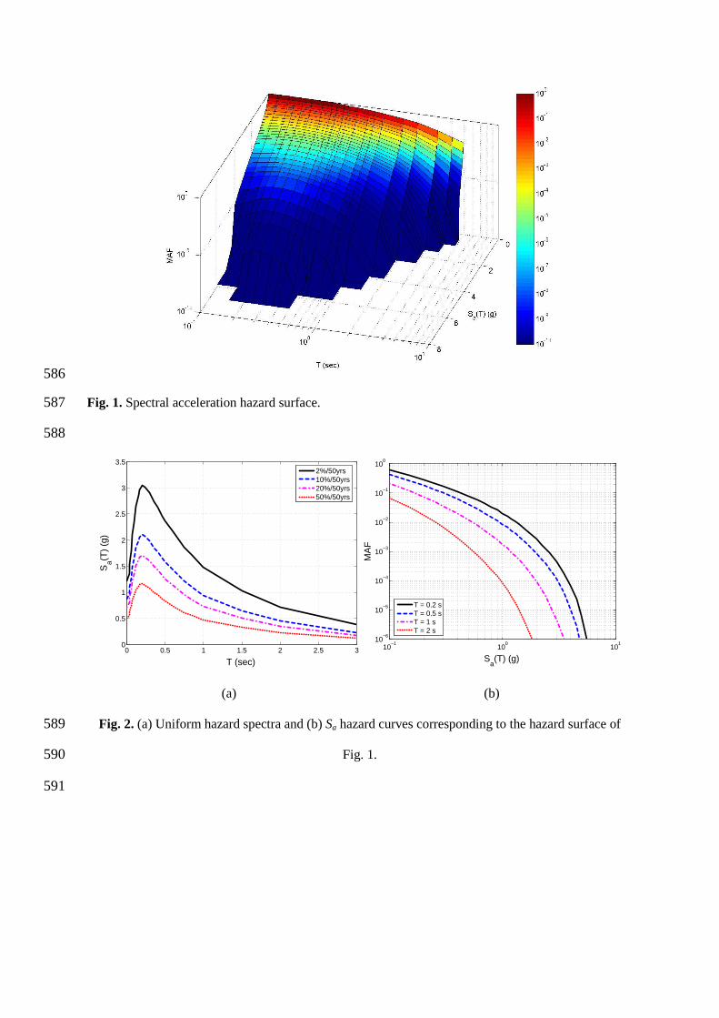
A comprehensive site hazard representation that is compatible with current design norms is 117

provided by the seismic hazard surface, a 3D plot of the mean annual frequency (MAF) of 118

exceeding any level of spectral acceleration Sa(T) for the full practical range of periods T 119

(Fig. 1). This is the true representation of seismic demands for elastic single-degree-of-120

freedom (SDOF) oscillators at any given site. More familiar 2D pictures can be produced by 121

taking cross sections (or contours) of the hazard surface. Cutting horizontally at given values 122

of MAF will provide the corresponding uniform hazard spectra (UHS). For example, at 123

Po = − ln(1 − 0.1)/50 = 0.0021, or a 10% in 50 yrs probability of exceedance (Fig. 2a), one 124

obtains the spectrum typically associated with design at the ultimate limit state (or Life 125

Safety). Taking a cross section at a given period T produces the corresponding Sa(T) hazard 126

curve (Fig. 2b). 127

Considerable uncertainty also may be introduced due to material properties and due to 128

the choice of model and analysis type. Details of soil, foundation and structural modeling 129

may heavily influence the outcome of any analysis method, as shown in Fig. 3 for the 130

capacity curve of a simple 5-story structure. With models under cyclic loading still under 131

development (e.g. Lignos and Krawinkler 2011) and with considerable uncertainty about 132

behavior in the high-deformation region (Fig. 4a), the accurate evaluation of structural 133

response within an analytical context remains a difficult task, and one that may lead to 134

inaccurate response estimates and consequently to structural designs with unsatisfactory or 135

non-homogeneous seismic reliability. This is particularly true in cases where simplified 136

modeling assumptions and analysis options have been employed and the structure approaches 137

its collapse capacity, where large deformations and complicated degradation come into play 138

as prominently shown in Fig. 4b (see also Villaverde 2007). 139

Performance-based assessment 140

Performance-based earthquake engineering has recently emerged to quantify in probabilistic 141

terms the performance of structures using metrics that are of immediate use to both engineers 142

and stakeholders (Yang et al. 2009). The use of a proper probabilistic framework for 143

propagating both aleatory and epistemic uncertainties to the final results obtained from a 144

variety of nonlinear analysis methods (e.g. static pushover and nonlinear response history 145

analysis) is best exemplified by the Cornell-Krawinkler framing equation adopted by the 146

Pacific Earthquake Engineering Research (PEER) Center (Cornell and Krawinkler 2000): 147

∫∫∫= )(d)|(d)|(d)|()( IMIMEDPGEDPDMGDMDVGDV λλ (1) 148

for which DV is one or more decision variables, such as cost, time-to-repair or human 149

casualties that are meant to enable decision-making by the stakeholders; DM represents the 150

damage measures, typically discretized in a number of progressive damage states for 151

structural and non-structural elements and even building contents; EDP contains the 152

engineering demand parameters such as interstory drift or peak floor acceleration that the 153

engineers are accustomed to using when determining the structural behavior; and, IM is the 154

seismic intensity measure, for example represented by the 5%-damped first-mode spectral 155

acceleration Sa(T1). The relationship of EDP and IM is obtained by structural analysis and can 156

be established through incremental dynamic analysis (IDA, Vamvatsikos and Cornell 2002), 157

using multiple ground motion records scaled to different intensity levels (and exceedance 158

frequencies). An example is shown in Fig. 5, where even for an SDOF system, considerable 159

variability is present. The function λ(y) provides the MAF of exceedance of values of its 160

operand y, thus making λ(IM) the seismic hazard, while G(x) is the complementary 161

cumulative distribution function (CCDF) of its variable x. Finally, note that all differentials in 162

Eq. (1) appear as absolute values since they concern monotonically decreasing functions, and 163

thus they would otherwise be negative. 164

Stakeholders care about DV and perhaps even DM, or damage states. Engineers, on the 165

other hand, prefer to focus on EDP to express performance. This may be best achieved by 166

moving to the familiar territory of limit states and appropriately modifying the Cornell-167

Krawinkler framing equation (Vamvatsikos and Cornell 2004). Defining DV and DM to be 168

simple indicator variables that become 1.0 when a given limit-state (LS) is exceeded, 169

transforms Eq. (1) to estimate λLS, the MAF of violating LS: 170

∫= )(d)|(LS IMIMEDPG λλ (2) 171

Both approaches represented by Eq. (1) and Eq. (2) find excellent uses but they are 172

presently limited to assessment, i.e., the forward derivation of a given structure’s 173

performance. A proper performance-based design would mean at least inverting such 174

equations to allow deriving the desired properties of the structure that would satisfy a given 175

value of λLS, for example the 0.002 per annum to successfully fulfill the Life Safety 176

requirements. Closed-form approximations of the integral in Eq. (2) can offer significant help 177

in achieving such a design-oriented solution. The best known such expression is offered by 178

Cornell et al. (2002), using a power-law approximation for both the hazard curve and the 179

median EDP versus IM relationship. To improve the inherent accuracy issues (see Bradley 180

and Dhakal 2008), Lazar and Dolsek (2014) have suggested the introduction of appropriate 181

integration bounds, while Vamvatsikos (2014) has recommended the use of a biased fit to the 182

hazard curve that favors lower intensities, and/or the introduction of a second-order power-183

law approximation for the hazard curve. 184

Design approach characteristics 185

Each approach to design has its own characteristics in terms of how the design problem is 186

defined and how one goes about solving it. The design problem is essentially an optimization 187

problem, where specific performance objectives are set and an approach is offered on how to 188

achieve them. How these objectives are defined and what approach is taken to meet them is 189

what essentially establishes the basis of design. In the following we distinguish different 190

methodologies that have appeared in the literature based on three essential characteristics: 191

how one chooses to (a) express the performance targets, (b) treat uncertainty, and (c) connect 192

performance targets to the design of members and thus solve the optimization problem. 193

Performance targets 194

Each performance objective can be thought of as a specific value of a “performance variable” 195

paired with a (maximum allowable) target MAF of exceeding it. Eqs (1) and (2) represent 196

two different approaches for defining the performance variable and estimating the 197

corresponding MAF. For example, let us consider a Life Safety performance objective tied to 198

the well-known 10% probability of exceedance in 50 years, or MAF of 0.0021. The 199

difference in employing Eq. (1) versus Eq. (2) appears in the metrics used to define Life 200

Safety itself. In Eq. (1) this is expressed in terms of one or more DVs, for example by 201

requesting casualties less than x% of the inhabitants and property damage less than y% of the 202

total investment at the given MAF. In Eq. (2), this could be a more familiar limitation in 203

terms of one or more EDPs, e.g., having a maximum interstory drift ratio lower than 2% at 204

the given MAF without any brittle failure of structural components. 205

While being able to design a structure that can satisfy performance objectives that 206

actually make sense to stakeholders may be considered to be the ultimate goal of 207

performance-based design, estimating such losses is not a trivial procedure (see Baker and 208

Cornell 2008). Absent crude approximations for seismic losses, only full-scale optimization 209

approaches can accurately solve this problem. A prime example of the challenges involved in 210

properly accounting for seismic losses in design is offered by the conceptual approach of 211

Krawinkler et al. (2006). 212

Propagation of uncertainty 213

The uncertainty in seismic hazard is of such magnitude that a design method that does not 214

account for it is inconceivable. The difference among design methods is in the way that this 215

uncertainty is taken into account. Herein, performance objectives were explicitly defined as 216

specific DV or EDP values tied to a target MAF, the latter conveying the probabilistic nature 217

of the (output) measure of performance of the design. In contrast, the typical approach is to 218

consider hazard uncertainty at the input intensity level, i.e., by designating the MAF of 219

exceeding specific IM levels of the (input) ground motion. This is incorporated in all current 220

design codes, in the form of the (smoothed) uniform hazard design spectra (see Fig. 2a) that 221

contain all the Sa(T1) values that correspond to a given MAF of exceedance. By subjecting the 222

structure to forces consistent with such a spectrum one derives the output values of DV or 223

EDP; if the limit is not violated, the design complies with code requirements and is deemed 224

adequate (although the MAF of exceedance of the DV or EDP remains unknown). 225

Code design formats have their roots in the partial safety factor approach (load and 226

resistance factor design) that is generally used in the linear (or near-linear) range of structural 227

response. Therein, the linear equations that tie the loads and their effects essentially ensure 228

that uncertainty applied at the input is properly propagated to the output, at least in terms of 229

preserving the first and second moment (mean and variability), if not the distribution type. On 230

the other hand, the nonlinearity that is inherent in extreme seismic events means that no such 231

assumptions can be made. Further to this point, Cornell et al. (2002) showed that the shape of 232

the hazard curve and the variability in the EDP–IM relationship mean that multiple hazard 233

levels need to be considered to evaluate performance. Actually, since the lognormal 234

distribution of EDP given IM has a heavy right tail (i.e., a high proportion of extreme 235

responses) and the lower IM values appear more frequently (i.e., correspond to a higher MAF 236

of exceedance in Fig. 2b), they contribute significantly more to the system’s rate of exceeding 237

any limit-state. For example, the MAF of exceedance of a prescribed (output) EDP value is 238

guaranteed to be higher than the MAF of the (input) IM that it corresponds to, on average, 239

often by factors higher than 100%. Thus, whenever probability is controlled/applied/checked 240

at the input intensity of a nonlinear structure, it will often result to a (mean) output of 241

unknown magnitude. 242

The inconsistency of specifying probability at the input rather than the output 243

undermines the probabilistic basis of all such approaches and becomes an important liability. 244

There is truly no “right” value for the safety factors (typically incorporated within material 245

safety factors and the conservativeness in choosing R, q) that can be both safe and 246

economical when applied to an entire class of buildings. Designs complying with code 247

requirements may be too safe (and therefore, costly) or the opposite, as blanket safety factors 248

do not provide the same performance across the range of building configurations (or 249

archetypes, in the terminology of FEMA P-695 (2009)) allowed within a building code. As 250

well, since the calibration of code design parameters results in a range of performance for 251

code compliant designs, it is not clear what (stricter) performance criteria should be imposed 252

to obtain user-prescribed “better than code” performance. The use of importance factors to 253

amplify the design spectrum or equivalently, reduce demands for the given design spectrum, 254

are an imprecise substitute. Only design formats that accurately propagate the uncertainty 255

from input IM to output DV or EDP and are theoretically consistent can allow the MAF of 256

exceedance of the output to be controlled; this is necessary in our opinion for a design 257

approach to truly be “performance-based”. 258

Design solution process 259

Having defined the performance objectives, the grand question of how one goes about 260

establishing a structure that can meet them must be addressed. All design approaches are 261

essentially methods to solve this inverse problem, which is challenging because the 262

functional relationship between the design variables, e.g., member sizes, and the target 263

objectives is not invertible, and may not be precisely known. Thus, iteration is required. 264

Engineers can easily solve the forward problem of applying the “seismic loads” to determine 265

individual member forces or deformations and invert (explicitly or implicitly through 266

iterations) the equations that define section or member resistance to derive the minimum 267

required member size. The question is how to determine the loads to apply, since (a) they 268

depend on the dynamic characteristics of the yet to be determined structure and (b) they need 269

to be consistent with the design objectives. Here one needs to choose between working with 270

the multi-degree-of-freedom (MDOF) system using a simpler proxy, or making use of a 271

database (or sequence) of relevant candidate MDOF designs. 272

Assessing the performance of candidate MDOF designs is a conceptually simple direct-273

search problem that is well suited to optimization. At its simplest implementation, an 274

engineer is guided by his/her intuition to incrementally change an initial design to 275

satisfaction. Each iteration, though, is equivalent to a cycle of re-design and re-analysis, 276

where the latter is a full-blown performance-based assessment involving nonlinear static or 277

dynamic runs, as discussed in Krawinkler et al. (2006). Any method built on this paradigm 278

essentially is an iterated assessment procedure. Many researchers have also chosen to 279

improve upon the efficiency of the re-design to achieve a fast convergence, often leading to 280

the use of numerical optimization. An optimization algorithm provides candidate structures 281

for performance assessment. Force and deformation checks are encoded as constraints, while 282

the initial or lifecycle cost of the structure can be the optimization objective (Fragiadakis and 283

Lagaros 2011). Mackie and Stojadinovic (2007) have suggested this approach for bridges 284

while Fragiadakis and Papadrakakis (2008), Franchin and Pinto (2012) and Lazar and Dolsek 285

(2012) have all used optimization techniques for the performance-based seismic design of 286

reinforced-concrete structures. 287

While using the MDOF system is arguably more comprehensive and accurate, it is also 288

considerably more expensive. A simpler approach entails using a surrogate system, typically 289

an SDOF oscillator, to help translate the MAFs of exceedance of EDP limits to design loads. 290

Thus, the complexity of guessing the MDOF system’s properties is reduced to determining 291

the strength and stiffness that define the surrogate oscillator (often assumed to have elasto-292

plastic behavior). Any two of the following quantities define the oscillator yield point: (a) 293

period, T, (b) yield strength, Fy, (usually normalized by the (known) weight W to equal the 294

base shear coefficient at yield, Cy = Fy /W), and (c) yield displacement, δy. These three 295

quantities are functionally related: 296

gC

Ty

yδπ2= (3) 297

Assuming now that a structural configuration has been decided, one needs only to 298

determine the minimal member sizes that satisfy the objectives. This is essentially akin to a 299

Newton-Raphson algorithm for finding the root (or minimum) of a nonlinear “black-box” 300

equation: a local estimate of the function tangent is employed and assumed to remain 301

constant to linearize the problem in order to point to a potential solution. This tangent is 302

essentially an assumed invariant term that is updated at the end of each iteration until 303

convergence. Presently, there are two distinct flavors of the SDOF-proxy approach, based on 304

what term is considered to be invariant (or approximately stable). 305

Force-based approaches are the basis of practically all current seismic codes, and operate 306

on an invariant T basis. This is in turn used to determine Sa(T) that is multiplied by the system 307

mass m (hence the “force-basis”) and divided by the ubiquitous R or q factor to determine the 308

desired base shear at yield, Vy. For a given mass, the same information as Vy is conveyed by 309

the spectral acceleration at yield, Say(T), or similarly, Cy where Cy = Say when Say is expressed 310

in units of g. The R- or q-factors are approximate methods to account for the effect of 311

overstrength and ductility on peak response. Note that while higher mode periods can be used 312

to determine the loads in a modal response analysis, the approach remains essentially SDOF-313

based as R and q always refer back to the first mode only. The MDOF structure is then 314

designed to be safe against the required effects of loads consistent with Cy. An eigenvalue 315

analysis of the newly designed system provides an updated period and if a significant 316

difference is found, a new cycle of design and analysis is performed. A key feature of this 317

approach is the use of approximate formulas to provide an initial guess for T. A good guess 318

essentially eliminates the need for repeated cycles, something that is often the case when an 319

experienced engineer is facing a structure and associated performance objectives he/she is 320

comfortable with. Nevertheless, inaccurate estimates may be expected where more stringent 321

performance objectives call for more than usual lateral stiffness. 322

Alternatively, one may assume instead that the yield displacement δy is the invariant 323

term. This has been suggested by Priestley (2000) and Aschheim (2002) as a much more 324

stable parameter compared to the period T, thus significantly reducing the need for iterations. 325

Here, the design process starts by deriving an initial guess for δy (rather than T), and then 326

using derived limits on ductility, μ, and appropriate R-μ-T relationships to determine the 327

seismic coefficient Cy. The process has been encoded by Aschheim (2002) into a visual 328

design tool termed Yield Point Spectra (Fig. 6). Having established Cy, member sizes may be 329

determined. In the infrequent cases where iteration on δy is needed, a new yield displacement 330

is derived and the process is repeated. The refinement of the yield displacement is much like 331

the refinement of period that occurs in current force-based methods of design. 332

Table 1 summarizes the defining characteristics of different design approaches. 333

Practically all code-sanctioned methods use an EDP-basis and a force-based SDOF proxy, 334

while lacking uncertainty propagation. This description covers nearly 100% of current 335

engineering practice. At the academic level, considerable advances have appeared in the 336

MDOF-based indirect approach for performance-based design, often employing proper 337

uncertainty propagation and either an EDP (Franchin and Pinto 2012) or a DV basis (Mackie 338

and Stojadinovic 2007). Still, there are considerable usability barriers in adopting such 339

powerful approaches in practice. A methodology that, in the terms of Table 1, employs full 340

uncertainty propagation, an EDP-basis and a displacement-invariant SDOF proxy to achieve 341

“directness” may have a better chance. Only recently, Vamvatsikos and Aschheim (2015) 342

proposed such a methodology to correctly propagate uncertainty at the SDOF level through 343

the use of YFS. 344

Origin, definition, and use of Yield Frequency Spectra 345

The essential ingredients of the YFS approach to performance-based design are (a) the site 346

hazard and (b) some assumption about the system’s behavior (e.g. elastic, elastoplastic, etc) 347

that is used to define the SDOF proxy. Then, for a given capacity curve shape (or system 348

type) we are asked to estimate the yield strength and the period, T, for not exceeding a 349

limiting displacement δlim at a rate higher than Po. Even for an SDOF system, the introduction 350

of yielding, ductility and the resulting record-to-record response variability fundamentally 351

changes the nature of the problem. This is best represented in the familiar coordinates of the 352

IM, taken here as the first mode spectral acceleration Sa(T), and the EDP, i.e., the 353

displacement response δ. The structural response then appears in the form of IDA curves as 354

shown in Fig. 5 for a T = 1 s system with a capacity curve having positive and then negative 355

post-yield stiffness. Formally, this relationship may be represented by the following integral 356

(Jalayer 2003; Vamvatsikos and Cornell 2004), that is equivalent to Eq. (2): 357

[ ]∫+∞

=ΙΜ>=0

)(d|)( ssEDPP λδδλ (4) 358

where ]|[ sIMEDPP => δ is the probability of exceeding a certain level of response δ 359

given a seismic intensity of s, equivalent to )|( IMEDPG , the CCDF of EDP given IM 360

evaluated at specific values of each (e.g., Fig. 5). λ(s) is the associated hazard rate. 361

Using Eq. (4) together with R-μ-T relationships that offer the probabilistic distribution of 362

structural response given intensity ]|[ sIMEDPP => δ (e.g. Vamvatsikos and Cornell 363

2006), rather than just the mean, allows the estimation of the so-called inelastic displacement 364

(or drift) hazard curves. For a yielding system these are the direct equivalent of spectral 365

displacement hazard curves. They have appeared at least in the work of Inoue and Cornell 366

(1990) and subsequently further discussed by Bazzurro and Cornell (1994) and Jalayer 367

(2003). While useful for assessment, they lack the necessary parameterization to become 368

helpful for design. An appropriate normalization may be achieved for oscillators with yield 369

strength and displacement Fy and δy, respectively, by employing ductility μ, rather than 370

displacement δ and the seismic coefficient Cy instead of the strength. 371

Up to this point, what has been proposed is similar to the results presented by Ruiz-372

Garcia and Miranda (2007) on the derivation of maximum inelastic displacement hazard 373

curves. What truly makes the difference is defining δy as a constant for a given structural 374

system, for relevance to displacement-based design. Then Cy essentially replaces the period 375

T, as expressed in Eq. (3). 376

For a given site hazard and oscillator properties—system damping, δy, value of Cy (or 377

period), and capacity curve shape (e.g. as normalized in terms of R = F/Fy and μ)—a unique 378

representation of the oscillator’s probabilistic response may be gained through the 379

displacement (or ductility) hazard curves produced via Eq. (4). Damping, δy and the capacity 380

curve shape are considered as stable system characteristics, as they would be in a 381

displacement-based design process. By plotting such curves of λ(μ), for a range of μlim 382

limiting values and a range of Cy, we obtain contours of the inelastic displacement hazard 383

surface for constant values of Cy. These contours allow the direct evaluation of system 384

strength and period—i.e., the Cy required to satisfy any combination of performance 385

objectives defined as Po = λ(μlim), where each limiting value of ductility μlim is associated with 386

a maximum MAF of exceedance Po, as shown in Fig. 7. 387

The resulting YFS are thus proposed as a design aid, being a direct visual representation 388

of a system’s performance that quantitatively links the MAF of exceeding any displacement 389

value (or ductility μ) with the system yield strength (or seismic coefficient Cy). YFS are 390

plotted for a specified yield displacement; thus, periods of vibration represented in YFS vary 391

with Cy. Fig. 7 presents an example for an elastic-perfectly-plastic oscillator. In this case, 392

three performance objectives are specified (the red “x” symbols) while curves representing 393

the site hazard convolved with the system fragility are plotted for fixed values of Cy. Of 394

course, increases in Cy always reduce the MAF of exceeding a given ductility value. Thus, 395

the minimum acceptable Cy (within some tolerance) that fulfils the set of performance 396

objectives for the site hazard can be determined for an SDOF system. This strength is used as 397

a starting point for the performance-based design of more complex structures, potentially 398

solving the problem in a single step having begun with a good estimate of the yield 399

displacement. 400

At a certain level, YFS can be considered as a building- and user-specific extension of 401

concepts behind the IBC (2011) risk-targeted design spectra. Whereas the latter are meant to 402

offer a uniform measure of safety, they only do so for one limit-state (global collapse), one 403

specific target probability (1% in 50 years) and a given assumed fragility regardless of the 404

type of lateral-load resisting system. On the contrary, YFS can target any number of 405

concurrent limit-states, each for a user-defined level of performance (or safety), and employ 406

building-specific fragility functions, as implied by the supplied capacity curve shape. The 407

practical estimation of YFS is thus based on the case-by-case solution of the integral in 408

Eq. (4). This involves a comprehensive evaluation for a number of SDOF oscillators with the 409

same capacity curve shape and yield displacement but different periods and yield strengths. If 410

a numerical approach is employed, then we can obtain the comprehensive view shown in 411

Fig. 7 at the cost of a few minutes of computer time. Alternatively, if one seeks only the 412

value of Cy corresponding to each performance objective, then an analytical approach can be 413

used that offers accurate results with only a few iterations (Vamvatsikos and Aschheim 414

2015). 415

As an example of application, we consider an H = 32.8m high, 8-story reinforced-416

concrete space-frame building (from FEMA 2009) to be designed for a high-seismicity site 417

having a (10% in 50 year) design spectrum anchored at Sa(0.5s) = 1.5g and falling off with 418

1/T in the period range of interest. A yield displacement of 0.22m (0.67% yield roof drift) 419

was determined for the MDOF system, translated to 0.13m for the equivalent SDOF 420

(Vamvatsikos et al. 2015), while a serviceability requirement of 0.75% maximum interstory 421

drift was adopted at the 10% in 10 years frequency (or a MAF of 0.0105), becoming the 422

governing performance target. For a ratio of maximum interstory drift to roof drift of about 423

1.5, this translated to a ductility limit of μ = 0.75% / (1.5 ∙ 0.67%) = 0.76. A simplified model 424

of the hazard was employed (Cornell et al. 2002), assuming hazard curves of constant slope k 425

= 2.5 in lognormal coordinates. As solution was sought in the nominally elastic region (μ < 1) 426

a low, yet non-zero, dispersion of 20% was assumed for the response distribution in Eq. (4). 427

YFS suggested a required first-mode period (cracked section properties) of T = 1.24s and a 428

yield base shear of Vy ≈ 2500kN. Having determined member sizes for the entire structure on 429

these two premises, performance was assessed through IDA. The MAF of violating the 430

serviceability limit-state was found to be 0.0097, i.e., lower than the 0.0105 threshold, 431

soundly validating the proposed approach. 432

Conclusions 433

There are many published design approaches for achieving the desired performance 434

compliance for any structure. Current code approaches are arguably the simplest and most 435

practical ones. Yet, they are invariably limited in accuracy due to their far-from-perfect 436

handling of uncertainty, which can severely bias the output design to be either too 437

conservative, or even unconservative, and with unknown MAFs of exceedance. Furthermore, 438

their use of a force-basis means that some iterations may be needed, unless a good 439

approximation of the desired period is available. On the other end of the spectrum lie the 440

modern methods that employ full system optimization to achieve the required performance in 441

terms of reducing actual seismic losses. These may truly fulfill the actual target of 442

performance-based design, yet they are severely encumbered by their computational 443

complexity. Most, if not all, are only applicable within an academic environment. Attempting 444

to bridge this distance, Yield Frequency Spectra have been introduced as an intuitive and 445

practical approach to performance-based design. They allow design to approximately satisfy 446

an arbitrary number of performance objectives that can be connected to the global 447

displacement of an equivalent single-degree-of-freedom oscillator. Within this relatively 448

benign constraint, our approach incorporates uncertainty and accurately propagates it to the 449

output structural response, where performance is checked. Thus, it can help deliver 450

preliminary designs that are close to their performance targets, requiring few (if any) cycles 451

of re-analysis and re-design to reach the final stage. Only time will tell if engineering practice 452

is ready to adopt a new design paradigm. 453

Acknowledgements 454

Financial support was provided by the European Research Executive Agency via Marie Curie 455

grant PCIG09-GA-2011-293855 and by Greece and the European Social Funds through the 456

Operational Program “Human Resources Development” of the National Strategic Framework 457

(NSRF) 2007-2013. 458

References 459

Aschheim, M. (2002). “Seismic design based on the yield displacement.” Earthq. Spectra, 18(4), 460

581–600. 461

ASCE (2007). “Seismic Rehabilitation of Existing Buildings.” ASCE/SEI 41-06, American Society of 462

Civil Engineers, Structural Engineering Institute, Reston, VA. 463

Baker, J. W., and Cornell, C. A. (2008). “Uncertainty propagation in probabilistic seismic loss 464

estimation.” Struct. Safety, 30, 236–252. 465

Bazzurro, P., and Cornell, C. A. (1994). “Seismic hazard analysis of nonlinear structures. II: 466

Applications.” J. Struct. Engng, 120(11), 3345–3365. 467

Bazzurro, P., Cornell, C. A., Shome, N., and Carballo, J. E. (1998). “Three proposals for 468

characterizing MDOF nonlinear seismic response.” J. Struct. Engng, 124(11), 1281–1289. 469

Bradley, B. A., and Dhakal, R. P. (2008). “Error estimation of closed-form solution for annual rate of 470

structural collapse.” Earthq. Eng. Struct. Dyn., 37(15), 1721–1737. 471

CEN (2005). “Eurocode 8: Design of structures for earthquake resistance — Part 3: Assessment and 472

retrofitting of buildings.” EN1998-3, European Committee for Standardization, Brussels. 473

Cornell, C.A., Jalayer, F., Hamburger, R.O., and Foutch, D.A. (2002). “The probabilistic basis for the 474

2000 SAC/FEMA steel moment frame guidelines.” J. Struct. Engng, 128(4), 526–533. 475

Cornell, C.A., and Krawinkler, H. (2000). “Progress and challenges in seismic performance 476

assessment.” PEER Center News 3 (2), 2000. URL 477

http://peer.berkeley.edu/news/2000spring/index.html, (Feb. 14, 2014). 478

Der Kiureghian, A. (2005). “Non-ergodicity and PEER’s framework formula.” Earthq. Engng Struct. 479

Dyn., 34, 1643–1652. 480

Dymiotis, C., Kappos, A. J., and Chryssanthopoulos, M. K. (1999). “Seismic reliability of RC frames 481

with uncertain drift and member capacity.” J. Struct. Engng, 125(9), 1038–1047. 482

Fajfar P., and Dolsek, M. (2010). “A practice-oriented approach for probabilistic seismic assessment 483

of building structures.” Advances in Performance-Based Earthquake Engineering, Geotechnical, 484

Geological, and Earthquake Engineering (Fardis M.N. ed.), Chapter 21, Springer, Dordrecht. 485

DOI 10.1007/978-90-481-8746-1_21. 486

FEMA (2009). “Quantification of Building Seismic Performance Factors.” Rep. No. FEMA P-695, 487

prepared by Applied Technology Council for the Federal Emergency Management Agency, 488

Washington, D.C. 489

FEMA (2011). “Quantification of Building System Performance and Response Factors - Component 490

Equivalency Methodology.” Rep. No. FEMA P-795, prepared by Applied Technology Council, 491

prepared for the Federal Emergency Management Agency, Washington, D.C. 492

Fragiadakis, M., and Lagaros, N. D. (2011). “An overview to structural seismic design optimisation 493

frameworks.” Comput. Struct., 89, 1155–1165. 494

Fragiadakis, M. and Papadrakakis, M. (2008). “Performance-based optimum seismic design of 495

reinforced concrete structures.” Earthq. Engng Struct. Dyn., 37, 825–844. 496

Franchin, P., and Pinto, P. (2012). “Method for probabilistic displacement-based design of RC 497

structures.” J. Struct. Engng, 138 (5), 585–591. 498

IBC (2011). “2012 International Building Code.” International Code Council, IL. 499

Inoue, T., and Cornell, C. A. (1990). “Seismic hazard analysis of multi-degree-of-freedom structures.” 500

Report RMS-08, Reliability of Marine Structures Program, Stanford University, Stanford, CA,. 501

Jalayer, F. (2003). “Direct probabilistic seismic analysis: Implementing non-linear dynamic 502

assessments.” PhD Dissertation, Department of Civil and Environmental Engineering, Stanford 503

University, Stanford, CA. 504

Kazantzi, A. K., Righiniotis, T. D., and Chryssanthopoulos, M. K. (2008). “Fragility and hazard 505

analysis of a welded steel moment resisting frame.” J. Earthq. Engng, 12(4), 596–615. 506

Kazantzi, A. K., Righiniotis, T. D., and Chryssanthopoulos, M. K. (2011). “A simplified fragility 507

methodology for regular steel MRFs.” J. Earthq. Engng, 15(3), 390–403. 508

Krawinkler, H., Zareian, F., Medina, R. A., and Ibarra, L.F. (2006). “Decision support for conceptual 509

performance-based design.” Earthq. Engng Struct. Dyn., 35(1), 115–133. 510

Krawinkler, H., and Miranda, E. (2004). “Performance-based earthquake engineering.” In: Bozorgnia, 511

Y., Bertero, V.V. (eds). Earthquake engineering: from engineering seismology to performance-512

based engineering. CRC Press, New York. 513

Kwon, O. S., and Elnashai, A. (2006). “The effect of material and ground motion uncertainty on the 514

seismic vulnerability curves of RC structure.” Engng Struct., 28(2), 289–303. 515

Lazar N., and Dolsek M., (2014). “Incorporating intensity bounds for assessing the seismic safety of 516

structures: Does it matter?” Earthq. Engng Struct. Dyn., 43, 717–738 517

Lazar, N., and Dolsek, M. (2012). “Risk-based seismic design - An alternative to current standards for 518

earthquake-resistant design of buildings.” Proceedings of the 15th World Conference on 519

Earthquake Engineering, Lisbon, Portugal. 520

Lignos, D. G., and Krawinkler, H. (2011). “Deterioration modeling of steel components in support of 521

collapse prediction of steel moment frames under earthquake loading”. J. Struct. Engng, 137(11), 522

1291–1302. 523

Mackie, K. R., and Stojadinovic, B. (2007). “Performance-based seismic bridge design for damage 524

and loss limit states.” Earthq. Engng Struct. Dyn., 36, 1953–1971. 525

Moehle, J. P. (1992). “Displacement-Based Design of RC Structures Subjected to Earthquakes.” 526

Earthq. Spectra, 8(3), 403–427. 527

Priestley, M. J. N. (2000). “Performance based seismic design.” Bull. New Zealand Society for 528

Earthq. Engng, 33(3), 325–346. 529

Ruiz-Garcia, J., and Miranda, E. (2007). “Probabilistic estimation of maximum inelastic displacement 530

demands for performance-based design.” Earthq. Engng Struct. Dyn., 36:1235–1254. 531

Tzimas, A. S., Karavasilis, T. L., Bazeos, N., and Beskos, D. E. (2013). “A hybrid force/displacement 532

seismic design method for steel building frames.” Engng Struct., 56, 1452-1463. 533

Vamvatsikos, D. (2014). “Accurate application and second-order improvement of SAC/FEMA 534

probabilistic formats for seismic performance assessment.” J. Struct. Engng, 140(2), 04013058. 535

Vamvatsikos D., and Aschheim, M. A. (2015). “Performance-based seismic design via Yield 536

Frequency Spectra.” Earthq. Engng Struct. Dyn., (in review). 537

Vamvatsikos, D., and Cornell, C. A. (2002). “Incremental dynamic analysis.” Earthquake Eng. Struct. 538

Dyn., 31(3), 491–514. 539

Vamvatsikos, D. and Cornell, C. A. (2004). “Applied incremental dynamic analysis.” Earthq. Spectra, 540

20(2), 523–553. 541

Vamvatsikos, D., and Cornell, C. A. (2006). “Direct estimation of the seismic demand and capacity of 542

oscillators with multi-linear static pushovers through Incremental Dynamic Analysis.” 543

Earthquake Eng. Struct. Dyn., 35(9), 1097–1117. 544

Vamvatsikos, D., and Fragiadakis, M. (2010). “Incremental dynamic analysis for estimating seismic 545

performance uncertainty and sensitivity.” Earthquake Eng. Struct. Dyn., 39(2), 141–163. 546

Vamvatsikos D., Katsanos E. I., and Aschheim M. A. (2015). A case study in performance-based 547

design using yield frequency spectra. Proc. SECED 2015 Conf., Cambridge, UK 548

Villaverde, R. (2007). “Methods to assess the seismic collapse capacity of building structures: state of 549

the art.” J. Struct. Engng, 133(1), 57–66. 550

Wen, Y. K., Ellingwood, B. R. , Veneziano, D., and Bracci, J. (2003). “Uncertainty Modeling in 551

Earthquake Engineering.” MAE Center Project FD-2 Report, Urbana, IL. 552

Yang, T. Y., Moehle, J., Stojadinovic, B., Der Kiureghian, A. (2009). “Seismic performance 553

evaluation of facilities: Methodology and implementation.” J. Struct. Engng, 135(10), 1146–554

1154. 555

Zeris, C., Vamvatsikos, D., Giannitsas, P., and Alexandropoulos, K. (2007). “Impact of FE modeling 556

in the seismic performance prediction of existing RC buildings.” Proc. COMPDYN2007 Conf. 557

on Comp. Methods in Struct. Dyn. and Earthq. Engng, Rethymno, Greece. 558

559

Figure Captions 560

Fig. 1. Spectral acceleration hazard surface. 561

Fig. 2. (a) Uniform hazard spectra and (b) Sa hazard curves corresponding to the hazard 562

surface of Fig. 1. 563

Fig. 3. The effect of alternative structural modeling choices on the capacity curve of a 5-story 564

reinforced concrete building, as estimated via first-mode static pushover (adapted from Zeris 565

et al. 2007). 566

Fig. 4. Steel beam plastic hinge uncertainties and their effect: (a) cumulative distribution 567

functions of θpc, or the difference between hinge rotation at maximum moment and at 568

complete loss of strength (adapted from Lignos and Krawinkler 2011) and (b) the estimated 569

dispersion of the median response in spectral acceleration versus maximum interstory drift 570

terms for a 9-story frame (from Vamvatsikos and Fragiadakis 2010). 571

Fig. 5. IDA curves for a T = 1s oscillator showing the distribution of the EDP response given 572

intensity s, and the estimation of the corresponding probability of exceeding a certain EDP 573

value of δ, P[EDP > δ | ΙΜ = s]. 574

Fig. 6. Yield Point Spectra computed for the 1940 NS El Centro record. The response of a 575

system with yield displacement δy ≈ 4 cm, yield strength coefficient Cy ≈ 0.18, and Τ = 1 s is 576

shown. The yield point falls on the μ = 2 curve, indicating that the peak displacement is twice 577

the yield displacement (from Aschheim 2002). 578

Fig. 7. YFS contours at Cy = 0.1,…,1.0 determined for an elastoplastic system (δy = 0.06m) 579

subjected to the hazard of Fig.1. The red “x” symbols represent three performance objectives 580

(μ = 1, 2, 4 at 50%, 10% and 2% in 50yrs exceedance rates, respectively). The third objective 581

governs with Cy ≈ 0.93. The corresponding period is T ≈ 0.51s. 582

Table 1. Summary of different characteristics of design approaches. 583

Characteristic Low fidelity High fidelity

decision variable structural response (DV=EDP)

cost, casualties, downtime, (actual DVs)

uncertainty propagation None, probability controlled via input intensity only

Accurate, probability checked at output

design invariant term Period or yield displacement via SDOF proxy

None, full MDOF is used

584

585

586

Fig. 1. Spectral acceleration hazard surface. 587

588

0 0.5 1 1.5 2 2.5 30

0.5

1

1.5

2

2.5

3

3.5

T (sec)

Sa(T

) (g

)

2%/50yrs10%/50yrs20%/50yrs50%/50yrs

10−1

100

101

10−6

10−5

10−4

10−3

10−2

10−1

100

Sa(T) (g)

MA

F

T = 0.2 sT = 0.5 sT = 1 sT = 2 s

(a) (b)

Fig. 2. (a) Uniform hazard spectra and (b) Sa hazard curves corresponding to the hazard surface of 589

Fig. 1. 590

591

592

593

Fig. 3. The effect of alternative structural modeling choices on the capacity curve of a 5-story 594

reinforced concrete building, as estimated via first-mode static pushover (adapted from Zeris et al. 595

2007). 596

597

0 0.1 0.2 0.3 0.4 0.50

0.2

0.4

0.6

0.8

1.0

θpc

Pro

ba

bili

ty o

f E

xce

ed

en

ce

CDFs for Post-Cap. Plastic Rot. θpc

(All Data)

θpc

(RBS)

Fitted Lognormal, β=0.32θ

pc (Other than RBS)

Fitted Lognormal, β=0.410 0.03 0.06 0.09 0.12 0.15

0

0.2

0.4

0.6

0.8

1

1.2

1.4

1.6

1.8

maximum interstory drift ratio, θ max

"firs

t−m

ode"

spe

ctra

l acc

eler

atio

n S

a(T1,5

%)

(g)

(a) (b)

Fig. 4. Steel beam plastic hinge uncertainties and their effect: (a) cumulative distribution functions of 598

θpc, or the difference between hinge rotation at maximum moment and at complete loss of strength 599

(adapted from Lignos and Krawinkler 2011) and (b) the estimated dispersion of the median response 600

in spectral acceleration versus maximum interstory drift terms for a 9-story frame (from Vamvatsikos 601

and Fragiadakis 2010).602

displacement, δ (m)

spec

tral

acc

eler

atio

n, S

a(T1,5

%)

(g)

P[EDP>δ|IM=s]

0 0.2 0.4 0.6 0.8 1 1.20

0.5

1

1.5

2

2.5

603

Fig. 5. IDA curves for a T = 1s oscillator showing the distribution of the EDP response given intensity 604

s, and the estimation of the corresponding probability of exceeding a certain EDP value of δ, 605

P[EDP > δ | ΙΜ = s]. 606

607

608

Fig. 6. Yield Point Spectra computed for the 1940 NS El Centro record. The response of a system 609

with yield displacement δy ≈ 4 cm, yield strength coefficient Cy ≈ 0.18, and Τ = 1 s is shown. The 610

yield point falls on the μ = 2 curve, indicating that the peak displacement is twice the yield 611

displacement (from Aschheim 2002). 612

613

614

615

0 0.5 1 1.5 2 2.5 3 3.5 4 4.5 510

−4

10−3

10−2

10−1

100

0.1 (1.55s)

0.2 (1.10s)

0.3 (0.90s)

0.4 (0.78s)

0.5 (0.69s) 0.6 (0.63s) 0.7 (0.59s) 0.8 (0.55s) 0.9 (0.52s) 1.0 (0.49s)

µ

MA

F a

h=0.00, a

c=−0.10

rp=0.00, d

y=0.06m

µc=5, µ

u=5

Conf @ mean

50/50yr

10/50yr

2/50yr

616

Fig. 7. YFS contours at Cy = 0.1,…,1.0 determined for an elastoplastic system (δy = 0.06m) subjected 617

to the hazard of Fig.1. The red “x” symbols represent three performance objectives (μ = 1, 2, 4 at 618

50%, 10% and 2% in 50yrs exceedance rates, respectively). The third objective governs with Cy ≈ 619

0.93. The corresponding period is T ≈ 0.51s. 620

621

622