Perfectly Matched Layer as an Absorbing Boundary Condition for the Linearized Euler Equations in...

JOURNAL OF COMPUTATIONAL PHYSICS144,213–234 (1998)ARTICLE NO. CP985997

Perfectly Matched Layer as an AbsorbingBoundary Condition for the Linearized Euler

Equations in Open and Ducted Domains

Christopher K. W. Tam,∗ Laurent Auriault,∗ and Francesco Cambuli†∗Department of Mathematics, Florida State University, Tallahassee, Florida 32306-4510; and†Dipartimento

di Ingegneria Meccanica, Universita degli Studi di Cagliari, Piazza d’Armi, 09123, Cagliari, ItalyE-mail: [email protected]

Received October 30, 1997; revised April 6, 1998

Recently, perfectly matched layer (PML) as an absorbing boundary conditionhas found widespread applications. The idea was first introduced by Berenger forelectromagnetic waves computations. In this paper, it is shown that the PML equationsfor the linearized Euler equations support unstable solutions when the mean flow has acomponent normal to the layer. To suppress such unstable solutions so as to render thePML concept useful for this class of problems, it is proposed that artificial selectivedamping terms be added to the discretized PML equations. It is demonstrated thatwith a proper choice of artificial mesh Reynolds number, the PML equations canbe made stable. Numerical examples are provided to illustrate that the stabilizedPML performs well as an absorbing boundary condition. In a ducted environment,the wave modes are dispersive. It will be shown that in the presence of a meanflow the group velocity and phase velocity of these modes can have opposite signs.This results in a band of transmitted waves in the PML to be spatially amplifyinginstead of evanescent. Thus in a confined environment, PML may not be suitable asan absorbing boundary condition unless there is no mean flow.c© 1998 Academic Press

1. INTRODUCTION

Recently, Berenger [1, 2] succeeded in formulating an absorbing boundary condition forcomputational electromagnetics that has the unusual characteristic that when an outgoingdisturbance impinges on the interface between the computation domain and the absorbinglayer surrounding it, no wave is reflected back into the computation domain. In other words,all the outgoing disturbances are transmitted into the absorbing layer where they are dampedout. Such a layer has come to be known as a perfectly matched layer (PML).

Since its initial development, PML has found widespread applications in elastic wavepropagation [3], computational aeroacoustics, and many other areas. Hu [4] was the first to

213

0021-9991/98 $25.00Copyright c© 1998 by Academic Press

All rights of reproduction in any form reserved.

214 TAM, AURIAULT, AND CAMBULI

apply PML to aeroacoustics problems governed by the linearized Euler equations, linearizedover a uniform mean flow. He has since extended his work to nonuniform mean flowand for the fully nonlinear Euler equations [5]. Further applications of PML to acousticsproblems including wavemodes in ducts can be found in the most recent works of Huand co-workers [6, 7]. In these references, examples are provided that indicate that highquality numerical solutions could be found with PML used as radiation or outflow boundaryconditions.

In open unbounded domains, acoustic waves are nondispersive and propagate with thespeed of sound relative to the local mean flow. Inside a duct, the situation is completelydifferent. Acoustic waves are repeatedly reflected back by the confining walls. For ductswith parallel walls, the continuous reflection of the acoustic waves by the wall leads to theformation of coherent wave patterns called duct modes [8, 9]. Unlike the open domain,duct modes are dispersive with phase and group velocities vary with axial wavenumber.Because of the dispersive nature of the duct modes many radiation boundary conditions thatwork well in open domains are known to be inappropriate for ducted environments. For thisreason, Tam [10] in a recent review on numerical boundary conditions for computationalaeroacoustics suggested that the boundary condition for a ducted environment be regardedas a category of its own.

There are three primary objectives in this work. First, we intend to show that in thepresence of a mean flow normal to a PML, the standard PML equations of the linearizedEuler equations support unstable solutions. Earlier Tam [10] pointed out that the PMLequations with mean flow have unstable solutions. However, he did not show that theexistence of instabilities is due to the mean flow component normal to the layer. The originand characteristics of these instabilities are investigated and analyzed. It is interesting tomention that in his earliest work, Hu [4] reported that his computation encountered numericalinstability. But by applying numerical filtering, he was able to obtain stable solutions. Inlight of our finding, we believe that what Hu encountered was not instability of his numericalscheme but that his numerical solution inadvertently excited the intrinsic unstable solutionof the PML equations. Not directly related to the instability of the PML equations, Abarbaneland Gottlieb [11] recently analyzed the electromagnetic PML equations. They concludedthat the equations are only weakly well-posed.

Second, we will show that the instability is not very strong, namely, the growth rates aresmall. Also the instabilities are confined primarily to short waves. It is, therefore, possibleto suppress the instabilities by the addition of artificial selective damping terms [12] tothe discretized PML equations. It is important to point out that artificial selective dampingeliminates mainly the short waves and has negligible effect on the long or the physicalwaves. Thus the addition of these damping terms does not effect the perfectly matchedconditions of the PML.

Third, we will show that a perfectly matched layer may not be suitable as an absorbingboundary condition for waves in a ducted flow environment. The major difference betweenacoustic waves in an open domain and acoustic waves inside a duct is that in an unboundedregion acoustic waves are nondispersive whereas duct modes are dispersive. It will be shownthat in the presence of a mean flow the group and phase velocity of the duct modes can haveopposite signs. Because of this, a band of transmitted waves will actually grow spatiallyinstead of being damped in the PML. In other words, the PML equations do not damp thesewave modes as absorbing boundary condition ought to do. The exception is when there is nomean flow in the duct. In this special case, all the transmitted waves are spatially damped.

PML FOR LINEARIZED EULER EQUATIONS 215

In Section 2, the use of PML for open domain problems is discussed. The stability ofthe PML governing equations is investigated. It will be shown that the addition of damp-ing terms to form the PML equations can actually cause the vorticity and acoustic wavemodes to become unstable. The splitting of the variables in formulating the PML equationsleads to a higher order system of equations. This higher system supports extra solutions.These extra or spurious solutions are found to become unstable when the damping coefficientis large. Numerical examples are provided to illustrate the spread of the unstable solutionfrom the PML back into the interior of the computation domain.

In Section 3, the effect of the addition of artificial selective damping terms to the dis-cretized PML equations is investigated. It is shown that with an appropriate choice ofmesh Reynolds number, the unstable solutions of the PML equations can be suppressed.Numerical examples are given to demonstrate the effectiveness of the modified PML as aradiation/outflow boundary condition.

Section 4 deals with the theory and application of PML to ducted internal flow problems.An eigenvalue analysis is carried out to show the existence of a band of frequency for whichthe PML exerts no damping on the acoustic duct modes. These wave modes actually wouldgrow in amplitude as they propagate through the PML. Numerical results are provided toillustrate the existence of this kind of amplifying ducted acoustic modes.

2. OPEN DOMAIN PROBLEMS

Let us consider the use of PML as absorbing boundary condition for the solution of thelinearized Euler equations (linearized over a uniform mean flow) in a two-dimensional opendomain as shown in Fig. 1. We will use1x=1y (the mesh size) as the length scale,a0

(the sound speed) as the velocity scale,1xa0

as the time scale, andρ0a20 (whereρ0 is the

FIG. 1. Two dimensional computation domain with Perfectly Matched Layers as boundaries.


mean density) as the pressure scale. The dimensionless governing equations in the PMLare formed by splitting the linearized Euler equations according to the spatial derivatives.An absorption term is added to each of the equations with spatial derivative in the directionnormal to the layer. For example, for the PML on the right boundary of Fig. 1 (not at thecorners) the governing equations are [4]

∂u1

∂t+ σu1+ Mx

∂

∂x(u1+ u2)+ ∂

∂x(p1+ p2) = 0

∂u2

∂t+ My

∂

∂y(u1+ u2) = 0

∂v1

∂t+ σv1+ Mx

∂

∂x(v1+ v2) = 0

∂v2

∂t+ My

∂

∂y(v1+ v2)+ ∂

∂y(p1+ p2) = 0

∂p1

∂t+ σp1+ Mx

∂

∂x(p1+ p2)+ ∂

∂x(u1+ u2) = 0

∂p2

∂t+ My

∂

∂y(p1+ p2)+ ∂

∂y(v1+ v2) = 0,

(1)

whereMx and My are the mean flow Mach numbers in thex and y directions.σ is theabsorption coefficient.

Suppose we look for solutions with(x, y, t)dependence in the form exp[i (αx+βy−ωt)].It is easy to find from (1) that the dispersion relations of the PML equations are(

1− αMx

ω + iσ− βMy

ω

)2

− α2

(ω + iσ)2− β

2

ω2= 0 (2)

1− αMx

ω + iσ− βMy

ω= 0. (3)

In the limit σ→ 0, (2) and (3) become the well-known dispersion relations of the acousticand the vorticity waves of the linearized Euler equations.

2.1. Mean Flow Parallel to PML

Dispersion relations (2) and (3) behave very differently depending on whether there isany mean flow normal to the PML. When the mean flow is parallel to the layer, i.e.,Mx = 0,the solutions are stable. This is easy to see from (3) for the vorticity wave. Physically, ifthe mean flow is parallel to the PML, the vorticity waves in the computation domain, beingconvected by the mean flow, cannot enter the layer and hence would not lead to unstablesolution.

To show that forMx = 0 all the solutions of (2) are stable, a simple mapping will suffice.Rewrite (2) in the form

F ≡ (ω − βMy)2− α2ω2

(ω + iσ)2= β2. (4)

Figure 2 shows the image of the upper-halfω-plane in theF plane. The upper-halfω-planeis mapped into the entireF plane except for the slitADC. But sinceβ2 is real and positive,


FIG. 2. The image of the upper halfω-plane in theF-plane.

for subsonic mean flow the pointβ2 lies outside the image. Thus no value ofω in theupper-halfω-plane would satisfy Eq. (2) indicating that there is no unstable solution.

2.2. Unstable Solutions of the PML Equations

For Mx 6= 0, the PML equations support unstable solutions. It is to be noted that, unlikethe original dispersion relation of the acoustic waves, Eq. (2) is a quadric equation inω. Ithas two extra roots in addition to the two modified acoustic modes. For smallσ , the twospurious roots are damped but one of the modified acoustic roots is unstable. For largerσ ,numerical solutions indicate that one of the spurious roots becomes unstable. In any case,the equation splitting procedure and the addition of an absorption term, both are vital to thesuppression of reflections at the interface between the computation domain and the PML,inadvertently, lead to instabilities.

For smallσ , the roots of (2) and (3) can be found by perturbation. Let

ω(a) = ω(a)0 + σω(a)1 + σ 2ω(a)2 + · · · (5)

ω(v) = ω(v)0 + σω(v)1 + σ 2ω(v)2 + · · · , (6)

where the roots of (2) and (3) are designated by a superscripta (for acoustic waves) andv


(for vorticity waves). Substituting (5) and (6) into (2) and (3), it is straightforward to find

ω(a)0 = ω+, ω−, 0, 0 (7)

where

ω± = (αMx + βMy)± (α2+ β2)12 (8)

ω(a)1 = i

[ −α2∓ αMx(α2+ β2)

12

α2+ β2± (αMx + βMy)(α2+ β2)12

](9)

ω(v)0 = αMx + βMy, 0 (9a)

ω(v)1 =

−i

1+ (My/Mx)(β/α). (9b)

Clearly ifω(a)1 orω(v)1 has a positive imaginary part, the mode is unstable. It is easy to show,especially in the caseMy= 0, that there are always values ofα andβ such thatω(a)1 of (9)is purely imaginary and positive. Similarly, from (9b) forβ

α< 0 and| β

α|> Mx

My, ω

(v)1 is also

purely positive imaginary. Thus the PML equations in the presence of a uniform flow withMx 6= 0 support unstable solutions.

The unstable solutions of dispersion relations (2) and (3) can also be found numerically.For a given(α, β) the growth rates,ωi , of the unstable solutions can be calculated in astraightforward manner. Figure 3 shows theωi contours of the most unstable solution ofEq. (2), the acoustic mode, in theα−β-plane for the caseMx = 0.3,My= 0.0, andσ = 1.5.Figure 4 shows a similar plot for the vorticity wave mode (Eq. (3)). In these figures onlythe unstable regions are shown. It is clear that there are instability waves over a wide rangeof wavenumbers. Numerical results indicate that, in general, the unstable regions expandas the flow Mach number or the damping coefficientσ increases.

FIG. 3. Contours of the growth rate of the most unstable wave (acoustic mode) in theα−β plane.Mx = 0.3,My= 0.0, σ = 1.5.


FIG. 4. Contours of the growth rate of the most unstable vorticity wave in theα−β plane. Mx = 0.3,My= 0.2, σ = 1.0.

2.3. Numerical Examples

The nature and characteristics of the unstable waves associated with the acoustic mode andthe vorticity mode are quite different. To illustrate the excitation of these unstable solutions inthe PML by disturbances propagating or convecting from the interior computation domain, aseries of numerical experiments has been carried out. Figure 5 shows the results of the case ofa vorticity pulse convected into the PML whenMx = 0.3,My= 0.2, andσ = 1.0. The initialconditions for the pulse are (same as the initial conditions used by Tam and Webb [13])

p = ρ = 0

u = 0.04y exp

[−(ln 2)

(x2+ y2

25

)]v = −0.04x exp

[−(ln 2)

(x2+ y2

25

)].

(10)

The DRP time marching scheme [13] is used in the simulation. The PML region extendsfrom x= 20 to the right boundary of the computation domain. At the outermost boundary,the boundary conditionp1= p2= ρ1= ρ2= u1= u2= v1= v2= 0 is imposed. Plotted inFig. 5 are contours of theu velocity component. Figure 5a shows the initial profile of thecontours att = 0. Figure 5b, att = 50, reveals that there is damping of the vorticity pulseas it begins to enter the PML. This damping is the result of the built-in damping,σ , of thePML. Figure 5c, at a later timet = 90, shows the growth of the excited unstable solutionin the PML. Finally, Fig. 5d (att = 130) shows the spread of the unstable solution backinto the interior computation domain. Figure 6 gives the corresponding waveform of thevorticity wave pulse. Figure 6d clearly indicates that the spread of the unstable vorticitywaves in the PML can quickly contaminate the entire computation domain.


FIG. 5. Numerical simulation showing the generation and propagation of unstable vorticity-mode waves inthe PML. Mx = 0.3,My= 0.2, σm= 1.0. (a) t = 0, (b) t = 50, (c)t = 90, (d) t = 130. Contours of theu velocitycomponent. —, 0.1; - -, 0.05; —·—, 0.01; — - —,−0.01; - - —,−0.05; · · · ,−0.1.

Figures 7 and 8 are similar plots illustrating the excitation of the acoustic mode unstablesolution in the PML. The Mach number and damping coefficient areMx = 0.5,My= 0.0,andσ = 1.5. The initial disturbance consists of a pressure pulse given by

p = ρ = exp

[−(ln 2)

(x2+ y2

9

)]u = v = 0.

(11)

The acoustic pulse generated by the initial disturbance propagates at a speed equal to thesound speed plus the flow velocity. Thus, the pulse leaves the small interior computationdomain(50× 50) very quickly. Figure 7a shows the pressure contours att = 140. At thistime, the acoustic pulse is gone. The contours are associated with the excited unstable wavesof the acoustic mode. These unstable waves move at a slow speed. Figure 7b is att = 200.On comparing Figs. 7a and 7b, it is evident that there is significant growth of the unstablewaves. Upon reaching the outermost boundary of the computation domain the unstable wa-ves are reflected back as short waves. This is illustrated in Fig. 7c. The reflected short wavespropagate at ultrafast speed. They contaminate the computation domain in a short period


FIG. 6. Waveforms ofu showing the generation of unstable vorticity-mode waves excited by vorticity wavesconvected from the interior computation domain to the PML and the subsequent contamination of the interiorcomputation domain.Mx = 0.3,My= 0.2, σm= 1.0.

of time as shown in Fig. 7d. Figure 8 shows the growth of the pressure waveform of theunstable acoustic mode waves in the PML before they reach the outer boundary of thecomputation domain. The measured growth rate of the most unstable wave has been foundto agree with that calculated by the dispersion relation.

3. DEVELOPMENT OF A STABLE PML

3.1. Artificial Selective Damping

To ensure practicality, the thickness of a PML would normally be limited to around 15 to20 mesh spacings. For a PML with such a thickness, it is easy to show that if the transmittedwave from the computation domain is to be reduced by a factor of 105 in the presenceof a subsonic mean flow, the damping coefficientσ of (1) should have a value of about1.5. By solving the dispersion relations (2) and (3) numerically, it has been found that forσ = 1.5 the unstable wave solutions have only a modest rate of growth. Moreover, thesewaves, generally, have short wavelengths. Mild instabilities of this type can be effectivelysuppressed by the addition of artificial selective damping terms [12, 14] to the discretizedgoverning equations. The advantage of using artificial selective damping is that the dampingis confined primarily to short waves. Thus, the perfectly matched condition is not adverselyaffected for the long waves (the physical waves) of the computation.


FIG. 7. Numerical simulation showing the generation and propagation of unstable acoustic-mode waves in thePML. Mx = 0.5,My= 0.0, σm= 1.5. Contours of pressure. (a)t = 140, —p= 10−4; (b) t = 200, —p= 5.10−3;(c) t = 260, —p= 5.10−2; (d) t = 300, —p= 5.10−2.

Consider the first equation of (1). Let(l ,m) be the spatial indices in thex- andy-directions. The semi-discretized form of this equation using the DRP scheme with artifi-cial selective damping terms added to the right side is

d

dt(u1)l ,m + σ(u1)l ,m +

3∑j=−3

aj [Mx(u1+ u2)l+ j,m + (p1+ p2)l+ j,m]

= − 1

R1

3∑j=−3

dj [(u1)l+ j,m + (u1)l , j+m], (12)

wheredj ’s are the artificial selective damping coefficients [14] andR1=a∞ 1xνa

is theartificial mesh Reynolds number. Terms similar to those on the right side of (12) are to beadded to all the other discretized equations.

For the purpose of suppressing unstable solutions in the PML, we recommend the useof a damping curve with a slightly larger half-width then those given in Ref. [14]. In this


FIG. 8. Waveforms of pressure alongy= 0 showing the generation of unstable acoustic-mode waves in thePML excited by acoustic disturbances from the computation domain.Mx = 0.5,My= 0.0, σm= 1.5.

work, the following damping coefficients (half-width= 0.35π) are used:

d0 = 0.3705630354

d1 = d−1 = −0.2411788110

d2 = d−2 = 0.0647184823

d3 = d−3 = −0.0088211899.

(13)

The damping rate of the artificial selective damping terms can be found by taking theFourier transform of the right side of (12) (see [12]). Let (α, β) be the transform variablesin the(x, y)-plane. The rate of damping for wavenumber (α, β) is

damping rate= 1

R1D(α, β), (14)

where

D(α, β) =3∑

j=−3

dj (ei j α + ei jβ). (15)

Contours of the damping functionD(α, β) in theα−β-plane are shown in Fig. 9.To demonstrate that suppression of the unstable solutions can be achieved by adding

artificial selective damping terms to the discretized form of Eq. (1), let us consider the


FIG. 9. Contours of constantD(α, β) in theα−β plane. Damping coefficientsdj ’s are given by (13).

unstable solution with growth rate given by Fig. 3. On combining the growth rate of Fig. 3and the damping rate of Fig. 9 withR1= 1.421, the resulting growth contours, (Im(ω) −D(α, β)/R1), are shown in Fig. 10. Outside the dotted lines (wavenumbers inside thevertical dotted lines correspond to wavelengths too long to fit into a 15 mesh spacing PML)

FIG. 10. Contours of combined growth and damping rates.Mx = 0.3,My= 0.0, σ = 1.5, R1= 1.42. Dampingcoefficientsdj ’s are given by (13).


the combined effects result in damping of the waves. Thus all the instabilities of the PMLequations are effectively suppressed.

3.2. Distributions ofσ and R−11 in the PML

In the implementation of PML as an absorbing boundary condition, Hu [4] suggestedlettingσ vary spatially in the form

σ = σm

(d

D

)λ, (16)

whereD is the thickness of the PML,d is the distance from the interface with the interiordomain, andλ is a constant. With the inclusion of artificial selective damping, we have foundthat the use of a well-designed smooth distribution ofσ and R−1

1 at the interface regionis important if the perfectly matched condition is to be maintained in the finite differenceform of the system of equations.

Figure 11 shows a distribution ofσ and R−11 we found to work well with the 7-point

stencil DRP scheme. TheR−11 curve is zero for the first two mesh points closest to the

interface. It attends its full value(R−11 )max at the 6th mesh point. A cubic spline curve is

used in the transition region. With this arrangement, the first point where artificial dampingoccurs is the third point from the interface. This allows the use of the 7-point symmetricdamping stencil in the PML except the last three points at the outer boundary. For thesepoints, the 5-point and the 3-point stencil [14] should be used instead.

Theσ curve begins with the valueσ = 0 at the fifth mesh point from the interface. Thefull valueσmax is reached at 8 mesh points further away. Again, a cubic spline curve is usedin the transition region. The choice of starting theσ curve at the fifth point is to ensure thatthe R−1

1 curve has attained its full value whenσ becomes nonzero.

FIG. 11. Distributions ofσ andR−11 in a 20 mesh spacings PML.


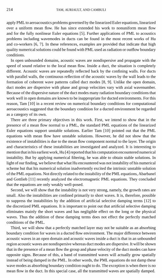
FIG. 12. Damping of a vorticity wave packet in the PML including artificial selective damping terms.Mx = 0.3,My= 0.2, σm= 1.0, (R−1

1 )max= 1.0. (a) t = 0, (b) t = 50, (c) t = 90, (d) t = 170. Contours of theuvelocity component. —, 0.1; - -, 0.05; —·—, 0.01; — - —,−0.01; - - —,−0.05; · · · ,−0.1.


To demonstrate the effectiveness of using artificial selective damping terms to suppressthe instabilities of the PML equations, the numerical examples of Subsection 2.3 are recon-sidered here. Artificial damping is now included in the simulations. Figure 12 shows theu-contours of the vorticity waves(Mx = 0.3,My= 0.2, σm= 1.0, (R−1

1 )max= 1.0) as theyare convected from the interior domain to the PML. The vorticity wave packet is steadilydamped. No sign of unstable waves of the type shown in Fig. 5 is detected. Figure 13 showsthe corresponding waveform ofu at a few selected times. It is clear that the pulse is dampedcontinuously once it propagates into the PML. The case of the acoustic disturbance has alsobeen repeated with similar results. Based on these findings, it is concluded that a stable PMLcan be developed by the inclusion of artificial selective damping. Such a PML performsvery effectively as an absorbing boundary condition in an open domain.

4. PML IN DUCTED ENVIRONMENTS

We will now consider the use of PML inside a circular duct of radiusR. Dimensionlessvariables with respect to length scaleR, velocity scaleat (speed of sound atr = R), time


FIG. 13. Waveforms showing the damping of a vorticity wave packet as it is convected into a PML withartificial selective damping terms.Mx = 0.3,My= 0.2, σm= 1.0, (R−1

1 )max= 1.0.

scaleRat

, density scaleρt (mean density atr = R), and pressure scaleρta2t will be used. The

velocity components in the(x, r, φ)directions of a cylindrical coordinate system are denotedby (u, v, w). For an inviscid compressible flow, the most general mean flow (designated byan overbar) is

u = u(r ), v = 0, w = w(r ), ρ = ρ(r )

p = −∫ 1

r

ρw2

rdr + p0. (17)

Small amplitude disturbances superimposed on mean flow (17) are governed by thelinearized Euler equations. They are

∂ρ

∂t+ 1

r

∂

∂r(ρvr )+ w

r

∂ρ

∂φ+ u

∂ρ

∂x+ ρ

(1

r

∂w

∂φ+ ∂u

∂x

)= 0 (18a)

ρ

[∂v

∂t+ u

∂v

∂x+ w

r

∂v

∂φ− 2ww

r

]− ρ w

2

r= −∂p

∂r(18b)

ρ

[∂w

∂t+ u

∂w

∂x+ vdw

dr+ w

r

∂w

∂φ+ wv

r

]= −1

r

∂p

∂φ(18c)


ρ

[∂u

∂t+ u

∂u

∂x+ vdu

dr+ w

r

∂u

∂φ

]= −∂p

∂x(18d)

∂p

∂t+ u

∂p

∂x+ w

r

∂p

∂φ+ ρw

2

rv + γ p

[1

r

∂vr

∂r+ 1

r

∂w

∂φ+ ∂u

∂x

]= 0, (18e)

whereγ is the ratio of specific heats. The boundary condition at the duct wall is

r = 1, v = 0. (19)

Solutions of (18) and (19) representing propagating wave modes in the duct may bewritten in the form

ρ

uv

w

p

= Re

ρ(r )u(r )v(r )w(r )p(r )

exp[i (kx+mφ − ωt)]

. (20)

Substitution of (20) into (18) and (19) leads to the eigenvalue problem

ρ + i

ωr

d

dr(ρvr )− mw

ωrρ − ku

ωρ − ρ

(m

ωrw + k

ωu

)= 0 (21a)

ρ

[(1− k

ωu− mw

ωr

)v − i

2ww

ωr

]− i ρw2

ωr= − i

ω

d p

dr(21b)

ρ

[(1− k

ωu− mw

ωr

)w + i

ωv

dw

dr+ i w

ωrv

]= m

ωrp (21c)

ρ

[(1− k

ωu− mw

ωr

)u+ i

ωv

du

dr

]= k

ωp (21d)

(1− ku

ω− mw

ωr

)p+ i

ω

ρw2

rv + γ p

[i

ωr

d(vr )

dr− m

ωrw − k

ωu

]= 0 (21e)

r = 1, v = 0. (22)

For a given azimuthal mode numberm and frequencyω, k (the wavenumber) is the eigen-value. Corresponding to an eigenvalue is an eigenvector [ ˜ρ, u, v, w, p], which describesthe radial profile of the wave mode.

4.1. Perfectly Matched Condition in Ducted Flows

Suppose a perfectly matched layer is to be set up as a termination boundary of a compu-tation domain inside a duct. By splitting the variables, e.g.,ρ= ρ1+ ρ2, etc., in the stan-dard manner, the PML equations corresponding to the linearized Euler equations ((18a)


to (18e)) are

∂ρ1

∂t+ 1

r

∂

∂r[ρ(v1+ v2)r ] + w

r

∂(ρ1+ ρ2)

∂φ+ ρ

r

∂(w1+ w2)

∂φ= 0 (23a)

∂ρ2

∂t+ σρ2+ u

∂(ρ1+ ρ2)

∂x+ ρ ∂(u1+ u2)

∂x= 0 (23b)

ρ

[∂v1

∂t+ w

r

∂(v1+ v2)

∂φ− 2w(w1+ w2)

r

]− (ρ1+ ρ2)

w2

r= − ∂

∂r(p1+ p2) (23c)

ρ

[∂v2

∂t+ σv2+ u

∂(v1+ v2)

∂x

]= 0 (23d)

ρ

[∂w1

∂t+ (v1+ v2)

dw

dr+ w

r

∂(w1+ w1)

∂φ+ w

r(v1+ v2)

]= −1

r

∂(p1+ p2)

∂φ(23e)

ρ

[∂w2

∂t+ σw2+ u

∂(w1+ w2)

∂x

]= 0 (23f)

ρ

[∂u1

∂t+ (v1+ v2)

du

dr+ w

ru∂(u1+ u2)

∂φ

]= 0 (23g)

ρ

[∂u2

∂t+ σu2+ u

∂(u1+ u2)

∂x

]= −∂(p1+ p2)

∂x(23h)

∂p1

∂t+ w

r

∂(p1+ p2)

∂φ+ ρw

2

r(v1+ v2)+γ p

[1

r

∂r (v1+ v2)

∂r+ 1

r

∂(w1+w2)

∂φ

]= 0 (23i)

∂p2

∂t+ σp2+ u

∂(p1+ p2)

∂x+ γ p

∂(u1+ u2)

∂x= 0, (23j)

whereσ is the damping coefficient in the PML. The boundary condition is

r = 1, v1+ v2 = 0. (24)

In the PML, the duct modes are represented by solutions of the form (similar to (20))

ρ1(r, φ, x, t) = Re[ρ1(r )e

i (κx+mφ−ωt)], (25)

etc., whereκ is the wavenumber. On substituting (25) into (23) and (24) and on defining

ρ = ρ1+ ρ2

u = u1+ u2

v = v1+ v2

w = w1+ w2

p = p1+ p2

(26)

it is straightforward to find that the duct modes in the PML are given by the solutions of theeigenvalue problem

ρ + i

ωr

d

dr(ρvr )− mw

ωrρ − κu

ω + iσρ − ρ

(m

ωrw + κ

ω + iσu

)= 0 (27a)


ρ

[(1− κ

ω + iσu− mw

ωr

)v − i

2ww

ωr

]− i ρw2

ωr= − i

ω

d p

dr(27b)

ρ

[(1− κ

ω + iσu− mw

ωr

)w + i

ωv

dw

dr+ i w

ωrv

]= m

ωrp (27c)

ρ

[(1− κ

ω + iσu− mw

ωr

)u+ i

ωv

du

dr

]= κ

ω + iσp (27d)

(1− κu

ω + iσ− mw

ωr

)p+ i

ω

ρw2

rv + γ p

[i

ωr

d(vr )

dr− m

ωrw − κ

ω + iσu

]= 0. (27e)

The boundary condition is

r = 1, v = 0. (28)

The eigenvalue isκ. On comparing the eigenvalue problem (21) and (22) with the eigenvalueproblem (27) and (28), it is immediately clear that they are the same ifk

ωin (21) is replaced

by κω+ iσ . Thus the eigenvalues are related by

κ = k

(1+ iσ

ω

). (29)

On the other hand, the eigenvectors are identical. The fact that the eigenvectors of a ductmode in the interior region of the computation domain is the same as that in the PML assuresthat there is perfect matching. That is, a propagating duct mode incident on the PML will betotally transmitted into the PML without reflection. If the mean flow is nonuniform, someof the duct modes may involve Kelvin–Helmholtz or other types of flow instability waves.However, the perfectly matched condition is still valid for these waves.

4.2. The Case of Uniform Mean Flow

From (25) and (29), the transmitted wave mode has the form

[ρ(r ), u(r ), v(r ), w(r ), p(r )]ei [k(1+ iσω)x+mφ−ωt ] . (30)

If the wave mode is nondispersive, thenkω

, the inverse of the phase velocity, is positivefor waves propagating in thex-direction and negative in the opposite direction. For thesenondispersive waves, the transmitted waves are spatially damped, a condition needed bythe PML if it is to serve as an absorbing boundary condition. However, inside a duct, thewave modes are dispersive. The direction of propagation is given by the group velocitydω

dk .We will now show that in the presence of a uniform mean flow there is a band of acousticduct modes for which the group velocity and the phase velocity have opposite signs. There-fore, for this band of waves, the transmitted waves would grow spatially instead of beingdamped.

By eliminating all the other variables in favor ofp(r ), it is straightforward to find, in thecase of a uniform mean flow of Mach numberM , (21) and (22) reduce to the followingsimple eigenvalue problem,

d2 p

dr2+ 1

r

d p

dr+[(ω − Mk)2− k2− m2

r 2

]p = 0 (31)


r = 1,d p

dr= 0. (32)

The eigenfunction is

p = Jm(λmnr ), (33)

whereJm( ) is themth order Bessel function andλmn is thenth root of

J ′m(λmn) = 0. (34)

By substitution of (33) into (31), it is found that the dispersion relation or eigenvalueequation for the(m, n)th acoustic duct mode is

(ω − Mk)2− k2 = λ2mn. (35)

The axial wavenumbers of the mode at frequencyω are given by the solution of (35). Theyare

k± =−ωM ± [ω2− (1− M2)λ2

mn

] 12

(1− M2). (36)

The group velocity of the duct mode may be determined by implicit differentiation of (35).This gives

dω

dk= ±

[ω2− (1− M2)λ2

mn

] 12 (1− M2)

ω ∓ M[ω2− (1− M2)λ2

mn

] 12

. (37)

In (37), the upper sign corresponds tok= k+ and the lower sign corresponds tok= k−.For subsonic mean flow, clearlydωdk > 0 for k= k+ and dω

dk < 0 for k= k−. Therefore, thedownstream propagating waves have wavenumber given byk= k+, while the upstreampropagating waves have wavenumber equal tok−.

From (37), it is easy to show that for(1− M2)12λmn<ω<λmn the phase velocityk+

ω

is negative although the group velocity is positive. According to (29), for waves in thisfrequency band, the transmitted wave in the PML will amplify spatially. This renders thePML useless as an absorbing layer except forM = 0. In the absence of a mean flow normalto the PML(M = 0), k+ will not be negative by (36). Thus, the transmitted waves in thePML are evanescent. For this special condition, the PML can again be used as an absorbingboundary condition.


To demonstrate that a PML in a ducted environment actually supports a band of amplifyingwave modes, a series of numerical simulations has been carried out. In the simulations, auniform mesh with1x=1r = 0.04 covering the entire computation domain fromx=−6.0to x= 12.0 is used. The PML in the upstream direction begins atx=−3.0 and extends


to x=−6.0. In the downstream direction, the PML occupies the region fromx= 3.0 tox= 12.0. The dimensionless damping constant (nondimensionalized bya∞

R ) σ is set equalto 25.0. The results of two simulations, one with a mean flow Mach number 0.4, the othertwo no mean flow, are reported below.

For convenience, only the axisymmetric duct modes are considered. The computationuses the 7-point stencil DRP scheme [13]. The acoustic disturbances in the computationdomain are initiated by a pressure pulse located atx= 0 andr = 0.5. The initial condi-tion is

t = 0, u = v = 0, p = ρ = exp

[−(ln 2)

(x2+ (r − 0.5)2)

16

]. (38)

Figure 14 shows the time evolution of the acoustic disturbance inside the computationdomain atM = 0.4. Specifically, the pressure waveforms along the liner = 0.38 are shownat t = 10, 13, 15, and 16. As can be seen, once the pressure pulse is released, it spreads outand propagates upstream and downstream. Figure 14a indicates that at timet = 10 the frontof the acoustic disturbance has just entered the PML in the downstream direction. There is noevidence of wave reflection at the interface between the PML and the interior computationdomain. The transmitted wave grows spatially as shown in Fig. 14b. The amplitude of thetransmitted wave increases steadily as they propagate across the PML. This is shown in

FIG. 14. Pressure waveforms along the liner = 0.38 of a circular duct with uniform mean flow at Mach 0.4showing the excitation and growth of the unstable solution in the PML by an acoustic pulse.1x=1r = R

25,

σm= 25.0.


FIG. 15. Pressure waveforms along the liner = 0.38 of a circular duct without mean flow showing the dampingof an acoustic pulse in the PML.1x=1r = R

25, σm= 25.0.

Figs. 14c and 14d. When the amplified waves reach the outermost boundary of the PML,large amplitude spurious waves are reflected back. This quickly contaminates the entirecomputation domain.

Figure 15 shows the same simulation except that there is no mean flow. In the absence ofa mean flow, the PML acts as an absorbing layer. Figure 15a shows the entry of the acousticpulse into the downstream PML. Figures 15b to 15d show the damping of the acousticpulse in time in the PML. The slowest components to decay are the long waves. This is inagreement with the analysis of the previous section.

5. CONCLUDING REMARKS

In this paper, we have shown that the application of PML as an absorbing boundarycondition for the linearized Euler equations works well as long as there is no mean flowin the direction normal to the layer. For open domain problems, the PML equations, inthe presence of a subsonic mean flow normal to the layer, support unstable solutions. Thegrowth rate of the unstable solutions is, however, not large. These unstable solutions can,generally, be suppressed by the addition of artificial selective damping. In the case of aducted environment, we find that because of the highly dispersive nature of the duct modes,a band of the transmitted waves in the PML amplifies instead of being damped. This bandconsists of long waves so that they are not readily suppressed by the inclusion of artificial


selective damping. This seemingly renders the PML totally ineffective as an absorbingboundary condition.

One of the important advantages of using an absorbing boundary condition instead ofother numerical boundary treatments is that the boundary of the computation domain maybe put much closer to the source of disturbances. In this way, a smaller computation domainmay be used in a numerical simulation. For open domains, such an absorbing boundarycondition can be developed by the use of PML with artificial selective damping terms.Unfortunately, the same is not possible for internal ducted flow. An effective numericalanechoic termination for ducted domains has yet to be developed.

ACKNOWLEDGMENT

This work was supported by NASA Langley Research Grant NAG 1-1776.

REFERENCES

1. J. P. Berenger, A perfectly matched layer for the absorption of electromagnetic waves,J. Comput. Phys.114,185 (1994).

2. J. P. Berenger, Three dimensional perfectly matched layer for the absorption of electromagnetic waves,J. Comput. Phys.127, 363 (1996).

3. F. D. Hastings, J. B. Schneider, and S. L. Broschat, Application of the perfectly matched layer (PML) absorbingboundary condition to elastic wave propagation,J. Acoust. Soc. Amer.100, 3061 (1996).

4. F. Q. Hu, On absorbing boundary conditions for linearized Euler equations by a perfectly matched layer,J. Comput. Phys.129, 201 (1996).

5. F. Q. Hu, On perfectly matched layer as an absorbing boundary condition, AIAA paper 96-1664, 1996.

6. M. Hayder, F. Q. Hu, and Y. M. Hussaini, Toward perfectly matched boundary conditions for Euler equations,AIAA paper 97-2075, 1997.

7. F. Q. Hu and J. L. Manthey, Application of PML absorbing boundary conditions to the benchmark problemsof computational aeroacoustics, inProc. Second Comput. Aeroacoustics Workshop on Benchmark Problems(NASA CP-3352, 1997), p. 119.

8. P. M. Morse and K. U. Ingard,Theoretical Acoustics(McGraw–Hill, New York, 1968).

9. W. Eversman, Theoretical models for duct acoustic propagation and radiation, inAeroacoustics of FlightVehicles: Theory and Practice(NASA RP-1258, 1991), Vol. 2, Chap. 13, p. 101.

10. C. K. W. Tam, Advances in numerical boundary conditions for computational aeroacoustics,J. Comput.Acoustics, in press.

11. S. Abarbanel and D. Gottlieb, A mathematical analysis of the PML method,J. Comput. Phys.134, 357 (1997).

12. C. K. W. Tam, J. C. Webb, and Z. Dong, A study of the short wave components in computational acoustics,J. Comput. Acoustics1, 1 (1993).

13. C. K. W. Tam and J. C. Webb, Dispersion-relation-preserving finite difference schemes for computationalacoustics,J. Comput. Phys.107, 262 (1993).

14. C. K. W. Tam, Computational aeroacoustics: Issues and methods,AIAA J.33, 1788 (1995).

Perfectly Matched Layer as an Absorbing Boundary Condition for the Linearized Euler Equations in...

Documents

Transcript of Perfectly Matched Layer as an Absorbing Boundary Condition for the Linearized Euler Equations in...