Robotics GroupThe Maersk Mc-Kinney Moller Institute

University of Southern Denmark

Technical Report no. 2007 – 3

Perceptual Operations and Relations between2D or 3D Visual Entities

Sinan Kalkan, Nicolas Pugeault, Mogens Christiansen, Norbert Kruger

January 22, 2007

Title Perceptual Operations and Relations between 2D or 3D Visual Entities

Copyright c© 2007 Sinan Kalkan, Nicolas Pugeault, Mogens Christiansen,Norbert Kruger. All rights reserved.

Author(s) Sinan Kalkan, Nicolas Pugeault, Mogens Christiansen, Norbert Kruger

Publication History

Abstract

In this paper, we present a set of perceptual relations, namely, co-colority, co-planarity, collinearityand symmetry that are defined between multi-modal visual features that we call primitives.

1 Introduction

According to Marr’s paradigm [29], vision involves extraction of meaningful representations from inputimages, starting at the pixel level and building up its interpretation more or less in the following order: localfilters, extraction of important features, the 21

2 -D sketch and the 3-D sketch.There is psychophysical evidence and evidence from the statistical properties of natural images that the hu-man visual system utilizes a set of visual-entity-combining processes, called perceptual organization in theliterature, for forming bigger, sparser and more complete interpretations of the scene (see, e.g., [18, 19, 35]).Such processes include (i) extraction of the boundary of the objects in the image from the set of unconnectededge pixels or features [3, 8, 10, 21, 27, 31, 39] utilizing Gestalt laws of grouping, and (ii) interpolation andextrapolation of unconnected sparse 3D entities for forming more complete 3D surfaces (see, e.g., [13]) uti-lizing the relations between the 3D entities. Gestalt principles include collinearity, proximity, common fateand similarity whereas inference of 3D surfaces from a set of 3D entities include relations like coplanarity,collinearity, co-colority etc. These are essentially second order and higher order relations of local features.In [26], we have introduced a specific form of a local descriptor that we call a ’multi–modal primitive’(see section 2) and which can be seen as a functional abstraction of a hypercolumn (see [24]). We distin-guish between 2D primitives describing local image information and 3D primitives covering local 3D sceneinformation in a condensed symbolic way.These primitives serve as a basis for an early cognitive vision system [23, 26, 33] in which operations andrelations on these primitives realizing perceptual grouping principles are used in different contexts (see [26]for applications). We have utilized these relations for different problems including stereo [34], RBM [32],estimation of initial grasping reflexes from stereo [5], estimation of depth at homogeneous image structures[16], and analysis of second-order relations between 3D features [17].In this paper, we present the set of 2D and 3D relations defined upon the primitives. These relations includecollinearity, cocolority, coplanarity and symmetry. Of these relations, collinearity, cocolority and symmetryare defined for 2D as well as 3D primitives whereas by definition, coplanarity is meaningful only for 3Dprimitives. Table 1 summarizes the relations and on which dimension they are defined.

Relation 2D 3Dco-planarity ×

√

co-colority√ √

collinearity√ √

symmetry√ √

Table 1: The relations and in which dimension they are defined.

This paper does not focus on any specific application domain but provides a technically detailed definitionof these relations that are usually not described in such detail in publications making use of them.The paper is organized as follows: In section 2, we briefly introduce our visual features, namely primitives.In section 3, we describe our definitions of perceptual relations between the visual primitives. In section 5,we conclude the paper.

1

2 Primitives

Numerous feature detectors exist in the literature (see [30] for a review). Each feature based approachcan be divided into an interest point detector (e.g. [14, 4]) and a descriptor describing a local patch ofthe image at this location, that can be based on histograms (e.g. [6, 30]), spatial frequency [20], localderivatives [15, 11, 1] steerable filters [12], or invariant moments ([28]). In [30] these different descriptorshave been compared, showing a best performance for SIFT-like descriptors.The primitives we will be using in this work are local, multi–modal edge descriptors that were introducedin [25]. In contrast to the above mentioned features these primitives focus on giving a semantically andgeometrically meaningful description of the local image patch. The importance of such a semantic ground-ing of features for a general purpose vision front–end, and the relevance of edge–like structures for thispurposes were discussed in [9].The primitives are extracted sparsely at locations in the image that are the most likely to contain edges.This likelihood is computed using the intrinsic dimensionality measure proposed in [22]. The sparsenessis assured using a classical winner take all operation, insuring that the generative patches of the primitivesdo not overlap (for details, see [26]). Each of the primitive encodes the image information contained by alocal image patch. Multi–modal information is gathered from this image patch, including the position mof the centre of the patch, the orientation θ of the edge, the phase ω of the signal at this point, the colour csampled over the image patch on both sides of the edge and the local optical flow f . Consequently a localimage patch is described by the following multi–modal vector:

π = (m, θ, ω, c,f , ρ)T , (1)

that we will name 2D primitive in the following.Note that these primitives are of lower dimensionality than, e.g., SIFT (10 vs. 128) and therefore sufferof a lesser distinctiveness. Nonetheless, as shown in [34] that they are distinctive enough for a reliablestereo matching if the epipolar geometry of the cameras is known. Furthermore, their semantic in terms ofgeometric and appearance based information allow for a good description of the scene content. It has beenpreviously argued in [9] that edge pixels contain all important information in an image. As a consequence,the ensemble of all primitives extracted from an image describe the shapes present in this image.Advantageously, the rich information carried by the 2D–primitives can be reconstructed in 3D, providing amore complete scene representation. Having geometrical meaning for the primitive allows to describe therelation between proximate primitives in terms of perceptual grouping.In a stereo scenario 3D primitives can be computed from the correspondences of 2D primitives (see figure1 and [34]):

Π = (M ,Θ,Ω,C)T , (2)

such that we have a projection relation:P : Π → π . (3)

3 Relations

In this section, we present collinearity, cocolority, coplanarity and symmetry relations that are defined onour visual features.

3.1 Collinearity in 2D and 3D

As the primitives are local contour descriptors, scene contours are expected to be represented by strings ofprimitives that are locally close to collinear. In the following, we will explain methods for grouping 2D and3D primitives into contours.

2

Primitive :

1. Orientation ( )q

2. Phase ( )w

3. Colour ( )c

4. Optical flow ( )f

1

4

33

2

a)

b)

c)

d)

e)

Figure 1: Illustration of the primitive extraction process from a video sequence. The 2D–primitives ex-tracted from the input image (a) (see section 2), and finally the 3D–primitives reconstructed from thestereo–matches as described as described in [34]. (a) An example input image. (b) A graphic descrip-tion of the 2D–primitives. (c) A magnification of the image representation. (d) Perceptual grouping of theprimitives as described in [34]. (e) The reconstructed 3D entities. Note that the structure reconstructed isquite far from the cameras, leading to a certain imprecision in the reconstruction of the 3D–primitives. Asimple scheme addressing this problem is described in [34].

3

Figure 2: Illustration of the values used for the collinearity computation. If we consider two primitives πi

and πj , then the vector between the centres of these two primitives is written vij , and the orientations ofthe two primitives are designated by the vectors ti and tj , respectively. The angle formed by vij and ti iswritten αi, and between vij and tj is written αj . ρ is the radius of the image patch used to generate theprimitive.

3.1.1 Collinearity in 2D

In the following, c(li,j) refers to the likelihood for two primitives πi and πj to be linked: i.e. grouped todescribe the same contour.Position and orientation of primitives are intrinsically related. As primitives represent local edge estimators,their positions are points along the edge, and their orientation can be seen as a tangent at such a point. Theestimated likelihood of the contour described by those tangents is based upon the assumption that simplercurves are more likely to describe the scene structures, and highly jagged contours are more likely to bemanifestations of erroneous and noisy data.Therefore, for a pair of primitives πi and πj in image I , we can formulate the likelihood for these primitivesto describe the same contour as a combination of three basic constraints on their relative position andorientation — see [34].

Proximity (cp[li,j ]): A contour is more likely if it is described by a dense population of primitives. Largeholes in the primitive description of the contour is an indication that there are two contours which arecollinear yet different. The proximity constraint is defined by the following equation:

cp[li,j ] = 1− e−max

„1−

||vi,j||ρτ

,0

«, (4)

where ρ stands for the size of the receptive field of the primitives in pixels; ρτ is the size of the neighbour-hood considered in pixels; and, ‖vi,j‖ is the distance in pixels separating the centres of the two primitives.

Collinearity (cco[li,j ]): A contour is more likely to be linear, or to form a shallow curve rather than a sharpone. A sharp curve might be an indication of two intersecting or occluding contours.

cco[li,j ] = 1−∣∣∣∣sin(

|αi|+ |αj |2

)∣∣∣∣ , (5)

where αi and αj are the angles between the line joining the two primitives centres and the orientation of,respectively, πi and πj .

Co–circularity (cci[li,j ]): A contour is more likely to have a continuous, or smoothly changing curvature,rather than a varying one. An unstable curvature is an indicator of a noisy, erroneous or under–sampledcontour, all of which are unreliable.

cci[li,j ] = 1−∣∣∣∣sin(

αi + αj

2

)∣∣∣∣ , (6)

4

Geometric Constraint (Gi,j): The combination of those three criteria provided above forms the follow-ing geometric affinity measure:

Gi,j = 3

√ce[li,j ] · cco[li,j ] · cci[li,j ], (7)

where Gi,j is the geometric affinity between two primitives πi and πj . This affinity represents the likelihoodthat two primitives πi and πi are part of an actual contour of the scene.

Multi–modal Constraint (Mi,j): The geometric constraint offers a suitable estimation of the likelihoodof the curve described by the pair of primitives. Other modalities of the primitives allow inferring moreabout the qualities of the physical contour they represent. The colour, phase and optical flow of the primi-tives further define the properties of the contour, and thus consistency constraints can also be enforced overthose modalities. Effectively, the less difference there is between the modalities of two primitives, the morelikely that they are expressions of the same contour. In [7], it is already proposed that the intensity can beused as a cue for perceptual grouping; our definition goes beyond this proposal by using a combination ofthe phase, colour and optical flow modalities of the primitives to decide if they describe the same contour:

Mi,j = wωcω[li,j ] + wccc[li,j ] + wfcf [li,j ], (8)

where cω is the phase criterion, cc the colour criterion and cf the optical flow criterion. Each of the threewω, wc and wf is the relative scaling for each modality, with wω + wc + wf = 1.

Primitive Affinity (Ai,j): The overall affinity between all primitives in an image is formalised as a matrixA, where Ai,j holds the affinity between the primitives πi and πj . We define this affinity from equations 7and 8, such that (1) two primitives complying poorly with the good continuation rule have an affinity closeto zero; and (2) two primitives complying with the good continuation rule yet strongly dissimilar will haveonly an average affinity. The affinity is formalised as follows:

c(li,j) = Ai,j =√

G (αGi,j + (1− α)Mi,j), (9)

where α is the weighting of geometric and multi–modal (i.e. phase, colour and optical flow) informationin the affinity. A setting of α = 1 implies that only geometric information ( proximity, collinearity andco-circularity) is used, while α = 0 means that geometric and multi–modal information are evenly mixed.

3.1.2 Collinearity in 3D

Collinearity in 3D is more difficult to define. Due to the inaccuracy in stereo–reconstruction of 3D positionand orientation, it is impossible to apply strong alignment constraints such as the ones we applied in the 2Dcase. Consequently we will define 3D collinearity as follows:

Definition 1 Two 3D–primitives Πi and Πj are said collinear if the 2D–primitives πxi and πx

j they projectonto the camera plane x (defined by a projection relation Px : Πk → πk) are all collinear (according tothe definition of 2D–primitive collinearity presented above).

and therefore in the standard case where we have two stereo cameras labelled l and r we have the followingrelation:

c(Li,j) = c(lli,j) · c(lri,j). (10)

5

πjπi πk

Figure 3: Co–colority of three 2D primitives πi, πj and πk. In this case, πi and πj are cocolor, so are πi

and πk; however, πj and πk are not cocolor.

3.2 Cocolority in 2D and 3D

Two spatial primitives Πi and Πj are co–color iff their parts that face each other have the same color. Inthe same way as collinearity, co–colority of two spatial primitives Πi and Πj is computed using their 2Dprojections PΠi = πi and πj . We define the co–colority of two 2D primitives πi and πj as:

coc(πi, πj) = 1− dc(ci, cj),

where ci and cj are the RGB representation of the colors of the parts of the primitives πi and πj that faceeach other; and, dc(ci, cj) is Euclidean distance between RGB values of the colors ci and cj . In Fig. 3, apair of co–color and not co–color primitives are shown.Euclidean color distance dc is a simple one compared to color distance metrics developed by different in-stitutes like International Commission on Illumination (CIE). Such metrics are developed to match our per-ception of colour and are computationally expensive (see, e.g., [38]). For our purposes, Euclidean distancebetween RGB values is sufficient and can be replaced by a more complicated distance metric, if desired.3D co-colority is defined as follows:

Definition 2 Two 3D–primitives Πi and Πj are said cocolor if the 2D–primitives πxi and πx

j they projectonto the camera plane x (defined by a projection relation Px : Πk → πk) are co-color (according to thedefinition of 2D–primitive cocolority presented above).

3.3 Coplanarity

According to [37],

a set of points in space is coplanar if the points all lie in a geometric plane. For example, threepoints are always coplanar; but four points in space are usually not coplanar.

Although the definitions are more or less the same, there are different ways to check the coplanarity of aset of points [36, 37]. For a set of n points x1...xn where xi = (xi, yi, zi), the following methods can beadopted:

• For n = 4, x1...xn are coplanar

– iff the volume of the tetrahedron defined by them is 0 [36], i.e.,∣∣∣∣∣∣∣∣x1 y1 z1 1x2 y2 z2 1x3 y3 z3 1x4 y4 z4 1

∣∣∣∣∣∣∣∣ = 0. (11)

– iff the pair of lines determined by the four points are not skew [36]:

(x3 − x1).[(x2 − x1)× (x4 − x3)] = 0. (12)

6

– iff x4 is on the plane defined by x1,x2,x3:

d(x4, P (x1,x2,x3)) = 0, (13)

where P (x1,x2,x3) is the plane defined by P (x1,x2,x3), and d(x,p) is the distance betweenpoint x and plane p.

• For n > 4, x1...xn are coplanar iff point-plane distances of x4..xn to the plane defined by (x1,x2,x3)are all zero:

n∑i=4

d(xi, P (x1,x2,x3)) = 0. (14)

3.3.1 Coplanarity of bounded planes

A bounded plane pb is part of the plane p with a certain size s and position x. In other words, pb isequivalent to (n,x, s) where n,x, s are respectively the normal (i.e., orientation), position (i.e., center) andthe size of the bounded plane.As suggested in [17], two bounded planes pb

1,pb2 are coplanar if:

(α(n1,n2) < Tα) ∧ (d(x1,pb

2)d(x1, x2)

< Td), (15)

where α(n1,n2) is the angle between the two orientations vectors n1 and n1, and Tα and Td are the thresh-olds.

3.3.2 Coplanarity of 3D primitives

Two spatial primitives Πi and Πj are co–planar iff their orientation vectors lie on the same plane, i.e.:

cop(Πi,Πj) = 1− |projtj×vij(ti × vij)|, (16)

where vij is defined as the vector (M i −M j); ti and tj denote the vectors defined by the 3D orientationsΘi and Θj , respectively; and proju(a) is defined as:

proju(a) =a · u‖ u ‖2

u. (17)

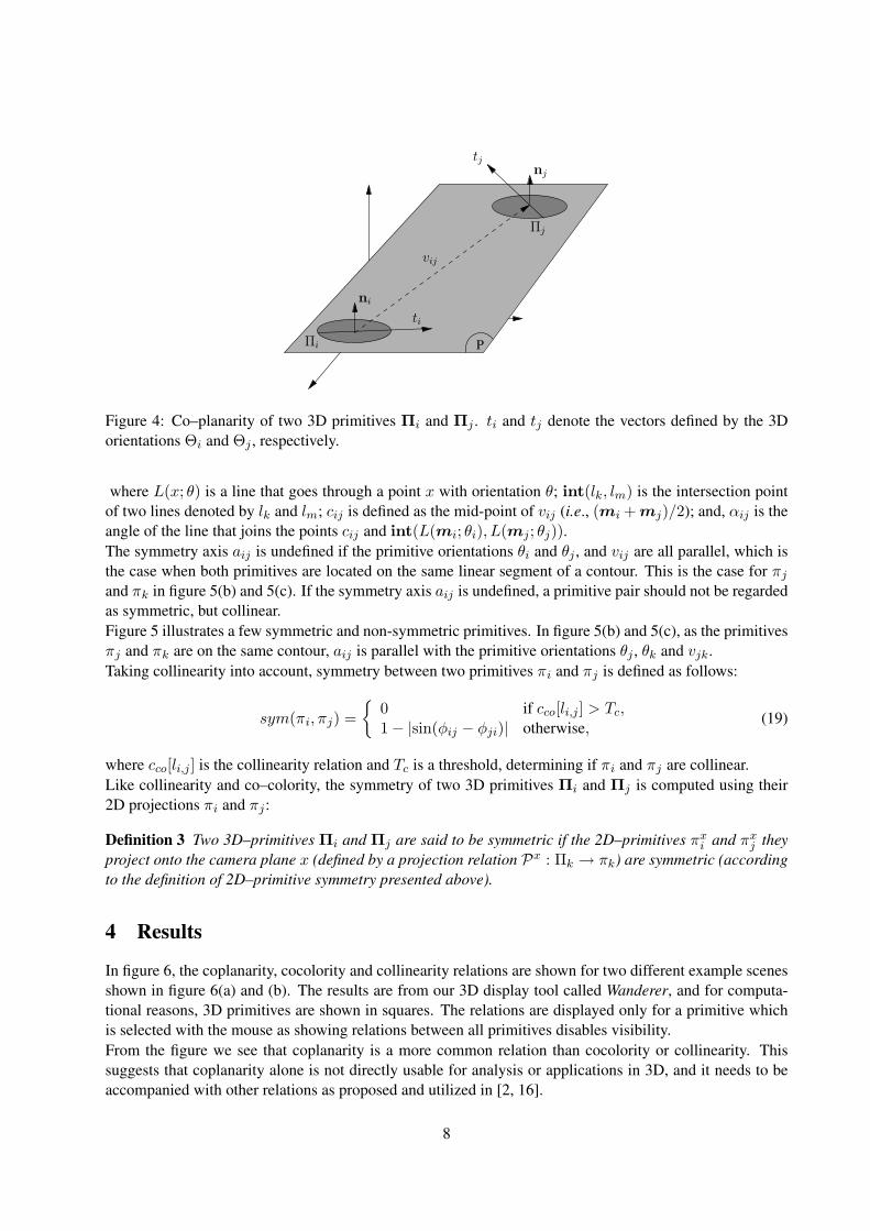
The co–planarity relation is illustrated in Fig. 4.

3.4 Symmetry in 2D and 3D

Two primitives are symmetric if they are located on two contours which are reflections of each other (seefigure 5(a)). This reflective symmetry between two primitives can be measured by utilizing the anglesbetween the orientations of the primitives and the line that joins the centers of the primitives.Let vij denote the line joining the centers of the primitives, πi and πj , and also φij and φji be the anglesbetween vij and the lines defined by the orientations of πi and πj , respectively (see figure 5). Then, two2D primitives πi and πj can be considered symmetric, if φij = φji with a symmetry axis aij defined asfollows:

aij =

L(cij ; θi) if θi = θj ,L(cij ;αij), otherwise,

(18)

7

PΠi

Πj

nj

vij

ni

tj

ti

Figure 4: Co–planarity of two 3D primitives Πi and Πj . ti and tj denote the vectors defined by the 3Dorientations Θi and Θj , respectively.

where L(x; θ) is a line that goes through a point x with orientation θ; int(lk, lm) is the intersection pointof two lines denoted by lk and lm; cij is defined as the mid-point of vij (i.e., (mi + mj)/2); and, αij is theangle of the line that joins the points cij and int(L(mi; θi), L(mj ; θj)).The symmetry axis aij is undefined if the primitive orientations θi and θj , and vij are all parallel, which isthe case when both primitives are located on the same linear segment of a contour. This is the case for πj

and πk in figure 5(b) and 5(c). If the symmetry axis aij is undefined, a primitive pair should not be regardedas symmetric, but collinear.Figure 5 illustrates a few symmetric and non-symmetric primitives. In figure 5(b) and 5(c), as the primitivesπj and πk are on the same contour, aij is parallel with the primitive orientations θj , θk and vjk.Taking collinearity into account, symmetry between two primitives πi and πj is defined as follows:

sym(πi, πj) =

0 if cco[li,j ] > Tc,1− |sin(φij − φji)| otherwise,

(19)

where cco[li,j ] is the collinearity relation and Tc is a threshold, determining if πi and πj are collinear.Like collinearity and co–colority, the symmetry of two 3D primitives Πi and Πj is computed using their2D projections πi and πj :

Definition 3 Two 3D–primitives Πi and Πj are said to be symmetric if the 2D–primitives πxi and πx

j theyproject onto the camera plane x (defined by a projection relation Px : Πk → πk) are symmetric (accordingto the definition of 2D–primitive symmetry presented above).

4 Results

In figure 6, the coplanarity, cocolority and collinearity relations are shown for two different example scenesshown in figure 6(a) and (b). The results are from our 3D display tool called Wanderer, and for computa-tional reasons, 3D primitives are shown in squares. The relations are displayed only for a primitive whichis selected with the mouse as showing relations between all primitives disables visibility.From the figure we see that coplanarity is a more common relation than cocolority or collinearity. Thissuggests that coplanarity alone is not directly usable for analysis or applications in 3D, and it needs to beaccompanied with other relations as proposed and utilized in [2, 16].

8

5 Conclusion

In this paper, we presented cocolority, coplanarity, collinearity and symmetry relations defined on multi-modal visual features, called primitives.Such relations have been utilized in different perceptual organization problems as well as analysis of howthe natural scenes are structured (see, e.g., ([3, 8, 10, 13, 16, 17, 21, 27, 31, 34, 39]), and the importanceof such relations, as well as their psychophysical and biological plausibility have been acknowledged in theliterature (see, e.g., [18, 19, 35]).

6 Acknowledgments

We would like to thank Florentin Worgotter and Daniel Aarno for their fruitful contributions. This work issupported by the Drivsco and the PACO+ projects.

References

[1] A. Baumberg. Reliable Feature Matching across Widely Separated Views. In Proc. Conf. ComputerVision and Patter Recognition, pages 774–781, 2000.

[2] D. Aarno, J. Sommerfeld, D. Kragic, N. Pugeault, S. Kalkan, F. Worgotter, D. Kraft, and N. Kruger.Model-independent grasping initializing object-model learning in a cognitive architecture. IEEE In-ternational Conference on Robotics and Automation (ICRA), Workshop: From features to actions -Unifying perspectives in computational and robot vision, 2007.

[3] E. Brunswik and J. Kamiya. Ecological cue–validity of ’proximity’ and of other Gestalt factors.American Journal of Psychologie, LXVI:20–32, 1953.

[4] Cordelia Schmid and Roger Mohr and Christian Baukhage. Evaluation of Interest Point Detectors.International Journal of Computer Vision, 37(2):151–172, 2000.

[5] J. S. D. Aarno, D. Kragic, N. Pugeault, S. Kalkan, F. Worgotter, D. Kraft, and N. Kruger. Earlyreactive grasping with second order 3d feature relations. IEEE Conference on Robotics and Automation(submitted), 2007.

[6] David G. Lowe. Distinctive Image Features from Scale–Invariant Keypoints. International Journal ofComputer Vision, 60(2):91–110, Nov. 2004.

[7] J. Elder and R. Goldberg. Inferential reliability of contour grouping cues in natural images. PerceptionSupplement, 27, 1998.

[8] J. Elder and R. Goldberg. Ecological statistics of Gestalt laws for the perceptual organization ofcontours. Journal of Vision, 2(4):324–353, 8 2002.

[9] J. H. Elder. Are edges incomplete ? International Journal of Computer Vision, 34:97–122, 1999.

[10] J. H. Elder, A. Krupnik, and L. A. Johnston. Contour grouping with prior models. IEEE Transactionson Pattern Analysis and Machine Intelligence, 25(25):1–14, 2003.

[11] Frederik Schaffalitzky and Andrew Zisserman. Multi–view Matching for Unordered Image Sets, or“How Do I Organize My Holiday Snaps?”. Lecture Notes in Computer Science, 2350:414–431, 2002.in Proceedings of the BMVC02.

[12] W. Freeman and E. Adelson. The design and use of steerable filters. IEEE-PAMI, 13(9):891–906,1991.

9

[13] W. E. L. Grimson. A Computational Theory of Visual Surface Interpolation. Royal Society of LondonPhilosophical Transactions Series B, 298:395–427, Sept. 1982.

[14] C. G. Harris and M. Stephens. A combined corner and edge detector. In 4th Alvey Vision Conference,pages 147–151, 1988.

[15] J. J. Koenderink and A. J. van Doorn. Representation of Local Geometry in the Visual System. Bio-logical Cybernetics, 55:367–375, 1987.

[16] S. Kalkan, F. Worgotter, and N. Kruger. Depth prediction at homogeneous image structures. InTechnical report of the Robotics Group, Maersk Institute, University of Southern Denmark, number2007-2, 2007.

[17] S. Kalkan, F. Worgotter, and N. Kruger. Statistical analysis of second-order relations of 3d structures.International Conference on Computer Vision Theory and Applications (VISAPP), 2007.

[18] K. Koffka. Principles of Gestalt Psychology. Lund Humphries, London, 1935.

[19] K. Kohler. Gestalt Psychology: An introduction to new concepts in psychology. New York: Liveright,1947.

[20] P. Kovesi. Image features from phase congruency. Videre: Journal of Computer Vision Research,1(3):1–26, 1999.

[21] N. Kruger. Collinearity and parallelism are statistically significant second order relations of complexcell responses. Neural Processing Letters, 8(2):117–129, 1998.

[22] N. Kruger and M. Felsberg. A continuous formulation of intrinsic dimension. Proceedings of theBritish Machine Vision Conference, pages 261–270, 2003.

[23] N. Kruger, M. V. Hulle, and F. Worgotter. Ecovision: Challenges in early-cognitive vision. Interna-tional Journal of Computer Vision, accepted.

[24] N. Kruger, M. Lappe, and F. Worgotter. Biologically motivated multi-modal processing of visualprimitives. The Interdisciplinary Journal of Artificial Intelligence and the Simulation of Behaviour,1(5):417–428, 2004.

[25] N. Kruger, M. Lappe, and F. Worgotter. Biologically motivated multi-modal processing of visualprimitives. Interdisciplinary Journal of Artificial Intelligence & the Simulation of Behavious, AISBJournal, 1(5):417–427, 2004.

[26] N. Kruger, N. Pugeault, and F. Worgotter. Multi-modal primitives: Local, condensed, and semanticallyrich visual descriptors and the formalization of contextual information. In Technical report of theRobotics Group, Maersk Institute, University of Southern Denmark, number 2007-4, 2007.

[27] N. Kruger and F. Worgotter. Statistical and deterministic regularities: Utilisation of motion and group-ing in biological and artificial visual systems. Advances in Imaging and Electron Physics, 131:82–147,2004.

[28] Luc Van Gool and Theo Moons and Dorin Ungureanu. Affine / Photometric Invariants for PlanarIntensity Patterns. Lecture Notes In Computer Science, 1064:642–651, 1996. in Proceedings of the4th European Conference on Computer Vision — Volume 1.

[29] D. Marr. Vision: A computational investigation into the human representation and processing of visualinformation. Freeman, 1977.

[30] K. Mikolajczyk and C. Schmid. A performance evaluation of local descriptors. IEEE Transactions onPattern Analysis and Machine Intelligence, 27(10):1615–1630, 2005.

[31] N. Pugeault, N. Kruger, and F. Worgotter. A non-local stereo similarity based on collinear groups.Proceedings of the Fourth International ICSC Symposium on Engineering of Intelligent Systems, 2004.

10

[32] N. Pugeault, N. Kruger, and F. Worgotter. Rigid body motion estimation in an early cognitive visionframework. In IEEE Advances In Cybernetic Systems, 2006.

[33] N. Pugeault, F. Worgotter, , and N. Kruger. Disambiguation .....

[34] N. Pugeault, F. Worgotter, and N. Kruger. Multi-modal scene reconstruction using perceptual groupingconstraints. In Proc. IEEE Workshop on Perceptual Organization in Computer Vision (in conjunctionwith CVPR’06), 2006.

[35] S. Sarkar and K. Boyer. Computing Perceptual Organization in Computer Vision. World Scientific,1994.

[36] E. W. Weisstein. Coplanar. from mathworld–a wolfram web resource, 2006. http://mathworld.wolfram.com/Coplanar.html.

[37] Wikipedia. Coplanarity — wikipedia, the free encyclopedia, 2006. http://en.wikipedia.org/w/index.php?title=Coplanarity&oldid=37490165.

[38] X. Zhang and B. A. Wandell. Color image fidelity metrics evaluated using image distortion maps.Signal Processing, 70(3):201–214, 1998.

[39] S. C. Zhu. Embedding gestalt laws in markov random fields. IEEE Transactions on Pattern Analysisand Machine Intelligence, 21(11):1170–1187, 1999.

11

i j

i j j i

ik

k i

v i j

ti t j

tk

kai j

v ik

aik

(a)

ti t j

tk

ik

k i

v i j

v ik

i j

kai j=aik

j i

i j

(b)

j

i j

ti

j i

i

t j

tk

k

vi j

v ik

ai j=aik

k i

ik

(c)

Figure 5: Illustration of the definition of symmetry. ti, tj and tk denote the vectors defined by the orienta-tions θi, θj and θk, respectively. Primitives πi and πj are symmetric in (a) and (b), but not in (c). πi and πk

are symmetric in (c), but not in (a) or (b).

12

a) b)C

opla

nari

tyC

ocol

ority

Col

linea

rity

Figure 6: The coplanarity, cocolority and collinearity relations on two different examples shown in (a) and(b). The results are from our 3D display tool called Wanderer, and for the sake of speed, 3D primitives areshown in squares. The relations are shown only for a selected primitive as showing relations between allprimitives disables visibility.

13