“Peak car” effects on scheme appraisal - CORE
130
National Technical University of Athens MSc Geoinformatics “Peak car” effects on scheme appraisal MSc candidate Christina Spiliopoulou Thesis supervisor Constantinos Antoniou Examinerd by B. Psarianos I. Spiropoulou October 2014
-
Upload
khangminh22 -
Category
Documents
-
view
2 -
download
0
Transcript of “Peak car” effects on scheme appraisal - CORE

National Technical University of Athens
MSc Geoinformatics
“Peak car” effects on scheme appraisal
MSc candidate
Christina Spiliopoulou
Thesis supervisor
Constantinos Antoniou
Examinerd by
B. Psarianos
I. Spiropoulou
October 2014

Table of Contents
Abstract 5
Εκτεταμένη περίληψη 6
1. Introduction 1
1.1 Introduction 1
1.2 Thesis contributions 2
1.3 Application 3
1.4 Thesis Outline 3
2. Background 5
2.1 The importance of forecasting 5
2.2 Sources of failure 11
2.3 Land use transport interaction modelling (LUTI) 17
3. Peak Car 20
3.1 Introduction 20
3.2 Evidence and data 22
3.3 Car ownership and traffic forecasting in U.K. 28
3.3.1 Introduction 28
3.3.2 National trip End Model (NTEM) 29
3.3.3 National Car Ownership Model 31
4. Methodology 34
4.1 Introduction 34
4.2 Group Step 1 36
4.3 Group Step 2 37
4.4 Group Step 3 38
4.5 Group Step 4 39
5. Application 41
5.1 Introduction 41
5.2 Group Step 1 – Data collection and forecasting 41
5.2.1 Data Sources 41
5.2.2 Study Area 44
5.2.3 Data availability and set-up 45
5.3 Group Step 2 – Calculation of externalities 51
5.3.1 Tool that calculates the externalities 51
5.4 Group Step 3 – Economic Analysis 61

5.5 Group Step 4 – Compare the Generalised Cost of the Externalities 67
6. Recommendations / Conclusions 69
7. Bibliography 72
APPENDIX A – DfT Data 77
DfT AADF Temporal Data Analysis 77
APPENDIX B Group Step 3 Detailed matrices 78
List of Figures
Figure 2-1 Manchester modal share temporal comparison for inbound trips per day (2002-
2012) ............................................................................................................... 6
Figure 2-2 Variations between predicted and observed traffic ........................................... 7
Figure 2-3 Budget allocate to four most costly sectors by four wealthy countries .............. 9
Figure 2-4 LUTI explanatory diagrams ............................................................................ 17
Figure 3-1 Passenger kilometres by private car (1990=100) ........................................... 20
Figure 3-2 Distance by motorized modes per trip maker and day, by age, (1976 – 2007)
kilometres ...................................................................................................... 24
Figure 3-3 Car use growth trends in developed cities from 1960 to 2005 using Global
Cities Database. ............................................................................................ 25
Figure 3-4 Basic steps in generating the NTEM 6.2 dataset ............................................ 29
Figure 3-5 Structure of a possible series of scenario tests using Scenario Generator ..... 30
Figure 3-6 NTEM: Car ownership through time – comparison of version (6.2) with version
(5.4) ............................................................................................................... 30
Figure 4-1 Methodology Outline ...................................................................................... 35
Figure 4-2 Group step 1 of the methodology ................................................................... 36
Figure 4-3 Group step 2 of the methodology ................................................................... 37
Figure 4-4 Group step 3 of the methodology ................................................................... 38
Figure 4-5 Group step 4 of the methodology ................................................................... 39
Figure 5-1 DfT’s website for traffic counts downloading .................................................. 42
Figure 5-2 DMRB – Defining link capacity Step 1 of 2 ..................................................... 43
Figure 5-3 DMRB – Defining link capacity Step 2 of 2 ..................................................... 43
Figure 5-4 The section of the A12 under study ................................................................ 44
Figure 5-5 A12 broken down in 10 segments, as per JTDB ............................................ 46
Figure 5-6 AADF analysis on the A12 (both directions) ................................................... 50
Figure 5-7 AADF analysis on the A12 (both directions) by vehicle type ........................... 50
Figure 5-8 Example of VDF Graphs ................................................................................ 52
Figure 5-9 Methodology steps for the economic analysis ................................................ 62
Figure 5-10 Traffic split per trip purpose ........................................................................ 62
Figure 5-11 Values of Time per journey purpose ........................................................... 63

List of Tables
Table 2-1 Inaccuracies in the study of McCray et al (2012) .............................................. 6
Table 2-2 Different GDP growth scenarios according to an EU study ............................ 11
Table 2-3 A psychological perspective on large project issues at the Planning .............. 16
Table 2-4 General Causes of transport projects underperformance ............................... 16
Table 3-1 Comprehensive list of causes of reduced car use in developed countries ...... 21
Table 3-2 Abbreviations and description of U.K. specific terms ...................................... 28
Table 3-3 TEMPRO screenshot: Initial set of options ..................................................... 28
Table 5-1 Available and analysed data for the base Year (2013) ................................... 47
Table 5-2 Available and analysed data for the Basic Forecast Scenario (2031) ............. 49
Table 5-3 Calibration process for Section 1 NB PM ....................................................... 53
Table 5-4 Parameters a and b for all sets of data and Max Travel time on the links ....... 54
Table 5-5 (1 out of 6) Travel Times and Delays as calculated for Base Year, Basic
Forecasting Scenario and Sensitivity Testing Forecasting Scenarios ............. 55
Table 5-6 (2 out of 6) Travel Times and Delays as calculated for Base Year, Basic
Forecasting Scenario and Sensitivity Testing Forecasting Scenarios ............. 56
Table 5-7 (3 out of 6) Travel Times and Delays as calculated for Base Year, Basic
Forecasting Scenario and Sensitivity Testing Forecasting Scenarios ............. 57
Table 5-8 (4 out of 6) Travel Times and Delays as calculated for Base Year, Basic
Forecasting Scenario and Sensitivity Testing Forecasting Scenarios ............. 58
Table 5-9 (5 out of 6) Travel Times and Delays as calculated for Base Year, Basic
Forecasting Scenario and Sensitivity Testing Forecasting Scenarios ............. 59
Table 5-10 (6 out of 6) Travel Times and Delays as calculated for Base Year, Basic
Forecasting .................................................................................................... 60
Table 5-11 Table of contents related to Cost Benefit Analysis ......................................... 61
Table 5-12 Vehicle classification factors .......................................................................... 62
Table 5-13 Trip purpose split factors ................................................................................ 63
Table 5-14 Average GDP per person ............................................................................... 64
Table 5-15 Value of time per vehicle based on distance travelled .................................... 65
Table 5-16 Summary of annual costs of delays (£) for all tested scenarios - Split per trip
purpose, peak hour and vehicle type. ............................................................ 66
Table 5-17 Cost of delays on the A12 for the base and forecast year and sensitivity test. 68

Abstract
The phenomenon of peak car has been introduced among transport professionals and
academics during the past decade. It is based on the analysis of a series of indicators
related to car use and travel behaviour. It implies that the use of car, that has been
increasing since its first appearance, will either drop or increase at a significantly decreased
rate. The basic indicator examined behind this theory is the average distance travelled by
car that has dropped in combination with a decreased number of driving licenses among
young adults, mainly men. These trends have been observed to be similar in different
countries of the world, implying a universal trend.
Should peak car occur in the future, it will affect our current forecasting. This study focuses
on the impact that peak car would have on scheme appraisal and specifically its economic
impacts, should our current forecasts be proven to be wrong. It focuses on the example of
an 80km section of the A12 that forms part of the strategic road network οf the U.K. The
official scheme appraisal guidelines and best practice methods followed in the U.K. have
been used and combined with a methodology that assesses the economic impact of
inaccuracies in traffic forecasting.
The results of this study reveal a significant additional cost if the current forecasting is
proven to be wrong. A range of forecasting inaccuracies has been tested and it is shown that
if they occur in the future, the basis on which decisions are done today will be out of date
and the economic inaccuracies will be significant. It signifies the need to better investigate
travel trends and incorporate a series of alternative scenarios in scheme appraisal to
account for inaccuracies in the present forecasts.

Εκτεταμένη περίληψη
Την τελευταία δεκαετία συγκοινωνιολόγοι και ακαδημαϊκοί έχουν εντοπίσει μια αλλαγή στη συμπεριφορά όσο αφορά στη χρήση του αυτοκινήτου: Η κατ’ άτομο μέση διανυόμενη απόσταση με αυτοκίνητο έχει μειωθεί και ο αριθμός των νέων άδειων οδήγησης από άτομα νεαρής ηλικίας έχει επίσης μειωθεί. Το φαινόμενο αυτό που υποδηλώνει μια συμπεριφοριστική μεταβολή ως προς την επιλογή μέσου μεταφοράς, έχει ονομαστεί peak car και απασχολεί ολοένα και περισσότερο την επιστημονική κοινότητα καθώς επηρεάζει όποιο είδος προβλέψεων γίνονται για τη μελλοντική συμπεριφορά των μετακινούμενων.
Οι τάσεις αυτές έχουν παρατηρηθεί με μικρές διακυμάνσεις σε διαφορετικές χώρες. Το φαινόμενο του peak car ισχυρίζεται ότι η χρήση του αυτοκινήτου, η οποία είναι σε ανοδική πορεία από την αρχή της χρήσης του, είτε θα μειωθεί είτε θα συνεχίσει να αυξάνεται αλλά με σημαντικά μειωμένους ρυθμούς. Παρόλαυτά δεν είναι ακόμα ξεκάθαρο εάν πρόκειται για μια νέα τάση η οποία θα συνεχιστεί ή θα σταματήσει.
Έχει αποδειχτεί μέσω πολυάριθμων μελετών ότι οι προβλέψεις ζήτησης που έχουν γίνει για έργα υποδομής είναι συνήθως ανακριβείς. Οι προβλέψεις αυτές χρησιμοποιούνται σε μελέτες σκοπιμότητας οι οποίες στη συνέχεια χρησιμοποιούνται για λήψη αποφάσεων. Οι αποφάσεις που σχετίζονται με έργα υποδομής σχετικά με τις μεταφορές αποτελούν ένα σημαντικό μέρος του προϋπολογισμού κάθε χώρας. Κατ’ επέκταση, εάν το peak car ισχύσει και οι προβλέψεις που χρησιμοποιούμε τώρα αποδειχτούν λάθος, οι οικονομικές επιπτώσεις των τωρινών αποφάσεων θα είναι σημαντικές.
Θεωρήθηκε σκόπιμο να μελετηθεί μια μεθοδολογία που να βοηθάει στην λήψη τέτοιου είδους αποφάσεων. Εάν οι αρμόδιες αρχές είναι ενημερωμένες για το περιθώριο λάθους των προβλέψεων και το πώς αυτό μεταφράζεται σε χρηματικές τιμές, θα ήταν πιο ξεκάθαρα τα ρίσκα που παίρνουν, ειδικά όταν πρόκειται για μεγάλα έργα με μεγάλο χρονικό ορίζοντα. Ουσιαστικά, η μεθοδολογία που μελετάται είναι μια μελέτη ευαισθησίας που δοκιμάζει διαφορετικά σενάρια για διαφορετικές συμπεριφορές και προτιμήσεις ως προς τη χρήση του αυτοκινήτου.
Η μεθοδολογία για τη μελέτη των οικονομικών επιπτώσεων του φαινομένου υπό μελέτη απαρτίζεται από τέσσερις ομάδες βημάτων που έχουν ως εξής:
Ομάδα βημάτων 1
Έναρξη επιλέγοντας το έργο που θα αξιολογηθεί. Μπορεί να είναι έργο οδικής υποδομής, ανάπτυξη σχεδίου κινητικότητας μιας πόλης, προώθηση «πράσινων» μέσων μεταφοράς κλπ. Αφού επιλεχθεί το έργο, γίνεται η συλλογή δεδομένων.
Το δεύτερο βήμα είναι η εφαρμογή πολλαπλασιαστών ανάπτυξης ώστε να υπολογιστεί η μελλοντική ζήτηση στην περιοχή.

Τα επόμενα βήματα είναι παρόμοια και πρόκειται για εφαρμογή πολλαπλασιαστών ανάπτυξης ώστε να υπολογιστεί η μελλοντική ζήτηση για τα διάφορα σενάρια της μελέτης ευαισθησίας.
Ομάδα βημάτων 2
Το πρώτο βήμα είναι η χρήση ενός υπολογιστικού εργαλείου ώστε να εισαχθούν όλα τα δεδομένα που συλλέχθηκαν στην ομάδα βημάτων 1 και να παραχθούν τιμές για τους δείκτες υπό μελέτη. Σε αυτό το βήμα επίσης επιλέγονται οι δείκτες που θα χρησιμοποιηθούν, λαμβάνοντας υπόψη τα διαθέσιμα δεδομένα. Οι δείκτες αυτοί μπορεί να ανήκουν σε διάφορες κατηγορίες. Ενδεικτικά, μπορεί να είναι δείκτες κυκλοφοριακής κατάστασης (φόρτοι, μήκος ουρών, καθυστερήσεις), περιβαλλοντικοί (επίπεδα CO2, επίπεδα θορύβου), οδικής ασφάλειας (αριθμός και είδος ατυχημάτων).
Το επόμενο βήμα είναι ο υπολογισμός των δεικτών για το βασικό σενάριο μελλοντικών συνθηκών και τα σενάρια ευαισθησίας. Το επιλεγμένο εργαλείο χρησιμοποιείται πάλι σε αυτό το βήμα. Θα πρέπει να ληφθεί υπόψη ότι μελετώντας το peak car ο βασικός δείκτης που μπορεί να αλλάξει είναι η χρήση του αυτοκινήτου. Ως εκ τούτου ο καταμερισμός στα μέσα μπορεί επίσης να αλλάξει και το επιλεγμένο εργαλείο θα πρέπει να υπολογίσει αυτές τις επιπτώσεις.
Ομάδα βημάτων 3
Τα βήματα αυτής της ομάδας είναι παρόμοια. Σε αυτό το στάδιο της μεθοδολογίας οι δείκτες που προηγουμένως επιλέχθηκαν για την παρούσα κατάσταση, τη μελλοντική κατάσταση και τα σενάρια ευαισθησίας μεταφράζονται σε οικονομικούς δείκτες. Μια αξία αντιστοιχίζεται για κάθε μονάδα των δεικτών. Για παράδειγμα, οι καθυστερήσεις στο οδικό δίκτυο μπορούν να μεταφραστούν σε οικονομικούς δείκτες πολλαπλασιάζοντας με την αξία του χρόνου ανά σκοπό ταξιδιού και είδος οχήματος.
Ομάδα βημάτων 4
Σε αυτό το στάδιο υπολογίζεται το γενικευμένο κόστος όλων των δεικτών και γίνεται σύγκριση ανάμεσα στα επιλεγμένα σενάρια.
Το έργο που επιλέχθηκε για μελέτη είναι ένας οδικός άξονας που είναι μέρος του στρατηγικού οδικού δικτύου της Αγγλίας (Α12). Το κομμάτι που μελετήθηκε βρίσκεται εξολοκλήρου στα όρια μιας διοικητικής μονάδας (Εssex county) ώστε να υπάρχει αντιστοίχηση με τις συνθήκες μιας πραγματικής μελέτη. Το μήκος του οδικού άξονα είναι 80km και έχει ειπωθεί σε πολυάριθμες μελέτες ότι πρόκειται για ένα προβληματικό κομμάτι που χρησιμοποιείται από ένα μείγμα είδος μεταφορών.
Η συλλογή των δεδομένων έγινε εξολοκλήρου από επίσημες πηγές δεδομένων που είναι διαθέσιμες στο κοινό. Μπόρεσαν να συλλεχθούν οι φόρτοι για τον δρόμο ο οποίος είναι καταμερισμένος σε δέκα τμήματα. Το Υπουργείο μεταφορών (DfT) συντηρεί μια βάση δεδομένων η οποίος χρησιμοποιήθηκε στην προκειμένη περίπτωση. Επιπλέον των φόρτων συλλέχθηκε η πληροφορία για το μήκος των δέκα

τμημάτων και τη μέση ταχύτητα διαδρομής. Χρησιμοποιώντας το μήκος του κάθε τμήματος και την επιτρεπόμενη ταχύτητα υπολογίστηκε ο χρόνος ελεύθερης ροής. και η καθυστέρηση σε κάθε τμήμα ως η διαφορά του χρόνου ταξιδιού με τον χρόνο ελεύθερης ροής. Τα δεδομένα και οι υπολογισμοί έγιναν για την πρωινή και απογευματινή ώρα αιχμής. Οι πολλαπλασιαστές ανάπτυξης που χρησιμοποιήθηκαν αντιστοιχούν στις επίσημες κρατικές προβλέψεις και αντιστοιχούν σε 28,4% αύξηση φόρτων για την πρωινή ώρα αιχμής και 29,4% για την απογευματινή. Ως εκ τούτου οι μελλοντικοί φόρτοι υπολογίστηκαν. Ως έτος βάσης επιλέχθηκε το 2013 και έτος πρόβλεψης το 2031. Επιλέχθηκε να δοκιμαστούν 20 σενάρια για διαφορετικούς παράγοντες ανάπτυξης που να διαφέρουν από τις επίσημες προβλέψεις -1% έως -20%. Το βήμα που επιλέχθηκε να δοκιμαστεί είναι 1%. Δεν ήταν ξεκάθαρο πώς η ιδιοκτησία και χρήση αυτοκινήτου εμπλέκεται στους παράγοντες πρόβλεψης, επομένως έγινε η επιλογή που αναφέρθηκε για τη δοκιμή διαφορετικών σεναρίων για τη μελέτη ευαισθησίας.
Ως δείκτες για την αξιολόγηση των οικονομικών επιπτώσεων του peak car επιλέχθηκαν οι καθυστερήσεις στον δρόμο. Η απλή μέθοδος που περιγράφηκε ακολουθήθηκε και στην περίπτωση της παρούσας κατάστασης και για τη μελλοντική κατάσταση χρησιμοποιήθηκε μια συνάρτηση φόρτου-καθυστερήσεων (VDF του BPR). Η συνάρτηση βαθμονομήθηκε για κάθε ένα από τα δέκα τμήματα ξεχωριστά και υπολογίστηκαν οι βασικές παράμετροι a και b. Έτσι μπόρεσαν να υπολογιστούν οι καθυστερήσεις για το βασικό μελλοντικό σενάριο και για τα σενάρια ευαισθησίας. Στις περιπτώσεις όπου ο φόρτος ήταν μεγαλύτερος της χωρητικότητας και συνθήκες συμφόρησης θα επικρατούσαν, υποτεθηκε μια ελάχιστη ταχύτητα 15km/h και έτσι υπολογίστηκαν οι χρόνοι διαδρομής και οι καθυστερήσεις.
Η καθυστερήσεις μεταφράστηκαν σε χρηματικά ποσά πολλαπλασιάζοντας με την αξία του χρόνου. Η τιμές για την αξία του χρόνου που χρησιμοποιήθηκαν είναι μέρος της επίσημης κρατικής μεθοδολογίας και είναι διαχωρισμένες ως προς τον σκοπό της μετακίνησης και το είδος του οχήματος. Όλες οι τιμές έχουν αναχθεί στο 2013 που είναι το έτος των δεδομένων για την παρούσα κατάσταση.
Συγκρίνοντας τα γενικευμένα κόστη, βρέθηκε ότι το κόστος των καθυστερήσεων στο μέλλον αυξάνεται σημαντικά κυρίως εξ’ αιτίας των καθυστερήσεων λόγω κυκλοφοριακής συμφόρησης και της υπόθεσης για ελάχιστη ταχύτητα 15 km/h. Το ετήσιο κόστος των καθυστερήσεων για το έτος βάσης υπολογίστηκε £22,795,222 και το αντίστοιχο για το σενάριο μελλοντικών συνθηκών υπολογίστηκε £155,546,846. Η μελέτη ευαισθησίας έδειξε ότι το κόστος των μελλοντικών καθυστερήσεων εάν ο παράγοντας ανάπτυξης είναι 1% μικρότερος θα είναι £154,126,746 και εάν είναι 10% μικρότερος το αντίστοιχο κόστος θα είναι £120,481,007
Η εφαρμογή που παρουσιάζεται αδυνατεί εξ’ αιτίας των περιορισμένων δεδομένων που δεν επέτρεψαν τη δημιουργία ενός λεπτομερούς μοντέλου. Βασίζεται σε μια σειρά υποθέσεων, παρόλαυτά είναι αρκετή για να δείξει ότι οι οικονομικές επιπτώσεις του peak car και των επακόλουθων ανακριβειών στις προβλέψεις των παραγόντων ανάπτυξης θα ήταν σημαντικές. Στο μέλλον η εφαρμογή της μεθοδολογίας, έχοντας στη διάθεση όλα τα απαραίτητα δεδομένα, θα μπορούσε να χρησιμοποιηθεί από τους μελετητές ώστε να αναδείξει το περιθώριο λάθους των μελετών και να χρησιμοποιηθεί από τις αρμόδιες αρχές στη διαδικασία λήψης αποφάσεων. Η λήψη αποφάσεων θα έγκειται πάντα σε ένα περιθώριο λάθους και η

μεθοδολογία αυτή θα μπορούσε να ελαχιστοποιήσει τις οικονομικές επιπτώσεις μιας λάθος απόφασης. Ένα επιπλέον μέτρο που θα μπορούσε να ληφθεί είναι η σταδιακή λήψη αποφάσεων ανά τακτά χρονικά διαστήματα. Έτσι οι προβλέψεις θα είναι πιο βραχυπρόθεσμες και πιο ακριβείς.

Christina Spiliopoulou
NTUA - MSc Geoinformatics Thesis: “Peak car” effects on scheme appraisal 1
1. Introduction
1.1 Introduction
Demand forecasting among the first stages of scheme appraisal and strategic infrastructure
decision making: Decision makers are based on socio economic studies when considering
proposed major infrastructure projects. Attention has been drawn several times on assessing
the accuracy of forecasts for existing projects: an EU study by the European Court of
Auditors (2014), Spycer (2006), Halkias and Tyrogianni (2008), McCray et al (2012) and
many more have studied the before and after traffic demand of infrastructure projects of
different scales. The studies have been carried out across different countries and different
types of projects. Road schemes like the Birmingham M6 toll road have attracted less
passengers that predicted whereas others like the Manchester Metrolink have attracted more
passengers than predicted and have revealed a change in modal share. Though in some
cases road scheme demand predictions have been found to be more accurate than rail
scheme demand predictions.
Governments each year decide on their spending and transport infrastructure projects are
among the highest share of budget. An amount between 3% and 11% is spent for the
transportation sector at the U.S.A, U.K., Saudi Arabia and China. According to EU studies
the Gross Domestic Product (GDP) within the member states is predicted to grow between
2006 and 2031 due to the infrastructure developments that will take place in the EU
countries. Therefore decision making related to transportation infrastructure development
and transportation related schemes is crucial for a country’s economic welfare and
development. Since forecasting plays an important role in appraising such schemes, the
related inaccuracies can be translated to economic inaccuracies if a decision is made that
turns out to have less significantly less demand than predicted.
The reasons why forecasts fail have been studied by a number of researchers such as
Wegener (2010), Flyvjberg (2005), Edwards and Mackett (1996) and Tal and Cohen-
Blankshstain (2011) . They conclude that there is a combination of factors affecting
forecasting, varying from the researcher’s personal beliefs and national background, to
politics and favoured strategies at the time of the appraisal. Researchers like Metz (2014)
and Antoniou et al (2011) draw the attention to parallel growth and changes in behaviour due
to infrastructure projects: technologies that can change travel speed patterns can also
change the modes travel available that will transfer people further in the same time; a new
motorway may create induced traffic and urban sprawl and development by improving the
access to previously isolated areas. These side effects of infrastructure projects should be
accounted for and an appropriate means to do so is the suggested land Use Transport
Interaction Modelling (LUTI). Shiftan (2007) and Wegener and Fürst (1999) have further
investigated the application of such models and their fit for purpose of assessing the effects
of transportation infrastructure developments to land use developments and vice versa.
All the above evidence signifies the importance of having as sound and accurate forecasting
methodologies as possible in order to minimise the financial consequences of wrong
Christina Spiliopoulou
NTUA - MSc Geoinformatics Thesis: “Peak car” effects on scheme appraisal 2
decision making, when it comes to transportation infrastructure schemes. Building up on the
accuracy of our forecasts, there has been significant research during the past couple of
decades on a behavioural shift in demand of transportation mode. Goodwin (2012) was
among the first to observe a drop in the average distance travelled per capita in different
countries of the world. Following that Metz (2014), Le Vine S. (2014b) and numerous other
researchers have observed that the car ownership rate has started falling and that young
adults are less eager to learn how to drive, especially men. The term “peak car” describes
exactly those trends and implies that the average distance travelled by car as well as the
related car ownership will either drop in the future or continue to increase but in a decreased
rate.
Goodwin (2012) summarised a number of socio-economic reasons for that behavioural shift.
Melia (2012) presents a synopsis of the attention drawn to peak car by different researchers.
Goodwin and Dender (2013) review seven papers on the topic on peak car. In May 2014
U.K. transport experts gathered to discuss about peak car, following the New Zealand’s
Ministry of Transport request. Figuoera et al. (2014) compared the travel patterns of the older
and younger generation of Danish. The list on research related to peak car continues and it
is evident that there is a behavioural change that concerns contemporary researchers and
professionals.
Although the amount of research on the topic reveals its importance and implication to
decision making, it is not yet clear whether this phenomenon will continue to occur or cease
after a few years. Lovallo and Kahneman (2003) have suggested a method of dealing with
forecasting inaccuracies related to optimism bias, that is known as reference class
forecasting. It suggest comparing the current project to similar past projects, examining their
accuracy in forecasting based on ex-ante studies and adjusting the forecasting of the current
project in question accordingly. This thesis also suggests via its application to run a
sensitivity testing during scheme appraisal in order to assess the range of economic impact
of different traffic growth factors. Specifically, focusing on the attributes related to car
ownership and modal share and their implication to calculating the growth factors, to define
the range of the sensitivity testing to cover different scenarios related to peak car.
1.2 Thesis contributions
The peak car theory is still under development and whether it will occur or not in the future is
still arguable. There is discussion around the scheme appraisal methods we are using and
whether they reflect in the best way future conditions. Stakeholders use the outputs of such
methods in order to make decisions, based on the comparison between present and future
conditions and the economic benefits of different schemes.
This methodology aims at testing the economic impact of peak car and the related
forecasting inaccuracies. It tests different growth factors related to different car ownership
and modal share and measures the monetary values of the different results. Since it is not
clear whether peak car will continue to occur or not, it was found useful to have a tool to
assess different forecasting scenarios, so that decision makers can be informed of the
different economic impacts of their decisions in case of different growth scenarios. It should
not be seen a tool of questioning the current forecasting methodology, but as an additional
precautious measure that adds information to current scheme appraisal methods.

Christina Spiliopoulou
NTUA - MSc Geoinformatics Thesis: “Peak car” effects on scheme appraisal 3
This methodology is different than a simple sensitivity testing as it aims at identifying the
factors that are related to peak car and their implication to traffic growth forecasting. Then
the different scenarios applied are related to different choices of car use and car ownership,
revealing a testing of different behavioural scenarios. It may be used by transport appraisal
practitioners and decision makers, as well as by academics wishing to investigate further the
effects of peak car.
1.3 Application
This application consists of a sensitivity testing aiming at examining the economic impact of
different of traffic growth factors, in the appraisal process. An 80 km section of a road that
forms part of U.K.’s strategic road network has been examined (A12, within the boundary of
Essex County). Available data open to the public has been gathered an analysed to produce
an image of the road’s current traffic performance. The road has been analysed broken down
to ten sections, as per Highways Agency’s segmentation.
Due to lack of detailed data from junction to junction a model was not feasible to be built and
Bureau of Public Road’s Volume Delay Function (VDF) were used instead in order to
calculate the travel times on the links, according to the traffic travelling on them. Due to data
inconsistency between travel time and traffic flows a set of parameters a and b was
estimated for the CDF each of the ten links. Traffic forecasts were estimated applying the
traffic growth factors and a range of those for the sensitivity testing, varying from -20% to 1%
change, in order to account for reduced traffic flows due to peak car.
Traffic was split according to peak hour (AM and PM), vehicle type (car, LGV, HGV) and trip
purpose (work, non-work) and the respective values of time were applied to the delays and
the amount of traffic experiencing those delays. Therefore the annual cost of delays was
calculated for the AM and PM peak hours. A similar procedure was followed to calculate the
cost of the delays for the basic forecast scenario and the sensitivity testing forecast
scenarios. The comparison revealed a significant additional cost for the delays expected in
2031 as well as significant variances on that cost for the different growth factors assumed at
the sensitivity testing.
1.4 Thesis Outline
This thesis is structured as follows:
Chapter 2 - Background
This chapter studies the existing literature related to the importance traffic
forecasting, forecasting inaccuracies and why they occur, Land Use and Transport
Modelling Interaction (LUTI).
Chapter 3 - Peak Car
This chapter presents the Peak Car theory and the related evidence base as well as
the implication of car ownership in traffic growth factors estimation in the U.K.

Christina Spiliopoulou
NTUA - MSc Geoinformatics Thesis: “Peak car” effects on scheme appraisal 4
Chapter 4 - Methodology
This chapter explains the rationale behind the methodology for the application of this
study.
Chapter 5 – Application
This chapter presents a sensitivity testing that aims to test the effects of peak car on
economic figures used in appraisal methods.
Chapter 6 - Recommendations / Conclusions
This chapter summarises the main findings of this study.

Christina Spiliopoulou
NTUA - MSc Geoinformatics Thesis: “Peak car” effects on scheme appraisal 5
2. Background
2.1 The importance of forecasting
Demand forecasting is a core part of strategic infrastructure decision making: Decision makers are based on socio economic studies when considering proposed major infrastructure projects. Such studies are based on estimated values of demand for the development under consideration. Therefore, planning for the future is based on demand forecasts. Should a forecast be inaccurate or, the possibility and the severity of the financial and social losses is increased, thus the risk of investing in a project that will underperform is higher. There are numerous examples of projects that have either surpassed the demand forecasts or failed to meet them:
The EU study by the European Court of Auditors (2014) reveals that two thirds of European
funded Transport Projects underperform. The audit studied 26 projects in 11 member states.
They were all found to be meeting user standards, but were used by fewer passengers than
predicted.
Spycer (2006) presents the case of Bangkok’s US$2 billion Skytrain, a 23km elevated heavy
rail mass transit system with 22 stations in downtown Bangkok started operating in 1995.
The demand estimates were provided by four independent international companies and
varied from 788.000 to 600.000 (adjusted after the crisis in 1997) daily users for 2000. The
actual demand when the train operated was 150.000 passengers daily that rose to 350.000
in 2006.
Halkias and Tyrogianni (2008) refer to the road scheme “Attiki Odos”, a 65km interurban
motorway in Greece that was completed in 2004 and aimed at connecting numerous
municipalities of Greece with the rest of the strategic road network. Actual traffic exceeded
the forecasts, as it was estimated to be used by 240.000 users daily on 2010, but on 2007 it
was already used by almost 300.000 vehicles per day.
McCray et al (2012) carried out a case study and analysed forecast socioeconomic variables
for Lynchbourg, Virginia. The forecast was done in 1980 with a horizon of 20 years. The case
study compared the predicted figures with the actual ones on 2000. The variables that were
examined were population, households, employment and vehicle ownership.
Methodologically, the region of Lynchburg was divided into 68 smaller zones and the
“regional/zonal percentage error” was the difference between predicted and actual data. It
was also found that some planned developments that failed to be implemented in certain
zones, affected the forecast accuracy of the whole region. Both the average errors for the
entire region and the average errors for the smaller zones were examined. It was found that
the spatial distribution of errors is systematic and that the individual zones errors are bigger
that the regional errors. They also suggested that adjustment factors should be used by
modellers in order to assess different scenarios. Therefore, all possible outcomes of forecast
accuracies would be covered. They suggested factors, as summarized in Table 2-1 below,
based on the findings of the specific study.

Christina Spiliopoulou
NTUA - MSc Geoinformatics Thesis: “Peak car” effects on scheme appraisal 6
Regional forecast errors (%) Average of
forecast errors of the 68
zones
Suggested adjustment forecast
All zones included (68)
Excluding outlier zones
Region Zone
Vehicles <10% 45% ± 28 ± 45
Employment <10% 136% ± 12 ± 136
Population 48% 10% 39% ± 10 ± 39
Households 14% 1% 48% ± 1 ± 48
Table 2-1 Inaccuracies in the study of McCray et al (2012)
Omega Centre’s project profile report (2007) presented the M6 toll road in Birmingham, the
first and only road scheme under UK’s private Finance initiative. It is a 3-lane motorway of
43km length that was initially planned as a relief road. After a lot of policy changes, public
inquiries and controversial opinions, it opened in December 2003 and its cost was £1.68 bn.
The forecast daily usage was estimated to 70.000 vehicles per day (different scenarios were
run) and the actual daily usage in the summer of 2004 was 55.000 vehicles. A revised tolling
strategy was applied in 2007 in order to address this loss of expected revenue. The M6 toll
road is identified as being used by “hard core drivers” who are willing to pay for their journey
and their choice is not affected by changes in the toll pricing.
The Manchester Metrolink is a Light Rail Technology (LTR) train that was constructed under
Public Private Partnership (PPP) with a 15 year concession period and was opened in 1992.
Knowles (1999) conducted “before” and “after” surveys to measure the impact of Metrolink
Phase One and observed that the Scheme attracted more passengers that forecasted,
especially during off-peak periods. During peak period, demand was slightly less than
forecast though still higher than the previous rail service. Metz (2013) refers to the change in
modal share of means of transportation in Manchester that is illustrated in Figure 2-1 below.
Figure 2-1 Manchester modal share temporal comparison for inbound trips per day (2002-2012) Source: Metz (2013)
Omega Centre’s project profile report (2011) examines the Arlandabanan rail link,
constructed in Sweden in order to connect the city’s rail network with the Stockholm Arlanda
airport. It is a PPP project with 60 years concession period that suffered from changes in the

Christina Spiliopoulou
NTUA - MSc Geoinformatics Thesis: “Peak car” effects on scheme appraisal 7
government. It was constructed on time and on budget, opened in 1999 and so far the
passenger traffic has been less that forecasted.
Crozet (2013) in his presentation prepared for the Roundtable on The Economics of
Investment in High Speed Rail (2013, New Delhi), mentions that “Since 1982, France has
had a legal instrument which requires the administration, for all major infrastructure projects,
to carry out an ex-post assessment in order to compare traffic and socio-economic viability
with forecasts.” Additionally, when presenting the variations of passenger demand on entry
into services (MES) and in fully operational mode (Croisiere) the actual demand was found to
be up to 50% less than predicted for the TGV nord and 35% less for the Sud-Est link,
situated east of Paris.
Figure 2-2 Variations between predicted and observed traffic
Source: Crozet, 2013
The literature review reveals an ongoing discussion about forecasting accuracy methods
used for decision making. Both ex ante and ex post studies assess implemented and
proposed projects and the accuracy of the forecasts:
Parthasarathi and Levinson (2010) researched the accuracy of forecasts that were used for
decision making in road infrastructure projects, by the Minnesota Department of
Transportation, since 1970. The estimated demand was tested against the actual demand
and the results revealed that demand was underestimated in 47% of projects and it was
overestimated in 49% of projects.
Welde and Odeck (2011) analyzed the traffic forecast accuracy among Norwegian road
projects. In particular, they studied toll road schemes against toll free road schemes. They
concluded that the toll free road traffic forecasts are more prone to inaccuracies due to a
combination of factors: underestimation of induced traffic and low traffic growth factors
provided by the national database. They also noticed that when it comes to toll road projects,
planners are more meticulous therefore optimism bias is limited. As a possible solution, they
suggest independent consultants to provide forecasts.
Bain (2009) presents the results from a study of toll road forecasting performance in a range
of 100 privately funded projects internationally. By gaining access to commercial
documentation and datasets related to project finances and spending four years compiling
the results and comparing predicted with actual traffic volumes he concludes that toll traffic
forecasts are characterised by large errors and optimism bias.

Christina Spiliopoulou
NTUA - MSc Geoinformatics Thesis: “Peak car” effects on scheme appraisal 8
Nobuhiro et al (2013) realised a case study for the evaluation for the Tokdai line rail service in the suburb of Nagoya in Japan that operated in 1991. They compared five factors and investigated their forecast accuracy: target area (the usage of the line was underestimated), overnight population (the usage was overestimated), modal split (the demand was overestimated), consideration of the effects of a competitive railway (the demand was overestimated), selection of modal split model (the demand was overestimated) and incomplete network (the network completion and fare reduction led to increased demand). This reveals that the methods we are using are not accurate enough to plan for the future.
Chatterjee and Gordon (2006) were commissioned by the British Department for Transport
(DfT) to undertake a study where they described five alternatives scenarios for the Great
Britain of 2030 and studied their implications in travel demand and traffic provision. They
compared the scenarios with a reference scenario of the National Transport Model (NTM).
Their main challenge was to quantify the aspects of the different scenarios they examined.
They studied the outcomes with greater interest to the uncertainty on the inputs of the model
rather than the specifications and parameters of the model. They found that changes in
policy could lead to changes in traffic and congestion levels: The introduction of congestion
charging in the urban network was found effective in limiting traffic growth within the urban
area. The oil price assumed for the NTM was found to be higher than when the NTM was
built and this might have an impact in traffic demand. Should current policies continue to be
applied and comparing 2000 to 2030, traffic is forecasted to increase by 51% and congestion
by 68%. Under the improvement of vehicle efficiency scenario, respectively, traffic is
forecasted to increase by 36%, congestion by 43% and carbon emissions to decrease by
19%.
Vuk and Hansen (2006) validated the passenger traffic model of Copenhagen (OTM), “[...]
that consists of an operative model of Copenhagen often used for generating 10 - 20 year
forecasts”. The accuracies and weaknesses of the model were identified in order to be used
later as an input to model updates. The OTM is calibrated to its 1992 base year and in the
study the model is validated for the period 2000 - 2004. They pointed out the importance of
validating models that is often neglected in the model development phase. The 1992 model
was found to behave satisfyingly in terms of overall demand, however the metro passenger
flows were over-predicted by 11% for 2001 and 50% for 2005.
Ülengin et al. (2013) realised an ex ante study in order to estimate the demand for 13
committed major road infrastructure projects in Turkey. They built an integrated gravity-
based model and assessed scenarios so as to predict the demand in 2020. The Gross
Domestic Product’s (GDP) estimation by the World Bank was taken as a fact and it was
assumed that that the Gross Value Added (GVA) to the origin and destination areas of the
road projects would also have a similar pattern of growth. Based on the growth rates of the
GDP and GVA, the demand projection was calculated. They concluded that among the
sample only one seemed promising in terms of both passenger and freight demand in 2020.
De Jong et al. (2007) reviewed the literature about quantifying traffic forecasting uncertainty
and also realised a case study where they examined both the input and the model
uncertainty. The literature on the topic was found limited. They used a combination of
methods to quantify the uncertainty of the Dutch national model. They concluded that their
method could be used in assessments of projects that are using the specific model, but it is
too computer-intensive to be used for smaller projects.

Christina Spiliopoulou
NTUA - MSc Geoinformatics Thesis: “Peak car” effects on scheme appraisal 9
The need to establish solid forecast methodologies is vital in strategic planning and
infrastructure policy. However, the assumptions and the input parameters to the forecasts
define the outcomes. These assumptions are closely related to social behaviour and the
changes in the structure and collective beliefs are widely contributing to the future conditions.
As Chatterjee and Gordon (2006) mention: “The scenarios considered involve in some cases
quite significant changes to society. Taking the concept of paradigm shifts introduced by
Kuhn (1962) in ‘the structure of scientific revolutions’ (1962) such changes to society will not
happen instantaneously (they are dependent on changes to human values and attitudes
amongst other factors) and will typically require at least 20 years to come about”. There is a
deeper connection between society trends and the forecast for transport planning.
In the Executive Summary of the U.K. National Audit Office’s (NAO) report on Planning for
Economic Infrastructure (2013), it is mentioned that the areas of particular risks related to
economic performance of infrastructure projects include:
- Novel infrastructure projects for which there is no precedent comparable dataset to
predict demand.
- Forecasts on how fast the effects of the economic recession will fade away
- Infrastructure investment may form new patterns of demand
Demand forecasting is used in the assessment process of infrastructure projects and
strategies. The importance of it being accurate may be revealed by studying the financial
outcome of a bad decision. The amount of GDP and budgeting countries spend in
infrastructure investment shows that this money is well valued and they should be wisely
spent. The Economist mentions that, worldwide, never before has infrastructure investment
used such a big GDP percentage before (“Building BRICs of growth” - 2008). Errors in
decision making would lead to errors in governmental spending. An indicator of the financial
gravity of spending related to transport infrastructure is the proportion of budgeting that
invested in this sector. In Figure 2-3 below is presented the percentage of budget allocated
to Health, Education, Defence and Transport & Infrastructure by four of the wealthiest
countries worldwide. Transportation and related infrastructure investment take an average of
6.1% of governmental spending.
Figure 2-3 Budget allocate to four most costly sectors by four wealthy countries
Sources: USA - Fiscal year 2015 - BUDGET OF THE U.S. GOVERNMENT UK - Office for Budget Responsibility, 2014-15 estimates. Allocations to functions are based on HM Treasury analysis. http://www.ukpublicspending.co.uk Saudi Arabia - http://www.us- bc.org/custom/news/details.cfm?id=1541#.U4DSHnZGRVI China - 2014 budget

Christina Spiliopoulou
NTUA - MSc Geoinformatics Thesis: “Peak car” effects on scheme appraisal 10
According to the U.S.A.’s Department of Transportation (DoT) and deriving from the Fiscal
Year 2015 Budget: “[...] The FY 2015 President’s Budget request includes a $302 billion four-
year surface transportation reauthorization proposal that will improve the operation and
condition of the Nation’s surface transportation systems. By targeting funding and
implementing innovative reforms, this proposal will improve the way government operates,
will ensure resources reach areas of need, and will create opportunities for all Americans.
According to the draft 2014 budget announced by the Chinese Ministry of Finance, on March
3rd 2014, a percentage of 5.1% of the total expenditure will be allocated to transport.
For 2015 only, U.K’s Department for Transportation (DfT) has been allocated $91 billion,
equivalent to 5% of the total amounts allocated. This makes it the third financial priority, after
Small Business Administration (related to generation of jobs and promotion of competitive
markets) and the Department of Defence. According to the U.K. budget for 2014-2015, the
spendings for Transport are £23 billion ($38.64 bi) and the Total Managed Expenditure is
expected to be around £732 billion. It is specifically mentioned that “[...] U.K. is committed to
developing its transport infrastructure with major projects like CrossRail and HS2” that are
currently being designed and implemented. CrossRail is an innovative project crossing
London east to west and extending to nearby cities. It has been impressive how the works
have managed to take place and implement a new rail line in a city with millions of daily
visitors, a complex overground and underground system. The amount of money and
planning time that has been spent to ensure that Health and Safety requirements are kept
while the tunnels are also built is an excellent indicator of the government’s commitment to
expand transportation networks and meet the capital’s growing needs. HS2 is a controversial
project planned to connect London with the north of England while providing high speed
connections. There has been a lot of discussion around the need for it and its high cost, but
the fact that it is going forward is another indicator of a commitment to provide good quality
cross-country connection.
According to the EU study (2006) “Strategic Evaluation on Transport Investment Priorities
under Structural and Cohesion Funds for the Programming - Period 2007-2013”, the GDP is
predicted to grow between 2006 and 2031 due to the infrastructure developments that will
take place in the EU countries. A model was developed to assess the impact of different
scenarios of developments under the cohesion strategy that was applied after the increase of
the EU member countries. Two scenarios were assessed, a “maximum” scenario assumed
all the planned infrastructure projects will go forward and a balanced scenario that assumes
budget restriction and selection of projects to go forward according to their Benefit Cost Ratio
(BCR) and contribution to specific objectives and needs. The growth of the GDP varies
according to the scenario applied and for each country, as presented in Table 2-2. However,
the increase of GDP per capita is foreseen to be between 0.2% - 0.6%.

Christina Spiliopoulou
NTUA - MSc Geoinformatics Thesis: “Peak car” effects on scheme appraisal 11
Scenarios
2006 GDP
2031 Reference
GDP
Max Road Max Rail Max Balanced
Lithuania 2390 4361 0.20% 1.90% 1.90% 1.80%
Cyprus 18192 33670 n/a n/a n/a 0%
Latvia 3108 6490 0% 1.70% 1.80% 1.60%
Romania 1693 3528 1.20% 0.60% 1.70% 1.20%
Estonia 4543 9003 0.10% 1.60% 1.70% 0.10%
Portugal 13814 28075 0.10% 1.40% 1.50% 0.70%
Poland 5258 14003 0.60% 0.40% 0.90% 0.80%
Czech Republic 6525 15180 0.30% 0.40% 0.70% 0.70%
Hungary 5263 14906 0.30% 0.30% 0.60% 0.60%
Bulgaria 2012 5344 0.40% 0.30% 0.60% 0.10%
Spain 18660 30914 0.10% 0.40% 0.50% 0.30%
Greece 13739 21548 0.20% 0.20% 0.40% 0.40%
Malta 10677 21657 n/a n/a 0.40% 0.40%
Slovakia 4909 11952 0.20% 0.10% 0.20% 0.30%
Slovenia 14309 27276 0.10% 0% 0.10% 0.10%
Table 2-2 Different GDP growth scenarios according to an EU study Data Source: Strategic Evaluation on Transport Investment Priorities under Structural and Cohesion Funds for the Programming - Period 2007-2013 No 2005.CE.16.AT.014 Synthesis Report Final, 2006
So far, we have seen that the research on traffic forecast is wide and in many cases it is
accompanied with case studies and alternative scenario analysis that produce some kind of
sensitivity testing. The factors affecting forecasts are related to both the inputs, methodology
and optimism bias. Additionally, forecasting is in the heart of decision making for
infrastructure and given the fact that infrastructure is given among the highest percentages of
leading nations’ budgeting, it can be assumed that demand forecasting related to transport
planning is of vital importance for any country’s growth to be well targeted to accommodate
the needs of future generations.
2.2 Sources of failure
Wegener (2010) presents a future transport situation where environmental and financial
(mainly related to petrol price) constraints will lead to a change in urban mobility patterns and
also questions the ability of today’s models to adequately accommodate such changes. He
argues that the majority of current models are not flexible enough to incorporate changes in

Christina Spiliopoulou
NTUA - MSc Geoinformatics Thesis: “Peak car” effects on scheme appraisal 12
transport cost, interaction with land use and changes in modal split. He presents an EU study
(EU 6th RTD Framework project STEPs - Scenarios for the Transport System and Energy
Supply and their Potential Effects) where different scenarios for a combination of oil price
and environmental factors were used to assess the use of car and alternative modes of
transportation until the year 2013. The study proved what was initially expected: an increase
in oil price and environmental restrictions will lead to decreased car use and shifting to
different means of transportation. Wegener concludes that future energy scarcity and climate
change would lead to new urban planning policies and that transportation modelling would
need to keep up with such changes. Current widely used techniques for urban modelling
would have to consider including the above mentioned factors in order to be realistic and
reliable in forecasting. He makes two lists regarding future models:
Weak points if future models fail to consider climate changes and changes in the cost of
travelling:
- too much extrapolation of past trends
- too much extrapolation of past trends
- too much belief in equilibrium
- too much reliance on observed behaviour
- too much attention to preferences
- too much emphasis on calibration
- too much focus on incremental solution
- too much effort spent on detail
What needs to change in the philosophy and method of urban modelling:
- less extrapolation, more fundamental change
- less equilibrium, more dynamics
- less observed behaviour, more theory
- less preferences, more constraints
- less calibration, more plausibility analysis
- less detail, more basic essentials
- less forecasting, more backcasting
Tal and Cohen-Blankshstain (2011) studied the relation between forecast bias and the
researcher’s background, by focusing on forecasts done for two types of policies related to
reduction of car use: telecommuting and car-sharing. They observed four characteristics for
their contribution to forecasting biases:
- researcher’s attitude and beliefs regarding the policy at stake

Christina Spiliopoulou
NTUA - MSc Geoinformatics Thesis: “Peak car” effects on scheme appraisal 13
- researcher’s affiliation
- institute performing the study
- publication type
The study resulted in finding no association between the above mentioned characteristics
and forecast bias. They believe that the researchers are not homogenous in their beliefs,
therefore their biases are not homogenous either. Additionally, a mix of sceptic and optimistic
researchers creates a mix of biases. With the sceptics being introduced later than the
optimistics, biases have reduced but in a very slow rate.
Flyvjberg (2005) considers two sets of common arguments about the usual methodology for
measuring the accuracy of project demand forecasts and concludes that the existing
methods are fit for purpose. The first argument is that the basis for the comparison should
not be the demand of the decision making year. The second argument supports that the
actual implemented project demand should not be calculated by only the first year of
operation’s demand but include a set of several years to cover “demand ramp-up”. As an
example of non-successful operation year demand, the Eurotunnel (underwater tunnel
connecting France and U.K.) is brought up, as its actual use during the first year of
operations was not as high as expected. Many projects face start-up problems and it takes
time for people to get accustomed to a new transport choice and respond to this by shifting
demand toward it.
Flyvjberg (2005) agrees that using a year further down the project’s operation is good in
principle but not in practice: Some studies take into consideration the ramp-up of demand
and examine the demand after three or five years of operation. The error deriving from the
ramp-up comparison has minor impact on the present value calculations, when compared to
the error brought by the first year.
In the same work, Flyvjberg (2005) presents the scarcity of reliable data for researchers
when executing N-studies (ie studies of a large number of projects) to calculate the accuracy
of forecasts: The data available by the government or private sector is often biased, “cooked”
or not available in an extend to allow for a reliable sample. Therefore, the researcher have to
use techniques such as questionnaires, resulting in assumptions made in a basis of data that
are far from ideal.
Flyvbjerg et al. (2006) investigated the forecasting accuracy of hundreds of projects
worldwide, realised during a 30 year period (1968-1998) and the related reasons. Forecasts
for rail projects were found less accurate when compared to those for road projects. The
Project Managers and researchers linked to the projects were interviewed in order to define
the reasons behind the inaccuracies in forecasting: the forecast demand for rail projects is
more likely to be overestimated and the costs underestimated in order to favour positive
decision making and promote governmental strategic commitments. Also, the forecasts were
not found to have become more accurate over the years. Therefore, according to Flyvbjerg
et al. (2006), if the methodology and the approach to forecasting does not change, the
accuracies achieved will not change either.
Edwards and Mackett (1996) provide with an alternative approach to the rationality of
strategic infrastructure decision making in the UK of the 1990’s, by challenging its base,
hence the politics and legislation. They examined the process of decision making in the UK

Christina Spiliopoulou
NTUA - MSc Geoinformatics Thesis: “Peak car” effects on scheme appraisal 14
infrastructure and in particular, by studying 11 new and planned systems. They argued that
the light rail projects, that were favoured at the time, would not be used to capacity. They
challenged the legislation behind decision making, as they state that the bus schemes, being
discriminated at the time, could consist of a cost-effective alternative to rail. They concluded
that: “although transport planners make rational decisions within the current political
framework, the framework and therefore some of the decisions, are not rational”.
Parthasarathi and Levinson (2010) researched the reasons affecting demand (in)accuracies
for major infrastructure projects in Minnesota-USA, throughout the decades. The estimated
demand was tested against the actual demand and the results revealed that demand was
underestimated in 47% of projects and it was overestimated in 49% of projects. The
accuracy varies according to the road type, the available counts and the year of the study. A
qualitative study was also done and the modellers who had been involved in forecasting
were interviewed by the authors in order to illustrate their perception of the reasons behind
the abovementioned inaccuracies; the inability to predict social changes and to
accommodate those in the forecasting was one of the key reasons to cause inaccuracies.
Such changes may have been:
- Women coming into workforce
- Late retirement age
- Emerging technologies enabling work from home
This stresses the importance to include in current forecasts the possibility of new
technologies and social changes, in addition to economic and population growth changes.
Additionally, there are worldwide large scale events that cannot be predicted and affect travel
patterns, such being economic recession, oil price variations, terrorists attacks etc. The
interviewees pointed out that the numbers of the models should be used by decision makers
as one of many tools in their task and that they should have a clear understanding of their
meaning and their interpretation. The use of the correct scale of model is also vital: a macro-
level model should not be used to assess the impacts of a project that need micro-level of
detail. Finally, decision makers should bear in mind that the modelling results are best used
to compare different scenarios rather than as absolute numbers.
Metz (2014) questions whether new technologies will lead to change travel speed and
patterns. As such technologies are referred the new vehicle types (electric, automated),
travel information systems, wide use of the internet allowing working from home and e-
commerce. He states that such although emerging technologies will bring along incremental
improvements to the way we travel, the future of the car and of other transport technologies
is likely to be rather unexciting as we get most of what we need from travel at current
speeds.
Antoniou et al (2011) present the problem of predicting the performance and inaccuracy of
forecasts and specifically its ability to predict induced traffic. They focus on the factor of land-
use-transport-interaction and use as an example the renovation of a motorway in Greece.
They compare it with two similar Greek motorways. They review the literature and present a
series of proposed solutions, like integrating land use with traffic modelling and forecasts,
and they point out the need to bridge the gap between stat-of-the-art and state-of-the-
practices.

Christina Spiliopoulou
NTUA - MSc Geoinformatics Thesis: “Peak car” effects on scheme appraisal 15
Flyvbjerg et al. (2006) refer to a new forecast methodology, based on reduced cognitive bias
and they call it “reference class forecasting”. This method is based on theories introduced by
the psychologist Daniel Kanhneman in the nobel-prize-winning work on bias on economic
forecasting (Kahneman and Trevsky 1979 and Kahneman 1994). In this methodology, a
series of past projects and their forecast accuracy levels (as calculated by ex-post studies)
may be used to inform and adjust current forecasts.
Alkhorayef and Pearman (2013) researched the reasons behind major transport projects
underperformance, mainly from a psychological point of view. They observed a recurring
thread of projects underperforming due to poor management and focused of four cognitive
biases:
- Optimism bias
- Escalation of commitment
- Illusion of control
- Planning Fallacy
They conducted interviews with 29 senior decision makers in major Saudi Arabia
construction projects:
- 4 Project Observers – Members of Consultative Assembly of Saudi Arabia (PO)
- 12 Project Managers (PM)
- 3 Key Decision Makers – Ministers (KDM)
- 4 Project Consultants (PC-Cons)
- 3 Project Contractors (PC-Cont)
- 3 Project Sponsors - Ministry of Finance (PS)
They listed the interviewees’ opinions on the general causes of project failure as well as the
psychological causes of project issues at the planning stage. The results of this study are
presented in Table 2-3 and Table 2-4 below.

Christina Spiliopoulou
NTUA - MSc Geoinformatics Thesis: “Peak car” effects on scheme appraisal 16
PM PC PS PO KDM
All
[29] %
Lack of accountability 50% 57% 67% 50% 67% 16 55%
Incomplete Information 50% 43% 67% 50% 67% 15 52%
Urgency 42% 57% 67% 0% 67% 13 45%
Out-dated forecasting techniques 42% 57% 100% 0% 0% 12 41%
PM's poor technical ability 33% 29% 67% 50% 33% 11 38%
Lack of cooperation between stakeholders 25% 14% 0% 25% 33% 6 21%
Ignorance of project management best practices 17% 43% 0% 25% 0% 6 21%
Unpredicted issues 33% 0% 0% 0% 0% 4 14%
Delays in decision (long process) 8% 0% 0% 0% 67% 3 10%
Too optimistic forecasting 58% 86% 67% 50% 67% 19 66%
Too confident in forecasting 33% 57% 33% 25% 33% 11 38%
Personality 8% 43% 67% 50% 67% 10 34%
Seeking quick success 33% 0% 0% 75% 33% 8 28%
Role of thumb forecasting 8% 43% 33% 0% 33% 6 21%
Self-justification bias 8% 0% 33% 75% 0% 5 17%
Table 2-3 A psychological perspective on large project issues at the Planning Stage Data Source: Alkhorayef and Pearman(2013)
All [29] %
Poor business Case (poor estimates, poor documentation etc) 21 72%
Urgency (Public complain, head of state pressure etc) 19 66%
Project Contractor's technical ability (ill qualified employees, workload etc) 18 62%
External Factors (price changes, shortage row materials, busy environment etc) 17 59%
Project Manager's Employees poor performance (ill qualified employees, workload etc) 16 55%
Project Manager's delays (approvals, payments, site handover, bureaucracy etc) 15 52%
Lack of accountability 15 52%
Poor project design 14 48%
Project Contractor's financial ability 14 48%
Poor coordination and cooperation between government bodies 14 48%
Table 2-4 General Causes of transport projects underperformance Data Source: Alkhorayef and Pearman (2013)

Christina Spiliopoulou
NTUA - MSc Geoinformatics Thesis: “Peak car” effects on scheme appraisal 17
2.3 Land use transport interaction modelling
(LUTI)
The two way interaction of land use and transport choices has been studied for decades.
The use of the effects of land use to inform and update transport models, and vice versa, is
broadly known as Land Use Transport Interaction (LUTI) modelling. It takes into
consideration the effects that land use has on people’s travel choices and analyses the ways
in which travellers interact with their surroundings. It has been considered a relatively safe
and accurate way of calculating trip distribution, as it considers the source of travelling,
namely the visit to different places/land use. The integration of land use and transport has
been given special attention by different governmental bodies in countries such as Germany,
the Netherlands and Austria.
Shiftan (2007) presents the need to include land use policies when studying travel
behaviour. He supports that activity-based modelling is a suitable approach to achieve this,
as it is able to capture changes in land use and people’s reactions to them, as opposed with
trip-based modelling that is not equally adaptable. As a case study, Shiftan uses an activity
based model of Portland that also includes a stated preference residential choice model: A
package of land use policies is introduced and its effects on travel distribution are examined.
In this case, the residential choice model reveals great changes in the urban environment:
16% increase of households in the urban centre and 13% increase in the urban growth area.
However, the application of the activity based model both to the base scenario and to the
urban growth scenario shows only marginal effects regional travel patterns.
Wegener and Fürst (1999) present three groups of the theoretical approaches to LUTI:
- Technical theories ( urban mobility systems)
- Economic theories (cities as markets)
- Social theories (society and urban space)
In Figure 2-4 below is shown the continuous interaction between land use and transport,
their link to accessibility and activities as well as the intermediate steps, decisions and
factors affecting this interaction.
Figure 2-4 LUTI explanatory diagrams
Source: Wegener and Fürst (1999)

Christina Spiliopoulou
NTUA - MSc Geoinformatics Thesis: “Peak car” effects on scheme appraisal 18
Wegener and Fürst (1999) present the land use characteristics that influence transport
choices: residential density, employment density, neighbourhood design, location and city
size. They also present the influence of transport in land use, by presenting the findings of a
series of empirical studies. Consequently, there is correlation between these two spatial
features and their interaction cannot be ignored. The use of model considering this
interaction has been growing during the past decades and there are now various examples
of such models and case studies:
Coppola et al. (2013) used LUTI in order to simulate the overall equilibrium for the city of
Santander, Spain. They used a combination of random utility theory and hedonic regression
in order to define the locations of population, economic activities and average real estate
prices within the zones of the city and their interaction with accessibility means. The model
was used for the base year and also to predict the impacts of different future transport
infrastructure scenarios. It was consistently found that accessibility was a major factor
affecting the sensitivity of the location for the three above mentioned aspects. The travel
times from home to work were found to have an explanatory role in house location. It was
found that accessibility of sites was an important factor in the location of economic activities.
Aspects like property prices and prestige value of housing was sensitive to income levels.
Finally, it was concluded that the fit for purpose of the model could be improved by
disaggregating the types of households and economic sectors as well as by having a data
collection range to allow for more complex specifications of the utility theory.
Guzman et al. (2013) suggested an alternative approach to decision making for long term
transport infrastructure planning. They tested a combination of forecasting, assessment and
optimisation by using LUTI modelling for the long term evaluation of different scenarios. The
social welfare of the different policies studied was measured using cost benefit analysis
(CBA) and maximised using an optimisation process. A toll ring road scheme was used for
the purposes of the study, the base year was considered to be 2004 and the planning
horizon was 30 years. It was found that certain pricing policies could be useful for the city in
a long term basis: the social welfare Net Present Value (NPV) due to the scheme would drop
in the short term but increase steadily after 2012 and the toll value during peak hour would
increase from 0 to 1 on 2009 and then continue to increase with a smaller rate throughout
the study period. Car usage of the priced road would drop by 9% at the end of the 30 year
study period and modal shift revealed an increased PT use by 3%. This shift would produce
a PT fare revenue of 22M€ and general benefits for both road users (e.g. greater speeds)
and PT users. However the destination pattern for 6% of car users changed and loss of trips
to the Central Business District was observed. Additionally, environmental impacts of the
scheme were studied. Therefore, the integration of LUTI models with existing socio-
economic assessments methods for mobility planning is proved to be helpful and considering
a broader variety of objectives and interlinked factors like mobility and travel patterns.
Wegener and Fürst (1999) state that there are three methods to predict the impacts of land
use and transport policies: stated preference, revealed preference and mathematical
methods. The latter being the only one with the ability to forecast unknown conditions and
make assumptions for changing only one constant and keeping everything else stable.
The interaction of transport infrastructure and urban development is evident in the area of
Canary Wharf in London. It used to be a Dockland and plans to redevelop it led to a newly
emerged financial and commercial centre with lots of world leading banks and financial
institutions having their headquarters there. The development was accompanied by an

Christina Spiliopoulou
NTUA - MSc Geoinformatics Thesis: “Peak car” effects on scheme appraisal 19
extension to London’s tube and excellent connections to the city. Additionally, as Metz
(2014) mentions in Canary Wharf there are only 3.000 parking spaces for 100.000 staff, thus
indicating the minimised use of car in an area that some of the capital’s highest earners visit
daily. Moreover, the Shard in London is the tallest building in the European Union but only
has 48 parking spaces. This is balanced by its central location and excellent connectivity via
public transport.

Christina Spiliopoulou
NTUA - MSc Geoinformatics Thesis: “Peak car” effects on scheme appraisal 20
3. Peak Car
3.1 Introduction
The term “Peak Car” was introduced by Goodwin (2012), formerly Professor of Transport
Policy at the Centre for Transport Studies, University College London, and currently Emeritus
Professor. The theory explains that the use of car and the car ownership as revealed by the
distance travelled per capita that has been increasing since its first appearance, has reached
a maximum and either will decrease or increase at significantly decreased rates. The
indicator under study is the distance travelled per capita which seems to have been
increasing in a decreased rate or even stayed stable in seven countries, as presented in the
International Transport Forum’s graph in Figure 3-1 below.
Figure 3-1 Passenger kilometres by private car (1990=100) Source: International Transport Forum. The Federal Highway Administration estimate of vehicle
occupancy in the US has been revised for 2009 based on the 2009 National Household Travel
Survey (NHTS), resulting in a lower occupancy rate than previously. High estimate applies the
vehicle occupancy based on 2001 NHTS while low estimate is based on a gradual decline from
2001 rate to 2009 rate
This phenomenon studies a combination of factors and indicators that reveal similar trends
over the world. Metz (2014) shows the decoupling of income and car use, revealing that high
earners, especially men, use their car in a decreasing rate. Additionally, the number of new
driving licences in the U.K. has decreased and the car is becoming less attractive means of
transportation among young people, especially men. Wegener (2010) outlines a number of
new trends that could be related to the phenomenon of peak car. Such trends are the
technological innovations, finite fossil fuel reserves, environment-protecting policies set out
at country or world level. The list of possible contributing factors goes on, including on-line
shopping, working from home, consumers’ interest shift to technological gadgets, health
initiatives.
Goodwin (2012) summarises a series of factors that may be related to this change in the use
of the car and separates them into two categories: the first one being based on economic
and governmentally driven factors such as GDP changes, buyer’ s purchasing power, fuel

Christina Spiliopoulou
NTUA - MSc Geoinformatics Thesis: “Peak car” effects on scheme appraisal 21
prices or cost of use; the second one being a less tangible one that is driven by cultural,
social and policy factors. They are presented in Table 3-1 below:
Traditional ‘economic’ factors of prices and incomes
General economic conditions
Fuel prices
cost of learning to drive
acquire and run cars
congestion charging
insurance costs
parking costs
Fares subsidies on public transport
Changes in regulation
taxing and funding of company cars
Decoupling of income growth from travel growth
Changes to the relative quality and reliability of travel
Improvements in public transport, due to priority access to infrastructure and better operations
Congestion Provision of cycle lanes and other support
Pedestrianisation of town centres and traffic calming in residential areas
Development of urban rail systems with consequential impacts on property values and attractiveness of locations well served by public transport
Reallocation of road capacity from car to wider pavements, priority lanes, etc
Parking conditions and policy
Increased availability and lower (relative) prices of alternative long distance mode (rail, air) which may lead to substitution for given destinations but perhaps more importantly
substitution of destinations and modes
Developments in land use planning
Redevelopment of brown-field sites and inner city areas with high densities
Retail and service development favouring urban localities rather than out-of-town sites
Inner city development of a type which becomes preferred by higher income groups and opinion formers, changing fashions away from suburbs
Better understanding of economic benefits of public realm improvements
New social/technical patterns and preferences seen as influences on behaviour
Travel time budgets, especially in the context of natural saturation level
Application of ‘smarter choices’ programmes
Cultural and psychological shifts including a cooling or disappearance of the ‘love affair with the car’
Concern with motivations less favourable to the car (notably environmental impacts and personal health)
Various different forms of e-commerce (tele-commuting, on-line shopping, virtual conferences and meetings) and e-leisure (social networks, virtual worlds) especially associated with mobile commuting (which in turn is more favourable to public transport use than car driving)
Social changes such that the driving license as a key rite of passage into adulthood no longer has the universality it had seemed to be acquiring, especially among young men whose propensity to learn to drive and buy a car has reduced in many countries
Decline of the status, fashion, social esteem, implicit sexuality and ‘buzz’ of car ownership and use, and their replacement by other products and icons
Changing demographic structures and lifestyles, including those which affect the longevity of particular life-cycle stages and the locations where people prefer to spend them, for example shifts from inner cities to suburbs of young couples, returning to cities when their children leave home
Growth of immigrant numbers (in the broadest sense) who bring different cultural attitudes and habits of travel to their new homes, whose effects may go in either direction depending on the specific two cultures concerned
Shift in the direction of transmission of attitudes, i.e. from children to parents
Complex balance of aging and gender effects, such that women are catching up with the car access of men, men are catching up towards the longevity of women, both are living longer with a tendency to keep on with car use in the early years of retirement but then to have a longer period of life when it is less easy to sustain car use and the skills
which go with it.
New patterns of work, shopping, entertainment and leisure
Shift of certain categories of what has traditionally been considered as ‘personal’ travel to ‘commercial’ travel, notably in home delivery of some goods previously been transported by car
Telecommuting, high-technical versions of home working shifts of some travel from car to air, and from air to train
Reduction in traditional forms of car dependence, including by development of new patterns of car use moving away from traditional ownership to various sharing, leasing or renting schemes
Direct and indirect effects of technologies providing mobile internet access
Opportunities for entertainment, social contact and productive work during travel, tending to favour public transport more than car use.
Better travel planning, including recovery from disruption
Table 3-1 Comprehensive list of causes of reduced car use in developed countries Source: Goodwin (2012)

Christina Spiliopoulou
NTUA - MSc Geoinformatics Thesis: “Peak car” effects on scheme appraisal 22
Peak car has been related to energy consumption and the term peak oil. Peak oil theory
implies that there has been a maximum rate of oil extraction around 2000 and that thereafter
the oil consumption will continue to decrease. Nick Butler mentions in the Financial Times
(2013) that the US transport sector oil demand is falling and that this phenomenon is due to
social changes rather than the economic downturn. He compares the “peak car” term with
“peak oil” term that has been used for several years. Using current technologies and with the
non-oil powered car market still rising, the level of car use affects the demand for oil. As
Sheikh Zaki Yamani, a Saudi Arabian ex-oil Minister has stated “The Stone Age did not end
for lack of stone and the Oil Age will end long before the world runs out of oil”. This might be
the case with car ownership and usage, considering all the new trends of young people
preferring public transport, getting less driving licenses and generally preferring to acquire
new technological gadgets rather that a new car.
3.2 Evidence and data
The main indicator change that was noticed and fired the peak car discussion is the distance
travelled per capita that has not increased as expected a few years ago and has been
presented in Figure 3-1. Goodwin (2013) presents a series of similar analyses for more
countries, forecasting and estimated trends regarding the future use of car per person as
well as comparative analysed between previously estimated traffic growth factors and traffic
actual growth.
Le Vine S. (2014b) sifts the attention to “Generation Next”, namely the demographic group of
pre-driving age teenagers and states that they are less economically vibrant and less
economically active than their predecessors. Another point that is noted is that as a result of
the economic recession, less young people are now working and the purchasing power of
those who are working has not yet reached the level seen in 2001. Therefore, suggesting
that the phenomenon of young people in the U.K. driving less may be linked to personal
economic strength of the individuals.
In May 2014 U.K. transport experts gathered to discuss about peak car, following the New
Zealand’s Ministry of Transport request. New Zealand is currently considering reviewing its
own transport strategy. Lyons and Goodwin (2014) summarise the discussed topics. They
make a distinction between miles travelled per capita and total miles travelled. The first that
has declined reveals a shift in behaviour and is an indicator of peak car whereas the second
may have increased as a result of population growth. As far as policy makers are concerned
distinction between the two is not significant as it is the forecast total amount of traffic on the
roads that they are concerned about when making decisions.
The Institute for Mobility Research (IFMO) (2013) has carried out a research gathering data
from six developed countries: Germany, France, Great Britain, Norway, Japan and the USA
in order to analyse the mobility of Generation Y, namely the generation of children born
between 1980 and 2000. Their findings are supportive of the peak car theory:
There is great interest in the appearance of some common features in many countries, notably including changes in the propensity to get driving licenses among young adults (especially teenage men), an apparent weakening of the association between income and mobility, a greater influence of public transport, walking and cycling to economic prosperity in some of the most successful cities, and the development of e-commerce, telecommuting, and social networks. Source: Goodwin (2013)

Christina Spiliopoulou
NTUA - MSc Geoinformatics Thesis: “Peak car” effects on scheme appraisal 23
- While licence-holding among young adults has stagnated at a high level in recent
years in France, Germany and Norway, it has decreased in Great Britain, the USA
and Japan.
- Car availability – measured in terms of personal licence-holding coinciding with
household car ownership – fell among young adults in all study countries except
Japan.
- The modal share of the car among trips made by young adults has decreased in all
study countries except the USA and Japan; this trend was particularly strong in
Germany.
- A decrease in average annual distance travelled by car by young adults, in all
study countries, is the result of these behavioural changes.
- Across all study countries, the trend towards lower automobility was more
pronounced among men than among women.
The research lists a number of possible reasons related to this behavioural change of young
adults in the countries studied:
- Increasing prevalence of life situations which do not engender car use: increase of
people attending tertiary education, increase of the age at which people have family
etc.
- Changes in transport supply: policies that favour the use of public transport/bicycle
and discourage the use of car etc.
- The rise of Information and Communication Technology (ICT): The rise of
technological gadgets that are used while travelling and limit the ability to use a car or
the fact that they may now be the new status measure. Though they were found to
have a negligible impact in the context of the research.
- Other factors and country-specific developments: environmental awareness, cost of
mobility, unemployment and income levels etc.
The behavioural changes they observed in the UK and Germany were the most noteworthy,
thus they examined the two countries as a more detailed case study.
Le Vine (2014a) in his latest research on young adults mobility concludes that there remain
evidence gaps in the backing up of the peak car theory and that current evidence suggest
that environmental sensitivity and on-line activity have not played a significant role. Though it
is definite that economic growth has shifted to older ages and that the process of driving
license acquisition, at least in the UK, has added to the barriers of travelling by car. Lastly,
concludes that we do not yet fully understand the drop in distance travelled by car among
young drivers and that it is unlikely that it is related to the drop of number of young drivers.
Figuoera et al. (2014) compared the travel patterns of two age groups of the Danish
population: the older generation (64-84 years old) and the younger generation (18-64 years
old). They conclude that there are significant changes in the travel behaviour, with the older
generation less likely to sift to alternative means of transportation in high density and well
areas served by public transportation. This may be attributed to the older group’s choice to
use the car as a compensatory tool for physical loses and maintain mobility, as well as to the
extended hours of availability to drive due to not working.
Kuhmnihof et al. (2012) examined the temporal change in travel patterns among adults
between 19-28 years old in Germany. They used four datasets in order to achieve their goal:

Christina Spiliopoulou
NTUA - MSc Geoinformatics Thesis: “Peak car” effects on scheme appraisal 24
two German national household surveys, serving as main sources of travel data (1976 and
1995-2009 datasets) and two German income and expenditure surveys serving as a source
of car ownership data (1998 and 2008 datasets). They concluded that young adults in
Germany have reduced their use of automobiles and related this to increased multi-modality
among car owners and decrease in car ownership.
Kuhnimhof et al. (2011) studied the travel pattern trends among young adults in both
Germany and the U.K. They used data deriving from national travel surveys starting from the
1970s. They concluded that young adults have decreased their travel with automobiles
during the past decade, as illustrated in Figure 3-2 below. This was found to be occurred due
to a combination of factors: car ownership has decreased; modal sift is evident with
decreasing use of the car; long-distance travelling has become longer, therefore air travel is
preferred; men have reduced their automobile travelling more significantly than women. They
point out that similar trends were found in both Germany and U.K. implying that this may be
a trend that is also evident in other countries.
Figure 3-2 Distance by motorized modes per trip maker and day, by age, (1976 – 2007) kilometres
travelled by car (driver and passenger).
Source: Kuhnimhof et al. (2011)
Metz (2013) mentions the three first eras of travel, namely the first (60.000 years ago) when
humans started walking and hunting, the second (10000 years ago) when domestication
started and humans gathered around plantations and the third (19th century) when the
railway was invented and suggests that we have now entered the fourth era marked by the
phenomenon of peak car when the average per capita growth of daily travel has ceased to
increase. He examines a number of factors and trends related to peak car such as
demographics, technology and modal share. He suggests that the main factors driving the
choice of transportation mode in the future will be demographic, namely population growth,
urbanisation and increasing longevity.
Germany
.
U.K
..

Christina Spiliopoulou
NTUA - MSc Geoinformatics Thesis: “Peak car” effects on scheme appraisal 25
Newman and Kenworthy (2011) examined data related to the existence of peak car for the
USA, Australia and eight nations. The data consists of trends in distance travelled per capita
as summarised in Figure 3-3, modal share, fuel prices, urban density and car use, trends
among different age groups. They conclude that peak car has indeed started to apply in big
cities and is caused by a combination of factors: inability of the car to support urban sprawl
and serve within a desired time frame; improved and increased existence of transit options in
the cities; unattractiveness of the car among the older generation and the younger adult
generation. The result of peak car is a paradigm shift for planners, engineers and
economists.
Figure 3-3 Car use growth trends in developed cities
1 from 1960 to 2005 using Global Cities
Database.
Source: Newman and Kenworthy (2011)
Lee and Senior (2011) examined the effects of four light rail schemes on travel mode in four cities in the U.K. Specifically, the examined before and after conditions using census data for the following schemes: Greater Manchester Metrolink, South Yorkshire Supertram, Midland Metro and Croydon Tramlink. They concluded that the new schemes did not affect car modal share significantly but mainly the bus modal share.
Goodwin and Dender (2013) review seven papers2 on themes related to peak car and
summarised their findings: young adults drive less than their predecessors but it is not
predictable how they will behave in the future; the location and density of an area affects
significantly the use of car; regarding the economics side, elasticities related to income and
price are falling and finally with respect to policy making they suggest that instead of deciding
1 US cities: Boston, Chicago, Denver, Houston, Los Angeles, New York, Phoenix, Portland, San
Francisco. Canadian cities: Calgary, Winnipeg. Australian cities: Adelaide, Brisbane, Melbourne, Perth, Sydney. European cities: Amsterdam, Brussels, Copenhagen, Frankfurt, Hamburg, London, Munich, Paris, Stockholm. 2 The seven papers reviewed:
- Metz, D. (2010). Saturation of demand for daily travel. Transport Reviews, 30(5), 659–674.
- Metz, D. (2012). Demographic determinants of daily travel demand. Transport Policy, 21(1), 20–25
- Schipper, L. (2011). Automobile use, fuel economy and CO2 emissions in industrialized countries: Encouraging trends
through 2008? Transport Policy, 18(2011), 358–372.
- Newman, P., & Kenworthy, J. (2011). Peak car use: Understanding the demise of automobile dependence. World Transport
Policy and Practice, 17(2), 31–42.
- Goodwin, P. (2011). Three views on ‘Peak Car’, special issue on ‘A future beyond the car’, guest editor S. Melia. World
Transport Policy and Practice, 17(4), 8–17.
- Kuhnimhof, T., Armoogum, J., Buehler, R., Dargay, J., Denstadli, J. M., & Yamamoto, T. (2012). Men shape downward
trend in car use among young adults—Evidence from six industrialised countries. Transport Reviews, 32(6), 761–780.
- ITF (2011). Transport outlook — Meeting the needs of 9 billion people. Paris: ITF.

Christina Spiliopoulou
NTUA - MSc Geoinformatics Thesis: “Peak car” effects on scheme appraisal 26
based on one forecast scenario, there should be a range of possible scenarios to base
decision making on.
In the U.K., as stated by the Parliamentary Office of Science and Technology (POST) and
JMP’s Beswick A., the key definition for “peak car” in the UK assumes that the annual car
miles per person have been flattening or decreasing since
the early 1990s and that they will continue to decline or
stay static. This is contradictory with the NTM where the
prediction is that they will begin to grow alongside
economic recovery, but at a declining rate. The NTM is
used in forecast planning, therefore all the strategic
infrastructure cases supported by the Government, are
assessed based on growth factors provided by the NTM. It
is important to understand the contradiction and the related the risk taking of using data that
may differentiate with official behavioural forecasts. Concerns about the forecasting
methodology used in the U.K. and its relevance to the latest research in travelling trends was
raised by 32 renown academics and two professional societies, in their open letter to the
Secretary of State that was published on January 22nd 2013.
Metz (2014) examines the example of the U.K. and puts the average distance travelled
under the spotlight. He explains how it has increased over the past centuries and that the
innovations in travelling modes, let it be new road infrastructure, rail lines, advancing
complex networks, has affected the distance people have been travelling and the
possibilities for urban sprawl and inter urban connectivity. He argues that given the fact that
the time we are willing to spend at daily travelling is definite, improving transportation speed
can help people reach further therefore assisting urban sprawl. Transport-related
infrastructure development has led to urban development and the two should always be
seen in conjunction rather that separately.
Changes in car usage have been attributed to a combination of environmental, planning and
socio-economic factors: A sample capturing a global perspective is the synopsis of Melia
(2012) of five opinions related to the new era of car use:
- the three views on Peak Car, as stated by Goodwin (2012), that the car use has
reached a peak, is in decline or will start growing after the economic downturn
- the need for sustainable travel, as outlined by Hillman (2012)
- the movement towards more walkable cities worldwide with a specific example for
Australia, as presented by Matan and Newman (2012)
- a possible movement towards a car-free York (U.K.), as investigated by and the
study on the delivery of freight in car-free cities, by Crawford (2012).
New technologies and more sustainable modes of transportation may influence the use of
car in the U.K., especially when combined with large scale rail infrastructure projects that are
on the way. Though the NTM report states that the impact these developments would have
on the use of car in total, is negligible and that this risk has been incorporated in the
appropriate sensitivity testing.
According to the U.K.’s Office for National Statistics (ONS), the population of England is due
to increase by 2040 by an average of 20%. Additionally, according to the Office for Budget
responsibility (OBR) the GDP per capita is predicted to rise by an average of 66% by 2040.
“Peak Car” [...] Whether this hypothesis turns out to be true has huge consequences for the future of London’s transport network, and attempting to unpick the factors that may contribute to it or act against it is central to our ability to plan and invest for London’s long-term future.
Source: TFL (2012)

Christina Spiliopoulou
NTUA - MSc Geoinformatics Thesis: “Peak car” effects on scheme appraisal 27
The fuel cost for cars and LGVs is predicted to fall around 24% and 7% respectively. The
extreme highs and lows of those figures create a number of combinations that lead to
different growth factors. The NTM’s “Road Transport Forecasts 2013” clearly states that its
forecasts are an approximation of what will happen on the roads up to 2040, based on
current understanding of travel patterns, key factors affecting demand (micro and macro
factors) and assuming no change in government policy. The assumptions and methodology
of the NTM are constantly monitored in order to provide with “[...] robust results and fit for
purpose as a high level strategic model”.
Lovallo and Kahneman (2003) explain how optimism may affect decision making at a
business and financial level. When a business decision needs to be made, forecasting is
used for the indicators related to the decision under consideration in order to define whether
it is financially worth proceeding with or not. It is said that people tend to be optimistic about
their forecasts due to their own nature (most people are optimistic as persons), anchoring
(insisting on the initial business proposal and not taking into consideration dynamic changes
in budgeting), competitor neglect (not considering the competition as an influential factor) or
organisational pressure (need to deliver a successful proposal in a limited time-frame and a
competitive environment that leads to using optimistic and favouring forecasts). They state
that for most people the tendency towards optimism is unavoidable and that most companies
indeed use this as motivation to their staff and as a means to keep them resilient to changes
and difficult situations. They suggest a method to minimise this optimism bias and call it
“reference class forecasting” It consists of establishing an “outside view” that means,
completely ignoring the details of the project at hand and instead “examine the
experiences of a class of similar projects, lay out a rough distribution of outcomes for
this reference class, and then position the current project in that distribution. The
resulting forecast is much more accurate.”
This theory has been mentioned by Flyvbjerg et al. (2006) and it could be used in the
transport related forecasting and specifically in identifying the optimism in forecasting and
bringing it down to a realistic level. In order to take this “Outside View”, Lovallo and
Kahneman (2003) suggest the following certain steps:
1. Select a reference class: Carefully select the relative projects to reflect the conditions
of our current problem.
2. Assess the distribution of outcomes: Document the outcomes of the prior projects and
arrange them as distribution, showing the extremes, the median and any clusters.
3. Make an intuitive prediction of your project’s position in the distribution: This step is
highly likely to be biased; therefore the following two steps will assist in a more
realistic forecast.
4. Assess the reliability of your prediction: Base the current choice on past choices’
accuracy and historical data in order to assess its reliability. In the absence of such
information, make an effort to statistically rank the reliability of the current prediction
according to other types of predictions. It may be useful to recruit an experienced
statistician at this stage.
5. Correct the intuitive estimates: Adjust the initial estimate towards the average, based
on the analysis of predictability from Step 4.

Christina Spiliopoulou
NTUA - MSc Geoinformatics Thesis: “Peak car” effects on scheme appraisal 28
3.3 Car ownership and traffic forecasting in U.K.
3.3.1 Introduction
This section as well as some parts of the application and the methodology refer to U.K.
specific processes. Table 3-2 includes some useful information about the abbreviations and
documentation names that are used later on in the methodology.
Full Name Description
DfT Department for Transport
HA Highways Agency
WEB TAG DfT’s Transport Analysis Guidance
Contains guidance on the conduct of transport studies. The guidance includes or provides links to advice on how to: - set objectives and identify problems - develop potential solutions - create a transport model for the appraisal of the alternative solutions - how to conduct an appraisal which meets the department’s requirements
NTEM National Trip End Model (U.K.)
The National Trip End Model (NTEM) forecasts and the TEMPRO (Trip End Model Presentation Program) software are used for transport planning purposes. The forecasts include: - population - employment - households by car ownership - trip ends - traffic growth factors based on data from the National Transport Model (NTM). The data and software are available for free, for anyone to use.
TEMPRO Trip End Model Presentation Program
Table 3-2 Abbreviations and description of U.K. specific terms
In the U.K. the growth factors related to traffic forecasts are provided by the DfT via the Trip
TEMPRO. This section examines the methodology behind the growth factors estimation:
TEMPRO uses as underlying data the NTEM and provides with results for a combination of
categories that may be defined by the user, as presented in Table 3-3. Car ownership is
implicated in this method via the NTEM that is using the National Car Ownership Model.
Data selections Trip end
selections Trip end by time period selections
Dataset version Trip purpose definition
Trip end type: - Production/attraction - origin/destination
Results type: - Trip ends by time period - Trip ends by car availability - Car ownership data - Planning data
Transport mode: - Walk - Cycle - Car driver - Car passenger - Bus/coach - Rail/underground
Time period: - Weekday AM peak period - Weekday PM peak period - Weekday interpeak - Weekday off-peak - Saturdays - Sundays - Average weekday - Average day
Definition of base year and future year
Table 3-3 TEMPRO screenshot: Initial set of options

Christina Spiliopoulou
NTUA - MSc Geoinformatics Thesis: “Peak car” effects on scheme appraisal 29
3.3.2 National Τrip End Model (NTEM)
In the U.K. the DfT is responsible for supervising and maintaining traffic forecasting
methodologies. The NTEM is the underlying information of the TEMPRO software that gives
the growth factors used in planning schemes. This section examines the information included
in the latest version of the NTEM (v 6.2) and how car ownership is involved in the growth
factors estimation. The previous version of the NTEM (v 5.4) was released in 2008.
The U.K. is divided into zones based on the 2001 Census output areas “[...] to give a good
representation of urbanicity and rurality at a defined geographical level”. The U.K. is divided
in 2,496 NTEM zones. The process followed by the NTEM is summarised in Figure 3-4
below: A scenario generator is run and creates planning data forecasts that are used for
input to the Car Ownership Model and the National Trip Ends Model. The scenario generator
reads projections for population, households and employment as well as Expected Growth
Factors (EGFs) that represent the level of growth that is expected in each zone taking into
consideration the area type or the observed changes in employment. The software used
base year (2001) demographics for each zone.
Figure 3-4 Basic steps in generating the NTEM 6.2 dataset Source: NTEM Planning Data Version 6.2 – Guidance note – DfT
The structure of a possible series of forecast runs is presented in Figure 3-5 below. Each set
of forecast is run for a 5 year interval.
The main input data that in the forecasting process are households, population and
employment. These inputs are generally government provided trend projections and may be
modified in the process of producing a set of planning led forecasts. Households are
examined by size in the study area. Population is examined by gender and age. Employment
is examined by sector, gender and working status.

Christina Spiliopoulou
NTUA - MSc Geoinformatics Thesis: “Peak car” effects on scheme appraisal 30
Figure 3-5 Structure of a possible series of scenario tests using Scenario Generator
Source: NTEM Planning Data Version 6.2 – Guidance note – DfT
As far as the forecasts are concerned, they are done in different ways for each data
category: Population forecasts are produced by the ONS. Each county (administration unit)
is responsible for the projections of households. The dwelling stock is extracted from
published data from the ONS and it is combined with the projected annual averages of
housing. The employment forecasts are produced by the DfT using:
Office for Budget Responsibility Employment growth and the treasury employment
forecasts for the national level
Experian business studies for the local authority/district level
Historic data at a national level
The DfT employment forecasting model
The scenario generator uses the EGFs and they influence how much the employment and
household development from a zone is distributed to its constituents. The EGF methodology
is essential in the absence of a complete set of specific data on housing and employment
sites. The newest version of the NTEM has incorporated differences related to the car
ownership model. Though these differences are not significant are related to purchase costs
and GDP. The new NTEM version has a slightly lower proportion of households without a car
and greater proportion of one-car households. The differences in the projection of car
ownership in the previous and the new version of the NTEM are presented in Figure Figure
3-6 below.
Figure 3-6 NTEM: Car ownership through time – comparison of version (6.2) with version (5.4) Source: NTEM Planning Data Version 6.2 – Guidance note – DfT

Christina Spiliopoulou
NTUA - MSc Geoinformatics Thesis: “Peak car” effects on scheme appraisal 31
3.3.3 National Car Ownership Model
The DfT has for many years been responsible for maintaining the national car ownership
model and has had a number of reports related to the underlying methodology:
In the 1960s and 1970s National Road Traffic Forecast (NRTF) car ownership forecasting
model was aggregate and based on trend extrapolation techniques developed by the Road
Research Laboratory. Later on discrete choice models gathered pace they also got adopted
by the DfT’ s forecasting methodology. The model maintained its aggregate nature as it had
been previously developed but augmented its forecasts at a local level using a partially
disaggregate ownership model. This model showed the proportion of houses with zero, one
and two or more cars in each model zone based on estimates of market saturation,
household, income and the proportion of adults holding a full driving license. The
methodology was slightly altered later on in 1989.
A disaggregate approach was first implemented in the 1997 NRTF and it involved the
calibration of two household choice models showing the probability of owing at least one car
or at least two cars if one was already owned. In 1999 DfT wanted to develop the model in
order to be used for policy analysis and made recommendation for a number of
improvements to its car ownership forecasting methodology (NATCOP). The study was
carried out in 2001 (Wheelan et al. 2001) and aimed to work on two key areas: Improve the
structure of the previous 1997 model to include a number of policy sensitive variables and
use the newest calibration techniques; introduce a new car ownership forecasting
methodology to generate local forecasts across all regions of Great Britain. These
improvements took into account a
number of factors:
- increase in multiple-vehicle
households
- assess the impact of company
cars on ownership levels
- identify market saturation
- assess the impact of
employment levels on car
ownership
- test the sensitivity of the model
to purchase and use costs
The latest updated report regarding the National Car Ownership Model is the DfT’ s 2007
report conducted by MVA consultancy. It aimed at updating some of the demographic data to
include the latest updates; update the model to run for a 2001 base year; recalibrate the
model to TEMPRO 5 data; provide a brief reporting on the updates carried out and the
model’s performance.
The model assesses the possibility of a household owing zero, one, two or more vehicles by
applying three binary logit models. The mathematical expression for this probability
assessment is presented in Equation 1 below. All three models estimated draw data from the
Family Expenditure Survey and the National Travel Survey and relate the number of cars
Prototypical Sampling
The most obvious way to produce samples representative of future conditions is to generate an artificial population which has, as far as is known, the characteristics of the future population. However, the forecasts that are generally available - e.g. from planning authorities - typically refer to aggregate statistics such as age-sex population distribution, rather than the composition of individual households. A method is therefore required for generating a sample of households that is internally consistent, i.e. that it 'looks like' a typical population, while also achieving consistency with such aggregate statistics as are available.
The objective of the method is thus to use an existing household sample to produce a sample that is or will be representative of one or more target areas. The key method used for adjusting the samples is the adjustment of the expansion weights present on the survey records (the FES does not include expansion weights all households are weighted by the total population divided by the sample size).
Source: Wheelan et al. (2001)

Christina Spiliopoulou
NTUA - MSc Geoinformatics Thesis: “Peak car” effects on scheme appraisal 32
owned to the utility of ownership which is related to a number of socio-economic
characteristics of the household, its geographic location, purchase cost and license holding.
The results of the models estimation is a number of estimated model coefficients. As far as
the model’s application is concerned it is mentioned that: “[...] the most practical way to
generate unbiased forecasts from a choice model is by a technique known as sample
enumeration. This approach rests on the assumption that the sample (usually the sample on
which the model is calibrated) is representative of the population and that the forecast
demand for each alternative can be estimated”.
𝑃1+ =𝑆1𝑎ℎ
[1+𝑒𝑥𝑝(−𝑈1+)]
𝑃2+|1+ =𝑆2𝑎ℎ
[1 + 𝑒𝑥𝑝(−𝑈2+|1+)]
𝑃3+|2+ =𝑆3𝑎ℎ
[1 + 𝑒𝑥𝑝(−𝑈3+|2+)]
Equation 1 Car Ownership Model mathematical specification Source: Updating National Car Ownership Model, DfT, 2007
where:
𝑆 : Saturation level by area (a) and household type (h)
𝑈 : Utility of ownership, specified as follows:
𝑈1+ = 𝐴𝑆𝐶1 + 𝑏1𝐿𝑃𝐴 + (𝑐1 + 𝑐ℎ1𝐷ℎ + 𝑐𝑎1𝐷𝑎1)𝑌 + 𝑑1𝐸 + 𝑒1𝑂 + 𝑓1𝑅
𝑈2+|1+ = 𝐴𝑆𝐶2 + 𝑏2𝐿𝑃𝐴 + (𝑐2 + 𝑐ℎ2𝐷ℎ + 𝑐𝑎2𝐷𝑎2)𝑌 + 𝑑2𝐸 + 𝑒2𝑂 + 𝑓2𝑅 + 𝑔21𝐶𝐶1
𝑈3+|2+ = 𝐴𝑆𝐶3 + 𝑏3𝐿𝑃𝐴 + (𝑐3 + 𝑐ℎ3𝐷ℎ + 𝑐𝑎3𝐷𝑎3)𝑌 + 𝑑3𝐸 + 𝑒3𝑂 + 𝑓3𝑅 + 𝑔31𝐶𝐶1 + 𝑔32𝐶𝐶2
where:
LPA is the number of driving licences per adult for Great Britain as a whole
Y is household income
𝐷ℎ is a vector od household type dummy variables
𝐷𝑎 is a vector of area type dummy variables
E is the number of adults employed
O is an index of purchase costs
R is an index of vehicle use costs
𝐶𝐶1 is a dummy variable if there is one company car in the household
𝐶𝐶2 is a dummy variable if there are two company cars in the household
ASC is a vector of alternative specific constants
For model estimation we have assembled data from the Family Expenditure Survey (now the Expenditure and Food Survey), National Travel Survey, CACI Income data and constructed indices for car ownership costs, car running costs and general prices (RPI), together with data showing historical trends in the average number of driving licences per adult.
Source: Updating National Car Ownership Model, DfT, 2007

Christina Spiliopoulou
NTUA - MSc Geoinformatics Thesis: “Peak car” effects on scheme appraisal 33
a,b,c,d,e,f,g are parameter vectors to be estimated
The models with their estimated coefficients and using the enumeration technique may be
used to generate ownership forecasts for each of the 2,496 forecast zones in a six stage
application method:
Stage 1: Base sample definition
Stage 2: Target area definition
Stage 3: Forecasting period definition
Stage 4: Target variable definition
Stage 5: Household category definition
Stage 6: Adjusting the constants

Christina Spiliopoulou
NTUA - MSc Geoinformatics Thesis: “Peak car” effects on scheme appraisal 34
4. Methodology
4.1 Introduction
Peak car theory is related to the use of car and it is implicated in passenger demand and
traffic forecasts, as it has been explained in the literature review. Whether peak car happens
or not, our forecasts have been proven to be inaccurate in many cases and when this comes
to infrastructure investment, the financial loss of such inaccuracies is significant. This
methodology focuses on the impacts of the peak car theory in order to strengthen the need
for more attention to the theory and for new methods to come to place for dealing with the
inaccuracies in forecasting.
It was considered useful to have a tool that calculates the financial implications of forecasting
inaccuracies. That tool may be used by stakeholders and decision maker to assess the
financial impact of their decisions in case the forecasts that have been used for scheme
appraisal have been inaccurate.
This methodology provides with a holistic approach that aims at identifying the monetary
value of forecasting inaccuracies by examining a variety of factors. In Figure 4-1 below is a
general outline of the methodology. The rationale behind the methodology is based on
assessing road schemes but it can also be applied at any kind of infrastructure scheme,
provided that the base year and forecast key factors can be calculated and translated into
monetary values.
The general concept is that once the scheme under study has been selected and all the
present year data has been gathered, it can be input to a tool (e.g. a model) that analyses
them. Therefore, a number of externalities (examined factors) may be extracted from the
tool. Those externalities may be translated into monetary values by applying a function or
just multiplying with a value of cost for each of them. Therefore the base year generalised
cost of the externalities is calculated.
The basic forecasting values are applied to the base year data, thus the forecast values are
input to the tool that calculates the forecast values for the externalities. The steps mentioned
above are then repeated to calculate the generalised cost for the forecast values of the
externalities. The difference between base year and forecast year cost of the externalities is
the cost of the future year conditions.
The next step is to run the sensitivity test in order to assess the financial impacts of
forecasting inaccuracies. The basic change is the growth factors applied to the base year
values in order to calculate the sensitivity testing input data for the tool. Therefore the
sensitivity testing forecast values of the externalities are calculated alongside the related
generalised cost. The difference between forecast year cost of the externalities and the
sensitivity testing cost of the externalities is the cost of forecasting inaccuracies.
This procedure may be repeated as many times as the application considers useful in order
to produce a satisfying dataset of generalised costs for the sensitivity testing. The steps of
the methodology are explained more in detail later on in this chapter.

Christina Spiliopoulou
NTUA - MSc Geoinformatics Thesis: “Peak car” effects on scheme appraisal 35
Figure 4-1 Methodology Outline

Christina Spiliopoulou
NTUA - MSc Geoinformatics Thesis: “Peak car” effects on scheme appraisal 36
4.2 Group Step 1
This section describes the first group of steps in this methodology as shown in Figure 4-2
below.
Figure 4-2 Group step 1 of the methodology
START - Scheme selection and data collection
This is the first sub-step and it does not differ to the initial approach to most scheme
appraisal projects. The scheme that will be assessed is selected in this step and all the
relevant available data is gathered. The scheme under consideration could be any kind of
infrastructure scheme that is related to transport management and mobility: it may be a
transport strategy, a road improvement, a relief road implementation, a new railway, a bus
scheme etc. The data that is collected is also relevant to the nature of the scheme. Generally
it may consist of traffic demand data, passenger demand data, modal share, composition of
traffic, geometrical characteristics of the network etc.
Apply growth factors to calculate forecast data
This is the second sub-step and does not differ to the initial approach to most scheme
appraisal projects. The base year conditions will have to be compared to forecast conditions,
therefore a growth factor is usually applied to the base year demand data. This sub-step
applies the officially given growth factors to the base year data in order to produce a forecast
dataset to be input to the tool at the next step.
Apply sensitivity testing growth factor to calculate forecast data
In this sub-step is decided the alternative growth factors that should be applied to the base
year demand data in order to produce the sensitivity testing forecasting values. This third
sub-step and it may be repeated several times according to the sensitivity testing
requirements. There may be a need to run only 5-10 alternative scenarios or hundreds of
different combinations. This number relates to the nature of the scheme, the importance of it
and the gravity of the inaccuracies in case they occur.
The official growth factors are usually given by a governmental body and the goal of this
methodology is to use those and compare with a set of different scenarios of growth, in case

Christina Spiliopoulou
NTUA - MSc Geoinformatics Thesis: “Peak car” effects on scheme appraisal 37
peak car becomes more evident in the future. The official forecasting methodology and the
implication of car ownership in it are questioned here. In some countries there may be
enough data as to how the forecasts are done and in some other countries it is hard to clarify
that. In the first case it may be possible to calculate the sensitivity testing growth factors to
assess the impacts of different combinations car ownership and distance travelled per capita.
In the second case a set of assumptions may be made as to what the step of the sensitivity
testing will be. In both cases the purpose of this methodology is served: the implication of the
forecasting inaccuracies is made evident.
4.3 Group Step 2
This section describes the second group of steps in this methodology as shown in Figure 4-3
below.
Figure 4-3 Group step 2 of the methodology
Tool that inputs available data and calculates the values of the examined
externalities
This is the first sub-step and it involves a calculative procedure that will convert the input
data to a set of outputs that consist of the externalities to be examined. The decisions that
are made in this step are relevant to the tool that will be used and the set of externalities that
will be used. The two decisions are also related to each other as the one may impose
constraints on the other.
As far as the tool is considered, ideally it is a model that includes the network under
consideration and can adequately calculate the interaction of the input data and produce
results for the selected externalities. The externalities are the factors that will be used later
on in this methodology to assess the impact of peak car. It is important to include a wide
range of factors that are similar to those used for scheme appraisal. Ideally, the externalities
include a series of factors as listed below:
Traffic performance indicators such as: traffic demand volumes, delays on the links,
queuing levels, fuel consumption.
Environmental assessment indicators such as: CO2 emissions, noise levels.
Safety indicators such as: number of incidents, number of accidents, casualties.

Christina Spiliopoulou
NTUA - MSc Geoinformatics Thesis: “Peak car” effects on scheme appraisal 38
Calculate forecast values of externalities
This is the second sub-step and it is the same with the third sub-step and all the iterations
run after that for the sensitivity testing. It consists of changing the inputs to the calculation
tool in order to accommodate forecast demand conditions and extracting the values for the
externalities.
It should be noted that peak car, should it occur in the future, it will affect the distance
travelled per capita and possibly the number of vehicles on the roads. The tool used in this
step would ideally calculate the demand sift and assess the above mentioned indicators
accordingly. For example, should car be used less and demand sifts to walking and cycling,
the number of incidents and accidents may increase. Therefore, while the change in our
input is related to traffic volumes (as described in Group Step 1), the modal share of this
change should also be considered as it will affect the image on the network in the future.
4.4 Group Step 3
This section describes the third group of steps in this methodology as shown in Figure 4-4
below.
Figure 4-4 Group step 3 of the methodology
This step calculates the monetary values of the externalities that have been extracted at
Group Step 3. The procedure is the same for all sub-steps and only two factors are changing
between the first sub-step and the rest:
The inputs, thus the values of the externalities
The values (cost) of the externalities for the forecast year(s) have to be adjusted to
represent current values. This is a correction that is done to account for changes in
GDP or inflation. Therefore, all the monetary values may be compared on the same
basis.
In order to translate the externalities to monetary values, a cost should be assigned to each
unit of the externality. According to what the externality represents, the cost is calculated
differently. Below is described the methodology for each group of externalities described in
the previous section:

Christina Spiliopoulou
NTUA - MSc Geoinformatics Thesis: “Peak car” effects on scheme appraisal 39
Traffic performance indicators
The delays on the links can be translated in monetary values by multiplying with the value of
time. The value of time is different for drivers and passengers, different according to the
purpose of the trip (work, leisure etc.) and according to the vehicle type (car, LGV, HGV).
Therefore the above mentioned factors should have been defined so that the delays have
been broken down to categories and they are multiplied with the correct value of time for
each category.
The queuing may be translated into time lost and increased greenhouse gasses emission
and therefore will fall under the category of delays or CO2 emissions. A fuel consumption
externality may be used and multiplied with the value of fuel in order to calculate the
difference in the cost for fuel demand.
Environmental assessment indicators
The units of CO2 emissions and the change in noise levels is multiplied by a cost for the two
indicators. Therefore, the cost of environmentally related externalities is calculated.
Safety indicators
Once the number of accidents and casualties has been calculated they should be multiplied
with the cost per accident/casualty in order to provide with the cost for the two externalities.
The accidents should be classified for their severance and the location where they happened
in order to apply different costs to them. The cost of an accident should not only include the
cost of the physical damages but also the cost of the emergency units and time of the staff
involved.
4.5 Group Step 4
This section describes the fourth group of steps in this methodology as shown in Figure 4-5
below.
Figure 4-5 Group step 4 of the methodology

Christina Spiliopoulou
NTUA - MSc Geoinformatics Thesis: “Peak car” effects on scheme appraisal 40
The first sub-step sums all the previously calculated costs of the externalities and calculates
the generalised cost for the current conditions. The process is simple and the same for all
sub-steps.
The final step of this methodology is to compare the generalised costs and if necessary
proceed to an additional iteration. The comparison of the generalised costs is done between
the base year and all forecast generalised costs. Thus, the increased/decreased cost for the
official forecasts can be compared with a range of costs for the sensitivity testing scenarios.
Comparison methodology
𝐺𝐶𝐹𝑌 − 𝐺𝐶𝐵𝑌
𝐺𝐶𝑆𝑇1 − 𝐺𝐶𝐵𝑌
𝐺𝐶𝑆𝑇2 − 𝐺𝐶𝐵𝑌
𝐺𝐶𝑆𝑇3 − 𝐺𝐶𝐵𝑌
𝐺𝐶𝑆𝑇𝑛 − 𝐺𝐶𝐵𝑌
where:
𝐺𝐶 is the Generalised Cost
𝐵𝑌 is the Base Year
𝐹𝑌 is the Forecast Year with the official forecast growth factors
𝑆𝑇𝑖 is the Forecast Year with the (i) iteration sensitivity testing growth factors
compare with

Christina Spiliopoulou
NTUA - MSc Geoinformatics Thesis: “Peak car” effects on scheme appraisal 41
5. Application
5.1 Introduction
Discussion about peak car comes down to what means of transport people will choose in the
future and how accurate our predictions are. It is still uncertain how to make accurate
predictions and as it has been shown that there are a few methods on minimising forecasting
errors by using back-casting. The purpose of this application is to explore in the best
possible way the effect of peak car on scheme appraisal. Specifically, it aims in observing
the sensitivity of cost parameters - widely used in scheme appraisal - to the change in car
ownership and the subsequent traffic forecasts. The methodology has been adjusted to
better reflect the limited data availability and constraints.
It was chosen to run a sensitivity test to the outcomes of the national traffic forecasting
system of the U.K. The U.K. was selected as there is plenty of traffic data that is frequently
updated and open to the public. Moreover, the author lives and works in the U.K. and is
familiar with the processes and data collection there. Road traffic forecasts have been
selected to be examined: A great amount of infrastructure scheme appraisal is based on
strategic planning studies. A strategy for a road or a road network may imply the need for
improvements on the road itself, improvements on the public transport network and
measures that do not directly relate to the road but may contribute to enhancing future
conditions. Such studies are used to strengthen the case for infrastructure developments. Of
course there is a number of factors that is considered when developing a strategy
(environmental issues, highway design issues, safety concerns, public rights of way etc.).
Therefore, it was found useful to examine how peak car could affect that part of the evidence
base for a road based strategy.
In this section is presented the study area and its characteristics, the methodology that has
been adjusted for this application and results of the sensitivity testing.
5.2 Group Step 1 – Data collection and forecasting
This section describes the application of Group Step 1 of the methodology.
5.2.1 Data Sources
The selection of the facility is usually related to the needs of the study. If it is a strategic
planning study, then the local authorities decide on the route that should be examined. In the
case of this application, an 80km section of an “A-road” has been selected. The section falls
within the boundaries of a county in order to make the application related to an
administration unit. Any route could be examined and the level of detail and the accuracy of
the results would depend on the available data and the application of the methodology.
The basic data that is required is the traffic flows on the road and the associated delays. The
level of detail depends on data availability and defines the accuracy and reliability of the

Christina Spiliopoulou
NTUA - MSc Geoinformatics Thesis: “Peak car” effects on scheme appraisal 42
results. The data ideally should be available on every link, from junction to junction in order
to capture conditions on a set of “closed” systems.
Traffic data sources in the U.K. include the HA and DfT. The central authorities run a
systematic program of traffic data collection that is available online for general use. This
methodology is based on easily accessible information that can be found free of charge. The
most reliable sources of traffic information are the DfT’s traffic counts and the HA’s traffic
databases. Though should there be additional data available, this could only add to the
accuracy of the outcomes.
The DfT Traffic Counts “[...] provides street-level traffic data for every junction-to-junction link
on the 'A' road and motorway network in Great Britain”. Though in practice, traffic data are
not necessarily always available for all the links from junction to junction and the Interactive
map/regions search (see Figure 5-1) can be used to show if data is available and their
date/type. Available data include estimated Average Annual Daily Flows (AADF) and raw
manual counts data.
Figure 5-1 DfT’s website for traffic counts downloading
The HA “[...] currently maintains, operates and develops three traffic databases and
associated applications. The Traffic Flow Data System (TRADS) holds information on traffic
flows at sites on the network. The Journey Time Database (JTDB) system holds information
on journey times and traffic flows for links of the network. These two databases are known
collectively as the HA Traffic Information System (HATRIS)”. Data for both databases are
collected from a variety of sources and collated by the HA before given to the public. It is not
clear as to where each dataset derives from but there is not a way to clarify that. The TRADS
data are usually given from link to link though the JTDB data are given for bigger link
sections, according to the data available to the HA.
Other data required for this methodology are related to the geometry of the links examined
and consist of the type of the link (urban, sub-urban, connector etc), the number of lanes, the
lane width and all data required to define the link capacity.
In the U.K. the capacity of a link can be defined using the Design Manual for Road and
Bridges (DMRB) Volume 5 Section1: the link is categorised according to its features (see

Christina Spiliopoulou
NTUA - MSc Geoinformatics Thesis: “Peak car” effects on scheme appraisal 43
Figure 5-2) and then the capacity is defined according to the number of lanes and lane width
(see Figure 5-3). In the same document, there is also provision in case of great flows of
heavy vehicles reaching up to 15%-25% of the traffic flows.
Figure 5-2 DMRB – Defining link capacity Step 1 of 2
Source: DMRB – available online
Figure 5-3 DMRB – Defining link capacity Step 2 of 2 Source: DMRB – available online

Christina Spiliopoulou
NTUA - MSc Geoinformatics Thesis: “Peak car” effects on scheme appraisal 44
5.2.2 Study Area
For the purpose of this study the road that has been selected is the A12 trunk road in the
U.K. It is a strategic road link at the East of the UK, starting from the Docklands area in
London, crossing the M25 London ring road and reaching up to Great Yarmouth on its
northern end. It has a total length of approximately 205km. Apart from London, it runs
through the towns of Chelmsford, Colchester, Ipswick and Great Yarmouth, providing with an
almost unique connecting main road network link between those towns. The A12 also serves
a great amount of freight traffic, as it intersects and overlaps at some point with the A120 that
connects the Haven ports with Stansted airport and the rest of UK’ s road network. Haven
ports (Felixstove and Harwick) are two of the most heavily trafficked ports of the U.K., where
almost 40% of all UK freight transport takes place. In general, the A12 is known to serve a
combination of commuting, freight, tourist and leisure traffic. The section of the road that has
been studied and will from now on be mentioned as “A12” is the part from the Junction with
the M25 (J11) until the junction with the A14 (J33) and covers a length of approximately
80km, as shown in Figure 5-4 below.
A12
Section studied
Figure 5-4 The section of the A12 under study

Christina Spiliopoulou
NTUA - MSc Geoinformatics Thesis: “Peak car” effects on scheme appraisal 45
The A12 has repeatedly been identified as being part of UK’s strategic road network that
suffers from congestion during peak hours and congestion due to incident management. It is
an important link to transfer people and goods and contributing to the economy and general
welfare. The section that is studied is within Essex County and during the next decades there
is planned growth in the area, in terms of both housing and jobs. There is also a planned
upgrading of Haven ports that would bring in more freight traffic to the distributing roads.
Therefore, the A12 that has been identified as problematic at present would have to
accommodate additional future traffic. There are concerns as to how the road should be
managed in order to assist in the general growth locally, regionally and nationally. In this
study, the present traffic conditions are analysed and a variety of future growth scenarios are
tested for their economic impacts. The focus is on the road itself and the indicator that is
used is the value of lost time in terms of delays for the total number of road users during
peak hours.
Below is presented the analysis of the available data for the Base Year and the calculated
growth factors according to the standard forecasting method. The selected base year is
2013, due to data availability. Most frequently, Strategic Planning in the UK uses a time
horizon of approximately 20 years. In order to have a realistic and comparable basis of data,
2031 has been selected as “forecast” year. The available data for the road consist of data
issued by the DfT, JTDB and HATRIS.
5.2.3 Data availability and set-up
Traffic Data – Base Year (2013)
The HA’s JTDB provides with data of traffic volumes, journey times and delays on segments
of the road network. The A12 section that under study is broken down to 10 sections as
shown in Figure 5-5 below. For those segments the JTDB data has been analysed in order
to provide with base year conditions. The data availability for the specific road led to
selecting June 2013 as a representative base year month for this analysis.
Each segment may include a number of junctions; therefore the actual number of vehicles
travelling on each link of the road may not be calculated accurately when using this dataset.
The alternative would be to use HATRIS volume data that is more detailed and include
information for each link from junction to junction. Thought HATRIS data does not include
information about travel time and delays, which is essential for the purpose of this study.
HATRIS data would be useful if a model was built but due to lack of additional information on
traffic distribution, an estimated OD matrix would need to be calculated and a static model
would be used. The model would not be any more accurate that its inputs available. In this
study the delays and the traffic volumes are under examination. Therefore a model would not
add up to the existing methodology. Nevertheless, HATRIS data has been analysed in order
to reinforce the case of present conditions and to ensure that the problematic areas have
been accurately identified.

Christina Spiliopoulou
NTUA - MSc Geoinformatics Thesis: “Peak car” effects on scheme appraisal 46
Figure 5-5 A12 broken down in 10 segments, as per JTDB
Data source: HATRIS
The JTDB available data that has been analysed for the A12 refers to both AM and PM peak
hour data and is presented in Table 5-1. It consist of:
- Link Length (km)
- Average Travel Times (sec)
- Total Flows (vehicles)
The speed limit for the area is known. The theoretical capacity of the road is calculated using
the Design Manual for Roads and Bridges (DMRB) and considers the geometric
characteristics of the road. For the studied area it varies between 3200 and 5200 veh/hour
for a 2-lane or a 3-lane link accordingly. Therefore the Free Flow Travel Time (To) and the
Total Hourly Delays (vehicle sec) have been calculated as per Equation 2 and Equation 3
below.
𝑻𝒐 =𝑳𝒊𝒏𝒌 𝑳𝒆𝒏𝒈𝒕𝒉
𝑺𝒑𝒆𝒆𝒅
Equation 2 Free Flow Travel Time (sec)
𝑫 = (𝑻𝒓𝒂𝒗𝒆𝒍 𝑻𝒊𝒎𝒆 − 𝑻𝒐) ∗ 𝑻𝒐𝒕𝒂𝒍 𝑭𝒍𝒐𝒘
Equation 3 Total Hourly Delay (vehicle sec)
1
2
3
6
7 8
9 (no data)
4
5
10

Christina Spiliopoulou
NTUA - MSc Geoinformatics Thesis: “Peak car” effects on scheme appraisal 47
HATRIS – JTDB
AM peak hour PM peak hour
Link Name in the analysis
Link Length (km)
Speed limit (kph) To (sec) Capacity
Travel Time (secs)
Total Flow (vehicles)
Travel Time (secs)
Total Flow (vehicles)
1 – NB 7.22 112 232 3600 261 2330 323 3370
1 – SB 7.28 112 234 3600 285 2889 345 2145
2– NB 8.3 112 267 3600 242 2490 353 3469
2– SB 8.22 112 264 3600 86 3063 523 2379
3– NB 7.16 112 230 3600 191 1996 1140 3205
3– SB 7.2 112 231 3600 820 2879 5683 2018
4– NB 2.18 112 70 3600 108 2913 117 3705
4– SB 2.18 112 70 3600 79 2879 80 2018
5– NB 4.76 112 153 3600 777 3020 751 3698
5– SB 4.74 112 152 3600 321 3420 283 3282
6– NB 23.66 112 761 3600 295 3065 276 4137
6– SB 23.7 112 762 3600 262 3379 242 2690
7– NB 3.14 112 101 5200 86 3286 83 3886
7– SB 3.18 112 102 5200 190 3677 164 3265
8– NB 2.06 112 66 5200 880 4157 797 4642
8– SB 2.02 112 65 5200 114 3982 111 3911
10– NB 18.4 112 591 3600 79 2253 84 2343
10– SB 18.22 112 586 3600 669 2322 619 2289 Table 5-1 Available and analysed data for the base Year (2013)

Christina Spiliopoulou
NTUA - MSc Geoinformatics Thesis: “Peak car” effects on scheme appraisal 48
Traffic Data – Forecast year (2031)
The national forecasting methodology that is used in order to assess schemes uses the
NTEM via the software TEMPRO that is being maintained and updated under the DfT’ s
supervision. The relation between the growth factors and car ownership has been explained
earlier: Growth factors are calculated as a combination of demographic, housing and
employment forecast data. Though it is not clear how exactly car ownership enters the
equation of forecasting and planners may only access the results of the forecasting.
The national forecasting methodology that is used in order to assess schemes uses the
NTEM via the software TEMPRO that is being maintained and updated under the DfT’ s
supervision. For the A12 and a time horizon of 2031, TEMPRO gives a traffic growth factor of
28.4% for the AM period and 29.4% for the PM period. This traffic growth is associated with:
New land use developments
Changes in fuel price and income affecting travel choices
Demographic factors including population age profiles which affect timing and
purpose of travel
Using the traffic growth factors as described above and the calculations described in
Equation 2 and Equation 3 the data that has been calculated for 2031 is presented in Table
5-2 below.

Christina Spiliopoulou
NTUA - MSc Geoinformatics Thesis: “Peak car” effects on scheme appraisal 49
HATRIS – JTDB
AM peak hour PM peak hour
Link Name in the analysis
Link Length (km)
Speed limit (kph) To (sec) Capacity
Travel Time (secs)
Total Flow (vehicles)
Travel Time (secs)
Total Flow (vehicles)
1 – NB 7.22 112 232 3600 310 2992 1740 4361
1 – SB 7.28 112 234 3600 317 3197 1982 4489
2– NB 8.3 112 267 3600 263 2563 1723 4147
2– SB 8.22 112 264 3600 523 3740 523 4794
3– NB 7.16 112 230 3600 1140 3877 1140 4786
3– SB 7.2 112 231 3600 5683 3935 5683 5354
4– NB 2.18 112 70 3600 121 4220 147 5028
4– SB 2.18 112 70 3600 490 5338 490 6007
5– NB 4.76 112 153 3600 1097 2892 1038 3032
5– SB 4.74 112 152 3600 1740 3709 370 2775
6– NB 23.66 112 761 3600 1982 3933 296 3079
6– SB 23.7 112 762 3600 1723 3697 260 2611
7– NB 3.14 112 101 5200 523 3697 107 2611
7– SB 3.18 112 102 5200 1140 4391 1140 4247
8– NB 2.06 112 66 5200 5683 4339 862 3481
8– SB 2.02 112 65 5200 135 4722 127 4225
10– NB 18.4 112 591 3600 103 5113 117 5061
10– SB 18.22 112 586 3600 813 2982 680 2962 Table 5-2 Available and analysed data for the Basic Forecast Scenario (2031)

Christina Spiliopoulou
NTUA - MSc Geoinformatics Thesis: “Peak car” effects on scheme appraisal 50
General trends
The DfT provides with data for the Average Annual Daily Traffic (AADF) and a temporal analysis for the A12 for both directions from 2000 until 2013 is presented in Figure 5-6 below. Traffic has been growing since 2000 and is currently 16% more. There has
been a drop after 2009 due to recession but since 2011 traffic has started to grow again. It is
evident that the increase between 2011 and 2012 was bigger that between 2012 and 2013
and it is arguable how it will behave in the future. Currently, traffic levels on the A12 are
almost similar to pre-recession period.
Figure 5-6 AADF analysis on the A12 (both directions)
Data source: DfT
The above analysis has been broken down to vehicle types and is presented in Figure 5-7. During the recession period there was a significant drop in LGVs that has been
reversed after 2010. The increased use of LGVs may be related to the increase of e-
commerce and use of small vehicles to carry goods from the shop to the consumer’s door.
Figure 5-7 AADF analysis on the A12 (both directions) by vehicle type
Data source: DfT
The underlying data for the above graphs is presented in matrices in Error! Reference
source not found..
100%
102%
104%
106%
108%
110%
112%
114%
116%
118%
120%
A12 - % change, accumulative
AADF 2-way
90%
100%
110%
120%
130%
140%
150%
A12 - % change, accumulative
AADF 2-way Cars&Taxis LightGoodsVehicles AllHGVs

Christina Spiliopoulou
NTUA - MSc Geoinformatics Thesis: “Peak car” effects on scheme appraisal 51
5.3 Group Step 2 – Calculation of externalities
This section describes the application of the second step of this methodology. In this step a
tool is used where all the input data is analysed and produces outcomes for the externalities
that are later on analysed. Due to the lack of available data for every link of the network,
setting up a traffic model would not be an accurate method of calculating outputs. Therefore,
it should be noted that this application cannot account for delays caused at junctions. But,
the general methodology has been adjusted in the best possible way so that the cost of over
estimating future demand if peak car is established and car usage does not increase as
predicted by governmental forecasting can be calculated.
5.3.1 Tool that calculates the externalities
Selection of Volume Delay Function as a tool
In this application, the measure of the economic effects of the route conditions is the delays
experienced by the road users and how these are translated into monetary values. As
described in the methodology chapter, the generic process is to multiply the traffic volumes
(split per trip purpose, vehicle type etc.) with the delays and use this value to multiply with a
VoT. Therefore, three components are substantial:
traffic volumes (split in vehicle type and trip purpose per peak hour)
delays experienced by that traffic (present, basic forecast, sensitivity testing forecast)
VoT (per vehicle type and trip purpose)
Once the forecast traffic and future VoT have been calculated it remains to calculate the
delays caused by that level of traffic. The volume Delay Functions (VDF) are widely used to
calculate the delays related to a certain amount of traffic. They do not account for delays
caused on the junctions but this has been identified as a weakness of this application.
The VDF that has been selected is that of the Bureau of Public Roads (BPR) that is widely
used and accepted as a reliable function when calculating delays. The general concept is
that the function is calibrated to the sample and then it may be used to produce results. The
values that need to be defined in Equation 4 are the parameters a and b. As a starting point
for the calibration the values of a=0.15 and b=4 are usually used. The data required for the
calibration is a large sample of sets of journey time and traffic volumes on the link examined.
𝑇 = 𝑇0 ∗ [1 + 𝛼 (𝑉
𝐶)
𝛽]
𝑇 ∶ 𝐽𝑜𝑢𝑟𝑛𝑒𝑦 𝑡𝑖𝑚𝑒
𝑇0 ∶ 𝐹𝑟𝑒𝑒 𝑓𝑙𝑜𝑤 𝑡𝑖𝑚𝑒
𝛼, 𝛽 ∶ 𝑝𝑎𝑟𝑎𝑚𝑒𝑡𝑒𝑟𝑠
Equation 4 BPR’s VDF
The delays do not change in a linear way as traffic flow changes; they increase with a faster
pace as the link approaches capacity. A sample of VDF is presented in Figure 5-8.

Christina Spiliopoulou
NTUA - MSc Geoinformatics Thesis: “Peak car” effects on scheme appraisal 52
Therefore, it is not accurate to use the same function/parameters when the link is under and
over capacity. There simple option is to recalibrate the function to values when the link is
over capacity. Thus there will be two sets of parameters a and b that should be used to
produce travel times on the link when the traffic flow is under or over the capacity limit.
Figure 5-8 Example of VDF Graphs
Sources: (a) Davis A.G and Xiong H. (2007) (b) Jastrzebski P. W. (2000)
Jastrzebski P. W. (2000) studied an alternative VDF and run a set of tests to compare it with
other widely used VDFs. This study resulted from the need to prepare a traffic model for
Warsaw and they needed a reliable VDF to use during the assignment and the
calibration/validation process. The main problem they face with existing VDFs is that they
would assign traffic even after the break point (link capacity), also known as over-
assignment. They concluded that:
The new function allows assigning bigger trip matrices without over-assignment
The new function needs more iteration to reach an equilibrium state in the network
Therefore, the method used is determined by the size of the network and the availability of
data. The BPR can be easily used and provide with reliable results, provided that its
calibration is done both for under and over capacity conditions.
Data Constraints and VDF calibration
This application calculates the delays related to the traffic volumes and tests different
scenarios according to different growth factors, therefore test the “peak car” effects on the
forecasts. The VDF are widely used in order to create such results. As it has been mentioned
in the methodology, the BPR’s VDF is a reliable function to calculate delays, as long as it has
been calibrated to the data for both under and over capacity traffic conditions.
The data available for this application is not enough to produce a sound calibration. The
correlation between saturation (V/C) and delays has been tested and the R² was used as a
measure. The R² varies between 0.033 and 0.287 for the four sets of data available, namely
Northbound AM and PM and Southbound AM and PM data. The available data consists of a
combination of traffic data for 9 sections of the A12 and it is not a big or consistent enough
sample to create a reliable calibration. Therefore it was considered more appropriate to
define sets of values for a and b for all 9 sections and for each direction and peak hour
separately. Namely, 36 sets of parameters have been calculated for a and b.

Christina Spiliopoulou
NTUA - MSc Geoinformatics Thesis: “Peak car” effects on scheme appraisal 53
A calibration process has been followed for each one of the 36 sets of data where the value
of a was altered by a step of 0.025 initially that was changed if necessary. The value of b
was kept constant. An example of the calibration process is presented in Table 5-3 below, as
it was done for Section 1 of the road NB direction and PM peak hour:
Iteration a b To T (VDF) T actual % difference
1 0.15 4 232 259 324 -25%
2 0.17 4 232 262 324 -23%
3 0.19 4 232 266 324 -22%
4 0.21 4 232 269 324 -20%
5 0.23 4 232 273 324 -19%
6 0.25 4 232 277 324 -17%
7 0.27 4 232 280 324 -16%
8 0.29 4 232 284 324 -14%
9 0.31 4 232 287 324 -13%
10 0.33 4 232 291 324 -11%
11 0.35 4 232 294 324 -10%
12 0.37 4 232 298 324 -9%
13 0.39 4 232 302 324 -7%
14 0.41 4 232 305 324 -6%
15 0.43 4 232 309 324 -5%
16 0.45 4 232 312 324 -4%
17 0.47 4 232 316 324 -3%
18 0.49 4 232 319 324 -1%
19 0.51 4 232 323 324 0%
20 0.53 4 232 327 324 1%
21 0.55 4 232 330 324 2%
22 0.57 4 232 334 324 3%
23 0.59 4 232 337 324 4%
24 0.61 4 232 341 324 5%
25 0.63 4 232 344 324 6%
26 0.65 4 232 348 324 7%
27 0.67 4 232 351 324 8%
28 0.69 4 232 355 324 9%
29 0.71 4 232 359 324 10%
30 0.73 4 232 362 324 11%
31 0.75 4 232 366 324 11%
32 0.77 4 232 369 324 12%
33 0.79 4 232 373 324 13%
34 0.81 4 232 376 324 14%
35 0.83 4 232 380 324 15%
36 0.85 4 232 384 324 16%
37 0.87 4 232 387 324 16%
38 0.89 4 232 391 324 17%
39 0.91 4 232 394 324 18%
40 0.93 4 232 398 324 19%
Table 5-3 Calibration process for Section 1 NB PM
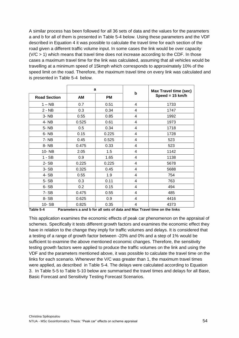
Christina Spiliopoulou
NTUA - MSc Geoinformatics Thesis: “Peak car” effects on scheme appraisal 54
A similar process has been followed for all 36 sets of data and the values for the parameters
a and b for all of them is presented in Table 5-4 below. Using these parameters and the VDF
described in Equation 4 it was possible to calculate the travel time for each section of the
road given a different traffic volume input. In some cases the link would be over capacity
(V/C > 1) which means that travel time does not increase according to the CDF. In those
cases a maximum travel time for the link was calculated, assuming that all vehicles would be
travelling at a minimum speed of 15kmph which corresponds to approximately 10% of the
speed limit on the road. Therefore, the maximum travel time on every link was calculated and
is presented in Table 5-4 below.
a b
Max Travel time (sec) Speed = 15 km/h Road Section AM PM
1 – NB 0.7 0.51 4 1733
2 - NB 0.3 0.34 4 1747
3- NB 0.55 0.85 4 1992
4- NB 0.525 0.61 4 1973
5- NB 0.5 0.34 4 1718
6- NB 0.15 0.225 4 1728
7- NB 0.45 0.525 4 523
8- NB 0.475 0.33 4 523
10- NB 2.05 1.5 4 1142
1 - SB 0.9 1.65 4 1138
2- SB 0.225 0.225 4 5678
3- SB 0.325 0.45 4 5688
4- SB 0.55 1.9 4 754
5- SB 0.3 0.11 4 763
6- SB 0.2 0.15 4 494
7- SB 0.475 0.55 4 485
8- SB 0.625 0.9 4 4416
10- SB 0.825 0.35 4 4373
Table 5-4 Parameters a and b for all sets of data and Max Travel time on the links
This application examines the economic effects of peak car phenomenon on the appraisal of
schemes. Specifically it tests different growth factors and examines the economic effect they
have in relation to the change they imply for traffic volumes and delays. It is considered that
a testing of a range of growth factor between -20% and 0% and a step of 1% would be
sufficient to examine the above mentioned economic changes. Therefore, the sensitivity
testing growth factors were applied to produce the traffic volumes on the link and using the
VDF and the parameters mentioned above, it was possible to calculate the travel time on the
links for each scenario. Whenever the V/C was greater than 1, the maximum travel times
were applied, as described in Table 5-4. The delays were calculated according to Equation
3. In Table 5-5 to Table 5-10 below are summarised the travel times and delays for all Base,
Basic Forecast and Sensitivity Testing Forecast Scenarios.

Christina Spiliopoulou
NTUA - MSc Geoinformatics Thesis: “Peak car” effects on scheme appraisal 55
Base Year Basic Forecast Scenario
Sensitivity Testing Scenario -1% Growth
Sensitivity Testing Scenario -2% Growth
AM PM AM PM AM PM AM PM
Road Section
To (sec)
Travel Time
Delay per
vehicle (h)
Travel Time
Delay per
vehicle (h)
Travel Time
Delay per
vehicle (h)
Travel Time
Delay per
vehicle (h)
Travel Time
Delay per
vehicle (h)
Travel Time
Delay per
vehicle (h)
Travel Time
Delay per
vehicle (h)
Travel Time
Delay per
vehicle (h)
1 – NB 232 261 0.008 323 0.025 310 0.022 1740 0.419 307 0.021 1740 0.419 307 0.021 1740 0.419
2 - NB 234 285 0.005 345 0.022 317 0.014 1982 0.477 315 0.013 1982 0.477 315 0.013 1982 0.477
3- NB 267 242 0.003 353 0.034 263 0.009 1723 0.415 262 0.009 1723 0.415 262 0.009 1723 0.415
4- NB 264 86 0.004 523 0.126 523 0.126 523 0.126 523 0.126 523 0.126 523 0.126 523 0.126
5- NB 230 191 0.011 1140 0.274 1140 0.274 1140 0.274 1140 0.274 1140 0.274 1140 0.274 1140 0.274
6- NB 231 820 0.017 5683 1.367 5683 1.367 5683 1.367 5683 1.367 5683 1.367 5683 1.367 5683 1.367
7- NB 70 108 0.002 117 0.005 121 0.005 147 0.013 120 0.005 146 0.012 120 0.005 146 0.012
8- NB 70 79 0.004 80 0.004 490 0.118 490 0.118 490 0.118 490 0.118 490 0.118 490 0.118
10- NB 153 777 0.052 751 0.044 1097 0.140 1038 0.124 1081 0.136 1024 0.120 1081 0.136 1024 0.120
1 - SB 152 321 0.024 283 0.014 1740 0.418 370 0.038 1740 0.418 366 0.037 1740 0.418 366 0.037
2- SB 761 295 0.009 276 0.003 1982 0.477 296 0.009 1982 0.477 295 0.009 1982 0.477 295 0.009
3- SB 762 262 0.009 242 0.003 1723 0.414 260 0.008 1723 0.414 259 0.008 1723 0.414 259 0.008
4- SB 101 86 0.004 83 0.004 523 0.126 107 0.010 523 0.126 106 0.010 523 0.126 106 0.010
5- SB 102 190 0.010 164 0.003 1140 0.274 1140 0.274 1140 0.274 1140 0.274 1140 0.274 1140 0.274
6- SB 66 880 0.033 797 0.010 5683 1.367 862 0.028 5683 1.367 859 0.027 5683 1.367 859 0.027
7- SB 65 114 0.003 111 0.002 135 0.009 127 0.007 134 0.009 126 0.007 134 0.009 126 0.007
8- SB 591 79 0.004 84 0.005 103 0.011 117 0.015 102 0.010 116 0.014 102 0.010 116 0.014
10- SB 586 669 0.023 619 0.009 813 0.063 680 0.026 806 0.061 677 0.025 806 0.061 677 0.025
Table 5-5 (1 out of 6) Travel Times and Delays as calculated for Base Year, Basic Forecasting Scenario and Sensitivity Testing Forecasting Scenarios

Christina Spiliopoulou
NTUA - MSc Geoinformatics Thesis: “Peak car” effects on scheme appraisal 56
Sensitivity Testing Scenario -3% Growth
Sensitivity Testing Scenario -4% Growth
Sensitivity Testing Scenario -5% Growth
Sensitivity Testing Scenario -6% Growth
AM PM AM PM AM PM AM PM
Road Section
To (sec)
Travel Time
Delay per
vehicle (h)
Travel Time
Delay per
vehicle (h)
Travel Time
Delay per
vehicle (h)
Travel Time
Delay per
vehicle (h)
Travel Time
Delay per
vehicle (h)
Travel Time
Delay per
vehicle (h)
Travel Time
Delay per
vehicle (h)
Travel Time
Delay per
vehicle (h)
1 – NB 232 307 0.021 1740 0.419 307 0.021 1740 0.419 307 0.021 1740 0.419 307 0.021 1740 0.419
2 - NB 234 315 0.013 1982 0.477 315 0.013 1982 0.477 315 0.013 1982 0.477 315 0.013 1982 0.477
3- NB 267 262 0.009 1723 0.415 262 0.009 1723 0.415 262 0.009 1723 0.415 262 0.009 1723 0.415
4- NB 264 523 0.126 523 0.126 523 0.126 523 0.126 523 0.126 523 0.126 523 0.126 523 0.126
5- NB 230 1140 0.274 1140 0.274 1140 0.274 1140 0.274 1140 0.274 1140 0.274 1140 0.274 1140 0.274
6- NB 231 5683 1.367 5683 1.367 5683 1.367 5683 1.367 5683 1.367 5683 1.367 5683 1.367 5683 1.367
7- NB 70 120 0.005 146 0.012 120 0.005 146 0.012 120 0.005 146 0.012 120 0.005 146 0.012
8- NB 70 490 0.118 490 0.118 490 0.118 490 0.118 490 0.118 490 0.118 490 0.118 490 0.118
10- NB 153 1081 0.136 1024 0.120 1081 0.136 1024 0.120 1081 0.136 1024 0.120 1081 0.136 1024 0.120
1 - SB 152 1740 0.418 366 0.037 1740 0.418 366 0.037 1740 0.418 366 0.037 1740 0.418 366 0.037
2- SB 761 1982 0.477 295 0.009 1982 0.477 295 0.009 1982 0.477 295 0.009 1982 0.477 295 0.009
3- SB 762 1723 0.414 259 0.008 1723 0.414 259 0.008 1723 0.414 259 0.008 1723 0.414 259 0.008
4- SB 101 523 0.126 106 0.010 523 0.126 106 0.010 523 0.126 106 0.010 523 0.126 106 0.010
5- SB 102 1140 0.274 1140 0.274 1140 0.274 1140 0.274 1140 0.274 1140 0.274 1140 0.274 1140 0.274
6- SB 66 5683 1.367 859 0.027 5683 1.367 859 0.027 5683 1.367 859 0.027 5683 1.367 859 0.027
7- SB 65 134 0.009 126 0.007 134 0.009 126 0.007 134 0.009 126 0.007 134 0.009 126 0.007
8- SB 591 102 0.010 116 0.014 102 0.010 116 0.014 102 0.010 116 0.014 102 0.010 116 0.014
10- SB 586 806 0.061 677 0.025 806 0.061 677 0.025 806 0.061 677 0.025 806 0.061 677 0.025
Table 5-6 (2 out of 6) Travel Times and Delays as calculated for Base Year, Basic Forecasting Scenario and Sensitivity Testing Forecasting Scenarios

Christina Spiliopoulou
NTUA - MSc Geoinformatics Thesis: “Peak car” effects on scheme appraisal 57
Sensitivity Testing Scenario -7% Growth
Sensitivity Testing Scenario -8% Growth
Sensitivity Testing Scenario -9% Growth
Sensitivity Testing Scenario -10% Growth
AM PM AM PM AM PM AM PM
Road Section
To (sec)
Travel Time
Delay per
vehicle (h)
Travel Time
Delay per
vehicle (h)
Travel Time
Delay per
vehicle (h)
Travel Time
Delay per
vehicle (h)
Travel Time
Delay per
vehicle (h)
Travel Time
Delay per
vehicle (h)
Travel Time
Delay per
vehicle (h)
Travel Time
Delay per
vehicle (h)
1 – NB 232 307 0.021 1740 0.419 307 0.021 1740 0.419 307 0.021 1740 0.419 307 0.021 1740 0.419
2 - NB 234 315 0.013 1982 0.477 315 0.013 1982 0.477 315 0.013 1982 0.477 315 0.013 1982 0.477
3- NB 267 262 0.009 1723 0.415 262 0.009 1723 0.415 262 0.009 1723 0.415 262 0.009 1723 0.415
4- NB 264 523 0.126 523 0.126 523 0.126 523 0.126 523 0.126 523 0.126 523 0.126 523 0.126
5- NB 230 1140 0.274 1140 0.274 1140 0.274 1140 0.274 1140 0.274 1140 0.274 1140 0.274 1140 0.274
6- NB 231 5683 1.367 5683 1.367 5683 1.367 5683 1.367 5683 1.367 5683 1.367 5683 1.367 5683 1.367
7- NB 70 120 0.005 146 0.012 120 0.005 146 0.012 120 0.005 146 0.012 120 0.005 146 0.012
8- NB 70 490 0.118 490 0.118 490 0.118 490 0.118 490 0.118 490 0.118 490 0.118 490 0.118
10- NB 153 1081 0.136 1024 0.120 1081 0.136 1024 0.120 1081 0.136 1024 0.120 1081 0.136 1024 0.120
1 - SB 152 1740 0.418 366 0.037 1740 0.418 366 0.037 1740 0.418 366 0.037 1740 0.418 366 0.037
2- SB 761 1982 0.477 295 0.009 1982 0.477 295 0.009 1982 0.477 295 0.009 1982 0.477 295 0.009
3- SB 762 1723 0.414 259 0.008 1723 0.414 259 0.008 1723 0.414 259 0.008 1723 0.414 259 0.008
4- SB 101 523 0.126 106 0.010 523 0.126 106 0.010 523 0.126 106 0.010 523 0.126 106 0.010
5- SB 102 1140 0.274 1140 0.274 1140 0.274 1140 0.274 1140 0.274 1140 0.274 1140 0.274 1140 0.274
6- SB 66 5683 1.367 859 0.027 5683 1.367 859 0.027 5683 1.367 859 0.027 5683 1.367 859 0.027
7- SB 65 134 0.009 126 0.007 134 0.009 126 0.007 134 0.009 126 0.007 134 0.009 126 0.007
8- SB 591 102 0.010 116 0.014 102 0.010 116 0.014 102 0.010 116 0.014 102 0.010 116 0.014
10- SB 586 806 0.061 677 0.025 806 0.061 677 0.025 806 0.061 677 0.025 806 0.061 677 0.025
Table 5-7 (3 out of 6) Travel Times and Delays as calculated for Base Year, Basic Forecasting Scenario and Sensitivity Testing Forecasting Scenarios

Christina Spiliopoulou
NTUA - MSc Geoinformatics Thesis: “Peak car” effects on scheme appraisal 58
Sensitivity Testing Scenario -11% Growth
Sensitivity Testing Scenario -12% Growth
Sensitivity Testing Scenario -13% Growth
Sensitivity Testing Scenario -14% Growth
AM PM AM PM AM PM AM PM
Road Section
To (sec)
Travel Time
Delay per
vehicle (h)
Travel Time
Delay per
vehicle (h)
Travel Time
Delay per
vehicle (h)
Travel Time
Delay per
vehicle (h)
Travel Time
Delay per
vehicle (h)
Travel Time
Delay per
vehicle (h)
Travel Time
Delay per
vehicle (h)
Travel Time
Delay per
vehicle (h)
1 – NB 232 307 0.021 1740 0.419 307 0.021 1740 0.419 307 0.021 1740 0.419 307 0.021 1740 0.419
2 - NB 234 315 0.013 1982 0.477 315 0.013 1982 0.477 315 0.013 1982 0.477 315 0.013 1982 0.477
3- NB 267 262 0.009 1723 0.415 262 0.009 1723 0.415 262 0.009 1723 0.415 262 0.009 1723 0.415
4- NB 264 523 0.126 523 0.126 523 0.126 523 0.126 523 0.126 523 0.126 523 0.126 523 0.126
5- NB 230 1140 0.274 1140 0.274 1140 0.274 1140 0.274 1140 0.274 1140 0.274 1140 0.274 1140 0.274
6- NB 231 5683 1.367 5683 1.367 5683 1.367 5683 1.367 5683 1.367 5683 1.367 5683 1.367 5683 1.367
7- NB 70 120 0.005 146 0.012 120 0.005 146 0.012 120 0.005 146 0.012 120 0.005 146 0.012
8- NB 70 490 0.118 490 0.118 490 0.118 490 0.118 490 0.118 490 0.118 490 0.118 490 0.118
10- NB 153 1081 0.136 1024 0.120 1081 0.136 1024 0.120 1081 0.136 1024 0.120 1081 0.136 1024 0.120
1 - SB 152 1740 0.418 366 0.037 1740 0.418 366 0.037 1740 0.418 366 0.037 1740 0.418 366 0.037
2- SB 761 1982 0.477 295 0.009 1982 0.477 295 0.009 1982 0.477 295 0.009 1982 0.477 295 0.009
3- SB 762 1723 0.414 259 0.008 1723 0.414 259 0.008 1723 0.414 259 0.008 1723 0.414 259 0.008
4- SB 101 523 0.126 106 0.010 523 0.126 106 0.010 523 0.126 106 0.010 523 0.126 106 0.010
5- SB 102 1140 0.274 1140 0.274 1140 0.274 1140 0.274 1140 0.274 1140 0.274 1140 0.274 1140 0.274
6- SB 66 5683 1.367 859 0.027 5683 1.367 859 0.027 5683 1.367 859 0.027 5683 1.367 859 0.027
7- SB 65 134 0.009 126 0.007 134 0.009 126 0.007 134 0.009 126 0.007 134 0.009 126 0.007
8- SB 591 102 0.010 116 0.014 102 0.010 116 0.014 102 0.010 116 0.014 102 0.010 116 0.014
10- SB 586 806 0.061 677 0.025 806 0.061 677 0.025 806 0.061 677 0.025 806 0.061 677 0.025
Table 5-8 (4 out of 6) Travel Times and Delays as calculated for Base Year, Basic Forecasting Scenario and Sensitivity Testing Forecasting Scenarios

Christina Spiliopoulou
NTUA - MSc Geoinformatics Thesis: “Peak car” effects on scheme appraisal 59
Sensitivity Testing Scenario -15% Growth
Sensitivity Testing Scenario -16% Growth
Sensitivity Testing Scenario -17% Growth
Sensitivity Testing Scenario -18% Growth
AM PM AM PM AM PM AM PM
Road Section
To (sec)
Travel Time
Delay per
vehicle (h)
Travel Time
Delay per
vehicle (h)
Travel Time
Delay per
vehicle (h)
Travel Time
Delay per
vehicle (h)
Travel Time
Delay per
vehicle (h)
Travel Time
Delay per
vehicle (h)
Travel Time
Delay per
vehicle (h)
Travel Time
Delay per
vehicle (h)
1 – NB 232 307 0.021 1740 0.419 307 0.021 1740 0.419 307 0.021 1740 0.419 307 0.021 1740 0.419
2 - NB 234 315 0.013 1982 0.477 315 0.013 1982 0.477 315 0.013 1982 0.477 315 0.013 1982 0.477
3- NB 267 262 0.009 1723 0.415 262 0.009 1723 0.415 262 0.009 1723 0.415 262 0.009 1723 0.415
4- NB 264 523 0.126 523 0.126 523 0.126 523 0.126 523 0.126 523 0.126 523 0.126 523 0.126
5- NB 230 1140 0.274 1140 0.274 1140 0.274 1140 0.274 1140 0.274 1140 0.274 1140 0.274 1140 0.274
6- NB 231 5683 1.367 5683 1.367 5683 1.367 5683 1.367 5683 1.367 5683 1.367 5683 1.367 5683 1.367
7- NB 70 120 0.005 146 0.012 120 0.005 146 0.012 120 0.005 146 0.012 120 0.005 146 0.012
8- NB 70 490 0.118 490 0.118 490 0.118 490 0.118 490 0.118 490 0.118 490 0.118 490 0.118
10- NB 153 1081 0.136 1024 0.120 1081 0.136 1024 0.120 1081 0.136 1024 0.120 1081 0.136 1024 0.120
1 - SB 152 1740 0.418 366 0.037 1740 0.418 366 0.037 1740 0.418 366 0.037 1740 0.418 366 0.037
2- SB 761 1982 0.477 295 0.009 1982 0.477 295 0.009 1982 0.477 295 0.009 1982 0.477 295 0.009
3- SB 762 1723 0.414 259 0.008 1723 0.414 259 0.008 1723 0.414 259 0.008 1723 0.414 259 0.008
4- SB 101 523 0.126 106 0.010 523 0.126 106 0.010 523 0.126 106 0.010 523 0.126 106 0.010
5- SB 102 1140 0.274 1140 0.274 1140 0.274 1140 0.274 1140 0.274 1140 0.274 1140 0.274 1140 0.274
6- SB 66 5683 1.367 859 0.027 5683 1.367 859 0.027 5683 1.367 859 0.027 5683 1.367 859 0.027
7- SB 65 134 0.009 126 0.007 134 0.009 126 0.007 134 0.009 126 0.007 134 0.009 126 0.007
8- SB 591 102 0.010 116 0.014 102 0.010 116 0.014 102 0.010 116 0.014 102 0.010 116 0.014
10- SB 586 806 0.061 677 0.025 806 0.061 677 0.025 806 0.061 677 0.025 806 0.061 677 0.025
Table 5-9 (5 out of 6) Travel Times and Delays as calculated for Base Year, Basic Forecasting Scenario and Sensitivity Testing Forecasting Scenarios
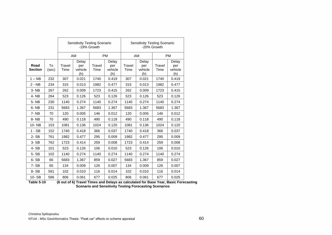
Christina Spiliopoulou
NTUA - MSc Geoinformatics Thesis: “Peak car” effects on scheme appraisal 60
Sensitivity Testing Scenario -19% Growth
Sensitivity Testing Scenario -20% Growth
AM PM AM PM
Road Section
To (sec)
Travel Time
Delay per
vehicle (h)
Travel Time
Delay per
vehicle (h)
Travel Time
Delay per
vehicle (h)
Travel Time
Delay per
vehicle (h)
1 – NB 232 307 0.021 1740 0.419 307 0.021 1740 0.419
2 - NB 234 315 0.013 1982 0.477 315 0.013 1982 0.477
3- NB 267 262 0.009 1723 0.415 262 0.009 1723 0.415
4- NB 264 523 0.126 523 0.126 523 0.126 523 0.126
5- NB 230 1140 0.274 1140 0.274 1140 0.274 1140 0.274
6- NB 231 5683 1.367 5683 1.367 5683 1.367 5683 1.367
7- NB 70 120 0.005 146 0.012 120 0.005 146 0.012
8- NB 70 490 0.118 490 0.118 490 0.118 490 0.118
10- NB 153 1081 0.136 1024 0.120 1081 0.136 1024 0.120
1 - SB 152 1740 0.418 366 0.037 1740 0.418 366 0.037
2- SB 761 1982 0.477 295 0.009 1982 0.477 295 0.009
3- SB 762 1723 0.414 259 0.008 1723 0.414 259 0.008
4- SB 101 523 0.126 106 0.010 523 0.126 106 0.010
5- SB 102 1140 0.274 1140 0.274 1140 0.274 1140 0.274
6- SB 66 5683 1.367 859 0.027 5683 1.367 859 0.027
7- SB 65 134 0.009 126 0.007 134 0.009 126 0.007
8- SB 591 102 0.010 116 0.014 102 0.010 116 0.014
10- SB 586 806 0.061 677 0.025 806 0.061 677 0.025
Table 5-10 (6 out of 6) Travel Times and Delays as calculated for Base Year, Basic Forecasting Scenario and Sensitivity Testing Forecasting Scenarios

Christina Spiliopoulou
NTUA - MSc Geoinformatics Thesis: “Peak car” effects on scheme appraisal 61
5.4 Group Step 3 – Economic Analysis
The DfT’s WEB TAG and the TAG data book include all the information required for a cost
benefit analysis. This methodology has been found sufficient for this application and also
aligns with officially used methodology for scheme appraisal. The TAG Data book’s table of
content related to Cost Benefit Analysis is presented in Table 5-11. The TAG Data book
used in this study is the latest version (May 2014), therefore all references and data are
related to that. Though it is strongly advised to consult the latest version of the TAG Data
Book (available online) as the table names and content may change.
TAG Unit
Section Title
Unit Title Worksheet Table Title
Cover Department for Transport contact information
User Parameters User - defined price year and initial forecast year
Audit Version log
TAG1 WebTAG1 table look-up
Annual Parameters
Forecast annual economic and demographic parameters
A 1.1 Cost Benefit Analysis
A 1.1.1 Discount rates
A 1.3
User & Provider Impacts
Values of time A 1.3.1 Values of time per person (working and non-working)
A 1.3.2 Forecast values of time per person (working and non-working)
A 1.3.3
Car and vehicle occupancies (2000); Annual percentage change in car passenger occupancy up to 2036
A 1.3.4 Proportion of travel and trips in work and non-work time
A 1.3.5 Market price values of time per vehicle based on distance travelled
A 1.3.6 Forecast market price values of time per vehicle based on distance travelled
Operating costs A 1.3.7 Fuel and electricity prices and components
A 1.3.8 Fuel / energy consumption parameter values
A 1.3.9 Forecast proportion of car, LGV and other vehicle kilometres using petrol / diesel / electricity
A 1.3.10 Forecast assumed vehicle fuel efficiency improvements to 2035
A 1.3.11 Forecast fuel / energy consumption parameters
A 1.3.12 Forecast vehicle fuel / energy cost formulae parameters (work)
A 1.3.13 Forecast vehicle fuel / energy cost formulae parameters (non-work)
A 1.3.14 Non-fuel resource vehicle operating costs
A 1.3.15 Forecast non-fuel resource car operating costs to 2035
Social Impact of buses
A 1.3.16 Proportion of bus trips by car ownership, trip purpose and concessionary travel pass status.
A 1.3.17 Proportion of bus trips by that would “not go” if bus not available.
A 1.3.18 Value of the social impact per return bus trip
Table 5-11 Table of contents related to Cost Benefit Analysis Source: TAG Data Book (May 2014)

Christina Spiliopoulou
NTUA - MSc Geoinformatics Thesis: “Peak car” effects on scheme appraisal 62
Once the data has been collected and analysed for the base year, as per Group Steps 1 and
2, the next step is to translate the delays in monetary values. The same procedure is
followed once the forecast traffic flows and the related delays have been calculated.
Therefore a comparable base may be established and the values may be used for decision
making by stakeholders. The general process is described in Figure 5-9 below.
Figure 5-9 Methodology steps for the economic analysis
Traffic flows need to be split to different vehicle types, namely passenger cars (Car), Light
Good Vehicles (LGV) and Heavy Good Vehicles (HGV). The percentages for this split
depend on the data available. In this application they have been taken from the Highway
Agency’s “Route Base Strategy” for the A12.
Car type percentages
Car LGV HGV
0.74 0.16 0.1
Table 5-12 Vehicle classification factors Source: HA RBS for the A12
After traffic has been split to vehicle types, it needs to be split according to trip purpose.
Table A 1.3.4 of TAG data book (May 2014) that is presented in Figure 5-10 includes
information for the proportion of travel in work and non-work time, split for different vehicle
types according to national trends.
Figure 5-10 Traffic split per trip purpose Source: TAG Data Book (May 2014) – Table A1.3.4
The information available is the percentage split according to the following four types:
Percentage of Distance Travelled by Vehicles
Percentage of Vehicle Trips
Percentage of Distance Travelled by Occupants
Percentage of Person Trips
Table A 1.3.4: Proportion of travel in work and non-work time Proportion of trips made in work and non-work time
Weekday Weekend All Week Weekday Weekend All Week
Mode / Vehicle Type 7am – 10am 10am – 4pm 4pm – 7pm 7pm – 7am Average Average Average 7am – 10am 10am – 4pm 4pm – 7pm 7pm – 7am Average Average Average
& Journey Purpose Percentage of Distance Travelled by Vehicles Percentage of Vehicle Trips
Car Work 18.1 19.9 13.0 12.3 16.4 3.2 13.1 6.8 8.3 5.5 3.6 6.5 1.7 5.0
Commuting 46.0 11.4 40.8 36.2 31.0 8.5 25.3 40.6 11.6 32.3 26.4 25.4 9.1 20.3
Other 35.9 68.7 46.2 51.5 52.5 88.3 61.6 52.7 80.1 62.2 70.0 68.1 89.3 74.7
LGV Work (freight) 88.0 88.0 88.0 88.0 88.0 88.0 88.0 88.0 88.0 88.0 88.0 88.0 88.0 88.0
Non – Work 12.0 12.0 12.0 12.0 12.0 12.0 12.0 12.0 12.0 12.0 12.0 12.0 12.0 12.0
OGV1 Work 100.0 100.0 100.0 100.0 100.0 100.0 100.0 100.0 100.0 100.0 100.0 100.0 100.0 100.0
OGV2 Work 100.0 100.0 100.0 100.0 100.0 100.0 100.0 100.0 100.0 100.0 100.0 100.0 100.0 100.0
Percentage of Distance Travelled by Occupants Percentage of Person Trips
Car Work 15.4 13.8 10.2 9.9 12.6 2.0 9.2 5.2 2.2 4.1 1.2 4.7 1.1 3.4
Commuting 38.3 8.1 32.2 29.1 23.9 5.1 18.0 33.3 15.6 25.8 10.9 20.0 6.4 15.2
Other 46.4 78.1 57.6 61.0 63.5 92.9 72.7 61.5 82.2 70.1 87.9 75.3 92.5 81.4
PSV Work 3.9 2.0 3.9 5.7 3.4 1.5 2.9 1.5 1.2 1.8 2.6 1.5 1.0 1.4
Commuting 30.0 11.1 36.6 38.1 25.5 6.4 20.5 41.7 10.6 43.0 47.4 26.9 12.4 24.3
Other 66.1 86.9 59.5 56.2 71.1 92.0 76.6 56.8 88.2 55.2 50.0 71.5 86.6 74.3
Heavy Rail Work 14.1 22.4 16.4 23.2 18.3 6.3 16.5 6.7 13.6 6.7 8.8 8.3 2.8 7.6
Commuting 51.9 10.2 55.9 53.1 43.7 4.3 37.8 71.7 14.9 68.0 60.4 58.2 11.1 52.2
Other 34.1 67.4 27.7 23.7 38.1 89.5 45.7 21.6 71.5 25.4 30.8 33.5 86.1 40.3
Light Rail Work 1.9 0.2 1.8 2.3 1.3 0.4 1.2 2.8 0.7 3.3 5.3 2.4 1.2 2.2
Commuting 82.4 8.5 75.7 28.9 50.1 23.3 45.8 83.0 10.8 70.7 23.7 48.2 21.7 43.8
Other 15.7 91.3 22.5 68.9 48.6 76.3 53.1 14.2 88.5 26.0 71.1 49.4 77.1 54.0

Christina Spiliopoulou
NTUA - MSc Geoinformatics Thesis: “Peak car” effects on scheme appraisal 63
The first category has been selected for this application, as there was no information for
number of trips or number of occupants per vehicle.
Car LGV HGV
Work Commuting Other Work Non-work
AM 0.181 0.460 0.359 0.880 0.120 1
PM 0.130 0.408 0.462 0.880 0.120 1 Table 5-13 Trip purpose split factors Source: DFT – Web TAG data book – Table A1.3.4
The delays that have been previously calculated for the total of traffic for AM and PM peak
hours are now split by vehicle type and trip purpose. The next step is to apply a cost per time
unit in order to calculate the cost of the delays per vehicle type and per trip purpose. The
TAG data book includes tables with the value of time (VoT) and it is advised to use the type
of VoT that is more suitable for the data available. Indicatively, Figure 5-11 presents the VoT
per vehicle based on travelled distance as given by the TAG Data Book (May 2014).
Figure 5-11 Values of Time per journey purpose Source: TAG Data Book (May 2014) – Table A1.3.5
The cost of delay is calculated for each vehicle type and trip purpose, as outlined in the
methodology. The total amount of cost for all the delays is calculated on a daily basis for the
AM and PM peak hours. Multiplied by 252 (working days per year), it gives the total annual
cost of delays.
The prices included in the TAG Data Book refer to 2010 values. Therefore, they should be
factored to reflect GDP conditions during the year of study. The method to do this is
described in the TAG Unit A11 – Cost-Benefit Analysis: “there are indices in the TAG Data
Book that can be used to calculate a real value, in the DfT’ s price base, for a future year y”
using the Formula 5-1.
𝑅𝑒𝑎𝑙 𝑉𝑎𝑙𝑦𝑒𝑦 = 𝑅𝑒𝑎𝑙 𝑉𝑎𝑙𝑢𝑒𝐵𝑎𝑠𝑒 ∗𝐺𝐷𝑃 𝑖𝑛𝑑𝑒𝑥𝑦
𝐺𝐷𝑃 𝑖𝑛𝑑𝑒𝑥𝐵𝑎𝑠𝑒
Formula 5-1 GDP correction factor for the VoT
Source: TAG Unit A11 – Cost-Benefit Analysis
Table A 1.3.5: Market Price Values of Time per Vehicle based on distance travelled
(£ per hour, 2010 prices and 2010 values)
Vehicle Weekday
Type Journey Purpose 7am – 10am 10am – 4pm 4pm – 7pm 7pm – 7am Average Weekend All Week
Car Work 31.56 30.81 30.34 30.58 30.99 32.54 30.99
Commuting 7.83 7.77 7.65 7.66 7.71 7.72 7.71
Other 10.06 10.46 10.74 10.48 10.49 11.61 10.90
Average Car 12.92 14.20 12.03 11.93 12.98 11.95 12.73
LGV Work (freight) 14.62 14.62 14.62 14.62 14.62 15.35 14.62
Commuting & Other 9.15 9.15 9.15 9.15 9.15 12.72 9.97
Average LGV 13.96 13.96 13.96 13.96 13.96 15.03 14.06
OGV1 Working 14.35 14.35 14.35 14.35 14.35 14.35 14.35
OGV2 Working 14.35 14.35 14.35 14.35 14.35 14.35 14.35
PSV Work 22.57 18.72 22.57 26.22 21.56 17.70 20.54
(Occupants) Commuting 24.93 9.22 30.41 31.66 21.19 5.32 17.03
Other 48.74 64.08 43.88 41.44 52.43 67.84 56.49
Total 96.24 92.02 96.86 99.32 95.18 90.86 94.06

Christina Spiliopoulou
NTUA - MSc Geoinformatics Thesis: “Peak car” effects on scheme appraisal 64
The full list of GDP indices may be found in the TAG Data Book (May 2014). Table 5-14
below presents the average GDP per person for the years 2010 to 2031 (our forecast year).
Year
Average GDP per person
Historic value
Annual growth (%pa)
Index 1996=100
2010 23,672 0.85 144.97
2011 23,737 0.28 145.38
2012 23,646 -0.38 144.82
2013 - 1.07 146.36
2014 - 2.05 149.37
2015 - 1.67 151.86
2016 - 1.95 154.82
2017 - 1.99 157.90
2018 - 1.90 160.90
2019 - 2.23 164.49
2020 - 2.24 168.19
2021 - 1.86 171.31
2022 - 1.87 174.52
2023 - 1.89 177.81
2024 - 1.90 181.19
2025 - 2.02 184.85
2026 - 2.04 188.61
2027 - 2.05 192.49
2028 - 2.07 196.47
2029 - 2.09 200.57
2030 - 2.10 204.79
2031 - 2.02 208.93 Table 5-14 Average GDP per person
Source: TAG Data Book (May 2014) – Annual Parameters
The value of time is taken from the DfT’s TAG data book (May 2014) and includes the hourly
market prices per vehicle for year 2010, as presented in Table 5-14. These values have
been adjusted according to GDP in order to represent monetary values for the year 2013, as
shown in Formula 5-2 and Formula 5-3 below.
𝑉𝑜𝑇2013 = 𝑉𝑜𝑇2010 ∗146.36
144.97= 𝑉𝑜𝑇2010 ∗ 1.0095
Formula 5-2 GDP adjustment factor for 2013
𝑉𝑜𝑇2031 = 𝑉𝑜𝑇2010 ∗208.93
144.97= 𝑉𝑜𝑇2010 ∗ 1.4412
Formula 5-3 GDP adjustment factor for 2031
Therefore, the Value of Time has been calculated for this application and the results are summarised in
Table 5-15 below. The values of time that will be applied to the split traffic per trip purpose
and vehicle type, as it has been adjusted to reflect the 2013 base year values.

Christina Spiliopoulou
NTUA - MSc Geoinformatics Thesis: “Peak car” effects on scheme appraisal 65
Table 5-15 Value of time per vehicle based on distance travelled
Data source: DFT – Web TAG data book (May 2014) - Table A1.3.5
Group Step 3 has been applied as described to all the examined scenarios:
Base Year (2013)
Basic forecast year (2031)
20 Scenarios for all the variations of the Sensitivity Testing Forecasting (2031)
The detailed results matrices are included in APPENDIX B Group Step 3 Detailed matrices.
Table 5-16 below summarises the costs broken down per trip purpose and vehicle type for
the AM and PM peak hours. The costs of the delays are presented in annual values in £.
£ per hour, 2010 prices and 2010 values GDP growth - Adjusted values for 2013
GDP growth - Adjusted values for 2031
Vehicle Type
Journey Purpose
Weekday Weekday Weekday
7-10 am 4-7 pm 7-10 am 4-7 pm 7-10 am 4-7 pm
Car
Work 31.56 30.34 31.86 30.63 45.48 43.73
Commuting 7.83 7.65 7.90 7.72 11.28 11.03
Other 10.06 10.74 10.15 10.85 14.49 15.48
Average Car 12.92 12.03 13.05 12.14 18.63 17.34
LGV
Work (freight)
14.62 14.62 14.75 14.75 21.06 21.06
Commuting & Other
9.15 9.15 9.24 9.24 13.19 13.19
Average LGV 13.96 13.96 14.09 14.09 20.12 20.12
HGV Working 14.35 14.35 14.49 14.49 20.68 20.68

Christina Spiliopoulou
NTUA - MSc Geoinformatics Thesis: “Peak car” effects on scheme appraisal 66
Car LGV HGV
AM:
Work PM:
Work AM:
Commute PM:
Commute AM:
Other PM:
Other AM:
Work PM:
Work AM:
Non-work PM:
Non-work AM PM
Base Year (2013) 2701 22638 1703 17914 1707 28491 973 11812 83 1008 109 1318
Basic Forecast Year (2031) 127638 74414 80473 58888 80673 93653 45982 38826 3926 3315 5131 4332
Sensitivity Testing Growth Factor -1% 126486 73725 79747 58342 79945 92785 45568 38467 3890 3284 5084 4292
Sensitivity Testing Growth Factor -2% 125494 73151 79121 57888 79317 92062 45210 38167 3860 3258 5044 4259
Sensitivity Testing Growth Factor -3% 124501 72577 78495 57433 78690 91340 44852 37867 3829 3233 5004 4225
Sensitivity Testing Growth Factor -4% 123508 72002 77869 56979 78062 90617 44494 37568 3799 3207 4965 4192
Sensitivity Testing Growth Factor -5% 122515 71428 77243 56524 77435 89895 44137 37268 3768 3182 4925 4158
Sensitivity Testing Growth Factor -6% 121522 70854 76617 56070 76807 89172 43779 36969 3738 3156 4885 4125
Sensitivity Testing Growth Factor -7% 120529 70280 75991 55616 76180 88449 43421 36669 3707 3131 4845 4091
Sensitivity Testing Growth Factor -8% 119537 69706 75365 55161 75552 87727 43064 36369 3676 3105 4805 4058
Sensitivity Testing Growth Factor -9% 118544 69132 74739 54707 74925 87004 42706 36070 3646 3079 4765 4025
Sensitivity Testing Growth Factor -10% 117551 68557 74113 54253 74297 86281 42348 35770 3615 3054 4725 3991
Sensitivity Testing Growth Factor -11% 116558 67983 73487 53798 73670 85559 41991 35471 3585 3028 4685 3958
Sensitivity Testing Growth Factor -12% 115565 67409 72861 53344 73042 84836 41633 35171 3554 3003 4645 3924
Sensitivity Testing Growth Factor -13% 114572 66835 72235 52889 72415 84114 41275 34872 3524 2977 4605 3891
Sensitivity Testing Growth Factor -14% 113580 66261 71609 52435 71787 83391 40918 34572 3493 2952 4565 3857
Sensitivity Testing Growth Factor -15% 112587 65686 70983 51981 71160 82668 40560 34272 3463 2926 4526 3824
Sensitivity Testing Growth Factor -16% 111594 65112 70357 51526 70532 81946 40202 33973 3432 2900 4486 3791
Sensitivity Testing Growth Factor -17% 110601 64538 69731 51072 69905 81223 39845 33673 3402 2875 4446 3757
Sensitivity Testing Growth Factor -18% 109608 63964 69105 50618 69277 80500 39487 33374 3371 2849 4406 3724
Sensitivity Testing Growth Factor -19% 108615 63390 68479 50163 68650 79778 39129 33074 3341 2824 4366 3690
Sensitivity Testing Growth Factor -20% 107623 62816 67853 49709 68022 79055 38772 32774 3310 2798 4326 3657
Table 5-16 Summary of annual costs of delays (£) for all tested scenarios - Split per trip purpose, peak hour and vehicle type.

Christina Spiliopoulou
NTUA - MSc Geoinformatics Thesis: “Peak car” effects on scheme appraisal 67
5.5 Group Step 4 – Compare the Generalised Cost
of the Externalities
This is the final step of the methodology that calculated the generalised cost of the
externalities and compares the different scenarios. In this application, there is only one
externality examined, so the generalised cost is basically the annual cost of the delays for
each scenario, as it has already been presented in Table 5-16.
Table 5-17 summarises the annual cost of the delays for all the examined scenarios: The
annual cost of the delays on the examined road during the base year is estimated to be
£22,795,222 and it is forecast to rise to £155,546,846 by 2031, creating an additional cost of
£132,751,624 due to increased delays on the A12. The different scenarios that have been
used for the sensitivity testing imply a gradient change in the forecasting factors and use a
step of -1% change. In the case of forecasting overestimation that is the case for peak car,
the growth factor in 2031 would be smaller than the one provided by TEMPRO. A total of 20
scenarios has been tested to cover a range of forecasting inaccuracy from -20% to 0%.
Therefore, the growth factor that is officially 1.284 for the AM peak period and 1.294 for the
PM peak period has been tested for its impact in the annual cost of delays for a range of
1.084-1.274 for the AM and 1.094-1.284 for the PM peak periods.
It is found that if the growth factor turns out to be 1% less than the official growth factor, the
annual cost of the delays will be £154,126,746 that is approximately £2m less than the basic
forecasting scenario. Respectively, a growth factor of 10% less would signify approximately
£12m less annual cost of delays and a growth factor of 20% less would signify approximately
£14m less in annual cost of delays.
The differences in the economic assessment of the annual delays are significant and should
be taken under consideration during scheme appraisal. A difference of 1% or 2% in the
growth factor is not something unrealistic and it would imply a difference in cost of delays of
a few million pounds.
It should be noted that there is a significant difference in the annual cost of delays between
the base year and all forecasting scenarios. This may be attributed to the calculation of the
travel time on the links under congestion: It has been assumed that if the volume on the lionk
exceeds capacity, a maximum travel time will be assumed on the link instead of using the
results of the VDF. This is logical, as when congestion occurs on a link the speed reduces
faster that when congestion is building up. In the future the number of links on the examined
part of the A12 that will experience a V/C>1 is great and the delays experienced on those
links have also been calculated and are significant. Therefore, the great difference in the
annual cost of delays is justified as a combination of increased delays experiences per
vehicle and an increased number of vehicles on the A12.

Christina Spiliopoulou
NTUA - MSc Geoinformatics Thesis: “Peak car” effects on scheme appraisal 68
Scenario Annual Cost of Delays
(£)
Cost of delays: (Scenario) – (Base Year)
(£)
Base year 2013
22,795,222
Forecast year 2031
155,546,846 132,751,624
Sensitiv
ity T
estin
g G
row
th F
acto
r %
chan
ge
-1% 154,126,746 131,331,523
-2% 152,921,133 130,125,911
-3% 151,715,520 128,920,298
-4% 150,509,907 127,714,685
-5% 149,304,294 126,509,072
-6% 148,098,681 125,303,459
-7% 146,893,068 124,097,846
-8% 145,687,455 122,892,233
-9% 144,481,843 121,686,620
-10% 143,276,230 120,481,007
-11% 142,070,617 119,275,394
-12% 140,865,004 118,069,782
-13% 139,659,391 116,864,169
-14% 138,453,778 115,658,556
-15% 137,248,165 114,452,943
-16% 136,042,552 113,247,330
-17% 134,836,939 112,041,717
-18% 133,631,326 110,836,104
-19% 132,425,714 109,630,491
-20% 131,220,101 108,424,878
Table 5-17 Cost of delays on the A12 for the base and forecast year and sensitivity test.

69
6. Recommendations / Conclusions This study has examined the importance of forecasting when it comes to traffic growth and
modal share. It has been shown that infrastructure projects are a great part of nations’
investment and they are vital to keep people and goods moving and the societies growing.
So far forecasting is a fundamental part of decision making and its accuracy is important in
terms of financial implications. It has been proven that the forecasting in major infrastructure
projects has failed in many cases and the economic implications of such failures are not to
be neglected.
As mentioned already, it has been established that the forecasting methods we are using are
failing to accurately predict future demand for transport infrastructure projects. There is a
wide range of bibliography and research on forecasting methodologies, methods to improve
accuracy and it is an ongoing conversation whether we have reached an era of falling out of
love with the car. A suggestion of implementing transport and land use has had lots of
positive response and has been successful in reducing inaccuracies and strengthening the
case for a more realistic approach to transport management.
Academic research and case studies ordered by governments have made a case for a need
for a holistic approach to forecasting and increased accuracy. Nevertheless, the methods
used by transportation specialists when producing results for stakeholders are the ones
suggested by government and the forecasting is done on a national level. Consequently, no
matter how much research and progress is done on forecasting methodologies, it will be of
no use unless it is incorporated in the national forecasting models.
This study has been motivated by the need to establish a better system in appraising
schemes, that will be more realistic and respond to people’s behavioural changes. The writer
lives and works in the U.K. and has experience of the appraisal processes there as well as
the best practices and guidance. The forecasting methodology in the U.K. and the cost
benefit analysis guidance are presented in this study and it was considered interesting to
test the sensitivity of economic appraisal to changes in the growth factors.
In order to achieve this a strategic road appraisal scheme was selected to be tested, namely
a part of the strategic road network was analysed for its current and forecast traffic
performance. Available data open to the public was used to assess traffic conditions on the
section of the A12 that is within the boundary of the county of Essex. The official growth
factors given by the Department for Transport were used to estimate future traffic on the
road and a range of growth factors was also applied to current conditions in order to
compare the results if peak car occurs and car usage decreases.
The methodology that was followed consists of four steps, namely data collection and
analysis; selection and calculation of the values for a series of externalities that will be used
to produce the economic performance of the road; translation of the externalities in monetary
values; comparison of the generalised costs of the externalities for the scenarios applied. As
scenarios, the needs to be a base year scenario, and official forecast scenario and a series
of scenarios for the sensitivity testing. The aim is to compare the costs for the different

70
scenarios and consequently the cost of the inaccuracies in forecasting in case peak car
occurs and has not been accounted for in the official forecasting.
During the application a series of constraints were faced and dealt with by adjusting the
methodology: The data available for the road were broken down in 10 sections and each
section included a number of junctions. Therefore it was not possible to use an accurate
traffic model. It was chosen to use the BPR’s VDF in order to input the traffic volumes on the
links and produce the travel times. The VDF was calibrated for each link separately as the
data was not consistent enough to produce a single set of parameters for the calibration.
The free flow travel time was calculated as a combination of the link length and the average
travel speed. Therefore, the delays were calculated on the links. In the cases where
congestion occurred and the V/C was greater than 1, the VDF could not accurately calculate
the travel time on the links and in those cases a maximum travel time was assumed as a
result of a minimum travel speed on the link at 15 km/h. This procedure allows to calculate
the travel times for any given input of traffic flow on the link.
The delays on the links were then translated into monetary values: the traffic was split per
trip purpose and vehicle type and a cost was assigned to each category. Additionally, the
delays per vehicle were split accordingly and a value of time was assigned to each category
of the delays. This methods allowed to calculate the annual cost of the delays on the road
during the peak hours.
The results revealed a significant increase in the cost of the delays mainly due to congestion
on a great number of road sections and their assigned maximum travel time. The annual
cost of the delays on the examined road during the base year is estimated to be
£22,795,222 and it is forecast to rise to £155,546,846 by 2031, creating an additional cost of
£132,751,624 due to increased delays on the A12. It was also found that if the growth factor
turns out to be 1% less than the official growth factor, the annual cost of the delays will be
£154,126,746 that is approximately £2m less than the basic forecasting scenario.
Respectively, a growth factor of 10% less would signify approximately £12m less annual cost
of delays and a growth factor of 20% less would signify approximately £14m less in annual
cost of delays.
The above mentioned figures reveal a significant impact of inaccuracies in forecasting, if
peak car occurs and has not been included in the official forecasts. They make a case for
drawing attention to current methodologies and point out that the economic impacts of
forecasting inaccuracies are not to be disregarded.
This application is subject to a series of constraints and assumptions, which leaves a great
margin of error in the results. Though, it has a sound base and reaches a logical conclusion.
Ideally, the methodology could be followed having a greater amount of data available, to
include all traffic performance, environmental and accident indicators to be examined. A
model would be a great improvement in the input of all the available data and the calculation
of the externalities. Therefore a socio-economic analysis could be run and a great breadth of
results could be compared to make a stronger case for peak car effects. In terms of the
economic assessment, it is considered that this analysis had enough data and resources
available to calculate the costs of the externalities.

71
Whether this application is accurate in terms of results or not, it makes a case for the effects
of inputs data inaccuracies in the economic appraisal of schemes. In most scheme
appraisals a relevant methodology is followed, comparing base year data with forecast data
with and without the scheme in question. The quality of the input data is crucial in the
outcomes of the appraisal process that will are later on used by stakeholders for decision
making. An alternative approach to dealing with forecasting inaccuracies would be to include
a set of sensitivity testing growth factors in scheme appraisal to account for such errors and
alert decision makers that their decisions are subject to a range of outcomes. Another
method to deal with peak car in case the forecasting cannot be more accurate is to adopt a
staged approach in decision making: break down the schemes in smaller time horizon parts
that are subject to greater accuracy. Therefore stakeholders can re assess the future
development of a scheme once it has partially worked and affected the network.

72
7. Bibliography Antoniou C., Psarianos B. and Brilon W. (2011). Induced traffic prediction inaccuracies as a
source of traffic forecasting failure. Transportation Letters: The International Journal
of Transportation Research (2011) 3: (253-264) DOI 10.3328/TL.2011.03.04.253-264
J. Ross Publishing, Inc. © 2011.
Alkhorayef A. and Pearman A (2013). Why do major transport projects underperform? An
empirical study from a psychological perspective. Conference paper presented at the
1st International Conference on Uncertainties in Transport Infrastructure Evaluation
(UNITE).
Bain R. (2009). Error and optimism bias in toll road traffic forecasts. Transportation
DOI 10.1007/s11116-009-9199-7, Springer Science+Business Media, LLC. 2009,
published online: 28 February 2009.
Beswick A. (2014). “Peak Car –What is it and Why Does it Matter?”,
http://www.jmp.co.uk/forward-thinking/update/peak-car-%E2%80%93what-it-and-
why-does-it-matter, Submitted online on Mon, 14/01/2013 - 09:54, last accessed on
17 April 2014.
Chatterjee K, Gordon A (2006). Planning for an unpredictable future: Transport in Great
Britain in 2030. Transport Policy 13 pg.254–264.
Coppola P., lbeas A., Olio A., Cordega R. (2013). LUTI Model for the Metropolitan Area of
Santander. Journal of Urban Planning and Development Vol 139 Issue 3 Sept 2013.
ASCE.
Crozet Y. (2013). High Speed Rail Performance in France: From Appraisal Methodologies to
Ex-post Evaluation. International Transport Forum, Discussion Paper No. 2013-26,
Prepared for the Roundtable on The Economics of Investment in High Speed Rail
(18-19 December 2013, New Delhi).
Crawford J.H. (2012). The Delivery of Freight in Carfree Cities. World Transport Policy and
Practice 17 (4) pg. 3-6. ISSN 1352- 7614.
Davis A.G and Xiong H. (2007). Access to Destinations Study. Report No3, University of
Minnesota.
De Jong, Daly A., Pietres M. (2007). Uncertainty in traffic forecasts: literature review and
new results for The Netherlands. Transportation 34 pg. 375–395. Springer Science
and Business Media B.V. 2006. DOI 10.1007/s11116-006-9110-8.
Edwards M, Macket L.R. (1996). Developing new urban public transport systems. Transport
Policy, Vol. 3. No. 4, pp. 225-5239 Elsevier Science Ltd Pll: 80967-070X(96)00023-6.
European Court of Editors (2014). EU funded urban transport projects underutilised, say EU
Auditors. Press Release ECA/14/11 by ECA Press, 12 rue Alcide De Gasperi - L-

73
1615 Luxembourg, T: (+352) 4398 45410 M: (+352) 621 55 22 24,
[email protected], Youtube: EUAuditorsECA. Luxembourg, 8 April 2014.
Figueroa M. J., Sick Nielsen T.A., Siren A. (2014). Comparing urban form correlations of the
travel patterns of older and younger adults. Transport Policy 35 pg.10–20, Elsevier
Science Ltd.
Flyvbjerg B. (2005).Measuring inaccuracy in travel demand forecasting: methodological
considerations regarding ramp up and sampling. Transportation Research Part A 39
(2005) pg. 522–530, Elsevier Science Ltd, doi:10.1016/j.tra.2005.02.003.
Goodwin P. (2012). Peak Car’ Where did the idea come from? And where is it going?.
Presented at CTS Winter Conference 2013.
Goodwin P. (2013). Peak Travel, Peak Car and the Future of Mobility: Evidence, Unresolved
Issues, Policy Implications, and a Research Agenda. Discussion Paper No. 2012-13,
Prepared for the Roundtable on Long-Run Trends in Travel Demand - November
2012. International Transport Forum.
Goodwin P., Dender, K. (2013). Peak Car – Themes and Issues. RAC, “On the move:
Making sense of car and train travel trends in Britain” (2013) [pg.iv].
Goodwin P., Denden K. (2014). “Peak Car’ — Themes and Issues. Transport Reviews: A
Transnational Transdisciplinary Journal, 33:3, pg. 243-254, DOI:
10.1080/01441647.2013.804133.
Guzman A.L., Hoz D., Monzon A. (2013). Optimal and Long-Term Dynamic Transport Policy
Design: Seeking Maximum Social Welfare through a Pricing Scheme. International
Journal of Sustainable Transportation, 8:4, 297-316, DOI:
10.1080/15568318.2012.696772. To link to this article:
http://dx.doi.org/10.1080/15568318.2012.696772 .
Halkias B, Tyrogianni H. (2008). PPP Projects in Greece: The case of Attika tollway. Review
Roads 2008 No342, pg.13-19, www.piarc.org.
Hillman M. (2012). The implications of climate change for the future of the car. World
Transport Policy and Practice 17 (4) pg. 3-6. ISSN 1352- 7614.
Institute for Mobility Research (IFMO) (2013). “'Mobility Y' – The Emerging Travel
Patterns of Generation Y”. A Research Establishment of the BMW Group.
Jastrzebski P. W. (2000). Volume Delay Functions, 15th International EMME/2 Users’ Group
Conference, October 18-20 2000, Vancouver B.C.
Knowles R.D. (1999). Transport impacts of Greater Manchester’s Metrolink light rail system.
Journal of Transport Geography Vol. 4 No.1 pg. 1-14. Pergamon editions.
Kuhnimhof T., Buehler R, Dargay J. (2011). A New Generation Travel Trends for Young
Germans and Britons. Transportation Research Record: Journal of the
Transportation Research Board,No. 2230, Transportation Research Board of the
National Academies, Washington D.C., pp. 58–67. DOI: 10.3141/2230-07

74
Kuhnimhof T., Buehler R., Wirtz M., Kalinowska D. (2012). Travel trends among young
adults in Germany: increasing multimodality and declining car use for men. Journal of
Transport Geography 24, pg. 443–450. Elsevier Ltd.
Le Vine, S. (2014a). Recent trends in young adults’ mobility. Presentation media presented
at: University of the West of England, Centre for Transport and Society, 17 Feb.
2014.
Le Vine S. (2014b). Look carefully at “Generation Next” – they can’t afford to become
tomorrow’s drivers. Local Transport Today, 651, 11 July – 24 July 2014.
Lee S. S. and Senior M. L. (2011). Do light rail services discourage car ownership and use?
Evidence from Census data for four English cities. Journal of Transport Geography,
issue 29 pg.11–23.
Lovallo D., Kahneman D. (2003). Delusion of success: How optimism undermines
executives’ decisions. Harvard Business Review, July 2003.
Lyons G., Goodwin P. (2014). Grow, peak or plateau – the outlook for car travel. Report for a
roundtable discussion held in London on 20 May 2014.
http://eprints.uwe.ac.uk/23277/
Matan A. and Newman P. (2012). Jan Gehl and new visions for walkable Australian cities.
World Transport Policy and Practice 17 (4) pg. 3-6. ISSN 1352- 7614.
Mc Cray R.D, Miller S. J., Hoel A. L (2012). Accuracy of Zonal Socioeconomic Forecasts for
Travel Demand Modeling - Retrospective Case Study. Transportation Research
Record: Journal of the Transportation Research Board, No. 2302, Transportation
Research Board of the National Academies, Washington, D.C., 2012, pg. 148–156.
DOI: 10.3141/2302-16.
Melia, S. (2012). A future beyond the car?” Editorial introduction. World Transport Policy and
Practice 17 (4) pg. 3-6. ISSN 1352- 7614.
Metz D. (2013). Peak Car and Beyond: The fourth Era of Travel, Transport Reviews: A
Transnational Transdisciplinary Journal, 33:3, pg. 255-270, DOI:
10.1080/01441647.2013.800615.
Metz D. (2014) Peak Car – The future of Travel, e-book edition first published in February
2014 in association with Landor LINKS (2014).
Newman P., Kenworthy J (2011). ‘Peak Car Use’: Understanding the Demise of Automobile
Dependence. World Transport Policy and Practice, Vol. 1 7, 2 June 2011.
Omega Centre - Centre for Mega Projects in transport and Development (2007). Project
Profile, UK, M 6 Toll Road. Available on-line at:
http://www.omegacentre.bartlett.ucl.ac.uk/studies/cases/road-m6_toll_2.php
Omega Centre - Centre for Mega Projects in transport and Development (2011). Sweden

75
Stockholm Air Link (Arlanda Express) Arlandabanan. Available on-line at:
http://www.omegacentre.bartlett.ucl.ac.uk/studies/cases/rail-
stockholm_air_link_2.php
Parthasarathi P., Levinson D. (2010). Post-construction evaluation of traffic forecast
accuracy. Transport Policy, Elsevier Ltd. doi:10.1016/j.tranpol.2010.04.010.
Parthasarathi P., Levinson D. (2009). Post-Construction Evaluation of Forecast Accuracy.
Technical report for the Minnesota Department of Transportation.
Sanko N., Morikawa T., Nagamatsu Y. (2013). Post-project evaluation of travel demand
forecasts: Implications from the case of a Japanese railway. Transport Policy2 pg.
209–218 Elsevier Science Ltd, http://dx.doi.org/10.1016/j.tranpol.2013.02.002.
Spycer M. (2006). BTS Skytrain Case Study – The experience of Bangkok’s first private
mass-transit concession. Presented at the WB Transport Learning Week 2006 -
Management of Large Infrastructure Contracts/Programs Session.
Tal G., Cohen-Blankshstain G. (2011). Understanding the role of the forecast-maker in
overestimation forecasts of policy impacts: The case of Travel Demand Management
policies. Transportation Research Part A (2011) pg. 389 – 400. Elsevier Ltd.
doi:10.1016/j.tra.2011.01.012.
Ülengin F., Özaydın Ö., Ülengin B., Kopp A., Önsel S., Kabak Ö, Aktaş E. (2013). Are road
transportation investments in line with demand projections? A gravity-based analysis
for Turkey. Transport Policy 29 (2013) pg. 227–235. Elsevier Ltd.
Vuk G., Hansen O.C. (2006). Validating the passenger traffic model for Copenhagen.
Transportation 33 pg. 371—392, Springer 2006, DOI 10.1007/s11116-005-4335-5.
Wegener M., Fürst F. (1999) Land-Use Transport Interaction: State of the Art. Deliverable 2a
of the project TRANSLAND (Integration of Transport and Land Use Planning) of the
4th RTD Framework Programme of the European Commission.
Welde M., Odeck J. (2011). Do Planners Get it Right? The Accuracy of Travel Demand
Forecasting in Norway. EJTIR, Issue 11(1) January 2011 pg. 80-95 ISSN: 1567-
7141. www.ejtir.tbm.tudelft.nl.
Wegener M. (2010). The future of mobility in cities: challenges for urban modelling. 12th
WCTR, July 11-15, 2010 – Lisbon, Portugal.
Whelan G., Fox K., Daly A. (2001). Updating Car Ownership Forecasts. University of Leeds,
Institute for transport studies. Final report to: The Department of the Environment,
Transport and the Regions.
U.K., Department for Transport (2007). Updating National Car Ownership Model. Final report
prepared by MVA consultancy for the DfT.
UK, Department for Transport (2012). Annual Road Traffic Estimates: Great Britain 2012.
UK, Department for Transport (2012). Action for roads: A network for the 21st century.
[pg.22].

76
UK, Department for Transport (2013). “Road Transport Forecasts” and “Road transport
forecasts 2013 – extended version”.
UK, Department for Transport (2013). The economic case for HS2.
UK, Highway Agency. Route Base Strategy for the A12.
UK, National Audit Office (NAO), 2013, Planning for economic infrastructure - Executive
Summary http://www.nao.org.uk/wp-content/uploads/2013/03/Economic-
infrastructure-Exec-Summ.pdf
U.K. NTEM Planning Data Version 6.2 – Guidance note - DfT
UK, ONS (2013). Peak Car Use in Britain, Social Trends: 40, Chapter 12: Transport (2010)
Dr Abbi Hobbs & Dr Lydia Harriss, Parliamentary Office of Science and Technology (POST),
as a briefing document for the Commons Transport Select Committee, November
2013
UK, HM Treasury (UK) Budget 2014. © Crown copyright 2014.
U.K., Transport for London (2013). Drivers of Demand for Travel in London: A review of
trends in travel demand and their causes. Available online:
https://www.tfl.gov.uk/cdn/static/cms/documents/drivers-of-demand-for-travel-in-
london.pdf
USA, Fiscal Year 2015 Budget of the U.S. government
Websites
http://www.konsult.leeds.ac.uk/private/level2/instruments/instrument002/l2_002c.htm
http://blogs.ft.com/nick-butler/2013/12/15/peak-oil-the-trend-to-watch-is-peak-car/
The Economist. Building BRICs of growth (2008). http://www.economist.com/node/11488749

77
APPENDIX A – DfT Data
DfT AADF Temporal Data Analysis
Year Pedal Cycles
2-wheeled Motor
Vehicles
Cars &Taxis
Buses &Coaches
LGVs All
HGVs AADF 2-
way
2000 83 7,766 752,898 3,966 121,963 102,401 988,994
2001 52 8,306 797,319 3,850 129,057 101,864 1,040,396
2002 25 8,137 814,344 4,310 129,887 114,810 1,071,488
2003 40 8,756 820,999 3,685 135,367 111,614 1,080,421
2004 23 7,940 840,792 3,715 139,627 113,930 1,106,004
2005 35 7,483 819,605 3,488 142,694 112,731 1,086,001
2006 28 7,487 839,194 4,077 155,980 112,543 1,119,281
2007 29 7,403 821,645 3,750 165,053 112,728 1,110,579
2008 67 7,322 825,099 3,136 169,942 107,631 1,113,130
2009 31 7,147 890,726 2,842 152,252 112,498 1,165,465
2010 14 6,960 831,265 2,959 138,772 115,093 1,095,049
2011 59 6,310 818,926 2,298 160,857 99,544 1,087,935
2012 40 5,719 860,469 2,626 169,584 98,261 1,136,670

78
APPENDIX B Group Step 3 Detailed matrices
2013 - From traffic flows to cost of delays (1 of 2)
2013
Traffic Volumes Split by vehicle type Traffic volumes - split per vehicle type AND trip purpose
Volume AM (veh) Volume PM (veh) Car LGV HGV
Road
Sectio
ns
All
traffic
Car
LG
V
HG
V
All
traffic
Car
LG
V
HG
V
AM
: W
ork
PM
: W
ork
AM
:
Com
mute
PM
: C
om
mute
AM
: O
ther
PM
: O
ther
AM
: W
ork
PM
: W
ork
AM
: N
on-
work
PM
: N
on-
work
AM
PM
NB
1 2330 1724 276 28 3370 2494 399 40 312 324 793 1017 619 1152 243 351 33 48 28 40
2 2490 1842 295 29 3469 2567 411 41 333 334 847 1047 661 1186 259 361 35 49 29 41
3 1996 1477 236 24 3205 2372 379 38 267 308 679 968 530 1096 208 334 28 46 24 38
4 2913 2155 345 34 3705 2742 439 44 390 356 991 1119 774 1267 303 386 41 53 34 44
5 3020 2234 358 36 3698 2737 438 44 404 356 1028 1117 802 1264 315 385 43 53 36 44
6 3065 2268 363 36 4137 3062 490 49 410 398 1043 1249 814 1414 319 431 44 59 36 49
7 3286 2432 389 39 3886 2875 460 46 440 374 1119 1173 873 1328 342 405 47 55 39 46
8 4157 3076 492 49 4642 3435 550 55 557 447 1415 1402 1104 1587 433 484 59 66 49 55
10 2253 1667 267 27 2343 1734 277 28 302 225 767 707 598 801 235 244 32 33 27 28
SB
1 2889 2138 342 34 2145 1587 254 25 387 206 983 647 767 733 301 223 41 30 34 25
2 3063 2267 363 36 2379 1761 282 28 410 229 1043 718 814 813 319 248 44 34 36 28
3 2879 2131 341 34 2018 1493 239 24 386 194 980 609 765 690 300 210 41 29 34 24
4 2879 2131 341 34 2018 1493 239 24 386 194 980 609 765 690 300 210 41 29 34 24
5 3420 2531 405 40 3282 2429 389 39 458 316 1164 991 909 1122 356 342 49 47 40 39
6 3379 2500 400 40 2690 1991 318 32 453 259 1150 812 898 920 352 280 48 38 40 32
7 3677 2721 435 44 3265 2416 387 39 493 314 1252 986 977 1116 383 340 52 46 44 39
8 3982 2947 471 47 3911 2894 463 46 533 376 1355 1181 1058 1337 415 408 57 56 47 46
10 2322 1719 275 27 2289 1694 271 27 311 220 791 691 617 783 242 239 33 33 27 27

79
2013 - From traffic flows to cost of delays (2 of 2)
2013
Delays Cost (£) of delays - split per vehicle type AND trip purpose
Road S
ectio
ns
Fre
e F
low
Tim
e
(sec)
Tim
e A
M
(sec)
AM
Dela
y
per
vehic
le
(hours
)
Tim
e P
M
(sec)
PM
dela
y
per
vehic
le
(hours
)
Car LGV HGV
AM
: W
ork
PM
: W
ork
AM
: C
om
mute
PM
:
Com
mute
AM
: O
ther
PM
: O
ther
AM
: W
ork
PM
: W
ork
AM
:
Non
-work
PM
:
Non
-work
AM
PM
NB
1 232 261 0.008 323 0.025 79 251 50 198 50 315 28 131 2 11 3 15
2 267 285 0.005 345 0.022 54 222 34 176 34 280 19 116 2 10 2 13
3 230 242 0.003 353 0.034 28 322 18 255 18 406 10 168 1 14 1 19
4 70 86 0.004 523 0.126 54 1374 34 1087 34 1729 20 717 2 61 2 80
5 153 191 0.011 1140 0.274 136 2988 85 2364 86 3760 49 1559 4 133 5 174
6 761 820 0.017 5683 1.367 218 16669 137 13191 138 20978 78 8697 7 742 9 970
7 101 108 0.002 117 0.005 28 53 18 42 18 66 10 27 1 2 1 3
8 66 79 0.004 80 0.004 63 53 40 42 40 66 23 28 2 2 3 3
10 591 777 0.052 751 0.044 496 305 313 242 314 384 179 159 15 14 20 18
SB
1 234 321 0.024 283 0.014 299 85 188 68 189 107 108 45 9 4 12 5
2 264 295 0.009 276 0.003 113 22 71 17 72 28 41 12 3 1 5 1
3 231 262 0.009 242 0.003 105 17 66 13 66 21 38 9 3 1 4 1
4 70 86 0.004 83 0.004 54 22 34 17 34 27 19 11 2 1 2 1
5 152 190 0.010 164 0.003 151 31 95 25 95 39 54 16 5 1 6 2
6 762 880 0.033 797 0.010 474 78 299 62 299 99 171 41 15 3 19 5
7 102 114 0.003 111 0.002 53 23 33 18 33 29 19 12 2 1 2 1
8 65 79 0.004 84 0.005 66 60 42 47 42 75 24 31 2 3 3 3
10 586 669 0.023 619 0.009 230 63 145 50 146 79 83 33 7 3 9 4 232 261 0.008 323 0.025 79 251 50 198 50 315 28 131 2 11 3 15
Cost of delays per working day £90,457
Cost of delays per year (252 working days) £22,795,222

80
2031 - From traffic flows to cost of delays (1 of 2)
2031
Traffic Volumes Split by vehicle type Traffic volumes - split per vehicle type AND trip purpose
Volume AM (veh) Volume PM (veh) Car LGV HGV
Road
Sectio
ns
All
traffic
Car
LG
V
HG
V
All
traffic
Car
LG
V
HG
V
AM
: W
ork
PM
: W
ork
AM
:
Com
mute
PM
: C
om
mute
AM
: O
ther
PM
: O
ther
AM
: W
ork
PM
: W
ork
AM
: N
on
-
work
PM
: N
on-
work
AM
PM
NB
1 2992 2214 354 35 4361 3227 516 52 401 419 1019 1317 795 1491 312 454 43 62 35 52
2 3197 2366 378 38 4489 3322 532 53 428 432 1088 1355 849 1535 333 468 45 64 38 53
3 2563 1896 303 30 4147 3069 491 49 343 399 872 1252 681 1418 267 432 36 59 30 49
4 3740 2768 443 44 4794 3548 568 57 501 461 1273 1447 994 1639 390 500 53 68 44 57
5 3877 2869 459 46 4786 3541 567 57 519 460 1320 1445 1030 1636 404 499 55 68 46 57
6 3935 2912 466 47 5354 3962 634 63 527 515 1340 1616 1045 1830 410 558 56 76 47 63
7 4220 3123 500 50 5028 3721 595 60 565 484 1436 1518 1121 1719 440 524 60 71 50 60
8 5338 3950 632 63 6007 4445 711 71 715 578 1817 1814 1418 2054 556 626 76 85 63 71
10 2892 2140 342 34 3032 2244 359 36 387 292 985 915 768 1037 301 316 41 43 34 36
SB
1 3709 2745 439 44 2775 2054 329 33 497 267 1263 838 985 949 386 289 53 39 44 33
2 3933 2911 466 47 3079 2278 365 36 527 296 1339 929 1045 1053 410 321 56 44 47 36
3 3697 2736 438 44 2611 1932 309 31 495 251 1258 788 982 893 385 272 53 37 44 31
4 3697 2736 438 44 2611 1932 309 31 495 251 1258 788 982 893 385 272 53 37 44 31
5 4391 3250 520 52 4247 3143 503 50 588 409 1495 1282 1167 1452 458 443 62 60 52 50
6 4339 3211 514 51 3481 2576 412 41 581 335 1477 1051 1153 1190 452 363 62 49 51 41
7 4722 3494 559 56 4225 3126 500 50 632 406 1607 1276 1254 1444 492 440 67 60 56 50
8 5113 3783 605 61 5061 3745 599 60 685 487 1740 1528 1358 1730 533 527 73 72 61 60
10 2982 2207 353 35 2962 2192 351 35 399 285 1015 894 792 1013 311 309 42 42 35 35

81
2031 - From traffic flows to cost of delays (2 of 2)
2031
Delays Cost (£) of delays - split per vehicle type AND trip purpose
Road S
ectio
ns
Fre
e F
low
Tim
e
(sec)
Tim
e A
M
(sec)
AM
Dela
y
per
vehic
le
(hours
)
Tim
e P
M
(sec)
PM
dela
y
per
vehic
le
(hours
)
Car LGV HGV
AM
: W
ork
PM
: W
ork
AM
:
Com
mute
PM
: C
om
mute
AM
: O
ther
PM
: O
ther
AM
: W
ork
PM
: W
ork
AM
:
Non
-work
PM
:
Non
-work
AM
PM
NB
1 232 310 0.022 1740 0.419 393 7683 248 6080 248 9670 141 4009 12 342 16 447
2 267 317 0.014 1982 0.477 269 8999 170 7122 170 11326 97 4695 8 401 11 524
3 230 263 0.009 1723 0.415 141 7235 89 5726 89 9106 51 3775 4 322 6 421
4 70 523 0.126 523 0.126 2868 2538 1808 2009 1813 3195 1033 1324 88 113 115 148
5 153 1140 0.274 1140 0.274 6476 5519 4083 4368 4093 6946 2333 2880 199 246 260 321
6 761 5683 1.367 5683 1.367 32783 30794 20669 24368 20720 38755 11810 16067 1008 1372 1318 1793
7 101 121 0.005 147 0.013 141 272 89 215 89 343 51 142 4 12 6 16
8 66 490 0.118 490 0.118 3825 2972 2411 2352 2417 3740 1378 1551 118 132 154 173
10 591 1097 0.140 1038 0.124 2473 1581 1559 1251 1563 1990 891 825 76 70 99 92
SB
1 234 1740 0.418 370 0.038 9452 442 5960 350 5974 556 3405 231 291 20 380 26
2 264 1982 0.477 296 0.009 11437 114 7211 91 7229 144 4120 60 352 5 460 7
3 231 1723 0.414 260 0.008 9333 88 5884 70 5899 111 3362 46 287 4 375 5
4 70 523 0.126 107 0.010 2835 112 1787 89 1792 141 1021 59 87 5 114 7
5 152 1140 0.274 1140 0.274 7340 4901 4627 3879 4639 6168 2644 2557 226 218 295 285
6 762 5683 1.367 862 0.028 36134 406 22782 321 22838 511 13018 212 1111 18 1452 24
7 102 135 0.009 127 0.007 264 121 166 96 167 152 95 63 8 5 11 7
8 65 103 0.011 117 0.015 328 310 207 245 207 390 118 162 10 14 13 18
10 586 813 0.063 680 0.026 1148 325 724 257 725 409 413 170 35 14 46 19 232 310 0.022 1740 0.419 393 7683 248 6080 248 9670 141 4009 12 342 16 447
Cost of delays per working day £617,249
Cost of delays per year (252 working days) £155,546,846

82
Sensitivity Testing Growth Factor -1% - From traffic flows to cost of delays (1 of 2)
2031
Traffic Volumes Split by vehicle type Traffic volumes - split per vehicle type AND trip purpose
Volume AM (veh) Volume PM (veh) Car LGV HGV
Road
Sectio
ns
All
traffic
Car
LG
V
HG
V
All
traffic
Car
LG
V
HG
V
AM
: W
ork
PM
: W
ork
AM
:
Com
mute
PM
: C
om
mute
AM
: O
ther
PM
: O
ther
AM
: W
ork
PM
: W
ork
AM
: N
on
-
work
PM
: N
on
-
work
AM
PM
NB
1 2969 2197 352 35 4327 3202 512 51 398 416 1011 1306 789 1479 309 451 42 61 35 51
2 3172 2347 376 38 4455 3296 527 53 425 429 1080 1345 843 1523 330 464 45 63 38 53
3 2543 1882 301 30 4115 3045 487 49 341 396 866 1243 675 1407 265 429 36 58 30 49
4 3711 2746 439 44 4757 3520 563 56 497 458 1263 1436 986 1626 387 496 53 68 44 56
5 3847 2847 455 46 4749 3514 562 56 515 457 1309 1434 1022 1624 401 495 55 67 46 56
6 3905 2889 462 46 5312 3931 629 63 523 511 1329 1604 1037 1816 407 553 55 75 46 63
7 4187 3098 496 50 4989 3692 591 59 561 480 1425 1506 1112 1706 436 520 59 71 50 59
8 5296 3919 627 63 5961 4411 706 71 709 573 1803 1800 1407 2038 552 621 75 85 63 71
10 2870 2124 340 34 3008 2226 356 36 384 289 977 908 762 1028 299 313 41 43 34 36
SB
1 3680 2723 436 44 2754 2038 326 33 493 265 1253 831 978 941 383 287 52 39 44 33
2 3903 2888 462 46 3055 2261 362 36 523 294 1329 922 1037 1044 407 318 55 43 46 36
3 3668 2714 434 43 2591 1917 307 31 491 249 1249 782 975 886 382 270 52 37 43 31
4 3668 2714 434 43 2591 1917 307 31 491 249 1249 782 975 886 382 270 52 37 43 31
5 4357 3224 516 52 4214 3119 499 50 584 405 1483 1272 1158 1441 454 439 62 60 52 50
6 4305 3186 510 51 3454 2556 409 41 577 332 1465 1043 1144 1181 449 360 61 49 51 41
7 4685 3467 555 55 4192 3102 496 50 628 403 1595 1266 1245 1433 488 437 67 60 55 50
8 5073 3754 601 60 5022 3716 595 59 679 483 1727 1516 1348 1717 529 523 72 71 60 59
10 2959 2189 350 35 2939 2175 348 35 396 283 1007 887 786 1005 308 306 42 42 35 35

83
Sensitivity Testing Growth Factor -1% - From traffic flows to cost of delays (2 of 2)
2031
Delays Cost (£) of delays - split per vehicle type AND trip purpose
Road S
ectio
ns
Fre
e F
low
Tim
e
(sec)
Tim
e A
M
(sec)
AM
Dela
y
per
vehic
le
(hours
)
Tim
e P
M
(sec)
PM
dela
y
per
vehic
le
(hours
)
Car LGV HGV
AM
: W
ork
PM
: W
ork
AM
:
Com
mute
PM
: C
om
mute
AM
: O
ther
PM
: O
ther
AM
: W
ork
PM
: W
ork
AM
:
Non
-work
PM
:
Non
-work
AM
PM
NB
1 232 307 0.021 1740 0.419 378 7624 238 6033 239 9595 136 3978 12 340 15 444
2 267 315 0.013 1982 0.477 259 8930 163 7066 164 11238 93 4659 8 398 10 520
3 230 262 0.009 1723 0.415 136 7180 85 5682 86 9036 49 3746 4 320 5 418
4 70 523 0.126 523 0.126 2846 2519 1794 1993 1798 3170 1025 1314 88 112 114 147
5 153 1140 0.274 1140 0.274 6425 5477 4051 4334 4061 6892 2315 2857 198 244 258 319
6 761 5683 1.367 5683 1.367 32527 30556 20508 24180 20559 38455 11718 15943 1000 1361 1307 1779
7 101 120 0.005 146 0.012 135 262 85 207 85 329 49 137 4 12 5 15
8 66 490 0.118 490 0.118 3795 2949 2393 2333 2398 3711 1367 1539 117 131 153 172
10 591 1081 0.136 1024 0.120 2378 1521 1499 1203 1503 1914 857 793 73 68 96 89
SB
1 234 1740 0.418 366 0.037 9379 425 5913 336 5928 535 3379 222 288 19 377 25
2 264 1982 0.477 295 0.009 11348 110 7155 87 7172 138 4088 57 349 5 456 6
3 231 1723 0.414 259 0.008 9260 85 5838 67 5853 106 3336 44 285 4 372 5
4 70 523 0.126 106 0.010 2813 108 1773 86 1778 136 1013 56 87 5 113 6
5 152 1140 0.274 1140 0.274 7282 4863 4591 3849 4603 6121 2624 2538 224 217 293 283
6 762 5683 1.367 859 0.027 35853 391 22604 309 22661 492 12916 204 1103 17 1441 23
7 102 134 0.009 126 0.007 254 116 160 92 160 146 91 61 8 5 10 7
8 65 102 0.010 116 0.014 316 298 199 236 199 376 114 156 10 13 13 17
10 586 806 0.061 677 0.025 1104 313 696 248 697 394 398 163 34 14 44 18
Cost of delays per working day £611,614
Cost of delays per year (252 working days) £154,126,746

84
Sensitivity Testing Growth Factor -2% - From traffic flows to cost of delays (1 of 2)
2031
Traffic Volumes Split by vehicle type Traffic volumes - split per vehicle type AND trip purpose
Volume AM (veh) Volume PM (veh) Car LGV HGV
Road
Sectio
ns
All
traffic
Car
LG
V
HG
V
All
traffic
Car
LG
V
HG
V
AM
: W
ork
PM
: W
ork
AM
:
Com
mute
PM
: C
om
mute
AM
: O
ther
PM
: O
ther
AM
: W
ork
PM
: W
ork
AM
: N
on-
work
PM
: N
on-
work
AM
PM
NB
1 2946 2180 349 35 4293 3177 508 51 395 413 1003 1296 783 1468 307 447 42 61 35 51
2 3147 2329 373 37 4420 3271 523 52 422 425 1071 1334 836 1511 328 461 45 63 37 52
3 2523 1867 299 30 4083 3022 483 48 338 393 859 1233 670 1396 263 425 36 58 30 48
4 3682 2724 436 44 4720 3493 559 56 493 454 1253 1425 978 1614 384 492 52 67 44 56
5 3817 2824 452 45 4712 3487 558 56 511 453 1299 1423 1014 1611 398 491 54 67 45 56
6 3874 2867 459 46 5271 3900 624 62 519 507 1319 1591 1029 1802 404 549 55 75 46 62
7 4154 3074 492 49 4950 3663 586 59 556 476 1414 1495 1104 1692 433 516 59 70 49 59
8 5255 3889 622 62 5914 4376 700 70 704 569 1789 1786 1396 2022 548 616 75 84 62 70
10 2847 2107 337 34 2985 2209 353 35 381 287 969 901 756 1020 297 311 40 42 34 35
SB
1 3651 2702 432 43 2732 2022 323 32 489 263 1243 825 970 934 380 285 52 39 43 32
2 3872 2865 458 46 3031 2243 359 36 519 292 1318 915 1029 1036 403 316 55 43 46 36
3 3639 2693 431 43 2571 1902 304 30 487 247 1239 776 967 879 379 268 52 37 43 30
4 3639 2693 431 43 2571 1902 304 30 487 247 1239 776 967 879 379 268 52 37 43 30
5 4323 3199 512 51 4182 3094 495 50 579 402 1472 1262 1148 1430 450 436 61 59 51 50
6 4271 3161 506 51 3427 2536 406 41 572 330 1454 1035 1135 1172 445 357 61 49 51 41
7 4648 3440 550 55 4159 3078 492 49 623 400 1582 1256 1235 1422 484 433 66 59 55 49
8 5033 3725 596 60 4983 3688 590 59 674 479 1713 1505 1337 1704 524 519 72 71 60 59
10 2935 2172 348 35 2916 2158 345 35 393 281 999 881 780 997 306 304 42 41 35 35

85
Sensitivity Testing Growth Factor -2% - From traffic flows to cost of delays (2 of 2)
2031
Delays Cost (£) of delays - split per vehicle type AND trip purpose
Road S
ectio
ns
Fre
e F
low
Tim
e
(sec)
Tim
e A
M
(sec)
AM
Dela
y
per
vehic
le
(hours
)
Tim
e P
M
(sec)
PM
dela
y
per
vehic
le
(hours
)
Car LGV HGV
AM
: W
ork
PM
: W
ork
AM
:
Com
mute
PM
: C
om
mute
AM
: O
ther
PM
: O
ther
AM
: W
ork
PM
: W
ork
AM
:
Non-w
ork
PM
:
Non-w
ork
AM
PM
NB
1 232 307 0.021 1740 0.419 375 7564 236 5986 237 9520 135 3947 12 337 15 440
2 267 315 0.013 1982 0.477 257 8860 162 7011 162 11151 93 4623 8 395 10 516
3 230 262 0.009 1723 0.415 134 7124 85 5637 85 8965 48 3717 4 317 5 415
4 70 523 0.126 523 0.126 2823 2499 1780 1978 1784 3145 1017 1304 87 111 113 145
5 153 1140 0.274 1140 0.274 6375 5434 4019 4300 4029 6839 2297 2835 196 242 256 316
6 761 5683 1.367 5683 1.367 32272 30318 20347 23992 20397 38156 11626 15818 993 1350 1297 1765
7 101 120 0.005 146 0.012 134 260 85 206 85 327 48 136 4 12 5 15
8 66 490 0.118 490 0.118 3765 2926 2374 2315 2380 3682 1356 1527 116 130 151 170
10 591 1081 0.136 1024 0.120 2359 1509 1488 1194 1491 1899 850 787 73 67 95 88
SB
1 234 1740 0.418 366 0.037 9305 422 5867 334 5881 531 3352 220 286 19 374 25
2 264 1982 0.477 295 0.009 11259 109 7098 86 7116 137 4056 57 346 5 453 6
3 231 1723 0.414 259 0.008 9188 84 5793 66 5807 106 3310 44 283 4 369 5
4 70 523 0.126 106 0.010 2791 107 1760 85 1764 135 1005 56 86 5 112 6
5 152 1140 0.274 1140 0.274 7225 4826 4555 3819 4567 6073 2603 2518 222 215 290 281
6 762 5683 1.367 859 0.027 35572 388 22427 307 22483 488 12815 202 1094 17 1430 23
7 102 134 0.009 126 0.007 252 115 159 91 159 145 91 60 8 5 10 7
8 65 102 0.010 116 0.014 313 296 197 234 198 373 113 154 10 13 13 17
10 586 806 0.061 677 0.025 1095 310 690 246 692 391 394 162 34 14 44 18
232 307 0.021 1740 0.419 375 7564 236 5986 237 9520 135 3947 12 337 15 440
Cost of delays per working day £606,830
Cost of delays per year (252 working days) £152,921,133

86
Sensitivity Testing Growth Factor -3% - From traffic flows to cost of delays (1 of 2)
2031
Traffic Volumes Split by vehicle type Traffic volumes - split per vehicle type AND trip purpose
Volume AM (veh) Volume PM (veh) Car LGV HGV
Road
Sectio
ns
All
traffic
Car
LG
V
HG
V
All
traffic
Car
LG
V
HG
V
AM
: W
ork
PM
: W
ork
AM
: C
om
mute
PM
:
Com
mute
AM
: O
ther
PM
: O
ther
AM
: W
ork
PM
: W
ork
AM
: N
on-
work
PM
: N
on-
work
AM
PM
NB
1 2330 3370 2922 2162 346 35 4259 3152 504 50 391 410 995 1286 776 1456 304 444 42 61
2 2490 3469 3122 2310 370 37 4385 3245 519 52 418 422 1063 1324 829 1499 325 457 44 62
3 1996 3205 2503 1852 296 30 4051 2998 480 48 335 390 852 1223 665 1385 261 422 36 58
4 2913 3705 3653 2703 432 43 4683 3466 554 55 489 451 1243 1414 970 1601 381 488 52 67
5 3020 3698 3786 2802 448 45 4675 3459 553 55 507 450 1289 1411 1006 1598 395 487 54 66
6 3065 4137 3843 2844 455 46 5229 3870 619 62 515 503 1308 1579 1021 1788 400 545 55 74
7 3286 3886 4121 3050 488 49 4912 3635 582 58 552 472 1403 1483 1095 1679 429 512 59 70
8 4157 4642 5213 3858 617 62 5868 4342 695 69 698 564 1775 1772 1385 2006 543 611 74 83
10 2253 2343 2825 2090 334 33 2962 2192 351 35 378 285 962 894 750 1012 294 309 40 42
SB
1 2889 2145 3622 2680 429 43 2711 2006 321 32 485 261 1233 818 962 927 377 282 51 39
2 3063 2379 3842 2843 455 45 3007 2225 356 36 515 289 1308 908 1021 1028 400 313 55 43
3 2879 2018 3611 2672 428 43 2550 1887 302 30 484 245 1229 770 959 872 376 266 51 36
4 2879 2018 3611 2672 428 43 2550 1887 302 30 484 245 1229 770 959 872 376 266 51 36
5 3420 3282 4289 3174 508 51 4149 3070 491 49 574 399 1460 1253 1139 1418 447 432 61 59
6 3379 2690 4237 3136 502 50 3400 2516 403 40 568 327 1442 1027 1126 1162 441 354 60 48
7 3677 3265 4612 3413 546 55 4127 3054 489 49 618 397 1570 1246 1225 1411 480 430 66 59
8 3982 3911 4993 3695 591 59 4944 3659 585 59 669 476 1700 1493 1327 1690 520 515 71 70
10 2322 2289 2912 2155 345 34 2893 2141 343 34 390 278 991 874 774 989 303 301 41 41

87
Sensitivity Testing Growth Factor -3% - From traffic flows to cost of delays (2 of 2)
2031
Delays Cost (£) of delays - split per vehicle type AND trip purpose
Road S
ectio
ns
Fre
e F
low
Tim
e
(sec)
Tim
e A
M
(sec)
AM
Dela
y
per
vehic
le
(hours
)
Tim
e P
M
(sec)
PM
dela
y
per
vehic
le
(hours
)
Car LGV HGV
AM
: W
ork
PM
: W
ork
AM
:
Com
mute
PM
: C
om
mute
AM
: O
ther
PM
: O
ther
AM
: W
ork
PM
: W
ork
AM
:
Non-w
ork
PM
:
Non-w
ork
AM
PM
NB
1 232 307 0.021 1740 0.419 372 7505 234 5939 235 9445 134 3916 11 334 15 437
2 267 315 0.013 1982 0.477 255 8791 161 6956 161 11063 92 4587 8 392 10 512
3 230 262 0.009 1723 0.415 133 7068 84 5593 84 8895 48 3688 4 315 5 411
4 70 523 0.126 523 0.126 2801 2480 1766 1962 1770 3121 1009 1294 86 110 113 144
5 153 1140 0.274 1140 0.274 6324 5391 3987 4266 3997 6785 2278 2813 195 240 254 314
6 761 5683 1.367 5683 1.367 32017 30080 20186 23803 20236 37856 11534 15694 985 1340 1287 1751
7 101 120 0.005 146 0.012 133 258 84 204 84 324 48 134 4 11 5 15
8 66 490 0.118 490 0.118 3735 2903 2355 2297 2361 3653 1346 1515 115 129 150 169
10 591 1081 0.136 1024 0.120 2341 1497 1476 1185 1479 1884 843 781 72 67 94 87
SB
1 234 1740 0.418 366 0.037 9232 419 5820 331 5835 527 3326 218 284 19 371 24
2 264 1982 0.477 295 0.009 11170 108 7042 86 7060 136 4024 57 344 5 449 6
3 231 1723 0.414 259 0.008 9115 83 5747 66 5761 105 3284 43 280 4 366 5
4 70 523 0.126 106 0.010 2769 106 1746 84 1750 134 997 56 85 5 111 6
5 152 1140 0.274 1140 0.274 7168 4788 4519 3789 4531 6025 2582 2498 220 213 288 279
6 762 5683 1.367 859 0.027 35290 385 22250 304 22305 484 12713 201 1085 17 1419 22
7 102 134 0.009 126 0.007 250 115 157 91 158 144 90 60 8 5 10 7
8 65 102 0.010 116 0.014 311 294 196 232 196 370 112 153 10 13 12 17
10 586 806 0.061 677 0.025 1086 308 685 244 687 388 391 161 33 14 44 18
232 307 0.021 1740 0.419 372 7505 234 5939 235 9445 134 3916 11 334 15 437
Cost of delays per working day £602,046
Cost of delays per year (252 working days) £151,715,520

88
Sensitivity Testing Growth Factor -4% - From traffic flows to cost of delays (1 of 2)
2031
Traffic Volumes Split by vehicle type Traffic volumes - split per vehicle type AND trip purpose
Volume AM (veh) Volume PM (veh) Car LGV HGV
Road
Sectio
ns
All
traffic
Car
LG
V
HG
V
All
traffic
Car
LG
V
HG
V
AM
: W
ork
PM
: W
ork
AM
: C
om
mute
PM
:
Com
mute
AM
: O
ther
PM
: O
ther
AM
: W
ork
PM
: W
ork
AM
: N
on-
work
PM
: N
on-
work
AM
PM
NB
1 2330 3370 2899 2145 343 34 4226 3127 500 50 388 407 987 1276 770 1445 302 440 41 60
2 2490 3469 3097 2292 367 37 4350 3219 515 52 415 419 1054 1313 823 1487 323 453 44 62
3 1996 3205 2483 1837 294 29 4019 2974 476 48 333 387 845 1213 660 1374 259 419 35 57
4 2913 3705 3623 2681 429 43 4646 3438 550 55 485 447 1233 1403 963 1588 378 484 51 66
5 3020 3698 3756 2780 445 44 4638 3432 549 55 503 446 1279 1400 998 1586 391 483 53 66
6 3065 4137 3813 2821 451 45 5188 3839 614 61 511 499 1298 1566 1013 1774 397 541 54 74
7 3286 3886 4088 3025 484 48 4873 3606 577 58 548 469 1392 1471 1086 1666 426 508 58 69
8 4157 4642 5172 3827 612 61 5821 4308 689 69 693 560 1760 1758 1374 1990 539 607 73 83
10 2253 2343 2802 2074 332 33 2938 2174 348 35 375 283 954 887 744 1004 292 306 40 42
SB
1 2889 2145 3593 2659 425 43 2689 1990 318 32 481 259 1223 812 955 919 374 280 51 38
2 3063 2379 3811 2820 451 45 2983 2208 353 35 510 287 1297 901 1012 1020 397 311 54 42
3 2879 2018 3582 2651 424 42 2530 1872 300 30 480 243 1219 764 952 865 373 264 51 36
4 2879 2018 3582 2651 424 42 2530 1872 300 30 480 243 1219 764 952 865 373 264 51 36
5 3420 3282 4255 3148 504 50 4116 3046 487 49 570 396 1448 1243 1130 1407 443 429 60 58
6 3379 2690 4204 3111 498 50 3373 2496 399 40 563 325 1431 1018 1117 1153 438 351 60 48
7 3677 3265 4575 3385 542 54 4094 3030 485 48 613 394 1557 1236 1215 1400 477 427 65 58
8 3982 3911 4953 3666 586 59 4905 3630 581 58 663 472 1686 1481 1316 1677 516 511 70 70
10 2322 2289 2889 2138 342 34 2871 2124 340 34 387 276 983 867 767 981 301 299 41 41

89
Sensitivity Testing Growth Factor -4% - From traffic flows to cost of delays (2 of 2)
2031
Delays Cost (£) of delays - split per vehicle type AND trip purpose
Road S
ectio
ns
Fre
e F
low
Tim
e
(sec)
Tim
e A
M
(sec)
AM
Dela
y
per
vehic
le
(hours
)
Tim
e P
M
(sec)
PM
dela
y
per
vehic
le
(hours
)
Car LGV HGV
AM
: W
ork
PM
: W
ork
AM
:
Com
mute
PM
: C
om
mute
AM
: O
ther
PM
: O
ther
AM
: W
ork
PM
: W
ork
AM
:
Non-w
ork
PM
:
Non-w
ork
AM
PM
NB
1 232 307 0.021 1740 0.419 369 7446 232 5892 233 9371 133 3885 11 332 15 433
2 267 315 0.013 1982 0.477 253 8721 159 6901 160 10976 91 4550 8 388 10 508
3 230 262 0.009 1723 0.415 132 7012 83 5549 84 8825 48 3658 4 312 5 408
4 70 523 0.126 523 0.126 2779 2460 1752 1947 1756 3096 1001 1283 85 110 112 143
5 153 1140 0.274 1140 0.274 6274 5349 3956 4233 3965 6731 2260 2791 193 238 252 311
6 761 5683 1.367 5683 1.367 31761 29842 20025 23615 20074 37557 11442 15570 977 1329 1277 1737
7 101 120 0.005 146 0.012 132 256 83 202 83 322 48 133 4 11 5 15
8 66 490 0.118 490 0.118 3705 2880 2336 2279 2342 3624 1335 1503 114 128 149 168
10 591 1081 0.136 1024 0.120 2322 1485 1464 1175 1468 1869 837 775 71 66 93 86
SB
1 234 1740 0.418 366 0.037 9158 415 5774 329 5788 523 3299 217 282 18 368 24
2 264 1982 0.477 295 0.009 11081 107 6986 85 7003 135 3992 56 341 5 445 6
3 231 1723 0.414 259 0.008 9042 83 5701 65 5715 104 3258 43 278 4 363 5
4 70 523 0.126 106 0.010 2747 106 1732 84 1736 133 989 55 84 5 110 6
5 152 1140 0.274 1140 0.274 7111 4750 4483 3759 4494 5978 2562 2478 219 212 286 277
6 762 5683 1.367 859 0.027 35009 382 22072 302 22127 480 12612 199 1077 17 1407 22
7 102 134 0.009 126 0.007 248 114 156 90 157 143 89 59 8 5 10 7
8 65 102 0.010 116 0.014 308 291 194 231 195 367 111 152 9 13 12 17
10 586 806 0.061 677 0.025 1078 306 679 242 681 384 388 159 33 14 43 18
232 307 0.021 1740 0.419 369 7446 232 5892 233 9371 133 3885 11 332 15 433
Cost of delays per working day £597,262
Cost of delays per year (252 working days) £150,509,907

90
Sensitivity Testing Growth Factor -5% - From traffic flows to cost of delays (1 of 2)
2031
Traffic Volumes Split by vehicle type Traffic volumes - split per vehicle type AND trip purpose
Volume AM (veh) Volume PM (veh) Car LGV HGV
Road
Sectio
ns
All
traffic
Car
LG
V
HG
V
All
traffic
Car
LG
V
HG
V
AM
: W
ork
PM
: W
ork
AM
: C
om
mute
PM
:
Com
mute
AM
: O
ther
PM
: O
ther
AM
: W
ork
PM
: W
ork
AM
: N
on-
work
PM
: N
on-
work
AM
PM
NB
1 2330 3370 2876 2128 340 34 4192 3102 496 50 385 403 979 1266 764 1433 300 437 41 60
2 2490 3469 3072 2273 364 36 4316 3194 511 51 412 415 1046 1303 816 1475 320 450 44 61
3 1996 3205 2463 1822 292 29 3987 2950 472 47 330 384 838 1204 654 1363 257 415 35 57
4 2913 3705 3594 2660 426 43 4609 3411 546 55 481 443 1224 1392 955 1576 374 480 51 65
5 3020 3698 3726 2757 441 44 4601 3405 545 54 499 443 1268 1389 990 1573 388 479 53 65
6 3065 4137 3782 2799 448 45 5147 3809 609 61 507 495 1287 1554 1005 1760 394 536 54 73
7 3286 3886 4055 3001 480 48 4834 3577 572 57 543 465 1380 1459 1077 1653 423 504 58 69
8 4157 4642 5130 3796 607 61 5775 4273 684 68 687 556 1746 1744 1363 1974 535 602 73 82
10 2253 2343 2780 2057 329 33 2915 2157 345 35 372 280 946 880 738 996 290 304 39 41
SB
1 2889 2145 3564 2638 422 42 2668 1974 316 32 477 257 1213 805 947 912 371 278 51 38
2 3063 2379 3780 2797 448 45 2960 2190 350 35 506 285 1287 894 1004 1012 394 308 54 42
3 2879 2018 3553 2629 421 42 2510 1857 297 30 476 241 1209 758 944 858 370 262 50 36
4 2879 2018 3553 2629 421 42 2510 1857 297 30 476 241 1209 758 944 858 370 262 50 36
5 3420 3282 4220 3123 500 50 4083 3021 483 48 565 393 1437 1233 1121 1396 440 425 60 58
6 3379 2690 4170 3086 494 49 3346 2476 396 40 558 322 1419 1010 1108 1144 434 349 59 48
7 3677 3265 4538 3358 537 54 4062 3006 481 48 608 391 1545 1226 1206 1389 473 423 64 58
8 3982 3911 4914 3636 582 58 4866 3601 576 58 658 468 1673 1469 1305 1664 512 507 70 69
10 2322 2289 2866 2121 339 34 2848 2107 337 34 384 274 975 860 761 974 299 297 41 40

91
Sensitivity Testing Growth Factor -5% - From traffic flows to cost of delays (2 of 2)
2031
Delays Cost (£) of delays - split per vehicle type AND trip purpose
Road S
ectio
ns
Fre
e F
low
Tim
e
(sec)
Tim
e A
M
(sec)
AM
Dela
y
per
vehic
le
(hours
)
Tim
e P
M
(sec)
PM
dela
y
per
vehic
le
(hours
)
Car LGV HGV
AM
: W
ork
PM
: W
ork
AM
:
Com
mute
PM
: C
om
mute
AM
: O
ther
PM
: O
ther
AM
: W
ork
PM
: W
ork
AM
:
Non-w
ork
PM
:
Non-w
ork
AM
PM
NB
1 232 307 0.021 1740 0.419 366 7386 231 5845 231 9296 132 3854 11 329 15 430
2 267 315 0.013 1982 0.477 251 8652 158 6846 158 10888 90 4514 8 385 10 504
3 230 262 0.009 1723 0.415 131 6956 83 5505 83 8754 47 3629 4 310 5 405
4 70 523 0.126 523 0.126 2756 2440 1738 1931 1742 3071 993 1273 85 109 111 142
5 153 1140 0.274 1140 0.274 6224 5306 3924 4199 3934 6678 2242 2768 191 236 250 309
6 761 5683 1.367 5683 1.367 31506 29604 19864 23427 19913 37257 11350 15446 969 1319 1266 1723
7 101 120 0.005 146 0.012 131 254 83 201 83 319 47 132 4 11 5 15
8 66 490 0.118 490 0.118 3676 2857 2317 2261 2323 3596 1324 1491 113 127 148 166
10 591 1081 0.136 1024 0.120 2303 1473 1452 1166 1456 1854 830 769 71 66 93 86
SB
1 234 1740 0.418 366 0.037 9084 412 5727 326 5742 518 3273 215 279 18 365 24
2 264 1982 0.477 295 0.009 10992 107 6930 84 6947 134 3960 56 338 5 442 6
3 231 1723 0.414 259 0.008 8970 82 5655 65 5669 103 3231 43 276 4 361 5
4 70 523 0.126 106 0.010 2725 105 1718 83 1722 132 982 55 84 5 110 6
5 152 1140 0.274 1140 0.274 7054 4712 4447 3729 4458 5930 2541 2458 217 210 284 274
6 762 5683 1.367 859 0.027 34727 379 21895 300 21949 476 12511 198 1068 17 1396 22
7 102 134 0.009 126 0.007 246 113 155 89 155 142 89 59 8 5 10 7
8 65 102 0.010 116 0.014 306 289 193 229 193 364 110 151 9 13 12 17
10 586 806 0.061 677 0.025 1069 303 674 240 676 381 385 158 33 13 43 18
232 307 0.021 1740 0.419 366 7386 231 5845 231 9296 132 3854 11 329 15 430
Cost of delays per working day £592,477
Cost of delays per year (252 working days) £149,304,294

92
Sensitivity Testing Growth Factor -6% - From traffic flows to cost of delays (1 of 2)
2031
Traffic Volumes Split by vehicle type Traffic volumes - split per vehicle type AND trip purpose
Volume AM (veh) Volume PM (veh) Car LGV HGV
Road
Sectio
ns
All
traffic
Car
LG
V
HG
V
All
traffic
Car
LG
V
HG
V
AM
: W
ork
PM
: W
ork
AM
: C
om
mute
PM
:
Com
mute
AM
: O
ther
PM
: O
ther
AM
: W
ork
PM
: W
ork
AM
: N
on-
work
PM
: N
on-
work
AM
PM
NB
1 2330 3370 2852 2111 338 34 4158 3077 492 49 382 400 971 1256 758 1422 297 433 41 59
2 2490 3469 3047 2255 361 36 4281 3168 507 51 408 412 1037 1293 810 1464 318 446 43 61
3 1996 3205 2443 1808 289 29 3955 2927 468 47 327 380 832 1194 649 1352 255 412 35 56
4 2913 3705 3565 2638 422 42 4572 3383 541 54 478 440 1214 1380 947 1563 371 476 51 65
5 3020 3698 3696 2735 438 44 4564 3377 540 54 495 439 1258 1378 982 1560 385 476 53 65
6 3065 4137 3751 2776 444 44 5105 3778 604 60 502 491 1277 1541 997 1745 391 532 53 73
7 3286 3886 4022 2977 476 48 4795 3548 568 57 539 461 1369 1448 1069 1639 419 500 57 68
8 4157 4642 5088 3765 602 60 5728 4239 678 68 682 551 1732 1730 1352 1958 530 597 72 81
10 2253 2343 2757 2040 326 33 2891 2139 342 34 369 278 939 873 732 988 287 301 39 41
SB
1 2889 2145 3536 2616 419 42 2646 1958 313 31 474 255 1204 799 939 905 368 276 50 38
2 3063 2379 3750 2775 444 44 2936 2173 348 35 502 282 1276 886 996 1004 391 306 53 42
3 2879 2018 3524 2608 417 42 2490 1843 295 29 472 240 1200 752 936 851 367 259 50 35
4 2879 2018 3524 2608 417 42 2490 1843 295 29 472 240 1200 752 936 851 367 259 50 35
5 3420 3282 4186 3098 496 50 4050 2997 480 48 561 390 1425 1223 1112 1385 436 422 59 58
6 3379 2690 4136 3061 490 49 3319 2456 393 39 554 319 1408 1002 1099 1135 431 346 59 47
7 3677 3265 4501 3331 533 53 4029 2981 477 48 603 388 1532 1216 1196 1377 469 420 64 57
8 3982 3911 4874 3607 577 58 4827 3572 571 57 653 464 1659 1457 1295 1650 508 503 69 69
10 2322 2289 2843 2103 337 34 2825 2090 334 33 381 272 968 853 755 966 296 294 40 40

93
Sensitivity Testing Growth Factor -6% - From traffic flows to cost of delays (2 of 2)
2031
Delays Cost (£) of delays - split per vehicle type AND trip purpose
Road S
ectio
ns
Fre
e F
low
Tim
e
(sec)
Tim
e A
M
(sec)
AM
Dela
y
per
vehic
le
(hours
)
Tim
e P
M
(sec)
PM
dela
y
per
vehic
le
(hours
)
Car LGV HGV
AM
: W
ork
PM
: W
ork
AM
:
Com
mute
PM
: C
om
mute
AM
: O
ther
PM
: O
ther
AM
: W
ork
PM
: W
ork
AM
:
Non-w
ork
PM
:
Non-w
ork
AM
PM
NB
1 232 307 0.021 1740 0.419 363 7327 229 5798 229 9221 131 3823 11 326 15 427
2 267 315 0.013 1982 0.477 249 8582 157 6791 157 10801 90 4478 8 382 10 500
3 230 262 0.009 1723 0.415 130 6900 82 5460 82 8684 47 3600 4 307 5 402
4 70 523 0.126 523 0.126 2734 2421 1724 1916 1728 3047 985 1263 84 108 110 141
5 153 1140 0.274 1140 0.274 6173 5263 3892 4165 3902 6624 2224 2746 190 234 248 306
6 761 5683 1.367 5683 1.367 31251 29366 19703 23238 19752 36958 11258 15322 961 1308 1256 1710
7 101 120 0.005 146 0.012 130 252 82 199 82 317 47 131 4 11 5 15
8 66 490 0.118 490 0.118 3646 2834 2299 2243 2304 3567 1313 1479 112 126 147 165
10 591 1081 0.136 1024 0.120 2285 1462 1441 1157 1444 1839 823 763 70 65 92 85
SB
1 234 1740 0.418 366 0.037 9011 409 5681 323 5695 514 3246 213 277 18 362 24
2 264 1982 0.477 295 0.009 10903 106 6874 84 6891 133 3928 55 335 5 438 6
3 231 1723 0.414 259 0.008 8897 81 5609 64 5623 102 3205 42 274 4 358 5
4 70 523 0.126 106 0.010 2702 104 1704 82 1708 131 974 54 83 5 109 6
5 152 1140 0.274 1140 0.274 6997 4674 4411 3699 4422 5882 2521 2439 215 208 281 272
6 762 5683 1.367 859 0.027 34446 376 21717 297 21771 473 12409 196 1059 17 1385 22
7 102 134 0.009 126 0.007 244 112 154 88 154 141 88 58 7 5 10 7
8 65 102 0.010 116 0.014 303 287 191 227 192 361 109 150 9 13 12 17
10 586 806 0.061 677 0.025 1060 301 668 238 670 378 382 157 33 13 43 18
232 307 0.021 1740 0.419 363 7327 229 5798 229 9221 131 3823 11 326 15 427
Cost of delays per working day £587,693
Cost of delays per year (252 working days) £148,098,681

94
Sensitivity Testing Growth Factor -7% - From traffic flows to cost of delays (1 of 2)
2031
Traffic Volumes Split by vehicle type Traffic volumes - split per vehicle type AND trip purpose
Volume AM (veh) Volume PM (veh) Car LGV HGV
Road
Sectio
ns
All
traffic
Car
LG
V
HG
V
All
traffic
Car
LG
V
HG
V
AM
: W
ork
PM
: W
ork
AM
: C
om
mute
PM
:
Com
mute
AM
: O
ther
PM
: O
ther
AM
: W
ork
PM
: W
ork
AM
: N
on-
work
PM
: N
on-
work
AM
PM
NB
1 2330 3370 2829 2093 335 33 4125 3052 488 49 379 397 963 1245 752 1410 295 430 40 59
2 2490 3469 3022 2237 358 36 4246 3142 503 50 405 409 1029 1282 803 1452 315 442 43 60
3 1996 3205 2423 1793 287 29 3923 2903 464 46 325 377 825 1184 644 1341 252 409 34 56
4 2913 3705 3536 2617 419 42 4535 3356 537 54 474 436 1204 1369 939 1550 368 473 50 64
5 3020 3698 3666 2713 434 43 4527 3350 536 54 491 435 1248 1367 974 1548 382 472 52 64
6 3065 4137 3721 2753 441 44 5064 3747 600 60 498 487 1267 1529 988 1731 388 528 53 72
7 3286 3886 3990 2952 472 47 4756 3520 563 56 534 458 1358 1436 1060 1626 416 496 57 68
8 4157 4642 5047 3735 598 60 5682 4205 673 67 676 547 1718 1716 1341 1943 526 592 72 81
10 2253 2343 2735 2024 324 32 2868 2122 340 34 366 276 931 866 727 980 285 299 39 41
SB
1 2889 2145 3507 2595 415 42 2625 1942 311 31 470 253 1194 793 932 897 365 273 50 37
2 3063 2379 3719 2752 440 44 2912 2155 345 34 498 280 1266 879 988 996 387 303 53 41
3 2879 2018 3495 2587 414 41 2470 1828 292 29 468 238 1190 746 929 844 364 257 50 35
4 2879 2018 3495 2587 414 41 2470 1828 292 29 468 238 1190 746 929 844 364 257 50 35
5 3420 3282 4152 3072 492 49 4017 2973 476 48 556 386 1413 1213 1103 1373 433 419 59 57
6 3379 2690 4102 3036 486 49 3292 2436 390 39 549 317 1396 994 1090 1126 427 343 58 47
7 3677 3265 4464 3304 529 53 3996 2957 473 47 598 384 1520 1207 1186 1366 465 416 63 57
8 3982 3911 4834 3577 572 57 4788 3543 567 57 647 461 1646 1445 1284 1637 504 499 69 68
10 2322 2289 2819 2086 334 33 2802 2073 332 33 378 270 960 846 749 958 294 292 40 40

95
Sensitivity Testing Growth Factor -7% - From traffic flows to cost of delays (2 of 2)
2031
Delays Cost (£) of delays - split per vehicle type AND trip purpose
Road S
ectio
ns
Fre
e F
low
Tim
e
(sec)
Tim
e A
M
(sec)
AM
Dela
y
per
vehic
le
(hours
)
Tim
e P
M
(sec)
PM
dela
y
per
vehic
le
(hours
)
Car LGV HGV
AM
: W
ork
PM
: W
ork
AM
:
Com
mute
PM
: C
om
mute
AM
: O
ther
PM
: O
ther
AM
: W
ork
PM
: W
ork
AM
:
Non-w
ork
PM
:
Non-w
ork
AM
PM
NB
1 232 307 0.021 1740 0.419 360 7268 227 5751 227 9146 130 3792 11 324 14 423
2 267 315 0.013 1982 0.477 247 8512 156 6736 156 10713 89 4441 8 379 10 496
3 230 262 0.009 1723 0.415 129 6844 81 5416 82 8613 47 3571 4 305 5 398
4 70 523 0.126 523 0.126 2712 2401 1710 1900 1714 3022 977 1253 83 107 109 140
5 153 1140 0.274 1140 0.274 6123 5221 3860 4131 3870 6570 2206 2724 188 233 246 304
6 761 5683 1.367 5683 1.367 30995 29128 19542 23050 19590 36658 11166 15198 953 1297 1246 1696
7 101 120 0.005 146 0.012 129 250 81 197 81 314 46 130 4 11 5 15
8 66 490 0.118 490 0.118 3616 2811 2280 2224 2285 3538 1303 1467 111 125 145 164
10 591 1081 0.136 1024 0.120 2266 1450 1429 1147 1432 1824 816 756 70 65 91 84
SB
1 234 1740 0.418 366 0.037 8937 405 5635 321 5649 510 3220 211 275 18 359 24
2 264 1982 0.477 295 0.009 10813 105 6818 83 6835 132 3896 55 333 5 435 6
3 231 1723 0.414 259 0.008 8824 81 5564 64 5577 101 3179 42 271 4 355 5
4 70 523 0.126 106 0.010 2680 103 1690 82 1694 130 966 54 82 5 108 6
5 152 1140 0.274 1140 0.274 6939 4636 4375 3669 4386 5835 2500 2419 213 207 279 270
6 762 5683 1.367 859 0.027 34164 372 21540 295 21593 469 12308 194 1051 17 1373 22
7 102 134 0.009 126 0.007 242 111 152 88 153 140 87 58 7 5 10 6
8 65 102 0.010 116 0.014 301 284 190 225 190 358 108 148 9 13 12 17
10 586 806 0.061 677 0.025 1052 298 663 236 665 375 379 156 32 13 42 17
232 307 0.021 1740 0.419 360 7268 227 5751 227 9146 130 3792 11 324 14 423
Cost of delays per working day £582,909
Cost of delays per year (252 working days) £146,893,068

96
Sensitivity Testing Growth Factor -8% - From traffic flows to cost of delays (1 of 2)
2031
Traffic Volumes Split by vehicle type Traffic volumes - split per vehicle type AND trip purpose
Volume AM (veh) Volume PM (veh) Car LGV HGV
Road
Sectio
ns
All
traffic
Car
LG
V
HG
V
All
traffic
Car
LG
V
HG
V
AM
: W
ork
PM
: W
ork
AM
: C
om
mute
PM
:
Com
mute
AM
: O
ther
PM
: O
ther
AM
: W
ork
PM
: W
ork
AM
: N
on-
work
PM
: N
on-
work
AM
PM
NB
1 2330 3370 2806 2076 332 33 4091 3027 484 48 376 394 955 1235 745 1399 292 426 40 58
2 2490 3469 2998 2218 355 35 4212 3117 499 50 401 405 1020 1272 796 1440 312 439 43 60
3 1996 3205 2403 1778 285 28 3891 2879 461 46 322 374 818 1175 638 1330 250 405 34 55
4 2913 3705 3507 2595 415 42 4498 3328 533 53 470 433 1194 1358 932 1538 365 469 50 64
5 3020 3698 3635 2690 430 43 4490 3322 532 53 487 432 1238 1356 966 1535 379 468 52 64
6 3065 4137 3690 2731 437 44 5023 3717 595 59 494 483 1256 1516 980 1717 384 523 52 71
7 3286 3886 3957 2928 468 47 4717 3491 559 56 530 454 1347 1424 1051 1613 412 492 56 67
8 4157 4642 5005 3704 593 59 5636 4170 667 67 670 542 1704 1702 1330 1927 522 587 71 80
10 2253 2343 2712 2007 321 32 2844 2105 337 34 363 274 923 859 721 972 283 296 39 40
SB
1 2889 2145 3478 2574 412 41 2603 1927 308 31 466 250 1184 786 924 890 362 271 49 37
2 3063 2379 3688 2729 437 44 2888 2137 342 34 494 278 1256 872 980 987 384 301 52 41
3 2879 2018 3467 2565 410 41 2450 1813 290 29 464 236 1180 740 921 837 361 255 49 35
4 2879 2018 3467 2565 410 41 2450 1813 290 29 464 236 1180 740 921 837 361 255 49 35
5 3420 3282 4118 3047 488 49 3985 2949 472 47 552 383 1402 1203 1094 1362 429 415 59 57
6 3379 2690 4068 3011 482 48 3266 2417 387 39 545 314 1385 986 1081 1116 424 340 58 46
7 3677 3265 4428 3276 524 52 3964 2933 469 47 593 381 1507 1197 1176 1355 461 413 63 56
8 3982 3911 4794 3548 568 57 4748 3514 562 56 642 457 1632 1434 1274 1623 500 495 68 67
10 2322 2289 2796 2069 331 33 2779 2056 329 33 375 267 952 839 743 950 291 290 40 39

97
Sensitivity Testing Growth Factor -8% - From traffic flows to cost of delays (2 of 2)
2031
Delays Cost (£) of delays - split per vehicle type AND trip purpose
Road S
ectio
ns
Fre
e F
low
Tim
e
(sec)
Tim
e A
M
(sec)
AM
Dela
y
per
vehic
le
(hours
)
Tim
e P
M
(sec)
PM
dela
y
per
vehic
le
(hours
)
Car LGV HGV
AM
: W
ork
PM
: W
ork
AM
:
Com
mute
PM
: C
om
mute
AM
: O
ther
PM
: O
ther
AM
: W
ork
PM
: W
ork
AM
:
Non-w
ork
PM
:
Non-w
ork
AM
PM
NB
1 232 307 0.021 1740 0.419 357 7208 225 5704 225 9072 129 3761 11 321 14 420
2 267 315 0.013 1982 0.477 245 8443 154 6681 155 10626 88 4405 8 376 10 492
3 230 262 0.009 1723 0.415 128 6788 81 5372 81 8543 46 3542 4 302 5 395
4 70 523 0.126 523 0.126 2689 2381 1695 1885 1700 2997 969 1243 83 106 108 139
5 153 1140 0.274 1140 0.274 6072 5178 3828 4098 3838 6517 2188 2702 187 231 244 301
6 761 5683 1.367 5683 1.367 30740 28890 19381 22862 19429 36359 11074 15073 945 1287 1236 1682
7 101 120 0.005 146 0.012 128 248 81 196 81 312 46 129 4 11 5 14
8 66 490 0.118 490 0.118 3586 2788 2261 2206 2267 3509 1292 1455 110 124 144 162
10 591 1081 0.136 1024 0.120 2247 1438 1417 1138 1421 1810 810 750 69 64 90 84
SB
1 234 1740 0.418 366 0.037 8863 402 5588 318 5602 506 3193 210 273 18 356 23
2 264 1982 0.477 295 0.009 10724 104 6761 82 6778 131 3864 54 330 5 431 6
3 231 1723 0.414 259 0.008 8752 80 5518 63 5531 101 3153 42 269 4 352 5
4 70 523 0.126 106 0.010 2658 102 1676 81 1680 129 958 53 82 5 107 6
5 152 1140 0.274 1140 0.274 6882 4598 4339 3639 4350 5787 2479 2399 212 205 277 268
6 762 5683 1.367 859 0.027 33883 369 21362 292 21416 465 12207 193 1042 16 1362 22
7 102 134 0.009 126 0.007 240 110 151 87 152 138 86 57 7 5 10 6
8 65 102 0.010 116 0.014 298 282 188 223 188 355 107 147 9 13 12 16
10 586 806 0.061 677 0.025 1043 296 658 234 659 372 376 154 32 13 42 17
232 307 0.021 1740 0.419 357 7208 225 5704 225 9072 129 3761 11 321 14 420
Cost of delays per working day £578,125
Cost of delays per year (252 working days) £145,687,455

98
Sensitivity Testing Growth Factor -9% - From traffic flows to cost of delays (1 of 2)
2031
Traffic Volumes Split by vehicle type Traffic volumes - split per vehicle type AND trip purpose
Volume AM (veh) Volume PM (veh) Car LGV HGV
Road
Sectio
ns
All
traffic
Car
LG
V
HG
V
All
traffic
Car
LG
V
HG
V
AM
: W
ork
PM
: W
ork
AM
: C
om
mute
PM
:
Com
mute
AM
: O
ther
PM
: O
ther
AM
: W
ork
PM
: W
ork
AM
: N
on-
work
PM
: N
on-
work
AM
PM
NB
1 2330 3370 2782 2059 329 33 4057 3002 480 48 373 390 947 1225 739 1387 290 423 40 58
2 2490 3469 2973 2200 352 35 4177 3091 495 49 398 402 1012 1261 790 1428 310 435 42 59
3 1996 3205 2383 1763 282 28 3859 2856 457 46 319 371 811 1165 633 1319 248 402 34 55
4 2913 3705 3478 2574 412 41 4461 3301 528 53 466 429 1184 1347 924 1525 362 465 49 63
5 3020 3698 3605 2668 427 43 4453 3295 527 53 483 428 1227 1344 958 1522 376 464 51 63
6 3065 4137 3659 2708 433 43 4981 3686 590 59 490 479 1246 1504 972 1703 381 519 52 71
7 3286 3886 3924 2904 465 46 4678 3462 554 55 526 450 1336 1413 1042 1599 409 487 56 66
8 4157 4642 4964 3673 588 59 5589 4136 662 66 665 538 1690 1687 1319 1911 517 582 71 79
10 2253 2343 2690 1990 318 32 2821 2087 334 33 360 271 916 852 715 964 280 294 38 40
SB
1 2889 2145 3449 2552 408 41 2582 1911 306 31 462 248 1174 780 916 883 359 269 49 37
2 3063 2379 3658 2707 433 43 2864 2120 339 34 490 276 1245 865 972 979 381 298 52 41
3 2879 2018 3438 2544 407 41 2429 1798 288 29 460 234 1170 733 913 831 358 253 49 35
4 2879 2018 3438 2544 407 41 2429 1798 288 29 460 234 1170 733 913 831 358 253 49 35
5 3420 3282 4084 3022 483 48 3952 2924 468 47 547 380 1390 1193 1085 1351 425 412 58 56
6 3379 2690 4035 2986 478 48 3239 2397 383 38 540 312 1373 978 1072 1107 420 337 57 46
7 3677 3265 4391 3249 520 52 3931 2909 465 47 588 378 1495 1187 1166 1344 457 410 62 56
8 3982 3911 4754 3518 563 56 4709 3485 558 56 637 453 1618 1422 1263 1610 495 491 68 67
10 2322 2289 2773 2052 328 33 2756 2040 326 33 371 265 944 832 737 942 289 287 39 39

99
Sensitivity Testing Growth Factor -9% - From traffic flows to cost of delays (2 of 2)
2031
Delays Cost (£) of delays - split per vehicle type AND trip purpose
Road S
ectio
ns
Fre
e F
low
Tim
e
(sec)
Tim
e A
M
(sec)
AM
Dela
y
per
vehic
le
(hours
)
Tim
e P
M
(sec)
PM
dela
y
per
vehic
le
(hours
)
Car LGV HGV
AM
: W
ork
PM
: W
ork
AM
:
Com
mute
PM
: C
om
mute
AM
: O
ther
PM
: O
ther
AM
: W
ork
PM
: W
ork
AM
:
Non-w
ork
PM
:
Non-w
ork
AM
PM
NB
1 232 307 0.021 1740 0.419 354 7149 223 5657 224 8997 127 3730 11 318 14 416
2 267 315 0.013 1982 0.477 243 8373 153 6626 153 10538 87 4369 7 373 10 487
3 230 262 0.009 1723 0.415 127 6732 80 5328 80 8473 46 3513 4 300 5 392
4 70 523 0.126 523 0.126 2667 2362 1681 1869 1686 2972 961 1232 82 105 107 137
5 153 1140 0.274 1140 0.274 6022 5135 3797 4064 3806 6463 2169 2679 185 229 242 299
6 761 5683 1.367 5683 1.367 30485 28652 19220 22674 19268 36059 10982 14949 938 1276 1225 1668
7 101 120 0.005 146 0.012 127 245 80 194 80 309 46 128 4 11 5 14
8 66 490 0.118 490 0.118 3556 2765 2242 2188 2248 3480 1281 1443 109 123 143 161
10 591 1081 0.136 1024 0.120 2229 1426 1405 1128 1409 1795 803 744 69 64 90 83
SB
1 234 1740 0.418 366 0.037 8790 399 5542 316 5556 502 3167 208 270 18 353 23
2 264 1982 0.477 295 0.009 10635 103 6705 82 6722 130 3831 54 327 5 427 6
3 231 1723 0.414 259 0.008 8679 79 5472 63 5485 100 3127 41 267 4 349 5
4 70 523 0.126 106 0.010 2636 101 1662 80 1666 128 950 53 81 5 106 6
5 152 1140 0.274 1140 0.274 6825 4560 4303 3609 4314 5739 2459 2379 210 203 274 265
6 762 5683 1.367 859 0.027 33602 366 21185 290 21238 461 12105 191 1033 16 1351 21
7 102 134 0.009 126 0.007 238 109 150 86 150 137 86 57 7 5 10 6
8 65 102 0.010 116 0.014 296 280 186 221 187 352 107 146 9 12 12 16
10 586 806 0.061 677 0.025 1034 293 652 232 654 369 373 153 32 13 42 17
232 307 0.021 1740 0.419 354 7149 223 5657 224 8997 127 3730 11 318 14 416
Cost of delays per working day £573,341
Cost of delays per year (252 working days) £144,481,843

100
Sensitivity Testing Growth Factor -10% - From traffic flows to cost of delays (1 of 2)
2031
Traffic Volumes Split by vehicle type Traffic volumes - split per vehicle type AND trip purpose
Volume AM (veh) Volume PM (veh) Car LGV HGV
Road
Sectio
ns
All
traffic
Car
LG
V
HG
V
All
traffic
Car
LG
V
HG
V
AM
: W
ork
PM
: W
ork
AM
: C
om
mute
PM
:
Com
mute
AM
: O
ther
PM
: O
ther
AM
: W
ork
PM
: W
ork
AM
: N
on-
work
PM
: N
on-
work
AM
PM
NB
1 2330 3370 2759 2042 327 33 4024 2977 476 48 370 387 939 1215 733 1376 287 419 39 57
2 2490 3469 2948 2181 349 35 4142 3065 490 49 395 398 1003 1251 783 1416 307 432 42 59
3 1996 3205 2363 1749 280 28 3827 2832 453 45 317 368 804 1155 628 1308 246 399 34 54
4 2913 3705 3449 2552 408 41 4424 3274 524 52 462 426 1174 1336 916 1512 359 461 49 63
5 3020 3698 3575 2646 423 42 4416 3268 523 52 479 425 1217 1333 950 1510 372 460 51 63
6 3065 4137 3629 2685 430 43 4940 3655 585 58 486 475 1235 1491 964 1689 378 515 52 70
7 3286 3886 3891 2879 461 46 4640 3433 549 55 521 446 1325 1401 1034 1586 405 483 55 66
8 4157 4642 4922 3642 583 58 5543 4102 656 66 659 533 1676 1673 1308 1895 513 578 70 79
10 2253 2343 2667 1974 316 32 2797 2070 331 33 357 269 908 845 709 956 278 291 38 40
SB
1 2889 2145 3420 2531 405 40 2561 1895 303 30 458 246 1164 773 909 875 356 267 49 36
2 3063 2379 3627 2684 429 43 2841 2102 336 34 486 273 1235 858 964 971 378 296 52 40
3 2879 2018 3409 2523 404 40 2409 1783 285 29 457 232 1160 727 906 824 355 251 48 34
4 2879 2018 3409 2523 404 40 2409 1783 285 29 457 232 1160 727 906 824 355 251 48 34
5 3420 3282 4049 2997 479 48 3919 2900 464 46 542 377 1378 1183 1076 1340 422 408 58 56
6 3379 2690 4001 2961 474 47 3212 2377 380 38 536 309 1362 970 1063 1098 417 335 57 46
7 3677 3265 4354 3222 516 52 3898 2885 462 46 583 375 1482 1177 1157 1333 454 406 62 55
8 3982 3911 4715 3489 558 56 4670 3456 553 55 631 449 1605 1410 1252 1597 491 487 67 66
10 2322 2289 2750 2035 326 33 2733 2023 324 32 368 263 936 825 730 934 286 285 39 39

101
Sensitivity Testing Growth Factor -10% - From traffic flows to cost of delays (2 of 2)
2031
Delays Cost (£) of delays - split per vehicle type AND trip purpose
Road S
ectio
ns
Fre
e F
low
Tim
e
(sec)
Tim
e A
M
(sec)
AM
Dela
y
per
vehic
le
(hours
)
Tim
e P
M
(sec)
PM
dela
y
per
vehic
le
(hours
)
Car LGV HGV
AM
: W
ork
PM
: W
ork
AM
:
Com
mute
PM
: C
om
mute
AM
: O
ther
PM
: O
ther
AM
: W
ork
PM
: W
ork
AM
:
Non-w
ork
PM
:
Non-w
ork
AM
PM
NB
1 232 307 0.021 1740 0.419 351 7089 221 5610 222 8922 126 3699 11 316 14 413
2 267 315 0.013 1982 0.477 241 8304 152 6571 152 10451 87 4333 7 370 10 483
3 230 262 0.009 1723 0.415 126 6676 79 5283 80 8402 45 3483 4 297 5 389
4 70 523 0.126 523 0.126 2645 2342 1667 1854 1671 2948 953 1222 81 104 106 136
5 153 1140 0.274 1140 0.274 5971 5093 3765 4030 3774 6409 2151 2657 184 227 240 296
6 761 5683 1.367 5683 1.367 30229 28414 19059 22485 19106 35760 10890 14825 930 1266 1215 1654
7 101 120 0.005 146 0.012 126 243 79 193 79 306 45 127 4 11 5 14
8 66 490 0.118 490 0.118 3527 2742 2223 2170 2229 3451 1271 1431 108 122 142 160
10 591 1081 0.136 1024 0.120 2210 1414 1393 1119 1397 1780 796 738 68 63 89 82
SB
1 234 1740 0.418 366 0.037 8716 395 5495 313 5509 498 3140 206 268 18 350 23
2 264 1982 0.477 295 0.009 10546 102 6649 81 6666 129 3799 53 324 5 424 6
3 231 1723 0.414 259 0.008 8606 79 5426 62 5440 99 3100 41 265 4 346 5
4 70 523 0.126 106 0.010 2614 101 1648 80 1652 127 942 52 80 4 105 6
5 152 1140 0.274 1140 0.274 6768 4523 4267 3579 4278 5692 2438 2360 208 201 272 263
6 762 5683 1.367 859 0.027 33320 363 21008 288 21060 457 12004 190 1025 16 1339 21
7 102 134 0.009 126 0.007 236 108 149 86 149 136 85 56 7 5 9 6
8 65 102 0.010 116 0.014 293 277 185 220 185 349 106 145 9 12 12 16
10 586 806 0.061 677 0.025 1026 291 647 230 648 366 369 152 32 13 41 17
232 307 0.021 1740 0.419 351 7089 221 5610 222 8922 126 3699 11 316 14 413
Cost of delays per working day £568,556
Cost of delays per year (252 working days) £143,276,230

102
Sensitivity Testing Growth Factor -11% - From traffic flows to cost of delays (1 of 2)
2031
Traffic Volumes Split by vehicle type Traffic volumes - split per vehicle type AND trip purpose
Volume AM (veh) Volume PM (veh) Car LGV HGV
Road
Sectio
ns
All
traffic
Car
LG
V
HG
V
All
traffic
Car
LG
V
HG
V
AM
: W
ork
PM
: W
ork
AM
: C
om
mute
PM
:
Com
mute
AM
: O
ther
PM
: O
ther
AM
: W
ork
PM
: W
ork
AM
: N
on-
work
PM
: N
on-
work
AM
PM
NB
1 2330 3370 2736 2025 324 32 3990 2953 472 47 366 384 931 1205 727 1364 285 416 39 57
2 2490 3469 2923 2163 346 35 4108 3040 486 49 391 395 995 1240 776 1404 305 428 42 58
3 1996 3205 2343 1734 277 28 3795 2808 449 45 314 365 798 1146 622 1297 244 395 33 54
4 2913 3705 3420 2530 405 40 4387 3246 519 52 458 422 1164 1324 908 1500 356 457 49 62
5 3020 3698 3545 2623 420 42 4379 3240 518 52 475 421 1207 1322 942 1497 369 456 50 62
6 3065 4137 3598 2663 426 43 4898 3625 580 58 482 471 1225 1479 956 1675 375 510 51 70
7 3286 3886 3858 2855 457 46 4601 3405 545 54 517 443 1313 1389 1025 1573 402 479 55 65
8 4157 4642 4881 3612 578 58 5496 4067 651 65 654 529 1661 1659 1297 1879 509 573 69 78
10 2253 2343 2645 1957 313 31 2774 2053 328 33 354 267 900 838 703 948 276 289 38 39
SB
1 2889 2145 3391 2509 402 40 2539 1879 301 30 454 244 1154 767 901 868 353 265 48 36
2 3063 2379 3596 2661 426 43 2817 2085 334 33 482 271 1224 850 955 963 375 293 51 40
3 2879 2018 3380 2501 400 40 2389 1768 283 28 453 230 1151 721 898 817 352 249 48 34
4 2879 2018 3380 2501 400 40 2389 1768 283 28 453 230 1151 721 898 817 352 249 48 34
5 3420 3282 4015 2971 475 48 3886 2876 460 46 538 374 1367 1173 1067 1329 418 405 57 55
6 3379 2690 3967 2936 470 47 3185 2357 377 38 531 306 1350 962 1054 1089 413 332 56 45
7 3677 3265 4317 3195 511 51 3866 2861 458 46 578 372 1470 1167 1147 1322 450 403 61 55
8 3982 3911 4675 3459 553 55 4631 3427 548 55 626 446 1591 1398 1242 1583 487 483 66 66
10 2322 2289 2726 2018 323 32 2710 2006 321 32 365 261 928 818 724 927 284 282 39 39

103
Sensitivity Testing Growth Factor -11% - From traffic flows to cost of delays (2 of 2)
2031
Delays Cost (£) of delays - split per vehicle type AND trip purpose
Road S
ectio
ns
Fre
e F
low
Tim
e
(sec)
Tim
e A
M
(sec)
AM
Dela
y
per
vehic
le
(hours
)
Tim
e P
M
(sec)
PM
dela
y
per
vehic
le
(hours
)
Car LGV HGV
AM
: W
ork
PM
: W
ork
AM
:
Com
mute
PM
:
Com
mute
AM
: O
ther
PM
: O
ther
AM
: W
ork
PM
: W
ork
AM
:
Non-w
ork
PM
:
Non-w
ork
AM
PM
NB
1 348 7030 219 5563 220 8848 125 3668 11 313 14 409 348 7030 219 5563 220
2 239 8234 150 6516 151 10363 86 4296 7 367 10 479 239 8234 150 6516 151
3 125 6620 79 5239 79 8332 45 3454 4 295 5 385 125 6620 79 5239 79
4 2622 2323 1653 1838 1657 2923 945 1212 81 103 105 135 2622 2323 1653 1838 1657
5 5921 5050 3733 3996 3742 6356 2133 2635 182 225 238 294 5921 5050 3733 3996 3742
6 29974 28176 18898 22297 18945 35460 10798 14701 922 1255 1205 1640 29974 28176 18898 22297 18945
7 125 241 79 191 79 304 45 126 4 11 5 14 125 241 79 191 79
8 3497 2719 2205 2152 2210 3422 1260 1419 108 121 141 158 3497 2719 2205 2152 2210
10 2191 1402 1382 1110 1385 1765 789 732 67 62 88 82 2191 1402 1382 1110 1385
SB
1 8643 392 5449 310 5462 493 3114 205 266 17 347 23 8643 392 5449 310 5462
2 10457 101 6593 80 6609 128 3767 53 322 5 420 6 10457 101 6593 80 6609
3 8534 78 5380 62 5394 98 3074 41 262 3 343 5 8534 78 5380 62 5394
4 2592 100 1634 79 1638 125 934 52 80 4 104 6 2592 100 1634 79 1638
5 6711 4485 4231 3549 4241 5644 2418 2340 206 200 270 261 6711 4485 4231 3549 4241
6 33039 360 20830 285 20882 453 11902 188 1016 16 1328 21 33039 360 20830 285 20882
7 234 107 147 85 148 135 84 56 7 5 9 6 234 107 147 85 148
8 291 275 183 218 184 346 105 144 9 12 12 16 291 275 183 218 184
10 1017 288 641 228 643 363 366 151 31 13 41 17 1017 288 641 228 643
348 7030 219 5563 220 8848 125 3668 11 313 14 409 348 7030 219 5563 220
Cost of delays per working day £563,772
Cost of delays per year (252 working days) £142,070,617

104
Sensitivity Testing Growth Factor -12% - From traffic flows to cost of delays (1 of 2)
2031
Traffic Volumes Split by vehicle type Traffic volumes - split per vehicle type AND trip purpose
Volume AM (veh) Volume PM (veh) Car LGV HGV
Road
Sectio
ns
All
traffic
Car
LG
V
HG
V
All
traffic
Car
LG
V
HG
V
AM
: W
ork
PM
: W
ork
AM
: C
om
mute
PM
:
Com
mute
AM
: O
ther
PM
: O
ther
AM
: W
ork
PM
: W
ork
AM
: N
on-
work
PM
: N
on-
work
AM
PM
NB
1 2330 3370 2713 2007 321 32 3956 2928 468 47 363 381 923 1194 721 1353 283 412 39 56
2 2490 3469 2898 2145 343 34 4073 3014 482 48 388 392 986 1230 770 1392 302 424 41 58
3 1996 3205 2323 1719 275 28 3763 2784 446 45 311 362 791 1136 617 1286 242 392 33 53
4 2913 3705 3390 2509 401 40 4350 3219 515 52 454 418 1154 1313 901 1487 353 453 48 62
5 3020 3698 3515 2601 416 42 4342 3213 514 51 471 418 1196 1311 934 1484 366 452 50 62
6 3065 4137 3567 2640 422 42 4857 3594 575 58 478 467 1214 1466 948 1661 372 506 51 69
7 3286 3886 3825 2831 453 45 4562 3376 540 54 512 439 1302 1377 1016 1560 399 475 54 65
8 4157 4642 4839 3581 573 57 5450 4033 645 65 648 524 1647 1645 1286 1863 504 568 69 77
10 2253 2343 2622 1940 310 31 2751 2035 326 33 351 265 893 830 697 940 273 287 37 39
SB
1 2889 2145 3362 2488 398 40 2518 1863 298 30 450 242 1145 760 893 861 350 262 48 36
2 3063 2379 3566 2639 422 42 2793 2067 331 33 478 269 1214 843 947 955 372 291 51 40
3 2879 2018 3352 2480 397 40 2369 1753 280 28 449 228 1141 715 890 810 349 247 48 34
4 2879 2018 3352 2480 397 40 2369 1753 280 28 449 228 1141 715 890 810 349 247 48 34
5 3420 3282 3981 2946 471 47 3853 2851 456 46 533 371 1355 1163 1058 1317 415 401 57 55
6 3379 2690 3933 2911 466 47 3158 2337 374 37 527 304 1339 953 1045 1080 410 329 56 45
7 3677 3265 4281 3168 507 51 3833 2836 454 45 573 369 1457 1157 1137 1310 446 399 61 54
8 3982 3911 4635 3430 549 55 4592 3398 544 54 621 442 1578 1386 1231 1570 483 478 66 65
10 2322 2289 2703 2000 320 32 2687 1989 318 32 362 259 920 811 718 919 282 280 38 38

105
Sensitivity Testing Growth Factor -12% - From traffic flows to cost of delays (2 of 2)
2031
Delays Cost (£) of delays - split per vehicle type AND trip purpose
Road S
ectio
ns
Fre
e F
low
Tim
e
(sec)
Tim
e A
M
(sec)
AM
Dela
y
per
vehic
le
(hours
)
Tim
e P
M
(sec)
PM
dela
y
per
vehic
le
(hours
)
Car LGV HGV
AM
: W
ork
PM
: W
ork
AM
:
Com
mute
PM
: C
om
mute
AM
: O
ther
PM
: O
ther
AM
: W
ork
PM
: W
ork
AM
:
Non-w
ork
PM
:
Non-w
ork
AM
PM
NB
1 232 307 0.021 1740 0.419 345 6971 217 5516 218 8773 124 3637 11 311 14 406
2 267 315 0.013 1982 0.477 237 8165 149 6461 150 10275 85 4260 7 364 10 475
3 230 262 0.009 1723 0.415 124 6565 78 5195 78 8262 45 3425 4 292 5 382
4 70 523 0.126 523 0.126 2600 2303 1639 1822 1643 2898 937 1202 80 103 105 134
5 153 1140 0.274 1140 0.274 5871 5007 3701 3963 3710 6302 2115 2613 181 223 236 292
6 761 5683 1.367 5683 1.367 29719 27938 18737 22109 18784 35161 10706 14577 914 1244 1195 1626
7 101 120 0.005 146 0.012 124 239 78 189 78 301 45 125 4 11 5 14
8 66 490 0.118 490 0.118 3467 2696 2186 2134 2191 3393 1249 1407 107 120 139 157
10 591 1081 0.136 1024 0.120 2173 1390 1370 1100 1373 1750 783 725 67 62 87 81
SB
1 234 1740 0.418 366 0.037 8569 389 5403 308 5416 489 3087 203 264 17 344 23
2 264 1982 0.477 295 0.009 10368 101 6537 80 6553 127 3735 52 319 4 417 6
3 231 1723 0.414 259 0.008 8461 77 5334 61 5348 97 3048 40 260 3 340 5
4 70 523 0.126 106 0.010 2570 99 1620 78 1624 124 926 52 79 4 103 6
5 152 1140 0.274 1140 0.274 6654 4447 4195 3519 4205 5596 2397 2320 205 198 267 259
6 762 5683 1.367 859 0.027 32757 357 20653 283 20704 450 11801 186 1007 16 1317 21
7 102 134 0.009 126 0.007 232 106 146 84 146 134 83 55 7 5 9 6
8 65 102 0.010 116 0.014 288 273 182 216 182 343 104 142 9 12 12 16
10 586 806 0.061 677 0.025 1008 286 636 226 637 360 363 149 31 13 41 17
232 307 0.021 1740 0.419 345 6971 217 5516 218 8773 124 3637 11 311 14 406
Cost of delays per working day £558,988
Cost of delays per year (252 working days) £140,865,004

106
Sensitivity Testing Growth Factor -13% - From traffic flows to cost of delays (1 of 2)
2031
Traffic Volumes Split by vehicle type Traffic volumes - split per vehicle type AND trip purpose
Volume AM (veh) Volume PM (veh) Car LGV HGV
Road
Sectio
ns
All
traffic
Car
LG
V
HG
V
All
traffic
Car
LG
V
HG
V
AM
: W
ork
PM
: W
ork
AM
: C
om
mute
PM
:
Com
mute
AM
: O
ther
PM
: O
ther
AM
: W
ork
PM
: W
ork
AM
: N
on-
work
PM
: N
on-
work
AM
PM
NB
1 2330 3370 2689 1990 318 32 3923 2903 464 46 360 377 915 1184 714 1341 280 409 38 56
2 2490 3469 2873 2126 340 34 4038 2988 478 48 385 388 978 1219 763 1381 299 421 41 57
3 1996 3205 2303 1704 273 27 3731 2761 442 44 308 359 784 1126 612 1275 240 389 33 53
4 2913 3705 3361 2487 398 40 4313 3191 511 51 450 415 1144 1302 893 1474 350 449 48 61
5 3020 3698 3485 2579 413 41 4305 3186 510 51 467 414 1186 1300 926 1472 363 449 50 61
6 3065 4137 3537 2617 419 42 4816 3564 570 57 474 463 1204 1454 940 1646 369 502 50 68
7 3286 3886 3792 2806 449 45 4523 3347 536 54 508 435 1291 1366 1008 1546 395 471 54 64
8 4157 4642 4797 3550 568 57 5404 3999 640 64 643 520 1633 1631 1274 1847 500 563 68 77
10 2253 2343 2600 1924 308 31 2727 2018 323 32 348 262 885 823 691 932 271 284 37 39
SB
1 2889 2145 3333 2467 395 39 2496 1847 296 30 446 240 1135 754 886 853 347 260 47 35
2 3063 2379 3535 2616 419 42 2769 2049 328 33 473 266 1203 836 939 947 368 289 50 39
3 2879 2018 3323 2459 393 39 2349 1738 278 28 445 226 1131 709 883 803 346 245 47 33
4 2879 2018 3323 2459 393 39 2349 1738 278 28 445 226 1131 709 883 803 346 245 47 33
5 3420 3282 3947 2921 467 47 3820 2827 452 45 529 368 1343 1153 1048 1306 411 398 56 54
6 3379 2690 3899 2886 462 46 3131 2317 371 37 522 301 1327 945 1036 1070 406 326 55 44
7 3677 3265 4244 3140 502 50 3800 2812 450 45 568 366 1445 1147 1127 1299 442 396 60 54
8 3982 3911 4595 3400 544 54 4553 3369 539 54 615 438 1564 1375 1221 1557 479 474 65 65
10 2322 2289 2680 1983 317 32 2665 1972 315 32 359 256 912 804 712 911 279 278 38 38

107
Sensitivity Testing Growth Factor -13% - From traffic flows to cost of delays (2 of 2)
2031
Delays Cost (£) of delays - split per vehicle type AND trip purpose
Road S
ectio
ns
Fre
e F
low
Tim
e
(sec)
Tim
e A
M
(sec)
AM
Dela
y
per
vehic
le
(hours
)
Tim
e P
M
(sec)
PM
dela
y
per
vehic
le
(hours
)
Car LGV HGV
AM
: W
ork
PM
: W
ork
AM
:
Com
mute
PM
: C
om
mute
AM
: O
ther
PM
: O
ther
AM
: W
ork
PM
: W
ork
AM
:
Non-w
ork
PM
:
Non-w
ork
AM
PM
NB
1 232 307 0.021 1740 0.419 342 6911 216 5469 216 8698 123 3606 11 308 14 402
2 267 315 0.013 1982 0.477 235 8095 148 6406 148 10188 84 4224 7 361 9 471
3 230 262 0.009 1723 0.415 123 6509 77 5151 78 8191 44 3396 4 290 5 379
4 70 523 0.126 523 0.126 2578 2283 1625 1807 1629 2874 929 1191 79 102 104 133
5 153 1140 0.274 1140 0.274 5820 4965 3669 3929 3679 6248 2097 2590 179 221 234 289
6 761 5683 1.367 5683 1.367 29463 27700 18576 21920 18622 34861 10614 14453 906 1234 1184 1613
7 101 120 0.005 146 0.012 123 237 77 188 77 299 44 124 4 11 5 14
8 66 490 0.118 490 0.118 3437 2673 2167 2115 2173 3364 1238 1395 106 119 138 156
10 591 1081 0.136 1024 0.120 2154 1379 1358 1091 1362 1735 776 719 66 61 87 80
SB
1 234 1740 0.418 366 0.037 8495 385 5356 305 5369 485 3061 201 261 17 341 22
2 264 1982 0.477 295 0.009 10279 100 6481 79 6497 126 3703 52 316 4 413 6
3 231 1723 0.414 259 0.008 8388 77 5289 61 5302 96 3022 40 258 3 337 4
4 70 523 0.126 106 0.010 2548 98 1606 78 1610 123 918 51 78 4 102 6
5 152 1140 0.274 1140 0.274 6596 4409 4159 3489 4169 5549 2376 2300 203 196 265 257
6 762 5683 1.367 859 0.027 32476 354 20475 280 20526 446 11700 185 999 16 1305 21
7 102 134 0.009 126 0.007 230 105 145 83 145 133 83 55 7 5 9 6
8 65 102 0.010 116 0.014 286 270 180 214 181 340 103 141 9 12 11 16
10 586 806 0.061 677 0.025 1000 284 630 224 632 357 360 148 31 13 40 17
232 307 0.021 1740 0.419 342 6911 216 5469 216 8698 123 3606 11 308 14 402
Cost of delays per working day £554,204
Cost of delays per year (252 working days) £139,659,391

108
Sensitivity Testing Growth Factor -14% - From traffic flows to cost of delays (1 of 2)
2031
Traffic Volumes Split by vehicle type Traffic volumes - split per vehicle type AND trip purpose
Volume AM (veh) Volume PM (veh) Car LGV HGV
Road
Sectio
ns
All
traffic
Car
LG
V
HG
V
All
traffic
Car
LG
V
HG
V
AM
: W
ork
PM
: W
ork
AM
: C
om
mute
PM
:
Com
mute
AM
: O
ther
PM
: O
ther
AM
: W
ork
PM
: W
ork
AM
: N
on-
work
PM
: N
on-
work
AM
PM
NB
1 2330 3370 2666 1973 316 32 3889 2878 460 46 357 374 907 1174 708 1330 278 405 38 55
2 2490 3469 2848 2108 337 34 4004 2963 474 47 381 385 970 1209 757 1369 297 417 40 57
3 1996 3205 2283 1690 270 27 3699 2737 438 44 306 356 777 1117 607 1265 238 385 32 53
4 2913 3705 3332 2466 395 39 4276 3164 506 51 446 411 1134 1291 885 1462 347 445 47 61
5 3020 3698 3454 2556 409 41 4268 3158 505 51 463 411 1176 1289 918 1459 360 445 49 61
6 3065 4137 3506 2595 415 42 4774 3533 565 57 470 459 1193 1441 931 1632 365 497 50 68
7 3286 3886 3760 2782 445 45 4484 3318 531 53 504 431 1280 1354 999 1533 392 467 53 64
8 4157 4642 4756 3519 563 56 5357 3964 634 63 637 515 1619 1617 1263 1831 496 558 68 76
10 2253 2343 2577 1907 305 31 2704 2001 320 32 345 260 877 816 685 924 269 282 37 38
SB
1 2889 2145 3305 2445 391 39 2475 1831 293 29 443 238 1125 747 878 846 344 258 47 35
2 3063 2379 3505 2593 415 41 2746 2032 325 33 469 264 1193 829 931 939 365 286 50 39
3 2879 2018 3294 2438 390 39 2328 1723 276 28 441 224 1121 703 875 796 343 243 47 33
4 2879 2018 3294 2438 390 39 2328 1723 276 28 441 224 1121 703 875 796 343 243 47 33
5 3420 3282 3913 2895 463 46 3788 2803 448 45 524 364 1332 1144 1039 1295 408 395 56 54
6 3379 2690 3866 2861 458 46 3104 2297 368 37 518 299 1316 937 1027 1061 403 323 55 44
7 3677 3265 4207 3113 498 50 3768 2788 446 45 563 362 1432 1138 1118 1288 438 393 60 54
8 3982 3911 4555 3371 539 54 4514 3340 534 53 610 434 1551 1363 1210 1543 475 470 65 64
10 2322 2289 2657 1966 315 31 2642 1955 313 31 356 254 904 798 706 903 277 275 38 38
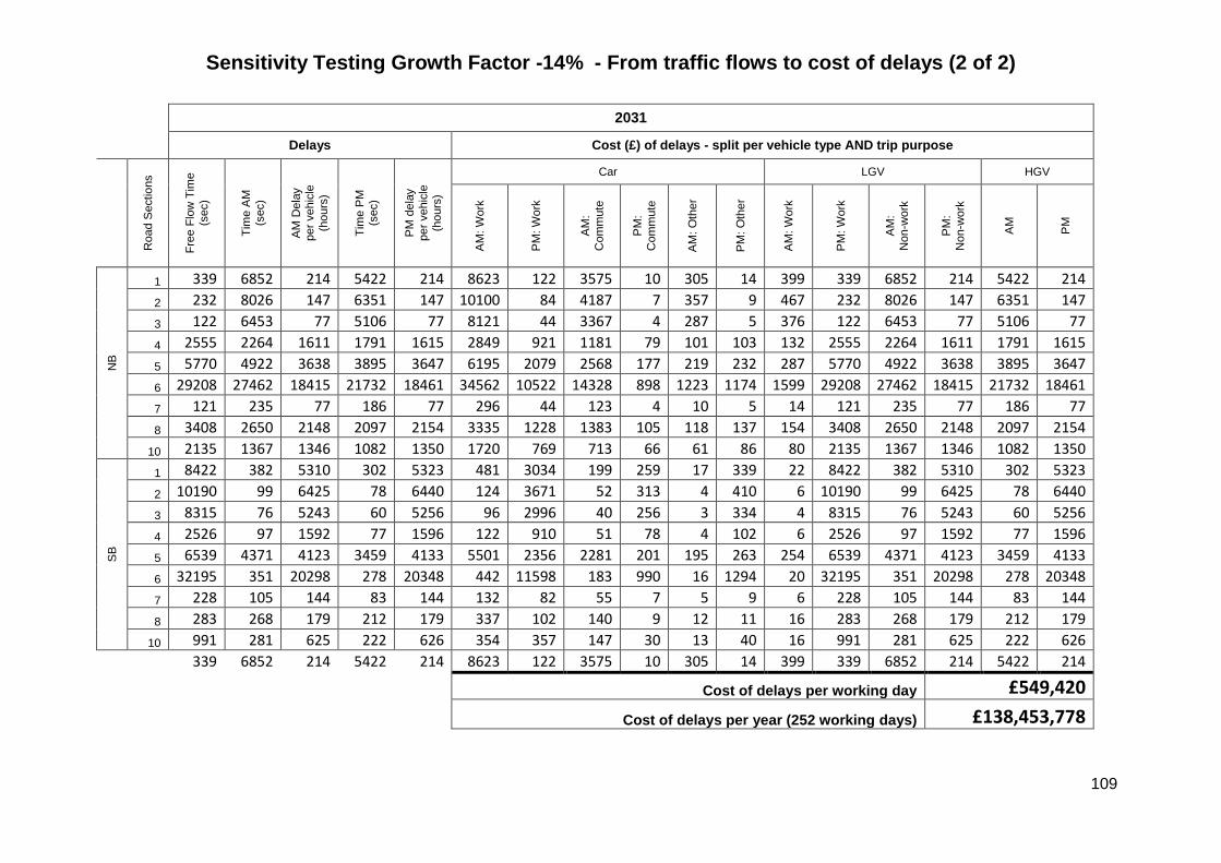
109
Sensitivity Testing Growth Factor -14% - From traffic flows to cost of delays (2 of 2)
2031
Delays Cost (£) of delays - split per vehicle type AND trip purpose
Road S
ectio
ns
Fre
e F
low
Tim
e
(sec)
Tim
e A
M
(sec)
AM
Dela
y
per
vehic
le
(hours
)
Tim
e P
M
(sec)
PM
dela
y
per
vehic
le
(hours
)
Car LGV HGV
AM
: W
ork
PM
: W
ork
AM
:
Com
mute
PM
:
Com
mute
AM
: O
ther
PM
: O
ther
AM
: W
ork
PM
: W
ork
AM
:
Non-w
ork
PM
:
Non-w
ork
AM
PM
NB
1 339 6852 214 5422 214 8623 122 3575 10 305 14 399 339 6852 214 5422 214
2 232 8026 147 6351 147 10100 84 4187 7 357 9 467 232 8026 147 6351 147
3 122 6453 77 5106 77 8121 44 3367 4 287 5 376 122 6453 77 5106 77
4 2555 2264 1611 1791 1615 2849 921 1181 79 101 103 132 2555 2264 1611 1791 1615
5 5770 4922 3638 3895 3647 6195 2079 2568 177 219 232 287 5770 4922 3638 3895 3647
6 29208 27462 18415 21732 18461 34562 10522 14328 898 1223 1174 1599 29208 27462 18415 21732 18461
7 121 235 77 186 77 296 44 123 4 10 5 14 121 235 77 186 77
8 3408 2650 2148 2097 2154 3335 1228 1383 105 118 137 154 3408 2650 2148 2097 2154
10 2135 1367 1346 1082 1350 1720 769 713 66 61 86 80 2135 1367 1346 1082 1350
SB
1 8422 382 5310 302 5323 481 3034 199 259 17 339 22 8422 382 5310 302 5323
2 10190 99 6425 78 6440 124 3671 52 313 4 410 6 10190 99 6425 78 6440
3 8315 76 5243 60 5256 96 2996 40 256 3 334 4 8315 76 5243 60 5256
4 2526 97 1592 77 1596 122 910 51 78 4 102 6 2526 97 1592 77 1596
5 6539 4371 4123 3459 4133 5501 2356 2281 201 195 263 254 6539 4371 4123 3459 4133
6 32195 351 20298 278 20348 442 11598 183 990 16 1294 20 32195 351 20298 278 20348
7 228 105 144 83 144 132 82 55 7 5 9 6 228 105 144 83 144
8 283 268 179 212 179 337 102 140 9 12 11 16 283 268 179 212 179
10 991 281 625 222 626 354 357 147 30 13 40 16 991 281 625 222 626
339 6852 214 5422 214 8623 122 3575 10 305 14 399 339 6852 214 5422 214
Cost of delays per working day £549,420
Cost of delays per year (252 working days) £138,453,778

110
Sensitivity Testing Growth Factor -15% - From traffic flows to cost of delays (1 of 2)
2031
Traffic Volumes Split by vehicle type Traffic volumes - split per vehicle type AND trip purpose
Volume AM (veh) Volume PM (veh) Car LGV HGV
Road
Sectio
ns
All
traffic
Car
LG
V
HG
V
All
traffic
Car
LG
V
HG
V
AM
: W
ork
PM
: W
ork
AM
: C
om
mute
PM
:
Com
mute
AM
: O
ther
PM
: O
ther
AM
: W
ork
PM
: W
ork
AM
: N
on-
work
PM
: N
on-
work
AM
PM
NB
1 2330 3370 2643 1956 313 31 3855 2853 456 46 354 371 900 1164 702 1318 275 402 38 55
2 2490 3469 2823 2089 334 33 3969 2937 470 47 378 382 961 1198 750 1357 294 414 40 56
3 1996 3205 2263 1675 268 27 3667 2713 434 43 303 353 770 1107 601 1254 236 382 32 52
4 2913 3705 3303 2444 391 39 4239 3137 502 50 442 408 1124 1280 877 1449 344 442 47 60
5 3020 3698 3424 2534 405 41 4231 3131 501 50 459 407 1166 1277 910 1446 357 441 49 60
6 3065 4137 3475 2572 411 41 4733 3502 560 56 466 455 1183 1429 923 1618 362 493 49 67
7 3286 3886 3727 2758 441 44 4445 3290 526 53 499 428 1269 1342 990 1520 388 463 53 63
8 4157 4642 4714 3489 558 56 5311 3930 629 63 631 511 1605 1603 1252 1816 491 553 67 75
10 2253 2343 2555 1890 302 30 2680 1983 317 32 342 258 870 809 679 916 266 279 36 38
SB
1 2889 2145 3276 2424 388 39 2453 1815 290 29 439 236 1115 741 870 839 341 256 47 35
2 3063 2379 3474 2571 411 41 2722 2014 322 32 465 262 1183 822 923 931 362 284 49 39
3 2879 2018 3265 2416 387 39 2308 1708 273 27 437 222 1111 697 867 789 340 241 46 33
4 2879 2018 3265 2416 387 39 2308 1708 273 27 437 222 1111 697 867 789 340 241 46 33
5 3420 3282 3878 2870 459 46 3755 2779 445 44 519 361 1320 1134 1030 1284 404 391 55 53
6 3379 2690 3832 2836 454 45 3077 2277 364 36 513 296 1304 929 1018 1052 399 321 54 44
7 3677 3265 4170 3086 494 49 3735 2764 442 44 559 359 1420 1128 1108 1277 435 389 59 53
8 3982 3911 4515 3341 535 53 4475 3311 530 53 605 430 1537 1351 1200 1530 470 466 64 64
10 2322 2289 2633 1949 312 31 2619 1938 310 31 353 252 896 791 700 895 274 273 37 37

111
Sensitivity Testing Growth Factor -15% - From traffic flows to cost of delays (2 of 2)
2031
Delays Cost (£) of delays - split per vehicle type AND trip purpose
Road S
ectio
ns
Fre
e F
low
Tim
e
(sec)
Tim
e A
M
(sec)
AM
Dela
y
per
vehic
le
(hours
)
Tim
e P
M
(sec)
PM
dela
y
per
vehic
le
(hours
)
Car LGV HGV
AM
: W
ork
PM
: W
ork
AM
:
Com
mute
PM
: C
om
mute
AM
: O
ther
PM
: O
ther
AM
: W
ork
PM
: W
ork
AM
:
Non-w
ork
PM
:
Non-w
ork
AM
PM
NB
1 232 307 0.021 1740 0.419 336 6793 212 5375 212 8549 121 3544 10 303 14 395
2 267 315 0.013 1982 0.477 230 7956 145 6296 146 10013 83 4151 7 354 9 463
3 230 262 0.009 1723 0.415 121 6397 76 5062 76 8051 43 3338 4 285 5 372
4 70 523 0.126 523 0.126 2533 2244 1597 1776 1601 2824 912 1171 78 100 102 131
5 153 1140 0.274 1140 0.274 5719 4879 3606 3861 3615 6141 2060 2546 176 217 230 284
6 761 5683 1.367 5683 1.367 28953 27224 18254 21544 18299 34262 10430 14204 890 1213 1164 1585
7 101 120 0.005 146 0.012 120 233 76 185 76 294 43 122 4 10 5 14
8 66 490 0.118 490 0.118 3378 2627 2130 2079 2135 3306 1217 1371 104 117 136 153
10 591 1081 0.136 1024 0.120 2117 1355 1335 1072 1338 1705 763 707 65 60 85 79
SB
1 234 1740 0.418 366 0.037 8348 379 5263 300 5276 477 3007 198 257 17 336 22
2 264 1982 0.477 295 0.009 10101 98 6368 78 6384 123 3639 51 311 4 406 6
3 231 1723 0.414 259 0.008 8243 75 5197 60 5210 95 2970 39 254 3 331 4
4 70 523 0.126 106 0.010 2504 96 1579 76 1582 121 902 50 77 4 101 6
5 152 1140 0.274 1140 0.274 6482 4333 4087 3429 4097 5453 2335 2261 199 193 261 252
6 762 5683 1.367 859 0.027 31913 348 20120 275 20170 438 11497 182 982 16 1283 20
7 102 134 0.009 126 0.007 226 104 142 82 143 130 81 54 7 5 9 6
8 65 102 0.010 116 0.014 281 266 177 210 178 335 101 139 9 12 11 15
10 586 806 0.061 677 0.025 982 279 619 221 621 351 354 145 30 12 39 16
232 307 0.021 1740 0.419 336 6793 212 5375 212 8549 121 3544 10 303 14 395
Cost of delays per working day £544,636
Cost of delays per year (252 working days) £137,248,165

112
Sensitivity Testing Growth Factor -16% - From traffic flows to cost of delays (1 of 2)
2031
Traffic Volumes Split by vehicle type Traffic volumes - split per vehicle type AND trip purpose
Volume AM (veh) Volume PM (veh) Car LGV HGV
Road
Sectio
ns
All
traffic
Car
LG
V
HG
V
All
traffic
Car
LG
V
HG
V
AM
: W
ork
PM
: W
ork
AM
: C
om
mute
PM
:
Com
mute
AM
: O
ther
PM
: O
ther
AM
: W
ork
PM
: W
ork
AM
: N
on-
work
PM
: N
on-
work
AM
PM
NB
1 2330 3370 2619 1938 310 31 3821 2828 452 45 351 368 892 1154 696 1306 273 398 37 54
2 2490 3469 2798 2071 331 33 3934 2911 466 47 375 378 953 1188 743 1345 292 410 40 56
3 1996 3205 2243 1660 266 27 3635 2690 430 43 300 350 764 1097 596 1243 234 379 32 52
4 2913 3705 3274 2423 388 39 4201 3109 497 50 439 404 1114 1269 870 1436 341 438 47 60
5 3020 3698 3394 2511 402 40 4194 3104 497 50 455 403 1155 1266 902 1434 354 437 48 60
6 3065 4137 3445 2549 408 41 4692 3472 555 56 461 451 1173 1416 915 1604 359 489 49 67
7 3286 3886 3694 2733 437 44 4406 3261 522 52 495 424 1257 1330 981 1506 385 459 52 63
8 4157 4642 4673 3458 553 55 5264 3896 623 62 626 506 1591 1589 1241 1800 487 548 66 75
10 2253 2343 2532 1874 300 30 2657 1966 315 31 339 256 862 802 673 908 264 277 36 38
SB
1 2889 2145 3247 2403 384 38 2432 1800 288 29 435 234 1105 734 863 831 338 253 46 35
2 3063 2379 3443 2548 408 41 2698 1996 319 32 461 260 1172 815 915 922 359 281 49 38
3 2879 2018 3236 2395 383 38 2288 1693 271 27 433 220 1102 691 860 782 337 238 46 33
4 2879 2018 3236 2395 383 38 2288 1693 271 27 433 220 1102 691 860 782 337 238 46 33
5 3420 3282 3844 2845 455 46 3722 2754 441 44 515 358 1309 1124 1021 1272 401 388 55 53
6 3379 2690 3798 2811 450 45 3050 2257 361 36 509 293 1293 921 1009 1043 396 318 54 43
7 3677 3265 4133 3059 489 49 3702 2740 438 44 554 356 1407 1118 1098 1266 431 386 59 53
8 3982 3911 4476 3312 530 53 4436 3282 525 53 599 427 1524 1339 1189 1516 466 462 64 63
10 2322 2289 2610 1932 309 31 2596 1921 307 31 350 250 889 784 693 887 272 270 37 37

113
Sensitivity Testing Growth Factor -16% - From traffic flows to cost of delays (2 of 2)
2031
Delays Cost (£) of delays - split per vehicle type AND trip purpose
Road S
ectio
ns
Fre
e F
low
Tim
e
(sec)
Tim
e A
M
(sec)
AM
Dela
y
per
vehic
le
(hours
)
Tim
e P
M
(sec)
PM
dela
y
per
vehic
le
(hours
)
Car LGV HGV
AM
: W
ork
PM
: W
ork
AM
:
Com
mute
PM
: C
om
mute
AM
: O
ther
PM
: O
ther
AM
: W
ork
PM
: W
ork
AM
:
Non-w
ork
PM
:
Non-w
ork
AM
PM
NB
1 232 307 0.021 1740 0.419 333 6733 210 5328 211 8474 120 3513 10 300 13 392
2 267 315 0.013 1982 0.477 228 7887 144 6241 144 9925 82 4115 7 351 9 459
3 230 262 0.009 1723 0.415 120 6341 75 5018 76 7980 43 3308 4 282 5 369
4 70 523 0.126 523 0.126 2510 2225 1583 1760 1587 2800 904 1161 77 99 101 130
5 153 1140 0.274 1140 0.274 5669 4837 3574 3828 3583 6087 2042 2524 174 215 228 282
6 761 5683 1.367 5683 1.367 28698 26986 18093 21355 18138 33963 10338 14080 883 1202 1154 1571
7 101 120 0.005 146 0.012 119 231 75 183 75 291 43 121 4 10 5 13
8 66 490 0.118 490 0.118 3348 2604 2111 2061 2116 3278 1206 1359 103 116 135 152
10 591 1081 0.136 1024 0.120 2098 1343 1323 1063 1326 1690 756 701 65 60 84 78
SB
1 234 1740 0.418 366 0.037 8275 376 5217 297 5230 473 2981 196 254 17 333 22
2 264 1982 0.477 295 0.009 10012 97 6312 77 6328 122 3607 51 308 4 402 6
3 231 1723 0.414 259 0.008 8170 75 5151 59 5164 94 2943 39 251 3 328 4
4 70 523 0.126 106 0.010 2482 95 1565 76 1569 120 894 50 76 4 100 6
5 152 1140 0.274 1140 0.274 6425 4295 4051 3399 4061 5406 2315 2241 198 191 258 250
6 762 5683 1.367 859 0.027 31632 345 19943 273 19993 434 11396 180 973 15 1271 20
7 102 134 0.009 126 0.007 224 103 141 81 141 129 81 54 7 5 9 6
8 65 102 0.010 116 0.014 278 264 176 209 176 332 100 137 9 12 11 15
10 586 806 0.061 677 0.025 974 276 614 219 615 348 351 144 30 12 39 16
232 307 0.021 1740 0.419 333 6733 210 5328 211 8474 120 3513 10 300 13 392
Cost of delays per working day £539,851
Cost of delays per year (252 working days) £136,042,552

114
Sensitivity Testing Growth Factor -17% - From traffic flows to cost of delays (1 of 2)
2031
Traffic Volumes Split by vehicle type Traffic volumes - split per vehicle type AND trip purpose
Volume AM (veh) Volume PM (veh) Car LGV HGV
Road
Sectio
ns
All
traffic
Car
LG
V
HG
V
All
traffic
Car
LG
V
HG
V
AM
: W
ork
PM
: W
ork
AM
: C
om
mute
PM
:
Com
mute
AM
: O
ther
PM
: O
ther
AM
: W
ork
PM
: W
ork
AM
: N
on-
work
PM
: N
on-
work
AM
PM
NB
1 2330 3370 2596 1921 307 31 3788 2803 448 45 348 364 884 1144 690 1295 270 395 37 54
2 2490 3469 2774 2052 328 33 3899 2886 462 46 371 375 944 1177 737 1333 289 406 39 55
3 1996 3205 2223 1645 263 26 3603 2666 427 43 298 347 757 1088 591 1232 232 375 32 51
4 2913 3705 3245 2401 384 38 4164 3082 493 49 435 401 1105 1257 862 1424 338 434 46 59
5 3020 3698 3364 2489 398 40 4157 3076 492 49 451 400 1145 1255 894 1421 350 433 48 59
6 3065 4137 3414 2526 404 40 4650 3441 551 55 457 447 1162 1404 907 1590 356 485 49 66
7 3286 3886 3661 2709 433 43 4368 3232 517 52 490 420 1246 1319 973 1493 381 455 52 62
8 4157 4642 4631 3427 548 55 5218 3861 618 62 620 502 1576 1575 1230 1784 483 544 66 74
10 2253 2343 2509 1857 297 30 2633 1949 312 31 336 253 854 795 667 900 261 274 36 37
SB
1 2889 2145 3218 2381 381 38 2410 1784 285 29 431 232 1095 728 855 824 335 251 46 34
2 3063 2379 3413 2525 404 40 2674 1979 317 32 457 257 1162 807 907 914 356 279 48 38
3 2879 2018 3208 2374 380 38 2268 1678 269 27 430 218 1092 685 852 775 334 236 46 32
4 2879 2018 3208 2374 380 38 2268 1678 269 27 430 218 1092 685 852 775 334 236 46 32
5 3420 3282 3810 2819 451 45 3689 2730 437 44 510 355 1297 1114 1012 1261 397 384 54 52
6 3379 2690 3764 2786 446 45 3023 2237 358 36 504 291 1281 913 1000 1034 392 315 53 43
7 3677 3265 4097 3032 485 49 3670 2716 434 43 549 353 1395 1108 1088 1255 427 382 58 52
8 3982 3911 4436 3283 525 53 4396 3253 521 52 594 423 1510 1327 1178 1503 462 458 63 62
10 2322 2289 2587 1914 306 31 2573 1904 305 30 347 248 881 777 687 880 270 268 37 37

115
Sensitivity Testing Growth Factor -17% - From traffic flows to cost of delays (2 of 2)
2031
Delays Cost (£) of delays - split per vehicle type AND trip purpose
Road S
ectio
ns
Fre
e F
low
Tim
e
(sec)
Tim
e A
M
(sec)
AM
Dela
y
per
vehic
le
(hours
)
Tim
e P
M
(sec)
PM
dela
y
per
vehic
le
(hours
)
Car LGV HGV
AM
: W
ork
PM
: W
ork
AM
:
Com
mute
PM
:
Com
mute
AM
: O
ther
PM
: O
ther
AM
: W
ork
PM
: W
ork
AM
:
Non-w
ork
PM
:
Non-w
ork
AM
PM
NB
1 330 6674 208 5281 209 8399 119 3482 10 297 13 389 330 6674 208 5281 209
2 226 7817 143 6186 143 9838 82 4079 7 348 9 455 226 7817 143 6186 143
3 119 6285 75 4974 75 7910 43 3279 4 280 5 366 119 6285 75 4974 75
4 2488 2205 1569 1745 1573 2775 896 1150 77 98 100 128 2488 2205 1569 1745 1573
5 5618 4794 3542 3794 3551 6034 2024 2501 173 214 226 279 5618 4794 3542 3794 3551
6 28442 26748 17932 21167 17977 33663 10246 13956 875 1191 1143 1557 28442 26748 17932 21167 17977
7 118 229 75 181 75 288 43 120 4 10 5 13 118 229 75 181 75
8 3318 2581 2092 2043 2097 3249 1195 1347 102 115 133 150 3318 2581 2092 2043 2097
10 2079 1331 1311 1053 1314 1675 749 695 64 59 84 77 2079 1331 1311 1053 1314
SB
1 8201 372 5170 295 5183 468 2954 194 252 17 330 22 8201 372 5170 295 5183
2 9923 96 6256 76 6272 121 3575 50 305 4 399 6 9923 96 6256 76 6272
3 8097 74 5105 59 5118 93 2917 39 249 3 325 4 8097 74 5105 59 5118
4 2460 95 1551 75 1555 119 886 49 76 4 99 6 2460 95 1551 75 1555
5 6368 4257 4015 3369 4025 5358 2294 2221 196 190 256 248 6368 4257 4015 3369 4025
6 31350 342 19766 271 19815 430 11294 178 964 15 1260 20 31350 342 19766 271 19815
7 222 102 140 81 140 128 80 53 7 5 9 6 222 102 140 81 140
8 276 261 174 207 174 329 99 136 8 12 11 15 276 261 174 207 174
10 965 274 608 217 610 345 348 143 30 12 39 16 965 274 608 217 610
330 6674 208 5281 209 8399 119 3482 10 297 13 389 330 6674 208 5281 209
Cost of delays per working day £535,067
Cost of delays per year (252 working days) £134,836,939

116
Sensitivity Testing Growth Factor -18% - From traffic flows to cost of delays (1 of 2)
2031
Traffic Volumes Split by vehicle type Traffic volumes - split per vehicle type AND trip purpose
Volume AM (veh) Volume PM (veh) Car LGV HGV
Road
Sectio
ns
All
traffic
Car
LG
V
HG
V
All
traffic
Car
LG
V
HG
V
AM
: W
ork
PM
: W
ork
AM
: C
om
mute
PM
:
Com
mute
AM
: O
ther
PM
: O
ther
AM
: W
ork
PM
: W
ork
AM
: N
on-
work
PM
: N
on-
work
AM
PM
NB
1 2330 3370 2573 1904 305 30 3754 2778 444 44 345 361 876 1133 683 1283 268 391 37 53
2 2490 3469 2749 2034 325 33 3865 2860 458 46 368 372 936 1167 730 1321 286 403 39 55
3 1996 3205 2203 1630 261 26 3570 2642 423 42 295 343 750 1078 585 1221 230 372 31 51
4 2913 3705 3216 2380 381 38 4127 3054 489 49 431 397 1095 1246 854 1411 335 430 46 59
5 3020 3698 3334 2467 395 39 4120 3049 488 49 446 396 1135 1244 886 1409 347 429 47 59
6 3065 4137 3384 2504 401 40 4609 3411 546 55 453 443 1152 1392 899 1576 353 480 48 65
7 3286 3886 3628 2685 430 43 4329 3203 513 51 486 416 1235 1307 964 1480 378 451 52 62
8 4157 4642 4590 3396 543 54 5171 3827 612 61 615 497 1562 1561 1219 1768 478 539 65 73
10 2253 2343 2487 1840 294 29 2610 1931 309 31 333 251 847 788 661 892 259 272 35 37
SB
1 2889 2145 3189 2360 378 38 2389 1768 283 28 427 230 1086 721 847 817 332 249 45 34
2 3063 2379 3382 2503 400 40 2650 1961 314 31 453 255 1151 800 898 906 352 276 48 38
3 2879 2018 3179 2352 376 38 2248 1663 266 27 426 216 1082 679 844 768 331 234 45 32
4 2879 2018 3179 2352 376 38 2248 1663 266 27 426 216 1082 679 844 768 331 234 45 32
5 3420 3282 3776 2794 447 45 3656 2706 433 43 506 352 1285 1104 1003 1250 393 381 54 52
6 3379 2690 3730 2761 442 44 2997 2217 355 35 500 288 1270 905 991 1024 389 312 53 43
7 3677 3265 4060 3004 481 48 3637 2691 431 43 544 350 1382 1098 1079 1243 423 379 58 52
8 3982 3911 4396 3253 520 52 4357 3224 516 52 589 419 1496 1316 1168 1490 458 454 62 62
10 2322 2289 2564 1897 304 30 2550 1887 302 30 343 245 873 770 681 872 267 266 36 36

117
Sensitivity Testing Growth Factor -18% - From traffic flows to cost of delays (2 of 2)
2031
Delays Cost (£) of delays - split per vehicle type AND trip purpose
Road S
ectio
ns
Fre
e F
low
Tim
e
(sec)
Tim
e A
M
(sec)
AM
Dela
y
per
vehic
le
(hours
)
Tim
e P
M
(sec)
PM
dela
y
per
vehic
le
(hours
)
Car LGV HGV
AM
: W
ork
PM
: W
ork
AM
:
Com
mute
PM
: C
om
mute
AM
: O
ther
PM
: O
ther
AM
: W
ork
PM
: W
ork
AM
:
Non-w
ork
PM
:
Non-w
ork
AM
PM
NB
1 232 307 0.021 1740 0.419 327 6614 206 5234 207 8324 118 3451 10 295 13 385
2 267 315 0.013 1982 0.477 224 7747 141 6131 142 9750 81 4042 7 345 9 451
3 230 262 0.009 1723 0.415 117 6229 74 4929 74 7839 42 3250 4 277 5 363
4 70 523 0.126 523 0.126 2466 2185 1555 1729 1559 2750 888 1140 76 97 99 127
5 153 1140 0.274 1140 0.274 5568 4752 3510 3760 3519 5980 2006 2479 171 212 224 277
6 761 5683 1.367 5683 1.367 28187 26510 17771 20979 17815 33364 10155 13832 867 1181 1133 1543
7 101 120 0.005 146 0.012 117 227 74 180 74 286 42 119 4 10 5 13
8 66 490 0.118 490 0.118 3288 2558 2073 2025 2078 3220 1185 1335 101 114 132 149
10 591 1081 0.136 1024 0.120 2061 1319 1299 1044 1303 1660 742 688 63 59 83 77
SB
1 234 1740 0.418 366 0.037 8127 369 5124 292 5137 464 2928 192 250 16 327 21
2 264 1982 0.477 295 0.009 9834 95 6200 76 6215 120 3543 50 302 4 395 6
3 231 1723 0.414 259 0.008 8025 73 5059 58 5072 92 2891 38 247 3 323 4
4 70 523 0.126 106 0.010 2438 94 1537 74 1541 118 878 49 75 4 98 5
5 152 1140 0.274 1140 0.274 6311 4220 3979 3339 3989 5310 2273 2202 194 188 254 246
6 762 5683 1.367 859 0.027 31069 339 19588 268 19637 427 11193 177 956 15 1249 20
7 102 134 0.009 126 0.007 220 101 139 80 139 127 79 53 7 4 9 6
8 65 102 0.010 116 0.014 273 259 172 205 173 326 99 135 8 12 11 15
10 586 806 0.061 677 0.025 956 271 603 215 604 342 345 142 29 12 38 16
232 307 0.021 1740 0.419 327 6614 206 5234 207 8324 118 3451 10 295 13 385
Cost of delays per working day £530,283
Cost of delays per year (252 working days) £133,631,326

118
Sensitivity Testing Growth Factor -19% - From traffic flows to cost of delays (1 of 2)
2031
Traffic Volumes Split by vehicle type Traffic volumes - split per vehicle type AND trip purpose
Volume AM (veh) Volume PM (veh) Car LGV HGV
Road
Sectio
ns
All
traffic
Car
LG
V
HG
V
All
traffic
Car
LG
V
HG
V
AM
: W
ork
PM
: W
ork
AM
: C
om
mute
PM
:
Com
mute
AM
: O
ther
PM
: O
ther
AM
: W
ork
PM
: W
ork
AM
: N
on-
work
PM
: N
on-
work
AM
PM
NB
1 2330 3370 2549 1887 302 30 3720 2753 440 44 341 358 868 1123 677 1272 266 388 36 53
2 2490 3469 2724 2016 322 32 3830 2834 453 45 365 368 927 1156 724 1309 284 399 39 54
3 1996 3205 2183 1616 259 26 3538 2618 419 42 292 340 743 1068 580 1210 227 369 31 50
4 2913 3705 3187 2358 377 38 4090 3027 484 48 427 393 1085 1235 847 1398 332 426 45 58
5 3020 3698 3303 2444 391 39 4083 3021 483 48 442 393 1124 1233 878 1396 344 425 47 58
6 3065 4137 3353 2481 397 40 4567 3380 541 54 449 439 1141 1379 891 1562 349 476 48 65
7 3286 3886 3595 2660 426 43 4290 3175 508 51 482 413 1224 1295 955 1467 375 447 51 61
8 4157 4642 4548 3366 538 54 5125 3792 607 61 609 493 1548 1547 1208 1752 474 534 65 73
10 2253 2343 2464 1824 292 29 2587 1914 306 31 330 249 839 781 655 884 257 270 35 37
SB
1 2889 2145 3160 2338 374 37 2368 1752 280 28 423 228 1076 715 840 809 329 247 45 34
2 3063 2379 3351 2480 397 40 2627 1944 311 31 449 253 1141 793 890 898 349 274 48 37
3 2879 2018 3150 2331 373 37 2228 1648 264 26 422 214 1072 673 837 762 328 232 45 32
4 2879 2018 3150 2331 373 37 2228 1648 264 26 422 214 1072 673 837 762 328 232 45 32
5 3420 3282 3742 2769 443 44 3624 2681 429 43 501 349 1274 1094 994 1239 390 378 53 51
6 3379 2690 3697 2736 438 44 2970 2198 352 35 495 286 1258 897 982 1015 385 309 53 42
7 3677 3265 4023 2977 476 48 3604 2667 427 43 539 347 1369 1088 1069 1232 419 376 57 51
8 3982 3911 4356 3224 516 52 4318 3195 511 51 583 415 1483 1304 1157 1476 454 450 62 61
10 2322 2289 2541 1880 301 30 2527 1870 299 30 340 243 865 763 675 864 265 263 36 36

119
Sensitivity Testing Growth Factor -19% - From traffic flows to cost of delays (2 of 2)
2031
Delays Cost (£) of delays - split per vehicle type AND trip purpose
Road S
ectio
ns
Fre
e F
low
Tim
e
(sec)
Tim
e A
M
(sec)
AM
Dela
y
per
vehic
le
(hours
)
Tim
e P
M
(sec)
PM
dela
y
per
vehic
le
(hours
)
Car LGV HGV
AM
: W
ork
PM
: W
ork
AM
: C
om
mu
te
PM
: C
om
mu
te
AM
: O
ther
PM
: O
ther
AM
: W
ork
PM
: W
ork
AM
:
Non-w
ork
PM
:
Non-w
ork
AM
PM
NB
1 232 307 0.021 1740 0.419 324 6555 204 5187 205 8250 117 3420 10 292 13 382
2 267 315 0.013 1982 0.477 222 7678 140 6076 141 9663 80 4006 7 342 9 447
3 230 262 0.009 1723 0.415 116 6173 73 4885 74 7769 42 3221 4 275 5 359
4 70 523 0.126 523 0.126 2443 2166 1541 1714 1544 2726 880 1130 75 96 98 126
5 153 1140 0.274 1140 0.274 5517 4709 3479 3726 3487 5926 1988 2457 170 210 222 274
6 761 5683 1.367 5683 1.367 27932 26272 17610 20790 17654 33064 10063 13708 859 1170 1123 1529
7 101 120 0.005 146 0.012 116 225 73 178 73 283 42 117 4 10 5 13
8 66 490 0.118 490 0.118 3259 2535 2054 2006 2060 3191 1174 1323 100 113 131 148
10 591 1081 0.136 1024 0.120 2042 1308 1288 1035 1291 1646 736 682 63 58 82 76
SB
1 234 1740 0.418 366 0.037 8054 366 5078 289 5090 460 2901 191 248 16 324 21
2 264 1982 0.477 295 0.009 9745 95 6144 75 6159 119 3511 49 300 4 392 6
3 231 1723 0.414 259 0.008 7952 73 5014 58 5026 92 2865 38 245 3 320 4
4 70 523 0.126 106 0.010 2415 93 1523 74 1527 117 870 48 74 4 97 5
5 152 1140 0.274 1140 0.274 6253 4182 3943 3309 3952 5263 2253 2182 192 186 251 243
6 762 5683 1.367 859 0.027 30787 336 19411 266 19459 423 11091 175 947 15 1238 20
7 102 134 0.009 126 0.007 218 100 137 79 138 126 78 52 7 4 9 6
8 65 102 0.010 116 0.014 271 257 171 203 171 323 98 134 8 11 11 15
10 586 806 0.061 677 0.025 948 269 597 213 599 338 341 140 29 12 38 16 232 307 0.021 1740 0.419 324 6555 204 5187 205 8250 117 3420 10 292 13 382
Cost of delays per working day £525,499
Cost of delays per year (252 working days) £132,425,714

120
Sensitivity Testing Growth Factor -20% - From traffic flows to cost of delays (1 of 2)
2031
Traffic Volumes Split by vehicle type Traffic volumes - split per vehicle type AND trip purpose
Volume AM (veh) Volume PM (veh) Car LGV HGV
Road
Sectio
ns
All
traffic
Car
LG
V
HG
V
All
traffic
Car
LG
V
HG
V
AM
: W
ork
PM
: W
ork
AM
: C
om
mute
PM
:
Com
mute
AM
: O
ther
PM
: O
ther
AM
: W
ork
PM
: W
ork
AM
: N
on-
work
PM
: N
on-
work
AM
PM
NB
1 2330 3370 2526 1869 299 30 3687 2728 436 44 338 355 860 1113 671 1260 263 384 36 52
2 2490 3469 2699 1997 320 32 3795 2809 449 45 361 365 919 1146 717 1298 281 395 38 54
3 1996 3205 2163 1601 256 26 3506 2595 415 42 290 337 736 1059 575 1199 225 365 31 50
4 2913 3705 3157 2336 374 37 4053 2999 480 48 423 390 1075 1224 839 1386 329 422 45 58
5 3020 3698 3273 2422 388 39 4046 2994 479 48 438 389 1114 1222 870 1383 341 422 47 57
6 3065 4137 3322 2458 393 39 4526 3349 536 54 445 435 1131 1367 883 1547 346 472 47 64
7 3286 3886 3562 2636 422 42 4251 3146 503 50 477 409 1213 1283 946 1453 371 443 51 60
8 4157 4642 4506 3335 534 53 5079 3758 601 60 604 489 1534 1533 1197 1736 470 529 64 72
10 2253 2343 2442 1807 289 29 2563 1897 303 30 327 247 831 774 649 876 254 267 35 36
SB
1 2889 2145 3131 2317 371 37 2346 1736 278 28 419 226 1066 708 832 802 326 244 44 33
2 3063 2379 3321 2457 393 39 2603 1926 308 31 445 250 1130 786 882 890 346 271 47 37
3 2879 2018 3121 2310 370 37 2207 1633 261 26 418 212 1062 666 829 755 325 230 44 31
4 2879 2018 3121 2310 370 37 2207 1633 261 26 418 212 1062 666 829 755 325 230 44 31
5 3420 3282 3707 2743 439 44 3591 2657 425 43 497 345 1262 1084 985 1228 386 374 53 51
6 3379 2690 3663 2711 434 43 2943 2178 348 35 491 283 1247 888 973 1006 382 307 52 42
7 3677 3265 3986 2950 472 47 3572 2643 423 42 534 344 1357 1078 1059 1221 415 372 57 51
8 3982 3911 4316 3194 511 51 4279 3167 507 51 578 412 1469 1292 1147 1463 450 446 61 61
10 2322 2289 2517 1863 298 30 2504 1853 297 30 337 241 857 756 669 856 262 261 36 36

121
Sensitivity Testing Growth Factor -20% - From traffic flows to cost of delays (2 of 2)
2031
Delays Cost (£) of delays - split per vehicle type AND trip purpose
Road S
ectio
ns
Fre
e F
low
Tim
e
(sec)
Tim
e A
M
(sec)
AM
Dela
y
per
vehic
le
(hours
)
Tim
e P
M
(sec)
PM
dela
y
per
vehic
le
(hours
)
Car LGV HGV
AM
: W
ork
PM
: W
ork
AM
:
Com
mute
PM
: C
om
mute
AM
: O
ther
PM
: O
ther
AM
: W
ork
PM
: W
ork
AM
:
Non-w
ork
PM
:
Non-w
ork
AM
PM
NB
1 232 307 0.021 1740 0.419 321 6496 203 5140 203 8175 116 3389 10 289 13 378
2 267 315 0.013 1982 0.477 220 7608 139 6021 139 9575 79 3970 7 339 9 443
3 230 262 0.009 1723 0.415 115 6117 73 4841 73 7699 42 3192 4 272 5 356
4 70 523 0.126 523 0.126 2421 2146 1526 1698 1530 2701 872 1120 74 96 97 125
5 153 1140 0.274 1140 0.274 5467 4666 3447 3693 3455 5873 1970 2435 168 208 220 272
6 761 5683 1.367 5683 1.367 27676 26034 17449 20602 17493 32765 9971 13583 851 1160 1112 1516
7 101 120 0.005 146 0.012 115 223 73 177 73 281 41 116 4 10 5 13
8 66 490 0.118 490 0.118 3229 2512 2036 1988 2041 3162 1163 1311 99 112 130 146
10 591 1081 0.136 1024 0.120 2023 1296 1276 1025 1279 1631 729 676 62 58 81 75
SB
1 234 1740 0.418 366 0.037 7980 362 5031 287 5044 456 2875 189 245 16 321 21
2 264 1982 0.477 295 0.009 9656 94 6088 74 6103 118 3478 49 297 4 388 5
3 231 1723 0.414 259 0.008 7879 72 4968 57 4980 91 2839 38 242 3 317 4
4 70 523 0.126 106 0.010 2393 92 1509 73 1513 116 862 48 74 4 96 5
5 152 1140 0.274 1140 0.274 6196 4144 3907 3279 3916 5215 2232 2162 191 185 249 241
6 762 5683 1.367 859 0.027 30506 333 19233 263 19281 419 10990 174 938 15 1226 19
7 102 134 0.009 126 0.007 216 99 136 78 136 125 78 52 7 4 9 6
8 65 102 0.010 116 0.014 268 254 169 201 170 320 97 133 8 11 11 15
10 586 806 0.061 677 0.025 939 267 592 211 593 335 338 139 29 12 38 16
232 307 0.021 1740 0.419 321 6496 203 5140 203 8175 116 3389 10 289 13 378
Cost of delays per working day £520,715
Cost of delays per year (252 working days) £131,220,101