PDF Pre-Calculus - Detroit Public Schools Community District

Pre-Calculus

Mathematics

Printed math problems in this packet come from the CPM Educational Program. Open eBook access is available at http://open-ebooks.cpm.org/.

© 2009, 2014 CPM Educational Program. All rights reserved.

Letter to Families from the DPSCD Office of Mathematics

Dear DPSCD Families,

The Office of Mathematics is partnering with families to support Distance Learning while

students are home. We empower you to utilize the resources provided to foster a

deeper understanding of grade-level mathematics.

In this packet, you will find links to videos, links to online practice, and pencil-and-paper

practice problems. The Table of Contents shows day-by-day lessons from April 14th to

June 19th. We encourage you to take every advantage of the material in this packet.

Daily lesson guidance can be found in the table of contents below. Each day has been

designed to provide you access to materials from Khan Academy and the academic

packet. Each lesson has this structure:

Watch: Khan Academy (if

internet access is available)

Practice: Khan Academy (if

internet access is available)

Pencil & Paper Practice:

Academic Packet

Watch and take notes on

the lesson video on Khan

Academy

Complete the practice

exercises on Khan Academy

Complete the pencil and

paper practice.

If one-on-one, live support is required, please feel free to call the Homework Hotline at

1-833-466-3978. Please check the Homework Hotline page for operating hours. We

have DPSCD mathematics teachers standing by and are ready to assist.

We appreciate your continued dedication, support and partnership with Detroit Public

Schools Community District and with your assistance we can press forward with our

priority: Outstanding Achievement. Be safe. Be well!

Tony R. Hawk

Deputy Executive Director of K-12 Mathematics

http://open-ebooks.cpm.org/

https://www.detroitk12.org/Page/9660#calendar16189/20200402/month



Important Links and Information

Clever

Students access Clever by visiting www.clever.com/in/dpscd.

What are my username and password for Clever?

Students access Clever using their DPSCD login credentials. Usernames and

passwords follow this structure:

Username: [email protected]

Ex. If Aretha Franklin is a DPSCD student with a student ID of 018765 her

username would be [email protected].

Password:

First letter of first name in upper case

First letter of last name in lower case

2-digit month of birth

2-digit year of birth

01 (male) or 02 (female)

For example: If Aretha Franklin’s birthday is March 25, 1998, her password and

password would be Af039802.

Accessing Khan Academy

To access Khan Academy, visit www.clever.com/in/dpscd. Once logged into

Clever, select the Khan Academy button:


https://clever.com/in/dpscd

mailto:[email protected]




Accessing Your CPM eBook

Students can access their CPM eBook in two ways:

Option 1: Access the eBook through Clever

1. Visit www.clever.com/in/dpscd. Login using your DPSCD credentials

above.

2. Click on the CPM icon:

Option 2: Visit http://open-ebooks.cpm.org/

1. Visit the website listed above.

2. Click “I agree”

3. Select the CPM Precalculus eBook:

Desmos Online Graphing Calculator

Access to a free online graphing and scientific calculator can be found at

https://www.desmos.com/calculator.




https://www.desmos.com/calculator



Table of Contents

In the following table, you will find the table of contents and schedule for the

week of April 13, 2020 through the week of June 15, 2020.

Week Date

Topic Watch

(10 minutes)

Online Practice

(10 minutes)

Pencil &

Paper

Practice

(25

minutes

Week 1

04/13-

04/17

5 Days

Day 1 Holiday N/A N/A N/A

Day 2

Lesson

3.1.1:

Operations

with

Rational

Expressions

Video: Adding

Rational Exp.

Video: Subtracting

Rational Exp.

Practice: Adding and

Subtracting Rational

Expressions

Problems

1 - 8

Day 3

Lesson

3.1.2:

Rewriting

Expressions

and

Equations

Video: Rewriting

Expressions

Practice: Rewriting

Expressions

Problems

1-6

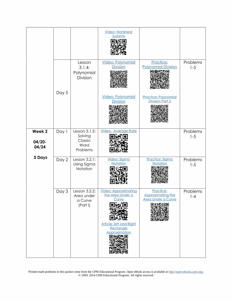
Day 5

Lesson

3.1.3:

Solving

Nonlinear

Systems of

Equations

Video: Nonlinear

Systems

Practice: Nonlinear

Systems

Problems

1-3


https://youtu.be/DrE_iiw1Mvk

https://youtu.be/DrE_iiw1Mvk

https://youtu.be/evmDZkDvlNw

https://youtu.be/evmDZkDvlNw

https://www.khanacademy.org/math/algebra2/x2ec2f6f830c9fb89:rational/x2ec2f6f830c9fb89:rational-add-sub-intro/e/adding_and_subtracting_rational_expressions_2?modal=1



https://youtu.be/lX0I-Yb0m-E

https://youtu.be/lX0I-Yb0m-E

https://www.khanacademy.org/math/algebra2/x2ec2f6f830c9fb89:rational/x2ec2f6f830c9fb89:cancel-common-factor/v/simplifying-rational-expressions-introduction

https://www.khanacademy.org/math/algebra2/x2ec2f6f830c9fb89:rational/x2ec2f6f830c9fb89:cancel-common-factor/v/simplifying-rational-expressions-introduction

https://youtu.be/Cy1Pxz_wLfA

https://youtu.be/Cy1Pxz_wLfA

https://www.khanacademy.org/math/algebra2/x2ec2f6f830c9fb89:eq/x2ec2f6f830c9fb89:quad-sys/e/quadratic-systems

https://www.khanacademy.org/math/algebra2/x2ec2f6f830c9fb89:eq/x2ec2f6f830c9fb89:quad-sys/e/quadratic-systems



Video: Nonlinear

Systems

Day 5

Lesson

3.1.4:

Polynomial

Division

Video: Polynomial

Division

Video: Polynomial

Division

Practice:

Polynomial Division

Practice: Polynomial

Division Part 2

Problems

1-5

Week 2

04/20-

04/24

5 Days

Day 1 Lesson 3.1.5:

Solving

Classic

Word

Problems

Video: Average Rate

Problems

1-5

Day 2 Lesson 3.2.1:

Using Sigma

Notation

Video: Sigma

Notation

Practice: Sigma

Notation

Problems

1-5

Day 3 Lesson 3.2.2:

Area under

a Curve

(Part I)

Video: Approximating

the Area Under a

Curve

Article: left and Right

Rectangle

Approximation

Practice:

Approximating the

Area Under a Curve

Problems

1-4


https://youtu.be/swFohliPgmQ

https://youtu.be/swFohliPgmQ

https://www.khanacademy.org/math/precalculus/x9e81a4f98389efdf:polynomials/x9e81a4f98389efdf:polynomial-division/v/dividing-polynomials-with-remainders-example?modal=1

https://www.khanacademy.org/math/precalculus/x9e81a4f98389efdf:polynomials/x9e81a4f98389efdf:polynomial-division/v/dividing-polynomials-with-remainders-example?modal=1

https://www.khanacademy.org/math/precalculus/x9e81a4f98389efdf:polynomials/x9e81a4f98389efdf:polynomial-division/v/dividing-polynomials-with-remainders?modal=1

https://www.khanacademy.org/math/precalculus/x9e81a4f98389efdf:polynomials/x9e81a4f98389efdf:polynomial-division/v/dividing-polynomials-with-remainders?modal=1

https://www.khanacademy.org/math/precalculus/x9e81a4f98389efdf:polynomials/x9e81a4f98389efdf:polynomial-division/e/divide-polynomials-by-monomials?modal=1

https://www.khanacademy.org/math/precalculus/x9e81a4f98389efdf:polynomials/x9e81a4f98389efdf:polynomial-division/e/divide-polynomials-by-monomials?modal=1

https://www.khanacademy.org/math/precalculus/x9e81a4f98389efdf:polynomials/x9e81a4f98389efdf:polynomial-division/e/dividing-polynomials-with-remainders?modal=1

https://www.khanacademy.org/math/precalculus/x9e81a4f98389efdf:polynomials/x9e81a4f98389efdf:polynomial-division/e/dividing-polynomials-with-remainders?modal=1

https://youtu.be/Uc2Tm4Lr7uI

https://youtu.be/Uc2Tm4Lr7uI

https://youtu.be/5jwXThH6fg4

https://youtu.be/5jwXThH6fg4

https://www.khanacademy.org/math/precalculus/x9e81a4f98389efdf:series/x9e81a4f98389efdf:geo-series-notation/e/evaluating-basic-sigma-notation

https://www.khanacademy.org/math/precalculus/x9e81a4f98389efdf:series/x9e81a4f98389efdf:geo-series-notation/e/evaluating-basic-sigma-notation

https://youtu.be/dEAk0BHBYCM




https://www.khanacademy.org/math/ap-calculus-ab/ab-integration-new/ab-6-2/a/left-and-right-riemann-sums




https://www.khanacademy.org/math/ap-calculus-ab/ab-integration-new/ab-6-2/e/using-rectangles-to-approximate-area-under-a-curve






Day 4 Lesson 3.2.3:

Area under

a Curve

(Part II)

Video:

Approximating the

Area Under a Curve

(Part II)

Problems

1 - 4

Day 5 Lesson 3.2.4:

Area under

a Curve

(Part III)

Video:

Approximating the

Area Under the

Curve (Part III)

Practice:

Approximating Area

Under the Curve

(Part III)

Problems

9-11

Week 3

04/27-

05/01

5 Days

Day 1 Lesson

3.2.Extra U-

Substitution

Video: Factoring Using

U-Substitution

Practice: Factoring

Using U-Substitution

Problems

1-18

Day 2 Lesson 4.1.1:

Graphs of

Polynomials

in Factored

Form

Video: Polynomial

Graphs in Factored

Form

Practice: Graphs of

Polynomials in

Factored Form

Problems

1-11

Day 3 Lesson

4.1.2:

Writing

Equations

of

Polynomial

Functions

Video: Roots of a

Polynomial

Video: Matching

Roots with the

Function

Practice: Roots of a

Polynomial

Problems

1-8


https://youtu.be/OaCVdzr3MjM




https://youtu.be/XmI80eJZAWM




https://www.khanacademy.org/math/ap-calculus-ab/ab-integration-new/ab-6-2/e/over-and-under-estimation-of-riemann-sums




https://youtu.be/Fr7jbWh8Ac4

https://youtu.be/Fr7jbWh8Ac4

http://www.personal.kent.edu/~bosikiew/Algebra-handouts/quadtype-Fact.pdf

http://www.personal.kent.edu/~bosikiew/Algebra-handouts/quadtype-Fact.pdf

https://youtu.be/f-xluUaAfwo



https://www.khanacademy.org/math/algebra2/x2ec2f6f830c9fb89:poly-graphs/x2ec2f6f830c9fb89:poly-zeros/e/using-zeros-to-graph-polynomials?modal=1



https://youtu.be/EtzwLlkoAnM

https://youtu.be/EtzwLlkoAnM

https://youtu.be/CtqwiX4wHEY



https://www.khanacademy.org/math/algebra2/x2ec2f6f830c9fb89:poly-graphs/x2ec2f6f830c9fb89:poly-zeros/e/using-zeros-to-graph-polynomials

https://www.khanacademy.org/math/algebra2/x2ec2f6f830c9fb89:poly-graphs/x2ec2f6f830c9fb89:poly-zeros/e/using-zeros-to-graph-polynomials



Day 4 Lesson 4.1.3:

Identifying

and Using

Roots of

Polynomials

Video: Identifying

Roots

Practice:

Identifying Roots

Problems

1-3, 14, 15

Day 5 Lesson 4.2.1:

Graphing

Transformations

of 𝑦 =1

𝑥

Video: Graphing

Transformations

Practice: Graphing

Transformations

Problems

1-5

Week 4

05/04-

05/08

5 Days

Day 1 Lesson

4.2.2:

Graphing

Rational

Functions

Video: Graphing

Rational Functions

Practice: Graphing

Rational Functions

Problems

6-11

Day 2 Lesson

4.2.3:

Graphing

Reciprocal

Functions

Video: Polynomial End

Behavior


End Behavior

Problems

1-5

Day 3 Lesson

4.3.1:

Polynomial

and

Rational

Inequalities

Video: Polynomial

and Rational

Inequalities


and Rational

Inequalities

Problems

1-7

Day 4 Lesson 4.3.2:

Applications

of

Polynomial

and

Rational

Functions

Video: Horizontal

Asymptotes

Video: Vertical

Asymptotes

Practice: Horizontal

and Vertical

Asymptotes

Problems

1-5


https://youtu.be/x9lb_frpkH0

https://youtu.be/x9lb_frpkH0

https://www.khanacademy.org/math/algebra-home/alg-polynomials/alg-finding-zeros-of-polynomials/e/find-the-zeros-of-polynomials

https://www.khanacademy.org/math/algebra-home/alg-polynomials/alg-finding-zeros-of-polynomials/e/find-the-zeros-of-polynomials

https://youtu.be/MDav5OMpCto

https://youtu.be/MDav5OMpCto

https://www.khanacademy.org/math/algebra2/x2ec2f6f830c9fb89:transformations/x2ec2f6f830c9fb89:shift/e/shift-functions?modal=1

https://www.khanacademy.org/math/algebra2/x2ec2f6f830c9fb89:transformations/x2ec2f6f830c9fb89:shift/e/shift-functions?modal=1

https://youtu.be/fvC0dm2wzIo

https://youtu.be/fvC0dm2wzIo

https://www.khanacademy.org/math/algebra2/x2ec2f6f830c9fb89:rational/x2ec2f6f830c9fb89:rational-graphs/e/graphs-of-rational-functions


https://www.khanacademy.org/math/algebra2/x2ec2f6f830c9fb89:poly-graphs/x2ec2f6f830c9fb89:poly-end-behavior/v/polynomial-end-behavior?modal=1

https://www.khanacademy.org/math/algebra2/x2ec2f6f830c9fb89:poly-graphs/x2ec2f6f830c9fb89:poly-end-behavior/v/polynomial-end-behavior?modal=1

https://www.khanacademy.org/math/algebra2/x2ec2f6f830c9fb89:poly-graphs/x2ec2f6f830c9fb89:poly-end-behavior/e/determine-the-end-behavior-of-polynomials?modal=1

https://www.khanacademy.org/math/algebra2/x2ec2f6f830c9fb89:poly-graphs/x2ec2f6f830c9fb89:poly-end-behavior/e/determine-the-end-behavior-of-polynomials?modal=1

https://youtu.be/OP91XWBRI1w




https://www.khanacademy.org/math/algebra/x2f8bb11595b61c86:solve-equations-inequalities/x2f8bb11595b61c86:multistep-inequalities/e/linear_inequalities?modal=1




https://www.khanacademy.org/math/algebra2/x2ec2f6f830c9fb89:rational/x2ec2f6f830c9fb89:rational-graphs/v/graphs-of-rational-functions-horizontal-asymptote

https://www.khanacademy.org/math/algebra2/x2ec2f6f830c9fb89:rational/x2ec2f6f830c9fb89:rational-graphs/v/graphs-of-rational-functions-horizontal-asymptote

https://www.khanacademy.org/math/algebra2/x2ec2f6f830c9fb89:rational/x2ec2f6f830c9fb89:rational-graphs/v/graphs-of-rational-functions-vertical-asymptotes

https://www.khanacademy.org/math/algebra2/x2ec2f6f830c9fb89:rational/x2ec2f6f830c9fb89:rational-graphs/v/graphs-of-rational-functions-vertical-asymptotes






Day 5 Chapter 4

Closure

N/A Practice: Rational

Functions Quiz

N/A

Week 5

05/11-

05/15

5 Days

Day 1 Lesson 5.1.1:

Applications

of

Exponential

Functions

Video: Writing

Exponential Equations

from two points

Video: Compound

Interest

Practice: Writing

Exponential Functions

from two points

Problems

1-7

Day 2 Lesson 5.1.2:

Stretching

Exponential

Functions

Video: Graphing

Horizontal Shifts

Problems

1-5

Day 3 Lesson

5.1.3: The

number e

Video: Logarithmic

functions to Exponential

Practice: Logarithmic

functions to Exponential

Problems1

-5

Day 4 Lesson

5.2.1:

Logarithms

Video: Writing

Inverse functions

Practice: Graphing

logarithmic functions

Problems

1-8

Day 5 Lesson

5.2.2:

Properties

of

Logarithms

Video: Introduction to

Logarithms part 1

Practice: Properties of

Logarithms

Problems

1-12


https://www.khanacademy.org/math/algebra2/x2ec2f6f830c9fb89:rational/quiz/x2ec2f6f830c9fb89:rational-quiz-2?modal=1

https://www.khanacademy.org/math/algebra2/x2ec2f6f830c9fb89:rational/quiz/x2ec2f6f830c9fb89:rational-quiz-2?modal=1

https://www.khanacademy.org/math/algebra/x2f8bb11595b61c86:exponential-growth-decay/x2f8bb11595b61c86:exponential-functions-from-tables-graphs/v/constructing-linear-and-exponential-functions-from-data




https://www.khanacademy.org/economics-finance-domain/core-finance/interest-tutorial/cont-comp-int-and-e/v/continuously-compounding-interest-formula-e

https://www.khanacademy.org/economics-finance-domain/core-finance/interest-tutorial/cont-comp-int-and-e/v/continuously-compounding-interest-formula-e

https://www.khanacademy.org/math/algebra/x2f8bb11595b61c86:exponential-growth-decay/x2f8bb11595b61c86:exponential-functions-from-tables-graphs/e/construct-basic-exponential-functions-from-table-or-graph




https://www.khanacademy.org/math/algebra2/x2ec2f6f830c9fb89:transformations/x2ec2f6f830c9fb89:exp-graphs/v/transforming-exponential-graphs-2

https://www.khanacademy.org/math/algebra2/x2ec2f6f830c9fb89:transformations/x2ec2f6f830c9fb89:exp-graphs/v/transforming-exponential-graphs-2

https://www.khanacademy.org/math/algebra2/x2ec2f6f830c9fb89:logs/x2ec2f6f830c9fb89:log-intro/v/exponential-to-logarithmic-form

https://www.khanacademy.org/math/algebra2/x2ec2f6f830c9fb89:logs/x2ec2f6f830c9fb89:log-intro/v/exponential-to-logarithmic-form

https://www.khanacademy.org/math/algebra2/x2ec2f6f830c9fb89:logs/x2ec2f6f830c9fb89:log-intro/e/understanding-logs-as-inverse-exponentials

https://www.khanacademy.org/math/algebra2/x2ec2f6f830c9fb89:logs/x2ec2f6f830c9fb89:log-intro/e/understanding-logs-as-inverse-exponentials

https://www.khanacademy.org/math/algebra-home/alg-functions/alg-finding-inverse-functions/v/function-inverse-example-1

https://www.khanacademy.org/math/algebra-home/alg-functions/alg-finding-inverse-functions/v/function-inverse-example-1

https://www.khanacademy.org/math/algebra-home/alg-exp-and-log/alg-introduction-to-logarithms/v/plotting-exponential-logarithm?modal=1

https://www.khanacademy.org/math/algebra-home/alg-exp-and-log/alg-introduction-to-logarithms/v/plotting-exponential-logarithm?modal=1

https://www.khanacademy.org/math/algebra-home/alg-exp-and-log/alg-properties-of-logarithms/v/introduction-to-logarithm-properties?modal=1

https://www.khanacademy.org/math/algebra-home/alg-exp-and-log/alg-properties-of-logarithms/v/introduction-to-logarithm-properties?modal=1

https://www.khanacademy.org/math/algebra-home/alg-exp-and-log/alg-properties-of-logarithms/e/logarithms_2?modal=1




Video: Introduction to

Logarithms part 2

Summary: Properties

of Logs

Week 6

05/18-

05/22

5 Days

Day 1 Lesson 5.2.3:

Solving

Exponential

and

Logarithmic

Equations

Video: Logarithmic

Product Rule

Video: Logarithmic

power Rule

Video: Using

properties of

Logarithms

Practice: Use the

properties of Logarithms

Problems

1-15

Day 2 Lesson 5.2.4:

Graphing

Logarithmic

Functions

Video: Solving

Exponential Equations

Practice: Solving

Exponential equations

using Logarithms

Problems

1-14

Day 3 Lesson 5.2.5:

Applications

of

Exponentials

and

Logarithms

Video: Solving

Logarithmic Equations

Practice: Solving

logarithmic equations

Problems

1-11


https://www.khanacademy.org/math/algebra-home/alg-exp-and-log/alg-properties-of-logarithms/v/introduction-to-logarithm-properties-part-2?modal=1

https://www.khanacademy.org/math/algebra-home/alg-exp-and-log/alg-properties-of-logarithms/v/introduction-to-logarithm-properties-part-2?modal=1

https://www.khanacademy.org/math/algebra-home/alg-exp-and-log/alg-properties-of-logarithms/a/properties-of-logarithms?modal=1

https://www.khanacademy.org/math/algebra-home/alg-exp-and-log/alg-properties-of-logarithms/a/properties-of-logarithms?modal=1

https://www.khanacademy.org/math/algebra-home/alg-exp-and-log/alg-properties-of-logarithms/v/sum-of-logarithms-with-same-base?modal=1

https://www.khanacademy.org/math/algebra-home/alg-exp-and-log/alg-properties-of-logarithms/v/sum-of-logarithms-with-same-base?modal=1

https://www.khanacademy.org/math/algebra-home/alg-exp-and-log/alg-properties-of-logarithms/v/logarithm-of-a-power?modal=1

https://www.khanacademy.org/math/algebra-home/alg-exp-and-log/alg-properties-of-logarithms/v/logarithm-of-a-power?modal=1

https://www.khanacademy.org/math/algebra-home/alg-exp-and-log/alg-properties-of-logarithms/v/using-multiple-logarithm-properties-to-simplify?modal=1






https://www.khanacademy.org/math/algebra-home/alg-exp-and-log/alg-solving-exponential-equations-with-logarithms/v/exponential-equation?modal=1

https://www.khanacademy.org/math/algebra-home/alg-exp-and-log/alg-solving-exponential-equations-with-logarithms/v/exponential-equation?modal=1

https://www.khanacademy.org/math/algebra-home/alg-exp-and-log/alg-exp-and-log/alg-solving-exponential-equations-with-logarithms/e/using-logarithms-to-solve-exponential-equations?modal=1




https://www.khanacademy.org/math/algebra-home/alg-exp-and-log/alg-logarithmic-equations/v/solving-logarithmic-equations?modal=1

https://www.khanacademy.org/math/algebra-home/alg-exp-and-log/alg-logarithmic-equations/v/solving-logarithmic-equations?modal=1

https://www.khanacademy.org/math/algebra-home/alg-exp-and-log/alg-solving-exponential-equations-with-logarithms/e/using-logarithms-to-solve-exponential-equations?modal=1

https://www.khanacademy.org/math/algebra-home/alg-exp-and-log/alg-solving-exponential-equations-with-logarithms/e/using-logarithms-to-solve-exponential-equations?modal=1



Day 4 Chapter 5

Closure

Lesson 7.1.1:

An

Introduction

to Limits

Closure

Introduction to Limits

Unit TEST (try your best)

Practice with Limits

Day 5 Lesson

7.1.2:

Working

with One

Sided Limits

One Sided Limits

One Sided Limits

Problems

1-2

Week 7

05/25-

05/29

5 Days

Day 1 Holiday N/A N/A N/A

Day 2 Lesson

7.1.3: The

Definition

of a Limit

Connecting limits

and graphs

Unbounded Limits

Practice with limits

and end behavior

Problems

1-15

Day 3 Lesson

7.1.4: Limits

and

Continuity

Connecting limits

and graphs (2)

Quiz on Limits

Problems

1-6

Day 4 Lesson

7.1.5:

Special

Limits

Limits of Trig

Functions

Practice with Trig

Limits


https://www.khanacademy.org/math/algebra-home/alg-exp-and-log

https://www.khanacademy.org/math/algebra-home/alg-exp-and-log

https://www.khanacademy.org/math/ap-calculus-ab/ab-limits-new/ab-1-2/v/introduction-to-limits-hd

https://www.khanacademy.org/math/ap-calculus-ab/ab-limits-new/ab-1-2/v/introduction-to-limits-hd

https://www.khanacademy.org/math/algebra-home/alg-exp-and-log/test/alg-exp-and-log-unit-test?modal=1

https://www.khanacademy.org/math/ap-calculus-ab/ab-limits-new/ab-1-2/e/limits-intro

https://www.khanacademy.org/math/ap-calculus-ab/ab-limits-new/ab-1-2/e/limits-intro

https://www.khanacademy.org/math/ap-calculus-ab/ab-limits-new/ab-1-3/v/one-sided-limits-from-graphs

https://www.khanacademy.org/math/ap-calculus-ab/ab-limits-new/ab-1-3/v/one-sided-limits-from-graphs

https://www.khanacademy.org/math/ap-calculus-ab/ab-limits-new/ab-1-3/e/one-sided-limits-from-graphs

https://www.khanacademy.org/math/ap-calculus-ab/ab-limits-new/ab-1-3/e/one-sided-limits-from-graphs

https://www.khanacademy.org/math/ap-calculus-ab/ab-limits-new/ab-1-3/v/connecting-limits-and-graphical-behavior

https://www.khanacademy.org/math/ap-calculus-ab/ab-limits-new/ab-1-3/v/connecting-limits-and-graphical-behavior

https://www.khanacademy.org/math/ap-calculus-ab/ab-limits-new/ab-1-3/v/unbounded-limits?modal=1

https://www.khanacademy.org/math/ap-calculus-ab/ab-limits-new/ab-1-3/v/unbounded-limits?modal=1

https://www.khanacademy.org/math/ap-calculus-ab/ab-limits-new/ab-1-3/e/connecting-limits-and-graphical-behavior

https://www.khanacademy.org/math/ap-calculus-ab/ab-limits-new/ab-1-3/e/connecting-limits-and-graphical-behavior

https://www.khanacademy.org/math/ap-calculus-ab/ab-limits-new/ab-1-5b/e/determining-trigonometric-limits


https://www.khanacademy.org/math/calculus-1/cs1-limits-and-continuity/quiz/cs1-limits-and-continuity-quiz-1?modal=1

https://www.khanacademy.org/math/calculus-1/cs1-limits-and-continuity/quiz/cs1-limits-and-continuity-quiz-1?modal=1

https://www.khanacademy.org/math/ap-calculus-ab/ab-limits-new/ab-1-5b/v/limits-of-trigonometric-functions

https://www.khanacademy.org/math/ap-calculus-ab/ab-limits-new/ab-1-5b/v/limits-of-trigonometric-functions





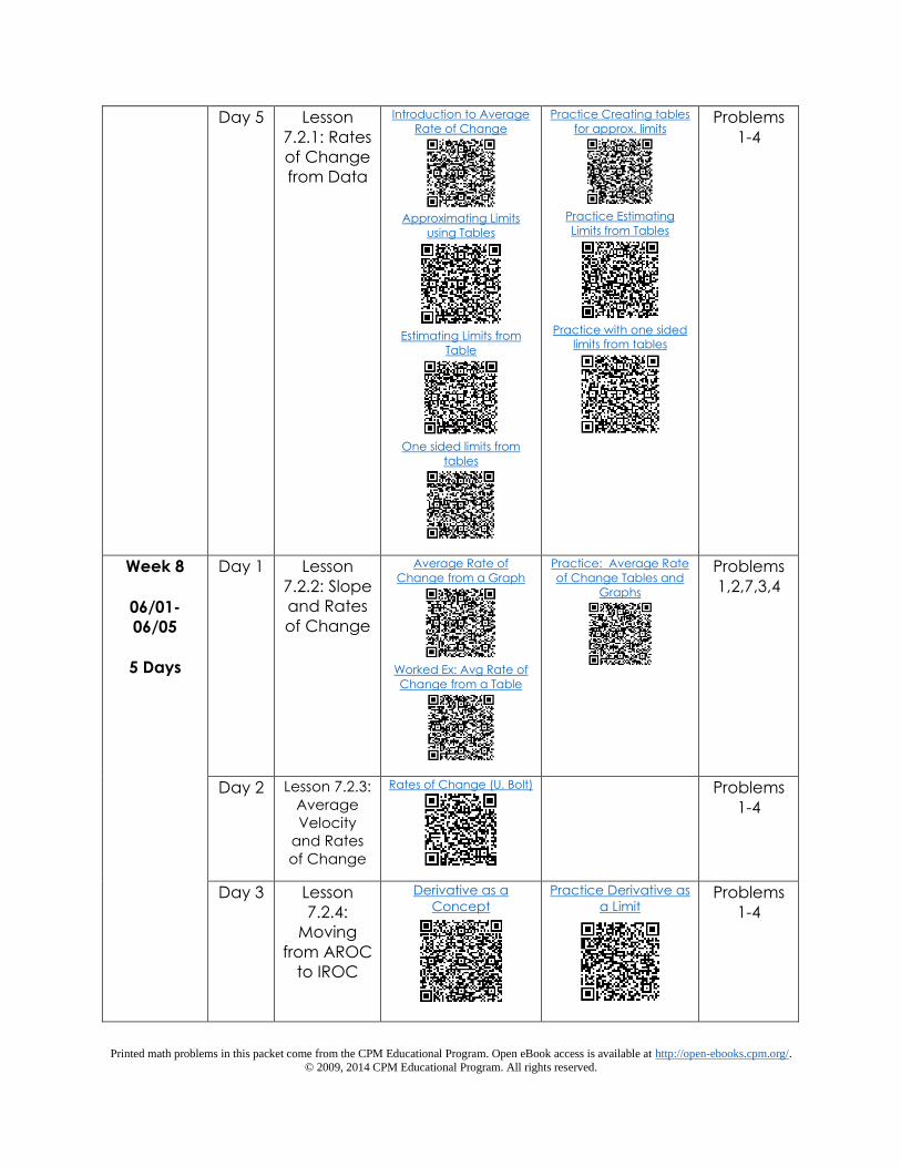
Day 5 Lesson

7.2.1: Rates

of Change

from Data

Introduction to Average

Rate of Change

Approximating Limits

using Tables

Estimating Limits from

Table

One sided limits from

tables

Practice Creating tables

for approx. limits

Practice Estimating

Limits from Tables

Practice with one sided

limits from tables

Problems

1-4

Week 8

06/01-

06/05

5 Days

Day 1 Lesson

7.2.2: Slope

and Rates

of Change

Average Rate of

Change from a Graph

Worked Ex: Avg Rate of

Change from a Table

Practice: Average Rate

of Change Tables and

Graphs

Problems

1,2,7,3,4

Day 2 Lesson 7.2.3:

Average

Velocity

and Rates

of Change

Rates of Change (U. Bolt)

Problems

1-4

Day 3 Lesson

7.2.4:

Moving

from AROC

to IROC

Derivative as a

Concept

Practice Derivative as

a Limit

Problems

1-4


https://www.khanacademy.org/math/algebra/x2f8bb11595b61c86:functions/x2f8bb11595b61c86:average-rate-of-change/v/introduction-to-average-rate-of-change

https://www.khanacademy.org/math/algebra/x2f8bb11595b61c86:functions/x2f8bb11595b61c86:average-rate-of-change/v/introduction-to-average-rate-of-change

https://www.khanacademy.org/math/calculus-1/cs1-limits-and-continuity/cs1-estimating-limits-from-tables/v/approximating-limit-from-table?modal=1




https://www.khanacademy.org/math/calculus-1/cs1-limits-and-continuity/cs1-estimating-limits-from-tables/v/one-sided-limits-from-tables?modal=1

https://www.khanacademy.org/math/calculus-1/cs1-limits-and-continuity/cs1-estimating-limits-from-tables/v/one-sided-limits-from-tables?modal=1

https://www.khanacademy.org/math/calculus-1/cs1-limits-and-continuity/cs1-estimating-limits-from-tables/e/creating-tables-to-approximate-limits?modal=1

https://www.khanacademy.org/math/calculus-1/cs1-limits-and-continuity/cs1-estimating-limits-from-tables/e/creating-tables-to-approximate-limits?modal=1

https://www.khanacademy.org/math/calculus-1/cs1-limits-and-continuity/cs1-estimating-limits-from-tables/e/finding-limits-numerically?modal=1

https://www.khanacademy.org/math/calculus-1/cs1-limits-and-continuity/cs1-estimating-limits-from-tables/e/finding-limits-numerically?modal=1

https://www.khanacademy.org/math/calculus-1/cs1-limits-and-continuity/cs1-estimating-limits-from-tables/e/one-sided-limits-from-tables?modal=1

https://www.khanacademy.org/math/calculus-1/cs1-limits-and-continuity/cs1-estimating-limits-from-tables/e/one-sided-limits-from-tables?modal=1

https://www.khanacademy.org/math/algebra/x2f8bb11595b61c86:functions/x2f8bb11595b61c86:average-rate-of-change/v/average-rate-of-change-example-1








https://www.khanacademy.org/math/calculus-1/cs1-derivatives-definition-and-basic-rules

https://www.khanacademy.org/math/calculus-1/cs1-derivatives-definition-and-basic-rules

https://www.khanacademy.org/math/calculus-1/cs1-derivatives-definition-and-basic-rules/cs1-average-vs-instantaneous-rate-of-change/v/derivative-as-a-concept?modal=1

https://www.khanacademy.org/math/calculus-1/cs1-derivatives-definition-and-basic-rules/cs1-average-vs-instantaneous-rate-of-change/v/derivative-as-a-concept?modal=1

https://www.khanacademy.org/math/ap-calculus-ab/ab-differentiation-1-new/ab-2-2/e/the-formal-and-alternate-form-of-the-derivative

https://www.khanacademy.org/math/ap-calculus-ab/ab-differentiation-1-new/ab-2-2/e/the-formal-and-alternate-form-of-the-derivative



Formal Definition of

Derivative

Day 4 Lesson 7.2.5:

Rate of

Change

Applications

Interpreting

Derivatives in Context

Practice Interpreting

Derivatives in Context

Problems

1-4

Day 5 Chapter 7

Closure

Strategy in Finding

Limits

Practice in Finding

Limits

Week 9

06/08-

06/12

5 Days

Day 1 Lesson 8.1.1:

Graphing

Transformations

of the Sine

Function

Graph of sin x

Amplitude of Sine

Functions

Problems

1-5

Day 2 Lesson

8.1.2:

Modeling

with

Periodic

Functions

Amp and Period of

Sine Functions

Modeling with Trig

Practice with Amp

and Period Problems

Practice with

Modeling and Trig

Problems 1-

5

Day 3 Lesson

8.1.3:

Improving

the Spring

Problem

Transform Sin Graphs

(vertical/reflection)

Graph Sin Functions

Problems

1-4


https://www.khanacademy.org/math/ap-calculus-ab/ab-differentiation-1-new/ab-2-2/v/calculus-derivatives-1-new-hd-version?modal=1

https://www.khanacademy.org/math/ap-calculus-ab/ab-differentiation-1-new/ab-2-2/v/calculus-derivatives-1-new-hd-version?modal=1

https://www.khanacademy.org/math/differential-calculus/dc-context-app/dc-interpret-derivatives/v/interpreting-the-meaning-of-the-derivative-in-context?modal=1

https://www.khanacademy.org/math/differential-calculus/dc-context-app/dc-interpret-derivatives/v/interpreting-the-meaning-of-the-derivative-in-context?modal=1

https://www.khanacademy.org/math/differential-calculus/dc-context-app/dc-interpret-derivatives/e/meaning-of-the-derivative-in-context?modal=1

https://www.khanacademy.org/math/differential-calculus/dc-context-app/dc-interpret-derivatives/e/meaning-of-the-derivative-in-context?modal=1

https://www.khanacademy.org/math/differential-calculus/dc-limits/dc-limit-strategy/v/flow-chart-of-limit-strategies?modal=1

https://www.khanacademy.org/math/differential-calculus/dc-limits/dc-limit-strategy/v/flow-chart-of-limit-strategies?modal=1

https://www.khanacademy.org/math/differential-calculus/dc-limits/dc-limit-strategy/e/selecting-procedures-for-calculating-limits-3

https://www.khanacademy.org/math/differential-calculus/dc-limits/dc-limit-strategy/e/selecting-procedures-for-calculating-limits-3

https://www.khanacademy.org/math/algebra2/x2ec2f6f830c9fb89:trig/x2ec2f6f830c9fb89:trig-graphs/v/we-graph-domain-and-range-of-sine-function?modal=1

https://www.khanacademy.org/math/algebra2/x2ec2f6f830c9fb89:trig/x2ec2f6f830c9fb89:trig-graphs/v/we-graph-domain-and-range-of-sine-function?modal=1

https://www.khanacademy.org/math/algebra2/x2ec2f6f830c9fb89:trig/x2ec2f6f830c9fb89:amp-mid-period/e/amplitude-of-trig-functions?modal=1

https://www.khanacademy.org/math/algebra2/x2ec2f6f830c9fb89:trig/x2ec2f6f830c9fb89:amp-mid-period/e/amplitude-of-trig-functions?modal=1

https://www.khanacademy.org/math/algebra2/x2ec2f6f830c9fb89:trig/x2ec2f6f830c9fb89:period/v/we-amplitude-and-period?modal=1

https://www.khanacademy.org/math/algebra2/x2ec2f6f830c9fb89:trig/x2ec2f6f830c9fb89:period/v/we-amplitude-and-period?modal=1

https://www.khanacademy.org/math/algebra2/x2ec2f6f830c9fb89:trig/x2ec2f6f830c9fb89:sinusoidal-models/v/modeling-with-shifted-trig-functions?modal=1

https://www.khanacademy.org/math/algebra2/x2ec2f6f830c9fb89:trig/x2ec2f6f830c9fb89:sinusoidal-models/v/modeling-with-shifted-trig-functions?modal=1

https://www.khanacademy.org/math/algebra2/x2ec2f6f830c9fb89:trig/x2ec2f6f830c9fb89:period/e/find-amplitude-of-a-sinusoid-from-formula?modal=1

https://www.khanacademy.org/math/algebra2/x2ec2f6f830c9fb89:trig/x2ec2f6f830c9fb89:period/e/find-amplitude-of-a-sinusoid-from-formula?modal=1

https://www.khanacademy.org/math/algebra2/x2ec2f6f830c9fb89:trig/x2ec2f6f830c9fb89:sinusoidal-models/e/modeling-with-periodic-functions-2?modal=1

https://www.khanacademy.org/math/algebra2/x2ec2f6f830c9fb89:trig/x2ec2f6f830c9fb89:sinusoidal-models/e/modeling-with-periodic-functions-2?modal=1

https://www.khanacademy.org/math/trigonometry/trig-function-graphs/graphing-sinusoids/v/example-amplitude-and-period-transformations?modal=1

https://www.khanacademy.org/math/trigonometry/trig-function-graphs/graphing-sinusoids/v/example-amplitude-and-period-transformations?modal=1

https://www.khanacademy.org/math/algebra2/x2ec2f6f830c9fb89:trig/x2ec2f6f830c9fb89:trig/x2ec2f6f830c9fb89:graphing-sinusoid/e/graphs_of_sine_and_cosine?modal=1

https://www.khanacademy.org/math/algebra2/x2ec2f6f830c9fb89:trig/x2ec2f6f830c9fb89:trig/x2ec2f6f830c9fb89:graphing-sinusoid/e/graphs_of_sine_and_cosine?modal=1



Transform Sin Graph

(horizontal stretch)

Phase Shifts

Phase Shifts

Day 4 Lesson 8.2.1:

Graphing

Reciprocal

Trigonometric

Functions

Finding Reciprocal Trig

Functions

Reciprocal Trig Ratios

Problems

1-5

Day 5 Lesson 8.3.1:

Simplifying

Trigonometric

Expressions

Using Trig Identities

Trig Ratio Reference

Sheet

Problems

1-6

Week 10

06/15-

06/19

5 Days

Day 1 Lesson 8.3.2:

Proving

Trigonometric

Identities

Trig Identity

Example Proof

Practice: Trig

Identities Challenge

Problems

1-10

Day 2 Lesson 8.3.3:

Angle Sum

and

Difference

Identities

Review of Trig Angle

Sum Identities

Using Trig Angle

Addition Identities

Problems

1-5, 1-3


https://www.khanacademy.org/math/trigonometry/trig-function-graphs/graphing-sinusoids/v/amplitude-and-period-cosine-transformations?modal=1

https://www.khanacademy.org/math/trigonometry/trig-function-graphs/graphing-sinusoids/v/amplitude-and-period-cosine-transformations?modal=1

https://www.khanacademy.org/math/algebra2/x2ec2f6f830c9fb89:trig/x2ec2f6f830c9fb89:trig/x2ec2f6f830c9fb89:graphing-sinusoid/e/graphs-of-trigonometric-functions?modal=1




https://www.khanacademy.org/math/geometry-home/right-triangles-topic/reciprocal-trig-ratios-geo/v/example-the-six-trig-ratios

https://www.khanacademy.org/math/geometry-home/right-triangles-topic/reciprocal-trig-ratios-geo/v/example-the-six-trig-ratios

https://www.khanacademy.org/math/geometry-home/right-triangles-topic/reciprocal-trig-ratios-geo/e/reciprocal_trig_funcs

https://www.khanacademy.org/math/precalculus/x9e81a4f98389efdf:trig/x9e81a4f98389efdf:using-trig-id/v/examples-using-pythagorean-identities-to-simplify-trigonometric-expressions

https://www.khanacademy.org/math/precalculus/x9e81a4f98389efdf:trig/x9e81a4f98389efdf:using-trig-id/v/examples-using-pythagorean-identities-to-simplify-trigonometric-expressions

https://www.khanacademy.org/math/precalculus/x9e81a4f98389efdf:trig/x9e81a4f98389efdf:using-trig-id/a/trig-identity-reference

https://www.khanacademy.org/math/precalculus/x9e81a4f98389efdf:trig/x9e81a4f98389efdf:using-trig-id/a/trig-identity-reference

https://www.khanacademy.org/math/in-in-grade-10-ncert/x573d8ce20721c073:in-in-chapter-8-introduction-to-trigonometrics/x573d8ce20721c073:in-in-trigonometric-identities/v/example-2-proving-trigonometric-identities

https://www.khanacademy.org/math/in-in-grade-10-ncert/x573d8ce20721c073:in-in-chapter-8-introduction-to-trigonometrics/x573d8ce20721c073:in-in-trigonometric-identities/v/example-2-proving-trigonometric-identities

https://www.khanacademy.org/math/in-in-grade-10-ncert/x573d8ce20721c073:in-in-chapter-8-introduction-to-trigonometrics/x573d8ce20721c073:in-in-trigonometric-identities/e/trigonometric-identities-challenge-problems

https://www.khanacademy.org/math/in-in-grade-10-ncert/x573d8ce20721c073:in-in-chapter-8-introduction-to-trigonometrics/x573d8ce20721c073:in-in-trigonometric-identities/e/trigonometric-identities-challenge-problems

https://www.khanacademy.org/math/precalculus/x9e81a4f98389efdf:trig/x9e81a4f98389efdf:angle-addition/v/trigonometry-identity-review-fun

https://www.khanacademy.org/math/precalculus/x9e81a4f98389efdf:trig/x9e81a4f98389efdf:angle-addition/v/trigonometry-identity-review-fun

https://www.khanacademy.org/math/precalculus/x9e81a4f98389efdf:trig/x9e81a4f98389efdf:angle-addition/e/trig_addition_identities

https://www.khanacademy.org/math/precalculus/x9e81a4f98389efdf:trig/x9e81a4f98389efdf:angle-addition/e/trig_addition_identities



Day 3 Lesson 8.3.4:

Double-

Angle and

Half-Angle

Identities

Using Double Angle

Cos Identity

Problems

2-5

Day 4 Lesson 8.3.5:

Solving

Complex

Trigonometric

Equations

Using Trig Angle

Identities

Trig Practice Problems

Quiz

Problems

1-7

Day 5 Chapter 8

Closure

Trigonometric

Identities Practice Test

Trigonometric Identities

Practice Test


https://www.khanacademy.org/math/precalculus/x9e81a4f98389efdf:trig/x9e81a4f98389efdf:angle-addition/v/double-angle-formula-for-cosine-example-c

https://www.khanacademy.org/math/precalculus/x9e81a4f98389efdf:trig/x9e81a4f98389efdf:angle-addition/v/double-angle-formula-for-cosine-example-c

https://www.khanacademy.org/math/precalculus/x9e81a4f98389efdf:trig/x9e81a4f98389efdf:using-trig-id/v/cosine-angle-addition?modal=1

https://www.khanacademy.org/math/precalculus/x9e81a4f98389efdf:trig/x9e81a4f98389efdf:using-trig-id/v/cosine-angle-addition?modal=1

https://www.khanacademy.org/math/precalculus/x9e81a4f98389efdf:trig/quiz/x9e81a4f98389efdf:trig-quiz-2?modal=1

https://www.khanacademy.org/math/precalculus/x9e81a4f98389efdf:trig/quiz/x9e81a4f98389efdf:trig-quiz-2?modal=1

https://www.khanacademy.org/math/trigonometry/trig-equations-and-identities






Week 1, Day 1

Lesson 3.1.1 Operations with Rational Expressions

Students will add, subtract, multiply, and divide rational expressions.

1. Simplify the following rational expressions.

a. b.


a. b.


a. b.

4. Simplify.

5. Simplify.

6. Simplify.

7. Simplify.

8. Simplify.




Week 1, Day 2

Lesson 3.1.2: Rewriting Expressions and Equations

Students will simplify complex fractions and use substitution to simplify and factor

algebraic expressions.

1. Simplify the following complex fraction.



4. Simplify.

5. Simplify.

6. Simplify.




Week 1, Day 3

Lesson 3.1.3 Solving Nonlinear Systems of Equations

Students will solve nonlinear systems of equations.

1. Solve the system:




Week 1, Day 4

Lesson 3.1.4 Polynomial Division

Student will Divide Polynomials.

1. Divide:

2. Divide:

3. Divide P(x) = x4 + x2 − 5x + 1 by x − 1.

4. Is x − 5 a factor of x3 − 3x2 − 6x − 20? Explain your reasoning.

5. Divide:




Week 2, Day 1

Lesson 3.1.5 Solving Classic Word Problems

Students will use a variety of strategies to solve classic types of word problems.

1. Sally rides her bike to run errands. It takes her 20 minutes at 15 mph to get to

her first stop. She spends 15 minutes riding at 12 mph to get to her second stop. It

then takes her 18 minutes riding at 10 mph to get home.

a. Draw a speed vs. time graph for the time that Sally spent riding her bike.

b. How far did she travel?

c. What was her average speed?

2. The lengths of the sides of a right triangle are given by , and . What

are the lengths of the sides?

3. A stick 4 feet tall casts a shadow 5 feet long at 6:36 p.m. How tall is a pole

that casts a shadow 32 feet long at the same time?

4. Fleta wants to earn $2000 in interest on her investments this year. She currently

has $35,000 in an account that earns 3% annual interest, but she is not allowed

to add to this account. She has more money to invest and the best rate the

bank can give her is 2.25% annual interest. How much does she need to invest in

the new account to meet her desired earnings?

5. A cone has a height of 10 inches and a radius of 4 inches. If a plane cuts the

cone inches below the cone’s peak, what is the area of the circular cross

section?




Week 2, Day 2

Lesson 3.2.1 Using Sigma Notation

Students will recognize and be able to calculate sums by expanding sigma

notation as well as write finite arithmetic series in sigma notation.

1. Expand.

2. Expand.

3. Write the following sum in expanded form.

4. Write the given expression using sigma notation.

5. Write the given expression using sigma notation.

0.2(43 + 43.2 + 43.4 + ... + 44.8)

Week 2, Day 3

Lesson 3.2.2 Area under a Curve (Part I)

Students will estimate the area under a curve and understand that area under a

velocity curve represents distance.

1. Let g(x) = (x − 2)2. Approximate A(g, ) using right endpoint rectangles

of width 0.5 units. Express your sum using sigma notation.

2. Given f(x) = , approximate A(f(x), 0 ≤ x ≤ 3) using 6 right endpoint

rectangles.

3. Given f(x)= 2x2, approximate A(f, ) using 5 left endpoint rectangles.

4. Given g(x) = , approximate A(g, 5 ≤ x ≤ 7) using ten left endpoint

rectangles.




Week 2, Day 4

Lesson 3.2.3 Area under a Curve (Part II)

Students will approximate area under a curve using left endpoint and right

endpoint rectangles. They will use sigma notation to express their

approximations.

1. Write the sigma notation for approximating the area under the curve f(x) = x2

+ x − 12 for 4 ≤ x ≤ 10 using 20 right endpoint rectangles.

2. Given g(x) = , approximate A(g, 2 ≤ x ≤ 5) using 8 right endpoint

rectangles.

3. Approximate the area under the curve y = −2x2 + x + 6 for using 6 left

endpoint rectangles.

4. Approximate the area under the curve y = for −3 ≤ x ≤ 0 using left

endpoint rectangles of width 0.1.

Week 2, Day 5

Lesson 3.2.4 Area under a Curve (Part III)

Students will practice approximating areas with left endpoint and right endpoint

rectangles.

1. Given j(x) = (x − 1)2 + 4, approximate A(j, 1 ≤ x ≤ 4) using 5 right endpoint

rectangles. Sketch the curve, showing the rectangles used to determine the

area. Use sigma notation to represent your approximation. Is the approximation

an underestimate or an overestimate of the actual area? Explain.

2. Given f(x)= 3x2 − 6x, approximate A(f, 1 ≤ x ≤ 4) using 7 left endpoint

rectangles.

a. Use sigma notation to show the sum.

b. Determine if the approximation is an underestimate or an overestimate of the

actual area. Justify your answer using a sketch.

c. How can you change your sigma notation to estimate the area using right

endpoint rectangles?

3. Sketch a graph of h(x) = + 7 over the interval −2 ≤ x ≤ 4. Determine an

underestimate of the area under the curve, for the given interval, using

rectangles of width




Week 3, Day 1

3.2.Extra U-Substitution

Students will factor expressions using substitution.

1. Factor completely.






7. Solve.

8. Solve. 9. Solve.

Week 3, Day 2

Lesson 4.1.1 Graphs of Polynomials in Factored Form

Students will graph polynomial functions from equations given in factored form.

1. Sketch the graph of f(x) = (x + 1)(x − 2)(x + 3)2 without using a graphing

calculator. Do not scale your axes, but be sure to label the important points.

2. Sketch the graph of f(x) = (x − 3)(x + 2)2 without using a graphing calculator.

Do not scale your axes, but be sure to label the important points.

3. Sketch the graph of f(x) = −(x + 3)2(x − 4) without using a graphing calculator.

Do not scale your axes, but be sure to label the important points.

4. Sketch the graph of f(x) = −(x + 1)(x + 2)(x − 3) without using a graphing


5. Sketch the graph of f(x) = − (x − 2)2(x + 3)2 without using a graphing


6. The Mariana Trench, in the Pacific Ocean, is the deepest place on earth. If

the x-axis represents the ocean basin (about 4.4 miles below sea level) the

portion below the ocean basin of the Mariana trench can be modeled by f(x) =

0.025(x − 1)3(x − 7) where f(x) is the depth below the ocean basin and x is

horizontal distance, both in miles. Sketch the graph and describe it completely.




Week 3, Day 3

Lesson 4.1.2 Writing Equations of Polynomial Functions

Students will write equations for the graphs of polynomial functions given the

x‑intercepts and one additional point.

1. Write an equation for a 3rd degree polynomial function in factored form, with

real coefficients, that has roots at x = 3 ± and x = −1 and passes through the

point (3, −10).

2. A 3rd degree polynomial function has roots at x = –2i and x = 5. The

y-intercept is (0, 25). Write an equation for this function in factored form with real

coefficients.

3. A polynomial function of degree 3 contains the point (−1, 45), has an

xintercept- of (4, 0), and has a root of x = −1 + . Write an equation for this

function in factored form with real coefficients.

4. Write an equation for a 5th degree polynomial function in factored form, with

real coefficients, that has a double root at x = 3 and roots at x = 7 + 2i and x =

−5. Write a possible equation for this function in factored form with real

coefficients.

5. A 5th degree polynomial function has roots at x = 3 − 2i, x = 1 + , and x = 8.

The y intercept- is (0, 26). Write an equation for this function in factored form with

real coefficients.




Week 3, Day 4

Lesson 4.1.3 Identifying and Using Roots of Polynomials

Students will identify roots of polynomial functions

1. Determine the roots of the given polynomial. Give exact

answers.


answers.


answers.


answers.

5. Let f(x) = 2x3 + 3x2 − 7x − 4.

a. Is x = 2 a root of the polynomial? Explain.

b. If x ≈ −1.7 is a local maximum and x ≈ 0.7 is a local minimum, what does that

tell you about the graph of the function?

c. Determine all of the zeros of the function. Give exact answers.

Week 3, Day 5

Lesson 4.2.1 Graphing Transformations of y =1/x

Students will rewrite rational expressions to transform functions in the form g(x) =

(ax+b)/(x-c) into transformations of y = 1/(x-h) + k.

1. Rewrite f(x) = as a transformation of g(x) = and sketch the graph of y = f(x).

2. Rewrite f(x) = as a transformation of g(x) = and sketch the graph of y = f(x).

3. Write a possible equation of a rational function that has a horizontal

asymptote at y = 13 and a vertical asymptote at x = −2.

4. Write a possible equation of a rational function that has a horizontal

asymptote at y = −12 and a vertical asymptote at x = 9.

5. Rewrite f(x) = as a transformation of g(x) = and sketch the graph

of y = f(x).




Week 4, Day 1

Lesson 4.2.2 Graphing Rational Functions

Students will graph rational functions with point discontinuities and slant

asymptotes.

1. Rewrite f(x) = as a transformation of g(x) = and sketch the graph

of y = f(x).

2. Let f(x) =

a. Sketch a graph of y = f(x).

b. State the domain and range of f.

3. Consider the rational function r(x) = .

a. Determine the value of n, such that f(x) = r(x) + n has a root at x = −10.

b. Rewrite f(x) from part (a) as single-term expression.

4. Consider the rational function r(x) = . Explain what values of a and b, if

any would result in the function having no x- or y-intercepts. Justify your answer

completely.

5. Write a possible equation for the rational function graphed below.

6. Write a possible equation for the rational function graphed below.




Week 4, Day 2

Lesson 4.2.3 Graphing Reciprocal Functions

Students will graph y = 1/f(x) given an equation for the graph of y = f(x).

1. Write the end-behavior function of f(x) = + 54.

2. Write the end-behavior function of f(x) = .




Week 4, Day 3

Lesson 4.3.1 Polynomial and Rational Inequalities

Students will solve polynomial and rational inequalities.

1. Solve the inequality .

2. Solve:

3. Solve:



6. Solve:

7. Solve:




Week 4, Day 4

Lesson 4.3.2 Applications of Polynomial and Rational Functions

Students will apply their knowledge of polynomial and rational functions to

analyze everyday situations.

1. State the locations of the asymptotes of .


3. Identify all of the asymptotes of .


5. A baby bird is learning to fly. Its height above/below a branch can be

modeled by the function f(t) = 0.005t(t − 2)2(t − 5)(t − 8) for 0 ≤ t ≤ 10, where t is

time in seconds and f(t) is height in feet.

a. For what times is the bird on the branch?

b. When is the bird above the branch?

c. Where is the bird when t = 7?




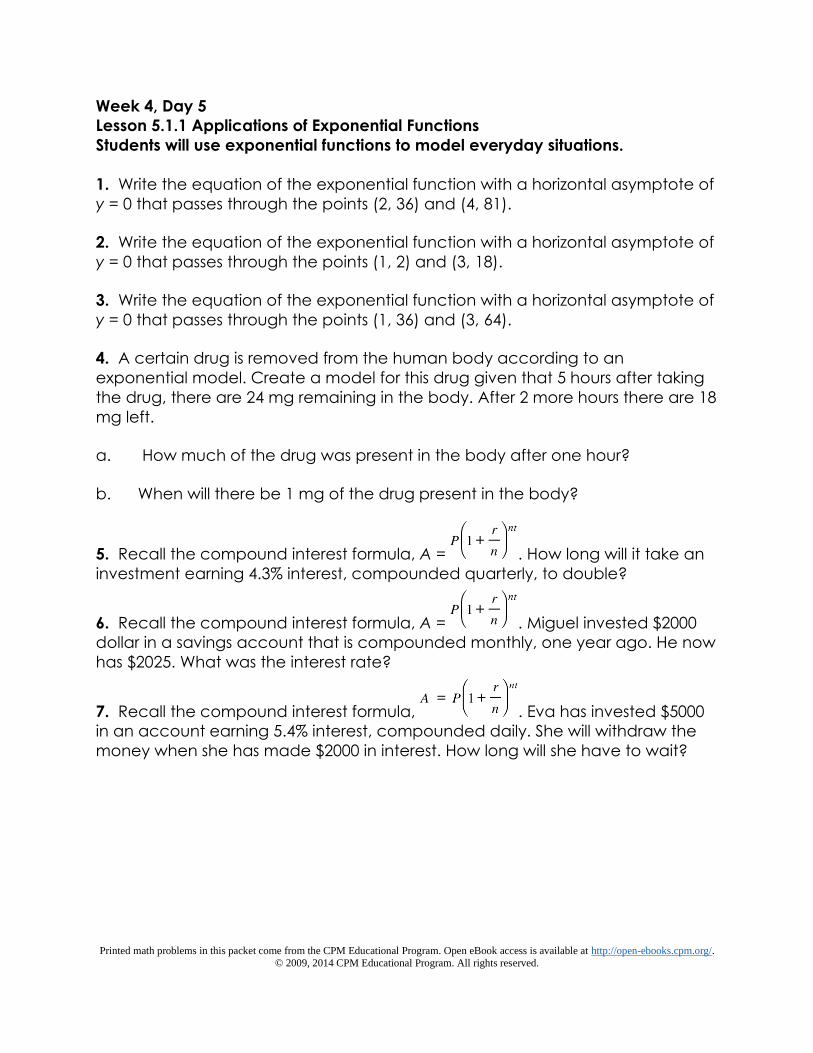
Week 4, Day 5

Lesson 5.1.1 Applications of Exponential Functions

Students will use exponential functions to model everyday situations.

1. Write the equation of the exponential function with a horizontal asymptote of

y = 0 that passes through the points (2, 36) and (4, 81).





4. A certain drug is removed from the human body according to an

exponential model. Create a model for this drug given that 5 hours after taking

the drug, there are 24 mg remaining in the body. After 2 more hours there are 18

mg left.

a. How much of the drug was present in the body after one hour?

b. When will there be 1 mg of the drug present in the body?

5. Recall the compound interest formula, A = . How long will it take an

investment earning 4.3% interest, compounded quarterly, to double?

6. Recall the compound interest formula, A = . Miguel invested $2000

dollar in a savings account that is compounded monthly, one year ago. He now

has $2025. What was the interest rate?

7. Recall the compound interest formula, . Eva has invested $5000

in an account earning 5.4% interest, compounded daily. She will withdraw the

money when she has made $2000 in interest. How long will she have to wait?




Week 5, Day 1

Lesson 5.1.2 Stretching Exponential Functions

Students will understand that for exponential functions, a horizontal shift can be

equivalently written as a vertical stretch.

1. Rewrite the given equation in form.



4. Rewrite in a form.

5. Write given equation in form.




Week 5, Day 2

Lesson 5.1.3 The number e

Students will learn about e and will solve problems involving continuous growth.

1. Rewrite each equation in the other (logarithmic/exponential) form.

a. = −3

b. Ay = B


a. 5−2 =

b. logB(M) = K


a. C = logV(I)

b. 7x = M


a. d −2 = logf(g)

b. 4x = n + 1

5. Determine the inverse for the function below. Make sure that you express

your answer using inverse function notation.

f(x) = log3(x + 2)




Week 5, Day 3

Lesson 5.2.1 Logarithms

Students will practice converting between exponential and logarithmic

equations.

1. Determine the inverse equation of f(x) = 4(5)x − 3.

2. Write a formula for the inverse of f(x) = 3(4)x + 5.

3. Write a formula for the inverse of f(x) = 6 log7(x) − 8.

4. Write a formula for the inverse of y = –2 log3(x) + 1, then graph the original

function.

5. The graph at right shows y = f(x). Let g(x) = 8x + 1 + 5.

a. Evaluate f–1(g–1(32)).

b. Write an equation for f(x).

6. The equation y = ln(f(x)) is graphed at right.

a. What type of function is f?

b. Write an equation for f(x).

7. Write the inverse of the function . Demonstrate that f and its

inverse function are inverses using three different methods.

8. Keira is uncertain what a logarithm is and when to use logarithms to solve an

equation. Provide a clear explanation for Keira. Include examples to illustrate

your explanation.




Week 5, Day 4

Lesson 5.2.2 Properties of Logarithms

Students will evaluate logarithms.

1. Without a calculator, evaluate the following logarithmic expressions.

a. b. c.


a. b. c.


a. b. c.


a. b. c.


a. b.


a. b.

7. Simplify each logarithmic expression.

a. b.


a. b.





a. b.


a. b.


a. b.


a. b.




Week 6, Day 1

Lesson 5.2.3 Solving Exponential and Logarithmic Equations

Students will solve equations with the variable in the exponent and equations

with logarithms.

1. Rewrite each of the expression using a single logarithm.

2. Use the properties of logarithms to expand the following

expression.


expression.


expression.

5. Given , and determine the exact value

of .


of .


of .

8. Given , evaluate .

9. Simplify:

10. Simplify.

11. Simplify.




12. Given and , evaluate .

13. Simplify.

14. Simplify.

15. Simplify.




Week 6, Day 2

Lesson 5.2.4 Graphing Logarithmic Functions

Students will solve logarithmic equations.

1. Solve 8x = 4(2−x).

2. Solve 33x – 1 = 243.

3. Solve 322x−1 = .

4. Solve 16x · = 8.

5. Solve 3 + 5 = 86.

6. Solve (3x)1/4 = 2.

7. Solve 20m1.5 = 1000.

8. Solve: 5x2/5 = 125

9. Solve: 3x3.2 − 3 = 570

10. Solve: 5(4x)5.5 − 1 = 54

11. Solve: 5(2)x = 50

12. Solve: 200 = 700

13. Solve: 8(10)x + 2 = 26

14. Solve: 7(3)x + 1 + 2 = 58




Week 6, Day 3

Lesson 5.2.5 Applications of Exponentials and Logarithms

Students will use exponential functions and logarithms to model and answer

questions about everyday situations.

1. Solve: logx(16) = −4

2. Solve: log3(x) = −2

3. Solve: = logx(5)

4. Solve: log3(95) = x

5. Solve for k: ekx = mx

(Note that e is the base of natural log and not a variable.)

6. Solve for x: 3x−1 + 5n−2 = 10

7. Solve:

a. b.

8. Solve:

a. 19(2)x+1 = 444 b. log2(x + 1) – log2(x – 2) = log3(9)

9. Solve:

10. Solve.

a. e4x – 13e2x + 12 = 0 b. log3(x – 1) + 5log5(2) – log3(x) = 0

11. Solve. a. ln(x – 2) – ln(e + 5) = 1




Week 6, Day 4

Lesson 7.1.1 An Introduction to Limits

Students will be introduced to the concept of a limit in a geometric context.

1. Use the graph of y = f(x) at right to evaluate the following expressions.

a. f(0) b.

c. d.

2. Given the graph of y = f(x), evaluate the following expressions.

a. f(x)

b. f(x)

c. f(x)

d. f(x)

e. f(−3) f. f(x) g. f(3)

h. f(x)




Week 7, Day 1

Lesson 7.1.2 Working with One Sided Limits

Students will work with one sided limits and limits at infinity


a. f(−6 ) b. f(x)

c. f(x) d. f(7)

e. f(x) f. f(x)

g. f(x)


a. f(−6) b. f(x) c. f(x)

d. f(x)

e. f(4) f.

3. Sketch the graph of . Use it to evaluate the limit

statements below.

a. b. c.




4. Sketch the graph of . Use it to evaluate the limit

statements below.

a. b. c.




Week 7, Day 2

Lesson 7.1.3 The Definition of a Limit

Students will analyze limits graphically and from tables.


a. f(x) b. f(x)

c. f(x) d. f(x)

e. f(−3) f. f(x)

g. f(3) h. f(x)

2.Given the graph of y = f(x), evaluate the following expressions.

a. f(−6) b. f(x) c. f(x) d. f(7)

e. f(x) f. f(x) g. f(x)


a. f(−6) b. f(x) c. f(x) d.

f(x)

e. f(4) f. g.




4. Evaluate .

5. Let . Complete the table of values below to predict the value

of .

6. Let . Complete the table of values below to predict the value

of .

7. Use a graph or a table to evaluate .










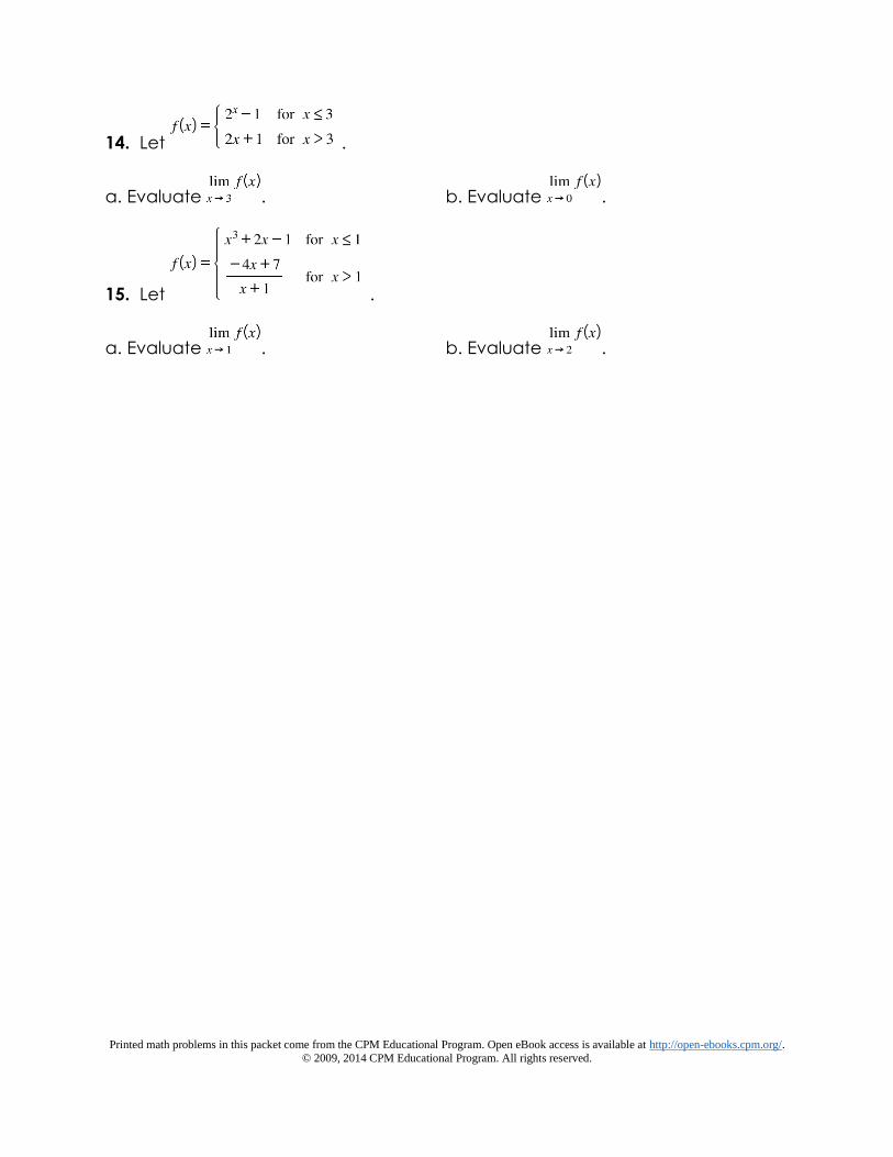
14. Let .

a. Evaluate . b. Evaluate .

15. Let .

a. Evaluate . b. Evaluate .




Week 7, Day 3

Lesson 7.1.4 Limits and Continuity

Students will apply the formal definition of continuity.

1. Use the graph at right to evaluate the following

expressions.

a. f(0)

b.

c. Is the function is continuous at x = 0? Explain your

answer using the formal definition of continuity.

2. Use the graph of y = h(x) below to complete the parts below.

Explain each of your answers using the formal definition of

continuity.

a. Is the function is continuous at x = 0?

b. Is the function is continuous at x = 2?

c. Is the function is continuous at x = 3?

3. Determine whether the given function is continuous at the given point.

Explain your answer using the formal definition of continuity.

f(x) = 3x+2 − 1 at x = −2



at x = 4



at x = −5






at x = 3




Week 7, Day 4

Lesson 7.2.1 Special Limits

Students will calculate average rates of change by calculating the slope of the

secant line between two data points.

1. The amount of money in a bank account at the end of each month is given

in the table below.

time

(months) 0 1 3 6 9 12

balance ($) 507 1276 1104 1353 987 1074

a. Graph the data.

b. Calculate the average change in the balance for each time interval ( 0 to 1,

2 to 3, …, 9 to 12 ). How does this relate to the graph?

c. Is the average rate of change for the entire 12 months increasing or

decreasing? By how much?

d. Assuming the account balance continues in a similar pattern, how much

money would you expect to be in the account after 10 years?

2. The table below shows the amount of carbon emissions (in million tons)

worldwide for the given years. Enter the data into your calculator and create a

plot of the data.

Year Emissions Year Emissions Year Emissions

1950 1620 1975 4527 1992 5926

1955 2020 1980 5170 1993 5919

1960 2543 1985 5286 1994 5989

1965 3095 1988 5809 1995 6080

1970 4006 1990 5943




a. Write an equation to model the data in the plot.

b. What is the average rate of growth between 1950 and 1995?

c. Use your model to predict the amount of carbon emissions in 2020 and the

rate at which the emissions will be changing near that time.

3. The amount of money in a bank account at the end of each month is given

in the table below.

time

(months) 0 1 3 6 9 12

balance

($) 507 1276 1104 1353 987 1074

a. Graph the data.

b. Calculate the average change in the balance for each time interval ( 0 to 1,

2 to 3, …, 9 to 12 ). How does this relate to the graph?

c. Is the average rate of change for the entire 12 months increasing or

decreasing? By how much?

d. Assuming the account balance continues in a similar pattern, how much

money would you expect to be in the account after 10 years?




4. The table below shows the amount of carbon emissions (in million tons)

worldwide for the given years. Enter the data into your calculator and create a

plot of the data.

Year Emissions Year Emissions Year Emissions

1950 1620 1975 4527 1992 5926

1955 2020 1980 5170 1993 5919

1960 2543 1985 5286 1994 5989

1965 3095 1988 5809 1995 6080

1970 4006 1990 5943

a. Write an equation to model the data in the plot.

b. What is the average rate of growth between 1950 and 1995?

c. Use your model to predict the amount of carbon emissions in 2020 and the

rate at which the emissions will be changing near that time.




Week 8, Day 1

Lesson 7.2.2 Slope and Rates of Change

Students will calculate average rates of change from an equation of a function.

1. A rocket is launched off of a platform such that its height is determined by the

function h(t) = −16t2 + 128t + 4, where t is time in seconds.

a. When will the rocket hit the ground?

b. Make a table of time versus height. Use 1-second increments. Use the table to sketch

a graph of the function over the interval that fits this situation.

c. What are the average velocities for each 1-second time interval that the ball is in the

air?

d. What is happening to the average velocity of the ball with respect to the time?

e. What does the average velocity tell you about the change in position of the ball?

2. A man standing on a bridge drops a coin into a water fountain from a height of 105

ft. The height of the coin with respect to time is given by the function h(t) = 105 − 16t2,

where t is in seconds and t ≥ 0.

a. Calculate the average rate of change of the coin for the first 2 seconds after it is

dropped. Include units in your answer.

b. What is the average rate of change of the coin between 2 seconds and the time it

takes to hit the water?

3. Let f(x) = − 10. Calculate the average rate of change from x = 2 to x = 4.

4. Let f(x) = − 7. Calculate the average rate of change from x = 4 to x = 10.

5. Let f(x) = − 5.

a. Calculate the average rate of change of f from x = 3 to x = 4.

b. Write an expression for the average rate of change of f from x = 9 to x = 9 + h.

c. Evaluate the expression in part (b) as h → 0. What does this tell you about the

function at x = 9?




Week 8, Day 2

Lesson 7.2.3 Average Velocity and Rates of Change

Students will calculate average rates of change on smaller and smaller intervals.

1. Write an expression for the average rate of change for the function f(x) = 2x2

− x between x = 3 and x = 3 + h. Simplify your answer completely.

2. Write an expression for the average rate of change for the function f(x) = x2 +

6x between x = 2 and x = 2 + h. Simplify your answer completely.

3. Write an expression for the average rate of change for the function f(x) = x2 −

4 between x = 5 and x = 5 + h. Simplify your answer completely.

4. Write an expression for the average rate of change for the function f(x) = 3x2

+ 4x between x = 2 and x = 2 + h. Simplify your answer completely.

Week 8, Day 3

Lesson 7.2.4: Moving from AROC to IROC

Students will use the limit as h→0 for the average rate of change to calculate the

instantaneous rate of change.

1. Write and simplify an expression for the average rate of change for the

function g(x) = −4x2 + 3x − 9 between x = −4 and x = −4 + h.


function h(x) = −7x2 + 5x − 4 between x = 8 and x = 8 + h.


function j(x) = between x = −1 and x = −1 + h.


function k(x) = between x = 9 and x = 9 + h.




Week 8, Day 4

Lesson 7.2.5 Rate of Change Applications

Students will use the limit as h→0 for the average rate of change to calculate the

instantaneous rate of change.

1. Let f(x) = − 5.

a. Calculate the average rate of change of f from x = 3 to x = 4.

b. Write an expression for the average rate of change of f from x = 9 to x = 9 +

h.

c. Evaluate the expression in part (b) as h → 0. What does this tell you about

the function at x = 9?

2. Let f(x) = − x.

a. Write and simplify an expression for the average rate of change of f from x =

7 to x = 7 + h.

b. Evaluate the expression in part (a) as h → 0. What does this tell you about

the function at x = 7?

3. Let f(x) = x2 + x + 5.


a to x = a + h.

b. Evaluate the expression in part (a) as h → 0. What does this tell you about the

function at x = a?

4. Let f(x) = 3x2 − 2x − 4.


a to x = a + h.

b. Evaluate the expression in part (a) as h → 0. What does this tell you about the

function at x = a?




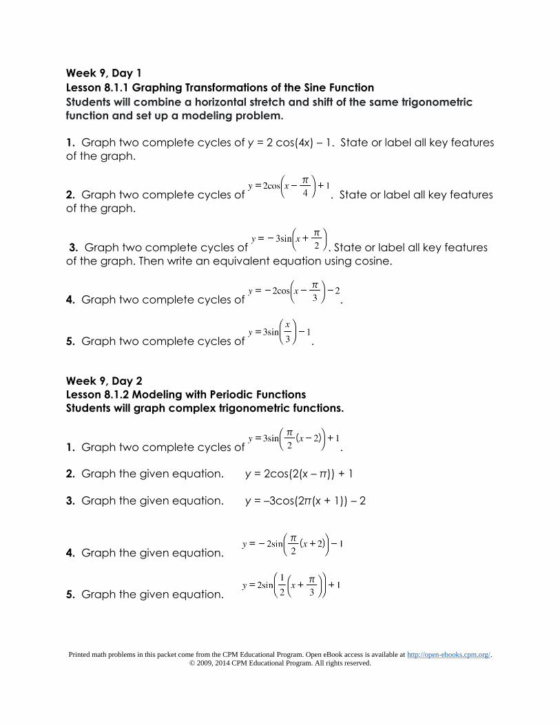
Week 9, Day 1

Lesson 8.1.1 Graphing Transformations of the Sine Function

Students will combine a horizontal stretch and shift of the same trigonometric

function and set up a modeling problem.

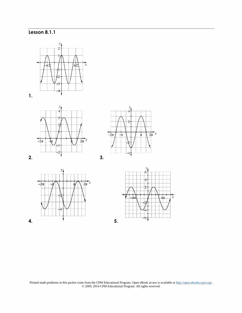
1. Graph two complete cycles of y = 2 cos(4x) – 1. State or label all key features

of the graph.

2. Graph two complete cycles of . State or label all key features

of the graph.

3. Graph two complete cycles of . State or label all key features

of the graph. Then write an equivalent equation using cosine.

4. Graph two complete cycles of .


Week 9, Day 2

Lesson 8.1.2 Modeling with Periodic Functions

Students will graph complex trigonometric functions.


2. Graph the given equation. y = 2cos(2(x – π)) + 1

3. Graph the given equation. y = –3cos(2π(x + 1)) – 2

4. Graph the given equation.

5. Graph the given equation.




Week 9, Day 3

Lesson 8.1.3 Improving the Spring Problem

Students will identify the amplitude and period of a trigonometric function and

transform their graphs.

1. Identify the amplitude, period, horizontal shift, and vertical shift of the given

trigonometric function. Use the information to sketch two complete cycles of the

function.

f(x) = 4 − 3sin(2πx + π)



function.

f(x) = −3cos(2x – 1) + 2



function.

f(x) = 2sin(4x + π) − 1



function.

f(x) = 3 + 2cos(3 − 6x)




Week 9, Day 4

Lesson 8.2.1 Graphing Reciprocal Trigonometric Functions

Students will look at the values and graphs of all 6 trigonometric functions.

1. If and , determine the values of the other five trigonometric

ratios.

2. If and , determine the values of the other five

trigonometric ratios.

3. If and , determine the values of the other five trigonometric

ratios.

4. If and , evaluate csc( ) and cot( ).

5. If and , determine the values of the other five

trigonometric ratios.

Week , Day 5

Lesson 8.3.1 Simplifying Trigonometric Expressions

Students will simplify trigonometric expressions by rewriting in terms of sine and

cosine and determine special angles for trigonometric ratios from the unit circle.

1. Rewrite the given expression as a single trigonometric ratio.

tan(A)(csc(A) − sin(A))

2. Rewrite the given expression as a single trigonometric ratio.

(csc(x) + cot(x))(1 − cos(x))

3. Simplify the following trigonometric expression.

4. Simplify the following trigonometric expression. (cos2(x))(sec2(x) − 1)


6. Simplify the following trigonometric expression. sin2(x) · sec(x) + cos(x)




Week 10, Day 1

Lesson 8.3.2 Proving Trigonometric Identities

Students will prove trigonometric identities.


2. Simplify: − sin(x)csc(x)

3. Simplify: cos(x) + tan(x) sin(x)

4. Let f(x) = csc(x) tan(x).

a. Graph y = f(x).

b. Evaluate .

c. Is f continuous at x = 0. Use the formal definition of continuity to explain your answer.

5. Let f(x) = .

a. Graph y = f(x).

b. Evaluate .

c. Use a table or graph to evaluate .

d. Is f continuous at x = 0. Use the formal definition of continuity to explain your answer.

6. Simplify:

7. Simplify: sec(x) − 8. Simplify: sin(x)[cot(x) + tan(x)]

9. Simplify: csc(θ)(csc(θ) − sin(θ)) + + cot(θ)

10. Simplify: − cot(A)




Week 10, Day 2

Lesson 8.3.3 Angle Sum and Difference Identities

Students will verify trigonometric identities.

1. Verify the given trigonometric identity. (tan(x) + cot(x))2 = sec2(x) + csc2(x)

2. Verify the given trigonometric identity.

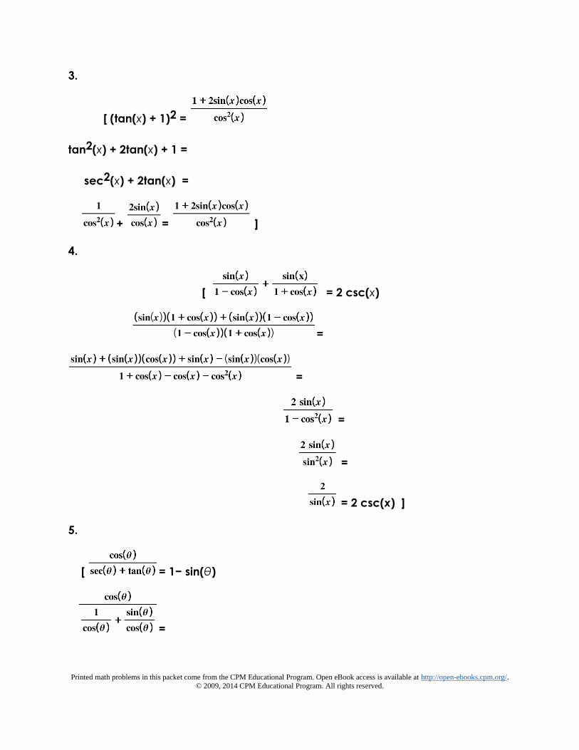
3. Verify the given trigonometric identity.

(tan(x) + 1)2 =

4. Verify the given trigonometric identity. = 2 csc(x)

5. Verify the trigonometric identity. = 1− sin(θ)

6. Solve sin(x) – sin(2x) = 0 for all values of x. Show all work.

7. Use at least one of trigonometric identities you have learned to simplify or

expand the given equation and then solve for x, given .

sin(2x) – sin(x) = 0

8. Use at least one of trigonometric identities you have learned to simplify or

expand the given equation and then solve for x, given .




Week 10, Day 3

Lesson 8.3.4 Double-Angle and Half-Angle Identities

Students will use the angle sum and difference identities and double-angle and

half-angle identities for sine and cosine to solve problems.

1. Use an angle sum or difference formula to determine the exact value of the

given expression.

sin(165º)

2. Use an angle sum or difference formula to determine the exact value of the

given expression.

tan(–15º)

3. Use an angle sum or difference formula to simplify the given expression and

determine its exact value.

cos(12º) cos(18º) – sin(12º) sin(18º)

4. Use an angle sum or difference formula to simplify the given expression and

determine its exact value.

sin(74º) cos(14º) – cos(74º) sin(14º)

Week 10, Day 4

Lesson 8.3.5 Solving Complex Trigonometric Equations

Students will solve trigonometric equations using identities and algebraic

simplifications.

1. Solve 2cos2(x) + sin(x) = 2 for . Show all work.

2. Solve sin(x) – sin(2x) = 0 for all values of x. Show all work.

3. Determine at least three values for x which satisfy the following equation:

sin2(x) – sin(x) = 2

4. Determine the solutions to the given trigonometric equation for .

sin2(x) – sin(x) = cos2(x)


tan(x)cos(x) = cos(x)





sin2(x) + cos(x) + 1 = 0


2sin(x)cos(x) = –sin(x)




Selected Answers

Lesson 3.1.1

1. a. b.

2. a. b.

3. a. b.

4. 5. 6. 7.

8.

Lesson 3.1.2

1. 2. 3. xy 4.

5. 6.

Lesson 3.1.3

1.

2.

3.

4.




Lesson 3.1.4

1. x2 – 2x – 3

2. 6x4 + 5x3 + 5x2 + 5x + 5

3. x3 + x2 + 2x –3 –

4. Yes, it divides with a remainder of 0.

5.

Lesson 3.1.5

1.

a. b. 11 miles c.

2. 12, 16, 20

3. 25.6 feet

4. $42,222.22

5.




Lesson 3.2.1

1. 31 + 107 + 255 + 499

2. 8 + 17 + 32 + 53

3. 5 + 9 + 13 + 17 + 21

4. Other answers are possible.

5. Other answers are possible.

Lesson 3.2.2

1.

2.

3.

4. [ ]

Lesson 3.2.3

1.

2.




3.

4.

Lesson 3.2.4

1. [0.6( (0.6n + 1 − 1)2 + 4)] = [0.6(0.12n2 + 4)]= 15.96 u2; overestimate

2.

a. ≈ 12.450

b. underestimate

c. Change the summation to be .

3. [ ( + 7) ≈ 37.482 un2 ]

4. ≈ 37.128 un2

U-Substitution

1. 2. 3.

4.

5. 6. 7.

8.

9.




Lesson 4.1.1

1. 2. 3.

4. 5.

6. The graph decreases and flattens at (1, 0) and then continues to decrease for another 4.5 miles until it

reaches the lowest point, approximately 3.4 miles below the ocean basin. The graph then starts to increase

until it reaches the ocean basin again at (7, 0).

Lesson 4.1.2

1. p(x) = (x2 – 6x + 4)(x + 1) 2. p(x) = (x2 – 4)(x – 5) 3. p(x) =

3(x2 + 2x – 2)(x – 4)

4. p(x) = a(x2 − 14x + 53)(x + 5)(x − 3)2 5. p(x) = (x2 – 6x + 13)(x2 –

2x – 4)(x – 8)

Lesson 4.1.3

1. 2.

3.

4.

5. a. No, f(2) ≠ 0.




b. The curve must cross the x-axis somewhere between those two points. More

specifically, it must cross the x-axis somewhere in the interval of −1.7 < x < 0

because the y-intercept is −4.

x = − ,

Lesson 4.2.1

1. f(x) = + 2;

2. f(x) = + 3;

3. f(x) = + 13

4. f(x) = − 12

5. f(x) = + 3;




Lesson 4.2.2

1. f(x) = + 2;

2. a.

b. D: x ≠ π, 6; R: y ≥ −4

3. a. n = −2 b. f(x) = −

4. r(x) = 1 + ; If b = 0, there is no y-intercept. For a ≠ b, no real values exist

for a such that there is no x intercept. If a = b, then there is no xintercept




because r(x) = 1, which is a horizontal line (with a hole at x = a).

5. Allow the use of a graphing calculator on this problem.

r(x) = ]

6. Allow the use of a graphing calculator on this problem.

r(x) =

Lesson 4.2.3

1. y = 54 2. y = –1 3. y = 0 4. y = 0 5. y =

Lesson 4.3.1

1. 2. 3.

4. ( ]

5. [ ) 6. 7. [ )

Lesson 4.3.2

1. 2.

3. slant: ; vertical: 4. ;

5. a. t = 0, 2, 5, 8

b. (0, 2) (2, 5) (8, 10)

c. 1.75 feet below the branch.




Lesson 5.1.1

1. y = 16 2. y = 3. y = 27

4. a. 42.67 g ] [ b. After ≈ 27 hours.

5. 16.2 years

6. 1.24%

7. 6.23 years

Lesson 5.1.2

1. 2. 3. 4. 5.

Lesson 5.1.3

1. a. b. logA (B) = y 2. a. = −2 b. BK = M

3. a. VC = I b. log7(M) = x

4. a. f d − 2 = g b. log4(n + 1) = x 5. f −1(x) = 3x − 2

Lesson 5.2.1

1. 2. 3.

4. ;




5. a. b. f(x) = log2(x + 2)

6. a. exponential (with base e) b.

7. ; Methods will vary, but may include using a composition of

functions to show that the end output is equal to the initial output, graphing the

functions to show that they are symmetric with respect to the line y = x, the use of

tables, and/or deriving the inverse equation using algebra.

8. Logarithms should be used to solve an equation that has the variable in the

exponent.

9. Keith is correct. The variable is not in the exponent in this

equation.

Lesson 5.2.2

1. a. 4 b. 2 c. 5

2. a. 3 b. 2 c. 1

3. a. 5 b. 0.5 c. 0

4. a. 4 b. 1.25 c. 21

5. a. b.

6. a. b. 4

7. a. 1 b.

8. a. 16 b.

9. a. b. 320

10. a. b. 2 ]

11. a. 71 b.




12. a. b.

Lesson 5.2.3

1. 2. 3.

4.

5. 3.2 6. 16.2 7. 5.4 8. 15.9

9. 10.

11. 12. 9.9 13. 14.

15.

Lesson 5.2.4

1. x = 2. x = 2 3. x = 4. x =

5. x = −1 6. x =

7. x ≈ 13.572 8. x = ±55 9. x = ±1915/16 ≈ ±5.162

10. x = ≈ 0.387

11. x = 3.32 12. x = 1.09 13. x = log(3) ≈ 0.477 14. x = 0.89

Lesson 5.2.5

1. x = 2. x = 3. x = 25 4. x = 10

5. k = ln(m)

6. x =




7. a. b.

8. a. x ≈ 3.546 b. x = 3 9. x = 15

10. a. or b.

11. a. x = e2 + 5e + 2 ≈ 22.980 b. x = –ln(7) ≈ –1.946

Lesson 7.1.1

1 a. 2 b. 1 c. 3 d. DNE

2. a. ∞ b. −1 c. DNE but f(x) → −∞ d. 1 e. −2 f. 1

g. 0 h. DNE

Lesson 7.1.2

1. a. −2 b. DNE but f(x) → − ∞ c. 1 d. 1 e. −3

f. DNE but f(x) → ∞ g. −2

2. a. −2 b. 3 c. 1 d. −1 e. −1 f. 2

g. DNE but f(x) → ∞

3. a. –5 b. 6 c. –1

4. a. –1 b. 11 c. 1

Lesson 7.1.3

1. a. ∞ b. −1 c. DNE but f(x) → −∞ d. 1 e. −2

f. 1 g. 0 h. DNE

2. a. −2 b. DNE but f(x) → − ∞ c. 1 d. 1 e. −3

f. DNE but f(x) → ∞ g. −2

3. a. −2 b. 3 c. 1 d. −1 e. −1 f. 2

g. DNE but f(x) → ∞




4. –4

5. See completed table below.

6. See completed table below.

7. 5 8. 2 9. DNE, but the function 10. 3

11. –5 12. –5

13. DNE, but the function 14. a. 7 b. 0

15. a. DNE b.

Lesson 7.1.4

1.

a. 3,

b. 1,

c. not continuous;

2.

a. no; ;

b. yes; ;

c. no;

3. continuous;




4. not continuous;

5. not continuous; f(−5) DNE

6. continuous;

Lesson 7.2.1

1. a.

b.

time

period

change in

account balance

0 − 1 769

1 − 3 –86

3 − 6 83

6 − 9 –122

9 − 12 29

c. Increasing by approximately $47.25 per month.

d. $6177

2. a. Note: Students should use a calculator to create a model. C(t) = 103.2t +

1677.3 where t is the number of years after 1950.

b. 99.11 million tons per year.




c. 8901 million tons. The graph is linear, so the carbon emissions will still be

increasing at a rate of approximately 103.2 million tons per year.]

3. b. See table below.

time interval (minutes) change in HR (bpm)

0 − 15 3.33

15 − 20 4

20 − 25 3

25 − 27 2.5

27 − 28 −13

28 − 30 −15

c. At first, the as the heart rate increases, so does the change in heart rate. After

20 minutes the heart rate continues to increase, but the change in heart rate

decreases. After 27 minutes the heart rate decreases and so does the change in

heart rate. This is seen by the concavity of the graph. After 15 minutes the graph

is concave down.

d. The person starts out jogging and their heart rate increases significantly. After

15 minutes the person starts to pick up speed. From approximately 25 to 27

minutes they run as fast as they can. They are then tired and go back to jogging

for 3 more minutes until they are done with their workout.]

Lesson 7.2.2

1. a. t ≈ 8.031 s

2. See table below.




c See table below.

d. It is decreasing by 32 over each interval. It changed from positive to negative

after 4 seconds.

e. Positive velocity indicates that the ball is rising for 4 seconds. The velocity

then changes to a negative value indicating that the ball is falling.

3. a. −32 ft/s

b. 2 − 2.56 seconds: AROC = −73 ft/s ]

c. Average velocity = 26.67 mph. Yes, at some point the car picked up speed

and was traveling at 22.67 mph.

d. The car leaves home and drives through a neighborhood. After 5 minutes

they realize that something was forgotten at home and must head back. After 10

minutes they arrive home. They head out again through the neighborhood. After

15 minutes they are on larger, faster city streets. After 30 minutes they get on a

highway where they can travel at a higher rate of speed, but there is some

traffic. ]

4.

5.

t 0 1 2 3 4 5 6 7 8 9

h(t) 4 116 196 244 260 244 196 116 4 −140

Δ t 0 − 1 1 − 2 2 − 3 3 − 4 4 − 5 5 − 6 6 − 7 7 − 8 8 − 9

Δ

h(t) 112 80 48 16 –16 −48 −80 −112 −144




6. a. 6 − b.

c. ; This is the slope of the line tangent to the curve at x = 9. ]

Lesson 7.2.3

1. 11 + 2h 2. 10 + h 3. 10 + h 4. 3h + 16 ]

Lesson 7.2.4

1. –4h + 35 2. –7h – 107 3. 4.

Lesson 7.2.5

1. a. 6 − b.

c. ; This is the slope of the line tangent to the curve at x = 9. ]

2. a. − 1

b. − 1 ; This is the slope of the line tangent to the curve at x = 7. ]

3. a. h + 2a + 1

b. 2a + 1; The slope of the line tangent to the curve at any point x = a is 2a + 1. ]

4. a. 3h + 6a − 2

b. 6a − 2; The slope of the line tangent to the curve at any point x = a is 2a + 1. ]




Lesson 8.1.1

1.

2. 3.

4. 5.




Lesson 8.1.2

1. 2.

3.

4. 5.




Lesson 8.1.3

1. amplitude = 3, period = 1, horizontal shift = units, vertical shift = 4 units.

2. amplitude = 3, period = π, horizontal shift = units, vertical shift = 2 units.

3. amplitude = 2, period = , horizontal shift = units, vertical shift = –1 units.

‘




4. amplitude = 2, period = , horizontal shift = units, vertical shift = 3 units.

5. amplitude = 2, period = 8, vertically reflected, shifted right 3 units, shifted up 1

unit.

Lesson 8.2.1

1.

2.

3.

4.

5.

Lesson 8.3.1

1. cos(A) 2. sin(x) 3. sin(x) 4. sin2(x)

5. csc(x) 6. sec(x)




Lesson 8.3.2

1. cos(x) 2. −cos2(x) 3. sec(x)

4. a. Teams should graph the function y = sec(x)., b. 0, c. No, the limit exists,

but f(0) is undefined. ]

5. a. Teams should graph y = sin(x)., b. DNE, c. 0, d. No, the limit exists, but f(0)

is undefined. ]

6. sec(x) 7. tan(x) 8. sec(x) 9. csc2(θ)

10. cos(A)

Lesson 8.3.3

1. (tan(x) + cot(x))2 = sec2(x) + csc2(x)

tan2(x) + 2tan(x) cot(x) + cot2(x) =

tan2(x) + 2 + cot2(x) =

tan2(x) + 1 + cot2(x) + 1 = sec2(x) + csc2(x) ]

2.

[ =

=

sin(x) · =

= ]




3.

[ (tan(x) + 1)2 =

tan2(x) + 2tan(x) + 1 =

sec2(x) + 2tan(x) =

+ = ]

4.

[ = 2 csc(x)

=

=

=

=

= 2 csc(x) ]

5.

[ = 1− sin(θ)

=




=

cos(θ) · =

=

=

= 1 − sin(θ) ]

6.

7.

Lesson 8.3.4

1. 2. 3. 4.

5.

Lesson 8.3.5

1. 2.

3.

4. 5. 6.

7.


PDF Pre-Calculus - Detroit Public Schools Community District

Documents

Transcript of PDF Pre-Calculus - Detroit Public Schools Community District