Path Planning for Self-Collision Avoidance of Space Modular ...

��

Citation: An, J.; Li, X.; Zhang, Z.;

Zhang, G.; Man, W.; Hu, G.; He, J.

Path Planning for Self-Collision

Avoidance of Space Modular

Self-Reconfigurable Satellites.

Aerospace 2022, 9, 141. https://

doi.org/10.3390/aerospace9030141

Academic Editor: Dario Modenini

Received: 19 February 2022

Accepted: 3 March 2022

Published: 5 March 2022

Publisher’s Note: MDPI stays neutral

with regard to jurisdictional claims in

published maps and institutional affil-

iations.

Copyright: © 2022 by the authors.

Licensee MDPI, Basel, Switzerland.

This article is an open access article

distributed under the terms and

conditions of the Creative Commons

Attribution (CC BY) license (https://

creativecommons.org/licenses/by/

4.0/).

aerospace

Article

Path Planning for Self-Collision Avoidance of Space ModularSelf-Reconfigurable SatellitesJiping An , Xinhong Li *, Zhibin Zhang, Guohui Zhang, Wanxin Man, Gangxuan Hu and Junwei He

Department of Aerospace Science and Technology, Space Engineering University, Beijing 101416, China;[email protected] (J.A.); [email protected] (Z.Z.); [email protected] (G.Z.);[email protected] (W.M.); [email protected] (G.H.); [email protected] (J.H.)* Correspondence: [email protected]

Abstract: Space modular self-reconfigurable satellite (SMSRS) is a new type of satellite. The researchon self-collision avoidance of SMSRS is important for its on-orbit safety but is not completely solved.This paper offers a new method for joint path planning for self-collision avoidance of SMSRS. Firstly,we establish the collision detection model for SMSRS based on forward kinematics and the sphericalnonholonomic envelope to detect the collision occurring in SMSRS. Then, to achieve offline pathplanning in joint space, we proposed the self-collision avoidance strategy, which splices multipleC-spaces based on the pre-defined joint path into a binary map, and then transforms the binarymap into a map with the dangerous potential field, and planning algorithms based on a mapwith the dangerous potential field is proposed to find the optimal collision-free path. The newmethod is applied to two cases and both find collision-free joint paths for SMSRS successfully, whichdemonstrates the feasibility of the method. In addition, this study bridges the gap in the study ofself-collision avoidance of super-redundant self-reconfigurable satellites.

Keywords: self-collision avoidance; path planning; self-reconfigurable satellite; collision detection model

1. Introduction

With the large-scale exploitation of outer space and the increasing frequency of space-craft and satellite launches, future space systems are expected to have low cost, rapidresponse, and multiple uses [1]. However, the traditional development mode cannot meetthe needs of future space systems [2]. For example, traditional space systems are almostspecially designed for missions, requiring subsystem-by-subsystem development and nu-merous iterations, which are slow, repetitive, and expensive [3]. In addition, the structuresof these traditional spacecraft systems are essentially permanently fixed and designed toperform a single mission that cannot be reconfigured for other missions. Long developmentcycles and launch-window limitations also make it difficult for them to respond quickly toemergencies [3].

To overcome these limitations of existing space systems, many new concept satelliteshave been proposed, and the most representative ones are CubeSats [4,5]. The primarygoal of CubeSats is to provide a small, lightweight, low-cost platform for academic andtechnology demonstration. A CubeSat is a 10 cm× 10 cm× 10 cm cube. It provides astandard for the design of picosatellites to reduce cost and development time, increaseaccessibility to space, and sustain frequent launches [6]. The spacecraft bus was designedto be versatile enough to accommodate different payloads that meet the mass, volume, andpower constraints. Presently, the CubeSat Projects become attractive for wide fields [7,8],such as exoplanet detection [9,10], space weather [11], weather forecasting [12], and river-flow estimation [13].

However, the utilization of a standard, low-cost satellite bus will reduce the reliabilityand decrease the lifetime of Cubesats [14,15]. A statistical study performed in 2013 on the

Aerospace 2022, 9, 141. https://doi.org/10.3390/aerospace9030141 https://www.mdpi.com/journal/aerospace

https://doi.org/10.3390/aerospace9030141


https://creativecommons.org/

https://creativecommons.org/licenses/by/4.0/

https://creativecommons.org/licenses/by/4.0/

https://www.mdpi.com/journal/aerospace

https://www.mdpi.com

https://orcid.org/0000-0001-6401-7934


https://www.mdpi.com/journal/aerospace

https://www.mdpi.com/article/10.3390/aerospace9030141?type=check_update&version=2

Aerospace 2022, 9, 141 2 of 27

first 100 launched CubeSats [16] shows that the mission failures of CubeSats are on a highlevel [17]. In addition, the structure of CubeSat is fixed, and it carries limited payloads sothat they can only perform a single space task.

Taking the design concept of CubeSat as the baseline, we proposed a new type ofsatellite with a reconfigurable structure and adjustable function, named Space ModularSelf-Reconfigurable Satellite (SMSRS). SMSRS has the following features:

(1) Modular: SMSRS has a chain structure composed of functional modules and joints.Common satellite subsystems are integrated into unit modules and are called subsystemmodules. The unit subsystem modules are installed with standard interfaces for payloadsand joints. According to shapes and work positions, the payloads are designed as externalstructures carrying standard docking interfaces to the subsystem modules, or as unitpayload modules. The modular design of SMSRS facilitates the structural folding andpackaging before launch and the reconfiguration in space [18].

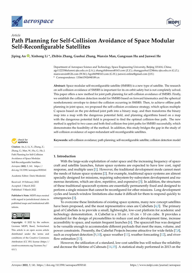
(2) Scalability: Payload and subsystem modules are functionally independent andphysically separated from each other. The volumes and masses of module units are dividedinto several series from small to large, which can be selected according to the demand ofpayloads. All modules have standard interfaces, which are used to connect with modularjoint modules for ground or in-orbit extension according to the type of space mission. Thetype and number of modules carried by SMSRS are configured to mission requirements.The model of the SMSRS with five modules is shown in Figure 1.

Aerospace 2022, 9, 141 2 of 28

However, the utilization of a standard, low-cost satellite bus will reduce the reliabil-ity and decrease the lifetime of Cubesats [14,15]. A statistical study performed in 2013 on the first 100 launched CubeSats [16] shows that the mission failures of CubeSats are on a high level [17]. In addition, the structure of CubeSat is fixed, and it carries limited pay-loads so that they can only perform a single space task.

Taking the design concept of CubeSat as the baseline, we proposed a new type of satellite with a reconfigurable structure and adjustable function, named Space Modular Self-Reconfigurable Satellite (SMSRS). SMSRS has the following features:

(1) Modular: SMSRS has a chain structure composed of functional modules and joints. Common satellite subsystems are integrated into unit modules and are called sub-system modules. The unit subsystem modules are installed with standard interfaces for payloads and joints. According to shapes and work positions, the payloads are designed as external structures carrying standard docking interfaces to the subsystem modules, or as unit payload modules. The modular design of SMSRS facilitates the structural folding and packaging before launch and the reconfiguration in space [18].

(2) Scalability: Payload and subsystem modules are functionally independent and physically separated from each other. The volumes and masses of module units are di-vided into several series from small to large, which can be selected according to the de-mand of payloads. All modules have standard interfaces, which are used to connect with modular joint modules for ground or in-orbit extension according to the type of space mission. The type and number of modules carried by SMSRS are configured to mission requirements. The model of the SMSRS with five modules is shown in Figure 1.

Figure 1. Model of SMSRS with five modules.

(3) Structural Reconfigurability: There are three mutually orthogonal joints between modules of SMSRS. The three joints form degrees of freedom (DOFs) between modules in relative rotation, roll, and yaw and enable the SMSRS to self-reconfigure adaptively to mission command.

(4) Risk resistance. The scalability and modularity together determine the risk re-sistance of SMSRS. Since modules are functionally independent, the failure of a local sat-ellite module makes the satellite not completely fail, and the multiple payloads it carries can still be reprogrammed functionally. In addition, multiple joints between modules al-low the modules to maintain some relative motion capability in the event of a single joint failure.

(5) Functional Adjustability: The types of payloads carried by SMSRS include optical cameras, SAR, communication payloads, etc. While carrying different payloads, SMSRS arranges and reorganizes these payloads in different space orientations by structural re-configuration and therefore achieves the ability to accomplish multiple types of space mis-sions. There are typical application scenarios for SMSRS: • When SMSRS carries multiple optical cameras, it could change the spatial orienta-

tions of these cameras through joint motions. With this, these cameras could achieve

Figure 1. Model of SMSRS with five modules.

(3) Structural Reconfigurability: There are three mutually orthogonal joints betweenmodules of SMSRS. The three joints form degrees of freedom (DOFs) between modulesin relative rotation, roll, and yaw and enable the SMSRS to self-reconfigure adaptively tomission command.

(4) Risk resistance. The scalability and modularity together determine the risk resis-tance of SMSRS. Since modules are functionally independent, the failure of a local satellitemodule makes the satellite not completely fail, and the multiple payloads it carries can stillbe reprogrammed functionally. In addition, multiple joints between modules allow themodules to maintain some relative motion capability in the event of a single joint failure.

(5) Functional Adjustability: The types of payloads carried by SMSRS include opticalcameras, SAR, communication payloads, etc. While carrying different payloads, SMSRSarranges and reorganizes these payloads in different space orientations by structuralreconfiguration and therefore achieves the ability to accomplish multiple types of spacemissions. There are typical application scenarios for SMSRS:

• When SMSRS carries multiple optical cameras, it could change the spatial orientationsof these cameras through joint motions. With this, these cameras could achieve anexpanded imaging area by stitching together their field of view as shown in Figure 2a,or achieve the reconnaissance of multiple targets as shown in Figure 2b.

• When SMSRS carries multiple communication payloads and adjusts them towardsdifferent orientations, it can achieve multi-area communication to the earth, as shownin Figure 2c.

Aerospace 2022, 9, 141 3 of 27

Aerospace 2022, 9, 141 3 of 28

an expanded imaging area by stitching together their field of view as shown in Figure 2a, or achieve the reconnaissance of multiple targets as shown in Figure 2b.

• When SMSRS carries multiple communication payloads and adjusts them towards different orientations, it can achieve multi-area communication to the earth, as shown in Figure 2c. The application scenarios of SMSRS are by no means limited to these, and there are

larger expansions. Moreover, in recent years, a large number of small satellite launches have led to space traffic congestion and burdened space traffic management. At the same time, a large amount of space debris is generated, which seriously threatens the safety of satellites in orbit. The multi-functional feature of SMSRS, which allows a single satellite to perform multiple functions adaptively, can reduce the number of satellite launches. It re-duces the pressure of space traffic management and the generation of space debris.

The target orbit of SMSRS is Low Earth Orbit (LEO). The advantage of standing high and seeing far in High Earth Orbit (HEO) can be compensated by the feature of SMSRS multi-payload synergy, e.g., the large field of view of HEO satellites can be achieved by using fields of view stitching of SMSRS. In addition, LEO launches can launch heavier mass satellites at a lower cost, providing margin for SMSRS in-orbit scalability.

When running on LEO, the satellite tracking is characterized by low transmission delay, low coverage, low link loss, and low power consumption. The low transmission delay and low loss are beneficial to the command transmission of the reconfiguration for SMSRS, and in solving the low coverage problem, as shown in Figure 2c, adjusting the orientation of the tracking system can be used to expand the tracking range.

(a) (b)

(c)

Figure 2. Application scenarios for SMSRS: (a) SMSRS carries multiple optical cameras and expands the imaging area by stitching together fields of view. (b) SMSRS reconnaissance of multiple targets by multiple optical cameras. (c) SMSRS carries multiple communication payloads to achieve multi-area communication to the earth.

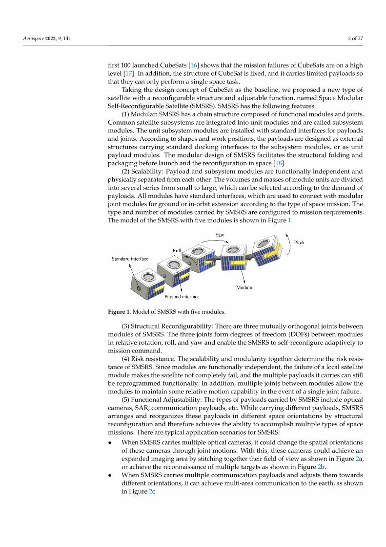
As shown in Figure 3, SMSRS are folded and packed on the ground before launch. After getting into orbit, the folded configuration is gradually unfolded and changed from the initial configuration to the work configuration for performing the designed mission. When the SMSRS receives a new mission command, its mission planning system will plan

Figure 2. Application scenarios for SMSRS: (a) SMSRS carries multiple optical cameras and expandsthe imaging area by stitching together fields of view. (b) SMSRS reconnaissance of multiple targets bymultiple optical cameras. (c) SMSRS carries multiple communication payloads to achieve multi-areacommunication to the earth.

The application scenarios of SMSRS are by no means limited to these, and there arelarger expansions. Moreover, in recent years, a large number of small satellite launcheshave led to space traffic congestion and burdened space traffic management. At the sametime, a large amount of space debris is generated, which seriously threatens the safety ofsatellites in orbit. The multi-functional feature of SMSRS, which allows a single satelliteto perform multiple functions adaptively, can reduce the number of satellite launches. Itreduces the pressure of space traffic management and the generation of space debris.

The target orbit of SMSRS is Low Earth Orbit (LEO). The advantage of standing highand seeing far in High Earth Orbit (HEO) can be compensated by the feature of SMSRSmulti-payload synergy, e.g., the large field of view of HEO satellites can be achieved byusing fields of view stitching of SMSRS. In addition, LEO launches can launch heavier masssatellites at a lower cost, providing margin for SMSRS in-orbit scalability.

When running on LEO, the satellite tracking is characterized by low transmissiondelay, low coverage, low link loss, and low power consumption. The low transmissiondelay and low loss are beneficial to the command transmission of the reconfiguration forSMSRS, and in solving the low coverage problem, as shown in Figure 2c, adjusting theorientation of the tracking system can be used to expand the tracking range.

As shown in Figure 3, SMSRS are folded and packed on the ground before launch.After getting into orbit, the folded configuration is gradually unfolded and changed fromthe initial configuration to the work configuration for performing the designed mission.When the SMSRS receives a new mission command, its mission planning system will planthe new mission configuration and send the joint control system command for reconfiguringto the new work configuration. Modules of SMSRS have solar cells attached to each surfaceto ensure battery recharging in different configurations.

Aerospace 2022, 9, 141 4 of 27

Aerospace 2022, 9, 141 4 of 28

the new mission configuration and send the joint control system command for reconfig-uring to the new work configuration. Modules of SMSRS have solar cells attached to each surface to ensure battery recharging in different configurations.

Figure 3. Configurations of SMSRS from the folded state to unfolded state and work state. (a) Folded state, (b) Unfolding, (c) Unfold state, (d) Work state.

The function switching of SMSRS depends largely on the motion of the joints. How-ever, from Figure 1, it can be seen that the modules of SMSRS are large in size but small in spacing between each other, and the motion of the joints allows the relative positions of these modules to change over a wide range so that collisions between modules can easily occur. When a collision occurs, it is likely to cause structural damage and instability of the system [19]. To avoid self-collisions between modules in whole reconfiguration pro-gress is crucial for the on-orbit safety of the system [20]. In this paper, we will study how to achieve self-collision avoidance in the reconfiguration of SMSRS.

The remaining paper is organized as follows. Section 2 sorts out the related work on self-collision avoidance of self-configuring systems. In Section 3, the collision detection model of SMSRS is established. Section 4 elaborates on the self-collision strategy of SMSRS. In Section 5, the parameters of SMSRS and two self-collision avoidance tasks are set. Section 6 verifies the self-collision avoidance path planning method. Section 7 sum-marizes the work of this paper.

2. Related Work The researches on avoiding self-collision are mainly for redundant robotic arms, and

the contents mainly involve two aspects: self-collision detection and self-collision avoid-ance strategies. Collision detection focuses on establishing an approximate geometric model of the collision-prone structures of the research object to calculate the relative po-sition between them [21] and to judge whether they will collide or have collided. There are two common methods to establish the collision detection model. The first method uses a large number of polygons [22,23] to model the geometrical shapes of collision-prone structures to fit them as closely as possible. This method is generally suitable for systems that have an irregular shape and higher requirements for collision detection accuracy, or are used to perform sophisticated tasks, but it requires higher computational costs. For systems with regular shapes or have low requirements for collision detection accuracy, using the sphere-based model to establish its approximate structural envelope is another method [20,21]. These approximate envelopes can be selected according to the shape of the system, including spheres [21,24], swept-spheres [25], cylinders [20], capsules [26], patch-based bounding volumes [27], etc. Although the second method could not accu-rately describe the shape of the collision-prone structures, it is computationally economi-cal.

In the present research, self-collision avoidance strategies are usually divided into the online reactive approach [27,28] and offline path planning. Of the two, the online re-active approach does not predetermine the angle motion path but detects collisions in real

Figure 3. Configurations of SMSRS from the folded state to unfolded state and work state. (a) Foldedstate, (b) Unfolding, (c) Unfold state, (d) Work state.

The function switching of SMSRS depends largely on the motion of the joints. However,from Figure 1, it can be seen that the modules of SMSRS are large in size but small inspacing between each other, and the motion of the joints allows the relative positions ofthese modules to change over a wide range so that collisions between modules can easilyoccur. When a collision occurs, it is likely to cause structural damage and instability of thesystem [19]. To avoid self-collisions between modules in whole reconfiguration progress iscrucial for the on-orbit safety of the system [20]. In this paper, we will study how to achieveself-collision avoidance in the reconfiguration of SMSRS.

The remaining paper is organized as follows. Section 2 sorts out the related work onself-collision avoidance of self-configuring systems. In Section 3, the collision detectionmodel of SMSRS is established. Section 4 elaborates on the self-collision strategy of SMSRS.In Section 5, the parameters of SMSRS and two self-collision avoidance tasks are set.Section 6 verifies the self-collision avoidance path planning method. Section 7 summarizesthe work of this paper.

2. Related Work

The researches on avoiding self-collision are mainly for redundant robotic arms, andthe contents mainly involve two aspects: self-collision detection and self-collision avoidancestrategies. Collision detection focuses on establishing an approximate geometric model ofthe collision-prone structures of the research object to calculate the relative position betweenthem [21] and to judge whether they will collide or have collided. There are two commonmethods to establish the collision detection model. The first method uses a large number ofpolygons [22,23] to model the geometrical shapes of collision-prone structures to fit themas closely as possible. This method is generally suitable for systems that have an irregularshape and higher requirements for collision detection accuracy, or are used to performsophisticated tasks, but it requires higher computational costs. For systems with regularshapes or have low requirements for collision detection accuracy, using the sphere-basedmodel to establish its approximate structural envelope is another method [20,21]. Theseapproximate envelopes can be selected according to the shape of the system, includingspheres [21,24], swept-spheres [25], cylinders [20], capsules [26], patch-based boundingvolumes [27], etc. Although the second method could not accurately describe the shape ofthe collision-prone structures, it is computationally economical.

In the present research, self-collision avoidance strategies are usually divided into theonline reactive approach [27,28] and offline path planning. Of the two, the online reactiveapproach does not predetermine the angle motion path but detects collisions in real timeduring joint movements. Online reactive approaches usually use the distance functionsas “repulsive potential” functions and then converts them into joint velocities based onJacobian Inverse Kinematics (IK) [26] and joint torques for torque control schemes [29], orregards them as a constraint in an optimization-based IK solver to adjusts the joint motionpath in real time [28,30], etc. To obtain smooth joint motion trajectories, some researchershave proposed a unified framework to detect collisions by using a series of sensors capableof estimating joint torques and accelerations in real time. However, the use of expensivehardware such as sensors always increases the cost [21]. Although the online reactive

Aerospace 2022, 9, 141 5 of 27

approach has a shorter computation time, it is mostly applied to ground-based humanoidrobots and is only applicable to systems with fewer DOFs because of its instability.

Offline path planning can be divided into two categories: path planning of end-effectorin workspace [31,32] and path planning of joints in joint space [33,34]. As there is no end-effector of SMSRS, we do not discuss the path planning of the end-effector, but focus onthe path planning of the joints in joint space. In contrast to the online method, offline pathplanning predetermines the motion path of joints and there would not be self-collision whenjoints move along the predetermined path. Compared with the online reactive approach,offline path planning is more stable and efficient, and the planned paths are guaranteedto be optimal, which are more suitable for space systems with higher requirements forstability. Moreover, for SMSRS, offline path planning will not make its joints detour inspace, which is also of great significance for energy conservation. Therefore, offline pathplanning is the more suitable choice for the self-collision avoidance strategy of SMSRS.

Currently, offline path planning for collision avoidance of self-configuration systemssuch as space robotic arms is mostly focused on avoiding collision with fixed obstaclesor target vehicles in the environment [20,35]. The methods to avoid collision with obsta-cles in the environment include using a random search algorithm to find a collision-freejoint path in the Configuration Space (C-Space) of the robotic arm, and commonly usedalgorithms include the A* algorithm [36] and the Rapid Exploration Random Tree (RRT)algorithm [37–39], and using optimization techniques [40], etc. In addition, the currentoffline path planning only needs to find collision-free joint paths to achieve the desiredpose of the end effector, regardless of the pose of other intermediate structures [20]. The re-searches on self-avoidance are also mainly focused on systems with fewer DOFs. Therefore,current research cannot meet the requirements of self-collision path planning of SMSRS,mainly because it has the following newly derived difficulties:

(1) SMSRS has a super-redundant structure, and its ultra-high DOFs make collisionsbetween each module possible and easy;

(2) The pose of each module of SMSRS is changed in real time during reconfiguration, forone module, all other modules are its dynamic obstacles—this also imposes a burdenon collision detection; and

(3) Different from the robots that only achieve the pose of the end effector withoutcollision, SMSRS requires all modules to achieve desired poses without collision afterpath planning.

In this paper, considering the above difficulties and the actual space mission require-ments, we proposed a new self-collision avoidance method for SMSRS, which consists of acollision detection model and a self-collision avoidance strategy. The collision detectionmodel is established based on the Forward Kinematics (FK) and spherical nonholonomicenvelope, which has no hardware cost and low computational cost. Among the offline andonline strategies, considering the high stability requirements of the SMSRS and reducingadditional hardware as much as possible, the offline path planning is selected to realizeself-collision avoidance of SMSRS, and a self-collision avoidance path planning strategybased on pre-defined path and spliced C-space is proposed.

The main contributions of this study are as follows: (1) a collision detection modelis developed using multiple discrete spherical, which can approximate envelop SMSRSusing a few spheres and execute collision detection for SSMSRS at a low computationalcost; (2) a method is proposed for splicing multiple C-spaces into a binary map basedon a pre-defined path, which transforms the path planning in dynamic C-space into theplanning of time sequence of joints on the pre-defined path; and (3) a new collision-freepath search algorithm based on the map with dangerous potential fields is proposed to findthe safest path without self-collision for SMSRS.

3. Collision Detection of SMSRS

The collision detection model of SMSRS is used to detect whether each module collideswith others, and the relative poses of modules are the basis of collision detection. SMSRS

Aerospace 2022, 9, 141 6 of 27

consists of a series of rigid bodies and its modules and inter-module connection structurescan also be regarded as links, and this structure forms a kinematic chain. We firstly ignorethe specific shape of modules and treat them as links, and calculate their space poses byestablishing an FK model in Section 3.1. On this basis, the collision detection model will becompleted after assigning the shape characteristics of these links in Section 3.2.

3.1. Module Pose

In SMSRS, each moveable joint defines a joint variable, all joints form a joints vectorq =

(θ1, θ1, · · · , θNj

)and the number of joints Nj defines DOFs of SMSRS. Calculating the

poses of links using the given values of the joint variables and the link parameters is aforward problem, which is known as FK [41,42]. In FK, the poses of links can be representedby a homogeneous transformation matrix. For example, the homogeneous transformationmatrix [43] of the ith link relative to the base coordinate system Σb is:

0i T =

nxi oxi axi pxinyi oyi ayi pyinzi ozi azi pzi0 0 0 1

=

[ [ni oi ai

]pi

0 1

]=

[Ri pi0 1

](1)

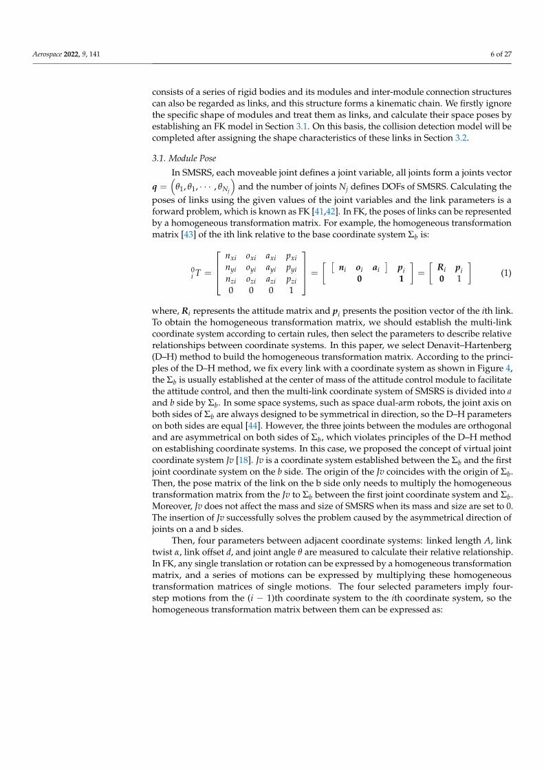
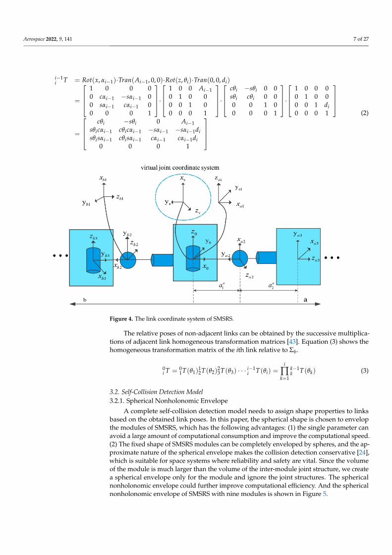
where, Ri represents the attitude matrix and pi presents the position vector of the ith link.To obtain the homogeneous transformation matrix, we should establish the multi-linkcoordinate system according to certain rules, then select the parameters to describe relativerelationships between coordinate systems. In this paper, we select Denavit–Hartenberg(D–H) method to build the homogeneous transformation matrix. According to the princi-ples of the D–H method, we fix every link with a coordinate system as shown in Figure 4,the Σb is usually established at the center of mass of the attitude control module to facilitatethe attitude control, and then the multi-link coordinate system of SMSRS is divided into aand b side by Σb. In some space systems, such as space dual-arm robots, the joint axis onboth sides of Σb are always designed to be symmetrical in direction, so the D–H parameterson both sides are equal [44]. However, the three joints between the modules are orthogonaland are asymmetrical on both sides of Σb, which violates principles of the D–H methodon establishing coordinate systems. In this case, we proposed the concept of virtual jointcoordinate system Jv [18]. Jv is a coordinate system established between the Σb and the firstjoint coordinate system on the b side. The origin of the Jv coincides with the origin of Σb.Then, the pose matrix of the link on the b side only needs to multiply the homogeneoustransformation matrix from the Jv to Σb between the first joint coordinate system and Σb.Moreover, Jv does not affect the mass and size of SMSRS when its mass and size are set to 0.The insertion of Jv successfully solves the problem caused by the asymmetrical direction ofjoints on a and b sides.

Then, four parameters between adjacent coordinate systems: linked length A, linktwist α, link offset d, and joint angle θ are measured to calculate their relative relationship.In FK, any single translation or rotation can be expressed by a homogeneous transformationmatrix, and a series of motions can be expressed by multiplying these homogeneoustransformation matrices of single motions. The four selected parameters imply four-step motions from the (i − 1)th coordinate system to the ith coordinate system, so thehomogeneous transformation matrix between them can be expressed as:

Aerospace 2022, 9, 141 7 of 27

i−1i T = Rot(x, αi−1)·Tran(Ai−1, 0, 0)·Rot(z, θi)·Tran(0, 0, di)

=

1 0 0 00 cαi−1 −sαi−1 00 sαi−1 cαi−1 00 0 0 1

·

1 0 0 Ai−10 1 0 00 0 1 00 0 0 1

·

cθi −sθi 0 0sθi cθi 0 00 0 1 00 0 0 1

·

1 0 0 00 1 0 00 0 1 di0 0 0 1

=

cθi −sθi 0 Ai−1

sθicαi−1 cθicαi−1 −sαi−1 −sαi−1disθisαi−1 cθisαi−1 cαi−1 cαi−1di

0 0 0 1

(2)

Aerospace 2022, 9, 141 7 of 28

Figure 4. The link coordinate system of SMSRS.

Then, four parameters between adjacent coordinate systems: linked length A, link twist 𝛼, link offset d, and joint angle θ are measured to calculate their relative relationship. In FK, any single translation or rotation can be expressed by a homogeneous transfor-mation matrix, and a series of motions can be expressed by multiplying these homogene-ous transformation matrices of single motions. The four selected parameters imply four-step motions from the (i-1)th coordinate system to the ith coordinate system, so the homo-geneous transformation matrix between them can be expressed as: 𝑇 = 𝑅𝑜𝑡(𝑥, 𝛼 ) ∙ 𝑇𝑟𝑎𝑛(𝐴 , 0,0) ∙ 𝑅𝑜𝑡(𝑧, 𝜃 ) ∙ 𝑇𝑟𝑎𝑛(0,0, 𝑑 )

= 1 0 0 00 𝑐𝛼 −𝑠𝛼 00 𝑠𝛼 𝑐𝛼 00 0 0 1 ∙ 1 0 0 𝐴0 1 0 00 0 1 00 0 0 1 ∙ 𝑐𝜃 −𝑠𝜃 0 0𝑠𝜃 𝑐𝜃 0 00 0 1 00 0 0 1 ∙ 1 0 0 00 1 0 00 0 1 𝑑0 0 0 1= 𝑐𝜃 −𝑠𝜃 0 𝐴𝑠𝜃 𝑐𝛼 𝑐𝜃 𝑐𝛼 −𝑠𝛼 −𝑠𝛼 𝑑𝑠𝜃 𝑠𝛼 𝑐𝜃 𝑠𝛼 𝑐𝛼 𝑐𝛼 𝑑0 0 0 1

(2)

The relative poses of non-adjacent links can be obtained by the successive multipli-cations of adjacent link homogeneous transformation matrices [43]. Equation (3) shows the homogeneous transformation matrix of the ith link relative to 𝛴 .

𝑇 = 𝑇(𝜃 ) 𝑇(𝜃 ) 𝑇(𝜃 ) ⋯ 𝑇(𝜃 ) = 𝑇(𝜃 ) (3)

3.2. Self-Collision Detection Model 3.2.1. Spherical Nonholonomic Envelope

A complete self-collision detection model needs to assign shape properties to links based on the obtained link poses. In this paper, the spherical shape is chosen to envelop the modules of SMSRS, which has the following advantages: (1) the single parameter can avoid a large amount of computational consumption and improve the computational speed. (2) The fixed shape of SMSRS modules can be completely enveloped by spheres, and the approximate nature of the spherical envelope makes the collision detection con-servative [24], which is suitable for space systems where reliability and safety are vital. Since the volume of the module is much larger than the volume of the inter-module joint

Figure 4. The link coordinate system of SMSRS.

The relative poses of non-adjacent links can be obtained by the successive multiplica-tions of adjacent link homogeneous transformation matrices [43]. Equation (3) shows thehomogeneous transformation matrix of the ith link relative to Σb.

0i T = 0

1T(θ1)12T(θ2)

23T(θ3) · · · i−1

i T(θi) =i

∏k=1

k−1k T(θk) (3)

3.2. Self-Collision Detection Model3.2.1. Spherical Nonholonomic Envelope

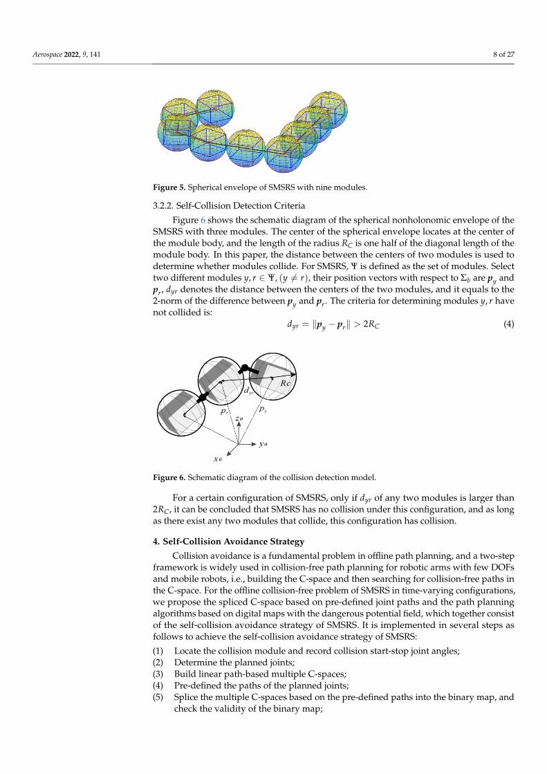
A complete self-collision detection model needs to assign shape properties to linksbased on the obtained link poses. In this paper, the spherical shape is chosen to envelopthe modules of SMSRS, which has the following advantages: (1) the single parameter canavoid a large amount of computational consumption and improve the computational speed.(2) The fixed shape of SMSRS modules can be completely enveloped by spheres, and the ap-proximate nature of the spherical envelope makes the collision detection conservative [24],which is suitable for space systems where reliability and safety are vital. Since the volumeof the module is much larger than the volume of the inter-module joint structure, we createa spherical envelope only for the module and ignore the joint structures. The sphericalnonholonomic envelope could further improve computational efficiency. And the sphericalnonholonomic envelope of SMSRS with nine modules is shown in Figure 5.

Aerospace 2022, 9, 141 8 of 27

Aerospace 2022, 9, 141 8 of 28

structure, we create a spherical envelope only for the module and ignore the joint struc-tures. The spherical nonholonomic envelope could further improve computational effi-ciency. And the spherical nonholonomic envelope of SMSRS with nine modules is shown in Figure 5.

Figure 5. Spherical envelope of SMSRS with nine modules.

3.2.2. Self-Collision Detection Criteria Figure 6 shows the schematic diagram of the spherical nonholonomic envelope of the

SMSRS with three modules. The center of the spherical envelope locates at the center of the module body, and the length of the radius RC is one half of the diagonal length of the module body. In this paper, the distance between the centers of two modules is used to determine whether modules collide. For SMSRS, 𝛹 is defined as the set of modules. Select two different modules 𝑦, 𝑟 ∈ 𝛹, (𝑦 ≠ 𝑟), their position vectors with respect to 𝛴 are 𝒑 and 𝒑 , 𝑑 denotes the distance between the centers of the two modules, and it equals to the 2-norm of the difference between 𝒑 and 𝒑 . The criteria for determining modules 𝑦, 𝑟 have not collided is: 𝑑 = 𝒑 − 𝒑 2𝑅 (4)

Figure 6. Schematic diagram of the collision detection model.

For a certain configuration of SMSRS, only if 𝑑 of any two modules is larger than 2𝑅 , it can be concluded that SMSRS has no collision under this configuration, and as long as there exist any two modules that collide, this configuration has collision.

4. Self-Collision Avoidance Strategy Collision avoidance is a fundamental problem in offline path planning, and a two-

step framework is widely used in collision-free path planning for robotic arms with few DOFs and mobile robots, i.e., building the C-space and then searching for collision-free paths in the C-space. For the offline collision-free problem of SMSRS in time-varying con-figurations, we propose the spliced C-space based on pre-defined joint paths and the path planning algorithms based on digital maps with the dangerous potential field, which to-gether consist of the self-collision avoidance strategy of SMSRS. It is implemented in sev-eral steps as follows to achieve the self-collision avoidance strategy of SMSRS:


3.2.2. Self-Collision Detection Criteria

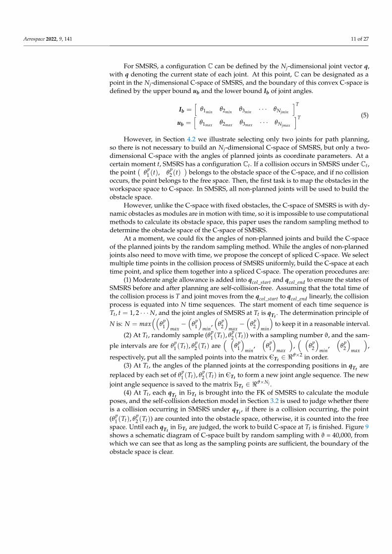
Figure 6 shows the schematic diagram of the spherical nonholonomic envelope of theSMSRS with three modules. The center of the spherical envelope locates at the center ofthe module body, and the length of the radius RC is one half of the diagonal length of themodule body. In this paper, the distance between the centers of two modules is used todetermine whether modules collide. For SMSRS, Ψ is defined as the set of modules. Selecttwo different modules y, r ∈ Ψ, (y 6= r), their position vectors with respect to Σb are py andpr, dyr denotes the distance between the centers of the two modules, and it equals to the2-norm of the difference between py and pr. The criteria for determining modules y, r havenot collided is:

dyr = ‖py − pr‖ > 2RC (4)

Aerospace 2022, 9, 141 8 of 28

structure, we create a spherical envelope only for the module and ignore the joint struc-tures. The spherical nonholonomic envelope could further improve computational effi-ciency. And the spherical nonholonomic envelope of SMSRS with nine modules is shown in Figure 5.


3.2.2. Self-Collision Detection Criteria Figure 6 shows the schematic diagram of the spherical nonholonomic envelope of the

SMSRS with three modules. The center of the spherical envelope locates at the center of the module body, and the length of the radius RC is one half of the diagonal length of the module body. In this paper, the distance between the centers of two modules is used to determine whether modules collide. For SMSRS, 𝛹 is defined as the set of modules. Select two different modules 𝑦, 𝑟 ∈ 𝛹, (𝑦 ≠ 𝑟), their position vectors with respect to 𝛴 are 𝒑 and 𝒑 , 𝑑 denotes the distance between the centers of the two modules, and it equals to the 2-norm of the difference between 𝒑 and 𝒑 . The criteria for determining modules 𝑦, 𝑟 have not collided is: 𝑑 = 𝒑 − 𝒑 2𝑅 (4)


For a certain configuration of SMSRS, only if 𝑑 of any two modules is larger than 2𝑅 , it can be concluded that SMSRS has no collision under this configuration, and as long as there exist any two modules that collide, this configuration has collision.

4. Self-Collision Avoidance Strategy Collision avoidance is a fundamental problem in offline path planning, and a two-

step framework is widely used in collision-free path planning for robotic arms with few DOFs and mobile robots, i.e., building the C-space and then searching for collision-free paths in the C-space. For the offline collision-free problem of SMSRS in time-varying con-figurations, we propose the spliced C-space based on pre-defined joint paths and the path planning algorithms based on digital maps with the dangerous potential field, which to-gether consist of the self-collision avoidance strategy of SMSRS. It is implemented in sev-eral steps as follows to achieve the self-collision avoidance strategy of SMSRS:


For a certain configuration of SMSRS, only if dyr of any two modules is larger than2RC, it can be concluded that SMSRS has no collision under this configuration, and as longas there exist any two modules that collide, this configuration has collision.

4. Self-Collision Avoidance Strategy

Collision avoidance is a fundamental problem in offline path planning, and a two-stepframework is widely used in collision-free path planning for robotic arms with few DOFsand mobile robots, i.e., building the C-space and then searching for collision-free paths inthe C-space. For the offline collision-free problem of SMSRS in time-varying configurations,we propose the spliced C-space based on pre-defined joint paths and the path planningalgorithms based on digital maps with the dangerous potential field, which together consistof the self-collision avoidance strategy of SMSRS. It is implemented in several steps asfollows to achieve the self-collision avoidance strategy of SMSRS:

(1) Locate the collision module and record collision start-stop joint angles;(2) Determine the planned joints;(3) Build linear path-based multiple C-spaces;(4) Pre-defined the paths of the planned joints;(5) Splice the multiple C-spaces based on the pre-defined paths into the binary map, and

check the validity of the binary map;

Aerospace 2022, 9, 141 9 of 27

(6) Transform the binary map into a map with the dangerous potential field;(7) Search collision-free path in the map with the dangerous potential field; and(8) Check paths.

The logical relationships of these steps are shown in Figure 7, where steps (1) to (2)are for initialization, (3) to (5) are for C-space construction, and (6) to (8) are for pathplanning algorithms based on digital maps with the dangerous potential field. The ideaand execution process of each step will be described below.

Aerospace 2022, 9, 141 9 of 28

(1) Locate the collision module and record collision start-stop joint angles; (2) Determine the planned joints; (3) Build linear path-based multiple C-spaces; (4) Pre-defined the paths of the planned joints; (5) Splice the multiple C-spaces based on the pre-defined paths into the binary map, and

check the validity of the binary map; (6) Transform the binary map into a map with the dangerous potential field; (7) Search collision-free path in the map with the dangerous potential field; and (8) Check paths.

The logical relationships of these steps are shown in Figure 7, where steps (1) to (2) are for initialization, (3) to (5) are for C-space construction, and (6) to (8) are for path plan-ning algorithms based on digital maps with the dangerous potential field. The idea and execution process of each step will be described below.

Figure 7. Steps of self-collision avoidance strategy of SMSRS.

4.1. Locate the Collision Module The initial configuration and final configuration with corresponding joint angles are

given by the mission planning system. The results of the path planning of SMSRS, on a self-collision-free basis, need to satisfy the pose requirements of each link, not only the desired poses of the end link while ignoring the poses of the other links. Therefore, the goal of the path planning of SMSRS is to find feasible paths for all joints so that the SMSRS can move from the initial configuration to the final configuration without collision. We set all joints of SMSRS to move in linear paths from initial angles to final angles, and locate the collision modules under their linear paths. If there are no additional optimization ob-jectives, the linear path is the most economical path, which avoids the energy waste caused by joints moving in complex paths and could facilitate the subsequent joint trajec-tory optimization.

Under the linear paths of joints, the collision detection model in Section 3.2 is used to determine whether there is a collision between modules in real time, and once a module collision is detected, the two modules are marked as collision modules, and the collision start angles of joints 𝒒 _ are recorded. The final configuration of the SMSRS is colli-sion-free, indicating the collision state will not last until the end, allowing the SMSRS to continue moving and recording the collision stop angles of joints 𝒒 _ .

Figure 7. Steps of self-collision avoidance strategy of SMSRS.

4.1. Locate the Collision Module

The initial configuration and final configuration with corresponding joint angles aregiven by the mission planning system. The results of the path planning of SMSRS, on aself-collision-free basis, need to satisfy the pose requirements of each link, not only thedesired poses of the end link while ignoring the poses of the other links. Therefore, the goalof the path planning of SMSRS is to find feasible paths for all joints so that the SMSRS canmove from the initial configuration to the final configuration without collision. We set alljoints of SMSRS to move in linear paths from initial angles to final angles, and locate thecollision modules under their linear paths. If there are no additional optimization objectives,the linear path is the most economical path, which avoids the energy waste caused by jointsmoving in complex paths and could facilitate the subsequent joint trajectory optimization.

Under the linear paths of joints, the collision detection model in Section 3.2 is used todetermine whether there is a collision between modules in real time, and once a modulecollision is detected, the two modules are marked as collision modules, and the collisionstart angles of joints qcol_start are recorded. The final configuration of the SMSRS is collision-free, indicating the collision state will not last until the end, allowing the SMSRS to continuemoving and recording the collision stop angles of joints qcol_end.

4.2. Determine the Planned Joints

Once the collision module and the qcol_start and qcol_end are clarified, there are twooptions for the selection of the joints to be planned: planning the path of all joints orplanning the path of only some selected joints. In this paper, the paths of two joints areselected to plan to avoid the self-collision, which is based on the following considerations:(1) the path planning with few joints can reduce the planning complexity and computationalcost, while a large number of stable and efficient path search algorithms for planes canbe utilized, which also improves the visibility; (2) SMSRS has wide ranges of joint angles,and by reasonably configuring the two planned joints, the configurations of SMSRS canbe substantially adjusted so that new collision-free paths can be found in the collections

Aerospace 2022, 9, 141 10 of 27

of these configurations; and (3) each joint needs to return to the desired angle after pathplanning, and when multiple joint angles are planned at the same time, it is difficult toensure that.

The principle of configuring the planned joints is the maximum success rate andmaximum stability. The so-called maximum success rate means that the selected joint canfind the collision-free path as successfully as possible after planning. Maximum stabilitymeans that the planned joint will not significantly change the configuration of the collision-free module, resulting in unnecessary collisions. Combining these two principles, wedevelop the following selection rules for the planned joints:

1. For ith joint, when its θi_col_start 6= θi_col_end, we call it motion joint, otherwise nomotion joint—when there are more than two motion joints between two collisionmodules, the two adjacent motion joints closest to the end of SMSRS are selected asthe planned joints;

2. When the selected joints cannot successfully avoid the self-collision after planning,another two adjacent motion joints between collision modules are selected from theend to the middle of SMSRS;

3. When the number of motion joints between collision modules is less than two, a nomotion joint closest to the end collision module and a motion joint are selected asplanned joints;

4. Under (3), if it is still not able to find self-collision-free paths, the motion joint and nomotion joint are configured from the end to the middle of SMSRS; and

5. After selection, we denote the planned joints as θp1 , θ

p2 , their start collision angles as

θp1_start, θ

p2_start, and end collision angles as θ

p1_end, θ

p2_end.

4.3. Splice Multiple C-Spaces Based on a Pre-Defined Path4.3.1. Multiple C-Spaces

The concept of C-space originates from collision detection and avoidance of robotics [12,13],which uses the pose parameters of rigid objects in the workspace as its coordinate parameters,and the kinematic relations map the poses of target objects and obstacles from the workspace tothe C-space.

C-space is often used for path planning of rigid objects in stationary obstacles. There-fore, C-space can be further divided into two subspaces: obstacle space and free space.The obstacle space refers to the space occupied by obstacles in the C-space, while thefree space refers to the space not occupied by obstacles in C-space. Unlike the physicalworkspace, the dimensions of the C-space are defined as the DOFs of all control variablesin the motion system [45]. A schematic of a two-dimensional C-space is shown in Figure 8.When the boundaries of the obstacle space and the free space in the C-space are determined,collision-free path planning is to search for a path in the C-space that connects the startpoint and end point and does not pass through the obstacles.

Aerospace 2022, 9, 141 11 of 28

Figure 8. Schematic of a two-dimensional C-space.

For SMSRS, a configuration ℂ can be defined by the 𝑁 -dimensional joint vector q, with q denoting the current state of each joint. At this point, ℂ can be designated as a point in the 𝑁 -dimensional C-space of SMSRS, and the boundary of this convex C-space is defined by the upper bound 𝒖 and the lower bound 𝑰 of joint angles. 𝑰𝒃 = 𝜃 𝜃 𝜃 ⋯ 𝜃𝒖𝒃 = 𝜃 𝜃 𝜃 ⋯ 𝜃 (5)

However, in Section 4.2 we illustrate selecting only two joints for path planning, so there is not necessary to build an 𝑁 -dimensional C-space of SMSRS, but only a two-di-mensional C-space with the angles of planned joints as coordinate parameters. At a certain moment t, SMSRS has a configuration ℂ . If a collision occurs in SMSRS under ℂ , the point 𝜃 (𝑡), 𝜃 (𝑡) belongs to the obstacle space of the C-space, and if no collision oc-curs, the point belongs to the free space. Then, the first task is to map the obstacles in the workspace space to C-space. In SMSRS, all non-planned joints will be used to build the obstacle space.

However, unlike the C-space with fixed obstacles, the C-space of SMSRS is with dy-namic obstacles as modules are in motion with time, so it is impossible to use computa-tional methods to calculate its obstacle space, this paper uses the random sampling method to determine the obstacle space of the C-space of SMSRS.

At a moment, we could fix the angles of non-planned joints and build the C-space of the planned joints by the random sampling method. While the angles of non-planned joints also need to move with time, we propose the concept of spliced C-space. We select multiple time points in the collision process of SMSRS uniformly, build the C-space at each time point, and splice them together into a spliced C-space. The operation procedures are:

(1) Moderate angle allowance is added into 𝒒 _ and 𝒒 _ to ensure the states of SMSRS before and after planning are self-collision-free. Assuming that the total time of the collision process is T and joint moves from the 𝒒 _ to 𝒒 _ linearly, the collision process is equated into N time sequences. The start moment of each time sequence is 𝑇 , 𝑡 = 1,2 ⋯ 𝑁, and the joint angles of SMSRS at 𝑇 is 𝒒𝑻𝒕. The determination principle of N is: 𝑁 = 𝑚𝑎𝑥 𝜃 − 𝜃 , 𝜃 − 𝜃 to keep it in a reason-able interval.

(2) At 𝑇 , randomly sample (𝜃 (𝑇 ), 𝜃 (𝑇 )) with a sampling number ϑ, and the sam-ple intervals are for 𝜃 (𝑇 ), 𝜃 (𝑇 ) are 𝜃 , 𝜃 , 𝜃 , 𝜃 , re-spectively, put all the sampled points into the matrix Є𝑻𝒕 ∈ 𝕽 × in order.

(3) At 𝑇 , the angles of the planned joints at the corresponding positions in 𝒒𝑻𝒕 are replaced by each set of 𝜃 (𝑇 ), 𝜃 (𝑇 ) in Є𝑻𝒕 to form a new joint angle sequence. The new joint angle sequence is saved to the matrix Б𝑻𝒕 ∈ 𝕽 × .

(4) At 𝑇 , each 𝒒𝑻𝒕 in Б𝑻𝒕 is brought into the FK of SMSRS to calculate the module poses, and the self-collision detection model in Section 3.2 is used to judge whether there

Figure 8. Schematic of a two-dimensional C-space.

Aerospace 2022, 9, 141 11 of 27

For SMSRS, a configuration C can be defined by the Nj-dimensional joint vector q,with q denoting the current state of each joint. At this point, C can be designated as apoint in the Nj-dimensional C-space of SMSRS, and the boundary of this convex C-space isdefined by the upper bound ub and the lower bound Ib of joint angles.

Ib =[

θ1min θ2min θ3min · · · θNjmin

]T

ub =[

θ1max θ2max θ3max · · · θNjmax

]T (5)

However, in Section 4.2 we illustrate selecting only two joints for path planning,so there is not necessary to build an Nj-dimensional C-space of SMSRS, but only a two-dimensional C-space with the angles of planned joints as coordinate parameters. At acertain moment t, SMSRS has a configuration Ct. If a collision occurs in SMSRS under Ct,the point

(θ

p1 (t), θ

p2 (t)

)belongs to the obstacle space of the C-space, and if no collision

occurs, the point belongs to the free space. Then, the first task is to map the obstacles in theworkspace space to C-space. In SMSRS, all non-planned joints will be used to build theobstacle space.

However, unlike the C-space with fixed obstacles, the C-space of SMSRS is with dy-namic obstacles as modules are in motion with time, so it is impossible to use computationalmethods to calculate its obstacle space, this paper uses the random sampling method todetermine the obstacle space of the C-space of SMSRS.

At a moment, we could fix the angles of non-planned joints and build the C-spaceof the planned joints by the random sampling method. While the angles of non-plannedjoints also need to move with time, we propose the concept of spliced C-space. We selectmultiple time points in the collision process of SMSRS uniformly, build the C-space at eachtime point, and splice them together into a spliced C-space. The operation procedures are:

(1) Moderate angle allowance is added into qcol_start and qcol_end to ensure the states ofSMSRS before and after planning are self-collision-free. Assuming that the total time ofthe collision process is T and joint moves from the qcol_start to qcol_end linearly, the collisionprocess is equated into N time sequences. The start moment of each time sequence isTt, t = 1, 2 · · ·N, and the joint angles of SMSRS at Tt is qTt

. The determination principle of

N is: N = max((

θp1

)max−(

θp1

)min

,(

θp2

)max−(

θp2

)min

)to keep it in a reasonable interval.

(2) At Tt, randomly sample (θp1 (Tt), θ

p2 (Tt)) with a sampling number ϑ, and the sam-

ple intervals are for θp1 (Tt), θ

p2 (Tt) are

( (θ

p1

)min

,(

θp1

)max

),( (

θp2

)min

,(

θp2

)max

),

respectively, put all the sampled points into the matrix ЄTt ∈ <ϑ×2 in order.(3) At Tt, the angles of the planned joints at the corresponding positions in qTt

arereplaced by each set of θ

p1 (Tt), θ

p2 (Tt) in ЄTt to form a new joint angle sequence. The new

joint angle sequence is saved to the matrix БTt ∈ <ϑ×Nj .

(4) At Tt, each qTtin БTt is brought into the FK of SMSRS to calculate the module

poses, and the self-collision detection model in Section 3.2 is used to judge whether thereis a collision occurring in SMSRS under qTt

, if there is a collision occurring, the point(θp

1 (Tt), θp2 (Tt)) are counted into the obstacle space, otherwise, it is counted into the free

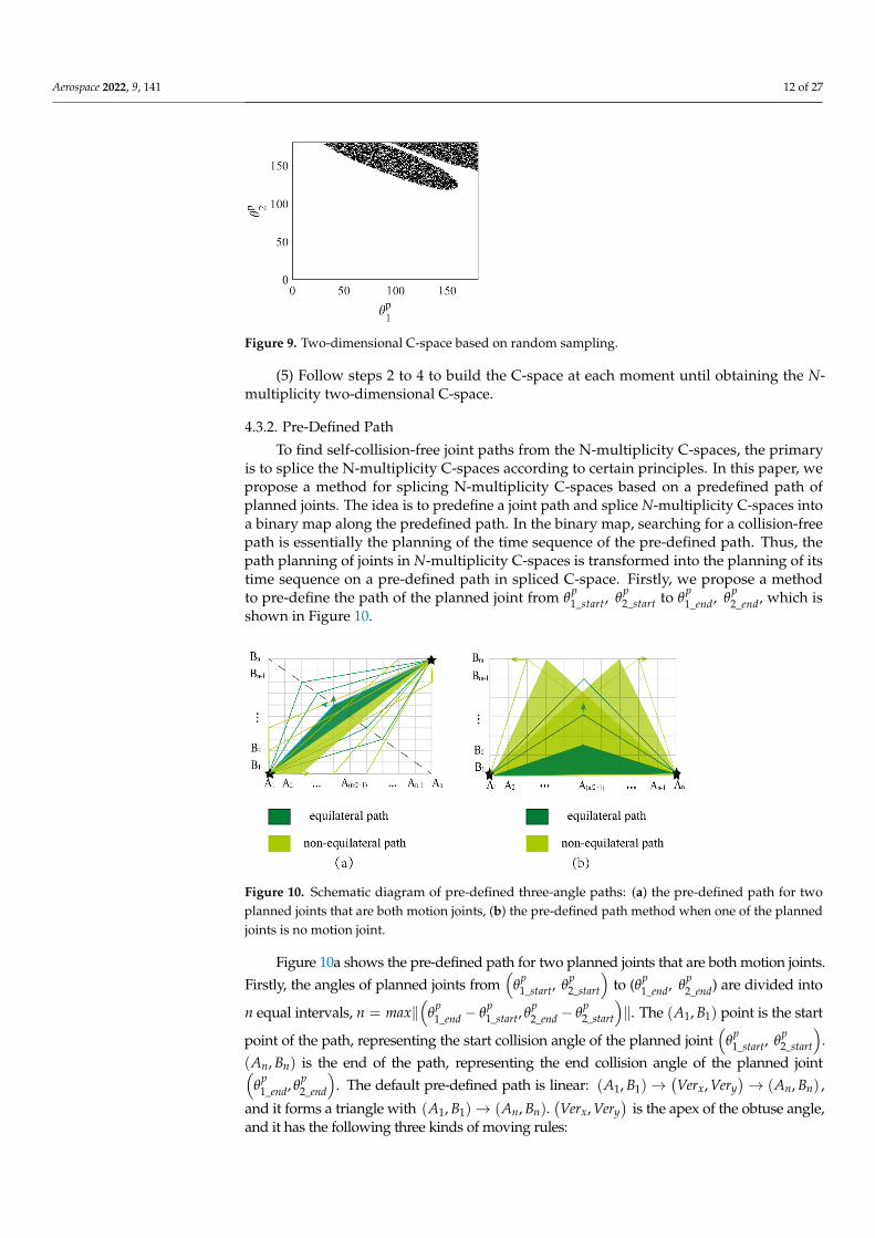
space. Until each qTtin БTt are judged, the work to build C-space at Tt is finished. Figure 9

shows a schematic diagram of C-space built by random sampling with ϑ = 40,000, fromwhich we can see that as long as the sampling points are sufficient, the boundary of theobstacle space is clear.

Aerospace 2022, 9, 141 12 of 27

Aerospace 2022, 9, 141 12 of 28

is a collision occurring in SMSRS under 𝒒𝑻𝒕 , if there is a collision occurring, the point (𝜃 (𝑇 ), 𝜃 (𝑇 )) are counted into the obstacle space, otherwise, it is counted into the free space. Until each 𝒒𝑻𝒕 in Б𝑻𝒕are judged, the work to build C-space at 𝑇 is finished. Figure 9 shows a schematic diagram of C-space built by random sampling with ϑ = 40,000, from which we can see that as long as the sampling points are sufficient, the boundary of the obstacle space is clear.

Figure 9. Two-dimensional C-space based on random sampling.

(5) Follow steps 2 to 4 to build the C-space at each moment until obtaining the N-multiplicity two-dimensional C-space.

4.3.2. Pre-Defined Path To find self-collision-free joint paths from the N-multiplicity C-spaces, the primary

is to splice the N-multiplicity C-spaces according to certain principles. In this paper, we propose a method for splicing N-multiplicity C-spaces based on a predefined path of planned joints. The idea is to predefine a joint path and splice N-multiplicity C-spaces into a binary map along the predefined path. In the binary map, searching for a collision-free path is essentially the planning of the time sequence of the pre-defined path. Thus, the path planning of joints in N-multiplicity C-spaces is transformed into the planning of its time sequence on a pre-defined path in spliced C-space. Firstly, we propose a method to pre-define the path of the planned joint from 𝜃 _ , 𝜃 _ to 𝜃 _ , 𝜃 _ , which is shown in Figure 10.

Figure 10. Schematic diagram of pre-defined three-angle paths: (a) the pre-defined path for two planned joints that are both motion joints, (b) the pre-defined path method when one of the planned joints is no motion joint.

Figure 10a shows the pre-defined path for two planned joints that are both motion joints. Firstly, the angles of planned joints from (𝜃 _ , 𝜃 _ ) to (𝜃 _ , 𝜃 _ ) are di-vided into n equal intervals, 𝑛 = max 𝜃 _ − 𝜃 _ , 𝜃 _ − 𝜃 _ . The (𝐴 , 𝐵 )



4.3.2. Pre-Defined Path

To find self-collision-free joint paths from the N-multiplicity C-spaces, the primaryis to splice the N-multiplicity C-spaces according to certain principles. In this paper, wepropose a method for splicing N-multiplicity C-spaces based on a predefined path ofplanned joints. The idea is to predefine a joint path and splice N-multiplicity C-spaces intoa binary map along the predefined path. In the binary map, searching for a collision-freepath is essentially the planning of the time sequence of the pre-defined path. Thus, thepath planning of joints in N-multiplicity C-spaces is transformed into the planning of itstime sequence on a pre-defined path in spliced C-space. Firstly, we propose a methodto pre-define the path of the planned joint from θ

p1_start, θ

p2_start to θ

p1_end, θ

p2_end, which is

shown in Figure 10.

Aerospace 2022, 9, 141 12 of 28

is a collision occurring in SMSRS under 𝒒𝑻𝒕 , if there is a collision occurring, the point (𝜃 (𝑇 ), 𝜃 (𝑇 )) are counted into the obstacle space, otherwise, it is counted into the free space. Until each 𝒒𝑻𝒕 in Б𝑻𝒕are judged, the work to build C-space at 𝑇 is finished. Figure 9 shows a schematic diagram of C-space built by random sampling with ϑ = 40,000, from which we can see that as long as the sampling points are sufficient, the boundary of the obstacle space is clear.



4.3.2. Pre-Defined Path To find self-collision-free joint paths from the N-multiplicity C-spaces, the primary

is to splice the N-multiplicity C-spaces according to certain principles. In this paper, we propose a method for splicing N-multiplicity C-spaces based on a predefined path of planned joints. The idea is to predefine a joint path and splice N-multiplicity C-spaces into a binary map along the predefined path. In the binary map, searching for a collision-free path is essentially the planning of the time sequence of the pre-defined path. Thus, the path planning of joints in N-multiplicity C-spaces is transformed into the planning of its time sequence on a pre-defined path in spliced C-space. Firstly, we propose a method to pre-define the path of the planned joint from 𝜃 _ , 𝜃 _ to 𝜃 _ , 𝜃 _ , which is shown in Figure 10.

Figure 10. Schematic diagram of pre-defined three-angle paths: (a) the pre-defined path for two planned joints that are both motion joints, (b) the pre-defined path method when one of the planned joints is no motion joint.

Figure 10a shows the pre-defined path for two planned joints that are both motion joints. Firstly, the angles of planned joints from (𝜃 _ , 𝜃 _ ) to (𝜃 _ , 𝜃 _ ) are di-vided into n equal intervals, 𝑛 = max 𝜃 _ − 𝜃 _ , 𝜃 _ − 𝜃 _ . The (𝐴 , 𝐵 )

Figure 10. Schematic diagram of pre-defined three-angle paths: (a) the pre-defined path for twoplanned joints that are both motion joints, (b) the pre-defined path method when one of the plannedjoints is no motion joint.

Figure 10a shows the pre-defined path for two planned joints that are both motion joints.Firstly, the angles of planned joints from

(θ

p1_start, θ

p2_start

)to (θp

1_end, θp2_end) are divided into

n equal intervals, n = max‖(

θp1_end − θ

p1_start, θ

p2_end − θ

p2_start

)‖. The (A1, B1) point is the start

point of the path, representing the start collision angle of the planned joint(

θp1_start, θ

p2_start

).

(An, Bn) is the end of the path, representing the end collision angle of the planned joint(θ

p1_end, θ

p2_end

). The default pre-defined path is linear: (A1, B1)→

(Verx, Very

)→ (An, Bn) ,

and it forms a triangle with (A1, B1)→ (An, Bn).(Verx, Very

)is the apex of the obtuse angle,

and it has the following three kinds of moving rules:

Aerospace 2022, 9, 141 13 of 27

(1) Equilateral path: along with the (An, B1)→ (A1, Bn) line, Verx move from theA(n/2+1) to both sides of A(n/2+1), Very move from B(n/2+1) to both sides of B(n/2+1).

(2) Non-equilateral path: Very = Bn, Verx move from An to A1; or Verx = An, Verxmove from Bn to B1.

(3) Non-equilateral path: Very = B1, Verx move from A1 to An; or Verx = A1, Verxmove from B1 to Bn.

Figure 10b shows the pre-defined path method when one of the planned joints is nomotion joint. Firstly, the angles of motion joints are divided into n equal intervals fromθ

p1_start to θ

p1_end, and θ

p2_end = θ

p2_start, n = ‖θp

1_end − θp1_start‖. The (A1, B1) point is the start

point of the path, representing the start collision angle of the planned joint(

θp1_start, θ

p2_start

).

(An, B1) is the end of the path, representing the end collision angle of the planned joint(θ

p1_end, θ

p2_end

). The side length of both X and Y directions of a grid are equal. The default

pre-defined path is linear: (A1, B1)→(Verx, Very

)→ (An, B1) , and it forms an equilateral

triangle with (A1, B1)→ (An, B1).(Verx, Very

)has two kinds of moving rules:

(1) Equilateral path:(Verx, Very

)move along

(A(n/2+1), B2

)→(

A(n/2+1), Bm

). Bm ∈( (

θp2

)min

,(

θp2

)max

).

(2) Non-equilateral path: Verx move from A(n/2+1) to both sides of A(n/2+1) and Very

move from B1 to Bm. Bm ∈( (

θp2

)min

,(

θp2

)max

).

We restrict(Verx, Very

)can only be located on the grid points in Figure 10, it generates

a new pre-defined path for each step forward on the grid. In Figure 10a, if there is nocollision-free path in the spliced C-space generated by the current pre-defined path, a newpath needs to be pre-defined according to rules (1)~(3) successively, and the pre-definedpath needs to be guaranteed the obtuse angle is greater than 100 degrees; In Figure 10b, ifall pre-defined paths in rule (1) are proved to be invalid, a new path shall be pre-definedaccording to rule (2), and the value of the two acute angles of the path should be less than80 degrees. As shown in Figure 7, if all the compliant pre-defined paths of the currentlyplanned joints are proved invalid, the progress needs to return to the step of determiningplanned joints.

4.3.3. Splice Multiple C-Space

Finding the time sequence for the planned joints on the pre-defined path with nocollisions is our inspiration for splicing N-multiplicity C-spaces. Equate the pre-definedpath into S segments. To ensure the length of the path segment is equal to the C-spacegrid, S = max(An − A1), (Bn − B1). Create an N × S dimensional matrix Z, calculate thepoint of joint angles

(θ

p1_j, θ

p2_j

), j ∈ 1, 2 · · · S of the start point of each segment on the

predefined path. For jth point, judge whether it is in free space or obstacle space of the ithmultiplicity C-space, and, if it is in the free space, Z(i, j) = 0; otherwise Z(i, j) = 1. Afterfinishing the judgments, the N-multiplicity C-spaces based on the pre-defined paths arespliced into matrix Z, which can be regarded as a two-dimensional digital map composedof the numbers 1 and 0 and is named as the binary map.

The N rows of the binary map present the N-multiplicity C-spaces and the S columnspresent the S segments of whole movement time along the pre-defined path. If we couldfind an all-0 path from the top-left to the bottom-right in the binary map, it means thatthe planned joints could cross the N-multiplicity C-spaces along the pre-defined pathcollision-freely under a specific time sequence. A binary map is valid if there exists an all-0path from the top-left to the bottom-right; otherwise, the map is invalid, and a pre-definedpath needs to be reselected. We propose an all-0 path search algorithm based on the totalpath length to determine whether the binary map is valid.

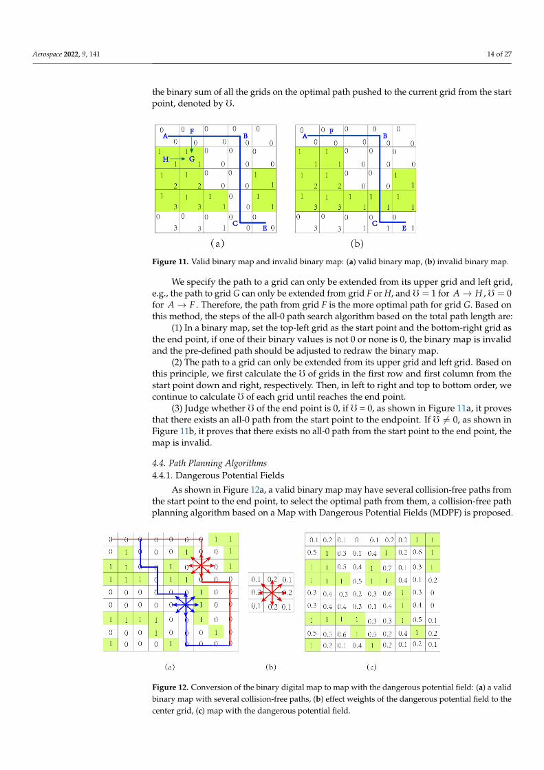
In Figure 11, the binary map is plotted into a map with grids. Every grid hastwo values, the top value represents its binary value, and the bottom value represents

Aerospace 2022, 9, 141 14 of 27

the binary sum of all the grids on the optimal path pushed to the current grid from the startpoint, denoted by 0.

Aerospace 2022, 9, 141 14 of 28

path needs to be reselected. We propose an all-0 path search algorithm based on the total path length to determine whether the binary map is valid.

In Figure 11, the binary map is plotted into a map with grids. Every grid has two values, the top value represents its binary value, and the bottom value represents the bi-nary sum of all the grids on the optimal path pushed to the current grid from the start point, denoted by ℧.

Figure 11. Valid binary map and invalid binary map: (a) valid binary map, (b) invalid binary map.

We specify the path to a grid can only be extended from its upper grid and left grid, e.g., the path to grid G can only be extended from grid F or H, and ℧ = 1 for 𝐴 → 𝐻, ℧ = 0 for 𝐴 → 𝐹. Therefore, the path from grid F is the more optimal path for grid G. Based on this method, the steps of the all-0 path search algorithm based on the total path length are:

(1) In a binary map, set the top-left grid as the start point and the bottom-right grid as the end point, if one of their binary values is not 0 or none is 0, the binary map is invalid and the pre-defined path should be adjusted to redraw the binary map.

(2) The path to a grid can only be extended from its upper grid and left grid. Based on this principle, we first calculate the ℧ of grids in the first row and first column from the start point down and right, respectively. Then, in left to right and top to bottom order, we continue to calculate ℧ of each grid until reaches the end point.

(3) Judge whether ℧ of the end point is 0, if ℧ = 0, as shown in Figure 11a, it proves that there exists an all-0 path from the start point to the endpoint. If ℧ ≠ 0, as shown in Figure 11b, it proves that there exists no all-0 path from the start point to the end point, the map is invalid.

4.4. Path Planning Algorithms 4.4.1. Dangerous Potential Fields

As shown in Figure 12a, a valid binary map may have several collision-free paths from the start point to the end point, to select the optimal path from them, a collision-free path planning algorithm based on a Map with Dangerous Potential Fields (MDPF) is pro-posed.

The dangerous potential field of the map is used to evaluate the possibility of poten-tial collisions of its grids. As shown in Figure 12b, a grid is centered on the eight surround-ing grids, and the values ℓ in the surrounding grids represent their effect weights to the dangerous potential field of the center grid. The dangerous potential field strength of the center grid is ℚ = ∑ ℓ ℒ , where ℒ is the binary value of its eight surrounding grids, and for the four oblique grids, ℓ = 0.1, for the other grids, ℓ = 0.2. Calculating the dan-gerous potential field strength of all grids in the binary map, we convert the binary map into a digital map with the dangerous potential field, as shown in Figure 12c. We expect to find an optimal path in the map with the dangerous potential field by the MDPF algo-rithm. The optimal path has the smallest total value of the dangerous potential field of all grids on the path, that is, the safest path with the lowest collision possibility.

Figure 11. Valid binary map and invalid binary map: (a) valid binary map, (b) invalid binary map.

We specify the path to a grid can only be extended from its upper grid and left grid,e.g., the path to grid G can only be extended from grid F or H, and 0 = 1 for A→ H , 0 = 0for A→ F . Therefore, the path from grid F is the more optimal path for grid G. Based onthis method, the steps of the all-0 path search algorithm based on the total path length are:

(1) In a binary map, set the top-left grid as the start point and the bottom-right grid asthe end point, if one of their binary values is not 0 or none is 0, the binary map is invalidand the pre-defined path should be adjusted to redraw the binary map.

(2) The path to a grid can only be extended from its upper grid and left grid. Based onthis principle, we first calculate the 0 of grids in the first row and first column from thestart point down and right, respectively. Then, in left to right and top to bottom order, wecontinue to calculate 0 of each grid until reaches the end point.

(3) Judge whether 0 of the end point is 0, if 0 = 0, as shown in Figure 11a, it provesthat there exists an all-0 path from the start point to the endpoint. If 0 6= 0, as shown inFigure 11b, it proves that there exists no all-0 path from the start point to the end point, themap is invalid.

4.4. Path Planning Algorithms4.4.1. Dangerous Potential Fields

As shown in Figure 12a, a valid binary map may have several collision-free paths fromthe start point to the end point, to select the optimal path from them, a collision-free pathplanning algorithm based on a Map with Dangerous Potential Fields (MDPF) is proposed.

Aerospace 2022, 9, 141 15 of 28

Figure 12. Conversion of the binary digital map to map with the dangerous potential field: (a) a valid binary map with several collision-free paths, (b) effect weights of the dangerous potential field to the center grid, (c) map with the dangerous potential field.

4.4.2. MDPF Algorithm Same as the all-0 path search algorithm in Section 4.3.3, the MDPF algorithm sets the

path start point at the top-left grid and the end point at the bottom-right grid, and ℧ of all grids are calculated in the same order. The difference is that the value at the top of the grid represents the value of ℚ, and the bottom value ℧ represents the sum of the ℚ of all grids on the optimal path from the start point to it. In addition, the all-0 path search algorithm uses ℧ to determine whether a binary map is valid, but the MDPF algorithm aims to find the safest path in the map with the dangerous potential field.

Since ℧ of all grids are calculated in the forward direction, the optimal path of one grid from the start point can be retracted based on the ℧ value of other grids. For exam-ple, in Figure 13, the path to grid G can only extend from grid C or grid D. Then we com-pare the ℧ of grid C and grid D, it can be found that ℧ = 0.6 for A→C and ℧ = 1.1 for A→D, therefore, the path to grid G is extended from grid C. According to the principle that the sub-path of the optimal path must also be optimal, the sub-path of the current path back one step is also the optimal path. Therefore, the mechanism for the MDPF algo-rithm is to find the optimal path by backtracking ℧ from the end point to the start end in the map with the dangerous potential field.

Figure 13. Path planning in the map with the dangerous potential field.

From the end point, we compare the ℧ values of its upper grid and left grid, and mark the grid with smaller ℧ as the target grid, then compare the ℧ values of the upper grid and left grid of the target grid, Following this step, the target grid can be backtracked to the start grid and all the target grids form the optimal path. The MDPF algorithm achieves the planning of the optimal path without traversing every path.

Figure 12. Conversion of the binary digital map to map with the dangerous potential field: (a) a validbinary map with several collision-free paths, (b) effect weights of the dangerous potential field to thecenter grid, (c) map with the dangerous potential field.

Aerospace 2022, 9, 141 15 of 27

The dangerous potential field of the map is used to evaluate the possibility of potentialcollisions of its grids. As shown in Figure 12b, a grid is centered on the eight surroundinggrids, and the values ì in the surrounding grids represent their effect weights to thedangerous potential field of the center grid. The dangerous potential field strength ofthe center grid is Q = ∑8

i=0 ìLi, where Li is the binary value of its eight surroundinggrids, and for the four oblique grids, ì = 0.1, for the other grids, ì = 0.2. Calculating thedangerous potential field strength of all grids in the binary map, we convert the binary mapinto a digital map with the dangerous potential field, as shown in Figure 12c. We expect tofind an optimal path in the map with the dangerous potential field by the MDPF algorithm.The optimal path has the smallest total value of the dangerous potential field of all grids onthe path, that is, the safest path with the lowest collision possibility.

4.4.2. MDPF Algorithm

Same as the all-0 path search algorithm in Section 4.3.3, the MDPF algorithm sets thepath start point at the top-left grid and the end point at the bottom-right grid, and 0 of allgrids are calculated in the same order. The difference is that the value at the top of the gridrepresents the value of Q, and the bottom value 0 represents the sum of the Q of all gridson the optimal path from the start point to it. In addition, the all-0 path search algorithmuses 0 to determine whether a binary map is valid, but the MDPF algorithm aims to findthe safest path in the map with the dangerous potential field.

Since 0 of all grids are calculated in the forward direction, the optimal path of onegrid from the start point can be retracted based on the 0 value of other grids. For example,in Figure 13, the path to grid G can only extend from grid C or grid D. Then we comparethe 0 of grid C and grid D, it can be found that 0 = 0.6 for A→C and 0 = 1.1 for A→D,therefore, the path to grid G is extended from grid C. According to the principle that thesub-path of the optimal path must also be optimal, the sub-path of the current path backone step is also the optimal path. Therefore, the mechanism for the MDPF algorithm is tofind the optimal path by backtracking 0 from the end point to the start end in the map withthe dangerous potential field.

Aerospace 2022, 9, 141 15 of 28

Figure 12. Conversion of the binary digital map to map with the dangerous potential field: (a) a valid binary map with several collision-free paths, (b) effect weights of the dangerous potential field to the center grid, (c) map with the dangerous potential field.

4.4.2. MDPF Algorithm Same as the all-0 path search algorithm in Section 4.3.3, the MDPF algorithm sets the

path start point at the top-left grid and the end point at the bottom-right grid, and ℧ of all grids are calculated in the same order. The difference is that the value at the top of the grid represents the value of ℚ, and the bottom value ℧ represents the sum of the ℚ of all grids on the optimal path from the start point to it. In addition, the all-0 path search algorithm uses ℧ to determine whether a binary map is valid, but the MDPF algorithm aims to find the safest path in the map with the dangerous potential field.

Since ℧ of all grids are calculated in the forward direction, the optimal path of one grid from the start point can be retracted based on the ℧ value of other grids. For exam-ple, in Figure 13, the path to grid G can only extend from grid C or grid D. Then we com-pare the ℧ of grid C and grid D, it can be found that ℧ = 0.6 for A→C and ℧ = 1.1 for A→D, therefore, the path to grid G is extended from grid C. According to the principle that the sub-path of the optimal path must also be optimal, the sub-path of the current path back one step is also the optimal path. Therefore, the mechanism for the MDPF algo-rithm is to find the optimal path by backtracking ℧ from the end point to the start end in the map with the dangerous potential field.


From the end point, we compare the ℧ values of its upper grid and left grid, and mark the grid with smaller ℧ as the target grid, then compare the ℧ values of the upper grid and left grid of the target grid, Following this step, the target grid can be backtracked to the start grid and all the target grids form the optimal path. The MDPF algorithm achieves the planning of the optimal path without traversing every path.


From the end point, we compare the 0 values of its upper grid and left grid, and markthe grid with smaller 0 as the target grid, then compare the 0 values of the upper grid andleft grid of the target grid, Following this step, the target grid can be backtracked to thestart grid and all the target grids form the optimal path. The MDPF algorithm achieves theplanning of the optimal path without traversing every path.

In the MDPF algorithm, for the current grid, if the 0 value of its upper grid is the sameas its left grid, different optimal paths will be obtained when setting different backtrackingdirections, including priority to the left; priority to the upper; priority to the upper left; andpriority to the previous direction, etc.

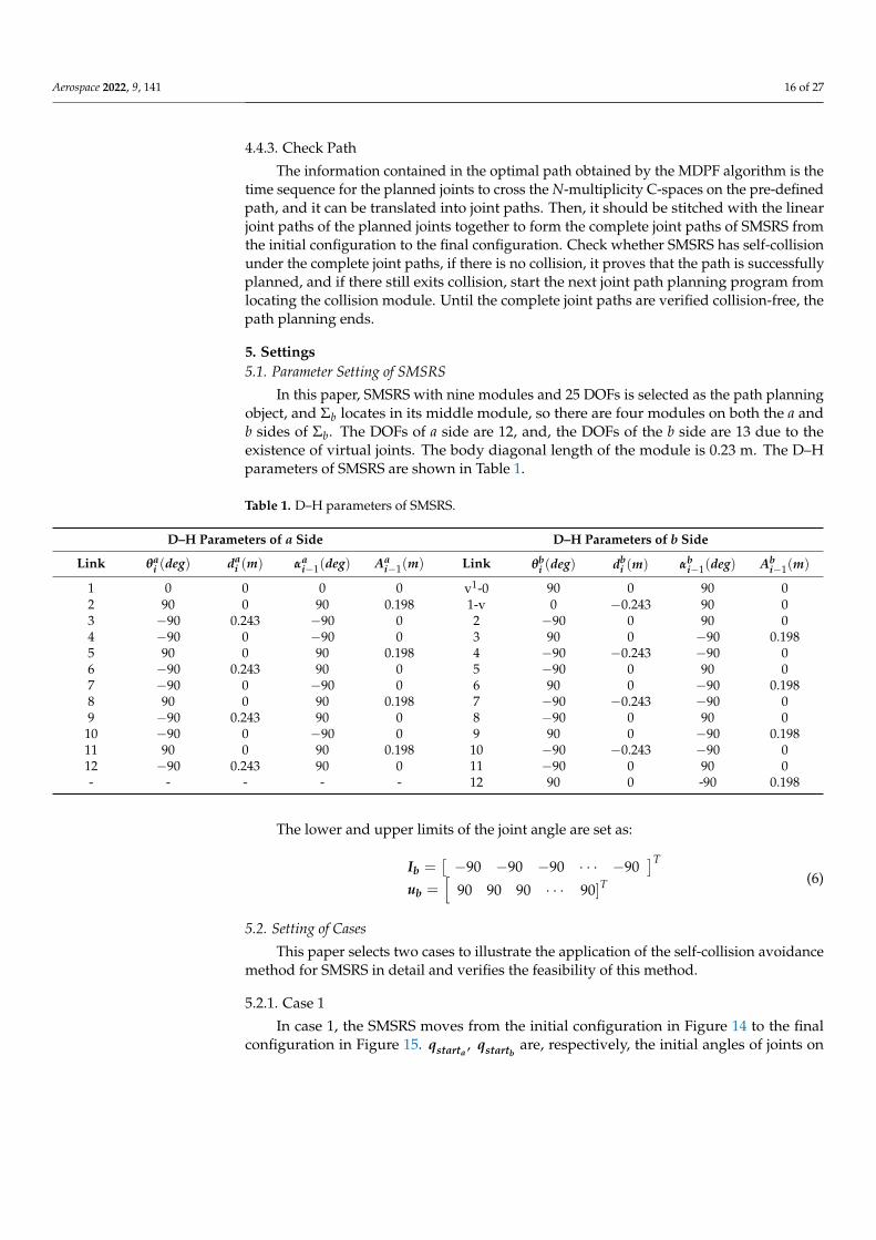
Aerospace 2022, 9, 141 16 of 27

4.4.3. Check Path

The information contained in the optimal path obtained by the MDPF algorithm is thetime sequence for the planned joints to cross the N-multiplicity C-spaces on the pre-definedpath, and it can be translated into joint paths. Then, it should be stitched with the linearjoint paths of the planned joints together to form the complete joint paths of SMSRS fromthe initial configuration to the final configuration. Check whether SMSRS has self-collisionunder the complete joint paths, if there is no collision, it proves that the path is successfullyplanned, and if there still exits collision, start the next joint path planning program fromlocating the collision module. Until the complete joint paths are verified collision-free, thepath planning ends.

5. Settings5.1. Parameter Setting of SMSRS

In this paper, SMSRS with nine modules and 25 DOFs is selected as the path planningobject, and Σb locates in its middle module, so there are four modules on both the a andb sides of Σb. The DOFs of a side are 12, and, the DOFs of the b side are 13 due to theexistence of virtual joints. The body diagonal length of the module is 0.23 m. The D–Hparameters of SMSRS are shown in Table 1.

Table 1. D–H parameters of SMSRS.

D–H Parameters of a Side D–H Parameters of b Side

Link θai (deg) da

i (m) αai−1(deg) Aa

i−1(m) Link θbi (deg) db

i (m) αbi−1(deg) Ab

i−1(m)

1 0 0 0 0 v1-0 90 0 90 02 90 0 90 0.198 1-v 0 −0.243 90 03 −90 0.243 −90 0 2 −90 0 90 04 −90 0 −90 0 3 90 0 −90 0.1985 90 0 90 0.198 4 −90 −0.243 −90 06 −90 0.243 90 0 5 −90 0 90 07 −90 0 −90 0 6 90 0 −90 0.1988 90 0 90 0.198 7 −90 −0.243 −90 09 −90 0.243 90 0 8 −90 0 90 0

10 −90 0 −90 0 9 90 0 −90 0.19811 90 0 90 0.198 10 −90 −0.243 −90 012 −90 0.243 90 0 11 −90 0 90 0- - - - - 12 90 0 -90 0.198

The lower and upper limits of the joint angle are set as:

Ib =[−90 −90 −90 · · · −90

]T

ub =[

90 90 90 · · · 90]T(6)

5.2. Setting of Cases

This paper selects two cases to illustrate the application of the self-collision avoidancemethod for SMSRS in detail and verifies the feasibility of this method.

5.2.1. Case 1

In case 1, the SMSRS moves from the initial configuration in Figure 14 to the finalconfiguration in Figure 15. qstarta

, qstartbare, respectively, the initial angles of joints on

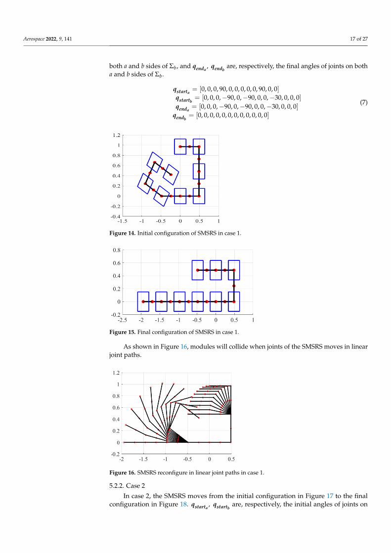
Aerospace 2022, 9, 141 17 of 27

both a and b sides of Σb, and qenda, qendb

are, respectively, the final angles of joints on botha and b sides of Σb.

qstarta= [0, 0, 0, 90, 0, 0, 0, 0, 0, 90, 0, 0]

qstartb= [0, 0, 0,−90, 0,−90, 0, 0,−30, 0, 0, 0]

qenda= [0, 0, 0,−90, 0,−90, 0, 0,−30, 0, 0, 0]

qendb= [0, 0, 0, 0, 0, 0, 0, 0, 0, 0, 0, 0]

(7)

Aerospace 2022, 9, 141 17 of 28

5.2.1. Case 1 In case 1, the SMSRS moves from the initial configuration in Figure 14 to the final

configuration in Figure 15. 𝒒𝒔𝒕𝒂𝒓𝒕𝒂, 𝒒𝒔𝒕𝒂𝒓𝒕𝒃 are, respectively, the initial angles of joints on both a and b sides of 𝛴 , and 𝒒𝒆𝒏𝒅𝒂, 𝒒𝒆𝒏𝒅𝒃 are, respectively, the final angles of joints on both a and b sides of 𝛴 . 𝒒𝒔𝒕𝒂𝒓𝒕𝒂 = 0,0,0,90,0,0,0,0,0,90,0,0𝒒𝒔𝒕𝒂𝒓𝒕𝒃 = 0,0,0, −90,0, −90,0,0, −30,0,0,0𝒒𝒆𝒏𝒅𝒂 = 0,0,0, −90,0, −90,0,0, −30,0,0,0𝒒𝒆𝒏𝒅𝒃 = 0,0,0,0,0,0,0,0,0,0,0,0 (7)

Figure 14. Initial configuration of SMSRS in case 1.

Figure 15. Final configuration of SMSRS in case 1.

As shown in Figure 16, modules will collide when joints of the SMSRS moves in linear joint paths.

Figure 16. SMSRS reconfigure in linear joint paths in case 1.


Aerospace 2022, 9, 141 17 of 28








As shown in Figure 16, modules will collide when joints of the SMSRS moves in linearjoint paths.

Aerospace 2022, 9, 141 17 of 28






Figure 16. SMSRS reconfigure in linear joint paths in case 1. Figure 16. SMSRS reconfigure in linear joint paths in case 1.

5.2.2. Case 2

In case 2, the SMSRS moves from the initial configuration in Figure 17 to the finalconfiguration in Figure 18. qstarta

, qstartbare, respectively, the initial angles of joints on

Aerospace 2022, 9, 141 18 of 27

both a and b sides of Σb, and qenda, qendb

are, respectively, the final angles of joints on botha and b sides of Σb.

qstarta= [0, 0, 0, 90, 0, 90, 90, 0, 0, 90, 30, 0]

qstartb= [0, 0, 0, 0, 0, 0, 0, 0, 0, 0, 0, 0]

qenda= [0, 0, 0, 90, 0,−90, 90, 0, 0, 90, 0, 0]

qendb= [0, 0, 0, 0, 0, 0, 0, 0, 0, 0, 0, 0]

(8)

Aerospace 2022, 9, 141 18 of 28


configuration in Figure 18. 𝒒𝒔𝒕𝒂𝒓𝒕𝒂, 𝒒𝒔𝒕𝒂𝒓𝒕𝒃 are, respectively, the initial angles of joints on both a and b sides of 𝛴 , and 𝒒𝒆𝒏𝒅𝒂, 𝒒𝒆𝒏𝒅𝒃 are, respectively, the final angles of joints on both a and b sides of 𝛴 . 𝒒𝒔𝒕𝒂𝒓𝒕𝒂 = 0,0,0,90,0,90,90,0,0,90,30,0𝒒𝒔𝒕𝒂𝒓𝒕𝒃 = 0,0,0,0,0,0,0,0,0,0,0,0𝒒𝒆𝒏𝒅𝒂 = 0,0,0,90,0, −90,90,0,0,90,0,0𝒒𝒆𝒏𝒅𝒃 = 0,0,0,0,0,0,0,0,0,0,0,0 (8)



As shown in Figure 19, modules will collide when joints of the SMSRS moves in linear paths.


5.3. Setting of Algorithm For case 1 and case 2, N = 180, and set the number of samples to ϑ = 40000. All algo-

rithms are implemented in MATLAB 2012a and run on the same machine with an Intel(R) Core(TM) i5-8300H CPU @ 2.30GHz and 8 G memory.


Aerospace 2022, 9, 141 18 of 28










As shown in Figure 19, modules will collide when joints of the SMSRS moves in linearpaths.

Aerospace 2022, 9, 141 18 of 28










5.3. Setting of Algorithm

For case 1 and case 2, N = 180, and set the number of samples to ϑ = 40,000. Allalgorithms are implemented in MATLAB 2012a and run on the same machine with anIntel(R) Core(TM) i5-8300H CPU @ 2.30GHz and 8 G memory.

6. Simulation Results and Analysis6.1. Case 16.1.1. Locate Collide Modules and Determine Planned Joints

Case 1 sets the joints moving from the initial angles to the final angles in linear paths.According to the collision detection model in Section 3 and the method for locating collisionmodules in Section 4.1, the two terminal modules of SMSRS are located as the collision

Aerospace 2022, 9, 141 19 of 27

modules by real-time detection, and the collision time sequence is (71, 364) when the totaltime of collision process is divided into 1000 segments.

According to the selection principle of the planned joints in Section 4.2, θp1 is set as the

tenth joint on a side and θp2 is set as the seventh joint on a side for case 1.

(θ

p1_start, θ

p2_start

)=

(86.31, 3.65),(

θp1_end, θ

p2_end

)= (52.74, 37.26),

( (θ

p1

)min

(θ

p1

)max

)= (−90, 90),( (

θp2

)min

(θ

p2

)max

)= (−90, 90).

6.1.2. Spliced C-Space

Follow the steps in Section 4.3.1 to create the 180-multiplicity C-spaces. When both ofthe planned joints are motion joints, their paths are pre-defined as shown in Figure 10a. Foreach pre-defined path, we judge whether the binary map generated by splicing C-spaceunder this pre-defined path is valid, and, if it is not, we re-select the pre-defined pathaccording to the principles in Section 4.3.2.

After multiple iterations shown in Figure 20, one pre-defined path is found as theneeded pre-defined path because the binary map generated by splicing 180-multiplicityC-spaces under it is valid, and it is marked obviously in Figure 20.

Aerospace 2022, 9, 141 19 of 28

6. Simulation Results and Analysis 6.1. Case 1 6.1.1. Locate Collide Modules and Determine Planned Joints

Case 1 sets the joints moving from the initial angles to the final angles in linear paths. According to the collision detection model in Section 3 and the method for locating colli-sion modules in Section 4.1, the two terminal modules of SMSRS are located as the colli-sion modules by real-time detection, and the collision time sequence is (71, 364) when the total time of collision process is divided into 1000 segments.

According to the selection principle of the planned joints in Section 4.2, 𝜃 is set as the tenth joint on a side and 𝜃 is set as the seventh joint on a side for case 1. 𝜃 _ , 𝜃 _ = (86.31, 3.65) , 𝜃 _ , 𝜃 _ = (52.74, 37.26), 𝜃 𝜃 =(−90, 90), 𝜃 𝜃 = (−90,90).

6.1.2. Spliced C-Space Follow the steps in Section 4.3.1 to create the 180-multiplicity C-spaces. When both

of the planned joints are motion joints, their paths are pre-defined as shown in Figure 10a. For each pre-defined path, we judge whether the binary map generated by splicing C-space under this pre-defined path is valid, and, if it is not, we re-select the pre-defined path according to the principles in Section 4.3.2.

After multiple iterations shown in Figure 20, one pre-defined path is found as the needed pre-defined path because the binary map generated by splicing 180-multiplicity C-spaces under it is valid, and it is marked obviously in Figure 20.

Figure 20. All iterated pre-defined paths and final pre-defined path in case 1.

Under the final pre-defined path, we splice 180-multiplicity C-spaces following steps in Section 4.3.3 and obtain the binary map shown in Figure 21. In the binary map, (0, 0) is the start point of the path, and (180, 37) is the end point, and there exist accessible paths from the start point to the end point.

Figure 20. All iterated pre-defined paths and final pre-defined path in case 1.

Under the final pre-defined path, we splice 180-multiplicity C-spaces following stepsin Section 4.3.3 and obtain the binary map shown in Figure 21. In the binary map, (0, 0) isthe start point of the path, and (180, 37) is the end point, and there exist accessible pathsfrom the start point to the end point.

Aerospace 2022, 9, 141 20 of 28

Figure 21. Binary map of case 1.

6.1.3. Path Planning The map with the dangerous potential field can be obtained by calculating the dan-

gerous field strength of all grids in the binary map. In the map with the dangerous poten-tial field, the MDPF algorithm could for search the collision-free path. Different paths will be obtained when setting different priority backtracking directions in the MDPF algo-rithm. Figure 22 shows the different collision-free paths founded by the MDPF algorithm. Among them, the priority backtracking directions set for path 1 is the previous direction, for path 2 is the bottom-left, for path 3 is the below, and for path 4 is the left.

Figure 22. Collision-free paths founded by the MDPF algorithm in the map with the dangerous potential field for case 1.

6.1.4. Check Path The collision-free path in the map with the dangerous potential field contains the

information of the time sequence of the planned joint from the first to the Nth multiplicity C-space based on the pre-defined path. we translate the collision-free path into the angle curves of planned joints in Figure 23.

0 50 100 150

5

10

15

20

25

30

35

path1path2path3path4


6.1.3. Path Planning

The map with the dangerous potential field can be obtained by calculating the danger-ous field strength of all grids in the binary map. In the map with the dangerous potential

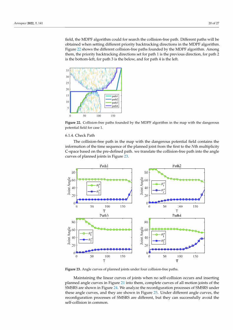
Aerospace 2022, 9, 141 20 of 27

field, the MDPF algorithm could for search the collision-free path. Different paths will beobtained when setting different priority backtracking directions in the MDPF algorithm.Figure 22 shows the different collision-free paths founded by the MDPF algorithm. Amongthem, the priority backtracking directions set for path 1 is the previous direction, for path 2is the bottom-left, for path 3 is the below, and for path 4 is the left.

Aerospace 2022, 9, 141 20 of 28



gerous field strength of all grids in the binary map. In the map with the dangerous poten-tial field, the MDPF algorithm could for search the collision-free path. Different paths will be obtained when setting different priority backtracking directions in the MDPF algo-rithm. Figure 22 shows the different collision-free paths founded by the MDPF algorithm. Among them, the priority backtracking directions set for path 1 is the previous direction, for path 2 is the bottom-left, for path 3 is the below, and for path 4 is the left.

Figure 22. Collision-free paths founded by the MDPF algorithm in the map with the dangerous potential field for case 1.


information of the time sequence of the planned joint from the first to the Nth multiplicity C-space based on the pre-defined path. we translate the collision-free path into the angle curves of planned joints in Figure 23.

0 50 100 150

5

10

15

20

25

30

35


Figure 22. Collision-free paths founded by the MDPF algorithm in the map with the dangerouspotential field for case 1.

6.1.4. Check Path

The collision-free path in the map with the dangerous potential field contains theinformation of the time sequence of the planned joint from the first to the Nth multiplicityC-space based on the pre-defined path. we translate the collision-free path into the anglecurves of planned joints in Figure 23.

Aerospace 2022, 9, 141 21 of 28

Figure 23. Angle curves of planned joints under four collision-free paths.

Maintaining the linear curves of joints when no self-collision occurs and inserting planned angle curves in Figure 21 into them, complete curves of all motion joints of the SMSRS are shown in Figure 24. We analyze the reconfiguration processes of SMSRS under these angle curves, and they are shown in Figure 25. Under different angle curves, the reconfiguration processes of SMSRS are different, but they can successfully avoid the self-collision in common.

(a) (b)

(c) (d)

Join

t Ang

le

Join

t Ang

le

Join

t Ang

le

Join

t Ang

le

Join

t Ang

le

Join

t Ang

le

Join

t Ang

le

Join

t Ang

le


Maintaining the linear curves of joints when no self-collision occurs and insertingplanned angle curves in Figure 21 into them, complete curves of all motion joints of theSMSRS are shown in Figure 24. We analyze the reconfiguration processes of SMSRS underthese angle curves, and they are shown in Figure 25. Under different angle curves, thereconfiguration processes of SMSRS are different, but they can successfully avoid theself-collision in common.

Aerospace 2022, 9, 141 21 of 27

Aerospace 2022, 9, 141 21 of 28



(a) (b)

(c) (d)

Join

t Ang

le

Join

t Ang

le

Join

t Ang

le

Join

t Ang

le

Join

t Ang

le

Join

t Ang

le

Join

t Ang

le

Join

t Ang

le

Figure 24. Paths of all motion joints of the SMSRS under four collision-free paths: (a) path 1, (b) path2, (c) path 3 and (d) path 4.

Aerospace 2022, 9, 141 22 of 28

Figure 24. Paths of all motion joints of the SMSRS under four collision-free paths: (a) path 1, (b) path 2, (c) path 3 and (d) path 4.

(a) (b)

(c) (d)

Figure 25. Reconfiguration processes of SMSRS under four collision-free paths: (a) path 1, (b) path 2, (c) path 3 and (d) path 4.

6.2. Case 2 6.2.1. Locate Collide Modules and Determine Planned Joints

Case 2 sets the joints moving from the initial angles to the final angles in linear paths. According to the collision detection model in Section 3 and the method for locating colli-sion modules in Section 4.1, the first and fifth modules on a side of SMSRS are located as the collision modules by real-time detection, and the collision time sequence is (245, 835) when the total time of collision process is divided into 1000 segments.

6.2.2. Spliced C-Space According to the principles in Section 4.2 to select planned joints, they are set as two

motion joints: 𝜃 is the eleventh joint on a side and 𝜃 is the sixth joint on a side. And 𝜃 _ , 𝜃 _ = (24.15, 54.9), 𝜃 _ , 𝜃 _ = (3.45, −69.3), 𝜃 , 𝜃 =(−90,90), 𝜃 , 𝜃 = (−90,90). The 180-multiplicity C-spaces are built follow-ing the steps in Section 4.3.1. However, after pre-defining paths according to the principles in Figure 10a, the binary map generated by splicing C-space under each pre-defined path of current planned joints is invalid, it proves the planned joints cannot avoid self-collision of SMSRS after path planning.

In this case, we reselect the planned joint and set 𝜃 as the eleventh joint on a side and 𝜃 as the tenth joint on a side. At this point, the 180-multiplicity C-spaces are re-built using the random sampling method following steps in Section 4.3.1. After multiple itera-tions shown in Figure 26, one pre-defined path is found as the needed pre-defined path because the binary map generated by splicing 180-multiplicity C-spaces under it is valid, and it is marked obviously in Figure 26.

Figure 25. Reconfiguration processes of SMSRS under four collision-free paths: (a) path 1, (b) path 2,(c) path 3 and (d) path 4.

Aerospace 2022, 9, 141 22 of 27

6.2. Case 26.2.1. Locate Collide Modules and Determine Planned Joints

Case 2 sets the joints moving from the initial angles to the final angles in linear paths.According to the collision detection model in Section 3 and the method for locating collisionmodules in Section 4.1, the first and fifth modules on a side of SMSRS are located as thecollision modules by real-time detection, and the collision time sequence is (245, 835) whenthe total time of collision process is divided into 1000 segments.

6.2.2. Spliced C-Space

According to the principles in Section 4.2 to select planned joints, they are set as twomotion joints: θ

p1 is the eleventh joint on a side and θ

p2 is the sixth joint on a side. And(

θp1_start, θ

p2_start

)= (24.15, 54.9),

(θ

p1_end, θ

p2_end

)= (3.45,−69.3),

((θ

p1

)min

,(

θp1

)max

)=

(−90, 90),((

θp2

)min

,(

θp2

)max

)= (−90, 90). The 180-multiplicity C-spaces are built follow-

ing the steps in Section 4.3.1. However, after pre-defining paths according to the principlesin Figure 10a, the binary map generated by splicing C-space under each pre-defined pathof current planned joints is invalid, it proves the planned joints cannot avoid self-collisionof SMSRS after path planning.

In this case, we reselect the planned joint and set θp1 as the eleventh joint on a side and

θp2 as the tenth joint on a side. At this point, the 180-multiplicity C-spaces are re-built using

the random sampling method following steps in Section 4.3.1. After multiple iterationsshown in Figure 26, one pre-defined path is found as the needed pre-defined path becausethe binary map generated by splicing 180-multiplicity C-spaces under it is valid, and it ismarked obviously in Figure 26.

Aerospace 2022, 9, 141 23 of 28

Figure 26. All iterated pre-defined paths and the final pre-defined path in case 2.

Under the final pre-defined path, splice 180-multiplicity C-spaces following steps in Section 4.3.3, and the binary map is shown in Figure 27. In the binary map, (0, 0) is the start point of the path, and (180, 37) is the end point, and there exist accessible paths from the start point to the end point.



gerous field strength of all grids in the binary map. In the map with the dangerous poten-tial field, the MDPF algorithm could search for the collision-free path. Different paths will be obtained when setting different priority backtracking directions in the MDPF algo-rithm. Figure 28 shows the different collision-free paths founded by the MDPF algorithm. Among them, the priority backtracking directions for path 1 is the previous direction, for path 2 is the bottom-left, for path 3 is the below, and for path 4 is the left.

5 10 15 20 25

0

20

40

60

80


Under the final pre-defined path, splice 180-multiplicity C-spaces following steps inSection 4.3.3, and the binary map is shown in Figure 27. In the binary map, (0, 0) is the startpoint of the path, and (180, 37) is the end point, and there exist accessible paths from thestart point to the end point.

6.2.3. Path Planning

The map with the dangerous potential field can be obtained by calculating the danger-ous field strength of all grids in the binary map. In the map with the dangerous potentialfield, the MDPF algorithm could search for the collision-free path. Different paths will beobtained when setting different priority backtracking directions in the MDPF algorithm.Figure 28 shows the different collision-free paths founded by the MDPF algorithm. Amongthem, the priority backtracking directions for path 1 is the previous direction, for path 2 isthe bottom-left, for path 3 is the below, and for path 4 is the left.

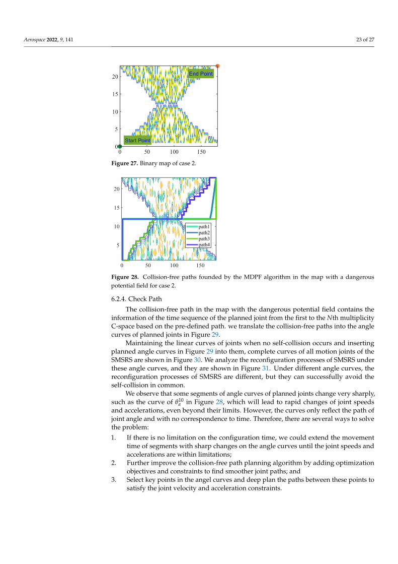
Aerospace 2022, 9, 141 23 of 27

Aerospace 2022, 9, 141 23 of 28


Under the final pre-defined path, splice 180-multiplicity C-spaces following steps in Section 4.3.3, and the binary map is shown in Figure 27. In the binary map, (0, 0) is the start point of the path, and (180, 37) is the end point, and there exist accessible paths from the start point to the end point.



gerous field strength of all grids in the binary map. In the map with the dangerous poten-tial field, the MDPF algorithm could search for the collision-free path. Different paths will be obtained when setting different priority backtracking directions in the MDPF algo-rithm. Figure 28 shows the different collision-free paths founded by the MDPF algorithm. Among them, the priority backtracking directions for path 1 is the previous direction, for path 2 is the bottom-left, for path 3 is the below, and for path 4 is the left.

5 10 15 20 25

0

20

40

60

80


Aerospace 2022, 9, 141 24 of 28

Figure 28. Collision-free paths founded by the MDPF algorithm in the map with a dangerous po-tential field for case 2.


information of the time sequence of the planned joint from the first to the Nth multiplicity C-space based on the pre-defined path. we translate the collision-free paths into the angle curves of planned joints in Figure 29.



0 50 100 150

5

10

15

20


Join

t Ang

le

Join

t Ang

le

Join

t Ang

le

Join

t Ang

le

Figure 28. Collision-free paths founded by the MDPF algorithm in the map with a dangerouspotential field for case 2.

6.2.4. Check Path

The collision-free path in the map with the dangerous potential field contains theinformation of the time sequence of the planned joint from the first to the Nth multiplicityC-space based on the pre-defined path. we translate the collision-free paths into the anglecurves of planned joints in Figure 29.

Maintaining the linear curves of joints when no self-collision occurs and insertingplanned angle curves in Figure 29 into them, complete curves of all motion joints of theSMSRS are shown in Figure 30. We analyze the reconfiguration processes of SMSRS underthese angle curves, and they are shown in Figure 31. Under different angle curves, thereconfiguration processes of SMSRS are different, but they can successfully avoid theself-collision in common.

We observe that some segments of angle curves of planned joints change very sharply,such as the curve of θ10

a in Figure 28, which will lead to rapid changes of joint speedsand accelerations, even beyond their limits. However, the curves only reflect the path ofjoint angle and with no correspondence to time. Therefore, there are several ways to solvethe problem:

1. If there is no limitation on the configuration time, we could extend the movementtime of segments with sharp changes on the angle curves until the joint speeds andaccelerations are within limitations;

2. Further improve the collision-free path planning algorithm by adding optimizationobjectives and constraints to find smoother joint paths; and

3. Select key points in the angel curves and deep plan the paths between these points tosatisfy the joint velocity and acceleration constraints.

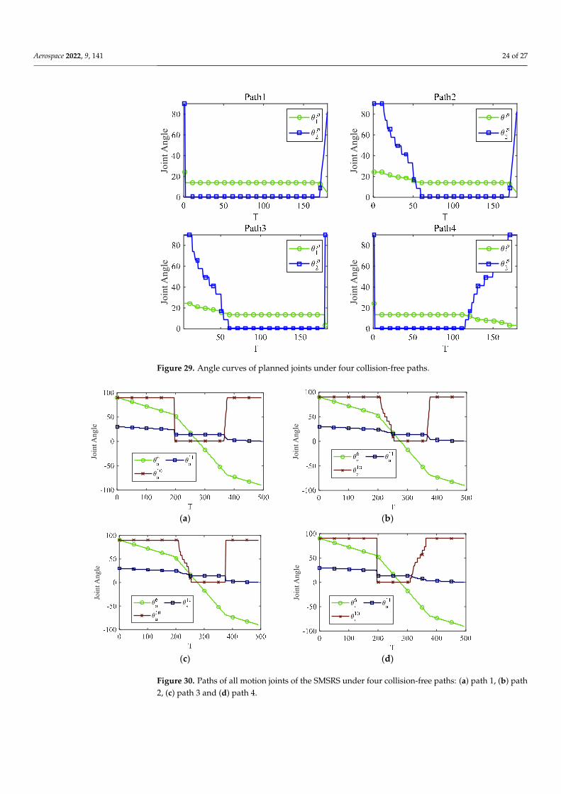
Aerospace 2022, 9, 141 24 of 27

Aerospace 2022, 9, 141 24 of 28

Figure 28. Collision-free paths founded by the MDPF algorithm in the map with a dangerous po-tential field for case 2.


information of the time sequence of the planned joint from the first to the Nth multiplicity C-space based on the pre-defined path. we translate the collision-free paths into the angle curves of planned joints in Figure 29.



0 50 100 150

5

10

15

20


Join

t Ang

le

Join

t Ang

le

Join

t Ang

le

Join

t Ang

leFigure 29. Angle curves of planned joints under four collision-free paths.

Aerospace 2022, 9, 141 25 of 28

(a) (b)

(c) (d)


(a) (b)

(c) (d)

Figure 31. Reconfiguration processes of SMSRS under four collision-free paths. (a) path 1, (b) path 2, (c) path 3 and (d) path 4.

Join

t Ang

le

Join

t Ang

le

Join

t Ang

le

Join

t Ang

le

Figure 30. Paths of all motion joints of the SMSRS under four collision-free paths: (a) path 1, (b) path2, (c) path 3 and (d) path 4.

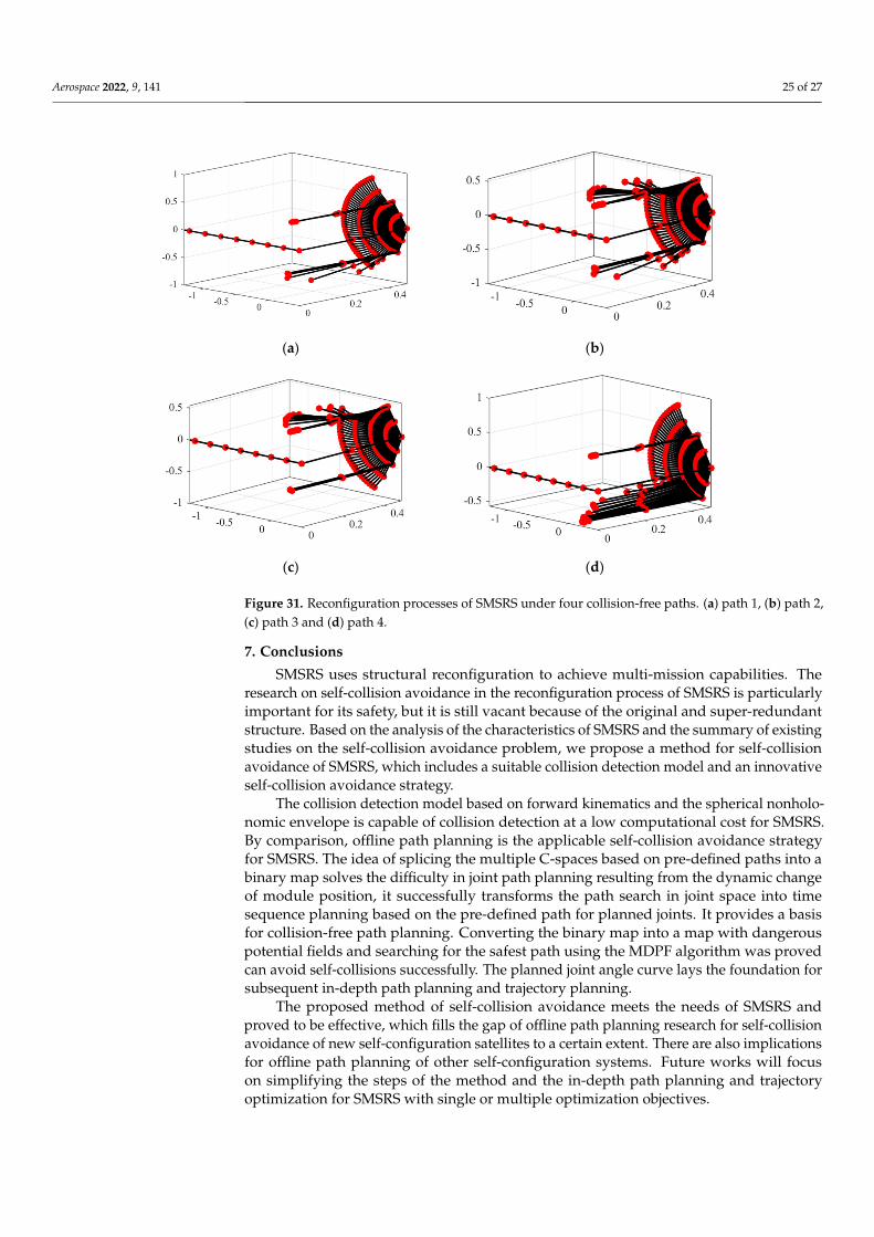
Aerospace 2022, 9, 141 25 of 27

Aerospace 2022, 9, 141 25 of 28

(a) (b)

(c) (d)


(a) (b)

(c) (d)

Figure 31. Reconfiguration processes of SMSRS under four collision-free paths. (a) path 1, (b) path 2, (c) path 3 and (d) path 4.

Join

t Ang

le

Join

t Ang

le

Join

t Ang

le

Join

t Ang

le

Figure 31. Reconfiguration processes of SMSRS under four collision-free paths. (a) path 1, (b) path 2,(c) path 3 and (d) path 4.

7. Conclusions

SMSRS uses structural reconfiguration to achieve multi-mission capabilities. Theresearch on self-collision avoidance in the reconfiguration process of SMSRS is particularlyimportant for its safety, but it is still vacant because of the original and super-redundantstructure. Based on the analysis of the characteristics of SMSRS and the summary of existingstudies on the self-collision avoidance problem, we propose a method for self-collisionavoidance of SMSRS, which includes a suitable collision detection model and an innovativeself-collision avoidance strategy.

The collision detection model based on forward kinematics and the spherical nonholo-nomic envelope is capable of collision detection at a low computational cost for SMSRS.By comparison, offline path planning is the applicable self-collision avoidance strategyfor SMSRS. The idea of splicing the multiple C-spaces based on pre-defined paths into abinary map solves the difficulty in joint path planning resulting from the dynamic changeof module position, it successfully transforms the path search in joint space into timesequence planning based on the pre-defined path for planned joints. It provides a basisfor collision-free path planning. Converting the binary map into a map with dangerouspotential fields and searching for the safest path using the MDPF algorithm was provedcan avoid self-collisions successfully. The planned joint angle curve lays the foundation forsubsequent in-depth path planning and trajectory planning.

The proposed method of self-collision avoidance meets the needs of SMSRS andproved to be effective, which fills the gap of offline path planning research for self-collisionavoidance of new self-configuration satellites to a certain extent. There are also implicationsfor offline path planning of other self-configuration systems. Future works will focuson simplifying the steps of the method and the in-depth path planning and trajectoryoptimization for SMSRS with single or multiple optimization objectives.

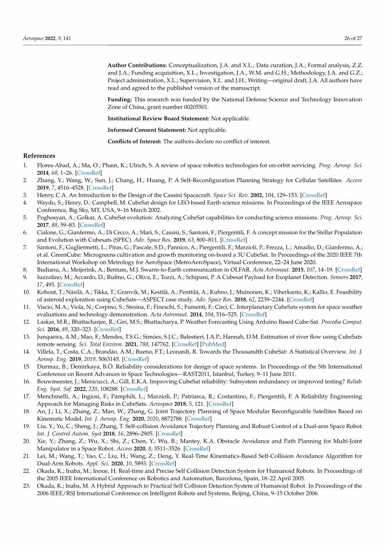
Aerospace 2022, 9, 141 26 of 27

Author Contributions: Conceptualization, J.A. and X.L.; Data curation, J.A.; Formal analysis, Z.Z.and J.A.; Funding acquisition, X.L.; Investigation, J.A., W.M. and G.H.; Methodology, J.A. and G.Z.;Project administration, X.L.; Supervision, X.L. and J.H.; Writing—original draft, J.A. All authors haveread and agreed to the published version of the manuscript.

Funding: This research was funded by the National Defense Science and Technology InnovationZone of China, grant number 00205501.

Institutional Review Board Statement: Not applicable.

Informed Consent Statement: Not applicable.

Conflicts of Interest: The authors declare no conflict of interest.

References1. Flores-Abad, A.; Ma, O.; Pham, K.; Ulrich, S. A review of space robotics technologies for on-orbit servicing. Prog. Aerosp. Sci.

2014, 68, 1–26. [CrossRef]2. Zhang, Y.; Wang, W.; Sun, J.; Chang, H.; Huang, P. A Self-Reconfiguration Planning Strategy for Cellular Satellites. Access

2019, 7, 4516–4528. [CrossRef]3. Henry, C.A. An Introduction to the Design of the Cassini Spacecraft. Space Sci. Rev. 2002, 104, 129–153. [CrossRef]4. Waydo, S.; Henry, D.; Campbell, M. CubeSat design for LEO-based Earth science missions. In Proceedings of the IEEE Aerospace

Conference, Big Sky, MT, USA, 9–16 March 2002.5. Poghosyan, A.; Golkar, A. CubeSat evolution: Analyzing CubeSat capabilities for conducting science missions. Prog. Aerosp. Sci.

2017, 88, 59–83. [CrossRef]6. Cialone, G.; Gianfermo, A.; Di Cecco, A.; Mari, S.; Cassisi, S.; Santoni, F.; Piergentili, F. A concept mission for the Stellar Population

and Evolution with Cubesats (SPEC). Adv. Space Res. 2019, 63, 800–811. [CrossRef]7. Santoni, F.; Gugliermetti, L.; Piras, G.; Pascale, S.D.; Pannico, A.; Piergentili, F.; Marzioli, P.; Frezza, L.; Amadio, D.; Gianfermo, A.;

et al. GreenCube: Microgreens cultivation and growth monitoring on-board a 3U CubeSat. In Proceedings of the 2020 IEEE 7thInternational Workshop on Metrology for AeroSpace (MetroAeroSpace), Virtual Conference, 22–24 June 2020.

8. Budianu, A.; Meijerink, A.; Bentum, M.J. Swarm-to-Earth communication in OLFAR. Acta Astronaut. 2015, 107, 14–19. [CrossRef]9. Iuzzolino, M.; Accardo, D.; Rufino, G.; Oliva, E.; Tozzi, A.; Schipani, P. A Cubesat Payload for Exoplanet Detection. Sensors 2017,

17, 493. [CrossRef]10. Kohout, T.; Näsilä, A.; Tikka, T.; Granvik, M.; Kestilä, A.; Penttilä, A.; Kuhno, J.; Muinonen, K.; Viherkanto, K.; Kallio, E. Feasibility

of asteroid exploration using CubeSats—ASPECT case study. Adv. Space Res. 2018, 62, 2239–2244. [CrossRef]11. Viscio, M.A.; Viola, N.; Corpino, S.; Stesina, F.; Fineschi, S.; Fumenti, F.; Circi, C. Interplanetary CubeSats system for space weather

evaluations and technology demonstration. Acta Astronaut. 2014, 104, 516–525. [CrossRef]12. Laskar, M.R.; Bhattacharjee, R.; Giri, M.S.; Bhattacharya, P. Weather Forecasting Using Arduino Based Cube-Sat. Procedia Comput.

Sci. 2016, 89, 320–323. [CrossRef]13. Junqueira, A.M.; Mao, F.; Mendes, T.S.G.; Simões, S.J.C.; Balestieri, J.A.P.; Hannah, D.M. Estimation of river flow using CubeSats

remote sensing. Sci. Total Environ. 2021, 788, 147762. [CrossRef] [PubMed]14. Villela, T.; Costa, C.A.; Brandão, A.M.; Bueno, F.T.; Leonardi, R. Towards the Thousandth CubeSat: A Statistical Overview. Int. J.

Aerosp. Eng. 2019, 2019, 5063145. [CrossRef]15. Durmaz, B.; Demirkaya, B.Ö. Reliability considerations for design of space systems. In Proceedings of the 5th International

Conference on Recent Advances in Space Technologies—RAST2011, Istanbul, Turkey, 9–11 June 2011.16. Bouwmeester, J.; Menicucci, A.; Gill, E.K.A. Improving CubeSat reliability: Subsystem redundancy or improved testing? Reliab.

Eng. Syst. Saf. 2022, 220, 108288. [CrossRef]17. Menchinelli, A.; Ingiosi, F.; Pamphili, L.; Marzioli, P.; Patriarca, R.; Costantino, F.; Piergentili, F. A Reliability Engineering

Approach for Managing Risks in CubeSats. Aerospace 2018, 5, 121. [CrossRef]18. An, J.; Li, X.; Zhang, Z.; Man, W.; Zhang, G. Joint Trajectory Planning of Space Modular Reconfigurable Satellites Based on

Kinematic Model. Int. J. Aerosp. Eng. 2020, 2020, 8872788. [CrossRef]19. Liu, Y.; Yu, C.; Sheng, J.; Zhang, T. Self-collision Avoidance Trajectory Planning and Robust Control of a Dual-arm Space Robot.

Int. J. Control Autom. Syst 2018, 16, 2896–2905. [CrossRef]20. Xie, Y.; Zhang, Z.; Wu, X.; Shi, Z.; Chen, Y.; Wu, B.; Mantey, K.A. Obstacle Avoidance and Path Planning for Multi-Joint

Manipulator in a Space Robot. Access 2020, 8, 3511–3526. [CrossRef]21. Lei, M.; Wang, T.; Yao, C.; Liu, H.; Wang, Z.; Deng, Y. Real-Time Kinematics-Based Self-Collision Avoidance Algorithm for

Dual-Arm Robots. Appl. Sci. 2020, 10, 5893. [CrossRef]22. Okada, K.; Inaba, M.; Inoue, H. Real-time and Precise Self Collision Detection System for Humanoid Robots. In Proceedings of

the 2005 IEEE International Conference on Robotics and Automation, Barcelona, Spain, 18–22 April 2005.23. Okada, K.; Inaba, M. A Hybrid Approach to Practical Self Collision Detection System of Humanoid Robot. In Proceedings of the

2006 IEEE/RSJ International Conference on Intelligent Robots and Systems, Beijing, China, 9–15 October 2006.

http://doi.org/10.1016/j.paerosci.2014.03.002

http://doi.org/10.1109/ACCESS.2018.2888588

http://doi.org/10.1023/A:1023696808894

http://doi.org/10.1016/j.paerosci.2016.11.002

http://doi.org/10.1016/j.asr.2018.10.012

http://doi.org/10.1016/j.actaastro.2014.10.041

http://doi.org/10.3390/s17030493

http://doi.org/10.1016/j.asr.2017.07.036


http://doi.org/10.1016/j.procs.2016.06.078

http://doi.org/10.1016/j.scitotenv.2021.147762

http://www.ncbi.nlm.nih.gov/pubmed/34022571

http://doi.org/10.1155/2019/5063145

http://doi.org/10.1016/j.ress.2021.108288

http://doi.org/10.3390/aerospace5040121

http://doi.org/10.1155/2020/8872788

http://doi.org/10.1007/s12555-017-0757-z

http://doi.org/10.1109/ACCESS.2019.2961167

http://doi.org/10.3390/app10175893

Aerospace 2022, 9, 141 27 of 27

24. Zhao, L.; Zhao, J.; Liu, H. Solving the Inverse Kinematics Problem of Multiple Redundant Manipulators with Collision Avoidancein Dynamic Environments. J. Intell. Robot. Syst. 2021, 101, 30. [CrossRef]

25. Cascio, J.; Karpenko, M.; Gong, Q.; Sekhavat, P.; Ross, I.M. Smooth proximity computation for collision-free optimal control ofmultiple robotic manipulators. In Proceedings of the 2009 IEEE/RSJ International Conference on Intelligent Robots and Systems,St. Louis, MO, USA, 10–15 October 2009.

26. Wang, W.; Zhu, M.; Wang, X.; He, S.; He, J.; Xu, Z. An improved artificial potential field method of trajectory planning andobstacle avoidance for redundant manipulators. Int. J. Adv. Robot. Syst. 2018, 15, 172988141879956. [CrossRef]

27. Koptev, M.; Figueroa, N.; Billard, A. Real-Time Self-Collision Avoidance in Joint Space for Humanoid Robots. IEEE Robot. Autom.Lett. 2021, 6, 1240–1247. [CrossRef]

28. Stasse, O.; Escande, A.; Mansard, N.; Miossec, S.; Evrard, P.; Kheddar, A. Real-time (self)-collision avoidance task on a hrp-2humanoid robot. In Proceedings of the 2008 IEEE International Conference on Robotics and Automation, Pasadena, CA, USA,19–23 May 2008.

29. Dietrich, A.; Wimbock, T.; Taubig, H.; Albu-Schaffer, A.; Hirzinger, G. Extensions to reactive self-collision avoidance for torqueand position controlled humanoids. In Proceedings of the 2011 IEEE International Conference on Robotics and Automation,Shanghai, China, 9–13 May 2011.

30. Quiroz-Omana, J.J.; Adorno, B.V. Whole-Body Control With (Self) Collision Avoidance Using Vector Field Inequalities. IEEERobot. Autom. Lett. 2019, 4, 4048–4053. [CrossRef]

31. Yahya, S.; Moghavvemi, M.; Mohamed, H.A.F. Geometrical approach of planar hyper-redundant manipulators: Inverse kinemat-ics, path planning and workspace. Simul. Model. Pract. Theory 2011, 19, 406–422. [CrossRef]

32. Dash, A.K.; Chen, I.M.; Yeo, S.H.; Yang, G. Workspace generation and planning singularity-free path for parallel manipulators.Mech. Mach. Theory 2005, 40, 776–805. [CrossRef]

33. Stilman, M. Global Manipulation Planning in Robot Joint Space With Task Constraints. IEEE Trans. Robot. 2010, 26, 576–584.[CrossRef]

34. Delgado, R.; Choi, B.W. Practical high curvature path planning algorithm in joint space. Electron. Lett. 2015, 51, 469–471.[CrossRef]

35. Rybus, T.; Wojtunik, M.; Basmadji, F.L. Optimal collision-free path planning of a free-floating space robot using spline-basedtrajectories. Acta Astronaut. 2022, 190, 395–408. [CrossRef]

36. Gao, X.; Jia, Q.; Sun, H.; Chen, G. Research on Path Planning for 7-DOF Space Manipulator to Avoid Obstacle Based on AAlgorithm. Sens. Lett. 2011, 9, 1515–1519. [CrossRef]

37. Serrantola, W.G.; Grassi, V. Trajectory Planning for a Dual-Arm Planar Free-Floating Manipulator using RRTControl. InProceedings of the 19th International Conference on Advanced Robotics (ICAR), Belo Horizonte, Brazil, 2–6 December 2019.

38. Wei, K.; Ren, B. A Method on Dynamic Path Planning for Robotic Manipulator Autonomous Obstacle Avoidance Based on anImproved RRT Algorithm. Sensors 2018, 18, 571. [CrossRef]

39. Gong, L.; Zhang, Y.; Cheng, J. Coordinated Path Planning Based on RRT Algorithm for Robot. Appl. Mech. Mater. 2014, 494–495,1003–1007. [CrossRef]

40. Liu, S.; Zhang, Q.; Zhou, D. Obstacle Avoidance Path Planning of Space Manipulator Based on Improved Artificial Potential FieldMethod. J. Inst. Eng. India Ser. C 2014, 95, 31–39. [CrossRef]

41. Tong, Y.; Liu, J.; Liu, Y.; Yuan, Y. Analytical inverse kinematic computation for 7-DOF redundant sliding manipulators. Mech.Mach. Theory 2021, 155, 104006. [CrossRef]

42. Yiyang, L.; Xi, J.; Hongfei, B.; Zhining, W.; Liangliang, S. A General Robot Inverse Kinematics Solution Method Based onImproved PSO Algorithm. IEEE Access 2021, 9, 32341–32350.

43. Lopez-Franco, C.; Hernandez-Barragan, J.; Alanis, A.Y.; Arana-Daniel, N. A soft computing approach for inverse kinematics ofrobot manipulators. Eng. Appl. Artif. Intel. 2018, 74, 104–120. [CrossRef]

44. Zhang, Q.; Wang, L.; Zhou, D.S. Trajectory Planning of 7-DOF Space Manipulator for Minimizing Base Disturbance. Int. J. Adv.Robot. Syst. 2016, 13, 10. [CrossRef]

45. Xie, Y.; Zhou, R.; Yang, Y. Improved Distorted Configuration Space Path Planning and Its Application to Robot Manipulators.Sensors 2020, 20, 6060. [CrossRef]

http://doi.org/10.1007/s10846-020-01279-w

http://doi.org/10.1177/1729881418799562

http://doi.org/10.1109/LRA.2021.3057024

http://doi.org/10.1109/LRA.2019.2928783

http://doi.org/10.1016/j.simpat.2010.08.001

http://doi.org/10.1016/j.mechmachtheory.2005.01.001

http://doi.org/10.1109/TRO.2010.2044949

http://doi.org/10.1049/el.2014.3926


http://doi.org/10.1166/sl.2011.1665

http://doi.org/10.3390/s18020571

http://doi.org/10.4028/www.scientific.net/AMM.494-495.1003

http://doi.org/10.1007/s40032-014-0099-z

http://doi.org/10.1016/j.mechmachtheory.2020.104006

http://doi.org/10.1016/j.engappai.2018.06.001

http://doi.org/10.5772/62123

http://doi.org/10.3390/s20216060

Path Planning for Self-Collision Avoidance of Space Modular ...

Documents

Transcript of Path Planning for Self-Collision Avoidance of Space Modular ...