Passive Beam Spreading

in Proton Radiation Therapy

Bernard Gottschalk

Harvard High Energy Physics Laboratory38 Oxford St., Cambridge, MA 01238, USA

gottschalk@huhepl.harvard.eduhttp://huhepl.harvard.edu/˜gottschalk

DRAFT

October 1, 2004

Contents

1 Introduction 51.1 Prerequisites . . . . . . . . . . . . . . . . . . . . . . . . . . . . . 51.2 Accuracy of the Method . . . . . . . . . . . . . . . . . . . . . . . 61.3 Mathematical Style . . . . . . . . . . . . . . . . . . . . . . . . . . 71.4 Software Platform . . . . . . . . . . . . . . . . . . . . . . . . . . 71.5 Acknowledgements . . . . . . . . . . . . . . . . . . . . . . . . . . 8

2 Symbol Definitions and Physical Constants 92.1 Acronyms . . . . . . . . . . . . . . . . . . . . . . . . . . . . . . . 92.2 Symbol Definitions . . . . . . . . . . . . . . . . . . . . . . . . . . 92.3 Physical Constants . . . . . . . . . . . . . . . . . . . . . . . . . . 102.4 Conversions . . . . . . . . . . . . . . . . . . . . . . . . . . . . . . 10

3 Preliminaries 113.1 Areal Density: g/cm2 . . . . . . . . . . . . . . . . . . . . . . . . 113.2 MeV . . . . . . . . . . . . . . . . . . . . . . . . . . . . . . . . . . 113.3 Mass Stopping Power . . . . . . . . . . . . . . . . . . . . . . . . . 123.4 Fluence . . . . . . . . . . . . . . . . . . . . . . . . . . . . . . . . 123.5 Physical Dose . . . . . . . . . . . . . . . . . . . . . . . . . . . . . 123.6 Biologically Effective Dose . . . . . . . . . . . . . . . . . . . . . . 133.7 Computing Dose from Fluence . . . . . . . . . . . . . . . . . . . 143.8 Computing Dose Rate from Proton Current Density . . . . . . . 153.9 Dose Rate in a Therapy Beam . . . . . . . . . . . . . . . . . . . 153.10 Air Filled Ionization Chambers . . . . . . . . . . . . . . . . . . . 173.11 Proton Kinematics . . . . . . . . . . . . . . . . . . . . . . . . . . 18

4 Gaussians 194.1 Small-Angle Approximation . . . . . . . . . . . . . . . . . . . . . 194.2 1D Gaussian Probability Density . . . . . . . . . . . . . . . . . . 194.3 2D Gaussian Probability Density . . . . . . . . . . . . . . . . . . 214.4 Implications for Single Scattering . . . . . . . . . . . . . . . . . . 214.5 Error Function . . . . . . . . . . . . . . . . . . . . . . . . . . . . 23

5 The Cubic Spline 265.1 Description . . . . . . . . . . . . . . . . . . . . . . . . . . . . . . 265.2 Cubic Spline Interpolation . . . . . . . . . . . . . . . . . . . . . . 265.3 Using the Cubic Spline . . . . . . . . . . . . . . . . . . . . . . . . 275.4 Cubic Spline Fit . . . . . . . . . . . . . . . . . . . . . . . . . . . 28

5.4.1 Choosing Initial Points . . . . . . . . . . . . . . . . . . . . 285.4.2 Optimizing the Fit . . . . . . . . . . . . . . . . . . . . . . 305.4.3 Pathologies . . . . . . . . . . . . . . . . . . . . . . . . . . 30

5.5 The Broken Spline . . . . . . . . . . . . . . . . . . . . . . . . . . 315.6 The Spline as a General-Purpose Function . . . . . . . . . . . . . 32

1

6 Stopping 336.1 Stopping Theory . . . . . . . . . . . . . . . . . . . . . . . . . . . 33

6.1.1 Qualitative . . . . . . . . . . . . . . . . . . . . . . . . . . 336.1.2 Quantitative . . . . . . . . . . . . . . . . . . . . . . . . . 34

6.2 Range . . . . . . . . . . . . . . . . . . . . . . . . . . . . . . . . . 356.3 Range Straggling . . . . . . . . . . . . . . . . . . . . . . . . . . . 366.4 Measuring Range . . . . . . . . . . . . . . . . . . . . . . . . . . . 376.5 Clinical Depth Prescription . . . . . . . . . . . . . . . . . . . . . 396.6 Interpolating Range-Energy Tables . . . . . . . . . . . . . . . . . 406.7 Finding the Energy Loss in a Degrader . . . . . . . . . . . . . . . 42

6.7.1 Using Range . . . . . . . . . . . . . . . . . . . . . . . . . 426.7.2 Using Stopping Power . . . . . . . . . . . . . . . . . . . . 426.7.3 In a Computer Program . . . . . . . . . . . . . . . . . . . 436.7.4 Exercise . . . . . . . . . . . . . . . . . . . . . . . . . . . . 436.7.5 Error Conditions . . . . . . . . . . . . . . . . . . . . . . . 43

6.8 Water Equivalence . . . . . . . . . . . . . . . . . . . . . . . . . . 436.8.1 Water Equivalence of Thin Degraders . . . . . . . . . . . 446.8.2 Equivalence in a Finely Divided Stack . . . . . . . . . . . 456.8.3 Measured Water Equivalence . . . . . . . . . . . . . . . . 45

6.9 Does the Order of Degraders Matter? . . . . . . . . . . . . . . . 456.10 Energy Spread of Degraded Beams . . . . . . . . . . . . . . . . . 466.11 Energy Stability of an Accelerator . . . . . . . . . . . . . . . . . 47

7 Scattering 497.1 Central Limit Theorem . . . . . . . . . . . . . . . . . . . . . . . 517.2 Moliere Theory . . . . . . . . . . . . . . . . . . . . . . . . . . . . 51

7.2.1 Thin Scatterer . . . . . . . . . . . . . . . . . . . . . . . . 527.2.2 Energy Loss . . . . . . . . . . . . . . . . . . . . . . . . . . 537.2.3 Compounds and Mixtures . . . . . . . . . . . . . . . . . . 547.2.4 Fano Correction . . . . . . . . . . . . . . . . . . . . . . . 547.2.5 Evaluation of the Integrals . . . . . . . . . . . . . . . . . 557.2.6 Numerical Results . . . . . . . . . . . . . . . . . . . . . . 55

7.3 Gaussian Approximations . . . . . . . . . . . . . . . . . . . . . . 597.3.1 Hanson’s Formula . . . . . . . . . . . . . . . . . . . . . . 597.3.2 Highland’s Formula . . . . . . . . . . . . . . . . . . . . . 597.3.3 Lynch and Dahl’s Formula . . . . . . . . . . . . . . . . . . 62

7.4 Fortran Function Theta0 . . . . . . . . . . . . . . . . . . . . . . . 627.5 Maximum Scattering from a Given Material . . . . . . . . . . . . 627.6 Adding Discrete Scatterers . . . . . . . . . . . . . . . . . . . . . 637.7 Summary . . . . . . . . . . . . . . . . . . . . . . . . . . . . . . . 64

8 Nuclear Interactions 658.1 Terminology . . . . . . . . . . . . . . . . . . . . . . . . . . . . . . 658.2 Elastic Scattering from Free Hydrogen . . . . . . . . . . . . . . . 668.3 Overview of Nonelastic Reactions . . . . . . . . . . . . . . . . . . 678.4 Local Energy Deposition Model . . . . . . . . . . . . . . . . . . . 678.5 Nuclear Buildup . . . . . . . . . . . . . . . . . . . . . . . . . . . 688.6 Predicting P . . . . . . . . . . . . . . . . . . . . . . . . . . . . . 728.7 Measuring P . . . . . . . . . . . . . . . . . . . . . . . . . . . . . 72

8.7.1 Simple Faraday Cup . . . . . . . . . . . . . . . . . . . . . 728.7.2 Multi Layer Faraday Cup . . . . . . . . . . . . . . . . . . 72

8.8 Summary . . . . . . . . . . . . . . . . . . . . . . . . . . . . . . . 75

2

9 Binary Degraders 779.1 High-Z and Low-Z Materials . . . . . . . . . . . . . . . . . . . . . 779.2 Notation to Describe Problems . . . . . . . . . . . . . . . . . . . 779.3 ‘Forward’ Problem . . . . . . . . . . . . . . . . . . . . . . . . . . 799.4 Single Degrader Inverse Problem . . . . . . . . . . . . . . . . . . 809.5 Binary Degrader Inverse Problem . . . . . . . . . . . . . . . . . . 819.6 Does the Order of Materials Matter? . . . . . . . . . . . . . . . . 829.7 Summary . . . . . . . . . . . . . . . . . . . . . . . . . . . . . . . 83

10 Degrader Stacks and Beam Spreading 8410.1 Beam Spreading . . . . . . . . . . . . . . . . . . . . . . . . . . . 8410.2 Experiment of Preston and Koehler . . . . . . . . . . . . . . . . . 8510.3 Effective Origin z0 . . . . . . . . . . . . . . . . . . . . . . . . . . 8610.4 Fermi-Eyges Theory . . . . . . . . . . . . . . . . . . . . . . . . . 8910.5 Summary . . . . . . . . . . . . . . . . . . . . . . . . . . . . . . . 89

11 The Bragg Peak 9011.1 Understanding the Bragg Peak . . . . . . . . . . . . . . . . . . . 90

11.1.1 Stopping Power, Straggling, Beam Energy Spread . . . . 9011.2 Theoretical Models . . . . . . . . . . . . . . . . . . . . . . . . . . 91

11.2.1 Beam Size . . . . . . . . . . . . . . . . . . . . . . . . . . . 9211.2.2 1/r2 Effect . . . . . . . . . . . . . . . . . . . . . . . . . . 9311.2.3 Tank Wall and Other Degraders . . . . . . . . . . . . . . 9311.2.4 Dosimeter . . . . . . . . . . . . . . . . . . . . . . . . . . . 9311.2.5 Low Energy Contamination . . . . . . . . . . . . . . . . . 9311.2.6 Nuclear Interactions . . . . . . . . . . . . . . . . . . . . . 9411.2.7 Electron and Nuclear Buildup . . . . . . . . . . . . . . . . 9511.2.8 Pathlength Effect . . . . . . . . . . . . . . . . . . . . . . . 9511.2.9 Checklist for Measuring the Bragg Peak . . . . . . . . . . 95

11.3 Commercial Equipment . . . . . . . . . . . . . . . . . . . . . . . 9611.3.1 Tank Size . . . . . . . . . . . . . . . . . . . . . . . . . . . 9611.3.2 Current vs. Charge Measurement . . . . . . . . . . . . . . 9711.3.3 Beam Monitor vs. Reference Chamber . . . . . . . . . . . 9711.3.4 Scanning vs. Dosimetry Mode . . . . . . . . . . . . . . . . 97

11.4 Fitting the Bragg Peak . . . . . . . . . . . . . . . . . . . . . . . . 9811.4.1 Overlying Material . . . . . . . . . . . . . . . . . . . . . . 9811.4.2 Extrapolation to Zero . . . . . . . . . . . . . . . . . . . . 99

11.5 Opening the BPK File . . . . . . . . . . . . . . . . . . . . . . . . . 9911.5.1 Removing the Fluence . . . . . . . . . . . . . . . . . . . . 10011.5.2 Adjusting the Energy . . . . . . . . . . . . . . . . . . . . 10011.5.3 Normalizing the Bragg Peak . . . . . . . . . . . . . . . . . 10011.5.4 A Closer Look at Normalization . . . . . . . . . . . . . . 101

12 Designing a Modulator 10412.1 Introduction . . . . . . . . . . . . . . . . . . . . . . . . . . . . . . 10412.2 Computing the Weights . . . . . . . . . . . . . . . . . . . . . . . 10612.3 Alternative Procedure for Weights . . . . . . . . . . . . . . . . . 10812.4 Defining Modulation . . . . . . . . . . . . . . . . . . . . . . . . . 10912.5 Step Size . . . . . . . . . . . . . . . . . . . . . . . . . . . . . . . 11012.6 Compensation . . . . . . . . . . . . . . . . . . . . . . . . . . . . . 11012.7 Useful Energy Range . . . . . . . . . . . . . . . . . . . . . . . . . 11212.8 Beam Gating . . . . . . . . . . . . . . . . . . . . . . . . . . . . . 11312.9 Beam Current Modulation . . . . . . . . . . . . . . . . . . . . . . 11412.10Physical Arrangement of Modulators . . . . . . . . . . . . . . . . 114

3

13 Single Scattering Energy Stacking Example 116

14 Double Scattering 11714.1 Introduction . . . . . . . . . . . . . . . . . . . . . . . . . . . . . . 11714.2 The Contoured Scatterer . . . . . . . . . . . . . . . . . . . . . . . 11914.3 Beam Imperfections . . . . . . . . . . . . . . . . . . . . . . . . . 12114.4 Solving the Forward Problem . . . . . . . . . . . . . . . . . . . . 12114.5 Scaling and the Generic Solution . . . . . . . . . . . . . . . . . . 12414.6 The Useful Radius . . . . . . . . . . . . . . . . . . . . . . . . . . 12514.7 Optimization . . . . . . . . . . . . . . . . . . . . . . . . . . . . . 12514.8 Returning to the Real World . . . . . . . . . . . . . . . . . . . . 127

15 Double Scattering Upstream Modulator Example 129

16 Beam Steering 130

17 Capabilities of Double Scattering Systems 131

18 Transverse Penumbra 132

19 Distal Falloff 133

20 Collimators 134

List of Tables 135

List of Figures 136

Bibliography 139

4

Chapter 1

Introduction

This writeup is a guide to designing passive beam spreading systems from firstprinciples using just three ingredients:

• EM stopping theory: the Bethe equation and its consequences1

• EM multiple scattering theory: Moliere theory and its consequences

• Bragg peaks measured in water

Nuclear effects and some others are accounted for by using measured, ratherthan computed, Bragg peaks. Designs based on these methods are usually closeenough to specifications for clinical use, though they should be checked of course.They also provide reasonably accurate estimates of dose rates and beam monitoroutput factors, though the latter must be refined experimentally.

This writeup is a companion to our design programs. The Fortran sourcecode for these programs may be downloaded from the Web site on the title page.Follow the instructions in the README file. Note the Disclaimer of Warranty.

1.1 Prerequisites

Our level of discussion aims at the college graduate in science or engineering. Nobackground in particle physics is required. Indeed the kind of course that wouldhelp, an account of the basic interactions of the common particles with matter,is rarely taught nowadays. Algebra and the elements of calculus are required, ofcourse. You must have a firm grasp of what is meant by a derivative or integral,but we shall only use the most elementary special functions and none of theadvanced techniques of integration. If you can read Numerical Recipes [1] orthe equivalent with good comprehension, you’ll be fine.

We have tried to make this writeup self-contained. However, to keep it withinbounds, we will discuss stopping and multiple scattering on an ‘engineering’ levelwithout repeating the standard derivations. For these, you should go to theliterature. In the same spirit, we will generally refer you to Numerical Recipes[1] for mathematical methods. Though there is a bibliography as a guide tofurther reading, a very few basic references will get you started:

• Numerical Recipes [1] unless you already know the material.

• A synopsis of stopping theory. The opening pages of ICRU49 [2] or Janni[3] are excellent.

1 EM: electromagnetic. See chapter 2 for acronyms and symbol definitions.

5

• A synopsis of Moliere’s multiple scattering theory. The HCL paper [4] is agood starting point. You will eventually need Bethe [5] if you really wantto work through the derivation and formulas for the angular distribution.If you know German, by all means read the two papers by Moliere [6, 7]which are beautifully written.

Concerning multiple scattering, be warned that the field is fairly tangled, andcertain experimental and theoretical papers are not helpful [4].

The article by Chu et al. [8] is a good review of beam spreading techniquesand instrumentation, broader in scope but with less emphasis on computationthan the present report.

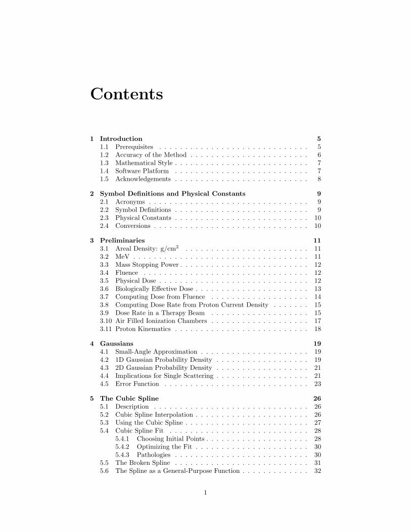
Figure 1.1: The first NEU design (1990), with experimental data.

1.2 Accuracy of the Method

How accurate are the methods described here? A double scattering systemwith a compensated upstream modulator and a compensated contoured secondscatterer was designed, built and tested at the Harvard Cyclotron Laboratory(HCL) in 1990, using an early version of the program NEU. Figure 1.1 showsexperimental data plotted against the prediction, using the 2004 version of NEU.A single normalization factor is used for all four panels. The depth-dose agreesextremely well with prediction. The transverse dose distributions agree fairlywell.

Of course, this proof of principle experiment was not an optimum design.The long throw (distance between first scatterer and isocenter) precluded that.The modulator overscatters in its thicker parts, as evidenced in the design by theabsence of compensating brass and in the transverse dose by the characteristic‘dished’ appearance. (If you don’t understand the previous sentence, we hope

6

you will by the time you’ve finished this report.) One can do much better underideal conditions. The essential point of Figure 1.1 is that the prediction agreespretty well with experiment.

1.3 Mathematical Style

We will solve most problems by numerical techniques, rather than trying foranswers in closed form. This reflects the general trend in applied science sincecomputers took over. Though analytic results have a nice closed feeling and, ifsimple, may yield good insights, the numerical approach

• May allow us to avoid certain approximations;

• Does not require extensive knowledge of special functions;

• May lead to more efficient computation.

Regrettably, the description of a sequence of numerical procedures has a moreamorphous feeling than a crisp sequence of equations.

Among the numerical techniques we will use are

• Cubic spline interpolation and fitting;

• Numerical integration (Simpson’s Rule);

• Root finding (False Position or Bisection);

• Matrix inversion (Gauss-Jordan elimination);

• Optimization (Linear Least-Squares, Marquardt, Grid Search).

These are all covered by Numerical Recipes [1]. If you are already familiar withthem you have a head start. The cubic spline is sufficiently central, and some ofour applications sufficiently unusual, that we devote a chapter to it. Even here,we leave the mathematical details to Numerical Recipes.

1.4 Software Platform

We will frequnetly use program fragments in Fortran to describe procedures.We have adapted our programs, many quite old, to the Compaq Visual Fortran(VF) V6.6a compiler. You can use any recent PC running any recent versionof Windows. Most applications, including the design of complicated doublescattering systems, take just a few seconds. They are not Monte Carlo programs.They are written in Fortran 77 (fixed-format .FOR) as distinct from Fortran 90.

The programs are grouped into ‘projects’ (a project is a group of moduleswith a single MAIN program) all of which use the VF ‘QuikWin’ option. Thisoffers simple but adequate graphics, which can be saved in bitmap .BMP format,and which we sometimes use to illustrate the text.

At this writing, we have made freely available certain end products in theform of executables (LOOKUP and NEU for example), as well as all of the sourcecode except two routines from Numerical Methods. We do not plan to distributethe underlying project structure. You can use the Fortran source code as studymaterial or as a basis for other projects. You may even be tempted to rewriteit in the computer language du jour, but it might be better to learn Fortran.

7

1.5 Acknowledgements

This report is a solo project but I owe my ability to write it to many personsassociated with the Harvard Cyclotron Lab (HCL). I came there in 1956 as agraduate student, stayed till 1965 as a postdoc, and returned in 1981. By thattime HCL was a full-time radiation therapy clinic. We treated our first patienton May 25, 1961 and our last on April 10, 2002: 9115 patients in 40 years. Forseveral decades HCL patients accounted for more than half the world total.

Karl Strauch was my thesis advisor, a good friend who taught me the craftof experimental physics. Richard Wilson, another important teacher during mygraduate years, became a staunch supporter of the clinical progam and, mostrecently, wrote the history of HCL [9]. Bill Preston, an exceptionally kind man,was Director during most of the physics research years, then helped preservethe Cyclotron for medical use, and made important contributions to the appliedphysics of proton beams.2

Andy Koehler succeeded Bill Preston, but insisted on being ‘Acting’ Directorfor his entire long tenure. More than anyone else, he managed to promote localmedical interest in proton beams and to pull the Cyclotron through its near-death experience in the late 1960’s. He made many important contributions tothe technology of proton beams and his name will come up frequently in thesenotes. Above all, Bill Preston, Andy Koehler, and Miles Wagner, who followedthem as Director, set a tone which made HCL a wonderful workplace. As DickWilson put it, HCL was a happy lab, and those who had the good fortune towork there will not forget the experience.

My friend Miles Wagner was my day-to-day colleague at HCL. We constantlybounced technical ideas off each other, and even though to this day our favoritesolutions to any given problem tend to be diametrically opposed, each of us gotthe job done in his own way.

With Miles, Andy and me, Janet Sisterson completed the ‘gang of four’ thatmet from time to time to discuss the Big Picture and plan the future at HCL.Janet represented the physics research side of HCL during the medical years,collaborating in the measurement of many reaction cross sections of interestin space physics. She also served the particle therapy community for decadeswith her ‘Particles’ newsletter, providing a forum and listing particle therapyfacilities worldwide. She has just now passed that job along.

Special thanks to Charles Mayo for his friendship and close collaboration,and to Rachel Platais, who built the first multi-layer Faraday Cup so well itworked right away. I also thank others at HCL: Gail Bradley, Jason Burns,Ethan Cascio, Lori Clarke, Alice Coggeshall, Dina Harp, Elliot Hammerman,Kris Johnson, Yefim Orsher, Jon Zoesman and Townsend Zwart. The HarvardPhysics Department and the High Energy Physics Lab, personified by GeorgeBrandenburg, have given me a home and generous support post-HCL.

In memory of many coffee outings and some long days and late nights fixing‘the machine’, I dedicate these notes to Miles and Andy.

2 The rejection of his early manuscript with Andy Koehler [10] was a signal failure of thepeer-review system.

8

Chapter 2

Symbol Definitions andPhysical Constants

2.1 Acronyms

EM electromagneticFC Faraday CupFWHM full width at half maximumHCL Harvard Cyclotron Laboratory (1949-2002)IC ionization chamberICRU International Commission on Radiation Units and Measurements, Inc.LHS left-hand side of an equationMLFC Multi Layer Faraday CupMU Monitor Unit(s)NEU Nozzle with Everything Upstream: a design program for scattering systems.

(A play on the German for ‘new’.)NPTC Northeast Proton Therapy CenterQA quality assuranceRHS right-hand side of an equationRV range verifierSOBP spread-out Bragg peakVF Visual Fortran

2.2 Symbol Definitions

A cm2 areaA relative atomic massAi g atomic weight, ith constituent of compoundd cm ion chamber gapD Gy physical absorbed doseE MeV total energyip nA proton currentiIC nA ion chamber currentL g/cm2 scatterer thicknessLR g/cm2 radiation lengthN number of protonsp MeV/c momentumP g/cm2 pathlength

9

P probabilityP ′ cm−1, cm−2 probability densityri # atoms per molecule, ith constituent of compoundR g/cm2 mean projected rangeS Mev/cm stopping power = − dE/dxt g/cm2 target thicknessT MeV kinetic energyv cm/sec speedWm MeV largest possible energy loss to a free electronx, y cm transverse coordinatesz projectile charge numberz cm longitudinal coordinateZ target atomic number

β proton v/cε scattering system efficiencyρ g/cm3 densityσ rms deviationσi mB reaction cross section, ith constituent of compoundθ radian multiple scattering angleθ0 radian characteristic multiple scattering angleχc radian characteristic single scattering angle

2.3 Physical Constants

Taken from the Review of Particle Properties [11].

c 2.998× 1010 cm/sec speed of light0.98 foot/nsec

e 1.602× 10−19 Coulomb quantum of chargee2/hc 1/137.036 fine structure constanthc 197.327 Mev fm conversion constantmec

2 0.5110 MeV electron rest energympc

2 938.27 MeV proton rest energyNA 6.0221× 1023 mol−1 Avogadro constantre 2.818× 10−13 cm classical electron radiusu 1.660× 10−24 g unified atomic mass unit (mass 12C atom)/12

2.4 Conversions

mb millibarn 10−27 cm2 reaction cross sectionGy Gray 1 Joule/kg physical absorbed dose

10

Chapter 3

Preliminaries

The purpose of this chapter is to introduce some basic quantitites and ideas.Properly speaking, units should be expressed in the MKS (meter, kilogram, sec-ond) system but since we never compute in that system we’ll express formulas inpractical units. We’ll assume the reader is familiar with the idea of dimensionalanalysis which is essential in checking and understanding equations.

3.1 Areal Density: g/cm2

The range of 160 MeV protons in water is 17.6 cm. In air it is 166 meters.The reason, of course, is that air is far less dense than water (830× less denseat standard conditions). To avoid such trivial density effects, and to see thedeeper underlying trends in stopping power and scattering power, we almostalways specify the thickness of degraders not as ∆x (cm) but in terms of theirareal density

ρ × ∆x g/cm2

where ρ (g/cm3) is the density of the degrader material. This takes some gettingused to, but it will become second nature.

For three reasons, the areal density of a degrader is preferably measured byweighing it and dividing by its area, not by measuring thickness and multiplyingby density. First, digital balances that will give us 5 significant figures arecommonplace, whereas it’s hard to measure thickness to comparable accuracy.Second, we don’t have to rely on tabulated densities, which are unreliable forsome materials. Last, we get the average value automatically, which is probablywhat we want. Of course it never hurts to measure the thickness as well andcheck the tabulated density.

3.2 MeV

In design work we almost always express energy in eV (electron volts) or MeV(million electron volts) rather than joules (the MKS unit of energy). An electronvolt (eV) by definition is the energy gained by one electron in falling through apotential difference of 1 V (V ≡ volt). That energy is given by

energy = charge× change in potential.

Let e = 1.602×10−19 C (C ≡ coulomb) be the magnitude of the electron charge.Then

1 eV = e × 1 V =( e

C

)C V =

( e

C

)1 J

11

(J ≡ joule). Rearranging the last equation we find that, in any expression, wecan replace e either by

1.602× 10−19 C or by 1(eV C

J

)(3.1)

whichever is more convenient. Alternatively, we can just use

1 MeV = 0.1602× 10−12 J

3.3 Mass Stopping Power

The central quantity of stopping theory is the proton’s rate of energy loss dE/dx.E (MeV) is the energy and x (cm) is distance along the proton path.1 dE/dxis negative: as x increases E decreases. One therefore defines the stoppingpower S ≡ −dE/dx which is positive. However, S almost always appears in thecombination

S

ρ≡ − 1

ρ

dE

dx

Mevg/cm2 (3.2)

which is called the mass stopping power. The term linear energy transfer orLET, which you may encounter but which we won’t use, is loosely equivalent to−dE/dx. See [12] for the precise definition.

3.4 Fluence

The proton fluence is defined by

Φ ≡ dN

dA,

protonscm2 (3.3)

Technically dN is the number of protons traversing a sphere of cross-sectionalarea dA centered at the point of interest [12]. However, we will always be dealingwith an essentially unidirectional beam of protons in which case dA is simplyan area perpendicular to the beam. The fluence rate is

Φ ≡ dΦdt

,protonscm2 s

(3.4)

Sometimes the lower-case Greek letter φ is used for Φ. As above, we’ll sometimesput in the word ‘protons’ to clarify an expression. ‘Protons’ is dimensionless.It is a substitute for the pure number 1.

3.5 Physical Dose

The physical absorbed dose at some point of interest in a radiation field is theenergy absorbed per unit target mass:

D ≡ dE

dm,

Jkg

(3.5)

This is one place we do use MKS units since 1 Gy ≡ 1 J/kg (Gy ≡ gray) is thestandard clinical unit of dose. However, old habits die hard and the rad (for

1 We’ll always call it dE/dx because that’s standard, but later on we’ll frequently use z asthe direction of particle motion and x, y as transverse coordinates, more in keeping with theconvention of particle accelerator physics.

12

‘radiation absorbed dose’) is also used frequently (1 rad ≡ 100 erg/g = 0.01 Gy).Frequently, radiotherapists hedge by using the term ‘centiGray’ (cGy) for ‘rad’.

The qualifiers ‘physical’ and ‘absorbed’ require discussion. The latter iseasier: the energy absorbed by the target material may be less than the energylost by the radiation. Protons, for instance, have nuclear interactions whichproduce neutrons among other secondaries. The neutrons (being neutral) go along way. Instead of depositing their energy in the target they will usually stopin the shield walls of the radiation therapy facility. This ‘lost’ energy typicallyamounts to a few percent. Chapter 11 will explain how we take it into account.

3.6 Biologically Effective Dose

‘Physical’ dose stands in contrast to ‘biologically effective’ and that is a broadsubject, filling many books. Physical dose is not, in fact, a very good measureof biological effect but a) it’s the accepted standard, b) it’s the best we have andc) it’s relatively easy to define and measure. Although this report is concernedentirely with how to produce prescribed physical dose distributions we’ll discussbiological dose very briefly as background.

The biological effect of a given physical dose depends on many factors: theparticular form of radiation, its LET, the target tissue type, the fraction ofan organ exposed and the fractionation schedule (time structure of the dosedelivery), to list just a few. The ‘relative biological effectiveness’ (RBE) is theratio of biological effect to that of the same physical dose of a standard radiation,usually the ≈ 1.3 MeV γ-rays from 60Co. The RBE of protons is around 1.1.In other words their biological effect for a given physical dose is not greatlydifferent from photons. That contrasts with the RBE of other heavy particles,for instance carbon ions (≈ 2.5) or neutrons (≈ 3) [13].

Biologically effective dose has its own units: sieverts (Sv) corresponding togray and rem (‘roentgen equivalent man’) corresponding to rad. Thus 1 gray ofcarbon ions equals 2.5 Sv and 1 rad equals 2.5 rem.2

Compared to physical dose, biological effect is hard to define and measure,particularly in vivo.3 What kind of precision do we aim for in clinical practice?A well designed ‘dose escalation’ study can, in many cases, detect the changein outcome from a 10% change in dose. Standard quality assurance practiceusually sets a upper limit of ±3% variation in dose delivered day to day. Weusually try to achieve ±1%.

To end this short detour we’ll list some typical doses. The average Americanreceives an annual dose of ≈ 360 mrem (millirem) about 80% of which is fromnatural sources [14]. A transcontinental roundtrip flight exposes you to ≈ 5mrem. The permissible dose for an adult U.S. radiation worker is ≈ 100 mremper week (see [15] for the exact regulation). Reference [16] is an excellent reviewof the health effects of low-level radiation. At the other end of the scale, a wholebody dose of 0.5-1.5 Gy will cause severe, frequently fatal, radiation disease.Nevertheless, 1-2 Gy to a limited target is a typical single fraction delivered inradiation therapy.

2 The RBE values used here are only typical, because they depend on all the factors listedand others.

3 In vivo experiments are done in the living organism. In vitro experiments, using cellcultures in artificial environments, are usually easier to quantify but may be less relevantclinically.

13

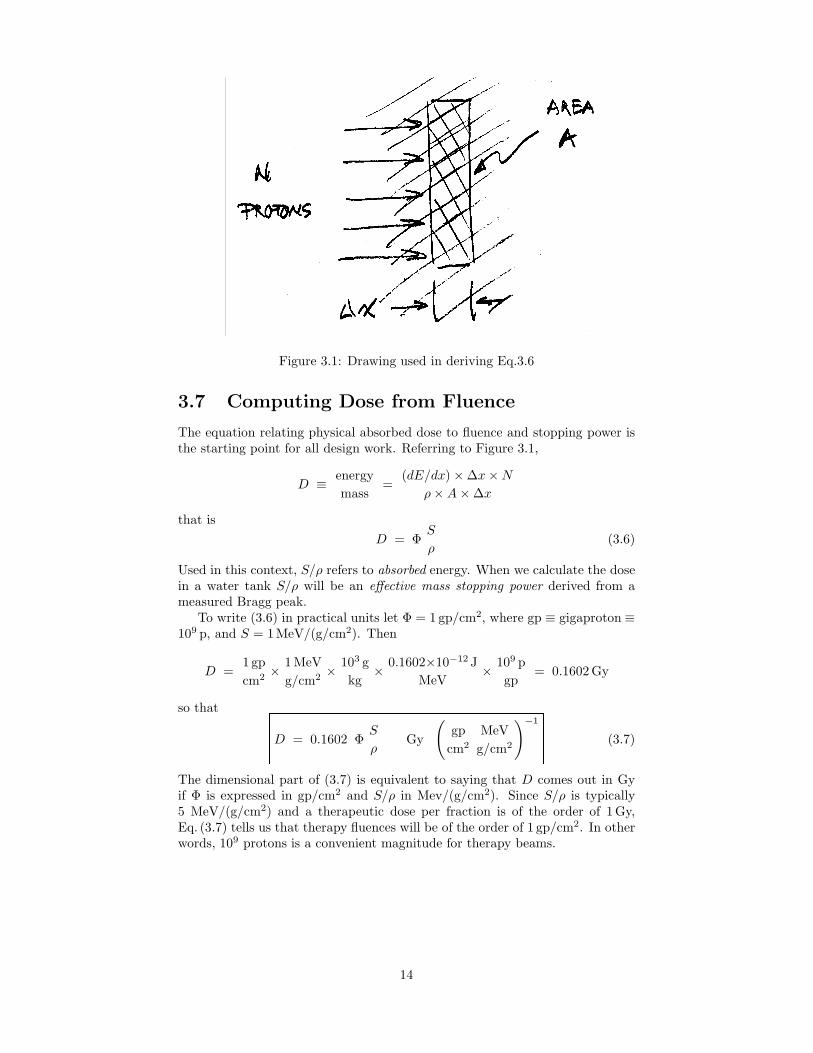
Figure 3.1: Drawing used in deriving Eq.3.6

3.7 Computing Dose from Fluence

The equation relating physical absorbed dose to fluence and stopping power isthe starting point for all design work. Referring to Figure 3.1,

D ≡ energymass

=(dE/dx) × ∆x × N

ρ × A × ∆x

that isD = Φ

S

ρ(3.6)

Used in this context, S/ρ refers to absorbed energy. When we calculate the dosein a water tank S/ρ will be an effective mass stopping power derived from ameasured Bragg peak.

To write (3.6) in practical units let Φ = 1 gp/cm2, where gp ≡ gigaproton ≡109 p, and S = 1MeV/(g/cm2). Then

D =1gpcm2 × 1 MeV

g/cm2 × 103 gkg

× 0.1602×10−12 JMeV

× 109 pgp

= 0.1602 Gy

so that

D = 0.1602 ΦS

ρGy

(gp

cm2

MeVg/cm2

)−1

(3.7)

The dimensional part of (3.7) is equivalent to saying that D comes out in Gyif Φ is expressed in gp/cm2 and S/ρ in Mev/(g/cm2). Since S/ρ is typically5 MeV/(g/cm2) and a therapeutic dose per fraction is of the order of 1Gy,Eq. (3.7) tells us that therapy fluences will be of the order of 1 gp/cm2. In otherwords, 109 protons is a convenient magnitude for therapy beams.

14

3.8 Computing Dose Rate from Proton Current

Density

Taking the time derivative of (3.6) we have D = ΦS/ρ. Current density isrelated to fluence rate by ip/A = Ne/A = eΦ. Therefore

D =1e

ipA

S

ρ=

ipA

S

ρ× J

eV C

using Eq. (3.1). To write this in practical units let ip/A = 1nA/cm2 and S =1Mev/(g/cm2). Then

D =1 nAcm2 × 1MeV cm2

g× J

eV C× 10−9C

nA s× 106 eV

MeV× 103 g

kg= 1

Gys

so the desired formula is

D =ipA

S

ρ

Gys

(nAcm2

MeVg/cm2

)−1

(3.8)

If the proton current density is 0.0033 nA/cm2 and S = 5 MeV/cm2 we findD = 0.017 Gy/s and the dose in 1 minute is 1 Gy.

We have assumed that ip is uniform over A. If not, ip/A should be interpretedas dip/dA and the dose rate will also be non-uniform. Similarly, if the fluencein Eq. (3.7) is non-uniform the dose will be non-uniform.

Exercise: in a water tank, a test region of radius 5 cm is exposed to auniform current of 2 nA of 160MeV protons for 10 s. The mass stoppingpower of water for 160 MeV protons is 5.210 MeV/(g/cm2). Compute thedose, first with Eq. (3.8) and then Eq. (3.7). Answer: A = πr2 = 78.5 cm2;i/A = 0.0255 nA/cm2; D = 0.132 Gy/s; D = D∆t = 1.32 Gy from (3.8). Thefluence is Φ = i∆t/(eA) = 1.59 gp/cm2; the dose from (3.7) is 1.33 Gy.

3.9 Dose Rate in a Therapy Beam

Eqs. (3.7) and (3.8) by themselves do not answer the question most likely to beasked: assuming a complete beam spreading system (single- or double-scatteringwith a modulator), what is the dose rate in the spread-out Bragg peak (SOBP)given the proton current entering the system?

The derivation anticipates some later chapters, so you may want to putoff this section for a while or revisit it later. Also, a properly written designprogram will give you essentially the same information—the incident gp neededfor a given dose—automatically, and more accurately. Nevertheless, the formulawe’re about to derive is convenient for back of the envelope estimates absent acomplete design.

Refer to Figure 3.2 (not to scale). The hypothetical scattering system hasan upstream range modulator and a compensated contoured second scatterer.We assume it produces a flat dose distribution over a circular area A at theentrance to the water tank. The proton current ip entering the first scatterer isassumed known (note the change in interpretation of ip). We wish to computethe dose rate at the most distal peak of the SOBP (#1). The dose rate is thesame everywhere else in the SOBP because the SOBP is flat. We start withEq. 3.8 and introduce three dimensionless factors:

15

Figure 3.2: Drawing used in deriving Eq.3.9

1. Because (3.8) requires the current at A, we must multiply by the efficiencyε of the scattering system, defined as the ratio of current entering the usefularea to current entering the scattering system. For a single scatteringsystem ε is typically 0.05; for a double scattering system, 0.40.

2. The pristine Bragg peak can be considered as a curve of the effectivestopping power of the actual proton beam vs. depth (see Ch. 11). Thestopping power for step #1 at the entrance to the water tank is easy:ignoring small nuclear effects, it is just the table value of dE/dx in waterat the energy of protons entering the tank (object 3) for step 1, T3,1. Since,however, we are interested in the dose rate at the top of the Bragg peakwe need to multiply by a factor fBP defined as the peak/entrance ratio ofthe pristine Bragg peak (typically 3.5).

3. We now need to think about how a range modulator works. In its simplestform it’s a propeller-shaped wheel that brings various thicknesses of plasticinto the beam as it rotates.4 We assume the proton current ip,1 enteringthe modulator (object 1) is constant. The dose rate at different parts of theSOBP is not constant, of course. The distal end, for instance, only receivesdose while the modulator is on step 1. We wish to compute the dose rate< D > averaged over one modulator cycle (or any integral number ofcycles). We therefore need a dimensionless factor fMOD defined as thedwell time for step 1 divided by the time for a full cycle. This depends onthe modulator design, and mostly, on the amount of modulation. fMOD =1 for no modulation and fMOD ≈ 0.3 for full modulation.

At last we have

< D > = ε fBP fMODip,1

A

(S

ρ

)W,T3,1

Gys

(nAcm2

MeVg/cm2

)−1

(3.9)

Eq. 3.9 also applies with beam gating and with beam current modulation. Bothare used at NPTC to reduce the library of modulators required. Beam gatingis a way of using a single modulator designed for full modulation to obtainanything less than full by simply turning the beam off during proximal steps.We must then take ip,1 as the proton current while the beam is on. Beam currentmodulation allows us to trim the performance of a given physical modulator.In that case we must take ip,1 as the current during the first modulator step.Gating can be thought of as an extreme form of beam current modulation.

4 Our modulator also has some lead: since it doubles as the first scatterer we want to keepthe scattering constant as it rotates.

16

3.10 Air Filled Ionization Chambers

Though this report is not about ionization chambers (IC’s) they are so importantin proton therapy nozzles that a few formulas may be useful. They apply to airfilled plane-parallel IC’s under standard conditions. We follow Boag [17]. Thecurrent from an IC is

iIC = q A d( 1

1 + ξ2

)(3.10)

where A is the effective area, d is the gap and q is the + or − charge liberatedper unit volume per second. The factor in parentheses is the correction for ionrecombination which we ignore for now (assume ξ2 = 0). q is given by

q =(e ρ

W

)D (3.11)

where e = 1.602 × 10−19 C is the quantum of charge, ρ = 0.00129g/cm3 isthe density of air at standard conditions, W = 34.3 eV is the average energyexpended per ion pair and D is the dose rate. Combining these equations,assuming A = 1cm2, d = 1cm and D = 1Gy/s, and working through theconversions we find in practical units

iIC = 37.6 A d D nA

(cm3 Gy

s

)−1

(3.12)

This relation between dose rate and output current is convenient if we have asmall active volume (such as a monitor pad) in a large beam. At the otherextreme, we might have a large chamber with an unknown fluence and dose ratebut we might know the total proton current ip. Nonuniform dose will not matterif recombination is negligible. Using (3.8) in (3.12) we find the IC multiplication

iIC

ip= 37.6 d

S

ρ

(cm

Mevg/cm2

)−1

(3.13)

Recombination of ions causes the measured current iIC to be less than theideal value given by Eqs.(3.12) and (3.13). It corresponds to non-zero ξ2 inEq. (3.10). Boag [17] gives, for standard air,

ξ2 = 0.673× 1014(V2 s

C m

) d4 q

V 2

Assuming this is not too large we can set q ≈ iIC/Ad. Rearranging, convertingto practical units (nA, cm) and working through the conversions we find

ξ2 ≈ 673iIC

A

( d

V

)2

d

(nAcm2

(cmV

)2

cm

)−1

(3.14)

One should use this only in the spirit of making sure it is sufficiently small forthe design under consideration. If recombination is a problem, the most effectiveremedy by far is to decrease the gap. Of course that also decreases the signal.The next best is to increase the voltage. The proton current density ip/A isusually a given, though iIC/A also depends on d. Note that A may be eitherthe active area of the chamber or the effective area of the beam, whichever issmaller. Recombination is usually detected experimentally by the dependence

17

of chamber output on V via Eq. 3.14. Boag [17] is the authoritative source andincludes a review of measurements.

In addition to the explicit parameters of Eq. 3.14, recombination depends onthe proton beam time structure via iIC because one must use the value while thebeam is on, not the long-term time average. Isochronous cyclotrons have fairlyconstant beam. The peak and average current are comparable, making it rathereasy to avoid recombination. FM cyclotrons may have a duty factor around 2%in which case iIC in (3.14) is ≈ 50× the average value, and recombination isgreater. Synchrotrons vary widely according to the method of beam extraction.The duty factor for slow extraction can be 1 s per 2 s or better. Single turnextraction, by contrast, may yield a duty factor on the order of 1 µs per 1 s. Inthat case IC’s are virtually useless, and other means of monitoring the beammust be found.

3.11 Proton Kinematics

Occasionally we need to convert from one kinematic quantity, say the kineticenergy T to another, say pv, where p is proton’s momentum and v its speed.Therapy protons are relativistic: their kinetic energy is not negligible comparedto the rest energy mpc

2 = 938.27 MeV. Fortunately, single particle relativistickinematics are trivial.5 We need only three equations. First, β ≡ v/c (c is thespeed of light) is given by

β =pc

E(3.15)

where E is the proton’s total energy. Second, E equals the kinetic energy plusthe rest energy:

E = T + mc2 (3.16)

Finally,E2 = (pc)2 + (mc2)2 (3.17)

In proton therapy we normally deal with T : whenever we simply say ‘energy’we mean T . Any kinematic quantity can be expressed in terms of T by usingthe previous three equations. For instance, the quantity pv, needed in multiplescattering theory, is found to be

pv =(T + 2mc2

T + mc2

)T =

E2 − (mc2)2

E(3.18)

As this example shows, it may be tidier to leave the expression in terms ofE. It’s always a good idea to check your work by taking the nonrelativisticlimit T � mpc

2. For instance, for Eq. 3.18 we find pv → 2T , consistent withT = mv2/2.

Exercise: it’s instructive to compute the β of a therapy proton. From ourthree basic equations you should be able to show that

β =

√(1 +

mc2

E

)(1 − mc2

E

)(3.19)

For instance, 160 MeV protons have 0.52 × the speed of light. Show thatEq. (3.19) gives the correct answer β =

√2T/mc2 in the nonrelativistic limit.

5 If you are interested in much more complicated situations the authority is Hagedorn [18].

18

Chapter 4

Gaussians

Multiple scattering of protons is nearly Gaussian. Though we need not makethat approximation in final calculations (there is no great advantage to begained) it is nevertheless useful to discuss Gaussian scattering in one and twodimensions because the equations are simple and give us some good insights,particularly into the properties of single-scattering systems.

4.1 Small-Angle Approximation

Figure 4.1 defines the coordinate system. z is the beam direction, y is up, andx, y, z form a right-handed system. For protons, the small-angle approximation

cos θ ≈ 1 , sin θ ≈ tan θ ≈ θ , (radian)

is always valid, as can be argued two ways. First, we’ll see in Chapter 7 thatthe maximum multiple scattering angle that can be obtained from lead underany circumstances is roughly 0.28 radians (≈ 16 ◦). Now sin(0.2800) = 0.2764so even here the approximation is pretty good. For a less extreme example, onecan look at the angles we typically obtain with passive systems. In a protongantry1 with a throw of 270 cm a number of factors limit us to a field radius of≈ 12 cm. In this case θ = 12/270 = 0.044 radian (about 2.5 ◦) where the smallangle approximation is excellent.

4.2 1D Gaussian Probability Density

Figure 4.1 shows the common situation where we have a scatterer at z0 and weare interested in the proton distribution on a measuring plane (MP) at zMP adistance L ≡ zMP − z0 away. In Chapter 7 we’ll see that multiple scatteringfrom a simple scatterer is approximately Gaussian and in the present chapterwe’ll assume it’s exactly Gaussian. Then the probability that the x componentof the angle with the beam for a single proton falls in dθx about θx is

f(θx) dθx =1√

2π θx0

e− 1

2

( θx

θx0

)2

dθx

where θx0 is a characteristic multiple scattering angle. For now, we’ll simplyassume that θx0 can be determined somehow. Exactly how we do that is thetopic of Chapter 7.

1 Numbers from NPTC.

19

Figure 4.1: Coordinates and definitions for scattering.

The corresponding distribution of protons on the MP is obtained by lettingx = Lθx and x0 = Lθx0:

f(x) dx =1√

2π x0

e− 1

2

( x

x0

)2

dx (4.1)

From here on we’ll deal only with spatial distributions on the MP which areof more immediate interest, easier to visualize, and somewhat easier to writedown. f(x) is not a probability. It is a one-dimensional (1D) probability density,which we emphasize by writing (4.1) with the redundant dx on both sides. Eachside of (4.1) is an infinitesimal probability. If N protons were incident on thescatterer and we had a strip detector of width ∆x located at x in the MP, itwould register (Nf(x) ∆x) counts.

Returning to a single incident proton, the probability that it lands somewherein the MP is ∫ ∞

−∞f(x) dx = 1 (4.2)

as it must be. The proof of (4.2) is indirect and will appear later. The limits ofintegration seem inconsistent with the small-angle approximation, but ∞ hereis merely shorthand for ‘a sufficiently large x’. For instance, if we integratebetween ± 5 x0 the exponential factor at each limit is only ≈ 4 × 10−6.

The root-mean-squared (rms) value of x, called σx, is a measure of the widthof the distribution on the MP. Using (4.2) we find

σx ≡ < x2 >1/2 =(∫ ∞

−∞x2 f(x) dx

)1/2

= x0 (4.3)

The integral is straightforward. The rms deviation from the mean of a 1DGaussian random variable is equal to the width parameter of the Gaussian.Because of this, many writers dispense with x0 and write equations such as(4.1) directly with σx. We will, however, always use separate symbols for thewidth parameter of a distribution and the rms deviation of the correspondingrandom variable. For many useful probability distributions they are not equal.For instance if x is uniformly distributed between ±h its rms value is h/

√3.

20

4.3 2D Gaussian Probability Density

So far we have said nothing about the distribution in y. It can be anything. Theprotons can all lie along the x axis, or they can be uniformly distributed betweentwo values of y. In the most common case, however, the multiple scattering isthe same for x and y and the distribution in y is Gaussian with the same widthparameter as x. Since the two scatters are independent, the probability that aproton falls in dx about x and dy about y is

f(x, y) dx dy =1√

2π x0

e− 1

2

( x

x0

)2

dx × 1√2π y0

e− 1

2

( y

y0

)2

dy

If we now let r0 ≡ x0 = y0 and transform to cylindrical coordinates r2 = x2 +y2

and dA = dx dy = r drdφ we obtain

f(r) r dr dφ =1

2π r20

e− 1

2

( r

r0

)2

r dr dφ (4.4)

f(r) is a 2D probability density. f(r) r dr dφ is the probability that a singleincident proton will hit the MP within dA. As before, the probability that asingle proton lands somewhere in the MP is

∫ 2π

0

∫ ∞

0

f(r) r dr dφ = 1 (4.5)

This integral, unlike (4.2), is straightforward, and is the indirect proof of Eq. (4.2)because the two describe the same physical situation. By contrast with (4.3),however

σr ≡ < r2 >1/2 ≡(∫ 2π

0

∫ ∞

0

r2 f(r) r dr dφ

)1/2

=√

2 r0 (4.6)

The rms value of r is√

2 times the rms value of x. We could, of course, haveabsorbed the

√2 into the definition of the width parameter, thus using a different

width parameter for the 1D Gaussian (4.1) and the 2D ‘cylindrical’ Gaussian(4.4), which would then read

f(r) r dr dφ =1

π σ2r

e−( r

σr

)2

r dr dφ

Many writers including Moliere [7] and Preston and Koehler [10] write it thatway, and in reading the literature one must take note of which form is used.

4.4 Implications for Single Scattering

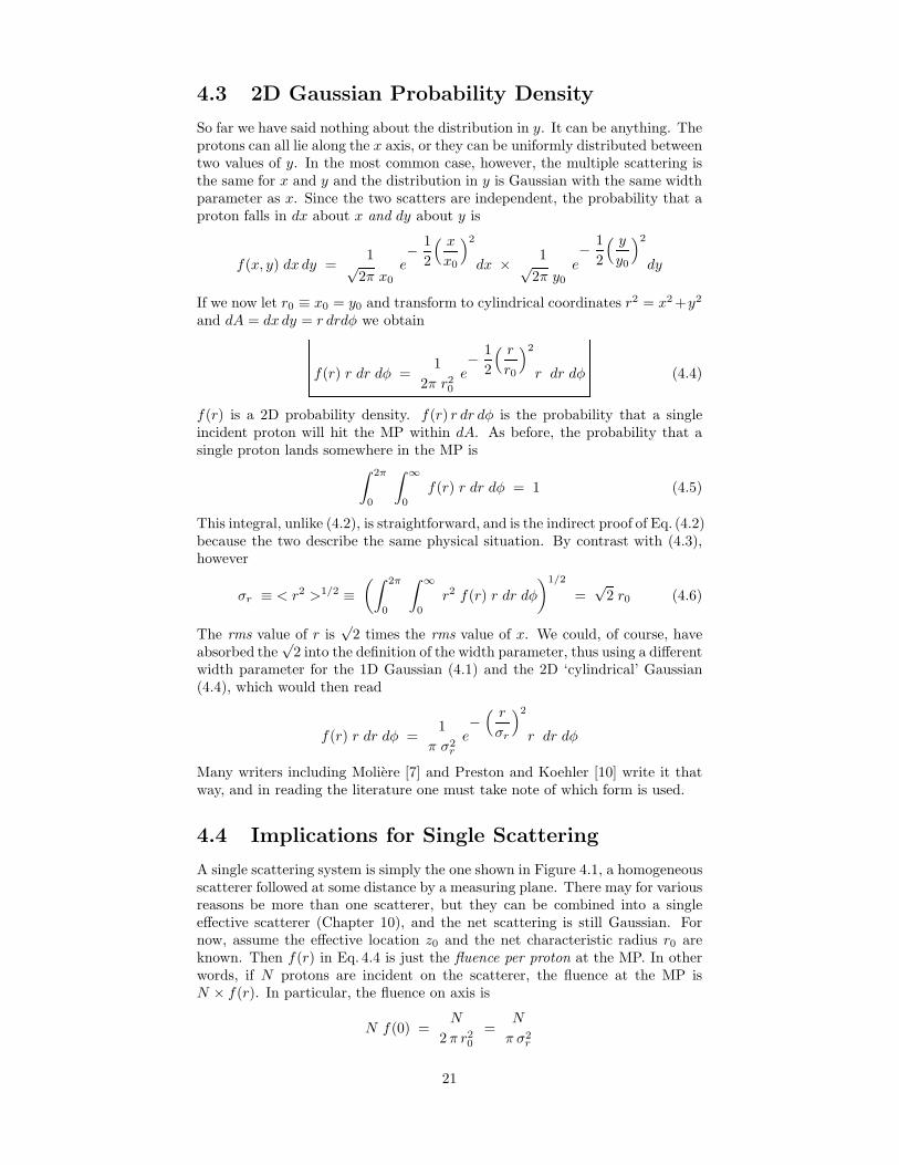
A single scattering system is simply the one shown in Figure 4.1, a homogeneousscatterer followed at some distance by a measuring plane. There may for variousreasons be more than one scatterer, but they can be combined into a singleeffective scatterer (Chapter 10), and the net scattering is still Gaussian. Fornow, assume the effective location z0 and the net characteristic radius r0 areknown. Then f(r) in Eq. 4.4 is just the fluence per proton at the MP. In otherwords, if N protons are incident on the scatterer, the fluence at the MP isN × f(r). In particular, the fluence on axis is

N f(0) =N

2 π r20

=N

π σ2r

21

0.0 0.5 1.0 1.5 2.0 2.5 3.0r (cm)

0.0

0.2

0.4

0.6

0.8

1.0

2πr 02

× f(

r)

r95 r61 ( = r0 )

0.95

0.606

Figure 4.2: Gaussian radial distribution assuming r0 = 1cm.

Off axis the fluence falls (Figure 4.2), reaching 61% at r = r0. With a singlescattering system, we simply use as much of the Gaussian as we can and still staywithin the prescribed dose uniformity. For instance, if ± 2.5% is required wecan use the Gaussian out to the 95% point r95 (Figure 4.2).2 Designing a singlescattering system is basically simple. The useful radius (r95 in our example) isgiven by the clinical requirement. We must use it to find the required r0 andθ0. We must then use multiple scattering theory to get that much scattering.

In the Gaussian approximation the first step, finding θ0, can be done exactly.Continuing with our 95% example, the exponential factor of Eq. 4.4 is 1 at r = 0and therefore we wish to find r0 such that

0.95 = e−1

2

(r95

r0

)2

given r95. The solution is

r0 = r95 (−2 ln 0.95)−1/2 , θ0 = r0/L (4.7)

with the obvious generalization to the case where the ‘95’ is something else. Forexample, suppose we want ± 2.5% uniformity out to 3 cm and the throw L is150 cm. We find

r0 = 3/√

−2 ln 0.95 = 9.37 cm, θ0 = 0.0624 radian

At 160 MeV incident, that will take about 8 mm of lead scatterer and theoutgoing energy will be 135 MeV—but that’s for later.

The efficiency ε of the scattering system is of considerable interest. Of theN protons, what fraction falls within the useful radius? Preston and Koehler[10] pointed out a simple and exact answer for single scattering in the Gaussian

2 Consistent with the notation r95 we should rename r0 ‘r61’ but we won’t.

22

approximation. ε is the probability that a particle falls within a radius R in theMP, namely

ε =∫ 2π

0

∫ R

0

12π r2

0

e− 1

2

( r

r0

)2

r dr dφ = 1 − e− 1

2

(R

r0

)2

orε = 1 − f(R)

/f(0) (4.8)

In our example, we capture only 1 − 0.95 = 5% of the incident protons. If wewanted ± 5% uniformity, we would capture 10% and so on. Single scatteringsystems have low efficiency and, as we saw above, they use up a lot of energy.To do better we need double scattering—but that, too, is for later.

Figure 4.3: Geometry of transverse penumbra calculation.

4.5 Error Function

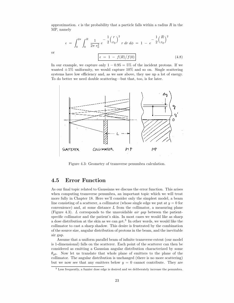
As our final topic related to Gaussians we discuss the error function. This ariseswhen computing transverse penumbra, an important topic which we will treatmore fully in Chapter 18. Here we’ll consider only the simplest model, a beamline consisting of a scatterer, a collimator (whose single edge we put at y = 0 forconvenience) and, at some distance L from the collimator, a measuring plane(Figure 4.3). L corresponds to the unavoidable air gap between the patient-specific collimator and the patient’s skin. In most cases we would like as sharpa dose distribution at the skin as we can get.3 In other words, we would like thecollimator to cast a sharp shadow. This desire is frustrated by the combinationof the source size, angular distribution of protons in the beam, and the inevitableair gap.

Assume that a uniform parallel beam of infinite transverse extent (our modelis 1-dimensional) falls on the scatterer. Each point of the scatterer can then beconsidered as emitting a Gaussian angular distribution characterized by someθy0. Now let us translate that whole plane of emitters to the plane of thecollimator. The angular distribution is unchanged (there is no more scattering)but we now see that any emitters below y = 0 cannot contribute. They are

3 Less frequently, a fuzzier dose edge is desired and we deliberately increase the penumbra.

23

blocked by the collimator. Now take the second step of projecting the remainingproton trajectories onto the MP. Each one can be represented by an arrowstarting at whatever y the proton had in the collimator plane, call it y′, andending at some y in the MP. y′ must be greater than 0 but y can be anything.The distribution of the length of these arrows is Gaussian with a characteristiclength y0 = Lθy0.

The relative number of protons falling in dy about y is gotten by integrat-ing over all arrows starting anywhere and ending in dy, weighting each by theprobability of its length |y − y′|:

p (y) dy =

[1√

2π y0

∫ ∞

0

e− 1

2

(y′ − y

y0

)2

dy′

]dy (4.9)

We now introduce the error function 4

erf x ≡ 2√π

∫ x

0

e−t2 dt (4.10)

which has the properties

erf (0) = 0 , erf (∞) = 1 , erf (−x) = − erf (x) (4.11)

See [19] for a numerical table, [1] for a Fortran subroutine based on the fact thatthe error function is a special case of the incomplete gamma function, and ourown subroutine ERF.FOR which uses series expansions [20] directly. If we need toevaluate an arbitrary definite integral of a standard 1D Gaussian, having widthparameter x0 and mean x, the following formula is easily derived from (4.10):

1√2π x0

∫ x2

x1

e− 1

2

(x − x

x0

)2

dx = .5(

erf(x2 − x√

2 x0

)− erf

(x1 − x√2 x0

))(4.12)

Applying this to the penumbra equation (4.9) we obtain

p (y) = 0.5 + 0.5 erf( y√

2 y0

)(4.13)

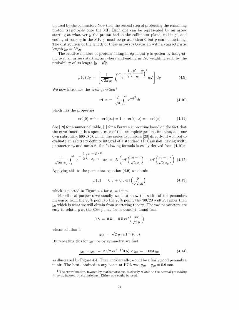
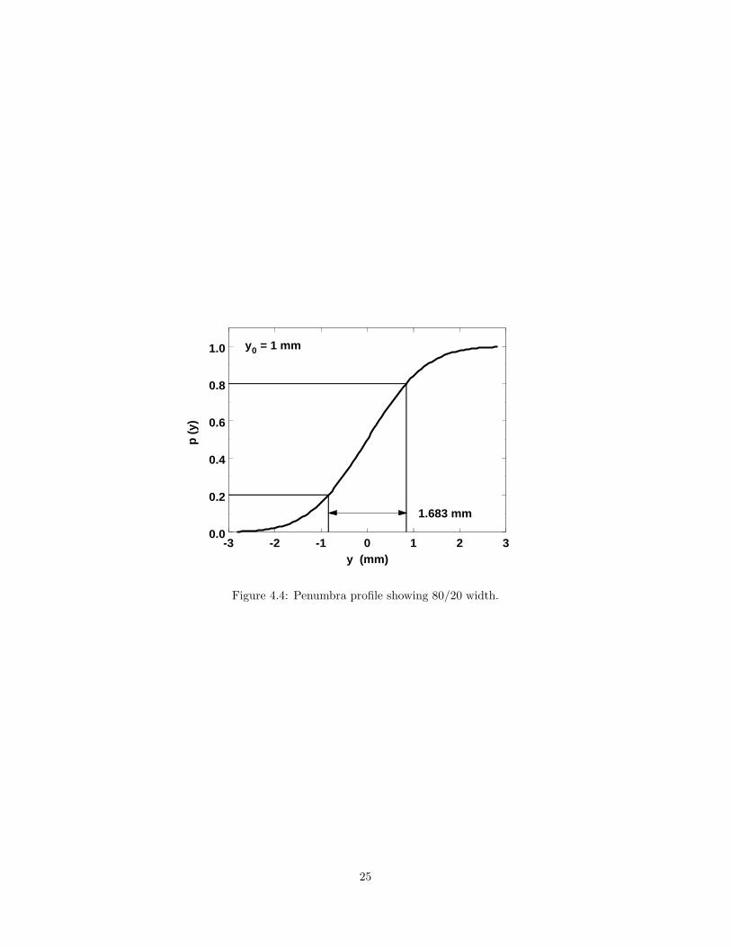
which is plotted in Figure 4.4 for y0 = 1mm.For clinical purposes we usually want to know the width of the penumbra

measured from the 80% point to the 20% point, the ‘80/20 width’, rather thany0 which is what we will obtain from scattering theory. The two parameters areeasy to relate. y at the 80% point, for instance, is found from

0.8 = 0.5 + 0.5 erf( y80√

2 y0

)

whose solution isy80 =

√2 y0 erf−1(0.6)

By repeating this for y20, or by symmetry, we find

y80 − y20 = 2√

2 erf−1(0.6) × y0 = 1.683 y0 (4.14)

as illustrated by Figure 4.4. That, incidentally, would be a fairly good penumbrain air. The best obtained in any beam at HCL was y80 − y20 ≈ 0.9mm.

4 The error function, favored by mathematicians, is closely related to the normal probabilityintegral, favored by statisticians. Either one could be used.

24

-3 -2 -1 0 1 2 3y (mm)

0.0

0.2

0.4

0.6

0.8

1.0

p (

y)

y0 = 1 mm

1.683 mm

Figure 4.4: Penumbra profile showing 80/20 width.

25

Chapter 5

The Cubic Spline

One idiosyncrasy of our programs is the very extensive use of the cubic spline.1

You may already know it as an option offered by graphics packages to join aset of points smoothly, cubic spline interpolation. We will use it that way, butalso as a fit function and as a generalized smooth function whose parametersare adjusted to meet some mathematical goal.

5.1 Description

Assume we have a set of N points xi, yi. The cubic spline is a smooth linewhich passes through all the points. In each interval e.g. x4 ≤ x ≤ x5 it isa cubic polynomial in x, but the four polynomial coefficients change from oneinterval to the next. They are computed [1] in such a way that the first andsecond derivatives are continuous at the interval boundaries, that is, at the givenpoints. That is what makes the cubic spline smooth. It has no corners, that is,no places where the first derivative jumps.

It turns out [1] that requiring the curve to pass through all the points andto have continuous first and second derivatives is not quite enough to determinethe 4(N − 1) polynomial coefficients. We also need to specify two boundaryconditions. At each end, we must either a) specify the first derivative y′ ≡ dy/dxor b) require that the second derivative y′′ be 0. The latter is called the ‘natural’boundary condition. The conditions can be mixed: natural at one end and aspecified y′ at the other. Our routine SPLINE.FOR is a slightly reorganizedversion of that given in [1] and uses the same mechanism (a non-physicallylarge y′) to signal that the ‘natural’ boundary condition is to be used at one orthe other end.

A natural cubic spline through just two points is simply the straight linejoining them.

5.2 Cubic Spline Interpolation

As described so far, the cubic spline is an interpolation function. It passesthrough all the data points. We will use it this way to interpolate range-energytables. However, cubic spline interpolation (or any other sophisticated method)may not work well if the data are noisy.

Figure 5.1 shows a set of points (solid squares) generated by picking pointsuniformly along a smooth curve, then adding some Gaussian noise in x and y

1 The name comes from a draftsman’s tool, a sort of bendable ruler, used to draw arbitrarysmooth curves.

26

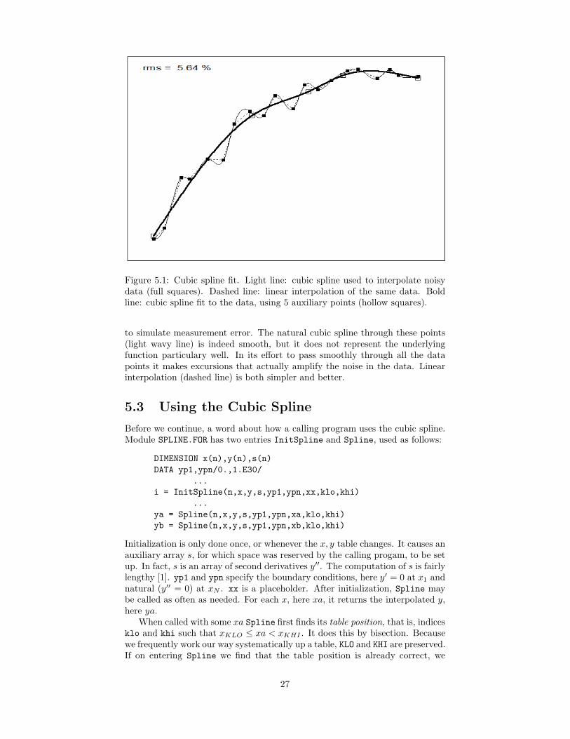
Figure 5.1: Cubic spline fit. Light line: cubic spline used to interpolate noisydata (full squares). Dashed line: linear interpolation of the same data. Boldline: cubic spline fit to the data, using 5 auxiliary points (hollow squares).

to simulate measurement error. The natural cubic spline through these points(light wavy line) is indeed smooth, but it does not represent the underlyingfunction particulary well. In its effort to pass smoothly through all the datapoints it makes excursions that actually amplify the noise in the data. Linearinterpolation (dashed line) is both simpler and better.

5.3 Using the Cubic Spline

Before we continue, a word about how a calling program uses the cubic spline.Module SPLINE.FOR has two entries InitSpline and Spline, used as follows:

DIMENSION x(n),y(n),s(n)DATA yp1,ypn/0.,1.E30/

...i = InitSpline(n,x,y,s,yp1,ypn,xx,klo,khi)

...ya = Spline(n,x,y,s,yp1,ypn,xa,klo,khi)yb = Spline(n,x,y,s,yp1,ypn,xb,klo,khi)

Initialization is only done once, or whenever the x, y table changes. It causes anauxiliary array s, for which space was reserved by the calling progam, to be setup. In fact, s is an array of second derivatives y′′. The computation of s is fairlylengthy [1]. yp1 and ypn specify the boundary conditions, here y′ = 0 at x1 andnatural (y′′ = 0) at xN . xx is a placeholder. After initialization, Spline maybe called as often as needed. For each x, here xa, it returns the interpolated y,here ya.

When called with some xa Spline first finds its table position, that is, indicesklo and khi such that xKLO ≤ xa < xKHI . It does this by bisection. Becausewe frequently work our way systematically up a table, KLO and KHI are preserved.If on entering Spline we find that the table position is already correct, we

27

can skip that step. Once the table position is known, ya is found by a shortcalculation using the arrays x, y and s.

In addition to the bisection routine, a linear interpolation routine is includedin SPLINE.FOR. It also has two entries, used in the same way just described. Inthis case s is an auxiliary array of precalculated slopes y′.

5.4 Cubic Spline Fit

In contrast to an interpolation function, which passes through the data points,a fit function passes near the data points in some mathematically defined sense.Most common by far is the least-squares fit which seeks to minimize

χ2 ≡N∑

1

(yi − y(xi))2 ,

the sum of squared vertical distances of the fit function from the data points.The mathematical form of y(x) is suggested either by the trend of the data orby some underlying physical theory we may have in mind. Its precise shapedepends on a set of fit parameters. It is these parameters we adjust to minimizeχ2. There is an extensive literature on the subject [1, 21].

For instance, a common fit function is the polynomial

y(x) = a1 + a2x + a3x2 + a4x

3 + a5x4 ,

where for illustration we have used a polynomial of the fourth degree havingfive parameters ai.2 Polynomials belong to a special class of functions whichare linear in their fit parameters and lead to a linear least-squares fit, for whichspecial techniques apply [1, 21].

The cubic spline is well adapted for use as a fit function since it can fit anysmooth curve. Pick a set of auxiliary points (the hollow squares in Figure 5.1),far fewer in number than the data points, and adjust their positions so thatthe cubic spline through the auxiliary points minimizes χ2 with respect to thedata points. The x and y coordinates of the auxiliary or ‘spline points’ as weshall call them are the adjustable parameters. However, we must lock the xcoordinates of the first and last points or the fit will collapse.

The cubic spline is nonlinear in its adjustable parameters even though itconsists of a set of polynomials. We therefore have a non-linear least-squares fitand must use methods that differ from the linear case [1, 21]. Fundamentally, allof these consist of making an educated guess at initial values of the parametersand then improving them by trial and error. In the case of the cubic spline fitthe educated guess is easy because the parameters are simply new points, whichmust lie very close to the data set we are trying to fit.

The bold line of Figure 5.1 is a spline fit to the data set. We have chosento use five spline points, picked their initial values using the density functionmethod described below, and optimized the fit with a grid search, also described.The fit represents the underlying trend of the data better than either spline orlinear interpolation. In this particular case, a low-order polynomial fit woulddo as well. However, polynomials do not work well for Bragg peaks.

5.4.1 Choosing Initial Points

The simplest way to choose initial points is to pick x uniformly and obtainy values by linear interpolation of the data set. That would work sufficiently

2 From the programmer’s point of view it is the number of parameters that matters more.

28

well in our artificial example, Figure 5.1. It does not work for Bragg peaks,whose curvature varies greatly. The cubic spline can, in each segment, mimicsomething as complicated as a skewed parabola. We waste this power if we usethe same density of points in the nearly straight entrance region as we need inthe peak. The fit function will have needlessly many parameters and will beginchasing experimental noise. We require an automatic procedure for pickingpoints more efficiently.

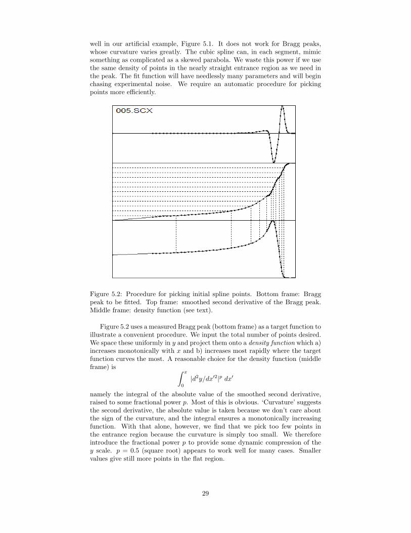
Figure 5.2: Procedure for picking initial spline points. Bottom frame: Braggpeak to be fitted. Top frame: smoothed second derivative of the Bragg peak.Middle frame: density function (see text).

Figure 5.2 uses a measured Bragg peak (bottom frame) as a target function toillustrate a convenient procedure. We input the total number of points desired.We space these uniformly in y and project them onto a density function which a)increases monotonically with x and b) increases most rapidly where the targetfunction curves the most. A reasonable choice for the density function (middleframe) is ∫ x

0

|d2y/dx′2|p dx′

namely the integral of the absolute value of the smoothed second derivative,raised to some fractional power p. Most of this is obvious. ‘Curvature’ suggeststhe second derivative, the absolute value is taken because we don’t care aboutthe sign of the curvature, and the integral ensures a monotonically increasingfunction. With that alone, however, we find that we pick too few points inthe entrance region because the curvature is simply too small. We thereforeintroduce the fractional power p to provide some dynamic compression of they scale. p = 0.5 (square root) appears to work well for many cases. Smallervalues give still more points in the flat region.

29

5.4.2 Optimizing the Fit

The gold standard for nonlinear least-squares fits is the Marquardt method[1, 21]. Spline fits seem, however, to be one case where a simple grid search withinverse parabolic interpolation [1] is not only more robust but actually faster.This method (see GridParab in BSFIT.FOR assumes that χ2 is an approximatelyparabolic function of any of the parameters near a minimum. We simply slogthrough each parameter in order, skipping the two x1, xN that must be heldconstant. (Those two initial increments are set to 0 as a signal to GridParab.)For each parameter, we look for a neighboring value where the overall χ2 issmaller, going back and forth and reducing the increment each time to avoid aninfinite loop. If we find such a value we go further in the same direction untilχ2 increases again. We have now bracketed a minimum of the parabola and weuse the formula given in [1] to locate it. This is a simpler version of the Brentprocedure [1] and seems fast enough.

The reason the grid search works so well is probably that the fit parametersare fairly independent in their effect. Changing one of them has very little effecta few spline points away. The entire process (say 15 spline points and 5 passes)takes hundredths of a second on a high-end PC.

Figure 5.3 shows the final result for a typical measured Bragg peak. Roughly50 points are reduced to 13 and experimental noise is averaged out.

Figure 5.3: Upper frame: Bragg peak with spline fit. Lower frame: deviationfrom fit. The dashed lines are at ± the rms deviation.

5.4.3 Pathologies

Once in a while it will happen that two of the points cross and the xi no longerincrease monotonically. This could probably be fixed by simply swapping thepoints in question but we have not tried that. Some trivial change in the startupfile (decreasing the number of spline points by 1 or slightly changing p) usuallysolves the problem.

30

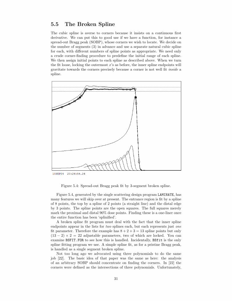
5.5 The Broken Spline

The cubic spline is averse to corners because it insists on a continuous firstderivative. We can put this to good use if we have a function, for instance aspread-out Bragg peak (SOBP), whose corners we wish to locate. We decide onthe number of segments (3) in advance and use a separate natural cubic splinefor each, with different numbers of spline points as appropriate. We need onlya crude corner-finding procedure to predefine the initial range of each spline.We then assign initial points to each spline as described above. When we turnthe fit loose, locking the outermost x’s as before, the inner spline endpoints willgravitate towards the corners precisely because a corner is not well fit inside aspline.

Figure 5.4: Spread-out Bragg peak fit by 3-segment broken spline.

Figure 5.4, generated by the single scattering design program LAMINATE, hasmany features we will skip over at present. The entrance region is fit by a splineof 8 points, the top by a spline of 2 points (a straight line) and the distal edgeby 3 points. The spline points are the open squares. The full squares merelymark the proximal and distal 90% dose points. Finding these is a one-liner oncethe entire function has been ‘splinified’.

A broken spline fit program must deal with the fact that the inner splineendpoints appear in the lists for two splines each, but each represents just onefit parameter. Therefore the example has 8 + 2 + 3 = 13 spline points but only(13 − 2) × 2 = 22 adjustable parameters, two of which are locked. You canexamine BSFIT.FOR to see how this is handled. Incidentally, BSfit is the onlyspline fitting program we use. A simple spline fit, as for a pristine Bragg peak,is handled as a single segment broken spline.

Not too long ago we advocated using three polynomials to do the samejob [22]. The basic idea of that paper was the same as here: the analysisof an arbitrary SOBP should concentrate on finding the corners. In [22] thecorners were defined as the intersections of three polynomials. Unfortunately,

31

the proximal and top polynomials sometimes fail to intersect. Then we mustchange gears and find the point of closest approach. Also, that part of the fitwhich finds the corners must be handled as an outer loop around the linearfit which determines each polynomial. All of this makes for messy code. Thebroken spline fit is much more elegant, and absolutely guarantees a continuousfunction representing the entire SOBP.

Figure 5.5: Compensated contoured second scatterer.

5.6 The Spline as a General-Purpose Function

Instead of using the cubic spline to fit a set of data points we may use it asa general smooth function and adjust its parameters to accomplish some othermathematical goal. It is used that way in designing contoured second scatterers(Figure 5.5). A quick outline of the method (details in Chapter 14) is as follows.First, a generic scatterer shape defined by spline points at four fixed radii isdesigned by varying the four scattering strengths to obtain, for a given firstscatterer strength, a flat dose distribution at the patient. Given the physicalrequirements of a specific problem (incident energy, throw, radius and depth)we can convert this generic mathematical shape to a specific profile for the leadand plastic3 by using the laws of stopping and scattering. We again use thespline, this time as an interpolation function, to express those profiles. If it isphysically impossible to meet the requirements (for example, if we ask for toolarge a radius at the given depth, energy and throw) the conversion to physicalprofiles will fail one way or another.

3 The plastic serves to make proton energy loss independent of radius. That is what wemean by ‘compensated’.

32

Chapter 6

Stopping

We discuss stopping before multiple scattering because multiple scattering hasalmost no effect on stopping. It only enters via the difference, negligible attherapy energies, between pathlength and projected range. By contrast, weneed stopping theory to compute multiple scattering in thick degraders.

The introduction to [2] will convince you to leave the actual computation ofrange-energy tables to the experts. We’ll only outline the theory. After that,we’ll take the existence of range-energy tables as a given and discuss how touse them. A range-energy table is a tabulation of stopping power and meanprojected range (which we’ll usually just call ‘range’) as a function of incidentenergy. Sometimes other things are included. For instance, Janni [3] tabulatesrange straggling and nuclear interaction probability.

6.1 Stopping Theory

6.1.1 Qualitative

Protons lose their energy by myriad electromagnetic (EM) interactions withatomic electrons. These interactions ionize and excite the target atoms andimpart kinetic energy to the electrons. The maximum kinetic energy that canbe imparted to an electron by a proton of kinetic energy T in a head-on collisionis approximately

Wm ≈ 4mec

2

mpc2T = 0.35 MeV (at 160 MeV)

(See (6.4) for the exact equation.) Most of the knock-on electrons have farlower energies than that. The more energetic ones are called δ rays. Knock-on electrons have further collisions and the net result is that all of the energythe proton loses in each electronic collision is deposited nearby in the stoppingmaterial. You can think of a track surrounded by a very short-range electroncloud.

Protons can also lose energy by elastic EM collisions with atomic nuclei.This gives rise to a ‘nuclear stopping power’ Snuc which is only important atincident energies far lower than the ones we’re interested in.

Protons also undergo nuclear (as distinct from EM) interactions with atomicnuclei of the stopping material. These are infrequent but not negligible. At160 MeV in water, ≈ 20% of the primary protons will have a nuclear interactionbefore they stop. Unlike the energy lost by EM interactions, some of the energylost to nuclear interactions is not deposited in the material because it is carriedby neutrons which can go a long way before interacting. Traditionally, these

33

nuclear interactions are treated separately. They do not enter into the tabulatedstopping power (or range) that we are discussing here. Nuclear interactions willbe taken up in chapter 8.

The most important thing about S is that it increases, down to very smallproton energy, as the proton slows down:

S ∝ 1v2

where v is the proton speed. This gives rise to the Bragg peak of ionizationwhich is one of the advantages of protons for radiation therapy.

6.1.2 Quantitative

We will not actually use the following formulas, which are only meant to givethe flavor of the theory and convince the reader to leave the calculation of range-energy tables to the experts. The discussion follows [2]. (No two authors statethe Bethe and ancillary equations exactly the same way.) See ICRU49 [2], Janni[3], the Review of Particle Physics [11] or Bethe and Ashkin [23] for formulasfor the various corrections and discussions of their range of validity. The Betheequation for mass stopping power is

(1/ρ)Scol = −(1/ρ)(dE/dx)el =4πr2

emec2

β2

1u

Z

Az2L(β) (6.1)

The function L(β) is called the stopping number. It takes into account the finedetails of the energy loss process whereas the factor preceding it gives the grossfeatures. L can be written

L(β) = L0(β) + zL1(β) + z2L2(β) (6.2)

zL1 is the ‘Barkas correction’ and z2L2, the ‘Bloch correction’. The main termL0 is given by

L0(β) =12

ln(

2mec2β2Wm

(1 − β2) I2

)− β2 − C

Z− δ

2(6.3)

Wm is the largest possible energy loss in a single collision with a free electron,given by

Wm =2mec

2β2

1 − β2×[1 + 2(me/mp)(1 − β2)−1/2 + (me/mp)2

]−1 (6.4)

The simpler version given earlier is a non-relativistic approximation. The factorin square brackets is very nearly unity. C/Z in (6.3) is the ‘shell correction’and δ/2, the ‘density-effect correction’. All of these corrections are made inrecent tables, but since they are difficult to calculate it is of interest to knowhow important they are in the proton therapy regime.

To help decide what proton energy range we’re interested in, here’s a veryshort range-energy table in water with numbers from [2]:

energy 1 3 10 30 100 300 MeVrange 0.002 0.014 0.123 0.885 7.718 51.45 cm H2O

For therapy, we certainly lose interest in a proton once its residual range is0.14 mm. At the other end, we don’t really need to consider depths above51 cm. Therefore the range of interest for radiation therapy is about 3-300 MeV.Happily, protons of this energy fall in a very favorable region for the theory.

34

The complicated low-energy region discussed at length in [2] and [3], where theBethe equation does not apply at all, does not need to be considered. TheBloch, Barkas, shell and density effect corrections are all small. The detourfactor (ratio of projected range to pathlength) due to multiple scattering is veryclose to 1, and Snuc is only a tiny fraction of S.

In fact, in the clinical range the largest uncertainty by far comes in viathe mean excitation energy I . In principle, I can be calculated from atomicstructure but this is not sufficiently accurate. In practice, I is adjusted to agreewith experimental data for elements where data exist, and is interpolated, withtheory as a guide, where it does not. Figure 2.4 of [2] shows that this is not atrivial task. When two modern range-energy tables such as [2] and [3] differ, itis most likely because of their choice of I .

Another issue is the assumption of additivity made when the stopping powerof a chemical compound is computed as the sum of the stopping powers ofits atomic constituents acting independently. Janni [3] discusses this at somelength, noting that the experimental data are ‘. . . contradictory and somewhatinconsistent.’ Fortunately, once again, non-additivity is only important at lowenergies.

To summarize this very brief discussion: a lot of complicated things canhappen, but they are all minor in the clinical energy range 3-300 MeV. Themain uncertainty is the choice of I , which must be made separately for eachelement. It is entirely possible for a given set of range-energy tables to beaccurate on the whole but poor for one or two elements or compounds.

The error in range associated with the uncertainty of I is roughly 1-2%.This is how much you might expect sets of tables to differ one from the other.Unfortunately, at a typical clinical range of 15 cm in water this translates to1.5-3 mm, not quite what we would like. We can get around this when necessaryby using range-energy tables for most of our design, then using measured water-equivalent thicknesses to polish the answer (see Chapter 13).

As an exercise, you might try using the equations of this section, ignoringall the named corrections, to compute the stopping power for 150 MeV protonsin amorphous carbon (I = 81 eV). A few intermediate results to help:

(4πr2emec

2/u) = 0.3072 MeV/(g/cm2)

(Zz2/Aβ2) = 1.946 Wm = 0.353 MeV

and don’t forget to convert I to MeV. You should find a value within ≈ 0.2% ofthe ICRU49 value, 4.844 MeV/(g/cm2), showing that the corrections are indeedsmall at this energy.

6.2 Range

Once the stopping power as a function of energy has been calculated over therange T0 to Tf , the computed pathlength is found by numerical integration:

P (T0) = P (Tf ) +∫ T0

Tf

(1ρ

dE

dx

)−1

dE g/cm2 (6.5)

Tf is some very small final kinetic energy and P (Tf ) is the corresponding path-length. Janni [3] takes these as 10 eV and 0 respectively. The mean projectedrange is a bit smaller than the wiggly pathlength. It is given by

R(T0) = R(Tf ) < cos θ >f +∫ T0

Tf

< cos θ >(1

ρ

dE

dx

)−1

dE g/cm2 (6.6)

35

where θ is the space angle between the nominal beam direction and the protondirection at any instant. Its average value < cos θ > is calculated by means ofmultiple scattering theory. However, as already stated, the resulting correction(the difference between P and R) is negligible over the clinical energy range:about 0.14% for 100 MeV protons in water.

0 50 100 150 200 250 300

energy (MeV)

0.0

0.5

1.0

1.5

2.0

2.5σ S

/ R

0 (

%)

leadbrass

water

lexan

beryllium

Figure 6.1: Range straggling in several materials, from Janni [3].

6.3 Range Straggling

Energy loss occurs in discrete interactions and thus has statistical fluctuations.Protons passing through a degrader will lose slightly different amounts of en-ergy. The energy loss distribution is of interest to persons designing particledetectors, and there is a considerable literature on the subject, associated withthe names Landau and Vavilov. Another consequence of the fluctuations is thatmonoenergetic protons stopping in some material will not all stop at exactly thesame depth. This effect, called ‘range straggling’, means that the number vs.depth distribution, and therefore the Bragg peak of ionization, will have someminimum width even if the incident beam has zero energy spread.

In designing passive beam spreading systems, range straggling raises onlyone issue of importance. Suppose we have an incoming beam of fixed energy.We may wish to decrease its depth in the patient (or in the usual proxy, a watertank) by adding material upstream. It is usually more convenient to use plasticrather than water for this extra degrader. If the beam spreading system alsocalls for more scattering, we may want to add some lead. When we do all this,we would like to make the approximation that the Bragg peak is simply ‘pulledback’ by the water equivalent of the extra material: that its width, in particular,is unaffected.

We therefore need to know how range straggling depends on the material.Janni’s tables [3] include range straggling. He considers fluctuations in energy

36

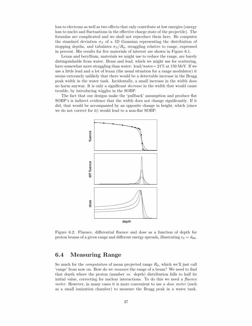
loss to electrons as well as two effects that only contribute at low energies (energyloss to nuclei and fluctuations in the effective charge state of the projectile). Theformulas are complicated and we shall not reproduce them here. He computesthe standard deviation σS of a 1D Gaussian representing the distribution ofstopping depths, and tabulates σS/R0, straggling relative to range, expressedin percent. His results for five materials of interest are shown in Figure 6.1.

Lexan and beryllium, materials we might use to reduce the range, are barelydistinguishable from water. Brass and lead, which we might use for scattering,have somewhat more straggling than water: lead/water= 21% at 150 MeV. If weuse a little lead and a lot of lexan (the usual situation for a range modulator) itseems extremely unlikely that there would be a detectable increase in the Braggpeak width in the water tank. Incidentally, a small increase in the width doesno harm anyway. It is only a significant decrease in the width that would causetrouble, by introducing wiggles in the SOBP.

The fact that our designs make the ‘pullback’ assumption and produce flatSOBP’s is indirect evidence that the width does not change significantly. If itdid, that would be accompanied by an opposite change in height, which (sincewe do not correct for it) would lead to a non-flat SOBP.

Figure 6.2: Fluence, differential fluence and dose as a function of depth forproton beams of a given range and different energy spreads, illustrating r0 = d80.

6.4 Measuring Range

So much for the computation of mean projected range R0, which we’ll just call‘range’ from now on. How do we measure the range of a beam? We need to findthat depth where the proton (number vs. depth) distribution falls to half itsinitial value, correcting for nuclear interactions. To do this we need a fluencemeter. However, in many cases it is more convenient to use a dose meter (suchas a small ionization chamber) to measure the Bragg peak in a water tank.

37

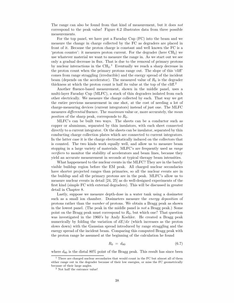
The range can also be found from that kind of measurement, but it does notcorrespond to the peak value! Figure 6.2 illustrates data from three possiblemeasurements.

For the top panel, we have put a Faraday Cup (FC) into the beam and wemeasure the change in charge collected by the FC as degraders are placed infront of it. Because the proton charge is constant and well known the FC is a‘proton counter’: it measures proton current. For the degrader (here CH2) weuse whatever material we want to measure the range in. As we start out we seeonly a gradual decrease in flux. That is due to the removal of primary protonsby nuclear interactions in the CH2.1 Eventually we reach a sharp decrease inthe proton count when the primary protons range out. The slope of this ‘cliff’comes from range straggling (irreducible) and the energy spread of the incidentbeam (depends on the accelerator). The measured value of R0 is the degraderthickness at which the proton count is half its value at the top of the cliff.2

Another fluence-based measurement, shown in the middle panel, uses amulti-layer Faraday Cup (MLFC), a stack of thin degraders isolated from eachother electrically. We measure the charge collected by each. That way we getthe entire previous measurement in one shot, at the cost of needing a lot ofcharge-measuring devices (current integrators) instead of just one. The MLFCmeasures differential fluence. The maximum value or, more accurately, the meanposition of the sharp peak, corresponds to R0.

MLFC’s can be built two ways. The sheets can be a conductor such ascopper or aluminum, separated by thin insulators, with each sheet connecteddirectly to a current integrator. Or the sheets can be insulator, separated by thinconducting charge collection plates which are connected to current integrators.In the latter case it is the charge electrostatically induced on the collectors thatis counted. The two kinds work equally well, and allow us to measure beamstopping in a large variety of materials. MLFC’s are frequently used as rangeverifiers to monitor the stability of accelerators and beam lines, because theyyield an accurate measurement in seconds at typical therapy beam intensities.

What happenened to the nuclear events in the MLFC? They are in the barelyvisible buildup region before the EM peak. All charged nuclear secondarieshave shorter projected ranges than primaries, so all the nuclear events are inthe buildup and all the primary protons are in the peak. MLFC’s allow us tomeasure nuclear events in detail [24, 25] as do well-designed experiments of thefirst kind (simple FC with external degraders). This will be discussed in greaterdetail in Chapter 8.

Lastly, suppose we measure depth-dose in a water tank using a dosimetersuch as a small ion chamber. Dosimeters measure the energy deposition ofprotons rather than the number of protons. We obtain a Bragg peak as shownin the lowest panel. (The peak in the middle panel is not a Bragg peak.) Somepoint on the Bragg peak must correspond to R0, but which one? That questionwas investigated in the 1960’s by Andy Koehler. He created a Bragg peaknumerically by folding the variation of dE/dx (which increases as the protonslows down) with the Gaussian spread introduced by range straggling and theenergy spread of the incident beam. Comparing this computed Bragg peak withthe proton range he assumed at the beginning of the calculation he found

R0 = d80 (6.7)

where d80 is the distal 80% point of the Bragg peak. This result has since been1 There are charged nuclear secondaries that would count in the FC but almost all of them

either range out in the degrader because of their low energies, or miss the FC geometricallybecause of their large angles.

2 Not half the entrance value!

38

confirmed several times [26, 27]. Note that this is a strictly numerical result. Infact, the real number is not exactly 80%, but 80% is close enough, and easy toremember.

Figure 6.3: d80 and d90 vs. range at nozzle entrance’ measured at NPTC.

Andy also found that (6.7) held independent of the energy spread he assumed.This confirms it as the true measure of mean projected range, because a meanvalue should not depend on the width of the underlying distribution. Figure6.2 shows what happens in each of the three measurements when we increasethe energy spread of the incident beam.3 d80 is the invariant point of the Braggpeak.

6.5 Clinical Depth Prescription

Usually, that the clinical specification refers to some level other than d80, suchas d90. A prescription might require that the distal 90% point be at exactly10.5 cm in water (d90 ≡ 10.5 cm). To fill this prescription we would need to

1. Measure (d80 − d90) of a Bragg peak at some range close to the specifiedd90. Suppose (d80 − d90) = 0.6 mm.

2. Add 0.6 mm to the prescribed value to get d80 = 10.56 cm.

3. Supply a beam of that range.

Often, as here, the correction is barely significant. Obviously, if we need to dothis frequently we should make a table or graph of premeasured values. d90 willdepend very slightly on the energy width of the beam; d80 will not. Figure 6.3

3 In the top two panels, we kept the total number of incident protons the same. In thelowest one, to illustrate R0 = d80 , we renormalized the curves to the peak value.

39

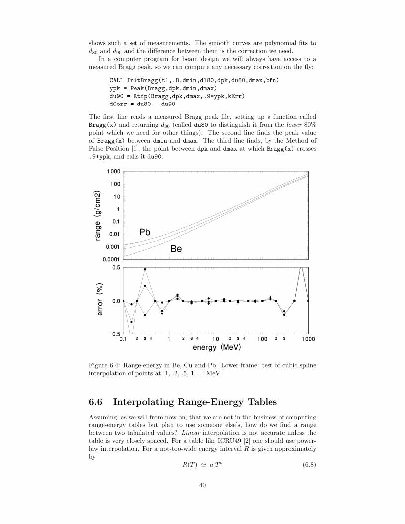
shows such a set of measurements. The smooth curves are polynomial fits tod80 and d90 and the difference between them is the correction we need.

In a computer program for beam design we will always have access to ameasured Bragg peak, so we can compute any necessary correction on the fly:

CALL InitBragg(t1,.8,dmin,dl80,dpk,du80,dmax,bfn)ypk = Peak(Bragg,dpk,dmin,dmax)du90 = Rtfp(Bragg,dpk,dmax,.9*ypk,kErr)dCorr = du80 - du90

The first line reads a measured Bragg peak file, setting up a function calledBragg(x) and returning d80 (called du80 to distinguish it from the lower 80%point which we need for other things). The second line finds the peak valueof Bragg(x) between dmin and dmax. The third line finds, by the Method ofFalse Position [1], the point between dpk and dmax at which Bragg(x) crosses.9*ypk, and calls it du90.

Figure 6.4: Range-energy in Be, Cu and Pb. Lower frame: test of cubic splineinterpolation of points at .1, .2, .5, 1 . . . MeV.

6.6 Interpolating Range-Energy Tables

Assuming, as we will from now on, that we are not in the business of computingrange-energy tables but plan to use someone else’s, how do we find a rangebetween two tabulated values? Linear interpolation is not accurate unless thetable is very closely spaced. For a table like ICRU49 [2] one should use power-law interpolation. For a not-too-wide energy interval R is given approximatelyby

R(T ) ' a T b (6.8)

40

Fitting this to the ICRU49 [2] table for water, Bortfeld [26] found that b = 1.77and a = 0.0022, assuming R is in cm (= g/cm2 for water) and T is in MeV,gave the range to ±1.5 mm over the range 0 < T < 200 MeV. Incidentally, (6.8)leads immediately to

T (R) ' 1a1/b

R1/b (6.9)

andS(R) ≡ −dT/dz ' 1

b a1/bR(1/b)−1 (6.10)

by the rules of differentiation.4 For power-law interpolation, use adjacent valuesR1(T1) and R2(T2) to determine a and b for that interval, then use (6.8) tocompute the desired R.

We want a method which can be used for any range-energy table and is moreaccurate than a single power-law approximation over the clinical range. Log-logplots of R(T ) are nearly straight lines (Figure 6.4). Using surprisingly few pointsT = .1, .2, .5, 1, . . . we can join them with a cubic spline interpolation function[1] which gives us ln R vs. ln T . Thats’s equivalent to approximating R by Traised to a cubic polynomial instead of a linear one. We use natural logarithmssince there’s no reason not to. The accuracy of this method is shown in thelower frame of Figure 6.4, where the error for intermediate points is plottedalong with that (zero, of course) for the given points. The error over the clinicalrange 3 − 300 MeV is less than 0.1% except for 300 MeV where it is 0.25%.5

This is a good time to introduce the program LOOKUP, a general-purposeproton desk calculator which computes range, energy, multiple scattering andother useful things. If you have LOOKUP you will never need to get out your range-energy tables, much less interpolate them. LOOKUP includes, among others, amodule RANGE.FOR which is used as follows:

i = InitRange(’\BGWARE\DATA\ICRU49.RET’)...

rnge = Range(engy,matl)...

engy = Energy(rnge,matl)

The call to InitRange reads the given range-energy table which is an ASCIIfile of range-energy data plus other data that will be required later for multi-ple scattering. You can easily add elements or compounds to this file, thoughICRU49 and MIXED already have most of what you’ll need for proton therapy.InitRange sets up the cubic spline interpolation table by constructing a list ofsecond derivatives at the given points [1]. This is done only once, at the startof the program. Afterwards, lines like the second and third will return rangeand energy values. LOOKUP is merely a driver for these and similar routines,providing a convenient keyboard dialog.

For many calculations it is important that T (R) be the exact inverse ofR(T ). For this reason, instead of setting up a cubic spline table ln T (lnR) asa companion to ln R(ln T ) (which would be exactly correct only at the datapoints), we solve the equation

ln R(ln T ) = ln Ra

where Ra is the range whose corresponding energy we desire and ln R(ln T ) isour cubic spline parametrization. We solve it numerically using the Method of

4 In (6.10) you can connect z and R by noting that a proton at depth z in a water tankhas residual range R = R0 − z if the initial range was R0. This gives dz = −dR.

5 In earlier work we used a polynomial fit to ln R(ln T ) (see [4] Figure 1). The cubic splineis better.

41

False Position [1], obtaining ln Ta. The root finder will converge quickly becauseln R(ln T ) is nearly a straight line. Finally, Ta = exp(ln Ta). The code reads

rlog = LOG(r) ! take logarithm of R_ax = Rtfp(RangeLog,xa,xb,rlog,k) ! find logarithm of T_aEnergy = EXP(x) ! raise e to that power

6.7 Finding the Energy Loss in a Degrader

The most basic range-energy problem is to find the proton energy emerging froma degrader of known thickness if the incoming energy is given. For instance: findthe energy out of 10 g/cm2 of lexan assuming 160 MeV incident protons. Sincewe have a single degrader we’ll call the material m1, its areal density (g/cm2) g1,the incoming energy (MeV) t1 and the outgoing energy (which is the incomingenergy for the next object, whatever that is) t2. Formally, we wish to find t2given m1, g1 and t1:

m1, g1, t1 → t2

6.7.1 Using Range

The exact method is straightforward:

1. Find the proton range in material m1 at energy t1.

2. Subtract g1 to obtain the residual range.

3. Find the energy in m1 for that range. That equals t2.

The numbers for this method are given in the next section.

6.7.2 Using Stopping Power

Less accurate method, but slightly easier:

1. Find the stopping power S in material m1 at energy t1.

2. Multiply by g1 to obtain the energy loss.

3. Subtract the energy loss from t1 to obtain t2.

The numbers for each method are:

method t1 S r1 r2 t2MeV MeV/(g/cm2) g/cm2 g/cm2 MeV

range-energy 160 18.523 13.523 133.66dE/dx 160 4.962 135.19

The second method will always give too high an answer because we’re lookingup S at the incoming energy, and S increases as t decreases during the proton’spassage through the degrader. Therefore the effective value of S is always higherthan S(t1). In our example the discrepancy is fairly serious because the degraderis fairly thick. In computer programs there is no real advantage in doing it thisway, so we won’t.

42

6.7.3 In a Computer Program

Assume we have at our disposal the two subprograms (‘functions’ in the Fortransense) mentioned in Section 6.6:

Range(energy, material)Energy(range, material)

We can implement the exact method as

r1 = Range(t1,m1) ! total range in material m1rr = r1 - g1 ! residual range in m1t2 = Energy(rr,m1) ! energy corresponding to that range

or condense the code to

t2 = Energy(Range(t1,m1)-g1,m1)

6.7.4 Exercise

As an example of another kind of problem, suppose that 30 MeV protons emergefrom 10 g/cm2 of lead (Pb). What was their energy going in ? (a) Write downthe formal problem, (b) write down the formal solution and (c) find the answerusing LOOKUP. Do the problem both ways: exactly, and using dE/dx. Theanswers for the exact method are

m1, g1, t2 → t1

rr = Range(t2,m1) ! residual range in material m1r1 = rr + g1 ! total range going into m1t1 = Energy(r1,m1) ! energy corresponding to that range

t1 = Energy(Range(t2,m1)+g1,m1)

83.4 MeV

Make up little problems like this and make sure you can do them. It is helpfulto organize your numbers in a little sketch of the problem.

6.7.5 Error Conditions

When we specify an outgoing energy we can always find an incoming energyno matter what the degrader thickness (unless we exceed the available range-energy table). When we specify an incoming energy and a thick degrader, theprotons could range out in the degrader and never emerge. The first problemis always well posed, the second may not be. A good program will test for sucherror conditions and take appropriate action. Programmers note: usually the‘appropriate action’ takes a good deal more thought than the test itself. If thisis part of a big program, we don’t necessarily want to bring everything to a halt!

6.8 Water Equivalence

We rarely use water equivalence in our programs, preferring to switch back andforth between R(T ) in different materials, using T as the common coin betweendegraders. However, water equivalence is frequently used, so we’ll briefly discussit and point out the pitfalls. Here we’ll occasionally refer to actual thickness(cm) rather than (g/cm2) so read carefully. When we’re talking about water itmakes no difference because ρwater = 1 g/cm2 by definition.

43

Figure 6.5: Range-energy over the clinically useful energy range for 4 usefulmaterials.

6.8.1 Water Equivalence of Thin Degraders

The water equivalent of a degrader is the thickness of water that has the sameenergy loss. More generally, a degrader of material 2 is said to be equivalent to adegrader of material 1 if the energy loss is the same. From S ≡ −(1/ρ)(dE/dx)we obtain

S2(T ) ρ2 ∆x2 = S1(T ) ρ1 ∆x1

which gives, for the lexan/water case

∆xW =SL(T )SW (T )

ρL

ρW∆xL (6.11)

We already know enough to be wary of equations like (6.11) if the degraders arenot thin. But there can be problems even if they are. The answer can depend onenergy, which makes it much less useful. The predicted water equivalent of 1 cmof lexan is 1.143 cm at 200 MeV and 1.144 cm at 70 MeV: no problem. But thewater equivalent of 0.62 cm of lead (the thickness of one of the second scatterersin the NPTC nozzle) is 3.556 cm at 200 MeV and 3.355 cm at 70 MeV. The2 mm difference is just enough to be troublesome, and the scatterer is in factexposed to that range of energies in clinical operations.

When we’re safe, and when not, can be seen from Figure 6.5, a log-logplot of R(T ) for four useful materials. The slopes are slightly different as wemove from low-Z to high-Z materials. That means the stopping power ratios inequations like (6.11) will depend on energy. ‘Equivalence’ is a good concept fortwo materials if they’re close in the periodic table (water and plastic) but notif they’re far apart (water and lead).

44

6.8.2 Equivalence in a Finely Divided Stack

In the case of a multi-layer Faraday Cup (MLFC), frequently used as a rangeverifier (RV), we have a finely-divided stack of two materials. For instance therange verifier at NPTC is a stack of 2 mm brass sheets separated from eachother by 0.05 mm of polyethylene. We would like to characterize measurementswith this RV as ‘range in brass’. How do we correct for the polyethylene?While the protons stop, they encounter brass and polyethylene at all energiesfrom the incident energy T to zero. What energy should we use to find theaverage stopping power ratio? The answer, which can be found numericallywith range-energy tables, is 0.52 × T . Ranges in any two materials are relatedby

R2

R1

∣∣∣∣T

=S1

S2

∣∣∣∣0.52T

(6.12)

If we have a stack of equal plates of brass, each B g/cm2, separated by equalsheets of polyethylene, each P g/cm2, the average brass equivalent < BP > ofa polyethylene sheet is

< BP > =SP

SB

∣∣∣∣0.52T

× P (6.13)

This rule works for any finely-divided stack independent of the materials andtheir relative thicknesses. The stopping power ratio depends on energy if thematerials are far apart on the periodic table. However, if the minor material isthin compared to the other, that effect is second-order.

6.8.3 Measured Water Equivalence

Though we are not in general fond of water equivalence, it has one very usefulproperty. We can measure it with equipment always found at proton therapycenters, and the measurement is trivial. Simply measure d80 of a Bragg peak ina water tank, then put the desired degrader in front of the tank and remeasured80. With good instrumentation you can do this to ±0.1 mm. The measuredwater equivalence found in that way can be used in the final stages of a designinstead of range-energy tables, which we have already seen are not quite goodenough because of their dependence on I . At HCL we measured the waterequivalence of lexan and lucite (plexiglas) a number of times and found

water equivalent of 1 cm lexan or lucite = 1.15 cm

which disagrees very slightly with the computed value given earlier.If you measure the water equivalence of lead this way, you’ll find it depends

on energy as we have already noted. Sometimes it happens (see Chapter 13)that the design conditions are such that the lead always sees the same, or nearlythe same, energy. In that case, improving the depth accuracy of the design byusing a measured water equivalent thickness for the lead can still be a usefulthing to do.

6.9 Does the Order of Degraders Matter?

The answer to this question is based on considerations of the previous section.The second degrader in a stack sees a lower energy than the first. If that doesn’tmatter, that is, if the stopping powers in the two materials vary the same waywith energy, then the order doesn’t matter. Putting it another way, the order oftwo materials doesn’t matter if their R(T ) are parallel on a log-log plot (Figure

45

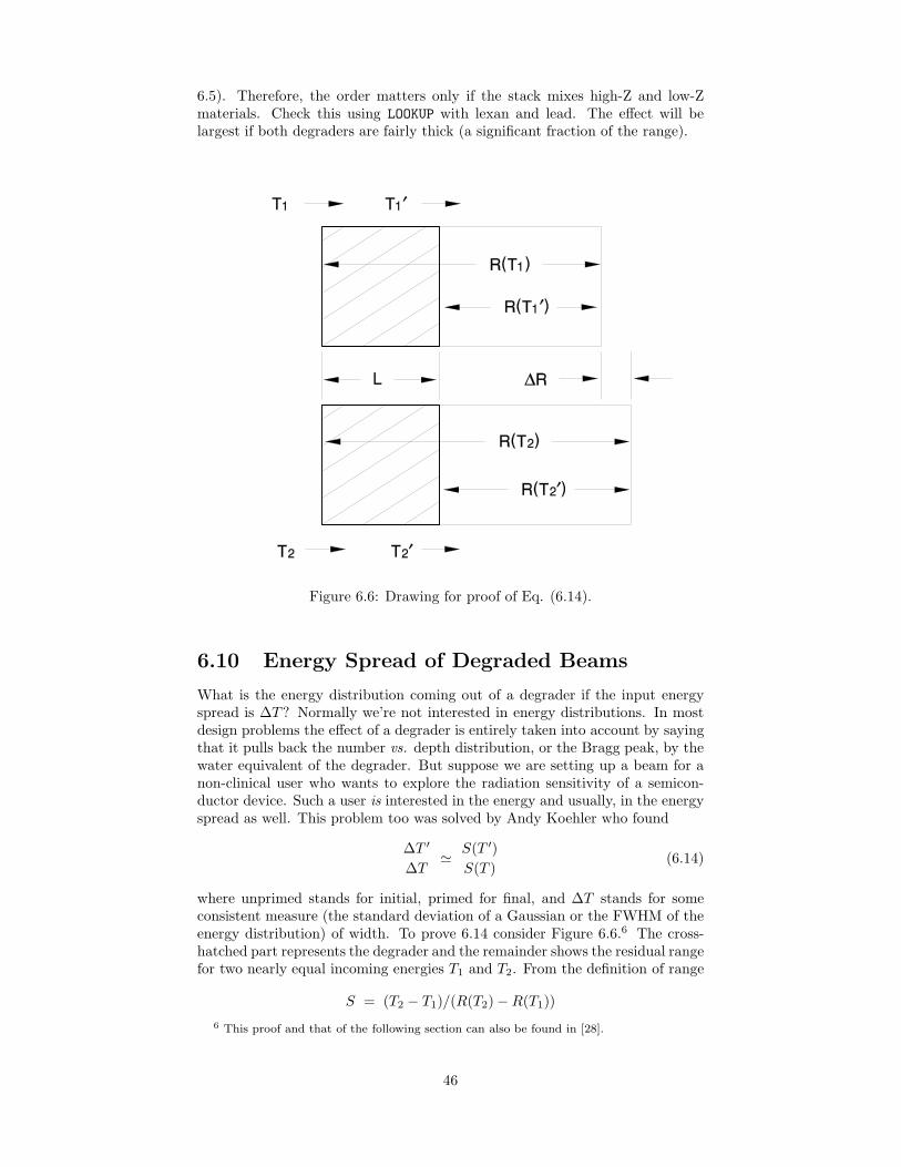
6.5). Therefore, the order matters only if the stack mixes high-Z and low-Zmaterials. Check this using LOOKUP with lexan and lead. The effect will belargest if both degraders are fairly thick (a significant fraction of the range).

Figure 6.6: Drawing for proof of Eq. (6.14).

6.10 Energy Spread of Degraded Beams

What is the energy distribution coming out of a degrader if the input energyspread is ∆T ? Normally we’re not interested in energy distributions. In mostdesign problems the effect of a degrader is entirely taken into account by sayingthat it pulls back the number vs. depth distribution, or the Bragg peak, by thewater equivalent of the degrader. But suppose we are setting up a beam for anon-clinical user who wants to explore the radiation sensitivity of a semicon-ductor device. Such a user is interested in the energy and usually, in the energyspread as well. This problem too was solved by Andy Koehler who found

∆T ′

∆T' S(T ′)

S(T )(6.14)

where unprimed stands for initial, primed for final, and ∆T stands for someconsistent measure (the standard deviation of a Gaussian or the FWHM of theenergy distribution) of width. To prove 6.14 consider Figure 6.6.6 The cross-hatched part represents the degrader and the remainder shows the residual rangefor two nearly equal incoming energies T1 and T2. From the definition of range

S = (T2 − T1)/(R(T2) − R(T1))

6 This proof and that of the following section can also be found in [28].

46

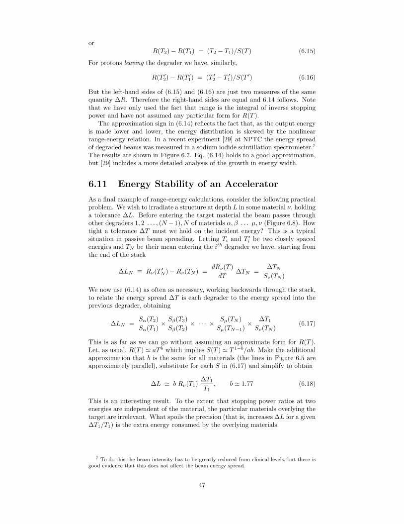
orR(T2) − R(T1) = (T2 − T1)/S(T ) (6.15)

For protons leaving the degrader we have, similarly,

R(T ′2) − R(T ′

1) = (T ′2 − T ′

1)/S(T ′) (6.16)

But the left-hand sides of (6.15) and (6.16) are just two measures of the samequantity ∆R. Therefore the right-hand sides are equal and 6.14 follows. Notethat we have only used the fact that range is the integral of inverse stoppingpower and have not assumed any particular form for R(T ).

The approximation sign in (6.14) reflects the fact that, as the output energyis made lower and lower, the energy distribution is skewed by the nonlinearrange-energy relation. In a recent experiment [29] at NPTC the energy spreadof degraded beams was measured in a sodium iodide scintillation spectrometer.7

The results are shown in Figure 6.7. Eq. (6.14) holds to a good approximation,but [29] includes a more detailed analysis of the growth in energy width.

6.11 Energy Stability of an Accelerator

As a final example of range-energy calculations, consider the following practicalproblem. We wish to irradiate a structure at depth L in some material ν, holdinga tolerance ∆L. Before entering the target material the beam passes throughother degraders 1, 2 . . . , (N −1), N of materials α, β . . . µ, ν (Figure 6.8). Howtight a tolerance ∆T must we hold on the incident energy? This is a typicalsituation in passive beam spreading. Letting Ti and T ′

i be two closely spacedenergies and TN be their mean entering the ith degrader we have, starting fromthe end of the stack

∆LN ≡ Rν(T ′N ) − Rν(TN ) =

dRν(T )dT

∆TN =∆TN

Sν(TN)

We now use (6.14) as often as necessary, working backwards through the stack,to relate the energy spread ∆T is each degrader to the energy spread into theprevious degrader, obtaining

∆LN =Sα(T2)Sα(T1)

× Sβ(T3)Sβ(T2)

× · · · × Sµ(TN )Sµ(TN−1)

× ∆T1

Sν(TN )(6.17)

This is as far as we can go without assuming an approximate form for R(T ).Let, as usual, R(T ) ' aT b which implies S(T ) ' T 1−b/ab. Make the additionalapproximation that b is the same for all materials (the lines in Figure 6.5 areapproximately parallel), substitute for each S in (6.17) and simplify to obtain

∆L ' b Rν(T1)∆T1

T1, b ' 1.77 (6.18)

This is an interesting result. To the extent that stopping power ratios at twoenergies are independent of the material, the particular materials overlying thetarget are irrelevant. What spoils the precision (that is, increases ∆L for a given∆T1/T1) is the extra energy consumed by the overlying materials.

7 To do this the beam intensity has to be greatly reduced from clinical levels, but there isgood evidence that this does not affect the beam energy spread.

47

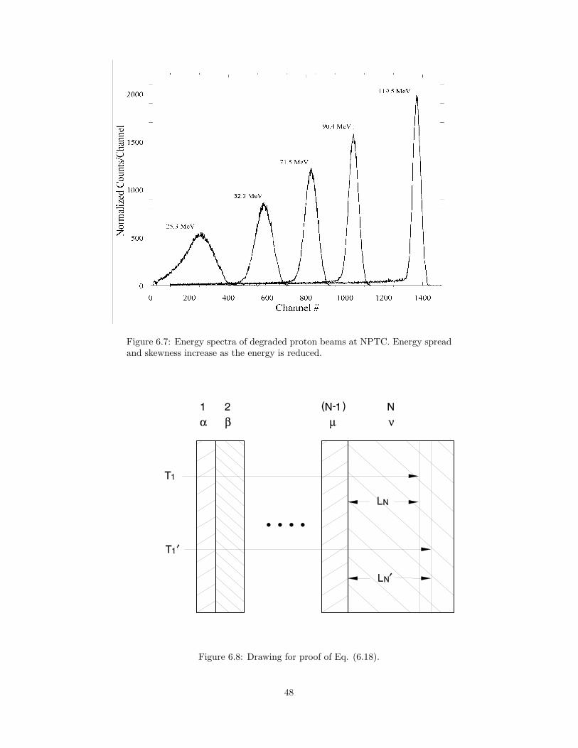
Figure 6.7: Energy spectra of degraded proton beams at NPTC. Energy spreadand skewness increase as the energy is reduced.

Figure 6.8: Drawing for proof of Eq. (6.18).

48

Chapter 7

Scattering

As protons slow down they also scatter, mainly by interaction with atomicnuclei rather than electrons, because collisions with electrons hardly deflect themassive proton. Most single deflections, even by nuclei, are very small, so it isthe net result of very many such events that we must compute. Because theinteraction is electromagnetic, through the Coulomb force, the phenomenon iscalled multiple Coulomb scattering.

The subject received wide attention in the 1930’s and 40’s. It was ultimatelylaid to rest in two papers by Moliere,1 whose solution to the problem is nowconsidered definitive. In the first paper [6] Moliere investigates single scatteringin the Coulomb field of the nucleus, which is screened by the atomic electrons.One needs a good model of single scattering before one can address multiplescattering. In the second [7] he applies this to plural scattering (just a fewscatters) and multiple scattering (very many scatters). His elegant and com-prehensive treatment includes the effect of energy loss by the primary particle,and allows the stopping medium to be a chemical element or a compound ormixture. Both extensions of the theory are very important in proton therapydesign, as we often deal with thick scatterers or compounds.

In 1993 an HCL group compared our and all other existing proton data withMoliere’s theory [4]. You should read [4] and some of the references therein ifyou wish to pursue the subject beyond these notes. By then the literature hadbecome somewhat tangled. There were at least four competing ‘exact’ theorieswith different domains of validity, whose relationship to each other is discussedby Bethe [5]. Some experimental groups were unaware that Moliere had treatedenergy loss2 and used ‘effective energy’ approaches to fill the perceived gap.Others found that Moliere’s predictions were incorrect. At least one theoreticalpaper [30] claimed to correct flaws in Moliere’s theory.

The HCL paper reviewed and in some cases reanalyzed all the experimentaldata and found that Moliere theory was correct. Figure 7.1 reproduced from[4] is a grand summary of the deviation of experimental data from Molieretheory for seven experiments spanning 1 MeV to 200 GeV incident energy. Datafrom each experiment have been averaged over everything but target material.The distribution of 39 independent measurements is normal with a mean value−0.3± 0.5% and an rms spread of 3%.

The sense in which ‘discrepancy from experiment’ is defined in Figure 7.11 Despite the name Moliere was German. He may have been a student of Heisenberg, who

is thanked in both papers. The second paper was his ‘Habilitationsschrift’ at the Universityof Tubingen, a publication which had to be formally accepted before one was admitted to thefaculty. He went on to make fundamental contributions in several fields of physics.

2 Perhaps because Bethe’s paper [5], more accessible to the English speaker than Moliere’s,omitted that aspect of the theory.

49

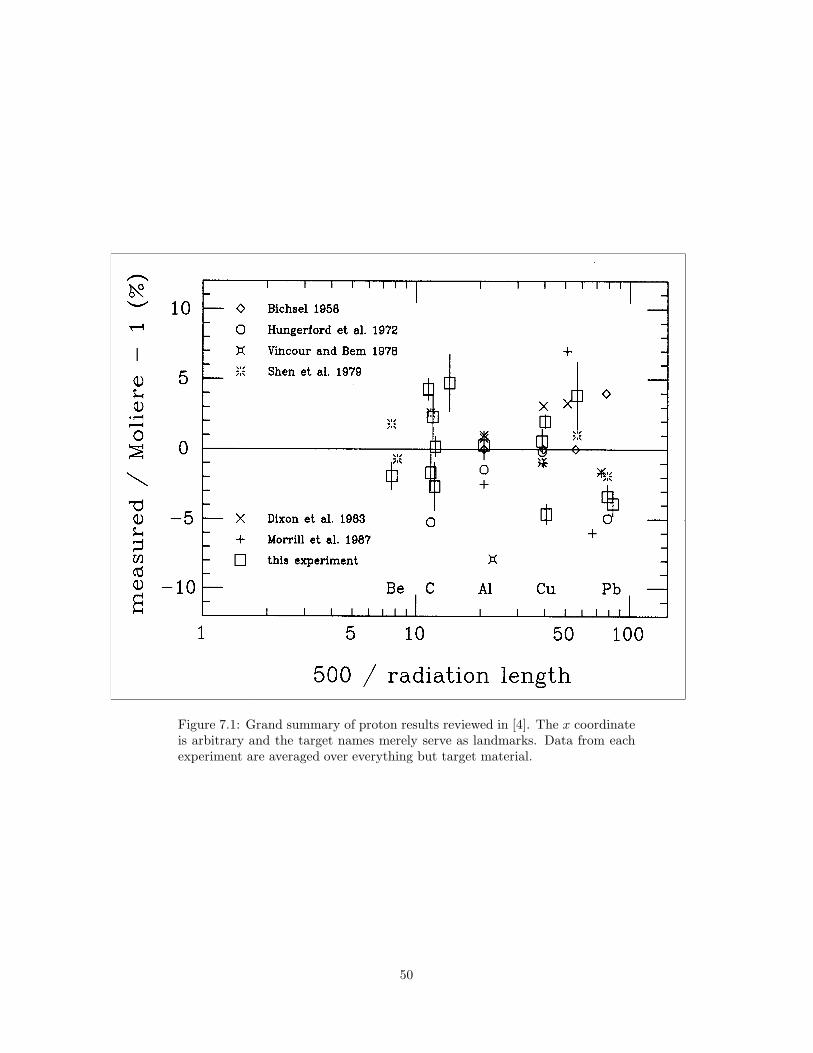
Figure 7.1: Grand summary of proton results reviewed in [4]. The x coordinateis arbitrary and the target names merely serve as landmarks. Data from eachexperiment are averaged over everything but target material.

50

means that Moliere is high by 0.3%, but this is statistically consistent with 0.In other words, one cannot say how good Moliere theory actually is for protonsbecause experimental errors, typically a few percent, dominate the comparison.Future experiments to test the theory more rigorously need to be considerablymore accurate, which will not be easy.

The only substantial theoretical improvement to Moliere theory was the Fanocorrection [31] for scattering by atomic electrons. This is appreciable only forvery light elements whose nuclei have low charge. This correction had beenapproximated earlier by Bethe by just substituting Z(Z + 1) for Moliere’s Z2

in the formula for χ2c . That is much simpler and works almost as well [4].

Moliere theory has no material dependent parameters, in fact no adjustableparameters at all. It is true that Moliere introduces an approximate numericalexpression (7.4) in evaluating the Thomas-Fermi model of the atom in order tocompute screening. However, that result has since been confirmed by computercalculations [4, 32] and is not material specific.

There are no ‘scattering tables’ analogous to range-energy tables. One mustcompute the characteristic multiple scattering angle from Moliere’s equationsor use one of the (far simpler) approximate formulas we will give. Our Fortranfunction Theta0 incorporates all of Moliere theory as well as the approximatetheories. It computes the equations given below, and was used to calculate thenumbers in [4] and in Table 7.2.5.

7.1 Central Limit Theorem

Let θ be the angle between the particle direction and the longitudinal axis andlet θ0 be a characteristic angle. If we assume that multiple scattering can becomputed by taking the quadratic sum of small angular kicks we will find thatthe angular distribution is Gaussian

f(θ, φ) θ dθ dφ =1

2π θ20

e− 1

2

( θ

θ0

)2

θ dθ dφ (7.1)

and that the width parameter θ0 is proportional to√

t where t is the scattererthickness. Both are consequences of the Central Limit Theorem, which statesthat the distribution of the sum of small random kicks tends toward a Gaussianas the number of kicks is increased. However, a condition for the theorem toapply is that all the random kicks must be small in a sense that can be mademathematically precise [33]. This condition is not met for the EM scatteringof protons by the nucleus (Rutherford scattering). To put it another way, asθ increases, Rutherford scattering falls off as 1/θ4, much more slowly than aGaussian. Therefore if (7.1) were to hold we would reach the absurd conclusionthat, at some angle, multiple scattering is less than single scattering. Multiplescattering must approach 1/θ4 at ‘large’ angles and be greater at small angles.This means that the full angular distribution cannot be Gaussian, though it willturn out to be nearly Gaussian at small angles, and that its characteristic widthcannot be exactly proportional to

√t.

7.2 Moliere Theory

What follows is the bare bones of Moliere’s algebra. For fuller discussions seethe HCL paper [4], Bethe [5], the extensive review by Scott [34] and, of course,Moliere [6, 7]. In place of the Gaussian’s single parameter θ0, Moliere theory has

51

two, χc (an angle) and B (a dimensionless quantity). A characteristic multiplescattering angle θM can be defined in terms of these as

θM =1√2

(χc

√B)

and this plays the same role in Moliere theory as θ0 does in the Gaussian. TheMoliere angular distribution depends strongly on θM and weakly on B, whichcarries the dependence on target thickness.

7.2.1 Thin Scatterer

Following Moliere we first assume a thin scatterer (so kinematic factors can beconsidered constant) made of a single chemical element. Later we’ll add energyloss, compounds and mixtures, and finally the Fano correction at low Z.

The characteristic single scattering angle χc is given by

χ2c = c3 t/(pv)2 (7.2)

where t is the target thickness (g/cm2), p and v the particle momentum andspeed, and

c3 ≡ 4 πNA

( e2

hc

)2

(hc)2z2Z2

A(7.3)

where Z and A are the atomic number and atomic weight of the target material,z is the charge number (charge/e) of the incident particle, NA is Avogadro’snumber, (e2/hc) is the fine structure constant and (hc) is the usual conversionconstant.3 χc has the physical meaning that, on the average, a particle suffersexactly one single scatter greater than χc in its traversal of the target [7, 4].

To find B we must next compute a screening angle χa from

χ2a = χ2

0 (1.13 + 3.76 α2) (7.4)

whereχ2

0 = c2/(pc)2 (7.5)

and the Born parameter α is given by

α2 = c1/β2 (7.6)

The constants are defined by

c1 ≡[( e2

hc

)z Z]2

(7.7)

and

c2 ≡[ 10.885

( e2

hc

)(mec

2) Z1/3]2

(7.8)

β stands for v/c of the incident particle and mec2 is the electron rest energy.

Next we compute a quantity

b = ln( χ2

c

1.167 χ2a

)(7.9)

b is interpreted as the natural logarithm of the effective number of collision inthe target. Finally the reduced target thickness B is defined as the root of theequation

B − ln B = b (7.10)3 Chapter 2 gives the values of physical constants.

52

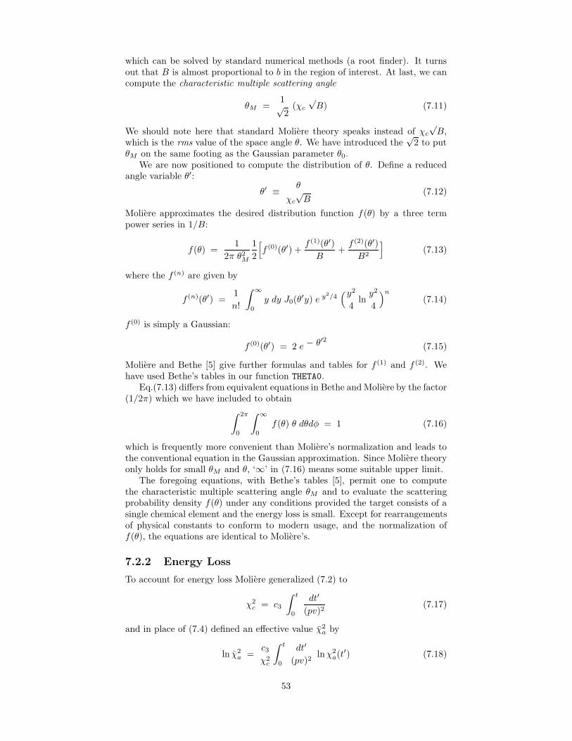
which can be solved by standard numerical methods (a root finder). It turnsout that B is almost proportional to b in the region of interest. At last, we cancompute the characteristic multiple scattering angle

θM =1√2

(χc

√B) (7.11)

We should note here that standard Moliere theory speaks instead of χc

√B,

which is the rms value of the space angle θ. We have introduced the√

2 to putθM on the same footing as the Gaussian parameter θ0.

We are now positioned to compute the distribution of θ. Define a reducedangle variable θ′:

θ′ ≡ θ

χc

√B

(7.12)

Moliere approximates the desired distribution function f(θ) by a three termpower series in 1/B:

f(θ) =1

2π θ2M

12

[f (0)(θ′) +

f (1)(θ′)B

+f (2)(θ′)

B2

](7.13)

where the f (n) are given by

f (n)(θ′) =1n!

∫ ∞

0

y dy J0(θ′y) e y2/4(y2

4ln

y2

4

)n

(7.14)

f (0) is simply a Gaussian:

f (0)(θ′) = 2 e − θ′2 (7.15)

Moliere and Bethe [5] give further formulas and tables for f (1) and f (2). Wehave used Bethe’s tables in our function THETA0.

Eq.(7.13) differs from equivalent equations in Bethe and Moliere by the factor(1/2π) which we have included to obtain

∫ 2π

0

∫ ∞

0

f(θ) θ dθdφ = 1 (7.16)

which is frequently more convenient than Moliere’s normalization and leads tothe conventional equation in the Gaussian approximation. Since Moliere theoryonly holds for small θM and θ, ‘∞’ in (7.16) means some suitable upper limit.

The foregoing equations, with Bethe’s tables [5], permit one to computethe characteristic multiple scattering angle θM and to evaluate the scatteringprobability density f(θ) under any conditions provided the target consists of asingle chemical element and the energy loss is small. Except for rearrangementsof physical constants to conform to modern usage, and the normalization off(θ), the equations are identical to Moliere’s.

7.2.2 Energy Loss

To account for energy loss Moliere generalized (7.2) to

χ2c = c3

∫ t

0

dt′

(pv)2(7.17)

and in place of (7.4) defined an effective value χ2a by

ln χ2a =

c3

χ2c

∫ t

0

dt′

(pv)2ln χ2

a(t′) (7.18)

53

where χ2a(t′) is found at each depth t′ in the target by means of (7.4), (7.5) and

(7.6) using the values of p and β appropriate at that depth. These generali-zations preserve the form of (7.9) so that it and subsequent equations through(7.16) remain valid. For instance (7.9) becomes

b = ln( χ2

c

1.167 χ2a

)(7.19)

and so forth.

7.2.3 Compounds and Mixtures

For compounds and mixtures Moliere introduced a sum over constituents inaddition to the integral over depth. Now

χ2c =

(∑

i

c3i

) ∫ t

0

dt′

(pv)2(7.20)

and

ln χ2a =

1χ2

c

∑

i

[c3i

∫ t

0

dt′

(pv)2ln χ2

ai(t′)]

(7.21)

where i runs over the number of elementary constituents in the target. χai isobtained from (7.4), (7.5) and (7.6) with the target constants c3i, c2i and c1i

defined as before with the replacements Z → Zi and (1/A) → (fi/Ai) wherefi is the fraction by weight of the ith constituent of the compound or mixture.Eqs.(7.9) through (7.16) still hold with these new definitions of χ2

c and χ2a.

Implicit in the integrals involving pv is the assumption that energy is awell-defined function of depth in the target. This fails for targets so thick thatthe energy spread from range straggling is comparable to the mean energy. Forthese ‘very thick’ targets we cannot expect Moliere theory or any similar analytictheory to apply. As we shall see, the data suggest that this occurs when thetarget thickness exceeds ≈ 97% of the mean proton range.

7.2.4 Fano Correction

Fano [31] derived the correction to Moliere theory for scattering of the incidentparticle by atomic electrons in addition to the screened Coulomb field of thenucleus. The expedient recommended by Bethe [5], replacing Z in formulas forχ2

c by Z(Z + 1), only works as long as the scattering by atomic electrons is wellapproximated by the Rutherford formula. Therefore it is not exactly correcteven for incident electrons, and less so for incident heavy particles. For theseFano recommends using Moliere’s original definition of χ2

c (that is, retainingZ2) and adding to Moliere’s b a quantity D/Z where

D = ln[

1130Z4/3

((1/β2) − 1

)]

− uin − 12

β2 (7.22)

and −uin is an integral over the incoherent scattering function. Fano quotesseveral calculations of −uin and suggests using the value −uin = 5. Eq.(7.22)only covers the thin elementary target case because D is a function of incidentparticle energy as well as target species. Fortunately Scott [34] fills this gap,showing how to include Fano’s correction in the theory for thick compoundtargets. The formula for χ2

c is unaffected, while (7.21) becomes

ln χ2a =

1χ2

c

∑

i

[c3i

∫ t

0

dt′

(pv)2(ln χ2

ai(t′) − Di

Zi

)](7.23)

54

(From here on we’ll drop the bar over χ2a because there is no risk of confusion.)

Scott uses −uin = 5.8, the value Fano quotes for the Thomas-Fermi model,instead of 5, the value recommended by Fano and the value we shall use.

In summary, what we call ‘Moliere theory’ will be defined by equations(7.20) for χ2

c and (7.23) for χ2a along with the equations of the first section

with kinematic and target dependences included as necessary. Although thefull generality of this approach is required only for thick, compound, low-Ztargets it is valid as well in the case of thin, elementary high-Z targets so wewill use it throughout.

7.2.5 Evaluation of the Integrals

We will evaluate the integrals in Eqs.(7.20) and (7.23) numerically using thecubic spline parametrization of the range-energy relation described in Chapter6. The integrals can be approximated as sums over finite slabs of the targetusing Simpson’s Rule [1]

∫ xc

xa

f(x) dx ≈ 16(fa + 4fb + fc) ∆x (7.24)

where ∆x ≡ xc − xa is the total thickness of the slab and xb is the midpoint.Simpson’s Rule [1] is exact if f(x) is a cubic or lower polynomial. It minimizesfunction calls because fc can be recycled as fa for the next interval.

Because of the 1/(pv)2 kinematic factor the integrand increases rapidly asthe proton slows down. Therefore it is inefficient to divide the target into slabsof equal thickness. Instead, we divide it equally in the logarithmic sense, that is,by equal thickness ratios. Each slab will be (say) 1.6× as thick as the previousone. To accomplish this let R1 be the range, in the target material, of the protonentering the target and let R2 be its residual range leaving the target. We wishto divide t into N slabs ti such that the ratio ρ > 1 of each thickness to theprevious one will be the same. This can be done by letting

ρ = (R1/R2)1/N

and

t1 = (ρ − 1)R2, t2 = ρ(ρ − 1)R2, · · · , tN = ρN−1(ρ − 1)R2 .

As a check

t1 + · · · + tN = (1 + ρ + · · · + ρN−1)(ρ − 1)R2 = (ρN − 1)R2 = R1 − R2

by Dwight 26 [20]. Rather than fixing N , leading to needless subdivision of thintargets, we let the computer choose N for each case so that ρ will not exceedsome given ρmax. Then N = 1 for any thin target.4 With ρmax = 1.6 we obtainbetter than 0.1% computational accuracy in θM , and this leads to a mere 8 slabsfor R2 ≈ 0.03R1 beyond which, as noted earlier, the theory no longer applies.

7.2.6 Numerical Results

Table 7.2.5 lists Moliere parameters as well as the final result θM for 158.6 MeVprotons incident on Be, Cu and Pb targets of normalized thicknesses t′ ≡ t/R0

ranging from 0.0001 to 0.97. It is an abridged and slightly altered version ofTable 1 in [4]. Slight differences in the results are probably due to the use

4 Using Simpson’s Rule (7.24) even for a single slab already guarantees we do much betterthan picking a single value for pv.

55

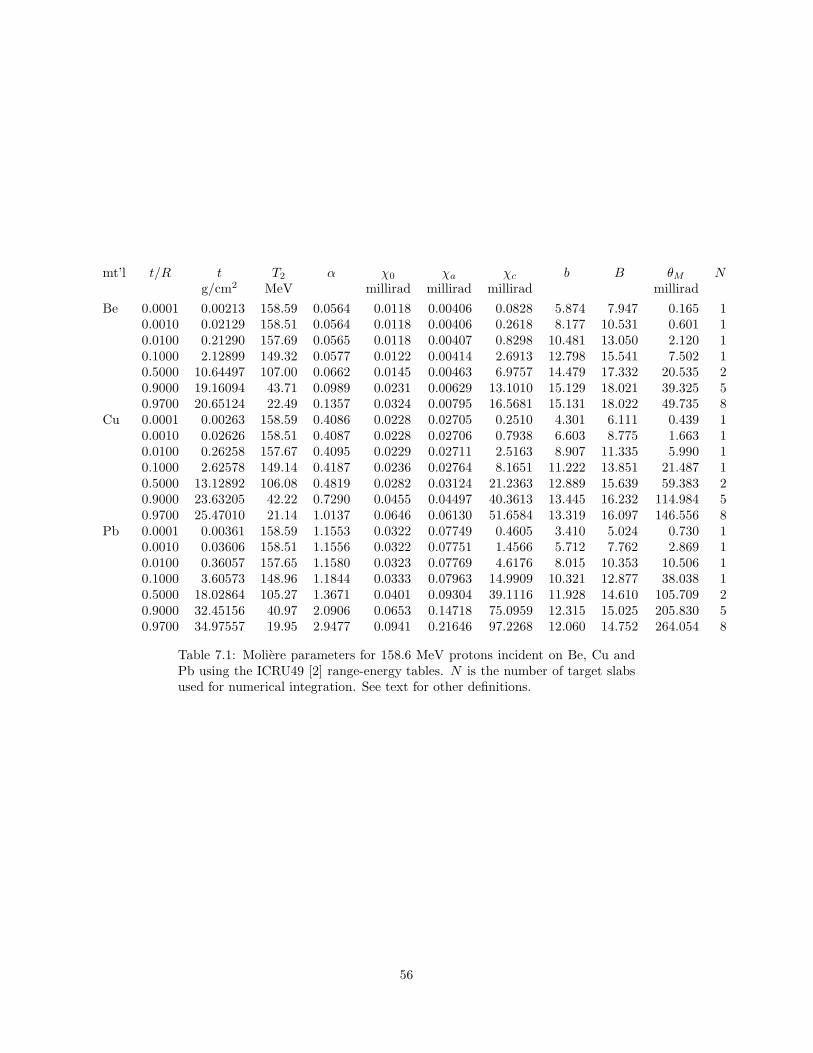
mt’l t/R t T2 α χ0 χa χc b B θM Ng/cm2 MeV millirad millirad millirad millirad

Be 0.0001 0.00213 158.59 0.0564 0.0118 0.00406 0.0828 5.874 7.947 0.165 10.0010 0.02129 158.51 0.0564 0.0118 0.00406 0.2618 8.177 10.531 0.601 10.0100 0.21290 157.69 0.0565 0.0118 0.00407 0.8298 10.481 13.050 2.120 10.1000 2.12899 149.32 0.0577 0.0122 0.00414 2.6913 12.798 15.541 7.502 10.5000 10.64497 107.00 0.0662 0.0145 0.00463 6.9757 14.479 17.332 20.535 20.9000 19.16094 43.71 0.0989 0.0231 0.00629 13.1010 15.129 18.021 39.325 50.9700 20.65124 22.49 0.1357 0.0324 0.00795 16.5681 15.131 18.022 49.735 8

Cu 0.0001 0.00263 158.59 0.4086 0.0228 0.02705 0.2510 4.301 6.111 0.439 10.0010 0.02626 158.51 0.4087 0.0228 0.02706 0.7938 6.603 8.775 1.663 10.0100 0.26258 157.67 0.4095 0.0229 0.02711 2.5163 8.907 11.335 5.990 10.1000 2.62578 149.14 0.4187 0.0236 0.02764 8.1651 11.222 13.851 21.487 10.5000 13.12892 106.08 0.4819 0.0282 0.03124 21.2363 12.889 15.639 59.383 20.9000 23.63205 42.22 0.7290 0.0455 0.04497 40.3613 13.445 16.232 114.984 50.9700 25.47010 21.14 1.0137 0.0646 0.06130 51.6584 13.319 16.097 146.556 8

Pb 0.0001 0.00361 158.59 1.1553 0.0322 0.07749 0.4605 3.410 5.024 0.730 10.0010 0.03606 158.51 1.1556 0.0322 0.07751 1.4566 5.712 7.762 2.869 10.0100 0.36057 157.65 1.1580 0.0323 0.07769 4.6176 8.015 10.353 10.506 10.1000 3.60573 148.96 1.1844 0.0333 0.07963 14.9909 10.321 12.877 38.038 10.5000 18.02864 105.27 1.3671 0.0401 0.09304 39.1116 11.928 14.610 105.709 20.9000 32.45156 40.97 2.0906 0.0653 0.14718 75.0959 12.315 15.025 205.830 50.9700 34.97557 19.95 2.9477 0.0941 0.21646 97.2268 12.060 14.752 264.054 8

Table 7.1: Moliere parameters for 158.6 MeV protons incident on Be, Cu andPb using the ICRU49 [2] range-energy tables. N is the number of target slabsused for numerical integration. See text for other definitions.

56

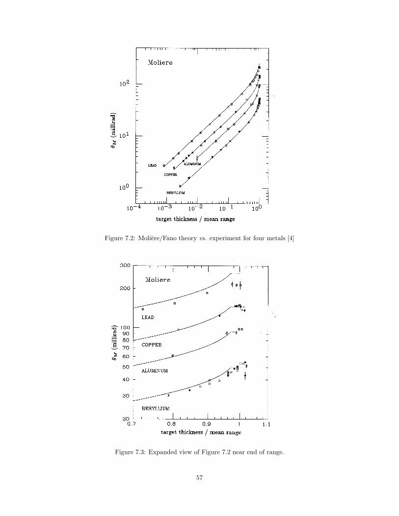
Figure 7.2: Moliere/Fano theory vs. experiment for four metals [4]

Figure 7.3: Expanded view of Figure 7.2 near end of range.

57

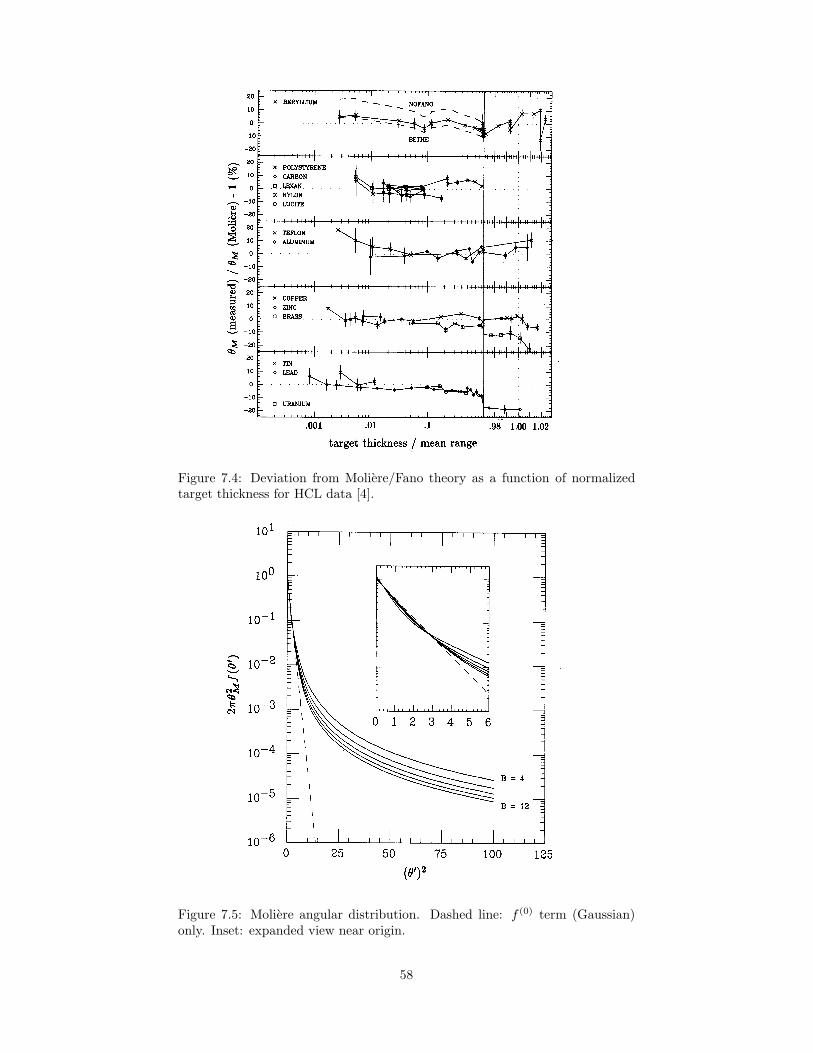
Figure 7.4: Deviation from Moliere/Fano theory as a function of normalizedtarget thickness for HCL data [4].

Figure 7.5: Moliere angular distribution. Dashed line: f (0) term (Gaussian)only. Inset: expanded view near origin.

58

of different range-energy tables and the cubic spline instead of the polynomialparametrization of the range-energy relation.

A study of this table reveals that Moliere’s reduced target thickness B isvery nearly proportional to the logarithm of the normalized target thickness,with a constant of proportionality that depends upon the material.

Figure 7.2, from [4], shows θM for four metals over three decades of norma-lized target thickness. The data points are from the HCL experiment. Therange of this parameter-free theory is astounding, and its accuracy holds upunder closer scrutiny (Figure 7.4). See [4] for details of the experiment andanalysis.

Figure 7.3 is an expanded view of Figure 7.2 near end-of-range, showing aleveling off of the multiple scattering angle for protons that just make it out ofthe target. There is no theoretical model in this region, though one can imaginethat the degrader itself filters out protons with larger angles. We approximatethis region in THETA0 by allowing θM to saturate at t/R0 = 0.97 as shown. Thisregion is unimportant in the design of beam spreading devices.

Figure 7.4 is a linear plot of the deviation from Moliere/Fano theory as afunction of normalized target thickness for the HCL data [4]. The window onthe right is an expanded view of the ‘very thick’ target region and should notbe used in judging the accuracy of the theory. As just stated, in this region wehave set θM to its value at t/R0 = 0.97.

7.3 Gaussian Approximations

Figure 7.5 shows the Moliere angular distribution plotted in the form 2πθ2Mf(θ′)

(equation 7.13) vs. (θ′)2 in which representation a Gaussian appears as a straightline. The inset is an expanded view near the origin. The dashed line shows theresult of using only the Gaussian term f (0). This plot illustrates two propertiesof the Moliere distribution. First, it depends only weakly on target thickness:recall that the B range corresponds to a factor ≈ 1000× in target thickness(Table 7.2.5). Second, f(θ) for small θ (on the order of the characteristic angleθM ) is nearly Gaussian, but not the Gaussian obtained by merely dropping f (1)

and f (2).

7.3.1 Hanson’s Formula

Hanson et al. [35] first pointed out that f(θ) is best approximated by a some-what narrower Gaussian, one obtained by replacing χc

√B by χc

√B − 1.2. We

defineθH ≡ 1√

2(χc

√B − 1.2) (7.25)

The Hanson approximation consists of going through the Moliere calculation,computing θH from equation 7.25 and using it as the characteristic width of aGaussian distribution, that is, replacing θ0 in (7.1) by θH .

7.3.2 Highland’s Formula

In the Hanson approximation f(θ) is far simpler but we still have to go throughthe complete Moliere calculation to find the characteristic angle. Highland [36]developed a formula which is vastly easier to compute but quite accurate:

θ0 =14.1 MeV

pvz

√L

LR

[1 +

19

log10

( L

LR

)]rad (7.26)

59

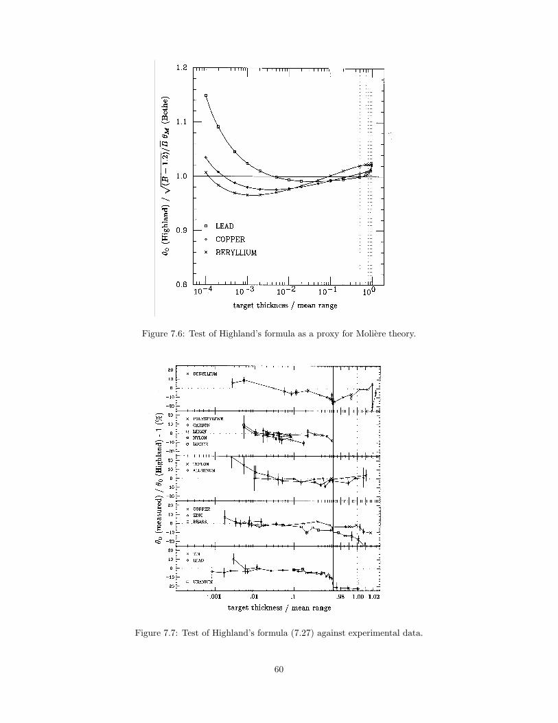
Figure 7.6: Test of Highland’s formula as a proxy for Moliere theory.

Figure 7.7: Test of Highland’s formula (7.27) against experimental data.

60

LR is the radiation length of the target material and L is the target thicknessin the same units. You can look up LR for many materials in [11]. Highlandobtained this formula by fitting the Bethe variant of Moliere theory (Z(Z + 1),no Fano correction) over a range of target thicknesses and materials. Figure7.6 shows that his parametrization is extremely effective. Except for the lowestpoints for Pb, which fall outside the range of validity claimed by Highland, thissimple formula has a peak error of ±4% and a typical error perhaps half that.It is definitely the formula of choice for pocket calculator work.

A brief discussion of formulas of the general type of (7.26) is in order becausethey occur widely in the early literature. The part preceding the square bracketsis the ‘Rossi’ formula [37], except that Rossi’s constant was 21 MeV insteadof 14.1. Most of this difference is in the usual

√2: putting that in, Rossi’s

constant is 15.0 MeV. The Rossi formula was widely used for rough estimates.It is typically 15% high, not good enough for design work. Over the years anumber of ad hoc material- and thickness-dependent corrections to the Rossiformula were published. They have all been superseded by Highland’s elegantresult. Highland’s formula makes explicit the point we raised earlier: becausethe Central Limit Theorem does not strictly apply to multiple scattering, thecharacteristic scattering angle cannot be exactly proportional to

√L.

The kinematic factor in (7.26) raises the usual problem of thick targets,which Highland [36] did not address. We have generalized (7.26) to thick targetsby regarding it as the formula for an infinitesimal slab, then integrating overthe target, adding contributions in quadrature. We obtain

θ0 = 14.1 z

[1 +

19

log10

( L

LR

)]×[∫ L

0

( 1pv

)2 dt′

LR

]1/2

rad (7.27)

The integral should be evaluated in similar fashion to the Moliere integralsdiscussed above. Use Simpson’s Rule to convert it to a finite sum and dividethe target by equal ratios.

We have taken the correction factor out of the integral thus regarding it asapplying to the entire target thickness. Without this step the integral would notexist since the integrand would become ever smaller with dt′. It would appearthat we could have avoided this problem by using a sum in the first place andnever attempting to write down an integral. But then the answer would changediscontinuously as we changed the number of slabs. Thus we would have tradedone arbitrary step (fixing the number of terms in a sum) for another (takingthe logarithmic correction out of the integral). This is another example of theimpossibility of obtaining the results of any exact multiple scattering theorysimply by adding contributions in quadrature.

As an alternative to integration for moderately thick targets you can apply(7.26) just once, with pv replaced by the geometric mean of initial and finalquantities,

√p1v1p2v2. The error in this shortcut, compared to integration, is

negligible for L/R0 < 0.2 and only ≈ 3% for L/R0 ≈ 0.7.We have tested (7.27) against experiment [4] and it is only slightly less

accurate than Moliere theory. The deviation from experiment for 115 points isnormally distributed with a mean of −2.6± 0.4% and an rms spread of 6%. Inother words, Highland’s formula is ≈ 2.6% higher than experiment, averagedover all HCL experimental points having L/R0 ≤ 0.97.

61

7.3.3 Lynch and Dahl’s Formula

Lynch and Dahl [38] have revised the constants in Highland’s formula thus:5

θL =13.6 MeV

pvz

√L

LR

[1 + 0.088 log10

( L

LR

)]rad (7.28)

Because this has the same form as Highland’s equation our method of treatingthick scatterers carries over directly. As with Highland’s equation, θL is to beused as the characteristic angle of a Gaussian distribution, Eq.7.1.

Unlike Highland, Lynch and Dahl did not fit Moliere theory directly. Theirconstants were obtained [38] by a maximum likelihood fit to the central 98% ofscatters generated by a Monte Carlo program which used Moliere theory. Wecompare the Lynch and Dahl formula with experiment in [4]. It is about 2.1%higher than experiment, slightly better than Highland’s formula.

7.4 Fortran Function Theta0

Theta0 incorporates all the formulas and procedures of this Chapter. Beforecalling it you must initialize the range-energy functions:

i = InitRange(’\BGWARE\DATA\ICRU49.RET’)...

mode = ’MOLIERE ’thetaM = Theta0(mode,tgm,t2,matl,bb)

Input parameters are MODE which is a code (8 characters) for the scatteringtheory; TGM, the target g/cm2; T2, the outgoing kinetic energy (MeV) and MATLwhich is a code for the target material (20 characters). Output, in addition tothe function value, is BB, Moliere’s B. There is also a COMMON block

COMMON/Extras/nn,alfasq,chi0sq,chiasq,chicsq,b

which allows the calling program to access the Moliere parameters. It need notbe used otherwise. NN is the number of target slabs used for integration; theothers are obvious. Theta0 has extensive comments: see these for details.

In addition to computing the characteristic angle for Moliere theory andits variants and approximations, THETA0.FOR also contains a subprogram forcomputing the multiple scattering angular distribution. This routine, BetheF,uses Bethe’s tables [5]. To see how it is used consult InitFscat in CSI.FOR.Note that Fscat is initialized by MAIN only once, using typical target parametersviz. LEAD, 1 g/cm2, 160 MeV. These are only used to compute B, on whichf(θ) depends very weakly (Figure 7.5).

7.5 Maximum Scattering from a Given Material

As an example of the use of Theta0, LOOKUP was used to create data for Figure7.8 which illustrates an interesting fact about multiple scattering. Becausemultiple scattering depends on 1/T it might be thought that one could geta larger θ0 (in whatever approximation) for a given material by lowering theincident energy. Not so. Figure 7.8 shows that the maximum scattering anglefor a given material is very nearly independent of incident energy. Each casewas run with TGM equal to the range at that incident energy and T2 = 0 which isa legal value and causes Theta0 to return the maximum angle. The maximum

5 The constant 0.038 in [11] appears to be a typographic error.

62

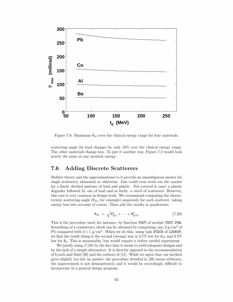
50 100 150 200 250t0 (MeV)

0

50

100

150

200

250

300

θm

ax (

mill

irad

)

Pb

Cu

Al

Be

Figure 7.8: Maximum θM over the clinical energy range for four materials.

scattering angle for lead changes by only 10% over the clinical energy range.The other materials change less. To put it another way, Figure 7.2 would looknearly the same at any incident energy.

7.6 Adding Discrete Scatterers

Moliere theory and the approximations to it provide an unambiguous answer forsingle scatterers, elemental or otherwise. One could even work out the answerfor a finely divided mixture of lead and plastic. Not covered is (say) a plasticdegrader followed by one of lead and so forth: a stack of scatterers. However,this case is very common in design work. We recommend computing the charac-teristic scattering angle (θMi for example) separately for each scatterer, takingenergy loss into account of course. Then add the results in quadrature:

θM =√

θ2M1 + · · · + θ2

MN (7.29)

This is the procedure used, for instance, by function TOUT of module TOUT.FOR.Something of a consistency check can be obtained by computing, say, 2 g/cm2 ofPb compared with 2× 1 g/cm2. When we do this, using task STACK of LOOKUP,we find the result doing it the second (wrong) way is 3.1% low for θM and 3.5%low for θ0. This is measurable, but would require a rather careful experiment.

We justify using (7.29) by the fact that it seems to yield adequate designs andby the lack of a simple alternative. It is directly opposed to the recommendationof Lynch and Dahl [38] and the authors of [11]. While we agree that our methodgives slightly too low an answer, the procedure detailed in [38] seems arbitrary,the improvement is not demonstrated, and it would be exceedingly difficult toincorporate in a general design program.

63

7.7 Summary

We have presented the formulas for the Moliere/Fano calculation of the charac-teristic multiple scattering angle θM , the reduced target thickness B and, withthe aid of Bethe’s tables, the angular distribution f(θ). θM must always be usedwith the Moliere angular distribution. It is incorrect to use it with a Gaussian.In design programs the Gaussian approximation carries little advantage since,for efficiency, one will tabulate f(θ) once and for all during initialization.

Nevertheless, it is almost certain that an equivalent Gaussian is sufficientlyaccurate since ≈ 98% of the protons are contained in the nearly Gaussian part ofthe distribution. To compute the width parameter of the equivalent Gaussianone may use Hanson’s prescription (essentially the full Moliere calculation),Highland’s formula, or Lynch and Dahl’s formula. The last two are easy tocompute and only slightly less accurate than Moliere/Fano.

Our programs usually invite the user either to run in MOLIERE mode (fullMoliere/Fano formalism) or in HANSON, HIGHLAND or LYNCH mode. For anychoice, you will get flat depth- and transverse dose distributions, assuming theproblem posed is solvable with physical materials. That is merely a test ofthe mathematical self-consistency of the program: it should work even if theunderlying scattering theory is seriously wrong! The only way to find out whichoption is better is to build the system both ways—the prescriptions for lead andplastic will be slightly different—and see which comes closer to the prediction.Since differences in the characteristic angle are ≈ 2% that experiment will haveto be done rather carefully. We generally prefer MOLIEREmode because we foundthe exact theory was, after all, in slightly better agreement with experimentaldata [4].

64

Chapter 8

Nuclear Interactions

In addition to electromagnetic (EM or Coulomb) interactions (stopping andmultiple scattering) protons suffer nuclear interactions. These are not rare.At therapy energies, some 20% of the protons suffer a nuclear reaction beforestopping. Even so, we appear to ignore nuclear processes when designing beam-spreading systems. Effectively, we include them by the simple expedient of usingmeasured rather than theoretical Bragg peaks for the depth-dose. The designproblem would be far harder if we had to evaluate nuclear effects explicitly.

That said, the rest of this chapter can be skipped on a first reading, sincenothing said here will affect how we actually design devices. However, someunderstanding of nuclear interactions is essential to a complete picture of theBragg peak: how they affect its shape, and how their effects can be observeddirectly. Key to all this is the ‘local energy deposition’ model. Before gettingto that we’ll introduce some terminology and look at the kinds of reactions thatgo on, the secondary particles they produce, and their characteristic energies.Then we’ll introduce the model and discuss how the functions that define it, Pand f , may be computed or measured. At our present state of knowledge, themodel does not seem to work as well as it should, an issue that will be taken upagain in chapter 11.

However, as just stated, that only means our understanding of nuclearprocesses is incomplete. It does not compromise our ability to design devices.

8.1 Terminology

ICRU63 [39] defines an elastic nuclear reaction as

. . . a reaction in which the incident projectile scatters off the targetnucleus, with the total kinetic energy being conserved (the internalstate of the target nucleus and of the projectile are unchanged bythe reaction).

while nonelastic

. . . is a general term referring to nuclear interactions that are notelastic (i.e. kinetic energy is not conserved). For instance, the tar-get nucleus may undergo breakup, it may be excited into a higherquantum state, or a particle transfer reaction may occur.

and inelastic

. . . refers to a specific type of nonelastic reaction in which the kineticenergy is not conserved, but the final nucleus is the same as thebombarded nucleus.

65

Thusp + 16O → p + 16O or 16O (p,p) 16O (8.1)

is elastic (16O is in its ground state),

p + 16O → p + 16O∗

or 16O (p,p) 16O∗

(8.2)

is inelastic (∗ denotes an excited state), and

p + 16O → p + p + 15N or 16O (p,2p) 15N (8.3)

(quasi-free p,p scattering [40] in oxygen) is nonelastic even if the N nucleusrecoils in its ground state, because it took energy (‘binding energy’) to removethe target proton from the nucleus.

Consider a proton beam passing through various absorbers and scatterersand stopping in a water tank. Some of the protons undergo nuclear interactionson the way, either in the absorbers and scatterers or in the water. At any givenpoint we call those particles primaries which have only suffered EM interactions:stopping by interactions with atomic electrons and scattering by screened atomicnuclei. Particles resulting from nuclear reactions are secondaries. Both finalstate protons from reactions like (8.3) are secondaries even though one (wecannot tell which) was the incident proton. All primaries are protons, of course,and all neutrons must be secondaries.

8.2 Elastic Scattering from Free Hydrogen

Water (H2O) and many plastics of interest (e.g. CH2) contain free hydrogen.Janni [3] and Berger [27] correctly note that the nonelastic cross section forhydrogen is negligible. The proton has no internal degrees of freedom at therapyenergies. Therefore interactions with H nuclei are traditionally omitted fromnuclear effects. We think this is inappropriate. Consider

p + 1H → p + p or 1H (p,p) p (8.4)

which is simply elastic scattering by a very light nucleus, a classic billiard-ballcollision. The final protons emerge at right angles to each other1 and sharethe incident kinetic energy. The more ‘forward’ proton carries more of theenergy and the other, less. These protons greatly resemble those from reactionslike (8.3) though they are slightly more energetic because there was no nuclearbinding energy. If we are interested in the changing composition of the beam,rather than the classification of reactions, we ought to include (8.4).

Having made this point we will not belabor it. From here on we’ll takethe conventional position that only nonelastic reactions diminish the primaryfluence.

The bremsstrahlung reaction

p + 1H → p + p + γ or 1H (p,pγ) p (8.5)

does occur at therapy energies. Though measurable [41], its cross section is tinyby comparison with (8.4).

1 Actually somewhat less because of relativistic effects: 87.5◦at 160 MeV incident.

66

8.3 Overview of Nonelastic Reactions

Possible secondaries from nonelastic reactions at therapy energies are protons,neutrons, heavy fragments such as alphas, γ rays, and the recoiling residualnucleus. Heavy fragments other than alphas are in fact quite rare. For 160 MeVprotons stopping in CH2 [25], per incident proton

1H (p) 2H (d) 3H (t) 3He 4He (α)0.24 0.09 0.01 0.03 0.13

Per nonelastic nuclear reaction induced by primaries or secondaries

p d t 3He α n1.16 0.46 0.06 0.13 0.71 0.41

By either reckoning the number of alphas is striking. Alphas are very stable andexist as preformed clusters in light nuclei [42]. The numbers quoted are from theprecompound model in the GEANT4 Monte Carlo, not from direct experiment.The precompound model is ultimately, however, a model of experimental results.

An alternative measure of the relative importance of secondaries is thefraction of initial energy carried away by each. For nonelastic interactions of150 MeV protons with 16O nuclei Seltzer [43] finds

p d t 3He α recoils n0.57 0.016 0.002 0.002 0.029 0.016 0.20

The total imparted to charged particles is 0.64 . Photons, not listed, presumablymake off with 0.16 . These numbers are also from a Monte Carlo, not directlyfrom experiment. The general picture is the same. Most of the final kineticenergy is in protons, neutrons and photons. Alphas stand out among the heavyfragments, but still have only 2.9% of the total energy.

In elastic scattering from free hydrogen, all of the secondary energy is carriedby protons, stengthening our argument for including them.

Though little of the energy goes into heavy fragments, they might havea significant relative biological effect (RBE) because of their high ionizationdensity. This has been investigated by Seltzer [43], Paganetti [44, 45] and others.It turns out that RBE enhancement due to heavy fragments and recoils is small.Their extremely high ionization density is outweighed by the fact that littleenergy goes into those channels. What RBE enhancement there is comes fromthe abundant low energy protons: secondaries and, at the distal end of theBragg peak, primaries. In any case, the present work is concerned with physicaldose, so we will speak no more of RBE.

Secondaries usually make large angles with the beam direction (think billiardballs) unlike primaries which, even after multiple scattering, rarely exceed a fewdegrees. This is important. It means that secondaries produced upstream inscatterers or absorbers will clear out of the beam for purely geometric reasonsbefore entering the volume of interest.

8.4 Local Energy Deposition Model

The local energy deposition model seeks to model the effects of nuclear reactionson the depth-dose without using the full-bore Monte Carlo approach (generatingand tracking all secondaries). It can be summarized as follows:

67

• Primary fluence is converted into secondary fluence.

• Energy of primaries is converted into energy of secondaries.

• Energy of charged secondaries is deposited on the spot.

• Energy of neutral secondaries is lost.

The energy of neutral secondaries is not destroyed, of course. It is deposited inthe shielding. Also, energy of charged secondaries is not really deposited on thespot: some secondaries have projected ranges of a few cm. Nevertheless, thsapproximation works in many situations because of longitudinal equilibrium,which will be discussed shortly.

Mathematically, the local energy deposition model requires two functions,P and f . Imagine protons stopping in a water tank. P (z; r0) is defined asthe probability that a proton of initial range r0 will have a nonelastic nuclearinteraction by the time it reaches depth z in the tank. Alternatively we canspeak of dP/dz ≡ P ′(z; r0). P ′(z; r0) dz is the probability of an interaction indz about z. We’ll find that P and P ′ are fairly easy to predict or measure.

f(z; r0) is the fraction of primary energy deposited locally. We have seenabove that f , averaged over all z, is ≈ 0.64 at 150 MeV (r0 = 15.8 g/cm2). fis difficult to measure. Microdosimetry sheds some light, or the detailed shapeof the Bragg peak can be compared with the local energy deposition model toinfer f [27]. However, we mainly have to rely on Monte Carlo estimates.

Instead of picking r0 and z as independent variables, we could have usedt0 and t, the incident and residual kinetic energy as the proton tranverses thetank. Either way works. Using depth and range instead of energy gives a moreimmediate connection with the Bragg peak.

8.5 Nuclear Buildup

A brief experimental interlude. During the commissioning of NPTC some depth-doses were taken with a vertical beam, that is, a wall-less water tank [46]. Veryfew nuclear secondaries enter the water because the density of air is ≈ 1000×less than water. Secondaries produced in large volumes far upstream clear outof the beam because of their large angles, and there is not enough air mass nearthe tank to create many secondaries that hit the region of interest.

The dose measurement (Figure 8.1) shows a small but definite defect at theentrance2, which we interpret as follows. At z = 0, nuclear reactions happenat the full rate, but their energy is deposited a bit downstream so the stoppingpower here is just SEM . As we move downstream, charged secondaries begin torange out and the stopping power acquires an additional term Snuclear . Soon(certainly by 4 g/cm2) we reach longitudinal equilibrium where there are asmany charged secondaries entering any ∆z as leaving, because the number andcomposition of secondaries changes very slowly with depth (energy). ‘Localenergy deposition’ does not mean that the energy is literally deposited on thespot where the secondaries were produced. It comes from volume elementsfurther upstream, but those secondaries are almost indistinguishable from thoseproduced on the spot.

Of course, longitudinal equilibrium cannot hold at a discontinuity in densitysuch as the tank entrance. That’s where we see buildup effects.

2 This is not observed in horizontal water tank scans because the usual tank wall introducesenough nuclear buildup to obscure it. It would, however, be easy to build a sufficiently thin-walled tank to show the buildup in horizontal scans.

68

Figure 8.1: Nuclear buildup in a Bragg peak.

Though this model works qualitatively, it doesn’t quite hold up numerically.Let’s compare energy absorption in ∆z about z = 0 and z = 4 g/cm2 wherelongitudinal equilibrium is fully established. The primary range, energy, EMstopping power, P and P ′ at the two positions are

z r t SEM P P ′

g/cm2 g/cm2 MeV MeV/(g/cm2) % %/(g/cm2)0 32 226 4.15 26.7 0.5714 28 209 4.36 24.4 0.600

P and P ′ come from the next section. Also, we know that f ≈ 0.64. Thereforeat z = 4, accounting for the decrease in primary fluence from z = 0, we have

∆E = 4.36× (1 − 0.023)× ∆z + 0.006× 0.64× 209× ∆z

∆E/∆z = 4.26 + 0.802 = 5.06 MeV/(g/cm2)

whereas at z = 0

∆E/∆z = SEM (226) = 4.15 MeV/(g/cm2)

giving a defect of 4.15/5.06 or ≈ 18%. The observed defect (Figure 8.1) is only≈ 8%.

The measurement of nuclear buildup, and that it is smaller than expected,dates back at least to 1977 when Carlsson and Carlsson [47] measured dosebuildup with 185 MeV protons incident on a stack of (C2F4)n sheets interleavedwith thermoluminescent detectors. They observed a nuclear buildup of ≈ 7%and characteristic length ≈ 2 g/cm2. They commented that it was ‘somewhatlower’ than expected, and cited dosimeter nonlinearity as a possible cause. Theirobservations in (C2F4)n agree well with ours in water.

Incidentally, Carlsson and Carlsson also measured the electron buildup whichis greater but has a much shorter characteristic distance (� 1 mm). Electronbuildup with incident protons can also be observed using very thin-walled ioni-zation chambers. In contrast with photon therapy, it does not yield useful skinsparing in clinical practice because the buildup length is so short.

69

0 5 10 15 20 25 30 35r0 (g/cm2)

0

100

200

300

400

500

600

σn

on

elas

tic

(m

B)

Figure 8.2: Total nonelastic cross section of oxygen versus proton range.

0 5 10 15 20 25 30 35r0 (g/cm2)

0

5

10

15

20

25

30

35

Pn

on

elas

tic

(%

)

Figure 8.3: Probability of a nonelastic interaction versus proton range in water.

70

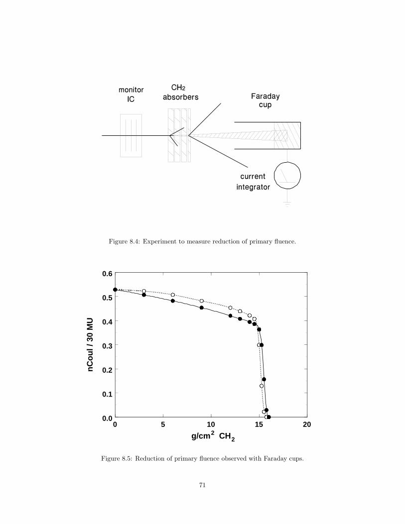
Figure 8.4: Experiment to measure reduction of primary fluence.

0 5 10 15 20

g/cm2 CH2

0.0

0.1

0.2

0.3

0.4

0.5

0.6

nC

ou

l / 3

0 M

U

Figure 8.5: Reduction of primary fluence observed with Faraday cups.

71

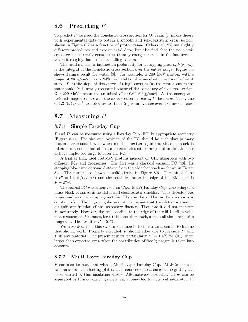
8.6 Predicting P

To predict P we need the nonelastic cross section for O. Janni [3] mixes theorywith experimental data to obtain a smooth and self-consistent cross section,shown in Figure 8.2 as a function of proton range. Others [43, 27] use slightlydifferent procedures and experimental data, but also find that the nonelasticcross section is nearly constant at therapy energies except in the last few cmwhere it roughly doubles before falling to zero.

The total nonelastic interaction probability for a stopping proton, P (r0; r0),is the integral of the nonelastic cross section over the entire range. Figure 8.3shows Janni’s result for water [3]. For example, a 209 MeV proton, with arange of 28 g/cm2, has a 24% probability of a nonelastic reaction before itstops. P ′ is the slope of this curve. At high energies (as the proton enters thewater tank) P ′ is nearly constant because of the constancy of the cross section.Our 209 MeV proton has an initial P ′ of 0.60 %/(g/cm2). As the energy andresidual range decrease and the cross section increases, P ′ increases. The valueof 1.2 %/(g/cm2) adopted by Bortfeld [26] is an average over therapy energies.

8.7 Measuring P

8.7.1 Simple Faraday Cup

P and P ′ can be measured using a Faraday Cup (FC) in appropriate geometry(Figure 8.4). The size and position of the FC should be such that primaryprotons are counted even when multiple scattering in the absorber stack istaken into account, but almost all secondaries either range out in the absorberor have angles too large to enter the FC.

A trial at HCL used 159 MeV protons incident on CH2 absorbers with twodifferent FCs and geometries. The first was a classical vacuum FC [48]. Itsstopping block was at some distance from the absorber stack as shown in Figure8.4. The results are shown as solid circles in Figure 8.5. The initial slopeis P ′ = 1.4 %/(g/cm2) and the total decline to the edge of the EM ‘cliff’ isP = 27%.

The second FC was a non-vacuum ‘Poor Man’s Faraday Cup’ consisting of abrass block wrapped in insulator and electrostatic shielding. This detector waslarger, and was placed up against the CH2 absorbers. The results are shown asempty circles. The large angular acceptance meant that this detector counteda significant fraction of the secondary fluence. Therefore it did not measureP ′ accurately. However, the total decline to the edge of the cliff is still a validmeasurement of P because, for a thick absorber stack, almost all the secondariesrange out. The result is P = 23%.

We have described this experiment merely to illustrate a simple techniquethat should work. Properly executed, it should allow one to measure P ′ andP in any material. The present results, particularly P ′ = 1.4% for CH2, seemlarger than expected even when the contribution of free hydrogen is taken intoaccount.

8.7.2 Multi Layer Faraday Cup

P can also be measured with a Multi Layer Faraday Cup. MLFCs come intwo varieties. Conducting plates, each connected to a current integrator, canbe separated by thin insulating sheets. Alternatively, insulating plates can beseparated by thin conducting sheets, each connected to a current integrator. In

72

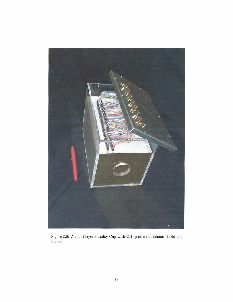
Figure 8.6: A multi-layer Faraday Cup with CH2 plates (aluminum shield notshown).

73

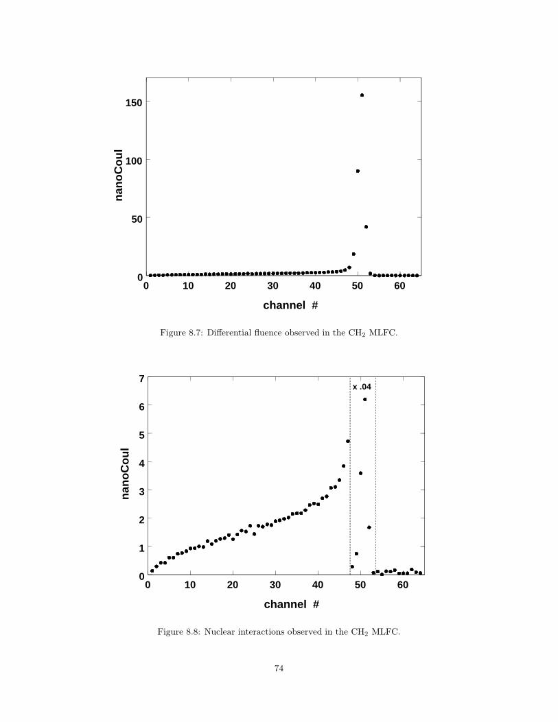
0 10 20 30 40 50 60

channel #

0

50

100

150

nan

oC

ou

l

Figure 8.7: Differential fluence observed in the CH2 MLFC.

0 10 20 30 40 50 60

channel #

0

1

2

3

4

5

6

7

nan

oC

ou

l

x .04

Figure 8.8: Nuclear interactions observed in the CH2 MLFC.

74

the latter case it is the charge induced on the conducting sheets that is detected.Both types have been built and operated at HCL.

We show data from an ‘insulating’ MLFC of CH2 sheets separated by thinbrass charge collectors (Figure 8.6). Figure 8.7 shows the charge distributionwhen a proton beam stops. MLFCs measure differential fluence as a functionof depth. A pronounced peak from primary protons stopping by EM processescorresponds to the ‘cliff’ in Figure 8.5. It is preceded by a barely visible buildupregion. If we zoom in (Figure 8.7) we see a well-defined curve, the projectedrange distribution of charged secondaries. Its shape is a test of Monte Carlomodels [24, 25, 49].

Here, however, we’ll focus on its area. The net charge deposited for eachreaction (including the recoil) is +e (the charge of the incoming proton) and allsecondaries have shorter projected ranges than primaries. Therefore

P =buildup area

buildup area + EM peak area

We find P = 20±1%. The error comes from estimating where the buildup endsand the EM peak begins. Janni [3] gives P = 18± 4%.

8.8 Summary

ICRU63 categorizes nuclear reactions as elastic, nonelastic and inelastic. It iscommon practice [3, 27, 43, 26] to consider only nonelastic nuclear reactionsin computing the reduction of primary fluence. We have argued that elasticscattering from free hydrogen has a very similar effect and should be included.

We looked at the breakdown of secondaries and the energies they carry.Most of the secondaries are protons, neutrons and recoiling nuclei. Chargedsecondaries share typically 60% of the initial energy and have projected rangesmuch shorter than primaries. Their energy can be considered to be depositedon the spot. The remaining 40% of energy is carried by neutrals and is lost tothe region of interest. This picture breaks down at discontinuities, for instancewhen the beam leaves air and enters a water tank. Here nuclear buildup canbe observed and longitudinal equilibrium takes a couple of g/cm2 to establishitself. There are at least two measurements, one of them published [47], thatshow nuclear buildup. In both cases the buildup distance is reasonable but themagnitude is about half that expected from the nuclear model.

The local energy deposition model is described by two functions. P (z; r0) isthe probability that a primary of range r0 will have a nuclear interaction beforeit gets to z. f(z; r0) is the fraction of primary energy in charged secondaries,considered to be deposited on the spot. P in water can be computed from theinteraction cross section for oxygen (and, we would suggest, hydrogen). f mustbe found by Monte Carlo methods. P and f have been tabulated by Berger [27]and Seltzer [43].

P is fairly easy to measure. All one needs is a fluence meter that somehowseparates primaries from secondaries. Either a Faraday Cup with appropriateangular acceptance, or a multi-layer Faraday Cup, can be used. f is difficult tomeasure, except perhaps by microdosimetry.

We have spent an entire chapter on nuclear reactions mainly to round out ourunderstanding of how protons interact with matter. In designing passive beamspreading systems we will constantly do computations with stopping theory andscattering theory. These theories of EM processes are accurate and well tested.By comparison, nuclear theory is exceedingly complicated and not as well tested.What saves us is that we do not need to use it explicitly. Using experimental

75

Bragg peaks in our designs seems to be a good enough way of including nucleareffects. On the rare occasion where we might want to estimate nuclear effects,the local energy deposition model should be a pretty good proxy for the fullmodel. Of course we can always resort to a full Monte Carlo simulation [50].

76

Chapter 9

Binary Degraders

In this chapter we learn how to design degraders with specified scattering1

(‘scatterers’), specified energy loss (‘absorbers’) or both. We’ll assume we haveat our disposal four functions

Range(energy, material)

Energy(range, material)

Dedx(energy, material)

Theta0(mode, target thickness, outgoing energy, material)

where material is a code e.g. ′WATER′, mode e.g. ′HIGHLAND′ specifies thescattering theory to be used, range and target thickness are in g/cm2 andenergies are kinetic energies in MeV. Dedx is the mass stopping power S inMev/(g/cm2). Note that input to theta0 is the outgoing energy; that way theproblem is always well posed.

If you wish to follow the examples, we’ll be using LOOKUP with the MIXEDrange-energy table (mostly ICRU49) in HIGHLAND mode when applicable.

9.1 High-Z and Low-Z Materials

Figure 9.1 shows scattering (top curve) and energy loss (bottom curve) of160 MeV protons incident on 1 g/cm2 degraders of various materials. The xcoordinate is the material’s radiation length LR. We have used this for x first,because it figures in Highland’s formula and second, because, unlike atomicnumber Z and mass A, LR is defined [11] for compounds and mixtures.

We see that materials low in the periodic table, which we’ll call low-Z, havesomewhat more stopping power and a great deal less scattering power thanhigh-Z materials. We can combine them to make a binary degrader with anydesired energy loss and scattering angle, within limits.

It goes without saying that, when we want energy loss with low scattering,we should use a low-Z material. When we want scattering with low energy loss,we should use a high-Z material.

9.2 Notation to Describe Problems

Different problems can be posed for one or two degraders. It is convenient tohave a compact notation. Let

1 ‘Scattering’ should always be understood as ‘characteristic multiple scattering angle’.

77

0 10 20 30 40 50 60 70LR (g/cm2)

0

2

4

6

8

10

12

14

16

18

MeV

, m

Rad θ0

∆E

lead

brass

aluminum

waterlexan

beryllium

Figure 9.1: Scattering and stopping in various materials.

a denote scattering angle (rad)g thickness (g/cm2)m materialt kinetic energy (MeV)1 ‘entering the first element’2 ‘entering the second element’ . . .

Thena1, a2, t2 → g1, t1

is the single degrader problem ‘Given the incoming and outgoing angles and theoutgoing energy, find the thickness and the incoming energy.’ while

a1, a3, t1, t3 → g1, g2, t2

is the binary degrader problem ‘Given the incoming and outgoing angles andenergies, find the required thicknesses and the energy going into 2.’ Note that a)materials are always given and therefore not usually mentioned, b) the index 2(‘single’ problem) or 3 (‘binary’ problem) represents ‘the next element’ whateverthat is and c) the unknowns (or output variables if we’re talking subroutines)may include things you don’t happen to be interested in.

File BDG.FOR has subroutines for solving single degrader problems

1 : a1, a2, t2 → g1, t12 : a1, a2, t1 → g1, t2

78

and binary degrader problems

1 : a1, a3, t1, t3 → g1, g2, t22 : a1, a3, g1, t3 → g2, t1, t23 : a1, a3, g1, t1 → g2, t2, t34 : a1, a3, g2, t1 → g1, t2, t3

all of which are needed at one time or another. We have also listed the jumpindex which tells BDG or SDG which problem is to be solved. LOOKUP will remindyou of these if you enter a nonsense index e.g. 9. The rest of this chapterexplains how these routines work.

9.3 ‘Forward’ Problem

The problems listed are ‘inverse’ problems: at least one thickness is not known.The ‘forward’ single degrader problem is: ‘Given degrader material, thickness,incoming energy and incoming scattering angle, find the outgoing energy andangle.’ that is

m1, g1, t1, a1 → t2, a2

This is fairly straightforward:

1. Find the proton range in material m1 at energy t1.

2. Subtract g1 to obtain the residual range.

3. Find the energy in m1 for that range. That equals t2.

4. Use Theta0 to find the scattering.

5. Add it to a1 in quadrature to find a2.

You can repeat this for as many degraders as you have. Each time, there is arange-energy calculation and an angle calculation, which must be done in thatorder. There’s a shortcut for the range-energy calculation if the degrader isthin:

1. Find the stopping power S in material m1 at energy t1.

2. Multiply by g1 to obtain the energy loss.

3. Subtract the energy loss from t1 to obtain t2.

Example: find the energy and angle out of 10 g/cm2 of lexan assuming 160 MeVincident protons with no angular divergence. The two procedures are

t1 S r1 r2 t2 θ0

MeV MeV/(g/cm2) g/cm2 g/cm2 MeV mrad160 18.523 13.523 133.66 16.09160 4.962 135.19 15.94

The S method is slightly off because the degrader is fairly thick. S increasessignificantly through the degrader, but we are using the entrance value.

For general design problems it is very convenient to have a subroutine thatapplies the forward solution iteratively to an arbitrary stack of absorbers. Sucha routine, TOUT.FOR, can be found in source file TOUT.FOR. One can also runthe procedure backwards to obtain the input energy and angle given the outputenergy and angle. See TINP.FOR in the same file. The simple logic of bothprocedures is somewhat obscured by tests.

79

9.4 Single Degrader Inverse Problem

Considera1, a2, t1 → g1, t2

namely ‘How thick a scatterer do I need? what will the output energy be?’Before trying to solve an inverse problem we should test for conditions that

may rule out a solution. In this case the input energy may be so low thatthe desired scattering cannot be had before the proton ranges out. We canfind the maximum available scattering by computing the range in m1 at t1,then calling Theta0 with that degrader thickness and zero output energy, whichcauses Theta0 to return the maximum scattering available. If that is less thanthe desired a2 a sensible subroutine will return a2 reassigned to that value,assuming the user will test a2 if failure is at all likely. Otherwise, we canproceed.

We want a2 to equal some specified value. Let’s construct a function a2 =F (g2). F is not an algebraic function of g2 in closed form. Even if we could,with some thought, write down a sufficiently good approximation, that’s nothow we want to proceed. A numerical method is far more general and requiresfar less effort. F is simply a subprogram (‘function’ in the Fortran sense) which,given g1 and whatever else is needed, finds a2. We illustrate this below by listingthe subprogram for this problem. The procedure is exactly that of the previoussection for solving the forward problem. We have made the logic clearer bydeleting some safety tests (e.g. for negative argument of the square root).

C%%%%%%%%%%%%%%%%%%%%%%%%%%%%%%%%%%%%%%%%%%%%%%%%%%%%%%%%%%%%%%%%C

FUNCTION Asdg1(xx,m1,m2,g1,g2,t1,t2,t3,a1,a2,a3,mode)CC Angle out of single degrader as a function of xx = g1.C

CHARACTER*(*) m1,m2,modeC

rr = Range(t1,m1) - xxt2 = Energy(rr,m1)Asdg1 = SQRT(a1**2 + Theta0(mode,xx,t2,m1,bb)**2)

CEND

CC%%%%%%%%%%%%%%%%%%%%%%%%%%%%%%%%%%%%%%%%%%%%%%%%%%%%%%%%%%%%%%%%

Now let g2 be called x and the desired value of a2 = F (x) be called c. We needto find that value of x for which F (x) = c, that is, we need to solve

F (x) − c = 0

or find the root of F (x) − c. F (x) is not an algebraic expression so we needa numerical root finder. These are discussed in Numerical Methods [1]. Formost of our work the Method of False Position (regula falsa) offers the rightcombination of speed and robustness. Formally, we construct a Fortran function,call it RootFalse, such that the call

x = RootFalse(F,a,b,c)

returns x as the root of F (x) − c = 0. In addition to c, the desired value of F ,we must supply a and b, values of x which bracket the root, thus instructingthe routine to look for a solution between a and b. In the problem at hand theroot finder is invoked with

80

g1 = Rtf(Asdg1,0.,gg,a2,m1,m2,g1,g2,t1,t2,t3,a1,a2,a3,mode)

Asdg1 is our mnemonic for this particular F . 0 and gg (the proton range inmaterial m1 at incident energy t1) bracket the g1 we seek. We know this fromout preliminary test. c = a2 is the desired value of F . Many other argumentsare also passed because we want just one routine Rtf for all our single and binarydegrader problems. Therefore any quantity that might be needed as input oroutput is passed. In any given case, many are ignored.

Some closing remarks:

• The method always works if we can write a procedure for the forwardproblem. The programming task is to do this and make sure the necessaryquantities are supplied.

• We haven’t mentioned t2. It is computed as an intermediate step in Asdg1.Because of the way variables are passed, it will have assumed its correctvalue when Rtf returns without our having to lift a finger.

• The Method of False Position always stays within the initial brackets.Therefore routines like Range are never called with illegal arguments asRtf does its work.

• In many problems there is more than one choice for the ‘key’ variable, andmore than one will work. In our example we used g1 because its bracketsare obvious: the answer must lie somewhere between 0 and the range ofthe proton.

The other single degrader problem is handled the same way. It’s simpler becausethere is always a solution. See BDG.FOR for details.

9.5 Binary Degrader Inverse Problem

We’ll use as an example

a1 a3, t1, t3 → g1, g2, t2 (9.1)

or ‘Given some lead and lexan, the incoming energy and the desired outgoingenergy and scattering, what thicknesses do I use?’ The basic method is thesame. Focus on one of the unknowns (t2 is convenient), write down the forwardsolution a3(t2) in terms of it, then use a root finder to locate the value of t2that yields the desired a3. However, this problem is somewhat complicated sowe’ll first study a concrete case. Suppose 160 MeV protons enter a lead/lexandegrader. We want to reduce the energy to 140 MeV while obtaining exactly40 milliradians of scattering. What combination of lead and lexan do we need?Over what range of output energies can the problem be solved? What happensoutside that range?

Figure 9.2 shows a family of solutions for 20, 30 and 40 mrad. Let’s startat the lower right and work down the energy scale. Initially we want scatteringwith minimum energy loss so we use lead only. As we increase the lead, theoutput energy decreases and the scattering increases. Eventually the scatteringreaches 40 mrad, the desired value. To add more lead would be to exceed this,so we add lexan, moving further down the energy scale. There is some scatteringeven in the lexan, so as we add lexan we remove lead to stay on the 40 mradline. Eventually, all the lead is gone and the scattering in lexan is 40 mrad. Toreduce the energy further we have to use more lexan and accept more scattering.Finally, the curve flattens at very low t3. Here the lexan thickness is greater

81

0 20 40 60 80 100 120 140 160 180

t3 (MeV)

0

10

20

30

40

50

60

a3 (

mR

ad)

all lead

all lexan

3.19 g/cm 2 lead ,

7.26 g/cm 2 lexan

Figure 9.2: Scattering v. output energy for a lead/lexan degrader.

than 97% of the proton range. Multiple scattering saturates [4] and Theta0treats it as constant.Program (BDG(1...)) solves (9.1). It accepts any two materials in either orderbut you’ll only get the desired effect if one is higher-Z and the other lower-Z.Before attempting a solution BDG makes two tests and takes appropriate action:

1. If the desired scattering exceeds what can be obtained with all higher-Z, satisfy the energy requirement, return g(higher-Z), the scattering a3actually obtained, and g(lower-Z) = 0.

2. If the desired scattering is less than what can be obtained with all lower-Zmaterial, satisfy the energy requirement and return g(lower-Z), whatevera3 is obtained, and g(higher-Z) = 0.

Otherwise, we solve the problem as described in section 9.4 using t2, whosebrackets are obviously t1 and t3, as the primary variable. See BDG.FOR fordetails. If a3 returned equals its initial value, all specifications were met.

The three other binary degrader problems are solved in the same general way.We will meet them as we design modulators whose scattering is independent ofmodulator step (‘compensated absorbers’) or contoured scatterers whose energyloss is independent of radius (‘compensated scatterers’).

9.6 Does the Order of Materials Matter?

Definitely. If the lead is second it sees a lower energy (t2) and scatters more.Therefore less lead is needed. If we run our previous example (160 MeV in,110 MeV and 40 mrad out) through LOOKUP we find

82

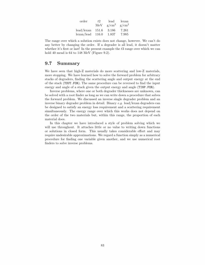
order t2 lead lexanMeV g/cm2 g/cm2

lead/lexan 151.6 3.186 7.261lexan/lead 116.0 1.837 7.985

The range over which a solution exists does not change, however. We can’t doany better by changing the order. If a degrader is all lead, it doesn’t matterwhether it’s first or last! In the present example the t3 range over which we canhold 40 mrad is 64 to 148 MeV (Figure 9.2).

9.7 Summary

We have seen that high-Z materials do more scattering and low-Z materials,more stopping. We have learned how to solve the forward problem for arbitrarystacks of degraders, finding the scattering angle and output energy at the endof the stack (TOUT.FOR). The same procedure can be reversed to find the inputenergy and angle of a stack given the output energy and angle (TINP.FOR).

Inverse problems, where one or both degrader thicknesses are unknown, canbe solved with a root finder as long as we can write down a procedure that solvesthe forward problem. We discussed an inverse single degrader problem and aninverse binary degrader problem in detail. Binary e.g. lead/lexan degraders canbe designed to satisfy an energy loss requirement and a scattering requirementsimultaneously. The energy range over which this works does not depend onthe order of the two materials but, within this range, the proportion of eachmaterial does.

In this chapter we have introduced a style of problem solving which wewill use throughout. It attaches little or no value to writing down functionsor solutions in closed form. This usually takes considerable effort and mayrequire undesirable approximations. We regard a function simply as a numericalprocedure for finding one variable given another, and we use numerical rootfinders to solve inverse problems.

83

Chapter 10

Degrader Stacks and BeamSpreading

In the previous chapter we learned how to find the output energy and scatteringangle for a stack of degraders, but that’s not the whole story. If we want to treatan extended stack as a single degrader we must find out where the protons seemto be coming from, their effective origin. To compute that we need to considerbeam spreading in a single degrader or a stack.

10.1 Beam Spreading

Preston and Koehler [10] used the method of projection onto a measuring plane(MP) to compute beam spreading in a thick degrader. Their method is easilygeneralized to a stack of n degraders. In the Gaussian approximation (which weuse throughout this chapter) the multiple scattering is Gaussian and, becausethe angles are small, its projection on an arbitrary measuring plane is alsoGaussian. Therefore the 2D fluence per proton at the MP is

P ′(r, φ) r dr dφ =1

2π r20

e−

12

( r

r0

)2

r dr dφ (10.1)

and we need to compute r0.Consider the characteristic multiple scattering dθ0 in a layer dz (Figure 10.1).

The characteristic transverse kick on the MP is dr0 = (Z − z)dθ0. Consistentwith the Gaussian approximation we want to add such kicks in quadratureto find r0. According to Highland’s formula (7.26) (dθ0)2 is proportional toρdz/LR. For a stack of n scatterers we obtain

r20(Z) =

n∑

j=1

[(1 +

19log10

Lj

LRj

)∫ zj+Lj

zj

(14.1(Z − z)pv

)2 ρj

LRjdz

](10.2)

The limits of integration are valid as shown if the MP is downstream of all thedegraders. The power of the method is that it need not be. It can be anywheredownstream of z1, and by computing r0 at various Z’s we find the envelopeof the beam. The limits of integration must, of course, be appropriate to theposition of the MP.

In (10.2) we have arbitrarily taken Highland’s logarithmic correction factoroutside the integral, evaluating it for each degrader as a whole rather than foreach infinitesimal layer. Some such step is necessary. Otherwise the integral

84

Figure 10.1: Displacement dr0 in MP from scattering in a target layer dz.

would not reach a limit as a function of dz. The answer would keep gettingsmaller. We could, instead, freeze the number of intervals in the integral, butthat too would be arbitrary. The ultimate justification of (10.2) is that it agreeswith experiment, as we will show.

Function Rch in file TOUT.FOR computes r0 according to (10.2) using Simp-son’s Rule (7.24) to evaluate the integral. pv decreases as the proton travelsdown the stack. It must be updated whenever the integrand is evaluated. Rchaccepts arbitrarily many degraders of arbitrary materials. Before computing r0

it checks that the degraders do not overlap in z.

10.2 Experiment of Preston and Koehler

Preston and Koehler [10] measured beam spreading for 127 and 134 MeV protonsincident on water and 112 and 158 MeV incident on aluminum. They showedthat σ(T )/σ(R0) is a universal function of y = T/R0, R0 being the initial rangein whatever material and T is the depth at which σ is measured (their notation).They found a closed expression for that function using the multiple scatteringtheory of Bethe and Ashkin [23]:

σ(T )/σ(R0) =[2(1 − y)2 ln

11 − y

+ 3y2 − 2y]1/2

(10.3)

Figure 10.2 reproduces their Figure 17 which shows excellent agreement betweentheory and experiment.

Much later we replotted their data (Figure 5a of [4]) against calculations froman early version of Rch and adding a measured point that had been omitted in[10]. The four curves (water and aluminum at two energies each) were identical:

85

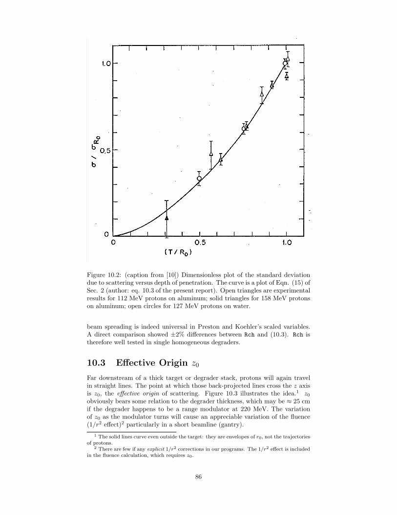
Figure 10.2: (caption from [10]) Dimensionless plot of the standard deviationdue to scattering versus depth of penetration. The curve is a plot of Eqn. (15) ofSec. 2 (author: eq. 10.3 of the present report). Open triangles are experimentalresults for 112 MeV protons on aluminum; solid triangles for 158 MeV protonson aluminum; open circles for 127 MeV protons on water.

beam spreading is indeed universal in Preston and Koehler’s scaled variables.A direct comparison showed ±2% differences between Rch and (10.3). Rch istherefore well tested in single homogeneous degraders.

10.3 Effective Origin z0

Far downstream of a thick target or degrader stack, protons will again travelin straight lines. The point at which those back-projected lines cross the z axisis z0, the effective origin of scattering. Figure 10.3 illustrates the idea.1 z0

obviously bears some relation to the degrader thickness, which may be ≈ 25 cmif the degrader happens to be a range modulator at 220 MeV. The variationof z0 as the modulator turns will cause an appreciable variation of the fluence(1/r2 effect)2 particularly in a short beamline (gantry).

1 The solid lines curve even outside the target: they are envelopes of r0, not the trajectoriesof protons.

2 There are few if any explicit 1/r2 corrections in our programs. The 1/r2 effect is includedin the fluence calculation, which requires z0.

86

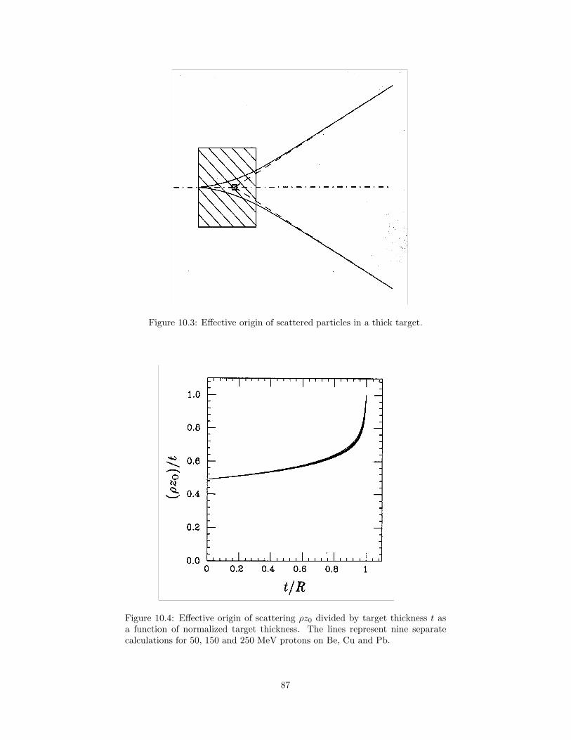
Figure 10.3: Effective origin of scattered particles in a thick target.

Figure 10.4: Effective origin of scattering ρz0 divided by target thickness t asa function of normalized target thickness. The lines represent nine separatecalculations for 50, 150 and 250 MeV protons on Be, Cu and Pb.

87

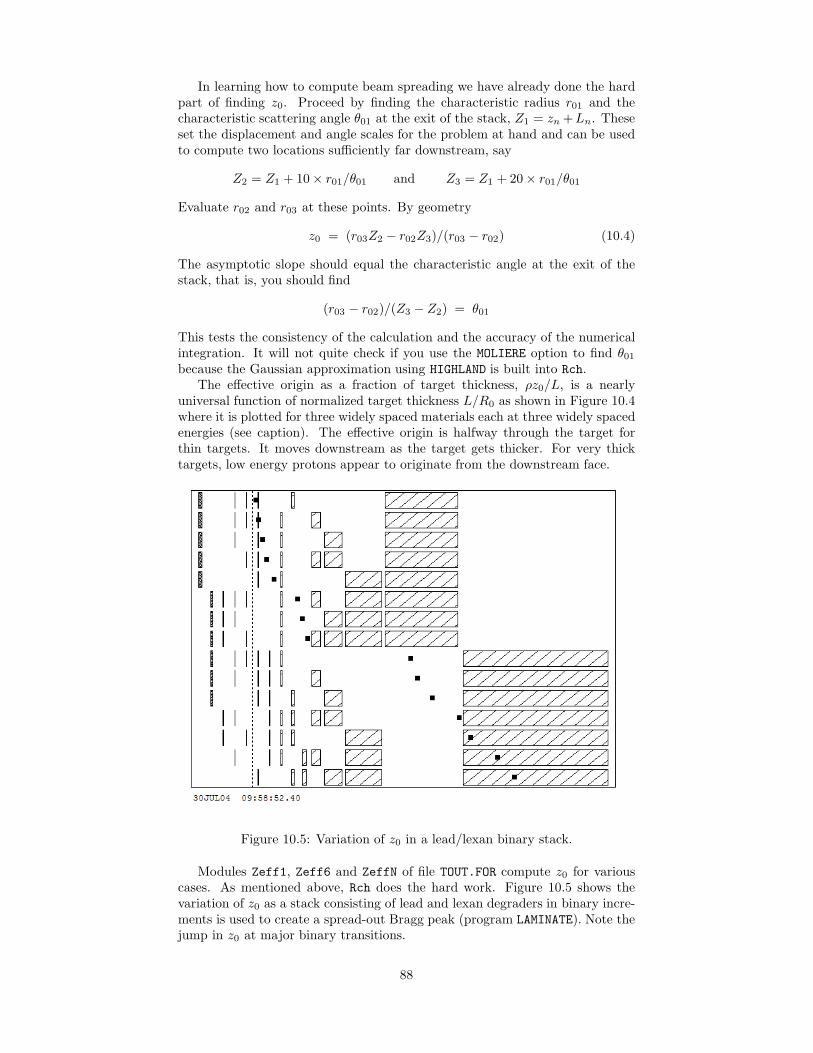
In learning how to compute beam spreading we have already done the hardpart of finding z0. Proceed by finding the characteristic radius r01 and thecharacteristic scattering angle θ01 at the exit of the stack, Z1 = zn +Ln. Theseset the displacement and angle scales for the problem at hand and can be usedto compute two locations sufficiently far downstream, say

Z2 = Z1 + 10× r01/θ01 and Z3 = Z1 + 20× r01/θ01

Evaluate r02 and r03 at these points. By geometry

z0 = (r03Z2 − r02Z3)/(r03 − r02) (10.4)

The asymptotic slope should equal the characteristic angle at the exit of thestack, that is, you should find

(r03 − r02)/(Z3 − Z2) = θ01

This tests the consistency of the calculation and the accuracy of the numericalintegration. It will not quite check if you use the MOLIERE option to find θ01

because the Gaussian approximation using HIGHLAND is built into Rch.The effective origin as a fraction of target thickness, ρz0/L, is a nearly

universal function of normalized target thickness L/R0 as shown in Figure 10.4where it is plotted for three widely spaced materials each at three widely spacedenergies (see caption). The effective origin is halfway through the target forthin targets. It moves downstream as the target gets thicker. For very thicktargets, low energy protons appear to originate from the downstream face.

Figure 10.5: Variation of z0 in a lead/lexan binary stack.

Modules Zeff1, Zeff6 and ZeffN of file TOUT.FOR compute z0 for variouscases. As mentioned above, Rch does the hard work. Figure 10.5 shows thevariation of z0 as a stack consisting of lead and lexan degraders in binary incre-ments is used to create a spread-out Bragg peak (program LAMINATE). Note thejump in z0 at major binary transitions.

88

10.4 Fermi-Eyges Theory

We shall not use Fermi-Eyges theory. It addresses the same problem as thischapter and is often cited, particularly for electron beams, so we will try to putit into perspective. The author is not expert in this theory so the followingcomments should be taken with a grain of salt.

Fermi wrote down the joint probability distribution for multiple scatteringin the Gaussian approximation: the probability that the particle acquires agiven angle (projected onto a plane) and a given displacement (also projected).Evidently he never published this but a University of Chicago lecture was quotedextensively by Rossi and Greisen in their review article [37]. Fermi ignoredenergy loss but Eyges [51] generalized the theory to include it.3 Formally, Fermi-Eyges theory is an elegant solution to the problem we have been discussing.However, it embodies the inaccurate Rossi formula for θ0, and it seems to berestricted to a single homogeneous degrader.

Let’s take the first point. Eyges defines a function A0(t) which is essentiallythe characteristic multiple scattering angle. t is depth in units of the radiationlength. Working through the differences in notation we find, in the case of noenergy loss, 2A0 = θ2

0 (Rossi). Referring to the second equation in the footnote,we see that Eyges’ angular distribution is just the familiar Gaussian with Rossi’sformula for θ0:

θ0 =15.0 MeV

p v

√L

LR(Rossi)

which is not good enough, at least for protons. For 160 MeV protons into1 g/cm2 Pb, which gives ≈ 1◦of scattering, θ0(Rossi) = 1.17 × θ0(Highland),and we know that Highland is just about right. It is not clear how intimatethe connection with Rossi’s formula is. Substituting a Highland-type formulawould clearly cause problems with the integral over t.

Eyges does not discuss the second point directly. If the theory applied tostacks of degraders of different materials, possibly with air gaps, one wouldexpect a discussion of how the scaled depth t is generalized and how the integralsdefining A0, A1 and A2 are broken up. [51] is written very much as though itapplies to a single material, though this is not stated. It may be that laterauthors have extended the theory.

10.5 Summary

We learned how to compute beam spreading r0 by adding characteristic kicks inquadrature on an imaginary measuring plane. Numerical results agree well withmeasurements and with earlier computations [10]. Using two measuring planes,sufficiently far downstream, we can project the beam envelope back to find theeffective origin z0. This can be computed for stacks of arbitrary complexity. Wediscussed the relationship of Fermi-Eyges theory to our method.

3 Eyges’ Eqns. (14) and (15) have typographic errors, corrected by Zerby and Keller [52].They should read respectively

F (t, y, θ) =1

4πB1/2exp

(−

θ2A2 − 2yθA1 + y2A0

4B

)∫ ∞

−∞F (t, y, θ)dy =

1

2(πA0)1/2exp

(−

θ2

4A0

)

89

Chapter 11

The Bragg Peak

The Bragg peak (BP) as we shall use the term is the depth-dose distribution, inwater, of a monoenergetic proton beam.1 A carefully measured Bragg peak isessential to designing a range modulator. In this chapter we will discuss factorsthat influence the shape of the Bragg peak, precautions needed in measuring it,and how to convert the measurements into a mathematically convenient formfor general use.

11.1 Understanding the Bragg Peak

Figure 11.1 shows a set of Bragg peaks measured at IBA during the cyclotronacceptance tests for NPTC.2 Each curve is normalized so that its entrance valuecorresponds to the tabulated mass stopping power in water at that incidentenergy. Therefore the curves may be regarded roughly as curves of effectivestopping power vs. depth averaged over all the protons at each beam energy.

11.1.1 Stopping Power, Straggling, Beam Energy Spread

The increase of stopping power as the proton slows down, followed by its plungeto zero when the proton stops, dominates the overall shape of the BP. If wecould measure the stopping power S/ρ of an individual proton we would see avery high and sharp spike. Because of range straggling, protons stop at slightlydifferent depths. The distribution of endpoints is Gaussian with some σS thatcan be found from straggling theory and has been tabulated for many materialsby Janni [3]. The depth-dose of a large cohort of stopping protons is thereforethe convolution of S/ρ with a Gaussian describing the range straggling.

If the incident beam is not strictly monoenergetic but has some energyspread, we must add that in quadrature to σS after converting it to an equivalentrange spread.

Range straggling expressed as a percentage of range falls slightly with energy,but that means that absolute straggling increases strongly with energy [3]:

MeV straggle straggle% g/cm2

70 1.210 0.050150 1.123 0.179250 1.063 0.407

1 We may use ‘Bragg peak’ either for the entire curve or for the peak in the curve.2 We are indebted to Damien Prieels of IBA for these data.

90

Figure 11.1: Measured Bragg peaks from 69 to 231MeV.

Therefore the Bragg peak grows wider as energy increases (Figure 11.1). Thisis an important factor in the design of range modulators.

11.2 Theoretical Models

We briefly interrupt the physics discussion to comment on theoretical models ofthe Bragg peak vs. direct measurement. Many writers have modeled the Braggpeak mathematically, performing the convolution graphically [53], analytically[26], numerically [54] or by means of Monte Carlo calculations [55]. The citationsare just samples from a large literature. All three approaches work, though thebeam energy spread is invariably reserved as an adjustable parameter to improvethe agreement. Usually there are a few other free parameters such as a roughmodel of nuclear interactions.

In other words, we can take it as proven that the observed Bragg peak canbe rather accurately predicted from the underlying physics. Our approach todesign, however, does not rely on this or make use of it. Instead, we will measurethe Bragg peak relevant to our treatment setup, parametrize the measurementin a model independent way, and use that directly. If we are only doing a roughdesign and do not yet have the ability to measure Bragg peaks, we can borrowone that was taken under similar conditions. Before doing a final design andbuilding actual modulators, it is essential to remeasure the Bragg peak underthe prevailing conditions using the guidelines given below.

It would appear that a good theoretical model would make remeasurementunnecessary. In practice this is not the case. All available models have freeparameters that are not known a priori.

91

Figure 11.2: The relative dose on the axis of a uniform circular proton beamof initial range 12 cm of water and radius rc at the collimator. The curve forrc = ∞ is experimental, the others are calculated.

11.2.1 Beam Size

Consider the depth-dose distribution on the axis of a proton beam of large crosssection, a so-called ‘broad’ beam. As the beam penetrates the water, protonsscatter out of volume elements lying along the axis. However, there is no netloss. Because the beam is broad, an equal number of protons scatter into thosevolume elements. This condition is called transverse equilibrium. It obtains atall depths if the beam radius entering the tank is much larger than the finalradius of an entering pencil beam would be (see Chapter 10).

If the beam is not broad, there is a net loss of protons from on-axis volumeelements, increasing with depth because the cumulative scattering increases.In other words, the fluence on axis decreases with depth because of multiplescattering. Therefore the dose also tends to decrease with depth, counteractingits normal tendency to increase. We lose the Bragg peak.

Figure 11.2 from [10] is a calculation of this effect by Preston and Koehlerfor beams of circular cross section. Of course we must use a small dosimeter tomeasure this, that is, we must truly measure the dose on axis. In fact if we usea dosimeter, say a plane parallel ion chamber, that covers the whole beam wewill not see the effect at all. The Bragg peak will be the same as one measuredwith a small chamber in a broad beam. But that would not reflect the dosereceived by a small lesion on axis.

92

11.2.2 1/r2 Effect

Dose equals fluence times stopping power. If the incident beam is broad andparallel the fluence will be the same at all depths (ignoring nuclear interactions).In practice, the protons usually diverge in a cone from some effective source.They are therefore denser at the entrance to the tank than at depth. The fluencedecreases approximately as 1/r2 where r is the distance from the effective sourceto the depth of interest. This tends to decrease the peak to entrance ratio of theBragg peak, more so the shorter the source distance. Therefore it is a significanteffect in proton gantries, whose throw is short for practical reasons.

In design programs we must be careful to correct for 1/r2 but, by the sametoken, not to double-correct for it. The way we will handle this is to take 1/r2

out of the measured Bragg peak, that is, to convert it to what we would haveseen in a parallel beam. To do this we must of course know what r was atthe time of measurement. Later, when calculating with this modified Braggpeak, the finite source distance correction will come in automatically when wecompute the fluence in the given geometry.

11.2.3 Tank Wall and Other Degraders

The ideal Bragg peak for design purposes would be one measured at the nozzleentrance in an ideal (wall-less) tank with an ideal dosimeter. That is impractical.In practice, the water tank will be at isocenter. We’ll need one or two scatterersto spread the beam. The water tank has a wall to keep the water in, and thedosimeter has a wall to keep the water out. Therefore our measurements startat some finite water-equivalent depth rather than 0.

Like 1/r2, the presence of all this ‘dead’ material is not really a problemas long as we keep careful notes on the measurement. What we do with theinformation later is a bookkeeping problem that depends on the nature of thedesign program. We’ll discuss it in Section 11.4.

11.2.4 Dosimeter

Small (Markus-type) plane parallel air filled ionization chambers have the bestgeometry for heavy particle beams. They are usually assumed [12] to be idealdosimeters, having no energy dependence at the percent level. While argumentscan be made for this, it is worth pointing out that it is an assumption. To ourknowledge there are no experiments to prove it. By contrast, thimble chambersdo have small energy effects, geometric in origin [56]. A Bragg peak taken witha thimble chamber will exhibit a wider peak and a smaller peak/entrance ratiothan one taken with a Markus chamber under the same conditions.

Some semiconductor diodes have rather large energy effects. For instance,Koehler [57] reported a peak/entrance ratio ≈ 8% higher for a certain silicondiode than for a nitrogen filled plane parallel IC. Other diodes show little or nodifference from plane parallel IC’s.

The choice of dosimeter in a clinical program depends on a number of factors:size, cost, familiarity of the staff with that particular dosimeter and so on. Ourpoint here is merely that the dosimeter used to measure Bragg peaks for designpurposes should be the same as the one that will eventually be used to confirmthe spread-out Bragg peaks. Otherwise, discrepancies may be expected.

11.2.5 Low Energy Contamination

If there is a collimator near the water tank there will be some protons that enterthe front collimator material but scatter back out [58, 59]. These a) are directed

93

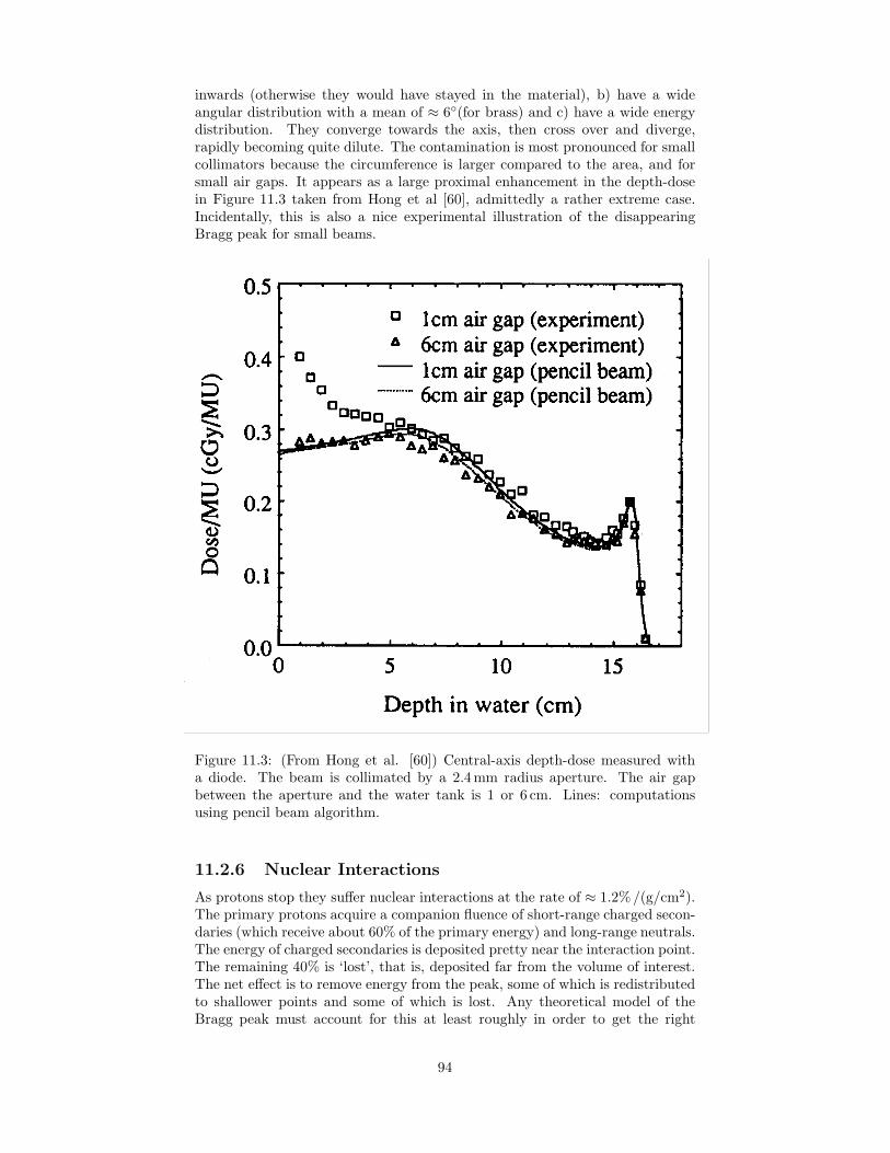
inwards (otherwise they would have stayed in the material), b) have a wideangular distribution with a mean of ≈ 6◦(for brass) and c) have a wide energydistribution. They converge towards the axis, then cross over and diverge,rapidly becoming quite dilute. The contamination is most pronounced for smallcollimators because the circumference is larger compared to the area, and forsmall air gaps. It appears as a large proximal enhancement in the depth-dosein Figure 11.3 taken from Hong et al [60], admittedly a rather extreme case.Incidentally, this is also a nice experimental illustration of the disappearingBragg peak for small beams.

Figure 11.3: (From Hong et al. [60]) Central-axis depth-dose measured witha diode. The beam is collimated by a 2.4mm radius aperture. The air gapbetween the aperture and the water tank is 1 or 6 cm. Lines: computationsusing pencil beam algorithm.

11.2.6 Nuclear Interactions

As protons stop they suffer nuclear interactions at the rate of ≈ 1.2%/(g/cm2).The primary protons acquire a companion fluence of short-range charged secon-daries (which receive about 60% of the primary energy) and long-range neutrals.The energy of charged secondaries is deposited pretty near the interaction point.The remaining 40% is ‘lost’, that is, deposited far from the volume of interest.The net effect is to remove energy from the peak, some of which is redistributedto shallower points and some of which is lost. Any theoretical model of theBragg peak must account for this at least roughly in order to get the right

94

peak/entrance ratio. Chapter 8 discusses this in much more detail.

11.2.7 Electron and Nuclear Buildup

If the Bragg peak is measured with little or no solid material just before thewater (no tank wall and a very thin dosimeter wall) you will see electron andnuclear buildup in the entrance region. The only published measurement ofboth that we know of is that of Carlsson and Carlsson [47], already discussed inChapter 8. To understand electron buildup, assume an uncontaminated beamenters the water from vacuum. (In practice, air is good enough.) The protonswill not yet have their accompanying sheath of low energy electrons caused byEM interactions. It takes ≈ 1mm for this sheath to build up. Because all theabsorbed dose to water is due to these secondary electrons, the true entrancedose is zero. However, it builds up to the equilibrium value very quickly, so youhave to work hard to see the effect. For instance, the standard cap suppliedwith a Markus chamber is already thick enough to establish electron buildup.

As an aside, we’ll comment that the rapid electron buildup is actually one ofthe disadvantages of protons relative to high-energy photon beams. The latter(being neutral) have considerably longer buildup which leads to skin sparingin clinical situations. Protons, because of their short buildup and the almostinevitable presence of some buildup material just before the skin, have little orno skin sparing. This must be taken into account in treatment plans.

Nuclear buildup is like electron buildup except that we are concerned withthe sheath of nuclear secondaries. Nuclear buildup is easier to see because thebuildup distance is of the order of a centimeter, but it is smaller because nuclearsecondaries account for only a small fraction of the absorbed dose. You will seeit if you do a vertical scan in a gantry (the easiest way to get a wall-less watertank) or if your water tank has a thin entrance window.

Do you want to measure it? Probably not. In the clinical application ofyour modulator you are very likely to have some buildup material or low-energybeam contamination from the patient specific collimator, so including the littleentrance dip in your design Bragg peak is probably a worse approximation ofreality.

11.2.8 Pathlength Effect

The EM peak in the number vs. depth curve which underlies the Bragg peak isnot exactly Gaussian but slightly skewed to the shallower side. This is becauseit refers to projected range, which can be smaller than, but never greater than,the pathlength. This is a very small effect for protons where the pathlength andprojected range are nearly the same [3]. Nevertheless it is included in the besttheoretical models [54].

11.2.9 Checklist for Measuring the Bragg Peak

This checklist summarizes the previous discussion.

• Be sure you have a broad beam. If you already have a beam spreadingsystem, use it. Otherwise, you can use a single lead scatterer at somedistance upstream from the tank. By now you should be able to computethe scatterer required. As a check, make sure the measured Bragg peakdoes not change when you move your measurement axis a centimeter ortwo to the side.

• Be sure you know your effective source distance and make it as large aspractical.

95

• Use the same dosimeter as you plan to use later in QA.

• Be sure you know the tank wall thickness, the dosimeter wall thicknessand the amount of water between the wall and the dosimeter when thescanning system reads ‘zero’. Record the beamline geometry including thethickness of everything in the beam: scatterers, monitor IC and so on.

• If the beam energy spread is adjustable by momentum selection slits, besure these are set to the value you plan to use for therapy.

11.3 Commercial Equipment

You will probably use commercial ‘water phantom’ hardware and software tomeasure the Bragg peak. Unfortunately, in our experience equipment designedfor conventional photon therapy is not as convenient for proton beams as itmight be, either for preliminary measurements or day-to-day QA. This situa-tion is unlikely to change because of the tiny market for particle beam therapyequipment.

11.3.1 Tank Size

Water tanks for conventional photon therapy are very large. They come withtheir own cart and a pump to fill and empty the tank. Setting these up can bequite burdensome in the schedule of a busy facility. Though NPTC owns suchdevices they are almost never used.

Miles Wagner had the important insight that a water tank for heavy chargedparticles can be quite small in cross section because protons and charged nuclearsecondaries do not move very far transversely to the beam. If we have a largewater tank we can insert any object we like a few cm off the scan axis and itwill have no effect on a depth-dose measurement. We can even go so far as toeliminate the water starting a few cm from the scan axis. Miles placed a high-Zscatterer along a water tank wall and then found out how close to it he had toscan before it had any effect on the depth-dose, concluding that a transversedistance of 5 cm between the dosimeter and the nearest tank wall would beample at 160MeV. This led to the computer controlled ‘Oilcan’ dosimeter usedfor many years at HCL to map dose fields in 3D.3 A small detector or detectorarray moves along the centered depth axis of a small water tank. Transversedistributions are mapped by moving the entire tank.

Even if you don’t go to all the effort of building a computer controlled device,you will probably want to replace your large commercial tank by a small onewhich you can set up by hand in a minute. The length should correspond towhatever depth-dose you want to measure plus a few cm. Of course it will onlyhave room for a single (depth) scan direction. To measure transverse dosesyou will have to use it sideways or scan the patient positioner on which it ismounted.

The tank wall of commercial tanks is much thicker than it needs to be, so apotentially important part of the depth-dose cannot be measured. It is relativelytrivial to furnish a smaller water tank with a large thin window of (say) 0.005 ′′

Kapton. If it bulges a little you need merely move the dosimeter to touch it andreset the scanner to zero.

3 The original concept called for a water tank similar in size and shape to the cylindricaltin can in which one used to buy motor oil. In time the tank became rectangular, which isprobably easier to fabricate anyway.

96

11.3.2 Current vs. Charge Measurement

There are two ways of mapping dose fields, electronically speaking. You canscan the dosimeter continuously, sampling the current from the dosimeter and areference IC simultaneously at frequent intervals. The CRS scanner [61] worksthat way. Or, you can move to a point, stop, measure dosimeter and referenceIC charges with a current integrator for some fixed period, then move to anotherpoint and repeat. The Scanditronix and Wellhofer tanks work that way. Thecurrent sampling method tends to be noisy and some mathematical smoothing isneeded. Although both ways work and have been used successfully at NPTC, wesomewhat favor the integrator method for conventional scans.4 Neither methodhas a clear speed advantage if they are used intelligently.

11.3.3 Beam Monitor vs. Reference Chamber

Conventional water tanks assume the user will place a reference chamber in somefixed location. They plot the ratio of the ‘field’ chamber to the reference. That isnot the most convenient arrangement in a proton therapy center. Particle beamsfequently have large transverse dose gradients. Also, we may be interested inchanging beam line parameters during a series of measurements. Therefore itmay be difficult to find a good fixed location for the reference chamber.

There is always a beam monitor IC somewhere in the beam line, if onlybecause we need to turn off the beam when the prescribed dose is reached. Thismonitor IC is the most convenient reference. If the measuring system keepstrack of the absolute monitor output as well as the absolute field IC output, eachmeasurement of a Bragg peak or SOBP automatically becomes a measurementof the monitor output factor for that beam line configuration. One difficultyis that the beam monitor output current already goes elsewhere in the controlsystem. We must find a way of either a) sharing it in such a way that thefraction going to the control system does not depend on whether the scanner isconnected or not or b) tapping into the electronic output of the monitor currentintegrator and convincing the scanner to use it as a reference.5 At NPTC wehave generally found it difficult to trick commercial scanning tanks into usingthe beam monitor as a reference.

11.3.4 Scanning vs. Dosimetry Mode

Proton facilities require QA (confirming SOBP shapes) as well as calibrations(confirming the monitor output factor). If stable current integrators are usedand absolute charges are recorded, a point by point SOBP measurement doublesas a measurement of the output factor for that scatterer and modulator system.One has only to use a calibrated dosimeter and record the temperature andpressure at the time of measurement.

Unfortunately, commercial water phantom software usually has completelyseparate ‘scanning’ and ‘dosimetry’ modes because of the conventions of photontherapy. In scanning mode the measured absolute charge tends to disappear ina welter of renormalizations. Inability to use scans for absolute measurementsleads to duplication of effort.

4 The CRS technique is used at NPTC for time-correlated depth-dose measurements, whichare useful in diagnosing range modulator performance.

5 One method is to convert the pulse train from the monitor integrator back into a currentand use that for the reference [62].

97

11.4 Fitting the Bragg Peak

Having measured our Bragg peak we wish to convert it into a standard form.We fit it with a cubic spline as explained in Chapter 5. It is convenient to dothis in an auxiliary program BPW (for Bragg Peak Width). BPW reads the data,fits the spline, produces graphic output and writes a .BPK file which contains allthe information needed by a subsequent programs. Figure 11.4 shows a typicalrun, whose output file RNE175.BPK is listed below the figure.

Figure 11.4: Bragg peak extrapolated to zero and fit with a cubic spline byprogram BPW. The BPK file is listed below.

put a comment here ...280.0 cm from source to Bragg peak18 0.10000E+31 0.10000E+31 # pts, yp1, ypn0.0000 1.8703 4.4415 6.9359 9.2388 11.0088 12.4067 cm H2O13.5244 14.3358 14.9433 15.4579 15.8944 16.1706 16.381216.7241 16.9718 17.2745 17.82500.4105 0.4196 0.4290 0.4418 0.4630 0.4877 0.5186 rel dose0.5599 0.6061 0.6689 0.7616 0.9325 0.9978 0.85500.3724 0.0908 0.0057 0.0014

11.4.1 Overlying Material

For any Bragg peak measurement there will be material in the beam, someassociated with the tank and measurement process (‘wall correction’) and someassociated with the beam line (scatterers, monitor IC’s, air . . .). We need tohandle this in a consistent fashion. Specifically, the scanning software usuallycalls the depth of the first point zero, since it has no way of knowing the truedepth. We need to add a water equivalent depth to each recorded depth tomake the depth-dose the same as what we would have measured with an idealtank and dosimeter.

The wall correction should always be made and usually has three parts: the

98

tank wall, some finite water gap when the scanner reads zero, and the waterequivalent thickness of the dosimeter cap or wall.

Material further upstream requires more thought since its treatment dependson how we plan to use the Bragg peak. At one limit, the prospective computerprogram may account explicitly for everything in the beam line at some futuretime and this may not be the same as it was at the time of measurement. Inthat case we want to conceptually ‘move’ the tank to nozzle entrance before wefit the Bragg peak, by adding to each point the water equivalent of everythingbetween nozzle entrance and the tank at the time of measurement. If thatincludes high-Z materials such as lead we must be careful because their waterequivalence depends on energy. Note also that air is not negligible: a meter ofair corresponds to about a millimeter of water.

Other computer programs treat explicitly only some of the objects in thebeam. For instance, NEU ‘knows’ about the first scatterer or modulator, pre- orpost-scatterers, and the second scatterer, but not about air and monitor IC’s.It assumes that the ignored things are the same ‘now’ as they were during theBragg peak measurement. Therefore the depth data should not be corrected forair and monitor IC, but should be corrected for scatterers in place at the timeof measurement.

11.4.2 Extrapolation to Zero

Once we have done the depth correction we will have a Bragg peak that nolonger starts at zero. Should we leave it that way (cf. Figure 11.1) or generatea fake point at zero, recognizing that what lies between it and the first measuredpoint is a guess (cf. Figure 11.4)?

This question is less important than it may seem for the following reason. Ifa prospective program really needs to know the Bragg peak upstream of the firsttrue point, we have not done a good enough job measuring it. We should useless upstream scatterer, a thinner tank wall or less ‘dead’ water. But usuallythe application will have its own upstream material which guarantees that theBragg peak is only accessed at depths where it is truly known. As a safety belt,SPLINE.FOR has some extrapolation capability. You can call it with a valuesomewhat less than the first table value and still get a sensible answer.

That said, I prefer to add a fake point so that the ‘measured’ Bragg peakstarts mathematically at zero. BPW does this using an input parameter (typically0.1) to control the fraction of data points used in a linear extrapolation, or zeroto skip it. The procedure usually works well except for low energy Bragg peakswhich may have appreciable curvature in the entrance region. But remember:you’re not really supposed to use that part of the Bragg peak.

11.5 Opening the BPK File

The BPK file is opened by using

CALL InitBragg(t1,fNucl,bLevel,dmin,dl80,dpk,du80,dmax,bfn)

where bfn is a file name. InitBragg sets up a function Bragg(x) which returnsthe effective mass stopping power of the proton beam at depth x, as we will nowexplain. We assume that the file contains a ‘splined’ depth-dose measurementwhere the dose is relative but the depth in cm H2O is known exactly.

99

11.5.1 Removing the Fluence

Eq. (3.7) relating dose to fluence and stopping power in practical units can berewritten

D

Φ= 0.1602

S

ρ

Gygp/cm2

(MeVg/cm2

)−1

(11.1)

which is to say that if the stopping power is expressed in MeV/(g/cm2) thenthe left-hand side, dose divided by fluence, will be in Gray/(gp/cm2). The firststep is to divide by the fluence. We do not know the absolute fluence but weknow that it varies as 1/r2 where r is given by the second line of the BPK file.Accordingly we divide by the relative fluence, in effect correcting for 1/r2. Thenew numbers will have a larger peak to entrance ratio than before.

11.5.2 Adjusting the Energy

InitBragg gives us the option of either using the Bragg peak as it stands orof linearly shrinking or stretching the depth scale to adapt the Bragg peak tosome desired energy. The latter case is useful for preliminary designs wherewe happen to have a Bragg peak at nearly, but not exactly, the right energy.The first option is exercised by calling InitBragg with t1=0. in which case t1will be returned at the value deduced from d80 and a range-energy table. Thesecond option is triggered by any non-zero t1.

11.5.3 Normalizing the Bragg Peak

The reason to normalize the Bragg peak (that is, convert it from a relative valueto absolute Gy/(gp/cm2)) is that subsequent calculations using it will give us theactual number of protons required for the prescribed dose rather than just therelative number at each modulator step. This is turn allows the design programto make a reasonably good estimate of the incident beam current needed for theprescribed dose rate.

We do not know the stopping power at the peak, where the proton fluenceis a complicated mix of low energies. We do, however, know it at the entrance.Recall that the Bragg peak is the convolution of the stopping power vs. depthcurve for a single proton with a Gaussian representing the proton number vs.depth curve. At the entrance this convolution has a negligible effect becausethe stopping power varies slowly. Therefore, once we have deduced from d80

that our Bragg peak corresponds to (say) 150Mev protons at the first measuredpoint, it follows that we can identify the relative dose at that point with thetabulated EM mass stopping power of water at 150MeV. Eq. 11.1 says that ifwe multiply that by 0.1602 the resulting function will be the effective stoppingpower of our beam expressed in Gy/(gp/cm2). This argument ignores nuclearreactions.

However, by an equally good argument, once we have assigned that valueto the first measured point, the area or integral under the Bragg curve startingwith that point should equal 150MeV, the average energy of a beam proton. Infact we will invariably find that the area is less than 150MeV. That is becausethe area argument also ignores nuclear reactions.

So far we have given two different ways of normalizing the Bragg peak,which should be consistent in some sense once we take nuclear reactions intoaccount. The next section will go into that more deeply. We will decide to usethe entrance normalization for want of something better. In the larger schemeof therapy beam line design this is a minor issue. After all, what is at stake ismerely the accuracy of our estimate of the required beam current. However, the

100

problem does appear to raise some concerns about our understanding of nuclearreactions. The reader who does not care would do well to stop here.

11.5.4 A Closer Look at Normalization

‘Entrance’ normalization to the tabulated EM mass stopping power ignores theabsorbed dose contribution from nuclear secondaries which is truly zero onlyat the entrance, if the beam has not passed through solid or liquid matter.Otherwise, the nuclear contribution builds up in ≈ 1 cm to a value which can beestimated if we believe the ‘local energy deposition’ model of nuclear reactions(Chapter 8). Assume for the sake of argument we have 150MeV protons atsome depth where nuclear buildup is already established. The model says thatP ′ = 1.2% of the primary fluence interacts every cm. For each reaction theentire 150MeV goes into secondaries and the model says that f ≈ 60% of thisenergy is deposited locally. Therefore, ignoring second order effects, 0.012 ×0.6 × 150 = 1.08MeV per average proton is deposited in the next cm so wemust add 1.08Mev/(g/cm2) to the 5.45Mev/(g/cm2) EM stopping power. Ofcourse we have also seen in Chapter 8 that this computation overestimates theobserved nuclear buildup by a factor of two.

‘Area’ normalization also ignores nuclear interactions if it assumes that thearea equals the average incident energy, because we know some of the energy thatgoes into nuclear secondaries is lost to the volume of interest. This calculationis slightly more complicated because the primary energy, hence the amount lost,varies from the initial energy to zero as the protons stop.

We can relate entrance and area normalization rather easily if we make theapproximations that P ′ and f are constant, independent of energy. These arenot very good approximations, but will give us a general idea of how thingsshould go. Let N0 be the number of protons incident and N(z) the survivingnumber of primaries at depth z. To avoid constant factors of ρ = 1 let’s expressz in g/cm2. Let B(z) be the energy absorbed by water per incident primaryper g/cm2, the effective stopping power of an average proton. Let S be thetabulated EM mass stopping power (normally S/ρ) and let T (z) be the kineticenergy. Then at some depth z in dz we have

N0 B dz = N S dz − f T dN

noting that dN is negative, or

B =N

N0S − 1

N0

dN

dzf T

Let P (z; T0) be the probability that an incident proton of energy T0 will have anuclear reaction by the time it reaches z.6 In other words

P (z) ≡ 1 −N(z)N0

(11.2)

andP ′ ≡ dP

dz= − 1

N0

dN

dz

andB(z) = (1 − P (z)) S(z) + P ′(z) f(z) T (z) (11.3)

At z = 0, if nuclear equilibrium is already established,

B(0) = S(0) + P ′(0) f(0) T (0) (11.4)6In our notation P (r0;T0) is the function tabulated by Janni [3].

101

which, in symbolic form, is just the argument we made above. Now considerthe energy obtained by finding the area of the entire Bragg peak:

TA ≡∫ ∞

0

B dz =∫ R0

0

(1 − P ) S dz +∫ R0

0

P ′ f T dz (11.5)

There is some sleight-of-hand with limits here. We want to take the integralover the entire measured Bragg peak on the LHS, because the act of folding thestopping power with a Gaussian does not change the area. It merely spreadsit out. On the RHS, however, we have mathematical functions that are onlydefined between 0 and R0, the mean range.

So far we have no assumptions about the z dependence of the quantitieson the RHS of Eq. 11.3. We do not need to: we can always do the integralnumerically. However, to get a simple result in closed form we approximate therange-energy relation by a power law

R = a T b , b = 1.77

so that

T (z) =(R0 − z

a

)1/b

andS(z) ≡ −dT

dz=

1b a1/b

(R0 − z)(1/b)−1

We also assume that

P ′(z) ≈ constant = 0.012 (g/cm2)−1

so thatP (z) = P ′ z

and further, thatf(z) ≈ constant = 0.6

The assumptions concerning P ′ and f amount to simplifications of the localenergy deposition model of nuclear reactions. We can now do the integrals inEq. 11.5 and we find

absorbed fraction ≡ TA

T0≈ 1 − 0.639 P ′ (1 − f) R0 (11.6)

Let’s briefly review the derivation. It starts with the assumption that, oncewe have determined normalized the measured Bragg peak at some point, itsarea (which we are then in a position to compute, and which has the dimensionsof energy) should represent the total energy absorbed by water for a averageproton. That can be estimated from the local energy deposition model, and wemake a couple of not too bad approximations to get the result in closed form.

To test this result we can take the set of Bragg peaks shown in Figure 11.1,compute the area TA of each starting with the first measured point, computethe energy T0 at that point from d80 and plot TA/T0 vs. R0. The integral ismade easy because we have fit the Bragg peaks with a cubic spline. Simpson’srule is exact for a cubic, so the integral is exact (that is, as good as the fit)so long as we use the spline points to delimit each integration interval. Theassumption of full nuclear buildup at the ‘entrance’ point is validated by theappearance of Figure 11.1. Each scan starts after a good deal of material.

Figure 11.5 shows the results. We have used two extremes to normalize theBragg peak. The open circles set the first measured point at S, completely

102

Figure 11.5: Absorbed energy fraction computed from the scans of Figure 11.1.Open circles: EM normalization. Full circles: EM + nuclear. Line: theoreticalprediction for P ′ = 0.012/(g/cm2), f = 0.6.

ignoring nuclear effects. The filled circles use Eq. 11.4, assuming full nuclearbuildup. Note that it is the filled circles that should follow the line, Eq. 11.6.Instead, they rise to a nonphysical value great than 1. At present we are ata loss to account for this result. It is almost certainly the same effect notedearlier [47], that the observed nuclear buildup is ≈ 2× less than predicted bynuclear models. Reducing the nuclear component at the entrance improves theagreement, and at least brings TA/T0 below 1.

Understanding nuclear effects in the Bragg peak quantitatively should be aninteresting topic for further investigation. However, as noted before, it is not aserious problem in designing of beam spreading systems. For the time being weshall use S normalization, ignoring nuclear effects.

103

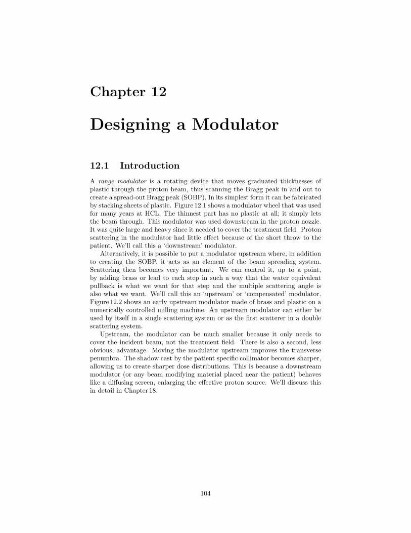
Chapter 12

Designing a Modulator

12.1 Introduction

A range modulator is a rotating device that moves graduated thicknesses ofplastic through the proton beam, thus scanning the Bragg peak in and out tocreate a spread-out Bragg peak (SOBP). In its simplest form it can be fabricatedby stacking sheets of plastic. Figure 12.1 shows a modulator wheel that was usedfor many years at HCL. The thinnest part has no plastic at all; it simply letsthe beam through. This modulator was used downstream in the proton nozzle.It was quite large and heavy since it needed to cover the treatment field. Protonscattering in the modulator had little effect because of the short throw to thepatient. We’ll call this a ‘downstream’ modulator.

Alternatively, it is possible to put a modulator upstream where, in additionto creating the SOBP, it acts as an element of the beam spreading system.Scattering then becomes very important. We can control it, up to a point,by adding brass or lead to each step in such a way that the water equivalentpullback is what we want for that step and the multiple scattering angle isalso what we want. We’ll call this an ‘upstream’ or ‘compensated’ modulator.Figure 12.2 shows an early upstream modulator made of brass and plastic on anumerically controlled milling machine. An upstream modulator can either beused by itself in a single scattering system or as the first scatterer in a doublescattering system.

Upstream, the modulator can be much smaller because it only needs tocover the incident beam, not the treatment field. There is also a second, lessobvious, advantage. Moving the modulator upstream improves the transversepenumbra. The shadow cast by the patient specific collimator becomes sharper,allowing us to create sharper dose distributions. This is because a downstreammodulator (or any beam modifying material placed near the patient) behaveslike a diffusing screen, enlarging the effective proton source. We’ll discuss thisin detail in Chapter 18.

104

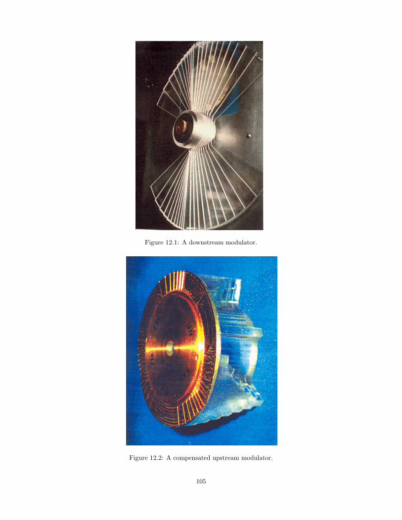
Figure 12.1: A downstream modulator.

Figure 12.2: A compensated upstream modulator.

105

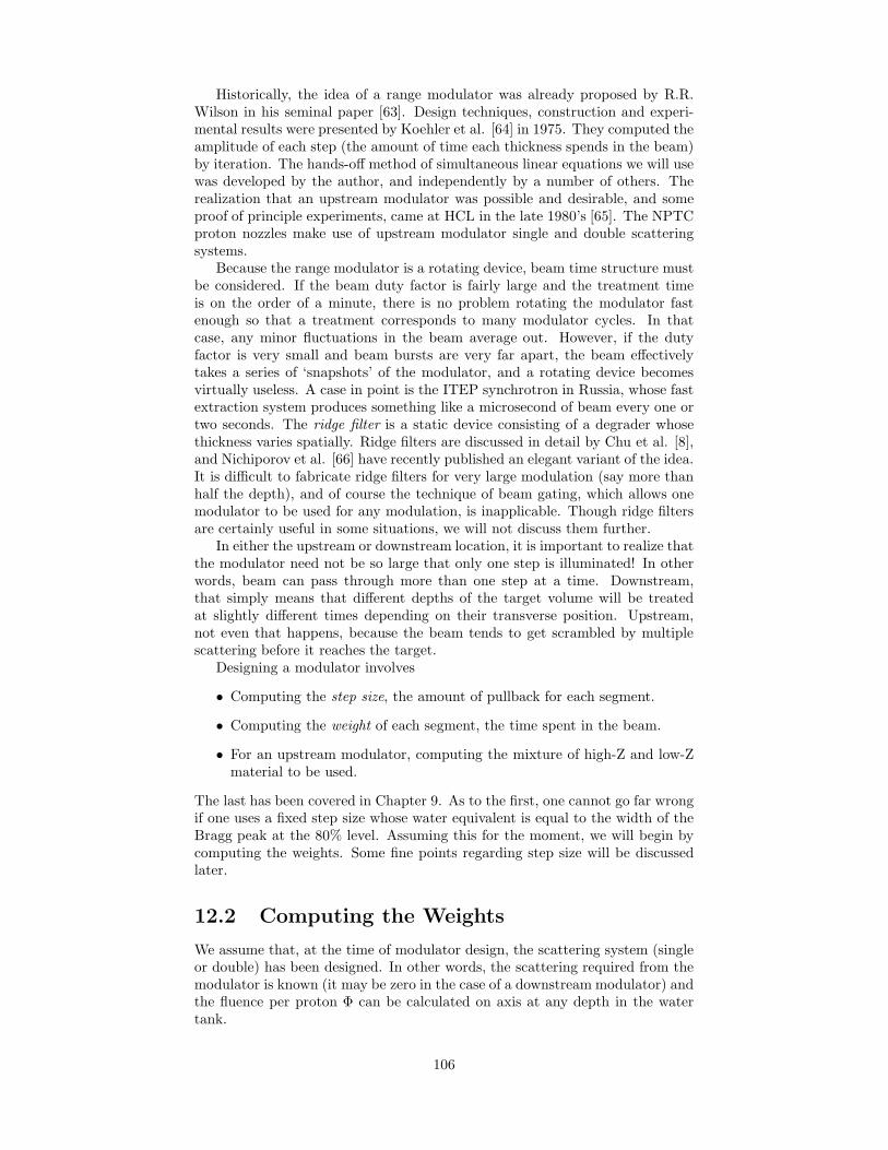
Historically, the idea of a range modulator was already proposed by R.R.Wilson in his seminal paper [63]. Design techniques, construction and experi-mental results were presented by Koehler et al. [64] in 1975. They computed theamplitude of each step (the amount of time each thickness spends in the beam)by iteration. The hands-off method of simultaneous linear equations we will usewas developed by the author, and independently by a number of others. Therealization that an upstream modulator was possible and desirable, and someproof of principle experiments, came at HCL in the late 1980’s [65]. The NPTCproton nozzles make use of upstream modulator single and double scatteringsystems.

Because the range modulator is a rotating device, beam time structure mustbe considered. If the beam duty factor is fairly large and the treatment timeis on the order of a minute, there is no problem rotating the modulator fastenough so that a treatment corresponds to many modulator cycles. In thatcase, any minor fluctuations in the beam average out. However, if the dutyfactor is very small and beam bursts are very far apart, the beam effectivelytakes a series of ‘snapshots’ of the modulator, and a rotating device becomesvirtually useless. A case in point is the ITEP synchrotron in Russia, whose fastextraction system produces something like a microsecond of beam every one ortwo seconds. The ridge filter is a static device consisting of a degrader whosethickness varies spatially. Ridge filters are discussed in detail by Chu et al. [8],and Nichiporov et al. [66] have recently published an elegant variant of the idea.It is difficult to fabricate ridge filters for very large modulation (say more thanhalf the depth), and of course the technique of beam gating, which allows onemodulator to be used for any modulation, is inapplicable. Though ridge filtersare certainly useful in some situations, we will not discuss them further.

In either the upstream or downstream location, it is important to realize thatthe modulator need not be so large that only one step is illuminated! In otherwords, beam can pass through more than one step at a time. Downstream,that simply means that different depths of the target volume will be treatedat slightly different times depending on their transverse position. Upstream,not even that happens, because the beam tends to get scrambled by multiplescattering before it reaches the target.

Designing a modulator involves

• Computing the step size, the amount of pullback for each segment.

• Computing the weight of each segment, the time spent in the beam.

• For an upstream modulator, computing the mixture of high-Z and low-Zmaterial to be used.

The last has been covered in Chapter 9. As to the first, one cannot go far wrongif one uses a fixed step size whose water equivalent is equal to the width of theBragg peak at the 80% level. Assuming this for the moment, we will begin bycomputing the weights. Some fine points regarding step size will be discussedlater.

12.2 Computing the Weights

We assume that, at the time of modulator design, the scattering system (singleor double) has been designed. In other words, the scattering required from themodulator is known (it may be zero in the case of a downstream modulator) andthe fluence per proton Φ can be calculated on axis at any depth in the watertank.

106

Figure 12.3: Figure illustrating modulator weight calculation.

We will use the following notation:

M # modulator steps = # z positionsi = 1 . . .M position indexj = 1 . . .M modulator step index (1 is deepest step)zi a measuring plane position along beam axisbi value of pristine Bragg peak at position zi

(effective stopping power in Gy/(gp/cm2)Φij fluence per proton on axis; depends on i via location

of measuring plane and on j via scattering effects(modulator thickness, proton energy)

di desired dose at position zi

Nj # gp (gigaprotons) required for step j

A 3-step modulator will suffice to illustrate the math. Refer to Figure 12.3. Thedesired doses di are usually the same (say 1 Gy) but they need not be. The doseat each point is the sum of contributions from three Bragg peaks:

d1 = (b1 Φ11) N1 + (b0 Φ12) N2 + (b−1 Φ13) N3

d2 = (b2 Φ21) N1 + (b1 Φ22) N2 + (b0 Φ23) N3

d3 = (b3 Φ31) N1 + (b2 Φ32) N2 + (b1 Φ33) N3

b0, the value of the Bragg peak one step up from the peak, is small and b−1 isalmost certainly zero but it does no harm to include them. The known quantitiesin parentheses are the elements of a matrix G and the system of linear equationscan be written formally

~d = G ~N

107

where ~d is a known vector and ~N is a vector to be found. The formal solution

~N = G−1 ~d

can be computed by a subroutine such as GaussJordan. See Numerical Recipesfor a description of ‘Gauss-Jordan elimination with full pivoting’ as well as someslightly faster techniques that could be used.

Although we traditionally call the Nj ‘weights’ implying a relative quantity,note that by virtue of the definition of Φ as the fluence at zi per proton incidenton the scattering system and of bi as the effective stopping power expressed inGy/(gp/cm2), the Nj are the actual numbers of incident gigaprotons for eachstep required to obtain the di. In other words, the design program tells us notonly the shape of the modulator but (by a trivial additional calculation) theincident proton current required for the prescribed dose rate. This estimate is,however, only as good as the normalization of b (Chapter 11).

Figure 12.4: Prieels’ argument for finite step size.

12.3 Alternative Procedure for Weights

It might reasonably be argued that we could achieve a better result by requiringthe dose to be flat1 everywhere or at a large number of points rather thanonly M points. This, and the closely related question of whether we wanta ‘stepped’ or ‘continuous’ modulator, was investigated by Prieels [67] usingan optimization procedure instead of solving a set of linear equations. Prieelssuppressed nonphysical solutions by adding a penalty for negative weights tothe objective function. This works better than a hard constraint. He wasable, for a given problem, to obtain two solutions depending on the startingpoint, one corresponding to a continuous modulator and the second to a steppedmodulator.

Surprisingly, the SOBP was slightly smoother for the stepped case. Prieelsgave a simple heuristic argument for this. Figure 12.4 from [67] shows that, if wetry to create a flat SOBP from triangular ‘Bragg peaks’, we will get the desiredresult by using peaks 1 and 3 and that any intermediate peak such as 2 must berejected. If we use real Bragg peaks and the algebraic method of the previous

1 From here on we’ll assume unless explicitly stated that the goal is a constant dose oversome extent in depth.

108

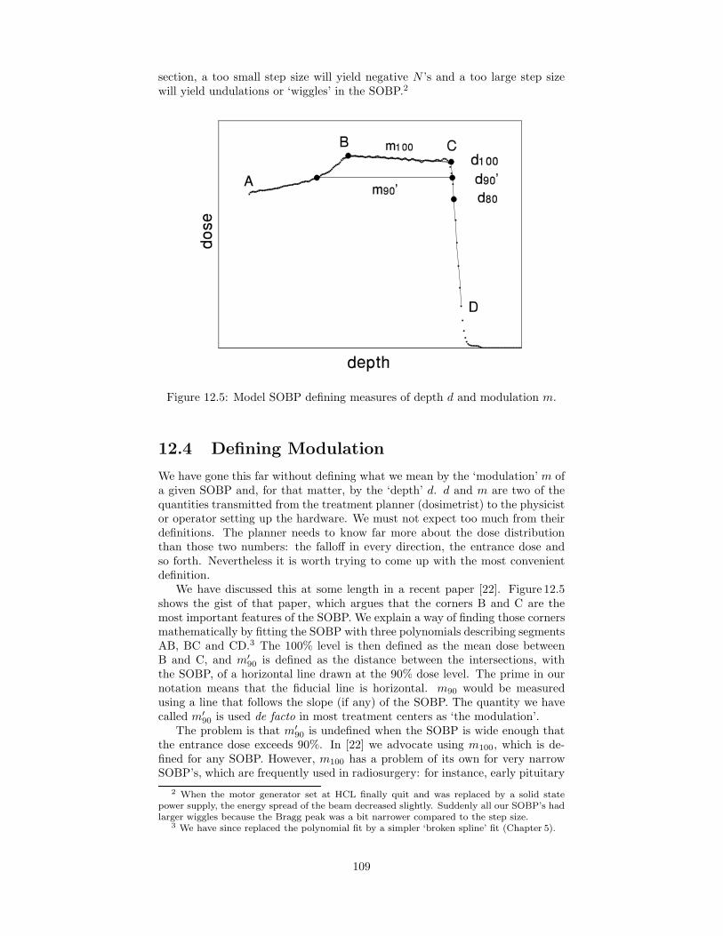
section, a too small step size will yield negative N ’s and a too large step sizewill yield undulations or ‘wiggles’ in the SOBP.2

Figure 12.5: Model SOBP defining measures of depth d and modulation m.

12.4 Defining Modulation

We have gone this far without defining what we mean by the ‘modulation’ m ofa given SOBP and, for that matter, by the ‘depth’ d. d and m are two of thequantities transmitted from the treatment planner (dosimetrist) to the physicistor operator setting up the hardware. We must not expect too much from theirdefinitions. The planner needs to know far more about the dose distributionthan those two numbers: the falloff in every direction, the entrance dose andso forth. Nevertheless it is worth trying to come up with the most convenientdefinition.

We have discussed this at some length in a recent paper [22]. Figure 12.5shows the gist of that paper, which argues that the corners B and C are themost important features of the SOBP. We explain a way of finding those cornersmathematically by fitting the SOBP with three polynomials describing segmentsAB, BC and CD.3 The 100% level is then defined as the mean dose betweenB and C, and m′

90 is defined as the distance between the intersections, withthe SOBP, of a horizontal line drawn at the 90% dose level. The prime in ournotation means that the fiducial line is horizontal. m90 would be measuredusing a line that follows the slope (if any) of the SOBP. The quantity we havecalled m′

90 is used de facto in most treatment centers as ‘the modulation’.The problem is that m′

90 is undefined when the SOBP is wide enough thatthe entrance dose exceeds 90%. In [22] we advocate using m100, which is de-fined for any SOBP. However, m100 has a problem of its own for very narrowSOBP’s, which are frequently used in radiosurgery: for instance, early pituitary

2 When the motor generator set at HCL finally quit and was replaced by a solid statepower supply, the energy spread of the beam decreased slightly. Suddenly all our SOBP’s hadlarger wiggles because the Bragg peak was a bit narrower compared to the step size.

3 We have since replaced the polynomial fit by a simpler ‘broken spline’ fit (Chapter 5).

109

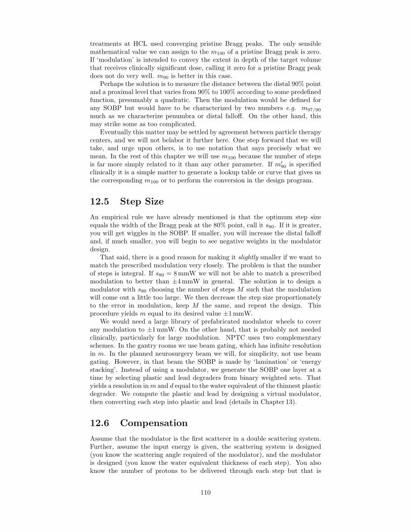
treatments at HCL used converging pristine Bragg peaks. The only sensiblemathematical value we can assign to the m100 of a pristine Bragg peak is zero.If ‘modulation’ is intended to convey the extent in depth of the target volumethat receives clinically significant dose, calling it zero for a pristine Bragg peakdoes not do very well. m90 is better in this case.

Perhaps the solution is to measure the distance between the distal 90% pointand a proximal level that varies from 90% to 100% according to some predefinedfunction, presumably a quadratic. Then the modulation would be defined forany SOBP but would have to be characterized by two numbers e.g. m97/90

much as we characterize penumbra or distal falloff. On the other hand, thismay strike some as too complicated.

Eventually this matter may be settled by agreement between particle therapycenters, and we will not belabor it further here. One step forward that we willtake, and urge upon others, is to use notation that says precisely what wemean. In the rest of this chapter we will use m100 because the number of stepsis far more simply related to it than any other parameter. If m′

90 is specifiedclinically it is a simple matter to generate a lookup table or curve that gives usthe corresponding m100 or to perform the conversion in the design program.

12.5 Step Size

An empirical rule we have already mentioned is that the optimum step sizeequals the width of the Bragg peak at the 80% point, call it s80. If it is greater,you will get wiggles in the SOBP. If smaller, you will increase the distal falloffand, if much smaller, you will begin to see negative weights in the modulatordesign.

That said, there is a good reason for making it slightly smaller if we want tomatch the prescribed modulation very closely. The problem is that the numberof steps is integral. If s80 = 8mmW we will not be able to match a prescribedmodulation to better than ±4mmW in general. The solution is to design amodulator with s80 choosing the number of steps M such that the modulationwill come out a little too large. We then decrease the step size proportionatelyto the error in modulation, keep M the same, and repeat the design. Thisprocedure yields m equal to its desired value ±1mmW.

We would need a large library of prefabricated modulator wheels to coverany modulation to ±1mmW. On the other hand, that is probably not neededclinically, particularly for large modulation. NPTC uses two complementaryschemes. In the gantry rooms we use beam gating, which has infinite resolutionin m. In the planned neurosurgery beam we will, for simplicity, not use beamgating. However, in that beam the SOBP is made by ‘lamination’ or ‘energystacking’. Instead of using a modulator, we generate the SOBP one layer at atime by selecting plastic and lead degraders from binary weighted sets. Thatyields a resolution in m and d equal to the water equivalent of the thinnest plasticdegrader. We compute the plastic and lead by designing a virtual modulator,then converting each step into plastic and lead (details in Chapter 13).

12.6 Compensation

Assume that the modulator is the first scatterer in a double scattering system.Further, assume the input energy is given, the scattering system is designed(you know the scattering angle required of the modulator), and the modulatoris designed (you know the water equivalent thickness of each step). You alsoknow the number of protons to be delivered through each step but that is

110

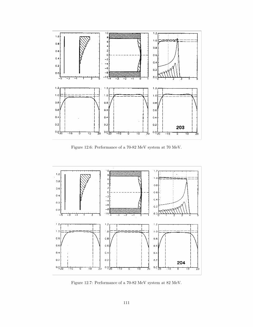
Figure 12.6: Performance of a 70-82 MeV system at 70 MeV.

Figure 12.7: Performance of a 70-82 MeV system at 82 MeV.

111

irrelevant at this time. Your task is to find the combination of lead and lexan(for instance) that will work properly. Do this one modulator step at a time,using the methods of Chapter 9, as follows:

• From d80 of that step, find the proton energy T into the tank.

• Backtrack through the second scatterer using its lead and lexan thicknesseson axis to find T into the second scatterer.

• Ditto through any ‘post absorber’ material between the modulator andthe second scatterer.

• You now know the energy out of the modulator. With this, the energyinto the modulator, and the scattering angle, you can compute the leadand the lexan.

Having done this for each step you will find, in the ideal case, that step 1 (thethinnest) is all lead, step M is all lexan, and every other step has some leadand some lexan. That is the design goal. We call it a ‘minimal’ modulator. Farmore likely, you will see one of these pathologies:

• (Harmless.) The modulator carries extra lexan. Remove lexan from thetrack or wheel and use a fixed absorber or, better, reduce the beam energy.

• (Harmless.) The modulator carries extra lead. Remove lead from thetrack or wheel and use a fixed scatterer.

• (Serious.) Steps before the end (before step M) have no lead.

Regrettably, the last is common. By implication it means that the required lexanalready overscatters. (You now recall that you got an error message ‘N failuresin compensation’.) You can fix this by decreasing the throw (which may notbe an option) or increasing the prescribed radius (which is undesirable) becauseeither move requires more scattering. Fortunately, you can always put up witha few uncompensated steps. The depth-dose on axis will be correct, because itis constrained to be, and the effect off-axis may be tolerable because the relativeweights of the last few steps are small. Too much of this, however, and you willsee the dished transverse scan characteristic of too strong a first scatterer.4 Youhave reached the natural limit of the upstream modulator.

12.7 Useful Energy Range

A physical modulator wheel, when it is the first scatterer in a double scatteringsystem, will only work satisfactorily over a certain range of incident energies.Below the design energy, the modulator overscatters and the SOBP acquires apositive slope. Above the design energy, the modulator underscatters and theSOBP acquires a negative slope. Figures 12.6 and 12.7 from [68] illustrate theseeffects. The energy range, 70-82Mev, can be taken as typical of what can beachieved, though the exact range will depend on your tolerances. Beam currentmodulation (Section 12.9) can extend the useful range greatly, at the expense ofa more complicated system and safety tests.

A second energy effect is the narrowing of the Bragg peak at lower energy. Ifthe modulator is designed at the high end using s80, the SOBP will have wigglesat the low end.

4 For mild examples of what we mean by ‘dished’ and ’domed’ see Figures 12.6 and 12.7respectively.

112

If a modulator is to cover a finite energy range, at what energy within thatrange should it be designed? The wiggle problem would be solved by designingthe modulator at the low end with s80. However, we would then not have fullmodulation at the high end and would have to come up with some procedurefor adding steps by hand. It seems better to us to design at the high end usinga step reduction factor so as to ensure a small enough step at the low end.

Figure 12.8: Beam gated SOBP showing rounding of proximal corner.

12.8 Beam Gating

If you have a variable energy proton generator you will want to adjust thebeam energy into the nozzle to suit the prescribed depth of each field. Youwill therefore need a library of modulators, one to deal with each energy range.5

Beam gating allows you to avoid a second dimension of this library by obtainingany prescribed modulation from a single modulator designed for full modulation.You simply cut off the cyclotron beam when the desired proximal depth isreached.

A modulator wheel or ‘track’ designed for gating must have a beam blocksection, as was first pointed out by D. Prieels. The reason is that, for anypractical sized design, the beam spot will inevitably illuminate more than onestep. Specifically, there will be a time during each revolution when appreciablebeam is on both the thickest and the thinnest step. If we cut off the beam atthis time to trim the most proximal step we will inevitably cut into the mostdistal step, spoiling that end of the SOBP. The beam block cleanly separatesthe two ends of the modulator.

The fact that more than one step is illuminated at a time produces a proximalcorner that is somewhat rounded. This is illustrated by Figure 12.8 from [69]which compares a simple and a gated modulator using beam and track sizestypical of NPTC.

5 The original NPTC design called for eight modulators to cover the range 70-230 MeV.This can be cut to five or so by using beam current modulation to correct the SOBP.

113

With gating, the average dose rate for a given beam current is lower thanwould be gotten with a simple modulator because the beam is off part of thetime. This is exacerbated by the need for a beam block, but is still a minordisadvantage.

A more important disadvantage is the fact that, with gating, we have asomewhat complicated system with significant potential for delivering the wrongSOBP if something fails. We need redundant, radiation resistant means ofknowing the modulator angle with sufficient resolution. Timing should be donein hardware because millisecond level timing in software is unreliable on a largemulti-tasking computer. With a simple modulator, we need merely confirmthat it is rotating at something like the right speed. By contrast, beam gatingrequires a higher level of engineering.

12.9 Beam Current Modulation

At a still higher level of complexity, we can change the cyclotron output currentin synchronism with modulator rotation to correct defects in the SOBP. AtNPTC this is done [70] under the control of a beam current modulation (BCM)file which specifies the current at each modulator angle. We will not go into thedetails of how the BCM file is computed from the SOBP to be corrected.

Cyclotron output current is measured by an ionization chamber (in whichrecombination and radiation damage are potential problems) and controlled bymeans of the cyclotron ion source current. The relation between ion sourceand output is non-linear and changes from day to day depending on machinesettings. A stand-alone feedback circuit, which needs to be ‘trained’ from timeto time, is used to linearize it over some range. That range determines howmuch correction can be obtained.

12.10 Physical Arrangement of Modulators

In a gantry based nozzle we want to change modulators remotely, for convenienceand to minimize radiation exposure to staff. Various layouts can be imagined.At one extreme we might have a number of independent modulators arrangedon the periphery of a large wheel which is turned to bring the desired modulatorinto play. Or, one might have a single large wheel with (say) nine modulatortracks cut into it. That turns out to be very large indeed when one considersthe sideways motion required, and rather inflexible. Miles Wagner proposed theelegant ‘3× 3’ scheme used by IBA (Figure 12.9). Three small wheels, each cutwith three tracks and driven by its own motor, are mounted on a large wheel.A simple rotation of the large wheel can bring any desired track into the beam.The small wheels are modular and fairly easy to change, though that has notproved necessary at NPTC.

114

Figure 12.9: The 3 × 3 arrangement of modulator wheels.

115

Chapter 13

Single Scattering EnergyStacking Example

This chapter will describe how LAMINATE uses single scattering and a set ofbinary weighted lead and lexan degraders to obtain a prescribed SOBP (depthand modulation). It also explains how to estimate the beam monitor outputfactor.

116

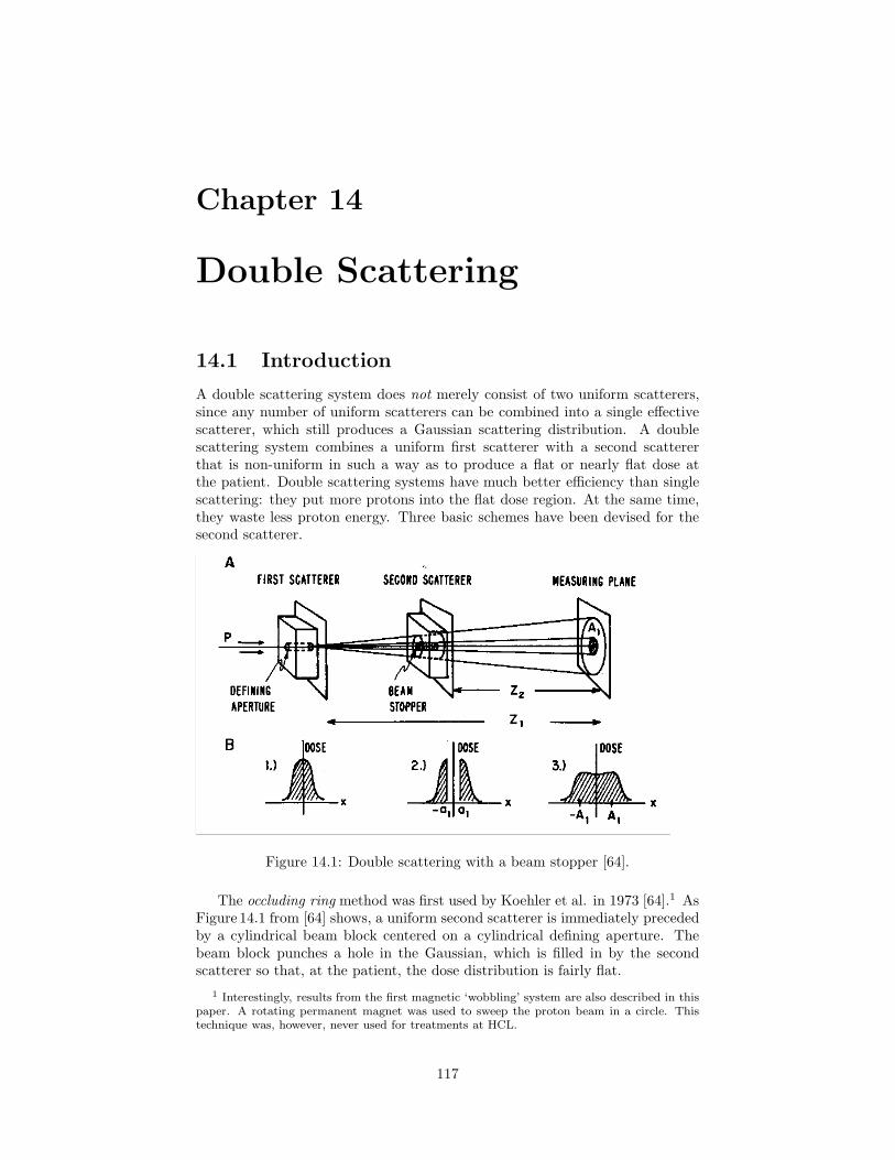
Chapter 14

Double Scattering

14.1 Introduction

A double scattering system does not merely consist of two uniform scatterers,since any number of uniform scatterers can be combined into a single effectivescatterer, which still produces a Gaussian scattering distribution. A doublescattering system combines a uniform first scatterer with a second scattererthat is non-uniform in such a way as to produce a flat or nearly flat dose atthe patient. Double scattering systems have much better efficiency than singlescattering: they put more protons into the flat dose region. At the same time,they waste less proton energy. Three basic schemes have been devised for thesecond scatterer.

Figure 14.1: Double scattering with a beam stopper [64].

The occluding ring method was first used by Koehler et al. in 1973 [64].1 AsFigure 14.1 from [64] shows, a uniform second scatterer is immediately precededby a cylindrical beam block centered on a cylindrical defining aperture. Thebeam block punches a hole in the Gaussian, which is filled in by the secondscatterer so that, at the patient, the dose distribution is fairly flat.

1 Interestingly, results from the first magnetic ‘wobbling’ system are also described in thispaper. A rotating permanent magnet was used to sweep the proton beam in a circle. Thistechnique was, however, never used for treatments at HCL.

117

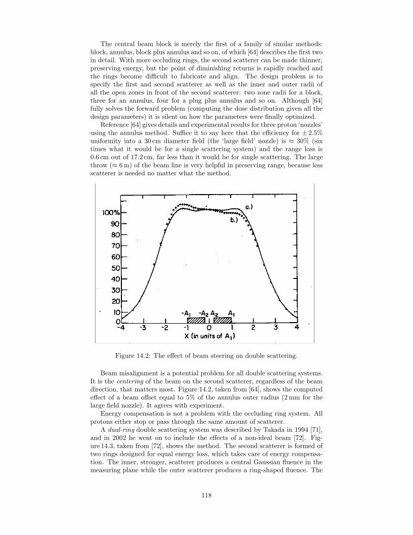
The central beam block is merely the first of a family of similar methods:block, annulus, block plus annulus and so on, of which [64] describes the first twoin detail. With more occluding rings, the second scatterer can be made thinner,preserving energy, but the point of diminishing returns is rapidly reached andthe rings become difficult to fabricate and align. The design problem is tospecify the first and second scatterer as well as the inner and outer radii ofall the open zones in front of the second scatterer: two zone radii for a block,three for an annulus, four for a plug plus annulus and so on. Although [64]fully solves the forward problem (computing the dose distribution given all thedesign parameters) it is silent on how the parameters were finally optimized.

Reference [64] gives details and experimental results for three proton ‘nozzles’using the annulus method. Suffice it to say here that the efficiency for ± 2.5%uniformity into a 30 cm diameter field (the ‘large field’ nozzle) is ≈ 30% (sixtimes what it would be for a single scattering system) and the range loss is0.6 cm out of 17.2 cm, far less than it would be for single scattering. The largethrow (≈ 6 m) of the beam line is very helpful in preserving range, because lessscatterer is needed no matter what the method.

Figure 14.2: The effect of beam steering on double scattering.

Beam misalignment is a potential problem for all double scattering systems.It is the centering of the beam on the second scatterer, regardless of the beamdirection, that matters most. Figure 14.2, taken from [64], shows the computedeffect of a beam offset equal to 5% of the annulus outer radius (2 mm for thelarge field nozzle). It agrees with experiment.

Energy compensation is not a problem with the occluding ring system. Allprotons either stop or pass through the same amount of scatterer.

A dual-ring double scattering system was described by Takada in 1994 [71],and in 2002 he went on to include the effects of a non-ideal beam [72]. Fig-ure 14.3, taken from [72], shows the method. The second scatterer is formed oftwo rings designed for equal energy loss, which takes care of energy compensa-tion. The inner, stronger, scatterer produces a central Gaussian fluence in themeasuring plane while the outer scatterer produces a ring-shaped fluence. The

118

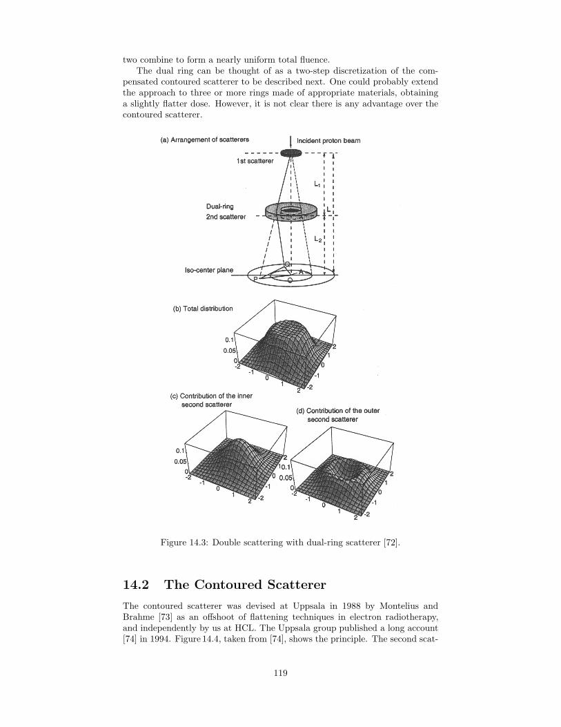
two combine to form a nearly uniform total fluence.The dual ring can be thought of as a two-step discretization of the com-

pensated contoured scatterer to be described next. One could probably extendthe approach to three or more rings made of appropriate materials, obtaininga slightly flatter dose. However, it is not clear there is any advantage over thecontoured scatterer.

Figure 14.3: Double scattering with dual-ring scatterer [72].

14.2 The Contoured Scatterer

The contoured scatterer was devised at Uppsala in 1988 by Montelius andBrahme [73] as an offshoot of flattening techniques in electron radiotherapy,and independently by us at HCL. The Uppsala group published a long account[74] in 1994. Figure 14.4, taken from [74], shows the principle. The second scat-

119

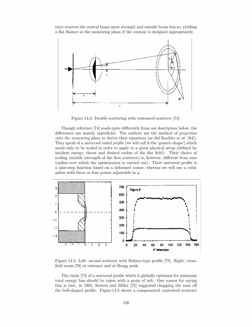
terer scatters the central beam more strongly and outside beam less so, yieldinga flat fluence at the measuring plane if the contour is designed appropriately.

Figure 14.4: Double scattering with contoured scatterer [74].

Though reference [74] reads quite differently from our description below, thedifferences are mainly superficial. The authors use the method of projectiononto the measuring plane to derive their equations (as did Koehler et al. [64]).They speak of a universal radial profile (we will call it the ‘generic shape’) whichneeds only to be scaled in order to apply to a given physical setup (defined byincident energy, throw and desired radius of the flat field). Their choice ofscaling variable (strength of the first scatterer) is, however, different from ours(radius over which the optimization is carried out). Their universal profile isa nine-step function based on a deformed cosine, whereas we will use a cubicspline with three or four points adjustable in y.

Figure 14.5: Left: second scatterer with Siebers-type profile [75]. Right: cross-field scans [76] at entrance and at Bragg peak.

The claim [74] of a universal profile which is globally optimum for minimumtotal energy loss should be taken with a grain of salt. One reason for sayingthis is that, in 1992, Siebers and Miller [75] suggested chopping the nose offthe bell-shaped profile. Figure 14.5 shows a compensated contoured scatterer

120

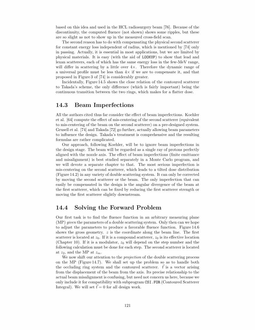
based on this idea and used in the HCL radiosurgery beam [76]. Because of thediscontinuity, the computed fluence (not shown) shows some ripples, but theseare so slight as not to show up in the measured cross-field scan.

The second reason has to do with compensating the physical second scattererfor constant energy loss independent of radius, which is mentioned by [74] onlyin passing. Actually, it is essential in most applications, but we are limited byphysical materials. It is easy (with the aid of LOOKUP) to show that lead andlexan scatterers, each of which has the same energy loss in the few-MeV range,will differ in scattering by a little over 4×. Therefore the dynamic range ofa universal profile must be less than 4× if we are to compensate it, and thatproposed in Figure 3 of [74] is considerably greater.

Incidentally, Figure 14.5 shows the close relation of the contoured scattererto Takada’s scheme, the only difference (which is fairly important) being thecontinuous transition between the two rings, which makes for a flatter dose.

14.3 Beam Imperfections

All the authors cited thus far consider the effect of beam imperfections. Koehleret al. [64] compute the effect of mis-centering of the second scatterer (equivalentto mis-centering of the beam on the second scatterer) on a pre-designed system.Grusell et al. [74] and Takada [72] go further, actually allowing beam parametersto influence the design. Takada’s treatment is comprehensive and the resultingformulas are rather complicated.

Our approach, following Koehler, will be to ignore beam imperfections inthe design stage. The beam will be regarded as a single ray of protons perfectlyaligned with the nozzle axis. The effect of beam imperfections (finite emittanceand misalignment) is best studied separately in a Monte Carlo program, andwe will devote a separate chapter to that. The most serious imperfection ismis-centering on the second scatterer, which leads to a tilted dose distribution(Figure 14.2) in any variety of double scattering system. It can only be correctedby moving the second scatterer or the beam. The only imperfection that caneasily be compensated in the design is the angular divergence of the beam atthe first scatterer, which can be fixed by reducing the first scatterer strength ormoving the first scatterer slightly downstream.

14.4 Solving the Forward Problem

Our first task is to find the fluence function in an arbitrary measuring plane(MP) given the parameters of a double scattering system. Only then can we hopeto adjust the parameters to produce a favorable fluence function. Figure 14.6shows the gross geometry. z is the coordinate along the beam line. The firstscatterer is located at z0. If it is a compound scatterer, z0 is its effective location(Chapter 10). If it is a modulator, z0 will depend on the step number and thefollowing calculation must be done for each step. The second scatterer is locatedat z2, and the MP at zm.

We now shift our attention to the projection of the double scattering processon the MP (Figure 14.7). We shall set up the problem so as to handle boththe occluding ring system and the contoured scatterer. ~t is a vector arisingfrom the displacement of the beam from the axis. Its precise relationship to theactual beam misalignment is confusing, but need not concern us here, because weonly include it for compatibility with subprogram CSI.FOR (Contoured ScattererIntegral). We will set ~t = 0 for all design work.

121

Figure 14.6: Geometry of double scattering system.

Figure 14.7: Double scattering projected on the measuring plane.

122

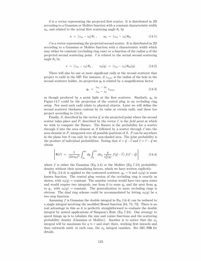
~u is a vector representing the projected first scatter. It is distributed in 2Daccording to a Gaussian or Moliere function with a constant characteristic widthu0, and related to the actual first scattering angle θ1 by

u = (zm − z0) θ1 , u0 = (zm − z0) θ01 (14.1)

~v is a vector representing the projected second scatter. It is distributed in 2Daccording to a Gaussian or Moliere function with a characteristic width whichmay either be constant (occluding ring case) or a function of the radius q of theprojected second scattering point. ~v is related to the actual second scatteringangle θ2 by

v = (zm − z2) θ2 , v0(q) = (zm − z2) θ02(q) (14.2)

There will also be one or more significant radii at the second scatterer thatproject to radii in the MP. For instance, if rmax is the radius of the hole in thesecond scatterer holder, its projection qb is related by a magnification factor

qb =zm − z0

zm − z2rmax (14.3)

as though produced by a point light at the first scatterer. Similarly, qa inFigure 14.7 could be the projection of the central plug in an occluding ringsetup. Nor need such radii relate to physical objects. Later we will define thesecond scatterer thickness contour by its value at certain radii, and these tooproject according to (14.3).

Finally, S, described by the vector ~q, is the projected point where the secondscatter takes place and P , described by the vector ~r, is the field point at whichwe wish to compute the fluence. The fluence is the probability for a scatterthrough ~u into the area element at S followed by a scatter through ~v into thearea element at P , integrated over all possible positions of S. P can be anywherein the plane but S can only be in the non-shaded area. The joint probability isthe product of individual probabilities. Noting that ~u = ~q −~t and ~v = ~r − ~q weobtain

Φ(~r) =1

(2πu0)2

∫ qb

qa

dq

∫ 2π

0

dφqq

v20(q)

f(~q − ~t ) f(~r − ~q) (14.4)

where f is either the Gaussian (Eq. 4.4) or the Moliere (Eq. 7.13) probabilitydensity without their normalizing factors, which we have written explicitly.

If Eq. (14.4) is applied to the contoured scatterer, qa = 0 and v0(q) is someknown function. The central plug version of the occluding ring is exactly asshown, with v0(q) = constant. The annulus version would have two open zonesand would require two integrals, one from 0 to some qa and the next from qb

to qc, with v0(q) = constant. The generalization to more occluding rings isobvious. The dual ring scheme could be accommodated by letting v0(q) be atwo step function.

Assuming f is Gaussian the double integral in Eq. (14.4) can be reduced toa single integral involving the modified Bessel function [64, 74, 72]. There is noreal advantage in this as it is perfectly straightforward to evaluate the doubleintegral by nested applications of Simpson’s Rule (Eq. 7.24). One strategy tospeed things up is to tabulate the sine and cosine functions and the scatteringprobability density (Gaussian or Moliere). Another is to notice that the φq

integral will be maximum for q ≈ r and start there, working first inwards andthen outwards until, in each case, the φq integral vanishes. See CSI.FOR fordetails.

123

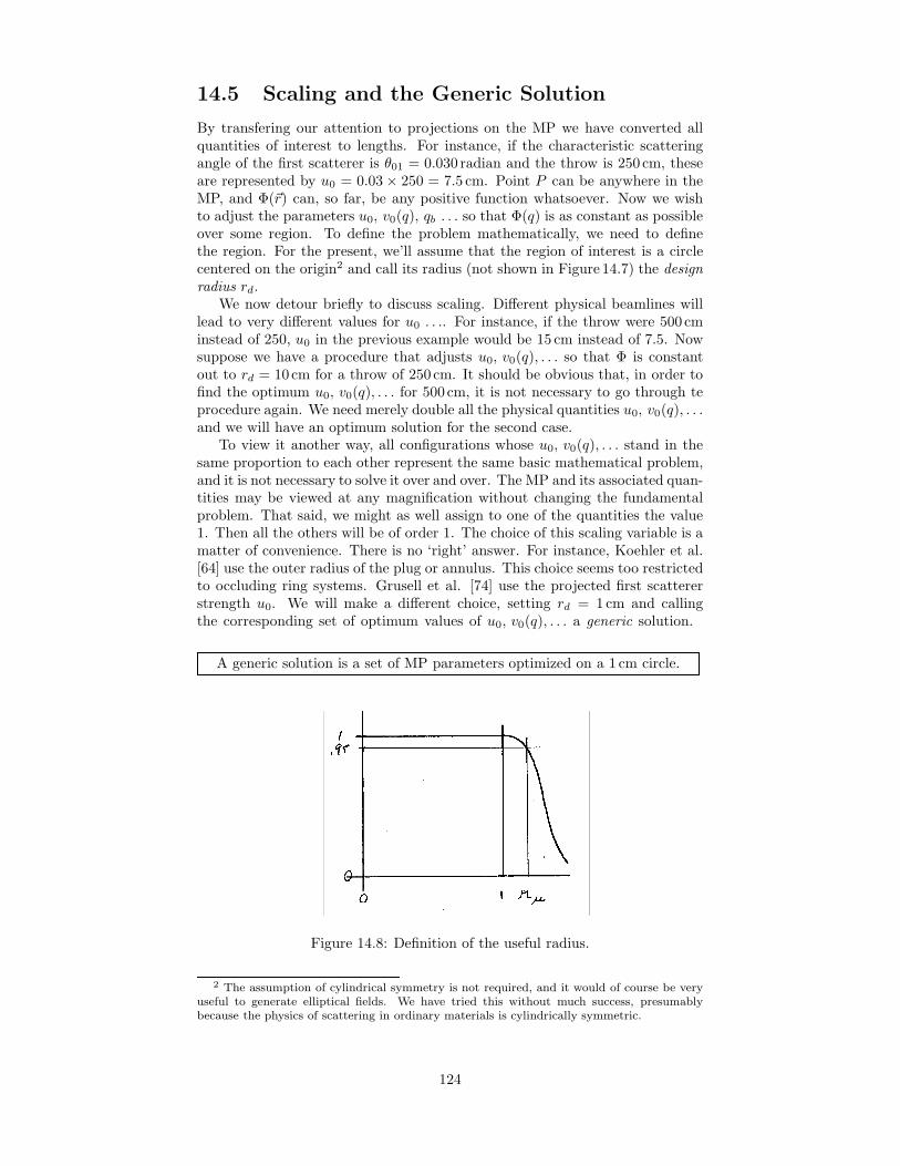
14.5 Scaling and the Generic Solution

By transfering our attention to projections on the MP we have converted allquantities of interest to lengths. For instance, if the characteristic scatteringangle of the first scatterer is θ01 = 0.030 radian and the throw is 250 cm, theseare represented by u0 = 0.03 × 250 = 7.5 cm. Point P can be anywhere in theMP, and Φ(~r) can, so far, be any positive function whatsoever. Now we wishto adjust the parameters u0, v0(q), qb . . . so that Φ(q) is as constant as possibleover some region. To define the problem mathematically, we need to definethe region. For the present, we’ll assume that the region of interest is a circlecentered on the origin2 and call its radius (not shown in Figure 14.7) the designradius rd.

We now detour briefly to discuss scaling. Different physical beamlines willlead to very different values for u0 . . .. For instance, if the throw were 500 cminstead of 250, u0 in the previous example would be 15 cm instead of 7.5. Nowsuppose we have a procedure that adjusts u0, v0(q), . . . so that Φ is constantout to rd = 10cm for a throw of 250 cm. It should be obvious that, in order tofind the optimum u0, v0(q), . . . for 500 cm, it is not necessary to go through teprocedure again. We need merely double all the physical quantities u0, v0(q), . . .and we will have an optimum solution for the second case.

To view it another way, all configurations whose u0, v0(q), . . . stand in thesame proportion to each other represent the same basic mathematical problem,and it is not necessary to solve it over and over. The MP and its associated quan-tities may be viewed at any magnification without changing the fundamentalproblem. That said, we might as well assign to one of the quantities the value1. Then all the others will be of order 1. The choice of this scaling variable is amatter of convenience. There is no ‘right’ answer. For instance, Koehler et al.[64] use the outer radius of the plug or annulus. This choice seems too restrictedto occluding ring systems. Grusell et al. [74] use the projected first scattererstrength u0. We will make a different choice, setting rd = 1cm and callingthe corresponding set of optimum values of u0, v0(q), . . . a generic solution.

A generic solution is a set of MP parameters optimized on a 1 cm circle.

Figure 14.8: Definition of the useful radius.

2 The assumption of cylindrical symmetry is not required, and it would of course be veryuseful to generate elliptical fields. We have tried this without much success, presumablybecause the physics of scattering in ordinary materials is cylindrically symmetric.

124

14.6 The Useful Radius

We need to introduce still one more radius to the MP, the useful radius ru

characteristic of a given generic solution (Figure 14.8). The optimization processmay well yield a fluence function Φ that is totally flat out to 1 cm, but thatusually exceeds the specification. If, for instance, we require ± 2.5% uniformity,we are able to use everything out to the 95% isodose. ru = 1.2 for the genericsolution is typical, depending, of course, on the uniformity requirement and theexact shape of Φ.

14.7 Optimization

In the general case covering both occluding rings and contoured scatterers theparameters to be adjusted are u0, v0(q) and at least one radius r. Finding ageneric solution consists of adjusting these by trial and error to obtain as flatas possible a function Φ in the unit circle. There are other considerations inaddition to dose uniformity:

• Efficiency: the fluence fraction inside ru should be as large as possible.

• Energy loss: the sum of u0 and v0 (max) should be as small as possible.

• Energy compensation: v0(q) should be realizable with physical materials.

Some may weigh more heavily than others depending on circumstances. Tomake the first quantitative it is useful to define the efficiency ε as

ε ≡∫ 2π

0

∫ ru

0

Φ(r) r dr dφ (14.5)

recalling that the integral to ru = ∞ is 1 3 because of the normalization of thescattering functions. As to the third, we have already noted that it requiresv0(max)/v0(min) ≤ 4 if we use lead and lexan.

For contoured scatterers we need to choose a trial function whose parameterswe will vary. Grusell et al [74] use a modified cosine which is later discretized tonine steps (it is not clear why this last step is necessary). We will choose a cubicspline because it is guaranteed to be smooth and because we can fix the firstderivative at either end if we wish to. Figure 14.9 illustrates how we do this. Inthe top frame, we have defined four radii, the first being 0 and the last, thatof the hole in the scatterer holder. The y values, that is to say, the vi ≡ v(ri),are the adjustable parameters of the fit. Requiring y′ = 0 at r = 0 certainlyseems to make sense, but the other end is less clear. We have found interestingsolutions either by requiring y′ = 0 or letting it float (natural spline). In thelatter case we obtain secondary ‘wings’ in the contour and a slightly larger ε,but the gain is not great and the physical scatterer is harder to fabricate. Thelower frame illustrates a Siebers-type trial function. The design program willuse this form if we enter rmin > 0.

In finding the best parameters we will usually vary some ‘by hand’ and others‘by machine’, turning some computer progam loose on them. The followingprocedures work reasonably well:

• Occluding rings: vary u0, v0 and rmax by hand, the other ri by machine.

• Contoured: vary u0, v0 (max) and rmax by hand, the other vi by machine.

3 Because our integration procedure is numerical and there are numerous sources of erroror inaccuracy, it is extremely useful for the design program to check this fact numerically.

125

The machine procedure can either be a grid search or the Marquardt procedure(faster but less robust) [1]. Whatever machine procedure is used, it is essentialto be able to ‘lock’ and ‘unlock’ selected parameters while studying their effect.

Figure 14.9: Spline trial functions. Upper: domed. Lower: Siebers type.

Like the literature cited so far, we have been vague on optimization. In ouropinion, no fully satisfactory method has yet been found. To be specific, let’sconsider the optimization of a simple 4-parameter ‘domed’ contoured scattererby NEU, that is, finding v2, v3 and v4 given u0, v1 and the ri. If you try this, youwill always get a perfectly flat fluence over some finite region but, otherwise, theprocedure suffers from every ill known to non-linear optimization. The solutiondepends on starting values and even the method (grid or Marquardt). Thatmeans there are many minima of the objective function (which is just the rmsdeviation of the fluence from a constant). In addition, we have had a lot oftrouble steering the solution by hand to one or another objective: maximumε or minimum energy loss, for instance, or in assuring that the solution willsatisfy v0(max)/v0(min) ≤ 4. The general behavior suggests that the contouris over-parametrized, yet we have not had much luck cutting back to three vi

instead of four.That said, we have come up with some pretty good solutions that have

worked well in practice, and we doubt (but cannot prove) that anything verymuch better is waiting in the wings. Some reasonable generic profiles can befound in the NEU examples on the website. One can get an efficiency ε around45%, significantly better than anything we have seen for occluding rings, andthe dose is dead flat over most of the useful radius. Depth of penetration isbetter, within limits, if we load more scattering onto the first scatterer (it hasa longer lever arm) but of course the limit of that is single scattering which hasexceedingly poor depth of penetration. There may also be secondary reasons

126

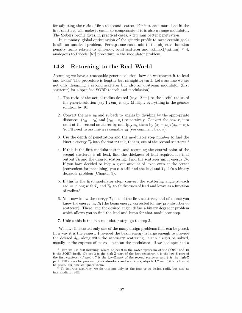
for adjusting the ratio of first to second scatter. For instance, more lead in thefirst scatterer will make it easier to compensate if it is also a range modulator.The Siebers profile gives, in practical cases, a few mm better penetration.

In summary, global optimization of the generic profile to meet certain goalsis still an unsolved problem. Perhaps one could add to the objective functionpenalty terms related to efficiency, total scatterer and v0(max)/v0(min) ≤ 4,analogous to Prieels’ [67] procedure in the modulator problem.

14.8 Returning to the Real World

Assuming we have a reasonable generic solution, how do we convert it to leadand lexan? The procedure is lengthy but straightforward. Let’s assume we arenot only designing a second scatterer but also an upstream modulator (firstscatterer) for a specified SOBP (depth and modulation).

1. The ratio of the actual radius desired (say 12 cm) to the useful radius ofthe generic solution (say 1.2 cm) is key. Multiply everything in the genericsolution by 10.

2. Convert the new u0 and vi back to angles by dividing by the appropriatedistances, (zm − z0) and (zm − z2) respectively. Convert the new ri intoradii at the second scatterer by multiplying them by (z2 − z0)/(zm − z0).You’ll need to assume a reasonable z0 (see comment below).

3. Use the depth of penetration and the modulator step number to find thekinetic energy T9 into the water tank, that is, out of the second scatterer.4

4. If this is the first modulator step, and assuming the central point of thesecond scatterer is all lead, find the thickness of lead required for thatoutput T9 and the desired scattering. Find the scatterer input energy T7.If you have decided to keep a given amount of lexan even at the center(convenient for machining) you can still find the lead and T7. It’s a binarydegrader problem (Chapter 9).

5. If this is the first modulator step, convert the scattering angle at eachradius, along with T7 and T9, to thicknesses of lead and lexan as a functionof radius.5

6. You now know the energy T5 out of the first scatterer, and of course youknow the energy in, T3 (the beam energy, corrected for any pre-absorber orscatterer). These, and the desired angle, define a binary degrader problemwhich allows you to find the lead and lexan for that modulator step.

7. Unless this is the last modulator step, go to step 3.

We have illustrated only one of the many design problems that can be posed.In a way it is the easiest. Provided the beam energy is large enough to providethe desired d80 along with the necessary scattering, it can always be solved,usually at the expense of excess lexan on the modulator. If we had specified a

4 Here we use NEU indexing, where object 9 is the water upstream of the SOBP and 10is the SOBP itself. Object 3 is the high-Z part of the first scatterer, 4 is the low-Z part ofthe first scatterer (if used), 7 is the low-Z part of the second scatterer and 8 is the high-Zpart. NEU allows for pre- and post- absorbers and scatterers, objects 1,2 and 5,6 which mustbe given. For now we ignore them.

5 To improve accuracy, we do this not only at the four or so design radii, but also atintermediate radii.

127

simple first scatterer rather than a modulator, the problem would be overdeter-mined. We cannot specify a beam energy, a scattering system and at the sametime, a depth of penetration. NEU is set up to handle many different problems.Here, we have only tried to show one of many paths through the woods.

We have also simplified the explanation by ignoring the dependence of z0 onmodulator step. This has two ramifications. First, the physical second scatterercan only be designed exactly for one modulator step. It makes sense to use thefirst (thinnest) step which has by far the greatest weight. Second, the entireprocess just described needs to be iterated over z0. As usual, you should lookat the program (NEU and its subroutines) for the exact logic.

It may happens that compensation fails for some steps. Second scatterercompensation will fail if the generic solution calls for too little scattering. Thenthe lexan required for the given energy loss (which always takes priority) alreadyoverscatters the protons. The same applies to the modulator. Compensationwill fail if the amount of lexan required for that step already overscatters theprotons. In either case, there will be error messages. Neither case is necessarilyfatal to an acceptable design. NEU automatically finishes in a playback modewhere the dose distribution is computed for the devices (modulator and secondscatterer) as designed rather than the ideal devices. The dose distributions willshow you whether the failures in compensation are acceptable or not.

128

Chapter 15

Double ScatteringUpstream ModulatorExample

This chapter will explain how NEU solves various problems involving a firstscatterer or modulator and a second scatterer (none or occluding ring or con-toured). A key feature is automatic playback of the design using components asdesigned rather than ideal components.

129

Chapter 16

Beam Steering

This chapter will explain the sensitivity of double scattering to beam imper-fections, in particular misalignment at the second scatterer. It will discussdynamic beam steering to correct misalignment, assuming we have a qualitycontrol chamber either near the second scatterer or near the patient (skewnessand all that).

130

Chapter 17

Capabilities of DoubleScattering Systems

This chapter will survey the global capabilities of double scattering systems.For instance, if we have a fixed beam energy but can vary the throw, whatcombinations of treatment depth and field radius are possible? How do thesecompare with clinical requirements?

131

Chapter 18

Transverse Penumbra

This chapter will discuss how to compute transverse penumbra at some depthof interest in the patient, given the nozzle configuration (e.g. position andthickness of range shifter and modulator). Transverse penumbra is minimizedby putting beam modifying materials as far upstream as possible.

132

Chapter 19

Distal Falloff

This short chapter will discuss how to sharpen distal falloff by minimizing excessmaterial in the beam.

133

Chapter 20

Collimators

This chapter will discuss collimator scatter and the wise and unwise use ofcollimators.

134

List of Tables

7.1 Moliere parameters for 158.6 MeV protons incident on Be, Cu andPb using the ICRU49 [2] range-energy tables. N is the numberof target slabs used for numerical integration. See text for otherdefinitions. . . . . . . . . . . . . . . . . . . . . . . . . . . . . . . 56

135

List of Figures

1.1 The first NEU design (1990), with experimental data. . . . . . . 6

3.1 Drawing used in deriving Eq.3.6 . . . . . . . . . . . . . . . . . . 143.2 Drawing used in deriving Eq.3.9 . . . . . . . . . . . . . . . . . . 16

4.1 Coordinates and definitions for scattering. . . . . . . . . . . . . . 204.2 Gaussian radial distribution assuming r0 = 1cm. . . . . . . . . . 224.3 Geometry of transverse penumbra calculation. . . . . . . . . . . . 234.4 Penumbra profile showing 80/20 width. . . . . . . . . . . . . . . 25

5.1 Cubic spline fit. Light line: cubic spline used to interpolate noisydata (full squares). Dashed line: linear interpolation of the samedata. Bold line: cubic spline fit to the data, using 5 auxiliarypoints (hollow squares). . . . . . . . . . . . . . . . . . . . . . . . 27

5.2 Procedure for picking initial spline points. Bottom frame: Braggpeak to be fitted. Top frame: smoothed second derivative of theBragg peak. Middle frame: density function (see text). . . . . . . 29

5.3 Upper frame: Bragg peak with spline fit. Lower frame: deviationfrom fit. The dashed lines are at ± the rms deviation. . . . . . . 30

5.4 Spread-out Bragg peak fit by 3-segment broken spline. . . . . . . 315.5 Compensated contoured second scatterer. . . . . . . . . . . . . . 32

6.1 Range straggling in several materials, from Janni [3]. . . . . . . . 366.2 Fluence, differential fluence and dose as a function of depth for

proton beams of a given range and different energy spreads, il-lustrating r0 = d80. . . . . . . . . . . . . . . . . . . . . . . . . . . 37

6.3 d80 and d90 vs. range at nozzle entrance’ measured at NPTC. . . 396.4 Range-energy in Be, Cu and Pb. Lower frame: test of cubic spline

interpolation of points at .1, .2, .5, 1 . . . MeV. . . . . . . . . . . . 406.5 Range-energy over the clinically useful energy range for 4 useful

materials. . . . . . . . . . . . . . . . . . . . . . . . . . . . . . . . 446.6 Drawing for proof of Eq. (6.14). . . . . . . . . . . . . . . . . . . . 466.7 Energy spectra of degraded proton beams at NPTC. Energy spread

and skewness increase as the energy is reduced. . . . . . . . . . . 486.8 Drawing for proof of Eq. (6.18). . . . . . . . . . . . . . . . . . . . 48

7.1 Grand summary of proton results reviewed in [4]. The x coordi-nate is arbitrary and the target names merely serve as landmarks.Data from each experiment are averaged over everything but tar-get material. . . . . . . . . . . . . . . . . . . . . . . . . . . . . . 50

7.2 Moliere/Fano theory vs. experiment for four metals [4] . . . . . . 577.3 Expanded view of Figure 7.2 near end of range. . . . . . . . . . . 577.4 Deviation from Moliere/Fano theory as a function of normalized

target thickness for HCL data [4]. . . . . . . . . . . . . . . . . . . 58

136

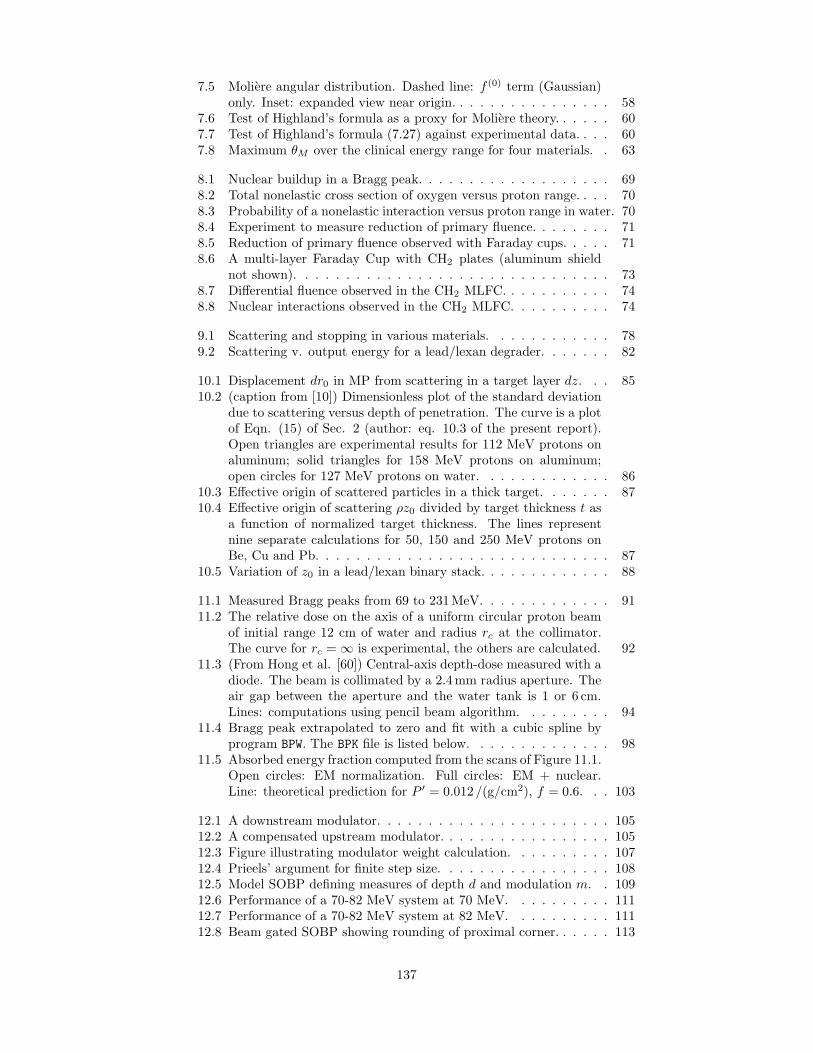
7.5 Moliere angular distribution. Dashed line: f (0) term (Gaussian)only. Inset: expanded view near origin. . . . . . . . . . . . . . . . 58

7.6 Test of Highland’s formula as a proxy for Moliere theory. . . . . . 607.7 Test of Highland’s formula (7.27) against experimental data. . . . 607.8 Maximum θM over the clinical energy range for four materials. . 63

8.1 Nuclear buildup in a Bragg peak. . . . . . . . . . . . . . . . . . . 698.2 Total nonelastic cross section of oxygen versus proton range. . . . 708.3 Probability of a nonelastic interaction versus proton range in water. 708.4 Experiment to measure reduction of primary fluence. . . . . . . . 718.5 Reduction of primary fluence observed with Faraday cups. . . . . 718.6 A multi-layer Faraday Cup with CH2 plates (aluminum shield

not shown). . . . . . . . . . . . . . . . . . . . . . . . . . . . . . . 738.7 Differential fluence observed in the CH2 MLFC. . . . . . . . . . . 748.8 Nuclear interactions observed in the CH2 MLFC. . . . . . . . . . 74

9.1 Scattering and stopping in various materials. . . . . . . . . . . . 789.2 Scattering v. output energy for a lead/lexan degrader. . . . . . . 82

10.1 Displacement dr0 in MP from scattering in a target layer dz. . . 8510.2 (caption from [10]) Dimensionless plot of the standard deviation

due to scattering versus depth of penetration. The curve is a plotof Eqn. (15) of Sec. 2 (author: eq. 10.3 of the present report).Open triangles are experimental results for 112 MeV protons onaluminum; solid triangles for 158 MeV protons on aluminum;open circles for 127 MeV protons on water. . . . . . . . . . . . . 86

10.3 Effective origin of scattered particles in a thick target. . . . . . . 8710.4 Effective origin of scattering ρz0 divided by target thickness t as

a function of normalized target thickness. The lines representnine separate calculations for 50, 150 and 250 MeV protons onBe, Cu and Pb. . . . . . . . . . . . . . . . . . . . . . . . . . . . . 87

10.5 Variation of z0 in a lead/lexan binary stack. . . . . . . . . . . . . 88

11.1 Measured Bragg peaks from 69 to 231MeV. . . . . . . . . . . . . 9111.2 The relative dose on the axis of a uniform circular proton beam

of initial range 12 cm of water and radius rc at the collimator.The curve for rc = ∞ is experimental, the others are calculated. 92

11.3 (From Hong et al. [60]) Central-axis depth-dose measured with adiode. The beam is collimated by a 2.4mm radius aperture. Theair gap between the aperture and the water tank is 1 or 6 cm.Lines: computations using pencil beam algorithm. . . . . . . . . 94

11.4 Bragg peak extrapolated to zero and fit with a cubic spline byprogram BPW. The BPK file is listed below. . . . . . . . . . . . . . 98

11.5 Absorbed energy fraction computed from the scans of Figure 11.1.Open circles: EM normalization. Full circles: EM + nuclear.Line: theoretical prediction for P ′ = 0.012/(g/cm2), f = 0.6. . . 103

12.1 A downstream modulator. . . . . . . . . . . . . . . . . . . . . . . 10512.2 A compensated upstream modulator. . . . . . . . . . . . . . . . . 10512.3 Figure illustrating modulator weight calculation. . . . . . . . . . 10712.4 Prieels’ argument for finite step size. . . . . . . . . . . . . . . . . 10812.5 Model SOBP defining measures of depth d and modulation m. . 10912.6 Performance of a 70-82 MeV system at 70 MeV. . . . . . . . . . 11112.7 Performance of a 70-82 MeV system at 82 MeV. . . . . . . . . . 11112.8 Beam gated SOBP showing rounding of proximal corner. . . . . . 113

137

12.9 The 3 × 3 arrangement of modulator wheels. . . . . . . . . . . . 115

14.1 Double scattering with a beam stopper [64]. . . . . . . . . . . . . 11714.2 The effect of beam steering on double scattering. . . . . . . . . . 11814.3 Double scattering with dual-ring scatterer [72]. . . . . . . . . . . 11914.4 Double scattering with contoured scatterer [74]. . . . . . . . . . . 12014.5 Left: second scatterer with Siebers-type profile [75]. Right: cross-

field scans [76] at entrance and at Bragg peak. . . . . . . . . . . 12014.6 Geometry of double scattering system. . . . . . . . . . . . . . . . 12214.7 Double scattering projected on the measuring plane. . . . . . . . 12214.8 Definition of the useful radius. . . . . . . . . . . . . . . . . . . . 12414.9 Spline trial functions. Upper: domed. Lower: Siebers type. . . . 126

138

Bibliography

[1] W.H. Press, B.P. Flannery, S.A. Teukolsky and W.T. Vetterling, “Numeri-cal Recipes: the Art of Scientific Computing,” Cambridge University Press(1986).

[2] Berger et al., ‘Stopping Powers and Ranges for Protons and Alpha Parti-cles,’ ICRU Report 49 (1993).

[3] J.F. Janni, ‘Proton Range-Energy Tables, 1KeV - 10 GeV,’ Atomic Dataand Nuclear Data Tables 27 parts 1 (compounds) and 2 (elements) (Aca-demic Press, 1982).

[4] Gottschalk et al., ‘Multiple Coulomb scattering of 160 MeV protons,’ Nucl.Instr. Meth. B74 (1993) 467-490. We have discovered the following errors:Eq.(2) should read

Ξ(χ) =1π

χ2c

(χ2 + χ2a)2

and in Table 1 the heading α should read α2 and ×109 under χ2c should

read ×106.

[5] H.A. Bethe, ‘Moliere’s theory of multiple scattering,’ Phys. Rev. 89 (1953)1256-1266. Four entries in the second column (the Gaussian) of Table IIare slightly incorrect (A. Cormack, priv. comm.) but the error (correctedin our programs) is at worst 1%.

[6] G. Moliere, ‘Theorie der Streuung schneller geladenen Teilchen I Einzel-streuung am abgeschirmten Coulomb-Feld,’ Z. Naturforschg. 2a (1947) 133-145.

[7] G. Moliere, ‘Theorie der Streuung schneller geladenen Teilchen II Mehrfach-und Vielfachstreuung,’ Z. Naturforschg. 3a (1948) 78-97.

[8] W.T. Chu, B.A. Ludewigt and T.R. Renner, ‘Instrumentation for treatmentof cancer using proton and light-ion beams,’ Rev. Sci. Instr. 64 (1993) 2055-2122.

[9] Richard Wilson, “A Brief History of the Harvard University Cyclotrons,”Harvard University Department of Physics (2004) (distributed by HarvardUniversity Press, Cambridge, Massachusetts).

[10] W.M. Preston and A.M. Koehler, ‘The effects of scattering on small protonbeams,’ unpublished manuscript (1968), Harvard Cyclotron Laboratory.

[11] Eidelman et al., ‘Review of Particle Physics,’ Phys. Lett. B592 (2004).Tables, listings, reviews and errata are also available at the Particle DataGroup website http://pdg.lbl.gov.

139

[12] Verhey et al., ‘Clinical Proton Dosimetry Part I: Beam Production, BeamDelivery and Measurement of Absorbed Dose,’ ICRU Report 59 (1998).

[13] M.R. Raju, “Heavy Particle Radiotherapy,” Academic Press (1980).

[14] NCRP Report #93, “Ionizing Radiation Exposure of the Population of theUnited States,” (1987). For an excerpt, Google ‘average annual exposure’.

[15] U.S. Nuclear Regulatory Commission 56FR23396 (Google ‘occupationaldose limits’).

[16] A.C. Upton, ‘Health effects of low-level ionizing radiation,’ Physics Today44/8 (1991) 34-39.

[17] J.W. Boag, ‘Ionization chambers,’ in “The Dosimetry of Ionizing Radi-ation,” ed. K.R. Kase, B.E. Bjarngard and F.H. Attix, Academic Press(1987) 169-243.

[18] R. Hagedorn, “Relativistic Kinematics,” W.A. Benjamin (1963).

[19] M. Abramowitz and I.A. Stegun, ‘Handbook of Mathematical Functions,’Dover, New York (Ninth printing, 1970).

[20] H.B. Dwight, ‘Tables of Integrals and Other Mathematical Data,’ Macmil-lan (1952).

[21] Philip R. Bevington, “Data Reduction and Error Analysis for the PhysicalSciences,” McGraw-Hill (1969).

[22] B. Gottschalk, ‘On the Characterization of Spread-Out Bragg Peaks andthe Definition of Depth and Modulation,’ technical report 28APR03 avail-able at http://huhepl.harvard.edu/˜gottschalk.

[23] H.A. Bethe and J. Ashkin, ‘Passage of radiations through matter,’ in Ex-perimental Nuclear Physics, E. Segre (ed.), Wiley, New York (1953): PartII, page 283 et seg.

[24] B. Gottschalk, R. Platais and H. Paganetti, ‘Nuclear interactions of 160MeV protons stopping in copper: a test of Monte Carlo nuclear models,’Med. Phys. 26(12) (1999) 2597-2601.

[25] H. Paganetti and B. Gottschalk, ‘Test of GEANT3 and GEANT4 nuclearmodels for 160 MeV protons stopping in CH2,’ Med. Phys. 30(7) (2003)1926-1931.

[26] Thomas Bortfeld, ‘An analytical approximation of the Bragg curve fortherapeutic proton beams,’ Med. Phys. 24(12) (1997) 2024-2033.

[27] Martin J. Berger, ‘Status of proton transport calculations,’ unpublishedNIST technical note (June 1992).

[28] G. Arduini, R. Cambria, C. Canzi, F. Gerardi, B. Gottschalk, R. Leone, L.Sangaletti and M. Silari, ‘Physical specifications of clinical proton beamsfrom a synchrotron,’ Med. Phys. 23(6) (1996) 939-951.

[29] E.W. Cascio, J.M. Sisterson, B. Gottschalk and S. Sarkar, ‘Measurementsof the Energy Spectrum of Degraded Proton Beams at NPTC,’ Proc. IEEERadiation Effects Data Workshop (2004) (in press).

140

[30] B.P. Nigam, M.K. Sundaresan and Ta-You Wu, ‘Theory of multiple scatter-ing: second Born approximation and corrections to Moliere’s work,’ Phys.Rev. 115 (1959) 491-502.

[31] U. Fano, ‘Inelastic collisions and the Moliere theory of multiple scattering,’Phys. Rev. 93 (1954) 117-120.

[32] M.J. Berger and R. Wang, in “Monte Carlo transport of electrons andphotons,’ eds. T.M. Jenkins, W.R. Nelson and A. Rindi (Plenum, 1989).

[33] C. Kittel, “Elementary Statistical Physics,” Wiley (1967).

[34] W.T. Scott, ‘The theory of small-angle multiple scattering of fast chargedparticles,’ Rev. Mod. Phys. 35 (1963) 231-313.

[35] A.O.Hanson, L.H. Lanzl, E.M. Lyman and M.B. Scott, ‘Measurement ofmultiple scattering of 15.7-MeV electrons,’ Phys. Rev. 84 (1951) 634-637.

[36] V.L. Highland,‘Some practical remarks on multiple scattering,’ Nucl. Instr.Meth. 129 (1975) 497-499 and Erratum, Nucl. Instr. Meth. 161 (1979) 171.

[37] B. Rossi and K. Greisen, ‘Cosmic-Ray Theory,’ Rev. Mod. Phys. 12 (1941)240-309.

[38] G.R. Lynch and O.I.Dahl, ‘Approximations to multiple Coulomb scatter-ing,’ Nucl. Instr. Meth. B58 (1991) 6.

[39] Chadwick et al., ‘Nuclear Data for Neutron and Proton Radiotherapy andfor Radiation Protection,’ ICRU Report 63 (2000).

[40] B. Gottschalk, K.H. Wang and K. Strauch, ‘Distorted momentum distri-butions from quasi-elastic proton-proton scattering in carbon at 160 MeV,’Nucl. Phys. A90 (1) (1967) 83-100.

[41] B. Gottschalk, W.J. Shlaer and K.H. Wang, ‘Proton-proton bremsstrahlungat 158 MeV,’ Nucl. Phys. 75 (3) (1965) 549-560.

[42] B. Gottschalk and S.L. Kannenberg, ‘Quasi-elastic scattering of 160 MeVprotons by alpha clusters in light nuclei I. Carbon,’ Phys. Rev. C2 (1)(1970) 24-40.

[43] Stephen M. Seltzer, ‘An assessment of the role of charged secondaries fromnonelastic nuclear interactions by therapy proton beams in water,’ NISTtechnical note NISTIR 5221 (1993) (available from the National TechnicalInformation Service, NTIS, U.S. Department of Commerce, Springfield, VA22161.

[44] H. Paganetti and M. Goitein, ‘Radiobiological significance of beam linedependent proton energy distributions in a spread-out Bragg peak,’ Med.Phys. 27 (2000) 1119-1126.

[45] H. Paganetti and M. Goitein, ‘Biophysical modeling of proton radiationeffects based amorphous track models,’ International Journal of RadiationBiology 77 (2001) 911-928.

[46] We thank Damien Prieels of Ion Beam Applications s.a. (IBA) for providingus with figure 8.1.

[47] C.A. Carlsson and G.A. Carlsson, ‘Proton dosimetry with 185 MeV pro-tons: dose buildup from secondary protons and recoil electrons,’ HealthPhys. 33 (1977) 481-484.

141

[48] Lynn J. Verhey, Andreas M. Koehler, Joseph C. McDonald, MichaelGoitein, I-Chang Ma, Robert J. Schneider and Miles Wagner, ‘The determi-nation of absorbed dose in a proton beam for purposes of charged-particleradiation therapy,’ Radiation Research 79 (1979) 34-54.

[49] A. Mascia, J. DeMarco, P. Chow and T. Solberg, ‘Benchmarking the MC-NPX nuclear interaction models for use in the proton therapy energy range,’Proc. XIVth Intl. Conf. on the Use of Computers in Radiation Therapy,Seoul, May 10-13 (2004) 478-481.

[50] H. Paganetti, H. Jiang, S.-Y. Lee and H.M. Kooy, ‘Accurate Monte Carlosimulations fro nozzle design, commissioning and quality assurance for aproton radiation therapy facility,’ Med. Phys. 31 (7) (2004) 2107-2118.

[51] L. Eyges, ‘Multiple scattering with energy loss,’ Phys. Rev. 74 (1948) 1534-1535.

[52] C.D. Zerby and F.L. Keller, ‘Electron transport theory, calculations, andexperiments,’ Nucl. Sci. Eng. 27 (1967) 190-218.

[53] A.M. Koehler, priv. comm.

[54] H. Bichsel and T. Hiraoka, ‘Energy spectra and depth-dose curves for 70MeV protons,’ Intl. Journ. Quant. Chem. 23 (1989) 565-574.

[55] Martin J. Berger, ‘Penetration of proton beams through water I. Depth-dose distribution, spectra and LET distribution,’ NIST technical note NI-STIR 5226 (1993) (available from the National Technical Information Ser-vice, NTIS, U.S. Department of Commerce, Springfield, VA 22161.

[56] H. Bichsel, ‘Calculated Bragg curves for ionization chambers of differentshapes,’ Med. Phys. 22(11) (1995) 1721-1726.

[57] A.M. Koehler, ‘Dosimetry of proton beams using small silicon diodes,’ Rad.Res. Suppl. 7 (1967) 53-63.

[58] E.J. Burge and D.A. Smith, ‘Theoretical study of slit scattering,’ Rev. Sci.Inst. 33 (1962) 1371-1377.

[59] P. van Luijk, A.A. van’t Veld, H.D. Zelle and J.M. Schippers, ‘Collimatorscatter and 2D dosimetry in small proton beams,’ Phys. Med. Biol 46(2001) 653-670.

[60] Hong et al., ‘A pencil beam algorithm for proton dose calculations,’ Phys.Med. Biol. 41 (1996) 1305-1330.

[61] Computerized Radiation Scanners Inc., 140 Sopwith Drive, Vero Beach, FL32968, tel (772) 562 0405, email crs5@juno.com.

[62] B. Gottschalk, ‘Logarithmic audible ratemeter for NPTC,’ technical noteHCL 3/17/00.

[63] R.R. Wilson, ‘Radiological use of fast protons,’ Radiology 47 (1946) 487-491.

[64] A.M. Koehler, R.J. Schneider and J.M. Sisterson, ‘Flattening of proton dosedistributions for large-field radiotherapy,’ Med. Phys. 4(4) (1977) 297-301.

[65] B. Gottschalk, A.M. Koehler, J.M. Sisterson and M.S. Wagner, ‘The casefor passive beam spreading,’ proc. Proton Therapy Workshop, Paul Scher-rer Institut (1991) 50-53 (PSI report 111).

142

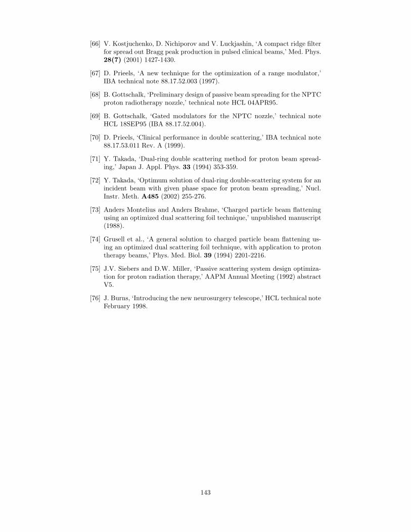
[66] V. Kostjuchenko, D. Nichiporov and V. Luckjashin, ‘A compact ridge filterfor spread out Bragg peak production in pulsed clinical beams,’ Med. Phys.28(7) (2001) 1427-1430.

[67] D. Prieels, ‘A new technique for the optimization of a range modulator,’IBA technical note 88.17.52.003 (1997).

[68] B. Gottschalk, ‘Preliminary design of passive beam spreading for the NPTCproton radiotherapy nozzle,’ technical note HCL 04APR95.

[69] B. Gottschalk, ‘Gated modulators for the NPTC nozzle,’ technical noteHCL 18SEP95 (IBA 88.17.52.004).

[70] D. Prieels, ‘Clinical performance in double scattering,’ IBA technical note88.17.53.011 Rev. A (1999).

[71] Y. Takada, ‘Dual-ring double scattering method for proton beam spread-ing,’ Japan J. Appl. Phys. 33 (1994) 353-359.

[72] Y. Takada, ‘Optimum solution of dual-ring double-scattering system for anincident beam with given phase space for proton beam spreading,’ Nucl.Instr. Meth. A485 (2002) 255-276.

[73] Anders Montelius and Anders Brahme, ‘Charged particle beam flatteningusing an optimized dual scattering foil technique,’ unpublished manuscript(1988).

[74] Grusell et al., ‘A general solution to charged particle beam flattening us-ing an optimized dual scattering foil technique, with application to protontherapy beams,’ Phys. Med. Biol. 39 (1994) 2201-2216.

[75] J.V. Siebers and D.W. Miller, ‘Passive scattering system design optimiza-tion for proton radiation therapy,’ AAPM Annual Meeting (1992) abstractV5.

[76] J. Burns, ‘Introducing the new neurosurgery telescope,’ HCL technical noteFebruary 1998.

143