Digital Surface Representation and the Constructibility of Gehry’s Architecture by Dennis R. Shelden Director of Computing, Gehry Partners, LLP. MS Civil and Environmental Engineering, MIT, 1997 Submitted to the Department of Architecture in partial fulfillment of the requirements for the degree of DOCTOR OF PHILOSOPHY IN THE FIELD OF ARCHITECTURE: DESIGN AND COMPUTATION AT THE MASACHUSETTS INSTITUTE OF TECHNOLOGY SEPTEMBER 2002 © 2002 Dennis R. Shelden. All rights reserved. The author hereby grants to MIT permission to reproduce and to distribute publicly paper and electronic copies of thesis document in whole or in part. Signature of Author:

Department of Architecture August 9, 2002

Certified by:

William J. Mitchell Dean of the School of Architecture and Planning

Professor of Architecture and Media Arts and Sciences Thesis Supervisor

Certified by:

Stanford Anderson Professor of History and Architecture

Chair, Department Committee on Graduate Students

1

READERS William J. Mitchell Dean of the School of Architecture and Planning, Professor of Architecture and Media Arts and Sciences, MIT Thesis Supervisor John R. Williams Associate Professor of Civil and Environmental Engineering, Associate Engineering Systems, MIT George Stiny Professor of Design and Computation, MIT

2

Digital Surface Representation and the Constructibility of Gehry’s Architecture

by

Dennis R. Shelden Director of Computing, Gehry Partners, LLP.

MS Civil and Environmental Engineering, MIT, 1997

Submitted To The Department Of Architecture on August 9, 2002 in Partial Fulfillment of the Requirements for the Degree of

Doctor of Philosophy in the Field Of Architecture: Design And Computation

ABSTRACT

This thesis presents work in the development of computational descriptions of Gehry’s architectural forms. In Gehry’s process for realizing buildings, computation serves as an intermediary agent for the integration of design intent with the geometric logics of fabrication and construction. This agenda for digital representation of both formal and operational intentions, in the context of an ongoing exploration of challenging geometries, has provided new roles for computation in architectural practice. The work described in this thesis focuses on the digital representation of surface geometry and its capacity for describing the constructibility of building enclosure systems. A particular class of paper surface forms – curved surfaces with minimal in plane deformation of the surface material – provide the specific object of inquiry for exploring the relationships between form, geometry and constructibility. An analysis and framework for the description of Gehry’s geometry is developed through existing theory of differential geometry and topology. Geometric rules of constructibility associated with several enclosure system strategies are presented in this framework. With this theoretical framework in place, the discussion turns to efforts to develop generative strategies for the rationalization of surface forms into constructible configurations.

Thesis Supervisor: William J. Mitchell Title: Dean of the School of Architecture and Planning, Professor of Architecture and Media Arts and Sciences, MIT

3

4

ACKNOWLEDGEMENTS

A work of this nature owes a heavy debt of gratitude to many persons. During the time that

this thesis has been prepared, it has been my rare privilege to work closely with a number of

enormously talented individuals, both members of Gehry’s firm as well as those of

associated engineering, construction and fabrication organizations. The products of their

efforts are often referenced in this work, and the inspiration for this inquiry would not have

occurred without their influence. In the interest of brevity, I can unfortunately only mention a

few of their names.

The first and foremost debt of gratitude is owed to Frank Gehry himself. His design vision

and exploratory energy have fostered the community of talent and ideas in which the work

described in this document has occurred. The efforts to realize his design ambitions have

resulted in a context of architectural and building practice for which there is perhaps no

equivalent at this point of writing. Furthermore, his commitment to the achievement of these

design intentions have translated into a support of computational efforts beyond that of his

contemporaries, and have provided the environment for computational inquiry in which the

work described in this document has taken place.

Jim Glymph has served as a mentor and inspiration on all matters architectural and

computational during my time with the firm. The description of a reconstructed architectural

practice presented in Part 1 of this document is largely attributable to many hours of formal

and informal discussions with this visionary practitioner.

The opportunity to apply this research to the firm’s projects has occurred through close

collaboration with the senior designers and project architects on these projects. I gratefully

acknowledge Partner Randy Jefferson, Project Designers Craig Webb and Edwin Chan, and

Project Architects Terry Bell (Disney Concert Hall), Marc Salette (MIT Stata Center), George

Metzger and Larry Tighe (Experience Music Project), Gerhard Mayer (Weatherhead) and

Michal Sedlacek (Museum of Tolerance), for their support and willingness to accommodate

these research efforts on their projects.

The firm’s computational methodologies are similarly the product of many persons’ efforts.

The work of Rick Smith of C-Cubed, Kristin Woehl, Henry Brawner and Kurt Komraus on

5

projects is extensively referenced in this document, while the efforts of Reg Prentice and

Cristiano Ceccato in the computing group have profoundly contributed to the development of

the firm’s computational practice. David Bonner of Dassault Systèmes Research and

Development and John Weatherwax from Department of Mathematics at MIT assisted

substantially in the formulation of the material simulation model described in Chapter VII.

On the academic front, I would like to thank the members of my Doctoral Committee, for their

guidance and support of what has become a circuitous path to the completion of this thesis.

Finally, I thank the Reader, for taking the time and interest to review the thoughts contained

herein.

6

TABLE OF CONTENTS

Abstract ................................................................................................................................... 3 Acknowledgements ................................................................................................................. 5 Table of Contents .................................................................................................................... 7 Table of Figures....................................................................................................................... 9 Table of Symbols................................................................................................................... 15 Referenced Projects and Abbreviations ................................................................................ 17 Foreword ............................................................................................................................... 19

Part 1: Digital Representation and Constructibility.......................................................... 21 I. Introduction..................................................................................................................... 23 II. The Development of Gehry’s Building Process.............................................................. 33

A. Project Cost Control ................................................................................................ 33 B. Building Team Organization and Information Flow ................................................. 37 C. Fabrication Economies............................................................................................ 43 D. Manufacturing Technologies and Methods ............................................................. 46 E. Dimensional Tolerances.......................................................................................... 47

III. The Master Model Methodology ................................................................................. 51 A. Introduction ............................................................................................................. 51 B. Project Control ........................................................................................................ 57 C. Performance Analysis ............................................................................................. 58 D. 3D – 2D Integration ................................................................................................. 63 E. The Physical / Digital Interface................................................................................ 68 F. Rationalization ........................................................................................................ 78 G. Model intelligence, Automation, and Parametrics ................................................... 89

Part 2: The Representation of Surface Constructibility ................................................... 97 IV. Materiality and its Geometric Representations ......................................................... 101

A. Planar Surfaces..................................................................................................... 101 B. “Free Form” Surfaces............................................................................................ 104 C. Paper Surfaces ..................................................................................................... 110

V. Mathematics of Curved Spaces and Objects............................................................ 119 A. Spaces in Mathematical Forms............................................................................. 119

7

B. Vector spaces ....................................................................................................... 122 C. Mappings............................................................................................................... 126 D. Curves and Surfaces............................................................................................. 130

VI. Differential Forms And Applications to Surface Constructibility ................................ 157 A. Constrained Gaussian Curvature.......................................................................... 157 B. Developable Surfaces ........................................................................................... 170 C. Summary of Existing Paper Surface Representations .......................................... 195

VII. Physical Modeling..................................................................................................... 203 A. Introduction ........................................................................................................... 203 B. Deformable Body Motion....................................................................................... 208 C. A Simple Example................................................................................................. 212 D. Implicit Integration Approach................................................................................. 218 E. Backwards Euler Method ...................................................................................... 220 F. Material Formulation ............................................................................................. 221 G. Solution Method .................................................................................................... 232 H. The Interactive Framework ................................................................................... 238 I. Isometries ............................................................................................................. 249 J. Materials Modeling Application: Guggenheim Installation ................................... 256

Part 3: The Generation of Surface Assemblies............................................................... 263 VIII. Generating Assemblies............................................................................................. 265

A. Generative Systems and Shape grammars .......................................................... 267 B. Manifold Grammars............................................................................................... 271 C. Summary............................................................................................................... 284

IX. Generative Rationalization........................................................................................ 285 A. Generative Applications on the Experience Music Project.................................... 286 B. Materials Based Rationalization............................................................................ 303

Conclusion........................................................................................................................... 333 Bibliography......................................................................................................................... 335

8

TABLE OF FIGURES

Figure I-1: Barcelona fish, physical and digital construction models. Photo: GP Archives.... 27

Figure II-1 Standard contractual organization ....................................................................... 38

Figure II-2: Communication path and controls....................................................................... 40

Figure III-1: Elements of 3D master model (DCH)................................................................. 53

Figure III-2: Structural wireframe contract model (EMP). Photo: L. Tighe, G. Metzger ......... 54

Figure III-3: Coordination model of ceiling space .................................................................. 57

Figure III-4: CIFE’s 4D modeling tool (DCH) ......................................................................... 58

Figure III-5: Finite element analysis of frame (Riscal) ........................................................... 59

Figure III-6: CFD fire safety analysis (Weatherhead) ............................................................ 60

Figure III-7: CFD wind studies (MIT)...................................................................................... 62

Figure III-8: Solar shadow studies (MIT)................................................................................ 62

Figure III-9: Drawing extraction from the CATIA master model (MOT).................................. 66

Figure III-10: Re-integration of two dimensional information in 3D (MIT) .............................. 67

Figure III-11: Digitized data, CAD model and prototyped model. (Ohr). Photo: W. Preston.. 70

Figure III-12: CAT scan and reconstruction of a complicated physical model (DCH)............ 73

Figure III-13: The physical master model and its digital counterpart (MIT)Photo:W.Preston 74

Figure III-14: Schematic design phase physical and digital structural studies....................... 75

Figure III-15: “Digital Mockup” studies................................................................................... 76

Figure III-16: Performance mockup of DCH cladding systems. Photo: H. Baumgartner ....... 77

Figure III-17: Physical model rationalized by digital modeling. Photo: W. Preston................ 79

Figure III-18: Segmented construction of planar curves (DCH). Photo: W. Preston.............. 82

Figure III-19: Arc segment generated primary structure (MIT). Photo: H. Brawner ............... 82

Figure III-20: Curved, planar pipe system (Weatherhead ) . Photo: G. Meyer ...................... 83

Figure III-21: Rationalization methods for planar curves ....................................................... 84

Figure III-22: Comparison of DCH and EMP structural schemes. Photo: Gehry Staff........... 86

Figure III-23: Connection geometry on DCH. Photo: Gehry Staff.......................................... 87

Figure III-24: Steps in the CNC fabrication of EMP structural ribs......................................... 88

Figure III-25: Two dramatically different fabrication systems for curved glass forms.

Photo:David Heald................................................................................................................. 89

Figure III-26: Curved surface glazed roof (Berlin Zoo, Schlaich Bergermann & Partner)...... 92

Figure III-27: Construction of the translation surface............................................................. 93

Figure III-28: Parametric modeling of MOT roof system........................................................ 94

9

Figure III-29: Attributes on enclosure system model (MIT), structural frame model (DCH)... 96

Figure IV-1: Examples of planar forms on Gehry project .Photo: Gehry Archives............... 104

Figure IV-2: Horse’s head (DG Bank) .Photo: Gehry Staff .................................................. 107

Figure IV-3 Horse’s head (Gagosian gallery) .Photo: Douglas M. Parker .......................... 107

Figure IV-4: CNC fabrication of cast concrete (Dusseldorf). Photo: Gehry Staff ................. 108

Figure IV-5: Geometries based on fabric materials. Photo:Josh White ............................... 109

Figure IV-6: Paper surface constructions – physical models. Photo:W. Preston................. 110

Figure IV-7: A wide range of “paper surface” materials and assemblies. Photos:A-C Gehry

Staff, D. Erika Barahona Ede .............................................................................................. 113

Figure IV-8: Rationalization of a sphere .............................................................................. 115

Figure IV-9: Macro and element scale sheet forms (Bilbao). Photo:Gehry Staff ................. 116

Figure V-1: A line as a function on end points..................................................................... 119

Figure V-2: Euclidean space basis vectors ......................................................................... 122

Figure V-3: Description of a point in an affine vector space ................................................ 123

Figure V-4: A vector field in R3 ............................................................................................ 124

Figure V-5: Expansion of a vector by orthonormal basis vectors. ....................................... 125

Figure V-6: A manifold, defined as a mapping between parametric and containing spaces 128

Figure V-7: A space curve as three mapping functions....................................................... 130

Figure V-8: Mapping of a curve to a unit arc length parameterization................................. 133

Figure V-9: Osculating plane of a curve .............................................................................. 133

Figure V-10: Normal plane of a curve.................................................................................. 134

Figure V-11: Curvature of a curve ....................................................................................... 135

Figure V-12: The Frenet frame vectors ............................................................................... 135

Figure V-13: Torsion of a space curve ................................................................................ 136

Figure V-14: The vectors t, n, and b as a vector field ......................................................... 137

Figure V-15: Parametric definition of a surface ................................................................... 138

Figure V-16: The partial derivatives of the surface function ................................................ 139

Figure V-17: Tangent plane defined by the differentiating the surface function .................. 140

Figure V-18: Isoparametric curves on surface..................................................................... 142

Figure V-19: The family of surface curves through a point .................................................. 143

Figure V-20: The angle between surface and curve normals .............................................. 145

Figure V-21: Decomposition of surface curve into normal and geodesic components........ 145

Figure V-22: The normal curves at a point .......................................................................... 147

Figure V-23: Positive gaussian curvature - “bowl” configuration ....................................... 149

10

Figure V-24: Positive gaussian curvature - “dome” configuration...................................... 150

Figure V-25: Negative gaussian curvature configuration..................................................... 150

Figure V-26: Gaussian curvature as a relationship among principal curvatures ................. 151

Figure V-27 Equivalent gaussian curvature family .............................................................. 152

Figure V-28: A family of polynomial curves ......................................................................... 154

Figure VI-1: Gaussian curvature samples and curve .......................................................... 160

Figure VI-2: Acceptable and unacceptable curvature configurations .................................. 160

Figure VI-3: Control of gaussian curvature by introduction of tangency discontinuities ...... 161

Figure VI-4: EMP site model. Photo:Josh White.................................................................. 162

Figure VI-5: Terrazzo mockup (EMP). Photo:Gehry Staff ................................................... 163

Figure VI-6: EMP design prior to selection of cladded surface system. Photo:Gehry Staff. 164

Figure VI-7: EMP design after rationalization for cladded surface construction Photo:Gehry

Staff ..................................................................................................................................... 164

Figure VI-8: Surface geometry conditions and associated test results (EMP)..................... 166

Figure VI-9: Gaussian curvature rationalization (EMP) ....................................................... 167

Figure VI-10: AZCO’s panel system .................................................................................... 168

Figure VI-11: Developable surface as the limit of a family of planes................................... 170

Figure VI-12: Parallel normal vectors on a developable surface ......................................... 171

Figure VI-13: Basic ruled surface definition......................................................................... 173

Figure VI-14: Ruled surface as a vector field ...................................................................... 173

Figure VI-15: General developable surface condition on parametric surfaces.................... 175

Figure VI-16: Space curve and Frenet field surfaces .......................................................... 176

Figure VI-17: Canonical developable surface forms............................................................ 178

Figure VI-18: Developable surface and its decomposition into developable regions .......... 179

Figure VI-19: A tangent developable surface of two sheets. ............................................... 179

Figure VI-20: Ruled surface defined by edge curves........................................................... 180

Figure VI-21: Input edge curves resulting in an infeasible developable surface condition .. 181

Figure VI-22: Paper sheet and developable regions ........................................................... 182

Figure VI-23: Developable surface approach based on (1,2) weighted Bézier patches...... 185

Figure VI-24: Results of the developable surface application ............................................. 186

Figure VI-25: Weatherhead project design model. Photo:W. Preston ................................. 187

Figure VI-26: Digital developable surface modeling (Weatherhead) ................................... 189

Figure VI-27 Curved surface concrete formwork. Photo:G. Mayer...................................... 190

Figure VI-28: Stick and pipe structural system. Photo:G. Mayer ......................................... 190

11

Figure VI-29: Ladder truss system. Photo:G. Mayer ........................................................... 191

Figure VI-30: Back pan on hat channels. Photo:G. Mayer .................................................. 192

Figure VI-31: Finish surface layers. Photo:G. Mayer........................................................... 192

Figure VI-32: Shingled developable form. Photo:G. Mayer ................................................. 192

Figure VI-33: Conic form rationalization through traditional documentation (Weissman). .

Photo:Gehry Archives, Don F. Wong .................................................................................. 196

Figure VI-34: Conic form rationalization through digital documentation (DCH). . Photo: W.

Preston ................................................................................................................................ 197

Figure VI-35: Gaussian curvature mapping on Bilbao project ............................................. 198

Figure VI-36: Rationalization comparison. Photo:G. Mayer, G. Metzger............................. 200

Figure VII-1: Deformable body mapping function ................................................................ 209

Figure VII-2: A simple mass-spring model of sheet materials ............................................. 212

Figure VII-3: Deformation modes of the idealized spring assembly .................................... 213

Figure VII-4: Results of materials simulation based on a simple spring model ................... 216

Figure VII-5: Sheet configuration and internal strain map ................................................... 227

Figure VII-6: Spring assembly with variations of spring force coefficient............................. 231

Figure VII-7: Varying the gravitational constant................................................................... 231

Figure VII-8: Variation of attractor force coefficient ............................................................. 232

Figure VII-9: Matrix organization ......................................................................................... 234

Figure VII-10: Sparsity pattern of a simple-mass spring system ......................................... 237

Figure VII-11: Paper simulator interface.............................................................................. 239

Figure VII-12: Sheet views .................................................................................................. 240

Figure VII-13: Sheet modifications ...................................................................................... 242

Figure VII-14: Remeshing.................................................................................................... 243

Figure VII-15: Mesh operations ........................................................................................... 244

Figure VII-16: Variation of simulation parameters ............................................................... 246

Figure VII-17: Elements of the simulation algorithm............................................................ 247

Figure VII-18: Isometries of parametric mapping on Bézier surfaces.................................. 251

Figure VII-19: Isometries of developable surfaces .............................................................. 252

Figure VII-20: Isometries of the materials based formulation .............................................. 253

Figure VII-21: Translation between developable and material representations................... 255

Figure VII-22: Original developable surface scheme (Guggenheim mesh installation) ....... 257

Figure VII-23: Initial design proposal based on materials simulation................................... 259

Figure VII-24: Dimensional data from simulator for sheet placement on site ...................... 259

12

Figure VII-25: Recalibration of material properties based on initial installation results........ 260

Figure VII-26: Materials simulation design iterations of mesh curtain installation ............... 261

Figure VII-27: Final installation and simulation.................................................................... 262

Figure VIII-1:Physical sketch model, showing two shape classes (Ohr Museum)............... 267

Figure VIII-2: Point set versus shape grammar subtraction................................................. 269

Figure VIII-3: Mapping of Euclidean space shape transformations ..................................... 274

Figure VIII-4: Mapping of shape transformations ................................................................ 274

Figure VIII-5: Composition of a curve on surface as manifold ............................................. 275

Figure VIII-6: Surface metrics as a parametric space labelling field.................................... 277

Figure VIII-7: Gaussian curvature mapping into parametric space...................................... 278

Figure VIII-8: Mapping of surface differential properties to a vector field ............................ 279

Figure VIII-9: Graph grammar resulting i n the subdivision of triangles.............................. 281

Figure VIII-10: A complex as adjacency graph.................................................................... 282

Figure VIII-11: Mapping of shared boundaries .................................................................... 283

Figure IX-1: Subdivision grammar metrics (EMP) ............................................................... 287

Figure IX-2: Base Mughul grammar production rule............................................................ 288

Figure IX-3: Image subdivision using a histogram metric. Image: W. Hokoda, W.J. Mitchell

............................................................................................................................................. 288

Figure IX-4: Subdivision grammar results ........................................................................... 289

Figure IX-5: Rules of the subdivision grammar.................................................................... 290

Figure IX-6: Basic parametric subdivision grammar............................................................ 291

Figure IX-7: Subdivision grammar applied to EMP design development models ................ 291

Figure IX-8 Grammar for face sheet layout on panels......................................................... 292

Figure IX-9: Subdivision grammar applied on EMP contract documents ............................ 294

Figure IX-10: Pipe routing through interstitial space............................................................ 295

Figure IX-11: Panel framing................................................................................................. 295

Figure IX-12: Elements of the EMP surface fabrication grammar.Photo:Gehry Staff.......... 297

Figure IX-13: Structural rib system ...................................................................................... 298

Figure IX-14: Tube and pedestal layout .............................................................................. 298

Figure IX-15: Panel and face sheet edges .......................................................................... 299

Figure IX-16: Finish surface ................................................................................................ 299

Figure IX-17: Fabricators rules for panel placement ........................................................... 300

Figure IX-18: AZCO’s Automatically generated shop drawings........................................... 301

Figure IX-19: Manifold elements of the paper surface grammar ......................................... 305

13

Figure IX-20: A construction of rectangular sheets and springs.......................................... 306

Figure IX-21: Boundary and resulting mesh configurations................................................. 307

Figure IX-22: Cut features and resolution in the triangulation ............................................. 308

Figure IX-23: Dodge insertion.............................................................................................. 310

Figure IX-24: Insert creation ................................................................................................ 311

Figure IX-25: Possible 2D feature shapes........................................................................... 314

Figure IX-26: Matrix of feature behaviors and shapes......................................................... 315

Figure IX-27: Shapes defined through sheet features......................................................... 316

Figure IX-28: Distance metric on sheet ............................................................................... 317

Figure IX-29: Strain map ..................................................................................................... 318

Figure IX-30:Gaussian curvature approximation on triangulated meshes........................... 319

Figure IX-31: Input shape to grammar, after initial convergence of the simulator ............... 320

Figure IX-32: Generative Rationalization Scheme .............................................................. 322

Figure IX-33: Surface patterns of rectangular sheets. Photo:Gehry Staff ........................... 323

Figure IX-36: Rectangle subtraction operations .................................................................. 325

Figure IX-37: Rectangle Boolean operators ........................................................................ 326

Figure IX-38: Mapping of the parametric space rectangle grammar ................................... 327

Figure IX-39: Basic rectangle split operation....................................................................... 328

Figure IX-40: Basic rectangle split operation....................................................................... 328

Figure IX-41: Feature generation response to design shape curvature .............................. 329

Figure IX-42: Curvature – angle relationship....................................................................... 330

Figure IX-43: Applications of the materials based rationalization grammars....................... 331

14

TABLE OF SYMBOLS

Topologies and manifolds

R ................... the set of real numbers, the real number line, the real number topology

Rn .................. n – dimensional Euclidean space, a Cartesian product of n real numbers n, m, etc ........... the ordinality or degree of a Cartesian product space (e.g. Rn)

I...................... the set of integers, the integer topology

Z ....................a set of discrete values, the discrete topology

α, β, φ, etc. .....a mapping function of the form Rn → Rm, e.g. curves and surfaces.

N, M, etc ........a bounded region of space in Rn, Rm, etc.

a, b, c, etc. .....a (typically scalar, real valued) variable

p, q, etc .........a vector or vector field

I, j, etc ............. the index of a vector component (e.g. pI )

Curves and surfaces

t......................a scalar parameter in the curve function α :t→ x

α’, α’’, etc, ......differentiation with respect to t

s ..................... the unit arc length parameterization of a curve

, ,α α& && etc .........differentiation with respect to s

u ....................a 2-dimensional position vector in R2 “parametric space”

u, v................. the scalar components of ui

x.....................a 3-dimensional position vector in R3 “world space”

x, y, z ............. the scalar components of xi

Physical modeling

m....................particle mass

M.................... the 3n x 3n particle mass matrix

t...................... time

h..................... time step (∆t)

n.....................vertex count

x..................... the 3n vector of particle locations

v.....................particle velocity

a.....................particle acceleration

15

f ..................... force on a particle xi ....................R3 location of particle i

x1, x2, x3,........ the individual (x,y,z) coordinates

φ..................... the R2 → R3 material mapping function

ω .................... the linear approximation of φ on a triangle

C .................... the behavior function

E .................... the system energy

K ....................a stiffness constant

16

REFERENCED PROJECTS AND ABBREVIATIONS

Santa Monica Place, Santa Monica, CA 1973-80

Gehry Residence, Santa Monica, California 1977-78; 1991-92

Winston Guest House, Wayzata, Minnesota 1983-87

Edgemar Development, Venice, California 1984-88

Chiat Day Building, Venice, CA 1985-91

Lewis Residence, Lyndhurst, Ohio, 1989-95 (unbuilt)

Team Disneyland Administration Building, Anaheim, California 1987- 96

DCH Walt Disney Concert Hall, Los Angeles, CA 1987-

Barcelona Vila Olimpica, Barcelona, Spain 1989-92

Weissman Frederick R. Weissman Art Museum, Minneapolis, Minnesota 1990-93

Bilbao Guggenheim Museum Bilbao, Bilbao, Spain 1991-97

Prague Nationale-Nederlanden Building, Prague, Czech Republic 1992-96

Dusseldorf Der Neue Zollhof, Dusseldorf, Germany 1994-99

EMP Experience Music Project, Seattle, Washington 1995-2000

Berlin DG Bank Building, Berlin, Germany 1995-2001

Weatherhead Peter B. Lewis Building, Weatherhead School of Management, Case Western Reserve University Cleveland, Ohio 1997-

MIT Ray and Maria Stata Center, Cambridge, Massachusetts 1998-

OHR Ohr-O’Keefe Museum, Biloxi, Mississippi 1999-

MOT Winnick Institute Museum of Tolerance, Jerusalem, Israel 2000-

17

18

FOREWORD

Over the past decade, Gehry’s firm has developed a unique and innovative approach to the

process of delivering complex building projects. Computer based project information plays a

vital and integral role in enabling this process. The concepts and strategies that have

emerged though the development of the firm’s methodologies offer profound lessons for the

design community, not simply in the ways that computing may be applied to architectural

practice, but in the ways by which computing methods can change the process of building. It

is with an eye to providing further insight into this important example of computing and

practice that this thesis has been prepared.

This thesis offers a view into Gehry Partner’s computer aided design methodologies, based

on the author’s experiences with the firm over the past half decade. Rather than attempting

to tell this story in a historical or encyclopedic fashion, this thesis takes as its object of inquiry

a specific set of building intentions, and associated computational strategies, playing a

fundamental role in the firm’s work: the design, engineering and fabrication of surface forms

on Gehry’s projects. This set of issues is explored as a topic of substantial interest in its own

right, while serving as an example of the larger sets of intentions exhibited by the firm’s

practice.

The qualities of materials and the role of craftsmanship as guiding intentions of Gehry’s work

have received considerable discussion41. These intentions have critical counterparts in

project documentation and construction activities, and in associated computational

constructs. The goal of adequately representing intentions of materiality and craft in digital

form is perhaps the most important and complex aspect of the firm’s computing efforts.

These intentions are fundamental motivations of the firm’s approach to digital representation

of the geometry of project forms, and of the fabrication processes responsible for their

realization. These are central themes of this thesis.

This body of this text is organized into three parts. Part 1 offers an introduction to the role of

computing in Gehry’s design and building delivery process. Computing is explored in its

relationship to key project design, analysis and construction intentions. Important concepts

guiding the development of the firm’s computing efforts are presented, including the nature of

geometric representations employed by the firm, and the role of analytically driven operations

19

on project geometry. A set of materially guided intentions fundamental to the generation of

Gehry’s surface forms are introduced. Examples and case studies are provided that

demonstrate the application of these tenets on recent projects. This introductory section

establishes the framework for the inquiry developed in the remainder of the text.

Part 2 focuses on developing a formal representation of materially guided surface forms. This

section describes the firm’s efforts to develop digital counterparts to the behavior of surface

materials in modeling and fabrication. A review of the theory of topology and manifolds

underlying representations of curved spatial objects is presented in Chapter V, followed by a

rigorous formal exploration of the geometric structures employed by the firm and their

applications to specific constructibility problems. A promising new approach to the

representation of surfaces through physical modeling of material behaviors is presented in

detail in Chapter VII. This Part establishes a unified geometric framework for the modeling,

simulation and analysis of the elementary shape elements employed in the firm’s designs.

Part 3 expands on this geometrical framework, in developing a formal methodology for

considering assemblies of these basic surface elements. This extended framework has

implications for the digital representation of project scale gestures, as well as utility for

addressing localized surfacing system fabrication and assembly requirements. With a formal

framework for the representation of surface organizations established, the discussion turns to

operations on these assemblies. The potential is demonstrated for automaton of key

processes addressing constructibility requirements of building systems. Several examples of

these generative approaches to the design of surface systems are documented. The thesis

concludes by presenting a computational framework for the generation of materially guided

surface assemblies.

20

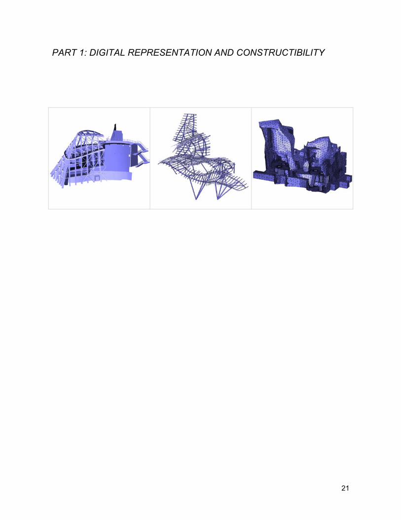
PART 1: DIGITAL REPRESENTATION AND CONSTRUCTIBILITY

21

22

I. INTRODUCTION

It seems that Gehry’s practice has become synonymous with cutting edge computing

technology and CAD / CAM manufacturing processes. But the path to the firm’s prominence

in architectural computing applications has not been easy or straight forward. Gehry himself

remains skeptical of computing as a tool for design96. He speaks with a certain degree of

pride in his inability to operate a computer, and suggests that the quality of the digital image

is dangerous and subversive to the designer’s eye.

Gehry’s design process is perhaps best characterized by its emphasis on physical objects as

the principal artifacts on which design takes place. The firm places a unique emphasis on the

development of designs through physical models, full scale mockups and other physical

artifacts as the means for understanding and developing design intentions. These artifacts of

include numerous sketch models, some undergoing active transformation while others wait

on shelves or in storage, documented in photos, serving as records of design intentions at

significant points in the process. These models are often deliberately developed to a rough,

unfinished state, in order to allow suggestion of new directions of development as the

designers contemplate the objects. The power of this design process springs in part from the

ambiguity presented by this multiplicity of physical design representations.

These evocative qualities of the firm’s designs persist in the further development of projects

as they enter documentation and construction phases. Project engineering and detailing

strategies are often developed that accommodate the real world indeterminacy of on-site

construction events. Many building system strategies have involved in-situ fabrication and

placement of system elements as a means for responding to on-site conditions. This reliance

on the efforts of craftsmen, operating in the field, again reflects the profound concern for

physical artifacts and events as driving elements of the design process and the aesthetic that

results.

The role of computer-based methodologies in this fundamentally tactile, evocative process

presents a dilemma. Contemporary CAD modeling capabilities seem to stand in marked

contrast to these design intentions. CAD modeling strips away ambiguity, producing definitive

geometric forms that “leave little to the imagination”. These digital, logically founded

23

constructs stand in curious contrast to the indeterminacy of physical based activities and

artifacts.

The physical / digital interactions, and the tension between these realms of the process have

become fundamental to the success of the firm’s design process. At the heart of the process

is an ongoing affinity between a disparate set of design intentions, embodied in multiple

physical representations, and a coherent set of computer based representations. The

process utilizes the definitiveness computer representations at points in the process where it

is appropriate, and draws these digital descriptions into the assemblage of representations.

The computer based description represents the glue that ties the physical design

representations together, and ultimately document their convergence. Computer

representations allow the intentions embodied in multiple physical representations to be

resolved, translations of scale to be performed, and incursion of system fabrication decisions

to be resolved into the design intent.

Three dimensional computer aided design applications provide a critical characteristic

relative to traditional building documentation, in the ability to translate design intentions from

physical design artifacts to constructed objects without recourse to two-dimensional

representations. On more “conventional” building projects, this direct translation is

unnecessary and perhaps inefficient. Conventional two dimensional architectural documents,

comprised of plans, sections, elevations and details, compress the full spatial and

dimensional scope of a design into a set of inter-related representations. The regularity of an

object whose dimensions may vary little or not at all from floor to floor can be efficiently

described by a single floor plan background, repeated for each floor. Variations in fit out can

be overlaid on this normalizing representation. Typical details may be specified as a single

detailed drawing. Its application across the project is specified by annotation on floor plans or

sections, or in specifications. For buildings with repetitive components, and regular floor

plans, the necessity for individually describing each element as a three dimensional model

correctly positioned in space would require substantial additional labor. The ability to

mentally resolve multiple two-dimensional representations of a design into a coherent

understanding of the three dimensional object and its methods of construction is a core part

of traditional architectural training and heritage. Architects take a professional pride in the

development of this mental ability.

24

The relationships between tools, process of making enabled by tools, and the objects

produced by operating tools are subtle and deep. The operations enabled by a chosen tool

guide the operator to make specific types of objects or products that the tool affords. The

parallel rule and triangle, blue print and tracing paper overlay of conventional document

production facilitated the design of orthogonally organized building designs. The compass

allows circular arcs to be included in these compositions. When two-dimensional plans are

extruded perpendicularly to the plane of the paper in a uniform fashion, a single drawing

presents a slice through the designed objects whose applicability is invariant of where the cut

is taken. The two dimensional drawing construction provides tremendous expressive power

in describing this geometric regularity. In turn, the designer is subtly guided toward the

development of designs for which the utility of this geometric construct holds. More elaborate

geometries than simple extruded form are of course possible, by combining multiple sections

either in parallel or orthogonally, but the “trace” of the tool is inevitably felt in the resulting

designs.

The adoption of the tools of two-dimensional representation has provided a basis for the

development of descriptive conventions unifying the building industries. This shared

language has Euclidean geometric forms and their sectional representations as an

underlying construct. Straight lines stand in for wall and floor planes, arcs represent

cylindrical forms. Parallel bold lines represent vertical walls, dashed lines represent overhead

elements, usually aligned with elements on a floor plan cut at a higher elevation. This

common understanding among participants in a building project is so deeply shared that it

eludes dissection. An architect and contactor can discuss the layout and construction of a

building on the basis of a two dimensional floor plan without any discussion of what the

elements in the drawing mean. In parallel with the development of this common language of

Euclidean elements, numerous interwoven industries and industrial processes have been

developed around the making of Euclidean objects and building components. Saw mills turn

trees into straight lumber of square profile and flat, rectangular sheets of plywood, steel mills

extrude molten steel into linear members with invariant profiles. Carpenters use plumb bobs,

string, levels and 3:4:5 triangle measurements to produce straight, vertical walls and their

perpendiculars. So pervasive has the “tyranny” of Euclidean geometry become in the building

industries that any building designed without strict accordance to its rules is subject to

characterization as impossible to build.

25

In Gehry’s design process, physical model making is the principal design tool. This primacy

of the construction of physical objects as the vehicle for design explorations in itself propels

the firm’s work beyond the constraints of the Euclidean rationale. In its place, a new set of

guiding rules have been developed, directly related to the materials and operations available

to the processes of object making. Viewed in isolation, the operations of physical modeling

are insufficient to guarantee the constructibility of the full scale products that models are

intended to represent. However, in Gehry’s process, models serve not simply to describe the

object in scale. Rather, the processes and materials of model making are brought into

alignment with, and stand in for, those of craftsmen and fabricators on the resulting building

construction. Materials and construction strategies are selected to emulate aspects of their

full scale counterparts. This approach binds the operations of design directly to those of

building, bypassing the filter of a common language of Euclidean geometry.

Prior to the firm’s adoption of computing based practices, the firm’s process suffered a key

limitation in its methods of project documentation. While the firm could reasonably guarantee

that the designs could be fabricated, the designs still required rendition into conventional two-

dimensional description to support steps of the conventional construction process, including

building permit submissions, bidding and on-site project layout. In order to bring the design

back into the language of building industry convention, two dimensional plans, sections and

elevations needed to be developed. Often, the forms of the models would require re-

interpretation into conventional Euclidean forms of planes, cylinders and cones, simply to be

consistently described through plans and sections.

Even with this painstaking development of project documentation, the geometry was still

beyond the norms of conventional construction description. While fabricators could build the

shapes, the process of bidding and coordinating the projects presented difficulty to

construction managers. Accuracy of quantity takeoffs could not be guaranteed using

conventional methods of measuring off of plans. Shop drawings – necessary for describing

the detailed fabrication geometry – were difficult to render into orthogonal views. Spatial

coordination of building elements became unmanageable as component details were

developed. The limitations of understanding the project geometry through the lens of two

dimensional views exacerbated perceptions of project complexity.

26

The history of the development of computer assisted building delivery by the firm in response

to these limitations has been well documented52. Jim Glymph joined Gehry’s firm in 1989.

Glymph had substantial experience in the role of Executive Architect on several substantially

complex building projects, including the San Diego and Los Angeles Convention Centers. At

the time, 3D CAD was beginning to have application to architectural visualization, movie

animation and automotive and aerospace design. Glymph realized that these technologies

could be applied to the processes of architectural documentation, independent of the

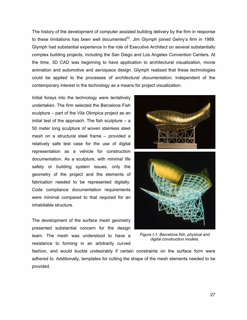
contemporary interest in the technology as a means for project visualization. Initial forays into the technology were tentatively

undertaken. The firm selected the Barcelona Fish

sculpture – part of the Vila Olimpica project as an

initial test of the approach. The fish sculpture – a

50 meter long sculpture of woven stainless steel

mesh on a structural steel frame – provided a

relatively safe test case for the use of digital

representation as a vehicle for construction

documentation. As a sculpture, with minimal life

safety or building system issues, only the

geometry of the project and the elements of

fabrication needed to be represented digitally.

Code compliance documentation requirements

were minimal compared to that required for an

inhabitable structure.

The development of the surface mesh geometry

presented substantial concern for the design

team. The mesh was understood to have a

resistance to forming in an arbitrarily curved

fashion, and would buckle undesirably if certain constraints on the surface form were

adhered to. Additionally, templates for cutting the shape of the mesh elements needed to be

provided.

Figure I-1: Barcelona fish, physical and

digital construction models.

27

Glymph contacted William J. Mitchell, then Professor of Architecture at the Harvard Graduate

School of Design, who produced an initial model of the design in the Alias software package

with graduate student Evan Smythe. While the results of the study demonstrated the

possibility of representing construction documentation in digital form, a critical limitation

emerged in the Alias software’s underlying representation of surfaces. Alias represented the

surface of the sculpture through a tessellation of triangular faces. While this representation

was sufficient to provide visual fidelity to Gehry’s initial physical model, geometric operations

on the surface required to produce the structural steel model were problematic. The

sculpture’s skeleton is constructed as a set of planar, vaulted truss “ribs”, offset from the

surface, and connected to a cross braced structural steel skeleton. Intersections of the rib

planes with the tessellated surface resulted in segmented polylines. It was difficult to control

the segmentation of the mesh surface produced by Alias to correctly produce the required

segmentation of the steel trusses. Offsetting of curves to produce the bottom chord of the

trusses and other geometric operations produced similar undesirable linearization of the

geometry.

Realizing that this segmentation of smooth surfaces would be a critical limitation to its digital

construction documentation process, the firm began to search for more advanced

representational capabilities in other software packages. At the time, the CATIA software

package was one of the few CAD platforms offering true smooth surface representations.

CATIA – initially developed by Dassault Aviation as an in house CAD application for the

development of the Mirage fighter plane – had recently been released as a commercial

application through IBM and was gaining acceptance by the automotive and aerospace

industries. At the time CATIA Version 3 had achieved a commercially viable CAD application

based on Bézier curve and surface algorithms28.

As an engineering tool, CATIA also offered capabilities for surface analysis not provided by

Alias. While unable to provide a detailed assessment of the mesh behavior, capabilities for

analyzing surface curvature were supported. Additionally, CATIA allowed curved surfaces to

be flattened into shapes allowing a reasonable approximation of the mesh profiles required to

cover the surface. These utilities, while representing quite loose approximations of the true

mesh behavior, were sufficiently powerful to support the design and detailing of the mesh

surface.

28

Rick Smith – proprietor of the consulting company C-Cubed - was at the time an independent

IBM business partner, providing CATIA services to the southern California aerospace

industries. Smith revisited the digital modeling of the fish, demonstrating the possibility of

accurately creating the curved geometry of the surface and the construction of the structural

steel geometry as offsets and intersections derived from the curved surface model.

Construction of the sculpture was awarded to Permasteelisa, an Italian curtain wall

fabrication company, for what would be the first of many successful collaborations between

the two firms. Smith brought his model and CATIA station to Italy and worked directly with

the Permasteelisa’s engineers and fabricators to produce the shop drawings for the steel and

layouts for the mesh elements.

Glymph characterizes the experiences of the Barcelona Fish project as a breakthrough in

many ways. The fact that the project, with its admitted geometric complexity, was completed

on time and on budget, while the conventional steel construction of the rest of the Pavilion

complex was suffering construction delays and on site reworking of steel elements “showed

that [the firm] was onto something” in identifying a new process for project documentation.

Furthermore, the direct collaboration with Permasteelisa on the development of shop

drawings - with the endorsement of the project owner - circumvented the conventional

disassociation between architect and fabricator.

At the same time as initial experiments in digital project description were being conducted by

the firm, Dassault Systèmes, the developers of CATIA, were developing a comprehensive

methodology to support the design of Boeing’s 777 aircraft line. Dassault termed this

methodology Digital Mockup (DMU), with the intent to support design, detailing and CNC

fabrication of the 777 aircraft and all components in an integrated, paperless fashion. This

development effort resulted in software functionality within the CATIA product line beyond the

limited functionality of curved surface description that Gehry’s firm had initially sought. The

story of these developments in the digital design of manufactured products presents a

parallel history to Gehry Partners’ efforts in developing similar methodologies for the support

of building projects, and served as an important example closely observed by the firm. The

parallel development of these manufacturing methodologies has also disclosed important

differences in economies and supply chain organization between “vertically integrated”

industries such as the aerospace industry, with opportunities afforded by economies of scale,

29

and the constraints of process imposed by construction industry. Comparisons between the

methodologies of these industries are discussed below.

Applications to building projects followed shortly. The Nationale-Nederland Building in

Prague and Team Disneyland Building drew on elements of the process proven on the

Barcelona Fish. The development of the firm’s process culminated with the opening of the

Guggenheim Bilbao museum in 1997. While refinements of the process continue, the

essential elements of the process and its applications were defined in the early successes of

these projects.

It would seem, from the success of these projects, that digital representation is poised to free

architecture from the constraints imposed by historically developed project description.

Complexity of geometric representation and methods of constructibility are apparent in the

design and construction of Gehry’s projects, but digital technology seems to have proven up

to the task of resolving this complexity. Digital modeling now allows free form, non-Euclidean

shapes to be represented with exacting tolerances. Digital CNC fabrication technologies,

developed to serve the automotive, aerospace, and Hollywood animation industries stand

ready for application to building, faithfully rendering building components to similar

exactness. The Boeing 777 project and other manufacturing processes have proven the

viability of a fully digital design development process. To the delight of some critics and the

dismay of others, digital technology seems poised to cast off the last relics of a historically

developed building context, translating the designer’s gesture effortlessly into final form

through Hollywood animation software coupled to robotic production devices. As post

modern historicism freed design from contextual constraints, digital representation seems

poised to remove the remaining constraints imposed by historically developed conventions of

building description and production.

It would be unfortunate to draw so simple a lesson from Gehry’s work. The firm’s ability to

successfully realize innovative forms springs partly from its ability to bring these projects

within the context of conventional construction documentation and building process. A view

of the development of Gehry’s body of work shows a formal language that originates in the

forms and materials of conventional construction, and an ongoing experimentation to press

these materials and methods to their limits. The succession of Gehry’s built projects shows a

gradual, continual coaxing of the conventions of fabrication and building, each work drawing

30

on the lessons learned from previous successes to push building method in new directions

and to further limits. The power of Gehry’s architecture springs partly from a struggle,

negotiation and ultimate reconciliation with existing context and conventions.

Part of the role of digital technology in the firm’s process has been to disclose simplicity

within the geometric complexity, and to bring the description of building elements and

processes within the conventional language of contemporary construction practice. This

discipline is key to the success the firm has enjoyed in successfully completing projects.

Perhaps surprisingly, much of the detailing of building components relies on extensions to

conventional processes of building, and seldom relies on aerospace or Hollywood methods

of object making. Rather, the firm strives to work with the existing processes of craftsmen

and fabricators, and attempts to produce detailing and documentation strategies that reflect a

deep understanding of the methods and constraints of existing fabrication processes. Two

dimensional documentation, flat patterns, Euclidean cut edges and profiles are the norm in

these fabrication methods. Digital technology is drawn on to render Gehry’s forms within

these conventions; is it not seen as an opportunity to discard the capabilities of traditional

craftsmanship. Part of the reason for this approach is of course necessity. Even where fully

digital fabrication technologies are available, the costs of these methods are frequently

prohibitive. But part of this methodology seems to be drawn from Gehry’s embracing of

material qualities and craftsmanship, and an aesthetic that pushes conventions to their limits,

rather than creating a design language from scratch.

Viewed from a geometric perspective, the methods drawn on in the digital description and

documentation of projects are enabled by capabilities for developing project descriptions in

full three dimensional, digital form, using non-Euclidean geometric constructs. However, the

reliance on non-Euclidean geometric constructs in no way means that these structures are

constraint free. Non-Euclidean, digital representations bring their own constraints and

artifacts to description processes, in the forms that can be represented, the geometric

operations that can be performed, and the fabrication processes that are enabled. This

structuring of non-Euclidean geometry on surface representation and associated

constructibility will be a central theme of this thesis. It will be shown that the non-Euclidean

representational constructs at the heart of the firm’s digital process can in fact be positioned

as extensions of Euclidean constructs into a more general framework, in which Euclidean

and a variety of non-Euclidean descriptive elements coexist on equal footing.

31

32

II. THE DEVELOPMENT OF GEHRY’S BUILDING PROCESS

In order to realize the innovations of Gehry’s forms on built projects, corresponding

innovations of design development and building process have been required. The firm’s

computational innovations have been developed parallel to, and as part of, these building

process innovations. To understand the context in which the firm’s digital process has

evolved, it is appropriate to review some of the guiding intentions of the firm’s building

delivery methodologies that these digital representations serve.

A. PROJECT COST CONTROL

It may not be overstatement to say that project budget control – and the reconciliation of

design intent with project financial requirements – are the most important driving forces

behind the firm’s design development phase decisions. Certainly, project cost control has

been the most important factor in the development of the firm’s digital building delivery

process. This position may surprise readers. It is sometimes assumed that Gehry’s practice

engages predominately or exclusively in “budget less” projects, with clients for whom money

is no object. This is far from the truth. The firm has achieved its successful track record of

completed projects by providing buildings within clients’ budgets, and within the rough per

square foot costs of more conventional projects of similar building usage types.

Project costs can be broken down in a number of different ways. First, the distinction is often

made between the “soft costs” of a project, including the design services of architects and

engineers, versus the ‘hard” costs attributed to actual construction materials and labor.

Second, there is an important distinction to be made between costs identified prior to

commencement of construction, roughly up the GMP (Guaranteed Maximum Price) bid

phase, and cost overruns that can crop up during construction. Both of these distinctions are

subject to further inspection in light of the new forms and processes championed by Gehry’s

firm.

It is often assumed by owners that the hard costs of a building are a fixed factor in building

construction, while soft costs are an area for flexibility. This reasoning seems at a preliminary

glance to be valid. In theory, a 2x4 stud is a 2x4, a cubic foot of concrete is a known quantity.

The unit prices of these materials seem relatively fixed. Buildings of a certain size require

33

certain amounts of material. Metrics for these material quantities relative to square footages

of given construction types are available in the industry. Quantity estimating on conventional

construction is a fairly straight forward process. The estimator adds up linear wall lengths

from the 2D drawings, multiplies this length by the height of the walls to determine square

footages, throws in a percentage for material waste, and multiplies these quantities by

established local costs for the building materials and per quantity estimates of hours and

rates of construction labor, to arrive at a cost for the construction of a given building system.

If the client is interested in higher quality materials or construction, these decisions can

increase the cost of construction, but in theory the client “gets what he or she asks for” in

terms of a higher quality product. In turn, it is perceived that the soft costs of the architectural

and engineering services have some flexibility. If the architect spends less time in schematic

design, the number of billed hours can be reduced, beneficially impacting the bottom line of

the building construction budget. On many conventional building projects, the design

services are seen as an area to squeeze some cost reduction.

The above distinctions between soft and hard costs of construction may be valid for

conventional construction, where quantities and associated costs are relatively well

established. On unconventional construction, where established industry costs for the type of

construction are not available, the rules of the game are thrown wide open. Even the straight

forward activity of quantity estimating can be difficult to accurately perform if these quantities

can not be easily determined from conventional 2D documentation. Material waste factors

can be difficult to estimate, since atypically shaped building elements can be more difficult to

fit on industry standard sheets of material. The labor associated with unit quantities of

unconventional construction systems can be difficult to anticipate.

Even on conventional construction, construction budgeting is less of a science than it first

appears. For conventional construction, rough per unit cost rules of thumb are available in

the industry, and are known to architects and construction managers. These unit costs vary

widely from region to region, and are substantially impacted by short term localized economic

factors. Factors contributing to the cost of a given system include local availability of

materials and equipment, availability of skilled vs. unskilled labor and the influence of trade

unions, and competition among projects in a given locale for certain elements of

construction. A “hot” building market will drive up costs for most basic construction systems,

as demand for sub-contractors is driven up. The history of Gehry’s projects is rife with

34

anecdotes of these local and temporary economic considerations. The economic feasibility of

titanium for the Guggenheim Bilbao project is traced to a temporary glut of available titanium

in the world market after the fall of the Soviet Union. The Big Dig project in Boston reduced

the available concrete contractors in the local market during the construction of the Stata

Center. Low demand for skilled carpenters in the Czech Republic after the fall of

communism contributed to the development of a hybrid digital / manual fabrication process

for concrete panels of the Nationale – Nederland project.

The premium on direct hard costs associated with unconventional project geometry is an

important factor in preliminary project budgeting. This premium is acknowledged by clients as

a cost associated with the acquiring one of the firm’s designs. The rationale of cost

associated with receiving a superior product is applicable to Gehry’s buildings. Many

budgetary tradeoffs are made throughout schematic design phase decision making. For

example, Gehry’s design aesthetic suggests more economical, conventional materials used

in unconventional forms, in lieu of more expensive finishes applied to conventional geometry.

Mixing project geometry to include conventional construction and geometry along with more

highly shaped elements is an important element of the design process. These tradeoffs can

be managed in schematic design in order to meet client budget requirements.

A more problematic aspect of project budgeting can be identified, in terms of risk

management. In North America, construction sub contracts are typically awarded based on

guaranteed price bids. Typically, construction sub contracts are awarded through a

competitive bidding process, with the low bidder being awarded the contract. The recipient of

the contract is obligated to perform the agreed upon services – specified through project

documentation - for a contractually committed price. On conventional construction, sub

contract estimators have a good understanding of their internal unit price costs for

conducting work, and can make trade offs between competitive pricing and profit margin. On

unconventional construction, where prior experience and industry established price points do

not exist, cost estimation is difficult to conduct with any guarantee of successful completion

of the project. The level of risk associated with contracting to perform the work at any specific

price can be substantial. The result can be sub contractor bids containing large factors of

safety, which ultimately represent premiums on the price of construction. Many sub

contractors will simply elect not to consider taking on the work, reducing the competitive pool

of providers and resulting in higher cost bids being accepted. The premiums cannot be

35

construed to be costs associated with a superior product, but simply represent higher costs

for the same quality of construction. This price of risk can dwarf the premiums that can be

expected due purely to additional labor or materials.

While the pre-construction pricing exercises can jeopardize the commencement of a project,

lack of project and associated cost control during construction present even greater jeopardy

to the project and participating organizations. The major risks in terms of cost overruns

during construction can be traced to lack of dimensional coordination, and errors and

omissions in construction documentation or their interpretation. Errors in dimensional

coordination can result from mis-communication between trades, misunderstanding of

dimensions of components, and complexities of routing equipment through tight spaces,

such as duct runs of mechanical systems. Obvious errors of miscalculating dimensions on

traditional 2D documents or not updating dimensions on plans when updates and changes

are made occur all to frequently on conventionally documented construction drawings. When

such errors escape notice until they are discovered in the field, at best re-work is necessary.

More significantly, this rework can cause delays impacting many of the trades on the job. If

these delays are significant enough, they can cause a “ripple affect” where subsequent

trades are impacted. For example, the mis-sizing of a single primary steel beam, discovered

in the field can delay the placement of adjoining members while the erroneous member is

rebuilt and shipped. In turn, placement of any system to be attached to the primary steel

system may be held up. If delays are significant, they can put in jeopardy guaranteed

contracts with sub contractors, who may have other work scheduled in anticipation of

completing their portion of the job by a certain date. The costs of running a large construction

site per day can be substantial even without the subcontractor labor costs.

Improved project information provided by 3D CAD documentation has the potential to

address many of these issues, allowing control of, and dramatically reducing, the so called

“hard costs” of project construction. Much of the cost saving opportunities offered by

information technology can be traced to reduction of risk. By facilitating improved unit

quantity estimates early in schematic design, budget tradeoffs can be played out before

detailed design has begun. Improved dimensional coordination can be a direct outcome of

“virtually” constructing the building and its components to some level of detail prior to

generating contract documents. Tricky or idiosyncratic conditions for typical system details –

at corners or atypical interfaces with other systems – can be identified prior to committing

36

work contractually. Admittedly, this added information may give prospective bidders better

insight into the complexity of the project, resulting in higher initial bids. However, if this

complexity were to be discovered after the fact, disputes about the completeness of

construction documents would need to be resolved, likely resulting in remediation.

Part of the successful design development practices of Gehry’s firm results from the frequent

use of conventional system detailing, applied to unconventional geometry. The firm is

continually cognizant of the availability of locally available talented craftsmanship, and seeks

to take advantage of the materials and practices of their local construction practices. This is

part of the contextual aesthetic of Gehry’s designs, and an aspect of the respect of

craftsmanship for which the firm is known. One strategy for reducing project costs is to be

able to provide construction information in a format familiar to these local trades. The 3

dimensional project database allows information to be “sliced and diced” to extract

information supporting construction practices familiar to these local trades. If the description

of complex geometry can be provided in a format that supports practices familiar to these

trades, the risk factor can be reduced or eliminated. Complex geometry may still carry a

premium in labor and material, but these factors can be understood in terms of real impact

on the costs of construction, not buried in excessive cost contingencies to protect the

contractor from unknown risks.

B. BUILDING TEAM ORGANIZATION AND INFORMATION FLOW

The conventions of contractual relationships among organizations participating in a

construction project vary widely in different parts of the world. In many ways, the North

American construction environment is among the most difficult for supporting unconventional

building practices. It is partly for this reason that many of the early successes of the firm’s

digital building delivery process were achieved on projects outside North America. Much of

the development of the divisions between design and construction teams can be traced to

the increase in construction litigation that has occurred in America since the 1950s. To

protect the various partners from litigation, strict boundaries have been defined for the scope

of responsibility each party takes on, and the flow of information between parties.

37

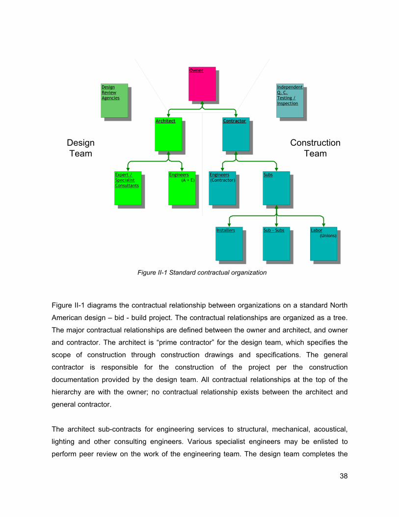
Contractor

Owner

Architect

SubsExpert /SpecialistConsultants

Engineers(A + E)

Engineers(Contractor)

Sub - SubsMaterialSuppliers

Installers Labor (Unions)

ProductSuppliers

DesignReviewAgencies

IndependentQ. C.Testing /Inspection

DesignTeam

ConstructionTeam

Figure II-1 Standard contractual organization

Figure II-1 diagrams the contractual relationship between organizations on a standard North

American design – bid - build project. The contractual relationships are organized as a tree.

The major contractual relationships are defined between the owner and architect, and owner

and contractor. The architect is “prime contractor” for the design team, which specifies the

scope of construction through construction drawings and specifications. The general

contractor is responsible for the construction of the project per the construction

documentation provided by the design team. All contractual relationships at the top of the

hierarchy are with the owner; no contractual relationship exists between the architect and

general contractor.

The architect sub-contracts for engineering services to structural, mechanical, acoustical,

lighting and other consulting engineers. Various specialist engineers may be enlisted to

perform peer review on the work of the engineering team. The design team completes the

38

specification of the project to demonstrate conformance with local building codes, and to

sufficient level of detail to guarantee in theory that the project can be built without errors or

conflicts between the activities of building trades.

The general contractor in turn apportions work, at their discretion, to internal resources or to

subcontractors. These contracts need only to guarantee that the specifications of the design

team are met; beyond these base line requirements the contractor is free to select any

contracting organizations that can reasonably be expected to perform the work. The

contractor will generally award sub contracts on the basis of lowest bid.

Sub contracting organizations “fill in the details” of the project specification through shop

drawings that describe building systems and components to a level of detail necessary for

actual construction. The sub contracting organizations have their own engineering teams that

conduct detailed engineering of system components to verify that proposed fabrication meets

the standards specified by the design team. Again in theory, the contract documents

provided by the design team have anticipated all the geometric and coordination conditions

that will occur as a consequence of the systems that have been selected for the project. In

practice, the level of detail performed by the design team to define the resolution of typical

conditions may not anticipate all the actual localized conditions generated by the specified

systems. The level of detail provided by the shop drawing detailing may be necessary to

disclose the full range of implications of a selected building system strategy. Any

discrepancies between general and actual localized conditions can be a source of dispute

between the design and construction teams. These shop drawings are submitted to the

design team for review, comment or exception. The design team is usually responsible for

guaranteeing that the details specified in the shop drawings can be dimensionally

coordinated between trades. Note that dimensional conflicts between the work of different

trades may not be apparent in any single trade’s shop drawing submissions. Coordination

through integrating information contained on numerous shop drawings may be required for

the design team’s review. Problems can be difficult to detect when this information is

contained on disparate two dimensional documents.

When a condition is detected by the sub contractor that is beyond the scope of the details

specified by the bid package, requests for information (RFIs) are generated by the sub

contractor and sent through the contractual hierarchy to the architect - as head of the design

39

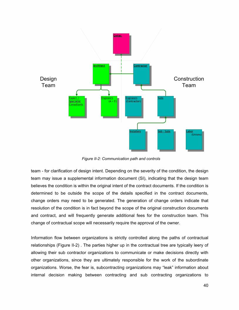
Contractor

Owner

Architect

SubsExpert /SpecialistConsultants

Engineers(A + E)

Engineers(Contractor)

Sub - SubsInstallers Labor (Unions)

DesignTeam

ConstructionTeam

Figure II-2: Communication path and controls

team - for clarification of design intent. Depending on the severity of the condition, the design

team may issue a supplemental information document (SI), indicating that the design team

believes the condition is within the original intent of the contract documents. If the condition is

determined to be outside the scope of the details specified in the contract documents,

change orders may need to be generated. The generation of change orders indicate that

resolution of the condition is in fact beyond the scope of the original construction documents

and contract, and will frequently generate additional fees for the construction team. This

change of contractual scope will necessarily require the approval of the owner.

Information flow between organizations is strictly controlled along the paths of contractual

relationships (Figure II-2) . The parties higher up in the contractual tree are typically leery of

allowing their sub contractor organizations to communicate or make decisions directly with

other organizations, since they are ultimately responsible for the work of the subordinate

organizations. Worse, the fear is, subcontracting organizations may “leak” information about

internal decision making between contracting and sub contracting organizations to

40

organizations “on the other side of the fence”, who may use this information to their

advantage if disputes arise.

When construction proceeds smoothly (which it seldom does, even on conventional

construction!) this strict control of information generation and dissemination protects all

parties from erroneous decision making that would jeopardize the intent of the project

specifications that form the basis of the contractual relationships. For conventional

construction, where the work of each party is fairly well defined by standard details and other

conventions of practice, the process of design and construction decision making can be

accommodated by this tightly contractually controlled process.

For innovative, complex or unconventional construction, the disaggregation of information

and limitations imposed on communications between decision makers can virtually

guarantee that problems will occur in project coordination. When they do occur during

construction, resolution of problems can be difficult. Problems which could be quickly fixed

on the spot - if the construction team had sufficient authority - require a chain of events and

decisions, above all a determination of the party responsible for the condition. While the

resolution of decisions are winding their way through the chain of command, construction

delays can ensue, further aggravating the impact the condition has on the project schedule

and cost. Communication technologies have been drawn on to assist in the speed of

resolution of on site conditions, including simple technologies (such as emailed digital

photos) and more elaborate technologies including information tracking Web sites.

More problematic for innovation of construction is that the true sources of fabrication

innovation – and the parties ultimately responsible for execution of this innovation – are the

fabricators themselves. These are the organizations that will ultimately be required to

develop innovations of process necessary to efficiently construct innovative project

geometries. This expertise is best included in the design process during design development

decision making, before the contract documents have been completed. In the contractual

scheme defined above, these entities are excluded from the decision making process.

Worse, sophisticated fabricators may be better informed of the actual effort and cost required

to perform sophisticated construction work. This knowledge may work to their detriment,

since the bids they submit may reflect the actual cost required to complete the project. Their

bids may be turned down by the general contractor in favor of less qualified fabricators, who

41

may turn out be unable to execute the work to which they have committed themselves. The

specification and bidding process also can fail to turn the award of contracts in favor of

fabricators who perform higher quality work.

Gehry’s design aesthetic has always tended to favored innovation of fabrication and craft

over that of engineering. These intentions would conspire to flip the standard contractual

process around. Theoretically, the fabricators would work directly with the architect and

engineers of the design team to provide the specification of the work to be performed.

Unfortunately, this tight relationship between design team and craftsmen violates many of the

contractual conventions of North American construction.

To address this issue, GP has occasionally – with the consent of owner and general

contractor - entered into unconventional contractual relations with fabricators in the design

development phase. These design assist contracts are forged between the architect and

skilled fabricators. The fabricator serves as a quasi consulting engineer for the specification

of a building system, and is compensated for this service. There is no commitment by the

general contractor to ultimately award the contract to the particular fabricator; it may be

awarded to the fabricator’s competition, if the fabricator’s bid is unreasonable. In practice,

this is however seldom the case.

A second issue of potential impact on contractual relations is the availability of computing

capabilities by the fabrication organizations. The accurate performance of shop drawing work

requires the fabricator to dig into the master model database. Until recently, the skills

necessary to operate CATIA, and familiarity with a 3D centric approach to detailing were

unavailable outside of Gehry Partners. While the ability to fabricate the components existed

in skilled fabrication shops, the necessary CAD expertise was not part of these organizations’

services. When CAD expertise existed, data would still need to be translated into formats

appropriate for the fabricator’s work. This lack of availability of computational expertise has

often required Gehry Partners to perform services as part of construction administration

phase activities, well beyond those conventionally within the architect’s scope. In order to

address the contractual ambiguity of these services, C-Cubed – Rick Smith’s CATIA

consulting organization – has often been recommended as a sub contractor to general

contractors and fabricators. C-Cubed provides both CATIA operator expertise, as well as

familiarity with the firm’s digital methodologies. C-Cubed has contracted directly to contractor

42

and sub contractor organizations to perform digital shop drawing services, removing Gehry

Partners from any direct work and contractual relationship with these organizations.

On recent projects, 3D CAD capabilities have become more prevalent in fabricating

organizations. Often these organizations have developed sophisticated digital methods of

their own, or have acquired 3rd party applications whose development targets the specific

activities of their trade. CAD activities to support these relationships have turned more

toward translation of data between the CATIA master model and these proprietary formats.

Often, Gehry Partners will engage in development of translation processes to serve particular

contracting organizations. These capabilities are officially provided “for reference only”; the

CATIA database remains the official format for 3D data on the firm’s projects. When

appropriate, GP has provided these translation technologies to the general contractor, who

becomes responsible for data coordination with their subcontractors.

C. FABRICATION ECONOMIES

Building projects are predominately singular endeavors. Site conditions, local building

practices and codes, client specific requirements, and the need to work with locally based

construction firms and their heavy equipment, all are conditions that contribute to the

necessity for treating each project as a unique undertaking.

This characteristic is perhaps the single most important distinction between building

construction and product manufacturing industries. The products of manufacturing industries

vary widely in scale, complexity and cost. Airplanes are enormously complex design and

engineering endeavors, and carry very high unit costs. Only a few hundred or thousand units

may be produced over the lifetime of an aircraft product line. A toy is a relatively simple

object to engineer and produce. Hundreds of thousands or even millions of identical toys

may be produced in the lifetime of the product line.

Economies of scale unify the production these different manufactured products. There are

many implications of mass production on the economics and opportunities afforded by

product lines. With economies of scale, the up front cost of engineering and tooling design

required to develop the product line is distributed over the cost of each unit. Even if these

costs are high relative to the unit cost, substantial design and engineering activity can be

43

undertaken with limited impact on this unit cost. These implications impact the fabrication

methods available to mass production, and in turn have consequences on the shapes that be

manufactured. The tooling of dies for extrusion molding or stamping fabrication technologies

often represent a high fixed cost of product manufacturing. Metal stamping requires the

fabrication of a positive and negative dies. The manufacturing of these dies in manufacturing

is often a multi-step process. A wax positive form may be constructed, or highly finished CNC

routed positive is developed in foam. Then, a high strength negative form is cast from the

sculpted positive form. Depending on the stamping process, a second positive in high

strength material may be developed from the negative form, and a high strength steel die

formed from this element. This elaborate process can be easily justified for large scale runs

of identical parts. It is fairly obvious that application of such a process to one of a kind

component runs would be drastically expensive. Yet, for fully free form surface forms,

elements of a stamping or molding process are still required.

A more subtle implication of economies of scale – or lack thereof – is found in the cost of

information required to develop a given component. This cost of information can be

identified in the design, engineering, and modeling or drafting associated with the

development of the component. With large product runs, the cost of engineering and

modeling a component is again a small component of the cost of fabricating the individual

unit. In the development of singular products and components, the relative cost of

engineering to that of materials or fabrication labor can be high. It may be more economical

to over design the specification for all units, adding more material and hence strength into the

objects’ designs, than to engineer each unit to a more optimal configuration. Similarly, it may

be more cost effective to use additional fabrication effort - allowing the craftsman working on

the component to figure out aspects of the component’s configuration – than it would be to

fully detail an individual component through computer based or traditional drafting.

Issues of mass production have been a topic for architecture since the industrial revolution44.

While a full treatment of this topic is well beyond the scope of this thesis, some observations

may be made on the geometric organization of building projects and its affordance of mass

production. The regularized, Euclidean organizations of building layout strategies have

historically provided the basis for incorporating mass produced elements. Modular systems

based on grid layouts - repetition of rectangular dimensions in the organization of building

designs – allow components of identical proportions to be mass produced and deployed

44

across the project. Countless examples of such designs exist, we note in passing much of

the work of Mies van der Rohe and fellow high modernists. These strategies rely on

dimensional repetition as a means for achieving geometric symmetries supporting the

incorporation of identical elements. Rotatational symmetries afford similar dimensional

repetition. Variations in localized performance requirements may exist across elements of

identical dimensions. The wind forces on the glazing modules of high rise buildings are

greater at the top than at the bottom. This localized performance variation may be trivially

satisfied by over designing the unit to satisfy the worst case design conditions; the

inefficiency of deploying materials in a less than optimal fashion may be vastly outweighed

by the informational economy of engineering the unit a single time.

There is perhaps an even greater body of built work drawing on regularities of Euclidean

geometry to support systems founded on mass produced raw materials. The conventional

American 2x4 system is a key such example. This system does not require modular

dimensions, but rather relies on easily formed raw materials with certain assumed constraints

on the building geometry to which they will be applied. The obvious constraints of the 2x4

system are planar wall, floor and roof geometries. Straight, rectangular edges and

perpendicular wall organizations are suggested by this system; however, the system can

accommodate angles between planar elements and non-perpendicular edges with minor

customization. Gehry’s early work (Section IV.A) explored the limits of these building

systems and materials.

The non-repetitive geometries that characterize Gehry’s recent work afford neither modular

dimensional regularities nor other regularities afforded by Euclidean systems. However, in

order to satisfy budgetary and schedule requirements on the firm’s projects, systematic

building strategies are still required. This imperative has caused design development

strategies and geometric modeling efforts to pursue the identification of geometric

regularities that do exist in the design geometry, or can be imposed on the geometry with

minimal impact on the design intent. The term rationalization (Section III.F, below) is used

within the firm to describe this process of pursuing and incorporating geometric regularities in

the building form. The disclosure and constructibility implications of geometric regularities in

non-Euclidean geometry are a central topic of this thesis. Considerable discussion of

different geometric forms present in Gehry’s designs, the regularities inherent to these

45

geometries, and constructibility strategies that take advantage of these regularities will be

provided in Parts 2 and 3 of this thesis.

D. MANUFACTURING TECHNOLOGIES AND METHODS

CNC (Computer Numerically Controlled) production methods hold promise to alleviate some

of the geometric constraints on mass production strategies. CNC fabrication equipment can

dramatically reduce the labor associated with controlled fabrication of custom components.

CNC technologies include a variety of different technologies, including laser or plasma

cutting of flat sheet materials, automated hole punching used in structural steel fabrication, 3

and 5 axis routing, automatic lathing, and full fledged robotic manufacturing. However, there

are economic and formal considerations in applying these technologies. The cost of this

equipment is substantial relative to more conventional fabrication equipment. This up front

cost must be amortized over the life of the machine, which can in it self result in significant

costs per cutting operation. Certain combinations of materials, sizes of elements and shapes

have no current CNC solutions. For example, re-configurable mold technologies are currently

being researched, but to date these technologies are unavailable in commercial applications

for high quality fabrication of steel plate or other high strength materials. The cost of

generating and processing the information necessary to drive the equipment must be

considered as well. Long machine run times on expensive equipment (such as 5 axis milling)

can make applications of these technologies prohibitively expensive. Computer based

modeling requires highly skilled operators, frequently working on high priced workstations

and software. The amount of information necessary to generate shop drawing information for

CNC fabrication may be more than that necessary to generate equivalent shop drawings for

manual fabrication. To date, few building fabrication shops have invested in these

technologies. The limited competition among firms for this type of work has to date resulted

in premiums for full CNC enabled approaches to building component generation. Certainly,

we can expect to see continual reductions in the cost of these technologies over time. The

automation of shop drawing production combined with the ongoing reduction in cost of

computer hardware promises to beneficially impact the cost of generating building

components with unique configurations.

Gehry’s firm has promoted the use of CNC manufacturing technologies in these production

processes. CNC technologies are utilized in the manufacturing process to produce the

46

custom geometry of individual components at exact tolerances. Manufacturing tool paths

may be exported directly from the CATIA master model to the CNC production equipment,

resulting in building components that conform to the local geometric requirements of the

project. The building systems that result from this method offer tremendous flexibility in

addressing programmatic or aesthetic considerations. Using CNC production methods tied

directly to the definitive 3D project information additionally results in improved coordination of

connection geometries throughout the project, fewer dimensional conflicts between building

system components, and fewer costly modifications of components at the construction site.

In other situations, the more traditional methods associated with manual construction

techniques have proven to be more cost effective. When traditional construction methods

are adopted, the resulting systems are subjected to similar requirements of dimensional

coordination with the three dimensional computer master model. To fulfill this requirement,

manual fabrication is directed through the use of loft drawings - full scale construction

templates. With the full three dimensional model in place, information may be extracted in

forms appropriate for the support of traditional trade practices.

The processes that have been developed by the firm provide interfaces to both traditional

manual construction practices, and to technical innovations associated with CNC

manufacturing. For each building system, a manufacturing process is developed through

close collaboration between Gehry’s firm and partnering fabricators. The resulting process is

rigorously substantiated through full scale mockups in conjunction with computer modeling

and analysis, and subjected to value engineering assessment. The approach which is

ultimately pursued can combine traditional, manual construction techniques with advanced

computer based manufacturing methods, to arrive at an optimal solution both from the

perspective of cost as well as the quality of the resulting system.

E. DIMENSIONAL TOLERANCES

Building construction neither provides nor requires the tight fabrication tolerances of aircraft

and automotive manufacturing. The tightest tolerances that can be achieved through typical

fabrication and construction techniques are on the order of 1/8” to 1/16”. In practice many

building fabrication systems have far lower tolerances. Primary structural steel fabrication in

North America can be expected to have tolerances of no better than 1 inch. These tolerances

47

differ greatly from those expected in manufacturing industries, where tolerances tighter than

1 mil may be expected. CNC fabrication methods can offer higher tolerances of components

to their corresponding digital description. However, CNC developed components often still

require assembly through traditional manual methods, and the typical construction tolerances

are often re-introduced into these systems during manual assembly. As a general rule, one

can anticipate a premium for fabrication with tighter construction tolerances, and lower

tolerances for one of a kind objects relative to those produced through machine automated

mass production methods.

Construction tolerances are closely related to the issue of dimensional control of the project.

The exacting numerical specificity of contemporary CAD modeling applications are of little

utility if building components can not reasonably be expected to be accurately positioned in

space in conformance with the digital model. On site digital surveying capabilities allow

components to be positioned in space in tight conformance with the digital model. However,

the labor involved with positioning building components through digital surveying is

significant. Building system strategies that rely on sampling vast quantities of surveyed points

can be expected to have associated project cost and schedule implications. Even if such

exacting positioning of certain building system elements is presumed, the relative fabrication

tolerances of adjoining building components can require adjustable connection strategies for

resolving dimensional discrepancies.

An alternative strategy for positioning building components is to rely on one building system

to serve as the positioning device or dimensional control mechanism for adjoining elements.

The benefits of such a strategy are readily apparent. The dimensional control element serves

simultaneously as building component, jig for the positioning of other elements, and

structural support for the elements that join it. This requires, however, that the dimensional

control element be fabricated to the construction tolerances required of the adjoining

elements, with associated costs of a potentially high tolerance fabrication. Typically, the

dimensional control component will be a more primary element than the elements that frame

in. The costs for fabricating primary structural elements to tight tolerance may be far greater

than that of fabricating secondary systems to similar tolerances. For example, primary steel

can be used as the dimensional control for a stud framed wall system that it supports. The

construction tolerances of the stud wall system are dictated by the requirements of the

cladding system, while primary steel would normally be subject to more generous tolerances

48

than that required for the wall system. This generates a higher unit cost for the primary steel.

On the other hand, only relative system conformance to the dimensions specified in the CAD

model may be required. The positioning of framing members in the above example may need

to tightly correspond to the edge geometry of the primary steel and to one another, but where

this assemblage winds up relative to other elements of the project may be of little

consequence. If so, then the tolerance requirements of the dimensional control system can

be relaxed.

CNC fabrication technologies can often support the development of registration information

as part of the fabrication process. Laser or plasma cutting tools, operated at lower power

levels than required to burn through material, can allow dimensionally accurate registration

marks and even textual annotation as part of the cutting process66.

Issues of tolerance and dimensional control have profound implications for project cost and

quality. Tolerance decisions can not be isolated from the system design and modeling

strategies. These decisions will have implications for manufacturability, erection and project

cost which can impact the design, coordination and site logistics with implications beyond the

actual system on which these decisions are made. A judicious use of tolerance and flexibility

in the dimensional control of project geometries has been an important part of the firm’s

success in realizing projects within reasonable construction budgets.

49

50

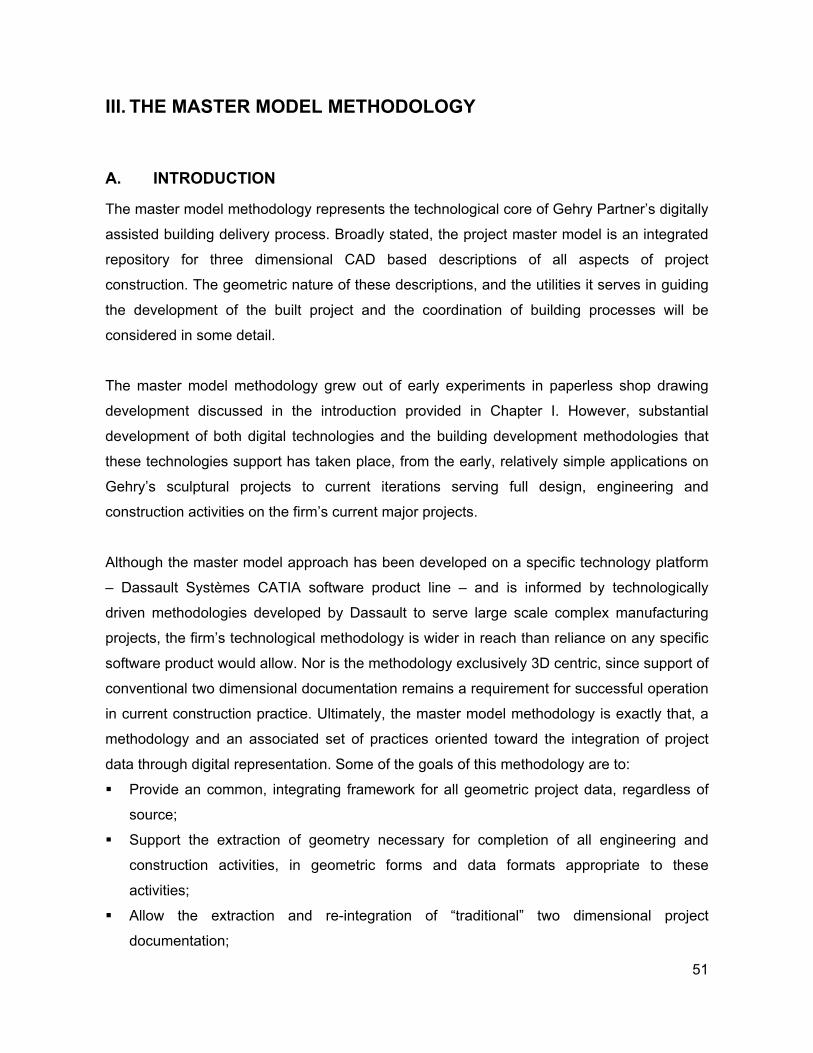
III. THE MASTER MODEL METHODOLOGY

A. INTRODUCTION

The master model methodology represents the technological core of Gehry Partner’s digitally

assisted building delivery process. Broadly stated, the project master model is an integrated

repository for three dimensional CAD based descriptions of all aspects of project

construction. The geometric nature of these descriptions, and the utilities it serves in guiding

the development of the built project and the coordination of building processes will be

considered in some detail.

The master model methodology grew out of early experiments in paperless shop drawing

development discussed in the introduction provided in Chapter I. However, substantial

development of both digital technologies and the building development methodologies that

these technologies support has taken place, from the early, relatively simple applications on

Gehry’s sculptural projects to current iterations serving full design, engineering and

construction activities on the firm’s current major projects.

Although the master model approach has been developed on a specific technology platform

– Dassault Systèmes CATIA software product line – and is informed by technologically

driven methodologies developed by Dassault to serve large scale complex manufacturing

projects, the firm’s technological methodology is wider in reach than reliance on any specific

software product would allow. Nor is the methodology exclusively 3D centric, since support of

conventional two dimensional documentation remains a requirement for successful operation

in current construction practice. Ultimately, the master model methodology is exactly that, a

methodology and an associated set of practices oriented toward the integration of project

data through digital representation. Some of the goals of this methodology are to:

Provide an common, integrating framework for all geometric project data, regardless of

source;

Support the extraction of geometry necessary for completion of all engineering and

construction activities, in geometric forms and data formats appropriate to these

activities;

Allow the extraction and re-integration of “traditional” two dimensional project

documentation;

51

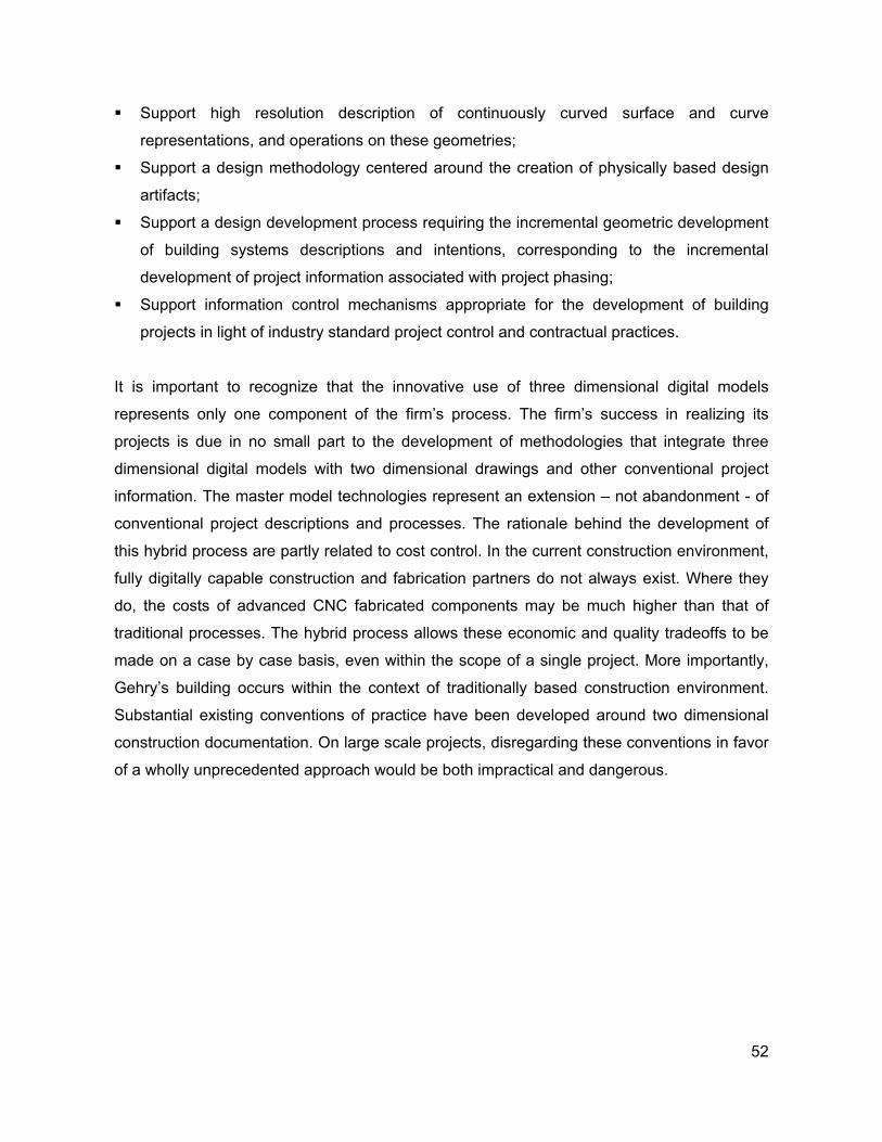
Support high resolution description of continuously curved surface and curve

representations, and operations on these geometries;

Support a design methodology centered around the creation of physically based design

artifacts;

Support a design development process requiring the incremental geometric development

of building systems descriptions and intentions, corresponding to the incremental

development of project information associated with project phasing;

Support information control mechanisms appropriate for the development of building

projects in light of industry standard project control and contractual practices.

It is important to recognize that the innovative use of three dimensional digital models

represents only one component of the firm’s process. The firm’s success in realizing its

projects is due in no small part to the development of methodologies that integrate three

dimensional digital models with two dimensional drawings and other conventional project

information. The master model technologies represent an extension – not abandonment - of

conventional project descriptions and processes. The rationale behind the development of

this hybrid process are partly related to cost control. In the current construction environment,

fully digitally capable construction and fabrication partners do not always exist. Where they

do, the costs of advanced CNC fabricated components may be much higher than that of

traditional processes. The hybrid process allows these economic and quality tradeoffs to be

made on a case by case basis, even within the scope of a single project. More importantly,

Gehry’s building occurs within the context of traditionally based construction environment.

Substantial existing conventions of practice have been developed around two dimensional

construction documentation. On large scale projects, disregarding these conventions in favor

of a wholly unprecedented approach would be both impractical and dangerous.

52

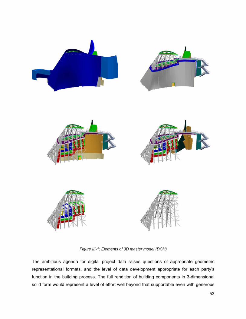
Figure III-1: Elements of 3D master model (DCH)

The ambitious agenda for digital project data raises questions of appropriate geometric

representational formats, and the level of data development appropriate for each party’s

function in the building process. The full rendition of building components in 3-dimensional

solid form would represent a level of effort well beyond that supportable even with generous

53

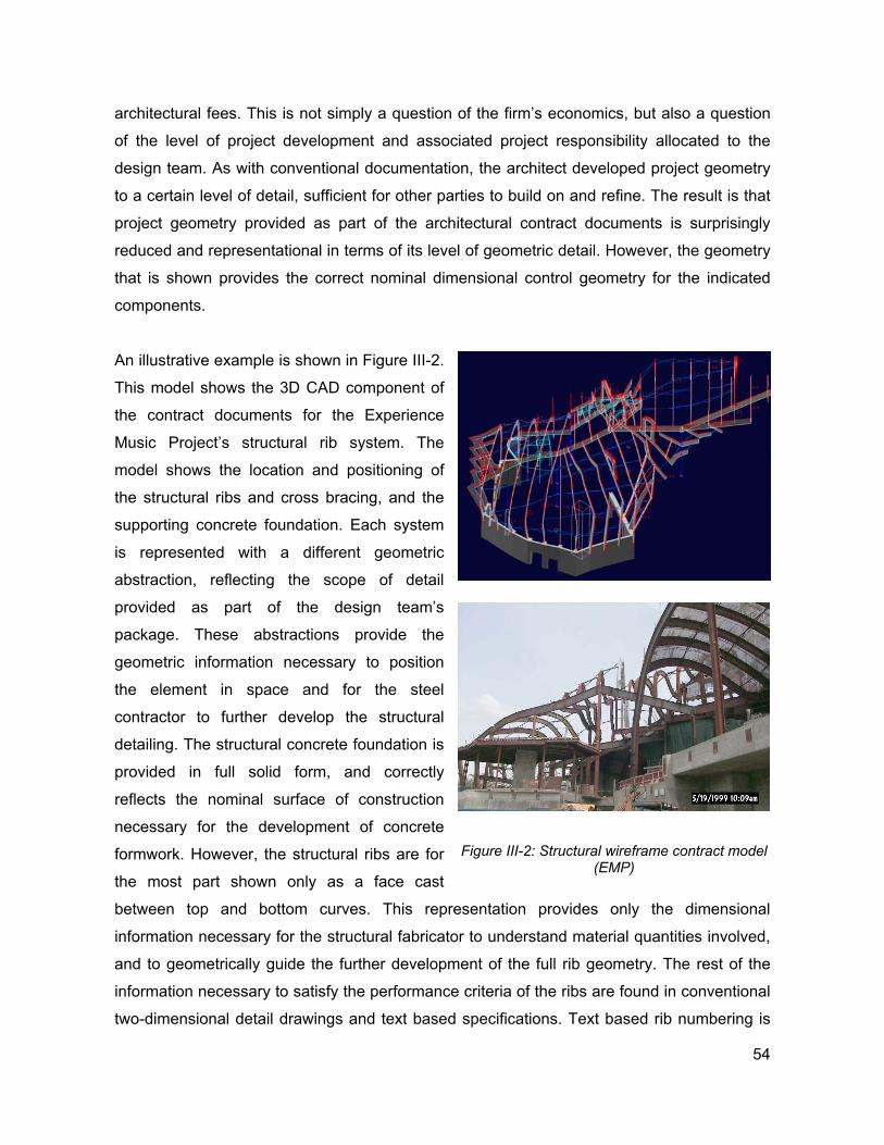
architectural fees. This is not simply a question of the firm’s economics, but also a question

of the level of project development and associated project responsibility allocated to the

design team. As with conventional documentation, the architect developed project geometry

to a certain level of detail, sufficient for other parties to build on and refine. The result is that

project geometry provided as part of the architectural contract documents is surprisingly

reduced and representational in terms of its level of geometric detail. However, the geometry

that is shown provides the correct nominal dimensional control geometry for the indicated

components.

An illustrative example is shown in Figure III-2.

This model shows the 3D CAD component of

the contract documents for the Experience

Music Project’s structural rib system. The

model shows the location and positioning of

the structural ribs and cross bracing, and the

supporting concrete foundation. Each system

is represented with a different geometric

abstraction, reflecting the scope of detail

provided as part of the design team’s

package. These abstractions provide the

geometric information necessary to position

the element in space and for the steel

contractor to further develop the structural

detailing. The structural concrete foundation is

provided in full solid form, and correctly

reflects the nominal surface of construction

necessary for the development of concrete

formwork. However, the structural ribs are for

the most part shown only as a face cast

between top and bottom curves. This representation provides only the dimensional

information necessary for the structural fabricator to understand material quantities involved,

and to geometrically guide the further development of the full rib geometry. The rest of the

information necessary to satisfy the performance criteria of the ribs are found in conventional

two-dimensional detail drawings and text based specifications. Text based rib numbering is

Figure III-2: Structural wireframe contract model (EMP)

54

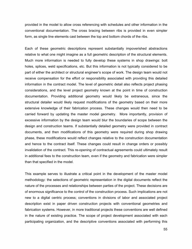
provided in the model to allow cross referencing with schedules and other information in the

conventional documentation. The cross bracing between ribs is provided in even simpler

form, as single line elements cast between the top and bottom chords of the ribs.

Each of these geometric descriptions represent substantially impoverished abstractions

relative to what one might imagine as a full geometric description of the structural elements.

Much more information is needed to fully develop these systems in shop drawings: bolt

holes, splices, weld specifications, etc. But this information is not typically considered to be

part of either the architect or structural engineer’s scope of work. The design team would not

receive compensation for the effort or responsibility associated with providing this detailed

information in the contract model. The level of geometric detail also reflects project phasing

considerations, and the level project geometry known at the point in time of construction

documentation. Providing additional geometry would likely be extraneous, since the

structural detailer would likely request modifications of the geometry based on their more

extensive knowledge of their fabrication process. These changes would then need to be

carried forward by updating the master model geometry. More importantly, provision of

excessive information by the design team would blur the boundaries of scope between the

design and construction teams. If substantially detailed geometry were provided in contract

documents, and then modifications of this geometry were required during shop drawing

phase, these modifications would reflect changes relative to the construction documentation

and hence to the contract itself. These changes could result in change orders or possibly

invalidation of the contract. This re-opening of contractual agreements could ultimately result

in additional fees to the construction team, even if the geometry and fabrication were simpler

than that specified in the model.

This example serves to illustrate a critical point in the development of the master model

methodology: the selections of geometric representation in the digital documents reflect the

nature of the processes and relationships between parties of the project. These decisions are

of enormous significance to the control of the construction process. Such implications are not

new to a digital centric process; conventions in divisions of labor and associated project

description exist in paper driven construction projects with conventional geometries and

fabrication systems. However, in more traditional projects these conventions are well defined

in the nature of existing practice. The scope of project development associated with each

participating organization, and the descriptive conventions associated with performing this

55

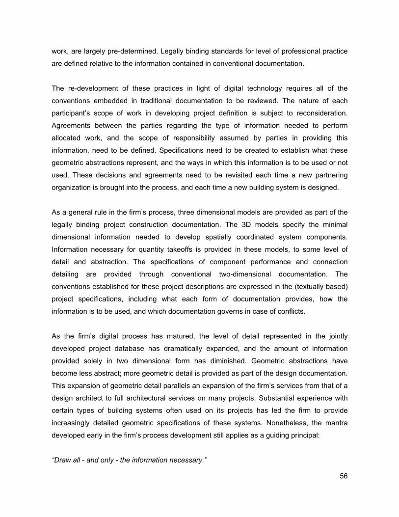
work, are largely pre-determined. Legally binding standards for level of professional practice

are defined relative to the information contained in conventional documentation.

The re-development of these practices in light of digital technology requires all of the

conventions embedded in traditional documentation to be reviewed. The nature of each

participant’s scope of work in developing project definition is subject to reconsideration.

Agreements between the parties regarding the type of information needed to perform

allocated work, and the scope of responsibility assumed by parties in providing this

information, need to be defined. Specifications need to be created to establish what these

geometric abstractions represent, and the ways in which this information is to be used or not

used. These decisions and agreements need to be revisited each time a new partnering

organization is brought into the process, and each time a new building system is designed.

As a general rule in the firm’s process, three dimensional models are provided as part of the

legally binding project construction documentation. The 3D models specify the minimal

dimensional information needed to develop spatially coordinated system components.

Information necessary for quantity takeoffs is provided in these models, to some level of

detail and abstraction. The specifications of component performance and connection

detailing are provided through conventional two-dimensional documentation. The

conventions established for these project descriptions are expressed in the (textually based)

project specifications, including what each form of documentation provides, how the

information is to be used, and which documentation governs in case of conflicts.

As the firm’s digital process has matured, the level of detail represented in the jointly

developed project database has dramatically expanded, and the amount of information

provided solely in two dimensional form has diminished. Geometric abstractions have

become less abstract; more geometric detail is provided as part of the design documentation.

This expansion of geometric detail parallels an expansion of the firm’s services from that of a

design architect to full architectural services on many projects. Substantial experience with

certain types of building systems often used on its projects has led the firm to provide

increasingly detailed geometric specifications of these systems. Nonetheless, the mantra

developed early in the firm’s process development still applies as a guiding principal:

“Draw all - and only - the information necessary.”

56

B. PROJECT CONTROL

Beginning in design development phase,

responsibility for development of portions of

the project description begins to be turned

over to partnering organizations – engineers,

construction managers and fabricators.

Elements of the 3D models are turned over to

these partnering entities, who begin to develop

the project information required for their roles

in the process. The information developed by

these organizations needs to be coordinated.

Project coordination is within the traditional

scope of the architect’s role on a building project. Conventionally, this role is conducted by

reviewing 2D drawing documentation provided by each partnering organization in format

founded on conventions of their discipline. Coordination of the assembled body of

documentation from these numerous partners in their native physical drawing formats is an

extraordinarily difficult undertaking, and a major source of errors and omissions on

construction projects.

Figure III-3: Coordination model of ceiling space

(DCH)

The comprehensive 3D model that resides at the center of the firm’s process provides an

enormous aid for coordination. Even when two dimensional documentation is employed by a

partner, this 2D documentation can be translated back into three dimensions, and oriented

appropriately in 3D space relative to the other information on the project. When partners

employ 3D documentation – as is increasingly becoming the case – this information may be

directly imported and overlaid on the architectural models. The result is a comprehensive

repository for all geometric data generated by the partners in the design process. By

assembling and filtering this information, the process of system coordination is radically

improved. System interferences may be detected, either via visual inspection or through tools

that automate checking for spatial clashes or violations of system envelopes by other

systems.

57

Time based visualization of construction

sequencing has become a useful coordination

tool on the firm’s larger projects, including the

Experience Music Project, the Disney Concert

Hall, and the Stata Center at MIT. This

detailed coordination of on site activities is part

of the general contractor’s responsibility. The

enabling technology – developed by Disney

Imagineering in collaboration with Stanford

University’s Center for Integrated Facilities

Management (CIFE)40 allows 3D project geometry to be associated with information from

project scheduling software such as Primavera. Project managers and personnel

responsible for on-site coordination can simulate the progression of activities on the

construction site.

Figure III-4: CIFE’s 4D modeling tool (DCH)

C. PERFORMANCE ANALYSIS

The ease by which specific engineering and other analytical models may be supported is a

core benefit of the 3D project master model. The transfer of project information to and from

formats satisfying the requirements of engineering and fabrication partners is a critical

component of design development activities.

Numerous computational engineering analysis techniques have become available over the

past two decades. Examples of such techniques include structural analysis, energy

simulation and computation fluid dynamics based air flow studies, equipment performance

simulation, as well as lighting and acoustic simulation. Much of this development has been

through the use of finite element and finite difference techniques. These techniques

approximate complicated geometric forms into assemblies of simplified elements. The global

solution for the form is achieved by simultaneous solution of the individual elements’

performances. These techniques are well suited to the analysis of the geometry on Gehry’s

projects. The feasibility of Gehry’s recent projects is due in no small measure to the

availability of these analytical approaches.

58

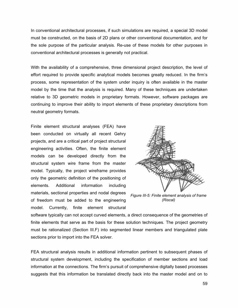
In conventional architectural processes, if such simulations are required, a special 3D model

must be constructed, on the basis of 2D plans or other conventional documentation, and for

the sole purpose of the particular analysis. Re-use of these models for other purposes in

conventional architectural processes is generally not practical.

With the availability of a comprehensive, three dimensional project description, the level of

effort required to provide specific analytical models becomes greatly reduced. In the firm’s

process, some representation of the system under inquiry is often available in the master

model by the time that the analysis is required. Many of these techniques are undertaken

relative to 3D geometric models in proprietary formats. However, software packages are

continuing to improve their ability to import elements of these proprietary descriptions from

neutral geometry formats.

Finite element structural analyses (FEA) have

been conducted on virtually all recent Gehry

projects, and are a critical part of project structural

engineering activities. Often, the finite element

models can be developed directly from the

structural system wire frame from the master

model. Typically, the project wireframe provides

only the geometric definition of the positioning of

elements. Additional information including

materials, sectional properties and nodal degrees

of freedom must be added to the engineering

model. Currently, finite element structural

software typically can not accept curved elements, a direct consequence of the geometries of

finite elements that serve as the basis for these solution techniques. The project geometry

must be rationalized (Section III.F) into segmented linear members and triangulated plate

sections prior to import into the FEA solver.

Figure III-5: Finite element analysis of frame

(Riscal)

FEA structural analysis results in additional information pertinent to subsequent phases of

structural system development, including the specification of member sections and load

information at the connections. The firm’s pursuit of comprehensive digitally based processes

suggests that this information be translated directly back into the master model and on to

59

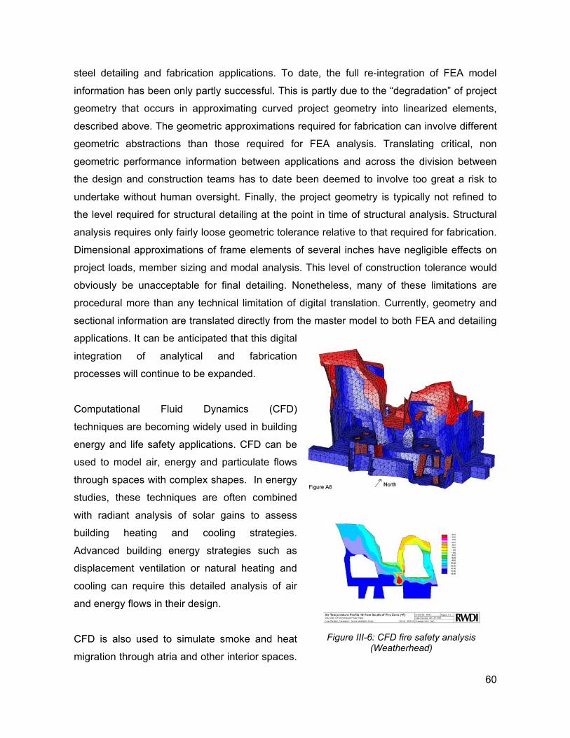
steel detailing and fabrication applications. To date, the full re-integration of FEA model

information has been only partly successful. This is partly due to the “degradation” of project

geometry that occurs in approximating curved project geometry into linearized elements,

described above. The geometric approximations required for fabrication can involve different

geometric abstractions than those required for FEA analysis. Translating critical, non

geometric performance information between applications and across the division between

the design and construction teams has to date been deemed to involve too great a risk to

undertake without human oversight. Finally, the project geometry is typically not refined to

the level required for structural detailing at the point in time of structural analysis. Structural

analysis requires only fairly loose geometric tolerance relative to that required for fabrication.

Dimensional approximations of frame elements of several inches have negligible effects on

project loads, member sizing and modal analysis. This level of construction tolerance would

obviously be unacceptable for final detailing. Nonetheless, many of these limitations are

procedural more than any technical limitation of digital translation. Currently, geometry and

sectional information are translated directly from the master model to both FEA and detailing

applications. It can be anticipated that this digital

integration of analytical and fabrication

processes will continue to be expanded.

Computational Fluid Dynamics (CFD)

techniques are becoming widely used in building

energy and life safety applications. CFD can be

used to model air, energy and particulate flows

through spaces with complex shapes. In energy

studies, these techniques are often combined

with radiant analysis of solar gains to assess

building heating and cooling strategies.

Advanced building energy strategies such as

displacement ventilation or natural heating and

cooling can require this detailed analysis of air

and energy flows in their design.

Figure III-6: CFD fire safety analysis

(Weatherhead)

CFD is also used to simulate smoke and heat

migration through atria and other interior spaces.

60

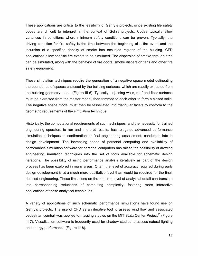
These applications are critical to the feasibility of Gehry’s projects, since existing life safety

codes are difficult to interpret in the context of Gehry projects. Codes typically allow

variances in conditions where minimum safety conditions can be proven. Typically, the

driving condition for fire safety is the time between the beginning of a fire event and the

incursion of a specified density of smoke into occupied regions of the building. CFD

applications allow specific fire events to be simulated. The dispersion of smoke through atria

can be simulated, along with the behavior of fire doors, smoke dispersion fans and other fire

safety equipment.

These simulation techniques require the generation of a negative space model delineating

the boundaries of spaces enclosed by the building surfaces, which are readily extracted from

the building geometry model (Figure III-6). Typically, adjoining walls, roof and floor surfaces

must be extracted from the master model, then trimmed to each other to form a closed solid.

The negative space model must then be tessellated into triangular facets to conform to the

geometric requirements of the simulation technique.

Historically, the computational requirements of such techniques, and the necessity for trained

engineering operators to run and interpret results, has relegated advanced performance

simulation techniques to confirmation or final engineering assessment, conducted late in

design development. The increasing speed of personal computing and availability of

performance simulation software for personal computers has raised the possibility of drawing

engineering simulation techniques into the set of tools available for schematic design

iterations. The possibility of using performance analysis iteratively as part of the design

process has been explored in many areas. Often, the level of accuracy required during early

design development is at a much more qualitative level than would be required for the final,

detailed engineering. These limitations on the required level of analytical detail can translate

into corresponding reductions of computing complexity, fostering more interactive

applications of these analytical techniques.

A variety of applications of such schematic performance simulations have found use on

Gehry’s projects. The use of CFD as an iterative tool to assess wind flow and associated

pedestrian comfort was applied to massing studies on the MIT Stata Center Project20 (Figure

III-7). Visualization software is frequently used for shadow studies to assess natural lighting

and energy performance (Figure III-8).

61

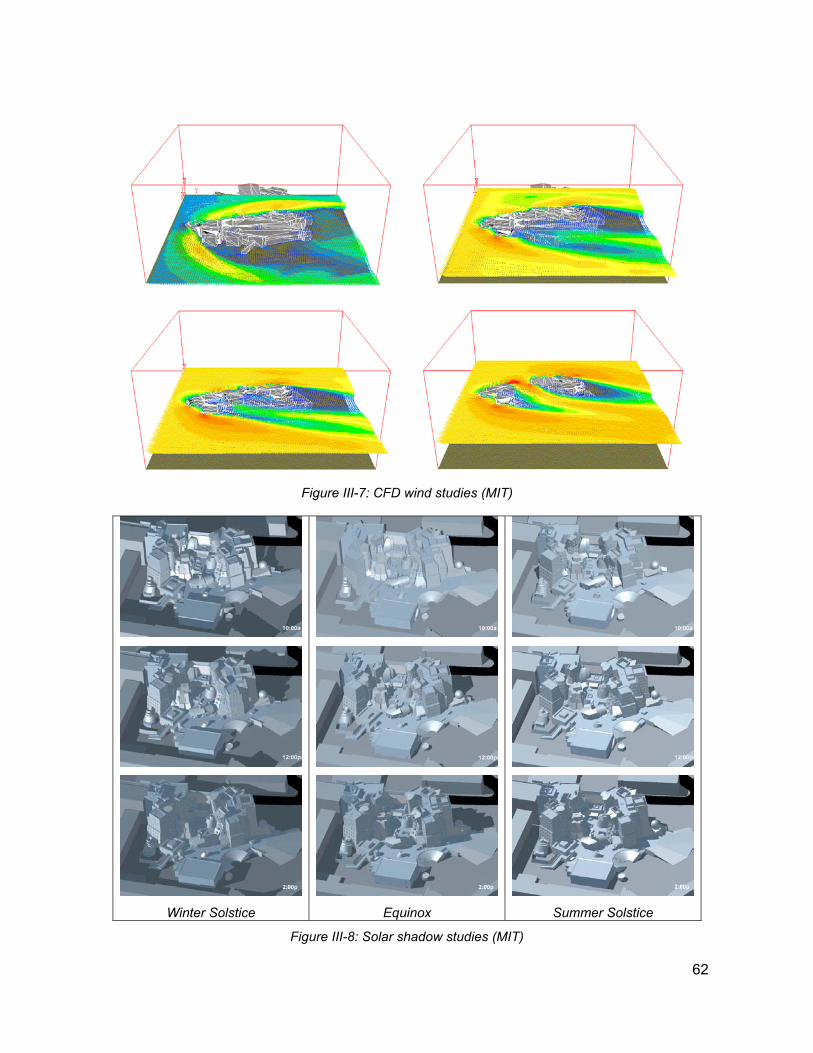
Figure III-7: CFD wind studies (MIT)

Winter Solstice Equinox Summer Solstice

Figure III-8: Solar shadow studies (MIT)

62

The use of materials simulation techniques, described in Chapter VII, is a further example of

the interactive performance applications that become available through tradeoffs between

simulation accuracy and speed. This migration of performance analysis techniques from

engineering to design applications is an important opportunity for the development of project

design activities, and is again enabled through the existence of the building master model.

D. 3D – 2D INTEGRATION

The need to of carry both three dimensional and two dimensional descriptions of the project

through the many design iterations and document submissions over the lifetime of a

construction project has been one of the most difficult aspects of the firm’s digital process.

There are many reasons why two dimensional representations remain a necessary

component of project descriptions for the foreseeable future:

Interaction needs to occur with many organizations using traditional processes.

Increasingly, technologically sophisticated partners are available who can provide

favorable prices for services through efficiencies generated by technological

advancement. However partners may, for regional cultural or economic reasons, provide

the best price for services through traditional methods, or there may simply be no

technologically enabled alternatives.

It is largely the building agencies that remain most firmly entrenched in conventional

documentation processes. These are the local governmental authorities that approve

building permits, and review code compliance. These agencies need approval processes

that serve the “lowest common denominator” for building projects within their jurisdiction.

They also have neither direct financial incentives nor economic resources to justify

technological advancements of process. Most building agencies will not accept even two

dimensional CAD documentation.

Building information is often symbolic in nature at points in the design process. Elements

such as door swings, tile patterns and bathroom fixtures either do not merit full 3D

geometric description, or the full geometric nature may not be known at a given point in

time. The building description is facilitated by treating these elements as symbols on

plans, rather than developing such abstract or trivial information into detailed three

dimensional representations. As technology continues to be adopted industry wide, and

63

efficient standards for including and reviewing this information become available, this

symbolic information may eventually be migrated to a three dimensional form.

Many building components have important two dimensional qualities. Many of the

efficiencies in building systems used on Gehry projects are derived from building

components that are essentially two dimensional. CNC cut plate elements, flattenable

surface elements, floor finishes, all have geometric natures efficiently expressed through

appropriately oriented two dimensional views.

For these reasons, two dimensional project descriptions are likely to be an important element

of design and construction processes for some time to come. The technical and procedural

integration of 3D and 2D information is a substantial focus of technological development by

the firm. At times, the process has had the flavor of maintaining a dual database: one

database of three dimensional data, and the other embodied in two dimensional drawings.

The process of integrating between these two representations, distanced by technological

and representational conventions, is not yet ideal.

A number of technological approaches support this integration between 2D and 3D project

representations. However, not all are applicable to complex non-Euclidean geometry. Until

recently, brute force geometric operations were required to extract drawings from 3D models.

Section cuts could be easily generated by intersecting the model geometry with a plane at

the location of the cut. Utilities also existed for performing isometric or perspective

projections. However, hidden line removal utilities did function correctly for all geometric

objects. Laborious geometric operations were needed to remove hidden geometry such as

pattern curves on surfaces. Creation of section / projection views required manually splitting

the master model at the cut plane, and erasing geometry prior to drawing extraction! This two

dimensional geometry was then exported to AutoCAD and cleaned up. Finally, annotation,

text, and hatching, line weight correction and other two dimensional “dress up” were

manually applied in 2D.

Even minor changes to the project geometry required redoing the entire process. Existing

two dimensional annotations could be manually repositioned, rather than re-drawing. Any

drawings unaffected by changes in geometry would of course not be re-processed. The

whole process took enormous amounts of time for each revision. In times of project

64

deadlines, shorts would be taken. The 2D drawings might be manually changed, rather than

modifying the 3D geometry and repeating the process. The result has been difficulty in

maintaining the integrity of the dual database. This difficulty was exacerbated as the detail in

project models has grown.

This dual 2D / 3D nature of project geometry, and the necessity for its integration has been

known to software developers for some time. Various approaches to the 2D / 3D integration,

and the integration of symbolic expressions of project information with geometric

representations, have been proposed by researchers and vendors. The support of automatic

3D to 2D geometric extractions has improved. Other approaches involving the “intelligent” re-

writing of the building objects in various contexts have been proposed as well. For example,

AutoDesk’s Architectural Desktop software allows walls, and other project objects to be

drawn in 2D, while retaining knowledge of their behavior and representation in 3D. This

approach works satisfactorily for conventional, Euclidean project geometry, but is ill suited to

Gehry’s geometry, where the 3D behavior of building geometry can not easily be predicted

from simple two dimensional views. The firm’s strategy has been to find ways to easily

embed necessary project information in 3D representations, then draw on more powerful

geometric and symbolic extraction mechanisms to produce 2D representations.

Recent enhancements in the CATIA modeling platform promise to streamline this process.

The software allows parametric definitions of geometric drawing extractions to be defined in

a persistent manner. Section cuts can be defined in the 3D model space. When project

geometry is modified, drawing extraction is achieved through a simple (though slow in terms

of computer time) update request. These improvements have allowed an approximately 90%

increase in operator efficiency for generating backgrounds for two dimensional

documentation from the 3D model. Opportunities for automated extraction to 2D of

annotation from non geometric attributes defined on 3D objects are also being pursued.

Figure III-9 provides views of this drawing extraction process. These developments promise

an eventual integration of two- and three- dimensional information into a single,

comprehensive project database.

65

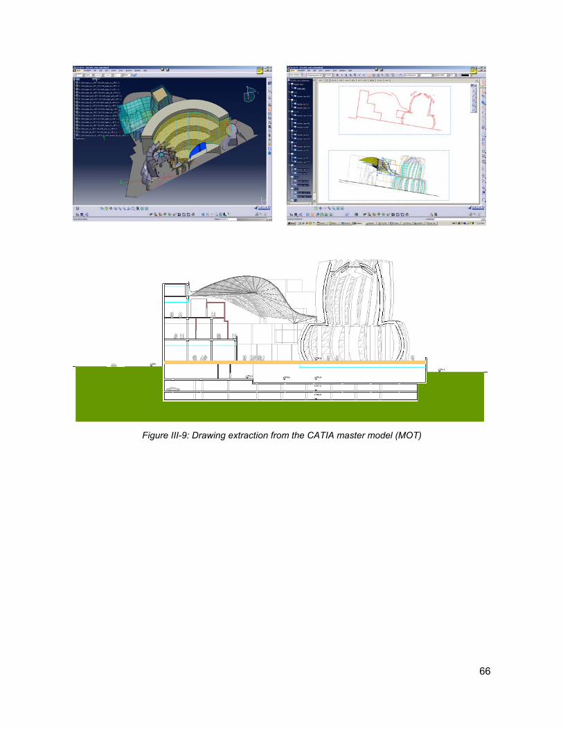
Figure III-9: Drawing extraction from the CATIA master model (MOT)

66

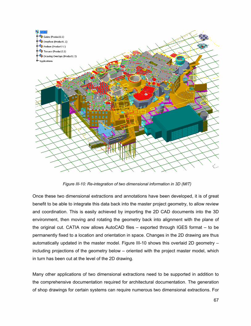
Figure III-10: Re-integration of two dimensional information in 3D (MIT)

Once these two dimensional extractions and annotations have been developed, it is of great

benefit to be able to integrate this data back into the master project geometry, to allow review

and coordination. This is easily achieved by importing the 2D CAD documents into the 3D

environment, then moving and rotating the geometry back into alignment with the plane of

the original cut. CATIA now allows AutoCAD files – exported through IGES format – to be

permanently fixed to a location and orientation in space. Changes in the 2D drawing are thus

automatically updated in the master model. Figure III-10 shows this overlaid 2D geometry –

including projections of the geometry below – oriented with the project master model, which

in turn has been cut at the level of the 2D drawing.

Many other applications of two dimensional extractions need to be supported in addition to

the comprehensive documentation required for architectural documentation. The generation

of shop drawings for certain systems can require numerous two dimensional extractions. For

67

example, concrete detailing requires many simple plan and section cuts of small areas of the

project for detailed layout of re-bar. The utility of simple sketch drawings is preferable to the

detailed generation of 3 dimensional layouts in this case. These simple cuts are easily

achieved by planar intersections with the project geometry. Usually, these operations are

performed either by the fabricator or by the general contractor as a service to the fabricator.

E. THE PHYSICAL / DIGITAL INTERFACE

The role of physical objects in Gehry’s design process has had a profound role in the

development of the firm’s digital process. In any architectural or product design process, this

relationship exists, since the products of the process are ultimately physical objects. Other

firms do on occasion generate presentation models using CAD / CAM prototyping. The

unique aspects of the physical / digital interaction in Gehry’s process stem from the authority

bestowed on physical objects and processes of making. Physical models are the primary

elements of the process where the project design is developed. These physical objects

define and embody the formal design intent as it is developed over the course of the project.

Digital representations serve to capture this intent and allow for its processing and

communication.

On more conventional project geometry, this division between physical and digital

representation might not be so problematic. There are perfectly adequate ways of digitally

and physically modeling orthogonally configured planar objects, and great geometric affinity

between these digital and physical forms. Digitizing such conventional geometries is straight

forward. A few dimensions can be measured, and then orthogonal planes can be positioned

in digital space and intersected to form boundaries of surfaces. It is even arguable that the

digital representation of such assemblies is a “better” representation of the design intent.

Physical modeling necessarily introduces fabrication errors relative to pure Euclidean

geometry. Materials warp, elements are cut too short or too long, edges are not perfectly

straight, corners are not completely tight. While these imperfections might be imperceptible

on well constructed scale models, when fully scaled these imperfections would likely be

outside of construction tolerances. A gap at a corner of 1/32” on an 1/8” scale model represents

a 3” hole at the corner of the construction! CAD modeling allows these imperfections to be

cleaned up to within machine tolerances, well below the tolerances of construction. It is thus

arguable that, if the design intent of a project is concerned with Euclidean geometry, digital

68

modeling can provide a more exact representation for the description of this intent than any

scale physical representation. 3D CAD can even be a more efficient interface for generating

this geometry, as the digital tools for performing cutting, positioning, moving, and editing of

planar geometries can be easier than corresponding operations on physical modeling

materials.

Gehry’s process introduces a number of problematic issues into this clean relationship

between physical and digital representations. Gehry’s design models also contain

imperfections of construction. However, unlike Euclidean geometries, established reference

formalisms that serve to define the “true” geometry behind the shape do not necessarily

exist. The geometry of the physical model provides the only definitive reference of design

intent that digital representations must strive to emulate.

Highly accurate digitizing technologies exist that can sample points in tight conformance with

physical objects. However, these representations still need to be cleaned up, to remove

imperfections in the physical object and to simplify digital geometry to a form that can be

manipulated. These operations introduce artifacts of the geometric representation underlying

the CAD system – representational constructs whose characteristics may be radically

different than those of the modeling materials. Distinctions between features of the physical

object that are desired and those that are model imperfections or noise are qualitative, and

must be undertaken through the filter of the CAD system’s geometric representation.

A closely related issue emerges in comparing the “user interfaces” afforded by physical and

digital modeling operations. Physical materials afford the development of certain forms,

guided by the behavior of materials and operations that are facilitated by these materials. In

the development of non-Euclidean geometries, these behaviors can be subtle and complex,

as materials are driven to deformation at the limits of their material behavior. These effects

generate formal qualities in the physical models important to the designers. The natural and

intuitive operations of designers operating on these physical objects can be difficult to even

approximately reproduce in digital form. As a result, either digital operations can result in

subtly but critically different geometries, or the development of shapes with similar qualities

can take substantial skill, time and attention by operators.

69

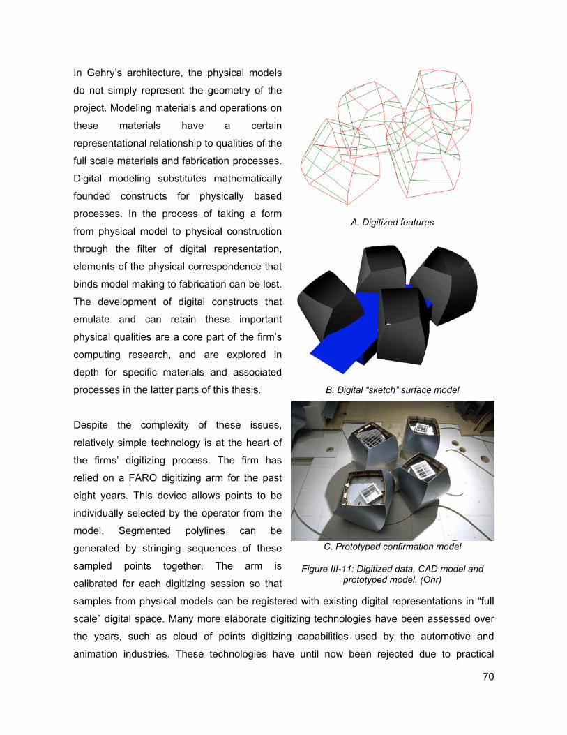
In Gehry’s architecture, the physical models

do not simply represent the geometry of the

project. Modeling materials and operations on

these materials have a certain

representational relationship to qualities of the

full scale materials and fabrication processes.

Digital modeling substitutes mathematically

founded constructs for physically based

processes. In the process of taking a form

from physical model to physical construction

through the filter of digital representation,

elements of the physical correspondence that

binds model making to fabrication can be lost.

The development of digital constructs that

emulate and can retain these important

physical qualities are a core part of the firm’s

computing research, and are explored in

depth for specific materials and associated

processes in the latter parts of this thesis.

Despite the complexity of these issues,

relatively simple technology is at the heart of

the firms’ digitizing process. The firm has

relied on a FARO digitizing arm for the past

eight years. This device allows points to be

individually selected by the operator from the

model. Segmented polylines can be

generated by stringing sequences of these

sampled points together. The arm is

calibrated for each digitizing session so that

samples from physical models can be registered with existing digital representations in “full

scale” digital space. Many more elaborate digitizing technologies have been assessed over

the years, such as cloud of points digitizing capabilities used by the automotive and

animation industries. These technologies have until now been rejected due to practical

A. Digitized features

B. Digital “sketch” surface model

C. Prototyped confirmation model

Figure III-11: Digitized data, CAD model and

prototyped model. (Ohr)

70

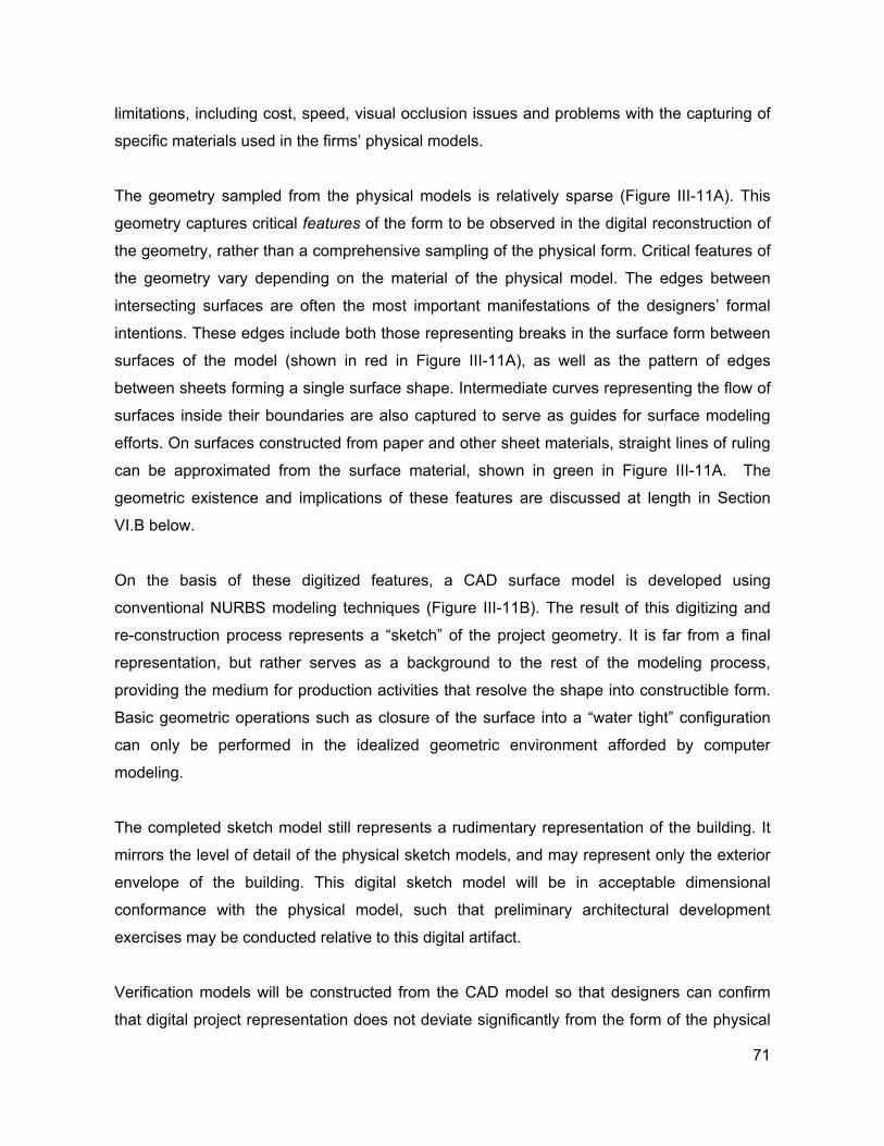
limitations, including cost, speed, visual occlusion issues and problems with the capturing of

specific materials used in the firms’ physical models.

The geometry sampled from the physical models is relatively sparse (Figure III-11A). This

geometry captures critical features of the form to be observed in the digital reconstruction of

the geometry, rather than a comprehensive sampling of the physical form. Critical features of

the geometry vary depending on the material of the physical model. The edges between

intersecting surfaces are often the most important manifestations of the designers’ formal

intentions. These edges include both those representing breaks in the surface form between

surfaces of the model (shown in red in Figure III-11A), as well as the pattern of edges

between sheets forming a single surface shape. Intermediate curves representing the flow of

surfaces inside their boundaries are also captured to serve as guides for surface modeling

efforts. On surfaces constructed from paper and other sheet materials, straight lines of ruling

can be approximated from the surface material, shown in green in Figure III-11A. The

geometric existence and implications of these features are discussed at length in Section

VI.B below.

On the basis of these digitized features, a CAD surface model is developed using

conventional NURBS modeling techniques (Figure III-11B). The result of this digitizing and

re-construction process represents a “sketch” of the project geometry. It is far from a final

representation, but rather serves as a background to the rest of the modeling process,

providing the medium for production activities that resolve the shape into constructible form.

Basic geometric operations such as closure of the surface into a “water tight” configuration

can only be performed in the idealized geometric environment afforded by computer

modeling.

The completed sketch model still represents a rudimentary representation of the building. It

mirrors the level of detail of the physical sketch models, and may represent only the exterior

envelope of the building. This digital sketch model will be in acceptable dimensional

conformance with the physical model, such that preliminary architectural development

exercises may be conducted relative to this digital artifact.

Verification models will be constructed from the CAD model so that designers can confirm

that digital project representation does not deviate significantly from the form of the physical

71

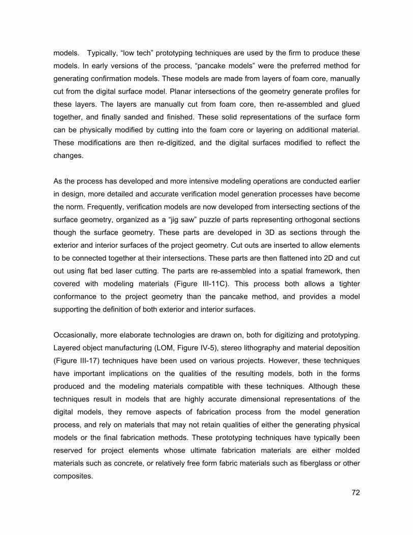
models. Typically, “low tech” prototyping techniques are used by the firm to produce these

models. In early versions of the process, “pancake models” were the preferred method for

generating confirmation models. These models are made from layers of foam core, manually

cut from the digital surface model. Planar intersections of the geometry generate profiles for

these layers. The layers are manually cut from foam core, then re-assembled and glued

together, and finally sanded and finished. These solid representations of the surface form

can be physically modified by cutting into the foam core or layering on additional material.

These modifications are then re-digitized, and the digital surfaces modified to reflect the

changes.

As the process has developed and more intensive modeling operations are conducted earlier

in design, more detailed and accurate verification model generation processes have become

the norm. Frequently, verification models are now developed from intersecting sections of the

surface geometry, organized as a “jig saw” puzzle of parts representing orthogonal sections

though the surface geometry. These parts are developed in 3D as sections through the

exterior and interior surfaces of the project geometry. Cut outs are inserted to allow elements

to be connected together at their intersections. These parts are then flattened into 2D and cut

out using flat bed laser cutting. The parts are re-assembled into a spatial framework, then

covered with modeling materials (Figure III-11C). This process both allows a tighter

conformance to the project geometry than the pancake method, and provides a model

supporting the definition of both exterior and interior surfaces.

Occasionally, more elaborate technologies are drawn on, both for digitizing and prototyping.

Layered object manufacturing (LOM, Figure IV-5), stereo lithography and material deposition

(Figure III-17) techniques have been used on various projects. However, these techniques

have important implications on the qualities of the resulting models, both in the forms

produced and the modeling materials compatible with these techniques. Although these

techniques result in models that are highly accurate dimensional representations of the

digital models, they remove aspects of fabrication process from the model generation

process, and rely on materials that may not retain qualities of either the generating physical

models or the final fabrication methods. These prototyping techniques have typically been

reserved for project elements whose ultimate fabrication materials are either molded

materials such as concrete, or relatively free form fabric materials such as fiberglass or other

composites.

72

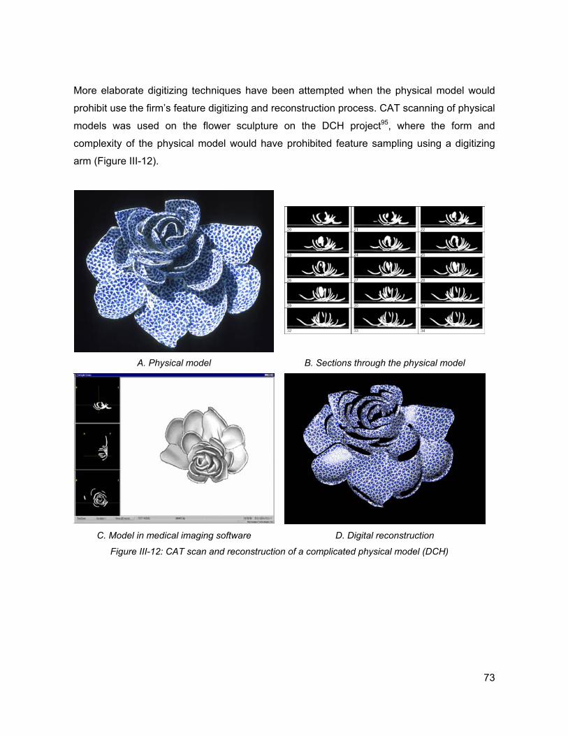
More elaborate digitizing techniques have been attempted when the physical model would

prohibit use the firm’s feature digitizing and reconstruction process. CAT scanning of physical

models was used on the flower sculpture on the DCH project95, where the form and

complexity of the physical model would have prohibited feature sampling using a digitizing

arm (Figure III-12).

A. Physical model B. Sections through the physical model

C. Model in medical imaging software D. Digital reconstruction

Figure III-12: CAT scan and reconstruction of a complicated physical model (DCH)

73

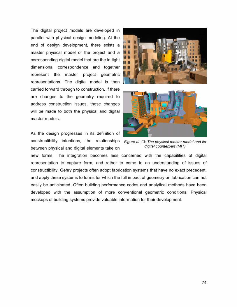
The digital project models are developed in

parallel with physical design modeling. At the

end of design development, there exists a

master physical model of the project and a

corresponding digital model that are the in tight

dimensional correspondence and together

represent the master project geometric

representations. The digital model is then

carried forward through to construction. If there

are changes to the geometry required to

address construction issues, these changes

will be made to both the physical and digital

master models.

As the design progresses in its definition of

constructibility intentions, the relationships

between physical and digital elements take on

new forms. The integration becomes less concerned with the capabilities of digital

representation to capture form, and rather to come to an understanding of issues of

constructibility. Gehry projects often adopt fabrication systems that have no exact precedent,

and apply these systems to forms for which the full impact of geometry on fabrication can not

easily be anticipated. Often building performance codes and analytical methods have been

developed with the assumption of more conventional geometric conditions. Physical

mockups of building systems provide valuable information for their development.

Figure III-13: The physical master model and its

digital counterpart (MIT)

74

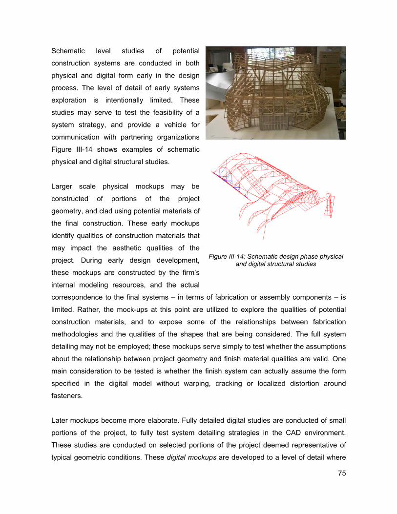
Schematic level studies of potential

construction systems are conducted in both

physical and digital form early in the design

process. The level of detail of early systems

exploration is intentionally limited. These

studies may serve to test the feasibility of a

system strategy, and provide a vehicle for

communication with partnering organizations

Figure III-14 shows examples of schematic

physical and digital structural studies.

Larger scale physical mockups may be

constructed of portions of the project

geometry, and clad using potential materials of

the final construction. These early mockups

identify qualities of construction materials that

may impact the aesthetic qualities of the

project. During early design development,

these mockups are constructed by the firm’s

internal modeling resources, and the actual

correspondence to the final systems – in terms of fabrication or assembly components – is

limited. Rather, the mock-ups at this point are utilized to explore the qualities of potential

construction materials, and to expose some of the relationships between fabrication

methodologies and the qualities of the shapes that are being considered. The full system

detailing may not be employed; these mockups serve simply to test whether the assumptions

about the relationship between project geometry and finish material qualities are valid. One

main consideration to be tested is whether the finish system can actually assume the form

specified in the digital model without warping, cracking or localized distortion around

fasteners.

Figure III-14: Schematic design phase physical

and digital structural studies

Later mockups become more elaborate. Fully detailed digital studies are conducted of small

portions of the project, to fully test system detailing strategies in the CAD environment.

These studies are conducted on selected portions of the project deemed representative of

typical geometric conditions. These digital mockups are developed to a level of detail where

75

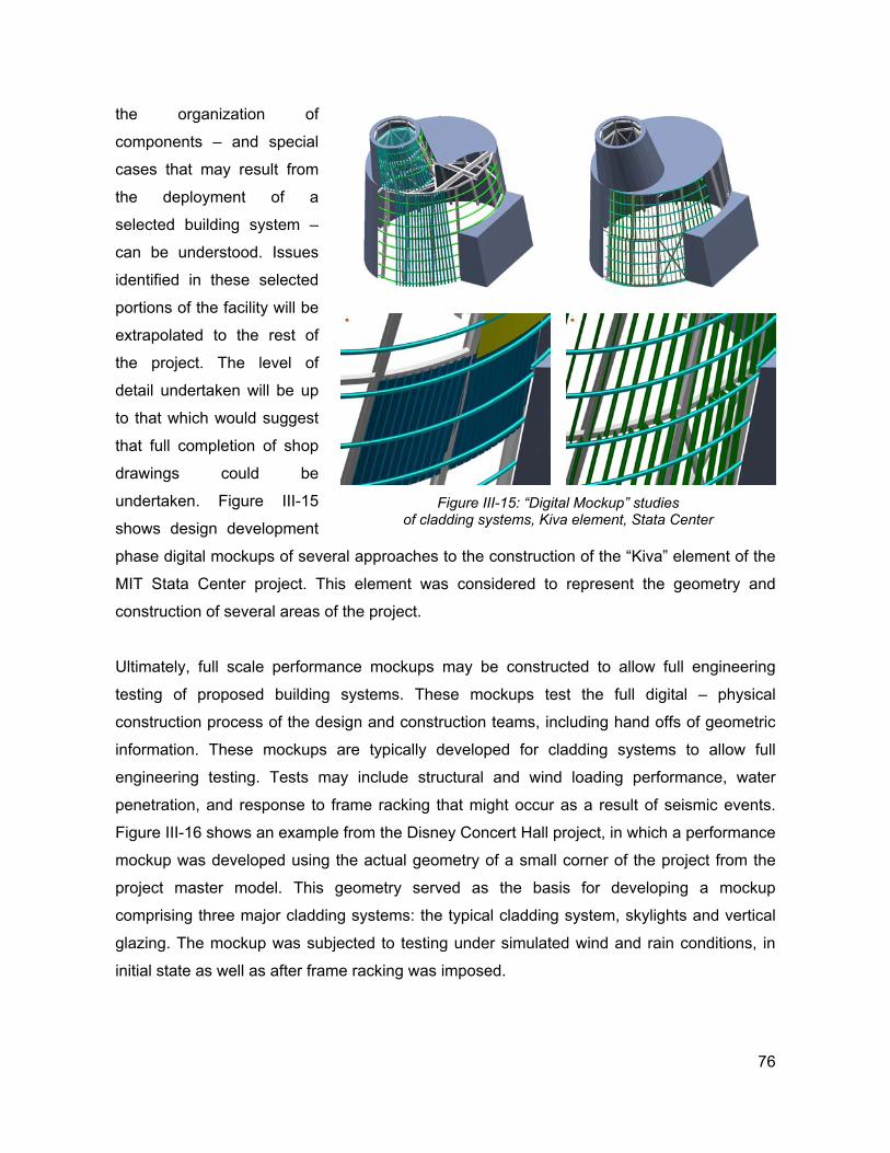
the organization of

components – and special

cases that may result from

the deployment of a

selected building system –

can be understood. Issues

identified in these selected

portions of the facility will be

extrapolated to the rest of

the project. The level of

detail undertaken will be up

to that which would suggest

that full completion of shop

drawings could be

undertaken. Figure III-15

shows design development

phase digital mockups of several approaches to the construction of the “Kiva” element of the

MIT Stata Center project. This element was considered to represent the geometry and

construction of several areas of the project.

Figure III-15: “Digital Mockup” studies of cladding systems, Kiva element, Stata Center

Ultimately, full scale performance mockups may be constructed to allow full engineering

testing of proposed building systems. These mockups test the full digital – physical

construction process of the design and construction teams, including hand offs of geometric

information. These mockups are typically developed for cladding systems to allow full

engineering testing. Tests may include structural and wind loading performance, water

penetration, and response to frame racking that might occur as a result of seismic events.

Figure III-16 shows an example from the Disney Concert Hall project, in which a performance

mockup was developed using the actual geometry of a small corner of the project from the

project master model. This geometry served as the basis for developing a mockup

comprising three major cladding systems: the typical cladding system, skylights and vertical

glazing. The mockup was subjected to testing under simulated wind and rain conditions, in

initial state as well as after frame racking was imposed.

76

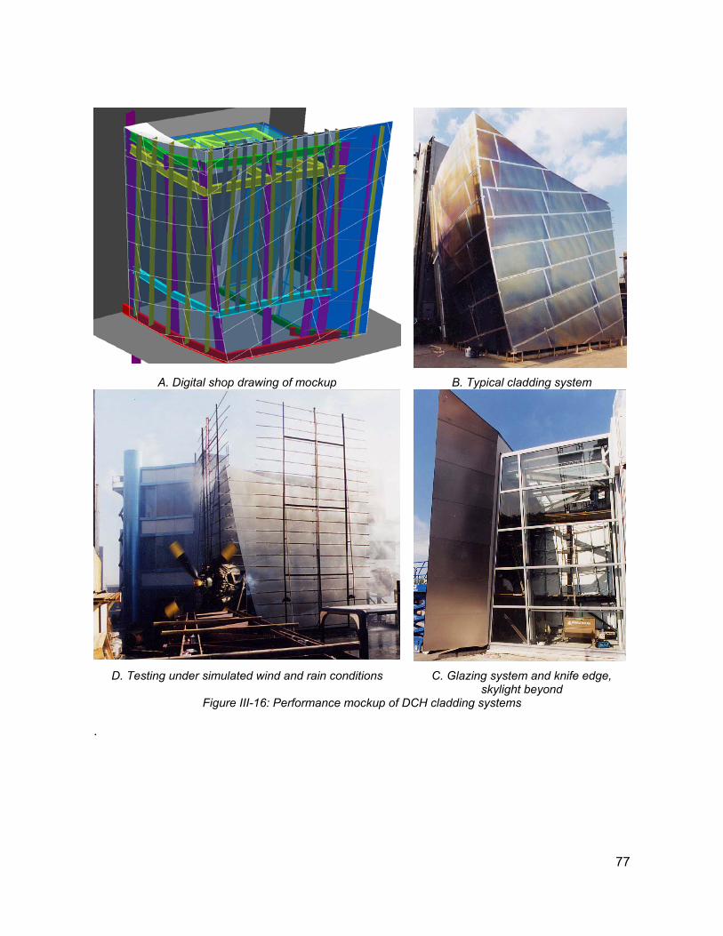
A. Digital shop drawing of mockup B. Typical cladding system

D. Testing under simulated wind and rain conditions C. Glazing system and knife edge,

skylight beyond Figure III-16: Performance mockup of DCH cladding systems

.

77

F. RATIONALIZATION

The concept of rationalization is at the heart of Gehry Partner’s computing and construction

methodologies. Broadly stated, rationalization is the resolution of rules of constructibility into

project geometry. The concept encompasses broad applications in the firm’s process. Many

of these applications can have substantial impact on the formal qualities and design intent of

the project architecture. Others can have dramatic effects on the cost and control of

construction, and hence can determine the feasibility of building strategies.

This issue of problem description through mathematics and geometry, and the fitness of a

mathematical / geometric model to a given solution approach is of course nothing new in

engineering and physics applications. In Gehry’s building process, geometric representation

and its role in providing the syntax for describing the project design intent, and supporting its

translation into constructibility and building intentions deserves some inspection.

Mitchell makes reference to the role of rationalization on constructibility decisions in his

comparison of the Sydney Opera House and Guggenheim Bilbao projects57. The Sydney

Opera House (1957-73) designed and constructed just before the advent of digital geometric

modeling, required the designed form to be rationalized into spherical elements simply to be

describable using contemporary drafting and engineering methods. With the advent of digital

curved surface modeling, these limitations on designer’s descriptive capabilities seem to

have largely been addressed. However, experience by the firm indicates issues of project

description and geometric constraints are still very much in play.

Simply the operation of rendering a physical shape into digital form implies a structuring

through the geometric representations of the CAD application. A broad palette geometric

forms with various characteristics – one, two or three dimensional, Euclidean or other

differentiable forms – are available to serve as representational bases for the surface

geometry or any other element of the building. Selection of a set of geometric elements as a

basis for the digital representation in itself imbues the digital description with certain

characteristics. In the process of rendering the project design surface into digital form,

variations between the shapes produced by physical modeling and that produced through

digitizing occur. This is not so much due to any specific, substantial deviation in the sampling

of geometry, but rather more subtly due to the qualities of the smoothing functions embodied

78

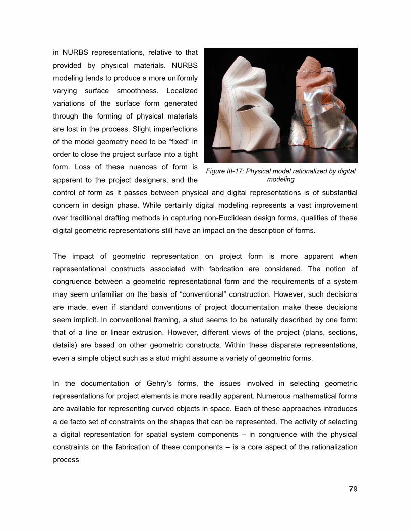
in NURBS representations, relative to that

provided by physical materials. NURBS

modeling tends to produce a more uniformly

varying surface smoothness. Localized

variations of the surface form generated

through the forming of physical materials

are lost in the process. Slight imperfections

of the model geometry need to be “fixed” in

order to close the project surface into a tight

form. Loss of these nuances of form is

apparent to the project designers, and the

control of form as it passes between physical and digital representations is of substantial

concern in design phase. While certainly digital modeling represents a vast improvement

over traditional drafting methods in capturing non-Euclidean design forms, qualities of these

digital geometric representations still have an impact on the description of forms.

Figure III-17: Physical model rationalized by digital

modeling

The impact of geometric representation on project form is more apparent when

representational constructs associated with fabrication are considered. The notion of

congruence between a geometric representational form and the requirements of a system

may seem unfamiliar on the basis of “conventional” construction. However, such decisions

are made, even if standard conventions of project documentation make these decisions

seem implicit. In conventional framing, a stud seems to be naturally described by one form:

that of a line or linear extrusion. However, different views of the project (plans, sections,

details) are based on other geometric constructs. Within these disparate representations,

even a simple object such as a stud might assume a variety of geometric forms.

In the documentation of Gehry’s forms, the issues involved in selecting geometric

representations for project elements is more readily apparent. Numerous mathematical forms

are available for representing curved objects in space. Each of these approaches introduces

a de facto set of constraints on the shapes that can be represented. The activity of selecting

a digital representation for spatial system components – in congruence with the physical

constraints on the fabrication of these components – is a core aspect of the rationalization

process

79

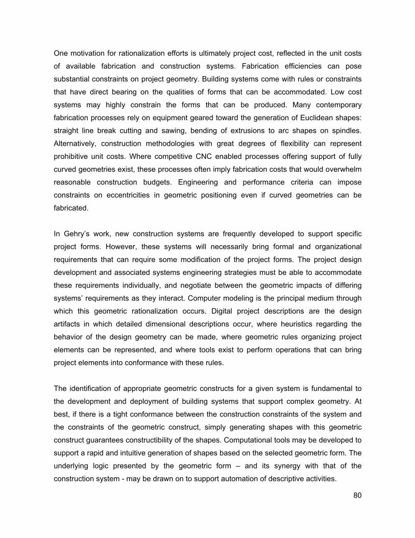
One motivation for rationalization efforts is ultimately project cost, reflected in the unit costs

of available fabrication and construction systems. Fabrication efficiencies can pose

substantial constraints on project geometry. Building systems come with rules or constraints

that have direct bearing on the qualities of forms that can be accommodated. Low cost

systems may highly constrain the forms that can be produced. Many contemporary

fabrication processes rely on equipment geared toward the generation of Euclidean shapes:

straight line break cutting and sawing, bending of extrusions to arc shapes on spindles.

Alternatively, construction methodologies with great degrees of flexibility can represent

prohibitive unit costs. Where competitive CNC enabled processes offering support of fully

curved geometries exist, these processes often imply fabrication costs that would overwhelm

reasonable construction budgets. Engineering and performance criteria can impose

constraints on eccentricities in geometric positioning even if curved geometries can be

fabricated.

In Gehry’s work, new construction systems are frequently developed to support specific

project forms. However, these systems will necessarily bring formal and organizational

requirements that can require some modification of the project forms. The project design

development and associated systems engineering strategies must be able to accommodate

these requirements individually, and negotiate between the geometric impacts of differing

systems’ requirements as they interact. Computer modeling is the principal medium through

which this geometric rationalization occurs. Digital project descriptions are the design

artifacts in which detailed dimensional descriptions occur, where heuristics regarding the

behavior of the design geometry can be made, where geometric rules organizing project

elements can be represented, and where tools exist to perform operations that can bring

project elements into conformance with these rules.

The identification of appropriate geometric constructs for a given system is fundamental to

the development and deployment of building systems that support complex geometry. At

best, if there is a tight conformance between the construction constraints of the system and

the constraints of the geometric construct, simply generating shapes with this geometric

construct guarantees constructibility of the shapes. Computational tools may be developed to

support a rapid and intuitive generation of shapes based on the selected geometric form. The

underlying logic presented by the geometric form – and its synergy with that of the

construction system - may be drawn on to support automation of descriptive activities.

80

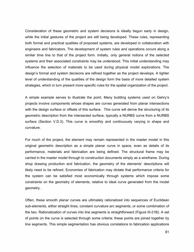
Consideration of these geometric and system decisions is ideally begun early in design,

while the initial gestures of the project are still being developed. These rules, representing

both formal and practical qualities of proposed systems, are developed in collaboration with

engineers and fabricators. The development of system rules and operations occurs along a

similar time line to that of the project form. Initially, only general notions of the selected

systems and their associated constraints may be understood. This initial understanding may

influence the selection of materials to be used during physical model explorations. The

design’s formal and system decisions are refined together as the project develops. A tighter

level of understanding of the qualities of the design form the basis of more detailed system

strategies, which in turn present more specific rules for the spatial organization of the project.

A simple example serves to illustrate the point. Many building systems used on Gehry’s

projects involve components whose shapes are curves generated from planar intersections

with the design surface or offsets of this surface. This curve will derive the structuring of its

geometric description from the intersected surface, typically a NURBS curve from a NURBS

surface (Section V.D.3). This curve is smoothly and continuously varying in shape and

curvature.

For much of the project, the element may remain represented in the master model in this

original geometric description as a simple planar curve in space, even as details of its

performance, materials and fabrication are being defined. The structural frame may be

carried in the master model through to construction documents simply as a wireframe. During

shop drawing production and fabrication, the geometry of the elements’ descriptions will

likely need to be refined. Economies of fabrication may dictate that performance criteria for

the system can be satisfied most economically through systems which impose some

constraints on the geometry of elements, relative to ideal curve generated from the model

geometry.

Often, these smooth planar curves are ultimately rationalized into sequences of Euclidean

sub-elements, either straight lines, constant curvature arc segments, or some combination of

the two. Rationalization of curves into line segments is straightforward (Figure III-21B). A set

of points on the curve is selected through some criteria; these points are joined together by

line segments. This simple segmentation has obvious correlations to fabrication applications

81

(Figure III-18), and fairly obvious impacts on the

tolerance of the resulting system relative to the

ideal geometry expressed by the input curve.

Segmented members can be constructed out of

extruded profiles, including I beams or custom

channels. The selection of segmentation points

can be dictated by a number of criteria,

including connection relations to other project

geometry, maximum or minimum efficient

material lengths, angle criteria, maximum

distance deviation from the ideal curve, etc.

These fabrication efficiencies can be expressed

as geometric rules and encoded in the

segmentation strategy. Numerous systems on

Gehry projects have employed this geometric

rationalization strategy, driven by widely

different fabrication criteria and corresponding

geometric rules.

There are several limitations of a straight line

segmentation approach from the perspective of constructibility. Segmentation produces

angles between segments; which will cause kinks in the system that may disadvantageously

affect the architectural form. The resulting angles may need to be resolved through

complicated beveled connections. The deviation between the ideal curve and the linear

segments can result in conflicts with other systems. Of course, the deviation can be

controlled by increasing the number of segments, but this will also increase the number of

parts and connections, which can drive up the cost of fabrication.

Figure III-18: Segmented construction of planar

curves (DCH)

Figure III-19:Arc Segment generated primary

structure (MIT)

A second approach, used on several projects, rationalizes planar curves into sequences of

arc segments, with tangency constraints imposed between the segments (Figure III-19). This

can ameliorate some of the limitations of the linear segmentation strategy above. The

connections between elements will be smooth, so no kinking of the system or the resulting

connections results. The relationship between number of segments and deviation from the

design curve is improved. Of course, bending material into an arc is likely to be more

82

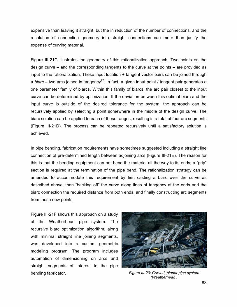
expensive than leaving it straight, but the in reduction of the number of connections, and the

resolution of connection geometry into straight connections can more than justify the

expense of curving material.

Figure III-21C illustrates the geometry of this rationalization approach. Two points on the

design curve – and the corresponding tangents to the curve at the points – are provided as

input to the rationalization. These input location + tangent vector pairs can be joined through

a biarc – two arcs joined in tangency97. In fact, a given input point / tangent pair generates a

one parameter family of biarcs. Within this family of biarcs, the arc pair closest to the input

curve can be determined by optimization. If the deviation between this optimal biarc and the

input curve is outside of the desired tolerance for the system, the approach can be

recursively applied by selecting a point somewhere in the middle of the design curve. The

biarc solution can be applied to each of these ranges, resulting in a total of four arc segments

(Figure III-21D). The process can be repeated recursively until a satisfactory solution is

achieved.

In pipe bending, fabrication requirements have sometimes suggested including a straight line

connection of pre-determined length between adjoining arcs (Figure III-21E). The reason for

this is that the bending equipment can not bend the material all the way to its ends; a ”grip”

section is required at the termination of the pipe bend. The rationalization strategy can be

amended to accommodate this requirement by first casting a biarc over the curve as

described above, then “backing off” the curve along lines of tangency at the ends and the

biarc connection the required distance from both ends, and finally constructing arc segments

from these new points.

Figure III-21F shows this approach on a study

of the Weatherhead pipe system. The

recursive biarc optimization algorithm, along

with minimal straight line joining segments,

was developed into a custom geometric

modeling program. The program includes

automation of dimensioning on arcs and

straight segments of interest to the pipe

bending fabricator.

83

Figure III-20: Curved, planar pipe system

(Weatherhead )

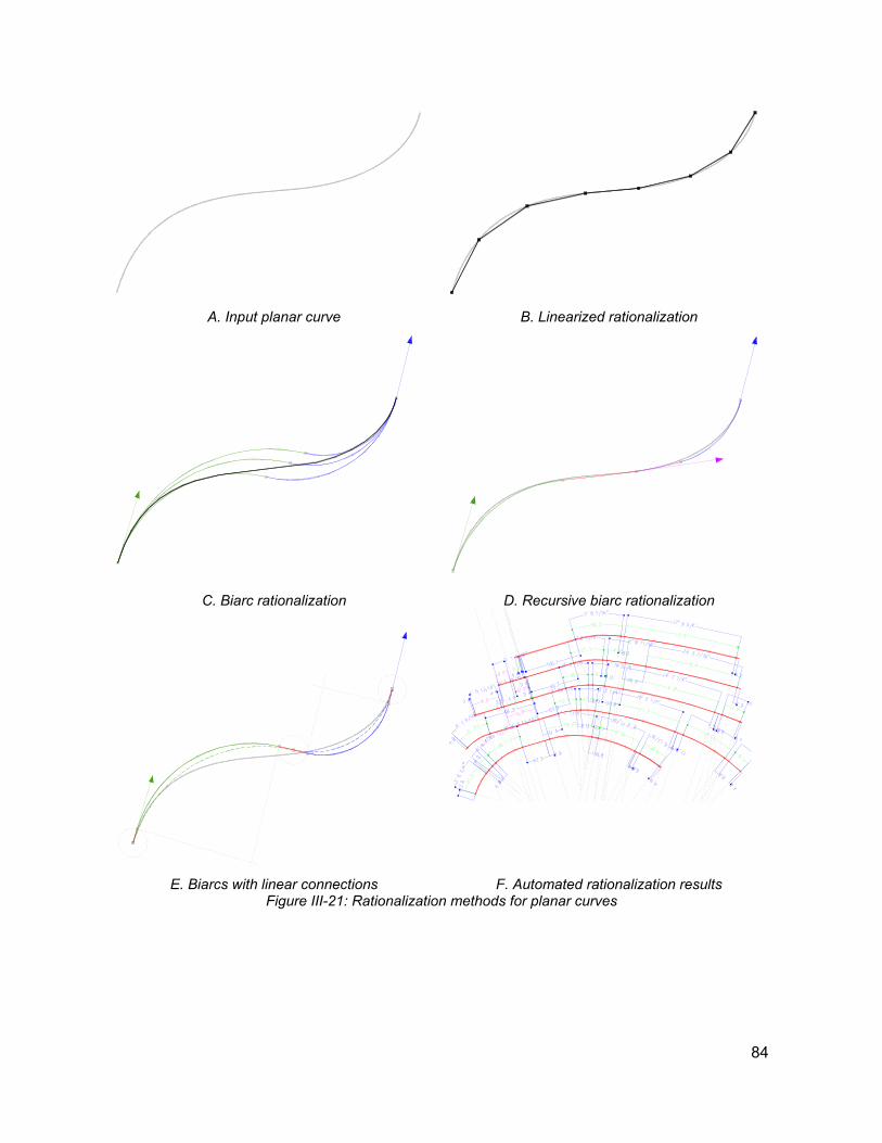
A. Input planar curve B. Linearized rationalization

C. Biarc rationalization D. Recursive biarc rationalization

E. Biarcs with linear connections F. Automated rationalization results Figure III-21: Rationalization methods for planar curves

84

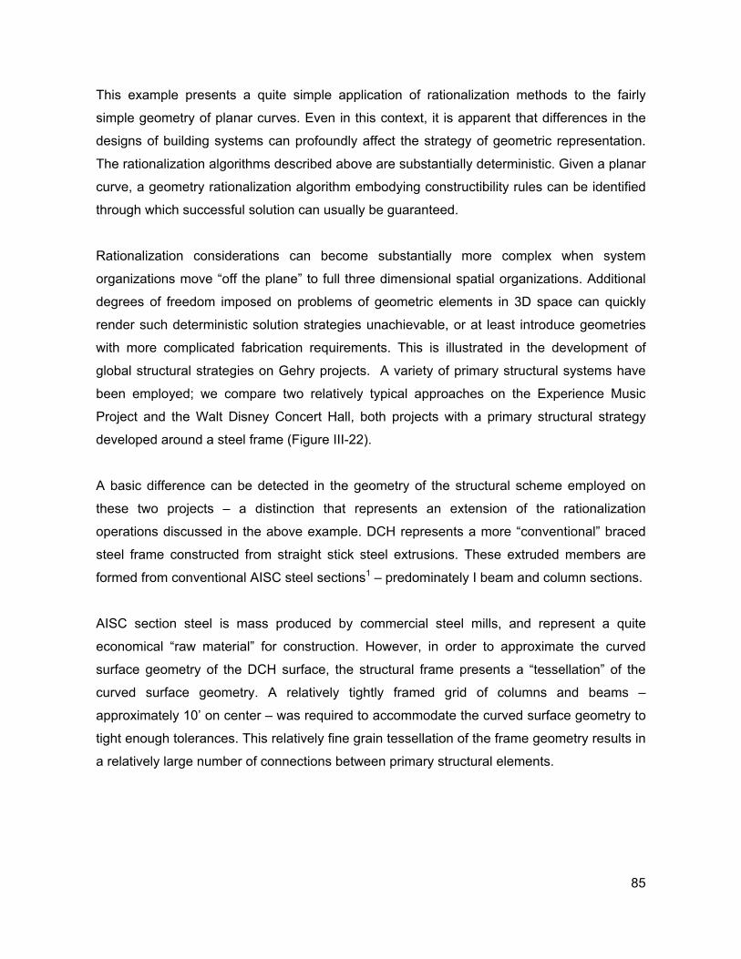
This example presents a quite simple application of rationalization methods to the fairly

simple geometry of planar curves. Even in this context, it is apparent that differences in the

designs of building systems can profoundly affect the strategy of geometric representation.

The rationalization algorithms described above are substantially deterministic. Given a planar

curve, a geometry rationalization algorithm embodying constructibility rules can be identified

through which successful solution can usually be guaranteed.

Rationalization considerations can become substantially more complex when system

organizations move “off the plane” to full three dimensional spatial organizations. Additional

degrees of freedom imposed on problems of geometric elements in 3D space can quickly

render such deterministic solution strategies unachievable, or at least introduce geometries

with more complicated fabrication requirements. This is illustrated in the development of

global structural strategies on Gehry projects. A variety of primary structural systems have

been employed; we compare two relatively typical approaches on the Experience Music

Project and the Walt Disney Concert Hall, both projects with a primary structural strategy

developed around a steel frame (Figure III-22).

A basic difference can be detected in the geometry of the structural scheme employed on

these two projects – a distinction that represents an extension of the rationalization

operations discussed in the above example. DCH represents a more “conventional” braced

steel frame constructed from straight stick steel extrusions. These extruded members are

formed from conventional AISC steel sections1 – predominately I beam and column sections.

AISC section steel is mass produced by commercial steel mills, and represent a quite

economical “raw material” for construction. However, in order to approximate the curved

surface geometry of the DCH surface, the structural frame presents a “tessellation” of the

curved surface geometry. A relatively tightly framed grid of columns and beams –

approximately 10’ on center – was required to accommodate the curved surface geometry to

tight enough tolerances. This relatively fine grain tessellation of the frame geometry results in

a relatively large number of connections between primary structural elements.

85

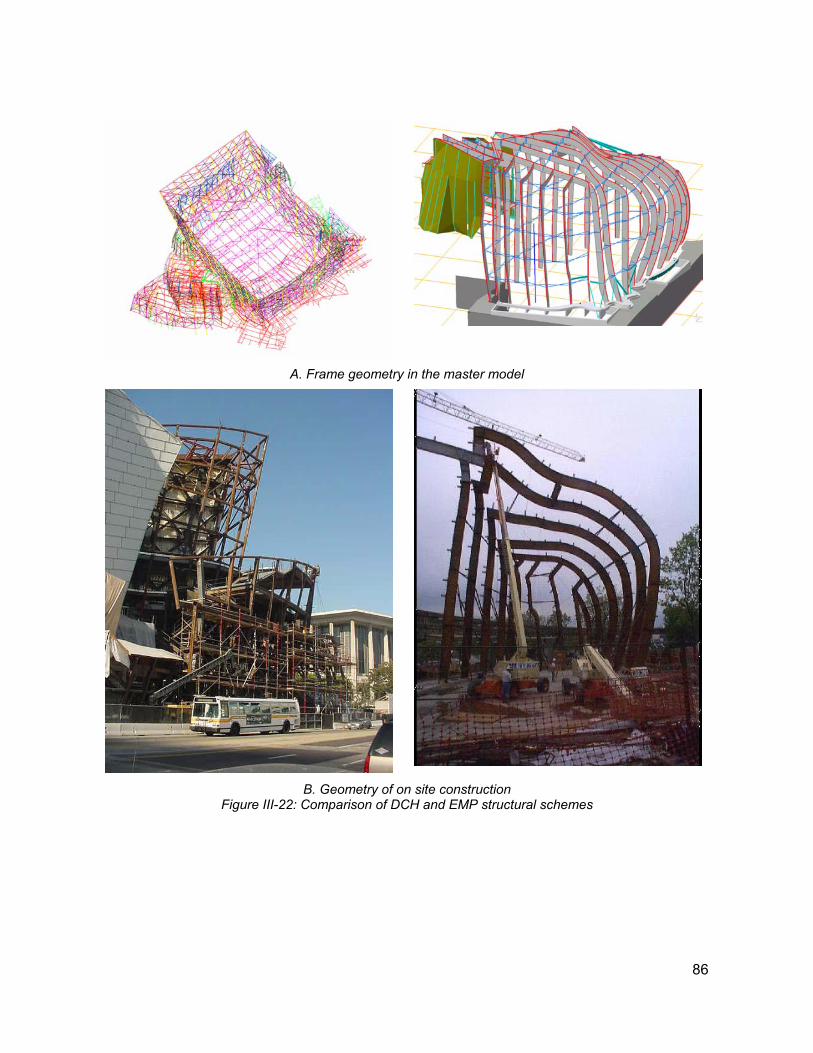
A. Frame geometry in the master model

B. Geometry of on site construction Figure III-22: Comparison of DCH and EMP structural schemes

86

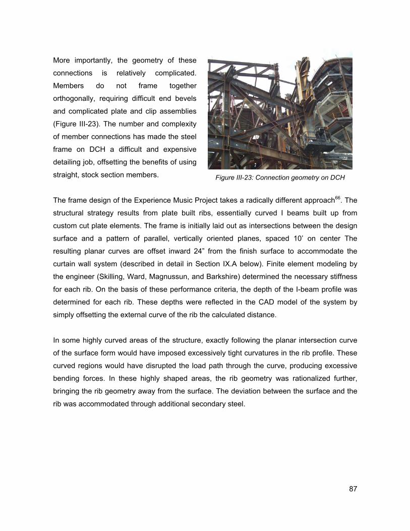
More importantly, the geometry of these

connections is relatively complicated.

Members do not frame together

orthogonally, requiring difficult end bevels

and complicated plate and clip assemblies

(Figure III-23). The number and complexity

of member connections has made the steel

frame on DCH a difficult and expensive

detailing job, offsetting the benefits of using

straight, stock section members.

Figure III-23: Connection geometry on DCH

The frame design of the Experience Music Project takes a radically different approach66. The

structural strategy results from plate built ribs, essentially curved I beams built up from

custom cut plate elements. The frame is initially laid out as intersections between the design

surface and a pattern of parallel, vertically oriented planes, spaced 10’ on center The

resulting planar curves are offset inward 24” from the finish surface to accommodate the

curtain wall system (described in detail in Section IX.A below). Finite element modeling by

the engineer (Skilling, Ward, Magnussun, and Barkshire) determined the necessary stiffness

for each rib. On the basis of these performance criteria, the depth of the I-beam profile was

determined for each rib. These depths were reflected in the CAD model of the system by

simply offsetting the external curve of the rib the calculated distance.

In some highly curved areas of the structure, exactly following the planar intersection curve

of the surface form would have imposed excessively tight curvatures in the rib profile. These

curved regions would have disrupted the load path through the curve, producing excessive

bending forces. In these highly shaped areas, the rib geometry was rationalized further,

bringing the rib geometry away from the surface. The deviation between the surface and the

rib was accommodated through additional secondary steel.

87

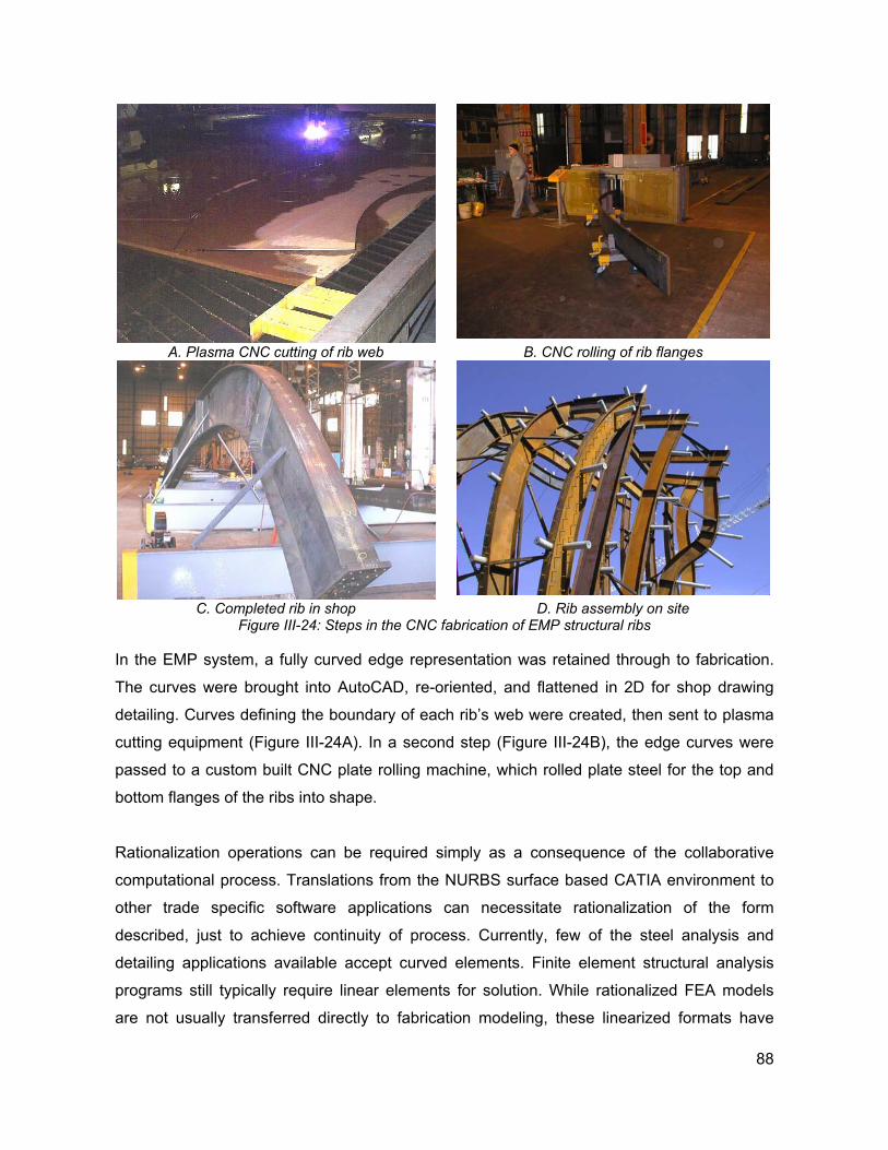
A. Plasma CNC cutting of rib web B. CNC rolling of rib flanges

C. Completed rib in shop D. Rib assembly on site

Figure III-24: Steps in the CNC fabrication of EMP structural ribs

In the EMP system, a fully curved edge representation was retained through to fabrication.

The curves were brought into AutoCAD, re-oriented, and flattened in 2D for shop drawing

detailing. Curves defining the boundary of each rib’s web were created, then sent to plasma

cutting equipment (Figure III-24A). In a second step (Figure III-24B), the edge curves were

passed to a custom built CNC plate rolling machine, which rolled plate steel for the top and

bottom flanges of the ribs into shape.

Rationalization operations can be required simply as a consequence of the collaborative

computational process. Translations from the NURBS surface based CATIA environment to

other trade specific software applications can necessitate rationalization of the form

described, just to achieve continuity of process. Currently, few of the steel analysis and

detailing applications available accept curved elements. Finite element structural analysis

programs still typically require linear elements for solution. While rationalized FEA models

are not usually transferred directly to fabrication modeling, these linearized formats have

88

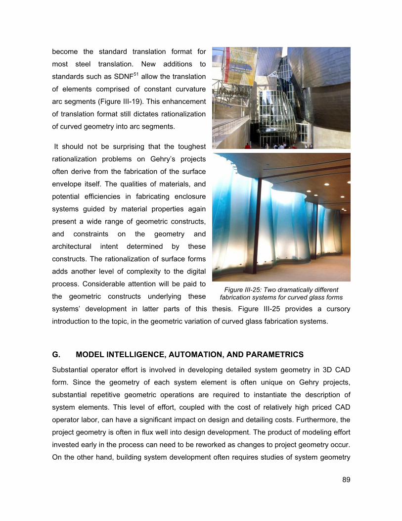
become the standard translation format for

most steel translation. New additions to

standards such as SDNF51 allow the translation

of elements comprised of constant curvature

arc segments (Figure III-19). This enhancement

of translation format still dictates rationalization

of curved geometry into arc segments.

It should not be surprising that the toughest

rationalization problems on Gehry’s projects

often derive from the fabrication of the surface

envelope itself. The qualities of materials, and

potential efficiencies in fabricating enclosure

systems guided by material properties again

present a wide range of geometric constructs,

and constraints on the geometry and

architectural intent determined by these

constructs. The rationalization of surface forms

adds another level of complexity to the digital

process. Considerable attention will be paid to

the geometric constructs underlying these

systems’ development in latter parts of this thesis. Figure III-25 provides a cursory

introduction to the topic, in the geometric variation of curved glass fabrication systems.

Figure III-25: Two dramatically different

fabrication systems for curved glass forms

G. MODEL INTELLIGENCE, AUTOMATION, AND PARAMETRICS

Substantial operator effort is involved in developing detailed system geometry in 3D CAD

form. Since the geometry of each system element is often unique on Gehry projects,

substantial repetitive geometric operations are required to instantiate the description of

system elements. This level of effort, coupled with the cost of relatively high priced CAD

operator labor, can have a significant impact on design and detailing costs. Furthermore, the

project geometry is often in flux well into design development. The product of modeling effort

invested early in the process can need to be reworked as changes to project geometry occur.

On the other hand, building system development often requires studies of system geometry

89

to be conducted to some level of detail early in design, to ensure that system strategies

address varying local geometric conditions. These issues of modeling effort have been

addressed in the firm’s process in several ways. Earlier in the development of the firm’s

digital process, virtually all CAD modeling was deferred until late in the design process, when

the project designers had “closed” or finalized the building form. Prior to that point, only

digital sketch models – rough surface models corresponding to the basic form of the physical

models – were developed, usually only to provide geometry for cut extraction associated with

specific document packages.

A general decline in the cost of computer modeling hardware, software and labor has

allowed greater application of digital modeling earlier in the design process. However, issues

of labor associated with large scale instantiation of system component definitions persist.

The costs associated with this effort are partly addressed by limiting the level of detail of

component geometric representations, and by performing detailed system studies or “digital

mockups” on only small portions of the project geometry.

The dual goals of increasing efficiency of 3D digital documentation efforts, and supporting re-

use of this information as variations in the building form occur, have been topics of research

and development efforts by the firm and its partners. Much of this work as been centered

around the development of procedural CAD modeling scripts to automate repetitive geometry

generation tasks. Often a simple geometric operation requires several intermediate

constructions to produce the required geometry. These operations are typically performed

relative to some existing geometry of the model. Scripting of these tasks can reduce the time

required to generate geometric descriptions of building components. For example,

commercially available steel detailing packages such as X-Steel and SDS-2 provide macros

for the generation of categories of steel connections. These macros perform cut backs, fillets,

bolt holes, and other difficult geometric operations on steel members in 3D form, in addition

to placing plates, clip angles and other connection components. Unfortunately, these

applications have often been shown to make orthogonality and other geometric assumptions

that do not necessarily hold on Gehry project geometry. These macros have required re-

coding to support the geometric conditions in the firm’s projects.

Sophisticated fabricators have developed their own programs to support the automation of

repetitive geometric tasks during shop drawing generation. One example, A. Zahner

90

Company’s Automated Panel Layout Application (ZAPLA), is described in Section IX.A

below.

While these examples of procedural or scripted automation provide an element of modeling

efficiency, they can not address requirements for updating information in response to

changes in project geometry. The geometric scripts and any associated manual interactions

must be re-applied on any modified input geometry. Toward the goal of addressing this

limitation of scripted approaches to automation, the firm has recently begun intensive efforts

to incorporate parametric technology into its digital process.

Parametric technology allows relationships among geometric elements to be encoded in the

model as part of operations on these elements. For example, when a curve is generated as

the intersection of a surface and a plane in space, the nature of this curve as a geometric

relationship between the surface and plane is retained in its digital description. Changes to

the input geometry – by modifying the surface or moving the plane - will flag an update and

regeneration of the curve. Variables may be included in the descriptions of geometries;

changes to the values of these variables can also be used to trigger updates of geometry.

Parametric modeling capabilities have existed in commercial applications for more than a

decade. The technology has been the focus of architectural computing research in describing

design typologies55. However, until recently, these applications were unmanageably slow for

large scale geometric models. Furthermore, the user interface requirements for generating

geometric associations between elements were unwieldy. The mathematical models

underlying curved object representations add substantial computational requirements to the

geometric description of objects, further slowing the updating of models.

Parametric technology has had substantial application in mechanical design applications,

where changes to product definitions can be limited to dimensional variations of the product.

Marc Burry’s efforts to develop parametrically based models of elements on the Sagrada

Familia construction project over the last ten years15 provide a notable example of the

application of parametrics in an architectural setting.

Recent improvements in the user interfaces to parametric modeling applications, and the

inexorable advances in computational power, seem to have finally brought applications of

91

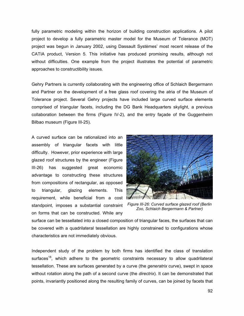
fully parametric modeling within the horizon of building construction applications. A pilot

project to develop a fully parametric master model for the Museum of Tolerance (MOT)

project was begun in January 2002, using Dassault Systèmes’ most recent release of the

CATIA product, Version 5. This initiative has produced promising results, although not

without difficulties. One example from the project illustrates the potential of parametric

approaches to constructibility issues.

Gehry Partners is currently collaborating with the engineering office of Schlaich Bergermann

and Partner on the development of a free glass roof covering the atria of the Museum of

Tolerance project. Several Gehry projects have included large curved surface elements

comprised of triangular facets, including the DG Bank Headquarters skylight, a previous

collaboration between the firms (Figure IV-2), and the entry façade of the Guggenheim

Bilbao museum (Figure III-25).

A curved surface can be rationalized into an

assembly of triangular facets with little

difficulty. However, prior experience with large

glazed roof structures by the engineer (Figure

III-26) has suggested great economic

advantage to constructing these structures

from compositions of rectangular, as opposed

to triangular, glazing elements. This

requirement, while beneficial from a cost

standpoint, imposes a substantial constraint

on forms that can be constructed. While any

surface can be tessellated into a closed composition of triangular faces, the surfaces that can

be covered with a quadrilateral tessellation are highly constrained to configurations whose

characteristics are not immediately obvious.

Figure III-26: Curved surface glazed roof (Berlin

Zoo, Schlaich Bergermann & Partner)

Independent study of the problem by both firms has identified the class of translation

surfaces18, which adhere to the geometric constraints necessary to allow quadrilateral

tessellation. These are surfaces generated by a curve (the generatrix curve), swept in space

without rotation along the path of a second curve (the directrix). It can be demonstrated that

points, invariantly positioned along the resulting family of curves, can be joined by facets that

92

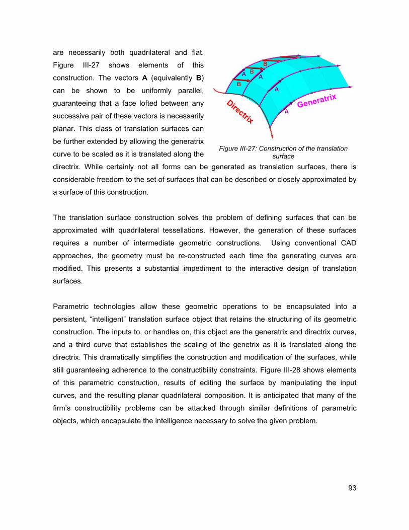
are necessarily both quadrilateral and flat.

Figure III-27 shows elements of this

construction. The vectors A (equivalently B)

can be shown to be uniformly parallel,

guaranteeing that a face lofted between any

successive pair of these vectors is necessarily

planar. This class of translation surfaces can

be further extended by allowing the generatrix

curve to be scaled as it is translated along the

directrix. While certainly not all forms can be generated as translation surfaces, there is

considerable freedom to the set of surfaces that can be described or closely approximated by

a surface of this construction.

Figure III-27: Construction of the translation

surface

The translation surface construction solves the problem of defining surfaces that can be

approximated with quadrilateral tessellations. However, the generation of these surfaces

requires a number of intermediate geometric constructions. Using conventional CAD

approaches, the geometry must be re-constructed each time the generating curves are

modified. This presents a substantial impediment to the interactive design of translation

surfaces.

Parametric technologies allow these geometric operations to be encapsulated into a

persistent, “intelligent” translation surface object that retains the structuring of its geometric

construction. The inputs to, or handles on, this object are the generatrix and directrix curves,

and a third curve that establishes the scaling of the genetrix as it is translated along the

directrix. This dramatically simplifies the construction and modification of the surfaces, while

still guaranteeing adherence to the constructibility constraints. Figure III-28 shows elements

of this parametric construction, results of editing the surface by manipulating the input

curves, and the resulting planar quadrilateral composition. It is anticipated that many of the

firm’s constructibility problems can be attacked through similar definitions of parametric

objects, which encapsulate the intelligence necessary to solve the given problem.

93

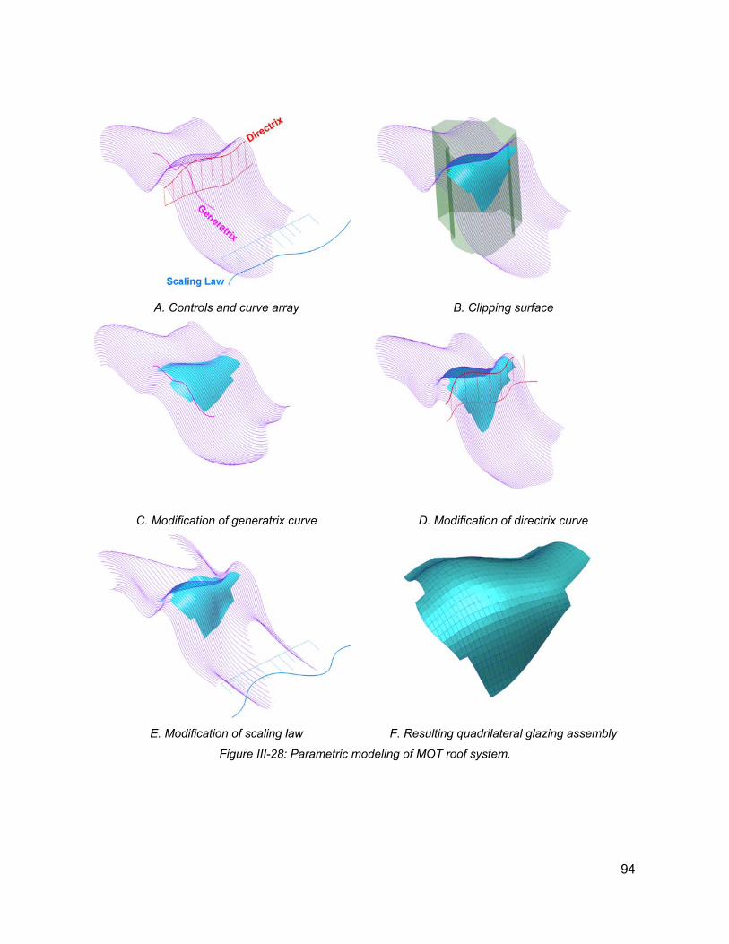
A. Controls and curve array B. Clipping surface

C. Modification of generatrix curve D. Modification of directrix curve

E. Modification of scaling law F. Resulting quadrilateral glazing assembly

Figure III-28: Parametric modeling of MOT roof system.

94

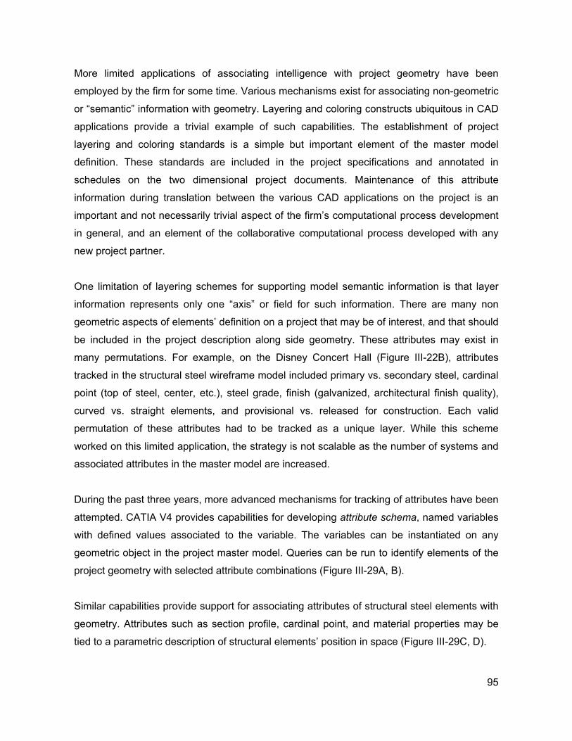
More limited applications of associating intelligence with project geometry have been

employed by the firm for some time. Various mechanisms exist for associating non-geometric

or “semantic” information with geometry. Layering and coloring constructs ubiquitous in CAD

applications provide a trivial example of such capabilities. The establishment of project

layering and coloring standards is a simple but important element of the master model

definition. These standards are included in the project specifications and annotated in

schedules on the two dimensional project documents. Maintenance of this attribute

information during translation between the various CAD applications on the project is an

important and not necessarily trivial aspect of the firm’s computational process development

in general, and an element of the collaborative computational process developed with any

new project partner.

One limitation of layering schemes for supporting model semantic information is that layer

information represents only one “axis” or field for such information. There are many non

geometric aspects of elements’ definition on a project that may be of interest, and that should

be included in the project description along side geometry. These attributes may exist in

many permutations. For example, on the Disney Concert Hall (Figure III-22B), attributes

tracked in the structural steel wireframe model included primary vs. secondary steel, cardinal

point (top of steel, center, etc.), steel grade, finish (galvanized, architectural finish quality),

curved vs. straight elements, and provisional vs. released for construction. Each valid

permutation of these attributes had to be tracked as a unique layer. While this scheme

worked on this limited application, the strategy is not scalable as the number of systems and

associated attributes in the master model are increased.

During the past three years, more advanced mechanisms for tracking of attributes have been

attempted. CATIA V4 provides capabilities for developing attribute schema, named variables

with defined values associated to the variable. The variables can be instantiated on any

geometric object in the project master model. Queries can be run to identify elements of the

project geometry with selected attribute combinations (Figure III-29A, B).

Similar capabilities provide support for associating attributes of structural steel elements with

geometry. Attributes such as section profile, cardinal point, and material properties may be

tied to a parametric description of structural elements’ position in space (Figure III-29C, D).

95

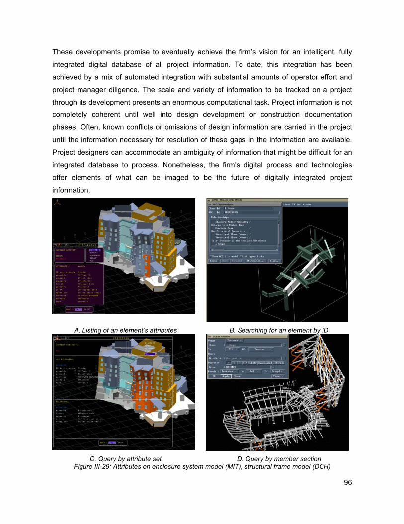
These developments promise to eventually achieve the firm’s vision for an intelligent, fully

integrated digital database of all project information. To date, this integration has been

achieved by a mix of automated integration with substantial amounts of operator effort and

project manager diligence. The scale and variety of information to be tracked on a project

through its development presents an enormous computational task. Project information is not

completely coherent until well into design development or construction documentation

phases. Often, known conflicts or omissions of design information are carried in the project

until the information necessary for resolution of these gaps in the information are available.

Project designers can accommodate an ambiguity of information that might be difficult for an

integrated database to process. Nonetheless, the firm’s digital process and technologies

offer elements of what can be imaged to be the future of digitally integrated project

information.

A. Listing of an element’s attributes B. Searching for an element by ID

C. Query by attribute set D. Query by member section

Figure III-29: Attributes on enclosure system model (MIT), structural frame model (DCH)

96

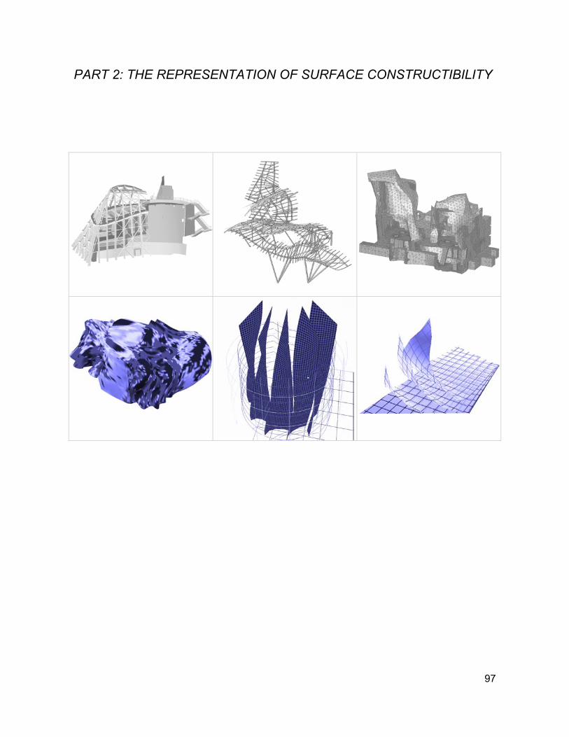
PART 2: THE REPRESENTATION OF SURFACE CONSTRUCTIBILITY

97

98

In Part 1 of this thesis, issues in the development of Gehry’s Partners’ building delivery

process and associated computing methodologies were presented. Important relationships

between the representation of project geometry and the operations of fabrication and

construction were introduced. The concept of rationalization was introduced, through which

requirements of constructibility are interpreted into geometric constraints on the project form.

Examples of rationalizing geometric strategies were discussed in relationship to the building

systems on which they have been applied.

While these issues impact the development of all building systems on Gehry projects, the

most profound impacts are realized in the development of projects’ exterior surface forms,

and the corresponding building envelope systems that ultimately realize these forms. This

exterior project geometry sets the stage for all subsequent constructibility strategies. It is

here that subtleties of geometric interpretation can have the most profound consequences on

the aesthetic qualities of the project.

The variety of geometric forms presented in Gehry’s works eludes the development of a

comprehensive taxonomy. However, in the body of work being developed by Gehry’s firm at

the current point of writing, there are a set of qualities which are identifiable and largely

unique to Gehry’s work: the smoothly curved surfaces which create the energetic, undulating

forms on many projects. In these shapes there exists an important set of common building

intentions, unified by similar approaches to the manipulation of surface materials, and guided

by a common set of constructibility constraints and associated economies. The research

presented in the remainder of this thesis is directed toward a geometric analysis of these

forms, toward the goal of supporting the definition of constructibility requirements in

computational form.

This discussion focuses on the set of shapes constructed from sheet materials, shaped in

space without large scale material deformations that would require forming through molding

or stamping. These shapes have been termed paper surfaces by members of the firm. The

term “paper surface” is employed in this thesis in a deliberately pre-analytic and evocative

sense, to reflect the wide range of formal and tectonic issues embodied in this class of

shapes. Other more formal terms will be employed to characterize specific geometric

constructs within this general class of surface forms.

99

This section is introduced through a qualitative survey of the surface geometries and

associated formal, material and constructibility issues of Gehry’s projects, provided in

Chapter IV. Following this introduction, a review of the mathematical foundations of

differential geometry underlying the description of curved spatial forms is provided. This

mathematical foundation forms the basis for the definition of specific representational

constructs supporting the description of paper surface forms. The definition of these

constructs is provided in Chapters VI and VII, along with examples of their application to the

definition of constructibility requirements on the firm’s past and current projects.

100

IV. Materiality and its Geometric Representations

The previous chapters described the relationships between constraints on project forms

introduced by economies and methods of fabrication, and corresponding constraints on the

physical and digital representations of these forms. In Gehry’s process, these constraints are

represented in parallel: through the selection of physical modeling materials in the

construction of scale models, and the selection of digital elements, defined by specific

geometric constructs. We may consider the confluence of these physical, digital and

fabrication constraints to define a class of surface forms.

It is possible to view the historical progression of Gehry’s built projects as a progressive

development of these classes of surface forms. The possibility of building the ambitious

geometries exhibited in Gehry’s recent work did not occur spontaneously. Rather, one can

witness in his work the progressive development of an increasingly ambitious geometric

vocabulary, beginning with the fairly conventional forms of his early commercial and

residential projects, through to the extreme geometric forms of the Experience Music Project.

Each project pushes the successful precedents and experiences developed on prior projects

to new limits. On contemporary projects, Gehry often includes elements with geometries

reminiscent of previous projects, as well as elements with ambitious extensions of prior

geometries and, occasionally, elements for which no particular precedent yet exists.

Corresponding to this formal development is a progressive development of engineering,

fabrication and digital description techniques. While the progression of Gehry’s gestural

intentions may be difficult to decipher over the distance of time, the development of the

underlying geometry can be discerned directly from the traditional and digital representations

that document his works.

A. PLANAR SURFACES

The point of departure for this inquiry into classes of surface forms is the simplest and most

obvious such class, embodied by planar surfaces. The basis for physical modeling of these

surfaces are rigid sheet materials such as foam core or stiff cardboard, which may easily be

formed into planar shapes. One can inquire what the geometric limits of these physical

materials are. Non-planar shapes such as spheres or other curved surfaces are of course

inappropriate for modeling with flat foam core. There are ways that this can be done, by

101

cutting and stacking, or wetting the material to achieve a paper-mache quality. But

undertaking these activities using rigid flat materials seems to be qualitatively different than

simply cutting out a piece of rigid material and positioning it in space. One may capture this

observation as a rule regarding the behavior of stiff sheet materials, that “rigid sheet

materials enable - and are constrained to - planar geometries”. As one works with rigid

materials in scale, it is possible to “read through” the behavior of these modeling materials

and to infer that, by working with these materials in an appropriate fashion, one is guided by

these materials’ spatial behaviors to produce shapes within a vocabulary of planar forms.

Having built in model form an assembly of planar objects, one may have reasonable

confidence that the assembly may be constructed using certain real world construction

systems. There are of course a wide variety of construction systems supporting planar forms,

from stud framing to glass curtain walls to concrete formwork. The economical deployment of

these fabrication systems again suggests their application to, or enables, the construction of

planar surface geometries. Notably, from the perspective of geometric performance, planar

modeling materials may be used interchangeably to represent any of these construction

systems. Although one may choose foam core of various thicknesses to represent concrete

block or stud framing construction, or plexiglass to represent glazing systems, this selection

impacts the perceptual fidelity with their represented constructions, not any further geometric

conditioning on the modeled forms imposed by these materials. In extending this discussion

to other geometric forms, this simplicity of geometric equivalence among physical modeling

representations will no longer necessarily be the case.

Simple, precise mathematical descriptions exist for these Euclidean geometries, conducive

to formulation in digital modeling applications. There are in fact multiple such descriptions. A

plane in three dimensional space can be described as a relationship between three points in

space, as a relationship between two intersecting lines or vectors, or through an implicit

function of four variables14. A plane may be completely described by – and is “dual to” – a

specially chosen point in space10. Each of these representations affords particular utility to

specific geometric operations. However, these representations are equivalent, in the sense

that we can translate between them explicitly; no loss of geometric information is incurred

through this translation.

102

With the definition of this basic class of planar constructible forms in hand, one can begin to

explore the limits of forms that respect the constraints of planar geometry. In typical

construction, planar forms are organized orthogonally: vertical, perpendicular walls,

horizontal floors. We may consider geometries of such orthogonally positioned planar

elements to be a more highly constrained subclass of the general planar surface class. There

are various fabrication and engineering efficiencies afforded by adoption this further

restriction on geometries. Eccentric loading conditions are largely eliminated on vertical

walls. Detailing of connections between orthogonally positioned wall and floor systems is

simplified.

On conventional framed construction, pitched roofs provide an exception to the conventions

of orthogonal, planar construction, and establish a precedent for the exploration of more

ambitious planar forms. The geometry and corresponding detailing of hip or gable roof

forms63 is somewhat more complicated and expensive than that of the floors and walls below,

but the documentation, engineering and fabrication associated with these geometries is well

established in conventional wood frame construction practice.

Gehry’s early works demonstrate precisely this exploration. The radical proposition or

“violence”21 of this early work is precisely in its demonstration that conventional, industrial

materials and constructions could generate unconventional forms, applied unconventionally

to non-industrial architectural programs. Along the way, the economies associated with this

relatively conventional geometry and associated fabrication efficiencies are realized42.

These geometries have persisted on elements of Gehry’s more recent projects, even as his

geometric vocabulary has expanded. Partly, this is a result of a budgetary strategy employed

on Gehry’s designs. These geometries remain inexpensive to construct, relative to the more

recent additions to the vocabulary of geometric forms. Judicious use of conventional

construction in concert with less constrained geometries has allowed the firm to meet project

programmatic requirements within allocated budgets.

103

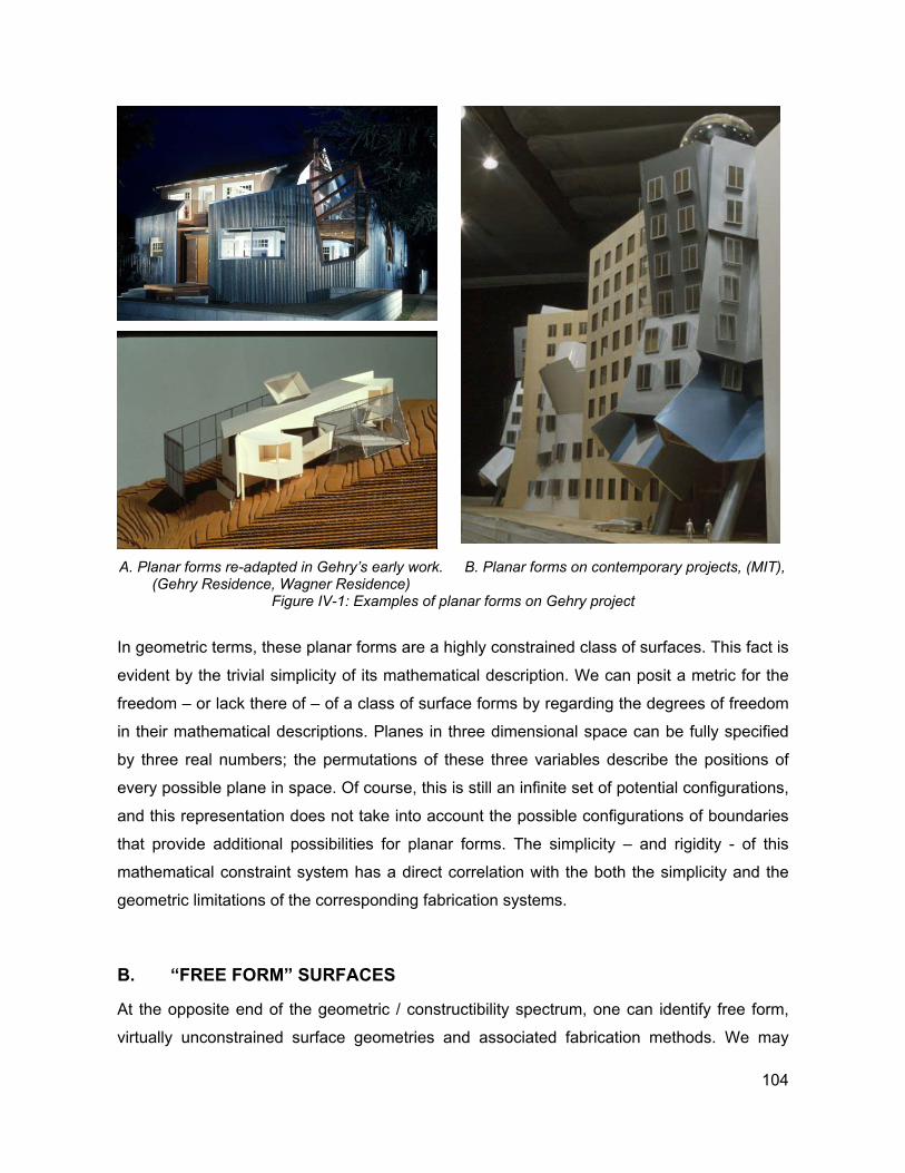
A. Planar forms re-adapted in Gehry’s early work.

(Gehry Residence, Wagner Residence) B. Planar forms on contemporary projects, (MIT),

Figure IV-1: Examples of planar forms on Gehry project

In geometric terms, these planar forms are a highly constrained class of surfaces. This fact is

evident by the trivial simplicity of its mathematical description. We can posit a metric for the

freedom – or lack there of – of a class of surface forms by regarding the degrees of freedom

in their mathematical descriptions. Planes in three dimensional space can be fully specified

by three real numbers; the permutations of these three variables describe the positions of

every possible plane in space. Of course, this is still an infinite set of potential configurations,

and this representation does not take into account the possible configurations of boundaries

that provide additional possibilities for planar forms. The simplicity – and rigidity - of this

mathematical constraint system has a direct correlation with the both the simplicity and the

geometric limitations of the corresponding fabrication systems.

B. “FREE FORM” SURFACES

At the opposite end of the geometric / constructibility spectrum, one can identify free form,

virtually unconstrained surface geometries and associated fabrication methods. We may

104

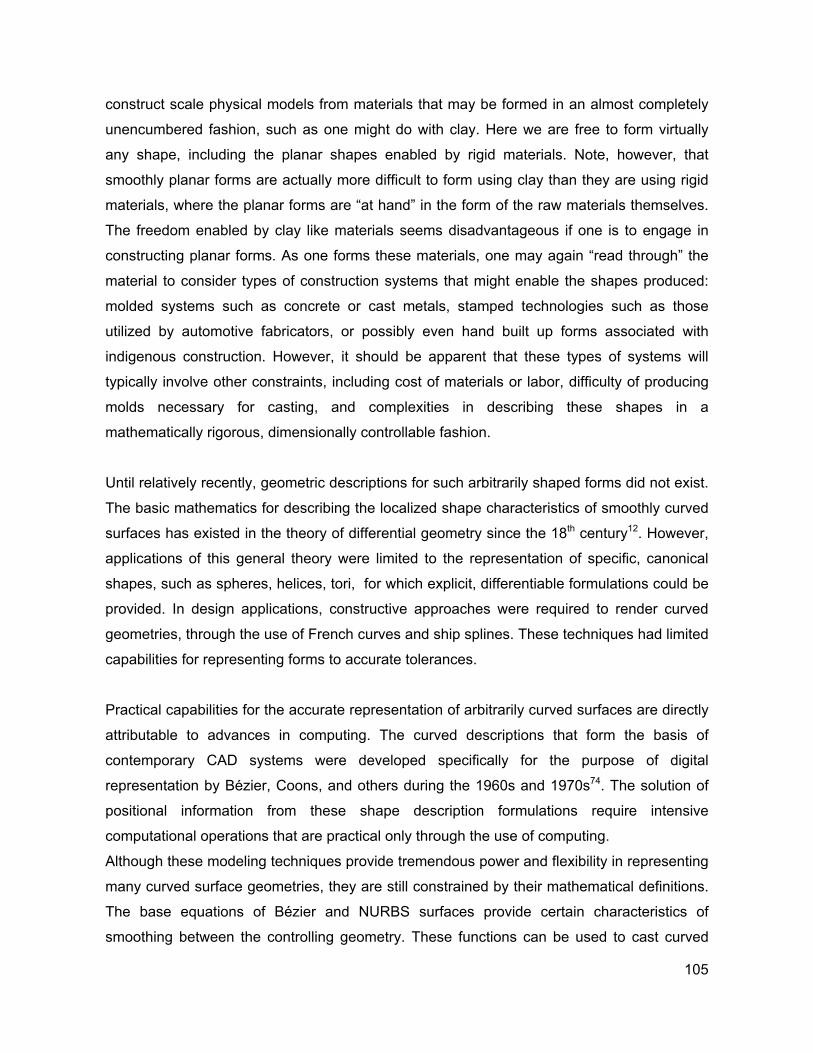
construct scale physical models from materials that may be formed in an almost completely

unencumbered fashion, such as one might do with clay. Here we are free to form virtually

any shape, including the planar shapes enabled by rigid materials. Note, however, that

smoothly planar forms are actually more difficult to form using clay than they are using rigid

materials, where the planar forms are “at hand” in the form of the raw materials themselves.

The freedom enabled by clay like materials seems disadvantageous if one is to engage in

constructing planar forms. As one forms these materials, one may again “read through” the

material to consider types of construction systems that might enable the shapes produced:

molded systems such as concrete or cast metals, stamped technologies such as those

utilized by automotive fabricators, or possibly even hand built up forms associated with

indigenous construction. However, it should be apparent that these types of systems will

typically involve other constraints, including cost of materials or labor, difficulty of producing

molds necessary for casting, and complexities in describing these shapes in a

mathematically rigorous, dimensionally controllable fashion.

Until relatively recently, geometric descriptions for such arbitrarily shaped forms did not exist.

The basic mathematics for describing the localized shape characteristics of smoothly curved

surfaces has existed in the theory of differential geometry since the 18th century12. However,

applications of this general theory were limited to the representation of specific, canonical

shapes, such as spheres, helices, tori, for which explicit, differentiable formulations could be

provided. In design applications, constructive approaches were required to render curved

geometries, through the use of French curves and ship splines. These techniques had limited

capabilities for representing forms to accurate tolerances.

Practical capabilities for the accurate representation of arbitrarily curved surfaces are directly

attributable to advances in computing. The curved descriptions that form the basis of

contemporary CAD systems were developed specifically for the purpose of digital

representation by Bézier, Coons, and others during the 1960s and 1970s74. The solution of

positional information from these shape description formulations require intensive

computational operations that are practical only through the use of computing.

Although these modeling techniques provide tremendous power and flexibility in representing

many curved surface geometries, they are still constrained by their mathematical definitions.

The base equations of Bézier and NURBS surfaces provide certain characteristics of

smoothing between the controlling geometry. These functions can be used to cast curved

105

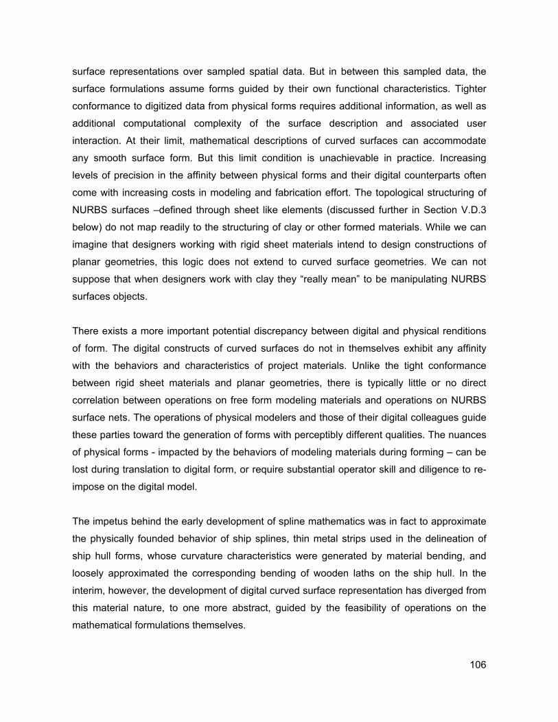
surface representations over sampled spatial data. But in between this sampled data, the

surface formulations assume forms guided by their own functional characteristics. Tighter

conformance to digitized data from physical forms requires additional information, as well as

additional computational complexity of the surface description and associated user

interaction. At their limit, mathematical descriptions of curved surfaces can accommodate

any smooth surface form. But this limit condition is unachievable in practice. Increasing

levels of precision in the affinity between physical forms and their digital counterparts often

come with increasing costs in modeling and fabrication effort. The topological structuring of

NURBS surfaces –defined through sheet like elements (discussed further in Section V.D.3

below) do not map readily to the structuring of clay or other formed materials. While we can

imagine that designers working with rigid sheet materials intend to design constructions of

planar geometries, this logic does not extend to curved surface geometries. We can not

suppose that when designers work with clay they “really mean” to be manipulating NURBS

surfaces objects.

There exists a more important potential discrepancy between digital and physical renditions

of form. The digital constructs of curved surfaces do not in themselves exhibit any affinity

with the behaviors and characteristics of project materials. Unlike the tight conformance

between rigid sheet materials and planar geometries, there is typically little or no direct

correlation between operations on free form modeling materials and operations on NURBS

surface nets. The operations of physical modelers and those of their digital colleagues guide

these parties toward the generation of forms with perceptibly different qualities. The nuances

of physical forms - impacted by the behaviors of modeling materials during forming – can be

lost during translation to digital form, or require substantial operator skill and diligence to re-

impose on the digital model.

The impetus behind the early development of spline mathematics was in fact to approximate

the physically founded behavior of ship splines, thin metal strips used in the delineation of

ship hull forms, whose curvature characteristics were generated by material bending, and

loosely approximated the corresponding bending of wooden laths on the ship hull. In the

interim, however, the development of digital curved surface representation has diverged from

this material nature, to one more abstract, guided by the feasibility of operations on the

mathematical formulations themselves.

106

Truly free form shapes – constructed through

CNC driven molded or stamped fabrication

technologies – have had a relatively minor

role in Gehry’s work. The reasons for this

limited role are largely practical and

economic. Currently, molding or stamping of

materials requires a unique, custom mold to

be developed for each surface element. The

labor and material required to develop the

mold can at the very least add a premium to

the cost of the system. This mold making

process can ultimately be vastly more

expensive than the typical costs of cladding

systems, particularly in metal stamping

process, where high strength materials must

be formed (Section II.C). Specific examples

exist, notably the conference room of the DG

Bank Headquarters project (Figure IV-2),

formed from stamped plate steel. A second

version of this form was developed for the Gagosian gallery (Figure IV-3), this time through a

manual labor process of forming of sheet lead – highly malleable material.

Figure IV-2: Horse’s head (DG Bank)

Figure IV-3 Horse’s head (Gagosian gallery)

This issue was elegantly addressed in the Neue Zollhof project in Dusseldorf (Figure IV-4),

where recyclable Styrofoam molds were developed as part of an innovative CNC based

process for forming cast concrete. The feasibility of this process resulted directly from

efficiencies found in the CNC mold forming process. The low strength of Styrofoam allowed it

to be routed at extremely high speed, reducing the machine time cost. Relatively low

tolerances and allowable roughness of the mold finish allowed the routing to be done with a

single pass of a large (approximately 2”) bit. The Styrofoam was recycled after the concrete

panel was formed, further reducing the material costs associated with the molding process.

107

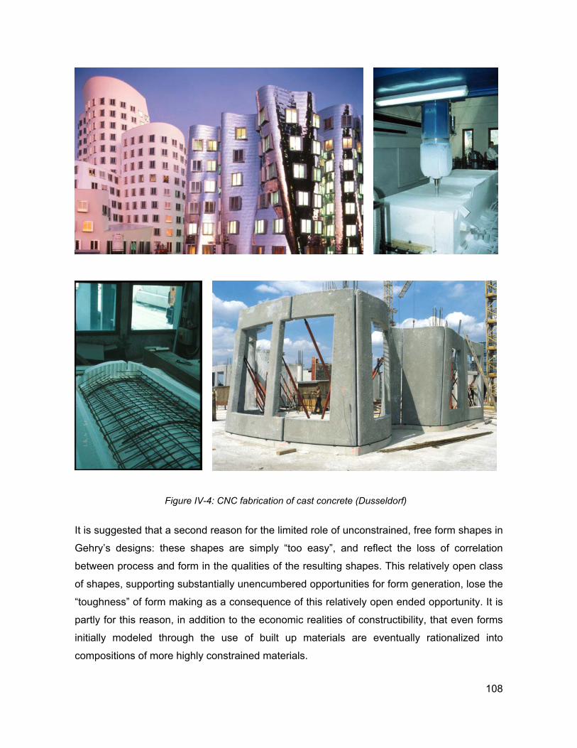
Figure IV-4: CNC fabrication of cast concrete (Dusseldorf)

It is suggested that a second reason for the limited role of unconstrained, free form shapes in

Gehry’s designs: these shapes are simply “too easy”, and reflect the loss of correlation

between process and form in the qualities of the resulting shapes. This relatively open class

of shapes, supporting substantially unencumbered opportunities for form generation, lose the

“toughness” of form making as a consequence of this relatively open ended opportunity. It is

partly for this reason, in addition to the economic realities of constructibility, that even forms

initially modeled through the use of built up materials are eventually rationalized into

compositions of more highly constrained materials.

108

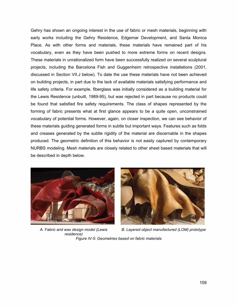
Gehry has shown an ongoing interest in the use of fabric or mesh materials, beginning with

early works including the Gehry Residence, Edgemar Development, and Santa Monica

Place. As with other forms and materials, these materials have remained part of his

vocabulary, even as they have been pushed to more extreme forms on recent designs.

These materials in unrationalized form have been successfully realized on several sculptural

projects, including the Barcelona Fish and Guggenheim retrospective installations (2001,

discussed in Section VII.J below). To date the use these materials have not been achieved

on building projects, in part due to the lack of available materials satisfying performance and

life safety criteria. For example, fiberglass was initially considered as a building material for

the Lewis Residence (unbuilt, 1989-95), but was rejected in part because no products could

be found that satisfied fire safety requirements. The class of shapes represented by the

forming of fabric presents what at first glance appears to be a quite open, unconstrained

vocabulary of potential forms. However, again, on closer inspection, we can see behavior of

these materials guiding generated forms in subtle but important ways. Features such as folds

and creases generated by the subtle rigidity of the material are discernable in the shapes

produced. The geometric definition of this behavior is not easily captured by contemporary

NURBS modeling. Mesh materials are closely related to other sheet based materials that will

be described in depth below.

A. Fabric and wax design model (Lewis

residence) B. Layered object manufactured (LOM) prototype

Figure IV-5: Geometries based on fabric materials

109

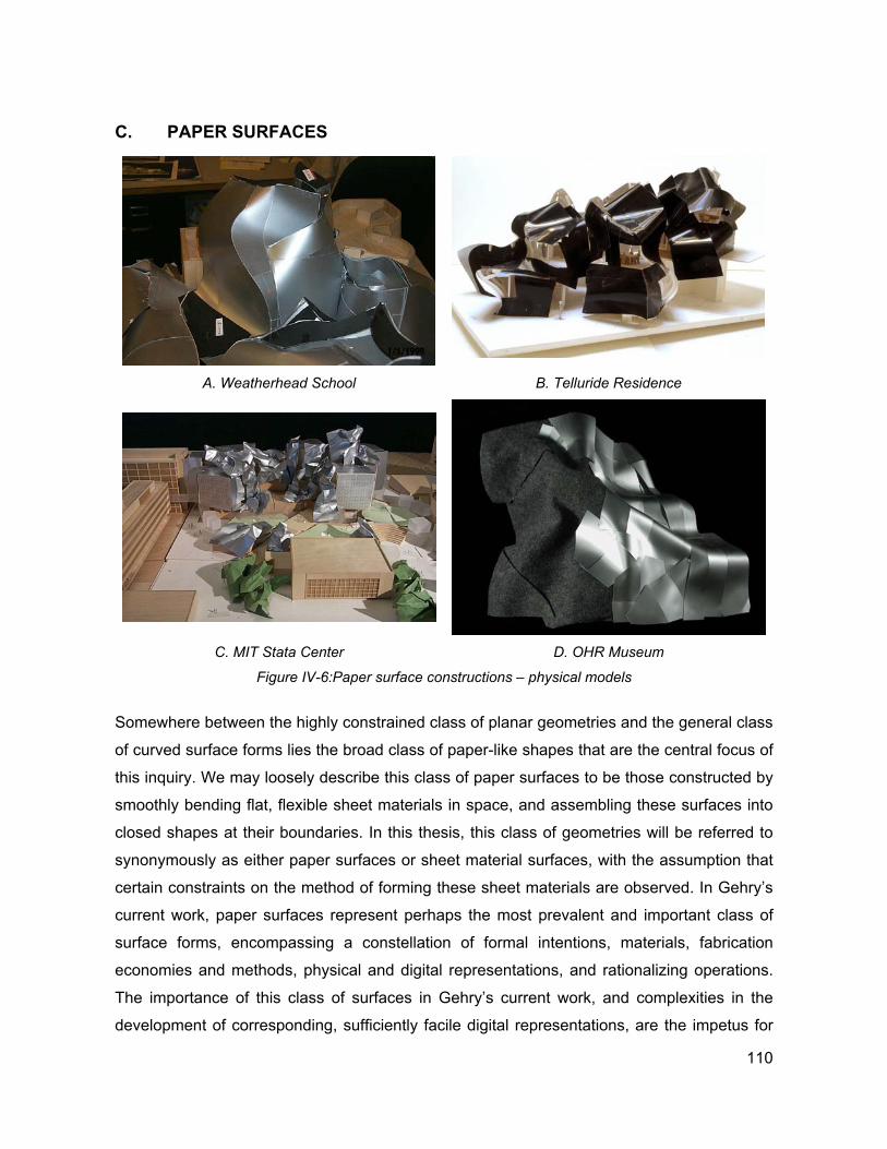
C. PAPER SURFACES

A. Weatherhead School B. Telluride Residence

C. MIT Stata Center D. OHR Museum

Figure IV-6:Paper surface constructions – physical models

Somewhere between the highly constrained class of planar geometries and the general class

of curved surface forms lies the broad class of paper-like shapes that are the central focus of

this inquiry. We may loosely describe this class of paper surfaces to be those constructed by

smoothly bending flat, flexible sheet materials in space, and assembling these surfaces into

closed shapes at their boundaries. In this thesis, this class of geometries will be referred to

synonymously as either paper surfaces or sheet material surfaces, with the assumption that

certain constraints on the method of forming these sheet materials are observed. In Gehry’s

current work, paper surfaces represent perhaps the most prevalent and important class of

surface forms, encompassing a constellation of formal intentions, materials, fabrication

economies and methods, physical and digital representations, and rationalizing operations.

The importance of this class of surfaces in Gehry’s current work, and complexities in the

development of corresponding, sufficiently facile digital representations, are the impetus for

110

the research described in the remainder of this thesis. A qualitative description of their role in

Gehry’s design and building processes will serve as an introduction to the formal description

of their geometric representations in subsequent sections.

The forms assumed by paper and other sheet materials in scale physical models have

important counterparts in full scale construction. Many materials of construction have

analogous constraints that at least qualitatively constrain full scale fabricated building

elements to assume sheet like forms (Figure IV-7). These materials may be readily formed

by manual methods into curved shapes in space, so long as these forms do not require

stretch forming of the material that would produce plastic deformation in the plane of the

surface material. This relationship between the material constraints of modeling materials in

scale and the constraints of fabrication may only be approximate. However, for schematic

design purposes, this approximate correspondence may be sufficient to guarantee the

constructibility of designed forms.

Paper surface shapes are obviously less constrained than the class of planar Euclidean

shapes, and may be viewed as a super-set of these forms. This is easily, albeit qualitatively,

demonstrated by positioning a sheet of paper flat on a table, then lifting up one of its corners.

The paper surface class encompasses the flat configuration and the final configuration of the

sheet, as well as of the intermediate states between.

At the same time, the class is clearly quite constrained. While there is a broad class of

shapes that may be constructed from a single sheet of paper positioned in space, there is

certainly a much larger set of shapes (spheres, airplanes, Walt Disney characters, etc.) that

can not be tightly covered by a paper sheet. Attempting to force the sheet tightly onto these

shapes will be only partly successful, as wrinkling, creasing or ripping of the sheet will occur.

Unlike planar geometries, where the shapes formed by rigid materials are independent of the

actual materials of construction, shapes formed from flexible sheet materials are highly

conditioned by the material. Paper, rubber sheet, plate steel, plaster board, aluminum foil, all

of these materials impose significantly different constraints on their corresponding set of

constructible shapes. Some will break before they achieve the shapes enabled by others,

some will assume shapes with a more less continuous or smooth form. Of course, if such

features as creases, wrinkles and rips are desired, a potentially larger class of shapes is

111

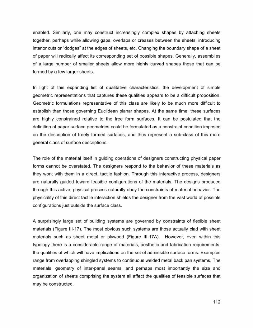
enabled. Similarly, one may construct increasingly complex shapes by attaching sheets

together, perhaps while allowing gaps, overlaps or creases between the sheets, introducing

interior cuts or “dodges” at the edges of sheets, etc. Changing the boundary shape of a sheet

of paper will radically affect its corresponding set of possible shapes. Generally, assemblies

of a large number of smaller sheets allow more highly curved shapes those that can be

formed by a few larger sheets.

In light of this expanding list of qualitative characteristics, the development of simple

geometric representations that captures these qualities appears to be a difficult proposition.

Geometric formulations representative of this class are likely to be much more difficult to

establish than those governing Euclidean planar shapes. At the same time, these surfaces

are highly constrained relative to the free form surfaces. It can be postulated that the

definition of paper surface geometries could be formulated as a constraint condition imposed

on the description of freely formed surfaces, and thus represent a sub-class of this more

general class of surface descriptions.

The role of the material itself in guiding operations of designers constructing physical paper

forms cannot be overstated. The designers respond to the behavior of these materials as

they work with them in a direct, tactile fashion. Through this interactive process, designers

are naturally guided toward feasible configurations of the materials. The designs produced

through this active, physical process naturally obey the constraints of material behavior. The

physicality of this direct tactile interaction shields the designer from the vast world of possible

configurations just outside the surface class.

A surprisingly large set of building systems are governed by constraints of flexible sheet

materials (Figure III-17). The most obvious such systems are those actually clad with sheet

materials such as sheet metal or plywood (Figure III-17A). However, even within this

typology there is a considerable range of materials, aesthetic and fabrication requirements,

the qualities of which will have implications on the set of admissible surface forms. Examples

range from overlapping shingled systems to continuous welded metal back pan systems. The

materials, geometry of inter-panel seams, and perhaps most importantly the size and

organization of sheets comprising the system all affect the qualities of feasible surfaces that

may be constructed.

112

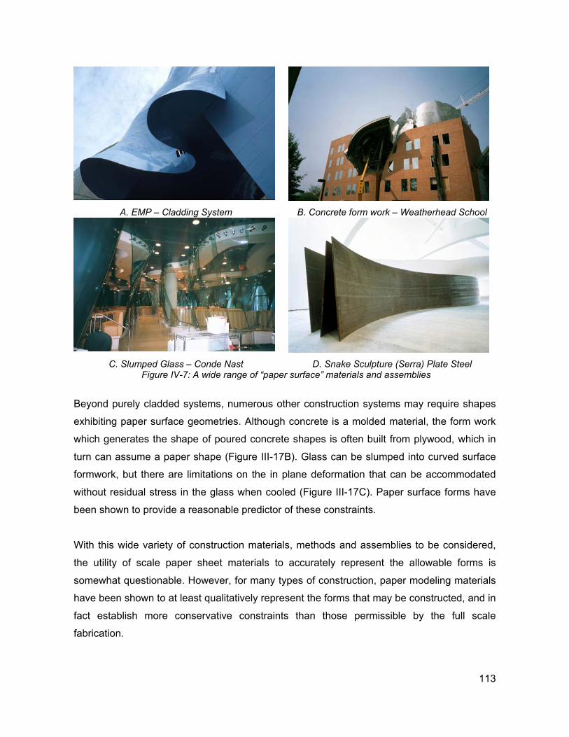
A. EMP – Cladding System B. Concrete form work – Weatherhead School

C. Slumped Glass – Conde Nast D. Snake Sculpture (Serra) Plate Steel

Figure IV-7: A wide range of “paper surface” materials and assemblies

Beyond purely cladded systems, numerous other construction systems may require shapes

exhibiting paper surface geometries. Although concrete is a molded material, the form work

which generates the shape of poured concrete shapes is often built from plywood, which in

turn can assume a paper shape (Figure III-17B). Glass can be slumped into curved surface

formwork, but there are limitations on the in plane deformation that can be accommodated

without residual stress in the glass when cooled (Figure III-17C). Paper surface forms have

been shown to provide a reasonable predictor of these constraints.

With this wide variety of construction materials, methods and assemblies to be considered,

the utility of scale paper sheet materials to accurately represent the allowable forms is

somewhat questionable. However, for many types of construction, paper modeling materials

have been shown to at least qualitatively represent the forms that may be constructed, and in

fact establish more conservative constraints than those permissible by the full scale

fabrication.

113

In the following development of digital modeling representations for sheet surface fabrication

constraints, it will be useful to keep in mind some of the qualitative features that characterize

these systems and contribute to these constraints.

The overall, global shape of the surface assembly is the point of departure for considering

qualities contributing to the form’s constructibility. It is here that the initial physical modeling

and materials used in this process contribute to an understanding of the shape’s

constructibility. Individual sheets employed on physical models vary in character and size,

from full height wall size sheets to smaller panels perhaps 10’ in scale. Critical issues such

as the shape of boundaries of these macro scale sheets and the ways in which they are

attached together have enormous implications on the types of forms that may be feasibly

generated.

Localized smoothness of form is an inherent characteristic of the paper shape class. Again,

while “catastrophic” operations- such as crumpling, ripping or stretching by stamping - can

be undertaken, these operations and the forms that are generated represent extensions or

violations of the rules of construction and corresponding definition of the class. Sheet

materials respond to externally applied forces and actions by assuming smooth variation

between these externally applied constraints. However, sheet materials have limits on the

magnitude of deformation they can respond to. Beyond those limits, the material will either

refuse to go, perhaps popping fasteners intended to hold the material into shape, perhaps

buckling or tearing. The intentional introduction of discontinuities into a smoothly continuous

surface can alleviate the materials’ resistance to being positioned in a given way. If the

design intent for the form allows discontinuities in the material’s shape, then considerably

more flexibility in the global nature of the shape is possible.

As a trivial example, spheres of any size can be constructed by tessellating the surface into

triangles, resulting in a geodesic dome31,32. The panels of the dome do not necessarily have

to be flat, but rather could assume some limited degree of curvature. The remainder of the

sphere’s curvature would continue to be made up at the panel seams. In this simple

example, the tradeoffs between surface curvature, tangency discontinuities and fitness to the

“design” surface are readily apparent (Figure IV-8).

114

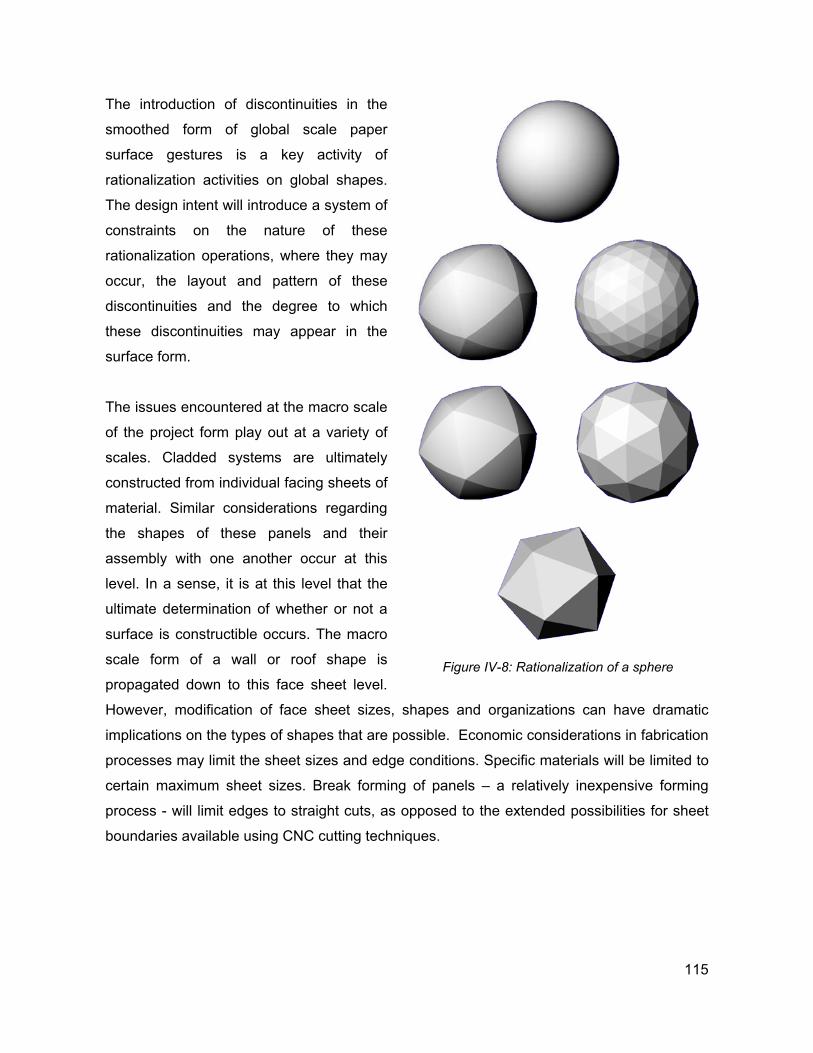
The introduction of discontinuities in the

smoothed form of global scale paper

surface gestures is a key activity of

rationalization activities on global shapes.

The design intent will introduce a system of

constraints on the nature of these

rationalization operations, where they may

occur, the layout and pattern of these

discontinuities and the degree to which

these discontinuities may appear in the

surface form.

The issues encountered at the macro scale

of the project form play out at a variety of

scales. Cladded systems are ultimately

constructed from individual facing sheets of

material. Similar considerations regarding

the shapes of these panels and their

assembly with one another occur at this

level. In a sense, it is at this level that the

ultimate determination of whether or not a

surface is constructible occurs. The macro

scale form of a wall or roof shape is

propagated down to this face sheet level.

However, modification of face sheet sizes, shapes and organizations can have dramatic

implications on the types of shapes that are possible. Economic considerations in fabrication

processes may limit the sheet sizes and edge conditions. Specific materials will be limited to

certain maximum sheet sizes. Break forming of panels – a relatively inexpensive forming

process - will limit edges to straight cuts, as opposed to the extended possibilities for sheet

boundaries available using CNC cutting techniques.

Figure IV-8: Rationalization of a sphere

115

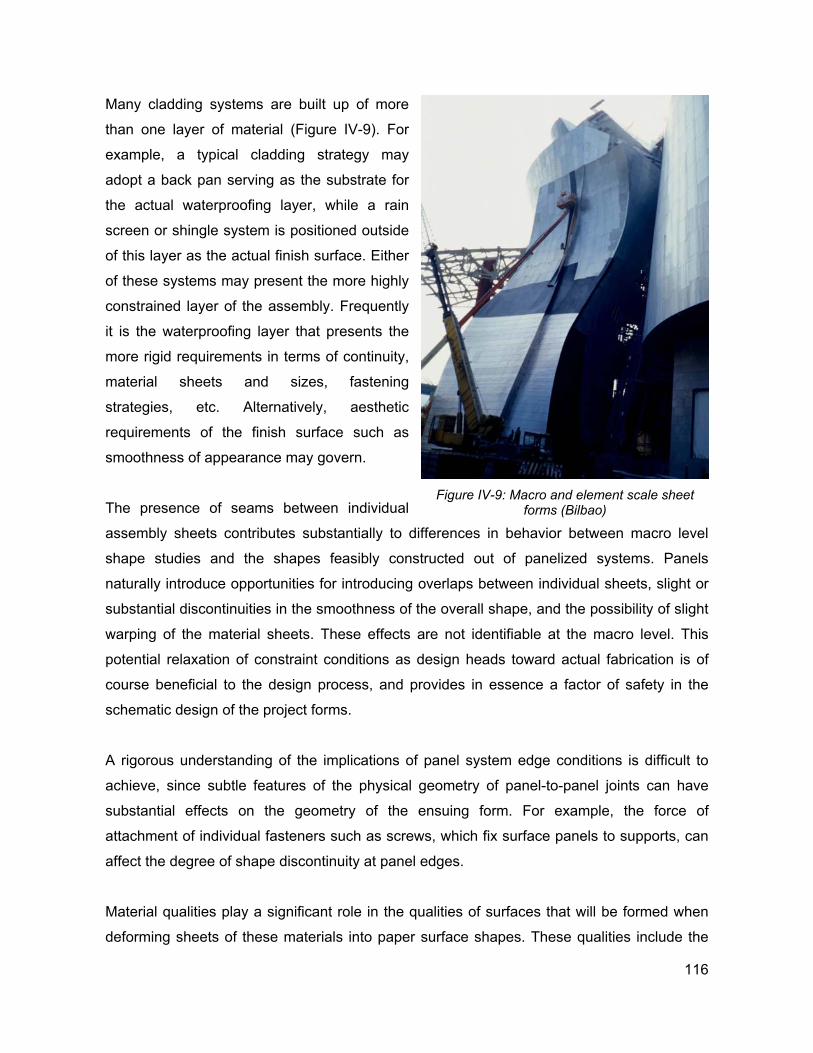
Many cladding systems are built up of more

than one layer of material (Figure IV-9). For

example, a typical cladding strategy may

adopt a back pan serving as the substrate for

the actual waterproofing layer, while a rain

screen or shingle system is positioned outside

of this layer as the actual finish surface. Either

of these systems may present the more highly

constrained layer of the assembly. Frequently

it is the waterproofing layer that presents the

more rigid requirements in terms of continuity,

material sheets and sizes, fastening

strategies, etc. Alternatively, aesthetic

requirements of the finish surface such as

smoothness of appearance may govern.

The presence of seams between individual

assembly sheets contributes substantially to differences in behavior between macro level

shape studies and the shapes feasibly constructed out of panelized systems. Panels

naturally introduce opportunities for introducing overlaps between individual sheets, slight or

substantial discontinuities in the smoothness of the overall shape, and the possibility of slight

warping of the material sheets. These effects are not identifiable at the macro level. This

potential relaxation of constraint conditions as design heads toward actual fabrication is of

course beneficial to the design process, and provides in essence a factor of safety in the

schematic design of the project forms.

Figure IV-9: Macro and element scale sheet

forms (Bilbao)

A rigorous understanding of the implications of panel system edge conditions is difficult to

achieve, since subtle features of the physical geometry of panel-to-panel joints can have

substantial effects on the geometry of the ensuing form. For example, the force of

attachment of individual fasteners such as screws, which fix surface panels to supports, can

affect the degree of shape discontinuity at panel edges.

Material qualities play a significant role in the qualities of surfaces that will be formed when

deforming sheets of these materials into paper surface shapes. These qualities include the

116

actual material properties such as stiffness and brittleness. Material thickness and forming

activities will affect the behavior of these materials. Thick plywood sheets will behave

differently under deformation than layered assemblies of thin plywood sheets with the same

thickness. Where titanium panels have been used, these sheets have typically been used

with a thinner gauge than stainless steel or aluminum panels. Titanium is resistant to ductile

deformation, and will thus typically be resistant to being forced into shapes with any in plane

deformation. In contrast, lead and pewter sheet materials are highly ductile, and will readily

assume shapes that would require molding or stamping of more conventional surfacing

materials. Stainless steel has been used on different projects with a wide variety of gauges,

from thin sheet to plate steel, with large differences in the limitations on shapes that can be

produced.

Strategies for the organization of system components will have many implications on the

surface qualities of paper surfaces. Similarly, the design intent in terms of the desired surface

qualities will guide the selection of surface fabrication strategies. Surface fabrication systems

will introduce a host of constraints presenting rules for the organization of surface

components. Patterning strategies for sheet layouts will obviously be affected by the

organization of sub-framing systems. Systems using straight members organized in an

undulating form have been successfully applied to the construction of paper surface forms

(Chapter V.B.). The economics of specific fabrication strategies that generate the constraints

of paper surface forms will likely include specific additional implications for the way in which

the systems components are organized, and the types of shapes that may be economically

constructed using a given fabrication system. It is also possible for several different systems

to be employed on different regions of a project, depending on the complexity of the localized

surface form. For example, less curved surface areas may afford more straight forward

construction, while more highly curved areas of are addressed with a more forgiving, less

economical fabrication approach.

The formidable role of paper surface systems in Gehry’s work and the complexity of these

systems’ formal constraints have placed a substantial demand on CAD modeling efforts. The

geometric controls and operations by which paper surfaces are constructed in digital form

are radically different than - and in many ways impoverished compared to - the flexibility and

intuitiveness of direct material manipulation. For this reason, the process of faithfully re-

constructing the physically generated forms in a digital context has been a time and labor-

117

intensive process. More troubling is that these surface modeling techniques may introduce

constraints on the digital surface forms that are different than those of physical modeling

materials or their fabricated counterparts.

This dichotomy between physical objects and their analytical counterparts is not new. In

traditional engineering, limitations of analytical approaches to perfectly represent real world

conditions are addressed implicitly by introducing factors of safety: backing away from the

true limits of the materials and engineering in a more conservative manner than might be

possible. Changes in analytical methods have at times allowed less conservative approaches

to similar systems, such as the introduction of plastic deformation considerations into steel

frame design in the 1980s.

These issues play out in the engineering and construction of paper surface forms as well.

Many of the techniques for modeling paper surface systems include notions of factors of

safety, constraining the surface form somewhat in order to be able to guarantee

constructibility. Other approaches rely on rationalizing paper surface forms into canonical

shapes such as cylinders and planes whose constructibility may by nature be guaranteed.

Both of these approaches present obvious drawbacks, in that the qualities of shapes

generated by rationalizing may be qualitatively different than the ideal surfaces, and may

also not truly represent the limits of what can be fabricated. This discrepancy between the

initial physically modeled forms, those that can possibly be fabricated, and the rationalized

forms representing the limits of our predictive capabilities may not be completely resolvable.

Nonetheless, an ongoing goal of computational research by the firm is to achieve greater

parity between these three worlds as materials are pushed further toward their limits.

In the context of Gehry’s digital building delivery process, the limits imposed by digital

representation present an ultimate constraint on the inclusion of forms in the design

vocabulary. If forms can not be described in the project documentation in a manner through

which their constructibility can be substantiated, then they can not feasibly be

accommodated in construction, regardless of the actual abilities of craftsmen to perform the

work. This limiting condition creates urgency for developing representations of sheet

materials, which accurately reflect fabrication constraints without imposing additional

constraints resulting purely from limitations of the geometric representation itself.

118

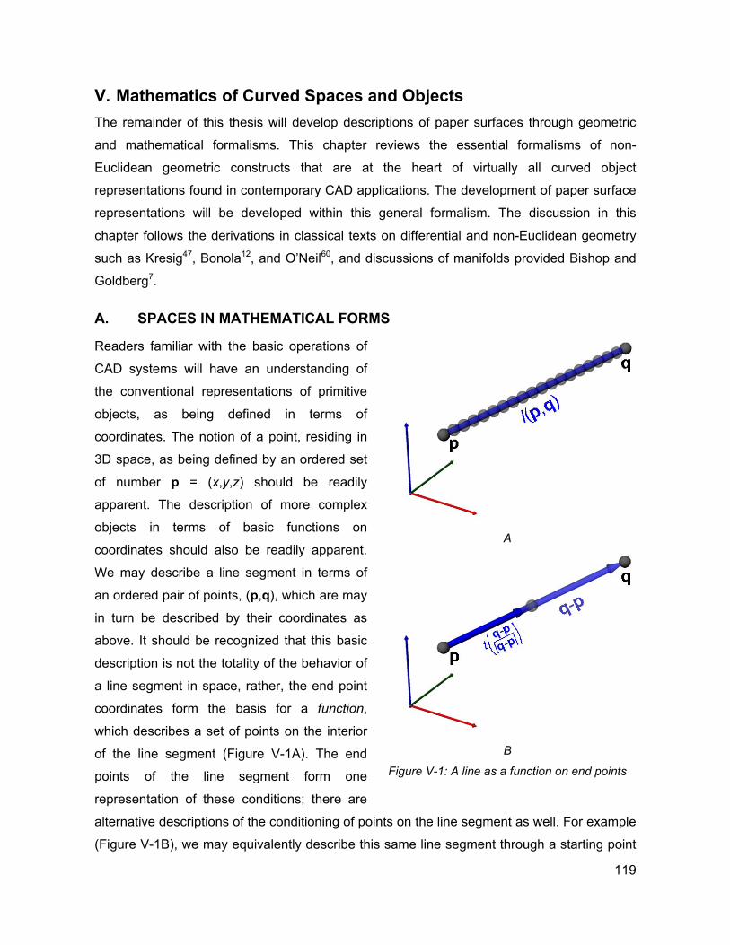
V. Mathematics of Curved Spaces and Objects The remainder of this thesis will develop descriptions of paper surfaces through geometric

and mathematical formalisms. This chapter reviews the essential formalisms of non-

Euclidean geometric constructs that are at the heart of virtually all curved object

representations found in contemporary CAD applications. The development of paper surface

representations will be developed within this general formalism. The discussion in this

chapter follows the derivations in classical texts on differential and non-Euclidean geometry

such as Kresig47, Bonola12, and O’Neil60, and discussions of manifolds provided Bishop and

Goldberg7.

A. SPACES IN MATHEMATICAL FORMS

Readers familiar with the basic operations of

CAD systems will have an understanding of

the conventional representations of primitive

objects, as being defined in terms of

coordinates. The notion of a point, residing in

3D space, as being defined by an ordered set

of number p = (x,y,z) should be readily

apparent. The description of more complex

objects in terms of basic functions on

coordinates should also be readily apparent.

We may describe a line segment in terms of

an ordered pair of points, (p,q), which are may

in turn be described by their coordinates as

above. It should be recognized that this basic

description is not the totality of the behavior of

a line segment in space, rather, the end point

coordinates form the basis for a function,

which describes a set of points on the interior

of the line segment (Figure V-1A). The end

points of the line segment form one

representation of these conditions; there are

alternative descriptions of the conditioning of points on the line segment as well. For example

(Figure V-1B), we may equivalently describe this same line segment through a starting point

A

B

Figure V-1: A line as a function on end points

119

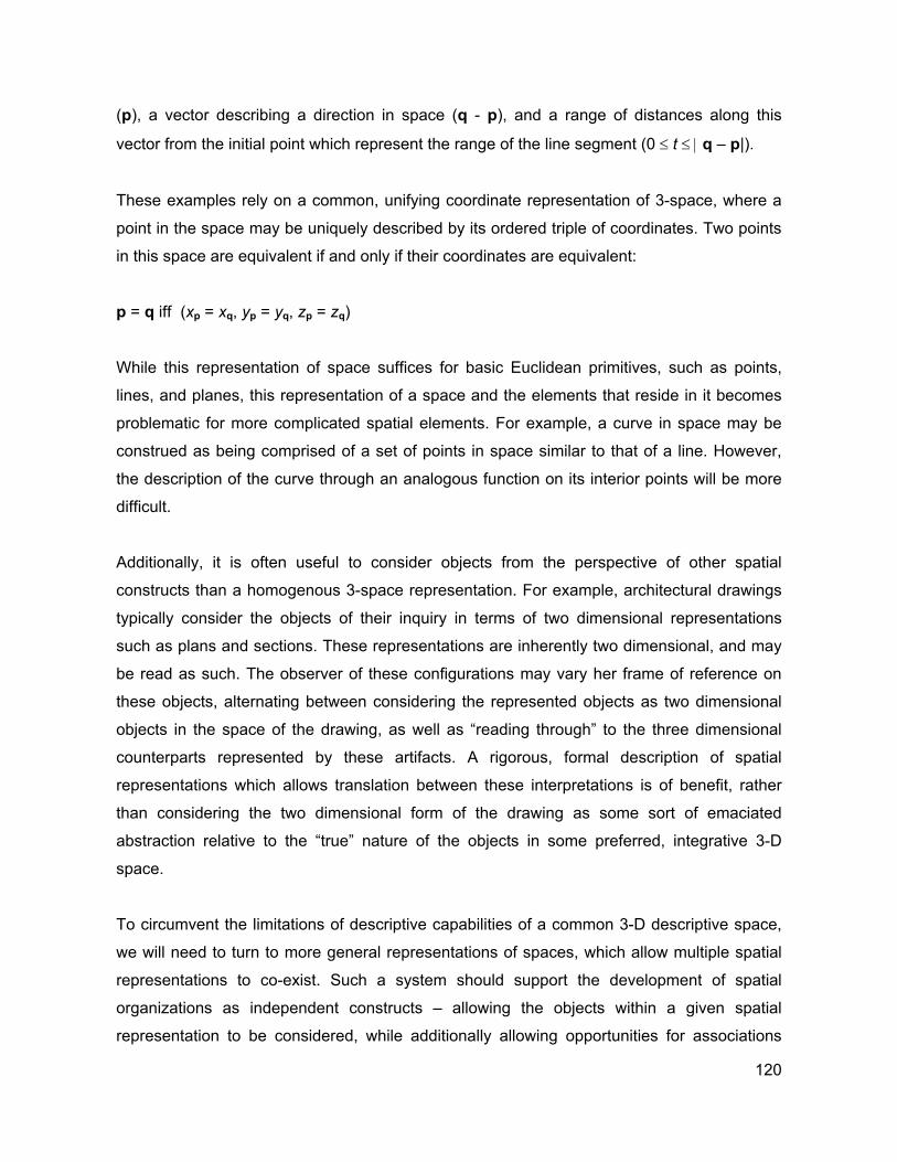
(p), a vector describing a direction in space (q - p), and a range of distances along this

vector from the initial point which represent the range of the line segment (0 ≤ t ≤ | q – p|).

These examples rely on a common, unifying coordinate representation of 3-space, where a

point in the space may be uniquely described by its ordered triple of coordinates. Two points

in this space are equivalent if and only if their coordinates are equivalent:

p = q iff (xp = xq, yp = yq, zp = zq)

While this representation of space suffices for basic Euclidean primitives, such as points,

lines, and planes, this representation of a space and the elements that reside in it becomes

problematic for more complicated spatial elements. For example, a curve in space may be

construed as being comprised of a set of points in space similar to that of a line. However,

the description of the curve through an analogous function on its interior points will be more

difficult.

Additionally, it is often useful to consider objects from the perspective of other spatial

constructs than a homogenous 3-space representation. For example, architectural drawings

typically consider the objects of their inquiry in terms of two dimensional representations

such as plans and sections. These representations are inherently two dimensional, and may

be read as such. The observer of these configurations may vary her frame of reference on

these objects, alternating between considering the represented objects as two dimensional

objects in the space of the drawing, as well as “reading through” to the three dimensional

counterparts represented by these artifacts. A rigorous, formal description of spatial

representations which allows translation between these interpretations is of benefit, rather

than considering the two dimensional form of the drawing as some sort of emaciated

abstraction relative to the “true” nature of the objects in some preferred, integrative 3-D

space.

To circumvent the limitations of descriptive capabilities of a common 3-D descriptive space,

we will need to turn to more general representations of spaces, which allow multiple spatial

representations to co-exist. Such a system should support the development of spatial

organizations as independent constructs – allowing the objects within a given spatial

representation to be considered, while additionally allowing opportunities for associations

120

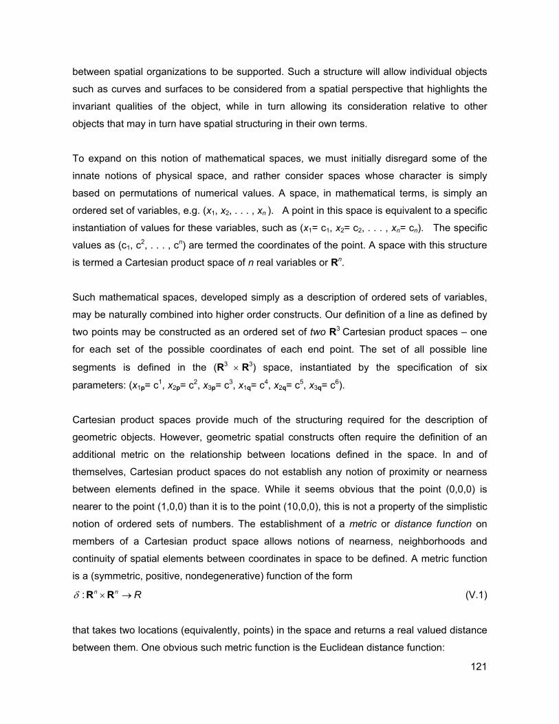
between spatial organizations to be supported. Such a structure will allow individual objects

such as curves and surfaces to be considered from a spatial perspective that highlights the

invariant qualities of the object, while in turn allowing its consideration relative to other

objects that may in turn have spatial structuring in their own terms.

To expand on this notion of mathematical spaces, we must initially disregard some of the

innate notions of physical space, and rather consider spaces whose character is simply

based on permutations of numerical values. A space, in mathematical terms, is simply an

ordered set of variables, e.g. (x1, x2, . . . , xn ). A point in this space is equivalent to a specific

instantiation of values for these variables, such as (x1= c1, x2= c2, . . . , xn= cn). The specific

values as (c1, c2, . . . , cn) are termed the coordinates of the point. A space with this structure

is termed a Cartesian product space of n real variables or Rn.

Such mathematical spaces, developed simply as a description of ordered sets of variables,

may be naturally combined into higher order constructs. Our definition of a line as defined by

two points may be constructed as an ordered set of two R3 Cartesian product spaces – one

for each set of the possible coordinates of each end point. The set of all possible line

segments is defined in the (R3 × R3) space, instantiated by the specification of six

parameters: (x1p= c1, x2p= c2, x3p= c3, x1q= c4, x2q= c5, x3q= c6).

Cartesian product spaces provide much of the structuring required for the description of

geometric objects. However, geometric spatial constructs often require the definition of an

additional metric on the relationship between locations defined in the space. In and of

themselves, Cartesian product spaces do not establish any notion of proximity or nearness

between elements defined in the space. While it seems obvious that the point (0,0,0) is

nearer to the point (1,0,0) than it is to the point (10,0,0), this is not a property of the simplistic

notion of ordered sets of numbers. The establishment of a metric or distance function on

members of a Cartesian product space allows notions of nearness, neighborhoods and

continuity of spatial elements between coordinates in space to be defined. A metric function

is a (symmetric, positive, nondegenerative) function of the form

: n n Rδ × →R R (V.1)

that takes two locations (equivalently, points) in the space and returns a real valued distance

between them. One obvious such metric function is the Euclidean distance function:

121

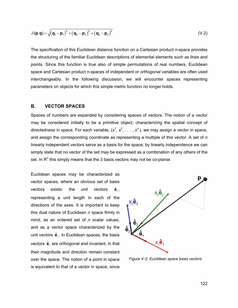
( ) ( ) ( )2 21 1 2 2 3 3( , )δ = − + − + −p q q p q p q p 2

ˆ i

(V.2)

The specification of this Euclidean distance function on a Cartesian product n-space provides

the structuring of the familiar Euclidean descriptions of elemental elements such as lines and

points. Since this function is true also of simple permutations of real numbers, Euclidean

space and Cartesian product n-spaces of independent or orthogonal variables are often used

interchangeably. In the following discussion, we will encounter spaces representing

parameters on objects for which this simple metric function no longer holds.

B. VECTOR SPACES

Spaces of numbers are expanded by considering spaces of vectors. The notion of a vector

may be considered initially to be a primitive object, characterizing the spatial concept of

directedness in space. For each variable, (x1, x2, . . . , xn ), we may assign a vector in space,

and assign the corresponding coordinate as representing a multiple of this vector. A set of n

linearly independent vectors serve as a basis for the space; by linearly independence we can

simply state that no vector of the set may be expressed as a combination of any others of the

set. In R3 this simply means that the 3 basis vectors may not be co-planar.

Euclidean spaces may be characterized as

vector spaces, where an obvious set of basis

vectors exists: the unit vectors e ,

representing a unit length in each of the

directions of the axes. It is important to keep

this dual nature of Euclidean n space firmly in

mind, as an ordered set of n scalar values,

and as a vector space characterized by the

unit vectors e . In Euclidean spaces, the basis

vectors are orthogonal and invariant, in that

their magnitude and direction remain constant

over the space. The notion of a point in space

is equivalent to that of a vector in space, since

ˆ i

ˆ ie

Figure V-2: Euclidean space basis vectors

122

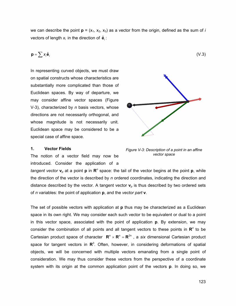
we can describe the point p = (x1, x2, x3) as a vector from the origin, defined as the sum of i

vectors of length xi in the direction of : ˆ ie

ˆi ix= ∑p e (V.3)

In representing curved objects, we must draw

on spatial constructs whose characteristics are

substantially more complicated than those of

Euclidean spaces. By way of departure, we

may consider affine vector spaces (Figure

V-3), characterized by n basis vectors, whose

directions are not necessarily orthogonal, and

whose magnitude is not necessarily unit.

Euclidean space may be considered to be a

special case of affine space.

1. Vector Fields The notion of a vector field may now be

introduced. Consider the application of a

tangent vector vp at a point p in Rn space: the tail of the vector begins at the point p, while

the direction of the vector is described by n ordered coordinates, indicating the direction and

distance described by the vector. A tangent vector vp is thus described by two ordered sets

of n variables: the point of application p, and the vector part v.

Figure V-3: Description of a point in an affine

vector space

The set of possible vectors with application at p thus may be characterized as a Euclidean

space in its own right. We may consider each such vector to be equivalent or dual to a point

in this vector space, associated with the point of application p. By extension, we may

consider the combination of all points and all tangent vectors to these points in Rn to be

Cartesian product space of character Rn × Rn = R2n , a six dimensional Cartesian product

space for tangent vectors in R3. Often, however, in considering deformations of spatial

objects, we will be concerned with multiple vectors emanating from a single point of

consideration. We may thus consider these vectors from the perspective of a coordinate

system with its origin at the common application point of the vectors p. In doing so, we

123

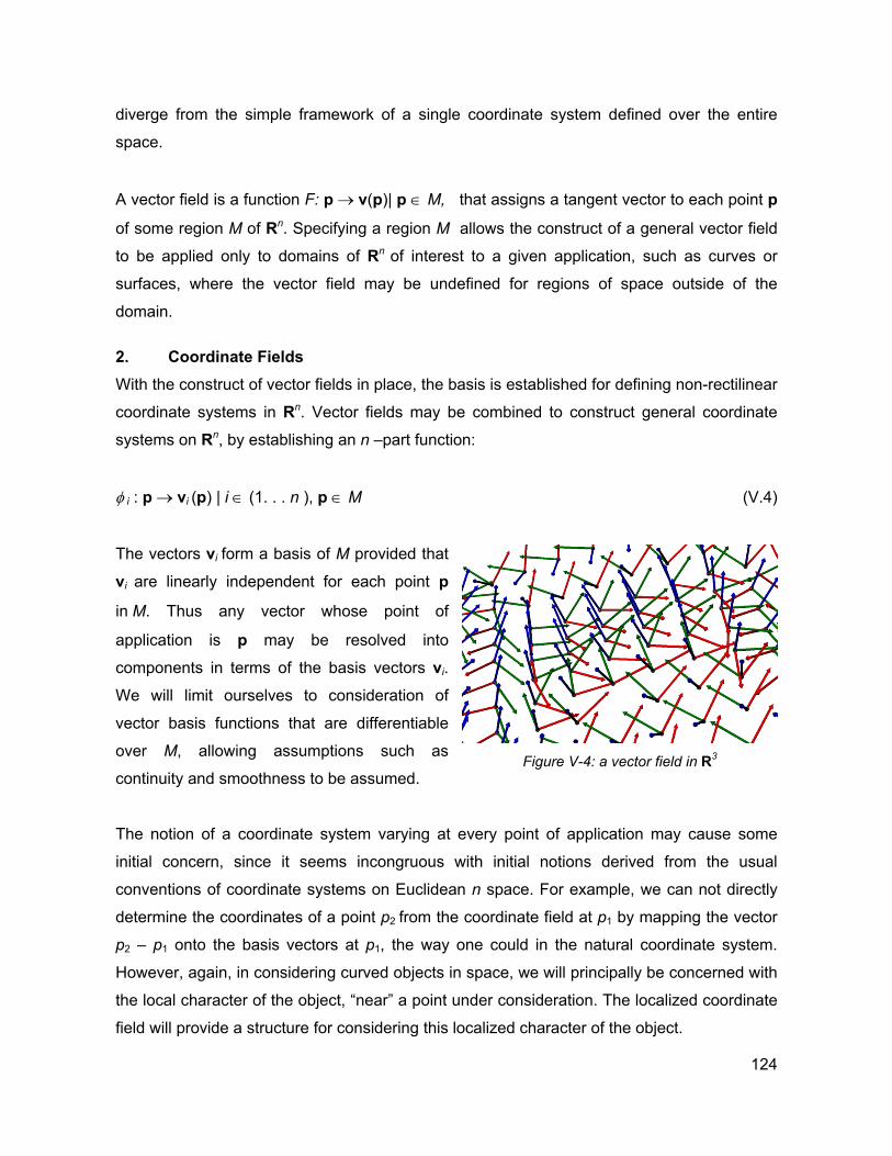
diverge from the simple framework of a single coordinate system defined over the entire

space.

A vector field is a function F: p → v(p)| p ∈ M, that assigns a tangent vector to each point p

of some region M of Rn. Specifying a region M allows the construct of a general vector field

to be applied only to domains of Rn of interest to a given application, such as curves or

surfaces, where the vector field may be undefined for regions of space outside of the

domain.

2. Coordinate Fields With the construct of vector fields in place, the basis is established for defining non-rectilinear

coordinate systems in Rn. Vector fields may be combined to construct general coordinate

systems on Rn, by establishing an n –part function:

φ i : p → vi (p) | i ∈ (1. . . n ), p ∈ M (V.4)

The vectors vi form a basis of M provided that

vi are linearly independent for each point p

in M. Thus any vector whose point of

application is p may be resolved into

components in terms of the basis vectors vi.

We will limit ourselves to consideration of

vector basis functions that are differentiable

over M, allowing assumptions such as

continuity and smoothness to be assumed.

Figure V-4: a vector field in R3

The notion of a coordinate system varying at every point of application may cause some

initial concern, since it seems incongruous with initial notions derived from the usual

conventions of coordinate systems on Euclidean n space. For example, we can not directly

determine the coordinates of a point p2 from the coordinate field at p1 by mapping the vector

p2 – p1 onto the basis vectors at p1, the way one could in the natural coordinate system.

However, again, in considering curved objects in space, we will principally be concerned with

the local character of the object, “near” a point under consideration. The localized coordinate

field will provide a structure for considering this localized character of the object.

124

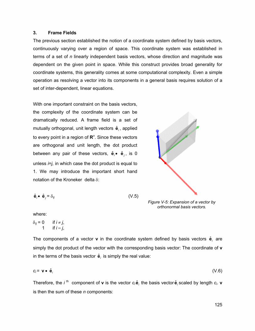
3. Frame Fields The previous section established the notion of a coordinate system defined by basis vectors,

continuously varying over a region of space. This coordinate system was established in

terms of a set of n linearly independent basis vectors, whose direction and magnitude was

dependent on the given point in space. While this construct provides broad generality for

coordinate systems, this generality comes at some computational complexity. Even a simple

operation as resolving a vector into its components in a general basis requires solution of a

set of inter-dependent, linear equations.

With one important constraint on the basis vectors,

the complexity of the coordinate system can be

dramatically reduced. A frame field is a set of

mutually orthogonal, unit length vectors e , applied

to every point in a region of Rn. Since these vectors

are orthogonal and unit length, the dot product

between any pair of these vectors, e • , is 0

unless i=j, in which case the dot product is equal to

1. We may introduce the important short hand

notation of the Kroneker delta δ:

ˆ i

eˆ

Figure V-5: Expansion of a vector by

orthonormal basis vectors.

i j

ˆ ie • e = δij (V.5) ˆ j

where:

δij = 0 if i ≠ j, 1 if i = j, The components of a vector v in the coordinate system defined by basis vectors are

simply the dot product of the vector with the corresponding basis vector: The coordinate of v

in the terms of the basis vector e is simply the real value:

ˆ ie

ˆ i

ci = v • (V.6) ˆ ie Therefore, the i th component of v is the vector ci the basis vector scaled by length ci. v

is then the sum of these n components:

ˆ ie ˆ ie

125

ˆ ˆ( )i= •∑v v e ie (V.7)

The process of resolving a vector into its components in terms of the frame vectors is termed

orthonormal expansion.

Having previously established the notion of a general coordinate field in Section 6, the frame

field represents a “step backward” to a less general construct. Note that the “natural”

coordinate system (x,y,z), is a special, additionally constrained frame field whose basis

vectors are invariant over the space. Frame fields enjoy some of the simplicity of Euclidean

space, but only at local points of application. In investigating the shape of curved spatial

objects, we will be establishing appropriate frame fields on these objects that highlight their

localized characteristics.

C. MAPPINGS

We will next consider mappings between spatial representations - the means by which

disparate spaces and objects expressed in these spaces may be integrated. A mapping may

be defined between pairs of spatial representations. A mapping from a space N = (x1, x2,. . . ,

xn), to a space M = (y1, y2,. . . , ym) is a set of m functions, that expresses the relationships

between the coordinates of the two spaces:

(y1, y2,. . . , ym) = (φ1(x1, x2,. . . , xn), φ2(x1, x2,. . . , xn) ,. . . , φm(x1, x2,. . . , xn))

We may consider this mapping both in terms of the individual coordinate mapping functions:

φi ∈ (φ1. . . φm),

or simplify our notation in considering the set of functions to be a single multi-part function, of

the form:

φ: N → M (read: φ maps N to M )

126

Similarly, we should expect that if such a mapping function exists, then an inverse function

exists, mapping from the space M back into the space N, of the form:

φ -1 : M → N (read: the inverse of φ maps M to N )

For the purposes of exploring curved spatial objects, we will presume that these mapping

functions are differentiable to the degree appropriate for the required application, i.e. that

rates of change in the coordinate variables of the space M can be determined by considering

the rates of change in the variables of the space N. A mapping function is infinitely

differentiable if each of the coordinate mapping functions φi possesses valid derivates up to

infinite order. Typically we will be interested in mappings that present derivatives at least up

to some finite order.

In considering the forms of curved spatial objects, the structure presented by these

differentials will often have greater significance than the actual mapping functions

themselves. While we may of course be interested in the actual placement of objects in

space, the geometric nature of these objects are frequently invariant, should the object be

subject to some translation in the space. In such an event, the localized rates of change of

the mapping function between the parametric and embedding space will be preserved, while

the specific functions mapping coordinates between these spatial representations may not.

We will from time to time consider the structure of curved spatial objects in terms of these

derivative functions, without explicitly stating the characteristics of the mapping functions

themselves.

Mapping between frame fields is a straight forward computation. Given a vector v with

components vi = ci , we wish to determine its components vj = dj in some second

coordinate system, whose basis are the orthogonal, unit length vectors . The

transformation is found by resolving each basis vector into its components in the frame .

These components are found by conducting an orthonormal expansion of each vector :

ˆ ie ˆjf

ˆjf

ˆ ie ˆjf

ˆ ie

aij = • (V.8) ˆ ie ˆjf

127

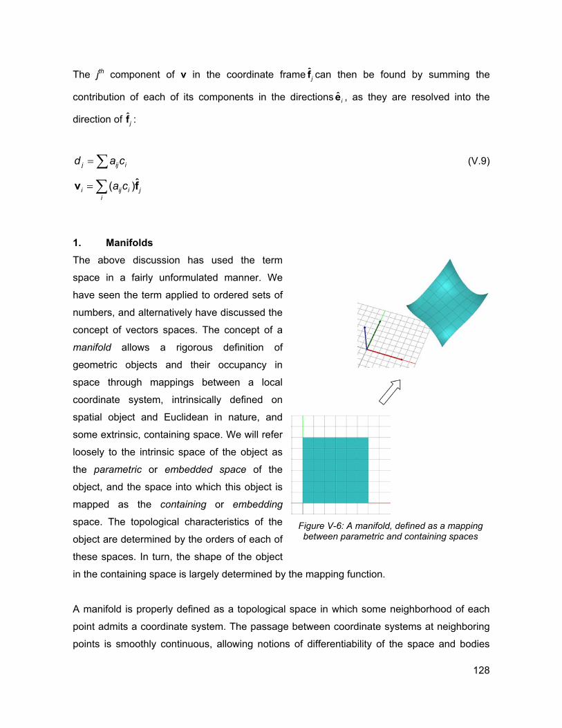
The jth component of v in the coordinate frame can then be found by summing the

contribution of each of its components in the directions , as they are resolved into the

direction of f :

ˆjf

ˆ ie

ˆj

= ∑j ij id a c

j

(V.9)

ˆ( )i ij ii

a c= ∑v f

1. Manifolds The above discussion has used the term

space in a fairly unformulated manner. We

have seen the term applied to ordered sets of

numbers, and alternatively have discussed the

concept of vectors spaces. The concept of a

manifold allows a rigorous definition of

geometric objects and their occupancy in

space through mappings between a local

coordinate system, intrinsically defined on

spatial object and Euclidean in nature, and

some extrinsic, containing space. We will refer

loosely to the intrinsic space of the object as

the parametric or embedded space of the

object, and the space into which this object is

mapped as the containing or embedding

space. The topological characteristics of the

object are determined by the orders of each of

these spaces. In turn, the shape of the object

in the containing space is largely determined by the mapping function.

Figure V-6: A manifold, defined as a mapping between parametric and containing spaces

A manifold is properly defined as a topological space in which some neighborhood of each

point admits a coordinate system. The passage between coordinate systems at neighboring

points is smoothly continuous, allowing notions of differentiability of the space and bodies

128

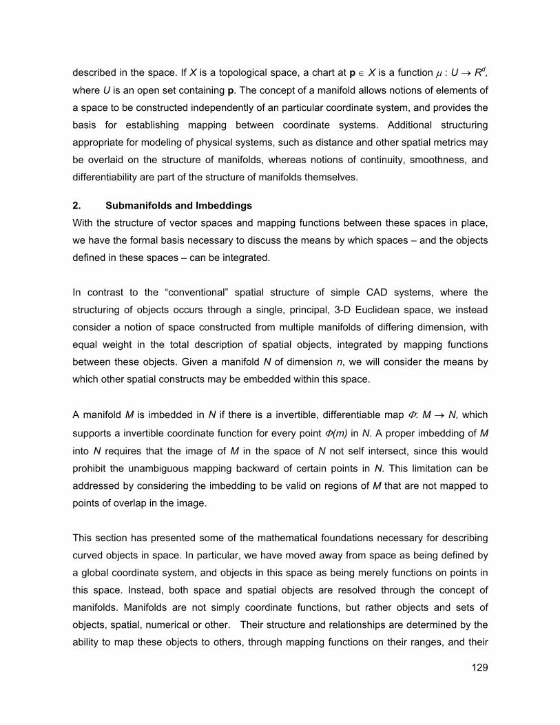
described in the space. If X is a topological space, a chart at p ∈ X is a function µ : U → Rd,

where U is an open set containing p. The concept of a manifold allows notions of elements of

a space to be constructed independently of an particular coordinate system, and provides the

basis for establishing mapping between coordinate systems. Additional structuring

appropriate for modeling of physical systems, such as distance and other spatial metrics may

be overlaid on the structure of manifolds, whereas notions of continuity, smoothness, and

differentiability are part of the structure of manifolds themselves.

2. Submanifolds and Imbeddings With the structure of vector spaces and mapping functions between these spaces in place,

we have the formal basis necessary to discuss the means by which spaces – and the objects

defined in these spaces – can be integrated.

In contrast to the “conventional” spatial structure of simple CAD systems, where the

structuring of objects occurs through a single, principal, 3-D Euclidean space, we instead

consider a notion of space constructed from multiple manifolds of differing dimension, with

equal weight in the total description of spatial objects, integrated by mapping functions

between these objects. Given a manifold N of dimension n, we will consider the means by

which other spatial constructs may be embedded within this space.

A manifold M is imbedded in N if there is a invertible, differentiable map Φ: M → N, which

supports a invertible coordinate function for every point Φ(m) in N. A proper imbedding of M

into N requires that the image of M in the space of N not self intersect, since this would

prohibit the unambiguous mapping backward of certain points in N. This limitation can be

addressed by considering the imbedding to be valid on regions of M that are not mapped to

points of overlap in the image.

This section has presented some of the mathematical foundations necessary for describing

curved objects in space. In particular, we have moved away from space as being defined by

a global coordinate system, and objects in this space as being merely functions on points in

this space. Instead, both space and spatial objects are resolved through the concept of

manifolds. Manifolds are not simply coordinate functions, but rather objects and sets of

objects, spatial, numerical or other. Their structure and relationships are determined by the

ability to map these objects to others, through mapping functions on their ranges, and their

129

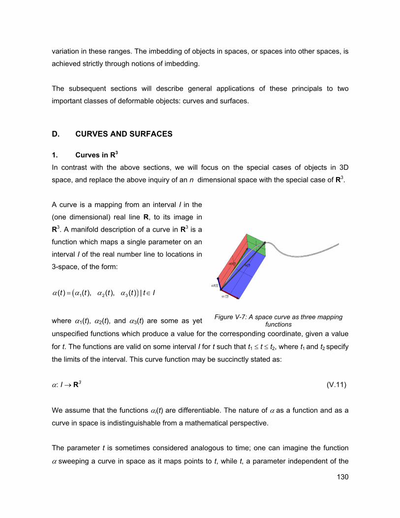
variation in these ranges. The imbedding of objects in spaces, or spaces into other spaces, is

achieved strictly through notions of imbedding.

The subsequent sections will describe general applications of these principals to two

important classes of deformable objects: curves and surfaces.

D. CURVES AND SURFACES

1. Curves in R3 In contrast with the above sections, we will focus on the special cases of objects in 3D

space, and replace the above inquiry of an n dimensional space with the special case of R3.

A curve is a mapping from an interval I in the

(one dimensional) real line R, to its image in

R3. A manifold description of a curve in R3 is a

function which maps a single parameter on an

interval I of the real number line to locations in

3-space, of the form:

( )1 2 3( ) ( ), ( ), ( ) |t t t t tα α α α= I∈ (V.10)

where α1(t), α2(t), and α3(t) are some as yet

unspecified functions which produce a value for the corresponding coordinate, given a value

for t. The functions are valid on some interval I for t such that t1 ≤ t ≤ t2, where t1 and t2 specify

the limits of the interval. This curve function may be succinctly stated as:

Figure V-7: A space curve as three mapping

functions

α: I → R3 (V.11)

We assume that the functions αi(t) are differentiable. The nature of α as a function and as a

curve in space is indistinguishable from a mathematical perspective.

The parameter t is sometimes considered analogous to time; one can imagine the function

α sweeping a curve in space as it maps points to t, while t, a parameter independent of the

130

space R3, structures this sweeping through space. In keeping with this temporal analogy, we

may consider the first derivative of the function α at a particular value of t to be the velocity

vector of α at t, of the form:

31 2

( )

( ) ( ), ( ), ( )t

t t t tt t t α

αα αα ∂∂ ∂′ = ∂ ∂ ∂ (V.12)

This function determines the instantaneous direction of travel of the curve at a specific point

in space, in much the same way that the velocity of an object passing through space

indicates the instantaneous direction of the object’s travel. Geometrically, this derivative with

respect to t is the tangent of the curve α. The vector α ’(t) also has a length or magnitude.

This magnitude is derived from the parameterization of the function α, and is not discernable

from the geometric shape of the curve itself. As this discussion of curved objects progresses,

the distinction will be explored between the parametric, functionally derived qualities of a

curve on one hand, and the purely spatial properties of the curve on the other.

By way of progression to discussing these purely geometric properties of curves, we

consider the fact that the specific parameterization of the function α does not uniquely

describe the curve in space; rather, there are a potentially unlimited number of

parameterizations which can describe the same path through space. Drawing on the

temporal analogy, a given path in space may be traversed by any number of speeds, and

variations of speed along the path. This reparametrization of the curve α may be constructed

as follows:

Let α: I → R3 be a curve. Let η: J → I be a differentiable function on an open interval J of R.

The function:

( ( ))sβ α η= (V.13)

is a reparametrization of α by η. The function η imbeds the interval J into I, and is of the form

R → R. The velocity vector β’ is related to α’ through the chain rule:

131

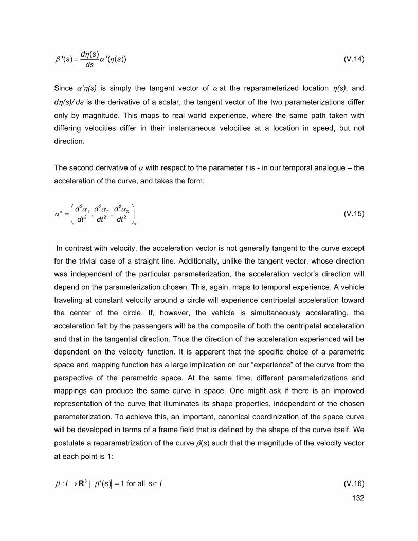
( )'( ) '( ( ))d ssdsηβ α= sη (V.14)

Since α’η(s) is simply the tangent vector of α at the reparameterized location η(s), and

dη(s)/ ds is the derivative of a scalar, the tangent vector of the two parameterizations differ

only by magnitude. This maps to real world experience, where the same path taken with

differing velocities differ in their instantaneous velocities at a location in speed, but not

direction.

The second derivative of α with respect to the parameter t is - in our temporal analogue – the

acceleration of the curve, and takes the form:

22 2

31 22 2 2, , dd d

dt dt dtα

αα αα

′′ =

(V.15)

In contrast with velocity, the acceleration vector is not generally tangent to the curve except

for the trivial case of a straight line. Additionally, unlike the tangent vector, whose direction

was independent of the particular parameterization, the acceleration vector’s direction will

depend on the parameterization chosen. This, again, maps to temporal experience. A vehicle

traveling at constant velocity around a circle will experience centripetal acceleration toward

the center of the circle. If, however, the vehicle is simultaneously accelerating, the

acceleration felt by the passengers will be the composite of both the centripetal acceleration

and that in the tangential direction. Thus the direction of the acceleration experienced will be

dependent on the velocity function. It is apparent that the specific choice of a parametric

space and mapping function has a large implication on our “experience” of the curve from the

perspective of the parametric space. At the same time, different parameterizations and

mappings can produce the same curve in space. One might ask if there is an improved

representation of the curve that illuminates its shape properties, independent of the chosen

parameterization. To achieve this, an important, canonical coordinization of the space curve

will be developed in terms of a frame field that is defined by the shape of the curve itself. We

postulate a reparametrization of the curve β(s) such that the magnitude of the velocity vector

at each point is 1:

3: | ( )I sβ β ′→ =R 1 for all s (V.16) I∈

132

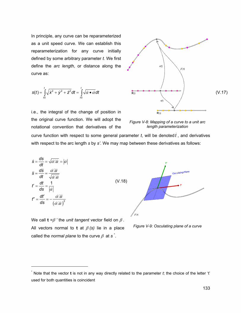
In principle, any curve can be reparameterized

as a unit speed curve. We can establish this

reparameterization for any curve initially

defined by some arbitrary parameter t. We first

define the arc length, or distance along the

curve as:

α α= + + = •∫ ∫& & & & &2 2 2

0 0

( )t t

t t

s t x y z dt dt (V.17)

i.e., the integral of the change of position in

the original curve function. We will adopt the

notational convention that derivatives of the

curve function with respect to some general parameter t, will be denoted , and derivatives

with respect to the arc length s by s’. We may map between these derivatives as follows:

t&

Figure V-8: Mapping of a curve to a unit arc

length parameterization

( )2

1

dssdtdssdtdttdsdttds

α α α

α αα α

α

α αα α

= = =

= =

′ = =

′′′ = = −

& & & &

& & &&&&

& &

&

& &&

& &

(V.18)

Figure V-9: Osculating plane of a curve

We call t =β ’ the unit tangent vector field on β .

All vectors normal to t at β (s) lie in a place

called the normal plane to the curve β at s *.

* Note that the vector t is not in any way directly related to the parameter t; the choice of the letter ‘t’

used for both quantities is coincident

133

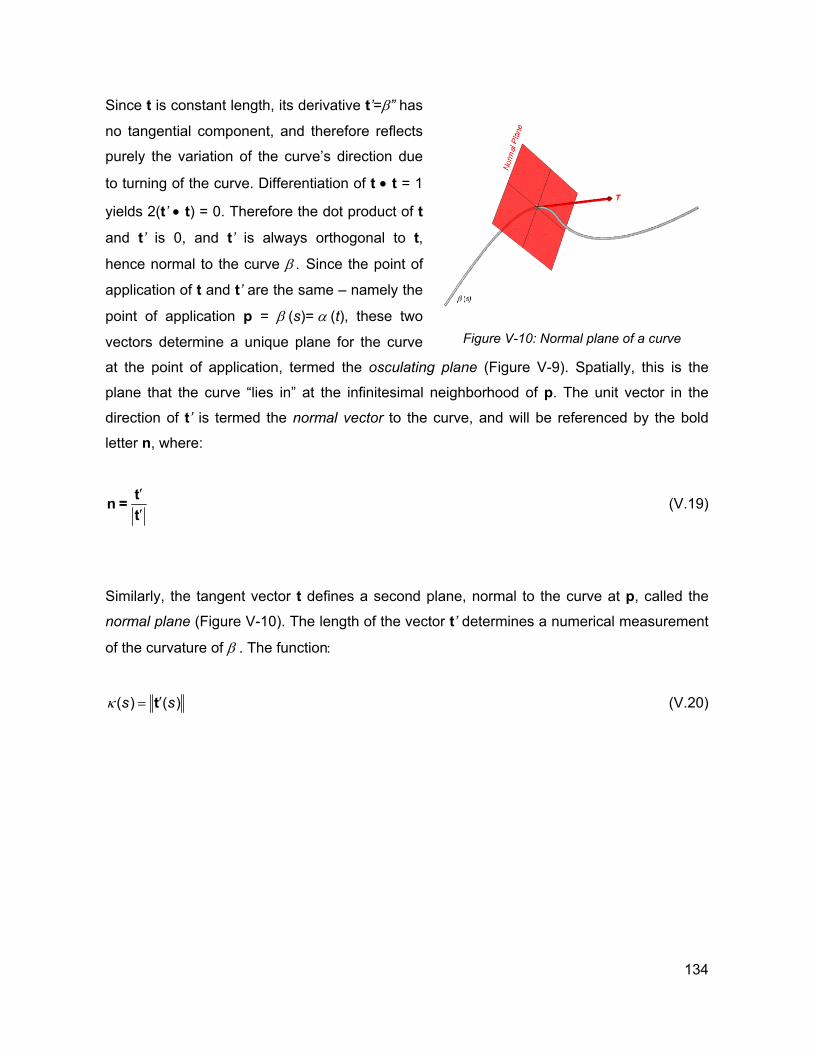
Since t is constant length, its derivative t’=β” has

no tangential component, and therefore reflects

purely the variation of the curve’s direction due

to turning of the curve. Differentiation of t • t = 1

yields 2(t’ • t) = 0. Therefore the dot product of t

and t’ is 0, and t’ is always orthogonal to t,

hence normal to the curve β . Since the point of

application of t and t’ are the same – namely the

point of application p = β (s)= α (t), these two

vectors determine a unique plane for the curve

at the point of application, termed the osculating plane (Figure V-9). Spatially, this is the

plane that the curve “lies in” at the infinitesimal neighborhood of p. The unit vector in the

direction of t’ is termed the normal vector to the curve, and will be referenced by the bold

letter n, where:

Figure V-10: Normal plane of a curve

′′

tn =t

(V.19)

Similarly, the tangent vector t defines a second plane, normal to the curve at p, called the

normal plane (Figure V-10). The length of the vector t’ determines a numerical measurement

of the curvature of β . The function:

( ) ( )s sκ ′= t (V.20)

134

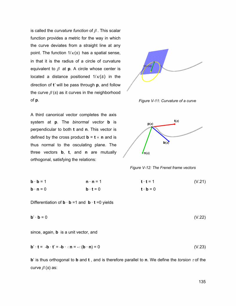
is called the curvature function of β . This scalar

function provides a metric for the way in which

the curve deviates from a straight line at any

point. The function 1/ has a spatial sense,

in that it is the radius of a circle of curvature

equivalent to β at p. A circle whose center is

located a distance positioned 1/

( )sκ

κ ( )s in the

direction of t’ will be pass through p, and follow

the curve β (s) as it curves in the neighborhood

of p.

Figure V-11: Curvature of a curve

A third canonical vector completes the axis

system at p. The binormal vector b is

perpendicular to both t and n. This vector is

defined by the cross product b = t × n and is

thus normal to the osculating plane. The

three vectors b, t, and n are mutually

orthogonal, satisfying the relations: Figure V-12: The Frenet frame vectors

b ⋅ b = 1 n ⋅ n = 1 t ⋅ t = 1 (V.21)

b ⋅ n = 0 b ⋅ t = 0 t ⋅ b = 0

Differentiation of b ⋅ b =1 and b ⋅ t =0 yields

b’ ⋅ b = 0 (V.22)

since, again, b is a unit vector, and

b’ ⋅ t = -b ⋅ t’ = -b ⋅ κn = -κ(b ⋅ n) = 0 (V.23)

b’ is thus orthogonal to b and t , and is therefore parallel to n. We define the torsion τ of the

curve β (s) as:

135

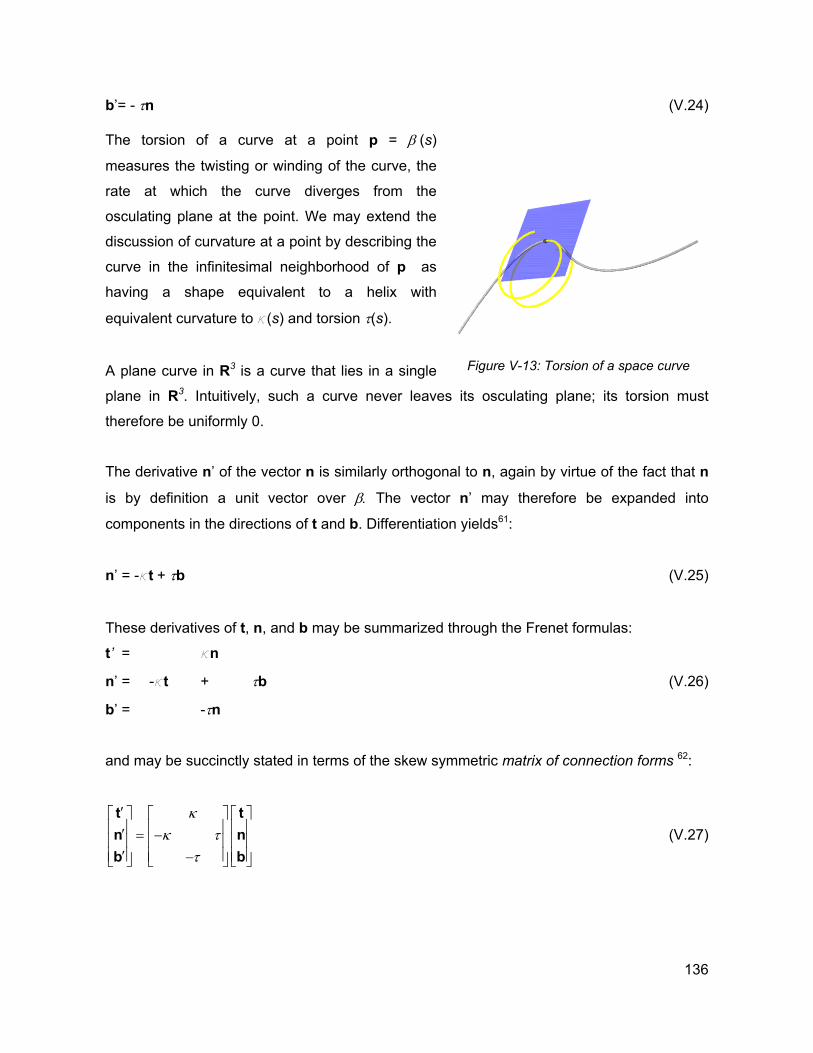
b’= - τn (V.24) The torsion of a curve at a point p = β (s)

measures the twisting or winding of the curve, the

rate at which the curve diverges from the

osculating plane at the point. We may extend the

discussion of curvature at a point by describing the

curve in the infinitesimal neighborhood of p as

having a shape equivalent to a helix with

equivalent curvature to κ(s) and torsion τ(s).

A plane curve in R3 is a curve that lies in a single

plane in R3. Intuitively, such a curve never leaves its osculating plane; its torsion must

therefore be uniformly 0.

Figure V-13: Torsion of a space curve

The derivative n’ of the vector n is similarly orthogonal to n, again by virtue of the fact that n

is by definition a unit vector over β. The vector n’ may therefore be expanded into

components in the directions of t and b. Differentiation yields61:

n’ = -κt + τb (V.25)

These derivatives of t, n, and b may be summarized through the Frenet formulas:

t’ = κn

n’ = -κt + τb (V.26)

b’ = -τn

and may be succinctly stated in terms of the skew symmetric matrix of connection forms 62:

κκ τ

τ

′ ′ = − ′ −

t tnb b

n (V.27)

136

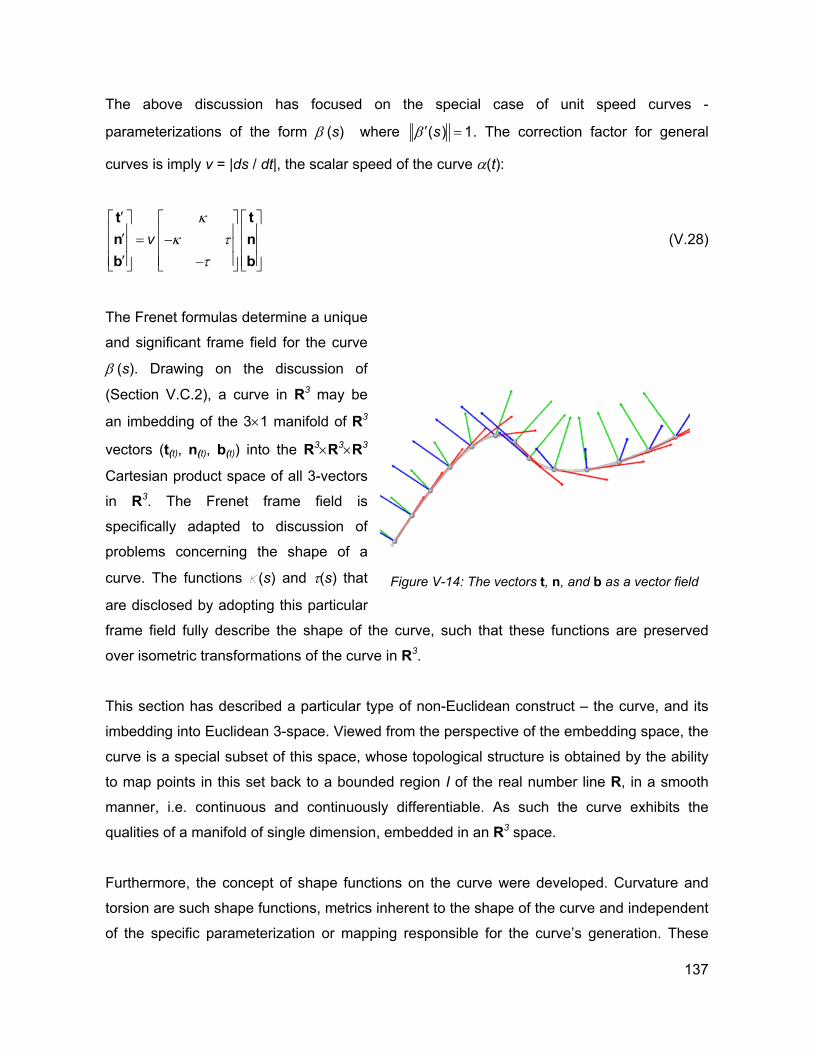
The above discussion has focused on the special case of unit speed curves -

parameterizations of the form β (s) where ( ) 1sβ ′ = . The correction factor for general

curves is imply v = |ds / dt|, the scalar speed of the curve α(t):

vκ

κ ττ

′ ′ = − ′ −

t tnb b

n (V.28)

The Frenet formulas determine a unique

and significant frame field for the curve

β (s). Drawing on the discussion of

(Section V.C.2), a curve in R3 may be

an imbedding of the 3×1 manifold of R3

vectors (t(t), n(t), b(t)) into the R3×R3×R3

Cartesian product space of all 3-vectors

in R3. The Frenet frame field is

specifically adapted to discussion of

problems concerning the shape of a

curve. The functions κ(s) and τ(s) that

are disclosed by adopting this particular

frame field fully describe the shape of the curve, such that these functions are preserved

over isometric transformations of the curve in R3.

Figure V-14: The vectors t, n, and b as a vector field

This section has described a particular type of non-Euclidean construct – the curve, and its

imbedding into Euclidean 3-space. Viewed from the perspective of the embedding space, the

curve is a special subset of this space, whose topological structure is obtained by the ability

to map points in this set back to a bounded region I of the real number line R, in a smooth

manner, i.e. continuous and continuously differentiable. As such the curve exhibits the

qualities of a manifold of single dimension, embedded in an R3 space.

Furthermore, the concept of shape functions on the curve were developed. Curvature and

torsion are such shape functions, metrics inherent to the shape of the curve and independent

of the specific parameterization or mapping responsible for the curve’s generation. These

137

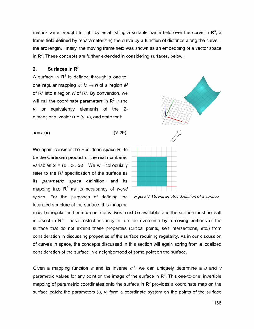
metrics were brought to light by establishing a suitable frame field over the curve in R3, a

frame field defined by reparameterizing the curve by a function of distance along the curve –

the arc length. Finally, the moving frame field was shown as an embedding of a vector space

in R3. These concepts are further extended in considering surfaces, below.

2. Surfaces in R3 A surface in R3 is defined through a one-to-

one regular mapping σ: M → N of a region M

of R2 into a region N of R3. By convention, we

will call the coordinate parameters in R2 u and

v, or equivalently elements of the 2-

dimensional vector u = (u, v), and state that:

( )σ=x u (V.29)

We again consider the Euclidean space R3 to

be the Cartesian product of the real numbered

variables x = (x1, x2, x3). We will colloquially

refer to the R2 specification of the surface as

its parametric space definition, and its

mapping into R3 as its occupancy of world

space. For the purposes of defining the

localized structure of the surface, this mapping

must be regular and one-to-one: derivatives must be available, and the surface must not self

intersect in R3. These restrictions may in turn be overcome by removing portions of the

surface that do not exhibit these properties (critical points, self intersections, etc.) from

consideration in discussing properties of the surface requiring regularity. As in our discussion

of curves in space, the concepts discussed in this section will again spring from a localized

consideration of the surface in a neighborhood of some point on the surface.

Figure V-15: Parametric definition of a surface

Given a mapping function σ and its inverse σ-1, we can uniquely determine a u and v

parametric values for any point on the image of the surface in R3. This one-to-one, invertible

mapping of parametric coordinates onto the surface in R3 provides a coordinate map on the

surface patch; the parameters (u, v) form a coordinate system on the points of the surface

138

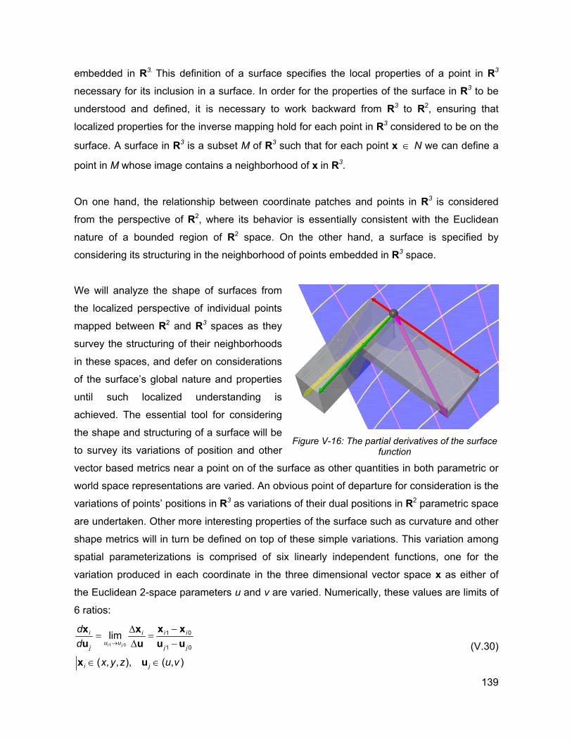
embedded in R3. This definition of a surface specifies the local properties of a point in R3

necessary for its inclusion in a surface. In order for the properties of the surface in R3 to be

understood and defined, it is necessary to work backward from R3 to R2, ensuring that

localized properties for the inverse mapping hold for each point in R3 considered to be on the

surface. A surface in R3 is a subset M of R3 such that for each point x ∈ N we can define a

point in M whose image contains a neighborhood of x in R3.

On one hand, the relationship between coordinate patches and points in R3 is considered

from the perspective of R2, where its behavior is essentially consistent with the Euclidean

nature of a bounded region of R2 space. On the other hand, a surface is specified by

considering its structuring in the neighborhood of points embedded in R3 space.

We will analyze the shape of surfaces from

the localized perspective of individual points

mapped between R2 and R3 spaces as they

survey the structuring of their neighborhoods

in these spaces, and defer on considerations

of the surface’s global nature and properties

until such localized understanding is

achieved. The essential tool for considering

the shape and structuring of a surface will be

to survey its variations of position and other

vector based metrics near a point on of the surface as other quantities in both parametric or

world space representations are varied. An obvious point of departure for consideration is the

variations of points’ positions in R3 as variations of their dual positions in R2 parametric space

are undertaken. Other more interesting properties of the surface such as curvature and other

shape metrics will in turn be defined on top of these simple variations. This variation among

spatial parameterizations is comprised of six linearly independent functions, one for the

variation produced in each coordinate in the three dimensional vector space x as either of

the Euclidean 2-space parameters u and v are varied. Numerically, these values are limits of

6 ratios:

Figure V-16: The partial derivatives of the surface

function

1 0

1 0

1 0

lim

( , , ), ( , )

i j

i ii iu u

j j

i j

dd

x y z u v

→

−∆= =

∆ −

∈ ∈

x xx xu u u

x uju (V.30)

139

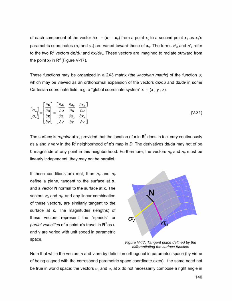
of each component of the vector ∆x = (x1 – x0) from a point x0 to a second point x1 as x1’s

parametric coordinates (u1 and v1) are varied toward those of x0. The terms σ-u and σ-

v refer

to the two R3 vectors dxi/du and dxi/dv,. These vectors are imagined to radiate outward from

the point x0 in R3 (Figure V-17).

These functions may be organized in a 2X3 matrix (the Jacobian matrix) of the function σ,

which may be viewed as an orthonormal expansion of the vectors dx/du and dx/dv in some

Cartesian coordinate field, e.g. a “global coordinate system” x = (x , y , z).

31 2

31 2

u

v

xx xu u u u

xx xv v v v

σσ

∂∂ ∂∂ ∂ ∂ ∂ ∂= = ∂ ∂∂ ∂ ∂ ∂ ∂ ∂

x

x (V.31)

The surface is regular at x0 provided that the location of x in R3 does in fact vary continuously

as u and v vary in the R2 neighborhood of x’s map in D. The derivatives dx/du may not of be

0 magnitude at any point in this neighborhood. Furthermore, the vectors σu and σv must be

linearly independent: they may not be parallel.

If these conditions are met, then σu and σv

define a plane, tangent to the surface at x,

and a vector N normal to the surface at x. The

vectors σu and σv, and any linear combination

of these vectors, are similarly tangent to the

surface at x. The magnitudes (lengths) of

these vectors represent the “speeds” or

partial velocities of a point x‘s travel in R3 as u

and v are varied with unit speed in parametric

space. Figure V-17: Tangent plane defined by the

differentiating the surface function

Note that while the vectors u and v are by definition orthogonal in parametric space (by virtue

of being aligned with the correspond parametric space coordinate axes), the same need not

be true in world space: the vectors σu and σv at x do not necessarily compose a right angle in

140

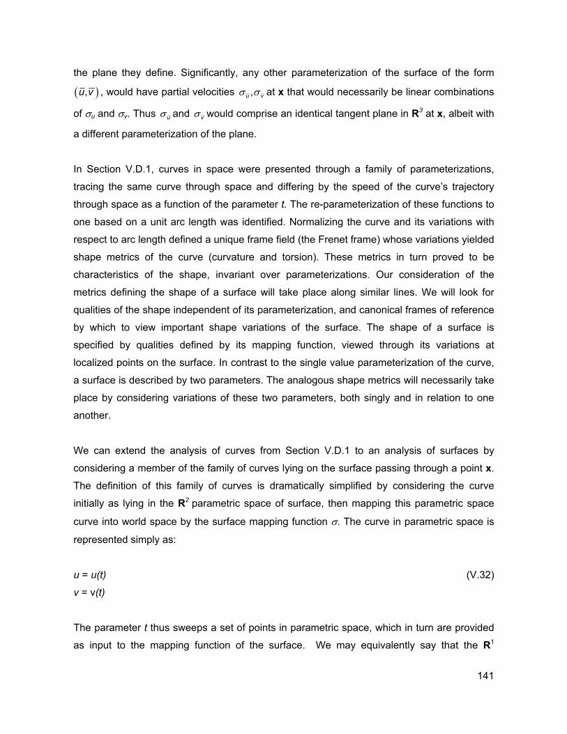
the plane they define. Significantly, any other parameterization of the surface of the form

( ),u v , would have partial velocities ,u vσ σ at x that would necessarily be linear combinations

of σu and σv. Thus uσ and vσ would comprise an identical tangent plane in R3 at x, albeit with

a different parameterization of the plane.

In Section V.D.1, curves in space were presented through a family of parameterizations,

tracing the same curve through space and differing by the speed of the curve’s trajectory

through space as a function of the parameter t. The re-parameterization of these functions to

one based on a unit arc length was identified. Normalizing the curve and its variations with

respect to arc length defined a unique frame field (the Frenet frame) whose variations yielded

shape metrics of the curve (curvature and torsion). These metrics in turn proved to be

characteristics of the shape, invariant over parameterizations. Our consideration of the

metrics defining the shape of a surface will take place along similar lines. We will look for

qualities of the shape independent of its parameterization, and canonical frames of reference

by which to view important shape variations of the surface. The shape of a surface is

specified by qualities defined by its mapping function, viewed through its variations at

localized points on the surface. In contrast to the single value parameterization of the curve,

a surface is described by two parameters. The analogous shape metrics will necessarily take

place by considering variations of these two parameters, both singly and in relation to one

another.

We can extend the analysis of curves from Section V.D.1 to an analysis of surfaces by

considering a member of the family of curves lying on the surface passing through a point x.

The definition of this family of curves is dramatically simplified by considering the curve

initially as lying in the R2 parametric space of surface, then mapping this parametric space

curve into world space by the surface mapping function σ. The curve in parametric space is

represented simply as:

u = u(t) (V.32)

v = v(t)

The parameter t thus sweeps a set of points in parametric space, which in turn are provided

as input to the mapping function of the surface. We may equivalently say that the R1

141

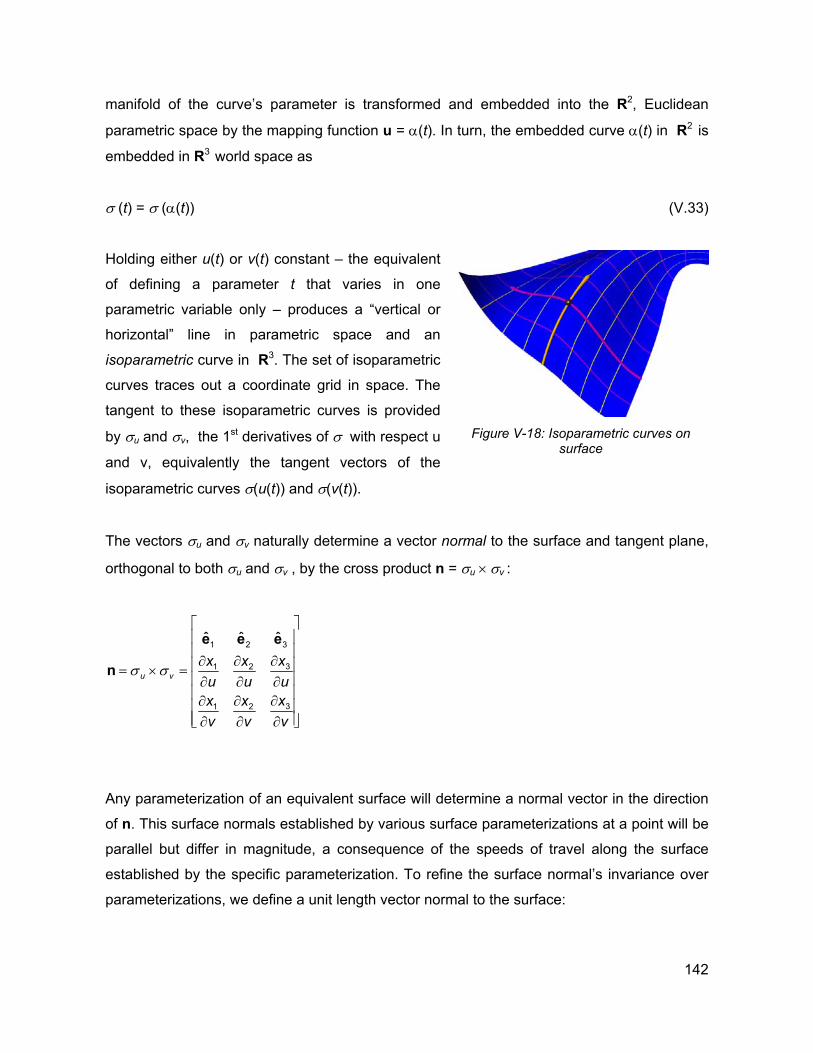
manifold of the curve’s parameter is transformed and embedded into the R2, Euclidean

parametric space by the mapping function u = α(t). In turn, the embedded curve α(t) in R2 is

embedded in R3 world space as

σ (t) = σ (α(t)) (V.33)

Holding either u(t) or v(t) constant – the equivalent

of defining a parameter t that varies in one

parametric variable only – produces a “vertical or

horizontal” line in parametric space and an

isoparametric curve in R3. The set of isoparametric

curves traces out a coordinate grid in space. The

tangent to these isoparametric curves is provided

by σu and σv, the 1st derivatives of σ with respect u

and v, equivalently the tangent vectors of the

isoparametric curves σ(u(t)) and σ(v(t)).

Figure V-18: Isoparametric curves on

surface

The vectors σu and σv naturally determine a vector normal to the surface and tangent plane,

orthogonal to both σu and σv , by the cross product n = σu × σv :

1 2 3

31 2

31 2

ˆ ˆ ˆ

u vxx x

u u uxx x

v v v

σ σ

∂∂ ∂ = × = ∂ ∂ ∂ ∂∂ ∂ ∂ ∂ ∂

e e e

n

Any parameterization of an equivalent surface will determine a normal vector in the direction

of n. This surface normals established by various surface parameterizations at a point will be

parallel but differ in magnitude, a consequence of the speeds of travel along the surface

established by the specific parameterization. To refine the surface normal’s invariance over

parameterizations, we define a unit length vector normal to the surface:

142

u v

u v

σ σσ σ

×= =

×N n (V.34)

This unit normal vector is the first important invariant of surface shape we will encounter. Its

variation over the surface forms an vector field on the surface, providing one component of

an invariant coordinate frame field on the surface, similar to the Frenet frames developed for

space curves in Section V.D.1. To complete this invariant frame field, we will need to seek

out appropriately invariant directions on the surface provided by the shape of the surface as

well.

The parameterization of a curve on the

surface through a point x on the surface

forms a basis for the considering the

variation of surface metrics. We can trace

variations of the surface’s shape as we move

along a curve. Then, drawing on the

coordinate framework established on the

surface, we can consider the expansion of

surface properties from our knowledge of

how the surface acts in these orthogonal

parametric directions.

Figure V-19: The family of surface curves through

a point

The arc length of a curve on the surface is found by integrating

ds dxdx dydy dzdz d dσ σ= + + = • (V.35)

The vector dσ/dt tangent to the curve may be expanded in terms of the curve’s

parameterization:

u vd dudt dt dtσ σ σ= +

dv (V.36)

Combining (V.35) and (V.36) results in the first important metric of the shape of surface at a

point: 143

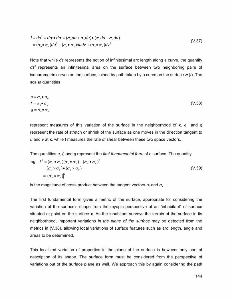
2

2

( ) ( )( ) ( ) ( )

u v u v

u u u v v v

I ds d d du du du dudu dudv dv

σ σ σ σ σ σ

σ σ σ σ σ σ

= = • = + • +

= • + • + • 2 (V.37)

Note that while ds represents the notion of infinitesimal arc length along a curve, the quantity

ds2 represents an infinitesimal area on the surface between two neighboring pairs of

isoparametric curves on the surface, joined by path taken by a curve on the surface σ (t). The

scalar quantities

u u

u v

v v

efg

σ σσ σσ σ

= •

= •

= •

(V.38)

represent measures of this variation of the surface in the neighborhood of x. e and g

represent the rate of stretch or shrink of the surface as one moves in the direction tangent to

u and v at x, while f measures the rate of shear between these two space vectors.

The quantities e, f, and g represent the first fundamental form of a surface. The quantity 2 2

2

( )( ) (( ) ( )

( )

u u v v u v

u v u v

u v

eg f σ σ σ σ σ σσ σ σ σ

σ σ

− = • • − •

= × • ×

= ×

) (V.39)

is the magnitude of cross product between the tangent vectors σu and σv.

The first fundamental form gives a metric of the surface, appropriate for considering the

variation of the surface’s shape from the myopic perspective of an ”inhabitant” of surface

situated at point on the surface x. As the inhabitant surveys the terrain of the surface in its

neighborhood, important variations in the plane of the surface may be detected from the

metrics in (V.38), allowing local variations of surface features such as arc length, angle and

areas to be determined.

This localized variation of properties in the plane of the surface is however only part of

description of its shape. The surface form must be considered from the perspective of

variations out of the surface plane as well. We approach this by again considering the path

144

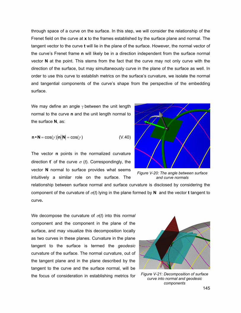
through space of a curve on the surface. In this step, we will consider the relationship of the

Frenet field on the curve at x to the frames established by the surface plane and normal. The

tangent vector to the curve t will lie in the plane of the surface. However, the normal vector of

the curve’s Frenet frame n will likely be in a direction independent from the surface normal

vector N at the point. This stems from the fact that the curve may not only curve with the

direction of the surface, but may simultaneously curve in the plane of the surface as well. In

order to use this curve to establish metrics on the surface’s curvature, we isolate the normal

and tangential components of the curve’s shape from the perspective of the embedding

surface.

We may define an angle γ between the unit length

normal to the curve n and the unit length normal to

the surface N, as:

γ γ= =cos( ) cos( )n • N n N (V.40)

The vector n points in the normalized curvature

direction t′ of the curve σ (t). Correspondingly, the

vector N normal to surface provides what seems

intuitively a similar role on the surface. The

relationship between surface normal and surface curvature is disclosed by considering the

component of the curvature of σ(t) lying in the plane formed by N and the vector t tangent to

curve.

Figure V-20: The angle between surface

and curve normals

We decompose the curvature of σ(t) into this normal

component and the component in the plane of the

surface, and may visualize this decomposition locally

as two curves in these planes. Curvature in the plane

tangent to the surface is termed the geodesic

curvature of the surface. The normal curvature, out of

the tangent plane and in the plane described by the

tangent to the curve and the surface normal, will be

the focus of consideration in establishing metrics for

145

Figure V-21: Decomposition of surface

curve into normal and geodesic components

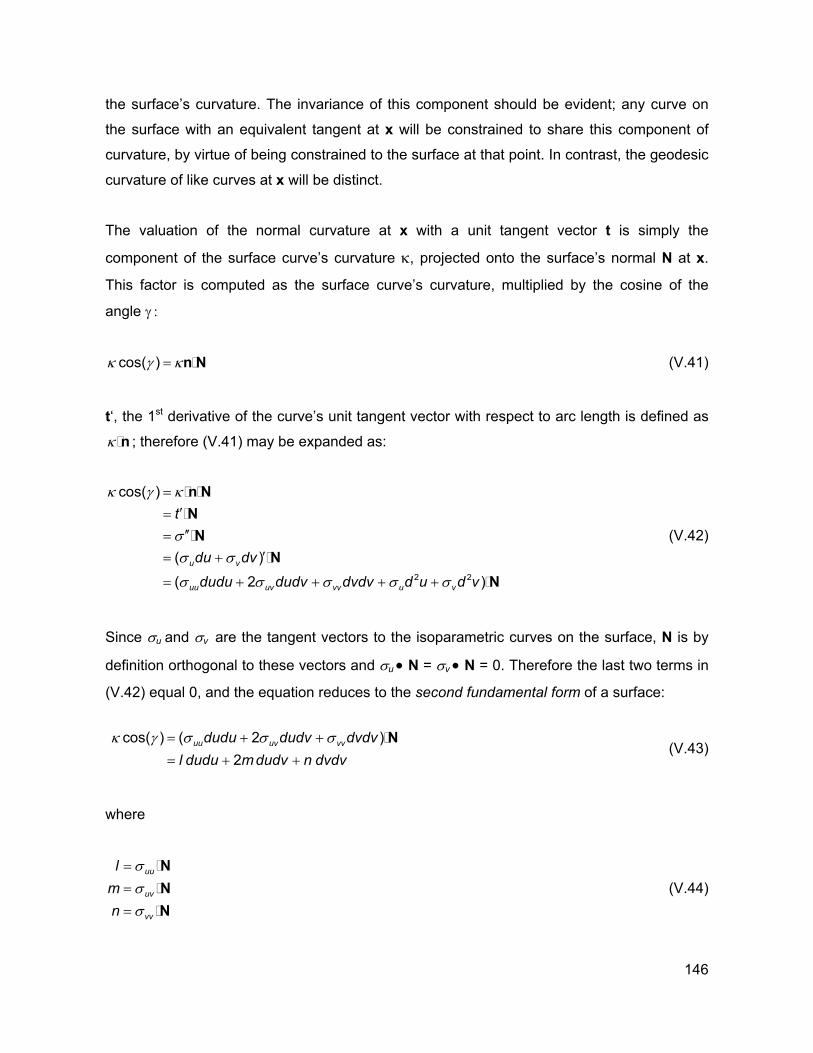
the surface’s curvature. The invariance of this component should be evident; any curve on

the surface with an equivalent tangent at x will be constrained to share this component of

curvature, by virtue of being constrained to the surface at that point. In contrast, the geodesic

curvature of like curves at x will be distinct.

The valuation of the normal curvature at x with a unit tangent vector t is simply the

component of the surface curve’s curvature κ, projected onto the surface’s normal N at x.

This factor is computed as the surface curve’s curvature, multiplied by the cosine of the

angle γ :

cos( )κ γ κ= n N (V.41)

t‘, the 1st derivative of the curve’s unit tangent vector with respect to arc length is defined as

; therefore (V.41) may be expanded as: κ n

2 2

cos( )

( )( 2

u v

uu uv vv u v

t

du dvdudu dudv dvdv d u d v

κ γ κ

σσ σ

σ σ σ σ σ

=′=′′=

′= +

= + + + +

n NNN

NN)

(V.42)

Since σu and σv are the tangent vectors to the isoparametric curves on the surface, N is by

definition orthogonal to these vectors and σu • N = σv • N = 0. Therefore the last two terms in

(V.42) equal 0, and the equation reduces to the second fundamental form of a surface:

(V.43) cos( ) ( 2 )

2uu uv vvdudu dudv dvdv

l dudu mdudv n dvdvκ γ σ σ σ= + +

= + +

N

where

uu

uv

vv

lmn

σσσ

=

=

=

NNN

(V.44)

146

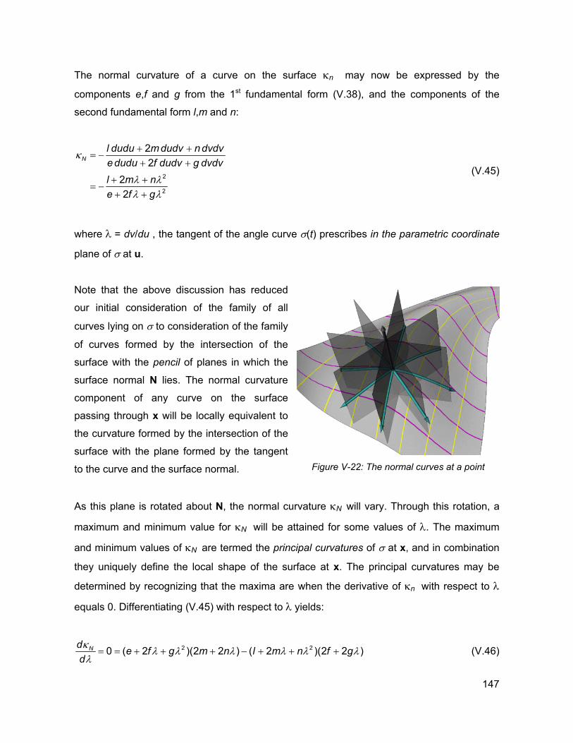
The normal curvature of a curve on the surface κn may now be expressed by the

components e,f and g from the 1st fundamental form (V.38), and the components of the

second fundamental form l,m and n:

2

2

22

22

Nl dudu m dudv n dvdvedudu f dudv g dvdvl m ne f g

κ

λ λλ λ

+ += −

+ +

+ += −

+ +

(V.45)

where λ = dv/du , the tangent of the angle curve σ(t) prescribes in the parametric coordinate

plane of σ at u.

Note that the above discussion has reduced

our initial consideration of the family of all

curves lying on σ to consideration of the family

of curves formed by the intersection of the

surface with the pencil of planes in which the

surface normal N lies. The normal curvature

component of any curve on the surface

passing through x will be locally equivalent to

the curvature formed by the intersection of the

surface with the plane formed by the tangent

to the curve and the surface normal.

Figure V-22: The normal curves at a point

As this plane is rotated about N, the normal curvature κN will vary. Through this rotation, a

maximum and minimum value for κN will be attained for some values of λ. The maximum

and minimum values of κN are termed the principal curvatures of σ at x, and in combination

they uniquely define the local shape of the surface at x. The principal curvatures may be

determined by recognizing that the maxima are when the derivative of κn with respect to λ

equals 0. Differentiating (V.45) with respect to λ yields:

20 ( 2 )(2 2 ) ( 2 )(2 2Nd e f g m n l m n f gdκ 2 )λ λ λ λ λλ

= = + + + − + + + λ (V.46)

147

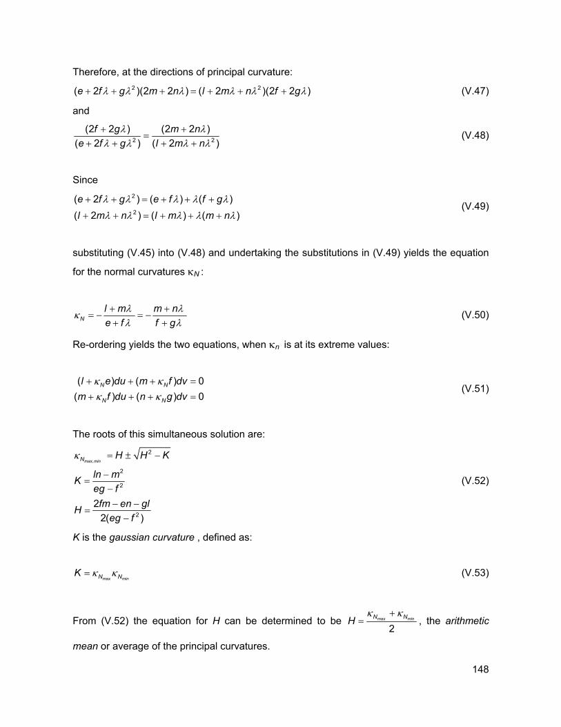
Therefore, at the directions of principal curvature: 2( 2 )(2 2 ) ( 2 )(2 2e f g m n l m n f g2 )λ λ λ λ λ+ + + = + + + λ (V.47)

and

2(2 2 ) (2 2 )

( 2 ) ( 2f g m n

e f g l m nλ

2 )λ

λ λ λ+ +

=+ + + + λ

)

(V.48)

Since 2

2

( 2 ) ( ) ( )( 2 ) ( ) (e f g e f f gl m n l m m n

λ λ λ λ λ

λ λ λ λ

+ + = + + +

+ + = + + + λ (V.49)

substituting (V.45) into (V.48) and undertaking the substitutions in (V.49) yields the equation

for the normal curvatures κN :

Nl m m ne f f g

λ λκλ λ

+= − = −

+ ++

00

=

=

(V.50)

Re-ordering yields the two equations, when κn is at its extreme values:

( ) ( )( ) ( )

N N

N N

l e du m f dvm f du n g dv

κ κκ κ

+ + +

+ + + (V.51)

The roots of this simultaneous solution are: 2

2

2

22

2( )

max,minN H H K

ln mKeg f

fm en glHeg f

κ = ± −

−=

−− −

=−

(V.52)

K is the gaussian curvature , defined as:

max minN NK κ κ= (V.53)

From (V.52) the equation for H can be determined to be 2

max minN Nκ κ+=H , the arithmetic

mean or average of the principal curvatures.

148

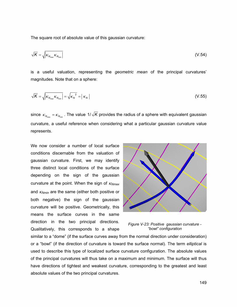
The square root of absolute value of this gaussian curvature:

max minN NK κ κ= (V.54)

is a useful valuation, representing the geometric mean of the principal curvatures’

magnitudes. Note that on a sphere:

2max minN N N NK κ κ κ κ= = = (V.55)

since . The value max minN Nκ κ= 1/ provides the radius of a sphere with equivalent gaussian

curvature, a useful reference when considering what a particular gaussian curvature value

represents.

K

We now consider a number of local surface

conditions discernable from the valuation of

gaussian curvature. First, we may identify

three distinct local conditions of the surface

depending on the sign of the gaussian

curvature at the point. When the sign of κNmax

and κNmin are the same (either both positive or

both negative) the sign of the gaussian

curvature will be positive. Geometrically, this

means the surface curves in the same

direction in the two principal directions.

Qualitatively, this corresponds to a shape

similar to a “dome” (if the surface curves away from the normal direction under consideration)

or a “bowl” (if the direction of curvature is toward the surface normal). The term elliptical is

used to describe this type of localized surface curvature configuration. The absolute values

of the principal curvatures will thus take on a maximum and minimum. The surface will thus

have directions of tightest and weakest curvature, corresponding to the greatest and least

absolute values of the two principal curvatures.

Figure V-23: Positive gaussian curvature - “bowl” configuration

149

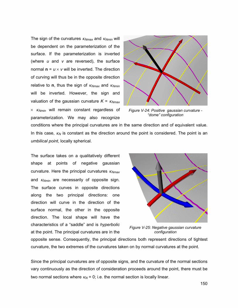
The sign of the curvatures κNmax and κNmin will

be dependent on the parameterization of the

surface. If the parameterization is inverted

(where u and v are reversed), the surface

normal n = u × v will be inverted. The direction

of curving will thus be in the opposite direction

relative to n, thus the sign of κNmax and κNmin

will be inverted. However, the sign and

valuation of the gaussian curvature K = κNmax

× κNmin will remain constant regardless of

parameterization. We may also recognize

conditions where the principal curvatures are in the same direction and of equivalent value.

In this case, κN is constant as the direction around the point is considered. The point is an

umbilical point, locally spherical.

Figure V-24: Positive gaussian curvature -

“dome” configuration

The surface takes on a qualitatively different

shape at points of negative gaussian

curvature. Here the principal curvatures κNmax

and κNmin are necessarily of opposite sign.

The surface curves in opposite directions

along the two principal directions: one

direction will curve in the direction of the

surface normal, the other in the opposite

direction. The local shape will have the

characteristics of a “saddle” and is hyperbolic

at the point. The principal curvatures are in the

opposite sense. Consequently, the principal directions both represent directions of tightest

curvature, the two extremes of the curvatures taken on by normal curvatures at the point.

Figure V-25: Negative gaussian curvature

configuration

Since the principal curvatures are of opposite signs, and the curvature of the normal sections

vary continuously as the direction of consideration proceeds around the point, there must be

two normal sections where κN = 0; i.e. the normal section is locally linear. 150

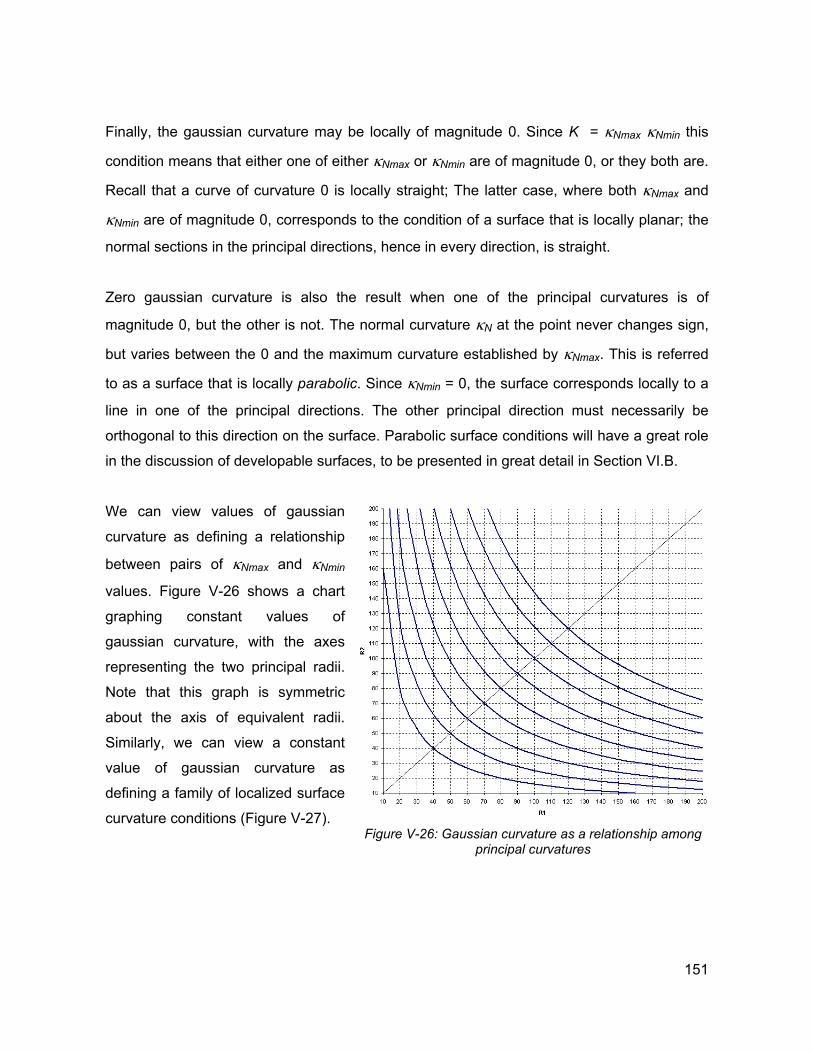
Finally, the gaussian curvature may be locally of magnitude 0. Since K = κNmax κNmin this

condition means that either one of either κNmax or κNmin are of magnitude 0, or they both are.

Recall that a curve of curvature 0 is locally straight; The latter case, where both κNmax and

κNmin are of magnitude 0, corresponds to the condition of a surface that is locally planar; the

normal sections in the principal directions, hence in every direction, is straight.

Zero gaussian curvature is also the result when one of the principal curvatures is of

magnitude 0, but the other is not. The normal curvature κN at the point never changes sign,

but varies between the 0 and the maximum curvature established by κNmax. This is referred

to as a surface that is locally parabolic. Since κNmin = 0, the surface corresponds locally to a

line in one of the principal directions. The other principal direction must necessarily be

orthogonal to this direction on the surface. Parabolic surface conditions will have a great role

in the discussion of developable surfaces, to be presented in great detail in Section VI.B.

We can view values of gaussian

curvature as defining a relationship

between pairs of κNmax and κNmin

values. Figure V-26 shows a chart

graphing constant values of

gaussian curvature, with the axes

representing the two principal radii.

Note that this graph is symmetric

about the axis of equivalent radii.

Similarly, we can view a constant

value of gaussian curvature as

defining a family of localized surface

curvature conditions (Figure V-27). Figure V-26: Gaussian curvature as a relationship among

principal curvatures

151

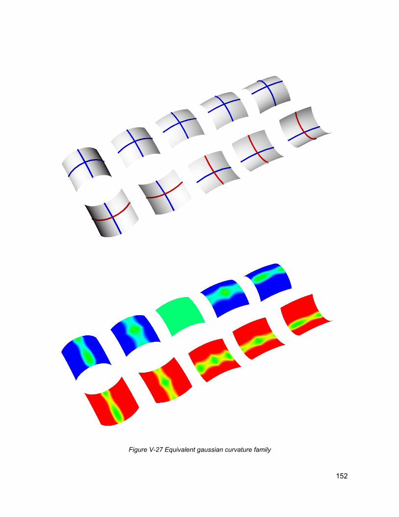
Figure V-27 Equivalent gaussian curvature family

152

The directions of maximum and minimum curvature, along with the normal, present three

vectors on the surface that are each orthogonal to the other. This fact provides the conditions

for a frame field (Section V.B.3) on the surface. This frame field is an analogue of the

important Frenet frames (V.26) found on curves: a unique coordinate system on the surface,

occurring purely as a result of the shape of the surface at local points and independent of the

parameterization of the surface.

The notion of shape metrics - established on curves through the definition of curvature and

torsion – were extended to surfaces through the definition of principal curvatures and

gaussian curvature. These metrics are properties of the shape of the surface, independent of

parametric description that generates the surface. These properties take the form of vector

fields, defined across the surface manifold. Shape metrics will be drawn on in following

sections to establish criteria for the constructibility of the designed shapes.

3. Bézier / NURBS formulations This chapter has established curves and surfaces as special types of topological objects:

manifolds embedded in 3-dimensional space through a mapping from an intrinsic parametric

space that is locally Euclidean. From these topological conditions, shape metrics resulting

from the differential properties of these mappings were identified. These principles were

developed without regard to the specific formulations of the mapping functions, other than

positing assumptions on the order of the mapping function and its differentiability.

In order to interpret these findings into numerical valuations, or simply to describe a specific

object’s inhabitation of R3, numerically evaluatable mapping functions will need to be to

defined. In this section, parametric mapping functions of utility to computer aided design will

be presented, and their ability to support differentiability and other conditions necessary for

shape metric evaluations will be demonstrated.

Classical texts on differential geometry87,47,36 typically present examples of spatial objects in

terms of simple polynomial and trigonometric functions for which differentiation can be

undertaken in a fairly straightforward fashion. For example the curve mapping function:

153

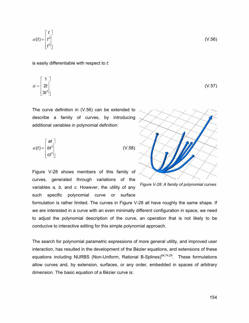
α =

2

3

( )t

t tt

(V.56)

is easily differentiable with respect to t:

α =

&2

123

tt

(V.57)

The curve definition in (V.56) can be extended to

describe a family of curves, by introducing

additional variables in polynomial definition:

2

3

( )at

t btct

α =

(V.58)

Figure V-28 shows members of this family of

curves, generated through variations of the

variables a, b, and c. However, the utility of any

such specific polynomial curve or surface

formulation is rather limited. The curves in Figure V-28 all have roughly the same shape. If

we are interested in a curve with an even minimally different configuration in space, we need

to adjust the polynomial description of the curve, an operation that is not likely to be

conducive to interactive editing for this simple polynomial approach.

Figure V-28: A family of polynomial curves

The search for polynomial parametric expressions of more general utility, and improved user

interaction, has resulted in the development of the Bèzier equations, and extensions of these

equations including NURBS (Non-Uniform, Rational B-Splines)64,74,29. These formulations

allow curves and, by extension, surfaces, or any order, embedded in spaces of arbitrary

dimension. The basic equation of a Bèzier curve is:

154

, where ( ) ( )1

3,

1:

n

i i ki

tα+

=

→ = ∑R R b B t 1min max, 2t t t k n≤ ≤ ≤ ≤ + (V.59)

The variable i denotes the order of the curve, while the vectors bi are the positions of control

point in the embedded space, Bi,k are B-Spline basis functions.

,!( ) (1 )

!( )!i

i nnB t u t

i n i−=

−n i− (V.60)

These basis functions provide a smoothing or averaging function on the locations of the

control points, that varies as a function of the parameter t. for the simple case of an order 1

curve, or line, equation (V.59) reduces to simply:

( ) 0(1 ) ( )t t tα = − +b 1b

,

(V.61)

The B-Spline basis functions may be extended into higher dimensions. The equation for a

Bèzier surface is:

, ,0 0

( , ) ( ) ( )n m

i n j m i ji j

u v B u B vσ= =

= ∑∑ b (V.62)

Where the control points b define an ordered mesh of control points in size i x j. ,i j

Parametric curve and surface representations represented through B-spline equations form

the basis for virtually all commercially available CAD representations at this point in time. The

descriptions of paper surface representations currently used in Gehry’s process are similarly

founded on these underlying parametric descriptions. However, it should again be noted that

these representations only specific examples of the set of potential manifold representations

of curved spatial objects. Other representations will be considered in latter parts of this

thesis.

155

156

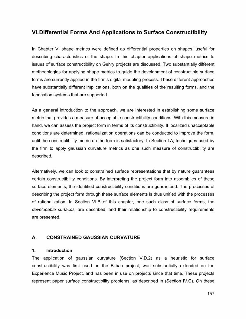
VI. Differential Forms And Applications to Surface Constructibility

In Chapter V, shape metrics were defined as differential properties on shapes, useful for

describing characteristics of the shape. In this chapter applications of shape metrics to

issues of surface constructibility on Gehry projects are discussed. Two substantially different

methodologies for applying shape metrics to guide the development of constructible surface

forms are currently applied in the firm’s digital modeling process. These different approaches

have substantially different implications, both on the qualities of the resulting forms, and the

fabrication systems that are supported.

As a general introduction to the approach, we are interested in establishing some surface

metric that provides a measure of acceptable constructibility conditions. With this measure in

hand, we can assess the project form in terms of its constructibility. If localized unacceptable

conditions are determined, rationalization operations can be conducted to improve the form,

until the constructibility metric on the form is satisfactory. In Section I.A, techniques used by

the firm to apply gaussian curvature metrics as one such measure of constructibility are

described.

Alternatively, we can look to constrained surface representations that by nature guarantees

certain constructibility conditions. By interpreting the project form into assemblies of these

surface elements, the identified constructibility conditions are guaranteed. The processes of

describing the project form through these surface elements is thus unified with the processes

of rationalization. In Section VI.B of this chapter, one such class of surface forms, the

developable surfaces, are described, and their relationship to constructibility requirements

are presented.

A. CONSTRAINED GAUSSIAN CURVATURE

1. Introduction The application of gaussian curvature (Section V.D.2) as a heuristic for surface

constructibility was first used on the Bilbao project, was substantially extended on the

Experience Music Project, and has been in use on projects since that time. These projects

represent paper surface constructibility problems, as described in (Section IV.C). On these

157

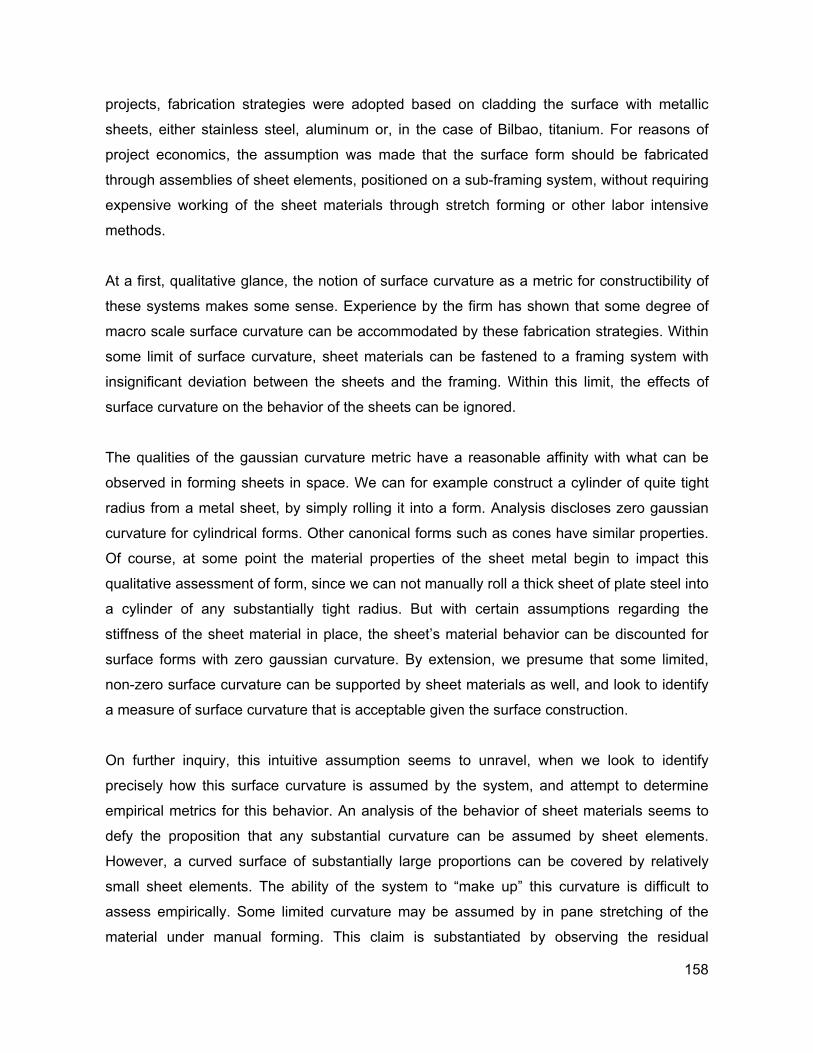
projects, fabrication strategies were adopted based on cladding the surface with metallic

sheets, either stainless steel, aluminum or, in the case of Bilbao, titanium. For reasons of

project economics, the assumption was made that the surface form should be fabricated

through assemblies of sheet elements, positioned on a sub-framing system, without requiring

expensive working of the sheet materials through stretch forming or other labor intensive

methods.

At a first, qualitative glance, the notion of surface curvature as a metric for constructibility of

these systems makes some sense. Experience by the firm has shown that some degree of

macro scale surface curvature can be accommodated by these fabrication strategies. Within

some limit of surface curvature, sheet materials can be fastened to a framing system with

insignificant deviation between the sheets and the framing. Within this limit, the effects of

surface curvature on the behavior of the sheets can be ignored.

The qualities of the gaussian curvature metric have a reasonable affinity with what can be

observed in forming sheets in space. We can for example construct a cylinder of quite tight

radius from a metal sheet, by simply rolling it into a form. Analysis discloses zero gaussian

curvature for cylindrical forms. Other canonical forms such as cones have similar properties.

Of course, at some point the material properties of the sheet metal begin to impact this

qualitative assessment of form, since we can not manually roll a thick sheet of plate steel into

a cylinder of any substantially tight radius. But with certain assumptions regarding the

stiffness of the sheet material in place, the sheet’s material behavior can be discounted for

surface forms with zero gaussian curvature. By extension, we presume that some limited,

non-zero surface curvature can be supported by sheet materials as well, and look to identify

a measure of surface curvature that is acceptable given the surface construction.

On further inquiry, this intuitive assumption seems to unravel, when we look to identify

precisely how this surface curvature is assumed by the system, and attempt to determine

empirical metrics for this behavior. An analysis of the behavior of sheet materials seems to

defy the proposition that any substantial curvature can be assumed by sheet elements.

However, a curved surface of substantially large proportions can be covered by relatively

small sheet elements. The ability of the system to “make up” this curvature is difficult to

assess empirically. Some limited curvature may be assumed by in pane stretching of the

material under manual forming. This claim is substantiated by observing the residual

158

deformation of the sheet if it is released from the substrate to which it is fastened. However,

this manual stretch forming is only a small part of the story. Additional macro scale surface

curvature is assumed by the sheet’s buckling into complex configurations with minimal

gaussian curvature as it is forced onto the framing system. The sheet does not assume the

surface form exactly, but deviates somewhat, in a manner dictated by its internal resolution

of the bending forces. Without conducting substantial material analysis for each sheet, the

exact resolution of these forces by the sheet is difficult to predict. However, the results of

these effects can be observed as the sheet is forced onto framing configurations that impose

increasing gaussian curvature. At some point, the edges of the sheet will begin to display

visible buckling. This phenomenon is highly dependent on sheet dimensions, fastening

strategies, and material properties. Efforts to control these imperfections by orienting panels

either with or against the direction of maximal surface curvature have been inconclusive.

Macro scale gaussian curvature may also be resolved in the fabricated assembly by

discontinuities between adjoining sheet elements. Neighboring sheets will deviate slightly

from one another in continuity or tangency. Small scale buckling independently assumed by

each of the sheets will result in some discontinuity between the sheets. This discontinuity

may have system fabrication or performance implications, and must remain within

established construction tolerances for the system.

As difficult as it is to establish the precise mechanisms by which surface curvature is

resolved by the fabrication system, the degree of imperfection allowable in a surface system

is similarly difficult to determine. When sheet materials are part of the waterproofing strategy

for the project, the allowable discontinuities between sheets must be kept to a minimum. On

many of the firm’s projects, surface fabrication strategies are employed that use several

layers of sheet materials, each with different material behaviors, sheet sizes, and

performance requirements.

In practice, it has often been the desired aesthetic qualities of the finish surface that have

determined the tolerance for imperfections of surface smoothness and the corresponding

degree of allowable surface curvature. The wrinkling of the titanium shingles on the Bilbao

project was part of the desired aesthetic; the curvature considerations on this project were

driven by constructibility requirements of the steel back pan sub-system. On the Experience

159

Music project, curvature considerations were driven largely by the desire for a smooth finish

surface.

An empirical analysis of this wide range of

phenomena and performance requirements –

as they play out on the infinitely variable local

conditions of the project form has not been

practical on Gehry’s projects to date. In

practice, gaussian curvature has proven to be

a reasonable heuristic of surface

constructibility, encompassing all of these

complex phenomena into one simple metric.

Part of the strategy in adopting gaussian

curvature to measure surface constructibility

assumes a factor of safety in developing a

gaussian curvature metric. Typically, mock up

studies of a surface system will be conducted

on the basis of maximum anticipated gaussian

curvature. The mockups are tested for

conformance to performance requirements,

and the qualities of the finish surface are

inspected. If the mockup is deemed successful

on the basis of this assessment, the gaussian

curvature exhibited by the digital rendition of

the mockup provides a bench mark. The

maximum acceptable surface curvature for the

project at large may be stepped back to more

conservative values, to allow a factor of safety.

Figure VI-1: Gaussian curvature samples and

curve

Figure VI-2: Acceptable and unacceptable

curvature configurations

When surface curvature is detected in the design surface that exceeds the established

curvature values for the project, the project form must be rationalized to reduce this

curvature. Several techniques have been developed to address surface conditions where

curvature constraints are not met. The simplest and most effective of these techniques is to

break the surface and introduce tangency discontinues. These tangent discontinuity features

160

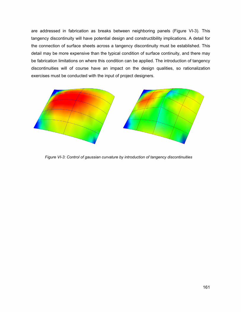
are addressed in fabrication as breaks between neighboring panels (Figure VI-3). This

tangency discontinuity will have potential design and constructibility implications. A detail for

the connection of surface sheets across a tangency discontinuity must be established. This

detail may be more expensive than the typical condition of surface continuity, and there may

be fabrication limitations on where this condition can be applied. The introduction of tangency

discontinuities will of course have an impact on the design qualities, so rationalization

exercises must be conducted with the input of project designers.

Figure VI-3: Control of gaussian curvature by introduction of tangency discontinuities

161

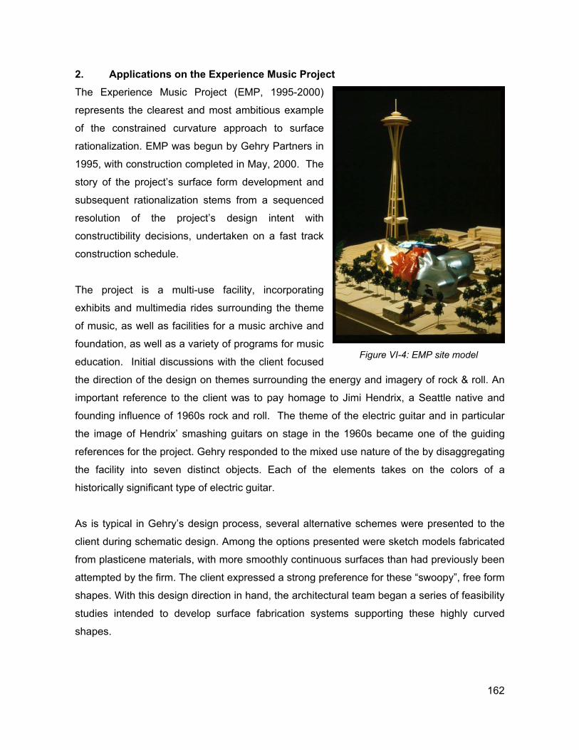
2. Applications on the Experience Music Project The Experience Music Project (EMP, 1995-2000)

represents the clearest and most ambitious example

of the constrained curvature approach to surface

rationalization. EMP was begun by Gehry Partners in

1995, with construction completed in May, 2000. The

story of the project’s surface form development and

subsequent rationalization stems from a sequenced

resolution of the project’s design intent with

constructibility decisions, undertaken on a fast track

construction schedule.

The project is a multi-use facility, incorporating

exhibits and multimedia rides surrounding the theme

of music, as well as facilities for a music archive and

foundation, as well as a variety of programs for music

education. Initial discussions with the client focused

the direction of the design on themes surrounding the energy and imagery of rock & roll. An

important reference to the client was to pay homage to Jimi Hendrix, a Seattle native and

founding influence of 1960s rock and roll. The theme of the electric guitar and in particular

the image of Hendrix’ smashing guitars on stage in the 1960s became one of the guiding

references for the project. Gehry responded to the mixed use nature of the by disaggregating

the facility into seven distinct objects. Each of the elements takes on the colors of a

historically significant type of electric guitar.

Figure VI-4: EMP site model

As is typical in Gehry’s design process, several alternative schemes were presented to the

client during schematic design. Among the options presented were sketch models fabricated

from plasticene materials, with more smoothly continuous surfaces than had previously been

attempted by the firm. The client expressed a strong preference for these “swoopy”, free form

shapes. With this design direction in hand, the architectural team began a series of feasibility

studies intended to develop surface fabrication systems supporting these highly curved

shapes.

162

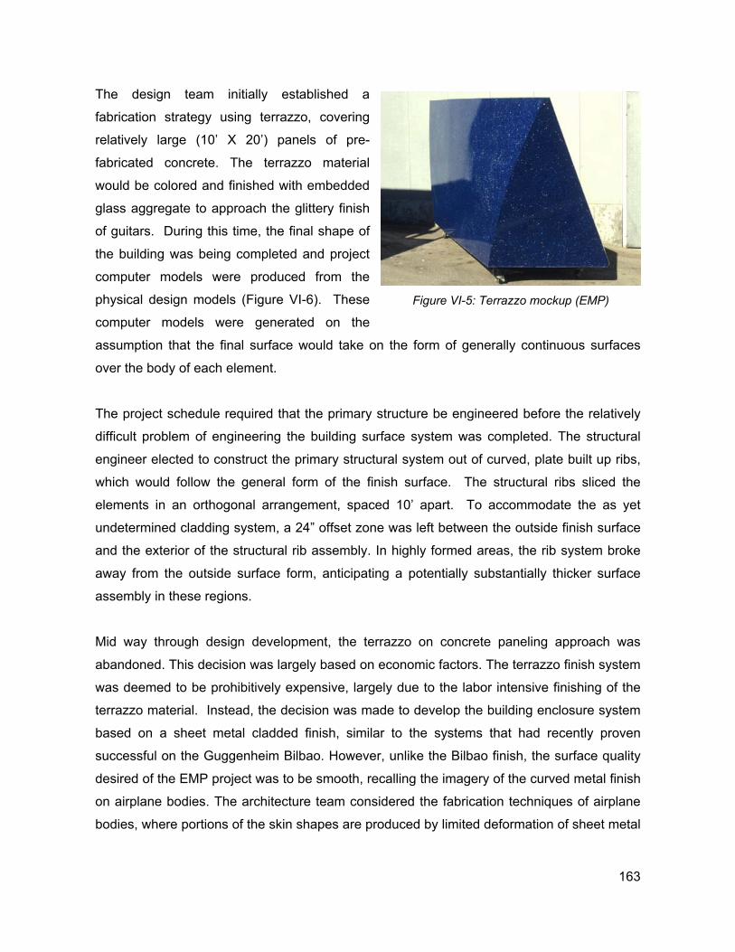
The design team initially established a

fabrication strategy using terrazzo, covering

relatively large (10’ X 20’) panels of pre-

fabricated concrete. The terrazzo material

would be colored and finished with embedded

glass aggregate to approach the glittery finish

of guitars. During this time, the final shape of

the building was being completed and project

computer models were produced from the

physical design models (Figure VI-6). These

computer models were generated on the

assumption that the final surface would take on the form of generally continuous surfaces

over the body of each element.

Figure VI-5: Terrazzo mockup (EMP)

The project schedule required that the primary structure be engineered before the relatively

difficult problem of engineering the building surface system was completed. The structural

engineer elected to construct the primary structural system out of curved, plate built up ribs,

which would follow the general form of the finish surface. The structural ribs sliced the

elements in an orthogonal arrangement, spaced 10’ apart. To accommodate the as yet

undetermined cladding system, a 24” offset zone was left between the outside finish surface

and the exterior of the structural rib assembly. In highly formed areas, the rib system broke

away from the outside surface form, anticipating a potentially substantially thicker surface

assembly in these regions.

Mid way through design development, the terrazzo on concrete paneling approach was

abandoned. This decision was largely based on economic factors. The terrazzo finish system

was deemed to be prohibitively expensive, largely due to the labor intensive finishing of the

terrazzo material. Instead, the decision was made to develop the building enclosure system

based on a sheet metal cladded finish, similar to the systems that had recently proven

successful on the Guggenheim Bilbao. However, unlike the Bilbao finish, the surface quality

desired of the EMP project was to be smooth, recalling the imagery of the curved metal finish

on airplane bodies. The architecture team considered the fabrication techniques of airplane

bodies, where portions of the skin shapes are produced by limited deformation of sheet metal

163

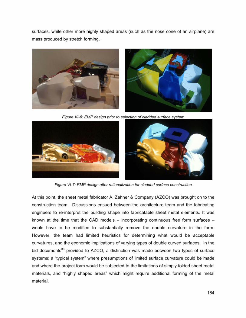
surfaces, while other more highly shaped areas (such as the nose cone of an airplane) are

mass produced by stretch forming.

Figure VI-6: EMP design prior to selection of cladded surface system

Figure VI-7: EMP design after rationalization for cladded surface construction

At this point, the sheet metal fabricator A. Zahner & Company (AZCO) was brought on to the

construction team. Discussions ensued between the architecture team and the fabricating

engineers to re-interpret the building shape into fabricatable sheet metal elements. It was

known at the time that the CAD models – incorporating continuous free form surfaces –

would have to be modified to substantially remove the double curvature in the form.

However, the team had limited heuristics for determining what would be acceptable

curvatures, and the economic implications of varying types of double curved surfaces. In the

bid documents33 provided to AZCO, a distinction was made between two types of surface

systems: a “typical system” where presumptions of limited surface curvature could be made

and where the project form would be subjected to the limitations of simply folded sheet metal

materials, and “highly shaped areas” which might require additional forming of the metal

material.

164

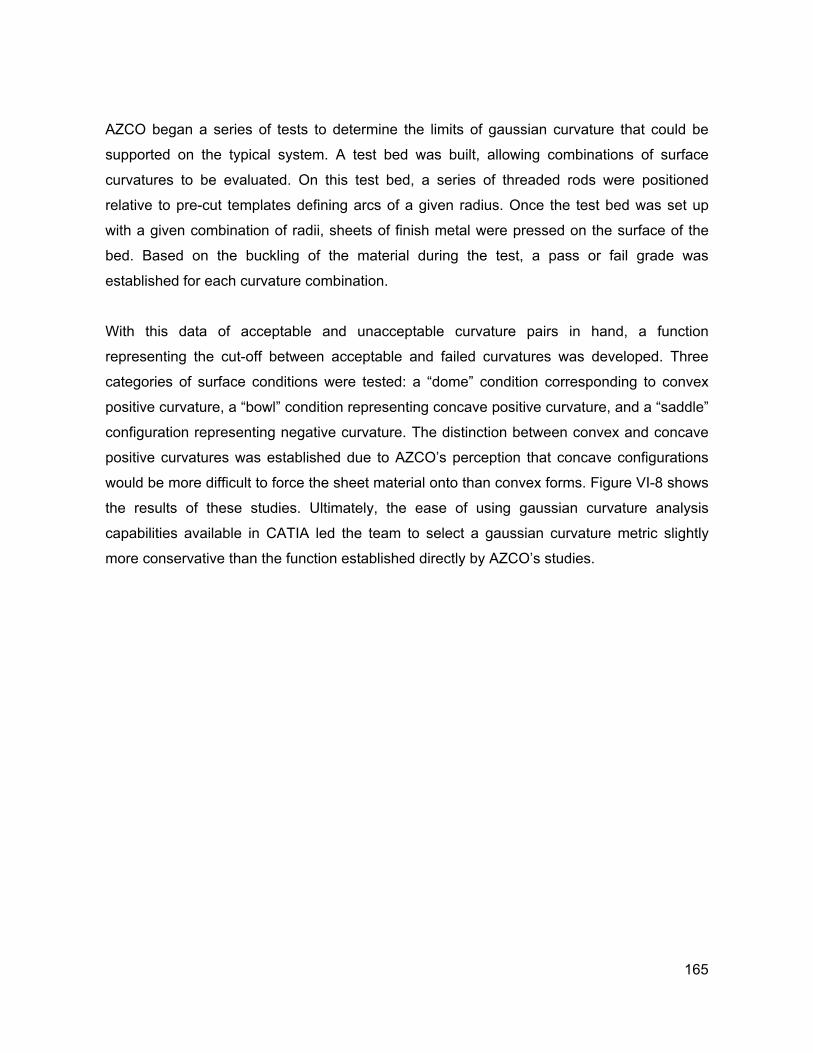
AZCO began a series of tests to determine the limits of gaussian curvature that could be

supported on the typical system. A test bed was built, allowing combinations of surface

curvatures to be evaluated. On this test bed, a series of threaded rods were positioned

relative to pre-cut templates defining arcs of a given radius. Once the test bed was set up

with a given combination of radii, sheets of finish metal were pressed on the surface of the

bed. Based on the buckling of the material during the test, a pass or fail grade was

established for each curvature combination.

With this data of acceptable and unacceptable curvature pairs in hand, a function

representing the cut-off between acceptable and failed curvatures was developed. Three

categories of surface conditions were tested: a “dome” condition corresponding to convex

positive curvature, a “bowl” condition representing concave positive curvature, and a “saddle”

configuration representing negative curvature. The distinction between convex and concave

positive curvatures was established due to AZCO’s perception that concave configurations

would be more difficult to force the sheet material onto than convex forms. Figure VI-8 shows

the results of these studies. Ultimately, the ease of using gaussian curvature analysis

capabilities available in CATIA led the team to select a gaussian curvature metric slightly

more conservative than the function established directly by AZCO’s studies.

165

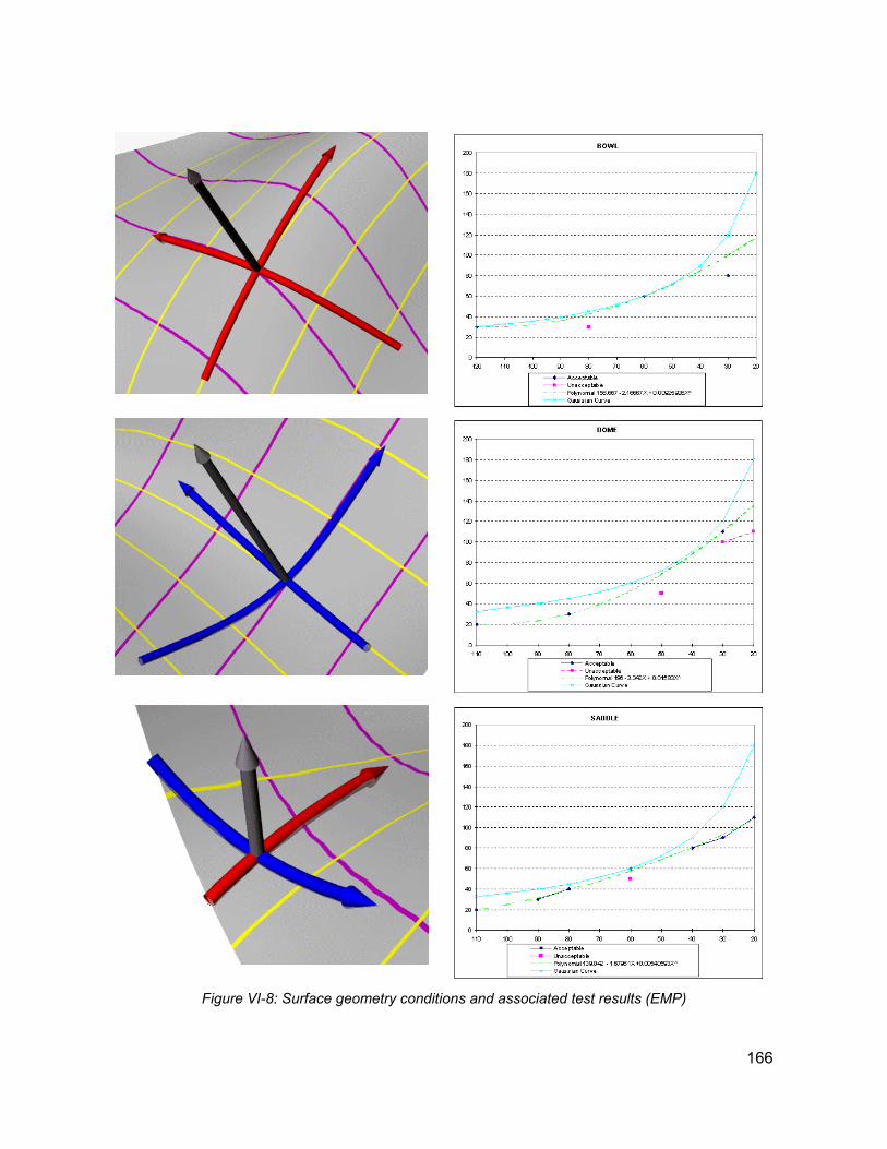
Figure VI-8: Surface geometry conditions and associated test results (EMP)

166

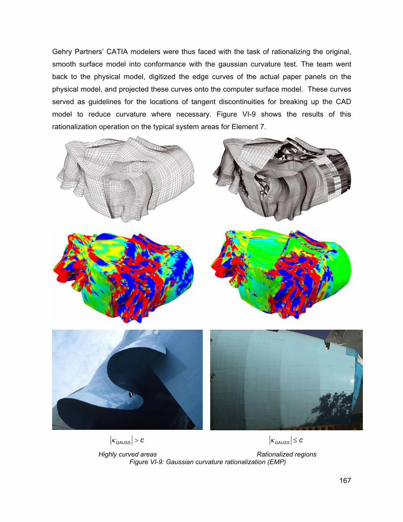
Gehry Partners’ CATIA modelers were thus faced with the task of rationalizing the original,

smooth surface model into conformance with the gaussian curvature test. The team went

back to the physical model, digitized the edge curves of the actual paper panels on the

physical model, and projected these curves onto the computer surface model. These curves

served as guidelines for the locations of tangent discontinuities for breaking up the CAD

model to reduce curvature where necessary. Figure VI-9 shows the results of this

rationalization operation on the typical system areas for Element 7.

GAUSS cκ > GAUSS cκ ≤

Highly curved areas Rationalized regions Figure VI-9: Gaussian curvature rationalization (EMP)

167

3. Summary By in large, the gaussian curvature metric established for the project has served its intended

function. The typical system areas required no additional forming of the finish materials, and

generally the fabrication assumptions in the design of the panel system posed few

unanticipated complications. However, a few unanticipated problems were encountered on

relatively high curvature areas when pre-punched holes did not line up correctly on

neighboring face sheets. Fabrication strategies where sheet materials form the waterproofing

membrane must obviously require a heightened level of attention to poor inter-sheet

continuity.

There are some important characteristics

inherent to any fabrication strategy adopted on

constrained curvature forms. These surfaces

are by nature bi-directionally curved, even if

this curvature is limited. Thus, framing

strategies for supporting the surfacing

materials must be curved in at least one

direction. On several projects including EMP,

panel assemblies have provided the sub-

framing technology (Figure VI-10). On EMP,

these panels were developed from planar

sheet materials. The top edge of each framing

member or “fin” is CNC cut to reflect the

curvature of the surface along its profile. Thus,

the panel itself provides the dimensional control of the surface, on the basis of surface

dimensional data provided by the digital master model. Additional discussion of the

development of the panel system and layout are presented in Part 3, below.

Figure VI-10: AZCO’s panel system

The constrained gaussian curvature approach employs surface curvature metrics inherent to

differential surface representations as a predictor of surface constructibility. The surface

elements are represented by the software as Bézier and NURBS surfaces, discussed in

Section V.D.3 above. Many available NURBS modeling packages provide utilities for

visualizing and analyzing gaussian curvature on surfaces. During rationalizing activities, CAD

168

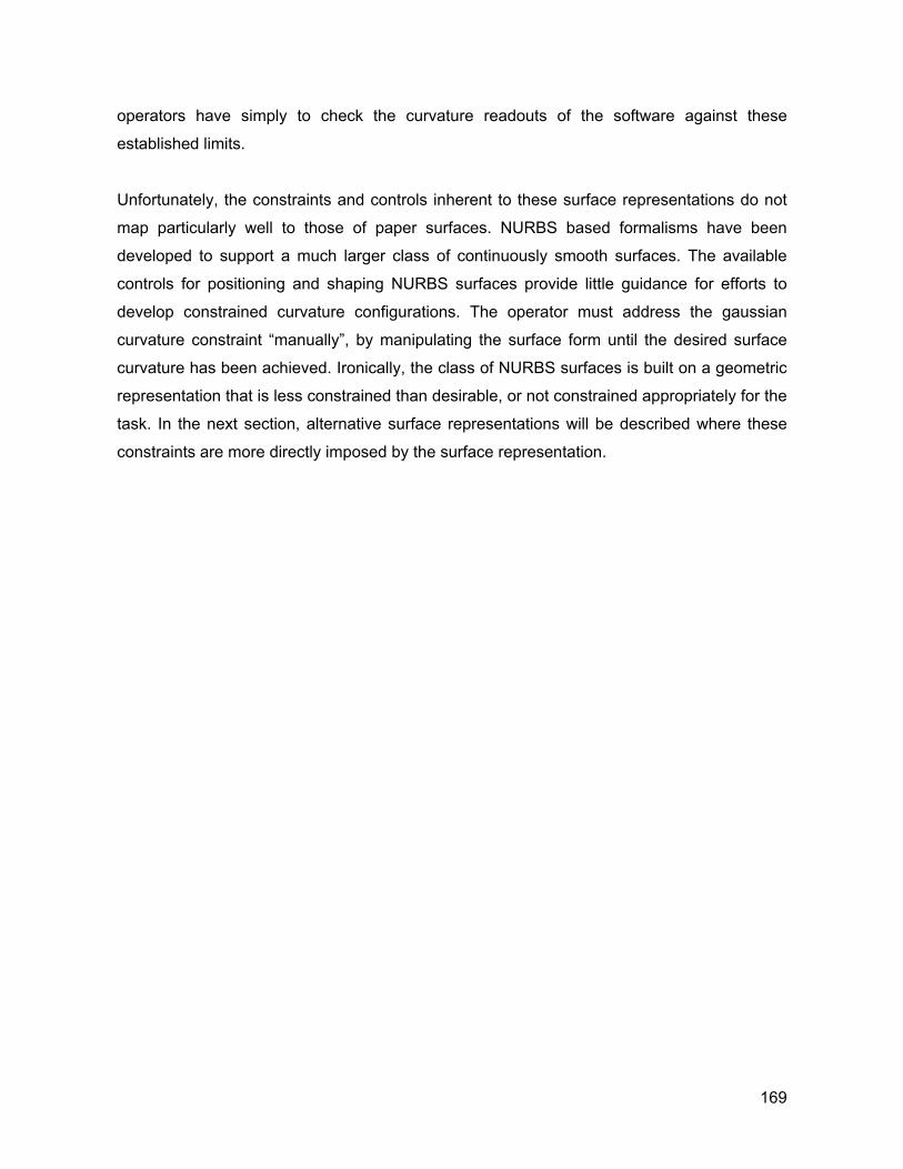
operators have simply to check the curvature readouts of the software against these

established limits.

Unfortunately, the constraints and controls inherent to these surface representations do not

map particularly well to those of paper surfaces. NURBS based formalisms have been

developed to support a much larger class of continuously smooth surfaces. The available

controls for positioning and shaping NURBS surfaces provide little guidance for efforts to

develop constrained curvature configurations. The operator must address the gaussian

curvature constraint “manually”, by manipulating the surface form until the desired surface

curvature has been achieved. Ironically, the class of NURBS surfaces is built on a geometric

representation that is less constrained than desirable, or not constrained appropriately for the

task. In the next section, alternative surface representations will be described where these

constraints are more directly imposed by the surface representation.

169

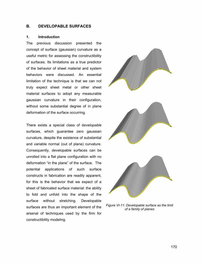
B. DEVELOPABLE SURFACES

1. Introduction The previous discussion presented the

concept of surface (gaussian) curvature as a

useful metric for assessing the constructibility

of surfaces. Its limitations as a true predictor

of the behavior of sheet material and system

behaviors were discussed. An essential

limitation of the technique is that we can not

truly expect sheet metal or other sheet

material surfaces to adopt any measurable

gaussian curvature in their configuration,

without some substantial degree of in plane

deformation of the surface occurring.

There exists a special class of developable

surfaces, which guarantee zero gaussian

curvature, despite the existence of substantial

and variable normal (out of plane) curvature.

Consequently, developable surfaces can be

unrolled into a flat plane configuration with no

deformation “in the plane” of the surface. The

potential applications of such surface

constructs in fabrication are readily apparent,

for this is the behavior that we expect of a

sheet of fabricated surface material: the ability

to fold and unfold into the shape of the

surface without stretching. Developable

surfaces are thus an important element of the

arsenal of techniques used by the firm for

constructibility modeling.

Figure VI-11: Developable surface as the limit of a family of planes

170

Developable surfaces map isometrically and conformally22 to a planar surface, in that arc

lengths of curves and angles between curves on the developable surface and its unfolded

configuration are equal. The notion of a plane, continually folded in space up to the

configuration of a developable surface should be kept firmly in mind, for the definition of

developable surfaces will indeed result in configuration of planes “rolled” into space.

One important consequence of this rolled

plane configuration is the existence of

straight lines of ruling on the surface,

where the surface normals at any two

points on a given line of ruling are

parallel. Spatially, we can envision these

lines of ruling as infinitesimally spaced

hinges along which the surface can

unfold without otherwise changing in

shape (Figure VI-11). This existence of a

straight line of ruling with invariant

surface normal is the basis for a

differential definition of developable surfaces, below. The following represent equivalent

definitions of conditions on developable surfaces:

Figure VI-12: Parallel normal vectors on a developable

surface

• The mapping of a developable surface onto a plane is isometric and conformal

• A surface whose gaussian curvature is zero

• A straight line of ruling exists on each point of the surface; a principal direction with 0

curvature is aligned with this line of ruling.

• The surface normals along a line of ruling are parallel.

In previous sections, the focus of discussion was the establishment of localized differential

properties of surfaces as a specific point of consideration. In moving forward with a

presentation of the definition of developable surfaces, we will again begin by considering the

localized conditions of developable surfaces at a point. However, in addition, this localized

consideration will be extended to the properties of surfaces “in large”, and the means by

which developable properties of surfaces can be guaranteed over the extent of the surface.

171

The definition of gaussian curvature, established in (V.53), was:

max minGAUSS N Nκ κ κ=

In order for κGAUSS to be equal to zero, necessarily at least one of the principal curvatures

must be of 0 magnitude. The geometric interpretation of a curve with 0 curvature is of course

a straight line. However, the existence of a localized straight line condition at points on the

surface will not be a sufficient condition to guarantee developability. The previous discussion

of surface curvature disclosed that a local straight line on the surface existed at every point

of negative curvature. We consider initially the class of surface forms generated as a family

of straight line isoparametric curves in one of their directions, and then subsequently

consider the conditions required to guarantee that a principal direction “lines up” with this

isoparametric curve on the surface at large. Elements of this general formulation are drawn

from Kreysig47 and Chalfant19.

2. Ruled Surfaces We begin by defining the class of surfaces generated by a straight line in one of its

parametric directions. The class of ruled surfaces is defined as a surface with at least a one

parameter family of straight lines as the isoparametric curves that generate the surface. We

might initially revisit our discussion of parametric surfaces to consider where this requirement

will be defined. The Euclidean nature of the R2 parametric (u,v) space is unaltered by this

requirement. The impact of this condition is felt in the qualities of the resulting, embedded

surface in R3. However, the locus of this constraint is in the embedding R2 → R3 function

itself. Our definition of ruled surface must thus define constraints on the mapping function

that results in this straight line condition observable on the embedded surface in R3.

By convention, for the purposes of consistency in this discussion, we will consider the

parameter v to be the parameter that traces a line in R3 as its value is traversed.

Geometrically, we may envision a ruled surface as the surface described by the path of a

straight line as it is travels through space. The resulting straight lines embedded in space are

termed the generatrices of the ruled surface. In turn, the path taken by the line as it travels

through space may be envisioned as a curve in space, termed the directrix of the surface48.

172

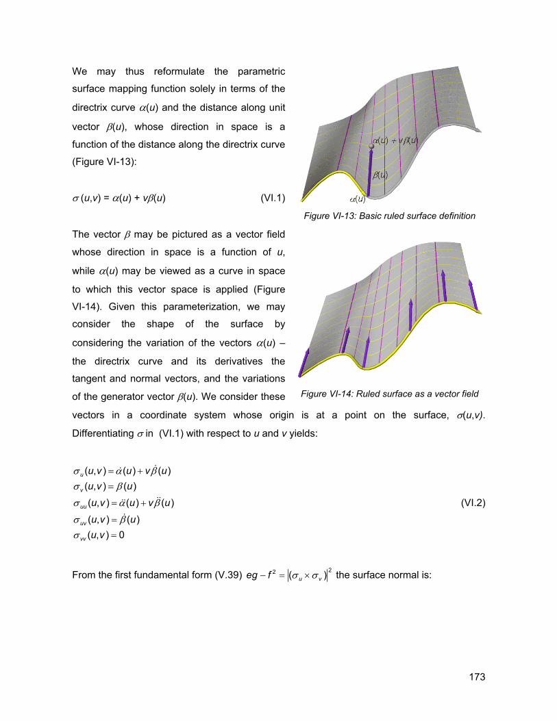
We may thus reformulate the parametric

surface mapping function solely in terms of the

directrix curve α(u) and the distance along unit

vector β(u), whose direction in space is a

function of the distance along the directrix curve

(Figure VI-13):

σ (u,v) = α(u) + vβ(u) (VI.1)

The vector β may be pictured as a vector field

whose direction in space is a function of u,

while α(u) may be viewed as a curve in space

to which this vector space is applied (Figure

VI-14). Given this parameterization, we may

consider the shape of the surface by

considering the variation of the vectors α(u) –

the directrix curve and its derivatives the

tangent and normal vectors, and the variations

of the generator vector β(u). We consider these

vectors in a coordinate system whose origin is at a point on the surface, σ(u,v).

Differentiating σ in (VI.1) with respect to u and v yields:

Figure VI-13: Basic ruled surface definition

Figure VI-14: Ruled surface as a vector field

( , ) ( ) ( )( , ) ( )( , ) ( ) ( )( , ) ( )( , ) 0

u

v

uu

uv

vv

u v u v uu v uu v u v uu v uu v

σ α βσ β

σ α

σ βσ

= +

=

= +

=

=

&&

&&&&

&

β (VI.2)

From the first fundamental form (V.39) 22 ( u veg f σ σ− = × ) the surface normal is:

173

( )

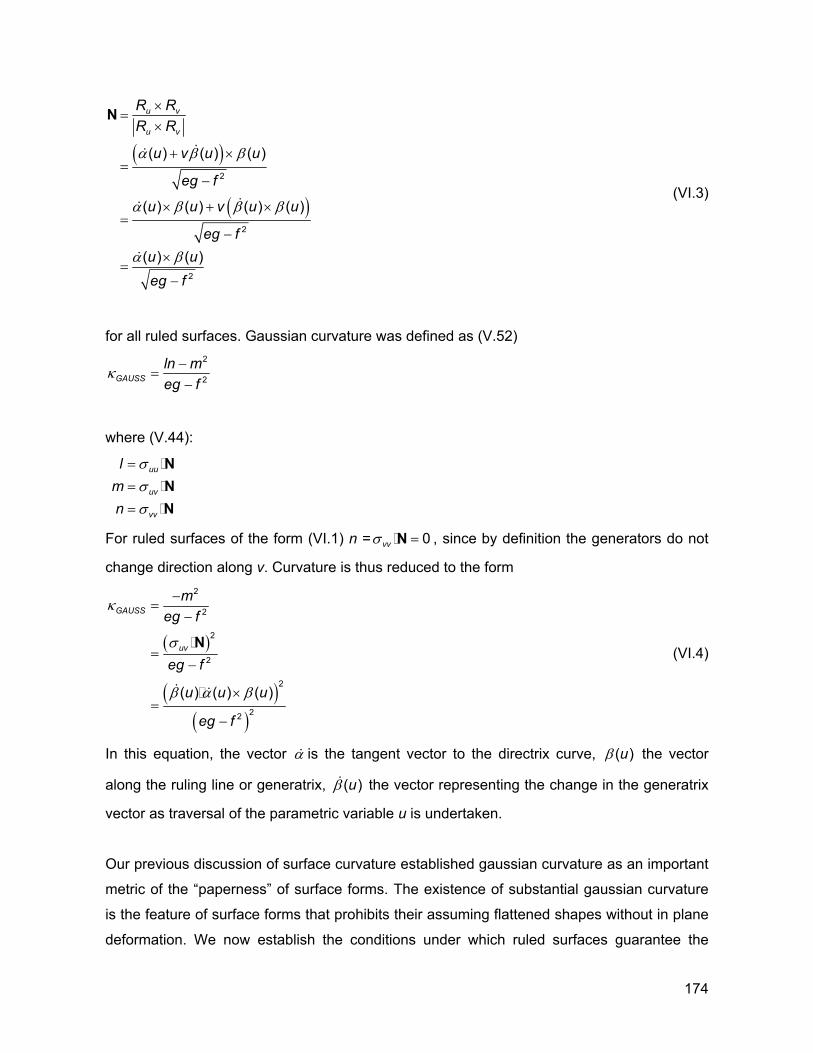
( )2

2

2

( ) ( ) ( )

( ) ( ) ( ) ( )

( ) ( )

u v

u v

R RR R

u v u u

eg f

u u v u u

eg fu ueg f

α β β

α β β β

α β

×=

×

+ ×=

−

× + ×=

−

×=

−

N

&&

&&

&

(VI.3)

for all ruled surfaces. Gaussian curvature was defined as (V.52) 2

2GAUSSln meg f

κ −=

−

where (V.44):

m uu

uv

vv

l

n

σσσ

=

=

=

NNN

For ruled surfaces of the form (VI.1) n = 0vvσ =N , since by definition the generators do not

change direction along v. Curvature is thus reduced to the form

( )

( )( )

2

2

2

2

2

22

( ) ( ) ( )

GAUSS

uv

meg f

eg f

u u u

eg f

κ

σ

β α β

−=

−

=−

×=

−

N

& &

(VI.4)

In this equation, the vector α& is the tangent vector to the directrix curve, β ( )u the vector

along the ruling line or generatrix, the vector representing the change in the generatrix

vector as traversal of the parametric variable u is undertaken.

β&( )u

Our previous discussion of surface curvature established gaussian curvature as an important

metric of the “paperness” of surface forms. The existence of substantial gaussian curvature

is the feature of surface forms that prohibits their assuming flattened shapes without in plane

deformation. We now establish the conditions under which ruled surfaces guarantee the

174

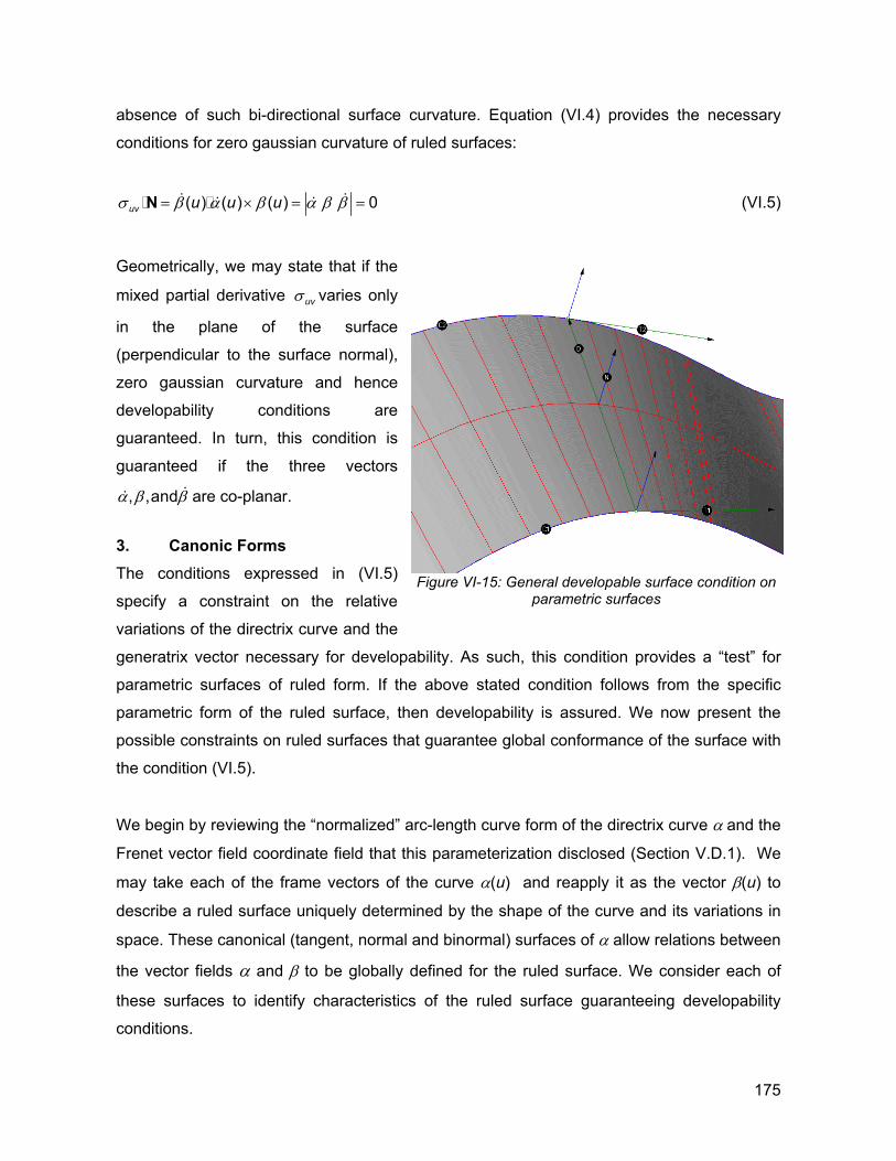
absence of such bi-directional surface curvature. Equation (VI.4) provides the necessary

conditions for zero gaussian curvature of ruled surfaces:

( ) ( ) ( ) 0uv u u uσ β α β α β β= × =N & & & =& (VI.5)

Geometrically, we may state that if the

mixed partial derivative uvσ varies only

in the plane of the surface

(perpendicular to the surface normal),

zero gaussian curvature and hence

developability conditions are

guaranteed. In turn, this condition is

guaranteed if the three vectors

, ,andα β && β are co-planar.

3. Canonic Forms The conditions expressed in (VI.5)

specify a constraint on the relative

variations of the directrix curve and the

generatrix vector necessary for developability. As such, this condition provides a “test” for

parametric surfaces of ruled form. If the above stated condition follows from the specific

parametric form of the ruled surface, then developability is assured. We now present the

possible constraints on ruled surfaces that guarantee global conformance of the surface with

the condition (VI.5).

Figure VI-15: General developable surface condition on

parametric surfaces

We begin by reviewing the “normalized” arc-length curve form of the directrix curve α and the

Frenet vector field coordinate field that this parameterization disclosed (Section V.D.1). We

may take each of the frame vectors of the curve α(u) and reapply it as the vector β(u) to

describe a ruled surface uniquely determined by the shape of the curve and its variations in

space. These canonical (tangent, normal and binormal) surfaces of α allow relations between

the vector fields α and β to be globally defined for the ruled surface. We consider each of

these surfaces to identify characteristics of the ruled surface guaranteeing developability

conditions.

175

A. Space curve B. Tangent surface

C. Normal surface D. Binormal surface

Figure VI-16: Space curve and Frenet field surfaces

In the case of the tangent surface (Figure VI-16B), the generatrix vector β is the tangent t of

the curve α, hence β = α& . The determinant of the matrix α β β α α β=&& & && is necessarily 0,

since two of the columns are equal. Thus the tangent surface of any space curve is a

developable surface. Tangent developable surfaces are an important class of developable

surfaces for potential consideration in developable surface applications. These surfaces will

be considered further below.

Next we apply the principal normal vector, and consider the conditions on the space curve

required to guarantee developability of the resulting ruled surface (Figure VI-16C). From

(VI.5) and (V.26):

( )α β β α α κ τ α τ= = − + =n n n t b n b& && & & & (VI.6)

176

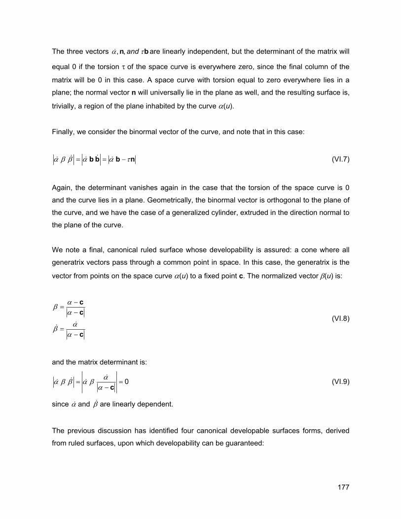
The three vectors , , andα τn& b are linearly independent, but the determinant of the matrix will

equal 0 if the torsion τ of the space curve is everywhere zero, since the final column of the

matrix will be 0 in this case. A space curve with torsion equal to zero everywhere lies in a

plane; the normal vector n will universally lie in the plane as well, and the resulting surface is,

trivially, a region of the plane inhabited by the curve α(u).

Finally, we consider the binormal vector of the curve, and note that in this case:

α β β α α τ= = −b b b n&&& & & (VI.7)

Again, the determinant vanishes again in the case that the torsion of the space curve is 0

and the curve lies in a plane. Geometrically, the binormal vector is orthogonal to the plane of

the curve, and we have the case of a generalized cylinder, extruded in the direction normal to

the plane of the curve.

We note a final, canonical ruled surface whose developability is assured: a cone where all

generatrix vectors pass through a common point in space. In this case, the generatrix is the

vector from points on the space curve α(u) to a fixed point c. The normalized vector β(u) is:

αβα

αβα

−=

−

=−&&

cc

c

(VI.8)

and the matrix determinant is:

αα β β α βα

=−&&& & 0

c= (VI.9)

since α& and β& are linearly dependent.

The previous discussion has identified four canonical developable surfaces forms, derived

from ruled surfaces, upon which developability can be guaranteed:

177

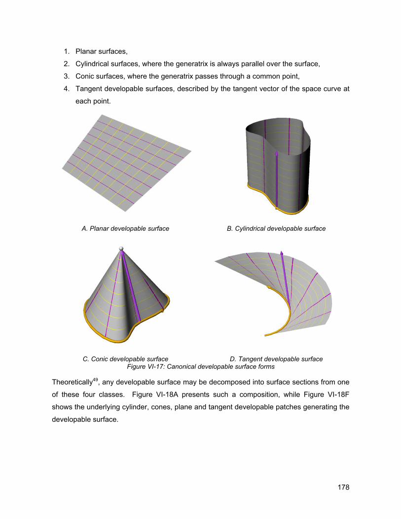
1. Planar surfaces,

2. Cylindrical surfaces, where the generatrix is always parallel over the surface,

3. Conic surfaces, where the generatrix passes through a common point,

4. Tangent developable surfaces, described by the tangent vector of the space curve at

each point.

A. Planar developable surface B. Cylindrical developable surface

C. Conic developable surface D. Tangent developable surface

Figure VI-17: Canonical developable surface forms

Theoretically49, any developable surface may be decomposed into surface sections from one

of these four classes. Figure VI-18A presents such a composition, while Figure VI-18F

shows the underlying cylinder, cones, plane and tangent developable patches generating the

developable surface.

178

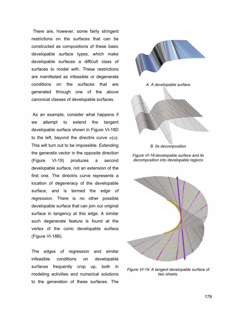
There are, however, some fairly stringent

restrictions on the surfaces that can be

constructed as compositions of these basic

developable surface types, which make

developable surfaces a difficult class of

surfaces to model with. These restrictions

are manifested as infeasible or degenerate

conditions on the surfaces that are

generated through one of the above

canonical classes of developable surfaces.

As an example, consider what happens if

we attempt to extend the tangent

developable surface shown in Figure VI-18D

to the left, beyond the directrix curve α(u).

This will turn out to be impossible. Extending

the generatix vector in the opposite direction

(Figure VI-19) produces a second

developable surface, not an extension of the

first one. The directrix curve represents a

location of degeneracy of the developable

surface, and is termed the edge of

regression. There is no other possible

developable surface that can join our original

surface in tangency at this edge. A similar

such degenerate feature is found at the

vertex of the conic developable surface

(Figure VI-18B).

The edges of regression and similar

infeasible conditions on developable

surfaces frequently crop up, both in

modeling activities and numerical solutions

to the generation of these surfaces. The

A. A developable surface

B. Its decomposition

Figure VI-18:developable surface and its decomposition into developable regions

Figure VI-19: A tangent developable surface of two sheets.

179

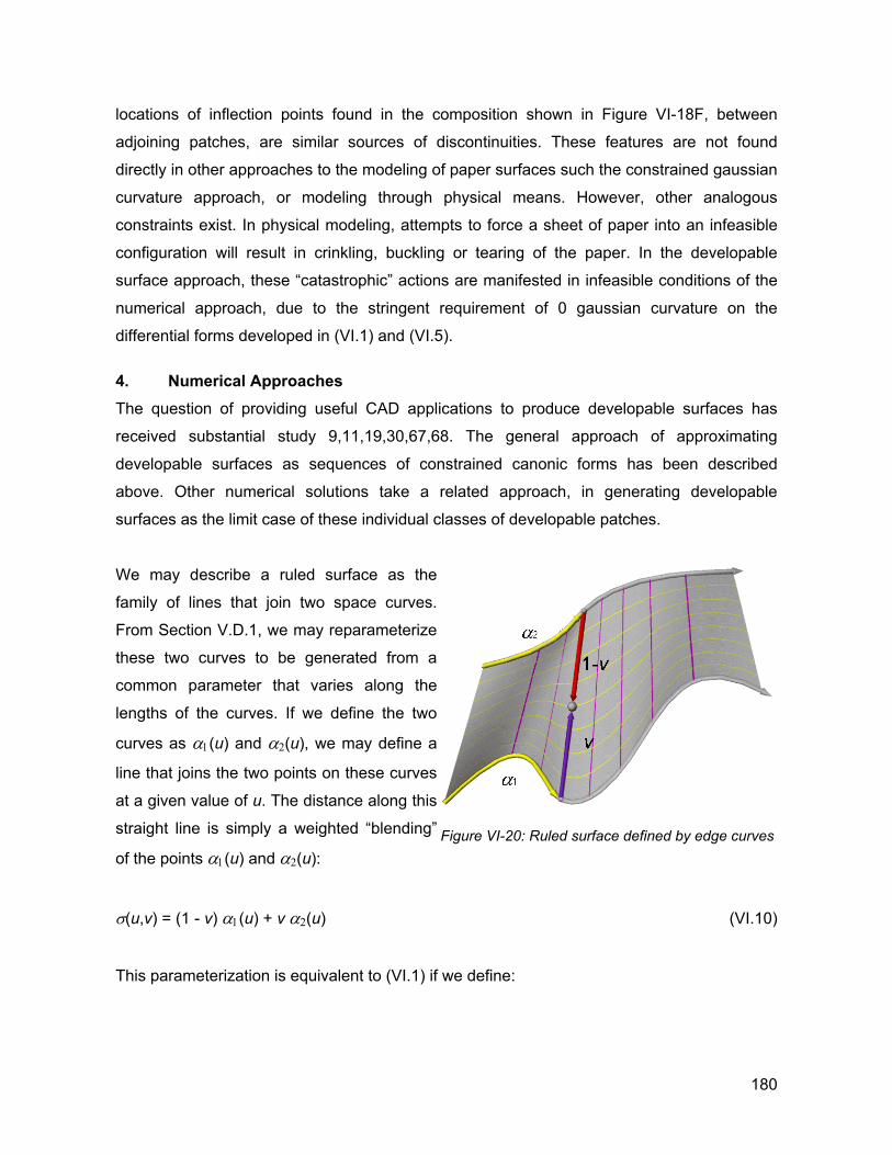
locations of inflection points found in the composition shown in Figure VI-18F, between

adjoining patches, are similar sources of discontinuities. These features are not found

directly in other approaches to the modeling of paper surfaces such the constrained gaussian

curvature approach, or modeling through physical means. However, other analogous

constraints exist. In physical modeling, attempts to force a sheet of paper into an infeasible

configuration will result in crinkling, buckling or tearing of the paper. In the developable

surface approach, these “catastrophic” actions are manifested in infeasible conditions of the

numerical approach, due to the stringent requirement of 0 gaussian curvature on the

differential forms developed in (VI.1) and (VI.5).

4. Numerical Approaches The question of providing useful CAD applications to produce developable surfaces has

received substantial study 9,11,19,30,67,68. The general approach of approximating

developable surfaces as sequences of constrained canonic forms has been described

above. Other numerical solutions take a related approach, in generating developable

surfaces as the limit case of these individual classes of developable patches.

We may describe a ruled surface as the

family of lines that join two space curves.

From Section V.D.1, we may reparameterize

these two curves to be generated from a

common parameter that varies along the

lengths of the curves. If we define the two

curves as α1(u) and α2(u), we may define a

line that joins the two points on these curves

at a given value of u. The distance along this

straight line is simply a weighted “blending”

of the points α1(u) and α2(u):

Figure VI-20: Ruled surface defined by edge curves

σ(u,v) = (1 - v) α1(u) + v α2(u) (VI.10)

This parameterization is equivalent to (VI.1) if we define:

180

( ) ( )

( ) ( ) ( )( ) ( )

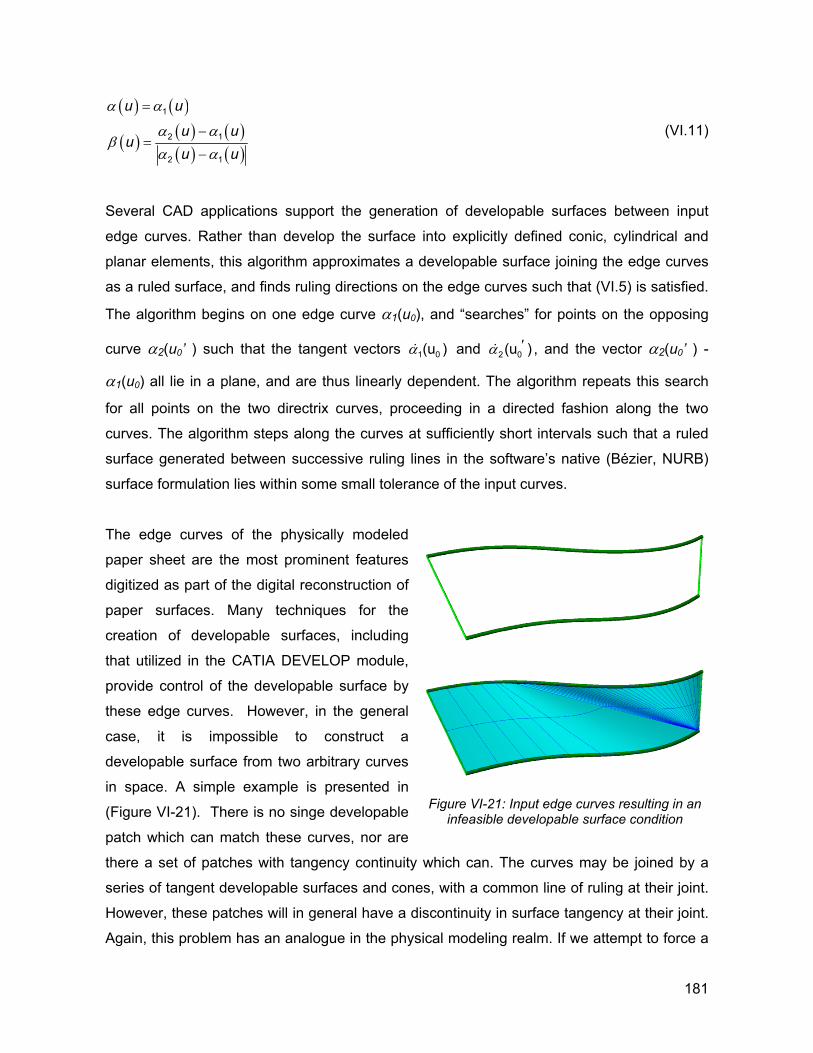
α α

α αβ

α α

=

−=

−

1

2 1

2 1

u u

u uu

u u (VI.11)

Several CAD applications support the generation of developable surfaces between input

edge curves. Rather than develop the surface into explicitly defined conic, cylindrical and

planar elements, this algorithm approximates a developable surface joining the edge curves

as a ruled surface, and finds ruling directions on the edge curves such that (VI.5) is satisfied.

The algorithm begins on one edge curve α1(u0), and “searches” for points on the opposing

curve α2(u0’ ) such that the tangent vectors α&1 0(u ) and α ′&2 0(u ) , and the vector α2(u0’ ) -

α1(u0) all lie in a plane, and are thus linearly dependent. The algorithm repeats this search

for all points on the two directrix curves, proceeding in a directed fashion along the two

curves. The algorithm steps along the curves at sufficiently short intervals such that a ruled

surface generated between successive ruling lines in the software’s native (Bézier, NURB)

surface formulation lies within some small tolerance of the input curves.

The edge curves of the physically modeled

paper sheet are the most prominent features

digitized as part of the digital reconstruction of

paper surfaces. Many techniques for the

creation of developable surfaces, including

that utilized in the CATIA DEVELOP module,

provide control of the developable surface by

these edge curves. However, in the general

case, it is impossible to construct a

developable surface from two arbitrary curves

in space. A simple example is presented in

(Figure VI-21). There is no singe developable

patch which can match these curves, nor are

there a set of patches with tangency continuity which can. The curves may be joined by a

series of tangent developable surfaces and cones, with a common line of ruling at their joint.

However, these patches will in general have a discontinuity in surface tangency at their joint.

Again, this problem has an analogue in the physical modeling realm. If we attempt to force a

Figure VI-21: Input edge curves resulting in an

infeasible developable surface condition

181

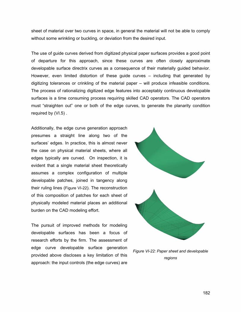
sheet of material over two curves in space, in general the material will not be able to comply

without some wrinkling or buckling, or deviation from the desired input.

The use of guide curves derived from digitized physical paper surfaces provides a good point

of departure for this approach, since these curves are often closely approximate

developable surface directrix curves as a consequence of their materially guided behavior.

However, even limited distortion of these guide curves – including that generated by

digitizing tolerances or crinkling of the material paper – will produce infeasible conditions.

The process of rationalizing digitized edge features into acceptably continuous developable

surfaces is a time consuming process requiring skilled CAD operators. The CAD operators

must “straighten out” one or both of the edge curves, to generate the planarity condition

required by (VI.5) .

Additionally, the edge curve generation approach

presumes a straight line along two of the

surfaces’ edges. In practice, this is almost never

the case on physical material sheets, where all

edges typically are curved. On inspection, it is

evident that a single material sheet theoretically

assumes a complex configuration of multiple

developable patches, joined in tangency along

their ruling lines (Figure VI-22). The reconstruction

of this composition of patches for each sheet of

physically modeled material places an additional

burden on the CAD modeling effort.

The pursuit of improved methods for modeling

developable surfaces has been a focus of

research efforts by the firm. The assessment of

edge curve developable surface generation

provided above discloses a key limitation of this

approach: the input controls (the edge curves) are

Figure VI-22: Paper sheet and developable

regions

182

ill suited to the solution, since these controls essentially guarantee infeasible conditions.

Furthermore, when infeasible conditions are encountered, there is poor feedback to guide

the operator toward improved conditions.

Often, the ruling lines on the physical surfaces are digitized in addition to the edge curves

(Figure III-11A). These ruling lines provide a good indication of the “flow” of the developable

surface, not apparent simply in the edge features. We can turn the problem around, and

consider these ruling lines to be the primary input controls to developable surface algorithms.

The formulation of developable surfaces as constraints on (1 × n ) Bézier or NURBS surfaces

has been pursued by several researchers3,19,9,11,68,67. Note that an order 1 curve in the u

direction guarantees a ruled surface. The two sets of control vertices (0,0…n-1) and (1,0…n-

1) describe the edge curves to the surface as in (VI.10) above. The problem now becomes

one of identifying the relative positions of control points in space that guarantee invariance of

surface normal along lines of ruling, and providing these constraints to the user in an intuitive

and interactive way. Lang and Röschel50 provide the key constraints on Bézier surfaces

guaranteeing developable conditions:

( ) ( ) ( ) ( )( ) [ ]det 0, , 1, , 0, , 1, 0 0,1u ux v x v x v x v v= ∀ ∈ (VI.12)

and derive a set of five equations satisfying this condition for weighted Bézier surfaces of

order (1,2):

0101

0102 0201

0202 0112 01201

0212 1202

1212

00

00

0

δδ δδ δ δδ δδ

=

+ =

+ + =

+ =

=

(VI.13)

where ijklδ is the determinate of four control vertices’ locations and weights:

0 0 1 1

0 0 1 1

0 0 1 1

0 0 1 1

1 1 1 1

det

w w w wijkl i j k l ijkl

x x x xi i k l

ijkl y y y yi j k l

z z z zi j k

B

B

δ =

=

p p p p

p p p pp p p pp p p p l

(VI.14)

183

This equation can be distilled down to two basic conditions on the weighted control points of

quadratic Bézier.

1. Successive pairs of (4) control points form a “ladder” configuration, where the four control

points describe a plane.

2. The weights of the six control points result in a proportional triple,

. Given values for the weights p p , and

predefined x,y,z locations for all vertices, we can solve for the remaining weights to

ensure developability of the surface. A quadratic equation determines the necessary

weight on the intermediate vertex p :

00 01 02 10 11 12( : : ) ( : :w w w w w w=p p p p p p ) 00 02 10, ,andw w wp

01w

( )2 0201 0202 021201 00 01

0201 0112 1202 1201 0212 0102

w w w B B BB B B B B B

=+

p p p (VI.15)

The remaining weights p can now be determined from the proportional triple,

above.

11 12,andw wp

This formulation furthermore provides a test for the feasibility of constructing a developable

surface based on the input vertices’ locations. If the quantity ( )2

01wp defined in (VI.15) is less

than zero, then the square root will not be a real number, and the vertex locations can not

produce a developable surface.

On the basis of this approach, an approach to the interactive construction of developable

surfaces has been created (Figure VI-23). In Figure VI-23A, the basic (1,2) developable

surface patch is shown. We distinguish between the two pairs of edge vertices, shown in

green, and the pair of intermediate vertices, shown in blue. Any of these vertices can be

manipulated interactively. The solver dynamically adjusts the locations of the other five

vertices to ensure a ladder configuration, and solves the quadratic equation (VI.15) to

determine the required vertex weights. More elaborate developable surface configurations

are supported as sequences of these basic developable patches. The patches are

constructed by associating the end vertex pair of an original patch with the beginning pair of

a subsequent patch (Figure VI-23B). A planarity condition is imposed on last four vertices of

the previous patch and the first four vertices of the subsequent patch, to ensure tangency at

the seam.

184

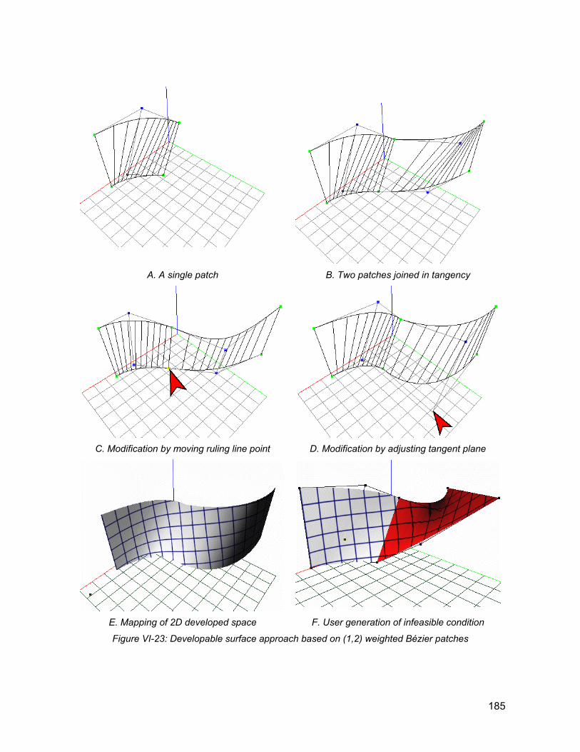
A. A single patch B. Two patches joined in tangency

C. Modification by moving ruling line point D. Modification by adjusting tangent plane

E. Mapping of 2D developed space F. User generation of infeasible condition

Figure VI-23: Developable surface approach based on (1,2) weighted Bézier patches

185

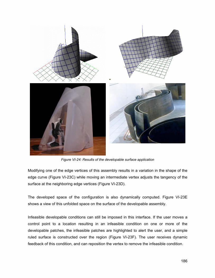
Figure VI-24: Results of the developable surface application

Modifying one of the edge vertices of this assembly results in a variation in the shape of the

edge curve (Figure VI-23C) while moving an intermediate vertex adjusts the tangency of the

surface at the neighboring edge vertices (Figure VI-23D).

The developed space of the configuration is also dynamically computed. Figure VI-23E

shows a view of this unfolded space on the surface of the developable assembly.

Infeasible developable conditions can still be imposed in this interface. If the user moves a

control point to a location resulting in an infeasible condition on one or more of the

developable patches, the infeasible patches are highlighted to alert the user, and a simple

ruled surface is constructed over the region (Figure VI-23F). The user receives dynamic

feedback of this condition, and can reposition the vertex to remove the infeasible condition.

186

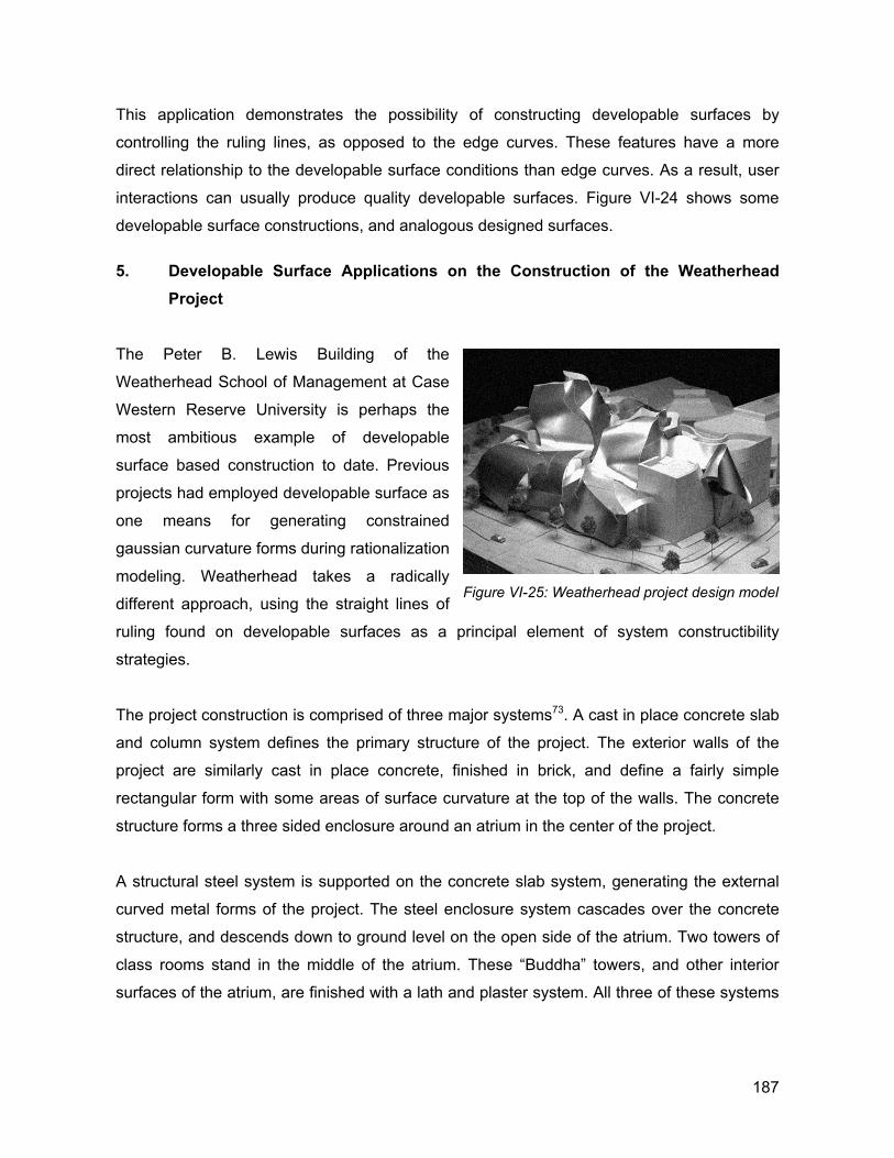
This application demonstrates the possibility of constructing developable surfaces by

controlling the ruling lines, as opposed to the edge curves. These features have a more

direct relationship to the developable surface conditions than edge curves. As a result, user

interactions can usually produce quality developable surfaces. Figure VI-24 shows some

developable surface constructions, and analogous designed surfaces.

5. Developable Surface Applications on the Construction of the Weatherhead Project

The Peter B. Lewis Building of the

Weatherhead School of Management at Case

Western Reserve University is perhaps the

most ambitious example of developable

surface based construction to date. Previous

projects had employed developable surface as

one means for generating constrained

gaussian curvature forms during rationalization

modeling. Weatherhead takes a radically

different approach, using the straight lines of

ruling found on developable surfaces as a principal element of system constructibility

strategies.

Figure VI-25: Weatherhead project design model

The project construction is comprised of three major systems73. A cast in place concrete slab

and column system defines the primary structure of the project. The exterior walls of the

project are similarly cast in place concrete, finished in brick, and define a fairly simple

rectangular form with some areas of surface curvature at the top of the walls. The concrete

structure forms a three sided enclosure around an atrium in the center of the project.

A structural steel system is supported on the concrete slab system, generating the external

curved metal forms of the project. The steel enclosure system cascades over the concrete

structure, and descends down to ground level on the open side of the atrium. Two towers of

class rooms stand in the middle of the atrium. These “Buddha” towers, and other interior

surfaces of the atrium, are finished with a lath and plaster system. All three of these systems

187

are generated from rationalized developable surface forms, and make some use of surface

lines of ruling in different ways.

Efficiencies of construction had to be found to meet the academic institutional budget of the

project. Two guiding intentions were employed in the development of project systems as a

means for reducing the project cost while still achieving the ambitions for the project form.

One innovative cost saving measure was to remove a secondary system strategy that had

been prevalently used on many prior projects. On projects including the Guggenheim Bilbao

and the Experience Music Project, the primary steel system only approximated the design

surface (Section III.F). The actual dimensional control system for these projects was

achieved through an additional system between the primary structure and the finish surface

enclosure. On the Guggenheim project, the dimensional control system is developed through

a series of template curved tubes that are attached to the primary system. On the EMP

project the finish form is achieved by a shaped panel system, attached to the primary

structural steel rib system by adjustable connections.

The Weatherhead cladding system removes the need for a secondary steel system, drawing

on the primary structural steel directly as both the support and dimensional control system for

the surface cladding. This strategy reduced the material and labor costs associated with an

additional system, but placed additional requirements on the tolerances and positioning of

the primary structural system.

With this strategy for the structure and dimensional definition of the surface system, a second

efficiency was enabled. The developable characteristics of the surface guaranteed that

straight geometry occurred in at least one direction on the curved surface. This vast

simplification of the form’s construction allowed the final surface system to be constructed in

the field, through low tech, manual construction methods performed directly on the building

surface. To enable these efficiencies, strictly developable surfaces would be required for all

project forms. The design surface model was rationalized in light of this requirement.

Rationalization of the project into purely developable forms proved to be an enormous

challenge. The strict limitations on surface forms imposed by developable surface

188

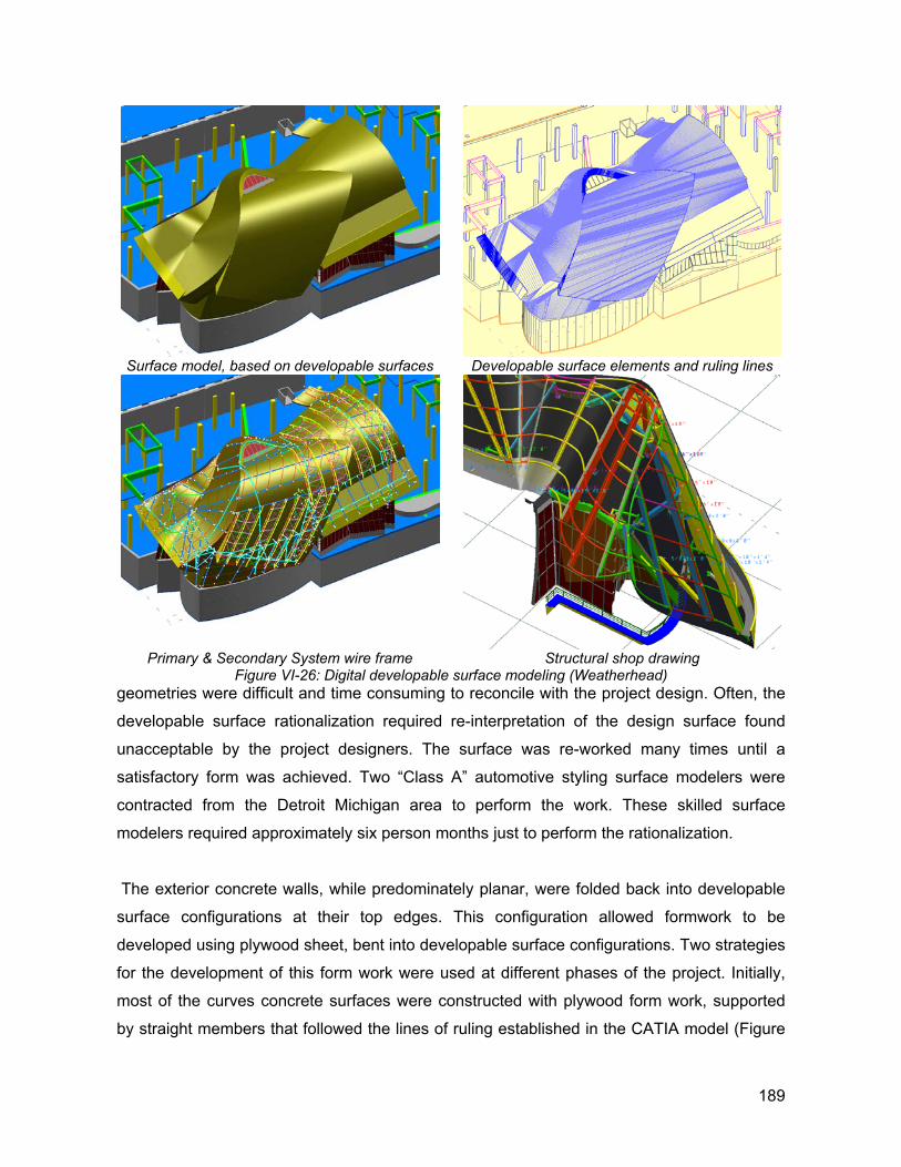
geometries were difficult and time consuming to reconcile with the project design. Often, the

developable surface rationalization required re-interpretation of the design surface found

unacceptable by the project designers. The surface was re-worked many times until a

satisfactory form was achieved. Two “Class A” automotive styling surface modelers were

contracted from the Detroit Michigan area to perform the work. These skilled surface

modelers required approximately six person months just to perform the rationalization.

Surface model, based on developable surfaces Developable surface elements and ruling lines

Primary & Secondary System wire frame Structural shop drawing Figure VI-26: Digital developable surface modeling (Weatherhead)

The exterior concrete walls, while predominately planar, were folded back into developable

surface configurations at their top edges. This configuration allowed formwork to be

developed using plywood sheet, bent into developable surface configurations. Two strategies

for the development of this form work were used at different phases of the project. Initially,

most of the curves concrete surfaces were constructed with plywood form work, supported

by straight members that followed the lines of ruling established in the CATIA model (Figure

189

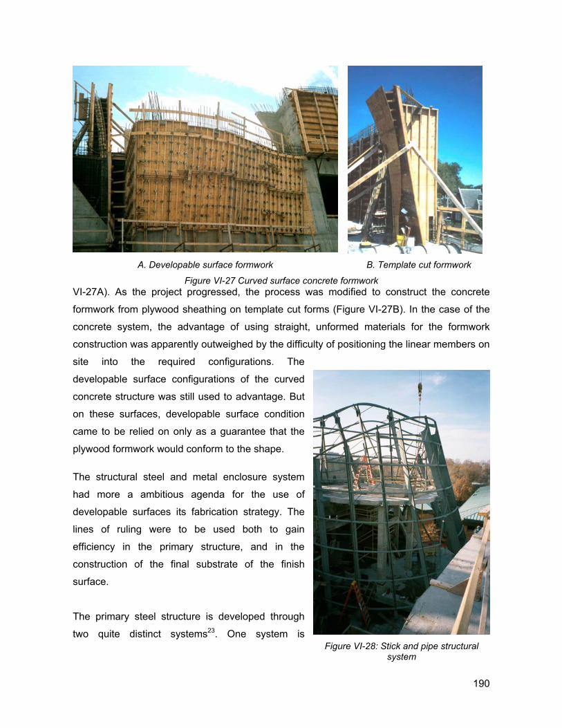
VI-27A). As the project progressed, the process was modified to construct the concrete

formwork from plywood sheathing on template cut forms (Figure VI-27B). In the case of the

concrete system, the advantage of using straight, unformed materials for the formwork

construction was apparently outweighed by the difficulty of positioning the linear members on

site into the required configurations. The

developable surface configurations of the curved

concrete structure was still used to advantage. But

on these surfaces, developable surface condition

came to be relied on only as a guarantee that the

plywood formwork would conform to the shape.

A. Developable surface formwork B. Template cut formwork

Figure VI-27 Curved surface concrete formwork

The structural steel and metal enclosure system

had more a ambitious agenda for the use of

developable surfaces its fabrication strategy. The

lines of ruling were to be used both to gain

efficiency in the primary structure, and in the

construction of the final substrate of the finish

surface.

The primary steel structure is developed through

two quite distinct systems23. One system is Figure VI-28: Stick and pipe structural

system

190

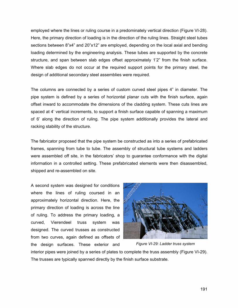
employed where the lines or ruling course in a predominately vertical direction (Figure VI-28).

Here, the primary direction of loading is in the direction of the ruling lines. Straight steel tubes

sections between 8”x4” and 20”x12” are employed, depending on the local axial and bending

loading determined by the engineering analysis. These tubes are supported by the concrete

structure, and span between slab edges offset approximately 1’2” from the finish surface.

Where slab edges do not occur at the required support points for the primary steel, the

design of additional secondary steel assemblies were required.

The columns are connected by a series of custom curved steel pipes 4” in diameter. The

pipe system is defined by a series of horizontal planar cuts with the finish surface, again

offset inward to accommodate the dimensions of the cladding system. These cuts lines are

spaced at 4’ vertical increments, to support a finish surface capable of spanning a maximum

of 6’ along the direction of ruling. The pipe system additionally provides the lateral and

racking stability of the structure.

The fabricator proposed that the pipe system be constructed as into a series of prefabricated

frames, spanning from tube to tube. The assembly of structural tube systems and ladders

were assembled off site, in the fabricators’ shop to guarantee conformance with the digital

information in a controlled setting. These prefabricated elements were then disassembled,

shipped and re-assembled on site.

A second system was designed for conditions

where the lines of ruling coursed in an

approximately horizontal direction. Here, the

primary direction of loading is across the line

of ruling. To address the primary loading, a

curved, Vierendeel truss system was

designed. The curved trusses as constructed

from two curves, again defined as offsets of

the design surfaces. These exterior and

interior pipes were joined by a series of plates to complete the truss assembly (Figure VI-29).

The trusses are typically spanned directly by the finish surface substrate.

Figure VI-29: Ladder truss system

191

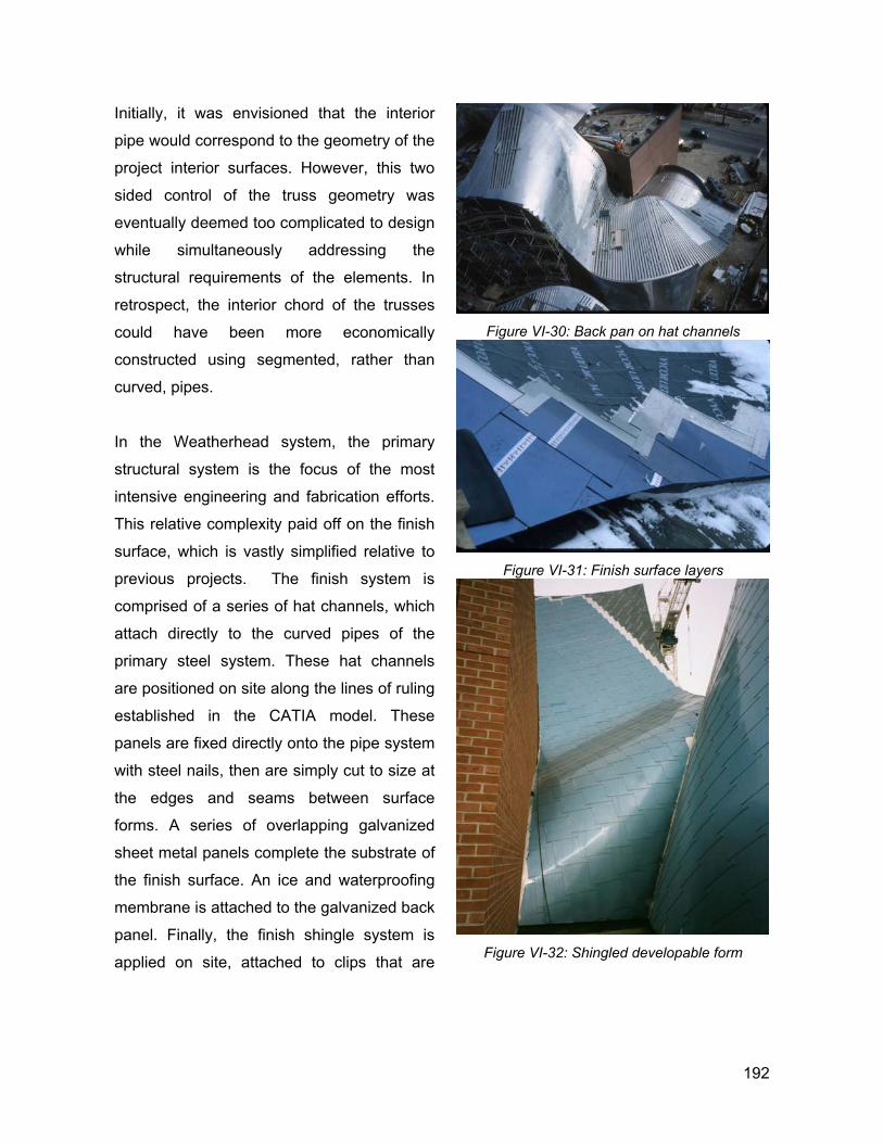
Initially, it was envisioned that the interior

pipe would correspond to the geometry of the

project interior surfaces. However, this two

sided control of the truss geometry was

eventually deemed too complicated to design

while simultaneously addressing the

structural requirements of the elements. In

retrospect, the interior chord of the trusses

could have been more economically

constructed using segmented, rather than

curved, pipes.

Figure VI-30: Back pan on hat channels

Figure VI-31: Finish surface layers

Figure VI-32: Shingled developable form

In the Weatherhead system, the primary

structural system is the focus of the most

intensive engineering and fabrication efforts.

This relative complexity paid off on the finish

surface, which is vastly simplified relative to

previous projects. The finish system is

comprised of a series of hat channels, which

attach directly to the curved pipes of the

primary steel system. These hat channels

are positioned on site along the lines of ruling

established in the CATIA model. These

panels are fixed directly onto the pipe system

with steel nails, then are simply cut to size at

the edges and seams between surface

forms. A series of overlapping galvanized

sheet metal panels complete the substrate of

the finish surface. An ice and waterproofing

membrane is attached to the galvanized back

panel. Finally, the finish shingle system is

applied on site, attached to clips that are

192

screwed through the self healing waterproofing membrane. The shingles are designed with a

small metal gutter channel, to further assist in diverting water to the outside of the system.

Insulation is provided on the interior side of the hat channels.

In cases where the finish surface slopes less than 25%, the cladding system is modified

slightly to become a roofing system. Stainless steel sheet is used in place of the galvanized

back panel to avoid corrosion. The stainless steel sheets welded together to form a

continuous water barrier. The shingle clips are tack welded directly to this surface.

The question of system tolerances was a major concern during the development of these

systems. As is many times the case on Gehry’s projects, no exact precedent for any of these

systems existed on prior projects by either the firm or any of the partnering construction

organizations. The strategies of using the primary structural system as the dimensional

control, and performing the rest of the fabrication on site, presented many opportunities for

loss of dimensional control through deviation from the CATIA geometry. Additionally, the

dimensional tolerances of the finish cladding system were not fully understood at the time,

but were presumed to be quite stringent. One concern was that the attachment of the hat

channels would be compromised if successive pipes did not result in perfectly straight lines

of ruling. A second concern was that either the back panel system or the shingle system

would fail, resulting in water leakage. An additional concern was that deviation of the pipe

system from the nominal locations established in the CATIA model would read through to the

finish as the surface substrate was forced over the pipes. To address these concerns, the

specification for the pipe system required that these elements be no more than 1/16” from

the CATIA geometry at any point.

None of these failure conditions have occurred in the construction. The surface assembly

exhibited enough flexibility of all components to accommodate the construction variations

from designed conditions. In retrospect, even the driving system requirement of purely

developable surfaces has proven to be an unnecessarily stringent requirement. The

Weatherhead system could be more appropriately represented as a ruled surface, with some

as yet not established gaussian curvature limitations. This would have provided additional

flexibility of the surface form to both the project designers and the CATIA modeling team.

However, it must be recognized that the initial design development decision to rationalize the

form into purely developable surfaces has resulted in a system with virtually no problems

193

during construction. This stringent requirement on the surfaces has translated into some

space to maneuver in the field.

Experiences on the Weatherhead project show the substantial opportunities for construction

efficiencies offered by developable surfaces. The presence of lines of ruling in the geometry

of developable surfaces is a major, somewhat serendipitous benefit of this representation of

paper surfaces. Additionally, the presence of an invariant surface normal facilitates

connections to framing members without angular variation in the connection detail. The

benefit of having at least one sub-system of the cladding strategy comprised of straight stick

elements is obvious.

There is, however, one major and non-intuitive draw back to the construction of developable

surface forms. The “flow” of the ruling lines on a developable surface is highly – and non-

intuitively – governed by subtle variations the surface quality. Supporting structural systems

are compelled to follow the spatial layouts of these ruling lines. This can result in a structural

organization with many special conditions for supports and column locations. This rather

complex organization stands in contrast to the relatively simple structural organizations of

planar cut ribs in curvature constrained panel systems. While the efficiency of constructing

curved surface forms from straight linear elements presents a potential cost efficiency over

planar rib constructions, this efficiency can be offset by the lack of control in the locations of

these members.

194

C. SUMMARY OF EXISTING PAPER SURFACE REPRESENTATIONS

In the historical progression of Gehry’s body of work, it is possible to trace the progressive

development of paper surface geometries and their associated techniques of description and

modeling. This progression shows a continuing expansion of the class of admissible paper

surface forms, as improved representation and fabrication techniques permit less

constrained geometries to be feasibly supported in the building process. The planar forms of

Gehry’s early work, described in Section IV.A, represent the point of departure of this

progression.

Cylindrical and conic forms begin to appear on relatively early projects, including the Winston

Guest House, Edgemar Development, and the Chiat Day Building. These forms appear

tentatively, sparing applied in an overall composition of planar forms. Prior to the introduction

of computer modeling techniques in the firm’s process, paper surfaces take Euclidean forms,

true cones and cylinders. Their more general counterparts were formulated as developable

surfaces in Section VI.B. This constraint is imposed on these early projects by limitations of

traditional documentation. The complexity of determining geometric relationships between

more complex, non-Euclidean conic forms was simply beyond the capabilities of traditional

architectural delineation.

The exploration of a vocabulary of conic forms continues to be expanded on Gehry’s projects

until the introduction of computer modeling in 1990. The Weissman Museum (Figure VI-33)

represents the culmination of this approach. Each face of the west façade is delineated

through traditional geometric constructions. The difficulty of performing this construction

though traditional architectural delineation is clearly evident in the construction

documentation.

195

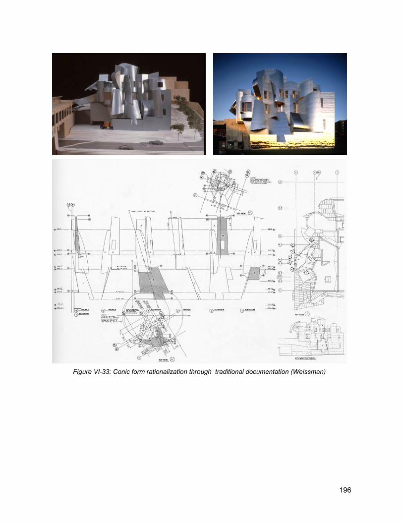
Figure VI-33: Conic form rationalization through traditional documentation (Weissman)

196

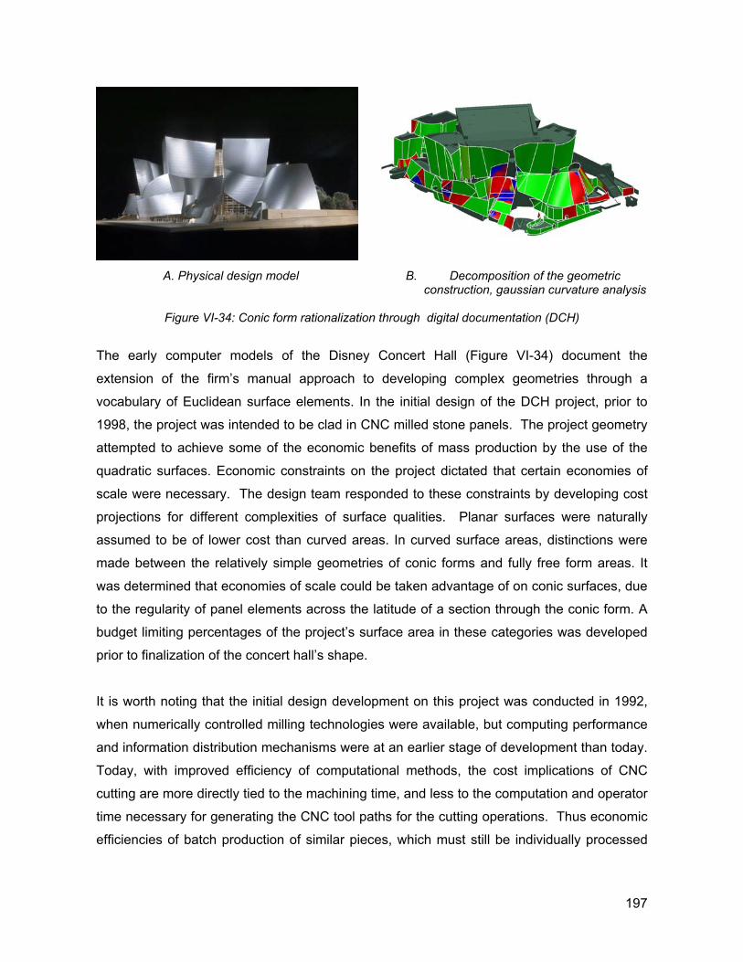
A. Physical design model B. Decomposition of the geometric construction, gaussian curvature analysis

Figure VI-34: Conic form rationalization through digital documentation (DCH)

The early computer models of the Disney Concert Hall (Figure VI-34) document the

extension of the firm’s manual approach to developing complex geometries through a

vocabulary of Euclidean surface elements. In the initial design of the DCH project, prior to

1998, the project was intended to be clad in CNC milled stone panels. The project geometry

attempted to achieve some of the economic benefits of mass production by the use of the

quadratic surfaces. Economic constraints on the project dictated that certain economies of

scale were necessary. The design team responded to these constraints by developing cost

projections for different complexities of surface qualities. Planar surfaces were naturally

assumed to be of lower cost than curved areas. In curved surface areas, distinctions were

made between the relatively simple geometries of conic forms and fully free form areas. It

was determined that economies of scale could be taken advantage of on conic surfaces, due

to the regularity of panel elements across the latitude of a section through the conic form. A

budget limiting percentages of the project’s surface area in these categories was developed

prior to finalization of the concert hall’s shape.

It is worth noting that the initial design development on this project was conducted in 1992,

when numerically controlled milling technologies were available, but computing performance

and information distribution mechanisms were at an earlier stage of development than today.

Today, with improved efficiency of computational methods, the cost implications of CNC

cutting are more directly tied to the machining time, and less to the computation and operator

time necessary for generating the CNC tool paths for the cutting operations. Thus economic

efficiencies of batch production of similar pieces, which must still be individually processed

197

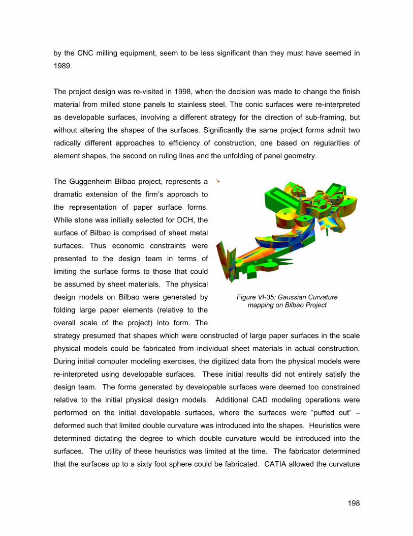
by the CNC milling equipment, seem to be less significant than they must have seemed in

1989.

The project design was re-visited in 1998, when the decision was made to change the finish

material from milled stone panels to stainless steel. The conic surfaces were re-interpreted

as developable surfaces, involving a different strategy for the direction of sub-framing, but

without altering the shapes of the surfaces. Significantly the same project forms admit two

radically different approaches to efficiency of construction, one based on regularities of

element shapes, the second on ruling lines and the unfolding of panel geometry.

The Guggenheim Bilbao project, represents a

dramatic extension of the firm’s approach to

the representation of paper surface forms.

While stone was initially selected for DCH, the

surface of Bilbao is comprised of sheet metal

surfaces. Thus economic constraints were

presented to the design team in terms of

limiting the surface forms to those that could

be assumed by sheet materials. The physical

design models on Bilbao were generated by

folding large paper elements (relative to the

overall scale of the project) into form. The

strategy presumed that shapes which were constructed of large paper surfaces in the scale

physical models could be fabricated from individual sheet materials in actual construction.

During initial computer modeling exercises, the digitized data from the physical models were

re-interpreted using developable surfaces. These initial results did not entirely satisfy the

design team. The forms generated by developable surfaces were deemed too constrained

relative to the initial physical design models. Additional CAD modeling operations were

performed on the initial developable surfaces, where the surfaces were “puffed out” –

deformed such that limited double curvature was introduced into the shapes. Heuristics were

determined dictating the degree to which double curvature would be introduced into the

surfaces. The utility of these heuristics was limited at the time. The fabricator determined

that the surfaces up to a sixty foot sphere could be fabricated. CATIA allowed the curvature

Figure VI-35: Gaussian Curvature mapping on Bilbao Project

198

at individual points on the surface to be sampled. The principal radii at these sampled points

was limited to a minimum of sixty feet in either of the two principal directions.

The geometric qualities of the EMP project represent in some sense a culmination of the

firm’s paper surface modeling research and design explorations. On this project, the fully

curved free form shapes of the original design were supported as a composition of gaussian

curvature constrained paper surface forms. Admittedly, this support of fully free form shapes

is approximate, as the forms are rationalized into shapes exhibiting curvature acceptable

given constructibility constraints. These rationalization operations can be read in the final

project (Figure VI-36).

In the period since the completion of EMP, developable surface and constrained gaussian

curvature applications have developed in parallel. Although the gaussian curvature approach

presents more generous constraints on project form, the economic efficiencies of straight

lines of ruling presented by the developable surface approach are considerable. The tough

constraints of developable surfaces on project forms seem to project the energy of the sheet

material surfaces as they are formed in space better than the more relaxed qualities of the

gaussian curvature approach. The Weatherhead project represents perhaps the most

ambitious application of developable surface forms to date.

The two paper surface representations present remarkably different strategies for the

representation of similar shapes. These differences are manifested in the substantially

different approaches to construction suggested by each representation. However, both

strategies require tight tolerances on the framing system required to achieve a form that will

match the predicted shape. If the geometry of the framing system does not adequately

provide a shape onto which sheet materials will form, then either substantial forming of the

cladding material will need to be undertaken, or warping of the surface will occur. Failures of

cladding or substrate materials may occur, or waterproofing requirements for the system may

not be achieved, resulting in a roof or wall system that leaks. Certainly, the desired

architectural quality of the surface will not be achieved, as the cladding buckles and ripples

about fasteners and joints. For simple, canonical classes of paper surfaces such as planar,

cylindrical or conical forms, the predictive capabilities required to assure developability of the

surface are not particularly great. However, to achieve the freely flowing shapes allowed by

the most general classes of paper surfaces, the predictive capabilities required to engineer

199

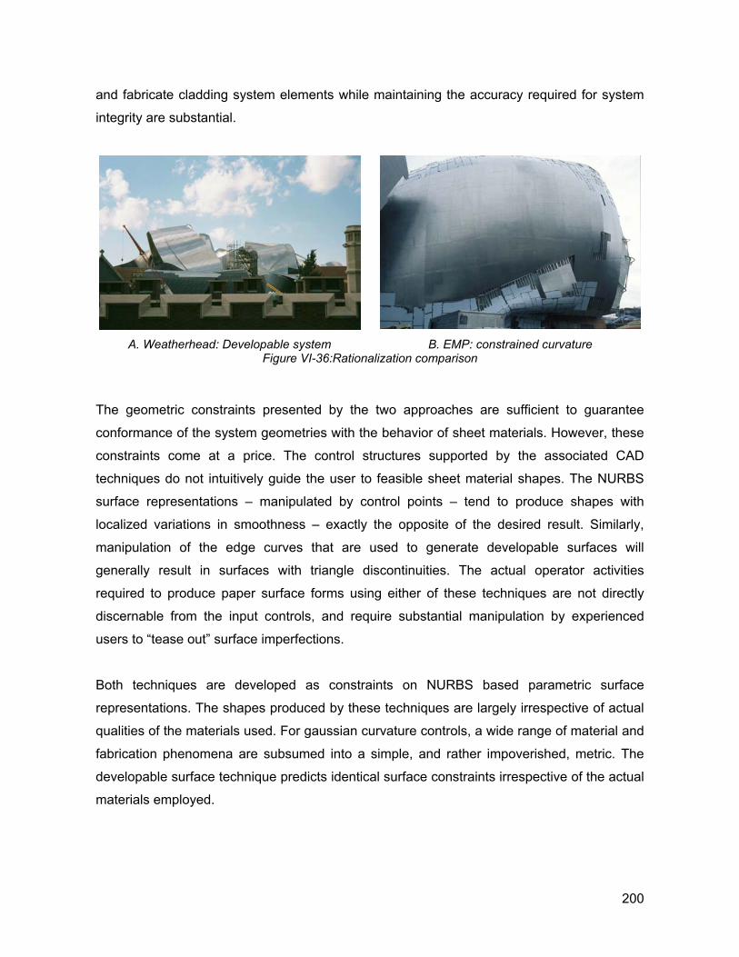
and fabricate cladding system elements while maintaining the accuracy required for system

integrity are substantial.

A. Weatherhead: Developable system B. EMP: constrained curvature

Figure VI-36:Rationalization comparison

The geometric constraints presented by the two approaches are sufficient to guarantee

conformance of the system geometries with the behavior of sheet materials. However, these

constraints come at a price. The control structures supported by the associated CAD

techniques do not intuitively guide the user to feasible sheet material shapes. The NURBS

surface representations – manipulated by control points – tend to produce shapes with

localized variations in smoothness – exactly the opposite of the desired result. Similarly,

manipulation of the edge curves that are used to generate developable surfaces will

generally result in surfaces with triangle discontinuities. The actual operator activities

required to produce paper surface forms using either of these techniques are not directly

discernable from the input controls, and require substantial manipulation by experienced

users to “tease out” surface imperfections.

Both techniques are developed as constraints on NURBS based parametric surface

representations. The shapes produced by these techniques are largely irrespective of actual

qualities of the materials used. For gaussian curvature controls, a wide range of material and

fabrication phenomena are subsumed into a simple, and rather impoverished, metric. The

developable surface technique predicts identical surface constraints irrespective of the actual

materials employed.

200

If the geometric properties of NURBS based surfaces are under constrained for paper

surface applications, then the properties of developable surface based representations and

systems fall at the other extreme. Developable surface representations are highly

constrained, often resulting failing to produce feasible configurations for digitized data from

physical paper models. The constraints of zero gaussian curvature and purely linear

directrices of developable surfaces are quite rigid constraints, which render these systems to

be somewhat incompatible with the characteristics and digitized features from the more

“lenient” paper prototypes.

On the other hand, the topological characteristics of parametric surface representations are

well suited to paper surfaces. The notion of a Euclidean, parametric space that is

topologically “sheet like” – and the extension of this representation to assemblies that are

combinatorially constructed from topological sheets - maps well to the qualities of paper and

other sheet like materials, and their organization in assemblies.

201

202

VII. PHYSICAL MODELING

A. INTRODUCTION

The approaches to digital modeling of paper surfaces described in the previous chapter have

substantial limitations relative to the qualities of such simple modeling tools as physical paper

materials. The common characteristics of both approaches – reliance on differential

geometry heuristics and constructs – have limited capabilities for representing the behavior

of physical materials and operations. The pursuit of digital representation techniques that

provide a closer affinity to the materials and operations of physical modeling and full scale

fabrication remains an active area of research by the firm’s computing staff. This section

presents research that more directly pursues representation of the properties of the sheet

materials themselves: their qualities and modes of deformation, physical properties such as

ability to stretch and bend, their response to forces, etc. A radically different alternative to the

simulation of paper surfaces will be presented, one that relies on direct simulation of material

properties and behaviors.

Materials simulation is far from a new topic. Vast research by the engineering community has

been directed toward the representation of structural and mechanical behaviors of physical

bodies. The materials and bodies pursued through these disciplines are as large as the class

of all materials and forms of use in engineering applications. The representation of paper

surface forms through physical simulation positions this work within this body of research.

Efforts to adopt a physical simulation approach to the modeling of paper surface forms are

complicated by the broad scope and ambiguities inherent to this problem, presented in

Section IV.C. In this effort, we seek to capture those formal and operational qualities that are

common among a wide scope of building design and construction activities, from schematic

design explorations in scale using physical modeling materials, through to the actual

operations of fabricating craftsmen in the shop or field. The accuracy of representing any of

these specific processes through a common representational strategy is likely to be

qualitative at best. On the other hand, the analysis of the firm’s existing techniques presented

in Chapter VI disclosed similar limitations. Despite these limitations, the existing approaches

have been able to successfully integrate representation of project formal qualities with

fabrication constraints. We should expect a physical modeling approach to the representation

203

of paper surface forms to provide at least some improvement in serving the common ground

between these disparate representational requirements.

The general class of problems concerning the motion and deformation of objects are

encompassed by kinematics. Within kinematics, applications where the concern is to

determine the ultimate rest state resulting from force effects on bodies are generally

approached as statics problems, while solutions where the response of the object to these

effects over time are considered through dynamics. While it may appear that the deformation

of paper surfaces is appropriate for solution through statics, it will turn out that elements of

the dynamic behavior of the sheets as they are deformed over time will be worthy of

consideration as well.

One broad class of analysis potentially applicable to paper surface modeling is the theory of

elasticity, wherein the geometric form of the sheet results from an initially un-deformed body

– with certain parameterizable material properties – whose shape results as a response to

externally applied forces by deformation of the body. Solution of such problems take the form

of well known relationships between body stress (internal forces incurred by the body,

usually as a result of externally applied forces) and the deformation or strain of the body.

Solutions are developed through an analysis of infinitesimal elements of the body and the

characteristics of these elements in response to stress forces of the loading scenario under

consideration. The overall behavior of the body is solved by integrating the element level

response over the totality of the body.

Until the advent of computer modeling, problems in these domains were largely limited to the

inquiry of certain canonical shapes (e.g. square plates, cylindrical shells, etc.) for which the

integration could be solved in closed form. The advent of high performance computing has

allowed for element level analysis to be extrapolated to the global deformation of the shape

by considering each element’s behavior independently within the context of the assembly

solution. These approaches consider elements, not of infinitesimal character, but rather as

elements of small but finite size. The body is discretized into assemblies of elements whose

individual shapes permit an explicit solution for deformation due to externally applied forces.

Conditions of continuity and compatibility between adjoining elements are imposed, and the

global behavior of the body is determined by considering the inter-related behavior of the

individual elements.

204

One broad distinction that is made in terms of solution techniques for elastic problems is the

question of linearity of the problem and its solution. Elasticity problems may introduce

linearity or non-linearity in two ways: material linearity, and deformation linearity. The general

stress – strain relationship defined by Hooke’s law:

f kd= (VII.1)

implies a linear relationship between stress and strain. Many materials exhibit effectively

linear stress-strain relationships for small scale deformations, but this simple relationship

becomes more complex as larger scale deformations introduce more complex responses.

Similarly, many solution techniques employ linearized approximations of geometric equations

in their solutions, including small angle approximations, where trigonometric functions are

approximated into simpler forms which hold approximately for small angles. For structural

analysis problems, where one may reasonably anticipate the deformation of a building

component will be small relative to its overall dimensions, linearized approximations of the

geometry of motion are completely appropriate.

In considering sheet material solutions of the types appropriate for modeling paper surfaces,

clearly the linear geometric approximations will be inappropriate, as the anticipated

deformation of the body will be quite large. However, the notion of linear approximation of

material properties seems to be plausible, at least at a qualitative level appropriate for

schematic design requirements. One problem characteristic that will indicate whether the

sheet material responds in a linear fashion would be whether plastic deformation occurs in

the material; that is to say, given input forces that deform the material, would the material

return to its original flattened shape if these forces were removed? In the simulation of paper

surfaces, the answer to this question would be: partly. Certainly the shapes under

consideration do not develop the large scale, ductile deformation associated with stretch

forming of material. However, typically some residual deformation of the sheet will remain in

sheet metal or plywood that has been substantially curved.

Analysis of sheet like bodies has taken a wide variety of forms, again dependent on the

characteristics of the body and results to be solved for. These techniques have been

developed for analysis of structural assemblies including concrete shells, and shear walls or

205

other structural elements whose behavior is principally two dimensional. These approaches

have been incorporated into a wide variety of commercially available structural finite element

solver programs. Most of the theory and application regarding the behavior of plates, shells,

and membranes under loading presumes small deformation appropriate for structural bodies

that are quite rigid, and are expected to experience small scale deformation relative to their

overall dimensions. Again, most of the commercial applications for building structural

engineering are concerned with the static behavior of these elements, although modal

analyses – an essentially static solution that supports the analysis of the system’s oscillatory

behavior – are also supported. These techniques can provide highly accurate, detailed

analysis of structural elements in reasonable solution times.

The theory and applications for the solution of fully deformable material bodies, including

non-linear inelastic behavior, is also quite mature. Techniques and commercial applications

in this category are varied, including solvers appropriate for the analysis of large scale plastic

deformation and even catastrophic events such as explosions. These applications may utilize

highly non-linear representations of strain behavior. Solution techniques may use non-linear

representations of geometric deformation, or may discretize the behavior of the system into

small, incremental motions over time. A potentially serious limitation of many of these

approaches is the time to solution. Robust techniques may require the solution of coupled

partial differential equations for the various modes of motion, and will require the iterative

solution of these equations over many time steps in order to perform the simulation.

As a generalization of physical modeling problems, differing representations of the problem

domain – involving differing approximations of the body’s shape and behavior – can produce

dramatically different accuracy of prediction, with related differences in computational

expense. This relationship between the accuracy of representation of a bodies behavior and

the computational expense to achieve the solution should be not surprising.

This question of desired accuracy of solution in the simulation of paper surfaces is an

important one. In principle, the problem domain could be tackled as one of extraordinary

complexity, involving plastic deformation of the sheet material under loading, friction

resistances between sheets at their joints, and accurate solutions for fastener’s structural

behavior. However, it is not clear whether this high level of complexity of solution technique

206

would provide results that would merit the substantial penalties in terms of computational

expense.

In developing a materials modeling based approach to paper surfaces for design

applications, a primary consideration is to achieve tools whose speed of solution is sufficient

for designers and drafters to model shapes interactively. A solution technique that accurately

produces the most subtle details of behavior will not be useful if modification of surfaces to

reflect changes in design requires hours of off-line computation. At a global level – where

large scale surface shapes are under consideration, a solution technique that can

qualitatively direct the shape to a feasible form may be sufficient, if interactive speeds can be

achieved. At the level of verifying a specific sheet’s shape to determine appropriate

placement of framing members, solution techniques with potentially higher accuracy may be

required.

The solution methods employed by the engineering communities have generally favored

detailed computational models of physical behavior, resulting in highly accurate solutions, at

the expense of potentially long solution times. This predilection is easy to understand in

engineering applications where life and equipment safety are issues.

At perhaps the opposite end of the spectrum, new physical modeling approaches are

appearing in computer animation applications. Substantial work has been undertaken in the

simulation of deformable objects in general, and in the simulation of deformable surfaces in

particular. These physical modeling applications provide reasonable, qualitative behavior of

physical bodies for the purposes of computer animation. These approaches are generally

concerned with the time variant behavior of the systems, with time varying effects such as

collisions between objects, temporally modified constraints on the objects (e.g. the motion of

a human character supporting a cloth object). Simulation for the purposes of computer

animation has the demand of achieving a visual realism that produces a perceptual accuracy

of physical behavior with substantial degrees of detail, but performs a certain trade off

between accuracy of the simulation and computational speed. These simulations are

typically rendered off line, so interactive speeds are not a requirement. The strongest

demand on such simulations is the degree of detail required.

207

Great attention by the computer graphics community has been focused on the simulation of

cloth, for the purpose of clothing characters in animations. Notable work in this domain has

been research by Feynman26, Terzopoulus89, Provot71, Baraff and Witkin5, and many others.

Ng59 provides an overview and comparison of the various techniques employed by these

authors.

B. DEFORMABLE BODY MOTION

This section outlines the basic framework of material body deformation, appropriate for

application to paper surface simulation. The discussion follows closely the derivations of

classical texts on the theory of elasticity, including Marsden and Hughes53. We will be

considering the motion of a material body, and the relative motion of parts of this body, in

response to external effects (typically represented as forces), over the progression of time. It

is useful when considering this transformation of the body over time, to focus on a primary,

invariant reference configuration B as the original, un-deformed state relative to which all

future deformed configurations of the body will be considered. We consider the reference

configuration B to have a coordinate system and “space” independent of the world space R3.

This will allow variations in positions to be viewed from the perspective of the body,

irrespective of deformation or positioning in space. It will be convenient when considering

rates of deformation of the body appropriate for calculation of stresses experienced by the

body to have this invariant coordinate system available to which changes in the body

configuration may be compared.

208

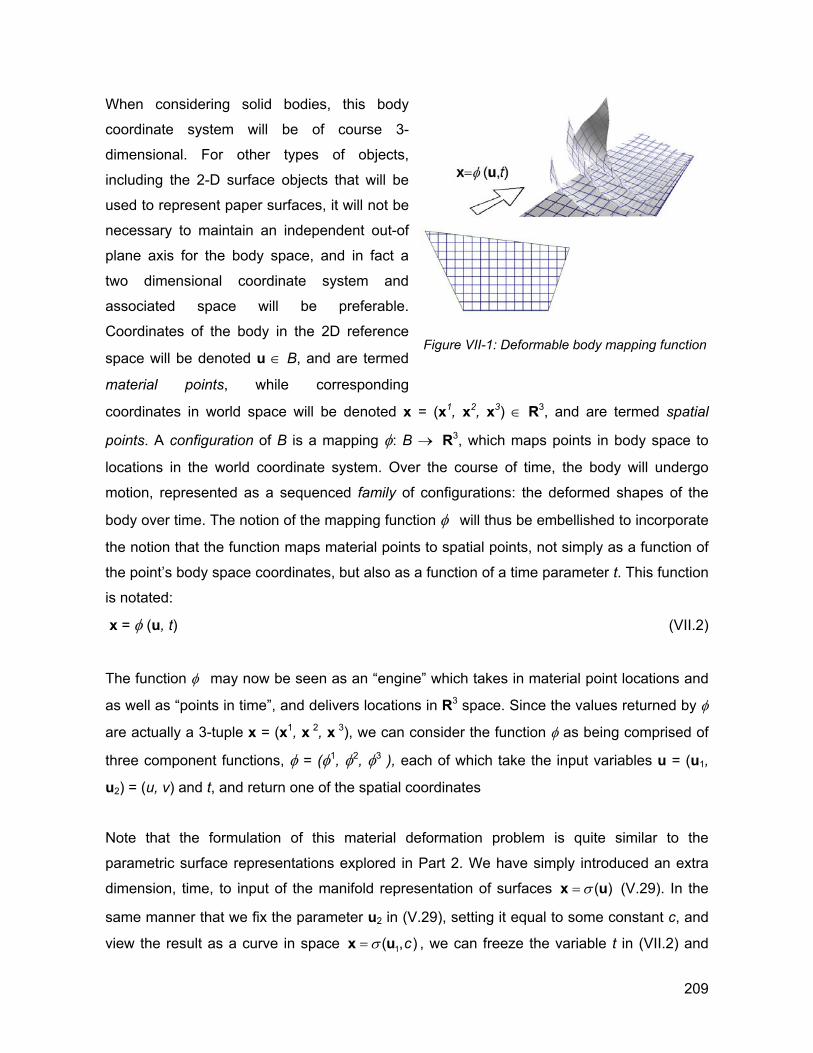
When considering solid bodies, this body

coordinate system will be of course 3-

dimensional. For other types of objects,

including the 2-D surface objects that will be

used to represent paper surfaces, it will not be

necessary to maintain an independent out-of

plane axis for the body space, and in fact a

two dimensional coordinate system and

associated space will be preferable.

Coordinates of the body in the 2D reference

space will be denoted u ∈ B, and are termed

material points, while corresponding

coordinates in world space will be denoted x = (x1, x2, x3) ∈ R3, and are termed spatial

points. A configuration of B is a mapping φ: B → R3, which maps points in body space to

locations in the world coordinate system. Over the course of time, the body will undergo

motion, represented as a sequenced family of configurations: the deformed shapes of the

body over time. The notion of the mapping function φ will thus be embellished to incorporate

the notion that the function maps material points to spatial points, not simply as a function of

the point’s body space coordinates, but also as a function of a time parameter t. This function

is notated:

Figure VII-1: Deformable body mapping function

x = φ (u, t) (VII.2)

The function φ may now be seen as an “engine” which takes in material point locations and

as well as “points in time”, and delivers locations in R3 space. Since the values returned by φ

are actually a 3-tuple x = (x1, x 2, x 3), we can consider the function φ as being comprised of

three component functions, φ = (φ1, φ2, φ3 ), each of which take the input variables u = (u1,

u2) = (u, v) and t, and return one of the spatial coordinates

Note that the formulation of this material deformation problem is quite similar to the

parametric surface representations explored in Part 2. We have simply introduced an extra

dimension, time, to input of the manifold representation of surfaces ( )σ=x u (V.29). In the

same manner that we fix the parameter u2 in (V.29), setting it equal to some constant c, and

view the result as a curve in space 1( , )cσ=x u , we can freeze the variable t in (VII.2) and

209

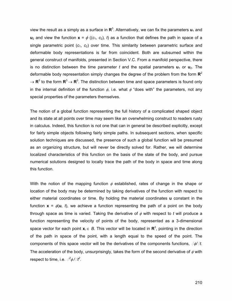
view the result as a simply as a surface in R3. Alternatively, we can fix the parameters u1 and

u2 and view the function x = φ ((c1, c2), t) as a function that defines the path in space of a

single parametric point (c1, c2) over time. This similarity between parametric surface and

deformable body representations is far from coincident. Both are subsumed within the

general construct of manifolds, presented in Section V.C. From a manifold perspective, there

is no distinction between the time parameter t and the spatial parameters u1 or u2. The

deformable body representation simply changes the degree of the problem from the form R2

→ R3 to the form R3 → R3. The distinction between time and space parameters is found only

in the internal definition of the function φ, i.e. what φ “does with” the parameters, not any

special properties of the parameters themselves.

The notion of a global function representing the full history of a complicated shaped object

and its state at all points over time may seem like an overwhelming construct to readers rusty

in calculus. Indeed, this function is not one that can in general be described explicitly, except

for fairly simple objects following fairly simple paths. In subsequent sections, when specific

solution techniques are discussed, the presence of such a global function will be presumed

as an organizing structure, but will never be directly solved for. Rather, we will determine

localized characteristics of this function on the basis of the state of the body, and pursue

numerical solutions designed to locally trace the path of the body in space and time along

this function.

With the notion of the mapping function φ established, rates of change in the shape or

location of the body may be determined by taking derivatives of the function with respect to

either material coordinates or time. By holding the material coordinates u constant in the

function x = φ(u, t), we achieve a function representing the path of a point on the body

through space as time is varied. Taking the derivative of φ with respect to t will produce a

function representing the velocity of points of the body, represented as a 3-dimensional

space vector for each point xi ∈ B. This vector will be located in R3, pointing in the direction

of the path in space of the point, with a length equal to the speed of the point. The

components of this space vector will be the derivatives of the components functions, dφ/dt.

The acceleration of the body, unsurprisingly, takes the form of the second derivative of φ with

respect to time, i.e. d2φ /dt2.

210

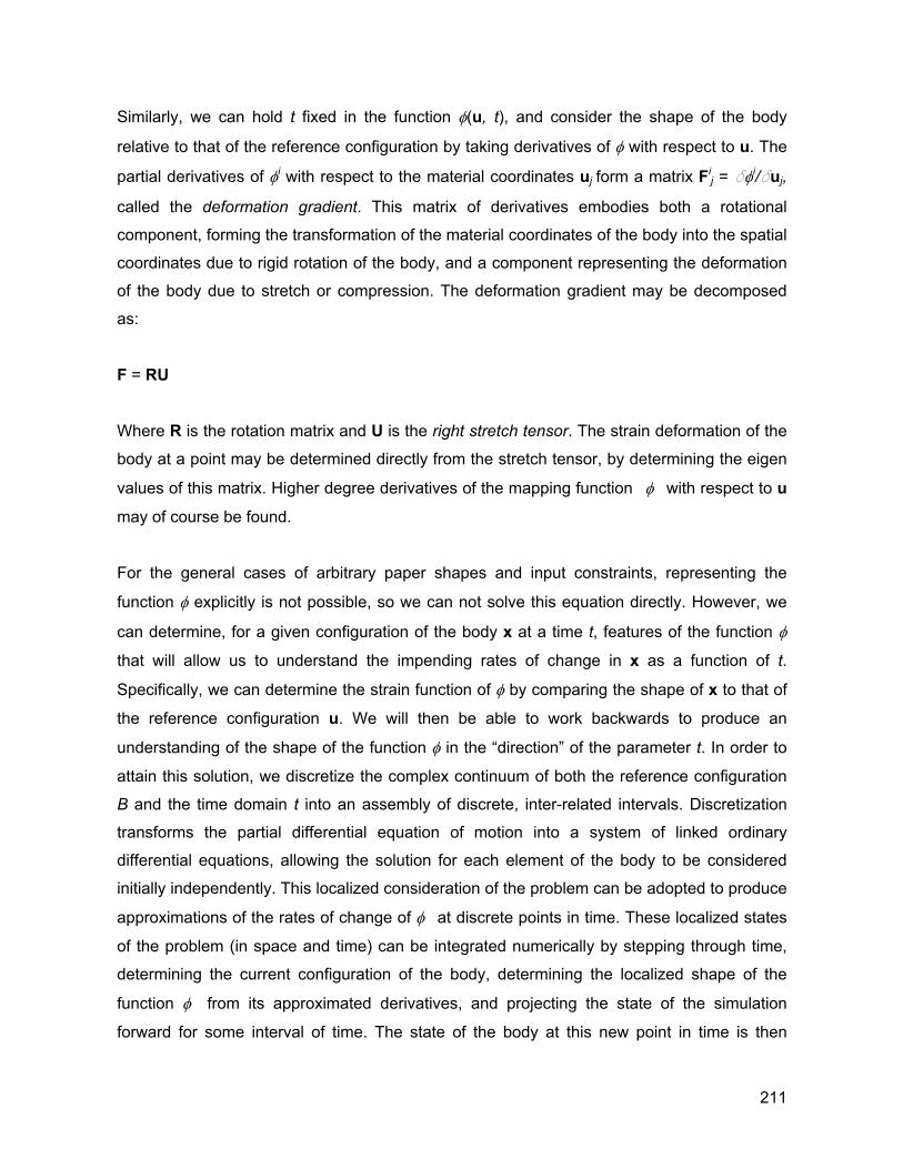
Similarly, we can hold t fixed in the function φ(u, t), and consider the shape of the body

relative to that of the reference configuration by taking derivatives of φ with respect to u. The

partial derivatives of φi with respect to the material coordinates uj form a matrix Fij = dφi/duj,

called the deformation gradient. This matrix of derivatives embodies both a rotational

component, forming the transformation of the material coordinates of the body into the spatial

coordinates due to rigid rotation of the body, and a component representing the deformation

of the body due to stretch or compression. The deformation gradient may be decomposed

as:

F = RU

Where R is the rotation matrix and U is the right stretch tensor. The strain deformation of the

body at a point may be determined directly from the stretch tensor, by determining the eigen

values of this matrix. Higher degree derivatives of the mapping function φ with respect to u

may of course be found.

For the general cases of arbitrary paper shapes and input constraints, representing the

function φ explicitly is not possible, so we can not solve this equation directly. However, we

can determine, for a given configuration of the body x at a time t, features of the function φ

that will allow us to understand the impending rates of change in x as a function of t.

Specifically, we can determine the strain function of φ by comparing the shape of x to that of

the reference configuration u. We will then be able to work backwards to produce an

understanding of the shape of the function φ in the “direction” of the parameter t. In order to

attain this solution, we discretize the complex continuum of both the reference configuration

B and the time domain t into an assembly of discrete, inter-related intervals. Discretization

transforms the partial differential equation of motion into a system of linked ordinary

differential equations, allowing the solution for each element of the body to be considered

initially independently. This localized consideration of the problem can be adopted to produce

approximations of the rates of change of φ at discrete points in time. These localized states

of the problem (in space and time) can be integrated numerically by stepping through time,

determining the current configuration of the body, determining the localized shape of the

function φ from its approximated derivatives, and projecting the state of the simulation

forward for some interval of time. The state of the body at this new point in time is then

211

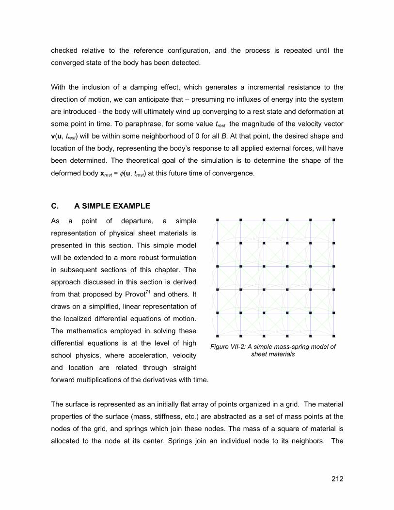
checked relative to the reference configuration, and the process is repeated until the

converged state of the body has been detected.

With the inclusion of a damping effect, which generates a incremental resistance to the

direction of motion, we can anticipate that – presuming no influxes of energy into the system

are introduced - the body will ultimately wind up converging to a rest state and deformation at

some point in time. To paraphrase, for some value trest the magnitude of the velocity vector

v(u, trest) will be within some neighborhood of 0 for all B. At that point, the desired shape and

location of the body, representing the body’s response to all applied external forces, will have

been determined. The theoretical goal of the simulation is to determine the shape of the

deformed body xrest = φ(u, trest) at this future time of convergence.

C. A SIMPLE EXAMPLE

As a point of departure, a simple

representation of physical sheet materials is

presented in this section. This simple model

will be extended to a more robust formulation

in subsequent sections of this chapter. The

approach discussed in this section is derived

from that proposed by Provot71 and others. It

draws on a simplified, linear representation of

the localized differential equations of motion.

The mathematics employed in solving these

differential equations is at the level of high

school physics, where acceleration, velocity

and location are related through straight

forward multiplications of the derivatives with time.

Figure VII-2: A simple mass-spring model of

sheet materials

The surface is represented as an initially flat array of points organized in a grid. The material

properties of the surface (mass, stiffness, etc.) are abstracted as a set of mass points at the

nodes of the grid, and springs which join these nodes. The mass of a square of material is

allocated to the node at its center. Springs join an individual node to its neighbors. The

212

relative location between two joined nodes determines the kind of stress to which the given

spring responds .

1. Springs which join a node to its nearest horizontal / vertical neighbors govern the

behavior of the node when subjected to internal axial forces.

2. Springs that join a node to its diagonal neighbors govern internal shear force response.

3. Springs which join a node to the horizontal / vertical neighbors located two units away

govern the flexural behavior of the intermediate node.

As the surface deforms from its initial flat

geometry, the relative lengthening or

shortening of the springs exert an opposing

force on the two nodes which join the spring.

Figure VII-3 provides a graphical

demonstration of the spring behavior. Each

force is represented as a vector, with both

direction in space and magnitude. A force on

a particle p0 due to a spring of rest length l

joining p0 to a particle p1 is simply:

1 0 1 0

1 0spring spring

lK

l− − −

=−

p p p pfp p

(VII.3)

ORIGINAL DEFORMED

SHEAR

AXIAL

DEFORMED

ORIGINAL

FLEXURE

ORIGINAL DEFORMED

Figure VII-3: Deformation modes of the idealized

spring assembly

where 1 0

1 0

−−

p pp p

is simply a unit vector in the direction p0→p1, and Kspring is a constant that

dictates the stiffness or force associated with the spring. Differing stiffness constants may be

allocated to the spring types (1 - 3). Variations in these relative spring constants affect the

qualitative behavior of the surface material. Approximate values for these spring constants

could be determined from the material properties of the material, thickness of the material

and distance between the nodes.

In addition to the internal forces of the material stiffness, the surface may be subjected to

external forces, including:

• gravity

213

• positioning during fabrication

• framing and fastening constraints.

These external actions on the surface can be formulated in a variety of ways, depending on

the type of behavior of interest. The actions manifest themselves as force vectors – possibly

varying over time – acting on the mass nodes. As a simple example, the action of gravity is

formulated as the vector:

gravity

0= 0

- gma

f

v

(VII.4)

where ag is the acceleration of gravity and m the mass of the node. This force is applied

constantly on each node in the surface representation.

An additional damping force is added to each node, based on the velocity of the node at a

give point in time:

0damp dampK= −f (VII.5)

The damping component tacked on to each particle as a function of its velocity, ensures that

a rest state will ultimately occur. If this damping factor were not figured in, the surface could

oscillate indefinitely.

To solve for the deformed surface under loading, all of the force vectors acting on an

individual node at a particular point in time t0 are summed, producing a force vector f acting

on the node. The surface state is then considered at an incremental time step t0 + h. The

algorithm uses a simple linear method for approximating the changes in surface state over

this time step:

We consider the system for a specific time step (t0, t0 + h), with a known position of all

particles x0 and known velocity =v x& , the system is solved for a new position vector x0+h,

and a new velocity vector v0+h. The differential equations representing the system are:

1 ( )d ddt dt −

= =

x x vx v M f x,& v

(VII.6)

214

Discretizing the equations, we define

0

0 0

t h tt h t

∆ +

∆ +

v = v( ) - v( )x = x( ) - x( )

0 (VII.7)

The solution to the differential equation in (VII.6) approximates ∆x and ∆v as

01

0

h −

∆ = ∆

vxM fv

(VII.8)

These equations are simply:

( , )h∆ =f x vv

m (VII.9)

0 h∆ = = + ∆x v v v (VII.10)

0 h= + ∆x x x (VII.11)

In this simple formulation, these three equations may be solved independently (for each

particle) and sequentially, once the force vector f(x,v) has been determined. First, ∆v is

solved for by multiplying the time step size by force, and dividing by the mass of the particle.

Adding the change in velocity to the previous velocity produces the new particle velocity.

The change in location is similarly solved for (VII.10), by multiplying the new velocity by

the time step. The change in particle location is added to the current location to produce the

particle location at the end of the time step.

∆v∆x

Note that a particle’s location and velocity are each represented by three values,

representing respectively, the location and velocity’s 3 spatial components. A total of 6

values must be stored for each particle during the simulation. Each component is

approximated as a linear function over the time step, and represents an independent function

that may be independently solved for.

The acceleration of the node is equal to the force on the node divided by the node’s mass:

a(t0) = f(t0 ) / m (VII.12)

The velocity of the node is equal to the old velocity plus the new acceleration multiplied by

the time step.

215

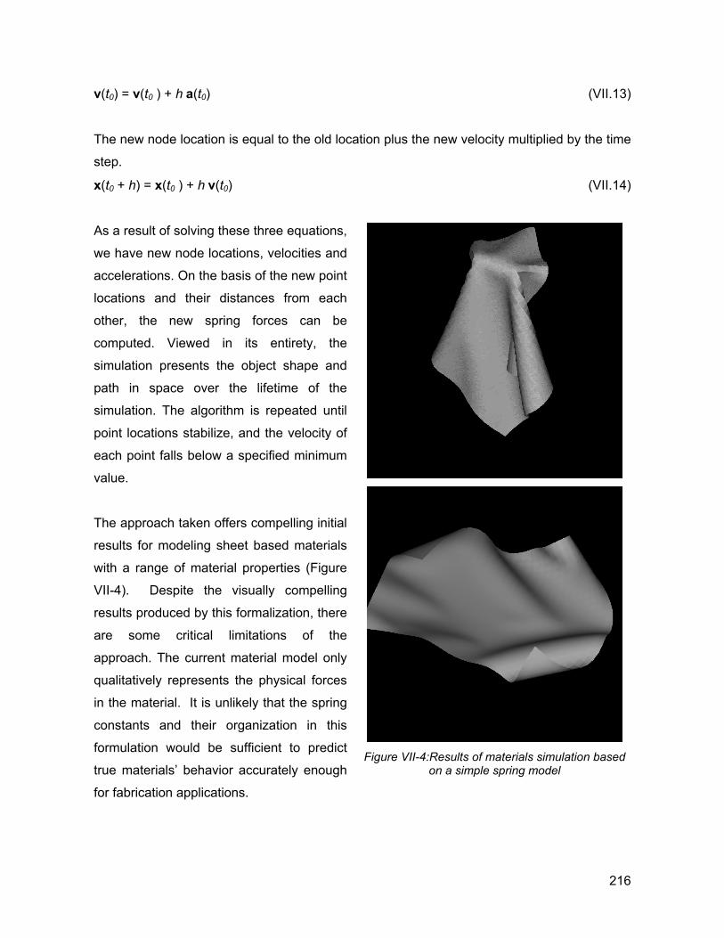
v(t0) = v(t0 ) + h a(t0) (VII.13)

The new node location is equal to the old location plus the new velocity multiplied by the time

step.

x(t0 + h) = x(t0 ) + h v(t0) (VII.14)

As a result of solving these three equations,

we have new node locations, velocities and

accelerations. On the basis of the new point

locations and their distances from each

other, the new spring forces can be

computed. Viewed in its entirety, the

simulation presents the object shape and

path in space over the lifetime of the

simulation. The algorithm is repeated until

point locations stabilize, and the velocity of

each point falls below a specified minimum

value.

The approach taken offers compelling initial

results for modeling sheet based materials

with a range of material properties (Figure

VII-4). Despite the visually compelling

results produced by this formalization, there

are some critical limitations of the

approach. The current material model only

qualitatively represents the physical forces

in the material. It is unlikely that the spring

constants and their organization in this

formulation would be sufficient to predict

true materials’ behavior accurately enough

for fabrication applications.

Figure VII-4:Results of materials simulation based

on a simple spring model

216

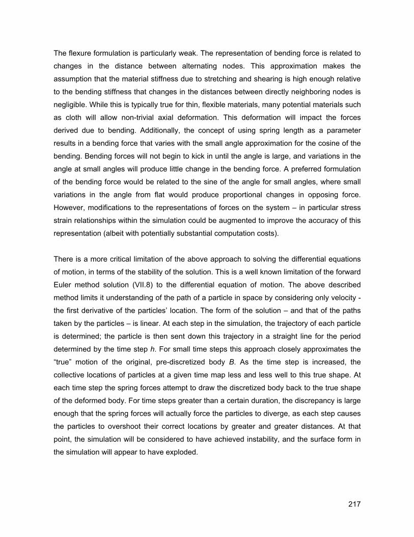
The flexure formulation is particularly weak. The representation of bending force is related to

changes in the distance between alternating nodes. This approximation makes the

assumption that the material stiffness due to stretching and shearing is high enough relative

to the bending stiffness that changes in the distances between directly neighboring nodes is

negligible. While this is typically true for thin, flexible materials, many potential materials such

as cloth will allow non-trivial axial deformation. This deformation will impact the forces

derived due to bending. Additionally, the concept of using spring length as a parameter

results in a bending force that varies with the small angle approximation for the cosine of the

bending. Bending forces will not begin to kick in until the angle is large, and variations in the

angle at small angles will produce little change in the bending force. A preferred formulation

of the bending force would be related to the sine of the angle for small angles, where small

variations in the angle from flat would produce proportional changes in opposing force.

However, modifications to the representations of forces on the system – in particular stress

strain relationships within the simulation could be augmented to improve the accuracy of this

representation (albeit with potentially substantial computation costs).

There is a more critical limitation of the above approach to solving the differential equations

of motion, in terms of the stability of the solution. This is a well known limitation of the forward

Euler method solution (VII.8) to the differential equation of motion. The above described

method limits it understanding of the path of a particle in space by considering only velocity -

the first derivative of the particles’ location. The form of the solution – and that of the paths

taken by the particles – is linear. At each step in the simulation, the trajectory of each particle

is determined; the particle is then sent down this trajectory in a straight line for the period

determined by the time step h. For small time steps this approach closely approximates the

“true” motion of the original, pre-discretized body B. As the time step is increased, the

collective locations of particles at a given time map less and less well to this true shape. At

each time step the spring forces attempt to draw the discretized body back to the true shape

of the deformed body. For time steps greater than a certain duration, the discrepancy is large

enough that the spring forces will actually force the particles to diverge, as each step causes

the particles to overshoot their correct locations by greater and greater distances. At that

point, the simulation will be considered to have achieved instability, and the surface form in

the simulation will appear to have exploded.

217

The time step size required for instability to occur depends on a number of factors4, including

the number of particles in the simulation, the proportion between time step and spring

constants, and the variation in spring constants in the simulation. The time step decreases at

least as a factor of the number of particles n. Since the number of computations during an

iteration is again proportional to n, the growth in time required for solution is at least n2. This

drastically limits the number of particles, and the level of detail, that can be supported by this

simple numerical solution. If the time step exceeds a value roughly constrained by the speed

at which forces propagate through the spring matrix, the solution becomes unstable. The

prototype of the application described above (written in AutoCAD r14 C++) takes

approximately 5 minutes to converge for a 30 x 30 node mesh – obviously too slow for

interactive applications.

D. IMPLICIT INTEGRATION APPROACH

A more robust alternative is to adopt a solution method that takes into account higher

derivatives of the differential equations of motion x = φ(u, t). This section takes an approach

closely related to that proposed by Baraf and Witken5 for the simulation of cloth materials –

one directly applicable to the simulation of paper surfaces as well.

In order to address the instability issues of the example, a formulation of the motions of mass

particles is adopted that is quadratic in time, as opposed to the linear example above. We will

thus be drawing on higher, second order derivatives of the equations of motion. The inclusion

of these higher order derivatives in the linked solution of the particle assembly introduces

additional computational requirements. The Taylor series expansion for the integration of the

position vector x at time t1 = t0 + h is: 2 3

0 0 0 0 0( ) ( ) ( ) ( ) ( ) ...2! 3! !

n n

nh h ht h t h t t t

n t∂

+ = + + + + +∂xx x x x x& && && (VII.15)

In the example above, the solution technique approximates this function only to the first

derivative, resulting in O(h2) error: 2

0 0 0( ) ( ) ( ) (t h t h t O h+ = + +x x x& ) (VII.16)

The current approach will introduce an additional, second order term:

218

23

0 0 0 0( ) ( ) ( ) ( ) ( )2!ht h t h t t O h+ = + + +x x x x& && (VII.17)

The solution technique is generally concerned with solving the ordinary differential equation:

1( E− ∂= − +

∂x M f

x&& ) (VII.18)

where E is a scalar energy function representing the internal state of the material, while f is a

function of x representing external forces acting on the body. The vector x is the geometric

state of the material – an ordered 3n vector composed of the x,y, and z coordinates of the

spatial points of the material. The matrix M represents the mass distribution of the body over

the spatial points.

The first step in this solution is to formulate the internal and external forces such that the first

and second derivative terms in (VII.17) may be computed. The solution technique begins by

introducing a behavior function, which models the various phenomena in the simulation as

localized equations in terms of the states of one or more of the particles. For example, the

behavior function for a spring between two particles is simply:

C(p, q) = | p - q | - l0 (VII.19)

i.e., the value is the difference of the distance between the two particles’ locations and some

ideal spring length l0. From the perspective of this single spring, the state of the particle

configuration is optimal when C(x1,x2) = 0, or the distance between the two points is equal to

the spring’s ideal length. Forces generated on particles by the behavior functions will be in

the direction of this optimal state. The force formulation is produced by first defining a scalar

energy function

=2skE C C (VII.20)

where ks is a stiffness constant. The force due to this scalar potential is the negative of the

energy gradient, so the force on a particle represented in the function C(x1, . . ., xn) is:

219

i si i

E k C∂= − = −

∂ ∂f

x xC∂

)

(VII.21)

Thus, we are able to determine on the basis of a general behavior function the direction and

magnitude of forces on the individual particles that minimize the non-optimality expressed by

the behavior functions.

E. BACKWARDS EULER METHOD

While in the simple example described in Section VII.C is solved using only a knowledge of

the state of the system at the beginning of a time step t0, the backwards Euler solution

requires knowledge of the state of the equations of motion at the terminus of the step t =t0 +h:

01 ( ,

h −

+ ∆∆ = + ∆ + ∆∆ 0 0

v vxM f x x v vv

(VII.22)

It is in the new formulation for the force function + ∆ + ∆( ,0 0f x x v v) that the higher order

terms that produce additional stability in the solution must be provided. This function is

rendered to first order approximation as:

∂ ∂+ ∆ + ∆ = + ∆ + ∆

∂ ∂0( , )0 0f ff x x v v f x vx v

(VII.23)

Substitution into (VII.22) yields:

− − −∂ ∂ ∂− − ∆ = +

∂ ∂ ∂2

0( ) (h h h h1 1 1f f fI M M v M f vv x x 0 ) (VII.24)

Left multiplying the equation by the mass matrix M results in:

20( ) (h h h h∂ ∂ ∂

− − ∆ = +∂ ∂ ∂

f f fM v fv x x 0 )v (VII.25)

This is the equation that will be solved in matrix form to produce the values for the vector Dv.

With the values of Dv determined, solution for the updated particle locations can be

determined by “plugging in” the values for Dv in the upper part of (VII.22).

220

Equation (VII.25) has the following components:

• M, the mass matrix.

• The force vector f0 determined from the energy function as per (VII.21).

• The jf/jx term, which appears twice, once on the left side of the equation multiplied

by h2 and Dv, and again on the right side of the equation multiplied by h and v0. This

is the first derivative of the force function by x, i.e. the second derivative of the energy

function. Consequently (VII.25) requires a second derivative of the behavior function

C. Taking the derivative (VII.21) with respect to x yields:

2( ) ( ) ( ) ( )

Ti

sj i j i j

C C Ck ∂ ∂ ∂ ∂

= − +∂ ∂ ∂ ∂ ∂

f x x x xx x x x x

C

• h ∂∂

fv

, where h is the time step and jf/jv the derivative of the force function with

respect to velocity.

F. MATERIAL FORMULATION

In this section, details of the formulation of the energy functions, corresponding to specific

modes of deformation for paper surfaces are presented. The modes of behavior of the

system that the solution will be concerned with are internal forces acting between mass

particles as a function of the deformation of the surface, and external forces such as springs,

cables, viscous damping and gravity. The internal behavior of the material are rendered into

three distinct deformation modes with corresponding force formulations:

1. Axial deformation, representing stretching or compression of the material. Of these,

stretch will be the most common behavior, since compressive actions will typically result

in buckling and bending of the material.

2. Shear deformation, representing in-plane skewing of the material. The treatment of this

action will be the main characteristic distinguishing the modeling of paper surfaces from

similar cloth simulations in the literature.

3. Bending deformation, represented as an angular deviation from flat at edges within the

body of the material.

221

In constructing the formulations of the internal material forces, the deformed body principles

of Section VII.B above will be revisited. It will be also beneficial to keep in mind the

terminology and representation of parametric surfaces presented in Section V.D.

1. Derivatives of the Mapping Function φ Consider a set of i particles with unchanging material coordinates (ui,vi) in a 2D planar space,

and simultaneous spatial xi coordinates in R3. The function:

φ(u,v) = x (VII.26)

maps 2D material coordinates to spatial coordinates in R3. The stretch deformation is

represented by the derivatives of this function with respect to u and v:

φu = jφ/ju (VII.27)

φv = jφ/jv

These functions describe vectors in R3, analogous to the tangent vectors to the parametric

curves describes in Chapter V. The magnitudes of these vectors for a given point represent

the stretch (or compression) in the material directions of (u,v).

We can approximate these functions locally, by considering the deformation of a triangular

region of the material in R3, and comparing the deformed shape of the triangle relative to its

shape in parametric space. On this basis, we approximate a mapping function x= ω(u,v)

between parametric and world space that is applied over the region of an individual triangle.

We consider the triangle with labeled nodes i, j, k. and define the R3 vectors representing the

differences between the vertices’ spatial coordinates:

Dx1= xj - xi (VII.28)

Dx2= xk - xi

And similar differences in the (u,v) planar, parametric space of the material coordinates:

Du1= uj - ui , Dv1= vj - vi (VII.29)

Du2= uk - ui , Dv2= vk - vi

Making the assumption that wu and wv are constant over the region defined by the triangle,

we may state:

222

Dx1= wuDu1 + wvDv1 (VII.30)

Dx2= wuDu2 + wvDv2

which in turn allows the solution for ωu and ωv, the derivates of ω with respect to u and v: 1

1 2v 1 2

1 2

2 21 2

1 11 2 2 1

1 2 2 1 1 2 2 1

1 2 2 1 1 2 2 1

( ) ( )

1 ( )

-

u

u uv v

v uv uu v u v

v v u uu v u v u v u v

ω ω−

∆ ∆ = ∆ ∆ ∆ ∆

∆ −∆ = ∆ ∆ −∆ ∆∆ ∆ − ∆ ∆

∆ ∆ − ∆ ∆ ∆ ∆ + ∆ ∆= ∆ ∆ − ∆ ∆ ∆ ∆ − ∆ ∆

x x

x x

x x x x

(VII.31)

2. Stretch Formulation With the differential functions for wu and wv defined, we defined energy functions associated

with stretch in the u and v directions as:

Cstretch_u(x) = a Kstretch_u ( |wu| - 1) (VII.32)

Cstretch_v(x) = a Kstretch_v ( |wv| - 1)

Where a is the area of the triangle (in constant, material space) and Kstretch_u, Kstretch_v are

constants indicating the relative stiffness of the material in stretch. While for many of

materials these two constants may be equal, there are many types of materials where we

may want to selectively vary the stiffness in the two directions (for example, corrugated

materials, plywood, chain link meshes, etc.)

1 1 1

1 2 3

2 2 2

1 2 3

3 3 3

1 2 3

u u u

i i u

u u u

i i i

u u u u

i i i i

u u u

i i i

ω ω ωω

ω ω ω

ω ω ω ω

ω ω ω

∂ ∂=

∂ ∂

∂ ∂ ∂ ∂ ∂ ∂ ∂ ∂ ∂ ∂

= ∂ ∂ ∂ ∂

∂ ∂ ∂ ∂ ∂ ∂

x x

x x x

x x x x

x x x

(VII.33)

223

If k l 0kuli

ω∂≠

∂x= , the derivative of ω with respect to a component of x is independent of any

other component of x, and we may say: 1

1

22 1

321 2 2

3

3

3

0 0

0 0

0 0

1 0 00 1 00 0 1

u

i

u u

i i

u

i

v vu v u v

ω

ω ω

ω

∂ ∂ ∂ ∂ −∆ + ∆

= = ∂ ∆ ∆∂

∂ ∂ =

x

Ix x

x

I

− ∆ ∆

(VII.34)

Similarly,

2 13

1 2 2

2 13

1 2 2

23

1 2 2

23

1 2 2

u

i

v

i

u

j

v

j

v vu v u v

u uu v u v

vu v u v

uu v u v

ω

ω

ω

ω

∂ −∆ + ∆=

∂ ∆ ∆ − ∆ ∆∂ ∆ − ∆

=∂ ∆ ∆ − ∆ ∆∂ ∆

=∂ ∆ ∆ − ∆ ∆

∂ −∆=

∂ ∆ ∆ − ∆ ∆

Ix

Ix

Ix

Ix

3. Shear Function Formulation The shear energy is approximated as by the angle of deformation in the plane of the

material, for each triangle. By small angle approximation, we can presume this angle is

approximately equal to its cosine for small angle deformations, and hence is formulated as

the inner product of the variations in the derivatives of the mapping function:

( ) ( )( ) ( ) ( )( )

1

1 2 3 2

3

2 1 21..3

21 2 1 2

( )

( )

Tshear u v

v

u u u v

v

n n n n n n n nj i k i j i k i

n

C a

a

a v v u

u v v u

ω ω

ωω ω ω ω

ω

=

=

=

− ∆ − − ∆ − − ∆ + − ∆=

∆ ∆ − ∆ ∆

∑

x

x x x x x x x x 1u

(VII.35)

224

( ) ( ) ( )( )( ) ( ) ( )( )

( ) ( )( )( ) ( )( )

2 1 2 1

2 1 2 11..3

21 2 1 2

2 2 1

2 2 11..3

1 2

u( )( )

( )(

n n n nj i k i

n n n nj i k i

shear n

i

n n n nj i k i

n n n nj i k i

shear n

j

v v u ua

u v vCu v v u

v u ua

u v vCu v

=

=

−∆ + ∆ − − ∆ + − ∆ + ∆ − ∆ − ∆ − − ∆ ∂ =

∂ ∆ ∆ − ∆ ∆

∆ − − ∆ + − ∆ − ∆ − ∆ − − ∆ ∂ =

∂ ∆ ∆ − ∆

x x x x

x x x xxx

x x x x

x x x xxx 2

1 2 )v u∆

(VII.36)

2 2

3 3

,

2

( ) ( )

( )

where is the kroneker delta, equal to 1 if , 0 otherwise. Therefore:

sheark l

i j i j k l

shear u uv vklk l k l l k

i j i j j i

kl

C C

C ax x x x

k l

ω ωω ωδ

δ

∂ ∂= ∈ ×

∂ ∂ ∂ ∂

∂ ∂ ∂∂ ∂= +

∂ ∂ ∂ ∂ ∂ ∂ =

x x R Rx x x x

xx x

2 ( ) shear u uv

i j i j j i

C a v

x x x xω ωω ω ∂ ∂ ∂∂ ∂

= +∂ ∂ ∂ ∂ ∂ ∂

xx x (VII.37)

4. Bend Function Formulation In contrast to the stretch and shear formulations, where these functions are considered

relative to the deformation of a single triangle, the bending of a triangulated mesh will be

considered by changes in the angle between two triangles, at the adjoining edge. If we

presume that the reference configuration is initially flat, initial angle at each edge is 0 and the

energy associated with bending deformation will be proportional to the angle Q formed at the

edge:

Cbend(x) = KbendQ (VII.38)

This angle is equivalent to the angle between the normals of the two triangles n1 and n2.

Letting e be the unit vector parallel to the edge, the trigonometric relations for the angle are:

sin(Q) = (n1 × n2) • e (VII.39)

cos(Q) = n1 • n2

225

1 2 2 11 2 1 22 0 0 21 2 1 20 1 1 01 2 1 2

1i j i k

i j i k i j i k

∆ ∆ − ∆ ∆ = × = ∆ ∆ − ∆ ∆ ∆ ∆ − ∆ ∆

x x x xx x x xn xx x x x x x x x x x x x

uuuuur uuuuur

uuuuur uuuuur uuuuur uuuuur x x x (VII.40)

j i

j i

=x x

ex x

uuuuur

uuuuur (VII.41)

If we presume that e varies little as a function of x, then

2 2 1 12 1 1 2

2 2 0 01 2 2 11 1 0 02 1 1 2

01 0

0i i j i k

−∆ + ∆ −∆ + ∆∂ = −∆ + ∆ −∆ ∂ −∆ + ∆ −∆ + ∆

x x x xn x x x xx x x x x x x x x

uuuuur uuuuur + ∆ (VII.42)

2 12 2

2 02 2

1 02 2

2 11 1

2 01 1

1 01 1

01 0

0

01 0

0

j i j i k

k i j i k

∆ −∆∂ = −∆ ∂ ∆ −∆

−∆ ∆∂ = ∆ ∂ −∆ ∆

x xn x xx x x x x x x

x xn x xx x x x x x x

uuuuur uuuuur

uuuuur uuuuur

∆

−∆

( )

1 cos(sin( )1 sin( )

cos( )

bend

i i

i

i

C θ

)θθ

θθ

∂ ∂=

∂ ∂

∂= −

∂

∂=

∂

xx x

x

x

(VII.43)

where

cos( ) sin( )

sin( ) cos( )

i

i i

i

θ θθ

θ θθ

∂ ∂= −

∂ ∂

∂ ∂=

∂ ∂

x x

x x

(VII.44)

226

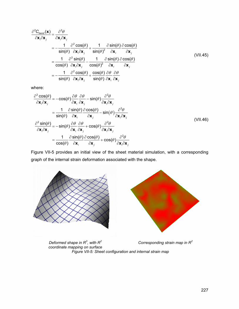
2 2

2

2

2

2

2

( )

1 cos( ) 1 sin( ) cos( ) sin( ) sin( )

1 sin( ) 1 sin( ) cos( ) cos( ) cos( )

1 cos( ) cos( )sin( ) sin( )

bend

i j i j

i j i j

i j i j

i j i j

C θ

θ θ θθ θ

θ θ θθ θ

θ θ θ θθ θ

∂ ∂=

∂ ∂ ∂ ∂

∂ ∂= − +

∂ ∂ ∂ ∂

∂ ∂ ∂= −

∂ ∂ ∂ ∂

∂ ∂ ∂= − +

∂ ∂ ∂ ∂

xx x x x

x x x x

x x x x

x x x x

∂

(VII.45)

where:

( )

2 2

2

2

cos( ) cos( ) sin( )

1 sin( ) cos( ) sinsin( )

sin( ) sin( ) cos( )

1 sin( ) cos( ) cos(cos( )

i j i j i j

i j i

i j i j i j

i j

θ θ θ θθ θ

2

j

θ θ θθθ

θ θ θ θθ θ

θ θθ

∂ ∂ ∂ ∂= − −

∂ ∂ ∂ ∂ ∂ ∂

∂ ∂ ∂= −

∂ ∂ ∂ ∂

∂ ∂ ∂ ∂= − +

∂ ∂ ∂ ∂ ∂ ∂

∂ ∂= +

∂ ∂

x x x x x x

x x x x

x x x x x x

x x

2

)i j

θθ ∂∂ ∂x x

(VII.46)

Figure VII-5 provides an initial view of the sheet material simulation, with a corresponding

graph of the internal strain deformation associated with the shape.

Deformed shape in R3, with R2 coordinate mapping on surface

Corresponding strain map in R2

Figure VII-5: Sheet configuration and internal strain map

227

5. Damping The definition of an appropriate damping function is critical to the simulation. Although the

formulation represents the behavior of the paper material as a dynamic, time based

simulation, the primary concern in this application is the ultimate, static behavior of the

materials once they have “settled down” to a minimal energy configuration state, and the

velocities and accelerations of the particles have fallen to within some threshold of 0. A

“springy” system without the presence of damping will oscillate about the rest state, and

never settle down. Thus damping serves the important function of driving the simulation to

the rest state, by dissipating the kinetic energy in the system. At the same time, damping

competes with the action of forces, and their associated accelerations and velocities, in

driving the system toward the minimal energy rest state. Thus, tuning the damping to allow

efficient translation of the mass particles toward the rest state, while minimizing over-

shooting and oscillation, is an important component in efficiently moving the simulation

toward solution.

Damping serves a second important function in the stability of the simulation. By damping out

residual forces resulting from the second order approximation of the differential equations of

motion, a damping component allows larger time steps to be achieved while still allowing

stability of the simulation.

A straight forward formulation of damping effects on a particle is viscous damping, where the

force on the particle is inversely proportional to the particle’s velocity:

fdamp = - Kdamp v(x) (VII.47)

which approximates the behavior as if it were immersed in some motion resistant medium

such as air, water, or “jelly” – depending on the value of Kdamp. Barraf and Witkin’s

formulation draws on the second term of (VII.24), h − ∂∂

1 fMv

, as the means for formulating

damping associated with a given deformation mode. The damping acts on the component of

system velocity in the jC/jx direction, and provides damping associated with a energy

function condition C as:

( )damp dampi

CK C∂= −

∂f

x& x (VII.48)

228

While this formulation results in more believable time based simulations of motion, it results

in additional computational overhead in computing the additional energy function derivatives.

Since our paper simulator application is concerned principally with accurately representing

the rest state of the body, this additional overhead required to provide a more realistic

simulation of the body’s behavior over time does not seem necessary, and the more straight

forward viscous damping formulation has been used in the simulator.

6. Springs In the paper modeler, a spring is typically an object – and associated energy condition - that

attempts to bring a mass particle within a specified distance of either a location in space or

another mass particle. The desired distance may be 0, or some desired rest length of the

spring. The general formulation of spring energy functions is :

Cspring(x1, x2) = Kspring (| x1 - x2 | - l ) (VII.49)

where l is the rest length of the spring. Note that we may select varying values of Kspring for

different springs in the system, resulting in differing types of behavior for individual springs.

There are a variety of useful applications of spring objects in the modeler:

• As a means for fixing the material in space. Individual mass particles can have springs

affixed to specific spatial locations. These springs will guide the simulation to a solution

where the particles remain spatially located near these determined points in space.

• As a means for user manipulation of the materials. Mass particles may be attached to

space points indicated by the user. These locations may be interactively manipulated by

mouse motion. The material particles will attempt to follow the motions of the mouse as

the simulation progresses. The location indicated by the user may be dynamically

updated between solution steps.

• As a means for joining mass particles together. Springs may be attached between two

mass particles, in which case the solver will attempt to bring these two particles within

229

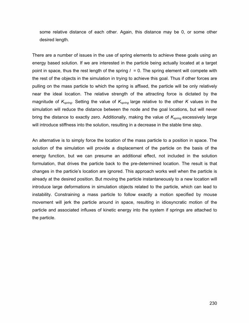
some relative distance of each other. Again, this distance may be 0, or some other

desired length.

There are a number of issues in the use of spring elements to achieve these goals using an

energy based solution. If we are interested in the particle being actually located at a target

point in space, thus the rest length of the spring l = 0. The spring element will compete with

the rest of the objects in the simulation in trying to achieve this goal. Thus if other forces are

pulling on the mass particle to which the spring is affixed, the particle will be only relatively

near the ideal location. The relative strength of the attracting force is dictated by the

magnitude of Kspring. Setting the value of Kspring large relative to the other K values in the

simulation will reduce the distance between the node and the goal locations, but will never

bring the distance to exactly zero. Additionally, making the value of Kspring excessively large

will introduce stiffness into the solution, resulting in a decrease in the stable time step.

An alternative is to simply force the location of the mass particle to a position in space. The

solution of the simulation will provide a displacement of the particle on the basis of the

energy function, but we can presume an additional effect, not included in the solution

formulation, that drives the particle back to the pre-determined location. The result is that

changes in the particle’s location are ignored. This approach works well when the particle is

already at the desired position. But moving the particle instantaneously to a new location will

introduce large deformations in simulation objects related to the particle, which can lead to

instability. Constraining a mass particle to follow exactly a motion specified by mouse

movement will jerk the particle around in space, resulting in idiosyncratic motion of the

particle and associated influxes of kinetic energy into the system if springs are attached to

the particle.

230

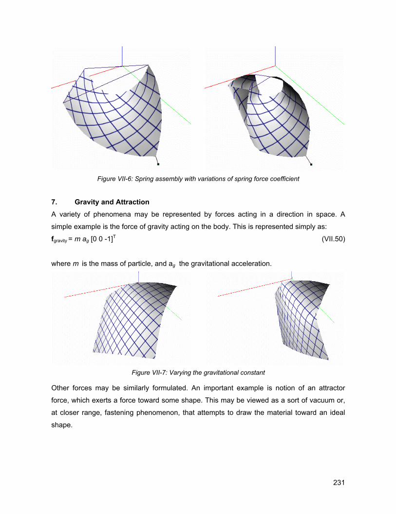
Figure VII-6: Spring assembly with variations of spring force coefficient

7. Gravity and Attraction A variety of phenomena may be represented by forces acting in a direction in space. A

simple example is the force of gravity acting on the body. This is represented simply as: fgravity = m ag [0 0 -1]T (VII.50)

where m is the mass of particle, and ag the gravitational acceleration.

Figure VII-7: Varying the gravitational constant

Other forces may be similarly formulated. An important example is notion of an attractor

force, which exerts a force toward some shape. This may be viewed as a sort of vacuum or,

at closer range, fastening phenomenon, that attempts to draw the material toward an ideal

shape.

231

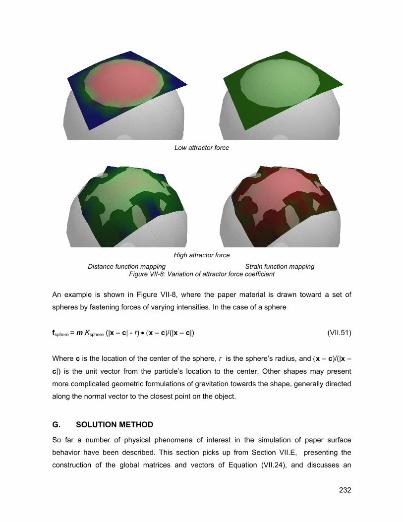
Low attractor force

High attractor force

Distance function mapping Strain function mapping Figure VII-8: Variation of attractor force coefficient

An example is shown in Figure VII-8, where the paper material is drawn toward a set of

spheres by fastening forces of varying intensities. In the case of a sphere

fsphere = m Ksphere (|x – c| - r) • (x – c)/(|x – c|) (VII.51)

Where c is the location of the center of the sphere, r is the sphere’s radius, and (x – c)/(|x –

c|) is the unit vector from the particle’s location to the center. Other shapes may present

more complicated geometric formulations of gravitation towards the shape, generally directed

along the normal vector to the closest point on the object.

G. SOLUTION METHOD

So far a number of physical phenomena of interest in the simulation of paper surface

behavior have been described. This section picks up from Section VII.E, presenting the

construction of the global matrices and vectors of Equation (VII.24), and discusses an

232

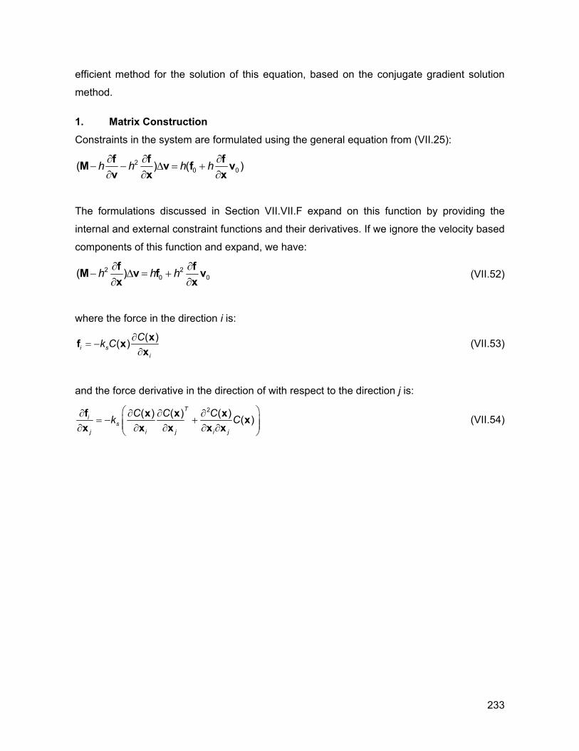
efficient method for the solution of this equation, based on the conjugate gradient solution

method.

1. Matrix Construction Constraints in the system are formulated using the general equation from (VII.25):

20 0( ) (h h h h∂ ∂ ∂

− − ∆ = +∂ ∂ ∂f f fM v fv x x

)v

The formulations discussed in Section VII.VII.F expand on this function by providing the

internal and external constraint functions and their derivatives. If we ignore the velocity based

components of this function and expand, we have:

20( )h h h∂ ∂

− ∆ = +∂f fM v fx x

20∂

v (VII.52)

where the force in the direction i is:

( )( )i si

Ck C ∂= −

∂xf x

x (VII.53)

and the force derivative in the direction of with respect to the direction j is:

2( ) ( ) ( ) ( )T

is

j i j i j

C C Ck ∂ ∂ ∂ ∂

= − +∂ ∂ ∂ ∂ ∂

f x x x xx x x x x

C (VII.54)

233

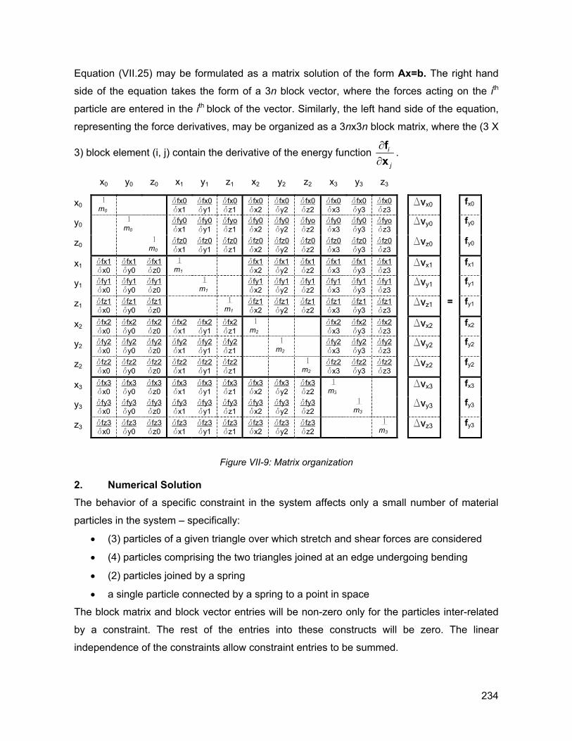
Equation (VII.25) may be formulated as a matrix solution of the form Ax=b. The right hand

side of the equation takes the form of a 3n block vector, where the forces acting on the ith

particle are entered in the ith block of the vector. Similarly, the left hand side of the equation,

representing the force derivatives, may be organized as a 3nx3n block matrix, where the (3 X

3) block element (i, j) contain the derivative of the energy function i

j

∂∂

fx

.

x

y

z

x

y

z

x

y

z

x

y

z

2T

p

T

b

i

x0 y0 z0 x1 y1 z1 x2 y2 z2 x3 y3 z3

0 1 m0

dfx0 dx1

dfx0 dy1

dfx0 dz1

dfx0 dx2

dfx0 dy2

dfx0 dz2

dfx0 dx3

dfx0 dy3

dfx0 dz3

Dvx0 fx0

0 1 m0

dfy0 dx1

dfy0 dy1

dfyo dz1

dfy0 dx2

dfy0 dy2

dfyo dz2

dfy0 dx3

dfy0 dy3

dfyo dz3

Dvy0 fy0

0 1 m0

dfz0 dx1

dfz0 dy1

dfz0 dz1

dfz0 dx2

dfz0 dy2

dfz0 dz2

dfz0 dx3

dfz0 dy3

dfz0 dz3

Dvz0 fy0

1 dfx1 dx0

dfx1 dy0

dfx1 dz0

1 m1

dfx1 dx2

dfx1 dy2

dfx1 dz2

dfx1 dx3

dfx1 dy3

dfx1 dz3

Dvx1 fx1

1 dfy1 dx0

dfy1 dy0

dfy1 dz0

1 m1 dfy1

dx2 dfy1 dy2

dfy1 dz2

dfy1 dx3

dfy1 dy3

dfy1 dz3

Dvy1 fy1

1 dfz1 dx0

dfz1 dy0

dfz1 dz0

1 m1

dfz1 dx2

dfz1 dy2

dfz1 dz2

dfz1 dx3

dfz1 dy3

dfz1 dz3

Dvz1 = fy1

2 dfx2 dx0

dfx2 dy0

dfx2 dz0

dfx2 dx1

dfx2 dy1

dfx2 dz1

1 m2

dfx2 dx3

dfx2 dy3

dfx2

dz3 Dvx2 fx2

2 dfy2 dx0

dfy2 dy0

dfy2 dz0

dfy2 dx1

dfy2 dy1

dfy2 dz1

1 m2

dfy2 dx3

dfy2 dy3

dfy2 dz3

Dvy2 fy2

2 dfz2 dx0

dfz2 dy0

dfz2 dz0

dfz2 dx1

dfz2 dy1

dfz2 dz1

1 m2

dfz2 dx3

dfz2 dy3

dfz2 dz3

Dvz2 fy2

3 dfx3 dx0

dfx3 dy0

dfx3 dz0

dfx3 dx1

dfx3 dy1

dfx3 dz1

dfx3 dx2

dfx3 dy2

dfx3 dz2

1 m3

Dvx3 fx3

3 dfy3 dx0

dfy3 dy0

dfy3 dz0

dfy3 dx1

dfy3 dy1

dfy3 dz1

dfy3 dx2

dfy3 dy2

dfy3 dz2

1 m3

Dvy3 fy3

3 dfz3 dx0

dfz3 dy0

dfz3 dz0

dfz3 dx1

dfz3 dy1

dfz3 dz1

dfz3 dx2

dfz3 dy2

dfz3 dz2

1 m3

Dvz3 fy3

Figure VII-9: Matrix organization

. Numerical Solution he behavior of a specific constraint in the system affects only a small number of material

articles in the system – specifically:

• (3) particles of a given triangle over which stretch and shear forces are considered

• (4) particles comprising the two triangles joined at an edge undergoing bending

• (2) particles joined by a spring

• a single particle connected by a spring to a point in space

he block matrix and block vector entries will be non-zero only for the particles inter-related

y a constraint. The rest of the entries into these constructs will be zero. The linear

ndependence of the constraints allow constraint entries to be summed.

234

Each particle in the system is represented as an object with a state, comprised of its:

• mass, mi ∈ R

• current position in space, xi ∈ R3

• current velocity, vi ∈ R3

• index into the global stiffness matrix and force vectors

At the beginning of each time step, the global derivative matrix A is initialized to be equal to

the inverse of the mass matrix 1/M, while the force vector global force vector b is set to 0. A

time step h is considered as input to the solution – the means for determining this time step

is presented in VI.H.3 below.

Each constraint is considered in turn, and for each constraint the related pairs of particles are

considered independently. The energy function C – a scalar - is computed for each

constraint. The derivatives of the constraint’s energy function ( ) / iC∂ ∂x x2

are determined for

each particle associated with the constraint. The second derivatives ( ) iC j∂ ∂ ∂x x x are then

computed for each particle pair.

The force on each particle fi is computed in a straightforward fashion using (VII.53),

multiplied by the time step, and the result added to the global force vector in the particle’s

associated block – the i th block of the force vector bi. Similarly, the second derivative

component 20h ∂

∂f vx

is computed from the force derivative of the particle, the time step

squared, and the velocity of the particle at the beginning of the time step.

The derivative of the force on particle i with respect to the variation in each of the constraint’s

associated particles j is next computed from the general form (VII.54), and added into the

global force derivative matrix at the block Ai,j . The change in velocity of the particles is

determined by solving the linear equation:

Dv = A-1b (VII.55)

From this result, the new velocities of the particles are computed in a straight forward fashion

by summing the particles’ velocities v0 with Dv. The new particle positions are then computed

235

by adding the multiplying this new velocity by the time step and adding to the original particle

position.

The solution of (VII.55) requires that the inverse of the matrix A be computed. Under the

most general circumstances, this inversion is of order O(n3) complexity – a potentially heavy

penalty in the performance of the backwards Euler simulation approach. However,

characteristics of the matrix can be taken advantage of to reduce the computational

complexity of this inversion. This linear system is sparse, since block matrix elements are

non zero only for those entries corresponding to particles inter-related by constraints: the

neighboring particles in the mesh, or particles joined by springs. The sparisty pattern for a

simple system is illustrate in Figure VII-10 below.

Additionally, since the matrix is symmetric. Furthermore the matrix A is

positive definite, since the energy in the system is never less than zero. These conditions are

sufficient to allow the matrix inversion to be conducted numerically, using a conjugate

gradient method70,76. This approach reduces the computational complexity of the matrix

inversion to approximately O(n logn), well justified on the basis of the larger time steps

afforded relative to the forward Euler solution method.

/i j j∂ ∂ = ∂ ∂f x f x/ i

236

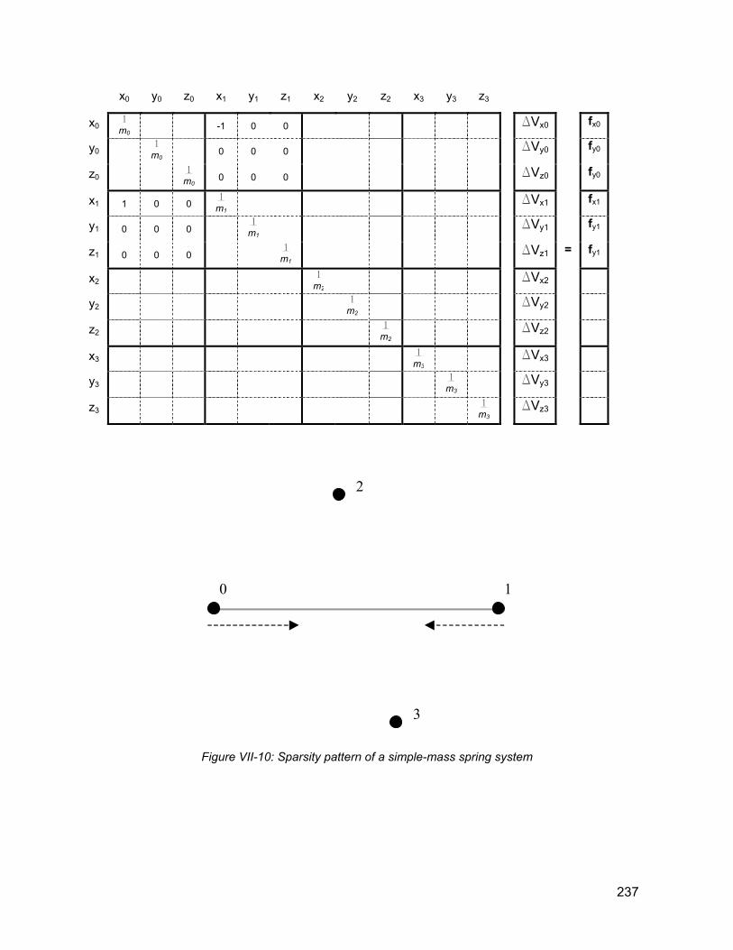
x

y

z

x

y

z

x

y

z

x

y

z

x0 y0 z0 x1 y1 z1 x2 y2 z2 x3 y3 z3

1 0 -1 0 0 m0

DVx0 fx0

0 1 m0

0 0 0 DVy0 fy0

0 1 m0

0 0 0 DVz0 fy0

1 1 0 0 1 m1

DVx1 fx1

1 0 0 0 1 m1 DVy1 fy1

1 0 0 0 1 m1 DVz1 = fy1

2 1 m2

DVx2

2 1 m2 DVy2

2 1 m2 DVz2

3 1 m3

DVx3

3 1 m3 DVy3

3 1 m3

DVz3

237

0 1

2

3

Figure VII-10: Sparsity pattern of a simple-mass spring system

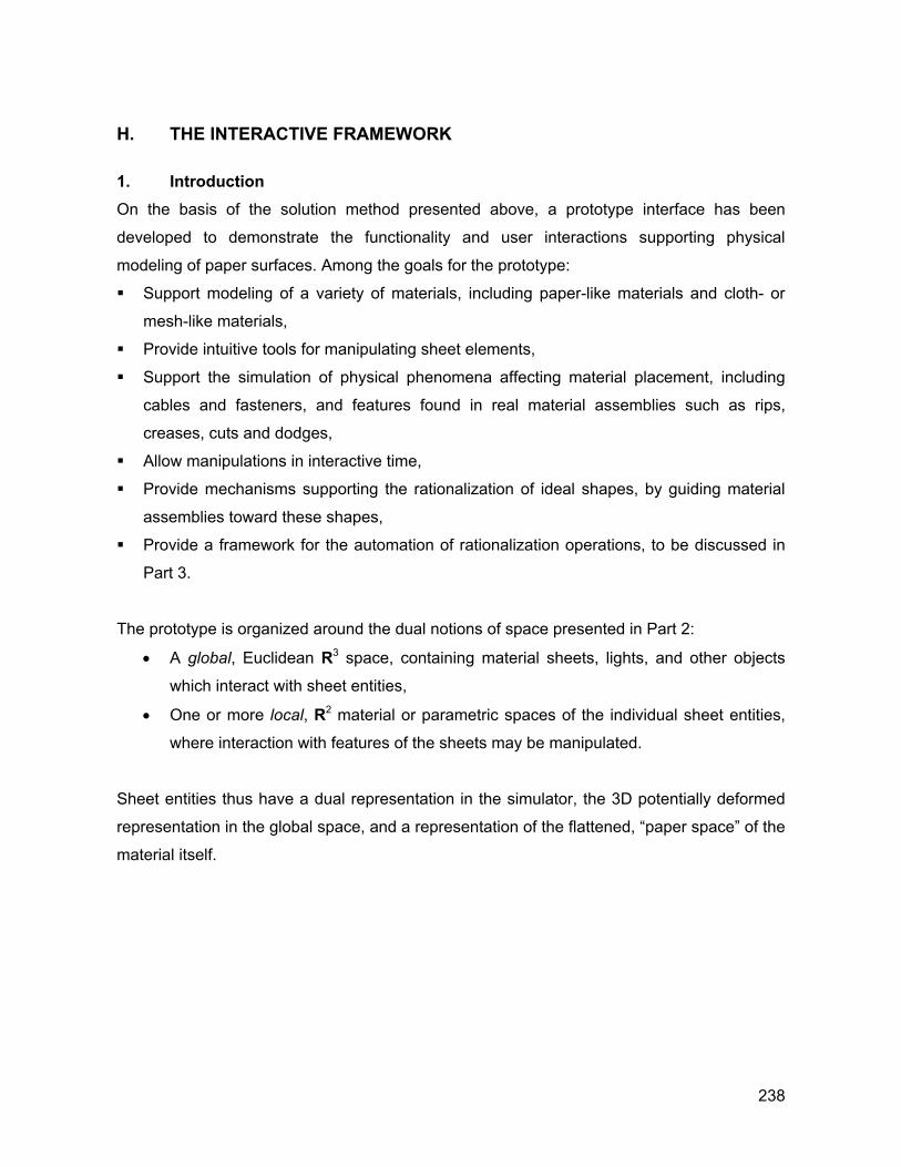
H. THE INTERACTIVE FRAMEWORK

1. Introduction On the basis of the solution method presented above, a prototype interface has been

developed to demonstrate the functionality and user interactions supporting physical

modeling of paper surfaces. Among the goals for the prototype:

Support modeling of a variety of materials, including paper-like materials and cloth- or

mesh-like materials,

Provide intuitive tools for manipulating sheet elements,

Support the simulation of physical phenomena affecting material placement, including

cables and fasteners, and features found in real material assemblies such as rips,

creases, cuts and dodges,

Allow manipulations in interactive time,

Provide mechanisms supporting the rationalization of ideal shapes, by guiding material

assemblies toward these shapes,

Provide a framework for the automation of rationalization operations, to be discussed in

Part 3.

The prototype is organized around the dual notions of space presented in Part 2:

• A global, Euclidean R3 space, containing material sheets, lights, and other objects

which interact with sheet entities,

• One or more local, R2 material or parametric spaces of the individual sheet entities,

where interaction with features of the sheets may be manipulated.

Sheet entities thus have a dual representation in the simulator, the 3D potentially deformed

representation in the global space, and a representation of the flattened, “paper space” of the

material itself.

238

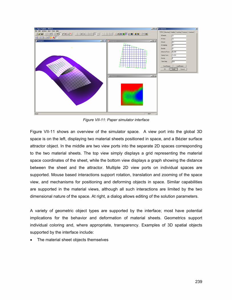
Figure VII-11: Paper simulator interface

Figure VII-11 shows an overview of the simulator space. A view port into the global 3D

space is on the left, displaying two material sheets positioned in space, and a Bézier surface

attractor object. In the middle are two view ports into the separate 2D spaces corresponding

to the two material sheets. The top view simply displays a grid representing the material

space coordinates of the sheet, while the bottom view displays a graph showing the distance

between the sheet and the attractor. Multiple 2D view ports on individual spaces are

supported. Mouse based interactions support rotation, translation and zooming of the space

view, and mechanisms for positioning and deforming objects in space. Similar capabilities

are supported in the material views, although all such interactions are limited by the two

dimensional nature of the space. At right, a dialog allows editing of the solution parameters.

A variety of geometric object types are supported by the interface; most have potential

implications for the behavior and deformation of material sheets. Geometrics support

individual coloring and, where appropriate, transparency. Examples of 3D spatial objects

supported by the interface include:

• The material sheet objects themselves

239

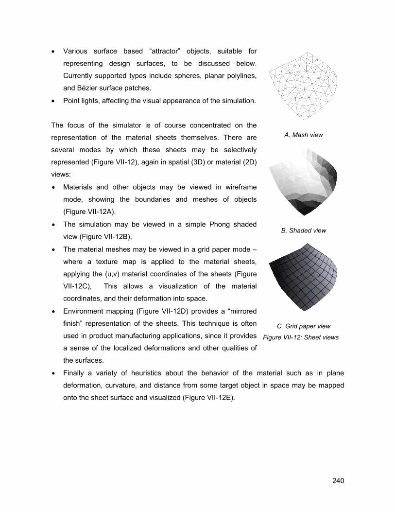
• Various surface based “attractor” objects, suitable for

representing design surfaces, to be discussed below.

Currently supported types include spheres, planar polylines,

and Bézier surface patches.

• Point lights, affecting the visual appearance of the simulation.

The focus of the simulator is of course concentrated on the

representation of the material sheets themselves. There are

several modes by which these sheets may be selectively

represented (Figure VII-12), again in spatial (3D) or material (2D)

views:

• Materials and other objects may be viewed in wireframe

mode, showing the boundaries and meshes of objects

(Figure VII-12A).

• The simulation may be viewed in a simple Phong shaded

view (Figure VII-12B),

• The material meshes may be viewed in a grid paper mode –

where a texture map is applied to the material sheets,

applying the (u,v) material coordinates of the sheets (Figure

VII-12C), This allows a visualization of the material

coordinates, and their deformation into space.

A. Mash view

B. Shaded view

C. Grid paper view

Figure VII-12: Sheet views

• Environment mapping (Figure VII-12D) provides a “mirrored

finish” representation of the sheets. This technique is often

used in product manufacturing applications, since it provides

a sense of the localized deformations and other qualities of

the surfaces.

• Finally a variety of heuristics about the behavior of the material such as in plane

deformation, curvature, and distance from some target object in space may be mapped

onto the sheet surface and visualized (Figure VII-12E).

240

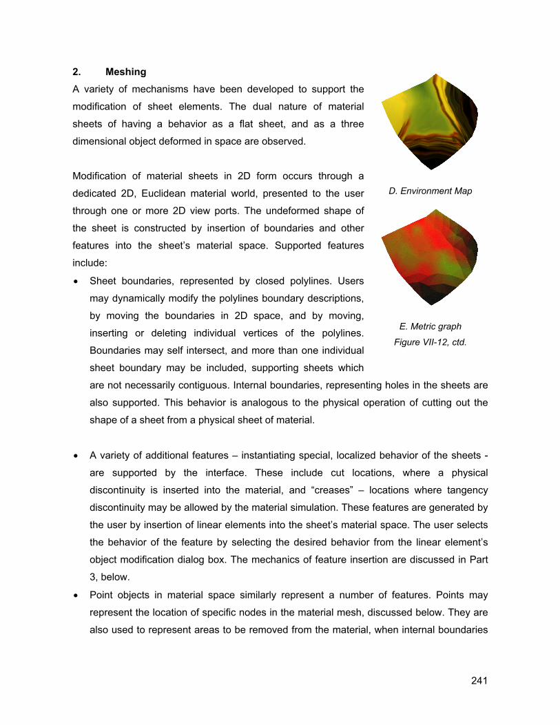
2. Meshing A variety of mechanisms have been developed to support the

modification of sheet elements. The dual nature of material

sheets of having a behavior as a flat sheet, and as a three

dimensional object deformed in space are observed.

Modification of material sheets in 2D form occurs through a

dedicated 2D, Euclidean material world, presented to the user

through one or more 2D view ports. The undeformed shape of

the sheet is constructed by insertion of boundaries and other

features into the sheet’s material space. Supported features

include:

• Sheet boundaries, represented by closed polylines. Users

may dynamically modify the polylines boundary descriptions,

by moving the boundaries in 2D space, and by moving,

inserting or deleting individual vertices of the polylines.

Boundaries may self intersect, and more than one individual

sheet boundary may be included, supporting sheets which

are not necessarily contiguous. Internal boundaries, representing holes in the sheets are

also supported. This behavior is analogous to the physical operation of cutting out the

shape of a sheet from a physical sheet of material.

D. Environment Map

E. Metric graph

Figure VII-12, ctd.

• A variety of additional features – instantiating special, localized behavior of the sheets -

are supported by the interface. These include cut locations, where a physical

discontinuity is inserted into the material, and “creases” – locations where tangency

discontinuity may be allowed by the material simulation. These features are generated by

the user by insertion of linear elements into the sheet’s material space. The user selects

the behavior of the feature by selecting the desired behavior from the linear element’s

object modification dialog box. The mechanics of feature insertion are discussed in Part

3, below.

• Point objects in material space similarly represent a number of features. Points may

represent the location of specific nodes in the material mesh, discussed below. They are

also used to represent areas to be removed from the material, when internal boundaries

241

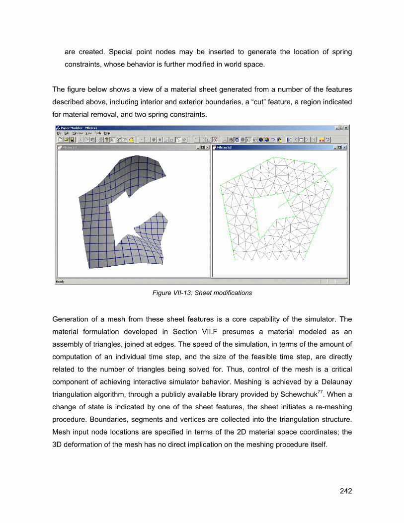
are created. Special point nodes may be inserted to generate the location of spring

constraints, whose behavior is further modified in world space.

The figure below shows a view of a material sheet generated from a number of the features

described above, including interior and exterior boundaries, a “cut” feature, a region indicated

for material removal, and two spring constraints.

Generation of a mesh from these sheet features is a core capability of the simulator. The

material formulation developed in Section VII.F presumes a material modeled as an

assembly of triangles, joined at edges. The speed of the simulation, in terms of the amount of

computation of an individual time step, and the size of the feasible time step, are directly

related to the number of triangles being solved for. Thus, control of the mesh is a critical

component of achieving interactive simulator behavior. Meshing is achieved by a Delaunay

triangulation algorithm, through a publicly available library provided by Schewchuk77. When a

change of state is indicated by one of the sheet features, the sheet initiates a re-meshing

procedure. Boundaries, segments and vertices are collected into the triangulation structure.

Mesh input node locations are specified in terms of the 2D material space coordinates; the

3D deformation of the mesh has no direct implication on the meshing procedure itself.

Figure VII-13: Sheet modifications

242

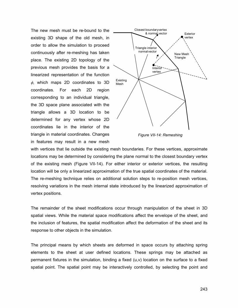
The new mesh must be re-bound to the

existing 3D shape of the old mesh, in

order to allow the simulation to proceed

continuously after re-meshing has taken

place. The existing 2D topology of the

previous mesh provides the basis for a

linearized representation of the function

φ, which maps 2D coordinates to 3D

coordinates. For each 2D region

corresponding to an individual triangle,

the 3D space plane associated with the

triangle allows a 3D location to be

determined for any vertex whose 2D

coordinates lie in the interior of the

triangle in material coordinates. Changes

in features may result in a new mesh

with vertices that lie outside the existing mesh boundaries. For these vertices, approximate

locations may be determined by considering the plane normal to the closest boundary vertex

of the existing mesh (Figure VII-14). For either interior or exterior vertices, the resulting

location will be only a linearized approximation of the true spatial coordinates of the material.

The re-meshing technique relies on additional solution steps to re-position mesh vertices,

resolving variations in the mesh internal state introduced by the linearized approximation of

vertex positions.

E xterior vertex

Interior vertex

New Mesh Triangle

Existing Mesh

Closest boundary vertex & normal vector

Triangle interior normal vector

Figure VII-14: Remeshing

The remainder of the sheet modifications occur through manipulation of the sheet in 3D

spatial views. While the material space modifications affect the envelope of the sheet, and

the inclusion of features, the spatial modification affect the deformation of the sheet and its

response to other objects in the simulation.

The principal means by which sheets are deformed in space occurs by attaching spring

elements to the sheet at user defined locations. These springs may be attached as

permanent fixtures in the simulation, binding a fixed (u,v) location on the surface to a fixed

spatial point. The spatial point may be interactively controlled, by selecting the point and

243

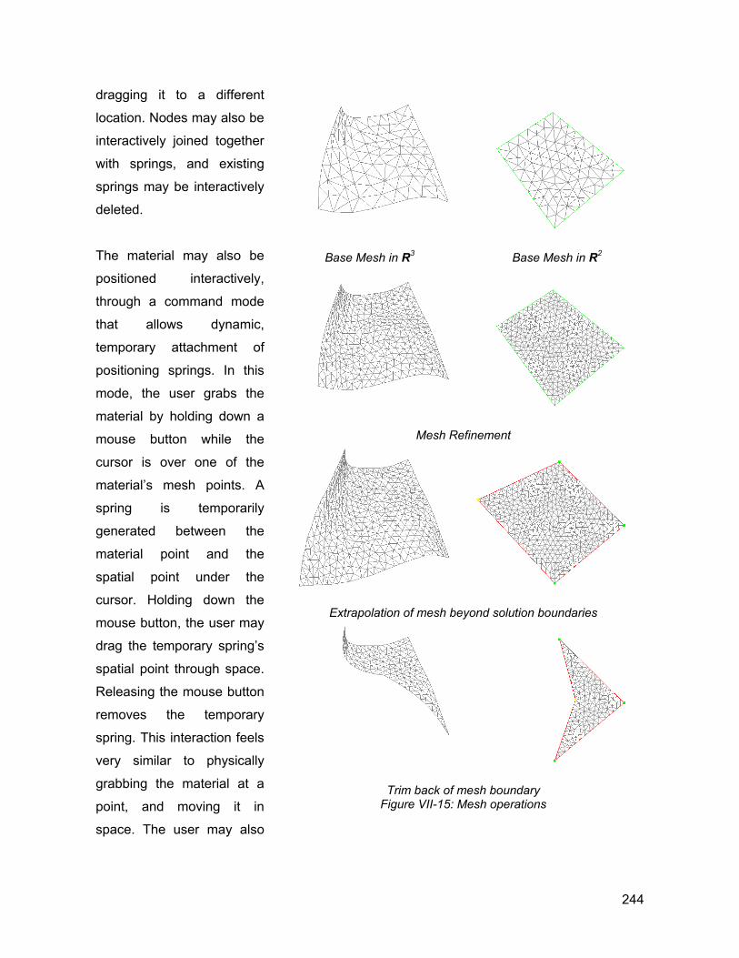
dragging it to a different

location. Nodes may also be

interactively joined together

with springs, and existing

springs may be interactively

deleted.

The material may also be

positioned interactively,

through a command mode

that allows dynamic,

temporary attachment of

positioning springs. In this

mode, the user grabs the

material by holding down a

mouse button while the

cursor is over one of the

material’s mesh points. A

spring is temporarily

generated between the

material point and the

spatial point under the

cursor. Holding down the

mouse button, the user may

drag the temporary spring’s

spatial point through space.

Releasing the mouse button

removes the temporary

spring. This interaction feels

very similar to physically

grabbing the material at a

point, and moving it in

space. The user may also

Base Mesh in R3 Base Mesh in R2

Mesh Refinement

Extrapolation of mesh beyond solution boundaries

Trim back of mesh boundary Figure VII-15: Mesh operations

244

elect to make the spring permanent – fixing the material point permanently to the desired

location.

3. Attractor Objects The simulator is not simply intended to allow interactive manipulation of sheet materials. A

second important application is to allow the rationalization of ideal surface shapes. This use

is addressed by allowing the selective application of an attractive force between the material

sheets and other shapes in the simulation. A variety of spatial objects support this attractive

force, including sphere objects and smoothly continuous surface objects based on Bézier

surface patches.

The attractor force is represented as a force between each of the material points in the

sheet, and the closest point of the closest attracting object in the simulation. For each object

in the simulation comprised of a smoothly continuous surface, the closest point to a given

material point will be point on the object whose surface normal passes through the material

points location in R3. For spheres this is an easy computation, since this normal will be

aligned with the line between the material point and the sphere’s center point. For Bézier

surfaces, a algorithm is used that finds this point on the surface65. For each of the sheet’s

mesh vertices, these closest point algorithms are run for each attractor object in the

simulation, and the closest of these points is selected as the actual attractor object. A force in

the direction of the vector between the mesh point and the surface normal point of the

attractor is enacted on the mesh point. The strength of this attractive force is controlled by a

parameter set globally for the simulation.

The effect is to draw the sheet materials to objects in the simulation. At the same time, the

material’s internal constraints counteract the tendency of the attractor objects to deform the

sheet into a potentially infeasible shape. The magnitude of this force must of course be

limited, so that the attractive force does not overwhelm the internal material constraints.

245

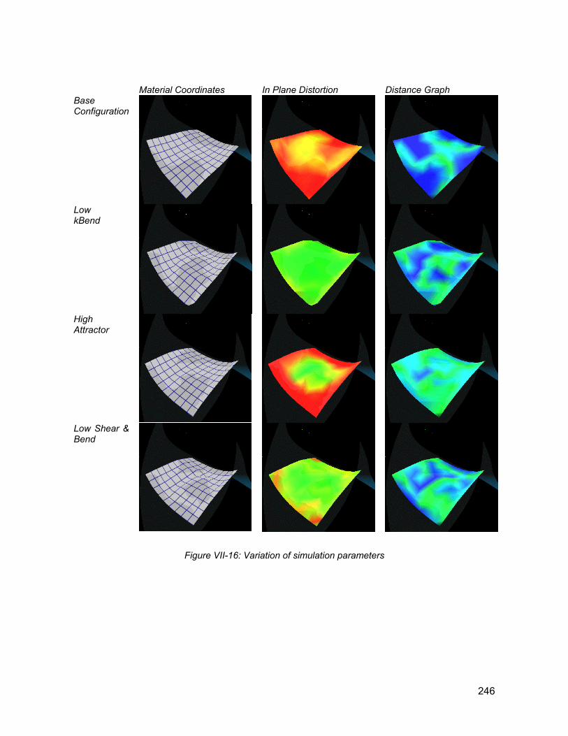
Material Coordinates In Plane Distortion Distance Graph Base Configuration

Low kBend

High Attractor

Low Shear & Bend

Figure VII-16: Variation of simulation parameters

246

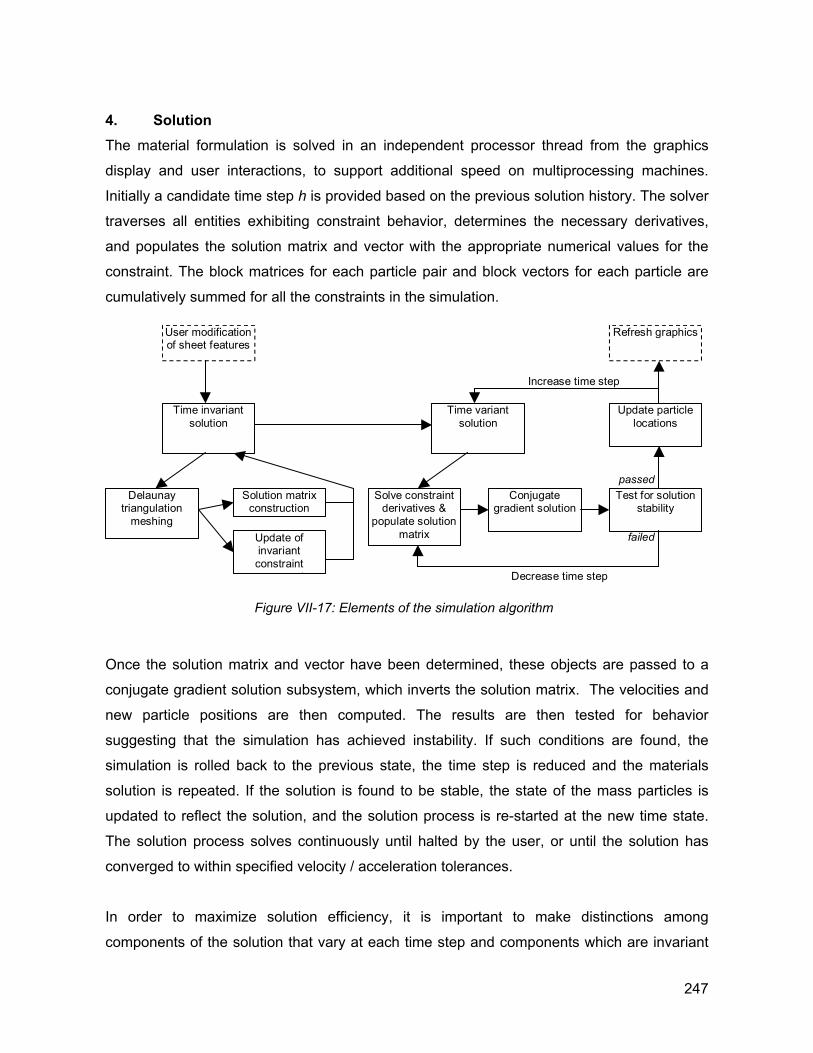
4. Solution The material formulation is solved in an independent processor thread from the graphics

display and user interactions, to support additional speed on multiprocessing machines.

Initially a candidate time step h is provided based on the previous solution history. The solver

traverses all entities exhibiting constraint behavior, determines the necessary derivatives,

and populates the solution matrix and vector with the appropriate numerical values for the

constraint. The block matrices for each particle pair and block vectors for each particle are

cumulatively summed for all the constraints in the simulation.

Time invariant solution

User modification of sheet features

Delaunay triangulation

meshing

Solution matrix construction

Update of invariant constraint

t

Time variant solution

Solve constraint derivatives &

populate solution matrix

Conjugate gradient solution

Update particle locations

Refresh graphics

Test for solution stability

passed

failed

Decrease time step

Increase time step

Figure VII-17: Elements of the simulation algorithm

Once the solution matrix and vector have been determined, these objects are passed to a

conjugate gradient solution subsystem, which inverts the solution matrix. The velocities and

new particle positions are then computed. The results are then tested for behavior

suggesting that the simulation has achieved instability. If such conditions are found, the

simulation is rolled back to the previous state, the time step is reduced and the materials

solution is repeated. If the solution is found to be stable, the state of the mass particles is

updated to reflect the solution, and the solution process is re-started at the new time state.

The solution process solves continuously until halted by the user, or until the solution has

converged to within specified velocity / acceleration tolerances.

In order to maximize solution efficiency, it is important to make distinctions among

components of the solution that vary at each time step and components which are invariant

247

as long as the 2D mesh remains the same. Different user or simulation events may trigger

refreshing of either or both of these sets of components. Changes in sheet features requiring

a change of the mesh will require a refresh of time invariant components. Changes requiring

a refresh of time invariant components will require re-generation of the time dependent

components as well.

Components of the solution which are invariant over time steps include:

• The mesh topology, including vertex / edge / triangle structure and adjacencies

• Vertex material coordinates, and components of the solution determined solely from

material coordinates, including the triangle derivates Du1,Du2,Dv1,Dv2, and the inverse

of the material gradient 1

1 2

1 2

u uv v

−∆ ∆ ∆ ∆

from Section VII.B,

• The size and sparsity structures of the solution matrix A and vector b from Section

VII.G.1.

• The mass matrix M, and a pre-conditioning matrix for the conjugate gradient solver

M-1.

Components of the solution that are time variant, and must be re-generated at each step

include:

• The spatial coordinates of end locations for fixed springs – if modified by users,

• Changes in material or constraint constants, including stretch, shear, bending, and

spring forces.

• Spatial coordinates, velocity and Dv vectors for all mass particles,

• The energy function derivates

• The numerical valuation of the solution matrix and vector A and b,

5. Time step selection and instability detection The initial time step for the solution is provided by a default, or provided by the user through

a dialog box. In order to achieve computational efficiency of the solution, the time step should

be as large as possible without resulting in instability. Unfortunately, there is no determinate

way to compute either the appropriate time step or to detect for instability. Additionally, the

size of a stable time step varies over the course of the simulation. For example, a flat mesh

with no acceleration or constraints can be solved for an indeterminately large time step

248

(although the results aren’t particularly interesting!). Heuristics are employed to search for an

appropriately large time step, and to check the solution to determine whether instability has

occurred.

If the previous solution was achieved in a stable manner, the current time step may be

increased slightly. We multiply the existing time step by a small factor, which may be set by

the user. A default multiplier of 110% is used for increasing the time step between

subsequent stable solutions. If the solution is determined to be unstable, a more drastic

reduction multiplier (default 70%) is used to get the solution quickly back on track, with the

knowledge that subsequent stable solutions will soon get the solution moving forward again

quickly.

There are a number of heuristics that can be employed to check for stability. The most

obvious and direct is to check for what seem like dangerous changes in velocity – the Dv

resulting from the solution of the matrix equation. An excessive deformation of any triangle

edge relative to its undeformed configuration may also signal impending instability.

I. ISOMETRIES

The materials modeling formulation presented in this chapter offers some substantial

improvements over the existing paper surface representations currently employed in the

firm’s digital process. The principal benefits of the materials simulation representation are the

result of a more sophisticated representation of the actual constraints imposed by the surface

materials on project forms. The material formulation provides the solution of paper surface

configurations internally, allowing the user to interact with the surfaces in a manner similar to

that provided by physical sheet materials. Certain features of physical sheet forms are quite

difficult to reconstruct using constrained gaussian curvature approaches, and are prohibited

by developable surface representations.

At the same time, the material simulation representation has much in common with these

representations, by virtue of their shared topological basis as <R2 x R3 > manifolds. This

shared topological basis suggests some additional comparisons of these representations,

and allows the possibility for either integrating these representations into a common

framework.

249

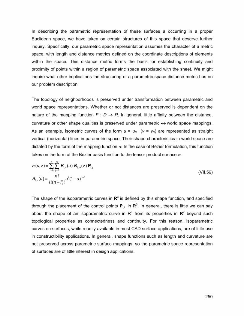
In describing the parametric representation of these surfaces a occurring in a proper

Euclidean space, we have taken on certain structures of this space that deserve further

inquiry. Specifically, our parametric space representation assumes the character of a metric

space, with length and distance metrics defined on the coordinate descriptions of elements

within the space. This distance metric forms the basis for establishing continuity and

proximity of points within a region of parametric space associated with the sheet. We might

inquire what other implications the structuring of a parametric space distance metric has on

our problem description.

The topology of neighborhoods is preserved under transformation between parametric and

world space representations. Whether or not distances are preserved is dependent on the

nature of the mapping function F : D → R. In general, little affinity between the distance,

curvature or other shape qualities is preserved under parametric ↔ world space mappings.

As an example, isometric curves of the form u = uC (v = vC) are represented as straight

vertical (horizontal) lines in parametric space. Their shape characteristics in world space are

dictated by the form of the mapping function σ. In the case of Bézier formulation, this function

takes on the form of the Bézier basis function to the tensor product surface σ:

, ,0 0

,

( , ) ( ) ( )

!( ) (1 )!( )!

n m

i n j m i ji j

i n ii n

u v B u B v

nB u u ui n i

σ= =

−

=

= −−

∑∑ P ,

(VII.56)

The shape of the isoparametric curves in R3 is defined by this shape function, and specified

through the placement of the control points Pi,j in R3. In general, there is little we can say

about the shape of an isoparametric curve in R3 from its properties in R2 beyond such

topological properties as connectedness and continuity. For this reason, isoparametric

curves on surfaces, while readily available in most CAD surface applications, are of little use

in constructibility applications. In general, shape functions such as length and curvature are

not preserved across parametric surface mappings, so the parametric space representation

of surfaces are of little interest in design applications.

250

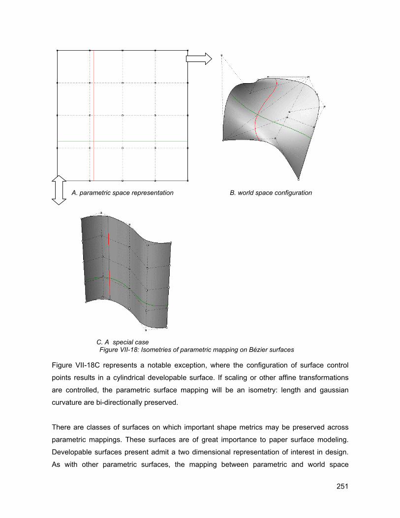
A. parametric space representation B. world space configuration

C. A special case Figure VII-18: Isometries of parametric mapping on Bézier surfaces

Figure VII-18C represents a notable exception, where the configuration of surface control

points results in a cylindrical developable surface. If scaling or other affine transformations

are controlled, the parametric surface mapping will be an isometry: length and gaussian

curvature are bi-directionally preserved.

There are classes of surfaces on which important shape metrics may be preserved across

parametric mappings. These surfaces are of great importance to paper surface modeling.

Developable surfaces present admit a two dimensional representation of interest in design.

As with other parametric surfaces, the mapping between parametric and world space

251

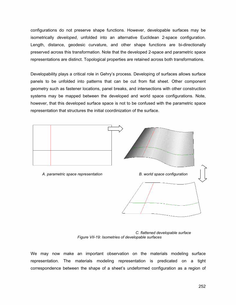
configurations do not preserve shape functions. However, developable surfaces may be

isometrically developed, unfolded into an alternative Euclidean 2-space configuration.

Length, distance, geodesic curvature, and other shape functions are bi-directionally

preserved across this transformation. Note that the developed 2-space and parametric space

representations are distinct. Topological properties are retained across both transformations.

Developability plays a critical role in Gehry’s process. Developing of surfaces allows surface

panels to be unfolded into patterns that can be cut from flat sheet. Other component

geometry such as fastener locations, panel breaks, and intersections with other construction

systems may be mapped between the developed and world space configurations. Note,

however, that this developed surface space is not to be confused with the parametric space

representation that structures the initial coordinization of the surface.

A. parametric space representation B. world space configuration

C. flattened developable surface

Figure VII-19: Isometries of developable surfaces

We may now make an important observation on the materials modeling surface

representation. The materials modeling representation is predicated on a tight

correspondence between the shape of a sheet’s undeformed configuration as a region of

252

material space, and its deformed configuration in R3. The energy functions presented in

Section VII.F are described by stretch and shear deformation, computed from the derivatives

of the mapping function.

In applying the physical modeling approach to paper surfaces, we are principally concerned

with materials where the in plane stretch and shear siffness is quite high compared to

bending and other force phenomena. We can achieve large scale deformations of the sheet’s

configuration in world space while incurring insubstantial deformation in the sheet.

If we presume small in-plane deformation of the surface in its R3 configuration, the mapping

between parametric and world spaces will be approximately isometric. Qualitatively, we can

observe this fact in the material simulations presented in Chapter VII and below. Lengths,

angles and geodesic curvatures are preserved between geometric features in parametric

space and their transformed counterparts on the surface in R3.

Material space configuration “world” space configuration Figure VII-20: Isometries of the materials based formulation

The material space representation thus has an important spatial and design quality. It is the

originating, two dimensional paper space of the surface in its flat, pre-configured state.

Designed objects draw important shape qualities from their occupancy of this space. Cuts

and other operations performed by designers on the materials are appropriately represented

by shape features in material space. The impacts of these features’ shapes on the feasible

253

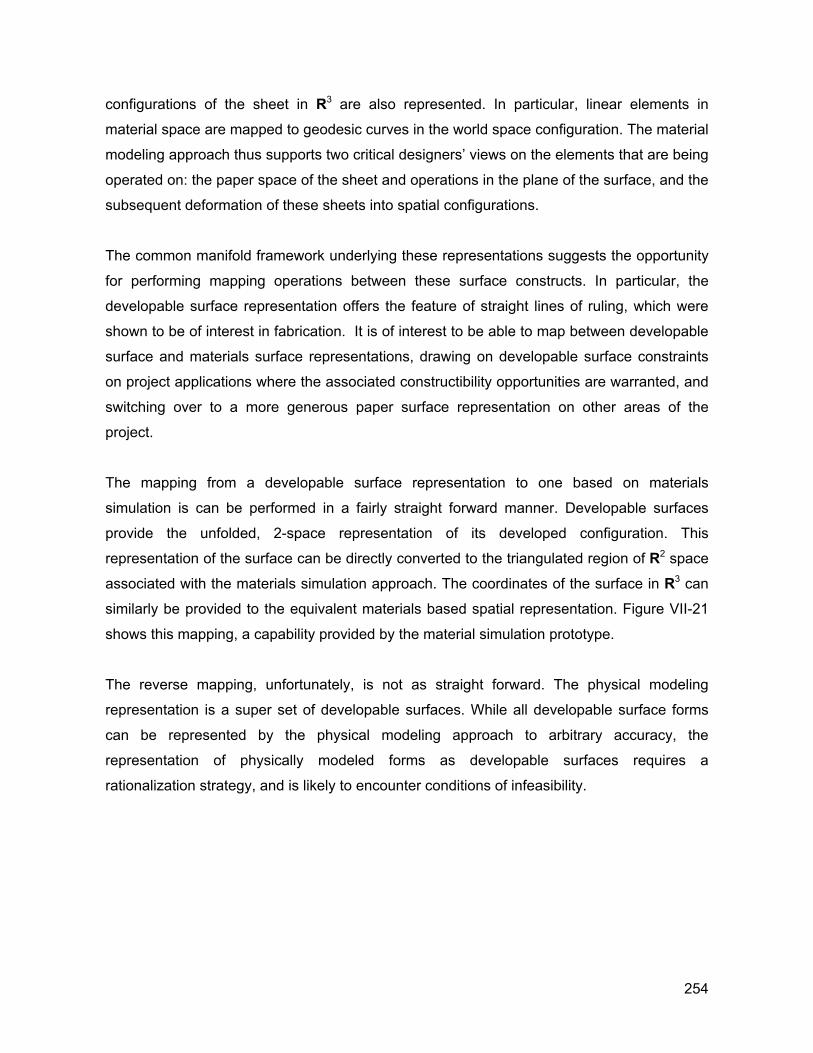
configurations of the sheet in R3 are also represented. In particular, linear elements in

material space are mapped to geodesic curves in the world space configuration. The material

modeling approach thus supports two critical designers’ views on the elements that are being

operated on: the paper space of the sheet and operations in the plane of the surface, and the

subsequent deformation of these sheets into spatial configurations.

The common manifold framework underlying these representations suggests the opportunity

for performing mapping operations between these surface constructs. In particular, the

developable surface representation offers the feature of straight lines of ruling, which were

shown to be of interest in fabrication. It is of interest to be able to map between developable

surface and materials surface representations, drawing on developable surface constraints

on project applications where the associated constructibility opportunities are warranted, and

switching over to a more generous paper surface representation on other areas of the

project.

The mapping from a developable surface representation to one based on materials

simulation is can be performed in a fairly straight forward manner. Developable surfaces

provide the unfolded, 2-space representation of its developed configuration. This

representation of the surface can be directly converted to the triangulated region of R2 space

associated with the materials simulation approach. The coordinates of the surface in R3 can

similarly be provided to the equivalent materials based spatial representation. Figure VII-21

shows this mapping, a capability provided by the material simulation prototype.

The reverse mapping, unfortunately, is not as straight forward. The physical modeling

representation is a super set of developable surfaces. While all developable surface forms

can be represented by the physical modeling approach to arbitrary accuracy, the

representation of physically modeled forms as developable surfaces requires a

rationalization strategy, and is likely to encounter conditions of infeasibility.

254

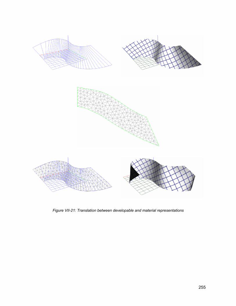
Figure VII-21: Translation between developable and material representations

255

J. MATERIALS MODELING APPLICATION: GUGGENHEIM INSTALLATION

The first application of the materials modeling prototype on a Gehry project occurred in June,

2001, on a sculptural installation in the Gehry Retrospective show, installed in the rotunda of

the New York Guggenheim museum. The sculpture called for the installation of 10 steel

mesh curtains, to be hung from the concrete radial structural members supporting the

skylight of Wright’s design. The curtain assembly was to be constructed out a wire mesh

material, comprised of interwoven spirals of steel wire oriented approximately horizontally.

The curtains were built up out of three layers of the material, separated approximately 6” by

wire spacers. The curtains were to be positioned by a series of cables attached from the

curtains to points on the ceilings of the galleries neighboring the rotunda.

An initial design for the installation was developed during approximately three months prior to

the opening of the exhibit. Each of the curtains was designed to be suspended the full height

of the rotunda, from an attachment mechanism on the skylight structural members to a height

of approximately 10’ above the rotunda floor, for an approximate vertical dimension of 80’.

The cables would be connected to two parallel steel rods, attached to the mesh face, and

located approximately ¼ of the distance from the edges of each panel. These steel rods

would provide additional stiffness of the material in the vertical direction, and locally stiffen

the material, to minimize distortion of the material at the points of connection to the cables.

From its initial position oriented radially aligned with the skylight structural members, each

curtain would describe an S-shaped curve, sweeping downward and clockwise in a similar

sense to the organization of the rotunda parapet and galleries, until it eventually aligned

roughly with the surface of the rotunda parapet.

Each of the curtain assemblies was to be tied back from both sides of the curtain at each

level of the rotunda. The Guggenheim required that no attachments be made into the

surfaces facing the rotunda itself. Additional structural requirements of the galleries dictated

that attachments for tension cables be placed in a ring approximately 12’ outward from the

parapet edge into the ceiling of the galleries.

256

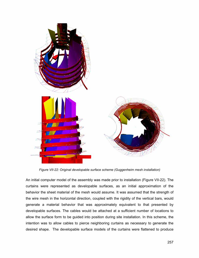
Figure VII-22: Original developable surface scheme (Guggenheim mesh installation)

An initial computer model of the assembly was made prior to installation (Figure VII-22). The

curtains were represented as developable surfaces, as an initial approximation of the

behavior the sheet material of the mesh would assume. It was assumed that the strength of

the wire mesh in the horizontal direction, coupled with the rigidity of the vertical bars, would

generate a material behavior that was approximately equivalent to that presented by

developable surfaces. The cables would be attached at a sufficient number of locations to

allow the surface form to be guided into position during site installation. In this scheme, the

intention was to allow cables to pierce neighboring curtains as necessary to generate the

desired shape. The developable surface models of the curtains were flattened to produce

257

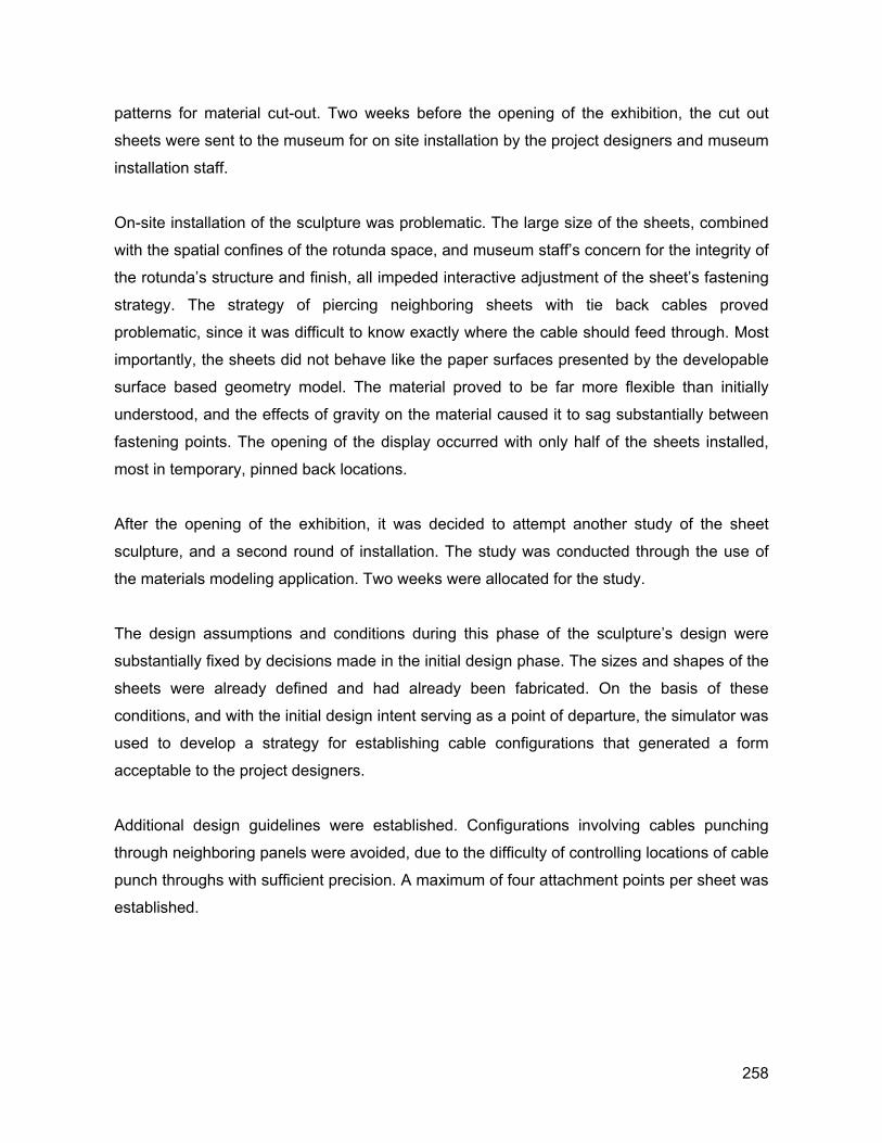
patterns for material cut-out. Two weeks before the opening of the exhibition, the cut out

sheets were sent to the museum for on site installation by the project designers and museum

installation staff.

On-site installation of the sculpture was problematic. The large size of the sheets, combined

with the spatial confines of the rotunda space, and museum staff’s concern for the integrity of

the rotunda’s structure and finish, all impeded interactive adjustment of the sheet’s fastening

strategy. The strategy of piercing neighboring sheets with tie back cables proved

problematic, since it was difficult to know exactly where the cable should feed through. Most

importantly, the sheets did not behave like the paper surfaces presented by the developable

surface based geometry model. The material proved to be far more flexible than initially

understood, and the effects of gravity on the material caused it to sag substantially between

fastening points. The opening of the display occurred with only half of the sheets installed,

most in temporary, pinned back locations.

After the opening of the exhibition, it was decided to attempt another study of the sheet

sculpture, and a second round of installation. The study was conducted through the use of

the materials modeling application. Two weeks were allocated for the study.

The design assumptions and conditions during this phase of the sculpture’s design were

substantially fixed by decisions made in the initial design phase. The sizes and shapes of the

sheets were already defined and had already been fabricated. On the basis of these

conditions, and with the initial design intent serving as a point of departure, the simulator was

used to develop a strategy for establishing cable configurations that generated a form

acceptable to the project designers.

Additional design guidelines were established. Configurations involving cables punching

through neighboring panels were avoided, due to the difficulty of controlling locations of cable

punch throughs with sufficient precision. A maximum of four attachment points per sheet was

established.

258

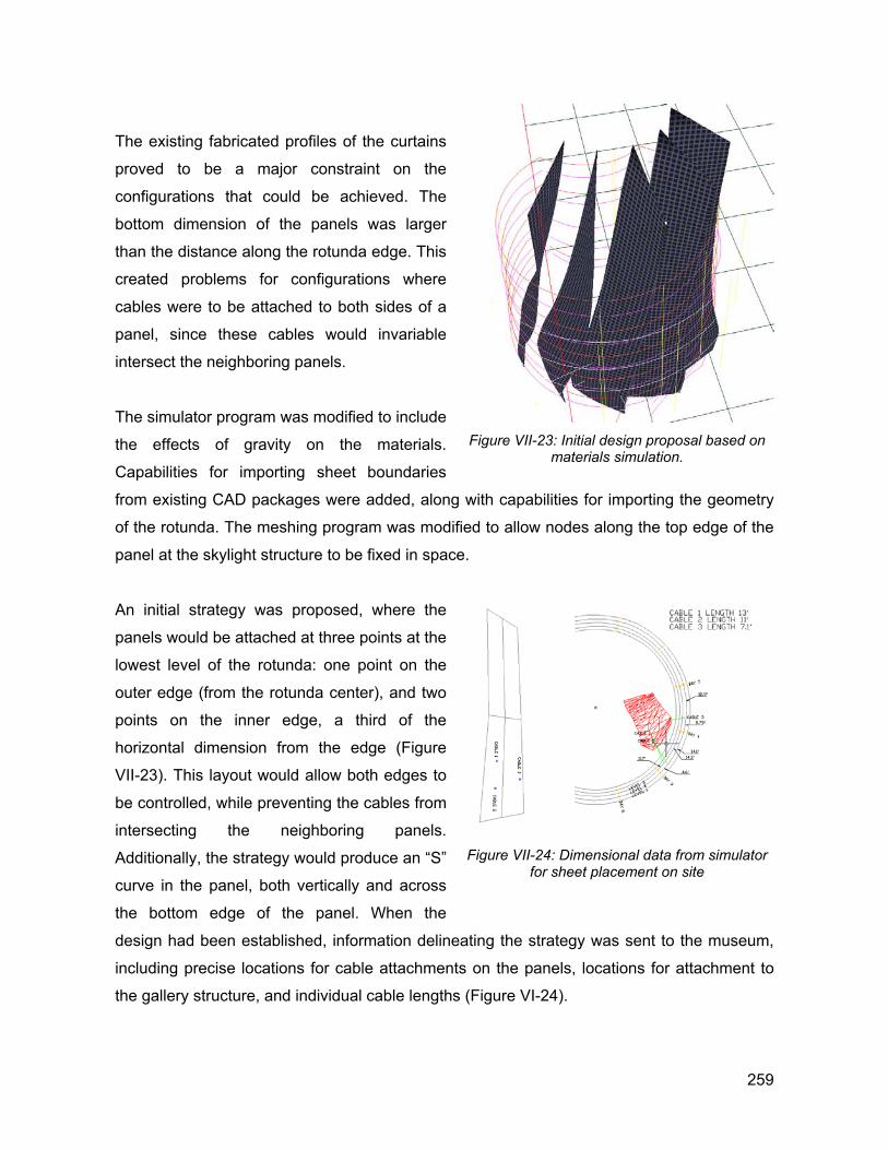
The existing fabricated profiles of the curtains

proved to be a major constraint on the

configurations that could be achieved. The

bottom dimension of the panels was larger

than the distance along the rotunda edge. This

created problems for configurations where

cables were to be attached to both sides of a

panel, since these cables would invariable

intersect the neighboring panels.

The simulator program was modified to include

the effects of gravity on the materials.

Capabilities for importing sheet boundaries

from existing CAD packages were added, along with capabilities for importing the geometry

of the rotunda. The meshing program was modified to allow nodes along the top edge of the

panel at the skylight structure to be fixed in space.

Figure VII-23: Initial design proposal based on

materials simulation.

An initial strategy was proposed, where the

panels would be attached at three points at the

lowest level of the rotunda: one point on the

outer edge (from the rotunda center), and two

points on the inner edge, a third of the

horizontal dimension from the edge (Figure

VII-23). This layout would allow both edges to

be controlled, while preventing the cables from

intersecting the neighboring panels.

Additionally, the strategy would produce an “S”

curve in the panel, both vertically and across

the bottom edge of the panel. When the

design had been established, information delineating the strategy was sent to the museum,

including precise locations for cable attachments on the panels, locations for attachment to

the gallery structure, and individual cable lengths (Figure VI-24).

Figure VII-24: Dimensional data from simulator

for sheet placement on site

259

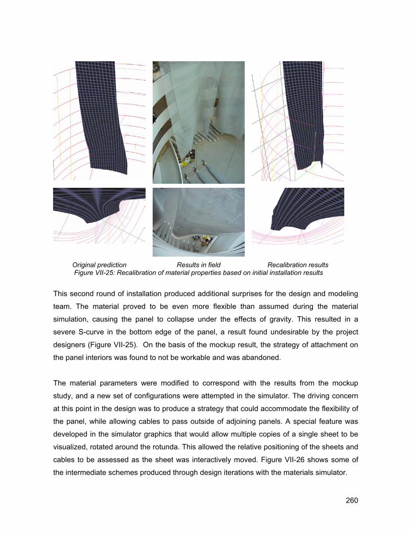
Original prediction Results in field Recalibration results Figure VII-25: Recalibration of material properties based on initial installation results

This second round of installation produced additional surprises for the design and modeling

team. The material proved to be even more flexible than assumed during the material

simulation, causing the panel to collapse under the effects of gravity. This resulted in a

severe S-curve in the bottom edge of the panel, a result found undesirable by the project

designers (Figure VII-25). On the basis of the mockup result, the strategy of attachment on

the panel interiors was found to not be workable and was abandoned.

The material parameters were modified to correspond with the results from the mockup

study, and a new set of configurations were attempted in the simulator. The driving concern

at this point in the design was to produce a strategy that could accommodate the flexibility of

the panel, while allowing cables to pass outside of adjoining panels. A special feature was

developed in the simulator graphics that would allow multiple copies of a single sheet to be

visualized, rotated around the rotunda. This allowed the relative positioning of the sheets and

cables to be assessed as the sheet was interactively moved. Figure VII-26 shows some of

the intermediate schemes produced through design iterations with the materials simulator.

260

261

Interim layout strategy Final layout strategy Figure VII-26: Materials simulation design iterations of mesh curtain installation

The design team finally settled on a strategy where each panel would curve “above and over”

its neighbor, prior to being attached at the outside edge only. This strategy required

attachments higher up on the panels. The distances between the panels would be tight at

this the point of passing over, so the prediction of the materials modeler would have to be

substantially correct. On the basis of this scheme, data was again sent to the museum for on

site mock up.

This time, the results of the mock up confirmed the assumptions of the simulator, and the

feasibility of the strategy. Dimensions for cable placement on the flat patterns of the

individual sheets, cable lengths, and locations for cable attachment points in the rotunda

were established for each panel. These dimensions were again provided to team as per

Figure VII-24 above.

Figure VII-27 below shows relationships between the materials modeling simulation and the

final mesh curtain installation in the exhibit.

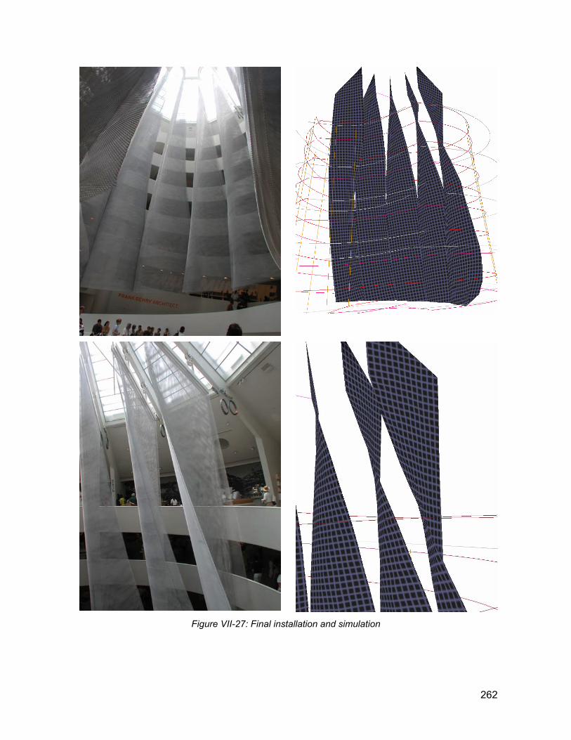
Figure VII-27: Final installation and simulation

262

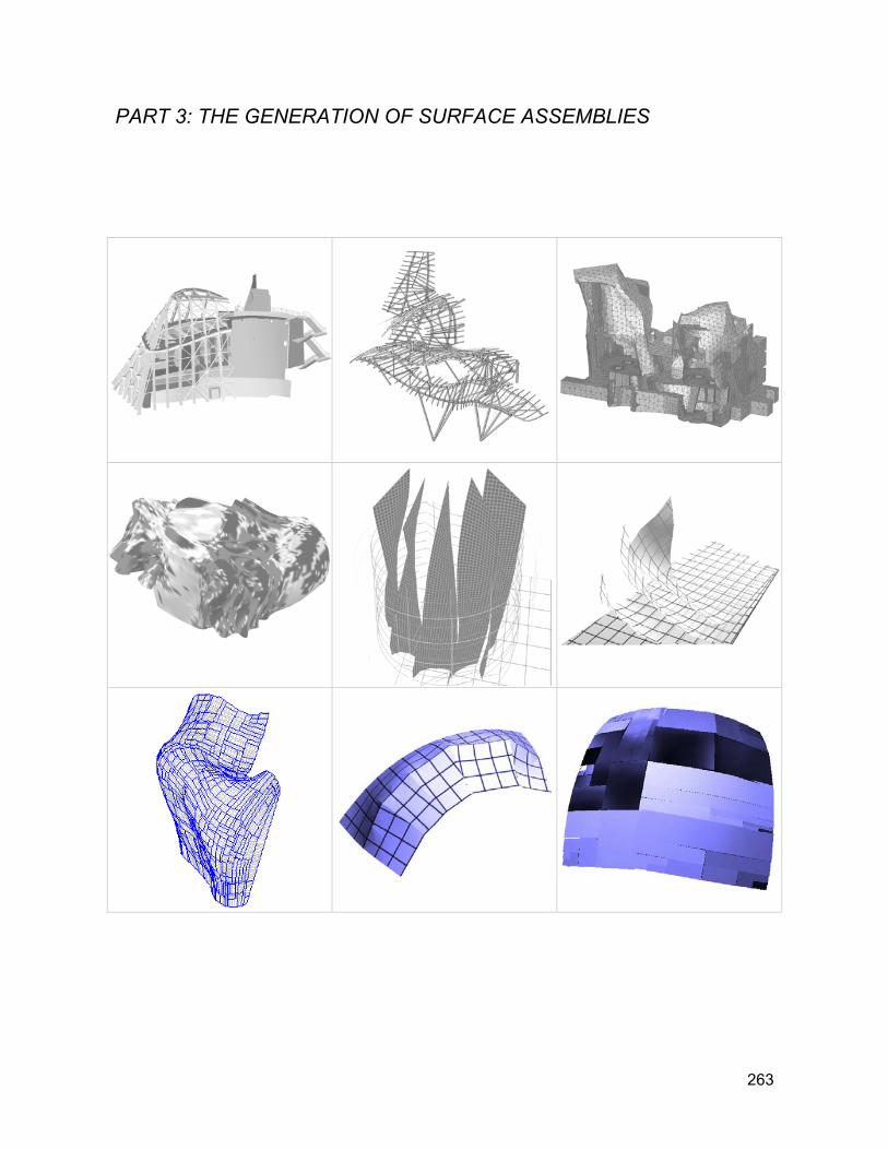
PART 3: THE GENERATION OF SURFACE ASSEMBLIES

263

264

VIII. GENERATING ASSEMBLIES

In Part 1 of this thesis, a set of issues were identified in the rationalization, documentation

and constructibility of Gehry’s surface forms. The notion was presented of materially guided

intentions and systems in the physical modeling, digital modeling and fabrication of these

forms. The class of “paper surfaces” were introduced in Part 2, shapes whose qualities are

defined by a set of specific material behaviors and constructibility requirements. Issues in the

computational modeling of these materially guided surfaces and systems were presented.

This section extends these geometric constructs – initially developed toward simulating the

geometric behavior of individual material surfaces - to consider the behavior of surface

elements as they combine to form larger organizations. The motivation for this work will be to

direct the mathematical constructs developed in Part 2 toward solutions of constructibility

issues on larger scale compositions of sheet assemblies. This effort will specifically target

rationalization activities, developing approaches to the generation of surface element

assemblies whose organizations are guided by rules of constructibility and other project

performance requirements.

In order to apply the formalisms developed previously in this work to the rationalization of

surface assemblies, we must extend the previously defined geometric models of paper

surfaces in two fundamental ways:

1. Extension of the topological model. The constructs developed in Part 2 focused on the

notion of an R2 manifold embedded in Euclidean 3-space. The Euclidean structuring of the

parametric space representation provided certain regularity to the descriptions of the sheet

elements, regularity unavailable from a perspective based purely on the sheets’ description

in the containing 3-space. Certain topological properties such as connectedness of the

shape’s region and its relationship to its boundary were identified on the basis of the sheets’

parametric space descriptions.

Extending this approach to inspect assemblies of elements will require extending the

topological model of surfaces as manifolds to consider the ways in which these spatial

representations combine. Well established theory of such combinatoric topologies exists2,38.

In applying these topological combinatorics to the construction of sheet assemblies, we will

265

principally be concerned with operations performed on the boundaries of sheet elements as

they are “stitched together” to form larger organizations. This inquiry will provide a

mathematical basis to support operations on organizations of surface manifolds.

2. Generative operations on surface assemblies. With a formal structure in place to

structure the description of surface element assemblies, the inquiry will turn toward ways in

which operations on these assemblies may be performed. Rationalization operations will be

re-formulated as transformation operations on assemblies, directed toward goals of satisfying

performance metrics on these assemblies. The topological structuring of sheet assemblies

may be drawn on to support contemporary approaches to the development of generative

systems.

With these structures in place, we will have a basis for formally defining shape families or

classes, on the basis of sets of assumptions regarding element geometric representation,

organizations of elements and operations on these elements. A shape class may be defined

by a description of the type of geometric element used, and the allowable organizations of

these elements. Alternatively, we can view the shape class as the set of all shapes

generated from a specification of elements and transformations. Both aspects of this

description provide constraints on the feasible set of “valid” shapes. A shape is a member of

a shape class if it can be generated using only the assumptions valid in the definition of the

class. If the organizational rules have been developed in response to constructibility

requirements then, by definition, satisfactory inclusion of candidate shapes into an

appropriately defined shape class will guarantee satisfaction of these constructibility

requirements, and any shape which is a member of the class will satisfy these requirements.

Specific surface fabrication and construction systems will be closely associated with a

specific shape class.

266

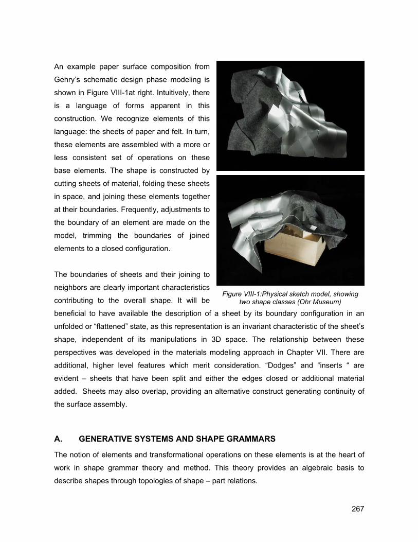
An example paper surface composition from

Gehry’s schematic design phase modeling is

shown in Figure VIII-1at right. Intuitively, there

is a language of forms apparent in this

construction. We recognize elements of this

language: the sheets of paper and felt. In turn,

these elements are assembled with a more or

less consistent set of operations on these

base elements. The shape is constructed by

cutting sheets of material, folding these sheets

in space, and joining these elements together

at their boundaries. Frequently, adjustments to

the boundary of an element are made on the

model, trimming the boundaries of joined

elements to a closed configuration.

The boundaries of sheets and their joining to

neighbors are clearly important characteristics

contributing to the overall shape. It will be

beneficial to have available the description of a sheet by its boundary configuration in an

unfolded or “flattened” state, as this representation is an invariant characteristic of the sheet’s

shape, independent of its manipulations in 3D space. The relationship between these

perspectives was developed in the materials modeling approach in Chapter VII. There are

additional, higher level features which merit consideration. “Dodges” and “inserts “ are

evident – sheets that have been split and either the edges closed or additional material

added. Sheets may also overlap, providing an alternative construct generating continuity of

the surface assembly.

Figure VIII-1:Physical sketch model, showing

two shape classes (Ohr Museum)

A. GENERATIVE SYSTEMS AND SHAPE GRAMMARS

The notion of elements and transformational operations on these elements is at the heart of

work in shape grammar theory and method. This theory provides an algebraic basis to

describe shapes through topologies of shape – part relations.

267

The basic algebraic components of shape grammars are often presented in the literature80

as:

A → B (VIII.1)

C ≥ τ (A) (VIII.2)

C → C - τ(A) + τ(B) (VIII.3)

Equation (VIII.1) establishes the transformation rule to be considered for application. Shape

A, identified in some field of consideration is replaced with a separate shape B. Typically, the

field of consideration in which this identification will occur is a design - an existing shape C.

Equation (VIII.2) defines the identification operation by which the transformation rule is

applied to a design C. Some transformation of A is identified as being a part of the design

shape C. In the existing literature, this transformation is presumed to be one of the Euclidean

transformations.

Finally, Equation (VIII.3) presents the production operations on the base shape C, given the

defined transformation, and the identification circumstances identified in (VIII.2).

Often, grammar applications to design applications presume multiple transformation rules,

operating sequentially on a progressively developed design shape. A grammar is defined in

(Stiny, Gips84, 81) as a 4-tuple of the form:

S = < VT, VM, R, I> (VIII.4)

where:

• VT is a finite a set of terminal shapes, a spatially organized set of (maximal) Euclidean

elements

• VM is a finite a set of marker shapes, a spatially organized set of (maximal) Euclidean

elements

• R is a finite set of transformation rules, of the form u → v , where u and v are shapes

composed of shapes from VT and VM .

268

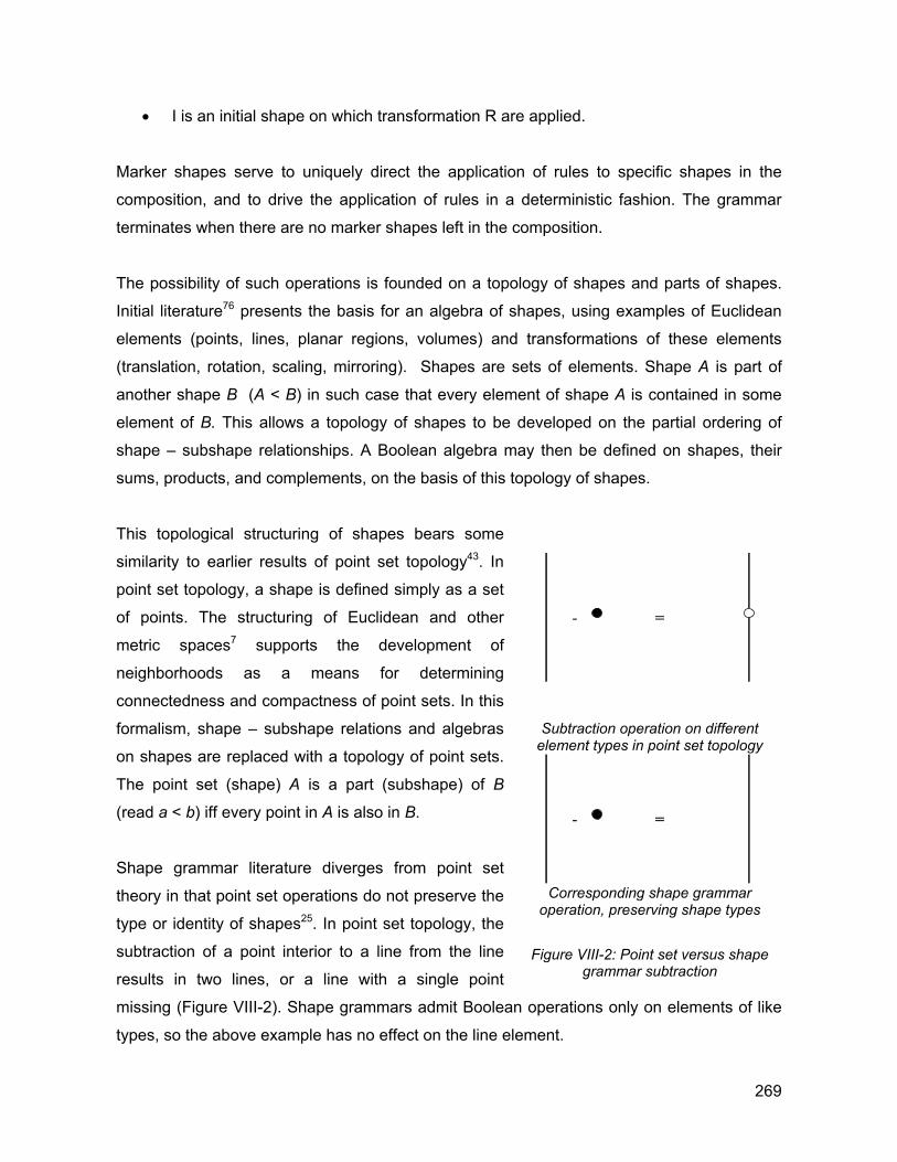
• I is an initial shape on which transformation R are applied.

Marker shapes serve to uniquely direct the application of rules to specific shapes in the

composition, and to drive the application of rules in a deterministic fashion. The grammar

terminates when there are no marker shapes left in the composition.

The possibility of such operations is founded on a topology of shapes and parts of shapes.

Initial literature76 presents the basis for an algebra of shapes, using examples of Euclidean

elements (points, lines, planar regions, volumes) and transformations of these elements

(translation, rotation, scaling, mirroring). Shapes are sets of elements. Shape A is part of

another shape B (A < B) in such case that every element of shape A is contained in some

element of B. This allows a topology of shapes to be developed on the partial ordering of

shape – subshape relationships. A Boolean algebra may then be defined on shapes, their

sums, products, and complements, on the basis of this topology of shapes.

This topological structuring of shapes bears some

similarity to earlier results of point set topology43. In

point set topology, a shape is defined simply as a set

of points. The structuring of Euclidean and other

metric spaces7 supports the development of

neighborhoods as a means for determining

connectedness and compactness of point sets. In this

formalism, shape – subshape relations and algebras

on shapes are replaced with a topology of point sets.

The point set (shape) A is a part (subshape) of B

(read a < b) iff every point in A is also in B.

Shape grammar literature diverges from point set

theory in that point set operations do not preserve the

type or identity of shapes25. In point set topology, the

subtraction of a point interior to a line from the line

results in two lines, or a line with a single point

missing (Figure VIII-2). Shape grammars admit Boolean operations only on elements of like

types, so the above example has no effect on the line element.

- =

Subtraction operation on different element types in point set topology

- =

Corresponding shape grammar

operation, preserving shape types

Figure VIII-2: Point set versus shape grammar subtraction

269

In much of the original literature by Stiny83, the shape grammar formalism is described

through examples of Euclidean elements (lines, points, and higher dimensional shapes

described by boundaries comprised of these elements) and Euclidean transformations. Stiny

has shown that Euclidean shape grammars are closed under transformation. The regularities

of such well defined objects, operated on in Euclidean space, lend a simplicity and elegance

to the structuring of computations on these objects.

The introduction of non-Euclidean spatial structures into shape grammar theory requires us

to re-consider the structure of shape grammars, distinguishing between elements of the

formalism that are topological or algebraic in nature, and which are assumptions based on

Euclidean characteristics of the space in which elements are described and transformed.

Specifically, we wish to re-cast previous work on Euclidean space grammars into a form

which can represent - and support operations on - more general manifolds.

Earl24 develops further the topological structuring of shapes and their subshapes, and

develops a treatment of shapes and their boundaries. This argument assumes

connectedness and continuity of the space in which operations occur. These characteristics

require that the space in which operations occur adopt the characteristics of a metric space

(Section V.A), but do not require this metric space to be necessarily Euclidean. As such,

Earle’s formulation of shape – boundary relations are potentially applicable to the non-

Euclidean realm of surface manifolds without modification.

The elements (lines and points) on which grammars operate are considered to be elemental,

in a manner similar to Euclid38 – constructs whose definition is implicit, and shared between

author and reader. In computational applications, explicit descriptions of these elements

must be formulated45,46. This explicit definition of shapes through numerical evaluations is

sometimes perceived as an effort in mechanics, whose relationship to the algebraic

formalisms of grammars is ill defined.

270

B. MANIFOLD GRAMMARS

1. Introduction In Part 2 of this thesis, the description of surface shapes was developed through the

structuring of manifolds. This section considers the formalisms necessary to adopt shape

grammar theory to such shapes.

The structures of manifold theory provide the basic structures necessary and sufficient to

establish algebras of shapes as presented above:

The notion of Cartesian product spaces, including spaces of real numbers Rn and vector

product spaces. The existence of metric functions on these spaces, necessary to define

closure, continuity and neighborhoods or bounded regions, is presumed.

Transformations or mapping functions between these spatial constructs.

It can be shown that these structures are sufficient to support the constructs associated with

shape grammar theory:

The notions of shapes, and spaces in which these shapes occur,

Topologies of shape – part relationships, sufficient to allow the definition of Boolean

algebras,

Transformations on shapes.

In the conventional formalism of shape grammars, shapes are seen as entities occurring in,

and distinct from, the spaces they inhabit. Manifold theory makes no such distinction

between space and shape. Instead, a shape is perceived as a mapping or contract between

two distinct spatial constructs, one intrinsic to the shape and presumed to be locally

Euclidean, the other extrinsic, into which the shape is embedded or resides. The notion of a

shape in analogously viewed in manifold theory as a transformational function that binds

together, or translates between, spatial views of the object. This definition of shape-as-

function is the basis for the shape’s identity79, and provides the basis for this identity to be

preserved through transformations on the shape. Closure operators83 may be defined on

these functions. The structuring of shape-as-function furthermore consolidates the definition

of the shape with a functional definition necessary to perform numerical computations.

271

Shapes described as mapping functions take on the topological characteristics of an M × N

product space define by their relationship on these spaces. This product space not

necessarily Euclidean nature, even if the spaces M are N. Rather, the manifold takes on

spatial qualities determined by the mapping function. For differentiable maps, metric

functions analogous to that Euclidean distance can be determined. Topologies of

neighborhoods are typically preserved across this mapping.

As point of departure, we may consider trivial example of a line segment in R2, defined as an

R1 × R2 manifold. A might may be defined is a function of two R2 vectors:

( ): |t t tλ → + ∈p q 0,1

)

(VIII.5)

although certainly other equivalent definitions of the line function might be used. The

boundaries of λ are the 0-dimensional points p and p + q.

The line λ may be viewed equivalently from three distinct spatial perspectives:

as a closed region of the real line t,

as a line element embedded in Euclidean 2-space,

as a function or constraint defined in the <R × R2 > product space.

This last perspective is perhaps the least obvious, but most important perspective on the

nature of this element. In the case of the above stated line definition (VIII.5), the line forms a

constraint on the three variables of the product space (t, u1, u2):

( (VIII.6) 1 1 1 1, ,t t t+ +p q p q

We often state as a condition for further extensions of the manifold structuring that the

mapping function is invertible. In the case of the line, we can define an inverse function

, which maps from Euclidean 2-space parameters back to locations on the scalar

number line t. A point on this line with R2 coordinates ui maps to a point in line t by the vector

dot product:

1 : i tλ− →u

( )t = −qu pq

(VIII.7)

272

This inverse mapping is obviously only valid for regions R2 that are in the image of the

original mapping function λ.

With this invertible function in hand, we may establish a topology of parts between similarly

defined elements. Given two line segments l2 and l1 :

( )( )

1 1 1 1 1 1

2 2 2 2 2 2

: |

: |

t t t

t t t

λ

λ

→ + ∈

→ + ∈

p qp q

0,1 ,

0,1

1

2

(VIII.8)

with inverse functions: 1

1 11

2 2

::

tt

λ

λ

−

−

→

→

uu

We can determine product functions that map between the parametric space descriptions of

these lines:

( )( )

11 2 1 2 2 2 1 1

12 1 2 1 1 1 2 2

: ,

: ,

t t t t

t t t t

λ λ

λ λ

−→

−→

→ =

→ =

o

o

λ

λ (VIII.9)

A topology of part relations can be defined on these functions and their embeddings into a

common space. A line segment λ2 is a part of λ1 (λ1 ≥ λ2 ) in such case that the function λ2→1

maps t2 into t1 on the range ( ) ( )2 11 2 0,1λ

→= ∈t t . Production rules for determination of maximal

elements may similarly be established. If ( ) ( ) ( ) ( )1 1 2 1 2 1 1 1 2 1 2 2λ λ→ →< < + < +p p p q pt t then

the maximal line λ1 + λ2 may be defined as the function:

q

( )( ) ( )1 2 1 2 1 2 2 1: t t tλ λ+ →→ + + − ∈p p q p | 0,1 (VIII.10)

Coordinates on λ2 may be mapped into this new parameterization. Operations of

complement (-) and product (.) are similarly established.

This approach to grammars on manifolds may be extended directly to higher order manifolds

of arbitrary dimensions <Rm × Rn>. In this thesis, our focus is on surface elements,

embedded in R3. The structuring of manifolds is naturally extended to the descriptions and

transformations of surfaces and their combinatorics.

273

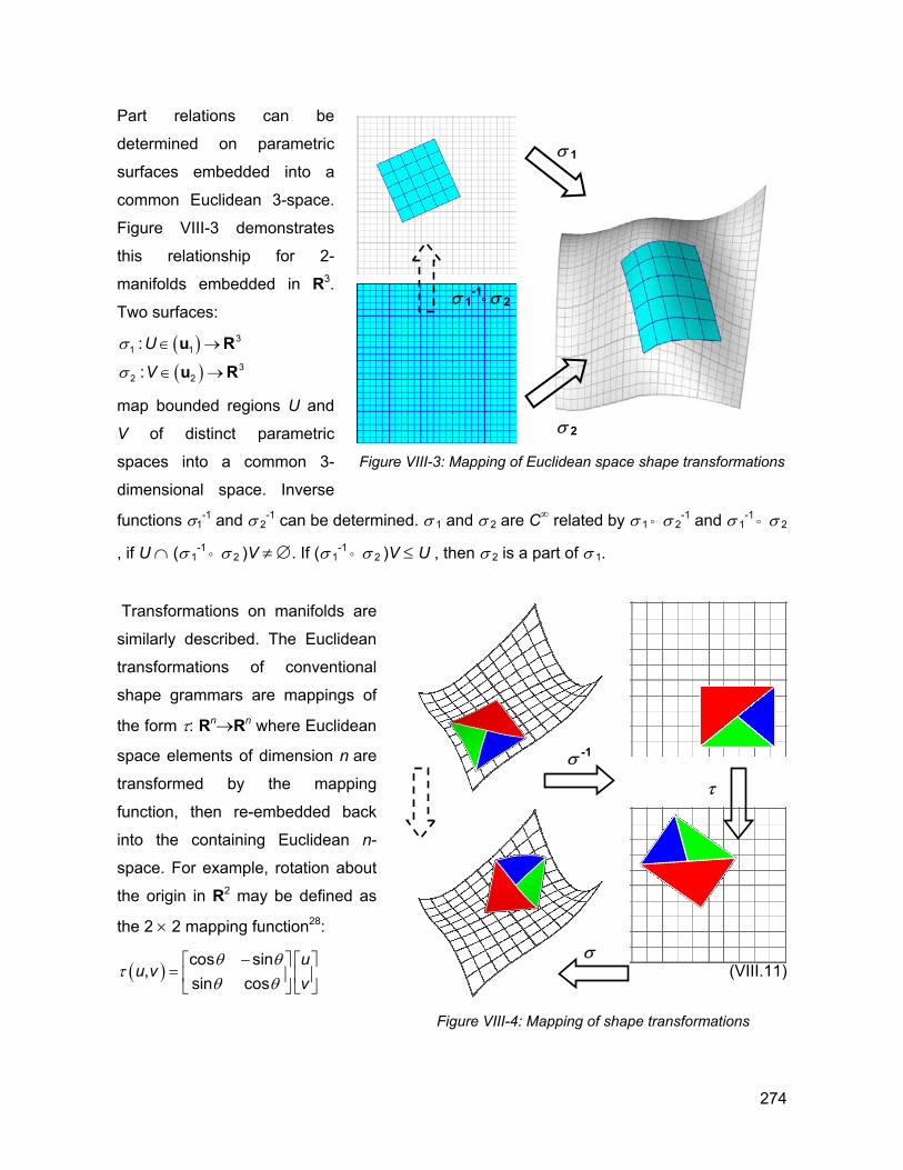
Part relations can be

determined on parametric

surfaces embedded into a

common Euclidean 3-space.

Figure VIII-3 demonstrates

this relationship for 2-

manifolds embedded in R3.

Two surfaces:

( )( )

31 1

32 2

:

:

U

V

σ

σ

∈ →

∈ →

u Ru R

map bounded regions U and

V of distinct parametric

spaces into a common 3-

dimensional space. Inverse

functions σ1-1 and σ 2

-1 can be determined. σ 1 and σ 2 are C∞

, if U ∩ (σ 1-1

° σ 2 )V ≠ ∅. If (σ 1-1

° σ 2 )V ≤ U , then σ 2 is a pa

Transformations on manifolds are

similarly described. The Euclidean

transformations of conventional

shape grammars are mappings of

the form τ: Rn→Rn where Euclidean

space elements of dimension n are

transformed by the mapping

function, then re-embedded back

into the containing Euclidean n-

space. For example, rotation about

the origin in R2 may be defined as

the 2 × 2 mapping function28:

( ) cos sin,

sin cosu

u vv

θ θτ

θ θ−

=

Figure VIII-3: Mapping of Euc

Figure VIII-4: Ma

σ 2

σ 1

σ 1-1

° σ 2

related by σ 1 ° σ 2

-1 and σ 1-1

° σ 2

rt of σ 1.

lidean space shape transformations

ppin

σ -1

σ

g of shape transfor

τ

(VIII.11)

mations

274

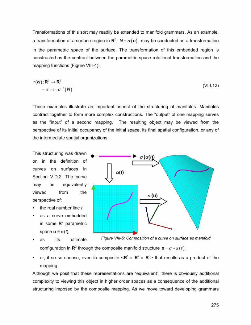
Transformations of this sort may readily be extended to manifold grammars. As an example,

a transformation of a surface region in R3, ( )N σ∈ u , may be conducted as a transformation

in the parametric space of the surface. The transformation of this embedded region is

constructed as the contract between the parametric space rotational transformation and the

mapping functions (Figure VIII-4):

( )

3 3

1

( ) :NN

τ

σ τ σ −

→

=

R Ro o

(VIII.12)

These examples illustrate an important aspect of the structuring of manifolds. Manifolds

contract together to form more complex constructions. The “output” of one mapping serves

as the “input” of a second mapping. The resulting object may be viewed from the

perspective of its initial occupancy of the initial space, its final spatial configuration, or any of

the intermediate spatial organizations.

This structuring was drawn

on in the definition of

curves on surfaces in

Section V.D.2. The curve

may be equivalently

viewed from the

perspective of:

the real number line t,

as a curve embedded

in some R2 parametric

space u = α(t),

as its ultimate

configuration in R3 through the composite manifold structure ( )tσ α=x o ,

Figure VIII-5: Composition of a curve on surface as manifold

α(t)

σ (u)

σ (α(t))

or, if se so choose, even in composite <R1 × R2 × R3> that results as a product of the

mapping.

Although we posit that these representations are “equivalent”, there is obviously additional

complexity to viewing this object in higher order spaces as a consequence of the additional

structuring imposed by the composite mapping. As we move toward developing grammars

275

on manifold objects, it will be beneficial to have any and all of these spatial views available in

which we may choose at our discretion to define elements of the grammar. The mapping

functions allow us to “know” a great deal about an object’s higher order behavior, while still

performing computations in reduced spatial representations to take advantage of problem

simplifications afforded in these spaces.

2. Other Topological Spaces So far, this discussion has focused on manifolds defined in real number Cartesian product

spaces Rn, to provide the basis for establishing differentiable mapping functions between

spatial views on these objects. In many shape grammar applications, such real valued

geometric descriptions alone are insufficient to capture the semantic requirements of the

problem.

Labels and Weights

In Stiny’s shape grammar formulation, labels and weights82 present examples of such not-

necessarily real valued or geometric shape attributes. Labels are, roughly, tokenized

information, which may be bound to shapes in a design. As an example, lines on an

architectural plan may represent materials; the set of material tokens may include {WOOD,

CONCRETE, SHEET_ROCK, etc.}. Elements of different labellings do not combine in the

Stiny’s. Production rules employing multiple labeled elements may be considered to be

grammars operating as parallel grammars, operating in the distinct spaces associated with

each label. Weights may be considered to be values associated with design elements. These

values may combine according to production rules. The product of a line of color RED and

one colored YELLOW may be defined in a production rule to result in a line of color

ORANGE.

The structure of manifold grammars naturally extends to include such additional, non-spatial

parameters. In manifold theory, there is no distinction between variables that are spatial and

those that are not. The inclusion of additional, real valued parameters on a manifold simply

requires the extension of the problem formulation into a higher order space. For example, a

colored line could be formulated as a 4-Dimensional object of the form < t × R × G × B >,

where R, G and B are the red, green and blue intensity values associated with the line. Such

a “weighted” line may be mapped to the domain other line segments through the

276

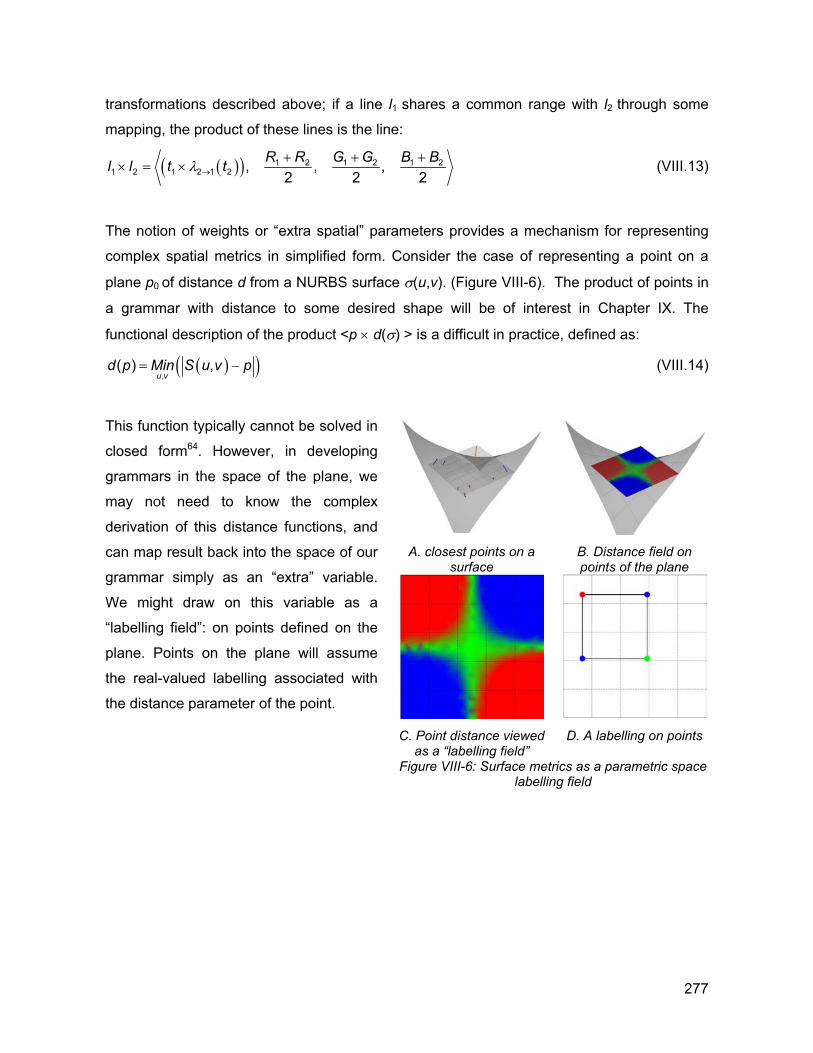
transformations described above; if a line l1 shares a common range with l2 through some

mapping, the product of these lines is the line:

( )( ) 1 2 1 2 1 21 2 1 2 1 2 , , ,

2 2 2R R G G B Bl l t tλ →

+ + +× = × (VIII.13)

The notion of weights or “extra spatial” parameters provides a mechanism for representing

complex spatial metrics in simplified form. Consider the case of representing a point on a

plane p0 of distance d from a NURBS surface σ(u,v). (Figure VIII-6). The product of points in

a grammar with distance to some desired shape will be of interest in Chapter IX. The

functional description of the product <p × d(σ) > is a difficult in practice, defined as:

( )(,

( ) ,u v

d p Min S u v p= )− (VIII.14)

This function typically cannot be solved in

closed form64. However, in developing

grammars in the space of the plane, we

may not need to know the complex

derivation of this distance functions, and

can map result back into the space of our

grammar simply as an “extra” variable.

We might draw on this variable as a

“labelling field”: on points defined on the

plane. Points on the plane will assume

the real-valued labelling associated with

the distance parameter of the point.

A. closest points on a

surface B. Distance field on points of the plane

C. Point distance viewed

as a “labelling field” D. A labelling on points

Figure VIII-6: Surface metrics as a parametric space labelling field

277

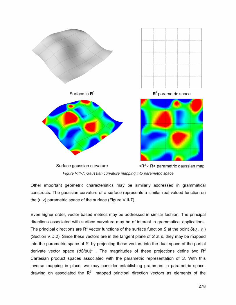
Surface in R3 R2 parametric space

Surface gaussian curvature <R2 × R> parametric gaussian map Figure VIII-7: Gaussian curvature mapping into parametric space

Other important geometric characteristics may be similarly addressed in grammatical

constructs. The gaussian curvature of a surface represents a similar real-valued function on

the (u,v) parametric space of the surface (Figure VIII-7).

Even higher order, vector based metrics may be addressed in similar fashion. The principal

directions associated with surface curvature may be of interest in grammatical applications.

The principal directions are R3 vector functions of the surface function S at the point S(up, vp)

(Section V.D.2). Since these vectors are in the tangent plane of S at p, they may be mapped

into the parametric space of S, by projecting these vectors into the dual space of the partial

derivate vector space (dS/du)* . The magnitudes of these projections define two R2

Cartesian product spaces associated with the parametric representation of S. With this

inverse mapping in place, we may consider establishing grammars in parametric space,

drawing on associated the R2 mapped principal direction vectors as elements of the

278

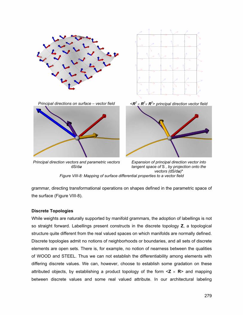
Principal directions on surface – vector field <R2 × R2× R2> principal direction vector field

Principal direction vectors and parametric vectors

dS/du Expansion of principal direction vector into tangent space of S , by projection onto the

vectors (dS/du)* Figure VIII-8: Mapping of surface differential properties to a vector field

grammar, directing transformational operations on shapes defined in the parametric space of

the surface (Figure VIII-8).

Discrete Topologies While weights are naturally supported by manifold grammars, the adoption of labellings is not

so straight forward. Labellings present constructs in the discrete topology Z, a topological

structure quite different from the real valued spaces on which manifolds are normally defined.

Discrete topologies admit no notions of neighborhoods or boundaries, and all sets of discrete

elements are open sets. There is, for example, no notion of nearness between the qualities

of WOOD and STEEL. Thus we can not establish the differentiability among elements with

differing discrete values. We can, however, choose to establish some gradation on these

attributed objects, by establishing a product topology of the form <Z × R> and mapping

between discrete values and some real valued attribute. In our architectural labeling

279

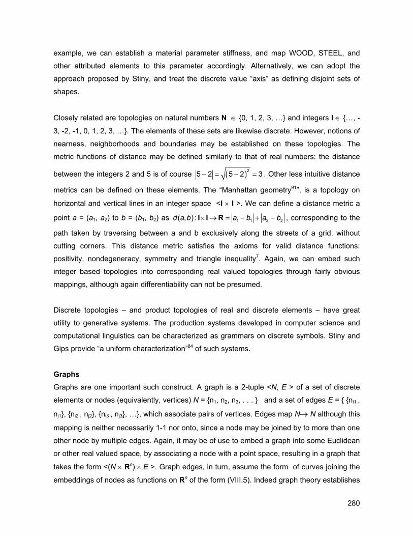
example, we can establish a material parameter stiffness, and map WOOD, STEEL, and

other attributed elements to this parameter accordingly. Alternatively, we can adopt the

approach proposed by Stiny, and treat the discrete value “axis” as defining disjoint sets of

shapes.

Closely related are topologies on natural numbers N ∈ {0, 1, 2, 3, …} and integers I ∈ {…, -

3, -2, -1, 0, 1, 2, 3, …}. The elements of these sets are likewise discrete. However, notions of

nearness, neighborhoods and boundaries may be established on these topologies. The

metric functions of distance may be defined similarly to that of real numbers: the distance

between the integers 2 and 5 is of course ( )25 2 5 2 3− = − = . Other less intuitive distance

metrics can be defined on these elements. The “Manhattan geometry91”, is a topology on

horizontal and vertical lines in an integer space <I × I >. We can define a distance metric a

point a = (a1, a2) to b = (b1, b2) as 1 1 2 2( , ) :b a b a b× → = − + −I I Rd a , corresponding to the

path taken by traversing between a and b exclusively along the streets of a grid, without

cutting corners. This distance metric satisfies the axioms for valid distance functions:

positivity, nondegeneracy, symmetry and triangle inequality7. Again, we can embed such

integer based topologies into corresponding real valued topologies through fairly obvious

mappings, although again differentiability can not be presumed.

Discrete topologies – and product topologies of real and discrete elements – have great

utility to generative systems. The production systems developed in computer science and

computational linguistics can be characterized as grammars on discrete symbols. Stiny and

Gips provide “a uniform characterization”84 of such systems.

Graphs Graphs are one important such construct. A graph is a 2-tuple <N, E > of a set of discrete

elements or nodes (equivalently, vertices) N = {n1, n2, n3, . . . } and a set of edges E = { {ni1 ,

nj1}, {ni2 , nj2}, {ni3 , nj3}, …}, which associate pairs of vertices. Edges map N→ N although this

mapping is neither necessarily 1-1 nor onto, since a node may be joined by to more than one

other node by multiple edges. Again, it may be of use to embed a graph into some Euclidean

or other real valued space, by associating a node with a point space, resulting in a graph that

takes the form <(N × Rn) × E >. Graph edges, in turn, assume the form of curves joining the

embeddings of nodes as functions on Rn of the form (VIII.5). Indeed graph theory establishes

280

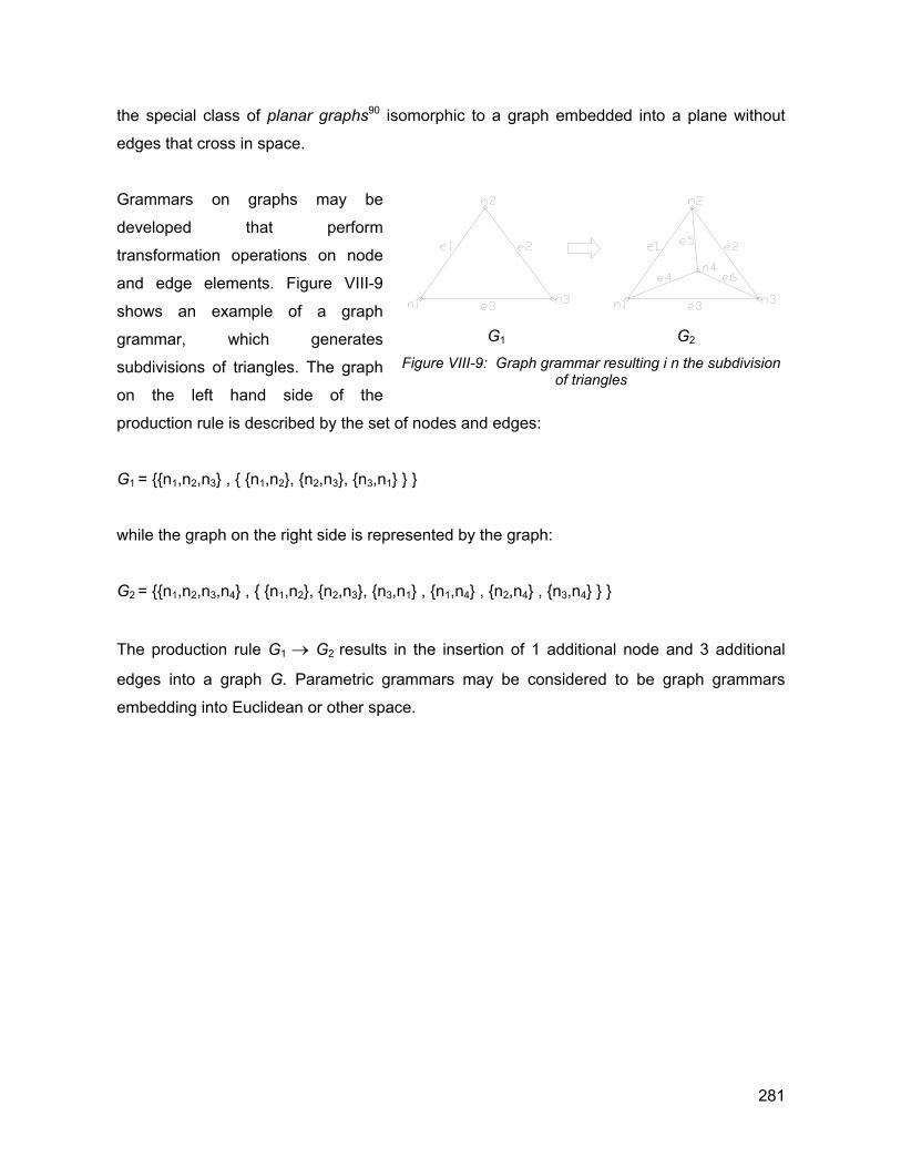
the special class of planar graphs90 isomorphic to a graph embedded into a plane without

edges that cross in space.

Grammars on graphs may be

developed that perform

transformation operations on node

and edge elements. Figure VIII-9

shows an example of a graph

grammar, which generates

subdivisions of triangles. The graph

on the left hand side of the

production rule is described by the set of nodes and edges:

G1 G2

Figure VIII-9: Graph grammar resulting i n the subdivision of triangles

G1 = {{n1,n2,n3} , { {n1,n2}, {n2,n3}, {n3,n1} } }

while the graph on the right side is represented by the graph:

G2 = {{n1,n2,n3,n4} , { {n1,n2}, {n2,n3}, {n3,n1} , {n1,n4} , {n2,n4} , {n3,n4} } }

The production rule G1 → G2 results in the insertion of 1 additional node and 3 additional

edges into a graph G. Parametric grammars may be considered to be graph grammars

embedding into Euclidean or other space.

281

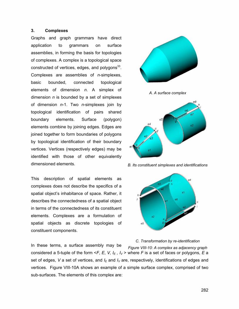
3. Complexes Graphs and graph grammars have direct

application to grammars on surface

assemblies, in forming the basis for topologies

of complexes. A complex is a topological space

constructed of vertices, edges, and polygons33.

Complexes are assemblies of n-simplexes,

basic bounded, connected topological

elements of dimension n. A simplex of

dimension n is bounded by a set of simplexes

of dimension n-1. Two n-simplexes join by

topological identification of pairs shared

boundary elements. Surface (polygon)

elements combine by joining edges. Edges are

joined together to form boundaries of polygons

by topological identification of their boundary

vertices. Vertices (respectively edges) may be

identified with those of other equivalently

dimensioned elements.

This description of spatial elements as

complexes does not describe the specifics of a

spatial object’s inhabitance of space. Rather, it

describes the connectedness of a spatial object

in terms of the connectedness of its constituent

elements. Complexes are a formulation of

spatial objects as discrete topologies of

constituent components.

In these terms, a surface assembly may be

considered a 5-tuple of the form <F, E, V, IE , IV > where F is a set of faces or polygons, E a

set of edges, V a set of vertices, and IE and IV are, respectively, identifications of edges and

vertices. Figure VIII-10A shows an example of a simple surface complex, comprised of two

sub-surfaces. The elements of this complex are:

A. A surface complex

B. Its constituent simplexes and identifications

C. Transformation by re-identification

Figure VIII-10: A complex as adjacency graph

282

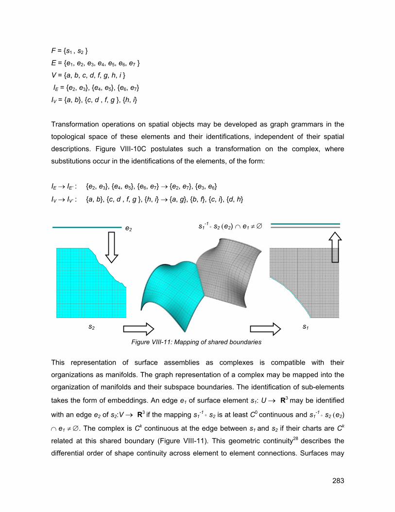
F = {s1 , s2 }

E = {e1, e2, e3, e4, e5, e6, e7 }

V = {a, b, c, d, f, g, h, i }

IE = {e2, e3}, {e4, e5}, {e6, e7}

IV = {a, b}, {c, d , f, g }, {h, i}

Transformation operations on spatial objects may be developed as graph grammars in the

topological space of these elements and their identifications, independent of their spatial

descriptions. Figure VIII-10C postulates such a transformation on the complex, where

substitutions occur in the identifications of the elements, of the form:

IE → IE’ : {e2, e3}, {e4, e5}, {e6, e7} → {e2, e7}, {e3, e6}

IV → IV’ : {a, b}, {c, d , f, g }, {h, i} → {a, g}, {b, f}, {c, i}, {d, h}

e2 s1-1

° s2 (e2) ∩ e1 ≠ ∅

s2

s1

Figure VIII-11: Mapping of shared boundaries

This representation of surface assemblies as complexes is compatible with their

organizations as manifolds. The graph representation of a complex may be mapped into the

organization of manifolds and their subspace boundaries. The identification of sub-elements

takes the form of embeddings. An edge e1 of surface element s1: U → R3 may be identified

with an edge e2 of s2:V → R3 if the mapping s1-1

° s2 is at least C0 continuous and s1-1

° s2 (e2)

∩ e1 ≠ ∅. The complex is Ck continuous at the edge between s1 and s2 if their charts are Ck

related at this shared boundary (Figure VIII-11). This geometric continuity28 describes the

differential order of shape continuity across element to element connections. Surfaces may

283

simply be touching or closed (order G0), tangent (G1) or curvature continuous (G2). Higher

order differential continuities are possible. In practical paper surface applications, gradations

of these qualities exist. Open seam conditions exist where edges are associated but do not

exactly touch. An edge may be only close to joining, connected but with large gaps, tape or

loosely fastened rivets or screws. An overlapping edge may partially constrain tangency or

curvature continuity, but allow a certain degree of deviation from true G1 or G2 connectivity.

Geometric continuity may be represented in the incidence graph as labellings on edge

identifications.

The connectedness of a complex may be represented in the discrete space of graphs whose

elements are these incidence coefficients33. We can draw on this simplified representation to

perform transformations on surface assemblies. The triangle subdivision grammar shown in

Figure VIII-9 presents one such example. This representation of this operation on the

complex graph presents a vast simplification of the problem space. Of course, this

representation hides all detail of how the transformation affects the actual embedding of the

triangle assembly in space. If, as is likely, this knowledge is important to decision making by

the grammar, we will again need to map spatial metrics back into the graph space, or

conduct our grammar in the product space of the embedded graph with other spatial

representations of the complex’s constituent elements.

C. SUMMARY

This chapter has established a formal basis for the development of shape grammars of

surface assemblies. This structuring views shapes as real, differentiable functions operating

in Cartesian product spaces of the form <Rn × Rm>. Shape boundaries are similarly described

as sub-manifolds of the form <Rn-1 × Rn>, embedded in the parametric space of the shape.

The important algebraic foundations of the shape grammar formalism, including notions of

shape – part relations, Boolean algebras on shapes, and shape labellings and weights, were

developed through this manifold representation.

The structuring of manifolds provides the potential for grammar operations on complicated

spatial objects, such as our paper surface assemblies, to be conducted in spaces

representing alternative, simplified, representations of these objects, while allowing the full

richness of the objects’ spatial behaviors to be referenced by the grammar.

284

IX. GENERATIVE RATIONALIZATION

This chapter presents several examples of grammars that have been applied on Gehry

projects or are currently under development. In general, these applications are directed

toward rationalization of the surface forms to address specific constructibility requirements.

The strategies taken in this chapter differ depending on the application and the specific

requirements of the surface fabrication strategy. However, some general characterizations of

these approaches may be made.

• A pre-rationalized “ideal surface form” – perhaps the product of digitized physical models-

is admitted as the input shape for rationalization operations.

• Surface elements and their boundary forms serve as the elements of the grammar.

These surface elements are formally described as parametric mapping functions in <R2 × R3> space. The characteristics of this differentiable mapping function are specific to the

constructibility problem under consideration. Examples include the constrained curvature,

developable and materials based surface representations presented in Chapters VI and

VII.

• The surface manifold is considered both a “micro” representation of the surface elements

and a “macro” scale perspective of the assembly’s organization as a whole. To simplify

operations, grammars are typically conducted at least partially in the parametric space of

the surface elements, drawing on Euclidean characteristics of this space, and the

corresponding reduction of the space’s dimensional order. Macro level operations are

often conducted on the graph of boundary element identifications.

• Shape metrics and other heuristics from the 3-dimensional configuration are mapped

onto these representations as labellings on grammar elements. These metrics provide

the grammar with heuristics to assess the constructibility of assembly.

• The grammars perform substitution operations on sheet boundaries and other features in

parametric space, and operations such as splitting or insertion of faces in the graph of the

285

surface complex. Substitution operations are performed toward the goal of satisfying

constructibility conditions of the assembly.

A. GENERATIVE APPLICATIONS ON THE EXPERIENCE MUSIC PROJECT

The genesis of these applications was a series of rationalization studies conducted during

design development on the Experience Music Project. Section VI.2 described the macro

scale constrained gaussian curvature approach taken to rationalizing EMP’s form. Additional

rationalization operations were conducted both at a global scale as well as on the localized

configuration of sheets during shop drawing generation. Automation efforts were conducted

in parallel with the manual operations.

1. Design Development Applications Initial design development rationalization studies were pursued over the period between

March and May of 1997. The approach described in this section is based on an assumption

that surface forms of any curvature can be constructed from flat sheets, deformed within

some limited range, presuming that the dimensions of the surface sheets are varied in

response to the surface curvature. Breaks in tangency between sheets accommodate some

degree of curvature in the macro scale surface form. Decreasing the size of panels should

increase the number of these tangency breaks, allowing greater degrees of curvature to be

accommodated.

The design surface (Figure IX-1A) was initially approximated as a fine grained, rectangular

grating33 (Figure IX-1B). This regularized, integer space parameterization provided an

efficient spatial construct on which to perform the grammar operations. The goal of the

grammar was to determine a configuration of surface regions whose deviation from a plane

was within a predetermined tolerance.

286

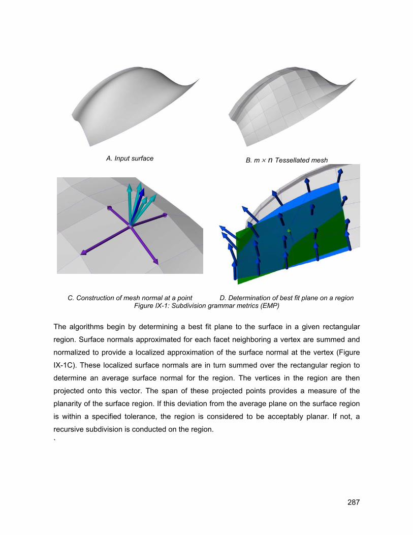
A. Input surface B. m × n Tessellated mesh

C. Construction of mesh normal at a point D. Determination of best fit plane on a region Figure IX-1: Subdivision grammar metrics (EMP)

The algorithms begin by determining a best fit plane to the surface in a given rectangular

region. Surface normals approximated for each facet neighboring a vertex are summed and

normalized to provide a localized approximation of the surface normal at the vertex (Figure

IX-1C). These localized surface normals are in turn summed over the rectangular region to

determine an average surface normal for the region. The vertices in the region are then

projected onto this vector. The span of these projected points provides a measure of the

planarity of the surface region. If this deviation from the average plane on the surface region

is within a specified tolerance, the region is considered to be acceptably planar. If not, a

recursive subdivision is conducted on the region.

`

287

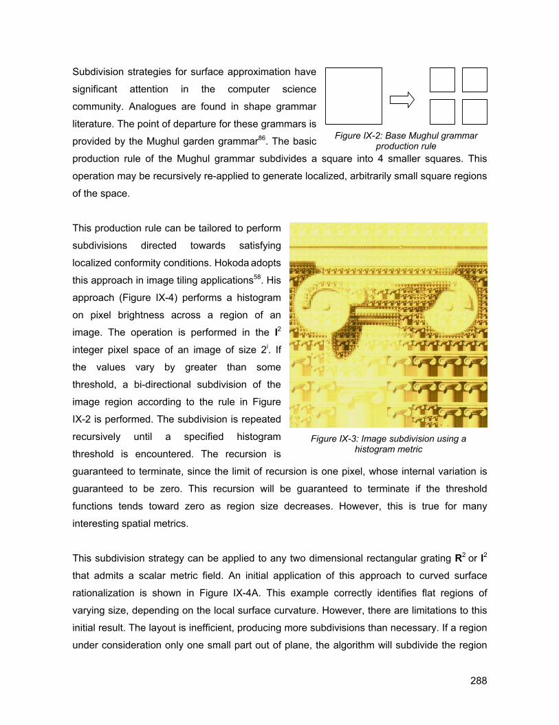
Subdivision strategies for surface approximation have

significant attention in the computer science

community. Analogues are found in shape grammar

literature. The point of departure for these grammars is

provided by the Mughul garden grammar86. The basic

production rule of the Mughul grammar subdivides a square into 4 smaller squares. This

operation may be recursively re-applied to generate localized, arbitrarily small square regions

of the space.

Figure IX-2: Base Mughul grammar

production rule

This production rule can be tailored to perform

subdivisions directed towards satisfying

localized conformity conditions. Hokoda adopts

this approach in image tiling applications58. His

approach (Figure IX-4) performs a histogram

on pixel brightness across a region of an

image. The operation is performed in the I2 integer pixel space of an image of size 2i. If

the values vary by greater than some

threshold, a bi-directional subdivision of the

image region according to the rule in Figure

IX-2 is performed. The subdivision is repeated

recursively until a specified histogram

threshold is encountered. The recursion is

guaranteed to terminate, since the limit of recursion is one pixel, whose internal variation is

guaranteed to be zero. This recursion will be guaranteed to terminate if the threshold

functions tends toward zero as region size decreases. However, this is true for many

interesting spatial metrics.

Figure IX-3: Image subdivision using a

histogram metric

This subdivision strategy can be applied to any two dimensional rectangular grating R2 or I2

that admits a scalar metric field. An initial application of this approach to curved surface

rationalization is shown in Figure IX-4A. This example correctly identifies flat regions of

varying size, depending on the local surface curvature. However, there are limitations to this

initial result. The layout is inefficient, producing more subdivisions than necessary. If a region

under consideration only one small part out of plane, the algorithm will subdivide the region

288

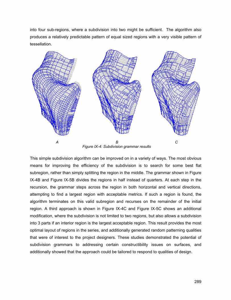
into four sub-regions, where a subdivision into two might be sufficient. The algorithm also

produces a relatively predictable pattern of equal sized regions with a very visible pattern of

tessellation.

A B C

Figure IX-4: Subdivision grammar results

This simple subdivision algorithm can be improved on in a variety of ways. The most obvious

means for improving the efficiency of the subdivision is to search for some best flat

subregion, rather than simply splitting the region in the middle. The grammar shown in Figure

IX-4B and Figure IX-5B divides the regions in half instead of quarters. At each step in the

recursion, the grammar steps across the region in both horizontal and vertical directions,

attempting to find a largest region with acceptable metrics. If such a region is found, the

algorithm terminates on this valid subregion and recurses on the remainder of the initial

region. A third approach is shown in Figure IX-4C and Figure IX-5C shows an additional

modification, where the subdivision is not limited to two regions, but also allows a subdivision

into 3 parts if an interior region is the largest acceptable region. This result provides the most

optimal layout of regions in the series, and additionally generated random patterning qualities

that were of interest to the project designers. These studies demonstrated the potential of

subdivision grammars to addressing certain constructibility issues on surfaces, and

additionally showed that the approach could be tailored to respond to qualities of design.

289

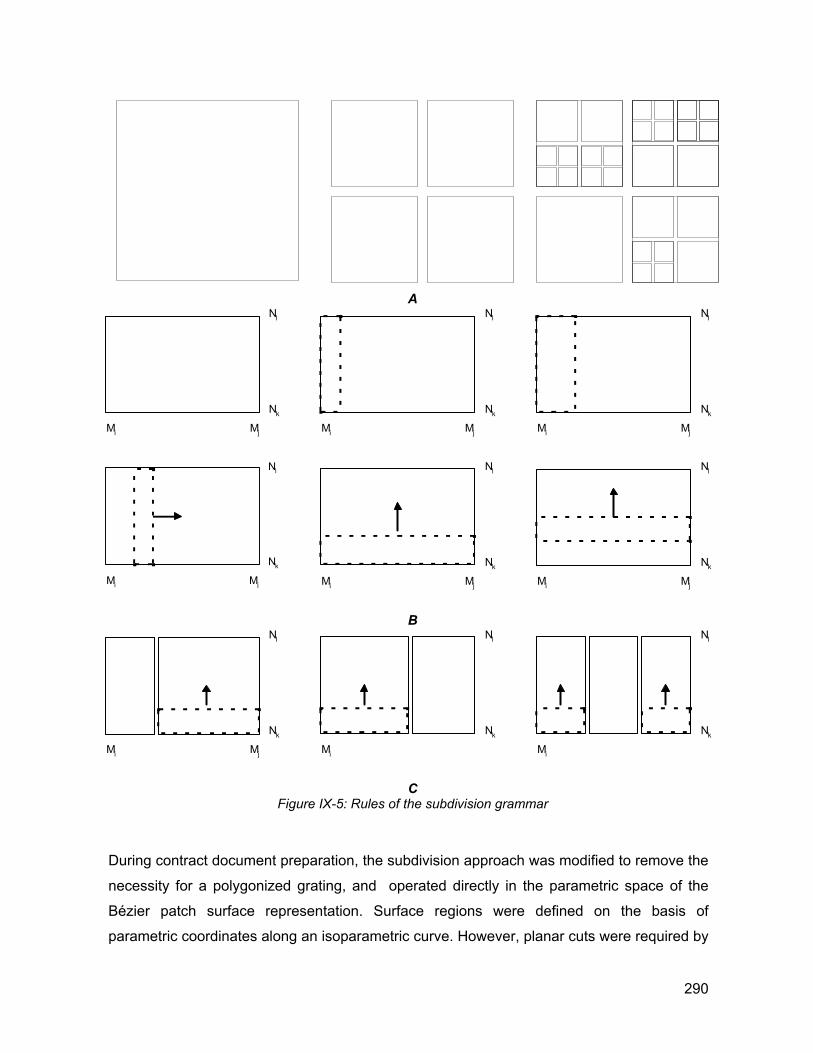
A

MjMi

Nk

Nl

MjMi

Nk

Nl

MjMi

Nk

Nl

M j M i

N k

N l

MjMi

Nk

Nl

MjMi

Nk

Nl

B

MjMi

Nk

Nl

Mi

Nk

Nl

Mi

Nk

Nl

C Figure IX-5: Rules of the subdivision grammar

During contract document preparation, the subdivision approach was modified to remove the

necessity for a polygonized grating, and operated directly in the parametric space of the

Bézier patch surface representation. Surface regions were defined on the basis of

parametric coordinates along an isoparametric curve. However, planar cuts were required by

290

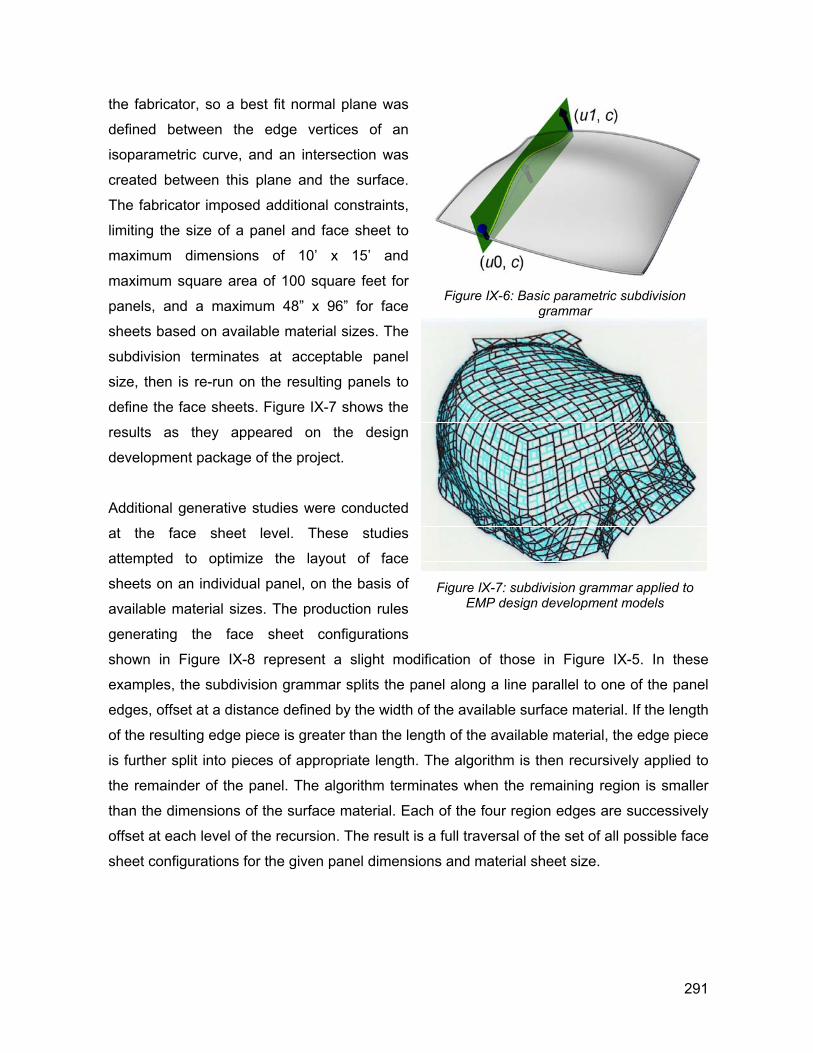
the fabricator, so a best fit normal plane was

defined between the edge vertices of an

isoparametric curve, and an intersection was

created between this plane and the surface.

The fabricator imposed additional constraints,

limiting the size of a panel and face sheet to

maximum dimensions of 10’ x 15’ and

maximum square area of 100 square feet for

panels, and a maximum 48” x 96” for face

sheets based on available material sizes. The

subdivision terminates at acceptable panel

size, then is re-run on the resulting panels to

define the face sheets. Figure IX-7 shows the

results as they appeared on the design

development package of the project.

Additional generative studies were conducted

at the face sheet level. These studies

attempted to optimize the layout of face

sheets on an individual panel, on the basis of

available material sizes. The production rules

generating the face sheet configurations

shown in Figure IX-8 represent a slight modification of those in Figure IX-5. In these

examples, the subdivision grammar splits the panel along a line parallel to one of the panel

edges, offset at a distance defined by the width of the available surface material. If the length

of the resulting edge piece is greater than the length of the available material, the edge piece

is further split into pieces of appropriate length. The algorithm is then recursively applied to

the remainder of the panel. The algorithm terminates when the remaining region is smaller

than the dimensions of the surface material. Each of the four region edges are successively

offset at each level of the recursion. The result is a full traversal of the set of all possible face

sheet configurations for the given panel dimensions and material sheet size.

Figure IX-6: Basic parametric subdivision

grammar

Figure IX-7: subdivision grammar applied to

EMP design development models

291

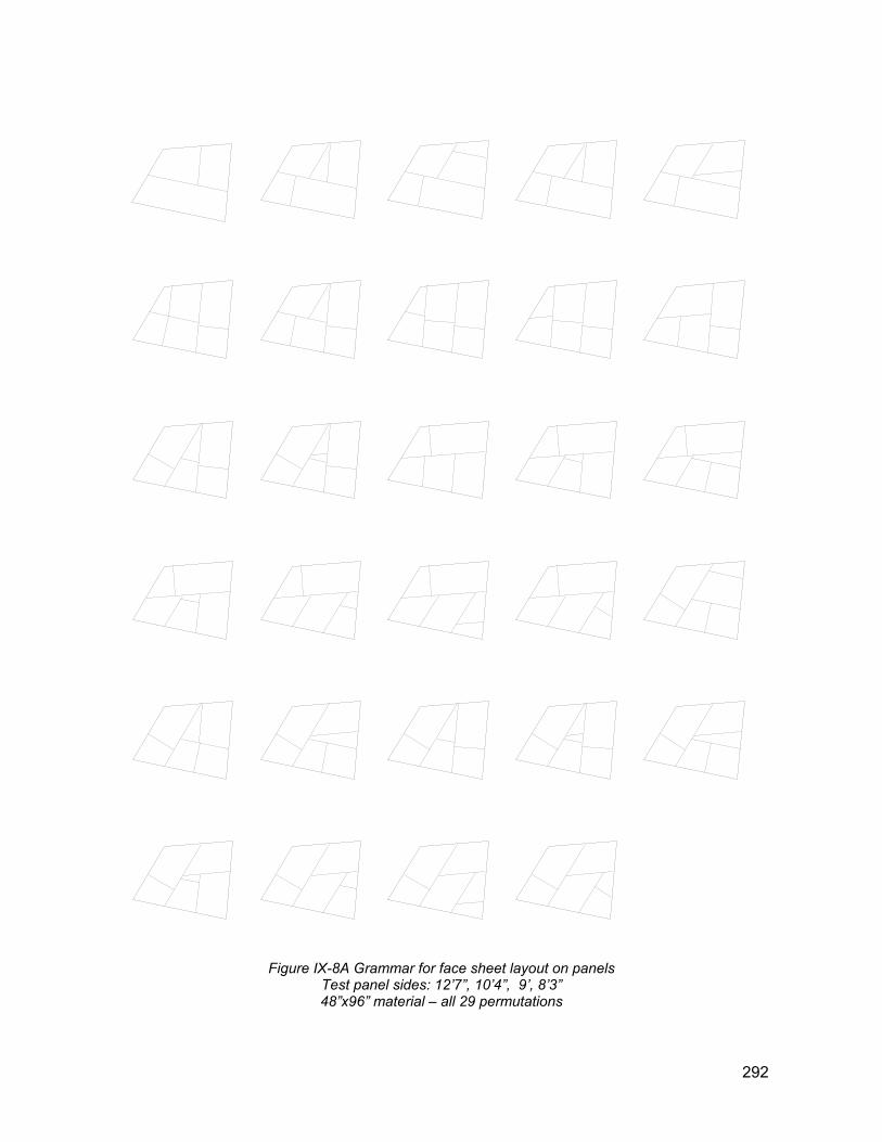
Figure IX-8A Grammar for face sheet layout on panels

Test panel sides: 12’7”, 10’4”, 9’, 8’3” 48”x96” material – all 29 permutations

292

Figure IX-8B 24”x96” material – 30 of 11941 permutations

293

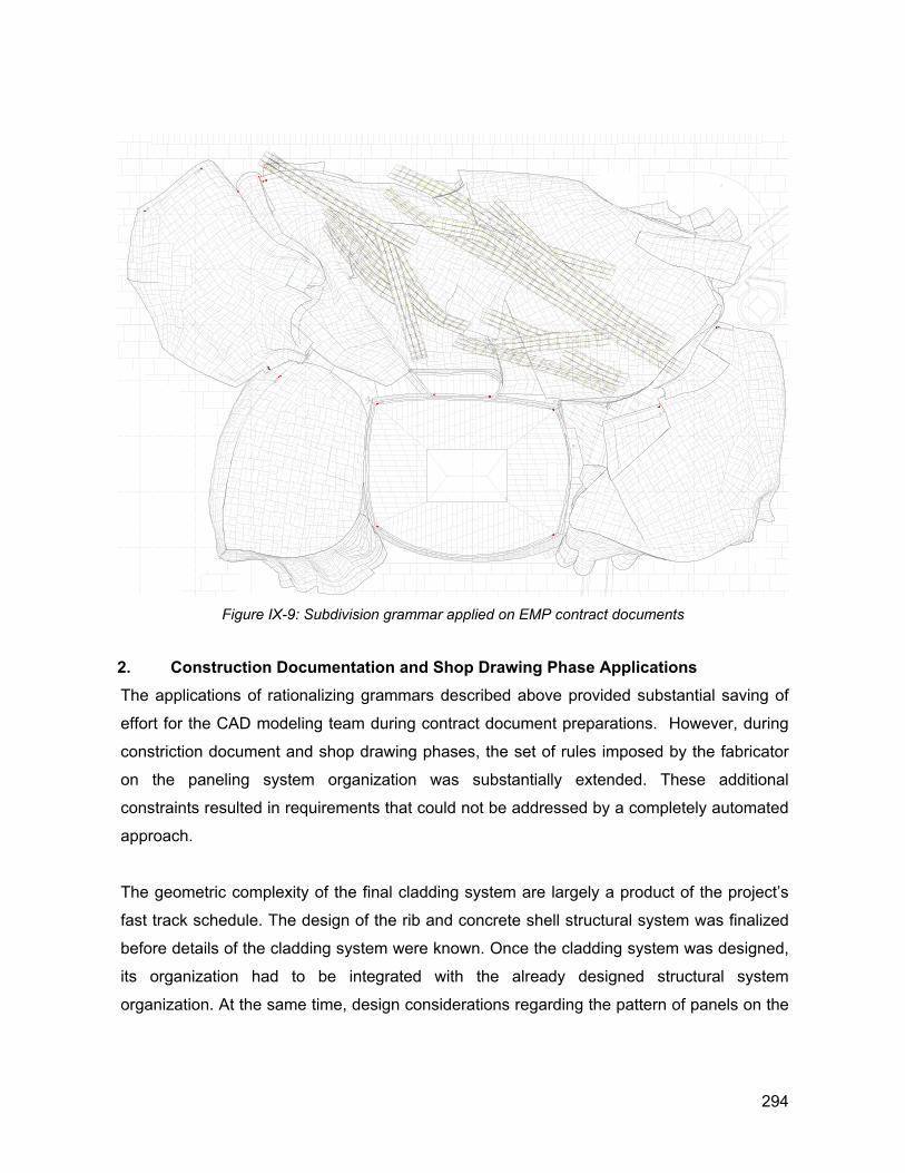
Figure IX-9: Subdivision grammar applied on EMP contract documents

2. Construction Documentation and Shop Drawing Phase Applications The applications of rationalizing grammars described above provided substantial saving of

effort for the CAD modeling team during contract document preparations. However, during

constriction document and shop drawing phases, the set of rules imposed by the fabricator

on the paneling system organization was substantially extended. These additional

constraints resulted in requirements that could not be addressed by a completely automated

approach.

The geometric complexity of the final cladding system are largely a product of the project’s

fast track schedule. The design of the rib and concrete shell structural system was finalized

before details of the cladding system were known. Once the cladding system was designed,

its organization had to be integrated with the already designed structural system

organization. At the same time, design considerations regarding the pattern of panels on the

294

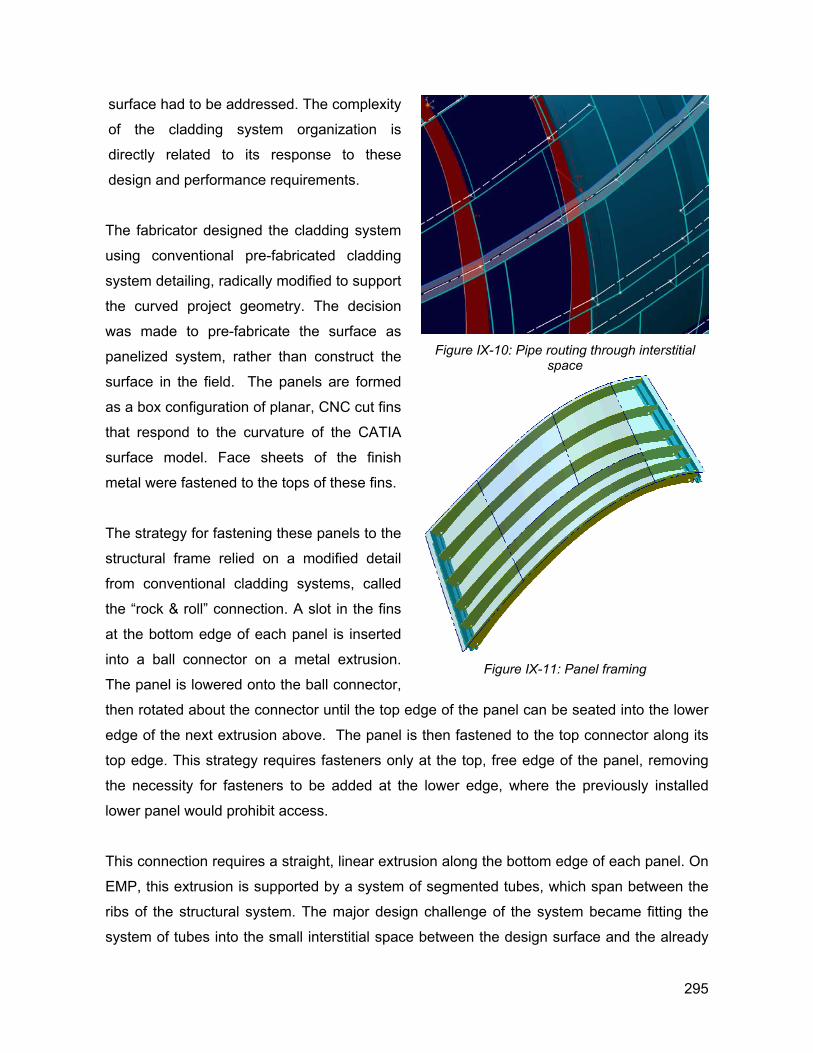
surface had to be addressed. The complexity

of the cladding system organization is

directly related to its response to these

design and performance requirements.

The fabricator designed the cladding system

using conventional pre-fabricated cladding

system detailing, radically modified to support

the curved project geometry. The decision

was made to pre-fabricate the surface as

panelized system, rather than construct the

surface in the field. The panels are formed

as a box configuration of planar, CNC cut fins

that respond to the curvature of the CATIA

surface model. Face sheets of the finish

metal were fastened to the tops of these fins.

The strategy for fastening these panels to the

structural frame relied on a modified detail

from conventional cladding systems, called

the “rock & roll” connection. A slot in the fins

at the bottom edge of each panel is inserted

into a ball connector on a metal extrusion.

The panel is lowered onto the ball connector,

then rotated about the connector until the top edge of the panel can be seated into the lower

edge of the next extrusion above. The panel is then fastened to the top connector along its

top edge. This strategy requires fasteners only at the top, free edge of the panel, removing

the necessity for fasteners to be added at the lower edge, where the previously installed

lower panel would prohibit access.

Figure IX-10: Pipe routing through interstitial space

Figure IX-11: Panel framing

This connection requires a straight, linear extrusion along the bottom edge of each panel. On

EMP, this extrusion is supported by a system of segmented tubes, which span between the

ribs of the structural system. The major design challenge of the system became fitting the

system of tubes into the small interstitial space between the design surface and the already

295

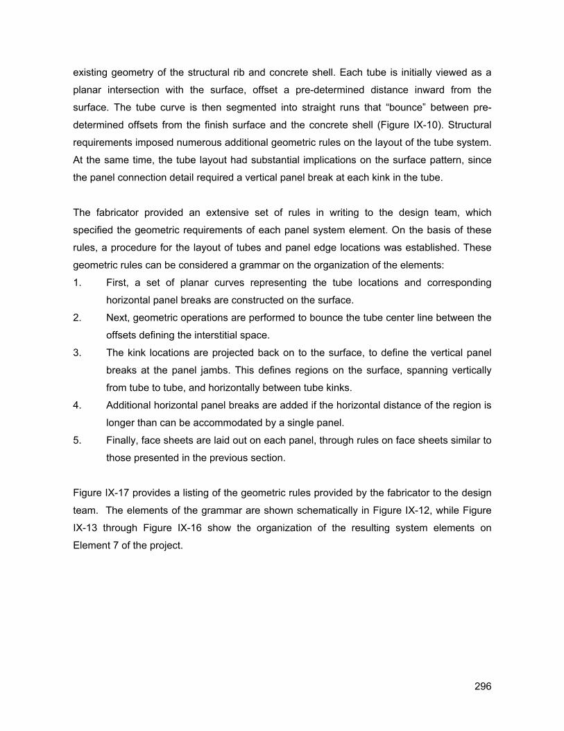
existing geometry of the structural rib and concrete shell. Each tube is initially viewed as a

planar intersection with the surface, offset a pre-determined distance inward from the

surface. The tube curve is then segmented into straight runs that “bounce” between pre-

determined offsets from the finish surface and the concrete shell (Figure IX-10). Structural

requirements imposed numerous additional geometric rules on the layout of the tube system.

At the same time, the tube layout had substantial implications on the surface pattern, since

the panel connection detail required a vertical panel break at each kink in the tube.

The fabricator provided an extensive set of rules in writing to the design team, which

specified the geometric requirements of each panel system element. On the basis of these

rules, a procedure for the layout of tubes and panel edge locations was established. These

geometric rules can be considered a grammar on the organization of the elements:

1. First, a set of planar curves representing the tube locations and corresponding

horizontal panel breaks are constructed on the surface.

2. Next, geometric operations are performed to bounce the tube center line between the

offsets defining the interstitial space.

3. The kink locations are projected back on to the surface, to define the vertical panel

breaks at the panel jambs. This defines regions on the surface, spanning vertically

from tube to tube, and horizontally between tube kinks.

4. Additional horizontal panel breaks are added if the horizontal distance of the region is

longer than can be accommodated by a single panel.

5. Finally, face sheets are laid out on each panel, through rules on face sheets similar to

those presented in the previous section.

Figure IX-17 provides a listing of the geometric rules provided by the fabricator to the design

team. The elements of the grammar are shown schematically in Figure IX-12, while Figure

IX-13 through Figure IX-16 show the organization of the resulting system elements on

Element 7 of the project.

296

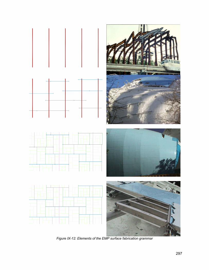
Figure IX-12: Elements of the EMP surface fabrication grammar

297

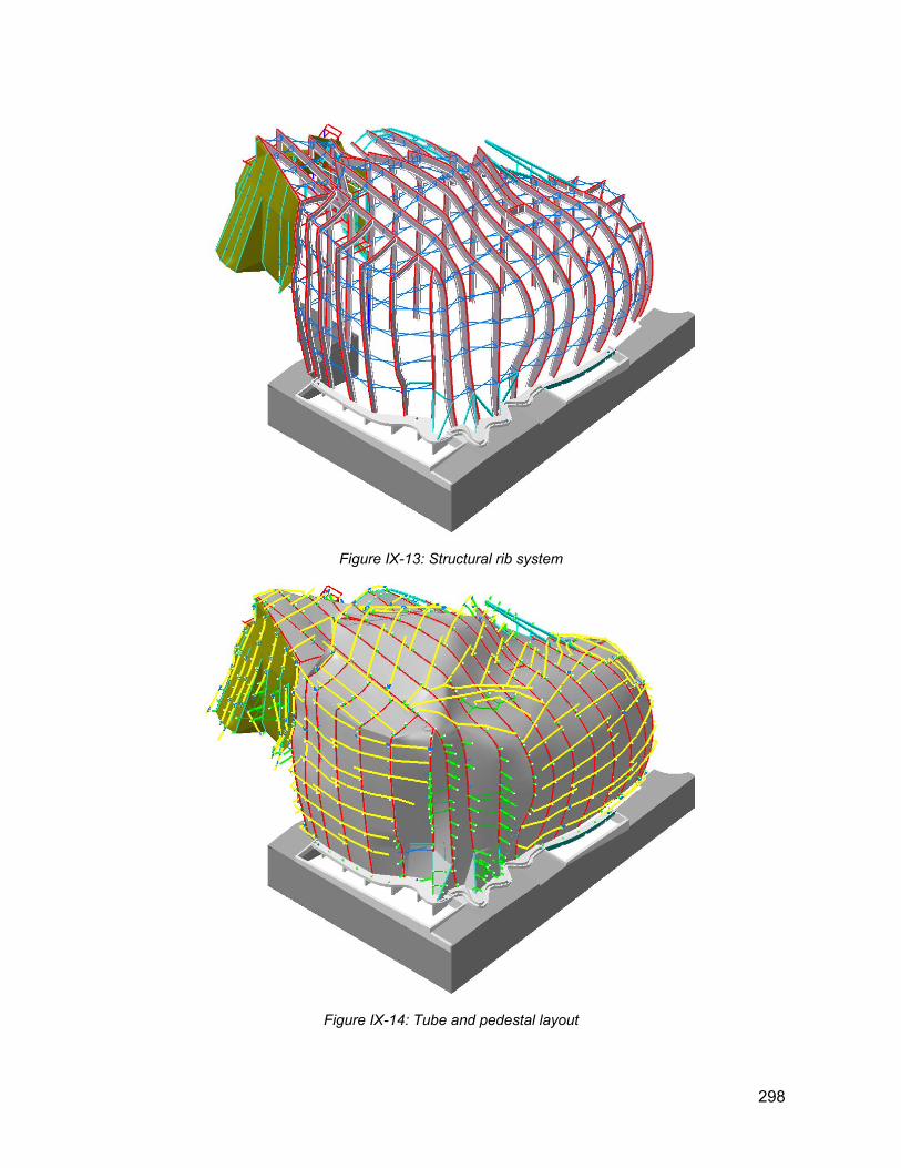
Figure IX-13: Structural rib system

Figure IX-14: Tube and pedestal layout

298

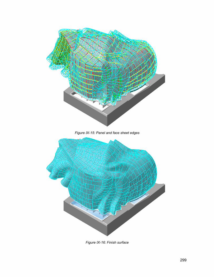
Figure IX-15: Panel and face sheet edges

Figure IX-16: Finish surface

299

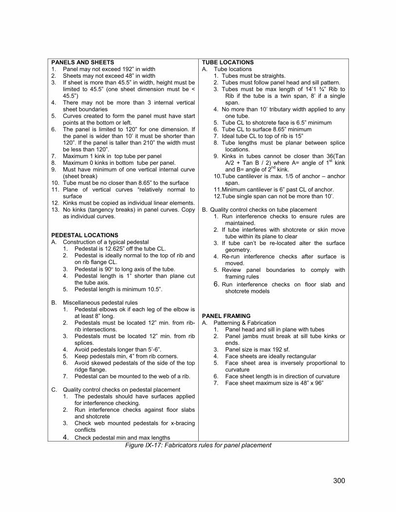
PANELS AND SHEETS 1. Panel may not exceed 192” in width 2. Sheets may not exceed 48” in width 3. If sheet is more than 45.5” in width, height must be

limited to 45.5” (one sheet dimension must be < 45.5”)

4. There may not be more than 3 internal vertical sheet boundaries

5. Curves created to form the panel must have start points at the bottom or left.

6. The panel is limited to 120” for one dimension. If the panel is wider than 10’ it must be shorter than 120”. If the panel is taller than 210” the width must be less than 120”.

7. Maximum 1 kink in top tube per panel 8. Maximum 0 kinks in bottom tube per panel. 9. Must have minimum of one vertical internal curve

(sheet break) 10. Tube must be no closer than 8.65” to the surface 11. Plane of vertical curves “relatively normal to

surface 12. Kinks must be copied as individual linear elements. 13. No kinks (tangency breaks) in panel curves. Copy

as individual curves. PEDESTAL LOCATIONS A. Construction of a typical pedestal

1. Pedestal is 12.625” off the tube CL. 2. Pedestal is ideally normal to the top of rib and

on rib flange CL. 3. Pedestal is 90° to long axis of the tube. 4. Pedestal length is 1” shorter than plane cut

the tube axis. 5. Pedestal length is minimum 10.5”.

B. Miscellaneous pedestal rules

1. Pedestal elbows ok if each leg of the elbow is at least 8” long.

2. Pedestals must be located 12” min. from rib-rib intersections.

3. Pedestals must be located 12” min. from rib splices.

4. Avoid pedestals longer than 5’-6”. 5. Keep pedestals min, 4” from rib corners. 6. Avoid skewed pedestals of the side of the top

ridge flange. 7. Pedestal can be mounted to the web of a rib.

C. Quality control checks on pedestal placement

1. The pedestals should have surfaces applied for interference checking.

2. Run interference checks against floor slabs and shotcrete

3. Check web mounted pedestals for x-bracing conflicts

4. Check pedestal min and max lengths

TUBE LOCATIONS A. Tube locations

1. Tubes must be straights. 2. Tubes must follow panel head and sill pattern. 3. Tubes must be max length of 14’1 ¾” Rib to

Rib if the tube is a twin span, 8’ if a single span.

4. No more than 10’ tributary width applied to any one tube.

5. Tube CL to shotcrete face is 6.5” minimum 6. Tube CL to surface 8.65” minimum 7. Ideal tube CL to top of rib is 15” 8. Tube lengths must be planar between splice

locations. 9. Kinks in tubes cannot be closer than 36(Tan

A/2 + Tan B / 2) where A= angle of 1st kink and B= angle of 2nd kink.

10. Tube cantilever is max. 1/5 of anchor – anchor span.

11. Minimum cantilever is 6” past CL of anchor. 12. Tube single span can not be more than 10’.

B. Quality control checks on tube placement

1. Run interference checks to ensure rules are maintained.

2. If tube interferes with shotcrete or skin move tube within its plane to clear

3. If tube can’t be re-located alter the surface geometry.

4. Re-run interference checks after surface is moved.

5. Review panel boundaries to comply with framing rules

6. Run interference checks on floor slab and shotcrete models

PANEL FRAMING A. Patterning & Fabrication

1. Panel head and sill in plane with tubes 2. Panel jambs must break at sill tube kinks or

ends. 3. Panel size is max 192 sf. 4. Face sheets are ideally rectangular 5. Face sheet area is inversely proportional to

curvature 6. Face sheet length is in direction of curvature 7. Face sheet maximum size is 48” x 96”

Figure IX-17: Fabricators rules for panel placement

300

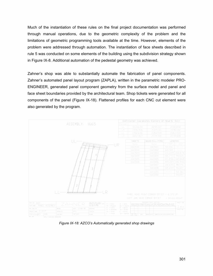
Much of the instantiation of these rules on the final project documentation was performed

through manual operations, due to the geometric complexity of the problem and the

limitations of geometric programming tools available at the time. However, elements of the

problem were addressed through automation. The instantiation of face sheets described in

rule 5 was conducted on some elements of the building using the subdivision strategy shown

in Figure IX-8. Additional automation of the pedestal geometry was achieved.

Zahner’s shop was able to substantially automate the fabrication of panel components.

Zahner’s automated panel layout program (ZAPLA), written in the parametric modeler PRO-

ENGINEER, generated panel component geometry from the surface model and panel and

face sheet boundaries provided by the architectural team. Shop tickets were generated for all

components of the panel (Figure IX-18). Flattened profiles for each CNC cut element were

also generated by the program.

Figure IX-18: AZCO’s Automatically generated shop drawings

301

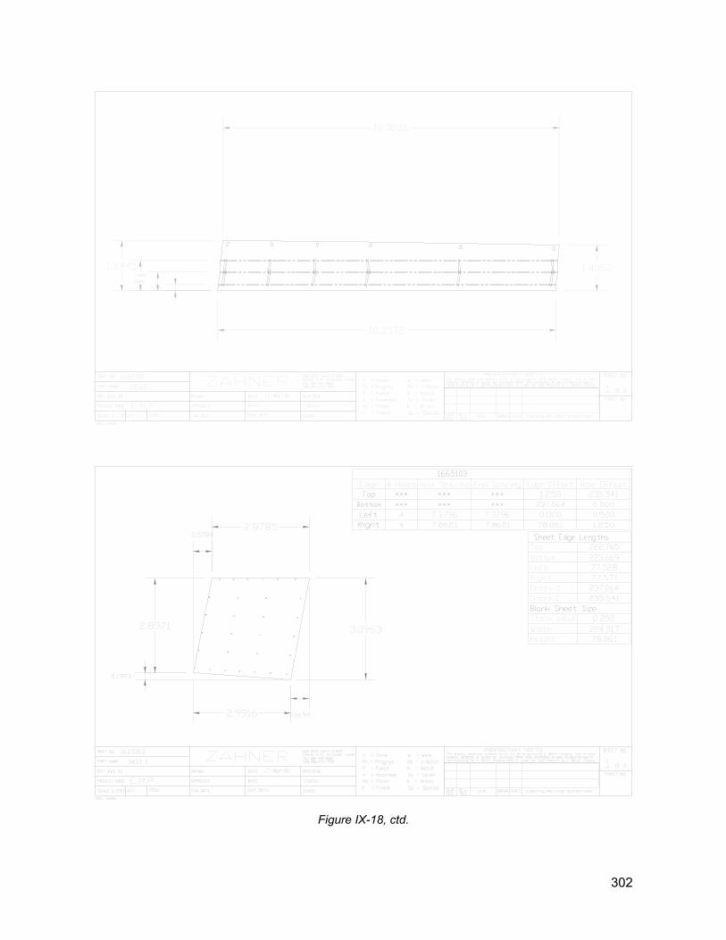
Figure IX-18, ctd.

302

B. MATERIALS BASED RATIONALIZATION

In this final section, discussion turns to the development of grammars on the basis of the

materials simulation constructs developed in Chapter VII. In this section, the constructs

developed to support materials based modeling of sheet materials will be re-directed toward

applications of surface rationalization.

The materials modeling approach is well suited to applications of grammars on manifolds

developed in Chapter VIII.B. We direct this application to problems where a desired surface

form – provided by digitizing of schematic design physical models – is rationalized into

constructible by assemblies of material sheets. Such a generative strategy will require the

definition of the following components:

1. A notion of the space in which shapes, elements and transformation are defined,

2. A set of elements, with a topology of element-part relationships defined on these

elements,

3. A set of possible transformations on these elements, and shapes developed as

compositions of elements.

To this set of conditions, we will add the following to direct the definition of grammars toward

the rationalization activities:

4. A goal toward the satisfaction of which shape transformations are directed,

5. A set of heuristics measuring of the fitness of produced shapes toward satisfaction of

the goal.

1. Spaces and Elements In Euclidean grammars, the notion of a space in which elements are defined and

transformations occur is often assumed with little discussion. This space provides the

“playing field” on which grammars occur, and contributes implicitly to the specification of valid

elements of the grammar. The set of elements in Euclidean space grammars are the valid

Euclidean elements of the space: points, lines, and bounded planar regions in Euclidean 2-

space, with the inclusion of bounded volumes in R3.

303

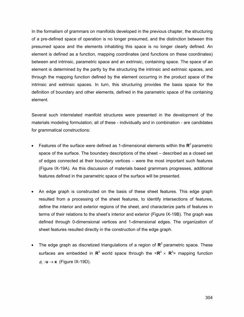
In the formalism of grammars on manifolds developed in the previous chapter, the structuring

of a pre-defined space of operation is no longer presumed, and the distinction between this

presumed space and the elements inhabiting this space is no longer clearly defined. An

element is defined as a function, mapping coordinates (and functions on these coordinates)

between and intrinsic, parametric space and an extrinsic, containing space. The space of an

element is determined by the partly by the structuring the intrinsic and extrinsic spaces, and

through the mapping function defined by the element occurring in the product space of the

intrinsic and extrinsic spaces. In turn, this structuring provides the basis space for the

definition of boundary and other elements, defined in the parametric space of the containing

element.

Several such interrelated manifold structures were presented in the development of the

materials modeling formulation; all of these - individually and in combination - are candidates

for grammatical constructions:

• Features of the surface were defined as 1-dimensional elements within the R2 parametric

space of the surface. The boundary descriptions of the sheet – described as a closed set

of edges connected at their boundary vertices – were the most important such features

(Figure IX-19A). As this discussion of materials based grammars progresses, additional

features defined in the parametric space of the surface will be presented.

• An edge graph is constructed on the basis of these sheet features. This edge graph

resulted from a processing of the sheet features, to identify intersections of features,

define the interior and exterior regions of the sheet, and characterize parts of features in

terms of their relations to the sheet’s interior and exterior (Figure IX-19B). The graph was

defined through 0-dimensional vertices and 1-dimensional edges. The organization of

sheet features resulted directly in the construction of the edge graph.

• The edge graph as discretized triangulations of a region of R2 parametric space. These

surfaces are embedded in R3 world space through the <R2 × R3> mapping function

:tφ →u x (Figure IX-19D).

304

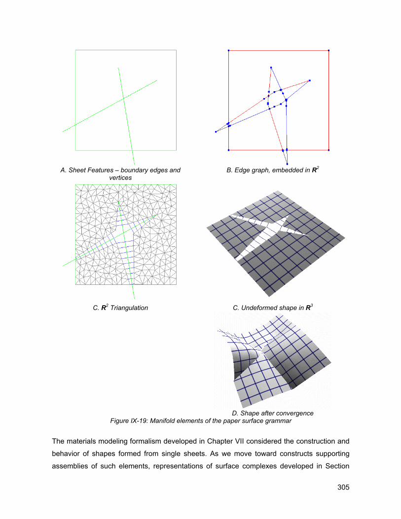
A. Sheet Features – boundary edges and

vertices B. Edge graph, embedded in R2

C. R2 Triangulation C. Undeformed shape in R3

D. Shape after convergence

Figure IX-19: Manifold elements of the paper surface grammar

The materials modeling formalism developed in Chapter VII considered the construction and

behavior of shapes formed from single sheets. As we move toward constructs supporting

assemblies of such elements, representations of surface complexes developed in Section

305

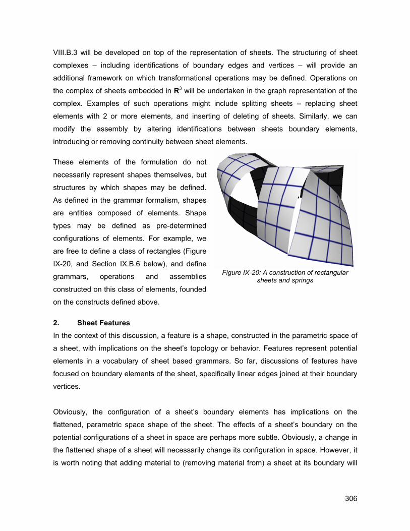
VIII.B.3 will be developed on top of the representation of sheets. The structuring of sheet

complexes – including identifications of boundary edges and vertices – will provide an

additional framework on which transformational operations may be defined. Operations on

the complex of sheets embedded in R3 will be undertaken in the graph representation of the

complex. Examples of such operations might include splitting sheets – replacing sheet

elements with 2 or more elements, and inserting of deleting of sheets. Similarly, we can

modify the assembly by altering identifications between sheets boundary elements,

introducing or removing continuity between sheet elements.

These elements of the formulation do not

necessarily represent shapes themselves, but

structures by which shapes may be defined.

As defined in the grammar formalism, shapes

are entities composed of elements. Shape

types may be defined as pre-determined

configurations of elements. For example, we

are free to define a class of rectangles (Figure

IX-20, and Section IX.B.6 below), and define

grammars, operations and assemblies

constructed on this class of elements, founded

on the constructs defined above.

Figure IX-20: A construction of rectangular

sheets and springs

2. Sheet Features In the context of this discussion, a feature is a shape, constructed in the parametric space of

a sheet, with implications on the sheet’s topology or behavior. Features represent potential

elements in a vocabulary of sheet based grammars. So far, discussions of features have

focused on boundary elements of the sheet, specifically linear edges joined at their boundary

vertices.

Obviously, the configuration of a sheet’s boundary elements has implications on the

flattened, parametric space shape of the sheet. The effects of a sheet’s boundary on the

potential configurations of a sheet in space are perhaps more subtle. Obviously, a change in

the flattened shape of a sheet will necessarily change its configuration in space. However, it

is worth noting that adding material to (removing material from) a sheet at its boundary will

306

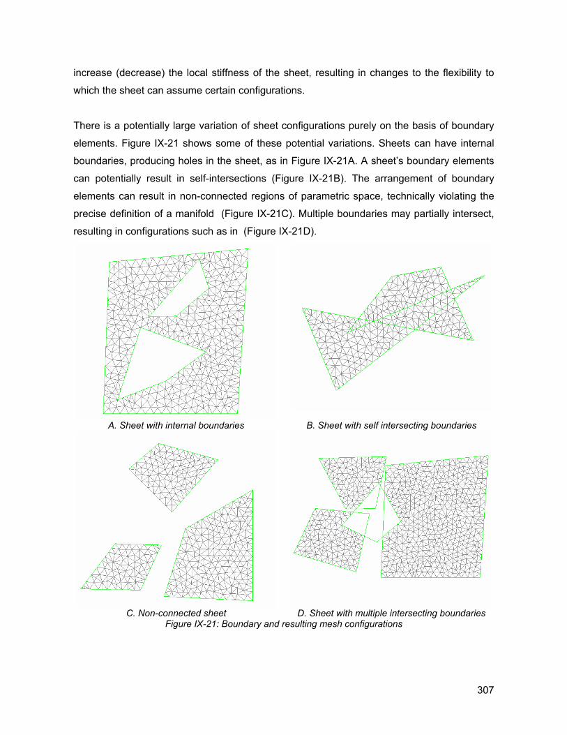
increase (decrease) the local stiffness of the sheet, resulting in changes to the flexibility to

which the sheet can assume certain configurations.

There is a potentially large variation of sheet configurations purely on the basis of boundary

elements. Figure IX-21 shows some of these potential variations. Sheets can have internal

boundaries, producing holes in the sheet, as in Figure IX-21A. A sheet’s boundary elements

can potentially result in self-intersections (Figure IX-21B). The arrangement of boundary

elements can result in non-connected regions of parametric space, technically violating the

precise definition of a manifold (Figure IX-21C). Multiple boundaries may partially intersect,

resulting in configurations such as in (Figure IX-21D).

A. Sheet with internal boundaries B. Sheet with self intersecting boundaries

C. Non-connected sheet D. Sheet with multiple intersecting boundaries

Figure IX-21: Boundary and resulting mesh configurations

307

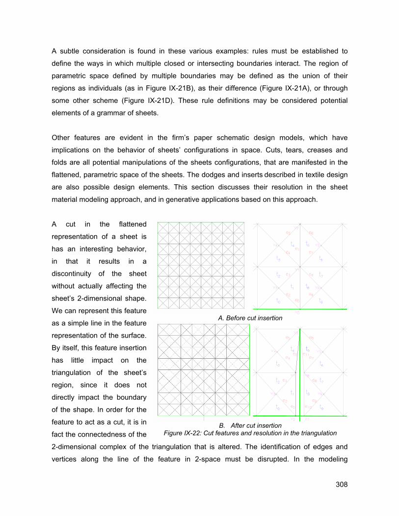
A subtle consideration is found in these various examples: rules must be established to

define the ways in which multiple closed or intersecting boundaries interact. The region of

parametric space defined by multiple boundaries may be defined as the union of their

regions as individuals (as in Figure IX-21B), as their difference (Figure IX-21A), or through

some other scheme (Figure IX-21D). These rule definitions may be considered potential

elements of a grammar of sheets.

Other features are evident in the firm’s paper schematic design models, which have

implications on the behavior of sheets’ configurations in space. Cuts, tears, creases and

folds are all potential manipulations of the sheets configurations, that are manifested in the

flattened, parametric space of the sheets. The dodges and inserts described in textile design

are also possible design elements. This section discusses their resolution in the sheet

material modeling approach, and in generative applications based on this approach.

A cut in the flattened

representation of a sheet is

has an interesting behavior,

in that it results in a

discontinuity of the sheet

without actually affecting the

sheet’s 2-dimensional shape.

We can represent this feature

as a simple line in the feature

representation of the surface.

By itself, this feature insertion

has little impact on the

triangulation of the sheet’s

region, since it does not

directly impact the boundary

of the shape. In order for the

feature to act as a cut, it is in

fact the connectedness of the

2-dimensional complex of the triangulation that is altered. The identification of edges and

vertices along the line of the feature in 2-space must be disrupted. In the modeling

A. Before cut insertion

B. After cut insertion

Figure IX-22: Cut features and resolution in the triangulation

308

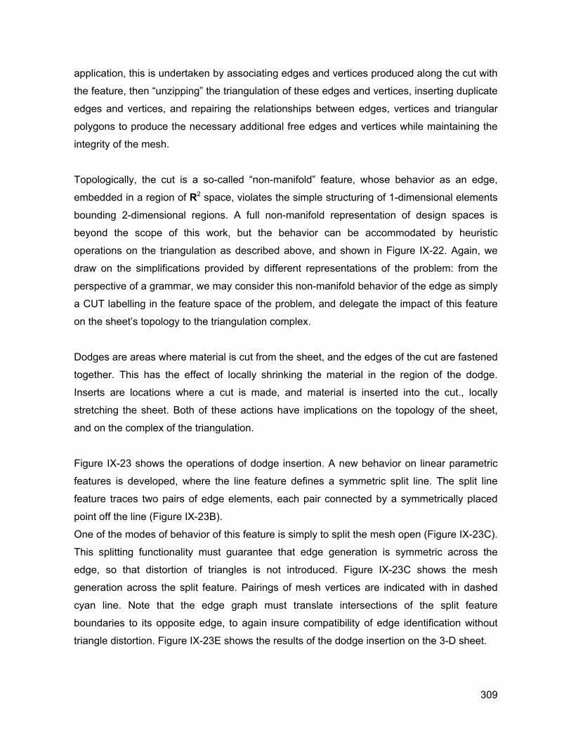
application, this is undertaken by associating edges and vertices produced along the cut with

the feature, then “unzipping” the triangulation of these edges and vertices, inserting duplicate

edges and vertices, and repairing the relationships between edges, vertices and triangular

polygons to produce the necessary additional free edges and vertices while maintaining the

integrity of the mesh.

Topologically, the cut is a so-called “non-manifold” feature, whose behavior as an edge,

embedded in a region of R2 space, violates the simple structuring of 1-dimensional elements

bounding 2-dimensional regions. A full non-manifold representation of design spaces is

beyond the scope of this work, but the behavior can be accommodated by heuristic

operations on the triangulation as described above, and shown in Figure IX-22. Again, we

draw on the simplifications provided by different representations of the problem: from the

perspective of a grammar, we may consider this non-manifold behavior of the edge as simply

a CUT labelling in the feature space of the problem, and delegate the impact of this feature

on the sheet’s topology to the triangulation complex.

Dodges are areas where material is cut from the sheet, and the edges of the cut are fastened

together. This has the effect of locally shrinking the material in the region of the dodge.

Inserts are locations where a cut is made, and material is inserted into the cut., locally

stretching the sheet. Both of these actions have implications on the topology of the sheet,

and on the complex of the triangulation.

Figure IX-23 shows the operations of dodge insertion. A new behavior on linear parametric

features is developed, where the line feature defines a symmetric split line. The split line

feature traces two pairs of edge elements, each pair connected by a symmetrically placed

point off the line (Figure IX-23B).

One of the modes of behavior of this feature is simply to split the mesh open (Figure IX-23C).

This splitting functionality must guarantee that edge generation is symmetric across the

edge, so that distortion of triangles is not introduced. Figure IX-23C shows the mesh

generation across the split feature. Pairings of mesh vertices are indicated with in dashed

cyan line. Note that the edge graph must translate intersections of the split feature

boundaries to its opposite edge, to again insure compatibility of edge identification without

triangle distortion. Figure IX-23E shows the results of the dodge insertion on the 3-D sheet.

309

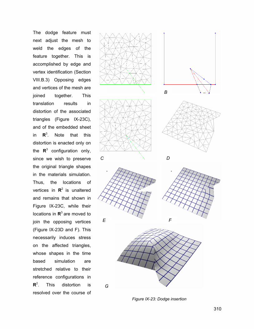
The dodge feature must

next adjust the mesh to

weld the edges of the

feature together. This is

accomplished by edge and

vertex identification (Section

VIII.B.3) Opposing edges

and vertices of the mesh are

joined together. This

translation results in

distortion of the associated

triangles (Figure IX-23C),

and of the embedded sheet

in R3. Note that this

distortion is enacted only on

the R3 configuration only,

since we wish to preserve

the original triangle shapes

in the materials simulation.

Thus, the locations of

vertices in R2 is unaltered

and remains that shown in

Figure IX-23C, while their

locations in R3 are moved to

join the opposing vertices

(Figure IX-23D and F). This

necessarily induces stress

on the affected triangles,

whose shapes in the time

based simulation are

stretched relative to their

reference configurations in

R2. This distortion is

resolved over the course of

A

Figure IX-23: Do

B

C

d

D

E

g

F

G

e insertion

310

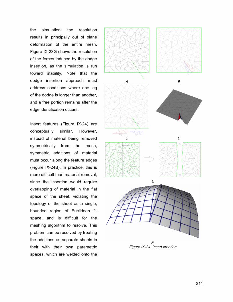
the simulation; the resolution

results in principally out of plane

deformation of the entire mesh.

Figure IX-23G shows the resolution

of the forces induced by the dodge

insertion, as the simulation is run

toward stability. Note that the

dodge insertion approach must

address conditions where one leg

of the dodge is longer than another,

and a free portion remains after the

edge identification occurs.

Insert features (Figure IX-24) are

conceptually similar. However,

instead of material being removed

symmetrically from the mesh,

symmetric additions of material

must occur along the feature edges

(Figure IX-24B). In practice, this is

more difficult than material removal,

since the insertion would require

overlapping of material in the flat

space of the sheet, violating the

topology of the sheet as a single,

bounded region of Euclidean 2-

space, and is difficult for the

meshing algorithm to resolve. This

problem can be resolved by treating

the additions as separate sheets in

their with their own parametric

spaces, which are welded onto the

A B

C D

E

F.

Figure IX-24: Insert creation

311

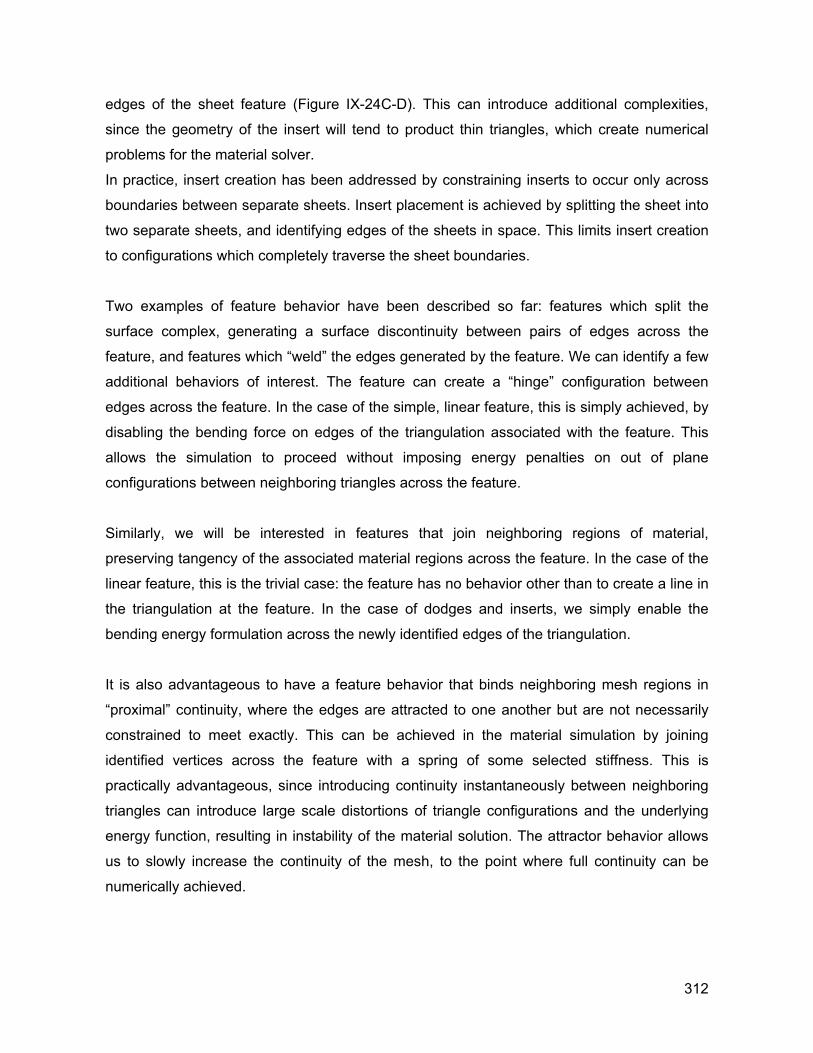
edges of the sheet feature (Figure IX-24C-D). This can introduce additional complexities,

since the geometry of the insert will tend to product thin triangles, which create numerical

problems for the material solver.

In practice, insert creation has been addressed by constraining inserts to occur only across

boundaries between separate sheets. Insert placement is achieved by splitting the sheet into

two separate sheets, and identifying edges of the sheets in space. This limits insert creation

to configurations which completely traverse the sheet boundaries.

Two examples of feature behavior have been described so far: features which split the

surface complex, generating a surface discontinuity between pairs of edges across the

feature, and features which “weld” the edges generated by the feature. We can identify a few

additional behaviors of interest. The feature can create a “hinge” configuration between

edges across the feature. In the case of the simple, linear feature, this is simply achieved, by

disabling the bending force on edges of the triangulation associated with the feature. This

allows the simulation to proceed without imposing energy penalties on out of plane

configurations between neighboring triangles across the feature.

Similarly, we will be interested in features that join neighboring regions of material,

preserving tangency of the associated material regions across the feature. In the case of the

linear feature, this is the trivial case: the feature has no behavior other than to create a line in

the triangulation at the feature. In the case of dodges and inserts, we simply enable the

bending energy formulation across the newly identified edges of the triangulation.

It is also advantageous to have a feature behavior that binds neighboring mesh regions in

“proximal” continuity, where the edges are attracted to one another but are not necessarily

constrained to meet exactly. This can be achieved in the material simulation by joining

identified vertices across the feature with a spring of some selected stiffness. This is

practically advantageous, since introducing continuity instantaneously between neighboring

triangles can introduce large scale distortions of triangle configurations and the underlying

energy function, resulting in instability of the material solution. The attractor behavior allows

us to slowly increase the continuity of the mesh, to the point where full continuity can be

numerically achieved.

312

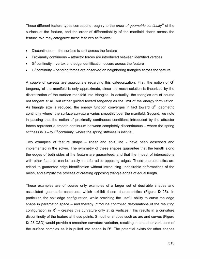
These different feature types correspond roughly to the order of geometric continuity28 of the

surface at the feature, and the order of differentiability of the manifold charts across the

feature. We may categorize these features as follows:

• Discontinuous – the surface is split across the feature

• Proximally continuous – attractor forces are introduced between identified vertices

• G0 continuity – vertex and edge identification occurs across the feature

• G1 continuity – bending forces are observed on neighboring triangles across the feature

A couple of caveats are appropriate regarding this categorization. First, the notion of G1

tangency of the manifold is only approximate, since the mesh solution is linearized by the

discretization of the surface manifold into triangles. In actuality, the triangles are of course

not tangent at all, but rather guided toward tangency as the limit of the energy formulation.

As triangle size is reduced, the energy function converges in fact toward G2 geometric

continuity where the surface curvature varies smoothly over the manifold. Second, we note

in passing that the notion of proximally continuous conditions introduced by the attractor

forces represent a smooth continuum between completely discontinuous – where the spring

stiffness is 0 – to G0 continuity, where the spring stiffness is infinite.

Two examples of feature shape – linear and split line - have been described and

implemented in the solver. The symmetry of these shapes guarantee that the length along

the edges of both sides of the feature are guaranteed, and that the impact of intersections

with other features can be easily transferred to opposing edges. These characteristics are

critical to guarantee edge identification without introducing undesirable deformations of the

mesh, and simplify the process of creating opposing triangle edges of equal length.

These examples are of course only examples of a larger set of desirable shapes and

associated geometric constructs which exhibit these characteristics (Figure IX-25). In

particular, the spit edge configuration, while providing the useful ability to curve the edge

shape in parametric space – and thereby introduce controlled deformations of the resulting

configuration in R3 – creates this curvature only at its vertices. This results in a curvature

discontinuity of the feature at these points. Smoother shapes such as arc and curves (Figure

IX-25 C&D) would provide a smoother curvature variation, resulting in smoother variations of

the surface complex as it is pulled into shape in R3. The potential exists for other shapes

313

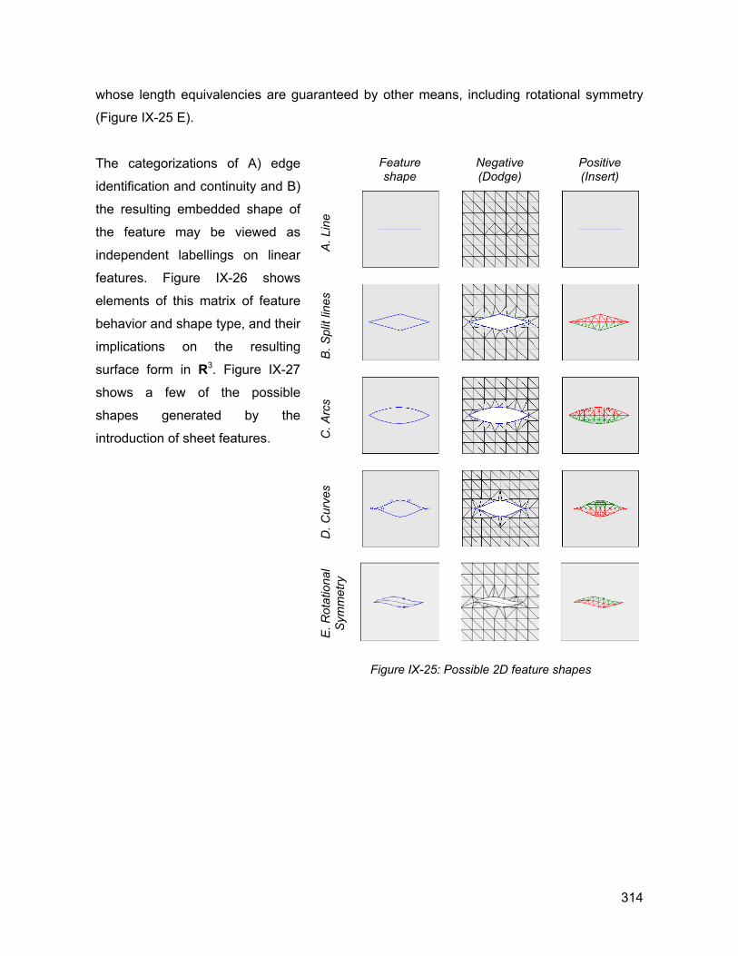
whose length equivalencies are guaranteed by other means, including rotational symmetry

(Figure IX-25 E).

The categorizations of A) edge

identification and continuity and B)

the resulting embedded shape of

the feature may be viewed as

independent labellings on linear

features. Figure IX-26 shows

elements of this matrix of feature

behavior and shape type, and their

implications on the resulting

surface form in R3. Figure IX-27

shows a few of the possible

shapes generated by the

introduction of sheet features.

Feature shape

Negative (Dodge)

Positive (Insert)

A. L

ine

B. S

plit

lines

C. A

rcs

D. C

urve

s

E. R

otat

iona

l Sy

mm

etry

Figure IX-25: Possible 2D feature shapes

314

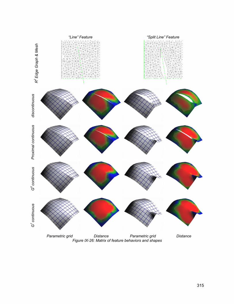
“Line” Feature “Split Line” Feature

R2 Ed

ge G

raph

& M

esh

disc

ontin

uous

Prox

imal

con

tinuo

us

G0 co

ntin

uous

G1 co

ntin

uous

Parametric grid Distance Parametric grid Distance Figure IX-26: Matrix of feature behaviors and shapes

315

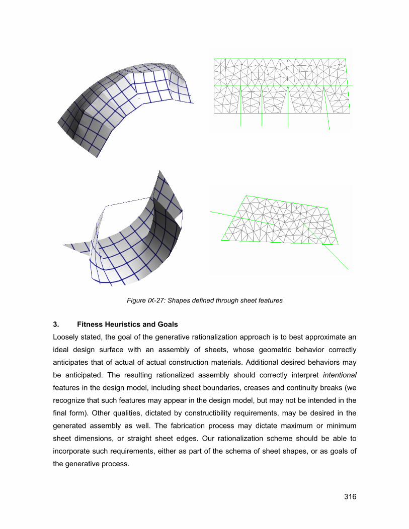
Figure IX-27: Shapes defined through sheet features

3. Fitness Heuristics and Goals Loosely stated, the goal of the generative rationalization approach is to best approximate an

ideal design surface with an assembly of sheets, whose geometric behavior correctly

anticipates that of actual of actual construction materials. Additional desired behaviors may

be anticipated. The resulting rationalized assembly should correctly interpret intentional

features in the design model, including sheet boundaries, creases and continuity breaks (we

recognize that such features may appear in the design model, but may not be intended in the

final form). Other qualities, dictated by constructibility requirements, may be desired in the

generated assembly as well. The fabrication process may dictate maximum or minimum

sheet dimensions, or straight sheet edges. Our rationalization scheme should be able to

incorporate such requirements, either as part of the schema of sheet shapes, or as goals of

the generative process.

316

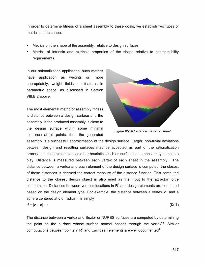
In order to determine fitness of a sheet assembly to these goals, we establish two types of

metrics on the shape:

Metrics on the shape of the assembly, relative to design surfaces

Metrics of intrinsic and extrinsic properties of the shape relative to constructibility

requirements

In our rationalization application, such metrics

have application as weights or, more

appropriately, weight fields, on features in

parametric space, as discussed in Section

VIII.B.2 above.

The most elemental metric of assembly fitness

is distance between a design surface and the

assembly. If the produced assembly is close to

the design surface within some minimal

tolerance at all points, then the generated

assembly is a successful approximation of the design surface. Larger, non-trivial deviations

between design and resulting surfaces may be accepted as part of the rationalization

process; in these circumstances other heuristics such as surface smoothness may come into

play. Distance is measured between each vertex of each sheet in the assembly. The

distance between a vertex and each element of the design surface is computed; the closest

of these distances is deemed the correct measure of the distance function. This computed

distance to the closest design object is also used as the input to the attractor force

computation. Distances between vertices locations in R3 and design elements are computed

based on the design element type. For example, the distance between a vertex v and a

sphere centered at c of radius r is simply

Figure IX-28:Distance metric on sheet

d = |v - c| - r (IX.1)

The distance between a vertex and Bézier or NURBS surfaces are computed by determining

the point on the surface whose surface normal passes through the vertex64. Similar

computations between points in R3 and Euclidean elements are well documented13.

317

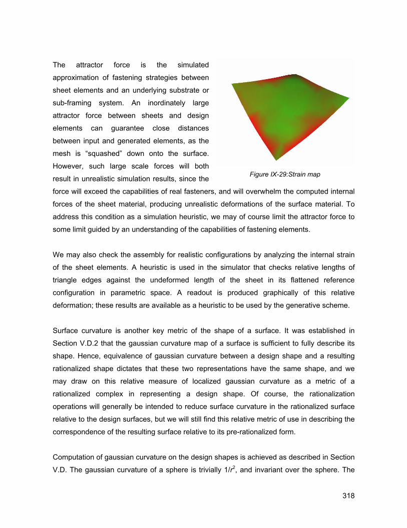
The attractor force is the simulated

approximation of fastening strategies between

sheet elements and an underlying substrate or

sub-framing system. An inordinately large

attractor force between sheets and design

elements can guarantee close distances

between input and generated elements, as the

mesh is “squashed” down onto the surface.

However, such large scale forces will both

result in unrealistic simulation results, since the

force will exceed the capabilities of real fasteners, and will overwhelm the computed internal

forces of the sheet material, producing unrealistic deformations of the surface material. To

address this condition as a simulation heuristic, we may of course limit the attractor force to

some limit guided by an understanding of the capabilities of fastening elements.

Figure IX-29:Strain map

We may also check the assembly for realistic configurations by analyzing the internal strain

of the sheet elements. A heuristic is used in the simulator that checks relative lengths of

triangle edges against the undeformed length of the sheet in its flattened reference

configuration in parametric space. A readout is produced graphically of this relative

deformation; these results are available as a heuristic to be used by the generative scheme.

Surface curvature is another key metric of the shape of a surface. It was established in

Section V.D.2 that the gaussian curvature map of a surface is sufficient to fully describe its

shape. Hence, equivalence of gaussian curvature between a design shape and a resulting

rationalized shape dictates that these two representations have the same shape, and we

may draw on this relative measure of localized gaussian curvature as a metric of a

rationalized complex in representing a design shape. Of course, the rationalization

operations will generally be intended to reduce surface curvature in the rationalized surface

relative to the design surfaces, but we will still find this relative metric of use in describing the

correspondence of the resulting surface relative to its pre-rationalized form.

Computation of gaussian curvature on the design shapes is achieved as described in Section

V.D. The gaussian curvature of a sphere is trivially 1/r2, and invariant over the sphere. The

318

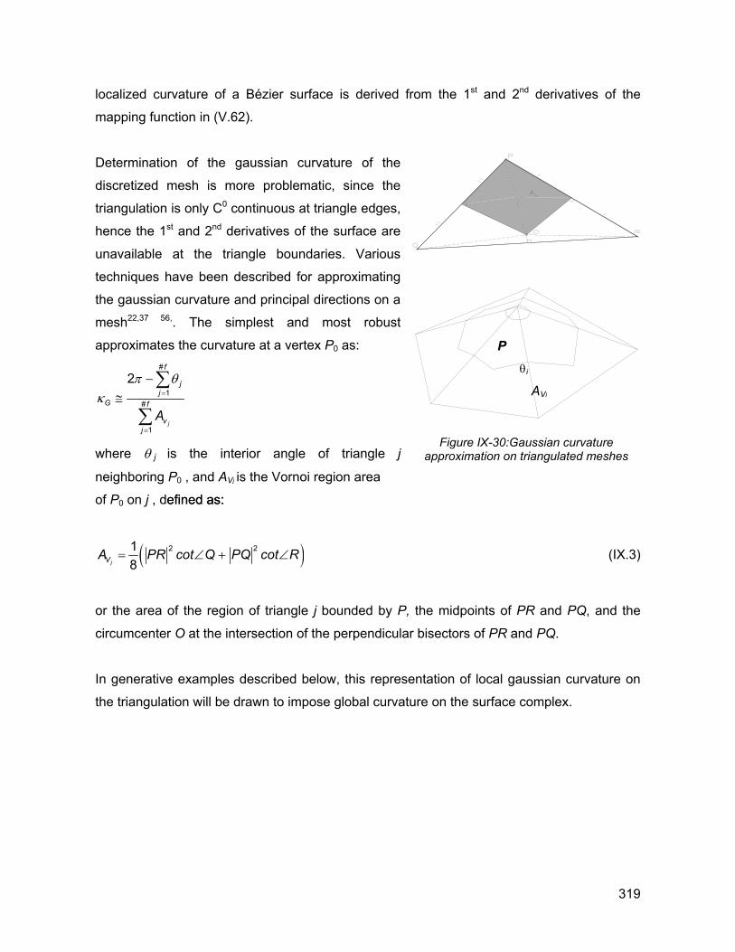
localized curvature of a Bézier surface is derived from the 1st and 2nd derivatives of the

mapping function in (V.62).

Determination of the gaussian curvature of the

discretized mesh is more problematic, since the

triangulation is only C0 continuous at triangle edges,

hence the 1st and 2nd derivatives of the surface are

unavailable at the triangle boundaries. Various

techniques have been described for approximating

the gaussian curvature and principal directions on a

mesh22,37 56,. The simplest and most robust

approximates the curvature at a vertex P0 as: #

1#

1

2

j

f

jj

G f

vj

A

π θκ =

=

−≅

∑

∑

Figure IX-approximatiowhere θ j is the interior angle of triangle j

neighboring P0 , and AVj is the Vornoi region area

of P0 on j , defined as: efined as:

( )2 218jVA PR cot Q PQ cot R= ∠ + ∠

or the area of the region of triangle j bounded by P, the midpoints

circumcenter O at the intersection of the perpendicular bisectors of P

In generative examples described below, this representation of loc

the triangulation will be drawn to impose global curvature on the sur

P

30:Gn on

of

R a

al g

face

θi

a t

P

n

au

c

AVj

(IX.2)

ussian curvature riangulated meshes

(IX.3)

R and PQ, and the

d PQ.

ssian curvature on

omplex.

319

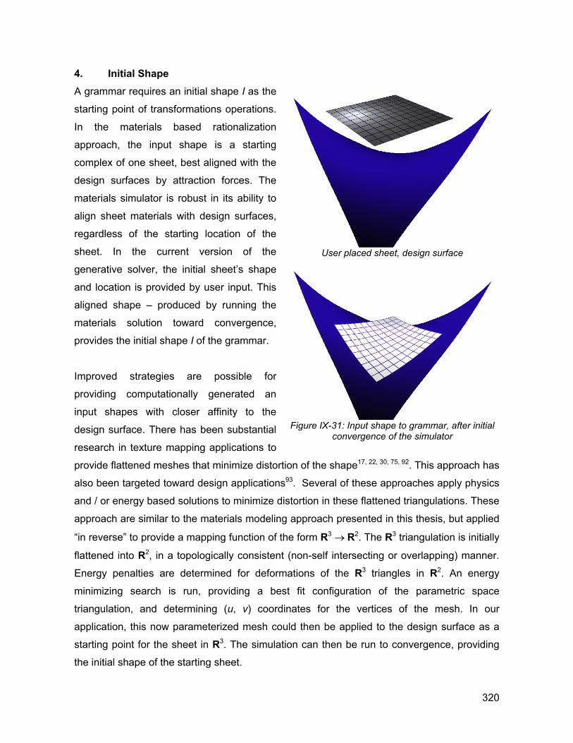
4. Initial Shape A grammar requires an initial shape I as the

starting point of transformations operations.

In the materials based rationalization

approach, the input shape is a starting

complex of one sheet, best aligned with the

design surfaces by attraction forces. The

materials simulator is robust in its ability to

align sheet materials with design surfaces,

regardless of the starting location of the

sheet. In the current version of the

generative solver, the initial sheet’s shape

and location is provided by user input. This

aligned shape – produced by running the

materials solution toward convergence,

provides the initial shape I of the grammar.

Improved strategies are possible for

providing computationally generated an

input shapes with closer affinity to the

design surface. There has been substantial

research in texture mapping applications to

provide flattened meshes that minimize distortion of the shape17, 22, 30, 75, 92. This approach has

also been targeted toward design applications93. Several of these approaches apply physics

and / or energy based solutions to minimize distortion in these flattened triangulations. These

approach are similar to the materials modeling approach presented in this thesis, but applied

“in reverse” to provide a mapping function of the form R3 → R2. The R3 triangulation is initially

flattened into R2, in a topologically consistent (non-self intersecting or overlapping) manner.

Energy penalties are determined for deformations of the R3 triangles in R2. An energy

minimizing search is run, providing a best fit configuration of the parametric space

triangulation, and determining (u, v) coordinates for the vertices of the mesh. In our

application, this now parameterized mesh could then be applied to the design surface as a

starting point for the sheet in R3. The simulation can then be run to convergence, providing

the initial shape of the starting sheet.

User placed sheet, design surface

Figure IX-31: Input shape to grammar, after initial

convergence of the simulator

320

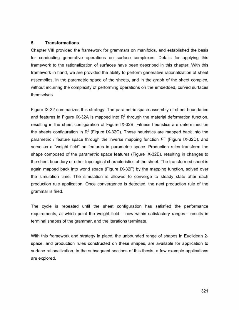
5. Transformations Chapter VIII provided the framework for grammars on manifolds, and established the basis

for conducting generative operations on surface complexes. Details for applying this

framework to the rationalization of surfaces have been described in this chapter. With this

framework in hand, we are provided the ability to perform generative rationalization of sheet

assemblies, in the parametric space of the sheets, and in the graph of the sheet complex,

without incurring the complexity of performing operations on the embedded, curved surfaces

themselves.

Figure IX-32 summarizes this strategy. The parametric space assembly of sheet boundaries

and features in Figure IX-32A is mapped into R3 through the material deformation function,

resulting in the sheet configuration of Figure IX-32B. Fitness heuristics are determined on

the sheets configuration in R3 (Figure IX-32C). These heuristics are mapped back into the

parametric / feature space through the inverse mapping function F-1 (Figure IX-32D), and

serve as a “weight field” on features in parametric space. Production rules transform the

shape composed of the parametric space features (Figure IX-32E), resulting in changes to

the sheet boundary or other topological characteristics of the sheet. The transformed sheet is

again mapped back into world space (Figure IX-32F) by the mapping function, solved over

the simulation time. The simulation is allowed to converge to steady state after each

production rule application. Once convergence is detected, the next production rule of the

grammar is fired.

The cycle is repeated until the sheet configuration has satisfied the performance

requirements, at which point the weight field – now within satisfactory ranges - results in

terminal shapes of the grammar, and the iterations terminate.

With this framework and strategy in place, the unbounded range of shapes in Euclidean 2-

space, and production rules constructed on these shapes, are available for application to

surface rationalization. In the subsequent sections of this thesis, a few example applications

are explored.

321

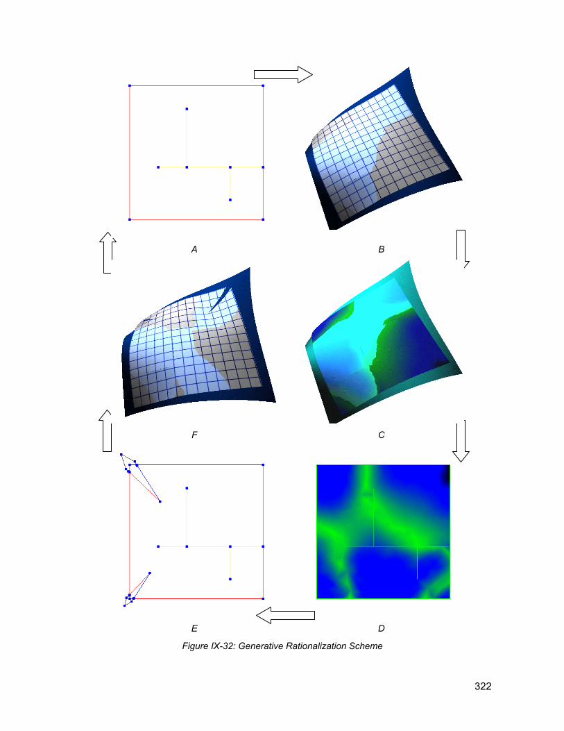
A B

F C

E D

Figure IX-32: Generative Rationalization Scheme

322

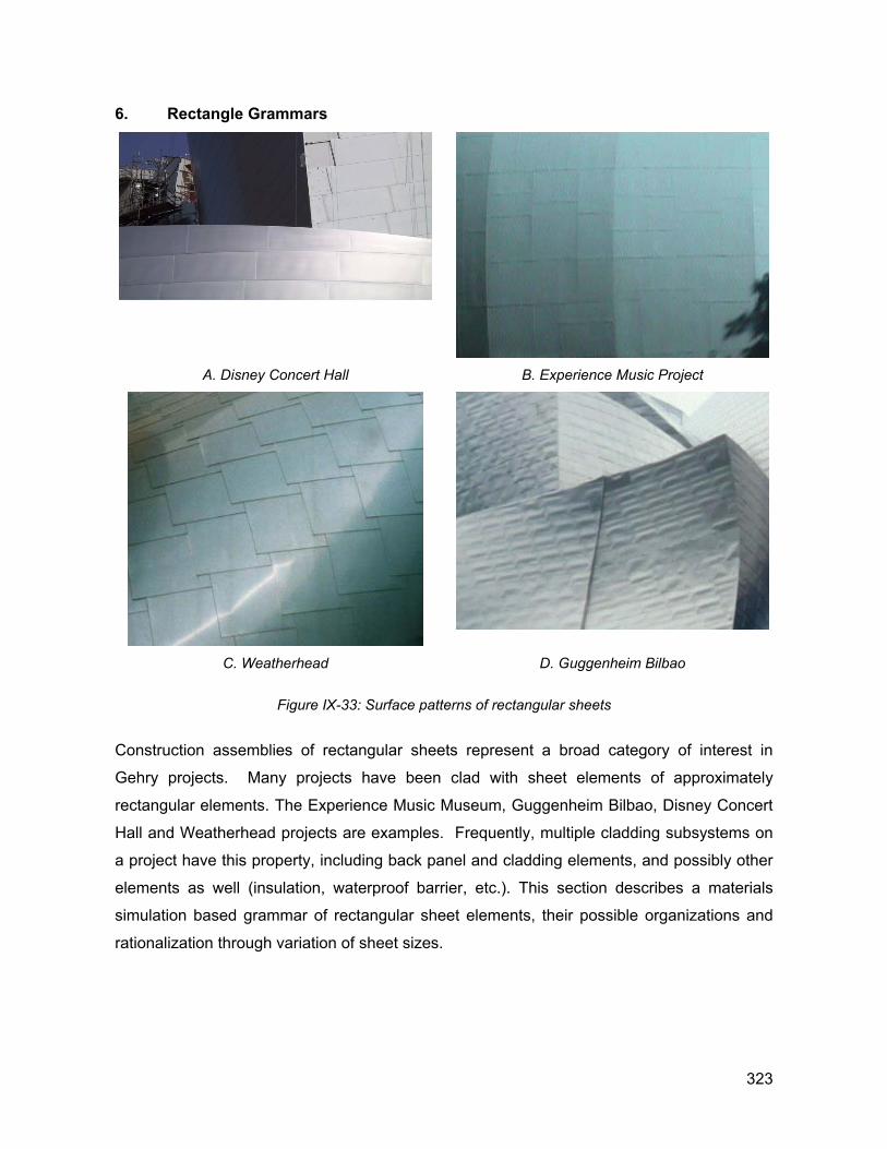
6. Rectangle Grammars

A. Disney Concert Hall B. Experience Music Project

C. Weatherhead D. Guggenheim Bilbao

Figure IX-33: Surface patterns of rectangular sheets

Construction assemblies of rectangular sheets represent a broad category of interest in

Gehry projects. Many projects have been clad with sheet elements of approximately

rectangular elements. The Experience Music Museum, Guggenheim Bilbao, Disney Concert

Hall and Weatherhead projects are examples. Frequently, multiple cladding subsystems on

a project have this property, including back panel and cladding elements, and possibly other

elements as well (insulation, waterproof barrier, etc.). This section describes a materials

simulation based grammar of rectangular sheet elements, their possible organizations and

rationalization through variation of sheet sizes.

323

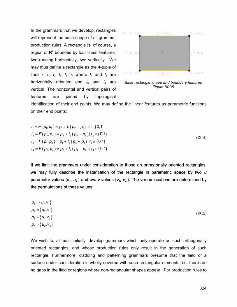
In the grammars that we develop, rectangles

will represent the base shape of all grammar

production rules. A rectangle is, of course, a

region of R2 bounded by four linear features,

two running horizontally, two vertically. We

may thus define a rectangle as the 4-tuple of

lines < l1, l2, l3, l4 >, where l1 and l2 are

horizontally oriented and l3 and l4 are

vertical. The horizontal and vertical pairs of

features are joined by topological

identification of their end points. We may defin

on their end points:

( ) ( ) ( )( ) ( ) (( ) ( ) (( ) ( ) (

1 1 2 1 1 2 1 1

2 3 4 3 2 4 3 2

3 1 3 1 3 3 1 3

4 2 4 2 4 4 2 4

, |

, |

, |

, |

l F p p p t p p t

l F p p p t p p t

l F p p p t p p t

l F p p p t p p t

= = + − ∈

= = + − ∈

= = + − ∈

= = + − ∈

)))

0,1

0,1

0,1

0,1

If we limit the grammars under consideration t

we may fully describe the instantiation of th

parameter values {u1, u2 } and two v values {v1,

the permutations of these values:

If we limit the grammars under consideration t

we may fully describe the instantiation of th

parameter values {u1, u2 } and two v values {v1,

the permutations of these values:

{{ }{ }{ }{ }

1 1 1

2 2 1

3 1 2

4 2 2

,

,

,

,

p u v

p u v

p u v

p u v

=

=

=

=

We wish to, at least initially, develop gramma

oriented rectangles, and whose production r

rectangle. Furthermore, cladding and pattern

surface under consideration is wholly covered w

no gaps in the field or regions where non-rectan

Base rectangle shape and boundary featuresFigure IX-35

e the linear features as parametric functions

(IX.4)

o those on orthogonally oriented rectangles,

e rectangle in parametric space by two u

v2 }. The vertex locations are determined by

o those on orthogonally oriented rectangles,

e rectangle in parametric space by two u

v2 }. The vertex locations are determined by

(IX.5)

rs which only operate on such orthogonally

ules only result in the generation of such

ing grammars presume that the field of a

ith such rectangular elements, i.e. there are

gular shapes appear. For production rules to

324

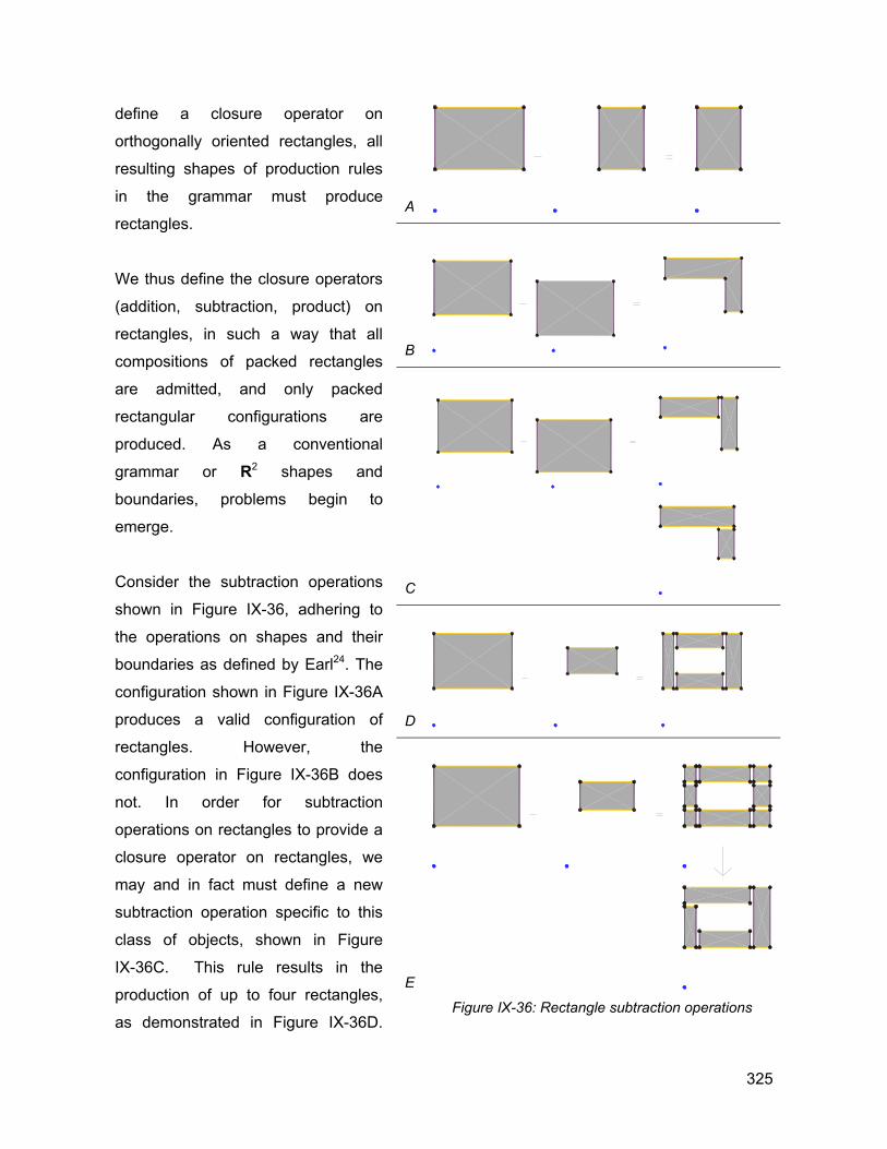
define a closure operator on

orthogonally oriented rectangles, all

resulting shapes of production rules

in the grammar must produce

rectangles.

We thus define the closure operators

(addition, subtraction, product) on

rectangles, in such a way that all

compositions of packed rectangles

are admitted, and only packed

rectangular configurations are

produced. As a conventional

grammar or R2 shapes and

boundaries, problems begin to

emerge.

Consider the subtraction operations

shown in Figure IX-36, adhering to

the operations on shapes and their

boundaries as defined by Earl24. The

configuration shown in Figure IX-36A

produces a valid configuration of

rectangles. However, the

configuration in Figure IX-36B does

not. In order for subtraction

operations on rectangles to provide a

closure operator on rectangles, we

may and in fact must define a new

subtraction operation specific to this

class of objects, shown in Figure

IX-36C. This rule results in the

production of up to four rectangles,

as demonstrated in Figure IX-36D.

A

B

C

D

E

Figure IX-36: Rectangle subtraction operations

325

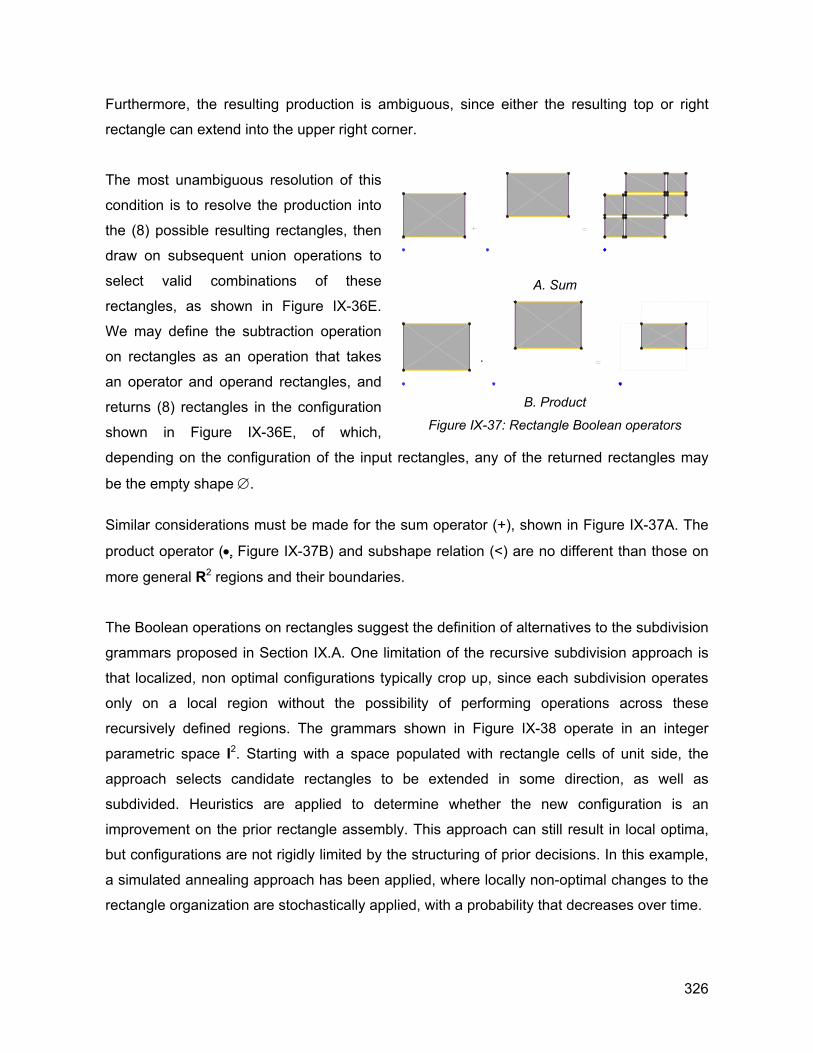
Furthermore, the resulting production is ambiguous, since either the resulting top or right

rectangle can extend into the upper right corner.

The most unambiguous resolution of this

condition is to resolve the production into

the (8) possible resulting rectangles, then

draw on subsequent union operations to

select valid combinations of these

rectangles, as shown in Figure IX-36E.

We may define the subtraction operation

on rectangles as an operation that takes

an operator and operand rectangles, and

returns (8) rectangles in the configuration

shown in Figure IX-36E, of which,

depending on the configuration of the input rectangles, any of the returned rectangles may

be the empty shape ∅.

A. Sum

B. Product Figure IX-37: Rectangle Boolean operators

Similar considerations must be made for the sum operator (+), shown in Figure IX-37A. The

product operator (•, Figure IX-37B) and subshape relation (<) are no different than those on

more general R2 regions and their boundaries.

The Boolean operations on rectangles suggest the definition of alternatives to the subdivision

grammars proposed in Section IX.A. One limitation of the recursive subdivision approach is

that localized, non optimal configurations typically crop up, since each subdivision operates

only on a local region without the possibility of performing operations across these

recursively defined regions. The grammars shown in Figure IX-38 operate in an integer

parametric space I2. Starting with a space populated with rectangle cells of unit side, the

approach selects candidate rectangles to be extended in some direction, as well as

subdivided. Heuristics are applied to determine whether the new configuration is an

improvement on the prior rectangle assembly. This approach can still result in local optima,

but configurations are not rigidly limited by the structuring of prior decisions. In this example,

a simulated annealing approach has been applied, where locally non-optimal changes to the

rectangle organization are stochastically applied, with a probability that decreases over time.

326

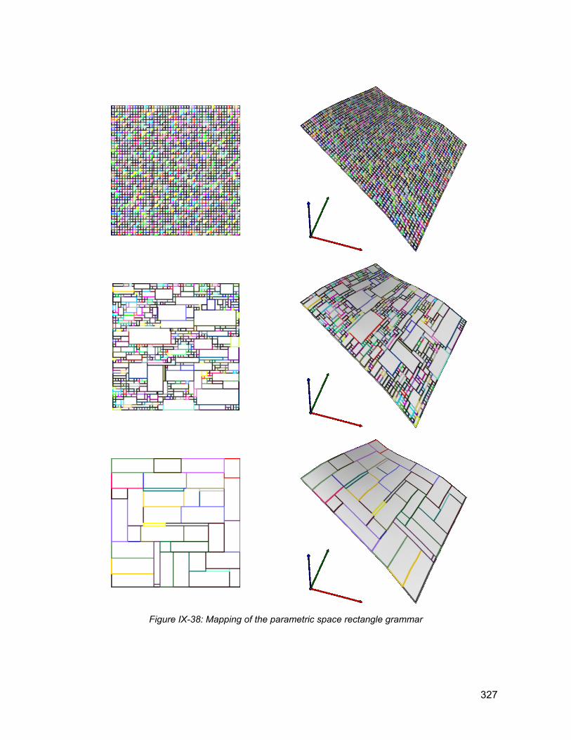
Figure IX-38: Mapping of the parametric space rectangle grammar

327

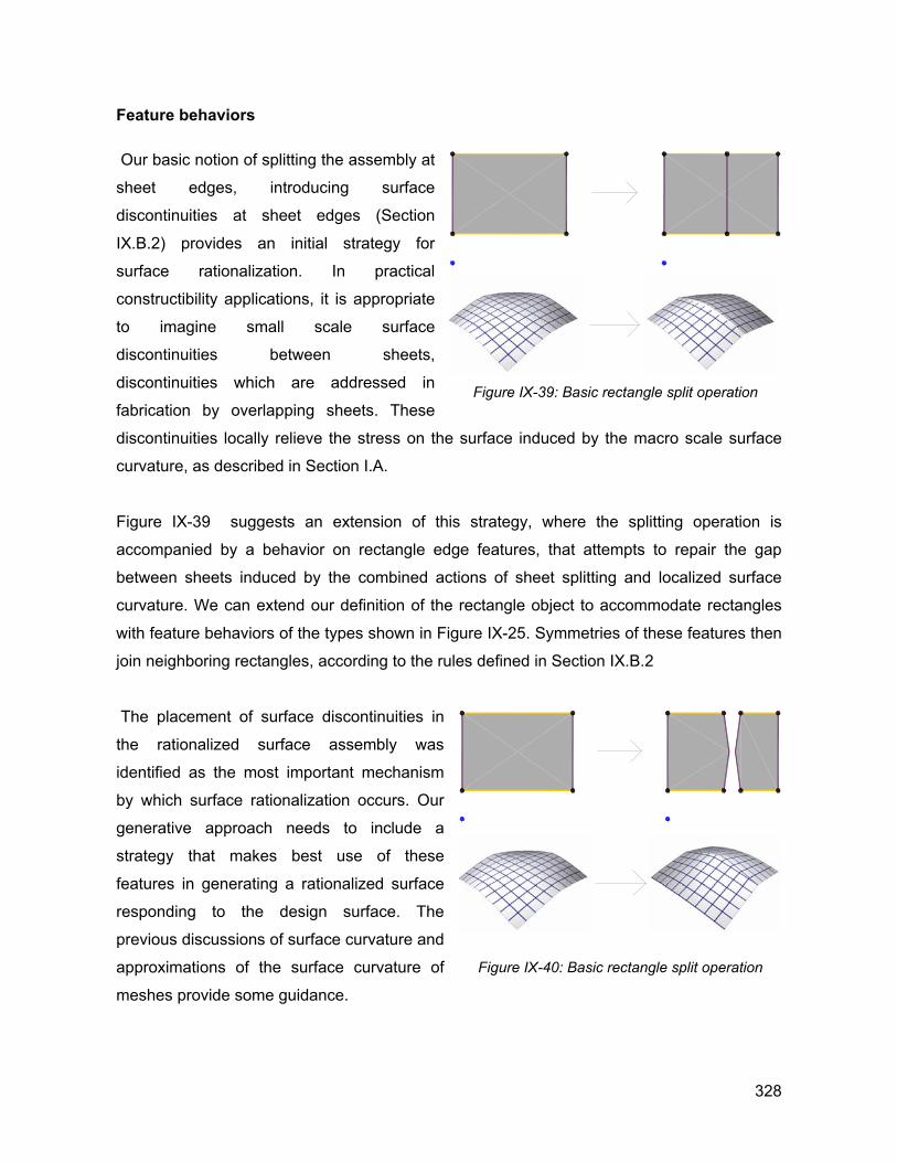
Feature behaviors

Our basic notion of splitting the assembly at

sheet edges, introducing surface

discontinuities at sheet edges (Section

IX.B.2) provides an initial strategy for

surface rationalization. In practical

constructibility applications, it is appropriate

to imagine small scale surface

discontinuities between sheets,

discontinuities which are addressed in

fabrication by overlapping sheets. These

discontinuities locally relieve the stress on the surface induced by the macro scale surface

curvature, as described in Section I.A.

Figure IX-39: Basic rectangle split operation

Figure IX-39 suggests an extension of this strategy, where the splitting operation is

accompanied by a behavior on rectangle edge features, that attempts to repair the gap

between sheets induced by the combined actions of sheet splitting and localized surface

curvature. We can extend our definition of the rectangle object to accommodate rectangles

with feature behaviors of the types shown in Figure IX-25. Symmetries of these features then

join neighboring rectangles, according to the rules defined in Section IX.B.2

The placement of surface discontinuities in

the rationalized surface assembly was

identified as the most important mechanism

by which surface rationalization occurs. Our

generative approach needs to include a

strategy that makes best use of these

features in generating a rationalized surface

responding to the design surface. The

previous discussions of surface curvature and

approximations of the surface curvature of

meshes provide some guidance.

Figure IX-40: Basic rectangle split operation

328

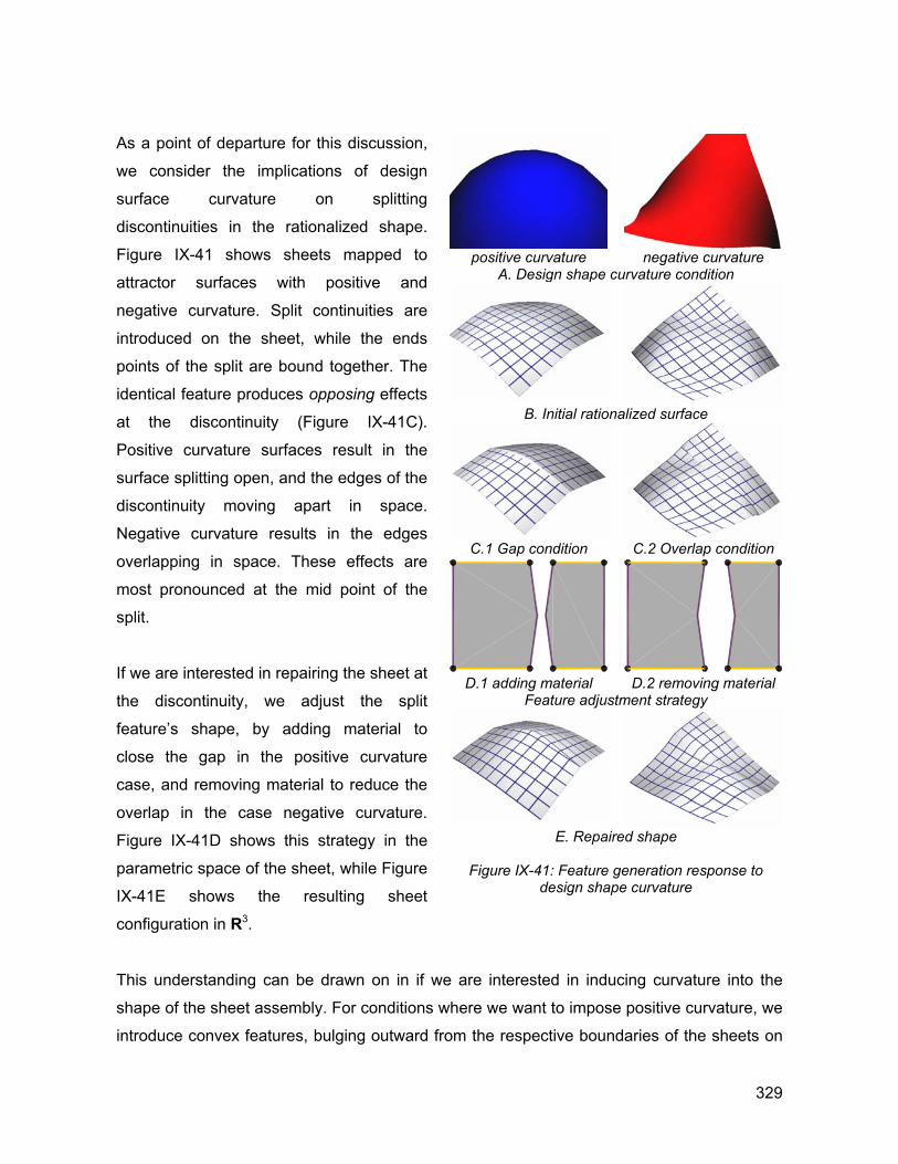
As a point of departure for this discussion,

we consider the implications of design

surface curvature on splitting

discontinuities in the rationalized shape.

Figure IX-41 shows sheets mapped to

attractor surfaces with positive and

negative curvature. Split continuities are

introduced on the sheet, while the ends

points of the split are bound together. The

identical feature produces opposing effects

at the discontinuity (Figure IX-41C).

Positive curvature surfaces result in the

surface splitting open, and the edges of the

discontinuity moving apart in space.

Negative curvature results in the edges

overlapping in space. These effects are

most pronounced at the mid point of the

split.

If we are interested in repairing the sheet at

the discontinuity, we adjust the split

feature’s shape, by adding material to

close the gap in the positive curvature

case, and removing material to reduce the

overlap in the case negative curvature.

Figure IX-41D shows this strategy in the

parametric space of the sheet, while Figure

IX-41E shows the resulting sheet

configuration in R3.

positive curvature negative curvature A. Design shape curvature condition

B. Initial rationalized surface

C.1 Gap condition C.2 Overlap condition

D.1 adding material D.2 removing material Feature adjustment strategy

E. Repaired shape

Figure IX-41: Feature generation response to design shape curvature

This understanding can be drawn on in if we are interested in inducing curvature into the

shape of the sheet assembly. For conditions where we want to impose positive curvature, we

introduce convex features, bulging outward from the respective boundaries of the sheets on

329

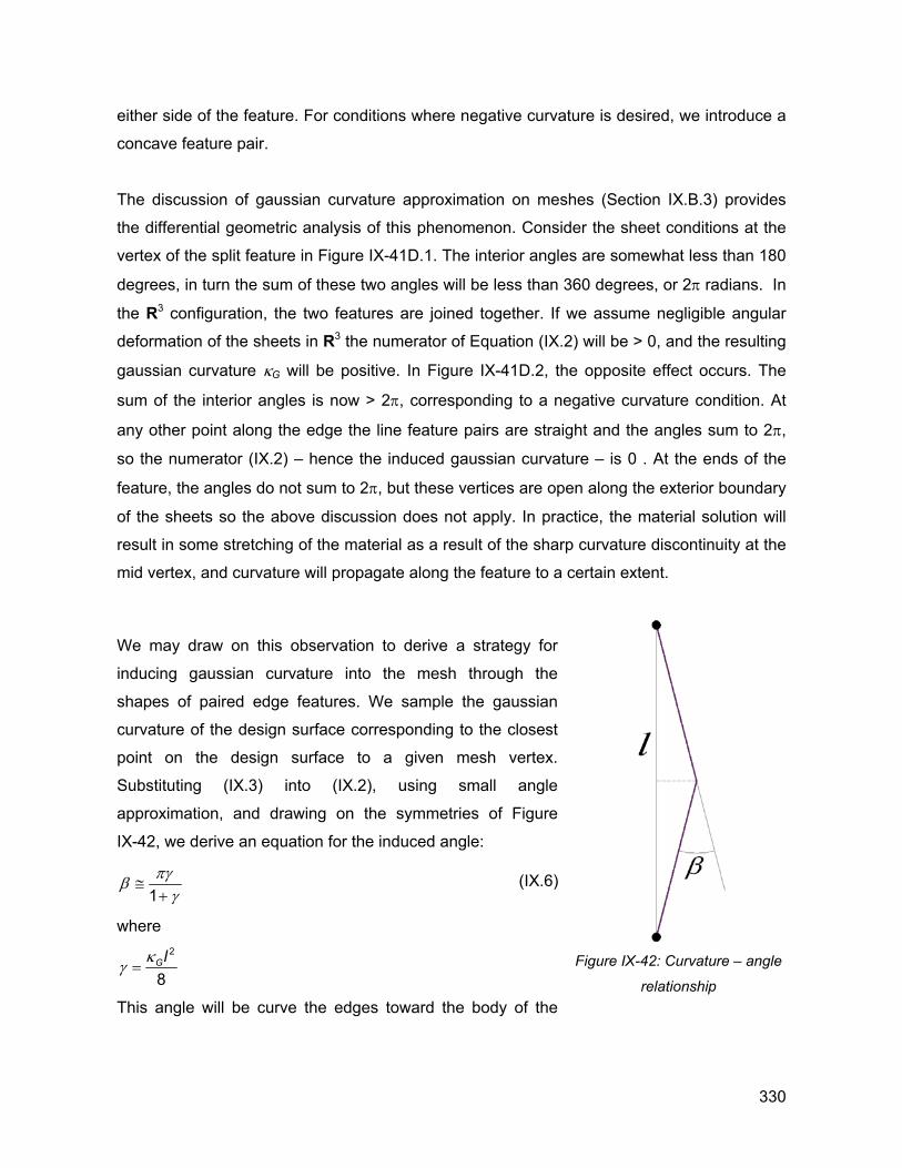
either side of the feature. For conditions where negative curvature is desired, we introduce a

concave feature pair.

The discussion of gaussian curvature approximation on meshes (Section IX.B.3) provides

the differential geometric analysis of this phenomenon. Consider the sheet conditions at the

vertex of the split feature in Figure IX-41D.1. The interior angles are somewhat less than 180

degrees, in turn the sum of these two angles will be less than 360 degrees, or 2π radians. In

the R3 configuration, the two features are joined together. If we assume negligible angular

deformation of the sheets in R3 the numerator of Equation (IX.2) will be > 0, and the resulting

gaussian curvature κG will be positive. In Figure IX-41D.2, the opposite effect occurs. The

sum of the interior angles is now > 2π, corresponding to a negative curvature condition. At

any other point along the edge the line feature pairs are straight and the angles sum to 2π,

so the numerator (IX.2) – hence the induced gaussian curvature – is 0 . At the ends of the

feature, the angles do not sum to 2π, but these vertices are open along the exterior boundary

of the sheets so the above discussion does not apply. In practice, the material solution will

result in some stretching of the material as a result of the sharp curvature discontinuity at the

mid vertex, and curvature will propagate along the feature to a certain extent.

We may draw on this observation to derive a strategy for

inducing gaussian curvature into the mesh through the

shapes of paired edge features. We sample the gaussian

curvature of the design surface corresponding to the closest

point on the design surface to a given mesh vertex.

Substituting (IX.3) into (IX.2), using small angle

approximation, and drawing on the symmetries of Figure

IX-42, we derive an equation for the induced angle:

Figure IX-42: Curvature – angle

relationship

1πγβ

γ≅

+ (IX.6)

where 2

8Glκ

γ =

This angle will be curve the edges toward the body of the

330

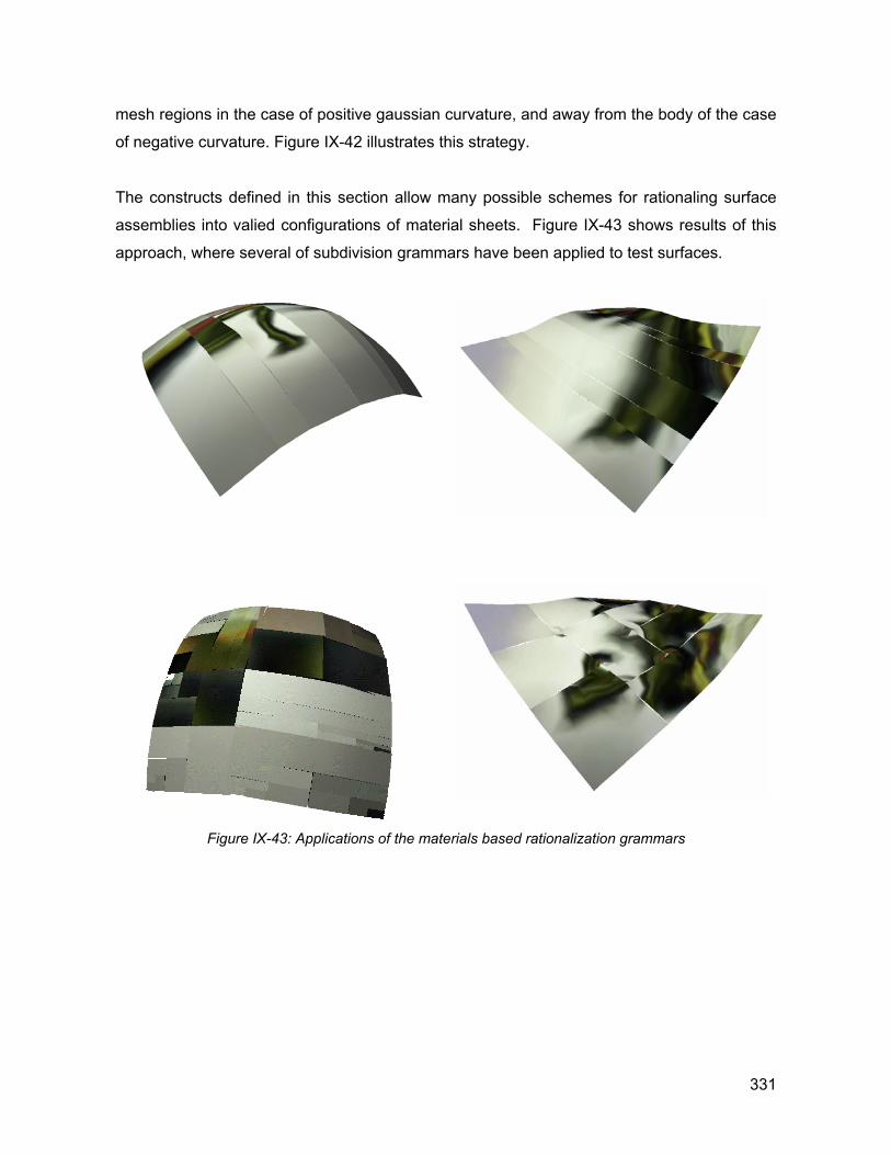
mesh regions in the case of positive gaussian curvature, and away from the body of the case

of negative curvature. Figure IX-42 illustrates this strategy.

The constructs defined in this section allow many possible schemes for rationaling surface

assemblies into valied configurations of material sheets. Figure IX-43 shows results of this

approach, where several of subdivision grammars have been applied to test surfaces.

Figure IX-43: Applications of the materials based rationalization grammars

331

332

CONCLUSION

This thesis has documented efforts to describe computationally one aspect of Gehry’s

architecture: a set of paper surface forms whose nature is defined by the intersection of a

broad set of aesthetic, material and fabrication intentions. A geometric definition of these

surface forms has been developed within the framework of shape grammars. With this

vocabulary of shapes and operations on shapes defined in a computationally rigorous

manner, it has been possible to develop applications, operating within the space of paper

surface configurations, which automate the solution of certain design and constructibility

problems. This inquiry has deliberately avoided attempting to formalize the more elusive,

evocative elements of Gehry’s design intentions, focusing rather on the design development

decisions regarding the constructibility of forms, for which explicit geometric rules are often

defined. The automation of repetitive, lower level design operations associated with the

propagation of system design decisions across the variations in project geometry is deemed

to be of great value to the firm’s process. At the same time, these rationalization decisions

can have substantial impact on the project design intent, in addition to their more direct

implications on building performance and fabrication economies, and are positioned within

the broad scope of design decisions resulting in the ultimate development of the project form.

It is suggested that this specific inquiry of surface forms is indicative of broader opportunities

for computation in design theory and practice. Gehry’s ambitious formal explorations have

resulted in new vocabularies of architectural forms. In order to realize these forms, explicit

descriptions of these vocabularies must be developed to communicate design intent across

the spectrum of building activities. Digital media present broad new capabilities that can

allow new design intentions to be communicated in a formally rigorous manner.

However, this rewriting of the rules of architectural communication can not be undertaken in

a thoughtless manner. Computing methodologies bring an inherent structure and logic to the

products and processes they support. This explicit structuring renders transparent the

underlying assumptions for their construction, and allows these assumptions to be critically

assessed. At the same time, the definition of any formal descriptive structure unambiguously

not only defines a class of intentions admissible in this framework, but also imposes limits to

intentions admissible in the framework, and by implication suggests a world of possibility for

which the framework has no application. A firm understanding of these qualities of

333

computation, integrated with a rigorous understanding of the conventions and historical

development of building process, must be achieved for computing applications to

appropriately serve design. When computational structures are inappropriately applied, the

structuring of a computational framework limits descriptive capabilities in critical and

disadvantageous ways. Alternatively, when a synergy between the logic of computation and

that of the activities of design is achieved, the result is not simply tools to support existing

processes, but rather the disclosure and critique of the supported process and, perhaps, the

identification of new opportunities and avenues for design.

`

334

BIBLIOGRAPHY 1. AISC, Manual of Steel Construction: Allowable Stress Design, 9th Edition. AISC, Chicago, IL,

1989.

2. Alexandrov, P.S. Combinatorial Topology. Dover Publications, NY, 1960.

3. Aumann, G. Interpolation with Developable Bézier Patches. Computer Aided Geometric Design,

8:409-420, 1991.

4. Baraff, D., Witkin, A., and Katz, M. An Introduction to Physically Based Modeling. Siggraph Course

Notes, 1997.

5. Baraff, D., and Witkin, A. Large Steps in Cloth Simulation. SIGGRAPH ’98 Proceedings.

6. Bennis, C., Vezien, J., Iglesias, G., and Gagalowicz, A. Piecewise Surface Flattening for Non-

Distorted Texture Mapping. Computer Graphics (Proceedings of SIGGRAPH 91) 25 4, 1991: 237-

246.

7. Bishop, R., and Goldberg, S. Tensor Analysis on Manifolds. Dover Publications, NY, 1980.

8. Borischenko, A., and Tarapov, I. Vector and Tensor Analysis with Applications. Dover

Publications, NY, 1979.

9. Boddului, Ravani. Design Of Developable Surfaces Using Duality Between Plane And Point

Geometries. Computer Aided Design 25 (1993): 621-632.

10. Ibid, p. 622.

11. Boddului, Ravani. Geometric Design and Fabrication of Developable Surfaces. ASMD Advanced

Design Automation 2 (1992),: 243-250.

12. Bonola, R. Non-Euclidean Geometry. Dover Publications, NY, 1955.

13. Bowyer, A., and Woodwark, J. A Programmer’s Geometry. Butterworth’s, London, 1983.

14. Ibid, p. 104.

15. Breen, D. A Particle Based Model for Simulating the Draping Behavior of Woven Cloth. doctoral

dissertation, Rensalaer Polytechnic Institute, 1993.

16. Burry, MC. Parametric Design and the Sagrada Familia. Architecture Research Quarterly, UK,

1996.

335

17. Campagna, S., and Seidel, H. Parameterization of Meshes with Arbitrary Topology. In Image and

Multidimensional Digital Signal Processing 1998: 287-290.

18. Ceccato, C., Glymph, G., Shelden, D., et. al. A Parametric Strategy for Freeform Glass Structures

Using Quadrilateral Planar Glass Facets. Submitted, Acadia 2002 Conference Proceedings.

19. Chalfant, J. Analysis and Design of Developable surfaces for Shipbuilding. Masters Thesis in

Naval Architecture and Mechanical Engineering, MIT, 1997.

20. Chen, Q. Simulation of Wind Around the Stata Complex at MIT. Research report, 1999.

21. Colomina, B. The House that Built Gehry. in Ragheb, 2001: 300-321.

22. Desbrun, M. Meyer, M., Alliez, P. Intrinsic Parameterization of Surface Meshes. Eurographics

2002, 21 2.

23. DeSimone, V., and Roorda, D. Structure as Art. Civil Engineering, June 2002: 40-47.

24. Earl, C.F. Shape Boundaries. Environment and Planning : Planning and Design 24: 669-687.

25. Earl, C.F. Generated Designs: Structure and Composition. Artificial Intelligence in Engineering

Design 13, 1999: 277-285.

26. Feynman, C. Modeling the Appearance of Cloth. Masters Thesis, MIT, 1986.

27. Friedman, M., and Ragheb, J. (ed). Frank Gehry, Architect, Exhibition Catalog. Guggenheim

Museum Publications, NY, 2001.

28. Foley, J., VanDam, A, et. al. Computer Graphics Principles and Practice, 2nd Edition. Addison

Wesley, NY, 1990.

29. Ibid: 521-523.

30. Floater, M. Parameterization and Smooth Approximation of Surface Triangulations. Computer

aided Geometric Design 14 3, 1997: 231-250.

31. Fuller, R. Buckminster. Synergetics. Macmillan Publishing, NY, 1982: 701-717.

32. Gasson, P. Geometry of Spatial Forms. Ellis Horwood Limited, NY, 1983: 312-319.

33. Frank O. Gehry & Associates. Exterior Closure Metal Systems Bid Package. Experience Music

Project, Seattle Washington, May 20, 1997.

336

34. Glymph, J., informal conversations, 1997-2002.

35. Grimm, C., and Hughes, J. Modeling Surface with Arbitrary Topology Using Manifolds.

SIGGRAPH '95: 359-368.

36. Guggenheimer, H. Differential Geometry. Dover Publications, NY, 1977.

37. Hamann, B. Curvature Approximation for Triangulated Surfaces. In G. Farin, et. al., editor,

Geometric Modeling, Springer Verlag, 1993, p139-153.

38. Heath T. (trans). The Thirteen Books of Euclid’s Elements. Dover Publications, NY, 1956.

39. Henle, M. A Combinatorial Introduction to Topology. Dover Publications, NY, 1979.

40. Haymaker, J. and Fischer, M. Challenges and Benefits of 4D Modeling on the Walt Disney

Concert Hall Project. CIFE Working Paper #64, Stanford University, Stanford, CA, 2001.

41. JaeHong, L. Frank O. Gehry, Museums and Cultural Institutions 1984-1996. Korean Architects,

Seoul, 1996.

42. Ibid: 17.

43. Jänich, K. Topology. Springer-Verlag, Berlin, 1980.

44. Kostof, S. A History of Architecture: Settings and Rituals, Oxford University Press, 1985: 651,702.

45. Krishnamurti, R. The Arithmetic of Shapes. Environment and Planning B 7, 1980: 463-484.

46. Krishnamurti, R. The Construction of Shapes. Environment and Planning B 8, 1980: 5-40.

47. Kreysig, E. Differential Geometry. Dover Publications, NY, 1981.

48. ibid: 179-180.

49. ibid: 185.

50. Lang, Roschel. Developable (1,n) Bézier Surfaces. Computer Aided Geometric Design 9 1992:

291-298.

51. Lewis, S. Structural Steel Detailing Neutral File: Electronic Data Interface Between Structural

Engineers and Fabricators. Fluor Daniel internal report.

52. Lindsey, B. Digital Gehry, Material Resistance, Digital Construction. Basel: Birkhauser, 2001.

337

53. Marsden, J. and Hughes, T. Mathematical Foundations of Elasticity. Dover Publications, NY,

1983.

54. Mayer, Gerhard. Personal interview on Weatherhead project. Conducted June 15, 2002.

55. McCullough, M. Abstracting Craft: The Practiced Digital Hand. MIT Press, Cambridge, MA, 1997:

229.

56. Meyer, M., Desbrun, M. et. al. Discrete Differential-Geometry Operators for Triangulated 2-

Manifolds. Submitted, found at http://www.multires.caltech.edu/pubs/diffGeoOps.pdf, 2002.

57. Mitchell, W. J. Roll Over Euclid. In Ragheb, 2001: 353-364.

58. Mitchell, W. J. The Logic of Architecture : Design, Computation, and Cognition. MIT Press,

Cambridge, MA, 1990.

59. Ng, H., Grimsdale, R. Computer Graphics Techniques for Modeling Cloth. IEEE Computer

Graphics and Applications, 1996: 28-41.

60. O’Neill, B. Elementary Differential Geometry, 2nd Edition. Academic Press, 1997.

61. ibid: 58.

62. ibid: 87.

63. Packard, R. (ed). Architectural Graphic Standards, 7th edition, John Wiley & Sons, NY., 1981: 325-

328.

64. Piegl, L., and Tiller, W. The NURBS Book, 2nd Edition. Springer, NY, 1997.

65. ibid: 233-234.

66. Post, N. and Daniels, S. Plum Job in Seattle Lifts Haze Over Technology. Engineering News

Record, February 28, 2000: 76-83.

67. Pottman, Farin. Developable Rational Bézier and B-spline Surfaces. Computer Aided Geometric

Design 12, 1995: 513-531.

68. Pottman, Wallner. Approximation Algorithms for Developable Surfaces. Computer Aided

Geometric Design 16 (1999), 539-556.

338

69. Press, W.H., Flannery, B.P., Vetterling, W.T. Numerical Recipies. Cambridge University Press,

1986.

70. ibid: 83-89.

71. Provot, X. Deformation Constraints in a Mass-Spring Model to Describe Rigid Cloth Behavior.

Proceedings Of Graphics Interface, 1995: 147-154.

72. Ragheb, J. F., Editor. Frank Gehry, Architect. New York: Guggenheim Museum Publications,

2001.

73. Roe, A. Cleveland Gets a Case of Gehry’s Totally Unreserved Architecture. Engineering News

Record, May 27, 2002: 44-45.

74. Rogers, D. An Introduction to NURBS, with Historical Perspective. Kaufman, San Francisco, 2001.

75. Sheffer, A., and De Struler, E. Surface Parameterization for Meshing by Triangulation Flattening.

Proceedings of the 9th International Meshing Roundtable, Sandia National Laboratories, 2000:

161-172.

76. Shewchuk, J. An Introduction to the Conjugate Gradient Method Without the Agonizing Pain.

Technical Report CMU-CS-TR-94-125, Carnegie Mellon University, 1994.

77. Shewchuk, J. Triangle: Engineering a 2D Quality Mesh Generator and Delaunay Triangulator.

First Workshop on Applied Computational Geometry, Association for Computing Machinery

Philadelphia, PA, 1996: 124-133.

78. Stiny, G. Introduction to Shape and Shape Grammars. Environment and Planning B 7, 1980: 343-

351.

79. Stiny, G. Shapes are Individuals. Environment and Planning B 9, 1982: 359-367.

80. Stiny, G. What is a Design? Environment and Planning B 171990: 97-103.

81. Stiny, G. Two Exercises in Formal Composition. Environment and Planning B 3, 1976: 187-210.

82. Stiny, G. Weights. Environment and Planning B 19, 1992: S49-S78.

83. Stiny, G. Shape Rules: Closure, Continuity and Emergence. Environment and Planning B 19,

1994: 413-430.

339

340

84. Stiny, G., and Gips, J. Production Systems and Grammars: a Uniform Characterization.

Environment and Planning B 7, 1980: 399-408.

85. Stiny, G., and Gips, J. Shape Grammars And The Generative Specification Of Painting And

Sculpture. Information Processing 71, 1972: 1460-1465.

86. Stiny, G., and Mitchell, W J. The Grammar of Paradise: on the generation of Mughul gardens.

Environment and Planning B 7, 1980: 209-226.

87. Struik, D. Lectures on Classical Differential Geometry, 2nd Edition. Dover Publications, NY, 1961.

88. Synge, J., and Schild, A. Tensor Calculus. Dover Publications, NY, 1978.

89. Terzopolous, D., J. Platt, A. Barr and K. Fleisher. Elastically Deformable Models. Computer

Graphics, V 21 4, 1987: 205-214.

90. Trudeau, R. Introduction to Graph Theory. Dover Publications, NY, 1993.

91. Sedgewick, R. Algorithms in C. Addison Wesley, NY, 1990

92. Wang, C., Chen, S., and Yuen, M. Surface Flattening Based on Energy Model. Accepted,

Computer Aided Design.

93. Wang, C., Chen, S., Fan, J., and Yuen, M. Two-dimensional trimmed Surface Development Using

a Physics-based Model. in Proceedings of the 25th Design Automation Conference, 1999.

94. Weil, J. The Synthesis of Cloth Objects. Computer Graphics, 20, 1,1986: 49-54.

95. Yeh, B. Obtaining data from complex physical models. FOG/A research document 11039802,

1998.

96. Futagawa, Y. (ed). Frank O. Gehry: 13 Projects Since Bilbao. GA Document 68, A.D.A. EDITA,

Tokyo, Japan, 2002.

97. Meek, DS and Walton, DJ. Approximation of Discrete Data by G1 Arc Splines. Computer Aided

Design, 24 6, 1992.