Parametric inference of incomplete data with competing risks among several groups
11
IEEE TRANSACTIONS ON RELIABILITY, VOL. 53, NO. 1, MARCH 2004 11 Parametric Inference of Incomplete Data With Competing Risks Among Several Groups Chanseok Park and K. B. Kulasekera Abstract—We develop parametric inferential methods for the competing risks problem where data arise due to multiple causes of failure in several groups with censoring and possibly missing causes. We provide the general likelihood method and the closed-form maximum-likelihood estimators for the exponential model. Parametric tests are given for comparing different causes and groups. An extensive numerical and graphical investigation is presented to substantiate the proposed methods. A real-data example is illustrated. Index Terms—Censored data, competing risks, exponential dis- tribution, maximum likelihood, missing cause. ACRONYMS 1 implies: statistical(ly) cdf cumulative distribution function pdf probability density function CIF cumulative incidence function CSHF cause-specific hazard function MLE maximum-likelihood estimator MSE mean square error MVN multivariate -normally distributed SRE simulated relative efficiency NOTATION lifetime of the th subject in the th group due to the th cause censoring indicator variable vector parameters of the distribution of parameter matrix of pdf of cdf of survival function of hazard function of likelihood function without missing causes likelihood function with missing causes Indicator function Fisher information matrix Manuscript received March 7, 2003; revised June 22, 2003 and November 20, 2003. The work of C. Park was supported in part by Clemson RGC award. The work of K. B. Kulasekera was supported in part by NIH grant R01 CA 92504-02. The authors are with the Department of Mathematical Sciences, Clemson University, Clemson, SC 29634 USA (e-mail: [email protected]; [email protected]). Digital Object Identifier 10.1109/TR.2003.821946 1 The singular and plural of an acronym are always spelled the same. I. INTRODUCTION I N MANY engineering and medical studies, lifetime distri- butions of items or individuals are of interest. Experimenters use various indexes associated with lifetime distributions to evaluate systems. Typically, lifetime measurements are taken from the relevant population(s) and statistical inferences on the corresponding indexes are conducted. Often the items or indi- viduals fail due to more than one failure mechanism, commonly referred to as competing risks. In this setting, usually the cause of failure is known when the lifetime is observed. Furthermore, the items or individuals may also be grouped according to some criteria so that one has observations from multiple populations where each observation is due to one of the failure mechanisms. For example, one may wish to study the effect of the brand of air-conditioning systems which can fail either due to leaks of refrigerant or wear of drive belts. In these situations, an item of interest would be to know whether there are significant differences due to brand(s) and the cause of failure. A typical lifetime data analysis problem of the above type is further complicated due to possible censoring and unknown cause of failure. In the example above, the experimenter fails to observe the exact lifetime of an air-conditioning system if the building or facility is destroyed or renovated thus discarding all functioning systems. In such a situation one observes a right-censored lifetime value. In some situations, the exact cause of failure may not be observed although the lifetime is observed, thus masking the cause. We formally formulate the problem in the following required notation. The traditional approach when dealing with competing risks is to consider the hypothetical latent lifetimes corresponding to each cause in the absence of the others [1]. Therefore, a subject in the th group, , is exposed to several potential causes of failure. Let there be a finite number of -independent causes of failure indexed by . Let denote the latent lifetime of the th subject in the th group due to the th cause, where and . It is assumed that are -independent for all and are identically distributed for all for a given . The corresponding cdf, pdf, survival function, and hazard function of are denoted in general by , , , and , respectively, where is a vector of real valued parameters, one for each . Then the observed life- time of the th subject in the th group is given by the random variable 0018-9529/04$20.00 © 2004 IEEE
Transcript of Parametric inference of incomplete data with competing risks among several groups
IEEE TRANSACTIONS ON RELIABILITY, VOL. 53, NO. 1, MARCH 2004 11
Parametric Inference of Incomplete Data WithCompeting Risks Among Several Groups
Chanseok Park and K. B. Kulasekera
Abstract—We develop parametric inferential methods forthe competing risks problem where data arise due to multiplecauses of failure in several groups with censoring and possiblymissing causes. We provide the general likelihood method and theclosed-form maximum-likelihood estimators for the exponentialmodel. Parametric tests are given for comparing different causesand groups. An extensive numerical and graphical investigationis presented to substantiate the proposed methods. A real-dataexample is illustrated.
Index Terms—Censored data, competing risks, exponential dis-tribution, maximum likelihood, missing cause.
ACRONYMS1
implies: statistical(ly)cdf cumulative distribution functionpdf probability density functionCIF cumulative incidence functionCSHF cause-specific hazard functionMLE maximum-likelihood estimatorMSE mean square errorMVN multivariate -normally distributedSRE simulated relative efficiency
NOTATION
lifetime of the th subject in the th group due to theth cause
censoring indicator variablevector parameters of the distribution ofparameter matrix ofpdf ofcdf ofsurvival function ofhazard function oflikelihood function without missing causeslikelihood function with missing causes
Indicator functionFisher information matrix
Manuscript received March 7, 2003; revised June 22, 2003 and November20, 2003. The work of C. Park was supported in part by Clemson RGC award.The work of K. B. Kulasekera was supported in part by NIH grant R01 CA92504-02.
The authors are with the Department of Mathematical Sciences, ClemsonUniversity, Clemson, SC 29634 USA (e-mail: [email protected];[email protected]).
Digital Object Identifier 10.1109/TR.2003.821946
1 The singular and plural of an acronym are always spelled the same.
I. INTRODUCTION
I N MANY engineering and medical studies, lifetime distri-butions of items or individuals are of interest. Experimenters
use various indexes associated with lifetime distributions toevaluate systems. Typically, lifetime measurements are takenfrom the relevant population(s) and statistical inferences on thecorresponding indexes are conducted. Often the items or indi-viduals fail due to more than one failure mechanism, commonlyreferred to as competing risks. In this setting, usually the causeof failure is known when the lifetime is observed. Furthermore,the items or individuals may also be grouped according to somecriteria so that one has observations from multiple populationswhere each observation is due to one of the failure mechanisms.For example, one may wish to study the effect of the brand ofair-conditioning systems which can fail either due to leaks ofrefrigerant or wear of drive belts. In these situations, an itemof interest would be to know whether there are significantdifferences due to brand(s) and the cause of failure. A typicallifetime data analysis problem of the above type is furthercomplicated due to possible censoring and unknown causeof failure. In the example above, the experimenter fails toobserve the exact lifetime of an air-conditioning system if thebuilding or facility is destroyed or renovated thus discardingall functioning systems. In such a situation one observes aright-censored lifetime value. In some situations, the exactcause of failure may not be observed although the lifetime isobserved, thus masking the cause. We formally formulate theproblem in the following required notation.
The traditional approach when dealing with competing risksis to consider the hypothetical latent lifetimes corresponding toeach cause in the absence of the others [1]. Therefore, a subjectin the th group, , is exposed to several potentialcauses of failure. Let there be a finite number of -independentcauses of failure indexed by . Let denote thelatent lifetime of the th subject in the th group due to the thcause, where and . It is assumedthat are -independent for all and are identicallydistributed for all for a given . The corresponding cdf,pdf, survival function, and hazard function of are denotedin general by , , ,and , respectively, where is a vector of realvalued parameters, one for each . Then the observed life-time of the th subject in the th group is given by the randomvariable
0018-9529/04$20.00 © 2004 IEEE
12 IEEE TRANSACTIONS ON RELIABILITY, VOL. 53, NO. 1, MARCH 2004
Typically, in reliability analysis problems, complete obser-vation of may not be possible due to various censoringschemes which are inherent in data collection processes. In thiswork, it is further assumed that each can be right-censoredby censoring times which are -independent of lifetimes
for all and . Thus, one only observes ,where , and are censoring in-dicator variables defined as
if
if .(1)
Our objectives are:
1) Estimate the vector parameters of the distributionof .
2) Perform the following tests of hypotheses:• : for all ,• : for all for a given , and• : for all for a given .
Here, the alternative hypothesis in each case is taken to be thenegation of the statement given in the null hypothesis. The firstnull states that there is no cause or group effect; the second stip-ulates that there is no group effect for a given cause; and thethird stipulates that there is no cause effect in a given group.
The analysis of exponential data with two causes in a singlegroup was studied by Cox [2]; and was extended to multiplecauses by Herman and Patell [3]. The parametric estimationproblem for the case of a single group with two causes andpossible missing causes but without censoring has been dis-cussed by Miyakawa [4]. Kundu and Basu [5] extended thiswork to provide the approximate and asymptotic properties ofthe parameter estimators, -confidence intervals, and bootstrap
-confidence bounds. They provided the closed-form MLE forthe exponential case and constructed likelihood equations forthe Weibull case. However, they did not consider censoring.Also, although they stated that their solutions extend to the mul-tiple cause case, no explicit expressions were provided.
An alternative to the traditional latent lifetime framework isthe parametric mixture-model approach adopted by Larson andDinse [6]. An attractive feature of this approach is that it re-laxes the -independence assumption of the latent lifetime ap-proach. However, the drawback is that finding the MLE in theparametric mixture model is quite difficult; and requires intenseand often unstable numerical calculations. Recently, Maller andZhou [7] extended this model to allow the possibility that thecompeting risks considered may not be exhaustive.
In this article, we give the closed-form MLE for the exponen-tial model with multiple groups, multiple causes, censored data,and missing causes together. The proposed estimators includethe estimators given by Kundu and Basu [5] as a special case.For the Weibull model, when the shape parameter is commonfor all groups and causes, using the proposed estimators, onecan easily obtain the closed-form MLE for scale parametersafter the common shape parameter is estimated by the likeli-hood method. These lead to the construction of reasonable test
statistics for testing the above hypotheses. Our methods are thefirst to address the competing risks failure data in several groupswith censoring and missing causes together.
When it is inappropriate or undesirable to assume a specificparametric form and -independence in the competing risksproblem, one can use distribution-free methods. There is ex-tensive literature on nonparametric estimation and testing. Gray[8] proposed a class of -sample tests for comparing the CIFbetween groups for a given cause. Aly [9] proposed tests fortesting the equality of two CSHF with censoring. Sun and Ti-wari [10] provided a simple method of testing for comparingthe CIF. Lam [11] tests whether the CSHF are the same whenthere are -dependence between multiple causes. Recently, Ku-lathinal and Gasbarra [12] extended the work of Lindkvist andBelyaev [13] and Luo and Turnbull [14] by looking at compar-ison of groups.
We provide the general likelihood method in Section II.Parameter estimation, asymptotic distributions and hypothesistesting for the exponential model are handled in Section III.A real-data example is illustrated in Section IV and somesimulation results in Section V.
II. LIKELIHOOD CONSTRUCTION
In this section, we develop the likelihood functions of theparameters of the underlying distributions . Let bethe indicator function of an event . For convenience, denote
, and
.... . .
...
The likelihood function of the censored sample is
PARK AND KULASEKERA: PARAMETRIC INFERENCE OF INCOMPLETE DATA 13
where
Maximizing with respect to is equivalent to separatelymaximizing with respect to forand . Thus we have reduced the joint maximum-likelihood problem for the parameters of distributions to
separate estimation problems for the parameters of eachdistribution.
When lifetimes of subjects are observed with causes of failurebeing unknown (missing), we have to add the sub-density func-tions of the time for each th cause into the likelihood func-tion. The CIF for each th cause is
Then we have the corresponding sub-density function
Therefore the pdf of is given by
Denote if cause of failure is unknown. Then thelikelihood is given by
where
and
Maximizing with respect to is equivalent to maxi-mizing with respect to for . Thuswe have reduced the joint maximum-likelihood problem for theparameters of distributions to separate estimation prob-lems for the parameters of each distribution.
III. EXPONENTIAL MODEL
In this section, we provide the closed-form MLE for the ex-ponential model and the asymptotic distribution of the proposedMLE. Parametric tests are also given for comparing differentcauses and groups.
A. Closed-Form MLE
We assume that is an exponential random variable withthe rate parameter . The pdf of is
Then the pdf of is obtained by
where . The likelihood function of is
where . With , thelog-likelihood function becomes
Define for . Thenwe have
Because , we have
(2)
The MLE of are obtained by solving the following:
(3)From the above, we have
14 IEEE TRANSACTIONS ON RELIABILITY, VOL. 53, NO. 1, MARCH 2004
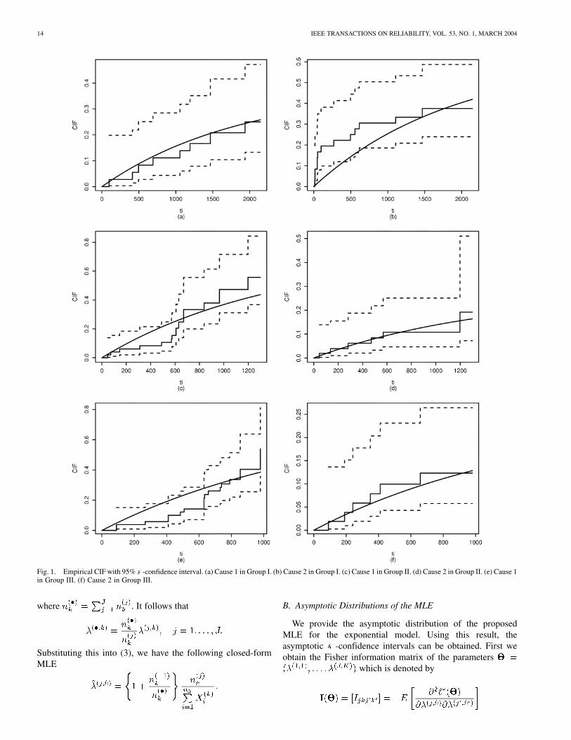
Fig. 1. Empirical CIF with 95% s -confidence interval. (a) Cause 1 in Group I. (b) Cause 2 in Group I. (c) Cause 1 in Group II. (d) Cause 2 in Group II. (e) Cause 1in Group III. (f) Cause 2 in Group III.
where . It follows that
Substituting this into (3), we have the following closed-formMLE
B. Asymptotic Distributions of the MLE
We provide the asymptotic distribution of the proposedMLE for the exponential model. Using this result, theasymptotic -confidence intervals can be obtained. First weobtain the Fisher information matrix of the parameters
which is denoted by
PARK AND KULASEKERA: PARAMETRIC INFERENCE OF INCOMPLETE DATA 15
for and . Then we obtain
and
and
for all .
Because has a binomial distributionfor , we have . Thenwe have
and
and
for all .
Using this, we have the following partitioned Fisher informationmatrix of the parameters
. . .
. . .
where and
. Note that whenever .Hence we have
. . .
The matrix is diagonally partitioned, so its inverse isgiven by
where . Using Theorem 8.3.3 in Graybill[15] and doing some algebra, we have
This inverse always exists unless ( i.e.,, each subjectin the th group is observed only with censoring or missingcauses) but this condition is extremely unrealistic in practice.Then we have the following asymptotic distribution of
from the property of MLE
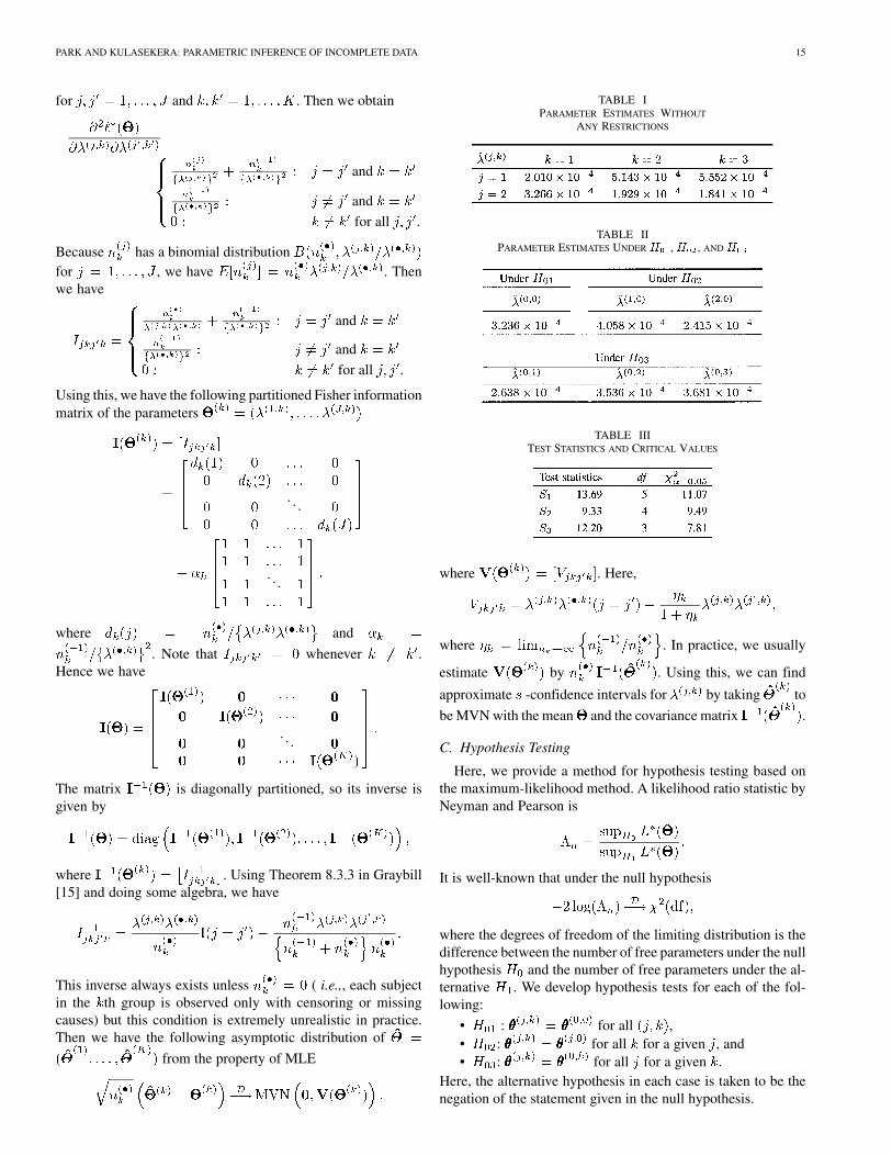
TABLE IPARAMETER ESTIMATES WITHOUT
ANY RESTRICTIONS
TABLE IIPARAMETER ESTIMATES UNDER H ,H , AND H
TABLE IIITEST STATISTICS AND CRITICAL VALUES
where . Here,
where . In practice, we usually
estimate by . Using this, we can find
approximate -confidence intervals for by taking to
be MVN with the mean and the covariance matrix .
C. Hypothesis Testing
Here, we provide a method for hypothesis testing based onthe maximum-likelihood method. A likelihood ratio statistic byNeyman and Pearson is
It is well-known that under the null hypothesis
where the degrees of freedom of the limiting distribution is thedifference between the number of free parameters under the nullhypothesis and the number of free parameters under the al-ternative . We develop hypothesis tests for each of the fol-lowing:
• : for all ,• : for all for a given , and• : for all for a given .
Here, the alternative hypothesis in each case is taken to be thenegation of the statement given in the null hypothesis.
16 IEEE TRANSACTIONS ON RELIABILITY, VOL. 53, NO. 1, MARCH 2004
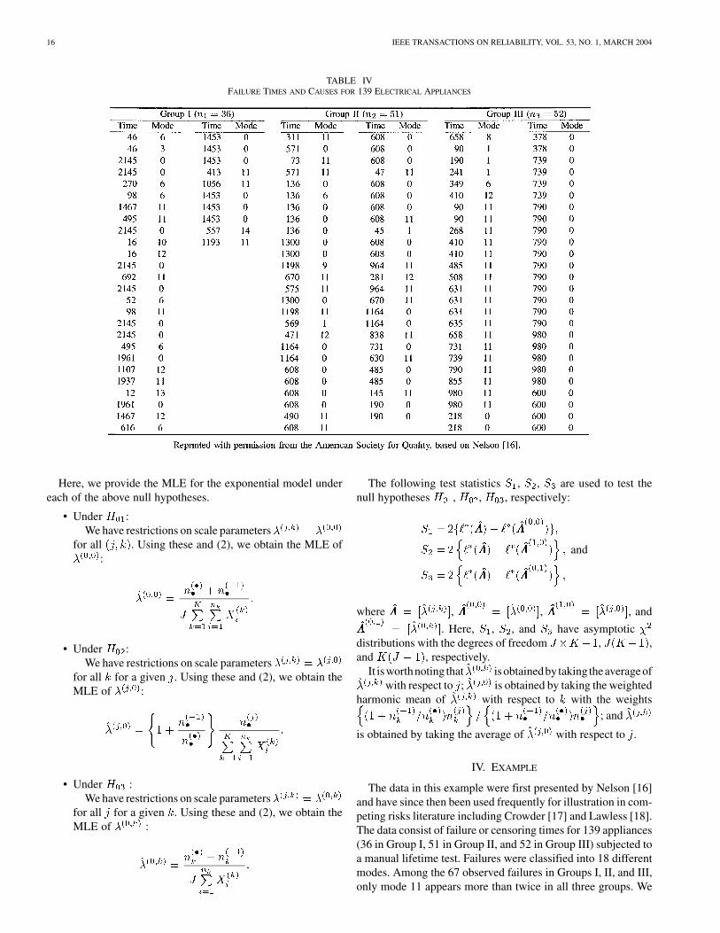
TABLE IVFAILURE TIMES AND CAUSES FOR 139 ELECTRICAL APPLIANCES
Here, we provide the MLE for the exponential model undereach of the above null hypotheses.
• Under :We have restrictions on scale parameters
for all . Using these and (2), we obtain the MLE of:
• Under :We have restrictions on scale parameters
for all for a given . Using these and (2), we obtain theMLE of :
• Under :We have restrictions on scale parameters
for all for a given . Using these and (2), we obtain theMLE of :
The following test statistics , , are used to test thenull hypotheses , , , respectively:
and
where , , , and
. Here, , , and have asymptoticdistributions with the degrees of freedom , ,and , respectively.
It isworthnoting that isobtainedby taking theaverageofwith respect to ; is obtained by taking the weighted
harmonic mean of with respect to with the weights; and
is obtained by taking the average of with respect to .
IV. EXAMPLE
The data in this example were first presented by Nelson [16]and have since then been used frequently for illustration in com-peting risks literature including Crowder [17] and Lawless [18].The data consist of failure or censoring times for 139 appliances(36 in Group I, 51 in Group II, and 52 in Group III) subjected toa manual lifetime test. Failures were classified into 18 differentmodes. Among the 67 observed failures in Groups I, II, and III,only mode 11 appears more than twice in all three groups. We
PARK AND KULASEKERA: PARAMETRIC INFERENCE OF INCOMPLETE DATA 17
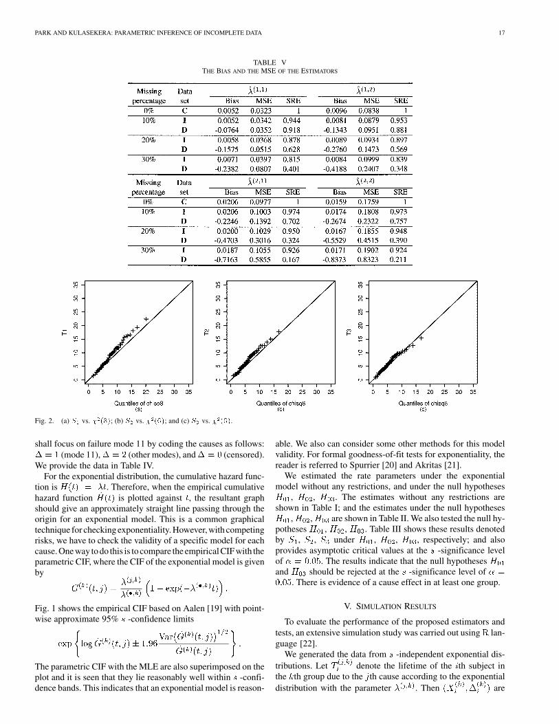
TABLE VTHE BIAS AND THE MSE OF THE ESTIMATORS
Fig. 2. (a) S vs. � (8); (b) S vs. � (6); and (c) S vs. � (6).
shall focus on failure mode 11 by coding the causes as follows:(mode 11), (other modes), and (censored).
We provide the data in Table IV.For the exponential distribution, the cumulative hazard func-
tion is . Therefore, when the empirical cumulativehazard function is plotted against , the resultant graphshould give an approximately straight line passing through theorigin for an exponential model. This is a common graphicaltechnique for checking exponentiality. However, with competingrisks, we have to check the validity of a specific model for eachcause. One way to do this is to compare the empirical CIF with theparametric CIF, where the CIF of the exponential model is givenby
Fig. 1 shows the empirical CIF based on Aalen [19] with point-wise approximate 95% -confidence limits
The parametric CIF with the MLE are also superimposed on theplot and it is seen that they lie reasonably well within -confi-dence bands. This indicates that an exponential model is reason-
able. We also can consider some other methods for this modelvalidity. For formal goodness-of-fit tests for exponentiality, thereader is referred to Spurrier [20] and Akritas [21].
We estimated the rate parameters under the exponentialmodel without any restrictions, and under the null hypotheses
, , . The estimates without any restrictions areshown in Table I; and the estimates under the null hypotheses
, , are shown in Table II. We also tested the null hy-potheses , , . Table III shows these results denotedby , , under , , , respectively; and alsoprovides asymptotic critical values at the -significance levelof . The results indicate that the null hypothesesand should be rejected at the -significance level of
. There is evidence of a cause effect in at least one group.
V. SIMULATION RESULTS
To evaluate the performance of the proposed estimators andtests, an extensive simulation study was carried out using lan-guage [22].
We generated the data from -independent exponential dis-tributions. Let denote the lifetime of the th subject inthe th group due to the th cause according to the exponentialdistribution with the parameter . Then are
18 IEEE TRANSACTIONS ON RELIABILITY, VOL. 53, NO. 1, MARCH 2004
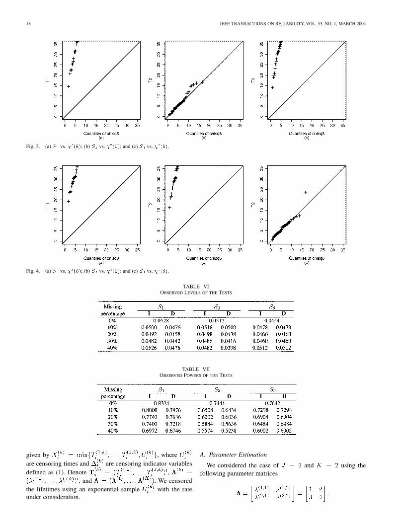
Fig. 3. (a) S vs. � (8); (b) S vs. � (6); and (c) S vs. � (6).
Fig. 4. (a) S vs. � (8); (b) S vs. � (6); and (c) S vs. � (6).
TABLE VIOBSERVED LEVELS OF THE TESTS
TABLE VIIOBSERVED POWERS OF THE TESTS
given by , whereare censoring times and are censoring indicator variablesdefined as (1). Denote ,
, and . We censoredthe lifetimes using an exponential sample with the rateunder consideration.
A. Parameter Estimation
We considered the case of and using thefollowing parameter matrices
PARK AND KULASEKERA: PARAMETRIC INFERENCE OF INCOMPLETE DATA 19
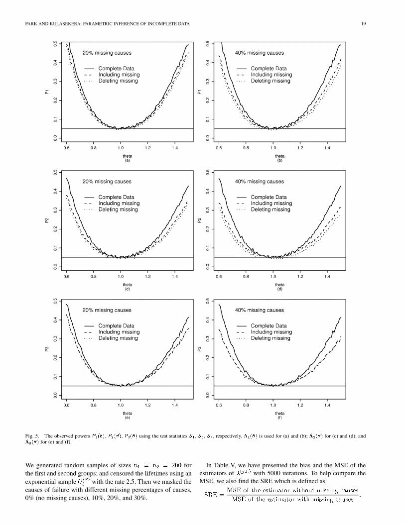
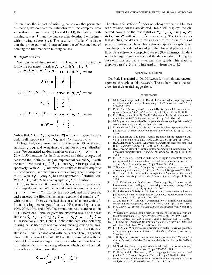
Fig. 5. The observed powers P (�), P (�), P (�) using the test statistics S , S , S , respectively. ��� (�) is used for (a) and (b); ��� (�) for (c) and (d); and��� (�) for (e) and (f).
We generated random samples of sizes forthe first and second groups; and censored the lifetimes using anexponential sample with the rate 2.5. Then we masked thecauses of failure with different missing percentages of causes,0% (no missing causes), 10%, 20%, and 30%.
In Table V, we have presented the bias and the MSE of theestimators of with 5000 iterations. To help compare theMSE, we also find the SRE which is defined as
20 IEEE TRANSACTIONS ON RELIABILITY, VOL. 53, NO. 1, MARCH 2004
To examine the impact of missing causes on the parameterestimation, we compare the estimates with the complete dataset without missing causes (denoted by ), the data set withmissing causes , and the data set after deleting the lifetimeswith missing causes . The results in Table V indicatethat the proposed method outperforms the ad hoc method ofdeleting the lifetimes with missing causes.
B. Hypothesis Tests
We considered the case of and using thefollowing parameter matrices with .
1) , where
2) , where
3) , where
Notice that , , and with give the dataunder null hypotheses , , and , respectively.
In Figs. 2–4, we present the probability plots [23] of the teststatistics , , and against the quantiles of the distribu-tions. We generated random samples of sizes
with 50 iterations for the first, second and third groups; andcensored the lifetimes using an exponential sample withthe rate 1. We used , , and in Figs. 2–4, re-spectively. With , all three test statistics have asymptotic
distributions, and the figure shows a fairly good asymptoticresult. With , only has an asymptotic distribution.With , only has an asymptotic distribution.
Next, we turn our attention to the levels and the powers ofeach hypothesis test. We generated random samples of sizes
for the first, second, and third groups;and censored the lifetimes using an exponential samplewith the rate 1. Then we masked the causes of failure with dif-ferent missing percentages of causes, 0% (no missing causes),10%, 20%, 30%, and 40%. The simulation results are based on
iterations. Table VI gives the observed levels of the teststatistics , , using , ,
, respectively. Here, and denote the data sets includingmissing-cause lifetimes and excluding missing-cause lifetimes,respectively. The table shows that the observed levels of the teststatistics and associated with the data set are, in general,closer to the nominal level of 0.05 than those associated with thedata set . It is interesting to note that the observed levels of thetest statistic are the same regardless of which data set is used.This is because it is shown that
Therefore, this statistic does not change when the lifetimeswith missing causes are deleted. Table VII displays the ob-served powers of the test statistics , , using ,
, with , respectively. The table showsthat deleting the data with missing causes results in a loss ofpower. To make the above observations graphically explicit, wecan change the value of and plot the observed powers of thethree data sets—the complete data set (0% missing), the dataset including missing causes, and the data set after deleting thedata with missing causes—on the same graph. This graph isdisplayed in Fig. 5 over a fine grid of from 0.6 to 1.5.
ACKNOWLEDGMENT
Dr. Park is grateful to Dr. M. Leeds for his help and encour-agement throughout this research. The authors thank the ref-erees for their useful suggestions.
REFERENCES
[1] M. L. Moeshberger and H. A. David, “Life tests under competing causesof failure and the theory of competing risks,” Biometrics, vol. 27, pp.909–933, 1971.
[2] D. R. Cox, “The analysis of exponentially distributed lifetimes with twotypes of failures,” J. Royal Stat. Soc. B, vol. 21, pp. 411–421, 1959.
[3] R. J. Herman and R. K. N. Patell, “Maximum likelihood estimation formulti-risk model,” Technometrics, vol. 13, pp. 385–396, 1971.
[4] M. Miyakawa, “Analysis of incomplete data in competing risks model,”IEEE Trans. Rel., vol. 33, pp. 293–296, 1984.
[5] D. Kundu and S. Basu, “Analysis of incomplete data in presence of com-peting risks,” J. Statistical Planning and Inference, vol. 87, pp. 221–239,2000.
[6] M. G. Larson and G. E. Dinse, “A mixture model for the regression anal-ysis of competing risks data,” Appl. Stat., vol. 34, pp. 201–211, 1985.
[7] R. A. Maller and X. Zhou, “Analysis of parametric models for competingrisks,” Statistica Sinica, vol. 12, pp. 725–750, 2002.
[8] R. J. Gray, “A class of k -sample tests for comparing the cumulative inci-dence of a competing risk,” Annals of Statistics, vol. 16, pp. 1140–1154,1988.
[9] E.-E. A. A. Aly, S. C. Kochar, and I. W. McKeague, “Some tests for com-paring cumulative incidence functions and cause-specific hazard rates,”J. Amer. Stat. Association, vol. 89, pp. 994–999, 1994.
[10] Y. Sun and R. C. Tiwari, “Comparing cumulative incidence functions ofa competing-risks model,” IEEE Trans. Rel., vol. 46, pp. 247–253, 1997.
[11] K. F. Lam, “A class of tests for the equality of k cause-specific hazardrates in a competing risks model,” Biometrika, vol. 85, pp. 179–188,1998.
[12] S. B. Kulathinal and D. Gasbarra, “Testing equality of cause-specifichazard rates corresponding tom competing risks among k groups,” Life-time Data Analysis, vol. 8, pp. 147–161, 2002.
[13] H. Lindkvist and Y. Belyaev, “A class of nonparametric tests in the com-peting risks model for comparing two samples,” Scandinavian Journalof Statistics, vol. 25, pp. 143–150, 1998.
[14] X. Luo and B. W. Turnbull, “Comparing two treatments with multiplecompeting risks endpoints,” Statistica Sinica, vol. 9, pp. 986–998, 1999.
[15] F. A. Graybill, Matrices With Applications in Statistics: Wadsworth, Inc.,1983.
[16] W. Nelson, “Hazard plotting methods for analysis of life data with dif-ferent failure modes,” J. Qual. Technol., vol. 2, pp. 126–149, 1970.
[17] M. J. Crowder, Classical Competing Risks: Chapman and Hall, 2001.[18] J. F. Lawless, Statistical Models and Methods for Lifetime Data, 2nd
ed. New York: John Wiley & Sons, 2003.[19] O. O. Aalen, “Nonparametric estimation of partial transition probabil-
ities in multiple decrement models,” Annals of Statistics, vol. 6, pp.534–545, 1978.
[20] J. D. Spurrier, “An overview of tests for exponentiality,” Communica-tions in Statistics, Part A—Theory and Methods, vol. 13, pp. 1635–1654,1984.
[21] M. G. Akritas, “Pearson-type goodness-of-fit tests: The univariate case,”J. Amer. Stat. Association, vol. 83, pp. 222–230, 1988.
[22] R. Ihaka and R. Gentleman, “R: a language for data analysis andgraphics,” J. Comput. Graphical Stat., vol. 5, pp. 299–314, 1996.
[23] M. B. Wilk and R. Gnanadesikan, “Probability plotting methods for theanalysis of data,” Biometrika, vol. 55, pp. 1–17, 1968.
PARK AND KULASEKERA: PARAMETRIC INFERENCE OF INCOMPLETE DATA 21
Chanseok Park is an Assistant Professor of Mathematical Sciences at ClemsonUniversity, Clemson, SC. He received his B.S. in Mechanical Engineering fromSeoul National University; his M.A. in Mathematics from the University ofTexas at Austin; and his Ph.D. in Statistics in 2000 from the Pennsylvania StateUniversity. His research interests include survival analysis, competing risks, sta-tistical inference using quadratic inference function, robust inference, and sta-tistical computing and simulation.
K. B. Kulasekera is a Professor of Mathematical Sciences at Clemson Univer-sity. He received his B.S. in 1979 from the University of Sri Lanka; his M.A.in Statistics from the University of New Brunswick; and his Ph.D. in Statisticsfrom the University of Nebraska, Lincoln, NE. His research interests includesurvival analysis, nonparametric regression, and multivariate methods.