Parameterised Electromagnetic Scattering Solutions

for a Range of Incident Wave Angles

P.D. Ledger∗1, J. Peraire†, K. Morgan∗, O. Hassan∗ & N.P. Weatherill∗

∗Civil and Computational Engineering Centre, University of Wales, Swansea, U.K.

†Aeronautics and Astronautics, M.I.T. Cambridge, Massachusetts, U.S.A

Abstract

This paper considers the numerical simulation of 2D electromagnetic wave scattering problems anddescribes the construction of a reduced–order approximation which enables the rapid predictionof the scattering width distribution for a range of incident wave directions. Associated certaintybounds ensure confidence in the results of the computed approximation. Numerical examples areincluded to demonstrate the performance of the proposed procedure.

1 Introduction

The simulation of electromagnetic wave scattering problems is of importance in many practicalapplication areas where, typically, the interest lies in determining the scattering width distributionfor a new design. Computational methods can provide assistance in this area, provided that thesimulations allow the full problem parameter space of interest to be rapidly, and accurately,investigated. In general, the parameter space will include changes in the direction of the incidentwave, changes in the wave frequency and changes in the geometry and structure of the scatterer.It should also be noted that this requirement for the rapid computation of the scattering width fora range of problem parameters also arises when the solution of inverse problems is considered [1].

The finite element method is a popular domain based approach for the solution of electromag-netic wave scattering problems, in which an approximation to the scattering width distributionmay be obtained by post–processing the computed solution. With this approach, a new compu-tation is necessary to produce the revised scattering width distribution following a change in anyof the problem parameters. The implication is that the associated computational costs will bevery high for a study involving a large number of parameter changes. In this paper, we present areduced–order approximation which addresses this problem and can lead to significant reductionin the computational costs.

Reduced—order approximations operate in two stages. In an initial off–line stage, full solutionsare computed for a set of specified problem parameters and the results of these computations arestored. In an on–line stage, specified outputs of interest are computed at low cost for new sets ofthe problem parameters. In addition, for the outputs to be of practical use, it is important thataccuracy can be guaranteed. Reduced–order approximations with these properties have alreadybeen successfully applied in the area of computational aerodynamics [2, 3], while sophisticatedmethods for determining error bounds on the outputs produced by reduced–order approximationshave also been developed [4, 5].

We aim to apply a reduced–order approximation in the area of electromagnetic wave scattering.For this initial study, we consider two dimensional wave scattering problems and we have restrictedthe parameter space investigation to allow only variations in the direction of the incident wave.The selected output of interest is the scattering width distribution and the implementation detailsdescribe how it can be effectively computed. To assess the accuracy of the proposed reduced–order approximation, a novel approach for obtaining certainty bounds on the computed output isdescribed. Here certainty is assessed with respect to a full solution computed for the parameter set.

1Corresponding Author: Civil and Computational Engineering Centre, University of Wales Swansea, Singleton

Park, Swansea SA2 8PP, Wales, U.K. Email: P.D.Ledger@swansea.ac.uk

1

It will be shown that these certainty bounds can be computed in the on–line stage, requiring littleadditional computation and providing certainty on the scattering width distributions. For theoff–line stage of the approach, we achieve accurate solutions to two dimensional electromagneticwave scattering problems by employing a Galerkin finite element method in the frequency domain,with the arbitrary order edge elements of Ainsworth and Coyle [6]. This has been shown to bean effective approach for obtaining accurate scattering width distributions, over a large frequencyrange, for a variety of different scatterers [7, 8].

The presentation of the work proceeds as follows: In Section 2, a brief description of the elec-tromagnetic wave scattering problem, with a prescribed incident wave angle, is presented. Then,the weak variational formulation of the problem is described and an overview of the arbitraryorder finite element discretisation is given, together with an outline of the approach employed forthe calculation of the scattering width distribution. This is followed, in Section 3, by the presen-tation of the reduced–order approximation which will enable the rapid prediction of the scatteringwidth distribution for new incident wave directions. The approach adopted for obtaining certaintybounds on the outputs produced by the reduced–order approximation is also described. In Sec-tion 4, we discuss the computational costs of the reduced–order approximation and the associatedcertainty bounds and, in Section 5, numerical examples are presented to illustrate the capabilityof the proposed method. Finally, some concluding remarks are given.

2 The Scattering Problem for a Prescribed Incident Wave Angle

2.1 Problem Description

Our interest lies in the simulation of scattering problems, in which electromagnetic waves interactwith a general scatterer. We will restrict consideration to the case where the scatterer is a perfectconductor, but the method that is proposed is readily extendable to enable the modelling of moregeneral scatterers. It is assumed that the scatterer is surrounded by a region of free space and thatwaves are generated by a known source located in the far field. The unknowns for this problemare the electric and magnetic field vectors, which are expressed relative to a Cartesian coordinatesystem Oxyz in the form Et = (Et

x, Ety, E

tz)

T and Ht = (Htx, Ht

y, Htz)

T respectively. Here, thesuperscripts t and T denote the total field and the vector transpose respectively. For scatteringsimulations, these total fields may be decomposed, into incident and scattered components, as

Et = Ei + E Ht = H i + H (1)

where the superscript i denotes the incident field and the vectors E and H are the scatteredelectric and magnetic fields respectively. For a frequency domain approach, where a time variationeiωt is assumed, the dimensionless Maxwell curl equations in free space can be expressed in theform

curl E = iωH curl H = −iωE (2)

and the Maxwell divergence equations written as

div E = 0 div H = 0 (3)

In these expressions i2 = −1 and ω = 2π/λ, where λ is the wavelength of the incident wave. Thecurl equations (2) may be combined to produce the reduced vector wave equation

curl curlE − ω2E = 0 (4)

for the scattered electric field. We now restrict consideration to two–dimensional transverseelectric (TE) problems, in which E and H are functions of x and y only and have the form,E = (Ex, Ey, 0)

T and H = (0, 0, Hz)T respectively. If one was to adopt a transverse magnetic

formulation (TM), then the fields would have the form H = (Hx, Hy, 0)T and E = (0, 0, Ez)

T .

2

2.2 Boundary Conditions

2.2.1 Perfect Magnetic Conductor (PMC)

At the surface of the PMC scatterer, the boundary conditions

n ∧ H = −n ∧ H i n · E = −n · Ei (5)

should be applied. The surface of the PMC is denoted by Γ1.

2.2.2 Perfect Electrical Conductor (PEC)

At the surface of the PEC scatterer, the boundary conditions are

n ∧ E = −n ∧ Ei n · H = −n · H i (6)

The surface of the PEC is denoted by Γ2. It should be noted that applying a PMC condition fora TE problem is equivalent to applying a PEC condition for a TM problem.

2.2.3 Far Field Condition

The scattered fields E and H are required to satisfy the Silver–Muller radiation conditions [9]

er ∧ curl E − iωE = O(r−3/2) (7)

er ∧ curl H − iωH = O(r−3/2) (8)

as r → ∞, where (r, θ) are cylindrical polar coordinates and er denotes the unit radial vector.With a finite element solution procedure in mind, we aim to approximate this condition bytruncating the free space region at a finite distance from the scatterer and then imposing anappropriate boundary condition. This may be accomplished in a variety of different ways e.g. viainfinite elements [10, 9], using absorbing boundary conditions [11], applying DtN maps [12] orcoupling boundary and finite element methods [13]. Here, we choose to satisfy the condition byadding an absorbing layer, denoted by Ωp, to the truncated free space region Ωf , as illustrated

3Γ

Γ Γor 1 2

Ωf

Ωp

Incident Wave

Figure 1: The addition of Ωp, the PML region, to the domain Ωf

in Figure 1. For the absorbing medium, we employ a curvilinear, anisotropic, perfectly matchedlayer (PML) [14, 15, 7].

3

2.3 Strong Statement of the Problem

It follows that a strong statement of the problem can be formulated as: find E such that

curl curl E − ω2E = 0 in Ωdiv E = 0 in Ω

n ∧ curl E = −n ∧ curlEi n · E = −n · Ei on Γ1

n ∧ E = −n ∧ Ei on Γ2

er ∧ curl E − iωE = O(r−3/2) as r → ∞

. (9)

This equation set can be shown to be equivalent to the problem description given in section 2.1and the boundary conditions given in section 2.2 [16]. Note that the normal condition n · H

associated with Γ2 can be discarded because the normal condition n ·E = −n ·Ei on Γ1 impliesthat n · H = −n · H i on Γ2.

2.4 Weak Variational Statement and Discretisation

A weak variational formulation of the scattering problem given in equation (9) may now beexpressed as [7, 8]: find E ∈ XD, such that

A(E, W ) = `(W ) ∀W ∈ X (10)

where the spaces XD and X are defined by

XD = v |v ∈ H(curl; Ω); n ∧ v = −n ∧ Ei on Γ2; n ∧ v = 0 on Γ3 (11)

X = v |v ∈ H(curl; Ω); n ∧ v = 0 on Γ2; n ∧ v = 0 on Γ3 (12)

and the operator A is defined by

A(E, W ) = a(E, W ) − ω2m(E, W ) (13)

The bilinear forms employed here are defined by

a(E, W ) =

∫

Ωf+Ωp

Λ−11 curlE · curlW dΩ m(E, W ) =

∫

Ωf+Ωp

Λ2E · WdΩ (14)

and the linear form is given by

`(W ) =

∫

Γ1

(n ∧ Λ−1

1 curl Ei)· W dΓ (15)

In these expressions, Λ1 and Λ2 represent complex tensors of position in Ωp and are equal to theidentity tensor in Ωf [7], while an overbar denotes the complex conjugate. One might expect thata Lagrange multiplier term should be included in equation (10) to enforce the zero divergencecondition. However, it can be shown that, for scattering problems with a prescribed non-zero ω,the Lagrange multiplier turns out to be equal to zero and therefore can be omitted [8]. As thenormal boundary condition n · E = −n · Ei on Γ1 is associated with the divergence condition itdoes not appear in the variational statement (10).

An approximate solution EH ∈ XDH ⊂ XD to the problem expressed by the variational

statement of equation (10) is obtained by employing the Galerkin procedure. Initially, the domainΩf + Ωp is discretised using an unstructured assembly of triangular and quadrilateral elements.Then, the scattered field is approximated, to a degree p, as [6]

EH =4∑

i=1

p∑

j=0

eijφ

i

j +

p∑

j=0

p∑

k=1

eIξ

j,kφIξ

j,k +

p∑

j=0

p∑

k=1

eIη

j,kφIη

j,k (16)

4

over a master quadrilateral element and as

EH =

3∑

i=1

p∑

j=0

eijφ

i

j +

3∑

i=1

p−2∑

j=0

ePIi,j φ

PI

i,j +

p−3∑

j=0

p−3∑

k=0︸ ︷︷ ︸

j+k≤p−3

eGIξ

j,k φGIξ

j,k +

p−3∑

j=0

p−3∑

k=0︸ ︷︷ ︸

j+k≤p−3

eGIη

j,k φGIη

j,k (17)

over a master triangular element. The vectors φ, expressed relative to a master element coordinatesystem, denote the hierarchic edge element basis functions, while the scalars e are the unknowncoefficients. These scalar coefficients are related to weighted moments of the tangential componentof the field and continuity of these coefficients is enforced on inter–element edges. This resultsin a scheme which has continuous tangential components between elements, whilst allowing fordiscontinuous normal components.

The basis functions can be generated numerically through recursive relations [6]. Elementintegrals can be evaluated by employing a covariant mapping [17] and Gauss quadrature [7].Following this approach, the Galerkin approximation is obtained as the solution of a discreteproblem which can be expressed as: find EH ∈ XD

H such that

A(EH , W ) = `(W ) ∀W ∈ XH ⊂ X (18)

The complex linear equation systemAEH = L (19)

which results from equation (18) is solved using a LINPACK banded solver. Here, we use the no-tation EH to denote the vector of unknown coefficients associated with a pth order discretisation.

2.5 Scattering Width Evaluation

The computed scattering width distribution σ(EH ; φ) is a function of the finite element solutionEH and the far field viewing angle φ. To evaluate the scattering width distribution, the form ofthe solution on a collection surface Γc, which totally encloses the scatterer, is determined. It isconvenient to express the scattering width distribution in the form [18]

σ(EH ; φ) = LO(EH ; φ)LO(EH ; φ) (20)

where

LO(EH ; φ) =

∫

Γc

(n ∧ EH · V ) dΓ +∑

∫

k

(ω2EH · Y H − curlEH · curl Y H

)dΩ (21)

Here, the summation extends over all elements k ∈ Ω, such that ∂k ∪ Γc 6= ∅ and

V = −[0, 0, 1]T expiω

(x′ cos φ + y′ sin φ

)(22)

Y =1

iω[sin φ,− cos φ, 0]T exp

iω

(x′ cos φ + y′ sin φ

)(23)

The quantity Y H is the finite element interpolant of Y . It should be noted that equation (21)follows from adopting the approach of Monk and co–workers [19, 20, 21], who suggested usingan area integral approach to evaluate the flux term which appears in the basic scattering widthexpression. The scattering width distribution is generally displayed in decibels and, in this case,it is the quantity

σ = 10 log10

(ω

4σ(EH ; φ)

)

(24)

that is plotted against the viewing angle φ.

5

3 Reduced Order Approximation

3.1 Computing the Reduced Order Approximation

Consider now the development of a reduced–order approximation for the prediction of the scat-tering width distribution for an electromagnetic scattering problem. We take incident waves ofthe form

Ei =

− sin θcos θ

0

expiω(x cos θ + y sin θ) (25)

where θ is the angle between the direction of propagation of the incident wave and the x axis. Wereturn to the standard Galerkin statement of equation (18), but now expressed in the form [4]:find EH(θ) ∈ XD

H such that

A(EH(θ), W ) = ` (W ; θ) ∀W ∈ XH (26)

for a given incident wave direction, θ. Our goal is to develop a reduced–order approximation fora parameterised solution EH(θ). The computed output is selected to be sH(θ; φ) ∈ C, where

sH(θ, φ) = LO(EH(θ); φ) (27)

and LO is defined in equation (21). We introduce the associated adjoint solution, ΨH(φ) ∈ XH ,which is defined to satisfy the requirement

A(W ,ΨH(φ)) = −LO(W ; φ) ∀W ∈ XH (28)

Note that here we prefer to use LO(W ; φ) for the adjoint computation, rather than the lin-earised form of σ which we previously proposed when evaluating a–posteriori error bounds on thescattering width [18]. The reasons for this choice are

1. Use of the the linearised form of σ results in asymptotic bounds, which although applicablein the case of evaluating a–posteriori error bounds is not in the case of this reduced ordermodel. Indeed, if the linearised form of σ is employed for this reduced order model we wouldlose the guarantee of being able to prove that the bounds we obtain are strict;

2. Use of the linearised form of σ as the output adjoint for a reduced–order approximationwould, in the approach to be followed, necessitate the calculation of a large number ofadditional adjoint solutions, since the linearised adjoint then depends on the solution EH .

The discrete adjoint problem, given in equation (28), may be written in matrix notation as

ATΨH = −g (29)

where g is the right hand vector which results from the linear form LO(W ; φ).To construct reduced–order spaces, we adopt a parameter set θ1, · · · , θNθ

of incident waveangles and a parameter set φ1, · · · , φNφ

of viewing angles of the scattering width. Correspondingsolutions EH(θ1), · · · , EH(θNθ

) and adjoints Ψ(φ1), · · · ,Ψ(φNφ) are computed, and the spaces

WNθ= spanEH(θi); i = 1, · · · , Nθ WNφ

= spanΨH(φi); i = 1, · · · , Nφ (30)

are defined. If we are presented with a new incident angle, θ, the approach is then to look forEH(θ) ∈ WNθ

⊂ XDH such that

A(EH , W ) = ` (W ; θ) ∀W ∈ WNθ(31)

For this angle of incidence, we compute ΨH(φ) ∈ WNφ⊂ XH , for a given φ, such that

A(W , ΨH) = −LO(W ; φ) ∀W ∈ WNφ(32)

6

Here, EH denotes a reduced–order approximation to EH(θ) and ΨH is a reduced–order approx-imation to ΨH(φ).

With the viewing angle, φ, and the incident wave direction, θ, specified, equation (27) maybe expressed as

sH(θ, φ) = LO(EH(θ); φ) = LO(EH ; φ) + LO(EH(θ) − EH ; φ) (33)

since LO(E; φ) is linear in E. Then, using equations (28) and (26), it follows that we can write

sH(θ, φ) = sH(θ, φ) + r(θ, φ) (34)

HeresH(θ, φ) = LO(EH ; φ) −

[

`(ΨH) −A(EH , ΨH)]

(35)

is computable from the known data, while the term

r(θ, φ) = A(EH(θ) − EH ,ΨH(φ) − ΨH) (36)

is not computable without prior knowledge of EH(θ) or ΨH(φ). Although this term is not com-putable, we will see below that it may be bounded, and this enables us to deduce the magnitudeof the error made when we employ sH as a reduced order approximation to sH . We note that thisapproach differs to the direct method of employing LO(EH ; φ) as the reduced order approximationto sH and results in a much improved approximation.

To summarise this process, the steps involved in the off–line and on–line stages of the reduced–order approximation procedure are presented in algorithmic form in Table 1.

3.2 Bounding the Error in the Reduced Order Approximation

Certainty bounds may be constructed for the reduced–order approximation to the output, withthe bounds being measured with respect to the output given by the finite element solution. Fromequations (34)–(36), it can be seen that the error in the reduced order approximation may bewritten as

sH − sH = r(θ, φ) = A(e, ε) (37)

wheree = EH − EH ε = ΨH − ΨH (38)

Given the reduced order approximations EH and ΨH , we define residuals RU (W ) : XH → R andRΨ(W ) : XH → R according to

RU (W ) = `(W ) −A(EH , W ) RΨ(W ) = −LO(W ) −A(W , ΨH) (39)

and we note thatRU (ε) = RΨ(e) = A(e, ε) (40)

For the space XH , we introduce a norm ‖ · ‖∗, defined by

‖W ‖∗ = n(W , W ) ≥ 0 (41)

where n is a coercive bilinear form and the particular choice adopted for n will be described below.For the residuals RU (W ) and RΨ(W ), we also define the dual norm ‖ · ‖−∗ of ‖ · ‖∗ according to

‖R‖−∗ = supW ∈XH

R(W )

‖W ‖∗(42)

From this dual norm definition, it follows that

|R(W )| ≤ ‖R‖−∗‖W ‖∗ ∀ W ∈ XH (43)

7

Off–Line Stage:

Select θ1, · · · , θNθ and φ1, · · · , φNφ

Compute the coefficents EHi for i = 1, · · ·Nθ by solving

AEHi = Li

Compute the coefficients ΨHi for i = 1, · · ·Nφ by solving

ATΨHi = −gi

On–Line Stage:

Select a new incident wave direction θ

Compute the coefficients αi of EH

=

Nθ∑

i=1

αiEHi by solving

(EHi )TAE

H= (EH

i )T Li i = 1, ·, Nθ

Compute the coefficents βi of ΨH

=

Nφ∑

i=1

βiΨHi by solving

(ΨHi )TAT Ψ

H= −(ΨH

i )T gi i = 1, · · · , Nφ

Then compute sH from

sH = gT EH−

[

LT ΨH−

(

ΨH

)TAE

H]

The scattering width distribution is then given byσ = sH sH

Table 1: Algorithmic description of the reduced–order approximation procedure for the scatteringwidth distribution, detailing the off–line and on–line stages

so that, in particular, when W = e,∣∣RΨ(e)

∣∣ ≤ ‖RΨ‖−∗‖e‖∗ (44)

In order to be able to determine a computable bound for sH − sH , we require the existence of adiscrete inf–sup parameter β that satisfies

infV ∈XH

supW ∈XH

|A(V , W )|

‖V ‖∗‖W ‖∗≥ β > 0 (45)

It should be noted that the existence of this parameter is a requirement for the original problemof equation (18) to be well–posed. Now, if we set V = e in this equation, we may deduce that

supW ∈XH

|A(e, W )|

‖W ‖∗≥ β‖e‖∗ (46)

When this result is combined with equations (40) and (42), we see immediately that

‖e‖∗ ≤1

β‖RU‖−∗ (47)

8

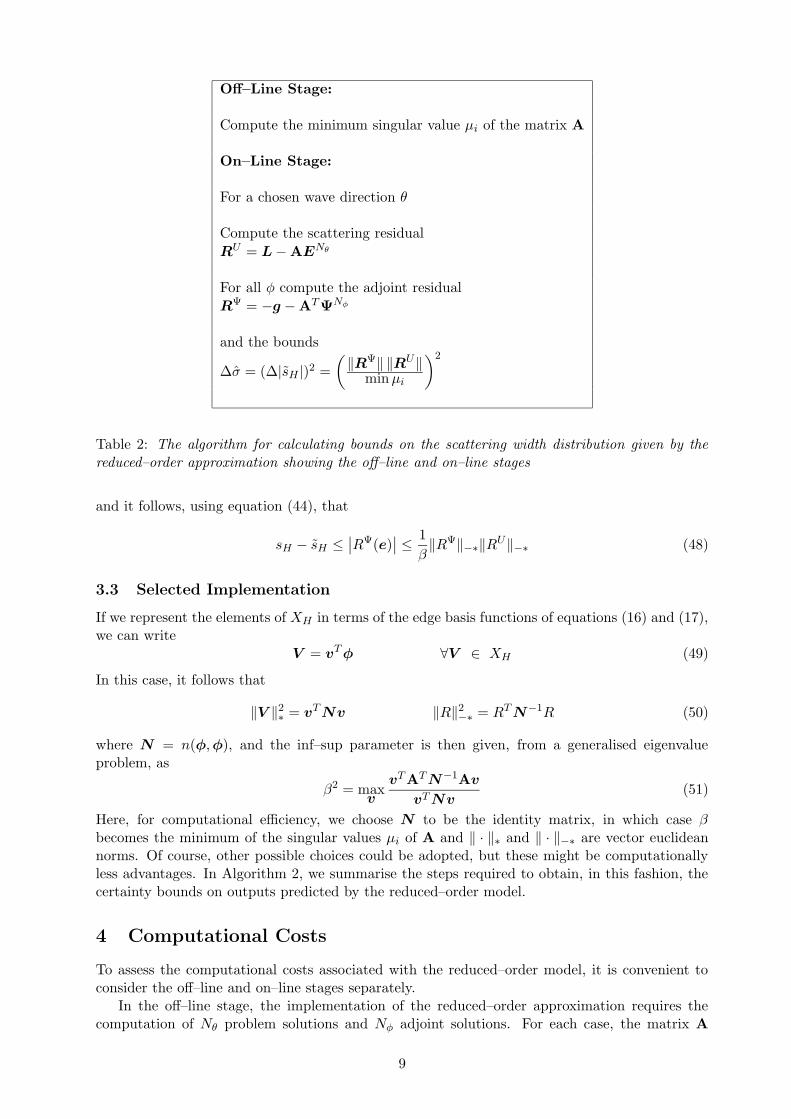
Off–Line Stage:

Compute the minimum singular value µi of the matrix A

On–Line Stage:

For a chosen wave direction θ

Compute the scattering residual

RU = L − AENθ

For all φ compute the adjoint residual

RΨ = −g − ATΨNφ

and the bounds

∆σ = (∆|sH |)2 =

(

‖RΨ‖ ‖RU‖min µi

)2

Table 2: The algorithm for calculating bounds on the scattering width distribution given by thereduced–order approximation showing the off–line and on–line stages

and it follows, using equation (44), that

sH − sH ≤∣∣RΨ(e)

∣∣ ≤

1

β‖RΨ‖−∗‖R

U‖−∗ (48)

3.3 Selected Implementation

If we represent the elements of XH in terms of the edge basis functions of equations (16) and (17),we can write

V = vT φ ∀V ∈ XH (49)

In this case, it follows that

‖V ‖2∗ = vT Nv ‖R‖2

−∗ = RT N−1R (50)

where N = n(φ, φ), and the inf–sup parameter is then given, from a generalised eigenvalueproblem, as

β2 = maxv

vTAT N−1Av

vT Nv(51)

Here, for computational efficiency, we choose N to be the identity matrix, in which case βbecomes the minimum of the singular values µi of A and ‖ · ‖∗ and ‖ · ‖−∗ are vector euclideannorms. Of course, other possible choices could be adopted, but these might be computationallyless advantages. In Algorithm 2, we summarise the steps required to obtain, in this fashion, thecertainty bounds on outputs predicted by the reduced–order model.

4 Computational Costs

To assess the computational costs associated with the reduced–order model, it is convenient toconsider the off–line and on–line stages separately.

In the off–line stage, the implementation of the reduced–order approximation requires thecomputation of Nθ problem solutions and Nφ adjoint solutions. For each case, the matrix A

9

remains unaltered and only the right hand side vectors g and L change. By using a LINPACKdirect solution technique which allows for multiple right hand side vectors, we are able to computeall these solutions simultaneously. In preparation for the calculation of bounds, we are required

Figure 2: Scattering by a PEC/PMC circular cylinder of diameter D = 2λ showing the structuredmesh of 200 triangular elements

to evaluate the minimum of the singular values of the matrix A. Although this is an expensiveO(N3) operation, it only has to be undertaken once for all incident wave directions.

In the on–line stage, we prescribe new incident wave directions and compute EH

and ΨH

aslinear combinations of the predetermined data given in WNθ

and WNφ. The Nθ × Nθ and the

Nφ × Nφ matrices which result from equations (31) and (32) can be precomputed to reduce thecost of computing subsequent outputs for new θ values. Inversion of the resulting system for

EH

, ΨH

is at most, O(max(N3θ , N3

φ)) and we deduce that, for small Nθ and Nφ, sH is much lessexpensive to compute than sH .

Further computational efficiencies can be obtained by storing quantities which remain unal-tered during evaluation of different RCS values.

5 Numerical Examples

A number of numerical examples are now considered to demonstrate the performance of theproposed procedure. Initially, the reduced–order approximation of equation (35) is used to predictthe scattering width distribution, following the algorithm shown in Table 1. Then, we demonstratethe evaluation of bounds for the scattering width distribution using equation (48) and the selectedimplementation, following the algorithm outlined in Table 2.

5.1 Performance of the Reduced–Order Approximation

To demonstrate the performance of the reduced–order approximation, consider initially the prob-lem of scattering of a plane TE wave by a PMC circular cylinder of diameter D = 2λ. Thecomputational domain is in the form of a circular annulus of inner radius λ and outer radius2λ. This domain is discretised using a structured mesh of 200 triangular elements of polynomialorder p = 4, as illustrated in Figure 2. For this example, off–line solutions corresponding toNθ = 3, with incident wave directions θi = −90, 0, 90 degrees, and viewing angles Nφ = 18with φi = −180 + 20(i − 1) degrees for i = 1, 2, . . . , 18, are computed. Using these computedresults, the reduced–order approximation is invoked, in the on–line stage, to predict the scatter-ing width distributions for waves incident at angles of θ = 0, 10, 20, 40, 120 degrees in turn. Acomparison between the resulting distributions in decibels and the distributions obtained fromthe full finite element solutions are shown in Figure 3. It can be observed that for the case θ = 0,which corresponds to one of the primal problems, the reduced–order approximation produces re-sults that are in exact agreement with the finite element distribution. For angles of incidence

10

2

4

6

8

10

12

14

16

-200 -150 -100 -50 0 50 100 150 200

RC

S

phi

Reduced modelFE solution

2

4

6

8

10

12

14

16

-200 -150 -100 -50 0 50 100 150 200

RC

S

phi

Reduced modelFE solution

θ = 0o θ = 10o

2

4

6

8

10

12

14

16

-200 -150 -100 -50 0 50 100 150 200

RC

S

phi

Reduced modelFE solution

2

4

6

8

10

12

14

16

-200 -150 -100 -50 0 50 100 150 200

RC

S

phi

Reduced modelFE solution

θ = 20o θ = 40o

2

4

6

8

10

12

14

16

-200 -150 -100 -50 0 50 100 150 200

RC

S

phi

Reduced modelFE solution

θ = 120o

Figure 3: Scattering of a plane TE wave by a PMC circular cylinder of diameter D = 2λ show-ing a comparison between the scattering width distributions computed using the adjoint enhancedreduced–order model solution and the finite element solution, for waves incident at different angles,θ.

11

-25

-20

-15

-10

-5

0

5

10

15

-200 -150 -100 -50 0 50 100 150 200

RC

S

phi

Reduced modelFE solution

-25

-20

-15

-10

-5

0

5

10

15

-200 -150 -100 -50 0 50 100 150 200

RC

S

phi

Reduced modelFE solution

θ = 0 θ = 10

-25

-20

-15

-10

-5

0

5

10

15

-200 -150 -100 -50 0 50 100 150 200

RC

S

phi

Reduced modelFE solution

-25

-20

-15

-10

-5

0

5

10

15

-200 -150 -100 -50 0 50 100 150 200

RC

S

phi

Reduced modelFE solution

θ = 20 θ = 40

-25

-20

-15

-10

-5

0

5

10

15

-200 -150 -100 -50 0 50 100 150 200

RC

S

phi

Reduced modelFE solution

θ = 120

Figure 4: Scattering of a plane TE wave by a PEC circular cylinder of diameter D = 2λ show-ing a comparison between the scattering width distributions computed using the adjoint enhancedreduced–order model solution and the finite element solution, for waves incident at different angles,θ.

12

θ = 10, 20, 40, 120, which do not correspond to one of the primal problems, the reduced–orderapproximation is in excellent agreement with the output given by the corresponding full finiteelement solution.

In Figure 4, the corresponding results for the scattering of a TE wave by a PEC circularcylinder of diameter D = 2λ are displayed. For this example, we employ the same mesh andcompute Nθ = 3 scattering solutions and Nφ = 18 adjoint solutions. As in the PMC case, it isobserved that the scattering width distributions produced by the reduced–order approximationare again in excellent agreement with those obtained from the full finite element solution.

As an example of a problem involving a more complicated geometry, the calculation of thescattering width distribution for the problem of scattering of a plane TE wave by PEC NACA0012aerofoil of electrical length 2λ is considered. The hybrid mesh that is employed is illustrated in

Figure 5: Scattering by a PEC NACA0012 aerofoil of chord length 2λ showing the hybrid meshof 668 triangles and 60 quadrilaterals.

Figure 5 and contains 668 triangles and 60 quadrilaterals with uniform polynomial order p = 3.Off–line calculations are undertaken with Nθ = 3 and Nφ = 18. The reduced–order modelscattering width distributions, for incident wave directions θ = 0, 10, 20, 40, 120, are comparedwith the distributions computed from the full finite element solution in Figure 6. It can be seenthat excellent agreement is again obtained.

5.2 Bounds for the Reduced Order Approximation

To obtain tight bounds, it has been found to be necessary to increase the number of incidentdirections employed for the off–line computations 2. However, this poor effectivity is offset by thefact that certainty of the solution is obtained and that the reduced order model computationsare cheap. To illustrate this, consider again the case of scattering of a plane TE wave by a PMCcircular cylinder of diameter D = 2λ, but now involving off–line computations for Nθ = 20, withθi = −180+18(i−1) degrees, i = 1, · · · , 20, and Nφ = 20, with φi = −180+18(i−1), i = 1, · · · , 20.In Figure 7, we show the corresponding upper and lower certainty bounds for the scatteringwidth distributions which are obtained for on–line solutions with incident wave directions θ =0, 10, 20, 40, 120 degrees. It may be observed that the bound gap vanishes completely for θ = 0, asthis angle represents one of the values of θi for the primal problem. At other incident directions,we see that the bound gap vanishes at locations of φ corresponding to one of the values of φi forthe dual problem. The magnitude of the certainty bounds for an on–line solution at an incidentwave direction of θ = 20 are smaller than those obtained for an on–line solution with an incidentwave direction of θ = 10. This is because the incident wave direction θ = 10 degrees lies furtheraway from the incident wave directions that were selected for the primal problem. Increasing Nθ

and Nφ has the effect of reducing the magnitude of the bound gap.

2The size of the bound gap depends on the product of the norms of the residuals for the primal and dual

problems. Therefore, to obtain tight bounds one must make this product sufficiently small. This can be achieved

by increasing either Nθ or Nφ. However, we believe it is more computationally advantages to have Nθ ≈ Nφ

13

-26

-24

-22

-20

-18

-16

-14

-12

-10

-8

-200 -150 -100 -50 0 50 100 150 200

RC

S

phi

Reduced modelFE solution

-50

-45

-40

-35

-30

-25

-20

-15

-10

-5

0

-200 -150 -100 -50 0 50 100 150 200

RC

S

phi

Reduced modelFE solution

θ = 0 θ = 10

-35

-30

-25

-20

-15

-10

-5

0

5

-200 -150 -100 -50 0 50 100 150 200

RC

S

phi

Reduced modelFE solution

-50

-40

-30

-20

-10

0

10

-200 -150 -100 -50 0 50 100 150 200

RC

S

phi

Reduced modelFE solution

θ = 20 θ = 40

-40

-35

-30

-25

-20

-15

-10

-5

0

5

10

-200 -150 -100 -50 0 50 100 150 200

RC

S

phi

Reduced modelFE solution

θ = 120

Figure 6: Scattering of a plane TE wave by a PEC NACA0012 of electrical length 2λ show-ing a comparison between the scattering width distributions computed using the adjoint enhancedreduced–order model solution and the finite element solution, for waves incident at different angles,θ.

14

2

4

6

8

10

12

14

16

-200 -150 -100 -50 0 50 100 150 200

RC

S

phi

s^+s_Ns^-

2

4

6

8

10

12

14

16

-200 -150 -100 -50 0 50 100 150 200

RC

S

phi

s^+s_Ns^-

θ = 0 θ = 10

2

4

6

8

10

12

14

16

-200 -150 -100 -50 0 50 100 150 200

RC

S

phi

s^+s_Ns^-

2

4

6

8

10

12

14

16

-200 -150 -100 -50 0 50 100 150 200

RC

S

phi

s^+s_Ns^-

θ = 20 θ = 40

0

2

4

6

8

10

12

14

16

-200 -150 -100 -50 0 50 100 150 200

RC

S

phi

s^+s_Ns^-

θ = 120

Figure 7: Scattering of a plane TE wave by a PMC cylinder of electrical length 2λ showing theupper and lower certainty bounds and the predicted scattering width distributions for the reduced–order model at different angles, θ.

15

-26

-24

-22

-20

-18

-16

-14

-12

-10

-8

-200 -150 -100 -50 0 50 100 150 200

RC

S

phi

s^+s_Ns^-

-45

-40

-35

-30

-25

-20

-15

-10

-5

0

-200 -150 -100 -50 0 50 100 150 200

RC

S

phi

s^+s_Ns^-

θ = 0 θ = 10

-30

-25

-20

-15

-10

-5

0

5

-200 -150 -100 -50 0 50 100 150 200

RC

S

phi

s^+s_Ns^-

-50

-40

-30

-20

-10

0

10

-200 -150 -100 -50 0 50 100 150 200

RC

S

phi

s^+s_Ns^-

θ = 20 θ = 40

-50

-40

-30

-20

-10

0

10

-200 -150 -100 -50 0 50 100 150 200

RC

S

phi

s^+s_Ns^-

θ = 120

Figure 8: Scattering of a plane TE wave by a PEC NACA0012 aerofoil of electrical length 2λshowing the upper and lower certainty bounds and the predicted scattering width distributions forthe reduced–order model at different angles, θ.

16

The minimum singular value for the matrix A for this problem was found to be approximately1.12, which is close to unity. This means that the magnitude of the bounds are effectively governedby the Euclidean norms of the residuals.

To complete this section, we illustrate the computation of bounds for the problem of scatteringof a plane TE wave by a PEC NACA0012 aerofoil of electrical length 2λ. In this case, forthe off–line computations we take Nθ = 19 scattering solutions, with incident directions θi =−180 + (360/19)(i − 1) degrees for i = 1, · · · , 19, and Nφ = 19 adjoint solutions, with viewingangles φi = −180 + (360/19)(i − 1) degrees for i = 1, · · · , 19. The corresponding upper andlower bounds for the scattering width distributions which are obtained for on–line solutions withθ = 0, 10, 20, 40, 120 degrees are displayed in Figure 8. It can be observed that the upper andlower bounds are very tight and almost indistinguishable from the distribution predicted by thereduced–order model.

Finally, in Figure 9 we examine the convergence of the maximum relative bound gap forincreasing values of Nθ and Nφ. For this, we consider the scattering of a TE wave by a PMCcylinder of diameter D = 2λ and the RCS distributions at θ = 10, 20, 40, 120. We increaseNθ = Nφ from 14 to 21, and determine the maximum of the relative bound gap in each case.We observe, that for all values of θ considered, the trend is an exponential type convergence withincreasing Nθ = Nφ. Note that for the case of Nθ = Nφ = 18 and the angles θ = 20, 40, 120 thebound gap vanishes and the reduced-order prediction coincides with the finite element solution,hence no point on the graph is given.

0.001

0.01

0.1

1

10

100

1000

10000

12 14 16 18 20 22 24

Max

Rel

ativ

e B

ound

N_theta=N_phi

theta=10theta=20theta=40

theta=120

Figure 9: Scattering of a plane TE wave by a PMC cylinder of electrical length 2λ showing theconvergence of the maximum relative bound gap for the reduced–order model at different angles,θ and different values of Nθ = Nφ.

6 Conclusions

In this paper, a reduced–order approximation for the rapid calculation of scattering width dis-tributions in two dimensional electromagnetic wave scattering problems has been proposed. Themethod has been shown to produce accurate scattering width distributions for new incident wavedirections, using data from only a small number of off–line solutions. A novel method for obtain-ing tight bounds on the distribution predicted by the reduced–order approximation has also beendescribed. Work is currently in progress to extend this approach to include varying frequencyand changes in geometry.

Acknowledgements

Paul Ledger acknowledges the support of the UK Engineering and Physical Sciences ResearchCouncil (EPSRC) in the form of a PhD studentship under grant GR/M59112. Jaime Peraire

17

acknowledges the support of EPSRC in the form of a visiting fellowship award under grantGR/N09084.

References

[1] Kirsch A. An Introduction to the Mathematical Theory of Inverse Problems, Springer–Verlag1996.

[2] Wilcox KE, Paduano JD, Peraire J. Low order aerodynamic models for areoelastic controlof turbomachines. in 40th Structures, Structural Dynamics and Materials Conference, AIAA99–1467, St–Louis, 1999.

[3] Wilcox KE, Peraire J, White J. An Arnoldi approach for generation of reduced–order modelsfor turbomachinery. Submitted to Computers and Fluids, 1999.

[4] Machiels L, Maday Y, Patera AT. Output bounds for reduced–order approximations of ellipticpartial differential equations. Computer Methods in Applied Mechanics and Engineering 2001;190: 3413-3426.

[5] Maday Y, Patera AT, Rovas DV. A black box reduced–basis output bound method fornon–coercive problems. in Non–linear Partial Differential Equations and their Applications.Proceedings of the College De France Seminars, 2001.

[6] Ainsworth M, Coyle J. Hierarchic hp–edge element families for Maxwell’s equations in hybridquadrilateral/triangular meshes. Computer Methods in Applied Mechanics and Engineering2001; 190:6709–6733.

[7] Ledger PD, Morgan K, Hassan O, Weatherill NP. Arbitrary order edge elements for electro-magnetic scattering simulations using hybrid meshes and a PML. International Journal forNumerical Methods in Engineering 2002;55:339–358.

[8] Ledger PD. An hp–Adaptive Finite Element Procedure for Electromagnetic Scattering Prob-lems PhD Thesis University of Wales, Swansea, 2001.

[9] Cecot W, Demkowicz L, Rachowicz W. A two-dimensional infinite element for Maxwell’sequations. Computer Methods in Applied Mechanics and Engineering 2000;188:625–643.

[10] Bettess P. Infinite Elements, Penshaw Press, Sunderland 1992.

[11] Bayliss A, Turkel E. Radiation boundary conditions for wave–like equations. Communicationsin Pure and Applied Mathematics 1980;33: 707–725.

[12] Givoli D. Recent advances in the DtN FE Method. Archives of Computational Methods inEngineering 1999;6:71–116.

[13] Jin J–M, Volakis JL, Collins JD. A finite element–boundary integral method for scatteringand radiation by two– and three–dimensional structures. IEEE Antennas and PropagationMagazine 1991; 33:22–32.

[14] Berenger J–P. A perfectly matched layer for the absorption of electromagnetic waves. Journalof Computational Physics 1994; 114: 185–200.

[15] Kuzuoglu M, Mittra R. Investigation of non-planar perfectly matched absorber for finiteelement mesh truncation. IEEE Transactions on Antennas and Propagation 1997; 45: 474–486.

18

[16] Demkowicz L, Vardapetyan L. Modelling of electromagnetic absorption/scattering problemsusing hp-adaptive finite elements. Computer Methods in Applied Mechanics and Engineering1998 152: 103–124.

[17] Stratton JA. Electromagnetic Theory, McGraw–Hill, New York, 1941.

[18] Ledger PD, Morgan K, Peraire J, Hassan O, Weatherill NP. Efficient, highly accurate hp–adaptive finite element computations of the scattering width output of Maxwell’s equationsSubmitted to International Journal for Numerical Methods in Fluids, 2002.

[19] Monk P. The near to far field transformation. International Journal for Computation andMathematics in Electrical and Electronic Engineering 1995;14:41–56.

[20] Monk P, Suli E. The adaptive computation of far field patterns by a–posteriori error estima-tion of linear functionals. SIAM Journal of Numerical Analysis 1998;36: 251–274.

[21] Monk P, Parott K. Phase accuracy and improved farfield estimates for 3–D edge elements ontetrahedral meshes. Journal of Computational Physics 2001;170:614-641.

19