Parameter Estimation with BEAMS in the presence of biases and correlations

Mon. Not. R. Astron. Soc. 000, 1–19 (2010) Printed 31 October 2011 (MN LATEX style file v2.2)

Parameter Estimation with BEAMS in the presence ofbiases and correlations

J. Newling1,2?, B. Bassett1,2,3, R. Hlozek4, M. Kunz5, M. Smith2,6 , M. Varughese71Department of Mathematics and Applied Mathematics, University of Cape Town, Rondebosch 7701, South Africa2African Institute for Mathematical Sciences, 6-8 Melrose Road, Muizenberg, 7945, South Africa3South African Astronomical Observatory, PO Box 9, Observatory 7935, South Africa4Department of Astrophysics, Oxford University, Oxford OX1 3RH, United Kingdom5Departement de Physique Theorique, Universite de Geneve, Geneve CH1211, Switzerland6Astrophysics, Cosmology and Gravity Centre, University of Cape Town, Rondebosch 7701, South Africa7Department of Statistical Sciences, University of Cape Town, Rondebosch 7701, South Africa

Not submitted to arXiv at last compile: 31 October 2011

ABSTRACT

The original formulation of BEAMS - Bayesian Estimation Applied to MultipleSpecies - showed how to use a dataset contaminated by points of multiple underlyingtypes to perform unbiased parameter estimation. An example is cosmological parame-ter estimation from a photometric supernova sample contaminated by unknown TypeIbc and II supernovae. Where other methods require data cuts to increase purity,BEAMS uses all of the data points in conjunction with their probabilities of beingeach type. Here we extend the BEAMS formalism to allow for correlations betweenthe data and the type probabilities of the objects as can occur in realistic cases. Weshow with simple simulations that this extension can be crucial, providing a 50% re-duction in parameter estimation variance when such correlations do exist. We then goon to perform tests to quantify the importance of the type probabilities, one of whichillustrates the effect of biasing the probabilities in various ways. Finally, a general pre-sentation of the selection bias problem is given, and discussed in the context of futurephotometric supernova surveys and BEAMS, which lead to specific recommendationsfor future supernova surveys.

Key words: BEAMS, supernova, classification, typing, machine learning, selectionbias, biased probabilities, Bayesian

1 INTRODUCTION

Type Ia Supernovae (SNeIa) provided the first widely ac-cepted evidence for cosmic acceleration in the late 1990s(Riess et al. 1998; Perlmutter et al. 1999). While theywere based on relatively small numbers of spectroscopically-confirmed SNeIa, those results have since been confirmedby independent analyses of other data sets(Eisenstein et al.2005; Percival et al. 2007; Mantz et al. 2010; Fu et al. 2008;Giannantonio et al. 2008; Percival et al. 2010; Komatsu et al.2011).

Next generation SN surveys such as LSST will be funda-mentally different, yielding thousands of high-quality candi-dates every night for which spectroscopic confirmation willprobably be impossible. Creating optimal ways of using thisexcellent photometric data is a key challenge in SN cosmol-

? E-mail: [email protected]

ogy for the coming decade. There are two ways that one canimagine using photometric candidates. The first approach isto try to classify the candidates into Ia, Ibc or II SNe (John-son & Crotts 2006; Kuznetsova & Connolly 2007; Poznanskiet al. 2007; Rodney & Tonry 2009) and then use only thoseobjects that are believed to be SNeIa above some thresholdof confidence. This has recently been discussed by Sako et al.(2011) who showed that photometric cuts could achieve highpurity. Nevertheless it is clear that this approach can stilllead to biases and systematic errors from the small contam-inating group when used in conjunction with the simplestparameter estimation approaches such as the maximum like-lihood method.

A second approach is to use all the SNe, irrespectiveof how likely they are to actually be a SNIa. This is theapproach exemplified by the BEAMS formalism, which ac-counts for the contamination from non-Ia SN data using theappropriate Bayesian framework, as presented in Kunz et al.

c© 2010 RAS

arX

iv:1

110.

6178

v1 [

astr

o-ph

.IM

] 2

7 O

ct 2

011

2 Newling et al.

(2007), hereafter referred to as KBH. In KBH, two threadsare woven: a general statistical framework, and a discussionof how it may be applied to SNeIa. As noted in KBH, thegeneral framework can be applied to any parameter estima-tion problem involving several populations, and indeed mayhave already been done so in other fields. In this paper wetake the same approach as in KBH of keeping the notationgeneral enough for application to other problems, while dis-cussing its relevance to SNe.

We will attempt to use the same notation as in KBH,but differ where we consider it necessary. For example, wewrite conditional probability functions as fΘ|D(θ|d). Thequantity fΘ|D(θ|d)∆θ, should be interpreted as the prob-ability that Θ lies in the interval (θ, θ+ ∆θ), conditional onD = d (for small ∆θ).

We preserve capital letters for random variables andlowercase letters for their observed values. In the BEAMSframework, one wishes to estimate parameter(s) Θ from Nobservations of the random variable X. We will use theboldface X to denote a vector of N such random variables:X = X1···N . An observation of X we will denote by x, sothat the full set of N observations is denoted by x = x1···N .For SNe, the observations x are the photometric data of theN SNe. As such, for SNe the probability density function(pdf) fX|Θ(x|θ) is the likelihood of observing the photo-metric data x assuming some cosmological parameters θ,which we will discuss. The relationship between raw photo-metric data (X) and the true cosmological parameters (Θ) ishighly intricate, resulting in a pdf which cannot realisticallybe worked with, and so one first reduces each observation xto a single feature d for which there is a direct Θ-dependentmodel. For SNe, if the parameters Θ are for example ΩΛ andΩm, then d will consist of an estimated luminosity distanceand redshift. If the parameter of interest Θ is a luminositydistance at a given redshift, then d will be simply a fitteddistance modulus. Unless stated otherwise, this is the case.

The correct treatment of redshifts will be important toBEAMS as applied to future SN surveys. Future surveyswill likely have only photometric information for the SNebut will have a spectroscopic redshift for the host galaxyobtained by chance (because of overlap with existing sur-veys) or through a targeted follow-up program. The SDSS-II supernova survey (Abazajian et al. 2009) is an exampleof both of these. There were host redshifts available fromthe main SDSS galaxy sample and there was also a targetedhost followup program as part of the BOSS survey. Futurelarge galaxy surveys like SKA, EUCLID or BigBOSS willlikely provide a very large number of host galaxy redshiftsfor free.

BEAMS is unique in that the underlying types of theobservations are not assumed known. In the case where thereare two underlying types (T ∈ A,B), each observation hasan associated type probability (P ) of being type A,

Pdef= P(T = A|XP ),

where XP is a subset of features of X. In other words, XPis the component of the raw data X on which type proba-bilities are conditional. Note that we treat P as a randomvariable: while the value of P is completely determined byXP , which in turn is completely determined by X, X is arandom variable and therefore so too is P . The realizationsof the type probabilities P of theN observations are denoted

by p = p1···N , and we will call them τA-probabilities. TheτA-probability for a SN is thus the probability of being typeIa, conditional on knowing the subset xP of the the pho-tometric data. xP may be the full photometric time-series,the earliest segment of the SN’s light curve, a fitted shapeparameter, or any other extracted photometric information.

Finally, we mention that the type of the SN (T ) is arandom variable with realisation denoted τ . A summary ofall the variables used in the paper is given in Table 1.

Attempts to approximate τA-probabilities include thoseof Poznanski et al. (2002); Newling et al. (2011); Richardset al. (2011) and as implemented in SALT2 (Guy et al.2007). Note that values obtained using these methods areonly approximations of τA-probabilities, as the algorithmsare trained on only a handful of spectroscopically confirmedSNe. Note too that there is no sense in which one set of τA-probabilities is the correct set, as this depends on what XPis. Obtaining unbiased estimates of τA-probabilities is noteasy, and we will consider the problems faced in doing soin Section 7. For SNe, the problem is made especially diffi-cult by the fact that spectroscopically confirmed SNe, whichare used to train τA-probability estimating algorithms, arebrighter than unconfirmed photometric SNe.

In 2009 the Supernova Photometric Classification Chal-lenge (SNPCC) was run to encourage work on SN classifica-tion by lightcurves alone (Kessler et al. 2010). Performanceof the classification algorithms was judged according to thefinal purity and efficiency of extracted Ia samples. While theprocessing of photometric data is essential to the workings ofBEAMS for SNe, the classification of objects is not required.It would be interesting to hold another competition whereentrants are required to calculate τA-probabilities for SNe.Algorithms would then not only need to recognise SNeIa,but would also need to provide precise, unbiased probabili-ties of the object being an SNeIa.

In brief, this paper consists of three more or less in-dependent parts. In Section 2 we present an extension ofBEAMS to the case where certain correlations, which wereignored in KBH, are present. In Section 3, we discuss the rel-evance of τA-probabilities in a broader context, and specif-ically the importance to of them in BEAMS. Then is Sec-tions 4, 5 and 6, we perform simulations to better under-stand the importance of sample sizes, nearness of populationdistributions, biases of τA-probabilities and decisivenessesof τA-probabilities (to be defined). Finally, in Section 7 wepresent new ideas from the machine learning literature de-scribing when and how τA-probability biases emerge andhow to correct for them. This is then discussed in the con-text of the SNPCC in Section 8.

2 INTRODUCING AND MODIFYING THEBEAMS EQUATIONS

The posterior probability on the parameter(s) Θ, given thedata D, is derived in Section II of KBH as

fΘ|D(θ|d) ∝ fΘ(θ) × (1)∑τ∈[A,B]N

fD|Θ,T (d|θ, τ )∏τi=A

pi∏τj=B

(1− pj),

c© 2010 RAS, MNRAS 000, 1–19

Parameter Estimation with BEAMS in the presence of biases and correlations 3

Random Variables

R.V. Data Definition

P pThe probability of being type A conditionalon XP . We call P the τA-probability.

D d

A particular feature of an object whose distri-

bution depends directly on the parameter(s)we wish to approximate using BEAMS. SNe:

D is luminosity distance.

T τThe type of an object, T ∈ A,B SNe: T ∈Ia, nIa

X xAll the features observed of an object. SNe:

X is the photometric data.

XF xF

That part of the features which affects con-firmation probability. SNe: XF are peak ap-

parent magnitudes.

XP xP

That part of the features used to determinethe τA-probability. SNe: XP could be any

reduction of X.

F fWhether the object is confirmed or not. ForSNe: F = 1 if a spectroscopic confirmation is

performed.

P pIs exactly P if the object is unconfirmed and1 or 0 if confirmed, depending on type.

Table 1. A description of all the random variables used in thispaper.

where the pis are τA-probabilities. The summation is over allof the 2N possible ways that the N observations can be clas-sified into two classes. We will refer to the expression on theright of (1) as the KBH posterior. When the N observationsare assumed to be independent, that is when

fD|Θ,T (d|θ, τ ) =

N∏i=1

fDi|Θ,Ti(di|θ, τi),

the KBH posterior reduces,

N∏i=1

[fDi|Θ,Ti

(di|θ,A) pi + fDi|Θ,Ti(di|θ,B) (1− pi)

]. (2)

There is one substitution in the derivation of the KBHposterior on which we would like to focus, given in KBH aseqn. (5) on page 3:

fT (τ ) =∏τi=A

pi∏τi=B

(1− pi) . (3)

Equation (3) states that the l.h.s. prior probability ofthe SNe having types τ is given by the product on ther.h.s. involving τA-probabilities. We argue that this prod-uct should not be treated as the prior fT , but rather as theconditional fT |P . In effect, we argue that KBH should notuse the τA-probabilities p unless P is explicitly included asa conditional parameter. It is to this end that we now red-erive the posterior on Θ, taking fΘ|D,P (θ|d,p) as a startingpoint, discussing at each line what has been used.

fΘ|D,P (θ|d,p)

→ We will first use the definiton of conditional probabilityto obtain,

=fΘ,D,P (θ,d,p)

fD,P (d,p).

→ The term in the numerator can then be written as thesum over all 2N possible type vectors,

=∑τ

fΘ,D,P ,T (θ,d,p, τ )

fD,P (d,p).

→ The numerator is again modified using the definition ofconditional probability,

=∑τ

fD|Θ,P ,T (d|θ,p, τ )fΘ,P ,T (θ,p, τ )

fD,P (d,p).

→ We will now assume that the probability of having τA-probabilities and types p and τ respectively are independentof Θ. As noted following eqn.(4) in KBH, for SNe this as-sumption rests on the fact that Θ (that is Ωm, ΩΛ) describeslarge scale evolution, while the SN types τ depend on localgastrophysics, with little or no dependence on perturbationsin dark matter.

=∑τ

fD|Θ,P ,T (d|θ,p, τ )fΘ(θ)fP ,T (p, τ )

fD,P (d,p).

→ Rearranging this, and again using the definition of con-ditional probability, we obtain,

=fP (p)

fD,P (d,p)fΘ(θ)

∑τ

fD|Θ,P ,T (d|θ,p, τ )fT |P (τ |p).

→ The first term on the line above is constant with re-spect to Θ, and so is absorbed into a proportionality con-stant. We now make one final weak assumption: fT |P (τ |p) =∏Ni=1 fTi|Pi

(τi|pi). This assumption will be necessary tomake a comparison with the KBH posterior. Making thisassumption we arrive at,

∝ fΘ(θ)∑τ

fD|Θ,P ,T (d|θ,p, τ )∏τi=A

pi∏τj=B

(1− pj).

(4)

We will refer to the newly derived expression (4) as the fullposterior. Let us now consider the difference between theKBH posterior (1) and the full posterior, and notice that inthe full posterior, the likelihood of the data D is conditionalon Θ,P and T , whereas in the KBH posterior D is onlyconditional on Θ and T . This is the only difference betweenthe two posteriors, and so whenD|Θ,T is independent of P ,the posterior (4) reduces to the KBH posterior (1), makingthem equivalent. This is an important result: when D|Θ,Tand P are independent, the KBH and full posteriors are thesame.

Our results can be summarised as follows,

(1) As the posterior fΘ|D(θ|d) is not conditional on τA-probabilities it should be independent of τA-probabilities,and we thus prefer to replace the KBH posterior in (1) by

fΘ|D(θ|d) ∝ fΘ(θ) ×∑τ∈[A,B]N

fD|Θ,T (d|θ, τ )∏τi=A

π∏τj=B

(1− π),

c© 2010 RAS, MNRAS 000, 1–19

4 Newling et al.

where π is an estimate of the global proportion of type Aobjects.

(2) fΘ|D,P (θ|d,p) is always given by the full posterior (4).WhenD|Θ,T and P are independent, it reduces to the KBHposterior (1).

It is worth discussing for SNe the statement, “D|Θ,Tand P are not independent”. One incorrect interpretation ofthis statement is, “given that we know the cosmology is Θ,observing1 P for a SN of unknown type adds no informationto the estimation of the distance modulus.” Indeed it is dif-ficult to imagine how this could be the case: we know thatSNeIa are brighter that other SNe, and therefore obtain-ing a τA-probability close to 1 shifts the estimated distancemodulus downwards (towards being brighter).

A correct interpretation of the statement is, “given thecosmology Θ, observing P of a SN of known type adds noinformation to the estimation of the distance modulus.” Itmay seem necessarily true that a τA-probability contributesno new information if the type of the SN is already known,but this is not in general the case; it depends on the methodby which τA-probabilities are obtained.

Currently for SNe, fitted distance moduli and approxi-mations of τA-probabilities are frequently obtained simulta-neously, using for example SALT2 (Guy et al. 2007). This initself suggests that D|Θ,T and P will not be independent.In some cases however, τA-probabilities are calculated fromthe early stages of the light curves (Sullivan et al. 2006;Sako et al. 2008) while the distance modulus is estimatedfrom the peak of the light curve, and so the dependencemay be weak. As another example, in Section 4.4 of Newl-ing et al. (2011) τA-probabilities are obtained directly froma Hubble diagram. Objects lying in regions of high relativeSNIa density are given higher τA-probabilities than objectslying in low relative SNIa density. As a result, at a givenredshift, brighter nIa SNe have higher τA-probabilities thanfaint nIa SNe. Similarly, at a given fitted distance modulus(fitted assuming type Ia), nIa will lie on average at lowerredshifts than Ia. Both of these cases, (distance modulus |Θ, type) being correlated with P , and (redshift | Θ, type)being correlated with P , are precisely when D|Θ,T and Pare dependent. In Section 6 a simulation illustrating thisdependence is presented.

For completeness, we mention that in the case of inde-pendent observations, that is when,

fD|Θ,P ,T (d|θ,p, τ ) =

N∏i=1

fDi|Θ,Pi,Ti(di|θ, pi, τi),

the full posterior (4) reduces to,

fΘ|D,P (θ|d,p) ∝N∏i=1

[fDi|Θ,Pi,Ti

(di| θ, pi, A)pi + (5)

fDi|Θ,Pi,Ti(di|θ, pi, B) (1− pi)

].

In Section 7 we will make suggestions as to what

1 Of course we mean “observing” in the statistical sense, thatis obtaining the realistation of the τA-probability (p) with some

software

0.0 0.2 0.4 0.6 0.8 1.0τA-probability

0.0

0.5

1.0

1.5

2.0

0.0 0.2 0.4 0.6 0.8 1.0τA-probability

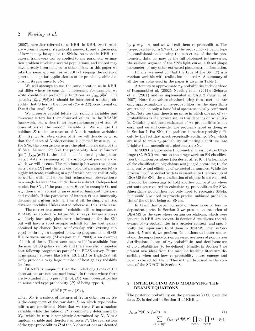
Figure 1. Two τA-probability distributions, both with means of0.5. Using a threshold of 0.6, we have on left: FPR = 0.17, FNR

= 0.45 and on right: FPR: 0.15, FNR = 0.28

functional form may be chosen for fDi|Θ,Pi,Tiwhen using

BEAMS for independent SNe.

3 RATING τA-probabilities

An object’s τA-probability is the expected proportion ofother objects with its features which are type A. In otherwords, if an object has features x, its τA-probability is theexpected proportion of objects with features x which aretype A. Suppose that the global distribution of P is fP . Theexpected total proportion of type A objects is then

P(T = A) = 〈P 〉 =

∫ 1

0

pfP (p) dp. (6)

In some circumstances, it is necessary to go beyond calcu-lating τA-probabilities and commit to an absolute classifi-cation, as was the case in the SNPCC. In such cases theoptimal strategy moving from a τA-probability to an abso-lute type (A or B) is to classify objects positively (A) whenthe τA-probability is above some threshold probability (c).The False Positive Rate (FPR) using such a strategy is

FPR(fP ) = P(P > c|T = B)

=

∫ 1

c(1− p)fP (p) dp∫ 1

0(1− p)fP (p) dp

, (7)

and the False Negative Rate is

FNR(fP ) = P(P < c|T = A)

=

∫ c0p fP (p) dp∫ 1

0p fP (p) dp

. (8)

For SNe the FPR is the proportion of nIa SNe whichare misclassified, while the FNR is the proportion of SNeIawhich are misclassified (missed).

Intuition dictates that for classification problems, a use-ful fP will be one whose mass predominates around 0 and1. That is, an fP which with high probability attachesdecisive2 τA-probabilities to observations. To minimize theFPR and FNR this is optimal, as illustrated in Figure 1.

We will be presenting a simulation illustrating how thedecisiveness of τA-probabilities affects the parameter estima-tion of BEAMS. To simplify our study of the effect of thedecisiveness of τA-probabilities on BEAMS, we introduce a

2 we say p1 is more decisive than p2 if |p1 − 0.5| > |p2 − 0.5|.

c© 2010 RAS, MNRAS 000, 1–19


family of distributions: For each P ∈ [0.5, 1] we have thedistribution

fP(p) =1

2(δP(p) + δ1−P(p)) (9)

where δP and δ1−P are δ-functions centered at P and 1−Prespectively. It is worth mentioning that we will be draw-ing probabilities from this distribution, which is potentiallyconfusing. Drawing a observation of P from (9) is equivalentto drawing it from 1− P,P with equal probability:

P(P = p) =

0.5 if p = P0.5 if p = 1− P.

If P1 is more decisive than P2, we say that the distri-bution fP1 is more decisive than fP2 .

On page 5 of KBH it is stated that the expected propor-tion of type A objects (6) determines the expected error inestimating a parameter which is independent of populationB. Specifically, they present the result that the expected er-ror when estimating a parameter µ with N objects usingBEAMS is given by,

σµ ∝√〈P 〉N. (10)

It should be noted that the the result from KBH (10)is an asymptotic result in N . For small N , the decisivenessof the probabilities plays an important part. If (6) were theonly factor determining the expected error (σµ), then f0.5

would be equivalent to f1 in terms of expected error. Thiswould mean that perfect type knowledge does not reduceerror, which would be surprising. An example in Section 4.1illustrates that decisiveness does play a role in determiningthe error.

As mentioned on page 8 of KBH, the effect of biasesin τA-probabilities on BEAMS can be catastrophic. Thereinthey consider the case where there is a uniform bias (a) of theτA-probabilities. That is, if observation i has a claimed τA-probability pi of being typeA, then there is a real probabilitypi − a that it is type A. KBH show how, by including a freeglobal shift parameter, such a bias is completely removed.However it is not clear what to do if the form of the biasis unknown. For example, it could be that there is an ‘over-confidence’ bias, where to obtain the true τA-probabilitiesone needs to transform the claimed priors (p) by

p = 0.2 + 0.6 p. (11)

Introducing a bias such as the one defined by (11) willhave no effect on the optimal FPR and FNR, providedthe probability threshold is chosen optimally. This is be-cause (11) is a one-to-one biasing, and so a threshold (c)on biased probabilities results in exactly the same parti-tioning as a threshold in the unbiased space of 0.2 + 0.6c.However, introducing a bias such as (11) does have an ef-fect on BEAMS parameter estimation, as we show in Sec-tion 5. In Section 7 we discuss how to guarantee that theτA-probabilities are free of bias.

4 EFFECTS OF DECISIVENESS ANDSAMPLE SIZE ON BEAMS

In this section we will perform simulations to better under-stand the key factors in BEAMS. The data generated will

50 100 150 200 250 300 350N

0.5

0.6

0.7

0.8

0.9

1.0

P

0

25

50

75

100

125

150

175

200

Figure 2. Contour plot of h(N,P). The solid lines are approxi-

mations to lines of constant h, of the form (13).

have the following cosmological analogy: Θ - distance mod-ulus at a given redshift z0; d - the fitted distance moduli ofSNe at z0. Furthermore, D|Θ,T and P will be independent,such that the KBH and full posterior are equivalent.

4.1 Simulation 1: Estimating a population mean

This simulation was performed to see how the performanceof BEAMS is affected by the decisiveness of τA-probabilities,and by the size of the data set. The two populations (A andB) were chosen to have distributions,

fD|T (d, τ) = Normal(µτ , 1), (12)

where µA = −1 and µB = +1, as illustrated in Figure 3.The τA-probability distribution is chosen to be fP , so thatabout half of the observations have a τA-probability of P,with the remaining observations having τA-probabilities of1− P. By varying P we vary the decisiveness.

Let us make it clear how the data for this simulationis generated. First, a τA-probability (p) is selected to beeither P with probability 0.5 or 1−P with probability 0.5,that is according to fP . Second, the type of the observationis chosen, with probability p it is chosen as A, and withprobability 1 − p it is chosen as B. Finally, the data (d) isdrawn from (12). Notice that D|T is independent of P , andso the KBH posterior is equivalent to the full posterior.

In this simulation we only estimate µA, with all otherparameters known. We use the following Figure of Merit tocompare the performance with different sample sizes (N)and decisivenesses (P):

h(N,P) =1

〈µA − µA〉2,

where µA is the maximum likelihood estimate of µAusing the KBH posterior on a sample of size N with τA-probabilities from fP , and 〈·〉 denotes an expectation. Valuesof h were obtained by simulation, illustrating in Figure 2 theperformance of BEAMS for various (N,P) combinations. Agood approximation to the FoM h in Figure 2 appears to be

h(N,P) ≈ N(

0.32 + 1.44(P − 1

2)3

), (13)

c© 2010 RAS, MNRAS 000, 1–19

6 Newling et al.

−3 −2 −1 0 1 2 3fD|T and observations d

0.0

0.1

0.2

0.3

0.4

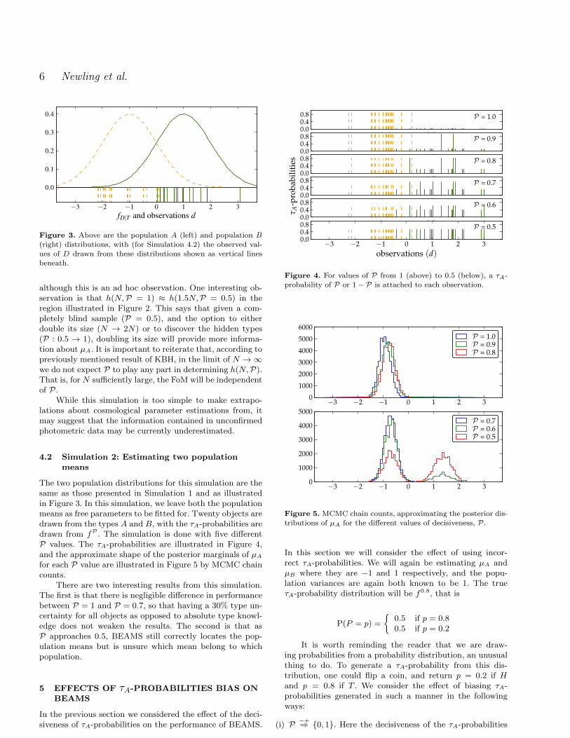
Figure 3. Above are the population A (left) and population B

(right) distributions, with (for Simulation 4.2) the observed val-ues of D drawn from these distributions shown as vertical lines

beneath.

although this is an ad hoc observation. One interesting ob-servation is that h(N,P = 1) ≈ h(1.5N,P = 0.5) in theregion illustrated in Figure 2. This says that given a com-pletely blind sample (P = 0.5), and the option to eitherdouble its size (N → 2N) or to discover the hidden types(P : 0.5 → 1), doubling its size will provide more informa-tion about µA. It is important to reiterate that, according topreviously mentioned result of KBH, in the limit of N →∞we do not expect P to play any part in determining h(N,P).That is, for N sufficiently large, the FoM will be independentof P.

While this simulation is too simple to make extrapo-lations about cosmological parameter estimations from, itmay suggest that the information contained in unconfirmedphotometric data may be currently underestimated.

4.2 Simulation 2: Estimating two populationmeans

The two population distributions for this simulation are thesame as those presented in Simulation 1 and as illustratedin Figure 3. In this simulation, we leave both the populationmeans as free parameters to be fitted for. Twenty objects aredrawn from the types A and B, with the τA-probabilities aredrawn from fP . The simulation is done with five differentP values. The τA-probabilities are illustrated in Figure 4,and the approximate shape of the posterior marginals of µAfor each P value are illustrated in Figure 5 by MCMC chaincounts.

There are two interesting results from this simulation.The first is that there is negligible difference in performancebetween P = 1 and P = 0.7, so that having a 30% type un-certainty for all objects as opposed to absolute type knowl-edge does not weaken the results. The second is that asP approaches 0.5, BEAMS still correctly locates the pop-ulation means but is unsure which mean belong to whichpopulation.

5 EFFECTS OF τA-PROBABILITIES BIAS ONBEAMS

In the previous section we considered the effect of the deci-siveness of τA-probabilities on the performance of BEAMS.

observations (d)0.00.40.8 P = 1.0



observations (d)0.00.40.8

τ A-p

roba

bilit

ies

P = 0.7


−3 −2 −1 0 1 2 3observations (d)

0.00.40.8 P = 0.5

Figure 4. For values of P from 1 (above) to 0.5 (below), a τA-

probability of P or 1− P is attached to each observation.

−3 −2 −1 0 1 2 30

1000

2000

3000

4000

5000

6000P = 1.0P = 0.9P = 0.8

−3 −2 −1 0 1 2 30

1000

2000

3000

4000

5000P = 0.7P = 0.6P = 0.5

Figure 5. MCMC chain counts, approximating the posterior dis-tributions of µA for the different values of decisiveness, P.

In this section we will consider the effect of using incor-rect τA-probabilities. We will again be estimating µA andµB where they are −1 and 1 respectively, and the popu-lation variances are again both known to be 1. The trueτA-probability distribution will be f0.8, that is

P(P = p) =

0.5 if p = 0.80.5 if p = 0.2

It is worth reminding the reader that we are draw-ing probabilities from a probability distribution, an unusualthing to do. To generate a τA-probability from this dis-tribution, one could flip a coin, and return p = 0.2 if Hand p = 0.8 if T . We consider the effect of biasing τA-probabilities generated in such a manner in the followingways:

(i) P −+⇒ 0, 1. Here the decisiveness of the τA-probabilities

c© 2010 RAS, MNRAS 000, 1–19


0.5 1.0 1.5 2.0µB

−1.6

−1.4

−1.2

−1.0

−0.8

−0.6

−0.4

µ A

P = 0.8

P −+⇒ 0,1P +−⇒ 0.4,0.6P −−⇒ 0,0.6P ++⇒ 0.4,1P σ⇒+U

Figure 6. The 99 % posterior confidence regions using the five

biasings of the τA-probabilities, as described in Section 5.

is overestimated, so that p = 0.8 → p = 1 and p = 0.2 →p = 0.

(ii) P +−⇒ 0.4, 0.6. Here the decisiveness of the τA-probabilities is underestimated, so that p = 0.8 → p = 0.6and p = 0.2→ p = 0.4.

(iii) P −−⇒ 0, 0.6. Here the τA-probabilities are underesti-mated by 0.2, so that p = 0.8→ p = 0.6 and p = 0.2→ p =0.

(iv) P ++⇒ 0.4, 1. Here the τA-probabilities are overestimatedby 0.2, so that p = 0.8→ p = 1 and p = 0.2→ p = 0.4.

(v) P σ⇒ U . Here, to each τA-probability a uniform randomnumber from [−0.2, 0.2] is independently added.

The 99% posterior confidence regions obtained usingthese biased τA-probabilities in a simulation of 400 pointsare illustrated in Figure (6). The underestimation of deci-siveness (ii) has little effect on the final confidence region,but overestimating the τA-probability decisiveness (i) resultsin a 6σ bias. Note that overestimating decisiveness results inthe estimate (µA, µB) being biased towards (µB , µA). Thisis caused by type B objects which are too confidently be-lieved to be type A, which pull µA towards µB , and typeA objects which are too confidently believed to be type B,which pull µB towards µA.

The contrast in effect between underestimating andoverestimating the decisiveness of τA-probabilities is inter-esting, and not easy to explain. One suggestion we havereceived is to consider the cause of the observed effect as be-ing analogous to the increased contamination rate inducedby overestimating the decisiveness in the case BEAMS isnot used. With an increased contamination rate comes anincreased bias, precisely as observed in Figure 6. It is worthmentioning that underestimating the decisiveness is not en-tirely without effect, as simulations with more pronounceddrops in P (0.95→ 0.55) result in noticable increases in thesize of the 99% confidence region.

The effect of the flat τA-probability shifts (iii) and (iv)introduce biases larger than 4σ. This case was consideredin KBH where, as we have already mentioned, it was shownthat simultaneously fitting for this bias completely compen-sates for it. While this is a pleasing result, one would preferto know that the τA-probabilities are correct, as one cannotbe sure what form the biasing will take.

One phenomenon which is observed in this simulation,as it was in simulations as summarised in Table II on page

8 of KBH, is that a flat τA-probability shift in confidencetowards being type B (iii) does not bias the estimate of µAas much as it does the estimate of µB , and vica versa. Inother words, underestimating the probabilities that objectsare type A will result in less biased population A parame-ters than overestimating the probabilities. This result mayalso be understood in light of an analogy to increased con-tamination versus reduced population size in the case whereBEAMS in not used.

Finally, we notice that in this simulation the addition ofunbiased noise to the τA-probabilities (v) has an insignificanteffect. This suggests that systematic biases should be theprimary concern of future work on the estimation of τA-probabilities.

6 WHEN GIVEN TYPE, THE DATA IS STILLDEPENDENT ON τ -PRIORS

In this section we consider for the first time a simulation inwhich the data is not drawn from fD|T , but from fD|T,P , sothat there is a dependence of the data on the τA-probabilityeven when the type is known. The conditional pdfs areshown in Figure 7. To clarify the difference between thissimulation and the previous ones, prior to this data wassimulated as follows:

P → T |P → D|T,

where at the last step, the data was generated with a de-pendence only on type. Now it will be simulated as:

P → T |P → D|P, T.

More specifically, to generate data we start by drawing aτA-probability from f0.7,

P(P = p) =

0.5 if p = 0.70.5 if p = 0.3.

Note that the above distribution guarantees that P(T =A) = 1

2. When the τA-probability (p) has been generated,

we draw a type (τ) from A,B according to

P(T = τ) =

p if τ = A1− p if τ = B.

Once we have p and τ , we generate d. The marginalsfD|P,T (d|p, τ) have been chosen such that we have

fD|T (d|A) = Normal (−1, 1) (14)

fD|T (d|B) = Normal (1, 1), (15)

as before. The marginal fD|P,T (d|0.7, A) is composed ofthe halves of two Gaussian curves with different σs, chosensuch that the tail away from the B population is longer thanthe one towards the B population. Specifically,

fD|P,T (d|0.7, A) =

=

K exp − 1

2(d+ 1)2 if d < −1

K exp − 10032

(d+ 1)2 if d > −1

where K is a normalizing constant. The marginalfD|P,T (d|0.3, A) is then constructed to guarantee (14). Theabove construction guarantees that the population of A ob-jects with low τA-probabilities (0.3) lie on average closer tothe B mean than do objects with high (0.7) τA-probabilities.

c© 2010 RAS, MNRAS 000, 1–19

8 Newling et al.

−4 −3 −2 −1 0 1 2 3 4d

0.00.10.20.30.40.50.60.70.8 type A

−4 −3 −2 −1 0 1 2 3 4d

0.00.10.20.30.40.50.60.70.8 type B

Figure 7. Plots of fD|P,T (d|p, τ) (filled curves) for p= 0.7 (light)and p = 0.3 (dark), and for type A (left) and type B (right).

Overlying are fD|T (d|A) (light) and fD|T (d|B) (dark).

The marginals of the B population are constructed to mirrorexactly the A population marginals, as illustrated in Fig-ure 7.

To compare the use of the KBH BEAMS posterior (2)with the full conditional posterior (5), we randomly draw 40data points from the above distribution and construct therespective posterior distributions, as illustrated in Figure 8.Observe that the KBH posterior is significantly wider thanthe full posterior. Indeed, approximately half of the interiorof the 80% region of the KBH posterior is ruled out to 1%by the full posterior. It is interesting to note that, whilethe KBH posterior is wider than the full posterior, it is notbiased. This result goes against our intuition; we believedthat the KBH posterior would result in estimates for µAand µB which exaggerated |µA−µB |. Whether it is a generalresult that no bias exists when the KBH posterior is used, orif there can exist dependencies between P and D for whichthe use of (1) leads to a bias, remains an open question.

Figure 8 illustrates one realistation from the distribu-tion we have described, but repeated realisations show thaton average, the variance in the maximum likelihood estima-tor using the KBH posterior is ∼ 3 times larger than thevariance using the modified posterior. While these simula-tions are too simple to draw conclusions about cosmologicalparameter estimation from, they do suggest that where cor-relations between τA-probabilities and distance moduli existwithin a class of SNe, it may be worthwhile accounting forit by using the modified posterior. Currently it is most com-mon when modelling SNe for cosmology, to assume that thelikelihood fD|Θ,T (d|θ, τ) is a Gaussian with unknown meanand variance,

D|θ, P, T = Normal(µ(θ, T ), σ(T )2).

If one wishes to include the τA-probabilities in the like-lihood, one could include a linear shift in P for the mean orvariance. That is,

D|θ, P, T = Normal(µ(θ, T ) + c1P, σ(T )2 + c2P ).

Of course this is just one possibility, and one would needto analyse SN data to get a better idea of how P should enterinto the above equation.

0.5 1.0 1.5 2.0µB

−1.5

−1.0

−0.5

0.0

µ A

originalmodified

Figure 8. Posterior distributions on the parameters (µA, µB)

using the correct posterior (4) (solid) and the KBH posterior (1)(dashed). The KBH posterior assumes independence betweenD|Tand P . Plotted are the 80%, 95% and 99% confidence levels. The

true parameters (orange point) lie within the 95 % confidenceregions of both posteriors.

7 OBTAINING UNBIASEDτA-PROBABILITIES

In this section we investigate likely sources of τA-probabilitybiases such as those presented in Section 5, and discuss howto detect and remove them. For SNe, one source of τA-probability bias could be the failure to take into accountthe preferential confirmation of bright objects. This type ofbias has been considered in the machine learning literatureunder the name of selection bias, and we here present therelevant ideas from there. We end the section with a briefdiscussion on how one could model the pdfs fD|Θ,P ,T andfD|Θ,F ,P ,T , which are the likelihoods appearing in the ex-tended posteriors introduced in Section 2.

7.1 Selection Bias

With respect to classification methods, selection bias refersto the situation where the confirmed data is a non-representative sample of the unconfirmed data. A selectionbias is sometimes also referred to as a covariate shift al-though the two are defined slightly differently, as describedin Bickel et al. (2007). With selection bias, the confirmeddata set is first randomly selected from the full set, andthen at a second stage it is non-randomly reduced. Suchis the situation with a population census, where at a firststage, a random sample of people is selected from the fullpopulation, and then at a second stage, people of a certaindisposition cooperate more readily than others, resulting ina biased sample of respondees.

A form of selection bias which is well known in observa-tional astronomy is the Malmquist bias, whereby magnitudelimited surveys lead to the preferential detection of intrinsi-cally bright (low apparent magnitude) objects. In the caseof SN cosmology, the bias is also towards the confirming ofbright SNe. A reason for this bias is that the telescope timerequired to accurately classify a SN is inversely proportionalto the SN’s brightness. It is therefore relatively cheap to con-firm bright objects and expensive to confirm faint ones.

If the SN confirmation bias is ignored, certain infer-ences made about the global population of SNe are likely to

c© 2010 RAS, MNRAS 000, 1–19


be inaccurate. In particular, estimates of a classifier’s FalsePositive and False Negative Rates will be biased, and theestimated τA-probabilities will be biased in certain circum-stances, as we will discuss in the following section.

7.1.1 Formalism

Following where possible the notation of Fan et al. (2005), inwhat follows we assume that variables (X, T , F ) are drawnfrom X × T × F , where

(i) X is the feature space,(ii) T = A,B is the binary type space,

(iii) F = 0, 1 is the binary confirmation space, where F = 1if confirmed (F for followed-up).

A realisation (x, τ , f) lies in either the test set or the trainingsets, defined respectively as:

test setdef= (x, τ, f) s.t. f = 0

training setdef= (x, τ, f) s.t. f = 1.

For SN cosmology it could be that X , T and F are respec-tively,

(i) X is the space of all possible photometric data, where aSN’s photometric data consists of apparent magnitudes andobservational standard deviations in four colour bands overseveral nights.

(ii) T = Ia, nIa, type Ia and non-Ia SNe.(iii) F = 0, 1, where F = 1 if the SN has been spectroscopi-

cally confirmed and thus has its type known.

By having a training set be unbiased we mean that it is arepresentative sample of the test set, specifically that F isindependent of both X and T . That is, the probability ofconfirmation is independent of features and type:

P(F = 1|X = x, T = τ) = P(F = 1). (16)

When the training set is unbiased, training set and testset objects are drawn from the same distribution over X×T .This distribution over X × T can be estimated from thetraining set, so directly providing an estimate of the moreuseful test set distribution.

There are three important ways in which the indepen-dence relation (16) can break down, resulting in a biasedtraining set, as described in Zadrozny (2004) and listed be-low. By removing bias from a training set, we mean reweight-ing the training points such that the training set becomesunbiased.

(i) Confirmation is independent of features only when condi-tioned on type: F |T and X are independent. This is thesimplest kind of biasing, and there are methods for correct-ing for it (Bishop 1996), (Elkan 2001). This is not the biaswhich exists in SN data.

(ii) Confirmation is independent of type only when given fea-tures: F |X and T are independent. If the decision to confirmis based on X and perhaps some other factors which are in-dependent of T , this is the bias which exists. This is probablythe bias which exists in SN data, and there are methods forcorrecting for it, as we will discuss.

(iii) Confirmation depends on both features and type simulta-neously. In this case, it is not possible to remove the biasfrom the data unless the exact form of the bias is known.

The decision to confirm a SN can be dictated by differentfeatures, examples include Sako et al. (2008); Sullivan et al.(2006), all of which are contained in the photometric data X.Such was the also case in the SNPCC where the probabilityof confirmation was based entirely on the peak magnitudein the r and i f, as we will discuss in Section 8. In reality,there are other factors which affect the confirmation decisionsuch as the weather and telescope availability, but these areindependent of SN type. Therefore the type (ii) bias above isthe bias which exists in the SN data. Thus, for the remainderof this section we’ll assume the type (ii) bias, that is

P(F = 1|X = x, T = τ) = P(F = 1|X = x). (17)

The assumption of the type (ii) bias can be made stronger.The decision to confirm an object does not in general dependon all of X but only a low-dimensional component (XF ) ofit, and so we have

P(F = 1|X = x, T = τ) = P(F = 1|XF = xF ), (18)

where XF is contained in X. For SNe, XF could be the peakapparent magnitude in certain colour bands.

In the following subsection we will describe how to cor-rectly obtain τA-probabilities under the assumption of a biasdescribed by (18).

7.2 Correctly obtaining τA-probabilities

Let us remind the reader as to how we defined τA-probabilities in the introduction:

τA-probabilitydef= P(Ti = A|XP,i = xP,i) = pi, (19)

where XP,i is an observable feature of the ith object,extracted from Xi. Estimates of pi values can be obtainedusing several methods, of which those mentioned previouslyare Poznanski et al. (2002); Newling et al. (2011); Richardset al. (2011); Guy et al. (2007) It is worth rementioningthat these different methods attempt to estimate differentprobability functions, as they each condition on differentSN features. Thus there is no sense in which one set of τA-probabilities estimates is the correct set.

We now make an adjustment to definition (19), to takeinto account that biased follow-up may result in an addi-tional conditional dependence on F :

τA-probabilitydef= P(Ti = A|Fi = fi, XP,i = xP,i) = Pi.

(20)The most informative τA-probabilities one could use

would be those conditional on all of the features at one’sdisposal,

XP = X : pi = P(T = A|F = 0, X = x). (21)

However, when X is a high-dimensional non-homogeneous space, as is the case with photometricSN data, it can be difficult to approximate (21) accurately.It is for this reason that it is necessary to reduce thefeatures to a lower dimensional quantity XP ∈ XP , sothat the τA-probabilities are calculated from a subspace(XP ) of the full feature space, as described by (20). Thesubspace XP should be chosen to retain as much typespecific information as possible while being of a sufficiently

c© 2010 RAS, MNRAS 000, 1–19

10 Newling et al.

low dimension. In the SNPCC Newling et al. (2011) choseXP to be a 20-dimensional space of parameters obtained byfitting lightcurves.

The job of obtaining estimated τA-probabilities for testset objects (F = 0) is one of obtaining an estimate of thetype probability mass function,

fT |F,XP. (22)

Again, for (22) we prefer not to use the standard mass func-tion notation, in order to to neaten certain integrals whichfollow. The τA-probability of a test set object can now beexpressed in the following way,

P(T = A|F = 0, XP = xP ) = fT |F,XP(A|0, xP ).

Using kernel density estimation, boosting, or any othermethod of approximating a probability function, one canconstruct an approximation (f) of the type probability func-tion for training set objects,

f(xP ) ≈ fT |F,XP(A|1, xP ). (23)

Using the estimate f in (23) one can estimate the τA-probabilities for the training set objects:

P(T = A|F = 1, XP = xP ) ≈ f(xP ). (24)

The estimate (24) is not directly important as the train-ing set object types are known exactly. But it is only throughthe training set objects that we can learn anything about thetypes of the test set objects.

How f from the training set is related to fT |F=0,XP(22)

depends on the relationship between XF (the data which de-termines confirmation probability) and XP (the data used tocalculate τA-probabilities). There are two cases to consider.The first, which we write as XF ⊂ XP , is when the datawhich determines confirmation probabilities is completelycontained in the data used to calculate τA-probabilities.That is,

XF ⊂ XPdef↔ P(F = 1|XP = xP ) = P(F = 1|XF = xF ).

The second case, when XF 6⊂ XP is when not all confir-mation information is contained in XP ,

XF 6⊂ XPdef↔ P(F = 1|XP = xP ) 6= P(F = 1|XF = xF ).

In the case of XF ⊂ XP , it can be shown that,

P(F = 1|T = τ,XP = xP ) = P(F = 1|XF = xF ). (25)

7.2.1 XF ⊂ XP

We will show that in the case of XF ⊂ XP , a type probabilityfunction approximating the training population (f) is anunbiased approximation for the type probability function ofthe test population (F = 0). To show this we start with thetype probability of a test object:

P(T = τ |F = 0, XP = xP ).

→ Using Bayes’ Theorem, we have

=P(F = 0|T = τ,XP = xP ) · P(T = τ |XP = xP )

P(F = 0|XP = xP )

→Then using (25), we have

=P(F = 0|XF = xF ) · P(T = τ |XP = xP )

P(F = 0|XF = xF )

= P(T = τ |XP = xP ). (26)

→ Using the same steps as above but in reverse and withF = 1, we arrive at

= P(T = τ |F = 1, XP = xP ).

→ This is the type probability function for training set ob-jects, and it can be approximated:

≈ f(xP ). (27)

This is a useful result, as it says that f is not onlyan approximation of the type probability function of thetraining data, but also of the test set. Thus, f should provideunbiased τA-probabilities for the test set when XF ⊂ XP .

It should be noted that for f to be a good approximationfor the test set, it is necessary that the training set covers allregions of XP where there are test points. That is, if thereare values of xP for which P(XP = xP |F = 1) = 0 andP(XP = xP |F = 0) 6= 0, then the approximation f will notconverge to fT |F=0,XP

as the training set size grows. Onecan refer to Fan et al. (2005) for a full treatment of thistopic.

With respect to SNe, the requirement of the precedingparagraph is that, if a SN is too faint to be confirmed and toenter the training set, it should not enter the test set either.We will return to this point again in Section 8.

One important question which we do not attempt toanswer here is, how many SNe of different apparent mag-nitudes should be confirmed to obtain as rapid as possibleconvergence of f to fT |F=0,XP

. An interesting method fordeciding which SNe to confirm may be one based on thereal-time approach proposed in Freund et al. (1997), wherethe decision to add an object to the training set is based onthe uncertainty of its type using the currently fitted f . InSection 8 we discuss this further.

7.2.2 XF 6⊂ XP

If XF 6⊂ XP we will not be able to use f to estimate the τA-probabilities in the test set, as (27) required XF ⊂ XP . Inaddition to this problem of not being able to use f to obtainunbiased τA-probabilities for the test set objects, if XF 6⊂ XPthen

P(T = τ |XP = xP ) 6= P(T |XP = xP , XF = xF ).

This tells us that there is additional type information to beobtained from XF , and so by not including XF one is wast-ing type information. For this reason we recommend recon-structing the τA-probabilities based on redefined features,XP ← (XF , XP ).

However, it is possible that one explicitly does not wantto use XF in calculating τA-probabilities. This may be thecase if one wishes to reduce the dependence between D andP , as presented in Section 2. For SNe, this may involve ob-taining τA-probabilities from shape alone, independent ofmagnitude, so that XP is a space whose dimensions describeonly shape and not magnitude. In this case, as we cannot

c© 2010 RAS, MNRAS 000, 1–19


use f , we need to use the relationship derived in Shimodaira(2000),

P(T = τ |F = 0, XP )

=

∫XF

fT,XF |F,XP(τ, xF |1, xP ) · w(xF , xP ) dxF , (28)

where the weight function is defined as

w(xF , xP ) =fF |XF

(0|xF )fF |XP(1|xP )

fF |XF(1|xF )fF |XP

(0|xP ). (29)

Notice that if XF ⊂ XP , then w(xF , xP ) = 1 and so (28)reduces to the type probability function for training setobjects, approximated by f as expected from (27). Whenw(xF , xP ) 6= 1, the training set type probability functionf cannot be used directly as an approximation to the testset type probability function. However, if each training setobject is weighted using (28), then an unbiased test set typeprobability function approximation can be obtained.

The weight function (29) does not require any type in-formation and so can be estimated as a first step. This ad-ditional step of estimation introduces additional error intothe final estimate of (22), a theoretical analysis of which ispresented in Cortes et al. (2008). An alternative to the two-stage approach would be to fit the two terms in (28) simulta-neously, as suggested and described by (Bickel et al. 2007).The use of (29) was first suggested in Shimodaira (2000),where a detailed analysis of the asymptotic behaviour of itsapproximation is given. Therein, it is suggested that (29) beapproximated by kernel density estimation.

In the case where F andXP are independent, the weightfunction reduces to one of only XF ,

w(XF = xF ) =P(F = 0|XF = xF )P(F = 1)

P(F = 1|XF = xF )P(F = 0). (30)

This reduction in dimension may be valuable in approx-imating the weight function.

7.3 Detecting and removing biases inτA-probabilities

In the previous section we presented the correct way in whichto estimate τA-probabilities in the case XF 6⊂ XP . In thissection we will present an example illustrating this process,but in the context of bias removal.

Suppose that we have a program which outputs scalarvalues (p), which are purported τA-probabilities. We believethat the output values have some unspecified bias, whichwe wish to remove. An assumption we make is that the pvalues are calculated in the same way for training and testsets. That is that the program does not process cases F = 0and F = 1 differently. It may seem strange to be interestedin what the program does when F = 1, but as already men-tioned it is only from the training set that we can learnanything about the test set. The idea now is to treat thereceived p values as the xP s from the previous section, andnot directly as τA-probabilities.

For this example, we choose XF = [0, 1]. To nowtransform a test set value p ∈ [0, 1] into an unbi-ased τA-probability using (28), one needs to estimate cer-tain probability functions using kernel density estima-

0.0 0.2 0.4 0.6 0.8 1.0XF

0.0

0.2

0.4

0.6

0.8

1.0

X P

0.0 0.2 0.4 0.6 0.8 1.0XF

Figure 9. Realisations of a training set (left) containing type

A (red pluses) and type B (blue points) objects, and a test set(right), drawn according to (31). Overlaid are faint lines delineat-

ing the discrete regions described by (31)

tion. The necessary functions we see from (28) and(29) are fT,XF |F,XP

(τ, xF |1, p), fF |XF(1, xF ), fF |XP

(0, p),fF |XF

(0, xF ) and fF |XP(0, xP ).

It is an interesting and important question as to howaccurately these probability functions can be approximatedwith few data points, but for this example we assume themknown,

fT,XF |F,XP(A, xF |1, p) =

xF if 1

2x2F < p < 1− 1

2x2F ,

2 · xF if p > 1− 12x2F

0 if p < 12x2F .

fF |XF(0, xF ) = (1− xF ),

fF |XF(1, xF ) = xF , (31)

fF |XP(1|p) = fF |XP

(0|p) =1

2.

Realisations from the above distribution are illustratedin Figure 9. By integrating xF out of fT,XF |F,XP

(A, xF |1, p)in (31), we have that

P(T = A|F = 1, XP = p) = p. (32)

That is, in the training set p is an unbiased estimate of aτA-probability. The τA-probabilities for objects in the testset we estimate using (28),

P(T = A|F = 0, XP = p)

=

∫XF

fT,XF |F,XP(τ, xF |0, xP ) dxF

=

∫XF

fT,XF |F,XP(τ, xF |1, xP )w(xF , p) dxF

=

∫XF

fT,XF |F,XP(τ, xF |1, xP )

1− xFxF

dxF

=

√2 p− p if p < 0.5,

2− p−√

2− 2p if 0.5 < p.(33)

The τA-probabilities (32) and (33) are plotted inFigure 10, where we see that p provided accurate τA-probabilities for the training set, but not for the test set.This is not unexpected in reality, where the program pro-viding the τA-probabilities may have been trained only onthe biased training data. It is important to remember thatthis bias should only arise when XF 6⊂ XP .

c© 2010 RAS, MNRAS 000, 1–19

12 Newling et al.

0.0 0.2 0.4 0.6 0.8 1.0P

0.0

0.2

0.4

0.6

0.8

1.0

P(A|P,F

)

F = 0F = 1

Figure 10. Corrected τA-probabilities. The disproportionatelylarge number of training SNe with decisive τA-probabilities (as

depicted in Figure 9), causes p values to be too confident as test

set τA-probability estimates.

8 SUPERNOVA SURVEYS AND THE SNPCC

The SNPCC provided a simulated spectroscopic trainingdata set of approximately 1000 known SNe. The challengewas then to predict the types of approximately 20 000 otherobjects3 from their lightcurves alone. Since the end of thecompetition, the types of all the simulated SNe have beenreleased, making a post competition autopsy relatively easyto perform. In the results paper Kessler et al. (2010) we seethat the probability that a SN was confirmed was based onthe r-band and i-band quantities,

εbandspec = ε0

(1− xl

)x

def=

mbandpeak −Mband

min

mbandlim −Mband

min

.

where mbandpeak is the band-specific apparent magnitude of

a SN, and Mbandmin and mband

min are constants. In Kessler et al.(2010) it is given that for col = r and col = i,

εrspec = ε0(1− x5) x

def=

mrpeak − 16.0

5.5(34)

εispec = ε0(1− x6) x

def=

mipeak − 21.5

2.0

where ε0 is some constant. Once εispec and εrspec have beencalculated, if a [0→ 1] uniform random number is less thaneither of them, confirmation is performed. As confirmationdepends only on εispec and εrspec, we have from (26) that

P(T = τ |F = 0,mipeak,m

rpeak) = P(T = τ |F = 1,mi

peak,mrpeak).

(35)Equation (35) can be interpreted as saying that the ratioIa:nIa is the same in a given mi

peak,mrpeak bin. The man-

ner in which the follow-up was simulated should of courseguarantee that (35) holds. In theory one should be able todeduce the verity of (35) from Figure 11, but the redshiftbins with large numbers of confirmed SNe are too sparselypopulated by unconfirmed SNe to check that the Ia:nIa isinvariant. To be in a position where (35) can be checked isin general an unrealistic luxury, as without the types of thetest objects this is impossible.

In terms of obtaining accurate τA-probabilities, a dis-turbing feature of Figure 11 is the absence of training SNewith high apparent magnitudes. With no training SNe with

3 These lightcurves are available at http://sdssdp62.fnal.gov/

sdsssn/SIMGEN PUBLIC/

20 21 22 23 24 25 26 27 28mr

peak

020406080

100120140

IanIa

20 21 22 23 24 25 26 27 28mr

peak

0500

100015002000250030003500

IanIa

20 21 22 23 24 25 26 27 28mi

peak

020406080

100120140

IanIa

20 21 22 23 24 25 26 27 28mi

peak

0500

1000150020002500300035004000

IanIa

Figure 11. Counts of confirmed (left) and not confirmed (right)

SNe, Ia (dashed) and non-Ia (solid) as a function of mrpeak (above)

and mipeak (below).

i-band apparent magnitudes greater than 23.5, we cannot in-fer the types of test SNe with apparent magnitudes greaterthan 23.5. Indeed there would be no non-astrophysical rea-son not to believe that all SNe with apparent magnitudesgreater than 23.5 are non-Ia. As already mentioned in Sec-tion 7.1, in situations where the training set does not spanthe test set, one should ignore unrepresented test objectsfrom all analyses. All test SNe other than those for whichthere are training SNe of comparable peak apparent magni-tudes in r and i bands should be removed from a BEAMSanalysis, unless there is a valid astrophysical reason not todo so. This entails ignoring about 95% of unconfirmed SNe;an enormous cut. We therefore consider it important to con-firm more faint SNe.

In Newling et al. (2011), a comparison is made betweentraining a boosting algorithm on the non-representativespectroscopically confirmed SNe and a representative sam-ple, randomly selected from the unconfirmed SN set.Therein, the authors use twenty fitted lightcurve parame-ters, including fitted apparent magnitudes in r and i bands.This corresponds to the situation discussed in Section 7.2.1,where XP ⊂ XF . For this reason, the probability densityfunction f in 24 as estimated by their boosting algorithmshould be an unbiased estimate for fT |F=0,XP

. But beingunbiased does not guarantee low error, and when trained onthe confirmed SNe, regions of parameter space correspond-ing to high apparent magnitude had no training SNe withwhich to learn, and so the approximation of 22 was poor.However when trained on the representative set, every re-gion of populated parameter space was represented by thetraining set, and the approximation of 22 was greatly im-proved.

In their paper, Richards et al. (2011) describe their en-try in the SNPCC, and they report how a semi-supervisedlearning algorithm performs better with a few faint trainingSNe than with many bright ones. The comparison was per-

c© 2010 RAS, MNRAS 000, 1–19


formed while keeping the total confirmation time constant.Thus their conclusion was the same as ours; that it is im-portant to obtain a more representative SN training sample.

9 CONCLUSIONS ANDRECOMMENDATIONS

In this paper we discussed BEAMS, and extended the KBHposterior probability function to the case when D|T (dis-tance modulus | type) and P (type probability) are depen-dent. In Section 6 we considered an example where the de-pendence between D|T and P is strong, and observed a largereduction in the posterior width using the extended poste-rior as opposed to the KBH posterior. No bias is observedwhen using either the extended or the KBH posterior.

In Section 4 we considered examples where the KBHposterior is valid, that is when D|T and P are independent.We performed tests to ascertain the importance to BEAMSof i) the decisiveness of the τA-probabilities (observationsof P ), and ii) sample size. In one test (4.1), we observedhow doubling a sample size reduces error in parameter es-timation more than obtaining the true type identity of theobjects does. In another test (4.2), we observed how BEAMSaccurately locates two population means, but fails to matcheach mean to its population.

We looked at the effects of using biased τA-probabilitiesin Section (5). The result of KBH, that τA-probability bi-ases towards population A affect the population’s parame-ter estimates less than biases in favour of population B, wasobserved. A similar result which is uncovered is that biasestowards high decisiveness are more damaging than biasestowards low decisiveness. In other words, it is better to beconservative in your prior type beliefs than too confident.

Our recommendations for BEAMS may thus be sum-marised as follows. Firstly, the inclusion in the likeli-hood function of τA-probabilitiescan dramatically reduce thewidth of the final posterior, providing tighter constraintson cosmological parameters. Secondly, conservative estima-tion of τA-probabilities is less harmful than too decisive anestimation. Thirdly, it is possible to remove biases in τA-probabilities using the techniques described in Section (7).

In Section 7 we considered the problem of debiasingτA-probabilities. Interpreting recent results from the ma-chine learning literature in terms of SN cosmology, we dis-cussed the different ways in which training sets can be bi-ased and how to remove such biases. The key to under-standing and correcting biases is the relationship betweenXF and XP , where XF are object features which determineconfirmation probability, and XP are those features whichdetermine τA-probabilities. In brief, when XP contains XF ,τA-probabilities should be unbiased, but if this is not thecase, there are sometimes ways for correcting the bias.

With respect to future SN surveys, we emphasize theimportance of an accurate record as to what information isused when deciding whether or not a SN is confirmed. Us-ing this information, one should in theory be able to removeall the affects of selection bias when XF 6⊂ XP . In otherwords, using all the variables which are considered in de-ciding whether to follow-up a SN, it will always be possibleto obtain unbiased τA-probabilities, irrespective of what theτA-probabilities are based on. Such follow-up variables may

include early segments of light curves, χ2 goodness of fits, fitprobabilities, host galaxy position and type, expected peakapparent magnitude in certain filters, etc.

Our second recommendation for SN surveys is thatmore faint objects are confirmed. While it not necessary formost machine learning algorithms to have a spectroscopictraining set which is exactly representative of the photo-metric test set, it is necessary that the spectroscopic set atleast covers the photometric set. Thus having large numbersof faint unconfirmed objects without any confirmed faint ob-jects is suboptimal.

10 ACKNOWLEDGEMENTS

JN has a SKA bursary and MS is funded by a SKA fellow-ship. BB acknowledges funding from the NRF and RoyalSociety. MK acknowledges financial support by the SwissNSF. RH acknowledges funding from the Rhodes Trust.

APPENDIX A: POSTERIOR TYPEPROBABILITIES

We here derive the posterior type probabilities based on themodifications of Section 2. The posterior type probabilitywill be derived, conditional onD and P . This derivation canbe easily extended to posterior type probabilities conditionalon D,F and P .

fTi|D,P (A|d,p)

=

∫θ

fTi|Θ,D,P (A|θ,d,p)fΘ|D,P (θ|d,p) dθ

=

∫θ

fTi|Θ,Di,Pi(A|θ, di, pi)fΘ|D,P (θ|d,p) dθ

→ we have assumed that the objects are independent,

=

∫θ

fDi|Θ,Pi,Ti(di|θ, pi, A)fTi|Θ,Pi

(A|θ, pi)fDi|Θ,Pi

(di|θ, pi)×

× fΘ|D,P (θ|d,p) dθ

→ we have used Bayes’ Theorem,

=

∫θ

(Ai

Ai +Bi

)fΘ|D,P (θ|d,p) dθ. (A1)

→ where Ai = P(di|θ, pi, Ti = A)pi, Bi = P(di|θ, pi,Ti = B)(1 − pi), and we have assumed used thatfTi|Θ,Pi

(A|θ, pi) = pi.

If the posterior fΘ|D,P confines θ to a region sufficientlysmall such that Ai and Bi are approximately constant, thenthe posterior type probability (A1) is well approximated by

Ai(θ)/(Ai(θ) +Bi(θ)

)where θ is the maximum likelihood

estimator of fΘ|D,P (θ|d,p). Furthermore, the posterior oddsratio,

posterior odds ratiodef=

fTi|D,P (A|d,p)

fTi|D,P (B|d,p)

c© 2010 RAS, MNRAS 000, 1–19

14 Newling et al.

can be shown to be given by the prior odds ratio multipliedby the Bayes Factor,

posterior odds ratio =

(pi

1− pi

)×

(fDi|Θ,Pi,Ti

(di|θ, pi, A)

fDi|Θ,Pi,Ti(di|θ, pi, B)

).

APPENDIX B: ADDITIONAL CONDITIONINGON THE CONFIRMATION OF SUPERNOVATYPE

In this paper we did not distinguished between the contri-butions of unconfirmed and confirmed objects to the pos-terior. While we can calculate approximate τA-probabilitiesfor confirmed objects, these values should not enter the pos-terior, but be replaced by 0 (if type B) or 1 (if type A). Letus introduce the random variable F to denote whether anobject is confirmed, so that F = 1 if confirmed and F = 0 ifunconfirmed. With this introduced, we wish to replace theτA-probabilities p by p, where,

pi =

pi if fi = 0,1 if fi = 1 and τi = A,0 if fi = 1 and τi = B.

We must be careful to let the new information which weintroduce in p be absorbed elsewhere in the posterior. Tothis end, as we did in Section ?? we start afresh the pos-terior derivation, explicitly including the vector (f) whichdescribes which objects have been followed-up. Doing this,we arrive at the following posterior distribution

fΘ|D,F ,P (θ|d,f ,p) ∝ fΘ(θ) × (B1)∑τ

fD|Θ,F ,P ,T (d|θ,f ,p, τ )∏τi=A

pi∏τj=B

(1− pj).

The new information (f) has been absorbed into thelikelihood, fD|···. For a particular application, one may nowask if the addition of F in fD|··· is necessary. We have al-ready mentioned that for SNe D|θ,T is unlikely to be inde-pendent of P . It is also unlikely that D|θ,T is independentof F , as bright SNe, which have lower fitted distance moduliat a given redshift, are confirmed more regularly than faintones. However, it is possible that by additionally condition-ing D on P this confirmation dependence is broken, so thatD|θ,P ,T and F are independent. We leave this as an openquestion.

In the case of independent SNe, the posterior (B1) re-duces to

fΘ|D,F ,P (θ|d,f ,p) ∝N∏i=1

[fDi|Θ,Fi,Pi,Ti

(di|θ, fi, pi, A)pi +

fDi|Θ,Fi,Pi,Ti(di|θ, fi, pi, B) (1− pi)

].(B2)

REFERENCES

Abazajian K. N., Adelman-McCarthy J. K., Agueros M. A.,Allam S. S., Allende Prieto C., An D., Anderson K. S. J.,Anderson S. F., Annis J., Bahcall N. A., et al. 2009, ApJS,182, 543

Bickel S., Bruckner M., Scheffer T., 2007, in ICML ’07: Pro-ceedings of the 24th international conference on Machinelearning Discriminative learning for differing training andtest distributions. ACM, New York, NY, USA, pp 81–88

Bishop C. M., 1996, Neural Networks for Pattern Recogni-tion, 1st edn. Oxford University Press, USA

Cortes C., Mohri M., Riley M., Rostamizadeh A., 2008,CoRR, abs/0805.2775

Eisenstein D. J., et al., 2005, ApJ, 633, 560Elkan C., 2001, in Proceedings of the Seventeenth Inter-national Joint Conference on Artificial Intelligence Thefoundations of cost-sensitive learning. pp 973–978

Fan W., Davidson I., Zadrozny B., Yu P. S., 2005, in Pro-ceedings of the Fifth IEEE International Conference onData Mining, An improved categorization of classifierssensitivity on sample selection bias

Freund Y., Seung H. S., Shamir E., Tishby N., 1997, inMachine Learning Selective sampling using the Query byCommittee algorithm. pp 133–168

Fu L., et al., 2008, a, 479, 9Giannantonio T., Scranton R., Crittenden R. G., NicholR. C., Boughn S. P., Myers A. D., Richards G. T., 2008,Phys. Rev. D, 77, 123520

Guy J., Astier P., Baumont S., Hardin D., 2007, A&A, 466,11

Johnson B. D., Crotts A. P. S., 2006, AJ, 132, 756Kessler R., Conley A., Jha S., Kuhlmann S., 2010,arXiv:1001.5210

Kessler R., et al., 2010, PASP, 122, 1415Komatsu E., et al., 2011, ApJS, 192, 18Kunz M., Bassett B. A., Hlozek R. A., 2007, Phys. Rev. D,75, 103508

Kuznetsova N. V., Connolly B. M., 2007, ApJ, 659, 530Mantz A., Allen S. W., Rapetti D., Ebeling H., 2010, MN-RAS, 406, 1759

Newling J., Varughese M., Bassett B., Campbell H., HlozekR., Kunz M., Lampeitl H., Martin B., Nichol R., Parkin-son D., Smith M., 2011, MNRAS, 414, 1987

Percival W. J., Cole S., Eisenstein D. J., Nichol R. C.,Peacock J. A., Pope A. C., Szalay A. S., 2007, MNRAS,381, 1053

Percival W. J., et al., 2010, MNRAS, 401, 2148Perlmutter S., et al., 1999, ApJ, 517, 565Poznanski D., Gal-Yam A., Maoz D., Filippenko A. V.,Leonard D. C., Matheson T., 2002, PASP, 114, 833

Poznanski D., Maoz D., Gal-Yam A., 2007, AJ, 134, 1285Richards J. W., Homrighausen D., Freeman P. E., SchaferC. M., Poznanski D., 2011, ArXiv 1103.6034

Riess A. G., et al., 1998, AJ, 116, 1009Rodney S. A., Tonry J. L., 2009, ApJ, 707, 1064Sako M., Bassett B., Connolly B., Dilday B., Campbell H.,Frieman J., Gladney L., Kessler R., Lampeitl H., Mar-riner J., Miquel R., Nichol R., Schneider D., Smith M.,Sollerman J., 2011, ArXiv e-prints

Sako M., et al., 2008, AJ, 135, 348Shimodaira H., 2000, Journal of Statistical Planning andInference, 90, 227

Sullivan M., et al., 2006, AJ, 131, 960Zadrozny B., 2004, in Proceedings of the twenty-first inter-national conference on Machine learning ICML ’04, Learn-ing and evaluating classifiers under sample selection bias.ACM, New York, NY, USA, pp 114–

c© 2010 RAS, MNRAS 000, 1–19

Parameter Estimation with BEAMS in the presence of biases and correlations

Documents

Transcript of Parameter Estimation with BEAMS in the presence of biases and correlations