
Paper One Computer Science Notes - Ashwin Ahuja
154
2017 Paper One Computer Science Notes UNIVERSITY OF CAMBRIDGE, PART IA ASHWIN AHUJA
-
Upload
khangminh22 -
Category
Documents
-
view
3 -
download
0
Transcript of Paper One Computer Science Notes - Ashwin Ahuja

2017
Paper One Computer Science Notes UNIVERSITY OF CAMBRIDGE, PART IA ASHWIN AHUJA
Ashwin Ahuja – Part IA Paper One Notes
2
Table of Contents
Foundations of Computer Science ........................................................................................8 Introduction to Programming ....................................................................................................... 8
Abstraction and Abstraction Barrier: ......................................................................................... 8 Date .......................................................................................................................................... 8 Representational Abstraction and Datatypes ............................................................................ 8 Goal of Programming ................................................................................................................ 9 Why ML .................................................................................................................................... 9 ML Items................................................................................................................................... 9
Recursion and Efficiency ............................................................................................................. 10 Iterative Methods ................................................................................................................... 10 Recursion vs Iteration ............................................................................................................. 10 Time Complexities .................................................................................................................. 10
Lists ............................................................................................................................................ 11 Calculating Length .................................................................................................................. 11 List Concatenation (and reversal) ............................................................................................ 11 Take and Drop ........................................................................................................................ 12 Linear Search .......................................................................................................................... 12 Polymorphism......................................................................................................................... 12 Equality Types ......................................................................................................................... 12 Zip and Unzip .......................................................................................................................... 13 Making Change ....................................................................................................................... 13
Strings and Characters ................................................................................................................ 13 Sorting ........................................................................................................................................ 13
Why sort? ............................................................................................................................... 13 Random Number Generator ................................................................................................... 14 Optimal Speed of Sorting ........................................................................................................ 14 Insertion Sort .......................................................................................................................... 14 Quicksort ................................................................................................................................ 14 Merging and Merge Sort ......................................................................................................... 15 Radix Sort ............................................................................................................................... 16
Datatypes and Trees ................................................................................................................... 16 Declaring Datatypes ................................................................................................................ 16 Exceptions .............................................................................................................................. 17 Binary Trees ............................................................................................................................ 18
Dictionaries and Functional Arrays ............................................................................................. 18 Dictionary Idea ....................................................................................................................... 18 Binary Search Trees ................................................................................................................ 18 Traversing Trees ..................................................................................................................... 19 Functional Arrays .................................................................................................................... 20
Functions .................................................................................................................................... 21 Currying .................................................................................................................................. 21 Map ........................................................................................................................................ 22 Predicate Functionals .............................................................................................................. 22
Lazy Lists..................................................................................................................................... 22 Pipeline................................................................................................................................... 22 Definition ................................................................................................................................ 23 Implementation ...................................................................................................................... 23 Convert to List ........................................................................................................................ 23 Joining .................................................................................................................................... 24
Ashwin Ahuja – Part IA Paper One Notes
3
Functionals ............................................................................................................................. 24 Numerical Computations ........................................................................................................ 24
Queues and Search Strategies .................................................................................................... 24 Breadth-First vs Depth-First Tree Traversal ............................................................................. 24 Breadth-First Traversal ............................................................................................................ 25 Iterative Deepening ................................................................................................................ 26 Depth-First Search .................................................................................................................. 27 Search Methods Conclusion .................................................................................................... 27
Polynomial Arithmetic ................................................................................................................ 27 Data Structure for Polynomials ............................................................................................... 27 Polynomial Operations ............................................................................................................ 28 Addition .................................................................................................................................. 28 Multiplication ......................................................................................................................... 28 Division ................................................................................................................................... 29 GCD ........................................................................................................................................ 29
Procedural Programming............................................................................................................ 29 Definition ................................................................................................................................ 29 References .............................................................................................................................. 29 Commands ............................................................................................................................. 30 Iteration ................................................................................................................................. 30 Arrays ..................................................................................................................................... 31 Other things in ML .................................................................................................................. 31
Object-Oriented Programming............................................................................................32 Types, Objects & Classes ............................................................................................................ 32
Declarative vs Imperative ........................................................................................................ 32 Control Flow ........................................................................................................................... 32 Procedures, Functions & Methods .......................................................................................... 33 Function Prototypes ............................................................................................................... 33 Mutability ............................................................................................................................... 33 Explicit Types & Type Inference............................................................................................... 33 Java Primitives ........................................................................................................................ 34 Polymorphism and Overloading .............................................................................................. 34 Classes and Objects................................................................................................................. 34
Designing Classes ....................................................................................................................... 35 Identifying Classes .................................................................................................................. 35 UML ........................................................................................................................................ 36 OOP Concepts ......................................................................................................................... 37 Immutability ........................................................................................................................... 38 Parametrization ...................................................................................................................... 38
Pointers, References and Memory ............................................................................................. 39 Pointers and References ......................................................................................................... 39 Call Stack ................................................................................................................................ 40 Heap ....................................................................................................................................... 41 Pass-by-value vs Pass-by-reference ......................................................................................... 41
Inheritance ................................................................................................................................. 41 Casting .................................................................................................................................... 42 Shadowing .............................................................................................................................. 42 Overriding............................................................................................................................... 42 Abstract Methods and Classes ................................................................................................ 42
Polymorphism ............................................................................................................................ 43 Static Polymorphism ............................................................................................................... 43

Ashwin Ahuja – Part IA Paper One Notes
4
Dynamic Polymorphism .......................................................................................................... 43 Implementations of Polymorphism ......................................................................................... 43 Multiple Inheritance and Interfaces ........................................................................................ 43
Object Lifecycle .......................................................................................................................... 44 Process of creating an object .................................................................................................. 44 Destruction ............................................................................................................................. 45
Java Collections .......................................................................................................................... 46 Collections and Generics ......................................................................................................... 46
Object Comparisons ................................................................................................................... 48 Imposing ordering on data collections: ................................................................................... 48 Object Equality ....................................................................................................................... 48 Comparator and Comparable .................................................................................................. 48
Error Handling ............................................................................................................................ 49 Types of errors ........................................................................................................................ 49 Minimising bugs ...................................................................................................................... 49 Dealing with errors ................................................................................................................. 50 Things to never do .................................................................................................................. 52
Copying Objects.......................................................................................................................... 52 Shallow Copy vs Deep Copy .................................................................................................... 52 Cloning ................................................................................................................................... 53 Copy Constructors .................................................................................................................. 54
Language Evolution .................................................................................................................... 54 Generics ................................................................................................................................. 55 Java 8...................................................................................................................................... 55
Design Patterns .......................................................................................................................... 56 The Decorator Pattern ............................................................................................................ 57 The Singleton Pattern ............................................................................................................. 58 The State Pattern .................................................................................................................... 59 The Strategy Pattern ............................................................................................................... 60 The Composite Pattern ........................................................................................................... 60 The Observer Pattern .............................................................................................................. 61 Classifying and Analysing Patterns .......................................................................................... 62 Java, the JVM and Bytecode .................................................................................................... 62
Algorithms ..........................................................................................................................64 Introduction ............................................................................................................................... 64 Sorting ........................................................................................................................................ 64
Documentation, Preconditions and Postconditions ................................................................. 64 Correctness............................................................................................................................. 64 Computational Complexity...................................................................................................... 65 Insertion Sort .......................................................................................................................... 67 Optimal Sorting ....................................................................................................................... 68 Selection Sort ......................................................................................................................... 68 Binary Insertion Sort ............................................................................................................... 69 Bubble Sort ............................................................................................................................. 70 Mergesort ............................................................................................................................... 71 Quicksort ................................................................................................................................ 72 Median and order statistics using Quicksort ............................................................................ 74 Heapsort ................................................................................................................................. 74 Stability .................................................................................................................................. 77 Counting Sort .......................................................................................................................... 78 Bucket Sort ............................................................................................................................. 79
Ashwin Ahuja – Part IA Paper One Notes
5
Radix Sort ............................................................................................................................... 79 Strategies for Algorithm Design.................................................................................................. 79
Divide and Conquer ................................................................................................................ 79 Dynamic Programming............................................................................................................ 79 Greedy Algorithm ................................................................................................................... 80 Other ...................................................................................................................................... 81
Data Structures .......................................................................................................................... 81 Primitive Data Types ............................................................................................................... 81 List ADT .................................................................................................................................. 82 Vector ADT ............................................................................................................................. 83 Stack ADT ............................................................................................................................... 83 Queue ADT ............................................................................................................................. 84 Set and Dictionary ADT ........................................................................................................... 85 Data Structures for Sets / Dictionaries .................................................................................... 87
Graph Algorithms ....................................................................................................................... 97 Notation and Representation .................................................................................................. 97 Breadth-First Search ............................................................................................................... 98 Depth-First Search ................................................................................................................ 100 Dijkstra’s ............................................................................................................................... 100 Bellman-Ford ........................................................................................................................ 102 Johnson’s Algorithm ............................................................................................................. 104 All-Pairs Shortest Paths with Matrices ................................................................................... 105 Prim’s Algorithm ................................................................................................................... 106 Kruskal’s Algorithm ............................................................................................................... 108 Topological Sort .................................................................................................................... 110
Networks and Flows ................................................................................................................. 111 Matchings in bipartite graphs 18 ........................................................................................... 111 Max-flow min-cut theorem ................................................................................................... 112 Ford-Fulkerson...................................................................................................................... 113
Advanced Data Structures ........................................................................................................ 115 Priority Queue ADT ............................................................................................................... 115 Binary Heap .......................................................................................................................... 116 Amortized Analysis ............................................................................................................... 116 Binomial Heap ...................................................................................................................... 118 Fibonacci Heap ..................................................................................................................... 119 Disjoint Sets .......................................................................................................................... 123
Geometric Algorithms .............................................................................................................. 125 Segment Intersection ............................................................................................................ 125 Jarvis’ March ......................................................................................................................... 126 Graham’s Scan ...................................................................................................................... 127
Exam Suggestions ..................................................................................................................... 128
Numerical Methods .......................................................................................................... 129 Part 1: Reminders ..................................................................................................................... 129
Integer Representation ......................................................................................................... 129 Scientific Notation ................................................................................................................ 129 Significant Figures ................................................................................................................. 129 Computer Representation..................................................................................................... 130 Long Multiplication: Broadside Addition ............................................................................... 130 Long Division ........................................................................................................................ 130 Integer Input (ASCII to Binary) ............................................................................................... 131 Integer Output (Binary to ASCII) ............................................................................................ 131
Ashwin Ahuja – Part IA Paper One Notes
6
Floating Point Output (Double Precision to ASCII) ................................................................. 131 Ceiling and Floor Functions ................................................................................................... 132
Part 2: Floating Point Representation ...................................................................................... 132 Standards ............................................................................................................................. 132 IEEE 754 ................................................................................................................................ 133 Hidden Bit and Exponent Representation .............................................................................. 133 Division by a Constant ........................................................................................................... 133 Signed Zeros ......................................................................................................................... 134 Exceptions ............................................................................................................................ 134
Part 3: Floating Point Operations ............................................................................................. 134 IEEE Arithmetic ..................................................................................................................... 134 IEEE Rounding ....................................................................................................................... 134 Other Operators ................................................................................................................... 135 Errors .................................................................................................................................... 135 Machine Epsilon ................................................................................................................... 135
Part 4: Simple Maths, Simple Programs ................................................................................... 136 Map-Reduce ......................................................................................................................... 136
Part 5: Infinite and Limiting Computations ............................................................................... 136 Different Types of Error ........................................................................................................ 136 Differentiation ...................................................................................................................... 137 Order of an Algorithm ........................................................................................................... 138 Root Finding: f(x) = 0. ............................................................................................................ 138 Summing a Taylor Series ....................................................................................................... 139 Definite Integrals Between Definite Limits ............................................................................ 140 Lagrange Interpolation .......................................................................................................... 140 Splines and Knots .................................................................................................................. 140 Chebyshev Polynomials......................................................................................................... 141 Volder’s Algorithm – CORDIC ................................................................................................ 141 Double vs Float ..................................................................................................................... 142 Error Accumulation ............................................................................................................... 142
Part 6: Ill-Conditionedness and Condition Number .................................................................. 143 (Relative) Condition Number................................................................................................. 143 L’Hôpital’s Rule ..................................................................................................................... 144 Backwards Stability ............................................................................................................... 144 Monte-Carlo Technique ........................................................................................................ 144 Adaptive Methods ................................................................................................................ 144 Chaotic Systems .................................................................................................................... 144
Part 7: Solving Systems of Simultaneous Equations ................................................................. 145 Gaussian Elimination ............................................................................................................. 145 L/U Decomposition ............................................................................................................... 145 Cholesky Transform .............................................................................................................. 146 When to use what technique ................................................................................................ 146
Part 8: Alternative Floating-Point Technologies ....................................................................... 146 Interval Arithmetic ................................................................................................................ 147 Arbitrary Precision Arithmetic ............................................................................................... 147 Exact Real Arithmetic (CRCalc, XR, IC Reals, iRRAM) .............................................................. 147
Part 9: FDTD (Finite-Difference, Time-Domain Simulation) and Monte Carlo Simulation ......... 147 Definitions ............................................................................................................................ 147 Monte Carlo Example ........................................................................................................... 148 FDTD Simulations .................................................................................................................. 148 Euler Method Stability .......................................................................................................... 149

Ashwin Ahuja – Part IA Paper One Notes
7
Forwards and Backwards Differences .................................................................................... 149 Stability of Interacting Elements ........................................................................................... 150
Part 10: Fluid Network Simulation ........................................................................................... 150 Circuit Simulation: Finding the Steady State (DC) Operating Point ......................................... 151 Component Templates / Patterns ......................................................................................... 152 Non-Linear Components ....................................................................................................... 152 Time-Varying Components .................................................................................................... 154 Adaptive Timestep ................................................................................................................ 154

Ashwin Ahuja – Part IA Paper One Notes
8
Foundations of Computer Science Introduction to Programming Abstraction and Abstraction Barrier: Abstraction is the idea that large systems can only be understood in levels, with each level further subdivided into functions, with the higher level supplying the services. The idea is that you don’t need to know about the lower levels to use something, only about the next highest level. Recurring issues: 1. What services at each level 2. How to implement them using lower-level services 3. How to allow levels to communicate Abstraction Barrier: Allowing one level of a system to be changed without affecting levels above it. When a chip manufacturer changes the processor, existing programs must continue to be able to run on them. Date This is an example of problem of ensuring that old formats of items continue to be useable. Programming languages like ML allow you to define the method of storing information, but the system must still allow for old formats to work. Methods of storing: 1. Abstract Level – Dates over a certain interval 2. Concrete Level – Typically YYMMDD (with one byte for each digit).
a. However, this threw up the issue of the millennium crisis, when they could easily simply add another two digits.
b. However, already using 48 bits, which is enough for the entire lifetime of the universe.
3. Digital’s PDP-10: Uses 12 bit dates a. This only allows for dates for 11 years, therefore it doesn’t work
Representational Abstraction and Datatypes The idea of representational abstraction is that we invoke a type of an object without caring about how it is implemented in hardware. Datatypes: 1. How a value is represented inside the computer 2. The suite of operations given to the programmers regarding the datatypes. 3. Valid and invalid (or exceptional) results. Possible Inaccuracies Floating point inaccuracies are common, with errors spiralling out of control since not all numbers are necessarily representable using the floating-point representation in hardware. (For this, a mantissa and an exponent are stored).
Ashwin Ahuja – Part IA Paper One Notes
9
Precisions Range of precisions are possible, for example 32 bits, 64 bits etc which defines the amount of memory space which would be given to that. Goal of Programming 1. To describe a computation so that it can be done mechanically.
a. Expressions compute values i. For describing mathematical formulae and suchlike. ii. Original contribution of FORTRAN (Formula Translator)
b. Commands cause effects i. Commands describe how control should flow from one part of the program
to another. 2. To do so efficiently and correctly, giving the right answers quickly 3. To allow easy modification as needs change
a. Through orderly structure based on abstraction principles i. Such as modules and classes (OOP)
• Modules encapsulate a body of code, allowing outside access only through a programmer-defined interface.
• Abstract Datatypes: Simpler version of this concept, which implement a single concept such as dates or floating-point numbers.
Why ML 1. Interactive 2. Flexible notion of data types. 3. Hides the underlying hardware, ie no crashes. 4. Programs can easily be understood mathematically. 5. Distinguishing naming something from updating memory (you have no idea what’s
happening in the memory). 6. Manages storage for us ML Items Value Declaration: Makes a name (identifier) stand for an item (such as val pi = 3.14159;) Infix Operators: Infix operator is effectively a function which acts on two arguments which is defined as ‘infix’. When defined as infix, the function name is placed between the two arguments – such as ‘a * b’ Functions: A method of encapsulated computation taking a number of inputs and returning an output (this output may be a unit – () ) Recursion: Recursion is the idea that a function calls itself, normally with different arguments and a base case at which the recursion stops. Overloading: Overloading is the idea that the type of a function may be ambiguous, since a number of operators (~, +, -, *) and relations (<, <=, >, >=) are defined for both integers and reals. In this case, the type of the function can be defined using the following (‘: real’ for example) or otherwise the ML compiler defaults to an integer. Boolean Expressions: Boolean Expressions are any expressions which return one of two values, either a ‘true’ or a ‘false’. They are expressed using relational operators as well as Boolean operators for negation (not), conjunction (andalso) or disjunction (orelse). N.B.
Ashwin Ahuja – Part IA Paper One Notes
10
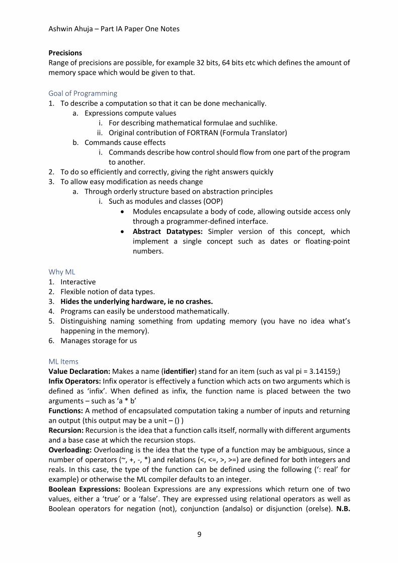
andalso and orelse work by stopping evaluating as soon as possible, i.e. if there is a 0 in the first argument of an andalso, it will stop (and same for a 1 in orelse). Recursion and Efficiency Iterative Methods A recursive function whose computation does not nest is called iterative or tail-recursive, by introducing another element, often known as the accumulator. This ensures that the space complexity is much reduced generally and therefore it is often better to use. fun summing(n, total) = if n=0 then total else summing(n-1, n+total); fun summing (n) = if n=0 then 0 else n + summing(n-1);
Recursion vs Iteration NB: Iterative functions are functions which produce computations reflecting those which can be done using while-loops in conventional languages. All other ‘iterative’ functions are tail-recursive functions • Tail-recursion is efficient only if the compiler detects it. • Iterative functions save space and often run faster. • However, it leads to functions having more arguments than are necessary. Generally, write straightforward code first (often recursive) simply avoiding gross inefficiency and then consider how long it would take to run. Time Complexities Asymptotic Complexity: It refers to how costs – normally time or space – grow with increasing inputs (as the number of inputs go to infinity). Space complexity can never exceed time complexity as it takes time to do anything with space. Notation: 1. O Notation defined by
𝑓(𝑛) = 𝑂(𝑔(𝑛)*𝑝𝑟𝑜𝑣𝑖𝑑𝑒𝑑|𝑓(𝑛)| ≤ 𝑐|𝑔(𝑛)| where f(n) is bounded by some constant c for all sufficiently large n. 2. W is a lower bound for a function asymptotically. 3. Q is an exact bound – ie W(f(n)) = O(f(n)) = Q(f(n)) O Notation
Ashwin Ahuja – Part IA Paper One Notes
11
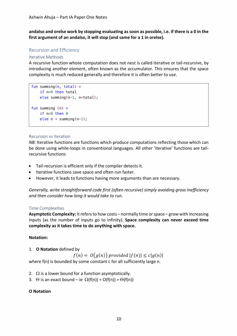
O(2g(n)) = O(g(n)) O(log10n) = O(ln n) (since it is a scalar factor to convert between the two) O(n2 + 50n + 36) = O(n2) O(n2) is contained within O(n3) O(2n) is contained within O(2n) – ie if f(n) = O(2n) => f(n) = O(3n) by triviality but the reverse doesn’t hold. O(log n) is contained within O(n1/2) O(1) = constant O(log n) = logarithmic O(n) = linear O(n log n) = quasi-linear O(n2) = quadratic O(n3) = cubic O(an) = exponential Recurrence Relations
T(n+1) = T(n) + 1 O(n) T(n+1) = T(n) + n O(n2) T(n) = T(n/2) + 1 O(log n) T(n) = 2T(n/2) + n O(n log n)
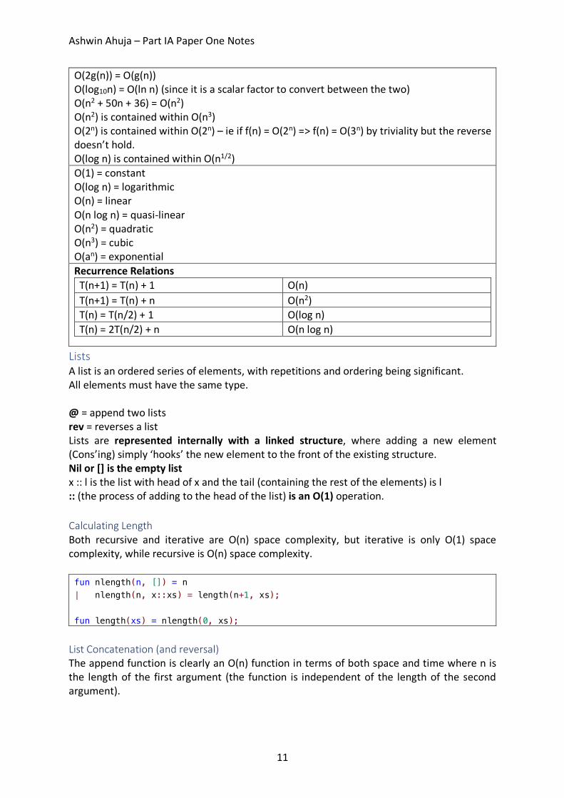
Lists A list is an ordered series of elements, with repetitions and ordering being significant. All elements must have the same type. @ = append two lists rev = reverses a list Lists are represented internally with a linked structure, where adding a new element (Cons’ing) simply ‘hooks’ the new element to the front of the existing structure. Nil or [] is the empty list x :: l is the list with head of x and the tail (containing the rest of the elements) is l :: (the process of adding to the head of the list) is an O(1) operation. Calculating Length Both recursive and iterative are O(n) space complexity, but iterative is only O(1) space complexity, while recursive is O(n) space complexity. fun nlength(n, []) = n | nlength(n, x::xs) = length(n+1, xs); fun length(xs) = nlength(0, xs);
List Concatenation (and reversal) The append function is clearly an O(n) function in terms of both space and time where n is the length of the first argument (the function is independent of the length of the second argument).
Ashwin Ahuja – Part IA Paper One Notes
12
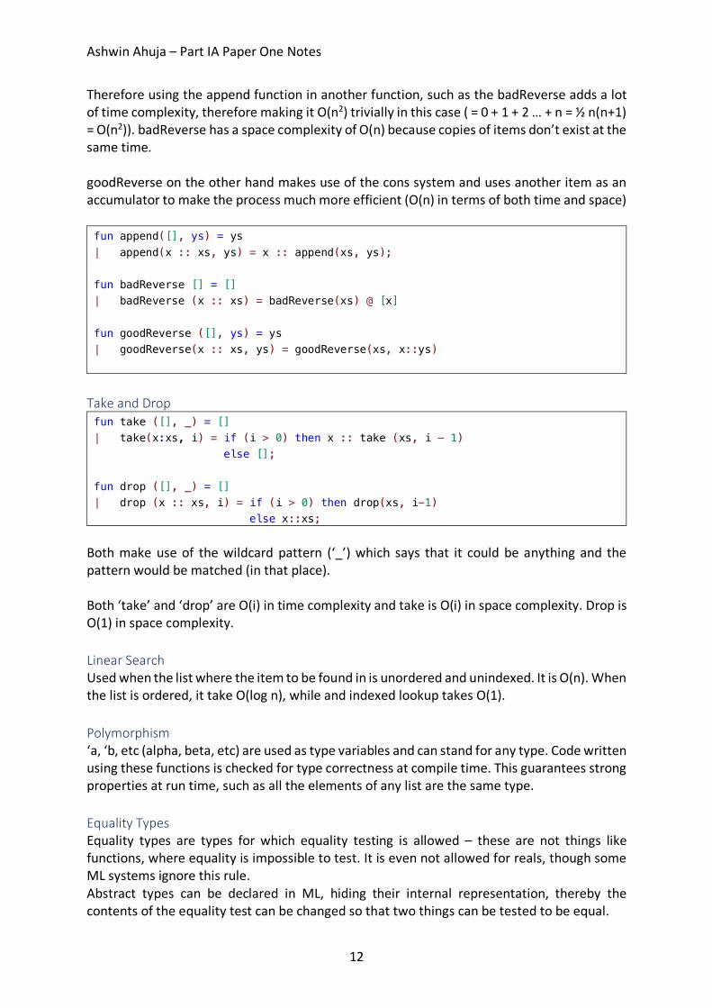
Therefore using the append function in another function, such as the badReverse adds a lot of time complexity, therefore making it O(n2) trivially in this case ( = 0 + 1 + 2 … + n = ½ n(n+1) = O(n2)). badReverse has a space complexity of O(n) because copies of items don’t exist at the same time. goodReverse on the other hand makes use of the cons system and uses another item as an accumulator to make the process much more efficient (O(n) in terms of both time and space) fun append([], ys) = ys | append(x :: xs, ys) = x :: append(xs, ys); fun badReverse [] = [] | badReverse (x :: xs) = badReverse(xs) @ [x] fun goodReverse ([], ys) = ys | goodReverse(x :: xs, ys) = goodReverse(xs, x::ys)
Take and Drop fun take ([], _) = [] | take(x:xs, i) = if (i > 0) then x :: take (xs, i - 1) else []; fun drop ([], _) = [] | drop (x :: xs, i) = if (i > 0) then drop(xs, i-1) else x::xs;
Both make use of the wildcard pattern (‘_’) which says that it could be anything and the pattern would be matched (in that place). Both ‘take’ and ‘drop’ are O(i) in time complexity and take is O(i) in space complexity. Drop is O(1) in space complexity. Linear Search Used when the list where the item to be found in is unordered and unindexed. It is O(n). When the list is ordered, it take O(log n), while and indexed lookup takes O(1). Polymorphism ‘a, ‘b, etc (alpha, beta, etc) are used as type variables and can stand for any type. Code written using these functions is checked for type correctness at compile time. This guarantees strong properties at run time, such as all the elements of any list are the same type. Equality Types Equality types are types for which equality testing is allowed – these are not things like functions, where equality is impossible to test. It is even not allowed for reals, though some ML systems ignore this rule. Abstract types can be declared in ML, hiding their internal representation, thereby the contents of the equality test can be changed so that two things can be tested to be equal.
Ashwin Ahuja – Part IA Paper One Notes
13
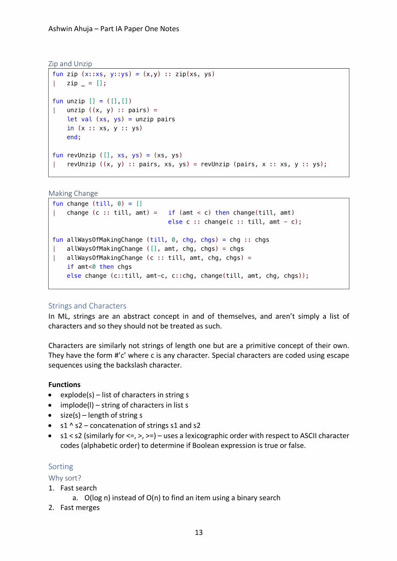
Zip and Unzip fun zip (x::xs, y::ys) = (x,y) :: zip(xs, ys) | zip _ = []; fun unzip [] = ([],[]) | unzip ((x, y) :: pairs) = let val (xs, ys) = unzip pairs in (x :: xs, y :: ys) end; fun revUnzip ([], xs, ys) = (xs, ys) | revUnzip ((x, y) :: pairs, xs, ys) = revUnzip (pairs, x :: xs, y :: ys);
Making Change fun change (till, 0) = [] | change (c :: till, amt) = if (amt < c) then change(till, amt) else c :: change(c :: till, amt - c); fun allWaysOfMakingChange (till, 0, chg, chgs) = chg :: chgs | allWaysOfMakingChange ([], amt, chg, chgs) = chgs | allWaysOfMakingChange (c :: till, amt, chg, chgs) = if amt<0 then chgs else change (c::till, amt-c, c::chg, change(till, amt, chg, chgs));
Strings and Characters In ML, strings are an abstract concept in and of themselves, and aren’t simply a list of characters and so they should not be treated as such. Characters are similarly not strings of length one but are a primitive concept of their own. They have the form #’c’ where c is any character. Special characters are coded using escape sequences using the backslash character. Functions • explode(s) – list of characters in string s • implode(l) – string of characters in list s • size(s) – length of string s • s1 ^ s2 – concatenation of strings s1 and s2 • s1 < s2 (similarly for <=, >, >=) – uses a lexicographic order with respect to ASCII character
codes (alphabetic order) to determine if Boolean expression is true or false.
Sorting Why sort? 1. Fast search
a. O(log n) instead of O(n) to find an item using a binary search 2. Fast merges
Ashwin Ahuja – Part IA Paper One Notes
14
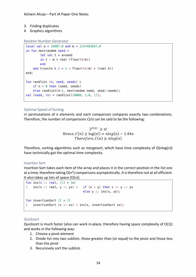
3. Finding duplicates 4. Graphics algorithms Random Number Generator local val a = 16807.0 and m = 2147483647.0 in fun nextrandom seed = let val t = a*seed in t - m * real (floor(t/m)) end and truncto k r = 1 + floor((r/m) * (real k)) end; fun randlist (n, seed, seeds) = if n = 0 then (seed, seeds) else randlist(n-1, nextrandom seed, seed::seeds); val (seed, rs) = randlist(10000, 1.0, []);
Optimal Speed of Sorting n! permutations of n elements and each comparison compares exactly two combinations. Therefore, the number of comparisons C(n) can be said to be the following:
26(7) ≥ 𝑛! 𝐻𝑒𝑛𝑐𝑒, 𝐶(𝑛) ≥ log(𝑛!) ≈ 𝑛𝑙𝑜𝑔(𝑛) − 1.44𝑛
𝑇ℎ𝑒𝑟𝑒𝑓𝑜𝑟𝑒, 𝐶(𝑛) ≥ 𝑛𝑙𝑜𝑔(𝑛) Therefore, sorting algorithms such as mergesort, which have time complexity of O(nlog(n)) have technically got the optimal time complexity. Insertion Sort Insertion Sort takes each item of the array and places it in the correct position in the list one at a time, therefore taking O(n2) comparisons asymptotically. It is therefore not at all efficient. It also takes up lots of space (O(n)). fun ins(x :: real, []) = [x] | ins(x :: real, y :: ys) = if (x < y) then x :: y :: ys else y :: ins(x, ys); fun insertionSort [] = [] | insertionSort (x :: xs) = ins(x, insertionSort xs);
Quicksort Quicksort is much faster (also can work in-place, therefore having space complexity of O(1)) and works in the following way:
1. Choose a pivot element 2. Divide list into two sublists: those greater than (or equal) to the pivot and those less
than the pivot 3. Recursively sort the sublists
Ashwin Ahuja – Part IA Paper One Notes
15
4. Combine the sorted lists by appending one to the other. Obviously, it seems well suited to using appending of lists, however, we can also do it without appends, which would of course make the system more efficient. In terms of specific time complexity, we can consider both the average case and the worst-case complexity. In the average case, the pivot will fall in the middle of the list, therefore making the problem of this sort:
𝑇(𝑛) = 2𝑇 H12𝑛I + 𝑛, 𝑇(1) = 1
This can be followed down to: 𝑇(𝑛) = 𝑂(𝑛𝑙𝑜𝑔(𝑛))
However, in the worst case, where the item is either reverse sorted or almost sorted. In this case, nearly all the elements fall on one side of the pivot, therefore:
𝑇(𝑛) = 𝑇(𝑛 − 1) + 𝑛, 𝑇(1) = 1 This becomes:
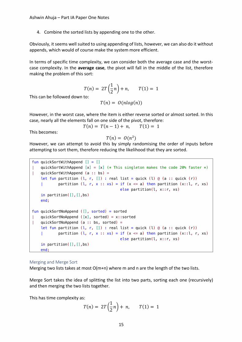
𝑇(𝑛) = 𝑂(𝑛K) However, we can attempt to avoid this by simply randomising the order of inputs before attempting to sort them, therefore reducing the likelihood that they are sorted. fun quickSortWithAppend [] = [] | quickSortWithAppend [x] = [x] (* This singleton makes the code 20% faster *) | quickSortWithAppend (a :: bs) = let fun partition (l, r, []) : real list = quick (l) @ (a :: quick (r)) | partition (l, r, x :: xs) = if (x <= a) then partition (x::l, r, xs) else partition(l, x::r, xs) in partition([],[],bs) end; fun quickSortNoAppend ([], sorted) = sorted | quickSortNoAppend ([x], sorted) = x::sorted | quickSortNoAppend (a :: bs, sorted) = let fun partition (l, r, []) : real list = quick (l) @ (a :: quick (r)) | partition (l, r, x :: xs) = if (x <= a) then partition (x::l, r, xs) else partition(l, x::r, xs) in partition([],[],bs) end;
Merging and Merge Sort Merging two lists takes at most O(m+n) where m and n are the length of the two lists. Merge Sort takes the idea of splitting the list into two parts, sorting each one (recursively) and then merging the two lists together. This has time complexity as:
𝑇(𝑛) = 2𝑇 H12𝑛I + 𝑛, 𝑇(1) = 1
Ashwin Ahuja – Part IA Paper One Notes
16
This becomes: 𝑇(𝑛) = 𝑂(𝑛 log(𝑛))
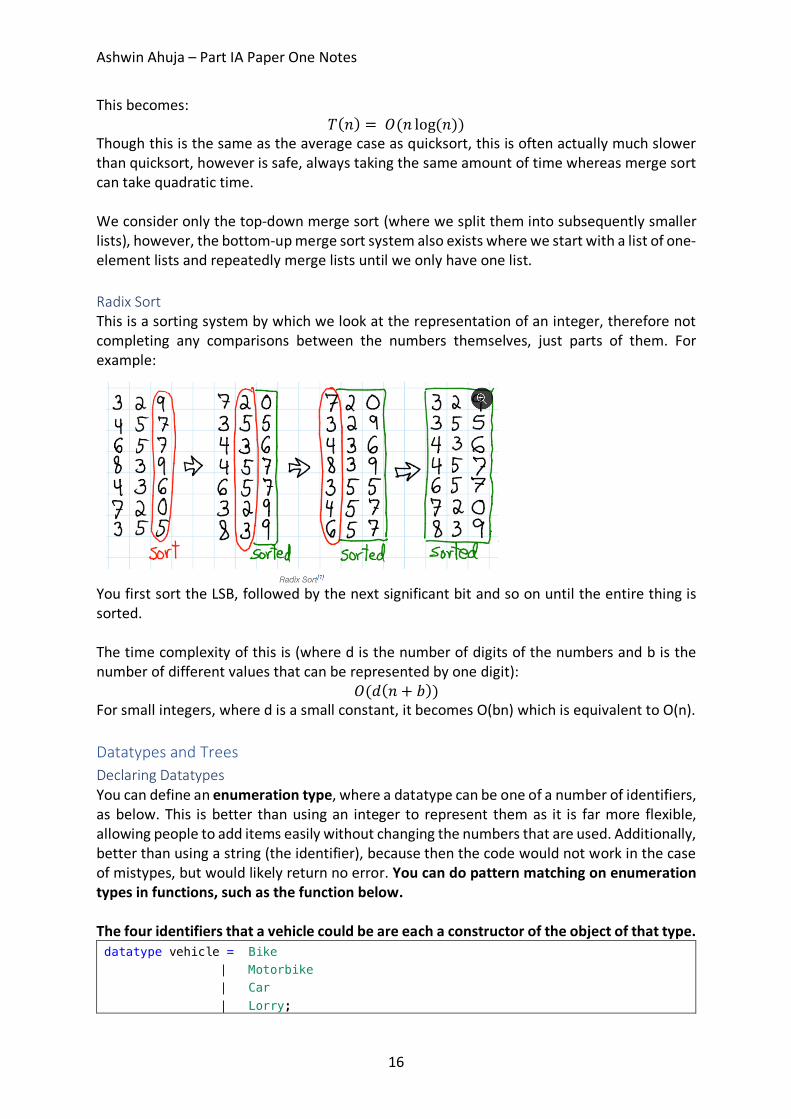
Though this is the same as the average case as quicksort, this is often actually much slower than quicksort, however is safe, always taking the same amount of time whereas merge sort can take quadratic time. We consider only the top-down merge sort (where we split them into subsequently smaller lists), however, the bottom-up merge sort system also exists where we start with a list of one-element lists and repeatedly merge lists until we only have one list. Radix Sort This is a sorting system by which we look at the representation of an integer, therefore not completing any comparisons between the numbers themselves, just parts of them. For example:
You first sort the LSB, followed by the next significant bit and so on until the entire thing is sorted. The time complexity of this is (where d is the number of digits of the numbers and b is the number of different values that can be represented by one digit):
𝑂(𝑑(𝑛 + 𝑏)) For small integers, where d is a small constant, it becomes O(bn) which is equivalent to O(n). Datatypes and Trees Declaring Datatypes You can define an enumeration type, where a datatype can be one of a number of identifiers, as below. This is better than using an integer to represent them as it is far more flexible, allowing people to add items easily without changing the numbers that are used. Additionally, better than using a string (the identifier), because then the code would not work in the case of mistypes, but would likely return no error. You can do pattern matching on enumeration types in functions, such as the function below. The four identifiers that a vehicle could be are each a constructor of the object of that type. datatype vehicle = Bike | Motorbike | Car | Lorry;
Ashwin Ahuja – Part IA Paper One Notes
17
fun wheels Bike = 2 | wheels Motorbike = 2 | wheels Car = 4 | wheels Lorry = 18;
As the identifiers are constructors, ML allows data to be associated with each constructor, eg: datatype vehicle2 = Bike | Motorbike of int | Car of bool | Lorry of real;
Here vehicle2 is an example of a concept consisting of several varieties with distinct features. In other programming languages, these are often represented by things close to datatypes, often called union types or variant records (where tag fields are effectively the constructor). Exceptions Exceptions are necessary because it is not always possible to tell in advance whether or not an error will occur. Rather than crashing, programs should check whether things have gone wrong and attempt an alternative computation. Exception handling allows us to recover properly: 1. Raising an exception abandons the current computation 2. Handling the exception attempts an alternative computation 3. Raising and handling can be far apart in code 4. Errors of different sorts can be handled separately In ML, before an exception can be used, it must be declared, as follows: exception Failure; exception NoChange of int;
Exception names are constructors of the special datatype exn. This lets exception handlers use pattern matching. In order to raise and handle exceptions, the following can be used: raise Failure; raise (NoChange 10) handle Failure => E (* E is a function that should be called *) handle NoChange (n) => return n
N.B. Unlike in Java there is no indication that a function can throw an exception. One alternative to exceptions is to return a value of a new datatype datatype 'a option = NONE | SOME of 'a;
Where NONE represents than an error and SOME x is the solution x. While clean, this would be very annoying, needing to check for NONE in a lot of places (not just being able to handle it).
Ashwin Ahuja – Part IA Paper One Notes
18
Binary Trees A tree is a data structure with multiple branching, providing efficient storage and retrieval of information. In a binary tree, a node is either empty (leaf node) or is a branch with a label and two subtrees. datatype 'a tree = Lf | Br of 'a * 'a tree * 'a tree;
Counting number of nodes fun count Lf = 0 | count Br(_, tl, tr) = 1 + count tl + count tr;
Finding depth of tree fun depth Lf = 0 | depth Br (_, tl, tr) = 1 + Int.max(depth tl, depth tr);
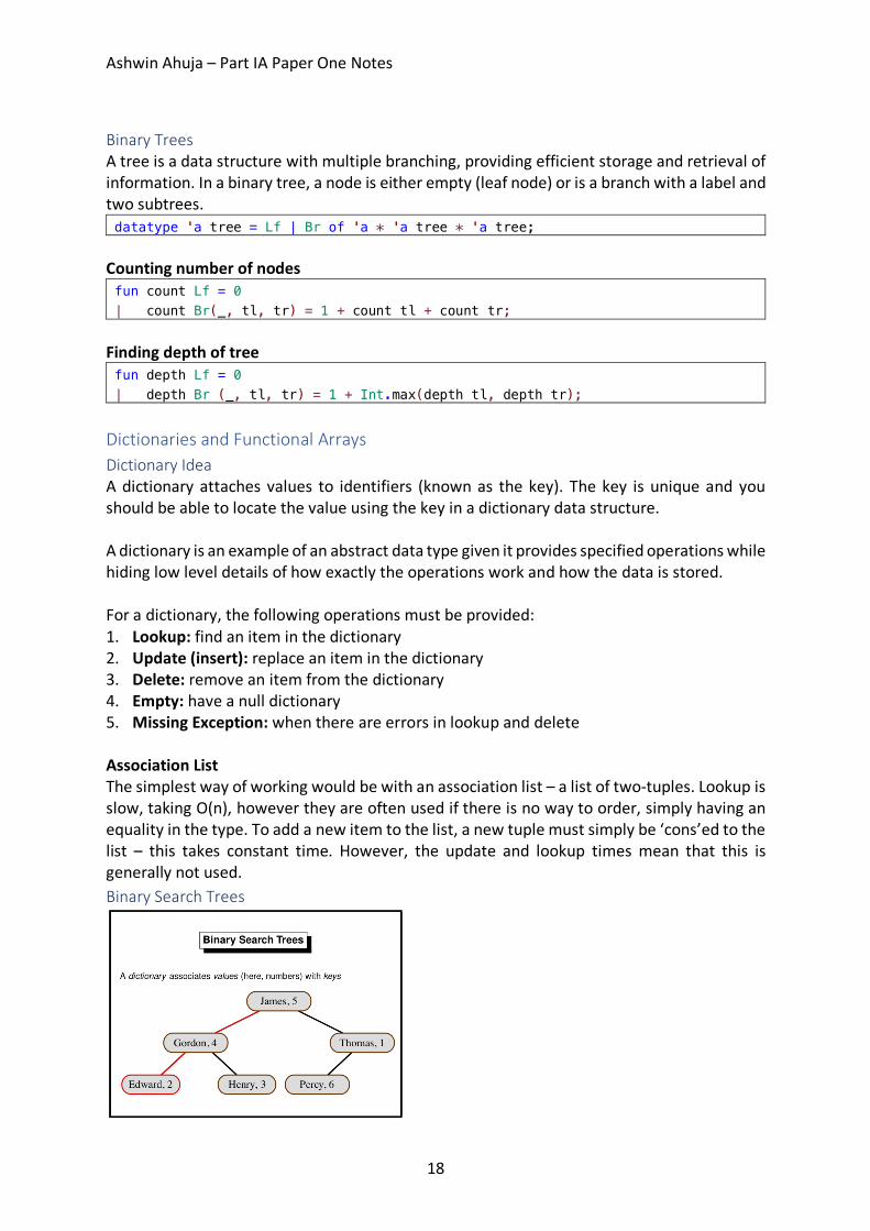
Dictionaries and Functional Arrays Dictionary Idea A dictionary attaches values to identifiers (known as the key). The key is unique and you should be able to locate the value using the key in a dictionary data structure. A dictionary is an example of an abstract data type given it provides specified operations while hiding low level details of how exactly the operations work and how the data is stored. For a dictionary, the following operations must be provided: 1. Lookup: find an item in the dictionary 2. Update (insert): replace an item in the dictionary 3. Delete: remove an item from the dictionary 4. Empty: have a null dictionary 5. Missing Exception: when there are errors in lookup and delete Association List The simplest way of working would be with an association list – a list of two-tuples. Lookup is slow, taking O(n), however they are often used if there is no way to order, simply having an equality in the type. To add a new item to the list, a new tuple must simply be ‘cons’ed to the list – this takes constant time. However, the update and lookup times mean that this is generally not used. Binary Search Trees
Ashwin Ahuja – Part IA Paper One Notes
19
Each branch of the tree carries a (key, value) pair with the left subtree containing items with smaller keys and the right subtree containing items with larger keys. If the tree is reasonably balanced, then update and lookup both take O(log n) for a tree of size n. Meanwhile, an unbalanced tree has a linear (O(n)) access time in the worst case. In addition to being used for dictionaries, binary search trees are also used for sorting – adding all elements to a tree, before doing an in-order traversal to get the items in order. There are also self-balancing trees, called Red-Black trees, which are O(log n) for access in the worst case. However, these are generally rather hard to implement. exception Missing of string; fun lookup (Lf, b) = raise Missing b; | lookup (Br((a,x), tl, tr), b) = if (b < a) then lookup(tl, b) else if (b > a) then lookup (tr, b) else x; fun update (Lf, b : string, y) = Br ((b, y), Lf, Lf) | update (Br((a,x), tl, tr)) = if (b < a) then Br((a,x), update(tl, b, y), tr) else if (b > a) then Br((a,x, tl, update(tr, b, y))) else Br((a,y), tl, tr);
Since (for update) the paths are simply copied, the parts of the tree are shared, not copied. Traversing Trees
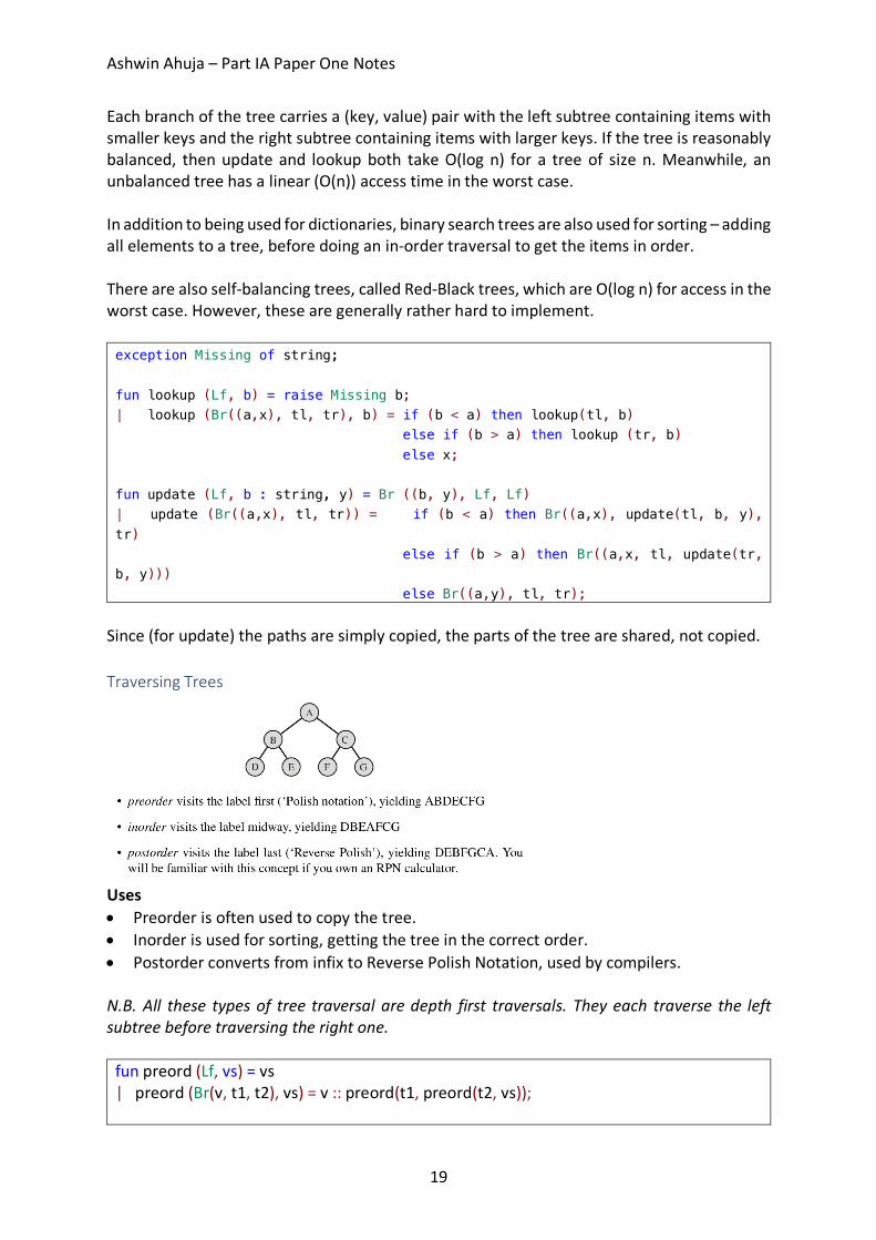
Uses • Preorder is often used to copy the tree. • Inorder is used for sorting, getting the tree in the correct order. • Postorder converts from infix to Reverse Polish Notation, used by compilers. N.B. All these types of tree traversal are depth first traversals. They each traverse the left subtree before traversing the right one.
fun preord (Lf, vs) = vs | preord (Br(v, t1, t2), vs) = v :: preord(t1, preord(t2, vs));
Ashwin Ahuja – Part IA Paper One Notes
20
fun inord (Lf, vs) = vs | inord (Br(v, t1, t2), vs) = inord(t1, v :: inord(t2, vs)); fun postord (Lf, vs) = vs | postord(Br(v, t1, t2), vs) = postord(t1, postord(t2, v::vs));
Intersection of two Binary Trees fun intersection (Lf, t2, out) = out | intersection(Br((a,x), tl, tr), t2, out) = let val newTree = intersection(tl, t2, (intersection(tr,t2, out ))) in if(lookup(u,a) = x) then update(newTree, a, x) else newTree handle Missing _ => newTree end;
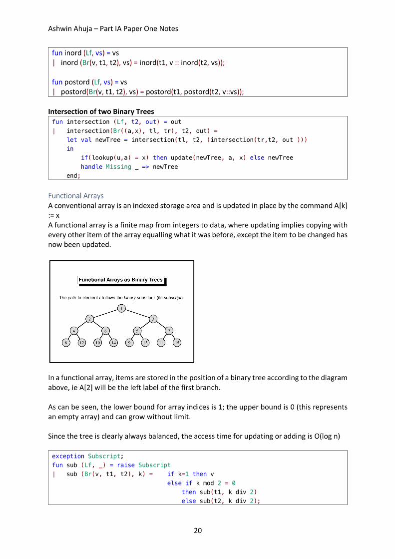
Functional Arrays A conventional array is an indexed storage area and is updated in place by the command A[k] := x A functional array is a finite map from integers to data, where updating implies copying with every other item of the array equalling what it was before, except the item to be changed has now been updated.
In a functional array, items are stored in the position of a binary tree according to the diagram above, ie A[2] will be the left label of the first branch. As can be seen, the lower bound for array indices is 1; the upper bound is 0 (this represents an empty array) and can grow without limit. Since the tree is clearly always balanced, the access time for updating or adding is O(log n) exception Subscript; fun sub (Lf, _) = raise Subscript | sub (Br(v, t1, t2), k) = if k=1 then v else if k mod 2 = 0 then sub(t1, k div 2) else sub(t2, k div 2);
Ashwin Ahuja – Part IA Paper One Notes
21
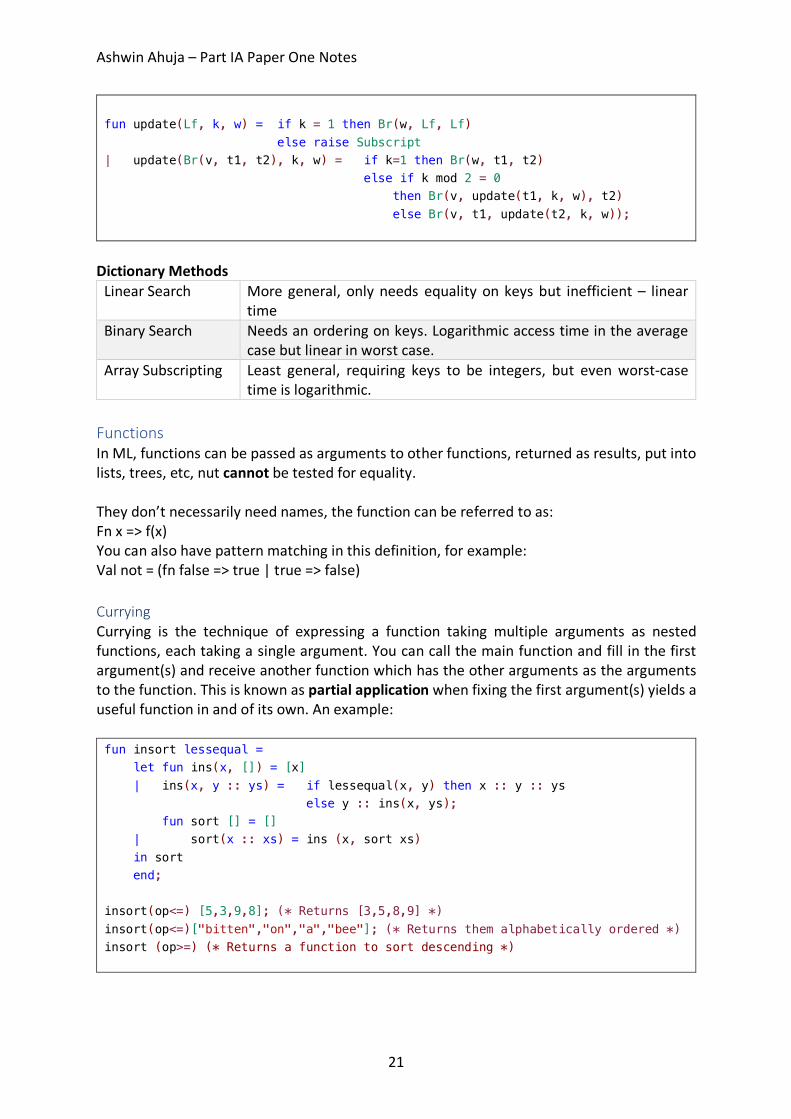
fun update(Lf, k, w) = if k = 1 then Br(w, Lf, Lf) else raise Subscript | update(Br(v, t1, t2), k, w) = if k=1 then Br(w, t1, t2) else if k mod 2 = 0 then Br(v, update(t1, k, w), t2) else Br(v, t1, update(t2, k, w));
Dictionary Methods
Linear Search More general, only needs equality on keys but inefficient – linear time
Binary Search Needs an ordering on keys. Logarithmic access time in the average case but linear in worst case.
Array Subscripting Least general, requiring keys to be integers, but even worst-case time is logarithmic.
Functions In ML, functions can be passed as arguments to other functions, returned as results, put into lists, trees, etc, nut cannot be tested for equality. They don’t necessarily need names, the function can be referred to as: Fn x => f(x) You can also have pattern matching in this definition, for example: Val not = (fn false => true | true => false) Currying Currying is the technique of expressing a function taking multiple arguments as nested functions, each taking a single argument. You can call the main function and fill in the first argument(s) and receive another function which has the other arguments as the arguments to the function. This is known as partial application when fixing the first argument(s) yields a useful function in and of its own. An example: fun insort lessequal = let fun ins(x, []) = [x] | ins(x, y :: ys) = if lessequal(x, y) then x :: y :: ys else y :: ins(x, ys); fun sort [] = [] | sort(x :: xs) = ins (x, sort xs) in sort end; insort(op<=) [5,3,9,8]; (* Returns [3,5,8,9] *) insort(op<=)["bitten","on","a","bee"]; (* Returns them alphabetically ordered *) insort (op>=) (* Returns a function to sort descending *)
Ashwin Ahuja – Part IA Paper One Notes
22
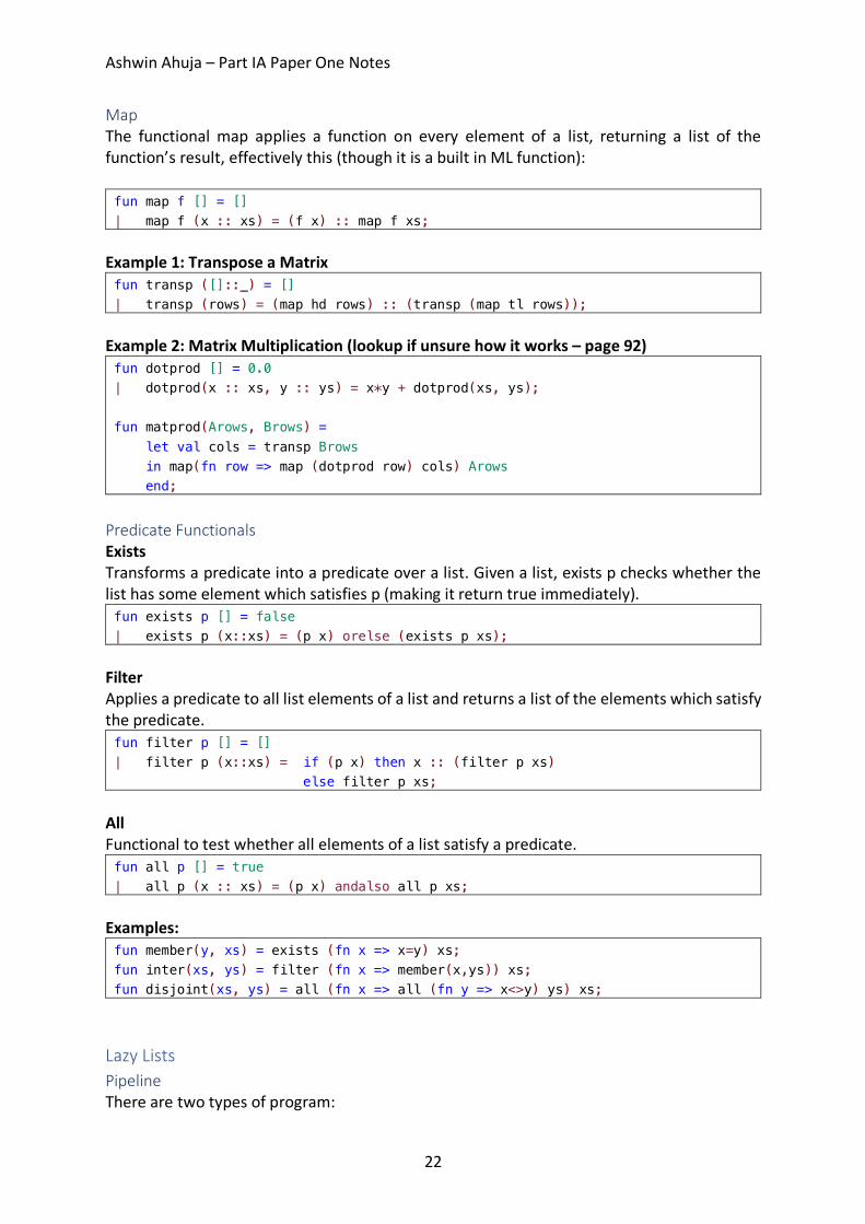
Map The functional map applies a function on every element of a list, returning a list of the function’s result, effectively this (though it is a built in ML function): fun map f [] = [] | map f (x :: xs) = (f x) :: map f xs;
Example 1: Transpose a Matrix fun transp ([]::_) = [] | transp (rows) = (map hd rows) :: (transp (map tl rows));
Example 2: Matrix Multiplication (lookup if unsure how it works – page 92) fun dotprod [] = 0.0 | dotprod(x :: xs, y :: ys) = x*y + dotprod(xs, ys); fun matprod(Arows, Brows) = let val cols = transp Brows in map(fn row => map (dotprod row) cols) Arows end;
Predicate Functionals Exists Transforms a predicate into a predicate over a list. Given a list, exists p checks whether the list has some element which satisfies p (making it return true immediately). fun exists p [] = false | exists p (x::xs) = (p x) orelse (exists p xs);
Filter Applies a predicate to all list elements of a list and returns a list of the elements which satisfy the predicate. fun filter p [] = [] | filter p (x::xs) = if (p x) then x :: (filter p xs) else filter p xs;
All Functional to test whether all elements of a list satisfy a predicate. fun all p [] = true | all p (x :: xs) = (p x) andalso all p xs;
Examples: fun member(y, xs) = exists (fn x => x=y) xs; fun inter(xs, ys) = filter (fn x => member(x,ys)) xs; fun disjoint(xs, ys) = all (fn x => all (fn y => x<>y) ys) xs;
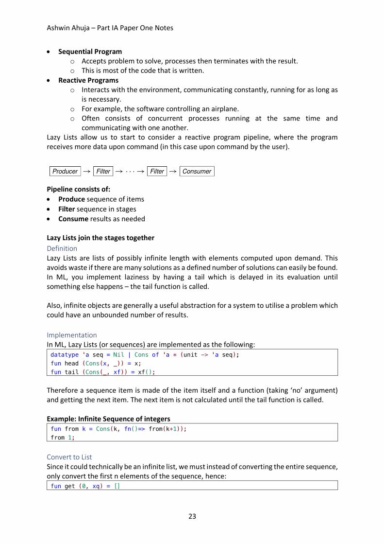
Lazy Lists Pipeline There are two types of program:
Ashwin Ahuja – Part IA Paper One Notes
23
• Sequential Program o Accepts problem to solve, processes then terminates with the result. o This is most of the code that is written.
• Reactive Programs o Interacts with the environment, communicating constantly, running for as long as
is necessary. o For example, the software controlling an airplane. o Often consists of concurrent processes running at the same time and
communicating with one another. Lazy Lists allow us to start to consider a reactive program pipeline, where the program receives more data upon command (in this case upon command by the user).
Pipeline consists of: • Produce sequence of items • Filter sequence in stages • Consume results as needed Lazy Lists join the stages together Definition Lazy Lists are lists of possibly infinite length with elements computed upon demand. This avoids waste if there are many solutions as a defined number of solutions can easily be found. In ML, you implement laziness by having a tail which is delayed in its evaluation until something else happens – the tail function is called. Also, infinite objects are generally a useful abstraction for a system to utilise a problem which could have an unbounded number of results. Implementation In ML, Lazy Lists (or sequences) are implemented as the following: datatype 'a seq = Nil | Cons of 'a * (unit -> 'a seq); fun head (Cons(x, _)) = x; fun tail (Cons(_, xf)) = xf();
Therefore a sequence item is made of the item itself and a function (taking ‘no’ argument) and getting the next item. The next item is not calculated until the tail function is called. Example: Infinite Sequence of integers fun from k = Cons(k, fn()=> from(k+1)); from 1;
Convert to List Since it could technically be an infinite list, we must instead of converting the entire sequence, only convert the first n elements of the sequence, hence: fun get (0, xq) = []
Ashwin Ahuja – Part IA Paper One Notes
24
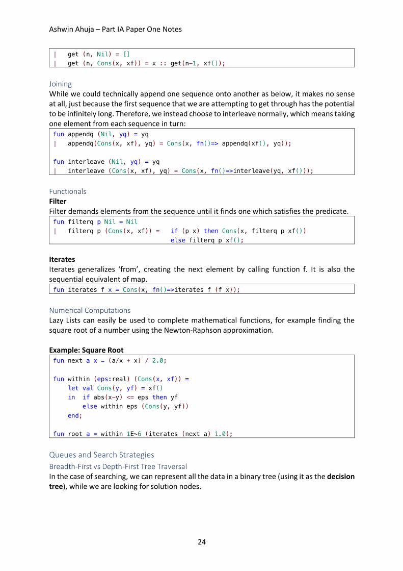
| get (n, Nil) = [] | get (n, Cons(x, xf)) = x :: get(n-1, xf());
Joining While we could technically append one sequence onto another as below, it makes no sense at all, just because the first sequence that we are attempting to get through has the potential to be infinitely long. Therefore, we instead choose to interleave normally, which means taking one element from each sequence in turn: fun appendq (Nil, yq) = yq | appendq(Cons(x, xf), yq) = Cons(x, fn()=> appendq(xf(), yq)); fun interleave (Nil, yq) = yq | interleave (Cons(x, xf), yq) = Cons(x, fn()=>interleave(yq, xf()));
Functionals Filter Filter demands elements from the sequence until it finds one which satisfies the predicate. fun filterq p Nil = Nil | filterq p (Cons(x, xf)) = if (p x) then Cons(x, filterq p xf()) else filterq p xf();
Iterates Iterates generalizes ‘from’, creating the next element by calling function f. It is also the sequential equivalent of map. fun iterates f x = Cons(x, fn()=>iterates f (f x));
Numerical Computations Lazy Lists can easily be used to complete mathematical functions, for example finding the square root of a number using the Newton-Raphson approximation. Example: Square Root fun next a x = (a/x + x) / 2.0; fun within (eps:real) (Cons(x, xf)) = let val Cons(y, yf) = xf() in if abs(x-y) <= eps then yf else within eps (Cons(y, yf)) end; fun root a = within 1E~6 (iterates (next a) 1.0);
Queues and Search Strategies Breadth-First vs Depth-First Tree Traversal In the case of searching, we can represent all the data in a binary tree (using it as the decision tree), while we are looking for solution nodes.
Ashwin Ahuja – Part IA Paper One Notes
25
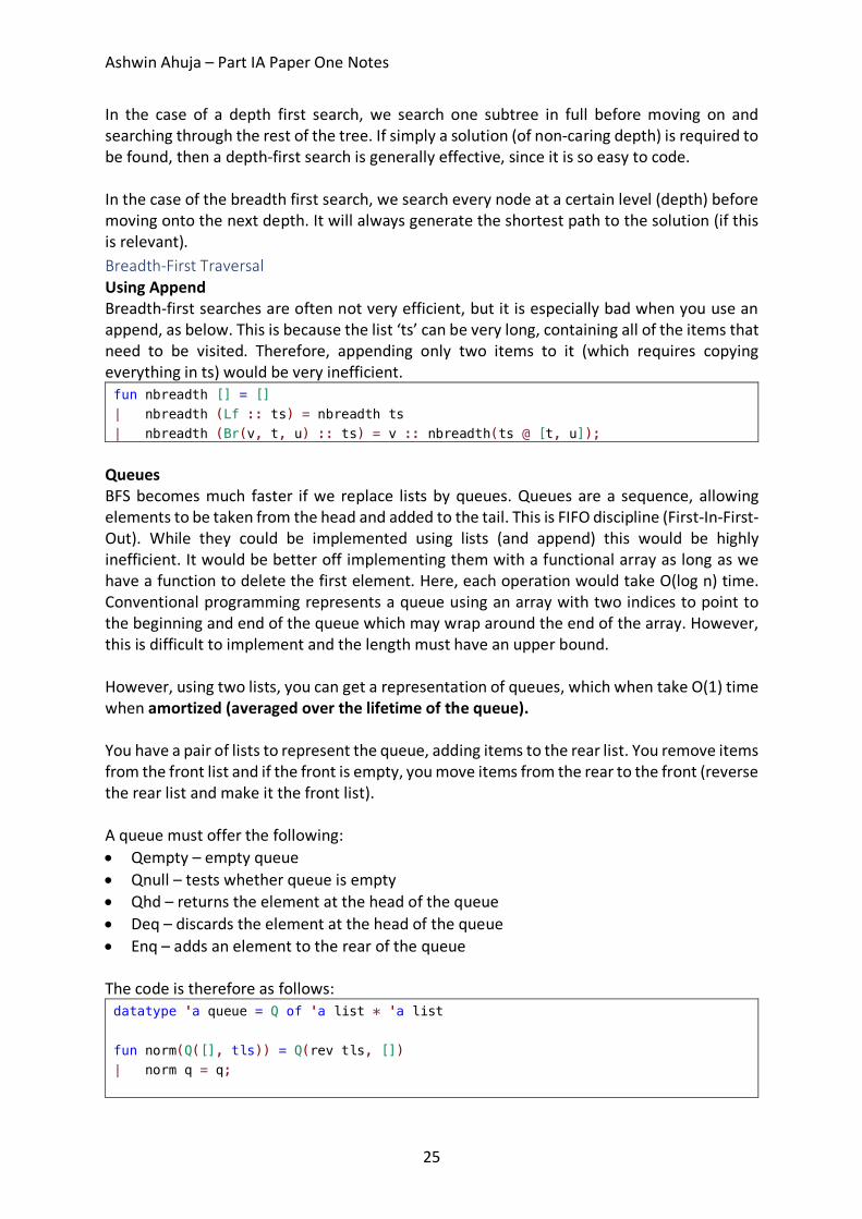
In the case of a depth first search, we search one subtree in full before moving on and searching through the rest of the tree. If simply a solution (of non-caring depth) is required to be found, then a depth-first search is generally effective, since it is so easy to code. In the case of the breadth first search, we search every node at a certain level (depth) before moving onto the next depth. It will always generate the shortest path to the solution (if this is relevant). Breadth-First Traversal Using Append Breadth-first searches are often not very efficient, but it is especially bad when you use an append, as below. This is because the list ‘ts’ can be very long, containing all of the items that need to be visited. Therefore, appending only two items to it (which requires copying everything in ts) would be very inefficient. fun nbreadth [] = [] | nbreadth (Lf :: ts) = nbreadth ts | nbreadth (Br(v, t, u) :: ts) = v :: nbreadth(ts @ [t, u]);
Queues BFS becomes much faster if we replace lists by queues. Queues are a sequence, allowing elements to be taken from the head and added to the tail. This is FIFO discipline (First-In-First-Out). While they could be implemented using lists (and append) this would be highly inefficient. It would be better off implementing them with a functional array as long as we have a function to delete the first element. Here, each operation would take O(log n) time. Conventional programming represents a queue using an array with two indices to point to the beginning and end of the queue which may wrap around the end of the array. However, this is difficult to implement and the length must have an upper bound. However, using two lists, you can get a representation of queues, which when take O(1) time when amortized (averaged over the lifetime of the queue). You have a pair of lists to represent the queue, adding items to the rear list. You remove items from the front list and if the front is empty, you move items from the rear to the front (reverse the rear list and make it the front list). A queue must offer the following: • Qempty – empty queue • Qnull – tests whether queue is empty • Qhd – returns the element at the head of the queue • Deq – discards the element at the head of the queue • Enq – adds an element to the rear of the queue The code is therefore as follows: datatype 'a queue = Q of 'a list * 'a list fun norm(Q([], tls)) = Q(rev tls, []) | norm q = q;
Ashwin Ahuja – Part IA Paper One Notes
26
fun qnull(Q([],[])) = true | qnull (_) = false; fun enq(Q(hds, tls), x) = norm(Q(hds, x :: tls)); fun deq(Q(x::hds, tls)) = norm(Q(hds, tls)); val qempty = Q([],[]); fun qhd(Q(x::_, _)) = x;
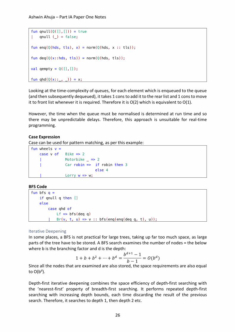
Looking at the time-complexity of queues, for each element which is enqueued to the queue (and then subsequently dequeued), it takes 1 cons to add it to the rear list and 1 cons to move it to front list whenever it is required. Therefore it is O(2) which is equivalent to O(1). However, the time when the queue must be normalised is determined at run time and so there may be unpredictable delays. Therefore, this approach is unsuitable for real-time programming. Case Expression Case can be used for pattern matching, as per this example: fun wheels v = case v of Bike => 2 | Motorbike _ => 2 | Car robin => if robin then 3 else 4 | Lorry w => w;
BFS Code fun bfs q = if qnull q then [] else case qhd of Lf => bfs(deq q) | Br(v, t, u) => v :: bfs(enq(enq(deq q, t), u));
Iterative Deepening In some places, a BFS is not practical for large trees, taking up far too much space, as large parts of the tree have to be stored. A BFS search examines the number of nodes = the below where b is the branching factor and d is the depth:
1 + 𝑏 + 𝑏K + ⋯+ 𝑏N =𝑏NOP − 1𝑏 − 1 = 𝑂(𝑏N)
Since all the nodes that are examined are also stored, the space requirements are also equal to O(bd). Depth-first iterative deepening combines the space efficiency of depth-first searching with the ‘nearest-first’ property of breadth-first searching. It performs repeated depth-first searching with increasing depth bounds, each time discarding the result of the previous search. Therefore, it searches to depth 1, then depth 2 etc.
Ashwin Ahuja – Part IA Paper One Notes
27
It can be shown that the time needed for iterative deepening to reach depth d is only QQRP
times that for the time required for a breadth first search. This is a constant factor – both have time complexity = O(bd), but iterative deepening has space complexity of O(d). Depth-First Search Stacks Stack is a sequence such that items can be added or removed from the head only, obeying a LIFO (Last-In-First-Out) discipline. Lists can easily be used to implement stacks. However, stacks are often regarded as an imperative data structure (popping or pushing should affect the original stack not return a new one). In conventional programming languages, a stack is often implemented by storing items in an array, using a stack pointer to count them. Stacks must have the following things: • Empty – ability to have an empty stack • Null – ability to test for an empty stack • Top – ability to return the item at the top of stack • Pop – ability to remove the item at the top of the stack • Push – ability to add an element to the top of the stack Search Methods Conclusion 1. DFS – use a stack
a. It is efficient but incomplete – does not always return the best solution 2. BFS – use a queue
a. Effective but uses too much space 3. Iterative deepening – effectively uses (1) to get the benefits of (2)
a. It trades time for space 4. Best-First – uses a priority queue
a. Nodes are an ordered sequence, placing a ranking function to the nodes. For example, may be to estimate the distance from the node to a solution. If the estimate is good, the solution is located quickly.
b. The priority queue can be kept as a sorted list, although this is slow. Binary search tree would be better.
Polynomial Arithmetic A polynomial is a linear combination of products of certain variables. Polynomials in one variable is called univariate. For the section, we only consider univariate closed-form polynomials. Being able to do maths on polynomials is highly useful, as it would allow us to derive and use formulas for science and engineering. Data Structure for Polynomials We might represent a polynomial with a dense representation – using a list of coefficients [an, an-1, …, a0] where the formula is anxn + an-1xn-1. This is very inefficient if many coefficients are zero.
Ashwin Ahuja – Part IA Paper One Notes
28
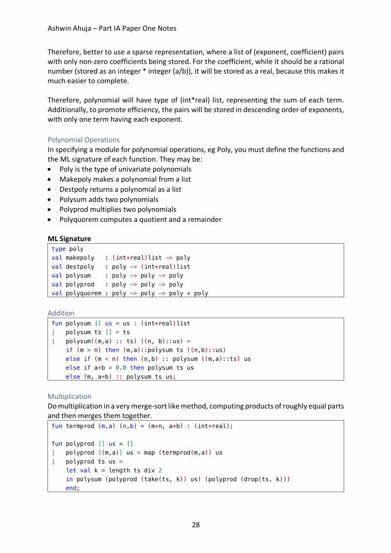
Therefore, better to use a sparse representation, where a list of (exponent, coefficient) pairs with only non-zero coefficients being stored. For the coefficient, while it should be a rational number (stored as an integer * integer (a/b)), it will be stored as a real, because this makes it much easier to complete. Therefore, polynomial will have type of (int*real) list, representing the sum of each term. Additionally, to promote efficiency, the pairs will be stored in descending order of exponents, with only one term having each exponent. Polynomial Operations In specifying a module for polynomial operations, eg Poly, you must define the functions and the ML signature of each function. They may be: • Poly is the type of univariate polynomials • Makepoly makes a polynomial from a list • Destpoly returns a polynomial as a list • Polysum adds two polynomials • Polyprod multiplies two polynomials • Polyquorem computes a quotient and a remainder ML Signature type poly val makepoly : (int*real)list -> poly val destpoly : poly -> (int*real)list val polysum : poly -> poly -> poly val polyprod : poly -> poly -> poly val polyquorem : poly -> poly -> poly * poly
Addition fun polysum [] us = us : (int*real)list | polysum ts [] = ts | polysum((m,a) :: ts) ((n, b)::us) = if (m > n) then (m,a)::polysum ts ((n,b)::us) else if (m < n) then (n,b) :: polysum ((m,a)::ts) us else if a+b = 0.0 then polysum ts us else (m, a+b) :: polysum ts us;
Multiplication Do multiplication in a very merge-sort like method, computing products of roughly equal parts and then merges them together. fun termprod (m,a) (n,b) = (m+n, a*b) : (int*real); fun polyprod [] us = [] | polyprod [(m,a)] us = map (termprod(m,a)) us | polyprod ts us = let val k = length ts div 2 in polysum (polyprod (take(ts, k)) us) (polyprod (drop(ts, k))) end;

Ashwin Ahuja – Part IA Paper One Notes
29
Division fun polyquorem ts ((n,b)::us) = let fun quo [] qs = (rev qs, []) | quo ((m,a)::ts) qs = if (m<n) then (rev qs, (m,a)::ts) else quo(polysum ts (map (termprod(m-n, ~a/b)) us)) ((m-n, a/b) :: qs) in quo ts [] end; fun polyquo ts us = #1(polyquorem ts us) and polyrem ts us = #2(polyquorem ts us) (* If k is any positive integer constant, then k is the ML function to return the kth component of a tuple. Tuples are a special case of ML records, and the # notation works for arbitrary record fields. *)
GCD fun polygcd [] us = us | polygcd ts us = polygcd (polyrem us ts) ts;
This is using Euclid’s algorithm, however, for polynomials its behaviour is slightly odd. It gives the GCD of x2 + 2x + 1 and x2 – 1 as -2x – 2 and x2 + 2x + 1 and x5 + 1 as 5x + 5. Both should have the answer x + 1. However, this difficulty can be fixed by dividing through by the leading coefficient. However, more importantly, the algorithm is far too slow, and therefore this algorithm shouldn’t be used. Procedural Programming Definition • Procedural programming is programming where the programming state is repeatedly
transformed by the execution of commands or statements. o A state change might be local to the machine and consist of updating a variable or
array, or consist of sending data to the outside world. (Even reading data counts as a state change, since this act normally removes the data from the environment).
• It also provides primitive commands and control structures for combining them. o Primitive commands include assignment for updating variables and input / output
commands for communication o Control commands include branching, iteration and procedures.
• Use abstractions of the computer’s memory o References to memory cells o Arrays for blocks of memory cells o Linked Structures; especially linked lists
References References offer a way of creating a reference, thereby getting at a specific memory cell which prevails.
Ashwin Ahuja – Part IA Paper One Notes
30
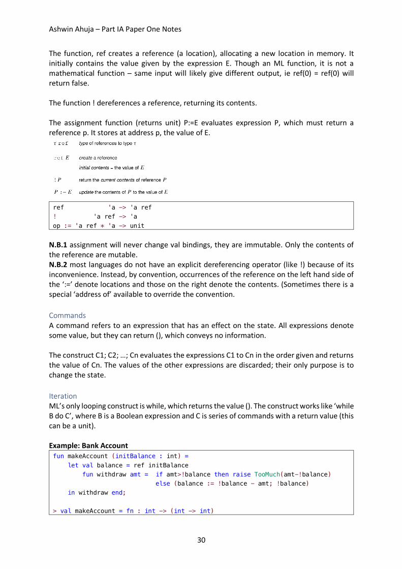
The function, ref creates a reference (a location), allocating a new location in memory. It initially contains the value given by the expression E. Though an ML function, it is not a mathematical function – same input will likely give different output, ie ref(0) = ref(0) will return false. The function ! dereferences a reference, returning its contents. The assignment function (returns unit) P:=E evaluates expression P, which must return a reference p. It stores at address p, the value of E.
ref 'a -> 'a ref ! 'a ref -> 'a op := 'a ref * 'a -> unit
N.B.1 assignment will never change val bindings, they are immutable. Only the contents of the reference are mutable. N.B.2 most languages do not have an explicit dereferencing operator (like !) because of its inconvenience. Instead, by convention, occurrences of the reference on the left hand side of the ‘:=’ denote locations and those on the right denote the contents. (Sometimes there is a special ‘address of’ available to override the convention. Commands A command refers to an expression that has an effect on the state. All expressions denote some value, but they can return (), which conveys no information. The construct C1; C2; …; Cn evaluates the expressions C1 to Cn in the order given and returns the value of Cn. The values of the other expressions are discarded; their only purpose is to change the state. Iteration ML’s only looping construct is while, which returns the value (). The construct works like ‘while B do C’, where B is a Boolean expression and C is series of commands with a return value (this can be a unit). Example: Bank Account fun makeAccount (initBalance : int) = let val balance = ref initBalance fun withdraw amt = if amt>!balance then raise TooMuch(amt-!balance) else (balance := !balance - amt; !balance) in withdraw end; > val makeAccount = fn : int -> (int -> int)

Ashwin Ahuja – Part IA Paper One Notes
31
The function makeAccount models a bank. Calling the function with an initial balance creates a new reference (balance) to maintain the account balance and returns a function (withdraw) having sole access to that reference. Each call to makeAccount returns a copy of withdraw holding a fresh instance of the reference balance. There is no access to the account balance except via the corresponding withdraw function. If that function is discarded, the reference cell becomes unreachable – the computer will eventually get rid of it. We can generalise makeAccount to return several functions that jointly manage information held in shared references. (The functions might be packaged using ML records, which are discussed elsewhere. Most procedural languages do not support the concept of private references, although OOP has it as a basic theme). Arrays ML arrays are like references that hold several elements instead of one. The primitives are as follows:
This has ML signature of:
Other things in ML Mutable (linked) lists are easy to create: datatype 'a mlist = Nil | Cons of 'a * ‘a mlist ref;
ML’s system of Modules includes structures, which can be seen as encapsulated groups of declarations and signatures, which are specifications of structures listing the name and type of each component. Finally, there are functors, which are analogous to functions that combine a number of argument structures, and which can be used to plug program components together. ML also provides comprehensive input / output primitives for various types of file and operating system.
Ashwin Ahuja – Part IA Paper One Notes
32
Object-Oriented Programming Types, Objects & Classes Declarative vs Imperative Declarative languages specify what should be done but not necessarily how it should be done. In a functional language, you specify what you want to happen by providing an example of how it can be achieved. For example, the ML compiler can do exactly that or something equivalent (it can do something else but it must give the same output or result for a given output). For example, in SQL, you specify what you want to achieve, but not how it should be done. Imperative languages specify exactly how something should be done. An imperative compiler acts very robotically – it does exactly what you tell it to and you can easily map your code to what happens at a machine code level. Procedural Programming involves the use of procedures to group statements together into pieces of code that can be called in order to manipulate the state. Java as a purely Procedural Programming Language: • Since Java is designed as an Object-Oriented Language, in order to force it to act
procedurally requires us to do annoying things. o All functions have to be static o Placeholder classes are required o Lots of boilerplate code is required
Object-Oriented Programming is an extension to procedural programming where we recognise that the functions can be usefully grouped together and that it also makes sense to group the state they affect with them. Considering the way ML is a Declarative Language In ML, you appeared to specify how a function did something. However, you are actually specifying the desired result by giving an example of how it might be obtained. The compiler may or may not be the same as the example (it would generally optimise how it works) – so long as it gives the same outputs for all inputs, it is irrelevant. Control Flow Decision Making Decision making is making use of: if(...) { ... } else { ... }
Looping Two types of loops, for and while. for (initialisation; termination; increment) { ... } //eg for (int i = 0; i < 10; i++) { ... } while(boolean_expression) { ... }
Branching
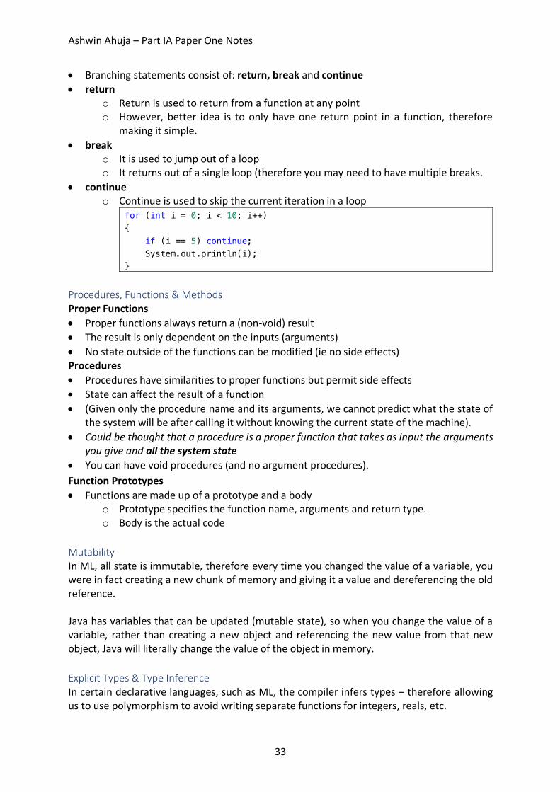
Ashwin Ahuja – Part IA Paper One Notes
33
• Branching statements consist of: return, break and continue • return
o Return is used to return from a function at any point o However, better idea is to only have one return point in a function, therefore
making it simple. • break
o It is used to jump out of a loop o It returns out of a single loop (therefore you may need to have multiple breaks.
• continue o Continue is used to skip the current iteration in a loop
for (int i = 0; i < 10; i++) { if (i == 5) continue; System.out.println(i); }
Procedures, Functions & Methods Proper Functions • Proper functions always return a (non-void) result • The result is only dependent on the inputs (arguments) • No state outside of the functions can be modified (ie no side effects) Procedures • Procedures have similarities to proper functions but permit side effects • State can affect the result of a function • (Given only the procedure name and its arguments, we cannot predict what the state of
the system will be after calling it without knowing the current state of the machine). • Could be thought that a procedure is a proper function that takes as input the arguments
you give and all the system state • You can have void procedures (and no argument procedures). Function Prototypes • Functions are made up of a prototype and a body
o Prototype specifies the function name, arguments and return type. o Body is the actual code
Mutability In ML, all state is immutable, therefore every time you changed the value of a variable, you were in fact creating a new chunk of memory and giving it a value and dereferencing the old reference. Java has variables that can be updated (mutable state), so when you change the value of a variable, rather than creating a new object and referencing the new value from that new object, Java will literally change the value of the object in memory. Explicit Types & Type Inference In certain declarative languages, such as ML, the compiler infers types – therefore allowing us to use polymorphism to avoid writing separate functions for integers, reals, etc.
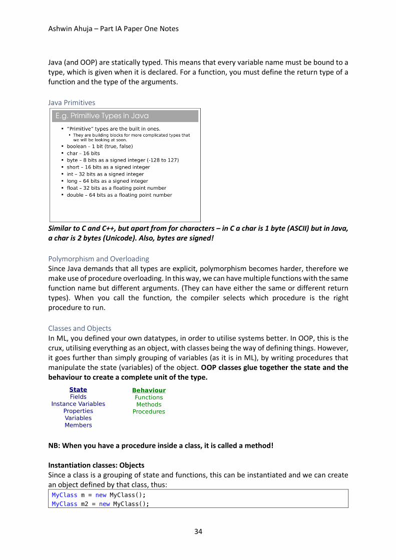
Ashwin Ahuja – Part IA Paper One Notes
34
Java (and OOP) are statically typed. This means that every variable name must be bound to a type, which is given when it is declared. For a function, you must define the return type of a function and the type of the arguments. Java Primitives
Similar to C and C++, but apart from for characters – in C a char is 1 byte (ASCII) but in Java, a char is 2 bytes (Unicode). Also, bytes are signed! Polymorphism and Overloading Since Java demands that all types are explicit, polymorphism becomes harder, therefore we make use of procedure overloading. In this way, we can have multiple functions with the same function name but different arguments. (They can have either the same or different return types). When you call the function, the compiler selects which procedure is the right procedure to run. Classes and Objects In ML, you defined your own datatypes, in order to utilise systems better. In OOP, this is the crux, utilising everything as an object, with classes being the way of defining things. However, it goes further than simply grouping of variables (as it is in ML), by writing procedures that manipulate the state (variables) of the object. OOP classes glue together the state and the behaviour to create a complete unit of the type.
NB: When you have a procedure inside a class, it is called a method! Instantiation classes: Objects Since a class is a grouping of state and functions, this can be instantiated and we can create an object defined by that class, thus: MyClass m = new MyClass(); MyClass m2 = new MyClass();
Ashwin Ahuja – Part IA Paper One Notes
35
For reference: Classes define what properties and procedures every object of the type should have, while each object is a specific implementation with particular values. Programs are therefore made out of lots and lots of Objects which we manipulate. Defining Classes: • Constructors
a. To define a class we need to declare the state and define the methods it contains. However, it also needs to define what should happen when the object gets constructed. When you call the keyword new …(), the …() is actual a function call, calling the constructor method of the class.
b. A constructor has the same name as the class and has no return type (already has the new type, which returns a reference to the new object).
c. However, there can be multiple constructors with different arguments. d. There is also a default constructor – when you provide no constructor, the default
constructor is created which is empty, simply calling super() if there is a parent class.
e. In C++, you can instantiate an object in two different ways. i. MyClass x = new MyClass()
ii. MyClass *y = new MyClass() f. The difference is subtle. X is associated with an object – when x goes out of scope,
so does the object. g. Y is actually a pointer to a newly created object, so when y goes out of scope,
• Static a. If there is state which is more logically associated with a class than an object, it is
made to be static – therefore it is only created once in the program’s execution despite being declared as part of a class and therefore being a part of every object of that class.
b. A static variable is only instantiated once per class not per object. You don’t even need to create an object to access a static variable, simply MyClass.MyVariable would work.
c. Methods can also be static. In this case they must not use anything other than local or static variables, ie cannot use anything which is instance-specific.
d. Why use static methods? i. Easier to debug – only depends on static state
ii. It is self documenting iii. Can call methods without requiring to have an object of that class.t iv. Compiler can produce more efficient code since no specific object involved.
Designing Classes Identifying Classes We always aim to split things into coherent classes, each with a specific item in it, each embodying a specific well-defined concept. We want it to be a grouping of conceptually related state and behaviour.
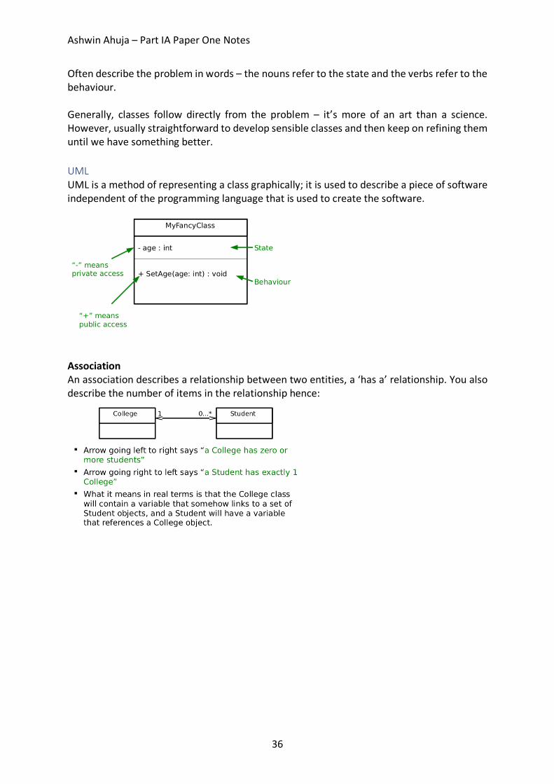
Ashwin Ahuja – Part IA Paper One Notes
36
Often describe the problem in words – the nouns refer to the state and the verbs refer to the behaviour. Generally, classes follow directly from the problem – it’s more of an art than a science. However, usually straightforward to develop sensible classes and then keep on refining them until we have something better. UML UML is a method of representing a class graphically; it is used to describe a piece of software independent of the programming language that is used to create the software.
Association An association describes a relationship between two entities, a ‘has a’ relationship. You also describe the number of items in the relationship hence:

Ashwin Ahuja – Part IA Paper One Notes
37
N.B. If you have a relationship with a 0 on one side, you can simply leave out the arrowhead instead of writing an arrowhead and writing 0. OOP Concepts Modularity Modularity is breaking complex problems into more tractable sub-problems. Each class represents a sub-unit of code that can be developed, tested and updated independently from the rest of the code. This allows two classes (that achieve the same thing but working in different ways) to be easily swapped. This also means that a class can be easily lifted and used in other programs. Code Re-use Code re-use through modularity allows us to take objects from one piece of code and put it into other programs. So, once you’ve developed and tested a class that embodies everything about an item, you can easily use it in lots of other programs with minimal effort. Java also has the method of using packages to group together classes which are conceptually linked together – uk.ac.cam.aa2001… Encapsulation and Information Hiding The idea that a class should expose a clean interface that allows full interaction with the class without exposing anything about its internal state or how it manipulates it. We do this be setting the access modifiers such that the scope of variables and methods are such that only things which are required to see something can see it.
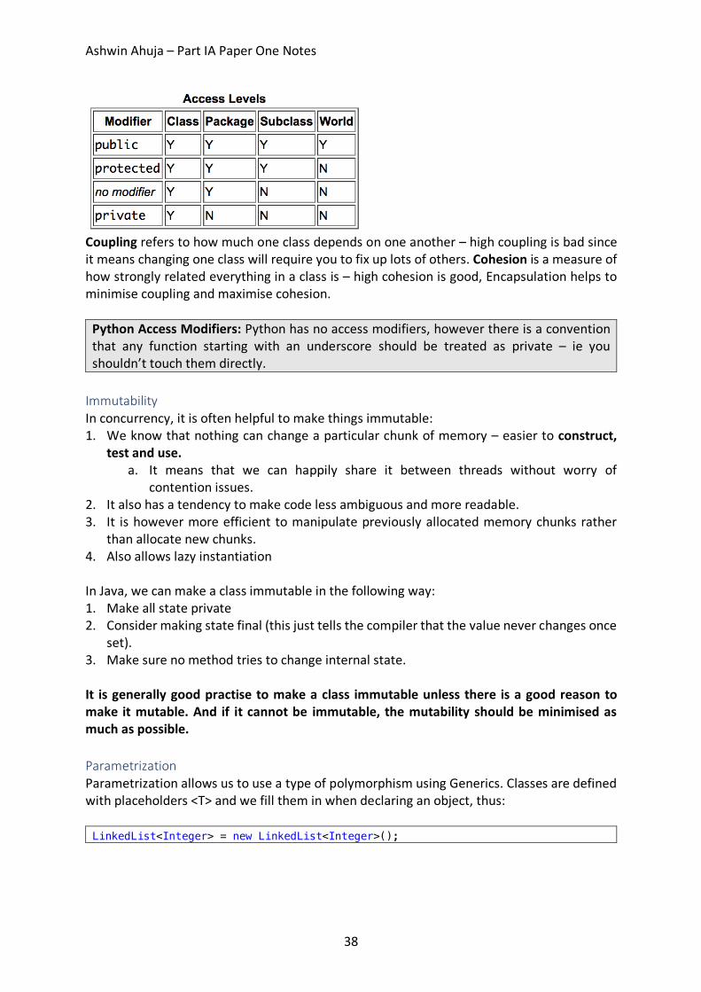
Ashwin Ahuja – Part IA Paper One Notes
38
Coupling refers to how much one class depends on one another – high coupling is bad since it means changing one class will require you to fix up lots of others. Cohesion is a measure of how strongly related everything in a class is – high cohesion is good, Encapsulation helps to minimise coupling and maximise cohesion.
Python Access Modifiers: Python has no access modifiers, however there is a convention that any function starting with an underscore should be treated as private – ie you shouldn’t touch them directly.
Immutability In concurrency, it is often helpful to make things immutable: 1. We know that nothing can change a particular chunk of memory – easier to construct,
test and use. a. It means that we can happily share it between threads without worry of
contention issues. 2. It also has a tendency to make code less ambiguous and more readable. 3. It is however more efficient to manipulate previously allocated memory chunks rather
than allocate new chunks. 4. Also allows lazy instantiation In Java, we can make a class immutable in the following way: 1. Make all state private 2. Consider making state final (this just tells the compiler that the value never changes once
set). 3. Make sure no method tries to change internal state. It is generally good practise to make a class immutable unless there is a good reason to make it mutable. And if it cannot be immutable, the mutability should be minimised as much as possible. Parametrization Parametrization allows us to use a type of polymorphism using Generics. Classes are defined with placeholders <T> and we fill them in when declaring an object, thus: LinkedList<Integer> = new LinkedList<Integer>();
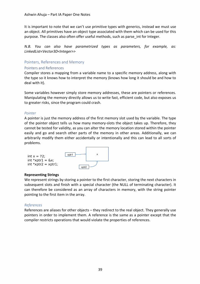
Ashwin Ahuja – Part IA Paper One Notes
39
It is important to note that we can’t use primitive types with generics, instead we must use an object. All primitives have an object type associated with them which can be used for this purpose. The classes also often offer useful methods, such as parse_int for Integer. N.B. You can also have parametrized types as parameters, for example, as: LinkedList<Vector3D<Integer>> Pointers, References and Memory Pointers and References Compiler stores a mapping from a variable name to a specific memory address, along with the type so it knows how to interpret the memory (knows how long it should be and how to deal with it). Some variables however simply store memory addresses, these are pointers or references. Manipulating the memory directly allows us to write fast, efficient code, but also exposes us to greater risks, since the program could crash. Pointer A pointer is just the memory address of the first memory slot used by the variable. The type of the pointer object tells us how many memory-slots the object takes up. Therefore, they cannot be tested for validity, as you can alter the memory location stored within the pointer easily and go and search other parts of the memory in other areas. Additionally, we can arbitrarily modify them either accidentally or intentionally and this can lead to all sorts of problems.
Representing Strings We represent strings by storing a pointer to the first character, storing the next characters in subsequent slots and finish with a special character (the NULL of terminating character). It can therefore be considered as an array of characters in memory, with the string pointer pointing to the first item in the array. References References are aliases for other objects – they redirect to the real object. They generally use pointers in order to implement them. A reference is the same as a pointer except that the compiler restricts operations that would violate the properties of references.
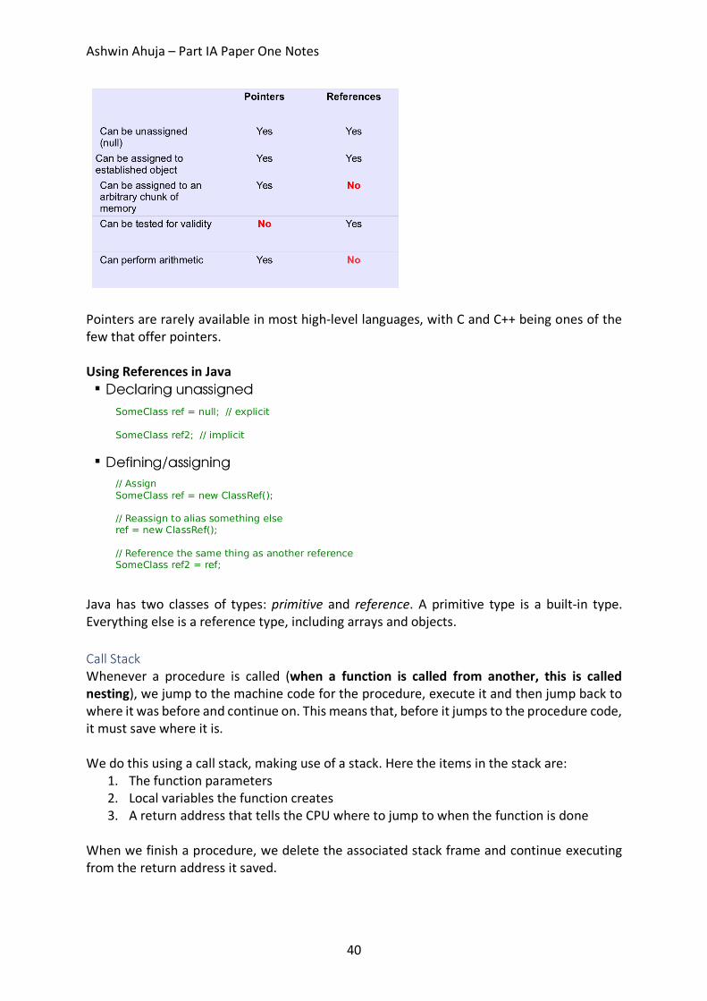
Ashwin Ahuja – Part IA Paper One Notes
40
Pointers are rarely available in most high-level languages, with C and C++ being ones of the few that offer pointers. Using References in Java
Java has two classes of types: primitive and reference. A primitive type is a built-in type. Everything else is a reference type, including arrays and objects. Call Stack Whenever a procedure is called (when a function is called from another, this is called nesting), we jump to the machine code for the procedure, execute it and then jump back to where it was before and continue on. This means that, before it jumps to the procedure code, it must save where it is. We do this using a call stack, making use of a stack. Here the items in the stack are:
1. The function parameters 2. Local variables the function creates 3. A return address that tells the CPU where to jump to when the function is done
When we finish a procedure, we delete the associated stack frame and continue executing from the return address it saved.
Ashwin Ahuja – Part IA Paper One Notes
41
It is important to note that after completing a recursive function or nested functions, you have to return all the way down the stack frame, which takes time (Java is not optimised for recursion). Additionally, while tail-recursive functions are better in ML, they’re only better if the compiler knows it can optimise them to use O(1) space. Java compilers don’t so, so normal iteration is simply better. Heap The heap is a large pool of free memory, which is available to be used, and dynamically allocated rather than statically allocated as per the stack. When we allocate the memory we need from the heap, we store a pointer to the chunk we allocated in the stack. Pointers are of known size, so won’t even increase. For example, if we want to resize our array, we create a new, bigger array, we copy the contents across and update the pointer within the stack. The reference for the array is updated to refer to the array. In fact, the heap gets fragmented, as we create and delete stuff, we leave holes in memory. Occasionally we have to spend time compacting the holes, so it can be used more efficiently. Pass-by-value vs Pass-by-reference Pass-by-value is when an object is copied into a new value in the stack when it is passed as an argument to a procedure, whereas pass-by-reference when a reference is created to the object and this is passed to the procedure. Here you can alter the variable and the change will prevail when you return to the original procedure. Arguments are always passed-by-value in Java, however, you need to be careful about what this means, for the two types of things, primitives and references. In the case of primitives, a copy of the primitive is created and so when the primitive is altered in the procedure, it is irrelevant to the original procedure. However, in the case of objects passed as arguments to the procedure, the reference is what is used to define the object. Therefore, the reference is passed to the procedure (simply a memory address), where an identical copy of the reference is added to the stack frame. Therefore, when the object is altered in the procedure, the value of the changes is maintained when we return to the original procedure.
In C, you can define whether an argument is passed by value or by reference, by putting an ampersand in front of the argument. While powerful, this has the potential to lead to silly errors making programs not work.
Inheritance Inheritance is an extremely powerful concept that is used extensively in good OOP. It is an ‘is-a’ relationship. It means that all state (non-private) and behaviours are taken by the subclass. If a class B extends another class A:
• A is the superclass of B • A is the parent of B • A is the base class of B
Ashwin Ahuja – Part IA Paper One Notes
42
• B is the child of A • B derives from A • B extends A • B inherits from A • B subclasses A
Casting Casting creates a new reference with a different type and points it to the same chunk of memory as the object is in. Everything we need will be in the chunk if we cast to a parent class (plus extra things). If we try to cast to a child class, there won’t be all the necessary info in the memory so it will fail. However, the compiler will still be fine with the case, just returning a runtime error if anything goes wrong. N.B. Casting primitive numeric types ‘(int)2.0’ for example is different, since a new variable of the primitive type is created and assigned the relevant value. Shadowing When using subclasses and superclasses with state, you can do something called shadowing when you create a variable with the same name as one which exists in a subclass. You can deal with both variables separately, using the ‘super.x’ and ‘this.x’ keywords (when referring to variable x). Overriding When a method is written and has the same name as a method in a parent class, there are a couple of things that could happen. It could be treated the same as for fields and the base method could be shadowed and still be accessible. This is the default in C++, but not for Java. In Java, instead the parent class method is overridden, that is it is no longer accessible. You should generally write @Override before the method that is overriding a parent class method, for two reasons. It makes it clear to a programmer that a method has been overridden, also allowing the compiler to check that a method has been overridden, checking for a misspelling or things like that. Abstract Methods and Classes An abstract method is used in a base class to force a class that extends it to implement a method, but you don’t know what the implementation will be in the parent class. Therefore an abstract method can be used for this – it only contains the function definition (the method prototype or method stub) of the function, rather than having the implementation of the function at all. It works in a contractual way, any non-abstract class that inherits from this class must have that method implemented.
Ashwin Ahuja – Part IA Paper One Notes
43
If a class has an abstract method, it must also be abstract. This means that the class is not able to be instantiated, therefore you can’t make an object from it. This is useful when we have an abstract concept that is used a base class – for example a car (when we then define models of cars are then defined); we don’t want to be able therefore to just make a generic car object. A class is shown as being abstract in UML by having the class or method in italics. Polymorphism There is the general problem of when we refer to an object via a parent type and both types implement a particular method, which method should it run, such as in this: Student s = new Student(); // Person and Student both have a dance method Person p = (Person)s; p.dance();
Static Polymorphism In static polymorphism, we decide which method to run at compile-time (this is also called early binding). Since we don’t know what the true type of the object will be, we just run the parent method. Therefore, if there are any type errors, they appear at compile-time. Dynamic Polymorphism In dynamic polymorphism, the method is run in the child. Therefore, it must be done at run-time since that is when we know the child’s type. Therefore, any errors will cause run-time faults… (the program will entirely crash). This form of polymorphism is OOP-specific and is called sub-type or ad-hoc polymorphism. Because it must check types at runtime (late binding), there is a performance overhead associated with dynamic polymorphism. However, it gives us more flexibility and makes code more readable. Implementations of Polymorphism
Though some people would consider Java’s use of the word final as a way of using static polymorphism, in fact it just means the method cannot be overridden in a subclass, which is entirely different. The compiler isn’t really choosing between multiple implementations but rather enforcing that there can only be one implementation. Multiple Inheritance and Interfaces The theory of multiple inheritance is that we can create a class which is made of up multiple things, for example DrawableFish is a DrawableEntity and a Fish.
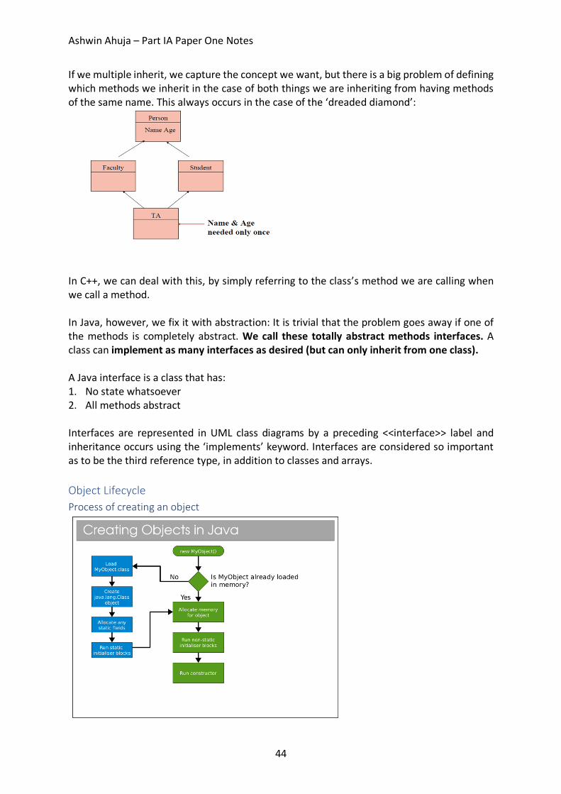
Ashwin Ahuja – Part IA Paper One Notes
44
If we multiple inherit, we capture the concept we want, but there is a big problem of defining which methods we inherit in the case of both things we are inheriting from having methods of the same name. This always occurs in the case of the ‘dreaded diamond’:
In C++, we can deal with this, by simply referring to the class’s method we are calling when we call a method. In Java, however, we fix it with abstraction: It is trivial that the problem goes away if one of the methods is completely abstract. We call these totally abstract methods interfaces. A class can implement as many interfaces as desired (but can only inherit from one class). A Java interface is a class that has: 1. No state whatsoever 2. All methods abstract Interfaces are represented in UML class diagrams by a preceding <<interface>> label and inheritance occurs using the ‘implements’ keyword. Interfaces are considered so important as to be the third reference type, in addition to classes and arrays. Object Lifecycle Process of creating an object
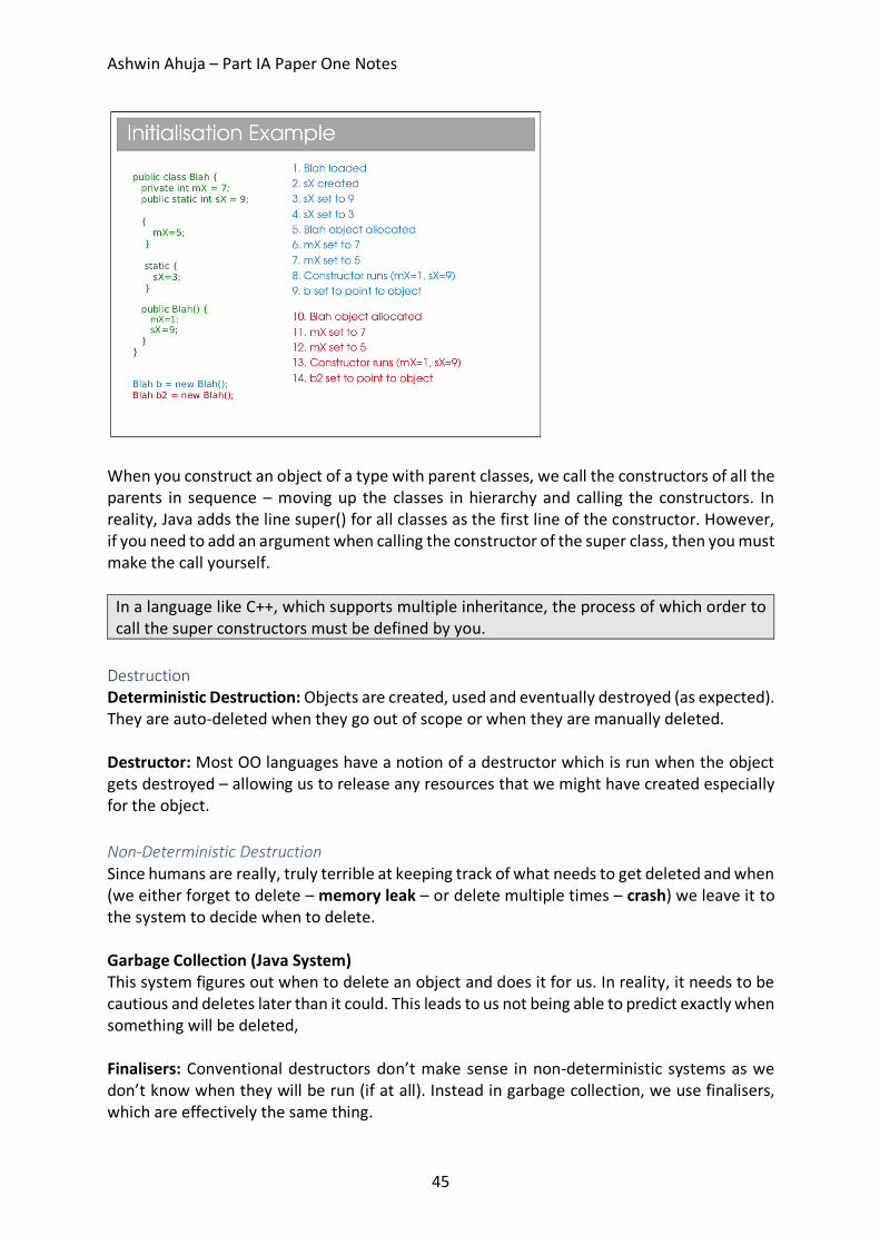
Ashwin Ahuja – Part IA Paper One Notes
45
When you construct an object of a type with parent classes, we call the constructors of all the parents in sequence – moving up the classes in hierarchy and calling the constructors. In reality, Java adds the line super() for all classes as the first line of the constructor. However, if you need to add an argument when calling the constructor of the super class, then you must make the call yourself.
In a language like C++, which supports multiple inheritance, the process of which order to call the super constructors must be defined by you.
Destruction Deterministic Destruction: Objects are created, used and eventually destroyed (as expected). They are auto-deleted when they go out of scope or when they are manually deleted. Destructor: Most OO languages have a notion of a destructor which is run when the object gets destroyed – allowing us to release any resources that we might have created especially for the object. Non-Deterministic Destruction Since humans are really, truly terrible at keeping track of what needs to get deleted and when (we either forget to delete – memory leak – or delete multiple times – crash) we leave it to the system to decide when to delete. Garbage Collection (Java System) This system figures out when to delete an object and does it for us. In reality, it needs to be cautious and deletes later than it could. This leads to us not being able to predict exactly when something will be deleted, Finalisers: Conventional destructors don’t make sense in non-deterministic systems as we don’t know when they will be run (if at all). Instead in garbage collection, we use finalisers, which are effectively the same thing.
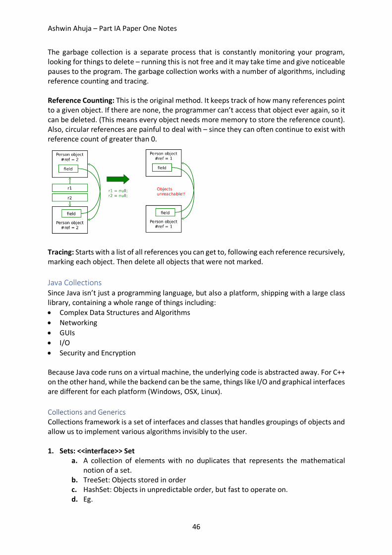
Ashwin Ahuja – Part IA Paper One Notes
46
The garbage collection is a separate process that is constantly monitoring your program, looking for things to delete – running this is not free and it may take time and give noticeable pauses to the program. The garbage collection works with a number of algorithms, including reference counting and tracing. Reference Counting: This is the original method. It keeps track of how many references point to a given object. If there are none, the programmer can’t access that object ever again, so it can be deleted. (This means every object needs more memory to store the reference count). Also, circular references are painful to deal with – since they can often continue to exist with reference count of greater than 0.
Tracing: Starts with a list of all references you can get to, following each reference recursively, marking each object. Then delete all objects that were not marked. Java Collections Since Java isn’t just a programming language, but also a platform, shipping with a large class library, containing a whole range of things including: • Complex Data Structures and Algorithms • Networking • GUIs • I/O • Security and Encryption Because Java code runs on a virtual machine, the underlying code is abstracted away. For C++ on the other hand, while the backend can be the same, things like I/O and graphical interfaces are different for each platform (Windows, OSX, Linux). Collections and Generics Collections framework is a set of interfaces and classes that handles groupings of objects and allow us to implement various algorithms invisibly to the user. 1. Sets: <<interface>> Set
a. A collection of elements with no duplicates that represents the mathematical notion of a set.
b. TreeSet: Objects stored in order c. HashSet: Objects in unpredictable order, but fast to operate on. d. Eg.
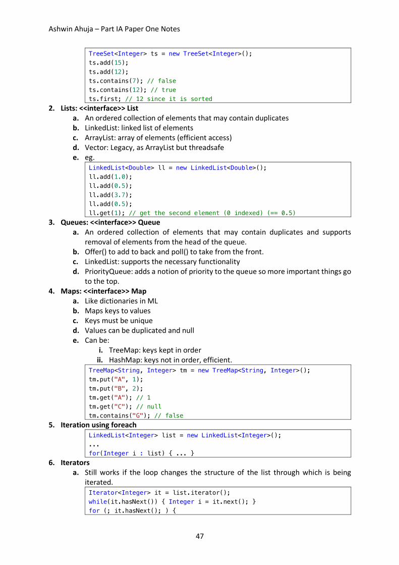
Ashwin Ahuja – Part IA Paper One Notes
47
TreeSet<Integer> ts = new TreeSet<Integer>(); ts.add(15); ts.add(12); ts.contains(7); // false ts.contains(12); // true ts.first; // 12 since it is sorted
2. Lists: <<interface>> List a. An ordered collection of elements that may contain duplicates b. LinkedList: linked list of elements c. ArrayList: array of elements (efficient access) d. Vector: Legacy, as ArrayList but threadsafe e. eg.
LinkedList<Double> ll = new LinkedList<Double>(); ll.add(1.0); ll.add(0.5); ll.add(3.7); ll.add(0.5); ll.get(1); // get the second element (0 indexed) (== 0.5)
3. Queues: <<interface>> Queue a. An ordered collection of elements that may contain duplicates and supports
removal of elements from the head of the queue. b. Offer() to add to back and poll() to take from the front. c. LinkedList: supports the necessary functionality d. PriorityQueue: adds a notion of priority to the queue so more important things go
to the top. 4. Maps: <<interface>> Map
a. Like dictionaries in ML b. Maps keys to values c. Keys must be unique d. Values can be duplicated and null e. Can be:
i. TreeMap: keys kept in order ii. HashMap: keys not in order, efficient.
TreeMap<String, Integer> tm = new TreeMap<String, Integer>(); tm.put("A", 1); tm.put("B", 2); tm.get("A"); // 1 tm.get("C"); // null tm.contains("G"); // false
5. Iteration using foreach LinkedList<Integer> list = new LinkedList<Integer>(); ... for(Integer i : list) { ... }
6. Iterators a. Still works if the loop changes the structure of the list through which is being
iterated. Iterator<Integer> it = list.iterator(); while(it.hasNext()) { Integer i = it.next(); } for (; it.hasNext(); ) {
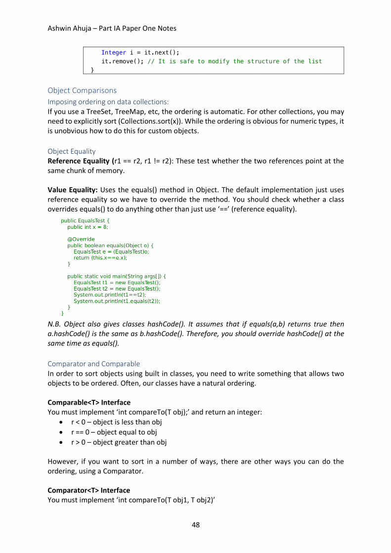
Ashwin Ahuja – Part IA Paper One Notes
48
Integer i = it.next(); it.remove(); // It is safe to modify the structure of the list }
Object Comparisons Imposing ordering on data collections: If you use a TreeSet, TreeMap, etc, the ordering is automatic. For other collections, you may need to explicitly sort (Collections.sort(x)). While the ordering is obvious for numeric types, it is unobvious how to do this for custom objects. Object Equality Reference Equality (r1 == r2, r1 != r2): These test whether the two references point at the same chunk of memory. Value Equality: Uses the equals() method in Object. The default implementation just uses reference equality so we have to override the method. You should check whether a class overrides equals() to do anything other than just use ‘==’ (reference equality).
N.B. Object also gives classes hashCode(). It assumes that if equals(a,b) returns true then a.hashCode() is the same as b.hashCode(). Therefore, you should override hashCode() at the same time as equals(). Comparator and Comparable In order to sort objects using built in classes, you need to write something that allows two objects to be ordered. Often, our classes have a natural ordering. Comparable<T> Interface You must implement ‘int compareTo(T obj);’ and return an integer:
• r < 0 – object is less than obj • r == 0 – object equal to obj • r > 0 – object greater than obj
However, if you want to sort in a number of ways, there are other ways you can do the ordering, using a Comparator. Comparator<T> Interface You must implement ‘int compareTo(T obj1, T obj2)’
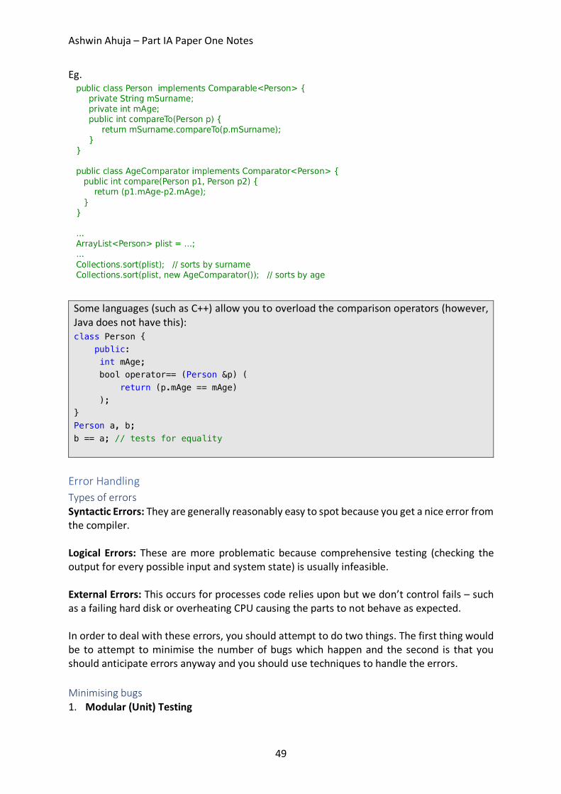
Ashwin Ahuja – Part IA Paper One Notes
49
Eg.
Some languages (such as C++) allow you to overload the comparison operators (however, Java does not have this): class Person { public: int mAge; bool operator== (Person &p) ( return (p.mAge == mAge) ); } Person a, b; b == a; // tests for equality
Error Handling Types of errors Syntactic Errors: They are generally reasonably easy to spot because you get a nice error from the compiler. Logical Errors: These are more problematic because comprehensive testing (checking the output for every possible input and system state) is usually infeasible. External Errors: This occurs for processes code relies upon but we don’t control fails – such as a failing hard disk or overheating CPU causing the parts to not behave as expected. In order to deal with these errors, you should attempt to do two things. The first thing would be to attempt to minimise the number of bugs which happen and the second is that you should anticipate errors anyway and you should use techniques to handle the errors. Minimising bugs 1. Modular (Unit) Testing
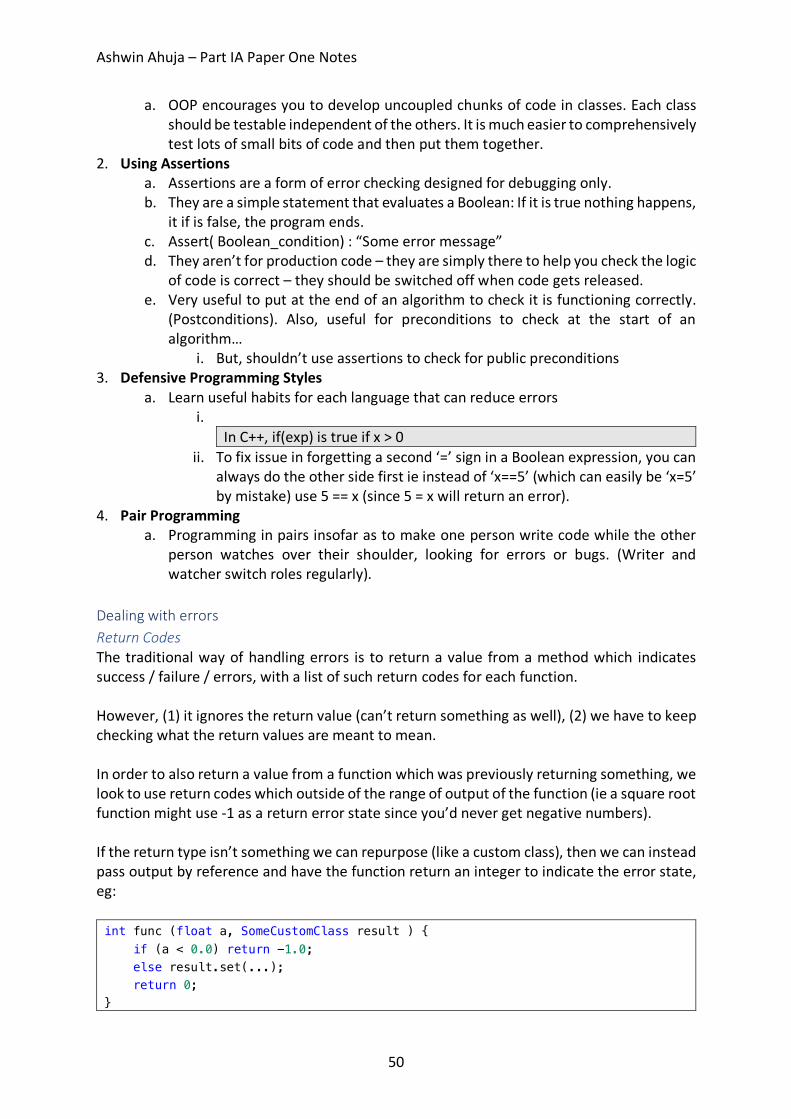
Ashwin Ahuja – Part IA Paper One Notes
50
a. OOP encourages you to develop uncoupled chunks of code in classes. Each class should be testable independent of the others. It is much easier to comprehensively test lots of small bits of code and then put them together.
2. Using Assertions a. Assertions are a form of error checking designed for debugging only. b. They are a simple statement that evaluates a Boolean: If it is true nothing happens,
it if is false, the program ends. c. Assert( Boolean_condition) : “Some error message” d. They aren’t for production code – they are simply there to help you check the logic
of code is correct – they should be switched off when code gets released. e. Very useful to put at the end of an algorithm to check it is functioning correctly.
(Postconditions). Also, useful for preconditions to check at the start of an algorithm…
i. But, shouldn’t use assertions to check for public preconditions 3. Defensive Programming Styles
a. Learn useful habits for each language that can reduce errors i.
In C++, if(exp) is true if x > 0 ii. To fix issue in forgetting a second ‘=’ sign in a Boolean expression, you can
always do the other side first ie instead of ‘x==5’ (which can easily be ‘x=5’ by mistake) use 5 == x (since 5 = x will return an error).
4. Pair Programming a. Programming in pairs insofar as to make one person write code while the other
person watches over their shoulder, looking for errors or bugs. (Writer and watcher switch roles regularly).
Dealing with errors Return Codes The traditional way of handling errors is to return a value from a method which indicates success / failure / errors, with a list of such return codes for each function. However, (1) it ignores the return value (can’t return something as well), (2) we have to keep checking what the return values are meant to mean. In order to also return a value from a function which was previously returning something, we look to use return codes which outside of the range of output of the function (ie a square root function might use -1 as a return error state since you’d never get negative numbers). If the return type isn’t something we can repurpose (like a custom class), then we can instead pass output by reference and have the function return an integer to indicate the error state, eg: int func (float a, SomeCustomClass result ) { if (a < 0.0) return -1.0; else result.set(...); return 0; }
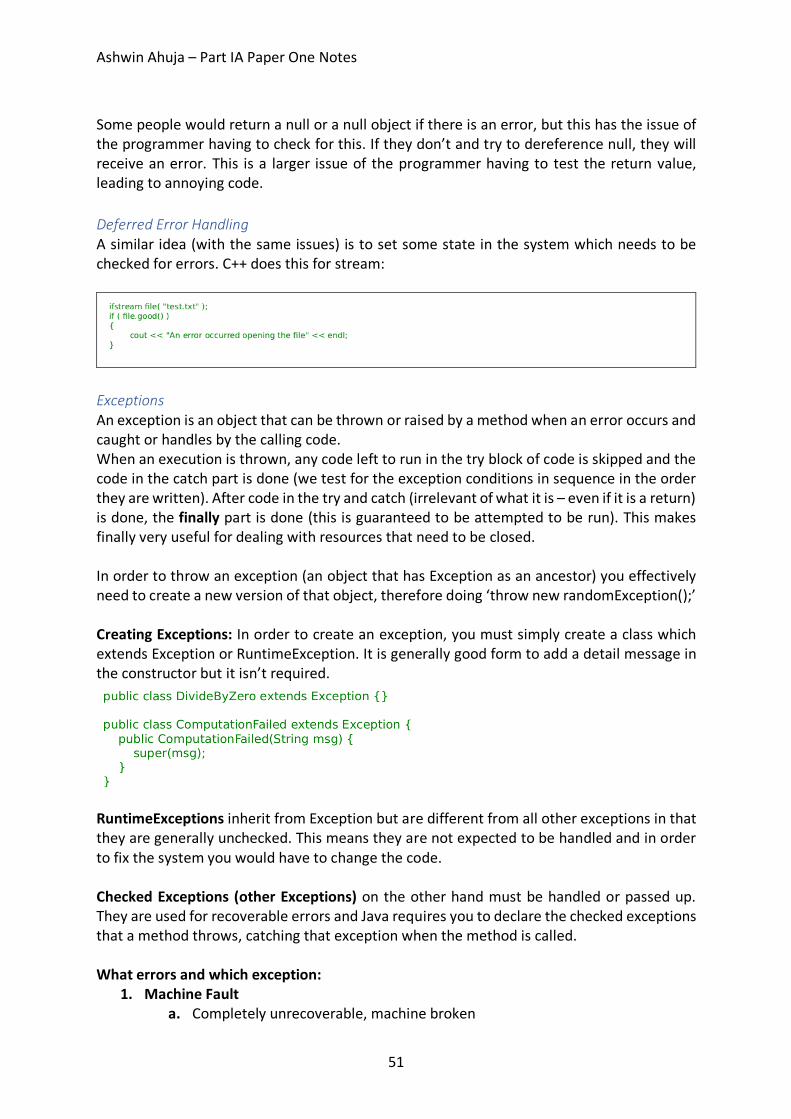
Ashwin Ahuja – Part IA Paper One Notes
51
Some people would return a null or a null object if there is an error, but this has the issue of the programmer having to check for this. If they don’t and try to dereference null, they will receive an error. This is a larger issue of the programmer having to test the return value, leading to annoying code. Deferred Error Handling A similar idea (with the same issues) is to set some state in the system which needs to be checked for errors. C++ does this for stream:
Exceptions An exception is an object that can be thrown or raised by a method when an error occurs and caught or handles by the calling code. When an execution is thrown, any code left to run in the try block of code is skipped and the code in the catch part is done (we test for the exception conditions in sequence in the order they are written). After code in the try and catch (irrelevant of what it is – even if it is a return) is done, the finally part is done (this is guaranteed to be attempted to be run). This makes finally very useful for dealing with resources that need to be closed. In order to throw an exception (an object that has Exception as an ancestor) you effectively need to create a new version of that object, therefore doing ‘throw new randomException();’ Creating Exceptions: In order to create an exception, you must simply create a class which extends Exception or RuntimeException. It is generally good form to add a detail message in the constructor but it isn’t required.
RuntimeExceptions inherit from Exception but are different from all other exceptions in that they are generally unchecked. This means they are not expected to be handled and in order to fix the system you would have to change the code. Checked Exceptions (other Exceptions) on the other hand must be handled or passed up. They are used for recoverable errors and Java requires you to declare the checked exceptions that a method throws, catching that exception when the method is called. What errors and which exception:
1. Machine Fault a. Completely unrecoverable, machine broken
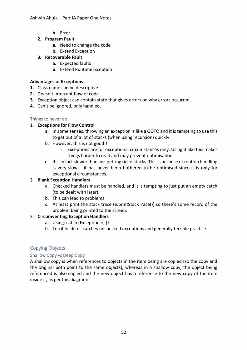
Ashwin Ahuja – Part IA Paper One Notes
52
b. Error 2. Program Fault
a. Need to change the code b. Extend Exception
3. Recoverable Fault a. Expected faults b. Extend RuntimeException
Advantages of Exceptions 1. Class name can be descriptive 2. Doesn’t interrupt flow of code 3. Exception object can contain state that gives errors on why errors occurred. 4. Can’t be ignored, only handled. Things to never do 1. Exceptions for Flow Control
a. In some senses, throwing an exception is like a GOTO and it is tempting to use this to get out of a lot of stacks (when using recursion) quickly
b. However, this is not good!! i. Exceptions are for exceptional circumstances only. Using it like this makes
things harder to read and may prevent optimisations c. It is in fact slower than just getting rid of stacks. This is because exception handling
is very slow – it has never been bothered to be optimised since it is only for exceptional circumstances.
2. Blank Exception Handlers a. Checked handlers must be handled, and it is tempting to just put an empty catch
(to be dealt with later). b. This can lead to problems c. At least print the stack trace (e.printStackTrace()) so there’s some record of the
problem being printed to the screen. 3. Circumventing Exception Handlers
a. Using: catch (Exception e) {} b. Terrible idea – catches unchecked exceptions and generally terrible practise.
Copying Objects Shallow Copy vs Deep Copy A shallow copy is when references to objects in the item being are copied (so the copy and the original both point to the same objects), whereas in a shallow copy, the object being referenced is also copied and the new object has a reference to the new copy of the item inside it, as per this diagram:
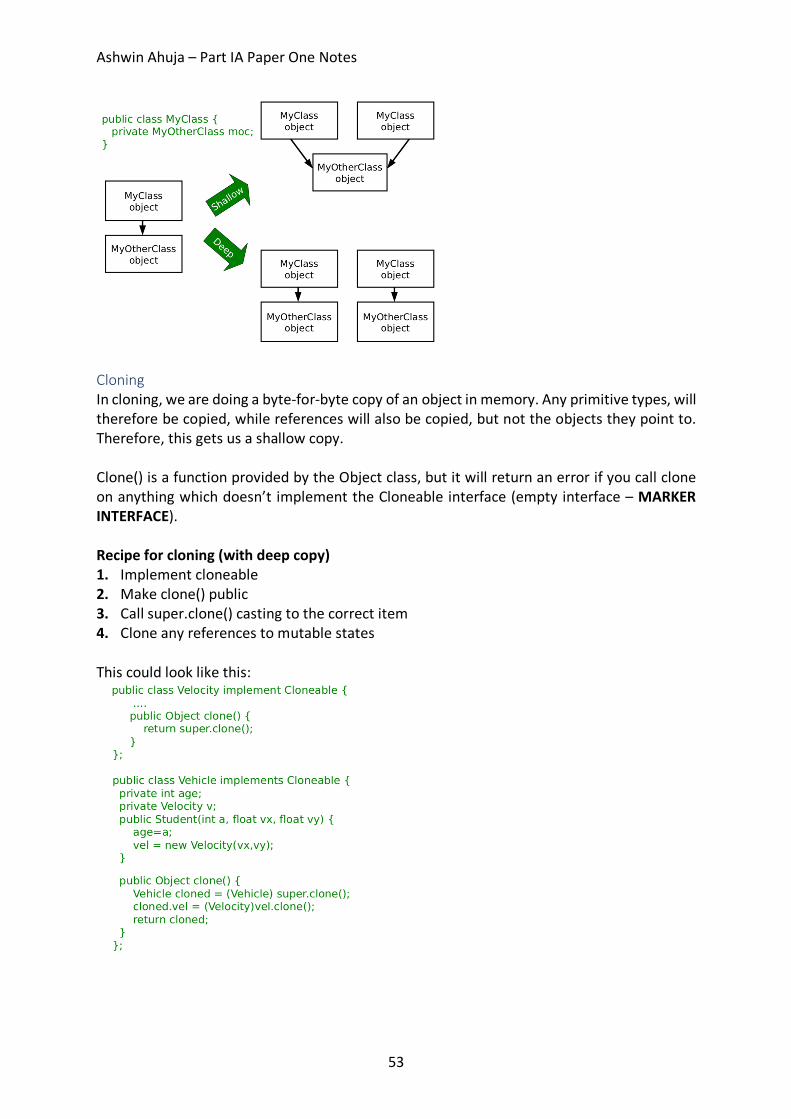
Ashwin Ahuja – Part IA Paper One Notes
53
Cloning In cloning, we are doing a byte-for-byte copy of an object in memory. Any primitive types, will therefore be copied, while references will also be copied, but not the objects they point to. Therefore, this gets us a shallow copy. Clone() is a function provided by the Object class, but it will return an error if you call clone on anything which doesn’t implement the Cloneable interface (empty interface – MARKER INTERFACE). Recipe for cloning (with deep copy) 1. Implement cloneable 2. Make clone() public 3. Call super.clone() casting to the correct item 4. Clone any references to mutable states This could look like this:
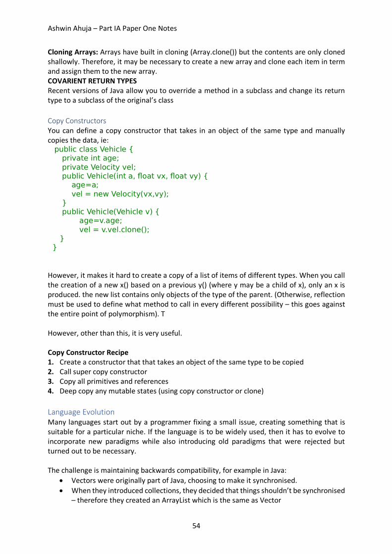
Ashwin Ahuja – Part IA Paper One Notes
54
Cloning Arrays: Arrays have built in cloning (Array.clone()) but the contents are only cloned shallowly. Therefore, it may be necessary to create a new array and clone each item in term and assign them to the new array. COVARIENT RETURN TYPES Recent versions of Java allow you to override a method in a subclass and change its return type to a subclass of the original’s class Copy Constructors You can define a copy constructor that takes in an object of the same type and manually copies the data, ie:
However, it makes it hard to create a copy of a list of items of different types. When you call the creation of a new x() based on a previous y() (where y may be a child of x), only an x is produced. the new list contains only objects of the type of the parent. (Otherwise, reflection must be used to define what method to call in every different possibility – this goes against the entire point of polymorphism). T However, other than this, it is very useful. Copy Constructor Recipe 1. Create a constructor that that takes an object of the same type to be copied 2. Call super copy constructor 3. Copy all primitives and references 4. Deep copy any mutable states (using copy constructor or clone) Language Evolution Many languages start out by a programmer fixing a small issue, creating something that is suitable for a particular niche. If the language is to be widely used, then it has to evolve to incorporate new paradigms while also introducing old paradigms that were rejected but turned out to be necessary. The challenge is maintaining backwards compatibility, for example in Java:
• Vectors were originally part of Java, choosing to make it synchronised. • When they introduced collections, they decided that things shouldn’t be synchronised
– therefore they created an ArrayList which is the same as Vector
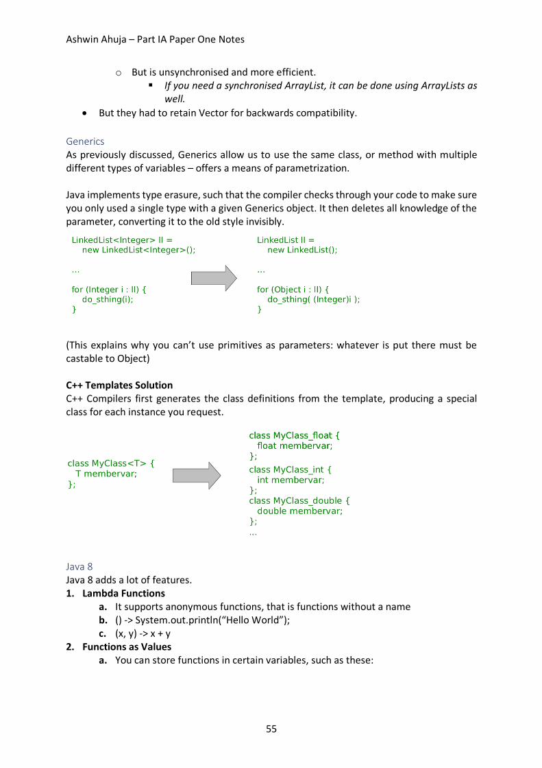
Ashwin Ahuja – Part IA Paper One Notes
55
o But is unsynchronised and more efficient. § If you need a synchronised ArrayList, it can be done using ArrayLists as
well. • But they had to retain Vector for backwards compatibility.
Generics As previously discussed, Generics allow us to use the same class, or method with multiple different types of variables – offers a means of parametrization. Java implements type erasure, such that the compiler checks through your code to make sure you only used a single type with a given Generics object. It then deletes all knowledge of the parameter, converting it to the old style invisibly.
(This explains why you can’t use primitives as parameters: whatever is put there must be castable to Object) C++ Templates Solution C++ Compilers first generates the class definitions from the template, producing a special class for each instance you request.
Java 8 Java 8 adds a lot of features. 1. Lambda Functions
a. It supports anonymous functions, that is functions without a name b. () -> System.out.println(“Hello World”); c. (x, y) -> x + y
2. Functions as Values a. You can store functions in certain variables, such as these:
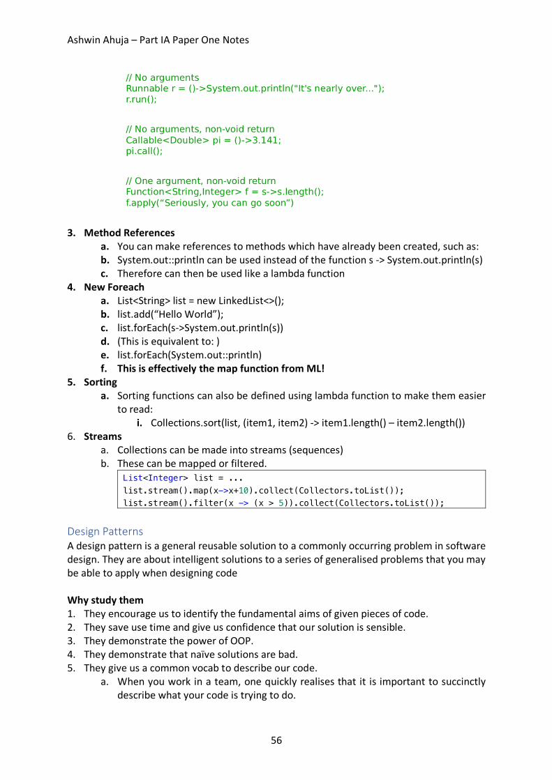
Ashwin Ahuja – Part IA Paper One Notes
56
3. Method References
a. You can make references to methods which have already been created, such as: b. System.out::println can be used instead of the function s -> System.out.println(s) c. Therefore can then be used like a lambda function
4. New Foreach a. List<String> list = new LinkedList<>(); b. list.add(“Hello World”); c. list.forEach(s->System.out.println(s)) d. (This is equivalent to: ) e. list.forEach(System.out::println) f. This is effectively the map function from ML!
5. Sorting a. Sorting functions can also be defined using lambda function to make them easier
to read: i. Collections.sort(list, (item1, item2) -> item1.length() – item2.length())
6. Streams a. Collections can be made into streams (sequences) b. These can be mapped or filtered.
List<Integer> list = ... list.stream().map(x->x+10).collect(Collectors.toList()); list.stream().filter(x -> (x > 5)).collect(Collectors.toList());
Design Patterns A design pattern is a general reusable solution to a commonly occurring problem in software design. They are about intelligent solutions to a series of generalised problems that you may be able to apply when designing code Why study them 1. They encourage us to identify the fundamental aims of given pieces of code. 2. They save use time and give us confidence that our solution is sensible. 3. They demonstrate the power of OOP. 4. They demonstrate that naïve solutions are bad. 5. They give us a common vocab to describe our code.
a. When you work in a team, one quickly realises that it is important to succinctly describe what your code is trying to do.
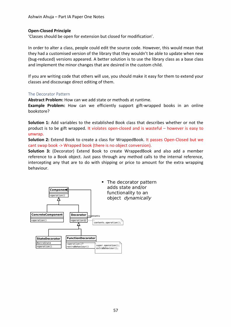
Ashwin Ahuja – Part IA Paper One Notes
57
Open-Closed Principle ‘Classes should be open for extension but closed for modification’. In order to alter a class, people could edit the source code. However, this would mean that they had a customised version of the library that they wouldn’t be able to update when new (bug-reduced) versions appeared. A better solution is to use the library class as a base class and implement the minor changes that are desired in the custom child. If you are writing code that others will use, you should make it easy for them to extend your classes and discourage direct editing of them. The Decorator Pattern Abstract Problem: How can we add state or methods at runtime. Example Problem: How can we efficiently support gift-wrapped books in an online bookstore? Solution 1: Add variables to the established Book class that describes whether or not the product is to be gift wrapped. It violates open-closed and is wasteful – however is easy to unwrap. Solution 2: Extend Book to create a class for WrappedBook. It passes Open-Closed but we cant swap book -> Wrapped book (there is no object conversion). Solution 3: (Decorator) Extend Book to create WrappedBook and also add a member reference to a Book object. Just pass through any method calls to the internal reference, intercepting any that are to do with shipping or price to amount for the extra wrapping behaviour.
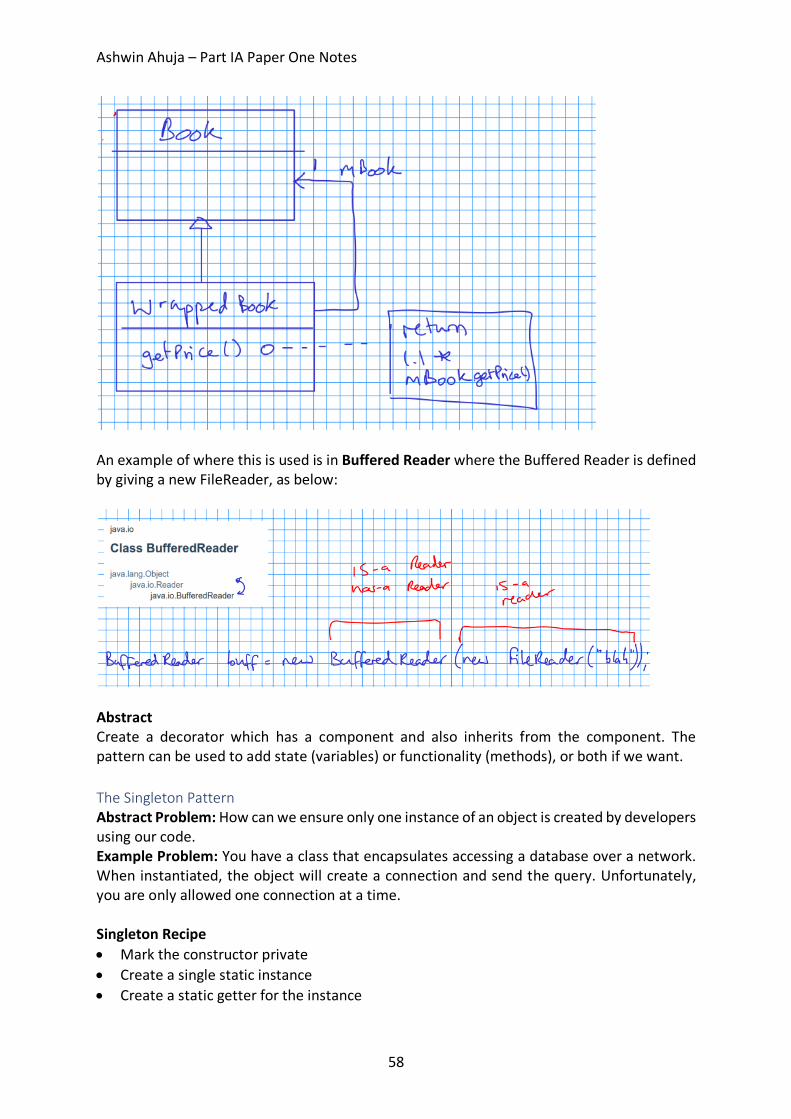
Ashwin Ahuja – Part IA Paper One Notes
58
An example of where this is used is in Buffered Reader where the Buffered Reader is defined by giving a new FileReader, as below:
Abstract Create a decorator which has a component and also inherits from the component. The pattern can be used to add state (variables) or functionality (methods), or both if we want. The Singleton Pattern Abstract Problem: How can we ensure only one instance of an object is created by developers using our code. Example Problem: You have a class that encapsulates accessing a database over a network. When instantiated, the object will create a connection and send the query. Unfortunately, you are only allowed one connection at a time. Singleton Recipe • Mark the constructor private • Create a single static instance • Create a static getter for the instance
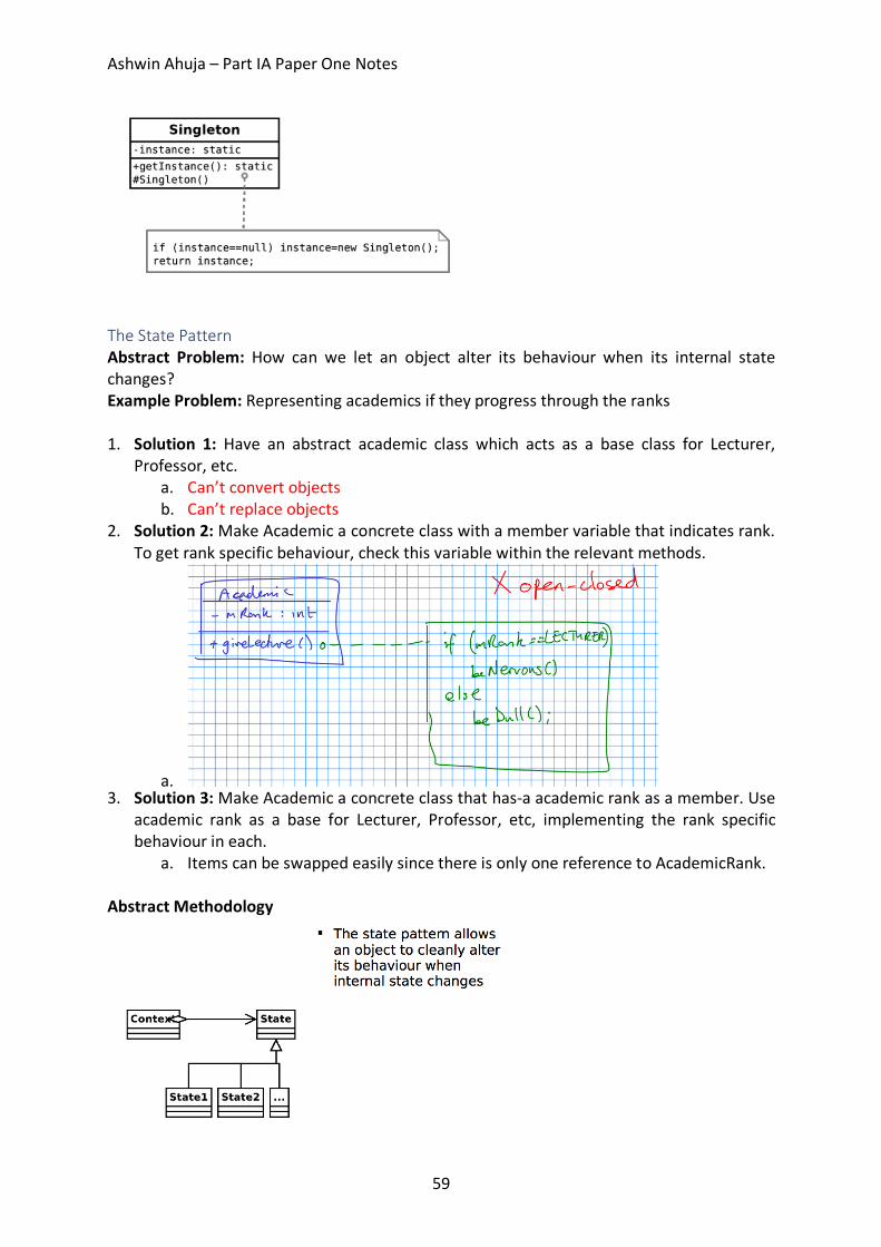
Ashwin Ahuja – Part IA Paper One Notes
59
The State Pattern Abstract Problem: How can we let an object alter its behaviour when its internal state changes? Example Problem: Representing academics if they progress through the ranks 1. Solution 1: Have an abstract academic class which acts as a base class for Lecturer,
Professor, etc. a. Can’t convert objects b. Can’t replace objects
2. Solution 2: Make Academic a concrete class with a member variable that indicates rank. To get rank specific behaviour, check this variable within the relevant methods.
a. 3. Solution 3: Make Academic a concrete class that has-a academic rank as a member. Use
academic rank as a base for Lecturer, Professor, etc, implementing the rank specific behaviour in each.
a. Items can be swapped easily since there is only one reference to AcademicRank. Abstract Methodology
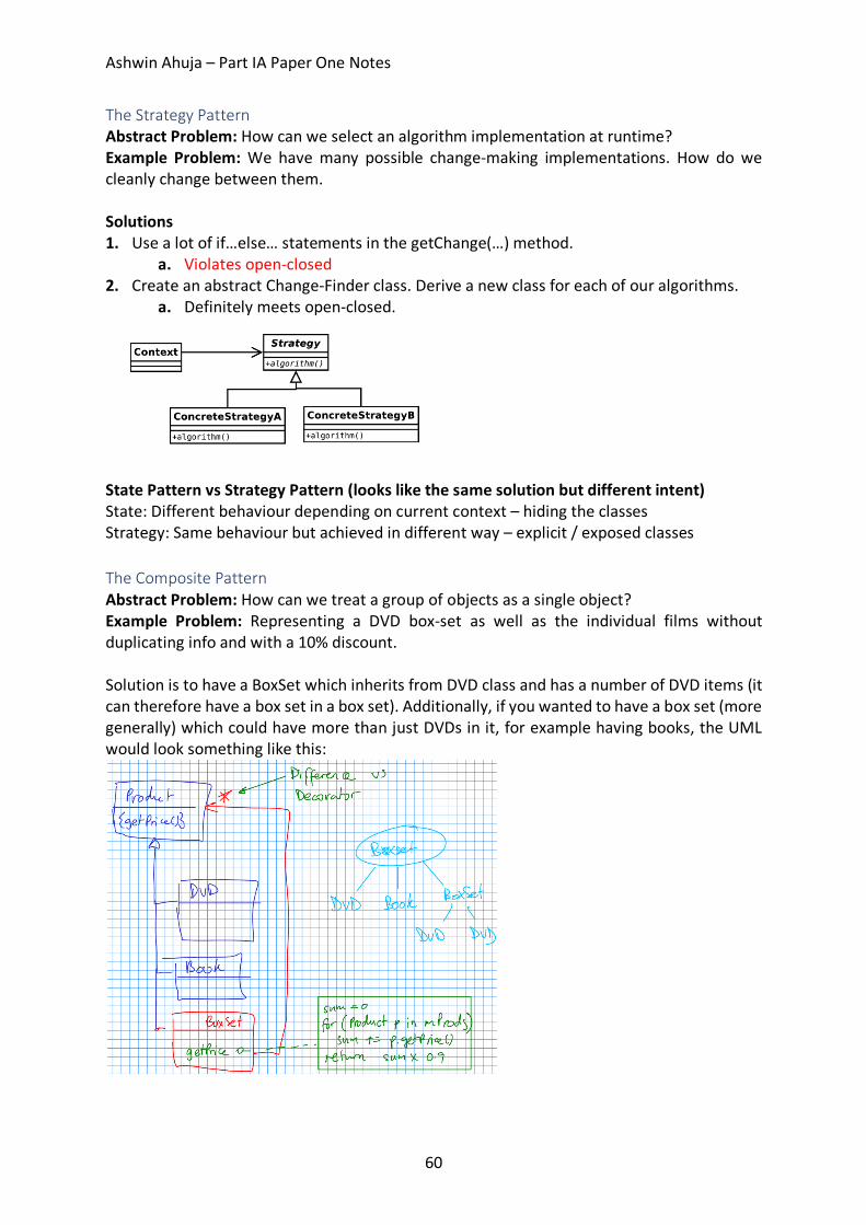
Ashwin Ahuja – Part IA Paper One Notes
60
The Strategy Pattern Abstract Problem: How can we select an algorithm implementation at runtime? Example Problem: We have many possible change-making implementations. How do we cleanly change between them. Solutions 1. Use a lot of if…else… statements in the getChange(…) method.
a. Violates open-closed 2. Create an abstract Change-Finder class. Derive a new class for each of our algorithms.
a. Definitely meets open-closed.
State Pattern vs Strategy Pattern (looks like the same solution but different intent) State: Different behaviour depending on current context – hiding the classes Strategy: Same behaviour but achieved in different way – explicit / exposed classes The Composite Pattern Abstract Problem: How can we treat a group of objects as a single object? Example Problem: Representing a DVD box-set as well as the individual films without duplicating info and with a 10% discount. Solution is to have a BoxSet which inherits from DVD class and has a number of DVD items (it can therefore have a box set in a box set). Additionally, if you wanted to have a box set (more generally) which could have more than just DVDs in it, for example having books, the UML would look something like this:
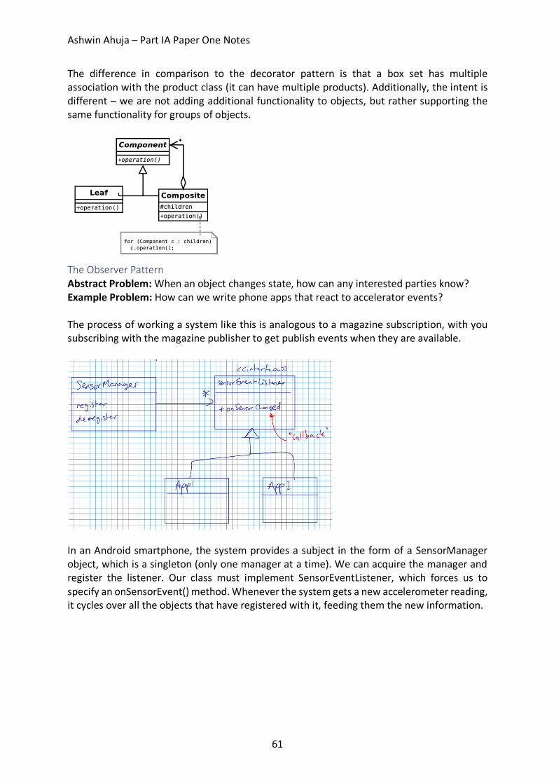
Ashwin Ahuja – Part IA Paper One Notes
61
The difference in comparison to the decorator pattern is that a box set has multiple association with the product class (it can have multiple products). Additionally, the intent is different – we are not adding additional functionality to objects, but rather supporting the same functionality for groups of objects.
The Observer Pattern Abstract Problem: When an object changes state, how can any interested parties know? Example Problem: How can we write phone apps that react to accelerator events? The process of working a system like this is analogous to a magazine subscription, with you subscribing with the magazine publisher to get publish events when they are available.
In an Android smartphone, the system provides a subject in the form of a SensorManager object, which is a singleton (only one manager at a time). We can acquire the manager and register the listener. Our class must implement SensorEventListener, which forces us to specify an onSensorEvent() method. Whenever the system gets a new accelerometer reading, it cycles over all the objects that have registered with it, feeding them the new information.
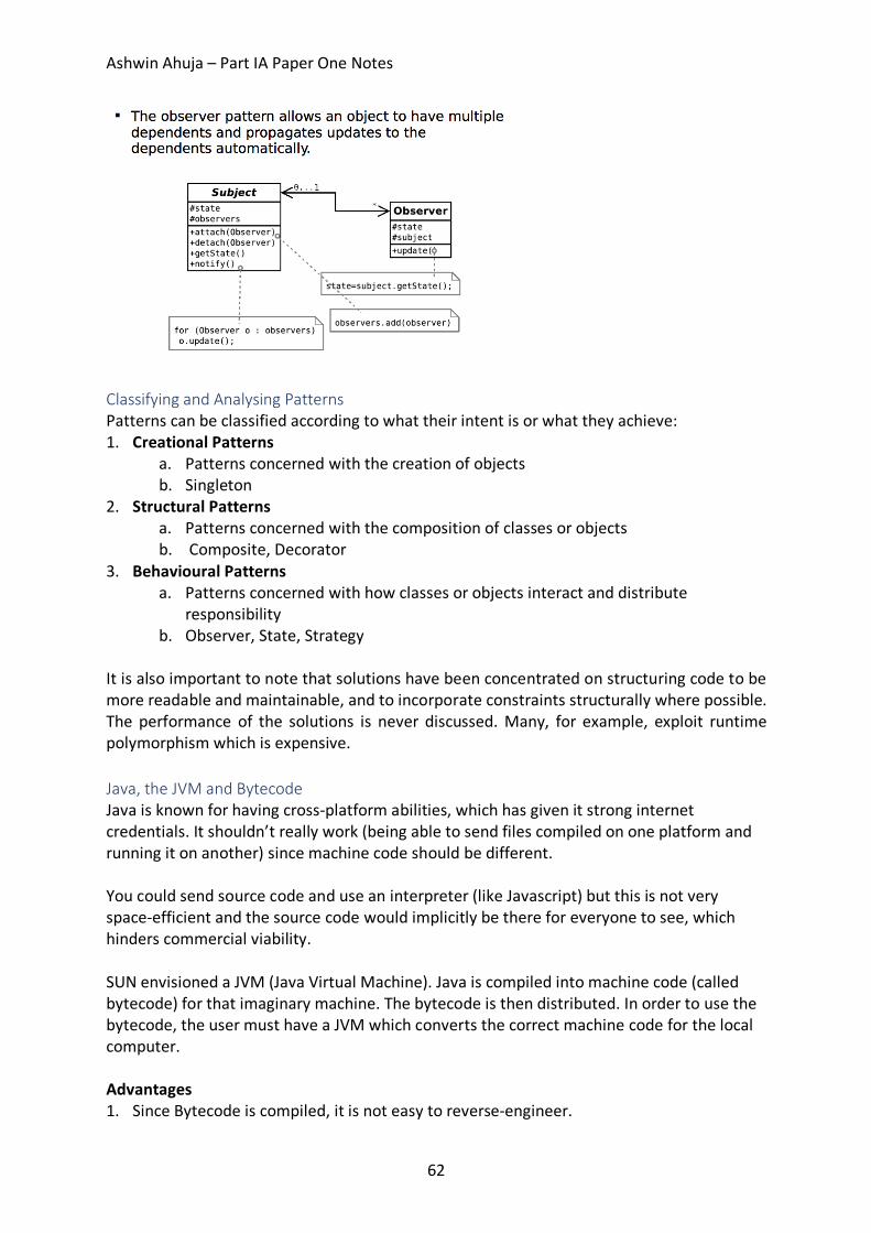
Ashwin Ahuja – Part IA Paper One Notes
62
Classifying and Analysing Patterns Patterns can be classified according to what their intent is or what they achieve: 1. Creational Patterns
a. Patterns concerned with the creation of objects b. Singleton
2. Structural Patterns a. Patterns concerned with the composition of classes or objects b. Composite, Decorator
3. Behavioural Patterns a. Patterns concerned with how classes or objects interact and distribute
responsibility b. Observer, State, Strategy
It is also important to note that solutions have been concentrated on structuring code to be more readable and maintainable, and to incorporate constraints structurally where possible. The performance of the solutions is never discussed. Many, for example, exploit runtime polymorphism which is expensive. Java, the JVM and Bytecode Java is known for having cross-platform abilities, which has given it strong internet credentials. It shouldn’t really work (being able to send files compiled on one platform and running it on another) since machine code should be different. You could send source code and use an interpreter (like Javascript) but this is not very space-efficient and the source code would implicitly be there for everyone to see, which hinders commercial viability. SUN envisioned a JVM (Java Virtual Machine). Java is compiled into machine code (called bytecode) for that imaginary machine. The bytecode is then distributed. In order to use the bytecode, the user must have a JVM which converts the correct machine code for the local computer. Advantages 1. Since Bytecode is compiled, it is not easy to reverse-engineer.
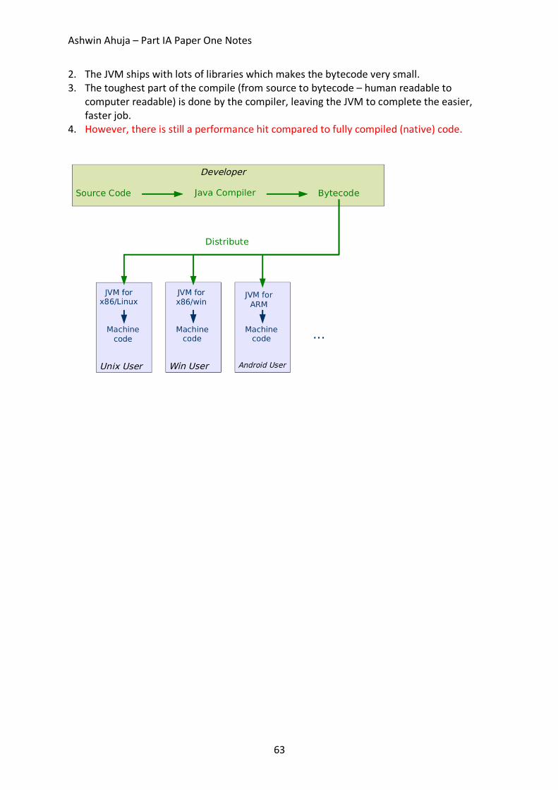
Ashwin Ahuja – Part IA Paper One Notes
63
2. The JVM ships with lots of libraries which makes the bytecode very small. 3. The toughest part of the compile (from source to bytecode – human readable to
computer readable) is done by the compiler, leaving the JVM to complete the easier, faster job.
4. However, there is still a performance hit compared to fully compiled (native) code.
Ashwin Ahuja – Part IA Paper One Notes
64
Algorithms Introduction An algorithm is a systematic recipe for solving a problem. Therefore, we have to precisely specify the problem and before we can consider it complete, we need a proof that it works (correctness) and an analysis of the performance. By having complete solutions to common sub-problems, it allows us to simplify more complicated problems which we have split into the requisite sub-problems to be combined together. For an algorithm, we need to consider:
1. Strategy 2. Actual algorithm 3. Data structure(s) 4. Proof of correctness of the algorithm 5. Proof of time complexity analysis algorithm 6. Other important ranking consideration between algorithms completing the same
problem a. For sorting this may include in-place-ness and stability.
Sorting Documentation, Preconditions and Postconditions Precondition: Request, specifying what the routine expects to receive from its caller Postconditions: Promise, specifying what the routine will do for its caller (provided the precondition is met) Together, the precondition and postconditions form some kind of “contract” (this is terminology of Bertrand Meyer) between the routine and its caller. Correctness When we have considered an algorithm, we must always consider if the algorithm is correct. In order to do this, we can do a few things: 1. Specify the objects as clearly as possible
a. This allows us to actually say if the algorithm is correct or not – without a specification, we do not know whether something is correct or not.
2. Reduce a large problem to a sequence of smaller sub problems where we can apply mathematical induction.
3. Assertions a. These act as stepping stones which mean we can assume that we have reached a
certain point in the algorithm with everything being as expected. b. We can prove each assertion for each point with the final assertion being that the
entire problem has been solved. c. It is particularly useful to have an assertion at the start of each significant loop,
saying how the previous loop affected the state. Therefore, we can prove this inductively (with a base case going into the first loop and then showing the inductive step over one loop).
Ashwin Ahuja – Part IA Paper One Notes
65
Computational Complexity We make a number of assumptions which help us to simplify the process to perform the cost estimation. The most commonly used assumptions are:
1. Only worry about the worst possible amount of time that the activity could take 2. Rather than measuring absolute computing times, we only look at rates of growth and
we ignore constants. 3. Any finite number of exceptions to a cost estimate are unimportant as long as the
estimate is valid for all large enough values of n. 4. We do not restrict ourselves to just reasonably values of n or apply any other reality
checks. The cost estimation will be carried through as an abstract mathematical activity.
Worst, average and amortized costs Usually the simplest way of analysing an algorithm is to find the worst case performance. This is very important where we must often consider when the algorithm is at its worst and may take the most time that it would ever take. This is particularly important for real-time applications, where we want to consider what would happen in the worst case. Average case analysis should generally be more interesting to most people. However, before useful average cost analysis can be performed, you need a model for the probabilities of all possible inputs. If in some particular application, the distribution of inputs is significantly skewed, then analysis based on uniform probabilities might not be valid. For worst case analysis, it is only necessary to study one limiting case – therefore being mathematically much harder. Amortized analysis is applicable where the data structure supports a number of operations and these will be performed in sequence. Quite often the cost of any particular operation will depend on the history of what has been done before and sometimes a plausible overall design makes most operations cheap at the cost of occasional expensive internal reorganisation of the data. In amortized analysis, we treat the cost of this reorganisation as the joint responsibility of all the operations previously performed and provides a firm basis for seeing if it was worthwhile. Big-O, Θ and Ω notation A function f(n) is said to be O(g(n)) if there exists constants k > 0 and N > 0, such that:
0 ≤ 𝑓(𝑛) ≤ 𝑘𝑔(𝑛)𝑓𝑜𝑟𝑛 > 𝑁 Therefore, effectively g(n) provides an upper bound that, for sufficiently large values of n, f(n) will never exceed, except for what can be compensated by a constant factor. A function f(n) is said to be Θ(g(n)) if there are constants k1 > 0, k2 > 0, N > 0, such that:
0 ≤ 𝑘P𝑔(𝑛) ≤ 𝑓(𝑛) ≤ 𝑘K𝑔(𝑛)𝑓𝑜𝑟𝑛 > 𝑁 In other words, for sufficiently large values of n, the functions f() and g() agree within a constant factor. This constraint is much tighter than the Bug-O.

Ashwin Ahuja – Part IA Paper One Notes
66
We use Ω as the dual of O() to provide a lower bound. Therefore: 𝑓(𝑛)𝜖Ω(𝑔(𝑛)* means that f(n) grows at least like g(n) It is important to state that providing a bound for a function does not mean that it is a good bound for it. Some people, therefore use O() and Ω() to describe bounds that might be tight, but o() and ⍵()for bounds that are definitely not tight.
N.B. Very common to say f(n) = O(g(n)) instead of f(n) 𝜖O(g(n)) Logarithms: For the purposes of time complexity, we consider logs as a singular concept, i.e. O(log2(m)) = O(log5(m)) = O(lg(m)). This is clearly because they are a scalar away from one another. Models of Memory We always assume that computers to run algorithms will always have enough memory and that the memory can be arranged in a single address space so that one can have unambiguous memory addresses and pointers. Obviously, this is not true, and in fact, we normally also assume that any element of an array can be accessed in unit time, however large the array gets – associated assumption is that integer arithmetic operations needed to computer array subscripts can also be done at unit cost. Today, what with caches, obviously, not all memory retrieval is equivalent, and some may be instant, and some may take tens or hundreds of clock cycles. Models of Arithmetic Normal model for computer arithmetic is that each arithmetic operation takes unit time, irrespective of the values of the numbers being combined and regardless of whether fixed or floating-point numbers are involved. In fact, as long as are using Θ notation, we swallow up constant factors in timing. We must sometimes consider a theoretical problem where numbers may be many orders larger than native computer arithmetic will support directly. Here, we need to show the cost analysis to explicitly consider how much extra work which will be involved in doing the multiple precision arithmetic, and then timing estimates will generally depend, not only on the number of values involved in a problem but the number of bits needed to specify each value.
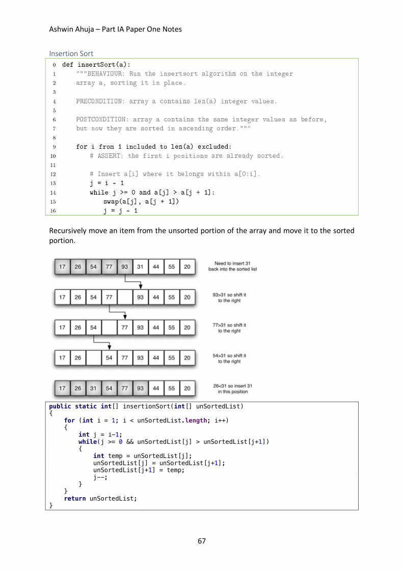
Ashwin Ahuja – Part IA Paper One Notes
67
Insertion Sort
Recursively move an item from the unsorted portion of the array and move it to the sorted portion.
public static int[] insertionSort(int[] unSortedList) { for (int i = 1; i < unSortedList.length; i++) { int j = i-1; while(j >= 0 && unSortedList[j] > unSortedList[j+1]) { int temp = unSortedList[j]; unSortedList[j] = unSortedList[j+1]; unSortedList[j+1] = temp; j--; } } return unSortedList; }
Ashwin Ahuja – Part IA Paper One Notes
68
The outer loop of line 9 (pseudocode) is executed exactly n-1 times (regardless of the values of the elements in the input array), while the inner loop is executed a number of times that depends on the number of swaps to be performed. In the worst case, during the ith invocation of the outer loop, the inner loop will be performed i times. Therefore for the whole algorithm, the execution number won’t exceeed the nth triangular number (1 + 2 + … + n) which is equal to ½ n(n+1) = O(n2) Optimal Sorting If I have n items in an array and I need to rearrange them in ascending order, whatever the algorithm there are two elementary operations that I can plausibly expect to use repeatedly in the process. The first takes two items and compares them to see which should come first. The second swaps the contents of two array locations. Assertion 1 (lower bound on exchanges): If there are n items in an array then Θ(n) exchanges always suffice to put the items in order. In the worst case, Θ(n) exchanges are actually needed. Proof: Identify the smallest item present, if it not already in the right place then one exchange moves it to the start of the array. A second exchange moves the second smallest, etc. Therefore, after n-1, we will be done therefore equal to Θ(n) we would be guaranteed to be done. Assertion 2 (lower bound on comparisons): Sorting by pairwise comparisons, assuming that all possible arrangements might actually occur as an input, necessarily costs at least Ω(n lg n) Proof: There are n! permutations of n items and in sorting, we identify one of these. In each test, we half the possible number of correct arrangements. Therefore, we need log2(n!) tests. Stirling’s formula tells us that n! is approximately equal to nn therefore log (n!) is approximately equal to n lg n More importantly, 𝑙𝑔(𝑛!) ≥ 𝑛𝑙𝑔𝑛 (for O notation) simply by:
lg(𝑛!) = lg(𝑛) + lg(𝑛 − 1) +⋯+ lg(1) ≤ n lg𝑛 Therefore, lg(n!) is bounded by n lg n. Conversely, since the lg function is monotonic, the first n/2 terms from lg n to lg n/2 are all greater than or equal to lg (n/2) = lg n – lg 2 = lg n – 1. Therefore:
Thus, when n is large enough n lg n is bounded by k lg n!. Therefore lg(n!) = Θ(n lg n) Selection Sort The idea of the proof showing Θ(n) swaps acts as the strategy for this sorting strategy. In this case, for each iteration, we need to find the smallest item of the array. Here we can scan
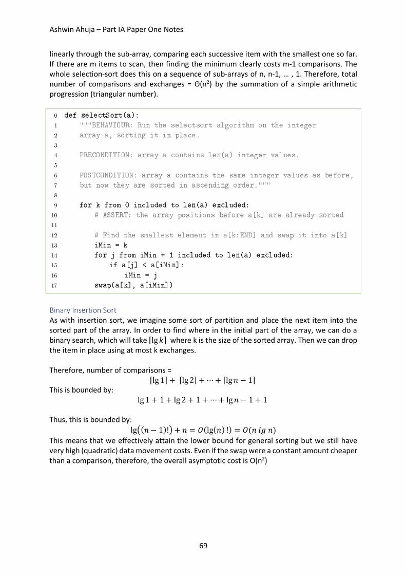
Ashwin Ahuja – Part IA Paper One Notes
69
linearly through the sub-array, comparing each successive item with the smallest one so far. If there are m items to scan, then finding the minimum clearly costs m-1 comparisons. The whole selection-sort does this on a sequence of sub-arrays of n, n-1, … , 1. Therefore, total number of comparisons and exchanges = Θ(n2) by the summation of a simple arithmetic progression (triangular number).
Binary Insertion Sort As with insertion sort, we imagine some sort of partition and place the next item into the sorted part of the array. In order to find where in the initial part of the array, we can do a binary search, which will take ⌈lg 𝑘⌉ where k is the size of the sorted array. Then we can drop the item in place using at most k exchanges. Therefore, number of comparisons =
⌈lg 1⌉ + ⌈lg 2⌉ +⋯+ ⌈lg𝑛 − 1⌉ This is bounded by:
lg 1 + 1 + lg 2 + 1 +⋯+ lg𝑛 − 1 + 1 Thus, this is bounded by:
lg((𝑛 − 1)!* + 𝑛 = 𝑂(lg(𝑛) !) = 𝑂(𝑛𝑙𝑔𝑛) This means that we effectively attain the lower bound for general sorting but we still have very high (quadratic) data movement costs. Even if the swap were a constant amount cheaper than a comparison, therefore, the overall asymptotic cost is O(n2)
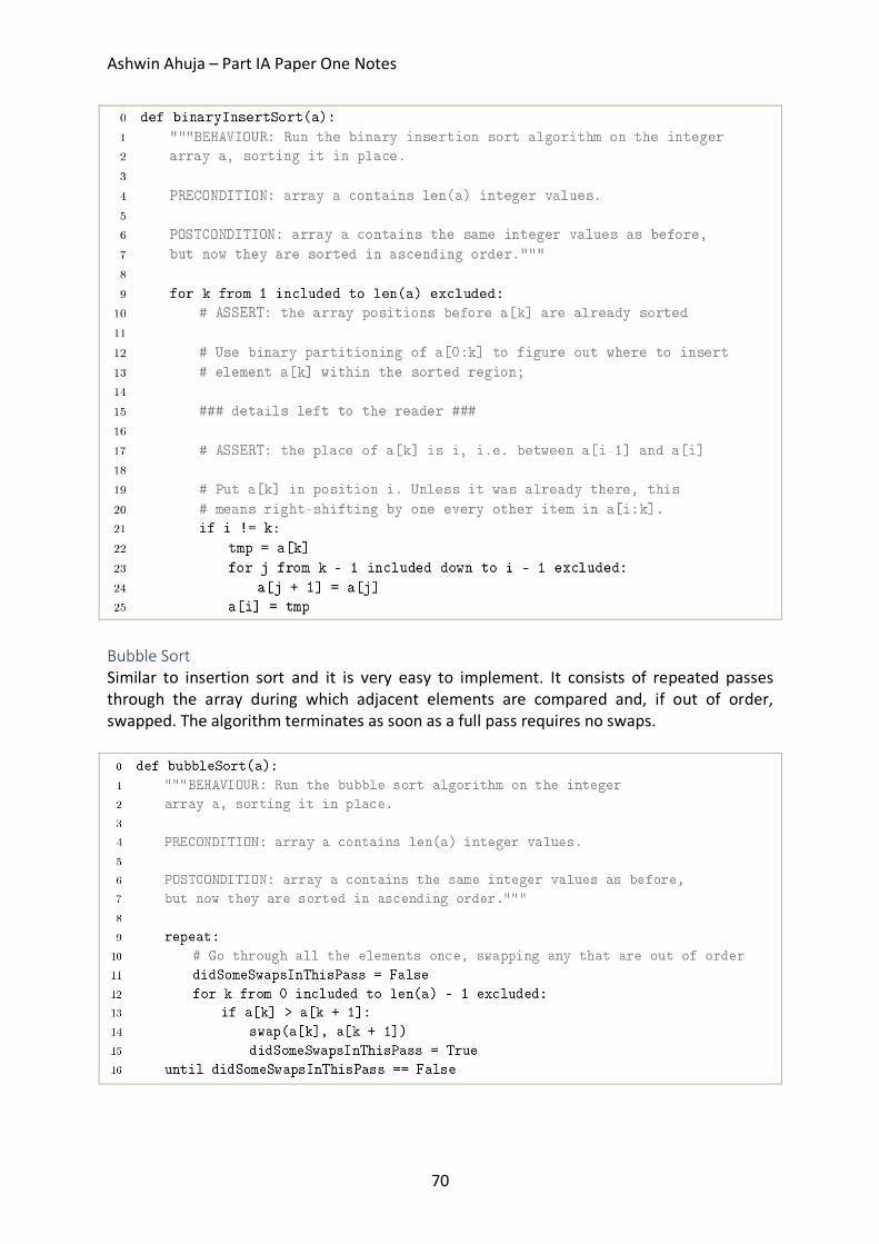
Ashwin Ahuja – Part IA Paper One Notes
70
Bubble Sort Similar to insertion sort and it is very easy to implement. It consists of repeated passes through the array during which adjacent elements are compared and, if out of order, swapped. The algorithm terminates as soon as a full pass requires no swaps.
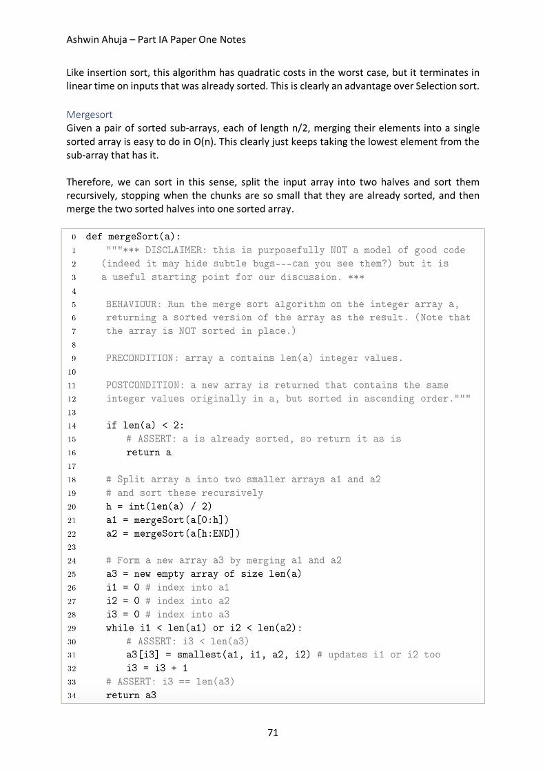
Ashwin Ahuja – Part IA Paper One Notes
71
Like insertion sort, this algorithm has quadratic costs in the worst case, but it terminates in linear time on inputs that was already sorted. This is clearly an advantage over Selection sort. Mergesort Given a pair of sorted sub-arrays, each of length n/2, merging their elements into a single sorted array is easy to do in O(n). This clearly just keeps taking the lowest element from the sub-array that has it. Therefore, we can sort in this sense, split the input array into two halves and sort them recursively, stopping when the chunks are so small that they are already sorted, and then merge the two sorted halves into one sorted array.
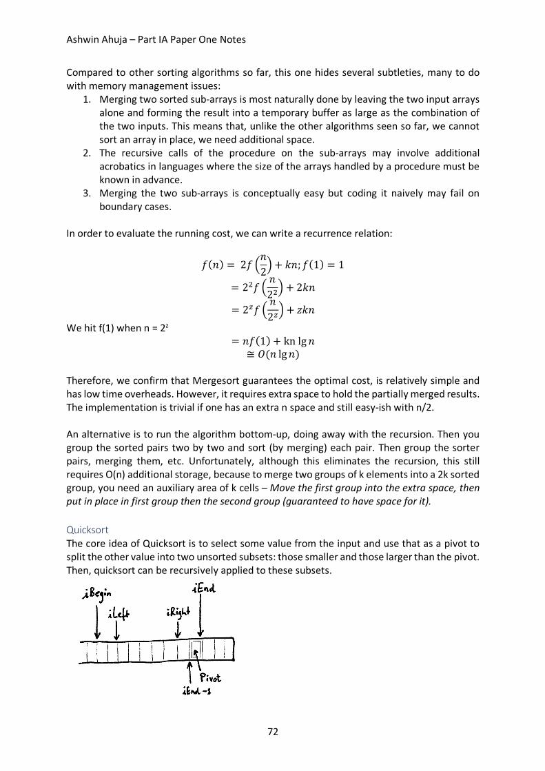
Ashwin Ahuja – Part IA Paper One Notes
72
Compared to other sorting algorithms so far, this one hides several subtleties, many to do with memory management issues:
1. Merging two sorted sub-arrays is most naturally done by leaving the two input arrays alone and forming the result into a temporary buffer as large as the combination of the two inputs. This means that, unlike the other algorithms seen so far, we cannot sort an array in place, we need additional space.
2. The recursive calls of the procedure on the sub-arrays may involve additional acrobatics in languages where the size of the arrays handled by a procedure must be known in advance.
3. Merging the two sub-arrays is conceptually easy but coding it naively may fail on boundary cases.
In order to evaluate the running cost, we can write a recurrence relation:
𝑓(𝑛) = 2𝑓 ]𝑛2^ + 𝑘𝑛; 𝑓
(1) = 1
= 2K𝑓 ]𝑛2K^ + 2𝑘𝑛
= 2`𝑓 ]𝑛2`^ + 𝑧𝑘𝑛
We hit f(1) when n = 2z = 𝑛𝑓(1) + knlg 𝑛
≅ 𝑂(𝑛 lg𝑛) Therefore, we confirm that Mergesort guarantees the optimal cost, is relatively simple and has low time overheads. However, it requires extra space to hold the partially merged results. The implementation is trivial if one has an extra n space and still easy-ish with n/2. An alternative is to run the algorithm bottom-up, doing away with the recursion. Then you group the sorted pairs two by two and sort (by merging) each pair. Then group the sorter pairs, merging them, etc. Unfortunately, although this eliminates the recursion, this still requires O(n) additional storage, because to merge two groups of k elements into a 2k sorted group, you need an auxiliary area of k cells – Move the first group into the extra space, then put in place in first group then the second group (guaranteed to have space for it). Quicksort The core idea of Quicksort is to select some value from the input and use that as a pivot to split the other value into two unsorted subsets: those smaller and those larger than the pivot. Then, quicksort can be recursively applied to these subsets.
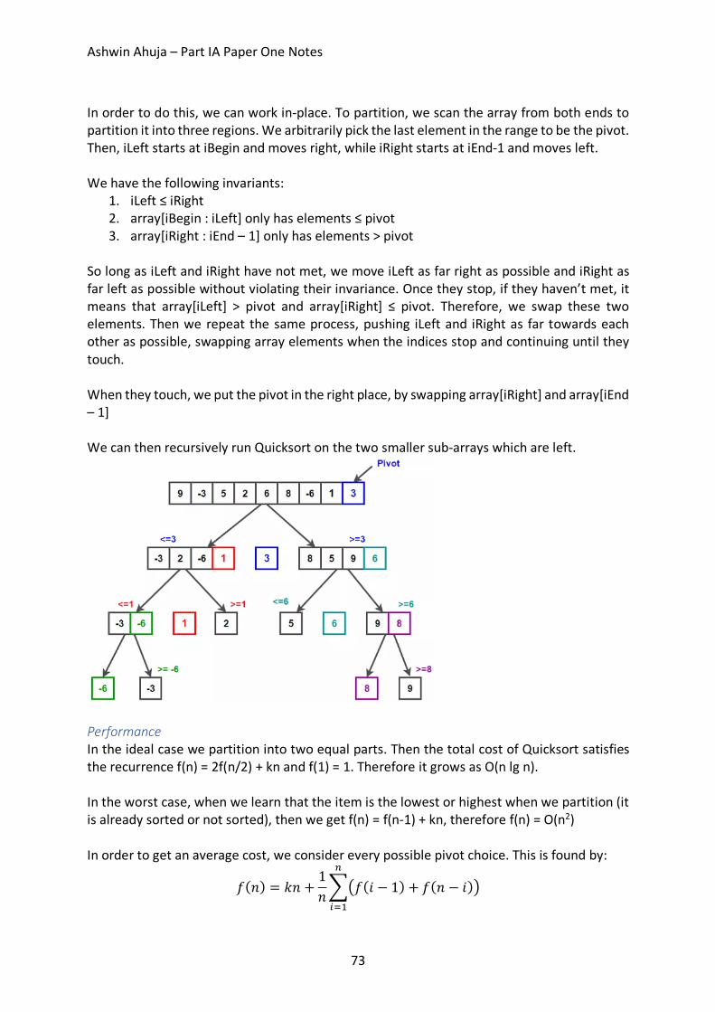
Ashwin Ahuja – Part IA Paper One Notes
73
In order to do this, we can work in-place. To partition, we scan the array from both ends to partition it into three regions. We arbitrarily pick the last element in the range to be the pivot. Then, iLeft starts at iBegin and moves right, while iRight starts at iEnd-1 and moves left. We have the following invariants:
1. iLeft ≤ iRight 2. array[iBegin : iLeft] only has elements ≤ pivot 3. array[iRight : iEnd – 1] only has elements > pivot
So long as iLeft and iRight have not met, we move iLeft as far right as possible and iRight as far left as possible without violating their invariance. Once they stop, if they haven’t met, it means that array[iLeft] > pivot and array[iRight] ≤ pivot. Therefore, we swap these two elements. Then we repeat the same process, pushing iLeft and iRight as far towards each other as possible, swapping array elements when the indices stop and continuing until they touch. When they touch, we put the pivot in the right place, by swapping array[iRight] and array[iEnd – 1] We can then recursively run Quicksort on the two smaller sub-arrays which are left.
Performance In the ideal case we partition into two equal parts. Then the total cost of Quicksort satisfies the recurrence f(n) = 2f(n/2) + kn and f(1) = 1. Therefore it grows as O(n lg n). In the worst case, when we learn that the item is the lowest or highest when we partition (it is already sorted or not sorted), then we get f(n) = f(n-1) + kn, therefore f(n) = O(n2) In order to get an average cost, we consider every possible pivot choice. This is found by:
𝑓(𝑛) = 𝑘𝑛 +1𝑛d
(𝑓(𝑖 − 1) + 𝑓(𝑛 − 𝑖)*7
efP
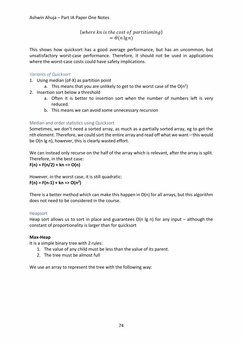
Ashwin Ahuja – Part IA Paper One Notes
74
{𝑤ℎ𝑒𝑟𝑒𝑘𝑛𝑖𝑠𝑡ℎ𝑒𝑐𝑜𝑠𝑡𝑜𝑓𝑝𝑎𝑟𝑡𝑖𝑡𝑖𝑜𝑛𝑖𝑛𝑔} = 𝛩(𝑛 lg𝑛)
This shows how quicksort has a good average performance, but has an uncommon, but unsatisfactory worst-case performance. Therefore, it should not be used in applications where the worst-case costs could have safety implications. Variants of Quicksort 1. Using median (of-X) as partition point
a. This means that you are unlikely to get to the worst case of the O(n2) 2. Insertion sort below a threshold
a. Often it is better to insertion sort when the number of numbers left is very reduced.
b. This means we can avoid some unnecessary recursion Median and order statistics using Quicksort Sometimes, we don’t need a sorted array, as much as a partially sorted array, eg to get the nth element. Therefore, we could sort the entire array and read off what we want – this would be O(n lg n), however, this is clearly wasted effort. We can instead only recurse on the half of the array which is relevant, after the array is split. Therefore, in the best case: F(n) = F(n/2) + kn => O(n) However, in the worst case, it is still quadratic: F(n) = F(n-1) + kn => O(n2) There is a better method which can make this happen in O(n) for all arrays, but this algorithm does not need to be considered in the course. Heapsort Heap sort allows us to sort in place and guarantees O(n lg n) for any input – although the constant of proportionality is larger than for quicksort Max-Heap It is a simple binary tree with 2 rules:
1. The value of any child must be less than the value of its parent. 2. The tree must be almost full
We use an array to represent the tree with the following way:
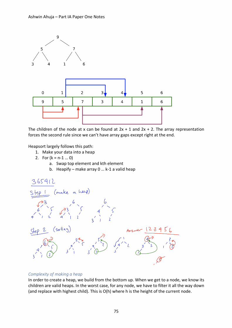
Ashwin Ahuja – Part IA Paper One Notes
75
The children of the node at x can be found at 2x + 1 and 2x + 2. The array representation forces the second rule since we can’t have array gaps except right at the end. Heapsort largely follows this path:
1. Make your data into a heap 2. For (k = n-1 … 0)
a. Swap top element and kth element b. Heapify – make array 0 … k-1 a valid heap
Complexity of making a heap In order to create a heap, we build from the bottom up. When we get to a node, we know its children are valid heaps. In the worst case, for any node, we have to filter it all the way down (and replace with highest child). This is O(h) where h is the height of the current node.
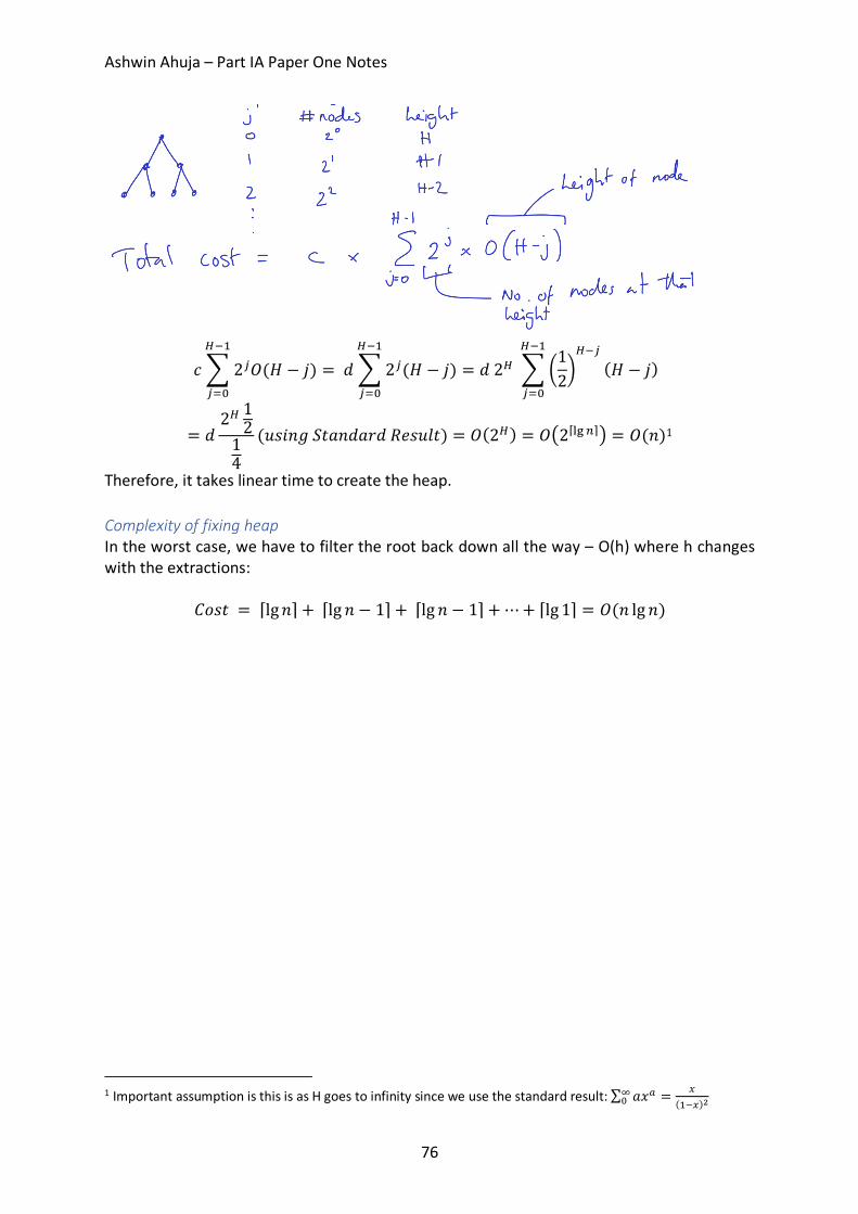
Ashwin Ahuja – Part IA Paper One Notes
76
𝑐 d 2n𝑂(𝐻 − 𝑗)pRP
nfq
= 𝑑 d 2n(𝐻 − 𝑗)pRP
nfq
= 𝑑2p d H12I
pRn(𝐻 − 𝑗)
pRP
nfq
= 𝑑2p 1214
(𝑢𝑠𝑖𝑛𝑔𝑆𝑡𝑎𝑛𝑑𝑎𝑟𝑑𝑅𝑒𝑠𝑢𝑙𝑡) = 𝑂(2p) = 𝑂(2⌈uv 7⌉* = 𝑂(𝑛)1
Therefore, it takes linear time to create the heap. Complexity of fixing heap In the worst case, we have to filter the root back down all the way – O(h) where h changes with the extractions:
𝐶𝑜𝑠𝑡 = ⌈lg𝑛⌉ +⌈lg 𝑛 − 1⌉ +⌈lg 𝑛 − 1⌉ +⋯+ ⌈lg1⌉ = 𝑂(𝑛 lg 𝑛)
1 Important assumption is this is as H goes to infinity since we use the standard result: ∑ 𝑎𝑥y = z
(PRz){|q
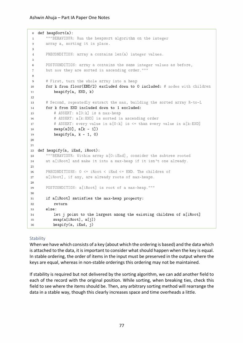
Ashwin Ahuja – Part IA Paper One Notes
77
Stability When we have which consists of a key (about which the ordering is based) and the data which is attached to the data, it is important to consider what should happen when the key is equal. In stable ordering, the order of items in the input must be preserved in the output where the keys are equal, whereas in non-stable orderings this ordering may not be maintained. If stability is required but not delivered by the sorting algorithm, we can add another field to each of the record with the original position. While sorting, when breaking ties, check this field to see where the items should be. Then, any arbitrary sorting method will rearrange the data in a stable way, though this clearly increases space and time overheads a little.
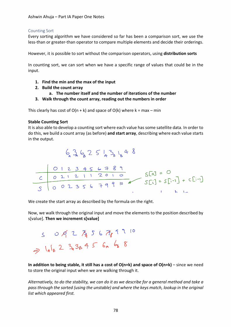
Ashwin Ahuja – Part IA Paper One Notes
78
Counting Sort Every sorting algorithm we have considered so far has been a comparison sort, we use the less-than or greater-than operator to compare multiple elements and decide their orderings. However, it is possible to sort without the comparison operators, using distribution sorts In counting sort, we can sort when we have a specific range of values that could be in the input.
1. Find the min and the max of the input 2. Build the count array
a. The number itself and the number of iterations of the number 3. Walk through the count array, reading out the numbers in order
This clearly has cost of O(n + k) and space of O(k) where k = max – min Stable Counting Sort It is also able to develop a counting sort where each value has some satellite data. In order to do this, we build a count array (as before) and start array, describing where each value starts in the output.
We create the start array as described by the formula on the right. Now, we walk through the original input and move the elements to the position described by s[value]. Then we increment s[value]
In addition to being stable, it still has a cost of O(n+k) and space of O(n+k) – since we need to store the original input when we are walking through it. Alternatively, to do the stability, we can do it as we describe for a general method and take a pass through the sorted (using the unstable) and where the keys match, lookup in the original list which appeared first.

Ashwin Ahuja – Part IA Paper One Notes
79
Bucket Sort Assuming we have n keys uniformly distributed over some known range, in bucket sort we create an array of n linked lists. A linear scan adds each key to the list at index which fits the bucket. Say the keys were distributed between 0 and 1, then it would be at index kn for key k. We expect the length of each list to be one, but there will some of length 0, some of length of 1, etc. If a list contains more than 1 it is then sorted – we can do this using any algorithm since the list should be very short (insertion sort for example). Even though the O(n2) algorithm is used for the sorting, this is our worst case, however, we find that the average case is O(n) It clearly only takes space O(n) Radix Sort When the range of the numbers is much larger than the number of things to sort, counting sort is very bad. Instead we sort by digits, using another sorter, which must be stable. It works best using the lowest digit first.
Strategies for Algorithm Design Divide and Conquer 1. DIVIDE: split the problem into parts – almost always two
a. If the instance is very small, you should instead solve it. b. The subproblems should be of a similar size
2. CONQUER: Use recursion to solve the smaller problems. 3. COMBINE: Create a solution to the final problem by using information from the solution
of the smaller problems. Dynamic Programming Dynamic Programming is Divide and Conquer where the subproblems overlap. This means that we save lots of effort and saves us doing the same problem a large number of times.
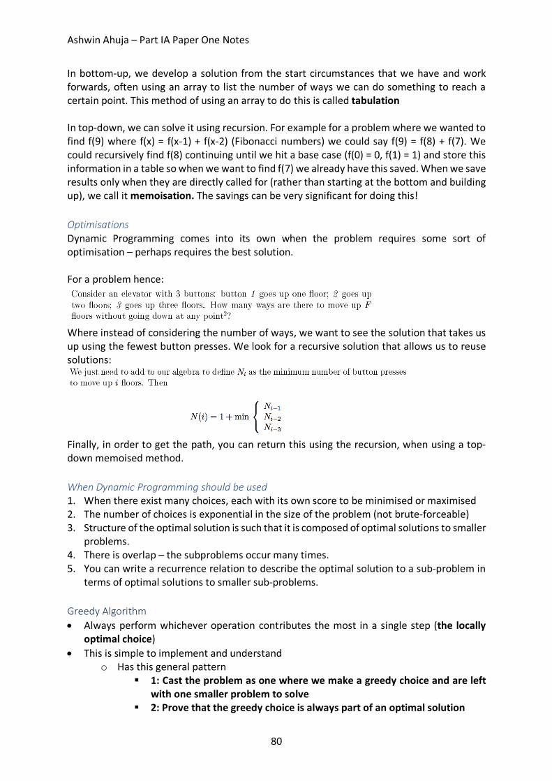
Ashwin Ahuja – Part IA Paper One Notes
80
In bottom-up, we develop a solution from the start circumstances that we have and work forwards, often using an array to list the number of ways we can do something to reach a certain point. This method of using an array to do this is called tabulation In top-down, we can solve it using recursion. For example for a problem where we wanted to find f(9) where f(x) = f(x-1) + f(x-2) (Fibonacci numbers) we could say f(9) = f(8) + f(7). We could recursively find f(8) continuing until we hit a base case (f(0) = 0, f(1) = 1) and store this information in a table so when we want to find f(7) we already have this saved. When we save results only when they are directly called for (rather than starting at the bottom and building up), we call it memoisation. The savings can be very significant for doing this! Optimisations Dynamic Programming comes into its own when the problem requires some sort of optimisation – perhaps requires the best solution. For a problem hence:
Where instead of considering the number of ways, we want to see the solution that takes us up using the fewest button presses. We look for a recursive solution that allows us to reuse solutions:
Finally, in order to get the path, you can return this using the recursion, when using a top-down memoised method. When Dynamic Programming should be used 1. When there exist many choices, each with its own score to be minimised or maximised 2. The number of choices is exponential in the size of the problem (not brute-forceable) 3. Structure of the optimal solution is such that it is composed of optimal solutions to smaller
problems. 4. There is overlap – the subproblems occur many times. 5. You can write a recurrence relation to describe the optimal solution to a sub-problem in
terms of optimal solutions to smaller sub-problems. Greedy Algorithm • Always perform whichever operation contributes the most in a single step (the locally
optimal choice) • This is simple to implement and understand
o Has this general pattern § 1: Cast the problem as one where we make a greedy choice and are left
with one smaller problem to solve § 2: Prove that the greedy choice is always part of an optimal solution
Ashwin Ahuja – Part IA Paper One Notes
81
§ 3: Prove that there’s optimal substructure, i.e. that the greedy choice plus an optimal solution of the subproblem yields an optimal solution for the overall problem.
• But it doesn’t always optimize fully o We can perform greedy algorithm when it meets two requirements
§ 1: Greedy choice property: You can make a locally optimal choice based only on past choices. This means you need a way of quantifying the value of each choice
§ 2: Optimal Substructure: The optimal solution(s) contain optimal solutions to subproblems.
Other 1. Recognise a variant on a known problem 2. Reduce to a simpler problem 3. Backtracking
a. If the algorithm requires a search, backtracking can be used. b. This splits the design of the procedure into two parts. The first part just ploughs
ahead and investigates what it thinks is the most sensible path to explore, while the second backtracks when needed.
c. The first path will reach a dead end and when it does, it backtracks. 4. MM Method
a. Throw the problem to a large number of people (or to a random array of random changes) and wait a period of time and see which solution works.
5. Seek wasted work in a simple method a. Firstly design a simple algorithm to solve a problem then analyse it to the extent
that the critically costly parts of it can be identified. b. Then we can seek to eliminate these elements and improve the algorithm.
6. Seek formal mathematical lower bound a. By finding a properly proved lower bound, we can prevent wasted time seeking
improvement where none is possible. 7. Brute Force
a. Generate all possible solutions and test each of them to see if it is the correct solution until you find it.
b. You should only use when the number of possibilities is very low. Data Structures An Abstract Data Type is a mathematical model of a data type – a logical description that does not concern itself with the specific implementation. A data structure is a concrete implementation of a data type. An ADT is a user of the type and a data structure is for the implementer of the type. This whole idea employs the notion of data hiding and encapsulation, where how the ADT is actually working is completely irrelevant and does not need to be considered. Primitive Data Types We can generally assume that we have a set of primitive values that exist
1. Boolean 2. Character 3. Integer
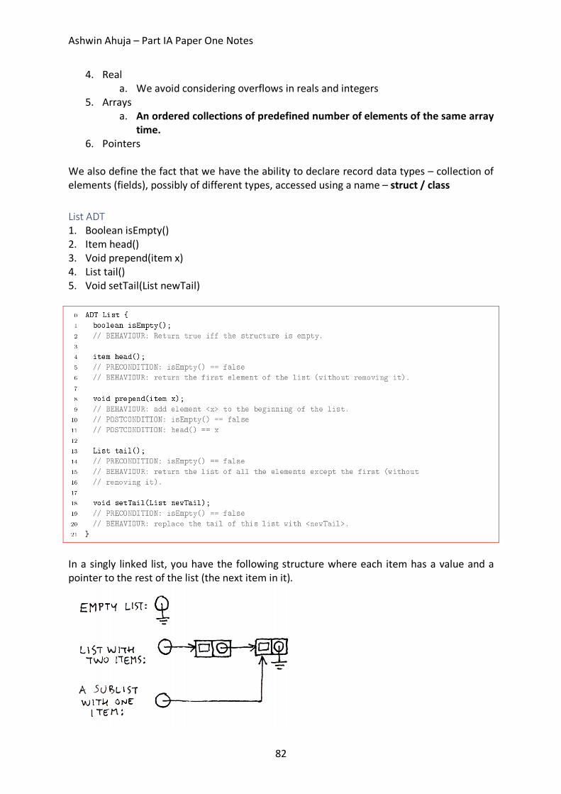
Ashwin Ahuja – Part IA Paper One Notes
82
4. Real a. We avoid considering overflows in reals and integers
5. Arrays a. An ordered collections of predefined number of elements of the same array
time. 6. Pointers
We also define the fact that we have the ability to declare record data types – collection of elements (fields), possibly of different types, accessed using a name – struct / class List ADT 1. Boolean isEmpty() 2. Item head() 3. Void prepend(item x) 4. List tail() 5. Void setTail(List newTail)
In a singly linked list, you have the following structure where each item has a value and a pointer to the rest of the list (the next item in it).
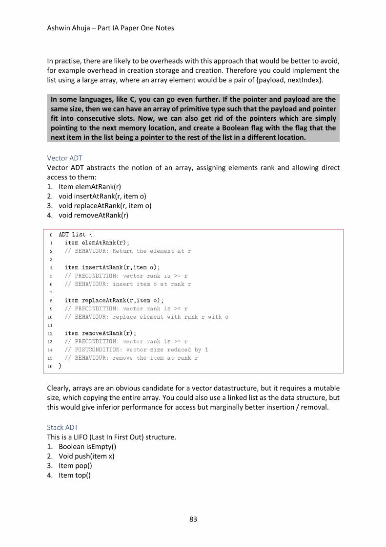
Ashwin Ahuja – Part IA Paper One Notes
83
In practise, there are likely to be overheads with this approach that would be better to avoid, for example overhead in creation storage and creation. Therefore you could implement the list using a large array, where an array element would be a pair of {payload, nextIndex}.
In some languages, like C, you can go even further. If the pointer and payload are the same size, then we can have an array of primitive type such that the payload and pointer fit into consecutive slots. Now, we can also get rid of the pointers which are simply pointing to the next memory location, and create a Boolean flag with the flag that the next item in the list being a pointer to the rest of the list in a different location.
Vector ADT Vector ADT abstracts the notion of an array, assigning elements rank and allowing direct access to them: 1. Item elemAtRank(r) 2. void insertAtRank(r, item o) 3. void replaceAtRank(r, item o) 4. void removeAtRank(r)
Clearly, arrays are an obvious candidate for a vector datastructure, but it requires a mutable size, which copying the entire array. You could also use a linked list as the data structure, but this would give inferior performance for access but marginally better insertion / removal. Stack ADT This is a LIFO (Last In First Out) structure. 1. Boolean isEmpty() 2. Void push(item x) 3. Item pop() 4. Item top()
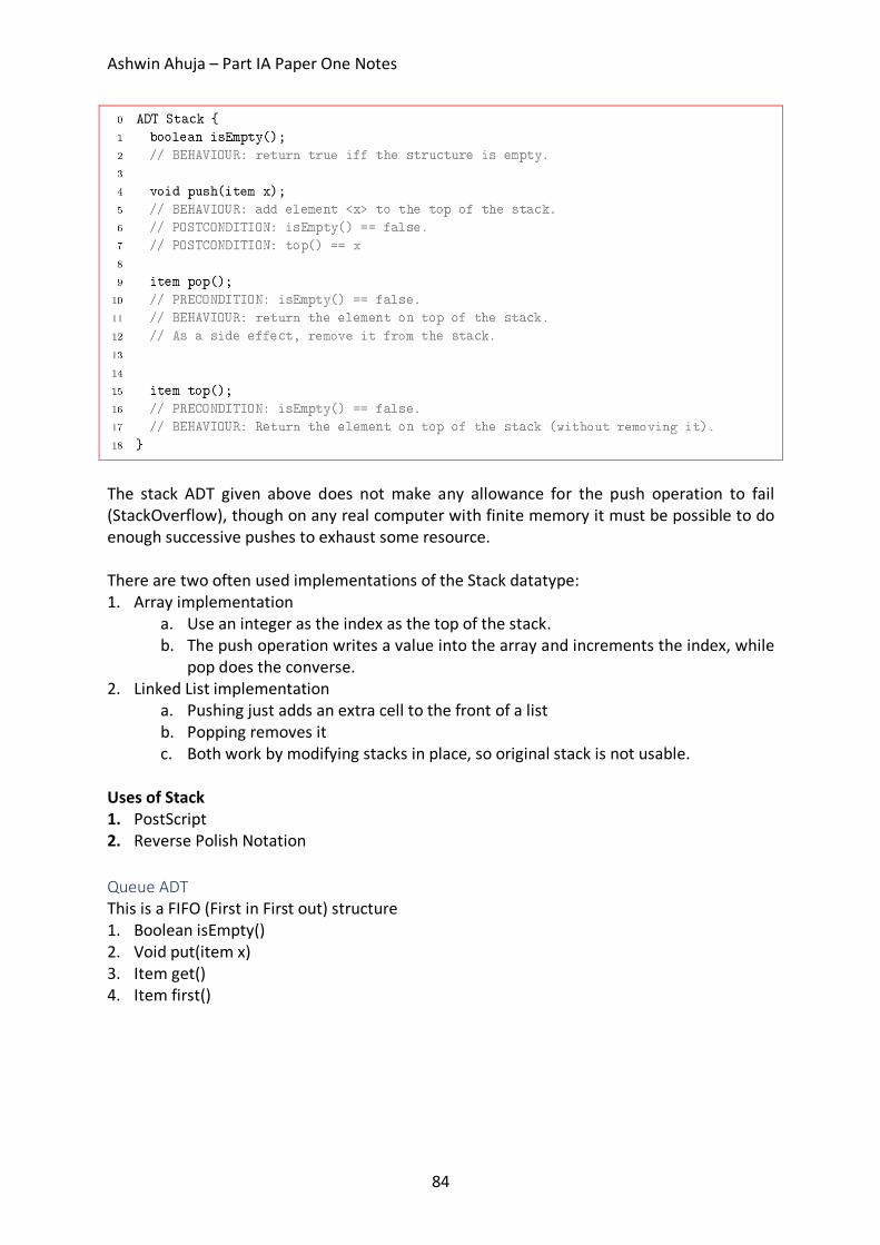
Ashwin Ahuja – Part IA Paper One Notes
84
The stack ADT given above does not make any allowance for the push operation to fail (StackOverflow), though on any real computer with finite memory it must be possible to do enough successive pushes to exhaust some resource. There are two often used implementations of the Stack datatype: 1. Array implementation
a. Use an integer as the index as the top of the stack. b. The push operation writes a value into the array and increments the index, while
pop does the converse. 2. Linked List implementation
a. Pushing just adds an extra cell to the front of a list b. Popping removes it c. Both work by modifying stacks in place, so original stack is not usable.
Uses of Stack 1. PostScript 2. Reverse Polish Notation Queue ADT This is a FIFO (First in First out) structure 1. Boolean isEmpty() 2. Void put(item x) 3. Item get() 4. Item first()
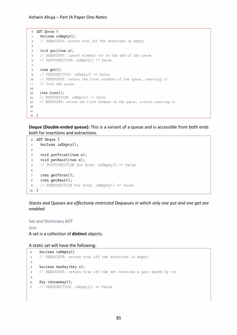
Ashwin Ahuja – Part IA Paper One Notes
85
Deque (Double-ended queue): This is a variant of a queue and is accessible from both ends both for insertions and extractions.
Stacks and Queues are effectively restricted Dequeues in which only one put and one get are enabled. Set and Dictionary ADT Sets A set is a collection of distinct objects. A static set will have the following:
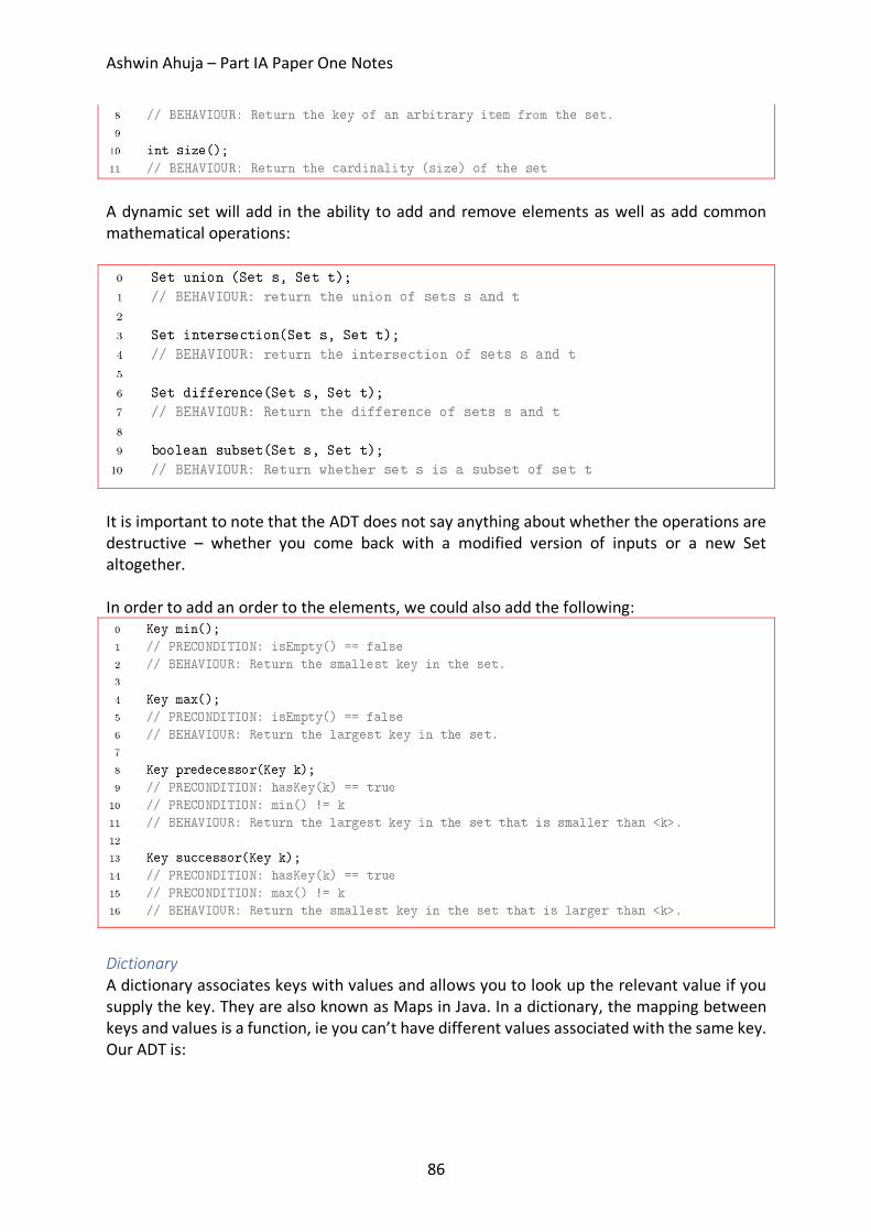
Ashwin Ahuja – Part IA Paper One Notes
86
A dynamic set will add in the ability to add and remove elements as well as add common mathematical operations:
It is important to note that the ADT does not say anything about whether the operations are destructive – whether you come back with a modified version of inputs or a new Set altogether. In order to add an order to the elements, we could also add the following:
Dictionary A dictionary associates keys with values and allows you to look up the relevant value if you supply the key. They are also known as Maps in Java. In a dictionary, the mapping between keys and values is a function, ie you can’t have different values associated with the same key. Our ADT is:
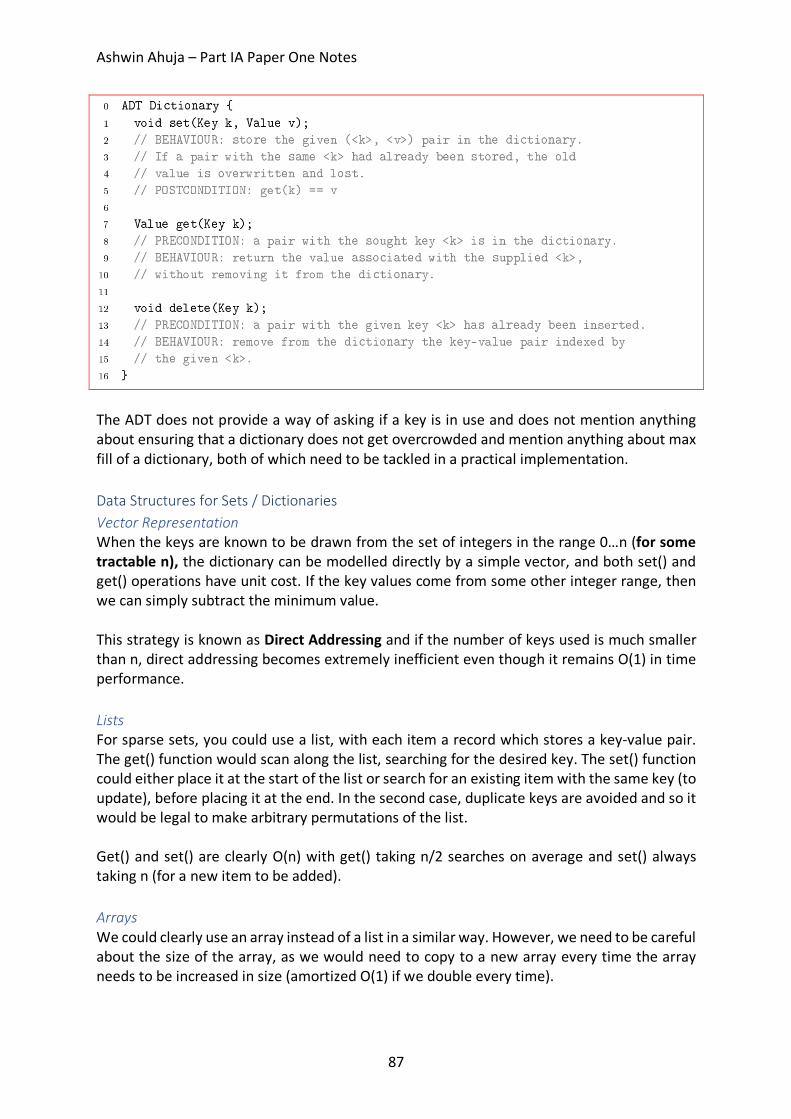
Ashwin Ahuja – Part IA Paper One Notes
87
The ADT does not provide a way of asking if a key is in use and does not mention anything about ensuring that a dictionary does not get overcrowded and mention anything about max fill of a dictionary, both of which need to be tackled in a practical implementation. Data Structures for Sets / Dictionaries Vector Representation When the keys are known to be drawn from the set of integers in the range 0…n (for some tractable n), the dictionary can be modelled directly by a simple vector, and both set() and get() operations have unit cost. If the key values come from some other integer range, then we can simply subtract the minimum value. This strategy is known as Direct Addressing and if the number of keys used is much smaller than n, direct addressing becomes extremely inefficient even though it remains O(1) in time performance. Lists For sparse sets, you could use a list, with each item a record which stores a key-value pair. The get() function would scan along the list, searching for the desired key. The set() function could either place it at the start of the list or search for an existing item with the same key (to update), before placing it at the end. In the second case, duplicate keys are avoided and so it would be legal to make arbitrary permutations of the list. Get() and set() are clearly O(n) with get() taking n/2 searches on average and set() always taking n (for a new item to be added). Arrays We could clearly use an array instead of a list in a similar way. However, we need to be careful about the size of the array, as we would need to copy to a new array every time the array needs to be increased in size (amortized O(1) if we double every time).
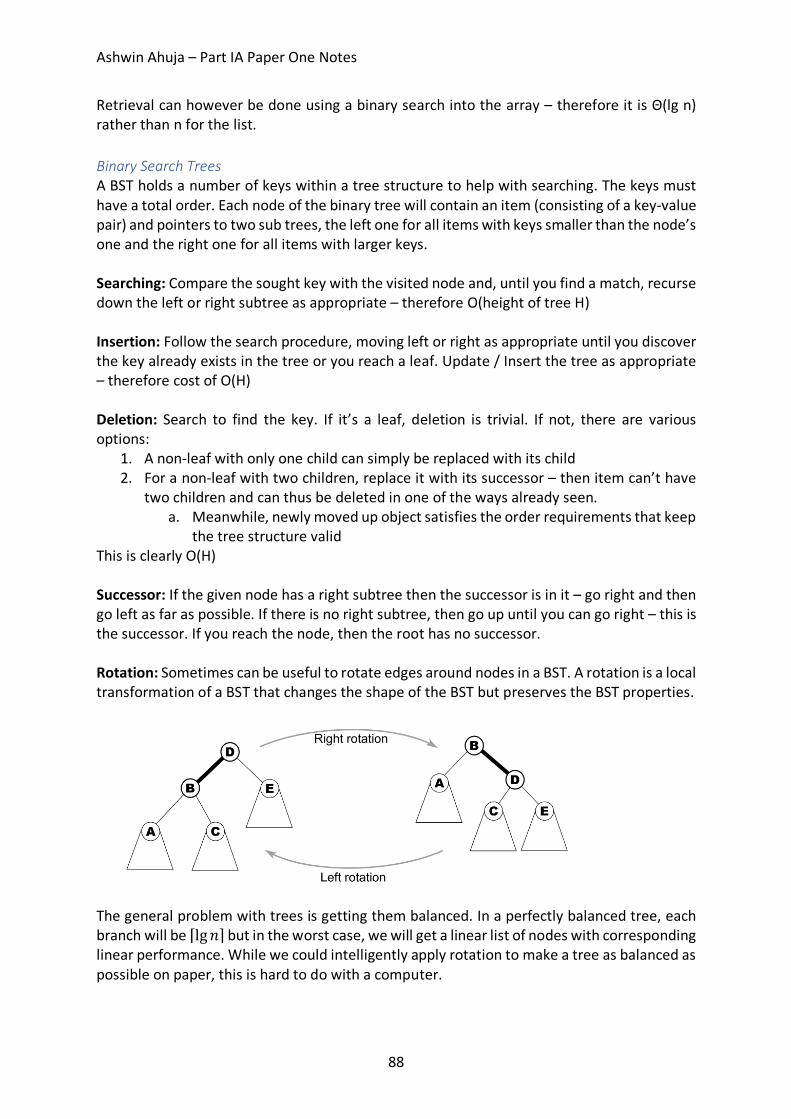
Ashwin Ahuja – Part IA Paper One Notes
88
Retrieval can however be done using a binary search into the array – therefore it is Θ(lg n) rather than n for the list. Binary Search Trees A BST holds a number of keys within a tree structure to help with searching. The keys must have a total order. Each node of the binary tree will contain an item (consisting of a key-value pair) and pointers to two sub trees, the left one for all items with keys smaller than the node’s one and the right one for all items with larger keys. Searching: Compare the sought key with the visited node and, until you find a match, recurse down the left or right subtree as appropriate – therefore O(height of tree H) Insertion: Follow the search procedure, moving left or right as appropriate until you discover the key already exists in the tree or you reach a leaf. Update / Insert the tree as appropriate – therefore cost of O(H) Deletion: Search to find the key. If it’s a leaf, deletion is trivial. If not, there are various options:
1. A non-leaf with only one child can simply be replaced with its child 2. For a non-leaf with two children, replace it with its successor – then item can’t have
two children and can thus be deleted in one of the ways already seen. a. Meanwhile, newly moved up object satisfies the order requirements that keep
the tree structure valid This is clearly O(H) Successor: If the given node has a right subtree then the successor is in it – go right and then go left as far as possible. If there is no right subtree, then go up until you can go right – this is the successor. If you reach the node, then the root has no successor. Rotation: Sometimes can be useful to rotate edges around nodes in a BST. A rotation is a local transformation of a BST that changes the shape of the BST but preserves the BST properties.
The general problem with trees is getting them balanced. In a perfectly balanced tree, each branch will be ⌈lg𝑛⌉ but in the worst case, we will get a linear list of nodes with corresponding linear performance. While we could intelligently apply rotation to make a tree as balanced as possible on paper, this is hard to do with a computer.
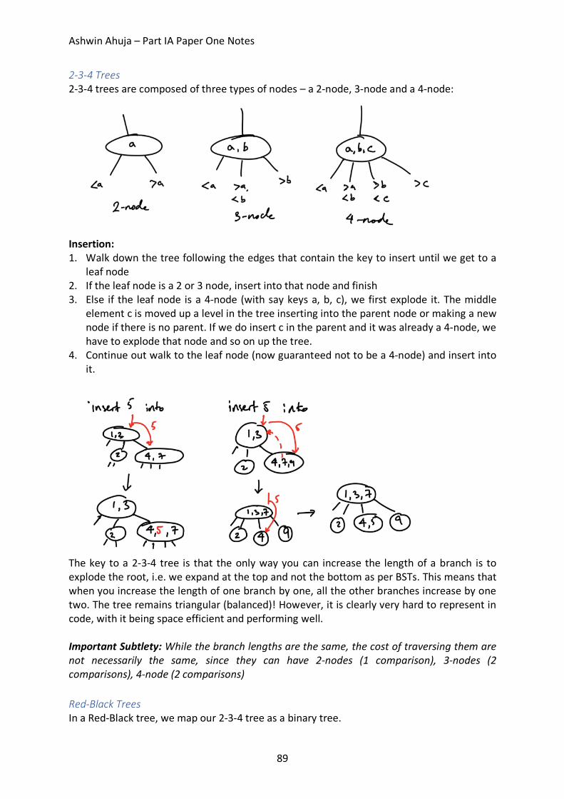
Ashwin Ahuja – Part IA Paper One Notes
89
2-3-4 Trees 2-3-4 trees are composed of three types of nodes – a 2-node, 3-node and a 4-node:
Insertion: 1. Walk down the tree following the edges that contain the key to insert until we get to a
leaf node 2. If the leaf node is a 2 or 3 node, insert into that node and finish 3. Else if the leaf node is a 4-node (with say keys a, b, c), we first explode it. The middle
element c is moved up a level in the tree inserting into the parent node or making a new node if there is no parent. If we do insert c in the parent and it was already a 4-node, we have to explode that node and so on up the tree.
4. Continue out walk to the leaf node (now guaranteed not to be a 4-node) and insert into it.
The key to a 2-3-4 tree is that the only way you can increase the length of a branch is to explode the root, i.e. we expand at the top and not the bottom as per BSTs. This means that when you increase the length of one branch by one, all the other branches increase by one two. The tree remains triangular (balanced)! However, it is clearly very hard to represent in code, with it being space efficient and performing well. Important Subtlety: While the branch lengths are the same, the cost of traversing them are not necessarily the same, since they can have 2-nodes (1 comparison), 3-nodes (2 comparisons), 4-node (2 comparisons) Red-Black Trees In a Red-Black tree, we map our 2-3-4 tree as a binary tree.
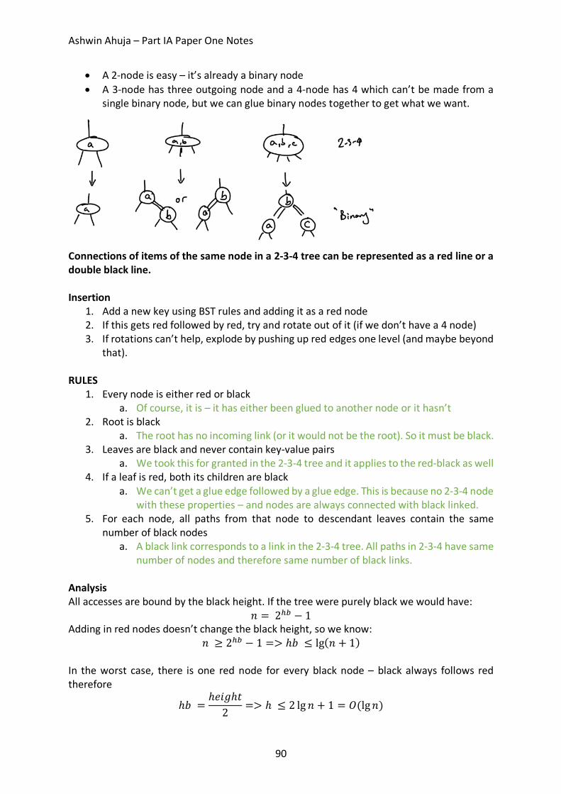
Ashwin Ahuja – Part IA Paper One Notes
90
• A 2-node is easy – it’s already a binary node • A 3-node has three outgoing node and a 4-node has 4 which can’t be made from a
single binary node, but we can glue binary nodes together to get what we want.
Connections of items of the same node in a 2-3-4 tree can be represented as a red line or a double black line. Insertion
1. Add a new key using BST rules and adding it as a red node 2. If this gets red followed by red, try and rotate out of it (if we don’t have a 4 node) 3. If rotations can’t help, explode by pushing up red edges one level (and maybe beyond
that). RULES
1. Every node is either red or black a. Of course, it is – it has either been glued to another node or it hasn’t
2. Root is black a. The root has no incoming link (or it would not be the root). So it must be black.
3. Leaves are black and never contain key-value pairs a. We took this for granted in the 2-3-4 tree and it applies to the red-black as well
4. If a leaf is red, both its children are black a. We can’t get a glue edge followed by a glue edge. This is because no 2-3-4 node
with these properties – and nodes are always connected with black linked. 5. For each node, all paths from that node to descendant leaves contain the same
number of black nodes a. A black link corresponds to a link in the 2-3-4 tree. All paths in 2-3-4 have same
number of nodes and therefore same number of black links. Analysis All accesses are bound by the black height. If the tree were purely black we would have:
𝑛 = 2}Q − 1 Adding in red nodes doesn’t change the black height, so we know:
𝑛 ≥ 2}Q − 1 => ℎ𝑏 ≤ lg(𝑛 + 1) In the worst case, there is one red node for every black node – black always follows red therefore
ℎ𝑏 =ℎ𝑒𝑖𝑔ℎ𝑡2 => ℎ ≤ 2 lg 𝑛 + 1 = 𝑂(lg𝑛)
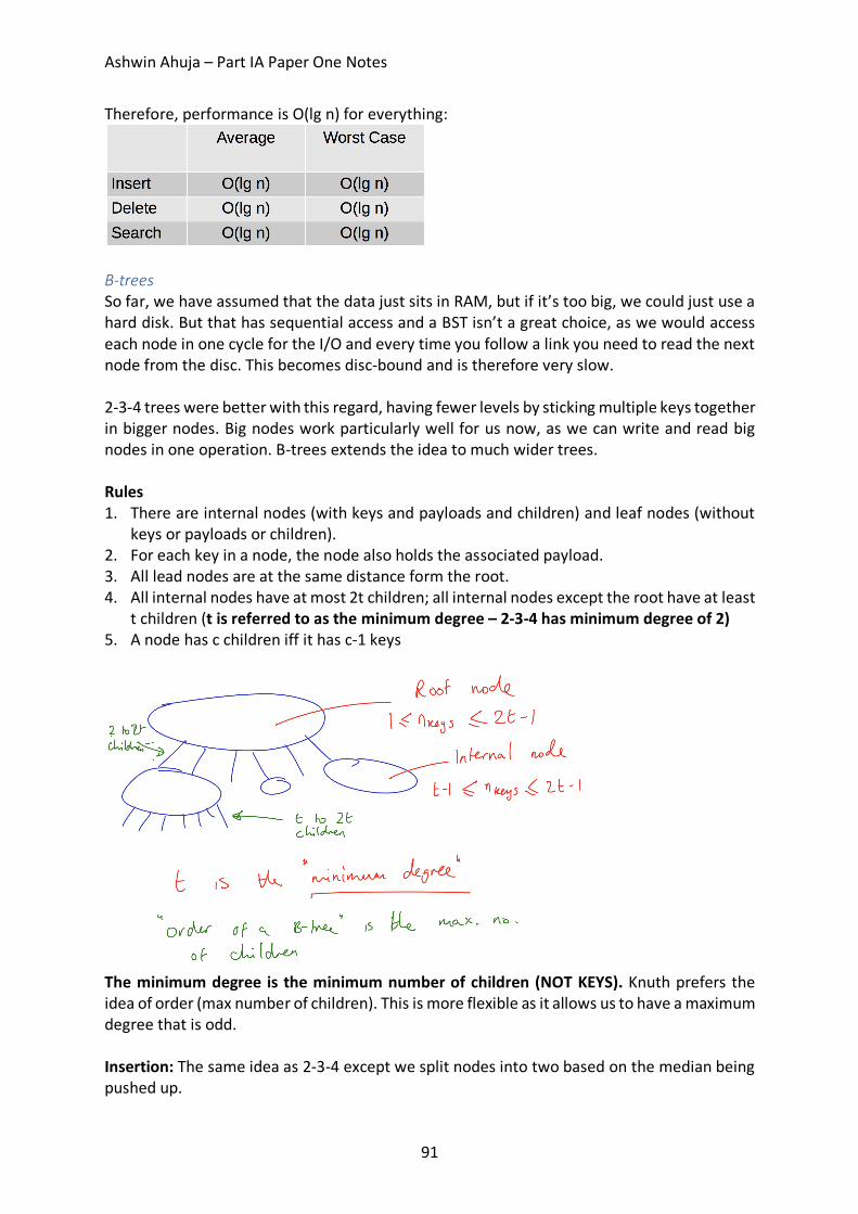
Ashwin Ahuja – Part IA Paper One Notes
91
Therefore, performance is O(lg n) for everything:
B-trees So far, we have assumed that the data just sits in RAM, but if it’s too big, we could just use a hard disk. But that has sequential access and a BST isn’t a great choice, as we would access each node in one cycle for the I/O and every time you follow a link you need to read the next node from the disc. This becomes disc-bound and is therefore very slow. 2-3-4 trees were better with this regard, having fewer levels by sticking multiple keys together in bigger nodes. Big nodes work particularly well for us now, as we can write and read big nodes in one operation. B-trees extends the idea to much wider trees. Rules 1. There are internal nodes (with keys and payloads and children) and leaf nodes (without
keys or payloads or children). 2. For each key in a node, the node also holds the associated payload. 3. All lead nodes are at the same distance form the root. 4. All internal nodes have at most 2t children; all internal nodes except the root have at least
t children (t is referred to as the minimum degree – 2-3-4 has minimum degree of 2) 5. A node has c children iff it has c-1 keys
The minimum degree is the minimum number of children (NOT KEYS). Knuth prefers the idea of order (max number of children). This is more flexible as it allows us to have a maximum degree that is odd. Insertion: The same idea as 2-3-4 except we split nodes into two based on the median being pushed up.
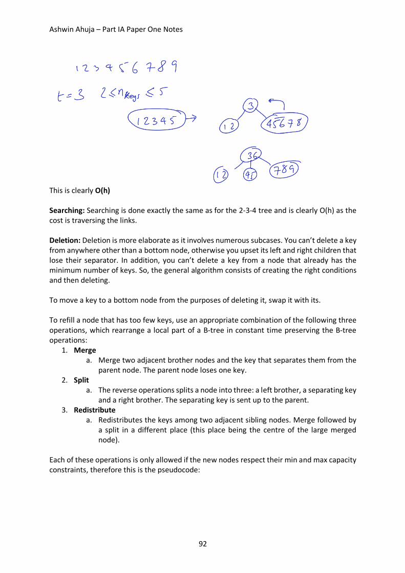
Ashwin Ahuja – Part IA Paper One Notes
92
This is clearly O(h) Searching: Searching is done exactly the same as for the 2-3-4 tree and is clearly O(h) as the cost is traversing the links. Deletion: Deletion is more elaborate as it involves numerous subcases. You can’t delete a key from anywhere other than a bottom node, otherwise you upset its left and right children that lose their separator. In addition, you can’t delete a key from a node that already has the minimum number of keys. So, the general algorithm consists of creating the right conditions and then deleting. To move a key to a bottom node from the purposes of deleting it, swap it with its. To refill a node that has too few keys, use an appropriate combination of the following three operations, which rearrange a local part of a B-tree in constant time preserving the B-tree operations:
1. Merge a. Merge two adjacent brother nodes and the key that separates them from the
parent node. The parent node loses one key. 2. Split
a. The reverse operations splits a node into three: a left brother, a separating key and a right brother. The separating key is sent up to the parent.
3. Redistribute a. Redistributes the keys among two adjacent sibling nodes. Merge followed by
a split in a different place (this place being the centre of the large merged node).
Each of these operations is only allowed if the new nodes respect their min and max capacity constraints, therefore this is the pseudocode:

Ashwin Ahuja – Part IA Paper One Notes
93
EXAMPLE:
Bounding the B-Tree Height n keys; min degree t; height H In the worst case, we are trying to make H as large as possible, while minimising the keys for the notional H.
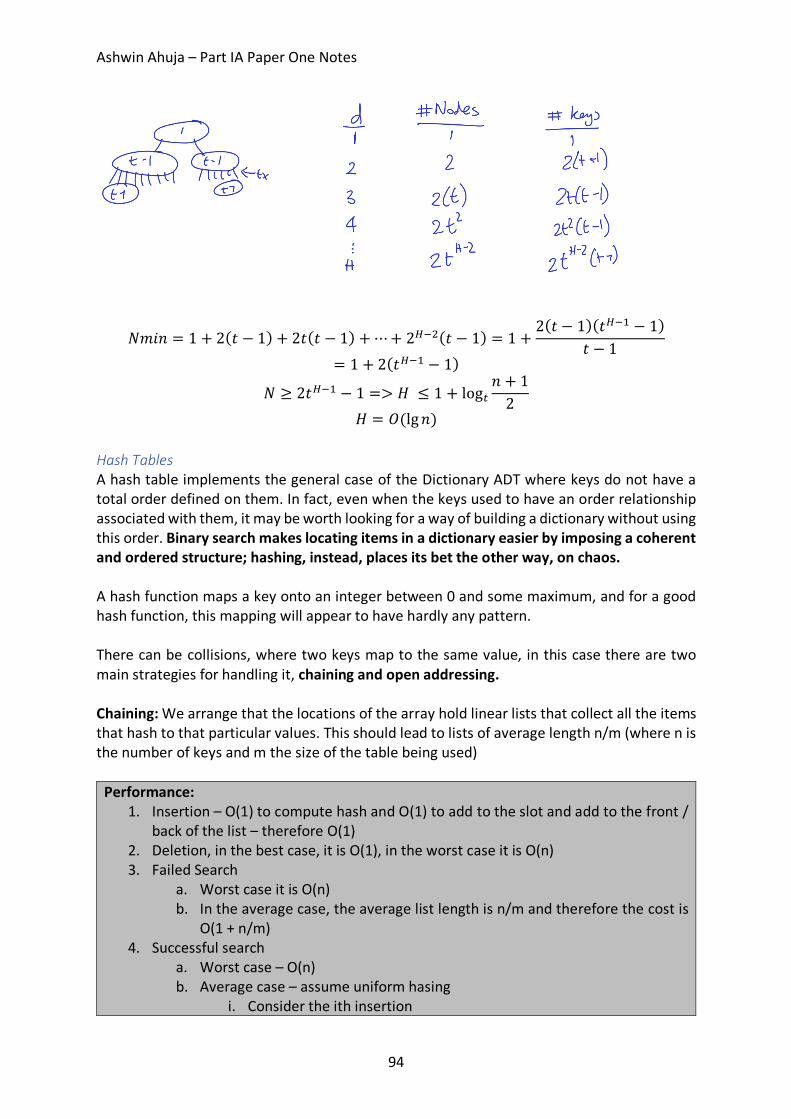
Ashwin Ahuja – Part IA Paper One Notes
94
𝑁𝑚𝑖𝑛 = 1 + 2(𝑡 − 1) + 2𝑡(𝑡 − 1) +⋯+ 2pRK(𝑡 − 1) = 1 +2(𝑡 − 1)(𝑡pRP − 1)
𝑡 − 1
= 1 + 2(𝑡pRP − 1)
𝑁 ≥ 2𝑡pRP − 1 => 𝐻 ≤ 1 + log�𝑛 + 12
𝐻 = 𝑂(lg𝑛) Hash Tables A hash table implements the general case of the Dictionary ADT where keys do not have a total order defined on them. In fact, even when the keys used to have an order relationship associated with them, it may be worth looking for a way of building a dictionary without using this order. Binary search makes locating items in a dictionary easier by imposing a coherent and ordered structure; hashing, instead, places its bet the other way, on chaos. A hash function maps a key onto an integer between 0 and some maximum, and for a good hash function, this mapping will appear to have hardly any pattern. There can be collisions, where two keys map to the same value, in this case there are two main strategies for handling it, chaining and open addressing. Chaining: We arrange that the locations of the array hold linear lists that collect all the items that hash to that particular values. This should lead to lists of average length n/m (where n is the number of keys and m the size of the table being used)
Performance: 1. Insertion – O(1) to compute hash and O(1) to add to the slot and add to the front /
back of the list – therefore O(1) 2. Deletion, in the best case, it is O(1), in the worst case it is O(n) 3. Failed Search
a. Worst case it is O(n) b. In the average case, the average list length is n/m and therefore the cost is
O(1 + n/m) 4. Successful search
a. Worst case – O(n) b. Average case – assume uniform hasing
i. Consider the ith insertion
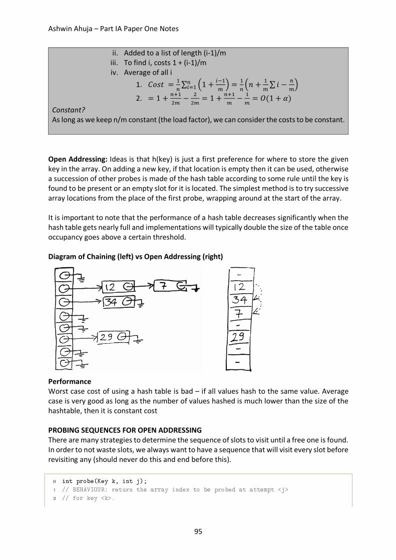
Ashwin Ahuja – Part IA Paper One Notes
95
ii. Added to a list of length (i-1)/m iii. To find i, costs 1 + (i-1)/m iv. Average of all i
1. 𝐶𝑜𝑠𝑡 = P7∑ ]1 + eRP
�^ = P
7]𝑛 + P
�∑ 𝑖 − 7
�^7
efP
2. = 1 + 7OPK�
− KK�
= 1 + 7OP�− P
�= 𝑂(1 + 𝛼)
Constant? As long as we keep n/m constant (the load factor), we can consider the costs to be constant.
Open Addressing: Ideas is that h(key) is just a first preference for where to store the given key in the array. On adding a new key, if that location is empty then it can be used, otherwise a succession of other probes is made of the hash table according to some rule until the key is found to be present or an empty slot for it is located. The simplest method is to try successive array locations from the place of the first probe, wrapping around at the start of the array. It is important to note that the performance of a hash table decreases significantly when the hash table gets nearly full and implementations will typically double the size of the table once occupancy goes above a certain threshold. Diagram of Chaining (left) vs Open Addressing (right)
Performance Worst case cost of using a hash table is bad – if all values hash to the same value. Average case is very good as long as the number of values hashed is much lower than the size of the hashtable, then it is constant cost PROBING SEQUENCES FOR OPEN ADDRESSING There are many strategies to determine the sequence of slots to visit until a free one is found. In order to not waste slots, we always want to have a sequence that will visit every slot before revisiting any (should never do this and end before this).
Ashwin Ahuja – Part IA Paper One Notes
96
Int m = size of hash table; Linear Probing: Just returns h(k) + j mod m. Therefore always try the next cell in sequence. This is simple to understand and implement, but leads to primary clustering, where many failed attempts hit the same slot and spill over to the same follow-up spots. The result is longer and longer runs of occupied slots, increasing search time. Quadratic Probing: With quadratic probing, you return h(k) + cj + dj2 mod m for some constants c and d. This works much better than linear probing, provided that c and d are chosen appropriately: when two distinct probing sequences hit the same slot, in subsequent probes they then hit secondary slots. However, still leads to secondary clustering because any keys that hash to the same value will yield the same probing sequence. Double Hashing: Probing sequence is h1(k) + h2(k) mod m, using two different hash functions h1 and h2. Even keys that hash to the same value (under h1) are assigned different probing sequences. However, access costs another hash function computation. Using the probing sequence 1. GET
a. Correct slot is the first one in the sequence which contains the sought key and if an empty slot is found then the key is not in the dictionary
b. A ‘deleted’ tag should be passed through c. Otherwise, if m probes completed, then not in hash table
2. SET a. If a slot with the sought key is found, then that is the one to use. b. Otherwise, the first empty slot (can use slots with a deleted tag) can be used. c. If m probes unsuccessful, array full.
3. DELETE a. Find the slot to delete using GET b. Mark it as deleted
i. This solution makes the GET operation become slower and slower if lots of deletes are occurring.
ii. Therefore we should rehash reasonably regularly after lots of deletes with not enough sets.
Open Addressing Search Performance
1. Average Number of Probes in a failed search a. < 𝟏
𝟏R𝜶
2. Average Number of Probes in a successful search
a. 𝟏𝜶𝒍𝒏 ] 𝟏
𝟏R𝜶^ + 𝟏
𝜶
Rehashing: Create a new array (normally twice the size to amortize the cost of the operation), with a new hash function. Insert every key-value pair of the old array into the new one and
Ashwin Ahuja – Part IA Paper One Notes
97
delete the old array. The deleted slots are not copied. This is necessary when the load factor becomes too high – HashMap in Java has a rehash load factor of 75%. Chaining vs Open Addressing • Open Addressing
o Faster for low load factor: slow as load factor approaches 1 o Better cache performance o Good hash functions hard to find o Best for small records that fit completely in the array and fit in a cache line
• Chaining o Can keep growing beyond a load factor of 1 (at cost of reduced performance) o Has extra space requirements.
Why don’t we always use a hash-table?
• To keep the load factor low, we need large arrays – not space efficient • Worst case is O(n), much worse than RB tree at O(lg n) • O(1) assumes a uniform distribution of keys but this isn’t guaranteed • We lose all notion of order and can’t iterate over the keys in a meaningful way
Graph Algorithms Notation and Representation A graph is a set of vertices (or nodes, or locations) and edges (or connections) between them. • A graph can be denoted by g = (V, E) where V is the set of vertices and E is the set of edges. • A graph may be directed or undirected.
o For a directed graph v1 -> v2 denotes an edge from v1 to v2 o For an undirected graph, v1 – v2 denotes an edge from v1 to v2 and from v2 to v1
• We assume there are not multiple edges between a pair of nodes • A path in a graph is a sequence of vertices connected by edges
o They may visit the same vertex more than once • A cycle is a path from a vertex back to itself • A directed acyclic graph or DAG is a directed graph without any cycles. • An undirected graph is connected if for every pair of vertices there is path between them.
A forest is an undirected acyclic graph. • A tree is a connected forest. There are generally two ways to store a graph in computer code: as an Adjacency List or as an Adjacency Matrix Adjacency List Takes up O(V + E) space, and here we store (for each vertex) a list of all the points it can get to.
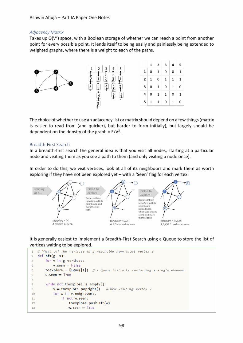
Ashwin Ahuja – Part IA Paper One Notes
98
Adjacency Matrix Takes up O(V2) space, with a Boolean storage of whether we can reach a point from another point for every possible point. It lends itself to being easily and painlessly being extended to weighted graphs, where there is a weight to each of the paths.
The choice of whether to use an adjacency list or matrix should depend on a few things (matrix is easier to read from (and quicker), but harder to form initially), but largely should be dependent on the density of the graph = E/V2. Breadth-First Search In a breadth-first search the general idea is that you visit all nodes, starting at a particular node and visiting them as you see a path to them (and only visiting a node once). In order to do this, we visit vertices, look at all of its neighbours and mark them as worth exploring if they have not been explored yet – with a ‘Seen’ flag for each vertex.
It is generally easiest to implement a Breadth-First Search using a Queue to store the list of vertices waiting to be explored.
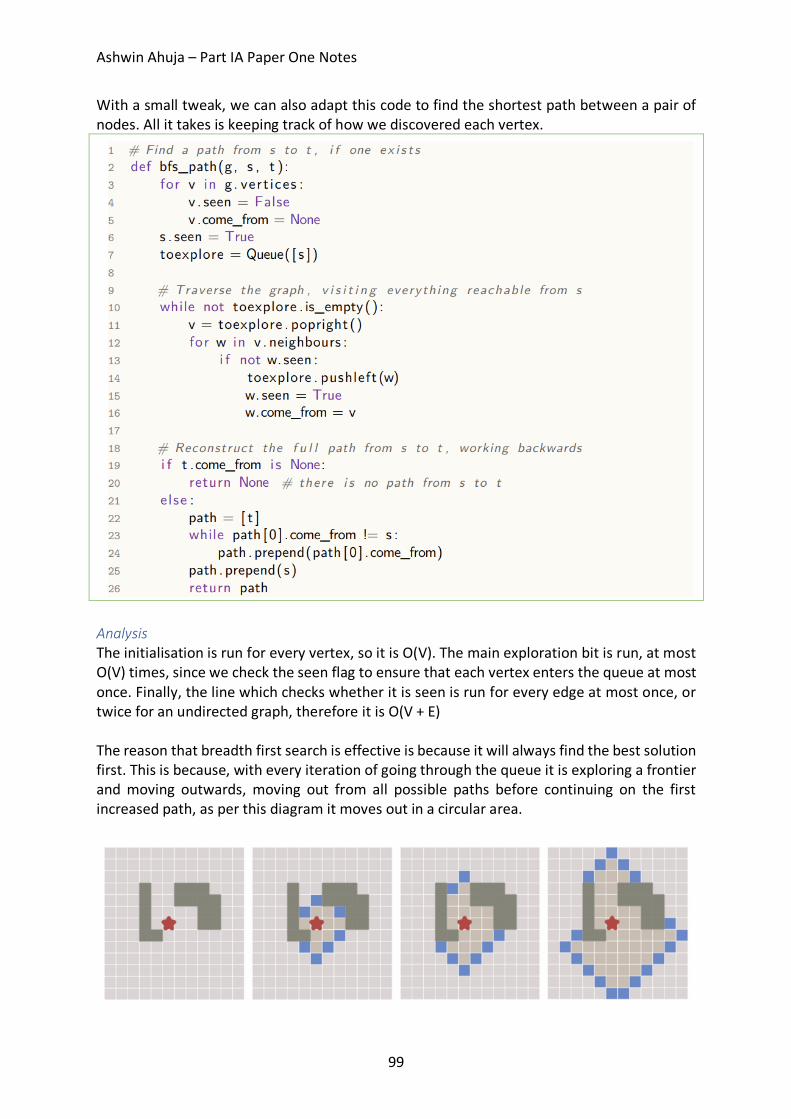
Ashwin Ahuja – Part IA Paper One Notes
99
With a small tweak, we can also adapt this code to find the shortest path between a pair of nodes. All it takes is keeping track of how we discovered each vertex.
Analysis The initialisation is run for every vertex, so it is O(V). The main exploration bit is run, at most O(V) times, since we check the seen flag to ensure that each vertex enters the queue at most once. Finally, the line which checks whether it is seen is run for every edge at most once, or twice for an undirected graph, therefore it is O(V + E) The reason that breadth first search is effective is because it will always find the best solution first. This is because, with every iteration of going through the queue it is exploring a frontier and moving outwards, moving out from all possible paths before continuing on the first increased path, as per this diagram it moves out in a circular area.
Ashwin Ahuja – Part IA Paper One Notes
100
Depth-First Search Depth-First Search is a backtracking based algorithm, where you attempt to go as far down a path as possible before backtracking if you hit a dead end then take a different route, backtracking as little as possible. We can use a stack to store all the vertices waiting to be explored.
It is also possible to do this using recursion, as here:
It is clear that the dfs algorithm has O(V+E) running time based on exactly the same logic as the analysis used for the breadth first search algorithm. The recursive equivalent is clearly also the same, hence: Line 4 is called once per vertex; visit is called once per vertex (when we check if it is visited) and the for loop is gone through once per edge in total over the entire process, therefore it O(V + V + E) = O(V + E) Dijkstra’s
Problem Statement: Given a directed graph where each edge is labelled with a cost ≥ 0, and a start vertex s, compute the distance from s to every other vertex
Dijkstra’s algorithm gets the shortest path between two nodes in a weighted graph. In a breadth first search, we visited the vertices in order of how many hops they are from the start vertex. For Dijkstra’s algorithm, we are visiting them in order of distance from the start vertex.
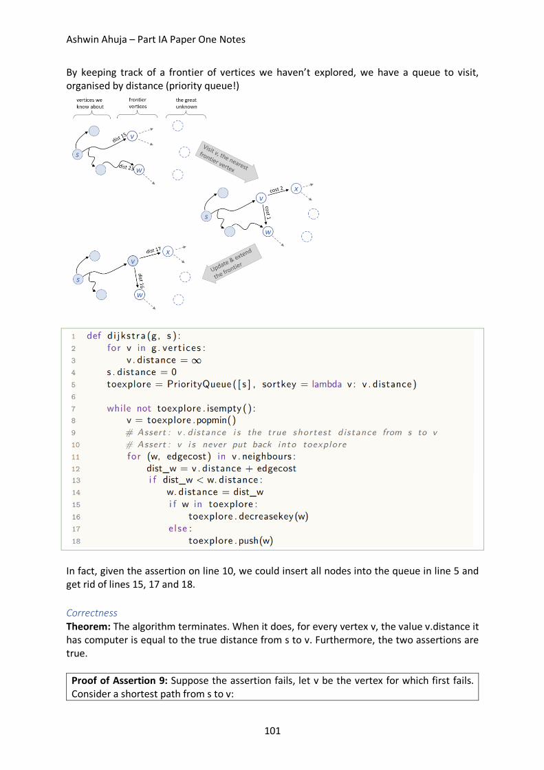
Ashwin Ahuja – Part IA Paper One Notes
101
By keeping track of a frontier of vertices we haven’t explored, we have a queue to visit, organised by distance (priority queue!)
In fact, given the assertion on line 10, we could insert all nodes into the queue in line 5 and get rid of lines 15, 17 and 18. Correctness Theorem: The algorithm terminates. When it does, for every vertex v, the value v.distance it has computer is equal to the true distance from s to v. Furthermore, the two assertions are true.
Proof of Assertion 9: Suppose the assertion fails, let v be the vertex for which first fails. Consider a shortest path from s to v:
Ashwin Ahuja – Part IA Paper One Notes
102
s = u1 -> … -> uk = v Let ui be the first vertex in this sequence which has not been popped from toexplore so far at this point in execution. Then:
• distance(s to v) o < v.distance
§ Since assertion failed o ≤ ui.distance
§ Since toexplore is a Priority Queue which had both ui and v o ≤ ui-1.distance + cost(ui-1 -> ui)
§ By lines 13-18 when ui-1 was popped o = distance(s to ui-1) + cost(ui-1 -> ui)
§ Assertion didn’t fail on ui-1 o ≤ distance (s to v)
This is a contradiction, therefore the premise (that Assertion 9 failed at some point) is false. Proof of Assertion 10 Once a vertex v has been popped, Assertion 9 guarantees that v.distance == distance (s to v). The only way that v could be pushed back into toexplore is if we found a shorter path to v which is impossible.
Since vertices can never be re-pushed into toexplore, the algorithm must terminate. At termination, all the vertices that are reachable from s must have been visited and popped, and when they were popped they passed Assertion 9. They can’t have had v.distance changed subsequently. Running Time The exact running time depends on how the Priority Queue is implemented. If we use a Fibonacci Heap, we get O(1) (amortized) running time for both push() and decreasekey() and O(log n) for popmin(). Line 3 and 8 is run once per vertex, and line 12-18 are run once per edge. Therefore O(V + VlogV + E) = O(E + V log V) Bellman-Ford
Problem Statement: Given a directed graph where each edge is labelled with a weight, and a start vertex s, (i) if the graph contains no negative-weight cycles reachable from s then for every vertex v compute the minimum weight from s to v; (ii) otherwise report that there is a negative weight cycle reachable from s.
Bellman-Ford can do effectively the same as Dijkstra, but while being able to deal with graphs with negative edge weights. The general idea is that relax all our edges (seeing if it could make us reach a node more easily) lots and lots of times. The effectiveness works in that we only have to do this a set number of times, the number of vertices in the graph.
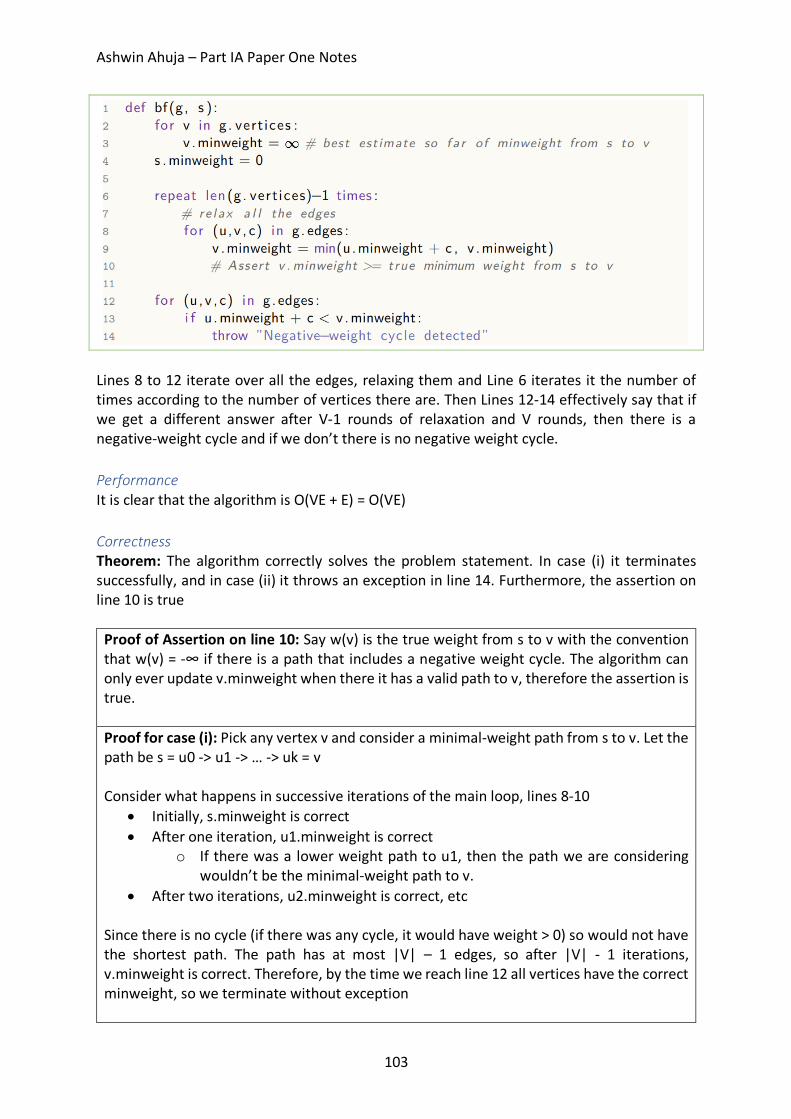
Ashwin Ahuja – Part IA Paper One Notes
103
Lines 8 to 12 iterate over all the edges, relaxing them and Line 6 iterates it the number of times according to the number of vertices there are. Then Lines 12-14 effectively say that if we get a different answer after V-1 rounds of relaxation and V rounds, then there is a negative-weight cycle and if we don’t there is no negative weight cycle. Performance It is clear that the algorithm is O(VE + E) = O(VE) Correctness Theorem: The algorithm correctly solves the problem statement. In case (i) it terminates successfully, and in case (ii) it throws an exception in line 14. Furthermore, the assertion on line 10 is true
Proof of Assertion on line 10: Say w(v) is the true weight from s to v with the convention that w(v) = -∞ if there is a path that includes a negative weight cycle. The algorithm can only ever update v.minweight when there it has a valid path to v, therefore the assertion is true. Proof for case (i): Pick any vertex v and consider a minimal-weight path from s to v. Let the path be s = u0 -> u1 -> … -> uk = v Consider what happens in successive iterations of the main loop, lines 8-10
• Initially, s.minweight is correct • After one iteration, u1.minweight is correct
o If there was a lower weight path to u1, then the path we are considering wouldn’t be the minimal-weight path to v.
• After two iterations, u2.minweight is correct, etc Since there is no cycle (if there was any cycle, it would have weight > 0) so would not have the shortest path. The path has at most |V| – 1 edges, so after |V| - 1 iterations, v.minweight is correct. Therefore, by the time we reach line 12 all vertices have the correct minweight, so we terminate without exception
Ashwin Ahuja – Part IA Paper One Notes
104
Proof for case (ii): Suppose there is a negative weight cycle reachable from s 𝑠 → ⋯ → 𝑣q →𝑣P → ⋯ → 𝑣� → 𝑣q
where 𝑤𝑒𝑖𝑔ℎ𝑡(𝑣q → 𝑣P) +⋯+ 𝑤𝑒𝑖𝑔ℎ𝑡(𝑣� → 𝑣q) < 0
If the algorithm terminates without throwing an exception, then all the edges pass the test in line 13, i.e.
𝑣q.𝑚𝑖𝑛𝑤𝑒𝑖𝑔ℎ𝑡 + 𝑤𝑒𝑖𝑔ℎ𝑡(𝑣q → 𝑣P) ≥ 𝑣P.𝑚𝑖𝑛𝑤𝑒𝑖𝑔ℎ𝑡 𝑣P.𝑚𝑖𝑛𝑤𝑒𝑖𝑔ℎ𝑡 + 𝑤𝑒𝑖𝑔ℎ𝑡(𝑣P → 𝑣K) ≥ 𝑣K.𝑚𝑖𝑛𝑤𝑒𝑖𝑔ℎ𝑡
etc 𝑣�.𝑚𝑖𝑛𝑤𝑒𝑖𝑔ℎ𝑡 + 𝑤𝑒𝑖𝑔ℎ𝑡(𝑣� → 𝑣q) ≥ 𝑣q.𝑚𝑖𝑛𝑤𝑒𝑖𝑔ℎ𝑡
Therefore,
𝑣q.𝑚𝑖𝑛𝑤𝑒𝑖𝑔ℎ𝑡 + 𝑤𝑒𝑖𝑔ℎ𝑡(𝑣q → 𝑣P) +⋯+ 𝑤𝑒𝑖𝑔ℎ𝑡(𝑣� → 𝑣q) ≥ 𝑣q.𝑚𝑖𝑛𝑤𝑒𝑖𝑔ℎ𝑡 Therefore, the cycle has weight ≥ 0. This contradicts the premise – so at least one of the edges must fail the test in line 13 and so the exception will be thrown.
Johnson’s Algorithm
Problem Statement: Given a directed graph where each edge is labelled with a weight, (i) if the graph contains no negative-weight cycles then for every pair of vertices compute the weight of the minimal weight path between those vertices; (ii) if the graph contains a negative-weight cycle then detect that this is so.
Allows us to compute shortest paths between all pairs of vertices. The betweeness centrality of an edge is defined to be the number of shortest paths to use that edge over all the shortest paths between all pairs of vertices in a graph. It is a measure of how important an edge is, and its used for summarizing the shape of the graph. A primary idea is that we could just run Dijkstra’s algorithm V times, once from each vertex leading to a complexity of O(VE + V2logV). If some edge weights are less than 0, we could run Bellman-Ford from each vertex, which would have running time O(V2E) But, we can Bellman-Ford once, then run Dijkstra once from each vertex, then run some cleanup for every pair of vertices, with running time = O(VE) + O(VE + V2logV) + O(V2) = O(VE + V2logV) This works by constructing an extra helper graph, running a computation in it and applying the results of the computation to the original problem. The helper graph is the original graph with an extra vertex s and zero weight edges s->v for all vertices v Implementation:
1. The Helper Graph: Run Bellman-Ford on the helper graph and let the minimum weight from s to v to be dv. If Bellman-Ford reports a negative-weight cycle, then stop.

Ashwin Ahuja – Part IA Paper One Notes
105
2. The Tweaked Graph: Define a tweaked graph which is like the original graph but with different edge weights
a. w’(u->v) = du + w(u->v) – dv b. In this graph, every edge has w’(u->v) > 0
i. The relaxation equation, applied to the helper graph says that: ii. dv ≤ du + w(u -> v) therefore w’(u -> v) ≥ 0
3. Dijkstra on the tweaked graph: Run Dijkstra V times on the tweaked graph, once from each vertex. All edges have weight >= 0
a. The claim is that the minimum-weight paths in the tweaked graphs are the same as in the original graph
Proof: Pick any two vertices p and q, and any path between them. p = v0 -> v1 -> … -> vk = q
Weight in tweaked graph = dp + w(v0 -> v1) – dv1 + dv1 + w(v1 -> v2) – dv2 + … = dp + w(v0 -> v1) + w(v1 -> v2) + … + w(v(k-1) -> vk) – dq = weight in original graph + dp – dq
Since dp-dq is the same for every path from p to q, the ranking of the paths is the same in the tweaked graph as in the original graph.
4. Wrap Up
a. All-Pairs Shortest Paths with Matrices There is another possible algorithm, which solves the same problem as for Johnson’s, with a running time of O(V3logV) – worse than Johnson’s but is very simple. The general idea is utilising a matrix to solve the problem using dynamic programming:
We can define Ml in terms of Ml-1 and this leads to an algorithm for computing Ml. If we pick l big enough (at least the maximum number of edges in any path), then we’ve solved the problem. We also define W as our path matrix (representing the paths between two nodes and their distance).
This is a n x n matrix, where n is |W|
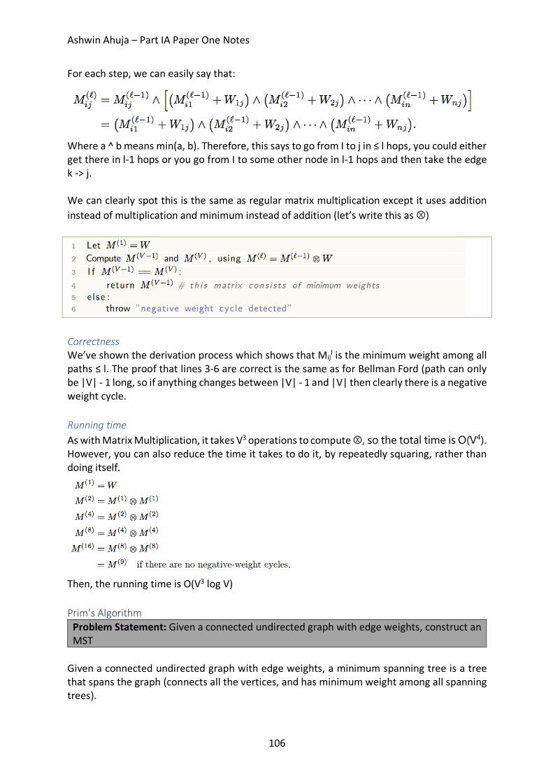
Ashwin Ahuja – Part IA Paper One Notes
106
For each step, we can easily say that:
Where a ^ b means min(a, b). Therefore, this says to go from I to j in ≤ l hops, you could either get there in l-1 hops or you go from I to some other node in l-1 hops and then take the edge k -> j. We can clearly spot this is the same as regular matrix multiplication except it uses addition instead of multiplication and minimum instead of addition (let’s write this as Ⓧ)
Correctness We’ve shown the derivation process which shows that Mij
l is the minimum weight among all paths ≤ l. The proof that lines 3-6 are correct is the same as for Bellman Ford (path can only be |V| - 1 long, so if anything changes between |V| - 1 and |V| then clearly there is a negative weight cycle. Running time As with Matrix Multiplication, it takes V3 operations to compute Ⓧ, so the total time is O(V4). However, you can also reduce the time it takes to do it, by repeatedly squaring, rather than doing itself.
Then, the running time is O(V3 log V) Prim’s Algorithm
Problem Statement: Given a connected undirected graph with edge weights, construct an MST
Given a connected undirected graph with edge weights, a minimum spanning tree is a tree that spans the graph (connects all the vertices, and has minimum weight among all spanning trees).
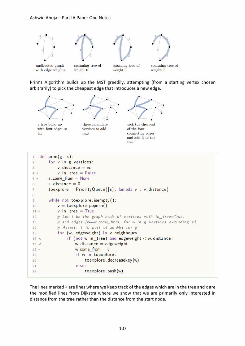
Ashwin Ahuja – Part IA Paper One Notes
107
Prim’s Algorithm builds up the MST greedily, attempting (from a starting vertex chosen arbitrarily) to pick the cheapest edge that introduces a new edge.
The lines marked + are lines where we keep track of the edges which are in the tree and x are the modified lines from Dijkstra where we show that we are primarily only interested in distance from the tree rather than the distance from the start node.
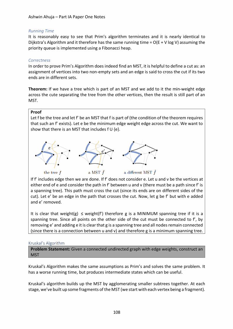
Ashwin Ahuja – Part IA Paper One Notes
108
Running Time It is reasonably easy to see that Prim’s algorithm terminates and it is nearly identical to Dijkstra’s Algorithm and it therefore has the same running time = O(E + V log V) assuming the priority queue is implemented using a Fibonacci heap. Correctness In order to prove Prim’s Algorithm does indeed find an MST, it is helpful to define a cut as: an assignment of vertices into two non-empty sets and an edge is said to cross the cut if its two ends are in different sets. Theorem: If we have a tree which is part of an MST and we add to it the min-weight edge across the cute separating the tree from the other vertices, then the result is still part of an MST.
Proof Let f be the tree and let f’ be an MST that f is part of (the condition of the theorem requires that such an f’ exists). Let e be the minimum edge weight edge across the cut. We want to show that there is an MST that includes f U {e}.
If f’ includes edge then we are done. If f’ does not consider e. Let u and v be the vertices at either end of e and consider the path in f’ between u and v (there must be a path since f’ is a spanning tree). This path must cross the cut (since its ends are on different sides of the cut). Let e’ be an edge in the path that crosses the cut. Now, let g be f’ but with e added and e’ removed. It is clear that weight(g) ≤ weight(f’) therefore g is a MINIMUM spanning tree if it is a spanning tree. Since all points on the other side of the cut must be connected to f’, by removing e’ and adding e it is clear that g is a spanning tree and all nodes remain connected (since there is a connection between u and v) and therefore g is a minimum spanning tree.
Kruskal’s Algorithm
Problem Statement: Given a connected undirected graph with edge weights, construct an MST
Kruskal’s Algorithm makes the same assumptions as Prim’s and solves the same problem. It has a worse running time, but produces intermediate states which can be useful. Kruskal’s algorithm builds up the MST by agglomerating smaller subtrees together. At each stage, we’ve built up some fragments of the MST (we start with each vertex being a fragment).
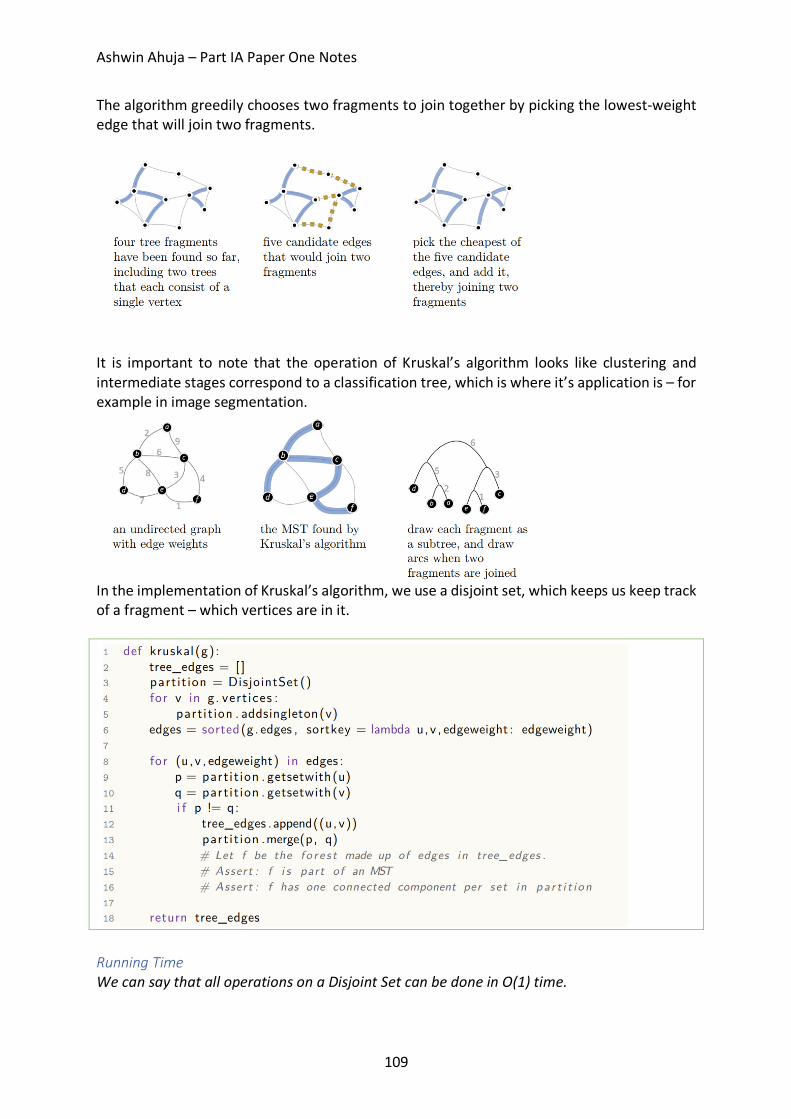
Ashwin Ahuja – Part IA Paper One Notes
109
The algorithm greedily chooses two fragments to join together by picking the lowest-weight edge that will join two fragments.
It is important to note that the operation of Kruskal’s algorithm looks like clustering and intermediate stages correspond to a classification tree, which is where it’s application is – for example in image segmentation.
In the implementation of Kruskal’s algorithm, we use a disjoint set, which keeps us keep track of a fragment – which vertices are in it.
Running Time We can say that all operations on a Disjoint Set can be done in O(1) time.
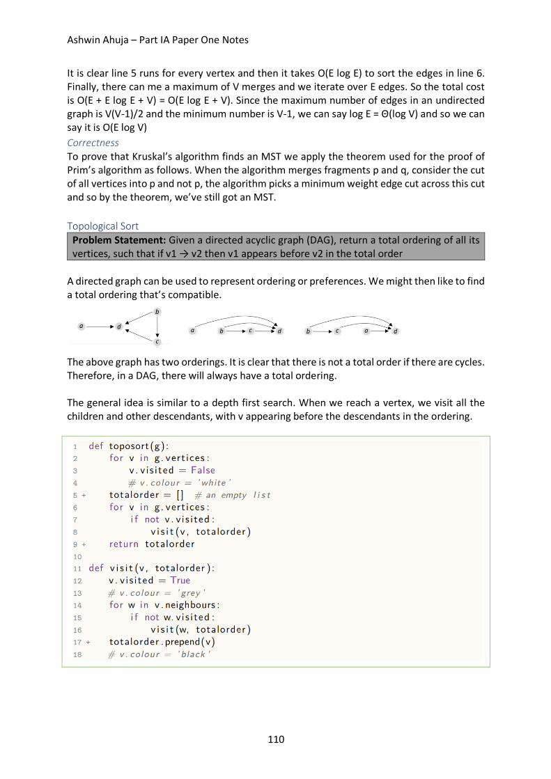
Ashwin Ahuja – Part IA Paper One Notes
110
It is clear line 5 runs for every vertex and then it takes O(E log E) to sort the edges in line 6. Finally, there can me a maximum of V merges and we iterate over E edges. So the total cost is O(E + E log E + V) = O(E log E + V). Since the maximum number of edges in an undirected graph is V(V-1)/2 and the minimum number is V-1, we can say log E = Θ(log V) and so we can say it is O(E log V) Correctness To prove that Kruskal’s algorithm finds an MST we apply the theorem used for the proof of Prim’s algorithm as follows. When the algorithm merges fragments p and q, consider the cut of all vertices into p and not p, the algorithm picks a minimum weight edge cut across this cut and so by the theorem, we’ve still got an MST. Topological Sort
Problem Statement: Given a directed acyclic graph (DAG), return a total ordering of all its vertices, such that if v1 → v2 then v1 appears before v2 in the total order
A directed graph can be used to represent ordering or preferences. We might then like to find a total ordering that’s compatible.
The above graph has two orderings. It is clear that there is not a total order if there are cycles. Therefore, in a DAG, there will always have a total ordering. The general idea is similar to a depth first search. When we reach a vertex, we visit all the children and other descendants, with v appearing before the descendants in the ordering.
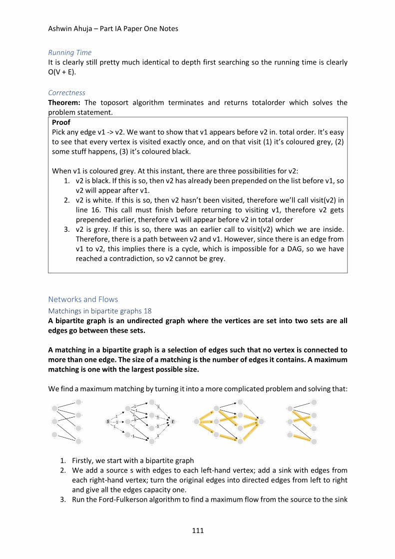
Ashwin Ahuja – Part IA Paper One Notes
111
Running Time It is clearly still pretty much identical to depth first searching so the running time is clearly O(V + E). Correctness Theorem: The toposort algorithm terminates and returns totalorder which solves the problem statement.
Proof Pick any edge v1 -> v2. We want to show that v1 appears before v2 in. total order. It’s easy to see that every vertex is visited exactly once, and on that visit (1) it’s coloured grey, (2) some stuff happens, (3) it’s coloured black. When v1 is coloured grey. At this instant, there are three possibilities for v2:
1. v2 is black. If this is so, then v2 has already been prepended on the list before v1, so v2 will appear after v1.
2. v2 is white. If this is so, then v2 hasn’t been visited, therefore we’ll call visit(v2) in line 16. This call must finish before returning to visiting v1, therefore v2 gets prepended earlier, therefore v1 will appear before v2 in total order
3. v2 is grey. If this is so, there was an earlier call to visit(v2) which we are inside. Therefore, there is a path between v2 and v1. However, since there is an edge from v1 to v2, this implies there is a cycle, which is impossible for a DAG, so we have reached a contradiction, so v2 cannot be grey.
Networks and Flows Matchings in bipartite graphs 18 A bipartite graph is an undirected graph where the vertices are set into two sets are all edges go between these sets. A matching in a bipartite graph is a selection of edges such that no vertex is connected to more than one edge. The size of a matching is the number of edges it contains. A maximum matching is one with the largest possible size. We find a maximum matching by turning it into a more complicated problem and solving that:
1. Firstly, we start with a bipartite graph 2. We add a source s with edges to each left-hand vertex; add a sink with edges from
each right-hand vertex; turn the original edges into directed edges from left to right and give all the edges capacity one.
3. Run the Ford-Fulkerson algorithm to find a maximum flow from the source to the sink
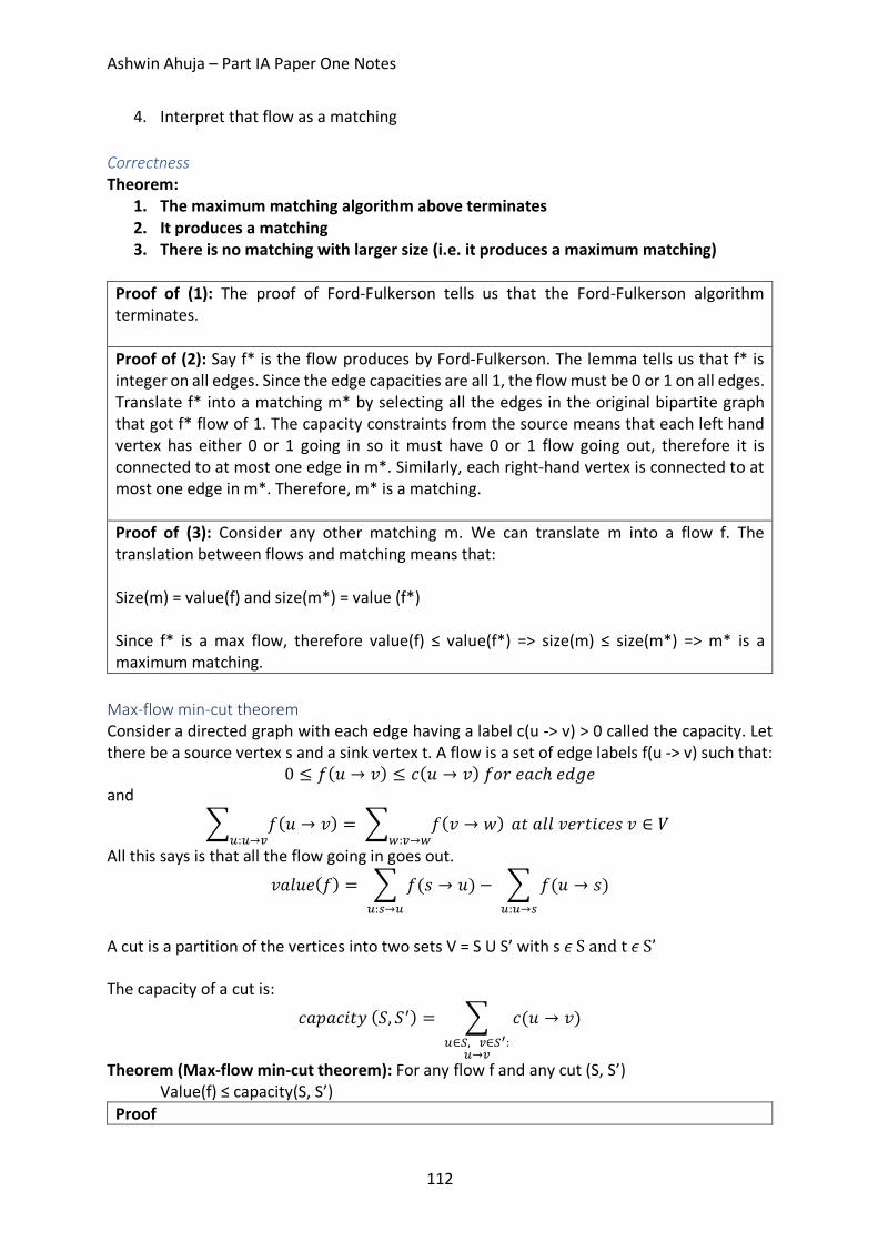
Ashwin Ahuja – Part IA Paper One Notes
112
4. Interpret that flow as a matching Correctness Theorem:
1. The maximum matching algorithm above terminates 2. It produces a matching 3. There is no matching with larger size (i.e. it produces a maximum matching)
Proof of (1): The proof of Ford-Fulkerson tells us that the Ford-Fulkerson algorithm terminates. Proof of (2): Say f* is the flow produces by Ford-Fulkerson. The lemma tells us that f* is integer on all edges. Since the edge capacities are all 1, the flow must be 0 or 1 on all edges. Translate f* into a matching m* by selecting all the edges in the original bipartite graph that got f* flow of 1. The capacity constraints from the source means that each left hand vertex has either 0 or 1 going in so it must have 0 or 1 flow going out, therefore it is connected to at most one edge in m*. Similarly, each right-hand vertex is connected to at most one edge in m*. Therefore, m* is a matching. Proof of (3): Consider any other matching m. We can translate m into a flow f. The translation between flows and matching means that: Size(m) = value(f) and size(m*) = value (f*) Since f* is a max flow, therefore value(f) ≤ value(f*) => size(m) ≤ size(m*) => m* is a maximum matching.
Max-flow min-cut theorem Consider a directed graph with each edge having a label c(u -> v) > 0 called the capacity. Let there be a source vertex s and a sink vertex t. A flow is a set of edge labels f(u -> v) such that:
0 ≤ 𝑓(𝑢 → 𝑣) ≤ 𝑐(𝑢 → 𝑣)𝑓𝑜𝑟𝑒𝑎𝑐ℎ𝑒𝑑𝑔𝑒 and
d 𝑓(𝑢 → 𝑣)�:�→�
= d 𝑓(𝑣 → 𝑤)�:�→�
𝑎𝑡𝑎𝑙𝑙𝑣𝑒𝑟𝑡𝑖𝑐𝑒𝑠𝑣 ∈ 𝑉
All this says is that all the flow going in goes out.
𝑣𝑎𝑙𝑢𝑒(𝑓) = d 𝑓(𝑠 → 𝑢)�:�→�
− d 𝑓(𝑢 → 𝑠)�:�→�
A cut is a partition of the vertices into two sets V = S U S’ with s 𝜖Sandt𝜖S’The capacity of a cut is:
𝑐𝑎𝑝𝑎𝑐𝑖𝑡𝑦(𝑆, 𝑆�) = d 𝑐(𝑢 → 𝑣)�∈�,�∈��:
�→�
Theorem (Max-flow min-cut theorem): For any flow f and any cut (S, S’) Value(f) ≤ capacity(S, S’)
Proof
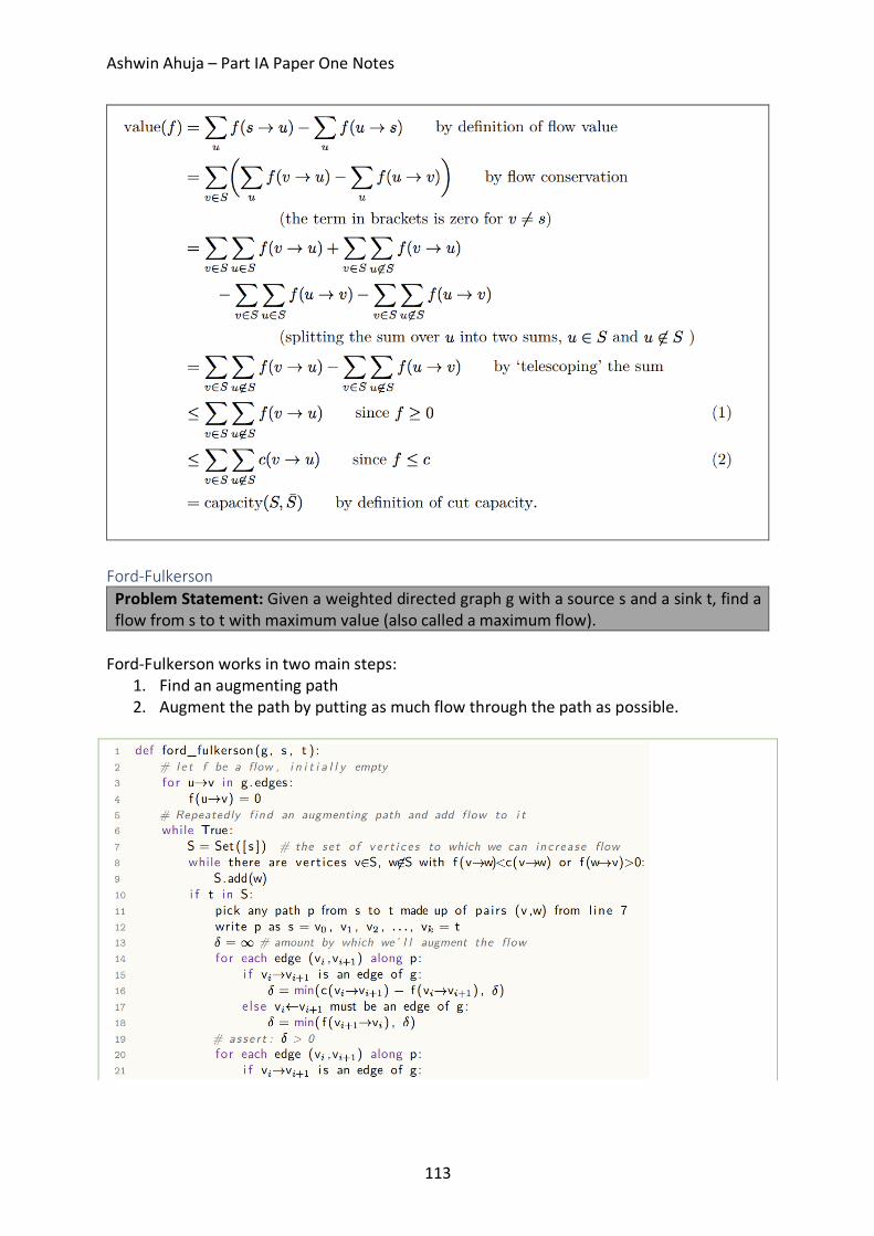
Ashwin Ahuja – Part IA Paper One Notes
113
Ford-Fulkerson
Problem Statement: Given a weighted directed graph g with a source s and a sink t, find a flow from s to t with maximum value (also called a maximum flow).
Ford-Fulkerson works in two main steps:
1. Find an augmenting path 2. Augment the path by putting as much flow through the path as possible.
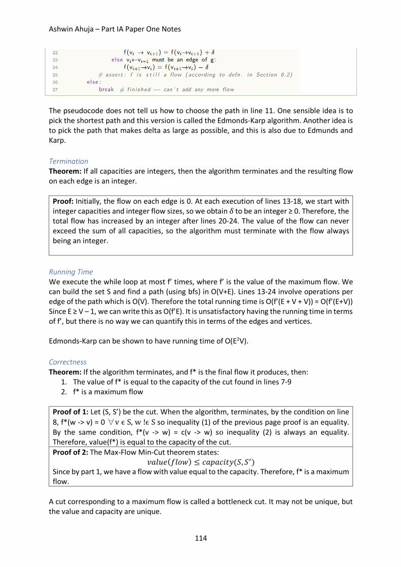
Ashwin Ahuja – Part IA Paper One Notes
114
The pseudocode does not tell us how to choose the path in line 11. One sensible idea is to pick the shortest path and this version is called the Edmonds-Karp algorithm. Another idea is to pick the path that makes delta as large as possible, and this is also due to Edmunds and Karp. Termination Theorem: If all capacities are integers, then the algorithm terminates and the resulting flow on each edge is an integer.
Proof: Initially, the flow on each edge is 0. At each execution of lines 13-18, we start with integer capacities and integer flow sizes, so we obtain 𝛿to be an integer ≥ 0. Therefore, the total flow has increased by an integer after lines 20-24. The value of the flow can never exceed the sum of all capacities, so the algorithm must terminate with the flow always being an integer.
Running Time We execute the while loop at most f’ times, where f’ is the value of the maximum flow. We can build the set S and find a path (using bfs) in O(V+E). Lines 13-24 involve operations per edge of the path which is O(V). Therefore the total running time is O(f’(E + V + V)) = O(f’(E+V)) Since E ≥ V – 1, we can write this as O(f’E). It is unsatisfactory having the running time in terms of f’, but there is no way we can quantify this in terms of the edges and vertices. Edmonds-Karp can be shown to have running time of O(E2V). Correctness Theorem: If the algorithm terminates, and f* is the final flow it produces, then:
1. The value of f* is equal to the capacity of the cut found in lines 7-9 2. f* is a maximum flow
Proof of 1: Let (S, S’) be the cut. When the algorithm, terminates, by the condition on line 8, f*(w -> v) = 0 ∀vϵS,w!ϵSso inequality (1) of the previous page proof is an equality. By the same condition, f*(v -> w) = c(v -> w) so inequality (2) is always an equality. Therefore, value(f*) is equal to the capacity of the cut. Proof of 2: The Max-Flow Min-Cut theorem states:
𝑣𝑎𝑙𝑢𝑒(𝑓𝑙𝑜𝑤) ≤ 𝑐𝑎𝑝𝑎𝑐𝑖𝑡𝑦(𝑆, 𝑆�) Since by part 1, we have a flow with value equal to the capacity. Therefore, f* is a maximum flow.
A cut corresponding to a maximum flow is called a bottleneck cut. It may not be unique, but the value and capacity are unique.
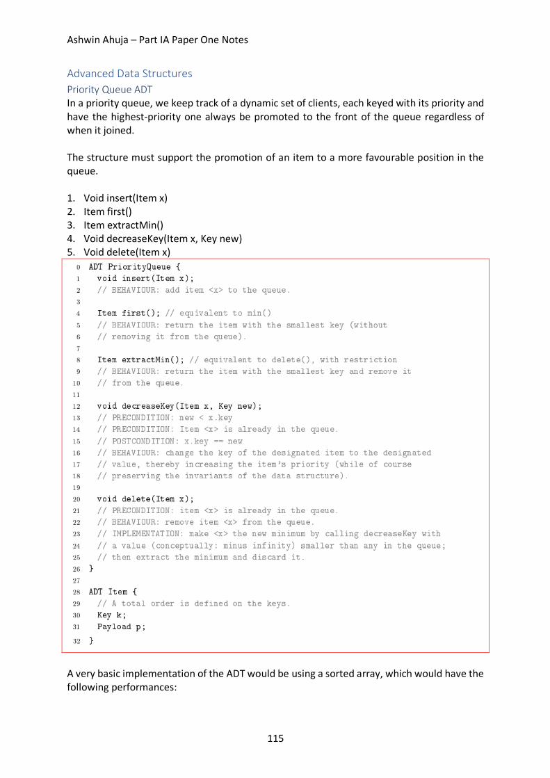
Ashwin Ahuja – Part IA Paper One Notes
115
Advanced Data Structures Priority Queue ADT In a priority queue, we keep track of a dynamic set of clients, each keyed with its priority and have the highest-priority one always be promoted to the front of the queue regardless of when it joined. The structure must support the promotion of an item to a more favourable position in the queue. 1. Void insert(Item x) 2. Item first() 3. Item extractMin() 4. Void decreaseKey(Item x, Key new) 5. Void delete(Item x)
A very basic implementation of the ADT would be using a sorted array, which would have the following performances:

Ashwin Ahuja – Part IA Paper One Notes
116
Binary Heap What a heap is, was covered in the description of heapsort. Here we use a min-heap rather than a max-heap. A min-heap is a binary tree which satisfies two additional invariants. It is “almost full” and the lowest level is filled left to right, and it obeys the heap property, that is each node has a key less than or equal to those of its children. • As a consequence of heap property, the root is the smallest value – therefore to read out
the highest priority item, we just look at the root (O(1)). • To insert an item, we add it to the end of the heap and let it bubble up – O(H). • To extract the root, we read it out, then replace it with last item and let that sink down –
O(H) • To reposition an item after decreasing the key, we let it bubble up towards the root – O(H) Since the tree is balanced – it is always full, the height is always O(log n) therefore the asymptotic complexities are:
Amortized Analysis For some data structures, looking at the worst-case run time per operation may be unduly pessimistic, especially in two situations:
1. Some data structures are designed so that most operations are cheap, but some of them have occasional expensive internal housekeeping.
2. Sometimes we want to know the aggregate cost of a sequence of operations, not the individual costs of each operation.
Aggregate Analysis: Working out the worst-case total cost of a sequence of operations.
Example: Consider a dynamically-sized array with initial capacity 1 which doubles when it becomes full. Assume that the cost of doubling capacity from m to 2m is m. After adding n elements, the total cost from all the doubling is:
𝟏 + 𝟐 + ⋯+𝟐⌊𝒍𝒈𝒏R𝟏⌋
Ashwin Ahuja – Part IA Paper One Notes
117
which is ≤ 2n – 3. The cost of writing in the n values is n. Therefore, the total cost is ≤ 3n-3 which is O(n)
Amortized Cost When we look at the aggregate cost of a sequence of operations, we can reassign costs like this:
𝑐P + ⋯+𝑐n ≤ 𝑐�P +⋯+ 𝑐′n Where c’s are your amortized costs.
Example: Consider a dynamically-sized array with initial capacity 1 which doubles when it becomes full. If we assign a cost c’ = 3 to each append operation, we ensure that the true cost is less than the amortized cost we have said. (We said that n calls to append cost ≤ 3n – 3). Therefore, the amortized cost is O(1).
The Potential Method We define a function ɸ, called a potential function, that maps possible states of the data structure to real numbers ≥ 0. For an operation with true cost c, for which the state just beforehand was Sante and the state just after is Spost, define the amortized cost of the operation to be:
𝑐� = 𝑐 + ɸ(𝑆¤¥��* − ɸ(𝑆y7�¦)
Proof that c’ is a valid amortized cost: Consider a sequence of operations
𝑆q − 𝑐P → 𝑆P − 𝑐K → 𝑆K − 𝑐§ → ⋯− 𝑐� → 𝑆� Aggregate Amortized Cost
Therefore we have proved this.
Example: Consider a dynamically-sized array with initial capacity 1 which doubles when it becomes full. Define the potential function as:
ɸ = [2(𝑛𝑢𝑚𝑂𝑓𝐼𝑡𝑒𝑚𝑠𝐼𝑛𝐴𝑟𝑟𝑎𝑦) − 𝑐𝑎𝑝𝑎𝑐𝑖𝑡𝑦𝑂𝑓𝐴𝑟𝑟𝑎𝑦]O This potential function is ≥ 0, and for an empty data structure it is = 0. Now, consider the two ways that append could play out:

Ashwin Ahuja – Part IA Paper One Notes
118
1. We could add the new item without needing to double the capacity. The true cost is c = O(1) and the change in potential is = 2, therefore the amortized cost = O(1) + 2
2. Alternatively, we need to double the capacity. Let n be the number of items just before. The true cost is O(n), to create the new array and copy n items and then write in the new value. The change in potential is 2 – n, so the amortized cost = O(n) + 2 – n = O(1)
In both cases, the amortized cost of an append is O(1)
Binomial Heap A binomial heap is a compromise between the linked list and binary heap methods of keeping a priority queue. It maintains a list rather than obsessively tidying everything into a single heap so that push is fast, but it still keeps some heap structure so that popmin is fast. It is defined hence:
1. A binomial tree of order 0 is a single node. A binomial tree of order of order k is a tree obtained by combining two binomial trees of order k-1, by appending one of the trees to the root of the other
2. A binomial heap is a collection of binomial tree, at most one for each tree order, each obeying the heap property.
3. This is a binomial heap consisting of one binomial tree of order 0 and one of order 3. (The dotted parts simply say there are no trees of order 1 or 2).
Basic Properties
1. Binomial tree of order k has 2k nodes and height k. 2. In a binomial tree of order k, the root node has k children – the degree of the root is k 3. In a binomial tree of order k, the root node’s j children are binomial trees of order k-
1, k-2, …, 0 4. In a binomial heap with n nodes, the 1s in the binary expansion of the number n
correspond to the orders of trees contained in the heap. 5. If a binomial heap contains n nodes, it contains O(lg n) binomial trees and the largest
of those trees has O(lg n) Operations
1. Merge (h1, h2) – O(log n) a. To merge two binomial heaps, we start from order 0 and go up, as if doing
binary addition, but instead of adding digits in place k, we merge binomial trees of order k, keeping the tree with smaller root on top. If n is the total number

Ashwin Ahuja – Part IA Paper One Notes
119
of nodes in both heaps together, then there are O(log n) trees in each heap and O(log n) operations in total.
2. Push (v, k) – O(log n) a. Though it has true worst case cost of O(log n), it has an amortized cost of O(1)
i. A series of adding a single order 0 tree is effectively looking for the first 0 in the sequence of the original heap each time. Equivalent to incrementing a binary counter and seeing which things need to be changed.
ii. N changes to last, n/2 to second last, n/4 to next, etc iii. SumOfNumberOfChanges = GP with r = ½ iv. S = 2n(1 – 2(0.5)k) {for a k order heap} v. Therefore amortized cost of O(1)
b. Treat the new item as a binomial heap with only one node and merge it. 3. DecreaseKey (v, newK) – O(log n)
a. Proceed, as with a normal binary heap, applied to the tree with v belongs, change and bubble up as needed, therefore O(log n)
4. PopMin() – O(log n) a. First, scan the roots of all the trees in the heap, at cost O(log n) to find which
root to remove. Cut it out from its. It’s children for a binomial heap by property 3 and merge this with the rest of the original heap at cost O(log n)
Fibonacci Heap A fibonnaci heap is a fast priority queue, specifically designed to speed up Dijkstra’s algorithm. The general idea is that we should just be lazy while we are doing push and decreasekey, only doing O(1) work, and just accumulating a collection of unsorted items, only doing cleanup on calls to popmin. The general reasoning for this is that adding n items to a binary heap one by one is O(n log n), but only O(n) to heapify them together. The other big idea is for decreasekey to be O(1), by only touching a small part of the datastructure. Push and Popmin
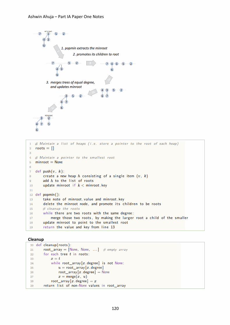
Ashwin Ahuja – Part IA Paper One Notes
120
Cleanup
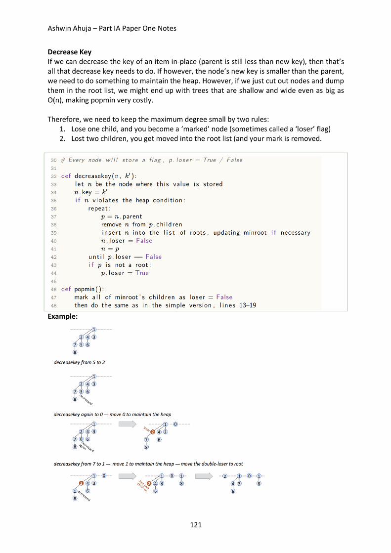
Ashwin Ahuja – Part IA Paper One Notes
121
Decrease Key If we can decrease the key of an item in-place (parent is still less than new key), then that’s all that decrease key needs to do. If however, the node’s new key is smaller than the parent, we need to do something to maintain the heap. However, if we just cut out nodes and dump them in the root list, we might end up with trees that are shallow and wide even as big as O(n), making popmin very costly. Therefore, we need to keep the maximum degree small by two rules:
1. Lose one child, and you become a ‘marked’ node (sometimes called a ‘loser’ flag) 2. Lost two children, you get moved into the root list (and your mark is removed.
Example:
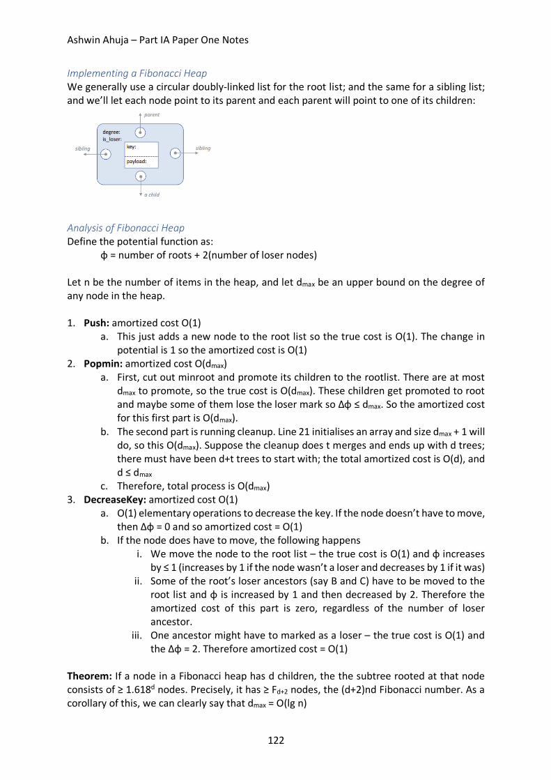
Ashwin Ahuja – Part IA Paper One Notes
122
Implementing a Fibonacci Heap We generally use a circular doubly-linked list for the root list; and the same for a sibling list; and we’ll let each node point to its parent and each parent will point to one of its children:
Analysis of Fibonacci Heap Define the potential function as: ɸ = number of roots + 2(number of loser nodes) Let n be the number of items in the heap, and let dmax be an upper bound on the degree of any node in the heap. 1. Push: amortized cost O(1)
a. This just adds a new node to the root list so the true cost is O(1). The change in potential is 1 so the amortized cost is O(1)
2. Popmin: amortized cost O(dmax) a. First, cut out minroot and promote its children to the rootlist. There are at most
dmax to promote, so the true cost is O(dmax). These children get promoted to root and maybe some of them lose the loser mark so Δɸ ≤ dmax. So the amortized cost for this first part is O(dmax).
b. The second part is running cleanup. Line 21 initialises an array and size dmax + 1 will do, so this O(dmax). Suppose the cleanup does t merges and ends up with d trees; there must have been d+t trees to start with; the total amortized cost is O(d), and d ≤ dmax
c. Therefore, total process is O(dmax) 3. DecreaseKey: amortized cost O(1)
a. O(1) elementary operations to decrease the key. If the node doesn’t have to move, then Δɸ = 0 and so amortized cost = O(1)
b. If the node does have to move, the following happens i. We move the node to the root list – the true cost is O(1) and ɸ increases
by ≤ 1 (increases by 1 if the node wasn’t a loser and decreases by 1 if it was) ii. Some of the root’s loser ancestors (say B and C) have to be moved to the
root list and ɸ is increased by 1 and then decreased by 2. Therefore the amortized cost of this part is zero, regardless of the number of loser ancestor.
iii. One ancestor might have to marked as a loser – the true cost is O(1) and the Δɸ = 2. Therefore amortized cost = O(1)
Theorem: If a node in a Fibonacci heap has d children, the the subtree rooted at that node consists of ≥ 1.618d nodes. Precisely, it has ≥ Fd+2 nodes, the (d+2)nd Fibonacci number. As a corollary of this, we can clearly say that dmax = O(lg n)
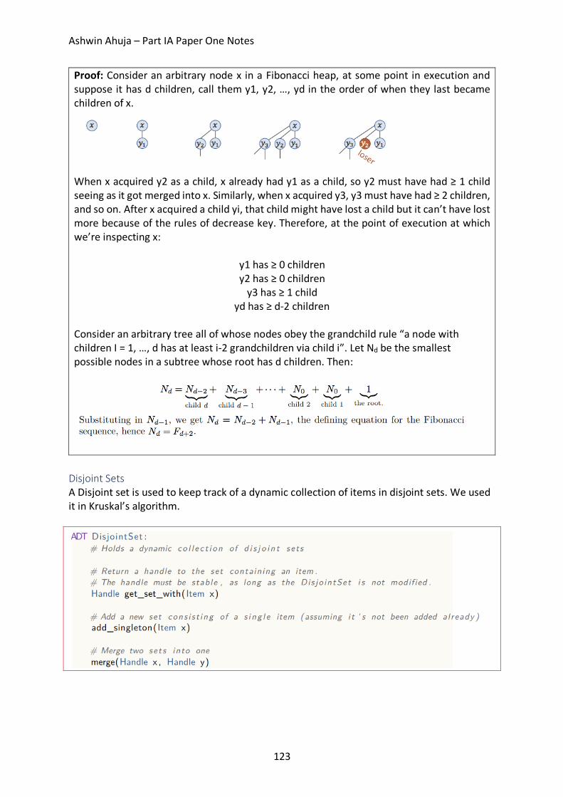
Ashwin Ahuja – Part IA Paper One Notes
123
Proof: Consider an arbitrary node x in a Fibonacci heap, at some point in execution and suppose it has d children, call them y1, y2, …, yd in the order of when they last became children of x.
When x acquired y2 as a child, x already had y1 as a child, so y2 must have had ≥ 1 child seeing as it got merged into x. Similarly, when x acquired y3, y3 must have had ≥ 2 children, and so on. After x acquired a child yi, that child might have lost a child but it can’t have lost more because of the rules of decrease key. Therefore, at the point of execution at which we’re inspecting x:
y1 has ≥ 0 children y2 has ≥ 0 children
y3 has ≥ 1 child yd has ≥ d-2 children
Consider an arbitrary tree all of whose nodes obey the grandchild rule “a node with children I = 1, …, d has at least i-2 grandchildren via child i”. Let Nd be the smallest possible nodes in a subtree whose root has d children. Then:
Disjoint Sets A Disjoint set is used to keep track of a dynamic collection of items in disjoint sets. We used it in Kruskal’s algorithm.
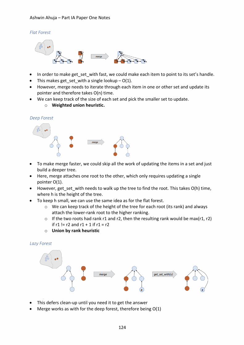
Ashwin Ahuja – Part IA Paper One Notes
124
Flat Forest
• In order to make get_set_with fast, we could make each item to point to its set’s handle. • This makes get_set_with a single lookup – O(1). • However, merge needs to iterate through each item in one or other set and update its
pointer and therefore takes O(n) time. • We can keep track of the size of each set and pick the smaller set to update.
o Weighted union heuristic. Deep Forest
• To make merge faster, we could skip all the work of updating the items in a set and just
build a deeper tree. • Here, merge attaches one root to the other, which only requires updating a single
pointer O(1). • However, get_set_with needs to walk up the tree to find the root. This takes O(h) time,
where h is the height of the tree. • To keep h small, we can use the same idea as for the flat forest.
o We can keep track of the height of the tree for each root (its rank) and always attach the lower-rank root to the higher ranking.
o If the two roots had rank r1 and r2, then the resulting rank would be max(r1, r2) if r1 != r2 and r1 + 1 if r1 = r2
o Union by rank heuristic Lazy Forest
• This defers clean-up until you need it to get the answer • Merge works as with for the deep forest, therefore being O(1)
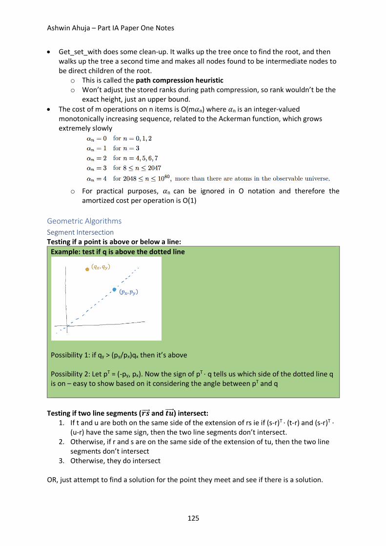
Ashwin Ahuja – Part IA Paper One Notes
125
• Get_set_with does some clean-up. It walks up the tree once to find the root, and then walks up the tree a second time and makes all nodes found to be intermediate nodes to be direct children of the root.
o This is called the path compression heuristic o Won’t adjust the stored ranks during path compression, so rank wouldn’t be the
exact height, just an upper bound. • The cost of m operations on n items is O(m𝛼n) where𝛼nis an integer-valued
monotonically increasing sequence, related to the Ackerman function, which grows extremely slowly
o For practical purposes, 𝛼n can be ignored in O notation and therefore the
amortized cost per operation is O(1) Geometric Algorithms Segment Intersection Testing if a point is above or below a line:
Example: test if q is above the dotted line
Possibility 1: if qy > (py/px)qx then it’s above Possibility 2: Let pT = (-py, px). Now the sign of pT · q tells us which side of the dotted line q is on – easy to show based on it considering the angle between pT and q
Testing if two line segments (𝒓𝒔®®®®⃗ and 𝒕𝒖®®®®⃗ ) intersect:
1. If t and u are both on the same side of the extension of rs ie if (s-r)T · (t-r) and (s-r)T · (u-r) have the same sign, then the two line segments don’t intersect.
2. Otherwise, if r and s are on the same side of the extension of tu, then the two line segments don’t intersect
3. Otherwise, they do intersect OR, just attempt to find a solution for the point they meet and see if there is a solution.
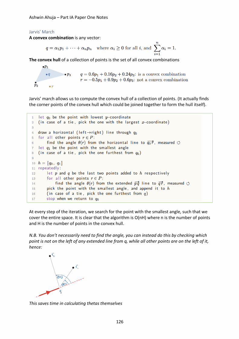
Ashwin Ahuja – Part IA Paper One Notes
126
Jarvis’ March A convex combination is any vector:
The convex hull of a collection of points is the set of all convex combinations
Jarvis’ march allows us to compute the convex hull of a collection of points. (It actually finds the corner points of the convex hull which could be joined together to form the hull itself).
At every step of the iteration, we search for the point with the smallest angle, such that we cover the entire space. It is clear that the algorithm is O(nH) where n is the number of points and H is the number of points in the convex hull. N.B. You don’t necessarily need to find the angle, you can instead do this by checking which point is not on the left of any extended line from q, while all other points are on the left of it, hence:
This saves time in calculating thetas themselves
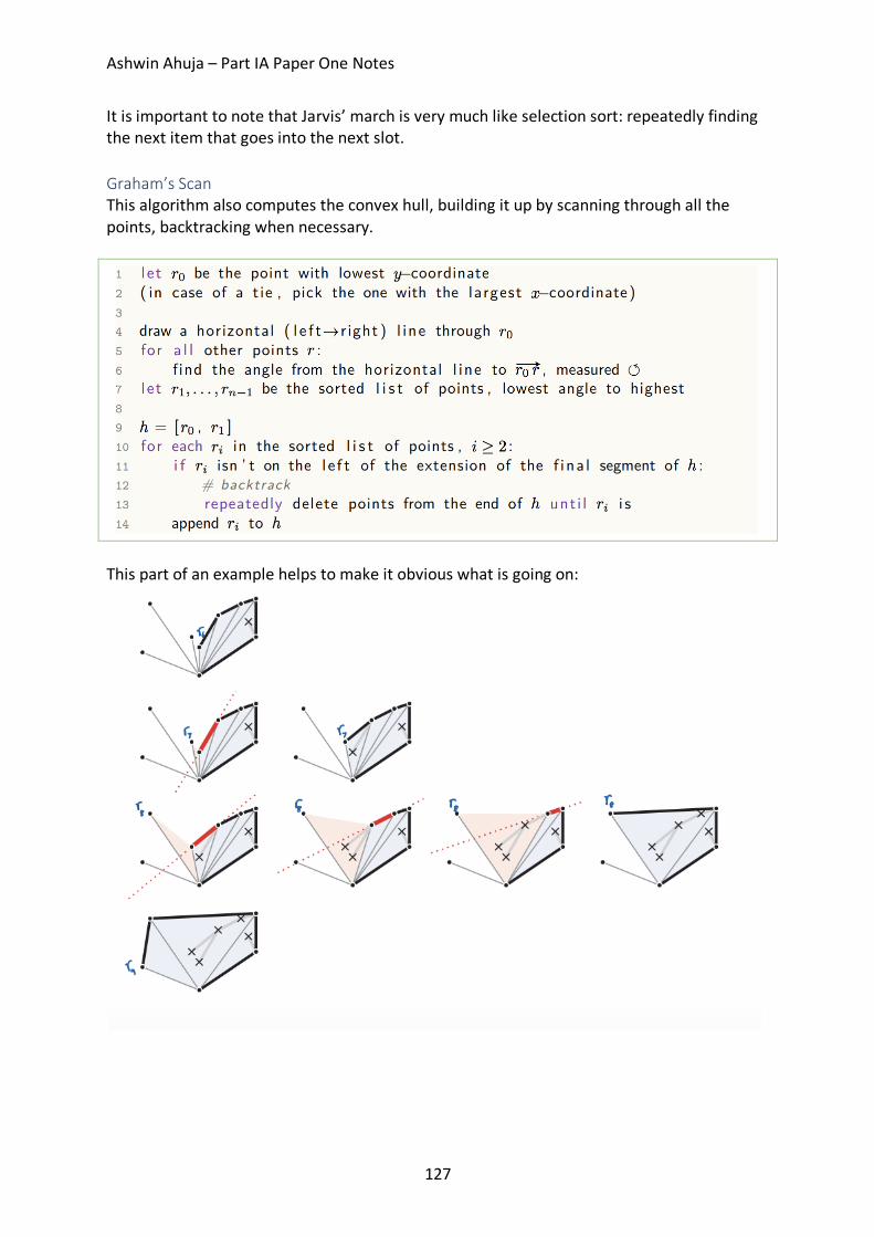
Ashwin Ahuja – Part IA Paper One Notes
127
It is important to note that Jarvis’ march is very much like selection sort: repeatedly finding the next item that goes into the next slot. Graham’s Scan This algorithm also computes the convex hull, building it up by scanning through all the points, backtracking when necessary.
This part of an example helps to make it obvious what is going on:
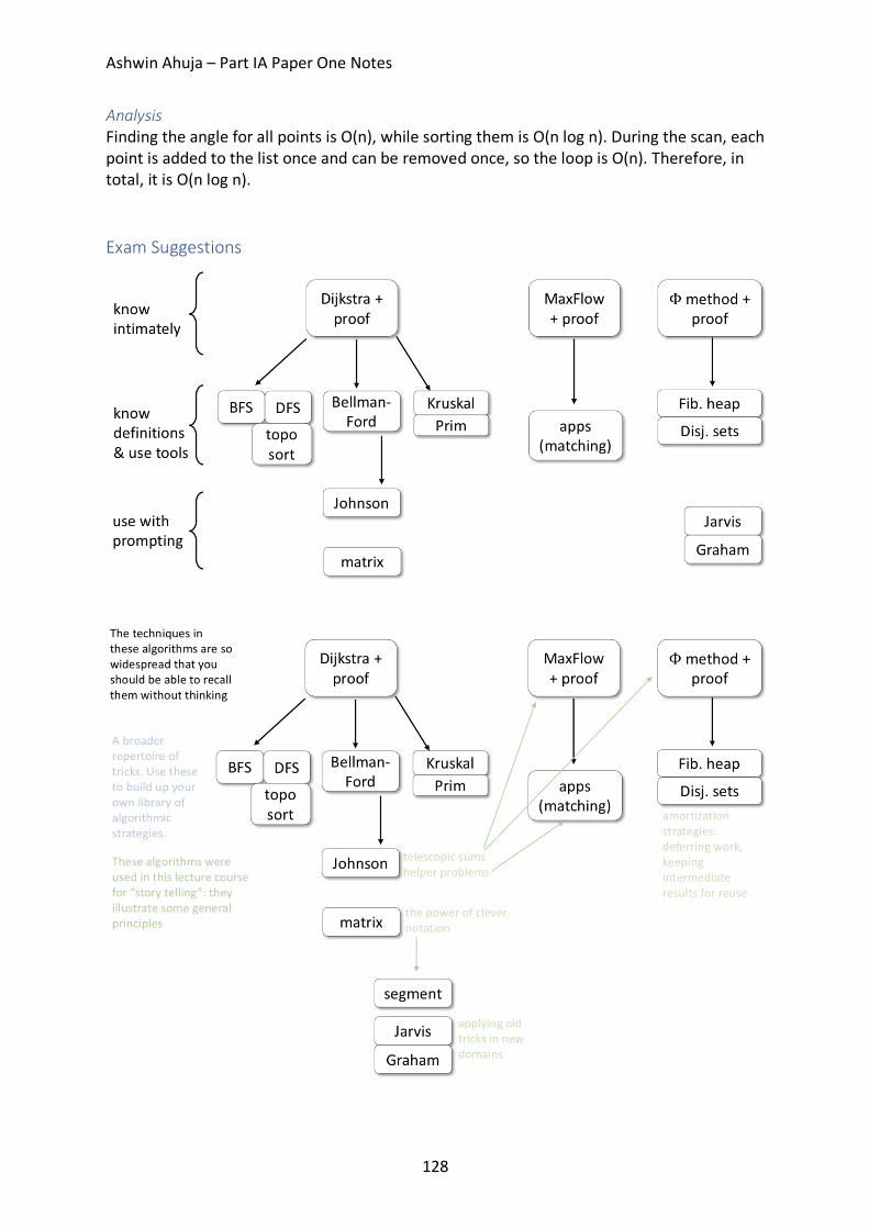
Ashwin Ahuja – Part IA Paper One Notes
128
Analysis Finding the angle for all points is O(n), while sorting them is O(n log n). During the scan, each point is added to the list once and can be removed once, so the loop is O(n). Therefore, in total, it is O(n log n). Exam Suggestions
Ashwin Ahuja – Part IA Paper One Notes
129
Numerical Methods Part 1: Reminders We must always be careful about when a computer program is working – we should implement unit tests to check if the program is correct. We must also be aware that even if a program ‘implements’ a mathematical formula, they are not necessarily correct. What causes errors: 1. Wrong mathematical model 2. Overfitting – parameters chosen to fit the expected value 3. Model being too sensitive to input values 4. Discretisation of continuous model 5. Propagation of inaccuracies (floating point inaccuracies) 6. Programming errors Integer Representation Signed and Unsigned integers are two methods of representation (with signed having a bit at the front which says whether the integer is positive or negative). These place the decimal point at the end. We can create a fixed-point number by placing the decimal point somewhere else in the number. These however, are prone to overflow. We can use saturating, therefore 2 * 10000111 = 11111111 (therefore goes to highest representable value). However, we can much more easily reduce the overflow by allowing the decimal point to be determined at run-time – this is floating point numbers Scientific Notation a x 10b. a is any real numbers, called the significand or mantissa. B is the exponent. In normalised form, 1 ≤ a < 10 Multiplication and Division: x0 = a0 x 10b0, x1 = a1 x 10b1
x0 x x1 = (a0 x a1) x 10b0 + b1 x0 / x1 = (a0 / a1) x 10b0 – b1 Addition and Subtraction: Requires the numbers to be represented using the same exponent – normally the larger of b0 and b1 Say b0 > b1 => x1 = (a1 x 10b1 – b0) x 10b0 x0 ± x1 = (a0 ± (a1 x 10b1 – b0)) x 10b0
This may require a number of shifts to normalise the result. Significant Figures While significant figures are much used, they are generally a little risky:
1. There may be 3sf in the result of a computation, but little accuracy left 2. Changing the ulp (unit in last place) may change the value by different amounts –
relative error
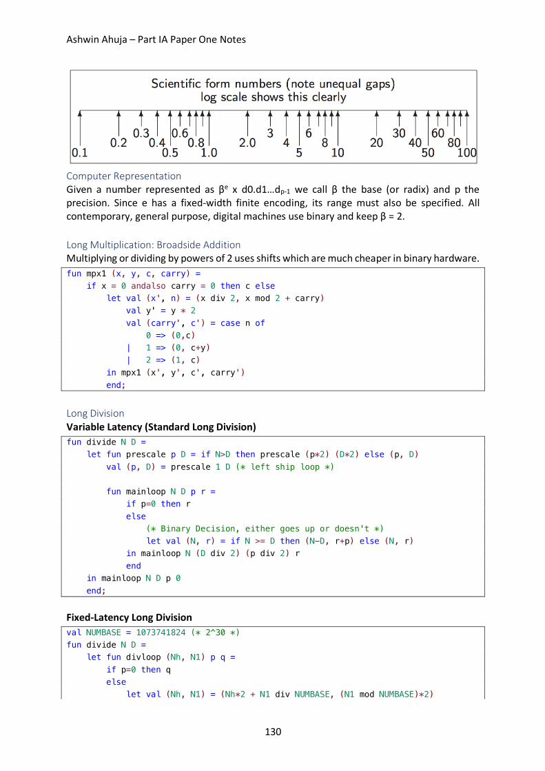
Ashwin Ahuja – Part IA Paper One Notes
130
Computer Representation Given a number represented as βe x d0.d1…dp-1 we call β the base (or radix) and p the precision. Since e has a fixed-width finite encoding, its range must also be specified. All contemporary, general purpose, digital machines use binary and keep β = 2. Long Multiplication: Broadside Addition Multiplying or dividing by powers of 2 uses shifts which are much cheaper in binary hardware. fun mpx1 (x, y, c, carry) = if x = 0 andalso carry = 0 then c else let val (x', n) = (x div 2, x mod 2 + carry) val y' = y * 2 val (carry', c') = case n of 0 => (0,c) | 1 => (0, c+y) | 2 => (1, c) in mpx1 (x', y', c', carry') end; Long Division Variable Latency (Standard Long Division) fun divide N D = let fun prescale p D = if N>D then prescale (p*2) (D*2) else (p, D) val (p, D) = prescale 1 D (* left ship loop *) fun mainloop N D p r = if p=0 then r else (* Binary Decision, either goes up or doesn't *) let val (N, r) = if N >= D then (N-D, r+p) else (N, r) in mainloop N (D div 2) (p div 2) r end in mainloop N D p 0 end; Fixed-Latency Long Division val NUMBASE = 1073741824 (* 2^30 *) fun divide N D = let fun divloop (Nh, N1) p q = if p=0 then q else let val (Nh, N1) = (Nh*2 + N1 div NUMBASE, (N1 mod NUMBASE)*2)
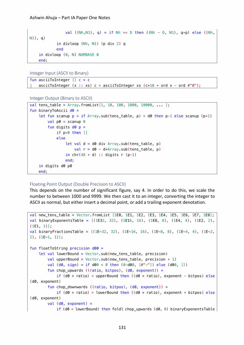
Ashwin Ahuja – Part IA Paper One Notes
131
val ((Nh,N1), q) = if Nh >= D then ((Nh - D, N1), q+p) else ((Nh, N1), q) in divloop (Nh, N1) (p div 2) q end in divloop (0, N) NUMBASE 0 end; Integer Input (ASCII to Binary) fun asciiToInteger [] c = c | asciiToInteger (x :: xs) c = asciiToInteger xs (c*10 + ord x - ord #"0"); Integer Output (Binary to ASCII) val tens_table = Array.fromList[1, 10, 100, 1000, 10000, ... ]; fun binaryToAscii d0 = let fun scanup p = if Array.sub(tens_table, p) > d0 then p-1 else scanup (p+1) val p0 = scanup 0 fun digits d0 p = if p<0 then [] else let val d = d0 div Array.sub(tens_table, p) val r = d0 - d*Array.sub(tens_table, p) in chr(48 + d) :: digits r (p-1) end; in digits d0 p0 end; Floating Point Output (Double Precision to ASCII) This depends on the number of significant figure, say 4. In order to do this, we scale the number to between 1000 and 9999. We then cast it to an integer, converting the integer to ASCII as normal, but either insert a decimal point, or add a trailing exponent denotation. val new_tens_table = Vector.fromList [1E0, 1E1, 1E2, 1E3, 1E4, 1E5, 1E6, 1E7, 1E8]; val binaryExponentsTable = [(1E32, 32), (1E16, 16), (1E8, 8), (1E4, 4), (1E2, 2), (1E1, 1)]; val binaryFractionsTable = [(1E~32, 32), (1E~16, 16), (1E~8, 8), (1E~4, 4), (1E~2, 2), (1E~1, 1)]; fun floatToString precision d00 = let val lowerBound = Vector.sub(new_tens_table, precision) val upperBound = Vector.sub(new_tens_table, precision + 1) val (d0, sign) = if d00 < 0 then (0-d00, [#"-"]) else (d00, []) fun chop_upwards ((ratio, bitpos), (d0, exponent)) = if (d0 * ratio) < upperBound then ((d0 * ratio), exponent - bitpos) else (d0, exponent) fun chop_downwards ((ratio, bitpos), (d0, exponent)) = if (d0 * ratio) > lowerBound then ((d0 * ratio), exponent + bitpos) else (d0, exponent) val (d0, exponent) = if (d0 < lowerBound) then foldl chop_upwards (d0, 0) binaryExponentsTable
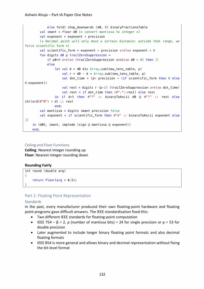
Ashwin Ahuja – Part IA Paper One Notes
132
else foldl chop_downwards (d0, 0) binaryFractionsTable val imant = floor d0 (* convert mantissa to integer *) val exponent = exponent + precision (* Decimal point will only move a certain distance: outside that range, we force scientific form *) val scientific_form = exponent > precision orelse exponent < 0 fun digits d0 p trailZeroSuppression = if p0<0 orelse (trailZeroSuppression andalso d0 = 0) then [] else let val d = d0 div Array.sub(new_tens_table, p) val r = d0 - d * Array.sub(new_tens_table, p) val dot_time = (p= precision + (if scientific_form then 0 else 0-exponent)) val rest = digits r (p-1) (trailZeroSuppression orelse dot_time) val rest = if dot_time then (#"."::rest) else rest in if d>9 then #"?" :: binaryToAscii d0 @ #"!" :: rest else chr(ord(#"0") + d) :: rest end; val mantissa = digits imant precision false val exponent = if scientific_form then #"e" :: binaryToAscii exponent else [] in (d00, imant, implode (sign @ mantissa @ exponent)) end; Ceiling and Floor Functions Ceiling: Nearest integer rounding up Floor: Nearest integer rounding down Rounding Fairly int round (double arg) { return Floor(arg + 0.5); } Part 2: Floating Point Representation Standards In the past, every manufacturer produced their own floating-point hardware and floating point programs gave difficult answers. The IEEE standardisation fixed this:
• Two different IEEE standards for floating-point computation • IEEE 754 – β = 2, p (number of mantissa bits) = 24 for single precision or p = 53 for
double precision • Later augmented to include longer binary floating point formats and also decimal
floating formats • IEEE 854 is more general and allows binary and decimal representation without fixing
the bit-level format
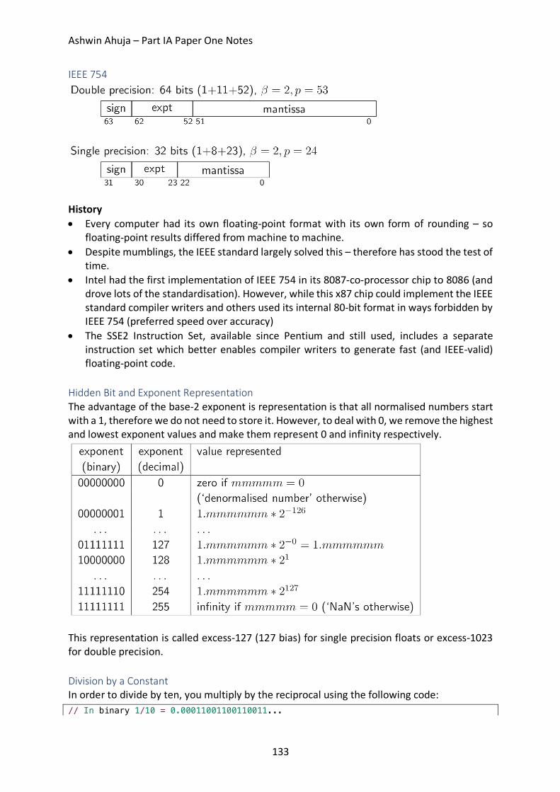
Ashwin Ahuja – Part IA Paper One Notes
133
IEEE 754
History • Every computer had its own floating-point format with its own form of rounding – so
floating-point results differed from machine to machine. • Despite mumblings, the IEEE standard largely solved this – therefore has stood the test of
time. • Intel had the first implementation of IEEE 754 in its 8087-co-processor chip to 8086 (and
drove lots of the standardisation). However, while this x87 chip could implement the IEEE standard compiler writers and others used its internal 80-bit format in ways forbidden by IEEE 754 (preferred speed over accuracy)
• The SSE2 Instruction Set, available since Pentium and still used, includes a separate instruction set which better enables compiler writers to generate fast (and IEEE-valid) floating-point code.
Hidden Bit and Exponent Representation The advantage of the base-2 exponent is representation is that all normalised numbers start with a 1, therefore we do not need to store it. However, to deal with 0, we remove the highest and lowest exponent values and make them represent 0 and infinity respectively.
This representation is called excess-127 (127 bias) for single precision floats or excess-1023 for double precision. Division by a Constant In order to divide by ten, you multiply by the reciprocal using the following code: // In binary 1/10 = 0.00011001100110011...
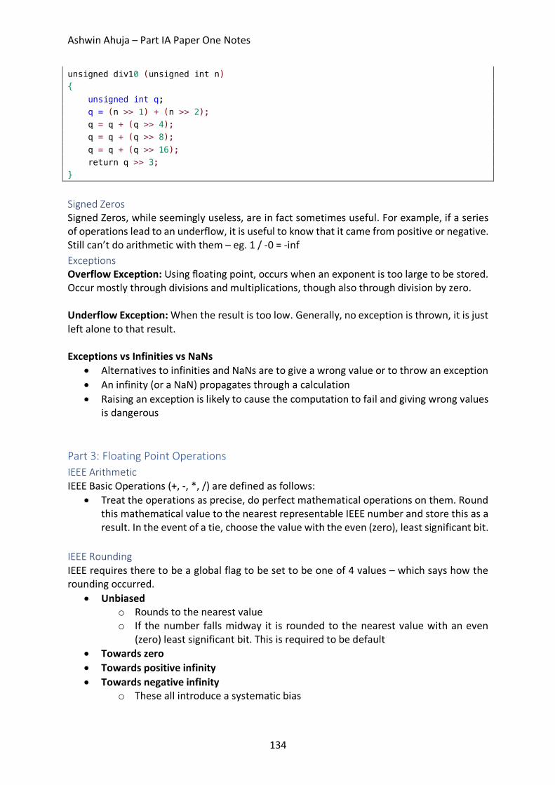
Ashwin Ahuja – Part IA Paper One Notes
134
unsigned div10 (unsigned int n) { unsigned int q; q = (n >> 1) + (n >> 2); q = q + (q >> 4); q = q + (q >> 8); q = q + (q >> 16); return q >> 3; } Signed Zeros Signed Zeros, while seemingly useless, are in fact sometimes useful. For example, if a series of operations lead to an underflow, it is useful to know that it came from positive or negative. Still can’t do arithmetic with them – eg. 1 / -0 = -inf Exceptions Overflow Exception: Using floating point, occurs when an exponent is too large to be stored. Occur mostly through divisions and multiplications, though also through division by zero. Underflow Exception: When the result is too low. Generally, no exception is thrown, it is just left alone to that result. Exceptions vs Infinities vs NaNs
• Alternatives to infinities and NaNs are to give a wrong value or to throw an exception • An infinity (or a NaN) propagates through a calculation • Raising an exception is likely to cause the computation to fail and giving wrong values
is dangerous Part 3: Floating Point Operations IEEE Arithmetic IEEE Basic Operations (+, -, *, /) are defined as follows:
• Treat the operations as precise, do perfect mathematical operations on them. Round this mathematical value to the nearest representable IEEE number and store this as a result. In the event of a tie, choose the value with the even (zero), least significant bit.
IEEE Rounding IEEE requires there to be a global flag to be set to be one of 4 values – which says how the rounding occurred.
• Unbiased o Rounds to the nearest value o If the number falls midway it is rounded to the nearest value with an even
(zero) least significant bit. This is required to be default • Towards zero • Towards positive infinity • Towards negative infinity
o These all introduce a systematic bias
Ashwin Ahuja – Part IA Paper One Notes
135
Other Operators • Other mathematical operators are typically implemented in libraries – these examples
include sin, sqrt, log. It is important to ask whether implementations of these satisfy the IEEE requirements.
• Generally, a library is only as good as the vendor’s careful explanation of what error bound the result is accurate to.
• ±1 ulp is considered good – 0.5 ulp is required for a perfect accuracy result. • The results must also be semi-monotonic
o Given the function is monotonically increasing, the libraries answers must also be monotonically increasing.
Errors Quantisation Errors: Arising from the inexact representation of constants in the program and numbers read in as data. Rounding Errors: Produced by every IEEE operation Truncation Errors and also underflow and cancellation / loss of significance.
Errors in +, -: these sum the absolute errors Errors in *, /: these sum the relative errors Error amplification is generally far more important than the random error through floating point computation. (Systematic Error Propagation) Machine Epsilon • Defined as the difference between 1.0 and the smallest representable number which is
greater than 1 (2-23 in single precision) • Useful as it gives an upper bound on the relative error caused by getting a floating-point
number wrong by 1 ulp and is therefore useful for expressing errors independent of floating point size.
• Wrong description o Smallest number which when added to one gives a number greater than 1 o With rounding to nearest, this only needs to be slightly more than half of our
machine epsilon o Error used by Microsoft and even the GNU documentation o It is almost the maximum error but not quite
• Negative Epsilon o Difference between 1 and the smallest representable number greater than 1 o This is exactly 50% of machine epsilon
§ Witching-Hour effect § 20 x 1.0000…
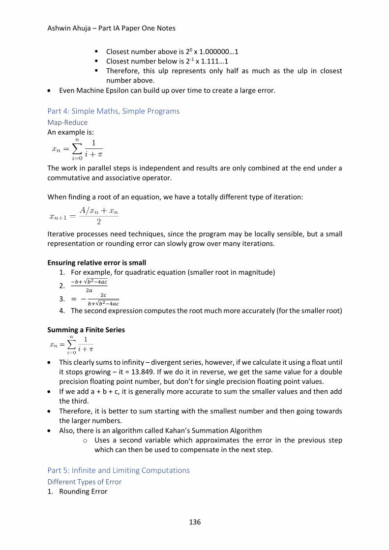
Ashwin Ahuja – Part IA Paper One Notes
136
§ Closest number above is 20 x 1.000000…1 § Closest number below is 2-1 x 1.111…1 § Therefore, this ulp represents only half as much as the ulp in closest
number above. • Even Machine Epsilon can build up over time to create a large error. Part 4: Simple Maths, Simple Programs Map-Reduce An example is:
The work in parallel steps is independent and results are only combined at the end under a commutative and associative operator. When finding a root of an equation, we have a totally different type of iteration:
Iterative processes need techniques, since the program may be locally sensible, but a small representation or rounding error can slowly grow over many iterations. Ensuring relative error is small
1. For example, for quadratic equation (smaller root in magnitude)
2. RQO√Q{R³y´Ky
3. =− K´QO√Q{R³y´
4. The second expression computes the root much more accurately (for the smaller root)
Summing a Finite Series
• This clearly sums to infinity – divergent series, however, if we calculate it using a float until
it stops growing – it = 13.849. If we do it in reverse, we get the same value for a double precision floating point number, but don’t for single precision floating point values.
• If we add a + b + c, it is generally more accurate to sum the smaller values and then add the third.
• Therefore, it is better to sum starting with the smallest number and then going towards the larger numbers.
• Also, there is an algorithm called Kahan’s Summation Algorithm o Uses a second variable which approximates the error in the previous step
which can then be used to compensate in the next step. Part 5: Infinite and Limiting Computations Different Types of Error 1. Rounding Error
Ashwin Ahuja – Part IA Paper One Notes
137
a. Error we get by using finite arithmetic during a computation 2. Truncation Error (Discretisation Error)
a. Error we get by stopping an infinitary process after a finite point
Differentiation 𝑓′(𝑥) = lim
}→q
·(zO})R·(z)}
How to pick h:
• We technically want it to be as small as possible • But if h is less than the machine epsilon then for x about 1, x + h will compute to the
same value as x • Also, if h is too small, then f(x+h) – f(x) will produce lots of cancelling – therefore a lot
of relative error – rounding error o Assume machine epsilon error is returned in evaluations of f and get (assume
f(x) and f’(x) ≅1 o (f(x+h) – f(x))/h = (f(x) + hf’(x) ± macheps – f(x))/h o 1 ± macheps/h o Therefore rounding error is macheps / h
• However, if h is too big, we create truncation error. o Truncation error can be calculated by Taylor expansion
o 𝑓(𝑥 + ℎ) = 𝑓(𝑥) + ℎ𝑓�(𝑥) + }{·��(z)K
+ 𝑂(ℎ§)
o This works out as approximately }·��(z)K
• Since errors vary oppositely with regards to h, we compromise by making the two
errors of the same order to minimise their total effect. • Equating the rounding error and the truncation error gives h = macheps/h
o That is h = ¸𝑚𝑎𝑐ℎ𝑒𝑝𝑠 However, can also do 𝒇(𝒙O𝒉)R𝒇(𝒙R𝒉)
𝟐𝒉
• Truncation error = h2f’’(x)/3! • Rounding error = macheps/h • Therefore h = ¸𝑚𝑎𝑐ℎ𝑒𝑝𝑠¼
When finitely approximating a limiting process, there is a number h which is small, or a number n which is large. Often, there are multiple algorithms which mathematically have the same limit, but approach at different speeds – as well as having different rounding error accumulation.
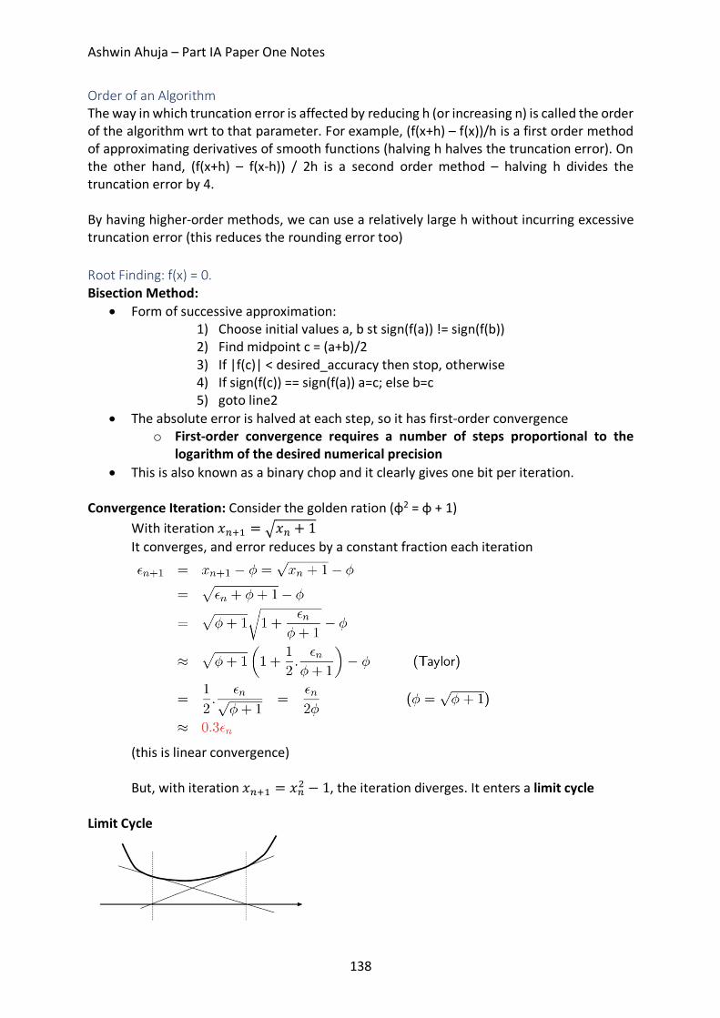
Ashwin Ahuja – Part IA Paper One Notes
138
Order of an Algorithm The way in which truncation error is affected by reducing h (or increasing n) is called the order of the algorithm wrt to that parameter. For example, (f(x+h) – f(x))/h is a first order method of approximating derivatives of smooth functions (halving h halves the truncation error). On the other hand, (f(x+h) – f(x-h)) / 2h is a second order method – halving h divides the truncation error by 4. By having higher-order methods, we can use a relatively large h without incurring excessive truncation error (this reduces the rounding error too) Root Finding: f(x) = 0. Bisection Method:
• Form of successive approximation: 1) Choose initial values a, b st sign(f(a)) != sign(f(b)) 2) Find midpoint c = (a+b)/2 3) If |f(c)| < desired_accuracy then stop, otherwise 4) If sign(f(c)) == sign(f(a)) a=c; else b=c 5) goto line2
• The absolute error is halved at each step, so it has first-order convergence o First-order convergence requires a number of steps proportional to the
logarithm of the desired numerical precision • This is also known as a binary chop and it clearly gives one bit per iteration.
Convergence Iteration: Consider the golden ration (ɸ2 = ɸ + 1) With iteration 𝑥7OP = ¸𝑥7 + 1 It converges, and error reduces by a constant fraction each iteration
(this is linear convergence)
But, with iteration 𝑥7OP = 𝑥7K − 1, the iteration diverges. It enters a limit cycle Limit Cycle
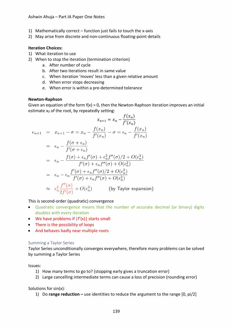
Ashwin Ahuja – Part IA Paper One Notes
139
1) Mathematically correct – function just fails to touch the x-axis 2) May arise from discrete and non-continuous floating-point details Iteration Choices: 1) What iteration to use 2) When to stop the iteration (termination criterion)
a. After number of cycle b. After two iterations result in same value c. When iteration ‘moves’ less than a given relative amount d. When error stops decreasing e. When error is within a pre-determined tolerance
Newton-Raphson Given an equation of the form f(x) = 0, then the Newton-Raphson iteration improves an initial estimate x0 of the root, by repeatedly setting:
𝑥7OP = 𝑥7 −𝑓(𝑥7)𝑓′(𝑥7)
This is second-order (quadratic) convergence • Quadratic convergence means that the number of accurate decimal (or binary) digits
doubles with every iteration • We have problems if |f’(x)| starts small • There is the possibility of loops • And behaves badly near multiple roots Summing a Taylor Series Taylor Series unconditionally converges everywhere, therefore many problems can be solved by summing a Taylor Series Issues:
1) How many terms to go to? (stopping early gives a truncation error) 2) Large cancelling intermediate terms can cause a loss of precision (rounding error)
Solutions for sin(x):
1) Do range reduction – use identities to reduce the argument to the range [0, pi/2]
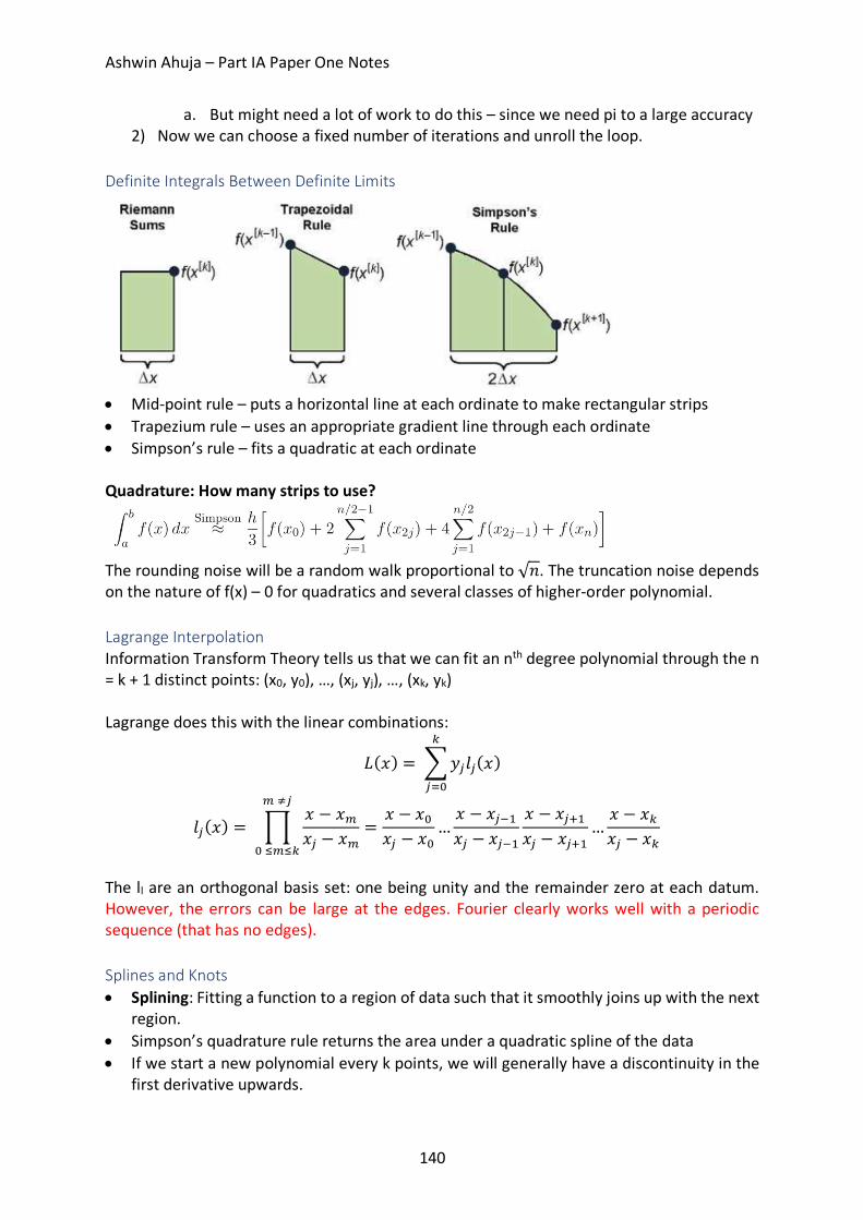
Ashwin Ahuja – Part IA Paper One Notes
140
a. But might need a lot of work to do this – since we need pi to a large accuracy 2) Now we can choose a fixed number of iterations and unroll the loop.
Definite Integrals Between Definite Limits
• Mid-point rule – puts a horizontal line at each ordinate to make rectangular strips • Trapezium rule – uses an appropriate gradient line through each ordinate • Simpson’s rule – fits a quadratic at each ordinate Quadrature: How many strips to use?
The rounding noise will be a random walk proportional to √𝑛. The truncation noise depends on the nature of f(x) – 0 for quadratics and several classes of higher-order polynomial. Lagrange Interpolation Information Transform Theory tells us that we can fit an nth degree polynomial through the n = k + 1 distinct points: (x0, y0), …, (xj, yj), …, (xk, yk) Lagrange does this with the linear combinations:
𝐿(𝑥) = d𝑦n𝑙n(𝑥)�
nfq
𝑙n(𝑥) = ¾𝑥 − 𝑥�𝑥n − 𝑥�
=𝑥 − 𝑥q𝑥n − 𝑥q
…𝑥 − 𝑥nRP𝑥n − 𝑥nRP
𝑥 − 𝑥nOP𝑥n − 𝑥nOP
…𝑥 − 𝑥�𝑥n − 𝑥�
�Àn
qÁ�Á�
The ll are an orthogonal basis set: one being unity and the remainder zero at each datum. However, the errors can be large at the edges. Fourier clearly works well with a periodic sequence (that has no edges). Splines and Knots • Splining: Fitting a function to a region of data such that it smoothly joins up with the next
region. • Simpson’s quadrature rule returns the area under a quadratic spline of the data • If we start a new polynomial every k points, we will generally have a discontinuity in the
first derivative upwards.
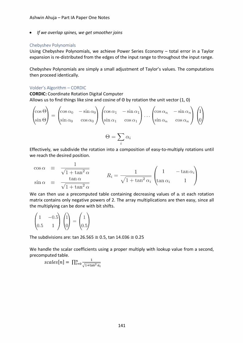
Ashwin Ahuja – Part IA Paper One Notes
141
• If we overlap spines, we get smoother joins Chebyshev Polynomials Using Chebyshev Polynomials, we achieve Power Series Economy – total error in a Taylor expansion is re-distributed from the edges of the input range to throughout the input range. Chebyshev Polynomials are simply a small adjustment of Taylor’s values. The computations then proceed identically. Volder’s Algorithm – CORDIC CORDIC: Coordinate Rotation Digital Computer Allows us to find things like sine and cosine of Θ by rotation the unit vector (1, 0)
Effectively, we subdivide the rotation into a composition of easy-to-multiply rotations until we reach the desired position.
We can then use a precomputed table containing decreasing values of ai st each rotation matrix contains only negative powers of 2. The array multiplications are then easy, since all the multiplying can be done with bit shifts.
The subdivisions are: tan 26.565 ≅ 0.5, tan 14.036 ≅ 0.25 We handle the scalar coefficients using a proper multiply with lookup value from a second, precomputed table. 𝑠𝑐𝑎𝑙𝑒𝑠[𝑛] = ∏ P
¸POÃÄÅ{ yÆ7efq
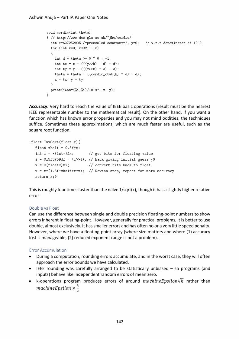
Ashwin Ahuja – Part IA Paper One Notes
142
Accuracy: Very hard to reach the value of IEEE basic operations (result must be the nearest IEEE representable number to the mathematical result). On the other hand, if you want a function which has known error properties and you may not mind oddities, the techniques suffice. Sometimes these approximations, which are much faster are useful, such as the square root function.
This is roughly four times faster than the naïve 1/sqrt(x), though it has a slightly higher relative error Double vs Float Can use the difference between single and double precision floating-point numbers to show errors inherent in floating-point. However, generally for practical problems, it is better to use double, almost exclusively. It has smaller errors and has often no or a very little speed penalty. However, where we have a floating-point array (where size matters and where (1) accuracy lost is manageable, (2) reduced exponent range is not a problem). Error Accumulation • During a computation, rounding errors accumulate, and in the worst case, they will often
approach the error bounds we have calculated. • IEEE rounding was carefully arranged to be statistically unbiased – so programs (and
inputs) behave like independent random errors of mean zero. • k-operations program produces errors of around 𝑚𝑎𝑐ℎ𝑖𝑛𝑒𝐸𝑝𝑠𝑖𝑙𝑜𝑛√𝑘 rather than
𝑚𝑎𝑐ℎ𝑖𝑛𝑒𝐸𝑝𝑠𝑖𝑙𝑜𝑛 × �K
Ashwin Ahuja – Part IA Paper One Notes
143
Part 6: Ill-Conditionedness and Condition Number In solving simultaneous equations, we simply want to find the intersection of the lines. Iff you have a small a, b, c, d in the matrix, as below:
Then we get large values for the inverse of the matrix, therefore any small absolute errors in p or q will be greatly amplified in x and y. (This occurs when the lines are nearly parallel). Ill-Conditioned: When a solution (x, y) is excessively dependent on small variations (these may arise from measurement error or rounding or truncation error from previous calculations) on the value of the inputs (a, b, c, d, p, q). Such systems are called ill-conditioned. Simple example is matrices but is a problem for many real-life situations. We can get insight by calculating a bound for partial derivatives wrt the inputs, near the point in question: ÉzÉy, … , Éz
ÉÊ,… , ÉË
Éy, … , ÉË
ÉÊ
(Relative) Condition Number The log10 ratio of relative error in the output to that of the input. A problem with a high condition number is said to be ill-conditioned. Examples: 1. A large function:
a. F(x) = 1022 – well behaved b. Cond = -inf
2. A large derivative: a. F(x) = 1022x b. Cond = 0
3. A spiking function: a. 𝐹(𝑥) = P
q.qqPOq.ÍÍÍ(zRPqqq)
b. This has a very nasty pole 4. A cancelling function:
a. F(x) = x – 1000 b. It apparently looks well behaved but:
i. F(x(1+n)) = x(1+n) – 1000
ii. Cond = 𝑙𝑜𝑔Pq ]7�
7^ = logPq(
·(z(PO7)*R·(z)7.·(z)
)
iii. = logPq ]z7
7(zRPqqq)^
Ashwin Ahuja – Part IA Paper One Notes
144
L’Hôpital’s Rule
Backwards Stability Inverse algorithm exists that can accurately regenerate the input from the output. This implies Well-Conditionedness (not being degenerate). Monte-Carlo Technique • If formal methods are inappropriate for determining conditionedness of a problem, you
can resort to probabilistic (Monte Carlo) techniques. • Method
o Take the original problem and solve o Then take many variants of the problem, each perturbing the value of one or more
parameters or input variables by a few ulp or a fraction of a percent. o We then solve all of these. o If these all give similar solutions, then the original problem is likely to be well-
conditioned. o If not, then there is likely to be some instability.
Adaptive Methods • Sometimes, there are problems which are well-behaved in some regions but behaves
badly in another. • Therefore, the best way is to discretise the problem into small blocks which has finer
discretisation (lower truncation) in problematic areas (for accuracy) but larger in the rest (for speed)
o Otherwise, can use a dynamically varying ΔT • Sometimes, an iterative solution to a differential equation is fasted solved by solving for
a course discretisation or large step size and then refining. • Simulated Annealing
o Standard technique – large jumps and random decisions used initially but as the temperature control parameter is reduced, the procedure becomes more conservative.
Chaotic Systems Nastier form of ill-conditionedness for which the computed function is highly discontinuous – small input regions for which a wide range of output values occur. Examples:
• Mandelbrot Set o For each point (x, y), the number of iterations of fc(z) = z2 + c until |fk(z)| > 2
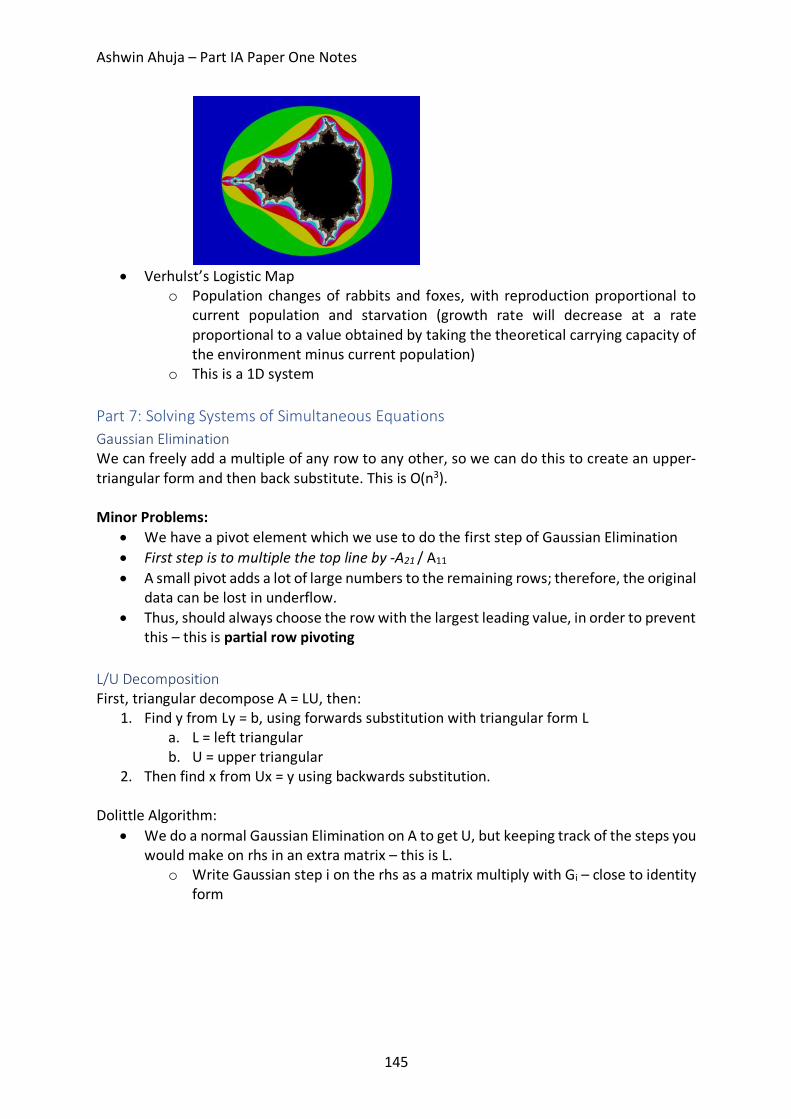
Ashwin Ahuja – Part IA Paper One Notes
145
• Verhulst’s Logistic Map
o Population changes of rabbits and foxes, with reproduction proportional to current population and starvation (growth rate will decrease at a rate proportional to a value obtained by taking the theoretical carrying capacity of the environment minus current population)
o This is a 1D system Part 7: Solving Systems of Simultaneous Equations Gaussian Elimination We can freely add a multiple of any row to any other, so we can do this to create an upper-triangular form and then back substitute. This is O(n3). Minor Problems:
• We have a pivot element which we use to do the first step of Gaussian Elimination • First step is to multiple the top line by -A21 / A11 • A small pivot adds a lot of large numbers to the remaining rows; therefore, the original
data can be lost in underflow. • Thus, should always choose the row with the largest leading value, in order to prevent
this – this is partial row pivoting
L/U Decomposition First, triangular decompose A = LU, then:
1. Find y from Ly = b, using forwards substitution with triangular form L a. L = left triangular b. U = upper triangular
2. Then find x from Ux = y using backwards substitution. Dolittle Algorithm:
• We do a normal Gaussian Elimination on A to get U, but keeping track of the steps you would make on rhs in an extra matrix – this is L.
o Write Gaussian step i on the rhs as a matrix multiply with Gi – close to identity form
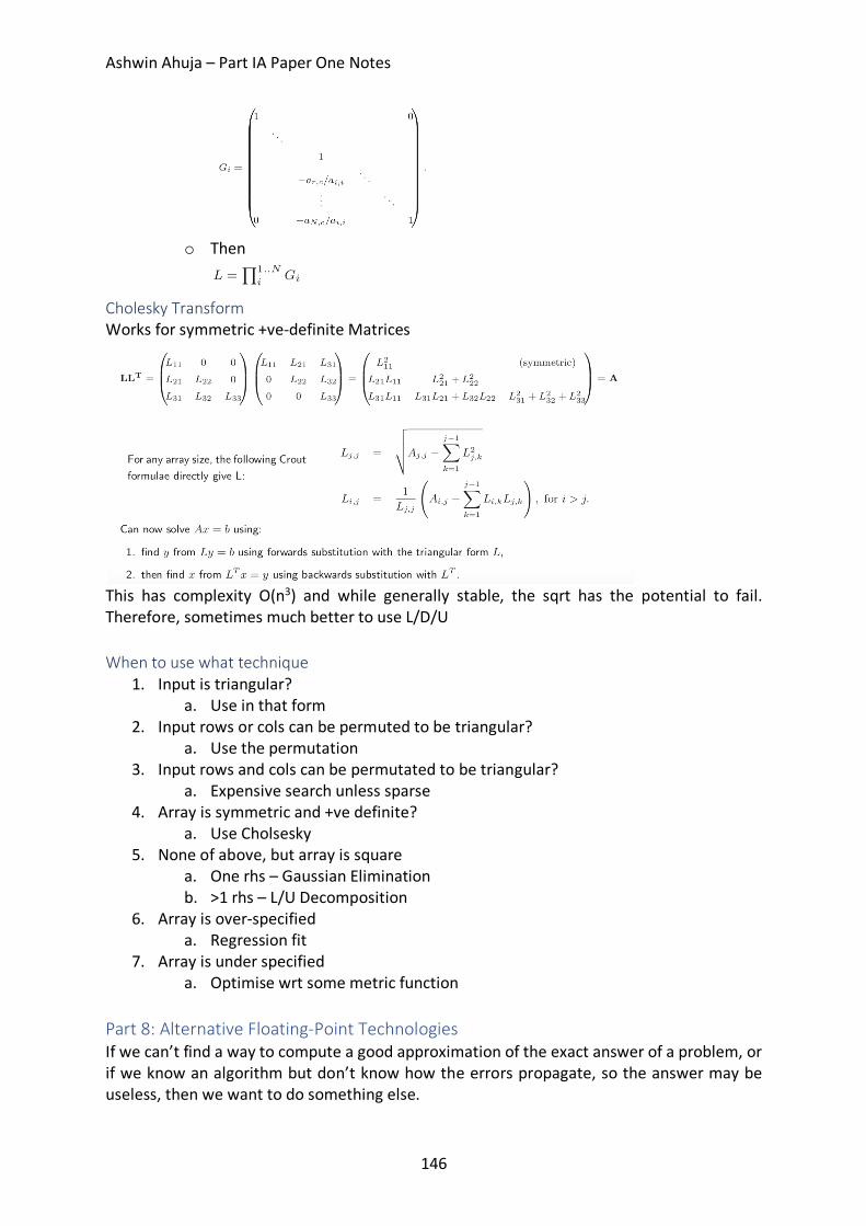
Ashwin Ahuja – Part IA Paper One Notes
146
o Then
Cholesky Transform Works for symmetric +ve-definite Matrices
This has complexity O(n3) and while generally stable, the sqrt has the potential to fail. Therefore, sometimes much better to use L/D/U When to use what technique
1. Input is triangular? a. Use in that form
2. Input rows or cols can be permuted to be triangular? a. Use the permutation
3. Input rows and cols can be permutated to be triangular? a. Expensive search unless sparse
4. Array is symmetric and +ve definite? a. Use Cholsesky
5. None of above, but array is square a. One rhs – Gaussian Elimination b. >1 rhs – L/U Decomposition
6. Array is over-specified a. Regression fit
7. Array is under specified a. Optimise wrt some metric function
Part 8: Alternative Floating-Point Technologies If we can’t find a way to compute a good approximation of the exact answer of a problem, or if we know an algorithm but don’t know how the errors propagate, so the answer may be useless, then we want to do something else.
Ashwin Ahuja – Part IA Paper One Notes
147
Interval Arithmetic Represent a mathematical real number with two IEEE floating point number. One gives a representable number guaranteed to be lower or equal to the actual value and the other greater than or equal. +:
1. It naturally copes with uncertainty in input values 2. IEEE arithmetic rounding modes (to +ve, -ve infinity) do much of the work
-:
1. It will be slower 2. Some algorithms converge in practise while the computed bounds can be far apart. 3. Need a big more work that you would expect if the range of the denominator in a
division includes 0, since the output range then includes zero 4. Conditions can become both true and false!
Arbitrary Precision Arithmetic Some packages allow you to set the precision with which you want to work with on a run-by-run basis. It is clear that you can run with any number of significant figures and still get the same errors, but they would generally arise at a different point. Adaptive Precision: Some packages even allow adaptive precision, where you reduce the number of significant figures you work with if you find out that it is not necessary to do that.
Example: GNU MPFR library gives multiple-precision floating-point computations. Most high-level languages have a binding for access without using C or C++
Exact Real Arithmetic (CRCalc, XR, IC Reals, iRRAM) Here, we consider using digit streams, that is lazy lists of digits, for infinite precision real arithmetic. It obviously however, has some failures – can never even get the first digit of 0. 3̇ + 0. 6̇ Part 9: FDTD (Finite-Difference, Time-Domain Simulation) and Monte Carlo Simulation Definitions Event-Driven: A lot of computer-based simulation uses discrete events and a time-sorted pending event queue – used for systems where activity is locally concentrated and unevenly spaced (digital logic and queues) Numeric, finite difference: Iterates over fixed or adaptive time domain steps and inter-element differences are exchanged with neighbours at each step. Monte Carlo: Either of the above simulators is run with many different random-seeded starting points and ensemble metrics are computed. Ergodic: For systems where the time average is the ensemble average (do not get stuck), we can use one starting seed and average in the time domain.
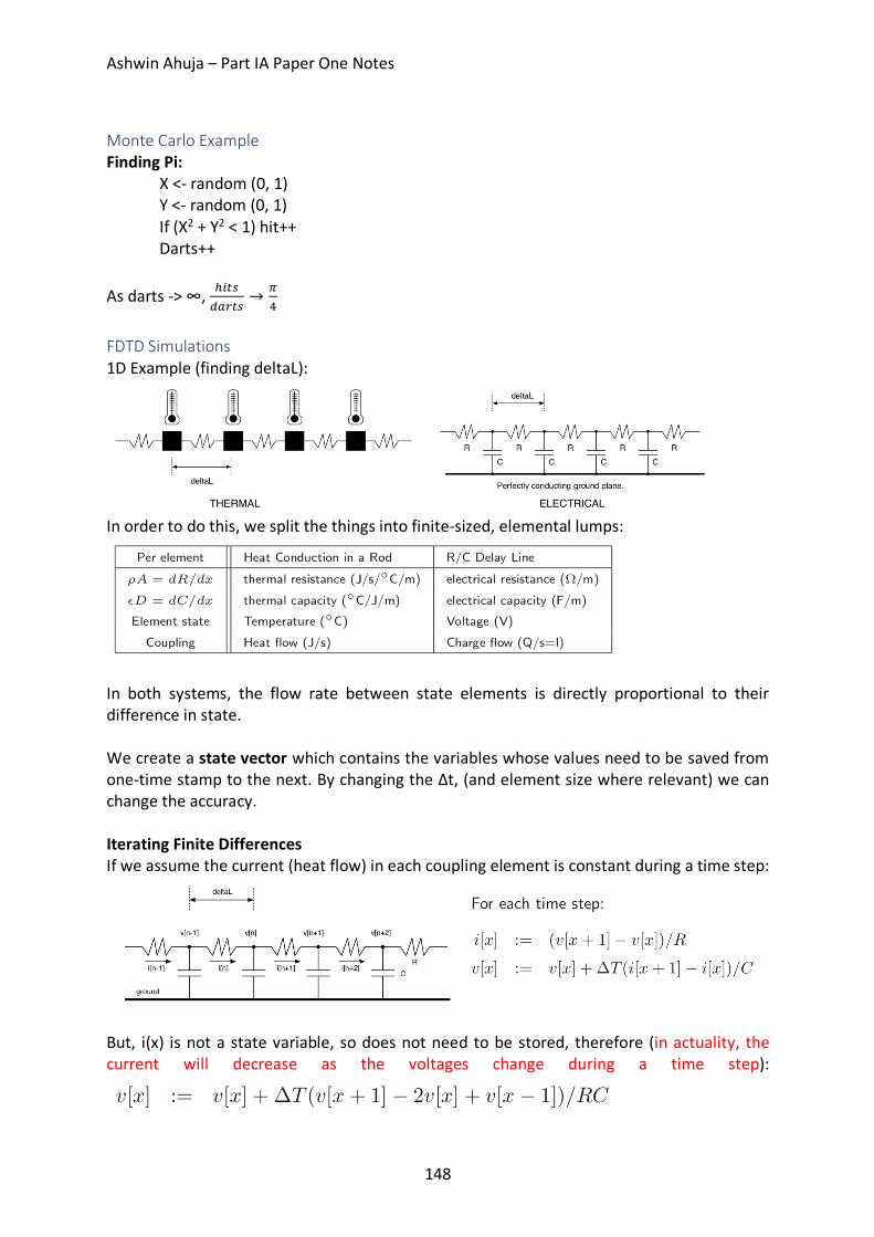
Ashwin Ahuja – Part IA Paper One Notes
148
Monte Carlo Example Finding Pi: X <- random (0, 1) Y <- random (0, 1) If (X2 + Y2 < 1) hit++ Darts++ As darts -> ∞, }e��
NyÑ��→ Ò
³
FDTD Simulations 1D Example (finding deltaL):
In order to do this, we split the things into finite-sized, elemental lumps:
In both systems, the flow rate between state elements is directly proportional to their difference in state. We create a state vector which contains the variables whose values need to be saved from one-time stamp to the next. By changing the Δt, (and element size where relevant) we can change the accuracy. Iterating Finite Differences If we assume the current (heat flow) in each coupling element is constant during a time step:
But, i(x) is not a state variable, so does not need to be stored, therefore (in actuality, the current will decrease as the voltages change during a time step):
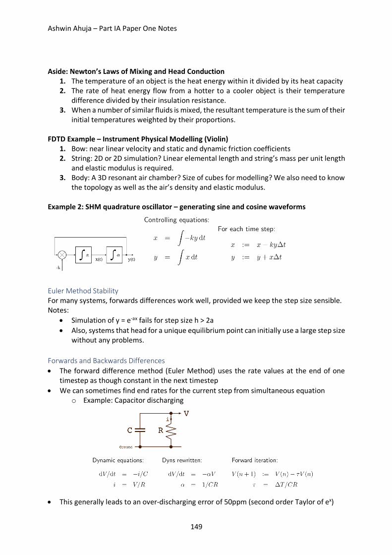
Ashwin Ahuja – Part IA Paper One Notes
149
Aside: Newton’s Laws of Mixing and Head Conduction
1. The temperature of an object is the heat energy within it divided by its heat capacity 2. The rate of heat energy flow from a hotter to a cooler object is their temperature
difference divided by their insulation resistance. 3. When a number of similar fluids is mixed, the resultant temperature is the sum of their
initial temperatures weighted by their proportions. FDTD Example – Instrument Physical Modelling (Violin)
1. Bow: near linear velocity and static and dynamic friction coefficients 2. String: 2D or 2D simulation? Linear elemental length and string’s mass per unit length
and elastic modulus is required. 3. Body: A 3D resonant air chamber? Size of cubes for modelling? We also need to know
the topology as well as the air’s density and elastic modulus. Example 2: SHM quadrature oscillator – generating sine and cosine waveforms
Euler Method Stability For many systems, forwards differences work well, provided we keep the step size sensible. Notes:
• Simulation of y = e-ax fails for step size h > 2a • Also, systems that head for a unique equilibrium point can initially use a large step size
without any problems. Forwards and Backwards Differences • The forward difference method (Euler Method) uses the rate values at the end of one
timestep as though constant in the next timestep • We can sometimes find end rates for the current step from simultaneous equation
o Example: Capacitor discharging
• This generally leads to an over-discharging error of 50ppm (second order Taylor of ex)
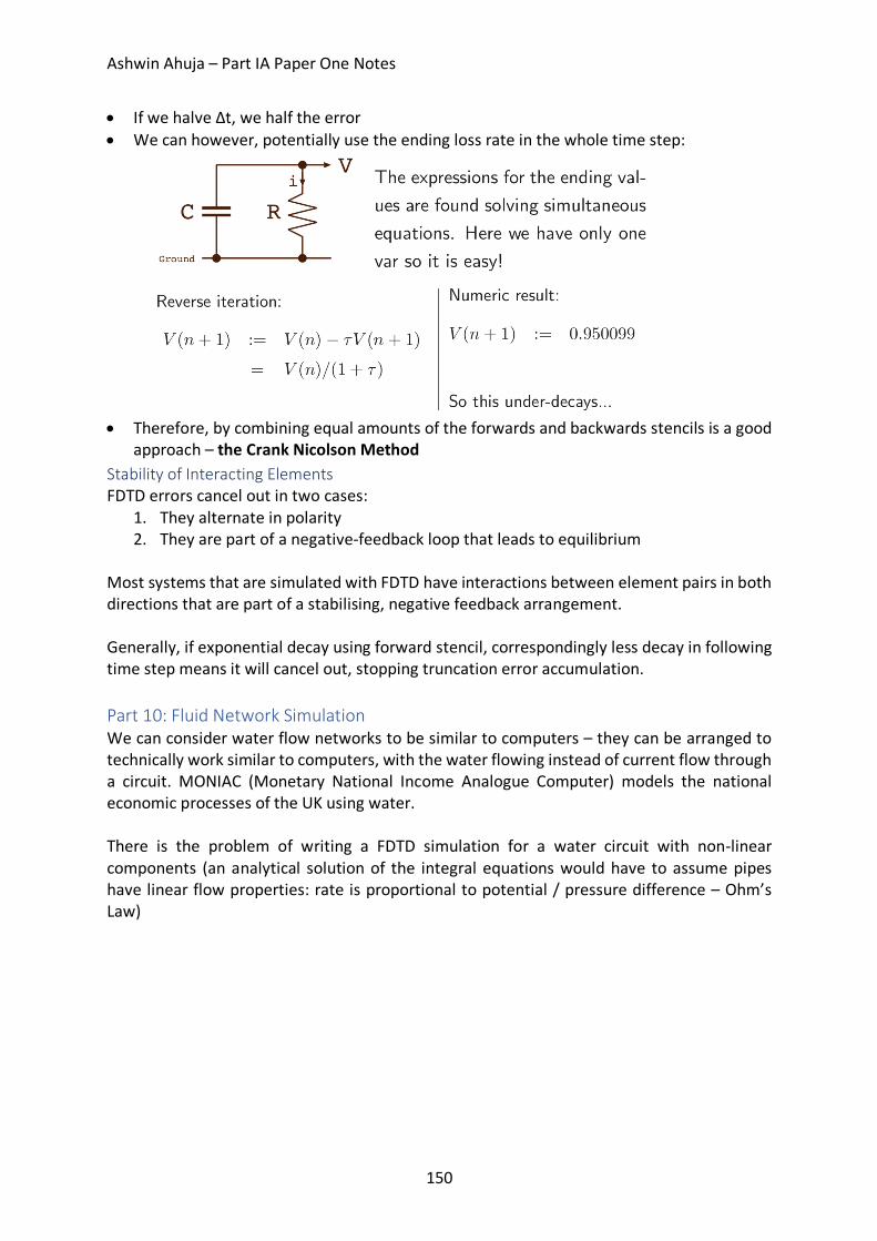
Ashwin Ahuja – Part IA Paper One Notes
150
• If we halve Δt, we half the error • We can however, potentially use the ending loss rate in the whole time step:
• Therefore, by combining equal amounts of the forwards and backwards stencils is a good
approach – the Crank Nicolson Method Stability of Interacting Elements FDTD errors cancel out in two cases:
1. They alternate in polarity 2. They are part of a negative-feedback loop that leads to equilibrium
Most systems that are simulated with FDTD have interactions between element pairs in both directions that are part of a stabilising, negative feedback arrangement. Generally, if exponential decay using forward stencil, correspondingly less decay in following time step means it will cancel out, stopping truncation error accumulation. Part 10: Fluid Network Simulation We can consider water flow networks to be similar to computers – they can be arranged to technically work similar to computers, with the water flowing instead of current flow through a circuit. MONIAC (Monetary National Income Analogue Computer) models the national economic processes of the UK using water. There is the problem of writing a FDTD simulation for a water circuit with non-linear components (an analytical solution of the integral equations would have to assume pipes have linear flow properties: rate is proportional to potential / pressure difference – Ohm’s Law)
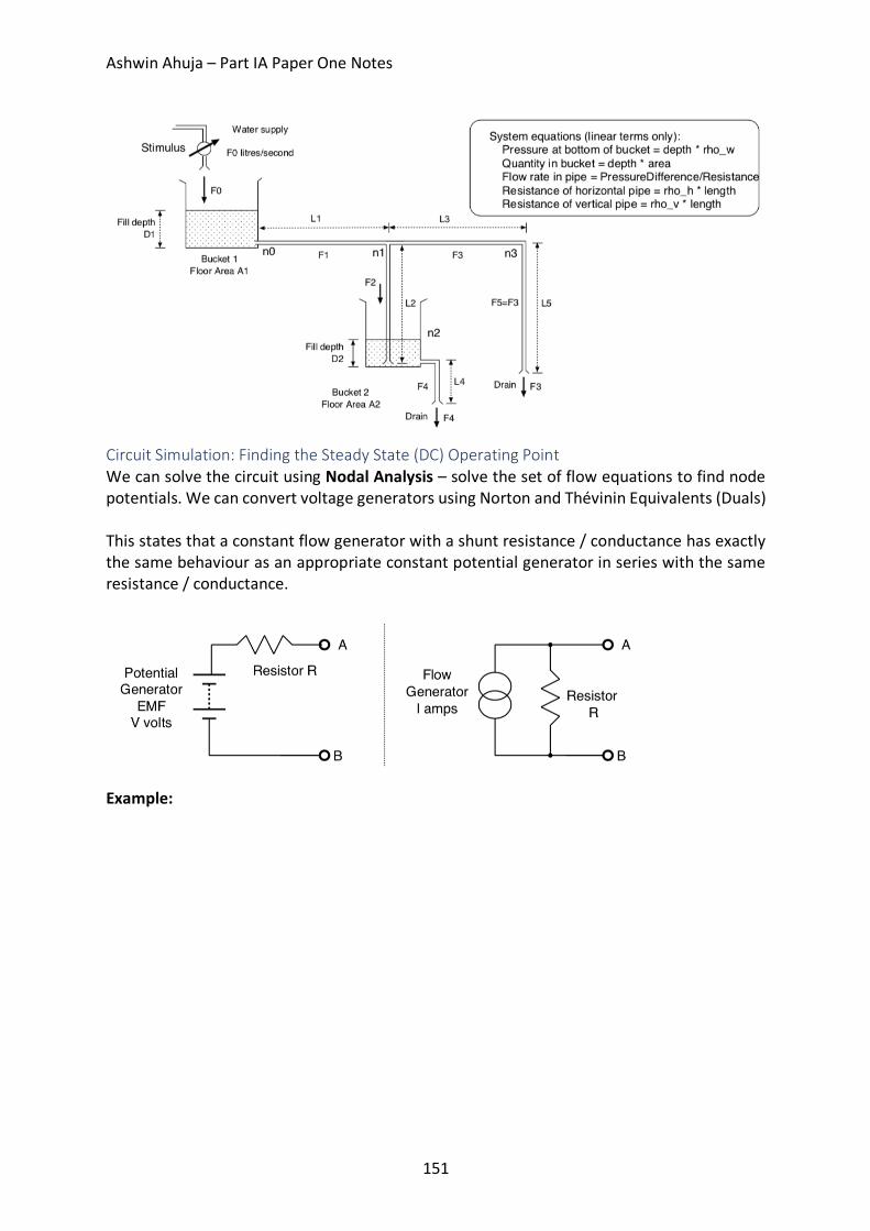
Ashwin Ahuja – Part IA Paper One Notes
151
Circuit Simulation: Finding the Steady State (DC) Operating Point We can solve the circuit using Nodal Analysis – solve the set of flow equations to find node potentials. We can convert voltage generators using Norton and Thévinin Equivalents (Duals) This states that a constant flow generator with a shunt resistance / conductance has exactly the same behaviour as an appropriate constant potential generator in series with the same resistance / conductance.
Example:
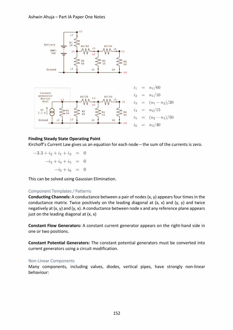
Ashwin Ahuja – Part IA Paper One Notes
152
Finding Steady State Operating Point Kirchoff’s Current Law gives us an equation for each node – the sum of the currents is zero.
This can be solved using Gaussian Elimination. Component Templates / Patterns Conducting Channels: A conductance between a pair of nodes (x, y) appears four times in the conductance matrix. Twice positively on the leading diagonal at (x, x) and (y, y) and twice negatively at (x, y) and (y, x). A conductance between node x and any reference plane appears just on the leading diagonal at (x, x) Constant Flow Generators: A constant current generator appears on the right-hand side in one or two positions. Constant Potential Generators: The constant potential generators must be converted into current generators using a circuit modification. Non-Linear Components Many components, including valves, diodes, vertical pipes, have strongly non-linear behaviour:
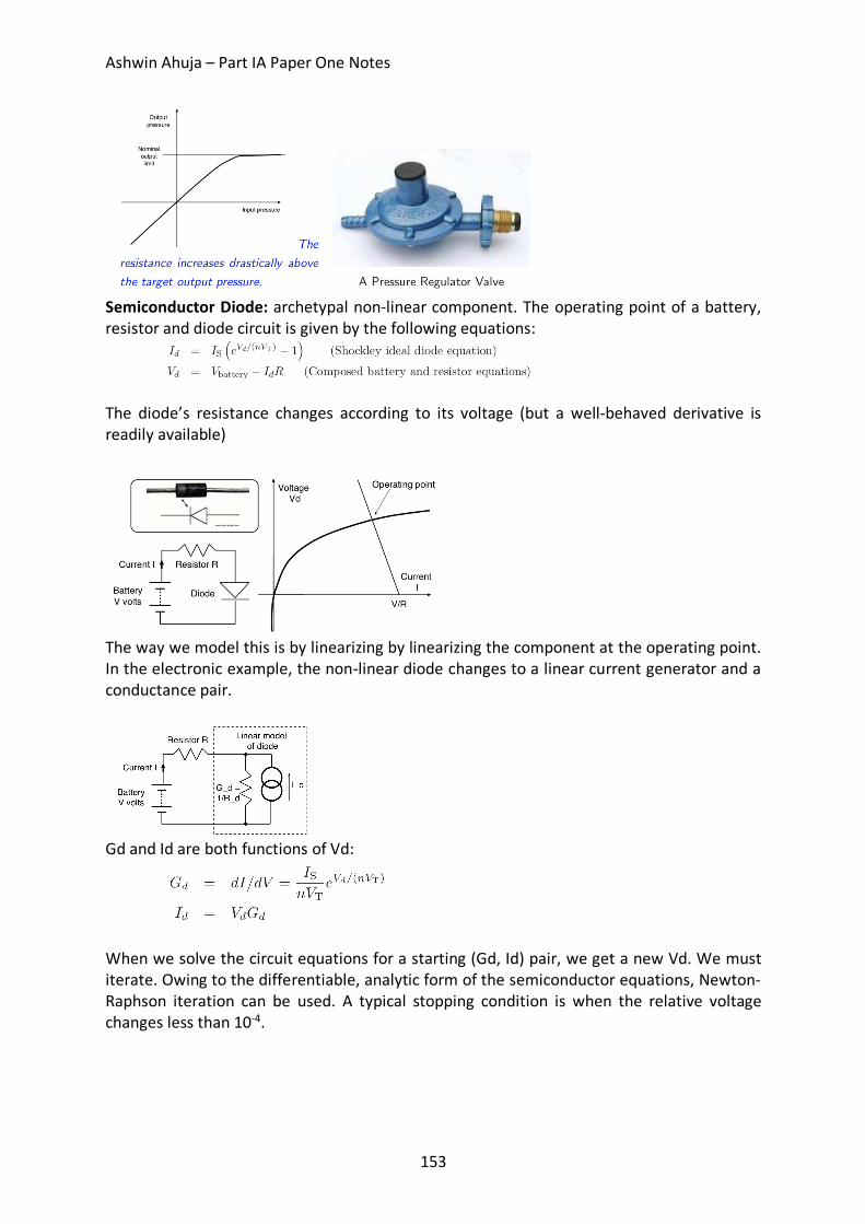
Ashwin Ahuja – Part IA Paper One Notes
153
Semiconductor Diode: archetypal non-linear component. The operating point of a battery, resistor and diode circuit is given by the following equations:
The diode’s resistance changes according to its voltage (but a well-behaved derivative is readily available)
The way we model this is by linearizing by linearizing the component at the operating point. In the electronic example, the non-linear diode changes to a linear current generator and a conductance pair.
Gd and Id are both functions of Vd:
When we solve the circuit equations for a starting (Gd, Id) pair, we get a new Vd. We must iterate. Owing to the differentiable, analytic form of the semiconductor equations, Newton-Raphson iteration can be used. A typical stopping condition is when the relative voltage changes less than 10-4.
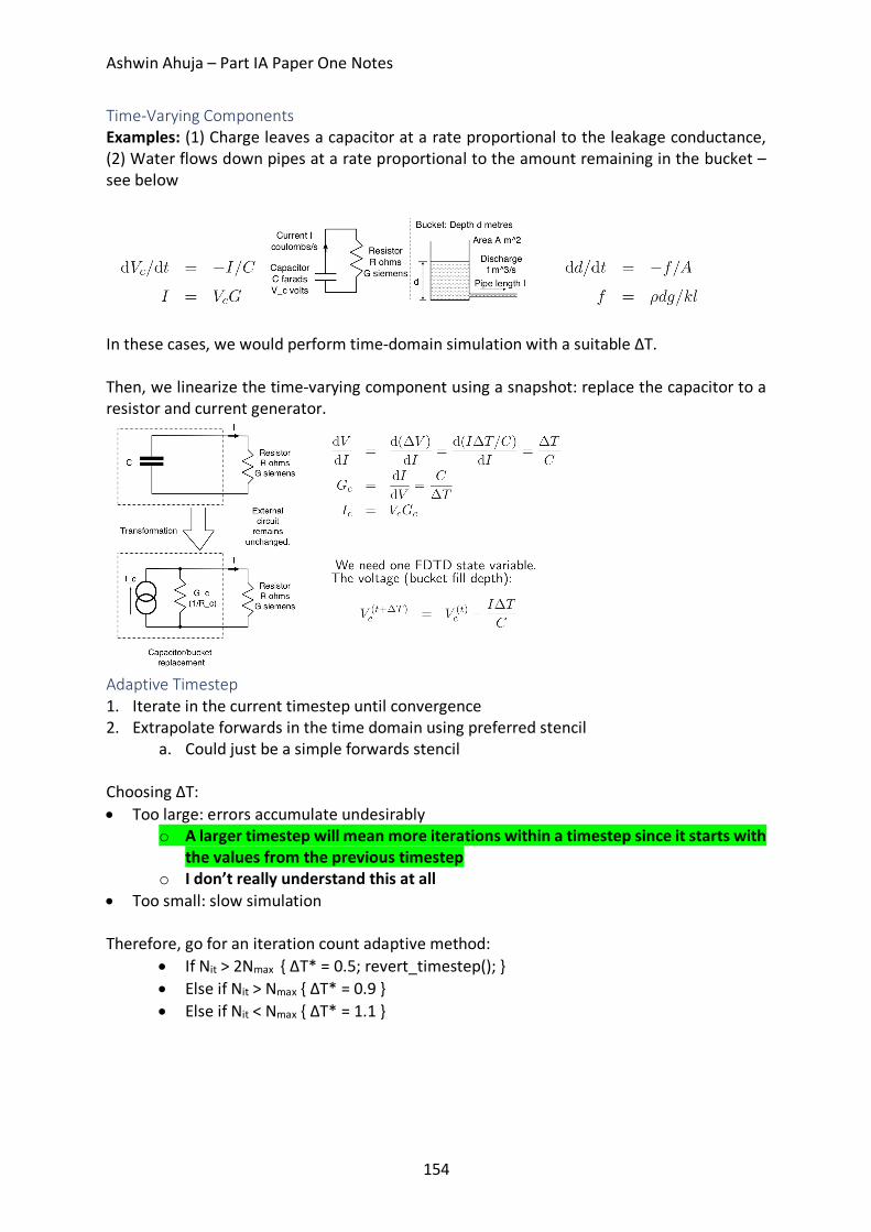
Ashwin Ahuja – Part IA Paper One Notes
154
Time-Varying Components Examples: (1) Charge leaves a capacitor at a rate proportional to the leakage conductance, (2) Water flows down pipes at a rate proportional to the amount remaining in the bucket – see below
In these cases, we would perform time-domain simulation with a suitable ΔT. Then, we linearize the time-varying component using a snapshot: replace the capacitor to a resistor and current generator.
Adaptive Timestep 1. Iterate in the current timestep until convergence 2. Extrapolate forwards in the time domain using preferred stencil
a. Could just be a simple forwards stencil Choosing ΔT: • Too large: errors accumulate undesirably
o A larger timestep will mean more iterations within a timestep since it starts with the values from the previous timestep
o I don’t really understand this at all • Too small: slow simulation Therefore, go for an iteration count adaptive method:
• If Nit > 2Nmax { ΔT* = 0.5; revert_timestep(); } • Else if Nit > Nmax { ΔT* = 0.9 } • Else if Nit < Nmax { ΔT* = 1.1 }