Panel Data Estimates of the Production Function and Product and Labor Market Imperfections

Panel data estimates of the production function

and product and labor market imperfections∗

Sabien DOBBELAERE† Jacques MAIRESSE‡

January 2007

Abstract

Embedding the efficient bargaining model into the R. Hall (1988) ap-proach for estimating price-cost margins shows that both imperfections inthe product and labor markets generate a wedge between factor elastici-ties in the production function and their corresponding shares in revenue.This article investigates these two sources of discrepancies both at the in-dustry level and the firm level using an unbalanced panel of 10646 Frenchfirms in 38 manufacturing industries over the period 1978-2001. By esti-mating standard production functions and comparing the estimated factorelasticities for labor and materials and their shares in revenue, we are ableto derive estimates of average price-cost mark-up and extent of rent shar-ing parameters. For manufacturing as a whole, our estimates of theseparameters are of an order of magnitude of 1.17 and 0.44 respectively.Our industry-level results indicate that industry differences in these pa-rameters and in the underlying estimated factor elasticities and shares arequite sizeable. Since firm production function, behavior and market envi-ronment are very likely to vary even within industries, we also investigatefirm-level heterogeneity in estimated mark-up and rent-sharing parame-ters. To determine the degree of true heterogeneity in these parameters,we adopt the P.A. Swamy (1970) methodology allowing to correct the ob-served variance in the firm-level estimates from their sampling variance.The median of the firm estimates of the price-cost mark-up ignoring la-bor market imperfections is of 1.10, while as expected it is higher of 1.20when taking them into account and the median of the corresponding firm

∗We are grateful to Susantu Basu, Michael Burda, Ferre De Graeve, Bronwyn Hall, BenoitMulkay, Mark Rogers, Chad Syversson, Philip Vermeulen, and other participants at the ZEWConference on the Economics of Innovation and Patenting (Mannheim, 2005), the Interna-tional Industrial Organization Conference (Boston, MA, 2006), the NBER Productivity Sem-inar (Cambridge, MA, 2006) and the ECB/CEPR 2006 Labour Market Workshop on Wageand Labour Cost Dynamics (Frankfurt, 2006) for helpful comments and suggestions. Allremaining errors are ours.

†Ghent University, K.U.Leuven, IZA Bonn, visiting CREST. Postdoctoral Fellow of theResearch Foundation - Flanders (FWO).

‡CREST, Institut National de la Statistique et des Etudes Economiques (INSEE), MERIT-Maastricht University, NBER.

1

estimates of the extent of rent sharing is of 0.62. The Swamy correspond-ing robust estimates of true dispersion are of about 0.18, 0.37 and 0.35,showing indeed very sizeable within-industry firm heterogeneity. We findthat firm size, capital intensity, distance to the industry technology fron-tier and investing in R&D seem to account for a significant part of thisheterogeneity.

JEL classification : C23, D21, J51, L13.Keywords : Rent sharing, price-cost mark-ups, production function, paneldata.

1 Introduction

In a world of perfect competition, the output contribution of individual pro-duction factors equals their respective revenue shares. In numerous markets,however, market imperfections and distortions are prevalent. The most com-mon sources for market power in product as well as labor markets are productdifferentiation, barriers to entry and imperfect information. Focusing on thelabor side, market power generally originates from coalitions between employersand employees. The labor economics literature is dominated by the standardrent sharing models where, for example, costs of hiring, firing and training canbe exploited by employees to gain market power. Those models generate wagedifferentials that are unrelated to productivity differentials and hinder the com-petitive market mechanism.1

Since the 1970s, models of imperfect competition have separately permeatedmany fields of economics ranging from industrial organization (see Bresna-han, 1989; Schmalensee, 1989 for surveys) to international trade (Brander andSpencer, 1985; Krugman, 1979) to labor economics (see Booth, 1995; Man-ning, 2003 for surveys). Recently, there has been a number of attempts toexamine simultaneously imperfections in both the product and the labor mar-ket (Bughin, 1996; Crepon-Desplatz-Mairesse, 1999, 2002; Neven-Roller-Zhang,2002; Dobbelaere, 2004).2 These articles aim at bridging the gap between theeconometric literature on estimating product market imperfections and the oneon estimating labor market imperfections. Two methods dominate the mostrecent approaches to simultaneously estimate product market and labor marketimperfections. One is the production function approach which entails estimat-ing a structural model including the full set of explicitly specified factor shareequations and the production function (see Bughin, 1996 and Neven et al.,2002). The other approach is an extension of a microeconomic version of R.Hall’s (1988) framework and boils down to estimating a reduced form equation(see Crepon et al., 1999, 2002 and Dobbelaere, 2004). Following Marschak and

1Recently, the monopsony model (Manning, 2003) has received attention in the laboreconomics literature. Contrary to the classical rent sharing models, search frictions generateupward sloping labor supply curves to individual firms, giving employers some market power.

2For theoretical contributions on this issue, we refer to Blanchard and Giavazzi (2003) andNickell (1999).

2

Andrews’ 1944 Econometrica article, many studies have applied the simulta-neous equations methodology to production function estimation (see Grilichesand Mairesse, 1998 and Ackerberg-Benkard-Berry-Pakes, 2006 for surveys). Thecore of this paper is to provide an in-depth analysis of imperfections in the prod-uct and the labor markets as two sources of discrepancies between the marginalproducts of input factors and the apparent factor prices. By doing so, we con-tribute to the econometric productivity literature on estimating microeconomicproduction functions and to the recent econometric literature on simultaneouslyestimating imperfections in product and factor markets.

This article differs from the existing literature in the following ways. Consis-tent with the standard models of imperfect competition in the labor marketpointed out above, we reflect on an extension of a microeconomic version of R.Hall’s (1988) framework. Following Crepon et al. (1999, 2002), we presumethat employees possess a degree of market power when negotiating with thefirm over wages and employment (efficient bargaining model, McDonald andSolow, 1981). Under this presumption, it can be shown that product and labormarket imperfections generate a wedge between factor elasticities in the produc-tion function and their corresponding shares in revenue. By estimating stan-dard production functions and comparing the estimated factor elasticities forlabor and materials and their shares in revenue, we are able to derive estimatesof average price-cost mark-up and extent of rent sharing parameters. Takingadvantage of a rich panel of French manufacturing firms covering the period1978-2001 (INSEE, SESSI, DEP), we analyze across- as well as within-industryheterogeneity in the estimated output elasticities and the retrieved parametersof interest. Our industry-level results indicate that industry differences in theestimated price-cost mark-up and extent of rent sharing parameters and in theunderlying estimated factor elasticities and shares are quite sizeable, as couldbe expected. The estimated price-cost mark-up is lower than 1.04 for the firstquartile of industries and exceeds 1.19 for the top quartile. There is no evidenceof rent sharing for the first quartile of industries but we estimate it to be higherthan 0.33 for the top quartile. The estimated across-industry heterogeneity inthese parameters is partly explained by differences in profitability, technologyintensity, unionization and import penetration. Since firm production function,behavior and market environment are very likely to vary even within industries,we also investigate within-industry firm heterogeneity in estimated mark-up andrent-sharing parameters (and the estimated factor elasticities and their shares).To determine the degree of true heterogeneity in the production function coeffi-cients and parameters of interest, we adopt the P.A. Swamy (1970) methodologyas a variance decomposition approach (see Mairesse-Griliches, 1990 for a relatedanalysis). The median of the firm estimates of the price-cost mark-up ignoringlabor market imperfections is of 1.10, while as expected it is higher of 1.20 whentaking them into account and the median of the corresponding firm estimatesof the extent of rent sharing is of 0.62. The Swamy corresponding robust esti-mates of true dispersion are of about 0.18, 0.37 and 0.35, showing evidence ofindeed very sizeable within-industry firm heterogeneity. Firm size, capital in-

3

tensity, distance to the industry technology frontier and investing in R&D seemto account for a significant part of this heterogeneity.

We proceed as follows. Section 2 briefly presents our theoretical framework. InSection 3, we discuss the data and provide estimates of output elasticities, price-cost mark-ups and the extent of rent sharing at the manufacturing level. Section4 focuses on across-industry heterogeneity and investigates different dimensionsacross industries. In Section 5 , we provide different estimators and indicators ofheterogeneity in the firm price-cost mark-up and the extent of rent sharing andlook at within-industry heterogeneity. In addition, we concentrate on the roleof specific firm-level variables in explaining part of the estimated heterogeneity.Section 6 concludes.

2 Theoretical framework

Consistent with two models of imperfect competition in the labor market thatare currently commonplace in the literature, the efficient bargaining model andthe monopsony model, we originally reflect on two extensions of Hall’s (1988)framework. First, following Crepon et al. (1999, 2002), we presume that, forexample, costs of firing, hiring and training can be exploited by employees togain market power when negotiating with the firm over wages and employment(efficient bargaining). In this framework, the firm price-cost mark-up and theextent of rent sharing generate a wedge between output elasticities and factorshares. Second, we abstain from the assumption that the labor supply curvefacing an individual employer is perfectly elastic (monopsony model). In thissetting, the firm price-cost mark-up and the firm wage elasticity of the laborsupply curve elicit deviations between marginal products of input factors andinput prices.Both extensions entail estimating a reduced-form equation which allows usto identify the structural parameters -measures of product and labor marketimperfections- derived from theory. Having a priori a prediction about themagnitude of economically meaningful parameter estimates, we can reject theextension anchoring the monopsony model on the basis of the data. The under-lying theoretical model and a summary of the results at the manufacturing, theindustry and the firm level are briefly presented in Appendix B. Based on theestimates, we did not follow that route in the remaining of the paper.This section explains the theoretical framework encompassing the efficient bar-gaining model and derives the reduced-forms.

4

2.1 Efficient bargaining model

Following Crepon et al. (1999, 2002),3 we start from a production functionQit = ΘitF (Nit, Mit, Kit), where i is a firm index, t a time index, N is labor,M is material input, K is capital and Θit = Ae

ηi+ut+υit is an index of technicalchange or ”true” total factor productivity. The logarithmic specification of theproduction function gives:

qit = εQNitnit + εQMit

mit + εQKitkit + θit (1)

We first assume that firms operate under imperfect competition in the productmarket and act as price takers in the input markets. Assuming that labor andmaterial input are variable factors, short run profit maximization implies thefollowing two first-order conditions:

εQNit= µitαNit

(2)

εQMit= µitαMit (3)

where αJit =PJitJitPitQit

(J = N, M) is the share of inputs in total revenue. µit =PitCQ,it

refers to the mark-up of price over marginal cost. Assuming that the

elasticity of scale, λit = εQNit+ εQMit

+ εQKit, is known, the capital elasticity can

be expressed as:

εQKit= λit − µitαNit − µitαMit (4)

Inserting (2), (3) and (4) in (1) and rearranging terms gives the following ex-pression:

qit − kit = µit [αNit(nit − kit) + αMit(mit − kit)] + (λit − 1) kit + θit (5)

Let us now abstain from the assumption that labor is priced competitively.We assume that the union and the firm are involved in an efficient bargainingprocedure, with both wages (w) and labor (N) being the subject of agreement.The union objective is to maximize U(wit, Nit) = Nitwit+(N it−Nit)wit, whereN it is union membership (0 < Nit ≤ N it) and wit ≤ wit is the alternative or thereservation wage. The firm objective is to maximize its short-run profit function:π(wit, Nit, Mit) = Rit − witNit − jitMit. The outcome of the bargaining is theasymmetric generalized Nash solution to:

maxwit, Nit,Mit

©Nitwit +

¡N it −Nit

¢wit −N itwit

ªφit {Rit − witNit − jitMit}1−φit(6)

3For technical details, see Crepon et al. (1999, 2002).

5

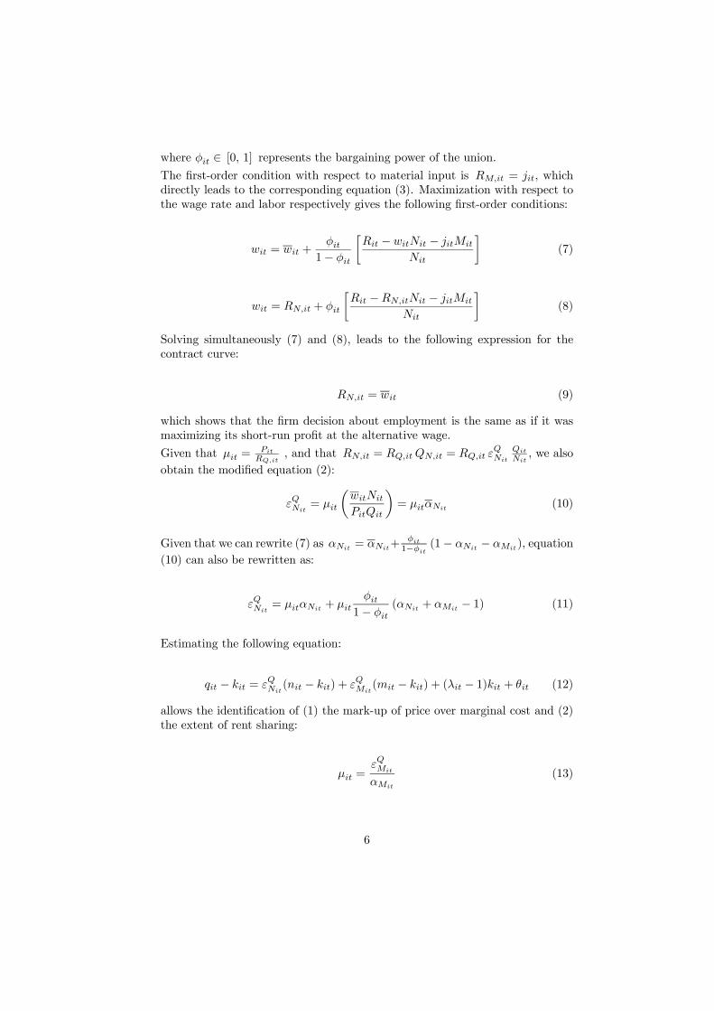
where φit ∈ [0, 1] represents the bargaining power of the union.The first-order condition with respect to material input is RM,it = jit, whichdirectly leads to the corresponding equation (3). Maximization with respect tothe wage rate and labor respectively gives the following first-order conditions:

wit = wit +φit

1− φit

·Rit − witNit − jitMit

Nit

¸(7)

wit = RN,it + φit

·Rit −RN,itNit − jitMit

Nit

¸(8)

Solving simultaneously (7) and (8), leads to the following expression for thecontract curve:

RN,it = wit (9)

which shows that the firm decision about employment is the same as if it wasmaximizing its short-run profit at the alternative wage.

Given that µit =PitRQ,it

, and that RN,it = RQ,itQN,it = RQ,it εQNit

Qit

Nit, we also

obtain the modified equation (2):

εQNit= µit

µwitNitPitQit

¶= µitαNit (10)

Given that we can rewrite (7) as αNit = αNit+φit1−φit (1− αNit − αMit), equation

(10) can also be rewritten as:

εQNit= µitαNit + µit

φit1− φit

(αNit + αMit − 1) (11)

Estimating the following equation:

qit − kit = εQNit(nit − kit) + εQMit

(mit − kit) + (λit − 1)kit + θit (12)

allows the identification of (1) the mark-up of price over marginal cost and (2)the extent of rent sharing:

µit =εQMit

αMit

(13)

6

γit =φit

1− φit=

εQNit−³εQMit

αNitαMit

´εQMit

αMit(αNit

+ αMit− 1)

(14)

φit =γit

1 + γit(15)

By embedding the efficient bargaining model into a microeconomic version ofHall’s (1988) framework, it follows that the firm price-cost mark-up and theextent of rent sharing generate a wedge between output elasticities and factorshares.4 The advantages of this extended approach are twofold: it avoids theproblematic computation of the user cost of capital to assess the magnitude ofthe price-cost mark-up and it avoids the measurement of the alternative wageto estimate the extent of rent sharing.

3 Data description and a first look at generalresults

In this section, we discuss the data and present the results of estimating theproduction function -both with and without imposing constant returns to scale-at the manufacturing level over the complete period under consideration. Weconcentrate on a range of estimators (levels OLS, first-differenced OLS, first-differenced GMM and system GMM). By comparing the estimated averageproduction function coefficients, i.e. the estimated average factor elasticitiesof labor and materials, with the average shares of labor and materials in rev-enue,5 we derive average price-cost mark-up and average extent of rent sharingparameters at the manufacturing level.

3.1 Data description

We use an unbalanced panel of French manufacturing firms over the period 1978-2001, based mainly on firm accounting information from EAE (”Enquete An-nuelle d’ Entreprise”, ”Service des Etudes et Statistiques Industrielles” (SESSI)).We only keep firms for which we have at least 12 years of observations, endingup with an unbalanced panel of 10646 firms with the number of observations for

4Note that to accommodate two imperfectly competitive markets, we need at least twovariable input factors to identify the model. Going beyond Hall (1988) is hence not possiblewhen starting from a value added specification.

5Variation in input shares is idiosyncratic and possibly related to variation in hours ofwork, machinery, capacity utilization (variation in the business cycle). When deriving our keyparameters, measures of product and labor market imperfections, we want to abstract fromthis possible source of contamination. Consistent with the constancy of bµ (only) and bφ, weassume constant input shares.

7

each firm varying between 12 and 24.6 We use real current production deflatedby the two-digit producer price index of the French industrial classification asa proxy for output (Q). Labor (N) refers to the average number of employ-ees in each firm for each year and material input (M) refers to intermediateconsumption deflated by the two-digit intermediate consumption price index.The capital stock (K) is measured by the gross bookvalue of fixed assets. Theshares of labor (αN ) and material input (αM ) are constructed by dividing re-spectively the firm total labor cost and undeflated intermediate consumption bythe firm undeflated production and by taking the average of these ratios overadjacent years. Table 1 reports the means, standard deviations and first andthird quartiles of our main variables. The average growth rate of real firm out-put for the overall sample is 2.1% per year over the period 1978-2001. Capitalhas decreased at an average annual growth rate of 0.1%, while materials andlabor have increased at an average annual growth rate of 4% and 0.6% respec-tively. As expected for firm-level data, the dispersion of all these variables isconsiderably large. For example, capital growth is smaller than -7.2% for thefirst quartile of firms and higher than 6% for the fourth quartile.

<Insert Table 1 about here>

3.2 Manufacturing-level results

Being interested in average output elasticities and derived average reduced-formparameters, we estimate the following specification for manufacturing as a wholeover the period 1978-2001:

qit − kit = εQN (nit − kit) + εQM (mit − kit) + (λ− 1) kit + ζit (16)

with and without imposing constant returns to scale.

Part 1 of Table 2 shows the results of estimating the basic production function(Eq.(16)) under the assumption of constant returns to scale (λ = 1), while Part2 allows for non constant returns to scale. We present both set of results fora range of estimators. Columns 1 and 2 report the levels OLS and the first-differenced OLS estimates, respectively. From column 3 onwards, we take intoaccount endogeneity problems. Columns 3 and 5 show the results of estimatingthe model in first differences to eliminate unobserved firm-specific effects andusing appropriate lags of the variables in levels (n, m and k) as instrumentsfor the differenced regressors to correct for simultaneity (standard panel first-differenced GMM). As argued by, for example, Blundell and Bond (2000), thefirst-differenced GMM estimator might be subject to large finite sample biasesdue to the time series persistence properties of some of the variables. In columns4 and 6, we therefore adopt a more efficient GMM estimator which includes level

6Putting the number of firms between brackets and the number of observations betweensquare brackets, the structure of the data is given by: (1398) [12], (1369) [13], (1403) [14],(1315) [15], (3414) [16], (226) [17], (215) [18], (200) [19], (164) [20], (153) [21], (180) [22], (136)[23], (473) [24]. The average number of observations per firm is 15.5 and the total number ofobservations is 165009.

8

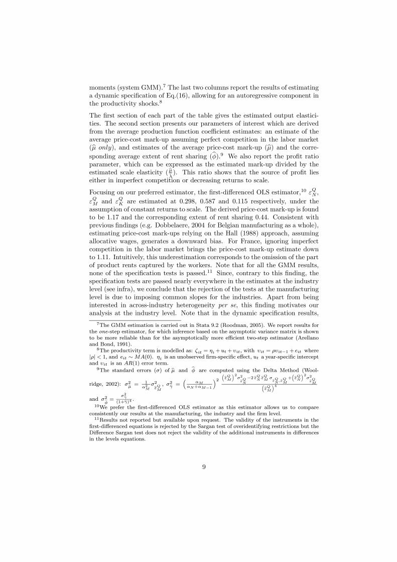
moments (system GMM).7 The last two columns report the results of estimatinga dynamic specification of Eq.(16), allowing for an autoregressive component inthe productivity shocks.8

The first section of each part of the table gives the estimated output elastici-ties. The second section presents our parameters of interest which are derivedfrom the average production function coefficient estimates: an estimate of theaverage price-cost mark-up assuming perfect competition in the labor market(bµ only), and estimates of the average price-cost mark-up (bµ) and the corre-sponding average extent of rent sharing (bφ).9 We also report the profit ratioparameter, which can be expressed as the estimated mark-up divided by theestimated scale elasticity ( bµbλ ). This ratio shows that the source of profit lieseither in imperfect competition or decreasing returns to scale.

Focusing on our preferred estimator, the first-differenced OLS estimator,10 εQN ,

εQM and εQK are estimated at 0.298, 0.587 and 0.115 respectively, under theassumption of constant returns to scale. The derived price-cost mark-up is foundto be 1.17 and the corresponding extent of rent sharing 0.44. Consistent withprevious findings (e.g. Dobbelaere, 2004 for Belgian manufacturing as a whole),estimating price-cost mark-ups relying on the Hall (1988) approach, assumingallocative wages, generates a downward bias. For France, ignoring imperfectcompetition in the labor market brings the price-cost mark-up estimate downto 1.11. Intuitively, this underestimation corresponds to the omission of the partof product rents captured by the workers. Note that for all the GMM results,none of the specification tests is passed.11 Since, contrary to this finding, thespecification tests are passed nearly everywhere in the estimates at the industrylevel (see infra), we conclude that the rejection of the tests at the manufacturinglevel is due to imposing common slopes for the industries. Apart from beinginterested in across-industry heterogeneity per se, this finding motivates ouranalysis at the industry level. Note that in the dynamic specification results,

7The GMM estimation is carried out in Stata 9.2 (Roodman, 2005). We report results forthe one-step estimator, for which inference based on the asymptotic variance matrix is shownto be more reliable than for the asymptotically more efficient two-step estimator (Arellanoand Bond, 1991).

8The productivity term is modelled as: ζit = ηi +ut + υit, with υit = ρυit−1+ eit where|ρ| < 1, and eit ∼MA(0). ηi is an unobserved firm-specific effect, ut a year-specific interceptand υit is an AR(1) error term.

9The standard errors (σ) of bµ and bφ are computed using the Delta Method (Wool-

ridge, 2002): σ2bµ = 1α2M

σ2bεQM , σ2bγ =³

αMαN+αM−1

´2 ³bεQM´2σ2bεQ

N

−2 bεQN bεQM σbεQN,bεQM

+³bεQN´2σ2bεQ

M³bεQM´4and σ2bφ = σ2bγ

(1+bγ)4 .10We prefer the first-differenced OLS estimator as this estimator allows us to compare

consistently our results at the manufacturing, the industry and the firm level.11Results not reported but available upon request. The validity of the instruments in the

first-differenced equations is rejected by the Sargan test of overidentifying restrictions but theDifference Sargan test does not reject the validity of the additional instruments in differencesin the levels equations.

9

the test of common factor restrictions is never passed.12

Comparing the results allowing for non constant returns to scale (Part 2 of Table2) with those imposing constant returns to scale (Part 1 of Table 2), leadsto the following insights. The returns to scale assumption evidently affectsthe estimated output elasticities of factor inputs. In general, the productionfunction coefficients are estimated to be lower when allowing for non constantreturns to scale. However, since the first-order conditions with respect to thevariable input factors -Eq.(2) or (11) for labor and Eq.(3) for materials- do notdepend on the returns to scale assumption, our key parameters (bµ only, bµ andbφ) are robust to this assumption.13 This crucial result along with our objectiveto compare consistently estimates of product and labor market imperfectionsat the manufacturing, the industry and the firm level, motivates our decisionto maintain the constant returns to scale assumption in the remaining of thepaper. Due to the finding of decreasing returns to scale, the average profit ratioparameter is estimated to be lower when allowing for non constant returns toscale.


By way of sensitivity test, we restrict the total sample to those firms for whichwe have 24 years of observations and estimate Eq.(16) imposing constant returnsto scale. The results are reported in Table A.1. in Appendix A. On average, theprice-cost mark-up parameters are estimated to be higher and the correspondingextent of rent sharing parameters are estimated to be lower than those of thetotal sample across the different estimators.14

4 Across-industry heterogeneity in µ and bφThis section concentrates on across-industry heterogeneity. We first presentthe detailed results of estimating the production function (Eq.(16)) under theassumption of constant returns to scale for each of our 38 industries. Hav-ing observed considerable heterogeneity in the difference between the factors’

12Using ζit = ηi+ut+υit, with υit = ρυit−1+eit and eit ∼MA(0), and assuming constantreturns to scale (λ = 1), we can transform (16) through substitution to obtain qit − kit =π1(qit−1 − kit−1) + π2(nit − kit) + π3(nit−1 − kit−1) + π4(mit − kit) + π5(mit−1 − kit−1) +η∗i +u

∗t+eit, where π1 = ρ, π2 = εQN , π3 = −ρ εQN , π4 = εQM , π5 = −ρ εQM , η∗i = (1− ρ) ηi and

u∗t = ut − ρut−1. Given consistent estimates of the unrestricted parameter vector π = (π1,π2, π3, π4, π5), the two non-linear common factor restrictions π3 = −π1 π2 and π5 = −π1 π4can be tested using minimum distance to get the restricted parameter vector

³εQN , ε

QM , ρ

´.

13Except for the estimated price-cost mark-up (bµ) using the first-differenced GMM estima-tor, which is estimated to be much lower when allowing for non constant returns to scale (seePart 2 of Table 2). This result is due to the considerable decrease in the estimated output

elasticity of materials (bεQM ) when abstaining from the constant returns to scale assumption.14In contrast to the total sample results, the Sargan test does not reject the joint validity of

the lagged levels of n, m and k dated (t−2) (and earlier) as instruments in the first-differencedequations. However, the validity of the additional first-differenced variables as instruments inthe levels equations is rejected by the Difference Sargan test.

10

estimated marginal products and their measured payments, we then tie this es-timated heterogeneity to observables (profitability, technology intensity, union-ization and import penetration).

4.1 Across-industry estimates

Being interested in average parameters, the average industry-level price-costmark-up (µj), relative extent of rent sharing (bγj) and extent of rent sharing(bφj) are derived from comparing the estimated average output elasticities with

the average input shares: µj =bεQMj

αMj, bγj = bεQNj−

µbεQMj

αNjαMj

¶bεQMjαMj

(αNj+αMj−1)

and bφj = bγj1+bγj .

We decompose the total sample into 38 manufacturing industries according tothe French industrial classification (”Nomenclature economique de synthese -Niveau 3” [NES 114]). Table A.2 in Appendix A shows the industry repartitionof the sample. Table 3 summarizes the first-differenced OLS and the systemGMM results of the industry analysis. For each estimator, we consider twosubsamples. The first subsample contains the estimates for which the price-costmark-up equals or exceeds 1 and the corresponding extent of rent sharing liesin the [0, 1]-interval.15 The second subsample includes the estimates showingno evidence of rent sharing and a price-cost mark-up ignoring labor market im-perfections that equals or exceeds 1.16 Both estimators have 21 industries incommon in the first subsample and 8 in the second subsample. Detailed infor-mation on the first-differenced OLS and the system GMM estimates is presentedin Table A.3.a in Appendix A. In the left part of Table A.3.a [Part 1-2], we com-pute the average shares of labor, material input and capital for each industry.The middle part reports the first-differenced OLS and the system GMM esti-mates of the output elasticities. The right part presents the derived parametersof interest: the price-cost mark-up assuming that labor is priced competitively(bµj only), the price-cost mark-up taking into account labor market imperfec-tions (bµj), the relative extent of rent sharing (bγj) and the extent of rent sharing(bφj). For each estimator, we first report the estimates of the first subsample[24 industries for OLS DIF and 26 for system GMM], followed by those of thesecond subsample [14 for OLS DIF and 11 for system GMM17]. Within each

15This subsample contains 24 industries using the first-differenced OLS estimator. Theestimates of bµj (≥ 1) and bµj only (≥ 1) are significant for all industries, whereas bφj (∈ [0, 1])is significant for 19 out of 24 industries. As to the system GMM results, 26 industries belongto this subsample. bµj (≥ 1) and bµj only (≥ 1) are significant for all industries, whereasbφj (∈ [0, 1]) is significant for 16 out of 26 industries.16This subsample contains 14 industries using the first-differenced OLS estimator. The

estimates of bµj only (≥ 1) are significant for all industries, whereas bµj (≥ 1) is significant for9 out of 14 industries. 4 out of 14 estimated rent sharing parameters (bφj = 0) are significant.As to the system GMM results, 11 industries belong to this subsample. bµj only (≥ 1) and bµj(≥ 1) are significant for all industries, whereas there is only one significantly estimated rent

sharing parameter (bφj = 0).17In Table A.3.a [Part 4], we also report the estimates of industry 1, for which bφj =

11

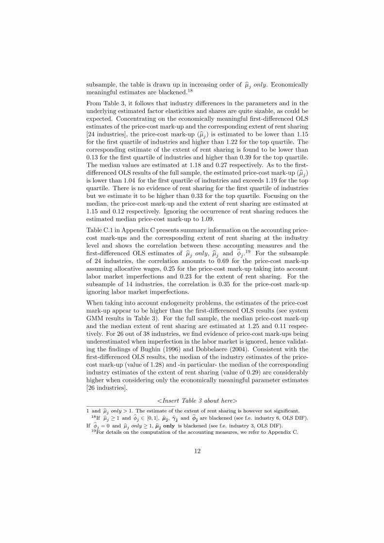
subsample, the table is drawn up in increasing order of bµj only. Economicallymeaningful estimates are blackened.18

From Table 3, it follows that industry differences in the parameters and in theunderlying estimated factor elasticities and shares are quite sizable, as could beexpected. Concentrating on the economically meaningful first-differenced OLSestimates of the price-cost mark-up and the corresponding extent of rent sharing[24 industries], the price-cost mark-up (bµj) is estimated to be lower than 1.15for the first quartile of industries and higher than 1.22 for the top quartile. Thecorresponding estimate of the extent of rent sharing is found to be lower than0.13 for the first quartile of industries and higher than 0.39 for the top quartile.The median values are estimated at 1.18 and 0.27 respectively. As to the first-differenced OLS results of the full sample, the estimated price-cost mark-up (bµj)is lower than 1.04 for the first quartile of industries and exceeds 1.19 for the topquartile. There is no evidence of rent sharing for the first quartile of industriesbut we estimate it to be higher than 0.33 for the top quartile. Focusing on themedian, the price-cost mark-up and the extent of rent sharing are estimated at1.15 and 0.12 respectively. Ignoring the occurrence of rent sharing reduces theestimated median price-cost mark-up to 1.09.

Table C.1 in Appendix C presents summary information on the accounting price-cost mark-ups and the corresponding extent of rent sharing at the industrylevel and shows the correlation between these accounting measures and thefirst-differenced OLS estimates of bµj only, bµj and bφj .19 For the subsampleof 24 industries, the correlation amounts to 0.69 for the price-cost mark-upassuming allocative wages, 0.25 for the price-cost mark-up taking into accountlabor market imperfections and 0.23 for the extent of rent sharing. For thesubsample of 14 industries, the correlation is 0.35 for the price-cost mark-upignoring labor market imperfections.

When taking into account endogeneity problems, the estimates of the price-costmark-up appear to be higher than the first-differenced OLS results (see systemGMM results in Table 3). For the full sample, the median price-cost mark-upand the median extent of rent sharing are estimated at 1.25 and 0.11 respec-tively. For 26 out of 38 industries, we find evidence of price-cost mark-ups beingunderestimated when imperfection in the labor market is ignored, hence validat-ing the findings of Bughin (1996) and Dobbelaere (2004). Consistent with thefirst-differenced OLS results, the median of the industry estimates of the price-cost mark-up (value of 1.28) and -in particular- the median of the correspondingindustry estimates of the extent of rent sharing (value of 0.29) are considerablyhigher when considering only the economically meaningful parameter estimates[26 industries].


1 and bµj only > 1. The estimate of the extent of rent sharing is however not significant.18If bµj ≥ 1 and bφj ∈ [0, 1], bµj, bγ j and bφj are blackened (see f.e. industry 6, OLS DIF).

If bφj = 0 and bµj only ≥ 1, bµj only is blackened (see f.e. industry 3, OLS DIF).19For details on the computation of the accounting measures, we refer to Appendix C.

12

Table A.3.b in Appendix A summarizes all the industry estimates. The upperpart displays the correlation between our parameters of interest for a rangeof estimators (first-differenced OLS, first-differenced GMM and system GMM).The lower part of the table shows the correlation of the parameters across thedifferent estimators. The left part of the table considers the full sample while theright part restricts the sample to those industries for which the estimated extentof rent sharing lies in the [0, 1]-interval. The correlation between the estimatedprice-cost mark-up ignoring the occurrence of rent sharing (bµj only) and theestimate taking into account labor market imperfections (bµj) amounts to 0.6for each estimator (see upper part of Table A.3.b). The correlation betweenthe price-cost mark-up estimate (bµj) and the estimated relative extent of rentsharing (bγj) is found to be 0.8 for the whole sample and 0.5 for the restrictedsample. From the lower part of Table A.3.b, it follows that particularly thefirst-differenced OLS and the system GMM estimates are highly correlated.

4.2 Different dimensions across industries

To investigate different dimensions across industries, we classify the industriesaccording to profitability, technology intensity, unionization and import pene-tration. For each dimension, we consider four types (low, medium low, mediumhigh and high). As to the profitability dimension, we calculate the averageindustry-level price-cost margin (PCM)20 and determine the different typesbased on the quartile values. The identification of the technology types relies onthe OECD classification. This methodology uses two indicators of technologyintensity, R&D expenditures divided by value added and R&D expendituresdivided by production (OECD, 2005). To construct our measure of the degreeof unionization, we merge our original dataset consisting of firms from EAE(SESSI) with the REPONSE 1998 (”Relations Professionnelles et Negociationsd’ Entreprises”) database collected by the French Ministry of Labor. Having911 firms left, we compute the average industry-level union density.21 Similar tothe profitability dimension, the quartile values define the four types. As to theopenness dimension, we compute the average industry-level import penetrationratio as the ratio of industry product imports to the sum of these imports plusthe value of domestic production in the industry using the input-output tablesdefined at the three-digit level (National Institute for Statistics and EconomicStudies (INSEE)). The different types are identified through the quartile values.For each dimension, columns 4-7 in Table A.2 in Appendix A indicate the typeto which each industry belongs.

Graphs 1-4 aim at discerning a pattern in the economically meaningful industryestimates of bµj and bφj .22 Each graph corresponds to one of the four dimen-sions (profitability, technology intensity, unionization and import penetration).

20The price-cost margin is defined as the difference between revenue and variable cost overrevenue (see Schmalensee, 1989 p. 960).21Since we use a small non-representative subsample (only 911 firms) to define the degree

of industry-level unionization, the resulting classification has to be interpreted with caution.22The corresponding industries are blackened in Table A.2 in Appendix A.

13

Within each dimension, different symbols refer to each of the four types (low,medium low, medium high and high). The dashed lines denote the median val-

ues (bµj,med = 1.18, bφj,med = 0.27). Given the positive correlation between bµjand bφj of 0.48, most industries are situated either in the upper right part or thelower left part of the graphs. Focusing on Graph 1, the price-cost mark-up oftwo thirds of the highly profitable industries is higher than the median price-costmark-up. As to bφj , no clear pattern can be detected. From Graph 2, it followsthat nearly two thirds of the low-technology industries are characterized by arelatively high bµj and bφj (see upper right part of the graph).23 Concentratingon Graph 3, nearly two thirds of the industries with a high degree of unionizationhave a price-cost mark-up exceeding the median value. All weakly unionizedindustries are situated in the lower part of the graph, being characterized by anestimated price-cost mark-up below the median value. The estimated extent ofrent sharing of half of those industries is lower than the median value.24 Graph4 shows that industries with high import penetration rates have estimated price-cost mark-ups below the median value, while industries shielded from importcompetition display an estimated extent of rent sharing exceeding the medianvalue. These findings confirm those of Abraham et al. (2006) and Boulhol et al.(2006). They also provide support for the imports-as-product-and-labor-marketdiscipline hypothesis using Belgian and UK firm-level data, respectively.

<Insert Graphs 1-4 about here>

5 Within-industry heterogeneity in µ and bφProduction behavior is very likely to vary even within industries, because inputcombinations differ, labor markets are not homogeneous and demand might bemore elastic or inelastic in one firm than another. In this section, we allow forheterogeneous production behavior across firms. Since production is primarilyaffected by input factors and only secondarily by -for example- demand con-ditions, we assume that the relationships among variables are proper but theproduction function coefficients differ across firms. Therefore, we estimate theproduction function for each firm i and retrieve the firm price-cost mark-upbµi and the extent of rent sharing bφi from the estimated firm output elasticities

(bεQJi , J = N,M,K).25This section starts with a brief discussion of the Swamy (1970) methodology.We then apply this methodology to analyze whether there is real firm-levelheterogeneity in the estimated average factor elasticities and average shares,

23Note that in contrast to Graphs 1, 3 and 4, 12 industries belong to the low-technologycategory.24Graphs 1-4 display the first-differenced OLS estimates of bµj and bφj (see blackened indus-

try estimates in Table A.3.a, Part 1). Plotting the system GMM estimates of bµj against bφj(see blackened industry estimates in Table A.3.a, Part 3) leads largely to the same conclusions.25Besides allowing for the possible heterogeneity across firms, we could also focus on the

stability of the structural parameters over time. However, relaxing the constancy of µi andφi in the time dimension would strain our already overextended computational framework.

14

and the derived average mark-up and rent sharing parameters. We end thesection by tying the sizeable estimated firm heterogeneity in product and labormarket imperfection parameters to observables.

5.1 Swamy (1970) methodology

To determine the degree of true heterogeneity in the coefficients and parametersof interest, we adopt the Swamy (1970) methodology as a variance decompo-sition approach. This method allows us to estimate the variance componentsof heterogeneity in the estimated firm output elasticities (bεQJi , J = N,M,K)

and the derived structural parameters (µi only, µi, bγi and φi), i.e., the puresampling variance and the true heterogeneity.Considering random production function coefficients that vary across firms, let-ting x1it ≡ 1 and assuming constant returns to scale, we can rewrite the pro-duction function as follows:26

qit =KXk=1

εkitxkit + ξit (17)

εi is assumed to be randomly distributed with εi = eε + ηi. eε = (eε1, ..., eεK)0represents the common-mean coefficient vector and ηi = (η1i, ..., ηKi)

0the in-

dividual deviation from the common mean eε. Following Swamy (1970), weassume that the errors for firm i are uncorrelated across firms and allow forheteroskedasticity across firms, ξi ∼ N

¡0, σ2i I

¢. E (ηi) = 0, E

¡ηiη

0j

¢= ∆, if

i = j, E¡ηiη

0j

¢= 0, otherwise. Swamy suggests first estimating Eq. (17) for

each firm i by OLS giving:

bεi = (X 0iXi)

−1X 0i qi with (18)bξi = qi −Xibεi (19)

Using (18) and (19), we obtain unbiased estimators of σ2i and ∆, given byEq. (20) and (21) respectively.

bσ2i = bξ0ibξiT −K (20)

with the estimated variance-covariance matrix V ar (bεi) = bσ2i (X 0iXi)

−1. Defin-

ing the mean of bεi as ε = 1N

NPi=1

bεi, their variance can be estimated as:26For the sake of parsimony, we denote the explanatory variables by xkit (k = 1,..,K)

and the firm output elasticities by εkit (dropping the superscript (Q) and the subscript(J = N,M)).

15

b∆ =1

N − 1NPi=1

(bεi − ε) (bεi − ε)0 − 1

N

NPi=1

V ar (bεi)=

1

N − 1NPi=1(bεi − ε) (bεi − ε)0| {z }(1)

− 1

N

NPi=1

σ2i (X0iXi)

−1

| {z }(2)

(21)

The logic behind the definition of b∆, the Swamy estimate of true variance of thecoefficients, is that due to noisy estimates (bεi), much of the variation in bεi isnot caused by ”real” parameter variability but purely by sampling error. Swamy(1970) thus suggests to correct for this sampling variability by subtracting itoff.Two major advantages of the Swamy methodology are that these estimates arethe most straightforward to obtain among the different estimators of coefficientheterogeneity and that they are robust to the possibility of correlated effectsbetween the firm intercept and slope parameters and the other variables in theequation since they are based on individual regression estimates (see Mairesse-Griliches, 1990).27

5.2 General overview

Table 4 summarizes the first-differenced OLS results of estimating Eq.(17) foreach firm i in a comprehendible fashion. Consistent with the across-industryestimates, we consider two subsamples of estimates. The first part of Table4 shows the results of the first subsample keeping only the firm estimates ofwhich µi ≥ 1 and φi ∈ [0, 1] [5906 firms].28 The second part of Table 4 presentsthe results of the second subsample restricting the firm estimates to those ofwhich φi = 0 and µi only ≥ 1 [1239 firms].29 The last part of Table 4 summa-rizes the results of all the firm estimates [10646 firms]. Each part is split intothree sections, focusing on the simple mean, the weighted mean and the medianrespectively. Table A.4 in Appendix A, which is structured in the same way

27Besides the Swamy method, the random coefficient model literature suggests anotherapproach to estimate the variance components of heterogeneity, using the maximum likelihood(ML) estimator and the more flexible approach of regressing the squares and the cross-productsof residuals on comparable squares and cross-products of the independent variables (Hildrethand Houck, 1968; Amemiya, 1977; MaCurdy, 1985). Contrary to the Swamy estimates, theML estimates and those based on the regression of the squares and cross-products of theresiduals assume either the independence of the firm slope parameteres or the independencebetween both the firm intercept and slope parameters and the other variables in the equation,i.e., the absence of correlated effects (see Mairesse-Griliches, 1990 for a comparison of thethree different approaches).28Looking at the significance of the parameter estimates, we find that 5817 out of 5906

estimates of bµi (≥ 1), 4414 out of 5906 estimates of bφi (∈ [0, 1]) and 4426 out of 5906estimates of bµi only (≥ 1) are significant.29Within this subsample, 1238 out of 1239 estimates of bµi only (≥ 1) are significant. As

to bµi (≥ 1), 983 out of 1239 estimates are significant. None of the estimated rent sharing

parameters (bφi = 0). is found to be significant.16

as Table 4, reports detailed information on the results of applying the Swamy(1970) methodology. For comparison purposes, we list also similar statistics forthe firm input shares (αJi , J = N,M,K). Within each part, the last row of eachsection reports the F-statistic for the hypothesis of equality of the estimates (orthe computed variables) across firms.

The first section of each part of Table A.4 gives the original Swamy estimatesof true variance [bσ2true, corresponding to b∆ in Eq. (21)], which are computed asthe difference between the observed variance of the individually estimated firmcoefficients [bσ2o, corresponding to term (1) in Eq. (21)] and the mean of the cor-responding sampling variance [bσ2s, corresponding to term (2) in Eq. (21)].30 Theobserved variance

³bσ2o´ illustrates the sizeable dispersion in the estimated firmoutput elasticities and the derived parameters and shows that the heterogeneityat the firm level is largely magnified by large sampling errors arising from the

rather short time series available. Due to the large sampling variance³bσ2s´, we

even find zero estimates of true variance in the individually estimated extent ofrent sharing φi in the first subsample [5906 firms] and the total sample [10646firms]. All the observed variability is either common to all firms, transitory orattributable to sampling variability. Given the large number of degrees of free-dom, all the F-statistics are significant at conventional significance levels (the

critical value barely exceeds 1 for our sample size), except for φi.31 Except for

µi only, the large sampling variance drives the true variance in all the derivedparameters towards zero in the second subsample [1239 firms].

To investigate whether the true heterogeneity is not just an artefact of outliersand large sampling errors, we look at the Swamy estimates of the weighted truevariance and the Swamy estimates of the robust true variance. The Swamyestimate of the weighted true variance, which is calculated as the weightedobserved variance minus the weighted sampling variances, is reported in thesecond section of each part of Table A.4.32 The weight is defined as the inverseof the sampling variance. As to the estimated firm output elasticities (bεQJi ,J = N,M,K), the weighted observed and -even more so- the weighted samplingvariance are considerably smaller than the corresponding simple observed and

30Taking into account the unbalanced nature of the sample, the equivalent for the in-

put shares αJ can be expressed as: eσ2true = 1N−1

NPi=1

¡αJi − αJ

¢2 − 1Teσ2s, where nt de-

notes the number of years within firm i and Nnt the number of firms having nt years

of observations. T =24P

nt=12

³NntNnt´, αJi = 1

T

ntPt=1

αJit , αJ = 1N

NPi=1

αJi and eσ2s =

1N(T−1)

NPi=1

ntPt=1

¡αJit − αJi

¢2.

31One can question, however, the validity of these F-statistics in such large samples. A moresymmetric treatment of the inference problem, advocated by Leamer (1978), would necessitateusing a critical value which increases with the number of degrees of freedom. This would leadto less certainty in rejecting the hypothesis of homogeneity (Mairesse-Griliches, 1990).

32In practice, the weighted sampling variance is calculated as NNPi=1

bσ2i .

17

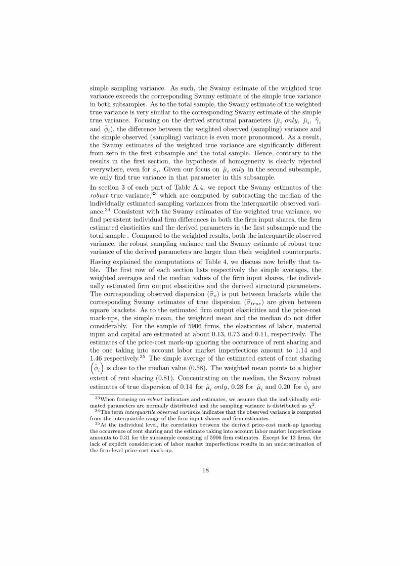
simple sampling variance. As such, the Swamy estimate of the weighted truevariance exceeds the corresponding Swamy estimate of the simple true variancein both subsamples. As to the total sample, the Swamy estimate of the weightedtrue variance is very similar to the corresponding Swamy estimate of the simpletrue variance. Focusing on the derived structural parameters (µi only, µi, bγiand φi), the difference between the weighted observed (sampling) variance andthe simple observed (sampling) variance is even more pronounced. As a result,the Swamy estimates of the weighted true variance are significantly differentfrom zero in the first subsample and the total sample. Hence, contrary to theresults in the first section, the hypothesis of homogeneity is clearly rejectedeverywhere, even for φi. Given our focus on µi only in the second subsample,we only find true variance in that parameter in this subsample.

In section 3 of each part of Table A.4, we report the Swamy estimates of therobust true variance,33 which are computed by subtracting the median of theindividually estimated sampling variances from the interquartile observed vari-ance.34 Consistent with the Swamy estimates of the weighted true variance, wefind persistent individual firm differences in both the firm input shares, the firmestimated elasticities and the derived parameters in the first subsample and thetotal sample . Compared to the weighted results, both the interquartile observedvariance, the robust sampling variance and the Swamy estimate of robust truevariance of the derived parameters are larger than their weighted counterparts.

Having explained the computations of Table 4, we discuss now briefly that ta-ble. The first row of each section lists respectively the simple averages, theweighted averages and the median values of the firm input shares, the individ-ually estimated firm output elasticities and the derived structural parameters.The corresponding observed dispersion (bσo) is put between brackets while thecorresponding Swamy estimates of true dispersion (bσtrue) are given betweensquare brackets. As to the estimated firm output elasticities and the price-costmark-ups, the simple mean, the weighted mean and the median do not differconsiderably. For the sample of 5906 firms, the elasticities of labor, materialinput and capital are estimated at about 0.13, 0.73 and 0.11, respectively. Theestimates of the price-cost mark-up ignoring the occurrence of rent sharing andthe one taking into account labor market imperfections amount to 1.14 and1.46 respectively.35 The simple average of the estimated extent of rent sharing³φi

´is close to the median value (0.58). The weighted mean points to a higher

extent of rent sharing (0.81). Concentrating on the median, the Swamy robust

estimates of true dispersion of 0.14 for µi only, 0.28 for µi and 0.20 for φi are

33When focusing on robust indicators and estimates, we assume that the individually esti-mated parameters are normally distributed and the sampling variance is distributed as χ2.34The term interquartile observed variance indicates that the observed variance is computed

from the interquartile range of the firm input shares and firm estimates.35At the individual level, the correlation between the derived price-cost mark-up ignoring

the occurrence of rent sharing and the estimate taking into account labor market imperfectionsamounts to 0.31 for the subsample consisting of 5906 firm estimates. Except for 13 firms, thelack of explicit consideration of labor market imperfections results in an underestimation ofthe firm-level price-cost mark-up.

18

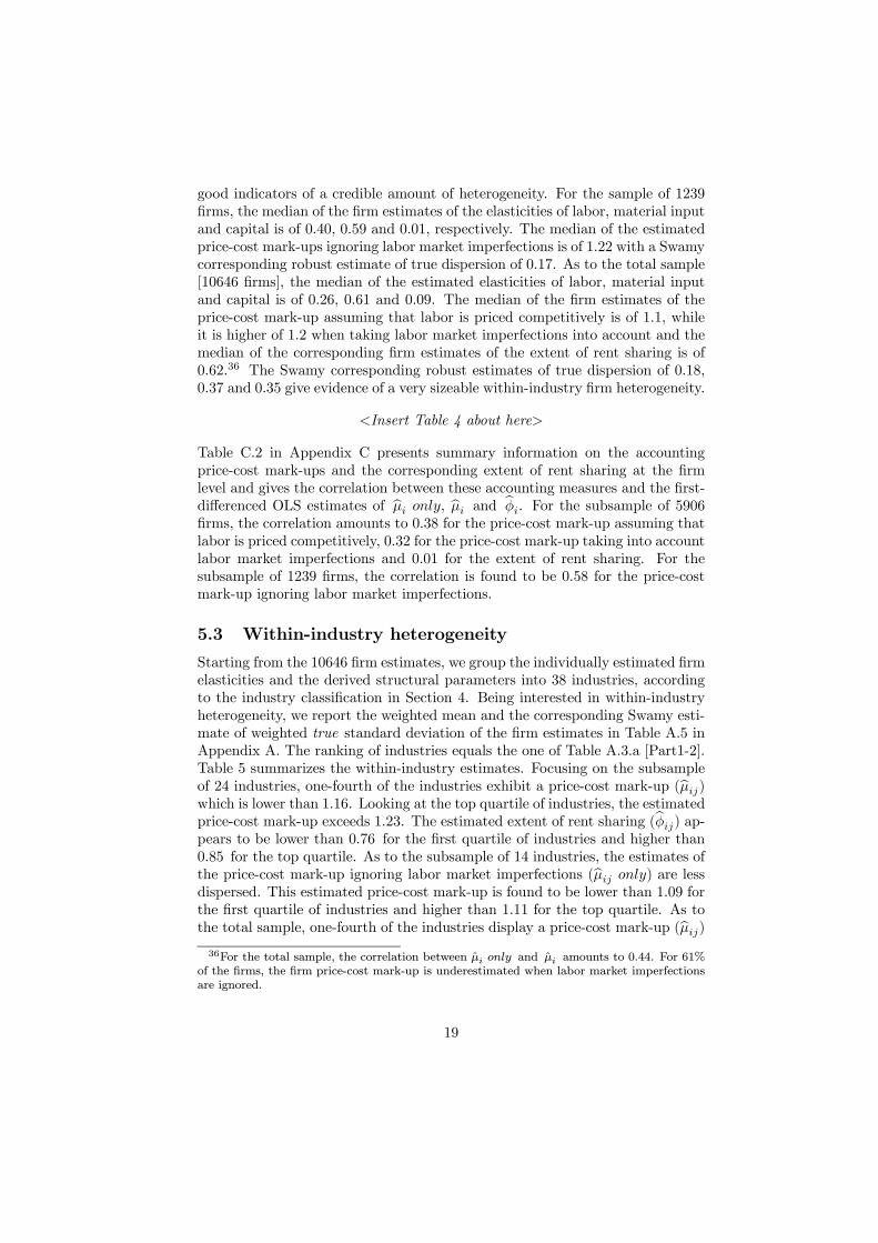
good indicators of a credible amount of heterogeneity. For the sample of 1239firms, the median of the firm estimates of the elasticities of labor, material inputand capital is of 0.40, 0.59 and 0.01, respectively. The median of the estimatedprice-cost mark-ups ignoring labor market imperfections is of 1.22 with a Swamycorresponding robust estimate of true dispersion of 0.17. As to the total sample[10646 firms], the median of the estimated elasticities of labor, material inputand capital is of 0.26, 0.61 and 0.09. The median of the firm estimates of theprice-cost mark-up assuming that labor is priced competitively is of 1.1, whileit is higher of 1.2 when taking labor market imperfections into account and themedian of the corresponding firm estimates of the extent of rent sharing is of0.62.36 The Swamy corresponding robust estimates of true dispersion of 0.18,0.37 and 0.35 give evidence of a very sizeable within-industry firm heterogeneity.


Table C.2 in Appendix C presents summary information on the accountingprice-cost mark-ups and the corresponding extent of rent sharing at the firmlevel and gives the correlation between these accounting measures and the first-differenced OLS estimates of bµi only, bµi and bφi. For the subsample of 5906firms, the correlation amounts to 0.38 for the price-cost mark-up assuming thatlabor is priced competitively, 0.32 for the price-cost mark-up taking into accountlabor market imperfections and 0.01 for the extent of rent sharing. For thesubsample of 1239 firms, the correlation is found to be 0.58 for the price-costmark-up ignoring labor market imperfections.

5.3 Within-industry heterogeneity

Starting from the 10646 firm estimates, we group the individually estimated firmelasticities and the derived structural parameters into 38 industries, accordingto the industry classification in Section 4. Being interested in within-industryheterogeneity, we report the weighted mean and the corresponding Swamy esti-mate of weighted true standard deviation of the firm estimates in Table A.5 inAppendix A. The ranking of industries equals the one of Table A.3.a [Part1-2].Table 5 summarizes the within-industry estimates. Focusing on the subsampleof 24 industries, one-fourth of the industries exhibit a price-cost mark-up (bµij)which is lower than 1.16. Looking at the top quartile of industries, the estimatedprice-cost mark-up exceeds 1.23. The estimated extent of rent sharing (bφij) ap-pears to be lower than 0.76 for the first quartile of industries and higher than0.85 for the top quartile. As to the subsample of 14 industries, the estimates ofthe price-cost mark-up ignoring labor market imperfections (bµij only) are lessdispersed. This estimated price-cost mark-up is found to be lower than 1.09 forthe first quartile of industries and higher than 1.11 for the top quartile. As tothe total sample, one-fourth of the industries display a price-cost mark-up (bµij)36For the total sample, the correlation between µi only and µi amounts to 0.44. For 61%

of the firms, the firm price-cost mark-up is underestimated when labor market imperfectionsare ignored.

19

which is higher than 1.09. At the top quartile, the estimated price-cost mark-upexceeds 1.22. The estimated extent of rent sharing appears to be lower than0.76 for the first quartile of industries and higher than 0.84 for the top quar-tile. The correlation between the estimated price-cost mark-up assuming thatlabor is priced competitively (bµij only) and the estimate taking into accountlabor market imperfections (bµij) is found to be 0.34. The correlation betweenthe price-cost mark-up estimate (bµij) and the estimated relative extent of rentsharing (bγij) amounts to 0.45. Comparing the upper part of Table 3 with Table5, it follows that the match between the industry and the firm estimates is quitegood for bµ only and bµ, but far less so for bγ and φ.


5.4 Determinants of estimated heterogeneity

In this subsection, we investigate whether firm-level variables, like size, capitalintensity, being a mixed or pure R&D firm and distance to the industry tech-nology frontier, explain part of the estimated heterogeneity in the price-costmark-up and relative extent of rent sharing parameters. First, we discuss thedata. Then, we analyze whether the firm-level variables influence µ and bγ atthe firm level.

Data description

We only consider the economically meaningful firm estimates as dependent vari-ables. More specifically, the dependent variable is either the vector of ln(bµionly− 1) (i = 1, ..., 1239), the vector of ln(bµi− 1) (i = 1, ..., 5906) or the vectorof ln(bγi) (i = 1, ..., 5906).37 For each of these dependent variables, we havefour different matrices of regressors. Each set consists of a firm-level variable(size, capital intensity, the R&D identifier, distance to the industry technologyfrontier) and industry dummies. All variables are centered around the industrymean. Size (ni) is measured by the logarithm of the average number of employ-ees in each firm and capital intensity (capinti) by the logarithm of the grossbook-value of fixed assets divided by sales. To construct the R&D variable, wemerge accounting information of the considered firms from EAE (SESSI) withdata of Research & Development collected by DEP (”Ministere de l’Educationet de la Recherche”). The R&D surveys (DEP) provide two R&D variables: adichotomous R&D indicator and total R&D expenditure. We assume that thesample is exhaustive, i.e., a firm which does not report any R&D expenditure isconsidered to be a non-R&D firm. Based on this criterion, we define three sub-samples: the pure non-R&D firms, the mixed R&D firms for which we have dataon R&D expenditure for less than 12 years (mixentri) and the pure R&D firmsfor which we have data on R&D expenditure for at least 12 years (rdentri).

38

Our measure of the distance of a firm to its industry technology frontier takes

37Consistent with Section 5.2, we consider two subsamples. The first subsample consists ofbµi ≥ 1 and bφi ∈ [0, 1] (5906 estimates) and the second subsample consists of bφi = 0 and bµionly ≥ 1 (1239 estimates).38Among the 5906 firms in the first subsample, 182 firms are identified as pure R&D firms,

20

the following form disti = p95 ln

¡V AN

¢j− ln ¡V AN ¢

ij, where i is a firm index, j

a industry index and V AN value added per employee. We use the 95th percentile,

instead of the maximum, to drop outliers.

Results

The OLS, WLS, where the weight is defined as the inverse of the sampling vari-ance, and the median regression coefficients of the set of regressors explainingthe vector of ln(bµi only − 1), the vector of ln(bµi − 1) or the vector of ln(bγi)are reported in Table 6. The 0.50 quantile regression can be interpreted as arobust equivalent of OLS. Although the regression coefficients are listed in rowsfor each of the three sets of regressors, they are for single firm-level variable re-gressions (including industry dummies), except for the regression including theR&D identifier which includes two firm-level variables (mixentri) and (rdentri)and industry dummies. Large firms experience a negative effect on the esti-mated price-cost mark-up taking into account labor market imperfections, andon the corresponding relative extent of rent sharing while capital-intensive firmsexperience a positive impact on the estimated price-cost mark-up but a nega-tive impact on the corresponding relative extent of rent sharing. Being a R&Dfirm exerts a negative effect on the relative extent of rent sharing. This effectis strongest for the pure R&D firms. Firms which are nearer to the indus-try technology frontier experience a positive effect on the estimated price-costmark-up. This impact becomes negative when labor market imperfections aretaken into consideration. Hence, consistent with the across-industry results,low-technology firms experience a positive effect on the price-cost mark-up andthe corresponding relative extent of rent sharing.39

As a robustness check, we ran multivariate specifications for each set of regres-sors where we include all firm-level variables and industry dummies.40 Theresults discussed above are not sensitive to using these multivariate specifica-tions, except for the negative effect of being a capital-intensive firm or a R&Dfirm on the estimated extent of rent sharing. More specifically, the former effectlooses significance, while the latter effect becomes significantly positive with theeffect being strongest for the pure R&D firms.


584 as mixed R&D firms and -the complement- 5140 as pure non-R&D firms. The secondsubsample of 1239 firms includes 75 pure R&D firms, 177 mixed R&D firms and 987 purenon-R&D firms.39Technological change (either captured by our R&D variable or our measure of the distance

of a firm to its industry technology frontier) might exert an effect on the relative extent of rentsharing by impacting the nature of the production process. However, this effect is, a priori,unclear. As discussed in Betcherman (1991), it depends on the importance of labor costs inthe firm’s total costs and on the workers’ essentiality in the production process. Horn andWolinsky (1988) develop a similar argument.40Results not reported but available upon request.

21

6 Conclusion

This article thoroughly investigates product and labor market imperfectionsas two sources of discrepancies between the output contribution of individualproduction factors and their respective revenue shares. By doing so, we con-tribute to the econometric productivity literature on estimating microeconomicproduction functions and to the recent econometric literature on simultaneouslyestimating imperfections in product and factor markets. Embedding the efficientbargaining model into the R. Hall (1988) approach shows that the firm price-cost mark-up and the extent of rent sharing generate a wedge between marginalproducts of input factors and the apparent factor prices. To econometrically ex-plore these particular sources of discrepancies, we start by estimating a standardproduction function using a panel of 10646 French manufacturing firms cover-ing the period 1978-2001. From the production function coefficients, i.e., theoutput elasticities, we derive our parameters of interest. At the manufacturinglevel, the first-differenced OLS estimates point to an average price-cost mark-upof 1.17 and an average extent of rent sharing of 0.44. The next step into ourempirical strategy is to examine across-industry heterogeneity in the productionfunction coefficients and the retrieved parameters. Splitting the sample into 38industries, we find a considerable degree of across-industry heterogeneity. Themedian price-cost mark-up and the median extent of rent sharing are estimatedat 1.15 and 0.12 respectively. The median values of the economically meaningfulindustry estimates are of an order of magnitude of 1.18 and 0.27 respectively.Highly profitable industries display a price-cost mark-up that is higher than themedian value. Low-technology industries, likely to be typified as less compet-itive industries, display a price-cost mark-up and extent of rent sharing abovethe respective median values. Weakly unionized industries are characterized bya price-cost mark-up below the respective median value. The estimated extentof rent sharing of half of those industries is lower than the respective medianvalue. Industries faced by high import competition show an estimated price-cost mark-up below the median value. The estimated extent of rent sharing inindustries that are shielded from import competition exceeds the median value.Since production behavior is likely to vary across firms, we finally take intoaccount firm-level heterogeneity and look at within-industry heterogeneity. Todetermine the degree of heterogeneity in the production function coefficientsand parameters of interest, we adopt the Swamy (1970) methodology as a vari-ance decomposition approach. This method allows us to estimate the variancecomponents of heterogeneity, i.e., the pure sampling variance and the true het-erogeneity or dispersion. The median of the firm estimates of the price-costmark-up ignoring the occurrence of rent sharing is of 1.10, while it is higher of1.20 when taking them into account and the median of the corresponding firmestimates of the extent of rent sharing is of 0.62. The Swamy correspondingrobust estimates of true dispersion of 0.18, 0.37 and 0.35 are good indicators ofa credible amount of heterogeneity. Firm size, capital intensity, distance to theindustry technology frontier and investing in R&D seem to explain part of theestimated heterogeneity in price-cost mark-ups and the extent of rent sharing.

22

References

[1] Abraham, F., J. Konings and S. Vanormelingen, 2006, Price and WageSetting in an Integrating Europe: Firm Level Evidence, NBB ResearchPaper 200610-5, National Bank of Belgium.

[2] Amemiya, T., 1977, A Note on a Heteroskedastic Model, Journal of Econo-metrics, 5, 295-299.

[3] Ackerberg, J., L. Benkard, S. Berry and A. Pakes, 2006, Econometric Toolsfor Analyzing Market Outcomes, in: Heckman, J.J. (Ed.), Handbook ofEconometrics, forthcoming.

[4] Arellano, M. and S. Bond, 1991, Some Tests of Specification for Panel Data:Monte Carlo Evidence and an Application to Employment Equations, Re-view of Economic Studies, 58(2), 277-297.

[5] Betcherman, G., 1991, Does Technological Change Affect Union BargainingPower? British Journal of Industrial Relations, 29(3), 447-462.

[6] Blanchard, O. and F. Giavazzi, 2003, Macroeconomic Effects of Regulationand Deregulation in Goods and Labor Markets, The Quarterly Journal ofEconomics, 18(3), 879-907.

[7] Blundell, R. and S. Bond, 2000, GMM Estimation with Persistent PanelData: An Application to Production Functions, Econometric Review, 19,321-340.

[8] Booth, A., 1995, The Economics of the Trade Union, Cambridge: Cam-bridge University Press.

[9] Boulhol, H., S. Dobbelaere and S. Maioli, 2006, Imports as Product and La-bor Market Discipline, IZA Discussion Paper 2178, Institute for the Studyof Labor, Bonn.

[10] Brander, J. A. and B. J. Spencer, 1985, Export Subsidies and InternationalMarket Share Rivalry, Journal of International Economics, 18(1-2), 83-100.

[11] Bresnahan, T., 1989, Empirical Studies of Industries with Market Power, in:Schmalensee, R., Willig R. (Eds.), Handbook of Industrial Organization,vol. 2, Amsterdam: North Holland.

[12] Bughin, J., 1996, Trade Unions and Firms’ Product Market Power, TheJournal of Industrial Economics, XLIV(3), 289-307.

[13] Crepon, B., R. Desplatz and J. Mairesse, 1999, Estimating Price-Cost Mar-gins, Scale Economies and Workers’ Bargaining Power at the Firm Level,CRESTWorking Paper G9917, Centre de Recherche en Economie et Statis-tique.

23

[14] Crepon, B., R. Desplatz and J. Mairesse, 2002, Price-Cost Margins andRent Sharing: Evidence from a Panel of French Manufacturing Firms, Cen-tre de Recherche en Economie et Statistique, revised version.

[15] Dobbelaere, S., 2004, Estimation of Price-Cost Margins and Union Bargain-ing Power for Belgian Manufacturing, International Journal of IndustrialOrganization, 22(10), 1381-1398.

[16] Doornik, J.A., M. Arellano and S. Bond, 2002, Panel Data Estimationusing DPD for Ox, Nuffield College, Oxford.

[17] Griliches, Z. and J. Mairesse, 1998, Production Functions: The Search forIdentification, in: Strom, S. (Ed.), Essays in Honour of Ragnar Frisch,Econometric Society Monograph Series, Cambridge: Cambridge UniversityPress.

[18] Hall, R.E., 1988, The Relationship between Price and Marginal Cost in USIndustry, Journal of Political Economy, 96, 921-947.

[19] Hildreth, C. and H. Houck, 1968, Some Estimates for a Linear Model withRandom Coefficients, Journal of the American Association, 63, 584-595.

[20] Horn, H. and A. Wolinsky, 1988, Worker Substitutability and Patterns ofUnionisation, The Economic Journal, 98(391), 484-497.

[21] Koenker, R. and G. Bassett, 1978, Regression Quantiles, Econometrica, 46,33-50.

[22] Krugman, P., 1979, Increasing Returns, Monopolistic Competition and In-ternational Trade, Journal of International Economics, 9(4), 469-479.

[23] Leamer, E.E., 1978, Specification Searches: Ad hoc Inference with Nonex-perimental Data, New York: John Wiley and Sons.

[24] MaCurdy, T., 1985, A Guide to Applying Time Series Models to PanelData, Stanford, CA: Stanford University.

[25] Mairesse, J. and Z. Griliches, 1990, Heterogeneity in Panel Data: Are thereStable Production Functions?, in: Champsaur, P., Deleau, M., Grandmont,J.M., Laroque, G., Guesnerie, R., Henry, C., Laffont, J.J., Mairesse, J.,Monfort, A., Younes, Y. (Eds.), Essays in Honor of Edmond Malinvaud,vol. 3, Cambridge, MA: MIT Press.

[26] Manning, A., 2003, Monopsony in Motion: Imperfect Competition in LaborMarkets, Princeton: Princeton University Press.

[27] Marschak, J. and W.H. Andrews, 1944, Random Simultaneous Equationsand the Theory of Production, Econometrica, 12(3-4), 143-205.

[28] McDonald, I.M. and R.M. Solow, 1981, Wage bargaining and employment,American Economic Review, 71(5), 896-908.

24

[29] Neven, D.J., L. Roller and Z. Zhang, 2002, Endogenous Costs and Price-Costs Margins, DIW Berlin Discussion Paper 294, German Institute forEconomic Research, Berlin.

[30] Nickell, S., 1999, Product Markets and Labour Markets, Labour Economics,6(1), 1-20.

[31] OECD, 2005, OECD Science, Technology and Industry Scoreboard2005, Organisation for Economic Co-operation and Development,www.oecd.org/sti/scoreboard.

[32] Roodman, D., 2005, xtabond2: Stata Module to Extend xtabond DynamicPanel Data Estimator. Center for Global Development, Washington.

[33] Schmalensee, R., 1989, Inter-industry Studies of Structure and Perfor-mance, in: Schmalensee, R., Willig R.(Eds.), Handbook of Industrial Or-ganization, vol.2, Amsterdam: North Holland.

[34] Swamy, P.A.V.B., 1970, Efficient Inference in a Random Coefficient Model,Econometrica, 38, 311-323.

[35] Veugelers, R., 1989, Wage Premia, Price Cost Margins and BargainingPower in Belgian Manufacturing, European Economic Review, 33(1), 169-180.

[36] Woolridge, J., 2002, Econometric Analysis of Cross sections and PanelData, Cambridge, MA: MIT Press.

25

Table 1Summary statistics

Variables 1978-2001Mean Sd. Q1 Q3 N

Real firm output growth rate ∆q 0.021 0.152 -0.061 0.103 154363Labor growth rate ∆n 0.006 0.123 -0.043 0.054 154363Capital growth rate ∆k -0.001 0.151 -0.072 0.060 154363Materials growth rate ∆m 0.040 0.192 -0.060 0.139 154363Labor share in nominal output αN 0.307 0.136 0.208 0.387 165009Materials share in nominal output αM 0.503 0.159 0.399 0.614 165009∆q −∆k 0.022 0.188 -0.081 0.126 154363∆n−∆k 0.007 0.166 -0.073 0.088 154363∆m−∆k 0.041 0.220 -0.079 0.160 154363

26

Table 2Estimates of output elasticities bεQJ (J = N,M,K), mark-up µ (only) and extent of rent sharing φ :Full sample: 10646 firms, each firm between 12 and 24 years of observations - Period 1978-2001Part 1: Imposing constant returns to scale: bεQK = 1− bεQN − bεQM

STATIC SPECIFICATION DYNAMIC SPECIFICATION

OLS

LEVELS

OLS

DIF

GMM DIF

(t− 2)(t− 3)GMM SYS

(t− 2)(t− 3)GMM DIF


(t− 2)(t− 3)bεQN 0.331

(0.003)

0.298

(0.003)

0.138

(0.020)

0.298

(0.008)

0.134

(0.032)

0.201

(0.015)bεQM 0.592

(0.003)

0.587

(0.003)

0.726

(0.017)

0.675

(0.007)

0.595

(0.022)

0.541

(0.019)bεQK 0.077 0.115 0.137 0.027 0.271 0.258

λ 1 1 1 1 1 1

bµ only = bµ onlyλ

1.144

(0.003)

1.112

(0.002)

1.129

(0.013)

1.211

(0.007)

1.041

(0.032)

0.934

(0.020)

bµ = bµλ

1.177

(0.007)

1.167

(0.005)

1.443

(0.033)

1.342

(0.015)

1.184

(0.043)

1.076

(0.039)bφ 0.393

(0.006)

0.440

(0.004)

0.619

(0.009)

0.490

(0.008)

0.605

(0.018)

0.534

(0.015)bρ 0.713

(0.023)

0.619

(0.018)

Part 2: Not imposing constant returns to scale: bεQK = bλ− bεQN − bεQMSTATIC SPECIFICATION DYNAMIC SPECIFICATION

OLS

LEVELS

OLS

DIF

GMM DIF




(t− 2)(t− 3)bεQN 0.331

(0.001)

0.189

(0.002)

0.149

(0.022)

0.240

(0.011)

0.111

(0.031)

0.057

(0.025)bεQM 0.592

(0.001)

0.554

(0.002)

0.566

(0.020)

0.696

(0.008)

0.554

(0.023)

0.562

(0.020)bεQK 0.077

(0.002)

0.049

(0.003)

-0.027(0.038)

0.033

(0.017)

0.033

(0.057)

0.241

(0.027)bλ 1

(0.0006)

0.792

(0.003)

0.688

(0.020)

0.969

(0.004)

0.803

(0.052)

0.860

(0.025)

bµonly 1.153

(0.004)

1.011

(0.004)

0.890

(0.022)

1.219

(0.008)

1.011

(0.035)

0.916

(0.033)

bµ onlybλ 1.145

(0.003)

1.189

(0.003)

1.398

(0.035)

1.212

(0.007)

1.074

(0.054)

0.897

(0.022)

bµ 1.177

(0.002)

1.102

(0.004)

1.126

(0.039)

1.383

(0.016)

1.100

(0.046)

1.117

(0.041)bφ 0.395

(0.002)

0.552

(0.002)

0.589

(0.015)

0.549

(0.007)

0.615

(0.017)

0.651

(0.011)

bµbλ 1.178

(0.002)

1.392

(0.006)

1.637

(0.055)

1.427

(0.020)

1.371

(0.088)

1.299

(0.057)bρ 0.723

(0.023)

0.609

(0.020)

Robust standard errors and first-step robust standard errors in columns 1-2 and columns 3-6 respectively.

Time dummies are included but not reported.

(1) Input shares: αN = 0.307, αM = 0.503, αK = 0.190.(2) GMM DIF : the set of instruments includes the lagged levels of n, m and k dated (t− 2) and (t− 3).(3) GMM SY S: the set of instruments includes the lagged levels of n, m and k dated (t− 2) and (t− 3) in the first-differenced

equations and correspondingly the lagged first-differences of n, m and k dated (t− 1) in the levels equations.

27

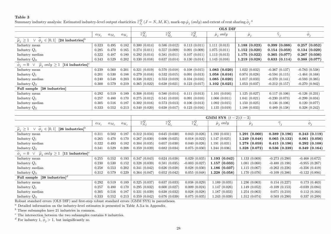
Table 3Summary industry analysis: Estimated industry-level output elasticities bεQJj (J = N,M,K), mark-up µj (only) and extent of rent sharing φj a

OLS DIF

αNj αMj αKj bεQNj bεQMjbεQKj

µj only µj bγj φjbµj ≥ 1 ∨ bφj ∈ [0, 1] [24 industries]bIndustry mean 0.323 0.495 0.182 0.300 (0.014) 0.586 (0.012) 0.113 (0.011) 1.111 (0.013) 1.188 (0.023) 0.399 (0.088) 0.257 (0.052)Industry Q1 0.285 0.470 0.165 0.274 (0.011) 0.557 (0.009) 0.091 (0.009) 1.075 (0.011) 1.152 (0.020) 0.154 (0.059) 0.134 (0.029)Industry median 0.322 0.487 0.180 0.292 (0.014) 0.581 (0.011) 0.107 (0.011) 1.113 (0.013) 1.175 (0.022) 0.365 (0.077) 0.267 (0.036)Industry Q3 0.343 0.529 0.202 0.330 (0.016) 0.637 (0.014) 0.130 (0.014) 1.143 (0.016) 1.219 (0.028) 0.633 (0.114) 0.388 (0.077)bφj = 0 ∨ bµj only ≥ 1 [14 industries]c

Industry mean 0.239 0.560 0.201 0.321 (0.019) 0.570 (0.018) 0.108 (0.015) 1.083 (0.020) 1.022 (0.032) -0.367 (0.137) -0.783 (0.538)Industry Q1 0.201 0.530 0.188 0.279 (0.016) 0.532 (0.015) 0.091 (0.013) 1.058 (0.016) 0.974 (0.028) -0.594 (0.115) -1.464 (0.168)Industry median 0.240 0.548 0.203 0.338 (0.021) 0.553 (0.019) 0.104 (0.016) 1.085 (0.020) 1.017 (0.033) -0.370 (0.141) -0.593 (0.385)Industry Q3 0.300 0.579 0.219 0.365 (0.022) 0.638 (0.021) 0.123 (0.017) 1.102 (0.025) 1.053 (0.037) -0.212 (0.157) -0.270 (0.942)Full sample [38 industries]

Industry mean 0.292 0.519 0.189 0.308 (0.016) 0.580 (0.014) 0.111 (0.013) 1.101 (0.016) 1.125 (0.027) 0.117 (0.106) -0.126 (0.231)Industry Q1 0.257 0.480 0.170 0.275 (0.012) 0.541 (0.010) 0.091 (0.010) 1.066 (0.011) 1.041 (0.021) -0.230 (0.073) -0.299 (0.034)

Industry median 0.305 0.516 0.187 0.302 (0.016) 0.573 (0.013) 0.106 (0.013) 1.092 (0.015) 1.150 (0.025) 0.136 (0.106) 0.120 (0.077)

Industry Q3 0.333 0.552 0.213 0.340 (0.020) 0.638 (0.017) 0.123 (0.016) 1.135 (0.019) 1.188 (0.033) 0.489 (0.138) 0.328 (0.242)

GMM SYS (t− 2)(t− 3)αNj αMj αKj bεQNj bεQMj

bεQKjµj only µj bγj φjbµj ≥ 1 ∨ bφj ∈ [0, 1] [26 industries]b

Industry mean 0.311 0.502 0.187 0.312 (0.034) 0.645 (0.030) 0.043 (0.026) 1.193 (0.031) 1.291 (0.060) 0.389 (0.196) 0.243 (0.119)Industry Q1 0.265 0.470 0.170 0.267 (0.030) 0.606 (0.025) 0.018 (0.022) 1.147 (0.025) 1.249 (0.048) 0.065 (0.132) 0.061 (0.056)Industry median 0.322 0.493 0.182 0.304 (0.035) 0.657 (0.030) 0.040 (0.026) 1.191 (0.031) 1.278 (0.059) 0.415 (0.196) 0.292 (0.108)Industry Q3 0.341 0.529 0.208 0.359 (0.039) 0.682 (0.034) 0.075 (0.030) 1.244 (0.036) 1.328 (0.072) 0.536 (0.239) 0.349 (0.164)bφj = 0 ∨ bµj only ≥ 1 [11 industries]c

Industry mean 0.255 0.552 0.193 0.347 (0.043) 0.624 (0.038) 0.029 (0.035) 1.193 (0.042) 1.133 (0.069) -0.273 (0.290) -0.468 (0.672)Industry Q1 0.230 0.530 0.152 0.328 (0.039) 0.581 (0.035) -0.003 (0.027) 1.157 (0.033) 1.081 (0.060) -0.488 (0.198) -0.955 (0.267)Industry median 0.258 0.553 0.202 0.341 (0.042) 0.626 (0.038) 0.028 (0.030) 1.186 (0.037) 1.115 (0.067) -0.262 (0.226) -0.356 (0.419)Industry Q3 0.312 0.579 0.229 0.364 (0.047) 0.652 (0.042) 0.055 (0.048) 1.228 (0.058) 1.170 (0.076) -0.109 (0.386) -0.122 (0.894)Full sample [38 industries]d

Industry mean 0.292 0.519 0.189 0.325 (0.037) 0.637 (0.033) 0.038 (0.029) 1.189 (0.035) 1.236 (0.063) 0.154 (0.227) 0.173 (0.463)

Industry Q1 0.257 0.480 0.170 0.295 (0.032) 0.600 (0.027) 0.009 (0.024) 1.147 (0.026) 1.149 (0.052) -0.109 (0.153) -0.039 (0.084)Industry median 0.305 0.516 0.187 0.331 (0.039) 0.638 (0.032) 0.028 (0.028) 1.187 (0.033) 1.254 (0.063) 0.071 (0.210) 0.112 (0.164)

Industry Q3 0.333 0.552 0.213 0.359 (0.042) 0.676 (0.039) 0.075 (0.035) 1.243 (0.039) 1.312 (0.074) 0.503 (0.290) 0.337 (0.289)

Robust standard errors (OLS DIF) and first-step robust standard errors (GMM SYS) in parentheses.a Detailed information on the industry-level estimates is presented in Table A.3.a in Appendix.b These subsamples have 21 industries in common.c The intersection between the two subsamples contains 8 industries.d For industry 1, bφj > 1, but insignificantly so.

28

Table 4Heterogeneity of firm output elasticities bεQJi (J = N,M,K), mark-up µi (only) and extent of rent sharing φi :Different indicators and first-differenced OLS estimatesa

αNi αMi αKi bεQNibεQMi

bεQKiµi only µi bγi φibµi ≥ 1 ∨ bφi ∈ [0, 1] [5906 firms]

Simple mean

Observed dispersion bσoTrue dispersion bσtrue

0.335

(0.130)

[0.130]

0.489

(0.138)

[0.134]

0.175

(0.089)

[0.084]

0.132

(0.224)

[0.063]

0.736

(0.197)

[0.114]

0.131

(0.205)

[0.084]

1.148

(0.276)

[0.173]

1.580

(0.533)[0.315]

1.859

(1.759)[1.126]

0.544

(0.214)[0]

Weighted mean

Weighted observed dispersion bσoWeighted true dispersion bσtrue

0.368

(0.138)

[0.138]

0.559

(0.141)

[0.141]

0.251

(0.138)

[0.138]

0.132

(0.167)

[0.122]

0.730

(0.184)

[0.158]

0.080

(0.141)

[0.109]

1.137

(0.170)

[0.134]

1.367

(0.295)[0.237]

1.328

(1.175)[1.104]

0.813

(0.114)[0.109]

Median

Interquartile observed dispersion bσoRobust true dispersion bσtrue

0.322

(0.138)

[0.138]

0.495

(0.158)

[0.155]

0.150

(0.105)

[0.100]

0.137

(0.192)

[0.109]

0.737

(0.195)

[0.148]

0.111

(0.173)

[0.109]

1.134

(0.212)

[0.141]

1.442

(0.387)[0.279]

1.384

(1.391)[1.158]

0.580

(0.237)[0.202]bφi = 0 ∨ bµi only ≥ 1 [1239 firms]

Simple mean


0.252

(0.100)

[0.100]

0.508

(0.134)

[0.130]

0.239

(0.118)

[0.114]

0.417

(0.158)

[0]

0.594

(0.164)

[0]

-0.012(0.167)

[0]

1.298

(0.277)[0.167]

1.186

(0.239)

[0]

-0.437(0.286)

[0]

-4.687(26.192)

[0]

Weighted mean


0.275

(0.109)

[0.109]

0.590

(0.141)

[0.141]

0.352

(0.158)

[0.158]

0.366

(0.148)

[0.071]

0.621

(0.161)

[0.130]

0.007

(0.114)

[0.063]

1.187

(0.170)[0.141]

1.137

(0.155)

[0]

-0.282(0.257)

[0]

-0.139(0.192)

[0]

Median


0.241

(0.109)

[0.109]

0.520

(0.170)

[0.167]

0.201

(0.152)

[0.148]

0.402

(0.152)

[0]

0.593

(0.167)

[0.105]

0.008

(0.134)

[0]

1.222

(0.224)[0.167]

1.134

(0.192)

[0]

-0.416(0.366)

[0]

-0.712(1.340)

[0]

Full sample [10646 firms]

Simple mean


0.307

(0.126)

[0.126]

0.503

(0.138)

[0.134]

0.190

(0.100)

[0.095]

0.288

(0.305)

[0.195]

0.599

(0.257)

[0.195]

0.112

(0.241)

[0.130]

1.097

(0.310)

[0.212]

1.238

(0.610)

[0.443]

-0.880

(56)

[0]

0.583

(18)

[0]

Weighted mean


0.339

(0.138)

[0.138]

0.570

(0.141)

[0.141]

0.278

(0.148)[0.148]

0.222

(0.232)

[0.197]

0.627

(0.234)

[0.212]

0.071

(0.161)

[0.126]

1.107

(0.195)

[0.161]

1.172

(0.373)

[0.327]

1.129

(1.272)

[1.167]

0.822

(0.122)

[0.114]

Median


0.291

(0.134)

[0.134]

0.510

(0.161)

[0.158]

0.160

(0.114)

[0.109]

0.262

(0.277)

[0.217]

0.613

(0.261)

[0.226]

0.094

(0.197)

[0.138]

1.096

(0.245)

[0.184]

1.200

(0.457)

[0.367]

0.528

(1.950)

[1.578]

0.617

(0.435)

[0.348]a Detailed information on the firm-level estimates is presented in Table A.4 in Appendix.

29

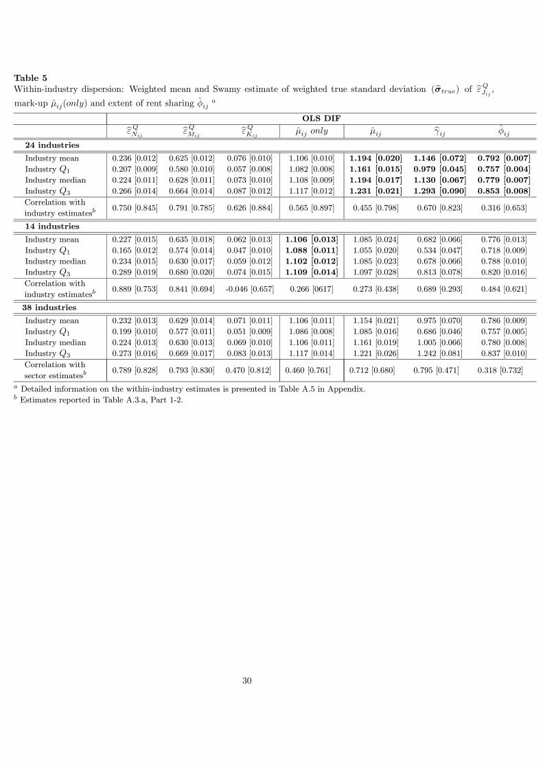
Table 5Within-industry dispersion: Weighted mean and Swamy estimate of weighted true standard deviation (bσtrue) of bεQJij ,mark-up µij(only) and extent of rent sharing φij

a

OLS DIFbεQNijbεQMij

bεQKijµij only µij bγij φij

24 industries

Industry mean 0.236 [0.012] 0.625 [0.012] 0.076 [0.010] 1.106 [0.010] 1.194 [0.020] 1.146 [0.072] 0.792 [0.007]Industry Q1 0.207 [0.009] 0.580 [0.010] 0.057 [0.008] 1.082 [0.008] 1.161 [0.015] 0.979 [0.045] 0.757 [0.004]Industry median 0.224 [0.011] 0.628 [0.011] 0.073 [0.010] 1.108 [0.009] 1.194 [0.017] 1.130 [0.067] 0.779 [0.007]Industry Q3 0.266 [0.014] 0.664 [0.014] 0.087 [0.012] 1.117 [0.012] 1.231 [0.021] 1.293 [0.090] 0.853 [0.008]Correlation with

industry estimatesb0.750 [0.845] 0.791 [0.785] 0.626 [0.884] 0.565 [0.897] 0.455 [0.798] 0.670 [0.823] 0.316 [0.653]

14 industries

Industry mean 0.227 [0.015] 0.635 [0.018] 0.062 [0.013] 1.106 [0.013] 1.085 [0.024] 0.682 [0.066] 0.776 [0.013]

Industry Q1 0.165 [0.012] 0.574 [0.014] 0.047 [0.010] 1.088 [0.011] 1.055 [0.020] 0.534 [0.047] 0.718 [0.009]

Industry median 0.234 [0.015] 0.630 [0.017] 0.059 [0.012] 1.102 [0.012] 1.085 [0.023] 0.678 [0.066] 0.788 [0.010]

Industry Q3 0.289 [0.019] 0.680 [0.020] 0.074 [0.015] 1.109 [0.014] 1.097 [0.028] 0.813 [0.078] 0.820 [0.016]

Correlation with

industry estimatesb0.889 [0.753] 0.841 [0.694] -0.046 [0.657] 0.266 [0617] 0.273 [0.438] 0.689 [0.293] 0.484 [0.621]

38 industries

Industry mean 0.232 [0.013] 0.629 [0.014] 0.071 [0.011] 1.106 [0.011] 1.154 [0.021] 0.975 [0.070] 0.786 [0.009]

Industry Q1 0.199 [0.010] 0.577 [0.011] 0.051 [0.009] 1.086 [0.008] 1.085 [0.016] 0.686 [0.046] 0.757 [0.005]

Industry median 0.224 [0.013] 0.630 [0.013] 0.069 [0.010] 1.106 [0.011] 1.161 [0.019] 1.005 [0.066] 0.780 [0.008]

Industry Q3 0.273 [0.016] 0.669 [0.017] 0.083 [0.013] 1.117 [0.014] 1.221 [0.026] 1.242 [0.081] 0.837 [0.010]

Correlation with

sector estimatesb0.789 [0.828] 0.793 [0.830] 0.470 [0.812] 0.460 [0.761] 0.712 [0.680] 0.795 [0.471] 0.318 [0.732]

a Detailed information on the within-industry estimates is presented in Table A.5 in Appendix.b Estimates reported in Table A.3.a, Part 1-2.

30

Table 6Determinants of firm-level ln(µi only − 1), ln(µi − 1) and ln(bγi):OLS, WLS and median regression coefficients

Variables ni capinti mixentri rdentri disti

βOLS

ln(µi only − 1) 0.040

(0.031)

-0.023

(0.054)

0.083

(0.085)

-0.087

(0.157)

-0.512∗∗∗

(0.111)

ln(µi − 1) -0.048∗∗∗

(0.014)

0.066∗∗∗

(0.021)

-0.143∗∗∗

(0.047)

-0.101

(0.080)

0.158∗∗∗

(0.047)

ln(bγi) -0.210∗∗∗

(0.015)

-0.088∗∗∗

(0.023)

-0.226∗∗∗

(0.049)

-0.419∗∗∗

(0.084)

0.949∗∗∗

(0.051)

βWLS

ln(µi only − 1) -0.058

(0.049)

-0.031

(0.054)

-0.020

(0.075)

-0.159∗

(0.084)

-0.065

(0.128)

ln(µi − 1) -0.048∗∗∗

(0.016)

0.140∗∗∗

(0.025)

-0.097∗

(0.055)

-0.179∗∗∗

(0.070)

0.251∗∗∗

(0.058)

ln(bγi) -0.191∗∗∗

(0.029)

-0.127∗∗∗

(0.047)

-0.299∗∗∗

(0.095)

-0.508∗∗∗

(0.087)

0.750∗∗∗

(0.115)

β(0.50)

ln(µi only − 1) 0.081

(0.026)

0.025

(0.070)

0.110

(0.100)

0.247∗

(0.146)

-0.513∗∗∗

(0.115)

ln(µi − 1) -0.032∗∗

(0.015)

0.105∗∗∗

(0.018)

-0.069

(0.052)

-0.047

(0.090)

0.182∗∗∗

(0.054)

ln(bγi) -0.222∗∗∗

(0.014)

-0.096∗∗∗

(0.023)

-0.234∗∗∗

(0.055)

-0.418∗∗∗

(0.094)

0.942∗∗∗

(0.050)∗∗∗ Significant at 1%; ∗∗ Significant at 5%; ∗ Significant at 10%. Robust standard errors in parentheses.(1) The vector of ln(bµi only − 1) includes 1239 estimates, the vector of ln(bµi − 1) or ln(bγi) consists of 5906 estimates.(2) The dependent and the explanatory variables are centered around the industry mean.(3) The coefficients are for single firm-level variable regressions (including industry dummies), except for the regression

including the R&D identifier which includes two firm-level variables (mixentri and rdentri) and industry dummies.

31

32

16 17

18

20

22

27

33

368

11

28

35

5

612

13

14

30

7

15 23

24

26

37

1.05

1.1

1.15

1.2

1.25

1.3

0 0.1 0.2 0.3 0.4 0.5 φ j

low medium lowmedium high high

Source: Table A.3.a [Part 1] estimates

Graph 1 Profitability differences across industries

µ j

5

6

78

11

24

27

28

30

35 36

37

13

15

16 17

18

20

22 26

331214 23

1.05

1.1

1.15

1.2

1.25

1.3

0 0.1 0.2 0.3 0.4



Graph 2 Technology differences across industries

µ j

φ j

0.5

33

8

17

18

35 36

511

16

2627

3314 15

20

22 24

30 37

6

7

12

13

23

28

1.05

1.1

1.15

1.2

1.25

1.3

0 0.1 0.2 0.3 0.4 0.5

low medium low

medium high high


Graph 4 Openness differences across industries

φ j

µ j

6

13

17

18

7

12

16

23

26

33

36

511

14

20

27

37

8

15 22 24 28

30

35

1.05

1.1

1.15

1.2

1.25

1.3

0 0.1 0.2 0.3 0.4 0.5



Graph 3 Unionization differences across industries

µ j

φ j

Appendix A: Detailed results

Table A.1Estimates of output elasticities bεQJ (J = N,M,K), mark-up µ (only) and extent of rent sharing φ :Balanced sample: 473 firms, each firm 24 years of observations - Period 1978-2001

STATIC SPECIFICATION DYNAMIC SPECIFICATION

OLS

LEVELS

OLS

DIF

GMM DIF

(t− 2)GMM SYS

(t− 2)GMM DIF

(t− 2)GMM SYS

(t− 2)bεQN 0.257

(0.016)

0.320

(0.011)

0.134

(0.067)

0.241

(0.022)

0.302

(0.032)

0.262

(0.028)bεQM 0.646

(0.015)

0.586

(0.011)

0.664

(0.051)

0.666

(0.022)

0.602

(0.023)

0.628

(0.023)bεQK 0.097 0.094 0.202 0.093 0.096 0.110

λ 1 1 1 1 1 1

bµ only = bµonlyλ

1.208

(0.014)

1.190

(0.011)

1.121

(0.042)

1.213

(0.023)

1.204

(0.026)

1.159

(0.028)

bµ = bµλ

1.319

(0.031)

1.197

(0.023)

1.357

(0.105)

1.359

(0.045)

1.230

(0.048)

1.282

(0.048)bφ 0.345

(0.024)

0.182

(0.033)

0.481

(0.053)

0.374

(0.029)

0.230

(0.068)

0.328

(0.044)bρ 0.712

(0.022)

0.390

(0.035)

Robust standard errors and first-step robust standard errors in columns 1-2 and columns 3-6 respectively.


(1) bε QK = 1− bεQN − bεQM .(2) Input shares: αN = 0.270, αM = 0.490, αK = 0.240.(3) GMM DIF : the set of instruments includes the lagged levels of n, m and k dated (t− 2) and earlier.(4) GMM SY S: the set of instruments includes the lagged levels of n, m and k dated (t− 2) and earlier in the

first-differenced equations and the lagged first-differences of n, m and k dated (t− 1) in the levels equations.

34

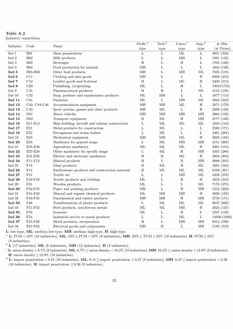
Table A.2Industry repartition

Industry Code NameProfit.a

type

Tech.b

type

Union.c

type

Imp.d

type

# Obs.

(# Firms)

Ind 1 B01 Meat preparations L L ML L 4881 (324)

Ind 2 B02 Milk products L L MH L 1981 (122)

Ind 3 B03 Beverages H L H L 1705 (106)

Ind 4 B04 Food production for animals MH L L L 1942 (126)

Ind 5 B05-B06 Other food products MH L MH ML 7835 (518)

Ind 6 C11 Clothing and skin goods MH L L H 6938 (453)

Ind 7 C12 Leather goods and footwear H L ML H 3400 (213)

Ind 8 C20 Publishing, (re)printing ML L H L 10919 (724)

Ind 9 C31 Pharmaceutical products H H L ML 2153 (130)

Ind 10 C32 Soap, perfume and maintenance products ML MH L L 1877 (114)

Ind 11 C41 Furniture ML L MH ML 5043 (322)

Ind 12 C42, C44-C46 Accommodation equipment MH MH ML H 2871 (179)

Ind 13 C43 Sport articles, games and other products MH ML L H 2390 (156)

Ind 14 D01 Motor vehicles MH MH MH MH 2064 (133)

Ind 15 D02 Transport equipment H ML H MH 2177 (129)

Ind 16 E11-E14 Ship building, aircraft and railway construction L ML ML ML 1834 (110)

Ind 17 E21 Metal products for construction L ML L L 2590 (171)

Ind 18 E22 Ferruginous and steam boilers L ML L L 4461 (294)

Ind 19 E23 Mechanical equipment MH MH ML H 3020 (182)

Ind 20 E24 Machinery for general usage L ML MH MH 4151 (268)

Ind 21 E25-E26 Agriculture machinery ML ML ML H 2391 (154)

Ind 22 E27-E28 Other machinery for specific usage L ML H MH 4355 (286)

Ind 23 E31-E35 Electric and electronic machinery H H ML H 2934 (203)

Ind 24 F11-F12 Mineral products H L H MH 3099 (205)

Ind 25 F13 Glass products H ML H ML 1681 (104)

Ind 26 F14 Earthenware products and construction material H ML ML ML 6109 (391)

Ind 27 F21 Textile art L L MH ML 4338 (270)

Ind 28 F22-F23 Textile products and clothing ML L H H 4858 (310)

Ind 29 F31 Wooden products ML L L ML 7170 (475)

Ind 30 F32-F33 Paper and printing products MH L H MH 5312 (330)

Ind 31 F41-F42 Mineral and organic chemical products ML MH MH H 3026 (192)

Ind 32 F43-F45 Parachemical and rubber products MH MH H MH 2759 (171)

Ind 33 F46 Transformation of plastic products L ML ML ML 9037 (600)

Ind 34 F51-F52 Steel products, non-ferrous metals ML ML MH H 2024 (125)

Ind 35 F53 Ironware ML L H L 2247 (138)

Ind 36 F54 Industrial service to metal products L L ML L 14930 (1000)

Ind 37 F55-F56 Metal products, recuperation H L MH MH 9314 (599)

Ind 38 F61-F62 Electrical goods and components MH H L MH 5193 (319)

L: low-type, ML: medium low-type, MH: medium high-type, H: high-type.a L: PCM< 19% (10 industries),ML: 19%≤PCM< 22% (9 industries),MH: 22%≤ PCM< 24% (10 industries), H: PCM≥ 24%(9 industries).

b L (17 industries), ML (6 industries), MH (12 industries), H (3 industries).c L: union density< 6.7% (9 industries),ML: 6.7%≤union density< 10.2% (10 industries),MH: 10.2%≤union density< 12.9% (9 industries),H: union density≥ 12.9% (10 industries).

d L: import penetration< 0.15 (10 industries), ML: 0.15≤ import penetration < 0.27 (9 industries), MH: 0.27≤ import penetration < 0.36(10 industries), H: import penetration ≥ 0.36 (9 industries).

35

Table A.3.aIndustry analysis: Estimated industry-level output elasticities bεQJj (J = N,M,K), mark-up µj (only) and extent of rent sharing φjPart 1: OLS DIF: bµj ≥ 1 ∨ bφj ∈ [0, 1] [24 industries]

OLS DIF

Industry # Firms αNjαMj

αKjbεQNj

bεQMjbεQKj

µj only µj bγj φjInd 6 453 0.424 0.398 0.178 0.370 (0.011) 0.457 (0.008) 0.173 (0.009) 1.037 (0.011) 1.150 (0.020) 0.573 (0.073) 0.364 (0.029)Ind 18 294 0.406 0.482 0.112 0.341 (0.011) 0.556 (0.008) 0.103 (0.010) 1.053 (0.011) 1.153 (0.017) 0.992 (0.114) 0.498 (0.029)Ind 17 171 0.286 0.594 0.120 0.265 (0.016) 0.645 (0.013) 0.090 (0.014) 1.054 (0.015) 1.085 (0.022) 0.352 (0.153) 0.261 (0.084)Ind 20 268 0.313 0.535 0.152 0.322 (0.015) 0.574 (0.012) 0.103 (0.012) 1.063 (0.013) 1.073 (0.021) 0.083 (0.124) 0.077 (0.106)Ind 16 110 0.345 0.496 0.159 0.352 (0.021) 0.536 (0.015) 0.112 (0.018) 1.066 (0.019) 1.081 (0.030) 0.122 (0.163) 0.109 (0.129)Ind 22 286 0.379 0.482 0.139 0.313 (0.015) 0.566 (0.011) 0.121 (0.013) 1.073 (0.014) 1.174 (0.022) 0.808 (0.115) 0.477 (0.035)Ind 28 310 0.334 0.483 0.183 0.289 (0.012) 0.566 (0.011) 0.145 (0.010) 1.078 (0.012) 1.173 (0.023) 0.478 (0.075) 0.324 (0.035)Ind 5 518 0.285 0.528 0.187 0.207 (0.009) 0.646 (0.011) 0.148 (0.008) 1.079 (0.011) 1.223 (0.020) 0.621 (0.049) 0.383 (0.018)Ind 13 156 0.322 0.465 0.213 0.323 (0.018) 0.519 (0.017) 0.158 (0.017) 1.081 (0.021) 1.115 (0.037) 0.151 (0.106) 0.131 (0.080)Ind 23 203 0.385 0.450 0.165 0.375 (0.018) 0.518 (0.014) 0.107 (0.016) 1.090 (0.018) 1.150 (0.032) 0.360 (0.132) 0.264 (0.072)Ind 11 322 0.317 0.518 0.165 0.254 (0.011) 0.628 (0.011) 0.118 (0.010) 1.095 (0.012) 1.211 (0.022) 0.645 (0.073) 0.392 (0.027)Ind 33 600 0.282 0.552 0.166 0.256 (0.008) 0.641 (0.008) 0.103 (0.007) 1.099 (0.008) 1.162 (0.014) 0.370 (0.054) 0.270 (0.029)Ind 8 724 0.341 0.478 0.181 0.286 (0.008) 0.615 (0.008) 0.099 (0.005) 1.126 (0.007) 1.288 (0.016) 0.661 (0.017) 0.398 (0.017)Ind 36 1000 0.385 0.443 0.172 0.317 (0.007) 0.577 (0.005 0.106 (0.005) 1.129 (0.006) 1.303 (0.012) 0.825 (0.017) 0.452 (0.012)Ind 12 179 0.331 0.480 0.188 0.351 (0.016) 0.559 (0.014) 0.091 (0.012) 1.131 (0.015) 1.163 (0.029) 0.158 (0.017) 0.136 (0.080)Ind 24 205 0.265 0.497 0.238 0.261 (0.016) 0.585 (0.012) 0.154 (0.014) 1.135 (0.016 1.177 (0.024) 0.180 (0.068) 0.153 (0.049)Ind 7 213 0.334 0.470 0.197 0.281 (0.015) 0.596 (0.013) 0.123 (0.012) 1.138 (0.015) 1.269 (0.027) 0.569 (0.076) 0.363 (0.031)Ind 27 270 0.309 0.514 0.178 0.274 (0.013) 0.634 (0.011) 0.091 (0.011) 1.143 (0.011) 1.235 (0.022) 0.489 (0.078 0.328 (0.035)Ind 37 599 0.322 0.442 0.236 0.337 (0.010) 0.526 (0.009) 0.137 (0.008) 1.144 (0.012) 1.188 (0.019) 0.162 (0.049) 0.140 (0.037)Ind 14 133 0.258 0.558 0.185 0.296 (0.020) 0.646 (0.017) 0.059 (0.014) 1.155 (0.017) 1.157 (0.031) 0.013 (0.122) 0.013 (0.119)Ind 35 138 0.333 0.491 0.177 0.276 (0.017) 0.640 (0.016) 0.083 (0.015) 1.161 (0.018) 1.306 (0.033) 0.685 (0.093) 0.406 (0.017)Ind 15 129 0.259 0.533 0.208 0.287 (0.017) 0.630 (0.014) 0.083 (0.014) 1.167 (0.016) 1.182 (0.026) 0.078 (0.088) 0.072 (0.075)Ind 26 391 0.294 0.471 0.236 0.309 (0.012) 0.571 (0.011) 0.120 (0.010) 1.168 (0.013) 1.214 (0.024) 0.166 (0.060) 0.143 (0.044)Ind 30 330 0.237 0.529 0.234 0.275 (0.012) 0.642 (0.012) 0.084 (0.008) 1.200 (0.011) 1.212 (0.022) 0.044 (0.058) 0.042 (0.053)Total 8002 0.327 0.486 0.187 0.296 (0.002) 0.586 (0.002) 0.118 1.118 (0.003) 1.206 (0.004) 0.998 (0.011) 0.499 (0.003)

36

Table A.3.a (ctd)

Industry analysis: Estimated industry-level output elasticities bεQJj (J = N,M,K), mark-up µj (only) and extent of rent sharing φjPart 2: OLS DIF: bφj = 0 ∨ bµj only ≥ 1 [14 industries]

OLS DIF

Industry # Firms αNj αMj αKj bεQNjbεQMj

bεQKjµj only µj bγj φj

Ind 3 106 0.183 0.579 0.238 0.288 (0.022) 0.549 (0.021) 0.163 (0.021) 1.027 (0.027) 0.949 (0.036) -0.503 (0.127) -1.013 (0.514)Ind 21 154 0.300 0.553 0.147 0.344 (0.021) 0.556 (0.016) 0.099 (0.016) 1.037 (0.018) 1.006 (0.030) -0.284 (0.195) -0.396 (0.380)

Ind 2 122 0.137 0.693 0.170 0.234 (0.022) 0.675 (0.026) 0.092 (0.016) 1.049 (0.024) 0.974 (0.037) -0.605 (0.178) -1.534 (1.145)Ind 32 171 0.230 0.565 0.205 0.337 (0.021) 0.541 (0.019) 0.123 (0.015) 1.058 (0.020) 0.957 (0.034) -0.594 (0.155) -1.464 (0.942)Ind 4 126 0.116 0.681 0.202 0.240 (0.022) 0.656 (0.027) 0.104 (0.017) 1.061 (0.027) 0.963 (0.039) -0.656 (0.157) -1.908 (1.331)

Ind 19 182 0.326 0.486 0.188 0.381 (0.019) 0.502 (0.015) 0.117 (0.014) 1.070 (0.017) 1.032 (0.031) -0.230 (0.144) -0.299 (0.242)

Ind 10 114 0.250 0.531 0.219 0.339 (0.021) 0.532 (0.019) 0.129 (0.015) 1.080 (0.021) 1.002 (0.036) -0.405 (0.138) -0.679 (0.389)Ind 1 324 0.201 0.607 0.192 0.255 (0.012) 0.639 (0.014) 0.107 (0.009) 1.090 (0.011) 1.053 (0.022) -0.212 (0.084) -0.270 (0.135)Ind 29 475 0.257 0.538 0.205 0.292 (0.010) 0.579 (0.010) 0.128 (0.008) 1.090 (0.011) 1.076 (0.019) -0.073 (0.063) -0.079 (0.073)Ind 31 192 0.260 0.544 0.196 0.339 (0.016) 0.566 (0.015) 0.094 (0.013) 1.100 (0.016) 1.041 (0.028) -0.336 (0.115) -0.506 (0.262)Ind 38 319 0.330 0.500 0.170 0.365 (0.013) 0.550 (0.010) 0.085 (0.010) 1.102 (0.011) 1.100 (0.021) -0.012 (0.098) -0.012 (0.100)

Ind 9 130 0.232 0.530 0.238 0.385 (0.024) 0.527 (0.022) 0.088 (0.018) 1.122 (0.025) 0.994 (0.041) -0.653 (0.155) -1.882 (1.291)Ind 25 104 0.312 0.459 0.229 0.423 (0.026) 0.472 (0.022) 0.105 (0.019 1.126 (0.025) 1.028 (0.048) -0.434 (0.179) -0.767 (0.560)

Ind 34 125 0.218 0.569 0.213 0.279 (0.024) 0.643 (0.019) 0.078 (0.017) 1.153 (0.020) 1.131 (0.033) -0.135 (0.125) -0.156 (0.168)Total 2644 0.247 0.554 0.199 0.314 (0.005) 0.579 (0.004) 0.107 1.090 (0.006) 1.045 (0.008) 0.039 (0.025) 0.037 (0.024)Robust standard errors in parentheses. Time dummies are included but not reported.

37

Table A.3.a (ctd)

Industry analysis: Estimated sector-level output elasticities bεQJj (J = N,M,K), mark-up µj (only) and extent of rent sharing φjPart 3: GMM SYS: bµj ≥ 1 ∨ bφj ∈ [0, 1] [26 industries]

GMM SYS (t− 2)(t− 3)Industry # Firms bεQNj

bεQMjbεQKj

µj only µj bγj φj Sargan m1 m2

Ind 6 453 0.399 (0.030) 0.526 (0.017) 0.075 (0.029) 1.213 (0.033) 1.323 (0.043) 0.685 (0.157) 0.407 (0.055) 0.004 -9.91 -2.40

Ind 2 122 0.152 (0.035) 0.797 (0.024) 0.051 (0.027) 1.147 (0.025) 1.151 (0.035) 0.027 (0.192) 0.026 (0.182) 1.000 -4.03 -0.68

Ind 18 294 0.373 (0.030) 0.606 (0.030) 0.021 (0.016) 1.104 (0.018) 1.258 (0.061) 0.982 (0.33) 0.495 (0.084) 0.998 -8.24 0.59

Ind 16 110 0.342 (0.042) 0.632 (0.030) 0.026 (0.034) 1.174 (0.037) 1.276 (0.061) 0.486 (0.262) 0.327 (0.119) 1.000 -5.89 -1.79

Ind 22 286 0.261 (0.035) 0.636 (0.025) 0.103 (0.026) 1.100 (0.027) 1.320 (0.052) 1.306 (0.230) 0.566 (0.043) 0.995 -9.91 2.41

Ind 28 310 0.359 (0.042) 0.626 (0.034) 0.015 (0.027) 1.227 (0.031) 1.296 (0.070) 0.311 (0.244) 0.237 (0.142) 0.435 -8.87 -2.96

Ind 5 518 0.239 (0.016) 0.677 (0.023) 0.084 (0.022) 1.117 (0.028) 1.281 (0.043) 0.527 (0.086) 0.345 (0.037) 0.006 -9.15 -2.24

Ind 13 156 0.406 (0.041) 0.600 (0.040) -0.006 (0.035) 1.281 (0.046) 1.290 (0.086) 0.034 (0.222) 0.033 (0.208) 1.000 -7.38 0.90

Ind 23 203 0.409 (0.040) 0.563 (0.041) 0.028 (0.041) 1.162 (0.050) 1.249 (0.092) 0.348 (0.292) 0.258 (0.161) 1.000 -8.18 -2.72

Ind 29 475 0.301 (0.023) 0.665 (0.027) 0.034 (0.020) 1.220 (0.027) 1.236 (0.050) 0.064 (0.130) 0.060 (0.114) 0.619 -11.45 -2.05

Ind 11 322 0.314 (0.042) 0.698 (0.034) -0.012 (0.030) 1.247 (0.033) 1.348 (0.065) 0.503 (0.239) 0.335 (0.106) 0.676 -9.46 -2.81

Ind 33 600 0.298 (0.034) 0.654 (0.027) 0.047 (0.019) 1.147 (0.021) 1.185 (0.048) 0.180 (0.229) 0.152 (0.164) 0.000 -12.15 -2.98

Ind 31 192 0.298 (0.043) 0.625 (0.053) 0.077 (0.028) 1.149 (0.036) 1.149 (0.097) 0.002 (0.291) 0.002 (0.289) 1.000 -5.53 -0.83

Ind 38 319 0.356 (0.035) 0.558 (0.058) 0.086 (0.025) 1.102 (0.031) 1.116 (0.075) 0.065 (0.294) 0.061 (0.259) 0.172 -8.07 -1.86

Ind 8 724 0.295 (0.024) 0.682 (0.021) 0.023 (0.014) 1.219 (0.018) 1.429 (0.045) 0.746 (0.121) 0.427 (0.040) 1.000 -10.59 -0.33

Ind 36 1000 0.372 (0.020) 0.563 (0.017) 0.065 (0.013) 1.142 (0.016) 1.272 (0.038) 0.537 (0.132) 0.349 (0.056) 0.000 -16.96 -3.45

Ind 12 179 0.337 (0.033) 0.688 (0.025) -0.025 (0.027) 1.285 (0.032) 1.431 (0.052) 0.508 (0.153) 0.337 (0.067) 1.000 -7.58 -2.44

Ind 24 205 0.264 (0.038) 0.623 (0.030) 0.113 (0.020) 1.174 (0.024) 1.253 (0.061) 0.227 (0.167) 0.185 (0.111) 1.000 -6.16 0.52

Ind 7 213 0.359 (0.039) 0.566 (0.035) 0.075 (0.037) 1.164 (0.045) 1.206 (0.075) 0.183 (0.228) 0.155 (0.163) 0.999 -6.25 0.30

Ind 27 270 0.280 (0.039) 0.674 (0.030) 0.046 (0.023) 1.193 (0.024) 1.312 (0.058) 0.536 (0.214) 0.349 (0.091) 0.692 -7.98 -1.73

Ind 37 599 0.238 (0.040) 0.692 (0.032) 0.070 (0.024) 1.243 (0.029) 1.564 (0.072) 0.719 (0.132) 0.418 (0.045) 0.000 -11.94 -2.24

Ind 34 125 0.267 (0.034) 0.714 (0.045) 0.019 (0.037) 1.249 (0.049) 1255 (0.080) 0.022 (0.174) 0.021 (0.167) 1.000 -6.16 0.52

Ind 35 138 0.335 (0.028) 0.668 (0.021) -0.003 (0.022) 1.244 (0.025) 1.362 (0.044) 0.490 (0.147) 0.329 (0.066) 1.000 -7.18 -0.58

Ind 15 129 0.307 (0.043) 0.674 (0.029) 0.019 (0.033) 1.245 (0.034) 1.265 (0.054) 0.078 (0.201) 0.072 (0.173) 1.000 -5.42 -1.98

Ind 26 391 0.252 (0.032) 0.659 (0.030) 0.088 (0.028) 1.189 (0.038) 1.401 (0.064) 0.482 (0.120) 0.325 (0.055) 0.015 -9.16 -2.00

Ind 30 330 0.295 (0.024) 0.703 (0.028) 0.002 (0.025) 1.295 (0.035) 1.328 (0.053) 0.063 (0.103) 0.060 (0.091) 0.100 -8.52 -3.32

Total 8663 0.291 (0.008) 0.687 (0.008) 0.022 1.208 (0.008) 1.401 (0.017) 1.125 (0.001) 0.529 (0.007) 0.000 -36.83 -4.97

38

Table A.3.a (ctd)

Industry analysis: Estimated industry-level output elasticities bεQJj (J = N,M,K), mark-up µj (only) and extent of rent sharing φjPart 4: GMM SYS: bφj = 0 ∨ bµj only ≥ 1 [11 industries] - bφj = 1 ∨ bµj only ≥ 1 [1 industry]

GMM SYS (t− 2)(t− 3)Industry # Firms bεQNj

bεQMjbεQKj

µj only µj bγj φj Sargan m1 m2

Ind 3 106 0.331 (0.044) 0.640 (0.038) 0.028 (0.052) 1.228 (0.058) 1.107 (0.066) -0.489 (0.198) -0.955 (0.756) 1.000 -4.39 -1.42

Ind 21 154 0.357 (0.047) 0.647 (0.042) -0.003 (0.030) 1.175 (0.035) 1.170 (0.076) -0.029 (0.386) -0.030 (0.409) 1.000 -6.88 -0.28

Ind 17 171 0.331 (0.049) 0.626 (0.036) 0.043 (0.029) 1.081 (0.026) 1.053 (0.060) -0.238 (0.520) -0.312 (0.894) 1.000 -6.24 0.27

Ind 32 171 0.311 (0.033) 0.611 (0.033) 0.078 (0.028) 1.162 (0.037) 1.084 (0.069) -0.281 (0.207) -0.390 (0.399) 1.000 -5.28 -1.67

Ind 4 126 0.217 (0.029) 0.754 (0.046) 0.028 (0.049) 1.186 (0.064) 1.107 (0.067) -0.396 (0.153) -0.655 (0.419) 1.000 -2.07 -2.45

Ind 20 268 0.447 (0.039) 0.606 (0.040) -0.053 (0.027) 1.222 (0.033) 1.133 (0.074) -0.536 (0.375) -1.155 (1.741) 0.983 -8.95 -1.79

Ind 19 182 0.431 (0.062) 0.559 (0.042) 0.010 (0.037) 1.211 (0.039) 1.149 (0.087) -0.263 (0.419) -0.356 (0.770) 1.000 -7.77 -0.34

Ind 10 114 0.341 (0.039) 0.652 (0.037) 0.006 (0.030) 1.266 (0.036) 1.228 (0.069) -0.130 (0.203) -0.149 (0.267) 1.000 -5.30 0.43

Ind 1 324 0.415 (0.046) 0.576 (0.041) 0.009 (0.040) 1.014 (0.054) 0.949 (0.067) -1.228 (0.368) 5.393 (7.108) 0.252 -6.86 -1.21

Ind 9 130 0.329 (0.046) 0.677 (0.027) -0.005 (0.037) 1.309 (0.040) 1.276 (0.051) -0.109 (0.180) -0.122 (0.227) 1.000 -4.37 -1.24

Ind 25 104 0.357 (0.043 0.512 (0.039) 0.131 (0.048) 1.128 (0.062) 1.115 (0.086) -0.037 (0.226) -0.039 (0.244) 1.000 -3.74 -1.36

Ind 14 133 0.364 (0.042) 0.581 (0.037) 0.055 (0.026) 1.157 (0.030) 1.042 (0.066) -0.496 (0.321) -0.983 (1.264) 1.000 -6.57 -0.34

Total 1983 0.161 (0.022) 0.805 (0.019) 0.034 1.214 (0.016) 1.438 (0.035) 1.082 (0.073) 0.520 (0.017) 0.000 -17.52 -2.32Time dummies are included but not reported. First-step robust standard errors in parentheses.

(1) Input shares: see Part 1-2 of this table.(2) Instruments used: the lagged levels of n, m and k dated (t−2) and (t−3) in the first-differenced equations and

the lagged first-differences of n, m and k dated (t− 1) in the levels equations.(3) Sargan: test of overidentifying restrictions, asymptotically distributed as χ2df . p-values are reported.(4) m1 andm2 : tests for first-order and second-order serial correlation in the first-differenced residuals, asymptotically distributed asN(0, 1).

39

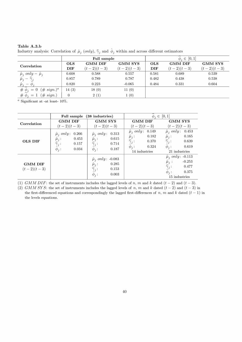
Table A.3.bIndustry analysis: Correlation of µj (only), bγj and φj within and across different estimators

Full sample bφj ∈ [0, 1]Correlation

OLS

DIF

GMM DIF


(t− 2)(t− 3)OLS

DIF

GMM DIF


(t− 2)(t− 3)µj only − µj 0.608 0.588 0.557 0.581 0.689 0.539

µj − bγj 0.857 0.789 0.787 0.482 0.438 0.538

µj − φj 0.820 0.223 -0.065 0.484 0.331 0.604

# bφj = 0 (# sign.)a 14 (3) 18 (0) 11 (0)

# bφj = 1 (# sign.) 0 2 (1) 1 (0)a Significant at -at least- 10%.

Full sample (38 industries) bφj ∈ [0, 1]Correlation

GMM DIF




(t− 2)(t− 3)

OLS DIF

µj only : 0.266

µj : 0.453bγj : 0.157

φj : 0.034

µj only : 0.313

µj : 0.615bγj : 0.714

φj : 0.187

µj only : 0.149

µj : 0.182bγj : 0.370

φj : 0.324

14 industries

µj only : 0.453

µj : 0.165bγj : 0.639

φj : 0.619

21 industries

GMM DIF

(t− 2)(t− 3)

µj only : -0.083µj : 0.285bγj : 0.153

φj : 0.003

µj only : -0.113µj : -0.253bγj : 0.477

φj : 0.375

15 industries

(1) GMM DIF : the set of instruments includes the lagged levels of n, m and k dated (t− 2) and (t− 3).(2) GMM SY S: the set of instruments includes the lagged levels of n, m and k dated (t− 2) and (t− 3) in

the first-differenced equations and correspondingly the lagged first-differences of n, m and k dated (t− 1) inthe levels equations.

40

Table A.4Heterogeneity of firm output elasticities bεQJi (J = N,M,K), mark-up µi (only) and extent of rent sharing φi :Different indicators and first-differenced OLS estimatesPart 1: bµi ≥ 1 ∨ bφi ∈ [0, 1] [5906 firms] - bφi = 0 ∨ bµi only ≥ 1 [1239 firms]


bεQKiµi only µi bγi φibµi ≥ 1 ∨ bφi ∈ [0, 1] [5906 firms]

SIMPLE

Observed variance bσ2o 0.017 0.019 0.008 0.050 0.039 0.042 0.076 0.284 3.093 0.046

Sampling variance bσ2s 0.0002 0.0006 0.001 0.046 0.026 0.035 0.046 0.185 1.825 0.172

True variance bσ2truea 0.017 0.018 0.007 0.004 0.013 0.007 0.030 0.099 1.268 0

F-testb 85 31.667 8 1.087 1.500 1.200 1.652 1.535 1.695 0.267

WEIGHTED



True variance bσ2truea 0.019 0.020 0.019 0.015 0.025 0.012 0.018 0.056 1.219 0.012

F-testb 475 667 47.5 2.154 3.778 2.500 2.636 2.806 8.571 13

MEDIAN

Interquartile observed variance bσ2o 0.019 0.025 0.011 0.037 0.038 0.030 0.045 0.150 1.935 0.056

Robust sampling variance bσ2s 0.0002 0.0008 0.0012 0.025 0.016 0.018 0.025 0.072 0.594 0.015

Robust true variance bσ2truea 0.019 0.024 0.010 0.012 0.022 0.012 0.020 0.078 1.341 0.041

F-testb 95 31.25 9.167 1.480 2.375 1.667 1.800 2.083 3.257 3.733bφi = 0 ∨ bµi only ≥ 1 [1239 firms]

SIMPLE

Observed variance bσ2o 0.010 0.018 0.014 0.025 0.027 0.028 0.077 0.057 0.082 686

Sampling variance bσ2s 0.0002 0.0007 0.001 0.050 0.027 0.036 0.049 0.153 2.660 2.40 108

True variance bσ2truea 0.010 0.017 0.013 0 0 0 0.028 0 0 0

F-testb 50 25.714 14 0.500 1 0.778 1.571 0.372 0.031 2.858 10−6

WEIGHTED



True variance bσ2truea 0.012 0.020 0.025 0.005 0.017 0.004 0.020 0 0 0

F-testb 300 667 125 1.294 2.889 1.444 3.222 0.774 0.182 0.044

MEDIAN



Robust true variance bσ2truea 0.012 0.028 0.022 0 0.011 0 0.028 0 0 0

F-testb 60 36.25 23 0.767 1.647 0.947 2.273 0.528 0.130 0.174

41

Table A.4 (ctd)

Heterogeneity of firm output elasticities bεQJi (J = N,M,K), mark-up µi (only) and extent of rent sharing φi :Different indicators and first-differenced OLS estimatesPart 2: Full sample [10646 firms]


bεQKiµi only µi bγi φi

Full sample [10646 firms]

SIMPLE

Observed variance bσ2o 0.016 0.019 0.010 0.093 0.066 0.058 0.096 0.372 3146 327

Sampling variance bσ2s 0.0002 0.0006 0.0009 0.055 0.028 0.041 0.051 0.176 8.45 108 1.55 109

True variance bσ2truea 0.016 0.018 0.009 0.038 0.038 0.017 0.045 0.196 0 0

F-testb 80 31.667 11.111 1.690 2.357 1.415 1.822 2.114 3.72 10−6 2.11 10−7

WEIGHTED



True variance bσ2truea 0.019 0.020 0.022 0.039 0.045 0.016 0.026 0.107 1.362 0.013

F-testb 475 667 73.33 3.600 5.500 2.600 3.167 4.343 6.300 7.500

MEDIAN



Robust true variance bσ2truea 0.018 0.025 0.012 0.047 0.051 0.019 0.034 0.135 2.491 0.121

F-testb 90 43.333 11.818 2.567 4 1.950 2.308 2.824 2.899 2.779a The estimated true variance is computed by adjusting the observed variance for the sampling variability: bσ2true = bσ2o− bσ2s.b F-test=

bσ2obσ2s .

42

Table A.5Within-industry dispersion: Weighted mean and Swamy estimate of weighted true standard deviation (bσtrue) of bεQJij ,mark-up µij(only) and extent of rent sharing φij

OLS DIF

Industry bεQNijbεQMij

bεQKijµij only µij bγij φij

Ind 6 0.276 [0.010] 0.490 [0.012] 0.082 [0.009] 1.109 [0.009] 1.207 [0.015] 1.782 [0.082] 0.857 [0.004]Ind 18 0.318 [0.010] 0.607 [0.007] 0.078 [0.009] 1.107 [0.007] 1.184 [0.011] 1.275 [0.098] 0.881 [0.004]Ind 17 0.212 [0.011] 0.719 [0.011] 0.050 [0.009] 1.077 [0.009] 1.170 [0.015] 1.311 [0.102] 0.855 [0.008]Ind 20 0.274 [0.013] 0.632 [0.011] 0.062 [0.010] 1.099 [0.007] 1.134 [0.015] 1.051 [0.065] 0.867 [0.008]Ind 16 0.260 [0.024] 0.577 [0.018] 0.067 [0.016] 1.080 [0.016] 1.163 [0.030] 1.008 [0.120] 0.774 [0.009]Ind 22 0.263 [0.013] 0.569 [0.011] 0.083 [0.012] 1.062 [0.010] 1.159 [0.021] 2.006 [0.105] 0.859 [0.005]Ind 28 0.199 [0.011] 0.609 [0.011] 0.131 [0.010] 1.078 [0.010] 1.196 [0.017] 1.242 [0.064] 0.834 [0.007]Ind 5 0.118 [0.007] 0.721 [0.010] 0.070 [0.006] 1.083 [0.008] 1.271 [0.020] 1.567 [0.056] 0.794 [0.004]Ind 13 0.218 [0.014] 0.566 [0.018] 0.125 [0.017] 1.026 [0.020] 1.167 [0.037] 1.013 [0.116] 0.852 [0.007]Ind 23 0.351 [0.019] 0.501 [0.019] 0.068 [0.013] 1.055 [0.015] 1.080 [0.036] 1.338 [0.155] 0.922 [0.004]Ind 11 0.192 [0.008] 0.685 [0.010] 0.070 [0.008] 1.107 [0.009] 1.249 [0.016] 1.235 [0.055] 0.757 [0.006]Ind 33 0.207 [0.007] 0.660 [0.007] 0.077 [0.007] 1.097 [0.006] 1.144 [0.012] 1.025 [0.043] 0.781 [0.005]Ind 38 0.227 [0.007] 0.650 [0.007] 0.052 [0.008] 1.114 [0.005] 1.248 [0.011] 1.250 [0.038] 0.733 [0.004]Ind 36 0.249 [0.006] 0.583 [0.006] 0.105 [0.006] 1.111 [0.005] 1.268 [0.011] 1.452 [0.033] 0.771 [0.003]Ind 12 0.269 [0.016] 0.621 [0.014] 0.051 [0.010] 1.158 [0.010] 1.228 [0.019] 1.185 [0.079] 0.778 [0.009]Ind 24 0.225 [0.010] 0.634 [0.011] 0.123 [0.010] 1.143 [0.011] 1.210 [0.018] 0.521 [0.043] 0.640 [0.010]Ind 7 0.208 [0.012] 0.668 [0.014] 0.038 [0.012] 1.148 [0.015] 1.335 [0.021] 0.812 [0.074] 0.814 [0.018]Ind 27 0.223 [0.012] 0.627 [0.012] 0.051 [0.010] 1.111 [0.008] 1.152 [0.018] 1.045 [0.063] 0.820 [0.007]Ind 37 0.195 [0.008] 0.593 [0.009] 0.106 [0.008] 1.117 [0.008] 1.233 [0.015] 1.076 [0.032] 0.694 [0.004]Ind 14 0.253 [0.014] 0.763 [0.012] 0.027 [0.011] 1.173 [0.012] 1.222 [0.017] 0.508 [0.070] 0.761 [0.012]Ind 35 0.204 [0.014] 0.636 [0.012] 0.081 [0.016] 1.109 [0.016] 1.193 [0.029] 1.272 [0.083] 0.751 [0.009]Ind 15 0.215 [0.015] 0.694 [0.017] 0.069 [0.011] 1.160 [0.012] 1.184 [0.019] 0.724 [0.075] 0.708 [0.010]Ind 26 0.253 [0.010] 0.630 [0.011] 0.080 [0.008] 1.117 [0.009] 1.222 [0.016] 0.752 [0.041] 0.764 [0.008]Ind 30 0.289 [0.016] 0.562 [0.015] 0.091 [0.011] 1.101 [0.012] 1.033 [0.030] 0.950 [0.046] 0.757 [0.008]Ind 3 0.165 [0.019] 0.633 [0.027] 0.051 [0.022] 1.101 [0.027] 1.016 [0.038] 0.334 [0.051] 0.877 [0.023]

Ind 21 0.249 [0.013] 0.630 [0.015] 0.058 [0.013] 1.073 [0.011] 1.100 [0.028] 0.769 [0.048] 0.837 [0.015]

Ind 2 0.084 [0.012] 0.796 [0.018] 0.045 [0.011] 1.102 [0.011] 1.096 [0.021] 0.686 [0.049] 0.655 [0.016]

Ind 32 0.197 [0.018] 0.631 [0.017] 0.085 [0.016] 1.109 [0.018] 1.085 [0.026] 0.736 [0.080] 0.761 [0.009]

Ind 4 0.132 [0.013] 0.800 [0.020] 0.047 [0.009] 1.106 [0.012] 1.097 [0.020] 0.216 [0.044] 0.662 [0.023]

Ind 19 0.328 [0.016] 0.522 [0.015] 0.090 [0.011] 1.107 [0.012] 1.066 [0.023] 0.638 [0.079] 0.851 [0.009]

Ind 10 0.273 [0.019] 0.535 [0.023] 0.074 [0.015] 1.102 [0.017] 1.034 [0.032] 0.534 [0.077] 0.703 [0.015]

Ind 1 0.156 [0.009] 0.680 [0.014] 0.060 [0.007] 1.080 [0.006] 1.055 [0.015] 0.650 [0.044] 0.817 [0.009]

Ind 29 0.180 [0.009] 0.680 [0.011] 0.054 [0.009] 1.153 [0.008] 1.243 [0.016] 1.002 [0.033] 0.718 [0.005]

Ind 31 0.295 [0.015] 0.574 [0.017] 0.062 [0.013] 1.088 [0.014] 1.018 [0.026] 0.866 [0.075] 0.813 [0.011]

Ind 38 0.289 [0.012] 0.559 [0.012] 0.074 [0.010] 1.091 [0.008] 1.085 [0.020] 1.142 [0.066] 0.820 [0.006]

Ind 9 0.330 [0.022] 0.593 [0.020] 0.039 [0.015] 1.162 [0.014] 1.087 [0.029] 0.496 [0.066] 0.774 [0.016]

Ind 25 0.277 [0.009] 0.592 [0.024] 0.039 [0.012] 1.130 [0.011] 1.120 [0.023] 0.814 [0.112] 0.797 [0.010]

Ind 34 0.219 [0.019] 0.669 [0.018] 0.094 [0.021] 1.086 [0.013] 1.084 [0.021] 0.669 [0.100] 0.779 [0.009]

43

Appendix B: Extension embedding the monopsony model

B.1 Model

The R. Hall (1988) model is based on the assumption that there is a potentially infinite supply ofemployees wanting a job in the firm. Limited mobility on the part of the employees and entry costson the part of competing firms might however create rents to jobs. This gives employers some powerover their workers as a small wage cut will no longer induce them to leave the firm.Consider a firm facing a labor supply Nit (wit), which is an increasing function of the wage wit. Themonopsonist firm objective is to maximize its short-run profit function, taking the labor supply curveas a given:

maxwit,Mit

π(wit, Nit, Mit) = Rit(Nit (wit) , Mit)− witNit (wit)− jitMit (B.1)

Maximization with respect to material input gives RM,it = jit, which directly leads to the correspond-ing equation (3). Maximization with respect to the wage rate gives the following first-order condition:

wit =

µεNwit

1 + εNwit

¶RN,it (B.2)

where εNwit ∈ <+ represents the elasticity of the labor supply. From (B.2), it follows that the degree

of monopsony power, measured by³RN,itwit

´, depends negatively on εNwit . Rewriting (B.2) results in a

modified equation (2):

εQNit= µitαNit

µ1 +

1

εNwit

¶(B.3)

Assuming constant returns to scale, estimation of the reduced-form equation qit − kit = εQNit(nit −

kit)+ εQMit(mit− kit)+ θit, allows the identification of (1) the mark-up of price over marginal cost and

(2) the elasticity of the supply of labor of the firm with respect to the wage rate:

µit =εQMit

αMit

(B.4)

βit =εNwit

1 + εNwit=

αNit

αMit

εQMit

εQNit

(B.5)

εNwit =βit

1− βit(B.6)

44

B.2 Results

We first present the estimates of the labor supply elasticity at the manufacturing, the industry andthe firm level and then comment on the results at the different levels.

Manufacturing-level results

Table B.1Estimates of output elasticities bεQJ (J = N,M,K), mark-up µ and labor supply elasticity bεNw :Full sample: 10646 firms - Period 1978-2001

OLS

LEVELS

OLS

DIF

GMM DIF


(t− 2)(t− 3)bεQN 0.331

(0.003)

0.298

(0.003)

0.138

(0.020)

0.298

(0.008)bεQM 0.592

(0.003)

0.587

(0.003)

0.726

(0.017)

0.675

(0.007)bεQK 0.077 0.115 0.137 0.027bµ 1.177

(0.007)

1.167

(0.005)

1.443

(0.033)

1.342

(0.015)bεNw -12.343

(2.106)

-6.246

(0.425)

-1.453

(0.109)

-3.623

(0.327)

Robust standard errors and first-step robust standard errors in columns 3-4.


(1) bεQK = 1− bεQN − bεQM .(2) Input shares: αN = 0.307, αM = 0.503, αK = 0.190.

Across-industry estimates

Table B.2Estimated industry-level output elasticities bεQJj (J = N,M,K), mark-up µj and labor supply elasticity bεNwj a

OLS DIF

38 industries bεQNj bεQMjbεQKj

bµj bεNwjIndustry mean 0.308 (0.016) 0.580 (0.014) 0.111 (0.013) 1.125 (0.027) -1.665 (66.79)Industry Q1 0.275 (0.012) 0.541 (0.010) 0.091 (0.010) 1.041 (0.021) -6.782 (0.399)Industry median 0.302 (0.016) 0.573 (0.013) 0.106 (0.013) 1.150 (0.025) -2.972 (1.324)Industry Q3 0.340 (0.020) 0.638 (0.017) 0.123 (0.016) 1.188 (0.033) 1.894 (7.007)Robust standard errors in parentheses.a Detailed information on the industry-level estimates is available upon request.

45

Within-industry firm estimates

Table B.3Estimated firm-level output elasticities bεQJi (J = N,M,K), mark-up µi and labor supply elasticity bεNwi a

OLS DIF

10646 firms bεQNibεQMi

bεQKibµi bεNwi

Firm mean 0.288 (0.201) 0.599 (0.149) 0.112 (0.171) 1.239 (0.334) -6.132 (30 104)Firm Q1 0.094 (0.119) 0.434 (0.094) -0.025 (0.097) 0.908 (0.179) -1.685 (0.309)Firm median 0.263 (0.174) 0.614 (0.132) 0.094 (0.145) 1.200 (0.273) -0.928 (0.913)Firm Q3 0.459 (0.249) 0.778 (0.185) 0.236 (0.211) 1.508 (0.410) 0.520 (4.096)Robust standard errors in parentheses.a Detailed information on the firm-level estimates is available upon request.

Discussion results

Contrary to the theoretical prediction, the labor supply elasticity is estimated to be significantlynegative across the different estimators at the manufacturing level (see Table B.1). Focusing on thefirst-differenced OLS estimator, the labor supply elasticity estimate amounts to -6.25.From Table B.2, it follows that the elasticity of the labor supply with respect to the wage rate isestimated to be lower than -6.78 for the first quartile of industries and higher than 1.89 for the topquartile. More specifically, the labor supply elasticity estimate is positive for 14 out of 38 industries,with 10 out of 14 estimates being significantly positive.1 For those industries, bεNwj lies in the [0.88, 7.53]-interval.Table B.3 shows that εNwi is estimated to be lower than -1.68 for the first quartile of firms and higherthan 0.52 for the top quartile. For 4024 out of 10646 firms, the labor supply elasticity estimate ispositive. However, only 355 of these estimates are significantly positive.2 For these firms, bεNwi lies inthe [0.04, 2.78]-interval.Based on these findings, we conclude that the extension embedding the monopsony model is rejectedby the data.

1Note that bµj ≥ 1 ∨ bεNwj > 0 for 9 industries. 5 of these industries have a significantly positive labor supply

elasticity estimate.2Note that bµi ≥ 1 ∨ bεNwi > 0 for only 1340 firms. 91 of these firms have a significantly positive labor supply

elasticity estimate.

46

Appendix C: Accounting measures of product and labor market imperfections atthe industry and the firm level

To compare our estimated price-cost mark-up and extent of rent sharing parameters, µ only, µ, and φ ,with accounting measures, we follow Veugelers (1989) and compute the following three variables, µ onlya, µaand φa, as follows:

µ onlya =PQ − jM − wN

PQ(C.1)

µa =PQ − jM − wN

PQ= µ onlya +

(w − w)NPQ

(C.2)

φa =(w − w)N

PQ − jM − wN = 1− µ onlyaµa

(C.3)

where the alternative wage w is measured by the 5th percentile value of the nominal wage per worker in theindustry in which the firm operates.

Tables C.1 and C.2 present summary information on the accounting price-cost mark-ups (µ onlya and µa)and the extent of rent sharing (φa) at the industry and the firm level and show the correlation between theaccounting measures of product and labor market imperfections and the estimated (first-differenced OLS)parameters at both levels. Consistent with section 4.1 and section 5.2 , we consider two subsamples. Thefirst subsample consists of industry (firm) estimates for which the price-cost mark-up equals or exceeds 1and the corresponding extent of rent sharing lies in the [0, 1]-interval. The second subsample includes theindustry (firm) estimates showing no evidence of rent sharing and a price-cost mark-up ignoring labor marketimperfections that equals or exceeds 1.

Table C.1Accounting versus estimated price-cost mark-ups and extent of rent sharing at the industry level

Correlation withc

Ind. mean Ind. Q1 Ind. median Ind.Q3 µ onlyj − 1 µj − 1 φj24 industriesa

µ onlyaj 0.178 0.163 0.175 0.197 0.689

µaj 0.260 0.239 0.264 0.277 0.251

φaj 0.315 0.221 0.342 0.443 0.231

14 industriesb

µ onlyaj 0.197 0.185 0.199 0.213 0.354a bµj ≥ 1 ∨ bφj ∈ [0, 1].b bφj = 0 ∨ bµj only ≥ 1.c For detailed information on the industry-level estimates, see Table A.3.a [Part 1-2] in Appendix A.

47

Table C.2Accounting versus estimated price-cost mark-ups and extent of rent sharing at the firm level

Correlation withc

Firm mean Firm Q1 Firm median Firm Q3 µ onlyi − 1 µi − 1 φi5906 firmsa

µ onlyai 0.177 0.104 0.148 0.210 0.381

µai 0.252 0.182 0.239 0.310 0.324

φai 0.321 0.219 0.359 0.521 0.011

1239 firmsb

µ onlyai 0.234 0.144 0.208 0.293 0.580a bµi ≥ 1 ∨ bφi ∈ [0, 1].b bφi = 0 ∨ bµi only ≥ 1.c For detailed information on the firm-level estimates, see Table A.4 [Part 1] in Appendix A.

48

Panel Data Estimates of the Production Function and Product and Labor Market Imperfections

Documents

Transcript of Panel Data Estimates of the Production Function and Product and Labor Market Imperfections