Panel Data Estimates of the Production Function and Product and Labor Market Imperfections
Upload
khangminh22Category
view
0download
0
.
Thes
ede
doct
orat
THESE pour obtenir le grade de:
DOCTEUR DE L’UNIVERSITE GRENOBLE ALPESSpecialite: Physique de la Matiere Condensee et du RayonnementArrete ministeriel: 25 mai 2016
Presentee par
RAFAEL CELESTRE
Investigations of the effect of optical imperfections onpartially coherent X-ray beam by combining opticalsimulations with wavefront sensing experiments
- ou -
Etude de l’effet des imperfections optiques sur un faisceaude rayons X partiellement coherent en combinant des
simulations optiques avec des experiences de detectionde front d’onde.
These de doctorat dirigee par:
Dr. Manuel SANCHEZ DEL R IO, physicien HDRESRF - the European Synchrotron Directeur de theseDr. Thomas ROTH, physicienESRF - the European Synchrotron Co-encadrant de these
preparee a Installation Europeenne de Rayonnement Synchrotron (ESRF - the EuropeanSynchrotron) dans Ecole Doctorale de Physique (n◦ 47).
These presentee et soutenue publiquement a Grenoble, le 1er fevrier, 2021 devant le jurycompose de :
Dr. Jose Emilio LORENZO DIAZ, directeur de rechercheInstitut Neel CNRS,Universite Grenoble Alpes President
Dr. Chris JACOBSEN, professeurDept. of Physics & Astronomy, Northwestern University,Advanced Photon Source, Argonne National Lab., Etats-Unis Rapporteur
Dr. David PAGANIN, professeur adjointSchool of Physics and Astronomy, Monash University, Australie Rapporteur
Dr. Christian SCHROER, professeurInst. fur Nanostruktur- und Festkorperphysik, Universitat Hamburg,Deutsches Elektronen-Synchrotron DESY, Allemagne Examinateur
Dr. Lucia ALIANELLI, chercheuse seniorDiamond Light Source Ltd, Royaume-Uni Examinatrice
Dr. Vincent FAVRE-NICOLIN, maıtre de conferences HDRESRF - the European Synchrotron,Universite Grenoble Alpes Examinateur
Dr. Raymond BARRETT, chef du groupe d’optique des rayons XESRF - the European Synchrotron Invite


Self-assertion
I hereby declare that I have produced the present work independently and using no more thanthe mentioned literature and auxiliary means. The parts taken directly or indirectly from outsidesources are identified as such. The work has so far not been presented or published in the sameor similar form to any other examination body.
Grenoble, France, 01/02/2021
Rafael Celestre


Acknowledgements
Working on my PhD project and bringing it to a conclusion would not have been possible withoutthe help of several people. I would like to take a moment to thank them while having in mindthat when naming so many people, there is always the risk of missing a name or two. To thatend, if your name is missing, I apologise.
I start this long list by thanking my PhD supervisors Manuel Sanchez del Rio - whom I metway back in 2015: long before my PhD project started - and Thomas Roth. While Manolo helpedme getting started with my simulations and introduced me to prominent researchers in my field,Thomas was a great company during several beamtimes - more often than not, until very earlyin the morning - in Grenoble and Chicago. Both Manolo and Thomas were always open fordiscussions at every stage of the research project while allowing this PhD thesis to be my work.Similarly, I would like to extend my sincere thanks to Ray Barrett, who helped to steer this workin the right direction whenever he thought I needed it.
I also want to express my gratitude to the members of my jury: Lucia Alianelli, VincentFavre-Nicolin, Chris Jacobsen, Jose Emilio Lorenzo Dias, David Paganin and Christian Schroerfor accepting reviewing and reporting on my work. Our exchanges were very rich and it was apleasure to expose my work to them.
This work made extensive use of experimental data and I must thank the staff of the BM05and ID06 beamlines at the ESRF. Special thanks to Sebastien Berujon (BM05) and CarstenDetlefs (ID06). Always very attentive, Seb introduced me to wavefront sensing with specklesand helped me gain proficiency at the beamline. Carsten is an early enthusiast of the project -always keen on providing insightful feedback and accommodating Thomas and me on the tightbeamline schedule. I would be remiss if I didn’t thank our colleagues from the 1-BM/X-rayOptics Group from the Advanced Photon Source - Argonne National Laboratory (APS/ANL), whohosted our experiments during the long ESRF shutdown for the ESRF-EBS upgrade: LahsenAssoufid, Xianbo Shi, Zhi Qiao, Michal Wojcik and their great technical staff. Also, thanks toCarsten Detlefs; Terence Manning; Sergey Antipov; Arndt Last & Elisa Konnermann; ChristianDavid & Frieder Koch; and Paw Kristiansen for providing samples for the beamtimes.
I would like to acknowledge Oleg Chubar, whom I met while still working on my master’sthesis in 2017. Oleg has often made himself available for our numerous discussions - always verypatient when explaining the ins and outs of simulations with SRW, physical optics or acceleratorphysics. This good synergy can be exemplified by the two visits to the National SynchrotronLight Source-II/Brookhaven National Laboratory, where Oleg and I could work closely together.We acknowledge the ”DOE BES Field Work Proposal PS-017 funding” for partially financing these
v
two stays. I should also thank Luca Rebuffi for, among other things, showing interest in my workand for creating a pip-installable version of my python libraries to be distributed with OASYS.
A general shout out to all the people I have had fruitful discussions with, E-mails exchangesor (watered down) coffees during conference breaks: Sajid Ali, Ruxandra Cojocaru, VincentFavre-Nicolin, Wallan Grizolli, Herbert Gross, Chris Jacobsen, Michael Krisch, Arndt Last, SérgioLordano, Virendra Mahajan, Bernd Meyer, Peter Munro, Boaz Nash, David Paganin, MaksimRakitin, Claudio Romero, Andreas Schropp, Frank Seiboth, Irina Snigireva, Pedro Tavares (. . . )
My research was conducted within the X-ray Optics Group (XOG) from the InstrumentationServices & Development Division (ISDD) at the European Synchrotron (ESRF) and I would liketo thank my colleagues, especially the XOG, for providing a very nice work environment. AmparoVivo merits a special thanks for proof-reading the French parts of my thesis.
I do not know when I realised I wanted to have a career in science, but for as long as I canremember, I wanted to be a lumberjack, I mean, a scientist. Following that dream would not havebeen possible without the support and incentive of my parents, grandparents & my family. Aspecial mention to my friends from República Beijos me Liga and Coloc la Flemme - too manyto mention by name; to Baptiste Belescot, Gaetan PC Girard, Edoardo Zatterin, Luca Capasso,Rafael Vescovi, Jan Sandner, Maik Rosenberger and the Konnermanns. These are the people whohave been there for me since I left Brazil and I am thankful.
Finally, there is a quotation by Joe Walsh that sums up very well how writing this PhD thesiswas like to me: "I can’t complain, but sometimes I still do. Life’s been good to me so far".
Muito obrigado,Rafael Celestre
vi

Résumé
Le déploiement des installations synchrotron à haute énergie de 4e génération (ESRF-EBS etles projets APS-U, HEPS, PETRA-IV et SPring-8 II) et des lasers à électrons libres (Eu-XFEL,SLAC) allié aux récents développements d’optiques réfractives « free-form » de haute qualitévisant à conditionner le faisceau de rayons X, a ravivé l’intérêt pour les lentilles réfractivescomposées (CRL) permettant la propagation du faisceau, ou son conditionnement pour la microet la nano-analyse, ou encore pour les applications d’imagerie. Dans ce contexte, l’ESRF arepris en 2018 la fabrication et les tests de lentilles bi-concaves en aluminium à focalisation2D. Les optiques réfractives actuelles, commerciales ou non, présentent des aberrations quidétériorent leurs performances finales. Aussi, une modélisation précise incluant des donnéesde métrologie est nécessaire pour évaluer la dégradation du front d’onde afin de proposer desstratégies d’amélioration.
En optique physique, les éléments faiblement focalisant sont généralement simulés commeun seul élément mince dans l’approximation de projection. Alors qu’une seule lentille rayons Xdans des conditions de fonctionnement typique peut souvent être représentée de cette manière,la simulation d’une CRL entière avec une approche similaire conduit à un modèle idéalisé quimanque de polyvalence. Ce travail propose de décomposer une CRL en ses lentilles élémentairesséparées par une propagation en espace libre, comme dans la technique dite de multi-coupes(multi-slicing - MS) déjà utilisées dans les simulations optiques. L’attention est portée sur lamodélisation de la lentille élémentaire en lui ajoutant des degrés de liberté supplémentairespermettant de simuler des désalignements typiques ou des erreurs de fabrication. Des polynômesorthonormaux décrivant les aberrations optiques ainsi que des données de métrologie obtenuesavec les rayons X sont également utilisés pour obtenir des résultats de simulation réalistes, quisont présentés dans plusieurs simulations cohérentes et partiellement cohérentes tout au longde ce travail. Les résultats ainsi obtenus se comparant qualitativement bien avec les donnéesexpérimentales, sont utilisés pour évaluer l’effet des imperfections optiques sur la dégradationdu faisceau de rayons X partiellement cohérent ainsi que la pertinence de facteurs de méritecommuns. Contrairement à d’autres travaux, la modélisation présentée ici peut être utiliséede façon transparente avec l’un des codes les plus populaires pour la conception de lignes defaisceaux de rayons X, "Synchrotron Radiation Workshop" (SRW), et est disponible sur GitLab.
Les imperfections optiques mesurées avec une haute résolution spatiale peuvent être ajoutéesà la représentation MS d’une CRL pour simuler avec précision de vraies lentilles rayons X. Le suivivectoriel du speckle des rayons X (XSVT) est une technique polyvalente qui permet d’obtenirfacilement les erreurs de forme des lentilles rayons X dans l’approximation de projection avecune haute résolution spatiale. Elle a été utilisée pour caractériser les lentilles 2D-berylliumqui sont ensuite utilisées dans les modélisations présentées ici. Cette thèse présente une revue
vii

des concepts les plus pertinents de l’imagerie basée sur le speckle des rayons X appliquée à lamétrologie des lentilles.
La mise en œuvre du modèle MS d’une CRL incluant des données de métrologie permetd’extraire les erreurs cumulées résultantes de l’empilement des lentilles ainsi que le calcul descorrections de phase. Cette thèse se termine par la présentation d’une méthodologie de calculdu profil des correcteurs de réfraction, qui est appliquée pour produire des plaques de phaseablatées en diamant. Les premiers résultats expérimentaux montrent une amélioration du profildu faisceau, mais l’alignement transversal de la plaque est un facteur limitant. Des améliorationsconcernant la métrologie des lentilles et des plaques de correction, ainsi que les protocolesd’alignement seront nécessaires optimiser les performances de ces correcteurs optiques.
viii

Abstract
The advent of the 4th generation high-energy synchrotron facilities (ESRF-EBS and the plannedAPS-U, HEPS, PETRA-IV and SPring-8 II) and free-electron lasers (Eu-XFEL, SLAC) allied withthe recent demonstration of high-quality free-form refractive optics for beam shaping and opticalcorrection has reinforced interest in compound refractive lenses (CRLs) as optics for beamtransport, probe formation in X-ray micro- and nano-analysis as well as for imaging applications.Within this context, in 2016, the ESRF resumed the fabrication and tests of 2D focusing bi-concave aluminium X-ray lenses. Current refractive optics, commercial or otherwise, havenon-negligible aberrations which deteriorate their final performance and accurate modellingwith input from metrology is necessary to evaluate the wavefront degradation and in order topropose mitigation strategies.
In physical optics, weakly focusing elements are usually simulated as a single thin element inthe projection approximation. While a single X-ray lens at typical operation conditions can oftenbe represented in this way, simulating a full CRL with a similar approach leads to an idealisedmodel that lacks versatility. This work proposes decomposing a CRL into its lenslets separated bya free-space propagation, which resembles the multi-slicing techniques (MS) already used foroptical simulations. Attention is given to modelling the single lens element by adding additionaldegrees of freedom allowing the modelling of typical misalignments and fabrication errors.Orthonormal polynomials for optical aberrations as well as at-wavelength metrology data arealso used to obtain realistic simulation results, which are presented in several coherent- andpartially-coherent simulations throughout this work. They compare qualitatively well withthe experimental data and are used to evaluate the effect of optical imperfections on partiallycoherent X-ray beam and the suitability of common figures of merit. Unlike other works, themodelling presented here can be used transparently with one of the most popular codes for X-raybeamline design, "Synchrotron Radiation Workshop" (SRW), and is publicly available on GitLab.
Optical imperfections measured with high spatial resolution can be added to the MSrepresentation of a CRL to accurately represent real X-ray lenses. X-ray speckle vector tracking(XSVT) is a versatile technique that conveniently obtains the figure errors of X-ray lenses in theprojection approximation with high spatial resolution and is used in this work for characterisinglenses to be used in the modelling presented here. This thesis presents a review of most relevantconcepts of X-ray speckle based imaging applied to lens metrology.
Implementing the MS model of a CRL using metrology data allows extraction of theaccumulated figure errors of stacked lenses and enables the calculation of phase corrections.Finally, this thesis presents a methodology for calculating the profile of refractive correctors,which is applied to produce phase plates ablated from diamond. Early experimental results
ix

show an improvement on the beam profile, but the transverse alignment of the phase-plate isa limiting factor. Further improvements to the metrology of lenses and correction plates andalignment protocols are necessary to optimise the performance of these optical correctors.
x

Contents
Self-assertion iii
Préface 1
Aperçu . . . . . . . . . . . . . . . . . . . . . . . . . . . . . . . . . . . . . . . . . . . . . 2
Prelude 5
Outline . . . . . . . . . . . . . . . . . . . . . . . . . . . . . . . . . . . . . . . . . . . . 6
1 On a new kind of rays 9
1.1 From the Crookes-Hittorf tube to the ESRF-EBS . . . . . . . . . . . . . . . . . . . 9
1.1.1 X-ray sources . . . . . . . . . . . . . . . . . . . . . . . . . . . . . . . . . . 10
1.1.2 High brilliance X-ray sources . . . . . . . . . . . . . . . . . . . . . . . . . . 12
1.1.3 Undulators as a primary source of coherent X-rays . . . . . . . . . . . . . . 14
1.2 Physical optics . . . . . . . . . . . . . . . . . . . . . . . . . . . . . . . . . . . . . 16
1.2.1 Free-space propagation . . . . . . . . . . . . . . . . . . . . . . . . . . . . 16
1.2.2 Transmission elements . . . . . . . . . . . . . . . . . . . . . . . . . . . . . 22
1.2.3 Optical coherence . . . . . . . . . . . . . . . . . . . . . . . . . . . . . . . 29
1.3 X-ray optical simulations . . . . . . . . . . . . . . . . . . . . . . . . . . . . . . . . 32
1.3.1 Ray-tracing . . . . . . . . . . . . . . . . . . . . . . . . . . . . . . . . . . . 33
1.3.2 Wave propagation . . . . . . . . . . . . . . . . . . . . . . . . . . . . . . . 34
1.3.3 Partially coherent simulations . . . . . . . . . . . . . . . . . . . . . . . . . 34
References . . . . . . . . . . . . . . . . . . . . . . . . . . . . . . . . . . . . . . . . . . . 35
2 X-rays as a branch of optics 41
2.1 The early days of X-ray optics . . . . . . . . . . . . . . . . . . . . . . . . . . . . . 41
2.1.1 X-ray focusing optics . . . . . . . . . . . . . . . . . . . . . . . . . . . . . . 42
– Diffractive optics . . . . . . . . . . . . . . . . . . . . . . . . . . . . . . . 42
– Reflective optics . . . . . . . . . . . . . . . . . . . . . . . . . . . . . . . . 42
– Refractive optics . . . . . . . . . . . . . . . . . . . . . . . . . . . . . . . 43
2.2 The compound refractive lenses (CRL) . . . . . . . . . . . . . . . . . . . . . . . . 44
2.2.1 Lens materials and the index of refraction . . . . . . . . . . . . . . . . . . 45
2.2.2 CRL anatomy . . . . . . . . . . . . . . . . . . . . . . . . . . . . . . . . . . 47
2.2.3 CRL modelling . . . . . . . . . . . . . . . . . . . . . . . . . . . . . . . . . 49
– Ideal thin lens and single lens equivalent . . . . . . . . . . . . . . . . . . 49
– Multi-slicing representation . . . . . . . . . . . . . . . . . . . . . . . . . 50
2.2.4 CRL performance . . . . . . . . . . . . . . . . . . . . . . . . . . . . . . . . 51
– Diffraction limited focal spot . . . . . . . . . . . . . . . . . . . . . . . . 51
xi

– Tolerance conditions for aberrations . . . . . . . . . . . . . . . . . . . . 52– Chromatic aberrations . . . . . . . . . . . . . . . . . . . . . . . . . . . . 53
References . . . . . . . . . . . . . . . . . . . . . . . . . . . . . . . . . . . . . . . . . . . 54
3 Modelling optical imperfections in refractive lenses 613.1 Optical imperfections in refractive lenses . . . . . . . . . . . . . . . . . . . . . . . 623.2 Misalignments . . . . . . . . . . . . . . . . . . . . . . . . . . . . . . . . . . . . . 63
3.2.1 Transverse offset . . . . . . . . . . . . . . . . . . . . . . . . . . . . . . . . 643.2.2 Tilted lens . . . . . . . . . . . . . . . . . . . . . . . . . . . . . . . . . . . . 65
3.3 Fabrication errors . . . . . . . . . . . . . . . . . . . . . . . . . . . . . . . . . . . . 673.3.1 Longitudinal offset of the parabolic section . . . . . . . . . . . . . . . . . . 673.3.2 Transverse offset of the parabolic section . . . . . . . . . . . . . . . . . . . 673.3.3 Tilted parabolic section . . . . . . . . . . . . . . . . . . . . . . . . . . . . 68
3.4 Other sources of deviations from the parabolic shape . . . . . . . . . . . . . . . . 683.4.1 Orthornormal polynomials . . . . . . . . . . . . . . . . . . . . . . . . . . . 693.4.2 Metrology data . . . . . . . . . . . . . . . . . . . . . . . . . . . . . . . . . 71
3.5 Implementation . . . . . . . . . . . . . . . . . . . . . . . . . . . . . . . . . . . . . 72References . . . . . . . . . . . . . . . . . . . . . . . . . . . . . . . . . . . . . . . . . . . 74
4 Measuring optical imperfections in refractive lenses 774.1 At wavelength-metrology . . . . . . . . . . . . . . . . . . . . . . . . . . . . . . . 77
4.1.1 X-ray (near field) speckle vector tracking (XSVT) . . . . . . . . . . . . . . 784.1.2 Foundation . . . . . . . . . . . . . . . . . . . . . . . . . . . . . . . . . . . 794.1.3 Experimental setup . . . . . . . . . . . . . . . . . . . . . . . . . . . . . . . 804.1.4 Data acquisition, processing and analysis . . . . . . . . . . . . . . . . . . . 85
4.2 X-ray lens metrology . . . . . . . . . . . . . . . . . . . . . . . . . . . . . . . . . . 904.2.1 Single lens measurements . . . . . . . . . . . . . . . . . . . . . . . . . . . 914.2.2 Stacked lenses measurements . . . . . . . . . . . . . . . . . . . . . . . . . 92
References . . . . . . . . . . . . . . . . . . . . . . . . . . . . . . . . . . . . . . . . . . . 95
5 Effect of optical imperfections on an X-ray beam 995.1 Lenses and lens stacks . . . . . . . . . . . . . . . . . . . . . . . . . . . . . . . . . 995.2 Software and computing infrastructure . . . . . . . . . . . . . . . . . . . . . . . . 1005.3 Fully coherent simulations . . . . . . . . . . . . . . . . . . . . . . . . . . . . . . . 100
5.3.1 The PSF: ideal focusing . . . . . . . . . . . . . . . . . . . . . . . . . . . . 1015.3.2 The beam caustics . . . . . . . . . . . . . . . . . . . . . . . . . . . . . . . 102
5.4 Partially coherent simulations . . . . . . . . . . . . . . . . . . . . . . . . . . . . . 1025.4.1 X-ray source . . . . . . . . . . . . . . . . . . . . . . . . . . . . . . . . . . . 1025.4.2 Beam characteristics at the focal position . . . . . . . . . . . . . . . . . . . 1045.4.3 Beam profile evolution along the optical axis . . . . . . . . . . . . . . . . . 104
5.5 Discussion . . . . . . . . . . . . . . . . . . . . . . . . . . . . . . . . . . . . . . . . 1105.5.1 Metrology of individual lenses vs. stacked lenses . . . . . . . . . . . . . . 1105.5.2 The effect of optical imperfections . . . . . . . . . . . . . . . . . . . . . . 1115.5.3 The Strehl ratio for X-ray lenses . . . . . . . . . . . . . . . . . . . . . . . . 1145.5.4 Simulation time . . . . . . . . . . . . . . . . . . . . . . . . . . . . . . . . . 115
xii
References . . . . . . . . . . . . . . . . . . . . . . . . . . . . . . . . . . . . . . . . . . . 116
6 Correcting optical imperfections in refractive lenses 1196.1 Corrective optics . . . . . . . . . . . . . . . . . . . . . . . . . . . . . . . . . . . . 119
6.1.1 Design . . . . . . . . . . . . . . . . . . . . . . . . . . . . . . . . . . . . . . 1196.1.2 Correction phase plate calculation . . . . . . . . . . . . . . . . . . . . . . 121
6.2 Prototype . . . . . . . . . . . . . . . . . . . . . . . . . . . . . . . . . . . . . . . . 1266.2.1 Early tests on an X-ray beam . . . . . . . . . . . . . . . . . . . . . . . . . . 126
6.3 Discussion . . . . . . . . . . . . . . . . . . . . . . . . . . . . . . . . . . . . . . . . 1306.3.1 Design and expected performance . . . . . . . . . . . . . . . . . . . . . . . 1306.3.2 Early phase plate tests on an X-ray beam . . . . . . . . . . . . . . . . . . . 131
References . . . . . . . . . . . . . . . . . . . . . . . . . . . . . . . . . . . . . . . . . . . 133
7.en Conclusion 137References . . . . . . . . . . . . . . . . . . . . . . . . . . . . . . . . . . . . . . . . . . . 140
7.fr Conclusion 143Références . . . . . . . . . . . . . . . . . . . . . . . . . . . . . . . . . . . . . . . . . . . 146
A Publication list 149
xiii


List of Figures
1.1 Synchrotron radiation emission . . . . . . . . . . . . . . . . . . . . . . . . . . . . . 11
1.2 Emittance matching . . . . . . . . . . . . . . . . . . . . . . . . . . . . . . . . . . . 14
1.3 Hierarchical optical theories . . . . . . . . . . . . . . . . . . . . . . . . . . . . . . . 16
1.4 Scalar diffraction problem geometry . . . . . . . . . . . . . . . . . . . . . . . . . . 19
1.5 Replicas and aliasing . . . . . . . . . . . . . . . . . . . . . . . . . . . . . . . . . . . 21
1.6 Transmission elements . . . . . . . . . . . . . . . . . . . . . . . . . . . . . . . . . . 23
1.7 The validity of the Fresnel approximation . . . . . . . . . . . . . . . . . . . . . . . 27
1.8 X-ray optical simulation methods . . . . . . . . . . . . . . . . . . . . . . . . . . . . 33
2.1 1D and 2D focusing X-ray lenses . . . . . . . . . . . . . . . . . . . . . . . . . . . . . 45
2.2 Refraction and total external reflection in the X-ray regime . . . . . . . . . . . . . . 45
2.3 Index of refraction for common lens materials . . . . . . . . . . . . . . . . . . . . . 47
2.4 CRL anatomy . . . . . . . . . . . . . . . . . . . . . . . . . . . . . . . . . . . . . . . 48
2.5 Intensity transmission and accumulated thickness profile of CRLs . . . . . . . . . . 49
2.6 Hierarchical CRL representation . . . . . . . . . . . . . . . . . . . . . . . . . . . . . 50
2.7 Chromatic aberrations . . . . . . . . . . . . . . . . . . . . . . . . . . . . . . . . . . 54
3.1 Modelling misalignments and fabrication errors in CRLs . . . . . . . . . . . . . . . 62
3.2 Optical layout used for modelling imperfections in CRL . . . . . . . . . . . . . . . . 63
3.3 The ideal single X-ray lens . . . . . . . . . . . . . . . . . . . . . . . . . . . . . . . . 64
3.4 Effects of a transverse CRL offset . . . . . . . . . . . . . . . . . . . . . . . . . . . . 65
3.5 Effects of a CRL tilt . . . . . . . . . . . . . . . . . . . . . . . . . . . . . . . . . . . . 66
3.6 Effects of the longitudinal offset of the parabolic section . . . . . . . . . . . . . . . 67
3.7 Effects of the transverse offset of the parabolic section . . . . . . . . . . . . . . . . 68
3.8 Effects of the tilted parabolic section . . . . . . . . . . . . . . . . . . . . . . . . . . 69
3.9 Other sources of deviations from the parabolic shape . . . . . . . . . . . . . . . . . 70
3.10 Effects of other sources of deviations from the parabolic shape - single lens . . . . . 71
3.11 Effects of other sources of deviations from the parabolic shape - 10-lens stack . . . 72
3.12 Strehl ratio summarising the results from the diverse models presented . . . . . . . 73
4.1 Stationary diffuser and associated speckle-pattern . . . . . . . . . . . . . . . . . . . 80
4.2 Tracking of speckle grain . . . . . . . . . . . . . . . . . . . . . . . . . . . . . . . . . 80
4.3 Speckle-based imaging geometry . . . . . . . . . . . . . . . . . . . . . . . . . . . . 81
4.4 Speckle-based imaging experimental setup at the BM05 beamline, ESRF. . . . . . . 82
4.5 Experimental setup at the BM05 beamline, ESRF. . . . . . . . . . . . . . . . . . . . 83
4.6 X-ray (near field) speckle vector tracking (XSVT) . . . . . . . . . . . . . . . . . . . 86
4.7 Normalised cross-correlation map . . . . . . . . . . . . . . . . . . . . . . . . . . . . 87
xv

4.8 Recovered phase gradient and residues . . . . . . . . . . . . . . . . . . . . . . . . . 884.9 Recovered figure errors in projection approximation . . . . . . . . . . . . . . . . . . 884.10 XSVT sensitivity calculation sketch . . . . . . . . . . . . . . . . . . . . . . . . . . . 904.11 XSVT sensitivity calculation . . . . . . . . . . . . . . . . . . . . . . . . . . . . . . . 904.12 XSVT experimental sensitivity calculation . . . . . . . . . . . . . . . . . . . . . . . 914.13 Optical layout used for artificially stacking lenses . . . . . . . . . . . . . . . . . . . 924.14 Figure errors from the artificially stacked lenses - L01-L10 . . . . . . . . . . . . . . 934.15 Figure errors from stack 1 . . . . . . . . . . . . . . . . . . . . . . . . . . . . . . . . 934.16 Figure errors from the artificially stacked lenses - L11-L20 . . . . . . . . . . . . . . 944.17 Figure errors from stack 2 . . . . . . . . . . . . . . . . . . . . . . . . . . . . . . . . 94
5.1 Beamlines for coherent- and partially-coherent simulations . . . . . . . . . . . . . . 1005.2 Complex degree of coherence . . . . . . . . . . . . . . . . . . . . . . . . . . . . . . 1035.3 Artificially stacked lenses L01-L11 vs. stack 1 comparison . . . . . . . . . . . . . . . 1055.4 Artificially stacked lenses L11-L21 vs. stack 2 comparison . . . . . . . . . . . . . . . 1065.5 Effects of stacking lenses . . . . . . . . . . . . . . . . . . . . . . . . . . . . . . . . . 1075.6 Effects of different spatial frequencies ranges on a X-ray beam . . . . . . . . . . . . 1085.7 L01-L10 studied under fully- and partially-coherent illuminations . . . . . . . . . . 1095.8 Strehl ratio of L01-L10 vs. stack 1 and L11-L20 vs. stack 2 simulations . . . . . . . 1115.9 Accumulative figure errors . . . . . . . . . . . . . . . . . . . . . . . . . . . . . . . . 1115.10 High frequency errors profile . . . . . . . . . . . . . . . . . . . . . . . . . . . . . . 1135.11 High frequency errors studied under fully- and partially-coherent illuminations . . 1145.12 Strehl ratio from numerical simulations . . . . . . . . . . . . . . . . . . . . . . . . . 1155.13 Intensity cut for σz scan . . . . . . . . . . . . . . . . . . . . . . . . . . . . . . . . . 116
6.1 Schematic for phase correction calculation . . . . . . . . . . . . . . . . . . . . . . . 1206.2 Diamond correction plate profile cut . . . . . . . . . . . . . . . . . . . . . . . . . . 1226.3 Schematic for residual thickness error calculation after phase correction . . . . . . 1226.4 Residual profile after phase correction . . . . . . . . . . . . . . . . . . . . . . . . . 1236.5 Beamlines for coherent- and partially-coherent simulations . . . . . . . . . . . . . . 1246.6 Expected performance of the diamond phase corrector . . . . . . . . . . . . . . . . 1246.7 Strehl ratio for the corrected system . . . . . . . . . . . . . . . . . . . . . . . . . . 1256.8 Alignment sensitivity scan for the corrected system . . . . . . . . . . . . . . . . . . 1256.9 Lens casing, frame and correction plates . . . . . . . . . . . . . . . . . . . . . . . . 1266.10 XSVT metrology of phase-plate PP01.v1-PP01.v3 . . . . . . . . . . . . . . . . . . . 1286.11 Scanning confocal laser microscopy of PP01.v2 phase-plate . . . . . . . . . . . . . . 1296.12 Profile cuts of the correction plates . . . . . . . . . . . . . . . . . . . . . . . . . . . 1296.13 Residual thickness after installation of the correction plates PP01.v1-v3 . . . . . . . 1296.14 Experimental beam caustics for the aberrated and corrected systems . . . . . . . . 1306.15 Index of refraction ratio for common phase plate materials . . . . . . . . . . . . . . 133
xvi

List of Tables
4.1 Lens stack 1 main parameters from XSVT metrology . . . . . . . . . . . . . . . . . . 934.2 Lens stack 2 main parameters from XSVT metrology . . . . . . . . . . . . . . . . . . 94
5.1 FWHM of the PSF for the simulated models in Figs. 5.3-5.7 . . . . . . . . . . . . . . 1015.2 Strehl ratio for the simulated models in Figs. 5.3-5.7 . . . . . . . . . . . . . . . . . 1025.3 Summary of the simulation times for different CRL models . . . . . . . . . . . . . . 116
6.1 Residual figure error profile value for L01-L10 and for the corrected system . . . . . 1226.2 Strehl ratio for L01-L10 and for the corrected system . . . . . . . . . . . . . . . . . 1236.3 Residual figure error profile value for L01-L10 and for the corrected system . . . . . 127
xvii


Préface
L’amélioration de la qualité des sources de rayons X modernes impose des optiques pour rayonsX de qualité considérablement accrue, permettant de conserver la brillance de la source mêmefocalisée. Pour cela, il faut réduire au minimum la perturbation du front d’onde des rayons X, leseffets néfastes sur les points focaux et les pertes d’intensité. Pour y parvenir avec des lentillesrayons X, elles doivent présenter une fidélité de forme, des surfaces lisses et une structure internehomogène et pure.
Ce projet de doctorat visait à déterminer l’effet des erreurs de forme des lentilles réfractives,de la rugosité de surface et des impuretés sur un faisceau de rayons X partiellement cohérentayant des caractéristiques similaires à celles d’une ligne de lumière avec onduleur après la miseà niveau de l’ESRF-EBS. Sur la base de développements récents, l’atténuation des erreurs deforme des lentilles à l’aide d’optiques correctives a également été étudiée. Pour atteindre lesobjectifs proposés, ce projet reposait sur deux piliers : théorique et expérimental, avec desaspects techniques liés aux deux. Ce projet a abordé des aspects importants du programme deR&D en optique des rayons X de l’ESRF-EBS, tel qu’il est défini dans le plan stratégique de miseà niveau (Orange book).
Le volet théorique du travail a consisté à étudier les limites de la modélisation actuelle etles approximations utilisées dans la plupart des codes de simulation pour traiter les élémentsoptiques. Après avoir évalué la validité des outils existants, des propositions d’extension et denouveaux développements ont été proposés. Les objectifs étaient également, d’une part, d’ajouteraux simulations la capacité de traiter les données de métrologie et de développer un cadre pour laconception d’optiques réfractives correctives, et d’autre part, d’intégrer les modèles de simulationà des simulations cohérentes et partiellement cohérentes pour obtenir de manière réaliste l’effetdes imperfections optiques sur un faisceau de rayons X et de comparer les résultats avec lalittérature et les données expérimentales. Les objectifs techniques liés à cette partie théoriquecomprenaient le développement de bibliothèques Python permettant d’utiliser facilement lamodélisation nouvellement développée avec le code "Synchrotron Radiation Workshop" (SRW)pour la conception des lignes de faisceaux. Une partie de ce développement a été menéen collaboration avec O. Chubar (auteur du SRW) au cours de deux visites scientifiques auBrookhaven National Lab. aux États-Unis. Cette nouvelle bibliothèque Python est disponiblepour une intégration dans des interfaces graphiques utilisateur telles que OrAnge SYnchrotronSuit (OASYS).
Afin d’obtenir des résultats de simulation réalistes, des techniques de détection de frontd’onde en champ proche basées sur le speckle des rayons X ont été utilisées pour caractériser
1

les lentilles produites en interne, les lentilles et optiques de type « free-form » dans le cadre decollaborations scientifiques, et les lentilles commerciales récemment acquises. La métrologiedite « en longueur d’onde » a été effectuée sur la ligne de lumière BM05 de l’ESRF jusqu’à sonarrêt début décembre 2018, puis sur la ligne 1-BM de l’APS à Chicago en 2019 et enfin sur laligne ID06 pendant la période de mise en service de l’ESRF-EBS. Outre la mesure de composantsoptiques pour rayons X et la création d’une base de données de métrologie pour les lentillesrayons X, les objectifs techniques de cette partie expérimentale étaient de former le doctorantpour le rendre autonome et compétant dans la mise en œuvre du dispositif expérimental sur uneligne de lumière, mais aussi dans l’acquisition et le traitement des données. Le développementde protocoles d’alignement, de standardisation des mesures et d’analyse des données étaientégalement attendus.
Par la suite, l’étude de récents développements concernant les techniques de fabrication ad-ditive et soustractive pour la réalisation d’éléments de correction optique s’est avérée nécessaire.C’est donc naturellement que cette formation doctorale s’est achevée par la conception d’unpremier correcteur de phase suivi d’expériences pour évaluer ses performances sur le faisceau derayons X à l’ESRF.
AperçuCe travail est divisé en six chapitres, une conclusion et une annexe résumant les publications
pertinentes de l’auteur au cours de ce projet de doctorat :
Chapitre 1 - On a new kind of rays est le premier de deux chapitres essentiellement théoriques.Le titre est un clin d’œil au titre de la publication qui relate la découverte des rayons X en 1895.Il commence par introduire les concepts de brillance et les relie aux sources de rayons X baséessur les accélérateurs. Les sources de rayons X à haute brillance sont ensuite présentées et leconcept de rayons X latéralement cohérents est illustré. L’optique physique est ensuite présentéecomme la description la plus appropriée des champs (partiellement) cohérents. La propagationen espace libre et l’approximation paraxiale sont expliquées et la propagation des rayons X àtravers la matière est modélisée par l’introduction de l’élément de transmission. Une brèvediscussion sur la cohérence optique et la présentation de quelques concepts de base sont faites àla fin de cette section. Ce chapitre se termine par une discussion sur les simulations, méthodeset approches pour optiques des rayons X.
Chapitre 2 - X-rays as a branch of optics, en référence au discours de A. Compton lauréatdu prix Nobel. Ce chapitre s’ouvre sur un récit historique des débuts de la science des rayonsX montrant les étapes qui ont conduit à la compréhension des rayons X comme branche del’optique. Un bref examen des développements de l’optique de focalisation des rayons X enfonction des phénomènes optiques est donné pour contextualiser l’évolution récente de l’optiqueréfractive. La modélisation d’une lentille rayons X idéale et celle d’un empilement idéal, basé surdes techniques de type multi-coupes, sont présentés. Avec peu de modifications, ce modèle peutaccepter des cartographies d’erreurs arbitraires pour tenir compte des imperfections optiques.Des mesures déterminantes pour l’évaluation des performances de CRL sont introduites et les
2

conditions de tolérance des aberrations sont présentées. Ce chapitre conclut la présentation desaspects théoriques nécessaires à cette thèse.
Chapitre 3 - Modelling optical imperfections in refractive lenses se concentre sur la modéli-sation d’une lentille rayons X. En ajoutant des degrés de liberté latéraux et angulaires aux facesavant et arrière des éléments focalisants, il est possible d’imiter les désalignements et les erreursde fabrication typiques rencontrés dans les lentilles réelles. Dans les cas où ces degrés de libertéparamétrés ne suffisent pas, une modélisation d’erreurs de forme plus complexe est possibleen utilisant les polynômes orthonormaux Zernike ou 2D Legendre, ou encore des données demétrologie. Ce chapitre se termine par le détail des bibliothèques Python implémentées pour lamodélisation des imperfections de phase pour les lentilles rayons X.
Chapitre 4 - Measuring optical imperfections in refractive lenses présente une descriptioncomplète de la technique de suivi des vecteurs de speckle en champ proche par rayons X (XSVT)employée pour inspecter les lentilles utilisées dans cette thèse. Il commence par décrire ladiversité des techniques de métrologie en longueur d’onde et explique pourquoi la techniqueXSVT est la plus appropriée pour ce travail. Un examen des principaux aspects du dispositifexpérimental, de l’acquisition, du traitement et de l’analyse des données est présenté et unediscussion sur la métrologie des lentilles rayons X par rapport aux empilements de lentilles clôtce chapitre.
Chapitre 5 - Effect of optical imperfections on an X-ray beam traite les effets induits parles imperfections optiques sur la dégradation du faisceau de rayons X en présentant de nom-breuses simulations des caustiques du faisceau, de la fonction d’étalement du point et du profildu faisceau à des positions déterminées le long de l’axe optique pour différentes configurationsoptiques. Une étude comparative des simulations de la métrologie des lentilles individuelles parrapport aux lentilles empilées est présentée, suivie d’une discussion sur l’effet des imperfectionsoptiques et la pertinence du rapport de Strehl pour les lentilles rayons X. Quelques commentairessur les temps de simulation concluent le chapitre.
Chapitre 6 - Correcting optical imperfections in refractive lenses est le dernier chapitreet conclut ce voyage qui a commencé dans le Chapitre 2 par la modélisation des lentilles idéales,en passant par la modélisation des lentilles aberrantes dans le Chapitre 3, en mesurant leursimperfections dans le Chapitre 4 et en comprenant leurs effets sur un faisceau de rayons Xdans le Chapitre 5. Ce chapitre commence par énumérer les étapes importantes des techniquesextrêmement précises de fabrication additive et soustractive qui ont permis de produire desoptiques « free-form » très précises pour la correction des aberrations optiques. Un récapitulatifdes stratégies de correction des imperfections optiques pour les rayons X est donné et uneapproche méthodique du calcul de la plaque réfractive de correction de phase est présentée. Lesoutils de simulation développés pour cette thèse ont permis d’évaluer la performance attendue dela plaque corrective ainsi que les tolérances d’alignement. Un prototype en diamant est présentéet une première expérience sur une ligne de lumière démontre une amélioration qualitativedu profil du faisceau de rayons X. Une longue discussion sur la conception et les performancesattendues confrontées aux résultats expérimentaux obtenus avec la plaque corrective sur le
3

faisceau de rayons X est présentée à la fin de ce chapitre.
Chapitre 7.fr - Conclusion résumant la signification, les implications, les contributions etles limites de cette thèse et exposant les orientations futures.
Annexe A - Publication list liste les publications réalisées par le doctorant au cours de ceprojet.
4

Prelude
Improvements in the quality of modern X-ray sources place increasingly stringent demandsupon the quality of X-ray optics, which ideally when interacting with X-ray beams should notdegrade the X-ray source brilliance. To achieve this, the perturbation of the X-ray wavefront,adverse effects on the focal spots, and intensity losses all need to be minimised. To achieve thatwith refractive optics, X-ray lenses shape fidelity, smooth surfaces and a homogeneous internalstructure are of particular importance.
This PhD project aimed at determining the effect of refractive lens shape errors, surfaceroughness and impurities on a partially coherent X-ray beam the characteristics of a typicalundulator beamline after the ESRF-EBS upgrade. Based on recent developments, the mitigationof lens shape error employing corrective optics was also investigated. To achieve the proposedgoals, this project was based on two pillars: a theoretical one and an experimental one, withtechnical aspects related to both. This project addressed important aspects of the ESRF-EBSX-ray optics R&D programme as laid out in the strategic upgrade plan (Orange book).
The theoretical facet of the work involved studying the limitations of current modelling andapproximations used in most simulation codes for dealing with the optical elements. After evalu-ating the validity of the existing tools, extensions and new developments were proposed. Addingto such simulations the capability of handling metrology data and developing a framework forthe design of refractive corrective optics was also targeted. A subsequent aim was to incorporatesuch modelling into coherent- and partially-coherent X-ray beam propagation simulations topredict the effect of optical imperfections on an X-ray beam and compare the results with theliterature and experimental data. The technical goals related to this theoretical part included thedevelopment of Python libraries for straightforward use of the newly developed modelling with"Synchrotron Radiation Workshop" (SRW) code for beamline design. Part of this implementationwas developed in collaboration with O. Chubar (SRW author) during two scientific visits to theBrookhaven National Lab. in the U.S.A. This newly-developed Python library was the base forfurther integration in user graphical interfaces like OrAnge SYnchrotron Suit (OASYS).
To obtain realistic results for the simulations, near-field X-ray speckle-based wavefront sens-ing techniques were used to characterise in-house produced lenses; lenses and free-form opticsin the context of scientific collaborations; and newly-acquired commercial lenses. Measurementcampaigns for at-wavelength metrology were routinely conducted at the BM05 beamline at theESRF before its shutdown in early December 2018, the 1-BM beamline at the APS in Chicagoduring the year of 2019 and at the ID06 beamline, during the ESRF-EBS commissioning periodin 2020. Besides the measurement of X-ray optics and curation of a metrology database for X-ray
5

lenses, the technical goals of this experimental part were training the PhD candidate to be ableto conduct X-ray experiments with understanding, proficiency and autonomy: the setting up theexperimental setup at the beamline, data acquisition and data processing. Developing internalmeasurement protocols in terms of probe alignment and standardising the measurements anddata analysis were also expected.
At a later stage, investigating recent developments in additive and subtractive manufacturingtechniques for the manufacturing of optical correction was also required. Designing and testingthe performance on an X-ray beam of the first phase correctors at the ESRF was performed as anatural way of concluding the PhD.
OutlineThis work is divided into six chapters, a conclusion and one appendix summarizing the
author’s relevant publications during this PhD project:
Chapter 1 - On a new kind of rays is the first of two predominantly theoretical chapters.The title is a reference to the title of the publication reporting the discovery of X-rays in 1895.It begins by introducing the concepts of brilliance and connecting it to accelerator-based X-raysources. High-brilliance X-ray sources are then presented and the concept of laterally coherentX-rays are explained. Physical optics is then presented as the most appropriate description of(partially-) coherent fields. Free-space propagation and the paraxial approximation are explainedand the propagation of X-ray though matter is modelled through the introduction of the trans-mission element. A short discussion on optical coherence with the presentation of some basicconcepts is done at the end of this section. This chapter concludes with a discussion on X-rayoptical simulations, methods and approaches.
Chapter 2 - X-rays as a branch of optics, a reference to A. Compton’s Nobel lecture, openswith a historical recount of the early days of X-ray science showing the milestones that ledto the understanding of X-rays as a branch of optics. A short review of the developments inX-ray focusing optics divided by optical phenomena is given for contextualising the relativenovelty of refractive optics. The modelling of the ideal X-ray lenses and the ideal lens stacksbased on multi-slicing-like techniques are presented. With little modification, this model canaccept arbitrary 2D figure error maps to account for optical imperfections. Important metricsfor evaluating the CRL performance are introduced and tolerance conditions for aberrations arepresented. This chapter concludes the presentation of the theoretical aspects necessary for thisdissertation.
Chapter 3 - Modelling optical imperfections in refractive lenses focuses on modelling theX-ray lenslet. By adding to the front- and back- focusing surfaces lateral- and angular- degreesof freedom, it is possible to mimic typical misalignments and fabrication errors encountered inreal lenses. For the cases where the newly parametrised degrees of freedom are not enough, themodelling of more intricate shape errors is enabled by employing the Zernike or 2D Legendreorthonormal polynomials or metrology data. This chapter finishes with the details of the Python
6

libraries implemented for modelling phase imperfections in X-ray lenses.
Chapter 4 - Measuring optical imperfections in refractive lenses presents a complete de-scription of the X-ray near field speckle vector tracking (XSVT) technique used to inspect thelenses used in this thesis. It begins by describing the wide variety of at-wavelength metrologytechniques which have been demonstrated in the X-ray regime and indicates why XSVT is themost appropriate technique to be used in this work. A review of the main aspects of the exper-imental setup, data acquisition, processing and analysis is presented and a discussion on themetrology of X-ray lenses vs. lens stacks closes this chapter.
Chapter 5 - Effect of optical imperfections on an X-ray beam discusses the effect of op-tical imperfections on the X-ray beam degradation by presenting an extensive collection ofsimulations of beam-caustics, the point-spread function and the beam profile at selected posi-tions along the optical axis for several optical setups. A discussion on the metrology of individuallenses vs. stacked lenses from the point of view of the simulations are presented, followed by adiscussion on the effect of optical imperfections and the adequacy of the Strehl ratio for X-raylenses. Some comments on the simulation time conclude the chapter.
Chapter 6 - Correcting optical imperfections in refractive lenses is the last chapter andconcludes the journey that began in Chapter 2 with the modelling of ideal lenses, passingthrough the modelling of aberrated lenses in Chapter 3, measuring the very same imperfectionsin Chapter 4 and understanding the their effects on an X-ray beam in Chapter 5. This chapterbegins by listing important milestones in extremely accurate additive and subtractive manufactur-ing techniques that enabled producing very accurate free-form optics for the correction of opticalaberrations. A review on strategies for correcting optical imperfections in X-ray optics is givenand a methodical method for the refractive correction phase plate calculation is given. Using thesimulations tools developed for this thesis, the expected performance of the correction plate canbe calculated and alignment tolerances can be drawn. A prototype diamond correction plate ispresented and an early test on an aberrated X-ray beam is shown to demonstrate a qualitativeimprovement on the beam profile. A discussion on the design and expected performance versusthe early phase plate tests on an X-ray beam is presented at the end of this chapter.
Chapter 7.en - Conclusion summarising the significance, implications, contributions andlimitations of this thesis and laying out future directions.
Appendix A - Publication list of the works produced by the PhD candidate during this project.
7


1On a new kind of rays
Hard X-rays are electromagnetic radiation with wavelength below1 2 Å. From their discovery in1895 by W. C. Röntgen [Röntgen, 1896b], the first observation of synchrotron radiation (SR) in1947 [Elder et al., 1947], the first (late 1950s and early 1960s), second (late 1970s and early1980s), third (end of 1980s and early 1990s) and the fourth generation (late 2000s and early2010s) of accelerator-based X-ray sources, the brilliance and consequently, the coherent fractionhas increased out-passing Moore’s law [Robinson, 2015]. This chapter is divided into three mainparts. The first part introduces the concept of brilliance and relates it to the coherent fraction ofsynchrotron radiation emission, presenting undulators as the mains source of coherent X-raysin synchrotron radiation facilities. In the second part of this chapter, the scalar wave theoryis presented as a framework for modelling X-ray propagation through free-space and opticalelements. Some definitions regarding optical coherence are also presented. The last part ofthis chapter deals with simulation strategies based on the degree of spatial coherence of theradiation.
1.1 From the Crookes-Hittorf tube to the ESRF-EBSSince the discovery2 of X-rays in late November 1895 by W. C. Röntgen [Röntgen, 1896b]
up to the concept and implementation of the fourth generation high-energy synchrotron lightsources in the second half of the 2010s [Eriksson, 2016], there has been an Herculean amountof effort directed towards increasing a key energy-dependent quality parameter of x-ray sources,called brilliance3:
B0 = ϕ
4π2εhεv, (1.1)
where ϕ is the X-ray photon flux for a given bandwidth ∆E/E = 0.001 centred at energy E, givenin (photons/s/0.1%bw.). Both εh and εv refer to the photon-beam emittances in the horizontaland vertical planes, respectively. The photon beam emittance is defined as:
εh,v ≡ Σh,v · Σ′h,v. (1.2)
Here Σh,v stands for the beam size and Σ′h,v is the photon-beam divergence. The usual unitused for the beam size is (mm) and for beam divergence is (mrad), hence brilliance is commonlygiven in (ph/s/0.1%bw./mm2/mrad2) [Kim, 1986]. It is clear from Eq. 1.1 that increasing
1The choice of wavelength or energy to limit soft-, tender- and hard- X-rays is rather arbitrary. The conversion ofenergy to wavelength in practical unit is given by E(keV) = 12.3984/λ(Å).
2W. C. Röntgen has published his first notes on the discovery of X-rays in January 1896 [Röntgen, 1896b]. In Marchthe same year, Röntgen went on to publish some additional notes on his discovery [Röntgen, 1896a]. Furtherobservations of the X-ray properties were later published [Röntgen, 1897].
3Although a common jargon in X-ray science and technology, the term brilliance is not unanimously agreed upon.For an insightful discussion on the terminology, please refer to the discussion in [Mills et al., 2005] and to theChapter 3.9 and Table 3.1 in [Talman, 2006]. Eq. 1.1 is an approximate result. For an accurate calculation of thebrilliance, please, refer to [Walker, 2019].
9

the brilliance means increasing the spectral photon flux ϕ and/or reducing the photon-beamemittance in both horizontal and vertical directions (εh and εv), i.e. having a smaller and morecollimated X-ray source.
1.1.1 X-ray sources
Two main processes are responsible for generating X-rays: acceleration of charged particles,for example, electrons; and the change of an electron state from a higher atomic or ionic energylevel to a lower one.
In the very early X-ray sources4 such as the Crookes-Hittorf tube used by Röntgen5
or any modern X-ray tube (electron-impact X-ray sources) both processes generate X-rays:Bremsstrahlung by rapid deceleration of fast electrons, generating a broad-band smooth spec-trum; and characteristic radiation (X-ray fluorescence), responsible for narrow spikes in thespectrum. Although modern sources can focus the electron-beam into the target (anode),reducing the source size considerably, the emission of X-rays happens in a large solid angle,4π (steradians). The emission angle, in conjunction with the fact that the X-ray flux is limited bythe low current of electrons due to target heating, makes X-ray tubes relatively low brilliancesources [Michette and Buckley, 1993, §1.6 & §2].
In accelerator-based X-ray sources, more specifically, storage-ring-like facilities6, (ultra-relativistic7) electrons are usually chosen for generating X-rays as they are simple to generateusing a thermionic source and their low rest mass means that they emit by far the most radiationfor given particle energy. Charged particles in storage rings are subjected to a magnetic fieldperpendicular to the direction of motion and this causes the particle to move in a circulartrajectory (centripetal acceleration). If the particle is non-relativistically accelerated, the emittedradiation is described by the Larmor pattern (torus-shaped profile), which shows no radiationin the direction of acceleration as the radiation goes out transverse to the direction of motion.However, for a particle in the ultra-relativistic regime, the Lorentz-transformed radiation patternshows that the (synchrotron) radiation pattern is very peaked in the forward direction with anarrow angular divergence (cf. Fig. 1.18) [Jackson, 1998].
4This works focuses only on artificial X-ray sources, most specifically storage-rings. X-rays and synchrotron radiationalso occur in nature with astrophysical sources of synchrotron radiation, which exist across the full electromagneticspectrum, being of extremely scientific relevance [Ginzburg and Syrovatskii, 1965; Wielebinski, 2006].
5On the opening sentence of his most important work "On a new kind of rays", Röntgen mentions that X-rays can beproduced by [sic.] "an electric discharge passing through a Hittorf ’s tube or a well-exhausted Lenard’s or Crook’stube" [Röntgen, 1896b].
6Linear accelerators are also used as a source of intense X-rays, in particular in free-electron lasers (XFELs) [Huangand Kim, 2007].
7At an energy of ∼11.43 MeV, the electron reaches v/c = 99.9% and at roughly 36.13 MeV the ratio is v/c = 99.99%,where v is the particle velocity and c is the speed of light. Storage rings dedicated to synchrotron radiation operateat least above a few hundred MeV.
8This illustration, Fig. 1.1, is an oversimplification of the real spectra and emission profiles, showing general trends.Depending on strength of the magnetic field applied to the electron beam and the magnetic period, the spectrumof a wiggler can be spiky. The increase in flux relative to bending magnet radiation is partly due to field strength,and partly due to having a number of dipole-like sources adding up along the line of sight. In an undulator, oddharmonics involve transverse motion and thus forward radiation, while even harmonics involve longitudinalmotion and thus sideways radiation that is relativistically contracted to a hollow ring in the forward direction.The even harmonics are weak on axis with moderately low emittance, and zero with diffraction-limited emittance,but their angle integrated flux is much stronger than shown.
10 Chapter 1 On a new kind of rays
E
φ
(i) spectrum
𝑒!
(ii) emission profile
(a) bending magnet radiation
E
φ
(i) spectrum
𝑒!
(ii) emission profile
(b) wiggler radiation
E
φ
(i) spectrum
𝑒!
(ii) emission profile
(c) undulator radiation
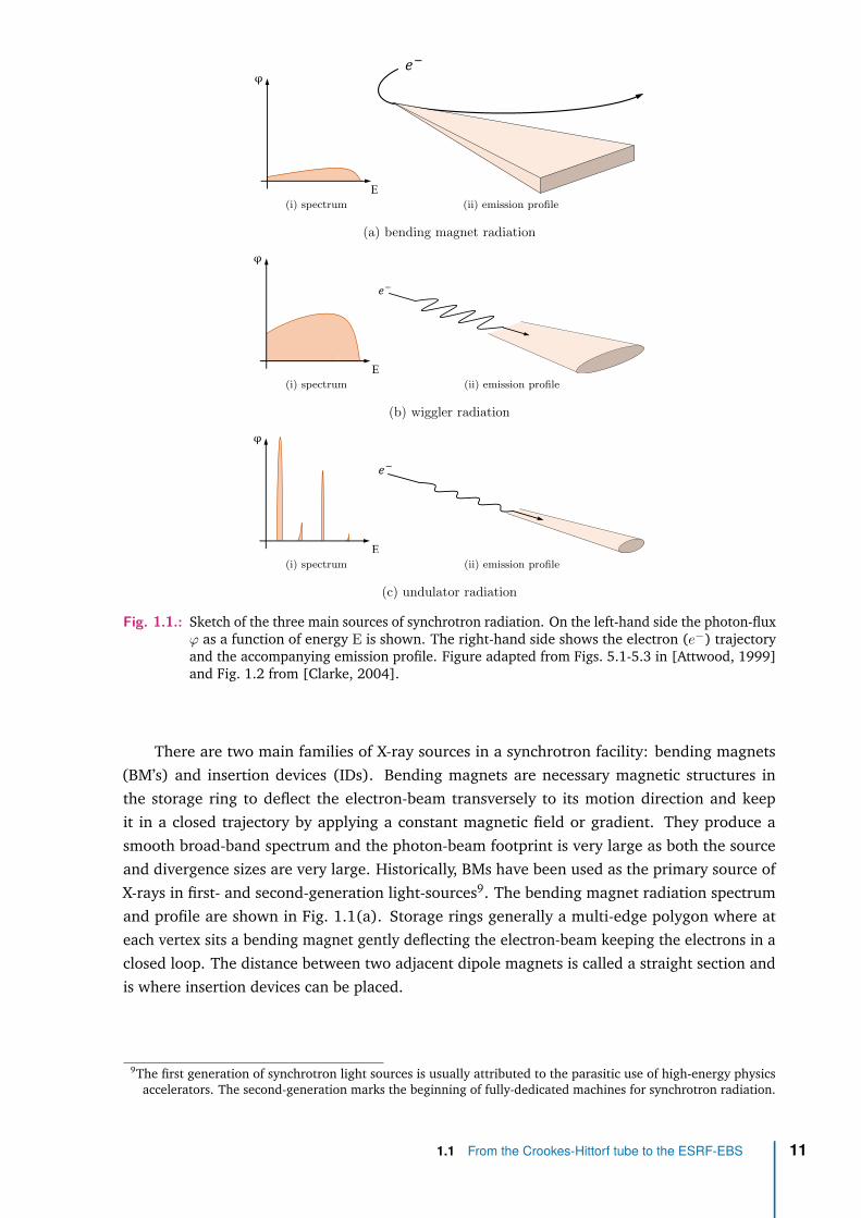
Fig. 1.1.: Sketch of the three main sources of synchrotron radiation. On the left-hand side the photon-fluxϕ as a function of energy E is shown. The right-hand side shows the electron (e−) trajectoryand the accompanying emission profile. Figure adapted from Figs. 5.1-5.3 in [Attwood, 1999]and Fig. 1.2 from [Clarke, 2004].
There are two main families of X-ray sources in a synchrotron facility: bending magnets(BM’s) and insertion devices (IDs). Bending magnets are necessary magnetic structures inthe storage ring to deflect the electron-beam transversely to its motion direction and keepit in a closed trajectory by applying a constant magnetic field or gradient. They produce asmooth broad-band spectrum and the photon-beam footprint is very large as both the sourceand divergence sizes are very large. Historically, BMs have been used as the primary source ofX-rays in first- and second-generation light-sources9. The bending magnet radiation spectrumand profile are shown in Fig. 1.1(a). Storage rings generally a multi-edge polygon where ateach vertex sits a bending magnet gently deflecting the electron-beam keeping the electrons in aclosed loop. The distance between two adjacent dipole magnets is called a straight section andis where insertion devices can be placed.
9The first generation of synchrotron light sources is usually attributed to the parasitic use of high-energy physicsaccelerators. The second-generation marks the beginning of fully-dedicated machines for synchrotron radiation.
1.1 From the Crookes-Hittorf tube to the ESRF-EBS 11

Insertion devices (IDs) are generally periodic magnetic structures that sinusoidally deflectthe electron-beam transversely to its direction of motion10. IDs can be sub-grouped into twocategories based on the amplitude of the electron motion inside them and their magnetic period:wigglers have a higher magnetic field applied to the electron-beam causing the amplitude ofelectron motion to be large. This generates a broad-band spectrum several times more intensethan that of a bending magnet (higher flux) - wigglers are also called wavelength shifters. Thebeam footprint is also very large: in the transverse direction the source size is enlarged and thebeam has a high divergence. Figure 1.1(b) shows the spectrum and emission profile of a wigglerinsertion device. The second member of the ID family is the undulator. In it, the amplitude ofthe transverse electron oscillations is much smaller than inside a wiggler. This is because in theundulators a less intense magnetic field is applied to the electrons and because the magneticperiod is usually smaller than the one of a wiggler. The small excursion of the electrons insidethe undulator accounts for a small photon source size with low divergence. Due to the lowelectron-motion amplitude, constructive interference between the emitted radiation occurs andthe spectrum of an undulator is composed of narrow-band peaks called undulator harmonics11.This is possible because, in an undulator, the electron excursion is smaller than the X-ray coneemission. Figure 1.1(c) shows the spectrum and emission profile of an undulator. A very usefulmetric used for summarising the effects of the and ultimately classifying an ID as a wiggler or anundulator is the dimensionless deflection parameter K given by
K = B0e
m0c
Λ2π , (1.3)
where B0 is the magnetic field, e is the electron charge, m0 is the electron rest mass, c is the lightspeed in vacuum and Λ is the magnetic period. It is generally accepted that IDs with K >> 1are classified as wigglers, while undulators have a K < 1 leaving a grey area where K is in therange of 1 to 10 and the radiation may exhibit some features of the wiggler or the undulator[Clarke, 2004, §3.1].
The advent of storage rings especially designed to accommodate ID’s marks the thirdgeneration of synchrotron light sources, from which the ESRF - European Synchrotron ResearchFacility (1994) in France is the pioneering machine, followed by the APS - Advanced PhotonSource (1996) in the USA and the SPring-8 - Super Photon ring-8 GeV (1999) in Japan.
1.1.2 High brilliance X-ray sources
The small photon source size and low divergence of the X-rays emitted by an undulator makeit a great candidate for generating high-brilliance X-ray beams. As Eq. 1.1 suggests, increasingthe brilliance for a given storage ring energy can be done by two different strategies: increasingthe photon flux, which is done by increasing the electron current in the storage ring; and/or byreducing the photon-beam emittance.
10It is important to acknowledge the existence of exotic ID designs that are not strictly periodic magnetic structures,namely the quasi-periodic undulator family [Onuki and Elleaume, 2013, §7.2].
11For diffraction-limited photon-beam emittances, if the observer is on-axis with the electron motion, only oddharmonics are observed. Away from the emission axis, even harmonics start being observed [Clarke, 2004, §4.2].
12 Chapter 1 On a new kind of rays

The radiation profile (beam sizes and divergences) emitted by an undulator is given by theconvolution between the electron-beam profile and the radiation pattern specific to the X-raysource12:
Σh,v = σeh,v ∗ σuh,v , (1.4a)
Σ′h,v = σ′eh,v ∗ σ′uh,v . (1.4b)
Here Σh,v and Σ′h,v are the already defined photon-beam size and divergence. The σeh,v and σ′eh,vrepresent the electron-beam size and divergence. Lastly, σuh,v and σ′uh,v are the specific radiationpattern size and divergence of the insertion device - these are then obtained by calculating theemission of a single-electron or a filament electron-beam (negligible dimension and divergence)passing through the magnetic field of the insertion device. Once designed, the specific radiationpattern of an undulator13 is considered to be a fundamental wavelength-dependent property ofthe insertion device14.
A closer look into Eqs. 1.4 allows one to suppose three distinct regimes for the photon-beamcharacteristics: a) εeh,v � εuh,v in this regime, the photon-beam characteristics are dominated bythe electron-beam, which is well approximated by a Gaussian distribution. This is usually thecase for horizontal emittance in third-generation synchrotrons; b) an intermediate state wherethe electron-beam emittance εeh,v is comparable to εuh,v leading to a photon-beam profile withclear contributions from both the electron-beam and specific radiation pattern of the undulator;c) the electron-beam emittance can be further reduced so that εeh,v � εuh,v and the photon-beamprofile is dominated by the undulator’s specific radiation pattern. Since εuh,v is a fundamentallimit, efforts to reducing the electron-beam beyond that limit will not have any impact in thephoton-beam profile. Mathematically, the three emittance regimes can be expressed as:
εh,v∣∣∣εeh,v�εuh,v
'(σeh,v ∗ δuh,v
)(σ′eh,v ∗ δuh,v
)= σeh,vσ
′eh,v , (1.5a)
εh,v∣∣∣εeh,v∼εuh,v
'(σeh,v ∗ σuh,v
)(σ′eh,v ∗ σ
′uh,v
)= Σh,vΣ′h,v, (1.5b)
εh,v∣∣∣εeh,v�εuh,v
'(δeh,v ∗ σuh,v
)(δeh,v ∗ σ
′uh,v
)= σuh,vσ
′uh,v . (1.5c)
Where δ represents the Dirac function. The electron-beam emittance matching to the undulator’sspecific radiation pattern is shown in Fig. 1.2. Fourth-generation synchrotron storage-ring-based
12This is true for any accelerator-based X-ray source - cf. chapter "3.10 - Photon beam features inherited from theelectron beam" in [Talman, 2006].
13The specific radiation pattern of an undulator is a function of its magnetic period, number of periods, magneticfield, storage ring energy and X-ray emission-wavelength.
14In the literature, there is a variety of formulae for calculating the specific radiation pattern size and divergence [Kim,1986, 1989; Tanaka and Kitamura, 2009; Onuki and Elleaume, 2013]. Different assumptions, approximationsand fits are done on their derivation. It is important to state that those are approximations and should not beregarded as fundamental results - please, refer to the discussion in [Walker, 2019]. The exact calculation of theradiation pattern can be done by computing the electric field of an electron subjected to an arbitrary magneticfield - cf. [Chubar, 1995, 2001] or by calculating the Wigner-function for synchrotron radiation [Bazarov, 2012]as in [Tanaka, 2014].
1.1 From the Crookes-Hittorf tube to the ESRF-EBS 13

𝜎
𝜎′
(a) εe � εu
𝜎
𝜎′
(b) εe ∼ εu
𝜎
𝜎′
(c) εe � εu
electron-beamspecific radiation patternphoton-beam
Fig. 1.2.: Matching of the electron-beam emittance to the undulator specific radiation pattern to increasethe photon-beam brilliance, where σ stands for beam size and σ′ for beam divergence. Adaptedfrom Fig. 21.20 in [Wiedemann, 2015].
light-sources15 use emittance-matching - Eq. 1.5(b) mainly, but ideally Eq. 1.5(c) - as the mainsource of increasing the X-ray brilliance16 [Wiedemann, 2015, §21.8.1].
1.1.3 Undulators as a primary source of coherent X-rays
Let’s consider the case of a filament electron-beam passing through a planar undulator. Theassociated emission at a resonant photon energy is almost symmetric and σuh ≈ σuv = σu andσ′uh = σ′uv = σ′u [Kim, 1989]. Because the electron bunch has negligible emittance εe in bothhorizontal and vertical directions, the photon-beam emittance is given by εh,v = σuσ
′u = εu. The
associated brilliance of such a filament beam is given by:
B0 = ϕ
4π2ε2u(1.6)
Since the emission of a filament electron-beam is fully-coherent, it makes sense to define acoherent photon flux of a zero-electron-emittance-beam:
ϕcoh. = 4π2ε2uB0 =(λ
2
)2
B0. (1.7)
15The fourth-generation synchrotron light sources or ultra-low emittance machines have been proposed as early as the1990s [Einfeld et al., 1996, 2014], but were deemed to be technologically unfeasible for high-energy storage rings[Ropert et al., 2000; Elleaume and Ropert, 2003]. Overcoming the technological barriers [Borland et al., 2014]was essential in paving the way for high energy storage rings with ultra-low emittance [Bei et al., 2010; Eriksson,2016]. The first machines to come online using the multi-bend-achromat design (MBA) are the MAX-IV in Sweden(2016) and the SIRIUS in Brazil (2019) - the former operating with two storage rings: 1.5 GeV and 3 GeV and thelatter operating at 3 GeV. The ESRF upgrade programme has opted for a hybrid-multi-bend-achromat (HMBA)magnetic lattice for its new storage ring [Biasci et al., 2014] and it is the first of its kind to operate at high-energies(6 GeV). The lattice concept behind the Extremely Brilliant Source (ESRF-EBS) has its origins in 2006 with theSuperB project for an electron-positron collider [P. Raimondi, 2017] and in early 2020 has produced the firstX-rays.
16This is because, with the new storage-ring designs (multi-bend-achromat and its variations), the electron-beamemittance can be routinely reduced by one to two orders of magnitude, when compared to current third-generationlight sources. To obtain equivalent gain in brilliance by just increasing the electron-beam current is very challengingin function of collective effects (coherent and incoherent). On top of that, there are thermal load issues on thevacuum system and on the beamline optics, that is, the X-ray transport system to the sample. This footnote is theresult of discussions with Pedro F. Tavares (MAX-IV, Sweden) and Boaz Nash (RadiaSoft LLC, USA).
14 Chapter 1 On a new kind of rays

Although Eq. 1.7 implies that εu = σuσ′u = λ/4π, it has been demonstrated that the non-Gaussian
behaviour of the undulator emission makes the photon-beam emittance approach asymptoticallyλ/2π instead [Onuki and Elleaume, 2013; Tanaka and Kitamura, 2009]. However, it is importantto mention that the right-hand side of Eq. 1.7 is valid for any symmetric electric field distributionat any value of undulator detuning and it does not depend on a Gaussian approximation of theundulator specific radiation pattern [Walker, 2019]. One can define the coherent fraction asthe ratio between the coherent flux ϕcoh. (Eq. 1.7) and the nominal photon-flux ϕ = 4π2εhεvB0
(Eq. 1.1):
ζ = ϕcoh.ϕ
= ε2uεhεv
. (1.8)
Eq. 1.8 allows to deduce that by reducing the electron-beam emittance, the coherence fractionis increased (cf. Eqs. 1.5). An important conclusion to be drawn is that emittance-matching as aform of increasing the photon-beam brilliance in fourth-generation synchrotrons increases theX-ray beam transverse (spatial) coherence17.
Temporal Coherence
Lastly, the temporal coherence18 of the synchrotron radiation emitted by storage rings shouldbe addressed. Without further conditioning, the radiation emitted on the X-ray region exhibitslow temporal coherence for high energies. Spectral filtering with monochromators increases thetemporal coherence at the expense of photon-flux reduction. Compressing the electron bunchlength also offers an increased temporal coherence for X-rays, as coherent synchrotron radiation(CSR) naturally appears when the electron-beam bunch length is comparable to the observedradiation wavelength - cf. [Chubar, 2006], [Talman, 2006, §3.8 & §13] and [Wiedemann, 2015,§21.7].
Recommended literature
The correct description of the electron-beam inside each different source of X-rays in astorage ring is of primary importance for accurate modelling of the radiation spectrum andphoton spatial distribution, with consequences for X-ray optical design. An extensive review onparticle accelerator physics is given by [Duke, 2000] and by [Wiedemann, 2015]. An in-depthlook into X-rays from accelerator sources can be found in [Clarke, 2004], in [Talman, 2006] andin [Onuki and Elleaume, 2013].
The accurate calculation of the brilliance from undulators in low-emittance accelerators andthe coherence properties of the emitted X-rays is an active area of research topic and a deeperlook into it is offered by [Bazarov, 2012; Tanaka, 2014; Geloni et al., 2015, 2008; Walker, 2019;Khubbutdinov et al., 2019]. See also [Singer and Vartanyants, 2014].
17Please, refer to §1.2.3 - Optical coherence for a definition of spatial and temporal coherence.18See footnote 17.
1.1 From the Crookes-Hittorf tube to the ESRF-EBS 15

Quantum opticsElectromagnetic opticsWave opticsRay optics
Classical optics
Fig. 1.3.: Hierarchical optical theories. Optical modelling in the X-ray regime can be accurately rep-resented in the realms of wave optics for most cases where coherence effects are present.Adapted from Fig. 1.0-1 in [Saleh and Teich, 2019].
1.2 Physical optics
The increasing coherent fraction of X-rays from fourth-generation storage rings requires anappropriate framework for their representation. Light can be described by an electromagneticwave phenomenon governed by the Maxwell equations - cf. [Born et al., 1999, §1.1]:
∇ · E = ρ
ε(Gauß’s law), (1.9a)
∇ · B = 0 (Gauß’s law for magnetism), (1.9b)
∇× E = − ∂
∂tB (Faraday’s law), (1.9c)
∇× B = µ
(J + ε
∂
∂tE
)(Ampère’s law modified by Maxwell). (1.9d)
Where E ≡ E(x, y, z, t) is the electric field, B ≡ B(x, y, z, t) is the magnetic induction, ε ≡ε(x, y, z, t) and µ ≡ µ(x, y, z, t) are the electric permittivity and magnetic permeability, ρ ≡ρ(x, y, z, t) is the charge density and J ≡ J(x, y, z, t) is the current density. The operator ∇ · •denotes the divergence of a vectorial field (scalar function) and ∇ × • is the curl operator(vectorial function), where • is a generic vectorial field. The Cartesian coordinates (x, y, z) andtime t have been omitted in favour of a more compact notation. Although electromagnetic opticsprovides the most complete framework for classical optical phenomena, it is possible to moveaway from the vectorial treatment of light towards a scalar wave theory in order treat a largevariety of relevant optical phenomena. This simplified treatment of light is commonly referredto scalar wave optics or physical optics (cf. Fig. 1.3 for the hierarchical representaion of opticaltheories). X-ray wave-fields in free-space are discussed in §1.2.1 - Free-space propagation andtheir transmission through generic refractive optical elements is discussed in §1.2.2 - Transmissionelements.
1.2.1 Free-space propagation
In order to describe wave-fields in free-space under the scalar theory, one usually starts19
by obtaining the Maxwell equations for free-space (vacuum). This is done considering that the
19The developments in §1.2.1 - Free-space propagation are inspired by the derivations from [Paganin, 2006, §1] and[Goodman, 2017, §3 & §4].
16 Chapter 1 On a new kind of rays
medium where the wave-fields exist are uncharged and non-conducting, which is done by lettingρ = 0 and J = 0 in Eqs. 1.9a and 1.9d:
∇ · E = 0, (1.10a)
∇× B = µ0ε0∂
∂tE. (1.10b)
Where ε0 and µ0 are the vacuum electric permittivity and magnetic permeability. Direct conse-quences of deriving the scalar theory for waves in vacuum is that the medium is assumed to belinear (permittivity is linear), isotropic (permittivity is independent of polarisation direction),homogeneous (permittivity is constant within the region of propagation), nondispersive (permit-tivity is independent of wavelength throughout the region of interest) and, finally, nonmagnetic(the magnetic permeability constant and equal to µ0) [Goodman, 2017, §3.2].
The wave-equation
The d’Alembert wave-equation for the electric field can be obtained by applying the curloperator ∇× • to both sides of Faraday’s law, using the vector calculus identity ∇× (∇× •) =∇(∇ · •)−∇2• to the electric field E, and making use of the Maxwell equations for free-space(Eqs. 1.9 and 1.10): (
ε0µ0∂2
∂t2−∇2
)E = 0. (1.11)
The same reasoning can be applied to the magnetic induction B:(ε0µ0
∂2
∂t2−∇2
)B = 0. (1.12)
Each vectorial component of E and B satisfies individually a scalar form of the wave-equation andeach of the individual components are uncoupled from each other - cf. [Paganin, 2006, §1.1]. Itis possible to define a (complex) scalar field u(x, y, z, t) representing any of the components of Eor B such that: (
1c2∂2
∂t2−∇2
)u = 0. (1.13)
with c = 1/√ε0µ0 (speed of light in vacuum). This complex scalar solution of the d’Alembertequation can be spectrally decomposed as a superposition of monochromatic fields using theFourier transform:
u(x, y, z, t) = 1√2π
∞∫−∞
U(x, y, z) exp (−iωt) dω (1.14)
The argument of the integral in Eq. 1.14 implies that the monochromatic field can be writtendown as a product of a spatial dependent function and a time dependent function (separation ofvariables) [Paganin, 2006, §1.2]. Plugging Eq. 1.14 in Eq. 1.13:
(∇2 + k2)U(x, y, z) = 0, (1.15)
where k = ω/c = 2π/λ is the wavevenumber and λ, the associated wavelength. Eq. 1.15 isknow as the Helmholtz equation. Given a volume in space and boundary conditions, the scalar
1.2 Physical optics 17

diffraction theory consists in finding the solutions to q. 1.15 [Paganin, 2006, §1.2]. One of thesimplest solutions to the Helmholtz equation in free-space is the so-called plane-wave:
U(r) = A exp(−ik · r) = A exp[−i(kxx+ kyy + kzz)], (1.16)
where A is a complex constant (complex envelope), k = (kx, ky, kz) is the wavevector such as|k| = k and r = (x, y, z). A second solution is a spherical wave:
U(r) = A
rexp(−ikr), (1.17)
here |r| = r =√x2 + y2 + z2 is the distance from the origin of the wavefront. Defining
henceforth the z−axis as the optical axis, the paraboloidal wave is given by:
U(r) = A
zexp(−ikz) exp
(− ikx
2 + y2
2z
), (1.18)
Eq. 1.18 is a paraxial20 approximation of the spherical wave defined by Eq. 1.17. The paraboloidalwave does not, however, formally satisfy the Helmholtz equation as defined by Eq. 1.15. It doesobey a paraxial form of the Helmholtz wave-equation21. This assumes a plane wave as definedin Eq. 1.16 can be modulated by a complex envelope A(r) that slowly varies along a distanceλ = 2π/k along the optical axis z. It can be shown22 that plugging this modulated plane-wave inthe Helmholtz equation (Eq. 1.15) leads to:(
i2k ∂∂z−∇2
T
)A = 0. (1.19)
where ∇2T ≡ ∂2/∂x2 + ∂2/∂y2 is the transverse Laplace operator. Eq. 1.19 is the paraxial
Helmholtz equation [Saleh and Teich, 2019, §2.2]. Determining the evolution in space of thesolutions to the Helmholtz equation (Eq. 1.15) or the paraxial Helmholtz equation (Eq. 1.19) isthe core of what is called scalar diffraction theory.
Fresnel diffraction
Consider a Cartesian coordinate system where the z−axis is the optical axis (cf. Fig 1.4),suppose a transverse component of a wave-field complying with Eq. 1.15 can be completelydescribed at a position z0, that is, U(x, y, z0) is known for all the xy−plane. The wave-field
20Consider a spherical wave with r = (x, y, z) and that |r| = r =√x2 + y2 + z2 and take a sufficiently large
coordinate along the z−axis (optical axis). The paraxial approximation of the spherical wave can be obtainedby choosing points in the xy−plane near enough to the z−axis so that
√x2 + y2 � z holds. It follows that
r = z√
1 + (x2 + y2)/z2 can be expanded in a Taylor series: r ≈ z + (x2 + y2)/2z and directly plugged intothe exponent in Eq. 1.17 leading to Eq. 1.18 [Saleh and Teich, 2019, §2.2]. The paraxial approximation of thespherical wave is also called the Fresnel approximation.
21The Gaussian beam is another very common solution of the paraxial Helmholtz equation. Consider the paraboloidalwave as defined by Eq. 1.18. Evaluating it along the optical axis at a position z+ = z + ∆z also yields a solutionto the paraxial Helmholtz equation (cf. Eq. 1.19) even if ∆z is a purely imaginary number [Saleh and Teich, 2019,Exercise 2.2-2]. The Gaussian beam can be obtained from the paraboloidal wave by substituting z in Eq. 1.18 byz − iz0, for a real z0 [Saleh and Teich, 2019, §3.1]
22The complete derivation of the paraxial wave-equation can be found in [Saleh and Teich, 2019, §2.2.C].
18 Chapter 1 On a new kind of rays
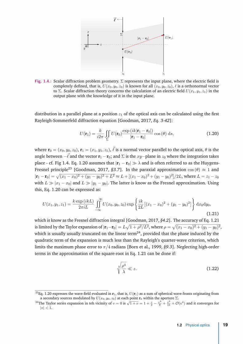
ℓ
U(r0)
U(r1)
z0 z1
|r1 – r0|Σ
x
yz
Fig. 1.4.: Scalar diffraction problem geometry. Σ represents the input plane, where the electric field iscompletely defined, that is, U(x0, y0, z0) is known for all (x0, y0, z0), ` is a orthonormal vectorto Σ. Scalar diffraction theory concerns the calculation of an electric field U(x1, y1, z1) in theoutput plane with the knowledge of it in the input plane.
distribution in a parallel plane at a position z1 of the optical axis can be calculated using the firstRayleigh-Sommerfeld diffraction equation [Goodman, 2017, Eq. 3-42]:
U(r1) = k
i2π
x
ΣU(r0)exp (ik|r1 − r0|)
|r1 − r0|cos (θ) ds, (1.20)
where r0 = (x0, y0, z0), r1 = (x1, y1, z1), ~ is a normal vector parallel to the optical axis, θ is theangle between −~ and the vector r1− r0; and Σ is the xy−plane in z0 where the integration takesplace - cf. Fig 1.4. Eq. 1.20 assumes that |r1 − r0| � λ and is often referred to as the Huygens-Fresnel principle23 [Goodman, 2017, §3.7]. In the paraxial approximation cos (θ) ≈ 1 and|r1− r0| =
√(x1 − x0)2 + (y1 − y0)2 + L2 ≈ L+ [(x1− x0)2 + (y1− y0)2]/2L, where L = z1− z0
with L� |x1 − x0| and L� |y1 − y0|. The latter is know as the Fresnel approximation. Usingthis, Eq. 1.20 can be expressed as:
U(x1, y1, z1) = k exp (ikL)2πiL
∞x
−∞U(x0, y0, z0) exp
{ik
2L[(x1 − x0)2 + (y1 − y0)2]} dx0dy0,
(1.21)which is know as the Fresnel diffraction integral [Goodman, 2017, §4.2]. The accuracy of Eq. 1.21is limited by the Taylor expansion of |r1−r0| = L
√1 + ρ2/L2, where ρ =
√(x1 − x0)2 + (y1 − y0)2,
which is usually usually truncated on the linear term24, provided that the phase induced by thequadratic term of the expansion is much less than the Rayleigh’s quarter-wave criterion, whichlimits the maximum phase error to π/4 radians [Born et al., 1999, §9.3]. Neglecting high-orderterms in the approximation of the square-root in Eq. 1.21 can be done if:
3
√ρ4
λ� z. (1.22)
23Eq. 1.20 expresses the wave-field evaluated in r1, that is, U(r1) as a sum of spherical wave-fronts originating froma secondary sources modulated by U(x0, y0, z0) at each point r0 within the aperture Σ.
24The Taylor series expansion in teh vicinity of v = 0 is√
1 + v = 1 + v2 −
v2
8 + v3
16 + O(v4) and it converges for|v| < 1.
1.2 Physical optics 19

Fraunhofer diffraction
Still analysing Eq. 1.21, the quadratic term in the exponential part of the integrand can beexpanded and rearranged:
U(x1, y1, z1) = k exp (ikL)2πiL exp
[ik
2L(x21 + y2
1)]·
·∞x
−∞U(x0, y0, z0) exp
[ik
2L(x2
0 + y20 − 2x1x0 − 2y1y0)
]dx0dy0. (1.23)
Applying the Rayleigh’s quarter-wave criterion to the k(x20 + y2
0)/2L term in Eq. 1.23:
4x20 + y2
0λ
� z, (1.24)
which allows to further simplify Eq. 1.21 into:
U(x1, y1, z1) = k exp (ikL)2πiL exp
[ik
2L(x21 + y2
1)]·
·∞x
−∞U(x0, y0, z0) exp
[− ik
L
(x1x0 + y1y0)
]dx0dy0, (1.25)
Eq. 1.25 is known as the Fraunhofer diffraction integral.
Numerical computation of the Fresnel and Fraunhofer diffraction
The numerical calculation of the diffraction integrals is a vast subject and has been addressedby many authors [D’Arcio et al., 1994], [Kelly, 2014], [Goodman, 2017, §5], [Buitrago-Duqueand Garcia-Sucerquia, 2019] and [Chubar and Celestre, 2019], among others. This arises fromthe fact that unless the resulting field U(x1, y1, z1) has an analytical representation, numericallycalculating the integrals in Eq. 1.21 and Eq. 1.25 will forcefully result in tackling issues likereplicas and aliasing. This comes from the fact that the diffraction integrals are intimatelyconnected with the Fourier analysis.
Upon closer inspection, it is apparent that the Fresnel diffraction integral (Eq. 1.21) is atwo-dimensional convolution type integral [Goodman, 2017, §2.1]:
g(x, y) ∗ h(x, y) =∞x
−∞g(u, v)h(x− u, y − u) dudv, (1.26)
which can be computed by invoking the convolution theorem:
g(x, y) ∗ h(x, y) = F−1{F{g(x, y)} · F{h(x, y)}}, (1.27)
20 Chapter 1 On a new kind of rays

ROI
(a) analytical solution
ROI
(b)
ROI
(c)
ROI
(d)
Fig. 1.5.: Replicas and aliasing from numeric calculations of the diffraction integrals. (a) analyticalsolution of the integrals have no signal replicas. Sampling the input plane signal will introducereplicas in the output plane [Kelly, 2014]. (b) appropriate sampling - cf. Eq. 5 in [Chubar andCelestre, 2019] - makes the unavoidable replicas appear far enough so that cross-talk betweenthem is negligible within the region of interest (ROI). (c) coarser sampling brings replicascloser together to a point that (d) replicas are so close that aliasing is apparent (red signal).
where F{•} is the two-dimensional Fourier transform and F−1{•} denotes inverse Fouriertransform:
F{g(x, y)} =∞x
−∞g(x, y) exp
[− i2π(fxx+ fyy)
]dxdy (1.28a)
F−1{G(fx, fy)} =∞x
−∞G(fx, fy) exp
[i2π(fxx+ fyy)
]dfxdfy. (1.28b)
It is common to represent the Fourier analysis and syntheses as F{g(x, y)} ≡ G(fx, fy) andF−1{G(fx, fy)} ≡ g(x, y), where (fx, fy) are generally referred to as frequencies. The Fresneldiffraction integral in Eq. 1.21 can be rewritten as a convolution (Eq. 1.27) where the kernel,that is F{h(x, y)}, has an analytical solution:
k
2πiLF{h(x, y)} = k
2πiLF{
exp[ik
2L(x2 + y2)]} = exp
[− i2Lπ2
k
(f2x + f2
y
)], (1.29)
This formulation allows to calculate the Fresnel diffraction integral (Eq. 1.21) by means of theconvolution theorem (Eq. 1.27) by applying a Fourier transform to the input field, multiplyingit by an analytical kernel and applying an inverse Fourier transform to the result. It is alsoevident that the Fraunhofer diffraction integral (Eq. 1.25) is a Fourier type integral, differingfrom Eq. 1.28a by a multiplicative factor outside the integrand.
1.2 Physical optics 21

It should be clear, then, that the paraxial diffraction equations are intertwined with Fourieranalysis. Numerically computation of the Fresnel or Fraunhofer diffraction implies a-) samplingthe input plane U(x0, y0, z0) and b-) limiting its extent by either defining an aperture of finiteextent or simply by cropping (truncating) the input field. It follows from sampling theory andthe discrete Fourier transform (DFT) [Bracewell, 2000, §10 & §11] that sampling the input fieldcauses replicas of the main signal to appear (cf. Fig. 1.5). Generally, the finer the sampling inthe input plane, the further apart the replicas. Consequently, the coarser the mesh, the closerthey become until the replicas are close enough to each other that they start cross-talking. Theinteraction between the main signal and its replicas is called aliasing. Due to the finite extentof the input plane (either by limiting the signal with an aperture or by simply truncating it), itis inevitable that power from neighbouring replicas leaks into each other. Sampling should besufficiently high to make this inevitable cross-talk negligible [Kelly, 2014]. On the other hand,a very dense sampling leads to very inefficient calculations largely because of the size of theinput and output planes - cf. considerations in [Goodman, 2015, §5]. Efforts towards memoryand CPU efficient computation of the Fresnel free-space propagator in Fourier optics have beenreported in [Chubar and Celestre, 2019].
1.2.2 Transmission elements
The propagation of X-rays in the presence of matter can also be modelled with the Maxwellequations (Eqs. 1.9). It is possible to derive a Helmholtz equation in the presence of scattererswith a similar treatment given in the previous section, albeit considerably more algebraic - adetailed account of the derivation is given by [Paganin, 2006, §2.1]. Restricting the analysisto linear isotropic non-magnetic materials where both the electric permittivity and magneticpermeability are independent of time (static medium) and considering again that the waves existin a uncharged and non-conducting material, that is, ρ = 0 and J = 0:[
ε(x, y, z)µ0∂2
∂t2−∇2
]E(x, y, z, t) = 0, (1.30a)
[ε(x, y, z)µ0
∂2
∂t2−∇2
]B(x, y, z, t) = 0. (1.30b)
considering that the scatterers are sufficiently slowly varying when compared to the radiationwavelength - cf. Eqs. 2.18-2.21 in [Paganin, 2006]. Eqs. 1.30 resemble the vectorial wave-equations 1.11 and 1.12. This enables application of the same scalar treatment used for derivingthe Helmholtz equation in free-space, that is, to propose a scalar field u(x, y, z, t) such as:
[ε(x, y, z)µ0
∂2
∂t2−∇2
]u = 0, (1.31)
and spectrally decompose u in its monochromatic Fourier components U(x, y, z) exp (−iωt) (cf.Eq. 1.14):
u(x, y, z, t) = 1√2π
∞∫−∞
U(x, y, z) exp (−iωt) dω
22 Chapter 1 On a new kind of rays
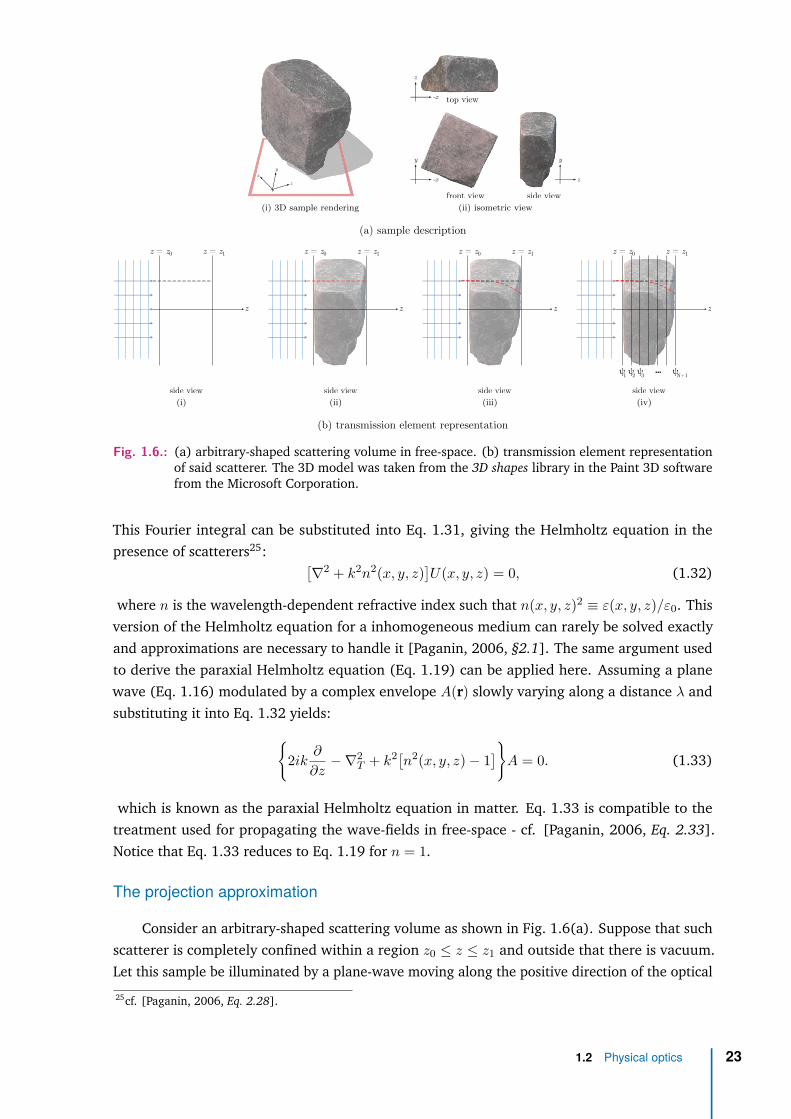
y
z
x
(i) 3D sample rendering
top view
front view side view
y
-x
y
z
z
-x
(ii) isometric view
(a) sample description
z
z = z0
side view
z = z1
(i)
z
side view
z = z0 z = z1
(ii)
z
side view
z = z0 z = z1
(iii)
ψ1ψ2ψ3
ψN+1
z
side view
z = z0 z = z1
(iv)
(b) transmission element representation
Fig. 1.6.: (a) arbitrary-shaped scattering volume in free-space. (b) transmission element representationof said scatterer. The 3D model was taken from the 3D shapes library in the Paint 3D softwarefrom the Microsoft Corporation.
This Fourier integral can be substituted into Eq. 1.31, giving the Helmholtz equation in thepresence of scatterers25: [
∇2 + k2n2(x, y, z)]U(x, y, z) = 0, (1.32)
where n is the wavelength-dependent refractive index such that n(x, y, z)2 ≡ ε(x, y, z)/ε0. Thisversion of the Helmholtz equation for a inhomogeneous medium can rarely be solved exactlyand approximations are necessary to handle it [Paganin, 2006, §2.1]. The same argument usedto derive the paraxial Helmholtz equation (Eq. 1.19) can be applied here. Assuming a planewave (Eq. 1.16) modulated by a complex envelope A(r) slowly varying along a distance λ andsubstituting it into Eq. 1.32 yields:{
2ik ∂∂z−∇2
T + k2[n2(x, y, z)− 1]}A = 0. (1.33)
which is known as the paraxial Helmholtz equation in matter. Eq. 1.33 is compatible to thetreatment used for propagating the wave-fields in free-space - cf. [Paganin, 2006, Eq. 2.33].Notice that Eq. 1.33 reduces to Eq. 1.19 for n = 1.
The projection approximation
Consider an arbitrary-shaped scattering volume as shown in Fig. 1.6(a). Suppose that suchscatterer is completely confined within a region z0 ≤ z ≤ z1 and outside that there is vacuum.Let this sample be illuminated by a plane-wave moving along the positive direction of the optical
25cf. [Paganin, 2006, Eq. 2.28].
1.2 Physical optics 23

axis (z−axis). In the absence of the scatterer, the gradient between the z = z0 and z = z1 planesis very well defined and parallel to the optical axis, as shown in Fig. 1.6(b-i). It follows from[Paganin, 2006, §2.2] that if the scatterer is sufficiently weak as to minimally disturb the paththat the wave-field would have taken in its absence, cf. Fig. 1.6(b-ii), the transmission of awave-field through this sample is given by:
U(x, y, z1) ≈ exp{− ik
2
z=z1∫z=z0
[1− n2(x, y, z)
]dz}U(x, y, z0). (1.34)
Eq. 1.34 shows that the effect of a weak scatterer can be accounted by a multiplicative complextransmission element represented by the complex exponential. In the X-ray regime the indexof refraction is typically very close to unity and often expressed as n = 1 − δ + i · β [Als-Nielsen and McMorrow, 2011, §1.6], which allows for the approximation 1 − n(x, y, z)2 ≈2[δ(x, y, z) + i · β(x, y, z)
]that can be substituted in Eq. 1.34. The z−dependence of δ and β is
abandoned in the projection approximation, hence the complex transmission element in Eq. 1.34can be reduced to:
T(x, y, z) = exp{− ik
z=z1∫z=z0
[δ(x, y) + i · β(x, y)
]dz}
= exp{− ik
[δ(x, y) + i · β(x, y)
]∆z(x, y)
},
T[∆z(x, y)] =
√TBL(x, y) exp
[iφ(x, y)
]. (1.35)
and:
TBL(x, y) = exp[− 2kβ(x, y)∆z(x, y)
](1.36a)
= exp[− µ(x, y)∆z(x, y)
],
φ(x, y) = −kδ(x, y)∆z(x, y). (1.36b)
∆z is the projected thickness along the z−axis and it depends on the transverse coordinates(x, y), which can be dropped out for a more concise representation.
Because of the multiplicative nature of the transmission element, Eq. 1.35 can be put inoperator26 form:
T(∆z) • =√
TBL(∆z) exp [iφ(∆z)] • . (1.37)
Eq. 1.36a shows the absorption experienced by the wave-field when passing through matter(Beer-Lambert law) and Eq. 1.36b shows the phase-shift experienced by the wave-field. Thecoefficient µ multiplying ∆z in TBL (Eq. 1.36a) is known as the linear attenuation coefficient µ[Als-Nielsen and McMorrow, 2011, §1.6].
26Using the operator formulation was inspired by discussions with David Paganin (Monash University, Australia) andVincent Favre-Nicolin (ESRF, France).
24 Chapter 1 On a new kind of rays

The multi-slice approximation
For the cases where the projection approximation may not be adequate to correctly representthe scattering volume in question, multi-slicing techniques27 (MS) can be used for describing thewave-field propagation inside an arbitrary-shaped scattering volume - cf. discussion in [Paganin,2006, §2.7], [Li et al., 2017] and [Munro, 2019].
Consider the scatterer depicted in Fig. 1.6(a). If its presence considerably disturbs the paththat the wave-field would have taken in its absence, cf. Fig. 1.6(b-iii), it is possible to section thesample into a number N of parallel slabs until the projection approximation is valid betweentwo adjacent slices - Fig. 1.6(b-iv). The projected thickness ∆z to be used in Eq. 1.35 is the onein between slices, which are ∆S = (z1 − z0)/N apart from each other. Each slice representedas a thin element in projection approximation is separated by vacuum. The propagation of awave-field propagation through this sample is done step-wise, where each step is composed ofa multiplication by a complex transmission element in projection approximation (cf. Eq. 1.35)and a Fresnel free-space propagation (Eq. 1.21) over a distance ∆S . The output field from thisoperation is again multiplied by complex transmission element in projection approximationfollowed by a free-space propagation from the plane ψj to the ψj+1 - refer to Fig. 1.6(b-iv).This operation is done recursively N times until the wave-field emerges from the sample. Themulti-slicing transmission operator can be written in operator form as:
TMS =N∏j=1D(∆S)
[Tj(∆z) •
](1.38)
where∏
indicates concatenation of operators to be performed from right to left, D(∆S) is theoperator formulation of the Fresnel free-space propagation over a distance ∆S:
D(∆S) • = k exp (ik∆S)2πi∆S
∞x
−∞• exp
{ik
2∆S
[(x1 − x)2 + (y1 − y)2]} dxdy, (1.39)
and Tj(∆z) is the j−th complex transmission element operator in projection approximationassociated with the j−th slice given by Eq. 1.37.
– On the validity of the Fresnel approximation for short propagation distances28
A case of particular importance for X-ray optical design is the application of the Fresnelpropagators in real or reciprocal space to very short propagation distances (from millimetresto hundreds of micrometres) at hard X-ray energies (wavelength of the order of the Ångstrom)with physical apertures of the order of the millimetre. For situations of practical interest such asthe one just described, Eq. 1.22 is generally very restrictive. This section presents conditionsunder which this constraint can be relaxed and even overlooked.
27This technique was first described in the context of the scattering of electrons by atoms and crystals [Cowley andMoodie, 1957].
28The author acknowledges the fruitful discussions with David Paganin (Monash University, Australia), Peter Munro(University College London, England), Oleg Chubar (Brookhaven National Lab., USA) and Chris Jacobsen (North-western University/Argonne National Lab., USA) when investigating the application of the Fresnel approximationfor short propagation distances.
1.2 Physical optics 25

Consider an X-ray wavefield with wavelength λ = 1 Å fully illuminating an apertureA = 500 µm situated at z = z0 along the optical axis as shown in Fig. 1.4. The X-rays passingthrough such an aperture will illuminate an identical aperture A at a distance z1 − z0 = L.Suppose one wants to place the second aperture at a distance L such that it is possible tocalculate the field distribution in z1 using the Fresnel diffraction integral in Eq. 1.21. UsingEq. 1.22 with the extreme points29 given by (x0 = −A/2, y0 = 0) and (x1 = A/2, y1 = 0), oneconcludes that L� 86 mm. However, if one wants to place the second aperture at a distance ofL = 1 mm and still be able to safely apply Eq. 1.21 to calculate the field distribution in z0, theapertures should be reduced to A� 18 µm according to Eq. 1.22. The situation just described isat odds with the employment of the Fresnel propagator for very short propagation distances athard X-ray energies with physical apertures of the order of the millimetre. Yet, with the exceptionof [Ali and Jacobsen, 2020], that explicitly uses the Huygens-Fresnel principle [Goodman, 2017,§3.7] in its reciprocal form for the wavefield propagation30, authors make extensive use of theFresnel propagator for multi-slicing applications under these conflicting conditions [Li et al.,2017; Munro, 2019; Celestre et al., 2020]. Possibly one of the few explicit mentions of thepropagation distance relation to the transverse plane size applied to multi-slicing techniquesis given by Eq. 15 in [Ishizuka and Uyeda, 1977]. It turns out that, indeed, Eq. 1.22, whenapplied to a collimated beam (either a plane-wave or a slowly diverging/converging wave), istoo restrictive and can be overlooked when applied to MS modelling of weak scatterers.
In [Southwell, 1981] the Fresnel diffraction integral (Eq. 1.21) is directly compared withthe Huygens-Fresnel integral (Eq. 1.20) in terms of amplitude and phase, it was shown thatthe Fresnel approximation has good accuracy: within 2% in amplitude and 0.02 rad in phase,when compared to the Huygens-Fresnel integral. The findings hold even for very high Fresnelnumbers31 along the optical axis within the projected aperture, that is, ∀ (x, y) ∈ A - [cf. Figs. 1–4 ibid.]. However, for points outside that region (∀ (x, y) /∈ A) at very high Fresnel numbers(shadow region), the approximation breaks down: although the amplitude calculation retainsgood agreement, the phase errors become unacceptably high [cf. Fig. 10 ibid.].
Another study that confirms the validity of the Fresnel approximation for a collimated beambeing propagated over a very short distance is presented by [Rees, 1987]. This work not onlyconfirms the numerical findings in [Southwell, 1981] but also provides physical explanations,some analytical formulations and derives quantitatively the shape of the region where the Fresnelapproximation is valid. By applying directly Eq. 1.22 and Eq. 1.24, one obtains the the regionsof validity for both Fresnel and Fraunhofer integrals as shown in Fig. 1.7(a), in which case,zFresnel is given by Eq. 1.22 - cf. Eq. 7 in [Rees, 1987]. The relaxing of such constraints is doneby invoking the concept of Fresnel zones32 and how much contribution they have to the totalamplitude and phase of the propagated beam. Considering that the first zone is unobstructed by
29For simplicity, the 1D case is analysed, but the conclusions are easily translated to a 2D system if U(x, y) =U(x)U(y).
30cf. Eq. 22 or procedure PropShort in Algorithm 1 from [Ali and Jacobsen, 2020].31The Fresnel number is defined as NF = a2/λL, where a is the half aperture, λ is the wavelength and L is the
propagation distance. A high Fresnel number indicates the region known as near-field, while the far-field regionis known for its low Fresnel numbers. In [Southwell, 1981], it is reported that even for L < a good agreementbetween the Fresnel approximation and the Huygens-Fresnel integral is found for a point within the projectedaperture.
32cf. [Hetch, 2017, §10.3.1]
26 Chapter 1 On a new kind of rays

(a) (b)
Fig. 1.7.: The Fresnel and Fraunhofer approximations region of validity according to the (a) Eqs. 1.22and 1.24. For a gently divergent, convergent or plane wavefield the constraints can berelaxed, increasing the region o applicability of said approximations. Region I represents theshadow zone, where neither approximations are valid. Region II is where only the Fresnelapproximation is valid. In region III, both approximations coexist, the Fraunhofer beingadvantageous computationally. Region IV illustrates an area where only the Fraunhoferapproximation is valid - this counter-intuitive result is discussed in [Rees, 1987], but is outof the scope here. The boundaries between regions I and II have been exaggerated for clarity.This figure is adapted from Fig. 4 and Fig. 5 in [Rees, 1987].
the aperture A, which is the case for all points not within the shadow region, the distance wherethe Fresnel diffraction integral starts to be accurate can be as low as zFresnel = 2λ - cf. Eq. 9 in[Rees, 1987]. This more relaxed regime is represented in Fig. 1.7(b).
Based on the results from [Southwell, 1981] and [Rees, 1987], it is possible to affirm thatprovided the object is illuminated with a plane wave and the output field is calculated in thevicinity of the projected aperture, the application of the Fresnel diffraction integral to very shortpropagation distances for hard X-ray optics modelling with MS techniques is not limited tothe constraints imposed by Eq. 1.22. Cases of interest often have non-plane-wave illuminationand require special handling to ensure MS with the Fresnel diffraction integral yields accurateresults. Approaches that rely on spherical-to-plane-wave conversion are often employed toavoid such accuracy issues: the angular spectrum of plane waves decomposition [Paganin, 2006,§1.3]33, the Fresnel-scaling theorem [Paganin, 2006, §A], the divergent-beam-to-plane-wavetransformation from [Munro, 2019] and the analytical treatment of the quadratic phase term[Chubar and Celestre, 2019], which is of particular interest within the context of this work, as itis the chosen method for the free-space wavefront propagation simulations presented here.
– Real and reciprocal space Fresnel propagators at short propagation distances
Because of the equivalency of the Fresnel diffraction integral (Eq. 1.21) and the convolutionintegral (Eq. 1.26), one can define the kernel of the Fresnel transform in real-space as:
h(x, y) = exp[iπ
λL
(x2 + y2)], (1.40)
33Also in [Goodman, 2017, §3.10 & §4.2.4].
1.2 Physical optics 27

while the kernel of the Fresnel transform in reciprocal-space is given by:
H(fx, fy) = exp[− iπλL
(f2x + f2
y
)]. (1.41)
The Eqs. 1.40 and 1.41 are related by: H(fx, fy) = i/(λL) · F{h(x, y)} (cf. Eq. 1.29). Whenpropagating a wave-field over a very small distance L with the Fresnel diffraction integral, theargument of the exponential function in the transformation kernel in real-space becomes verylarge and the kernel becomes less well-behaved due to fast oscillations, consequently smallpropagation distances are better represented in the reciprocal space. This hints to the fact thatwhen numerically evaluating the Fresnel transform for short propagation distances, methodsusing the reciprocal-space are more advantageous than in real-space and constrains like theEq. 1.22 can be overlooked provided the non-paraxial components of the Fourier spectrum ofthe input wavefield is negligible.
– The analytical treatment of the of the quadratic radiation phase term34
Consider an uncollimated wave-field U(x0, y0, z0) in free-space (eg. Eq. 1.17). The phaseterm of such wave has quadratic terms with radii of curvature in the horizontal and verticalplanes Rx and Ry and the transverse coordinates of the centre point (xc, yc). It is possible torewrite U(x0, y0, z0) as:
U(x0, y0, z0) = F (x0, y0, z0) exp{ik
2
[(x0 − xc)2
Ry+ (y0 − yc)2
Ry
]}, (1.42)
where F (x0, y0, z0) is the residual wavefront after the quadratic phase term is factorised.This residual wave-field satisfies the necessary conditions for the compliance with the Fresnelpropagation of collimated beams through very short propagation distances as required by[Southwell, 1981] and [Rees, 1987]. Substituting Eq. 1.42 in the Fresnel diffraction integral(Eq. 1.21):
U(x1, y1, z1) = k exp (ikL)2πiL
∞x
−∞F (x0, y0, z0)·
· exp{ik
2
[(x1 − x0)2 + (y1 − y0)2
L+ (x0 − xc)2
Ry+ (y0 − yc)2
Ry
]}dx0dy0, (1.43)
which can be conveniently expressed as:
U(x1, y1, z1) = F (x1, y1, z1) exp{ik
2
[(x1 − xc)2
Ry + L+ (y1 − yc)2
Ry + L
]}, (1.44)
34The analytical treatment of the of the quadratic radiation phase terms was introduced in 2007 for the SRW code[Chubar et al., 2008] (cf. §1.3.2 in §1.3 - X-ray optical simulations). A more detailed description of the memoryand CPU efficient computation of the Fresnel free-space propagator in Fourier optics simulations is given by[Chubar and Celestre, 2019], from which this section is partially based on.
28 Chapter 1 On a new kind of rays

with:
F (x1, y1, z1) = k exp (ikL)2πiL
∞x
−∞F (x0, y0, z0)·
· exp{ik
2L
[Rx + L
Rx
(Rxx1 + LxcRx + L
− x0
)2
+ Ry + L
Ry
(Ryy1 + LycRy + L
− y0
)2]}dx0dy0. (1.45)
It is evident that much like Eq. 1.21, Eq. 1.45 is a convolution-type integral with analytical Fouriertransform of the convolution kernel, hence the discussion presented in Numerical computation ofthe Fresnel and Fraunhofer diffraction in §1.2.1 - Free-space propagation is still applicable and theadvantages of the wave propagation at very short distances in reciprocal space are maintained.The analytical treatment of the quadratic radiation phase term reduces significantly the requiredtransverse sampling of the wave-field without compromising the accuracy of calculation, as theoscillations of the residual electric field are less rapid and require less dense sampling. Anotheradvantage of such rewriting of the Fresnel diffraction integral is that the convolution shownin Eq. 1.45 takes place with respect to the scaled transverse coordinates x1 ·Rx/(Rx + L) andy1 ·Ry/(Ry + L). When using the convolution-theorem formulation of free-space propagation(cf. Eqs. 1.26 and 1.27), the scaled coordinates re-scale without any additional re-sampling norinterpolation the output plane by ∆x1 = ∆x0 ·(Rx+L)/Rx and ∆y1 = ∆y0 ·(Ry+L)/Ry, where∆x0 and ∆y0 are the input plane dimensions. The formulation shown in Eqs. 1.44 and 1.45 hassingularities at Rx + L = 0 and Ry + L = 0, which happens when calculating the propagation ofa wavefront after a focusing element at the image plane. The singularities can be dealt with bysimply applying a R′x 6= 0 and R′y 6= 0 such as they are near Rx and Ry, but avoid the singularity.Using R′x 6= 0 and R′y 6= 0 still reduces the required transverse sampling and re-scales the outputplane when propagating the wave-field by using the convolution-theorem formulation. Thefree-space propagation presented throughout this work is numerically calculated considering theanalytical treatment of the quadratic radiation phase term as described in this section.
1.2.3 Optical coherence
Within the context of accelerator-based X-ray sources, more specifically, undulators in storagerings, it has been shown previously that increasing the brilliance of the X-rays by emittancematching (cf. Eq. 1.5 and Fig.1.2) implies increasing the coherent fraction of the emitted X-rays(Eq. 1.8). Later on, this increased coherent flux was used to justify using physical optics amongthe optical theories (Fig. 1.3) to provide a framework for describing X-rays propagation infree-space and within matter. The word coherence, be it temporal or spatial, has been usedthroughout this work but without a clear definition. This section should clarify its concept in thecontext of synchrotron radiation and provide some basic definitions35.
Mutual coherence function and cross-spectral density
Emission of synchrotron radiation is a fundamentally random process and as such, it shouldbe treated probabilistically. It has been demonstrated that although SR is intrinsically not
35The developments shown in this section are based on [Mandel and Wolf, 1995, §4].
1.2 Physical optics 29
stationary36 nor homogeneous37, under realistic conditions (practical cases of interest) SR canbe considered quasi-stationary and quasi-homogeneous thus the formalism of statistical opticscan be applied [Geloni et al., 2008].
Consider an arbitrary complex scalar wave-field u(r, t), where r = (x, y, z), satisfying thewave-equation 1.13. The correlation between the spatial and temporal fluctuations of u(r, t) attwo different positions in space, that is r1 = (x1, y1, z1) and r2 = (x2, y2, z2), and separated by atime delay38 τ = t2 − t1 is given by the mutual coherence function39 (MCF):
Γ(r1, r2, τ) =⟨u∗(r1, t)u(r2, t+ τ)
⟩, (1.46)
where •∗ indicates the complex conjugate. The normalised form of this cross-correlation function(Eq. 1.46) is called the complex degree of coherence40 (CDC):
γ(r1, r2, τ) = Γ(r1, r2, τ)√Γ(r1, r1, 0)Γ(r2, r2, 0)
, (1.47)
where the averaged intensity at a point r is given by:⟨I(r, t)
⟩=⟨u∗(r, t)u(r, t)
⟩= Γ(r, r, 0).
The absolute value of Eq. 1.47 is limited: 0 ≤ |γ(r1, r2, τ)| ≤ 1, where |γ| = 0 means totaluncorrelation and |γ| = 1 denotes full correlation of the fluctuations at positions r1 = (x1, y1, z1)and r2 = (x2, y2, z2) temporally separated by τ [Saleh and Teich, 2019, §11]. The extreme casesof |γ(r1, r2, τ)| = 0 and |γ(r1, r2, τ)| = 1 for all possible combinations of r1 and r2 are known asfully-incoherent and fully-coherent cases and all values in between those imply partially coherentradiation. Eq. 1.47 is connected to the cross-spectral density (CSD) by a Fourier transform41
with respect to τ :
W (r1, r2, ω) =∞∫−∞
Γ(r1, r2, τ) exp (−iωt) dτ . (1.48)
The normalised cross-spectral density function42 is given by:
µ(r1, r2, ω) = W (r1, r2, ω)√W (r1, r1, ω)W (r2, r2, ω)
. (1.49)
Eq. 1.49 is known as the spectral degree of coherence (SDC) and much like the absolute valueof Eq. 1.47, it is bounded by 0 ≤ |µ(r1, r2, ω)| ≤ 1. Although the mutual coherence function(Eq. 1.46) and the cross-spectral density (Eq. 1.48) are connected by a Fourier transform, thecomplex degree of coherence (Eq. 1.47) and the spectral degree of coherence (Eq. 1.49) are not[Mandel and Wolf, 1995, §4.3.2].
A well known result from coherence theory and the cross-spectral density representation ofthe mutual coherence function is the coherent mode representation of partially coherent fields
36A statistical process is stationarity if all ensemble averages are independent of time, which is not the case forsynchrotron radiation. The averaging brackets 〈•〉 indicate average over the bunches instead.
37Homogeneity implies a constant ensemble-averaged intensity along the transverse direction.38The dependency of Γ on τ and not explicitly on (t1, t2) comes from the "wide-sense stationary" characteristic of the
wave-field [Geloni et al., 2008].39cf. Eq. 4.3-6 in [Mandel and Wolf, 1995].40cf. Eq. 4.3-12a in [Mandel and Wolf, 1995].41Wiener–Khinchin theorem - cf. §2.4 in [Mandel and Wolf, 1995].42cf. Eq. 4.3-47a in [Mandel and Wolf, 1995].
30 Chapter 1 On a new kind of rays

in free-space [Mandel and Wolf, 1995, §4.7.1]. It is possible to decompose the CSD in a infinitesum of coherent modes43:
W (r1, r2, ω) =∞∑j=1
αj(ω)Φ∗j (r1, ω)Φj(r2, ω), (1.50)
where αj(ω) are the weights (eigenvalues) of the corresponding modes (eigenfunctions) Φj(r, ω).The modes described in Eq. 1.50 form an orthonormal set and maximise the CSD, that is,0 ≤ αj+1(ω) < αj(ω), making the truncation optimal. If the wave-field is completely coherent,it can be represented by a single mode [Mandel and Wolf, 1995, §4.7]. Equation 1.50 baresthe same formalism as the density matrix representation via ensemble average in quantummechanics [Bazarov, 2012]. Defining the mode occupancy as:
ηm = αm(ω)∞∑j=1
αj(ω), (1.51)
allows to define the coherent fraction as the occupancy of the first mode η1 (cf. Eq. 1.8) [Glassand Sanchez del Rio, 2017].
Spatial coherence
In the quasi-monochromatic regime44 Eqs. 1.46 and 1.47 can be approximated as:
Γ(r1, r2, τ) ≈ J(r1, r2) exp(iω0τ
), (1.52)
γ(r1, r2, τ) ≈ j(r1, r2) exp(iω0τ
). (1.53)
The aforementioned approximations are valid given that |τ | � 1/∆ω, where ∆ω is the radiationbandwidth and ω0 is its centre. The quantities J(r1, r2) ≡ Γ(r1, r2, 0) and j(r1, r2) ≡ γ(r1, r2, 0)are known as the equal-time-correlation functions45. J(r1, r2) is called the mutual opticalintensity (MOI) and j(r1, r2) is the complex degree of spatial coherence. The transverse coherencelength can be arbitrarily defined as a ∆cl⊥ = |r2 − r1| to which j(r1, r2) falls below a certainthreshold46. Alternatively, the transverse coherence length can be approximated by the van-Cittert-Zernike theorem47 - cf. [Mandel and Wolf, 1995, §4.4.4] and [Saleh and Teich, 2019,§11.3.C]. The experiment in classical optics mostly associated with the spatial coherence is theYoung’s double slit experiment [Goodman, 2015, §5.2.1].
43cf. Eq. 4.7-9 in [Mandel and Wolf, 1995].44Conditions for the quasi-monochromatic regime in the context of SR are discussed in [Geloni et al., 2008, §2.3].45cf. Eqs. 4.3-31–4.3-35 in [Mandel and Wolf, 1995].46Threshold values are arbitrary, but commonly encountered metrics are: 1/2, 1/e or 1/e2 of the normalised peak
intensity.47The applicability of the van-Cittert-Zernike theorem to SR is discussed in [Geloni et al., 2008, §4].
1.2 Physical optics 31

Temporal coherence
Alternatively, Eqs. 1.46 and 1.47 can be evaluated at a fixed position r, giving rise to to the(temporal) coherence function and the complex degree of (temporal) coherence, respectively:Γ(r, r, τ) and γ(r, r, τ):
Γ(r, r, τ) =⟨u∗(r, t)u(r, t+ τ)
⟩, (1.54)
γ(r, r, τ) = Γ(r, r, τ)Γ(r, r, 0) . (1.55)
The Fourier transform of Eq. 1.54 with respect to τ , F{Γ(r, r, τ)
}≡ S(r, ω), is called the
spectrum density of the wave-field. Similarly, a longitudinal coherence length can be arbitrarilydefined as a ∆cl‖ = cτ to which γ(r, r, τ) falls below a certain threshold. The experiment inclassical optics mostly associated with the temporal coherence is the Michelson’s interferometerexperiment [Goodman, 2015, §5.1.1].
Recommended literature
A comprehensive introduction to the scalar-wave-theory is presented by [Paganin, 2006,§1 & §2] and [Goodman, 2017]. The concept of degree of coherence and its applications tooptical problems is presented in [Zernike, 1938] and for a deeper look into statistical optics andpartially-coherent fields, please, refer to [Mandel and Wolf, 1995, §4], [Born et al., 1999, §10]or [Goodman, 2015, §5].
1.3 X-ray optical simulations
There are several software packages for optical design in the X-ray range48: SHADOW[Cerrina, 1984], RAY [Schäfers, 2008], McXtrace [Bergbäck Knudsen et al., 2013] and xrt[Klementiev and Chernikov, 2014] among others for ray-tracing calculations; and PHASE[Bahrdt, 1997], SRW [Chubar and Elleaume, 1998], WISEr [L. Raimondi and Spiga, 2010] andxrt [Chernikov and Klementiev, 2017] to name a few wave-propagation codes. From those,SHADOW (ray-tracing49) and SRW (wave-propagation) are by far the most widely used andbench-marked [Sanchez del Rio, 2013; Chubar, 2014]. The choice of technique for opticalbeamline50 simulation is based on several criteria, but is usually intimately connected to theexpected physical effects to be observed, the degree of coherence of the X-rays and the requiredaccuracy [Sanchez del Rio et al., 2019].
48As opposed to the optical systems design for the visible range, X-ray optical systems can often use strongly off-axisconfigurations with grazing incidence angles for reflective optics, crystals and other niche-specific optical elements.X-ray sources also differ from common visible light sources and often require special models (bending magnets,wigglers, undulators). Consequently, traditional approaches and commercial software for visible light are oftenill-suited for X-ray optical simulations.
49Phase ray-tracing - cf. [Lee and Zhang, 2007; Sanchez del Rio et al., 2011].50In accelerator-based X-ray physics, the optical system transporting the radiation from the accelerator to the sample
is called beamline.
32 Chapter 1 On a new kind of rays

beamline
oeN
oe1
oe2
-x
y
-x
y
z
(a) ray-tracing
-x
y
-x
y
z
beamline
oeN
oe1
oe2
(b) wave-propagation
-x
y
-x
y
z
beamline
oeN
oe1
oe2
(c) partially-coherent simulation
Fig. 1.8.: X-ray beamline optical simulation methods based on the degree of spatial coherence. A beamlineis composed of drift-spaces (free-space) and optical elements (OE). (a) ray tracing methodsare more adequate for cases where the degree of spatial coherence is low
(|j(r1, r2)| ≈ 0
). (b)
When the degree of coherence is close to unity(|j(r1, r2)| ≈ 1
)wave-propagation methods are
better suited, as they account for diffraction effects. (c) partially-coherent simulation surpassesthe accuracy of pure ray tracing or wave-propagation for cases where 0� |j(r1, r2)| � 1.
In general51 synchrotron radiation has very poor temporal coherence properties52, that is,|γ(r, r, τ)| ≈ 0. It follows that any reference to coherence in this thesis (or lack thereof) impliesspatial coherence.
1.3.1 Ray-tracing
For the cases where synchrotron radiation has low spatial coherence, that is, the complexdegree of spatial coherence |j(r1, r2)| ≈ 0 for a pair of points near opposed edges of the beamfootprint, ray-tracing techniques are often employed. The radiation source is simulated byMonte-Carlo sampling of the photon-beam phase-space53 described by specific numerical models[Canestrari et al., 2013] and each photon sampled from the source is transported through thebeamline using geometrical optics54. The propagated rays are accumulated at the observation
51For typical electron-bunch lengths larger than ∼ 30 ps, high energies and normal monochromatisation conditions[Geloni et al., 2008].
52A poor temporal coherence, typical of synchrotron radiation, is connected by a Fourier transform to the broad-bandnature of such radiation. See also [Mandel and Wolf, 1995, §4.4.3].
53Three spatial coordinates, two transverse angles to describe direction, and the electron-beam energy - the electronsin a storage ring have a Gaussian distribution around the central design energy. The statistical emission of photonsis the cause of a change of electron energy leading to energy spread within the electron beam [Wiedemann, 2015,8.3.1].
54Geometric optics is the limit of the physical optics theory when λ goes to zero [Saleh and Teich, 2019, §1.3.C &§2.3]. In free-space rays propagate in a straight line and have their direction changed by interacting with opticalelements. By adding to this pure geometrical model some physical properties, namely, polarisation, intensityand wavelength, it is possible to account for several optical elements based on specular reflection, refraction anddiffraction.
1.3 X-ray optical simulations 33

plane. To generate enough statistics and allow the method to converge, several thousands ofrays are typically used - cf. Fig. 1.8(a). Ray-tracing is a simple, fast and extremely powerfultechnique for calculating the main characteristics of the photon beam (size, divergence, photondistribution) at every plane along the beamline when diffraction effects are negligible.
1.3.2 Wave propagation
The other extreme is the fully coherent case, that is |j(r1, r2)| ≈ 1 for any two pair of pointsr1 and r2 inside the beam footprint. This regime is often prone to diffraction effects and theframework for dealing with those is best given by wave-propagation, which follows physicaloptics principles - cf. §1.2 - Physical optics. The X-ray source can be simply approximated byany solution of the Helmholtz equation (Eq. 1.15) or its paraxial form given by Eq. 1.19. Themost commonly used solutions are the plane wave (Eq. 1.16), the spherical wave (Eq. 1.17),the parabolic wave (Eq. 1.18) and the Gaussian beam (not covered here). Alternatively, thewavefront emerging from any accelerator-based X-ray source described by an arbitrary magneticfield can be calculated [Chubar, 1995, 2001]. This wave-field can then be propagated in thefree-space between the optical elements using the diffraction integrals (cf. Eqs. 1.20, 1.21 or1.25). The interaction between the wave and optical elements in the beamline is done by thecalculation of the appropriate transmission element55. After the said wave is propagated to theobservation plane, the intensity and phase can be calculated.
1.3.3 Partially coherent simulations
When performing optical design for X-ray beamlines in synchrotron radiation facilities,there are several cases of interest that are neither well approximated by |j(r1, r2)| ≈ 0 norby |j(r1, r2)| ≈ 1 for a pair of points near opposed edges of the beam footprint. Using pureray-tracing or a single-wave-field propagation to those partially-coherent cases may lead toinaccurate results [Sanchez del Rio et al., 2019]. With varying accuracy, several methods canaccount for partial-coherence effects.
Hybrid methods
One class of methods is based on the so-called hybrid methods mixing elements of ray-tracing and wave propagation simulations [Semichaevsky and Testorf, 2001]. One commonapproach is to simulate the geometric effects from optical elements with ray-tracing and theirdiffraction contributions56 with wave optics. The diffraction caused by the optical elements isthen integrated into ray-tracing by numerical convolution and sampling the calculated wave-frontwith rays [Shi et al., 2014]. Another approach is to take into account the optical path followedby individual rays and asserting to them a phase and interpreting them as a localised phase ofthe wave-front. If sampling is sufficiently high, it is possible to reconstruct a wave-front. These
55In addition to the theory describing the propagation of X-rays in the matter (§1.2.2 - Transmission elements) avariety of optical elements can be simulated within the wave optics by being able to describe them adequately astransmission elements, similar to a transfer function in signals and systems theory - cf. [Canestrari et al., 2014; Liet al., 2017].
56Diffraction contributions are usually due to beam clipping by either physical acceptance of an optical element orslits and optical errors.
34 Chapter 1 On a new kind of rays
special rays are propagated through the beamline using ray-tracing techniques and are addedcoherently57 at the observation plane [Keller, 1962].
Physical-optics-based methods
A second class of methods involves purely wave-front propagation methods. The radiationfrom the X-ray source can be decomposed in orthogonal modes. These can be propagated thoughthe beamline using the physical optics principles described in §1.2 - Physical optics. Once themodes are propagated to the observation plane, they can be added in intensity58. X-rays fromundulators are commonly decomposed into Gaussian-Schell modes [Coïsson and Marchesini,1997; Singer and Vartanyants, 2011], which becomes less accurate when dealing with ultra-lowemittance machines. More recently, different factorisations have been proposed to accuratelyrepresent beams in low-emittance machines [Lindberg and Kim, 2015; Glass and Sanchez del Rio,2017].
Alternatively, the fact that for high energies the emission from the electrons is uncorrelatedcan be explored. Each individual electron in a bunch has a different initial condition in termsof position s = (xe, ye, ze), direction s′ = (x′e, y′e) and energy γe. These electrons spread inthe 6D phase-space according to a probabilistic distribution59 f(s, s′, γe) in phase-space suchas∫f(s, s′, γe) dxedyedzedx′edy′edγe = 1. The multi-electron-emission method for partially
coherent simulations is based on individually calculating the synchrotron radiation emission ofseveral electrons subjected to the initial conditions sampled from f(s, s′, γe) passing through anarbitrary magnetic field describing the X-ray source [Chubar, 1995]. Each resulting electric fieldis then propagated through the beamline until the observation point, where the contributionsfrom different electrons are added in intensity. The function f(s, s′, γe) should be statisticallywell-sampled (Monte-Carlo methods) to guarantee convergence. This multi-electron-emissionmethod was first proposed and implemented by [Chubar et al., 2011]. This method is shown inFig. 1.8(c).
Other methods
A third class of methods is based on the propagation of the correlation functions60 throughthe beamline with methods resembling the ones from physical optics. The theory for such isdescribed in [Parrent, 1959] and [Mandel and Wolf, 1995, §4.4]. However, these methods are,at the time of this writing, not very commonly applied to X-ray optical simulations due to beingvery computationally expensive [Meng et al., 2015, 2017; Ren et al., 2019; Nash et al., 2021]and are certainly not made available on any common software for X-ray optical simulations. �
ReferencesAli, S. and Jacobsen, C. (2020). “Effect of tilt on circular zone plate performance”. In: Journal of the
Optical Society of America A 37.3, p. 374.
57Taking into account their relative phase.58cf. Eqs. 1.46, 1.48 and 1.50 evaluated for r = r1 = r2 and τ = 0.59The distribution f(s, s′, γe) is intimately connected to the nature of the X-ray source.60cf. §1.2.3 - Optical coherence.
References 35

Als-Nielsen, J. and McMorrow, D. (2011). Elements of Modern X-ray Physics. Second edition. John Wiley &Sons, Inc.
Attwood, D. (1999). “5 - Synchrotron Radiation”. In: Soft X-Rays and Extreme Ultraviolet Radiation. Firstedition. Cambridge University Press.
Bahrdt, J. (1997). “Wave-front propagation: design code for synchrotron radiation beam lines”. In: AppliedOptics 36.19, p. 4367.
Bazarov, I. V. (2012). “Synchrotron radiation representation in phase space”. In: Physical Review SpecialTopics - Accelerators and Beams 15.5, p. 050703.
Bei, M., Borland, M., Cai, Y., Elleaume, P., Gerig, R., Harkay, K., Emery, L., Hutton, A., Hettel, R., Nagaoka,R., Robin, D., and Steier, C. (2010). “The Potential of an Ultimate Storage Ring for Future LightSources”. In: Nuclear Instruments and Methods in Physics Research Section A: Accelerators, Spectrometers,Detectors and Associated Equipment 622.3, p. 518.
Bergbäck Knudsen, E., Prodi, A., Baltser, J., Thomsen, M., Kjær Willendrup, P., Sanchez del Rio, M.,Ferrero, C., Farhi, E., Haldrup, K., Vickery, A., Feidenhans’l, R., Mortensen, K., Meedom Nielsen, M.,Friis Poulsen, H., Schmidt, S., and Lefmann, K. (2013). “McXtrace : a Monte Carlo software packagefor simulating X-ray optics, beamlines and experiments”. In: Journal of Applied Crystallography 46.3,p. 679.
Biasci, J., Bouteille, J., Carmignani, N., Chavanne, J., Coulon, D., Dabin, Y., Ewald, F., Farvacque, L.,Goirand, L., Hahn, M., Jacob, J., LeBec, G., Liuzzo, S., Nash, B., Pedroso-Marques, H., Perron, T.,Plouviez, E., Raimondi, P., Revol, J., Scheidt, K., and Serrière, V. (2014). “A Low-Emittance Latticefor the ESRF”. In: Synchrotron Radiation News 27.6, p. 8.
Borland, M., Decker, G., Emery, L., Sajaev, V., Sun, Y., and Xiao, A. (2014). “Lattice design challenges forfourth-generation storage-ring light sources”. In: Journal of Synchrotron Radiation 21.5, p. 912.
Born, M., Wolf, E., Bhatia, A. B., Clemmow, P. C., Gabor, D., Stokes, A. R., Taylor, A. M., Wayman, P. A.,and Wilcock, W. L. (1999). Principles of Optics: Electromagnetic Theory of Propagation, Interferenceand Diffraction of Light. Seventh edition. Cambridge University Press.
Bracewell, R. (2000). The Fourier Transform & Its Applications. Third edition. McGraw-Hill Science,Engineering, Math.
Buitrago-Duque, C. and Garcia-Sucerquia, J. (2019). “Evaluation of Non-Approximated Numerical Cal-culation of the Diffraction Integral”. In: Digital Holography and Three-Dimensional Imaging 2019.Optical Society of America, W3A.12.
Canestrari, N., Chubar, O., and Reininger, R. (2014). “Partially coherent X-ray wavefront propagationsimulations including grazing-incidence focusing optics”. In: Journal of Synchrotron Radiation 21.5,p. 1110.
Canestrari, N., Chubar, O., and Sanchez del Rio, M. (2013). “Improved models for synchrotron radiationsources in SHADOW”. In: Journal of Physics: Conference Series - Proc. 11th International Conference onSynchrotron Radiation Instrumentation (SRI 2012) 425.16, p. 162007.
Celestre, R., Berujon, S., Roth, T., Sanchez del Rio, M., and Barrett, R. (2020). “Modelling phaseimperfections in compound refractive lenses”. In: Journal of Synchrotron Radiation 27.2, p. 305.
Cerrina, F. (1984). “Ray Tracing Of Recent VUV Monochromator Designs”. In: Proc. SPIE 0503, Application,Theory, and Fabrication of Periodic Structures, DiffractionGratings, and Moire Phenomena II, p. 68.
Chernikov, R. and Klementiev, K. (2017). “Recent progress of the XRT: ray tracing and wave propagationtoolkit (Conference Presentation)”. In: Proc. SPIE 10388, Advances in Computational Methods forX-Ray Optics IV, p. 6.
Chubar, O. (1995). “Precise computation of electron-beam radiation in nonuniform magnetic fields as atool for beam diagnostics”. In: Review of Scientific Instruments 66.2, p. 1872.
— (2001). “Wavefront calculations”. In: Proc. SPIE 4143, X-Ray FEL Optics and Instrumentation, p. 48.— (2006). “Simulation of emission and propagation of coherent synchrotron radiation wave fronts
using the methods of wave optics”. In: Infrared Physics & Technology 49.1-2, p. 96.
36 Chapter 1 On a new kind of rays

— (2014). “Recent updates in the “Synchrotron Radiation Workshop” code, on-going developments,simulation activities, and plans for the future”. In: Proc. SPIE 9209, Advances in ComputationalMethods for X-Ray Optics III, p. 920907.
Chubar, O., Berman, L., Chu, Y. S., Fluerasu, A., Hulbert, S., Idir, M., Kaznatcheev, K., Shapiro, D., Shen,Q., and Baltser, J. (2011). “Development of partially-coherent wavefront propagation simulationmethods for 3rd and 4th generation synchrotron radiation sources”. In: Proc. SPIE 8141, Advances inComputational Methods for X-Ray Optics II, p. 814107.
Chubar, O. and Celestre, R. (2019). “Memory and CPU efficient computation of the Fresnel free-spacepropagator in Fourier optics simulations”. In: Optics Express 27.20, p. 28750.
Chubar, O., Couprie, M. E., Labat, M., Lambert, G., Polack, F., and Tcherbakoff, O. (2008). “Time-dependent FEL wavefront propagation calculations: Fourier optics approach”. In: Nuclear Instrumentsand Methods in Physics Research, Section A: Accelerators, Spectrometers, Detectors and AssociatedEquipment 593.1-2, p. 30.
Chubar, O. and Elleaume, P. (1998). “Accurate And Efficient Computation Of Synchrotron Radiation InThe Near Field Region”. In: Proceedings of the European Particle Accelerator Conference (EPAC 98),p. 1177.
Clarke, J. A. (2004). The Science and Technology of Undulators and Wigglers. First edition. Oxford UniversityPress.
Coïsson, R. and Marchesini, S. (1997). “Gauss–Schell Sources as Models for Synchrotron Radiation”. In:Journal of Synchrotron Radiation 4.5, p. 263.
Cowley, J. M. and Moodie, A. F. (1957). “The scattering of electrons by atoms and crystals. I. A newtheoretical approach”. In: Acta Crystallographica 10.10, p. 609.
D’Arcio, L. A., Braat, J. J. M., and Frankena, H. J. (1994). “Numerical evaluation of diffraction integralsfor apertures of complicated shape”. In: Journal of the Optical Society of America A 11.10, p. 2664.
Duke, P. J. (2000). Synchrotron Radiation: Production and Properties. First edition. Oxford UniversityPress.
Einfeld, D., Plesko, M., and Schaper, J. (2014). “First multi-bend achromat lattice consideration”. In:Journal of Synchrotron Radiation 21.5, p. 856.
Einfeld, D., Schaper, J., and Plesko, M. (1996). “A lattice design to reach the theoretical minimumemittance for a storage ring”. In: Proceedings of the European Particle Accelerator Conference (EPAC’96),p. 638.
Elder, F. R., Gurewitsch, A. M., Langmuir, R. V., and Pollock, H. C. (1947). “Radiation from electrons in asynchrotron”. In: Physical Review 71.11, p. 829.
Elleaume, P. and Ropert, A. (2003). “The ultimate hard X-ray storage-ring-based light source”. In: NuclearInstruments and Methods in Physics Research Section A: Accelerators, Spectrometers, Detectors andAssociated Equipment 500.1-3, p. 18.
Eriksson, M. (2016). “The multi-bend achromat storage rings”. In: 12th International Conference onSynchrotron Radiation Instrumentation (SRI2015), p. 020001.
Geloni, G., Kocharyan, V., and Saldin, E. (2015). “Brightness of synchrotron radiation from undulatorsand bending magnets”. In: Journal of Synchrotron Radiation 22.2, p. 288.
Geloni, G., Saldin, E., Schneidmiller, E., and Yurkov, M. (2008). “Transverse coherence properties of X-raybeams in third-generation synchrotron radiation sources”. In: Nuclear Instruments and Methods inPhysics Research Section A: Accelerators, Spectrometers, Detectors and Associated Equipment 588.3,p. 463.
Ginzburg, V. L. and Syrovatskii, S. I. (1965). “Cosmic Magnetobremsstrahlung (Synchrotron Radiation)”.In: Annual Review of Astronomy and Astrophysics 3.1, p. 297.
Glass, M. and Sanchez del Rio, M. (2017). “Coherent modes of X-ray beams emitted by undulators in newstorage rings”. In: {EPL} (Europhysics Letters) 119.3, p. 34004.
Goodman, J. W. (2015). Statistical Optics. Second edition. John Wiley & Sons, Inc.— (2017). Introduction to Fourier Optics. Fourth edition. W. H. Freeman and Company.
References 37

Hetch, E. (2017). Optics. Fifth. Pearson Education.Huang, Z. and Kim, K.-J. (2007). “Review of x-ray free-electron laser theory”. In: Physical Review Special
Topics - Accelerators and Beams 10.3, p. 034801.Ishizuka, K. and Uyeda, N. (1977). “A new theoretical and practical approach to the multislice method”.
In: Acta Crystallographica Section A 33.5, p. 740.Jackson, J. D. (1998). “Ch. 14 - Radiation by moving charges”. In: Classical Electrodynamics. Third edition.
Wiley, p. 661.Keller, J. B. (1962). “Geometrical theory of diffraction.” In: Journal of the Optical Society of America 52.2,
p. 116.Kelly, D. P. (2014). “Numerical calculation of the Fresnel transform”. In: Journal of the Optical Society of
America A 31.4, p. 755.Khubbutdinov, R., Menushenkov, A. P., and Vartanyants, I. A. (2019). “Coherence properties of the
high-energy fourth-generation X-ray synchrotron sources”. In: Journal of Synchrotron Radiation 26.6,p. 1851.
Kim, K.-J. (1986). “Brightness, coherence and propagation characteristics of synchrotron radiation”. In:Nuclear Instruments and Methods in Physics Research Section A: Accelerators, Spectrometers, Detectorsand Associated Equipment 246.1-3, p. 71.
— (1989). “Characteristics of synchrotron radiation”. In: AIP Conference Proceedings. Vol. 184. AIP,p. 565.
Klementiev, K. and Chernikov, R. (2014). “Powerful scriptable ray tracing package xrt”. In: Proc. SPIE9209, Advances in Computational Methods for X-Ray Optics III, 92090A.
Lee, H. J. and Zhang, Z. M. (2007). “Applicability of Phase Ray-Tracing Method for Light Scattering fromRough Surfaces”. In: Journal of Thermophysics and Heat Transfer 21.2, p. 330.
Li, K., Wojcik, M., and Jacobsen, C. (2017). “Multislice does it all—calculating the performance ofnanofocusing X-ray optics”. In: Optics Express 25.3, p. 1831.
Lindberg, R. R. and Kim, K.-J. (2015). “Compact representations of partially coherent undulator radiationsuitable for wave propagation”. In: Physical Review Special Topics - Accelerators and Beams 18.9,p. 090702.
Mandel, L. and Wolf, E. (1995). Optical Coherence and Quantum Optics. First edition. Cambridge UniversityPress.
Meng, X., Shi, X., Wang, Y., Reininger, R., Assoufid, L., and Tai, R. (2017). “Mutual optical intensitypropagation through non-ideal mirrors”. In: Journal of Synchrotron Radiation 24.5, p. 954.
Meng, X., Xue, C., Yu, H., Wang, Y., Wu, Y., and Tai, R. (2015). “Numerical analysis of partially coherentradiation at soft x-ray beamline”. In: Optics Express 23.23, p. 29675.
Michette, A. G. and Buckley, C. J., eds. (1993). X-Ray Science and Technology. First edition. Institute ofPhysics Publishing.
Mills, D. M., Helliwell, J. R., Kvick, Å., Ohta, T., Robinson, I. A., and Authier, A. (2005). “Report ofthe Working Group on Synchrotron Radiation Nomenclature – brightness, spectral brightness orbrilliance?” In: Journal of Synchrotron Radiation 12.3, p. 385.
Munro, P. R. T. (2019). “Rigorous multi-slice wave optical simulation of x-ray propagation in inhomoge-neous space”. In: Journal of the Optical Society of America A 36.7, p. 1197.
Nash, B., Goldring, N., Edelen, J., Webb, S., and Celestre, R. (2021). “Propagation of partially coherentradiation using Wigner functions”. In: Physical Review Accelerators and Beams 24.1, p. 010702.
Onuki, H. and Elleaume, P., eds. (2013). Undulators, Wigglers and their Applications. First edition. Taylor& Francis.
Paganin, D. (2006). Coherent X-Ray Optics. First edition. Oxford University Press.Parrent, G. B. (1959). “On the Propagation of Mutual Coherence”. In: Journal of the Optical Society of
America 49.8, p. 787.
38 Chapter 1 On a new kind of rays

Raimondi, L. and Spiga, D. (2010). “Self-consistent computation of x-ray mirror point spread functionsfrom surface profile and roughness”. In: Proc. SPIE 7732, Space Telescopes and Instrumentation 2010:Ultraviolet to Gamma Ray, 77322Q.
Raimondi, P. (2017). “Hybrid Multi Bend Achromat: from SuperB to EBS”. In: Proceedings of the Interna-tional Particle Accelerator Conference (IPAC’17), p. 3670.
Rees, W. G. (1987). “The validity of the Fresnel approximation”. In: European Journal of Physics 8.1, p. 44.Ren, J., Wang, Y., Meng, X., Shi, X., Assoufid, L., and Tai, R. (2019). “In-plane wavevector distribution in
partially coherent X-ray propagation”. In: Journal of Synchrotron Radiation 26.4, p. 1198.Robinson, A. L. (2015). “History of Synchrotron Radiation”. In: Synchrotron Radiation News 28.4, p. 4.Röntgen, W. C. (1896a). “Über Eine Neue Art von Strahlen (Fortsetzung)”. In: Sitzungsberichte der
Würzburger Physik.-medic. Gesellschaft, Jg. 1896, p. 10.— (1896b). “Über Eine Neue Art von Strahlen (Vorläufige Mittheilung)”. In: Sonderabbdruck aus den
Sitzungsberichten der Würzburger Physik.-medic. Gesellschaft 1895, p. 132.— (1897). “Weitere Beobachtungen über die Eigenschaften der X-Strahlen”. In: Sitzungsberichte der
Königlich Preußischen Akademie der Wissenschaften zu Berlin, p. 576.Ropert, A., Filhol, J. M., Elleaume, P., Farvacque, L., Hardy, L., Jacob, J., and Weinrich, U. (2000). “Towards
the ultimate storage ring-based light source”. In: Proceedings of the European Particle AcceleratorConference (EPAC’00), p. 83.
Saleh, B. E. A. and Teich, M. C. (2019). Fundamentals of photonics. Third edition. John Wiley & Sons, Inc.Sanchez del Rio, M. (2013). “New challenges in ray tracing simulations of X-ray optics”. In: Journal of
Physics: Conference Series - Proc. 11th International Conference on Synchrotron Radiation Instrumenta-tion (SRI 2012) 425.16, p. 162003.
Sanchez del Rio, M., Canestrari, N., Jiang, F., and Cerrina, F. (2011). “SHADOW3 : a new version of thesynchrotron X-ray optics modelling package”. In: Journal of Synchrotron Radiation 18.5, p. 708.
Sanchez del Rio, M., Celestre, R., Glass, M., Pirro, G., Herrera, J. R., Barrett, R., Silva, J. C. da, Cloetens, P.,Shi, X., and Rebuffi, L. (2019). “A hierarchical approach for modeling X-ray beamlines: application toa coherent beamline”. In: Journal of Synchrotron Radiation 26.6, p. 1887.
Schäfers, F. (2008). “The BESSY Raytrace Program RAY”. In: Modern Developments in X-Ray and NeutronOptics, Springer Series in Modern Optical Sciences. Ed. by A. Erko, M. Idir, T. Krist, and A. Michette.First. Springer- Verlag, Berlin Heidelberg, p. 9.
Semichaevsky, A. V. and Testorf, M. E. (2001). “Anything optical rays cannot do?” In: Proc. SPIE 4436,Wave-Optical Systems Engineering, p. 56.
Shi, X., Reininger, R., Sanchez del Rio, M., and Assoufid, L. (2014). “A hybrid method for X-ray opticssimulation: combining geometric ray-tracing and wavefront propagation”. In: Journal of SynchrotronRadiation 21.4, p. 669.
Singer, A. and Vartanyants, I. A. (2011). “Modelling of partially coherent radiation based on the coherentmode decomposition”. In: Proc. SPIE 8141, Advances in Computational Methods for X-Ray Optics II,p. 814106.
— (2014). “Coherence properties of focused X-ray beams at high-brilliance synchrotron sources”. In:Journal of Synchrotron Radiation 21.1, p. 5.
Southwell, W. H. (1981). “Validity of the Fresnel approximation in the near field”. In: Journal of theOptical Society of America 71.1, p. 7.
Talman, R. (2006). Accelerator X-Ray Sources. First edition. WILEY-VCH Verlag GmbH & Co. KGaA.Tanaka, T. (2014). “Numerical methods for characterization of synchrotron radiation based on the Wigner
function method”. In: Physical Review Special Topics - Accelerators and Beams 17.6, p. 060702.Tanaka, T. and Kitamura, H. (2009). “Universal function for the brilliance of undulator radiation consider-
ing the energy spread effect”. In: Journal of Synchrotron Radiation 16.3, p. 380.Walker, R. P. (2019). “Undulator radiation brightness and coherence near the diffraction limit”. In: Physical
Review Accelerators and Beams 22.5, p. 050704.
References 39

Wiedemann, H. (2015). Particle Accelerator Physics. Forth edition. Graduate Texts in Physics. SpringerInternational Publishing.
Wielebinski, R. (2006). “Technical Report: History of Synchrotron Radiation in Astrophysics”. In: Syn-chrotron Radiation News 19.5, p. 4.
Zernike, F. (1938). “The concept of degree of coherence and its application to optical problems”. In:Physica 5.8, p. 785.
40 Chapter 1 On a new kind of rays

2X-rays as a branch of optics
In the late 1920s, not much longer after their discovery in late 1895, X-rays were alreadyconsolidated as a branch of optics. This chapter opens up with a brief account of the early days ofX-ray optics and main focusing optical element families. Compound refractive lenses (CRLs), themain topic of this work, are then presented at length and the modelling of ideal CRLs accountingfor their thick-element nature is derived. Some figures of merit for their optical performance arealso discussed.
2.1 The early days of X-ray opticsUpon reporting the discovery of X-rays [Röntgen, 1896], Röntgen describes several proper-
ties, among them: a) that refraction cannot be conclusively observed and if the tested materials1
do refract the X-rays, their index of refraction cannot be larger than 1.05 [cf. §7 ibid.]; b) thereis no noticeable regular reflection of the rays on any of the substances2 examined [cf. §8 ibid.];c) there are no observable interference phenomena [cf. §15 ibid.]; d) and finally, that the X-rayscannot be polarised3 by the usual means [cf. §17c ibid.]. At the time of the discovery of theX-rays, their only apparent similarity to visible was that they propagated in a straight line infree-space. It took about 30 years for this appreciation to change.
Between the years of 1904 and 1906 polarisation in X-rays was observed and describedby C. Barkla [Barkla, 1904, 1905, 1906]. Speculations and experiments regarding diffractionof X-rays start as early as the 1900s [Haga and Wind, 1903; Walter and Pohl, 1908, 1909],but it was not until the early 1910s that diffraction was successfully described [Laue, 1912],observed [Friedrich et al., 1912] and modelled by what came to be known as the Bragg law ofdiffraction [W. H. Bragg and W. L. Bragg, 1913]. Early experiments aiming direct observationof refraction failed but helped to narrow the estimation of the index of refraction for the X-rayregime4 to 0.999995 ≤ n ≤ 1.000005 [Barkla, 1916]. Further experimental observations ofBragg’s law started showing small deviations between expected and obtained values. Thesewere first reported by Stenström in 19195 and were attributed to the refraction of the X-raysas they penetrate the crystal6, limiting the index of refraction to n . 1 [Stenström, 1919, §3].
1The materials used were water, carbon disulfide, mica, ebonite and aluminium.2Platinum, lead, zinc and aluminium.3In fact, this observation is not accompanied by any experimental observation described in his manuscript, but it
comes from him speculating about the X-rays nature: "If one asks oneself what the X-rays [...] actually are [...]. Ifthe X-rays were to be ultraviolet light, this light should have the property: [...] c) that it cannot be polarised by theusual means;" [Röntgen, 1896, §17].
4C. Barkla’s experiment aimed to measure the refractive index of potassium bromide for radiation of wavelength inthe neighbourhood of 0.5 Å.
5The same kind of discrepancies were also observed and reported by Duane and Patterson in 1920 and Siegbahn in1920 and 1921.
6This was met by criticism from Knipping in 1920 (Knipping, 1920). However, as pointed out by A. Compton - cf.[Compton, 1923], theoretical calculations made by Ewald in 1920 showed good agreement between experimentalobservations and the refraction hypothesis [Ewald, 1920].
41

The experimental proof of the refraction of X-rays came in the mid-1920s with [Larsson et al.,1924]. Being able to detect refraction was very important, as it directly allows to assume theexistence of reflection which can only occur in a boundary surface if there is a discontinuity inthe indexes of refraction between the two media. If one of these phenomena is present, thenthe other one must too exist [Compton, 1928]. Based on earlier reports about the discrepanciesobserved on the Bragg’s law of refraction, A. Compton was able to estimate the glancing anglesfor polished surfaces of several materials and demonstrate the total external reflection of X-rays[Compton, 1923; Prins, 1927]. In fact, by the end of the 1920s, all fundamental characteristics7
of light have been found to be present for X-rays, making them undoubtedly a branch of optics[Compton, 1928].
2.1.1 X-ray focusing optics
Parallel to the early observation of the phenomena that showed that X-rays are a branch ofoptics, came the development of optical elements exploiting diffraction, reflection and refractionfor focusing of X-rays8.
Diffractive optics
The early optical elements based on diffraction for focusing of X-rays were curved crystalsoperating on the Bragg diffraction condition [Gouy, 1916; Seemann, 1916]. The use of curvedcrystals9 for focusing X-rays came in context of optimising the performance of spectrographs(spectrometers) with major contributions from [Johann, 1931; Johansson, 1933; Hámos, 1933,1937]. Other historical milestones are multi-layer mirrors [Gaponov et al., 1983; Aristov et al.,1986; Underwood et al., 1986]10, monochromators [Smith, 1941; DuMond, 1950] and gratingsmonochromators [Namioka et al., 1976; McKinney and Howells, 1980; Tonner and Plummer,1980] and zone-plates11 [Baez, 1960; Schmahl and Rudolph, 1969; Kirz, 1974]. More recentdevelopments include (multi-layer12) Laue lenses [Maser et al., 2004; Kang et al., 2005; Liu et al.,2005], diffractive elements for beam-shaping [Vogt et al., 2006; Jefimovs et al., 2008; RebernikRibic et al., 2017; Rösner et al., 2017; Marchesini and Sakdinawat, 2019] and corrective opticsfor focusing elements [Probst et al., 2020].
Reflective optics
Using total external reflection for focusing X-rays started around the late 1940s with[Ehrenberg, 1947; Kirkpatrick and Baez, 1948; Ehrenberg, 1949; Kirkpatrick, 1950] in the
7Reflection, refraction, diffraction, polarisation, diffuse scattering, emission and absorption spectra and the photo-electric effect are the essential characteristics of light considered by A. Compton in [Compton, 1928].
8This recount of the early days of X-ray focusing optics is oriented to accelerator-based X-rays. The field of X-rayoptics for astronomy is very rich but is not covered here. A review is available in [Gorenstein, 2010].
9Several early works on curved crystals often refer to "systems operating on Bragg reflection", which is actually aneuphemism for diffraction [Hart, 1971].
10In multi-layer mirrors it is not the total external reflection effect that reflects the X-rays, but Bragg diffraction fromthe periodic arrangement of the layered structture on the mirror surface [Morawe and Osterhoff, 2010].
11Often referred to X-ray lenses up until the early 1990s, when refractive X-ray lenses were demonstrated for the firsttime [Snigirev et al., 1996].
12For more on multi-layer optics, refer to [Aristov et al., 1988].
42 Chapter 2 X-rays as a branch of optics

context of direct imaging and X-ray microscopy13, moving away from the spectroscopy applicationof the previous decades. Soon after, several X-ray mirror designs emerged [Wolter, 1952; Montel,1957] and continue to do so today [Matsuyama et al., 2017; Yamada et al., 2019, 2020]. X-raymirrors have very wide use in X-ray optics and general reviews can be found in [Howells, 1993;Susini, 1993].
Refractive optics
Finally, the group of optical elements based on refraction of X-rays for focusing light shouldbe presented. Refractive X-ray optics comprises mainly lenses [Snigirev et al., 1996], kinoformlenses14 [Snigireva, Snigirev, Rau, et al., 2001; Snigireva, Snigirev, Kuznetsov, et al., 2001;David et al., 2004], prisms in several arrangements [Cederström et al., 2000; Jark et al., 2004]and most recently, free-form objects mainly for optical correction and beam-shaping [Seibothet al., 2017; Zverev et al., 2017; Márkus et al., 2018; Seiboth et al., 2019, 2020; Dhamgayeet al., 2020]. From those, compound refractive lenses (CRLs) - as X-ray lenses are called - are byfar the dominating refractive optical element in use throughout synchrotrons. In retrospective,they are the least mature, dating from the mid-1990s, while the use of diffractive focusing opticsdates to the early 1930s and reflective optics to the late 1940s.
- A bit of history15
X-ray lenses were long believed to be unfeasible: low refraction index leads to unpracticalfocal lengths and the transmission of X-rays through matter faces strong absorption. In one ofthe early works on focusing and imaging with X-ray optics, P. Kirkpatrick and A. Baez stated that:"about one hundred lens surfaces in series would be required to bring the focal length down to onehundred meters. This would produce a cumbersome and very weak lens system of poor transparency.These discouraging considerations incline us toward other methods"16 [Kirkpatrick and Baez, 1948].On the following year, Kirkpatrick went on to say: "Although the X-ray lens is thus possible it hasthe disadvantages of high absorption and strong chromatic aberration, and so would probably begenerally inferior to mirror systems" [Kirkpatrick, 1949].
It was not before 1991 that X-ray lenses would be reconsidered: in a scientific correspon-dence to the journal Nature, a Japanese group headed by S. Suehiro proposed the use of suchelements for the forthcoming third-generation light sources [Suehiro et al., 1991]. Such idea wasnot met with enthusiasm by the X-ray optics community, who still considered such technologiesto be impractical for focusing X-rays as it was made clear by A. Michette, who had writtenNature a reply to Suehiro’s communication. The text entitled "No X-ray lens" criticises the ideaof refractive optics for X-rays and lists the reasons why those were considered them unsuitablefor focusing X-rays [Michette, 1991]. In "Fresnel and refractive lenses for X-rays" by B. X. Yang,
13Early works on "X-ray microscopy" are based on imaging of the reciprocal space with the necessity of Fouriertransformations to recover the image in the direct space [W. L. Bragg, 1939, 1942].
14Kinoform lenses are a way of thinning refractive optics, thus reducing absorption. The lens thickness is obtained byremoving redundant material causing optical path differences of 2π rad or its integer multiples [Jordan et al.,1970; Ognev, 2005]. Depending on the degree of coherence from the illumination, diffraction effects appearwhen kinoform lenses are operated outside designed energy or present figure errors.
15This was originally published as §3.1 - Prelude in [Celestre, 2017].16Using f = R/δ, where f is the focal length and R is the refractive surface radius (cf. Eq 2.3). The estimation shows
values for R = 1cm, using beryllium lens at λ = 0.71Å, Kα line of molybdenum Kirkpatrick and Baez, 1948.
2.1 The early days of X-ray optics 43

written in 1992 and published in 1993, Yang revisited S. Suehiro’s idea and proposed ways toovercome the strong absorption of such lenses by using a Fresnel lenses shape instead [Yang,1993], however, those were of complicated fabrication and were not given too much attention.
The birth of the X-ray refractive lens as known today can be traced back to 1994, whenT. Tomie filed a patent for X-ray lenses in Japan [Tomie, 1994] - patents were also filed inUS and Germany on the following year. His concept for X-ray lenses was introduced to thescientific community as a poster on the XRM’96, Int. Conf. X-ray Microscopy and Spectroscopy,held in Würzburg, Germany, in 1996. The concept was simple, but innovative: a series of drilledholes into a single substrate along a straight line. The proposed design increased mechanicalrobustness, overcame alignment issues, reduced absorption by placing the drilled holes closeto each other and was relatively simple to be manufactured - although T. Tomie never wenton to produce them [Tomie, 2010]. Shortly after the presentation of the refractive lens to thescientific community at the XRM’96, the breakthrough came: A. Snigirev and other colleaguesproduced the first compound refractive lens and demonstrated its efficiency in focusing hardX-rays. It was only 100 years after the discovery of the X-rays that their focusing by refraction wasexperimentally demonstrated. This first experiment was performed at the European SynchrotronResearch Facility (ESRF) in Grenoble, France [Snigirev et al., 1996]. The group used a verysimilar approach to the one proposed by Tomie. The early lenses had a cylindrical or sphericalshape. This limited their wide-spread application. A significant advancement to refractive X-rayoptics came in 1999, when parabolic lenses were first demonstrated by B. Lengeler and his group[Lengeler et al., 1999, 2001]. Refractive optics have subsequently entered into widespread usein applications ranging from tabletop sources to large facilities [Snigirev and Snigireva, 2008].
Recommended literatureAn interesting account of the early days of X-ray optics is presented by [Compton, 1928,
1931], while a more general account of the history of X-ray optics and science leading up tomodern days is presented by [Willmott, 2019, §1] and [Jacobsen, 2019, §2]. A good review onfocusing X-ray optics is available in [Ice et al., 2011; Macrander and Huang, 2017].
2.2 The compound refractive lenses (CRL)X-ray lenses may have different surface shapes: in initial experiments, a cylindrical surface
was used [Snigirev et al., 1996; Protopopov and Valiev, 1998], which was soon replaced bya parabolic shape that almost completely removes geometrical aberrations [Elleaume, 1998;Lengeler et al., 1999]. Parabolic lenses are the most used X-ray lenses in CRL as they can focusin 1D (cylinder with parabolic section) or 2D (paraboloid of revolution) - cf. Fig. 2.1. It is worthnoting, that although less usual, X-ray lenses can assume other shapes: an elliptical profile whenfocusing collimated beams [Evans-Lutterodt et al., 2003], or a Cartesian oval for point-to-pointfocusing [Sanchez del Rio and Alianelli, 2012]. However, parabolic shapes always present a verygood approximation to geometric focusing and reduce the geometrical aberrations to levels thatare smaller than contributions from the fabrication errors and diffraction effects.
44 Chapter 2 X-rays as a branch of optics

y
zx
(a) 1D focusing lens
y
zx
(b) 2D focusing lens
500 μm
(c) 1D focusing Be lens with R = 100 µm
500 μm
(d) 2D focusing Be lens with R = 50 µm
Fig. 2.1.: 1D (left) and 2D focusing (right) X-ray lenses. The top row shows a 3D rendering of suchlenses with emphasis on the parabolic profile - shaded in purple is the vertical profile and ingreen, the horizontal profile. Bottom row shows scanning electron microscope (SEM) imagesof two Be lenses. Due to the limited field of view, image (c) is stitched, which explains thecolour discontinuation on the left side of the image.
n1 n2
n1>n2
𝜃1
𝜃2
(a)
n1 n2
n1>n2
𝜃1
𝜃2
(b)
n1 n2
n1>n2
𝜃1 𝜃2
(c)
Fig. 2.2.: Refraction and total external reflection in the X-ray regime.
2.2.1 Lens materials and the index of refraction
X-rays are electromagnetic radiation and as such, will primarily interact with the electronclouds in the atoms. When shone in matter, X-rays can either be scattered, absorbed or notinteract at all. Scattering can be elastic (Thomson) when there is no energy transfer from thephoton to an electron; or inelastic (eg. Compton), where the scattered photon has some energyloss. The absorption process occurs when a photon is absorbed by the atom with a correspondingemission of an electron [Als-Nielsen and McMorrow, 2011, §1.2-§1.3]. From the point of viewof optical design, there is rarely the need to go into too much depth regarding how X-raysinteract with matter17 and such interactions can be macroscopically described by either theindex of refraction in the case of reflection and refraction; or by interference theory in the caseof refraction by an ordered array of atoms (Bragg diffraction) or any well-defined geometricstructure (physical optics). The index of refraction is commonly written in the X-ray regime as:
n(λ) = 1− δ(λ) + i · β(λ), (2.1)
with δ being the refraction index decrement and β, the absorption index. This is the formulationalready in use in The projection approximation from §1.2.2 - Transmission elements. Both δ and β
17The interactions of X-ray with matter are presented with greater depth by [Als-Nielsen and McMorrow, 2011, §1]and [Attwood and Sakdinawat, 2016, §1 - §3].
2.2 The compound refractive lenses (CRL) 45

are positive real numbers much smaller than unity and when observing real part of the index ofrefraction <{n} = 1− δ one notices that the index of refraction of the lens material is less thanthat of the vacuum. As a consequence, when applying the law of refraction18:
n1 sin(θ1) = n2 sin(θ2), (2.2)
to an X-ray in vacuum (n1) penetrating the lens material (n1) with incidence angle θ1 will refractaway from the normal to the surface (θ2 > θ1) as shown in Fig.2.2(a). This is the reason whya focusing lens in the X-ray regime has a concave parabolic section - see Fig.2.1 and Fig. 2.4.The fact that n1 > n2 in the X-ray regime also explains the total external reflection in the X-rayregime - see Fig.2.2(b)-(c).
From a simplistic point of view, the choice of material for an X-ray lens is guided bymaximising the δ/β ratio for a given energy. This means choosing a material that will maximiserefraction and minimise absorption within the lens [Serebrennikov et al., 2016; Roth et al., 2017].This is largest for the lightest elements. On a further step, knowledge about the material innerstructure is also very relevant and minimising small-angle scattering from the lenses, speckleformation and unwanted diffraction becomes relevant [Roth et al., 2014; Chubar et al., 2020;Lyatun et al., 2020]. Ultimately, the choice of material is also connected to the manufacturingprocess of the lenses. Commonly19 used materials are aluminium and beryllium, which areusually associated with pressed lenses [Lengeler et al., 1999, 2002; Schroer et al., 2002]; nickeland SU-8 polymer for deep X-ray lithography and LIGA [Nazmov et al., 2004, 2005; Nazmovet al., 2007]; SU-8 and other polymeric materials are also associated with 3D printed lenses[Petrov et al., 2017; Sanli et al., 2018; Barannikov et al., 2019]; silicon and diamond forlithography and dry etching [Aristov et al., 2000; Nöhammer, David, et al., 2003; Nöhammer,Hoszowska, et al., 2003; Schroer et al., 2003]; and more recently, diamond for laser ablatedlenses [Kononenko et al., 2016; Polikarpov et al., 2016; Antipov, 2020; Medvedskaya et al.,2020]. Figure 2.3 shows δ, β and the ratio δ/β for energies ranging from 5 keV to 100 keV foraluminium, beryllium, diamond and SU-8.
18The observation of refraction, i.e. bending of light as it changes medium, is as old as time, with one of the earliestwritten references from ca 150 B.C.E. in a philosophical poem "De Rerum Natura" by Titus Lucretius Caro [Wilk,2004]. The first documented attempt to systematic describe refraction with a mathematical formulation andexperimental data can be attributed to Claudius Ptolemy of Alexandria. His work, found in "Optics" (from ca.150 C.E.), presents studies on refraction at air-glass and air-water interfaces and arrives at a fairly accuratemathematical formulation for rays close to the optical axis (small-angle approximation) [Kwan et al., 2002], butstill not the sine law found in any physics textbook. The sine law found in most physics course books (Eq. 2.2) iscommonly attributed to either Willebrord van Roijen Snell (obtained in 1621, but only published after his deathby Christiaan Huygens on "Dioptrica", 1703) or René Descartes (published in "La Dioptrique", annex to "Discours dela méthode" - 1637). The understanding and mathematical formulation can be traced back down to Abu Saidal-Ala Ibn Sahl with "On the burning instruments", 984 [Rashed, 1990]; in a private communication betweenJohannes Keppler and Thomas Harriot, the latter discloses to Johannes Keppler he knew the sine law as early asof 1602 [Kwan et al., 2002; Lohne, 1959]. In this work, equation 2.2 will be referred to as the law of refraction.
19A more broad overview on fabrication processes used for refractive X-ray lenses and materials is presented inTable I from the supplementary materials in [Roth et al., 2017].
46 Chapter 2 X-rays as a branch of optics

0 50 100keV
10−7
10−6
10−5
δ
AlBeDiamondSU-8
(a)
0 50 100keV
10−10
10−9
10−8
10−7
10−6
β
AlBeDiamondSU-8
(b)
0 50 100keV
102
103
δ/β
AlBeDiamondSU-8
(c)
Fig. 2.3.: (a) refraction index decrement, (b) absorption index and (c) the δ/β ratio for energies rangingfrom 5 keV to 100 keV for aluminium, beryllium, diamond and SU-8. Figures obtained usingthe xraylib library [Brunetti et al., 2004; Schoonjans et al., 2011].
2.2.2 CRL anatomy
Ideal parabolic X-ray lenses20 are usually defined by a small set of parameters as shownin Fig. 2.4(a). These are a) material, which, in conjunction with the operation energy definesthe complex index of refraction n; b) apex radius of curvature (Rx and Ry for horizontal andvertical radii21, respectively); c) lens thickness (L) or geometrical aperture (A); and d) distancebetween the apices of the parabolas (twall)22.
Firstly, one should start by defining the optical power F = f−1 of a single refracting surfaceof radius R, where f is its focal length. With the X-ray beam moving along the positive z-directionon Fig. 2.4, the refracting power of the vacuum/lens interface is given by:
F ≡ 1f
= n2 − n1−R
= δ
R, (2.3)
where n1 = 1 and n2 = <{1− δ + i · β}. Equation 2.3 considers only the real part of the indicesof refraction as this is the part that governs the focusing effect of the lenses. As illustrated byFig. 2.4(a), lenses are typically formed by two refracting surfaces of nominally the same radii.From paraxial optics, the total optical power of refracting surfaces in intimate contact is thesum of their powers. The same is valid for the cases where the distance between them can beignored. Typical materials used for X-ray lenses have 10−8 < δ < 10−4 for their usual applicationenergies [Serebrennikov et al., 2016]. To overcome the weak refraction of a single element,several X-ray lenses are stacked [Tomie, 1994; Snigirev et al., 1996]. Still, under the assumptionof thin elements:
fthin CRL = R
2Nδ , (2.4)
where the 2N comes from stacking N lenslets with two refracting surfaces each, as shown inFig. 2.4(b). A correction factor can be added to Eq. 2.4 in order to account for the thick-element
20Throughout this work, a single X-ray lens will be called a lenslet and two or more stacked lenses are referred to ascompound refractive lens (CRL).
21For a 1D focusing lens, one of the radii goes to infinity on the non-curved surface. For a 2D focusing lens, themanufacturing goal is generally to produce lenses with Ry = Ry = R to avoid astigmatism.
22The web thickness (twall) is directly linked to the absorption and transmission of a X-ray lens, having no usefuloptical function. It should be kept as small as possible as to minimise absorption but as thick as necessary asto maintain the lenslet mechanical integrity. The exaggerated thinning of the web thickness leads to the riskof breaking the lens in brittle materials and shape deformation in ductile materials, deteriorating the lensletperformance [Lengeler et al., 1998].
2.2 The compound refractive lenses (CRL) 47

L
twall
A R
n2 n1
y
z
(a) lens sagittal cut (b) effect of stacking lenslets
N elements
LCRL(c) N-stacked lenses to form a CRL
Fig. 2.4.: (a) Sagittal cut of an X-ray lens showing its main geometrical parameters. This concave lensfocuses X-rays in the y-direction if n1 > n2. (b) A single X-ray lens refracts very weakly. Toovercome this drawback - pointed out as early as the late 1940s [Kirkpatrick and Baez, 1948] -lenses are usually stacked, hence "compound" in compound refractive lenses. (c) N-stackedlenses to form a CRL.
nature of the CRL, as proposed in [V. Kohn et al., 2003]. The corrected focal length for a thickCRL is given by:
fCRL = R
2Nδ + LCRL
6 . (2.5)
This focal distance is taken from the middle of the CRL and LCRL is the CRL longitudinal size,that is, distance from the front surface of the first optical element to the back surface of the lastlens - cf. Fig. 2.4(c). The number of lenslets stacked in a CRL is mainly limited by absorption ofthe X-rays propagating within the lenses.
Another design parameter for an X-ray lens is the geometrical aperture A, as it provides anupper bound for the numerical aperture of the system and, ultimately, to the theoretical opticalresolving power. Assuming a parabolic profile of the refracting surface, the lens geometricalaperture can be calculated as:
A = 2√
(L− twall)R, (2.6)
where L is the lenslet thickness and twall is the distance between the apices of the parabolas,commonly referred to as web thickness. For a 1D-focusing lenslet, the aperture related tothe uncurved surface is limited only by manufacturing constraints and not the intrinsic lensparameters. Depending on the process used for lens production, it is convenient to isolate L inEq. 2.6:
L = A2
4R + twall. (2.7)
It is clear from Eqs. 2.6 and 2.7 that for a parabolic surface, A and L are intertwined. Moreoften than not, the maximum aperture A is limited by the absorption from the lens thicknesson the edge of the parabolic surface (lens active area). The geometrical aperture defined in
48 Chapter 2 X-rays as a branch of optics

0 50 100 150 200 250lens half-aperture (µm)
0.0
0.2
0.4
0.6
0.8
1.0
tran
smis
sion
8 keV10 keV12 keV20 keV
(i) N=1
0 50 100 150 200 250lens half-aperture (µm)
0.0
0.2
0.4
0.6
0.8
1.0
tran
smis
sion
8 keV10 keV12 keV20 keV
(ii) N=10
0 50 100 150 200 250lens half-aperture (µm)
0.0
0.2
0.4
0.6
0.8
1.0
tran
smis
sion
8 keV10 keV12 keV20 keV
(iii) N=20
(a) intensity transmission
0 50 100 150 200 250lens half-aperture (µm)
0
5
10
15
20
∆z
(mm
)
(i) N=1
0 50 100 150 200 250lens half-aperture (µm)
0
5
10
15
20
∆z
(mm
)
(ii) N=10
0 50 100 150 200 250lens half-aperture (µm)
0
5
10
15
20
∆z
(mm
)
(iii) N=20
(b) accumulated thickness ∆z
Fig. 2.5.: (a) Normalised intensity transmission and (b) accumulated profile thickness for a CRL com-posed of (i) 1, (ii) 10 and (iii) 20 2D-beryllium lenses with nominal radius R = 50 µm,geometric aperture A� = 445 µm and twall = 20 µm at different photon energies (for theintensity profiles). Vertical dashed line represents the lens geometrical half-aperture. Thetriangles in (a) indicate the full width at half maximum (fwhm) for the cases where this valuelies within the geometrical aperture.
Eq. 2.6 is greater than or equal to the effective lens aperture23 as indicated by [V. G. Kohn,2017]. Figure 2.5 shows the transmitted intensity profile of a CRL composed of a differentnumbers of 2D-beryllium lenses with nominal radius R = 50 µm and circular geometric apertureA� = 445 µm at several energies. Unlike visible optics, where the transmitted intensity profilewithin the aperture, closely follows that of the illumination, the transmitted profile through a(stack of) X-ray lens(es) has strong absorption towards the edge, which defines the CRL as anapodised optical system.
2.2.3 CRL modelling
Ideal thin lens and single-lens equivalent
At any point inside the geometric aperture of a single (bi-concave) paraboloidal X-ray lens,the projected thickness ∆z can be calculated as:
∆z(x, y) =
x2
Rx+y2
Ry+ twall, ∀ (x, y) ∈ A,
L, otherwise.
(2.8)
If the lens being modelled is a 1D focusing element, that is a cylinder with parabolic section, oneof the radii goes to infinity to account for the non-curved surface. The geometric aperture in thisdirection is not given by Eq. 2.6, but arbitrarily chosen (cf. Fig. 2.1). Eq. 2.8 can be substituted
23There are several reported ways of defining the effective lens aperture - [V. G. Kohn, 2017] discusses and comparessome of the different definitions.
2.2 The compound refractive lenses (CRL) 49

equivalent to:
(a) single lens equivalent
∆S
z
(b) CRL multi-slicing
∆S
z
(c) CRL multi-slicing with figure errors added
Fig. 2.6.: Hierarchical depiction of the CRL. (a) illustrates a single thin element equivalent of severallenslets. This representation accounts for net refraction and absorption in one transmissionelement but ignores intra-lens spacing. (b) multi-slice representation of a CRL. Here each lensof the stack is represented individually by one transmission element. Those are separated by adrift space corresponding to the typical distance between elements (∆s). (c) Not only can theCRL be represented as a series of thin elements separated by drift spaces, but also figure errorscan be added. They are placed directly after the thin element representing a single X-ray lens.
into Eqs. 1.36a and 1.36b to retrieve the complex transmission element expression for an X-raylens:
Tsingle lens(∆z) • = exp(− 2π
λβ∆z
)× exp
(− i2π
λδ∆z
)• . (2.9)
Eq. 2.9, the single lens model, accounts for the absorption (first exponential) and phase shift(second exponential) 24. The complex transmission representing a CRL composed of N elementsis, thus, represented by:
TCRL(∆z) • =[Tsingle lens(∆z)
]N•, (2.10)
which is equivalent to multiplying ∆z by N in Eq. 2.9. The model represented by Eq. 2.10will be referred to as the single lens equivalent. This model represents a lens stack by a singletransmission element with equivalent focal distance and the projected thickness of all the Nsingle lenses as shown in Fig. 2.6(a).
Multi-slicing representation
For a CRL composed of a very high number of lenslets, the single-lens equivalent approxi-mation (Eq. 2.10) may not be adequate to correctly represent such optical systems mainly due to
24The constant phase shift induced by twall in Eq. 2.9 (cf. Eq. 2.8) can often be disregarded, as it impinges a constantphase to the wave-field.
50 Chapter 2 X-rays as a branch of optics

the thick25 nature of the stack - evidenced by Eq. 2.5; and due to the progressive focusing insidethe CRL [Schroer and Lengeler, 2005] - exaggerated in Fig. 2.4. For such cases, it is possible toadapt the multi-slicing (MS) techniques26 for the calculation of the transmission of a wavefrontthrough a CRL. Unlike the methods described by [D. Paganin, 2006] and most recently, by [Liet al., 2017] and [Munro, 2019], where a single weakly-scattering optical element is slicedinto several slabs, it is sufficient for most practical cases to break down a CRL into its lensesas shown in Fig. 2.6(b). This can be justified by the fact that at their typical operation energy,the individual lenslets act as weak focusing elements where the projection approximation holds[Protopopov and Valiev, 1998]. The complex transmission representation of a CRL based on theMS approach is given by:
TCRL-MS(∆z) • = Tsingle lens(∆z) ·[D(∆s) · Tsingle lens(∆z)
]N−1•, (2.11)
where D(∆s) is the operator formulation of the Fresnel free-space propagation over a distance∆s (distance between the centres of two adjacent lenses) - cf. Eqs. 1.38 and 1.39.
Eq. 2.11 represents a wavefront • modified by a single lens complex transmission Tsingle lens,followed by free-space propagation D(∆s) over a distance ∆s with the multiplication of theresulting electric field by the transmission element and subsequent free-space propagation done(N − 1) times until the N th lens is reached and the last element of the lens stack is accounted for.
Optical imperfections measured with high spatial resolution can be readily converted intoa transmission element by direct application of Eq. 1.37 to the height profile, provided it is a2D map of the phase defects. In this case, the height profile will be the projected thickness of∆z(x, y) in the preceding equations. The MS model introduced earlier in this section can then beadapted to account for the phase errors of the individual lenses:
TCRL-MS(∆z) • = Timperfect lens(∆z) ·[D(∆s) · Timperfect lens(∆z)
]N−1•, (2.12)
with:Timperfect lens(∆z) = Tfigure errors(∆z) · Tsingle lens(∆z). (2.13)
This extended version of the MS model is shown in Fig. 2.6(c). In fact, the modelling of opticalelements by means of Eq. 2.12 allows for the description of inhomogenities in the index ofrefraction within the lens as differences in material density and grain size [Lyatun et al., 2020],inclusions and voids [Roth et al., 2014], and even include effects of diffuse scattering/SAXS fora 2D map with very high spatial resolution [D. M. Paganin and Morgan, 2019].
2.2.4 CRL performance
Diffraction limited focal spot
Even an ideal and the aberration-free finite optical element is not able to image a point-source to a point-like image. Limiting the extent of the focusing element by defining an aperturewill induce diffraction effects on the wavefront and these will limit the smallest reachable focus25In terms of optical element modelling.26cf. The Multi-slice approximation in §1.2.2 - Transmission elements.
2.2 The compound refractive lenses (CRL) 51

spot size. The normalised response of the optical system to this point-like source input is calledthe point-spread-function (PSF). For a system with circular aperture and uniform amplitudeacross the exit pupil, the intensity of such focused beam at the image plane is proportional toa squared first-order Bessel function of the first kind (Airy pattern). The FWHM of the centralcone is given by:
d = 1.22λ(1−M)fCRL
A, (2.14)
where the M is the magnification of the system, which goes to zero for a plane wave or a verydistant source. Systems with nonuniform illumination at the pupil exit, as typically observed forapodised systems such as CRLs, may present a different PSF shape depending on the truncationimposed by the aperture. A very weakly truncated focusing system will have a Gaussian-shapedfocal spot as little to no cropping occurs and therefore diffraction effects can be neglected.Increasing the truncation of the beam enhances diffraction effects from the geometric aperture.A strongly truncated focusing system will have a PSF that resembles the diffraction pattern inthe far-field associated with the aperture of the system27 [Mahajan, 1986].
Tolerance conditions for aberrations
Introducing errors to the optical system will reduce the peak intensity in the PSF [Mahajan,2011, §8.2]. The ratio between the peak intensities of the aberrated- and non-aberrated PSF ofa system with the same aperture and focal length is referred to as the Strehl ratio - cf. §9.1.3in [Born et al., 1999]. The optical aberrations on the exit pupil of an optical system can bedescribed by the aberration function Φ(x, y), with the dimension of metres, which representsany deviation in shape from an ideal profile. For small aberration values, the Strehl ratio can beapproximated28 by:
Sratio a = Iaberrated
Iaberration free≈ 1−
(2πλ
)2∆Φ2, (2.15)
where ∆Φ is the standard deviation of the aberration function Φ(x, y). An important conse-quence of Eq. 2.15 is that the reduction in the peak intensity on the focal plane does not dependon the type of aberration nor the focal length of the optical system, but on its standard deviationacross the exit pupil of the optical system [Born et al., 1999]. Alternative expressions to Eq. 2.15are available in §8.3 of [Mahajan, 2011], namely:
Sratio b ≈[1−
(2πλ
)2 ∆Φ2
2
]2, (2.16)
known as the Maréchal expression and:
Sratio c ≈ exp[−(2πλ
)2∆Φ2
], (2.17)
27The far-field diffraction pattern of a circular aperture is a squared first-order Bessel function profile while a squareaperture will produce a 2D sinc-squared pattern [Guasti and Heredia, 1993].
28Eqs. 2.15-2.17 were obtained using a fully-coherent illumination of the optical system, however, defining the Strehlratio as the ratio between the peak intensities of the aberrated- and non-aberrated optical under study transcendsthe nature of the illumination. A more complete derivation of the Strehl ratio (Eq. 2.15) can be found in §9.1.3 -A relation between the intensity and the average deformation of wave-fronts in [Born et al., 1999].
52 Chapter 2 X-rays as a branch of optics

an empiric expression that fits better numerical results [Wetherell, 1980]. However, for strongaberrations, there is no simple analytic expression to describe the relation between the Strehlratio and the standard deviation of the aberration function Φ(x, y) [Kessler, 1981].
It is possible to define an arbitrary minimum acceptable value to the Strehl ratio whenevaluating an optical element quality (tolerancing). This value depends on the final applicationand the desired performance. However, a value of Sratio ≥ 0.8 is commonly found throughoutliterature as an indicator of a well-corrected optical system29. Inserting Sratio ≥ 0.8 in Eq. 2.15,one obtains:
|∆Φ| ≤ λ
14 , (2.18)
which is known as the Maréchal criterion for optical quality. Equations 2.16 and 2.17 givesimilar limits: λ/13.67 and λ/13.30, respectively. In order to apply Eq. 2.18 to the case of anX-ray lens, one makes use of Eq. 1.36b with ∆φ = 2π
λ δσz = 2πλ |∆Φ|, where ∆φ is the standard
deviation of the phase, and replaces the projected thickness30 ∆z with the standard deviation ofthe projected figure error σz:
σz ≤λ
14δ . (2.19)
Equation 2.19 gives an upper limit to the standard deviation of accumulated figure errors forX-ray lenses in order to comply with the Maréchal criterion of tolerable wavefront aberrations,or in other words, to sustain a Sratio ≥ 0.8. For a more complete discussion on the aberratedPSF, Strehl ratio and tolerance conditions for primary aberrations, refer to §9 from [Born et al.,1999] and §8 from [Mahajan, 2011]. The limitations and applicability of the Maréchal criterionis presented in [Ross, 2009].
Chromatic aberrations
The optical properties of the X-ray lenses are strongly dependent on the wavelength as bothδ and β have an energy dependency - see Fig. 2.3. This energy-dependency causes chromaticaberrations and limitations on the optical performance of the CRL under an X-ray beam withfinite bandwidth. The X-ray lens performance focusing degradation due to chromatic aberrationsis shown schematically Fig. 2.7. An X-ray lens focusing a beam with a narrow bandwidth ∆Ecentred around the energy E0 will have an associated focal length f0. The lower-energy part ofthe spectrum, that is, E0 −∆E has a higher δ than δE0 , which is associated with a shorter focallength f0−∆f as shown in Eq. 2.5. The same reasoning can be applied to the higher-energy partof the spectrum. A beam with energy E0 + ∆E has a δ < δE0 and consequently, a larger associatedfocal length f0 + ∆f . A sufficiently large bandwidth can cause the change in focal length to besignificant, resulting in a blurring of the beam waist. This results in apparent increase of thefocal spot and a shift in the apparent focal length. X-ray lenses in storage rings are often usedafter a monochromator - eg. Si(111) with ∆E/E ≈ 10−4. Under such conditions the effects ofthe beam bandwidth can often be neglected, which is not the case for the white- or pink-beamfrom bending magnets and undulators [Seiboth et al., 2014]. The chromaticity of X-ray lenses
29This comes from historic reasons: both Rayleigh’s λ/4 criterion for spherical aberrations (1879) and the extendedMaréchal criterion for optical quality (1943) yield in a Strehl ratio of ∼ 0.8 [Born et al., 1999].
30cf. The projection approximation in §1.2.2 - Transmission elements.
2.2 The compound refractive lenses (CRL) 53

can, however, be used favourably for X-ray harmonic rejection from insertion devices and coarseX-ray spectrum filtering [Vaughan et al., 2011; Polikarpov et al., 2014]. �
z
f0–△f
f0
f0+△f
feff
Fig. 2.7.: Chromatic aberrations of an X-ray lens. Lower energy X-rays have a shorter focal length, whilemore energetic beams focus further away from the lens. If the beam bandwidth is sufficientlylarge, this causes an increase in the beam waist and a shift in the apparent focal length.
ReferencesAls-Nielsen, J. and McMorrow, D. (2011). Elements of Modern X-ray Physics. Second edition. John Wiley &
Sons, Inc.Antipov, S. P. (2020). “Laser microfabrication for applications in x-ray optics: from refractive lens to phase
corrector”. In: Proc. SPIE 11491, Advances in X-Ray/EUV Optics and Components XV 11491, p. 23.Aristov, V., Erko, A., and Martynov, V. (1988). “Principles of Bragg-Fresnel multilayer optics”. In: Revue de
Physique Appliquée 23.10, p. 1623.Aristov, V., Gaponov, S. V., Genkin, V. M., Gorbatov, Y. A., Erko, A. I., Martynov, V. V., Matveev, L. A.,
Salashchenko, N. N., and Fraerman, A. A. (1986). “Focusing properties of shaped multilayer x-raymirrors”. In: Soviet Journal of Experimental and Theoretical Physics Letters 44, p. 265.
Aristov, V., Grigoriev, M. V., Kuznetsov, S. M., Shabelnikov, L. G., Yunkin, V. A., Hoffmann, M., andVoges, E. (2000). “X-ray focusing by planar parabolic refractive lenses made of silicon”. In: OpticsCommunications 177.1, p. 33.
Attwood, D. and Sakdinawat, A. (2016). X-Rays and Extreme Ultraviolet Radiation. Second edition.Cambridge: Cambridge University Press.
Baez, A. V. (1960). “A Self-supporting Metal Fresnel Zone-plate to focus Extreme Ultra-violet and SoftX-Rays”. In: Nature 186.4729, p. 958.
Barannikov, A., Polikarpov, M., Ershov, P., Bessonov, V., Abrashitova, K., Snigireva, I., Yunkin, V., Bourenkov,G., Schneider, T., Fedyanin, A. A., and Snigirev, A. (2019). “Optical performance and radiation stabilityof polymer X-ray refractive nano-lenses”. In: Journal of Synchrotron Radiation 26.3, p. 714.
Barkla, C. G. (1904). “Polarisation in Röntgen Rays”. In: Nature 69.1794, p. 463.— (1905). “XIII. Polarised Röntgen radiation”. In: Philosophical Transactions of the Royal Society of
London. Series A, Containing Papers of a Mathematical or Physical Character 204.372-386, p. 467.— (1906). “Polarisation in secondary Röntgen radiation”. In: Proceedings of the Royal Society of London.
Series A, Containing Papers of a Mathematical and Physical Character 77.516, p. 247.— (1916). “XXXII. Note on experiments to detect refraction of X-rays”. In: The London, Edinburgh, and
Dublin Philosophical Magazine and Journal of Science 31.184, p. 257.Born, M., Wolf, E., Bhatia, A. B., Clemmow, P. C., Gabor, D., Stokes, A. R., Taylor, A. M., Wayman, P. A.,
and Wilcock, W. L. (1999). Principles of Optics: Electromagnetic Theory of Propagation, Interferenceand Diffraction of Light. Seventh edition. Cambridge University Press.
Bragg, W. H. and Bragg, W. L. (1913). “The reflection of X-rays by crystals”. In: Proceedings of the RoyalSociety of London. Series A, Containing Papers of a Mathematical and Physical Character 88.605, p. 428.
Bragg, W. L. (1939). “A new type of ’x-ray microscope’”. In: Nature 143.3625, p. 678.— (1942). “The X-ray microscope”. In: Nature 149.3782, p. 470.
54 Chapter 2 X-rays as a branch of optics

Brunetti, A., Sanchez del Rio, M., Golosio, B., Simionovici, A., and Somogyi, A. (2004). “A library forX-ray–matter interaction cross sections for X-ray fluorescence applications”. In: Spectrochimica ActaPart B: Atomic Spectroscopy 59.10-11, p. 1725.
Cederström, B., Cahn, R. N., Danielsson, M., Lundqvist, M., and Nygren, D. R. (2000). “Focusing hardX-rays with old LPs”. In: Nature 404.6781, p. 951.
Celestre, R. (2017). “Simulation and characterisation of refractive lenses for X-ray applications”. MScthesis. Fakultät für Maschinenbau, Technische Universität Ilmenau, Germany.
Chubar, O., Wiegart, L., Antipov, S., Celestre, R., Coles, R., Fluerasu, A., and Rakitin, M. S. (2020). “Analysisof hard x-ray focusing by 2D diamond CRL”. In: Proc. SPIE 11493, Advances in Computational Methodsfor X-Ray Optics V, pp. 11493–20.
Compton, A. H. (1923). “CXVII. The total reflexion of X-rays”. In: The London, Edinburgh, and DublinPhilosophical Magazine and Journal of Science 45.270, p. 1121.
— (1928). “X-Rays as a Branch of Optics”. In: Journal of the Optical Society of America 16.2, p. 71.— (1931). “The Optics of X-Rays*”. In: Journal of the Optical Society of America 21.2, p. 75.David, C., Weitkamp, T., Nöhammer, B., and Veen, J. van der (2004). “Diffractive and refractive X-ray
optics for microanalysis applications”. In: Spectrochimica Acta Part B: Atomic Spectroscopy 59.10-11,p. 1505.
Dhamgaye, V., Laundy, D., Baldock, S., Moxham, T., and Sawhney, K. (2020). “Correction of the X-raywavefront from compound refractive lenses using 3D printed refractive structures”. In: Journal ofSynchrotron Radiation 27.6.
Duane, W. and Patterson, R. A. (1920). “On the Relative Positions and Intensities of Lines in X-ray Spectra”.In: Proceedings of the National Academy of Sciences 6.9, p. 518.
DuMond, J. W. (1950). “Point-focus x-ray monochromators for low angle diffraction”. In: Review ofScientific Instruments 21.2, p. 188.
Ehrenberg, W. (1947). “X-Ray Optics”. In: Nature 160.4062, p. 330.— (1949). “X-ray optics; the production of converging beams by total reflection.” In: Journal of the
Optical Society of America 39.9, p. 741.Elleaume, P. (1998). “Optimization of compound refractive lenses for X-rays”. In: Nuclear Instruments and
Methods in Physics Research Section A: Accelerators, Spectrometers, Detectors and Associated Equipment412.2-3, p. 483.
Evans-Lutterodt, K., Ablett, J. M., Stein, A., Kao, C.-C., Tennant, D. M., Klemens, F., Taylor, A., Jacobsen,C., Gammel, P. L., Huggins, H., Ustin, S., Bogart, G., and Ocola, L. (2003). “Single-element ellipticalhard x-ray micro-optics”. In: Opt. Express 11.8, p. 919.
Ewald, P. P. (1920). “Zum Reflexionsgesetz der Röntgenstrahlen”. In: Zeitschrift für Physik 2.4, p. 332.Friedrich, W., Knipping, P., and Laue, M. von (1912). “Interferenz-Erscheinungen bei Röntgenstrahlen”. In:
Sitzungsberichte der Bayerischen Akademie der Wissenschaften zu München, Mathematisch-PhysikalischeKlasse 14, p. 303.
Gaponov, S. V., Gluskin, E. S., Gusev, S. A., Planonov, Y. Y., and Salashchenko, N. N. (1983). “Spherical andplane multilayer normal incidence mirrors for soft x-rays”. In: Optics Communications 48.4, p. 229.
Gorenstein, P. (2010). “Focusing X-Ray Optics for Astronomy”. In: X-Ray Optics and Instrumentation 2010,p. 1.
Gouy, M. (1916). “Sur la catoptrique des rayons X et son application à un spectrographe à foyers réels”.In: Annales de Physique 9.5, p. 241.
Guasti, M. F. and Heredia, M. D. L. C. (1993). “Diffraction Pattern of a Circle/Square Aperture”. In:Journal of Modern Optics 40.6, p. 1073.
Haga, H. and Wind, C. H. (1903). “Die Beugung der Röntgenstrahlen”. In: Annalen der Physik 315.2,p. 305.
Hámos, L. v. (1933). “Röntgenspektroskopie und Abbildung mittels gekrümmter Kristallreflektoren. I.Geometrisch-optische Betrachtungen”. In: Annalen der Physik 409.6, p. 716.
— (1937). “The x-ray microscope ”. In: Nature 140.3531, p. 30.
References 55

Hart, M. (1971). “Bragg reflection x ray optics”. In: Reports on Progress in Physics 34.2, p. 435.Howells, M. R. (1993). “Mirrors for Synchrotron-Radiation Beamiines”. In: New Directions in Research
with Third-Generation Soft X-Ray Synchrotron Radiation Sources. First edition. NATO Advanced StudyInstitute, p. 1.
Ice, G. E., Budai, J. D., and Pang, J. W. L. (2011). “The Race to X-ray Microbeam and Nanobeam Science”.In: Science 334.6060, p. 1234.
Jacobsen, C. (2019). X-ray Microscopy. First edition. Cambridge University Press.Jark, W., Pérennès, F., Matteucci, M., Mancini, L., Montanari, F., Rigon, L., Tromba, G., Somogyi, A.,
Tucoulou, R., and Bohic, S. (2004). “Focusing X-rays with simple arrays of prism-like structures”. In:Journal of Synchrotron Radiation 11.3, p. 248.
Jefimovs, K., Vila-Comamala, J., Stampanoni, M., Kaulich, B., and David, C. (2008). “Beam-shapingcondenser lenses for full-field transmission X-ray microscopy”. In: Journal of Synchrotron Radiation15.1, p. 106.
Johann, H. H. (1931). “Die Erzeugung lichtstarker Röntgenspektren mit Hilfe von Konkavkristallen”. In:Zeitschrift für Physik 69.3-4, p. 185.
Johansson, T. (1933). “Über ein neuartiges, genau fokussierendes Röntgenspektrometer - Erste Mitteilung”.In: Zeitschrift für Physik 82.7-8, p. 507.
Jordan, J. A., Hirsch, P. M., Lesem, L. B., and Van Rooy, D. L. (1970). “Kinoform Lenses”. In: Applied Optics9.8, p. 1883.
Kang, H. C., Stephenson, G. B., Liu, C., Conley, R., MacRander, A. T., Maser, J., Bajt, S., and Chapman,H. N. (2005). “High-efficiency diffractive x-ray optics from sectioned multilayers”. In: Applied PhysicsLetters 86.15, p. 1.
Kessler, D. (1981). “Image quality criteria in the presence of moderately large aberrations”. PhD thesis.The University of Arizona.
Kirkpatrick, P. (1949). “X-Ray Images by Refractive Focusing”. In: Journal of the Optical Society of America39.9, p. 796.
— (1950). “An Approach to X-Ray Microscopy”. In: Nature 166.4215, p. 251.Kirkpatrick, P. and Baez, A. V. (1948). “Formation of Optical Images by X-Rays”. In: Journal of the Optical
Society of America 38.9, p. 766.Kirz, J. (1974). “Phase zone plates for x rays and the extreme uv”. In: Journal of the Optical Society of
America 64.3, p. 301.Knipping, P. (1920). “Zur Frage der Brechung der Röntgenstrahlen”. In: Zeitschrift für Physik 1.1, p. 40.Kohn, V. G. (2017). “Effective aperture of X-ray compound refractive lenses”. In: Journal of Synchrotron
Radiation 24.3, p. 609.Kohn, V., Snigireva, I., and Snigirev, A. (2003). “Diffraction theory of imaging with X-ray compound
refractive lens”. In: Optics Communications 216.4-6, p. 247.Kononenko, T. V., Ralchenko, V. G., Ashkinazi, E. E., Polikarpov, M., Ershov, P., Kuznetsov, S., Yunkin, V.,
Snigireva, I., and Konov, V. I. (2016). “Fabrication of polycrystalline diamond refractive X-ray lens byfemtosecond laser processing”. In: Applied Physics A 122.3, p. 152.
Kwan, A., Dudley, J., and Lantz, E. (2002). “Who really discovered Snell’s law?” In: Physics World -PhysicsWeb.org April, p. 64.
Larsson, A., Siegbahn, M., and Waller, I. (1924). “Der experimentelle Nachweis der Brechung vonRöntgenstrahlen”. In: The Science of Nature 12.52, p. 1212.
Laue, M. von (1912). “Eine quantitative Prüfung der Theorie für die Interferenz-Erscheinungen beiRöntgenstrahlen”. In: Sitzungsberichte der Bayerischen Akademie der Wissenschaften zu München,Mathematisch-Physikalische Klasse 16, p. 363.
Lengeler, B., Tümmler, J., Snigirev, A., Snigireva, I., and Raven, C. (1998). “Transmission and gain ofsingly and doubly focusing refractive x-ray lenses”. In: Journal of Applied Physics 84.11, p. 5855.
56 Chapter 2 X-rays as a branch of optics
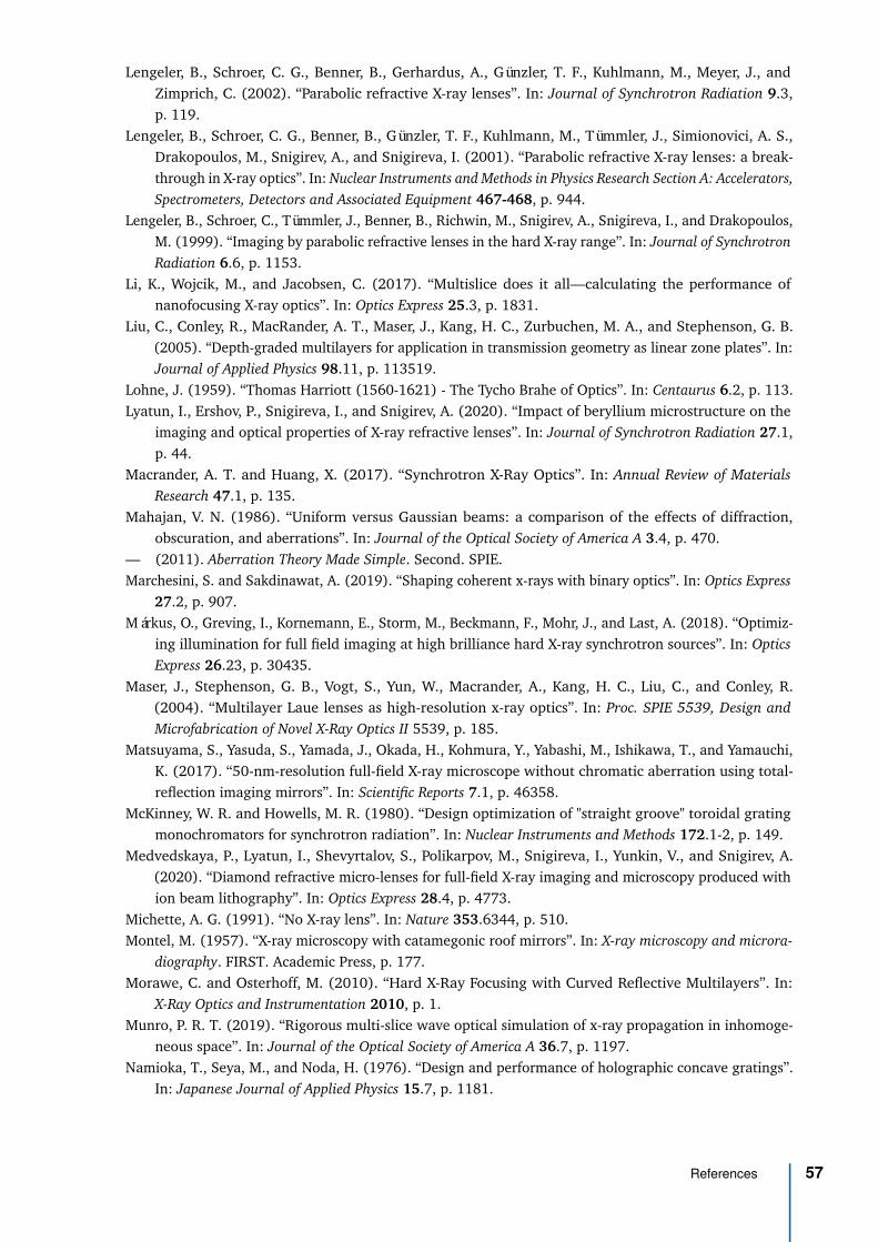
Lengeler, B., Schroer, C. G., Benner, B., Gerhardus, A., Günzler, T. F., Kuhlmann, M., Meyer, J., andZimprich, C. (2002). “Parabolic refractive X-ray lenses”. In: Journal of Synchrotron Radiation 9.3,p. 119.
Lengeler, B., Schroer, C. G., Benner, B., Günzler, T. F., Kuhlmann, M., Tümmler, J., Simionovici, A. S.,Drakopoulos, M., Snigirev, A., and Snigireva, I. (2001). “Parabolic refractive X-ray lenses: a break-through in X-ray optics”. In: Nuclear Instruments and Methods in Physics Research Section A: Accelerators,Spectrometers, Detectors and Associated Equipment 467-468, p. 944.
Lengeler, B., Schroer, C., Tümmler, J., Benner, B., Richwin, M., Snigirev, A., Snigireva, I., and Drakopoulos,M. (1999). “Imaging by parabolic refractive lenses in the hard X-ray range”. In: Journal of SynchrotronRadiation 6.6, p. 1153.
Li, K., Wojcik, M., and Jacobsen, C. (2017). “Multislice does it all—calculating the performance ofnanofocusing X-ray optics”. In: Optics Express 25.3, p. 1831.
Liu, C., Conley, R., MacRander, A. T., Maser, J., Kang, H. C., Zurbuchen, M. A., and Stephenson, G. B.(2005). “Depth-graded multilayers for application in transmission geometry as linear zone plates”. In:Journal of Applied Physics 98.11, p. 113519.
Lohne, J. (1959). “Thomas Harriott (1560-1621) - The Tycho Brahe of Optics”. In: Centaurus 6.2, p. 113.Lyatun, I., Ershov, P., Snigireva, I., and Snigirev, A. (2020). “Impact of beryllium microstructure on the
imaging and optical properties of X-ray refractive lenses”. In: Journal of Synchrotron Radiation 27.1,p. 44.
Macrander, A. T. and Huang, X. (2017). “Synchrotron X-Ray Optics”. In: Annual Review of MaterialsResearch 47.1, p. 135.
Mahajan, V. N. (1986). “Uniform versus Gaussian beams: a comparison of the effects of diffraction,obscuration, and aberrations”. In: Journal of the Optical Society of America A 3.4, p. 470.
— (2011). Aberration Theory Made Simple. Second. SPIE.Marchesini, S. and Sakdinawat, A. (2019). “Shaping coherent x-rays with binary optics”. In: Optics Express
27.2, p. 907.Márkus, O., Greving, I., Kornemann, E., Storm, M., Beckmann, F., Mohr, J., and Last, A. (2018). “Optimiz-
ing illumination for full field imaging at high brilliance hard X-ray synchrotron sources”. In: OpticsExpress 26.23, p. 30435.
Maser, J., Stephenson, G. B., Vogt, S., Yun, W., Macrander, A., Kang, H. C., Liu, C., and Conley, R.(2004). “Multilayer Laue lenses as high-resolution x-ray optics”. In: Proc. SPIE 5539, Design andMicrofabrication of Novel X-Ray Optics II 5539, p. 185.
Matsuyama, S., Yasuda, S., Yamada, J., Okada, H., Kohmura, Y., Yabashi, M., Ishikawa, T., and Yamauchi,K. (2017). “50-nm-resolution full-field X-ray microscope without chromatic aberration using total-reflection imaging mirrors”. In: Scientific Reports 7.1, p. 46358.
McKinney, W. R. and Howells, M. R. (1980). “Design optimization of "straight groove" toroidal gratingmonochromators for synchrotron radiation”. In: Nuclear Instruments and Methods 172.1-2, p. 149.
Medvedskaya, P., Lyatun, I., Shevyrtalov, S., Polikarpov, M., Snigireva, I., Yunkin, V., and Snigirev, A.(2020). “Diamond refractive micro-lenses for full-field X-ray imaging and microscopy produced withion beam lithography”. In: Optics Express 28.4, p. 4773.
Michette, A. G. (1991). “No X-ray lens”. In: Nature 353.6344, p. 510.Montel, M. (1957). “X-ray microscopy with catamegonic roof mirrors”. In: X-ray microscopy and microra-
diography. FIRST. Academic Press, p. 177.Morawe, C. and Osterhoff, M. (2010). “Hard X-Ray Focusing with Curved Reflective Multilayers”. In:
X-Ray Optics and Instrumentation 2010, p. 1.Munro, P. R. T. (2019). “Rigorous multi-slice wave optical simulation of x-ray propagation in inhomoge-
neous space”. In: Journal of the Optical Society of America A 36.7, p. 1197.Namioka, T., Seya, M., and Noda, H. (1976). “Design and performance of holographic concave gratings”.
In: Japanese Journal of Applied Physics 15.7, p. 1181.
References 57

Nazmov, V., Reznikova, E., Mohr, J., Snigirev, A., Snigireva, I., Achenbach, S., and Saile, V. (2004).“Fabrication and preliminary testing of X-ray lenses in thick SU-8 resist layers”. In: MicrosystemTechnologies. Vol. 10. 10, p. 716.
Nazmov, V., Reznikova, E., Snigirev, A., Snigireva, I., DiMichiel, M., Grigoriev, M., Mohr, J., Matthis, B.,and Saile, V. (2005). “LIGA fabrication of X-ray Nickel lenses”. In: Microsystem Technologies 11.4-5,p. 292.
Nazmov, V., Reznikova, E., Last, A., Mohr, J., Saile, V., Simon, R., and DiMichiel, M. (2007). “X-ray LensesFabricated by LIGA Technology”. In: AIP Conference Proceedings. Vol. 879. AIP, p. 770.
Nöhammer, B., David, C., Rothuizen, H., Hoszowska, J., and Simionovici, A. (2003). “Deep reactiveion etching of silicon and diamond for the fabrication of planar refractive hard X-ray lenses”. In:Microelectronic Engineering 67-68, p. 453.
Nöhammer, B., Hoszowska, J., Freund, A. K., and David, C. (2003). “Diamond planar refractive lenses forthird- and fourth-generation X-ray sources”. In: Journal of Synchrotron Radiation 10.2, p. 168.
Ognev, L. I. (2005). “Diffraction calculation for an X-ray refractive Kinoform Lens”. In: Technical PhysicsLetters 31.4, p. 314.
Paganin, D. (2006). Coherent X-Ray Optics. First edition. Oxford University Press.Paganin, D. M. and Morgan, K. S. (2019). “X-ray Fokker–Planck equation for paraxial imaging”. In:
Scientific Reports 9.1, p. 1.Petrov, A. K., Bessonov, V. O., Abrashitova, K. A., Kokareva, N. G., Safronov, K. R., Barannikov, A. A.,
Ershov, P. A., Klimova, N. B., Lyatun, I. I., Yunkin, V. A., Polikarpov, M., Snigireva, I., Fedyanin, A. A.,and Snigirev, A. (2017). “Polymer X-ray refractive nano-lenses fabricated by additive technology”. In:Optics Express 25.13, p. 14173.
Polikarpov, M., Kononenko, T. V., Ralchenko, V. G., Ashkinazi, E. E., Konov, V. I., Ershov, P., Kuznetsov, S.,Yunkin, V., Snigireva, I., Polikarpov, V. M., and Snigirev, A. (2016). “Diamond x-ray refractive lensesproduced by femto-second laser ablation”. In: Proc. SPIE 9963, Advances in X-Ray/EUV Optics andComponents XI 9963.15, 99630Q.
Polikarpov, M., Snigireva, I., and Snigirev, A. (2014). “X-ray harmonics rejection on third-generationsynchrotron sources using compound refractive lenses”. In: Journal of Synchrotron Radiation 21.3,p. 484.
Prins, J. A. (1927). “The Total Reflection of X-rays”. In: Nature 120.3014, p. 188.Probst, J., Braig, C., Langlotz, E., Rahneberg, I., Kühnel, M., Zeschke, T., Siewert, F., Krist, T., and Erko, A.
(2020). “Conception of diffractive wavefront correction for XUV and soft x-ray spectroscopy”. In:Applied Optics 59.8, p. 2580.
Protopopov, V. and Valiev, K. (1998). “Theory of an ideal compound X-ray lens”. In: Optics Communications151.4-6, p. 297.
Rashed, R. (1990). A Pioneer in Anaclastics: Ibn Sahl on Burning Mirrors and Lenses. Vol. 81. 3, p. 464.Rebernik Ribic, P., Rösner, B., Gauthier, D., Allaria, E., Döring, F., Foglia, L., Giannessi, L., Mahne, N.,
Manfredda, M., Masciovecchio, C., Mincigrucci, R., Mirian, N., Principi, E., Roussel, E., Simoncig, A.,Spampinati, S., David, C., and De Ninno, G. (2017). “Extreme-Ultraviolet Vortices from a Free-ElectronLaser”. In: Physical Review X 7.3, p. 031036.
Röntgen, W. C. (1896). “Über Eine Neue Art von Strahlen (Vorläufige Mittheilung)”. In: Sonderabbdruckaus den Sitzungsberichten der Würzburger Physik.-medic. Gesellschaft 1895, p. 132.
Rösner, B., Döring, F., Ribic, P. R., Gauthier, D., Principi, E., Masciovecchio, C., Zangrando, M., Vila-Comamala, J., De Ninno, G., and David, C. (2017). “High resolution beam profiling of X-ray freeelectron laser radiation by polymer imprint development”. In: Optics Express 25.24, p. 30686.
Ross, T. S. (2009). “Limitations and applicability of the Maréchal approximation”. In: Applied Optics 48.10,p. 1812.
Roth, T., Alianelli, L., Lengeler, D., Snigirev, A., and Seiboth, F. (2017). “Materials for x-ray refractivelenses minimizing wavefront distortions”. In: MRS Bulletin 42.06, p. 430.
58 Chapter 2 X-rays as a branch of optics
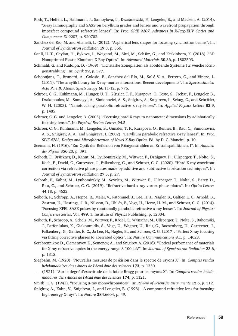
Roth, T., Helfen, L., Hallmann, J., Samoylova, L., Kwasniewski, P., Lengeler, B., and Madsen, A. (2014).“X-ray laminography and SAXS on beryllium grades and lenses and wavefront propagation throughimperfect compound refractive lenses”. In: Proc. SPIE 9207, Advances in X-Ray/EUV Optics andComponents IX 9207, p. 920702.
Sanchez del Rio, M. and Alianelli, L. (2012). “Aspherical lens shapes for focusing synchrotron beams”. In:Journal of Synchrotron Radiation 19.3, p. 366.
Sanli, U. T., Ceylan, H., Bykova, I., Weigand, M., Sitti, M., Schütz, G., and Keskinbora, K. (2018). “3DNanoprinted Plastic Kinoform X-Ray Optics”. In: Advanced Materials 30.36, p. 1802503.
Schmahl, G. and Rudolph, D. (1969). “Lichstarke Zoneplatten als abbildende Systeme für weiche Rönt-genstrahlung”. In: Optik 29, p. 577.
Schoonjans, T., Brunetti, A., Golosio, B., Sanchez del Rio, M., Solé, V. A., Ferrero, C., and Vincze, L.(2011). “The xraylib library for X-ray–matter interactions. Recent developments”. In: SpectrochimicaActa Part B: Atomic Spectroscopy 66.11-12, p. 776.
Schroer, C. G., Kuhlmann, M., Hunger, U. T., Günzler, T. F., Kurapova, O., Feste, S., Frehse, F., Lengeler, B.,Drakopoulos, M., Somogyi, A., Simionovici, A. S., Snigirev, A., Snigireva, I., Schug, C., and Schröder,W. H. (2003). “Nanofocusing parabolic refractive x-ray lenses”. In: Applied Physics Letters 82.9,p. 1485.
Schroer, C. G. and Lengeler, B. (2005). “Focusing hard X rays to nanometer dimensions by adiabaticallyfocusing lenses”. In: Physical Review Letters 94.5.
Schroer, C. G., Kuhlmann, M., Lengeler, B., Gunzler, T. F., Kurapova, O., Benner, B., Rau, C., Simionovici,A. S., Snigirev, A. A., and Snigireva, I. (2002). “Beryllium parabolic refractive x-ray lenses”. In: Proc.SPIE 4783, Design and Microfabrication of Novel X-Ray Optics. Ed. by D. C. Mancini, p. 10.
Seemann, H. (1916). “Zur Optik der Reflexion von Röntgenstrahlen an Kristallspaliflächen. I”. In: Annalender Physik 356.20, p. 391.
Seiboth, F., Brückner, D., Kahnt, M., Lyubomirskiy, M., Wittwer, F., Dzhigaev, D., Ullsperger, T., Nolte, S.,Koch, F., David, C., Garrevoet, J., Falkenberg, G., and Schroer, C. G. (2020). “Hard X-ray wavefrontcorrection via refractive phase plates made by additive and subtractive fabrication techniques”. In:Journal of Synchrotron Radiation 27.5, p. 27.
Seiboth, F., Kahnt, M., Lyubomirskiy, M., Seyrich, M., Wittwer, F., Ullsperger, T., Nolte, S., Batey, D.,Rau, C., and Schroer, C. G. (2019). “Refractive hard x-ray vortex phase plates”. In: Optics Letters44.18, p. 4622.
Seiboth, F., Schropp, A., Hoppe, R., Meier, V., Patommel, J., Lee, H. J., Nagler, B., Galtier, E. C., Arnold, B.,Zastrau, U., Hastings, J. B., Nilsson, D., Uhlén, F., Vogt, U., Hertz, H. M., and Schroer, C. G. (2014).“Focusing XFEL SASE pulses by rotationally parabolic refractive x-ray lenses”. In: Journal of Physics:Conference Series. Vol. 499. 1. Institute of Physics Publishing, p. 12004.
Seiboth, F., Schropp, A., Scholz, M., Wittwer, F., Rödel, C., Wünsche, M., Ullsperger, T., Nolte, S., Rahomäki,J., Parfeniukas, K., Giakoumidis, S., Vogt, U., Wagner, U., Rau, C., Boesenberg, U., Garrevoet, J.,Falkenberg, G., Galtier, E. C., Ja Lee, H., Nagler, B., and Schroer, C. G. (2017). “Perfect X-ray focusingvia fitting corrective glasses to aberrated optics”. In: Nature Communications 8.1, p. 14623.
Serebrennikov, D., Clementyev, E., Semenov, A., and Snigirev, A. (2016). “Optical performance of materialsfor X-ray refractive optics in the energy range 8-100 keV”. In: Journal of Synchrotron Radiation 23.6,p. 1315.
Siegbahn, M. (1920). “Nouvelles mesures de précision dans le spectre de rayons X”. In: Comptes rendushebdomadaires des séances de l’Académie des sciences 173, p. 1350.
— (1921). “Sur le degré d’exactitude de la loi de Bragg pour les rayons X”. In: Comptes rendus hebdo-madaires des séances de l’Académie des sciences 174, p. 1121.
Smith, C. S. (1941). “Focusing X-ray monochromators”. In: Review of Scientific Instruments 12.6, p. 312.Snigirev, A., Kohn, V., Snigireva, I., and Lengeler, B. (1996). “A compound refractive lens for focusing
high-energy X-rays”. In: Nature 384.6604, p. 49.
References 59

Snigirev, A. and Snigireva, I. (2008). “High energy X-ray micro-optics”. In: Comptes Rendus Physique 9.5-6,p. 507.
Snigireva, I., Snigirev, A., Rau, C., Weitkamp, T., Aristov, V., Grigoriev, M., Kuznetsov, S., Shabelnikov, L.,Yunkin, V., Hoffmann, M., and Voges, E. (2001). “Holographic X-ray optical elements: Transitionbetween refraction and diffraction”. In: Nuclear Instruments and Methods in Physics Research, SectionA: Accelerators, Spectrometers, Detectors and Associated Equipment 467-468.PART II, p. 982.
Snigireva, I., Snigirev, A., Kuznetsov, S., Rau, C., Weitkamp, T., Shabelnikov, L., Grigoriev, M., Yunkin, V.,Hoffmann, M., and Voges, E. I. (2001). “Refractive and diffractive x-ray optical elements”. In: Proc.SPIE 4499, X-Ray Micro- and Nano-Focusing: Applications and Techniques II 4499.13, p. 64.
Stenström, K. W. (1919). “Experimentelle Untersuchungen der Röntgenspektra”. PhD thesis. Mathematisch-Naturwissenschaftlichen Sektion der Philosophischen Fakultät zu Lund (present Lunds Universitet),Sweden.
Suehiro, S., Miyaji, H., and Hayashi, H. (1991). “Refractive lens for X-ray focus”. In: Nature 352.6334,p. 385.
Susini, J. (1993). “X-ray mirrors for high-brilliance synchrotron beamlines: R & D at the ESRF”. In: Proc.SPIE 1740, Optics for High-Brightness Synchrotron Radiation Beamlines, p. 44.
Tomie, T. (1994). X-ray lenses. Japan Patent 6-045288.— (2010). “The birth of the X-ray refractive lens”. In: Spectrochimica Acta Part B: Atomic Spectroscopy
65.3, p. 192.Tonner, B. P. and Plummer, E. (1980). “Design criteria and performance of a toroidal grating monochro-
mator”. In: Nuclear Instruments and Methods 177.1, p. 153.Underwood, J. H., Barbee, T. W., and Frieber, C. (1986). “X-ray microscope with multilayer mirrors”. In:
Applied Optics 25.11, p. 1730.Vaughan, G. B. M., Wright, J. P., Bytchkov, A., Rossat, M., Gleyzolle, H., Snigireva, I., and Snigirev, A.
(2011). “X-ray transfocators: focusing devices based on compound refractive lenses”. In: Journal ofSynchrotron Radiation 18.2, p. 125.
Vogt, U., Lindblom, M., Charalambous, P., Kaulich, B., and Wilhein, T. (2006). “Condenser for Koehler-likeillumination in transmission x-ray microscopes at undulator sources”. In: Optics Letters 31.10, p. 1465.
Walter, B. and Pohl, R. (1908). “Zur Frage der Beugung der Röntgenstrahlen”. In: Annalen der Physik330.4, p. 715.
— (1909). “Weitere Versuche über die Beugung der Röntgenstrahlen”. In: Annalen der Physik 334.7,p. 331.
Wetherell, W. B. (1980). “The Calculation of Image Quality”. In: Applied Optics and Optical Engineering.Vol. 8, p. 171.
Wilk, S. R. (2004). “Claudius Ptolemy’s Law of Refraction”. In: Optics & Photonics News October, p. 14.Willmott, P. (2019). An Introduction to Synchrotron Radiation. Second edition. Wiley.Wolter, H. (1952). “Spiegelsysteme streifenden Einfalls als abbildende Optiken für Röntgenstrahlen”. In:
Annalen der Physik 445.1-2, p. 94.Yamada, J., Matsuyama, S., Hirose, R., Takeda, Y., Kohmura, Y., Yabashi, M., Omote, K., Ishikawa, T., and
Yamauchi, K. (2020). “Compact full-field hard x-ray microscope based on advanced Kirkpatrick–Baezmirrors”. In: Optica 7.4, p. 367.
Yamada, J., Matsuyama, S., Sano, Y., Kohmura, Y., Yabashi, M., Ishikawa, T., and Yamauchi, K. (2019).“Compact reflective imaging optics in hard X-ray region based on concave and convex mirrors”. In:Optics Express 27.3, p. 3429.
Yang, B. X. (1993). “Fresnel and refractive lenses for X-rays”. In: Nuclear Instruments and Methods inPhysics Research Section A: Accelerators, Spectrometers, Detectors and Associated Equipment 328.3,p. 578.
Zverev, D., Barannikov, A., Snigireva, I., and Snigirev, A. (2017). “X-ray refractive parabolic axicon lens”.In: Optics Express 25.23, p. 28469.
60 Chapter 2 X-rays as a branch of optics

3Modelling optical imperfections inrefractive lenses
To understand the impact of CRL on the optical design of complete beamlines, it is necessaryto be able to simulate them realistically. The basic implementation of X-ray lenses is alreadyavailable on the two most widespread beamline simulation tools: SHADOW [Sanchez del Rioet al., 2011] and SRW [Chubar and Elleaume, 1998]. Both implementations, although basedon different schemes, ray tracing [Alianelli et al., 2007] and wave optics [Baltser et al., 2011]respectively, are based on an ideal model combining refraction and absorption for the stackedlenses. Much has been done in terms of refining the modelling of ideal X-ray lenses [Umbachet al., 2008; Sanchez del Rio and Alianelli, 2012; Osterhoff et al., 2013; Simons et al., 2017;Pedersen et al., 2018] and, to a certain extent, the modelling of optical imperfections [Pantellet al., 2001; Andrejczuk et al., 2010; Gasilov et al., 2017; Osterhoff et al., 2017]. Except forthe work presented in [Roth et al., 2014], investigating and simulating the inner structure ofX-ray lenses, the present models consider mainly the lens shape and departure from a perfectparabolic shape. The majority of these models, however, is not publicly available, nor arereadily compatible with standard beamline simulations suites like SHADOW and SRW. Anotherbottle-neck to the current literature or computer codes for simulating CRLs is that they do notinclude the data from real lens metrology, as is routinely done for X-ray mirrors simulations[Sanchez Del Rio et al., 2016], which renders more difficult the inclusion of CRLs in simulationsof complete beamline configurations in combination with other optical elements.
The modelling and functions presented here1 are based on the framework of physicaloptics (cf. §1.2 - Physical optics) and are tailored to be used transparently with SRW [Chubarand Elleaume, 1998], which already provides a model for the CRL [Baltser et al., 2011]- this basic ideal model combines refraction and absorption for the stacked lenses; opticalimperfections from material inhomogeneities (voids, impurities) were later added [Roth etal., 2014]. Expanding this model, we present the optical imperfections in refractive lenses inthree different groups: i-) misalignments of a single X-ray lens - Fig. 3.1(b)-(c); ii-) commonlyencountered fabrication errors such as transverse offsets as well as tilts of the individual parabolicsections - Fig. 3.1(d)-(g); iii-) and other sources of deviations from the parabolic shape modelledwith either polynomial decomposition of error functions or by using metrology data - Fig. 3.9.Each newly added feature is accompanied by a calculation of the residual thickness error, itsimpact on focusing by CRL and the beam caustic in the vicinity of the focal spot. The Strehlratios for the different misalignments, fabrication errors and other sources of deviations from theparabolic profile are summarised in Fig. 3.12. Calculations presented in this chapter are merelyillustrative and a systematic evaluation is presented in §5 - Effect of optical imperfections on anX-ray beam. All simulations shown throughout this chapter have similar conditions, that is, theymodel misalignments, fabrication errors or arbitrary residual errors of a single 2D-Beryllium lens
1This chapter is partially based on the work originally published in [Celestre, Chubar, et al., 2020].
61

(d) (e) (f) (g)
L
twall
A R
y
z
(a) (c)(b)
Fig. 3.1.: (a) ideal lens for reference. Lens typical misalignments are the (b) transverse offset and the (c)tilt or a combination of both. Common fabrication errors include the (d) longitudinal offset ofthe parabolic section, (e) transverse offset of the parabolic section and (f)-(g) tilted parabolicsections.
with nominal radius R = 50 µm, geometric aperture A� = 440 µm and twall = 20 µm at 8 keVin fully-coherent simulations. The optical layout used for the simulations is shown in Fig. 3.2.The code main functions implementing the ideal CRL and describing optical imperfections inrefractive lenses are subsequently presented. The metrology technique used to measure thephase errors that arise from material inhomogeneities (voids, impurities) and/or figure errorsfrom the lens forming process, namely, X-ray speckle tracking, is discussed in §4 - Measuringoptical imperfections in refractive lenses.
3.1 Optical imperfections in refractive lensesIn the paraxial approximation, the parabolic shape for a refracting surface is generally
regarded as the ideal shape2 for minimising aberrations. It is legitimate, then, to define aserrors any deviation from this ideal parabolic form3 regardless of their origin. The phase errorsinduced by an ideal lens misalignment will be presented first, then the typical fabrication errorsof bi-concave lenses will be presented shortly after. The misalignment and fabrication errorspresented in this section were derived from the accumulated experience in handling berylliumand aluminium bi-concave embossed lenses, which are the most available throughout beamlinesin diverse synchrotron facilities. However, the modelling presented here is generic and can beapplied to a wide-range of CRL from diverse fabrication processes4.
The optical layouts used throughout this chapter for all simulations is shown in Fig. 3.2.The emitted radiation is modelled by a filament-electron-beam passing through a CPMU18
2The shape of a focusing refracting surface can be derived from the Fermat’s principle, but the parabolic shape isgenerally regarded as a good approximation. Large apertures are often necessary when very small focused beamsare required, but increasing the geometric aperture of the optical element causes the parabolic approximation tounder-perform. Several aspheric surface shapes for different focusing conditions were reported in [Sanchez delRio and Alianelli, 2012, Fig 4]. For a deeper discussion on aspheric surfaces in the context of optics, please, referto [Schulz, 1988].
3Such definition, however, leaves out discrepancies in the radius of curvature R (designed vs. de facto) and theassociated defocus it may cause. Discrepancies between designed and executed lenses may render them to belabelled as out-of-specification and may cause the system to under-perform, but are not deviations of the parabolicshape, provided the ideal parabolic shape takes into account the de facto radius of curvature. Accounting for suchdiscrepancies can be done using the ideal model described by the transmission element Tsingle lens(∆z) (cf. Eq. 2.9)using the de facto radius of curvature.
4cf. Table 1 from the supplementary material relative to [Roth et al., 2017].
62 Chapter 3 Modelling optical imperfections in refractive lenses
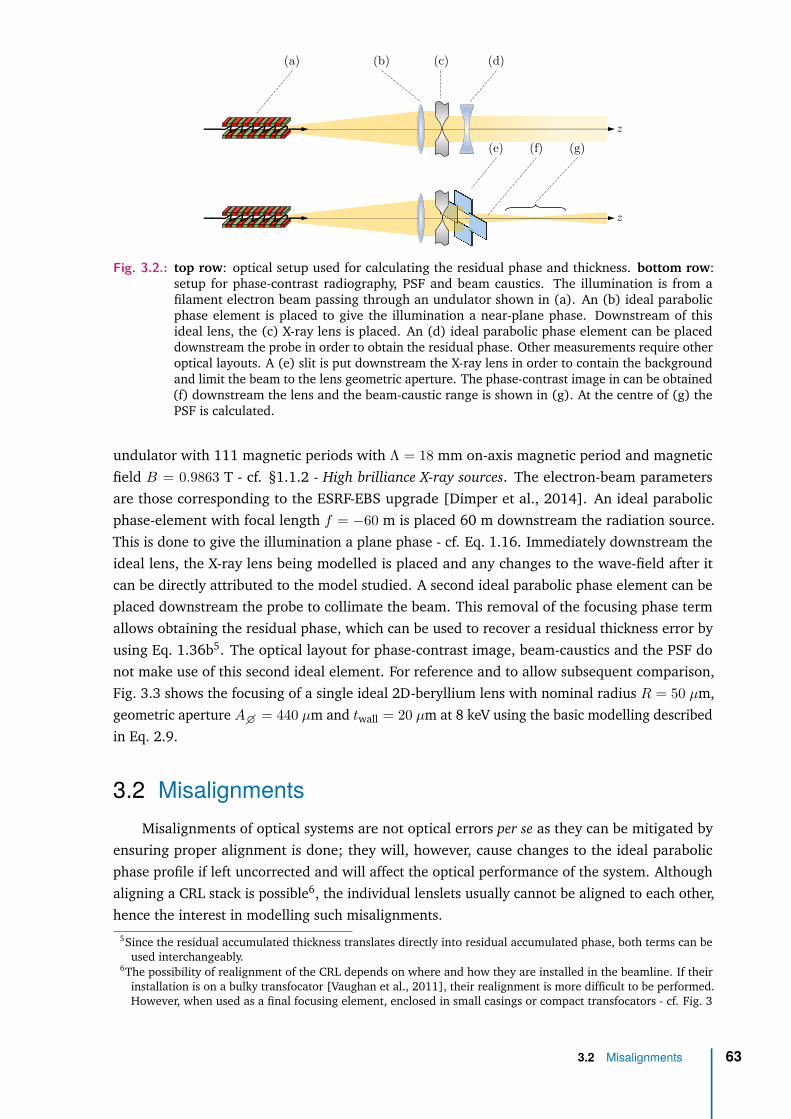
z
(b) (c)(a) (d)
z
(e) (g)(f)
Fig. 3.2.: top row: optical setup used for calculating the residual phase and thickness. bottom row:setup for phase-contrast radiography, PSF and beam caustics. The illumination is from afilament electron beam passing through an undulator shown in (a). An (b) ideal parabolicphase element is placed to give the illumination a near-plane phase. Downstream of thisideal lens, the (c) X-ray lens is placed. An (d) ideal parabolic phase element can be placeddownstream the probe in order to obtain the residual phase. Other measurements require otheroptical layouts. A (e) slit is put downstream the X-ray lens in order to contain the backgroundand limit the beam to the lens geometric aperture. The phase-contrast image in can be obtained(f) downstream the lens and the beam-caustic range is shown in (g). At the centre of (g) thePSF is calculated.
undulator with 111 magnetic periods with Λ = 18 mm on-axis magnetic period and magneticfield B = 0.9863 T - cf. §1.1.2 - High brilliance X-ray sources. The electron-beam parametersare those corresponding to the ESRF-EBS upgrade [Dimper et al., 2014]. An ideal parabolicphase-element with focal length f = −60 m is placed 60 m downstream the radiation source.This is done to give the illumination a plane phase - cf. Eq. 1.16. Immediately downstream theideal lens, the X-ray lens being modelled is placed and any changes to the wave-field after itcan be directly attributed to the model studied. A second ideal parabolic phase element can beplaced downstream the probe to collimate the beam. This removal of the focusing phase termallows obtaining the residual phase, which can be used to recover a residual thickness error byusing Eq. 1.36b5. The optical layout for phase-contrast image, beam-caustics and the PSF donot make use of this second ideal element. For reference and to allow subsequent comparison,Fig. 3.3 shows the focusing of a single ideal 2D-beryllium lens with nominal radius R = 50 µm,geometric aperture A� = 440 µm and twall = 20 µm at 8 keV using the basic modelling describedin Eq. 2.9.
3.2 MisalignmentsMisalignments of optical systems are not optical errors per se as they can be mitigated by
ensuring proper alignment is done; they will, however, cause changes to the ideal parabolicphase profile if left uncorrected and will affect the optical performance of the system. Althoughaligning a CRL stack is possible6, the individual lenslets usually cannot be aligned to each other,hence the interest in modelling such misalignments.
5Since the residual accumulated thickness translates directly into residual accumulated phase, both terms can beused interchangeably.
6The possibility of realignment of the CRL depends on where and how they are installed in the beamline. If theirinstallation is on a bulky transfocator [Vaughan et al., 2011], their realignment is more difficult to be performed.However, when used as a final focusing element, enclosed in small casings or compact transfocators - cf. Fig. 3
3.2 Misalignments 63

−200 0 200(µm)
−200
0
200
(µm
)
(a) radiography
−10 0 10(µm)
−10
0
10
(µm
)
0.0
0.5
1.0
0.0 0.5 1.0
(b) PSF
−200 0 200(mm)
−20
−10
0
10
20
(µm
)
0.00
0.25
0.500.751.00
(c) vertical caustics
Fig. 3.3.: Simulations of a single ideal 2D-beryllium lens with nominal radius R = 50 µm, geometricaperture A� = 440 µm and twall = 20 µm at 8 keV - cf. Fig 3.1(a). (a) phase-contrast image150 mm downstream the ideal lens, (b) point-spread function with cuts centred in (0, 0) and(c) the vertical beam caustics from −250 mm to 250 mm with respect to the focal plane atf = 4.701 m.
3.2.1 Transverse offset
Displacing a single element a transverse distance (∆x,∆y) can be simply done by calculating∆z(x − ∆x, y − ∆y) in Eq. 2.8. The shifted element is depicted in Fig. 3.1(b). For a pair ofcoordinates (x, y):
∆z(x−∆x, y −∆y) =
(x−∆x)2
Rx+
(y −∆y)2
Ry+ twall, ∀ (x−∆x, y −∆y) ∈ A,
L, otherwise.
(3.1)
Eq. 3.1 is the ideal parabolic profile of a bi-concave lens given by Eq. 2.8 with its vertices centredaround (∆x,∆y). While a single transversely shifted lens considered on its own is innocuous,piling up several shifted lenses has impacts on the overall accumulated phase parabolic shapeand resulting geometric aperture. Although the exact effect of relative misalignments betweenindividual lenses on the phase of the wave-field depends on the distance between lenslets, theenergy, footprint and divergence of the X-ray beam, some insight can be gained by consideringthe individual focusing elements as thin-optical elements in intimate contact. Consider Nstacked lenses transversely misaligned with their transverse distance to the optical axis givenby (∆xj ,∆yj ), with j = 1, 2, ..., N . Within the intersection of their geometric apertures, theaccumulated thickness is given by:
∆zΣ(x, y) =N∑j=1
∆z(∆xj ,∆yj )
=N∑j=1
x2
Rxj+ y2
Ryj︸ ︷︷ ︸(I)
− 2x∆xj
Rxj− 2y
∆yj
Ryj︸ ︷︷ ︸(II)
+∆2xj
Rxj+
∆2yj
Ryj+ twallj︸ ︷︷ ︸
(III)
. (3.2)
The first term in Eq. 3.2, (I) is a quadratic term and it indicates ideal focusing as in Eq. 2.8. Theresidual terms (II) and (III) are a linear term in x and y and a constant offset term, respectively.The first residual term, i.e. (II), adds a linear phase to the wave-front and acts like a prism,
in [Lengeler et al., 1999] and [Kornemann et al., 2017; Narikovich et al., 2019], their realignment can be donemore easily.
64 Chapter 3 Modelling optical imperfections in refractive lenses

−200 0 200(µm)
−25
0
25
∆z
(µm
)
(a) residues
−200 0 200(µm)
−200
0
200
(µm
)
(b) radiography
−10 0 10(µm)
−10
0
10
(µm
)
0.0
0.5
1.0
0.0 0.5 1.0
(c) PSF
−200 0 200(mm)
−20
−10
0
10
20
(µm
)
0.00
0.25
0.500.751.00
(d) vertical caustics
Fig. 3.4.: Simulations of an ideal lens shifted by ∆y = 5 µm - cf. Fig 3.1(b). (a) Residual thickness, (b)phase-contrast image of the lens, (c) point spread function with cuts centred in (0, 0) and (c)the vertical beam caustics from −250 mm to 250 mm with respect to the focal plane.
not deforming the monochromatic wave-field, but redirecting it. At the focal plane, the imageposition is transversely shifted but no change to the intensity and phase profiles is added.Symmetrically shifted lenses7 make (II) go to zero. The residual terms in (III) add a constantphase offset to the transmitted beam in addition to absorption. The effects of the transverseoffset to a single X-ray lens are shown in Fig. 3.4.
3.2.2 Tilted lensWhen rotating a lens in space as shown in Fig. 3.1(c) and calculating its projected thickness,
it is helpful to decouple the rotation of the front and back surfaces. This can be done by defininga point cloud in Cartesian coordinates:
zfront surface(x−∆x, y −∆y) = ∆z(x−∆x, y −∆y)2 , (3.3a)
zback surface(x−∆x, y −∆y) = −∆z(x−∆x, y −∆y)2 (3.3b)
where ∆z(x−∆x, y −∆y) is given by Eq. 3.1. The projected thickness is given by:
∆z(x, y) = zfront surface(x, y)− zback surface(x, y), (3.4)
provided those are calculated on the same grid (x, y). A tilted lens can be described by rotationmatrices in three dimensions. In a system where the position is represented8 as (x, y, z, 1) Thetransformation matrices allowing a rotation θx,y,z around each of the Cartesian axis are [Houseand Keyser, 2016]:
Rθx =
1 0 0 00 cx −sx 00 sx cx 00 0 0 1
, Rθy =
cy 0 sy 00 1 0 0−sy 0 cy 0
0 0 0 1
, Rθz =
cz −sz 0 0sz cz 0 00 0 1 00 0 0 1
, (3.5)
where cθ = cos(θ) and sθ = sin(θ). Rθx denotes a rotation around the x−axis, Rθy around they−axis and, finally, Rθz around the z−axis. Matrix multiplication is associative, which implies
7That is ∆xm = −∆xn or ∆ym = −∆yn for m,n ∈ (1, 2, ..., N).8Expressing the 3D coordinates as (x, y, z, 1) comes from homogeneous coordinates systems often used in projective
geometry [House and Keyser, 2016].
3.2 Misalignments 65
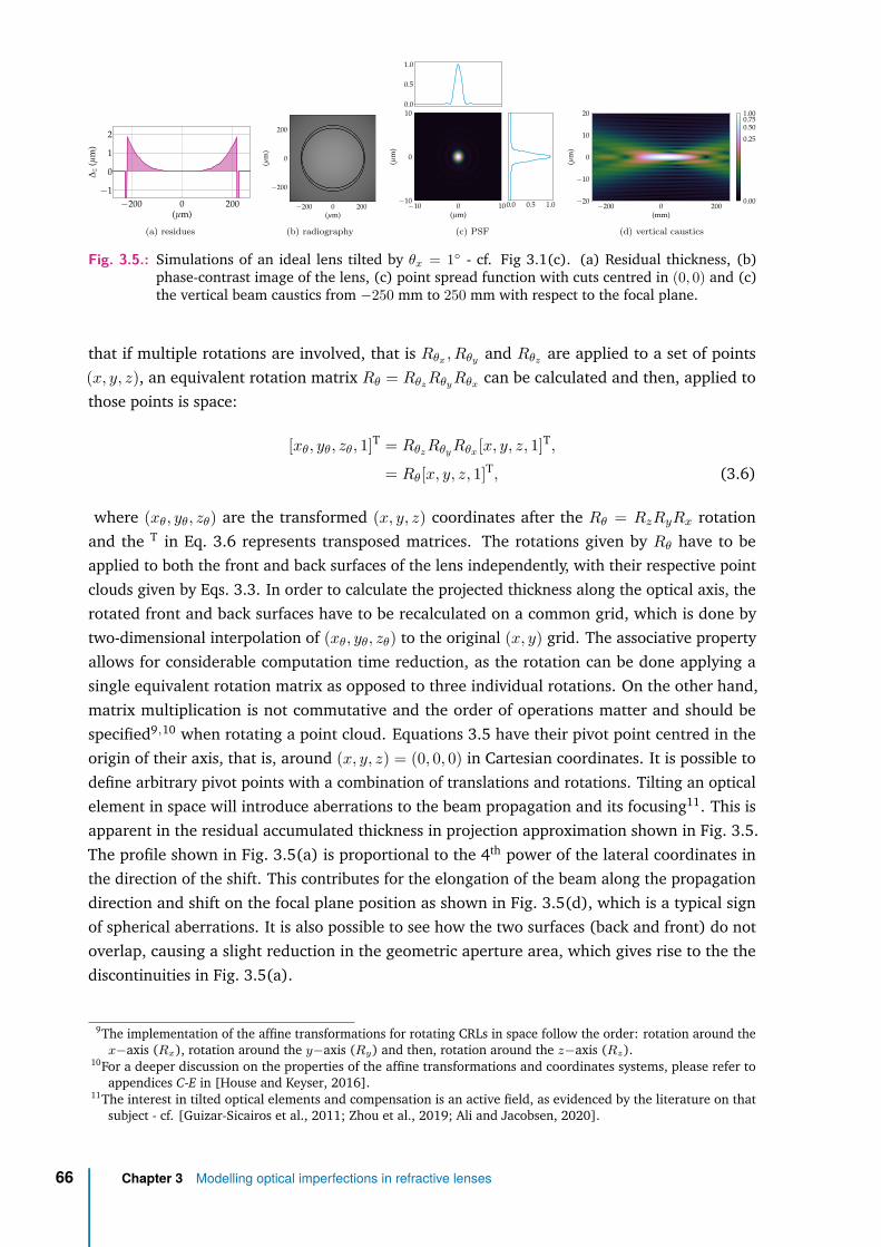
−200 0 200(µm)
−1
0
1
2
∆z
(µm
)
(a) residues
−200 0 200(µm)
−200
0
200
(µm
)
(b) radiography
−10 0 10(µm)
−10
0
10
(µm
)
0.0
0.5
1.0
0.0 0.5 1.0
(c) PSF
−200 0 200(mm)
−20
−10
0
10
20
(µm
)
0.00
0.25
0.500.751.00
(d) vertical caustics
Fig. 3.5.: Simulations of an ideal lens tilted by θx = 1◦ - cf. Fig 3.1(c). (a) Residual thickness, (b)phase-contrast image of the lens, (c) point spread function with cuts centred in (0, 0) and (c)the vertical beam caustics from −250 mm to 250 mm with respect to the focal plane.
that if multiple rotations are involved, that is Rθx , Rθy and Rθz are applied to a set of points(x, y, z), an equivalent rotation matrix Rθ = RθzRθyRθx can be calculated and then, applied tothose points is space:
[xθ, yθ, zθ, 1]T = RθzRθyRθx [x, y, z, 1]T,
= Rθ[x, y, z, 1]T, (3.6)
where (xθ, yθ, zθ) are the transformed (x, y, z) coordinates after the Rθ = RzRyRx rotationand the T in Eq. 3.6 represents transposed matrices. The rotations given by Rθ have to beapplied to both the front and back surfaces of the lens independently, with their respective pointclouds given by Eqs. 3.3. In order to calculate the projected thickness along the optical axis, therotated front and back surfaces have to be recalculated on a common grid, which is done bytwo-dimensional interpolation of (xθ, yθ, zθ) to the original (x, y) grid. The associative propertyallows for considerable computation time reduction, as the rotation can be done applying asingle equivalent rotation matrix as opposed to three individual rotations. On the other hand,matrix multiplication is not commutative and the order of operations matter and should bespecified9,10 when rotating a point cloud. Equations 3.5 have their pivot point centred in theorigin of their axis, that is, around (x, y, z) = (0, 0, 0) in Cartesian coordinates. It is possible todefine arbitrary pivot points with a combination of translations and rotations. Tilting an opticalelement in space will introduce aberrations to the beam propagation and its focusing11. This isapparent in the residual accumulated thickness in projection approximation shown in Fig. 3.5.The profile shown in Fig. 3.5(a) is proportional to the 4th power of the lateral coordinates inthe direction of the shift. This contributes for the elongation of the beam along the propagationdirection and shift on the focal plane position as shown in Fig. 3.5(d), which is a typical signof spherical aberrations. It is also possible to see how the two surfaces (back and front) do notoverlap, causing a slight reduction in the geometric aperture area, which gives rise to the thediscontinuities in Fig. 3.5(a).
9The implementation of the affine transformations for rotating CRLs in space follow the order: rotation around thex−axis (Rx), rotation around the y−axis (Ry) and then, rotation around the z−axis (Rz).
10For a deeper discussion on the properties of the affine transformations and coordinates systems, please refer toappendices C-E in [House and Keyser, 2016].
11The interest in tilted optical elements and compensation is an active field, as evidenced by the literature on thatsubject - cf. [Guizar-Sicairos et al., 2011; Zhou et al., 2019; Ali and Jacobsen, 2020].
66 Chapter 3 Modelling optical imperfections in refractive lenses

−200 0 200(µm)
−200
0
200
(µm
)
(a) simulation (b) experimental
Fig. 3.6.: (a) Simulated and (b) measured phase-contrast image of a single of a 2D-beryllium lens withnominal radius R = 50 µm with designed geometric aperture A� = 440 µm. The scale bar in(b) is 200 µm wide.
3.3 Fabrication errorsModelling the typical misalignment of X-ray lenses implies calculating the lateral displace-
ments and rotations in space of an ideal X-ray lens. However, bi-concave lenses may also presentmisalignments between the front and back focusing surfaces, which are closely related to themanufacturing processes involved in the lens production. Here, the front and back focusingsurfaces are treated independently, allowing to model longitudinal and transverse misalignmentsas well as tilts of the front and back focusing surface concerning the optical axis.
3.3.1 Longitudinal offset of the parabolic section
Longitudinal offsets of the parabolic portions of a bi-concave X-ray lens appear when, forthe same radius of curvature R, one parabolic portion reaches deeper into the lens disc than theother one - cf. Fig. 3.1(d). The first eminent observation is that front and back surfaces will havedifferent geometric apertures along the focusing direction. The new geometric aperture of thelongitudinally offset parabolic profile can be calculated as:
Aoffset = 2√
[L− (twall + 2 · offset)]R, (3.7)
where a positive offset increases the apparent web thickness of the half lens to twall/2 + offsetand decreases the geometric aperture for a fixed lens thickness. The aperture given by Aoffset
and the apparent web thickness are used in Eq. 3.4 (cf. Eqs. 3.1 and 3.3) when calculating theprojected thickness. Longitudinal offsets do not affect the parabolic accumulated shape of asingle lens within Aoffset and, consequently, do not impose any optical imperfection to an opticalsystem based on such lenses. However, they are often encountered in real lenses12 and merit theimplementation in the lens modelling. Fig. 3.6 shows the simulated profile and a radiography ofa real lens showing the effects of the longitudinal offset of the parabolic section.
3.3.2 Transverse offset of the parabolic section
Although parallel to the optical axis, it is possible that the parabolic surfaces axes are notcollinear. This is shown in Fig. 3.1(e). The modelling of the transverse offset of the frontor/and back surfaces of a lens concerning the optical axis is done by calculating the net offsetof each surface, that is the sum of lens transverse offset with the front or/and back surface
12Especially in embossed lenses, where different penetration depths of the punches often lead to asymmetric lenses.
3.3 Fabrication errors 67

−200 0 200(µm)
−5
0
5
∆z
(µm
)
(a) residues
−200 0 200(µm)
−200
0
200
(µm
)
(b) radiography
−10 0 10(µm)
−10
0
10
(µm
)
0.0
0.5
1.0
0.0 0.5 1.0
(c) PSF
−200 0 200(mm)
−20
−10
0
10
20
(µm
)
0.00
0.25
0.500.751.00
(d) vertical caustics
Fig. 3.7.: Simulations of a lens with front focusing parabolic section shifted by ∆y = −2 µm and backfocusing shifted by ∆y = −3 µm - cf. Fig 3.1(e). (a) Residual thickness, (b) phase-contrastimage of the lens, (c) point spread function with cuts centred in (0, 0) and (c) the vertical beamcaustics.
transverse offset, and applying it to Eqs. 3.3 when calculating Eq. 3.4. The effects on the residualaccumulated phase of non-collinear parabolic surfaces are the same as the one described in thesection §3.2.1 - Transverse offset, that is, the presence in the residual phase of a linear and aconstant term, which can be seen in Fig. 3.7.
3.3.3 Tilted parabolic sectionWhen the axes of the parabolic front or/and back surfaces are not parallel to the optical
axis, the lens active area appears to be tilted as shown in Figs. 3.1(f) and (g). Similarly towhat was introduced in the section §3.2.2 - Tilted lens, both front and back surfaces are rotatedaccording to the rotation matrices described in Eqs. 3.5 and the procedure described by Eq. 3.6.There are two subtle differences: the rotation angles from front and back surfaces can be chosenindependently and the rotation is only applied to the curved part of the lens, and not to the wholefront and back surfaces including the flat parts. The independent rotations allow for differentregimes: one where both imprints are tilted with the same angle as in shown in Fig. 3.1(f),which yields a residual phase similar to the one discussed in §3.2.2 - Tilted lens; and one wherefront and back surfaces are tilted with different angles, which yields an asymmetric residualphase as shown in Fig. 3.8. By not applying the rotation to the plane region the lens projectedthickness L is not changed. A close inspection of Fig. 3.8 shows that while the symmetric casehas a residual phase proportional to the 4th power of the lateral coordinates in the direction ofthe tilt, elongating the beam focusing in the propagation direction and shifting it on the samedirection - typical of spherical aberrations, the residual phase of the anti-symmetric case hasresidual phase proportional to the 3rd power of the lateral coordinates in the direction of thetilt and has a PSF typical of coma-aberrated systems. The behaviour of the anti-symmetric caseresulting in coma aberrations is commonly encountered in tilted one-sided kinoform lenses andzone-plates as reported in [Guizar-Sicairos et al., 2011; Ali and Jacobsen, 2020].
3.4 Other sources of deviations from the parabolic shapeSo far, the modelling described here relies on translations and rotations of an ideal parabolic
surface and investigating the residual phase. Another equally valid approach is to manipulatedirectly the residual phase and add it to the phase of an ideal focusing lens, which can be done
68 Chapter 3 Modelling optical imperfections in refractive lenses

−200 0 200(µm)
0.0
2.5
5.0
7.5∆
z(µ
m)
(a) residues
−200 0 200(µm)
−200
0
200
(µm
)
(b) radiography
−10 0 10(µm)
−10
0
10
(µm
)
0.0
0.5
1.0
0.0 0.5 1.0
(c) PSF
−200 0 200(mm)
−20
−10
0
10
20
(µm
)
0.00
0.25
0.500.751.00
(d) vertical caustics
Symmetric tilt of front- and back- surfaces by θxfront= θxback
= 1◦
−200 0 200(µm)
−25
0
25
∆z
(µm
)
(e) residues
−200 0 200(µm)
−200
0
200
(µm
)
(f) radiography
−10 0 10(µm)
−10
0
10
(µm
)
0.0
0.5
1.0
0.0 0.5 1.0
(g) PSF
−200 0 200(mm)
−20
−10
0
10
20
(µm
)
0.00
0.25
0.500.751.00
(h) vertical caustics
Anti-symmetric tilt of front- and back- surfaces by θxfront= −θxback
= 0.5◦
Fig. 3.8.: Simulations of a lens with front and back focusing parabolic sections independently tilted asshown in Fig 3.1(f) and (g). The (a) residual thickness, (b) phase-contrast image, (c) pointspread function and (c) the vertical beam caustics of the symmetric tilt are shown on the toprow. The (e) residual thickness, (f) phase-contrast image, (g) point spread function and (h) thevertical beam caustics for the anty-symmetric case with the same conditions is presented in thebottom row.
fitting arbitrary surfaces or by introducing data from metrology of the optical element to besimulated.
3.4.1 Orthornormal polynomials
A widespread form of representing optical aberrations of arbitrary shapes is by decomposingthem into an orthonormal base. Perhaps the most ubiquitous set of aberration functions isgiven by the Zernike polynomials for a circular aperture, first described in [Zernike, 1934].Their appeal comes from the fact that not only they are directly related to Seidel (primary),Schwarzschild (secondary) and tertiary-aberrations13 but also include piston and tilts; they forman orthonormal base, which means that the value of the coefficients is not affected by the removalof a particular term [Mahajan and Dai, 2007]. Another advantage of the Zernike polynomialdecomposition is that each orthonormal aberration coefficient is the standard deviation for thatparticular aberration over the exit pupil, which is valuable when evaluating the optical systemcompliance with the Maréchal criteria and calculating the Strehl ratio [Mahajan, 1983].
For the aforementioned decomposition of the aberration function in an orthonormal baseto retain its properties, the application of the circular Zernike polynomials must be limited tocircular apertures. Other shapes of apertures with- or without obscuration can be obtained by
13This jargon comes from a power-series expansion of the aberration function. There are five primary aberrations,nine secondary aberrations and fourteen aberration terms for the tertiary aberrations. They all involve sphericalaberration, coma, astigmatism, field curvature, distortion and variations of thereof [Mahajan, 2013].
3.4 Other sources of deviations from the parabolic shape 69

−200 0 200(µm)
−200
0
200
(µm
)
-2.50
0.00
2.50
(a) Be lens
Z1 · · · Z5 · · · ·Z10 · · · ·Z15 · · · ·Z20 · · · ·Z25 · · · ·Z30 · · · ·Z35 · ·
−0.50
−0.25
0.00
0.25
0.50
0.75
(µm
)
figure errors
(b) Polynomial decomposition
−200 0 200(µm)
−200
0
200
(µm
)
-2.50
0.00
2.50
(c) Reconstructed profile
−200 0 200(µm)
−200
0
200
(µm
)
-1.00
0.00
1.00
(d) Residual profile
−200 0 200(µm)
−200
0
200
(µm
)
-4.00
0.00
4.00
(e) Al lens
Z1 · · · Z5 · · · ·Z10 · · · ·Z15 · · · ·Z20 · · · ·Z25 · · · ·Z30 · · · ·Z35 · ·−2
−1
0(µ
m)
figure errors
(f) Polynomial decomposition
−200 0 200(µm)
−200
0
200
(µm
)
-4.00
0.00
4.00
(g) Reconstructed profile
−200 0 200(µm)
−200
0
200
(µm
)
-0.80
0.00
0.80
(h) Residual profile
−200 0 200(µm)
−200
0
200
(µm
)
-3.00
0.00
3.00
(i) Diamond lens
Z1 · · · Z5 · · · ·Z10 · · · ·Z15 · · · ·Z20 · · · ·Z25 · · · ·Z30 · · · ·Z35 · ·−0.75
−0.50
−0.25
0.00
0.25
0.50
(µm
)
figure errors
(j) Polynomial decomposition
−200 0 200(µm)
−200
0
200
(µm
)
-3.00
0.00
3.00
(k) Reconstructed profile
−200 0 200(µm)
−200
0
200
(µm
)
-1.50
0.00
1.50
(l) Residual profile
Fig. 3.9.: Comparison of the decomposition of errors in Zernike circle polynomials for beryllium, alu-minium and diamond 2D lenses. First row: Be lens with (a) projected profile with RMSvalue σz = 1.4 µm; (b) polynomial decomposition of the profile in (a); (c) the reconstructionbased on those coefficients with RMS value σz = 1.3 µm; and (d) the residual profile after thefit. Middle row: Al lens (e) projected profile with RMS value σz = 2.6 µm; (f) polynomialdecomposition of the profile in (e); (g) the reconstruction based on those coefficients withRMS value σz = 2.5 µm; and (h) the residual profile after the fit. Bottom row: diamond lenswith (i) projected profile with RMS value σz = 1.8 µm; (j) polynomial decomposition of theprofile in (i); (k) the reconstruction based on those coefficients with RMS value: σz = 1.6 µm;and (d) the residual profile after the fit.
Gram-Schmidt orthonormalisation and weighting of the Zernike circle polynomials [Swantnerand Chow, 1994; Mahajan, 1995]. X-ray optics systems often have a rectangular apertureand two sets of polynomials are of particular interest in optical design: the set of orthonormalZernike polynomials for a rectangular aperture [Mahajan and Dai, 2007; Mahajan, 2012] andthe 2D-Legendre polynomial set for a rectangular aperture [Mahajan, 2010]. Preferentially14,the Zernike circle polynomials are applied to 2D focusing lenses with a circular aperture. For2D focusing X-ray lenses with square aperture, low aspect ratio between horizontal and verticalapertures and not strongly astigmatic focusing, e.g. crossed planar X-ray lenses, the Zernikerectangular polynomials are preferred. The 1D focusing lens is better fit by the 2D Legendrepolynomial set15. Analysing and describing refractive X-ray optics using circular Zernike and 2DLegendre polynomials were first presented by [Koch et al., 2016].
Fitting a surface to a given set of orthonormal polynomials is very useful as it allows tocharacterise and classify optical systems based on the types of aberrations it presents, which canbe useful when mitigation strategies are being drawn (balancing aberrations). In addition tothat, surfaces mimicking optical can be generated by asserting coefficients to a given polynomialset. This can be used to understand and isolate the effects of a given type of aberration or beused to represent a real surface when the coefficients for a particular optical element are known.Profiles generated by Zernike circle polynomials are shown in Fig. 3.9. They were generated
14Prof. V. Mahajan (University of Arizona, USA) and Prof. H. Gross (University of Jena, Germany) are acknowledgedfor discussions on orthonormal polynomials in wavefront analysis and pointing out relevant literature.
15Please, refer to [Ye et al., 2014] for a comparison between 2D orthonormal sets for square apertures.
70 Chapter 3 Modelling optical imperfections in refractive lenses

−200 0 200(µm)
−200
0
200
(µm
)-2.50
0.00
2.50
(a) profile
−10 0 10(µm)
−10
0
10
(µm
)
0.0
0.5
1.0
0.0 0.5 1.0
(b) PSF
−200 0 200(mm)
−20
−10
0
10
20
(µm
)
0.00
0.25
0.500.751.00
(c) vertical caustics
Simulations using the metrology data
−200 0 200(µm)
−200
0
200
(µm
)
-2.50
0.00
2.50
(d) profile
−10 0 10(µm)
−10
0
10
(µm
)
0.0
0.5
1.0
0.0 0.5 1.0
(e) PSF
−200 0 200(mm)
−20
−10
0
10
20
(µm
)
0.00
0.25
0.500.751.00
(f) vertical caustics
Simulations using the Zernike circle polynomials
Fig. 3.10.: Simulations of a single 2D-beryllium lens with nominal radius R = 50 µm, geometric apertureA� = 440 µm and twall = 20 µm at 8 keV. top row: (a) metrology profile, (b) point-spreadfunction with cuts centred in (0, 0) and (c) vertical beam caustics from -250 mm to 250 mmwith respect to the focal plane. bottom row: (d) profile generated by the Zernike circlepolynomials coefficients, (e) PSF and (f) beam caustics.
using coefficients obtained from metrology data. The fit profiles resemble the metrology profilesthey are based on - cf. left-hand side of Fig. 3.9. A comparison between the effects on a coherentX-ray beam for both profiles is shown in Fig. 3.10. The difference between both simulationsets is almost imperceivable, whuch can be explained by the similarity between both figureerror profiles and the fact that the difference between the figure errors RMS value is almostnegligible: σz = 1.3 µm (Zernike polynomial reconstruction) against σz = 1.4 µm (metrologydata), while the Maréchal criterion calculated for beryllium lenses illuminated at 8 keV requiresthe accumulated projected figure errors to be σz ≤ 2.08 µm, which makes the impact in thereduction in intensity at the focal position is almost negligible - cf. Eqs. 2.15-2.19 for the Maréchalcriteria and Strehl ratio in Tolerance conditions for aberrations from §2.2.4 - CRL performance.Fig. 3.11 shows the same kind of comparison in Fig. 3.9, but with a less similar fit fit. Simulationsstill show good agreements, showing the same features: side-lobes (typical of trefoil aberration),elongated tail upstream the focal plane and ’Y’-shaped profile cut downstream.
3.4.2 Metrology data
Any (unintentional) deviation from the parabolic shape can be considered as a manufactur-ing error. Each manufacturing process has some type of (signature) error associated to it andwith the increasing number of exotic - or unconventional - designs and tailored manufacturingstrategies, it is unreasonable to create a model that could parametrise all sources of deviationsfrom the parabolic shape. To circumvent that and to accurately model phase imperfections in
3.4 Other sources of deviations from the parabolic shape 71

−200 −100 0 100 200(µm)
−200
−100
0
100
200
(µm
)
-8.00
0.00
8.00
(a) profile
−1 0 1(µm)
−1
0
1
0.0
0.5
1.0
0.0 0.5 1.0
(b) PSF
−10 −5 0 5 10(mm)
−2.5
0.0
2.5
(µm
)
0.00
0.25
0.500.751.00
(c) vertical caustics
Simulations using the metrology data
−200 −100 0 100 200(µm)
−200
−100
0
100
200
(µm
)
-8.00
0.00
8.00
(d) profile
−1 0 1(µm)
−1
0
1
0.0
0.5
1.0
0.0 0.5 1.0
(e) PSF
−10 −5 0 5 10(mm)
−2.5
0.0
2.5
(µm
)
0.00
0.25
0.500.751.00
(f) vertical caustics
Simulations using the Zernike circle polynomials
Fig. 3.11.: Simulations of 10 stacked 2D-beryllium lenses with nominal radius R = 50 µm, geometricaperture A� = 440 µm and twall = 20 µm at 8 keV. top row: (a) metrology profile, (b)point-spread function with cuts centred in (0, 0) and (c) vertical beam caustics from -10 mmto 10 mm with respect to the focal plane. bottom row: (d) profile generated by the Zernikecircle polynomials coefficients, (e) PSF and (f) beam caustics.
compound refractive lenses, metrology data can also be used for optically imperfect X-ray lenses[Celestre, Berujon, et al., 2020; Chubar et al., 2020]. Fig. 3.9 shows three examples of lens figureerrors from (a)-(d) a commercial pressed beryllium lens, (e)-(h) an in-house pressed aluminiumlens and a (i)-(l) in-development laser-ablated diamond lens from a commercial partner. Thefigure errors were measured with at-wavelength metrology16 and can be directly plugged intosimulations [Celestre, Berujon, et al., 2020]. The effects of optical imperfections from metrologydata on a coherent X-ray beam are shown in Fig. 3.10 and Fig. 3.11. The systematic use ofmetrology data for modelling optical imperfections in compound refractive lenses is exploredin depth in §5 - Effect of optical imperfections on an X-ray beam. The chapter §6 - Correctingoptical imperfections in refractive lenses exemplifies how the framework developed to model suchexperimentally determined phase errors also opens the avenue to calculating the effects of anyarbitrary phase modifying element.
3.5 Implementation
The implementation of the modelling of X-ray lenses with their typical misalignments,fabrication errors and other sources of optical imperfections is presented in the Python library
16cf. §4.1 - At wavelength-metrology.
72 Chapter 3 Modelling optical imperfections in refractive lenses

−10 0 10(µm)
0.0
0.5
1.0
inte
nsit
y(a
.u.)
ideal focusingoffset lenstilted lens
(a) misalignments
−10 0 10(µm)
0.0
0.5
1.0
inte
nsit
y(a
.u.)
ideal focusingoffset surfacessym. tilted lensanti-sym. tilted lens
(b) fabrication errors
−10 0 10(µm)
0.0
0.5
1.0
inte
nsit
y(a
.u.)
ideal focusingZernike surfacemetrology surface
(c) other sources or errors - single lens
−1 0 1(µm)
0.0
0.5
1.0
inte
nsit
y(a
.u.)
idealZernike surfacemetrology surface
(d) other sources or errors - 10x Be lenses
Fig. 3.12.: Strehl ratio of the vertical cut at x = 0 summarising the results from the diverse modelspresented.
barc4RefractiveOptics, available on GitLab17,18 under a CC BY-SA 4.0 license, where more in-formation on the implemented functions can be found. This library contains three main modules,namely: projected_thickness.py, wavefront_fitting.py and barc4RefractiveOptics.py.
The module projected_thickness.py is responsible for the calculation of the thickness inprojection approximation for the ideal lens (Eq. 2.9); lenses with the misalignments discussedin §3.2 - Misalignments; with the fabrication errors presented in §3.3 - Fabrication errors;and other sources of deviations from the parabolic profile described in §3.4.1 - Orthornormalpolynomials, which are based on Zernike (circular and rectangular) polynomials or the 2DLegendre polynomials19. To generate an arbitrary profile the user can either use a list with thecoefficients or enter an RMS value for their sum, in which case, the coefficients will be randomlycalculated and will add up to the RMS value limited by the user input. The fit of a wavefront toa set of orthonormal polynomials is a very important diagnostic tool for optical modelling andis available within the wavefront_fitting.py module, which currently supports the Zerkinecircle and rectangular as well as the 2D Legendre polynomial sets.
17https://gitlab.esrf.fr/celestre/barc4RefractiveOptics18An OASYS (OrAnge SYnchrotron Suite) distribution to be used with SRW, SHADOW and SHADOW-hybrid mode is
being prepared. For updates on that, please, refer to the project GitHub page: https://github.com/oasys-kit/oasys-barc4ro. The OASYS implementation of barc4RefractiveOptics is being lead by Luca Rebuffi (ArgonneNational Lab. USA).
19The functions used to generate the 2D circular Zernike polynomials contain pieces of codes from the modulelibtim-py from Tim van Werkhoven, that had to be brought to Python 3.7 and in some places, small bugs had tobe fixed - this module has a Creative Commons Attribution-Share Alike license. The 2D rectangular Zernike wasoriginally inspired by the analytical formulation from the module opticspy from Xing Fan, which has an MITlicense. The formulation from the module was based on the equations from [Mahajan and Dai, 2007], but had tobe corrected with the errata published in [Mahajan, 2012]. The 2D Legendre polynomials were implementedbased on the formulations in [Mahajan, 2010]. A lot of effort was done in bringing all these three distinct librariesinto a homogeneous and concise module.
3.5 Implementation 73

The modules just described generate 2D projected thickness maps and in conjunction withthe metrology data (2D height profiles) are interfaced to SRW20 by barc4RefractiveOptics.py.This module is written to be used transparently with the optical element class SRWLOpt de-scribed in the module srwlib.py from SRW. Each function representing either an X-ray lensor its figure errors returns a class SRWLOptT representing a generic transmission elementstoring amplitude transmission and optical path difference as a function of transverse co-ordinates. The main calculations for generating the X-ray lens transmission element is per-formed by the function srwl_opt_setup_CRL. The generation of the residual phase errorsbased on the polynomial expansion of the aberration function in the exit pupil is done bysrwl_opt_setup_CRL_errors. This function is used in conjunction with srwl_opt_setup_CRLas modelled in Eq. 2.13. The generation of a surface based on the metrology data is done bysrwl_opt_setup_CRL_metrology. The metrology data should be saved as an ASCII file (.dat)as defined by the function srwl_uti_save_intens_ascii from the module srwlib.py. Thefunction srwl_opt_setup_CRL_metrology can be used to simulate figure errors, in which case,much like srwl_opt_setup_CRL_errors it requires the use of srwl_opt_setup_CRL or it can beused to simulate a full measured profile.
Separating the calculation of the projected thickness ∆z from the interface to SRW allowsthe module projected_thickness.py to be used in any X-ray optical simulation code based onphysical optics as the transmission elements can be directly calculated from the 2D surface mapsby using the Eq. 1.37. �
ReferencesAli, S. and Jacobsen, C. (2020). “Effect of tilt on circular zone plate performance”. In: Journal of the
Optical Society of America A 37.3, p. 374.Alianelli, L., Sánchez del Río, M., and Sawhney, K. J. (2007). “Ray-tracing simulation of parabolic
compound refractive lenses”. In: Spectrochimica Acta - Part B Atomic Spectroscopy 62.6-7 SPEC. ISS.P. 593.
Andrejczuk, A., Krzywiski, J., Sakurai, Y., Itou, M., Krzywinski, J., Sakurai, Y., and Itou, M. (2010).“The role of single element errors in planar parabolic compound refractive lenses”. In: Journal ofSynchrotron Radiation 17.5, p. 616.
Baltser, J., Knudsen, E., Vickery, A., Chubar, O., Snigirev, A., Vaughan, G., Feidenhans’l, R., and Lefmann, K.(2011). “Advanced simulations of x-ray beam propagation through CRL transfocators using ray-tracing and wavefront propagation methods”. In: Proc. SPIE 8141, Advances in Computational Methodsfor X-Ray Optics II 8141, p. 814111.
Celestre, R., Berujon, S., Roth, T., Sanchez del Rio, M., and Barrett, R. (2020). “Modelling phaseimperfections in compound refractive lenses”. In: Journal of Synchrotron Radiation 27.2, p. 305.
Celestre, R., Chubar, O., Roth, T., Sanchez del Rio, M., and Barrett, R. (2020). “Recent developmentsin X-ray lenses modelling with SRW”. In: Proc. SPIE 11493, Advances in Computational Methods forX-Ray Optics V, pp. 11493–17.
Chubar, O. and Elleaume, P. (1998). “Accurate And Efficient Computation Of Synchrotron Radiation InThe Near Field Region”. In: Proceedings of the European Particle Accelerator Conference (EPAC 98),p. 1177.
20Available at https://github.com/ochubar/srw
74 Chapter 3 Modelling optical imperfections in refractive lenses
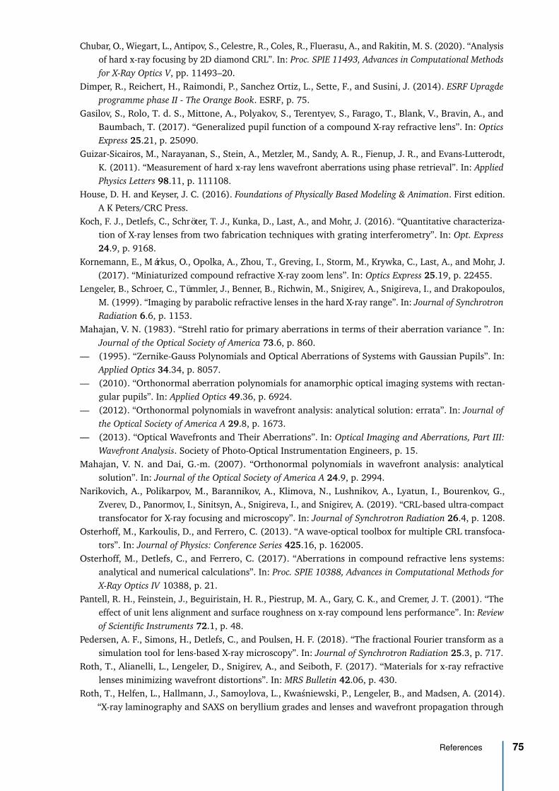
Chubar, O., Wiegart, L., Antipov, S., Celestre, R., Coles, R., Fluerasu, A., and Rakitin, M. S. (2020). “Analysisof hard x-ray focusing by 2D diamond CRL”. In: Proc. SPIE 11493, Advances in Computational Methodsfor X-Ray Optics V, pp. 11493–20.
Dimper, R., Reichert, H., Raimondi, P., Sanchez Ortiz, L., Sette, F., and Susini, J. (2014). ESRF Upragdeprogramme phase II - The Orange Book. ESRF, p. 75.
Gasilov, S., Rolo, T. d. S., Mittone, A., Polyakov, S., Terentyev, S., Farago, T., Blank, V., Bravin, A., andBaumbach, T. (2017). “Generalized pupil function of a compound X-ray refractive lens”. In: OpticsExpress 25.21, p. 25090.
Guizar-Sicairos, M., Narayanan, S., Stein, A., Metzler, M., Sandy, A. R., Fienup, J. R., and Evans-Lutterodt,K. (2011). “Measurement of hard x-ray lens wavefront aberrations using phase retrieval”. In: AppliedPhysics Letters 98.11, p. 111108.
House, D. H. and Keyser, J. C. (2016). Foundations of Physically Based Modeling & Animation. First edition.A K Peters/CRC Press.
Koch, F. J., Detlefs, C., Schröter, T. J., Kunka, D., Last, A., and Mohr, J. (2016). “Quantitative characteriza-tion of X-ray lenses from two fabrication techniques with grating interferometry”. In: Opt. Express24.9, p. 9168.
Kornemann, E., Márkus, O., Opolka, A., Zhou, T., Greving, I., Storm, M., Krywka, C., Last, A., and Mohr, J.(2017). “Miniaturized compound refractive X-ray zoom lens”. In: Optics Express 25.19, p. 22455.
Lengeler, B., Schroer, C., Tümmler, J., Benner, B., Richwin, M., Snigirev, A., Snigireva, I., and Drakopoulos,M. (1999). “Imaging by parabolic refractive lenses in the hard X-ray range”. In: Journal of SynchrotronRadiation 6.6, p. 1153.
Mahajan, V. N. (1983). “Strehl ratio for primary aberrations in terms of their aberration variance ”. In:Journal of the Optical Society of America 73.6, p. 860.
— (1995). “Zernike-Gauss Polynomials and Optical Aberrations of Systems with Gaussian Pupils”. In:Applied Optics 34.34, p. 8057.
— (2010). “Orthonormal aberration polynomials for anamorphic optical imaging systems with rectan-gular pupils”. In: Applied Optics 49.36, p. 6924.
— (2012). “Orthonormal polynomials in wavefront analysis: analytical solution: errata”. In: Journal ofthe Optical Society of America A 29.8, p. 1673.
— (2013). “Optical Wavefronts and Their Aberrations”. In: Optical Imaging and Aberrations, Part III:Wavefront Analysis. Society of Photo-Optical Instrumentation Engineers, p. 15.
Mahajan, V. N. and Dai, G.-m. (2007). “Orthonormal polynomials in wavefront analysis: analyticalsolution”. In: Journal of the Optical Society of America A 24.9, p. 2994.
Narikovich, A., Polikarpov, M., Barannikov, A., Klimova, N., Lushnikov, A., Lyatun, I., Bourenkov, G.,Zverev, D., Panormov, I., Sinitsyn, A., Snigireva, I., and Snigirev, A. (2019). “CRL-based ultra-compacttransfocator for X-ray focusing and microscopy”. In: Journal of Synchrotron Radiation 26.4, p. 1208.
Osterhoff, M., Karkoulis, D., and Ferrero, C. (2013). “A wave-optical toolbox for multiple CRL transfoca-tors”. In: Journal of Physics: Conference Series 425.16, p. 162005.
Osterhoff, M., Detlefs, C., and Ferrero, C. (2017). “Aberrations in compound refractive lens systems:analytical and numerical calculations”. In: Proc. SPIE 10388, Advances in Computational Methods forX-Ray Optics IV 10388, p. 21.
Pantell, R. H., Feinstein, J., Beguiristain, H. R., Piestrup, M. A., Gary, C. K., and Cremer, J. T. (2001). “Theeffect of unit lens alignment and surface roughness on x-ray compound lens performance”. In: Reviewof Scientific Instruments 72.1, p. 48.
Pedersen, A. F., Simons, H., Detlefs, C., and Poulsen, H. F. (2018). “The fractional Fourier transform as asimulation tool for lens-based X-ray microscopy”. In: Journal of Synchrotron Radiation 25.3, p. 717.
Roth, T., Alianelli, L., Lengeler, D., Snigirev, A., and Seiboth, F. (2017). “Materials for x-ray refractivelenses minimizing wavefront distortions”. In: MRS Bulletin 42.06, p. 430.
Roth, T., Helfen, L., Hallmann, J., Samoylova, L., Kwasniewski, P., Lengeler, B., and Madsen, A. (2014).“X-ray laminography and SAXS on beryllium grades and lenses and wavefront propagation through
References 75

imperfect compound refractive lenses”. In: Proc. SPIE 9207, Advances in X-Ray/EUV Optics andComponents IX 9207, p. 920702.
Sanchez del Rio, M. and Alianelli, L. (2012). “Aspherical lens shapes for focusing synchrotron beams”. In:Journal of Synchrotron Radiation 19.3, p. 366.
Sanchez Del Rio, M., Bianchi, D., Cocco, D., Glass, M., Idir, M., Metz, J., Raimondi, L., Rebuffi, L., Reininger,R., Shi, X., Siewert, F., Spielmann-Jaeggi, S., Takacs, P., Tomasset, M., Tonnessen, T., Vivo, A., andYashchuk, V. (2016). “DABAM: An open-source database of X-ray mirrors metrology”. In: Journal ofSynchrotron Radiation 23.3, p. 665.
Sanchez del Rio, M., Canestrari, N., Jiang, F., and Cerrina, F. (2011). “SHADOW3 : a new version of thesynchrotron X-ray optics modelling package”. In: Journal of Synchrotron Radiation 18.5, p. 708.
Schulz, G. (1988). “IV Aspheric Surfaces”. In: Progress in Optics 25.C, p. 349.Simons, H., Ahl, S. R., Poulsen, H. F., and Detlefs, C. (2017). “Simulating and optimizing compound
refractive lens-based X-ray microscopes”. In: Journal of Synchrotron Radiation 24.2, p. 392.Swantner, W. and Chow, W. W. (1994). “Gram–Schmidt orthonormalization of Zernike polynomials for
general aperture shapes”. In: Applied Optics 33.10, p. 1832.Umbach, M., Nazmov, V., Simon, M., Last, A., and Saile, V. (2008). “Numerical simulations of achromatic
x-ray lenses”. In: Proc. SPIE 7077, Advances in X-Ray/EUV Optics and Components III 7077, 70770G.Vaughan, G. B. M., Wright, J. P., Bytchkov, A., Rossat, M., Gleyzolle, H., Snigireva, I., and Snigirev, A.
(2011). “X-ray transfocators: focusing devices based on compound refractive lenses”. In: Journal ofSynchrotron Radiation 18.2, p. 125.
Ye, J., Gao, Z., Wang, S., Cheng, J., Wang, W., and Sun, W. (2014). “Comparative assessment of orthogonalpolynomials for wavefront reconstruction over the square aperture”. In: Journal of the Optical Societyof America A 31.10, p. 2304.
Zernike, v. F. (1934). “Beugungstheorie des Schneidenverfahrens und seiner verbesserten Form, derPhasenkontrastmethode”. In: Physica 1.7-12, p. 689.
Zhou, T., Wang, H., Fox, O. J., and Sawhney, K. J. (2019). “Optimized alignment of X-ray mirrors with anautomated speckle-based metrology tool”. In: Review of Scientific Instruments 90.2, p. 021706.
76 Chapter 3 Modelling optical imperfections in refractive lenses

4Measuring optical imperfections inrefractive lenses
Surface metrology methods commonly applied to X-ray mirrors [Alcock et al., 2016; Vivo etal., 2019] are not broadly employed for the metrology of X-ray lenses mainly due to theirsmall apertures and steep parabolic surfaces (cf. Fig. 3.3) [I. I. Lyatun et al., 2015]. Non-destructive methods using X-rays are often more appropriate for X-ray lens metrology. Thissection presents some of the commonly used at-wavelength metrology methods, with emphasison X-ray speckle vectorial tracking (XSVT), the experimental technique used throughout thiswork. The metrology of single- and stacked 2D-beryllium lens with R = 50 µm is presented andthe results are compared. The experimental data shown in this chapter were acquired duringseveral beamtimes1 at the BM05 beamline - ESRF [Ziegler et al., 2004] (from 2017 to 2018 -before the ESRF long shutdown for the EBS upgrade), at the 1-BM beamline - APS [Macranderet al., 2016] (during the ESRF long shutdown in 2019) and the ID06 beamline - ESRF [Kutsalet al., 2019] (in 2020 during the commissioning period of the ESRF-EBS upgrade).
4.1 At wavelength-metrologySurface metrology of X-ray optical elements is often done using the visible spectral range
[Alcock et al., 2016; Vivo et al., 2019] even if, ultimately, they will be employed in a differentspectral range. At-wavelength metrology is an umbrella term for measurements of opticalelements at photon energies closer to the ones they will be ultimately used - in the case ofX-ray lenses, in the range of few to several kilo-electron-volts. What follows is a non-exhaustivedescription of commonly used techniques for quality control applied to X-ray lenses and theircompliance to a parabolic shape. Other relevant at-wavelength characterisations of X-ray lensessuch as X-ray small-angle scattering [Roth et al., 2014; Chubar et al., 2020] or the impact ofmaterial micro-structures or shape errors on imaging [Chubar et al., 2020; I. Lyatun et al., 2020]are not covered here. A more complete survey on characterisation methods for X-ray lenses ispresented in the supplementary material from [Roth et al., 2017].
The simplest at-wavelength techniques consist of the direct imaging of a lens with X-rays bypropagation-based phase-contrast imaging [Endrizzi, 2018] since absorption contrast imagingonly generates a reduced contrast for a single lens and a low signal to noise ratio. With suchsimple techniques, 2D shapes and distances can be measured (e.g. radiographs for controllingthe distance and alignment between the parabolic surfaces of X-ray lenses). Still based onpropagation based-imaging techniques, X-ray laminography [Helfen et al., 2011; Roth et al.,2014] and X-ray tomography [Landis and Keane, 2010; Narikovich et al., 2017] of X-ray
1Acknowledgements to Sébastien Bérujon and Ruxandra Cojocaru (BM05-ESRF); Xianbo Shi, Zhi Qiao, MichaelWojcik and Lahsen Assoufid (1-BM-APS); and to Carsten Detlefs (ID06-ESRF) for the help during the experimentalsessions.
77

lenses provide a 3D reconstruction of the lens volume with high spatial resolution information.These techniques provide data on the shape of the refracting surfaces and the internal features(inhomogeneities) and can be used for modelling optical imperfections in refractive lenses.
Another large family of experimental techniques used for lens metrology and aiming atquantitative optical characterisation can be grouped under the wave-front sensing branch2.Wavefront-sensing is often employed as a beam-diagnostics tool for highly coherent sources[Seaberg et al., 2019]. Two conceptual approaches are often used: i-) absolute wavefrontmetrology at a specific point of the beam path measures the global state of the wavefront or ii-)differential measurements are done with and without the optical element under investigation,the differences in the wavefront being attributed to the optical contribution of the element undertest. Current wavefront-sensing techniques used so far in the community for evaluating thephase errors of CRLs (or individual X-ray lenses) are: i-) the Ronchi test, an interferometrictechnique that provides qualitative3 information on third-order optical aberrations [Nilsson et al.,2012; Uhlén et al., 2014]; ii-) the use of X-ray Shack–Hartmann sensors [Mayo and Sexton,2004; Mercere et al., 2005; Mikhaylov et al., 2020]; iii-) the ptychographic reconstruction ofthe wavefront emerging from a strongly focusing optics [Schropp et al., 2013; Sala et al., 2017;Seiboth et al., 2017]; iv-) grating interferometry and its variations [David et al., 2012; Koch et al.,2016; Grizolli et al., 2017]; v-) and the near-field-speckle-imaging-based (SBI) methods [Berujonet al., 2013; M.-C. Zdora et al., 2018; Berujon et al., 2020a]. The latter is the main experimentaltechnique used in this project primarily due to its easy experimental implementation and highspatial resolution. The remainder of this chapter will focus more deeply on its theoretical andexperimental aspects.
4.1.1 X-ray (near field) speckle vector tracking (XSVT)
The X-ray near-field-speckle-imaging is currently the chosen technique for systematic at-wavelength metrology of X-ray lenses at the ESRF4 and is available at the BM05 beamline[Berujon et al., 2020a] and more recently, at the ID06 beamline. The principal reasons for thischoice are: i-) the low requirements on transverse- and longitudinal coherence [Zanette et al.,2014; M. C. Zdora et al., 2015; Wang et al., 2016]; ii-) no requirement of specially tailored optics(nor accompanying complicated alignment procedures) [Morgan et al., 2012; Wang et al., 2016];iii-) successful benchmark against more established wave-front sensing techniques [Kashyapet al., 2016; Romell et al., 2017]; and iv-) its versatility as a metrology tool being able to measuremirrors, single- and stacked lenses [Berujon et al., 2020a]. Although the basic principles of theseveral X-ray near-field-speckle-based techniques are the same, the focus is given here to theX-ray (near field) speckle vector tracking (XSVT) as implemented and used for the metrologyof single- and stacked X-ray lenses used in this work [Berujon et al., 2020a,b]. An interesting
2With the advent of more coherent sources of X-rays as encapsulated by the emergence of 4th-generation synchrotronsand free-electron lasers, the topic of wavefront sensing has seen increased attention [Seaberg et al., 2019].
3It has been demonstrated that the Ronchi test can also retrieve quantitative information [Lee and Guizar-Sicairos,2010], but it has not yet been applied to X-ray lenses metrology.
4Other synchrotron facilities also offer X-ray lens metrology with the X-ray near field speckle imaging technique:1-BM at the APS in the U.S.A. [Qiao, Shi, Wojcik, et al., 2020] and the B16 beamline at the Diamond Light Sourcein the U.K. [Sawhney et al., 2013].
78 Chapter 4 Measuring optical imperfections in refractive lenses

review of different techniques using X-ray near-field speckle imaging is given by [M.-C. Zdora,2018] and [Berujon et al., 2020b].
4.1.2 Foundation
Near-field speckle is a manifestation in intensity of the summation of several complexelectric fields when the amplitudes and phases of such fields have random values. The resultingintensities may be locally high due to constructive interference or low, due to destructiveinterference [Goodman, 2020, §1]. For a speckle pattern over a defined region of interest, thespeckle contrast (or visibility) can be defined5 as:
v = σI
I, (4.1)
where σI is the standard deviation and I is the mean value of the intensity value of the specklepattern. In the X-ray regime, it appears when a sufficiently coherent X-ray beam is transmittedthrough matter with random spatial variation of δ and β, where the local optical path lengthvaries significantly when compared to the scale of the wavelength.
For a static random modulation of the wavefield (stationary scatterer6), it has been demon-strated that the speckle-grains7 preserve shape and size for free-space propagation distanceslimited to:
z < ∆cl⊥ξk, (4.2)
where ∆cl⊥ is transverse coherence length8 and ξ is the typical transverse length of the modulator,that is, the region where the spatial variation of δ and β is negligible [Cerbino et al., 2008].For propagation distances smaller than the imposed limit in Eq. 4.2, speckles can be used as awavefront marker, since the transverse position of the speckle grains in two parallel planes alongthe propagation direction can be inferred geometrically. The near-field regime is of particularinterest for the X-ray energy range, as very low wavelengths lead to an extended near-fieldregime. A stationary scatterer and the associated speckle-pattern are shown in Fig. 4.1.
Based on the uniqueness of each speckle grain, speckle-imaging-based techniques rely onidentifying similar patterns in two different images or image sets: a reference image and animage in the presence of the probe (perturbed) - cf. Fig. 4.2. The numerical implementationsused for tracking the lateral displacement of the speckle grains in the detector plane can beseveral: cross-correlation peak calculation [Bérujon et al., 2012; Morgan et al., 2012] andleast-square-minimisation [Zanette et al., 2014; M. C. Zdora et al., 2017] based approaches arethe two most used methods9,10. The lateral displacement of the speckle grain in the detector
5Other definitions are commonly found in the literature: v = Imax−IminImax+Imin
and v = Imax−Imin2I
, where Imax and Imin arethe maximum and minimum intensities found in the region of interest [M.-C. Zdora, 2018].
6As opposed to time-varying modulation of the speckle-field as in [Morgan et al., 2010; Goikhman et al., 2015].7Continous regions in space with a slowly-varying intensity that can be visually clustered together.8cf. Spatial coherence in §1.2.3 - Optical coherence.9Recently, an Euclidean-distance minimisation of the wavelet-transform method has been reported. Compared to
correlation-based techniques it is less computationally demanding and more robust to noise [Qiao, Shi, Celestre,et al., 2020].
10Regardless of the tracking method, the displacement vector ν must be equivalent, as it is linked to the sampleshape and material.
4.1 At wavelength-metrology 79
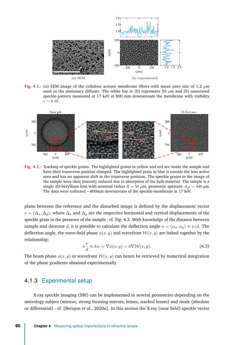
(a) SEM
−100 0 100(µm)
−100
0
100
(µm
)
1.0
1.5
2.0
1.0 1.5 2.0
(b) experimental
Fig. 4.1.: (a) SEM image of the cellulose acetate membrane filters with mean pore size of 1.2 µmused as the stationary diffuser. The white bar in (b) represents 50 µm and (b) associatedspeckle-pattern measured at 17 keV at 800 mm downstream the membrane with visibilityv ∼ 0.19.
Fig. 4.2.: Tracking of speckle grains. The highlighted grains in yellow and red are inside the sample andhave their transverse position changed. The highlighted grain in blue is outside the lens activearea and has no apparent shift in the transverse position. The speckle grains in the image ofthe sample have their intensity reduced due to absorption of the bulk material. The sample is asingle 2D-beryllium lens with nominal radius R = 50 µm, geometric aperture A� ∼ 440 µm.The data were collected ∼800mm downstream of the speckle-membrane at 17 keV.
plane between the reference and the disturbed image is defined by the displacement vectorν = (∆x,∆y), where ∆x and ∆y are the respective horizontal and vertical displacements of thespeckle grain in the presence of the sample - cf. Fig. 4.3. With knowledge of the distance betweensample and detector d, it is possible to calculate the deflection angle α = (αx, αy) ≈ ν/d. Thedeflection angle, the wave-field phase φ(x, y) and wavefrontW(x, y) are linked together by therelationship:
kν
d≈ kα = ∇φ(x, y) = k∇W(x, y). (4.3)
The beam phase φ(x, y) or wavefrontW(x, y) can hence be retrieved by numerical integrationof the phase gradients obtained experimentally.
4.1.3 Experimental setup
X-ray speckle imaging (SBI) can be implemented in several geometries depending on themetrology subject (mirrors, strong focusing mirrors, lenses, stacked lenses) and mode (absoluteor differential) - cf. [Berujon et al., 2020a]. In this section the X-ray (near field) speckle vector
80 Chapter 4 Measuring optical imperfections in refractive lenses

X-rays
reference ray
𝑑
X-rays
deflected ray
𝛼
𝜈
𝑙
Fig. 4.3.: Generic speckle-based imaging measurement geometry for the XSVT technique and the originof the displacement vector ν arising from the lens refraction. From left to right: X-ray beam,speckle-membrane, sample and 2D imaging detector. The distance between sample and detectoris noted d, the deflection angle is α and the transverse displacement vector in the detectorplane is ν.
tracking (XSVT) in the differential mode, as originally implemented at BM05 and shown inFigs. 4.3, 4.4 and 4.5 is described.
Illumination
Unlike other wavefront sensing techniques, speckle-based metrology has low requirementson transverse and longitudinal coherence11 as demonstrated by [Zanette et al., 2014; M. C. Zdoraet al., 2015; Wang et al., 2016]. The degree of lateral coherence of the illumination is intimatelyconnected with two important factors: the speckle contrast (cf. Eq. 4.1) and the propagationdistance where shape and size of the speckle grains are preserved (cf. Eq. 4.2). X-rays with lowertransverse coherence will produce speckle with low visibility (appearing thus as a smeared out orblurred image) and the numerical process of tracking signals will lose some of its accuracy. Formetrology applications, a minimum contrast of 0.1 (Eq. 4.1) is expected [Berujon et al., 2020a]for the algorithms to show an acceptable accuracy. A reduced propagation distance d betweenthe sample and the detector (cf. Fig. 4.3 and 4.4) arising from a reduced coherence length∆cl⊥ (Eq. 4.2) diminishes the angular sensitivity and will impact on the residual height errormeasurement sensitivity. When selecting an X-ray source, a higher degree of transverse coherenceis preferred. Nonetheless, bending magnets12 are readily well suited for speckle-imaging-basedmetrology since their beam usually offer the necessary minimum transverse coherence.
11Phase-contrast imaging with low-coherence sources has been demonstrated [Cloetens et al., 1996; Wilkins et al.,1996; Pfeiffer et al., 2006; Munro et al., 2012].
12At BM05, a bending magnet was the X-ray source used in this project until the ESRF-EBS upgrade long shutdown(December 2018). The BM05 bending magnet in place since the opening of the ESRF in 1994 was decommissionedin favour of a much shorter and brighter 2-pole wiggler, installed early 2020. All the data collected at BM05 andpresented hereafter were collected before this upgrade.
4.1 At wavelength-metrology 81

X-ray lens(es)
𝑒!
speckle generator
imaging detector
scintillator
monochromator
microscope objective
X-ray source
𝑑 𝑙 𝑅"
slits
slits
Fig. 4.4.: Generic speckle-based imaging experimental setup as originally implemented at the BM05beamline of the ESRF. right to left: an X-ray source (bending magnet) delivers a beam whoselarge spectral bandwidth is reduced with a Si(111) double crystal monochromator down to∆E/E ≈ 10−4. The now monochromatic beam hits the speckle-generator at a distance RS fromthe source. The stationary diffuser is composed of several stacked cellulose acetate membranefilters with a mean pore size of 1.2 µm. The membranes are mounted on a (piezoelectric)nano-positioner transverse translation stage so that the membranes can be scanned in thexy−plane. At a distance l downstream of the membrane, the sample is placed and alignedon the optical axis. Further downstream the probe, at a distance d, a scintillator converts theX-rays into visible light. The scintillator is imaged into a 2D imaging sensor, which is coupledwith a microscope objective to reach a small pixel size. Such experimental setup, without anystructural change, was later on used at the 1-BM (APS) and ID06 (ESRF) beamlines. Converselyto what depicted here, the X-ray source at the ID06 is an undulator and not a bending magnet.
Choosing the optimal experiment energy13 for X-ray lens metrology is about reaching acompromise between several competing constraints. For a fixed distance d, the energy should behigh enough so that the speckle grains being transmitted through the lens geometric apertureare not excessively deformed by focusing at the detection plane - the higher the energy, thelonger the focal length of an X-ray lens is (cf. Eq. 2.4) - on the other hand, lower energy giveslarger refraction angles, which increases the sensitivity of the experimental technique. Excessivedeformation of the detected speckle field, however, causes the tracking to fail in deliveringcredible results. Higher energy is also beneficial when considering the limit to the distance dimposed by Eq. 4.2. On the other hand, increasing the energy decreases the coherent fractionof the emitted beam, which in turn reduces the speckle visibility14. Lastly, the source spectrum(Fig. 1.1) and detector efficiency have also to be considered, as a higher photon flux allows forshorter acquisition time, meaning that experiments require less time and possible instabilities(vibrations, long time drifts and other external perturbations) have a lower impact on theacquired data. Requirements on the illumination monochromaticity are not stringent for SBI,but the metrology of X-ray lenses requires narrow bandwidths as these optics display intrinsic
13The energy chosen for most metrology experiments was E = 17 keV with ∆E/E ≈ 10−4 by using a Si(111) DCM.This energy was originally set at BM05 due to the source higher flux at this energy and the good compromisebetween absorption and sensitivity such working wavelength offer. Later, this same energy was also adopted forexperiments at other beamlines to facilitate direct comparison during the data-analysis.
14Slitting down the beam and increasing the propagation distance from the source to the speckle-membrane (Rsin Fig. 4.4) both help to increase the coherence length at the expense of photon flux - cf. van-Cittert-Zerniketheorem in [Mandel and Wolf, 1995, §4.4.4] or the applicability to SR in [Geloni et al., 2008, §4].
82 Chapter 4 Measuring optical imperfections in refractive lenses
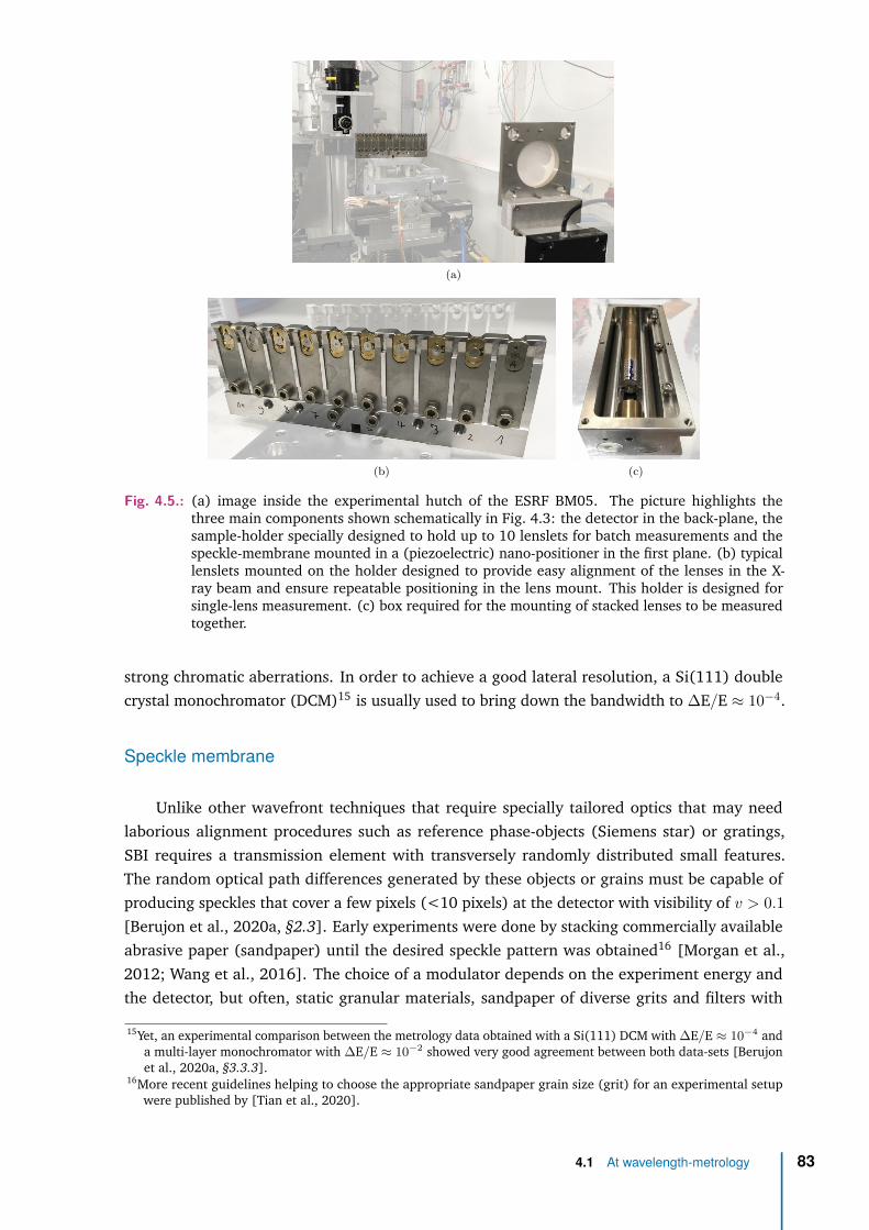
(a)
(b) (c)
Fig. 4.5.: (a) image inside the experimental hutch of the ESRF BM05. The picture highlights thethree main components shown schematically in Fig. 4.3: the detector in the back-plane, thesample-holder specially designed to hold up to 10 lenslets for batch measurements and thespeckle-membrane mounted in a (piezoelectric) nano-positioner in the first plane. (b) typicallenslets mounted on the holder designed to provide easy alignment of the lenses in the X-ray beam and ensure repeatable positioning in the lens mount. This holder is designed forsingle-lens measurement. (c) box required for the mounting of stacked lenses to be measuredtogether.
strong chromatic aberrations. In order to achieve a good lateral resolution, a Si(111) doublecrystal monochromator (DCM)15 is usually used to bring down the bandwidth to ∆E/E ≈ 10−4.
Speckle membrane
Unlike other wavefront techniques that require specially tailored optics that may needlaborious alignment procedures such as reference phase-objects (Siemens star) or gratings,SBI requires a transmission element with transversely randomly distributed small features.The random optical path differences generated by these objects or grains must be capable ofproducing speckles that cover a few pixels (<10 pixels) at the detector with visibility of v > 0.1[Berujon et al., 2020a, §2.3]. Early experiments were done by stacking commercially availableabrasive paper (sandpaper) until the desired speckle pattern was obtained16 [Morgan et al.,2012; Wang et al., 2016]. The choice of a modulator depends on the experiment energy andthe detector, but often, static granular materials, sandpaper of diverse grits and filters with
15Yet, an experimental comparison between the metrology data obtained with a Si(111) DCM with ∆E/E ≈ 10−4 anda multi-layer monochromator with ∆E/E ≈ 10−2 showed very good agreement between both data-sets [Berujonet al., 2020a, §3.3.3].
16More recent guidelines helping to choose the appropriate sandpaper grain size (grit) for an experimental setupwere published by [Tian et al., 2020].
4.1 At wavelength-metrology 83

micrometric pore-sizes can be used17. Low transmission, poor time stability and/or the presenceof strong diffraction are characteristics that should be avoided when choosing a speckle generator.Due to the random nature of the wavefront (static) modulation, the membrane does not requireany precise alignment with the beam.
XSVT is a scanning technique and usually18 N reference images are taken at N differenttransverse positions of the speckle generator with respect to the optical axis. The sample isput into the beam and another set of N images are taken with the speckle generator locatedat the exact previous N positions - cf. orange arrows in Fig. 4.3. The reproducibility of thespeckle generator transverse positions is of key importance as the difference in the speckle grainpositions from reference to sample image is attributed to the modulation of the beam. To makesure that during the collection of the jth (j ∈ [1, 2, ..., N ]) pair of images the position of thespeckle generator is repeated with precision as good as a fraction of effective pixel size, themodulator is mounted on a precise (piezoelectric) nano-positioner with a travel range of a fewhundred micrometres.
Sample
X-ray speckle vectorial tracking is a very attractive technique as it can measure weakly-focusing optics as well as very strong focusing systems with minor modifications of the setup - cf.[Berujon et al., 2020a] for some examples. Typically, two types of optical elements are todayroutinely measured at the ESRF: individual lenses and moderately focusing CRLs. Figure 4.5(b)and (c) shows typical lenses in their holder. Single lenses are mounted in an in-house-designedholder conceived to hold up to 10 lenslets next to each other, allowing serial measurementsand minimising manual intervention to change samples. Stacked lenses are measured in typicalcasings. The lens holder has to be mounted on a motorised support that can move transverselyto the beam (xy−plane) and has yaw, pitch, and roll rotations19 to compensate for the residualphase errors generated from misalignments - cf. §3.2 - Misalignments.
Detection
Although subpixel resolution for XSVT has been recently reported [Qiao, Shi, Celestre, et al.,2020], generally, the lateral resolution of the 2D surface maps obtained with XSVT is limited tothe detector effective pixel size. This makes the use of a 2D high-resolution imaging detectorscommon for speckle-based imaging. In real-space imaging with X-rays, since high resolution overa large field of view is usually wished, it is common to use indirect detection. Converting X-raysinto visible-light and subsequently imaging it onto a pixelated detector allows one to access tosmaller pixel sizes thanks to the use of magnifying optics and small pixel sensors designed forvisible-light detection.
17Experiments showed here used a stack of cellulose acetate membrane filters with a mean pore size of 1.2 µm usedas the stationary diffuser.
18More details in data acquisition are provided by §4.1.4 - Data acquisition, processing and analysis.19Yaw was defined in our case as the rotation around the z−axis, the pitch is around the y−axis and roll, the x−axis.
84 Chapter 4 Measuring optical imperfections in refractive lenses

A typical detection system20 is composed of three main parts: i-) the scintillator, which isresponsible for converting the X-rays into visible light. Its choice is a compromise between theyield in converting X-ray photons in visible photons and image resolution: a thin scintillator willgenerally result in a higher spatial resolution image, but at a cost of reduced photon flux, while athicker one will generate more light, but due to scattering in the bulk material, a low-resolutionimage will result; ii-) the transport optics that magnify and images the scintillator onto thesensor plane, but also may introduce aberrations to the system, this can be calibrated with theXSVT technique - cf. [Berujon et al., 2020a, §2.2]; and iii-) the imaging sensor, which ideallyshould be a low-noise 2D pixelated sensor with fast read-out. The final effective pixel size is aconvolution of the contributions from the choice of scintillator, magnification and point spreadfunction of the transport optics and the imaging device.
4.1.4 Data acquisition, processing and analysis
Data acquisition & analysis
The first implementations of X-ray speckle-tracking (XST) for metrology consisted of ac-quiring solely two images: the reference- and the sample-image with the same speckle pattern(cf. Fig. 4.2). The algorithms used to match the patterns in both images relied in setting in thereference image a small window around a pixel of interest wreference(xl, ym) and searching forit (possibly distorted) in a larger window in the sample image: wprobe(xl, ym). The referencewindow is rastered through the whole sample image (L×M pixels from the whole image) toreconstruct two 2D displacement maps (horizontal and vertical) with lateral resolution limitedto the speckle-grain size. In order to improve the limited resolution of XST, XSVT relies ontransversely scanning21 the speckle-generator across the X-ray beam and taking images at theN different points of the scan. Once the reference data-set is taken, the sample is inserted inthe beam and the scan is repeated at the exact same diffuser position. Each data set (referenceand probe) contains NL×M images where the jth (j ∈ [1, 2, ..., N ]) image in each stack indicatesthe same transverse coordinates of the scatterer scan - cf. Fig. 4.6. For a sufficiently large N , avector is obtained by sampling each jth image of the reference data-set around a pixel coordinate(xl, ym) with l ∈ [1, 2, ..., L] and m ∈ [1, 2, ...,M ]. This reference signal Ireference(xl, ym, j) isshown in green in Fig. 4.6. A ROI centred around (xl, ym) is set in the sample data-set andfor each pixel coordinate within this ROI, that is (xl+∆l, ym+∆m), a corresponding intensityvector is obtained: Iprobe(xl+∆l, ym+∆m, j) - cf. magenta and orange signals in Fig. 4.6. TheIreference(xl, ym, j) vector is compared22 individually to each of the Iprobe(xl+∆l, ym+∆m, j) vec-tors. Fig. 4.7 shows the normalised cross-correlation values for a particular lens, which are
20The detection systems use at the ESRF are composed of a 10 µm thick LSO:Tb scintillator that is imaged onto ansCMOS PCO Edge 4.2 or a FReLoN E2V CCD camera (2048 × 2048 pixels), coupled with a 10× magnificationmicroscope objective to reach a theoretical pixel size of about ∼ 0.62× 0.62 µm2. At the APS, the scintillator usedwas a 100 µm thick LuAG:Ce imaged into an Andor Neo sCMOS camera with 2560 × 2180 pixels also with a 10×magnification resulting in a pixel size of ∼ 0.65× 0.65 µm2.
21The nature of the scan is not particularly relevant for the data analysis in this particular metrology mode.22Which can be either using a cross-correlation peak calculation [Bérujon et al., 2012; Morgan et al., 2012], a
least-square-minimisation [Zanette et al., 2014; M. C. Zdora et al., 2017] or an Euclidean-distance minimisationof the wavelet-transform of the reference- and probe- vectors [Qiao, Shi, Celestre, et al., 2020]. In this workthe cross-correlation peak calculation is the preferred method for speckle-vector tracking [Bérujon et al., 2012;Morgan et al., 2012].
4.1 At wavelength-metrology 85

𝑗 = 0
𝑗 = 𝑁
𝑗 = 0
𝑗 = 𝑁
𝑗 = 𝑁
𝑗 = 0
Fig. 4.6.: X-ray (near field) speckle vector tracking (XSVT). In the differential mode, two data-sets aretaken: the reference and the one with the imaged sample. Each of the jth image pair of thedata-set is taken at a different transverse scan position of the speckle-generator across theX-ray beam. However, for a particular jth image-pair (reference and probe) the exact samediffuser position must be maintained. A reference intensity vector Ireference(xl, ym, j) (green) issearched in the sample stack,in a ROI centred around (xl, ym, j), where Iprobe(xl+∆l, ym+∆m, j)vectors are probed for a matching value. The purple signal is a well matched signal, while theorange signal shows the neighbouring-pixel intensity vector Iprobe(xl−2, ym−2, j).
used to evaluate the convergence of the tracking method. By repeating this procedure for allL×M pixels, it is possible to obtain two 2D displacement maps (vertical and horizontal) withlateral resolution down to the ∼ effective-pixel-size of the detector at the expense of an increaseddata-collection and data-processing time [Berujon and Ziegler, 2016; Berujon et al., 2020b].
Surface reconstruction & analysis
The phase gradients ∇φ(x, y) can be obtained from the two displacement maps by multiply-ing them by the wavenumber k and dividing the product by the distance between the sample anddetector (d) - cf. Eq. 4.3. An example of the horizontal and vertical gradient for a 2D-berylliumlens with R = 50 µm measured at 17 keV with d = 800 mm and pixel size ∆pixel = 0.63 µmis shown in Fig. 4.8(a)-(b) where the mismatch between front- and back- focusing surfaces isobvious - cf. Fig. 4.7. An ideal lens has phase gradients with linear dependencies on the focusingdirection. From Eq. 1.36b and Eq. 2.8:
∇φ(x, y) =(∂φ(x, y)∂x
,∂φ(x, y)∂y
)= −2kδ
(x
Rx,y
Ry
), (4.4)
86 Chapter 4 Measuring optical imperfections in refractive lenses

−200 0 200(µm)
−200
0
200
(µm
)
(a) radiography
−200 0 200(µm)
−200
0
200
(µm
)
0.80
0.90
1.00
(b) cross-correlation map
Fig. 4.7.: (a) radiography of a 2D-beryllium lens with R = 50 µm measured at 17 keV with d = 800 mmand pixel size ∆pixel = 0.63 µm. The different penetration depths of the parabolic profilescause the reduction of the geometric aperture, evidenced by the two concentric rings. (b)the normalised cross-correlation peak for the vector tracking algorithm. Regions with darkercolours have lower correlation peaks.
which is a linear function with the slope of the linear phase-gradient in the focusing directioninversely proportional to the radius of curvature of the X-ray lens. This information can beexperimentally retrieved with the knowledge of the X-ray energy used and the lens material(refraction index decrements). The phase gradient residues (or errors) are accessible by removinga linear fit from the gradients, which is shown in Fig. 4.8(c)-(d). In order to recover the thicknessprofile in projection approximation from the phase gradient (or from the residual phase gradient),the main step is the numerical 2D integration23 of the differential fields, which is done usingeither the Frankot-Chelappa method [Frankot and Chellappa, 1988] or the Harker-O’Learymethod (grad2surf) [Harker and O’Leary, 2015]. The profile resulting from the 2D integrationof the (residual) phase gradients can be converted into thickness in projection approximation by(cf. Eq. 1.36b):
∆z(x, y) = −φ(x, y)kδ
. (4.5)
Equation 4.5 is based on the assumption that the X-ray lens has a refractive index decrementδ with no variations in (x, y, z). Eq. 4.5 also justifies the use of a monochromator in theexperimental setup (cf. Fig. 4.4) since δ has a significant energy dependency. The figure errorsfrom a lens can be obtained by two approaches: i-) by first integrating the phase gradients,then fit and remove from the resulting surface either a cylinder with a parabolic section or aparaboloid of revolution depending on whether the lens is a 1D or 2D focusing element. Thetreatment shown in Eq. 4.5 is applied to this residual phase; or by ii-) directly integrating theresidual phase gradients and application of Eq. 4.5 to the integrated field. The residual thicknessin projection approximation for the previous lens is shown in Fig. 4.9(a). Valuable informationsuch as the RMS value of the figure errors; the decomposition of the wavefront into orthonormalpolynomials (cf. §3.4.1 - Orthornormal polynomials) for the systematic study of the opticalimperfections; and the power spectral density (PSD) of horizontal- and vertical- profile cutsshowing the spatial frequency distribution of the optical errors can all be obtained from theresidual thickness profile as shown in Fig. 4.9. The recovered thickness profile in Fig. 4.9(a) canbe later used as a ∆z(x, y) map in Eq. 1.37 to simulate the effects of optical imperfections inX-ray lenses as discussed in §3.4.2 - Metrology data.
23More on numerical integration of gradient fields in [Huang et al., 2015] and [Agrawal et al., 2006].
4.1 At wavelength-metrology 87

−200 0 200(µm)
−200
0
200
(µm
)
−10
0
10
−10 0 10
(a) horizontal gradient (µrad)
−200 0 200(µm)
−200
0
200
(µm
)
−10
0
10
−10 0 10
(b) vertical gradient (µrad)
−200 0 200(µm)
−200
0
200
(µm
)
−0.25
0.00
0.25
−0.250.00 0.25
(c) horizontal gradient residue (µrad)
−200 0 200(µm)
−200
0
200
(µm
)
−0.25
0.00
0.25
−0.250.00 0.25
(d) vertical gradient residue (µrad)
Fig. 4.8.: Phase gradients and respective gradient residues for a 2D-beryllium lens with R = 50 µmmeasured at 17 keV with d = 800 mm and a pixel size ∆pixel = 0.63 µm - cf. Fig. 4.7.
−200 0 200(µm)
−200
0
200
(µm
)
-1.50
0.00
1.50
(a) thickness error
−200 0 200(µm)
−200
0
200
(µm
)
-1.50
0.00
1.50
(b) Zernike circle pol. fit
−200 0 200(µm)
−200
0
200
(µm
)
-1.00
0.00
1.00
(c) residues
Z1 · · · Z5 · · · ·Z10 · · · ·Z15 · · · ·Z20 · · · ·Z25 · · · ·Z30 · · · ·Z35 · ·−0.6
−0.4
−0.2
0.0
0.2
0.4
(µm
)
figure errors
(d) Zernike circle polynomial fit coefficients
104 105 106
spatial frequency (m−1)
10−21
10−20
10−19
10−18
10−17
10−16
(m3 )
horizontal cut at y = 0vertical cut at x = 0
(e) PSD
Fig. 4.9.: (a) Recovered figure errors in projection approximation of a 2D-beryllium lens with R = 50 µmmeasured at 17 keV with d = 800 mm and pixel size ∆pixel = 0.63 µm, (b) Zernike circlepolynomial fit of the figure errors and (c) the residues from the fit. The coefficients of the fitare shown in (d). (e) Horizontal and vertical power spectrum density of the lens.
88 Chapter 4 Measuring optical imperfections in refractive lenses

Measurement sensitivity
Finally, some considerations on the measurement sensitivity are presented. Supposing anideal detection system with effective pixel size ∆pixel, the minimum measurable deflection angleis:
αmin = η∆pixel
d, (4.6)
where η is a factor accounting for the ability of the algorithm to track a displacement vector withsubpixel accuracy. Consider that the probe can be laterally sampled with the detector spatialresolution ∆pixel as shown in Fig. 4.10(a). Each projected pixel will have a mean height valueand the minimum detectable height difference between two adjacent pixels is ∆zmin. The angleαmin can be attributed to refraction caused by the local slope ϑ between two adjacent projectedpixel - cf. Fig. 4.10(b). A ray that is parallel to the optical axis will intercept this local slope atan angle θ1 = ϑ and will be refracted with an angle θ2 = ϑ+ αmin. With the law of refraction(Eq. 2.2) it is possible to estimate24 the longitudinal sensitivity of the XSVT as25:
∆zmin = ∆pixel ·sin(αmin)
11− δ − cos(αmin)
. (4.7)
Figure 4.11 shows the XSVT longitudinal sensitivity (∆zmin) based on Eq. 4.7 for beryllium,one of the most common materials for refractive optics manufacturing. From Eq. 4.7, it isclear that longitudinal resolution of the XSVT technique depends on several factors: distancebetween speckle-generator and detector d; material and experiment energy expressed as index ofrefraction decrement δ; and the effective pixel size ∆pixel, which is directly impacted by the PSFof the magnifying optics of the detector system. Other factors that contribute to the reduction inlateral resolution (increase of η): i-) the thickness of the scintillator used (blurring from thickermaterials), ii-) temporal beam-instabilities as they may reduce the apparent transverse coherenceif the integration time of the detector is longer than the instabilities period; iii-) vibrations of thesample holder with amplitudes larger than half of the pixel size and faster than the acquisitiontime; iv-) a low reproducibility of the speckle-generator membrane positioning.
Equation 4.7 is a geometric approximation of the problem and does not take into ac-count propagation of uncertainties associated with the different components in the experiment,template-matching accuracy of the tracking routines nor numerical errors associated with the
24From Fig. 4.7(a) one obtains: tan(ϑ) =∆zmin
∆pixel. Using n1 = 1, n2 = 1 − δ, θ1 = ϑ and θ2 = ϑ + αmin in the law
of refraction: sin(ϑ) = (1 − δ) sin(ϑ + αmin). Writing sin(ϑ + αmin) = sin(ϑ) cos(αmin) + sin(αmin) cos(ϑ) andcollecting terms, one obtains Eq. 4.7. Similar reasoning can be applied to a model with two refracting surfacesgiving very similar numerical results.
25It is also possible to derive an approximate expression by using physical-optics arguments. The accumulated phaseof a wave passing through a material with thickness ∆z and index of refraction n = 1− δ+ i ·β is φ(x, y) = kδ∆z
as shown in Eq. 1.36b. The gradient of this phase is: ∇φ(x, y) =
(kδ
∂
∂x∆z; kδ
∂
∂y∆z
). The partial derivatives
(local slopes) can be calculated as:∂
∂x∆z =
∂
∂y∆z =
∆z
∆pixelas a first approximation for a square pixel. With the
help of Eq. 4.3 and Eq. 4.6 one arrives at: ∆zmin = ∆pixel ·αmin
δ.
4.1 At wavelength-metrology 89

Δpixel
Δ𝑧
𝜗 𝜗
𝛼𝜃2
𝜃1
Fig. 4.10.: Sketch for aiding the calculation of the XSVT longitudinal sensitivity. The lateral resolution towhich the probe is sampled generates a local slope between adjacent pixels (red dashed linewith inclination given by ϑ). A beam parallel to the optical axis (purple) hits the sample isrefracted with an angle θ2.
500 1000 1500d (mm)
0
1
2
∆z m
in(µ
m)
(a) η = 0.5 (sub-pixel size)
500 1000 1500d (mm)
0
1
2
∆z m
in(µ
m)
(b) η = 1.0 (nominal pixel size)
500 1000 1500d (mm)
0
1
2
∆z m
in(µ
m)
(c) η = 2.0 (poor lateral resolution)
Fig. 4.11.: X-ray speckle vectorial tracking longitudinal sensitivity (∆zmin) for beryllium. The solid redline indicates the performance of the method at 10 keV, while the solid green line for 30 keV.The dashed purple line indicates the experimental performance at 17 keV (used energy forsuch experiments in this work.). Black point-dashed line indicates the nominal pixel size ofthe imaging detector ∆pixel = 0.65 µm.
wavefront reconstruction as described by [Fried, 1977; Southwell, 1980]. Those can be globallyestimated by applying the XSVT data analysis routine to two different reference data-sets takenunder the exact same experimental conditions. These two 2D deflection angle maps allow toobtain the angular sensitivity lower threshold and to estimate η under the conditions imposed bythe experimental setup. Figure 4.12 shows an example of such calculation with data taken at17 keV with d = 875 mm and pixel size ∆pixel = 0.63 µm. The horizontal and vertical gradientsRMS values for this particular experiment is 0.026 µrad and 0.025 µrad, respectively. UsingEq. 4.6, one can infer the η > 0.036. Those gradient maps can be integrated to obtain the phasenoise level (see Eq. 4.3) and an associated thickness can be estimated by using Eq. 4.5.
4.2 X-ray lens metrology
Since early 2017, metrology of individual X-ray lenses has been systematically performedat the ESRF. Measurements have been applied to quality control of commercially acquiredX-ray lenses for assessing the optical quality of already purchased lenses and for verifyingif newly-purchased lenses meet specifications. The metrology profiles extracted from such
90 Chapter 4 Measuring optical imperfections in refractive lenses

−250 0 250(µm)
−250
0
250
(µm
)
0.92
0.96
1.00
(a) cross-correlation map
−250 0 250(µm)
−250
0
250
(µm
)
−0.1
0.0
0.1
−0.1 0.0 0.1
(b) horizontal gradient
−250 0 250(µm)
−250
0
250
(µm
)
−0.1
0.0
0.1
−0.1 0.0 0.1
(c) vertical gradient
Fig. 4.12.: X-ray speckle vectorial tracking angular sensitivity calculated by applying the XSVT routine totwo distinct sets of reference images taken taken shortly after each other. The experimentwas performed at 17 keV with d = 875 mm and pixel size ∆pixel = 0.63 µm.
measurements have been used in X-ray beamline simulations26 [Celestre et al., 2020]. Morerecently, metrology started to be used to aid manufacturing of X-ray lenses produced in-house27
or as a co-development with external lens developers as it can offer insight into the relationbetween production parameters and their effects on the lens profile.
4.2.1 Single lens measurements
Tables 4.1 and 4.2 show a compilation of radii, figure errors and useful geometric aperturefor two sets of ten 2D-beryllium lenses with nominal radius R = 50 µm and geometric apertureA� = 440 µm measured individually and as stacks. These are the lenslets used in the opticalsimulations shown in §5 - Effect of optical imperfections on an X-ray beam and §6 - Correctingoptical imperfections in refractive lenses. The figure errors are divided in full profile, Zernikecircle polynomial fit (low frequency - LF) and residues from the fit (high-frequency - HF). Forthe particular case of the 2D-beryllium lenses, Zernike circle polynomials until the 37th order(3rd order spherical aberration) were used. In the context of this work, the low-frequencies(LF) span from ∼ 500 µm or 2 × 10³ m−1 (geometrical aperture of a lenslet) to ∼ 50 µm or2×104 m−1, while the mid- and high-frequencies span from ∼ 50 µm or 2×10⁴ m−1 to ∼ 0.5 µmor 2× 10⁶ m−1, which is obtained from the Nyquist frequency28 of the measured data.
Individually measured lenses can be artificially stacked to study the effects of pilling uplenses and to be later compared to the measurement of stacked lenses. This artificial stackingcan be done by propagating a plane wave through the CRL using the model described by Eq. 2.12and extracting any developed quadratic phase term at the exit pupil - Fig. 4.13 shows a typicaloptical setup for artificially stacking lenses. The phase can be readily converted into a thicknessprofile in projection approximation with the aid of Eq. 1.36b. The accumulated29 profiles for thestacks 1 and 2 are shown in Figs. 4.14 and 4.16 and compiled in Tables 4.1 and 4.2.
26Simulations using optical metrology of X-ray lenses have been reported in [Chubar et al., 2020].27See [Celestre, 2020].28Nyquist frequency is defined as one over twice the effective pixel size ∆pixel = 0.65 µm.29The progressive increase of figure errors for the full-, fit- and residual- profiles is shown in Fig. 5.9 from §5.5.1 -
Metrology of individual lenses vs. stacked lenses
4.2 X-ray lens metrology 91

z
(b) (c)(a) (d)
Fig. 4.13.: Optical setup used for artificially stacking lenses and calculating the phase errors. (a) Theillumination is the emission of a filament electron beam. An (b) ideal parabolic phase elementis used to give this illumination a plane phase. The stacked X-ray lenses are shown in (c). Theyfollow the model described by Eq. 2.12, that is, the CRL multi-slicing with figure errors added.An (d) ideal parabolic phase element with a radius of curvature matching the developedquadratic term is then added and the residuals (phase errors) can be extracted.
4.2.2 Stacked lenses measurementsBeing able to measure stacked lenses is of high interest as it allows not only to predict
the performance of such focusing compound elements in conditions relatively similar to theiremployment in beamlines but also enables the design of optical corrections for an aberratedsystem [Seiboth et al., 2017, 2020]. The values for radii, figure errors and useful geometricaperture for the two stacks used in this work are shown in Tables 4.1 and 4.2 and Figs. 4.15and 4.17. The stacks, composed of the lenses described in §4.2.1 - Single lens measurements canbe compared with the artificially accumulated profiles as shown in Figs. 4.14 and 4.16, whichshows reasonable qualitative agreement - improving the agreement between the two types ofmeasurements is important as it allows the prediction of performance and correction of a CRLcomposed of an arbitrary set of already measured and catalogued lenses. �
92 Chapter 4 Measuring optical imperfections in refractive lenses

Tab. 4.1.: Compilation of radii, figure errors and clear aperture for lenses L01 to L10 (stack 1) obtainedwith XSVT metrology.
lens radius figure errors† (r.m.s) µm useful aperturenumber µm full profile pol. fit residues µm
L01 48.77 0.57 0.45 0.35 439L02 48.24 0.80 0.69 0.43 442L03 48.76 0.77 0.55 0.54 432L04 49.20 1.05 0.92 0.51 435L05 48.41 0.81 0.67 0.44 440L06 48.70 1.07 0.72 0.79 443L07 48.91 0.70 0.53 0.46 442L08 49.23 0.84 0.62 0.56 447L09 48.09 0.93 0.79 0.49 434L10 48.10 0.88 0.76 0.44 431
accumulated: 4.84 4.36 2.18 400Stack 01: 5.46 5.75 5.20 2.47 399
† values given for A� = 400 µm
−200 −100 0 100 200(µm)
−200
−100
0
100
200
(µm
)
-8.00
0.00
8.00
(a) full profile
−200 −100 0 100 200(µm)
−200
−100
0
100
200
(µm
)
-8.00
0.00
8.00
(b) polynomial fit
−200 −100 0 100 200(µm)
−200
−100
0
100
200
(µm
)
-3.00
0.00
3.00
(c) residues
Z1 · · ·Z5 · · · ·Z10· · · ·Z15· · · ·Z20· · · ·Z25· · · ·Z30· · · ·Z35· ·
−2
0
(µm
)
figure errors
(d) polynomial decomposition
−200 0 200(µm)
0
10
20
(µm
)
(e) azimuthal averaged profile
Fig. 4.14.: Individually measured and artificially stacked lenses forming the stack 1. The individuallenses parameters are shown in Table 4.1. Profiles calculated for a geometric aperture ofA� = 400 µm.
−200 −100 0 100 200(µm)
−200
−100
0
100
200
(µm
)
-10.00
0.00
10.00
(a) full profile
−200 −100 0 100 200(µm)
−200
−100
0
100
200
(µm
)
-10.00
0.00
10.00
(b) polynomial fit
−200 −100 0 100 200(µm)
−200
−100
0
100
200
(µm
)
-4.00
0.00
4.00
(c) residues
Z1 · · ·Z5 · · · ·Z10· · · ·Z15· · · ·Z20· · · ·Z25· · · ·Z30· · · ·Z35· ·−4
−2
0
(µm
)
figure errors
(d) polynomial decomposition
−200 0 200(µm)
0
10
20
(µm
)
(e) azimuthal averaged profile
Fig. 4.15.: Measurement of a CRL composed of the lenses L01-L10 described in Table 4.1 (stack 1).Profiles calculated for a geometric aperture of A� = 400 µm.
4.2 X-ray lens metrology 93

Tab. 4.2.: Compilation of radii, figure errors and useful aperture for lenses L11 to L20 (stack 2) obtainedwith XSVT metrology.
lens radius figure errors† (r.m.s) µm useful aperturenumber µm full profile pol. fit residues µm
L11 49.05 0.71 0.57 0.43 440L12 49.27 0.80 0.68 0.44 460L13 48.98 0.94 0.75 0.56 435L14 48.26 1.06 0.95 0.47 452L15 48.25 1.44 1.36 0.46 444L16 49.25 0.69 0.55 0.42 443L17 48.94 0.72 0.61 0.39 433L18 48.30 1.22 1.15 0.42 439L19 47.78 1.24 1.21 0.25 419L20 48.62 0.80 0.72 0.36 456
accumulated 6.28 6.10 1.62 400Stack 02: 5.67 6.47 5.97 2.49 407
† values given for A� = 395 µm
−200 −100 0 100 200(µm)
−200
−100
0
100
200
(µm
)
-10.00
0.00
10.00
(a) full profile
−200 −100 0 100 200(µm)
−200
−100
0
100
200
(µm
)
-10.00
0.00
10.00
(b) polynomial fit
−200 −100 0 100 200(µm)
−200
−100
0
100
200
(µm
)
-2.50
0.00
2.50
(c) residues
Z1 · · ·Z5 · · · ·Z10· · · ·Z15· · · ·Z20· · · ·Z25· · · ·Z30· · · ·Z35· ·−4
−2
0
(µm
)
figure errors
(d) polynomial decomposition
−200 0 200(µm)
0
10
20
(µm
)
(e) azimuthal averaged profile
Fig. 4.16.: Individually measured and artificially stacked lenses forming the stack 2. The individuallenses parameters are shown in Table 4.2. Profiles calculated for a geometric aperture ofA� = 400 µm.
−100 0 100(µm)
−100
0
100
(µm
)
-16.00
-8.00
0.00
8.00
16.00
(a) full profile
−100 0 100(µm)
−100
0
100
(µm
)
-16.00
-8.00
0.00
8.00
16.00
(b) polynomial fit
−100 0 100(µm)
−100
0
100
(µm
)
-2.50
0.00
2.50
(c) residues
Z1 · · ·Z5 · · · ·Z10· · · ·Z15· · · ·Z20· · · ·Z25· · · ·Z30· · · ·Z35· ·−4
−2
0
(µm
)
figure errors
(d) polynomial decomposition
−200 0 200(µm)
0
5
(µm
)
(e) azimuthal averaged profile
Fig. 4.17.: Measurement of a CRL composed of the lenses L11-L20 described in Table 4.2 (stack 2).Profiles calculated for a geometric aperture of A� = 400 µm.
94 Chapter 4 Measuring optical imperfections in refractive lenses

ReferencesAgrawal, A., Raskar, R., and Chellappa, R. (2006). “What is the range of surface reconstructions from a
gradient field?” In: Lecture Notes in Computer Science (including subseries Lecture Notes in ArtificialIntelligence and Lecture Notes in Bioinformatics). Vol. 3951 LNCS. Springer Verlag, p. 578.
Alcock, S. G., Nistea, I., and Sawhney, K. (2016). “Nano-metrology: The art of measuring X-ray mirrorswith slope errors <100 nrad”. In: Review of Scientific Instruments 87.5, p. 051902.
Berujon, S., Wang, H., and Sawhney, K. J. (2013). “At-wavelength metrology using the X-ray speckletracking technique: Case study of a X-ray compound refractive lens”. In: Journal of Physics: ConferenceSeries. Vol. 425. PART 5. Institute of Physics Publishing, p. 052020.
Berujon, S., Cojocaru, R., Piault, P., Celestre, R., Roth, T., Barrett, R., and Ziegler, E. (2020a). “X-rayoptics and beam characterization using random modulation: experiments”. In: Journal of SynchrotronRadiation 27.2, p. 293.
— (2020b). “X-ray optics and beam characterization using random modulation: theory”. In: Journal ofSynchrotron Radiation 27.2, p. 284.
Berujon, S. and Ziegler, E. (2016). “X-ray Multimodal Tomography Using Speckle-Vector Tracking”. In:Physical Review Applied 5.4, p. 044014.
Bérujon, S., Ziegler, E., Cerbino, R., and Peverini, L. (2012). “Two-dimensional x-ray beam phase sensing”.In: Physical Review Letters 108.15, p. 158102.
Celestre, R. (2020). “Refractive lenses, at-wavelength metrology and optics simulation”. In: 12th 3-WayMeeting X-ray Optics Workshop (ESRF), Grenoble, France (presentation).
Celestre, R., Berujon, S., Roth, T., Sanchez del Rio, M., and Barrett, R. (2020). “Modelling phaseimperfections in compound refractive lenses”. In: Journal of Synchrotron Radiation 27.2, p. 305.
Cerbino, R., Peverini, L., Potenza, M. A., Robert, A., Bösecke, P., and Giglio, M. (2008). “X-ray-scatteringinformation obtained from near-field speckle”. In: Nature Physics 4.3, p. 238.
Chubar, O., Wiegart, L., Antipov, S., Celestre, R., Coles, R., Fluerasu, A., and Rakitin, M. S. (2020). “Analysisof hard x-ray focusing by 2D diamond CRL”. In: Proc. SPIE 11493, Advances in Computational Methodsfor X-Ray Optics V, pp. 11493–20.
Cloetens, P., Barrett, R., Baruchel, J., Guigay, J. P., and Schlenker, M. (1996). “Phase objects in synchrotronradiation hard x-ray imaging”. In: Journal of Physics D: Applied Physics 29.1, p. 133.
David, C., Rutishauser, S., Sprung, M., Zanette, I., and Weitkamp, T. (2012). “X-ray grating interferometry- Applications in metrology and wave front sensing”. In: AIP Conference Proceedings. Vol. 1466. 1.American Institute of PhysicsAIP, p. 23.
Endrizzi, M. (2018). “X-ray phase-contrast imaging”. In: Nuclear Instruments and Methods in PhysicsResearch, Section A: Accelerators, Spectrometers, Detectors and Associated Equipment 878, p. 88.
Frankot, R. T. and Chellappa, R. (1988). “A Method for Enforcing Integrability in Shape from ShadingAlgorithms”. In: IEEE Transactions on Pattern Analysis and Machine Intelligence 10.4, p. 439.
Fried, D. L. (1977). “Least-square fitting a wave-front distortion estimate to an array of phase-differencemeasurements”. In: Journal of the Optical Society of America 67.3, p. 370.
Geloni, G., Saldin, E., Schneidmiller, E., and Yurkov, M. (2008). “Transverse coherence properties of X-raybeams in third-generation synchrotron radiation sources”. In: Nuclear Instruments and Methods inPhysics Research Section A: Accelerators, Spectrometers, Detectors and Associated Equipment 588.3,p. 463.
Goikhman, A., Lyatun, I., Ershov, P., Snigireva, I., Wojda, P., Gorlevsky, V., Semenov, A., Sheverdyaev,M., Koletskiy, V., and Snigirev, A. (2015). “Highly porous nanoberyllium for X-ray beam specklesuppression”. In: Journal of Synchrotron Radiation 22.3, p. 796.
Goodman, J. W. (2020). Speckle Phenomena in Optics: Theory and Applications. Second edition. SPIE Press.
References 95

Grizolli, W. C., Shi, X., Assoufid, L., Kolodziej, T., and Shvyd’ko, Y. (2017). “Single-grating Talbot imagingfor wavefront sensing and x-ray metrology”. In: Proc. SPIE 10385, Advances in Metrology for X-Rayand EUV Optics VII, 1038502 10385.7, p. 1.
Harker, M. and O’Leary, P. (2015). “MATLAB toolbox for the regularized surface reconstruction fromgradients”. In: Proc. SPIE 9534, Twelfth International Conference on Quality Control by Artificial Vision2015 9534, 95341E.
Helfen, L., Myagotin, A., Mikulk, P., Pernot, P., Voropaev, A., Elyyan, M., Di Michiel, M., Baruchel, J.,and Baumbach, T. (2011). “On the implementation of computed laminography using synchrotronradiation”. In: Review of Scientific Instruments 82.6, p. 063702.
Huang, L., Idir, M., Zuo, C., Kaznatcheev, K., Zhou, L., and Asundi, A. (2015). “Comparison of two-dimensional integration methods for shape reconstruction from gradient data”. In: Optics and Lasersin Engineering 64, p. 1.
Kashyap, Y., Wang, H., and Sawhney, K. (2016). “Experimental comparison between speckle and grating-based imaging technique using synchrotron radiation X-rays”. In: Optics Express 24.16, p. 18664.
Koch, F. J., Detlefs, C., Schröter, T. J., Kunka, D., Last, A., and Mohr, J. (2016). “Quantitative characteriza-tion of X-ray lenses from two fabrication techniques with grating interferometry”. In: Opt. Express24.9, p. 9168.
Kutsal, M., Bernard, P., Berruyer, G., Cook, P. K., Hino, R., Jakobsen, A. C., Ludwig, W., Ormstrup, J.,Roth, T., Simons, H., Smets, K., Sierra, J. X., Wade, J., Wattecamps, P., Yildirim, C., Poulsen, H. F.,and Detlefs, C. (2019). “The ESRF dark-field x-ray microscope at ID06”. In: IOP Conference Series:Materials Science and Engineering 580, p. 12007.
Landis, E. N. and Keane, D. T. (2010). “X-ray microtomography”. In: Materials Characterization 61.12,p. 1305.
Lee, S. and Guizar-Sicairos, M. (2010). “Validation of quantitative Ronchi test through numerical propa-gation”. In: Optics Express 18.18, p. 18525.
Lyatun, I. I., Goikhman, A. Y., Ershov, P. A., Snigireva, I. I., and Snigirev, A. A. (2015). “On the problem ofthe metrology of refractive X-ray optics”. In: Journal of Surface Investigation 9.3, p. 446.
Lyatun, I., Ershov, P., Snigireva, I., and Snigirev, A. (2020). “Impact of beryllium microstructure on theimaging and optical properties of X-ray refractive lenses”. In: Journal of Synchrotron Radiation 27.1,p. 44.
Macrander, A., Erdmann, M., Kujala, N., Stoupin, S., Marathe, S., Shi, X., Wojcik, M., Nocher, D., Conley,R., Sullivan, J., Goetze, K., Maser, J., and Assoufid, L. (2016). “X-ray optics testing beamline 1-BMat the advanced photon source”. In: AIP Conference Proceedings. Vol. 1741. 1. American Institute ofPhysics Inc., p. 030030.
Mandel, L. and Wolf, E. (1995). Optical Coherence and Quantum Optics. First edition. Cambridge UniversityPress.
Mayo, S. C. and Sexton, B. (2004). “Refractive microlens array for wave-front analysis in the medium tohard x-ray range”. In: Optics Letters 29.8, p. 866.
Mercere, P., Bucourt, S., Cauchon, G., Douillet, D., Dovillaire, G., Goldberg, K. A., Idir, M., Levecq, X.,Moreno, T., Naulleau, P. P., Rekawa, S., and Zeitoun, P. (2005). “X-ray beam metrology and x-rayoptic alignment by Hartmann wavefront sensing”. In: Proc. SPIE 5921, Advances in Metrology forX-Ray and EUV Optics 5921, p. 592109.
Mikhaylov, A., Reich, S., Zakharova, M., Vlnieska, V., Laptev, R., Plech, A., and Kunka, D. (2020). “Shack-Hartmann wavefront sensors based on 2D refractive lens arrays and super-resolution multi-contrastX-ray imaging”. In: Journal of Synchrotron Radiation 27.3, p. 788.
Morgan, K. S., Irvine, S. C., Suzuki, Y., Uesugi, K., Takeuchi, A., Paganin, D. M., and Siu, K. K. (2010).“Measurement of hard X-ray coherence in the presence of a rotating random-phase-screen diffuser”.In: Optics Communications 283.2, p. 216.
Morgan, K. S., Paganin, D. M., and Siu, K. K. (2012). “X-ray phase imaging with a paper analyzer”. In:Applied Physics Letters 100.12, p. 124102.
96 Chapter 4 Measuring optical imperfections in refractive lenses

Munro, P. R., Ignatyev, K., Speller, R. D., and Olivo, A. (2012). “Phase and absorption retrieval usingincoherent X-ray sources”. In: Proceedings of the National Academy of Sciences of the United States ofAmerica 109.35, p. 13922.
Narikovich, A. S., Ershov, P. A., Leitsin, V. N., Savin, V. V., and Snigirev, A. A. (2017). “X-ray tomographyas a diagnostic method of X-ray refractive optics”. In: Instruments and Experimental Techniques 60.3,p. 390.
Nilsson, D., Uhlén, F., Holmberg, A., Hertz, H. M., Schropp, A., Patommel, J., Hoppe, R., Seiboth, F.,Meier, V., Schroer, C. G., Galtier, E., Nagler, B., Lee, H. J., and Vogt, U. (2012). “Ronchi test forcharacterization of nanofocusing optics at a hard x-ray free-electron laser”. In: Optics Letters 37.24,p. 5046.
Pfeiffer, F., Weitkamp, T., Bunk, O., and David, C. (2006). “Phase retrieval and differential phase-contrastimaging with low-brilliance X-ray sources”. In: Nature Physics 2.4, p. 258.
Qiao, Z., Shi, X., Celestre, R., and Assoufid, L. (2020). “Wavelet-transform-based speckle vector trackingmethod for X-ray phase imaging”. In: Optics Express 28.22, p. 33053.
Qiao, Z., Shi, X., Wojcik, M., Rebuffi, L., and Assoufid, L. (2020). “Single-shot speckle tracking methodbased on wavelet transform and multi-resolution analysis”. In: Proc. SPIE 11492, Advances in Metrologyfor X-Ray and EUV Optics IX, pp. 11492–22.
Romell, J., Zhou, T., Zdora, M., Sala, S., Koch, F. J., Hertz, H. M., and Burvall, A. (2017). “Comparison oflaboratory grating-based and speckle-tracking x-ray phase-contrast imaging”. In: Journal of Physics:Conference Series. Vol. 849. 1. Institute of Physics Publishing, p. 12035.
Roth, T., Alianelli, L., Lengeler, D., Snigirev, A., and Seiboth, F. (2017). “Materials for x-ray refractivelenses minimizing wavefront distortions”. In: MRS Bulletin 42.06, p. 430.
Roth, T., Helfen, L., Hallmann, J., Samoylova, L., Kwasniewski, P., Lengeler, B., and Madsen, A. (2014).“X-ray laminography and SAXS on beryllium grades and lenses and wavefront propagation throughimperfect compound refractive lenses”. In: Proc. SPIE 9207, Advances in X-Ray/EUV Optics andComponents IX 9207, p. 920702.
Sala, S., Daurer, B. J., Hantke, M. F., Ekeberg, T., Loh, N. D., Maia, F., and Thibault, P. (2017). “Ptycho-graphic imaging for the characterization of X-ray free-electron laser beams”. In: Journal of Physics:Conference Series. Vol. 849. 1. Institute of Physics Publishing, p. 12032.
Sawhney, K., Wang, H., Sutter, J., Alcock, S., and Berujon, S. (2013). “At-wavelength Metrology of X-rayOptics at Diamond Light Source”. In: Synchrotron Radiation News 26.5, p. 17.
Schropp, A., Hoppe, R., Meier, V., Patommel, J., Seiboth, F., Lee, H. J., Nagler, B., Galtier, E. C., Arnold, B.,Zastrau, U., Hastings, J. B., Nilsson, D., Uhlén, F., Vogt, U., Hertz, H. M., and Schroer, C. G. (2013).“Full spatial characterization of a nanofocused X-ray free-electron laser beam by ptychographicimaging”. In: Scientific Reports 3.1, p. 1.
Seaberg, M., Cojocaru, R., Berujon, S., Ziegler, E., Jaggi, A., Krempasky, J., Seiboth, F., Aquila, A., Liu, Y.,Sakdinawat, A., Lee, H. J., Flechsig, U., Patthey, L., Koch, F., Seniutinas, G., David, C., Zhu, D., Mikeš,L., Makita, M., Koyama, T., Mancuso, A. P., Chapman, H. N., and Vagovic, P. (2019). “Wavefrontsensing at X-ray free-electron lasers”. In: Journal of Synchrotron Radiation 26.4, p. 1115.
Seiboth, F., Brückner, D., Kahnt, M., Lyubomirskiy, M., Wittwer, F., Dzhigaev, D., Ullsperger, T., Nolte, S.,Koch, F., David, C., Garrevoet, J., Falkenberg, G., and Schroer, C. G. (2020). “Hard X-ray wavefrontcorrection via refractive phase plates made by additive and subtractive fabrication techniques”. In:Journal of Synchrotron Radiation 27.5, p. 27.
Seiboth, F., Schropp, A., Scholz, M., Wittwer, F., Rödel, C., Wünsche, M., Ullsperger, T., Nolte, S., Rahomäki,J., Parfeniukas, K., Giakoumidis, S., Vogt, U., Wagner, U., Rau, C., Boesenberg, U., Garrevoet, J.,Falkenberg, G., Galtier, E. C., Ja Lee, H., Nagler, B., and Schroer, C. G. (2017). “Perfect X-ray focusingvia fitting corrective glasses to aberrated optics”. In: Nature Communications 8.1, p. 14623.
Southwell, W. H. (1980). “Wave-front estimation from wave-front slope measurements”. In: Journal of theOptical Society of America 70.8, p. 998.
References 97

Tian, N., Jiang, H., Li, A., Liang, D., Yan, S., and Zhanga, Z. (2020). “Influence of diffuser grain size onthe speckle tracking technique”. In: Journal of Synchrotron Radiation 27.1, p. 146.
Uhlén, F., Rahomäki, J., Nilsson, D., Seiboth, F., Sanz, C., Wagner, U., Rau, C., Schroer, C. G., and Vogt, U.(2014). “Ronchi test for characterization of x-ray nanofocusing optics and beamlines”. In: Journal ofSynchrotron Radiation 21.5, p. 1105.
Vivo, A., Barrett, R., and Perrin, F. (2019). “Stitching techniques for measuring X-ray synchrotron mirrortopography”. In: Review of Scientific Instruments 90.2, p. 021710.
Wang, H., Kashyap, Y., and Sawhney, K. (2016). “From synchrotron radiation to lab source: Advancedspeckle-based X-ray imaging using abrasive paper”. In: Scientific Reports 6.1, p. 1.
Wilkins, S. W., Gureyev, T. E., Gao, D., Pogany, A., and Stevenson, A. W. (1996). “Phase-contrast imagingusing polychromatic hard X-rays”. In: Nature 384.6607, p. 335.
Zanette, I., Zhou, T., Burvall, A., Lundström, U., Larsson, D. H., Zdora, M., Thibault, P., Pfeiffer, F., andHertz, H. M. (2014). “Speckle-based x-ray phase-contrast and dark-field imaging with a laboratorysource”. In: Physical Review Letters 112.25, p. 253903.
Zdora, M. C., Thibault, P., Pfeiffer, F., and Zanette, I. (2015). “Simulations of x-ray speckle-based dark-fieldand phase-contrast imaging with a polychromatic beam”. In: Journal of Applied Physics 118.11.
Zdora, M. C., Thibault, P., Zhou, T., Koch, F. J., Romell, J., Sala, S., Last, A., Rau, C., and Zanette, I.(2017). “X-ray Phase-Contrast Imaging and Metrology through Unified Modulated Pattern Analysis”.In: Physical Review Letters 118.20, p. 203903.
Zdora, M.-C. (2018). “State of the Art of X-ray Speckle-Based Phase-Contrast and Dark-Field Imaging”. In:Journal of Imaging 4.5, p. 60.
Zdora, M.-C., Zanette, I., Zhou, T., Koch, F. J., Romell, J., Sala, S., Last, A., Ohishi, Y., Hirao, N., Rau, C.,and Thibault, P. (2018). “At-wavelength optics characterisation via X-ray speckle- and grating-basedunified modulated pattern analysis”. In: Optics Express 26.4, p. 4989.
Ziegler, E., Hoszowska, J., Bigault, T., Peverini, L., Massonnat, J. Y., and Hustache, R. (2004). “TheESRF BM05 metrology beamline: Instrumentation and performance upgrade”. In: AIP ConferenceProceedings. Vol. 705. 1. American Institute of Physics Inc., p. 436.
98 Chapter 4 Measuring optical imperfections in refractive lenses

5Effect of optical imperfections on anX-ray beam
The effects of the optical imperfections modelled and measured in Chapter 4 to an X-ray beam arepresented in this chapter in terms of fully- and partially- coherent simulations were done with theSRW code and the specially developed Python library for refractive optics (barc4RefractiveOptics)presented in Chapter 3. The fully-coherent simulations include the beam-caustics and the point-spread function (PSF - intensity and phase) for the system being modelled. Partially-coherentsimulations comprise the beam characteristics at the image plane and the beam profile atselected positions along the optical axis. These simulations are used to extensively evaluate theperformance of commercially available Be lenses; compare the validity of individually measuredand artificially stacked lenses against the stack measurement; and the different effects of distinctspatial frequency ranges in figure errors to the optical performance of the CRL.
5.1 Lenses and lens stacksThe modelled lenses are 2D-Be lenses with a nominal radius of R = 50 µm chosen as
representative of lenses used widely at beamlines at many synchrotrons - see Fig. 2.1(b) and (d).Such lenses have typically 1 mm thickness and are held in a 2 mm thick lens frame (newer ones1.6 mm thick), which delimits the spacing ∆s = 2 mm between individual lenses in Eq. 2.12.Those lenses can be manufactured with wall thickness in the range of ∼ 30 to 40 µm. ApplyingEq. 2.6, one obtains A� ≤ 440µm. At 8 keV, the energy used for the simulations, the index ofrefraction for beryllium is n = 1− 5.318× 10⁻⁶ + i · 2.071× 10⁻⁹ and the corresponding intensitytransmission of this lenslet is shown in Fig. 2.5(a). Applying Eq. 2.4 with N = 1, one obtainsthe focal length for a single lens: flens = 4.701 m. The lens stacks used are composed of N = 10lenses, except for the stacks used in the simulations shown in Fig. 5.5, where the number oflenses N varies (N = 1, 5, 10). The lens stack focal distance can be obtained by applying Eq. 2.5with N = 10 and L = (N − 1) · 2 mm = 18 mm: fCRL = 473 mm, giving a magnification ofapproximately 126 : 1 (M ≈ 8× 10⁻³ for a source 60 m away from the centre of the CRL) and adiffraction-limited spot size (Eq. 2.14) of ∼ 200 nm. The error profiles used for the simulationshave been described in §4.2.1 - Single lens measurements when measured individually and in§4.2.2 - Stacked lenses measurements when measured as a 10-element stack.
The comparison between the simulations using 10 different individually measured lensesagainst simulations using metrology from a lens stack composed of those very same lenses isshown in Fig. 5.3 for lenses L01-L10 and in Fig. 5.4 for the lenses L11-L20. Simulations of asingle lens (L01), five stacked lenses (L01-L05) and ten stacked lenses (L01-L10) are used toinvestigate the deterioration of the X-ray beam profile upon stacking lenses. These can be seenin Fig. 5.5. The effect of different spatial frequency ranges in the X-ray beam is shown in Fig. 5.6,where the performance of the accumulated figure error profile of lenses L01-L10 is compared
99

z
(b) (c)(a) (d) (e)
z
(f)
Fig. 5.1.: top row: beamline used for §5.3 - Fully coherent simulations. bottom row: beamline usedfor §5.4 - Partially coherent simulations. (a) shows the X-ray source: a CPMU18 undulator.An (b) ideal parabolic phase element with radius of curvature R = −60 m is placed 60 mdownstream the radiation source to give the illumination a near-plane phase - cf. Eq. 1.16. Thisideal element is only present for the fully-coherent simulations. The lenses being studied areshown in (c). They are immediately followed by a set of (d) slits to ensure the same geometricaperture for all simulations and aid direct calculation of the Strehl ratio. For the fully-coherentsimulations, the beam-caustic range is shown in (e) and the PSF is calculated at the centre ofit. For the partially-coherent simulations, the beam profile evolution along the optical axis isshown in (f) and the beam characteristics at the focal position are calculated at its centre.
against the performance of its decomposition in Zernike circular polynomials and the residues ofsuch fit. Finally, the lens stack formed by individually measured lenses L01-L10 is meticulouslystudied under fully- and partially-coherent illumination. Figure 5.7 shows transverse cuts alongthe optical axis, the beam caustics, PSF (intensity and phase) and the demagnified image of theX-ray source (CPMU181).
5.2 Software and computing infrastructure
All simulations presented here were done using the "Synchrotron Radiation Workshop"(SRW) [Chubar and Elleaume, 1998]2, as it conveniently offers the possibility of fully- andpartially-coherent calculations3, and presents parallelisation with the MPI standard [Chubaret al., 2011]. Fully coherent calculations were done using a single CPU of an Intel(R) Xeon(R)CPU E5-2680 v4 @ 2.40GHz, while partial coherent simulations used 28 CPUs of the same type(NICE OAR cluster at the ESRF). The specially developed python library for dealing with therefractive lenses with the addition of optical imperfections (barc4RefractiveOptics) presented inChapter 3 was also used in the simulations.
5.3 Fully coherent simulations
For this set of simulations, the X-ray source is a filament electron-beam passing througha CPMU18 undulator with 111 magnetic periods, Λ = 18 mm magnetic period and magneticfield B = 0.9863 T emitting a 1st harmonic photon beam at 8 keV (resonance). The photonsource size and divergence are given by the specific radiation pattern size and divergence of
1Cryogenic Permanent Magnet Undulator.2Available at https://github.com/ochubar/srw3See §1.3.2 - Wave propagation and §1.3.3 - Partially coherent simulations.
100 Chapter 5 Effect of optical imperfections on an X-ray beam

the insertion device and the emission is fully coherent4 - see §1.1.2 - High brilliance X-raysources. At 60 m away from the source, the beam footprint5 is large enough to illuminate the fullgeometric aperture of a lens with A� ≤ 440µm with an intensity variation of 2% (centre to theedge). The illumination profile in conjunction with the transmission profile of the lenses beingmodelled (Fig. 2.5) allows classifying such systems as apodised. In the paraxial approximation,the radiation phase for this source is dominated by a quadratic phase term [Chubar et al., 1999,2001; Chubar and Celestre, 2019]. At the position along the optical axis where the intensity iscalculated, this quadratic phase term can be compensated by placing an ideal lens with focallength f = −60 m. This ensures a plane-wave illumination (Eq. 1.16) downstream the idealelement, which is used to illuminate the different CRL models being studied. The lens stack andimperfect lenses are modelled using the CRL multi-slice approach with errors added describedby Eq. 2.12 and shown in Fig. 2.6(c) in §2.2.3 - CRL modelling. The evaluation of the effect ofoptical imperfections on an X-ray beam is performed at the image plane of the focusing systemand in its vicinity. The beamline used for the fully-coherent simulations is shown in Fig. 5.1.
Tab. 5.1.: Summary of the beam sizes in FWHM for various CRL models. The extended source image sizesare taken from the partially coherent simulations averaging the intensity of 104 wavefronts.
PSF (nm) source image (nm)lens model hor. ver. hor. ver.
analytic equations 223.3 603.8 241.7ideal CRL 217.5 218.7 626.4 247.5
Fig. 5.3 L01-L10 208.8 210.1 680.1 254.4stack 01 206.2 219.5 692.0 254.1
Fig. 5.4 L11-L20 194.7 197.5 835.1 374.8stack 02 192.1 203.1 748.6 268.9
Fig. 5.5 single ideal lens 1959.4 - -L01 1954.0 1957.3 - -
five ideal stacked lenses 401.3 - -L01-L05 384.5 399.0 - -
Fig. 5.6 LF L01-L10 214.8 206.0 731.4 263.7HF L01-L10 225.1 231.6 637.5 246.1
5.3.1 The PSF: ideal focusing
After passage through the CRL model being studied, the plane wave used for illuminatingthe optical system will develop a quadratic phase term that has a curvature radius equivalentto the effective focal distance of the optical system, which is given by Eq. 2.5. The propagationof the wavefront from the exit pupil of the CRL to the image plane located at a focal lengthdistance is equivalent to an optical 2D-Fourier transform of the system pupil function. The PSFof the optical system corresponds to the squared modulus of this Fourier transform, which isthe wavefront intensity at the focal plane, considering a plane wave illumination [Goodman,2017, §2.3.1 & §6.2]. The phase of the propagated field at the focal position, the normalisedPSF and relative intensities of the aberrated PSF normalised to the ideal case (Strehl ratio) areshown in Figs. 5.3-5.4(b-c) and (e); Fig. 5.5(b)-(d); Fig. 5.6(b-c) and (e); and Fig. 5.7(d)-(e).
4cf. §1.2.3 - Optical coherence.5Although commonly approximated by Gaussian distributions, undulator emission does not possess Gaussian
distribution not even at resonance. Please, refer to footnote 14 in §1.1.2 - High brilliance X-ray sources for a deeperdiscussion on the emission profile of undulator radiation and for further references.
5.3 Fully coherent simulations 101

Tab. 5.2.: Comparison of the Strehl ratio for the simulated models in Figs. 5.3-5.7
lens model σz (µm) Sa (Eq. 2.15) Sb (Eq. 2.16) Sc (Eq. 2.17) Sratio coh. Sratio part.-coh.Fig. 5.3 L01-L10 4.84 0.067 0.285 0.393 0.394 0.409
stack 01 5.75 - 0.054 0.215 0.374 0.375Fig. 5.4 L11-L20 6.28 - 0.007 0.160 0.185 0.211
stack 02 6.48 - 0.001 0.142 0.243 0.247Fig. 5.5 L01 0.57 0.985 0.985 0.985 0.981 -
L01-L05 2.67 0.669 0.696 0.718 0.684 -Fig. 5.6 LF L01-L10 4.36 0.116 0.311 0.413 0.335 0.359
HF L01-L10 2.18 0.779 0.791 0.802 0.796 0.778
The calculated FWHM of the central lobe of the PSF for the simulated models presented inFigs. 5.3-5.7 are displayed on Table 5.1 and the respective Strehl ratio, compiled in Table 5.2.
5.3.2 The beam caustics
The beam characteristics at the image plane are very important and the PSF simulations inFigs. 5.3 to 5.7 show obvious differences between ideal and aberrated focusing of CRLs. It isnecessary, however, to complement this with investigations of the effect of optical imperfectionsaway from the focal position, especially because several experimental applications may use adefocused beam for obtaining a larger footprint. To get an overview of the beam evolutionup- and downstream of the focal position, one can propagate the wavefront along the opticalaxis and for each position extract a cross-section of the beam. This will be referred to as thebeam caustic6. The beam caustics are shown in Figs. 5.3-5.6(a); and Fig. 5.7(c). The beamcross-section for selected positions along the beam optical axis can be seen in Fig. 5.7(b). Thevertical cuts were taken at x = 0. The zero position along the optical axis is given by the distancefrom the centre of the CRL to the image plane, position where the PSF is calculated. To calculatethe beam caustics, the wavefront was propagated from 10 mm upstream of the focal position to10 mm downstream in 4001 equally spaced steps along the optical axis.
5.4 Partially coherent simulationsThe PSF and beam caustic simulations presented previously are both fully-coherent calcula-
tions. They present the focusing of a perfect plane wavefront to a diffraction-limited spot. Thisshows the intrinsic limitations of the optical system, but inherently neglects the effects of anextended and partially coherent source.
5.4.1 X-ray source
The emission of a single electron passing through an undulator (filament beam) is fully co-herent. By changing the electron initial conditions (positions, direction and energy), propagatingthe emission of this electron through the beamline and adding up intensities, one can simulate
6Strictly speaking, the beam caustic is the envelope of light rays after passing through an optical element - see p. 60[Lawrence, 1972]. A more comprehensive theory of caustics in optics is given by [Kravstov and Orlov, 1999; Nye,1999].
102 Chapter 5 Effect of optical imperfections on an X-ray beam

−200 0 200(µm)
0.0
0.5
1.0
inte
nsit
y(a
.u.)
j(r1, 0)
j(0, r2)
Fig. 5.2.: Horizontal (j(r1, 0)) and vertical (j(0, r2)) cuts of the complex degree of coherence functionimmediately before the CRL - see §5.4.1 - X-ray source. The vertical dashed lines indicate thegeometric aperture used for the simulations.
partially coherent radiation if the electron beam phase space (5D) is sufficiently sampled asdiscussed in §1.3.3 - Partially coherent simulations - see also [Chubar et al., 2011].
For this section, a hypothetical beamline operating on the new Extremely Brilliant Source(ESRF-EBS) magnetic lattice [Dimper et al., 2014] is implemented. This beamline is shown inFig.5.1. The beamline sits on a straight section and has a CPMU18 undulator as an insertiondevice. The undulator was tuned to its first harmonic at 8 keV for all simulations. The photonsource size is ∼ 71.9 × 12.4 µm2 and its divergence ∼ 17.7 × 14.7 µrad2 (FWHM, horizontalvs. vertical). The first optical element was placed 60 m downstream of the centre of theundulator to ensure a beam footprint larger than the geometric aperture of the CRL beingstudied (A� ∼ 440 µm) and a constant intensity over it. The transverse coherence length ∆cl⊥
at the entrance of the optical system is estimated to be ∼ 60 × 448 µm2 (FWHM, horizontalvs. vertical), from the calculation of the complex degree of spatial coherence7 j(r1, r2) - seeFig. 5.2. This difference between the horizontal and vertical transverse coherence length is adirect consequence of the photon-source size asymmetry and the van-Cittert-Zernike theorem[Geloni et al., 2008, §4]. If there is no spatial filtering, the horizontal direction is less coherentthan in the vertical, leading to stronger blurring of the image in the less coherent direction[Goodman, 2017, §7.5].
On the convergence of the simulations
In a conservative approach, the partially coherent simulations presented here were doneusing 104 wavefronts to ensure convergence. The convergence of the partially-coherent simula-tions is connected to the sampling of the electron distribution f(s, s′, γe), where each electronin a bunch has a different initial condition in terms of position s = (xe, ye, ze = 0), directions′ = (x′e, y′e) and energy γe - see Physical-optics-based methods in §1.3.3 - Partially coherentsimulations. Commonly used criteria for evaluating the quality of the sampling of the electrondistribution are i-) smooth and homogeneous illumination at the aperture of the first opticalelement; ii-) the beamline overall transmission; and iii-) the smoothness of the beam profile atthe end of the optical system prior to taking into account optical imperfections [Sanchez del Rioet al., 2019].
7see Spatial coherence in §1.2.3 - Optical coherence.
5.4 Partially coherent simulations 103

5.4.2 Beam characteristics at the focal positionThe image of the extended X-ray source is similar to the convolution between the geomet-
rically demagnified image of the source and the 2D-PSF of the imaging system, provided thebeam is not strongly cropped anywhere in the beamline being simulated. For the cases beingstudied here, the beam footprint at the entrance pupil of the CRL system is several times largerthan the geometric aperture of a single lens and this convolution approach is not valid, hencethe necessity of the partially-coherent simulations for imaging the source in the centre of theCPMU18. Figures 5.3-5.4(e), Fig. 5.6(e) and Fig. 5.7(f) show the normalised demagnified imageof the undulator photon source while Table 5.1 presents the horizontal and vertical FWHMfor those simulations. Figures 5.3-5.4(f) and Fig. 5.6(f) show graphical representation of theintensity profiles of the different focusing conditions on a normalised scale where the idealdiffraction-limited focusing peak intensity is 1. Consequently, the peak intensities of the otherprofiles give the Strehl irradiance ratios for the corresponding configuration. These values arecompiled in Table 5.2.
5.4.3 Beam profile evolution along the optical axisCalculating the full beam caustic with partially-coherent simulations is impractical using
current simulation methods and computers/clusters especially if: i-) the beamline does notpresent a very high degree of coherence, thus requiring a very large number of wavefronts toaccurately simulate the partial-coherence; ii-) the beamline has a low transmission (strong beamcropping, diffraction orders outside apertures); or iii-) the sampling along the optical axis ishigh. Still, many applications require to operate up- or downstream of the focal position andassessing the beam quality on such positions is essential. Figure 5.7(a) shows the beam profileevolution spanning 20 mm along the optical axis for selected positions up- and downstream theimage plane. Images are displayed showing their relative intensity to the beam in the focal plane.The positions chosen were the same as in Fig. 5.7(b), selected cuts along the beam caustics, sodirect comparison between fully- and partially-coherent simulations can be done.
104 Chapter 5 Effect of optical imperfections on an X-ray beam

−10 −5 0 5 10(mm)
−2.5
0.0
2.5
(µm
)
0.00
0.25
0.500.751.00
(a) vertical caustics
−1 0 1(µm)
−1
0
1
(µm
)
−π
0
π
(b) PSF phase (rad)
−1 0 1(µm)
−1
0
1
0.0
0.5
1.0
0.0 0.5 1.0
(c) PSF intensity
−1 0 1(µm)
−1
0
1
0.0
0.5
1.0
0.0 0.5 1.0
(d) source image
ideal stacked lenses
−10 −5 0 5 10(mm)
−2.5
0.0
2.5
(µm
)
0.00
0.25
0.500.751.00
(a) vertical caustics
−1 0 1(µm)
−1
0
1
(µm
)
−π
0
π
(b) PSF phase (rad)
−1 0 1(µm)
−1
0
1
0.0
0.5
1.0
0.0 0.5 1.0
(c) PSF intensity
−1 0 1(µm)
−1
0
1
0.0
0.5
1.0
0.0 0.5 1.0
(d) source image
artificially stacked lenses L01-L10
−10 −5 0 5 10(mm)
−2.5
0.0
2.5
(µm
)
0.00
0.25
0.500.751.00
(a) vertical caustics
−1 0 1(µm)
−1
0
1
(µm
)
−π
0
π
(b) PSF phase (rad)
−1 0 1(µm)
−1
0
1
0.0
0.5
1.0
0.0 0.5 1.0
(c) PSF intensity
−1 0 1(µm)
−1
0
1
0.0
0.5
1.0
0.0 0.5 1.0
(d) source image
stack 1
−1 0 1(µm)
0.0
0.5
1.0
inte
nsit
y(a
.u.)
idealL01-L10stack 1
(e) fully-coherent
−1 0 1(µm)
0.0
0.5
1.0
inte
nsit
y(a
.u.)
idealL01-L10stack 1
(f) partially-coherent
normalised intensity profile cuts
Fig. 5.3.: Comparison between individually-measured lenses L01-L10 against the stack metrology ofthe same lenses. top row: ideal CRL, upper middle row: L01-L10 artificially stacked lensesmeasured individually. lower middle row: lenses measured as a stack. bottom row: horizon-tal (solid lines) and vertical (dashed lines) intensity cuts for coherent- and partially-coherentsimulations. The simulated CRLs are composed of 10 2D-beryllium lens with nominal radiusR = 50 µm, geometric aperture A� = 440 µm and twall = 20 µm at 8 keV. The error profilesused are the measured ones shown in Fig. 4.14 and 4.15.
5.4 Partially coherent simulations 105

−10 −5 0 5 10(mm)
−2.5
0.0
2.5
(µm
)
0.00
0.25
0.500.751.00
(a) vertical caustics
−1 0 1(µm)
−1
0
1
(µm
)
−π
0
π
(b) PSF phase (rad)
−1 0 1(µm)
−1
0
1
0.0
0.5
1.0
0.0 0.5 1.0
(c) PSF intensity
−1 0 1(µm)
−1
0
1
0.0
0.5
1.0
0.0 0.5 1.0
(d) source image
ideal stacked lenses
−10 −5 0 5 10(mm)
−2.5
0.0
2.5
(µm
)
0.00
0.25
0.500.751.00
(a) vertical caustics
−1 0 1(µm)
−1
0
1
(µm
)
−π
0
π
(b) PSF phase (rad)
−1 0 1(µm)
−1
0
1
0.0
0.5
1.0
0.0 0.5 1.0
(c) PSF intensity
−1 0 1(µm)
−1
0
1
0.0
0.5
1.0
0.0 0.5 1.0
(d) source image
artificially stacked lenses L11-L20
−10 −5 0 5 10(mm)
−2.5
0.0
2.5
(µm
)
0.00
0.25
0.500.751.00
(a) vertical caustics
−1 0 1(µm)
−1
0
1
(µm
)
−π
0
π
(b) PSF phase (rad)
−1 0 1(µm)
−1
0
1
0.0
0.5
1.0
0.0 0.5 1.0
(c) PSF intensity
−1 0 1(µm)
−1
0
1
0.0
0.5
1.0
0.0 0.5 1.0
(d) source image
stack 2
−1 0 1(µm)
0.0
0.5
1.0
inte
nsit
y(a
.u.)
idealL11-L20stack 2
(e) fully-coherent
−1 0 1(µm)
0.0
0.5
1.0
inte
nsit
y(a
.u.)
idealL11-L20stack 2
(f) partially-coherent
normalised intensity profile cuts
Fig. 5.4.: Comparison between individually-measured lenses L11-L20 against the stack metrology ofthe same lenses. top row: ideal CRL, upper middle row: L11-L20 artificially stacked lensesmeasured individually. lower middle row: lenses measured as a stack. bottom row: horizon-tal (solid lines) and vertical (dashed lines) intensity cuts for coherent- and partially-coherentsimulations. The simulated CRLs are composed of 10 2D-beryllium lens with nominal radiusR = 50 µm, geometric aperture A� = 440 µm and twall = 20 µm at 8 keV. The error profilesused are the measured ones shown in Fig. 4.16 and 4.17.
106 Chapter 5 Effect of optical imperfections on an X-ray beam

−1000 0 1000(mm)
−25
0
25
(µm
)
0.00
0.25
0.500.751.00
(a) vertical caustics
−5 0 5(µm)
−5
0
5(µ
m)
−π
0
π
(b) PSF phase (rad)
−5 0 5(µm)
−5
0
5
0.0
0.5
1.0
0.0 0.5 1.0
(c) PSF intensity
−10 0 10(µm)
0.0
0.5
1.0
inte
nsit
y(a
.u.)
idealL01
(d) normalised intensity profile cuts
L01
−50 0 50(mm)
−10
0
10
(µm
)
0.00
0.25
0.500.751.00
(a) vertical caustics
−1 0 1(µm)
−1
0
1
(µm
)
−π
0
π
(b) PSF phase (rad)
−1 0 1(µm)
−1
0
1
0.0
0.5
1.0
0.0 0.5 1.0
(c) PSF intensity
−2 0 2(µm)
0.0
0.5
1.0
inte
nsit
y(a
.u.)
idealL01 to L05
(d) normalised intensity profile cuts
L01 to L05 stack
−10 −5 0 5 10(mm)
−2.5
0.0
2.5
(µm
)
0.00
0.25
0.500.751.00
(a) vertical caustics
−1 0 1(µm)
−1
0
1
(µm
)
−π
0
π
(b) PSF phase (rad)
−1 0 1(µm)
−1
0
1
0.0
0.5
1.0
0.0 0.5 1.0
(c) PSF intensity
−1 0 1(µm)
0.0
0.5
1.0
inte
nsit
y(a
.u.)
idealL01 to L10
(d) normalised intensity profile cuts
L01 to L10 stack
Fig. 5.5.: Effects of artificially stacking individually measured lenses. top row: single L01 lens perfor-mance). middle row: L01-L05 artificially stacked lenses. bottom row L01-L10 artificiallystacked lenses. The simulated CRLs are composed of 2D-beryllium lens with nominal radiusR = 50 µm, geometric aperture A� = 440 µm and twall = 20 µm at 8 keV.
5.4 Partially coherent simulations 107

−10 −5 0 5 10(mm)
−2.5
0.0
2.5
(µm
)
0.00
0.25
0.500.751.00
(a) vertical caustics
−1 0 1(µm)
−1
0
1
(µm
)
−π
0
π
(b) PSF phase (rad)
−1 0 1(µm)
−1
0
1
0.0
0.5
1.0
0.0 0.5 1.0
(c) PSF intensity
−1 0 1(µm)
−1
0
1
0.0
0.5
1.0
0.0 0.5 1.0
(d) source image
figure errors
−10 −5 0 5 10(mm)
−2.5
0.0
2.5
(µm
)
0.00
0.25
0.500.751.00
(a) vertical caustics
−1 0 1(µm)
−1
0
1
(µm
)
−π
0
π
(b) PSF phase (rad)
−1 0 1(µm)
−1
0
1
0.0
0.5
1.0
0.0 0.5 1.0
(c) PSF intensity
−1 0 1(µm)
−1
0
1
0.0
0.5
1.0
0.0 0.5 1.0
(d) source image
polynomial fit profile
−10 −5 0 5 10(mm)
−2.5
0.0
2.5
(µm
)
0.00
0.25
0.500.751.00
(a) vertical caustics
−1 0 1(µm)
−1
0
1
(µm
)
−π
0
π
(b) PSF phase (rad)
−1 0 1(µm)
−1
0
1
0.0
0.5
1.0
0.0 0.5 1.0
(c) PSF intensity
−1 0 1(µm)
−1
0
1
0.0
0.5
1.0
0.0 0.5 1.0
(d) source image
residue profile
−1 0 1(µm)
0.0
0.5
1.0
inte
nsit
y(a
.u.)
idealHFLFFF
(e) fully-coherent
−1 0 1(µm)
0.0
0.5
1.0
inte
nsit
y(a
.u.)
idealHFLFFF
(f) partially-coherent
normalised intensity profile cuts
Fig. 5.6.: Effects of different spatial frequencies ranges on a X-ray beam. top row: full accumulatedprofile of individually measured and artificially measured L01-L10 lenses. second row: Zernikecircle polynomial reconstruction of the accumulated profile. third row: residual profile fromthe fit added to ideal lenses. bottom row:(−) horizontal (solid lines) and vertical (dashedlines) intensity cuts for coherent- and partially-coherent simulations. The simulated CRLsare composed of 10 2D-beryllium lens with nominal radius R = 50 µm, geometric apertureA� = 440 µm and twall = 20 µm at 8 keV. The error profiles used are shown in Fig. 4.14.
108 Chapter 5 Effect of optical imperfections on an X-ray beam

(a) partially-coherent simulations
0 mm +1 mm +2 mm +5 mm +10 mm–1 mm–2 mm–5 mm–10 mm
(b) coherent simulations
0 mm +1 mm +2 mm +5 mm +10 mm–1 mm–2 mm–5 mm–10 mm
(c) beam caustics (d) phase (rad) (e) PSF (f) source image
ideal lenses
(a) partially-coherent simulations
0 mm +1 mm +2 mm +5 mm +10 mm–1 mm–2 mm–5 mm–10 mm
(b) coherent simulations
0 mm +1 mm +2 mm +5 mm +10 mm–1 mm–2 mm–5 mm–10 mm
(c) beam caustics (d) phase (rad) (e) PSF (f) source image
L01 to L10 stack
Fig. 5.7.: Lens stack formed by individually measured lenses L01-L10 studied under fully- and partially-coherent illumination. (a) partially-coherent simulations show the beam profile up- anddownstream the focal position averaging 104 wavefronts to simulate the radiation emitted byan undulator; (b) the coherent simulations show the beam profile of a plane wavefront beingfocused; (c) beam propagation near the focal position (beam caustics) for a fully coherentbeam (horizontal cut around y = 0); (d) phase and (e) intensity of the PSF calculated focusinga plane-wavefront; (f) demagnified image of the undulator photon-source (extended source).The simulated CRLs are composed of 10 2D-beryllium lens with nominal radius R = 50 µm,geometric aperture A� = 440 µm and twall = 20 µm at 8 keV. The error profiles used areshown in Fig. 4.14.
5.4 Partially coherent simulations 109

5.5 DiscussionThe main results drawn from the simulations presented previously are discussed in this
section. Firstly, some considerations on the effect of optical imperfections on a (partially)coherent X-ray beam are drawn. The merit of using the Strehl ratio for X-ray lens tolerancing isalso discussed. Finally, some comments on the simulation times are presented.
5.5.1 Metrology of individual lenses vs. stacked lensesThe metrology of single lenses and that of lens stacks was already discussed in §4.2 - X-ray
lens metrology. The qualitative agreement between the obtained profiles from the measurementof a lens stack and the individually measured and artificially stacked lenses is shown in Figs. 4.14-4.17 and Tables 4.1 and 4.2. This qualitative agreement is confirmed by the simulations asshown in Figs. 5.3 and 5.4. Both sets of simulations, that is L01-L10 vs. stack 1 and L11-L20vs. stack 2, show good agreement for the beam caustic, PSF and source image. The lensesL11-L20 and stack 2 show a lower degree of similarity in the partially-coherent simulation asshown in Fig. 5.4(d). This can be attributed to the differences in the relative alignment of thelenses in the stack versus the lens holder in the individual measurements when performing thelenses metrology and subsequent software stacking. Figure 5.8 shows the Strehl ratio for bothcoherent and partially-coherent simulations for both stacks. The coherent Strehl ratio shows verygood agreement in terms of beam profile for both sets, despite the difference in intensity for theL11-L20 simulations. The L01-L10 simulations preserve the agreement on the partially-coherentsimulations, but the L11-L20 set shows more difference between the individually measuredlenses and the stack - see also Fig. 5.4(d), but the general beam profile is maintained. Whencomparing the results in Fig. 5.8 with the predicted Strehl ratios in Table 5.2, a large discrepancybetween the simulations of the L01-L10 lenses (individually measured and stack) is observed. Itis predicted that the simulations using the metrology data from the lens stack (as opposed to theindividually measured lenses) would have a much lower intensity due to a higher figure errorvalue across the pupil, which is not observed. Although a deeper discussion on the Strehl ratio ispresented in §5.5.3 - The Strehl ratio for X-ray lenses, it is worth noting that the probable causefor this comes from the fact that the Strehl ratio predictions from Eqs. 2.15-2.17 were appliedwithout weighing the errors with the beam transmission for this system - see Fig. 2.5. The stackmeasurement has a smaller effective aperture due to the absorption and phase-contrast effects.The values of the figure errors towards the edge of the effective aperture are large and tend tobe misrepresented when providing a single metric such as an RMS value for the figure error σzover the full aperture. This, however, does not seem to be the case for the lens stack 2.
The effect on the resulting aberrations of stacking X-ray lenses has been modelled anddiscussed in depth by [Osterhoff et al., 2017]. The progressive increase in the resulting figureerrors from artificially stacked lenses is shown in Fig. 5.9, which shows the evolution of the (a)full figure errors, (b) the polynomial fit of the full profile and (c) the residuals when stackinglenses. The simulations in Fig. 5.5 show the progressive deterioration of an X-ray beam by addingthe figure errors to the simulations by showing three scenarios: a single lens, five lenses and tenlenses, representing a low-, a moderate- and a high-aberrated system. This sensitivity study isonly possible because the metrology of individual lenses is available. Using the metrology of
110 Chapter 5 Effect of optical imperfections on an X-ray beam

−1 0 1(µm)
0.0
0.2
0.4
inte
nsit
y(a
.u.)
idealL01-L10stack 1
(a) fully-coherent
−1 0 1(µm)
0.0
0.2
0.4
inte
nsit
y(a
.u.)
idealL01-L10stack 1
(b) partially-coherent
L01-L10 vs. stack 1
−1 0 1(µm)
0.0
0.1
0.2
inte
nsit
y(a
.u.)
idealL11-L20stack 2
(c) fully-coherent
−1 0 1(µm)
0.0
0.1
0.2
inte
nsit
y(a
.u.)
idealL11-L20stack 2
(d) partially-coherent
L11-L20 vs. stack 2
Fig. 5.8.: Horizontal (solid lines) and vertical (dashed lines) intensity cuts for coherent- and partially-coherent simulations for the profiles in Figs. 4.14-4.15 (top row) and the for the profiles inFigs. 4.16 and 4.17 (bottom row) at 8 keV.
0 5 10stacked lenses
0
2
4
6
σz
(µm
)
stack 1stack 2
(a) full profile
0 5 10stacked lenses
0
2
4
6
σz
(µm
)
stack 1stack 2
(b) polynomial fit
0 5 10stacked lenses
0
2
4
6
σz
(µm
)
stack 1stack 2
(c) residues
Fig. 5.9.: Progressive increase of figure errors for the (a) full-, (b) fit- and (c) residual- profiles. Thegreen-diamond shaped marker indicates the artificially stacked lenses from the stack 1, whilethe magenta triangles, the stack 2. The black markers indicate the corresponding measuredstack. Figure errors calculated for a geometric aperture of A� = 400 µm.
a full-stack and scaling it would not adequately represent the system due to the existence ofcorrelated- and uncorrelated figure errors as pointed out by [Osterhoff et al., 2017] and shownin Fig. 5.9.
5.5.2 The effect of optical imperfections
Applying the Maréchal criterion (Eq. 2.18) calculated for beryllium lenses illuminated at8 keV requires the accumulated projected figure errors to be σz ≤ 2.08 µm. Tables 4.1 and4.2 show that the accumulated thickness for both stacks is larger and that the optical systemis operating far from ideal as the system exceeds the limit imposed by the Maréchal criterion.The decomposition of the figure error profiles into orthonormal polynomials and their resultingresiduals is convenient because it allows investigating the effects of specific frequency ranges inthe X-ray beam degradation. Following [Harvey et al., 1995], the figure errors of the lenses can
5.5 Discussion 111

be specified in terms of their spatial frequency, as they often have different effects on the imagequality. Three regions are commonly used for that: low-, mid- and high-spatial-frequencies. Thelow-spatial frequencies (LF) are responsible for changing the beam profile and reducing the peakintensity. They are related to the conventional optical aberrations [Born et al., 1999, §9.1-3]and they can be described by a set of orthonormal polynomials, which has been described in§3.4.1 - Orthornormal polynomials. Mid- and high-spatial frequencies (HF) are responsible forscattering the light around the (focused) beam and have potential for broadening it, togetherwith the expected reduction of the Strehl ratio. In this work, the mid- and high- frequenciesare the residuals from the polynomial fit of the aberrated profile. The full profile comprises allspatial frequencies and is referred to as FF. From the analysis of the experimental data from2D-beryllium lenses with nominal radius R = 50 µm and geometric aperture A� = 440 µm,Zernike circle polynomials until the 37th order (3rd order spherical aberration) were used. Whichcauses the low-frequencies (LF) to span from ∼ 500 µm or 2× 10³ m−1 (geometrical aperture ofa lenslet) to ∼ 50 µm or 2× 10⁴ m−1, while the mid- and high-frequencies span from ∼ 50 µmor 2× 10⁴ m−1 to ∼ 0.5 µm or 2× 10⁶ m−1, which is obtained from the Nyquist frequency of themeasured data. Figure 5.6 shows the effects of different spatial frequencies ranges on an X-raybeam.
The addition of the mid- and high-spatial frequency errors to an ideal CRL model isrelated to scattering around the focused beam, contributing thus to increasing backgroundand consequently reducing the peak intensity following [Harvey et al., 1995]. Using a linearscale, both the ideal PSF and the demagnified source image in Figs. 5.3(c)-(d) are almostindistinguishable from their aberrated counterparts in Figs. 5.6(c)-(d), which is because theaccumulated figure error complies to the Maréchal criterion. As pointed out by [Cocco, 2015;Cocco and Spiga, 2019], a high Strehl ratio does not guarantee a homogeneous beam profile up-and downstream of the focal position. This is apparent in the beam caustic shown in Fig. 5.6.The profile shown in Fig. 4.15(c) is not random and presents some concentric rings. This comesfrom the tooling of the punches used in the hot-embossing process of the Be lens fabrication. Amore diverse profile, such as the one shown in Fig. 5.10, which also comes from the metrologyof real Be lenses artificially stacked, allows to simulate the effects of a random HF error profile inthe beam shape and its contribution to the scattering of light outside the beam envelope definedby the ideal beam caustics - this is shown in Fig. 5.11. Comparing these simulations with theones in Fig. 5.7 permits to say that the high-frequency errors lead to scattering of the beam andspeckles, but generally, do not change the beam shape even away from the focal position.
When considering the low-spatial-frequency figure errors, however, the beam shape startsto change more drastically even at the focal position. The appearance of satellite peaks becomespronounced in the PSF and the demagnified source image. The beam caustics start presenting anelongated tail-like structure upstream of the focal position and a ring-like structure downstream.The elongation of the beam along the optical axis and the presence of homogeneous concentricrings on the PSF are a classical signature of spherical aberration, which is a major component ofthe LF figure errors - cf. Z11 in Figs. 4.15(d)-4.16(d). The predominance of spherical aberrationon 2D parabolic Be lenses has already been observed; see Fig. 6.14 of [Seiboth, 2016]. ThePSF due to spherical aberration can be seen also in Figs. 8.5 and 8.6 from [Mahajan, 2011].In the partially-coherent simulations, the satellite peaks around the main lobe seen at the PSF
112 Chapter 5 Effect of optical imperfections on an X-ray beam

−200 0 200(µm)
−200
0
200
(µm
)
-2.50
0.00
2.50
Fig. 5.10.: Artificially stacked high frequency error profile from 10 individually measure 2D-berylliumlens with nominal radius R = 50 µm, geometric aperture A� = 440 µm and twall = 20 µmused in the simulations shown in Fig. 2.15 and Fig. 5.11. The profile has a σz = 1.74 µm andthe colour bar scale is in µm.
simulations are stretched horizontally to the point that their visibility is maintained vertically, buthorizontal cuts (Fig. 5.6(d)) show almost no trace of them, due to the reduction in transversehorizontal coherence (blurring effect). Small misalignments between the lenslets and someresidual tilt from the LF errors contribute to a lateral displacement of the beam in the imageplane. Using the full-frequency-range figure errors yields a combined effect that is analogousto the superposition of the HF and LF figure errors. The complete set of simulations of thelenses L01-L10 using the CRL-MS modelling given by Eq. 2.12 can be seen in Fig. 5.7. Thediffraction effects from the aperture of the CRL are not easily observable because the systemhas an apodised Gaussian intensity at the exit pupil [Mahajan, 1986], but they contribute to theconcentric ring structures seen on the ideal lenses simulation in Fig. 5.7. In terms of wavefrontpreservation, X-ray lenses are more susceptible to the low-frequency figure errors, as they arethe ones that change the beam profile up- and downstream the focal position. Fortunately, thelow frequencies are those that can be readily corrected by the fitting of corrective optics - whichwill be discussed in §6 - Correcting optical imperfections in refractive lenses.
The simulations shown in Figs. 5.3 to 5.7 paint a very consistent picture of the beam shapealong the optical axis. Upstream of the image plane, a persistent central lobe is observed,albeit much less intense, with a high background around it thus reducing the signal to noiseratio. Downstream, the beam has a drop in intensity in the middle, looking like a doughnutwhen a cut transverse the optical axis is made. This behaviour is observed both on fully- andpartially-coherent simulations and is more evident in the simulations shown in Fig. 5.7 (beamprofiles). Such beam caustics have been extensively reported by experimental groups workingunder high coherent conditions, with similar optics and ptychographic reconstruction of X-raybeams - cf. Fig. 3 in [Schropp et al., 2013], Fig. 2 in [Seiboth et al., 2016], Fig. 3 in [Gasilovet al., 2017] and Fig. 4 in [Seiboth et al., 2020].
5.5 Discussion 113

(a) partially-coherent simulations
0 mm +1 mm +2 mm +5 mm +10 mm–1 mm–2 mm–5 mm–10 mm
(b) coherent simulations
0 mm +1 mm +2 mm +5 mm +10 mm–1 mm–2 mm–5 mm–10 mm
(c) beam caustics (d) phase (rad) (e) PSF (f) source image
Fig. 5.11.: High frequency error profile studied under fully- and partially-coherent illumination. (a)partially-coherent simulations show the beam profile up- and downstream the focal positionaveraging 104 wavefronts to simulate the radiation emitted by an undulator; (b) the coherentsimulations show the beam profile of a plane wavefront being focused; (c) beam propagationnear the focal position (beam caustics) for a fully coherent beam (horizontal cut aroundy = 0); (d) phase and (e) intensity of the PSF calculated focusing a plane-wavefront; (f)demagnified image of the undulator photon-source (extended source). The simulated CRLsare composed of 10 2D-beryllium lens with nominal radius R = 50 µm, geometric apertureA� = 440 µm and twall = 20 µm at 8 keV. The error profile used is shown in Fig. 5.10.
5.5.3 The Strehl ratio for X-ray lenses
The Strehl ratio for the CRL models is presented in Table 5.2. In the numerical simulations,the intensity at the centre of the beam is normalised to the intensity obtained by the ideal model.What is generally observed is that for values lower than the Maréchal criterion (Eq. 2.18), theanalytic equations Eqs. 2.15-2.17 show a good agreement and can be used to estimate theperformance of an optical system close to the ideal performance. However, for moderate orstrong values of aberrations the approximations used to derive those equations start to breakdown and other factors have to be taken into account, such as spatial distribution of the errorprofile and the transmission profile across the exit pupil. The values shown on Table 5.2 donot show a clear trend when it comes to the Strehl ratio and the RMS value of the figure erroracross the exit pupil of the system. In order to understand the numerically dependence of theStrehl ratio on the height error, each individual profile used to generate the profile shown inFig. 5.10 was scaled by a constant value to allow for a scanning of the total projected figureerror σz. The results in Figure 5.12 show the expected Strehl ratio as a function of the projectedfigure errors σz for different analytical approximations (Eqs. 2.15-2.17) and for the numericalcalculations with a fully- and partially-coherent illumination - these numerical calculations arealso shown in Fig. 5.13. All approaches show very good agreement up to Sratio > 0.8, when theystart diverging. The expressions for Sratio a (Eq. 2.15) and Sratio b (Eq. 2.16) can be considered as
114 Chapter 5 Effect of optical imperfections on an X-ray beam

0 2 4 6 8 10σz (µm)
0.0
0.2
0.4
0.6
0.8
1.0
Stre
hlra
tio
λ/14Sratio aSratio bSratio c
coherentpartially-coh.
Fig. 5.12.: Strehl ratio from numerical simulations and from the application of different approximations(Eqs. 2.15-2.17) as a function of the figure error σz from a lens stack made of berylliumilluminated at 8 keV. The vertical dashed black line indicates the maximum tolerable thicknesserror (Eq. 2.19) for complying with the Maréchal criterion (Eq. 2.18), that is, σλ/14 ≈ 2.08 µm.
approximations for Sratio c (Eq. 2.17), therefore are only expected to be valid over a restrictedrange (large Sratio). A fit of the simulation data (coral rhombuses and blue squares in Fig. 5.12)give:
Sratio coh. ≈ exp(− 2.32 · 1010σ2
z − 6.13 · 104σz + 2.54 · 10−2), (5.1a)
Sratio part.-coh. ≈ exp(− 2.28 · 1010σ2
z − 5.07 · 104σz + 2.29 · 10−2). (5.1b)
Unfortunately, due to the nature of the projected figure errors (in the range of few micrometresr.m.s.), it is not possible to discard the non-quadratic terms. Equations 5.1 can be rewritten as:
Sratio simulation ≈ exp[−(2πλ
)2(κ1∆Φ
)2 − 2πλκ2∆Φ− κ3
], (5.2)
where κ are scaling constants that, in principle, depend on the number of elements, lens material,energy and, mostly importantly, the spatial distribution of the accumulated errors over the opticalelement aperture. For our particular examples, κ1 = 0.71, κ2 = 0.28 and κ3 = 2.54 · 10−2 forthe coherent case and κ1 = 0.70, κ2 = 0.24 and κ3 = 2.29 · 10−2 for the partially-coherent case.When comparing Eq. 5.2 with Eq. 2.17, a κ < 1 suggests that there is some weighting of thephase errors reducing their effect, but simply multiplying the accumulated thickness errors (cf.Figs. 4.15-4.16) with the normalised optical system transmission (cf. Fig. 2.5) does not allowprediction of κ and this is still as an open question at the time of writing, which strengths thecase for the simulation framework developed for this thesis.
5.5.4 Simulation timeIncreasing the complexity of the simulation model comes at the expense of increasing the
overall simulation time, but as long as the transverse wavefront sampling is maintained, memoryconsumption is not affected from one model to another. The time increase in the simulations ismainly due to: i) increase in the number of drift spaces and the number of optical elements; ii)from reading the densely sampled metrology data. Table 5.3 presents the typical simulation timesfor this work. Those are particularly high because the transverse sampling of the wavefrontsis several times larger than the nominal minimal sampling necessary to mitigate artefacts orunder-resolved features on the wavefront. Employing 104 wavefronts for the partially coherent
5.5 Discussion 115

−2 −1 0 1 2(µm)
10−5
10−4
10−3
10−2
10−1
100
inte
nsit
y(a
.u.)
(a) horizontal cut
−2 −1 0 1 2(µm)
10−5
10−4
10−3
10−2
10−1
100
inte
nsit
y(a
.u.)
(b) vertical cut
coherent simulations
−2 −1 0 1 2(µm)
10−5
10−4
10−3
10−2
10−1
100
inte
nsit
y(a
.u.)
(c) horizontal cut
−2 −1 0 1 2(µm)
10−5
10−4
10−3
10−2
10−1
100
inte
nsit
y(a
.u.)
(d) vertical cut
partially-coherent simulations
0 5 102.5 7.5
(e) figure error (µm)
Fig. 5.13.: Intensity cuts as a function of the figure error σz from a lens stack made of berylliumilluminated at 8 keV. The accumulated profile used presents predominantly the high-frequencycontent and is shown in Fig. 5.10. The associated Strehl ratio are shown in Fig. 5.12. Thisspatial frequency range is related to scattering around the focused beam, contributing thus toincreased background and consequently reducing the peak intensity.
simulations is also exaggerated but was done to ensure that any changes on the simulation comefrom the change of model being studied and not from statistical nature of the sampling of theelectron-beam phase-space. The simulation times presented on Table 5.3 can be certainly bereduced without loss of accuracy by adopting a more sensible sampling. �
Tab. 5.3.: Summary of the simulation times for different CRL models. From the most simple one (singlelens equivalent) up to the more complex multi-slicing (MS) with figure errors. Simulationswere performed on a Intel(R) Xeon(R) CPU E5-2680 v4 @ 2.40GHz cluster at the ESRF.Partially coherent calculations were done using 28 cores in parallel.
model fully coherent partially coherent causticssingle lens equivalent (Eq. 2.10) 33 s 2 h 44 min 1 h 32 min
multi-slicing (Eq. 2.11) 58 s 5 h 12 min 1 h 33 minMS + figure errors (Eq. 2.12) 2 min 48 s 5 h 42 min 1 h 35 min
(1 wavefront) (104 wavefronts) (4001 pts.)
ReferencesBorn, M., Wolf, E., Bhatia, A. B., Clemmow, P. C., Gabor, D., Stokes, A. R., Taylor, A. M., Wayman, P. A.,
and Wilcock, W. L. (1999). Principles of Optics: Electromagnetic Theory of Propagation, Interferenceand Diffraction of Light. Seventh edition. Cambridge University Press.
116 Chapter 5 Effect of optical imperfections on an X-ray beam

Chubar, O., Elleaume, P., and Snigirev, A. (1999). “Phase analysis and focusing of synchrotron radiation”.In: Nuclear Instruments and Methods in Physics Research, Section A: Accelerators, Spectrometers,Detectors and Associated Equipment 435.3, p. 495.
— (2001). “Phase corrections for synchrotron radiation”. In: Nuclear Instruments and Methods in PhysicsResearch, Section A: Accelerators, Spectrometers, Detectors and Associated Equipment 467-468, p. 932.
Chubar, O., Berman, L., Chu, Y. S., Fluerasu, A., Hulbert, S., Idir, M., Kaznatcheev, K., Shapiro, D., Shen,Q., and Baltser, J. (2011). “Development of partially-coherent wavefront propagation simulationmethods for 3rd and 4th generation synchrotron radiation sources”. In: Proc. SPIE 8141, Advances inComputational Methods for X-Ray Optics II, p. 814107.
Chubar, O. and Celestre, R. (2019). “Memory and CPU efficient computation of the Fresnel free-spacepropagator in Fourier optics simulations”. In: Optics Express 27.20, p. 28750.
Chubar, O. and Elleaume, P. (1998). “Accurate And Efficient Computation Of Synchrotron Radiation InThe Near Field Region”. In: Proceedings of the European Particle Accelerator Conference (EPAC 98),p. 1177.
Cocco, D. (2015). “Recent Developments in UV Optics for Ultra-Short, Ultra-Intense Coherent LightSources”. In: Photonics 2.1, p. 40.
Cocco, D. and Spiga, D. (2019). “Wavefront preserving optics for diffraction-limited storage rings andfree-electron lasers”. In: Proc. SPIE 11111: X-Ray Lasers and Coherent X-Ray Sources: Development andApplications XIII 11111, p. 37.
Dimper, R., Reichert, H., Raimondi, P., Sanchez Ortiz, L., Sette, F., and Susini, J. (2014). ESRF Upragdeprogramme phase II - The Orange Book. ESRF, p. 75.
Gasilov, S., Rolo, T. d. S., Mittone, A., Polyakov, S., Terentyev, S., Farago, T., Blank, V., Bravin, A., andBaumbach, T. (2017). “Generalized pupil function of a compound X-ray refractive lens”. In: OpticsExpress 25.21, p. 25090.
Geloni, G., Saldin, E., Schneidmiller, E., and Yurkov, M. (2008). “Transverse coherence properties of X-raybeams in third-generation synchrotron radiation sources”. In: Nuclear Instruments and Methods inPhysics Research Section A: Accelerators, Spectrometers, Detectors and Associated Equipment 588.3,p. 463.
Goodman, J. W. (2017). Introduction to Fourier Optics. Fourth edition. W. H. Freeman and Company.Harvey, J. E., Lewotsky, K. L., and Kotha, A. (1995). “Effects of surface scatter on the optical performance
of x-ray synchrotron beam-line mirrors”. In: Appl. Opt. 34.16, p. 3024.Kravstov, Y. and Orlov, Y. (1999). Caustics, Catastrophes and Wave Fields. Second edition. Springer-Verlag.Lawrence, J. D. (1972). A catalog of special plane curves. First edition. Dover Publications.Mahajan, V. N. (1986). “Uniform versus Gaussian beams: a comparison of the effects of diffraction,
obscuration, and aberrations”. In: Journal of the Optical Society of America A 3.4, p. 470.— (2011). Aberration Theory Made Simple. Second. SPIE.Nye, J. F. (1999). Natural Focusing and Fine Structure of Light: Caustics and Wave Dislocations. First edition.
Institute of Physics Publishing.Osterhoff, M., Detlefs, C., and Ferrero, C. (2017). “Aberrations in compound refractive lens systems:
analytical and numerical calculations”. In: Proc. SPIE 10388, Advances in Computational Methods forX-Ray Optics IV 10388, p. 21.
Sanchez del Rio, M., Celestre, R., Glass, M., Pirro, G., Herrera, J. R., Barrett, R., Silva, J. C. da, Cloetens, P.,Shi, X., and Rebuffi, L. (2019). “A hierarchical approach for modeling X-ray beamlines: application toa coherent beamline”. In: Journal of Synchrotron Radiation 26.6, p. 1887.
Schropp, A., Hoppe, R., Meier, V., Patommel, J., Seiboth, F., Lee, H. J., Nagler, B., Galtier, E. C., Arnold, B.,Zastrau, U., Hastings, J. B., Nilsson, D., Uhlén, F., Vogt, U., Hertz, H. M., and Schroer, C. G. (2013).“Full spatial characterization of a nanofocused X-ray free-electron laser beam by ptychographicimaging”. In: Scientific Reports 3.1, p. 1.
References 117

Seiboth, F. (2016). “Refractive Hard X-ray Nanofocusing at Storage Ring and X-ray Free-Electron LasersSources”. PhD thesis. Fakultät für Mathematik, Informatik, und Naturwissenschaften, FachbereichPhysik, Universität Hamburg.
Seiboth, F., Brückner, D., Kahnt, M., Lyubomirskiy, M., Wittwer, F., Dzhigaev, D., Ullsperger, T., Nolte, S.,Koch, F., David, C., Garrevoet, J., Falkenberg, G., and Schroer, C. G. (2020). “Hard X-ray wavefrontcorrection via refractive phase plates made by additive and subtractive fabrication techniques”. In:Journal of Synchrotron Radiation 27.5, p. 27.
Seiboth, F., Kahnt, M., Scholz, M., Seyrich, M., Wittwer, F., Garrevoet, J., Falkenberg, G., Schropp, A., andSchroer, C. G. (2016). “Quantitative characterization of aberrations in x-ray optics”. In: Proc. SPIE9963, Advances in X-Ray/EUV Optics and Components XI, 99630P.
118 Chapter 5 Effect of optical imperfections on an X-ray beam

6Correcting optical imperfections inrefractive lenses
The interest and possibility of arbitrarily manipulating the X-ray wavefront has been teased since,at least, the early 2000s [Chubar et al., 1999, 2001]. It was not until the advent of extremelyaccurate additive and subtractive manufacturing techniques [Stöhr et al., 2015; M. Polikarpov,Kononenko, et al., 2016; Petrov et al., 2017; Roth et al., 2018; Sanli et al., 2018; Seiboth et al.,2019; Abrashitova et al., 2020; Antipov, 2020; Lin et al., 2020; Medvedskaya et al., 2020]that the demonstration of free-form X-ray refractive optics1 was done [Sawhney et al., 2016;Seiboth et al., 2017; Laundy et al., 2019; Seiboth et al., 2020; Dhamgaye et al., 2020]. Thepossibility of producing very accurate free-form optics for the correction of optical aberrationshas brought renewed interest in wavefront sensing [Berujon et al., 2015; Seaberg et al., 2019]and optical design simulations [Laundy et al., 2020]. This chapter presents the early resultson correcting optical imperfections in refractive lenses obtained at the ESRF. The design andexpected performance is based on the lenses presented in §4.2.1 - Single lens measurements andthe simulations shown in Chapter 5 - Effect of optical imperfections on an X-ray beam.
6.1 Corrective opticsCorrecting optical imperfections can be done by actively reshaping an optical element
(adaptive optics) [Sutter et al., 2012; Alcock et al., 2013] or by inserting a static (passive) opticalelement specially fitted to compensate the deviations from a perfect profile or the wavefront errorin relation to an idealised intensity [Donato et al., 2020] or phase profile. Phase manipulationfor wavefront manipulation can be done with diffractive elements [Probst et al., 2020] or withrefractive elements [Sawhney et al., 2016; Seiboth et al., 2017; Laundy et al., 2019; Seibothet al., 2020; Dhamgaye et al., 2020]. As indicated by the vast literature, refractive optics is themost popular method for correcting phase errors in partially-coherent X-ray beams. This sectionpresents the design of refractive optical correctors for refractive lens stacks.
6.1.1 DesignFormally, the computation of the phase correction2 for any optical system is done by
assuming that the wave-field will develop a specific phase φexit(x, y) distribution after passingthrough an arbitrary optical system. Perfect focusing of a wave-field to a point-source at adistance r from the exit pupil requires that the developed phase arg[Uexit(x, y)] to be that ofa spherical-wave as in Eq. 1.17 [Chubar et al., 1999]. Given the typical geometric apertures
1Although not discussed here, significant work for producing novel wavefronts has also been done using diffractiveoptics. Please, refer to Diffractive optics in §2.1.1 - X-ray focusing optics for references to diffractive optics forwavefront manipulation.
2The design of optical correctors for synchrotron radiation was first described in [Chubar et al., 1999, §2], revisitedin [Chubar et al., 2001] and first implemented for a 2D CRL in [Seiboth et al., 2017].
119

z
(b) (c)(a) (e)
(d)
Fig. 6.1.: Schematic for residual phase extraction. (a) an arbitrary X-ray source delivers a (b) wave-fieldUillum.(x, y) immediately before the (c) optical system being studied. The wave-field exits theoptical system and can be propagated a (d) distance ∆zpp from the exit pupil. At this position,the (e) extraction of the ideal phase from Uexit(x, y) is done according to Eq. 6.2.
and focal distances of a CRL composed of a few individual lenses3, it is possible to use thephase of the paraxial approximation of Eq. 1.17, that is, the parabolic-phase of the wavefrontin Eq. 1.18. If the wavefront illuminating the optical system is given by Uillum.(x, y), then, afterpassing through an aberrated lens system, Uexit(x, y) is given by:
Uexit(x, y) = D(∆zpp) · [TCRL-MS(∆z) · Uillum.(x, y)] , (6.1)
where D(∆zpp) is a free-space propagation from the exit pupil of the optical system to the positionalong the optical axis where the phase correction is performed (Eq. 1.39) and TCRL-MS(∆z) isthe operator description of a lens stack given by Eq. 2.12. The phase shift necessary to correctsuch wavefront can be calculated as:
φcorrection(x, y) = arg
exp(− ik x
2+y2
2zf
)Uexit(x, y)
. (6.2)
Where zf is the distance from the phase corrector to the image plane [Seiboth et al., 2017]. Thisphase extraction procedure is illustrated in Fig. 6.1. A phase corrector based on refractive opticscan be calculated directly from the phase obtained in Eq. 6.2 and the transmission element inprojection approximation phase-thickness relationship described by Eq. 1.36b:
∆pp(x, y) = −φcorrection(x, y)kδpp(x, y) . (6.3)
Where ∆pp(x, y) is the local phase plate thickness in projection approximation and δpp is therefraction index decrement of the material used for correcting φexit(x, y). The resulting cor-rection plate described by Eq. 6.3 is directly proportional to the phase errors at each (x, y)coordinate pair. Typical error maps are shown in Figs. 3.9, 4.9, 4.14-4.17. Current micro- andnanofabrication techniques used for manufacturing X-ray optics are capable of reproducing suchintricate shapes with high spatial and depth resolution, however the use of such correction platein an experimental setup is rather impractical due to the several degrees of freedom concernedwhen aligning it against the aberrated optical system. Furthermore, it has been observed that2D lenses produced by (hot) embossing are dominated by spherical aberration terms (primary,secondary, tertiary...) and other azimuathally symmetric errors due to intrinsic manufacturingprocesses [Schropp et al., 2013; Uhlén et al., 2014; Seiboth et al., 2016, 2017; Celestre et al.,
3Assuming that the focusing inside the CRL is negligible - cf. [Schroer and Lengeler, 2005] and [Seiboth et al., 2018,§6].
120 Chapter 6 Correcting optical imperfections in refractive lenses

2020; Seiboth et al., 2020] - see also the Zernike polynomial bar plots (orange bars) in Figs. 3.9,4.9, 4.14-4.17. Trading some of the correction accuracy for more practicality when employingthe correction plate in a beamline, it is possible to obtain a correction profile by azimuthallyaveraging ∆pp(x, y):
∆pp(r) =
2π∫0
∆pp(r, θ)rdθ
2π∫0
rdθ
, (6.4)
where r =√x2 + y2 and θ = arctan
(y/x
)are the transformation from Cartesian to polar
coordinates. The correction plate as calculated by Eqs. 6.3 and 6.4 is tailored for a specific setof lenses operating at a defined energy, due to the dispersion properties of δpp. Although truethat a correction plate design is suited to a specific lens combination, for a moderate number oflenses where the focusing inside the CRL can be neglected, it has been demonstrated that thecorrection plate can be used over a range of energies around the design energy Edesign as theindex of refraction decrement δ is proportional to λ2 [Seiboth et al., 2018, §6]. This can be doneby shifting the plate along the optical axis closer or further away from the design position ∆zpp ifthe new operation energy is lower or higher than Edesign. The same considerations on the beamchromaticity in Chromatic aberrations in §2.2.4 - CRL performance apply to the phase correctors.
Materials
It is natural to envision adopting the same materials used in X-ray lenses for the phasecorrectors. As for the lenses, the material used for the phase plate is intimately connectedto the manufacturing process. Phase plates for optical correction have been produced usingfused silica [Seiboth et al., 2017], diamond [M. Polikarpov, Kononenko, et al., 2016; Antipov,2020] and sapphire [Lin et al., 2020], manufactured with laser ablation or ion-beam lithography[Medvedskaya et al., 2020] (subtractive manufacturing); and polymeric resists such as SU-8(commonly used in LIGA [Nazmov et al., 2004] and other polymeric lenses [Stöhr et al., 2015])and the proprietary IP-S used in additive manufacturing via two-photon polymerisation [Petrovet al., 2017; Sanli et al., 2018; Abrashitova et al., 2020; Lin et al., 2020].
6.1.2 Correction phase plate calculationApplying the correction plate design methodology (Eqs. 6.1-6.4) to the individually mea-
sured and artificially stacked lenses L01-L10, which have been studied in depth - see Table. 4.1and Figs. 4.14, 5.3 and 5.7; it is possible to recover a phase plate that will improve the perfor-mance of that particular optical system. An optical corrector to be used 10 mm downstream ofthe last lens of the stack, made of diamond and designed to operate at 8 keV is shown (cut) inFig. 6.2. Due to the process described by Eq. 6.4, the profile of the corrective plate is smoothand does not have high spatial-frequency components. The obtained profile is similar to theones reported in [Seiboth et al., 2017, 2018, 2020], which were obtained for stacks composedof similar lenses. The correction plate was designed using diamond due to its relatively largerefractive index decrement δC* at the expense of a higher absorption, good thermal and mechan-ical properties and volume homogeneity which translates into low X-ray small-angle scattering
6.1 Corrective optics 121

−200 0 200(µm)
0
5
10
15
(µm
)
Fig. 6.2.: Profile cut of a diamond corrective plate for the lenses L01-L10 at 8 keV - cf. Fig. 4.14. Thecorrection plate was calculated 10 mm downstream of the exit pupil of the CRL.
z
(b) (c)(a) (e)(d)
Fig. 6.3.: Schematic for residual thickness error calculation after phase correction. (a) shows an arbitraryX-ray source. An (b) ideal parabolic phase element is placed downstream the radiation sourceto give the illumination a plane phase. The stacked X-ray lenses are placed immediatelydownstream. Any changes to the wave-field after (c) can be directly attributed to the modelunder study. The phase plate is placed in (d) to correct the accumulated phase errors. An (e)ideal parabolic phase element with a radius of curvature matching the developed quadraticterm is then added and the residues (phase errors) can be extracted.
when compared to beryllium lenses [Chubar et al., 2020]. These properties make diamond avery interesting material for (refractive) X-ray optics [M. Polikarpov, V. Polikarpov, et al., 2016;Shvyd’Ko et al., 2017].
Using the optical setup shown in Fig. 6.3, it is possible to recover the residual figure errorprofile after the correction plate, as shown in Fig. 6.4(a) and described in Table 6.1. Theprofiles in Fig. 6.4(b)-(c) are substantially changed from the Fig. 4.14(b)-(c). The polynomialfit in Fig. 6.4(b) has virtually no spherical aberration terms. The concentric rings from thepressing tool apparent in Fig. 4.14(c) are completely removed from the residual errors inFig. 6.4(c). Figure 6.3(d) reinforces the observation of the reduction in the figure errors bythe use of a azimuthally symmetric phase plate. The radially symmetric components (orangebars) in Fig. 6.3(d) are almost completely removed, while the purple bars remain almostunchanged. Finally, Fig. 6.3(e) shows a residual profile that is several times smaller than the onein Fig. 4.14(e).
Tab. 6.1.: Residual figure error profile r.m.s. value for L01-L10 (Fig. 4.14) and for the corrected system(Fig. 6.4).
figure errors† (r.m.s) µmfull profile pol. fit residues
L01-L10: 4.84 4.36 2.18L01-L10 + PP: 3.27 2.84 1.63
† values given for A� = 400 µm
Expected performance
By reproducing the simulations from §5.3 - Fully coherent simulations and §5.4 - Partiallycoherent simulations to the corrected optical system as shown in Fig. 6.5, it is possible to evaluate
122 Chapter 6 Correcting optical imperfections in refractive lenses
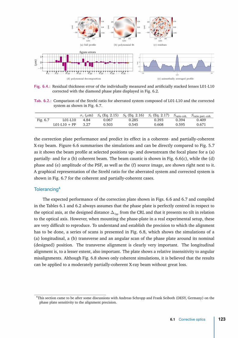
−100 0 100(µm)
−100
0
100
(µm
)
-5.00
0.00
5.00
(a) full profile
−100 0 100(µm)
−100
0
100
(µm
)
-5.00
0.00
5.00
(b) polynomial fit
−100 0 100(µm)
−100
0
100
(µm
)
-2.50
0.00
2.50
(c) residues
Z1 · · ·Z5 · · · ·Z10· · · ·Z15· · · ·Z20· · · ·Z25· · · ·Z30· · · ·Z35· ·−1
0
1
(µm
)
figure errors
(d) polynomial decomposition
−200 0 200(µm)
0.0
0.5
1.0
1.5
(µm
)
(e) azimuthally averaged profile
Fig. 6.4.: Residual thickness error of the individually measured and artificially stacked lenses L01-L10corrected with the diamond phase plate displayed in Fig. 6.2.
Tab. 6.2.: Comparison of the Strehl ratio for aberrated system composed of L01-L10 and the correctedsystem as shown in Fig. 6.7.
σz (µm) Sa (Eq. 2.15) Sb (Eq. 2.16) Sc (Eq. 2.17) Sratio coh. Sratio part.-coh.Fig. 6.7 L01-L10 4.84 0.067 0.285 0.393 0.394 0.409
L01-L10 + PP 3.27 0.503 0.545 0.608 0.595 0.671
the correction plate performance and predict its effect in a coherent- and partially-coherentX-ray beam. Figure 6.6 summarises the simulations and can be directly compared to Fig. 5.7as it shows the beam profile at selected positions up- and downstream the focal plane for a (a)partially- and for a (b) coherent beam. The beam caustic is shown in Fig. 6.6(c), while the (d)phase and (e) amplitude of the PSF, as well as the (f) source image, are shown right next to it.A graphical representation of the Strehl ratio for the aberrated system and corrected system isshown in Fig. 6.7 for the coherent and partially-coherent cases.
Tolerancing4
The expected performance of the correction plate shown in Figs. 6.6 and 6.7 and compiledin the Tables 6.1 and 6.2 always assumes that the phase plate is perfectly centred in respect tothe optical axis, at the designed distance ∆zpp from the CRL and that it presents no tilt in relationto the optical axis. However, when mounting the phase-plate in a real experimental setup, theseare very difficult to reproduce. To understand and establish the precision to which the alignmenthas to be done, a series of scans is presented in Fig. 6.8, which shows the simulations of a(a) longitudinal, a (b) transverse and an angular scan of the phase plate around its nominal(designed) position. The transverse alignment is clearly very important. The longitudinalalignment is, to a lesser extent, also important. The plate shows a relative insensitivity to angularmisalignments. Although Fig. 6.8 shows only coherent simulations, it is believed that the resultscan be applied to a moderately partially-coherent X-ray beam without great loss.
4This section came to be after some discussions with Andreas Schropp and Frank Seiboth (DESY, Germany) on thephase plate sensitivity to the alignment precision.
6.1 Corrective optics 123

z
(b) (c)(a) (e) (f)
z
(g)
(d)
Fig. 6.5.: top row: beamline used for §5.3 - Fully coherent simulations. bottom row: beamline usedfor §5.4 - Partially coherent simulations. (a) shows the X-ray source. An (b) ideal parabolicphase element is placed downstream the radiation source to give the illumination plane phase.This ideal element is only present for the fully-coherent simulations. The lenses being studiedare shown in (c), which are followed by the (d) the correction plate. A set of (e) slits toensure the same geometric aperture for all simulations. For the fully-coherent simulations,the beam-caustic range is shown in (f) and the PSF is calculated at the centre of it. For thepartially-coherent simulations, the beam profile evolution along the optical axis is shown in (g)and the beam characteristics at the focal position are calculated at its centre.
(a) partially-coherent simulations
0 mm +1 mm +2 mm +5 mm +10 mm–1 mm–2 mm–5 mm–10 mm
(b) coherent simulations
0 mm +1 mm +2 mm +5 mm +10 mm–1 mm–2 mm–5 mm–10 mm
(c) beam caustics (d) phase (rad) (e) PSF (f) source image
Fig. 6.6.: Expected performance of the diamond phase corrector. (a) partially-coherent simulations showthe beam profile up- and downstream the focal position averaging 104 wavefronts to simulatethe radiation emitted by an undulator; (b) the coherent simulations show the beam profile of aplane wavefront being focused; (c) beam propagation near the focal position (beam caustics)for a fully coherent beam (horizontal cut around y = 0); (d) phase and (e) intensity of the PSFcalculated focusing a plane-wavefront; (f) demagnified image of the undulator photon-source(extended source). The phase-plate was designed in diamond and a cut is shown in Fig. 6.3.The residual error profile after the correction is shown in Fig. 6.2.
124 Chapter 6 Correcting optical imperfections in refractive lenses

−1 0 1(µm)
0.0
0.5
1.0
inte
nsit
y(a
.u.)
idealaberratedcorrected
(a) fully-coherent
−1 0 1(µm)
0.0
0.5
1.0
inte
nsit
y(a
.u.)
idealaberratedcorrected
(b) partially-coherent
Fig. 6.7.: Visual representation of the Strehl ratio for the aberrated and corrected optical system. Coherentsimulations are shown in (a) and partially-coherent simulations in (b) at 8 keV.
z
(a)
−0.5 0.0 0.5(µm)
0.3
0.4
0.5
0.6
0.7
inte
nsit
y(a
.u.)
idealL01-L100 µm5 µm10 µm (nominal)15 µm20 µm25 µm30 µm
(b)
longitudinal scan
z
(c)
−0.5 0.0 0.5(µm)
0.0
0.2
0.4
0.6
inte
nsit
y(a
.u.)
idealL01-L10nominal+1 µm+2 µm+5 µm+10 µm+15 µm+20 µm
(d)
transverse scan
z
(e)
−0.5 0.0 0.5(µm)
0.0
0.2
0.4
0.6
inte
nsit
y(a
.u.)
idealL01-L10nominal0.1o
0.5o
1.0o
1.5o
2o
(f)
angular scan
Fig. 6.8.: Study of the precision requirements on longitudinal, transverse and angular alignment of thephase plate based on the optimisation of the Strehl ratio for a fully-coherent beam.
6.1 Corrective optics 125

(a) typical lens casing (b) lens in the frame (c) 1st gen. correction plate (d) 2nd gen. correction plate
Fig. 6.9.: Typical lens casing, lens frame and both generation of correction plates.
6.2 PrototypeA series of phase plates designed to correct the accumulated figure error of 10 Be lenses
(L01-L10) was commissioned based on the profile shown in Fig. 6.2, which was calculated tobe placed 10 mm downstream the last lens of the stack and to correct the errors at 8 keV. Theplates were ablated from diamond (HPHT IIb) by a femtosecond laser (515 nm, 3 W, 60 kHz,200 fs) by a third-party company. The refractive phase plates produced by such technique havea surface roughness of ∼700 nm, but the company offers polishing, which lowers the surfaceroughness down to ∼100 nm, at the expense of removing some high-spatial frequency featuresof the correctors, but it is possible to account for the uneven material removal during polishingon the design of the phase plate5 [Antipov, 2020]. Regardless of the surface finishing, a highshape fidelity to the profile in Fig. 6.2 is expected from the prototypes. Lastly, to facilitate theuse of the phase correctors, it was requested that the phase plates come in frames compatiblewith those used for X-ray lenses - see Fig. 6.9. The phase-plate should be precisely centred in the� = 12 mm aluminium-bronze disk, so it can be easily installed in the lens housing minimisingthe performance degradation from misalignments shown in Fig. 6.8.
6.2.1 Early tests on an X-ray beam
So far, only two generations of correction plates were produced - see Fig. 6.9. The firstgeneration of phase-plates was received and measured in Dec. 2019 with the XSVT techniquedescribed in §4 - Measuring optical imperfections in refractive lenses. This first iteration did not aimto produce useful plates, but it allowed to gain useful insights for the production of the secondgeneration correctors, which was delivered in June 2020 - this time to be used for correctionof optical imperfections in real CRLs. The phase-plates from the second generation designwere chosen to demonstrate some of the preliminary results correcting optical imperfections inrefractive lenses available at the ESRF.
The second generation of phase plates consisted of a set of three correction plates (PP01.v1to PP01.v3) based on the design shown in Fig. 6.2. The difference among the three plates is thescript used for laser ablation and the presence or not of surface post-processing. The v1 refersto an undisclosed laser polishing, while v2 and v3 have no post-processing. The PP01.v3 plateuses a different script for surface removal [Antipov, 2020]. Figure 6.10 shows the retrieved
5At the time of this writing this has not yet been tested.
126 Chapter 6 Correcting optical imperfections in refractive lenses

Tab. 6.3.: Residual figure error profile r.m.s. value for L01-L10 (Fig. 4.14) and for the corrected system(Fig. 6.4).
figure errors† (r.m.s) µmfull profile pol. fit residues
stack 01: 4.89 4.73 1.41stack 01 + PP01.v1: 3.03 2.91 1.66stack 01 + PP01.v2: 4.26 3.95 1.51stack 01 + PP01.v3: 3.44 3.10 1.44
† values given for A� = 320 µm
profile using the XSVT technique and experimental setup described in §4 - Measuring opticalimperfections in refractive lenses. The profiles are very similar among each other and no strongeffect in the surface shape of the polished phase-plate can be observed with XSVT. For thephase-plate PP01.v2, the manufacturer provided visible light metrology (scanning confocallaser microscopy), which is shown in Fig. 6.11. The surface roughness of the non-polishedplate is evident in Fig. 6.11(c). Figure 6.12 shows a profile cut of the retrieved thicknessesmeasured with XSVT and visible-light metrology against the designed profile, showing a initialgood agreement for the central part of the phase plate and lesser agreement towards the edge ofthe geometric aperture.
Once measured individually, the phase plates were added directly to the lens casing relyingon the assumption that the phase-plates were perfectly centred within their frames and thus,would ideally be perfectly aligned to the lens stack - see Fig. 6.9. The lens stack with thecorrection plate was then re-measured with the XSVT. For comparison, the lens stack withoutany correction was also measured under the very same conditions. The metrology is shown inFig. 6.13 and summarised in Table 6.3. It is evident that the correction plates are not centredwithin the lateral tolerance defined by Fig. 6.8(c)-(d) as no significant improvement in theresidual profile can be seen.
To be able to test the correction effectiveness and performance, it was decided to mount aphase-plate outside the lens case so at least the transverse alignment could be done. The phase-plate chosen for these tests was the PP01.v2 due to its good agreement with he designed profilein Fig. 6.2. The simplest alignment of the phase plate is based on maximising the peak intensityat the image plane. This approach, however, could not be employed due to the saturation of thedetector at the image plane even after a set of attenuators was used. Instead, the alignment ofthe phase-corrector was done trying to visually optimise, in terms of homogeneity, the far-fieldbeam-profile several tens of millimetres downstream the focal plane. Once the best transverseposition was found, a series of 2D images up- and downstream the optical axis was taken withthe same 2D imaging detector used for the XSVT (pixel size of ∼0.63 µm). The beam caustics canbe obtained from this series of images and it is shown in Fig. 6.14 for the aberrated and correctedsystem. Due to the saturation in the vicinity of the focal plane, a quantitative assessment of theimprovement cannot be done, however, a clear qualitative improvement on the beam profile up-and downstream the focal plane is seen.
6.2 Prototype 127

−100 0 100(µm)
−100
0
100
(µm
)-3.00
0.00
3.00
(a) full profile
−100 0 100(µm)
−100
0
100
(µm
)
-3.00
0.00
3.00
(b) polynomial fit
−100 0 100(µm)
−100
0
100
(µm
)
-0.60
0.00
0.60
(c) residues
Z1 · · ·Z5 · · · ·Z10· · · ·Z15· · · ·Z20· · · ·Z25· · · ·Z30· · · ·Z35· ·0
1
(µm
)
figure errors
(d) polynomial decomposition
−200 0 200(µm)
0.0
2.5
5.0
7.5
(µm
)
(e) azimuthally averaged profile
PP01.v1
−100 0 100(µm)
−100
0
100
(µm
)
-3.00
0.00
3.00
(a) full profile
−100 0 100(µm)
−100
0
100
(µm
)
-3.00
0.00
3.00
(b) polynomial fit
−100 0 100(µm)
−100
0
100
(µm
)-0.80
0.00
0.80
(c) residues
Z1 · · ·Z5 · · · ·Z10· · · ·Z15· · · ·Z20· · · ·Z25· · · ·Z30· · · ·Z35· ·0
1
(µm
)
figure errors
(d) polynomial decomposition
−200 0 200(µm)
0
5
(µm
)
(e) azimuthally averaged profile
PP01.v2
−100 0 100(µm)
−100
0
100
(µm
)
-2.50
0.00
2.50
(a) full profile
−100 0 100(µm)
−100
0
100
(µm
)
-2.50
0.00
2.50
(b) polynomial fit
−100 0 100(µm)
−100
0
100
(µm
)
-0.80
0.00
0.80
(c) residues
Z1 · · ·Z5 · · · ·Z10· · · ·Z15· · · ·Z20· · · ·Z25· · · ·Z30· · · ·Z35· ·0.0
0.5
1.0
(µm
)
figure errors
(d) polynomial decomposition
−200 0 200(µm)
0.0
2.5
5.0
7.5
(µm
)
(e) azimuthally averaged profile
PP01.v3
Fig. 6.10.: Phase-plate metrology using the XSVT as described in §4 - Measuring optical imperfections inrefractive lenses.
128 Chapter 6 Correcting optical imperfections in refractive lenses

−100 0 100(µm)
−100
0
100
(µm
)
-3.00
0.00
3.00
(a) full profile
−100 0 100(µm)
−100
0
100
(µm
)
-3.00
0.00
3.00
(b) polynomial fit
−100 0 100(µm)
−100
0
100
(µm
)
-0.80
0.00
0.80
(c) residues
Z1 · · ·Z5 · · · ·Z10· · · ·Z15· · · ·Z20· · · ·Z25· · · ·Z30· · · ·Z35· ·0
1
(µm
)
figure errors
(d) polynomial decomposition
−200 0 200(µm)
0
5
10
(µm
)
(e) azimuthally averaged profile
Fig. 6.11.: Scanning confocal laser microscopy of the PP01.v2 phase-plate provided by the manufacturer.
−200 0 200(µm)
0
5
10
(µm
)
designPP01.v1PP01.v2PP01.v3visible metrology
Fig. 6.12.: Profile cuts of the correction plates P01.v1-v3 measured with the XSVT metrology and fromthe P01.v2 plate measured with the visible-light metrology.
−100 0 100(µm)
−100
0
100
(µm
)
-8.00
0.00
8.00
(a)
−100 0 100(µm)
−100
0
100
(µm
)
-8.00
0.00
8.00
(b)
−100 0 100(µm)
−100
0
100
(µm
)
-2.00
0.00
2.00
(c)
Z1 · · ·Z5 · · · ·Z10· · · ·Z15· · · ·Z20· · · ·Z25· · · ·Z30· · · ·Z35· ·
−2
0
(µm
)
figure errors
(d)
lens stack 01
−100 0 100(µm)
−100
0
100
(µm
)
-5.00
0.00
5.00
(a)
−100 0 100(µm)
−100
0
100
(µm
)
-5.00
0.00
5.00
(b)
−100 0 100(µm)
−100
0
100
(µm
)
-2.50
0.00
2.50
(c)
Z1 · · ·Z5 · · · ·Z10· · · ·Z15· · · ·Z20· · · ·Z25· · · ·Z30· · · ·Z35· ·−1
0
1
(µm
)
figure errors
(d)
lens stack 01 + PP01.v1
−100 0 100(µm)
−100
0
100
(µm
)
-6.00
0.00
6.00
(a)
−100 0 100(µm)
−100
0
100
(µm
)
-6.00
0.00
6.00
(b)
−100 0 100(µm)
−100
0
100
(µm
)
-2.50
0.00
2.50
(c)
Z1 · · ·Z5 · · · ·Z10· · · ·Z15· · · ·Z20· · · ·Z25· · · ·Z30· · · ·Z35· ·−2
−1
0
1
(µm
)
figure errors
(d)
lens stack 01 + PP01.v2
−100 0 100(µm)
−100
0
100
(µm
)
-5.00
0.00
5.00
(a)
−100 0 100(µm)
−100
0
100
(µm
)
-5.00
0.00
5.00
(b)
−100 0 100(µm)
−100
0
100
(µm
)
-2.00
0.00
2.00
(c)
Z1 · · ·Z5 · · · ·Z10· · · ·Z15· · · ·Z20· · · ·Z25· · · ·Z30· · · ·Z35· ·−1
0
1
(µm
)
figure errors
(d)
lens stack 01 + PP01.v3
Fig. 6.13.: top row: thickness error of lens stack 01. centre-top to bottom row: residual thickness afterinstallation of the correction plates PP01.v1, PP01.v2 and PP01.v3 respectively.
6.2 Prototype 129

−20 0 20(µm)
−20
0
20
(µm
)
(a) -40 mm
−20 0 20(µm)
−20
0
20
(b) -30 mm
−20 0 20(µm)
−20
0
20
(c) -20 mm
−20 0 20(µm)
−20
0
20
(d) -10 mm
−20 0 20(µm)
−20
0
20
(e) +10 mm
−20 0 20(µm)
−20
0
20
(f) +20 mm
−20 0 20(µm)
−20
0
20
(g) +30 mm
−20 0 20(µm)
−20
0
20
0.00
0.25
0.50
0.75
1.00
(h) +40 mm
−100 −50 0 50 100(mm)
−100
−50
0
50
100
(µm
)
(i) beam caustics
−25 0 25(mm)
−40
−20
0
20
40
(µm
)
0.00
0.25
0.500.751.00
(j) zoomed beam caustics
aberrated system
−20 0 20(µm)
−20
0
20
(µm
)
(a) -40 mm
−20 0 20(µm)
−20
0
20
(b) -30 mm
−20 0 20(µm)
−20
0
20
(c) -20 mm
−20 0 20(µm)
−20
0
20
(d) -10 mm
−20 0 20(µm)
−20
0
20
(e) +10 mm
−20 0 20(µm)
−20
0
20
(f) +20 mm
−20 0 20(µm)
−20
0
20
(g) +30 mm
−20 0 20(µm)
−20
0
20
0.00
0.25
0.50
0.75
1.00
(h) +40 mm
−100 −50 0 50 100(mm)
−100
−50
0
50
100
(µm
)
(i) beam caustics
−25 0 25(mm)
−40
−20
0
20
40
(µm
)
0.00
0.25
0.500.751.00
(j) zoomed beam caustics
corrected system
Fig. 6.14.: Experimental beam caustics taken at 10.6 keV for the aberrated and corrected system.
6.3 Discussion
6.3.1 Design and expected performance
The concept and design of optical correction for the aberrated system are quite simple andcan be represented by the Eq. 6.3. Although current micro- and nano-manufacturing techniquescan reproduce such intricate profiles, its alignment on a beamline can be cumbersome and renderthe correction plate impractical. A successful compromise for 2D focusing CRLs is the adoptionof a radially symmetric correction plate described by Eq. 6.4 - these have been demonstrated towork by other groups [Seiboth et al., 2017, 2018, 2020; Dhamgaye et al., 2020].
Using the approach guided by Eq. 6.4, a design to compensate for the accumulated errorsfrom lenses L01-L10 (see Fig. 4.14) was calculated and it is shown in Fig. 6.2. Placing thisideal diamond phase-plate on the simulations and extracting the residual profile allows gainingsome insight into the expected performance of the corrected system. Although most, if not allspherical aberration was removed, there is still a high content on non-symmetric aberrations asshown in Figure 6.4(d), which will still degrade the beam focusing quality, but to a lesser extent.Figure 6.4(e) shows a (much reduced) residual profile, which indicates that the correction plateshould be calculation over a few iterations until the azimuthally averaged profile goes belowwhat is currently possible to be manufactured. Table 6.1 shows that the overall figure error r.m.s.value over the exit pupil is reduced to ∼68% of the L01-L10 figure error. The low-frequencies
130 Chapter 6 Correcting optical imperfections in refractive lenses

are more affected, being reduced to 65% its original value. The high frequencies are reduced to75% of the value before the correction. This reduction in the figure errors is accompanied byan increase in the Strehl ratio as evidenced by Table 6.2 and Fig. 6.7. The improvement of theStrehl ratio for the coherent case differs from the one for the partially-coherent case. Figure 5.12already showed a very small difference between both cases, but it was deemed to be insignificant.This difference shows the necessity of further studying the impact of the optical correction formoderate- and low-coherence systems.
The expected improvements brought by the optical correction also apply to the beam up-and down-stream the image plane as the several cuts along the beam caustics in Fig. 6.6 show.The elongated tail before the image plane and the doughnut shape from Fig. 5.7 are no longerpresent, however, at the image plane vicinity, satellite structures are seen around the mainlobe. The image plane is greatly improved for both the fully- and partially-coherent simulationswith great suppression of the side lobes, showing some similarities with the beam performancepredicted in Fig. 5.11. In fact, the better the correction plate is, the closer the system will behaveas in Fig. 5.11, a result of the high-frequency profile shown in Fig. 5.10. The performanceof very well corrected systems will be limited by the high-frequency content, which does notsignificantly changes the main-lobe, but significantly increases the background around it, asshown in Fig. 5.13.
It is important to point out that the expected performance and all previously improvementsare only obtained for the perfectly aligned phase-plate. Tolerance simulations were done tonarrow down the most critical degrees of freedom when aligning the phase-plate in respect tothe CRL to be corrected. The longitudinal scan is a useful tool when operating the phase plateoutside the design energy. Figure 6.8(a)-(b) shows that a longitudinal scan of a phase-plateoperating at its designed energy. Bringing the plate upstream of the nominal position ∆zpp
degrades its performance, but going downstream moderately improves it. This is probably dueto the higher absorption towards the edge of the plate and a smaller footprint of the beam. Thetransverse alignment is by far the most sensitive degree of freedom and a moderate misalignmentmay compromise the correction, bringing the Strehl ratio to the same value the aberrated systemoriginally had. Figure 6.8(c)-(d) reinforces what has been observed by other groups [Seiboth,2016, Fig. 5.12]. Finally, in terms of the Strehl ratio, the phase-plate is not too much influencedby the angular alignment, provided it is kept reasonably small. A tilt is introduced to the system,which laterally shifts the focused beam, but its intensity remains largely unchanged.
6.3.2 Early phase plate tests on an X-ray beam
The early tests with the second generation of phase-plate are encouraging and help delineatestrategies for further development of phase correctors to be used with the CRLs. Three phaseplates were produced trying to replicate the shape in Fig. 6.2 with differences in the scripts usedfor engraving the diamond slab and with post polishing or not. Figures 6.10 and 6.11 show a verysimilar profile for all three plates where the low-frequencies are well represented, but the residuesfrom the polynomial fit show a clear limitation of XSVT in showing the difference between apolished and non-polished plate. Although the effects of polishing are noticeable in the far-field(presence of small-angle scattering and speckle), XSVT cannot show the surface roughness as
6.3 Discussion 131

visible-light metrology does - Fig. 6.11. This makes the case for using complementary metrologymethods for a complete characterisation of the phase-plates. When overlapping the profile cuts,as in Fig. 6.12, the difference in the profiles becomes more evident. Visible light metrology anddesigned plate have a more similar profile, while the data collected with XSVT show lower heightvalues towards the edges of the phase-plate. The differences may come from the processingof the phase-gradients from the XSVT, small inaccuracies when measuring the distances in theexperimental setup or a difference between the tabled index of refraction/density and the realindex of refraction from the plate - something similar has been speculated in [Seiboth et al.,2020, §3.2] for justifying differences between design and measured phase-plates produced usingIP-S resist, a much less studied material than diamond.
One of the key aspects of the commissioned phase-plates is that they come perfectly centredin a frame compatible to the ones used for encasing X-ray lenses - Fig. 6.9(b) and (c), which isdone to circumvent the degradation in performance from the lateral misalignment in Fig. 6.8(c)-(d). Unfortunately, the phase plates of the current generation do not yet meet such requirementsas the metrology of the CRL with the correction plates suggests - see Fig. 6.13; improvements inthe centring of the phase plates are expected from the partner company, but are also separatelyunder way within the X-ray optics group at the ESRF.
Aligning the phase-plate to the CRL also revealed a very important aspect: the lack of aninternal protocol for alignment. Ideally, one would scan the phase-plate transversely at eachposition of the scan, the residual wavefront would be calculated and the minimisation of figureerrors would be sought. This approach is impractical for the XSVT due to the data acquisitionand processing time, not to mention the very large data-set it would generate. This highlightsthe necessity to re-implement speckle-tracking based on only two images (XST)6 for a fastevaluation of the figure errors at the expense of a lower spatial resolution. This technique wasless frequently used within the X-ray Optics Group due to the many advantages of XSVT [Berujonet al., 2020], but there is a necessity to use XST for a faster characterisation.
Trying to align the phase-plate by maximising the peak intensity was the next obvious step.However, these particular experiments took place at the ID06 beamline after the ESRF-EBSupgrade, an undulator beamline that naturally has a very high photon flux at the harmonicswhen compared to the typical emission of bending magnets7. This increase in photon flux iswelcome for the metrology but causes the imaging detector to saturate at the image plane evenafter attenuators were placed in the beam. As an alternative to the optimisation of the peakintensity, the qualitative improvement of the beam profile downstream the focal plane was done.The phase plate was scanned transversely while the far-field was registered. The final positionof the phase plate was where the beam was more homogeneous and the doughnut shape lessevident. The drawing of general guidelines for the alignment of the phase-plates and metrics toevaluate it are the topic of future work8.
The beam caustics and profiles shown in Fig. 6.14 for the aberrated beam confirm the resultsfrom the modelling presented in the chapter 5 - Effect of optical imperfections on an X-ray beam
6Refer to §4.1.2 - Foundation in §4 - Measuring optical imperfections in refractive lenses.7Refer to §1.1.1 - X-ray sources.8With the resumption of the ESRF user service mode, more access to beamtime is expected. The ESRF reopened to
the public on the 25th of August 2020, despite the COVID-19 pandemic [Cho, 2020].
132 Chapter 6 Correcting optical imperfections in refractive lenses

25 50 75 100keV
2.140
2.145
Diamond/Be
(a)
25 50 75 100keV
0.710
0.715
SU-8/Be
(b)
25 50 75 100keV
1.62
1.63
1.64 SiO2/Be
(c)
Fig. 6.15.: (a) diamond, (b) SU-8 and (c) fused silica (SiO2) refraction index decrement ratio againstberyllium. Figures obtained using the xraylib library [Brunetti et al., 2004; Schoonjans et al.,2011].
and published in [Celestre et al., 2020]. The presence of the tail upstream of the focal plane andthe doughnut shape downstream are clearly present. A direct comparison with the simulations isnot possible due to the limited caustic step and detector pixel size, but the main elements andtrends are present. Once the phase-plate is inserted and aligned, an improvement in the beamprofile homogeneity is seen, although quantification is not possible, due to the saturation of thedetector. The central tail is reduced, although still present upstream the image plane. Moreremarkable is the suppression of the doughnut shape. The performance of the correction plate isbetter near the image plane, but that could be from the low spatial resolution of the detector.
The experiments were conducted at 10.6 keV, while the design of the phase-plate wasoptimised for 8 keV. As mentioned previously, the correction plates can be used outside thedesigned energy if they were calculated for a modest number of lenses by shifting them along theoptical axis as described by [Seiboth et al., 2018, §6]. Figure 6.15 shows the ratio of the indexof refraction decrement and the δ of beryllium, which confirms an almost negligible variationover such a small energy difference. Figure 6.15 reinforces the conclusions in [Seiboth et al.,2018, §6] for commonly used phase plate materials.
The correction performance is, at the moment, far from the expected simulated performanceor the reported performance from other groups [Seiboth et al., 2017, 2018, 2020; Dhamgayeet al., 2020]. These are the performance of second-generation phase plates and with beamtimeavailability. Addressing the aforementioned issues with alignment, wavefront-sensing andprotocols for evaluating the performance of the phase-plates, improvements in the design andfabrication of phase plates are expected. �
ReferencesAbrashitova, K. A., Kulagin, G. E., Petrov, A. K., Bessonov, V. O., and Fedyanin, A. A. (2020). “Pyrolyzed 3D
compound refractive lens”. In: Journal of Physics: Conference Series. Vol. 1461. 1. Institute of PhysicsPublishing, p. 12129.
Alcock, S. G., Sutter, J. P., Sawhney, K. J., Hall, D. R., McAuley, K., and Sorensen, T. (2013). “Bimorphmirrors: The Good, the Bad, and the Ugly”. In: Nuclear Instruments and Methods in Physics ResearchSection A: Accelerators, Spectrometers, Detectors and Associated Equipment 710, pp. 87–92.
Antipov, S. P. (2020). “Laser microfabrication for applications in x-ray optics: from refractive lens to phasecorrector”. In: Proc. SPIE 11491, Advances in X-Ray/EUV Optics and Components XV 11491, p. 23.
References 133

Berujon, S., Cojocaru, R., Piault, P., Celestre, R., Roth, T., Barrett, R., and Ziegler, E. (2020). “X-ray opticsand beam characterization using random modulation: theory”. In: Journal of Synchrotron Radiation27.2, p. 284.
Berujon, S., Ziegler, E., and Cloetens, P. (2015). “X-ray pulse wavefront metrology using speckle tracking”.In: Journal of Synchrotron Radiation 22.4, p. 886.
Brunetti, A., Sanchez del Rio, M., Golosio, B., Simionovici, A., and Somogyi, A. (2004). “A library forX-ray–matter interaction cross sections for X-ray fluorescence applications”. In: Spectrochimica ActaPart B: Atomic Spectroscopy 59.10-11, p. 1725.
Celestre, R., Berujon, S., Roth, T., Sanchez del Rio, M., and Barrett, R. (2020). “Modelling phaseimperfections in compound refractive lenses”. In: Journal of Synchrotron Radiation 27.2, p. 305.
Cho, A. (2020). “Rebirth of leading European facility promises revolutionary advances in x-ray science”.In: Science.
Chubar, O., Elleaume, P., and Snigirev, A. (1999). “Phase analysis and focusing of synchrotron radiation”.In: Nuclear Instruments and Methods in Physics Research, Section A: Accelerators, Spectrometers,Detectors and Associated Equipment 435.3, p. 495.
— (2001). “Phase corrections for synchrotron radiation”. In: Nuclear Instruments and Methods in PhysicsResearch, Section A: Accelerators, Spectrometers, Detectors and Associated Equipment 467-468, p. 932.
Chubar, O., Wiegart, L., Antipov, S., Celestre, R., Coles, R., Fluerasu, A., and Rakitin, M. S. (2020). “Analysisof hard x-ray focusing by 2D diamond CRL”. In: Proc. SPIE 11493, Advances in Computational Methodsfor X-Ray Optics V, pp. 11493–20.
Dhamgaye, V., Laundy, D., Baldock, S., Moxham, T., and Sawhney, K. (2020). “Correction of the X-raywavefront from compound refractive lenses using 3D printed refractive structures”. In: Journal ofSynchrotron Radiation 27.6.
Donato, S., Arfelli, F., Brombal, L., Longo, R., Pinto, A., Rigon, L., and Dreossi, D. (2020). “Flattening filterfor Gaussian-shaped monochromatic X-ray beams: an application to breast computed tomography”.In: Journal of Synchrotron Radiation 27.2, p. 503.
Laundy, D., Dhamgaye, V., Moxham, T., and Sawhney, K. (2019). “Adaptable refractive correctors forx-ray optics”. In: Optica 6.12, p. 1484.
— (2020). “Measurements and simulations of wavefront correcting refractive x-ray optics”. In: Proc.SPIE 11493, Advances in Computational Methods for X-Ray Optics V, p. 16.
Lin, H., Yang, S.-N., and Liu, X.-Q. (2020). “X-ray kinoform lenses made using femtosecond laser tech-nique”. In: Proc. SPIE 11491, Advances in X-Ray/EUV Optics and Components XV, p. 37.
Medvedskaya, P., Lyatun, I., Shevyrtalov, S., Polikarpov, M., Snigireva, I., Yunkin, V., and Snigirev, A.(2020). “Diamond refractive micro-lenses for full-field X-ray imaging and microscopy produced withion beam lithography”. In: Optics Express 28.4, p. 4773.
Nazmov, V., Reznikova, E., Mohr, J., Snigirev, A., Snigireva, I., Achenbach, S., and Saile, V. (2004).“Fabrication and preliminary testing of X-ray lenses in thick SU-8 resist layers”. In: MicrosystemTechnologies. Vol. 10. 10, p. 716.
Petrov, A. K., Bessonov, V. O., Abrashitova, K. A., Kokareva, N. G., Safronov, K. R., Barannikov, A. A.,Ershov, P. A., Klimova, N. B., Lyatun, I. I., Yunkin, V. A., Polikarpov, M., Snigireva, I., Fedyanin, A. A.,and Snigirev, A. (2017). “Polymer X-ray refractive nano-lenses fabricated by additive technology”. In:Optics Express 25.13, p. 14173.
Polikarpov, M., Kononenko, T. V., Ralchenko, V. G., Ashkinazi, E. E., Konov, V. I., Ershov, P., Kuznetsov, S.,Yunkin, V., Snigireva, I., Polikarpov, V. M., and Snigirev, A. (2016). “Diamond x-ray refractive lensesproduced by femto-second laser ablation”. In: Proc. SPIE 9963, Advances in X-Ray/EUV Optics andComponents XI 9963.15, 99630Q.
Polikarpov, M., Polikarpov, V., Snigireva, I., and Snigirev, A. (2016). “Diamond X-ray Refractive Lenseswith High Acceptance”. In: Physics Procedia. Vol. 84. Elsevier B.V., p. 213.
134 Chapter 6 Correcting optical imperfections in refractive lenses

Probst, J., Braig, C., Langlotz, E., Rahneberg, I., Kühnel, M., Zeschke, T., Siewert, F., Krist, T., and Erko, A.(2020). “Conception of diffractive wavefront correction for XUV and soft x-ray spectroscopy”. In:Applied Optics 59.8, p. 2580.
Roth, T., Koch, F., Berujon, S., Celestre, R., Zinn, T., David, C., and Barrett, R. (2018). “2D focusingkinoform lenses produced by 3D direct printing”. In: International Conference on X-ray Optics andApplications (XOPT2018), Yokohama, Japan (presentation).
Sanli, U. T., Ceylan, H., Bykova, I., Weigand, M., Sitti, M., Schütz, G., and Keskinbora, K. (2018). “3DNanoprinted Plastic Kinoform X-Ray Optics”. In: Advanced Materials 30.36, p. 1802503.
Sawhney, K., Laundy, D., Dhamgaye, V., and Pape, I. (2016). “Compensation of X-ray mirror shape-errorsusing refractive optics”. In: Applied Physics Letters 109.5, p. 051904.
Schoonjans, T., Brunetti, A., Golosio, B., Sanchez del Rio, M., Solé, V. A., Ferrero, C., and Vincze, L.(2011). “The xraylib library for X-ray–matter interactions. Recent developments”. In: SpectrochimicaActa Part B: Atomic Spectroscopy 66.11-12, p. 776.
Schroer, C. G. and Lengeler, B. (2005). “Focusing hard X rays to nanometer dimensions by adiabaticallyfocusing lenses”. In: Physical Review Letters 94.5.
Schropp, A., Hoppe, R., Meier, V., Patommel, J., Seiboth, F., Lee, H. J., Nagler, B., Galtier, E. C., Arnold, B.,Zastrau, U., Hastings, J. B., Nilsson, D., Uhlén, F., Vogt, U., Hertz, H. M., and Schroer, C. G. (2013).“Full spatial characterization of a nanofocused X-ray free-electron laser beam by ptychographicimaging”. In: Scientific Reports 3.1, p. 1.
Seaberg, M., Cojocaru, R., Berujon, S., Ziegler, E., Jaggi, A., Krempasky, J., Seiboth, F., Aquila, A., Liu, Y.,Sakdinawat, A., Lee, H. J., Flechsig, U., Patthey, L., Koch, F., Seniutinas, G., David, C., Zhu, D., Mikeš,L., Makita, M., Koyama, T., Mancuso, A. P., Chapman, H. N., and Vagovic, P. (2019). “Wavefrontsensing at X-ray free-electron lasers”. In: Journal of Synchrotron Radiation 26.4, p. 1115.
Seiboth, F. (2016). “Refractive Hard X-ray Nanofocusing at Storage Ring and X-ray Free-Electron LasersSources”. PhD thesis. Fakultät für Mathematik, Informatik, und Naturwissenschaften, FachbereichPhysik, Universität Hamburg.
Seiboth, F., Brückner, D., Kahnt, M., Lyubomirskiy, M., Wittwer, F., Dzhigaev, D., Ullsperger, T., Nolte, S.,Koch, F., David, C., Garrevoet, J., Falkenberg, G., and Schroer, C. G. (2020). “Hard X-ray wavefrontcorrection via refractive phase plates made by additive and subtractive fabrication techniques”. In:Journal of Synchrotron Radiation 27.5, p. 27.
Seiboth, F., Kahnt, M., Lyubomirskiy, M., Seyrich, M., Wittwer, F., Ullsperger, T., Nolte, S., Batey, D.,Rau, C., and Schroer, C. G. (2019). “Refractive hard x-ray vortex phase plates”. In: Optics Letters44.18, p. 4622.
Seiboth, F., Kahnt, M., Scholz, M., Seyrich, M., Wittwer, F., Garrevoet, J., Falkenberg, G., Schropp, A., andSchroer, C. G. (2016). “Quantitative characterization of aberrations in x-ray optics”. In: Proc. SPIE9963, Advances in X-Ray/EUV Optics and Components XI, 99630P.
Seiboth, F., Schropp, A., Scholz, M., Wittwer, F., Rödel, C., Wünsche, M., Ullsperger, T., Nolte, S., Rahomäki,J., Parfeniukas, K., Giakoumidis, S., Vogt, U., Wagner, U., Rau, C., Boesenberg, U., Garrevoet, J.,Falkenberg, G., Galtier, E. C., Ja Lee, H., Nagler, B., and Schroer, C. G. (2017). “Perfect X-ray focusingvia fitting corrective glasses to aberrated optics”. In: Nature Communications 8.1, p. 14623.
Seiboth, F., Wittwer, F., Scholz, M., Kahnt, M., Seyrich, M., Schropp, A., Wagner, U., Rau, C., Garrevoet, J.,Falkenberg, G., and Schroer, C. G. (2018). “Nanofocusing with aberration-corrected rotationallyparabolic refractive X-ray lenses”. In: Journal of Synchrotron Radiation 25.1, p. 108.
Shvyd’Ko, Y., Blank, V., and Terentyev, S. (2017). “Diamond X-ray optics: Transparent, resilient, high-resolution, and wavefront preserving”. In: MRS Bulletin 42.6, p. 437.
Stöhr, F., Simons, H., Jakobsen, A. C., Nielsen, C. H., Michael-Lindhard, J., Jensen, F., Poulsen, H. F.,Hansen, O., and Hübner, J. (2015). “Injection molded polymeric hard X-ray lenses”. In: OpticalMaterials Express 5.12, p. 2804.
Sutter, J., Alcock, S., and Sawhney, K. (2012). “In situ beamline analysis and correction of active optics”.In: Journal of Synchrotron Radiation 19.6, p. 960.
References 135

Uhlén, F., Rahomäki, J., Nilsson, D., Seiboth, F., Sanz, C., Wagner, U., Rau, C., Schroer, C. G., and Vogt, U.(2014). “Ronchi test for characterization of x-ray nanofocusing optics and beamlines”. In: Journal ofSynchrotron Radiation 21.5, p. 1105.
136 Chapter 6 Correcting optical imperfections in refractive lenses

7.enConclusion
The new 4th generation of storage rings puts stringent requirements on the quality of opticalelements as to minimise the degradation of the X-ray beam [Schroer and Falkenberg, 2014;Yabashi et al., 2014]. The aim of this thesis, namely investigating and modelling the effect ofoptical imperfections in compound refractive lenses on a partially-coherent X-ray beam, addressesimportant aspects of the ESRF-EBS X-ray optics R&D programme as laid out in the Orange book[Dimper et al., 2014].
Based on the physical optics concepts presented in Chapter 1 and the already implementedoptical elements in SRW [Baltser et al., 2011], an expanded model for a thick ideal CRL waspresented. This model is similar to the multi-slicing technique already used for optical modelling[Li et al., 2017; Ali and Jacobsen, 2020], where each lens is considered to be a slice of the CRL.The complex transmission element representing a thick CRL is given by Eq. 2.11 and shown inFig. 2.6(b). This ideal model of a thick CRL can be modified to account for optical imperfectionswhen a 2D map of the figure errors of each lens is available. This model is shown in Fig. 2.6(c)and described by Eq. 2.12. This modelling of CRL as a thick optical element becomes morerelevant when the lens stack is composed of a large number of lenslets and there is significantfocusing inside the CRL [Schroer and Lengeler, 2005]. The extended modelling of CRLs waspublished in [Celestre, Berujon, et al., 2020].
Once the framework for the modelling of thick CRLs was defined, the attention was directedtowards modelling individual lenses. Typical misalignments and fabrication errors commonlypresent in embossed X-ray lenses (Fig. 3.1) were parametrised by allowing more degrees of free-dom to the ideal model for a single lens described in [Baltser et al., 2011]. This parametrisationis general enough to apply to lenses produced by other techniques, but this modelling couldprofit from adding the choice of the conic section to be used, currently limited to the paraboliccase, as already implemented by [Sanchez del Rio and Alianelli, 2012; Andrejczuk et al., 2010]for ray-tracing. Some groups have already experimented with non-parabolic shapes for focusingX-rays [Alianelli et al., 2007; Evans-Lutterodt et al., 2003; Alianelli et al., 2015; Sutter andAlianelli, 2017] and the availability of simulation tools could revive the interest in non-orthodoxdesigns. It would be amiss not to mention the similarities between the modelling presentedhere and the work presented by [Andrejczuk et al., 2010], where the modelling of the role ofsingle element errors in X-ray lenses is implemented for ray-tracing, but the analysis is limited tothe beam width and intensity in the image plane. The modelling of more intricate shape errorswas enabled by employing the Zernike or 2D Legendre orthonormal polynomials. This wasdone by unifying some already existing parts of Python libraries, adding new polynomial setsand interfacing them to be compatible with the framework already described. This unified andexpanded Python library was used throughout the thesis for fitting the figure errors presentedthroughout Chapters 3-6. The modelling of shape errors by either allowing more degrees offreedom to the ideal lens model or by directly generating the shape errors through orthonormal
137

polynomials is a useful tool for delineating tolerances on the manufacturing of X-ray lenses,which is of particular relevance for the ESRF in-house fabricated Al-lens project. Any arbitrary 2Dmap of surface imperfections (eg. metrology data or free-form surfaces for beam shaping) canalso be incorporated in the simulations using this framework. Several authors have developedtools with different degrees of complexity for simulating X-ray lenses and their aberrations.However, not only are those tools not available to the public but also the modelling is often notcompatible with already existing wide-spread simulation tools for X-ray optical design such asSHADOW (ray-tracing) and SRW (wavefront propagation). The modelling presented here isopen source, tailored to be used transparently with SRW and is currently available in a publicrepository in GitLab until the eventual merge with the SRW official distribution. Parallel to it,the code is being incorporated in the OASYS toolkit [Rebuffi and Sanchez del Rio, 2017] to bemade available for their distributions of SHADOW, hybrid ray-tracing and SRW. These recentdevelopments on X-ray lenses modelling were presented in [Celestre, Chubar, et al., 2020] andused in some of the simulations from [Chubar et al., 2020].
Ultimately, for simulations with realistic levels of imperfections, the modelling of the figureerrors on individual X-ray lenses was done with metrology data from 2D maps of local deviationsof the parabolic profile. The experimental metrology technique used for this thesis was theX-ray vectorial speckle tracking (XSVT). In addition to being relatively simple to implement, thistechnique has a high lateral resolution and good sensitivity. Furthermore, it delivers a 2D map offigure errors in projection approximation, which can conveniently be used with the wave-opticalsimulations. Several measurement campaigns at the ESRF, APS and ESRF-EBS were performedto assess the quality of in-house produced lenses; lenses and free-form optics in the contextof scientific collaborations; and newly-acquired commercial lenses. As a result, a large anddiverse database of metrology files was built. After some curation, a possible expansion of theDABAM (database for X-ray mirrors metrology) [Sanchez Del Rio et al., 2016] is envisioned.Making the metrology data of X-ray lenses available through an open-source database wouldhelp the consolidation of the framework developed here since DABAM is also distributed andinterfaced by OASYS. Before that, however, more effort has to be put into making the metrologyof single lens and subsequent stacking by software converge with the metrology of a lensstack composed by those same lenslets. The current state show some qualitative agreement(Fig. 4.14-4.17), which is transferred to the simulations shown in Figs. 5.3-5.4 and Fig. 5.8.This is sufficient for preliminary studies but leaves room for improvements and delineationof protocols for the metrology both in terms of sample alignment and data processing - theseshould be the aim of future work. The major importance of reliably being able to artificiallystack individually measured lenses is the possibility of evaluating the performance of a CRLcomposed of any arbitrary selection of lenses off-line, with immediate application to the designof optical correctors. The experience gained in the metrology campaigns and advancementsin the post-processing of the acquired data resulted in modest contributions to [Berujon et al.,2020a,b; Qiao et al., 2020].
A subset of lenses in the database was chosen to showcase the effect of optical imperfectionson partially coherent X-ray beam degradation. The simulations, shown in the first part ofChapter 5 and summarised by Fig. 5.7, show a beam caustic that has been reported severaltimes in literature for the same type of X-ray lenses [Schropp et al., 2013; Seiboth et al., 2017,
138 Chapter 7.en Conclusion

2020]. The experimental measurement of the beam caustics for this lens stack also showssimilarity to what was predicted by the simulations - cf. Fig. 6.14. The similarity between thesimulations and experimental data helps to validate the framework presented in this thesis andit is believed that they allow to qualitatively assess the effects of optical imperfections on thedegradation of the X-ray beam profile. The simulations also allow investigating the adequacyof the Strehl ratio as a figure of merit for the optical design of systems operating far from theMaréchal criterion for optical quality. Generally, the equations used for estimating the Strehlratio tend to underestimate the system performance in that region (Fig. 5.12). The failed attemptin obtaining simple replacement equations (cf. Eq. 5.2) indicate that the most straightforwardway to evaluate the Strehl ratio is by optical simulation of the system using realistic figureerrors. It is also relevant to mention that although fully- and partially coherent simulationsdo not differ significantly, it is premature to generalise this behaviour as the partially-coherentsimulations were done for a hypothetical undulator beamline operating at the upgraded ESRFmagnetic lattice. Another result from the simulations is the prediction that the systems with highspatial frequency figure errors do not present a broadening of the beam size at the focal plane,instead, the intensity is reduced by the scattering of photons around the main lobe, increasingthe background level - Fig. 5.13. The effects of high-spatial-frequency figure errors are importantas well-corrected optical systems would have them as a predominant source of shape errors. Thisanalysis was published in [Celestre, Berujon, et al., 2020].
The multi-slice modelling of a CRL including the metrology data of individually measuredlenses (Eq. 2.12) allows the extraction of the accumulated figure errors of a lens stack. Thiswas used to model a phase-plate in diamond to correct for those errors at the exit pupil ofthe system. Due to the limitations of the phase-plate alignment in a beamline, the symmetricdesign is preferred in detriment to the correction performance - reported results show excellentperformance even with this trade-off [Seiboth et al., 2020; Dhamgaye et al., 2020]. The beamprofile shown in Fig. 6.6 is more homogeneous up- and downstream the image plane andresembles the simulations for a system with predominantly high-spatial frequencies in Fig. 5.10.However, when analysing the Strehl ratio, the performance of the modelled phase-plate is limitedand beyond what other groups have reported. The main reasons for such discrepancies arethe fact that the profile to be corrected (Fig. 4.14) has significant non-symmetric components(trefoil aberration) in addition to the classical predominance of spherical aberrations. The lackof asymmetry found by other groups is likely connected to the fact that a larger number of lensesare used in their stacks and the addition of correlated errors of randomly rotated lenses would actto give a more symmetric shape to the accumulated errors by averaging out the non-symmetriccomponents. Randomly rotating the lenses in the simulations could help to improve the expectedStrehl ratio and similar procedure could be applied to the lens stack in an experiment. Thedesigned phase-plates were commissioned from a commercial partner and they were ablatedfrom diamond by a femtosecond laser. Initial tests on an X-ray beam showed that the phaseplates were not centred in the frame within the calculated tolerances, which is crucial for theirperformance. The phase-plate had to be aligned concerning the lens stack, which posed aninitial problem, as at the time no alignment protocols were delineated. This also brought to thesurface the necessity of re-implementation of faster wavefront sensing techniques which werediscontinued in favour of a higher spatial resolution. Other issues such as overexposure of the
139

detector even after strong attenuation of the beam limited the tests that could be done with thecorrection plate, so no quantitative value was generated to evaluate the correction performance,however, a beam caustic could be recorded for the aberrated and corrected system (Fig. 6.14)qualitatively showing a more homogeneous beam especially in the vicinity of the focal plane,with a better performance downstream.
The early results are promising but show the necessity of further beamtimes aimed to lookingfor alternative ways for rapidly extracting the residual wavefront and aligning the correctionplate, measuring the beam-caustics and quantitatively evaluating the correction performance.Exploring additive manufacturing for designing the corrective optics in other materials shouldalso be investigated as an alternative to diamond and lowering the prototyping costs. �
ReferencesAli, S. and Jacobsen, C. (2020). “Effect of tilt on circular zone plate performance”. In: Journal of the
Optical Society of America A 37.3, p. 374.Alianelli, L., Sánchez del Río, M., and Sawhney, K. J. (2007). “Ray-tracing simulation of parabolic
compound refractive lenses”. In: Spectrochimica Acta - Part B Atomic Spectroscopy 62.6-7 SPEC. ISS.P. 593.
Alianelli, L., Sánchez del Rio, M., Fox, O. J. L., and Korwin-Mikke, K. (2015). “Aberration-free short focallength x-ray lenses”. In: Optics Letters 40.23, p. 5586.
Andrejczuk, A., Krzywiski, J., Sakurai, Y., Itou, M., Krzywinski, J., Sakurai, Y., and Itou, M. (2010).“The role of single element errors in planar parabolic compound refractive lenses”. In: Journal ofSynchrotron Radiation 17.5, p. 616.
Baltser, J., Knudsen, E., Vickery, A., Chubar, O., Snigirev, A., Vaughan, G., Feidenhans’l, R., and Lefmann, K.(2011). “Advanced simulations of x-ray beam propagation through CRL transfocators using ray-tracing and wavefront propagation methods”. In: Proc. SPIE 8141, Advances in Computational Methodsfor X-Ray Optics II 8141, p. 814111.
Berujon, S., Cojocaru, R., Piault, P., Celestre, R., Roth, T., Barrett, R., and Ziegler, E. (2020a). “X-rayoptics and beam characterization using random modulation: experiments”. In: Journal of SynchrotronRadiation 27.2, p. 293.
— (2020b). “X-ray optics and beam characterization using random modulation: theory”. In: Journal ofSynchrotron Radiation 27.2, p. 284.
Celestre, R., Berujon, S., Roth, T., Sanchez del Rio, M., and Barrett, R. (2020). “Modelling phaseimperfections in compound refractive lenses”. In: Journal of Synchrotron Radiation 27.2, p. 305.
Celestre, R., Chubar, O., Roth, T., Sanchez del Rio, M., and Barrett, R. (2020). “Recent developmentsin X-ray lenses modelling with SRW”. In: Proc. SPIE 11493, Advances in Computational Methods forX-Ray Optics V, pp. 11493–17.
Chubar, O., Wiegart, L., Antipov, S., Celestre, R., Coles, R., Fluerasu, A., and Rakitin, M. S. (2020). “Analysisof hard x-ray focusing by 2D diamond CRL”. In: Proc. SPIE 11493, Advances in Computational Methodsfor X-Ray Optics V, pp. 11493–20.
Dhamgaye, V., Laundy, D., Baldock, S., Moxham, T., and Sawhney, K. (2020). “Correction of the X-raywavefront from compound refractive lenses using 3D printed refractive structures”. In: Journal ofSynchrotron Radiation 27.6.
Dimper, R., Reichert, H., Raimondi, P., Sanchez Ortiz, L., Sette, F., and Susini, J. (2014). ESRF Upragdeprogramme phase II - The Orange Book. ESRF, p. 75.
140 Chapter 7.en Conclusion

Evans-Lutterodt, K., Ablett, J. M., Stein, A., Kao, C.-C., Tennant, D. M., Klemens, F., Taylor, A., Jacobsen,C., Gammel, P. L., Huggins, H., Ustin, S., Bogart, G., and Ocola, L. (2003). “Single-element ellipticalhard x-ray micro-optics”. In: Opt. Express 11.8, p. 919.
Li, K., Wojcik, M., and Jacobsen, C. (2017). “Multislice does it all—calculating the performance ofnanofocusing X-ray optics”. In: Optics Express 25.3, p. 1831.
Qiao, Z., Shi, X., Celestre, R., and Assoufid, L. (2020). “Wavelet-transform-based speckle vector trackingmethod for X-ray phase imaging”. In: Optics Express 28.22, p. 33053.
Rebuffi, L. and Sanchez del Rio, M. (2017). “OASYS (OrAnge SYnchrotron Suite): an open-source graphicalenvironment for x-ray virtual experiments”. In: Proc. SPIE 10388, Advances in Computational Methodsfor X-Ray Optics IV, p. 28.
Sanchez del Rio, M. and Alianelli, L. (2012). “Aspherical lens shapes for focusing synchrotron beams”. In:Journal of Synchrotron Radiation 19.3, p. 366.
Sanchez Del Rio, M., Bianchi, D., Cocco, D., Glass, M., Idir, M., Metz, J., Raimondi, L., Rebuffi, L., Reininger,R., Shi, X., Siewert, F., Spielmann-Jaeggi, S., Takacs, P., Tomasset, M., Tonnessen, T., Vivo, A., andYashchuk, V. (2016). “DABAM: An open-source database of X-ray mirrors metrology”. In: Journal ofSynchrotron Radiation 23.3, p. 665.
Schroer, C. G. and Lengeler, B. (2005). “Focusing hard X rays to nanometer dimensions by adiabaticallyfocusing lenses”. In: Physical Review Letters 94.5.
Schroer, C. G. and Falkenberg, G. (2014). “Hard X-ray nanofocusing at low-emittance synchrotron radiationsources”. In: Journal of Synchrotron Radiation 21.5, pp. 996–1005.
Schropp, A., Hoppe, R., Meier, V., Patommel, J., Seiboth, F., Lee, H. J., Nagler, B., Galtier, E. C., Arnold, B.,Zastrau, U., Hastings, J. B., Nilsson, D., Uhlén, F., Vogt, U., Hertz, H. M., and Schroer, C. G. (2013).“Full spatial characterization of a nanofocused X-ray free-electron laser beam by ptychographicimaging”. In: Scientific Reports 3.1, p. 1.
Seiboth, F., Brückner, D., Kahnt, M., Lyubomirskiy, M., Wittwer, F., Dzhigaev, D., Ullsperger, T., Nolte, S.,Koch, F., David, C., Garrevoet, J., Falkenberg, G., and Schroer, C. G. (2020). “Hard X-ray wavefrontcorrection via refractive phase plates made by additive and subtractive fabrication techniques”. In:Journal of Synchrotron Radiation 27.5, p. 27.
Seiboth, F., Schropp, A., Scholz, M., Wittwer, F., Rödel, C., Wünsche, M., Ullsperger, T., Nolte, S., Rahomäki,J., Parfeniukas, K., Giakoumidis, S., Vogt, U., Wagner, U., Rau, C., Boesenberg, U., Garrevoet, J.,Falkenberg, G., Galtier, E. C., Ja Lee, H., Nagler, B., and Schroer, C. G. (2017). “Perfect X-ray focusingvia fitting corrective glasses to aberrated optics”. In: Nature Communications 8.1, p. 14623.
Sutter, J. P. and Alianelli, L. (2017). “Aberration-free aspherical lens shape for shortening the focaldistance of an already convergent beam”. In: Journal of Synchrotron Radiation 24.6, pp. 1120–1136.
Yabashi, M., Tono, K., Mimura, H., Matsuyama, S., Yamauchi, K., Tanaka, T., Tanaka, H., Tamasaku, K.,Ohashi, H., Goto, S., and Ishikawa, T. (2014). “Optics for coherent X-ray applications”. In: Journal ofSynchrotron Radiation 21.5, pp. 976–985.
References 141


7.frConclusion
La quatrième génération d’anneaux de stockage, récemment lancée, impose des exigences strictesquant à la qualité des éléments optiques afin de minimiser la dégradation du faisceau de rayonsX [Schroer and Falkenberg, 2014; Yabashi et al., 2014]. Cette thèse, dont l’objectif consiste àétudier et à modéliser l’effet des imperfections optiques des lentilles réfractives composées surun faisceau de rayons X partiellement cohérent, aborde des aspects importants du programmede R&D en optique des rayons X de l’ESRF-EBS, tel qu’il est exposé dans le Orange book [Dimperet al., 2014].
Basé sur les concepts d’optique physique présentés au chapitre 1 et les éléments optiquesdisponibles dans SRW [Baltser et al., 2011] un modèle étendu à une lentille réfractive composée(CRL) idéale et épaisse a été présenté. Ce modèle s’apparente à la technique de découpagemulti-coupes déjà utilisée pour la modélisation optique [Li et al., 2017; Ali and Jacobsen, 2020],où chaque lentille est considérée comme une tranche de la CRL. L’élément de transmissioncomplexe représentant une CRL épaisse est donné par Eq. 2.11 et illustré par la Fig. 2.6(b). Cemodèle idéal d’une CRL épaisse peut être modifié pour prendre en compte des imperfectionsoptiques lorsqu’une cartographie 2D des erreurs de forme de chaque lentille est disponible. Il estillustré par la Fig. 2.6(c) et décrit par Eq. 2.12. Cette modélisation de la CRL en tant qu’élémentoptique épais devient plus pertinente lorsque l’empilement est composé d’un grand nombre delentilles et que la focalisation au sein du CRL est importante [Schroer and Lengeler, 2005]. Lamodélisation étendue des CRL a été publiée dans [Celestre, Berujon, et al., 2020].
Les erreurs de fabrication couramment présentes dans les lentilles rayons X en relief (Fig. 3.1)ont été paramétrées en offrant plus de degrés de liberté au modèle idéal pour une seule lentillecomme décrit dans [Baltser et al., 2011]. Ce paramétrage est assez général pour s’appliqueraux lentilles produites par d’autres techniques, mais cette modélisation pourrait être amélioréeen offrant le choix de la section conique à utiliser, actuellement limitée au cas parabolique,comme cela a déjà été implémenté pour le ray-tracing par [Sanchez del Rio and Alianelli, 2012;Andrejczuk et al., 2010]. Certains groupes ont déjà expérimenté des formes non paraboliquespour la focalisation des rayons X [Alianelli et al., 2007; Evans-Lutterodt et al., 2003; Alianelliet al., 2015; Sutter and Alianelli, 2017] et la disponibilité d’outils de simulation pourrait raviverl’intérêt pour les conceptions non orthodoxes. Il serait inconvenant de ne pas mentionner lessimilitudes entre la modélisation présentée ici et les travaux présentés par [Andrejczuk et al.,2010], où la modélisation du rôle des erreurs d’un seul élément dans les lentilles à rayons Xest utilisée dans le ray-tracing, l’analyse étant cependant limitée à la largeur et à l’intensité dufaisceau dans le plan image. La modélisation d’erreurs de forme plus complexes a été renduepossible par l’utilisation des polynômes orthonormaux de Zernike ou de Legendre 2D. Cela aété fait en unifiant certaines parties déjà existantes des bibliothèques Python, en ajoutant denouveaux ensembles de polynômes et en les interfaçant pour les rendre compatibles avec le cadredéjà décrit. Cette bibliothèque Python unifiée et étendue a été utilisée tout au long de la thèse
143

pour ajuster les erreurs de forme présentées tout au long des chapitres 3-6. La modélisation deserreurs de forme réalisée soit en accordant plus de degrés de liberté au modèle de lentille idéal,soit en générant directement les erreurs de forme par des polynômes orthonormaux, est un outilutile pour définir les tolérances de fabrication des lentilles rayons X, ce qui est particulièrementpertinent pour le projet de fabrication en interne de lentilles en aluminium. Toute cartographiearbitraire des imperfections de surface (par exemple issue de données de métrologie ou desurfaces free-form pour la mise en forme du faisceau) peut également être intégrée dans lessimulations. Plusieurs auteurs ont développé de nombreux outils avec différents degrés decomplexité pour simuler les lentilles rayons X et leurs aberrations. Toutefois, non seulementces outils ne sont pas accessibles au public, mais la modélisation n’est souvent pas compatibleavec les outils de simulation déjà largement répandus pour la conception des optiques rayonsX, tels que SHADOW (ray-tracing) et SRW (propagation du front d’onde). La modélisationprésentée ici est de type open source, pouvant être utilisée de manière transparente avec SRW etest actuellement disponible dans un dépôt public sur GitLab jusqu’à la fusion éventuelle avec ladistribution officielle de SRW. Parallèlement, le code est incorporé dans la boîte à outils OASYS[Rebuffi and Sanchez del Rio, 2017] qui sera disponible pour les distributions de SHADOW, duray-tracing hybride et de SRW. Ces développements récents sur la modélisation des lentillesrayons X ont été présentés dans [Celestre, Chubar, et al., 2020] et utilisés dans certaines dessimulations de [Chubar et al., 2020].
Finalement, pour réaliser les simulations avec des niveaux d’imperfections réalistes, lamodélisation des erreurs de forme sur les lentilles rayons X individuelles a été faite avec desdonnées de métrologie sous forme de cartographie des déviations locales du profil parabolique.La technique de métrologie utilisée pour cette thèse était le XSVT (X-ray vectorial speckletracking). En plus d’être relativement simple à mettre en œuvre, cette technique possède unerésolution latérale élevée et une bonne sensibilité. De plus, elle fournit une cartographie deserreurs de forme dans l’approximation de la projection, qui peut être facilement utilisée avecles simulations de front d’ondes. Plusieurs campagnes de mesures ont été effectuées à l’ESRF, àl’APS et à l’ESRF-EBS pour évaluer la qualité des lentilles produites en interne, des lentilles etdes optiques free-form dans le cadre de collaborations scientifiques et des lentilles commercialesnouvellement acquises. En conséquence, une base de données importante et diversifiée defichiers de métrologie a été constituée. Une expansion possible de DABAM (base de donnéespour la métrologie des miroirs rayons X) [Sanchez Del Rio et al., 2016] est envisagée. La mise àdisposition des données de métrologie des miroirs rayons X par le biais d’une base de donnéesopen-source aiderait à consolider le projet développé ici puisque DABAM est également distribuéeet interfacée par OASYS. Auparavant, il faudra cependant parvenir à la convergence des résultatsde metrologie obtenus sur un empilement de lentilles avec celui du calcul logiciel réalisé àpartir de la métrologie des lentilles qui le composent. L’état actuel montre un certain accordqualitatif (Fig. 4.14-4.17)), qui est transféré aux simulations présentées dans les Figs. 5.3-5.4 etFig. 5.8. Cela est suffisant pour les études préliminaires mais laisse une marge de manœuvre pouraméliorer et délimiter les protocoles de métrologie, tant en termes d’alignement des échantillonsque de traitement des données - ce qui devrait être l’objectif de futurs études. L’intérêt majeurde pouvoir empiler de manière fiable des lentilles mesurées individuellement étant de pouvoirévaluer les performances d’une CRL composée d’une sélection arbitraire de lentilles, et concevoir
144 Chapter 7.fr Conclusion

les correcteurs optiques nécessaires. L’expérience acquise lors des campagnes de métrologie etles progrès réalisés dans le traitement des données acquises ont permis d’apporter de modestescontributions à [Berujon et al., 2020a,b; Qiao et al., 2020].
Les simulations, présentées dans la première partie du chapitre 5 et résumées par la figure5.7„ montrent une caustique du faisceau qui a été mentionnée plusieurs fois dans la littératurepour le même type de lentilles rayons X [Schropp et al., 2013; Seiboth et al., 2017, 2020].La mesure expérimentale de la caustique du faisceau pour cet empilement de lentilles montreégalement une similarité avec ce qui a été prédit par les simulations - cf. Fig. 6.14. L’accord entresimulations et données expérimentales contribue à valider l’approche du sujet de cette thèse eton estime que les simulations permettent d’évaluer qualitativement les effets des imperfectionsoptiques sur la dégradation du profil du faisceau de rayons X. Elles permettent égalementd’étudier la pertinence du rapport de Strehl comme facteur de qualité pour la conception desystèmes optiques fonctionnant loin du critère de Maréchal pour la qualité optique. En général,les équations utilisées pour estimer le rapport de Strehl tendent à sous-estimer la performance dusystème dans cette région (Fig. 5.12). L’impossibilité d’obtenir des équations de remplacementsimples (cf. Eq. 5.2) indique que la manière la plus simple d’évaluer le rapport de Strehl estla simulation optique du système en utilisant des erreurs de forme réalistes. Il faut égalementsouligner que bien que les simulations entièrement et partiellement cohérentes ne diffèrent pasde manière significative, il est prématuré de généraliser ce comportement car les simulationspartiellement cohérentes sont basées sur une hypothétique ligne de lumière fonctionnant avec leréseau magnétique ESRF amélioré. Un autre résultat des simulations est la prédiction que lessystèmes avec des erreurs de forme à haute fréquence spatiale ne présentent pas un élargissementde la taille du faisceau au plan focal, mais que l’intensité est plutôt réduite par la diffusion desphotons autour du lobe principal, ce qui augmente le bruit de fond - Fig. 5.13. Les effets deserreurs de forme à haute fréquence spatiale sont importants, car pour des systèmes optiques biencorrigés ils seraient une source prédominante d’erreurs de forme. Cette analyse a été publiéedans [Celestre, Berujon, et al., 2020].
La modélisation multi-coupes d’une CRL incluant les données métrologiques des lentillesmesurées individuellement (Eq. 2.12) permet l’extraction des erreurs de forme cumulées d’unempilement de lentilles. Ceci a été utilisé pour modéliser une plaque de phase en diamantdestinée à corriger ces erreurs en sortie du système. Afin de faciliter l’alignement de cette plaque,celle-ci est conçue de façon symétrique au détriment de la performance corrective - les résultatsrapportés montrent une excellente performance malgré ce compromis [Seiboth et al., 2020;Dhamgaye et al., 2020]. Le profil du faisceau illustré par la figure 6.6 est plus homogène enamont et en aval du plan image et ressemble aux simulations pour un système à prédominancede hautes fréquences spatiales - figure 5.10. Cependant, lors de l’analyse du rapport de Strehl,la performance de la plaque de phase modélisée est limitée et dépasse ce que d’autres groupesont rapporté. Les principales raisons de ces divergences sont le fait que le profil à corriger(Fig. 4.14) comporte des composantes non symétriques importantes (aberration en trèfle) enplus de la prédominance classique des aberrations sphériques. L’absence d’asymétrie constatéepar d’autres groupes est probablement liée au fait qu’un plus grand nombre de lentilles sontutilisées dans leurs empilements, ainsi les erreurs corrélées des lentilles dont la position enrotation est aléatoire seraient rendues plus symétriques par rapport aux erreurs accumulées par
145
un effet de moyennage des composantes non symétriques. La rotation aléatoire des lentilles dansles simulations pourrait contribuer à améliorer le rapport de Strehl attendu et une procéduresimilaire pourrait être appliquée à l’empilement de lentilles dans le cadre d’une expérience. Lesplaques de phase conçues ont été commandées à un partenaire commercial et sont obtenues parablation du diamant avec un laser femtoseconde. Les premiers essais sur un faisceau de rayons Xont montré que le centrage des plaques de phase dans leur cadre ne respectait pas les tolérancescalculées, ce qui est crucial pour leur performance. En l’absence de protocole d’alignementlors des premiers essais, cela a posé un problème, la plaque de phase devant être alignée parrapport à la pile de lentilles. Cela a également mis en évidence la nécessité de réimplémenter destechniques de détection de front d’onde plus rapides, qui ont été abandonnées au profit d’unerésolution spatiale plus élevée. D’autres problèmes tels que la surexposition du détecteur, mêmeaprès une forte atténuation du faisceau, ont limité les tests qui pouvaient être effectués avec laplaque corrective, de sorte qu’aucune valeur quantitative n’a pu être obtenue pour évaluer laperformance de la correction. Cependant, une caustique du faisceau a pu être enregistrée pourle système aberré et corrigé (Fig. 6.14) montrant qualitativement un faisceau plus homogènesurtout au voisinage du plan focal, avec une meilleure performance en aval. Les premiersrésultats sont prometteurs mais nécessitent de programmer de nouvelles expériences sur lignede lumière, de trouver des moyens d’extraire rapidement le front d’onde résiduel et d’alignerla plaque de correction, de mesurer la caustique du faisceau et d’évaluer quantitativementles performances de la correction. L’exploration de la fabrication additive pour la conceptiond’optiques correctives dans d’autres matériaux devrait également être étudiée comme alternativeau diamant et pour réduire les coûts de prototypage. �
ReferencesAli, S. and Jacobsen, C. (2020). “Effect of tilt on circular zone plate performance”. In: Journal of the
Optical Society of America A 37.3, p. 374.Alianelli, L., Sánchez del Río, M., and Sawhney, K. J. (2007). “Ray-tracing simulation of parabolic
compound refractive lenses”. In: Spectrochimica Acta - Part B Atomic Spectroscopy 62.6-7 SPEC. ISS.P. 593.
Alianelli, L., Sánchez del Rio, M., Fox, O. J. L., and Korwin-Mikke, K. (2015). “Aberration-free short focallength x-ray lenses”. In: Optics Letters 40.23, p. 5586.
Andrejczuk, A., Krzywiski, J., Sakurai, Y., Itou, M., Krzywinski, J., Sakurai, Y., and Itou, M. (2010).“The role of single element errors in planar parabolic compound refractive lenses”. In: Journal ofSynchrotron Radiation 17.5, p. 616.
Baltser, J., Knudsen, E., Vickery, A., Chubar, O., Snigirev, A., Vaughan, G., Feidenhans’l, R., and Lefmann, K.(2011). “Advanced simulations of x-ray beam propagation through CRL transfocators using ray-tracing and wavefront propagation methods”. In: Proc. SPIE 8141, Advances in Computational Methodsfor X-Ray Optics II 8141, p. 814111.
Berujon, S., Cojocaru, R., Piault, P., Celestre, R., Roth, T., Barrett, R., and Ziegler, E. (2020a). “X-rayoptics and beam characterization using random modulation: experiments”. In: Journal of SynchrotronRadiation 27.2, p. 293.
— (2020b). “X-ray optics and beam characterization using random modulation: theory”. In: Journal ofSynchrotron Radiation 27.2, p. 284.
Celestre, R., Berujon, S., Roth, T., Sanchez del Rio, M., and Barrett, R. (2020). “Modelling phaseimperfections in compound refractive lenses”. In: Journal of Synchrotron Radiation 27.2, p. 305.
146 Chapter 7.fr Conclusion

Celestre, R., Chubar, O., Roth, T., Sanchez del Rio, M., and Barrett, R. (2020). “Recent developmentsin X-ray lenses modelling with SRW”. In: Proc. SPIE 11493, Advances in Computational Methods forX-Ray Optics V, pp. 11493–17.
Chubar, O., Wiegart, L., Antipov, S., Celestre, R., Coles, R., Fluerasu, A., and Rakitin, M. S. (2020). “Analysisof hard x-ray focusing by 2D diamond CRL”. In: Proc. SPIE 11493, Advances in Computational Methodsfor X-Ray Optics V, pp. 11493–20.
Dhamgaye, V., Laundy, D., Baldock, S., Moxham, T., and Sawhney, K. (2020). “Correction of the X-raywavefront from compound refractive lenses using 3D printed refractive structures”. In: Journal ofSynchrotron Radiation 27.6.
Dimper, R., Reichert, H., Raimondi, P., Sanchez Ortiz, L., Sette, F., and Susini, J. (2014). ESRF Upragdeprogramme phase II - The Orange Book. ESRF, p. 75.
Evans-Lutterodt, K., Ablett, J. M., Stein, A., Kao, C.-C., Tennant, D. M., Klemens, F., Taylor, A., Jacobsen,C., Gammel, P. L., Huggins, H., Ustin, S., Bogart, G., and Ocola, L. (2003). “Single-element ellipticalhard x-ray micro-optics”. In: Opt. Express 11.8, p. 919.
Li, K., Wojcik, M., and Jacobsen, C. (2017). “Multislice does it all—calculating the performance ofnanofocusing X-ray optics”. In: Optics Express 25.3, p. 1831.
Qiao, Z., Shi, X., Celestre, R., and Assoufid, L. (2020). “Wavelet-transform-based speckle vector trackingmethod for X-ray phase imaging”. In: Optics Express 28.22, p. 33053.
Rebuffi, L. and Sanchez del Rio, M. (2017). “OASYS (OrAnge SYnchrotron Suite): an open-source graphicalenvironment for x-ray virtual experiments”. In: Proc. SPIE 10388, Advances in Computational Methodsfor X-Ray Optics IV, p. 28.
Sanchez del Rio, M. and Alianelli, L. (2012). “Aspherical lens shapes for focusing synchrotron beams”. In:Journal of Synchrotron Radiation 19.3, p. 366.
Sanchez Del Rio, M., Bianchi, D., Cocco, D., Glass, M., Idir, M., Metz, J., Raimondi, L., Rebuffi, L., Reininger,R., Shi, X., Siewert, F., Spielmann-Jaeggi, S., Takacs, P., Tomasset, M., Tonnessen, T., Vivo, A., andYashchuk, V. (2016). “DABAM: An open-source database of X-ray mirrors metrology”. In: Journal ofSynchrotron Radiation 23.3, p. 665.
Schroer, C. G. and Lengeler, B. (2005). “Focusing hard X rays to nanometer dimensions by adiabaticallyfocusing lenses”. In: Physical Review Letters 94.5.
Schroer, C. G. and Falkenberg, G. (2014). “Hard X-ray nanofocusing at low-emittance synchrotron radiationsources”. In: Journal of Synchrotron Radiation 21.5, pp. 996–1005.
Schropp, A., Hoppe, R., Meier, V., Patommel, J., Seiboth, F., Lee, H. J., Nagler, B., Galtier, E. C., Arnold, B.,Zastrau, U., Hastings, J. B., Nilsson, D., Uhlén, F., Vogt, U., Hertz, H. M., and Schroer, C. G. (2013).“Full spatial characterization of a nanofocused X-ray free-electron laser beam by ptychographicimaging”. In: Scientific Reports 3.1, p. 1.
Seiboth, F., Brückner, D., Kahnt, M., Lyubomirskiy, M., Wittwer, F., Dzhigaev, D., Ullsperger, T., Nolte, S.,Koch, F., David, C., Garrevoet, J., Falkenberg, G., and Schroer, C. G. (2020). “Hard X-ray wavefrontcorrection via refractive phase plates made by additive and subtractive fabrication techniques”. In:Journal of Synchrotron Radiation 27.5, p. 27.
Seiboth, F., Schropp, A., Scholz, M., Wittwer, F., Rödel, C., Wünsche, M., Ullsperger, T., Nolte, S., Rahomäki,J., Parfeniukas, K., Giakoumidis, S., Vogt, U., Wagner, U., Rau, C., Boesenberg, U., Garrevoet, J.,Falkenberg, G., Galtier, E. C., Ja Lee, H., Nagler, B., and Schroer, C. G. (2017). “Perfect X-ray focusingvia fitting corrective glasses to aberrated optics”. In: Nature Communications 8.1, p. 14623.
Sutter, J. P. and Alianelli, L. (2017). “Aberration-free aspherical lens shape for shortening the focaldistance of an already convergent beam”. In: Journal of Synchrotron Radiation 24.6, pp. 1120–1136.
Yabashi, M., Tono, K., Mimura, H., Matsuyama, S., Yamauchi, K., Tanaka, T., Tanaka, H., Tamasaku, K.,Ohashi, H., Goto, S., and Ishikawa, T. (2014). “Optics for coherent X-ray applications”. In: Journal ofSynchrotron Radiation 21.5, pp. 976–985.
References 147


APublication list
Journal publicationsNash, B., Goldring , N., Edelen, J., Webb, S. and Celestre, R., (2021). Propagation of
partially coherent radiation using Wigner functions. Physical Review Accelerators and Beams,24(1), 010702.
Qiao, Z., Shi, X., Celestre, R. and Assoufid, L. (2020). Wavelet-transform-based specklevector tracking method for X-ray phase imaging. Optics Express, 28(20), 1094.
Celestre, R., Berujon, S., Roth, T., Sanchez del Rio, M. and Barrett, R. (2020). Modellingphase imperfections in compound refractive lenses. Journal of Synchrotron Radiation, 27(2),305–318.
Berujon, S., Cojocaru, R., Piault, P., Celestre, R., Roth, T., Barrett, R. and Ziegler, E. (2020).X-ray optics and beam characterization using random modulation: experiments. Journal ofSynchrotron Radiation, 27(2), 293–304.
Berujon, S., Cojocaru, R., Piault, P., Celestre, R., Roth, T., Barrett, R. and Ziegler, E. (2020).X-ray optics and beam characterization using random modulation: theory. Journal of SynchrotronRadiation, 27(2), 284–292.
Sanchez del Rio, M., Celestre, R., Glass, M., Pirro, G., Herrera, J. R., Barrett, R., da Silva,J. C., Cloetens, P., Shi, X. and Rebuffi, L. (2019). A hierarchical approach for modeling X-ray beamlines: application to a coherent beamline. Journal of Synchrotron Radiation, 26(6),1887–1901.
Chubar, O. and Celestre, R. (2019). Memory and CPU efficient computation of the Fresnelfree-space propagator in Fourier optics simulations. Optics Express, 27(20), 28750.
Conference proceedingsCelestre, R., Chubar, O., Roth, T., Sanchez del Rio, M. and Barrett, R. (2020). Recent
developments in x-ray lenses modelling with SRW. Proc. SPIE 11493, Advances in ComputationalMethods for X-Ray Optics V, 11493-17.
Chubar, O., Wiegart, L., Antipov, S., Celestre, R., Coles, R., Fluerasu, A. and Rakitin, M.(2020). Analysis of hard x-ray focusing by 2D diamond CRL. Proc. SPIE 11493, Advances inComputational Methods for X-Ray Optics V, 11493-20.
Nome, R., Giles, C., Celestre, R., Tasca, K., Dias, C., Vescovi, R., Faria, G. and Ferbonink, G.(2018). Compact arrangement for femtosecond laser induced generation of broadband hardx-ray pulses. High-Brightness Sources and Light-Driven Interactions, ET1B.3.
149


.
Titre: Etude de l’effet des imperfections optiques aux faisceaux de rayonsX partiellement coherents en combinant les simulations optiques avec lesmesures du front d’onde
Mots cles: Simulations optiques, lentilles a rayons X, metrologie a la longueurd’onde, optique physique
Resume: En optique physique, leselements faiblement focalises sontgeneralement simules comme un seulelement mince. Alors qu’une seulelentille a rayons X dans des con-ditions de fonctionnement typiquespeut souvent etre representee decette maniere, la simulation d’unepile de lentilles complete avec uneapproche similaire manque de poly-valence. Ce travail propose dedecomposer un LCR en ses pe-tites lentilles separees par une prop-agation en espace libre, comme lefont les techniques de decoupage enplusieurs tranches deja utilisees pourles simulations optiques. Une at-tention particuliere est accordee ala modelisation de l’element lentilleunique en ajoutant des degres deliberte supplementaires permettantla modelisation des desalignementstypiques et des erreurs de fabri-cation. Des polynomes orthonor-maux pour les aberrations optiquesainsi que des donnees de metrologie
obtenues avec le suivi vectoriel duspeckle des rayons X (XSVT) sontegalement utilises pour obtenir desresultats de simulation realistes, quisont presentes dans plusieurs sim-ulations coherentes et partiellementcoherentes tout au long de ce tra-vail. La mise en œuvre d’unmodele de lentilles a rayons X util-isant des donnees de metrologie per-met d’extraire les erreurs de chiffresaccumulees et de calculer les correc-tions de phase. Enfin, cette thesepresente une methodologie pour lecalcul du profil des correcteurs derefraction, qui est appliquee pourproduire des plaques de phase ab-lationnees au diamant. Les pre-miers resultats experimentaux mon-trent une amelioration du profil dufaisceau. Ce projet a aborde desaspects importants du programmeESRF-EBS d’optique des rayons XR&D tel que defini dans le plan demise a niveau strategique (Orangebook ).
Title: Investigations of the effect of optical imperfections on partially coherentX-ray beam by combining optical simulations with wavefront sensing experi-ments
Keywords: Optical simulations, X-ray lenses, at-wavelengh metrology, physi-cal optics
Abstract: In physical optics, weaklyfocusing elements are usually simu-lated as a single thin element. Whilea single X-ray lens at typical operationconditions can often be representedin this way, simulating a full lens stackwith a similar approach lacks versa-tility. This work proposes decompos-ing a CRL into its lenslets separatedby a free-space propagation, similarto the multi-slicing techniques alreadyused for optical simulations. Atten-tion is given to modelling the singlelens element by adding additional de-grees of freedom allowing the mod-elling of typical misalignments andfabrication errors. Orthonormal poly-nomials for optical aberrations as wellas metrology data obtained with X-ray speckle vector tracking (XSVT)
are also used to obtain realistic sim-ulation results, which are presentedin several coherent- and partially-coherent simulations throughout thiswork. Implementing a model of X-ray lenses using metrology data al-lows extraction of the accumulatedfigure errors and enables the calcu-lation of phase corrections. Finally,this thesis presents a methodologyfor calculating the profile of refractivecorrectors, which is applied to pro-duce phase plates ablated from di-amond. Early experimental resultsshow an improvement on the beamprofile. This project addressed im-portant aspects of the ESRF-EBS X-ray optics R&D programme as laid outin the strategic upgrade plan (Orangebook).
Universite Grenoble Alpes621 avenue Centrale38400 Saint-Martin-d’Heres, France
Copyright © 2022 FDOKUMEN