panduan pembuatan buku dengan aplikasi latex
622
More Math Into L A T E X 4th Edition
-
Upload
independent -
Category
Documents
-
view
1 -
download
0
Transcript of panduan pembuatan buku dengan aplikasi latex

More Math Into LATEX4th Edition

George Gratzer
More Math Into LATEX4th Edition
Foreword byRainer SchopfLATEX3 team

George GratzerDepartment of MathematicsUniversity of ManitobaWinnipeg, MB R3T [email protected]
Cover design by Mary Burgess.Typeset by the author in LATEX.
Library of Congress Control Number: 2007923503
ISBN-13: 978-0-387-32289-6 e-ISBN-13: 978-0-387-68852-7
Printed on acid-free paper.
c©2007 Springer Science+Business Media, LLCAll rights reserved. This work may not be translated or copied in whole or in part without the written permission of thepublisher (Springer Science+Business Media LLC, 233 Spring Street, New York, NY 10013, USA) and the author, exceptfor brief excerpts in connection with reviews or scholarly analysis. Use in connection with any form of information storageand retrieval, electronic adaptation, computer software, or by similar or dissimilar methodology now known or hereafterdeveloped is forbidden.The use in this publication of trade names, trademarks, service marks and similar terms, even if they are not identified assuch, is not to be taken as an expression of opinion as to whether or not they are subject to proprietary rights.
9 8 7 6 5 4 3 2 1
springer.com (HP)

To the Volunteerswithout whose dedication over 15 years,
this book could not have been done
and to my four grandchildrenDanny (11),
Anna (8),
Emma (2),
and Kate (0)

Short Contents
Foreword xxi
Preface to the Fourth Edition xxv
Introduction xxix
I Short Course 1
1 Your LATEX 3
2 Typing text 7
3 Typing math 17
4 Your first article and presentation 35
II Text and Math 59
5 Typing text 61
6 Text environments 117
7 Typing math 151
8 More math 187
9 Multiline math displays 207

viii Short Contents
III Document Structure 245
10 LATEX documents 247
11 The AMS article document class 271
12 Legacy document classes 303
IV Presentations and PDF Documents 315
13 PDF documents 317
14 Presentations 325
V Customization 361
15 Customizing LATEX 363
VI Long Documents 419
16 BIBTEX 421
17 MakeIndex 449
18 Books in LATEX 465
A Installation 489
B Math symbol tables 501
C Text symbol tables 515
D Some background 521
E LATEX and the Internet 537
F PostScript fonts 543
G LATEX localized 547
H Final thoughts 551
Bibliography 557
Index 561

Contents
Foreword xxi
Preface to the Fourth Edition xxvAcknowledgments . . . . . . . . . . . . . . . . . . . . . . . . . . . . . . . xxvii
Introduction xxixIs this book for you? . . . . . . . . . . . . . . . . . . . . . . . . . . . . . xxix
I Short Course 1
1 Your LATEX 31.1 Your computer . . . . . . . . . . . . . . . . . . . . . . . . . . . . . 31.2 Sample files . . . . . . . . . . . . . . . . . . . . . . . . . . . . . . . 41.3 Editing cycle . . . . . . . . . . . . . . . . . . . . . . . . . . . . . . 41.4 Three productivity tools . . . . . . . . . . . . . . . . . . . . . . . . . 5
2 Typing text 72.1 The keyboard . . . . . . . . . . . . . . . . . . . . . . . . . . . . . . 82.2 Your first note . . . . . . . . . . . . . . . . . . . . . . . . . . . . . . 92.3 Lines too wide . . . . . . . . . . . . . . . . . . . . . . . . . . . . . . 122.4 More text features . . . . . . . . . . . . . . . . . . . . . . . . . . . . 13
3 Typing math 173.1 A note with math . . . . . . . . . . . . . . . . . . . . . . . . . . . . 173.2 Errors in math . . . . . . . . . . . . . . . . . . . . . . . . . . . . . . 193.3 Building blocks of a formula . . . . . . . . . . . . . . . . . . . . . . 223.4 Displayed formulas . . . . . . . . . . . . . . . . . . . . . . . . . . . 27
3.4.1 Equations . . . . . . . . . . . . . . . . . . . . . . . . . . . . 27

x Contents
3.4.2 Aligned formulas . . . . . . . . . . . . . . . . . . . . . . . . 303.4.3 Cases . . . . . . . . . . . . . . . . . . . . . . . . . . . . . . 33
4 Your first article and presentation 354.1 The anatomy of an article . . . . . . . . . . . . . . . . . . . . . . . . 35
4.1.1 The typeset sample article . . . . . . . . . . . . . . . . . . . 414.2 An article template . . . . . . . . . . . . . . . . . . . . . . . . . . . 44
4.2.1 Editing the top matter . . . . . . . . . . . . . . . . . . . . . 444.2.2 Sectioning . . . . . . . . . . . . . . . . . . . . . . . . . . . 464.2.3 Invoking proclamations . . . . . . . . . . . . . . . . . . . . . 464.2.4 Inserting references . . . . . . . . . . . . . . . . . . . . . . . 47
4.3 On using LATEX . . . . . . . . . . . . . . . . . . . . . . . . . . . . . 484.3.1 LATEX error messages . . . . . . . . . . . . . . . . . . . . . . 484.3.2 Logical and visual design . . . . . . . . . . . . . . . . . . . . 52
4.4 Converting an article to a presentation . . . . . . . . . . . . . . . . . 534.4.1 Preliminary changes . . . . . . . . . . . . . . . . . . . . . . 534.4.2 Making the pages . . . . . . . . . . . . . . . . . . . . . . . . 554.4.3 Fine tuning . . . . . . . . . . . . . . . . . . . . . . . . . . . 55
II Text and Math 59
5 Typing text 615.1 The keyboard . . . . . . . . . . . . . . . . . . . . . . . . . . . . . . 62
5.1.1 Basic keys . . . . . . . . . . . . . . . . . . . . . . . . . . . 625.1.2 Special keys . . . . . . . . . . . . . . . . . . . . . . . . . . 635.1.3 Prohibited keys . . . . . . . . . . . . . . . . . . . . . . . . . 63
5.2 Words, sentences, and paragraphs . . . . . . . . . . . . . . . . . . . 645.2.1 Spacing rules . . . . . . . . . . . . . . . . . . . . . . . . . . 645.2.2 Periods . . . . . . . . . . . . . . . . . . . . . . . . . . . . . 66
5.3 Commanding LATEX . . . . . . . . . . . . . . . . . . . . . . . . . . . 675.3.1 Commands and environments . . . . . . . . . . . . . . . . . 685.3.2 Scope . . . . . . . . . . . . . . . . . . . . . . . . . . . . . . 715.3.3 Types of commands . . . . . . . . . . . . . . . . . . . . . . 73
5.4 Symbols not on the keyboard . . . . . . . . . . . . . . . . . . . . . . 745.4.1 Quotation marks . . . . . . . . . . . . . . . . . . . . . . . . 755.4.2 Dashes . . . . . . . . . . . . . . . . . . . . . . . . . . . . . 755.4.3 Ties or nonbreakable spaces . . . . . . . . . . . . . . . . . . 765.4.4 Special characters . . . . . . . . . . . . . . . . . . . . . . . . 765.4.5 Ellipses . . . . . . . . . . . . . . . . . . . . . . . . . . . . . 785.4.6 Ligatures . . . . . . . . . . . . . . . . . . . . . . . . . . . . 795.4.7 Accents and symbols in text . . . . . . . . . . . . . . . . . . 795.4.8 Logos and dates . . . . . . . . . . . . . . . . . . . . . . . . . 80

Contents xi
5.4.9 Hyphenation . . . . . . . . . . . . . . . . . . . . . . . . . . 825.5 Comments and footnotes . . . . . . . . . . . . . . . . . . . . . . . . 85
5.5.1 Comments . . . . . . . . . . . . . . . . . . . . . . . . . . . 855.5.2 Footnotes . . . . . . . . . . . . . . . . . . . . . . . . . . . . 87
5.6 Changing font characteristics . . . . . . . . . . . . . . . . . . . . . . 885.6.1 Basic font characteristics . . . . . . . . . . . . . . . . . . . . 885.6.2 Document font families . . . . . . . . . . . . . . . . . . . . . 895.6.3 Shape commands . . . . . . . . . . . . . . . . . . . . . . . . 905.6.4 Italic corrections . . . . . . . . . . . . . . . . . . . . . . . . 915.6.5 Series . . . . . . . . . . . . . . . . . . . . . . . . . . . . . . 935.6.6 Size changes . . . . . . . . . . . . . . . . . . . . . . . . . . 935.6.7 Orthogonality . . . . . . . . . . . . . . . . . . . . . . . . . . 945.6.8 Obsolete two-letter commands . . . . . . . . . . . . . . . . . 945.6.9 Low-level commands . . . . . . . . . . . . . . . . . . . . . . 95
5.7 Lines, paragraphs, and pages . . . . . . . . . . . . . . . . . . . . . . 955.7.1 Lines . . . . . . . . . . . . . . . . . . . . . . . . . . . . . . 965.7.2 Paragraphs . . . . . . . . . . . . . . . . . . . . . . . . . . . 995.7.3 Pages . . . . . . . . . . . . . . . . . . . . . . . . . . . . . . 1005.7.4 Multicolumn printing . . . . . . . . . . . . . . . . . . . . . . 101
5.8 Spaces . . . . . . . . . . . . . . . . . . . . . . . . . . . . . . . . . . 1025.8.1 Horizontal spaces . . . . . . . . . . . . . . . . . . . . . . . . 1025.8.2 Vertical spaces . . . . . . . . . . . . . . . . . . . . . . . . . 1045.8.3 Relative spaces . . . . . . . . . . . . . . . . . . . . . . . . . 1055.8.4 Expanding spaces . . . . . . . . . . . . . . . . . . . . . . . . 106
5.9 Boxes . . . . . . . . . . . . . . . . . . . . . . . . . . . . . . . . . . 1075.9.1 Line boxes . . . . . . . . . . . . . . . . . . . . . . . . . . . 1075.9.2 Frame boxes . . . . . . . . . . . . . . . . . . . . . . . . . . 1095.9.3 Paragraph boxes . . . . . . . . . . . . . . . . . . . . . . . . 1105.9.4 Marginal comments . . . . . . . . . . . . . . . . . . . . . . 1125.9.5 Solid boxes . . . . . . . . . . . . . . . . . . . . . . . . . . . 1135.9.6 Fine tuning boxes . . . . . . . . . . . . . . . . . . . . . . . . 115
6 Text environments 1176.1 Some general rules for displayed text environments . . . . . . . . . . 1186.2 List environments . . . . . . . . . . . . . . . . . . . . . . . . . . . . 118
6.2.1 Numbered lists . . . . . . . . . . . . . . . . . . . . . . . . . 1196.2.2 Bulleted lists . . . . . . . . . . . . . . . . . . . . . . . . . . 1196.2.3 Captioned lists . . . . . . . . . . . . . . . . . . . . . . . . . 1206.2.4 A rule and combinations . . . . . . . . . . . . . . . . . . . . 120
6.3 Style and size environments . . . . . . . . . . . . . . . . . . . . . . 1236.4 Proclamations (theorem-like structures) . . . . . . . . . . . . . . . . 124
6.4.1 The full syntax . . . . . . . . . . . . . . . . . . . . . . . . . 128

xii Contents
6.4.2 Proclamations with style . . . . . . . . . . . . . . . . . . . . 1296.5 Proof environments . . . . . . . . . . . . . . . . . . . . . . . . . . . 1316.6 Tabular environments . . . . . . . . . . . . . . . . . . . . . . . . . . 133
6.6.1 Table styles . . . . . . . . . . . . . . . . . . . . . . . . . . . 1406.7 Tabbing environments . . . . . . . . . . . . . . . . . . . . . . . . . . 1416.8 Miscellaneous displayed text environments . . . . . . . . . . . . . . 143
7 Typing math 1517.1 Math environments . . . . . . . . . . . . . . . . . . . . . . . . . . . 1527.2 Spacing rules . . . . . . . . . . . . . . . . . . . . . . . . . . . . . . 1547.3 Equations . . . . . . . . . . . . . . . . . . . . . . . . . . . . . . . . 1567.4 Basic constructs . . . . . . . . . . . . . . . . . . . . . . . . . . . . . 157
7.4.1 Arithmetic operations . . . . . . . . . . . . . . . . . . . . . . 1577.4.2 Binomial coefficients . . . . . . . . . . . . . . . . . . . . . . 1597.4.3 Ellipses . . . . . . . . . . . . . . . . . . . . . . . . . . . . . 1607.4.4 Integrals . . . . . . . . . . . . . . . . . . . . . . . . . . . . . 1617.4.5 Roots . . . . . . . . . . . . . . . . . . . . . . . . . . . . . . 1617.4.6 Text in math . . . . . . . . . . . . . . . . . . . . . . . . . . 1627.4.7 Building a formula step-by-step . . . . . . . . . . . . . . . . 164
7.5 Delimiters . . . . . . . . . . . . . . . . . . . . . . . . . . . . . . . . 1667.5.1 Stretching delimiters . . . . . . . . . . . . . . . . . . . . . . 1677.5.2 Delimiters that do not stretch . . . . . . . . . . . . . . . . . . 1687.5.3 Limitations of stretching . . . . . . . . . . . . . . . . . . . . 1697.5.4 Delimiters as binary relations . . . . . . . . . . . . . . . . . 170
7.6 Operators . . . . . . . . . . . . . . . . . . . . . . . . . . . . . . . . 1707.6.1 Operator tables . . . . . . . . . . . . . . . . . . . . . . . . . 1717.6.2 Defining operators . . . . . . . . . . . . . . . . . . . . . . . 1737.6.3 Congruences . . . . . . . . . . . . . . . . . . . . . . . . . . 1737.6.4 Large operators . . . . . . . . . . . . . . . . . . . . . . . . . 1747.6.5 Multiline subscripts and superscripts . . . . . . . . . . . . . . 176
7.7 Math accents . . . . . . . . . . . . . . . . . . . . . . . . . . . . . . 1767.8 Stretchable horizontal lines . . . . . . . . . . . . . . . . . . . . . . . 178
7.8.1 Horizontal braces . . . . . . . . . . . . . . . . . . . . . . . . 1787.8.2 Overlines and underlines . . . . . . . . . . . . . . . . . . . . 1797.8.3 Stretchable arrow math symbols . . . . . . . . . . . . . . . . 179
7.9 Formula Gallery . . . . . . . . . . . . . . . . . . . . . . . . . . . . . 180
8 More math 1878.1 Spacing of symbols . . . . . . . . . . . . . . . . . . . . . . . . . . . 187
8.1.1 Classification . . . . . . . . . . . . . . . . . . . . . . . . . . 1888.1.2 Three exceptions . . . . . . . . . . . . . . . . . . . . . . . . 1888.1.3 Spacing commands . . . . . . . . . . . . . . . . . . . . . . . 1908.1.4 Examples . . . . . . . . . . . . . . . . . . . . . . . . . . . . 190

Contents xiii
8.1.5 The phantom command . . . . . . . . . . . . . . . . . . . . 1918.2 Building new symbols . . . . . . . . . . . . . . . . . . . . . . . . . 192
8.2.1 Stacking symbols . . . . . . . . . . . . . . . . . . . . . . . . 1928.2.2 Negating and side-setting symbols . . . . . . . . . . . . . . . 1948.2.3 Changing the type of a symbol . . . . . . . . . . . . . . . . . 195
8.3 Math alphabets and symbols . . . . . . . . . . . . . . . . . . . . . . 1958.3.1 Math alphabets . . . . . . . . . . . . . . . . . . . . . . . . . 1968.3.2 Math symbol alphabets . . . . . . . . . . . . . . . . . . . . . 1978.3.3 Bold math symbols . . . . . . . . . . . . . . . . . . . . . . . 1978.3.4 Size changes . . . . . . . . . . . . . . . . . . . . . . . . . . 1998.3.5 Continued fractions . . . . . . . . . . . . . . . . . . . . . . . 200
8.4 Vertical spacing . . . . . . . . . . . . . . . . . . . . . . . . . . . . . 2008.5 Tagging and grouping . . . . . . . . . . . . . . . . . . . . . . . . . . 2018.6 Miscellaneous . . . . . . . . . . . . . . . . . . . . . . . . . . . . . . 204
8.6.1 Generalized fractions . . . . . . . . . . . . . . . . . . . . . . 2048.6.2 Boxed formulas . . . . . . . . . . . . . . . . . . . . . . . . . 205
9 Multiline math displays 2079.1 Visual Guide . . . . . . . . . . . . . . . . . . . . . . . . . . . . . . 207
9.1.1 Columns . . . . . . . . . . . . . . . . . . . . . . . . . . . . 2099.1.2 Subsidiary math environments . . . . . . . . . . . . . . . . . 2099.1.3 Adjusted columns . . . . . . . . . . . . . . . . . . . . . . . 2109.1.4 Aligned columns . . . . . . . . . . . . . . . . . . . . . . . . 2109.1.5 Touring the Visual Guide . . . . . . . . . . . . . . . . . . . . 210
9.2 Gathering formulas . . . . . . . . . . . . . . . . . . . . . . . . . . . 2119.3 Splitting long formulas . . . . . . . . . . . . . . . . . . . . . . . . . 2129.4 Some general rules . . . . . . . . . . . . . . . . . . . . . . . . . . . 215
9.4.1 General rules . . . . . . . . . . . . . . . . . . . . . . . . . . 2159.4.2 Subformula rules . . . . . . . . . . . . . . . . . . . . . . . . 2159.4.3 Breaking and aligning formulas . . . . . . . . . . . . . . . . 2179.4.4 Numbering groups of formulas . . . . . . . . . . . . . . . . . 218
9.5 Aligned columns . . . . . . . . . . . . . . . . . . . . . . . . . . . . 2199.5.1 An align variant . . . . . . . . . . . . . . . . . . . . . . . . 2219.5.2 eqnarray, the ancestor of align . . . . . . . . . . . . . . . 2229.5.3 The subformula rule revisited . . . . . . . . . . . . . . . . . 2239.5.4 The alignat environment . . . . . . . . . . . . . . . . . . . 2249.5.5 Inserting text . . . . . . . . . . . . . . . . . . . . . . . . . . 226
9.6 Aligned subsidiary math environments . . . . . . . . . . . . . . . . . 2279.6.1 Subsidiary variants . . . . . . . . . . . . . . . . . . . . . . . 2279.6.2 Split . . . . . . . . . . . . . . . . . . . . . . . . . . . . . . . 230
9.7 Adjusted columns . . . . . . . . . . . . . . . . . . . . . . . . . . . . 2319.7.1 Matrices . . . . . . . . . . . . . . . . . . . . . . . . . . . . . 232

xiv Contents
9.7.2 Arrays . . . . . . . . . . . . . . . . . . . . . . . . . . . . . . 2369.7.3 Cases . . . . . . . . . . . . . . . . . . . . . . . . . . . . . . 239
9.8 Commutative diagrams . . . . . . . . . . . . . . . . . . . . . . . . . 2409.9 Adjusting the display . . . . . . . . . . . . . . . . . . . . . . . . . . 242
III Document Structure 245
10 LATEX documents 24710.1 The structure of a document . . . . . . . . . . . . . . . . . . . . . . 24810.2 The preamble . . . . . . . . . . . . . . . . . . . . . . . . . . . . . . 24910.3 Top matter . . . . . . . . . . . . . . . . . . . . . . . . . . . . . . . . 251
10.3.1 Abstract . . . . . . . . . . . . . . . . . . . . . . . . . . . . . 25110.4 Main matter . . . . . . . . . . . . . . . . . . . . . . . . . . . . . . . 251
10.4.1 Sectioning . . . . . . . . . . . . . . . . . . . . . . . . . . . 25210.4.2 Cross-referencing . . . . . . . . . . . . . . . . . . . . . . . . 25510.4.3 Floating tables and illustrations . . . . . . . . . . . . . . . . 258
10.5 Back matter . . . . . . . . . . . . . . . . . . . . . . . . . . . . . . . 26110.5.1 Bibliographies in articles . . . . . . . . . . . . . . . . . . . . 26110.5.2 Simple indexes . . . . . . . . . . . . . . . . . . . . . . . . . 267
10.6 Visual design . . . . . . . . . . . . . . . . . . . . . . . . . . . . . . 268
11 The AMS article document class 27111.1 Why amsart? . . . . . . . . . . . . . . . . . . . . . . . . . . . . . . 271
11.1.1 Submitting an article to the AMS . . . . . . . . . . . . . . . 27111.1.2 Submitting an article to Algebra Universalis . . . . . . . . . . 27211.1.3 Submitting to other journals . . . . . . . . . . . . . . . . . . 27211.1.4 Submitting to conference proceedings . . . . . . . . . . . . . 273
11.2 The top matter . . . . . . . . . . . . . . . . . . . . . . . . . . . . . . 27311.2.1 Article information . . . . . . . . . . . . . . . . . . . . . . . 27311.2.2 Author information . . . . . . . . . . . . . . . . . . . . . . . 27511.2.3 AMS information . . . . . . . . . . . . . . . . . . . . . . . . 27911.2.4 Multiple authors . . . . . . . . . . . . . . . . . . . . . . . . 28111.2.5 Examples . . . . . . . . . . . . . . . . . . . . . . . . . . . . 28211.2.6 Abstract . . . . . . . . . . . . . . . . . . . . . . . . . . . . . 285
11.3 The sample article . . . . . . . . . . . . . . . . . . . . . . . . . . . . 28511.4 Article templates . . . . . . . . . . . . . . . . . . . . . . . . . . . . 29411.5 Options . . . . . . . . . . . . . . . . . . . . . . . . . . . . . . . . . 29711.6 The AMS packages . . . . . . . . . . . . . . . . . . . . . . . . . . . 300

Contents xv
12 Legacy document classes 30312.1 Articles and reports . . . . . . . . . . . . . . . . . . . . . . . . . . . 303
12.1.1 Top matter . . . . . . . . . . . . . . . . . . . . . . . . . . . 30412.1.2 Options . . . . . . . . . . . . . . . . . . . . . . . . . . . . . 306
12.2 Letters . . . . . . . . . . . . . . . . . . . . . . . . . . . . . . . . . . 30812.3 The LATEX distribution . . . . . . . . . . . . . . . . . . . . . . . . . . 310
12.3.1 Tools . . . . . . . . . . . . . . . . . . . . . . . . . . . . . . 312
IV Presentations and PDF Documents 315
13 PDF documents 31713.1 PostScript and PDF . . . . . . . . . . . . . . . . . . . . . . . . . . . 317
13.1.1 PostScript . . . . . . . . . . . . . . . . . . . . . . . . . . . . 31713.1.2 PDF . . . . . . . . . . . . . . . . . . . . . . . . . . . . . . . 31813.1.3 Hyperlinks . . . . . . . . . . . . . . . . . . . . . . . . . . . 319
13.2 Hyperlinks for LATEX . . . . . . . . . . . . . . . . . . . . . . . . . . 31913.2.1 Using hyperref . . . . . . . . . . . . . . . . . . . . . . . . 32013.2.2 backref and colorlinks . . . . . . . . . . . . . . . . . . . 32013.2.3 Bookmarks . . . . . . . . . . . . . . . . . . . . . . . . . . . 32113.2.4 Additional commands . . . . . . . . . . . . . . . . . . . . . 322
14 Presentations 32514.1 Quick and dirty beamer . . . . . . . . . . . . . . . . . . . . . . . . . 326
14.1.1 First changes . . . . . . . . . . . . . . . . . . . . . . . . . . 32614.1.2 Changes in the body . . . . . . . . . . . . . . . . . . . . . . 32714.1.3 Making things prettier . . . . . . . . . . . . . . . . . . . . . 32814.1.4 Adjusting the navigation . . . . . . . . . . . . . . . . . . . . 328
14.2 Baby beamers . . . . . . . . . . . . . . . . . . . . . . . . . . . . . 33314.2.1 Overlays . . . . . . . . . . . . . . . . . . . . . . . . . . . . 33314.2.2 Understanding overlays . . . . . . . . . . . . . . . . . . . . . 33514.2.3 More on the \only and \onslide commands . . . . . . . . . 33714.2.4 Lists as overlays . . . . . . . . . . . . . . . . . . . . . . . . 33914.2.5 Out of sequence overlays . . . . . . . . . . . . . . . . . . . . 34114.2.6 Blocks and overlays . . . . . . . . . . . . . . . . . . . . . . 34314.2.7 Links . . . . . . . . . . . . . . . . . . . . . . . . . . . . . . 34314.2.8 Columns . . . . . . . . . . . . . . . . . . . . . . . . . . . . 34714.2.9 Coloring . . . . . . . . . . . . . . . . . . . . . . . . . . . . 348
14.3 The structure of a presentation . . . . . . . . . . . . . . . . . . . . . 35014.3.1 Longer presentations . . . . . . . . . . . . . . . . . . . . . . 35414.3.2 Navigation symbols . . . . . . . . . . . . . . . . . . . . . . 354
14.4 Notes . . . . . . . . . . . . . . . . . . . . . . . . . . . . . . . . . . 35514.5 Themes . . . . . . . . . . . . . . . . . . . . . . . . . . . . . . . . . 356

xvi Contents
14.6 Planning your presentation . . . . . . . . . . . . . . . . . . . . . . . 35814.7 What did I leave out? . . . . . . . . . . . . . . . . . . . . . . . . . . 358
V Customization 361
15 Customizing LATEX 36315.1 User-defined commands . . . . . . . . . . . . . . . . . . . . . . . . 364
15.1.1 Examples and rules . . . . . . . . . . . . . . . . . . . . . . . 36415.1.2 Arguments . . . . . . . . . . . . . . . . . . . . . . . . . . . 37015.1.3 Short arguments . . . . . . . . . . . . . . . . . . . . . . . . 37315.1.4 Optional arguments . . . . . . . . . . . . . . . . . . . . . . . 37415.1.5 Redefining commands . . . . . . . . . . . . . . . . . . . . . 37415.1.6 Redefining names . . . . . . . . . . . . . . . . . . . . . . . . 37515.1.7 Showing the definitions of commands . . . . . . . . . . . . . 37615.1.8 Delimited commands . . . . . . . . . . . . . . . . . . . . . . 378
15.2 User-defined environments . . . . . . . . . . . . . . . . . . . . . . . 38015.2.1 Modifying existing environments . . . . . . . . . . . . . . . 38015.2.2 Arguments . . . . . . . . . . . . . . . . . . . . . . . . . . . 38315.2.3 Optional arguments with default values . . . . . . . . . . . . 38415.2.4 Short contents . . . . . . . . . . . . . . . . . . . . . . . . . 38515.2.5 Brand-new environments . . . . . . . . . . . . . . . . . . . . 385
15.3 A custom command file . . . . . . . . . . . . . . . . . . . . . . . . . 38615.4 The sample article with user-defined commands . . . . . . . . . . . . 39215.5 Numbering and measuring . . . . . . . . . . . . . . . . . . . . . . . 398
15.5.1 Counters . . . . . . . . . . . . . . . . . . . . . . . . . . . . 39915.5.2 Length commands . . . . . . . . . . . . . . . . . . . . . . . 403
15.6 Custom lists . . . . . . . . . . . . . . . . . . . . . . . . . . . . . . . 40615.6.1 Length commands for the list environment . . . . . . . . . 40715.6.2 The list environment . . . . . . . . . . . . . . . . . . . . . 40915.6.3 Two complete examples . . . . . . . . . . . . . . . . . . . . 41115.6.4 The trivlist environment . . . . . . . . . . . . . . . . . . 414
15.7 The dangers of customization . . . . . . . . . . . . . . . . . . . . . . 415
VI Long Documents 419
16 BIBTEX 42116.1 The database . . . . . . . . . . . . . . . . . . . . . . . . . . . . . . 423
16.1.1 Entry types . . . . . . . . . . . . . . . . . . . . . . . . . . . 42316.1.2 Typing fields . . . . . . . . . . . . . . . . . . . . . . . . . . 42616.1.3 Articles . . . . . . . . . . . . . . . . . . . . . . . . . . . . . 42816.1.4 Books . . . . . . . . . . . . . . . . . . . . . . . . . . . . . . 429

Contents xvii
16.1.5 Conference proceedings and collections . . . . . . . . . . . . 43016.1.6 Theses . . . . . . . . . . . . . . . . . . . . . . . . . . . . . 43316.1.7 Technical reports . . . . . . . . . . . . . . . . . . . . . . . . 43416.1.8 Manuscripts and other entry types . . . . . . . . . . . . . . . 43516.1.9 Abbreviations . . . . . . . . . . . . . . . . . . . . . . . . . . 436
16.2 Using BIBTEX . . . . . . . . . . . . . . . . . . . . . . . . . . . . . . 43716.2.1 Sample files . . . . . . . . . . . . . . . . . . . . . . . . . . . 43716.2.2 Setup . . . . . . . . . . . . . . . . . . . . . . . . . . . . . . 43916.2.3 Four steps of BIBTEXing . . . . . . . . . . . . . . . . . . . . 44016.2.4 BIBTEX rules and messages . . . . . . . . . . . . . . . . . . 44316.2.5 Submitting an article . . . . . . . . . . . . . . . . . . . . . . 446
16.3 Concluding comments . . . . . . . . . . . . . . . . . . . . . . . . . 446
17 MakeIndex 44917.1 Preparing the document . . . . . . . . . . . . . . . . . . . . . . . . . 44917.2 Index commands . . . . . . . . . . . . . . . . . . . . . . . . . . . . 45317.3 Processing the index entries . . . . . . . . . . . . . . . . . . . . . . . 45917.4 Rules . . . . . . . . . . . . . . . . . . . . . . . . . . . . . . . . . . 46217.5 Multiple indexes . . . . . . . . . . . . . . . . . . . . . . . . . . . . 46317.6 Glossary . . . . . . . . . . . . . . . . . . . . . . . . . . . . . . . . . 46417.7 Concluding comments . . . . . . . . . . . . . . . . . . . . . . . . . 464
18 Books in LATEX 46518.1 Book document classes . . . . . . . . . . . . . . . . . . . . . . . . . 466
18.1.1 Sectioning . . . . . . . . . . . . . . . . . . . . . . . . . . . 46618.1.2 Division of the body . . . . . . . . . . . . . . . . . . . . . . 46718.1.3 Document class options . . . . . . . . . . . . . . . . . . . . 46818.1.4 Title pages . . . . . . . . . . . . . . . . . . . . . . . . . . . 46918.1.5 Springer’s document class for monographs . . . . . . . . . . 469
18.2 Tables of contents, lists of tables and figures . . . . . . . . . . . . . . 47318.2.1 Tables of contents . . . . . . . . . . . . . . . . . . . . . . . 47318.2.2 Lists of tables and figures . . . . . . . . . . . . . . . . . . . 47518.2.3 Exercises . . . . . . . . . . . . . . . . . . . . . . . . . . . . 476
18.3 Organizing the files for a book . . . . . . . . . . . . . . . . . . . . . 47618.3.1 The folders and the master document . . . . . . . . . . . . . 47718.3.2 Inclusion and selective inclusion . . . . . . . . . . . . . . . . 47818.3.3 Organizing your files . . . . . . . . . . . . . . . . . . . . . . 479
18.4 Logical design . . . . . . . . . . . . . . . . . . . . . . . . . . . . . . 47918.5 Final preparations for the publisher . . . . . . . . . . . . . . . . . . . 48218.6 If you create the PDF file for your book . . . . . . . . . . . . . . . . . 484

xviii Contents
A Installation 489A.1 LATEX on a PC . . . . . . . . . . . . . . . . . . . . . . . . . . . . . . 490
A.1.1 Installing MiKTeX . . . . . . . . . . . . . . . . . . . . . . . . 490A.1.2 Installing WinEdt . . . . . . . . . . . . . . . . . . . . . . . . 490A.1.3 The editing cycle . . . . . . . . . . . . . . . . . . . . . . . . 491A.1.4 Making a mistake . . . . . . . . . . . . . . . . . . . . . . . . 491A.1.5 Three productivity tools . . . . . . . . . . . . . . . . . . . . 494A.1.6 An important folder . . . . . . . . . . . . . . . . . . . . . . . 494
A.2 LATEX on a Mac . . . . . . . . . . . . . . . . . . . . . . . . . . . . . 495A.2.1 Installations . . . . . . . . . . . . . . . . . . . . . . . . . . . 495A.2.2 Working with TeXShop . . . . . . . . . . . . . . . . . . . . . 496A.2.3 The editing cycle . . . . . . . . . . . . . . . . . . . . . . . . 498A.2.4 Making a mistake . . . . . . . . . . . . . . . . . . . . . . . . 498A.2.5 Three productivity tools . . . . . . . . . . . . . . . . . . . . 498A.2.6 An important folder . . . . . . . . . . . . . . . . . . . . . . . 499
B Math symbol tables 501B.1 Hebrew and Greek letters . . . . . . . . . . . . . . . . . . . . . . . . 501B.2 Binary relations . . . . . . . . . . . . . . . . . . . . . . . . . . . . . 503B.3 Binary operations . . . . . . . . . . . . . . . . . . . . . . . . . . . . 506B.4 Arrows . . . . . . . . . . . . . . . . . . . . . . . . . . . . . . . . . 507B.5 Miscellaneous symbols . . . . . . . . . . . . . . . . . . . . . . . . . 508B.6 Delimiters . . . . . . . . . . . . . . . . . . . . . . . . . . . . . . . . 509B.7 Operators . . . . . . . . . . . . . . . . . . . . . . . . . . . . . . . . 510
B.7.1 Large operators . . . . . . . . . . . . . . . . . . . . . . . . . 511B.8 Math accents and fonts . . . . . . . . . . . . . . . . . . . . . . . . . 512B.9 Math spacing commands . . . . . . . . . . . . . . . . . . . . . . . . 513
C Text symbol tables 515C.1 Some European characters . . . . . . . . . . . . . . . . . . . . . . . 515C.2 Text accents . . . . . . . . . . . . . . . . . . . . . . . . . . . . . . . 516C.3 Text font commands . . . . . . . . . . . . . . . . . . . . . . . . . . . 516
C.3.1 Text font family commands . . . . . . . . . . . . . . . . . . 516C.3.2 Text font size changes . . . . . . . . . . . . . . . . . . . . . 517
C.4 Additional text symbols . . . . . . . . . . . . . . . . . . . . . . . . . 518C.5 Additional text symbols with T1 encoding . . . . . . . . . . . . . . . 519C.6 Text spacing commands . . . . . . . . . . . . . . . . . . . . . . . . . 520
D Some background 521D.1 A short history . . . . . . . . . . . . . . . . . . . . . . . . . . . . . 521
D.1.1 TEX . . . . . . . . . . . . . . . . . . . . . . . . . . . . . . . 521D.1.2 LATEX 2.09 and AMS-TEX . . . . . . . . . . . . . . . . . . . 522D.1.3 LATEX3 . . . . . . . . . . . . . . . . . . . . . . . . . . . . . 523

Contents xix
D.1.4 More recent developments . . . . . . . . . . . . . . . . . . . 524D.2 Structure . . . . . . . . . . . . . . . . . . . . . . . . . . . . . . . . . 525
D.2.1 Using LATEX . . . . . . . . . . . . . . . . . . . . . . . . . . . 525D.2.2 AMS packages revisited . . . . . . . . . . . . . . . . . . . . 528
D.3 How LATEX works . . . . . . . . . . . . . . . . . . . . . . . . . . . . 528D.3.1 The layers . . . . . . . . . . . . . . . . . . . . . . . . . . . . 528D.3.2 Typesetting . . . . . . . . . . . . . . . . . . . . . . . . . . . 529D.3.3 Viewing and printing . . . . . . . . . . . . . . . . . . . . . . 530D.3.4 LATEX’s files . . . . . . . . . . . . . . . . . . . . . . . . . . . 531
D.4 Interactive LATEX . . . . . . . . . . . . . . . . . . . . . . . . . . . . 534D.5 Separating form and content . . . . . . . . . . . . . . . . . . . . . . 535
E LATEX and the Internet 537E.1 Obtaining files from the Internet . . . . . . . . . . . . . . . . . . . . 537E.2 The TEX Users Group . . . . . . . . . . . . . . . . . . . . . . . . . . 541E.3 Some useful sources of LATEX information . . . . . . . . . . . . . . . 542
F PostScript fonts 543F.1 The Times font and MathTıme . . . . . . . . . . . . . . . . . . . . . 544F.2 Lucida Bright fonts . . . . . . . . . . . . . . . . . . . . . . . . . . . 546F.3 More PostScript fonts . . . . . . . . . . . . . . . . . . . . . . . . . . 546
G LATEX localized 547
H Final thoughts 551H.1 What was left out? . . . . . . . . . . . . . . . . . . . . . . . . . . . 551
H.1.1 LATEX omissions . . . . . . . . . . . . . . . . . . . . . . . . 551H.1.2 TEX omissions . . . . . . . . . . . . . . . . . . . . . . . . . 552
H.2 Further reading . . . . . . . . . . . . . . . . . . . . . . . . . . . . . 553H.3 What’s coming . . . . . . . . . . . . . . . . . . . . . . . . . . . . . 554
Bibliography 557
Index 561

Foreword
It was the autumn of 1989—a few weeks before the Berlin wall came down, PresidentGeorge H. W. Bush was president, and the American Mathematical Society decided tooutsource TEX programming to Frank Mittelbach and me.
Why did the AMS outsource TEX programming to us? This was, after all, a decadebefore the words “outsourcing” and “off-shore” entered the lexicon. There were manyAmerican TEX experts. Why turn elsewhere?
For a number of years, the AMS tried to port the mathematical typesetting featuresof AMS-TEX to LATEX, but they made little progress with the AMSFonts. Frank and Ihad just published the New Font Selection Scheme for LATEX, which went a long wayto satisfy what they wanted to accomplish. So it was logical that the AMS turned tous to add AMSFonts to LATEX. Being young and enthusiastic, we convinced the AMSthat the AMS-TEX commands should be changed to conform to the LATEX standards.Michael Downes was assigned as our AMS contact; his insight was a tremendous help.
We already had LATEX-NFSS, which could be run in two modes: compatible withthe old LATEX or enabled with the new font features. We added the reworked AMS-TEX code to LATEX-NFSS, thus giving birth toAMS-LATEX, released by the AMS at theAugust 1990 meeting of the International Mathematical Union in Kyoto.AMS-LATEX was another variant of LATEX. Many installations had several LATEX
variants to satisfy the needs of their users: with old and new font changing commands,with and without AMS-LATEX, a single and a multi-language version. We decidedto develop a Standard LATEX that would reconcile all the variants. Out of a group ofinterested people grew what was later called the LATEX3 team—and the LATEX3 projectgot underway. The team’s first major accomplishment was the release of LATEX 2ε inJune 1994. This standard LATEX incorporates all the improvements we wanted back in1989. It is now very stable and it is uniformly used.
Under the direction of Michael Downes, our AMS-LATEX code was turned intoAMS packages that run under LATEX just like other packages. Of course, the LATEX3

xxii Foreword
team recognizes that these are special; we call them “required packages” because theyare part and parcel of a mathematician’s standard toolbox.
Since then a lot has been achieved to make an author’s task easier. A tremendousnumber of additional packages are available today. The LATEX Companion, 2nd edition,describes many of my favorite packages.
George Gratzer got involved with these developments in 1990, when he got hiscopy of AMS-LATEX in Kyoto. The documentation he received explained that AMS-LATEX is a LATEX variant—read Lamport’s LATEX book to get the proper background.AMS-LATEX is not AMS-TEX either—read Spivak’s AMS-TEX book to get the properbackground. The rest of the document explained in what wayAMS-LATEX differs fromLATEX and AMS-TEX. Talk about a steep learning curve . . .
Luckily, George’s frustration working through this nightmare was eased by alengthy e-mail correspondence with Frank and lots of telephone calls to Michael. Threeyears of labor turned into his first book on LATEX, providing a “simple introduction toAMS-LATEX”.
This fourth edition is more mature, but preserves what made his first book sucha success. Just as in the first book, Part I is a short introduction for the beginner,dramatically reducing the steep learning curve of a few weeks to a few hours. Therest of the book is a detailed presentation of what you may need to know. George“teaches by example”. You find in this book many illustrations of even the simplestconcepts. For articles, he presents the LATEX source file and the typeset result side-by-side. For formulas, he discusses the building blocks with examples, presents a FormulaGallery, and a Visual Guide to multiline formulas.
Going forth and creating “masterpieces of the typesetting art”—as Donald Knuthput it at the end of the TEXbook—requires a fair bit of initiation. This is the book forthe LATEX beginner as well as for the advanced user. You just start at a different point.
The topics covered include everything you need for mathematical publishing.
Starting from scratch, by installing and running LATEX on your own computer
Instructions on creating articles, from the simple to the complex
Converting an article to a presentation
Customize LATEX to your own needs
The secrets of writing a book
Where to turn to get more information or to download updates
The many examples are complemented by a number of easily recognizable fea-tures:
Rules which you must followTips on how to achieve some specific resultsExperiments to show what happens when you make mistakes—sometimes, it can be
difficult to understand what went wrong when all you see is an obscure LATEXerror message

Foreword xxiii
This book teaches you how to convert your mathematical masterpieces into typo-graphical ones, giving you a lot of useful advice on the way. How to avoid the traps forthe unwary and how to make your editor happy. And hopefully, you’ll experience thefascination of doing it right. Using good typography to better express your ideas.
If you want to learn LATEX, buy this book and start with the Short Course. If youcan have only one book on LATEX next to your computer, this is the one to have. And ifyou want to learn about the world of LATEX packages, also buy a second book, the LATEXCompanion, 2nd edition.
Rainer SchopfLATEX3 team

Preface to theFourth Edition
This is my fourth full-sized book on LATEX.The first book, Math into TEX: A Simple Introduction toAMS-LATEX [19], written
in 1991 and 1992, introduced the brand new AMS-LATEX, a LATEX variant not compati-ble with the LATEX of the time, LATEX 2.09. It brought together the features of LATEX andthe math typesetting abilities of AMS-TEX, the AMS typesetting language.
The second book, Math into LATEX: An Introduction to LATEX and AMS-LATEX[27], written in 1995, describes the new LATEX introduced by the LATEX3 team and theAMS typesetting features implemented as extensions of LATEX, called packages.
The third book, Math into LATEX, 3rd edition [30], published in 2000, reports onthe same system. By 2000, both the “new” LATEX and the AMS packages were quitemature. The feverish debugging of the new LATEX every six months bore fruit. LATEXbecame very stable. It has changed little since 2000. Version 2.0 of the AMS packageswas released and it also became very stable. The third book reports on a rock solidtypesetting system.
What also changed between 1995 and 2000 is the widespread use of the Internet.Several chapters of the third book deal with the impact of the Internet on mathematicalpublications.
Now, seven years later, we can still report that LATEX—no longer new—and theAMS packages have changed very little. However, the impact of the Internet becameeven more important. Computers also changed. They are now much more powerful.When I started typesetting math with LATEX, it took two and a half minutes to typeseta page. This book takes 1.8 seconds to typeset on my computer, a Mac desktop from2006. As a result, we do not have to be very selective in what we load into memory;we can load everything we may possibly need.

xxvi Preface
Circumincession
So this is the first big change compared to the previous books. In this book, we rollTEX, LATEX, and the AMS packages into one, and we call it simply LATEX. This resultsin a great simplification in the exposition and makes the learning curve a little lesssteep.
I am sure with some advanced users this will prove to be a controversial decision.They want to know where a command is defined. For the beginner and the non-expertuser this does not make any difference. What matters is that the command they needbe available when they need it.
From the beginner’s point of view, this approach is very beneficial. Take as anexample the \text command. In all three of my books, we first introduce the LATEXcommand \mbox for typing text in math formulas. After half a page of discussioncomes the sentence: “It is better to enter text in formulas with the \text commandprovided by the amsmath package.” Then another half page discusses the command\text. In this book, we ignore \mbox and go right-away to \text. You do not haveto do anything to access the command, the amsmath package is always loaded for you.
And what to do if you want to find out where a command is defined. Now for boththe PC and the Mac, you can easily search for contents of files. Do you want to knowwhere a command is defined? Search for it and it is easy to find the file in which it isintroduced.
Presentations
The second big change is the widespread acceptance of the Adobe PDF format. As aresult, the majority of the lectures today at math meetings are given as presentations,PDF files projected to screens using computers. Blackboards and whiteboards havelargely disappeared and computer projections are overtaking projectors. So this booktakes up presentations as a major topic, introducing it in Part I and discussing it in detailin Chapter 14.
Installations
In the third book, I report a recurring question that comes up from my readers againand again:
Can you help me get started from scratch, covering everything from installing a work-ing LATEX system to the rudiments of text editing?
And here is the third big change that has happened in the last few years. While ear-lier there were dozens of different LATEX implementations and hundreds of text editors,today most PC users use MiKTeX with the text editor/front end WinEdt and most Macusers use TEX Live with the text editor/front end TeXShop. So if you want help to

Preface xxvii
install LATEX, it is easy for me to help you. Appendix A provides instructions on howto install these systems.
AcknowledgmentsThis book is based, of course, on the three previous books. I would like to thank themany people who read and reread those earlier manuscripts.
The editors Richard Ribstein, Thomas R. Scavo, Claire M. Connelly.
The professionals Michael Downes (the project leader for the AMS), Frank Mittel-bach and David Carlisle (of the LATEX3 team) read and criticized some or all ofthe three books.
Oren Patashnik (the author of BIBTEX) carefully corrected the BIBTEX chapterfor two editions.
Sebastian Rahtz (the author of the hyperref package and coauthor of The LATEXWeb Companion [18]) read the chapter on the Web in the third book.
Last but not least, Barbara Beeton of the AMS read all three books with incredi-ble insight.
The volunteers for the second book alone, there were 29—listed there. The volun-teer readers made tremendous contributions and offered hundreds of pages ofcorrections. No expert can substitute for the diverse points of view I got fromthem.
My colleagues especially Michael Doob, Harry Lakser, and Craig Platt, who havebeen very generous with their time.
The publishers Edwin Beschler, who believed in the project from the very beginningand guided it through a decade and Ann Kostant who continued Edwin’s work.
For this book, I have had the most talented and thorough group of readers ever:Andrew Adler of the University of British Columbia, Canada, Joseph Maria Font ofthe University of Barcelona, Spain, and Alan Litchfield, of the Auckland University ofTechnology, New Zealand. Chapter 14 was read by David Derbes, Adam Goldstein,Mark Eli Kalderon, Michael Kubovy, Matthieu Masquelet, and Charilaos Skiadas—and Chapter 15 by Ross Moore. Interestingly, only half of them are mathematicians,the rest are philosophers, linguists, and so on. Appendix A.1 was read by Brian Daveyand Appendix A.2 by Richard Koch (the author of TeXShop).
The fourth edition was edited by Barbara Beeton, Edwin Beschler, and Clay Mar-tin with Ann Kostant as the Springer editor. The roles of Edwin and Ann have changed,but not the importance of their contributions. The index was compiled with painstak-ing precision by Laura Kirkland. Barbara Beeton also provided a number of intriguingillustrations of quaint commands. My indebtedness to her cannot be overstated.
George Gratzer

Introduction
Is this book for you?This book is for the mathematician, physicist, engineer, scientist, linguist, or technicaltypist who has to learn how to typeset articles containing mathematical formulas ordiacritical marks. It teaches you how to use LATEX, a typesetting markup languagebased on Donald E. Knuth’s typesetting language TEX, designed and implemented byLeslie Lamport, and greatly improved by the AMS.
Part I provides a quick introduction to LATEX, from typing examples of text andmath to typing your first article (such as the sample article on pages 42–43) and creatingyour first presentation (such as the sample presentation on pages 57–58) in a very shorttime. The rest of the book provides a detailed exposition of LATEX.
LATEX has a huge collection of rules and commands. While the basics in Part Ishould serve you well in all your writings, most articles and presentations also requireyou to look up special topics. Learn Part I well and become passingly familiar enoughwith the rest of the book, so when the need arises you know where to turn with yourproblems.
You can find specific topics in one or more of the following sources: the ShortContents, the detailed Contents, and the Index.
What is document markup?When you work with a word processor, you see your document on the computer mon-itor more or less as it looks when printed, with its various fonts, font sizes, font shapes(e.g., roman, italic) and weights (e.g., normal, boldface), interline spacing, indentation,and so on.
Working with a markup language is different. You type the source file of yourarticle in a text editor, in which all characters appear in the same font. To indicatechanges in the typeset text, you must add text markup commands to the source file.

xxx Introduction
For instance, to emphasize the phrase detailed description in a LATEX source file,type
\emphdetailed description
The \emph command is a markup command. The marked-up text yields the typesetoutput
detailed description
In order to typeset math, you need math markup commands. As a simple example,you may need the formula
∫ √α2 + x2 dx in an article you are writing. To mark up
this formula in LATEX, type
$\int \sqrt\alpha^2 + x^2\,dx$
You do not have to worry about determining the size of the integral symbol or how toconstruct the square root symbol that covers α2 + x2. LATEX does it all for you.
On pages 290–293, I juxtapose the source file for a sample article with the typesetversion. The markup in the source file may appear somewhat challenging at first, but Ithink you agree that the typeset article is a pleasing rendering of the original input.
The three layersThe markup language we shall discuss comes in three layers: TEX, LATEX, and theAMS packages, described in detail in Appendix D. Most LATEX installations—includ-ing the two covered in Appendix A—automatically place all three on your computer.You do not have to know what comes from which layer, so we consider the threetogether and call it LATEX.
The three platformsMost of you run LATEX on one of the following three computer types:
A PC, a computer running Microsoft Windows
A Mac1, a Macintosh computer running OS X
A computer running a UNIX variant such as Solaris or Linux
The LATEX source file and the typeset version both look the same independent ofwhat computer you have. However, the way you type your source file, the way youtypeset it, and the way you look at the typeset version depends on the computer and onthe LATEX implementation you use. In Appendix A, we show you how to install LATEXfor a PC and a Mac. Many UNIX systems come with LATEX installed.
1In the old days, I used to run TEXTURES under OS 9. Unfortunately, TEXTURES does not run on newIntel Macs.

Introduction xxxi
What’s in the book?Part I is the Short Course; it helps you to get started quickly with LATEX, to type yourfirst articles, to prepare your first presentations, and it prepares you to tackle LATEX inmore depth in the subsequent parts. We assume here that LATEX is installed on yourcomputer. If it is not, jump to Appendix A.
Chapter 1 introduces the terminology we need to talk about your LATEX imple-mentations. Chapter 2 introduces how LATEX uses the keyboard and how to type text.You do not need to learn much to understand the basics. Text markup is quite easy.You learn math markup—which is not so straightforward—in Chapter 3. Several sec-tions in this chapter ease you into mathematical typesetting. There is a section on thebasic building blocks of math formulas. Another one discusses equations. Finally,we present the two simplest multiline formulas, which, however, cover most of youreveryday needs.
In Chapter 4, you start writing your first article and prepare your first presenta-tion. A LATEX article is introduced with the sample article intrart.tex. We analyze indetail its structure and its source file, and we look at the typeset version. Based on this,we prepare an article template, and you are ready for your first article. A quick conver-sion of the article intrart.tex to a presentation introduces this important topic.
Part II introduces the two most basic skills for writing with LATEX in depth, typingtext and typing math.
Chapters 5 and 6 introduce text and displayed text. Chapter 5 is especially im-portant because, when you type a LATEX document, most of your time is spent typingtext. The topics covered include special characters and accents, hyphenation, fonts,and spacing. Chapter 6 covers displayed text, including lists and tables, and for themathematician, proclamations (theorem-like structures) and proofs.
Typing math is the heart of any mathematical typesetting system. Chapter 7 dis-cusses inline formulas in detail, including basic constructs, delimiters, operators, mathaccents, and horizontally stretchable lines. The chapter concludes with the FormulaGallery.
Math symbols are covered in three sections in Chapter 8. How to space them,how to build new ones. We also look at the closely related subjects of math alphabetsand fonts. Then we discuss tagging and grouping equations.
LATEX knows a lot about typesetting an inline formula, but not much about howto display a multiline formula. Chapter 9 presents the numerous tools LATEX offers tohelp you do that. We start with a Visual Guide to help you get oriented.
Part III discusses the parts of a LATEX document. In Chapter 10, you learn aboutthe structure of a LATEX document. The most important topics are sectioning and cross-referencing. In Chapter 11, we discuss the amsart document class for articles. Inparticular, I present the title page information. Chapter 11 also features sampart.tex,a sample article for amsart, first in typeset form, then in mixed form, juxtaposing thesource file and the typeset article. You can learn a lot about LATEX just by reading thesource file one paragraph at a time and seeing how that paragraph is typeset. We con-

xxxii Introduction
clude this chapter with a brief description of the AMS distribution, the packages anddocument classes, of which amsart is a part.
In Chapter 12 the most commonly used legacy document classes are presented,article, report, and letter (the book class is discussed in Chapter 18), alongwith a description of the standard LATEX distribution. Although article is not assophisticated as amsart, it is commonly used for articles not meant for publication.
In Part IV, we start with Chapter 13, discussing PDF files, hyperlinks, and thehyperref package. This prepares you for presentations, which are PDF files withhyperlinks. In Chapter 14 we utilize the beamer package for making LATEX presenta-tions.
Part V (Chapter 15) introduces techniques to customize LATEX: user-definedcommands, user-defined environments, and command files. We present a sample com-mand file, newlattice.sty, and a version of the sample article utilizing this com-mand file. You learn how parameters that affect LATEX’s behavior are stored in countersand length commands, how to change them, and how to design your own custom lists.A final section discusses the pitfalls of customization.
In Part VI (Chapters 16 and 17), we discuss the special needs of longer doc-uments. Two applications, contained in the standard LATEX distribution, BIBTEX andMakeIndex, make compiling large bibliographies and indexes much easier.
LATEX provides the book and the amsbook document classes to serve as founda-tions for well-designed books. We discuss these in Chapter 18. Better quality bookshave to use document classes designed by professionals. We provide some samplepages from a book using Springer’s svmono.cls document class.
Detailed instructions are given in Appendix A on how to install LATEX on a PC anda Mac. On a PC we install WinEdt and MiKTeX. On a Mac, we install MacTeX, whichconsists of TEX Live and TeXShop. For both installations, we describe the editing cycleand three productivity tools in sufficient detail so that you be able to handle the taskson the sample files of the Short Course.
You will probably find yourself referring to Appendices B and C time and again.They contain the math and text symbol tables.
Appendix D relates some historical background material on LATEX. It gives yousome insight into how LATEX developed and how it works. Appendix E discusses themany ways we can find LATEX material on the Internet.
Appendix F is a brief introduction to the use of PostScript fonts in a LATEX docu-ment. Appendix G briefly describes the use of LATEX for languages other than Ameri-can English.
Finally, Appendix H discusses what we left out and points you towards someareas for further reading.

Introduction xxxiii
Mission statementThis book is a guide for typesetting mathematical documents within the constraintsimposed by LATEX, an elaborate system with hundreds of rules. LATEX allows you toperform almost any mathematical typesetting task through the appropriate applicationof its rules. You can customize LATEX by introducing user-defined commands and en-vironments and by changing LATEX parameters. You can also extend LATEX by invokingpackages that accomplish special tasks.
It is not my goal
to survey the hundreds of LATEX packages you can utilize to enhance LATEX
to teach how to write TEX code and to create your own packages
to discuss how to design beautiful documents by writing document classes
The definitive book on the first topic is Frank Mittelbach and Michel Goosens’sThe LATEX Companion, 2nd edition [46] (with Johannes Braams, David Carlisle, andChris Rowley). The second and third topics still await authoritative treatment.
ConventionsTo make this book easy to read, I use some simple conventions:
Explanatory text is set in this typeface: Times.
Computer Modern typewriter is used to show what you
should type, as well as messages from LaTeX. All the
characters in this typeface have the same width,
making it easy to recognize.
I also use Computer Modern typewriter to indicate
– Commands (\parbox)
– Environments (\align)
– Documents (intrart.tex)
– Document classes (amsart)
– Document class options (draft)
– Folders or directories (work)
– The names of packages, which are extensions of LATEX (verbatim)
When I show you how something looks when typeset, I use Computer Modern, TEX’sstandard typeface:

xxxiv Introduction
I think you find this typeface sufficiently different from the other typefaces Ihave used. The strokes are much lighter so that you should not have muchdifficulty recognizing typeset LATEX material. When the typeset material isa separate paragraph or paragraphs, corner brackets in the margin set it offfrom the rest of the text—unless it is a displayed formula.
For explanations in the text, such as
Compare iff with iff, typed as iff and iff, respectively.
the same typefaces are used. Because they are not set off spatially, it may be a littlemore difficult to see that iff is set in Computer Modern roman (in Times, it looks likethis: iff), whereas iff is set in the Computer Modern typewriter typeface.
I usually introduce commands with examples, such as
\\[22pt]
However, it is sometimes necessary to define the syntax of a command more formally.For instance,
\\[length ]
where length, typeset in Computer Modern typewriter italic font, represents thevalue you have to supply.
Good luck and have fun.
E-mail:[email protected]
Home page:http://www.maths.umanitoba.ca/homepages/gratzer.html

C H A P T E R
1
Your LATEX
Are you sitting in front of your computer, your LATEX implementation up and running?In this chapter we get you ready to tackle this Short Course. When you are done withPart I, you will be ready to start writing your articles in LATEX.
If you do not have a LATEX implementation up and running, go to Appendix A.There you find precise and detailed instructions how to set up LATEX on a PC or a Mac.There is enough in the appendix for you to be able to handle the tasks in this ShortCourse. You will be pleasantly surprised at how little time it takes to set LATEX up. Ifyou use some variant of UNIX, turn to a UNIX guru who can help you set up LATEX onyour computer and guide you through the basics. If all else fails, read the documenta-tion for your UNIX system.
1.1 Your computerWe assume very little, only that you are familiar with your keyboard and with theoperating system on your computer. You should know standard PC and Mac menus,pull down menus, buttons, tabs, the menu items, such as Edit>Paste, the menu itemPaste on the menu Edit. You should understand folders (we use this terminologyregardless of the platform, with apologies to our UNIX readers), and you need to knowhow to save a file and copy a file from one folder to another.

4 Chapter 1 Your LATEX
On a PC, work\test refers to the subfolder test of the folder work. On a Mac,work/test designates this subfolder. To avoid having to write every subfolder twice,we use work/test, with apologies to our PC readers.
1.2 Sample filesWe work with a few sample documents in this Short Course. You can type the sampledocuments as presented in the text, or you can download them from the Internet (seeSection E.1). The samples folder also contains a copy of SymbolTables.pdf, a PDF
version of Appendices B and C, the symbol tables.I suggest you create a folder on your computer named samples, to store the down-
loaded sample files, and another folder called work, where you will keep your workingfiles. Copy the documents from the samples to the work folder as needed. In thisbook, the samples and work folders refer to the folders you have created.
If you Save As... a sample file under a different name, remember the namingrule.
Rule Naming of source filesThe name of a LATEX source file should be one word (no spaces, no special characters),and end with .tex.
So first art.tex is bad, but art1.tex and FirstArt.tex are good.
1.3 Editing cycleWatch a friend type a mathematical article in LATEX and you learn some basic steps.
1. A text editor is used to create a LATEX source file. A source file might look like thetop window in Figure 1.1:
\documentclassamsart
\begindocument
The hypotenuse: $\sqrta^2 + b^2$. I can type math!
\enddocument
Note that the source file is different from a typical word processor file. All charactersare displayed in the same font and size.
2. Your friend “typesets” the source file (tells the application to produce a typeset ver-sion) and views the result on the monitor (the two corners indicate material typesetby LATEX):
The hypotenuse:√a2 + b2. I can type math!

1.4 Three productivity tools 5
as in the middle window in Figure 1.1.
3. The editing cycle continues. Your friend goes back and forth between the source fileand the typeset version, making changes and observing the results of these changes.
4. The file is printed. Once the typeset version is satisfactory, it is printed, creating apaper version of the typeset article. Alternatively, your friend creates a PDF file ofthe typeset version (see Chapter 13.1.2).
If LATEX finds a mistake when typesetting the source file, it opens a new window,the log window, illustrated as the bottom window in Figure 1.1, and displays an errormessage. The same message is saved into a file, called the log file. Look at the figuresin Appendix A, depicting a variety of editing windows, windows for the typeset article,and log windows for the two LATEX implementations discussed there.
Various LATEX implementations have different names for the source file, the texteditor, the typeset file, the typeset window, the log window, and the log file. Becomefamiliar with these names for the LATEX implementation you use, so you can followalong with our discussions. In Appendix A, we bring you up to speed for the LATEXimplementations discussed therein.
1.4 Three productivity toolsMost LATEX implementations have these important productivity tools:
Synchronization To move quickly between the source file and the typeset file, mostLATEX implementations offer synchronization, the ability to jump from the typeset
Figure 1.1: Windows for the source and typeset files and the log window.

6 Chapter 1 Your LATEX
file to the corresponding place in the source file and from the source file to thecorresponding place in the typeset file.
Block comment Block comments are very useful:
1. When looking for a LATEX error, you may want LATEX to ignore a block of textin the source file (see page 51).
2. Often you may want to make comments about your project but not have themprinted or you may want to keep text on hand while you try a different op-tion. To accomplish this, insert a comment character, %, at the start of eachline where the text appears. These lines are ignored when the LATEX file isprocessed.
Select a number of lines in a source document, then by choosing a menuoption all the lines (the whole block) are commented out (a % sign is placedat the beginning of each line). This is block comment. The reverse is blockuncomment.
Jump to a line This is specified by the line number in the source file. To find an error,LATEX suggests that you jump to a line.
Find out how your LATEX implements these features. In Appendix A, we discusshow these features are implemented for the LATEX we install.
Pay careful attention how your LATEX implementation works. This enables you torapidly perform the editing cycle and utilize the productivity tools when necessary.

C H A P T E R
2
Typing text
In this chapter, I introduce you to typesetting text by working through examples. Moredetails are provided throughout the book, in particular, in Chapters 5 and 6.
A source file is made up of text, math (formulas), and instructions (commands)to LATEX. For instance, consider the following variant of the first sentence of this para-graph:
A source file is made up of text, math (e.g.,
$\sqrt5$), and \emphinstructions to \LaTeX.
This typesets as
A source file is made up of text, math (e.g.,√
5), and instructions to LATEX.
In this sentence, the first part
A source file is made up of text, math (e.g.,
is text. Then
$\sqrt5$

8 Chapter 2 Typing text
is math
), and
is text again. Finally,
\emphinstructions to \LaTeX.
are instructions. The instruction \emph is a command with an argument, while theinstruction \LaTeX is a command without an argument.
Commands, as a rule, start with a backslash ( \ ) and tell LATEX to do somethingspecial. In this case, the command \emph emphasizes its argument (the text betweenthe braces). Another kind of instruction to LATEX is called an environment. For instance,the commands
\beginflushright
and
\endflushright
enclose a flushright environment; the content, that is, the text that is typed betweenthese two commands, is right justified (lined up against the right margin) when type-set. (The flushleft environment creates left justified text; the center environmentcreates text that is centered horizontally on the page.)
In practice, text, math, and instructions (commands) are mixed. For example,
My first integral: $\int \zeta^2(x) \, dx$.
is a mixture of all three; it typesets as
My first integral:∫ζ2(x) dx.
Creating a document in LATEX requires that we type the text and math in the sourcefile. So we start with the keyboard, proceed to type a short note, and learn some simplerules for typing text in LATEX.
2.1 The keyboardThe following keys are used to type text in a source file:
a-z A-Z 0-9
+ = * / ( ) [ ]

2.2 Your first note 9
You may also use the following punctuation marks:
, ; . ? ! : ‘ ’ -
and the space bar, the Tab key, and the Return (or Enter) key.Since TEX source files are “pure text” (ASCII files), they are very portable. There
is one possible problem limiting this portability, the line endings used in the sourcefile. When you press the Return key, your text editor writes an invisible code intoyour source file that indicates where the line ends. Since this code may be differenton different platforms (PC, Mac, and UNIX), you may have problems reading a sourcefile created on a different platform. Luckily, many text editors include the ability toswitch end-of-line codes and some, including the editors in WinEdt and TeXShop, doso automatically.
Finally, there are thirteen special keys that are mostly used in LATEX commands:
# $ % & ~ _ ^ \ @ " |
If you need to have these characters typeset in your document, there are commands toproduce them. For instance, $ is typed as \$, the underscore, , is typed as \_, and% is typed as \%. Only @ requires no special command, type @ to print @. Thereare also commands to produce composite characters, such as accented characters, forexample a, which is typed as \"a. See Section 5.4.4 for a complete discussion ofsymbols not available directly from the keyboard and Appendix C for the text sym-bol tables. Appendices B and C are reproduced in the samples folder as a PDF file,SymbolTables.pdf.
LATEX prohibits the use of other keys on your keyboard—unless you are using aversion of LATEX that is set up to work with non-English languages (see Appendix G).When trying to typeset a source file that contains a prohibited character, LATEX displaysan error message similar to the following:
! Text line contains an invalid character.
l.222 completely irreducible^^?
^^?
In this message, l.222 means line 222 of your source file. You must edit that line toremove the character that LATEX cannot understand. The log file (see Section D.3.4)also contains this message. For more about LATEX error messages, see Sections 3.2and 4.3.1.
2.2 Your first noteWe start our discussion on how to type a note in LATEX with a simple example. Supposeyou want to use LATEX to produce the following:

10 Chapter 2 Typing text
It is of some concern to me that the terminology used in multi-section mathcourses is not uniform.
In several sections of the course on matrix theory, the term “hamiltonian-reduced” is used. I, personally, would rather call these “hyper-simple”. I inviteothers to comment on this problem.
Of special concern to me is the terminology in the course by Prof. RudiHochschwabauer. Since his field is new, there is no accepted terminology. It isimperative that we arrive at a satisfactory solution.
To produce this typeset document, create a new file in your work folder with thename note1.tex. Type the following, including the spacing and linebreaks shown,but not the line numbers:
1 % Sample file: note1.tex
2 \documentclasssample
3
4 \begindocument
5 It is of some concern to me that
6 the terminology used in multi-section
7 math courses is not uniform.
8
9 In several sections of the course on
10 matrix theory, the term
11 ‘‘hamiltonian-reduced’’ is used.
12 I, personally, would rather call these
13 ‘‘hyper-simple’’. I invite others
14 to comment on this problem.
15
16 Of special concern to me is the terminology
17 in the course by Prof.~Rudi Hochschwabauer.
18 Since his field is new, there is no accepted
19 terminology. It is imperative
20 that we arrive at a satisfactory solution.
21 \enddocument
Alternatively, copy the note1.tex file from the samples folder (see page 4). Makesure that sample.cls is in your work folder.
The first line of note1.tex starts with %. Such lines are called comments andare ignored by LATEX. Commenting is very useful. For example, if you want to addsome notes to your source file and you do not want those notes to appear in the typesetversion of your article, you can begin those lines with a %. You can also comment outpart of a line:

2.2 Your first note 11
simply put, we believe % actually, it’s not so simple
Everything on the line after the % character is ignored by LATEX.Line 2 specifies the document class (in our case, sample)1 that controls how the
document is formatted.The text of the note is typed within the document environment, that is, between
the lines
\begindocument
and
\enddocument
Now typeset note1.tex. If you use WinEdt, click on the TeXify icon. If you useTeXShop, click the Typeset button. You should get the typeset document as shown onpage 10. As you can see from this example, LATEX is different from a word processor.It disregards the way you input and position the text, and follows only the formattinginstructions given by the markup commands. LATEX notices when you put a blank spacein the text, but it ignores how many blank spaces have been inserted. LATEX does notdistinguish between a blank space (hitting the space bar), a tab (hitting the Tab key),and a single carriage return (hitting Return once). However, hitting Return twice givesa blank line; one or more blank lines mark the end of a paragraph.
LATEX, by default, fully justifies text by placing a flexible amount of space be-tween words—the interword space—and a somewhat larger space between senten-ces—the intersentence space. If you have to force an interword space, you can use the\ command (in LATEX books, we use the symbol to mean a blank space). See Sec-tion 5.2.2 for a full discussion.
The ~ (tilde) command also forces an interword space, but with a difference;it keeps the words on the same line. This command is called a tie or nonbreakablespace (see Section 5.4.3).
Note that on lines 11 and 13, the left double quotes are typed as ‘‘ (two leftsingle quotes) and the right double quotes are typed as ’’ (two right single quotes orapostrophes). The left single quote key is not always easy to find. On an Americankeyboard,2 it is usually hidden in the upper-left or upper-right corner of the keyboard,and shares a key with the tilde (~).
1I know you have never heard of the sample document class. It is a special class created for theseexercises. You can find it in the samples folder (see page 4). If you have not yet copied it over to the workfolder, do so now.
2The location of special keys on the keyboard depends on the country where the computer was sold. Italso depends on whether the computer is a PC or a Mac. In addition, notebooks tend to have fewer keys thandesktop computers. Fun assignment: Find the tilde (~) on a Spanish and on a Hungarian keyboard.

12 Chapter 2 Typing text
2.3 Lines too wideLATEX reads the text in the source file one line at a time and when the end of a paragraphis reached, LATEX typesets the entire paragraph. Occasionally, LATEX gets into troublewhen trying to split the paragraph into typeset lines. To illustrate this situation, modifynote1.tex. In the second sentence, replace term by strange term and in the fourthsentence, delete Rudi , including the blank space following Rudi. Now save thismodified file in your work folder using the name note1b.tex. You can also findnote1b.tex in the samples folder (see page 4).
Typesetting note1b.tex, you obtain the following:
It is of some concern to me that the terminology used in multi-section mathcourses is not uniform.
In several sections of the course on matrix theory, the strange term “hamiltonian-reduced” is used. I, personally, would rather call these “hyper-simple”. I inviteothers to comment on this problem.
Of special concern to me is the terminology in the course by Prof. Hochschwabauer.Since his field is new, there is no accepted terminology. It is imperative that wearrive at a satisfactory solution.
The first line of paragraph two is about 1/4 inch too wide. The first line of para-graph three is even wider. In the log window, LATEX displays the following messages:
Overfull \hbox (15.38948pt
too wide) in paragraph at lines 9--15 []\OT1/cmr/m/n/10 In sev-eral
sec-tions of the course on ma-trix the-ory, the strange term
‘‘hamiltonian-
Overfull \hbox (23.27834pt too wide) in paragraph
at lines 16--21
[]\OT1/cmr/m/n/10 Of spe-cial con-cern to me is the
ter-mi-nol-ogy in the course by Prof. Hochschwabauer.
You will find the same messages in the log file (see Sections 1.3 and D.2.1).
The first message,
Overfull \hbox (15.38948pt too wide) in paragraph
at lines 9--15
refers to the second paragraph (lines 9–15 in the source file—its location in the typesetdocument is not specified). The typeset version of this paragraph has a line that is15.38948 points too wide. LATEX uses points (pt) to measure distances; there are about72 points in 1 inch (or about 28 points in 1 cm).

2.4 More text features 13
The next two lines,
[]\OT1/cmr/m/n/10 In sev-eral sec-tions of the course
on ma-trix
the-ory, the strange term ‘‘hamiltonian-
identify the source of the problem: LATEX did not properly hyphenate the word
hamiltonian-reduced
because it (automatically) hyphenates a hyphenated word only at the hyphen.The second reference,
Overfull \hbox (23.27834pt too wide) in paragraph
at lines 16--21
is to the third paragraph (lines 16–21 of the source file). There is a problem with theword Hochschwabauer; LATEX’s standard hyphenation routine cannot handle it (a Ger-man hyphenation routine would have no difficulty hyphenating this name—see Ap-pendix G). If you encounter such a problem, you can either try to reword the sentence orinsert one or more optional (or discretionary) hyphen commands (\-), which tell LATEXwhere it may hyphenate the word. In this case, you can rewrite Hochschwabauer asHoch\-schwa\-bauer and the second hyphenation problem disappears. You can alsoutilize the \hyphenation command (see Section 5.4.9).
Sometimes a small horizontal overflow can be difficult to spot. The draft doc-ument class option may help (see Sections 11.5, 12.1.2, and 18.1 for more about doc-ument class options). LATEX places a black box (or slug) in the margin to mark anoverfull line. You can invoke this option by changing the \documentclass line to
\documentclass[draft]sample
A version of note1b.tex with this option can be found in the samples folderunder the name noteslug.tex. Typeset it to see the “slugs”.
2.4 More text featuresNext, we produce the following note:
September 12, 2006
From the desk of George Gratzer
October 7–21 please use my temporary e-mail address:
George [email protected]

14 Chapter 2 Typing text
Type in the source file, without the line numbers. Save it as note2.tex in yourwork folder (note2.tex can be found in the samples folder—see page 4):
1 % Sample file: note2.tex
2 \documentclasssample
3
4 \begindocument
5 \beginflushright
6 \today
7 \endflushright
8 \textbfFrom the desk of George Gr\"atzer\\[22pt]
9 October~7--21 \emphplease use my
10 temporary e-mail address:
11 \begincenter
12 \textttGeorge\[email protected]
13 \endcenter
14 \enddocument
This note introduces several additional text features of LATEX:
The \today command (in line 6) to display the date on which the document is typeset(so you will see a date different from the date shown above in your own typesetdocument).
The environments to right justify (lines 5–7) and center (lines 11-13) text.
The commands to change the text style, including the \emph command (line 8) toemphasize text, the \textbf command (line 9) for bold text, and the \texttt com-mand (line 12) to produce typewriter style text.
These are commands with arguments. In each case, the argument of the com-mand follows the name of the command and is typed between braces, that is, between and .
The form of the LATEX commands: Almost all LATEX commands start with a backslash( \ ) followed by the command name. For instance, \textbf is a command andtextbf is the command name. The command name is terminated by the first non-alphabetic character, that is, by any character other than a–z or A–Z. So textbf1 isnot a command name, in fact, \textbf1 typesets as 1. (Let us look at this a bit moreclosely. \textbf is a valid command. If a command needs an argument and is notfollowed by braces, then it takes the next character as its argument. So \textbf1 isthe command \textbf with the argument 1, which typesets as bold 1: 1.) Note thatcommand names are case sensitive. Typing \Textbf or \TEXTBF generates an errormessage.
The multiple role of hyphens: Double hyphens are used for number ranges. Forexample, 7--21 (in line 9) typesets as 7–21. The punctuation mark – is called an en

2.4 More text features 15
dash. Use triple hyphens for the em dash punctuation mark—such as the one in thissentence.
The new line command, \\ (or \newline): To create additional space between lines(as in the last note, under the line From the desk. . . ), you can use the \\ commandand specify an appropriate amount of vertical space: \\[22pt]. Note that this com-mand uses square brackets rather than braces because the argument is optional. Thedistance may be given in points (pt), centimeters (cm), or inches (in). (There is ananalogous new page command, \newpage, not used in this short note.)
Special rules for special characters (see Section 2.1), for accented characters and forsome European characters. For instance, the accented character a is typed as \"a.Accents are explained in Section 5.4.7 (see also the tables in Section C.2).
When you need to know more about typing text than we have discussed here, seeChapters 5 and 6. See also Appendix C, where all text symbols are organized intotables. Recall that we also have the SymbolTables.pdf in the samples folder.

C H A P T E R
3
Typing math
While marking up text in LATEX is easy, marking up math is less intuitive becausemath formulas are two-dimensional constructs and we have to mark them up witha one-dimensional string of characters. However, even the most complicated two-dimensional formula is made up of fairly simple building blocks. So by concentratingon the building blocks—selectively, just learn the ones you need—you can get startedwith math quickly.
3.1 A note with mathIn addition to the regular text keys and the 13 special keys discussed in Section 2.1,two more keys are used to type math:
< >
The formula 2 < |x| > y (typed as $2 < |x| >y$) uses both. Note that such mathformulas, called inline, are enclosed by $ symbols. We discuss shortly another kind ofmath formula called displayed.
We begin typesetting math with the following note:

18 Chapter 3 Typing math
In first-year calculus, we define intervals such as (u, v) and (u,∞). Such aninterval is a neighborhood of a if a is in the interval. Students should realize that∞ is only a symbol, not a number. This is important since we soon introduceconcepts such as limx→∞ f(x).
When we introduce the derivative
limx→a
f(x)− f(a)x− a ,
we assume that the function is defined and continuous in a neighborhood of a.
To create the source file for this mixed text and math note, create a new documentwith your text editor. Name it math.tex, place it in the work folder, and type in thefollowing source file—without the line numbers—or simply copy math.tex from thesamples folder (see page 4):
1 % Sample file: math.tex
2 \documentclasssample
3
4 \begindocument
5 In first-year calculus, we define intervals such
6 as $(u, v)$ and $(u, \infty)$. Such an interval
7 is a \emphneighborhood of $a$
8 if $a$ is in the interval. Students should
9 realize that $\infty$ is only a
10 symbol, not a number. This is important since
11 we soon introduce concepts
12 such as $\lim_x \to \infty f(x)$.
13
14 When we introduce the derivative
15 \[
16 \lim_x \to a \fracf(x) - f(a)x - a,
17 \]
18 we assume that the function is defined and
19 continuous in a neighborhood of $a$.
20 \enddocument
This note introduces several basic concepts of math in LATEX:
There are two kinds of math formulas and environments in math.tex:
– Inline math environments open and close with $ (as seen throughout this book) oropen with \( and close with \).
– Displayed math environments open with \[ and close with \].

3.2 Errors in math 19
Within math environments, LATEX uses its own spacing rules and completely ignoresthe white space you type, with two exceptions:
– Spaces that terminate commands. So in $\infty a$ the space is not ignored,$\inftya$ produces an error.
– Spaces in the arguments of commands that temporarily revert to regular text.\text is such a command (see Sections 3.3 and 7.4.6).
The white space that you add when typing math is important only for the readabilityof the source file. We summarize with a simple rule.
Rule Spacing in text and mathMany spaces equal one space in text, whereas your spacing is ignored in math, unlessthe space terminates a command.
A math symbol is invoked by a command. For example, the command for ∞ is\infty and the command for→ is \to. The math symbols are organized into tablesin Appendix B (see also SymbolTables.pdf in the samples folder).
Some commands, such as \sqrt, need arguments enclosed by and . To typeset√5, type $\sqrt5$, where \sqrt is the command and 5 is the argument. Some
commands need more than one argument. To get
3 + x
5
type
\[
\frac3+x5
\]
where \frac is the command, 3+x and 5 are the arguments—we indent for readabil-ity.
3.2 Errors in mathEven in such a simple note there are opportunities for errors. To help familiarize your-self with some of the most commonly seen LATEX math errors and their causes, wedeliberately introduce mistakes into math.tex. The version of math.tex with mis-takes is mathb.tex. By inserting and deleting % signs, you make the mistakes visibleto LATEX one at a time—recall that lines starting with % are comments and are thereforeignored by LATEX.

20 Chapter 3 Typing math
Type the following source file, and save it under the name mathb.tex in the workfolder or copy the file mathb.tex from the samples folder (see page 4). Do not typethe line numbers—they are shown here to help you with the experiments.
1 % Sample file: mathb.tex
2 \documentclasssample
3
4 \begindocument
5 In first-year calculus, we define intervals such
6 % as $(u, v)$ and $(u, \infty)$. Such an interval
7 as $(u, v)$ and (u, \infty)$. Such an interval
8 is a \emphneighborhood of $a$
9 if $a$ is in the interval. Students should
10 realize that $\infty$ is only a
11 symbol, not a number. This is important since
12 we soon introduce concepts
13 such as $\lim_x \to \infty f(x)$.
14 %such as $\lim_x \to \infty f(x)$.
15
16 When we introduce the derivative
17 \[
18 \lim_x \to a \fracf(x) - f(a)x - a
19 % \lim_x \to a \fracf(x) - f(a) x - a
20 \]
21 we assume that the function is defined and
22 continuous in a neighborhood of $a$.
23 \enddocument
Experiment 1 In line 7, the $ before the (u is missing. Typeset the mathb.tex
source file. LATEX generates the following error message:
! Missing $ inserted.
<inserted text>
$
l.7 as $(u, v)$ and (u, \infty
)$. Such an interval
Since the $ was omitted, LATEX reads (u, \infty) as text; but the \infty commandinstructs LATEX to typeset a math symbol, which can only be done in a math formula.So LATEX offers to put a $ in front of \infty while typesetting the source file—it doesnot put the $ in the source file itself. LATEX attempts a cure, but in this example it comestoo late, because the math formula should start just before (u.

3.2 Errors in math 21
Whenever you see the ? prompt, you may press Return to ignore the error andcontinue typesetting the document. Section D.4 lists a number of other options andprompts.
Experiment 2 Uncomment line 6 by deleting the % at the beginning of line 6 andcomment out line 7 by inserting a % at the beginning of line 7. This eliminates theprevious error. Uncomment line 14 and comment out line 13. This introduces a newerror, the closing brace of the subscript is missing. Now typeset the note. You get theerror message
! Missing inserted.
<inserted text>
l.14 such as $\lim_x \to \infty f(x)$
LATEX reports that a closing brace () is missing, but it is not sure where the brace shouldbe. LATEX noticed that a subscript (see page 23) started with , but LATEX reached theend of the math formula before finding a closing brace . To remedy this, you mustlook in the formula for an opening brace that is not balanced, and insert the missingclosing brace . Make the necessary change and typeset again to view the difference.
Experiment 3 Uncomment line 13 and comment out line 14, removing the previouserror. Delete the % at the beginning of line 19 and insert a % at the beginning of line 18,introducing our final error, omitting the closing brace of the first argument and theopening brace of the second argument of \frac. Save and typeset the file. You get theerror message
! Too many ’s.
\frac #1#2->\begingroup #1\endgroup \@@over #2
l.20 \]
LATEX got confused. The second line of the message explains that \frac has twoarguments and it is not working out, but the error is incorrectly identified.
If the typo on line 19 is \fracf(x)-f(a) x-ag, then LATEX produces
f(x)− f(a)x− ag
and no error message is generated.
Experiment 4 Make sure all the errors are commented out. Typeset mathb.tex,testing that there are no errors. Now delete the two $ signs in line 22, that is, replace$a$ by a. Typeset the file. It typesets with no errors. Here is the last line of the typesetfile you get:

22 Chapter 3 Typing math
we assume that the function is defined and continuous in a neighborhood of a.
instead of
we assume that the function is defined and continuous in a neighborhood of a.
This is probably the error most often made by beginners. There is no error mes-sage by LATEX and the typeset version looks good. You need sharp eyes to catch suchan error.
See Section 4.3.1 for more information about finding and fixing problems in yourLATEX source files.
3.3 Building blocks of a formulaA formula is built from a large collection of components. We group them as follows:
Arithmetic
– Subscripts and superscripts
Binomial coefficients
Congruences
Delimiters
Ellipses
Integrals
Math accents
Matrices
Operators
– Large operators
Roots
Text
In this section, I describe each of these groups, and provide examples illustrating theiruse.
Arithmetic The arithmetic operations a + b, a − b, −a, a/b, and ab are typed inthe natural way (the spaces are typed only for readability, others may type fewerspaces):

3.3 Building blocks of a formula 23
$a + b$, $a - b$, $-a$, $a / b$, $a b$
If you wish to use · or × for multiplication, as in a · b or a × b, use \cdot or\times, respectively. The expressions a · b and a× b are typed as follows:
$a \cdot b$ $a \times b$
Displayed fractions, such as1 + 2x
x+ y + xy
are typed with \frac:
\[
\frac1 + 2xx + y + xy
\]
The \frac command is seldom used inline because it can disrupt the interlinespacing of the paragraph.
Subscripts and superscripts Subscripts are typed with (underscore) and su-perscripts with ^ (caret). Subscripts and superscripts should be enclosed inbraces, that is, typed between and . To get a1, type $a_1$. Omittingthe braces in this example causes no harm, but to get a10, you must type$a_10$. Indeed, $a_10$ is typeset as a10. Further examples, ai1 , a2,ai1 , a2
n, are typed as
$a_i_1$, $a^2$, $a^i_1$, $a_n^2$
There is one symbol, the prime (’), that is automatically superscripted in math.To get f ′(x), just type $f’(x)$.
Binomial coefficients Binomial coefficients are typeset with the \binom command.For example,
(ab+c
)is typed inline as
$\binomab + c$
whereas a displayed version, ( n2−12
n+ 1
)is typed as
\[
\binom \fracn^2 - 12 n + 1
\]

24 Chapter 3 Typing math
Congruences The two most important forms are
a ≡ v (mod θ) typed as $a \equiv v \pmod\theta$
a ≡ v (θ) typed as $a \equiv v \pod\theta$
Delimiters Parentheses and square brackets are examples of delimiters. They are usedto delimit some subformulas, as in $[(a*b)+(c*d)]^2$, which typesets as[(a ∗ b) + (c ∗ d)]2. LATEX can be instructed to expand them vertically to enclosea formula such as (
1 + x
2 + y2
)2
which is typed as
\[
\left( \frac1 + x2 + y^2 \right)^2
\]
The \left( and \right) commands tell LATEX to size the parentheses correctly,relative to the size of the symbols inside the parentheses. Two further examples,∣∣∣∣a+ b
2
∣∣∣∣ , ∥∥A2∥∥
would be typed as
\[
\left| \fraca + b2 \right|,
\quad \left\| A^2 \right\|
\]
where \quad is a spacing command (see Sections 8.1 and B.9).
Additional delimiters are listed in Sections 7.5 and B.6.
Ellipses The ellipsis ( . . . ) in text is provided by the \dots command:
A. . . Z is typed as A \dots Z
In formulas, the ellipsis is printed either as low (or on-the-line) dots:
F (x1, . . . , xn) is typed as $F(x_1, \dots, x_n)$
or as centered dots:
x1 + · · ·+ xn is typed as $x_1 + \dots + x_n$
The command \dots typesets the correct ellipsis with the correct spacing inmost cases. If it does not, see Section 7.4.3 on how to specify the appropriateellipsis from the four types available.

3.3 Building blocks of a formula 25
Integrals The command for an integral is \int. The lower limit is specified as asubscript and the upper limit is specified as a superscript. For example, theformula
∫ π0
sinx dx = 2 is typed as
$\int_0^\pi \sin x \, dx = 2$
where \, is a spacing command (see Sections 8.1 and B.9).
Math accents The four most frequently used math accents are:
a typed as $\bara$
a typed as $\hata$
a typed as $\tildea$
~a typed as $\veca$
See Sections 7.7 and B.8 for complete lists.
Matrices You type the matrix
a+ b+ c uv x− y 27a+ b u+ v z 134
with the \matrix command
\[
\beginmatrix
a + b + c & uv & x - y & 27\\
a + b & u + v & z & 134
\endmatrix
\]
The matrix environment separates adjacent matrix elements within a row withampersands (&). Rows are separated by new line commands (\\). Do not endthe last row with a new line command!
The matrix environment has to appear within a math environment, as in theexample. As a rule, it is in a displayed math environment, since inline it appearstoo large. It can be used in the align environment discussed in Section 3.4.2.
The matrix environment does not provide delimiters. Several variants do, in-cluding pmatrix and vmatrix. For example,
A =(a+ b+ c uv
a+ b u+ v
) ∣∣∣∣30 73 17
∣∣∣∣is typed as follows:

26 Chapter 3 Typing math
\[
\mathbfA =
\beginpmatrix
a + b + c & uv\\
a + b & u + v
\endpmatrix
\beginvmatrix
30 & 7\\
3 & 17
\endvmatrix
\]
As you can see, pmatrix typesets as a matrix between a pair of \left( and\right) commands, while vmatrix typesets as a matrix between a pair of\left| and \right| commands. See Section 9.7.1 for a listing of all the matrixvariants.
Operators To typeset the sine function, sinx, type $\sin x$.
Note that $sin x$ would be typeset as sinx because LATEX interprets this ex-pression as the product of four variables.
LATEX calls \sin an operator. Sections 7.6.1 and B.7 list a number of operators.See Section 7.6.2 for user-defined operators. Some are just like \sin. Othersproduce a more complex display, for example,
limx→0
f(x) = 0
is typed as
\[
\lim_x \to 0 f(x) = 0
\]
Large operators The command for sum is \sum and for product is \prod. Thefollowing examples,
n∑i=1
x2i
n∏i=1
x2i
are typed as
\[
\sum_i=1^n x_i^2 \qquad
\prod_i=1^n x_i^2
\]

3.4 Displayed formulas 27
where \qquad is a spacing command (see Sections 8.1 and B.9) used toseparate the two formulas, yielding twice the space produced by \quad.Sums and products are examples of large operators. They are typeset big-ger when displayed than inline. They are listed in Sections 7.6.4 and B.7.1.
Roots \sqrt produces a square root. For instance,√a+ 2b is typed as
$\sqrta + 2b$
The n-th root, n√
5, requires the use of an optional argument, which is specifiedusing brackets (see Section 5.3.1): $\sqrt[n]5$.
Text You can include text in a formula with a \text command. For instance,
a = b, by assumption
is typed as
\[
a = b, \text\qquad by assumption
\]
Note the spacing command \qquad in the argument of \text. You could alsotype
\[
a = b, \qquad \textby assumption
\]
because \qquad works in math as well as in text (see Sections 8.1 and B.9).
3.4 Displayed formulas3.4.1 Equations
The equation environment creates a displayed math formula and automatically gen-erates an equation number. The equation
(1)∫ π
0
sinx dx = 2
is typed as
\beginequation\labelE:firstInt
\int_0^\pi \sin x \, dx = 2
\endequation

28 Chapter 3 Typing math
The equation number, which is automatically generated, depends on how many othernumbered equations occur before the given equation.
To reference this formula without having to remember a number—which maychange when you edit your document—give the equation a symbolic label by using the\label command and refer to the equation in your document by using the symboliclabel, the argument of the \label command. In this example, I have called the firstequation firstInt (first integral), and used the convention that the label of an equationstarts with E:, so that the complete \label command is
\labelE:firstInt
The number of this formula is referenced with the \ref command. Its page isreferenced using the \pageref command. For example, to get
see (1) on page 27
type
see~(\refE:firstInt) on page~\pagerefE:firstInt
The \eqref command provides the reference number in parentheses. So the lastexample could be typed
see~\eqrefE:firstInt on page~\pagerefE:firstInt
The \eqref command is smart. Even if the equation number is referenced in empha-sized or italicized text, the reference typesets upright (in roman type).
Note the use of the nonbreakable space (~) to ensure that when typeset the equa-tion number is on the same line as the word see. (See the footnote on page 11.) Youshould always use a nonbreakable space to link a \ref command to the name of itspart, for instance, equation, page, section, chapter. Use two nonbreakable spaces in
Sections~\refS:main and~\refS:subsidiary.
The main advantage of this cross-referencing system is that when you add, delete,or rearrange equations, LATEX automatically renumbers the equations and adjusts thereferences that appear in your typeset document. You can split a long article into two ormove a section to the end, and LATEX takes care of the renumbering. This significantlyreduces the amount of time you need to spend working on your document. It alsoreduces the potential for errors in the finished project.
Rule Typeset twiceFor renumbering to work, you have to typeset the source file twice.

3.4 Displayed formulas 29
The first run creates a list of references that need to be linked. The second createsthe cross references and inserts the relevant text throughout the document (see Sec-tions 18.2 and D.3.4). LATEX issues a warning if you forget. Such warnings do notinterrupt the typesetting, you only see them in the log window—if the window isvisible—and in the log file. It is a good idea to check for warnings periodically.
An equation is numbered whether or not there is a \label command attached to it.Of course, if there is no \label command, the number generated for the equation byLATEX cannot be referenced with the command \ref or \eqref.
The system described here is called symbolic referencing. The symbol for thenumber is the argument of the \label command, and that symbol can be referencedwith \ref, \eqref, or \pageref commands. LATEX uses the same mechanism forall of the generated numbering systems: sections, subsections, subsubsections, equa-tions, theorems, lemmas, and bibliographic references—except that for bibliographicreferences, LATEX uses the \bibitem command to define a bibliographic item and the\cite command to cite a bibliographic item (see Section 4.2.4 and Chapter 16).
What happens if you misspell a reference, e.g., typing \refE:firstint in-stead of \refE:firstInt? LATEX typesets ??. There are two warnings in the log
file:
LaTeX Warning: Reference ‘E:firstint’ on page 39
undefined on input line 475.
for the typeset page and the other one close to the end:
LaTeX Warning: There were undefined references.
If a \cite is misspelled, you get [?] and similar warnings.Equations can also be tagged by attaching a name to the formula with the \tag
command. The tag replaces the equation number.For example,
(Int)∫ π
0
sinx dx = 2
is typed as
\beginequation
\int_0^\pi \sin x \, dx = 2 \tagInt
\endequation
Tags (of the type discussed here) are absolute. This equation is always referredto as (Int). Equation numbers, on the other hand, are relative, they may change whenequations are added, deleted, or rearranged.

30 Chapter 3 Typing math
3.4.2 Aligned formulasLATEX has many ways to typeset multiline formulas. We discuss three constructs in thissection: simple alignment, annotated alignment, and cases. See Chapter 9 for manyothers.
For simple and annotated alignment we use the align environment. Each line inthe align environment is a separate equation, which LATEX automatically numbers.
Simple alignment
Simple alignment is used to align two or more formulas. To obtain the formulas
r2 = s2 + t2,(2)
2u+ 1 = v + wα,(3)
x =y + z√s+ 2u
;(4)
type the following, using \\ as the line separator and & as the alignment point:
\beginalign
r^2 &= s^2 + t^2, \labelE:Pyth\\
2u + 1 &= v + w^\alpha, \labelE:alpha\\
x &= \fracy + z\sqrts + 2u;\labelE:frac
\endalign
Note that you should not have a \\ to terminate the last line.Figure 3.1 displays the source and the typeset versions of formulas (2)–(4), em-
phasizing the alignment points of the source and the typeset formula. Of course, in thesource, the alignment points do not have to line up.
These formulas are numbered (2), (3), and (4) because they are preceded by onenumbered equation earlier in this section.
The align environment can also be used to break a long formula into two or moreparts. Since numbering both lines in such a case would be undesirable, you can preventthe numbering of the second line by using the \notag command in the second part ofthe formula.
For example,
h(x) =∫ (
f(x) + g(x)1 + f2(x)
+1 + f(x)g(x)√
1− sinx
)dx(5)
=∫
1 + f(x)1 + g(x)
dx− 2 tan−1(x− 2)
is typed as follows:
\beginalign
h(x) &= \int \left( \fracf(x) + g(x)1+ f^2(x)

3.4 Displayed formulas 31
r2 = s2 + t2,(2)
2u + 1 = v + wα,(3)
x =y + z√s + 2u
;(4)
r^2 &= s^2 + t^2, \labelE:Pyth\\
2u + 1 &= v + w^\alpha, \labelE:alpha\\
alignment pointsof formulas
x &= \fracy + z\sqrts + 2u; \labelE:frac
Figure 3.1: Simple alignment: source and typeset.
+ \frac1+ f(x)g(x)\sqrt1 - \sin x
\right) \, dx\labelE:longInt\\
&= \int \frac1 + f(x)1 + g(x) \, dx
- 2 \tan^-1(x-2)\notag
\endalign
The rules for simple alignment are easy to remember.
Rule Simple alignments
Use the align environment.
Separate the lines with \\.
In each line, indicate the alignment point with &, one & per line. If the alignmentpoint is adjacent to an =, +, and so on, place it before to ensure proper spacing.
Place a \notag command in each line that you do not wish numbered.
If no line should be numbered, use the align* environment.
Place a \label command in each numbered line you may want to reference with\ref, \eqref, or \pageref.

32 Chapter 3 Typing math
x &= x \wedge (y \vee z) &&\text(by distributivity)\\
&= (x \wedge y) \vee (x \wedge z) &&\text(by condition (M))\\
&= y \vee z.
alignment pointsof formulas
aligned formulas annotation
alignment pointsof annotations
aligned formulas annotation
x = x ∧ (y ∨ z) (by distributivity)
= (x ∧ y) ∨ (x ∧ z) (by condition (M))
= y ∨ z.
alignment pointsof formulas
alignment pointsof annotations
Figure 3.2: Annotated alignment: source and typeset.
Annotated alignment
Annotated alignment allows you to align formulas and their annotations, that is, ex-planatory text, separately (see Figure 3.2):
x = x ∧ (y ∨ z) (by distributivity)(6)
= (x ∧ y) ∨ (x ∧ z) (by condition (M))
= y ∨ z.
This example is typed as
\beginalign
x &= x \wedge (y \vee z)
&&\text(by distributivity)\labelE:DoAlign\\
&= (x \wedge y) \vee (x \wedge z)
&&\text(by condition (M)) \notag\\
&= y \vee z. \notag
\endalign
The rules for annotated alignment are similar to the rules of simple alignment. Ineach line, in addition to the alignment point marked by &, there is also a mark for thestart of the annotation: &&.

3.4 Displayed formulas 33
3.4.3 CasesThe cases construct is a specialized matrix. It has to appear within a math environmentsuch as the equation environment (see Section 3.4.1) or the align environment (seeSection 3.4.2). Here is a typical example:
f(x) =
−x2, if x < 0;
α+ x, if 0 ≤ x ≤ 1;
x2, otherwise.
is typed as follows:
\[
f(x)=
\begincases
-x^2, &\textif $x < 0$;\\
\alpha + x, &\textif $0 \leq x \leq 1$;\\
x^2, &\textotherwise.
\endcases
\]
Notice how you can put inline math, opened and closed with $, inside the argument ofa \text command.
The rules for using the cases environment are the same as for matrices. Separatethe lines with \\ and indicate the annotation with &.

C H A P T E R
4
Your first articleand presentation
4.1 The anatomy of an articleTo begin, we use the sample article intrart.tex (in the samples folder) to examinethe anatomy of an article. Copy it over to the work folder or type it, and save it in thework folder as we discuss the parts of an article.
Every LATEX article has two parts, the preamble and the body. The preamble of anarticle is everything from the first line of the source file down to the line
\begindocument
For a schematic view of an article, see Figure 4.1.The preamble contains instructions affecting the entire document. The only re-
quired command in the preamble is the \documentclass command. There are othercommands (such as the \usepackage commands) that must be placed in the preambleif they are used, but these commands do not have to be present in every document.
Here is the preamble of the introductory sample article:

36 Chapter 4 Your first article and presentation
% Introductory sample article: intrart.tex
\documentclassamsart
\usepackageamssymb,latexsym
\usepackagegraphicx
\newtheoremtheoremTheorem
\newtheoremlemmaLemma
\newtheoremdefinitionDefinition
\newtheoremnotationNotation
The preamble specifies the document class and then the LATEX enhancements, orpackages, used in the article. The preamble can also specify additional commandsthat are used throughout the document, such as proclamation definitions, user-definedcommands, and so on.
intrart.tex specifies the amsart document class. This class defines the formatused by the AMS journals—and many others—for articles. LATEX then loads two pack-
\documentclass...\usepackage......
\begindocument
\title...\author...\address...\date...
\beginabstract...\endabstract\maketitle
\section...
\section...
\beginthebibliography9...\endthebibliography
\enddocument
preamble
body
top matter
back matter
main matter
abstract
Figure 4.1: A schematic view of an article.

4.1 The anatomy of an article 37
ages, latexsym and amssymb, that provide the names of some mathematical symbols.Finally, LATEX loads the graphicx package, which we need because of the illustration.
The preamble concludes with the proclamations. A proclamation is a theorem,lemma, definition, corollary, note, or other similar construct. The intrart.tex articledefines four proclamations. The first of these,
\newtheoremtheoremTheorem
defines the theorem environment, which then can be used in the body of the article, asexplained in Section 4.2.3. The other three are similar. LATEX automatically numbersand formats proclamations.
The article proper, called the body, is the content of the document environment—it is between the lines
\begindocument
and
\enddocument
as illustrated in Figure 4.1. The body of an article is split into several parts, startingwith the top matter containing title page information and the abstract. The top matterfollows the line
\begindocument
and concludes with the line
\maketitle
Here is the top matter of the introductory sample article:
\titleA construction of complete-simple\\
distributive lattices
\authorGeorge~A. Menuhin
\addressComputer Science Department\\
University of Winnebago\\
Winnebago, MN 53714
\dateMarch 15, 2006
\beginabstract
In this note, we prove that there exist
\emphcomplete-simple distributive lattices,
that is, complete distributive lattices
with only two complete congruences.
\endabstract
\maketitle

38 Chapter 4 Your first article and presentation
And here is the rest of the body of the introductory sample article with some commen-tary, exclusive of the bibliography:
\sectionIntroduction\labelS:intro
In this note, we prove the following result:
\begintheorem
There exists an infinite complete distributive
lattice~$K$ with only the two trivial complete
congruence relations.
\endtheorem
\sectionThe $\Pi^*$ construction\labelS:P*
The following construction is crucial in the proof
of our Theorem (see Figure~\refFi:products):
\begindefinition\labelD:P*
Let $D_i$, for $i \in I$, be complete distributive
lattices satisfying condition~\textup(J). Their
$\Pi^*$ product is defined as follows:
\[
\Pi^* ( D_i \mid i \in I ) =
\Pi ( D_i^- \mid i \in I ) + 1;
\]
that is, $\Pi^* ( D_i \mid i \in I )$ is
$\Pi ( D_i^- \mid i \in I )$ with a new
unit element.
\enddefinition
\beginnotation
If $i \in I$ and $d \in D_i^-$, then
\[
\langle \dots, 0, \dots, d, \dots, 0, \dots \rangle
\]
is the element of $\Pi^* ( D_i \mid i \in I )$ whose
$i$-th component is $d$ and all the other components
are $0$.
\endnotation
See also Ernest~T. Moynahan~\citeeM57a.
Next we verify the following result:

4.1 The anatomy of an article 39
\begintheorem\labelT:P*
Let $D_i$, $i \in I$, be complete distributive
lattices satisfying condition~\textup(J).
Let $\Theta$ be a complete congruence relation on
$\Pi^* ( D_i \mid i \in I )$.
If there exist $i \in I$ and $d \in D_i$ with
$d < 1_i$ such that, for all $d \leq c < 1_i$,
\beginequation\labelE:cong1
\langle \dots, d, \dots, 0, \dots \rangle \equiv
\langle \dots, c, \dots, 0, \dots \rangle
\pod\Theta,
\endequation
then $\Theta = \iota$.
\endtheorem
We include an illustration, products.eps or products.pdf (in your samplesfolder). We copy them over to the work folder and load the graphicx package. Wename the illustration in the figure environment. The illustration must be in the graphicimage file formats EPS or PDF (see Chapter 13.1.2). We left the argument of the\caption command empty—it normally contains the name or a description of thefigure. The illustration is centered with the \centering command (see Section 6.3).
\beginfigure[hbt]
\centering\includegraphicsproducts
\caption\labelFi:products
\endfigure
The figure environment floats, that is, LATEX decides where to place the typesetfigure. We can influence LATEX’s choice (see Section 10.4.3).
Then we place a proof in a proof environment.
\beginproof
Since
\beginequation\labelE:cong2
\langle \dots, d, \dots, 0, \dots \rangle \equiv
\langle \dots, c, \dots, 0, \dots \rangle
\pod\Theta,
\endequation
and $\Theta$ is a complete congruence relation,
it follows from condition~(J) that
\beginequation\labelE:cong
\langle \dots, d, \dots, 0, \dots \rangle \equiv
\bigvee ( \langle \dots, c, \dots, 0, \dots \rangle
\mid d \leq c < 1 ) \pod\Theta.

40 Chapter 4 Your first article and presentation
\endequation
Let $j \in I$, $j \neq i$, and let $a \in D_j^-$.
Meeting both sides of the congruence \eqrefE:cong2
with $\langle \dots, a, \dots, 0, \dots \rangle$,
we obtain that
\beginequation\labelE:comp
0 = \langle \dots, a, \dots, 0, \dots \rangle
\pod\Theta,
\endequation
Using the completeness of $\Theta$ and \eqrefE:comp,
we get:
\[
0 \equiv \bigvee ( \langle \dots, a, \dots, 0,
\dots \rangle \mid a \in D_j^- ) = 1
\pod\Theta,
\]
hence $\Theta = \iota$.
\endproof
At the end of the body, the bibliographic entries are typed between the lines
\beginthebibliography9
and
\endthebibliography
There are fewer than 10 references in this article, so we tell LATEX to make room forsingle-digit numbering by providing the argument 9 to the thebibliography envi-ronment. We use 99 if the number of references is between 10 and 99. The typesetbibliography is titled References.
The bibliography of intrart.tex is structured as follows:
\beginthebibliography9
\bibitemsF90
Soo-Key Foo,
\emphLattice Constructions,
Ph.D. thesis,
University of Winnebago, Winnebago, MN, December, 1990.
\bibitemgM68
George~A. Menuhin,

4.1 The anatomy of an article 41
\emphUniversal algebra.
D.~Van Nostrand, Princeton, 1968.
\bibitemeM57
Ernest~T. Moynahan,
\emphOn a problem of M. Stone,
Acta Math. Acad. Sci. Hungar. \textbf8 (1957),
455--460.
\bibitemeM57a
Ernest~T. Moynahan,
\emphIdeals and congruence relations in
lattices. II,
Magyar Tud. Akad. Mat. Fiz. Oszt. K\"ozl.
\textbf9 (1957), 417--434.
\endthebibliography
The body and the article end when the document environment is closed with
\enddocument
4.1.1 The typeset sample articleOn the next two pages, you find the typeset intrart.tex, the introductory samplearticle.

42 Chapter 4 Your first article and presentation
A CONSTRUCTION OF COMPLETE-SIMPLEDISTRIBUTIVE LATTICES
GEORGE A. MENUHIN
Abstract. In this note, we prove that there exist complete-simple distribu-
tive lattices, that is, complete distributive lattices with only two completecongruences.
1. Introduction
In this note, we prove the following result:
Theorem 1. There exists an infinite complete distributive lattice K with only thetwo trivial complete congruence relations.
2. The Π∗ construction
The following construction is crucial in the proof of our Theorem (see Figure 1):
Definition 1. Let Di, for i ∈ I, be complete distributive lattices satisfying condi-tion (J). Their Π∗ product is defined as follows:
Π∗(Di | i ∈ I) = Π(D−i | i ∈ I) + 1;
that is, Π∗(Di | i ∈ I) is Π(D−i | i ∈ I) with a new unit element.
Notation 1. If i ∈ I and d ∈ D−i , then
〈. . . , 0, . . . , d, . . . , 0, . . . 〉is the element of Π∗(Di | i ∈ I) whose i-th component is d and all the othercomponents are 0.
See also Ernest T. Moynahan [4].Next we verify the following result:
Theorem 2. Let Di, i ∈ I, be complete distributive lattices satisfying condition (J).Let Θ be a complete congruence relation on Π∗(Di | i ∈ I). If there exist i ∈ I andd ∈ Di with d < 1i such that, for all d ≤ c < 1i,
(1) 〈. . . , d, . . . , 0, . . . 〉 ≡ 〈. . . , c, . . . , 0, . . . 〉 (Θ),
then Θ = ι.
Proof. Since
(2) 〈. . . , d, . . . , 0, . . . 〉 ≡ 〈. . . , c, . . . , 0, . . . 〉 (Θ),
and Θ is a complete congruence relation, it follows from condition (J) that
(3) 〈. . . , d, . . . , 0, . . . 〉 ≡∨
(〈. . . , c, . . . , 0, . . . 〉 | d ≤ c < 1) (Θ).
Date: March 15, 2006.
1

4.1 The anatomy of an article 43
2 GEORGE A. MENUHIN
Π(Di | i ∈ I)
Π(D−i | i ∈ I)
Π(D−i | i ∈ I)
Π(D−i | i ∈ I) + 1;
Figure 1
Let j ∈ I, j 6= i, and let a ∈ D−j . Meeting both sides of the congruence (2) with
〈. . . , a, . . . , 0, . . . 〉, we obtain that
(4) 0 = 〈. . . , a, . . . , 0, . . . 〉 (Θ),
Using the completeness of Θ and (4), we get:
0 ≡∨
(〈. . . , a, . . . , 0, . . . 〉 | a ∈ D−j ) = 1 (Θ),
hence Θ = ι.
References
[1] Soo-Key Foo, Lattice Constructions, Ph.D. thesis, University of Winnebago, Winnebago, MN,
December, 1990.[2] George A. Menuhin, Universal algebra. D. Van Nostrand, Princeton, 1968.
[3] Ernest T. Moynahan, On a problem of M. Stone, Acta Math. Acad. Sci. Hungar. 8 (1957),
455–460.[4] Ernest T. Moynahan, Ideals and congruence relations in lattices. II, Magyar Tud. Akad. Mat.
Fiz. Oszt. Kozl. 9 (1957), 417–434.
Computer Science Department, University of Winnebago, Winnebago, MN 53714

44 Chapter 4 Your first article and presentation
4.2 An article templateIn this section, you create an article template. To start a new article, open the templateand start writing!
Make a copy of intrart.tex and give the copy an appropriate name. I namedmine gg.tex (it is in the samples folder). Remember the naming rule (page 4): Thename should have no spaces, no special characters, and end with .tex. So the namemy template.tex is not good, but MyTemplate.tex is fine.
4.2.1 Editing the top matterEdit the top matter to contain the relevant information, e.g., title and address, for yourtemplate. Here are some simple rules to follow.
Rule Top matter
1. \thanks places an unmarked footnote at the bottom of the first page, for instanceto acknowledge research support. If it is not needed, comment it out.
2. Separate the lines of your address with \\. Do not put a \\ at the end of the lastline.
3. \date\today typesets today’s date. If you do not want any date to appear, com-ment out the \date command. For a specific date, such as March 15, 2006, type\dateMarch 15, 2006.
4. The \title command is the only required command. The others are optional.
Actually, if you do not give the \maketitle command, even the \title com-mand is optional. On the other hand, if you do give the \maketitle command andomit the \title command, then you get the error message
! Undefined control sequence.
<argument> \shorttitle
l.27 \maketitle
Now delete all the content of the article, leaving you with the skeleton. Here isthe edited gg.tex (it is in your samples folder):
% GG’s article template: gg.tex
\documentclassamsart
\usepackageamssymb,latexsym
\usepackagegraphicx

4.2 An article template 45
\newtheoremtheoremTheorem
\newtheoremlemmaLemma
\newtheoremdefinitionDefinition
\newtheoremnotationNotation
\begindocument
\titleTitle!
\authorGeorge Gr\"atzer
\addressDepartment of Mathematics\\
University of Manitoba\\
Winnipeg, MB R3T 2N2\\
Canada
\date\today
\beginabstract
To come!
\endabstract
\maketitle
\sectionIntroduction\labelS:intro
\beginthebibliography9
\endthebibliography
\enddocument
I also made a version for a joint article with another author: gg2.tex (see thesamples folder). It adds the lines
\authorSecond author
\addressline1\\
line2\\
line3\\
line4
before the \date command.
When I start writing an article, I open gg.tex or gg2.tex, save it under a newname, and edit the top matter. Here are two more rules about the top matter to keep inmind:

46 Chapter 4 Your first article and presentation
Rule Top matter (continued)
5. If necessary, break the title into separate lines with \\. Do not put a \\ at the endof the last line.
6. Multiple authors get separate \author and \address commands.
4.2.2 SectioningAn article, as a rule, is divided into sections. To start the section Introduction, type
\sectionIntroduction\labelS:intro
after the \maketitle command. Introduction typesets as the title of the section.I use the convention that S: starts the label for a section, so the label is S:intro (orsomething similar). The section’s number is automatically assigned by LATEX. You canrefer to this section number with \refS:intro:
In Section~\refS:intro, we introduce
The command \section* produces an unnumbered section.Sections have subsections, and subsections have subsubsections. The correspond-
ing commands are
\subsection \subsubsection
Their unnumbered variants are
\subsection* \subsubsection*
4.2.3 Invoking proclamationsIn the preamble of the article intrart.tex, we defined the theorem, lemma, defini-tion, and notation proclamations. These proclamations define environments.
For example, you type a theorem within a theorem environment. The body of thetheorem, that is, the part of the source file that produces the theorem, is typed betweenthe lines
\begintheorem\labelT:xxx
and
\endtheorem
where T:xxx is the label for the theorem. You should replace xxx with a label that issomewhat descriptive of the contents of your theorem. LATEX automatically assigns anumber to the theorem, and the theorem can be referenced by using a command of theform \refT:xxx .

4.2 An article template 47
4.2.4 Inserting referencesThe works to be listed are placed in the bibliography. Below are typical entries forthe most frequently used types of references, an article in a journal, a book, a Ph.D.thesis, and a technical report. For more examples, see the bibliographic template file,bibl.tpl, in the samples folder.
\beginthebibliography9
\bibitemsF90
Soo-Key Foo,
\emphLattice Constructions,
Ph.D. thesis,
University of Winnebago, Winnebago, MN,
December, 1990.
\bibitemgM68
George~A. Menuhin,
\emphUniversal algebra.
D.~Van Nostrand, Princeton, 1968.
\bibitemeM57
Ernest~T. Moynahan,
\emphOn a problem of M. Stone,
Acta Math. Acad. Sci. Hungar. \textbf8 (1957),
455--460.
\bibitemeM57a
Ernest~T. Moynahan,
\emphIdeals and congruence relations in
lattices. II,
Magyar Tud. Akad. Mat. Fiz. Oszt. K\"ozl.
\textbf9 (1957), 417--434.
\endthebibliography
Each item listed in the bibliography can be referenced in the body of the article. Youreference with the \cite command. The argument is the argument of the \bibitem
command. So to reference Menuhin’s article, type
\citegM68
which typesets as [2] since Menuhin’s article is the second in the list. So
this result was first published in [2]
is typed as
this result was first published in~\citegM68

48 Chapter 4 Your first article and presentation
How you write each label is up to you, subject only to the rule in Section 10.4.2,provided the labels are unique. I use the convention that the label for a \bibitem con-sists of the initials of the author and the year of publication. For example, a publicationby Andrew B. Reich in 1987 would have the label aR87 (a second publication by thatauthor from that year would be aR87a). For joint publications, the label consists ofthe initials of the authors and the year of publication. For example, a publication byJohn Bradford and Andrew B. Reich in 1987 would have the label BR87.
You have to arrange the references in your document’s thebibliography envi-ronment in the order you wish to see them. LATEX only takes care of the numbering andthe citations in the text.
4.3 On using LATEXNow that you are ready to type your first article, we give you some pointers on usingLATEX.
4.3.1 LATEX error messages
You probably make a number of mistakes in your first article. These mistakes fall intothe following categories:
1. Typographical errors, which LATEX blindly typesets
2. Errors in mathematical formulas or in the formatting of the text
3. Errors in your instructions to LATEX, that is, in commands and environments
Typographical errors can be corrected by viewing and spell checking the typesetarticle, finding the errors, and then editing the source file.
Mistakes in the second and third categories probably trigger errors during thetypesetting process, such as the math errors in Section 3.2. Some of these mistakesmay have to be corrected before your article can be completely typeset.
We now look at some examples of the third class of errors by deliberately intro-ducing a number of mistakes into the source file of the article intrart.tex (in yoursamples folder, source file on pages 35–41, and shown typeset on pages 42–43), andexamining the error messages that occur.
When LATEX displays a ? prompt, you can either try to continue typesetting thedocument by pressing Return, or type x to stop typesetting immediately. See Sec-tion D.4 for other options.
Experiment 1 In intrart.tex, go to line 20 by using your editor’s Go to Line
command and remove the closing brace so that it reads
\beginabstract
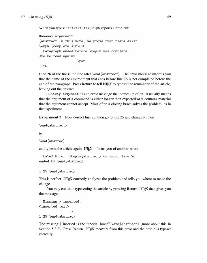
4.3 On using LATEX 49
When you typeset intrart.tex, LATEX reports a problem:
Runaway argument?
abstract In this note, we prove that there exist
\emph complete-sim\ETC.
! Paragraph ended before \begin was complete.
<to be read again>
\par
l.26
Line 26 of the file is the line after \endabstract. The error message informs youthat the name of the environment that ends before line 26 is not completed before theend of the paragraph. Press Return to tell LATEX to typeset the remainder of the article,leaving out the abstract.
Runaway argument? is an error message that comes up often. It usually meansthat the argument of a command is either longer than expected or it contains materialthat the argument cannot accept. Most often a closing brace solves the problem, as inthe experiment.
Experiment 2 Now correct line 20, then go to line 25 and change it from
\endabstract
to
\endabstrac
and typeset the article again. LATEX informs you of another error:
! LaTeX Error: \beginabstract on input line 20
ended by \endabstrac.
l.25 \endabstrac
This is perfect. LATEX correctly analyzes the problem and tells you where to make thechange.
You may continue typesetting the article by pressing Return. LATEX then gives youthe message:
! Missing inserted.
<inserted text>
l.25 \endabstrac
The missing inserted is the “special brace” \endabstract (more about this inSection 5.3.2). Press Return. LATEX recovers from this error and the article is typesetcorrectly.

50 Chapter 4 Your first article and presentation
Experiment 3 Instead of correcting the error in line 25, comment it out with
% \endabstrac
and also comment out the four lines of the figure environment using block comment.Introduce an additional error in line 96. This line reads
and $\Theta$ is a complete congruence relation,
Change \Theta to \Teta:
and $\Teta$ is a complete congruence relation,
Now, when you typeset the article, LATEX reports
! Undefined control sequence.
<recently read>\Teta
l.96 and $\Teta
$ is a complete congruence relation,
Pressing Return results in the message
! LaTeX Error: \beginabstract on input line 20
ended by \enddocument.
Type H <return> for immediate help.
...
l.150 \enddocument
These two mistakes are easy to identify: \Teta is a misspelling of \Theta, and since\endabstract is missing, LATEX is trying to match
\beginabstract
with
\enddocument
Now undo the changes you made to lines 25 and 96. Uncomment the figure.
Experiment 4 In line 42, delete the closing brace of the \label command:
\begindefinition\labelD:P*
This results in a message for line 54, the blank line following the paragraph, that
! Paragraph ended before \label was complete.

4.3 On using LATEX 51
This is easy to understand. You cannot begin a new paragraph within the argument ofa \label command.
Undo the change to line 42.
Experiment 5 Add a blank line following line 58:
\langle \dots, 0, \dots, d, \dots, 0, \dots \rangle
This change results in the message
! Missing $ inserted.
<inserted text>
$
l.59
There can be no blank lines within a displayed math environment. LATEX catches themistake, but the message itself is misleading. Pressing Return does not help; youcannot recover from the error. Delete the blank line.
Experiment 6 Add a $ somewhere in line 58 (such errors often occur when cuttingand pasting formulas):
\langle $\dots, 0, \dots, d, \dots, 0, \dots \rangle
You get the message:
! Display math should end with $$.
<to be read again>
\protect
l.58 \langle $\dots
, 0, \dots, d, \dots, 0, \dots \rangle
Maybe this could be more to the point?Error messages from LATEX are not always helpful, but there is always some in-
formation that can be gleaned from them. Try to identify the structure, that is, thecommand or environment, that causes the error—read the section of this book that de-scribes that command or environment. This should help you correct the error. Keep inmind that the error could be quite far from the line LATEX indicates, but it is always onor before that line in the source file.
If you have difficulty isolating a problem, block comment all but the paragraphyou suspect might have problems. If necessary, split a large paragraph into smallerpieces.
Tip Typeset often.

52 Chapter 4 Your first article and presentation
To some extent, you can avoid having to isolate problems by following this tip.For instance, if I were to typeset First Steps into LATEX [29], with the closing brace ofthe first \caption command on line 480 of the source file missing, I would get theerror message
! Text line contains an invalid character.
l.1227 ...pletely irreducible^^?
where the reference is to line 1227, about 700 lines removed from the actual error.However, if the only thing I did before typesetting was to insert that figure with itsincorrect caption command, at least I would know where to look for errors. If youmake a dozen corrections and then typeset, you may not know where to start.
4.3.2 Logical and visual design
The typeset version of intrart.tex (pp. 42–43) looks impressive. To produce sucharticles, you need to understand that there are two aspects to article design: visual andlogical.
As an example, let us look at a theorem from intrart.tex (see the typeset formof the theorem on page 43). You tell LATEX that you want to state a theorem by using atheorem environment:
\begintheorem\labelT:P*
Let $D_i$, $i \in I$, be complete distributive
lattices satisfying condition~\textup(J).
Let $\Theta$ be a complete congruence relation on
$\Pi^* ( D_i \mid i \in I )$.
If there exist $i \in I$ and $d \in D_i$ with
$d < 1_i$ such that, for all $d \leq c < 1_i$,
\beginequation\labelE:cong1
\langle \dots, d, \dots, 0, \dots \rangle \equiv
\langle \dots, c, \dots, 0, \dots \rangle
\pod\Theta,
\endequation
then $\Theta = \iota$.
\endtheorem
The logical part of the design is choosing to define a theorem by placing material insidea theorem environment. For the visual design, LATEX makes hundreds of decisions.Could you have specified all of the spacing, font size changes, centering, numbering,and so on? Maybe, but would you want to? And would you want to repeat that processfor every theorem in your document?
Even if you did, you would have spent a great deal of time and energy on thevisual design of the theorem rather than on the logical design of your article. The idea

4.4 Converting an article to a presentation 53
behind LATEX is that you should concentrate on what you have to say and let LATEX takecare of the visual design.
This approach allows you to easily alter the visual design by changing the docu-ment class (or its options, see Sections 11.5, 12.1.2, and 18.1). Section 11.1 providessome examples. If you code the visual design into the article—hard coding it, as aprogrammer would say—such changes are much harder to accomplish, for you and forthe journal publishing the article.
4.4 Converting an article to a presentationTo produce a document in LATEX for use as a presentation, you have to output it as aPDF file. You make your presentation using a PDF viewer such as Adobe Reader orprint the pages of the PDF file on transparencies and use a projector.
So a presentation is a PDF file. To display the presentation, connect your computerto a projector. Open the PDF file in Adobe Reader, put it in full screen mode. Thenproject the presentation a page at a time by pressing the space bar or the forward andback arrow keys.
In LATEX, you use a presentation package—really, a document class—to preparesuch a PDF file. We deal with presentations in detail in Chapter 14, but as a quickintroduction, we convert intrart.tex into a presentation.
For the conversion, we use the presentation package FoilTEX, while in Chapter 14we discuss the beamer package. To use the FoilTEX package, we have to learn onlyone new command, \foilhead.
Open intrart.tex, save it as intropres.tex in the work folder. We introducesome changes to the document to prepare it for the conversion. Once you are satisfiedwith the changes made, the tex file created for FoilTEX is typeset so as to producethe PDF file. For WinEdt, click on the PDF TeXify icon. For TeXShop, just click onTypeset. For other TEX installations, check your user manual on how to create a PDF
output.
4.4.1 Preliminary changes
Make the following changes in the preamble, top matter, and abstract.
1. Change the first line to% Introductory presentation:intropres.tex
2. Change the documentclass to foils.
3. Add the line\usepackageamsmath
after the documentclass line. We have to do this because FoilTEX does not automat-ically load the AMS math package.

54 Chapter 4 Your first article and presentation
4. Delete the definitions of theorem, lemma, and definition. FoilTEX redefinesthese.
5. Copy the address into the \author command:
\authorGeorge~A. Menuhin\\
Computer Science Department\\
University of Winnebago\\
Winnebago, MN 53714
and delete the \address command. This may seem strange, but it is necessary be-cause FoilTEX is based on a legacy document class that does not have an \addresscommand (see Chapter 12).
6. Move the abstract after the \maketitle command, as was customary in legacydocument classes.
7. Add the [scale=2] option to the \includegraphics command, so the commandbecomes
\centering\includegraphics[scale=2]products
FoilTEX uses fonts in 20 point size, twice the usual size. So it is appropriate that wescale up the illustration to 200%.
So the new version is
% Introductory presentation:intropres.tex
\documentclassfoils
\usepackageamsmath
\usepackageamssymb,latexsym
\usepackagegraphicx
\begindocument
\titleA construction of complete-simple\\
distributive lattices
\authorGeorge~A. Menuhin\\
Computer Science Department\\
University of Winnebago\\
Winnebago, MN 53714
\dateMarch 15, 2006
\maketitle
\beginabstract
In this presentation, we prove that there exist

4.4 Converting an article to a presentation 55
\emphcomplete-simple distributive lattices,
that is, complete distributive lattices
with only two complete congruences.
\endabstract
Declarations in the body
In your LATEX editor, perform four search and replace operations in the body of thearticle. Change all of the following:
1. theorem to Theorem
2. lemma to Lemma
3. definition to Definition
4. proof to Proof
FoilTEX defines and uses the capitalized versions.
Sectioning
Comment out all the \section commands. FoilTEX uses the \foilhead command tobreak the material into pages and also as a substitute for sectioning.
4.4.2 Making the pagesWe cut the presentation into pages (transparencies or foils) by inserting as many pagebreaking commands of FoilTEX, \foilhead, as seems appropriate. The argumentof the command becomes the “title” for the page. If the argument is empty, the pagehas no title.
Add the \foilheadThe result command after the abstract. This ends thetitle page and adds the title The result to the next page.
See the intropres.tex document for all the other \foilhead commands wehave added.
4.4.3 Fine tuningWe have eliminated the equation numbering, because it would make the equationstoo wide. Also, in a presentation, references to another page are not recommended.We made some additional changes to accommodate that we have fewer charactersper line. Compare the documents intrart.tex and intropres.tex to see all thechanges. Note how in the PDF file the fonts are automatically changed to sans serif,because sans serif text is easier to read when projected. The font size is 20pt, twice thesize of the font in the article.

56 Chapter 4 Your first article and presentation
Of course, intropres.tex is not the most elegant presentation. But I hope ithelps you to make your first presentation. On pages 57 and 58, we show the first twopages of this presentation.
There are, of course, a number of useful commands in FoilTEX in addition to theone we used, \foilhead. We did not even do justice to this one command. It has anoptional argument to enlarge or shrink the space between the header and the body ofthe foil. So
\foilhead[-.5in]A diagram
shrinks that space by half an inch. This is especially useful with large diagrams.For numerous other features of FoilTEX, see the user manual [33].

4.4 Converting an article to a presentation 57

58 Chapter 4 Your first article and presentation

C H A P T E R
5
Typing text
In Chapter 2, we briefly discussed how to type text in a document. Now we take upthis topic more fully.
This chapter starts with a discussion of the keyboard in Section 5.1 and continueswith the rules for spaces in Section 5.2. We cover a very important topic that mustprecede any in-depth discussion of LATEX, how to control LATEX with commands andenvironments, in Section 5.3.
A document may contain symbols that cannot be found on your keyboard. In Sec-tion 5.4, we show how to get these symbols in our typeset documents by using com-mands.
Some other characters are defined by LATEX as command characters. For example,the % character plays a special role in the source document. In Section 5.5.1, you willsee how % is used to comment out lines. In Section 5.5.2, we introduce the commandfor footnotes.
In Section 5.6, we discuss the commands (and environments) for changing fonts,their shapes and sizes. In Section 5.7, you learn about lines, paragraphs, and pages.The judicious use of horizontal and vertical spacing is an important part of document

62 Chapter 5 Typing text
formatting, and also the topic of Section 5.8. In Section 5.9, you learn how to typesettext in a “box”, which behaves as if it were a single large character.
To help the discussion along, we shall use the terms text mode and math modeto distinguish between typesetting text and math.
5.1 The keyboardMost of the keys on your computer’s keyboard produce characters, while others arefunction or modifier keys.
5.1.1 Basic keysThe basic keys are grouped as follows:
Letters The 52 letter keys:
a b c ... z A B C ... Z
Digits The ten digits:
1 2 ... 9 0
Old-style digits are available with the \oldstylenums command. The next lineshows the default digits followed by the old style digits:
1234567890
typed as
1234567890 \quad \oldstylenums1234567890
Punctuation There are nine punctuation marks:
, ; . ? ! : ‘ ’ -
The first six are the usual punctuation marks. The ‘ is the left single quote—also known as the grave accent—while ’ doubles as the right single quote andapostrophe (see Section 5.4.1). The - key is the dash or hyphen (see Sections5.4.2 and 5.4.9).
Parentheses There are four:
( ) [ ]
( and ) are parentheses; [ and ] are called (square) brackets.

5.1 The keyboard 63
Math symbols Seven math symbols correspond to keys. The math symbols are:
∗ + = − < > /
The last four characters have a role also in text mode:
The minus sign − corresponds to the hyphen key, - (see Section 7.4.1).
The math symbols < and > correspond to the keys < and >; use them only inmath mode.
Note that there is also a version of colon (:) for math formulas (see Sections 8.1and B.2).
Space keys Pressing the space bar gives the space character. Pressing the tab keygives the tab character. When typesetting the source file, LATEX does not distin-guish between these two. Pressing the Return key gives the end-of-line character.
These keys produce invisible characters that are normally not displayed on yourmonitor by the text editor. Different computer systems have different end-of-line characters, which may cause some problems when transferring files fromone system to another. A good text editor translates end-of-line characters auto-matically or on demand. Section 5.2.1 explains how LATEX handles the invisiblecharacters.
When explaining some rules of LATEX, sometimes it is important to show if aspace is required. In such cases, I use the symbol to indicate a space, forinstance, \in ut and \ .
The tilde ~ produces a nonbreakable space or tie (see Section 5.4.3 and the foot-note on page 11).
5.1.2 Special keysThere are 13 special keys on the keyboard:
# $ % & ~ _ ^ \ @ " |
They are mostly used to give instructions to LATEX and some are used in math mode(see Chapter 7), and some in BIBTEX (see Chapter 16). See Section 5.4.4 on how toprint these characters in text. Only @ requires no special command, type @ to print @.
5.1.3 Prohibited keysKeys other than those discussed in Sections 5.1.1 and 5.1.2 are prohibited! Specifically,do not use the computer’s modifier keys—Control, Alt, Escape, and others—to producespecial characters, such as accented characters. LATEX will either reject or misunder-stand them.

64 Chapter 5 Typing text
Prohibited characters may not cause problems in some newer LATEX implementa-tions. They may just print Ł if your source file has Ł, and ignore the invisible invalidcharacters. However, for portability reasons, you should avoid using prohibited char-acters.
The babel package provides support for using some modifier keys (see Ap-pendix G).
Tip If there is a prohibited character in your document, you may receive an error messagesuch as
! Text line contains an invalid character.
l.222 completely irreducible^^?
^^?
Delete and retype the offending word or line until the error goes away.
5.2 Words, sentences, and paragraphsText consists of words, sentences, and paragraphs. In text, words are separated by oneor more spaces, which may include a single end-of-line character (see the rule, Spacingin text), or by parentheses and punctuation marks. A group of words terminated by aperiod, exclamation point, or question mark forms a sentence (not all periods terminatea sentence, see the discussion in Section 5.2.2). A group of sentences terminated byone or more blank lines constitutes a paragraph.
5.2.1 Spacing rulesHere are the most important LATEX rules about spaces in text in the source file.
Rule Spacing in text
1. Two or more spaces in text are the same as one.
2. A tab or end-of-line character is the same as a space.
3. A blank line, that is, two end-of-line characters separated only by spaces and tabs,indicates the end of a paragraph. The \par command is equivalent.
4. Spaces at the beginning of a line are ignored.
Rules 1 and 2 make cutting and pasting text less error-prone. In your source file,you do not have to worry about the line length or the number of spaces separating words

5.2 Words, sentences, and paragraphs 65
or sentences, as long as there is at least one space or end-of-line character separatingany two words. Thus
You do not have to worry
about the number of spaces
separating words, as long as there
is at least one space or end-of-line character
separating any two words.
produces the same typeset text as
You do not have to worry about the number of spaces
separating words, as long as there is at least one space
or end-of-line character separating any two words.
However,
the number of spaces separating words,
as long
and
the number of spaces separating words
, as long
produce different results:
the number of spaces separating words, as longthe number of spaces separating words , as long
Notice the space between “words” and the comma in the second line. That space wasproduced by the end-of-line character in accordance with Rule 2.
It is very important to maintain the readability of your source file. LATEX may notcare about the number of spaces or line length, but you, your coauthor, or your editormight.
Rule 3 contradicts Rules 1 and 2, consider it an exception. Sometimes—especiallywhen defining commands and environments (see Sections 15.1 and 15.2)—it is moreconvenient to indicate the end of a paragraph with \par.
When e-mailing a source file, e-mail clients tend to break longer lines into shorterones. Because of the space rules, this does not effect the typeset version most of thetime.

66 Chapter 5 Typing text
5.2.2 PeriodsLATEX places a certain size space between words—the interword space—and a some-what larger space between sentences—the intersentence space. To know which spaceto use, LATEX must decide whether or not a period indicates the end of a sentence.
Rule 1 PeriodTo LATEX, a period after a capital letter, for instance, A. or caT., signifies an abbrevia-tion or an initial. Generally, every other period signifies the end of a sentence.
This rule works most of the time. When it fails—for instance, twice with e.g.—youneed to specify the type of space you want, using the following two rules.
Rule 2 PeriodIf an abbreviation does not end with a capital letter, for instance, etc., and it is not thelast word in the sentence, then follow the period by an interword space (\ ) or a tie (~),if appropriate (see Section 5.4.3).
Recall that \ provides an interword space.
The result was first published, in a first approximation,
in the Combin.\ Journal. The result was first published,
in a first approximation, in the Combin. Journal.
prints as
The result was first published, in a first approximation, in the Combin. Journal.The result was first published, in a first approximation, in the Combin. Journal.
Notice that Combin. in the first line is followed by a regular interword space. The in-tersentence space following Combin. in the second line is a little wider.
A tie (or nonbreakable space)—see also Section 5.4.3—is more appropriate than\ in phrases such as Prof. Smith, typed as Prof.~Smith, and pp. 271–292, typedas pp.~271--292.
Tip The thebibliography environment handles periods properly. You do not have tomark periods for abbreviations (in the form .\) in the name of a journal, so
Acta Math. Acad. Sci. Hungar.
is correct.

5.3 Commanding LATEX 67
Rule 3 PeriodIf a capital letter is followed by a period and is at the end of a sentence, precede theperiod with \@.
For example,
(1) follows from condition~H\@. We can proceed\\
(1) follows from condition~H. We can proceed
prints:
(1) follows from condition H. We can proceed(1) follows from condition H. We can proceed
Notice that there is not enough space after H. in the second line.Most typographers agree on the following rule (see, e.g., Robert Bringhurst’s
The Elements of Typographic Style [8], p. 30):
Rule 4 PeriodAdd no space or a thin space (\,) within strings of initials and be consistent.
So W.H. Lampstone with no space or W. H. Lampstone with thin space ispreferred over W. H. Lampstone. My personal choice is W. H. Lampstone with thinspace.
To make all intersentence spaces equal to the interword space—as required inFrench typography—you can use the command
\frenchspacing
To switch back to using spaces of different sizes, give the command
\nonfrenchspacing
5.3 Commanding LATEXHow do you command LATEX to do something special for you, such as starting a newline, changing emphasis, or displaying the next theorem? You use commands andspecial pairs of commands called environments, both briefly introduced at the start ofChapter 2.
Most, but not all, commands have arguments, which are usually fairly brief. Envi-ronments have contents, the text between the \begin and \end commands. The con-tents of an environment can be several paragraphs long.

68 Chapter 5 Typing text
5.3.1 Commands and environmentsThe \emphtext command instructs LATEX to emphasize its argument, text. The\& command has no argument. It instructs LATEX to typeset & (see Section 5.4.4).
The flushright environment instructs LATEX to right justify the content, the textbetween the two commands
\beginflushright
\endflushright
The content of the document environment is the body of the article (see Section 4.1)and the content of the abstract environment is the abstract.
Rule EnvironmentsAn environment starts with the command
\beginname
and ends with
\endname
Between these two lines is the content of the environment, affected by the definition ofthe environment.
Rule CommandsA LATEX command starts with a backslash, \, and is followed by the command name.The name of a command is either a single non-alphabetic character other than a tab orend-of-line character or a string of letters, that is, one or more letters.
So # and ’ are valid command names. The corresponding commands \# and \’ areused in Sections 5.4.4 and 5.4.7, respectively. input and date are also valid commandnames. However, input3, in#ut, and in ut are not valid names because 3, #, and
should not occur in a multicharacter command name. Note that is a command name,the command \ produces a blank.
LATEX has a few commands, for instance, $ (see Section 7.1) that do not followthis naming scheme, that is, they are not of the form \name. See also Section 15.1.8for special commands with special termination rules.

5.3 Commanding LATEX 69
Rule Command terminationLATEX finds the end of a command name as follows:
If the first character of the name is not a letter, the name is the first character.
If the first character of the name is a letter, the command name is terminated by thefirst nonletter.
If the command name is a string of letters, and is terminated by a space, then LATEXdiscards all spaces following the command name.
While input3 is an invalid name, \input3 is not an incorrect command. It is the\input command followed by the character 3, which is either part of the text followingthe command or the argument of the command.
LATEX also allows some command names to be modified with *. Such commandsare referred to as *-ed commands. Many commands have *-ed variants. \hspace* isan often-used *-ed command (see Section 5.8.1).
Rule Command and environment namesCommand and environment names are case sensitive. \ShowLabels is not the same as\showlabels.
Rule ArgumentsArguments are enclosed in braces, .Optional arguments are enclosed in brackets, [ ].
Commands may have arguments, typed in braces immediately after the command.The argument(s) are used in processing the command. Accents provide very simpleexamples. For instance, \’o—which produces o—consists of the command \’ andthe argument o (see Section 5.4.7). In \bibliographyarticle1, the command is\bibliography and the argument is article1 (see Section 16.2.2).
Sometimes, if the argument is a single character, the braces can be dropped: \’oalso typesets as o.
Some environments also have arguments. For example, the alignat environment(see Section 9.5.4) is delimited by the commands
\beginalignat2
and
\endalignat

70 Chapter 5 Typing text
The argument, 2, is the number of columns—it could be any number 1, 2, . . . A com-mand or environment may have more than one argument. The \frac command (seeSection 7.4.1) has two, $\frac12$ typesets as 1
2 . The user-defined command\con has three (see Section 15.1.2).
Some commands and environments have one or more optional arguments, that is,arguments that may or may not be present. The \sqrt command (see Section 7.4.5)has an optional argument for specifying roots other than the square root. To get 3
√25,
type \sqrt[3]25. The \documentclass command has an argument, the nameof a document class, and an optional argument, a list of options (see Section 10.2),for instance,
\documentclass[12pt,draft,leqno]amsart
Tip If you get an error when using a command, check that:
1. The command is spelled correctly, including the use of uppercase and lowercaseletters.
2. You have specified all required arguments in braces.
3. Any optional argument is in brackets, not braces or parentheses.
4. The command is properly terminated.
5. The package providing the command is loaded with the \usepackage command.
Most errors in the use of commands are caused by breaking the termination rule.We can illustrate some of these errors with the \today command, which produces to-day’s date. You have already seen this command in Section 2.4 (see also Section 5.4.8).The correct usage is
\today\ is the day
or
\today is the day
which both typeset as
July 19, 2006 is the day
In the first case, \today was terminated by \ , the command that produces an inter-word space. In the second case, it was terminated by the empty group .

5.3 Commanding LATEX 71
If there is no space after the \today command, as in
\todayis the day
you get the error message
! Undefined control sequence.
l.3 \todayis
the day
LATEX thinks that \todayis is the command, and, of course, does not recognize it.If you type one or more spaces after \today:
\today is the day
LATEX interprets the two spaces as a single space by the first space rule (see page 64),and uses that one space to delimit \today from the text that follows it. So LATEXproduces
July 19, 2006is the day
Section 15.1.8 discusses how best to avoid such errors.
Tip If a command—or environment—can have an optional argument and
none is given, and
the text following the command starts with [,
then type this as [.
This may happen, for instance, with the command \item (see page 123). To getan example for an environment, see Section 9.6.1 for subsidiary math environmentsand page 229 for the alignment options. See what happens if no option is given but themath starts, say, with [x].
5.3.2 ScopeA command issued inside a pair of braces has no effect beyond the right brace,except for the seldom occurring global commands (see Section 5.3.3). You can haveany number of pairs of braces:
... ... ... ... ...
The innermost pair containing a command is the scope of that command. The commandhas no effect outside its scope. We can illustrate this concept using the \bfseries
command that switches the font to boldface:
some text \bfseries bold text no more bold

72 Chapter 5 Typing text
typesets as
some text bold text no more bold
The commands \beginname and \endname bracketing an environment actalso as a pair of braces. In particular, $, \[, and \] are special braces.
Rule Braces
1. Braces must be balanced: An opening brace has to be closed, and a closing bracemust have a matching opening brace.
2. Pairs of braces cannot overlap.
Violating the first brace rule generates warnings and error messages. If there is onemore opening brace than closing brace, the document typesets, but you get a warning:
(\end occurred inside a group at level 1)
For two or more unmatched opening braces, you are warned that \end occurred insidea group at level 2, and so on. There is a tendency to disregard such warnings since yourarticle is already typeset and the error may be difficult to find. However, such errorsmay have strange consequences. At one point in the writing of my second LATEX book,there were two extra opening braces in Chapter 2. As a result, the title of Chapter 7was placed on a page by itself! So it is best not to disregard such warnings.
If you have one unmatched closing brace, you get an error message such as
! Too many ’s
If special braces, say, \beginname and \endname, do not balance, you get anerror message such as those discussed in Section 4.3.1:
! LaTeX Error: \beginname on input line 21
ended by \enddocument.
or
! LaTeX Error: \begindocument ended by \endname.
To illustrate the second rule, here are two simple examples of overlapping braces.
Example 1
\bfseries some text
\beginlemma

5.3 Commanding LATEX 73
more text final text
\endlemma
Example 2
some \bfseries text, then math: $\sqrt2 , \sqrt3$
In Example 1, the scope of \bfseries overlaps the braces \beginlemma and\endlemma, whereas in Example 2, the scope of \bfseries overlaps the specialbraces $ and $. Example 1 is easy to correct:
\bfseries some text
\beginlemma
\bfseries more text
final text
\endlemma
Example 2 may be corrected as follows:
some \bfseries text, then math: $\sqrt2, \sqrt3$
Actually,√
2 does not even have a bold version (see Section 8.3.3).If the braces do overlap and they are of the same kind, LATEX simply misunder-
stands the instructions. The closing brace of the first pair is regarded as the closingbrace of the second pair, an error that may be difficult to detect. LATEX can help ifspecial braces overlap. Typesetting Example 1 gives the error message
! Extra , or forgotten \endgroup.
l.7 more text
final text
5.3.3 Types of commandsIt may be useful at this point to note that commands can be of various types.
Some commands have arguments, and some do not. Some commands effectchange only in their arguments, while some commands declare a change. For instance,\textbfThis is bold typesets the phrase This is bold in bold type: This is
bold and has no effect on the text following the argument of the command. On the otherhand, the command \bfseries declares that the text that follows should be bold. Thiscommand has no argument. I call a command that declares change a command dec-laration. So \bfseries is a command declaration, while \textbf is not. As a rule,command declarations are commands without arguments.
Commands with arguments are called long if their argument(s) can contain a blankline or a \par command; otherwise they are short. For example, \textbf is a short

74 Chapter 5 Typing text
command. So are all the top matter commands discussed in Section 11.2. The \parboxcommand, discussed in Section 5.9.4, is long.
Finally, as discussed in Section 5.3.2, the effect of a command remains within itsscope. This is true only of local commands. There are also some global commands,such as the \setcounter command described in Section 15.5.1.
Fragile commands
As a rule, LATEX reads a paragraph of the source file, typesets it, and then goes on tothe next paragraph (see Section D.5). Some information from the source file, however,is separately stored for later use.
Examples include the title of an article, which is reused as a running head (Sec-tion 11.2.1); titles of parts, sections, subsections, and other sectioning commands,which are used in the table of contents (Sections 18.2 and 10.4.1); footnotes (Sec-tion 5.5.2); table and figure captions (Section 10.4.3), which are used in lists of tablesand figures (Section 10.4.3); and index entries (Chapter 17).
These are movable arguments, and certain commands embedded in them must beprotected from damage while being moved. LATEX commands that need such protectionare called fragile. The inline math delimiter commands (introduced on page 18) \(and \) are fragile, while $ is not.
In a movable argument, fragile commands must be protected with a \protect
command. Thus
The function \( f(x^2) \)
is not an appropriate section title, but
The function \protect \( f(x^2) \protect \)
is. So is
The function $f(x^2)$
To be on the safe side, you should protect every command that might cause problemsin a movable argument. Section 18.2 shows an example of what happens if a fragilecommand is not protected. Alternatively, use commands declared with
\DeclareRobustCommand
This command works the same way as \newcommand but the command defined isrobust, that is, not fragile.
5.4 Symbols not on the keyboardA typeset document may contain symbols that cannot be typed. Some of these symbolsmay even be available on the keyboard but you are prohibited from using them (see

5.4 Symbols not on the keyboard 75
Section 5.1.3). In this section, we discuss the commands that typeset some of thesesymbols in text.
5.4.1 Quotation marksTo produce single and double quotes, as in
‘subdirectly irreducible’ and “subdirectly irreducible”
type
‘subdirectly irreducible’ and ‘‘subdirectly irreducible’’
Here, ‘ is the left single quote and ’ is the right single quote. Note that the doublequote is obtained by pressing the single quote key twice, and not by using the doublequote key. If you need single and double quotes together, as in “She replied, ‘No.’ ”,separate them with \, (which provides a thin horizontal space):
‘‘She replied, ‘No.’\,’’
5.4.2 DashesDashes come in three lengths. The shortest dash, called a hyphen, is used to connectwords:
Mean-Value Theorem
This phrase is typed with a single dash:
Mean-Value Theorem
A medium-sized dash, called an en dash, is typed as -- and is used
For number ranges; for instance, the phrase see pages 23–45, is typed as
see pages~23--45
Note: ~ is a nonbreakable space or tie (see Section 5.4.3).
In place of a hyphen in a compound adjective when one of the elements of the adjec-tive is an open compound (such as New York) or hyphenated (such as non-English).For instance, the phrase Jonathan Schmidt–Freid adjoint, is typed as
Jonathan Schmidt--Freid adjoint
A long dash—called an em dash—is used to mark a change in thought or to addemphasis to a parenthetical clause, as in this sentence. The two em dashes in the lastsentence are typed as follows:

76 Chapter 5 Typing text
A long dash---called an \emphem dash---is used
In math mode, a single dash is typeset as the minus sign − (a binary operation) withsome spacing on both sides, as in 15− 3 or the “negative” as in −3 (see Sections 5.1.1and 7.4.1).
Note that there is no space before or after an en dash or em dash.
5.4.3 Ties or nonbreakable spacesA tie or nonbreakable space (sometimes called a blue space) is an interword spacethat cannot be broken across lines. For instance, when referencing P. Neukomm in anarticle, you do not want the initial P. at the end of a line and the surname Neukommat the beginning of the next line. To prevent such an occurrence, you should typeP.~Neukomm.
If your keyboard does not have ~, use the \nobreakspace command instead, andtype P.\nobreakspace Neukomm.
The following examples show some typical uses:
Theorem~\refT:main in Section~\refS:intro
Donald~E. Knuth
assume that $f(x)$ is (a)~continuous, (b)~bounded
the lattice~$L$.
Sections~\refS:modular and~\refS:distributive
In~$L$, we find
Of course, if you add too many ties, as in
Peter~G.~Neukomm% Incorrect!
LATEX may send you a line too wide error message (see Section 5.7.1).The tie (~) absorbs spaces, so typing P. ~ Neukomm works just as well. This
feature is convenient when you add a tie during editing.
5.4.4 Special charactersThe characters corresponding to nine of the 13 special keys (see Section 5.1.2) areproduced by typing a backslash (\) and then the key, as shown in Table 5.1.
If for some reason you want to typeset a backslash in your document, type thecommand \textbackslash, which typesets as \. You might think that you could get atypewriter style backslash by utilizing the \texttt command introduced in Section 2.4

5.4 Symbols not on the keyboard 77
\texttt\textbackslash
but this is not the case, \textbackslash and \texttt\textbackslash producethe same symbol, \, which is different from the typewriter style backslash: \. Look atthem side by side: \ \. For a typewriter style backslash you can use the \bsl commandintroduced in Section 15.1.1 or the \texttt\symbol92 command introducedlater in this section.
The | key is seldom used in text. If you need to typeset the math symbol | in text,type \textbar.
Note that in text, * typesets as *, whereas in a formula it typesets centered as ∗.To typeset a centered star in text, use the command \textasteriskcentered.
@ typesets as @.Finally, the " key should never be used in text. See Section 5.4.1 for the proper
way to typeset double quotes. Nevertheless, sometimes " may be used to typeset ", asin the computer code segment print("Hello!"). In BIBTEX and MakeIndex, " hasspecial meanings (see Chapters 16 and 17).
Tip Be careful when typing \ and \ to typeset the braces . Typing a brace withoutits backslash results in unbalanced braces, in violation of the first brace rule in Sec-tion 5.3.2.
We illustrated in Section 5.3.2 some consequences of unbalanced braces. You mayavoid some of these problems by introducing user-defined commands, as introduced inSection 15.3.
You can also produce special characters with the \symbol command:
\symbol94 typesets as ˆ
\symbol126 typesets as ˜
Name Type Typeset
Ampersand \& &Caret \^ ˆDollar Sign \$ $Left Brace \ Right Brace \ Underscore (or Lowline) \_Octothorp \# #Percent \% %Tilde \~ ˜
Table 5.1: Nine special characters.

78 Chapter 5 Typing text
0 1 2 3 4 5 6 7 8 9
x Γ ∆ Θ Λ Ξ Π Σ Υ Φ Ψ1x Ω ↑ ↓ ' ¡ ¿ ı ` ´2x ˇ ˘ ¯ ˚ ¸ ß æ œ ø Æ3x Œ Ø ! " # $ % & ’4x ( ) * + , - . / 0 15x 2 3 4 5 6 7 8 9 : ;6x < = > ? @ A B C D E7x F G H I J K L M N O8x P Q R S T U V W X Y9x Z [ \ ] ^ _ ‘ a b c10x d e f g h i j k l m11x n o p q r s t u v w12x x y z | ~ ¨
Table 5.2: Font table for the Computer Modern typewriter style font.
\texttt\symbol92 typesets as \
The argument of the \symbol command is a number matching the slot of thesymbol in the layout (encoding) of the font. The layout for the Computer Moderntypewriter style font is shown in Table 5.2.
Alternatively, instead of \texttt\symbol92, can use
\texttt\char‘\\
Any character x in the font can be accessed by typing the character itself as ‘\x.This way you don’t have to look up the position of the symbol.
You can obtain similar tables for any font in your LATEX implementation by usingthe fonttbl.tex file in your samples folder. The table format in this file is used inSection 6.6 as an example of the tabular environment.
For more about font tables, see the nfssfont.tex file, part of the standard LATEXdistribution (see Section 12.3) and see also Section 7.5.7 of The LATEX Companion, 2ndedition [46].
5.4.5 Ellipses
The text ellipsis, . . . , is produced using the \dots command. Typing three periodsproduces ... (notice that the spacing is wrong).
\dots is one of several commands that can be used to create ellipses in formulas(see Section 7.4.3).

5.4 Symbols not on the keyboard 79
5.4.6 LigaturesCertain groups of characters, when typeset, are joined together—such compound char-acters are called ligatures. There are five ligatures that LATEX typesets automatically(if you use the Computer Modern fonts): ff, fi, fl, ffi, and ffl.
If you want to prevent LATEX from forming a ligature, separate the characters withthe command \textcompwordmark. Compare iff with iff, typed as iff and
if\textcompwordmark f
Enclosing the second character in braces () is a crude method of preventing theligature, as used in Formula 4 of the Formula Gallery (see Section 7.9). This method,in some instances, may interfere with LATEX’s hyphenation algorithm.
5.4.7 Accents and symbols in textLATEX provides 15 European accents. Type the command for the accent ( \ and a char-acter), followed by the letter (in braces) on which you want the accent placed (seeTable 5.3).
For example, to get Gratzer Gyorgy, type
Gr\"atzer Gy\"orgy
and to get O type \"O.To place an accent on top of an i or a j, you must use the dotless version of i
and j. These are obtained by the commands \i and \j: \’\i typesets as ı and\v\j typesets as . Tables 5.4 and 5.5 list some additional text symbols and Europeancharacters available in LATEX when typing text. Using localized versions of LATEX, youget more accented and combined characters such as the Catalan geminated ell (seeAppendix G).
Name Type Typeset Name Type Typeset
acute \’o o macron \=o obreve \uo o overdot \.g gcaron/hacek \vo o ring \ru ucedilla \cc c tie \too oocircumflex \^o o tilde \~n ndieresis/umlaut \"u u underdot \dm m.double acute \Ho o underbar \bo o
¯grave \‘o o
dotless i \i ı dotless j \j \’\i ı \v\j
Table 5.3: European accents.

80 Chapter 5 Typing text
Note that the \textcircled command (in Table 5.5) takes an argument. It seemsto work best with a single lowercase character, like a© or α©. Capitals such as A© arenot very satisfactory. Section 5.9.6 explains how to create the symbol A©.
5.4.8 Logos and dates
\TeX produces TEX, \LaTeX produces LATEX, and \LaTeXe produces LATEX 2ε (theoriginal name of the current version of LATEX). The \AmS command produces the logoAMS.
Remember to type \TeX\ or \TeX if you need a space after TEX (similarlyfor the others). A better way to handle this problem is discussed in Section 15.1.1.
LATEX also stores some useful numbers:
\time is the time of day in minutes since midnight
\day is the day of the month
\month is the month of the year
\year is the current year
You can include these numbers in your document by using the \the command:
Year: \the\year; month: \the\month; day: \the\day
produces a result such as
Year: 2006; month: 7; day: 11
Of more interest is the \today command, which produces today’s date in theform: July 11, 2006. It is often used as the argument of the \date command (seeSection 11.2.1).
Remember the termination rule (Rule 3 in Section 5.3.1).
today’s date in the form: \today (you may want
produces
today’s date in the form: July 11, 2006(you may want
To get the desired effect, type \ or after the \today command:
today’s date in the form: \today\ (you may want

5.4 Symbols not on the keyboard 81
Name Type Typeset Type Typeset
a-ring \aa a \AA Aaesc \ae æ \AE Æethel \oe œ \OE Œeszett \ss ß \SS SSinverted question mark ?‘ ¿inverted exclamation mark !‘ ¡slashed L \l l \L Lslashed O \o ø \O Ø
Table 5.4: European characters.
Name Type Typeset
ampersand \& &asterisk bullet \textasteriskcentered ∗backslash \textbackslash \bar (caesura) \textbar |brace left \ brace right \ bullet \textbullet •circled a \textcircleda a©circumflex \textasciicircum ˆcopyright \copyright c©dagger \dag †double dagger (diesis) \ddag ‡dollar \$ $double quotation left \textquotedblleft or ‘‘ “double quotation right \textquotedblright or ’’ ”em dash \textemdash or --- —en dash \textendash or -- –exclamation down \textexclamdown or !‘ ¡greater than \textgreater >less than \textless <lowline \_midpoint \textperiodcentered ·octothorp \# #percent \% %pilcrow (paragraph) \P ¶question down \textquestiondown or ?‘ ¿registered trademark \textregistered R©section \S §
Table 5.5: Extra text symbols.

82 Chapter 5 Typing text
5.4.9 HyphenationLATEX reads the source file one line at a time until it reaches the end of the currentparagraph and then tries to balance the lines (see Section D.3.2). To achieve this goal,LATEX hyphenates long words using a built-in hyphenation algorithm, a database storedin the hyphen.tex file, and a long \hyphenation list in the AMS document classes.If you use a document class not containing such a list, copy the hyphenation list fromamsart to your document.
Rule Optional hyphenIf you find that LATEX cannot properly hyphenate a word, put optional hyphens in theword. An optional hyphen is typed as \- , and allows LATEX to hyphenate the wordwhere the optional hyphen is placed—and only at such points—if the need arises.
Examples: data\-base,an\-ti\-thet\-ic, set\-upNote that:
Optional hyphens prevent hyphenation at any other point in the word.
Placing an optional hyphen in a particular occurrence of a word does not affect thehyphenation of any other occurrences of that word.
Rule Hyphenation specificationsList the words that often need help in a command:
\hyphenationset-up as-so-ciate
All occurrences of the listed words following this command in your document arehyphenated as specified.
Note that in the \hyphenation command the hyphens are designated by - andnot by \-, and that the words are separated by spaces not by commas.
You must use optional hyphens for words with accented characters, as in
Gr\"at\-zer
Such words cannot be included in a \hyphenation list (unless you use the T1 fontencoding—see Appendix G).

5.4 Symbols not on the keyboard 83
Rule Preventing hyphenationTo prevent hyphenation of a word, put it in the argument of a \text command or placeit unhyphenated in a \hyphenation command.
For example, type
\textdatabase
if you do not want this instance of database hyphenated, or type
\hyphenationdatabase
if you do not want LATEX to hyphenate any occurrence of the word after this commandin your document. Of course, typing data\-base overrides the general prohibition forthis one instance.
You can have any number of \hyphenation commands in your document.
Tip LATEX does not break a hyphenated word except at the hyphen, nor does it break a wordfollowed by or preceding an em dash or en dash (see Section 5.4.2). LATEX often needshelp with such words.
Sometimes a hyphen in a phrase should not be broken. For instance, the phrasem-complete lattice should not be broken after m; so type it as
\text$\mathfrakm$-com\-plete lattice
(see Section 8.3.2 for \mathfrak).Use the \nobreakdash command (placed before the hyphen)
\nobreakdash- \nobreakdash-- \nobreakdash---
to prevent such breaks. For example,
pages~24\nobreakdash--47
Since LATEX does not hyphenate a hyphenated word except at the hyphen,
\nobreakdash-
prevents the hyphenation of the whole word as though it were enclosed in a \text
command. The form
\nobreakdash-\hspace0pt
allows the normal hyphenation of the word that follows the hyphen. For example,

84 Chapter 5 Typing text
$\mathfrakm$\nobreakdash-\hspace0ptcomplete lattice
allows the word complete to be hyphenated.This coding of the phrase m-complete lattice is a natural candidate for a user-
defined command (see Section 15.1.1).
Tip If you want to know how LATEX would hyphenate a list of words, place it in the argumentof a \showhyphens command.
For instance,
\showhyphenssummation reducible latticoid
The result,
sum-ma-tion re-ducible lat-ti-coid
is shown in the log file.
Tip Some text editors wrap lines in a source file by breaking them at a hyphen, introducingerrors in your typeset document.
For instance,
It follows from Theorem~\refT:M that complete-
simple lattices are very large.
is typeset by LATEX as follows:
It follows from Theorem 2 that complete- simple lattices are very large.
As you can see, there is a space between the hyphen and the word simple. The texteditor inserted an end-of-line character after the hyphen (by the second space rule,see Section 5.2.1). This end-of-line character was interpreted by LATEX as a space.To correct the error, make sure that there is no such line break, or comment out (seeSection 5.5.1) the end-of-line character:
It follows from Theorem~\refT:M that complete-%
simple lattices are very large.
Better yet, rearrange the two lines:
It follows from Theorem~\refT:M that
complete-simple lattices are very large.

5.5 Comments and footnotes 85
Of course, LATEX does not know everything about the complicated hyphenation rulesof the English language. Consult The Chicago Manual of Style, 15th edition [11] andLyn Dupre’s BUGS in Writing: A Guide to Debugging Your Prose, 2nd edition [13] foradditional guidance.
5.5 Comments and footnotesVarious parts of your source file do not get typeset like most of the rest. The twoprimary examples are comments that do not get typeset at all and footnotes that gettypeset at the bottom of the page.
5.5.1 CommentsThe % symbol tells LATEX to ignore the rest of the line. A common use might be acomment to yourself in the source file:
therefore, a reference to Theorem~1 % check this!
The % symbol has many uses. For instance, a document class command (seeSection 11.5),
\documentclass[twocolumn,twoside,legalpaper]amsart
may be typed with explanations, as
\documentclass[%
twocolumn,% option for two-column pages
twoside,% format for two-sided printing
legalpaper% print on legal-size paper
]amsart
so you can easily comment out some at a later time, as in
\documentclass[%
%twocolumn,% option for two-column pages
%twoside,% format for two-sided printing
legalpaper% print on legal-size paper
]amsart
Notice that the first line is terminated with a % to comment out the end-of-line character.
Tip Some command arguments do not allow any spaces. If you want to break a line withinan argument list, you can terminate the line with a %, as shown in the previous example.
See also the example at the end of Section 5.4.9.

86 Chapter 5 Typing text
It is often useful to start a document with a comment line giving the file name andidentifying the earliest version of LATEX that must be used to typeset it.
% This is article.tex
\NeedsTeXFormatLaTeX2e[1994/12/01]
The second line specifies the December 1, 1994 (or later) release of LATEX. You mayneed to use such a declaration if your document uses a feature that was not available inearlier releases. Since LATEX changes very little these days, this command is of limiteduse. (See, however, the discussion on page 311.)
Other uses of % include marking parts of the article for your own reference.For instance, you may include comments to explain command definitions (as in Sec-tion 15.3). If something goes wrong inside a multiline math display (see Chapter 9),LATEX does not tell you precisely where the error is. You can try commenting out allbut one of the lines, until each line works separately.
Note that % does not comment out lines in a BIBTEX database document (see Sec-tion 16.2.4).
Tip The 25% ruleIf you want a % sign in text, make sure you type it as \%. Otherwise, % comments outthe rest of the line. LATEX does not produce a warning.
Using % to comment out large blocks of text can be tedious even with block com-ment. The verbatim package includes the comment environment:
\begincomment
...the commented out text...
\endcomment
Rule comment environments
1. \endcomment must be on a line by itself.
2. There can be no comment within a comment.
In other words,
\begincomment
commented out text...
\begincomment
some more commented out text...
\endcomment

5.5 Comments and footnotes 87
and some more commented out text...
\endcomment
is not allowed. LATEX may give one of several error messages, depending on the circum-stances. For instance,
! LaTeX Error: \begindocument ended by \endcomment.
l.175 \endcomment
The comment environment can be very useful in locating errors. Suppose youhave unbalanced braces in your source file (see Section 5.3.2). Working with a copy ofyour source file, comment out the first half at a safe point (not within an environment!)and typeset. If you still get the same error message, the error is in the second half. Ifthere is no error message, the error is in the first half. Comment out the half that has noerror.
Now comment out half of the remaining text and typeset again. Check to seewhether the error appears in the first half of the remaining text or the second. Continueapplying this method until you narrow down the error to a paragraph that you caninspect visually.
Since the comment environment requires the verbatim package, you must in-clude the line
\usepackageverbatim
in the preamble of the source file (see Sections 12.3.1 and E.1).
5.5.2 FootnotesThe text of a footnote is typed as the argument of a \footnote command. To illustratethe use of footnotes, I have placed one here.1 This footnote is typed as
\footnoteFootnotes are easy to place.
If you want to use symbols to designate the footnotes, instead of numbers, typethe command
\renewcommand\thefootnote
\ensuremath\fnsymbolfootnote
before the first footnote; this provides up to nine symbols. In Section 15.1.1, we discussthe \ensuremath command. Section 3.2 of The LATEX Companion, 2nd edition [46]describes how to further customize footnotes.
In addition, there are title-page footnotes, such as the \thanks and \date com-mands in the top matter. See page 42 for a typeset example of \date. See also Sec-tion 11.2 and the typeset title page footnotes on page 286.
1Footnotes are easy to place.

88 Chapter 5 Typing text
You can add a footnote marked by ∗ to the title of an article. For instance, typethe title
\title[Complete congruence lattices]%
Complete congruence lattices$^*$
and add the lines
\renewcommand\thefootnote\fnsymbolfootnote
\setcounterfootnote1
\footnotetextLecture delivered at the \AMS
annual meeting in Brandon.
\setcounterfootnote0
The footnote will appear as the first footnote on page 1 marked by ∗. All the otherfootnotes are unmarked.
5.6 Changing font characteristicsAlthough a document class and its options determine how LATEX typesets characters,there are occasions when you want control over the shape or size of the font used.
5.6.1 Basic font characteristicsYou do not have to be a typesetting expert to recognize the following basic font at-tributes:
Shape Normal text is typeset:upright (or roman) as this textslanted as this text
italic as this textsmall caps as this text
Monospaced and proportional Typewriters used monospaced fonts, that is, fonts allof whose characters are of the same width. Most text editors display text us-ing a monospaced font. LATEX calls monospaced fonts typewriter style. In thisbook, such a font is used to represent user input and LATEX’s response, such as“typewriter style text”. Whereas, normal text is typeset in a proportionalfont, such as “proportional text with ii and mm”, in which i is narrow and mis wide:mmmmmm
iiiiii
monospaced
mmmmmmiiiiii
proportional

5.6 Changing font characteristics 89
Serifs A serif is a small horizontal (sometimes vertical) stroke used to finish off a ver-tical stroke of a letter, as on the top and bottom of the letter M. LATEX’s standardserif font is Computer Modern roman, such as “serif text”. Fonts without serifsare called sans serif, such as “sans serif text”. Sans serif fonts are often used fortitles or for special emphasis.
Series: weight and width The series is the combination of weight and width. A font’sweight is the thickness of the strokes and the width is how wide the characters are.
Light, medium (or normal), and bold often describe weight.
Narrow (or condensed), medium (or normal), and extended often describe width.
The Computer Modern family includes bold fonts. Traditionally, when the userasks for bold CM fonts, LATEX actually provides bold extended (a somewhatwider version).
Size Most LATEX articles are typeset with 10 point text unless otherwise instructed.Larger sizes are used for titles, section titles, and so on. Abstracts and footnotesare often set in 8-point type.
Font family The collections of all sizes of a font is called a font family.
5.6.2 Document font familiesIn a document class, the style designer designates three document font families:
1. Roman (upright and serifed) document font family
2. Sans serif document font family
3. Typewriter style document font family
and picks one of these (for articles, as a rule, the roman document font family) as thedocument font family or normal family. In all the examples in this book, the documentfont family is the roman document font family except for presentations which use sansserif (see Section 4.4 and Chapter 14). When you use Computer Modern fonts inLATEX, which is the default, the three document font families are Computer Modernroman, Computer Modern sans serif, and Computer Modern typewriter. The documentfont family is Computer Modern roman.
In this book, the roman document font family is Times, the sans serif documentfont family is Helvetica, and the typewriter style document font family is ComputerModern typewriter. The document font family is the roman document font familyTimes.
The document font family (normal family) is the default font. You can alwaysswitch back to it with
\textnormal... or \normalfont ...

90 Chapter 5 Typing text
Table 5.6 shows these two commands and three additional pairs of commands to helpyou switch among the three basic document font families. It also shows the commandpairs for the basic font shapes.
Command with Argument Command Declaration Switches to thefont family
\textnormal... \normalfont ... document\emph... \em ... emphasis\textrm... \rmfamily ... roman\textsf... \sffamily ... sans serif\texttt... \ttfamily ... typewriter style\textup... \upshape ... upright shape\textit... \itshape ... italic shape\textsl... \slshape ... slanted shape\textsc... \scshape ... small capitals\textbf... \bfseries ... bold\textmd... \mdseries ... normal weight and width
Table 5.6: Font family switching commands.
Command pairs
The font-changing commands of Table 5.6 come in two forms:
A command with an argument, such as \textrm..., changes its argument. Theseare short commands, i.e., they cannot contain a blank line or a \par command.
A command declaration, such as \rmfamily, carries out the font change followingthe command and within its scope (see Section 5.3.2).
You should always use commands with arguments for small changes within aparagraph. They have two advantages:
You are less likely to forget to change back to the normal font.
You do not have to worry about italic corrections (see Section 5.6.4).
Note that MakeIndex requires you to use commands with arguments to change the fontin which page numbers are typeset (see Section 17.1).
For font changes involving more than one paragraph, use command declarations.These commands are preferred if you want to create user-defined commands and envi-ronments (see Chapter 15).
5.6.3 Shape commandsThere are five pairs of commands to change the font shape:

5.6 Changing font characteristics 91
\textup... or \upshape ... switch to the upright shape.
\textit... or \itshape ... switch to the italic shape.
\textsl... or \slshape ... switch to the slanted shape.
\textsc... or \scshape ... switch to small capitals.
\emph... or \em ... switch to emphasis .
The document class specifies how emphasis is typeset. As a rule, it is italic or slantedunless the surrounding text is italic or slanted, in which case it is upright. For instance,
\emphRubin space
in the statement of a theorem is typeset as
the space satisfies all three conditions, a so-called Rubin space that ...
The emphasis changed the style of Rubin space from italic to upright.
Tip Be careful not to interchange the command pairs. For instance, if by mistake you type\textit serif, the result is serif. Only the s is italicized since \textit takes sas its argument.
Rule Abbreviations and acronymsFor abbreviations and acronyms use small caps, except for two-letter geographicalacronyms.
So Submitted to tug should be typed as
Submitted to \textsctug
Note that only the lowercase characters in the argument of the \textsc command areprinted as small caps.
5.6.4 Italic correctionsThe phrase
when using a serif font
may be typed as follows:

92 Chapter 5 Typing text
when using a \itshape serif\/ font
The \/ command before the closing brace is called an italic correction. No-tice that \itshape MM typesets as MM, where the M is leaning into the M. Type\itshape M\/M to get the correct spacing M M. Compare the typeset phrase fromthe previous example with and without an italic correction:
when using a serif fontwhen using a serif font
The latter is not as pleasing to the eye.
Rule 1 Italic correctionIf the emphasized text is followed by a period or comma, you should not type the italiccorrection.
For example,
Do not forget. My party is on Monday.
should be typed as
\itshape Do not forget. My party is on Monday.
Rule 2 Italic correctionThe shape commands with arguments do not require italic correction. The correctionsare provided automatically where needed.
Thus you can type the phrase when using a serif font the easy way:
when using a \textitserif font
Whenever possible, let LATEX take care of the italic correction. However, if LATEX isadding an italic correction where you feel it is not needed, you can override the cor-rection with the \nocorr command. LATEX does not add an italic correction beforea period or a comma. These two punctuation marks are stored in the \nocorrlist
command. By redefining this command, you can modify LATEX’s behavior.
Rule 3 Italic correctionThe italic correction is required with the commands \itshape, \slshape, \em.

5.6 Changing font characteristics 93
Command Sample text
\Tiny sample text
\tiny sample text
\SMALL or \scriptsize sample text
\Small or \footnotesize sample text
\small sample text
\normalsize sample text
\large sample text\Large sample text
\LARGE sample text
\huge sample text
\Huge sample text
Table 5.7: Font size commands.
5.6.5 Series
These attributes play a very limited role with the Computer Modern fonts. There isonly one important pair of commands,
\textbf... \bfseries ...
to change the font to bold (actually, bold extended). The commands
\textmd... \mdseries ...
which set both the weight and width to medium (normal) are seldom needed.
5.6.6 Size changes
Standard LATEX documents are typeset in 10 point type. The 11 point and 12 pointtype are often used for greater readability and some journals require 12 point—if thisis the case, use the 12pt document class option (see Sections 11.5, 12.1.2, and 18.1.3).The sizes of titles, subscripts, and superscripts are automatically set by the documentclass, in accordance with the font size option.
If you must change the font size for some text—it is seldom necessary to do so inan article—the following command declarations are provided (see Table 5.7):
\Tiny \tiny \SMALL \Small \small
\normalsize
\large \Large \LARGE \huge \Huge

94 Chapter 5 Typing text
The command \SMALL is also called \scriptsize and the command \Small is alsocalled \footnotesize. The font size commands are listed in order of increasing—tobe more precise, nondecreasing—size.
Two commands allow the user to increase or decrease font size: \larger movesup one size, \smaller moves down one. Both commands take an optional argument.For example, \larger[2] moves up 2 sizes.
5.6.7 OrthogonalityYou are now familiar with the commands that change the font family, shape, series, andsize. Each of these commands affects one and only one font attribute. For example,if you change the series, then the font family, shape, and size do not change. Thesecommands act independently. In LATEX terminology, the commands are orthogonal.From the user’s point of view this behavior has an important consequence: The orderin which these commands are given does not matter. Thus
\Large \itshape \bfseries
has the same effect as
\bfseries \itshape \Large
Note that LATEX 2.09’s two-letter commands (see Section 5.6.8) are not orthogonal.Orthogonality also means that you can combine these font attributes in any way
you like. For instance, the commands
\sffamily \slshape \bfseries \Large
instruct LATEX to change the font family to sans serif, the shape to slanted, the series tobold, and the size to \Large. If the corresponding font is not available, LATEX uses afont that is available, and issues a warning. The font substitution algorithm (see Section7.9.3 of The LATEX Companion, 2nd edition [46] for details) may not provide the fontyou really want, so it is your responsibility to make sure that the necessary fonts areavailable. We discuss this topic further in Section 18.5.
5.6.8 Obsolete two-letter commandsUsers of LATEX 2.09 andAMS-LATEX version 1.1 are accustomed to using the two-lettercommands \bf, \it, \rm, \sc, \sf, \sl, and \tt. These commands are not partof LATEX. They are, however, still defined in most document classes. The two-lettercommands
1. switch to the document font family,
2. change to the requested shape.
There are a number of reasons not to use them. The two-letter commands

5.7 Lines, paragraphs, and pages 95
are not part of LATEX,
require manual italic corrections,
are not orthogonal (see Section 5.6.7).\slshape \bfseries is the same as \bfseries \slshape (slanted bold), but\sl\bf is not the same as \bf\sl. Indeed, \sl\bf sample gives sample and\bf\sl sample produces sample.
5.6.9 Low-level commands
The font-characteristic changing commands we discussed in this section are the high-level font commands. Each of these commands is implemented by LATEX and the docu-ment class using low-level font commands. The low-level commands have been devel-oped for document class and package writers. See Section 7.9 of The LATEX Companion,2nd edition [46].
There is one use of low-level commands you should keep in mind. When youchoose a font size for your document or for some part thereof, you also determine the\baselineskip, the distance from the baseline of one line to the baseline of the next.Typically, a 10-point font size uses a 12 point \baselineskip. Occasionally, youmay want to change the font size along with the \baselineskip. A command foraccomplishing this is
\fontsize9pt11pt\selectfont
which changes the font size to 9 point and the \baselineskip to 11 point. To makethis change for a single paragraph, you can type
%special paragraph
\fontsize9pt11pt\selectfont
text
%end special paragraph
Observe the blank line that follows text and marks the end of the paragraph; \parwould accomplish the same thing.
5.7 Lines, paragraphs, and pagesWhen typesetting a document, LATEX breaks the text into lines, paragraphs, and pages.Sometimes you may not like how LATEX has chosen to lay out your text. There are waysto influence how LATEX does its work and these are discussed in this section.

96 Chapter 5 Typing text
5.7.1 Lines
LATEX typesets a document one paragraph at a time. It tries to split the paragraph intolines of equal width. If it fails to do so successfully and a line is too wide, you get anoverfull \hbox message. Here is a typical example:
Overfull \hbox (15.38948pt too wide) in paragraph
at lines 11--16
[]\OT1/cmr/m/n/10 In sev-eral sec-tions of the course
on ma-trix
the-ory, the strange term ‘‘hamiltonian-
The log file records these error messages. To place a visual warning in the typesetversion of your document as well, use the draft document class option
\documentclass[draft]amsart
Lines that are too wide are be marked with a slug (a black box) in the margin. A slugis a vertical bar of width \overfullrule.
Do not worry about such messages while writing the document. If you are prepar-ing the final version and receive a message for an overfull \hbox, the first line ofdefense is to see whether optional hyphens would help (see Section 5.4.9). Read thewarning message carefully to see which words LATEX cannot hyphenate properly. Ifadding optional hyphens does not help, a simple rephrasing of the problem sentenceoften does the trick.
Recall that there are 72.27 points in an inch (see Section 2.3). So if the errormessage indicates a 1.55812 pt overflow, for instance, you can safely ignore it.
Tip If you do not want the 1.55812pt overflow reported whenever the document is typeset,you can enclose the offending paragraph (including the blank line indicating the end ofthe paragraph) between the lines
\setlength\hfuzz2pt
and
% end of \hfuzz=2pt
Choose an argument that is slightly more than the reported error (maybe 2pt). Thisdoes not affect the typeset output, but the warning message and the slug, if you areusing the draft option, are suppressed.
Alternatively, enclose the offending paragraph including the blank line indicatingthe end of the paragraph in a setlength environment:

5.7 Lines, paragraphs, and pages 97
\beginsetlength\hfuzz2pt
\endsetlength
Breaking lines
There are two forms of the line breaking command:
The \\ and \newline commands break the line at the point of insertion but do notstretch it.
The \linebreak command breaks the line at the point of insertion and stretches theline to make it of the normal width.
The text following any of these commands starts at the beginning of the next line,without indentation. The \\ command is often used, but \linebreak is rarely seen.(See Section 18.6 for an application of the \linebreak command.) I illustrate theeffect of these commands:
There are two forms of the line breaking command:
There are two forms\\ of the line breaking command:
There are two forms \newline of the line breaking
command:
There are two forms \linebreak of the line breaking
command:
typeset as
There are two forms of the line breaking command:There are two forms
of the line breaking command:There are two forms
of the line breaking command:There are two forms
of the line breaking command:
If you force a line break in the middle of a paragraph with the \linebreak com-mand and LATEX thinks that there is too little text left on the line to stretch it to fullwidth, you get a message such as
Underfull \hbox (badness 4328) in paragraph
at lines 8--12

98 Chapter 5 Typing text
The \\ command has two important variants:
\\[length ], where length is the interline space you wish to specify after the linebreak, for instance, 12pt, .5in, or 1.2cm. Note how the units are abbreviated.
\\*, which prohibits a page break following the line break.
The \\*[length ] form combines the two variants. We illustrate the \\[length ]
command:
It is also semimodular.\\[15pt] In particular,
which is typeset as
It is also semimodular.
In particular,
Since \\ can be modified by * or by [ ], LATEX may get confused if the line aftera \\ command starts with a * or [. In such cases, type * as * or [ as [. Forinstance, to get
There are two sources of problems:[a] The next line starts with [.
type
There are two sources of problems:\\
[a] The next line starts with \texttt[.
If you fail to type [, you get the error message
! Missing number, treated as zero.
<to be read again>
a
l.16 [a]
The next line starts with \texttt[.
Rule \\
Without optional arguments, the \\ command and the \newline command are thesame in text, but not within environments or command arguments.

5.7 Lines, paragraphs, and pages 99
You can qualify the \linebreak command with an optional argument: 0 to 4.The higher the argument, the more it forces the occurrence of a line break. The\linebreak[4] command is the same as \linebreak, while \linebreak[0] al-lows the line break but does not force it.
The \nolinebreak command plays the opposite role. \nolinebreak[0] =\linebreak[0], and \nolinebreak[4] = \nolinebreak. \nolinebreak is sel-dom used since the tie (~) and the \text command (see Section 5.4.3) accomplish thesame goal most of the time.
Double spacing
It is convenient to proofread documents double spaced. Moreover, some journals re-quire submissions to be double spaced.
To typeset a document double spaced, include the command
\renewcommand\baselinestretch1.5
in its preamble. Alternatively, get George D. Greenwade’s setspace (see Section E.1on how to get it). Load this package with a
\usepackagesetspace
command in the preamble of the document and specify
\doublespacing
in the preamble. This changes not just the line spacing but a number of other parametersto make your article look good.
See also Section 3.1.13 of The LATEX Companion, 2nd edition [46].
5.7.2 ParagraphsParagraphs are separated by blank lines or by the \par command. Error messagesalways show paragraph breaks as \par. The \par form is also very useful in user-defined commands and environments (see Sections 15.1 and 15.2).
In some document classes, the first line of a paragraph is automatically indented.Indentation can be prevented with the \noindent command and can be forced withthe \indent command.
Sometimes—for instance, in a schedule, glossary, or index—you may want ahanging indent, where the first line of a paragraph is not indented, and all the othersare indented by a specified amount.
Hanging indents are created by specifying the amount of indentation specified by\hangindent and set with the \setlength command:
\setlength\hangindent30pt
\noindent

100 Chapter 5 Typing text
\textbfsentence a group of words terminated by
a period, exclamation point, or question mark.
\setlength\hangindent30pt
\noindent
\textbfparagraph a group of sentences terminated by a
blank line or by the new paragraph command.
produces
sentence a group of words terminated by a period, exclamation point, or ques-tion mark.
paragraph a group of sentences terminated by a blank line or by the new para-graph command.
Notice that the \setlength command must be repeated for each paragraph.Sometimes you may want to change the value of \hangafter, the length com-
mand that specifies the number of lines not to be indented. The default value is 1.To change it to 2, use the command
\setlength\hangafter2
For more about the \setlength command, see Section 15.5.2. The LATEX Companion,2nd edition [46] discusses in Section 3.1.4 the style parameters of a paragraph.
The preferred way to shape a paragraph or series of paragraphs is with a customlist environment (see Section 15.6).
5.7.3 Pages
There are two page breaking commands:
\newpage, which breaks the page at the point of insertion but does not stretch thecontent
\pagebreak, which breaks the page at the point of insertion and stretches the page’scontent to normal length
Text following either command starts at the beginning of the next page, indented.As you can see, the page breaking commands are analogous to the line break-
ing commands discussed in Section 5.7.1. This analogy continues with the optionalargument, 0 to 4:
\pagebreak[0] to \pagebreak[4]
\nopagebreak[0] to \nopagebreak[4]

5.7 Lines, paragraphs, and pages 101
There are also special commands for allowing or forbidding page breaks in mul-tiline math displays (see Section 9.9).
When preparing the final version of a document (see Section 18.5), you may haveto extend or shrink a page by a line or two to prevent it from breaking at an unsuitableline. You can do so with the \enlargethispage command. For instance,
\enlargethispage\baselineskip
adds one line to the page length. On the other hand,
\enlargethispage-\baselineskip
makes the page one line shorter.
\enlargethispage10000pt
makes the page very long.The *-ed version, \enlargethispage*, squeezes the page as much as possible.There are two more variants of the \newpage command. The
\clearpage
command does a \newpage and typesets all the figures and tables waiting to be pro-cessed (see Section 10.4.3). The variant
\cleardoublepage
is used with the twoside document class option (see Sections 11.5 and 12.1.2). It doesa \clearpage and in addition makes the next printed page a right-hand, that is, odd-numbered, page, by inserting a blank page if necessary. If for your document class thisdoes not work, use the package cleardoublepage.sty in the samples folder.
Section 18.6 discusses the use of some of these commands in the final preparationof books.
5.7.4 Multicolumn printing
Many document classes provide the twocolumn option for two-column typesetting (seeSections 11.5 and 12.1.2). In addition, there is a \twocolumn command which startsa new page by issuing a \clearpage and then typesets in two columns. An optionalargument provides a two-column wide title. Use the \onecolumn command to switchback to a one-column format.
Frank Mittelbach’s multicol package (see Section 12.3.1) provides the muchmore sophisticated multicols environment, which can start in the middle of a page,can handle more than two columns, and can be customized in a number of ways (seeSection 3.5.3 of The LATEX Companion, 2nd edition [46]).

102 Chapter 5 Typing text
5.8 SpacesThe judicious use of horizontal and vertical space is an important part of the formattingof a document. Fortunately, most of the spacing decisions are made by the documentclass, but LATEX has a large number of commands that allow the user to insert horizontaland vertical spacing.
Remember that LATEX ignores excess spaces, tabs, and end-of-line characters.If you need to add horizontal or vertical space, then you must choose from the com-mands in this section. Use them sparingly.
5.8.1 Horizontal spacesIn this section, we discuss fixed length horizontal space commands. Variable lengthhorizontal space is discussed in Section 5.8.4.
When typing text, there are three commands that are often used to create horizon-tal space, shown between the bars in the display below:
\
\quad
\qquad
The \quad command creates a 1 em space and \qquad creates a 2 em space(see Section 5.8.3). The interword space created by \ can both stretch and shrink.There are other commands that create smaller amounts of space. All the math spacingcommands of Section 8.1.3—with the exception of \mspace—can be used in ordinarytext (see Sections B.9 and C.6), but the \hspace and \phantom commands are moreappropriate.
The \hspace command takes a length as a parameter. The length may be nega-tive. For example,
\textbar\hspace12pt\textbar | |\textbar\hspace.5in\textbar | |\textbar\hspace1.5cm\textbar | |
or \hspace-40pt. The command \hspace is often used with a negative argumentwhen placing illustrations.
The \phantomargument command produces a space the width and height ofthe space that would be occupied by its typeset argument
\textbar need space\textbar |need space|\textbar\phantomneed space\textbar | |
and
alpha \phantombeta gamma \phantomdelta\\
\phantomalpha beta \phantomgamma delta

5.8 Spaces 103
produces
alpha gammabeta delta
The \phantom command is very useful for fine tuning aligned math formulas (seeSections 8.1 and 9.5.3). The variant
\hphantomargument
creates a space with the horizontal dimension that would be occupied by its typesetargument and with zero height.
For instance, the last two lines of the dedication of this book were typed as fol-lows:
\textbfEmma (2), \phantomand \textbfKate (0)\\[8pt]
and \textbfKate (0)
See Section C.6 for a table of all horizontal text-spacing commands.
Horizontal space variant
When LATEX typesets a line, it removes all spaces from the beginning of the line, in-cluding the space created by \hspace, \quad, and other spacing commands. Usingthe *-ed variant of \hspace, \hspace*, prevents LATEX from removing the space youhave specified.
For example,
And text\\
\hspace20ptAnd text\\
\hspace*20ptAnd text
is typeset as
And textAnd text
And text
Use the \hspace* command for creating customized indentation. To indent a para-graph by 24 points, give the command
\noindent\hspace*24ptAnd text
which typesets as

104 Chapter 5 Typing text
And text
To break a line and indent the next line by 24 points, give the command
And text\\
\hspace*24ptAnd text
which produces
And textAnd text
5.8.2 Vertical spacesYou can add some interline space with the command \\[length ], as discussed inSection 5.7.1. You can also do it with the \vspace command, which works just likethe \hspace command (see Section 5.8.1), except that it creates vertical space. Hereare some examples:
\vspace12pt \vspace.5in \vspace1.5cm.
Standard amounts of vertical space are provided by the three commands
\smallskip \medskip \bigskip
The space these commands create depends on the document class and the font size.With the document class and font I am using for this book, they represent a verticalspace of 3 points, 6 points, and 12 points, respectively. 12 points is the baseline skip(see Section 5.6.9) in standard LATEX documents with the default 10pt option.
Rule Vertical space commandsAll vertical space commands add the vertical space after the typeset line in which thecommand appears.
To obtain
end of text.
New paragraph after vertical space

5.8 Spaces 105
type
end of text.
\vspace12pt
New paragraph after vertical space
The following example illustrates the unexpected way the vertical space is placed if thecommand that creates it does not start a new paragraph:
end of text.
\vspace12pt
The following example illustrates the unexpected way
the vertical space is placed if the
command that creates it does not start a new paragraph:
It typesets as
end of text. The following example illustrates the unexpected way the vertical
space is placed if the command that creates it does not start a new paragraph:
Vertical space variants
LATEX removes vertical space from the beginning and end of each page, including spaceproduced by \vspace. The space created by the variant \vspace* is not removed byLATEX under any circumstances. Use this command, for instance, to start the typesettext (say, of a letter) not at the top of the page.
The \phantom command has also a vertical variant: \vphantom. The com-mand \vphantomargument creates a vertical space with the vertical dimensionthat would be occupied by its typeset argument, argument .
5.8.3 Relative spacesThe length of a space is usually given in absolute units: 12pt (points), .5cm (cen-timeters), 1.5in (inches). Sometimes, relative units, em and ex, are more appropriate,units that are relative to the size of the letters in the current font. The unit 1 em isapproximately the width of an M in the current font, 1 ex is approximately the heightof an x in the current font. These units are used in commands such as
\hspace12em and \vspace12ex
The \quad and \qquad commands (Section 5.8.1) produce 1 em and 2 em spaces.

106 Chapter 5 Typing text
5.8.4 Expanding spaces
Horizontal spaces
The \hfill, \dotfill, and \hrulefill commands fill all available space in the linewith spaces, dots, or a horizontal line, respectively. If there are two of these commandson the same line, the space is divided equally between them. These commands can beused to center text, to fill lines with dots in a table of contents, and so on.
To obtain
2. Boxes. . . . . . . . . . . . . . . . . . . . . . . . . . . . . . . . . . . . . . . . . . . . . . . . . . . . . . . . . . . . . . .34ABC and DEFABC and DEF
type
2. Boxes\dotfill 34\\
ABC\hfill and\hfill DEF\\
ABC\hrulefill and\hrulefill DEF
In a centered environment—such as a \title (see Section 11.2.1) or a center
environment (see Section 6.3)—you can use \hfill to set a line flush right:
This is the titleFirst Draft
Author
To achieve this effect, type
\begincenter
This is the title\\
\hfill First Draft\\
Author
\endcenter
Vertical spaces
The vertical analogue of \hfill is \vfill. This command fills the page with verticalspace so that the text before the command and the text after the command stretch tothe upper and lower margin. You can play the same games with it as with \hfill inSection 5.8.4.
The command \vfill stands for \vspace\fill, so it is ignored at the be-ginning of a page. Use \vspace*\fill if you need it at the beginning of a page.

5.9 Boxes 107
5.9 BoxesSometimes it can be useful to typeset text in an imaginary box, and treat that box as asingle large character. A single-line box can be created with the \text or \makeboxcommands and a multiline box of a prescribed width can be created with the \parboxcommand or minipage environment.
5.9.1 Line boxes
The \text command provides a line box that typesets its argument without line breaks.As a result, you may find the argument extending into the margin. The resulting box ishandled by LATEX as if it were a single large character. For instance,
\textdatabase
causes LATEX to treat the eight characters of the word database as if they were one.This technique has a number of uses. It prevents LATEX from braking the argument (seeSection 5.4.9). It also allows you to use the phrase in the argument in a formula (seeSection 7.4.6).
The argument of \text is typeset in a size appropriate for its use, for example, asa subscript or superscript. See Section 7.4.6 for an example.
Line boxes—a refinement
The \mbox command is the short form of the \makebox command. Both \mbox and\text prevent breaking the argument, but \mbox does not change size in subscriptsand superscripts.
The full form of the \makebox command is
\makebox[width ][alignment ]text
where the arguments are
width, the (optional) width of the box. If [width ] is omitted, the box is as wideas necessary to enclose its contents.
alignment, (optionally) one of c (the default), l, r, or s. The text is centered bydefault, l sets the argument flush left, r right, and s stretches the text the full lengthof the box if there is blank space in the argument.
text, the text in the box.
A width argument can be specified in inches (in), centimeters (cm), points (pt),or relative units such as em or ex (see Sections 5.8.3 and 15.5.2).

108 Chapter 5 Typing text
The following examples,
\makeboxShort title.End\\
\makebox[2in][l]Short title.End\\
\makebox[2in]Short title.End\\
\makebox[2in][r]Short title.End\\
\makebox[2in][s]Short title.End
typeset as
Short title.EndShort title. End
Short title. EndShort title.End
Short title.End
The optional width argument, width, can use four length commands:
\height \depth \totalheight and \width
These are the dimensions of the box that would be produced without the optional widthargument.
Here is a simple example. The command
\makeboxhello
makes a box of width \width. To typeset hello in a box three times the width, thatis, in a box of width 3\width, use the command
\makebox[3\width]hello
So
start\makebox[3\width]helloend
typesets as
start hello end
The formal definition of these four length commands is the following:
\height is the height of the box above the baseline
\depth is the depth of the box below the baseline
\totalheight is the sum of \height and \depth
\width is the width of the box

5.9 Boxes 109
There is an interesting variant of the \makebox command. The \rlap commandmakes a box and pretends that it is of width zero. For instance,
\newcommand\circwithdot
\mathbin\rlap$\mspace2mu\cdot$\hbox$\circ$
defines the command \circwithdot, so you can type
$f\circwithdot\varphi$
which prints as f ·ϕ. There is also an \llap command.
5.9.2 Frame boxes
Boxed text is very emphatic. For example, Do not touch! is typed as
\fboxDo not touch!
This is a frame box, hence the command \fbox or \framebox.Boxed text cannot be broken, so if you want a frame around more than one line
of text, you should put the text as the argument of a \parbox command or within aminipage environment (see Section 5.9.3), and then put that into the argument of an\fbox command. For instance,
\fbox\parbox3inBoxed text cannot be broken,
so if you want to frame more than one line
of text, place it in the argument of a
\bsl\textttparbox
command or within a
\textttminipage environment.
produces
Boxed text cannot be broken, so if you want toframe more than one line of text, place it inthe argument of a \parbox command or withina minipage environment.
The \bsl command is defined in Section 15.1.1. See Section 8.6.2 for boxed formulas.
The \framebox command works exactly like \makebox, except that it draws aframe around the box.
\framebox[2in][l]Short title

110 Chapter 5 Typing text
produces
Short title
You can use this command to typeset the number 1 in a square box, as required bythe title of Michael Doob’s TEX Starting from 1 [12]:
\framebox\makebox[\totalheight]1
which typesets as
1
Note that
\framebox[\totalheight]1
typesets as
1
which is not a square box. Indeed, \totalheight is the height of 1, which becomesthe width of the box. The total height of the box, however, is the height of the charac-ter 1 to which you have to add twice the \fboxsep, the separation between the contentsof the box and the frame, defined as 3 points, and twice the \fboxrule, the width ofthe line, or rule, defined as 0.4 points. These lengths are in general also added to thewidth of the box, but not in this case, because we forced the width to equal the heightof the character.
You can use the \fbox command to frame the name of an author:
\author\fboxauthor’s name
5.9.3 Paragraph boxesA paragraph box works like a paragraph. The text it contains is wrapped around intolines. The width of these lines is set by the user.
The \parbox command typesets the contents of its second argument as a para-graph with a line width supplied as the first argument. The resulting box is handled byLATEX as a single large character. For example, to create a 3-inch wide column,
Fred Wehrung’s new result shows the limitation ofE. T. Schmidt’s construction, especially for largelattices.

5.9 Boxes 111
type
\parbox3inFred Wehrung’s new result shows the
limitation of E.\,T. Schmidt’s construction,
especially for large lattices.
Paragraph boxes are especially useful when working within a tabular environment.See the subsection on refinements in Section 6.6 for examples of multiline entries.
The width of the paragraph box can be specified in inches (in), centimeters (cm),points (pt), or the relative measurements em and ex (see Section 5.8.3), among others(see Section 15.5.2 for a complete listing of measurement units).
Tip The \parbox command requires two arguments. Dropping the first argument resultsin an error message such as
! Missing number, treated as zero.
<to be read again>
T
l.175
Dropping the second argument does not yield an error message but the result is proba-bly not what you intended. The next character is taken as the contents of the \parbox.
Paragraph box refinements
The “character” created by a \parbox command is placed on the line so that its verticalcenter is aligned with the center of the line. An optional first argument b or t forcesthe paragraph box to align along its bottom or top. For an example, see Section 6.6.The full syntax of \parbox is
\parbox[alignment ][height ][inner-alignment ]width text
Just as for the \makebox command (see Section 5.9.1), the
\height \depth \totalheight and \width
commands may be used in the height argument instead of a numeric argument.The inner-alignment argument is the vertical equivalent of the alignment
argument for \makebox, determining the position of text within the box and it maybe any one of t, b, c, or s, denoting top, bottom, centered, or stretched alignment,respectively. When the inner-alignment argument is not specified, it defaults toalignment.

112 Chapter 5 Typing text
Paragraph box as an environment
The minipage environment is very similar to the \parbox command. It typesets thetext in its body using a line width supplied as an argument. It has an optional argumentfor bottom or top alignment, and the other \parbox refinements also apply. The dif-ference is that the minipage environment can contain displayed text environmentsdiscussed in Chapter 6.
The minipage environment can also contain footnotes (see Section 5.5.2) that aredisplayed within the minipage. See Section 3.2.1 of The LATEX Companion, 2nd edition[46] for complications that may arise therefrom.
5.9.4 Marginal commentsA variant of the paragraph box, the \marginpar command, allows you to add marginalcomments. So Do not
use thismuch.\marginparDo not use this much.
produces the comment displayed in the margin.The AMS warning in the book [30] (also displayed here below the marginal com-
ment) is defined as A©\marginpar\Large%
\textcircled\raisebox.7pt\normalsize\textbf A
The \textcircled command is discussed in Section 5.4.7, while the \raisebox
command is introduced in Section 5.9.6.
Rule Marginal comments and math environmentsDo not use marginal comments in equations or multiline math environments.
Tip Avoid using too many marginal comments on any given page—LATEX may have to placesome of them on the next page.
If the document is typeset two-sided, then the marginal comments are set in theoutside margin. The form
\marginpar[left-comment ]right-comment
uses the required argument right-comment when the marginal comment is set in theright margin and the optional argument left-comment when the marginal commentis set in the left margin.

5.9 Boxes 113
The width of the paragraph box for marginal comments is stored in the lengthcommand \marginparwidth (see Section 15.5.2 for length commands). If you wantto change it, use
\setlength\marginparwidthnew_width
as in
\setlength\marginparwidth90pt
The default value of this width is set by the document class. If you want to know thepresent setting, type
\the\marginparwidth
in your document and typeset it, or, in interactive mode (see Sections 15.1.7 and D.4),type
*\showthe\marginparwidth
(* is the interactive prompt).See Sections 3.2.8 and 4.1 of The LATEX Companion, 2nd edition [46] for other
style parameters pertaining to marginal notes.
5.9.5 Solid boxesA solid filled box is created with a \rule command. The first argument is the widthand the second is the height. For instance, to obtain
end of proof symbol:
type
end of proof symbol: \rule1.6ex1.6ex
In fact, this symbol is usually slightly lowered:
end of proof symbol:
This positioning is done with an optional first argument:
end of proof symbol: \rule[-.23ex]1.6ex1.6ex
Here is an example combining \rule with \makebox and \hrulefill:
1 inch:\quad\makebox[1in]\rule.4pt4pt%
\hrulefill\rule.4pt4pt

114 Chapter 5 Typing text
which produces
1 inch:
Struts
Solid boxes of zero width are called struts. Struts are invisible, but they force LATEX tomake room for them, changing the vertical alignment of lines. Standard struts can alsobe added with the \strut or \mathstrut command. To see how struts work, compare
ab and ab and ab
typed as
\fboxab and \fbox\strut ab and \fbox$\mathstrut$ab
Struts are especially useful for fine tuning tables (see Section 6.6, page 139) andformulas (see math struts in Section 8.4).
Rule Zero distance0pt, 0in, 0cm, 0em all stand for zero width. 0 by itself is not acceptable.
For example, \rule01.6ex gives the error message
! Illegal unit of measure (pt inserted).
<to be read again>
h
l.251 \rule01.6ex
If the \rule command has no argument or only one, LATEX generates an errormessage. For instance, \rule1.6ex gives the message
! Paragraph ended before \@rule was complete.
or
! Missing number, treated as zero.
In the first error message, the reference to \@rule suggests that the problem is withthe \rule command. Checking the syntax of the \rule command, you find that anargument is missing. The second error message is more informative, since there is,indeed, a missing number.

5.9 Boxes 115
5.9.6 Fine tuning boxesThe command
\raiseboxdisplacement text
typesets text in a box with a vertical displacement. If displacement is positive,the box is raised; if it is negative, the box is lowered.
The \raisebox command allows us to play games:
fine-\raisebox.5extun\raisebox-.5exing
produces fine-tuning.The \raisebox command has two optional arguments:
\raisebox0ex[1.5ex][0.75ex]text
forces LATEX to typeset text as if it extended 1.5 ex above and 0.75 ex below the line,resulting in a change in the interline space above and below the line. A simple versionof this command, \smash, is discussed in Section 8.4.
In the AMS warning in the book [30] (shown on page 112), the \raisebox com-mand is used to properly center the bold A in the circle:
\Large\textcircled\raisebox.7pt\normalsize\textbf A

C H A P T E R
6
Text environments
There are three types of text environments in LATEX:
1. Displayed text environments; text within such an environment usually is typesetwith some vertical space around it
2. Text environments that create a “large symbol”
3. Style and size environments
We start by discussing a very important rule about blank lines in displayed textenvironments. Then we proceed in Section 6.2 to the most often used displayed textenvironments: lists. We continue with the style and size environments in Section 6.3.
The most important displayed text environments in math are proclamations or the-orem-like structures, proclamations with style, and the proof environment, discussedin detail in Sections 6.4 and 6.5.
The tabular environment discussed in Section 6.6 produces a “large symbol”, atable, which is of limited use in math.

118 Chapter 6 Text environments
In Section 6.7, we discuss the tabbing environment, which is often used forcomputer code. The legacy environments quote, quotation, and verse are discussedin Section 6.8, along with the verbatim environment, which is often used to displayLATEX source in a typeset LATEX document.
6.1 Some general rules for displayed text environmentsAs you know, blank lines play a special role in LATEX, usually indicating a paragraphbreak. Since displayed text environments structure the printed display themselves,the rules about blank lines are relaxed somewhat. However, a blank line trailing anenvironment signifies a new paragraph for the text following the environment.
Rule Blank lines in displayed text environments
1. Blank lines are ignored immediately after \beginname or immediately before\endname except in a verbatim environment.
2. A blank line after \endname forces the text that follows to start a new paragraph.
3. As a rule, you should not have a blank line before \beginname .
4. The line after any theorem or proof always begins a new paragraph, even if there isno blank line or \par command.
The page breaking commands in Section 5.7.3 apply to text environments, as doesthe line breaking command \\ discussed in Section 5.7.1.
6.2 List environmentsLATEX provides three list environments: enumerate, itemize, and description.LATEX also provides a generic list environment that can be customized to fit yourneeds. See Section 15.6 on custom lists.
Most document classes redefine the spacing and some stylistic details of lists, es-pecially since the list environments in the legacy document classes are not very pleas-ing. In this section, the list environments are formatted as they are by our standarddocument class, amsart. Throughout the rest of the book, lists are formatted as speci-fied by this book’s designer.

6.2 List environments 119
6.2.1 Numbered listsA numbered list is created with the enumerate environment:
typed as
\noindent This space has the following properties:
\beginenumerate
\item Grade 2 Cantor\labelCantor;
\item Half-smooth Hausdorff\labelHausdorff;
\item Metrizably smooth\labelsmooth.
\endenumerate
Therefore, we can apply the Main Theorem.
Each item is introduced with an \item command. The numbers LATEX generatescan be labeled and cross-referenced (see Section 10.4.2). This construct can be used intheorems and definitions, for listing conditions or conclusions.
If you use \item in the form \item[], you get an unnumbered item in the list.
6.2.2 Bulleted listsA bulleted list is created with the itemize environment:
is typed as
\noindent We set out to accomplish a variety of goals:
\beginitemize
\item To introduce the concept of smooth functions.
\item To show their usefulness in differentiation.
\item To point out the efficacy of using smooth
functions in Calculus.
\enditemize

120 Chapter 6 Text environments
6.2.3 Captioned listsIn a captioned list each item has a title (caption) specified by the optional argument ofthe \item command. Such lists are created with the description environment:
is typed as
\noindent In this introduction, we describe
the basic techniques:
\begindescription
\item[Chopped lattice] a reduced form of a lattice;
\item[Boolean triples] a powerful lattice construction;
\item[Cubic extensions] a subdirect power flattening
the congruences.
\enddescription
6.2.4 A rule and combinationsThere is only one rule you must remember.
Rule List environmentsAn \item command must immediately follow\beginenumerate, \beginitemize, or \begindescription.
Of course, spaces and line breaks can separate them.If you break this rule, you get an error message. For instance,
\begindescription
This is wrong!
\item[Chopped lattice] a reduced lattice;
gives the error message
! LaTeX Error: Something’s wrong--perhaps a missing \item.
l.105 \item[Chopped lattice]
a reduced lattice;

6.2 List environments 121
If you see this error message, remember the rule for list environments and check fortext preceding the first \item.
You can nest up to four list environments; for instance,
which is typed as
\beginenumerate
\item First item of Level 1.
\beginenumerate
\item First item of Level 2.
\beginenumerate
\item First item of Level 3.
\beginenumerate
\item First item of Level 4.
\item Second item of Level 4.\labellevel4
\endenumerate
\item Second item of Level 3.
\endenumerate
\item Second item of Level 2.
\endenumerate
\item Second item of Level 1.
\endenumerate
Referencing the second item of Level 4: \reflevel4
Note that the label level4 collected all four of the counters (see Section 10.4.2).You can also mix list environments:

122 Chapter 6 Text environments
which is typed as
\beginenumerate
\item First item of Level 1.
\beginitemize
\item First item of Level 2.
\beginenumerate
\item First item of Level 3.
\beginitemize
\item First item of Level 4.
\item Second item of Level 4.\labelenums
\enditemize
\item Second item of Level 3.
\endenumerate
\item Second item of Level 2.
\enditemize
\item Second item of Level 1.
\endenumerate
Referencing the second item of Level 4: \refenums
Now the label enums collects only the two enumerate counters (see Section 10.4.2).The indentations are, of course, not needed. I use them to keep track of the level
of nesting.In all three types of list environment, the \item command may be followed by an
optional argument, which is displayed at the beginning of the typeset item:
\item[label ]
Note that for enumerate and itemize the resulting typography may leave somethingto be desired.

6.3 Style and size environments 123
Tip If the text following an \item command starts with an opening square bracket, [,then LATEX thinks that \item has an optional argument. To prevent this problem fromoccurring, type [ as [. Similarly, a closing square bracket, ], inside the optionalargument should be typed as ].
Tip You may want to use a list environment solely for the way the items are displayed,without any labels. You can achieve this effect by using \item[].
You can change the style of the numbers in an enumerate environment by re-defining the counter as suggested in Section 15.5.1:
\renewcommand\labelenumi\normalfont (\romanenumi)
The labels then are displayed as (i), (ii), and so on. This modification only works if youdo not want to reference these items. If you want the \ref command to work properly,use David Carlisle’s enumerate package (see Section 12.3.1). For an example of howto use Carlisle’s environment, see Section 15.2.1.
Section 3.3 of The LATEX Companion, 2nd edition [46] explains how to customizethe three list environments and discusses Bernd Schandl’s paralist package, whichprovides a number of new list environments and makes customizing the three legacylist environments much easier. For custom lists, see Section 15.6.
6.3 Style and size environmentsThere are several text environments that allow you to set font characteristics. Theyhave the same names as their corresponding command declarations:
rmfamily sffamily ttfamily
upshape itshape em slshape scshape
bfseries
For instance,
\beginttfamily
text
\endttfamily
typesets text just like \ttfamily text would. Remember to use the command-declaration names for the environment names, that is, use rmfamily, not textrm andttfamily, not texttt (see Section 5.6.2). There are also text environments for chang-ing the font size, from tiny to Huge (see Section 5.6.6).

124 Chapter 6 Text environments
If you are getting overwhelmed by the large number of environments changingstyle and size, consult Tables 5.6 and 5.7 (see also Section C.3.2).
Horizontal alignment of a paragraph is controlled by the flushleft, flush-right, and center environments. Within the flushright and center environments,it is customary to force new lines with the \\ command, while in the flushleft
environment, you normally allow LATEX to wrap the lines.These text environments can be used separately or in combination, as in
The simplest text environments set the printing style and size.The commands and the environments have similar names.
typed as
\beginflushright
The \beginbfseriessimplest\endbfseries
text environments set the
printing style and size.\\
The commands and the environments have similar names.
\endflushright
There are command declarations that correspond to these environments:
\centering centers text
\raggedright left aligns text
\raggedleft right aligns text
The effect of one of these commands is almost the same as that of the correspondingenvironment except that the environment places additional vertical space before andafter the displayed paragraphs. For such a command declaration to affect the waya paragraph is formatted, the scope must include the whole paragraph, including theblank line at the end of the paragraph, preferably indicated with a \par command.
The \centering command is used often with the \includegraphics command(see Section 10.4.3).
6.4 Proclamations (theorem-like structures)Theorems, lemmas, definitions, and so forth are a major part of mathematical writing.In LATEX, these constructs are typed in displayed text environments called proclama-tions or theorem-like structures.
In the intrart.tex sample article (see pp. 42–43), there are two theorems, adefinition, and a notation. These four environments have similar structures, only theirnames are different.

6.4 Proclamations (theorem-like structures) 125
In the sampart.tex sample article (see pp. 286–288), there are a number of dif-ferent proclamations in a variety of styles, with varying degrees of emphasis. Procla-mations with style are discussed in Section 6.4.2.
We discuss in Section 4.2.3 the two steps required by proclamations:Step 1 Define the proclamation with a \newtheorem command in the preamble
of the document. For instance, the line
\newtheoremtheoremTheorem
defines a theorem environment.Step 2 Invoke the proclamation as an environment in the body of your document.
Using the proclamation definition from Step 1, type
\begintheorem
My first theorem.
\endtheorem
to produce a theorem:
Theorem 1. My first theorem.
In the proclamation definition
\newtheoremtheoremTheorem
the first argument, theorem, is the name of the environment that invokes the theorem.The second argument, Theorem, is the name that is used when the proclamation istypeset. LATEX numbers the theorems automatically and typesets them with verticalspace above and below. The phrase Theorem 1. appears, followed by the theoremitself, which may be emphasized. Of course, the formatting of the theorem depends onthe document class and on the proclamation style (see Section 6.4.2).
You may also specify an optional argument,
\begintheorem[The Fuchs-Schmidt Theorem]
The statement of the theorem.
\endtheorem
that appears as the name of the theorem:
Theorem 1 (The Fuchs-Schmidt Theorem). The statement of the theorem.

126 Chapter 6 Text environments
LATEX is very fussy about how proclamations are defined. For example, in theintroductory article intrart.tex (see Section 4.1), if the closing brace is droppedfrom the end of line 8,
\newtheoremdefinitionDefinition
you get an error message such as
Runaway argument?
Definition \newtheorem notationNotation
! Paragraph ended before \@ynthm was complete.
<to be read again>
\par
l.10
Line 10 is the line after the \newtheorem commands. The message conveys the infor-mation that something is wrong in the paragraph before line 10.
If you forget an argument, as in
\newtheoremdefinition
LATEX produces an error message such as
! LaTeX Error: Missing \begindocument.
l.9 \newtheoremn
otationNotation
In the error message, the line
! LaTeX Error: Missing \begindocument.
usually means that LATEX became confused and believes that some text typed in thepreamble should be moved past the line
\begindocument
The mistake could be anywhere in the preamble above the line LATEX indicates. If youencounter such an error message, try to isolate the problem by commenting out partsof the preamble (see Section 5.5.1 and also Section 4.3.1).
Rule Lists in proclamationsIf a proclamation starts with a list environment, precede the list by \hfill.

6.4 Proclamations (theorem-like structures) 127
If you do not, as in
\begindefinition\labelD:prime
\beginenumerate
\item $u$ is \emphbold if $u = x^2$.\labelmi1
\item $u$ is \emphthin if $u = \sqrtx$.\labelmi2
\endenumerate
\enddefinition
your typeset list starts on the first line of the proclamation:
If you add the \hfill command,
\begindefinition\hfill
\beginenumerate
the list in the definition typesets correctly:
Consecutive numbering
If you want to number two sets of proclamations consecutively, you can do so by firstdefining one proclamation, and then using its name as an optional argument of thesecond proclamation. For example, to number the lemmas and propositions in yourpaper consecutively, you type the following two lines in your preamble:
\newtheoremlemmaLemma
\newtheoremproposition[lemma]Proposition
Lemmas and propositions are then consecutively numbered as Lemma 1, Proposi-
tion 2, Proposition 3, and so on.Let me emphasize: The optional argument of a proclamation definition must be
the name of a proclamation that has already been defined.
Numbering within a section
The \newtheorem command may also have a different optional argument; it causesLATEX to number the lemmas within sections. For example,

128 Chapter 6 Text environments
\newtheoremlemmaLemma[section]
numbers the lemmas in Section 1 as Lemma 1.1 and Lemma 1.2. In Section 2, youhave Lemma 2.1 and Lemma 2.2, and so on.
Instead of section, you may use any sectioning command provided by the doc-ument class, such as chapter, section, and subsection.
Consecutive numbering and numbering within a section can be combined. Forexample,
\newtheoremlemmaLemma[section]
\newtheoremproposition[lemma]Proposition
sets up the lemma and proposition environments so that they are numbered consec-utively within sections: Lemma 1.1, Proposition 1.2, Proposition 1.3 and Proposi-
tion 2.1, Lemma 2.2, and so on.
6.4.1 The full syntaxThe full form of \newtheorem is
\newtheoremenvname [procCounter ]Name [secCounter ]
where the two optional arguments are mutually exclusive, and
envname is the name of the environment to be used in the body of the document.For instance, you may use theorem for the envname of a theorem, so that atheorem is typed inside a theorem environment. Of course, envname is justa label; you are free to choose any environment name, such as thm or george(as long as the name is not in use as the name of another command or environ-ment). This argument is also the name of the counter LATEX uses to number thesetext environments.
procCounter is an optional argument. It sets the new proclamation to use the counterof a previously defined proclamation and the two proclamations are consecu-tively numbered.
Name is the text that is typeset when the proclamation is invoked. So if Theoremis given as Name, then you get Theorem 1, Theorem 2, and so on in yourdocument.
secCounter is an optional argument that causes Name environments to be numberedwithin the appropriate sectioning units. So if theorem is the envname andsection is the secCounter, then in Section 1 you have Theorem 1.1, Theo-
rem 1.2, and so on. In Section 2 you get Theorem 2.1, Theorem 2.2, and soon. Proclamations may be numbered within subsections, sections, chapters, orany other sectioning unit automatically numbered by LATEX.

6.4 Proclamations (theorem-like structures) 129
6.4.2 Proclamations with style
You can choose one of three styles for your proclamations by preceding the definitionswith the \theoremstylestyle command, where style is one of the following:
plain, the most emphatic
definition
remark, the least emphatic
There are a few extra options, including the \newtheorem* command, an unnum-bered version of \newtheorem.
The following commands set the styles in the sampart.tex article (see page 290).The typeset sample article (on pages 286–288) shows how the chosen styles affect thetypeset proclamations.
\theoremstyleplain
\newtheoremtheoremTheorem
\newtheoremcorollaryCorollary
\newtheorem*mainMain Theorem
\newtheoremlemmaLemma
\newtheorempropositionProposition
\theoremstyledefinition
\newtheoremdefinitionDefinition
\theoremstyleremark
\newtheorem*notationNotation
A proclamation created by a \newtheorem command has the style of the last\theoremstyle command preceding it. The default style is plain.
Three examples
Here are three sets of proclamation definitions to illustrate different styles and number-ing schemes.
Example 1
\theoremstyleplain
\newtheoremtheoremTheorem
\newtheoremlemma[theorem]Lemma
\newtheoremdefinition[theorem]Definition
\newtheoremcorollary[theorem]Corollary

130 Chapter 6 Text environments
In a document with this set of proclamation definitions you can use theorems,lemmas, definitions, and corollaries, typeset in the most emphatic (plain) style. Theyare all numbered consecutively: Definition 1, Definition 2, Theorem 3, Corollary 4,Lemma 5, Lemma 6, Theorem 7, and so on.
Example 2
\theoremstyleplain
\newtheoremtheoremTheorem
\newtheorem*mainMain Theorem
\newtheoremdefinitionDefinition[section]
\newtheoremlemma[definition]Lemma
\theoremstyledefinition
\newtheorem*RuleRule
In this document you may use theorems, definitions, and lemmas in the most em-phatic (plain) style, and unnumbered rules in the less emphatic (definition) style.Definitions and lemmas are numbered consecutively within sections. You may alsouse the unnumbered Main Theorem. So, for example, you may have Definition 1.1,Definition 1.2, Main Theorem, Rule, Lemma 1.3, Lemma 2.1, Theorem 1, and soon.
Example 3
\theoremstyleplain
\newtheoremtheoremTheorem
\newtheoremcorollaryCorollary
\newtheorem*mainMain Theorem
\newtheoremlemmaLemma
\newtheorempropositionProposition
\theoremstyledefinition
\newtheoremdefinitionDefinition
\theoremstyleremark
\newtheorem*notationNotation
With these proclamation definitions you can use theorems, corollaries, lemmas,and propositions in the most emphatic (plain) style, and an unnumbered Main Theo-rem. You can have definitions in the less emphatic (definition) style. All are sep-arately numbered. So in the document you may have Definition 1, Definition 2,Main Theorem, Lemma 1, Proposition 1, Lemma 2, Theorem 1, Corollary 1, andso on. You can also have Notations which are unnumbered and typeset in the leastemphatic (remark) style.

6.5 Proof environments 131
Number swapping
Proclamations can be numbered on the left, as for instance, 3.2 Theorem. To ac-complish this, type the \swapnumbers command before the \newtheorem commandcorresponding to the proclamation definition you want to change. This command af-fects all of the proclamation definitions that follow it, so the proclamation definitions inthe preamble should be in two groups. The regular ones should be listed first, followedby the \swapnumbers command, then all the proclamations that swap numbers.
Do not swap numbers unless the publisher demands it.
Custom theorem styles
You can define custom theorem styles with the \newtheoremstyle command. Youshould very seldom do this, the three theorem styles of the document class shouldsuffice. For more detail, see [5].
6.5 Proof environmentsA proof is the contents of a proof environment. For instance,
Proof. This is a proof, delimited by the q.e.d. symbol.
typed as
\beginproof
This is a proof, delimited by the q.e.d.\ symbol.
\endproof
A proof is set off from the surrounding text with some vertical space. The end ofthe proof is marked with the symbol at the end of the line. There are a few examplesof the proof environment in the sampart.tex sample article (pages 286–293).
We start with the same rule for proofs as we have for proclamations on page 126.
Rule Lists in proofsIf a proof starts with a list environment, precede the list by \hfill.
If you want to suppress the symbol at the end of a proof, give the command
\beginproof
...
\renewcommand\qedsymbol
\endproof

132 Chapter 6 Text environments
To suppress the end of the proof symbol in the whole article, give the
\renewcommand\qedsymbol
command in the preamble.To substitute another phrase for Proof, such as Necessity, as in
Necessity. This is the proof of necessity.
use the proof environment with an optional argument:
\beginproof[Necessity]
This is the proof of necessity.
\endproof
The optional argument may contain a reference, as in
\beginproof[Proof of Theorem~\refT:smooth]
which might be typeset as
Proof of Theorem 5. This is the proof.
It is easy to make the mistake of placing the optional argument after \begin:
\begin[Proof of Theorem~\refT:P*]proof
You get an error message
! LaTeX Error: Bad math environment delimiter.
l.91 \beginequation
\labelE:cong2
which is not very helpful.There is a problem with the placement of the q.e.d. symbol if the proof ends with
a displayed formula (or a list environment). For instance,
\beginproof
Now the proof follows from the equation
\[
a^2 = b^2 + c^2.
\]
\endproof

6.6 Tabular environments 133
typesets as
Proof. Now the proof follows from the equation
a2 = b2 + c2.
To correct the placement of the q.e.d. symbol, use the \qedhere command:
\beginproof
Now the proof follows from the equation
\[
a^2 = b^2 + c^2.\qedhere
\]
\endproof
which typesets as
Proof. Now the proof follows from the equation
a2 = b2 + c2.
6.6 Tabular environmentsA tabular environment creates a table that LATEX treats as a “large symbol”. In par-ticular, a table cannot be broken across pages.
Here is a simple table,
Name 1 2 3Peter 2.45 34.12 1.00John 0.00 12.89 3.71David 2.00 1.85 0.71
, typeset inline. This
looks awful, but it does make the point that the table is just a “large symbol”. The tableis typed as
\begintabular | l | r | r | r |
\hline
Name & 1 & 2 & 3 \\ \hline
Peter & 2.45 & 34.12 & 1.00\\ \hline
John & 0.00 & 12.89 & 3.71\\ \hline
David & 2.00 & 1.85 & 0.71\\ \hline
\endtabular
with no blank line before or after the environment.

134 Chapter 6 Text environments
This table can be horizontally centered with a center environment (see Sec-tion 6.3). It can also be placed within a table environment (see Section 10.4.3).This sets the table off from the surrounding text with vertical space and you can alsouse the float controls b, t, h, p to specify where the table should appear (see Sec-tion 10.4.3). This also allows you to define a caption, which can be placed before orafter the table:
\begintable
\begincenter
\begintabular | l | r | r | r |
\hline
Name & 1 & 2 & 3 \\ \hline
Peter & 2.45 & 34.12 & 1.00\\ \hline
John & 0.00 & 12.89 & 3.71\\ \hline
David & 2.00 & 1.85 & 0.71\\ \hline
\endtabular
\captionTabular table.\labelTa:first
\endcenter
\endtable
This table is displayed as Table 6.1.
Name 1 2 3Peter 2.45 34.12 1.00John 0.00 12.89 3.71David 2.00 1.85 0.71
Table 6.1: Tabular table.
It can be listed in a list of tables (see Section 10.4.3) and the table number may bereferenced using the command \refTa:first. Note that the label must be typedbetween the caption and the \endtable command.
For another example, look at the two tables in the fonttbl.tex file in yoursamples folder. The first is typed as
\begintabularr|l|l|l|l|l|l|l|l|l|l
& 0 & 1 & 2 & 3 & 4 & 5 & 6 & 7 & 8 & 9\\ \hline
0& \symbol0 &\symbol1&\symbol2&\symbol3&
\symbol4&\symbol5&\symbol6&\symbol7&
\symbol8&\symbol9\\ \hline
. . .

6.6 Tabular environments 135
120& \symbol120 &\symbol121&\symbol123&
\symbol123&\symbol124&\symbol125&\symbol126
&\symbol127 && \\ \hline
\endtabular
The second table is the same except that the numbers run from 128 to 255. The typesettable is shown in Section 5.4.4.
Rule tabular environments
1. \begintabular requires an argument consisting of a character l, r, or c, mean-ing left, right, or center alignment, for each column, and optionally, the | symbols.Each | indicates a vertical line in the typeset table. Spaces in the argument areignored but can be used for readability.
2. Columns are separated by ampersands (&) and rows are separated by \\.
3. & absorbs spaces on either side.
4. The \hline command creates a horizontal rule in the typeset table. It is placedeither at the beginning of the table (after the \begin line) or it must follow a \\
command.
5. If you use a horizontal line to finish the table, you must separate the last row of thetable from the \hline command with the \\ command.
6. \begintabular takes an optional argument, b or t, to specify the bottom or thetop vertical alignment of the table with the baseline. The default is center alignment.
Remember to put the optional argument b or t in square brackets, as in
\begintabular[b] | l | r | r | r |
If you forget to place an \hline command right after \\ in the last row, you getan error message such as
! Misplaced \noalign.
\hline ->\noalign
\ifnum 0=‘\fi \hrule \@height
\arrayrulew...
l.9 ....00 & 1.85 & 0.71 \hline

136 Chapter 6 Text environments
More column-formatting commands
The required argument of the tabular environment may contain column-formattingcommands of various types.
An @-expression, for instance, @., replaces the space LATEX normally insertsbetween two columns with its argument. For example,
\begintabularr @. l
3&78\\
4&261\\
4
\endtabular
creates a table with two columns separated by a decimal point. In effect, you get asingle, decimal-aligned column:
3.784.2614.
This example is an illustration. You should use David Carlisle’s dcolumn packageif you need a decimal-aligned column (see Section 12.3.1).
The width of a column depends on the entries in the column by default. You canspecify a width by using the p column specifier:
pwidth
For instance, if you want the first column of Table 6.1 to be 1 inch wide, then type
\begintabular | p1in | r | r | r | \hline
Name & 1 & 2 & 3 \\ \hline
Peter & 2.45 & 34.12 & 1.00\\ \hline
John & 0.00 & 12.89 & 3.71\\ \hline
David & 2.00 & 1.85 & 0.71\\ \hline
\endtabular
which typesets as
Name 1 2 3Peter 2.45 34.12 1.00John 0.00 12.89 3.71David 2.00 1.85 0.71

6.6 Tabular environments 137
To center the items in the first column, precede each item with a \centering com-mand (see Section 6.3). Note that the first column is actually somewhat over 1 inchwide, because of the extra space provided around the column boundaries.
The p column specifier can also be used for multiline entries.
Refinements
\hline draws a horizontal line the whole width of the table. \clinea-b draws ahorizontal line from column a to column b. For instance,
\cline1-3 or \cline4-4
Another useful command is \multicolumn, which is used to span more than onecolumn, for example,
\multicolumn3c\emphabsent
The first argument is the number of columns spanned by the entry, the second is thealignment (an optional vertical line designator | for this row only can also be included),and the third argument is the entry. Note that the entry for the spanned columns is inbraces. An example is shown in Table 6.2, typed as follows:
\begintable[h!]
Name 1 2 3Peter 2.45 34.12 1.00John absentDavid 2.00 1.85 0.71
Table 6.2: Table with \multicolumn.
Name Month Week AmountPeter Jan. 1 1.00
2 12.783 0.714 15.00
Total 29.49John Jan. 1 12.01
2 3.103 10.104 0.00
Total 25.21Grand Total 54.70
Table 6.3: Table with \multicolumn and \cline.

138 Chapter 6 Text environments
\begincenter
\begintabular | l | r | r | r | \hline
Name & 1 & 2 & 3\\ \hline
Peter & 2.45 & 34.12 & 1.00\\ \hline
John & \multicolumn3c |\emphabsent\\
\hline
David & 2.00 & 1.85 & 0.71\\ \hline
\endtabular
\captionTable with \bsl\textttmulticolumn.
\labelTa:mc
\endcenter
\endtable
The next example, shown in Table 6.3, uses the \multicolumn and \cline com-mands together:
\begintable[t]
\begincenter
\begintabular | c c | c | r | \hline
Name & Month & Week & Amount\\ \hline
Peter & Jan. & 1 & 1.00\\ \cline3-4
& & 2 & 12.78\\ \cline3-4
& & 3 & 0.71\\ \cline3-4
& & 4 & 15.00\\ \cline2-4
& \multicolumn2| lTotal & 29.49\\
\hline
John & Jan. & 1 & 12.01\\ \cline3-4
& & 2 & 3.10\\ \cline3-4
& & 3 & 10.10\\ \cline3-4
& & 4 & 0.00\\ \cline2-4
& \multicolumn2| lTotal & 25.21\\
\hline
\multicolumn3|lGrand Total & 54.70\\
\hline
\endtabular
\captionTable with \bsl\textttmulticolumn
and \bsl\textttcline.\labelTa:multicol+cline
\endcenter
\endtable
The \parbox command (see Section 5.9.3) can be used to produce a single mul-tiline entry. Recall that the first argument of \parbox is the width of the box. A p
width designator creates a column in which all entries can be multiline. As an example,to replace Grand Total by Grand Total for Peter and John, type the last line as

6.6 Tabular environments 139
\multicolumn3l \parbox[b]10emGrand Total\\
for Peter and John & 54.70\\ \hline
Note the use of the bottom alignment option (see Section 5.9.3). The last row of themodified table prints
Grand Totalfor Peter and John 54.70
The spacing above Grand Total is not quite right. It can be adjusted with a strut (seeSection 5.9.5),
\parbox[b]10em\strut Grand Total\\
for Peter and John:
Finally, vertical spacing can be adjusted by redefining \arraystretch. For in-stance, in the table
Area Students
5th Grade: 63.4 m2 226th Grade: 62.0 m2 19
Overall: 62.6 m2 20
typed as
\begincenter
\begintabular|r|c|c|\hline
& \textbfArea & \textbfStudents\\ \hline
\textbf5th Grade: & 63.4 m\textsuperscript2 &22\\
\hline
\textbf6th Grade: & 62.0 m\textsuperscript2 &19\\
\hline
\textbfOverall: & 62.6 m\textsuperscript2 &20\\
\hline
\endtabular
\endcenter
you may find that the rows are too crowded. The vertical spacing may be adjusted byadding the line
\renewcommand\arraystretch1.25
to the tabular environment. To limit its scope, add it after
\begincenter

140 Chapter 6 Text environments
The adjusted table is typeset as
Area Students
5th Grade: 63.4 m2 22
6th Grade: 62.0 m2 19
Overall: 62.6 m2 20
In some tables, horizontal and vertical lines do not always intersect as desired.Fine control over these intersections is provided by the hhline package (see Sec-tion 12.3.1).
Chapter 5 of The LATEX Companion, 2nd edition [46] deals with tabular mate-rial, discussing many extensions, including multipage tables, decimal-point alignment,footnotes in tables, tables within tables, and so on.
6.6.1 Table stylesLATEX can draw double horizontal and vertical lines in tables with ease. As a result,there are far too many double lines in LATEX tables, resulting in cluttered and confusingtables. The Chicago Manual of Style, 15th edition [11] has almost 80 pages on tables.For simple tables it advocates a simple style, as shown in Table 6.4.Notice
the generous space above and below the column heads, which has been achieved withthe \rule[-8pt]0pt22pt command,
some extra space above the first line of data, which has been achieved with the\rule0pt14pt command,
the columns of equal width, which has been achieved with p70pt commands,
and no vertical lines.
Most tables in this book have been designed according to this style using SimonFear’s booktabs package (see Section E.1).
Table 6.4: Smokers and Nonsmokers, by Sex.
Smoke Don’t Smoke Total
Males 1,258 2,104 3,362Females 1,194 2,752 3.946
Total 2,452 4,856 7,308

6.7 Tabbing environments 141
6.7 Tabbing environmentsAlthough of limited use for mathematical typesetting, the tabbing environment canbe useful for typing algorithms, computer programs, and so forth. LATEX calculates thewidth of a column in the tabular environment based on the widest entry (see Sec-tion 6.6). The tabbing environment allows you to control the width of the columns.
The \\ command is the line separator, tab stops are set by \= and are rememberedby LATEX in the order they are given, and \> moves to the next tab position.
You can easily reset tab positions. For instance, if you are past the second tabposition by using \> twice, and there is a third tab position, the \= command resets it.
Lines of comments may be inserted with the \kill command, see the examplesbelow, or with the % character. The difference is that a line with \kill can be used toset tab stops, whereas a commented out line cannot.
A simple example:
PrintTime
Block[timing],
timing = Timing[expr];
Print[ timing[[1]] ];
]
End[ ]
typed as
\ttfamily
\begintabbing
Print\=Time\\
\>Block\=[timing,\\
\>\>timing = Timing[expr];\\
(careful with initialization)\kill
\>\>Print[ timing[[1]] ];\\
\>]\\
End[]
\endtabbing
% end \ttfamily
An alternative method is to use a line to set the tab stops, and then \kill the lineso it does not print:
\ttfamily
\begintabbing
\hspace*.25in\=\hspace2ex\=\hspace2ex\=

142 Chapter 6 Text environments
\hspace2ex\kill
\> $k := 1$\\
\> $l_k := 0$; $r_k := 1$\\
\> loop\\
\> \> $m_k := (l_k + r_k)/2$\\
\> \> if $w < m_k$ then\\
\> \> \> $b_k := 0$; $r_k := m_k$\\
\> \> else if $w > m_k$ then\\
\> \> \> $b_k := 1$; $l_k := m_k$\\
\> \> end if\\
\> \> $k := k + 1$\\
\> end loop
\endtabbing
% end \ttfamily
which typesets as
k := 1lk := 0; rk := 1loop
mk := (lk + rk)/2if w < mk then
bk := 0; rk := mk
else if w > mk then
bk := 1; lk := mk
end if
k := k + 1end loop
Some simple rules:
There is no \\ command on a line containing the \kill command.
You may set the tabs in a \kill line with \hspace commands.
The \> command moves to the next tab stop, even if the text you have already typedextends past that stop, which can result in overprinting.
The tabbing environment has to be typeset with typewriter style font—note the\ttfamily command.

6.8 Miscellaneous displayed text environments 143
To illustrate the third rule, type
\begintabbing
This is short.\=\\
This is much longer, \> and jumps back.
\endtabbing
which typesets as
This is short.This is much longer,and jumps back.
If you do not follow the fourth rule, be careful with your tabbing. You do notreally have to use typewriter style font—just beware of the pitfalls.
For more information, please consult Chapter 5 of The LATEX Companion, 2ndedition [46].
6.8 Miscellaneous displayed text environmentsThere are four more displayed text environments, of limited use in math: quote,quotation, verse, and verbatim. We also discuss an inline version of the verbatimenvironment, the \verb command.
Quotes
The quote environment is used for short (one paragraph) quotations:
which is typed as:
\beginquote
It’s not that I’m afraid to die. I just don’t
want to be there when it happens.
\emphWoody Allen
Literature is news that STAYS news.
\emphEzra Pound
\endquote
Note that multiple quotes are separated by blank lines.

144 Chapter 6 Text environments
Quotations
In the quotation environment, blank lines mark new paragraphs:
is typed as
\beginquotation
KATH: Can he be present at the birth of his child?
ED: It’s all any reasonable child can expect
if the dad is present at the conception.
\beginflushright
\emphJoe Orton
\endflushright
\endquotation
Verses
A verse environment,
is typed as
\beginverse
I think that I shall never see\\
A poem lovely as a tree.
Poems are made by fools like me,\\
But only God can make a tree.
\beginflushright
\emphJoyce Kilmer

6.8 Miscellaneous displayed text environments 145
\endflushright
\endverse
Lines are separated by \\ and stanzas by blank lines. Long lines are typeset withhanging indent.
Verbatim typesetting
Finally, there is the verbatim text environment. You may need it if you write aboutLATEX or some other computer program or if you have to include portions of a sourcefile or user input in your typeset work. Most of the displayed source in this book waswritten in a verbatim environment. For instance, you may have to write to a journalabout an article you are proofreading:
Formula (2) in Section 3 should be typed as follows:
\beginequation
D = \\, x_0 \mid x_0 \Rightarrow a_1 \,\ \tag2
\endequation
Please make the necessary corrections.
The problem is that if you just type
Formula (2) in Section 3 should be typed as follows:
\beginequation
D = \\, x_0 \mid x_0 \Rightarrow a_1 \,\ \tag2
\endequation
Please make the necessary corrections.
it typesets as
Formula (2) in Section 3 should be typed as follows:
(2) D = x0 | x0 ⇒ a1
Please make the necessary corrections.
To get the proper typeset form, type it as follows:
Formula (2) in Section 3 should be typed as follows:
\beginverbatim
\beginequation
D = \\, x_0 \mid x_0 \Rightarrow a_1 \,\ \tag2
\endequation

146 Chapter 6 Text environments
\endverbatim
Please make the necessary corrections.
Rule verbatim text environmentsA verbatim environment cannot be placed within
Another verbatim environment
The argument of a command
The closing line, \endverbatim, must be on a line by itself.
A violation of the first rule results in unmatched environment delimiters. You getan error message such as
! \begindocument ended by \endverbatim.
A violation of the second rule gives an error message such as
! Argument of \@xverbatim has an extra .
Tip There are two traps to avoid when using the verbatim environment.
1. If the \endverbatim line starts with spaces, a blank line is added to the typesetversion.
2. Any characters following \endverbatim on the same line are dropped and youget a LATEX warning.
To illustrate the first trap, type the last two lines of the previous example as fol-lows:
\endverbatim
Please make the necessary corrections.
Then you find an unintended blank line before the last line.The second trap can be seen if you type the last line of the above example as
\endverbatim Please make the necessary corrections.
When typeset, Please make the necessary corrections. does not appear, and youreceive a warning
LaTeX Warning: Characters dropped after
‘\endverbatim’ on input line 17.

6.8 Miscellaneous displayed text environments 147
Several improved versions of the verbatim environment are provided by theverbatim package (see Section 12.3.1). To use this package, include the command
\usepackageverbatim
in the preamble. In fact, the rules discussed in this section are those of the verbatim
package.The verbatim environment has some interesting variants and a number of them
are discussed in Section 3.4 of The LATEX Companion, 2nd edition [46]. For instance,the alltt package, which is part of the standard LATEX distribution (see Section 12.3)is used to type the command syntax in this book. See the full syntax of \newtheorem
on page 128 for an example.
Verbatim typesetting inline
The verbatim environment also has an inline version called \verb. Here is an exam-ple:
Some European e-mail addresses contain \%;
recall that you have to type \verb+\%+ to get \%.
which prints
Some European e-mail addresses contain %; recall that you have to type\% to get %.
The character following the \verb command is a delimiter. In this example I haveused +. The argument starts with the character following the delimiter, and it is termi-nated by the next occurrence of the delimiter. In this example, the argument is \%.
Choose the delimiter character carefully. For instance, if you want to typeset
$\sin(\pi/2 + \alpha)$
verbatim, and you type
\verb+$\sin(\pi/2 + \alpha)$+
then you get the error message
! Missing $ inserted.
<inserted text>
$
l.5 \verb+$\sin(\pi/2 + \alpha
)$+
Indeed, the argument of \verb is $\sin(\pi/2 because the second + terminates the\verb command. Then LATEX tries to typeset \alpha)$+, but cannot because it is notin math mode. Use another character, such as !, in place of +:
\verb!$\sin(\pi/2 + \alpha)$!

148 Chapter 6 Text environments
Rule verb commands
The entire \verb command must be on a single line of your source file.
There can be no space between the \verb command and the delimiter.
The \verb command cannot appear in the argument of another command.
The \verb command cannot be used within an aligned math environment.
Do not use * as a delimiter.
If you violate the first rule, as in
\verb!$\sin(\pi/2 +
\alpha)$!
you get the error message
! LaTeX Error: \verb command ended by end of line.
l.6 \verb!$\sin(\pi/2 +
The \verb command has a *-ed version which prints spaces as symbols. Forexample, \today the is typed as \verb*+\today the+.
The \verb command can perform the function of the verbatim environment.The last error message, which was displayed in a verbatim environment, may betyped as follows:
you get the error message\\[8pt]
\verb|! LaTeX Error: \verb command ended by end of line.|\\
\verb| |\\
\verb|l.6 \verb!$\sin(\pi/2 +|\\[8pt]
Rule Simulating verbatim with verb
1. End the line before the verbatim environment with \\[8pt].
2. Each line xxx of the verbatim environment is placed in the construct:
\verb|xxx |
If | occurs in xxx, then choose a different delimiter.

6.8 Miscellaneous displayed text environments 149
3. The last line yyy of the verbatim environment is placed in the construct:
\verb|yyy |\\[8pt]
If | occurs in yyy, then choose a different delimiter.

C H A P T E R
7
Typing math
LATEX was designed for typesetting math. I address this topic in detail.A math formula can be typeset inline, as part of the current paragraph, or dis-
played, on a separate line or lines with vertical space before and after the formula.In this and the next chapter we discuss formulas that are set inline or displayed on
a single line. In Chapter 9 we address multiline math formulas.We start with a discussion of LATEX’s basic math environments (Section 7.1), spac-
ing rules in math (Section 7.2), and continue with the equation environment (Sec-tion 7.3). The basic constructs of a formula—arithmetic (including subscripts andsuperscripts), binomial coefficients, ellipses, integrals, roots, and text—are discussedin detail in Section 7.4. From the basic constructs of that section, you can build verycomplicated formulas, one step at a time. The process is illustrated in Section 7.4.7.
Delimiters, operators, and math accents are dealt with in Sections 7.5–7.7. In Sec-tion 7.8, we discuss three types of stretchable horizontal lines that can be used aboveor below a formula: braces, bars, and arrows. There are also stretchable arrow mathsymbols.
Section 7.9 is our Formula Gallery, in which you find a large number of illustra-tions, some straightforward, some more imaginative, of the math constructs introducedin the preceding sections.

152 Chapter 7 Typing math
7.1 Math environmentsA formula in a LATEX document can be typeset inline, like the congruence a ≡ b (θ) orthe integral
∫∞−∞ e−x
2dx =
√π, or displayed, as in
a ≡ b (θ)
or ∫ ∞−∞
e−x2dx =
√π
Notice how changing these two formulas from inline to displayed affects their appear-ance.
Inline and displayed math formulas are typeset using the math environments mathand displaymath, respectively. Because math formulas occur so frequently, LATEX hasabbreviations: the special braces \( and \) or $ are used for the math environment,and \[ and \] for the displaymath environment.1 So our inline example may betyped as
$a \equiv b \pod\theta$
or
\( a \equiv b \pod\theta \)
or
\beginmath
a \equiv b \pod\theta
\endmath
The displayed example can be typed as
\[
\int_-\infty^\infty e^-x^2 \, dx = \sqrt\pi
\]
or
\begindisplaymath
\int_-\infty^\infty e^-x^2 \, dx = \sqrt\pi
\enddisplaymath
Using $ as a delimiter for a math environment is a bit of an anomaly, since thesame character is used as both an opening and closing delimiter. This dual purpose usemakes it more difficult for LATEX to diagnose an incorrect use of $. For instance,
1TEX uses $$ to open and close a displayed math environment. In LATEX, this may occasionally causeproblems. Don’t do it! Try the fleqn document class option of amsart (see Section 11.5) as an example ofwhat can go wrong.

7.1 Math environments 153
Let $a be a real number, and let $f$ be a function.
would be interpreted by LATEX as follows:
Let is ordinary text
$a be a real number, and let $ is math
f is interpreted as ordinary text
$ be a function. is thought to be a math environment (opened by $) thatshould be closed by the next $ in the paragraph
Because the paragraph ends with no more dollar signs appearing, you get the errormessage
!! Missing $ inserted.
<inserted text>
$
l.29
and giving you the line number of the end of the paragraph. This message tells you thatLATEX would place a $ at the end of the paragraph when it proceeds with the typesetting.Press Return and LATEX produces the following:
Let abearealnumber, andletfbeafunction.
The text that ended up in a math environment is run together because math environ-ments ignore spaces (see Section 7.2).
If you use \( and \) as special braces for the math environment, LATEX handlesthe same mistake more elegantly:
Let \( a be a real number, and let \( f \) be a function.
gives the error message
! LaTeX Error: Bad math environment delimiter.
l.25 Let \( a be a real number, and let \(
f \) be a function.
LATEX realizes that the first \( opens a math environment, so the second \( must be inerror. In this case, the line number in the error message is correct.
Throughout this book, like nearly everyone else, I use $ to delimit inline math.
Rule Math environmentsNo blank lines are permitted in a math or displaymath environment.

154 Chapter 7 Typing math
If you violate this rule, LATEX generates an error message,
! Missing $ inserted.
<inserted text>
$
...
l.7
where the line number points inside the environment.Multiline math environments, such as the examples in Sections 3.4.2–3.4.3, are
discussed in Chapter 9.
7.2 Spacing rulesIn text, the most important spacing rule is that any number of spaces in the source fileequals one space in the typeset document. The spacing rule for math mode is evenmore straightforward.
Rule Spacing in mathLATEX ignores spaces in math.
In other words, all spacing in math mode is provided by LATEX. For instance,
$a+b=c$
and
$a + b = c$
are both typeset as a+ b = c.There are two exceptions to this rule:
1. A space indicating the end of a command name is recognized. For instance, in
$a \quad b$
LATEX does not ignore the space between \quad and b.
2. If you switch back to text mode inside a math formula with a \text command (seeSection 7.4.6), then the text spacing rules apply in the argument of such a command.
So, LaTeX provides controls for spaces in typeset math. The spaces you type inmath do not affect the typeset document. But keep this tip in mind.
Tip Format your source file so that it is easy to read.

7.2 Spacing rules 155
When typing a source file, the following is good practice:
Place \[ and \] on lines by themselves.
Leave spaces before and after binary operations and binary relations, including theequal sign.
Indent—by three spaces, for example—the contents of environments so they standout.
Keep a formula on a single line of the source file, if you can.
Develop your own style of typing math, and stick with it.
Tip The spacing after a comma is different in math and text.
I use the following rule: If the comma could be replaced with the word “and” or “or”,then I break the formula and move the comma out of the formula.
Example 1. Type “a, b ∈ B” as
$a$, $b \in B$
and not as
$a, b \in B$
Example 2. Type “x = a, b, or c” as
$x = a$, $b$, or $c$
and not as
$x = a, b$, or $c$
Compare:
x = a, b, or c (typed as $x = a$, $b$, or $c$)x = a, b, or c (typed as $x = a, b$, or $c$)
Example 3. Type “for i = 1, 2, . . . , n” as
“for $i = 1$,~$2$, \dots,~$n$”
Tip Do not leave a trailing comma in inline math.

156 Chapter 7 Typing math
So do not type
If $a = b,$ then
but move the comma out.
7.3 EquationsAn equation is a numbered formula displayed on a single typeset line.
Equations are typed in an equation environment. The equation environmentand displaymath environment are exactly the same except that the equation envi-ronment assigns a number to the displayed formula
(1)∫ ∞−∞
e−x2dx =
√π
This example is typed as
\beginequation\labelE:int
\int_-\infty^\infty e^-x^2 \, dx = \sqrt\pi
\endequation
The \label command in the equation environment is optional. If you use a\label command, the number assigned to the equation can be referenced with the\ref command. So
see~(\refE:int)
typesets as see (1). Even better, use the \eqref command, which places the parenthe-ses automatically:
see~\eqrefE:int
also typesets as see (1). In fact, the \eqref command does more: It typesets thereference upright, even in italicized or slanted text. For more information about cross-referencing, see Section 10.4.2.
Analogously, the \upn command forces the use of upright characters for digits,punctuations, parentheses, etc.
LATEX numbers equations consecutively. As a rule, equations are numbered con-secutively throughout articles, whereas in books, numbering starts from 1 at the start ofeach chapter. You may also choose to have equations numbered within each section—(1.1), (1.2), . . . , in Section 1; (2.1), (2.2), . . . , in Section 2; and so on—by includingthe command
\numberwithinequationsection

7.4 Basic constructs 157
in the preamble of your document (see Section 10.2). “Manual control” of numberingis discussed in Section 15.5.1, group numbering in Section 9.4.4.
The *-ed form of the equation environment suppresses numbering, so it is equiv-alent to the displaymath environment (or the special braces \[ and \]).
Rule Equation environmentNo blank lines are permitted within an equation or equation* environment.
If you typeset
\beginequation\labelE:int
\int_-\infty^\infty e^-x^2 \, dx = \sqrt\pi
\endequation
LATEX generates the familiar, but misleading, error message
! Missing $ inserted.
7.4 Basic constructsA formula is built up by combining various basic constructs. This section discusses thefollowing constructs:
Arithmetic operations– Subscripts and superscripts
Binomial coefficients
Ellipses
Integrals
Roots
Read carefully the basic constructs important for your work. Additional constructs arediscussed in subsequent sections.
7.4.1 Arithmetic operationsThe arithmetic operations are typed pretty much as you would expect. To get a+ b,a− b, −a, a/b, and ab, type
$a + b$, $a - b$, $-a$, $a / b$, $a b$

158 Chapter 7 Typing math
There are two other forms of multiplication and one of division: a · b, a × b, anda÷ b. They are typed as follows:
$a \cdot b$, $a \times b$, $a \div b$
In displayed formulas, fractions are usually typed with the \frac command. Toget
1 + 2xx+ y + xy
type
\[
\frac1 + 2xx + y + xy
\]
You can use display-style fractions inline with \dfrac, and inline-style frac-
tions in displayed math environments with \tfrac; for example,3 + a2
4 + bis typed as
$\dfrac3 + a^24 + b$ and
3+a2
4+b
is typed as
\[
\tfrac3 + a^24 + b
\]
The \dfrac command is often used in matrices whose entries would look too smallwith the \frac command. See Formula 20 in the Formula Gallery (Section 7.9) for anexample, and Section 8.6.1 for other fraction variants.
Subscripts and superscripts
Subscripts are typed with _ and superscripts with ^. Remember to enclose the sub-scripted or superscripted expression in braces:
\[
a_1,\ a_i_1,\ a^2,\ a^b^c,\ a^i_1,\
a_i + 1,\ a_i + 1,\ a_1^2,\ a^2_1
\]
typesets asa1, ai1 , a
2, abc
, ai1 , ai + 1, ai+1, a21, a
21
For abc
, type $a^b^c$, not $a^b^c$. If you type the latter, you get the errormessage

7.4 Basic constructs 159
! Double superscript.
Similarly, abc is typed as $a_b_c$, not as $a_b_c$.In many instances, the braces for the subscripts and superscripts could be omitted,
but you should type them anyway.
Tip You may safely omit the braces for a subscript or superscript that is a single digit orletter, as in $a_1$ and $(a + b)^x$, which are typeset as a1 and (a+b)x. Be careful,however. If you have to edit $a_1$ to make it a12, then the braces can no longer beomitted, you must type $a_12$ to obtain a12 because $a_12$ typesets as a12.
There is one symbol that is automatically superscripted in math mode, the prime,that is, ’. To get f ′(x), type $f’(x)$. However, to get f ′2 you must type
$f^\prime 2$
Typing $f’^2$ results in f ′2, with the 2 too high; typing it as $f’^2$ causesa double superscript error. Sometimes you may want a symbol to appear superscriptedor subscripted by itself, as in the phrase
use the symbol † to indicate the dualspace
typed as
use the symbol $^\dagger$ to indicate the dualspace
where is the empty group. The empty group can be used to separate symbols, toterminate commands, or as the base for subscripting and superscripting.
The \sb and \sp commands also typeset subscripts and superscripts, respectively,as in
$a\sb1 - a\spx + y$
which produces a1 − ax+y . These commands are seldom used, however, except in thealltt environment (see Section 12.3) and in the Mathematical Reviews of the AMS.
For multiline subscripts and superscripts, see Section 7.6.5.
7.4.2 Binomial coefficientsBinomials are typeset with the \binom command. Here are two examples shown inline,(ab+c
)and
(n2−12
n+1
), and displayed:(
a
b+ c
)and
( n2−12
n+ 1
)The latter is typed as

160 Chapter 7 Typing math
\[
\binomab + c \text and
\binom\fracn^2 - 12n + 1
\]
You can use display-style binomials inline with \dbinom, and inline-style bino-
mials in displayed math environments with \tbinom. For example,(
a
b+ c
)is typed
as $\dbinomab + c$. See Section 8.6.1 for other variants.
7.4.3 EllipsesThere are two types of ellipsis in math, the low or on-the-line ellipsis, as in
F (x1, x2, . . . , xn)
and the centered ellipsis, as in
x1 + x2 + · · ·+ xn
These two formulas are typed as
\[
F(x_1, x_2, \dots, x_n)
\]
and
\[
x_1 + x_2 + \dots + x_n
\]
LATEX uses the symbol following a \dots command to decide whether to use alow or centered ellipsis. If it fails to make the right decision as in
α(x1 + x2 + . . . )
typed as
\[
\alpha(x_1 + x_2 + \dots)
\]
help LATEX by giving the command \ldots for low and \cdots for centered ellipsis.So to get the last formula right, type
\[
\alpha(x_1 + x_2 + \cdots)
\]

7.4 Basic constructs 161
and it typesets correctly:α(x1 + x2 + · · · )
There are five more variants of the \dots command:
\dotsc, for an ellipsis followed by a comma
\dotsb, for an ellipsis followed by a binary operation or relation
\dotsm, for an ellipsis followed by multiplication
\dotsi, for an ellipsis with integrals
\dotso, for an “other” ellipsis
These commands not only force the ellipsis to be low or centered, but also adjust thespacing.
See Section 9.7.1 for an example of vertical dots with the \vdots command anddiagonal dots with the \ddots command.
7.4.4 Integrals
You have already seen the formula∫∞−∞ e−x
2dx =
√π in both inline and displayed
forms in the first section of this chapter. The lower limit is typeset as a subscriptand the upper limit is typeset as a superscript. To force the limits below and abovethe integral symbol, use the \limits command. The \nolimits command does the
reverse. To typeset∞∫−∞
e−x2dx =
√π, type
$\int\limits_-\infty^\infty e^-x^2 \, dx
= \sqrt\pi$
See Section 11.5 for a discussion of the intlimits document class option.There are five commands to produce variants of the basic integral symbol:
\oint \iint \iiint \iiiint \idotsint
which typeset as ∮ ∫∫ ∫∫∫ ∫∫∫∫ ∫· · ·∫
For complicated bounds, use the \substack command or the subarray environ-ment (see Section 7.6.5).
7.4.5 Roots
The \sqrt command produces a square root, for instance,

162 Chapter 7 Typing math
$\sqrt5$ typesets as√
5$\sqrta + 2b + c^2$ typesets as
√a+ 2b+ c2
Here is a more interesting example:√√√√√1 +
√√√√1 +
12
√1 +
13
√1 +
14√
1 + · · ·
typed as
\[
\sqrt1 + \sqrt1 + \frac12\sqrt1 + \frac13
\sqrt1 + \frac14\sqrt1 + \cdots
\]
For n-th roots other than the square root, that is, n 6= 2, specify n with an optionalargument. To get 3
√5, type $\sqrt[3]5$.
Root refinement
In g√
5, typed as $\sqrt[g]5$, the placement of g is not very pleasing. LATEXprovides two additional commands to allow you to adjust the position of g:
\leftroot moves g left—or right with a negative argument
\uproot moves g up—or down with a negative argument
You may prefer one of the following variants:g√
5 typed as $\sqrt[\leftroot2 \uproot2 g]5$g√
5 typed as $\sqrt[\uproot2 g]5$
Experiment with \leftroot and \uproot to find the best spacing.Note that LATEX is very finicky with this optional argument. Typing a space after [,
as in $\sqrt[ \uproot2 g]5$, gives the error message
! Package amsmath Error: Invalid use of \uproot.
There may also be problems with vertical spacing under the root symbol (seeSection 8.4).
7.4.6 Text in mathLATEX allows you to include text in formulas with the \text command. The formula
A = x | x ∈ Xi, for some i ∈ I
is typed as

7.4 Basic constructs 163
\[
A = \\, x \mid x \in X_i, \text for some
i \in I \,\
\]
Note that you have to leave space before for and after some inside the argument of\text. The argument of the \text command is always typeset in a single line.
Sometimes it is more convenient to go into math mode within the argument of a\text command rather than end the \text and start another, as in
A = x | for x large which is typed as
\[
A = \\, x \mid \textfor $x$ large \,\
\]
The \text command correctly sizes its argument to match the context. The for-mula
aleft + 2 = aright
is typed as
\[
a_\textleft + 2 = a_\textright
\]
Note that \text typesets its argument in the size and shape of the surrounding text.If you want the text in a formula to be typeset in the document font family (see Sec-tion 5.6.2) independent of the surrounding text, use
\textnormal ...
or
\normalfont ...
For instance, if you have a constant aright, then in a theorem:
Theorem 1. The constant aright is recursive in a.
The subscript is wrong. To get it right, type the constant as
$a_\normalfont\textright$
Now the theorem typesets as
Theorem 1. The constant aright is recursive in a.
Any of the text font commands with arguments (see Section 5.6.3) can also be used inmath formulas. For instance, \textbf uses the size and shape of the surrounding textto typeset its argument in bold (extended).

164 Chapter 7 Typing math
7.4.7 Building a formula step-by-stepIt is easy to build up complex formulas from the components described in this section.Try the formula
[ n2 ]∑i=1
(xi
2
i,i+1[i+33
])õ(i)
32 (i2 − 1)
3√ρ(i)− 2 + 3
√ρ(i)− 1
Build this formula in several steps. Create a new file in your work folder. Nameit formula.tex, type in the following lines, and save it:
% File: formula.tex
\documentclassamsart
\usepackageamssymb,latexsym
\begindocument
\enddocument
At present, the file has an empty document environment. Type each part of theformula as an inline or displayed formula within this environment so that you cantypeset the document and check for errors.
Step 1 We start with[n2
]. Type the following line into formula.tex:
$\left[ \fracn2 \right]$
and test it by typesetting the document.
Step 2 Now you can do the sum[ n
2 ]∑i=1
For the superscript, you can copy and paste the formula created in Step 1 (without thedollar signs), so that you have
\[
\sum_i = 1^ \left[ \fracn2 \right]
\]
Step 3 Next, do the two formulas in the binomial
xi2
i,i+1
[i+ 3
3
]Type them as separate formulas in formula.tex:
\[
x_i, i + 1^i^2\qquad\left[ \fraci + 33 \right]
\]

7.4 Basic constructs 165
Step 4 Now it is easy to do the binomial. Piece together the following formula bycopying and pasting the previous formulas and dropping the \qquad command:
\[
\binomx_i,i + 1^i^2\left[\fraci + 33\right]
\]
which typesets as (xi
2
i,i+1[i+33
])
Step 5 Next, type the formula under the square root, µ(i)32 (i2 − 1):
$\mu(i)^ \frac32 (i^2 - 1)$
and then the square root,õ(i)
32 (i2 − 1):
$\sqrt \mu(i)^ \frac32 (i^2 - 1) $
Step 6 The two cube roots, 3√ρ(i)− 2 and 3
√ρ(i)− 1, are easy to type:
$\sqrt[3] \rho(i) - 2 $ $\sqrt[3] \rho(i) - 1 $
Step 7 Now the fraction õ(i)
32 (i2 − 1)
3√ρ(i)− 2 + 3
√ρ(i)− 1
is typed, copied, and pasted together as
\[
\frac \sqrt \mu(i)^ \frac32 (i^2 -1)
\sqrt[3]\rho(i) - 2 + \sqrt[3]\rho(i) - 1
\]
Step 8 Finally, the whole formula,
[ n2 ]∑i=1
(xi
2
i,i+1[i+33
])õ(i)
32 (i2 − 1)
3√ρ(i)− 2 + 3
√ρ(i)− 1
is formed by copying and pasting the pieces together, leaving only one pair of displayedmath delimiters:

166 Chapter 7 Typing math
\[
\sum_i = 1^ \left[ \fracn2 \right]
\binom x_i, i + 1^i^2
\left[ \fraci + 33 \right]
\frac \sqrt \mu(i)^ \frac32 (i^2 - 1)
\sqrt[3]\rho(i)-2 + \sqrt[3]\rho(i) - 1
\]
Note the use of
Hierarchical indentation, to keep track of the structure of the formula
Spacing to help highlight the braces—some text editors help you balance braces
Separate lines for the various pieces of formulas that are more than a line long
It is to your advantage to keep your source file readable. LATEX does not care howits input is formatted, and would happily accept the following:
\[\sum_i=1^\left[\fracn2\right]\binomx_i,i+1
^i^2\left[\fraci+33\right]\frac\sqrt\mu(i)
^\frac32(i^2-1)\sqrt[3]\rho(i)-2+\sqrt[3]
\rho(i)-1\]
But this haphazard style not only makes it more difficult for your coauthors or editorto work with your source file, it also makes finding mistakes difficult. Try to find theerror in the next version:
\[\sum_i=1^\left[\fracn2\right]
\binomx_i,i+1^i^2\left[\fraci+33\right]
\frac\sqrt\mu(i)^\frac32(i^2-1)\sqrt[3]
\rho(i)-2+\sqrt[3]\rho(i)-1\]
Answer: \frac32 should be followed by and not by .
7.5 DelimitersDelimiters are used to enclose some subformulas. In the following formula we use twodelimiters: parentheses and square brackets: $[(a*b)+(c*d)]^2$; this typesets as[(a ∗ b) + (c ∗ d)]2. LATEX knows that parentheses and square brackets are delimiters,and spaces them accordingly.
The standard delimiters are shown in Table 7.1.Note that delimiters are math symbols with special spacing rules and you can use
them in any way you please, not only in pairs. LATEX does not stop you from typing\uparrow(x)], which typesets as ↑ (x)].
Observe the difference in spacing between ||a|| and ‖a‖. The first, ||a||, was typedincorrectly as $|| a ||$. As a result, the vertical bars are too far apart. The second

7.5 Delimiters 167
Name Type Typeset
left parenthesis ( (right parenthesis ) )left bracket [ or \lbrack [right bracket ] or \rbrack ]left brace \ or \lbrace right brace \ or \rbrace backslash \backslash \forward slash / /left angle bracket \langle 〈right angle bracket \rangle 〉vertical line | or \vert |double vertical line \| or \Vert ‖left floor \lfloor bright floor \rfloor cleft ceiling \lceil dright ceiling \rceil eupward \uparrow ↑double upward \Uparrow ⇑downward \downarrow ↓double downward \Downarrow ⇓up-and-down \updownarrow ldouble up-and-down \Updownarrow mupper-left corner \ulcorner pupper-right corner \urcorner qlower-left corner \llcorner xlower-right corner \lrcorner y
Table 7.1: Standard delimiters.
was typed correctly using the appropriate delimiter commands: $\| a \|$. Here theyare again side-by-side, enlarged: ||a|| ‖a‖.
7.5.1 Stretching delimitersAll delimiters, except the four “corners”, can stretch to enclose the subformula. Forexample, (
12
)αis typed as
\[
\left( \frac12 \right)^\alpha
\]

168 Chapter 7 Typing math
The \left and \right commands instruct LATEX to stretch the parentheses.The general construction is
\left delim1 and \right delim2
where delim1 and delim2 are chosen from Table 7.1. They are usually, but notalways, a matching pair—see the examples below. LATEX inspects the formula betweenthe \left and \right commands and decides what size delimiters to use. The \leftand \right commands must be paired in order for LATEX to know the extent of thematerial to be vertically measured. However, the delimiters need not be the same.
If you want to stretch a single delimiter, you have to pair it with a blank delimiter,represented by the \left. and \right. commands.
Here are some examples of stretching delimiters:∣∣∣∣a+ b
2
∣∣∣∣ , ∥∥A2∥∥ , (a
2, b], F (x)|ba
typed as
\[
\left| \fraca + b2 \right|, \quad
\left\| A^2 \right\|, \quad
\left( \fraca2, b \right], \quad
\left. F(x) \right|_a^b
\]
There are also two convenient abbreviations:\left< for \left\langle
\right> for \right\rangle
The \left and \right commands have one more use. For the delimiters |, \|,and all the arrows, the same symbol represents the left and right delimiters, which cansometimes cause problems as in Example 2 in Section 8.1.4. In such cases, you shoulduse the \left and \right commands to tell LATEX whether the delimiter is a left ora right delimiter. LATEX also provides the \lvert and \rvert for | as left and rightdelimiter, and \lVert and \rVert for \|.
7.5.2 Delimiters that do not stretch
LATEX provides the \big, \Big, \bigg, and \Bigg commands to produce delimiters oflarger sizes. These delimiters do not stretch. For example,
\[
(\quad \big(\quad \Big(\quad \bigg(\quad \Bigg(
\]

7.5 Delimiters 169
typesets as
(( ( ( (
LATEX also provides the more specific
\bigl, \Bigl, \biggl, \Biggl, \bigr, \Bigr, \biggr, and \Biggr
commands to produce larger left and right delimiters.
For integral evaluation, you can choose one of the following:
F (x)|ba F (x)∣∣ba
F (x)∣∣∣ba
typed as
\[
F(x) |^b_a \quad
F(x) \bigr|^b_a \quad
F(x) \Bigr|^b_a
\]
7.5.3 Limitations of stretchingIn a number of situations the stretching done by LATEX is not ideal, so you should use alarger sized non-stretching variant. Here are some typical examples:
1. Large operators
\[
\left[ \sum_i a_i \right]^1/p \quad
\biggl[ \sum_i a_i \biggr]^1/p
\]
typesets as [∑i
ai
]1/p [∑i
ai
]1/p
You may prefer the second version with \biggl[ and \biggr].
2. Groupings
\[
\left( (a_1 b_1) - (a_2 b_2) \right)
\left( (a_2 b_1) + (a_1 b_2) \right)
\quad

170 Chapter 7 Typing math
\bigl( (a_1 b_1) - (a_2 b_2) \bigr)
\bigl( (a_2 b_1) + (a_1 b_2) \bigr)
\]
typesets as
((a1b1)− (a2b2)) ((a2b1) + (a1b2))((a1b1)− (a2b2)
)((a2b1) + (a1b2)
)You may prefer the clearer groupings provided by \bigl( and \bigr).
3. Inline formulas
The delimiters produced by \left and \right use too much interline space in∣∣∣ b′d′ ∣∣∣,
typed as
\left\lvert \fracb’d’ \right\rvert
Use \bigl and \bigr to produce delimiters that fit within the normal line spacing:∣∣ b′d′∣∣, typed as
\bigl\lvert \fracb’d’ \bigr\rvert
7.5.4 Delimiters as binary relationsThe symbol | can be used as a delimiter, as in |x+ y|, and also as a binary relation, asin x ∈ R | x2 ≤ 2 . As a binary relation it is typed as \mid. The previous formulais typed as
$\\, x \mid x^2 \leq 2 \,\$
\bigm and \biggm produce larger variants, with spacing on either side like binaryrelations. For example,
x
∣∣∣∣ ∫ x
0
t2 dt ≤ 5
is typed as
\[
\left\\, x \biggm|\int_0^x t^2\, dt\leq 5\,\right\
\]
7.6 OperatorsYou cannot just type sin x to typeset the sine function in math mode. Indeed,
$sin x$

7.6 Operators 171
produces sinx instead of sinx, as you intended. Type this function as
$\sin x$
The \sin command prints sin with the proper style and spacing. LATEX calls \sin anoperator or log-like function.
7.6.1 Operator tablesThere are two types of operators:
1. Operators without limits, such as \sin
2. Operators with limits, such as \lim, that take a subscript in inline mode and a“limit” in displayed math mode. For example, limx→0 f(x) = 1 is typed as
$\lim_x \to 0 f(x) = 1$
The same formula displayed,limx→0
f(x) = 1
is typed as
\[
\lim_x \to 0 f(x) = 1
\]
The operators are listed in Tables 7.2 and 7.3 (see also Section B.6). The entriesin the last two rows of Table 7.3 can be illustrated by
limx→0
limx→0
lim−→x→0
lim←−x→0
which are typed as
\[
\varliminf_x \to 0 \quad \varlimsup_x \to 0 \quad
\varinjlim_x \to 0 \quad \varprojlim_x \to 0
\]
The following examples illustrate some more entries from Table 7.3:
inj limx→0
lim infx→0
lim supx→0
proj limx→0
These operators were typed as
\[
\injlim_x \to 0 \quad \liminf_x \to 0 \quad
\limsup_x \to 0 \quad \projlim_x \to 0
\]

172 Chapter 7 Typing math
You can force the limits in a displayed formula into the subscript position with the\nolimits command. For example, the formulas
inj limx→0 lim infx→0 lim supx→0 proj limx→0
are typed as
\[
\injlim\nolimits_x \to 0 \quad
\liminf\nolimits_x \to 0 \quad
\limsup\nolimits_x \to 0 \quad
\projlim\nolimits_x \to 0
\]
Type Typeset Type Typeset Type Typeset Type Typeset
\arccos arccos \cot cot \hom hom \sin sin\arcsin arcsin \coth coth \ker ker \sinh sinh\arctan arctan \csc csc \lg lg \tan tan\arg arg \deg deg \ln ln \tanh tanh\cos cos \dim dim \log log\cosh cosh \exp exp \sec sec
Table 7.2: Operators without limits.
Type Typeset Type Typeset
\det det \limsup lim sup\gcd gcd \max max\inf inf \min min\lim lim \Pr Pr\liminf lim inf \sup sup\injlim inj lim \projlim proj lim
\varliminf lim \varlimsup lim
\varinjlim lim−→ \varprojlim lim←−
Table 7.3: Operators with limits.

7.6 Operators 173
7.6.2 Defining operatorsThe powerful \DeclareMathOperator command defines a new operator:
\DeclareMathOperator\opCommand opName
Invoke the new operator with \opCommand, which is then typeset with opName.The \DeclareMathOperator command must be placed in the preamble. For example,to define the operator Truncat, invoked by the command \Trunc, place this in thepreamble:
\DeclareMathOperator\TruncTruncat
An operator is typeset in math roman with a little space after it, so $\Trunc A$ type-sets as TruncatA.
The second argument is typeset in math mode but - and * are typeset as theywould be in text. Here are some more examples. Define in the preamble two operators:
\DeclareMathOperator\TroneTrunc_1
\DeclareMathOperator\StstarStar-one*
Then in the body of the article$\Trone A$ is typeset as Truncat1A
$\Ststar A$ is typeset as Star-one*ATo define an operator with limits, use the *-ed form
\DeclareMathOperator*\doublesum\sum\sum
and then (see Section 7.6.5 for multiline subscripts)
\[
\doublesum_\beginsubarrayl
i^2+j^2 = 50\\
i,\ j \leq 10
\endsubarray
\fracx^i + y^j(i + j)!
\]
typesets as ∑∑i2+j2=50i, j≤10
xi + yj
(i+ j)!
7.6.3 Congruences\mod is a special operator used for congruences. Congruences are usually typeset usingthe \pmod or \pod variant. There is also the \bmod command, which is used as a binaryoperation. All four commands are shown in Figure 7.4.
See Sections 15.1.2 and 15.1.8 for a discussion of related user-defined commands.
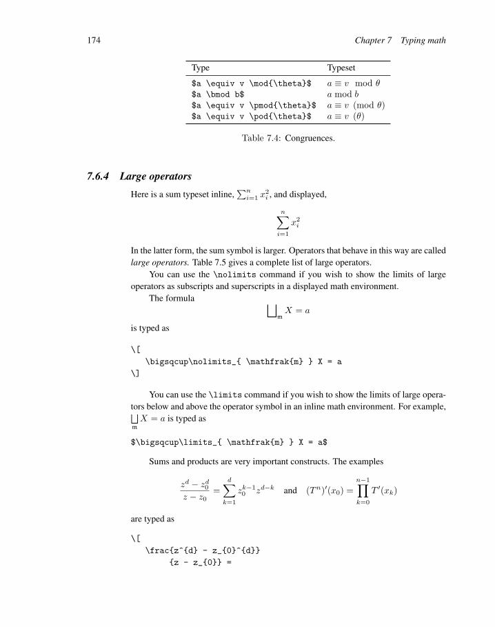
174 Chapter 7 Typing math
Type Typeset
$a \equiv v \mod\theta$ a ≡ v mod θ$a \bmod b$ a mod b$a \equiv v \pmod\theta$ a ≡ v (mod θ)$a \equiv v \pod\theta$ a ≡ v (θ)
Table 7.4: Congruences.
7.6.4 Large operatorsHere is a sum typeset inline,
∑ni=1 x
2i , and displayed,
n∑i=1
x2i
In the latter form, the sum symbol is larger. Operators that behave in this way are calledlarge operators. Table 7.5 gives a complete list of large operators.
You can use the \nolimits command if you wish to show the limits of largeoperators as subscripts and superscripts in a displayed math environment.
The formula ⊔mX = a
is typed as
\[
\bigsqcup\nolimits_ \mathfrakm X = a
\]
You can use the \limits command if you wish to show the limits of large opera-tors below and above the operator symbol in an inline math environment. For example,⊔mX = a is typed as
$\bigsqcup\limits_ \mathfrakm X = a$
Sums and products are very important constructs. The examples
zd − zd0z − z0
=d∑k=1
zk−10 zd−k and (Tn)′(x0) =
n−1∏k=0
T ′(xk)
are typed as
\[
\fracz^d - z_0^d
z - z_0 =

7.6 Operators 175
Type Inline Displayed
\int_a^b∫ ba
∫ b
a
\oint_a^b∮ ba
∮ b
a
\iint_a^b∫∫ ba
∫∫ b
a
\iiint_a^b∫∫∫ b
a
∫∫∫ b
a
\iiiint_a^b∫∫∫∫ b
a
∫∫∫∫ b
a
\idotsint_a^b∫ ·· · ∫ b
a
∫· · ·∫ b
a
\prod_i=1^n∏ni=1
n∏i=1
\coprod_i=1^n∐ni=1
n∐i=1
\bigcap_i=1^n⋂ni=1
n⋂i=1
\bigcup_i=1^n⋃ni=1
n⋃i=1
\bigwedge_i=1^n∧ni=1
n∧i=1
\bigvee_i=1^n∨ni=1
n∨i=1
\bigsqcup_i=1^n⊔ni=1
n⊔i=1
\biguplus_i=1^n⊎ni=1
n⊎i=1
\bigotimes_i=1^n⊗n
i=1
n⊗i=1
\bigoplus_i=1^n⊕n
i=1
n⊕i=1
\bigodot_i=1^n⊙n
i=1
n⊙i=1
\sum_i=1^n∑ni=1
n∑i=1
Table 7.5: Large operators.

176 Chapter 7 Typing math
\sum_k = 1^d z_0^k - 1 z^d - k
\text\quad and\quad
(T^n)’(x_0) = \prod_k=0^n - 1 T’(x_k)
\]
7.6.5 Multiline subscripts and superscriptsThe \substack command provides multiline limits for large operators. For instance,∑
i<ni even
x2i
is typed as
\[
\sum_ \substack i < n\\
i \text even
x_i^2
\]
There is only one rule to remember. Use the line separator command \\. You can usethe \substack command wherever subscripts or superscripts are used.
The lines are centered by \substack, so if you want them set flush left, as in∑i<ni even
x2i
then use the subarray environment with the argument l:
\[
\sum_ \beginsubarrayl
i < n\\
i \text even
\endsubarray
x_i^2
\]
See Section 7.6.2 for another example.
7.7 Math accentsThe accents used in text (see Section 5.4.7) cannot be used in math formulas. For ac-cents in formulas a separate set of commands is provided. All math accents are shownin Table 7.6 (see also Section B.8). The amsxtra package is needed for the accents inthe second column. To use them, make sure to place the line

7.7 Math accents 177
\usepackageamsxtra
in the preamble. For instance, $a\spbreve \ b\spddot\ c\sptilde$ typesets asa b.. c∼.
You can also use double accents, such as
\[
\hat\hatA
\]
which typesets as ˆA.
The two “wide” varieties, \widehat and \widetilde, expand to fit the symbols(their arguments) covered: A, ab, iii, aiai, iiiii, and A, ab, iii, aiai, iiiii (the lastexample is typed as $\widetildeiiiii$). If the base is too wide, the accent iscentered:
ABCDE
The “sp” commands, provided by the amsxtra package, are used for superscripts,as illustrated in Table 7.6. If you use a lot of accented characters, you should appreciateuser-defined commands (see Section 15.1.1).
Notice the difference between a and a, typed as
$\bara$ $\overlinea$
amsxtra
Type Typeset Type Typeset
\acutea a\bara a\brevea a \spbreve ˘\checka a \spcheck ∨
\dota a \spdot .
\ddota a \spddot ..
\dddota...a \spdddot ...
\ddddota....a
\gravea a\hata a\widehata a \sphat \mathringa a\tildea a\widetildea a \sptilde ∼
\veca ~a
Table 7.6: Math accents.

178 Chapter 7 Typing math
For other examples of the \overline command, see Section 7.8.2.To use an arbitrary symbol as an accent or to create “underaccents”, use Javier
Bezos’ accents package (see Section E.1 on how to obtain it).
7.8 Stretchable horizontal linesLATEX provides three types of stretchable horizontal lines that appear above or below aformula, braces, bars, and arrows. There are also stretchable arrow math symbols.
7.8.1 Horizontal bracesThe \overbrace command places a brace of variable size above its argument, as in︷ ︸︸ ︷
a+ b+ · · ·+ z
which is typed as
\[
\overbracea + b + \dots + z
\]
A superscript adds a label to the brace, as inn︷ ︸︸ ︷
a+ a+ · · ·+ a
which is typed as
\[
\overbracea + a + \dots + a^n
\]
The \underbrace command works similarly, placing a brace below its argument.A subscript adds a label to the brace, as in
a+ a+ · · ·+ a︸ ︷︷ ︸n
which is typed as
\[
\underbracea + a + \dots + a_n
\]
The following example combines these two commands:
(m−n)/2︷ ︸︸ ︷a+ · · ·+ a+ b+ · · ·+ b︸ ︷︷ ︸
n
+
(m−n)/2︷ ︸︸ ︷a+ · · ·+ a
︸ ︷︷ ︸m

7.8 Stretchable horizontal lines 179
This example is typed as
\[
\underbrace
\overbracea + \dots + a^(m - n)/2
+ \underbraceb + \dots + b_n
+ \overbracea + \dots + a^(m - n)/2
_m
\]
7.8.2 Overlines and underlinesThe \overline and \underline commands draw lines above or below a formula.For example,
X ∪X = X
is typed as
\[
\overline \overlineX \cup \overline\overlineX
= \overline \overlineX
\]
Similarly, you can place arrows above and below an expression:
←−a −→aa←→aaa aaaa←−−− aaaaa−−−→ aaaaaa←−−−→
which is typed as
\begingather*
\overleftarrowa \quad \overrightarrowaa\\
\overleftrightarrowaaa \quad \underleftarrowaaaa\quad
\underrightarrowaaaaa \quad \underleftrightarrowaaaaaa
\endgather*
7.8.3 Stretchable arrow math symbolsThere are two stretchable arrow math symbols that extend to accommodate a formulaabove or below the arrows with the \xleftarrow and \xrightarrow commands. Theformula on top is given as the argument (possibly empty) and the formula below is anoptional argument.
A1-1−−→ B
onto←−−−α→β
C ←−γD ←− E

180 Chapter 7 Typing math
is typed as
\[
A \xrightarrow\text1-1 B \xleftarrow[\alpha\to\beta]
\textonto C \xleftarrow[\gamma] D \xleftarrow E
\]
There are other stretchable arrow math symbols described in Section 9.8, but theycan only be used in commutative diagrams.
7.9 Formula GalleryIn this section I present a collection of formulas—some simple, some complex—thatillustrate the power of LATEX.
Some of these examples require the amssymb package, so it is a good idea toinclude the line
\usepackageamssymb,latexsym
following the \documentclass line of any article.
Formula 1 A set-valued function
x 7→ c ∈ C | c ≤ x
\[
x \mapsto \\, c \in C \mid c \leq x \,\
\]
To equalize the spacing around c ∈ C and c ≤ x, a thin space (\,) was added insideeach brace (see Section 8.1). The same technique is used in several other formulas inthis section.
Formula 2 ∣∣∣⋃( Ij | j ∈ J )∣∣∣ < m
\[
\left| \bigcup (\, I_j \mid j \in J \,) \right|
< \mathfrakm
\]
We use the delimiters \left| and \right| (see Section 7.5.1). The Fraktur m isintroduced in Section 8.3.2.

7.9 Formula Gallery 181
Formula 3 Note that you have to add spacing both before and after the text fragmentfor some in the following example. The argument of \text is typeset in text mode, sospaces are recognized.
A = x ∈ X | x ∈ Xi, for some i ∈ I
\[
A = \\, x \in X \mid x \in X_i,
\text for some $i \in I$ \,\
\]
Formula 4 Space to show logical structure:
〈a1, a2〉 ≤ 〈a′1, a′2〉 iff a1 < a′1 or a1 = a′1 and a2 ≤ a′2\[
\langle a_1, a_2 \rangle \leq
\langle a’_1, a’_2\rangle \qquad \textiff
\qquad a_1 < a’_1 \quad \textor
\quad a_1 = a’_1 \text and a_2 \leq a’_2
\]
Note that in iff (in the argument of the first \text) the second f is enclosed inbraces to avoid the use of the ligature—the merging of the two f’s. For the proper wayof typesetting iff without a ligature, see Section 5.4.6.
Formula 5 Here are some examples of Greek letters:
Γu′ = γ | γ < 2χ, Bα * u′, Bγ ⊆ u′
\[
\Gamma_u’ = \\,\gamma \mid \gamma < 2\chi,\ B_\alpha
\nsubseteq u’, \ B_\gamma \subseteq u’ \,\
\]
See Section B.1 for a complete listing of Greek letters. We use the command \ toproperly space the formula. This command can be used both in text and in math.
Formula 6 \mathbb allows you to use the blackboard bold math alphabet, whichonly provides capital letters:
A = B2 × Z\[
A = B^2 \times \mathbbZ
\]

182 Chapter 7 Typing math
Formula 7 \left[ and \right] provide stretched delimiters:
yC ≡ z ∨∨i∈C
[sCi]
(mod Φ)
\[
y^C \equiv z \vee \bigvee_ i \in C \left[ s_i^C
\right] \pmod \Phi
\]
Notice how the superscript is set directly above the subscript in sCi .
Formula 8 A complicated congruence:
y ∨∨
( [Bγ ] | γ ∈ Γ ) ≡ z ∨∨
( [Bγ ] | γ ∈ Γ ) (mod Φx)
\[
y \vee \bigvee (\, [B_\gamma] \mid \gamma
\in \Gamma \,) \equiv z \vee \bigvee (\, [B_\gamma]
\mid \gamma \in \Gamma \,) \pmod \Phi^x
\]
Formula 9 Use \nolimits to force the “limit” of the large operator to display as asubscript (see Section 7.6.4):
f(x) =∨
m
(∧m
(xj | j ∈ Ii ) | i < ℵα)
\[
f(\mathbfx) =
\bigvee\nolimits_\!\mathfrakm
\left(\,
\bigwedge\nolimits_\mathfrakm
(\, x_j \mid j \in I_i \,)
\mid i < \aleph_\alpha
\,\right)
\]
Notice that a negative space (\!) was inserted to bring the m a little closer to the bigjoin symbol
∨.
Formula 10 The \left. command gives a blank left delimiter, which is needed tobalance the \right| command:
F (x)∣∣∣ba
= F (b)− F (a)

7.9 Formula Gallery 183
\[
\left. \widehatF(x) \right|_a^b
= \widehatF(b) - \widehatF(a)
\]
Formula 11 The \underset and \overset commands build new symbols (see Sec-tion 8.2.1):
u+αv
1∼ w2∼ z
\[
u \underset\alpha+ v \overset1\thicksim w
\overset2\thicksim z
\]
Note that the new symbols 1∼ and 2∼ are binary relations and +α
is a binary operation.
Formula 12 Small size bold def:
f(x) def= x2 − 1
\[
f(x) \overset \mathbfdef = x^2 - 1
\]
Formula 13 Math accents run amok:˘n︷ ︸︸ ︷
a∨ + b∨ + · · ·+ z∨
\[
\overbracea\spcheck + b\spcheck + \dots + z\spcheck^
\breve\breven
\]
Recall that for the \sp commands you need the amsxtra package.
Formula 14 ∣∣∣∣a+ b+ c uv
a+ b c+ d
∣∣∣∣ = 7
\[
\beginvmatrix
a + b + c & uv\\
a + b & c + d
\endvmatrix
= 7
\]

184 Chapter 7 Typing math
∥∥∥∥a+ b+ c uv
a+ b c+ d
∥∥∥∥ = 7
\[
\beginVmatrix
a + b + c & uv\\
a + b & c + d
\endVmatrix
= 7
\]
Formula 15α2∑j∈N
bij yj =∑j∈N
b(λ)ij yj + (bii − λi)yiy
\[
\boldsymbol\alpha^2\sum_j \in \mathbfN b_ij
\haty_j = \sum_j \in \mathbfN
b^(\lambda)_ij\haty_j
+ (b_ii - \lambda_i) \haty_i \haty
\]
\mathbfN makes a bold N and \boldsymbol\alpha produces a bold α (seeSection 8.3.2).
Formula 16 To produce the formula( n∏j=1
xj
)Hc =
12kij det K(i|i)
try typing
\[
\left( \prod^n_\, j = 1 \hat x _j \right) H_c=
\frac12 \hatk_ij \det \hat \mathbfK (i|i)
\]
which typesets as n∏j=1
xj
Hc =12kij det K(i|i)
This is not quite right. You can correct the overly large parentheses by using the\biggl and \biggr commands in place of \left( and \right), respectively (seeSection 7.5.2). Adjust the small hat over K by using \widehat:

7.9 Formula Gallery 185
\[
\biggl( \prod^n_\, j = 1 \hat x _j \biggr)
H_c = \frac12\hat k _ij
\det \widehat \mathbfK (i|i)
\]
which gives you the desired formula.
Formula 17 In this formula, I have used \overlineI to get I . You could, instead,use \barI, which is typeset as I .
det K(t = 1, t1, . . . , tn) =∑I∈n
(−1)|I|∏i∈I
ti∏j∈I
(Dj + λjtj) det A(λ)( I|I ) = 0
\[
\det \mathbfK (t = 1, t_1, \dots, t_n) =
\sum_I \in \mathbfn (-1)^|I| \prod_i \in It_i
\prod_j \in I (D_j + \lambda_j t_j)
\det \mathbfA^(\lambda)
(\,\overlineI | \overlineI\,) = 0
\]
Formula 18 The command \| provides the ‖ math symbol in this formula:
lim(v,v′)→(0,0)
H(z + v)−H(z + v′)−BH(z)(v − v′)‖v − v′‖ = 0
\[
\lim_(v, v’) \to (0, 0)
\fracH(z + v) - H(z + v’) - BH(z)(v - v’)
\| v - v’ \| = 0
\]
Formula 19 This formula uses the calligraphic math alphabet (see Section 8.3.2):∫D|∂u|2Φ0(z)eα|z|
2 ≥ c4α∫D|u|2Φ0e
α|z|2 + c5δ−2
∫A
|u|2Φ0eα|z|2
\[
\int_\mathcalD | \overline\partial u |^2
\Phi_0(z) e^\alpha |z|^2
\geq c_4 \alpha \int_\mathcalD |u|^2\Phi_0
e^\alpha |z|^2
+ c_5 \delta^-2 \int_A |u|^2
\Phi_0 e^\alpha |z|^2
\]

186 Chapter 7 Typing math
Formula 20 The \hdotsfor command sets dots that span multiple columns in amatrix. The \dfrac command is the displayed variant of the \frac command (seeSection 7.4.1), used here because the matrix entries with \frac would look too small.
A =
ϕ ·Xn,1
ϕ1 × ε1(x+ ε2)2 · · · (x+ εn−1)n−1 (x+ εn)n
ϕ ·Xn,1
ϕ2 × ε1
ϕ ·Xn,2
ϕ2 × ε2· · · (x+ εn−1)n−1 (x+ εn)n
. . . . . . . . . . . . . . . . . . . . . . . . . . . . . . . . . . . . . . . . . . . . . . . . . . . .ϕ ·Xn,1
ϕn × ε1
ϕ ·Xn,2
ϕn × ε2· · · ϕ ·Xn,n−1
ϕn × εn−1
ϕ ·Xn,n
ϕn × εn
+ In
\[
\mathbfA =
\beginpmatrix
\dfrac\varphi \cdot X_n, 1 \varphi_1 \times
\varepsilon_1 & (x + \varepsilon_2)^2
& \cdots & (x + \varepsilon_n - 1)^n - 1
& (x + \varepsilon_n)^n\\[10pt]
\dfrac\varphi \cdot X_n, 1 \varphi_2 \times
\varepsilon_1 & \dfrac\varphi \cdot X_n, 2
\varphi_2 \times \varepsilon_2 & \cdots &
(x + \varepsilon_n - 1)^n - 1
& (x + \varepsilon_n)^n\\
\hdotsfor5\\
\dfrac\varphi \cdot X_n, 1 \varphi_n \times
\varepsilon_1 & \dfrac\varphi \cdot X_n, 2
\varphi_n \times \varepsilon_2 & \cdots
& \dfrac\varphi \cdot X_n, n - 1 \varphi_n
\times \varepsilon_n - 1 &
\dfrac\varphi\cdot X_n, n
\varphi_n \times \varepsilon_n
\endpmatrix
+ \mathbfI_n
\]
Recall the discussion of \dots vs. \cdots and \ldots in Section 7.4.3. In this for-mula, we have to use \cdots. Matrices are discussed in detail in Section 9.7.1.
Note the use of the command \\[10pt]. If you use \\ instead, the first andsecond lines of the matrix are set too close.
I show you in Section 15.1.2 how to rewrite the formula to make it shorter andmore readable.

C H A P T E R
8
More math
In the previous chapter, we discuss the basic building blocks of a formula and how toput them together to form more complex formulas. This chapter starts out by goingone step lower, to the characters that make up a formula. We discuss math symbols andmath alphabets.
LATEX was designed for typesetting math, so it is not surprising that it contains avery large number of math symbols. Section 8.1 classifies and describes them. Sec-tion 8.2 discusses how to build new symbols from existing ones. Math alphabets andsymbols are discussed in Section 8.3. Horizontal spacing commands in math are de-scribed in Section 8.4.
LATEX provides a variety of ways to number and tag equations. These techniquesare described in Section 8.5. We conclude the chapter with two minor topics: general-ized fractions (Section 8.6.1) and boxed formulas (Section 8.6.2).
8.1 Spacing of symbolsLATEX provides a large variety of math symbols: Greek characters (α), binary opera-tions (), binary relations (≤), negated binary relations (), arrows ( ), delimiters( ), and so on. All the math symbols provided by LATEX are listed in the tables of

188 Chapter 8 More math
Appendix B.Consider the formula
A = x ∈ X | xβ ≥ xy > (x+ 1)2 − α
which is typed as
\[
A = \\, x \in X \mid x \beta \geq x y
> (x + 1)^2 - \alpha \,\
\]
The spacing of the symbols in the formula varies. In xβ, the two symbols are veryclose. In x ∈ X , there is some space around the ∈, and in x + 1, there is somewhatless space around the +. There is a little space after and before —not quite enoughfor this formula, which is why the thinspace commands (\,) were added.
8.1.1 ClassificationLATEX classifies symbols into several categories or types and spaces them accordingly.In the formula
A = x ∈ X | xβ ≥ xy > (x+ 1)2 − α we find
Ordinary math symbols: A, x, X , β, and so on
Binary relations: =, ∈, |, ≥, and >
Binary operations: + and −Delimiters: , , (, and )
As a rule, you do not have to be concerned with whether or not a given symbol ina formula, say ×, is a binary operation. LATEX spaces the typeset symbol correctly.
8.1.2 Three exceptionsThere are three symbols with more than one classification: +, −, and |.
+ or − could be either a binary operation, for instance, a − b, or a sign, for in-stance, −b.
Rule + and−+ or − are binary operations when preceded and followed by a symbol or an emptygroup ( ).

8.1 Spacing of symbols 189
So, for instance, in
(A+BC)x+ Cy = 0,
Ex+ (F +G)y = 23.
which is typed as (see the alignat* environment in Section 9.5.4)
\beginalignat*2
(A + B C)x &+ &C &y = 0,\\
Ex &+ &(F + G)&y = 23.
\endalignat*
we use the empty groups, , to tell LATEX that the second + in line 1 and the first + inline 2 of the formula are binary operations. If we leave out the empty groups, and typeinstead
\beginalignat*2
(A + B C)x &+ &C &y = 0,\\
Ex &+ &(F + G)&y = 23.
\endalignat*
we get
(A+BC)x+ Cy = 0,
Ex+(F +G)y = 23.
Another illustration is given later in this section using the \phantom command.This problem often arises in split formulas, for example if the formula is split just
before a + or −, you should start the next line with + or -. See Section 9.3 forexamples.
The | symbol can play several different roles in a math formula, so LATEX providesseparate commands to specify the symbol’s meaning.
Rule The four roles of the | symbol
| ordinary math symbol
\mid binary relation
\left| left delimiter
\right| right delimiter
Note the differences between the spacing in a|b, typed as $a | b$, and in a | b,typed as $a \mid b$.

190 Chapter 8 More math
Name Width Short Long
1 mu (math unit) \mspace1muthinspace \, \thinspacemedspace \: \medspacethickspace \; \thickspaceinterword space \ 1 em \quad2 em \qquad
Negative space
1 mu \mspace-1muthinspace \! \negthinspacemedspace \negmedspacethickspace \negthickspace
Table 8.1: Math spacing commands.
8.1.3 Spacing commands
There are some situations where LATEX cannot typeset a formula properly and you haveto add spacing commands. Luckily, LATEX provides a variety of spacing commands,listed in Table 8.1. The \neg commands remove space by “reversing the print head”.
The \quad and \qquad commands are often used to adjust aligned formulas (seeChapter 9) or to add space before text in a math formula. The size of \quad (= 1 em)and \qquad (= 2 em) depends on the current font.
The \, and \! commands are the most useful for fine tuning math formulas, seesome examples in the Formula Gallery and in the next section. The \mspace commandand the math unit mu provides you with even finer control. 18 mu = 1 em, defined inSection 5.8.3. For example, \mspace3mu adds a space that is 1/6 em long. There isan interesting use of mu on page 109.
8.1.4 Examples
The Formula Gallery in Section 7.9 starts out with an example that shows the impor-tance of fine tuning. In set notation, when using \mid for “such that”, thin spaces areinserted just inside the braces. Some more examples of fine tuning follow. One moreexample can be found in Section 8.2.1.
Example 1 In Section 3.3, we type the formula∫ π
0sinx dx = 2 as
$\int_0^\pi \sin x \, dx = 2$
Notice the thinspace spacing command \, between \sin x and dx. Without the com-mand, LATEX would have crowded sinx and dx:
∫ π0
sinxdx = 2.

8.1 Spacing of symbols 191
Example 2 | − f(x)|, typed as $|-f(x)|$, is spaced incorrectly. − becomes abinary operation by the + and − rule. To get the correct spacing, as in |−f(x)|, type$\left|-f(x)\right|$. This form tells LATEX that the first | is a left delimiter, bythe | rule, and therefore− is the unary minus sign, not the binary subtraction operation.
Example 3 In√
5side, typed as
$\sqrt5 \textside$√
5 is too close to side. So type it as
$\sqrt5 \, \textside$
which typesets as√
5 side.
Example 4 In sinx/ log n, the division symbol / is too far from log n, so type
$\sin x / \! \log n$
which prints sinx/log n.
Example 5 In f(1/√n), typed as
$f(1 / \sqrtn)$
the square root almost touches the closing parenthesis. To correct it, type
$f(1 / \sqrtn\,)$
which typesets as f(1/√n ).
There is one more symbol with special spacing: the \colon command, usedfor formulas such as f : A → B (typed as $f \colon A \to B$). Observe that$f: A \to B$ typesets as f : A→ B. The spacing is awful.
See Section 8.2.3 on how to declare the type of a symbol.
8.1.5 The phantom commandThe \phantomargument command (introduced for text in Section 5.8.1) producesa space in a formula equivalent to the space that would be occupied by its typesetargument. This command is one of the most powerful tools available to us for finetuning alignments. Here are two simple illustrations:
A =
1 3 12 1 1−2 2 −1

192 Chapter 8 More math
typed as
\[
A = \beginpmatrix
\phantom-1 & \phantom-3 & \phantom-1\\
\phantom-2 & \phantom-1 & \phantom-1\\
-2 & \phantom-2 & -1\\
\endpmatrix
\]
and
a+ b+ c+ d = 0,
c+ d+ e = 5.
typed as
\beginalign*
a + b + c & + d \phantom +e = 0,\\
c & + d + e = 5.
\endalign*
Note that \phantom+e yields incorrect spacing by the + and − rule:
a+ b+ c+ d = 0,
c+ d+ e = 5.
See Section 9.6.2 for an additional example.
8.2 Building new symbolsNo matter how many math symbols LATEX provides—see a complete listing in Ap-pendix B—users always seem to want more.1 LATEX gives you excellent tools to buildnew symbols from existing ones.
8.2.1 Stacking symbolsTo place any symbol above, or below, any other, for instance, u∼, use the \overset
command. It takes two arguments—the first argument is set in a smaller size above thesecond argument. The spacing rules of the symbol in the second argument remain valid,i.e., the type remains the same. Since ∼ is a binary relation, so is u∼. The \undersetcommand is the same except that the first argument is set under the second argument.For example,
αa X
·
αai
αai
are typed as1The best is yet to come, see Section H.3.

8.2 Building new symbols 193
\[
\overset\alphaa \qquad
\underset\boldsymbol\cdotX \qquad
\overset\alpha a_i \qquad
\overset\alphaa_i
\]
For the \boldsymbol command, see Section 8.3.3. Note that in the third example,αai,
the α seems to be sitting too far to the right but the fourth example corrects that.You can also use these commands with binary relations, as in
f(x) def= x2 − 1
which is typed as
\[
f(x) \overset \textdef = x^2 - 1
\]
Since = is a binary relation, def= becomes a binary relation, as shown by the spacing oneither side. Here is another example,
a
b
u+c
d
l+e
f
which is typed as
\[
\fracab \oversetu+ \fraccd
\oversetl+ \fracef
\]
Note thatu+ and
l+ are properly spaced as binary operations.
As we discuss in Section 7.4.6, the safer definitions for these examples are
\[
f(x) \overset \normalfont\textdef = x^2 - 1
\]
and
\[
\fracab \overset\normalfont u+ \fraccd
\overset\normalfont l+ \fracef
\]

194 Chapter 8 More math
8.2.2 Negating and side-setting symbolsYou can negate with the \not command; for instance, a 6∈ b and a 6= b are typed as$a \not\in b$ and $a \not= b$, respectively. It is preferable, however, to use thenegated symbols /∈, typed as $\notin$, and 6=, typed as $\ne$. See the negated binaryrelations table in Section B.2. For instance, “a does not divide b”, a - b, should be typedas $a \nmid b$, not as $a \not\mid b$, which typesets as a 6| b. In Section 8.2.3,you learn how to improve a 6| b to a 6 | b, typed as $a \mathrel\not| b$. How-ever, $a \nmid b$ is still best.
LATEX provides the \sideset command to set symbols at the corners of largeoperators other than the “corners” (the last four delimiters in Table 7.1). This commandtakes three arguments:
\sideset _ll ^ul _lr ^ur large_op
where ll stands for the symbol to be placed at the lower left, ul for upper left, lr forlower right, and ur for upper right; large op is a large operator. These two examples,∏c
aand
e∏are typed as
\[
\sideset_a^c\prod\text and \sideset^e\prod
\]
Note that the two first arguments are compulsory, although one or the other may beempty, while the third argument must contain the large operator.
Here is a more meaningful example:
\[
\sideset’\sum_\substack i < 10\\ j < 10 x_iz_j
\]
is typeset as ∑′
i<10j<10
xizj
In this example, note that prime (′) is an automatically superscripted symbol (see Sec-tion 7.4.1), so you do not have to type ^’ in the second argument. Typing \sum’ wouldnot work, since LATEX would place the prime above the sum symbol.
Thus, \sideset helps in mixing sub- and superscripts in “limit” positions withothers in “nolimit” positions, allowing for a total of six positions in displayed operatorswith limits. Try
rc
a
∏i
en
typed as

8.3 Math alphabets and symbols 195
\[
\sideset_a^c_e^i\prod_n^r
\]
8.2.3 Changing the type of a symbolSome symbols are binary relations and some are binary operations (see Section 8.1).In fact, you can force any symbol to behave like either type.
The \mathbin command declares its argument to be a binary operation. For ex-ample,
\mathbin\alpha
makes this instance of \alpha behave like a binary operation, as in a α b, typed as
$a \mathbin\alpha b$
You can use the \mathrel command to make a symbol behave like a binary relation,as in the formula a α b, typed as
$a \mathrel \alpha b$
You can seea α b ($a \mathbin\alpha b$)a α b ($a \mathrel\alpha b$)that a binary relation provides a bit more space than a binary operation. There is aninteresting use of \mathbin on page 109.
In Section 7.6.2, we discussed the \DeclareMathOperator command and its*-ed version, to declare a symbol—or any text or formula—a math operator.
8.3 Math alphabets and symbolsThe classification of math symbols in the context of spacing was discussed in Sec-tion 8.1. The symbols in a formula can also be classified as characters from mathalphabets and math symbols. In the formula
A = x ∈ X | xβ ≥ xy > (x+ 1)2 − α
the following characters come from math alphabets:
A x X y 1 2
whereas these characters are math symbols:
= ∈ | β ≥ > ( + ) − α

196 Chapter 8 More math
8.3.1 Math alphabets
The letters and digits typed in a math formula come from math alphabets. LATEX’sdefault math alphabet—the one you get if you do not ask for something else—is Com-puter Modern math italic for letters. In the formula x2 ∨ y3 = α, the characters xand y come from this math alphabet. The default math alphabet for digits is ComputerModern roman and the digits 2 and 3 in this formula are typeset in Computer Modernroman.
LATEX has a number of commands to switch type style in math. The two mostimportant commands select the bold and italic versions:
Command Math alphabet Produces
\mathbfa math bold 2 Greek gammas, γ and Γ\mathita math italic 2 Greek gammas, γ and Γ
These commands change the style of letters, numbers, and upper case Greek characters.But beware of the pitfalls. For instance, in \mathitleft-side the hyphen
typesets as a minus: left − side .There are four more commands that switch math alphabets:
Command Math Alphabet Produces
\mathsfa math sans serif 2 Greek gammas, γ and Γ
\mathrma math roman 2 Greek gammas, γ and Γ\mathtta math typewriter 2 Greek gammas, γ and Γ
\mathnormala math italic Greek gammas, γ and Γ
Math roman is used in formulas for operator names, such as sin in sinx, and fortext. For operator names, you should use the \DeclareMathOperator command orthe *-ed version, which sets the name of the operator in math roman, and also providesthe proper spacing (see Section 8.2.3). For text, you should use the \text command(see Section 7.4.6).
The \mathnormal command switches to the default math alphabet, but this com-mand is seldom used in practice.
The Computer Modern fonts include a math bold italic alphabet, but LATEX doesnot provide a command to access it.
Rule Math alphabets vs. text alphabetsDo not use text alphabets in a math formula, except in the argument of a \text com-mand.

8.3 Math alphabets and symbols 197
It may not be easy for you to see the difference, but some things will not look rightor may not align properly.
8.3.2 Math symbol alphabetsYou may have noticed that α was not classified as belonging to an alphabet in theexample at the beginning of this section. Indeed, α is treated by LATEX as a mathsymbol rather than as a member of a math alphabet. You cannot italicize or slant it, noris there a sans serif version. There is a bold version, but you must use the \boldsymbolcommand to produce it. For instance, αβ, is typed as
$\boldsymbol\alpha_\boldsymbol\beta$
Note that β appears in a small size in αβ.Four “alphabets of symbols” are built into LATEX.
Greek The examples α, β, and Γ are typed as
$\alpha$, $\beta$, $\Gamma$
See Section B.1 for the symbol table.
Calligraphic an uppercase-only alphabet invoked with the \mathcal command.The examples A, C, and E are typed as
$\mathcalA$, $\mathcalC$, $\mathcalE$
Euler Fraktur invoked by the \mathfrak command. The examples n, p, N, and P
are typed as
$\mathfrakn$, $\mathfrakp$, $\mathfrakN$,
$\mathfrakP$
Blackboard bold uppercase-only math alphabet, invoked with \mathbb. The exam-ples A, B, C are typed as
$\mathbbA$, $\mathbbB$, $\mathbbC$
8.3.3 Bold math symbolsIn math, most characteristics of a font are specified by LATEX. One exception is bold-face. To make a letter from a math alphabet within a formula bold, use the \mathbf
command. For instance, in
we choose the vector v

198 Chapter 8 More math
v is produced by $\mathbfv$.To obtain bold math symbols, use the \boldsymbol command. For example, the
bold symbols5 α Λ A → A
are typed as
\[
\boldsymbol5 \quad \boldsymbol\alpha
\quad \boldsymbol\Lambda\quad\boldsymbol\mathcalA
\quad \boldsymbol\to \quad \boldsymbolA
\]
Note that \boldsymbolA typesets as A, a bold math italic A. To get an upright A,type $\mathbfA$.
5 did not really need \boldsymbol; \mathbf5 gives the same result.To make an entire formula bold, use the \mathversionbold command, as in
\mathversionbold $a \equiv c \pod\theta$
which typesets as a ≡ c (θ). Note that the \mathversionbold command isgiven before the formula.
To typesetAMS, type
$\boldsymbol \mathcalA \boldsymbol \mathcalM
\boldsymbol \mathcalS $
or
$\boldsymbol \mathcalAMS $
or
\mathversionbold $\mathcalAMS$
Within the scope of \mathversionbold, you can undo its effect with
\mathversionnormal
Not all symbols have bold variants. For example, if you type
$\sum \quad \boldsymbol\sum$
you get∑ ∑
, two identical symbols. If you want to obtain a bold version, use thepoor man’s bold invoked by the \pmb command. This command typesets the symbolthree times very close to one another producing a bold symbol of some quality. Notethat \pmb does destroy the type of the symbol, \pmb\sum is no longer spaced like alarge operator. To make it into a large operator, declare in the preamble

8.3 Math alphabets and symbols 199
\DeclareMathOperator\boldsum\pmb\sum
and
\DeclareMathOperator*\boldsumlim\pmb\sum
Compare the following four variants of sum:
n∑i=1
i2∑∑∑
ni=1i
2∑∑∑n
i=1i2
n∑∑∑i=1
i2
The first sum is typed (in displayed math mode) as
\sum_i = 1^n i^2
The second uses poor man’s bold, but does not declare the result to be a large operator:
\pmb\sum_i = 1^n i^2
The third uses the math operator declared:
\boldsum_i = 1^n i^2
The fourth uses the math operator with limit declared:
\boldsumlim_i = 1^n i^2
8.3.4 Size changesThere are four math font sizes, invoked by the command declarations
\displaystyle, normal size for displayed formulas
\textstyle, normal size for inline formulas
\scriptstyle, normal size for subscripted and superscripted symbols
\scriptscriptstyle, normal size for doubly subscripted and superscripted sym-bols
These commands control a number of style parameters in addition to the size.Compare the two fractions
1
2 +13
12 + 1
3
which are typed as
\[
\frac1\displaystyle 2 + \frac13 \quad
\frac1 2 + \frac13
\]

200 Chapter 8 More math
8.3.5 Continued fractionsIn addition to the \frac, \dfrac, and \tfrac commands (see Section 7.4.1), LATEXmakes typesetting continued fractions even easier by providing the \cfrac command.The \cfrac command takes an optional argument, l or r, to place the numerator onthe left or on the right. For example,
1
2 +1
3 + · · ·
1
2 +13 + · · ·
is typed as
\[
\cfrac1 2 + \cfrac13 + \cdots \qquad
\cfrac[l]12 + \cfrac[l]13 + \cdots
\]
8.4 Vertical spacingAs a rule, all horizontal and vertical spacing in a math formula is done by LATEX. Never-theless, you often need to adjust horizontal spacing (see Section 8.1). There is seldoma need to adjust vertical spacing, but there are a few exceptions.
The formula√a+√b does not look quite right, because the square roots are not
uniform. You can correct this with \mathstrut commands, which inserts an invisiblevertical space:
$\sqrt\mathstrut a + \sqrt\mathstrut b$
typesets as√a+
√b. See Section 5.9.5 for struts in general.
Another way to handle this situation is with the \vphantom (vertical phantom)command, which measures the height of its argument and places a math strut of thatheight into the formula. So
$\sqrt\vphantomb a + \sqrtb$
also prints uniform square roots,√a +√b. The \vphantom method is more versatile
than the previous one.Here is a more complicated example from a recent research article:
Θi =⋃(
Θ( a ∧ b, a ∧ b) | a, b ∈ Bi) ∨⋃(
Θ( a ∨ b, a ∨ b ) | a, b ∈ Bi),
typed as
\[
\Theta_i = \bigcup \big(\, \Theta (\,\overlinea

8.5 Tagging and grouping 201
\wedge b,\overline\vphantomba \wedge
\overlineb) \mid a,\ b \in B_i \,\big)
\vee \bigcup \big(\, \Theta(\,\overlinea \vee b,
\overline\vphantomba \vee \overlineb \,)
\mid a,\ b \in B_i \,\big),
\]
Another useful command for vertical spacing is the \smash command. It directsLATEX to pretend that its argument does not protrude above or below the line in whichit is typeset.
For instance, the two lines of this admonition:
It is very important that you memorize the integral 1∫f(x) dx
= 2g(x) + C,
which will appear on the next test.
are too far apart because LATEX had to make room for the fraction. However, in thisinstance, the extra vertical space is not necessary because the second line is very short.To correct this, place the formula in the argument of a \smash command:
It is \emphvery important that you memorize the
integral $\smash\frac1\int f(x) \, dx = 2g(x) + C$,
which will appear on the next test.
LATEX produces the following:
It is very important that you memorize the integral 1∫f(x) dx
= 2g(x) + C,which will appear on the next test.
An optional argument to the \smash command controls which part of the formulais ignored, t to smash the top, and b to smash the bottom.
8.5 Tagging and groupingYou can attach a name to an equation using the \tag command. In the equation orequation* environments,
\tagname
attaches the tag name to the equation—name is typeset as text. The tag replaces thenumber.
Recall that the numbering of an equation is relative, that is, the number assigned toan equation is relative to the placement of the equation with respect to other equationsin the document. An equation tag, on the other hand, is absolute—the tag remains thesame even if the equation is moved.
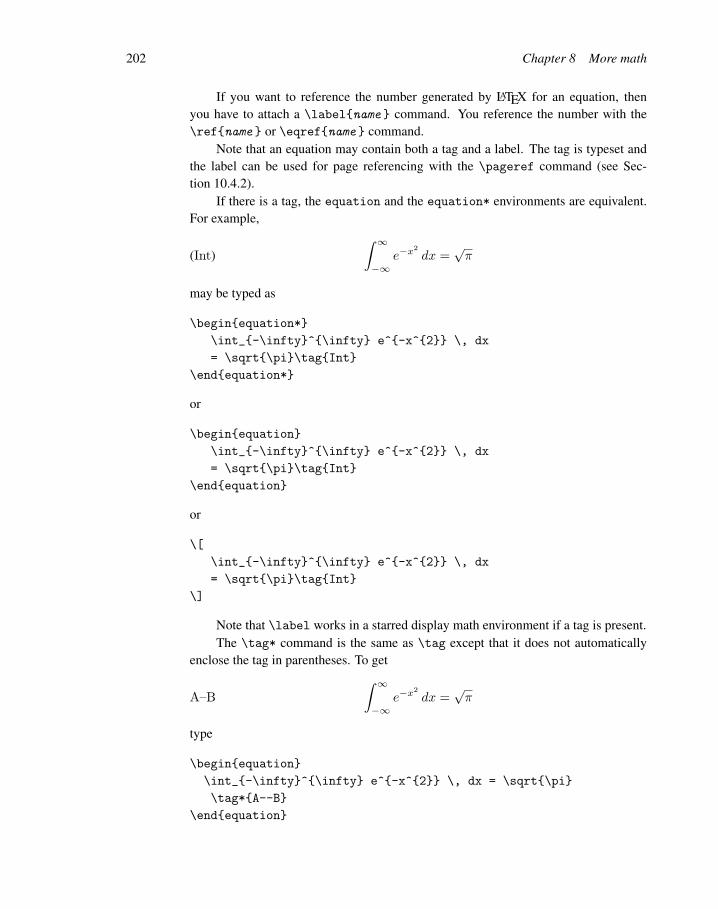
202 Chapter 8 More math
If you want to reference the number generated by LATEX for an equation, thenyou have to attach a \labelname command. You reference the number with the\refname or \eqrefname command.
Note that an equation may contain both a tag and a label. The tag is typeset andthe label can be used for page referencing with the \pageref command (see Sec-tion 10.4.2).
If there is a tag, the equation and the equation* environments are equivalent.For example,
(Int)∫ ∞−∞
e−x2dx =
√π
may be typed as
\beginequation*
\int_-\infty^\infty e^-x^2 \, dx
= \sqrt\pi\tagInt
\endequation*
or
\beginequation
\int_-\infty^\infty e^-x^2 \, dx
= \sqrt\pi\tagInt
\endequation
or
\[
\int_-\infty^\infty e^-x^2 \, dx
= \sqrt\pi\tagInt
\]
Note that \label works in a starred display math environment if a tag is present.The \tag* command is the same as \tag except that it does not automatically
enclose the tag in parentheses. To get
A–B∫ ∞−∞
e−x2dx =
√π
type
\beginequation
\int_-\infty^\infty e^-x^2 \, dx = \sqrt\pi
\tag*A--B
\endequation

8.5 Tagging and grouping 203
Tagging allows numbered variants of equations. For instance, the equation
(1) A[2] B[2] ∼= (A B)[2]
may need a variant:
(1′) A〈2〉 B〈2〉 ≡ (A B)〈2〉
If the label of the first equation is E:first, then the second equation may be typed asfollows:
\beginequation\tag\refE:first$’$
A^\langle 2 \rangle \diamond B^\langle 2\rangle
\equiv (A \diamond B)^\langle 2 \rangle
\endequation
Such a tag is absolute in the sense that it does not change if the equation is moved. Butif it references a label and the number generated by LATEX for the label changes, the tagchanges.
In contrast, grouping applies to a group of adjacent equations. Suppose the lastequation was numbered (1) and the next group of equations is to be referred to as (2),with individual equations numbered as (2a), (2b), and so on. Enclosing these equationsin a subequations environment accomplishes this goal. For instance,
(1a) A[2] B[2] ∼= (A B)[2]
and its variant
(1b) A〈2〉 B〈2〉 ≡ (A B)〈2〉
are typed as
\beginsubequations\labelE:joint
\beginequation\labelE:original
A^[2] \diamond B^[2] \cong (A \diamond B)^[2]
\endequation
\beginequation\labelE:modified
A^\langle 2 \rangle \diamond B^\langle 2\rangle
\equiv (A \diamond B)^\langle 2\rangle
\endequation
\endsubequations
Referring to these equations, you find that
\eqrefE:joint resolves to (1)
\eqrefE:original resolves to (1a)

204 Chapter 8 More math
\eqrefE:modified resolves to (1b)
Note that in this example, references to the second and third labels produce numbers,(1a) and (1b), that also appear in the typeset version. The group label, E:joint, refer-ences the entire group, but (1) does not appear in the typeset version unless referenced.
A subequations environment can contain the multiline math constructs dis-cussed in Chapter 9 (see Section 9.4.4).
8.6 Miscellaneous8.6.1 Generalized fractions
The generalized fraction command provides the facility to typeset many variants offractions and binomials, such as
a+b
cand
]a+bc
[. The syntax is
\genfracleft-delim right-delim thickness mathstyle
numerator denominator
where
left-delim is the left delimiter for the formula (default: none)
right-delim is the right delimiter for the formula (default: none)
thickness is the thickness of the fraction line, in the form x pt (default: the normalweight, 0.4pt), for instance, 12pt for 12 point width
mathstyle is one of
– 0 for \displaystyle
– 1 for \textstyle
– 2 for \scriptstyle
– 3 for \scriptscriptstyle
– Default: Depends on the context. If the formula is being set in display style, thenthe default is 0, and so on
numerator is the numerator
denominator is the denominator
All arguments must be specified. The empty argument, , gives the default value.
Examples
1. \fracnumerator denominator
is the same as

8.6 Miscellaneous 205
\genfracnumerator denominator
2. \dfracnumerator denominator
is the same as
\genfrac0numerator denominator
3. \tfracnumerator denominator
is the same as
\genfrac1numerator denominator
4. \binomnumerator denominator
is the same as
\genfrac()0ptnumerator denominator
5. Here are some more examples:
a+ b
c
a+ b
c
a+ b
c
a+ b
c
[a+ b
c
] ]a+ b
c
[typed as
\[
\fraca + bc \quad
\genfrac1pta + bc \quad
\genfrac1.5pta + bc \quad
\genfrac2pta + bc \quad
\genfrac[]0pta + bc \quad
\genfrac][0pta + bc
\]
You can choose the delimiters from Table 7.1.
If a \genfrac construct is used repeatedly, you should name it. See Section 15.1 foruser-defined commands.
8.6.2 Boxed formulasThe \boxed command puts its argument in a box, as in
(2)∫ ∞−∞
e−x2dx =
√π
typed as

206 Chapter 8 More math
\beginequation
\boxed \int_-\infty^\infty e^-x^2\, dx
= \sqrt\pi
\endequation
The \boxed command can also be used in the argument of a \text command.Note that
\fboxHello world
and
$\boxed\textHello world$
produce the same Hello world .Morten Høgholm’s mathtools package (see Section E.1 on how to get it), con-
tains many variants of boxes.

C H A P T E R
9
Multilinemath displays
9.1 Visual GuideLATEX is about typesetting math. It knows a lot about typesetting inline formulas, butnot much about how to display a multiline formula to best reflect its meaning in avisually pleasing way. So you have to decide the visual structure of a multiline formulaand then use the tools provided by LATEX to code and typeset it.
For many mathematical documents the three constructs of Chapter 3 suffice: sim-ple and annotated alignments, and the cases construct. To help you choose the appro-priate tool for more complicated constructs, we start by introducing the basic conceptsand constructions with the Visual Guide shown on the next page.

208 Chapter 9 Multiline math displays
gatherone column, centered
x1x2 + x21x
22 + x3
x1x3 + x21x
23 + x2
x1x2x3
multlineflush left, centered, flush right
splitone column, aligned
f(x) = x + yz g(x) = x + y + z
h(x) = xy + xz + yz k(x) = (x + y)(x + z)(y + z)
alignmulticolumn, aligned
alignatmulticolumn, aligned
f(x) = x + yz g(x) = x + y + z
h(x) = xy + xz + yz k(x) = (x + y)(x + z)(y + z)
flalignmulticolumn, aligned
Adjusted environments
Adjusted subsidiary environments
Aligned environments
1 0 . . . 00 1 . . . 0...
.... . .
...
0 0 . . . 1
matrix
multicolumn, centered
f(x) =
−x2, if x < 0;
α + x, if 0 ≤ x ≤ 1;
x2, otherwise.
casescolumns flush leftarray
multicolumn
each column adjusted independently
Aligned subsidiary environment
(x1x2x3x4x5x6)2
+ (x1x2x3x4x5 + x1x3x4x5x6 + x1x2x4x5x6 + x1x2x3x5x6)2
+ (x1x2x3x4 + x1x2x3x5 + x1x2x4x5 + x1x3x4x5)2
0 = 〈. . . , 0, . . . ,i
d, . . . , 0, . . . 〉 ∧ 〈. . . , 0, . . . ,ja, . . . , 0, . . . 〉
≡ 〈. . . , 0, . . . ,ja, . . . , 0, . . . 〉 (mod Θ)
(3.4)
a11x1 + a12x2 + a13x3 = y1(17)
a21x1 + a22x2 + a24x4 = y2(18)
a31x1 + a33x3 + a34x4 = y3(19)
a + b + c uv x− y 27a + b u + v z 134
Figure 9.1: The Visual Guide for multiline math formulas.

9.1 Visual Guide 209
9.1.1 Columns
Multiline math formulas are displayed in columns. The columns are either adjusted,that is, centered, or set flush left or right, or aligned, that is, an alignment point is des-ignated for each column and for each line. Moreover, the columns are either separatedby the intercolumn space or adjacent with no separation.
One column
As in Chapter 3, we start with a simple align:
r2 = s2 + t2,
2u+ 1 = v + wα
This is a single column, aligned at the = signs, and coded with the align environment(see Section 3.4.2).
Two columns
The annotated align, coded with the align environment,
x = x ∧ (y ∨ z) (by distributivity)
= (x ∧ y) ∨ (x ∧ z) (by condition (M))
= y ∨ z
has two columns. The first column is aligned like our example of simple align, but thesecond column is aligned flush left. There is a sizeable intercolumn space.
9.1.2 Subsidiary math environments
The cases example in Chapter 3:
f(x) =
−x2, if x < 0;
α+ x, if 0 ≤ x ≤ 1;
x2, otherwise.
introduces a new concept. The part of the formula to the right of = is a multilineconstruct. This is an example of a subsidiary math environment that can only be usedinside another math environment. It creates a “large math symbol”, in this case
−x2, if x < 0;
α+ x, if 0 ≤ x ≤ 1;
x2, otherwise.

210 Chapter 9 Multiline math displays
So the cases example:f(x) = large math symbol
is a single line displayed formula, where “large math symbol” is replaced by the casesconstruct.
9.1.3 Adjusted columnsAn adjusted column is either set centered, or flush left, or flush right. This may happenby default, built into the environment, or so specified in the code.
For instance, in the displayed formula
x1x2 + x21x
22 + x3,
x1x3 + x21x
23 + x2
typeset with the gather environment, by default all the lines are centered.On the other hand, in (
1 100 115201 0 1
)coded with the array subsidiary math environment, the first column is flush left, thesecond centered, the third flush right.
9.1.4 Aligned columnsAligned columns, on the other hand, are only of one kind, aligned by you. For instance,
f(x) = x+ yz g(x) = x+ y + z
h(x) = xy + xz + yz k(x) = (x+ y)(x+ z)(y + z)
is coded with the alignat environment. It has two aligned columns, both aligned atthe = sign.
9.1.5 Touring the Visual GuideFigure 9.1, the Visual Guide, shows thumbnail pictures of the various kinds of multilinemath environments and subsidiary math environments.
The first part of the Visual Guide illustrates gather and multline. The gatherenvironment is a one-column, centered math environment—discussed in Section 9.2—which is used to display a number of formulas collected into one multiline formula.In contrast, multline—discussed in Section 9.3—displays one long formula in a num-ber of lines. The first line is set flush left, the last line set flush right, and the rest (if any)of the lines are centered.
The third part of the Visual Guide illustrates the align environment and two ofits variants, alignat and flalign, discussed in Section 9.5.

9.2 Gathering formulas 211
Three adjusted subsidiary math environments—matrix, cases, and array—areillustrated in second part of the Visual Guide and presented in Section 9.7.
The aligned subsidiary math environments aligned and gathered look just likethe align and gather environments, so they are not illustrated in the Visual Guide.The aligned and gathered environments—along with \itemref—are discussed inSection 9.6, along with the split subsidiary math environment; this last one is illus-trated in the last part of the Visual Guide.
9.2 Gathering formulasThe gather environment groups a number of one-line formulas, each centered on aseparate line:
x1x2 + x21x
22 + x3,(1)
x1x3 + x21x
23 + x2,(2)
x1x2x3.(3)
Formulas (1)–(3) are typed as follows:
\begingather
x_1 x_2+x_1^2 x_2^2 + x_3,\labelE:1.1\\
x_1 x_3+x_1^2 x_3^2 + x_2,\labelE:1.2\\
x_1 x_2 x_3.\labelE:1.3
\endgather
Rule gather environment
1. Lines are separated with \\. Do not type a \\ at the end of the last line!
2. Each line is numbered unless it has a \tag or \notag on the line before the lineseparator \\.
3. No blank lines are permitted within the environment.
The gather* environment is like gather, except that all lines are unnumbered.They can still be \tag-ged.
It would seem natural to code formulas (1)–(3) with three equation environ-ments:
\beginequation
x_1 x_2+x_1^2 x_2^2 + x_3,\labelE:1.1
\endequation
\beginequation\label

212 Chapter 9 Multiline math displays
x_1 x_3+x_1^2 x_3^2 + x_2,\labelE:1.2
\endequation
\beginequation
x_1 x_2 x_3.\labelE:1.3
\endequation
Note how bad this looks typeset:
(1) x1x2 + x21x
22 + x3,
(2) x1x3 + x21x
23 + x2,
(3) x1x2x3.
9.3 Splitting long formulasThe multline environment is used to split one very long formula into several lines.The first line is set flush left, the last line is set flush right, and the middle lines arecentered:
(4) (x1x2x3x4x5x6)2
+ (y1y2y3y4y5 + y1y3y4y5y6 + y1y2y4y5y6 + y1y2y3y5y6)2
+ (z1z2z3z4z5 + z1z3z4z5z6 + z1z2z4z5z6 + z1z2z3z5z6)2
+ (u1u2u3u4 + u1u2u3u5 + u1u2u4u5 + u1u3u4u5)2
This formula is typed as
\beginmultline\labelE:mm2
(x_1 x_2 x_3 x_4 x_5 x_6)^2\\
+ (y_1 y_2 y_3 y_4 y_5
+ y_1 y_3 y_4 y_5 y_6
+ y_1 y_2 y_4 y_5 y_6
+ y_1 y_2 y_3 y_5 y_6)^2\\
+ (z_1 z_2 z_3 z_4 z_5
+ z_1 z_3 z_4 z_5 z_6
+ z_1 z_2 z_4 z_5 z_6
+ z_1 z_2 z_3 z_5 z_6)^2\\
+ (u_1 u_2 u_3 u_4 + u_1 u_2 u_3 u_5
+ u_1 u_2 u_4 u_5 + u_1 u_3 u_4 u_5)^2
\endmultline

9.3 Splitting long formulas 213
Rule multline environment
1. Lines are separated with \\. Do not type a \\ at the end of the last line!
2. The formula is numbered as a whole unless it is \tag-ged or the numbering issuppressed with \notag. (Alternatively, use the multline* environment.)
3. No blank lines are permitted within the environment.
4. Each line is a subformula (see Section 9.4.2).
If you are very observant, you may have noticed that we failed to type + follow-ing the line separators of the formula. In Section 8.1.2, you were told that this omissionwould result in the second line being typeset as
+(y1y2y3y4y5 + y1y3y4y5y6 + y1y2y4y5y6 + y1y2y3y5y6)2
The multline environment, however, knows that a long formula is being broken andso typesets + as a binary operation.
A common mistake is to write multiline for multline, resulting in the mes-sage:
! LaTeX Error: Environment multiline undefined.
In the multline* environment, the formula is not numbered but can be \tag-ged.The indentation of the first and last lines is controlled by the \multlinegap
length command, with a default of 10 points, unless there is a tag on one of thoselines. You can adjust the indentation by enclosing the multline environment in asetlength environment (see Section 15.5.2 ), as follows:
\beginmultline*
(x_1 x_2 x_3 x_4 x_5 x_6)^2\\
+ (x_1 x_2 x_3 x_4 x_5
+ x_1 x_3 x_4 x_5 x_6
+ x_1 x_2 x_4 x_5 x_6
+ x_1 x_2 x_3 x_5 x_6)^2\\
+ (x_1 x_2 x_3 x_4 + x_1 x_2 x_3 x_5
+ x_1 x_2 x_4 x_5 + x_1 x_3 x_4)^2
\endmultline*
\beginsetlength\multlinegap0pt
\beginmultline*
(x_1 x_2 x_3 x_4 x_5 x_6)^2\\
+ (x_1 x_2 x_3 x_4 x_5
+ x_1 x_3 x_4 x_5 x_6
+ x_1 x_2 x_4 x_5 x_6

214 Chapter 9 Multiline math displays
+ x_1 x_2 x_3 x_5 x_6)^2\\
+ (x_1 x_2 x_3 x_4 + x_1 x_2 x_3 x_5
+ x_1 x_2 x_4 x_5 + x_1 x_3 x_4)^2
\endmultline*
\endsetlength
which typesets as
(x1x2x3x4x5x6)2
+ (x1x2x3x4x5 + x1x3x4x5x6 + x1x2x4x5x6 + x1x2x3x5x6)2
+ (x1x2x3x4 + x1x2x3x5 + x1x2x4x5 + x1x3x4)2
(x1x2x3x4x5x6)2
+ (x1x2x3x4x5 + x1x3x4x5x6 + x1x2x4x5x6 + x1x2x3x5x6)2
+ (x1x2x3x4 + x1x2x3x5 + x1x2x4x5 + x1x3x4)2
Notice that the second variant is not indented.Any line of a multline environment can be typeset flush left or right by making
it the argument of a \shoveleft or \shoveright command, respectively (same withmultline*). For instance, to typeset the second line of formula (4) flush left, as in
(x1x2x3x4x5x6)2
+ (x1x2x3x4x5 + x1x3x4x5x6 + x1x2x4x5x6 + x1x2x3x5x6)2
+ (x1x2x3x4 + x1x2x3x5 + x1x2x4x5 + x1x3x4x5)2
type the formula as follows:
\beginmultline*
(x_1 x_2 x_3 x_4 x_5 x_6)^2\\
\shoveleft+ (x_1 x_2 x_3 x_4 x_5
+ x_1 x_3 x_4 x_5 x_6
+ x_1 x_2 x_4 x_5 x_6
+ x_1 x_2 x_3 x_5 x_6)^2\\
+ (x_1 x_2 x_3 x_4 + x_1 x_2 x_3 x_5
+ x_1 x_2 x_4 x_5
+ x_1 x_3 x_4 x_5)^2
\endmultline*
Observe that the entire line is the argument of the \shoveleft command, which isfollowed by \\ unless it is the last line of the environment.

9.4 Some general rules 215
9.4 Some general rules9.4.1 General rules
Even though you have only seen a few examples of multiline math environments, I ven-ture to point out now that the multiline math environments and subsidiary math envi-ronments share a number of rules.
Rule Multiline math environments
1. Lines are separated with \\. Do not type a \\ at the end of the last line!
2. No blank lines are permitted within an environment.
3. If an environment contains more than one formula, then, as a rule, each formula isnumbered separately. If you add a \label command to a line, then the equationnumber generated for that line can be cross-referenced.
4. You can suppress the numbering of a line by using a \notag command on the line.
5. You can also override numbering with the \tag command, which works just as itdoes for equations (see Section 8.5).
6. \tag and \label should always precede the line separator \\ for lines that areregarded as formulas in their own right. For instance, the lines of the multline
environment cannot be individually numbered or tagged. The \tag command worksfor individual lines, not for the environment as a whole.
7. For cross-referencing, use \label, \ref, and \eqref in the same way you wouldfor an equation (see Section 10.4.2).
8. Each multiline math environment has a *-ed form, which suppresses numbering.Individual formulas can still be \tag-ged.
A \notag command placed after the environment is ignored, but a \tag com-mand gives the error message
! Package amsmath Error: \tag not allowed here.
9.4.2 Subformula rulesA formula in the multline environment is split into a number of parts by \\ com-mands; for instance, formula (4) is split into three parts:
1. (x_1 x_2 x_3 x_4 x_5 x_6)^2

216 Chapter 9 Multiline math displays
2. + (x_1 x_2 x_3 x_4 x_5
+ x_1 x_3 x_4 x_5 x_6
+ x_1 x_2 x_4 x_5 x_6
+ x_1 x_2 x_3 x_5 x_6)^2
3. + (x_1 x_2 x_3 x_4+x_1 x_2 x_3 x_5 +
x_1 x_2 x_4 x_5+x_1 x_3 x_4 x_5)^2
Such parts of a formula are called subformulas.The first line of the aligned formula r2 = s2 + t2—from the simple alignment
example in Section 3.4.2—which is typed as
r^2 &= s^2 + t^2
is split into two parts:
1. r^2
2. = s^2 + t^2
In general, in a line of an aligned formula, the first part is everything between thebeginning of the line and the first & symbol. There can then be a number of partsdelimited by two consecutive & symbols. Finally, the last part is from the last & symbolto the end of the line or the line separator \\. These parts are also called subformulas.
Here are the last of the general rules.
Rule Subformula
1. Each subformula must be a formula that LATEX can typeset independently.
2. If a subformula starts with the binary operation + or -, type it as + or -.
3. If a subformula ends with the binary operation + or -, type it as + or -.
Suppose that you want to split the formula
x1 + y1 +
(∑i<5
(5i
)+ a2
)2
just before the binomial coefficient. Try
\beginmultline
x_1 + y_1 + \left( \sum_i < 5\\
\binom5i + a^2 \right)^2
\endmultline

9.4 Some general rules 217
When typesetting this formula, you get the error message
! Missing \right. inserted.
because the first subformula violates the first subformula rule.
x_1 + y_1 + \left( \sum_i < 5
cannot be typeset by LATEX because the \left( command must be matched by the\right command and some delimiter.
Testing for the first subformula rule is easy. Split the formula into its subformulas,and test each subformula separately by typesetting it.
9.4.3 Breaking and aligning formulasYou do not have to know where and how to break inline math formulas because LATEXdoes all the work for you.
Unfortunately, multiline formulas are different. LATEX gives you excellent toolsfor displaying multiline math formulas, but offers you no advice on deciding where tobreak a long formula into lines. And that is how it should be. You, the author, arethe only judge of where to break a long formula so that the result is mathematicallyinformative and follows the traditions of mathematical typesetting.
A strict set of rules is formulated in Mathematics into Type by Ellen Swanson,Arlene Ann O’Sean, and Antoinette Tingley Schleyer [58]. I state only three.
Rule Breaking displayed formulas
1. Try to break a long formula before a binary relation or binary operation.
2. If you break a formula before a + or -, start the next line with + or -.
3. If you break a formula within a bracket, indent the next line so that it begins to theright of the opening bracket.
Formula (4) on page 212 illustrates the first rule. Here is an illustration of the thirdrule:
f(x, y, z, u) = [(x+ y + z)× (x2 + y2 + z2 − 1)
× (x3 + y3 + z3 − u)× (x4 + y4 + z4 + u)]2
The rules for aligning columns are similar.

218 Chapter 9 Multiline math displays
Rule Aligning columns
1. Try to align columns at a binary relation or a binary operation.
2. If you align a column at a binary relation, put the & symbol immediately to the leftof the binary relation.
3. If you align a column at the binary operation + or -, put the & symbol to the left ofthe binary operation.
9.4.4 Numbering groups of formulasWith most constructs in this chapter, you have a number of equations typeset together,arranged in some way, aligned or adjusted. Each equation is numbered separately, un-less \tag-ged or \notag-ged. Often, you may want the equations to share a commonnumber, but still be able to reference each equation separately.
You can change the numbering of the equations on page 211 in formulas (1)–(3)to (1), (1a), and (1b) as follows:
\begingather
x_1 x_2 + x_1^2 x_2^2 + x_3,
\labelE:1\\
x_1 x_3 + x_1^2 x_3^2 + x_2,
\tag\refE:1a\\
x_1 x_2 x_3;\tag\refE:1b
\endgather
produces the desired result:
x1x2 + x21x
22 + x3,(1)
x1x3 + x21x
23 + x2,(1a)
x1x2x3;(1b)
To obtain (1′) or (1’) type
\tag\refE:1$’$
or
\tag(\refE:1\textquoteright)
and for (1a), type
\tag\refE:1$_\texta$

9.5 Aligned columns 219
Alternatively, you may include the gather environment in a subequations en-vironment (see Section 8.5):
x1x2 + x21x
22 + x3,(5a)
x1x3 + x21x
23 + x2,(5b)
x1x2x3,(5c)
typed as
\beginsubequations\labelE:gp
\begingather
x_1 x_2 + x_1^2 x_2^2 + x_3,
\labelE:gp1\\
x_1 x_3 + x_1^2 x_3^2 + x_2,
\labelE:gp2\\
x_1 x_2 x_3,\labelE:gp3
\endgather
\endsubequations
Then \eqrefE:gp references the whole group of equations as (5), while
\eqrefE:gp1, \eqrefE:gp2, and \eqrefE:gp3
reference the individual formulas as (5a), (5b), and (5c).
9.5 Aligned columnsThe lines of multiline formulas are naturally divided into columns. In this section, wediscuss how to typeset such formulas with aligned columns. All of these constructs areimplemented with the align math environment and its variants.
In Section 3.4.2, you saw two simple, one-column examples of aligned columns—which we called simple alignment—and a special case of aligned columns—which wecalled annotated alignment.
The align environment can also create multiple aligned columns. The numberof columns is restricted only by the width of the page. In the following example, thereare two aligned columns:
f(x) = x+ yz g(x) = x+ y + z(6)
h(x) = xy + xz + yz k(x) = (x+ y)(x+ z)(y + z)

220 Chapter 9 Multiline math displays
typed as
\beginalign\labelE:mm3
f(x) &= x + yz & g(x) &= x + y + z\\
h(x) &= xy + xz + yz & k(x) &= (x + y)(x + z)(y + z)
\notag
\endalign
f(x) &= x + yz & g(x) &= x + y + z\\
h(x) &= xy + xz + yz & k(x) &= (x + y)(x + z)(y + z)
alignment points
first column second column
alignment pointsof second columnof first column
start of second column
f(x) = x + yz g(x) = x + y + z(6)
h(x) = xy + xz + yz k(x) = (x + y)(x + z)(y + z)
second columnfirst column
intercolumn space
alignment pointsof second column
alignment pointsof first column
Figure 9.2: Two aligned columns: source and typeset.
Use Figure 9.2 to visualize how the alignment points in the source turn into align-ment points in the typeset formula and the role played by the intercolumn space. Re-member that the visual layout of the source is for your benefit only.
In a multicolumn align environment, the ampersand (&) plays two roles. It is amark for the alignment point and it is also a column separator. In the line
f(x) &= x + yz & g(x) &= x + y + z
the two columns are
f(x) &= x + yz
and
g(x) &= x + y + z

9.5 Aligned columns 221
In each column, we use a single ampersand to mark the alignment point. Of the three& symbols in the previous example,
The first & marks the alignment point of the first column.
The second & is a column separator that separates the first and second columns.
The third & marks the alignment point of the second column.
I use the convention of typing a space on the left of an alignment point & and no spaceon the right, and of putting spaces on both sides of & as a column separator.
If the number of columns is three, then there should be five &’s in each line. Even-numbered &’s are column separators and odd-numbered &’s are alignment marks.
Rule AmpersandsIf there are n aligned columns, then each line should have at most 2n − 1 amper-sands. Even-numbered &’s are column separators; odd-numbered &’s mark the align-ment points.
So for a single aligned column, you have to place one alignment point for eachline. For two aligned columns, you have to place at most three alignment points foreach line. The beginning of the line to the second & is the first column, then from thesecond & to the end of the line is the second column. Each line of each column has analignment point marked by &.
A column in a line may be empty—a gap is produced—or it may have only a fewcolumns. Both of these are illustrated by
a1 c1
b2 c2
a3
typed as
\beginalign*
& a_1 & & & &c_1\\
& & &b_2 & &c_2\\
& a_3
\endalign*
9.5.1 An align variantA variant of align is the flush alignment environment flalign, which moves theleftmost column as far left and the rightmost column as far right as space allows, mak-ing more room for the formula. Here is formula (6) again, followed by the flalign
variant:

222 Chapter 9 Multiline math displays
f(x) = x+ yz g(x) = x+ y + z(6)
h(x) = xy + xz + yz k(x) = (x+ y)(x+ z)(y + z)
f(x) = x+ yz g(x) = x+ y + z(7)
h(x) = xy + xz + yz k(x) = (x+ y)(x+ z)(y + z)
The variant is typed as follows:
\beginflalign\labelE:mm3fl
f(x) &= x + yz & g(x) &= x + y + z\\
h(x) &= xy + xz + yz & k(x) &= (x + y)(x + z)(y + z)
\notag
\endflalign
9.5.2 eqnarray, the ancestor of alignLATEX’s original aligned math environment is eqnarray. Here is an example:
\begineqnarray
x & = & 17y\\
y & > & a + b + c
\endeqnarray
which typesets as
x = 17y(8)
y > a+ b+ c(9)
You can type the same formulas with align:
\beginalign
x & = 17y\\
y & > a + b + c
\endalign
which typesets as
x = 17y(10)
y > a+ b+ c(11)
In the eqnarray environment the spacing is based on the spacing of the columns ratherthan on the spacing requirements of the symbols.
I mention eqnarray not for historical reasons but for a very practical one. Unfor-tunately, a large number of journal submissions still use this construct, and have to berecoded in the editorial offices. Be kind to your editor, and do not use eqnarray.

9.5 Aligned columns 223
9.5.3 The subformula rule revisitedSuppose that you want to align the formula
x1 + y1 +
(∑i
(5i
)+ a2
)2
with (∑i
(5i
)+ α2
)2
so that the + a2 in the first formula aligns with the + α2 in the second formula. Youmight try typing
\beginalign*
x_1 + y_1 + \left( \sum_i \binom5i
&+ a^2 \right)^2\\
\left( \sum_i \binom5i &+ \alpha^2 \right)^2
\endalign*
But when you typeset this formula, you get the error message
! Extra , or forgotten \right.
This alignment structure violates the subformula rule because LATEX cannot typeset
x_1 + y_1 + \left( \sum_i \binom5i
so it is not a subformula.As another simple example, try to align the + in
(a+b
2
)with the + in x+ y:
\beginalign
\binoma &+ b2\\
x &+ y
\endalign
When typesetting this formula, you get the error message
! Missing inserted.
Again, LATEX cannot typeset the subformula \binoma.To align the two formulas in the first example, add a \phantom command to push
the second line to the right:
\beginalign*
&x_1 + y_1 + \left( \sum_i < 5 \binom5i
+ a^2 \right)^2\\
&\phantomx_1 + y_1 +
\left( \sum_i < 5 \binom5i + \alpha^2
\right)^2
\endalign*

224 Chapter 9 Multiline math displays
yielding
x1 + y1 +
(∑i<5
(5i
)+ a2
)2
(∑i<5
(5i
)+ α2
)2
9.5.4 The alignat environment
Another variant of the align environment is the alignat environment, which is one ofthe most important alignment environments. While the align environment calculateshow much space to put between the columns, the alignat environment leaves spacingup to the user. It is important to note that the alignat environment has a requiredargument, the number of columns.
Here is formula (6) typed with the alignat environment:
\beginalignat2\labelE:mm3A
f(x) &= x + yz & g(x) &= x + y + z\\
h(x) &= xy + xz + yz & k(x) &= (x + y)(x + z)(y + z)
\notag
\endalignat
which typesets as
f(x) = x+ yz g(x) = x+ y + z(12)
h(x) = xy + xz + yzk(x) = (x+ y)(x+ z)(y + z)
This attempt did not work very well because alignat did not separate the two formulasin the second line. So you must provide the intercolumn spacing. For instance, if youwant a \qquad space between the columns, as in
f(x) = x+ yz g(x) = x+ y + z(13)
h(x) = xy + xz + yz k(x) = (x+ y)(x+ z)(y + z)
then type the formula as
\beginalignat2\labelE:mm3B
f(x) &= x + yz & g(x) &= x + y + z\\
h(x) &= xy + xz + yz \qquad & k(x) &= (x+y)(x+z)(y+z)
\notag
\endalignat

9.5 Aligned columns 225
The alignat environment is especially appropriate when annotating formulaswhere you would normally want a \quad between the formula and the text. To obtain
x = x ∧ (y ∨ z) (by distributivity)(14)
= (x ∧ y) ∨ (x ∧ z) (by condition (M))
= y ∨ ztype
\beginalignat2\labelE:mm4
x &= x \wedge (y \vee z) &
&\quad\text(by distributivity)\\
&= (x \wedge y) \vee (x \wedge z) & &
\quad\text(by condition (M))\notag\\
&= y \vee z \notag
\endalignat
alignat is very important for typing systems of equations such as
(A+BC)x+ Cy = 0,(15)
Ex+ (F +G)y = 23.(16)
typed as follows:
\beginalignat2
(A + B C)x &+ &C &y = 0,\\
Ex &+ &(F + G)&y = 23.
\endalignat
Note again +. See the subformula rule in Section 9.4.2.As a last example, consider
a11x1 + a12x2 + a13x3 = y1,(17)
a21x1 + a22x2 + a24x4 = y2,(18)
a31x1 + a33x3 + a34x4 = y3.(19)
typed as
\beginalignat4
a_11x_1 &+ a_12x_2 &&+ a_13x_3 &&
&&= y_1,\\
a_21x_1 &+ a_22x_2 && &&+ a_24x_4
&&= y_2,\\
a_31x_1 & &&+ a_33x_3 &&+ a_34x_4
&&= y_3.
\endalignat

226 Chapter 9 Multiline math displays
Note that the argument of alignat does not have to be precise. If you want twocolumns, the argument can be 2, or 3, or any larger number. If you want to, you cansimply type 10 and just ignore the argument. You may define a new environment (seeSection 15.2.1) that does just that.
9.5.5 Inserting textThe \intertext command places one or more lines of text in the middle of an alignedenvironment. For instance, to obtain
h(x) =∫ (
f(x) + g(x)1 + f2(x)
+1 + f(x)g(x)√
1− sinx
)dx(20)
The reader may find the following form easier to read:
=∫
1 + f(x)1 + g(x)
dx− 2 arctan(x− 2)
you would type
\beginalign\labelE:mm5
h(x) &= \int \left(
\frac f(x) + g(x)
1 + f^2(x) +
\frac1 + f(x)g(x)
\sqrt1 - \sin x
\right) \, dx\\
\intertextThe reader may find the following form
easier to read:
&= \int \frac1 + f(x)
1 + g(x)
\, dx - 2 \arctan(x - 2) \notag
\endalign
Notice how the equal sign in the first formula is aligned with the equal sign in thesecond formula even though a line of text separates the two.
Here is another example, this one using align*:

9.6 Aligned subsidiary math environments 227
f(x) = x+ yz g(x) = x+ y + z
The reader may also find the following polynomials useful:
h(x) = xy + xz + yz k(x) = (x+ y)(x+ z)(y + z)
is typed as
\beginalign*
f(x) &= x + yz & \qquad g(x) &= x + y + z\\
\intertextThe reader may also find the following
polynomials useful:
h(x) &= xy + xz + yz
& \qquad k(x) &= (x + y)(x + z)(y + z)
\endalign*
The \intertext command must follow a line separator command, \\ or \\*(see Section 9.9). If you violate this rule, you get the error message
! Misplaced \noalign. \intertext #1->\noalign
\penalty \postdisplaypenalty
\vskip ...
The text in \intertext can be centered using a center environment or with the\centering command (see Section 6.3).
9.6 Aligned subsidiary math environmentsA subsidiary math environment is a math environment that can only be used insideanother math environment. Think of it as creating a “large math symbol”.
In this section, we discuss aligned subsidiary math environments. We discussadjusted subsidiary math environments, including cases, in Section 9.7.
9.6.1 Subsidiary variantsThe align, alignat, and gather environments (see Sections 9.5, 9.5.4, and 9.2) havesubsidiary versions. They are called aligned, alignedat, and gathered. To obtain
x = 3 + p + α
y = 4 + q
z = 5 + r
u = 6 + s
using
p = 5 + a+ α
q = 12
r = 13
s = 11 + d

228 Chapter 9 Multiline math displays
type
\[
\beginaligned
x &= 3 + \mathbfp + \alpha\\
y &= 4 + \mathbfq\\
z &= 5 + \mathbfr\\
u &=6 + \mathbfs
\endaligned
\text\qquad using\qquad
\begingathered
\mathbfp = 5 + a + \alpha\\
\mathbfq = 12\\
\mathbfr = 13\\
\mathbfs = 11 + d
\endgathered
\]
Note how the list of aligned formulas
x = 3 + p+ α
y = 4 + q
z = 5 + r
u = 6 + s
and the list of centered formulas
p = 5 + a+ α
q = 12
r = 13
s = 11 + d
are treated as individual large symbols.The aligned, alignedat, and gathered subsidiary math environments follow
the same rules as align and gather. The aligned subsidiary math environmentallows any number of columns, but you must specify the intercolumn spacing as in thealignat environment.
You can use the aligned subsidiary math environment to rewrite formula (5)from Section 3.4.2 so that the formula number is centered between the two lines:
(21)h(x) =
∫ (f(x) + g(x)1 + f2(x)
+1 + f(x)g(x)√
1− sinx
)dx
=∫
1 + f(x)1 + g(x)
dx− 2 arctan(x− 2)

9.6 Aligned subsidiary math environments 229
is typed as
\beginequation\labelE:mm6
\beginaligned
h(x) &= \int \left(
\frac f(x) + g(x)
1 + f^2(x) +
\frac 1 + f(x)g(x)
\sqrt1 - \sin x
\right) \, dx\\
&= \int \frac 1 + f(x)
1 + g(x) \, dx - 2 \arctan (x - 2)
\endaligned
\endequation
See Section 9.6.2 for a better way to split a long formula.Symbols, as a rule, are vertically centrally aligned. This is not normally an is-
sue with math symbols, but it may be important with large symbols created by sub-sidiary math environments. The subsidiary math environments, aligned, gathered,and array, take c, t, or b as optional arguments to force vertically centered, top, orbottom alignment, respectively. The default is c (centered). To obtain
x = 3 + p + α
y = 4 + q
z = 5 + r
u = 6 + s using
p = 5 + a+ α
q = 12
r = 13
s = 11 + d
for example, you would type
\[
\beginaligned[b]
x &= 3 + \mathbfp + \alpha\\
y &= 4 + \mathbfq\\
z &= 5 + \mathbfr\\
u &=6 + \mathbfs
\endaligned
\text\qquad using\qquad
\begingathered[b]
\mathbfp = 5 + a + \alpha\\
\mathbfq = 12\\
\mathbfr = 13\\
\mathbfs = 11 + d
\endgathered
\]

230 Chapter 9 Multiline math displays
There is no numbering or \tag-ing allowed in subsidiary math environments be-cause LATEX does not number or tag what it considers to be a single symbol.
9.6.2 SplitThe split subsidiary math environment is used to split a long formula into alignedparts. There are two major reasons to use split:
1. The math environment that contains it considers the split environment to be asingle equation, so it generates only one number for it.
2. If a split environment appears inside an align environment, the alignment pointof the split environment is recognized by align and is used in aligning all theformulas in the align environment.
To illustrate the first reason, consider
(x1x2x3x4x5x6)2
+ (x1x2x3x4x5 + x1x3x4x5x6 + x1x2x4x5x6 + x1x2x3x5x6)2(22)
typed as
\beginequation\labelE:mm7
\beginsplit
(x_1x_2&x_3x_4x_5x_6)^2\\
&+ (x_1x_2x_3x_4x_5
+ x_1x_3x_4x_5x_6
+ x_1x_2x_4x_5x_6
+ x_1x_2x_3x_5x_6)^2
\endsplit
\endequation
See also the two examples of split in the sampart.tex sample article in Section 11.3and in the samples folder (see page 4).
To illustrate the second reason, here is an example of a split subsidiary mathenvironment within an align environment:
f = (x1x2x3x4x5x6)2
= (x1x2x3x4x5 + x1x3x4x5x6 + x1x2x4x5x6 + x1x2x3x5x6)2,(23)
g = y1y2y3.(24)
which is typed as
\beginalign\labelE:mm8
\beginsplit
f &= (x_1 x_2 x_3 x_4 x_5 x_6)^2\\
&= (x_1 x_2 x_3 x_4 x_5

9.7 Adjusted columns 231
+ x_1 x_3 x_4 x_5 x_6
+ x_1 x_2 x_4 x_5 x_6
+ x_1 x_2 x_3 x_5 x_6)^2,
\endsplit\\
g &= y_1 y_2 y_3.\labelE:mm9
\endalign
Notice the \\ command following \endsplit to separate the lines for align.
Rule split subsidiary math environment
1. split can only be used inside another math environment, such as
displaymath, equation, align, gather, flalign, gathered
and their *-ed variants.
2. A split formula has only one number, automatically generated by LATEX, or onetag from a \tag command. Use the \notag command to suppress numbering.
3. The \label, \tag, or \notag command must precede \beginsplit or follow\endsplit.
If you try to use split outside a displayed math environment, you get the errormessage
! Package amsmath Error: \beginsplit won’t work here.
You may want to read the discussion of AMS document classes and amsmath
package options in Section 11.5 that modify the placement of equation numbers.
9.7 Adjusted columnsIn an adjusted multiline math environment, the columns are adjusted so that they aredisplayed centered, flush left, or flush right, instead of aligned (as in Section 9.5). Sinceyou have no control line by line over the alignment of the columns, & has only one roleto play, it is the column separator.
In Sections 9.2 and 9.3, we discussed two adjusted one-column math environ-ments, gather and multline. All the other adjusted constructs are subsidiary mathenvironments. For example, a matrix environment (see Section 9.7.1) produces amulticolumn centered display:(
a+ b+ c uv x− y 27a+ b u+ v z 1340
)=(
1 100 115 27201 0 1 1340
)

232 Chapter 9 Multiline math displays
The array environment (see Section 9.7.2) produces a multicolumn adjusted display:(a+ b+ c uv x− y 27a+ b u+ v z 1340
)=(
1 100 115 27201 0 1 1340
)The columns are centered, flush left, or flush right. In this example, the first matrix hasthree centered columns and one flush right column, while the second matrix has fourflush right columns. A variant, cases (see Sections 3.4.3 and 9.7.3), produces twocolumns set flush left:
(25) f(x) =
−x2, if x < 0;
α+ x, if 0 ≤ x ≤ 1;
x2, otherwise.
9.7.1 MatricesUse the matrix subsidiary math environment to typeset matrices. For example,
\beginequation*
\left(
\beginmatrix
a + b + c & uv & x - y & 27\\
a + b & u + v & z & 1340
\endmatrix
\right) =
\left(
\beginmatrix
1 & 100 & 115 & 27\\
201 & 0 & 1 & 1340
\endmatrix
\right)
\endequation*
produces(a+ b+ c uv x− y 27a+ b u+ v z 1340
)=(
1 100 115 27201 0 1 1340
)If you use matrix on its own, i.e., outside a math environment,
\beginmatrix
a + b + c & uv & x - y & 27\\
a + b & u + v & z & 134
\endmatrix

9.7 Adjusted columns 233
you get the error message
! Missing $ inserted.
<inserted text>
$
l.5 \beginmatrix
obliquely reminding you that matrix is a subsidiary math environment.The matrix subsidiary math environment provides a matrix of up to 10 centered
columns. If you need more columns, you have to ask for them. The following examplesets the number of columns to 12:
\beginequation\labelE:mm12
\setcounterMaxMatrixCols12
\beginmatrix
1 & 2 & 3 & 4 & 5 & 6 & 7 & 8 & 9 & 10 & 11 & 12\\
1 & 2 & 3 & \hdotsfor7 & 11 & 12
\endmatrix
\endequation
produces
(26)1 2 3 4 5 6 7 8 9 10 11 121 2 3 . . . . . . . . . . . . . . . . . . . . . . 11 12
We discuss \setcounter and other counters further in Section 15.5.1.You can have dots span any number of columns with the \hdotsfor command.
The argument of the command specifies the number of columns to fill (which is onemore than the number of &’s the command replaces). The \hdotsfor command musteither appear at the beginning of a row or immediately following an ampersand (&). Ifyou violate this rule, you get the error message
! Misplaced \omit.
\multispan #1->\omit
\mscount #1\relax \loop \ifnum
\mscount ...
l.12 \endequation
The \hdotsfor command also takes an optional argument, a number that mul-tiplies the spacing between the dots. The default is 1. For instance, if we replace\hdotsfor7 in the previous example by \hdotsfor[3]7, then we get
(27)1 2 3 4 5 6 7 8 9 10 11 121 2 3 . . . . . . . . . . . . . 11 12

234 Chapter 9 Multiline math displays
We can replace a part of a matrix column with a large figure.
a =
(a11)· · · 0
(an1)
, (ak1) =
0 . . . 0 1 0 . . . 0
0
0 · · · 00
typed as
\newcommand\BigFig[1]\parbox12pt\Huge #1
\newcommand\BigZero\BigFig0
\[
a=\left(
\beginmatrix
(a_11)\\
\cdots & \BigZero \\
(a_n1)\\
\endmatrix
\right) ,\quad
(a_k1)=\left(
\beginmatrix
0\ldots 0 & 1 & 0\ldots 0\\
& 0\\
\BigZero & \cdots & \BigZero\\
& 0\\
\endmatrix
\right)
\]
Matrix variants
A matrix may be enclosed by delimiters (see Section 7.5.1) in a number of differentways:
a+ b+ c uv
a+ b c+ d
(a+ b+ c uv
a+ b c+ d
) [a+ b+ c uv
a+ b c+ d
]∣∣∣∣a+ b+ c uv
a+ b c+ d
∣∣∣∣ ∥∥∥∥a+ b+ c uv
a+ b c+ d
∥∥∥∥ a+ b+ c uv
a+ b c+ d
The first matrix is typed as
\beginmatrix
a + b + c & uv\\
a + b & c + d
\endmatrix

9.7 Adjusted columns 235
The others are typed in the same way, except that they use the pmatrix, bmatrix,vmatrix, Vmatrix, and Bmatrix environments, respectively. We can use other de-limiters, as in
\beginequation*
\left(
\beginmatrix
1 & 0 & \dots & 0\\
0 & 1 & \dots & 0\\
\vdots & \vdots & \ddots & \vdots\\
0 & 0 & \dots & 1
\endmatrix
\right]
\endequation*
which produces 1 0 . . . 00 1 . . . 0...
.... . .
...0 0 . . . 1
This example also uses vertical dots provided by the \vdots commands and diagonaldots provided by the \ddots commands.
Small matrix
If you put a matrix in an inline math formula, it may be too large. Instead, use the
smallmatrix environment. Compare(a+ b+ c uv
a+ b c+ d
), typed as
$\beginpmatrix
a + b + c & uv\\
a + b & c + d
\endpmatrix$
with the small matrix(a+b+c uva+b c+d
), typed as
$\left(
\beginsmallmatrix
a + b + c & uv\\
a + b & c + d
\endsmallmatrix
\right)$
There are no delimited variants of smallmatrix similar to those of matrix. Instead,use the \left and \right commands with delimiters to enclose a small matrix. The\hdotsfor command does not work in a small matrix.

236 Chapter 9 Multiline math displays
9.7.2 ArraysThe array subsidiary math environment is similar to the matrix subsidiary math en-vironment. There are two major differences, however. For an array you must specifythe alignment of each column and you have more options to customize it.
The first matrix in the introduction to Section 9.7 would be typed as follows usingthe array subsidiary math environment:
\beginequation*
\left(
\beginarraycccc
a + b + c & uv & x - y & 27\\
a + b & u + v & z & 134
\endarray
\right)
\endequation*
which produces (a+ b+ c uv x− y 27a+ b u+ v z 134
)
Rule array subsidiary math environment
1. Adjacent columns are separated by an ampersand (&).
2. The argument of \beginarray is mandatory. The argument is a series of theletters l, r, or c, signifying that the corresponding column in the array should be setflush left, flush right, or centered, respectively.
The matrix (a+ b+ c uv x− y 27a+ b u+ v z 134
)could not have been typeset with matrix since the last column is set flush right.Of course, this is not quite true. In a matrix environment, \hfill 27 would force thenumber 27 to be set flush right (see Section 5.8.4).
If the argument of \beginarray is missing, as in
\beginequation
\beginarray
a + b + c & uv & x - y & 27\\
a + b & u + v & z & 134
\endarray
\endequation

9.7 Adjusted columns 237
LATEX generates the error message
! Package array Error: Illegal pream-token (a): ‘c’ used.
If you change the first entry of the matrix to c + b + a, then the error message is
! Extra alignment tab has been changed to \cr.
<recently read> \endtemplate
l.5 c + b + a &
uv & x - y & 27\\
Note that the first character in c + b + a is not an
Illegal character in array arg.
because c is one possible argument of \beginarray.If the closing brace of the argument of \beginarray is missing, as in
\beginequation
\beginarraycccc
a + b + c & uv & x - y & 27\\
a + b & u + v & z & 134
\endarray
\endequation
you get the error message
Runaway argument?
cccc a + b + c & uv & x - y & 27\\ a + b
& u + v \ETC.
! Paragraph ended before \@array was complete.
In fact, the argument of array can be more complex than stated in the rule. Indeed,the array subsidiary math environment can take any argument that the tabular envi-ronment can take (see Section 6.6). For instance, here is a matrix with headers:
a b c
1 1 1 12 1 −1 −12 2 1 0

238 Chapter 9 Multiline math displays
typed as
\[
\beginarrayr|rrr
& a & b & c \\
\hline
1 & 1 & 1 & 1 \\
2 & 1 & -1 & -1 \\
2 & 2 & 1 & 0
\endarray
\]
In Section 9.7.1 we have the matrix example:
a =
(a11)· · · 0
(an1)
If rows are spanned, we need to use array instead of matrix:
a b
c d 0m n0 k l
typed as (the \BigZero command is defined on page 234)
\left[ \hspace-\arraycolsep
% spacing is automatic with matrix but not with array
\beginarraycccc
a & b &\multicolumn2c\\
c & d &\multicolumn2c
\raisebox1.5ex[0pt]\BigZero\\
\multicolumn2c& m & n \\
\multicolumn2c
\raisebox1.5ex[0pt]\BigZero& k & l
\endarray
\hspace-\arraycolsep \right]
\endequation*

9.7 Adjusted columns 239
9.7.3 CasesThe cases environment is also a subsidiary math environment. Here is the examplefrom Section 3.4.3 and the introduction to this section:
f(x) =
−x2, if x < 0;
α+ x, if 0 ≤ x ≤ 1;
x2, otherwise.
It is typed as
\beginequation
f(x)=
\begincases
-x^2, &\textif $x < 0$;\\
\alpha + x, &\textif $0 \leq x \leq 1$;\\
x^2, &\textotherwise.
\endcases
\endequation
It would be easy to code the cases environment as a special case of the array sub-sidiary math environment:
\beginequation
f(x) =
\left\
\beginarrayll
-x^2, &\textif $x < 0$;\\
\alpha + x, &\textif $0 \leq x \leq 1$;\\
x^2, &\textotherwise.
\endarray
\right.
\endequation
or of the alignedat subsidiary math environment:
\beginequation*
f(x) =
\left\
\beginalignedat2
&-x^2, &&\quad\textif $x < 0$;\\
&\alpha + x, &&\quad\textif $0 \leq x \leq 1$;\\
&x^2, &&\quad\textotherwise.
\endalignedat
\right.
\endequation*

240 Chapter 9 Multiline math displays
9.8 Commutative diagramsThe amscd package provides the CD subsidiary math environment for typesetting sim-ple commutative diagrams. To use it, make sure that the command
\usepackageamscd
is in the preamble of the document.For instance, to obtain
A −−−−→ By yC D
type
\[
\beginCD
A @>>> B\\
@VVV @VVV\\
C @= D
\endCD
\]
A commutative diagram is a matrix made up of two kinds of rows, horizontalrows, that is, rows with horizontal arrows; and vertical rows, rows with vertical arrows.For example,
A @>>> B
is a typical horizontal row. It defines two columns and a connecting horizontal arrow@>>>. There may also be more than two columns, as in
A @>>> B @>>> C @= D @<<< E @<<< F
The connecting pieces can be:
Stretchable right arrows, @>>>
Stretchable left arrows, @<<<
Stretchable equal signs, @=
Blanks, @.
The label above a stretchable arrow should be typed between the first and second >or < symbols, whereas the label below should be typed between the second and third >
or < symbols. You can have both.

9.8 Commutative diagrams 241
The following is a typical vertical row containing vertical arrows:
@VVV @VVV @AAA
The vertical pieces could be
Stretchable down arrows, @VVV
Stretchable up arrows, @AAA
Double vertical lines, @| or @\vert
Blanks, @.
The vertical arrows are placed starting with the first column.The label to the left of a stretchable vertical arrow should be typed between the
first and second V or A, whereas the label on the right should be typed between thesecond and third V or A symbols. You can have both.
These constructs are illustrated in
CH1−−−−→ C
H2−−−−→ C
Pc,3
y Pc,3
y yP−c,3
CH1−−−−→ C
H2−−−−→ C
typed as
\[
\beginCD
\mathbbC @>H_1>> \mathbbC @>H_2>>\mathbbC\\
@VP_c,3VV @VP_\barc,3VV @VVP_-c,3V\\
\mathbbC @>H_1>> \mathbbC @>H_2>> \mathbbC
\endCD
\]
Here is another example utilizing the \text command, followed by its source:
Alog−−−−→ B −−−−→
bottomC D ←−−−− E ←−−−− F
one-one
y xonto
∥∥∥X Y −−−−→ Z −−−−→ U
β
x xγ y yD
α−−−−→ E −−−−→ H I

242 Chapter 9 Multiline math displays
\[
\beginCD
A @>\log>> B @>>\textbottom> C
@= D @<<< E
@<<< F\\
@V\textone-oneVV @. @AA\textontoA @|\\
X @= Y @>>> Z
@>>> U\\
@A\beta AA @AA\gamma A @VVV @VVV\\
D @>\alpha>> E @>>> H
@. I\\
\endCD
\]
Diagrams requiring more advanced commands should be done with a drawing (ordrafting) application or with specialized packages. The AMS recommends Kristof-fer H. Rose and Ross Moore’s xy-pic package (see Section E.1).
9.9 Adjusting the displayBy default, the math environments described in this chapter do not allow page breaks.While a page break in a cases environment is obviously not desirable, it may be ac-ceptable in an align or gather environment. You can allow page breaks by using the
\allowdisplaybreaks
command. It allows page breaks in a multiline math environment within its scope. Forinstance,
\allowdisplaybreaks
\beginalign\labelE:mm13
a &= b + c,\\
d &= e + f,\\
x &= y + z,\\
u &= v + w.
\endalign
% end of \allowdisplaybreaks
allows a page break after any one of the first three lines.Within the scope of an \allowdisplaybreaks command, use the \\* command
to prohibit a break after that line. The line separators \\ and \\* can use an optionalargument to add some additional interline space (see Section 5.7.2).
Just before the line separator command (\\), include a \displaybreak commandto force a break, or a

9.9 Adjusting the display 243
\displaybreak[0]
command to allow one. \displaybreak[n ], where n is 1, 2, or 3, specifies theintermediate steps between allowing and forcing a break. \displaybreak[4] is thesame as \displaybreak. You can easily visualize these rules:
allow display break =\displaybreak[0] \displaybreak[1] ... \displaybreak[4]
= \displaybreak
= force display break
Note the similarity between the displaybreak sequence and the pagebreak sequencein Section 5.7.3.
If you want to allow page breaks in all multiline math environments in your docu-ment, place the \allowdisplaybreaks[1] command in the preamble of your docu-ment. The optional argument can be varied from 1 to 4, in order of increasing permis-siveness.
Note that none of the subsidiary math environments are affected by any variant ofthe \displaybreak or the \allowdisplaybreaks commands.

C H A P T E R
10
LATEX documents
In this chapter, we take up the organization of shorter documents. Longer documentsand books are discussed in Part VI.
If you are writing a simple article, start with a template (see Sections 4.2 and 11.4),then you can safely ignore much of the material discussed in this chapter. In morecomplicated articles you may need the material discussed in this chapter.
Section 10.1 discusses document structure in general, Section 10.2 presents thepreamble. Section 10.3 discusses the top matter, in particular, the abstract environ-ment. Section 10.4 presents the main matter, including sectioning, cross-referencing,tables, and figures. Section 10.5 covers the back matter, including the bibliography andindex.
In Section 10.1–10.5 we discuss the logical design of a LATEX document. Thevisual design is largely left to the document class. In Section 10.6, however, we brieflydiscuss one frequently adjusted aspect of visual design, the page style.

248 Chapter 10 LATEX documents
\documentclass...\usepackage......
\begindocument
\title...\author...\address...\date...
\beginabstract...\endabstract\maketitle
\section...
\section...
\beginthebibliography9...\endthebibliography
\enddocument
preamble
body
top matter
back matter
main matter
abstract
Figure 10.1: The structure of a LATEX document.
10.1 The structure of a documentThe source file of a LATEX document is divided into two main parts: the preamble andthe body (see Figure 10.1).
Preamble This is the portion of the source file before the
\begindocument
command. It contains definitions and instructions that affect the entire document.
Body This is the content of the document environment. It contains all the material tobe typeset.
These statements oversimplify the situation somewhat. For instance, you can de-fine a command in the preamble to typeset some text that will appear wherever thecommand is used in the body, but the text is actually typed in the preamble. Neverthe-less, I hope the division between the preamble and the body is clear.

10.2 The preamble 249
The body is divided into three parts:
Top matter This is the first part of the body. It is concluded with the \maketitle
command. Traditionally it included only the \title, the \author, and the\date commands. The top matter is derived from these commands and fromit the title page of an article was designed. This evolved to include a lot moreinformation about the author(s), for instance, their e-mail addresses, academicaffiliations, home pages, and about the article, for instance, research support,subject classification. The typeset top matter now is split into several locations,the top and bottom of the first page and the bottom of the last page. See pages 286and 288 for an example and Section 18.1.2 for more components that can be usedin longer documents and books.
Main matter This is the main part of the document, including any appendices.
Back matter This is the material that is typeset at the end of the document. For a typi-cal shorter document, the back matter is just the bibliography. See Section 18.1.2for more information about additional components—such as the index—that areoften used in longer documents and books.
10.2 The preambleYou were introduced to the preamble of a document in Section 4.1. Recall that thepreamble contains the crucial \documentclass line, specifying the document classand the options that modify its behavior. For instance,
\documentclass[draft,reqno]amsart
loads the document class amsart with the draft option, which paints a slug in themargin indicating lines that are too wide (see Section 5.7.1), and the reqno option,which places the equation numbers on the right (see Section 11.5).
article is the most popular legacy document class (see Section 12.1). The com-mand
\documentclass[titlepage,twoside]article
loads the document class article with the titlepage option, which creates a sep-arate title page and places the abstract on a separate page, and the twoside option,which formats the typeset article for printing on both sides of the paper.
The \documentclass command is usually followed by the \usepackage com-mands, which load LATEX enhancements called packages. For instance,
\usepackagelatexsym
loads a package that defines some additional LATEX symbol names (see Section 12.3),whereas

250 Chapter 10 LATEX documents
\usepackage[demo]graphicx
loads the graphicx package (see Section 10.4.3) with the demo option that insertsrectangles in place of the illustrations. Document class options are also passed on tothe packages as possible options, so
\documentclass[demo]amsart
\usepackagegraphicx
would also load the graphicx package with the demo option unless it is invoked with
\usepackage[final]graphicx
Any document class options that are not relevant for a package are ignored.\usepackage commands can also be combined:
\usepackageamssymb,latexsym
is the same as
\usepackageamssymb
\usepackagelatexsym
Document class files have a cls extension, whereas package files are designatedby the sty extension. The document class amsart is defined in the amsart.cls file,the graphicx package is defined in the graphicx.sty file. You may define your ownpackages, such as the newlattice package described in Section 15.3.
The preamble normally contains any user-defined commands (see Chapter 15)and the proclamation definitions (see Section 6.4). Some commands can only be inthe preamble. \DeclareMathOperator is such a command (see Section 7.6.2) andso is \numberwithin (see Section 7.3). If you put such a command in the body, forexample, \DeclareMathOperator, you get an error message:
! LaTeX Error: Can be used only in preamble.
l.103 \DeclareMathOperator
There is one command that may only be placed before the
\documentclass...
line:
\NeedsTeXFormatLaTeX2e[2005/12/01]
This command checks the version of LATEX being used to typeset the document andissues a warning if it is older than December 1, 2005 or whatever date you specified.Use this optional date argument if your document contains a feature that was introducedon or after the date specified or if an earlier version had a bug that would materiallyaffect the typesetting of your document.

10.3 Top matter 251
For instance, if you use the \textsubscript command, introduced in the De-cember 1, 2005 release (see page 311), then you may use the \NeedsTeXFormat lineshown above. LATEX now hardly changes from year to year, so this command is rarelyused except in document class files or package files. See, however, the discussion onpage 311.
10.3 Top matterThe top matter of an article is part of the article body and, as a rule, it contains thematerial used to create the “title page” and, optionally, an abstract.
Discussion of the top matter should take place in the context of a particular doc-ument class. We discuss the top matter of the amsart document class in Section 4.2,and we continue discussing it in much more detail in Section 11.2. The top matter ofthe article document class is covered in Section 12.1.1.
Long documents, such as books, have rather complicated top matter such as tablesof contents (see Chapter 18). In this section, we only discuss the abstract.
10.3.1 Abstract
Most standard document classes, except those for letters and books, make provision foran abstract, typed in an abstract environment.
The document class formats the heading as Abstract, or some variant, and, asa rule, typesets the text of the abstract in smaller type with wider margins.
The amsart document class requires that you place the abstract environment be-fore the \maketitle command (see Figure 10.1). See the abstract in the sample articleintrart.tex on page 37. If you forget to place it there, you get the warning
Class amsart Warning:
Abstract should precede \maketitle in AMS
documentclasses; reported on input line 21.
and the abstract is typeset wherever the abstract environment happens to be placed.In the article document class you place the abstract after the \maketitle com-
mand. If you place the abstract before the \maketitle command, the abstract is placedon page 1, and the article starts on page 2.
If the abstract and the “footnotes” from the top matter fill the first page, the secondpage has no running head. To fix this, follow the \maketitle command with the\clearpage command (see Section 5.7.3).
10.4 Main matterThe main matter contains most of the essential parts of the document, including theappendices.

252 Chapter 10 LATEX documents
We discuss now how to structure the main matter. We describe sectioning inSection 10.4.1, cross-referencing in Section 10.4.2, and tables and figures in Sec-tion 10.4.3.
10.4.1 Sectioning
The main matter of a typical shorter document is divided into sections. See Sec-tion 18.1.1 for a discussion on sectioning longer documents.
Sections
LATEX is instructed to start a section with the \section command, which takes the titleof the section as its argument. This argument may also be used for the running head andit is also placed in the table of contents (see Section 18.2), which means that you needto protect fragile commands with the \protect command (see Section 5.3.3). LATEXautomatically assigns a section number and typesets the section number followed bythe section title.
Any \section command may be followed by a \label command, so that youcan refer to the section number generated by LATEX, as in
\sectionIntroduction\labelS:intro
The command \refS:intro refers to the number of the section and the command\pagerefS:intro refers to the number of the typeset page where the section titleappears.
Other sectioning commands
A section may be subdivided into subsections, which may themselves be divided intosubsubsections, paragraphs, and subparagraphs. Subsections are numbered withina section (in Section 1, they are numbered 1.1, 1.2, and so on). Here is the wholehierarchy:
\section
\subsection
\subsubsection
\paragraph
\subparagraph
It is important to understand that the five levels of sectioning are not just fivedifferent styles for typesetting section headers but they form a hierarchy. You shouldnever have a subsection outside a section, a subsubsection outside a subsection, andso on. For instance, if the first sectioning command in your document is \subsection,the subsections are numbered 0.1, 0.2, . . . . Or if in the first section of your document

10.4 Main matter 253
the first sectioning command is \subsubsection, the subsubsections are numbered1.0.1, 1.0.2, . . . . Both are clearly undesirable.
There are two additional sectioning commands provided by the report and bythe book document classes (book and amsbook): \chapter and \part (see Sec-tion 18.1.1).
Any sectioning command may be followed by a \label command so that youcan refer to the number (if any) generated by LATEX and the page on which it appears(see Section 10.4.2).
There is also the seldom used top level \specialsection command. Articles donot have parts and chapters, but sometimes a long article may require further divisionusing the \specialsection command.
The form of sectioning commands
All sectioning commands take one of the following three forms, illustrated below withthe \section command:
Form 1 The simplest form is
\sectiontitle
where title is the section title, of course. You need to protect any fragile commandsin title with the \protect command (see Section 5.3.3).
Form 2 The sectioning command may have an optional argument
\section[short_title ]title
The optional short title argument is used in the running head. See Section 18.2 onwhat goes into the table of contents. Protect any fragile commands in short title
with the \protect command (see Section 5.3.3).
Form 3 Finally, we consider the *-ed version
\section*title
There are no section numbers printed and the title is not included in the runninghead. Remember that if you * a section, all subsections, and so on, must also be *-edto avoid having strange section numbers.
Sectioning commands typeset
Consider the following text:
\sectionIntroduction\labelS:Intro
We shall discuss the main contributors of this era.
\subsectionBirkhoff’s contributions\labelSS:contrib

254 Chapter 10 LATEX documents
\subsubsectionThe years 1935--1945\labelSSS:1935
Going to Oxford was a major step.
\paragraphThe first paper
What should be the definition of a universal algebra?
\subparagraphThe idea
One should read Whitehead very carefully.
This is how it looks typeset in the amsart document class:
1 Introduction
We shall discuss the main contributors of this era.
1.1 Birkhoff’s contributions
1.1.1 The years 1935–1945
Going to Oxford was a major step.
The first paper What should be the definition of a universal algebra?
The idea One should read Whitehead very carefully.
1
Notice that paragraphs and subparagraphs are not displayed prominently by the AMS.By contrast, look at the same text typeset in the legacy article document class:BLAH
1. Introduction
We shall discuss the main contributors of this era.
1.1. Birkhoff’s contributions.
1.1.1. The years 1935–1945. Going to Oxford was a major step.The first paper. What should be the definition of a universal algebra?The idea. One should read Whitehead very carefully.
1
This illustrates vividly one huge difference between the two document classes, thevisual handling of sectioning.
Section 15.5.1 discusses how you can change the format of the section numbers,and how to specify which sectioning levels are to be numbered.

10.4 Main matter 255
Section 2.2 of The LATEX Companion, 2nd edition [46] explains how to change thelayout of section headings, especially useful for document class designers.
Appendix
In the main matter, if the article contains appendices, mark the beginning of the appen-dices with the \appendix command. After the \appendix command, the \sectioncommand starts the appendices (for books, see Section 18.1.2):
\appendix
\sectionA proof of the Main Theorem\labelS:geom
This produces Appendix A with the given title, typeset just like a section.Note that appendices may be labeled and cross-referenced like any other section.
In an appendix, subsections are numbered A.1, A.2, and so on, subsubsections withinA.1 are numbered A.1.1, A.1.2, and so on.
Let me repeat, \appendix is not like \section. It is not a command withan argument. Appendices are named by arguments of the \section—or for books,\chapter—commands placed after the \appendix command.
10.4.2 Cross-referencingThere are three types of cross-referencing available in LATEX:
1. Symbolic referencing with \ref and \eqref for equations
2. Page referencing with \pageref
3. Bibliographic referencing with \cite
In this section, we discuss the first two, while bibliographies are discussed in Sec-tion 10.5.1 and in Chapter 16.
Symbolic referencing
Wherever LATEX can automatically generate a number in your document, you can placea \label command
\labelsymbol
Then, at any place in your document, you can use the \ref command
\refsymbol
to place that number in the document. We call symbol the label.You can use labels for sectioning units, equations, figures, tables, items in an
enumerated list environment (see Section 6.2.1), as well as for theorems and otherproclamations.

256 Chapter 10 LATEX documents
If the equation labeled E:int is the fifth equation in an article, then LATEX storesthe number 5 for the label E:int, so \refE:int produces the number 5. If equa-tions are numbered within sections (see Section 7.3), and an equation is the third equa-tion in Section 2, then LATEX stores the number 2.3 for the label E:int, so the reference\refE:int produces the number 2.3.
Example 1 The present section starts with the command
\sectionMain matter\labelS:MainMatter
So \refS:MainMatter produces the number 10.4 and we get the number of thetypeset page where the section title appears with \pagerefS:MainMatter, whichis 251.
Example 2
\beginequation\labelE:int
\int_0^\pi \sin x \, dx = 2.
\endequation
In this case, \refE:int produces the number of the equation, \eqrefE:intproduces the number of the equation in parentheses.
Tip If you have to reference an equation in the statement of a theorem, always use \eqref.Do not use \eqref to reference anything but proclamations. (See the \itemref com-mand introduced in Section 15.1.2.)
Example 3
\begintheorem\labelT:fund
Statement of theorem.
\endtheorem
The reference \refT:fund produces the number of the theorem.
Tip Typeset a document twice to see a change in a cross-reference.
See Section D.3.4 for a discussion of how LATEX stores these numbers and why you haveto typeset twice. If you typeset only once, and LATEX suspects that the cross-referenceshave not been updated, you get a warning:
LaTeX Warning: Label(s) may have changed.
Rerun to get cross-references right.

10.4 Main matter 257
Rule 1 \label commandThe argument of the \label command is a string of letters, punctuation marks, anddigits. It is case sensitive, so S:intro is different from S:Intro.
Rule 2 \label commandPlace a \label command immediately after the command that generates the number.
The following is not compulsory but advisable.
Tip When referencing:
see Section~\refS:Intro proved in Theorem~\refT:main
or
see Sections~\refS:Intro and~\refS:main
use ties (~).
It is difficult to overemphasize how useful automatic cross-referencing can bewhen writing a document.
Tip Make your labels meaningful to yourself, so they are easy to remember. Systematizeyour labels. For example, start the label for a section with S:, theorem with T:, lemmawith L:, and so on.
When you are cross-referencing, even if you follow these tips, it may not be easyto remember a label. David Carlisle’s showkeys package may help you out. It is partof the tools distribution (see Section 12.3.1 and Section E.1). Include the line
\usepackageshowkeys
in the preamble of your document. The showkeys package shows all symbolic refer-ences in the margin of the typeset document. With the notcite option, my preference,
\usepackage[notcite]showkeys
showkeys does not show the labels for bibliographic references. When the documentis ready for final typesetting, then comment out this line.

258 Chapter 10 LATEX documents
Section 2.4 of The LATEX Companion, 2nd edition [46] describes varioref, apackage which extends the power of \ref, and xr, a package for referencing externaldocuments.
Page referencing
The command
\pagerefsymbol
produces the number of the typeset page corresponding to the location of the command\labelsymbol . For example, if the following text is typeset on page 5,
There may be three types of problems with the
construction of such lattices.\labelproblem
and you type
Because of the problems associated with
the construction (see page~\pagerefproblem)
anywhere in the document, LATEX produces
Because of the problems associated with the construction (see page 5)
Because of the way LATEX typesets a page, page references may be off by one. Seethe discussion in Section 18.6 on how to guarantee that the page number is correct.
10.4.3 Floating tables and illustrationsMany documents contain tables and illustrations. These must be treated in a specialway since they cannot be broken across pages. If necessary, LATEX moves—floats—a table or an illustration to the top or bottom of the current or the next page if possibleand further away if not.
LATEX provides the table and the figure environments for typesetting floats.The two are essentially identical except that the figure environments are named Fig-ure 1, Figure 2, and so on, whereas the table environments are numbered as Table 1,Table 2, and so on.
Tables
A table environment is set up as follows:
\begintable
Place the table here
\captiontitle \labelTa:xxx
\endtable

10.4 Main matter 259
The \caption command is optional and may also precede the table. The optional\label command must be placed between the command \caption and the command\endtable. The label is used to reference the table’s number. A table environmentcan have more than one table, each with its own caption.
The table environment is primarily used for tables made with the tabular orsimilar environments (see Section 6.6). There are many examples of tables in thisbook, for instance, Section 5.4 has four.
If your document uses the twocolumn document class option, the table environ-ment produces tables that span only one column and the table* environment producestables that span both columns. Such tables can be placed only at the top of a page.
Figures
Illustrations, also called graphics or figures, include drawings, scanned images, digi-tized photos, and so on. These can be inserted with a figure environment:
\beginfigure
Place the graphics here
\captiontitle \labelFi:xxx
\endfigure
The above discussion of captions and labels for tables also applies to figures. Likethe table environment, if your document uses the twocolumn document class option,the figure environment produces figures that span only one column, but the figure*environment produces figures that span both columns. However, these figures can beplaced only at the top of a page.
The standard way of including a graphics file is with the commands providedby the graphicx package by David Carlisle and Sebastian Rahtz, which is part ofthe LATEX distribution (see Section 12.3). Save your graphics in EPS (EncapsulatedPostScript) or PDF (Portable Document Format) format. Your graphics can also bemade within a picture environment, an approach that is neither encouraged nor dis-cussed in this book.
Using the graphicx package, a typical figure is specified as follows:
\beginfigure
\centering\includegraphicsfile
\captiontitle \labelFi:xxx
\endfigure
The illustration circle.eps is included with the command
\includegraphicscircle
without the extension! LATEX and the graphicx package assumes the eps extension.On the other hand, versions of LATEX that produce a typeset file in PDF format assumethe pdf extension.

260 Chapter 10 LATEX documents
If you have to scale the graphics image, say to 68% of its original size, use thecommand
\includegraphics[scale=.68]file
For instance, the figure on page 526 is included with the commands
\beginfigure
\centering\includegraphics[scale=.8]StrucLaT
\captionThe structure of \protect\LaTeX.
\labelFi:StrucLaT
\endfigure
Float control
The table and figure environments may have an optional argument, with which youcan influence LATEX’s placement of the typeset table. The optional argument consistsof one to four letters:
b, the bottom of the page
h, here (where the environment appears in the text)
t, the top of the page
p, a separate page
For instance,
\begintable[ht]
requests LATEX to place the table “here” or at the “top” of a page. The default is [tbp]and the order of the optional arguments is immaterial, for example, [th] is the sameas [ht]. If h is specified, it takes precedence, followed by t and b.
LATEX has more than a dozen internal parameters that control a complicated algo-rithm that determines the placement of tables and figures. If you want to override theseparameters for one table or figure only, add an exclamation mark (!) to the optionalargument. For instance, [!h] requests that this table or figure be placed where it is inthe source file even if this placement violates the rules as set by some of the param-eters. For a detailed discussion of the float mechanism, see Chapter 6 of The LATEXCompanion, 2nd edition [46].
The \suppressfloats command stops LATEX from placing any more tables orfigures on the page it appears on. An optional argument t or b (but not both) prohibitsplacement of floats at the top or bottom of the current page. The table or figure that issuppressed appears on the next page or later in the document, if necessary.
Your demands and LATEX’s float mechanism may conflict with one another withthe result that LATEX may not place material where you want it. The default values

10.5 Back matter 261
of the float placement parameters are good only for documents with a small numberof floating objects. Combining two tables or illustrations into one sometimes helps.The \clearpage command not only starts a new page with the \newpage command,but also forces LATEX to print all the tables and figures it has accumulated but not yetplaced in the typeset document. See also some related commands discussed in Sec-tion 5.7.3.
For more information on graphics, see Chapter 10 of The LATEX Companion, 2ndedition [46] and Chapter 2 of The LATEX Graphics Companion [17]. See also the docu-mentation for the graphicx package in the LATEX distribution (see Section 12.3).
10.5 Back matterThe back matter of an article is very simple, as a rule. It is either empty or consists ofonly a bibliography. A long document, such as a book, may have more complicatedback matter (see Chapter 18). In this section, we discuss only the bibliography and avery simple index.
10.5.1 Bibliographies in articlesThe simplest way to typeset a bibliography is to type it directly into the article. For anexample, see the bibliography in the intrart.tex article (on page 43). This samplebibliography contains two examples, one short and one long, of each of the seven mostfrequently used kinds of items.
You type the text of a bibliography in a thebibliography environment, as shownin the following examples.
\beginthebibliography99
\bibitemhA70
Henry~H. Albert,
\emphFree torsoids,
Current trends in lattice theory.
D.~Van Nostrand, 1970.
\bibitemhA70a
Henry~H. Albert,
\emphFree torsoids,
Current trends in lattice theory
(G.\,H. Birnbaum, ed.).
vol.~7, D.~Van Nostrand, Princeton, January, 1970,
no translation available, pp.~173--215 (German).
\bibitemsF90
Soo-Key Foo,
\emphLattice Constructions,
Ph.D. thesis, University of Winnebago, 1990.

262 Chapter 10 LATEX documents
\bibitemsF90a
Soo-Key Foo,
\emphLattice Constructions,
Ph.D. thesis, University of Winnebago, Winnebago, MN,
December 1990, final revision not yet available.
\bibitemgF86
Grant~H. Foster,
\emphComputational complexity in lattice theory,
tech. report, Carnegie Mellon University, 1986.
\bibitemgF86a
Grant~H. Foster,
\emphComputational complexity in lattice theory,
Research Note 128A, Carnegie Mellon University,
Pittsburgh, PA, December, 1986,
research article in preparation.
\bibitempK69
Peter Konig,
\emphComposition of functions.
Proceedings of the Conference on Universal Algebra
(Kingston, 1969).
\bibitempK69a
Peter Konig,
\emphComposition of functions.
Proceedings of the Conference on Universal Algebra
(G.~H. Birnbaum, ed.).
vol.~7, Canadian Mathematical Society,
Queen’s Univ., Kingston, ON,
available from the Montreal office,
pp.~1--106 (English).
\bibitemwL75
William~A. Landau,
\emphRepresentations of complete lattices,
Abstract: Notices Amer. Math. Soc. \textbf18, 937.
\bibitemwL75a
William~A. Landau,
\emphRepresentations of complete lattices,
Abstract: Notices Amer. Math. Soc. \textbf18, 937,
December, 1975.
\bibitemgM68
George~A. Menuhin,
\emphUniversal algebra.
D.~Van Nostrand, Princeton, 1968.

10.5 Back matter 263
\bibitemgM68a
George~A. Menuhin,
\emphUniversal algebra. 2nd ed.,
University Series in Higher Mathematics, vol.~58,
D.~Van Nostrand, Princeton,
March, 1968 (English), no Russian translation.
\bibitemeM57
Ernest~T. Moynahan,
\emphOn a problem of M. Stone,
Acta Math. Acad. Sci. Hungar.
\textbf8~(1957), 455--460.
\bibitemeM57a
Ernest~T. Moynahan,
\emphOn a problem of M. Stone,
Acta Math. Acad. Sci. Hungar.
\textbf8~(1957), 455--460
(English), Russian translation available.
\endthebibliography
Figure 10.2 shows a typeset version of this bibliography in the amsart documentclass.
By contrast, look at the same bibliography typeset in the legacy article docu-ment class in Figure 10.3.
You can find these entries in the document inbibl.tpl in the samples folder(see page 4).
I use the convention that the label for a \bibitem consists of the initials of theauthor and the year of publication. The first cited publication by Andrew B. Reich in1987 would have the label aR87 and the second, aR87a. Of course, you can use anylabel you choose, but such conventions make the items easier to reuse.
The thebibliography environment takes an argument—in the previous exam-ple, this argument is 99—telling LATEX that the widest reference number it must gener-ate is two digits wide. For fewer than 10 items, use 9 and for 100 or more items, use999.
If the argument of \beginthebibliography is missing, you get the errormessage
! LaTeX Error: Something’s wrong--perhaps
a missing \item.
Each bibliographic item is introduced with \bibitem, which is used like the\label command. In your text, use \cite, in a similar way to \eqref—it providesthe number enclosed in brackets. So if the 13th bibliographic item is introduced with
\bibitemeM57

264 Chapter 10 LATEX documents
then
\citeeM57
refers to that item and typesets it as [13]. The bibliography of the article itself is auto-matically numbered by LATEX. It is up to the author to make sure that the listing of thebibliographic items is in the proper order.
Tip Do not leave spaces in a \cite command. For example, \citeeM57 produces [?]indicating an unknown reference.
You can use \cite to cite two or more items in the form
\citehA70,eM57
which typesets as [1, 13]. There is also an optional argument for \cite to specifyadditional information. For example,
References
[1] Henry H. Albert, Free torsoids, Current trends in lattice theory. D. Van Nostrand, 1970.[2] Henry H. Albert, Free torsoids, Current trends in lattice theory (G. H. Birnbaum, ed.). vol. 7,
D. Van Nostrand, Princeton, January, 1970, no translation available, pp. 173–215 (German).
[3] Soo-Key Foo, Lattice Constructions, Ph.D. thesis, University of Winnebago, 1990.[4] Soo-Key Foo, Lattice Constructions, Ph.D. thesis, University of Winnebago, Winnebago,
MN, December 1990, final revision not yet available.
[5] Grant H. Foster, Computational complexity in lattice theory, tech. report, Carnegie MellonUniversity, 1986.
[6] Grant H. Foster, Computational complexity in lattice theory, Research Note 128A, CarnegieMellon University, Pittsburgh, PA, December, 1986, research article in preparation.
[7] Peter Konig, Composition of functions. Proceedings of the Conference on Universal Algebra
(Kingston, 1969).[8] Peter Konig, Composition of functions. Proceedings of the Conference on Universal Algebra
(G. H. Birnbaum, ed.). vol. 7, Canadian Mathematical Society, Queen’s Univ., Kingston, ON,
available from the Montreal office, pp. 1–106 (English).[9] William A. Landau, Representations of complete lattices, Abstract: Notices Amer. Math.
Soc. 18, 937.
[10] William A. Landau, Representations of complete lattices, Abstract: Notices Amer. Math.Soc. 18, 937, December, 1975.
[11] George A. Menuhin, Universal algebra. D. Van Nostrand, Princeton, 1968.
[12] George A. Menuhin, Universal algebra. 2nd ed., University Series in Higher Mathematics,vol. 58, D. Van Nostrand, Princeton, March, 1968 (English), no Russian translation.
[13] Ernest T. Moynahan, On a problem of M. Stone, Acta Math. Acad. Sci. Hungar. 8 (1957),455–460.
[14] Ernest T. Moynahan, On a problem of M. Stone, Acta Math. Acad. Sci. Hungar. 8 (1957),
455–460 (English), Russian translation available.
Figure 10.2: The most important bibliographic entry types.

10.5 Back matter 265
Figure 10.3: Bibliography in the article document class.

266 Chapter 10 LATEX documents
\cite[pages~2--15]eM57
typesets as [13, pages 2–15].If you wish to use labels rather than numbers to identify bibliographic items, then
you can specify those labels with an optional argument of the \bibitem command:
typed as
\bibitem[EM57]eM57
Ernest~T. Moynahan, \emphOn a problem of M. Stone,
Acta Math. Acad. Sci. Hungar.
\textbf8 (1957), 455--460.
If this optional argument of \bibitem is used, then the \cite command produces[EM57]. The argument of \beginthebibliography must be set wide enough toallow for such labels.
Rule Label for a bibliographic itemA label cannot contain a comma or a space.
The examples I have used follow the formatting rules set by the AMS. Only titlesare italicized, and only volume numbers of journals are set in boldface. You also haveto watch the order in which the items are given, the punctuation, and the capitalization.
If an author appears repeatedly, use the \bysame command, which replaces theauthor’s name with a long dash followed by a thin space. For example,
\bibitemgF86
Grant~H. Foster,
\emphComputational complexity in lattice theory,
tech. report, Carnegie Mellon University, 1986.
\bibitemgF86a
\bysame,
\emphComputational complexity in lattice theory,
Research Note 128A, Carnegie Mellon University,
Pittsburgh PA, December 1986,
research article in preparation.
See sampart.tex on page 293 for a typeset example.

10.5 Back matter 267
Tip If you want a different title for your bibliography, say Bibliography, place the com-mand
\renewcommand\refnameBibliography
anywhere before the thebibliography environment (see Section 15.1.6). If you usea legacy document class or amsbook.cls, use the line
\renewcommand\bibnameBibliography
Tip You may have more than one thebibliography environment in a document. Be-cause each bibliography would number the entries from 1, you should provide labelsas optional parameters of the \bibitem commands for cross-referencing.
10.5.2 Simple indexesUsing the \label and \pageref commands (see Section 10.4.2), it is quite simple toproduce a small index in a theindex environment. At each point in the text that youwant to reference in the index, place a \label command. The corresponding entry inthe index typesets the page number with the \pageref command.
The \item, \subitem, and \subsubitem commands create an entry, subentry,and subsubentry, respectively. If you need additional vertical spacing when the firstletter changes, for instance, between the “h” entries and the “i” entries, you can use the\indexspace command. Here are some examples of index entries:
\begintheindex
\item Lakser, H., \pagerefLakser
\item Lattice, \pagerefLattice_intro,
\textbf\pagerefLattice
\subitem distributive, \pagerefLattice_distributive
\subitem modular, \pagerefLattice_distributive,
\textbf\pagerefLattice_distributive2
\item Linear subspace, \pagerefLinear_subspace
\endtheindex

268 Chapter 10 LATEX documents
And here is the typeset index:
For a larger index, you should use the MakeIndex application (see Chapter 17).
10.6 Visual designIn this chapter, we have discussed the logical design of a LATEX document. The visualdesign is largely left to the document class. But there is one small aspect of the visualdesign we have to discuss, the page style.
To get a visual representation of the page style of your document, use layout
package of Kent McPherson (see Section 12.3.1). Load the package with
\usepackagelayout
and place the \layout command somewhere in the body of your article. LATEX pro-duces a graphical representation of the page layout. Figure 10.4 shows the page layoutfor odd pages for the amsart document class with no options.
A typeset page has three parts, the running head or header, the body, and thefooter. As a rule, the document class takes care of the contents and formatting of allthree parts.
For the running head and footer, however, you can override the page design of thedocument class with the command
\pagestylestyle
where the argument style is one of the following:
plain The running head is empty and the footer contains only the page number
empty Both the running head and the footer are blank
headings The running head contains the information provided by the document classand the footer is empty
myheadings The running head contains the information provided by the commands\markboth and \markright, the footer is empty
The \markright command takes only one argument. The last \markright on a pageprovides the running head information for that page. The \markboth command hastwo arguments. The first provides the running head information for a left-hand page,the second provides the running head information for a right-hand page. The AMS

10.6 Visual design 269
Figure 10.4: Page layout for the amsart document class.

270 Chapter 10 LATEX documents
document classes also have a \markleft command for the running head informationfor a right-hand page.
The \thispagestyle command is the same as \pagestyle except that it affectsonly the current page.
For instance, if the current page is a full-page graphic, you might want to issuethe command
\thispagestyleempty
The \maketitle command automatically issues a
\thispagestyleplain
command, so if you want to suppress the page number on the first page of a document,you have to put
\thispagestyleempty
immediately after the \maketitle command.The commands listed in Figure 10.4 are length commands (see Section 15.5.2)
and can be changed with the commands introduced in that section. As a rule, you donot have to worry about these settings, they are chosen by the document class for you.Sometimes, however, you have a job that requires such changes. I once had to submita research plan on a form with a 7.5 inch by 5 inch box. To be able to cut and paste thetypeset report, I had to produce the text with a \textwidth of 7 inches. If I simply set
\setlength\textwidth7in
the text would overflow the printed page and the last few characters of each line wouldbe missing. So I had to change the margins by starting the document with
\documentclass[12pt]report
\setlength\textwidth7in
\setlength\oddsidemargin0pt
All of Chapter 4 of The LATEX Companion, 2nd edition [46] deals with page lay-outs. There you can find a description of the geometry package of Hideo Umeki,which computes all the parameters from the ones you supply. Also you find there adiscussion of Piet van Oostrum’s excellent package, fancyhdr, which allows you tocreate your own page style (see also [24]). See Section E.1 on how to get these pack-ages.
However, if you submit an article to a journal, do not change the type size, pagedimensions, headers. Use the document class and the article templates the journalprovides (if any). This will make your submission easier for you and the journal.

C H A P T E R
11
The AMS articledocument class
In this chapter, we discuss amsart, the main AMS document class for journal articles.The AMS book document class is discussed in Chapter 18.
In Section 11.1, I argue that there are good reasons why you should write yourarticles for publication in amsart. Section 11.2 introduces the rules governing the topmatter in the amsart document class. Section 11.3 contains a detailed sample article.We present the source file and the typeset version juxtaposed. In Section 4.2, youcreated a simple template for amsart articles. In Section 11.4, you are guided throughthe process for creating more detailed templates.
A document class is shaped by its options. In Section 11.5, we discuss the optionsof amsart. Section 11.6 briefly describes the various packages in the AMS distributionand their interdependencies.
11.1 Why amsart?11.1.1 Submitting an article to the AMS
You want to submit an article written with the amsart document class to the Proceed-ings of the American Mathematical Society.

272 Chapter 11 The AMS article document class
For general information on the AMS journals, go to the AMS Web site
http://www.ams.org/
and start discovering the wealth of relevant information in the column Publications
& Tools, especially in the Author Resource Center.Then click on the journal from the list, and on the Proceedings page, click on
Author packages. The page that comes up has everything you need, in particular,the proc-l.cls, the document class for the Proceedings. Click on it to download thedocument class. Place it in the folder with your article.
There is a more direct way to find proc-l.cls, and this will always work evenwhen the AMS changes the layout of its Web site. At the AMS Web site click onSearch. In the search field, type proc-l.cls. Do the search and click on the link toproc-l.cls.
Now, in the preamble of your article, replace the line
\documentclassamsart
with
\documentclassproc-l
Typeset the article and you are done. Your article is formatted as it will appear in theProceedings.
11.1.2 Submitting an article to Algebra UniversalisThere are many journals whose document class is based on amsart. For instance,
http://www.math.umanitoba.ca/homepages/au/
takes you to the home page of the journal Algebra Universalis. To find the documentclass, click on Instructions for authors and then click where indicated to getau.cls. Now in your article make the replacement
\documentclassau
and your article typesets in the format appropriate for this journal.
11.1.3 Submitting to other journalsA large number of journals use document classes based on amsart. Not all are asfriendly as Algebra Universalis, but as a rule a small number of changes in the articlesuffice.
All of them share the attribute that the top matter is given as the arguments of manycommands. In the introductory sample article, intrart.tex, on page 37, there wereonly four, but in the sample article sampart.tex, on page 290, there are nine—there

11.2 The top matter 273
could be many more. Contrast this with the legacy article class (see Section 12.1.1).As a result, the document class is able to shape the top matter as the journal requires.Even if the names of some of these commands are different (e.g., affiliation insteadof address), the principles you learn from the amsart document class apply.
Many journals insist that you use their own document classes. For these, you mayhave to add the AMS packages (see Section 11.6) to continue to use the enhancementsof the AMS.
A shrinking number of journals use document classes incompatible with the AMSpackages. If you can, avoid these journals.
11.1.4 Submitting to conference proceedings
The AMS also has a document class for articles for book-form proceedings of meetings.The differences in the rules for the amsart and amsproc document classes are so minorthat you can safely ignore them.
11.2 The top matterFor a fairly representative example, see the typeset top matter of the sampart.tex
article on pages 286 and 288. As you may recall from Section 4.1, part of the authorinformation is moved to the end of the typeset article—see page 288.
Title page information is provided as arguments of several commands. For yourconvenience, I divide them into three groups: information about the article, informationabout the author, and AMS related information.
There is only one general rule.
Rule Top matter commandsAll top matter commands are short.
This means that there can be no blank lines (or \par commands) in the argument ofany of these commands (see Section 5.3.3).
11.2.1 Article information
You have to supply five pieces of information about the article.
Rule Title
Command: \title
Separate lines with \\

274 Chapter 11 The AMS article document class
Optional argument: Short title for running head
Do not put a period at the end of a title
Do not use user-defined commands in the title
The typeset title is placed on the front page of the typeset article.Many titles are too long to be typeset on a single line in the font used by the
amsart document class for titles. If the way LATEX breaks the title is not satisfactory,you can indicate where the title should be broken with the \\ command. Alternatively,you may nudge LATEX in the right direction with ~ (see Section 5.4.3). For instance,the title:
The \textttamsart document class
is broken by LATEX between document and class. So either add \\:
The \textttamsart\\ document class
or replace document class with document~class:
The \textttamsart document~class
The running head (see Section 10.6) is the title on odd-numbered pages, set incapital letters. If the title is more than a few words long, use an optional argument tospecify a short title for the running head. Do not use \\ in the short title.
Example of a title:
\titleA construction of distributive lattices
A title with a short title:
\title[Complete-simple distributive lattices]
A construction of\\ complete-simple
distributive lattices
Note the AMS rules about short titles and the table of contents on Section 18.2.1.
Rule Translator
Command: \translator
Do not put a period at the end of the argument.

11.2 The top matter 275
The typeset \translator is placed on the last page of the typeset article, before theaddress(es). There can be more than one translator. Each should be given as the argu-ment of a separate \translator command.
Example:
\translatorHarry~M. Goldstein
Rule Dedication
Command: \dedicatory
Separate lines with \\
The typeset dedication is placed under the author(s).
Example:
\dedicatoryTo the memory of my esteemed
friend and teacher,\\ Harry~M. Goldstein
Rule Date
Command: \date
The typeset \date is placed on the front page of the typeset article as a footnote.
Examples:
\dateJanuary 22, 2006
You can use the \today command to get today’s date:
\date\today
Do not use this when you submit an article; specify the submission date.
To suppress the date, use \date or omit the \date command entirely.
11.2.2 Author information
There are seven pieces of information about yourself.

276 Chapter 11 The AMS article document class
Rule Author
Command: \author
Optional argument: Short form of the name for the running head
The typeset author is placed on the front page of the typeset article.Examples:An author:
\authorGeorge~A. Menuhin
An author with a short form of the name for the running head:
\author[G.\,A. Menuhin]George~A. Menuhin
Section 11.2.4 discusses how to specify multiple authors.
Rule Contributor
Command: \contrib
Optional argument: Describing the contribution
The typeset contributor’s name is placed on the front page of the typeset article. Thiscommand is very recent. It was introduced in amsart version 2.20.Examples:A contributor authoring an appendix:
\contrib[with an appendix by]John Blaise
If this appendix has two authors:
\contrib[with an appendix by]J. Blaise
\contrib[]W. Blaise
This typesets (with author G. A. Menuhin) the author line as
G.A. MENUHIN, WITH AN APPENDIX BY J. BLAISE AND W. BLAISE
Contributors can have addresses, current addresses, etc., just like authors.

11.2 The top matter 277
Rule Address
Command: \address
Separate lines with \\
Optional argument: Name of author
The typeset address is placed at the end of the typeset article.Example:
DEPARTMENT OF APPLIED MATHEMATICS, UNIVERSITY OF WINNEBAGO, WINNEBAGO, MN 53714
which is typed as
\addressDepartment of Applied Mathematics\\
University of Winnebago\\
Winnebago, MN 53714
Notice that LATEX replaces the \\ line separators with commas.If there are several authors, you can use the author’s name as an optional argument
of \address to avoid ambiguity. See Example 4 in Section 11.2.5 (page 283) for acomplete example.
Rule Current address
Command: \curraddr
Separate lines with \\
Optional argument: name of author
The typeset current address is placed at the end of the typeset article.Example:
Current address: Department of Mathematics, University of York, Heslington, York,
England
is typed as
\curraddrDepartment of Mathematics\\
University of York\\
Heslington, York, England

278 Chapter 11 The AMS article document class
If there are several authors, you can use the author’s name as an optional argumentof \curraddr to avoid ambiguity; for some examples, see Section 11.2.5.
Rule E-mail address
Command: \email
Optional argument: Name of author
The typeset e-mail address is placed at the end of the typeset article.Example:
Tip Some e-mail addresses contain the special underscore character ( _ ). Recall (see Sec-tion 5.4.4) that you have to type \_ to get _.
Example:
\emailGeorge\[email protected]
Tip Some older e-mail addresses contain the percent symbol (%); recall that you have totype \% to get % (see Section 5.4.4).
Example:
\emailh1175moy\%[email protected]
Rule Web (home) page (URL)
Command: \urladdr
Optional argument: Name of author

11.2 The top matter 279
The typeset Web (home) page is placed at the end of the typeset article.Example:
\urladdrhttp://www.maths.umanitoba.ca/homepages/gratzer/
Tip Many Internet addresses contain the tilde (~), indicating the home directory of theuser. Type ~ to get ~ and not \~, as recommended in Section 5.4.4. $\sim$ is alsounacceptable.
Example:
\urladdrhttp://kahuna.math.hawaii.edu/~ralph/
Rule Research support or other acknowledgments
Command: \thanks
Do not specify linebreaks.
Terminate the sentence with a period.
The typeset research support or other acknowledgments is placed on the front page ofthe typeset article as an unmarked footnote.Example:
\thanksSupported in part by NSF grant PAL-90-2466.
A \thanks command is ignored in typesetting.
11.2.3 AMS information
The AMS requires that you supply two more pieces of information about the article.The following are collected at the bottom of the first page as unmarked footnotes
along with the arguments of the \thanks and \date commands.
Rule AMS subject classifications
Command: \subjclass
Optional argument: 2000—the default is 1991.

280 Chapter 11 The AMS article document class
amsart supplies the phrase 1991 Mathematics Subject Classification and a periodat the end of the subject classification—with the optional argument 2000, the phraseis 2000 Mathematics Subject Classification
The argument should be either a five-character code or the phrase Primary: fol-lowed by a five-character code, a semicolon, the phrase Secondary: and one ormore additional five-character codes.
The typeset AMS subject classifications is placed at the bottom of the front page of thetypeset article as a footnote.Examples:
\subjclass[2000]06B10
\subjclass[2000]Primary: 06B10; Secondary: 06D05
The current subject classification scheme for mathematics was adopted in 2000,making the 1991 classification scheme obsolete. Thus, 2000 should be considered as acompulsory optional argument—maybe the only one in all of LATEX.
The current subject classification scheme, MSC 2000, is available from the AMSWeb site
http://www.ams.org/
Search for MSC. Or in the Author Resource Center click on MSC.
Rule Keywords
Command: \keywords
Do not indicate line breaks.
amsart supplies the phrase Key words and phrases. and a period at the end of thelist of keywords.
The typeset keywords are placed on the front page of the typeset article as a footnote.Example:
\keywordsComplete lattice, distributive lattice,
complete congruence, congruence lattice
Keywords are optional for many journals.

11.2 The top matter 281
Further footnotes An additional \thanks command creates an unmarked footnote.Examples:
\thanksThis is a preliminary version of this article,
prepared for the Second Annual Meeting of the
Statistical Association of Winnebago.
\thanksThis article is in final form, and no version
of it will be submitted elsewhere.
11.2.4 Multiple authors
If an article has several authors, repeat the author information commands for each one.Take care that the e-mail address follows the address.
If two authors share the same address, omit the \address command for the sec-ond author, who can still have a different e-mail address and Web home page. Anadditional \thanks command for the first author should precede any \thanks com-mands for the second author. Since the footnotes are not marked, the argument of the\thanks command for research support should contain a reference to the author:
\thanksThe research of the first author was supported
in part by NSF grant PAL-90-2466.
\thanksThe research of the second author was supported by
the Hungarian National Foundation for Scientific
Research, under Grant No.~9901.
Finally, if an article has more than two authors, supply the author informationfor each author as usual, but explicitly specify the running heads with the \markleftcommand:
\markleftfirst author ET AL.
where first author must be all capitals.If there are multiple authors, sometimes it may not be clear whose address, current
address, e-mail address, or Web home page is being given. In such cases you can givethe name of the author as an optional argument for these commands. For example,
Email address, Ernest T. Moynahan: [email protected].
is typed as
\email[Ernest~T. Moynahan][email protected]
See also Example 4 in Section 11.2.5.

282 Chapter 11 The AMS article document class
11.2.5 ExamplesThe following examples show typical top matter commands and can be found in thetopmat.tpl file in the samples folder (see page 4).
Example 1 One author.
% Article information
\title[Complete-simple distributive lattices]
A construction of complete-simple\\
distributive lattices
\date\today
% Author information
\authorGeorge~A. Menuhin
\addressComputer Science Department\\
University of Winnebago\\
Winnebago, MN 53714
\urladdrhttp://math.uwinnebago.edu/homepages/menuhin/
\thanksThis research was supported by
the NSF under grant number 23466.
% AMS information
\keywordsComplete lattice, distributive lattice,
complete congruence, congruence lattice
\subjclass[2000]Primary: 06B10; Secondary: 06D05
In the \title command, supplying the optional argument for the running head is therule, not the exception. The only required item is \title. If it is missing, you get thestrange error message:
! Undefined control sequence.
<argument> \shorttitle
l.49 \maketitle
Example 2 Two authors but only the first has a Web home page. I only show theauthor information section here. The other commands are the same as in Example 1.
% Author information
\authorGeorge~A. Menuhin
\addressComputer Science Department\\
University of Winnebago\\
Winnebago, MN 53714

11.2 The top matter 283
\urladdrhttp://math.uwinnebago.edu/homepages/menuhin/
\thanksThe research of the first author was
supported by the NSF under grant number 23466.
\authorErnest~T. Moynahan
\addressMathematical Research Institute
of the Hungarian Academy of Sciences\\
Budapest, P.O.B. 127, H-1364\\
Hungary
\emailh1175moy\%[email protected]
\thanksThe research of the second author
was supported by the Hungarian
National Foundation for Scientific Research,
under Grant No. 9901.
Example 3 Two authors, same department. I only show the author information sec-tion here. The other commands are identical to those in Example 1.
% Author information
\authorGeorge~A. Menuhin
\addressComputer Science Department\\
University of Winnebago\\
Winnebago, MN 53714
\email[George~A. Menuhin][email protected]
\urladdr[George~A. Menuhin]%
http://math.uwinnebago.edu/homepages/menuhin/
\thanksThe research of the first author was
supported by the NSF under grant number~23466.
\authorErnest~T. Moynahan
\email[Ernest~T. Moynahan][email protected]
\thanksThe research of the second author was supported
by the Hungarian National Foundation for
Scientific Research, under Grant No. 9901.
Note that the second author has no \address.
Example 4 Three authors, the first two from the same department, the second andthird with e-mail addresses and research support. I only show the author informationsection. The other commands are unchanged. There are various ways of handling thissituation. This example shows one solution.
% Author information
\authorGeorge~A. Menuhin

284 Chapter 11 The AMS article document class
\address[George~A. Menuhin and Ernest~T. Moynahan]
Computer Science Department\\
University of Winnebago\\
Winnebago, MN 53714
\email[George~A. Menuhin][email protected]
\urladdr[George~A. Menuhin]%
http://math.uwinnebago.edu/homepages/menuhin/
\thanksThe research of the first author was
supported by the NSF under grant number 23466.
\authorErnest~T. Moynahan
\email[Ernest~T. Moynahan][email protected]
\thanksThe research of the second author was supported
by the Hungarian National Foundation for
Scientific Research, under Grant No. 9901.
\authorFerenc~R. Richardson
\address[Ferenc~R. Richardson]
Department of Mathematics\\
California United Colleges\\
Frasco, CA 23714
\email[Ferenc~R. Richardson][email protected]
\thanksThe research of the third author was
supported by the NSF under grant number 23466.
Tip The most common mistake in the top matter is the misspelling of a command name;for instance, \adress. LATEX sends the error message
! Undefined control sequence.
l.37 \adress
Computer Science Department\\
which tells you exactly what you mistyped. Similarly, if you drop a closing brace, as in
you are told clearly what went wrong. Because the top matter commands are short (seeSection 5.3.3), LATEX gives the error message
Runaway argument?
[email protected] \thanks
The research of th\ETC.
!File ended while scanning use of \\email.
If you drop an opening brace,

11.3 The sample article 285
\author George~A. Menuhin
you get the error message
! Too many ’s.
l.43 \author George~A. Menuhin
If you enclose an optional argument in braces instead of brackets,
\titleComplete-simple distributive lattices%
A construction of complete-simple\\
distributive lattices
LATEX uses the short title as the title and the real title is typeset before the title of thetypeset article.
11.2.6 AbstractAs we discussed in Section 10.3.1, you type the abstract in an abstract environ-ment, which you place as the last item before the \maketitle command. The abstractshould be self-contained, so do not include cross-references and do not cite from thebibliography. Avoid user-defined commands.
If you place the abstract after the \maketitle command, LATEX typesets it wher-ever it happens to be and sends a warning.
11.3 The sample articlesampart.tex is the source file for our more advanced sample article using amsart (inthe samples folder, see page 4). A simpler article using amsart is presented in Part I(see Section 4.1).
The typeset sampart.tex is shown on the following three pages.

286 Chapter 11 The AMS article document class
A CONSTRUCTION OF COMPLETE-SIMPLEDISTRIBUTIVE LATTICES
GEORGE A. MENUHIN
Abstract. In this note we prove that there exist complete-simple distributive
lattices, that is, complete distributive lattices in which there are only twocomplete congruences.
1. Introduction
In this note we prove the following result:
Main Theorem. There exists an infinite complete distributive lattice K with onlythe two trivial complete congruence relations.
2. The D〈2〉 construction
For the basic notation in lattice theory and universal algebra, see Ferenc R.Richardson [5] and George A. Menuhin [2]. We start with some definitions:
Definition 1. Let V be a complete lattice, and let p = [u, v] be an interval of V .Then p is called complete-prime if the following three conditions are satisfied:
(1) u is meet-irreducible but u is not completely meet-irreducible;(2) v is join-irreducible but v is not completely join-irreducible;(3) [u, v] is a complete-simple lattice.
Now we prove the following result:
Lemma 1. Let D be a complete distributive lattice satisfying conditions (1) and (2).Then D〈2〉 is a sublattice of D2; hence D〈2〉 is a lattice, and D〈2〉 is a complete dis-tributive lattice satisfying conditions (1) and (2).
Proof. By conditions (1) and (2), D〈2〉 is a sublattice of D2. Hence, D〈2〉 is a lattice.Since D〈2〉 is a sublattice of a distributive lattice, D〈2〉 is a distributive lattice.
Using the characterization of standard ideals in Ernest T. Moynahan [3], D〈2〉 hasa zero and a unit element, namely, 〈0, 0〉 and 〈1, 1〉. To show that D〈2〉 is complete,let ∅ 6= A ⊆ D〈2〉, and let a =
∨A in D2. If a ∈ D〈2〉, then a =
∨A in D〈2〉;
otherwise, a is of the form 〈b, 1〉 for some b ∈ D with b < 1. Now∨A = 〈1, 1〉 in
D2 and the dual argument shows that∧A also exists in D2. Hence D is complete.
Conditions (1) and (2) are obvious for D〈2〉.
Corollary 1. If D is complete-prime, then so is D〈2〉.
Date: March 15, 2006.
2000 Mathematics Subject Classification. Primary: 06B10; Secondary: 06D05.Key words and phrases. Complete lattice, distributive lattice, complete congruence, congru-
ence lattice.
Research supported by the NSF under grant number 23466.
1

11.3 The sample article 287
2 GEORGE A. MENUHIN
The motivation for the following result comes from Soo-Key Foo [1].
Lemma 2. Let Θ be a complete congruence relation of D〈2〉 such that
(2.1) 〈1, d〉 ≡ 〈1, 1〉 (mod Θ),
for some d ∈ D with d < 1. Then Θ = ι.
Proof. Let Θ be a complete congruence relation of D〈2〉 satisfying (2.1). ThenΘ = ι.
3. The Π∗ construction
The following construction is crucial to our proof of the Main Theorem:
Definition 2. Let Di, for i ∈ I, be complete distributive lattices satisfying condi-tion (2). Their Π∗ product is defined as follows:
Π∗(Di | i ∈ I) = Π(D−i | i ∈ I) + 1;
that is, Π∗(Di | i ∈ I) is Π(D−i | i ∈ I) with a new unit element.
Notation. If i ∈ I and d ∈ D−i , then
〈. . . , 0, . . . ,i
d, . . . , 0, . . . 〉is the element of Π∗(Di | i ∈ I) whose i-th component is d and all the othercomponents are 0.
See also Ernest T. Moynahan [4]. Next we verify:
Theorem 1. Let Di, for i ∈ I, be complete distributive lattices satisfying condi-tion (2). Let Θ be a complete congruence relation on Π∗(Di | i ∈ I). If there existi ∈ I and d ∈ Di with d < 1i such that for all d ≤ c < 1i,
(3.1) 〈. . . , 0, . . . ,i
d, . . . , 0, . . . 〉 ≡ 〈. . . , 0, . . . , ic, . . . , 0, . . . 〉 (mod Θ),
then Θ = ι.
Proof. Since
(3.2) 〈. . . , 0, . . . ,i
d, . . . , 0, . . . 〉 ≡ 〈. . . , 0, . . . , ic, . . . , 0, . . . 〉 (mod Θ),
and Θ is a complete congruence relation, it follows from condition (3) that
〈. . . ,i
d, . . . , 0, . . . 〉≡∨
(〈. . . , 0, . . . , ic, . . . , 0, . . . 〉 | d ≤ c < 1) ≡ 1 (mod Θ).
(3.3)
Let j ∈ I for j 6= i, and let a ∈ D−j . Meeting both sides of the congruence (3.2)
with 〈. . . , 0, . . . , ja, . . . , 0, . . . 〉, we obtain
0 = 〈. . . , 0, . . . ,i
d, . . . , 0, . . . 〉 ∧ 〈. . . , 0, . . . , ja, . . . , 0, . . . 〉
≡ 〈. . . , 0, . . . , ja, . . . , 0, . . . 〉 (mod Θ).
(3.4)
Using the completeness of Θ and (3.4), we get:
0 ≡∨
(〈. . . , 0, . . . , ja, . . . , 0, . . . 〉 | a ∈ D−j ) = 1 (mod Θ),
hence Θ = ι.

288 Chapter 11 The AMS article document class
COMPLETE-SIMPLE DISTRIBUTIVE LATTICES 3
Theorem 2. Let Di for i ∈ I be complete distributive lattices satisfying conditions(2) and (3). Then Π∗(Di | i ∈ I) also satisfies conditions (2) and (3).
Proof. Let Θ be a complete congruence on Π∗(Di | i ∈ I). Let i ∈ I. Define
Di = 〈. . . , 0, . . . ,i
d, . . . , 0, . . . 〉 | d ∈ D−i ∪ 1.Then Di is a complete sublattice of Π∗(Di | i ∈ I), and Di is isomorphic to Di.Let Θi be the restriction of Θ to Di.
Since Di is complete-simple, so is Di, and hence Θi is ω or ι. If Θi = ρ for alli ∈ I, then Θ = ω. If there is an i ∈ I, such that Θi = ι, then 0 ≡ 1 (mod Θ),hence Θ = ι.
The Main Theorem follows easily from Theorems 1 and 2.
References
[1] Soo-Key Foo, Lattice Constructions, Ph.D. thesis, University of Winnebago, Winnebago, MN,
December, 1990.[2] George A. Menuhin, Universal algebra. D. Van Nostrand, Princeton, 1968.[3] Ernest T. Moynahan, On a problem of M. Stone, Acta Math. Acad. Sci. Hungar. 8 (1957),
455–460.[4] , Ideals and congruence relations in lattices. II, Magyar Tud. Akad. Mat. Fiz. Oszt.
Kozl. 9 (1957), 417–434 (Hungarian).
[5] Ferenc R. Richardson, General lattice theory. Mir, Moscow, expanded and revised ed., 1982(Russian).
Computer Science Department, University of Winnebago, Winnebago, MN 53714
E-mail address: [email protected]
URL: http://math.uwinnebago.edu/homepages/menuhin/

11.3 The sample article 289
The next two pages show the first page of the source file facing a fragment of thefirst page of the typeset article. It displays the part of this first typeset page that comesfrom the facing source file.
On the two pages after the facing first pages, some parts of the source file and thetypeset version are shown juxtaposed, so that you can see how the marked-up sourcefile becomes the typeset article.

290 Chapter 11 The AMS article document class
% Sample file: sampart.tex% The sample article for the amsart document class
\documentclassamsart\usepackageamssymb,latexsym
\theoremstyleplain\newtheoremtheoremTheorem\newtheoremcorollaryCorollary\newtheorem*mainMain~Theorem\newtheoremlemmaLemma\newtheorempropositionProposition
\theoremstyledefinition\newtheoremdefinitionDefinition
\theoremstyleremark\newtheorem*notationNotation
\numberwithinequationsection
\begindocument\title[Complete-simple distributive lattices]
A construction of complete-simple\\distributive lattices
\authorGeorge~A. Menuhin\addressComputer Science Department\\
University of Winnebago\\Winnebago, MN 53714
\[email protected]\urladdrhttp://math.uwinnebago.edu/homepages/menuhin/\thanksResearch supported by the NSF under grant number23466.\keywordsComplete lattice, distributive lattice,
complete congruence, congruence lattice\subjclass[2000]Primary: 06B10; Secondary: 06D05\dateMarch 15, 2006\beginabstract
In this note we prove that there exist \emphcomplete-simple distributivelattices, that is, complete distributive lattices in which there areonly two complete congruences.
\endabstract
\maketitle
\sectionIntroduction\labelS:introIn this note we prove the following result:
\beginmainThere exists an infinite complete distributive lattice~$K$ with onlythe two trivial complete congruence relations.
\endmain
\sectionThe $D^\langle 2 \rangle$ construction\labelS:DsFor the basic notation in lattice theory and universal algebra, see Ferenc~R.Richardson~\citefR82 and George~A. Menuhin~\citegM68. We start with somedefinitions:

11.3 The sample article 291
A CONSTRUCTION OF COMPLETE-SIMPLEDISTRIBUTIVE LATTICES
GEORGE A. MENUHIN
Abstract. In this note we prove that there exist complete-simple distributive
lattices, that is, complete distributive lattices in which there are only twocomplete congruences.
1. Introduction
In this note we prove the following result:Main Theorem. There exists an infinite complete distributive lattice K with onlythe two trivial complete congruence relations.
2. The D〈2〉 construction
For the basic notation in lattice theory and universal algebra, see Ferenc R.Richardson [5] and George A. Menuhin [2]. We start with some definitions:
Date: March 15, 2006.
2000 Mathematics Subject Classification. Primary: 06B10; Secondary: 06D05.Key words and phrases. Complete lattice, distributive lattice, complete congruence, congru-
ence lattice.
Research supported by the NSF under grant number 23466.
1

292 Chapter 11 The AMS article document class
Since $D^\langle 2 \rangle$ is a sublattice of a distributivelattice, $D^\langle 2 \rangle$ is a distributive lattice. Usingthe characterization of standard ideals in Ernest~T. Moynahan~\citeeM57,$D^\langle 2 \rangle$ has a zero and a unit element,namely, $\langle 0, 0 \rangle$ and $\langle 1, 1 \rangle$.To show that $D^\langle 2 \rangle$ is complete, let$\varnothing \ne A \subseteq D^\langle 2 \rangle$, and let$a = \bigvee A$ in $D^2$. If$a \in D^\langle 2 \rangle$, then$a = \bigvee A$ in $D^\langle 2 \rangle$; otherwise, $a$is of the form $\langle b, 1 \rangle$ for some$b \in D$ with $b < 1$. Now $\bigvee A = \langle 1, 1\rangle$in $D^2$ and the dual argument shows that $\bigwedge A$ alsoexists in $D^2$. Hence $D$ is complete. Conditions \eqrefm-iand~\eqrefj-i are obvious for $D^\langle 2 \rangle$.
\endproof
\begincorollary\labelC:primeIf $D$ is complete-prime, then so is $D^\langle 2 \rangle$.
\endcorollary
The motivation for the following result comes from Soo-Key Foo~\citesF90.
\beginlemma\labelL:ccrLet $\Theta$ be a complete congruence relation of$D^\langle 2 \rangle$ such that\beginequation\labelE:rigid
\langle 1, d \rangle \equiv \langle 1, 1 \rangle \pmod\Theta,\endequationfor some $d \in D$ with $d < 1$. Then $\Theta = \iota$.
\endlemma

11.3 The sample article 293
7
Since Di is complete-simple, so is Di, and hence Θi is ω or ι. If Θi = ρ for alli ∈ I, then Θ = ω. If there is an i ∈ I, such that Θi = ι, then 0 ≡ 1 (mod Θ),hence Θ = ι.
The Main Theorem follows easily from Theorems 1 and 2.
References
[1] Soo-Key Foo, Lattice Constructions, Ph.D. thesis, University of Winnebago, Winnebago, MN,December, 1990.
[2] George A. Menuhin, Universal algebra D. Van Nostrand, Princeton, 1968.
[3] Ernest T. Moynahan, On a problem of M. Stone, Acta Math. Acad. Sci. Hungar. 8 (1957),
455–460.
[4] , Ideals and congruence relations in lattices. II, Magyar Tud. Akad. Mat. Fiz. Oszt.
Kozl. 9 (1957), 417–434 (Hungarian).
[5] Ferenc R. Richardson, General lattice theory Mir, Moscow, expanded and revised ed., 1982
(Russian).
Computer Science Department, University of Winnebago, Winnebago, MN 53714E-mail address: [email protected]
URL: http://math.uwinnebago.edu/homepages/menuhin/
Since $D_i\) is complete-simple, so is $\widehatD_i$, andhence $\Theta_i$ is $\omega$ or $\iota$. If$\Theta_i = \rho$ for all $i \in I$, then$\Theta = \omega$. If there is an $i \in I$, such that$\Theta_i = \iota$, then $0 \equiv 1 \pmod\Theta$, hence$\Theta = \iota$.
\endproof
The Main Theorem follows easily from Theorems \refT:P* and~\refT:P*a.
\beginthebibliography9
\bibitemsF90Soo-Key Foo, \emphLattice Constructions, Ph.D. thesis, Universityof Winnebago, Winnebago, MN, December, 1990.
\bibitemgM68George~A. Menuhin, \emphUniversal algebra, D.~Van Nostrand,Princeton, 1968.
\bibitemeM57Ernest~T. Moynahan, \emphOn a problem of M. Stone, Acta Math.Acad. Sci. Hungar. \textbf8 (1957), 455--460.
\bibitemeM57a\bysame, \emphIdeals and congruence relations in lattices. II,Magyar Tud. Akad. Mat. Fiz. Oszt. K\"ozl. \textbf9 (1957),417--434 (Hungarian).
\bibitemfR82Ferenc~R. Richardson, \emphGeneral lattice theory, Mir, Moscow,expanded and revised ed., 1982 (Russian).
\endthebibliography\enddocument
.
.
.
.

294 Chapter 11 The AMS article document class
11.4 Article templatesIn this section, we create a template you can use for your amsart articles. A templateis a read-only file. Open it with a text editor and save it under a different name. You canthen start to write your new article using the new file, without having to remember thedetails governing the preamble and the top matter.
Create the template, which contains a customized preamble and top matter withsample bibliographic items, in several steps.
Step 1 In your text editor, open the amsart.tpl document from the samples folder(see page 4) and save it in your work subfolder as myams.tpl. Alternatively, type inthe lines as shown in this section.
The first few lines of the file are
% Sample file: amsart.tpl
% Preamble
\documentclassamsart
\usepackageamssymb,latexsym
Notice the use of commented out lines (lines that start with %) that have been added ascomments about the file.
Edit line 1 to read
% Template file: myams.tpl
The lines
\documentclassamsart
\usepackageamssymb,latexsym
specify the amsart document class and the use of the amssymb and latexsym pack-ages to gain access by name to all the symbols listed in Appendix B.
Step 2 After the \usepackage command, there are sets of proclamation definitionscorresponding to the examples in Section 6.4.2.
Choose Option 5 for myams.tpl by deleting all the lines related to the other op-tions. You are left with the lines
% Theorems, corollaries, lemmas, and propositions, in the
% most emphatic (plain) style. All are numbered separately.
% There is a Main Theorem in the most emphatic (plain)
% style, unnumbered. There are definitions, in the less
% emphatic(definition) style. There are notations, in the
% least emphatic (remark) style, unnumbered.

11.4 Article templates 295
\theoremstyleplain
\newtheoremtheoremTheorem
\newtheoremcorollaryCorollary
\newtheorem*mainMain Theorem
\newtheoremlemmaLemma
\newtheorempropositionProposition
\theoremstyledefinition
\newtheoremdefinitionDefinition
\theoremstyleremark
\newtheorem*notationNotation
Step 3 Two more choices are presented. You can have either one or two authors—formore complex situations, see Section 11.2.4. For the myams.tpl template, choose oneauthor by deleting everything between
% Two authors
and
% End Two authors
You are left with
\begindocument
% One author
\title[shorttitle]titleline1\\
titleline2
\authorname
\addressline1\\
line2\\
line3
\emailname@address
\urladdrhttp://homepage
\thanksthanks
% End one author
\keywordskeywords
\subjclass[2000]Primary: subject; Secondary: subject
\datedate
\beginabstract
abstract

296 Chapter 11 The AMS article document class
\endabstract
\maketitle
\beginthebibliography99
\endthebibliography
\enddocument
In the top matter, fill in your own personal information. For instance, I edited
\authorname
to read
\authorGeorge~Gr\"atzer
I also edited \address, \email, \urladdr, and \thanks. After editing, I had thefollowing:
% top matter
\title[shorttitle]titleline1\\
titleline2
\authorGeorge~Gr\"atzer
\addressUniversity of Manitoba\\
Department of Mathematics\\
Winnipeg, MB R3T 2N2\\
Canada
\urladdrhttp://server.maths.umanitoba.ca/homepages/gratzer/
\thanksResearch supported by the NSERC of Canada.
\keywordskeywords
\subjclass[2000]Primary: subject; Secondary: subject
\datedate
\beginabstract
abstract
\endabstract
\maketitle
\beginthebibliography99
\endthebibliography
\enddocument

11.5 Options 297
Since this template is meant to be used for all my future articles, I do not edit the linesthat change from article to article (\title, \keywords, and so on).
Remember that the short title is for running heads, the title shown at the top ofevery odd-numbered page other than the title page. If the title of your article is onlyone line long, delete the separation mark \\ and the second line, except for the closingbrace. If the full title of your article is short, delete [shorttitle].
Now save myams.tpl. I saved my template under the name ggamsart.tpl (inthe samples folder, see page 4). You can also make an additional template with twoauthors to be used as a template for joint articles. Note that at the end of the template,just before the line \enddocument, there are two lines:
\beginthebibliography99
\endthebibliography
The argument of \beginthebibliography should be 9 if there are fewer than10 references, 99 with 10–99 references, and so forth. We discuss how to formatbibliographic items in Sections 4.2.4 and 10.5.1. The templates for bibliographic itemsare listed after the \enddocument line.
To make sure that you do not overwrite your template, I recommend that you makeit read-only. How you do this depends on your computer’s operating system.
You should modify the template you create in this section to the template of thejournal you submit your article to. In the samples folder, you find the AMS templatefor the Proceedings of the AMS, called amsproc.template.
11.5 OptionsThe amsart document class supports a number of options, affecting many attributes.
For each attribute there is a default value that is used if a value is not specified.
Font size
Options: 9pt
10pt default11pt
12pt
This option declares the default font size. You may want to use the 12pt option forproofreading:
\documentclass[12pt]amsart
Remember, however, that changing the font size changes the line breaks, so changingthe 12pt option back to 10pt may require that you make some adjustments in the text(see Section 2.3).

298 Chapter 11 The AMS article document class
Paper size
Options: letterpaper (8.5 inches by 11 inches) defaultlegalpaper (8.5 inches by 14 inches)a4paper (210 mm by 297 mm)
Equations and equation numbers
A number of options deal with the placement of equations and equation numbers.
Options: leqno defaultreqno
By default, equation numbers are placed on the left, the default leqno option. Thereqno option places the equation numbers on the right.
Option: fleqn
This option positions equations a fixed distance from the left margin rather than cen-tering them. The fleqn option is typically used in conjunction with the reqno option.Here is how an equation looks with the fleqn and reqno options:∫ π
0
sinx dx = 2 (1)
typed as
\beginequation\labelE:firstInt
\int_0^\pi \sin x \, dx = 2
\endequation
Options: tbtags
centertags default
The tbtags option uses top-or-bottom tags for a split environment, that is, it placesthe equation number level with the last line if numbers are on the right, or level withthe first line if the numbers are on the left:
f = (x1x2x3x4x5x6)2
= (x1x2x3x4x5 + x1x3x4x5x6 + x1x2x4x5x6 + x1x2x3x5x6)2
= (x1x2x3x4 + x1x2x3x5 + x1x2x4x5 + x1x3x4x5)2
(1)
The centertags option (the default) vertically centers the equation number in asplit subsidiary math environment.

11.5 Options 299
Limits
Options: intlimits
nointlimits default
The intlimits option places the subscripts and superscripts of integral symbols aboveand below the integral symbol rather than on the side in a displayed math formula—with this option you can use the \nolimit command to disable the option for oneintegral. The nointlimits option positions the subscripts and superscripts of integralsymbols on the side.
Options: sumlimits defaultnosumlimits
The sumlimits option places the subscripts and superscripts of large operators, suchas∑
,∏
,∐
,⊗
,⊕
, above and below the large operator in a displayed math formula.nosumlimits positions them on the side (see Table 7.5 and Section B.7.1).
Options: namelimits defaultnonamelimits
The namelimits option places the subscripts and superscripts of operators with limitssuch as det, inf , lim, max, min, and so on, above and below the operator in a displayedmath formula. nonamelimits positions them on the side (see Tables 7.2, 7.3, andSection B.7).
Two-sided printing
Options: twoside defaultoneside
The twoside option formats the output for printing on both sides of the paper. Thealternative is the oneside option. This option influences running heads, the placementof page numbers, and so on.
Two-column printing
Options: twocolumn
onecolumn default
The twocolumn option typesets the document in two columns.
Title page
Options: titlepage
notitlepage default
The titlepage option creates a separate title page including the abstract.The notitlepage option splits the top matter between the first and last pages of thetypeset article.

300 Chapter 11 The AMS article document class
Draft
Options: draft
final default
The draft option prints a slug in the margin next to each line that is too wide. Thefinal option does not. Note that this option is passed on to some packages, such asgraphicx.
Fonts
Option: noamsfonts
With this option, the document class does not load the packages necessary for the useof the AMSFonts font set.
Option: psamsfonts
The psamsfonts option tells LATEX to use the PostScript version of the AMSFonts set.
No math
Option: nomath
By default, amsart loads the amsmath package (which, in turn, loads three more mathpackages). If you want to use the title page and related features without the mathfeatures, you can use the nomath option.
11.6 The AMS packagesIf you follow the recommendation of this book and begin each article with
\documentclassamsart
\usepackageamssymb,latexsym
then you can safely ignore most of the information in this section. There are two minorexceptions, the packages amsxtra and upref.
However, if you use a document class that does not load the same packages thatamsart loads, then you have to load the packages needed for your work. Typically,you have
\usepackageamsmath,amsfonts,amsthm
\usepackageamssymb,latexsym
as a minimum.The AMS distribution contains many packages that can be loaded together or by
themselves.

11.6 The AMS packages 301
Math enhancements
amsmath The primary math enhancement package, which loads the four packages,amsgen, amsbsy, amsopn, and amstext.
amsbsy Provides two commands for the use of bold math symbols, \boldsymbol and\pmb (see Section 8.3.3).
amscd Commands for creating simple commutative diagrams (see Section 9.8).
amsgen An auxiliary package that is never invoked directly. It is loaded by all theAMS math packages (except for upref).
amsopn Provides operator names and also the \DeclareMathOperator command fordefining new ones (see Section 7.6).
amstext Defines the \text command and redefines commands such as \textrm and\textbf to behave like the \text command (see Section 7.4.6).
amsxtra Provides the “sp” math accents (see Sections 7.7 and B.8) and loads theamsmath package.
upref Ensures that the \ref command always produces upright numbers.
AMSFonts
amsfonts Contains the basic commands needed to utilize the AMSFonts. It also de-fines the \mathfrak command which makes the Euler Fraktur math alphabetavailable (see Section 8.3.2). If you use the PostScript AMSFonts font set, youshould load this package with the option
\usepackage[psamsfonts]amsfonts
In addition, if you want to use the 12pt document class option, then you mustalso load the exscale package (see Section 12.3):
\usepackageexscale
amssymb Defines the symbol names for amsfonts. It loads amsfonts.
eucal Replaces the calligraphic math alphabet with the Euler Script math alphabet(see Section 8.3.2). If you load it with the option mathscr, as in
\usepackage[mathscr]eucal
then both the \mathscr and the \mathcal commands are available, so you canhave both CE and CE, typed as

302 Chapter 11 The AMS article document class
$\mathcalC\mathcalE$ and $\mathscrC\mathscrE$
eufrak Defines the Euler Fraktur math alphabet (see Section 8.3.2).
Loading packages
amsart contains code to provide more flexible formatting of proclamations and theproof environment (see Sections 6.4.2 and 6.5). By loading the amsthm package youcan add this functionality to a non-AMS document class. The amsthm package loadsthe amsgen package.
amsart loads four packages from the math enhancements group, the amsmath,amsbsy, amstext, amsopn, and amsgen packages, and the amsfonts package fromthe AMSFonts group.
A typical article using the legacy article document class (see Section 12.1) andthe AMS enhancements would normally have
\documentclassarticle
\usepackageamsmath% math enhancements
\usepackageamssymb,latexsym% AMSFonts and LaTeX symbol names
\usepackageamsthm% proclamations with style
and perhaps the following:
\usepackageeucal% Euler Script
Note that it is not critical for you to remember which packages load others. Noharm is done if you type
\usepackageamsmath
\usepackageamsbsy
The amsbsy package is loaded by the amsmath package, and the
\usepackageamsbsy
line is ignored by LATEX.All the math related options of amsart (see Section 11.5) are also options of the
amsmath package. So, for instance, if you want the equation numbers on the right,load amsmath with the reqno option:
\usepackage[reqno]amsmath
Multiple indices
The AMS distribution also contains the package amsmidx for creating multiple indices.This package is discussed in Section 17.5.

C H A P T E R
12
Legacydocument classes
Even though the AMS spent a few decades refining the amsart document class, someof the legacy document classes of LATEX are still around. If you want to whip up aquick report or write up a research note, the legacy article or report documentclasses may serve you well.
In this chapter, we discuss some of the legacy LATEX document classes. We takeup the book document class in Chapter 18.
We do not discuss the slides document class for preparing slides. It is nowconsidered obsolete. Use instead the beamer class which we discuss in Chapter 14 orthe FoilTEX class discussed in Section 4.4.
We conclude this chapter with a description of the components of the standardLATEX distribution.
12.1 Articles and reportsThe article and report document classes are very similar. There are two substantivedifferences to remember:
1. The report document class provides a separate page for the abstract by default, thearticle document class does not.

304 Chapter 12 Legacy document classes
2. The report document class has two additional sectioning commands, \chapterand \part. We discuss these commands in Section 18.1.1.
In the samples folder (see page 4) is the document legacy-article.tex, avariant of the introductory sample article, intrart.tex of Chapter 4. The first pageof this is typeset on the following page.
12.1.1 Top matterFor a detailed discussion of the top matter, refer to Chapter 10, in particular Sec-tions 10.1 and 10.3—see also Figure 10.1. Here is the top matter of the legacy article:
\titleA construction of complete-simple\\
distributive lattices
\authorGeorge~A. Menuhin\thanksResearch supported
by the NSF under grant number 23466.\\
Computer Science Department\\
Winnebago, MN 23714\\
\dateMarch 15, 2000
\maketitle
There are four commands for the top matter: \title, \author, \thanks, and\date.
Rule Top matter for the article document class
1. If necessary, break the title into separate lines with \\. Do not put a \\ at the endof the last line.
2. \thanks places a footnote at the bottom of the first page. If it is not needed, omit it.
3. Separate the lines of the address with \\. Do not put a \\ at the end of the last line.
4. Multiple authors are separated by \and. There is only one \author command,and it contains all the information—name, address, support—about all the authors.There is no \\ command before the \and command.
5. If there is no \date command, LATEX will insert the date on which you typeset thefile (\date\today will produce the same result). If you do not want any dateto appear, type \date. For a specific date, such as February 21, 2007, type\dateFebruary 21, 2007.
6. The \title command is the only required command. The others are optional.

12.1 Articles and reports 305
A construction of complete-simple
distributive lattices
George A. Menuhin∗
Computer Science DepartmentWinnebago, MN 23714
March 15, 2006
Abstract
In this note, we prove that there exist complete-simple distributivelattices, that is, complete distributive lattices in which there are only twocomplete congruences.
1 Introduction
In this note, we prove the following result:
Theorem 1 There exists an infinite complete distributive lattice K with onlythe two trivial complete congruence relations.
2 The Π∗ construction
The following construction is crucial in the proof of our Theorem:
Definition 1 Let Di, for i ∈ I, be complete distributive lattices satisfying con-dition (J). Their Π∗ product is defined as follows:
Π∗(Di | i ∈ I) = Π(D−i | i ∈ I) + 1;
that is, Π∗(Di | i ∈ I) is Π(D−i | i ∈ I) with a new unit element.
Notation 1 If i ∈ I and d ∈ D−i , then
〈. . . , 0, . . . , d, . . . , 0, . . .〉is the element of Π∗(Di | i ∈ I) whose i-th component is d and all the othercomponents are 0.
∗Research supported by the NSF under grant number 23466.
1

306 Chapter 12 Legacy document classes
As you see, the rules for the \date command here differ slightly from the rulesfor the \date command in the amsart document class. However, the rules for thecommand \author here are very different from the rules for the \author command inthe amsart document class.
For two authors use the following template:
\authorname1\thankssupport1\\
address1line1\\
address1line2\\
address1line3
\and
name2\thankssupport2\\
address2line1\\
address2line2\\
address2line3
Note the use of the \and command, which separates the two authors.One more difference to keep in mind. Place the abstract after the \maketitle
command.
12.1.2 OptionsThe article and report document classes have a similar range of options. These arelisted below.
Font size
Options: 10pt default11pt
12pt
Each option declares the specified size to be the default font size.
Paper size
Options: letterpaper (8.5 inches by 11 inches) defaultlegalpaper (8.5 inches by 14 inches)executivepaper (7.25 inches by 10.5 inches)a4paper (210 mm by 297 mm)a5paper (148 mm by 210 mm)b5paper (176 mm by 250 mm)
Draft
Options: draft
final default

12.1 Articles and reports 307
The draft option places a slug in the margin next to each line that is too wide (see Sec-tion 2.3). The final option does not. Note that this option is passed on to some pack-ages, such as graphicx. To prevent this, invoke graphicx with the final option.
Landscape printing
Option: landscape
The landscape option typesets the document in landscape format, swapping the widthand height of the paper.
Two-sided printing
Options: twoside
oneside default
The twoside option formats the output for printing on both sides of the paper.
Two-column printing
Options: twocolumn
onecolumn default
The twocolumn option typesets the document in two-column format. This option hasmany problems. It is better to use the multicol package (see Section 12.3.1).
Title page
Options: titlepage default for reportnotitlepage default for article
The titlepage option creates a separate title page and places the abstract on a separatepage. The notitlepage option places the title and the abstract together on the firstpage.
Equations and equation numbers
Options: leqno
reqno default
The leqno option places any equation number in the document on the left side andreqno places them on the right.
Option: fleqn
The fleqn option sets displayed formulas flush left. This option is typically used inconjunction with the reqno option.

308 Chapter 12 Legacy document classes
[1] Soo-Key Foo.Lattice Constructions.PhD thesis, University of Winnebago, Winnebago, MN, December 1990.
[2] George A. Menuhin.Universal Algebra.D. Van Nostrand, Princeton, 1968.
[3] Ernest T. Moynahan.Ideals and congruence relations in lattices. II.Magyar Tud. Akad. Mat. Fiz. Oszt. Kozl., 7:417–434, 1957.
[4] Ernest T. Moynahan.On a problem of M.H.Acta Math. Acad. Sci. Hungar., 8:455–460, 1957.
[5] Ferenc R. Richardson.General Lattice Theory.Mir, Moscow, expanded and revised edition, 1982.
Stone.
Figure 12.1: The openbib option.
Bibliography
Option: openbib
The openbib option typesets the bibliography in a spread out “open” format (see Fig-ure 12.1).
Combinations
Of course, these options can be combined with each other and are also used by mostlegacy document classes. For instance,
\documentclass[12pt,a4paper,twoside,twocolumn]report
produces a double-columned, two-sided report on A4 paper, the European standard, atthe 12-point font size.
12.2 LettersThe letter document class was developed for writing letters. One document cancontain any number of letters, each in its own letter environment. In the followingexample (letter.tex in the samples folder) there is only a single letter:
% Sample file: letter.tex
\documentclassletter

12.2 Letters 309
\begindocument
\addressGeorge Gr\"atzer\\
Department of Mathematics\\
University of Manitoba\\
Winnipeg, MB, R3T 2N2\\
Canada
\signatureGeorge Gr\"atzer
\date
\beginletterProf.~John Hurtig\\
Computer Science Department\\
University of Winnebago\\
Winnebago, Minnesota 23714
\openingDear John,
Enclosed you will find the first draft of the
five-year plan.
\closingFriendly greetings,
\ccCarla May\\
Barry Bold
\enclFive-year plan
\psP.S. Remember our lunch meeting tomorrow! G.
\endletter
\enddocument
Figure 12.2 shows the typeset letter.The argument of the letter environment is the name and address of the recipient.
It is a required argument and if it is omitted, you get an error message such as
! Incomplete \iffalse; all text was ignored
after line 21.
<inserted text>
\fi
l.21 \endletter
As with all multiline arguments, the lines are separated by \\.The arguments of some commands may apply to all the letter environments in the
document. Such commands should be placed before the first letter environment. Inthe example, \signature and \address are so placed.
If the \date command is absent, today’s date is typeset. If you want no date, usean empty argument \date, as in the example. If you want all the letters in the samedocument to have the same date, the \date command should precede the first letterenvironment.

310 Chapter 12 Legacy document classes
George GratzerDepartment of MathematicsUniversity of ManitobaWinnipeg, MB, R3T 2N2Canada
Prof. John HurtigComputer Science DepartmentUniversity of WinnebagoWinnebago, Minnesota 23714
Dear John,
Enclosed you will find the first draft of the five-year plan.
Friendly greetings,
George Gratzer
cc: Carla MayBarry Bold
encl: Five-year plan
P.S. Remember our lunch meeting tomorrow! G.
Figure 12.2: A letter.
Many of the options listed in Section 12.1.2 can also be invoked for the letter
document class.
12.3 The LATEX distributionThe LATEX distribution contains a number of document classes and packages, most ofwhich you have probably received with your TEX software. If you find that you aremissing some files, see Section E.1 on how to get them.
The files of the LATEX distribution on CTAN are grouped in the directory
/pub/tex/macros/latex
into four subdirectories.

12.3 The LATEX distribution 311
base contains all the files necessary to install the system. As a rule, for every package,say, exscale, it contains two files, exscale.ins and exscale.dtx. Typeset-ting the first gives you exscale.sty and typesetting the second produces theuser guide and the commented source code. Since most LATEX implementationsinstall the content of the unpacked directory, this directory is not for the averageuser.
doc contains LATEX documentation in PDF files and also the LATEX News.
required contains the directories amslatex, babel, cyrillic, graphics, psnfss,tools.
unpacked contains the unpacked LATEX distribution. Since most LATEX implementa-tions install this, you may never need it.
Of the packages and tex files included in the unpacked folder, the followingshould be of special interest to readers of this book.
latexsym Some symbol definitions (see the tables in Appendix B).
alltt The alltt environment, which is like the verbatim environment except that\, and , retain their usual meanings.
exscale Scaled versions of the math extension font.
makeidx Commands for producing indexes (see Chapter 17).
showidx A package to allow you to typeset the index entries in the margin of yourtypeset document (see Section 17.1).
nfssfont.tex Generates font tables for use with the \symbol command (see Sec-tion 5.4.4).
There is also the file fixltx2e.sty in the unpacked directory (and the corre-sponding fixltx2e.dtx and fixltx2e.ins in the base directory). This file containsfixes to latex.ltx, the main LATEX file, and also some new commands that did notmake it into the current release. The last fixltx2e.sty (Dec. 2005) contains two im-portant additions. It complements the \textsuperscript command (see Section C.4)with a \textsubscript command.
More importantly, it introduces a very useful new command \TextOrMath. Thiscommand has two arguments and it typesets the first in text and the second in math.For instance, if in newlattice.sty (see 15.3 ) you define
\newcommand\Gra\TextOrMath$\alpha$\xspace\alpha
then you can type \Gra in both test and math. Indeed.
this is \Gra in text, and this is $\Gra - x^2$ in math

312 Chapter 12 Legacy document classes
typesets as
this is α in text, and this is α− x2 in math
If you want to use these commands, include the line
\usepackagefixltx2e
in the preamble.In the required folder there are some major software distributions related to
LATEX.
amslatex Discussed in detail in this book, this directory contains the AMS mathpackages and document classes, while the font-related AMS files are in the di-rectory
/tex-archive/fonts/amsfonts/latex/
babel For typesetting languages other than American English.
cyrillic For typesetting Cyrillic characters.
graphicx For the inclusion and transformation of graphics and for typesetting in color(see Section 10.4.3). This package requires that you have a suitable printer driver.
psnfss For typesetting with a wide range of PostScript fonts (see Section F.1).
tools A range of tools for managing document production discussed in the next sec-tion.
Each of these packages comes with its own documentation. They are also de-scribed in The LATEX Companion, 2nd edition [46].
12.3.1 ToolsSome of these packages are so important that they could well have been incorporatedinto LATEX proper. Here is a brief listing.
afterpage Implements the \afterpage command. The commands specified in itsargument are expanded after the current page is output.
array Contains extended versions of the array and tabular environments withmany extra features.
bm Gives access to bold math symbols.
calc Allows algebraic manipulation of lengths and counter values when specifyinglengths and counters.

12.3 The LATEX distribution 313
dcolumn Provides alignment on decimal points in tabular entries. It requires thearray package.
delarray Adds “large delimiters” around arrays. It requires the array package.
enumerate Provides customized enumerate environments (see Sections 6.2.4 andalso Sections 15.2.1, 15.3, 15.4).
fileerr Helps with missing files.
fontsmpl Produces a test file for displaying “font samples”.
ftnright Places all footnotes in the right-hand column of documents typeset with thetwocolumn document class option.
hhline Provides control over horizontal lines in tables.
indentfirst Indents the first paragraph of each section.
layout Shows the page layout defined by a document class (see Section 10.6).
longtable Helps to create multipage tables. It does not require the array package,but it uses array’s extended features if both packages are loaded.
multicol Provides multicolumn typesetting with some advanced features.
rawfonts Preloads fonts using the old font names of LATEX 2.09.
showkeys Selectively prints the labels used by \label, \ref, \cite, and so forth, inthe margin (see Section 10.4.2).
somedefs Elective handling of package options. It is used by the rawfonts package.
tabularx Defines a variant of the tabular environment where all the columns arethe same width. It requires the array package.
theorem Allows the definition of proclamations in flexible formats. The AMS variant,the amsthm package, is discussed in Section 6.4.2.
trace Tracing help for macro writers.
varioref Provides smart as well as multilingual handling of page references.
verbatim Extends the verbatim environment and provides the comment environ-ment (see Sections 5.5.1 and 6.8).
xr Creates cross-references among documents.
xspace Provides a “smart space” command that helps you avoid the common mistakeof missing space after commands. It is mainly used in commands that expand tosome text (see Section 15.1.1).
All of these packages are discussed in The LATEX Companion, 2nd edition [46].

C H A P T E R
13
PDF documents
13.1 PostScript and PDF13.1.1 PostScript
PostScript is the preeminent platform and device independent page-description andprogramming language, introduced by Adobe Systems Inc. It describes the placementand shapes of all the elements in the document, including the fonts. Documents placedon the Web in PostScript format can be downloaded to any computer and print identi-cally on all PostScript printers. Until the appearance of PDF, PostScript was the formatof choice for sharing LATEX articles with diagrams or complex forms. There are a num-ber of disadvantages to using PostScript files on the Web:
The files tend to be very large.
They cannot be viewed until the whole file has been downloaded.
If a PostScript file does not include a particular font used in the document and you donot have that font installed on your computer, then another font—usually Courier—is substituted causing graphically unacceptable rendering.

318 Chapter 13 PDF documents
13.1.2 PDF
All of these concerns have been addressed by Adobe’s Portable Document Format(PDF). See Adobe Systems’ PDF Reference, Version 1.6, 5th edition [2] for a completedescription of this file format.
PDF is based on the PostScript language, with some important differences:
PDF is much more concise than PostScript. A PDF file is normally about 10 percentof the size of the corresponding PostScript file.
Missing fonts are usually substituted by fonts with the same metrics, so that the sizeof the substituted text is the same as that of the original. In particular, there are noincorrect line breaks caused by the substitution.
PDF files allow partial inclusion of fonts. As a result, it is much easier to obtainpermission to include proprietary fonts in PDF documents.
PDF files can be downloaded and viewed in a Web browser one page at a time, withouthaving to wait for the whole file to download first.
Many LATEX implementations, including the two discussed in Appendix A, producePDF files.
PDF files and Adobe Acrobat Professional offer many nice features, including:
Efficient navigational tools
Searching and indexing capability for documents and even for collections of docu-ments
Bookmarks
Thumbnails of pages
Limited editing
Annotations (notes, text, and voice) and markups
Hyperlinks to the same document or to another document or Web site (see Sec-tion 13.1.3)
The inclusion of programs, particularly JavaScript
The creation of interactive features
The inclusion of multimedia objects such as video and sound files
If you use a LATEX implementation that produces the typeset file in PDF format,then you already have the file you need. If not, the typeset file will be a DVI file,

13.2 Hyperlinks for LATEX 319
and you have to convert it to PDF format. Usually, this is a two step process. First youconvert the DVI file to PostScript and then from PostScript to PDF.
On a Mac, just click on a PostScript file and it is converted to PDF.If you have a PostScript printer, you can “print to file” to create the PostScript
version. To convert from Postscript to PDF, you need special software such as AdobeAcrobat Professional—free utilities to do this are also available for all operating sys-tems. When downloaded, a PDF file can be read and printed using Adobe Reader(or some other PDF viewer). Adobe Reader is available from Adobe free of charge fora PC, Mac, and some UNIX variants (see Section E.1 on how to get it).
PDF files can also be used to make legacy documents available on the Internet.For instance, if you go to my home page,
http://www.maths.umanitoba.ca/homepages/gratzer/
and click on Mathematical articles, then 1980-89, in the bottom frame you willfind entry 102, which links to a PDF file. I created that PDF file by scanning the pagesof the original article, converting them to PDF files (with Adobe Photoshop), and finallystringing them together into a single document (using Adobe Acrobat Professional).The scanned pages totalled 32 MB, the PDF file is 320 KB. The printed version of thePDF file is somewhat lower in quality than the original, but it is still quite satisfactory.See my article [32] on some practical pointers about scanning and PDF files.
13.1.3 Hyperlinks
With Adobe Acrobat Professional you can place hyperlinks in PDF documents. Click-ing on a hyperlink, you jump to another location in the same document, to an electronicdocument, or to a Web site. For instance, in the table of contents, you can put a hyper-link to Chapter 3, so that clicking on it takes you to Chapter 3. Adobe Acrobat’s helpsystem has ample information on how to set up links.
13.2 Hyperlinks for LATEXIt is tedious to set hyperlinks one at a time in your PDF file. Would it not be niceif hyperlinks corresponding to cross-references were set automatically? For instance,clicking on Lemma 6 in
This follows from Lemma 6 and the relevant definitions.
would cause the display to jump to the page containing Lemma 6.Sebastian Rahtz’s hyperref package (maintained now by Heiko Oberdiek) does
just that (see Section E.1 on how to get it).

320 Chapter 13 PDF documents
13.2.1 Using hyperref
You invoke the hyperref package with the command
\usepackagehyperref
as the last \usepackage line in the preamble of your LATEX document. If this does notdo the job, try this format, specifying the printer driver:
\usepackage[driver ]hyperref
The driver is one of hypertex, dvips, dvipsone, ps2pdf, tex4ht, pdftex,dvipdf, dvipdfm, dvipdfmx, dviwindo, vtex, textures. If none of these work,you are out of luck.
Figure 13.1 shows a page fragment from a mathematical article with hyperlinksto some sections, theorems, and citations automatically created by hypertex.
Figure 13.1: The hyperref package with the \autoref command.
See Section 13.2.4 for the autoref command. To see how hypertex works,look up the sampart-ref.tex article in the samples folder. It is the sample articleenhanced with the hyperref package. The article uses the hyperref options
pagebackref,colorlinks,bookmarks=true
See Section 13.2.2 for the pagebackref and colorlinks options. The third option,bookmarks=true, is discussed in Section 13.2.3.
Copy sampart-ref.tex into the work folder and typeset it twice. The PDF filecreated for you has some of the hyperref features, but not all. Open the pdf file withAdobe Reader. Look at the left pane. Bookmarks is a table of contents of the article,with links to the named sections. Pages is a thumbnail sketches of the pages, withlinks to them.
13.2.2 backref and colorlinks
A useful addition to hyperref is David Carlisle’s backref package. It is invoked asan option of hyperref:
\usepackage[backref]hyperref

13.2 Hyperlinks for LATEX 321
The items in your bibliography will be followed by a list of sections in which thebibliographic reference is cited. Each number printed after the cited reference becomesa hyperlink to the relevant section. Alternatively, you can use the pagebackref option,which produces a list of page numbers. Figure 13.2 shows a page fragment from abibliography displaying lists of section numbers. backref can be used to check if allitems in the bibliography have actually been referenced in the article. Any referencethat has not been cited does not have a page listed.
Figure 13.2: The hyperref package with the backref option.
Another popular option is colorlinks, which colors the text of the links insteadof underlining them.
13.2.3 BookmarksAn important navigational feature of Acrobat is the ability to set and use bookmarks.If you choose View>Navigation Tabs>Bookmarks in Adobe Reader, the navigationpane opens up showing the bookmarks.
For a sophisticated example, in Adobe Reader, view Adobe Reader Help, themenu item Help>Adobe Reader Help.... The bookmarks form a table of contents.Clicking on a chapter title bookmark displays the first page of the chapter or its tableof contents in the main pane. Click on the triangle next to the left of the chapter titlebookmark. It opens up the chapter title to show the sections within the chapter, whichare links to the sections.
The hyperref package option bookmarks=true makes bookmarks from the sec-tioning commands of the LATEX document, thereby producing a table of contents evenif the document had none. You can invoke all these options together:
\usepackage[backref,colorlinks,bookmarks=true]hyperref
Typesetting your LATEX document with the bookmarks=true option produces an out
file, which contains entries such as
\BOOKMARK [1][-]section.11. Introduction
\BOOKMARK [1][-]section*.2References
Once you have produced the final version of your document, you should edit this file tomake sure that it contains no LATEX code. Math formulas in titles create havoc. So do

322 Chapter 13 PDF documents
accented characters. hyperref does its best to convert internal encodings for accentedcharacters to the encoding used by Acrobat Reader, but it is still best to avoid them.Once this file has been edited, add the line
\let\WriteBookmarks\relax
at the start of the file to prevent it from being overwritten.
13.2.4 Additional commands
The hyperref package has dozens of commands and parameters, but we will discussonly four more commands.
Preventing links
If you do not want a \ref or \pageref command to appear as a link, you can use their*-ed forms, \ref* and \pageref*.
Long links
An often heard complaint is that in the link Theorem 6, only the 6 can be clicked toactivate the link, and it is too short. hyperref provides the \autoref command tohelp out. Instead of
Theorem~\refT:new
you can simply type
\autorefT:new
and hyperref will provide the word Theorem so that the link becomes Theorem 6.The names supported by the \autoref command are listed in Table 13.2.4.
For my own use, I redefine:
\renewcommand\chapternameChapter
\renewcommand\sectionnameSection
\renewcommand\subsectionnameSection
\renewcommand\subsubsectionnameSection
External links
External links can be links to websites or other files that are located on the Internet.Use the
\hrefaddress text

13.2 Hyperlinks for LATEX 323
Command Meaning
\figurename Figure\tablename Table\partname Part\appendixname Appendix\equationname Equation\Itemname item\chaptername chapter\sectionname section\subsectionname subsection\subsubsectionname subsubsection\paragraphname paragraph\Hfootnotename footnote\AMSname Equation\theoremname Theorem
Table 13.1: Redefinable names supported by \autoref.
command to typeset text and make it into a link to the Web address (URL).For instance, in your references, you may have
Robert Miner and Jeff Schaefer,
\emphGentle intoduction to MathML.\\
\hrefhttp://www.webeq.com/mathml/gitmml/
http://www.webeq.com/mathml/gitmml/
Then the last line of the address becomes a link and clicking on it takes you to the Website. As an even fancier example, note the top matter command \urladdr (see Sec-tion 11.2.2) in sampart-ref.tex:
\urladdr\hrefhttp://math.uwinnebago.edu/menuhin/
http://math.uwinnebago.edu/homepages/menuhin/
Then, as part of Menuhin’s address, you will find
http://math.uwinnebago.edu/menuhin/
Now clicking on the Web address will link to his Web page.hyperref, of course, offers a lot more than I have presented here. For more detail,
see the user manual and The LATEX Web Companion [18].

C H A P T E R
14
Presentations
In Section 4.4, we describe how a presentation is a PDF file that you open with AdobeReader. You can put it in full screen mode1 (View>Full screen), and then projectthe presentation one page at a time by pressing the space bar or the arrow keys.
Remember overhead transparencies? If we want to see half of what is on the trans-parency, we cover up the bottom part so that only the top part is projected. This waywe have control over what the audience sees and when. We sometimes used overlays:placing another transparency on top of the projected one to modify it by adding text orgraphics.
In this chapter, we discuss Till Tantau’s beamer package to help you preparepresentations with overlays and with stunning visual effects. beamer relies on otherpackages such as the hyperref package (see Section 13.2) to establish links, Till Tan-tau’s Portable Graphics Format package for creating graphics, Uwe Kern’s xcolor
package for coloring, the AMS packages for formatting math formulas and definingdeclarations, and some others.
The documentation for these packages runs to about a thousand pages. The goodnews is that you can use beamer “out of the box”. You only have to learn about 20
1If you have Adobe Acrobat Pro, open File>Document Properties and check mark Full Screen
Mode. Then the PDF document automatically opens in full screen mode.

326 Chapter 14 Presentations
commands—this is more than the one new command we had to learn in Section 4.4 butstill an easily manageable task.
So we set ourselves in this chapter a modest goal, using beamer “out of the box”.It is amazing how much you can achieve with a small investment of your time.
Getting started First, you need to install beamer. If you installed MikTeX for yourPC or TeXShop for your Mac as described in Appendix A, beamer is already installedfor you. Otherwise, consult Section E.1 on how to get it.
Second, the tex file created for beamer has to be turned into a PDF file to make itinto a presentation. For MikTeX, click on the PDF TeXify icon and for TeXShop, justclick on Typeset. For other TEX installations, check the user manual on how to createa PDF output.
14.1 Quick and dirty beamerWe convert the article intrart.tex (in the samples folder) to a beamer presentation.We will remove some commands that are appropriate for an article but not for a pre-sentation and add some commands—such as the frame commands—that are specificto presentations. This will not produce a very good presentation. Nevertheless, theconversion is a really quick introduction to some basic beamer concepts.
14.1.1 First changes
Open intrart.tex, save it as quickbeamer.tex in the work folder. The convertedtex version and the presentation quickbeamer.pdf are both in the samples folder.
Make the following changes in the preamble and top matter:
1. Change the first line to% Introductory beamer presentation: quickbeamer.tex
2. Change the documentclass to beamer.
3. Delete the six \usepackage and \newtheorem lines—beamer loads the necessarypackages and defines these declarations.
4. Change the \address to \institute—this is the beamer command for address.
5. Delete the abstract environment—this is not needed for the presentation.
Here is the new version of the preamble and top matter.
%Introductory beamer presentation: quickbeamer.tex
\documentclassbeamer
\begindocument
\titleA construction of complete-simple\\

14.1 Quick and dirty beamer 327
distributive lattices
\authorGeorge~A. Menuhin
\instituteComputer Science Department\\
University of Winnebago\\
Winnebago, MN 53714
\dateMarch 15, 2006
\maketitle
14.1.2 Changes in the body
1. Delete the notation and proof environments, but not the contents, that is, deletethe four lines
\beginnotation
\endnotation
\beginproof
\endproof
Both environments could theoretically stay, but the notation environment is notneeded since in the next step we put Notation in the frame title. The proof envi-ronment is not suitable for presentations because it can only be used within a frame(see Section 5.3.2).
2. Cut the presentation into frames (pages, transparencies, foils) with the frame envi-ronments. After each \beginframe we put a \frametitle command. The ar-gument of the command is the “title” for the frame, displayed prominently at thetop of the display.
It would be tedious to give you precise instructions on how to do this, insteadrefer to the quickbeamer.tex document (in the samples folder) for all the frameenvironments and \frametitle commands we have added.
3. Cut out the figure environment, except for the line
\centering\includegraphicsproducts
which should be moved to follow the
\frametitleIllustrating the construction
line and accordingly delete (see Figure~\refFi:products).
Now copy over the illustration products from the samples folder to the work
folder and typeset. That’s it, enjoy your first presentation.

328 Chapter 14 Presentations
14.1.3 Making things prettierNow you make some small changes to quickbeamer.tex to utilize beamer’s powerfor wonderful effects. Changes 1 and 3 are quite dramatic.
Save quickbeamer.tex with the name quickbeamer1.tex in the work folder.The edited version,quickbeamer1.tex, is in the samples folder along with the pre-sentation quickbeamer1.pdf.
1. Add \usethemeBerkeley after the documentclass line.
2. Change \maketitle to
\beginframe
\titlepage
\endframe
Make sure that the last (sub)section is followed by a frame, otherwise it will bemissing from the table of contents.
3. Add this frame after the titlepage frame:
\beginframe
\frametitleOutline
\tableofcontents[pausesections]
\endframe
This creates a table of contents frame, with the section titles appearing one at a time.
4. Replace all instances of equation by equation*. In a presentation a refer-ence to another frame is not recommended so equations should not be numbered.You might as well delete all the \label commands since these are not needed either.
5. In the second to last frame there are two references to equation numbers. Replacethe text the congruence \eqrefE:cong2 with the congruence, and alsoreplace \eqrefE:comp with the penultimate equation, or similar.
6. Change the bibliographic reference toSee also Ernest T. Moynahan, 1957.
Turning quickbeamer1.tex into a PDF file will get you a much prettier pre-sentation. The first four pages of the new presentation are displayed in Figures 14.1and 14.2—unfortunately, without the pretty colors.
14.1.4 Adjusting the navigationLooking at Figures 14.1 and 14.2, we see that the Berkeley theme turns the sidebarinto a navigation device and the section titles produce the table of contents (the Outlineframe). Remember to typeset a few times! But a number of problems come to light.

14.1 Quick and dirty beamer 329
A constructionof complete-
simpledistributive
lattices
George A.Menuhin
Introduction
The Π∗construction
A construction of complete-simpledistributive lattices
George A. Menuhin
Computer Science DepartmentUniversity of WinnebagoWinnebago, MN 53714
March 15, 2006
A constructionof complete-
simpledistributive
lattices
George A.Menuhin
Introduction
The Π∗construction
Outline
1 Introduction
2 The Π∗ construction
Figure 14.1: quickbeamer1 presentation, pages 1 and 2.

330 Chapter 14 Presentations
A constructionof complete-
simpledistributive
lattices
George A.Menuhin
Introduction
The Π∗construction
Outline
1 Introduction
2 The Π∗ construction
A constructionof complete-
simpledistributive
lattices
George A.Menuhin
Introduction
The Π∗construction
Introduction
In this note, we prove the following result:
Theorem
There exists an infinite complete distributive lattice K withonly the two trivial complete congruence relations.
Figure 14.2: quickbeamer1 presentation, pages 3 and 4.

14.1 Quick and dirty beamer 331
1. The title of the presentation is too long for the sidebar, so is the title of the secondsection.
2. There is no need to repeat the author’s name in the sidebar.
3. It was natural for the article intrart.tex to have only two sections. But sectionsplay a different role in a beamer presentation, they are navigation tools. The sidebarlists all the sections. It also highlights the section we are in. Moreover, by clickingon the name of a section, the presentation jumps there.
To correct these deficiencies, save the file quickbeamer1.tex as quickbeamer2.texin the work folder. The edited version is in the samples folder along with the PDF file.
1. Change the \title command to
\title[Complete-simple distributive lattices]%
A construction of complete-simple\\
distributive lattices
and the second \section command to
\section[Construction]The $\Pi^*$ construction
The bracketed parts are the short versions used in the sidebar.
2. Change the \author command to
\author[]George~A. Menuhin
The short version of the author command is blank, so the author’s name will notbe displayed in the sidebar.
3. Add the command
\section[Second result]The second result
before the frame of the same title and
\sectionProof
before the proof. We even add
\sectionReferences
before the frame of the same name.
Figure 14.3 shows page 7 of the quickbeamer2 presentation—this corresponds topage 4 of the quickbeamer1 presentation; the Outline accounts for the difference.Note how all the deficiencies listed above have been corrected. Compare page 7 of thispresentation with the Berkeley theme in Figure 14.3 and with the Warsaw theme inFigure 14.4. Themes are discussed in Section 14.5.

332 Chapter 14 Presentations
Complete-simple
distributivelattices
Introduction
Construction
Second result
Proof
References
Introduction
In this note, we prove the following result:
Theorem
There exists an infinite complete distributive lattice K withonly the two trivial complete congruence relations.
Figure 14.3: quickbeamer2 presentation, page 7 with Berkeley theme.
IntroductionConstructionSecond result
ProofReferences
Introduction
In this note, we prove the following result:
Theorem
There exists an infinite complete distributive lattice K with onlythe two trivial complete congruence relations.
Complete-simple distributive lattices
Figure 14.4: quickbeamer2 presentation, page 7 with Warsaw theme.

14.2 Baby beamers 333
14.2 Baby beamersIn the previous discussions you may have noticed two interesting features. First, theOutline frame (table of contents) created two pages in the quickbeamer1 presentationand five pages in the quickbeamer2 presentation. We discuss this in some detail nowwith the babybeamer presentations. You can find all the babybeamer presentations astex and PDF files in the samples folder. Second, the sidebar shows some links. Moreabout this in Section 14.2.7.
14.2.1 OverlaysThe outline frame of the quickbeamer2 presentation created five pages in the PDF file.Observe how each page, from the second on, completely overlaps the previous one,making it appear that the previous one stayed put and an additional line is displayed“on top of it”. In beamer terminology these pages are overlays or slides. The fiveoverlays will be referenced as overlay 1, . . . , overlay 5. A single frame may create oneor many overlays. The subsequent sections discuss many more variants.
beamer has many commands creating overlays. We start with some examples of\pause, then \only, and \onslide.
We introduce overlays with some presentations. The first, babybeamer1, intro-duces the \pause command to create overlays.
% babybeamer1 presentation
\documentclassbeamer
\begindocument
\beginframe
\frametitleSome background
We start our discussion with some concepts.
\pause
The first concept we introduce originates with Erd\H os.
\endframe
\enddocument
produces the presentation of Figure 14.5.
Rule The \pause command
1. A frame may have many \pause commands.
2. The \pause command cannot be given in an AMS multiline math environment.

334 Chapter 14 Presentations
Some background
We start our discussion with some concepts.
Some background
We start our discussion with some concepts.The first concept we introduce originates with Erdos.
Figure 14.5: babybeamer1 presentation.
You move past a \pause command the same way as you get to the next frame, bypressing the space bar or the forward arrow key.
Using the \pause commands you can create many overlays, each containing alittle more material on the overlays. If this is all you need, skip to Section 14.2.7, youdo not need the more detailed discussion of overlays in the next few pages.
We could have coded the same presentation with the \only command:
% babybeamer2 presentation
\documentclassbeamer
\begindocument
\beginframe
\frametitleSome background
\only<1,2>We start our discussion with some concepts.
\only<2>The first concept we introduce originates
with Erd\H os.

14.2 Baby beamers 335
\endframe
\enddocument
This presentation is slightly different from babybeamer1. Overlay 1 ignores thesecond \only command and displays the line as appropriate to display one line. Over-lay 2 displays the two lines as appropriate to display two lines. As a result, the firstline moves slightly up when passing from overlay 1 to overlay 2. The argument of the\only command is typeset only on the overlays specified. On the other overlays, it isignored.
If instead of the \only command you use the \onslide command (on slide, getit?), as in
\onslide<1,2>We start our discussion with some concepts.
\onslide<2>The first concept we introduce originates
with Erd\H os.
then the first line of overlay 2 completely overlaps the first line of overlay 1, so thefirst line seems to stay put. The argument of the \onslide command is typeset onthe overlays specified and on the other overlays it is typeset but invisible. This is thebehavior you would want most often, but you may find that sometimes you prefer\only.
14.2.2 Understanding overlaysIn Section 14.2.1 we introduced overlays, probably the most important new concept forpresentations. LATEX typesets the content of a frame and the typeset material
appears on all overlays for the parts of the source (maybe all) not modified by anycommand with an overlay specification;
appears only on the overlays specified and is ignored on the other overlays for thearguments of the \only commands;
appears on the overlays specified and is typeset but made invisible on the other over-lays for the arguments of the \onslide commands.
More on overlay specifications at the end of this section.Here are some illustrations.
Example 1
This is a very \only<1>very, very important concept.
\only<1,2>To start the definition \dots
will typeset overlay 1 as

336 Chapter 14 Presentations
This is a very very, very important concept. To start the definition . . .
and will typeset overlay 2 as
This is a very important concept. To start the definition . . .
Example 2
What is $2+2$? It is \onslide<2>$4$.
\only<1>Can you figure it out?
\onslide<2>I hope you all got it right.
will typeset overlay 1 as
What is 2 + 2? It is . Can you figure it out?
and will typeset overlay 2 as
What is 2 + 2? It is 4.I hope you all got it right.
Note that there is room in overlay 1 for the number 4.
Example 3
What is $2+2$?
\onslide<2>It is $4$.
Can you figure it out?
will typeset overlay 1 as
What is 2 + 2?
Can you figure it out?

14.2 Baby beamers 337
and will typeset overlay 2 as
What is 2 + 2?It is 4.Can you figure it out?
Note that there is room in overlay 1 for the “missing” second line.
Overlay specifications
The angle brackets contain the overlay specification. Here are some more examples:<1-2,4-> means all overlays from 1 to 2, and all overlays from 4 onwards.<-3> means all overlays up to 3.<2,4,6> means overlays 2, 4, and 6.
In the presentation babybeamer2 we have two overlay specifications: <1,2>
and <2>. Maybe, <1-> and <2-> would be better, so that if you add a third overlay youdo not have to change these.
The command \pause can only take the simplest overlay specification, a number.\pause<3> takes effect from overlay 3 on.
Note that overlay specifications are attached to commands but the overlays createdare overlays of the frame in which the commands appear.
14.2.3 More on the \only and \onslide commandsThe \only and \onslide commands can accomplish everything the \pause com-mand can and a lot more.
The basic syntax
The syntax of \only is
\only<overlay spec >source
where overlay spec is the overlay specification and source is the code typeset byLATEX.
A (partial) syntax of \onslide is
\onslide<overlay spec >source
With the same syntax you can give overlay specifications to many commands, in-cluding \textbf, \textit, \alert—beamer’s alternative to the \emph command—and then the command is in effect only on the overlays specified.

338 Chapter 14 Presentations
% babybeamer3 presentation
\documentclassbeamer
\begindocument
\beginframe
\frametitleSome background
\textbf<1>We start our discussion with some concepts.
\textbf<2>The first concept we introduce originates
with Erd\H os.
\endframe
\enddocument
So the babybeamer3 presentation (see Figure 14.6) has two overlays, each withtwo lines of text. On overlay 1 the first line is bold, on overlay 2 the second line is bold.
Some background
We start our discussion with some concepts.The first concept we introduce originates with Erdos.
Some background
We start our discussion with some concepts.The first concept we introduce originates with Erdos.
Figure 14.6: babybeamer3 presentation.

14.2 Baby beamers 339
A different syntax
The command \only has an alternate syntax:
\onlysource <overlay spec >
So
\only<1>Can you figure it out?
and
\onlyCan you figure it out?<1>
accomplish the same.With this syntax, you can define your own commands that allow overlay specifi-
cations. For instance, using the command \colorblue defined in Section 14.2.9,you can define the command
\newcommand\myblue\only\colorblue
Then
\myblue<2>Some more text
will color the text blue on overlay 2 only.
14.2.4 Lists as overlaysLists may be presented one item at a time, for example the babybeamer4 presentationin Figure 14.7 (in the samples folder) shows the four overlays of a list. R. Padmanab-han appears on the first, R. Padmanabhan and Brian Davey appear on the second, andso on. This is accomplished simply by adding the overlay specification <1-> to theitem for R. Padmanabhan, the overlay specification <2-> to the item for Brian Davey,and so on.
% babybeamer4 presentation
\documentclassbeamer
\begindocument
\beginframe
\frametitleOverlaying lists
We introduce our guests:
\beginitemize
\item<1-> R. Padmanabhan
\item<2-> Brian Davey

340 Chapter 14 Presentations
Overlaying lists
We introduce our guests:
R. Padmanabhan
Overlaying lists
We introduce our guests:
R. Padmanabhan
Brian Davey
Overlaying lists
We introduce our guests:
R. Padmanabhan
Brian Davey
Harry Lakser
Overlaying lists
We introduce our guests:
R. Padmanabhan
Brian Davey
Harry Lakser
Dick Koch
Figure 14.7: babybeamer4 presentation.

14.2 Baby beamers 341
\item<3-> Harry Lakser
\item<4-> Dick Koch
\enditemize
\endframe
\enddocument
Such an overlay structure is used so often that beamer has a shorthand for it,[<+->]. Here it is in babybeamer5.
% babybeamer5 presentation
\documentclassbeamer
\begindocument
\beginframe
\frametitleOverlaying lists
We introduce our guests:
\beginitemize[<+->]
\item R. Padmanabhan
\item Brian Davey
\item Harry Lakser
\item Dick Koch
\enditemize
\endframe
\enddocument
This shorthand allows adding and reordering items without having to change over-lay specifications.
Of course, if you do not want the items to appear in sequence, you have to useoverlay specifications.
14.2.5 Out of sequence overlays
We now present an example of “out of sequence overlays”. Look at Figure 14.8. I wantto make this part of my presentation. First, I want to show the theorem, then illustrateit with the diagram at the bottom. Finally, I present the proof in the middle. So I needthree overlays.
The theorem is on all three overlays, 1, 2, 3. Its illustration is on overlays 2 and 3,leaving room for the proof that appears only on overlay 3.
This is an example of “out of sequence overlays”. We code this in babybeamer6
(in the samples folder).Since declarations, proofs, and the \includegraphics command may all have
overlay specifications, this seems easy to accomplish.

342 Chapter 14 Presentations
% babybeamer6 presentation, first try
\documentclassbeamer
\begindocument
\beginframe
\frametitleOverlaying declarations and graphics
\begintheorem<1->
Every finite distributive lattice can be embedded
in a boolean lattice.
\endtheorem
\beginproof<3->
Use join-irreducible elements.
\endproof
\includegraphics<2,->cube
\endframe
\enddocument
This does not work too well. On overlay 1 the theorem appears in the middleand then it jumps up to make room for the illustration. This is the same problem weencountered in the babybeamer2 presentation in Section 14.2.1 and the solution is alsothe same, the use of the \onslide command. Replace the line
\includegraphics<2,->cube
with
\onslide<2->\includegraphicscube
TheoremEvery finite distributive lattice can be embedded in a booleanlattice.
Proof.Use join-irreducible elements.
Figure 14.8: The slide to represent.

14.2 Baby beamers 343
14.2.6 Blocks and overlaysYou can think of a theorem in beamer as the contents of the theorem environmentwith a heading and, optionally, with an overlay specification, and with most themes—see Section 14.5—colorful visual highlighting, see Figures 14.3 and 14.4.
beamer provides the block environment that works the same way except that youname the block. The (partial) syntax of the block environment is
\beginblock<overlay spec >title
source
\endblock
Blocks are shaped as theorems. If there is no title, you still need the braces. The overlayspecification is optional.
As an example, save babybeamer6.tex as babybeamer6block.tex in the workfolder (also in the samples folder along with the PDF file) and replace the theorem
environment with
\beginblock<1->Theorem
Every finite distributive lattice can be embedded
in a boolean lattice.
\endblock
If you want a block of LATEX code with an overlay specification but with no titleand no visual highlighting, use one of the commands, \onslide and \only.
14.2.7 LinksA presentation is a PDF file, so it is not surprising that you can set links of various typesin a beamer presentation. Just as the hyperref package helps us with hyperlinks in aPDF file (see Section 13.2), the beamer package allows us to conveniently set links ina presentation.
Some links are automatically provided. If you look closer at Figures 14.1 and 14.2,you see that the section titles are shown in the sidebar. In fact, the sidebar is a navi-gation bar. First, it shows which section you are in. Second, clicking on a section titletakes you to that section.
Creating a link is a two-step process.
1. Name the place you want to link to.
2. Create a button with the property that clicking on it jumps you to the designatedplace.
To illustrate this process, we modify the presentation babybeamer4. Open the filebabybeamer4.tex and save it as babybeamer7.tex in the work folder (the editedversion is in the samples folder along with the PDF file).

344 Chapter 14 Presentations
1. Name the frame you want to link to by adding a label to the \beginframe line.In babybeamer7, add a label to the frame fourguests:
\beginframe[label=fourguests]
Labels of frames are also useful for selective typesetting of your presentation, seeSection 14.6.
2. Add the following line to babybeamer7:
\hyperlinkfourguests<3>%
\beamergotobuttonJump to third guest
This creates a link to the third overlay of the frame named fourguests, and createsa button, with the text Jump to third guest. Clicking on this button will jumpto the third overlay of the frame fourguests.
3. To add variety to linking, include a new first frame:
\beginframe
\frametitleFirst frame with a button
Button example
Jumping to an overlay of a different frame
\bigskip
\hyperlinkfourguests<3>%
\beamergotobuttonJump to third guest
\endframe
which has a button for jumping to the third overlay of the fourguests frame.
4. We also add a new third frame.
\beginframe
\frametitleThird frame with a button
Button example
Jumping to another frame
\bigskip
\hyperlinkfourguests%
\beamergotobuttonJump to guest list
\endframe
with a button, with the text Jump to guest list. Clicking on this button willjump to the second frame, overlay not specified (defaults to 1).

14.2 Baby beamers 345
5. Add a fourth frame,
\beginframe
\frametitleHidden link
\hyperlinkfourguestsJumping to the guest list
\endframe
introducing another version of the \hyperlink command:
\hyperlinkfourguestsJumping to the guest list
which typesets the second argument as regular text, making it an invisible link.However, you may notice that the cursor changes when it hovers over the link.For instance, you may want to link the use of a concept to its earlier definition,where you also need a button for the return jump.
Here is babybeamer7:
% babybeamer7 presentation
\documentclassbeamer
\begindocument
\beginframe
\frametitleFirst frame with a button
Button example
Jumping to an overlay of a different frame
\bigskip
\hyperlinkfourguests<3>%
\beamergotobuttonJump to third guest
\endframe
\beginframe[label=fourguests]
\frametitleOverlaying lists
We introduce our guests:
\beginitemize
\item<1-> R. Padmanabhan
\item<2-> Brian Davey
\item<3-> Harry Lakser
\item<4-> Dick Koch
\enditemize

346 Chapter 14 Presentations
First frame with a button
Button exampleJumping to an overlay of a different frame
Jump to third guest
Overlaying lists
We introduce our guests:
R. Padmanabhan
Jump to third guest
Overlaying lists
We introduce our guests:
R. Padmanabhan
Brian Davey
Jump to third guest
Third frame with a button
Button exampleJumping to another frame
Jump to guest list
Figure 14.9: babybeamer7 presentation.

14.2 Baby beamers 347
\hyperlinkfourguests<3>%
\beamergotobuttonJump to third guest
\endframe
\beginframe
\frametitleThird frame with a button
Button example
Jumping to another frame
\bigskip
\hyperlinkfourguests%
\beamergotobuttonJump to guest list
\endframe
\beginframe
\frametitleHidden link
\hyperlinkfourguestsJumping to the guest list
\endframe
\enddocument
Figure 14.9 shows all these buttons. We do not show overlays 3 and 4 of frame 2and frame 4, where the button is invisible.
14.2.8 Columns
Often, it is useful to put the display into columns. A simple illustration is given inbabybeamer8:
% babybeamer8 presentation
\documentclassbeamer
\begindocument
\beginframe
\frametitleColumns, top alignment
\begincolumns[t]
\begincolumn2in
Is it true that there is no new result
on the Congruence Lattice Characterization Problem?
\endcolumn
\begincolumn2in

348 Chapter 14 Presentations
F. Wehrung found a distributive algebraic lattice that
cannot be represented as the congruence lattice
of a lattice.
\endcolumn
\endcolumns
\endframe
\enddocument
The environment is columns. It has an optional argument for alignment, t fortop, c for center, and b for bottom.
The columns, usually two, are both in the column environment; the width of thecolumn is in the argument; it can be given as a measurement—2in in the example—orrelative to the width of the whole frame as 0.4\textwidth.
Figure 14.10 shows the babybeamer8 presentation.
Columns, top alignment
Is it true that there is no newresult on the CongruenceLattice CharacterizationProblem?
F. Wehrung found adistributive algebraic latticethat cannot be represented asthe congruence lattice of alattice.
Figure 14.10: babybeamer8 presentation.
14.2.9 Coloring
LATEX’s job is to produce articles and books that contain text, math formulas, and graph-ics. Such publications—with the exception of textbooks—cannot afford color printing.Presentations are different. If you prepare a color presentation, it will project in color.
Nevertheless, the color commands are of limited use even for presentations. Youprobably use the color scheme of the chosen theme (see Section 14.5), and have lim-ited opportunity to color things yourself. If you do, be very careful, too much colordistracts from the presentation but judicious use of color—say, for highlighting a wordor phrase—may be very effective.
beamer uses the sophisticated xcolor package of Uwe Kern. It colors by specify-ing the color model: rgb (red, green, blue), or cmyk (cyan, magenta, yellow, black), orgray (black and white)—there are many more models to choose from—and how much

14.2 Baby beamers 349
of each color you want to mix. So \color[rgb]0,1,0 paints everything—withinits scope—green. You can color some text green with the command
\textcolor[rgb]0,1,0This text is green.
There are seventeen predefined colors: red, green, blue, cyan, magenta, yellow, orange,violet, purple, brown, pink, olive, black, darkgray, gray, lightgray, and white. With theproper options, there are hundreds more. So the previous command could also begiven as
\textcolorgreenThis text is green.
or as
\colorgreenThis text is green.
To pretty thing up, you can use \colorboxgreenGreen box, which putsthe argument in a green box and \fcolorboxredgreenGreen box, whichalso adds a red frame.
xcolor is automatically loaded by beamer. To make sure that xcolor is loadedwith the options desired, you have to include these options in the preamble in the
\documentclassbeamer
line. For instance, to have the dvipsnam option for xcolor, invoke beamer with
\documentclass[xcolor=dvipsnam]beamer
You can also mix predefined colors:
\colorgreen!40!yellow This text is of what color?
which sets the text 40% green and 60% yellow.There are commands for defining colors and color sets, as well as for coloring the
background, frames, and hyperlinks (see Uwe Kern, Extending LATEX’s color facilities:the xcolor package [36]).
Here is a simple illustration:
% babybeamer9 presentation
\documentclassbeamer
\begindocument
\setbeamercolornormal textbg=yellow!15
\beginframe
\frametitleColors
\begincolumns[t]
\begincolumn2in

350 Chapter 14 Presentations
\colorredIs it true that there is no new result
on the Congruence Lattice Characterization Problem?
\endcolumn
\begincolumn2in
\colorgreenF. Wehrung found a distributive
algebraic lattice that cannot be represented
as the congruence lattice of a lattice.
\endcolumn
\endcolumns
\endframe
\setbeamercolornormal textbg=green!15
\beginframe
\frametitleColors fading out
We introduce our guests:
\beginitemize
\item \colorredR. Padmanabhan
\item \colorred!60!whiteBrian Davey
\item \colorred!40!whiteHarry Lakser
\item \colorred!20!whiteDick Koch
\enditemize
\endframe
\enddocument
The command
\setbeamercolornormal textbg=yellow!15
sets the background color to light (15%) yellow. In the first column, the text is red, inthe second, green. Set the foreground with fg=.
The background of the second frame is light green. The four participants are inlighter and lighter shades of red.
Figure 14.11 shows the frames of the babybeamer9 presentation—unfortunately,not in color.
14.3 The structure of a presentationThe structure of your presentation is, by and large, determined by the sectioning com-mands: \section and \subsection. For a very long lecture there may also be \partcommands. The argument of any of these commands may have a short version for thenavigational side bar (see Section 14.1.4).
The sectioning commands used in a beamer presentation look the same as theydo for articles and books, but they play a different role. They do not display a section

14.3 The structure of a presentation 351
Colors
Is it true that there is no newresult on the CongruenceLattice CharacterizationProblem?
F. Wehrung found adistributive algebraic latticethat cannot be represented asthe congruence lattice of alattice.
Colors fading out
We introduce our guests:
R. Padmanabhan
Brian Davey
Harry Lakser
Dick Koch
Figure 14.11: babybeamer9 presentation.
title, but they add an entry to the table of contents. They also act as place markers inthe sense that if you click on the title of a section in a navigation bar, then you willjump to the frame following the section command.
Rule Sectioning commands
1. Sectioning commands can only be placed between frames.
2. There must be a frame following the last sectioning command.
3. For a long (sub)section title, use \breakhere to break a line.
4. The optional short versions are for the navigation bar.
These are illustrated with beamerstructure1, see Figure 14.12. The line
\tableofcontents[pausesections, pausesubsections]

352 Chapter 14 Presentations
Sec1
Sec1 Subsec1
Sec1 Subsec2
Sec1 Subsec3
Sec2
Outline
1 Section 1Section 1 – Subsection 1Section 1 – Subsection 2
Section 1 – Subsection 3
2 Section 2
Sec1
Sec1 Subsec1
Sec1 Subsec2
Sec1 Subsec3
Sec2
Outline
1 Section 1Section 1 – Subsection 1Section 1 – Subsection 2Section 1 – Subsection 3
2 Section 2
Figure 14.12: beamerstructure1 presentation, pages 3 and 5.
causes the table of contents to appear a line at a time. This command may also be usedwithout an option or only with one, pausesections.
The second page shown in Figure 14.12 is the table of contents. The page is abouthalf filled with only five listed items, so no more than 10 sections and subsectionswould fit. There should be fewer.
% beamerstructure1 presentation
\documentclassbeamer
\usethemeBerkeley
\begindocument
\beginframe
\frametitleOutline
\tableofcontents[pausesections, pausesubsections]
\endframe

14.3 The structure of a presentation 353
\section[Sec1]Section 1
\beginframe
\frametitleSection 1
Text of Section 1
\endframe
\subsection[Sec1 Subsec1]Section 1 -- Subsection 1
\beginframe
\frametitleSection 1\\Subsection 1
Text of Section 1, Subsection 1
\endframe
\subsection[Sec1 Subsec2]Section 1 -- Subsection 2
\beginframe
\frametitleSection 1\\Subsection 2
Text of Section 1, Subsection 2
\endframe
\subsection[Sec1 Subsec3]Section 1 -- Subsection 3
\beginframe
\frametitleSection 1\\Subsection 3
Text of Section 1, Subsection 3
\endframe
\section[Sec2]Section 2
\beginframe
\frametitleSection 2
Text of Section 2
\endframe
\enddocument

354 Chapter 14 Presentations
14.3.1 Longer presentationsLonger presentations may need parts and a more complicated table of contents. I willnot discuss these topics, but the presentation beamerstructure2 (in the samples
folder) illustrates the use of parts and some other features. I added some comments topoint these out. See Figure 14.13 for two sample pages of this presentation.
Outline
Sectionally complemented chopped lattices
George Gratzer1 Harry Lakser1 Michael Roddy2
1University of Manitoba
2Brandon University
Conference on Lattice Theory, 2006
George Gratzer, Harry Lakser, Michael Roddy Sectionally complemented chopped lattices
Chopped latticesIdeals and congruences
Part IOutline
1 Chopped lattices
2 Ideals and congruences
George Gratzer, Harry Lakser, Michael Roddy Sectionally complemented chopped lattices
Figure 14.13: beamerstructure2 presentation, pages 1 and 10.
14.3.2 Navigation symbolsThe more structure you have in a presentation, the more you may appreciate the nav-igation icons shown by default on each page in the last line on the right. The iconsare:
the slide
the frame
the section

14.4 Notes 355
the presentation icons
each surrounded by a left and a right arrow
the appendix
the back and forward icons (circular arrows)
the search icon (a magnifying glass)
If you decide not to have them, as in the presentation beamerstructure2, then givethe following command in the preamble:
\setbeamertemplatenavigation symbols
14.4 NotesYou can place notes in your presentation to remind yourself of what you want to say inaddition to what is being projected. A note is placed in the presentation as the argumentof the \note command, as in
\noteThis is really difficult to compute.
By default, notes are not shown in the presentation. If you invoke beamer with
\documentclass[notes=show]beamer
then the notes pages are included. The command
\documentclass[notes=show, trans]beamer
produces transparencies with notes, and
\documentclass[notes=only]beamer
produces only the note pages, one note page for every overlay of a frame with a note.To avoid this, print the output of
\documentclass[trans, notes=only]beamer
In addition to these examples, all the notes placed in a single frame are collectedtogether on one note page. And a note between frames becomes a page on its own.
beamer does an excellent job of producing notes pages, for example, see Fig-ure 14.14. In the upper-left corner, it displays precisely where we are in the structureof the presentation. The upper-right corner shows a small picture of the page to whichthe notes are attached.

356 Chapter 14 Presentations
The 1960 Theorem
Theorem (Gratzer-Schmidt 1960)
Let M be the chopped latticeconstructed from a finite order P by merging.
Then the ideal lattice of M is a sectionally complemented lattice.
2006-0
4-2
3
Sectionally complemented chopped lattices
Background
The 1960 sectional complement
The 1960 Theorem
And the congruence lattice of L is isomorphic to a finite distributivelattice D whose join-irreducible elements form an order isomorphic to P .
What we are discussing here is commonly called the Dilworth Theorem,
see the book Congruences of a finite lattice, Birkhauser Boston, 2005.
Figure 14.14: A note page.
14.5 ThemesIf you look carefully at Figures 14.1, 14.2, and 14.13 (even better, if you look at thePDF files of these presentations), you see how every little detail of the presentation isprovided by beamer. Figures 14.1 and 14.2 show a presentation style dominated by adark blue headline and left sidebar, a complete navigation bar in the left sidebar, thename of the author(s) and the title repeated in every overlay, section numbers in coloredsquares, and so on.
The presentation in Figure 14.13 has no sidebars, section numbers are in coloredcircles, the navigation elements are in the headline.
The display of lists and theorems (and other similar elements of a presentation)also vary a great deal.
You can achieve such detailed control over your presentation by defining all theseelements yourself. beamer places dozens of commands at your disposal to make thispossible. Or you can use a presentation theme that will do the job for you.
The command to name a presentation theme is \usetheme. The presentationbeamerstructure2 uses the theme Warsaw (see Figure 14.13), so following the doc-ument class line type the command
\usethemeWarsaw
quickbeamer1 uses the theme Berkeley (see Figures 14.1 and 14.2) and so doesbeamerstructure1 (see Figure 14.12).
The presentation themes are in the theme subfolder of the themes folder ofbeamer. As of this writing, there are 26 of them, named after cities:
Presentation Themes
Without Navigation Bars default, Bergen, Boadilla, Madrid, AnnArbor,CambridgeUS, Pittsburgh, Rochester
With a Navigation Bar Antibes, JuanLesPins, Montpellier

14.5 Themes 357
With a table of contents Sidebar Berkeley, PaloAlto, Goettingen,Marburg, Hannover
With Mini Frame Navigation Berlin, Ilmenau, Dresden, Darmstadt,Frankfurt, Singapore, Szeged
With Section and Subsection Table Copenhagen, Luebeck, Malmoe, Warsaw
How do you choose a presentation theme? After the presentation is finished, tryout the various themes. Ask yourself:
Do sidebars take too much room away from my illustrations?
Do stronger colors add to the presentation or do they distract?
Do I want to use a navigation bar?
Answering these questions will narrow your choice.The presentation theme defines all the colors, but you can alter them with the
command \usecolortheme. You have a choice of albatross, beetle, crane,fly, and seagull.
For instance,
\usethemeWarsaw
\usecolorthemeseagull
is a gray version of the Warsaw theme, appropriate for printing in black-and-white. Inaddition, you can further modify the “inner elements”, such as blocks, with
\usecolorthemelily
or orchid, or rose. You can modify the “outer elements”, such as headlines andsidebars, with
\usecolorthemewhale
or seahorse, or dolphin. So you can have, for instance,
\usethemeWarsaw
\usecolorthemelily
\usecolorthemewhale
This gives you 45 “out of the box” color schemes.Similarly, font themes can also be specified, modifying the presentation theme,
with the command \usefonttheme. You have the default and the following options:professionalfonts
structurebold
structureitalicserif
structuresmallcapserif.

358 Chapter 14 Presentations
14.6 Planning your presentationStep 1 As a rule, your presentation is based on one or more of your articles.
Collect them in one folder. Resolve naming conventions as necessary. There should beonly one Fig1!
Step 2 Rewrite the article(s) to sketch out your presentation. The pages cor-respond to frames. A page should not have too many words, say, no more than 40.Replace your numbered theorems with named theorems. Never reference anotherpage. Have few sections and subsections. Add a table of contents, which is a read-able overview of the new article.
Step 3 Base the new presentation on a presentation in the samples folder, a sam-ple presentation in beamer’s solution folder, or on one of your own or of a col-league’s older presentations. Turn the pages into frames.
Step 4 Design your frames and add frame titles. Completely disregard what wewrote in Section 4.3.2 (the idea behind LATEX is that you should concentrate on whatyou have to say and let LATEX take care of the visual design). The new principle is: Youare completely responsible for the visual appearance of every frame and overlay.
This is, of course, in addition to brevity and readability. Do not let LATEX breakyour lines. Do it with the \\ command and keep words that belong together on thesame line.
Step 5 Write notes to remind yourself what you want to say in your lecture thatis not on the slides. Print the notes for your lecture.
Step 6 Build in flexibility. For instance, if you have four examples to illustratea definition, put each one on a different frame or overlay, and add a link to each thatskips the rest of the examples. Depending on your audience’s understanding, show anexample or two, and skip the rest. The same way, you may skip proof ideas and eventopics.
Step 7 Prepare for the worst—the computer system may fail, but projectors sel-dom do—so print a set of transparencies for your lecture as a backup by invoking theoption trans of the documentclass
\documentclass[trans]beamer
To print a handout, use the handout option
\documentclass[handout]beamer
Open the presentation in Acrobat Reader. In Printer/Page Setup... set landscapeand 140% magnification. In the Print dialogue box in Layout choose two pages persheet and print—assuming, of course, that you have a printer offering these options.
14.7 What did I leave out?Since the beamer reference manual is over 200 pages long, it is clear that this chaptercovers maybe 10% of it.

14.7 What did I leave out? 359
For most presentations, you won’t even need most of what I have included. If youread Sections 14.1, 14.2.1 and maybe Section 14.3, you should have enough for mostmath presentations.
If you are in other fields, or if you are more ambitious, you may need more. Forexample, a computer scientist will want program listings in a verbatim environment.This is easy. Start your frame with
\beginframefragile
and then you can use the verbatim environment.If you want to include sounds or movies in your presentation, consult Till Tantau,
User’s Guide to the Beamer Class [59].You can do very simple animation with what we have covered here. This is illus-
trated with the babybeamer10 presentation (in the samples folder).
% babybeamer10 presentation
\documentclassbeamer
\begindocument
\beginframe
\includegraphics<1>basem3-1
\includegraphics<2>basem3-2
\includegraphics<3>basem3-3
\includegraphics<4>basem3-4
\endframe
\enddocument
The congruence generated by the dashed red line, see Figure 14.15, spreads in threesteps, illustrating an interesting result. The animation is quite effective and instructive.
If you want to place such changing pictures lower in a frame, put them in theoverprint environment.
I would recommend that you read Section 5 of Till Tantau, User’s Guide, whichhas many good pointers about creating presentations.

360 Chapter 14 Presentations
Figure 14.15: The four pictures of babybeamer10.

C H A P T E R
15
CustomizingLATEX
In Section D.1.2, we discuss that Donald E. Knuth designed TEX as a platform on whichconvenient work environments could be built. One such work environment, LATEX,predominates today, and it is indeed convenient.
Nevertheless, LATEX is designed for all of us, so it is not surprising that we couldimprove on it for our personal use. There are many reasons to customize LATEX:
Goal 1 to enhance the readability of the source file
Goal 2 to make notational and terminological changes easier
Goal 3 to redefine names used by LATEX
Goal 4 to introduce consistent layouts
There are many techniques to accomplish these.
Technique 1 Define commands and environments in order to enhance LATEX to meetyour particular needs (see Sections 15.1, 15.1.6, and 15.2).

364 Chapter 15 Customizing LATEX
Technique 2 Utilize delimited commands to write LATEX documents in a more read-able fashion (see Section 15.1.8).
Technique 3 Collect your frequently used commands into a command file (see Sec-tion 15.3).
Technique 4 Manipulate counters, integers—for instance, equation numbers and sec-tion numbers—and length commands, distance measurements—the \voffset
command is an example (see Section 15.5).
Technique 5 Create customized list environments with the list environment (seeSection 15.6).
Of course, there are many more reasons to customize and many more techniques toemploy. We cover them in detail in this chapter.
We dedicate the last section to the pitfalls of customization (see Section 15.7).While the benefits of customization are great, there are many practices to avoid.
15.1 User-defined commandsLATEX provides hundreds of commands. Chances are good, however, that you stillhave specific needs that are not directly addressed by these commands. By judiciouslyadding user-defined commands (or macros) you can make your work more productive.
User-defined commands follow the same rules as regular LATEX commands (seeSection 5.3.1).
15.1.1 Examples and rules
Commands to enhance readability
Let us start with a few examples of user-defined commands as shorthand for longercommand(s) or text in order to enhance readability of the source file (Goal 1).
1. If you use the \leftarrow command a lot, you could define
\newcommand\larr\leftarrow
Then you would only have to type \larr to obtain a left arrow.
2. Instead of
\widetildea
you could simply type \wtilda after defining
\newcommand\wtilda\widetildea
I show you how to define a generalized version of such a command in Section 15.1.2.

15.1 User-defined commands 365
3. If you want to suppress the ligature in iff (see Section 5.4.6), you would normallyhave to type
if\textcompwordmark f
By defining a command \Iff,
\newcommand\Iffif\textcompwordmark f
you can type \Iff to get iff. We name this command \Iff because \iff is thesymbol ⇐⇒ (see Section B.4).
4. If you use the construct D[2] ×D[3] often, you could introduce the \DxD (D timesD) command,
\newcommand\DxDD^[2]\times D^[3]
and then type \DxD instead of the longer, and hard to read, version throughout yourdocument—serves also Goal 2.
5. If you want to get a backslash in typewriter style, you would normally have to type(see Section 5.4.4)
\texttt\symbol92
Instead, you can introduce the \bsl command,
\newcommand\bsl\texttt\symbol92
and \bsl typesets as \.
6. You can also use commands as a shorthand for text. For instance, if you use thephrase subdirectly irreducible many times in your document, you could de-fine
\newcommand\subdirrsubdirectly irreducible
\subdirr is now shorthand for subdirectly irreducible, which typesets assubdirectly irreducible.
Tip With modern editors, the need to have user-defined commands as shorthand is re-duced. Most editors have “command completion” or “phrase completion”. Forinstance, in TeXShop, type the first few letters of a word and hit the escape key. Theremaining letters are entered to match the first entry in the completion dictionary.Hitting escape again cycles through all possible completions. To make this featureuseful, you have to customize the completion dictionary.

366 Chapter 15 Customizing LATEX
Rule User-defined commands
1. Issue the \newcommand command.
2. In braces, type the name of your new command, for example, \subdirr, includingthe backslash (\).
3. In a second pair of braces, define the command, in this example, subdirectlyirreducible.
4. Use the command as \subdirr\ or \subdirr before a space, before an alpha-betical character as \subdirr, and \subdirr otherwise.
Examples for Rule 4. For subdirectly irreducible lattice type\subdirr lattice or \subdirr\ lattice
and not \subdirr lattice. Indeed, typesetting \subdirr lattice results in sub-directly irreduciblelattice. By the first spacing rule, \subdirr lattice is not anybetter (see Section 5.2.1). If you want subdirectly irreducibles, you must use the\subdirr form. Indeed, \subdirrs typesets as subdirectly irreducibles.
Using new commands
It is good practice to place user-defined commands in the preamble of your document orin a command (style) file you load with a \usepackage command (see Section 15.3)—provided that you do not submit to a journal that does not allow this. Then you alwaysknow where to look for the command definitions. An exception is a user-defined com-mand that you want to restrict to a part of the document. Delimit the segment withbraces and define the user-defined command within those braces (see Section 5.3.2).Instead of a pair of braces, you can use \begingroup and \endgroup, which is easierto see. Section 15.2.5 recommends yet another approach.
Tip
If errors occur, isolate the problem. Comment out the user-defined commands andreintroduce them one at a time.
LATEX only checks whether the braces match in the command definition. Other mis-takes are found only when the command is used.
For instance, if you define a command with a spelling error
\newcommand\bfA\textfA
then at the first use of \bfA you get the error message

15.1 User-defined commands 367
! Undefined control sequence.
\bfA ->\textf
A
Note that LATEX is not complaining about \bfA but about the misspelled \textbf com-mand in the definition of \bfA.
Be careful not to define a user-defined command with a name that is already inuse. If you do, you get an error message such as
! LaTeX Error: Command \larr already defined.
To correct the error, replace the command name with a new one. On the other hand, ifyou need to replace an existing command, you have to redefine it. See Section 15.1.5for how to do so.
Tip Use spaces to make your source files more readable, but avoid them in definitions.
For example, you may type
$D^ \langle 2 \rangle + 2 = x^ \mathbfa $
This may help you see how the braces match, easily identify relations and operations,and so on. Do not add these spaces in command definitions because it may resultin unwanted spaces in your typeset document. You may start a new line to increasethe readability of a command definition, provided that you terminate the previous linewith %. For instance, borrowing an example from page 372:
\newcommand\Xquotphi[2]%
\dfrac\varphi \cdot X_n, #1%
\varphi_#2\times \varepsilon_#1
Tip In the definition of a new command, command declarations need an extra pair of braces(see Section 5.3.3).
Say you want to define a command that typesets the warning: Do not redefine thisvariable! It is very easy to make the following mistake:
\newcommand\Warn\em Do not redefine this variable!
\Warn typesets the warning emphasized, but everything that follows the warning is alsoemphasized (more precisely, until the end of the \Warn command’s scope). Indeed,\Warn is replaced by \em Do not redefine this variable! so the effect of \em
goes beyond the sentence to the next closing brace.

368 Chapter 15 Customizing LATEX
The correct definition is
\newcommand\Warn\em Do not redefine this variable!
Even simpler, you could use a command with an argument
\newcommand\Warn\emphDo not redefine this variable!
The xspace package
Rule 4 (on page 366) is the source of many annoying problems in LATEX. DavidCarlisle’s xspace package (see Section 12.3.1) helps eliminate such problems. In thepreamble, load the package with
\usepackagexspace
Whenever you define a command that may have such problems, add the \xspace com-mand to the definition. For instance, define \subdirr as
\newcommand\subdirrsubdirectly irreducible\xspace
Then all the following typesets subdirectly irreducible lattice correctly:
\subdirr\ lattice
\subdirr lattice
\subdirr lattice
Note that \xspace does not add space if followed by a punctuation mark, so to get
the lattice is subdirectly irreducible.
type
the lattice is \subdirr.
Tip Be careful not to use \xspace twice in a definition.
For instance, if you define
\newcommand\tex\TeX\xspace
\newcommand\bibtex\textscBib\kern-.1em\tex\xspace% Bad!!!
then
\bibtex, followed by a comma

15.1 User-defined commands 369
typesets as
BibTEX , followed by a comma
The correct definitions are\newcommand\tex\TeX\xspace
\newcommand\bibtex\textscBib\kern-.1em\TeX\xspace% Correct!
Of course, if you want to get TEXbook, you cannot use \xspace variant definition:\tex.
Ensuring math
The \ensuremath command is useful for defining commands that work in both textand math mode. Suppose you want to define a command for D〈2〉. If you define it as
\newcommand\DsqD^\langle2\rangle
then you can use the command in math mode, but not in text mode. If you define it as
\newcommand\Dsq$D^\langle2\rangle$
then it works in text mode, but not in math mode. Instead, define this command as
\newcommand\Dsq\ensuremathD^\langle2\rangle
Then \Dsq works correctly in both contexts.This example also shows the editorial advantages of user-defined commands. Sup-
pose the referee suggests that you change the notation to D[2]. To carry out the changeyou only have to change one line:
\newcommand\Dsq\ensuremathD^[2]
It is hard to overemphasize the importance of this example. You may want tochange notation because:
you found a better notation;
your coauthor insists;
your article appears in a conference proceedings, and the editor wants to unify thenotation;
you are reusing the code from this article in another one or in a book, where thenotation is different.
See also the discussion of the \TextOrMath command on page 311.

370 Chapter 15 Customizing LATEX
15.1.2 ArgumentsArguments of user-defined commands work the same way as for LATEX commands (seepage 69). Define
\newcommand\fsqAB(f^2)^[[\fracA^2B-1]]
Then \fsqAB typesets as (f2)[[ A2B−1 ]] in a math formula. If you want to use \fsqAB in
math and also by itself in text, define it with \ensuremath, as
\newcommand\fsqAB\ensuremath(f^2)^
[[\fracA^2B-1]]
However, if you use this construct for many functions f , then you may need a general-ized command, such as
\newcommand\sqAB[1]\ensuremath(#1^2)^
[[\fracA^2B-1]]
Now \sqABg typesets (g2)[[ A2B−1 ]]. The form of this \newcommand is the same as
before, except that after the name of the command in braces, \sqAB, we specify thenumber of arguments in brackets (in this example, [1]). Then we can use #1 in thedefinition of the command. When the command is invoked, the argument you provide
replaces #1 in the definition. Typing $\sqABq$ results in the formula (q2)[[ A2B−1 ]],
while $\sqABr$ gives (r2)[[ A2B−1 ]].
Notice how these examples disrupt the normal spacing between lines—a practiceto avoid!
A user-defined command may have up to nine arguments, numbered 1–9.The simplest examples just allow you to invoke an existing command under a
new name. For instance, the \eqref command introduced in Section 7.3 to referenceequations (the equation number upright, enclosed in parentheses), would also be usefulto reference items for the user-defined list environment enumeratei introduced inSection 15.2.1—see Example 3. Indeed, for the enumeratei environment, we wantreferences to items to be typeset upright, enclosed in parentheses. So if the first itemhas label First, we could reference it with \eqrefFirst, which typesets as (i).But \eqrefFirst seems awkward and inappropriate; we are referencing an itemnot an equation.
So define
\newcommand\itemref[1]\eqref#1
and now we can reference the first item with \itemrefFirst, which typesets as (i).Following are some simple examples of user-defined commands with arguments.
1. In the preamble of the source file for this book, I defined
\newcommand\env[1]\textnormal\texttt#1

15.1 User-defined commands 371
In this example, the \env command is used to typeset environment names. So theenvironment name center is typed as
\envcenter
Again the editorial advantage is obvious. If the editor wants the environment namesset in sans serif, only one line in the book has to be changed to alter every occurrenceof a typeset environment name:
\newcommand\env[1]\textsf#1
2. An argument (e.g., #1) may occur more than once in a definition. A natural exampleis provided by the \index command (see Section 17.1). Typically, if you wantedto include a phrase, say subdirectly irreducible lattice, in your index, you wouldhave to type
this proves that $L$ is a subdirectly irreducible
lattice\indexsubdirectly irreducible lattice
You could instead define an “index it” command such as
\newcommand\indexit[1]#1\index#1
The argument of this command is a phrase to be both typeset and included in theindex. Using this command, you can type
this proves that $L$ is a
\indexitsubdirectly irreducible lattice
If you want all such index entries to be typeset in italics, then \indexit should bedefined as
\newcommand\indexit[1]#1\index#1@\textit#1
in which #1 occurs three times. (See Chapter 17 for more information about indexcommands.)
3. Let us define a command with three arguments for congruences:
\newcommand\congr[3]#1\equiv#2\pod#3
Now type $\congrab\theta$ to typeset a ≡ b (θ). In Section 15.1.8,I present another command for typesetting congruences.
4. In the sampart.tex article (see Section 11.3), there are a lot of vectors with onlyone nonzero entry:
〈. . . , 0, . . . ,i
d, . . . , 0, . . . 〉the i above the d indicates that it is the ith component of the vector. A command

372 Chapter 15 Customizing LATEX
\vectsup, a vector with a superscript, producing this symbol can be defined as
\newcommand\vectsup[2]\langle\dots,0,\dots,
\overset#1#2,\dots,0,\dots\rangle
\vectsupid in a math formula now produces 〈. . . , 0, . . . ,i
d, . . . , 0, . . . 〉.5. Formula 20 of the Formula Gallery (Section 7.9),
A =
ϕ ·Xn,1
ϕ1 × ε1(x+ ε2)2 · · · (x+ εn−1)n−1 (x+ εn)n
ϕ ·Xn,1
ϕ2 × ε1
ϕ ·Xn,2
ϕ2 × ε2· · · (x+ εn−1)n−1 (x+ εn)n
. . . . . . . . . . . . . . . . . . . . . . . . . . . . . . . . . . . . . . . . . . . . . . . . . . . .ϕ ·Xn,1
ϕn × ε1
ϕ ·Xn,2
ϕn × ε2· · · ϕ ·Xn,n−1
ϕn × εn−1
ϕ ·Xn,n
ϕn × εn
+ In
is a good candidate for user-defined commands. By defining
\newcommand\Xquotphi[2]%
\dfrac\varphi \cdot X_n, #1%
\varphi_#2\times \varepsilon_#1
\newcommand\exn[1](x+\varepsilon_#1)^#1
the two new commands,\[
\Xquotphi23 \qquad \exnn
\]
are typeset asϕ ·Xn,2
ϕ3 × ε2(x+ εn)n
With these user-defined commands, you can rewrite Formula 20 as follows:
\[
\mathbfA =
\beginpmatrix
\Xquotphi11 & \exn2 & \cdots & \exnn - 1
& \exnn\\[10pt]
\Xquotphi12 & \Xquotphi22 & \cdots
& \exnn - 1 &\exnn\\
\hdotsfor5\\
\Xquotphi1n & \Xquotphi2n & \cdots &
\Xquotphin - 1n & \Xquotphinn
\endpmatrix
+ \mathbfI_n

15.1 User-defined commands 373
\]
Observe how much shorter this form is than the version shown in the FormulaGallery and how much easier it is to read. It is also easier to reuse in a subsequentarticle.
15.1.3 Short argumentsThere are three ways of defining new commands:
\newcommand \renewcommand \providecommand
We take up the last two in Section 15.1.5. They define commands that can take anynumber of paragraphs as arguments. The *-ed versions of these commands defineshort commands (see Section 5.3.3) that take a block of text that contains no paragraphbreak as an argument. For instance,
\newcommand\bigbold[1]\large\bfseries#1
makes its argument large and bold. So
\bigboldFirst paragraph.
Second paragraph.
prints
First paragraph.Second paragraph.
as expected. On the other hand, if you define
\newcommand*\bigbold[1]\large\bfseries#1
and then attempt to typeset the previous example, you get the error message
! Paragraph ended before \bigbold was complete.
<to be read again>
\par
Short commands are often preferable because of their improved error checking.

374 Chapter 15 Customizing LATEX
15.1.4 Optional argumentsYou can define a command whose first argument is optional, and provide a defaultvalue for this optional argument. To illustrate, let us define the command
\newcommand\SimpleSuma_1+a_2+\dots+a_n
$\SimpleSum$ now produces a1 + a2 + · · · + an. Now we change this command sothat we can sum from 1 to m if necessary, with n as the default:
\newcommand\BetterSum[1][n]a_1+a_2+\dots+a_#1
$\BetterSum$ still produces a1 + a2 + · · ·+ an, but $\BetterSum[m]$ typesets asa1 + a2 + · · ·+ am.
A \newcommand may have up to nine arguments, but only the first may be op-tional. The following command has two arguments, one optional:
\newcommand\BestSum[2][n]#2_1+#2_2+\dots+#2_#1
Now
$\BestSuma$ typesets as a1 + a2 + · · ·+ an$\BestSumb$ typesets as b1 + b2 + · · ·+ bn$\BestSum[m]c$ typesets as c1 + c2 + · · ·+ cm
15.1.5 Redefining commandsLATEX makes sure that you do not inadvertently define a new command with the samename as an existing command (see, for example, page 367). Assuming that you havealready defined the \larr command as in Section 15.1.1 (to typeset ←), to redefine\larr, use \renewcommand:
\renewcommand\larr\Longleftarrow
and now \larr typesets as⇐=.
Tip Use the \renewcommand command sparingly and make sure that you understand theconsequences of redefining an existing command. Redefining LATEX commands maycause LATEX to behave in unexpected ways, or even crash.
Blind redefinition is the route to madness.
See also the discussion in Section 15.7.You can also use \renewcommand to redefine commands defined by LATEX or any
package. For instance, the end of proof symbol, \qedsymbol, used by the proof
environment, can be changed to the solid black square some people prefer (defined inthe amssymb package) with the command

15.1 User-defined commands 375
\renewcommand\qedsymbol$\blacksquare$
Even better, define
\renewcommand\qedsymbol\ensuremath\blacksquare
so that you can use \qedsymbol in both text and math mode. Section 15.1.6 has moreon redefining names.
\renewcommand has a companion, \providecommand. If the command it de-fines has already been defined, the original command is left unchanged. Otherwise,the \providecommand command acts exactly like \newcommand. For instance, the\bysame command (see Section 10.5.1, page 266) is defined in some document classesas
\newcommand\bysame\makebox[3em]\hrulefill\thinspace
If you want to use the \bysame command in your bibliography and include this defini-tion in your document, LATEX generates an error message when you typeset your docu-ment using a document class that already defines \bysame (all AMS document classesdo). However, if you define \bysame in your document using \providecommand:
\providecommand\bysame%
\makebox[3em]\hrulefill\thinspace
the \bysame command typesets correctly whether or not the document class defines it.
15.1.6 Redefining names
A number of names, such as Table, List of Tables, Abstract, and so on, are typesetin your document by LATEX. You can easily change these names.
For instance, if you are preparing your manuscript for the proceedings of a meet-ing, and Abstract has to be changed to Summary, you can do so with
\renewcommand\abstractnameSummary
Table 15.1 lists the commands that define such names in various document classes,along with their default definitions and the major document classes using the com-mands. It is easy to check whether your document class defines such a command,simply open the appropriate cls file and search for the command.
If your document has photographs rather than figures, you could redefine
\renewcommand\figurenamePhotograph
\renewcommand\listfigurenameList of Photographs

376 Chapter 15 Customizing LATEX
Defined byDocument ClassCommand Default Value
\abstractname Abstract aa, ab, ap, a, p, r\appendixname Appendix aa, ab, ap, a, b, r\bibname Bibliography ab, b, r\ccname Cc l\chaptername Chapter ab, b, r\contentsname Contents aa, ab, ap, a, b, r\datename Date aa, ab, ap\enclname Enclosure l\figurename Figure aa, ab, ap, a, b, r\headtoname To l\indexname Index aa, ab, ap, a, b, r\keywordsname Key words and phrases aa, ab, ap\listfigurename List of Figures aa, ab, ap, a, b, r\listtablename List of Tables aa, ab, ap, a, b, r\pagename Page l, p\partname Part aa, ab, ap, a, b, r\proofname Proof aa, ab, ap\refname References aa, ap, a\see see aa, ab, ap\seealso see also aa, ab, ap\subjclassname 1991 Mathematics
SubjectClassification
aa, ab, ap
\subjclassname[2000] 2000 MathematicsSubjectClassification
aa, ab, ap
\tablename Table aa, ab, ap, a, b, r
Document class codes: aa amsart, ab amsbook, ap amsproc,a article, b book, l letter, p proc, and r report
Table 15.1: Redefinable name commands in LATEX.
15.1.7 Showing the definitions of commands
If you are defining a new command with \newcommand and an error message informsyou that the command name is already in use, then it may be useful to find out theexisting definition of the command. For instance, the \vects command is defined insampartu.tex (in the samples folder and in Section 15.4). If you called this newcommand \vec, you would get the error message
! LaTeX Error: Command \vec already defined.

15.1 User-defined commands 377
You can find out the definition of the \vec command by getting into interactive mode(see Section D.4) and typing
*\show \vec
LATEX responds with
> \vec=macro:
->\mathaccent "017E .
<*> \show \vec
informing you that \vec is a command, and, specifically, a math accent (see Sec-tions 7.7 and B.8). Now try \hangafter (see Section 5.7.2):
*\show \hangafter
> \hangafter=\hangafter.
<*> \show \hangafter
The response indicates that \hangafter is a primitive, defined by TEX itself. Redefin-ing a primitive is not a good idea.
Try one more command, \medskip (see Section 5.8.2), to find out how large it is:*\show \medskip
> \medskip=macro:
->\vspace \medskipamount .
The third line indicates that the length is stored in \medskipamount. If we use \showto ask what \medskipamount is defined to be:
*\show \medskipamount
> \medskipamount=\skip14.
we do not get a very useful answer. \medskipamount is unlike most of the commandsyou have seen so far. It is a length command (see Section 15.5.2), containing the valueof \medskip. You can ask for the value of a length command (or parameter) with the\showthe command:
*\showthe \medskipamount
> 6.0pt plus 2.0pt minus 2.0pt.
So \medskip is a vertical space of 6 points that can stretch or shrink by up to 2 points.LATEX has many registers that contain numbers:
counters containing integers, such as 3
dimensions such as 10.2pt. For example, \textwidth (see Section 10.6)

378 Chapter 15 Customizing LATEX
lengths, written in the form 6.0pt plus 2.0pt minus 2.0pt, also called a glueor a rubber length (see Sections 15.5.2 and D.3.2)
Use the \showthe command to display the value for any of these registers.You can also type the \show and \showthe commands directly into your docu-
ment rather than go into interactive mode. LATEX’s response appears in the log window,and is saved into the log file.
15.1.8 Delimited commands
You can define new commands in TEX using characters and symbols to delimit argu-ments. Such delimited commands provide a way to write more readable source docu-ments.
First we have to learn how to define a command using TEX’s \def command.Type \def, followed by the new command name (not in braces), then the definition inbraces. For example, the first command defined in Section 15.1.1,
\newcommand\larr\leftarrow
could be typed
\def\larr\leftarrow
TEX’s \def command does not check whether a new command name is alreadyin use, so \def behaves differently from the LATEX’s \newcommand, \renewcommand,and \providecommand (see Section 15.1.5). If the \larr command was defined pre-viously, the original definition is overwritten.
Tip It is your responsibility to ensure that your command name is unique when you definea command using \def. LATEX provides no protection. Use the techniques introducedin Section 15.1.7 to check a name before you define a command with \def.
Now we can start discussing delimited commands with a simple example, defininga command for vectors:
\def\vect<#1>\langle#1\rangle
Note that \vect is a command with one argument, #1. When invoked, it typesets 〈,the argument, and then 〉.
In the definition of \vect, the argument #1 is delimited by < and >. When thecommand is invoked, the argument must be delimited the same way. So to typeset thevector 〈a, b〉, we invoke \vect with
\vect<a,b>

15.1 User-defined commands 379
This looks somewhat like a vector, and the name \vect serves as a reminder.You have to be careful with delimited commands because the math spacing rules
(see Section 7.2) do not hold in either the definition or the invocation. So if there is aspace before #1, in the definition of \vect,
\def\vect< #1>\langle#1\rangle
then $\vect<a,b>$ results in the error message
! Use of \vect doesn’t match its definition.
l.12 $\vect<a
,b>$
which is clear enough. If the space is on the other side of the #1, as in
\def\vect<#1 >\langle#1\rangle
the error message is slightly more confusing:
Runaway argument?
a,b>$
! Paragraph ended before \vect was complete.
<to be read again>
\par
The moral is that if you use delimited commands, you must be very careful that eachinvocation exactly matches the definition.
In Example 3 of Section 15.1.2, we introduced a command with three argumentsfor typing congruences:
\newcommand\congr[3]#1\equiv#2\pod#3
$\congrab\theta$ produces a ≡ b (θ). This command is easy to remem-ber, but it does not make the source file more readable. For that, we use a delimitedcommand.
Let us redo the congruence example with a delimited command
\def\congr#1=#2(#3)#1\equiv#2\pod#3
so that $\congr a=b(\theta)$ produces a ≡ b (θ). In the source document, theformula \congr a=b(\theta) looks a bit like the typeset congruence and it is easierto read. I included this definition in the newlattice.sty command file (see Sec-tion 15.3).
There is only one catch. Suppose you want to typeset the formula
x = a ≡ b (θ)
If you type $\congr x=a=b(\theta)$, LATEX typesets it as x ≡ a = b (θ). Indeed,x is delimited on the right by the first =, so LATEX believes that the first argument is x.

380 Chapter 15 Customizing LATEX
The second argument is delimited by the first = and the left parenthesis, so it is a=b. Insuch cases, you can help LATEX find the correct first argument by enclosing it in braces:
$\congrx=a=b(\theta)$
Here is our final example. In Section 5.3.1 we discuss the problem of typing acommand such as \TeX (the example there was \today) in the form \TeX\ so that itis typeset as a separate word. The problem is that if you type \TeX without the trailing\ , TEX is merged with the next word, and there is no error message to warn you. Onesolution is to use a delimited command:
\def\tex/\TeX
Now to get TEX, type \tex/. If a space is needed after it, type \tex/ . If you forgetthe closing /, you get an error message.
A better solution to this problem is the use of the xspace package—provided youdo not want to typeset something like TEXbook (see Section 15.1.1). However, manydocuments use the delimited construct (including the AMS documentation), so youshould be familiar with it.
15.2 User-defined environmentsMost user-defined commands are new commands. User-defined environments, as arule, are built on existing environments. We start with such user-defined environments(Section 15.2.1) and then proceed to investigate
arguments (Section 15.2.2)
optional arguments (Section 15.2.3)
short arguments (Section 15.2.4)
Finally, we discuss how to define brand-new environments (Section 15.2.5).
15.2.1 Modifying existing environmentsIf you do not like the name of the proof environment and would prefer to use the namedemo, define
\newenvironmentdemo
\beginproof
\endproof
Note that this does not change how the environment is typeset, only the way it is in-voked.

15.2 User-defined environments 381
To modify an existing environment, oldenv, type
\newenvironmentname
begin_text
end_text
where begin text contains the command \beginoldenv and end text containsthe command \endoldenv .
Tip Do not give a new environment the name of an existing command or environment.
For instance, if you define
\newenvironmentparbox
...
...
you get the error message
! LaTeX Error: Command \parbox already defined.
If there is an error in such a user-defined environment, the message generatedrefers to the environment that was modified, not to your environment. For instance, ifyou misspell proof as prof when you define
\newenvironmentdemo
\beginprof
\endproof
then at the first use of the demo environment you get the message
! LaTeX Error: Environment prof undefined.
l.13 \begindemo
If you define
\newenvironmentdemo
\beginproof\em
\endprof
at the first use of demo you get the message
! LaTeX Error: \beginproof on input line 5
ended by \endprof.
l.14 \enddemo

382 Chapter 15 Customizing LATEX
Here are four more examples of modified environments.
1. The command
\newenvironmentdemo
\beginproof\em
\endproof
defines a demo environment that typesets an emphasized proof. Note that the scopeof \em is the demo environment.
2. The following example defines a very useful environment. It takes an argument tobe typeset as the name of a theorem:
\newtheorem*namedtheorem\theoremname
\newcommand\theoremnametesting
\newenvironmentnamed[1]
\renewcommand\theoremname#1
\beginnamedtheorem
\endnamedtheorem
For example,
\beginnamedName of the theorem
Body of theorem.
\endnamed
produces
Name of the theorem. Body of theorem.
in the style appropriate for the \newtheorem* declaration. This type of environ-ment is often used to produce an unnumbered Main Theorem (see Section 15.4)or when typesetting an article or book in which the theorem numbering is alreadyfixed, for instance, when publishing a book in LATEX that was originally typeset byanother typesetting system.
3. In Sections 6.2.4 and 12.3.1, we came across the enumerate package, which allowsyou to customize the enumerate environment. If the enumerate package is loaded,you can invoke the enumerate environment with an optional argument specifyinghow the counter should be typeset, for instance, with the option [\upshape (i)],
\beginenumerate[\upshape (i)]
\item First item\labelFirst
\endenumerate
items are numbered (i), (ii), and so on.

15.2 User-defined environments 383
So now we define
\newenvironmentenumeratei\beginenumerate%
[\upshape (i)]%
\endenumerate
and we can invoke the new environment with (see Sections 15.3 and 15.4)
\beginenumeratei
\item \label
\endenumeratei
Reference items in the enumeratei environment with the \itemref com-mand introduced in Section 15.1.2.
4. If you want to define an environment for displaying text that is numbered as anequation, you might try
\newenvironmenttexteqn
\beginequation \beginminipage0.9\linewidth
\endminipage \endequation
But there is a problem. If you use this environment in the middle of a paragraph, aninterword space appears at the beginning of the first line after the environment. Toremove this unwanted space, use the \ignorespacesafterend command, as in
\newenvironmenttexteqn
\beginequation \beginminipage0.9\linewidth
\endminipage \endequation \ignorespacesafterend
Examples 2 and 3 are included in the newlattice.sty command file (see Sec-tion 15.3). See the sample article, sampartu.tex in Section 15.4, for some instancesof their use.
See Section 15.6.3 for custom lists as user-defined environments.Redefine an existing environment with the \renewenvironment command. It is
similar to the \renewcommand command (see Section 15.1.5).There are some environments you cannot redefine; for instance, verbatim and all
the AMS multiline math environments.
15.2.2 Arguments
An environment defined by the \newenvironment command can take arguments (seeExample 2 in Section 15.2.1), but they can only be used in the begin text argumentof the \newenvironment command. Here is a simple example. Define a theorem
proclamation in the preamble (see Section 6.4), and then define a theorem that can bereferenced:

384 Chapter 15 Customizing LATEX
\newenvironmenttheoremRef[1]
\begintheorem\labelT:#1
\endtheorem
This is invoked with
\begintheoremReflabel
The theoremRef environment is a modified environment. It is a theorem that canbe referenced (with the \ref and \pageref commands, of course) and it invokes thetheorem environment when it defines T:label to be the label for cross-referencing.
15.2.3 Optional arguments with default values
The first argument of an environment created with the \newenvironment commandmay be an optional argument with a default value. For example,
\newenvironmentnarrow[1][3in]
\noindent\beginminipage#1
\endminipage
creates a narrow environment. By default, it sets the body of the environment in a3-inch wide box, with no indentation. So
\beginnarrow This text was typeset in a \textttnarrow
environment, in a 3-inch wide box, with no indentation.
\endnarrow
typesets as
This text was typeset in a narrow environment, ina 3-inch wide box, with no indentation.
You can also give an optional argument to specify the width. For example,\beginnarrow[3.5in]
This text was typeset in a \textttnarrow environment,
in a 3-inch wide box, with no indentation.
\endnarrow
which produces the following false statement:
This text was typeset in a narrow environment, in a 3-inchwide box, with no indentation.

15.2 User-defined environments 385
15.2.4 Short contentsWe have discussed two commands that define new environments,
\newenvironment and \renewenvironment
These commands allow you to define environments whose contents (begin text andend text ; see page 381) can include any number of paragraphs. The *-ed versions ofthese commands define short environments whose contents cannot contain a paragraphbreak (a blank line or a \par command).
15.2.5 Brand-new environmentsSome user-defined environments are not modifications of existing environments. Hereare two examples:
1. A command remains effective only within its scope (see Section 5.3.2). Now sup-pose that you want to make a change, say redefining a counter, for only a few para-graphs. You could simply place braces around these paragraphs, but they are hardto see. So define
\newenvironmentexception
\relax
\relax
and then
\beginexception
new commands
body
\endexception
The environment stands out better than a pair of braces, reminding you later aboutthe special circumstances. The \relax command does nothing, but it is customaryto include a \relax command in such a definition to make it more readable.
2. In this example, we define a new environment that centers its body vertically on anew page:
\newenvironmentvcenterpage
\newpage\vspace*\fill
\vspace*\fill\par\pagebreak
For \vspace, see Section 5.8.2 and for \fill, see the last subsection in Sec-tion 15.5.

386 Chapter 15 Customizing LATEX
15.3 A custom command fileUser-defined commands, of course, are a matter of individual need and taste. I havecollected some commands for writing papers in lattice theory in the newlattice.styfile, which you can find in the samples folder (see page 4). I hope that this modelhelps you to develop a command file of your own. Please remember that everythingwe discuss in this section is a reflection of my work habits. Many experts disagree withone or another aspect of the way I define the commands, so take whatever suits yourneeds. And keep in mind the dangers of customization discussed in Section 15.7.
Tip Some journals do not permit the submission of a separate custom command file. Forsuch journals, just copy the needed user-defined commands into the preamble of thearticle.
This file is named newlattice.sty. It can be loaded with \usepackage. Thishas a number of advantages.
Your command names should be mnemonic. If you cannot easily remember acommand’s name, rename it. The implication here is that your command file shouldnot be very large unless you have an unusual ability to recall abbreviations.
Here are the first few lines of the newlattice.sty command file:
% newlattice.sty
% New command file for lattice papers
\NeedsTeXFormatLaTeX2e[2005/12/01]
\ProvidesPackagenewlattice[2006/03/15 v1.2
New commands for lattices]
\RequirePackageamsmath
\RequirePackageamssymb
\RequirePackagelatexsym
\RequirePackage[mathscr]eucal
\RequirePackageverbatim
\RequirePackageenumerate
\RequirePackagexspace
The line
\NeedsTeXFormatLaTeX2e[2005/12/01]
gives an error message if a document loading the newlattice package is typeset withLATEX 2.09 or with an older version of the standard LATEX. The next line providesinformation that is written in your log file.
The next seven lines declare what packages are required. If some of these pack-ages have not yet been loaded, then the missing packages are loaded. A package loaded

15.3 A custom command file 387
with \RequirePackage is not read in again.Being able to specify the packages we need is one of the great advantages of
command files. When I write a document, the packages are there if I need them.You may want some justification for the inclusion of two of these packages in this
list. The verbatim package is on the list so that I can use the comment environmentto comment out large blocks of text (see Section 5.5.1), which is useful for findingerrors and typesetting only parts of a longer document—but do not forget to removeyour comments before submission. The enumerate package is on the list because theenumeratei and enumeratea environments, defined in newlattice.sty, require it.
If you start your article with
\documentclassamsart
\usepackagenewlattice
then the \listfiles command (see Section D.3.4) produces the following list whenyour document is typeset:
*File List*
amsart.cls 2004/08/06 v2.20
amsmath.sty 2000/07/18 v2.13 AMS math features
amstext.sty 2000/06/29 v2.01
amsgen.sty 1999/11/30 v2.0
amsbsy.sty 1999/11/29 v1.2d
amsopn.sty 1999/12/14 v2.01 operator names
umsa.fd 2002/01/19 v2.2g AMS font definitions
amsfonts.sty 2001/10/25 v2.2f
newlattice.sty 2006/03/15 New commands for lattices v1.2
amssymb.sty 2002/01/22 v2.2d
enumerate.sty 1999/03/05 v3.00 enumerate
extensions (DPC)
graphicx.sty 1999/02/16 v1.0f Enhanced LaTeX
Graphics (DPC,SPQR)
keyval.sty 1999/03/16 v1.13 key=value
parser (DPC)
trig.sty 1999/03/16 v1.09 sin cos tan (DPC)
graphics.cfg 2005/02/03 v1.3 graphics configuration
of teTeX/TeXLive
pdftex.def 2002/06/19 v0.03k graphics/color
for pdftex
umsa.fd 2002/01/19 v2.2g AMS font definitions
umsb.fd 2002/01/19 v2.2g AMS font definitions
ueuf.fd 2002/01/19 v2.2g AMS font definitions
***********

388 Chapter 15 Customizing LATEX
Now we continue with newlattice.sty. After the introductory section dealingwith LATEX and the packages, we define some commands for writing about lattices andsets:
% Lattice operations
\newcommand\jj\vee% join
\newcommand\mm\wedge% meet
\newcommand\JJ\bigvee% big join
\newcommand\MM\bigwedge% big meet
\newcommand\JJm[2]\JJ(\,#1\mid#2\,)% big join with a middle
\newcommand\MMm[2]\MM(\,#1\mid#2\,)% big meet with a middle
% Set operations
\newcommand\uu\cup% union
\newcommand\ii\cap% intersection
\newcommand\UU\bigcup% big union
\newcommand\II\bigcap% big intersection
\newcommand\UUm[2]\UU(\,#1\mid#2\,)% big union with a middle
\newcommand\IIm[2]\II(\,#1\mid#2\,)
% big intersection with a middle
% Sets
\newcommand\contd\subseteq% contained in
\newcommand\ncontd\nsubseteq% not \contd
\newcommand\scontd\subset% strictly contained in
\newcommand\contg\supseteq% containing with equality
\newcommand\ncontg\nsupseteq% not \contg
\newcommand\nin\notin% not \in
\newcommand\empset\varnothing% the empty set
\newcommand\set[1]\#1\% set
\newcommand\setm[2]\\,#1\mid#2\,\% set with a middle
\def\vect<#1>\langle#1\rangle% vector
So $a \jj b$ produces a ∨ b and $A \contd B$ produces A ⊆ B, and so on.The original commands are not redefined, so if a coauthor prefers $a \vee b$ to$a \jj b$, the \vee command is available.
The commands with a “middle” are exemplified by \setm:
$\setmx \in Rx^2 \leq 2$
typesets as x ∈ R | x2 ≤ 2 .Using the \set command, we can type the set a, b as $\seta,b$, which is
easier to read than $\a,b\$. Similarly, we type $\vect<a,b>$ for the vector 〈a, b〉,

15.3 A custom command file 389
so it looks like a vector.Next in newlattice.sty I map the Greek letters to easy to remember commands.
For some, I prefer to use the variants, but that is a matter of individual taste. It is also amatter of taste whether or not to change the commands for the Greek letters at all, andhow far one should go in changing commonly used commands.
% Greek letters
\newcommand\Gra\alpha
\newcommand\Grb\beta
\newcommand\Grc\chi
\newcommand\Grd\delta
\renewcommand\Gre\varepsilon
\newcommand\Grf\varphi
\renewcommand\Grg\gamma
\newcommand\Grh\eta
\newcommand\Gri\iota
\newcommand\Grk\kappa
\newcommand\Grl\lambda
\newcommand\Grm\mu
\newcommand\Grn\nu
\newcommand\Gro\omega
\newcommand\Grp\pi
\newcommand\Grq\theta
\newcommand\Grr\varrho
\newcommand\Grs\sigma
\newcommand\Grt\tau
\newcommand\Gru\upsilon
\newcommand\Grv\vartheta
\newcommand\Grx\xi
\newcommand\Gry\psi
\newcommand\Grz\zeta
\newcommand\GrG\Gamma
\newcommand\GrD\Delta
\newcommand\GrF\Phi
\newcommand\GrL\Lambda
\newcommand\GrO\Omega
\newcommand\GrP\Pi
\newcommand\GrQ\Theta
\newcommand\GrS\Sigma
\newcommand\GrU\Upsilon
\newcommand\GrX\Xi
\newcommand\GrY\Psi

390 Chapter 15 Customizing LATEX
I also introduce some new names for text font commands by abbreviating text to t
(so that \textbf becomes \tbf) and for math font commands by abbreviating math
to m (so that \mathbf becomes \mbf).% Font commands
\newcommand\tbf\textbf% text bold
\newcommand\tit\textit% text italic
\newcommand\tsl\textsl% text slanted
\newcommand\tsc\textsc% text small cap
\newcommand\ttt\texttt% text typewriter
\newcommand\trm\textrm% text roman
\newcommand\tsf\textsf% text sans serif
\newcommand\tup\textup% text upright
\newcommand\mbf\mathbf% math bold
\providecommand\mit\mathit% math italic
\newcommand\msf\mathsf% math sans serif
\newcommand\mrm\mathrm% math roman
\newcommand\mtt\mathtt% math typewriter
The math alphabets are invoked as commands with arguments: \Bold for bold, \Calfor calligraphic, \DD for blackboard bold (double), and \Frak for fraktur (GermanGothic) (see Section 8.3.2). Notice that \Cal and \Euler are different because of theoption mathscr of the eucal package (see Section 8.3.1).
\newcommand\Bold[1]\boldsymbol#1
% Bold math symbol, use as \Bold\alpha
\newcommand\Cal[1]\mathcal#1
% Calligraphics - only caps, use as \CalA
\newcommand\DD[1]\mathbb#1
% Doubled - blackboard bold - only caps, use as \DDA
\newcommand\Euler[1]\mathscr#1
% Euler Script - only caps, use as \EulerA
\newcommand\Frak[1]\mathfrak#1% Fraktur, use as \Fraka
\BoldA typesets bold italic A,A; to get upright bold, use \mathbfA, which type-sets as A. Here are some commands of importance in lattice theory:
% Constructs
\DeclareMathOperator\IdId
\DeclareMathOperator\FilFil
\DeclareMathOperator\ConCon
\DeclareMathOperator\AutAut
\DeclareMathOperator\SubSub

15.3 A custom command file 391
\DeclareMathOperator\PowPow
\DeclareMathOperator\PartPart
\DeclareMathOperator\KerKer
\newcommand\Ji[1]\tupJ(#1) %join irreducible
\newcommand\Mi[1]\tupM(#1) %meet irreducible
% Generated by
\newcommand\con[1]\tupcon(#1)
\newcommand\sub[1]\tupsub(#1)
\newcommand\id[1]\tupid(#1)
\newcommand\fil[1]\tupfil(#1)
\newcommand\Downg\downarrow\!% down-set generated by
Here are a few more commands and environments:
% Miscellaneous
\newcommand\newl\newline
\newcommand\overl[1]\overline#1
\newcommand\underl[1]\underline#1
\providecommand\bysame\makebox[3em]%
\hrulefill\thinspace
\newcommand\iso\cong% isomorphic
\def\congr#1=#2(#3)#1\equiv#2\pod#3
%congruence, use it as \congr a=b(\theta)%
\newcommand\itemref[1]\eqref#1
\newenvironmentenumeratei\beginenumerate%
[\upshape (i)]\endenumerate
%produces (i), (ii), etc. Reference with \itemref
\newenvironmentenumeratea\beginenumerate%
[\upshape (a)]\endenumerate
%produces (a), (b), etc. Reference with \itemref
\theoremstyleplain
\newtheorem*namedtheorem\theoremname
\newcommand\theoremnametesting
\newenvironmentnamed[1]\renewcommand\theoremname#1
\beginnamedtheorem
\endnamedtheorem
%use it as \beginnamedName of theorem
%Body of theorem \endnamed
\endinput
For the \congr command see Section 15.1.8. The enumeratei and named environ-ments are discussed in Section 15.2.1. The enumeratea environment is similar.
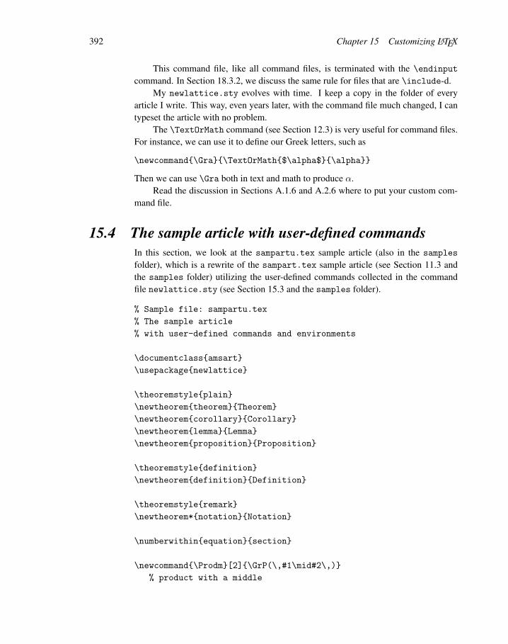
392 Chapter 15 Customizing LATEX
This command file, like all command files, is terminated with the \endinput
command. In Section 18.3.2, we discuss the same rule for files that are \include-d.My newlattice.sty evolves with time. I keep a copy in the folder of every
article I write. This way, even years later, with the command file much changed, I cantypeset the article with no problem.
The \TextOrMath command (see Section 12.3) is very useful for command files.For instance, we can use it to define our Greek letters, such as
\newcommand\Gra\TextOrMath$\alpha$\alpha
Then we can use \Gra both in text and math to produce α.Read the discussion in Sections A.1.6 and A.2.6 where to put your custom com-
mand file.
15.4 The sample article with user-defined commandsIn this section, we look at the sampartu.tex sample article (also in the samples
folder), which is a rewrite of the sampart.tex sample article (see Section 11.3 andthe samples folder) utilizing the user-defined commands collected in the commandfile newlattice.sty (see Section 15.3 and the samples folder).
% Sample file: sampartu.tex
% The sample article
% with user-defined commands and environments
\documentclassamsart
\usepackagenewlattice
\theoremstyleplain
\newtheoremtheoremTheorem
\newtheoremcorollaryCorollary
\newtheoremlemmaLemma
\newtheorempropositionProposition
\theoremstyledefinition
\newtheoremdefinitionDefinition
\theoremstyleremark
\newtheorem*notationNotation
\numberwithinequationsection
\newcommand\Prodm[2]\GrP(\,#1\mid#2\,)
% product with a middle

15.4 The sample article with user-defined commands 393
\newcommand\Prodsm[2]\GrP^*(\,#1\mid#2\,)
% product * with a middle
\newcommand\vectsup[2]\vect<\dots,0,\dots,%
\overset#1#2,\dots,0,\dots>% special vector
\newcommand\DsqD^\langle2\rangle
\begindocument
\title[Complete-simple distributive lattices]
A construction of complete-simple\\
distributive lattices
\authorGeorge~A. Menuhin
\addressComputer Science Department\\
University of Winnebago\\
Winnebago, Minnesota 23714
\urladdrhttp://math.uwinnebago.edu/homepages/menuhin/
\thanksResearch supported by the NSF under
grant number~23466.
\keywordsComplete lattice, distributive lattice,
complete congruence, congruence lattice
\subjclass[2000]Primary: 06B10; Secondary: 06D05
\dateMarch 15, 2006
\beginabstract
In this note we prove that there exist
\emphcomplete-simple distributive lattices, that is,
complete distributive lattices in which
there are only two complete congruences.
\endabstract
\maketitle
\sectionIntroduction\labelS:intro
In this note we prove the following result:
\beginnamedMain Theorem
There exists an infinite complete distributive lattice
$K$ with only the two trivial complete
congruence relations.
\endnamed
\sectionThe $\Dsq$ construction\labelS:Ds
For the basic notation in lattice theory
and universal algebra, see Ferenc~R.
Richardson~\citefR82 and George~A. Menuhin~\citegM68.

394 Chapter 15 Customizing LATEX
We start with some definitions:
\begindefinition\labelD:prime
Let $V$ be a complete lattice, and let
$\Frakp = [u, v]$ be an interval of $V$. Then
$\Frakp$ is called \emphcomplete-prime if the
following three conditions are satisfied:
\beginenumeratei
\item $u$ is meet-irreducible but $u$ is \emphnot
completely meet-irreducible;\labelm-i
\item $v$ is join-irreducible but $v$ is \emphnot
completely join-irreducible;\labelj-i
\item $[u, v]$ is a complete-simple lattice.\labelc-s
\endenumeratei
\enddefinition
Now we prove the following result:
\beginlemma\labelL:Dsq
Let $D$ be a complete distributive lattice satisfying
conditions \itemrefm-i and~\itemrefj-i.
Then $\Dsq$ is a sublattice of $D^2$; hence $\Dsq$
is a lattice, and $\Dsq$ is a complete distributive
lattice satisfying conditions
\itemrefm-i and~\itemrefj-i.
\endlemma
\beginproof
By conditions~\itemrefm-i and \itemrefj-i, $\Dsq$ is a
sublattice of $D^2$. Hence, $\Dsq$ is a lattice.
Since $\Dsq$ is a sublattice of a distributive
lattice, $\Dsq$ is a distributive lattice. Using the
characterization of standard ideals in
Ernest~T. Moynahan~\citeeM57,
$\Dsq$ has a zero and a unit element, namely,
$\vect<0, 0>$ and $\vect<1, 1>$. To show that $\Dsq$
is complete, let $\empset \ne A \contd \Dsq$, and let
$a = \JJ A$ in $D^2$. If $a \in \Dsq$, then
$a = \JJ A$ in $\Dsq$; otherwise, $a$ is of the form
$\vect<b, 1>$ for some $b \in D$ with $b < 1$. Now
$\JJ A = \vect<1, 1>$ in $D^2$, and

15.4 The sample article with user-defined commands 395
the dual argument shows that $\MM A$ also exists in
$D^2$. Hence $D$ is complete. Conditions \itemrefm-i
and~\itemrefj-i are obvious for $\Dsq$.
\endproof
\begincorollary\labelC:prime
If $D$ is complete-prime, then so is $\Dsq$.
\endcorollary
The motivation for the following result comes from
Soo-Key Foo~\citesF90.
\beginlemma\labelL:ccr
Let $\GrQ$ be a complete congruence relation of $\Dsq$
such that
\beginequation\labelE:rigid
\congr \vect<1, d>=\vect<1, 1>(\GrQ),
\endequation
for some $d \in D$ with $d < 1$. Then $\GrQ = \Gri$.
\endlemma
\beginproof
Let $\GrQ$ be a complete congruence relation of $\Dsq$
satisfying \itemrefE:rigid. Then $\GrQ = \Gri$.
\endproof
\sectionThe $\Grp^*$ construction\labelS:P*
The following construction is crucial to our proof of the
Main~Theorem:
\begindefinition\labelD:P*
Let $D_i$, for $i \in I$, be complete distributive
lattices satisfying condition~\itemrefj-i. Their
$\Grp^*$ product is defined as follows:
\[
\Prodsm D_i i \in I =
\Prodm D_i^- i \in I + 1;
\]
that is, $\Prodsm D_i i \in I$ is
$\ProdmD_i^-i \in I$ with a new unit element.
\enddefinition

396 Chapter 15 Customizing LATEX
\beginnotation
If $i \in I$ and $d \in D_i^-$, then
\[
\vectsupid
\]
is the element of $\Prodsm D_i i \in I$ whose
$i$-th component is $d$ and all the other
components are $0$.
\endnotation
See also Ernest~T. Moynahan~\citeeM57a. Next we verify:
\begintheorem\labelT:P*
Let $D_i$, for $i \in I$, be complete distributive
lattices satisfying condition~\itemrefj-i. Let $\GrQ$
be a complete congruence relation on
$\Prodsm D_i i \in I$. If there exist
$i \in I$ and $d \in D_i$ with $d < 1_i$ such
that for all $d \leq c < 1_i$,
\beginequation\labelE:cong1
\congr\vectsupid=\vectsupic(\GrQ),
\endequation
then $\GrQ = \Gri$.
\endtheorem
\beginproof
Since
\beginequation\labelE:cong2
\congr\vectsupid=\vectsupic(\GrQ),
\endequation
and $\GrQ$ is a complete congruence relation, it
follows from condition~\itemrefc-s that
\beginequation\labelE:cong
\beginsplit
&\langle \dots, \oversetid, \dots, 0,
\dots \rangle\\
&\equiv \bigvee ( \langle \dots, 0, \dots,
\oversetic,\dots, 0,\dots \rangle \mid d
\leq c < 1) \equiv 1 \pmod\Theta.
\endsplit
\endequation

15.4 The sample article with user-defined commands 397
Let $j \in I$, for $j \neq i$, and let
$a\in D_j^-$. Meeting both sides of the congruence
\itemrefE:cong with $\vectsupja$, we obtain
\beginequation\labelE:comp
\beginsplit
0 &= \vectsupid \mm \vectsupja\\
&\equiv \vectsupja\pod\GrQ.
\endsplit
\endequation
Using the completeness of $\GrQ$ and \itemrefE:comp,
we get:
\beginequation\labelE:cong3
\congr0=\JJm\vectsupja a \in D_j^-
=1(\GrQ),
\endequation
hence $\GrQ = \Gri$.
\endproof
\begintheorem\labelT:P*a
Let $D_i$, for $i \in I$, be complete distributive
lattices satisfying
conditions \itemrefj-i and~\itemrefc-s. Then
$\Prodsm D_i i \in I$ also satisfies
conditions~\itemrefj-i and \itemrefc-s.
\endtheorem
\beginproof
Let $\GrQ$ be a complete congruence on
$\Prodsm D_i i \in I$. Let $i \in I$. Define
\beginequation\labelE:dihat
\widehatD_i = \setm \vectsupid
d \in D_i^- \uu \set1.
\endequation
Then $\widehatD_i$ is a complete sublattice of
$\Prodsm D_i i \in I$, and $\widehatD_i$
is isomorphic to $D_i$. Let $\GrQ_i$ be the
restriction of $\GrQ$ to $\widehatD_i$. Since
$D_i$ is complete-simple, so is $\widehatD_i$,
hence $\GrQ_i$ is $\Gro$ or $\Gri$. If
$\GrQ_i=\Gro$, for all $i\in I$, then $\GrQ = \Gro$.
If there is an $i \in I$, such that $\GrQ_i = \Gri$,
then $\congr0=1(\GrQ)$, and hence $\GrQ = \Gri$.
\endproof

398 Chapter 15 Customizing LATEX
The Main Theorem follows easily from Theorems~\refT:P*
and \refT:P*a.
\beginthebibliography9
\bibitemsF90
Soo-Key Foo, \emphLattice Constructions,
Ph.D. thesis, University of Winnebago,
Winnebago, MN, December, 1990.
\bibitemgM68
George~A. Menuhin, \emphUniversal algebra. D.~Van
Nostrand, Princeton, 1968.
\bibitemeM57
Ernest~T. Moynahan,
\emphOn a problem of M. Stone,
Acta Math. Acad. Sci. Hungar. \tbf8 (1957),
455--460.
\bibitemeM57a
\bysame, \emphIdeals and congruence relations in
lattices.~II, Magyar Tud. Akad. Mat. Fiz. Oszt.
K\"ozl. \tbf9 (1957), 417--434 (Hungarian).
\bibitemfR82
Ferenc~R. Richardson,
\emphGeneral Lattice Theory.
Mir, Moscow, expanded and revised ed.,
1982 (Russian).
\endthebibliography
\enddocument
15.5 Numbering and measuringLATEX stores integers in counters. For example, the section counter contains the cur-rent section number. Distance measurements are saved in length commands. For in-stance, the \textwidth command contains the width of the text. For this book,\textwidth is set to 345.0 points.
In this section, we take a closer look at counters and length commands.

15.5 Numbering and measuring 399
15.5.1 CountersCounters may be defined by LATEX, by document classes, by packages, or by the user.
Standard LATEX counters
LATEX automatically generates numbers for equations, sections, theorems, and so on.Each such number is stored in a counter. Table 15.2 shows the standard LATEX counters.Their names are more or less self-explanatory. In addition, for every proclamationname, there is a matching counter called name (see Section 6.4).
Setting counters
The command for setting a counter’s value is \setcounter. When LATEX generates anumber, it first increments the appropriate counter, so if you want the next chapter tobe numbered 3, you should set the chapter counter to 2 by typing
\setcounterchapter2
before the \chapter command. The only exception to this rule is the page number,which is first used to number the current page, and then incremented. If you wanted toset the current page number to 63, you would include the command
\setcounterpage63
somewhere in the page.LATEX initializes and increments its standard counters automatically. Sometimes
you may want to manipulate them yourself. To typeset only chapter3.tex, the thirdchapter of your book, start with
\setcounterchapter2
\includechapter3
and when chapter3.tex is typeset, the chapter is properly numbered. You can alsotype
\setcounterpage63
equation part enumifigure chapter enumiifootnote section enumiiimpfootnote subsection enumivpage subsubsectiontable paragraph
subparagraph
Table 15.2: Standard LATEX counters.

400 Chapter 15 Customizing LATEX
if the first page of this chapter is supposed to be 63. Of course, the preferred wayto typeset parts of a larger document is with the \includeonly command (see Sec-tion 18.3.2).
Tip If you need to manipulate counters, always look for solutions in which LATEX does thework for you.
Defining new counters
You can define your own counters. For example,
\newcountermycounter
makes mycounter a new counter. In the definition, you can use an optional argument,the name of another counter:
\newcountermycounter[basecounter]
which automatically resets mycounter to 0 if basecounter changes value. This com-mand has the same form as the command LATEX uses internally for tasks such as num-bering theorems and subsections within sections.
Rule New countersNew counters should be defined in the preamble of the document. They should not bedefined in a file read in with an \include command (see Section 18.3.2).
Let us suppose that you define a new counter, mycounter, in chapter5.tex, whichis made part of your whole document with an \include command. When you typesetyour document with \includeonly commands not including chapter5.tex, you getan error message, such as
! LaTeX Error: No counter ’mycounter’ defined.
Counter styles
The value of counter can be displayed in the typeset document with the command
\thecounter
If you want to change the counter’s appearance when typeset, issue the command
\renewcommand\thecounter new_style

15.5 Numbering and measuring 401
Style Command Sample
Arabic \arabiccounter 1, 2, . . .Lowercase Roman \romancounter i, ii, . . .Uppercase Roman \Romancounter I, II, . . .Lowercase Letters \alphcounter a, b, . . . , zUppercase Letters \Alphcounter A, B, . . . , Z
Table 15.3: Counter styles.
where new style specifies the counter modified as shown in Table 15.3. The defaultstyle is arabic. For instance, if you give the command
\renewcommand\thetheorem\Alphtheorem
then the theorems appear as Theorem A, Theorem B, . . .Here is a more complicated example for a book:
\renewcommand\thechapter\arabicchapter
\renewcommand\thesection\thechapter-\arabicsection
\renewcommand\thesubsection%
\thechapter-\arabicsection.\arabicsubsection
With these definitions, Section 1 of Chapter 3 is numbered in the form 3-1 and Subsec-tion 2 of Section 1 of Chapter 3 is numbered in the form 3-1.2.
The \pagenumbering command is a shorthand method for setting the page num-bering in a given style. For instance, \pagenumberingroman numbers pages as i,ii, and so on.
The subequations environment (see Section 8.5) uses parentequation as thecounter for the whole equation group and it uses equation as the counter for thesubequations. To change the default format of the equation numbers from (2a), (2b),and so forth, to (2i), (2ii), and so on, type the following line inside the subequationsenvironment
\renewcommand\theequation%
\theparentequation\romanequation
If you want equation numbers like (2.i), (2.ii), and so on, type
\renewcommand\theequation%
\theparentequation.\romanequation

402 Chapter 15 Customizing LATEX
Counter arithmetic
The \stepcountercounter command increments counter and sets all the coun-ters that were defined with the optional argument counter to 0. The variant
\refstepcountercounter
does the same, and also sets the value for the next \label command.You can do some arithmetic with the command
\addtocountercounter n
where n is an integer. For example,
\setcountercounter5
\addtocountercounter2
sets counter to 7.The value stored in a counter can be accessed using the \value command, which
is mostly used with the \setcounter or \addtocounter commands. For instance,you can set counter to equal the value of another counter, oldcounter, by typing
\setcountercounter\valueoldcounter
Here is a typical example of counter manipulation. You might want a theorem(invoked in a theorem environment) to be followed by several corollaries (each ina corollary environment) starting with Corollary 1. In other words, Theorem 1should be followed by Corollary 1, Corollary 2, and so forth and so should Theo-rem 3. By default, LATEX numbers the next corollary as Corollary 3, even if it followsanother theorem. To tell LATEX to start numbering the corollaries from 1 again, issuethe command
\setcountercorollary0
after each theorem. But such a process is error-prone, and goes against the spiritof LATEX.
Instead, follow my advice on page 400, and let LATEX do the work for you. In thepreamble, type the proclamations
\newtheoremtheoremTheorem
\newtheoremcorollaryCorollary[theorem]
We are almost there. Theorem 1 now is followed by Corollary 1.1, Corollary 1.2 andTheorem 3 by Corollary 3.1. If we redefine \thecorollary,
\renewcommand\thecorollary\arabiccorollary
then Theorem 1 is followed by Corollary 1 and Corollary 2, and Theorem 3 is also

15.5 Numbering and measuring 403
followed by Corollary 1.If you need to perform more complicated arithmetic with counters, use Kresten K.
Thorup and Frank Jensen’s calc package (see Section 12.3.1). This package is dis-cussed in Section A.3.1 of The LATEX Companion, 2nd edition [46].
Two special counters
The secnumdepth and tocdepth counters control which sectional units are numberedand which are listed in the table of contents, respectively. For example,
\setcountersecnumdepth2
sets secnumdepth to 2. As a result, chapters—if they are present in the documentclass—sections, and subsections are numbered, but subsubsections are not. This com-mand must be placed in the preamble of the document. tocdepth is similar.
15.5.2 Length commandsWhile a counter contains integers, a length command contains a real number and adimensional unit.
LATEX recognizes many different dimensional units. We list five absolute units:
cm centimeter
in inch
pc pica (1 pc = 12 pt)
pt point (1 in = 72.27 pt)
mm millimeter
and two relative units:
em, approximately the width of the letter M in the current font
ex, approximately the height of the letter x in the current font
LATEX defines many length commands. For instance, Section 4.1 of The LATEXCompanion, 2nd edition [46] lists 17 length commands for page layout alone. You canfind some of them in Figure 10.4. A list environment sets about a dozen additionallength commands (see Figure 15.2). Length commands are defined for almost everyaspect of LATEX’s work, including displayed math environments—a complete list wouldprobably contain a few hundred. Many are listed in Leslie Lamport’s LATEX: A Docu-ment Preparation System, 2nd edition [43] and in The LATEX Companion, 2nd edition[46]. Many more are hidden in packages such as amsmath.

404 Chapter 15 Customizing LATEX
The most common length commands are:
\parindent, the amount of indentation at the beginning of a paragraph
\parskip, the extra vertical space inserted between paragraphs
\textwidth, the width of the text on a page
A more esoteric example is \marginparpush, the minimum vertical space betweentwo marginal notes. Luckily, you do not have to be familiar with many length com-mands because LATEX and the document class set them for you.
Defining new length commands
You can define your own length commands. For example,
\newlength\mylength
makes \mylength a new length command with a value of 0 points. Note that whileyou have to type
\newcountercounter
to get a new counter, typing
\newlengthmylength
results in an error message such as
! Missing control sequence inserted.
<inserted text>
\inaccessible
l.3 \newlengthmylength
Setting length
The \setlength command sets or resets the value of a length command. So
\setlength\textwidth3in
creates a very narrow page. The first argument of \setlength must be a length com-mand, not simply the command name, that is
\setlengthtextwidth3in % Bad
is incorrect. The second argument of \setlength must be a real number with a di-mensional unit, for instance, 3in, and not simply a real number. In other words,
\setlength\textwidth3 % Bad
is also incorrect.

15.5 Numbering and measuring 405
Tip A common mistake is to type a command such as
\setlength\marginpar0
Instead, type
\setlength\marginpar0pt
Always be sure to include a dimensional unit.
The \addtolength command adds a quantity to the value of a length command.For instance,
\addtolength\textwidth-10pt
narrows the page width by 10 points.If you define
\newlength\shorterlength
\setlength\shorterlength\mylength
\addtolength\shorterlength-.5in
then \parbox\shorterlength... always typesets its second argument in a box1/2 inch narrower than the parboxes set to be of width \mylength.
When LATEX typesets some text or math, it creates a box. Three measurements areused to describe the size of the box:
the width
the height, from the baseline to the top
the depth, from the baseline to the bottom
as illustrated in Figure 15.1. For instance, the box typesetting “aa” has a width of10.00003 pt, a height of 4.30554 pt, and a depth of 0 pt. The box typesetting “ag” has
Figure 15.1: The measurements of a box.

406 Chapter 15 Customizing LATEX
the same width and height, but a depth of 1.94444 pt. The box “Ag” (see Figure 15.1)has a width of 12.50003 pt, a height of 6.83331 pt, and a depth of 1.94444 pt.
The commands
\settowidth
\settoheight
\settodepth
each take two arguments. The first argument is a length command, the second is text(or math) to be measured by LATEX. The corresponding measurement of the box inwhich the second argument is typeset is assigned to the length command in the firstargument. For example, if \mylength is a length command, then
\settowidth\mylengthAg
assigns 12.50003 pt to \mylength. It should be clear from this example how the\phantom and \hphantom commands (see Section 5.8.1) are related to this command.
To perform more complicated arithmetic with length commands, use the calc
package.
Rubber lengths
In addition to rigid lengths, such as 3in, LATEX can also set rubber lengths, that is,lengths that are allowed to stretch and shrink. Here is an example:
\setlength\stretchspace3in plus 10pt minus 8pt
Assuming that \stretchspace is a length command, this command assigns it a valueof 3 inches that can stretch by 10 points or shrink by 8 points, if necessary. So a box ofwidth \stretchspace is 3 inches wide, plus up to 10 points, or minus up to 8 points.
Stretchable vertical spaces are often used before and after displayed text environ-ments. LATEX adjusts these spaces to make the page look balanced. An example can befound in Section 15.1.7. \medskipamount is defined as
6.0pt plus 2.0pt minus 2.0pt
See Section 15.6.3 for more examples.The \fill command is a special rubber length that can stretch any amount. The
stretching is done evenly if there is more than one \fill present. See the secondexample of brand-new environments in Section 15.2.5.
15.6 Custom listsAlthough there are three ready-made list environments provided by LATEX (see Sec-tion 6.2), it is often necessary to create one of your own using LATEX’s list environ-ment. In fact, LATEX itself uses the list environment to define many of its standardenvironments, including:

15.6 Custom lists 407
The three list environments (Section 6.2)
The quote, quotation, and verse environments (Section 6.8)
Proclamations (Section 6.4)
The style environments center, flushleft, and flushright (Section 6.3)
The thebibliography environment (Section 10.5.1)
The theindex environment (Section 10.5.2)
15.6.1 Length commands for the list environmentThe general layout of a list is shown in Figure 15.2. It uses six horizontal measurementsand three vertical measurements. I now list these length commands.
Vertical length commands
\topsep is most of the vertical space between the first item and the preceding text,and also between the last item and the following text. This space also includes\parskip, the extra vertical space inserted between paragraphs, and optionally,\partopsep, provided that the list environment starts a new paragraph.
\parsep is the space between paragraphs of the same item.
\itemsep is the space between items. Like \topsep, the actual gap is the sum of\itemsep and \parsep.
All of these vertical length commands are rubber lengths (see Section 15.5.2).
Horizontal length commands
By default, the margins of a list environment are the same as the margins of thesurrounding text. If the list is nested within a list, the margins are wider and so the textis narrower.
The \leftmargin and \rightmargin length commands specify the distance be-tween the edge of the item box and the left and right margins of the page.
The label is the text provided by the optional argument of an \item commandor provided as a default in the definition of the list environment. It is typeset in a box ofwidth \labelwidth, which is indented \itemindent units from the left margin, andseparated by a space of \labelsep units from the text box. If the label is too wide tofit in the box, it is typeset at its full natural width, and the first line in the text box isindented.
The second and subsequent paragraphs of an item are typeset with their first linesindented by \listparindent units.

408 Chapter 15 Customizing LATEX
Surrounding text
Surrounding text
Item 1
paragraph 1
Item 1
paragraph 2
Item 2
paragraph 1
\itemindent \labelsep
\labelwidth
\leftmargin \rightmargin
\topsep+\parskip
\parsep\listparindent
\itemsep+\parsep
label
label
\topsep+\parskip
Figure 15.2: The layout of a custom list.

15.6 Custom lists 409
15.6.2 The list environmentCustom lists are created with the list environment, which is invoked as follows:
\beginlistdefault_label declarations
\item item1
\item item2
...
\endlist
The arguments are
default label, the label for any items that do not specify their own, similar to theoptional argument of the \item command
declarations, the vertical and horizontal length commands and any other requiredparameters for the list
Here is a very simple example:
Here are the most important LATEX rules about spaces in text, sentences, andparagraphs:
♦ Rule 1: Two or more spaces in text are the same as one.
♦ Rule 2: A blank line (that is, two end-of-line characters sepa-rated only by blanks and tabs) indicates the end of a paragraph.
Rules 1 and 2 make typing and copying very convenient.
I have used the ♦ math symbol ($\diamondsuit$) as a default label, and I set theitem box 0.5 inch from either margin. So this example is typed as follows:
\noindent Here are the most important \LaTeX\ rules about
spaces in text, sentences, and paragraphs:
\beginlist$\diamondsuit$\setlength\leftmargin%
.5in\setlength\rightmargin.5in
\item \textbfRule 1: Two or more spaces in text
are the same as one.
\item \textbfRule 2: A blank line (that is, two
end-of-line characters separated only by blanks and tabs)
indicates the end of a paragraph.
\endlist
Rules 1 and~2 make typing and copying very convenient.
Here is a second variant:

410 Chapter 15 Customizing LATEX
Here are the most important LATEX rules about spaces in text, sentences, andparagraphs:
Rule 1: Two or more consecutive spaces in text are the same as one.
Rule 2: A blank line (that is, two end-of-line characters separatedonly by blanks and tabs) indicates the end of a paragraph.
Rules 1 and 2 make typing and copying very convenient.
In this example, I dropped the optional default label and typed Rule 1: and Rule 2:
as (optional) arguments of the \item commands:
\noindent Here are the most important \LaTeX\ rules about
spaces in text, sentences, and paragraphs:
\beginlist\setlength\leftmargin.5in%
\setlength\rightmargin.5in
\item[\textbfRule 1:] Two or more consecutive spaces in
text are the same as one.
\item[\textbfRule 2:] A blank line (that is,
two end-of-line characters separated only by blanks and
tabs) indicates the end of a paragraph.
\endlist
Rules 1 and~2 make typing and copying very convenient.
For further simple examples, you can look at various document class files to see howstandard environments such as verse, quote, and so on, are defined.
Using counters
It is not very LATEX-like to provide the numbers for the rules in the examples above.It would be more logical for LATEX to do the numbering. The following is a moreLATEX-like coding of the second example:
\noindent Here are the most important \LaTeX\ rules about
spaces in text, sentences, and paragraphs:
\newcounterspacerule
\beginlist\textbfRule \arabicspacerule:
\setlength\leftmargin.5in
\setlength\rightmargin.5in
\usecounterspacerule
\item Two or more consecutive spaces in text are the
same as one.\labelLi:Twoor
\item A blank line (that is, two end-of-line

15.6 Custom lists 411
characters separated only by blanks and tabs)
indicates the end of a paragraph.\labelLi:blankline
\endlist
Rules \refLi:Twoor and~\refLi:blankline make typing
and copying very convenient.
Note that
1. I declared the counter before the list environment with the line
\newcounterspacerule
2. I defined the default label as
\textbfRule \arabicspacerule: item In the declarations, I specifiedthat the list should use the spacerule counter with the command
\usecounterspacerule
15.6.3 Two complete examplesIn the previous examples, I set the values of \leftmargin and \rightmargin. Theother length commands were not redefined, so their values remained the values set bythe document class. In the following examples, I set the values of many more lengthcommands.
Example 1 To get the following list,
Here are the most important LATEX rules about spaces in text, sentences, andparagraphs:
Rule 1: Two or more consecutive spaces in text arethe same as one.
Rule 2: A blank line—that is, two end-of-line char-acters separated only by blanks and tabs—indicates the end of a paragraph.
Rules 1 and 2 make typing and copying very convenient.
we type
\noindent Here are the most important \LaTeX\ rules about
spaces in text, sentences, and paragraphs:
\newcounterspacerule
\beginlist\upshape\bfseries Rule \arabicspacerule:

412 Chapter 15 Customizing LATEX
\setlength\leftmargin1.5in
\setlength\rightmargin0.6in
\setlength\labelwidth1.0in
\setlength\labelsep0.2in
\setlength\parsep0.5ex plus 0.2ex
minus 0.1ex
\setlength\itemsep0ex plus 0.2ex
minus 0ex
\usecounterspacerule
\itshape
\item Two or more consecutive spaces in text are the
same as one.\labelLi:Twoor
\item A blank line---that is, two end-of-line
characters separated only by blanks and
tabs---indicates
the end of a paragraph.\labelLi:blankline
\endlist
Rules \refLi:Twoor and~\refLi:blankline make typing
and copying very convenient.
Note that
1. I declared the counter as in the previous example.
2. The last item in declarations is \itshape, which typesets the entire list in ital-ics.
3. The default label is defined as
\upshape\bfseries Rule \arabicspacerule
My first attempt was to define it as
\bfseries Rule \arabicspacerule
which typesets Rule in bold italics (because in Step 2 we set the whole list in ital-ics). To force the label to be typeset upright, I start the default label with the\upshape command.
4. The left margin is set to 1.5 inches and the right margin to 0.6 inches:
\setlength\leftmargin1.5in
\setlength\rightmargin0.6in
5. Next I set the width of the label to 1 inch, and the space between the label and theitem to 0.2 inches:

15.6 Custom lists 413
\setlength\labelwidth1.0in
\setlength\labelsep0.2in
6. Finally, I set the paragraph separation to 0.5 ex, allowing stretching by 0.2 ex andshrinking by 0.1 ex, and the item separation to 0 ex, allowing stretching by 0.2 exand no shrinking, by
\setlength\parsep0.5ex plus 0.2ex minus 0.1ex
\setlength\itemsep0ex plus 0.2ex minus 0ex
The actual amount of item separation is calculated by adding the values specifiedfor \parsep and \itemsep.
A complicated list such as this should be defined as a new environment. Forexample, you could define a myrules environment:
\newenvironmentmyrules
\beginlist
\upshape \bfseries Rule \arabicspacerule:
\setlength\leftmargin1.5in
\setlength\rightmargin0.6in
\setlength\labelwidth1.0in
\setlength\labelsep0.2in
\setlength\parsep0.5ex plus 0.2ex minus 0.1ex
\setlength\itemsep0ex plus 0.2ex minus 0ex
\usecounterspacerule
\itshape
\endlist
and then use it anywhere, as in
\beginmyrules
\item Two or more consecutive spaces in text are the
same as one.\labelLi:Twoor
\item A blank line---that is, two end-of-line
characters separated only by blanks and
tabs---indicates the end of a paragraph.
\labelLi:blankline
\endmyrules
Rules \refLi:Twoor and~\refLi:blankline make typing
and copying very convenient.
which typesets as the first example shown on page 411.

414 Chapter 15 Customizing LATEX
Example 2 In Section 5.7.2, we discussed the formatting of the following type ofglossary:
sentence is a group of words terminated by a period, exclamation point, orquestion mark.
paragraph is a group of sentences terminated by a blank line or by the \par
command.
Now we can create the glossary as a custom list:
\beginlist
\setlength\leftmargin30pt
\setlength\rightmargin0pt
\setlength\itemindent14pt
\setlength\labelwidth40pt
\setlength\labelsep5pt
\setlength\parsep0.5ex plus 0.2ex minus 0.1ex
\setlength\itemsep0ex plus 0.2ex minus 0ex
\item[\textbfsentence\hfill] is a group of words
terminated by a period, exclamation point,
or question mark.
\item[\textbfparagraph\hfill] is a group of sentences
terminated by a blank line or by the \compar command.
\endlist
There is nothing new in this example except the \hfill commands in the optionalarguments to left adjust the labels. With the long words in the example this adjustmentis not necessary, but it would be needed for shorter words.
See Section 3.3 of The LATEX Companion, 2nd edition [46] on how to customizethe three standard list environments and also for more complicated custom lists.
15.6.4 The trivlist environmentLATEX also provides a trivlist environment, meant more for programmers than users.The environment is invoked in the form
\begintrivlist
body
\endtrivlist
It is similar to the list environment except that there are no arguments, and all thelength commands are trivially set, most to 0 points, except for \listparindent and\parsep, which are set to equal \parindent and \parskip, respectively. For in-stance, LATEX defines the center environment as follows:

15.7 The dangers of customization 415
\begintrivlist
\centering \item[]
\endtrivlist
15.7 The dangers of customizationWe can customize LATEX in so many ways. We can add packages to expand its powerand define new commands that better suit our work habits. These enhance LATEX andmake it easier to work with. But they also introduce difficulties. Let us start with theobvious.
Whoever introduced the command \textcompwordmark knew that—even if weuse command completion—we are not going to type
if\textcompwordmark f
to avoid having a ligature (see Section 5.4.6). It is a lot of typing, and the source filebecomes hard to read. This cries out for a user-defined command, say, \Iff, which isshort and readable (see Section 15.1.1).
When introducing user-defined commands, watch out for the following traps.
Trap 1 Redefining a command that is a necessary part of LATEX.
This is easy to avoid. As discussed in Section 15.1.7, you can easily find out whether acommand is already in use. If it is, do not redefine it unless you really know what youare doing.
Trap 2 Defining too many commands.
This creates two problems. Your editor has a hard time making changes in your sourcefile. And a few years later, when you want to reuse the material, you have a difficulttime understanding all those clever commands.
Trap 3 Your contribution appears in a volume with many other authors and your user-definedcommands create conflicts.
As your article appears in a publication, some parts of it are used for the wholevolume. The title and maybe even the section titles are used in the table of contents.The abstracts may be collected for the whole volume or there may be a joint bibliogra-phy.

416 Chapter 15 Customizing LATEX
With the advent of the internet, there are now collections of thousands of matharticles; PlanetMath.org is one example. Write your articles so that even the editors ofPlanetMath.org can use it.
Rule 1 Do not use your own commands in the title of the article, in the abstract, in sectiontitles, in the bibliography, or in captions of figures and tables.
Trap 4 You submit the article to a journal that does not permit a separate custom commandfile.
For such journals, just copy the needed user-defined commands into the preambleof your article. Go through the list and delete those user-defined commands that arenot used in this article. This helps the editor to look up your commands from a shorterlist.
Rule 2 Introduce judiciously user-defined commands with very short names.
Introducing one-letter commands—for instance, using \C for the complex field—is dangerous because many one-letter commands are reserved by LATEX.
Two-letter user-defined commands are not quite this bad. Of the 2,500 or so possi-bilities only a few dozen are used by LATEX. The danger here is, of course, conflict withother authors and confusion for the editor. My command file has about 15 two-lettercommands. For instance \jj, part of the \jj, \JJ, \JJm family. Also \Id, becauseId is the standard notation for ideal lattices. Some editors may think that this is 15 toomany.
Rule 3 Do not use \def to define your commands, with the exception of a very few delimitedcommands.
Using \def means giving up LATEX’s built in defense. In the editorial office of myjournal, about half the submitted articles that we cannot typeset violate this rule.
Rule 4 Do not redefine length commands, especially, if you do not know what other lengthcommands are computed based on the ones you change.

15.7 The dangers of customization 417
The page layout diagram, Figure 10.4, should provide examples. Even simpler,Do not redefine length commands. Let the document class define them for your article.
Rule 5 Make sure that the packages you use are compatible.
For instance, the popular psfrag and epsfig packages cause problems if usedwith the AMS packages.
Be cautious when you use packages that redefine a lot of LATEX commands, suchas hyperref (see Section 13.2).
You can read more about the plight of authors in the hands of incompetent editorsin my article [31] and the difficult job of editors with articles violating the above rulesin Enrico Gregorio [16].

C H A P T E R
16
BIBTEX
The BIBTEX application, written by Oren Patashnik, assists LATEX users in compilingbibliographies, especially long ones. Short bibliographies can easily be placed in thedocument directly (see Section 10.5.1).
It takes a little effort to learn BIBTEX. But in the long run, the advantages of build-ing bibliographic databases that can be reused and shared outweigh the disadvantageof a somewhat steep learning curve.
The bibliographic database files, the bib files, contain the bibliographic entries.We discuss the format of these entries in Section 16.1, and then describe how to useBIBTEX to create bibliographies in Section 16.2.
BIBTEX uses a style, called a bibliographic style, or bst file, to format entries.On the next two pages we show the bibliography of the sampartb.tex sample articletypeset with six different style files.
To simplify our discussion, in the rest of this chapter I discuss only one style,the AMS plain style, amsplain.bst, version 2.0. All of the examples shown are inthis style, and several of the comments I make are true only for the AMS plain style.If you choose to use a different style, you should check its documentation for specialrules.

422 Chapter 16 BIBTEX
plain.bst
alpha.bst
amsplain.bst
amsalpha.bst
[1] Soo-Key Foo. Lattice Constructions. PhD thesis, University of Winnebago, Winnebago, MN,December 1990.
[2] George A. Menuhin. Universal Algebra. D. van Nostrand, Princeton, 1968.[3] Ernest T. Moynahan. Ideals and congruence relations in lattices. II. Magyar Tud. Akad. Mat.
Fiz. Oszt. Kozl., 7:417–434, 1957.[4] Ernest T. Moynahan. On a problem of M. Stone. Acta Math. Acad. Sci. Hungar., 8:455–460,
1957.
[5] Ferenc R. Richardson. General Lattice Theory. Mir, Moscow, expanded and revised edition,1982.
[Foo90] Soo-Key Foo. Lattice Constructions. PhD thesis, University of Winnebago, Winnebago,MN, December 1990.
[Men68] George A. Menuhin. Universal Algebra. D. van Nostrand, Princeton, 1968.[Moy57a] Ernest T. Moynahan. Ideals and congruence relations in lattices. II. Magyar Tud. Akad.
Mat. Fiz. Oszt. Kozl., 7:417–434, 1957.[Moy57b] Ernest T. Moynahan. On a problem of M. Stone. Acta Math. Acad. Sci. Hungar.,
8:455–460, 1957.[Ric82] Ferenc R. Richardson. General Lattice Theory. Mir, Moscow, expanded and revised
edition, 1982.
1. Soo-Key Foo, Lattice constructions, Ph.D. thesis, University of Winnebago, Winnebago, MN,December 1990.
2. George A. Menuhin, Universal algebra, D. van Nostrand, Princeton, 1968.3. Ernest T. Moynahan, Ideals and congruence relations in lattices. II, Magyar Tud. Akad. Mat.
Fiz. Oszt. Kozl. 7 (1957), 417–434 (Hungarian).
4. , On a problem of M. Stone, Acta Math. Acad. Sci. Hungar. 8 (1957), 455–460.5. Ferenc R. Richardson, General lattice theory, expanded and revised ed., Mir, Moscow, 1982
(Russian).
[Foo90] Soo-Key Foo, Lattice constructions, Ph.D. thesis, University of Winnebago, Winnebago,MN, December 1990.
[Men68] George A. Menuhin, Universal algebra, D. van Nostrand, Princeton, 1968.[Moy57a] Ernest T. Moynahan, Ideals and congruence relations in lattices. II, Magyar Tud. Akad.
Mat. Fiz. Oszt. Kozl. 7 (1957), 417–434 (Hungarian).
[Moy57b] Ernest T. Moynahan, On a problem of M. Stone, Acta Math. Acad. Sci. Hungar. 8(1957), 455–460.
[Ric82] Ferenc R. Richardson, General lattice theory, expanded and revised ed., Mir, Moscow,1982 (Russian).

16.1 The database 423
siam.bst
ieeetr.bst
[1] S.-K. Foo, Lattice Constructions, PhD thesis, University of Winnebago, Winnebago, MN,
Dec. 1990.
[2] G. A. Menuhin, Universal Algebra, D. van Nostrand, Princeton, 1968.
[3] E. T. Moynahan, Ideals and congruence relations in lattices. II, Magyar Tud. Akad. Mat.
Fiz. Oszt. Kozl., 7 (1957), pp. 417–434.
[4] , On a problem of M. Stone, Acta Math. Acad. Sci. Hungar., 8 (1957), pp. 455–460.
[5] F. R. Richardson, General Lattice Theory, Mir, Moscow, expanded and revised ed., 1982.
[1] F. R. Richardson, General Lattice Theory. Moscow: Mir, expanded and revised ed., 1982.
[2] G. A. Menuhin, Universal Algebra. Princeton: D. van Nostrand, 1968.
[3] E. T. Moynahan, “On a problem of M. Stone,” Acta Math. Acad. Sci. Hungar., vol. 8, pp. 455–460, 1957.
[4] S.-K. Foo, Lattice Constructions. PhD thesis, University of Winnebago, Winnebago, MN, Dec.
1990.
[5] E. T. Moynahan, “Ideals and congruence relations in lattices. II,” Magyar Tud. Akad. Mat.
Fiz. Oszt. Kozl., vol. 7, pp. 417–434, 1957.
16.1 The databaseA BIBTEX database is a text file containing bibliographic entries. To use BIBTEX, youfirst have to learn how to assemble a database. This section explains how to do that.
There may be special tools available for your computer system that assist you inbuilding and maintaining your bibliographic data. Such tools make compiling the dataeasier and may minimize formatting errors.
You can find all the examples in this section in the template.bib file in thesamples folder (see page 4).
16.1.1 Entry typesA bibliographic entry is given in pieces called fields. The style (see Section 16.2.2)specifies how these fields are typeset. Here are two typical entries:
@BOOKgM68,
author = "George A. Menuhin",
title = "Universal Algebra",
publisher = "D.~Van Nostrand",
address = "Princeton",
year = 1968,

424 Chapter 16 BIBTEX
@ARTICLEeM57,
author = "Ernest T. Moynahan",
title = "On a Problem of M. Stone",
journal = "Acta Math. Acad. Sci. Hungar.",
pages = "455-460",
volume = 8,
year = 1957,
The start of an entry is indicated with an at sign (@) followed by the entry type. In thefirst example, the entry type is BOOK, while in the second, it is ARTICLE. The entry typeis followed by a left brace (). The matching right brace () indicates the end of theentry. BIBTEX also allows you to use parentheses as delimiters for an entry. In thisbook, however, we use braces to enclose an entry.
The string @BOOK is followed by a label, gM68, which designates the name of theentry. Refer to this entry in your document with \citegM68. The label is followedby a comma and a series of fields. In this example, there are five fields, author, title,publisher, address, and year. Each field starts with the field name, followed by =
and the value of the field enclosed in double quotes ("). Be sure to use " and notLATEX double quotes (‘‘ or ’’). Alternatively, BIBTEX also allows you to use braces toenclose the field value. In this book, we use double quotes to enclose a field.
Numeric field values, that is, fields consisting entirely of digits, do not need to beenclosed in double quotes or braces, for instance, year in the examples above, volumein the second example, and number in some of the examples that follow. Page ranges,such as 455-460, are not numeric field values since they contain -, so they must beenclosed in double quotes or braces.
There must be a comma before each field. The comma before the first field isplaced after the label.
There are many standard entry types, including
ARTICLE an article in a journal or magazine
BOOK a book with an author (or editor) and a publisher
BOOKLET a printed work without a publisher
INBOOK a part of a book, such as a chapter or a page range that, in general, is not titledor authored separately
INCOLLECTION a part of a book with its own title and perhaps author
INPROCEEDINGS an article in a conference proceedings with its own title andauthor
MANUAL technical documentation

16.1 The database 425
MASTERSTHESIS a master’s thesis
MISC an entry that does not fit in any other category
PHDTHESIS a Ph.D. thesis
PROCEEDINGS the proceedings of a conference
TECHREPORT a report published by a school or institution
UNPUBLISHED an unpublished paper
Each entry includes a number of fields from the following list:
address institution pages
author journal publisher
booktitle key school
chapter language series
crossref month title
edition note type
editor number volume
howpublished organization year
The style you choose determines which of the fields within an entry are actually used.All the others are ignored. You may also add fields for your own use. For example, youmay want to add a mycomments field for personal comments. Such fields are ignoredunless you have a bibliography style that uses them.
Commonly used examples of new field names include URL, abstract, ISBN,keywords, mrnumber, and so on. The language field is used by the AMS styles butnot by any of the other styles mentioned in this chapter.
Tip
1. BIBTEX does not care whether you use uppercase or lowercase letters (or mixed)for the names of entry types and fields. In this book, the entry types are shown inuppercase and field names in lowercase.
2. Placing a comma after the last field is optional. I recommend that you put it thereso that when you append a new field to the entry, the required comma separating thefields is present.
For each entry type there are both required and optional fields. Later in this sec-tion, I give two examples of each entry type. The first example of an entry type uses asmall set of fields, while the second example is a maximal one, showing a large numberof optional fields.

426 Chapter 16 BIBTEX
16.1.2 Typing fieldsMake sure you type the field names correctly. If you misspell one, BIBTEX ignores thefield. BIBTEX also warns you if a required field is missing.
The author and editor fields require a name.
Rule Names
1. Most names can be typed as usual, "Ernest T. Moynahan" or "Moynahan,Ernest T.", with one comma separating the family name from the given names.
2. Type two or more names separated by and. For instance,
author= "George Blue and Ernest Brown and Soo-Key Foo",
3. The family name of Miguel Lopez Fernandez is Lopez Fernandez, so type it as"Lopez Fernandez, Miguel". This informs BIBTEX that Lopez is not a middlename.
4. Type Orrin Frink, Jr. as "Frink, Jr., Orrin".
Rules 3 and 4 are seldom needed. In a bibliography of about 1,500 items, I foundfewer than 10 names that could not be typed as usual. Note that you can type John vonNeumann as "John von Neumann" or "von Neumann, John". Because BIBTEXknows about von, it handles the name properly.
There are a few rules concerning the title field.
Rule Title
1. You should not put a period at the end of a title. The style supplies the appropriatepunctuation.
2. Many styles, including the AMS styles, convert titles, except for the first letter ofthe title, to lowercase for all entry types. If you want a letter to appear in uppercase,put it—or the entire word—in braces. The same rule applies to the edition field.Some other styles only do this conversion for the titles of non-book-like entries.
3. To maximize the portability of your database, you should type titles with each im-portant word capitalized:
title = "On a Problem of M. Stone",
The style used in this book, amsplain.bst, converts Problem to problem, so it

16.1 The database 427
makes no difference, but some styles do not. To be on the safe side, you shouldcapitalize all words that may have to be capitalized.
For the record, here are the complete rules for titles: Capitalize (1) the first word;(2) the first word in a subtitle (BIBTEX assumes that a subtitle follows a colon, so itcapitalizes the first word after a colon—a colon not introducing a subtitle should betyped in braces); (3) all other words except articles, unstressed conjunctions, and un-stressed prepositions. Words that should never be converted to lowercase, for exampleproper names such as Hilbert, should be enclosed in braces to prevent them frombeing converted to lowercase. In the example above, two letters in the title should notbe converted to lowercase, so we enclosed M. Stone in braces. We could also havetyped M. Stone or M. Stone.
BIBTEX and the style automatically handle a number of things for you that youwould have to handle yourself when typing text.
1. You do not have to mark periods in abbreviations, as .\ in the names of journals(see Section 5.2.2). So
journal = "Acta Math. Acad. Sci. Hungar.",
typesets correctly.
2. You can type a single hyphen for a page range instead of the usual -- in the pagesfield (see Section 5.4.2). So
pages = "455-460",
typesets correctly with an en dash.
3. You do not have to type nonbreakable spaces with ~ in the author or editor fields(see Section 5.4.3):
author = "George A. Menuhin",
is correct. Normally you would type George~A. Menuhin.
Finally, we state a rule about accented characters.
Rule AccentsPut accented characters in braces: \"a.
This rule means that
author = "Paul Erd\Hos",

428 Chapter 16 BIBTEX
is not recommended. Instead, type
author = "Paul Erd\Hos",
This rule is, again, about portability. Some styles, e.g., alpha and amsalpha,create a citation for an article from the first three letters of the name and the last twodigits of the year.
author = "Kurt G\"odel",
year = 1931,
creates the citation: [God31]. The accent is used only if the accents rule has beenfollowed.
The downside of this rule is that the braces suppress kerning.
16.1.3 Articles
Entry type ARTICLE
Required fields author, title, journal, year, pagesOptional fields volume, number, language, note
Examples:
1. Ernest T. Moynahan, On a problem of M. Stone, Acta Math. Acad. Sci.Hungar. 8 (1957), 455–460.
2. Ernest T. Moynahan, On a problem of M. Stone, Acta Math. Acad. Sci.Hungar. 8 (1957), no. 5, 455–460 (English), Russian translation available.
typed as
@ARTICLEeM57,
author = "Ernest T. Moynahan",
title = "On a Problem of M. Stone",
journal = "Acta Math. Acad. Sci. Hungar.",
pages = "455-460",
volume = 8,
year = 1957,
@ARTICLEeM57a,
author = "Ernest T. Moynahan",
title = "On a Problem of M. Stone",
journal = "Acta Math. Acad. Sci. Hungar.",
pages = "455-460",

16.1 The database 429
volume = 8,
number = 5,
year = 1957,
note = "Russian translation available",
language = "English",
16.1.4 BooksEntry type BOOK
Required fields author (or editor), title, publisher, yearOptional fields edition, series, volume, number, address,
month, language, note
Examples:
1. George A. Menuhin, Universal algebra, D. Van Nostrand, Princeton, 1968.2. George A. Menuhin, Universal algebra, second ed., University Series in
Higher Mathematics, vol. 58, D. Van Nostrand, Princeton, March 1968(English), no Russian translation.
typed as
@BOOKgM68,
author = "George A. Menuhin",
title = "Universal Algebra",
publisher = "D.~Van Nostrand",
address = "Princeton",
year = 1968,
@BOOKgM68a,
author = "George A. Menuhin",
title = "Universal Algebra",
publisher = "D.~Van Nostrand",
address = "Princeton",
year = 1968,
month = mar,
series = "University Series in Higher Mathematics",
volume = 58,
edition = "Second",
note = "no Russian translation",
language = "English",

430 Chapter 16 BIBTEX
Abbreviations, such as mar, are discussed in Section 16.1.9.A second variant of book has an editor instead of an author:
15. Robert S. Prescott (ed.), Universal algebra, D. Van Nostrand, Princeton,1968.
typed as
@BOOKrP68,
editor = "Robert S. Prescott",
title = "Universal Algebra",
publisher = "D.~Van Nostrand",
address = "Princeton",
year = 1968,
16.1.5 Conference proceedings and collectionsEntry type INPROCEEDINGS
Required fields author, title, booktitle, yearOptional fields address, editor, series, volume, number,
organization, publisher, month, note, pages, language
Examples:
7. Peter A. Konig, Composition of functions. Proceedings of the Conference onUniversal Algebra, 1970.
8. Peter A. Konig, Composition of functions. Proceedings of the Conference onUniversal Algebra (Kingston, ON) (G. H. Birnbaum, ed.), vol. 7, Cana-dian Mathematical Society, Queen’s Univ., December 1970, available fromthe Montreal office, pp. 1–106 (English).
typed as
@INPROCEEDINGSpK69,
author = "Peter A. Konig",
title = "Composition of Functions".
booktitle = "Proceedings of the Conference on
Universal Algebra",
year = 1970,

16.1 The database 431
@INPROCEEDINGSpK69a,
author = "Peter A. Konig",
title = "Composition of Functions".
booktitle = "Proceedings of the Conference on
Universal Algebra",
address = "Kingston, ON",
publisher = "Queen’s Univ.",
organization = "Canadian Mathematical Society",
editor = "G. H. Birnbaum",
pages = "1-106",
volume = 7,
year = 1970,
month = dec,
note = "available from the Montreal office",
language = "English",
The address field provides the location of the meeting. The address of the pub-lisher should be in the publisher field and the address of the organization in theorganization field.
Entry type INCOLLECTION
Required fields author, title, booktitle, publisher, yearOptional fields editor, series, volume, number, address,
edition, month, note, pages, languageExamples:
1. Henry H. Albert, Free torsoids, Current Trends in Lattices, D. Van Nos-trand, 1970.
2. Henry H. Albert, Free torsoids, Current Trends in Lattices (George Burns,ed.), vol. 2, D. Van Nostrand, Princeton, January 1970, new edition is duenext year, pp. 173–215 (German).
is typed as
@INCOLLECTIONhA70,
author = "Henry H. Albert",
title = "Free Torsoids",
booktitle = "Current Trends in Lattices".
publisher = "D.~Van Nostrand",
year = 1970,

432 Chapter 16 BIBTEX
@INCOLLECTIONhA70a,
author = "Henry H. Albert",
editor = "George Burns",
title = "Free Torsoids",
booktitle = "Current Trends in Lattices".
publisher = "D.~Van Nostrand",
address = "Princeton",
pages = "173-215",
volume = 2,
year = 1970,
month = jan,
note = "new edition is due next year",
language = "German",
The address field contains the address of the publisher.
Cross-referencing
If your database has several articles from the same conference proceedings and col-lections, you may prefer to make an entry for the entire volume, and cross-referenceindividual articles to that entry. For instance,
@PROCEEDINGSUA69,
title = "Proceedings of the Conference on,
Universal Algebra",
booktitle = "Proceedings of the Conference on
Universal Algebra",
address = "Kingston, ON",
publisher = "Canadian Mathematical Society",
editor = "G. H. Birnbaum",
volume = 7,
year = 1970,
may be the entry for the proceedings volume as a whole, and
@INPROCEEDINGSpK69a,
author = "Peter A. Konig",
title = "Composition of Functions",
booktitle = "Proceedings of the Conference on
Universal Algebra",
pages = "1-106",
crossref = "UA69",

16.1 The database 433
is the cross-referencing entry for a specific article. These two entries produce the fol-lowing:
1. G. H. Birnbaum (ed.), Proceedings of the conference on universal algebra,vol. 7, Kingston, ON, Canadian Mathematical Society, 1970.
2. Peter A. Konig, Composition of functions, in Birnbaum [1], pp. 1–106.
Rule Cross-references
1. All the required fields of the cross-referencing entry must appear in either that entryor in the cross-referenced entry.
2. The cross-referenced entry should have both a title and a booktitle field.
3. The cross-referenced entry must appear in the bib file later than any entry thatcross-references it.
16.1.6 ThesesEntry type MASTERSTHESIS or PHDTHESISRequired fields author, title, school, yearOptional fields type, address, month, note, pagesExamples:
1. Soo-Key Foo, Lattice constructions, Ph.D. thesis, University of Winnebago,1990.
2. Soo-Key Foo, Lattice constructions, Ph.D. dissertation, University of Win-nebago, Winnebago, MN, December 1990, final revision not yet available,pp. 1–126.
is typed as
@PHDTHESISsF90,
author = "Soo-Key Foo",
title = "Lattice Constructions",
school = "University of Winnebago",
year = 1990,

434 Chapter 16 BIBTEX
@PHDTHESISsF90a,
author = "Soo-Key Foo",
title = "Lattice Constructions",
school = "University of Winnebago",
address = "Winnebago, MN",
year = 1990,
month = dec,
note = "final revision not yet available",
type = "Ph.D. dissertation",
pages = "1-126",
If the type field is present, its content takes the place of the phrase Ph.D. thesis (orMaster’s thesis).
16.1.7 Technical reports
Entry type TECHREPORT
Required fields author, title, institution, yearOptional fields type, number, address, month, noteExamples:
1. Grant H. Foster, Computational complexity in lattice theory, tech. report,Carnegie Mellon University, 1986.
2. Grant H. Foster, Computational complexity in lattice theory, Research Note128A, Carnegie Mellon University, Pittsburgh, PA, December 1986, inpreparation.
is typed as
@TECHREPORTgF86,
author = "Grant H. Foster",
title = "Computational Complexity in Lattice Theory",
institution = "Carnegie Mellon University",
year = 1986,
@TECHREPORTgF86a,
author = "Grant H. Foster",
title = "Computational Complexity in Lattice Theory",
institution = "Carnegie Mellon University",
year = 1986,

16.1 The database 435
month = dec,
type = "Research Note",
address = "Pittsburgh, PA",
number = "128A",
note = "in preparation",
16.1.8 Manuscripts and other entry typesEntry type UNPUBLISHED
Required fields author, title, noteOptional fields month, year
Examples:
1. William A. Landau, Representations of complete lattices, manuscript,55 pages.
2. William A. Landau, Representations of complete lattices, manuscript,55 pages, December 1975.
is typed as
@UNPUBLISHEDwL75,
author = "William A. Landau",
title = "Representations of Complete Lattices",
note = "manuscript, 55~pages",
@UNPUBLISHEDwL75a,
author = "William A. Landau",
title = "Representations of Complete Lattices",
year = 1975,
month = dec,
note = "manuscript, 55~pages",
Other standard entry types include
Entry type BOOKLET
Required field title
Optional fields author, howpublished, address, month, year, note

436 Chapter 16 BIBTEX
Entry type INBOOK
Required fields author or editor, title, chapter or pages, publisher,year
Optional fields series, volume, number, type, address,edition, month, pages, language, note
Entry type MANUAL
Required field title
Optional fields author, organization, address, edition, month, year,note
Entry type MISC
Required field at least one of the optional fields must be presentOptional fields author, title, howpublished, month, year, note, pages
Entry type PROCEEDINGS
Required fields title, yearOptional fields editor, series, volume, number, address,
organization, publisher, month, note
16.1.9 AbbreviationsYou may have noticed the field month = dec in some of the examples. This field usesan abbreviation. Most BIBTEX styles, including the AMS styles, include abbreviationsfor the months of the year: jan, feb, . . . , dec. When an abbreviation is used, it is notenclosed in quotes (") or braces ( ). The style defines what is actually to be typeset.Most styles typeset dec as either Dec. or December.
The name of the abbreviation, such as dec, is a string of characters that starts witha letter, does not contain a space, an equal sign (=), a comma, or any of the specialcharacters listed in Section 5.4.4.
You may define your own abbreviations using the command @STRING. For exam-ple,
@STRINGau = "Algebra Universalis"
A string definition can be placed anywhere in a bib file, as long as it precedes the firstuse of the abbreviation in an entry.
The AMS supplies the mrabbrev.bib file containing the standard abbreviationsfor many mathematical journals. Find it at ams.org, under Reference Tools, clickon MR Serials Abbreviations for BibTeX. Based on this file, you can makeyour own abbrev.bib file containing entries for all the journals you reference withwhatever abbreviations you find easiest to remember. You should pare down the file,mrabbrev.bib, because it is too large for some systems to handle.

16.2 Using BIBTEX 437
If you use this scheme, the command you use to specify the bib files may looklike
\bibliographyabbrev,...
Section 16.2.1 explains the \bibliography command.
16.2 Using BIBTEXIn Section 16.1, you learned how to create database files. The sample bib files aretemplate.bib and sampartb.bib in the samples folder (see page 4). In this sec-tion, you learn how to use BIBTEX to process these files to create a bibliography. Weillustrate the process of working with BIBTEX with the sampartb sample article.
We use the amsplain style. To obtain all six examples of different styles shownon pages 422–423, just change amsplain to the appropriate style name in your docu-ment and typeset it.
One BIBTEX style behaves differently. The apacite style of the American Psy-chological Association requires that the preamble of your document include the line
\usepackageapalike
in addition to using the style file. The package can also be modified by a large numberof options.
16.2.1 Sample files
Type the following two lines to replace the thebibliography environment in thesampart.tex sample document:
\bibliographystyleamsplain
\bibliographysampartb
Save the new sample article as sampartb.tex. The first line specifies the bst file,amsplain.bst, which is part of the AMS distribution (see Section 11.6). The secondline specifies the database files used. In this case there is only one, sampartb.bib.
The contents of the sampartb.bib bibliographic database file are as follows:
@BOOKgM68,
author = "George A. Menuhin",
title = "Universal Algebra",
publisher = "D.~Van Nostrand",
address = "Princeton",
year = 1968,

438 Chapter 16 BIBTEX
@BOOKfR82,
author = "Ferenc R. Richardson",
title = "General Lattice Theory",
edition = "Expanded and Revised",
language = "Russian",
publisher = "Mir",
address = "Moscow",
year = 1982,
@ARTICLEeM57,
author = "Ernest T. Moynahan",
title = "On a Problem of M. Stone",
journal = "Acta Math. Acad. Sci. Hungar.",
pages = "455-460",
volume = 8,
year = 1957,
@ARTICLEeM57a,
author = "Ernest T. Moynahan",
title = "Ideals and Congruence Relations in
Lattices.~\textupII",
journal = "Magyar Tud. Akad. Mat. Fiz. Oszt. K\"ozl.",
language = "Hungarian",
pages = "417-434",
volume = 7,
year = 1957,
@PHDTHESISsF90,
author = "Soo-Key Foo",
title = "Lattice Constructions",
school = "University of Winnebago",
address = "Winnebago, MN",
year = 1990,
month = dec,
Type sampartb.bib or copy it from the samples folder to your work folder.

16.2 Using BIBTEX 439
16.2.2 SetupBefore you start BIBTEX, make sure that everything is set up properly as described inthis section.
To list database entries in the bibliography, use the \cite command. Refer toSection 10.5.1 for details on how to use citations. If you want to have a reference listedin the bibliography without a citation in the text, then use the \nocite command.For example,
\citepK57
includes the reference in the bibliography and cites the entry with label pK57, whereas
\nocitepK57
includes the reference in the bibliography but does not cite the entry. In either case,one of the bib files specified in the argument of the \bibliography command mustcontain an entry with the label pK57. The \nocite* command includes all theentries from the bibliographic databases you’ve specified.
Your document must specify the bibliography style and must name the bib filesto be used. For instance, the sampartb.tex sample article contains the lines
\bibliographystyleamsplain
\bibliographysampartb
The \bibliographystyle command specifies amsplain.bst as the style and the\bibliography command specifies the database file sampartb.bib. To use severaldatabase files, separate them with commas, as in
\bibliographyabbrev,gg,lattice,sampartb
where
abbrev.bib contains user-defined abbreviations
gg.bib contains personal articles
lattice.bib contains lattice theory articles by other authors
sampartb.bib contains additional references needed for sampartb.tex
It is important to make sure that the bst file, the bib file(s), and the LATEX docu-ment(s) are in folders where BIBTEX can find them. If you are just starting out, you cansimply copy all of them into one folder. Later, you may want to look for a more per-manent solution by keeping the files abbrev.bib and lattice.bib in one “central”location, while placing sampartb.bib in the same folder as its corresponding LATEXdocument.

440 Chapter 16 BIBTEX
16.2.3 Four steps of BIBTEXing
The following steps produce a typeset bibliography in your LATEX document. We usethe sampartb.tex sample article as an example.
Step 1 Check that BIBTEX, your LATEX document, and the bib files are placed in theappropriate folders.
Step 2 Typeset sampartb.tex to get a fresh aux file. This step is illustrated in Fig-ure 16.1.
sampartb.texthe source file
sampartb.auxthe aux file
typeset
LATEX
Figure 16.1: Using BIBTEX, step 2.
sampartb.aux sampartb.bblbibliography file
sampartb.blgthe log file
the aux file
Figure 16.2: Using BIBTEX, step 3.

16.2 Using BIBTEX 441
Step 3 Run BIBTEX on the sampartb.aux file in one of the following three ways:
by invoking it with the argument sampartb
by starting the application and then opening sampartb.aux
by running it by choosing it as a menu option of your editor or GUI front endor by clicking on an icon
If BIBTEX cannot find a crucial file, for example, the bst file, it stops. Thereason it stopped is shown in the log window and also written to a blg (bibli-ography log) file, sampartb.blg. Correct the error(s) and go back to step 2. Asuccessful run creates a bbl (bibliography) file, sampartb.bbl, in addition tosampartb.blg. This step is illustrated in Figure 16.2.
Step 4 Typeset the LATEX document sampartb.tex twice.
BIBTEX uses and creates a number of files when it is run. To illustrate this process,complete the four steps using sampartb.tex.
Step 1 Start fresh by deleting the aux, blg, and bbl files, if they are present.
Step 2 Typeset the article sampartb.tex to get an aux file (see Figure 16.1). Noticethat the log file contains warnings about missing references and a number ofother lines not relevant to the current discussion. The lines in the aux file con-taining bibliographic information are
\citationfR82
\citationgM68
\citationeM57
\citationsF90
\citationeM57a
\bibstyleamsplain
\bibdatasampartb
Each \citation command in this file corresponds to a \cite or \nocite com-mand in the article. The lines
\bibliographystyleamsplain
\bibliographysampartb
in sampartb.tex are written as
\bibstyleamsplain
\bibdatasampartb
in the sampartb.aux file.

442 Chapter 16 BIBTEX
Step 3 Now run BIBTEX on the sampartb.aux file (see Figure 16.2). How we do this,depends on the LATEX installation you have. In UNIX installations, you type
bibtex intrarti
at the command line. In newer user interfaces, BIBTEX is represented by an icon,and you drop intrarti.aux into it. In modern installations, your editor alsoruns BIBTEX. In WinEdt (see Section A.1.2), run BIBTEX by clicking on theBIBTEX button. In TeXShop (see Section A.2.1), change the LaTeX button toBibTeX and click on the Typeset button. Now change the BibTeX button backto LaTeX. Click on the Typeset button, and you have the typeset article with thebibliography.
BIBTEX generates two new files: sampartb.blg and sampartb.bbl. Look atsampartb.blg:
This is BibTeX, C Version 0.99c
The top-level auxiliary file: sampartb.aux
The style: amsplain.bst
Database file #1: sampartb.bib
On some systems, this file may be much longer than the one I show here. Atpresent, this blg file does not contain much important information. If there wereany warnings or errors, they would be listed in this file.
The sampartb.bbl file, in which BIBTEX created a thebibliography envi-ronment (see Section 10.5.1) is more interesting:
\providecommand\bysame\leavevmode%
\hbox to3em \hrulefill\thinspace
\beginthebibliography1
\bibitemsF90
Soo-Key Foo, \emphLattice constructions,
Ph.D. thesis, University of Winnebago,
Winnebago, MN, December 1990.
\bibitemgM68
George~A. Menuhin, \emphUniversal algebra,
D.~Van Nostrand, Princeton, 1968.
\bibitemeM57a
Ernest~T. Moynahan, \emphIdeals and congruence
relations in lattices.~\textupII,
Magyar Tud. Akad. Mat. Fiz. Oszt. K\"ozl.
\textbf7 (1957), 417-434 (Hungarian).

16.2 Using BIBTEX 443
\bibitemeM57
\bysame, \emphOn a problem of M. Stone, Acta
Math. Acad. Sci. Hungar. \textbf8 (1957),
455-460.
\bibitemfR82
Ferenc~R. Richardson, \emphGeneral lattice theory,
expanded and revised ed., Mir, Moscow,
1982 (Russian).
\endthebibliography
Observe that the nonbreakable spaces (ties) and the \bysame command havebeen provided in the author fields.
Step 4 Now typeset sampartb.tex again. The typeset version now has a Refer-
ences section, constructed from the bbl file, but the new log file has warningsabout missing entries. The new aux file contains five interesting new lines:
\bibcitesF901
\bibcitegM682
\bibciteeM57a3
\bibciteeM574
\bibcitefR825
These lines identify the cross-reference label sF90 (see the first line shown—thesymbol designates Foo’s thesis in sampartb.bib) with the number 1, and so on.Now typeset sampartb.tex again, and all the citations are correctly placed inthe typeset article.
Observe:
1. The crucial step 3, running the BIBTEX application, gives different error messagesand obeys different rules from LATEX—see Section 16.2.4.
2. The sampartb.bbl file was created by BIBTEX. It is not changed by running LATEX.
16.2.4 BIBTEX rules and messages
Rule BIBTEX and %
You cannot comment out a field with an %.

444 Chapter 16 BIBTEX
For example, the entry
@ARTICLEeM57,
author = "Ernest T. Moynahan",
title = "On a Problem of M. Stone",
journal = "Acta Math. Acad. Sci. Hungar.",
% pages = "455-460",
volume = 8,
year = 1957,
causes BIBTEX to generate the error message
You’re missing a field name
line 23 of file sampartb.bib
:
: % pages = "455-460",
(Error may have been on previous line)
I’m skipping whatever remains of this entry
Warning--missing year in eM57
Warning--missing pages in eM57
(There was 1 error message)
Recall that BIBTEX ignores field names it cannot recognize. So changing the field namepages, for example to pages-comment, does not give an error message. However,doing so removes a required field, so you get the warning message
Warning--missing pages in eM57
Rule BIBTEX field namesDo not abbreviate field names.
For instance, if you abbreviate volume to vol, as in
@ARTICLEeM57,
author = "Ernest T. Moynahan",
title = "On a Problem of M. Stone",
journal = "Acta Math. Acad. Sci. Hungar.",
pages = "455-460",
vol = 8,
year = 1957,
the vol field is simply ignored. This entry is typeset as

16.2 Using BIBTEX 445
3. Ernest T. Moynahan, On a problem of M. Stone, Acta Math. Acad. Sci.Hungar. (1957), 455–460.
instead of
3. Ernest T. Moynahan, On a problem of M. Stone, Acta Math. Acad. Sci.Hungar. 8 (1957), 455–460.
Rule BIBTEX field terminationsMake sure that every field of an entry, except possibly the last, is terminated with acomma.
If you drop a comma before a field, you get an error message such as
I was expecting a ‘,’ or a ‘)’
line 6 of file sampartb.bib
:
: year = 1968,
(Error may have been on previous line)
I’m skipping whatever remains of this entry
Warning--missing year in gM68
Rule BIBTEX field value terminationsMake sure that the field value is properly terminated.
You should be careful not to drop a double quote or brace. If you drop the closingquote on line 11 of the bib file,
title = "General Lattice Theory
you get the error message
I was expecting a ‘,’ or a ‘’
line 12 of file sampartb.bib
: edition = "
: Expanded and Revised",
I’m skipping whatever remains of this entry
Warning--missing publisher in fR82
Warning--missing year in fR82

446 Chapter 16 BIBTEX
If, instead, you drop the opening double quote in the same line, you get the errormessage
Warning--string name "general" is undefined
--line 11 of file sampartb.bib
I was expecting a ‘,’ or a ‘’
line 11 of file sampartb.bib
: title = general
: Lattice Theory",
I’m skipping whatever remains of this entry
Warning--missing title in fR82
Warning--missing publisher in fR82
Warning--missing year in fR82
(There was 1 error message)
BIBTEX assumed that general was an abbreviation, since it was not preceded by a ".The obvious conclusion is that you have to be very careful about typing your
bibliographic entries for BIBTEX. If you have access to special tools for maintainingyour bibliographic data, use them. Otherwise, refer to the template.bib file thatcontains templates of often-used entry types.
16.2.5 Submitting an article
If you submit an article to a journal that provides you with a BIBTEX style file, thenyou can submit the article and the BIBTEX database file, pared down of course. If thisis not the case, create the bbl file with amsplain.bst and copy and paste the contentinto the thebibliography environment in the article. Then the journal’s editor canedit the bibliography.
16.3 Concluding commentsThere is a lot more to BIBTEX than what has been covered in this chapter. For example,BIBTEX’s algorithm to alphabetize names is fairly complicated. Some names createadditional difficulties. Where should John von Neumann be placed, under the “v”-s orthe “N”-s? It depends on the style. How do we handle names where the first word isthe family name, as in Ho Chi Minh or Gratzer Gyorgy? Again, it depends on the style.
Oren Patashnik’s BIBTEXing [52] has many helpful hints. It includes a clever hackto order entries correctly even when the style does not do so. Chapter 13 of The LATEXCompanion, 2nd edition [46] has a long discussion of BIBTEX. It also contains a longlist of styles.
There are many tools to make BIBTEXing easier. BibDesk for the Mac is an excel-lent graphical BIBTEX-bibliography manager. For Windows, there is BibTexMng. ForUNIX, there is pybibliographer and if you are an Emacs user, there is Ebib. Written in

16.3 Concluding comments 447
Java, so available on most platforms, is JBibtexManager.There are many BIBTEX databases. The largest one may be “The Collection of
Computer Science Bibliographies” with more than two million references.You can easily build your own mathematical databases with MathSciNet from the
AMS. Do a search. When the result page comes up, go to the pull down menu nextto Batch Download and select Citations (BibTeX). Now you can check mark theitems you want by clicking on the little squares and then click on Retrieve Marked
next to the pull down menu or click on Retrieve First 50. For the latter to workwell, before your search, click on the Preferences button and click on the circle nextto 50, so you get at most 50 items per result page. Then Retrieve First 50 retrievesthem all.
Finally, after many years of development, the AMS released amsrefs, the kidbrother of BIBTEX, at its annual meeting in January 2002. The presentation was madeby Michael Downes, who designed and coded the package. I was very excited tohear his lecture—bibliographic management was the last block needed to complete therebuilding of LATEX. It turned out that amsrefs is not simply a BIBTEX replacement.It has a number of very important new features.
1. You can, with amsrefs, enter the marked up bibliographic entries into the docu-ment. This means that the document class of the journal publishing the paper canformat your bibliography.
2. amsrefs is a LATEX package. Therefore, you do not have to learn (another) esotericlanguage to control the formatting of your bibliography. Developing a format for ajournal is very easy.
3. The bibliographic data files are also LATEX files, so you can print them within LATEX,making it easy to maintain them.
After Michael Downes passed away, David Jones took over the project, and releasedversion 2.0 in June of 2004.
Unfortunately, unlike the BIBTEX and its bbl file, amsrefs directly creates thetypeset file. So if the journal you want to submit your article to does not have anamsrefs style file—and today only the AMS journals have them—then you have tomanually convert the amsrefs entries into the format the journal would accept. Thereis no option to set in amsrefs to produce a LATEX source file for the bibliographicentries. Therefore, unless you know that you intend to submit to an AMS journal—andyou know that it will accept your article for publication—you should not use amsrefs.
There is a second obstacle. There is no BibDesk or BibTexMng for amsrefs. ButI believe that if amsrefs overcomes the first obstacle, then the second obstacle wouldresolve itself fast.
There is a new development which shares some of Michael Downes’ goals. Itis Philipp Lehman’s biblatex package, now in version 0.6. It works with (some)BIBTEX databases and uses LATEX to format the bibliography.

C H A P T E R
17
MakeIndex
Pehong Chen’s MakeIndex application, described in Pehong Chen and Michael A. Har-rison’s Index preparation and processing [10], helps LATEX users create long indexes.For short indexes, you can easily do without it (see Section 10.5.2).
In Section 17.1, we show you by an example how to prepare an article for index-ing. We introduce formally the index commands in Section 17.2. In Section 17.3, wedescribe how LATEX and MakeIndex process the index entries. The rules are stated inSection 17.4.
Multiple indexes are almost as easy as single indexes. They are described inSection 17.5. We conclude with glossaries in Section 17.6.
Indexing is a difficult task. For an extensive discussion on how to create a usefulindex, consult The Chicago Manual of Style, 15th edition [11].
17.1 Preparing the documentLATEX provides the theindex environment (see Section 10.5.2). Within this environ-ment, it provides the \item, \subitem, and \subsubitem commands to typeset en-tries, subentries, and subsubentries, respectively, and the \indexspace command foradding vertical space between alphabetical blocks, see Figure 17.1 for an example.

450 Chapter 17 MakeIndex
The makeidx package provides the \index command for specifying the indexentry at a particular point in the document, which becomes a page reference for theentry in the typeset index.
Making an index entry with MakeIndex is easy. You simply place the index com-mands in your source file, and then let LATEX and MakeIndex do the work of gatheringthe entries and the page numbers for the entries, sorting them, and formatting the type-set index.There are three steps:
1. In the preamble of your LATEX document, include the line
\makeindex
If you do not use an AMS document class, include the two lines
\usepackagemakeidx
\makeindex
2. Type the line
\printindex
at the point in your document where you want the index to appear, usually as partof the back matter (see Section 10.5).
3. Mark all entries in your document with \index commands.
We illustrate this procedure with the intrarti.tex article, which modifies thearticle intrart.tex by inserting a number of index entries (both intrart.tex andintrarti.tex are in the samples folder; see page 4).
We now add a dozen \index commands to intrart.tex.
Command 1
Retype the line
\begintheorem
to read
\begintheorem\indexMain Theorem
Commands 2 and 3
Type the commands
\indexpistar@$\Pi^*$ construction%
\indexMain Theorem!exposition|(%
after the line
\sectionThe $\Pi^*$ construction\labelS:P*

17.1 Preparing the document 451
Command 4
Retype the line
See also Ernest~T. Moynahan~\citeeM57a.
as follows:
See also Ernest~T.
\indexMoynahan, Ernest~T.%
Moynahan~\citeeM57a.
Commands 5 to 7
Type the three index items
\indexlattice|textbf%
\indexlattice!distributive%
\indexlattice!distributive!complete%
before the line
\begintheorem\labelT:P*
Command 8
Type
\indexMain Theorem!exposition|)
after the line
hence $\Theta = \iota$.
Command 9
Retype the line
\bibitemsF90
as follows:
\bibitemsF90\indexFoo, Soo-Key%
Command 10
Retype the line
\bibitemgM68
as follows:
\bibitemgM68\indexMenuhin, George~A.%

452 Chapter 17 MakeIndex
Command 11
Retype the line
\bibitemeM57
as follows:
\bibitemeM57\indexMoynahan, Ernest~T.%
Command 12
Retype the line
\bibitemeM57a
as follows:
\bibitemeM57a\indexMoynahan, Ernest~T.%
These \index commands produce the index for the intrarti.tex article shown inFigure 17.1. Notice that although you typed 12 index commands, only 11 entries appearin the index. The last two entries for Moynahan (commands 11 and 12) occur on thesame typeset page, so only one page number shows up in the index.
Figure 17.1: A simple index.
The showidx package (see Section 12.3) lists all the index items of a page in atop corner on the margin. The top of the first page of the typeset intrarti.tex isshown in Figure 17.2.

17.2 Index commands 453
Figure 17.2: Using showidx.
17.2 Index commandsThere are a few major forms of \index commands. They are discussed in this section,illustrated by the commands shown in Section 17.1.
Simple \index commands
The index entry
Foo, Soo-Key, 2
was created by command 9,
\indexFoo, Soo-Key
This entry is an example of the simplest form of an index command:
\indexentry
The entry
lattice, 2
was created as command 5,
\indexlattice|textbf
Ignore, for the time being, the |textbf part. This entry has a subentry,
lattice, 2
distributive, 2
which was created by command 6,

454 Chapter 17 MakeIndex
\indexlattice!distributive
There is also a subsubentry,
lattice, 2
distributive, 2complete, 2
which was created by command 7,
\indexlattice!distributive!complete
The form of the \index command for subentries is
\indexentry !subentry
and for subsubentries it is
\indexentry !subentry !subsubentry
Modifiers
Command 5
\indexlattice|textbf
produces a bold page number in the entry lattice.The command whose name follows the symbol | (in this case, the command name
is textbf) is applied to the page number. For instance, if you want a large bold pagenumber, then define the command \LargeBold as
\newcommand\LargeBoldB[1]\textbf\Large #1
and type the \index command as
\indexentry |LargeBold
You can also modify \index commands to indicate page ranges:
Main Theorem, 1exposition, 1–2
The latter index entry has a page range. It was created with commands 3 and 8:
\indexMain Theorem!exposition|(
\indexMain Theorem!exposition|)

17.2 Index commands 455
Separate an entry from its modifier with |, open the page range with (, and close itwith ).
Modifiers can also be combined. The index commands
\indexMain Theorem!exposition|(textbf
\indexMain Theorem!exposition|)textbf
produce a bold page range.
Sorting control
Observe the \index command
\indexpistar@$\Pi^*$ construction
This produces the entry
Π∗ construction, 1
To place this entry in the correct place in the index, use a sort key. The general form ofan \index command with a sort key is
\indexsortkey @entry
In this example, the sortkey is pistar. When the entries are sorted, the sortkey isused to sort the entry. A few typical examples follow:
Example 1 An \index command for G.I. Zitomirskiı,
\indexZitomirskii@\vZitomirski\u\i, G.I.
sorts Zitomirskiı with the Z entries.
If you used the command
\index\vZitomirski\u\i, G.I.
Zitomirskiı would be sorted with the v’s.
Example 2 An \index command for the Ormester lemma,
\indexOrmester@\HOrmester lemma
would sort Ormester lemma with the O entries.
If you used the command
\index\HOrmester lemma
Ormester lemma would be sorted with the H’s.

456 Chapter 17 MakeIndex
Example 3 An \index command for truncated lattice,
\indextruncated lattice@\emphtruncated lattice
sorts truncated lattice with the t entries.
If you use the command
\index\emphtruncated lattice
this would sort truncated lattice with the e’s.
Example 4 We want to place the symbol Truncat f , typed as \Trunc f (see Sec-tion 7.6.2) in the index, sorted as Trunc.
\index$\Trunc f$
would place Truncat f near the beginning of the index, sorted with the $ symbol.If you use the command
\indexTrunc@$\Trunc f$
this would sort Truncat f with the T’s.
Sorting control and subentries
If you want to place a subentry under an entry with a sort key, you must include thesort key part of the entry as well:
\indexsortkey @entry !subentry
For instance,
\indexZitomirskii@\vZitomirski\u\i, G.I.!education
You can also use a sort key for subentries (and subsubentries), such as
\indexlattice!weakly distributive@
\emphweakly distributive
or, a more complicated example,
\indexZitomirskii@\vZitomirski\u\i, G.I.!elementary
education@\textbfelementary education

17.2 Index commands 457
Special characters
Since the !, @, and | characters have special meanings within an \index command,you need to quote those characters if you want them to appear as themselves. MakeIn-dex uses the double quote character (") for this purpose: "!, "@, and "|.
Because this usage makes the double quote a special character itself, it also has tobe quoted if you need to use it in an \index command: "".
Example 1 To produce the entry Start here!, type the \index command as
\indexStart here"!
Example 2 To produce the entry @ symbol, type the \index command as
\index"@ symbol
Example 3 To produce the entry |A|, type the \index command as
\index"|A"|@$"|A"|$
Cross-references
It is easy to make a cross-reference to another index entry. For instance, to list dis-tributive lattice by cross-referencing it to lattice, distributive, the command is
\indexdistributive lattice|seeonlylattice,
distributive
which produces the entry
distributive lattice, see lattice, distributive
For non-AMS document classes, seeonly should be see.A command of this form can be placed anywhere in the document.
Tip Put all cross-referencing \index commands in one place in your document, so theyare easy to keep track of.

458 Chapter 17 MakeIndex
Placement of \index commands
The principle is simple.
Rule Placement of \index commandsAn \index command should:
1. Reference the correct page
2. Not introduce unwanted space into the typeset document
For example, you should avoid placing \index commands as shown here:
Let $L$ be a distributive lattice
\indexlattice
\indexdistributive lattice
that is strongly complete.
This placement may result in unwanted extra space following the word lattice:
Let L be a distributive lattice that is strongly complete.
Note the placement of the \index commands in Section 17.1. In each case I haveplaced them as close to the referenced item as I could. If you place an index entryon a separate line, use % to comment out unwanted spaces including the end-of-linecharacter (see Section 5.5.1), as in
Let $L$ be a distributive lattice
\indexlattice%
\indexdistributive lattice%
that is strongly complete.
Read also Section 18.5 on page breaks and index entries.
Listing the forms of the \index command
We have discussed the following forms:
\indexentry
\indexentry !subentry
\indexentry !subentry !subsubentry
\indexentry |modifier
\indexentry |open/close modifier
\indexsortkey @entry

17.3 Processing the index entries 459
\indexsortkey @entry !subentry
\indexsortkey @entry !subsortkey @subentry
Of course, more combinations are possible; the following may be the longest form:
\indexsortkey @entry !subsortkey @subentry %
!subsubsortkey @subsubentry |open/close modifier
17.3 Processing the index entriesOnce you are satisfied with the \index commands, the index is ready to be created.
Step 1 Typeset intrarti.tex (see Figure 17.3).
Step 2 Run the MakeIndex application on intrarti.idx (see Figure 17.4).
Step 3 Typeset intrarti.tex again.
You find the index on page 3 of the typeset document.Let us look at this process in detail. In step 1 (see Figure 17.3), LATEX creates the
intrarti.idx file:
\indexentryMain Theorem1
\indexentrypistar@$\Pi^*$ construction1
\indexentryMain Theorem!exposition|(1
\indexentryMoynahan, Ernest~T.1
\indexentrylattice|textbf1
\indexentrylattice!distributive1
\indexentrylattice!distributive!complete1
\indexentryMain Theorem!exposition|)2
\indexentryFoo, Soo-Key2
\indexentryMenuhin, George~A.2
\indexentryMoynahan, Ernest~T.2
\indexentryMoynahan, Ernest~T.2
In step 2 (see Figure 17.4), MakeIndex processes intrarti.idx and creates theindex file intrarti.ind, which contains a theindex environment with all the indexentries:
\begintheindex
\item Foo, Soo-Key, 2
\indexspace

460 Chapter 17 MakeIndex
intrarti.texthe source file
intrarti.idxindex entry listing file
typeset
LATEX
Figure 17.3: Using MakeIndex, step 1.
intrarti.idxindex entry listing file
intrarti.ind index file
intrarti.ilgthe log file
MakeIndex
Figure 17.4: Using MakeIndex, step 2.
\item lattice, \textbf1
\subitem distributive, 1
\subsubitem complete, 1
\indexspace
\item Main Theorem, 1
\subitem exposition, 1--2
\item Menuhin, George~A., 2

17.3 Processing the index entries 461
\item Moynahan, Ernest~T., 1, 2
\indexspace
\item $\Pi^*$ construction, 1
\endtheindex
The \printindex command reads intrarti.ind during the next typesetting cycle.MakeIndex also produces the index log file intrarti.ilg:
This is makeindex, version 2.14 [02-Oct-2002]
(kpathsea + Thai support).
Scanning input file intrarti.idx....done
(12 entries accepted, 0 rejected).
Sorting entries....done (43 comparisons).
Generating output file intrarti.ind....done
(22 lines written, 0 warnings).
Output written in intrarti.ind.
Transcript written in intrarti.ilg.
It is important to understand that in step 1, LATEX does not process the index en-tries, it simply writes the arguments of the \index commands in the source file to theidx file as arguments of \indexentry commands verbatim (that is, with no change).MakeIndex then processes the idx file by removing the double quote marks for thespecial characters, sorting the entries, and collating the page numbers. The resultingind file is a normal LATEX source file (you can edit it, if necessary) that is included inthe original document by the \printindex command the next time you run LATEX.
In Step 2, we run the MakeIndex application on intrarti.idx. How we do thisdepends on the LATEX installation you have. In UNIX installations, you type
MakeIndex intrarti
at the command line. In newer user interfaces, MakeIndex is represented by an icon,and you drop intrarti.idx into it. In modern installations, your editor also runsMakeIndex. In WinEdt (see Section A.1.2), run MakeIndex by clicking on the MakeIn-dex button. In TeXShop (see Section A.2.1), change the LaTeX button to MakeIndexwith Typeset>MakeIndex and click on the Typeset button. Now change the MakeIn-dex button back to LaTeX with Typeset>LaTeX. Click on the Typeset button, and youhave the typeset article with the index.

462 Chapter 17 MakeIndex
17.4 RulesThere are some simple rules to keep in mind when entering index items.
Rule Spaces in \index
Do not leave unnecessary spaces in the argument of an \index command.
\indexitem, \index item, and \indexitem
produces three different entries.
There are options that instruct MakeIndex to ignore such spaces, but you are better offtyping the \index commands correctly in the first place.
Rule Spacing rules for MakeIndexLATEX’s text spacing rules (Section 5.2.1) do not apply. MakeIndex does not followthese rules when it sorts the index items. While LATEX ignores spaces, MakeIndex doesnot.
Rule Sort keysIn \indexsortkey @item , the sortkey is both space and case sensitive.
For instance,
\indexalpha@$\alpha$
\indexAlpha@$\alpha$
\indexALPHA@$\alpha$
represent three different items.
Rule BracesIn every entry, the braces must be balanced.
Normally, balancing braces is not a problem. The braces within a math formula ora TEX expression should always be balanced. However, the \index command thatcreates the entry for with the sort key leftbrace cannot be typed as
\index@\
because LATEX would give the error message

17.5 Multiple indexes 463
Runaway argument?
leftbrace@\
! Paragraph ended before \@wrindex was complete.
There are many ways to correct this \index command. Perhaps the simplest is todefine
\newcommand\printleftbrace\
and rewrite the \index command
\index@\printleftbrace
This produces the entry
, 1
There is, of course, a lot more to MakeIndex than what we have discussed in thisshort introduction, but what we have covered here should do for most documents. SeePehong Chen and Michael A. Harrison’s Index preparation and processing [10] formore detail. Chapter 12 of The LATEX Companion, 2nd edition [46] covers MakeIndexin great detail, including the customization of indexes.
17.5 Multiple indexesTo split your index file into two parts, the first with all names and the second with theother entries, include the following three lines in the preamble:
\usepackageamsmidx
\makeindexnames
\makeindexothers
For the package amsmidx, see Section 11.6.Now enter each index command in the form
\indexnames
or
\indexothers
So you would enter
\indexMoynahan, Ernest~T.
as
\indexnamesMoynahan, Ernest~T.

464 Chapter 17 MakeIndex
and
\indexMain Theorem
as
\indexothersMain Theorem
Where you want the two indexes to appear in the typeset article, enter the com-mands
\PrintindexnamesContributors
\PrintindexothersIndex
Of course, instead of Contributors and Index you may enter any titles for the twoindexes.
17.6 GlossaryUsing the glossary commands is very similar to using the corresponding index com-mands.
Instead of the \index and \makeindex commands, use the \glossary and\makeglossary commands, respectively. Glossary entries are written in the glo file,which corresponds to the idx file. LATEX gives you no further assistance in making aglossary file. There is no \printglossary command, theglossary environment, orMakeGlossary application. There is, however, Thomas Henlich’s makeglos package(see Section E.1).
17.7 Concluding commentsStyle files are available in a very limited form also for MakeIndex. Google
makeindex style
for an up-to-date listing.Indexing is a very complex process, so it is not surprising that there are many
index packages available. CTAN lists a number of them in the index directory. Thebest known is xindy, described in detail in The LATEX Companion, 2nd edition [46].

C H A P T E R
18
Books in LATEX
Since the introduction of LATEX, the visual quality of articles published in mathematicaljournals has improved dramatically. Unfortunately, the same cannot be said of bookspublished using LATEX. A record number of very ugly books have appeared.
It is easy to understand why. While amsart has been designed to produce high-quality printed output, the standard book document classes do not produce attractivebooks without additional work.
LATEX provides the book and the amsbook document classes to serve as founda-tions for well-designed books. Better quality books have to use document classes de-signed by professionals. We provide some sample pages from a book using Springer’ssvmono.cls document class. We briefly discuss logical and visual design in Sec-tion 4.3.2.
So this chapter is not about how to produce a finished book using LATEX. Our goalis much more modest, how to prepare a book manuscript for your publisher. In Sec-tion 18.1 we describe the book document classes book and amsbook. The table ofcontents and lists of figures and tables are discussed in Section 18.2.
Typesetting a book involves dozens of files. Section 18.3.3 gives some tips onhow to organize them. Section 18.4 covers logical design. Section 18.5 deals with thefinal preparation of your edited manuscript for your publisher. Finally, Section 18.6

466 Chapter 18 Books in LATEX
suggests a few more things to do if you typeset your book yourself.
18.1 Book document classesIn this section, we briefly discuss the way in which book and amsbook, the two stan-dard book document classes, differ from the corresponding article document classes.We also show a few pages from a book that was typeset with Springer Verlag’s docu-ment class for monographs: svmono.cls.
18.1.1 SectioningBook document classes have chapters, invoked with the \chapter command and parts,invoked with \part. The \part command is generally used to group chapters in longerdocuments, for instance in this book. Parts have no effect on the numbering of chapters,sections, and so on, so Chapter 1 of Part I is not numbered as I.1 but as 1.
Both \chapter and \part take a title as an argument, but the \chapter com-mand also has an optional argument:
\chapter[short_title ]title
The optional short title argument is used in the running head. You may need toprotect any fragile commands in title and short title with the \protect com-mand (see Section 5.3.3).
Here is the whole hierarchy:
\part
\chapter
\section
\subsection
\subsubsection
\paragraph
\subparagraph
Book document classes, as a rule, do not number subsubsections or any of thesectioning divisions below that level.
Equations in chapters
By default, equations are numbered from 1 within chapters. So in Chapter 1 as well asin Chapter 3, the equations are numbered (1), (2), and so forth. If you have the
\numberwithinequationchapter
command in the preamble, then equations in Chapter 2 are numbered as (2.1), (2.2),and so on.

18.1 Book document classes 467
18.1.2 Division of the body
The book document classes formalize the division of the body into three parts.
Front matter The material that appears in the front of the document, including the titlepages (normally four), table of contents, preface, introduction, and so on. LATEXnumbers these pages using roman numerals. The front matter is introduced withthe \frontmatter command.
Main matter The main part of the book, including the appendices if any. Page num-bering starts from 1 using arabic numerals. The main matter is introduced withthe \mainmatter command.
Back matter Material that appears in the back of the book, including the bibliography,index, and various other sections, such as the colophon, afterword, and so on.The back matter is introduced with the \backmatter command.
For the book document class—and the document classes built on it—in the frontand back matter, the \chapter command does not produce a chapter number but thetitle is listed in the table of contents. So you can start your introduction with
\chapterIntroduction
Within such a chapter, you should use the *-ed forms of the sectioning commands\section, \subsection, and so on, otherwise you have sections with numbers suchas 0.1.
In the main matter, the \appendix command marks the beginning of the appen-dices. Each subsequent chapter becomes a new appendix. For example,
\appendix
\chapterA proof of the Main Theorem\labelA:Mainproof
produces an appendix with the given title.Note that appendices may be labeled and cross-referenced. In Appendix A, sec-
tions are numbered A.1, A.2, and so on, subsections in A.1 are numbered A.1.1, A.1.2,and so on. The precise form these numbers take depends, of course, on the documentclass, packages, and user-specific changes (see Section 15.5.1).
See Section 18.3.1 for a detailed example.For the amsbook document class—and the document classes built on it—the
\chapter and \chapter* commands always produce a title listed in the table of con-tents.
The following two questions are frequently asked:My book has only one appendix. How can I get it to be called just “Appendix”,
not “Appendix A”?

468 Chapter 18 Books in LATEX
The single appendix in my book is being labeled “Appendix A”. How can I changethis to just “Appendix”? This appendix has a title, so the answer to the precedingquestion doesn’t apply.These questions are answered in the author FAQ of the AMS, go to
http://www.ams.org/authors/author-faq.html
18.1.3 Document class options
The options and defaults for the book document classes are the same as those of otherdocument classes (see Sections 11.5 and 12.1.2) with a few exceptions.
Two-sided printing
Options: twoside defaultoneside
The twoside option formats the output for printing on both sides of a page.
Titlepage
Options: titlepage defaultnotitlepage
The titlepage option creates a separate title page. The notitlepage option createsno separate pages.
Chapter start
Options: openright defaultopenany
A chapter always starts on a new page.The book document class—and the document classes built on it—use the option
openright to start each chapter on an odd page, while the option openany starts eachchapter on the first available new page. If you use the default option, end each chapterwith the command
\cleardoublepage
Then if a chapter ends on an odd page, a blank page is added with no header or pagenumber. The \cleardoublepage command is correctly coded if you use amsbook.Otherwise, use the package cleardoublepage.sty (in the samples folder).
The amsbook document class—and the document classes built on it—automatic-ally clears to a right-hand page and leaves a totally blank page if needed.

18.1 Book document classes 469
18.1.4 Title pagesThe book document class supports the commands: \title, \author, \date, and\maketitle (see Section 12.1.1). The amsbook document class supports the samecommands as amsart (see Section 11.2).
You can design your own title page within the titlepage environment, whichdoes not require the use of the \maketitle command. Title pages for books, of course,should be created by a book designer for the publisher.
18.1.5 Springer’s document class for monographsWe choose svmono.cls, Springer’s document class for monographs, to demonstratethe sophisticated appearance of a book typeset with a professionally designed docu-ment class. On the next three pages, I display the title page, the first Table of Contentspage, and the first page of Chapter 1 of Claudio Procesi’s book on Lie groups.

470 Chapter 18 Books in LATEX
Claudio ProcesiUniversita di Roma La Sapienza
Lie GroupsAn Approach through Invariants and Representations

18.1 Book document classes 471
Contents
Introduction . . . . . . . . . . . . . . . . . . . . . . . . . . . . . . . . . . . . . . . . . . . . . . . . . . xix
Conventional Notations . . . . . . . . . . . . . . . . . . . . . . . . . . . . . . . . . . . . . . . .xxiii
1 General Methods and Ideas . . . . . . . . . . . . . . . . . . . . . . . . . . . . . . . . . . . . . 11 Groups and Their Actions . . . . . . . . . . . . . . . . . . . . . . . . . . . . . . . . . . . . . . 1
1.1 Symmetric Group . . . . . . . . . . . . . . . . . . . . . . . . . . . . . . . . . . . . . . . . . 11.2 Group Actions . . . . . . . . . . . . . . . . . . . . . . . . . . . . . . . . . . . . . . . . . . . . 2
2 Orbits, Invariants and Equivariant Maps . . . . . . . . . . . . . . . . . . . . . . . . . . . 42.1 Orbits . . . . . . . . . . . . . . . . . . . . . . . . . . . . . . . . . . . . . . . . . . . . . . . . . . . 42.2 Stabilizer . . . . . . . . . . . . . . . . . . . . . . . . . . . . . . . . . . . . . . . . . . . . . . . . 52.3 Invariants . . . . . . . . . . . . . . . . . . . . . . . . . . . . . . . . . . . . . . . . . . . . . . . . 72.4 Basic Constructions . . . . . . . . . . . . . . . . . . . . . . . . . . . . . . . . . . . . . . . 72.5 Permutation Representations . . . . . . . . . . . . . . . . . . . . . . . . . . . . . . . . 82.6 Invariant Functions . . . . . . . . . . . . . . . . . . . . . . . . . . . . . . . . . . . . . . . . 102.7 Commuting Actions . . . . . . . . . . . . . . . . . . . . . . . . . . . . . . . . . . . . . . . 11
3 Linear Actions, Groups of Automorphisms, Commuting Groups . . . . . . 113.1 Linear Actions . . . . . . . . . . . . . . . . . . . . . . . . . . . . . . . . . . . . . . . . . . . 113.2 The Group Algebra . . . . . . . . . . . . . . . . . . . . . . . . . . . . . . . . . . . . . . . 133.3 Actions on Polynomials . . . . . . . . . . . . . . . . . . . . . . . . . . . . . . . . . . . . 153.4 Invariant Polynomials . . . . . . . . . . . . . . . . . . . . . . . . . . . . . . . . . . . . . 163.5 Commuting Linear Actions . . . . . . . . . . . . . . . . . . . . . . . . . . . . . . . . . 17
2 Symmetric Functions . . . . . . . . . . . . . . . . . . . . . . . . . . . . . . . . . . . . . . . . . . . 191 Symmetric Functions . . . . . . . . . . . . . . . . . . . . . . . . . . . . . . . . . . . . . . . . . . 19
1.1 Elementary Symmetric Functions . . . . . . . . . . . . . . . . . . . . . . . . . . . . 191.2 Symmetric Polynomials . . . . . . . . . . . . . . . . . . . . . . . . . . . . . . . . . . . . 21
2 Resultant, Discriminant, Bezoutiant . . . . . . . . . . . . . . . . . . . . . . . . . . . . . . 222.1 Polynomials and Roots . . . . . . . . . . . . . . . . . . . . . . . . . . . . . . . . . . . . 22

472 Chapter 18 Books in LATEX
1
General Methods and Ideas
Summary. In this chapter we will develop the formal language and some general methodsand theorems. To some extent the reader is advised not to read it too systematically since mostof the interesting examples will appear only in the next chapters. The exposition here is quitefar from the classical point of view since we are forced to establish the language in a ratherthin general setting. Hopefully this will be repaid in the chapters in which we will treat theinteresting results of Invariant Theory.
1 Groups and Their Actions
1.1 Symmetric Group
In our treatment groups will always appear as transformation groups, the main pointbeing that, given a set X , the set of all bijective mappings of X into X is a groupunder composition. We will denote this group S(X) and call it the symmetric groupof X .
In practice, the full symmetric group is used only for X a finite set. In this case itis usually more convenient to identify X with the discrete interval 1, . . . , n formedby the first n integers (for a given value of n). The corresponding symmetric grouphas n! elements and it is denoted by Sn . Its elements are called permutations.
In general, the groups which appear are subgroups of the full symmetric group,defined by special properties of the set X arising from some extra structure (such asfrom a topology or the structure of a linear space, etc.). The groups of interest to uswill usually be symmetry groups of the structure under consideration. To illustratethis concept we start with a definition:
Definition. A partition of a set X is a family of nonempty disjoint subsets Ai suchthat X = ∪i Ai .
A partition of a number n is a (non-increasing) sequence of positive numbers:
m1 ≥ m2 ≥ · · · ≥ mk > 0 withk∑
j=1
mj = n.

18.2 Tables of contents, lists of tables and figures 473
18.2 Tables of contents, lists of tables and figuresA long document, as a rule, has a table of contents. It may also include a list of figuresand a list of tables.
18.2.1 Tables of contentsWhat goes into the table of contents?
For the amsbook document class—and the document classes built on it—all titles,not the short titles, of the sectioning commands, whether *-ed or not, subject only to thevalue of the tocdepth counter, as described in the last subsection of Section 15.5.1.For instance, if tocdepth is set to 2, the default, then the titles of chapters, sections,and subsections are included in the table of contents, and subsubsections are excluded.
This leaves us with the problem, what do we do if the title is too long? You cannotbreak the line with \\, because this would the appear in table of contents. The AMScoded the following solution: enter the line break in the form
\excepttoc\linebreak
For the book document class—and the document classes built on it—the title oroptional argument of the sectioning commands, subject to the value of the tocdepth
counter, with the following exceptions:
In Section 10.4.1 we discuss the *-ed versions of sectioning commands. They areexcluded from the table of contents.
If the sectioning command has a short title, then it is the short title that is utilized.The example in Section 11.2 shows why this is important. If you have \\ in the title,you must have a short title without it, otherwise the linebreak would show up in therunning head and the table of contents.
When you typeset your document with a table of contents, LATEX creates a filewith the toc extension. The next time the document is typeset, the toc file is typesettoo and included in your typeset document at the point where the command
\tableofcontents
appears in the source file, normally in the front matter. If your source file is namedmyart.tex, the toc file is named myart.toc. This file lists all the sectioning units aswell as their titles and page numbers.
If you already have a toc file, the \tableofcontents command typesets a tableof contents using the previously created toc file and creates a new toc file.
LATEX adds a line to the table of contents, formatted like a section title, if youinclude the command
\addcontentslinetocsectiontext to be added
in your source file. There are three arguments:

474 Chapter 18 Books in LATEX
1. The first argument informs LATEX that a line, the third argument, should be added tothe toc file.
2. The second argument specifies how the line should be formatted in the table ofcontents. In our example, the second argument is section, so the line is formattedas a section title in the table of contents. The second argument must be the name ofa sectioning command.
3. The third argument is the text to be added.
You can add an unformatted line to the table of contents with the command
\addtocontentstoctext to be added
Such a command can also be used to add vertical spaces into the table of contents.For instance, if you want to add some vertical space before a part, you should insert thefollowing line before the sectioning command for the part:
\addtocontentstoc\protect\vspace10pt
The toc file is easy to read. The following are typical lines from the table ofcontents file for a document using the book document class:
\contentslinesection\numberline 5-4.Top matter119
\contentslinesubsection\numberline 5-4.1.
Article info119
\contentsline subsection\numberline 5-4.2.
Author info121
Section 15.5.1 explains how you can specify which levels of sectioning appear in thetable of contents. Section 2.3 of The LATEX Companion, 2nd edition [46] lists the styleparameters for the table of contents. It also shows you how to define new toc-like filesand use multiple tables of contents in a single document, for instance, adding a minitable of contents for each chapter.
Tip You may have to typeset the document three times to create the table of contents andset the numbering of the rest of the document right.
1. The first typesetting creates the toc file.
2. The second inserts the table of contents with the old page numbers into the typesetdocument, re-records in the aux file the page numbers, which may have changed asa result of the insertion, and cross-references in the aux file, and generates a newtoc file with the correct page numbers.

18.2 Tables of contents, lists of tables and figures 475
3. The third typesetting uses these new aux and toc files to typeset the documentcorrectly and creates a new toc file.
Fragile commands in a movable argument, such as a section (short) title, must be\protect-ed (see Section 5.3.3). Here is a simple example using the table of contents.If the document contains the \section command
\sectionThe function \( f(x^2) \)
the section title is stored in the toc file as
\contentsline section\numberline
1The function\relax $ f(x^2) \relax \GenericError
LaTeX Error: Bad math environment delimiterYour
command was ignored.\MessageBreak Type I <command>
<return> to replace it with another command,\MessageBreak
or <return> to continue without it.1
and the log file contains the message
! LaTeX Error: Bad math environment delimiter.
...
l.1 ...continue without it.1
Error messages usually refer to a line in the source file, but in this case the error mes-sage refers to a line in the toc file.
The correct form for this section title is
\sectionThe function \protect\( f(x^2) \protect\)
or, even simpler,
\sectionThe function $f(x^2)$
Note that this example is merely an illustration of unprotected fragile commands inmovable arguments. As a rule, avoid using formulas in (sectioning) titles.
18.2.2 Lists of tables and figures
If you place a \listoftables command in the document, LATEX stores informationfor the list of tables in a lot file. The list of tables is inserted into the body of your doc-ument at the point where the command appears, normally in the front matter, followingthe table of contents.
A list of figures, similar to a list of tables, can be compiled with the command\listoffigures. This command creates an auxiliary file with the extension lof.

476 Chapter 18 Books in LATEX
An optional argument of the \caption commands in your tables and figures canreplace the argument in the list of tables and figures. Typically, the optional argument isused to specify a shorter caption for the list of tables or list of figures. There are otheruses. For instance, you may notice that, as a rule, captions should be terminated byperiods. If in the list of tables or list of figures, your book style fills the space betweenthe text and the page number with dots, the extra period looks bad. This problem goesaway if you use the following form of the \caption command:
\caption[title ]title.
There are analogs of the table of contents commands for use with tables and fig-ures. The command
\addtocontentslotline_to_add
adds a line to the list of tables or to the list of figures with the first argument lof.
18.2.3 Exercises
For exercises, amsbook provides the xcb environment. It is used for a series of exer-cises at the end of a section or chapter. The argument of the environment specifies thephrase (such as Exercises) to begin the list:
\beginxcbExercises
\beginenumerate
\item A finite lattice $L$ is modular iff it does not
contain a pentagon.\labelE:pent
\item Can the numbers of covering pairs in\labelE:incr
Exercise~\refE:pent be increased?\labelE:incr
\endenumerate
\endxcb
which typesets as
Exercises(1) A finite lattice L is modular iff it does not contain a pentagon.(2) Can the numbers of covering pairs in Exercise 1 be increased?
18.3 Organizing the files for a bookAn article is typically one tex file and maybe some EPS and/or PDF files for the illus-trations. On the other hand, a book, like this one, is composed of hundreds of files. Inthis section, I describe how the files for this book are organized.

18.3 Organizing the files for a book 477
There are three commands that help with the organization:\include \includeonly \graphicspath
We discuss these commands in this section.
18.3.1 The folders and the master document
All the files for this book are in a folder MiL4 and in this folder the most importantdocument is MiL4.tex, the master document.
The master document, MiL4.tex reads, in a somewhat simplified form, as fol-lows:
%MiL4 master document
\documentclass[leqno]book
\usepackageMiL4
\usepackagemakeidx
\makeindex
\usepackagecleardoublepage
\includeonly
%frontmatter,
%intro,
%Chapter1,% terminology
...
Chapter18,% books
%appA,% install
...
\begindocument
\frontmatter
\includefrontmatter
\tableofcontents
\listoftables\listoffigures
\includeintro%Intro
\mainmatter
\includeChapter1%Setting up
...
\includeChapter18% writing books
\appendix
\includeAppendixA%install
...
\backmatter
\printindex
\enddocument

478 Chapter 18 Books in LATEX
Some parts of the master file deserve comment, for example, the third line,
\usepackageMiL4
loads the command file
MiL4.sty
which contains all the commands defined for the book and the code for the book style.Since the book style is based on book.cls, in line 5, we load the makeidx packageand print the index with \printindex (see Section 17.1).
Line 7 states
\usepackagecleardoublepage
This creates blank pages after chapters that end on an odd page number (see Sec-tion 18.1.3). For the three ...matter commands, see Section 18.1.2.
18.3.2 Inclusion and selective inclusionThis book is pieced together by the \include commands in the master document. Forexample,
\includeChapter18
inserts the contents of the file Chapter18.tex, starting on a new page, as though itscontents had been typed at that place in the document. The master document for thisbook has 29 \include commands.
Rule File terminationTerminate every file you \include with an \endinput command.
If you terminate an \include-ed file with \enddocument, LATEX gives a warn-ing such as:
(\end occurred when \iftrue on line 6 was incomplete)
(\end occurred when \ifnum on line 6 was incomplete)
If you use \include commands in the master file, as in the example in Section 18.3.1,then you can use the \includeonly command for selective inclusion. The lines ofthe \includeonly command parallel the \include commands. Block comment allthe lines of the argument of the \includeonly command, and uncomment the chapteryou are working on. In the example above, I am working on this chapter.
The argument of the \includeonly command is a list of files separated by com-mas. If you want to typeset the whole book, uncomment all the lines.

18.4 Logical design 479
18.3.3 Organizing your filesThe MiL4 folder, containing the files of this book, contains the master document,MiL4.tex, the command file MiL4.sty, and all the tex files listed in the master doc-ument, that is, the chapters, the frontmatter, the introduction, the appendices, and ofcourse, all the auxiliary files that LATEX creates.
This book contains about 300 illustrations in a subfolder Graphics of the folderMiL4.tex. We have to tell LATEX to look for the illustrations in this folder. We do thiswith the command
\graphicspathGraphics\
in the preamble. If you have two folders, Illustr1 and Illustr2 for illustrations,the \includegraphics command takes the form
\graphicspathIllustr1\Illustr2\
Even if you have more than one folder for the illustrations, you must make sure thateach graphics file has a unique name.
We place the \graphicspath command in MiL4.sty.In the above commands, \ is appropriate for Mac and UNIX computers. For a PC,
use / instead.If you submit a dvi file, you cannot use the \graphicspath command.
18.4 Logical designThe discussion of logical and visual design in Section 4.3.2 applies to books even morethan to articles. Since books are long and complex documents, errors in the logicaldesign are much harder to correct.
Let us review some common-sense rules.
Rule 1 Stick with the sectioning commands provided by the document class. Define the non-standard structures you wish to use as environments.
Here is an example which is obviously bad:
\vspace18pt
\noindent \textbfTheorem 1.1.
\textitThis is bad.
\vspace18pt

480 Chapter 18 Books in LATEX
And a good way to achieve the same result:
\begintheorem\labelT:Goodtheorem
This is a good theorem.
\endtheorem
The bad example creates a number of difficulties.
You have to number the theorems yourself. Adding, deleting, and rearranging theo-rems becomes difficult and updating cross-references is even harder.
It is difficult to keep such constructs consistent.
If the publisher decides to increase the white space before and after the theorems to20 points, finding and changing all the appropriate commands becomes a tedious anderror prone task.
Rule 2 Define frequently used constructs as commands.
Rather than
\textbfWarning! Do not exceed this amount!
define
\newcommand\important[1]\textbf#1
and type your warnings as
\importantWarning! Do not exceed this amount!
You or your editor can then change all the warnings to a different style with ease.
Rule 3 Avoid text style commands.
If you use small caps for acronyms, do not type
\textscibm
but rather define
\newcommand\ibm\textscibm
and then

18.4 Logical design 481
\ibm
or more generally
\newcommand\acronym[1]\textsc#1
and then
\acronymibm
Rule 4 Avoid white space commands.
Occasionally, you may feel that there should be some white space separating two para-graphs, so you do the following:
paragraph 1
\medskip
paragraph 2
It would be better to define a new command, say \separate, as
\newcommand\separate\medskip
and type the previous example as
paragraph 1
\separate
paragraph 2
Now such white space can be adjusted throughout the entire document by simply re-defining one command. Note that redefining \medskip itself may have unintendedside effects:
Many environments depend on LATEX’s definition of \medskip.
You may have used \medskip in other situations as well.
Here is a short list of commands you should avoid:
\bigskip \hfil \hspace \parskip \vfill \vspace
\break \hfill \kern \smallskip \vglue
\eject \hglue \medskip \vfil \vskip

482 Chapter 18 Books in LATEX
18.5 Final preparations for the publisherThroughout this book, there are a number of “don’ts”. Most are practices you shouldavoid while writing articles. When writing a book, it is even more important not toviolate these rules.
When the editors, including the copy editor, are finished with your manuscriptand you have the document class designed for the book, then you can start on the finalpreparations.
Step 1 Eliminate all TEX commands.
TEX commands, that is, Plain TEX commands that are not part of LATEX (not listedas LATEX commands in the index of this book) may interfere with LATEX in unexpectedways. They may also cause problems with the style file that is created for your book.
Step 2 Collect all your user-defined commands and environments together in one place, prefer-ably in a separate command file (see Section 15.3).
Step 3 Make sure that user-defined commands for notations and user-defined environmentsfor structures are used consistently throughout your document.
This book uses the command \doc for document names, so intrart is typed as\docintrart. Of course, \textttintrart gives the same result, but if youintermix \docintrart and \textttintrart commands, you lose the ability toeasily change the way document names are displayed.
Step 4 Watch out for vertical white space adding up.
Do not directly follow one displayed math environment with another. Multiple adja-cent lines of displayed mathematics should all be in the same environment.
If your style file uses interparagraph spacing, avoid beginning paragraphs with dis-played math.
For instance,
\[
x=y
\]

18.5 Final preparations for the publisher 483
\[
x=z
\]
is wrong. Use, instead, an align or gather environment.
Step 5 If possible, do not place “tall” mathematical formulas inline. All formulas that mightchange the interline spacing, as a rule, should be displayed.
You can find examples on pages 23 and 370. Here is one more example, double hat
accents used inline: ˆA.
Step 6 Read the log file.
Watch for line-too-wide warnings (see Section 2.3).
Check for font substitutions (see Section 5.6.7).
If you find lines that are too wide:
Fix wide lines by rewording the sentence or adding optional hyphens (see Sec-tion 5.4.9).
Break displayed formulas so that they fit comfortably within the line.
Adobe Acrobat Professional has a preflight utility in the Advanced menu. It willcheck whether the PDF version of your typeset document has all the fonts it requires.
Step 7 Do not assume that gray boxes or color illustrations appear when published exactly theway that they look on your monitor or printer.
Color work requires calibration of monitors and printers. It is often best left to theexperts at the publisher.
Step 8 Do not assume that the application that created your EPS files (see Section 10.4.3) cancreate high-quality EPS files.
Many applications can create EPS files or convert files to EPS format. Very few do itright. Ask your publisher what applications they recommend.

484 Chapter 18 Books in LATEX
Font substitutions can also cause problems:
A font that was used in typesetting the document may not be the font you intended.Missing fonts are substituted and the substitute fonts are rarely satisfactory.
A special trap: Your publisher may have more, or maybe fewer, fonts than you do!As a result, the font substitutions on your publisher’s system may be different fromthose on yours. Make sure that the fonts you use are not substituted.
18.6 If you create the PDF file for your bookMany publishers take your manuscript, prepared as described in Section 18.5, andguide it through the final steps for printing. Some books, however, are prepared bythe authors for printing using a custom document class for books and submitted to thepublisher as PDF files. If your book falls into this category, there are a few more thingsyou should do before you create the final PDF file for your book.
Adjust the pagesMake sure that you are satisfied with the way the document is broken into pagesby LATEX and with the placement of the figure and table environments (see Sec-tion 10.4.3). If necessary, you should make last-minute changes to adjust page breaks.You may find the \enlargethispage command (see Section 5.7.3) very helpful atthis stage. Just be sure to apply it on both facing pages.
To ensure that
Page numbers in the index are correct
\pageref references (see Section 10.4.2) are correct
Marginal comments (see Section 5.9.4) are properly placed
Tables and figures are properly placed
insert page breaks where necessary. Where pages break, add the three commands\linebreak, \pagebreak, and \noindent. Here is an example. The bottom ofpage 3 and the top of page 4 of my book General Lattice Theory [28] are shown inFigure 18.1.
Now let us assume that we have to manually do this page break because someindex items attached to this paragraph generate incorrect page numbers. The paragraphsplit by the page break is
In other words, lattice theory singles out a special type
of poset for detailed investigation. To make such a
definition worthwhile, it must be shown that this class
of posets is a very useful class, that there are many

18.6 If you create the PDF file for your book 485
such posets in various branches of mathematics (analysis,
topology, logic, algebra, geometry, and so on), and that
a general study of these posets will lead to a better
understanding of the behavior of the examples.
This was done in the first edition of G.~Birkhoff’s
\emphLattice Theory \citegB40. As we go along,
we shall see many examples, most of them in the
exercises. For a general survey of lattices in
mathematics, see G.~Birkhoff \citegB67 and H.~H.~Crapo
and G.-C.~Rota \citeCR70.
When typesetting this paragraph, LATEX inserts a page break following
This was done in the first edition of G.~Birkhoff’s.
So we edit four lines as follows:
understanding of the behavior of the examples.
This was done in the first edition of G.~Birkhoff’s
\linebreak
\pagebreak
\noindent \emphLattice Theory \citegB40. As we go
along, we shall see many examples, most of them in the
This change does not affect the appearance of the typeset page, but now pages 3 and 4
In other words, lattice theory singles out a special type of poset for detailedinvestigation. To make such a definition worthwhile, it must be shown that thisclass of posets is a very useful class, that there are many such posets in variousbranches of mathematics (analysis, topology, logic, algebra, geometry, and soon), and that a general study of these posets will lead to a better understandingof the behavior of the examples. This was done in the first edition of G. Birkhoff’s
4 I. First Concepts
Lattice Theory [1940]. As we go along, we shall see many examples, most of themin the exercises. For a general survey of lattices in mathematics, see G. Birkhoff[1967] and H. H. Crapo and G.-C. Rota [1970].
Figure 18.1: A page break.

486 Chapter 18 Books in LATEX
are separated by a \pagebreak. Make sure that any \index or \label commands aremoved to the appropriate half of the paragraph. Now all index commands generate thecorrect page numbers.
Of course, if the page break is between paragraphs, only the \pagebreak com-mand is needed. If the break occurs in the middle of a word, use \-\linebreak toadd a hyphen.
This method works about 95 percent of the time. Occasionally, you have to dropeither the \linebreak or the \pagebreak command.
Check for missing fonts and other defects
Open the PDF file of your book in Adobe Reader (or even better, in Adobe Acrobat Pro).Under File, go to Properties... and click on the Fonts tab. You will find a longlist of fonts. Each one should be marked Embedded Subset.
If all your fonts are embedded, you are in good shape.Adobe Acrobat Pro has an excellent set of utilities to check whether your PDF
file is ready for printing. You find them under Advanced>Preflight.... In thePreflightwindow, choose Digital printing (B/W)—unless your book will printin color, in which case choose Digital printing (color). Click on Execute.Adobe Acrobat Pro will correct all the mistakes it finds in the file and presents a de-tailed report.
Adobe Acrobat Pro also comes to the rescue if some fonts are not embedded.In the Preflight window, expand the PDF analysis group and select List text
using non-embedded fonts and click on Execute. The report will list all pageswith fonts missing and if you select a page, Snap view will show you the trouble spot.
In the help system of Adobe Acrobat Pro, search for Customize Adobe PDF
settings and Embed fonts using the TouchUp Text tool for detailed instruc-tions on how to embed the missing fonts.
Other adjustmentsMove the figure and table environments (see Section 10.4.3) physically close towhere they appear in the typeset version, and change the optional argument of thefigure and table environments to !h.
Balance the white space on each page as necessary.
Generate the index only after the page breaks are fixed.
Polish the auxiliary files
Typeset the document one last time and then place the \nofiles command in thepreamble (see Section D.3.4) to make sure that the auxiliary files are not overwritten.

18.6 If you create the PDF file for your book 487
Normally, you should not have to edit the table of contents (toc) file or the lot andlof files (see Section 18.2) and your style file should take care of the formatting.Sometimes, however, an unfortunate page break makes editing necessary. In an ap-propriate place, you may want to add to the text the command
\addtocontentstoc\pagebreak
to avoid such edits.
Create the index (ind) file from the new aux file, as described in Section 17.3.The Chicago Manual of Style, 15th edition [11] has a section on bad breaks, remedies,and Continued lines in the index. Break the ind file into pages. To minimize badbreaks, use the \enlargethispage command where necessary (see Section 5.7.3).Add any Continued entries.

APPENDIX
A
Installation
In case you do not already have a LATEX installation, in Sections A.1 and A.2, wedescribe how to install LATEX on your computer, a PC or a Mac. The installation ismuch easier if you obtain TEX Live 2007 (or later) from the TEX Users Group, TUG
(see Section E.2). It contains both the TEX implementations we discuss.No installation is given for UNIX computers. The attraction of UNIX to its users is
the incredibly large number of options, from the UNIX dialect, to the shell, the editor,and so on. A typical UNIX user downloads the code and compiles the system. This isobviously beyond the scope of this book. Nevertheless, TEX Live 2007 (or later) fromthe TEX Users Group supplies the compiled (binaries) of LATEX for a number of UNIX
variants.First read Chapter 1, so that in this Appendix you recognize the terminology we
introduce there. I will assume that you become sufficiently familiar with your LATEXdistribution to be able to perform the editing cycle with the sample documents.

490 Appendix A Installation
A.1 LATEX on a PCOn a PC, most mathematicians use MiKTeX and the editor WinEdt. So it seems appro-priate that we start there.
A.1.1 Installing MiKTeX
If you made a donation to MiKTeX or if you have the TEX Live 2007 (or later) from theTEX Users Group, then you have a CD or DVD with the MiKTeX installer. Installationthen is in one step and very fast. In case you do not have this CD or DVD, we showhow to install from the Internet. To begin, go to the MiKTeX home page:
http://miktex.org
and under the Download/Install click on the version you want to install.1 You aredirected to the MiKTeX download page, where you click on Download MikTeX Net
Installer. This takes you to a list of the download sites, called “mirrors”. Chooseone geographically close to you and click Download next to your pick. You are askedwhether to Run or Save the installer application. Choose Save to save and now youhave the setup application on your computer.
Run setup and the MiKTeX Setup Wizard should start automatically. Thenclick Next and choose the task, Download only. Click Next again to choose the sizeof the download and choose Complete MikTeX. Again you have to choose a downloadsite, and click Next a few more times, then Start, and the download starts. When itis complete, almost 35,000 files later, click Close. Now you have the files you need inthe next step.
The next task is installation. Run setup again, and up comes the Wizard. ClickNext, and the task Install MikTeX is selected for you. Click Next, make sure youselect Complete MikTeX. Click Next a few more times, select the default paper size,click Start, and the installation starts. When it is finished, click Close.
A.1.2 Installing WinEdt
You can download WinEdt from its Web site and use it for 30 days before you pay thelicense fee. We now install WinEdt from the CD you are sent after you pay the licensefee. Go to License and Registration at
http://www.winedt.com
Put the WinEdt installer CD in the DVD drive. The WinEdt Setup Wizard startsautomatically. After accepting the licence, click Next a few times until WinEdt isinstalled and then click Finish.
After installation, theWinEdt Configuration Wizard
1We follow the instructions for MiKTeX 2.5. Hopefully, this will also assist you with later versions.

A.1 LATEX on a PC 491
starts automatically. Click on the File Associations tab and click on Modify file
type associations... under Current User, which is down the right side of thewindow, and then click OK. This gives all TEX files a lion icon and automatically as-sociates them with WinEdt so that double clicking a TEX file automatically opens it inWinEdt. Clicking OK to close the Wizard.
WinEdt’s claim to fame is its incredible customizability. Once you become famil-iar with the basic operations, you can make WinEdt behave the way you like.
A.1.3 The editing cycleIn Section 1.2 you created the work folder for your work files. Start WinEdt by doubleclicking the WinEdt icon and open the file note1.tex in work, see the top half ofFigure A.1. Observe:
In the right-hand corner, under the X button, the close application button, there isa small black x. All windows of WinEdt have such an x, this is the close windowbutton.
There are two rows of icons. The seventh from the right in the first row, a darkenedlion’s head, is the TeXify button, use it to typeset your LATEX file. If you are not surewhat an icon represents, let the cursor hover over it, and a brief description appears.
A blue arrow in the left margin points at the line where the cursor is.
Click on the TeXify icon. MiKTeX typesets note1.tex and produces another file,note1.dvi. The new file is displayed by the application Yap, which was automaticallyinstalled for you with MiKTeX. Rearrange the WinEdt and Yap windows. You shouldget an arrangement similar to the bottom half of Figure A.1.
A.1.4 Making a mistakeWinEdt tells you if there is a mistake in your source file. To see what happens, clickon the WinEdt window, and add a \ in line 11 of note1.tex, so that personallyreads \personally. This makes \personally a command, which is a mistake (seeChapter 2). Click on the TeXify icon. We get the TeXify ... window, as in thetop part of Figure A.2. At the ? prompt, type x for “exit” and press Return.2 Younow see three windows, as shown in the bottom half of Figure A.2. The Yap win-dow is mostly covered up. There is a new window, note1.log, the log window, inwhich the information from the TeXify ... window is recorded. In the WinEdt
window, the blue arrow line pointer on the left indicates the offending line, and themistake, \personally, is highlighted in red. Correct the mistake by deleting \, clickon TeXify, and you are back in business.
2The user, recorded on Figure A.2, typed s for “scroll mode”. LATEX then completes the typesettingwithout stopping for errors (see Section D.4).

492 Appendix A Installation
Figure A.1: note1.tex opened in WinEdt and typeset.

A.1 LATEX on a PC 493
Figure A.2: The mistake identified and localized (showing the log window).

494 Appendix A Installation
A.1.5 Three productivity toolsNow we see how the three productivity tools introduced in Section 1.4 are implementedin WinEdt and MiKTeX.
Synchronization This is known as inverse search in WinEdt and MiKTeX. To set itup, open Yap, for example, by Texifying the document note1.tex. Choosethe menu item View>Options>Inverse DVI Search. A list now displays theeditors detected. Select WinEdt, click Apply, and click OK. You are done.
To jump from the typeset file in Yap to the source file in WinEdt, double clicka word in the typeset file.
To jump from the source file to the typeset file, click on the DVI Search icon,the magnifying glass with the green leaf attached to the handle. You then jumpto the typeset file, where a marker indicates the beginning of the typeset versionof the source line the cursor is on.
Block comment Select a number of lines in a source document and choose the menuoption Edit>Move/Fill>Insert comment. Block uncomment is done withEdit>Move/Fill>Remove comment.
Go to line This is done with Search>Go to Line...
The icons and menu options all have keyboard equivalents. For instance, Go to
line is Ctrl+G and TeXify is Ctrl+Shift and then press x.
A.1.6 An important folderWhen using MikTeX, where do you put new style files and packages?
You can always place these files in your working folder. This is the simplest, butthey will not be available when working with files outside that folder.
If you want these files accessible everywhere (from all folders), then make a newfolder in the LocalTeXFM folder tree, say
C:\LocalTeXMF\MyStyles
and place these files there. In order for MiKTeX to find these files, you now need toupdate the MiKTeX FileName Database. Do this:
All Programs>MikTeX>MikTeX Options>Refresh FNDB
or access it directly via the drop down menus from within WinEdt:
Accessories>MikTeX Options
The best way to install new packages from CTAN is via the Package Manager,which is accessed via

A.2 LATEX on a Mac 495
All Programs>MikTeX>Package Manager
The Package Manager downloads the files from a CTAN mirror of your choice, theninstalls all files in their correct folders and updates MikTeX’s filename database.
It is a good idea to run the MiKTeX Update Wizard on a regular basis to keepyour system up to date:
All Programs>MikTeX>MikTeX Update Wizard
A.2 LATEX on a MacA.2.1 Installations
For the Mac, we install MacTeX,3 which consists of the TUG’s TEX Live and RichardKoch’s TeXShop. If you have TEX Live (see Section E.2), put the DVD in your com-puter’s DVD drive and follow the simple instructions. In a few minutes you are done.Otherwise, go to
http://www.tug.org/mactex/
and in the Downloading section, click on MacTeX-2007. After downloading about700 MBs, you get the MacTeX-2007 “disk image” that contains the mactex installerpackage. The disk image should open and the application MacTeX-2007.mpkg shouldstart automatically. A few more clicks—as in all Mac installations—and you are done.
The spelling checker
Finally, get the spell checker cocoAspell by Anton Leuski by going to
http://people.ict.usc.edu/~leuski/cocoaspell/home.html
and clicking on the download link, cocoAspell. This downloads the disk imagecocoAspell.dmg, containing the installation package cocoAspell.mpkg. Follow thesame process as above to mount this. Then double click on the installer package andfollow the instructions.
In the Apple menu, choose System Preferences..., where you find a newone, Spelling. Double click on it, and choose a dictionary. I use the dictionaryEnglish(United States). You should also select the filters you need. They areexplained on the page you obtain by clicking on the Filter button. I selected Texinfoand TeX/LaTeX. You may have to restart the computer for the spelling checker to work.
To invoke the spelling checker, select a word and press Command+Shift and :.It suggests a correct spelling. You can also add words to the dictionary.
To learn more about the dictionaries, read the documents in
/Library/Application Support/cocoAspell/ aspell6-en-6.0-0/doc/3We follow the instructions for MacTeX-2007. Hopefully, this will also assist you with later versions.

496 Appendix A Installation
A.2.2 Working with TeXShop
Custom settings
In due course, you can fully customize TeXShop as an advanced user. But to begin,there are just a few things to do. In the TeXShop menu choose Preferences...
to open the TeXShop Preferences. To set the default font for the source files inTeXShop, click on the Document tab. Under Document Font click Set..., whichbrings up the Font window. Choose a font and size for the source files that is easy onyour eyes. I use Courier and 12. Close the Font window.
Make sure that under Editor all items except Auto Complete are selected.Now click the Preview tab and in the Preview Window Magnification enter
a number for the magnification to be used for viewing the typeset version—I use 150.Once you type in the number, press Set. For Default Mouse Mode, choose SelectText. For Default Page Style, choose Multi-Page.
Under After Window Resize, choose Fixed Magnification. Then click onOK. Close the TeXShop Preferences window.
When you become more familiar with TeXShop, you may want to revisit thesesettings.
Changing a document for TeXShop
If
you use the graphicx package, see intrart.tex in the samples folder as an ex-ample, and
your document contains illustrations that have been saved as EPS graphics and in-cluded with the \includegraphics command,
then add the line
\usepackageepstopdf
in the preamble below the line
\usepackagegraphicx
If you have many illustrations, it is preferable to open all the illustrations withTeXShop or Preview and save them in PDF format. Also, make sure that the extensionsare not given in the \includegraphics commands, that is,
\usepackagegraphicx
\includegraphicsproducts.eps
is changed to
\usepackagegraphicx
\includegraphicsproducts

A.2 LATEX on a Mac 497
Figure A.3: The document note1.tex: the source and the typeset version.

498 Appendix A Installation
A.2.3 The editing cycle
In your Document folder, you created the work folder (see page 4). We are going towork with the document note1.tex in the work folder.
To start TeXShop, double click on TeXShop.app in the Applications folder,select the menu File>Open..., and navigate to the folder
Documents/work/note1.tex
Open the document.In the upper left corner of the source window, click the Typeset button. A sec-
ond window opens, the preview window, showing note1.pdf, the typeset version ofnote1.tex. Unlike WinEdt, discussed in Section A.1, which produces a file callednote1.dvi, TeXShop produces a PDF file, note1.pdf.
Figure A.3 shows the two windows. At the top, you see TeXShop’s seven menus.For this introduction we ignore all but two menu options. You should use the Help
menu to learn more and the Macros Help in the Help window along with the Macro
Editor (open it with Macros>Open Macro Editor...) to become more productive.
A.2.4 Making a mistake
TeXShop tells you if there is a mistake in your source file. Open note1.tex again andintroduce a silly error, say, in the line \documentclassamsart, delete the closingbrace, so it reads \documentclassamsart. A new window—the third!—pops up,called note1 console, see Figure A.4. This is the log window (see Section 1.3).Click on the button Goto Error and the cursor is placed in the source document prettyclose to the error. Now you can correct the error and typeset again.
A.2.5 Three productivity tools
Now we see how the three productivity tools introduced in Section 1.4 are implementedin TeXShop.
Synchronization Command-click on a word in the source window. The preview win-dow shows the corresponding typeset phrase circled in red. Similarly, command-click on a word in the preview window and the corresponding source phraseis highlighted in yellow—it helps to click on text with no LATEX commandsclose by.
Block comment Select a number of lines in a source document, and choose the menuoption Format>Comment. All the lines, the whole block, are commented out.The reverse is done with Format>Uncomment.
Go to line This is done with Edit>Line Number...

A.2 LATEX on a Mac 499
Figure A.4: The note1.tex console (log window).
Buttons and menu options all have keyboard equivalents. For instance, Blockcomment is Command + and Go to line is Command + L.
A.2.6 An important folderCreate the texmf folder in the Library folder of your home folder—not the otherLibrary folder, which is in the same folder as Applications. In texmf, createthe tex folder, wherein you create the latex folder. Put all your personal (see Sec-tion 15.3) and additional sty files here.

APPENDIX
B
Math symbol tables
B.1 Hebrew and Greek lettersHebrew letters
Type Typeset
\aleph ℵ\beth i\daleth k\gimel ג

502 Appendix B
Greek letters
Lowercase
Type Typeset Type Typeset Type Typeset
\alpha α \iota ι \sigma σ
\beta β \kappa κ \tau τ
\gamma γ \lambda λ \upsilon υ
\delta δ \mu µ \phi φ
\epsilon ε \nu ν \chi χ
\zeta ζ \xi ξ \psi ψ
\eta η \pi π \omega ω
\theta θ \rho ρ
\varepsilon ε \varpi $ \varsigma ς
\vartheta ϑ \varrho % \varphi ϕ
\digamma z \varkappa κ
Uppercase
Type Typeset Type Typeset Type Typeset
\Gamma Γ \Xi Ξ \Phi Φ
\Delta ∆ \Pi Π \Psi Ψ
\Theta Θ \Sigma Σ \Omega Ω
\Lambda Λ \Upsilon Υ
\varGamma Γ \varXi Ξ \varPhi Φ
\varDelta ∆ \varPi Π \varPsi Ψ
\varTheta Θ \varSigma Σ \varOmega Ω
\varLambda Λ \varUpsilon Υ

B.2 Binary relations 503
B.2 Binary relationsType Typeset Type Typeset
< < > >
= = : :\in ∈ \ni or \owns 3\leq or \le ≤ \geq or \ge ≥\ll \gg \prec ≺ \succ \preceq \succeq \sim ∼ \approx ≈\simeq ' \cong ∼=\equiv ≡ \doteq
.=\subset ⊂ \supset ⊃\subseteq ⊆ \supseteq ⊇\sqsubseteq v \sqsupseteq w\smile ^ \frown _
\perp ⊥ \models |=\mid | \parallel ‖\vdash ` \dashv a\propto ∝ \asymp \bowtie ./
\sqsubset < \sqsupset =
\Join 1
Note the \colon command used in f : x→ x2, typed as
f \colon x \to x^2

504 Appendix B
More binary relations
Type Typeset Type Typeset
\leqq 5 \geqq =\leqslant 6 \geqslant >\eqslantless 0 \eqslantgtr 1\lesssim . \gtrsim &\lessapprox / \gtrapprox '\approxeq u\lessdot l \gtrdot m\lll ≪ \ggg ≫\lessgtr ≶ \gtrless ≷\lesseqgtr Q \gtreqless R\lesseqqgtr S \gtreqqless T\doteqdot + \eqcirc P\circeq $ \triangleq ,\risingdotseq : \fallingdotseq ;\backsim v \thicksim ∼\backsimeq w \thickapprox ≈\preccurlyeq 4 \succcurlyeq <\curlyeqprec 2 \curlyeqsucc 3\precsim - \succsim %\precapprox w \succapprox v\subseteqq j \supseteqq k\Subset b \Supset c\vartriangleleft C \vartriangleright B\trianglelefteq E \trianglerighteq D\vDash \Vdash \Vvdash \smallsmile ` \smallfrown a\shortmid p \shortparallel q\bumpeq l \Bumpeq m\between G \pitchfork t\varpropto ∝ \backepsilon \blacktriangleleft J \blacktriangleright I\therefore ∴ \because ∵

B.2 Binary relations 505
Negated binary relations
Type Typeset Type Typeset
\neq or \ne 6= \notin /∈\nless ≮ \ngtr ≯\nleq \ngeq \nleqslant \ngeqslant \nleqq \ngeqq \lneq \gneq \lneqq \gneqq \lvertneqq \gvertneqq \lnsim \gnsim \lnapprox \gnapprox \nprec ⊀ \nsucc \npreceq \nsucceq \precneqq \succneqq \precnsim \succnsim \precnapprox \succnapprox \nsim \ncong \nshortmid . \nshortparallel /\nmid - \nparallel ∦\nvdash 0 \nvDash 2\nVdash 1 \nVDash 3\ntriangleleft 6 \ntriangleright 7\ntrianglelefteq 5 \ntrianglerighteq 4\nsubseteq * \nsupseteq +\nsubseteqq " \nsupseteqq #\subsetneq ( \supsetneq )\varsubsetneq \varsupsetneq !\subsetneqq $ \supsetneqq %\varsubsetneqq & \varsupsetneqq '

506 Appendix B
B.3 Binary operationsType Typeset Type Typeset
+ + - −\pm ± \mp ∓\times × \cdot ·\circ \bigcirc ©\div ÷ \bmod mod\cap ∩ \cup ∪\sqcap u \sqcup t\wedge or \land ∧ \vee or \lor ∨\triangleleft / \triangleright .
\bigtriangleup 4 \bigtriangledown 5\oplus ⊕ \ominus \otimes ⊗ \oslash \odot \bullet •\dagger † \ddagger ‡\setminus \ \smallsetminus r\wr o \amalg q\ast ∗ \star ?
\diamond \lhd \rhd
\unlhd \unrhd
\dotplus u \centerdot \ltimes n \rtimes o\leftthreetimes h \rightthreetimes i\circleddash \uplus ]\barwedge Z \doublebarwedge [\curlywedge f \curlyvee g\veebar Y \intercal ᵀ\doublecap or \Cap e \doublecup or \Cup d\circledast ~ \circledcirc \boxminus \boxtimes \boxdot \boxplus \divideontimes > \vartriangle M\And &

B.4 Arrows 507
B.4 ArrowsType Typeset Type Typeset
\leftarrow ← \rightarrow or \to →\longleftarrow ←− \longrightarrow −→\Leftarrow ⇐ \Rightarrow ⇒\Longleftarrow ⇐= \Longrightarrow =⇒\leftrightarrow ↔ \longleftrightarrow ←→\Leftrightarrow ⇔ \Longleftrightarrow ⇐⇒\uparrow ↑ \downarrow ↓\Uparrow ⇑ \Downarrow ⇓\updownarrow l \Updownarrow m\nearrow \searrow \swarrow \nwarrow \iff ⇐⇒ \mapstochar 7\mapsto 7→ \longmapsto 7−→\hookleftarrow ← \hookrightarrow →\leftharpoonup \rightharpoonup
\leftharpoondown \rightharpoondown
\leadsto ;
\leftleftarrows ⇔ \rightrightarrows ⇒\leftrightarrows \rightleftarrows \Lleftarrow W \Rrightarrow V\twoheadleftarrow \twoheadrightarrow \leftarrowtail \rightarrowtail \looparrowleft " \looparrowright #\upuparrows \downdownarrows \upharpoonleft \upharpoonright \downharpoonleft \downharpoonright \leftrightsquigarrow ! \rightsquigarrow \multimap (\nleftarrow 8 \nrightarrow 9\nLeftarrow : \nRightarrow ;\nleftrightarrow = \nLeftrightarrow <\dashleftarrow L99 \dashrightarrow 99K\curvearrowleft x \curvearrowright y\circlearrowleft \circlearrowright \leftrightharpoons \rightleftharpoons \Lsh \Rsh

508 Appendix B
B.5 Miscellaneous symbolsType Typeset Type Typeset
\hbar ~ \ell `
\imath ı \jmath
\wp ℘ \partial ∂
\Im = \Re <\infty ∞ \prime ′\emptyset ∅ \varnothing ∅\forall ∀ \exists ∃\smallint ∫ \triangle 4\top > \bot ⊥\P ¶ \S §\dag † \ddag ‡\flat [ \natural \
\sharp ] \angle ∠\clubsuit ♣ \diamondsuit ♦\heartsuit ♥ \spadesuit ♠\surd
√\nabla ∇
\pounds £ \neg or \lnot ¬\Box 2 \Diamond 3
\mho 0
\hslash \complement \backprime 8 \nexists @\Bbbk k\diagup \diagdown \blacktriangle N \blacktriangledown H\triangledown O \eth ð\square \blacksquare \lozenge ♦ \blacklozenge \measuredangle ] \sphericalangle ^\circledS s \bigstar F\Finv ` \Game a

B.6 Delimiters 509
B.6 DelimitersName Type Typeset
left parenthesis ( (right parenthesis ) )left bracket [ or \lbrack [right bracket ] or \rbrack ]left brace \ or \lbrace right brace \ or \rbrace backslash \backslash \forward slash / /
left angle bracket \langle 〈right angle bracket \rangle 〉vertical line | or \vert |double vertical line \| or \Vert ‖left floor \lfloor bright floor \rfloor cleft ceiling \lceil dright ceiling \rceil eupward \uparrow ↑double upward \Uparrow ⇑downward \downarrow ↓double downward \Downarrow ⇓up-and-down \updownarrow ldouble up-and-down \Updownarrow mupper-left corner \ulcorner pupper-right corner \urcorner qlower-left corner \llcorner xlower-right corner \lrcorner y

510 Appendix B
B.7 Operators“Pure” operators, with no limits
Type Typeset Type Typeset Type Typeset Type Typeset
\arccos arccos \cot cot \hom hom \sin sin\arcsin arcsin \coth coth \ker ker \sinh sinh\arctan arctan \csc csc \lg lg \tan tan\arg arg \deg deg \ln ln \tanh tanh\cos cos \dim dim \log log\cosh cosh \exp exp \sec sec
Operators with limits
Type Typeset Type Typeset
\det det \limsup lim sup\gcd gcd \max max\inf inf \min min\lim lim \Pr Pr\liminf lim inf \sup sup\injlim inj lim \projlim proj lim
\varliminf lim \varlimsup lim
\varinjlim lim−→ \varprojlim lim←−

B.7 Operators 511
B.7.1 Large operators
Type Inline Displayed
\int_a^b∫ ba
∫ b
a
\oint_a^b∮ ba
∮ b
a
\iint_a^b∫∫ ba
∫∫ b
a
\iiint_a^b∫∫∫ b
a
∫∫∫ b
a
\iiiiint_a^b∫∫∫∫ b
a
∫∫∫∫ b
a
\idotsint_a^b∫ ·· · ∫ b
a
∫· · ·∫ b
a
\prod_i=1^n∏ni=1
n∏i=1
\coprod_i=1^n∐ni=1
n∐i=1
\bigcap_i=1^n⋂ni=1
n⋂i=1
\bigcup_i=1^n⋃ni=1
n⋃i=1
\bigwedge_i=1^n∧ni=1
n∧i=1
\bigvee_i=1^n∨ni=1
n∨i=1
\bigsqcup_i=1^n⊔ni=1
n⊔i=1
\biguplus_i=1^n⊎ni=1
n⊎i=1
\bigotimes_i=1^n⊗n
i=1
n⊗i=1
\bigoplus_i=1^n⊕n
i=1
n⊕i=1
\bigodot_i=1^n⊙n
i=1
n⊙i=1
\sum_i=1^n∑ni=1
n∑i=1

512 Appendix B
B.8 Math accents and fontsMath accents
amsxtra
Type Typeset Type Typeset
\acutea a
\bara a
\brevea a \spbreve ˘\checka a \spcheck ∨
\dota a \spdot .
\ddota a \spddot ..
\dddota...a \spdddot ...
\ddddota....a
\gravea a
\hata a
\widehata a \sphat \mathringa a
\tildea a
\widetildea a \sptilde ∼
\veca ~a
Math fonts
Type Typeset
LATEX\mathbfA A\mathcalA A\mathitA A\mathnormalA A
\mathrmA A\mathsfA A
\mathttA A
\boldsymbol\alpha α
\mathbbA A\mathfrakA A
\mathscra A
\mathscr requires the eucal package with the mathscr option

B.9 Math spacing commands 513
B.9 Math spacing commandsName Width Short Long
1 mu (math unit) \mspace1mu
thinspace \, \thinspace
medspace \: \medspace
thickspace \; \thickspace
interword space \
1 em \quad
2 em \qquad
Negative space
1 mu \mspace-1mu
thinspace \! \negthinspace
medspace \negmedspace
thickspace \negthickspace

APPENDIX
C
Text symbol tables
C.1 Some European charactersName Type Typeset Type Typeset
a-ring \aa a \AA A
aesc \ae æ \AE Æ
ethel \oe œ \OE Œ
eszett \ss ß \SS SS
inverted question mark ?‘ ¿
inverted exclamation mark !‘ ¡
slashed L \l l \L L
slashed O \o ø \O Ø

516 Appendix C
C.2 Text accentsName Type Typeset Name Type Typeset
acute \’o o macron \=o o
breve \uo o overdot \.g g
caron/hacek \vo o ring \ru u
cedilla \cc c tie \too oo
circumflex \^o o tilde \~n n
dieresis/umlaut \"u u underdot \dm m.double acute \Ho o underbar \bo o
¯grave \‘o o
dotless i \i ı dotless j \j
\’\i ı \v\j
C.3 Text font commandsC.3.1 Text font family commands
Command with Argument Command Declaration Switches to the
font family
\textnormal... \normalfont ... document
\emph... \em ... emphasis
\textrm... \rmfamily ... roman
\textsf... \sffamily ... sans serif
\texttt... \ttfamily ... typewriter style
\textup... \upshape ... upright shape
\textit... \itshape ... italic shape
\textsl... \slshape ... slanted shape
\textsc... \scshape ... small capitals
\textbf... \bfseries ... bold
\textmd... \mdseries ... normal weight and width

C.3 Text font commands 517
C.3.2 Text font size changes
Command LATEX sample text AMS sample text
\Tiny [not available] sample text
\tiny sample text sample text
\SMALL or \scriptsize sample text sample text
\Small or \footnotesize sample text sample text
\small sample text sample text
\normalsize sample text sample text
\large sample text sample text\Large sample text sample text
\LARGE sample text sample text
\huge sample text sample text
\Huge sample text sample text

518 Appendix C
C.4 Additional text symbolsName Type Typeset
ampersand \& &
asterisk bullet \textasteriskcentered ∗backslash \textbackslash \bar (caesura) \textbar |brace left \ brace right \ bullet \textbullet •circled a \textcircleda a©circumflex \textasciicircum ˆ
copyright \copyright c©dagger \dag †double dagger (diesis) \ddag ‡dollar \$ $
double quotation left \textquotedblleft or ‘‘ “
double quotation right \textquotedblright or ’’ ”
em dash \textemdash or --- —
en dash \textendash or -- –
exclamation down \textexclamdown or !‘ ¡
greater than \textgreater >
less than \textless <
lowline \_
midpoint \textperiodcentered ·octothorp \# #
percent \% %
pilcrow (paragraph) \P ¶question down \textquestiondown or ?‘ ¿
registered trademark \textregistered R©section \S §

C.5 Additional text symbols with T1 encoding 519
Additional text symbols, continued
Name Type Typeset
single quote left \textquoteleft or ‘ ‘
single quote right \textquoteright or ’ ’
sterling \pounds £
superscript \textsuperscripta a
tilde \textasciitilde ˜
trademark \texttrademark TM
visible space \textvisiblespace
For the \textsubscript command, see Section 12.3.
C.5 Additional text symbols with T1 encodingAn accent
Name Type Typeset
Ogonek \ke ę
European characters
Name Type Typeset Type Typeset
Eth \dh ð \DH ÐDyet \dj đ \DJ ÐEng \ng ŋ \NG ŊThorn \th þ \TH Þ
Quotation marks
Name Type Typeset Type Typeset
Single Guillemet \guilsinglleft ‹ \guilsinglright ›Double Guillemet \guillemotleft « \guillemotright »Single Quotation \quotesinglbase ‚ \textquoteright ’Double Quotation \quotedblbase „ \textquotedbl "

520 Appendix C
C.6 Text spacing commands
Name Width Short command Long command
Positive Space
Normal varies
Intersentence varies \@.
Interword varies \
Italic Corr. varies \/
Tie varies ~
Thinspace \, \thinspace
Medspace \: \medspace
Thickspace \; \thickspace
1 em \quad
2 em \qquad
Negative Space
Thinspace \! \negthinspace
Medspace \negmedspace
Thickspace \negthickspace

APPENDIX
D
Some background
In this book we define LATEX as the foundation TEX, the work platform LATEX, andthe superstructure AMS packages rolled into one. While you do not need to knowanything about LATEX’s detailed structure and history to use it, such knowledge mayhelp you understand how and why LATEX works the way it does.
In Section D.1, we present a short history of LATEX, where it has come from andwhere it is going. Section D.2 provides a description of the structure of LATEX. Ap-pendix D.3 provides a description of how LATEX works. In Appendix D.4, the variousprompts are defined and Appendix D.5 discusses the separation of visual and logicaldesign elements.
D.1 A short historyD.1.1 TEX
Donald E. Knuth’s multivolume work, The Art of Computer Programming [37], causedits author a great deal of frustration because it was very difficult to keep the volumestypographically uniform. To solve this problem, Knuth decided to create his own type-setting language. The result is described in The TEXbook [38].

522 Appendix D Some background
A mathematical typesetting language takes care of the multitude of details that areso important in mathematical typesetting, including
Spacing formulas properly
Breaking text into pleasingly typeset lines and paragraphs
Hyphenating words where necessary
Providing hundreds of symbols for typesetting mathematics
LATEX does all this and more on almost any computer: PC, Mac, UNIX, workstation,or mainframe. You can write your document on a PC and e-mail it to a coworker whomakes corrections on a Mac. The final manuscript might be sent to a publisher whouses a UNIX computer to prepare the document for printing.
Knuth realized that typesetting is only half the solution to the manuscript produc-tion problem. You also need a style designer—a specialist who determines what fontsto use, how large a vertical space to put before and after a theorem, and numerous otherdesign issues.
D.1.2 LATEX 2.09 andAMS-TEXKnuth also realized that typesetting a complex document in TEX requires a very knowl-edgeable user. So TEX was designed as a platform on which convenient work environ-ments—macro packages—could be built, more suitable for the average user to workwith. It is somewhat unfortunate that two such platforms were made available to themathematical community in the early 1980s, AMS-TEX and LATEX.
AMS-TEX was written by Michael D. Spivak for the American Mathematical So-ciety, whereas LATEX was developed by Leslie Lamport. The strengths of the two sys-tems were somewhat complementary. AMS-TEX provided many features needed bymathematical articles, including
Sophisticated math typesetting capabilities
Extensive options for formatting multiline formulas
Flexible bibliographic references
LATEX also provided many features, including
The use of logical units to separate the logical and the visual design of an article
Automatic numbering and cross-referencing
Bibliographic databases
Both AMS-TEX and LATEX became very popular, causing a split in the mathematicalcommunity as some chose one system over the other.

D.1 A short history 523
D.1.3 LATEX3When Lamport decided not to develop LATEX any further, the LATEX3 team1 took overwith the aim of actively supporting, maintaining, and updating LATEX.
The goals for LATEX3 are very ambitious. LATEX3 will
Provide high-quality typesetting for a wide variety of document types and typo-graphic requirements
Support direct formatting commands for editors and designers, which are essential tothe fine-tuning of document layout and page design
Process complex structured documents and support a document syntax that allowsautomatic translation of documents conforming to the international document-typedefinition standard SGML (Standard Generalized Markup Language, ISO 8879)
Provide a common foundation for a number of incompatible LATEX variants that havebeen developed, including the old LATEX 2.09, LATEX with the New Font SelectionScheme, and AMS-LATEX
See two articles by Frank Mittelbach and Chris Rowley, LATEX 2.09 → LATEX3 [47],1992, and The LATEX3 Project [49], 1994, for a statement of goals. Go to The LaTeX3
project at
http://www.latex-project.org/latex3.html
for more up-to-date articles and reports.A number of LATEX3 projects have already been completed and are part of LATEX,
including:
The New Font Selection Scheme LATEX uses Knuth’s Computer Modern fonts. TheNew Font Selection Scheme, NFSS, of Frank Mittelbach and Rainer Schopf,written in 1989, allows the independent changing of font attributes and the in-tegration of new font families into LATEX. With the proliferation of PostScriptfonts and printers, more and more users want to use PostScript fonts in theirLATEX documents.
New and improved environments Frank Mittelbach wrote a new multicolumn envi-ronment and Rainer Schopf improved the verbatim and comment environments.There have also been several improvements made to the tabular and array en-vironments. The extremely important graphicx package by David Carlisle andSebastian Rahtz was released.
1A talented group of mathematicians and programmers, Frank Mittelbach, Chris Rowley, and RainerSchopf. The group has since expanded with the addition of Johannes Braams, David Carlisle, MichaelDownes, Denys Duchier, Robin Fairbairns, Alan Jeffrey, and Martin Schroder; many volunteers have alsocontributed to the project. The current LATEX3 project team personnel are: Johannes Braams, David Carlisle,Robin Fairbairns, Frank Mittelbach, Chris Rowley, Rainer Schopf, Thomas Lotze, Morten Høgholm, andJavier Bezos.

524 Appendix D Some background
The first interim solution
In 1990, the AMS released AMS-LATEX, version 1.0—see Rainer Schopf’s Forewordto this book for a personal account. This release contained
AMS-TEX recoded to work with LATEX
The NFSS styles for proclamations
The new verbatim environment
AMS-LATEX, version 1.0, is a LATEX dialect. It was incompatible with the then currentLATEX—version 2.09.
While the LATEX3 team wanted to unify the mathematical community, this firstattempt by the AMS split it even further apart. ManyAMS-TEX users simply refused toswitch. Even today, 17 years later, many mathematicians cling to AMS-TEX. Even theLATEX community was split into users of the old LATEX, those whose LATEX incorporatedthe NFSS, and AMS-LATEX users.
The second interim solution
When it became obvious that the goals of LATEX3 could not be fulfilled any time soon,the LATEX3 team decided to issue a new version of LATEX, version 2e (also calledLATEX 2ε) in June of 1994. This version replaced LATEX 2.09, see the two Mittelbachand Rowley articles cited above. This interim release accomplished some of LATEX3’sgoals, including the projects listed previously. Since then, LATEX 2ε (called LATEX to-day) has become accepted as the standard LATEX.
In February of 1995, the AMS released version 1.2 of AMS-LATEX (which I callthe AMS packages in this book) built on top of the new LATEX. Michael Downes wasthe project leader.
The changes inAMS-LATEX were substantial. The align environment, for exam-ple, was completely rewritten by David M. Jones. The recoded AMS-TEX had nowbecome a LATEX package, amsmath.
It is extremely important to note that while AMS-LATEX 1.0 and 1.1 were mono-lithic structures, versions 1.2 and 2.0 (see Section D.1.4) are just collections of pack-ages that fit nicely into the LATEX model. You can use one AMS package or all, bythemselves or mixed with other LATEX packages. This book was typeset using the LATEXdocument class (book) and the AMS packages, version 2.13, along with a number ofother LATEX (non-AMS) packages.
D.1.4 More recent developmentsSince 1996, changes to LATEX have been minor. A few new symbols have been added.Much work has been done on character encoding and LM (Latin Modern) fonts by

D.2 Structure 525
Bogusław Jackowski and Janusz M. Nowacki to extend LATEX to languages other thanAmerican English (see Appendixes F and G).
In 1999, the American Mathematical Society released version 2.0 of the AMSpackages and in 2004, version 2.2. About the same time, a consortium (made up of theAMS, Blue Sky Research, and Y&Y) released free PostScript versions of the CM andAMS fonts. These PostScript fonts are now part of any LATEX distribution.
Interestingly, there are still those who argue that the AMS packages are not partand parcel of LATEX and typesetting math. In life, almost everything is a compromise,in software design, even more so. Using the AMS packages to typeset math is anexception. It costs you nothing—if you do not need their features for a document, thenyou don’t have to use them. You need not sacrifice anything in order to have the powerof the AMS packages available when you need them. This is why, in this book, byLATEX we mean LATEX with the AMS packages.
D.2 StructureLATEX’s core is a programming language called TEX, created by Donald E. Knuth,which provides low-level typesetting instructions. TEX comes with a set of fonts calledComputer Modern (CM). The CM fonts and the TEX programming language form thefoundation of a typical TEX system.
TEX is extensible—new commands can be defined in terms of more basic ones.LATEX is one of the best known extensions of TEX.
The visual layout of a LATEX document is primarily determined by the documentclass, such as amsart, article for articles, amsbook, book for books. Many journals,publishers, and schools have their own document classes for formatting articles, books,and theses.
Extensions of LATEX are called packages. They provide additional functionality byadding new commands and environments, or by changing the way previously definedcommands and environments work. It is essential that you find the packages that makeyour work easier. The LATEX Companion, 2nd edition [46] discusses a large number ofthe most useful packages.
The structure of LATEX is illustrated in Figure D.1. This figure suggests that inorder to work with a LATEX document, you first have to install TEX and the CM fonts,then LATEX, and finally specify the document class and the necessary packages. Thepackages must include amsmath, amsthm, and so on. The AMSFonts font set is veryuseful, but not absolutely necessary. Of course, chances are that your LATEX installationalready includes all of these.
D.2.1 Using LATEXFigure D.2 on page 527 illustrates the steps in the production of a typeset document.
You start by opening an existing LATEX source file or creating a new one with a

526 Appendix D Some background
document class
CM
Fonts
amsthm
package
amsmath
packagepackage
FontsAMS
Figure D.1: The structure of LATEX.
text editor. For this discussion, the source file is called myart.tex. Once the sourcefile is ready, you typeset it. Depending on the document class options you choose andthe packages the document loads, you end up with at least three additional files:
1. myart.dvi or myart.pdf The typeset article in machine-readable format—DVI
stands for DeVice Independent—or in PDF format.
2. myart.aux The auxiliary file, used by LATEX for internal bookkeeping, includingcross-references and bibliographic citations.
3. myart.log The log file. LATEX records the typesetting session in the log file,including any warnings and error messages that appear on your monitor in the logwindow.
Your computer uses a video driver to display the typeset article on your monitorand a printer driver to print the typeset article on a printer. The video and printerdrivers are computer and LATEX implementation dependent.
It should be emphasized that of the three applications used, only one is the samefor all computers and all implementations.

D.2 Structure 527
view
myart.texthe source file
myart.dvi
the typeset version
printer drivercreateedit
video driver
printed article
myart.auxthe aux file
myart.log
typeset
text editor
myart.pdf
the log file
the typesetversion on the
monitor
Figure D.2: Using LATEX.

528 Appendix D Some background
D.2.2 AMS packages revisitedThe AMS enhancements to LATEX fall into three groups: the AMS math enhancements,the document classes, and the AMSFonts. They consist of several packages.
An AMS document class automatically loads a number of AMS packages (seeSection 11.6 for a more detailed discussion) including:
amsmath, the main AMS math package
amsfonts, commands for math alphabets
amsbsy, bold symbol commands
The AMS document classes do not automatically load the amssymb package, whichprovides math symbol names. This package and other AMS or LATEX packages can beloaded as needed.
D.3 How LATEX worksIn this section, I present a very simplified overview of the inner workings of LATEX.
D.3.1 The layersTEX and LATEX consist of many layers. These include:
virtex TEX’s core, containing about 350 primitive commands such as
input accent hsize
virtex can also read format files, which are precompiled sets of commands.LATEX is nothing more than virtex reading in a large set of commands, builtlayer upon layer.
plain.tex The most basic layer built on virtex. It adds about 600 commands tovirtex. When you invoke the TeX command, virtex loads the plain format,which is the default. The core TEX commands combined with the commandsdefined by the plain format are called Plain TEX.
Plain TEX is described in detail in Appendix B of Knuth’s The TEXbook [38].You can also read plain.tex, a text file in the LATEX distribution. Plain TEX is power-ful enough that you could do all your work in it. This approach is advocated by many,including Michael Doob in his book, TEX Starting from 1 [12].
virtex cannot build (compile) format files. For that you need another version ofTEX called initex, which loads the most basic information a format needs, such asthe hyphenation tables and plain.tex, and creates a format file.

D.3 How LATEX works 529
LATEX
LATEX is a format file containing a compiled set of commands written by Leslie Lamportand others. It provides tools for logical document design, automatic numbering andcross-referencing, tables of contents, and many other features. The new LATEX we areusing is under the control of the LATEX3 group.
Document classes
The document class forms the next layer. You may choose
amsart, amsbook, or amsproc, provided by the AMS
article, book, letter, proc, report, or slides, the legacy classes
or any one of a large (and growing) number of other document classes provided bypublishers of books and journals, universities, and other interested parties
Packages
The next layer is made up of the packages loaded by the document. You can usestandard LATEX packages, AMS packages, or any of hundreds of other packages in theLATEX universe, mixed together as necessary. Any package may require other packages,or may automatically load other packages.
Documents
At the top of this hierarchy sit your documents, with their user-defined commands andenvironments, utilizing all the power derived from the layers below.
D.3.2 TypesettingWhen typesetting, LATEX uses two basic types of files, the source files and the fontmetric files.
A font metric file is designed to hold the information for a font of a given size andstyle. Each LATEX font metric file, called a tfm file, contains the size of each character,the kerning (the space placed between two adjacent characters), the length of the italiccorrection, the size of the interword space, and so on. A typical tfm file is cmr10.tfm,which is the LATEX font metric file for the font cmr (CM roman) at 10-point size.
LATEX reads the source file one line at a time. It converts the characters of eachline into a token sequence. A token is either a character—together with an indication ofwhat role the character plays—or a command. The argument of a command is the tokenfollowing it unless a group enclosed in braces follows it, in which case the contents ofthe group becomes the argument.2 An example of this behavior can be seen when you
2Delimited commands work somewhat differently (see Section 15.1.8).

530 Appendix D Some background
specify an exponent. LATEX looks for the next token as the exponent unless a groupenclosed in braces follows the ^ symbol. This explains why $2^3$ and $2^\alpha$
work, but $2^\mathfrakm$ does not. Indeed, 3 and \alpha each become a singletoken but \mathfrakm becomes more than one, four, in fact. Of course, if youalways use braces, as in
$ 2^3$, $2^\alpha$, $2^ \mathfrakm $
then you never have to think about tokens to type such expressions.After tokenizing the text, LATEX hyphenates it and attempts to split the para-
graph into lines of the required width. The measurements of the characters—alsocalled glyphs—are absolute, as are the distances between characters—called kerning.The spaces, interword space, intersentence space, and so on, are made of glue or rubberlength (see Section 15.5.2). Glue has three parameters:
the length of the space
stretchability, the amount by which it can be made longer
shrinkability, the amount by which it can be made shorter
LATEX stretches and shrinks glue to form lines of equal length.LATEX employs a formula to measure how much stretching and shrinking is neces-
sary in a line. The result is called badness. A badness of 0 is perfect, while a badnessof 10,000 is very bad. Lines that are too wide are reported with messages such as
Overfull \hbox (5.61168pt too wide) in paragraph
at lines 49--57
The badness of a line that is stretched too much is reported as follows:
Underfull \hbox (badness 1189) in paragraph
at lines 93--93
Once enough paragraphs are put together, LATEX composes a page from the typesetparagraphs using vertical glue. A short page generates a warning message such as
Underfull \vbox (badness 10000) has
occurred while \output is active
The typeset file is stored as a dvi (Device Independent) file or a PDF file.
D.3.3 Viewing and printingViewing and printing LATEX’s typeset output are not really part of LATEX proper, but theyare obviously an important part of your work environment. The printer driver prints thedvi and PDF files, and the video driver lets you view them on your monitor.

D.3 How LATEX works 531
D.3.4 LATEX’s files
Auxiliary files
LATEX is a one-pass compiler, that is, it reads the source file once only for typesetting.As a result, LATEX must use auxiliary files to store information it generates during a run.For each typesetting run, LATEX uses the auxiliary files compiled during the previoustypesetting run. This mechanism explains why you have to typeset twice or more (seeSection 18.2) to make sure that changes you have made to the source files are reflectedin the typeset document. Such an auxiliary file has the same base name as the sourcefile, the extension indicates its type.
The most important auxiliary file, the aux file, contains a great deal of informationabout the document, most importantly, the data needed for symbolic referencing. Hereare two typical entries:
\newlabelstruct52
\bibciteeM57a4
The first entry indicates that a new symbolic reference was introduced on page 2 of thetypeset document in Section 5 using the command
\labelstruct
The command \refstruct produces 5, while \pagerefstruct yields 2.The second entry indicates that the bibliographic entry with label eM57a has been
assigned the number 4, so \citeeM57a produces [4].There is an aux file for the source file being processed, and another one for each
file included in the main file by an \include command.No auxiliary file is written if the \nofiles command is given. The message
No auxiliary output files.
in the log file reminds you that \nofiles is in effect.The log file contains all the information shown in the log window during the
typesetting. The dvi file contains the typeset version of the source file.There are five auxiliary files that store information for special tasks. They are
written only if that special task is invoked by a command and there is no \nofiles
command. The additional auxiliary files are
glo Contains the glossary entries produced by \glossary commands. A new file iswritten only if there is a
\makeglossary
command in the source file (see Section 17.6).

532 Appendix D Some background
lof Contains the entries used to compile a list of figures. A new file is written only ifthere is a
\listoffigures
command in the source file (see Section 10.4.3).
lot Contains the entries used to compile a list of tables. A new file is written only ifthere is a
\listoftables
command in the source file (see Section 10.4.3).
toc Contains the entries used to compile a table of contents. A new file is written onlyif there is a
\tableofcontents
command in the source file (see Section 18.2).
For information about the auxiliary files created by BIBTEX and MakeIndex, seeSections 16.2.3 and 17.3, respectively. Some classes and packages create additionalauxiliary files (see Section 13.2.3 for an example).
Versions
A complete LATEX distribution consists of hundreds of files, all of which interact insome way. Since most of these files have had many revisions, you should make surethat they are all up-to-date and compatible with each other. You can check the versionnumbers and dates by reading the first few lines of each file in a text editor or by check-ing the dates and version numbers that are shown on the list created by the command\listfiles, which I discuss later in this section.
LATEX has been updated every year. While writing this book, I used the version ofLATEX that was issued on December 1, 2005.
When you typeset a LATEX document, LATEX prints its release date in the log filewith a line such as
LaTeX2e <2005/12/01>
If you use a LATEX feature that was introduced recently, you can put a command suchas the following into the preamble of your source file:
\NeedsTeXFormatLaTeX2e[2004/12/01]
This command specifies the date of the oldest version of LATEX that may be used totypeset your file. If someone attempts to typeset your file with an older version, LATEXgenerates a warning.

D.3 How LATEX works 533
The AMS math package amsmath is at version 2.13, the document classes at ver-sion 2.26, and the AMSFonts set is at version 2.2d. See Section E.1 for more informa-tion on obtaining updated versions.
If you include the \listfiles command in the preamble of your document, thelog file contains a detailed listing of all the files used in the typesetting of your docu-ment. Here are the first few (truncated) lines from such a listing:
*File List*
book.cls 1999/01/07 v1.4a Standard LaTeX document class
leqno.clo 1998/08/17 v1.1c Standard LaTeX option
(left equation numbers)
bk10.clo 2005/09/16 v1.4f Standard LaTeX file
(size option)
MiL4.sty 2006/09/15 Commands for MiL4
amsmath.sty 2000/07/18 v2.13 AMS math features
amstext.sty 2000/06/29 v2.01
amsgen.sty 1999/11/30 v2.0
amsbsy.sty 1999/11/29 v1.2d
amsopn.sty 1999/12/14 v2.01 operator names
amsthm.sty 2004/08/06 v2.20
verbatim.sty 2003/08/22 v1.5q LaTeX2e package for
verbatim enhancements
amsxtra.sty 1999/11/15 v1.2c
eucal.sty 2001/10/01 v2.2d Euler Script fonts
amssymb.sty 2002/01/22 v2.2d
amsfonts.sty 2001/10/25 v2.2f
omxcmex.fd 1999/05/25 v2.5h Standard LaTeX
font definitions
latexsym.sty 1998/08/17 v2.2e Standard LaTeX package
(lasy symbols)
amscd.sty 1999/11/29 v1.2d
alltt.sty 1997/06/16 v2.0g defines alltt environment
xspace.sty 2006/02/12 v1.11 Space after command
names (DPC,MH)
graphicx.sty 1999/02/16 v1.0f Enhanced LaTeX Graphics
(DPC,SPQR)
keyval.sty 1999/03/16 v1.13 key=value parser (DPC)
graphics.sty 2006/02/20 v1.0o Standard LaTeX Graphics
(DPC,SPQR)
trig.sty 1999/03/16 v1.09 sin cos tan (DPC)
This list looks quite up-to-date (in fact, it is completely up-to-date). To confirm

534 Appendix D Some background
this, open the file alltt.sty in the latest LATEX distribution. You find the lines
\ProvidesPackagealltt
[1997/06/16 v2.0g defines alltt environment]
that explain the date found in the listing.
D.4 Interactive LATEXIf LATEX cannot carry out your instructions, it displays a prompt and possibly an errormessage (see Section 4.3.1) in the log window.
The ** prompt means that LATEX needs to know the name of a source file to typeset.This usually means that you misspelled a file name, you are trying to typeset a docu-ment that is not located in LATEX’s current folder, or that there is a space in the nameof your source file.
The ? prompt indicates that LATEX has found an error in your source file, and wantsyou to decide what to do next. You can try to continue typesetting the file by pressing
– Return
– q to typeset in quiet mode, not stopping for errors. Depending on the nature of theerror, LATEX may either recover or generate more error messages
– x to stop typesetting your file
– h to get advice on how to correct the error
If you have misspelled the name of a package in a \usepackage command, or ifLATEX cannot find a file, it displays a message similar to the following:
! LaTeX Error: File ‘misspelled.sty’ not found.
Type X to quit or <RETURN> to proceed,
or enter new name. (Default extension: sty)
Enter file name:
You can either type the correct name of the file at the prompt, or type x to quit LATEX.
The * prompt signifies that LATEX is in interactive mode and is waiting for instruc-tions. To get such a prompt, comment out the line
\enddocument
in a source file, then typeset the file. Interactive instructions, such as \show and\showthe (see Section 15.1.7) may be given at the * prompt. To exit, type

D.5 Separating form and content 535
\enddocument
at the * prompt, and press Return.
If you get the * prompt and no error message, type \stop and press Return.
D.5 Separating form and contentIn Section 4.3.2, we discuss logical and visual design and how LATEX allows you toconcentrate on the logical design and takes care of the visual design.
LATEX uses four tools to separate the logical and visual design of a document:
1. Commands Information is given to LATEX in the arguments of commands. For in-stance, title page information is given in this form. The final organization andappearance of the title page is completely up to the document class and its op-tions.
A more subtle example is the use of a command for distinguishing a term ornotation. For instance, you may want to use an \env command for environmentnames. You may define \env as follows:
\newcommand\env[1]\texttt#1
This gives you a command that typesets all environment names in typewriterstyle (see Section 5.6.2). Logically, you have decided that an environment nameshould be marked up. Visually, you may change your decision any time.By changing the definition to
\newcommand\env[1]\textbf#1
all environment names are typeset in bold (see Section 5.6.5).
The following, more mathematical, example is taken from sampartu.tex (seeSection 11.3 and the samples folder). This article defines the construct D〈2〉
with the command
\newcommand\DsqD^\langle 2 \rangle
If a referee or coauthor suggests a different notation, editing this one line changesthe notation throughout the entire article.
2. Environments Important logical structures are placed within environments. For ex-ample, list items are typed within a list environment (see Section 6.2) and for-matted accordingly. If you later decide to change the type of the list, you can doso by simply changing the name of the environment.

536 Appendix D Some background
3. Proclamations You can change the style or numbering scheme of any proclamationat any time by changing that proclamation’s definition in the preamble. See thetypeset sampart article on pages 286–288 for examples of proclamations typesetwith different styles.
4. Numbering and cross-referencing Theorems, lemmas, definitions, sections, andequations are logical units that can be freely moved around. LATEX automaticallyrecalculates the numbers and cross-references.
You write articles to communicate your ideas. The closer you get to a separation oflogical and visual design, the more you are able to concentrate on that goal. Of course,you can never quite reach this ideal. For instance, a line too wide warning (seeSections 2.3 and 5.7.1) is a problem of visual design. When a journal changes thedocument class in an article you submitted, unless the new document class retainsthe same fonts and line width of the document class you used, new line too wide
problems arise. LATEX is successful in automatically solving visual design problemswell over 95% of the time. That is getting fairly close to the ideal.

APPENDIX
E
LATEXand the Internet
While LATEX is pretty stable, the rest of the world around us is changing very fast andthe Internet plays an ever larger role in our lives. This appendix deals with the Internetas a useful source of LATEX information.
The Internet is clearly the main repository of all matters LATEX, and the Com-prehensive TEX Archive Network (CTAN) is the preeminent collection of TEX-relatedmaterial. Section E.1 discusses how and where to find the LATEX distribution, AMS andLATEX packages, and the sample files for this book on CTAN.
Various international TEX user groups (especially TUG, the TEX Users Group)and the American Mathematical Society play a significant role in supporting LATEX.I discuss some of the major user groups in Section E.2.
Finally, you find a great deal of useful information on the Internet concerningLATEX. I provide some pointers in Section E.3.
E.1 Obtaining files from the InternetSay you are interested in using Piet van Oostrum’s fancyhdr package mentioned inSection 10.6. Chances are you can go ahead and use it, your LATEX installation alreadyhas it. In this age of gigantic hard disks, your LATEX installation places pretty much

538 Appendix E LATEX and the Internet
everything on your computer. But what if your version of fancyhdr needs updating oryou need a new package. How you go about getting it?
We discuss below the proper way of doing this, with an FTP client or a Webbrowser. But maybe the simplest approach is to google fancyhdr. The first line of thefirst entry of the complete list of 82,100 responses is
The TeX Catalogue OnLine, Entry for fancyhdr, Ctan Edition
Clicking on it takes you to a page describing the package. You can get the package byclicking on Download. It is this simple.
In general, there are two types of Internet sites from which you can downloadfiles:
FTP sites (using the file transfer protocol)
Web sites (using the HTTP protocol)
To access them, use a client application on your computer to connect to a serveron another machine. Today, most Web browsers, which are designed to connect to Websites, also handle FTP transfers.
All operating systems include a browser and an FTP client as part of the system.
The Comprehensive TEX Archive NetworkThe Comprehensive TEX Archive Network (CTAN) is the preeminent collection of TEX-related material on the Internet. There are three main CTAN hosts:
U.S.
– FTP address: ftp://tug.ctan.org/
– Web address: http://www.ctan.org/
U.K.
– FTP address: ftp://ftp.tex.ac.uk/
– Web address: http://www.tex.ac.uk/
Germany
– FTP address: ftp://ftp.dante.de/
– Web address: http://www.dante.de/
If you go to a CTAN site, at the very root you find README.structure, a veryimportant file. It describes the bottom of the archive tree.
biblio Systems for maintaining and presenting bibliographies within documentstypeset using LATEX

E.1 Obtaining files from the Internet 539
digests Collections of TEX mailing list digests, TEX-related ‘electronic maga-zines’, and indexes, etc., of printed publications
dviware Printer drivers and previewers, etc., for DVI files
fonts Fonts written in Metafont, and support for using fonts from other sources(e.g., those in Adobe Type 1 format)
graphics Systems and TEX macros for producing graphics
help FAQs and similar direct assistance, the catalogue
indexing Systems for maintaining and presenting indexes of documents typesetusing TEX.
info Manuals and extended how-to information, errata for TEX-related publica-tions, collections of project (e.g., LATEX and NTS) documents, etc.
language Support for various languages
macros TEX macros. Several directories have significant sub-trees:
– macros/context The Context distribution
– macros/generic Macros that work in several environments
– macros/latex The LATEX distribution and contributed matter
– macros/plain Donald Knuth’s example macro set
nonfree Material which is not freely-usable
obsolete Material which is now obsolete, including all of LATEX 2.09
support TEX support environments and the like
systems TEX systems. Organized by operating environment, but also including:
– systems/knuth Donald Knuth’s current distribution
– systems/generic Complete systems that can potentially operate in more thanone operating environment
tds The TEX Directory Structure standard
tools Tools of use for the archive maintainers
usergrps Information supplied by TEX User Groups
web ‘Literate Programming’ tools and systems

540 Appendix E LATEX and the Internet
All of these have many subdirectories, for instance, info has the examples sub-directory that contains the sample files for this book. This is a rather new subdirectory,older sample files are in info proper.
So if you are interested in BIBTEX, you go to biblio/, and so on. The expla-nations are clear. All matters LATEX are in macros/latex/, which has a number ofsubdirectories, including
base—the current LATEX distribution
required—packages that all LATEX installations should have, such as the AMS pack-ages, the LATEX tools, Babel, graphics, and PSNFSS for using PostScript fonts
contrib—user-contributed packages
unpacked—the base LATEX distribution in a form that can be downloaded and placeddirectly in your TEX input folder
There are many full mirrors, exact duplicates, of CTAN and many partial mirrors.At the root of CTAN you find the README.mirrors file listing them all. To reducenetwork load, you should try to use a mirror located near you.
Many CTAN sites now have easy search access with Web browsers. For instance,point your browser to
http://tug.ctan.org/search.html
In the search field, type fancyhdr, and you get a long list of links. Click on
macros/latex/contrib/fancyhdr.zip
and you are done. If you type gratzer, you get the links to the help files of my variousbooks—in info/ and info/examples/.
The AMS packagesChances are that you received the AMS packages with your LATEX distribution. If youdid not, or if you want to update them, go to a CTAN site:
/tex-archive/fonts/amsfonts/latex/
/tex-archive/macros/latex/required/amslatex/
or to the AMS site:
http://www.ams.org/tex/amslatex.html

E.2 The TEX Users Group 541
The sample filesThe sample files for this book, introduced in Section 1.2 on page 4, live on CTAN in thedirectory
/info/examples/Math_into_LaTeX-4
You can go to /info/examples/ and download it, or you can search for the directoryname Math_into_LaTeX-4. If you forget these, just search for gratzer.
You can also find the Short Course (Part I) on CTAN:
/info/Math_into_LaTeX-4/Short_Course.pdf
E.2 The TEX Users GroupThe TEX Users Group (TUG) does a tremendous job of supporting and promoting TEX,by publishing a journal, TUGboat, three times a year and organizing an annual inter-national conference. TUG also helps support the LATEX3 team in maintaining LATEX anddeveloping LATEX3.
Consider joining TUG if you have an interest in LATEX. TUG’s contact informa-tion is:
1466 NW Naito ParkwaySuite 3141Portland, OR 97209–2820
Telephone: (503) 223-9994E-mail: [email protected]
Web page: http://www.tug.org/
If you are a member, you receive every year a brand new TEX Live DVD, whichcontains everything you need to install LATEX as described in Appendix A.
International TEX users groupsThere are also many TEX users groups that are geographic or linguistic in nature. Someof the main groups include
Dante in Germany www.dante.org
GUTenberg in France www.gutenberg.eu.org
NTG in the Netherlands www.ntg.nl
UK TUG in the U.K. uk.tug.org
Click on User groups on the home page of TUG.

542 Appendix E LATEX and the Internet
The American Mathematical SocietyThe AMS provides excellent technical advice for using the AMS packages and AMS-Fonts. You can reach the AMS technical staff by e-mail at [email protected],or by telephone at (800) 321-4267 or (401) 455-4080. You can also find a great deal ofhelpful TEX information on the AMS Web site in the Author Resource Center.
E.3 Some useful sources of LATEX informationYou may find useful the Frequently Asked Questions (FAQ) documents maintained onCTAN in the /tex-archive/help/ directory. The U.K. TEX Users Group maintainsits own FAQ list at
http://www.tex.ac.uk/cgi-bin/texfaq2html?introduction=yes
The AMS FAQ is at
http://www.ams.org/authors/author-faq.html
You can also ask most TEX-related questions in the Usenet newsgroup comp.text.
tex.Most LATEX implementations have discussion groups. For the MiKTeX discus-
sion group go to MiKTeX.org and for the WinEdt editor/frontend go to WinEdt.org.On the Mac side, go to
http://www.esm.psu.edu/mac-tex/
or to the TeXShop user forum at
http://www.apfelwiki.de/forum/viewforum.php?f=6
Another useful place is Sebastian Rahtz’s Interesting TEX-related URLs
http://www.tug.org/interest.html
containing many links to many other useful sites.

APPENDIX
F
PostScript fonts
In the late 1990s, as we mentioned in Section D.1.4, a consortium (the AMS, Blue SkyResearch, and Y&Y) released a free PostScript version of the CM and AMS fonts, soeveryone could switch to PostScript fonts, a tremendous advance for LATEX users.
The Computer Modern fonts were originally “hardwired” into LATEX. Many usersliked LATEX but disliked the Computer Modern font, and with the spread of personalcomputers and PostScript laser printers, it was imperative that more PostScript fontsbe integrated into LATEX. In Section F.1, I describe how easy it is to use standardPostScript fonts, such as Times. In Section F.2, I show you how to replace the CM andAMS fonts in a LATEX document with the Lucida Bright fonts.
And now an apology. “PostScript font” is the terminology that lay people, like me,use. The proper terminology is Adobe Type 1 format font. PostScript has provision fora wide range of fonts including Type 3 and Type 1 (as well as Type 42 and Type 5, andso on). The Type 3 font category is very general and includes bitmap fonts, grayscaledfonts, and so on. Type 1 fonts are tightly constrained outline fonts, which can beaccurately rendered at almost any resolution, and have a special purpose code thatdeals only with Type 1 fonts.

544 Appendix F PostScript fonts
F.1 The Times font and MathTımeIn this section, we step through the process of incorporating the Adobe Times font intoa LATEX document to replace the Computer Modern text fonts, and, optionally, of usingthe MathTıme Pro 2 math fonts to replace the Computer Modern math fonts. To do so,we use the PSNFSS packages (see Section 12.3).
A document class specifies three standard font families (see Section 5.6.2):
A roman (or serif) font family
A sans serif font family
A typewriter style font family
The times package in the PSNFSS distribution makes Times the roman font fam-ily, Helvetica the sans serif font family, and Courier the typewriter style font family.
Setting up Times
First, install the Adobe Times, Helvetica, and Courier PostScript fonts and theirTEX font metric files.
Now typeset the psfonts.ins file—in the PSNFSS distribution. This producessty files for the standard PostScript fonts. The Times style file is called times.sty.If you do not already have it, copy it into a folder LATEX can access (see Sections A.1.6and A.2.6).
To use the times package, you must have the font definition (fd) files for the fontsspecified. By checking the times.sty file, you see that you need three files for thethree fonts: Times, Helvetica, and Courier. In the times package these are named ptm,phv, and pcr, respectively. The three file names, each comprising three characters, arethe font names in the naming scheme devised by Karl Berry. In ptm, p stands for thefoundry’s name (in this case, Adobe), tm stands for Times, hv for Helvetica, and cr forCourier. The corresponding font definition files are named ot1ptm.fd, ot1phv.fd,and ot1pcr.fd, respectively. OT1 designates the old TEX font encoding scheme, whichis not discussed here. You can get these files from CTAN (see Section E.1). If you do notalready have it, copy it into a folder LATEX can access (see Sections A.1.6 and A.2.6).
Using Times
In the preamble of your document, type
\usepackagetimes
after the \documentclass line. Then Times becomes the roman, Helvetica the sansserif, and Courier the typewriter style document font family. That is all there is to it.
Using the times package changes the document font family throughout your doc-ument. To switch to Times only occasionally, type

F.1 The Times font and MathTıme 545
\fontfamilyptm\selectfont phrase
The text preceding and following this construct is not affected. For example,
\fontfamilyptm\selectfont
This text is typeset in the Times font.
typesets as
This text is typeset in the Times font.
Similarly,
\fontfamilyptm\selectfont
This text is typeset in the Times font.
\normalfont
also typesets the same phrase in Times. Recall that the \normalfont command re-stores the document font family (see Section 5.6.2).
Setting up MathTıme
Looking at a mathematical article typeset with the Times text font, you may findthat the Computer Modern math symbols look too thin. To more closely match Timesand other PostScript fonts, Michael Spivak modified the CM math symbols, callingthese modified fonts MathTıme Pro 2. You can purchase these fonts from PersonalTeX,
http://store.pctexstore.com/
Install the MathTıme Pro 2 PostScript fonts and the TEX font metric files. If youdo not already have them, copy from PSNFSS the files
mathtime.ins mathtime.dtx mtfonts.fdd
into a folder LATEX can access (see Sections A.1.6 and A.2.6).Typeset mathtime.ins to produce the necessary fd files and the mathtime.sty
file.
Using MathTıme
If you want to use Times as the document font family and MathTıme as the defaultmath font, specify
\usepackage[LY1]fontenc %specify font encoding
\usepackage[LY1,mtbold]mathtime %switch math fonts
\usepackagetimes %switch text fonts
in the preamble of your document.The mathtime package has many options. See its documentation for more infor-
mation; typeset mathtime.dtx to get it.

546 Appendix F PostScript fonts
F.2 Lucida Bright fontsAnother alternative to Computer Modern fonts is Lucida Bright for both text and mathfonts. You can purchase the Lucida Bright fonts from TUG.
Copy the files
lucidabr.ins, lucidabr.dtx,
lucidabr.fdd,lucidabr.yy
into your TEX input folder (see Sections A.1.6 and A.2.6). Typeset lucidabr.yy,producing the lucidabr.sty file and a large number of fd files.
Now add the lines
\usepackage[LY1]fontenc %specify font encoding
\usepackage[LY1]lucidabr %switch text and math fonts
in the preamble of your document. The lucidabr package has many options. See itsdocumentation—typeset lucidabr.dtx to get it.
F.3 More PostScript fontsYou can obtain PostScript fonts from a wide variety of sources. There are many freePostScript fonts on CTAN. Table F.1 is a short list of the more prominent commercialvendors.
See also the Web page at http://www.microsoft.com/typography/ for a lotof useful information and links.
Foundry URL
Adobe www.adobe.com/type/
Agfa/Monotype www.agfamonotype.com/
Berthold www.bertholdtypes.com/
Bitstream www.bitstream.com/
Coniglio www.conigliotype.com/
Emigre www.emigre.com/
Hoefler www.typography.com/
ITC www.itcfonts.com/
Linotype www.linotype.com/
Monotype www.fonts.com/
Scriptorium www.fontcraft.com/
Vintage www.vintagetype.com/
Table F.1: Some type foundries on the Internet.

APPENDIX
G
LATEX localized
If the language in which you write articles is not American English and/or your key-board is not the standard American keyboard, you may find it annoying and sometimesdifficult to use standard LATEX. The annoyance may start with finding out how to type~ for a nonbreakable space, to LATEX’s inability to properly hyphenate Gr\"atzer,and LATEX’s inability to use a different alphabet.
Many of the improvements to LATEX in recent years have been to localize LATEX,that is, to adapt LATEX for use with languages other than American English and key-boards other than standard American keyboards. The
babel fontenc inputenc
packages are the major players, along with new font-encoding schemes, includingthe T1 encoding. You find these packages as part of the LATEX distribution (see Sec-tion 12.3).
The babel package is described in detail in Johannes Braams, Babel, a multilin-gual package for use with LATEX’s standard document classes [7] and in Chapter 9 ofThe LATEX Companion, 2nd edition [46].
If you are interested in using a localized LATEX, you should turn to the TEX usergroup for that linguistic group to find out what is available. You should also consult

548 Appendix G LATEX localized
the babel user guide.At a minimum, a supported language has translated redefinable names (see Table
15.1), and a localized variant of the \today command. Two very advanced languageadaptations are German and French.
We first illustrate the use of the babel package with the German language, whichgives you a rich set of features, including
Allows you to type "a for \"a
Introduces "s for sharp s (eszett)
Introduces "ck for a ck that becomes k-k when hyphenated
Type the following test file: (german.tex in the samples folder):
\documentclassarticle
\usepackage[german]babel
\usepackage[T1]fontenc
\begindocument
\sectionH"ullenoperatoren
Es sei $P$ eine teilweise geordnete Menge. Wir sagen,
dass in $P$ ein \emphH"ullenoperator $\lambda$
erkl"art ist, wenn sich jedem $a \in P$ ein eindeutig
bestimmtes $\lambda(a) \in P$ zuordnen l"a"st, so dass
die folgenden Bedingungen erf"ullt sind.
\enddocument
And here it is typeset:
1 HüllenoperatorenEs sei P eine teilweise geordnete Menge. Wir sagen, dass in P ein Hüllenoperatorλ erklärt ist, wenn sich jedem a ∈ P ein eindeutig bestimmtes λ(a) ∈ P zuordnenläßt, so dass die folgenden Bedingungen erfüllt sind.
1
The second example uses the following options for the packages:
\usepackage[T2A]fontenc
\usepackage[koi8-u]inputenc
\usepackage[ukrainian]babel
The encoding koi8-u is appropriate for Ukrainian.And here is the typeset Ukrainian sample file:

Appendix G LATEX localized 549
Поняття теорiї iгор
Вiктор Анякiн
31 липня 2006 р.
Логiчною основою теорiї iгор є формалiзацiя трьох понять, якi входятьв її визначення i є фундаментальними для всiєї теорiї:
• Конфлiкт,
• Прийняття рiшення в конфлiктi,
• Оптимальнiсть прийнятого рiшення.
Цi поняття розглядаються в теорiї iгор у найширшому сенсi. Їх форма-лiзацiї вiдповiдають змiстовним уявленням про вiдповiднi об’єкти.
Змiстовно, конфлiктом можна вважати всяке явище, вiдносно якого мо-жна казати про його учасникiв, про їхнi дiї, про результати явищ, до якихпризводять цi дiї, про сторони, якi так чи iнакше зацiкавленi в таких на-слiдках, i про сутнiсть цiєї зацiкавленостi.
Якщо назвати учасникiв конфлiкту коалiцiями дiї (позначивши їхнюмножину як <D, можливi дiї кожної iз коалiцiї дiї — її стратегiями (мно-жина всiх стратегiй коалiцiї дiї K позначається як S), результати конфлiкту— ситуацiями (множина всiх ситуацiй позначається як S; вважається, щокожна ситуацiя складається внаслiдок вибору кожної iз коалiцiй дiї дея-кої своєї стратегiї, так, що S ⊂
∏
K∈<
SK), зацiкавленi сторони — коалiцiями
iнтересiв (їх множина — <I) i, нарештi, говорити про можливi перевагидля кожної коалiцiї iнтересiв K однiєї ситуацiї s′ перед iншою s′′ (цей фактпозначається як s′ ≺
K
s′′ ), то конфлiкт в цiлому може бути описаний яксистема
Γ = 〈<D, SKK∈<D, S, <I , ≺
K
K∈<I〉
Така система, яка представляє конфлiкт, називається грою. Конкретизацiїскладових, якi задають гру, призводять до рiзноманiтних класiв iгор.
1

APPENDIX
H
Final thoughts
In this final appendix, I will outline some of the material I did not discuss and suggestsome additional reading to learn more about LATEX, typesetting, and writing. We con-clude by looking at some projects that may come to fruition soon.
H.1 What was left out?The mission statement in the introduction stated that my goal for this book was toprovide you with a good foundation in LATEX including the AMS packages, and that wewould not cover programming or visual design. As a result, I have omitted a great dealof material.
H.1.1 LATEX omissionsLATEX has some additional features that I have not discussed in this book:
1. The picture environment allows you to draw simple pictures with lines and circles.
2. The array, tabular, and tabbing environments have a number of additional fea-tures.

552 Appendix H Final thoughts
3. LATEX makes the style parameters of a document and of most LATEX constructs avail-able to the user for modification. Very few of these parameters have been mentionedin this book.
4. Low-level NFSS commands provide finer control over fonts.
The following are some pointers to additional information on these topics:
1. Drawing with the picture environment has the advantage of portability. This envi-ronment is described in Leslie Lamport’s LATEX: A Document Preparation System,2nd edition [43]. A very advanced internal drawing system is TikZ by Till Tantau,see
http://sourceforge.net/projects/pgf/
However, I believe that the best approach is to use a drawing application that cansave your illustrations in EPS or PDF format so that you can include them in yourdocument using the graphicx package (see Section 10.4.3).
2. The tabbing, tabular, and array environments—and their extensions—are de-scribed in detail in Leslie Lamport’s LATEX: A Document Preparation System, 2ndedition [43] and Chapter 5 of The LATEX Companion, 2nd edition [46].
3. The style parameters for LATEX are set by the document class. When a publisherchanges the document class loaded by your document, the style parameters arechanged to its specifications. If you explicitly change style parameters in your doc-ument, a publisher will have trouble getting your source file to conform to theirpublishing style. If you must change any basic style parameters, be sure to explainwhat you did with comments.
4. There are two types of commands defined in the NFSS, high-level and low-levelcommands. The latter are, by and large, meant for style designers and packagewriters. Nevertheless, anyone who wants to use fonts other than Computer Modern(the default) would do well to read Chapter 7 of The LATEX Companion, 2nd edition[46].
Low-level NFSS commands are briefly mentioned in Section 5.6.9 and are usedin Appendix F.
H.1.2 TEX omissionsAlmost all discussion of Plain TEX was omitted from this book. TEX is a powerfulprogramming language, allowing you to design any page layout or formula. Remem-ber, however, that to change any design feature, you should be knowledgeable notonly about TEX, but also about document design. Also keep in mind that making suchchanges may make it difficult or impossible for a publisher to make your documentconform to its own specifications.

H.2 Further reading 553
H.2 Further readingMuch documentation is included with the LATEX and the AMS distributions and manythird-party packages are also well documented. You will also find a great deal of doc-umentation on CTAN.
As you have no doubt noticed, there are many references to The LATEX Companion,2nd edition [46] in this book. While it is not a beginner’s book, it is indispensable foradvanced LATEX users with special needs. It is also the best overview of more than ahundred important packages. For package writers and students of NFSS, it is the basictextbook. For graphics work, read The LATEX Graphics Companion [17], and on Webpublishing The LATEX Web Companion [18].
Learning TEX is a bit more complicated than learning LATEX. You may want tostart with Wynter Snow’s TEX for the Beginner [57]. It introduces many of TEX’s basicconcepts in a very relaxed style with many examples. The notes on LATEX make thebook especially useful, and the author gives many examples of writing macros. Theuse of TEX as a programming language is not discussed.
Raymond Seroul and Silvio Levy’s A Beginner’s Book of TEX [56] is anothergood introduction. This book also includes a chapter on TEX programming. Donald E.Knuth’s The TEXbook [38] provides an easy introduction to TEX, as long as you avoidthe difficult parts marked by dangerous bend signs. Paul W. Abrahams, Karl Berry,and Kathryn A. Hargreaves’ TEX for the Impatient [1] explains many TEX commands,grouped by topic. This book has a very useful, nonsequential approach. Finally, VictorEijkhout’s TEX by Topic: A TEXnician’s Reference [14] is an excellent reference bookon TEX, mainly for experts. For many tutorial examples, see the articles and columnsin TUGboat (see Section E.2).
For advice to authors of mathematical articles and books, see Mathematics intoType [58] by Ellen Swanson (updated by Arlene Ann O’Sean and Antoinette TingleySchleyer). You may find it interesting to see how many of the rules in Swanson’s bookhave been incorporated into LATEX. The definitive book on style (in North America) isThe Chicago Manual of Style, 15th edition [11]. Two other views on copy editing arepresented in Judith Butcher’s Copy Editing: The Cambridge Handbook [9] and Hart’sRules for Compositors and Readers at the University Press, Oxford by Horace Hart[35], updated in R. M. Ritter’s New Hart’s Rules: The Handbook of Style for Writersand Editors [54]. The special problems of writing about math and computer scienceare admirably dissected in Lyn Dupre’s BUGS in Writing: A Guide to Debugging YourProse, 2nd edition [13].
Most people who write math have little or no background in typography, the art ofprinting with type. But when you become a typesetter, it can be useful to learn a littlebit about typography. I would highly recommend Robert Bringhurst’s The Elementsof Typographic Style [8]. See also Ruari McLean’s The Thames and Hudson Man-ual of Typography [44] and Alison Black’s Typefaces for Desktop Publishing: A UserGuide [6].

554 Appendix H Final thoughts
Harley Hahn’s A Student’s Guide to Unix [34] provides an excellent introductionto UNIX.
H.3 What’s comingI do not have a very good record forecasting what important projects will be completedin the near future. In 1995, when I completed my second big LATEX book, I thought thatLATEX3 was just around the corner. Now, more than a decade later, I am still hopeful.There seems to be some movement. In 2000, I thought that the new version of BIBTEXis just around the corner . . .
Today, maybe most progress is happening with Unicode, a character encodingstandard developed by the Unicode Consortium in cooperation with W3C and ISO,specifically, with ISO/IEC/JTC 1/SC2/WG2, which is responsible for refining the spec-ification and expanding the character set of ISO/IEC 10646. The goal of Unicode isto provide a uniform encoding for all the characters we need in all human languages,collectively, in addition to the thousands of symbols used in science, in particular, inmathematics. The project, STIX, which started more than 10 years ago, may see thelight of day before this year is out. STIX will provide fonts that include thousands ofmathematical symbols encoded in Unicode.
A number of important projects were and are undertaken to develop a Unicodebased LATEX, namely, Omega, Aleph, and X ETEX.
The first of these, Omega, was developed as an extension of TEX, to use withmultilingual texts. While Omega showed a lot of promise in the mid-1990s, its devel-opment stopped. The second of these, Aleph, merged e-TeX with the Omega codebase.In 2006, Omega2 has emerged, to continue the work.
The most promising project is X ETEX from Jonathan Kew who works for SILInternational. X ETEX is a typesetting system that extends TEX to work with Unicodeand modern font technologies such as OpenType. X ETEX was originally developed forMac OS X, but is now available on a variety of operating systems including Windowsand Linux.
X ETEX is approaching version 1, and is considered very solid. For more informa-tion, see the X ETEX home page
http://scripts.sil.org/xetex
There are a number of promising attempts to bring TEX into the 21st century.LuaTEX, see at
http://luatex.org/documentation.html
has an ambitious set of goals and a tight timetable. A similar project, εχTEX, see at
http://extex.org/
is based on the New Typesetting System that was started in 1992. It reached alpha stage

H.3 What’s coming 555
in 2000. Many parts of the system are ready and we may soon see an alpha release.Another very important area of development is OpenType, a successor font format
of TrueType by Apple computer and the Type 1 font format of Adobe. It became anISO standard “Open Font Format” in 2006. Microsoft’s Vista operating system usesOpen Type. The TEX fonts are not yet available in this format.

Bibliography
[1] Paul W. Abrahams, Karl Berry, and Kathryn A. Hargreaves, TEX for the Impatient.Addison-Wesley, Reading, MA, 1990.
[2] Adobe Systems, PDF Reference, Version 1.6. 5th edition. Adobe Press, 2004.
[3] American Mathematical Society, AMSFonts, Version 2.2 User’s Guide. Providence, RI,1997.
[4] , User’s Guide for the amsmath Package (version 2.0). Providence, RI, 1999. (Re-vised 2002.)
[5] , Using the amsthm package (version 2.20). Providence, RI, 2004.
[6] Alison Black, Typefaces for Desktop Publishing: A User Guide. Architecture Design andTechnology Press, London, 1990.
[7] Johannes Braams, Babel, a multilingual package for use with LATEX’s standard documentclasses. 2005, on CTAN.
[8] Robert Bringhurst, The Elements of Typographic Style. Hartley & Marks Publishers, 2004.
[9] Judith Butcher, Caroline Drake, Maureen Leach, Butcher’s Copy-editing: The CambridgeHandbook for Editors, Copy-editors and Proofreaders. 4th edition. Cambridge UniversityPress, London, 2006.
[10] Pehong Chen and Michael A. Harrison, Index preparation and processing. Software Prac-tice and Experience 19 (9) (1988), 897–915.
[11] The Chicago Manual of Style. 15th edition. University of Chicago Press, Chicago, 2003.
[12] Michael Doob, TEX Starting from 1 . Springer-Verlag, New York, 1993.
[13] Lyn Dupre, BUGS in Writing. A Guide to Debugging Your Prose. 2nd edition. Addison-Wesley Professional, Reading, MA, 1998.
[14] Victor Eijkhout, TEX by Topic: A TEXnician’s Reference. Addison-Wesley, Reading, MA,1991. Free download at http://www.eijkhout.net/tbt/

558 Bibliography
[15] Michel Goossens, Frank Mittelbach, and Alexander Samarin, The LATEX Companion.Addison-Wesley, Reading, MA, 1994.
[16] Enrico Gregorio, Horrors in LATEX: How to misuse LATEX and make a copy editor unhappy,TUGboat 26 (2005), 273–279.
[17] Michel Goossens, Sebastian Rahtz, and Frank Mittelbach, The LATEX Graphics Companion.Addison-Wesley, Reading, MA, 1997.
[18] Michel Goossens and Sebastian Rahtz (with Eitan Gurari, Ross Moore, and Robert Sutor),The LATEX Web Companion: Integrating TEX, HTML and XML. Addison-Wesley, Reading,MA, 1999.
[19] George Gratzer, Math into TEX: A Simple Introduction toAMS-LATEX. Birkhauser Boston,1993.
[20] , AMS-LATEX. Notices Amer. Math. Soc. 40 (1993), 148–150.
[21] , Advances in TEX implementations. I. PostScript fonts. Notices Amer. Math. Soc.40 (1993), 834–838.
[22] , Advances in TEX implementations. II. Integrated environments. Notices Amer.Math. Soc. 41 (1994), 106–111.
[23] , Advances in TEX implementations. III. A new version of LATEX, finally. NoticesAmer. Math. Soc. 41 (1994), 611–615.
[24] , Advances in TEX. IV. Header and footer control in LATEX. Notices Amer. Math.Soc. 41 (1994), 772–777.
[25] , Advances in TEX. V. Using text fonts in the new standard LATEX. Notices Amer.Math. Soc. 41 (1994), 927–929.
[26] , Advances in TEX. VI. Using math fonts in the new standard LATEX. Notices Amer.Math. Soc. 41 (1994), 1164–1165.
[27] , Math into LATEX: An Introduction to LATEX and AMS-LATEX. Birkhauser Boston,1996. 2nd printing, 1998.
[28] , General Lattice Theory. 2nd edition. Birkhauser Verlag, Basel, 1998. xix+663 pp.
[29] , First Steps in LATEX. Birkhauser Boston, Springer-Verlag, New York, 1999.
[30] , Math into LATEX. 3rd edition. Birkhauser Verlag, Boston, Springer-Verlag, NewYork, 2000. xl+584 pp. ISBN: 0-8176-4131-9; 3-7643-4131-9
[31] , Turbulent transition, TUGboat 21 (2001), 111–113.
[32] , Publishing legacy document on the Web, TUGboat 22 (2001), 74–77.
[33] James Hafner, FoilTEX. A LATEX 2εclass for overhead transparencies. 2002.
[34] Harley Hahn, Harley Hahn’s Student’s Guide to Unix. 2nd edition. McGraw-Hill, NewYork, 1993.

Bibliography 559
[35] Horace Hart, Hart’s Rules For Compositors and Readers at the University Press, Oxford.Oxford University Press, Oxford, 1991.
[36] Uwe Kern, Extending LATEX’s color facilities: the xcolor package. December 21, 2005.http:\\www.ukern.de\tex\xcolor.html
[37] Donald E. Knuth, The Art of Computer Programming. Volumes 1–3. Addison-Wesley,Reading, MA, 1968–1998.
[38] , The TEXbook. Computers and Typesetting. Vol. A. Addison-Wesley, Reading, MA,1984, 1990.
[39] , TEX: The Program. Computers and Typesetting. Vol. B. Addison-Wesley, Read-ing, MA, 1986.
[40] , The METAFONTbook. Computers and Typesetting. Vol. C. Addison-Wesley,Reading, MA, 1986.
[41] , METAFONT: The Program. Computers and Typesetting. Vol. D. Addison-Wesley, Reading, MA, 1986.
[42] , Computer Modern Typefaces. Computers and Typesetting. Vol. E. Addison-Wesley, Reading, MA, 1987.
[43] Leslie Lamport, LATEX: A Document Preparation System. 2nd edition. Addison-Wesley,Reading, MA, 1994.
[44] Ruari McLean, The Thames and Hudson Manual of Typography. Thames and Hudson,London, 1980.
[45] Frank Mittelbach, An extension of the LATEX theorem environment. TUGboat 10 (1989),416–426.
[46] Frank Mittelbach and Michel Goosens (with Johannes Braams, David Carlisle, and ChrisRowley), The LATEX Companion. 2nd edition. Addison-Wesley, Reading, MA, 2004.
[47] Frank Mittelbach and Chris Rowley, LATEX 2.09 → LATEX3. TUGboat 13 (1) (1992), 96–101.
[48] , LATEX—A new version of LATEX. TEX and TUG NEWS 2 (4) (1993), 10–11.
[49] , The LATEX3 project. Euromath Bulletin 1 (1994), 117–125.
[50] , LATEX3 in ’93. TEX and TUG NEWS 3 (1) (1994), 7–11.
[51] Frank Mittelbach and Rainer Schopf, The new font family selection—user interface tostandard LATEX. TUGboat 11 (1990), 297–305.
[52] Oren Patashnik, BIBTEXing. Document in the BIBTEX distribution.
[53] , BIBTEX 1.0. TUGboat 15 (1994), 269–273.
[54] R. M. Ritter, New Hart’s Rules: The Handbook of Style for Writers and Editors, Oxford.Oxford University Press, Oxford, 2005.

560 Bibliography
[55] Rainer Schopf, A new implementation of the LATEX verbatim and verbatim* environ-ments. TUGboat 11 (1990), 284–296.
[56] Raymond Seroul and Silvio Levy, A Beginner’s Book of TEX. Springer-Verlag New York,1995.
[57] Wynter Snow, TEX for the Beginner. Addison-Wesley, Reading, MA, 1992.
[58] Ellen Swanson, Mathematics into Type. Updated edition. Updated by Arlene Ann O’Seanand Antoinette Tingley Schleyer. American Mathematical Society, Providence, RI, 1999.
[59] Till Tantau, User’s Guide to the Beamer Class. 2005.http://latex-beamer.sourceforge.net

Index
Italic numbers indicate figures or tables, bold numbers indicate definitions.Special symbols are placed at the end of the Index.
Aa4paper (doc. class opt.), 298, 306a5paper (doc. class opt.), 306\AA (A), 81, 515\aa (a), 81, 515abbreviations
in bibliographic entries, 436–437defining, 436
periods in, 66–67using small caps for, 91, 480using ties (~) with, 66
Abrahams, Paul W., 553, 557absolute
names for equations, 201units, 12, 15, 89, 93, 95, 96, 105, 107, 111,
308, 403abstract (text env.), 36, 68, 251, 285
in beamer document class, 326in report document class, 303placement of, 251, 285
abstract (bibl. com.), 425\abstractname (redef. name), 375abstracts, 36, 251, 326
in AMS document classes, 285in presentations, 53–55in report document class, 303separate page for, 249, 299
accentsEuropean, 15, 79, 79–80, 519hyphenation of words with, 82in bibliographies, 427in hyperref titles, 322
math, 25, 176–178, 183, 185, 301, 377, 483double, 177
text, 9, 15, 69, 79, 79–80, 516, 519accents (pack.), 178acronyms, using small caps for, 91, 480acute ( ´ acute text accent), 79, 516\acute (x math accent), 177, 512\addcontentsline (table of contents com.)
and lists of figures and tables, 476arguments of, 473, 476
adding linesto lists of figures and tables, 476to tables of contents, 473–474
addition, 22, 63, 157\address (top matter com.), 54, 296, 326
in letters, 309optional arguments of, 277rules for using, 277with multiple authors, 281
address (BIBTEX database field), 424, 425addresses
in letters, 309of authors in articles, 44, 277, 281, 296
\addtocontents (table of contents com.)and lists of figures and tables, 476arguments of, 474, 476
\addtocounter (counter incr. com.), 402\addtolength (counter setting com.), 405adjusted
columns, 210, 231–242formulas, 210, 231–242
flush left and right, 214

562 AD–AM Index
adjustinginterline spacing, 95, 98–99placement of root with \sqrt, 162
AdobeAcrobat Professional, 318, 319, 321, 325,
483converting from Postscript to PDF, 319placing hyperlinks in documents, 319
Portable Document Format (PDF), seeunder PDF
PostScript (PS), see PS
Reader, 53, 321, 325, 358, 486Adobe Systems, 317–319, 557\AE Aesc (Æ), 81, 515\ae aesc (æ), 81, 515\afterpage (delay com.), 312afterpage (pack.), 312afterwords, of books, 467\aleph (ℵ Hebrew char.), 501\alert (beamer text style com.), 337align (math align. env.), 30–31, 33, 208, 209,
210, 219–224, 230, 483, 524annotated, 209page breaks in, 242
align* (math align. env.), 31, 221, 226alignat (math align. env.), 208, 210, 224–226
argument of, 226aligned
formulas, 30–32, 207–211, 219–226,230–232, 242, 298, 524
text in, 226–227math environments, 242align, 30–32, 208, 210, 219–224, 230,
242alignat, 208, 210, 224–226and \verb commands, 148eqnarray, 222flalign, 208, 210, 221inserting lines of text in, 226intercolumn space in, 209
subsidiary math environments, 227–231aligned, 211, 227–230alignedat, 227–230split, 208, 211, 230–231, 298
aligned (subsid. math align. env.), 211,227–230
and \allowdisplaybreaks commands,243
alignedat (subsid. math align. env.), 227–230and \allowdisplaybreaks commands,
243alignment
of columns in tabular environments, 135,136, 313
of formulas, see also under adjusted,219–231
annotated, 32, 209commands for, 214flush left and right, 209multiline, 30–33, 217–219simple, 31, 30–31
of large symbols, 229–230of text, 8, 68, 106, 124, 134, 227, 407
centering, 8, 14, 54, 124, 124, 134, 137,227, 327, 414
command declarations for, 124, 137flush left, 8, 14, 124flush right, 8, 14, 106, 124with trivlist environments, 414
of text boxes, vertical, 111point
for annotations (&&), 32for subformulas (&), 30, 31, 33, 216,
218, 221within text boxes, 107, 111
allowdisplaybreaks (display break com.),242
and subsidiary math environments, 243optional argument of, 243
alltt (disp. text env.), 159, 311alltt (pack.), 147, 311, 534\Alph (uppercase letter counter style com.), 401\alph (lowercase letter counter style com.), 401\alpha (α Greek char.), 502alpha (BIBTEX style), 428alphabets (counter styles), 401alphabets, math, 196, 195–196
blackboard bold, 181, 197, 390, 512calligraphic, 185, 197, 301, 390, 512Euler Fraktur, 180, 182, 197, 301, 302,
390, 512Euler Script, 301, 302, 390, 512Greek, 197symbol, 197–199
alphanumeric keys, 8–9\amalg (q math op.), 506American Standard Code for Information
Interchange, see ASCII
ampersand (&)as alignment point
for annotations, 32, 33for subformulas, 30, 31, 216, 218, 221
as column separator, 25, 135, 220, 221text symbol, 77, 81, 518
AMS (American Mathematical Society), xxix,525, 543
AMSFonts, see AMSFontsarticle templates, 294–297bibliographies

Index AM–AR 563
database files, 437fields, 425sample files, 437, 437–438styles, 266, 421, 421, 426, 437–438
distribution, 271, 300–302, 380, 436, 437,521, 528, 553
document classes, see document classesenvironments, see displayed math
environments, subsidiary mathenvironments, and text environments
front matter, see front matterpackages, see packagessample files, see under sample filessubject classifications, 279technical support provided by, 542top matter, see also under top matter
AMS specific information, 279–281article information, 273–275author information, 275–279commands, 273–285, 296examples of, 282–285rules for, 275–279with multiple authors, 281
Web site, 280, 542\AmS (AMS logo com.), 80AMS package distribution, 271, 300–302, 325,
380, 417, 436, 437, 521, 528, 553AMS-LATEX, 523, 524
history of, 521–525version 1.0, 524version 1.1, 524
two-letter font commands, 94version 1.2, 524version 2.0, 524
AMS-TEX, 522, 524history of, 521–525
amsalpha (BIBTEX style), 428amsart (doc. class), 36, 82, 125, 249–251, 254,
271–302, 465, 469, 525, 529, 536and numbered lists, 118front matter of, 285sample article, 125, 129, 131, 230, 266,
273, 285–293, 294, 371, 376, 383,392–398, 421, 437, 437–443, 535,536
top matter of, 251amsart.tpl (sample file), 294amsbook (doc. class), xxxii, 253, 376, 465,
466–473, 525, 529for exercises, 476
amsbsy (pack.), 301, 302, 528amscd (pack.), 301AMSFonts, 300, 301–302, 525, 528
document class options for, 300
PostScript versions of, 300, 301, 524, 525,533
technical support for, 542updates to, 533
amsfonts (pack.), 301–302, 528options, 301
amsgen (pack.), 301, 302amslatex (LATEX distr. directory), 311, 312,
540amsmath (pack.), xxvi, 53, 231, 300, 301, 302,
403, 524, 525, 528, 533document class options affecting, 299options, 299
amsmath.sty (AMS distr. file), 387amsmidx (pack.), 302\AMSname (hyperref redef. name), 323amsopn (pack.), 301, 302amsplain (BIBTEX style), 421, 437, 439, 441amsplain.bst (BIBTEX style file), 421, 421,
426, 437, 439, 446amsproc (doc. class), 273, 376, 529amsproc.template (AMS sample template
file), 297amsrefs, 447
creating typeset bibliography, 447amssymb (pack.), 37, 180, 294, 300, 301, 374,
528amstext (pack.), 301, 302amsthm (pack.), 302, 525amsxtra (pack.), 176, 177, 300, 301\And (& math op.), 506\and, top matter command, 304, 306and, in bibliographies, 426\angle (∠ math sym.), 508annotations
alignment of, 32, 32alignment point for (&&), 32of formulas, 225
apalike (pack.), 437apostrophe (’), 11, 62
key, 23, 194appendices, 255, 467
numbering of, 255, 467\appendix (struct. com.), 255, 467\appendixname (redef. name), 376
and hyperref package, 323\approx (≈ binary rel.), 503\approxeq (u binary rel.), 504\arabic (numeric counter style com.), 401,
401, 411\arccos (arccos math op.), 172, 510\arcsin (arcsin math op.), 172, 510\arctan (arctan math op.), 172, 510\arg (arg math op.), 172, 510

564 AR–AU Index
argumentsand tokens, 529empty ( ), 39, 55, 70, 159, 179, 188, 189,
194, 204, 279, 309errors in, see error messageslong, 73movable, 74, 475negative, 102, 162of commands, see also under specific
commands, 327, 335, 349, 350, 355of commutative diagram symbols, 240of environments, see also under specific
environmentsof top matter commands, see also top
matter, 272, 273, 279, 281, 284of user-defined commands, 370–373
multiple, 370, 371optional, 374short, 373–374
of user-defined environmentsoptional, 380, 382, 384short, 385
optional, 15, 71, 98, 100, 112, 113, 115,125, 162, 179, 233, 242, 250
multiple, 70of commands, 120, 122, 123, 127, 200,
201, 264, 266, 276–279, 348, 400,402, 407, 409, 410, 414, 475
of environments, 69, 125, 128, 132, 135,229, 243, 260, 384, 486
of sectioning commands, 253, 473of structural commands, 255, 466of top matter commands, 273–281use square brackets ([ ]), 15, 27, 69–70,
123, 132, 135, 285required, 111, 112, 179, 194, 272, 273, 535
multiple, 19, 70, 137, 192, 194, 268,311, 379, 404–406
of commands, 19, 69, 137, 192, 194,257, 268, 280, 404, 473, 478, 516
of environments, 69, 135, 136, 224, 226,236, 237, 263–264, 266, 309,383–385, 476
use braces ( ), 8, 14, 19, 69, 70, 530short, 73single character, 69spacing within, 19, 85, 107, 154, 163, 181,
192, 462specifying zero in, 114
arithmeticoperations, 22–23, 157–159with counters, 312, 402–403with length commands, 312, 405
array (subsid. math env.), 208, 210, 229, 232,236–238, 312, 313, 523, 551, 552
arguments of, 236, 237array (pack.), 312arrays, 25–26, 236–238\arraystretch (table com.), 139
adjusting vertical spacing with, 139arrow keys, 53arrows, math, 179, 187, 240, 507
as delimiters, 167, 168, 509ARTICLE (bibl. entry type), 424, 428article (doc. class), 249, 251, 273, 302, 303,
303–308, 376, 525, 529anatomy of, 35–43bibliographies in, 263, 265sectioning commands provided by, 254
articlesbibliographic entries in, 40–41bibliographies in, 47–48, 261–267, 423,
436, 437–438, 446creating templates for, 44–45, 294–297in BIBTEX database files, 428–429, 436sectioning of, 46, 252–255top matter information, 44–46
AMS specific, 273–285AMS subject classifications, 279author addresses, 44, 277, 281, 296author names, 46, 276, 296contributor, 276current addresses, 277, 281dedications, 275e-mail addresses, 278, 281, 296Internet addresses, 278, 281, 296keywords, 280, 297research support, 44, 279, 281, 296, 304title, 44, 273, 297
ASCII (American Standard Code for InformationInterchange), see also plain text, 9
\ast ( ∗ math op.), 506asterisk (* text symbol), 81, 518\asymp ( binary rel.), 503at sign (@)
in BIBTEX database (bib) files, 424in \index commands, 455, 456
\author (top matter com.), 37, 54, 249, 304,306, 331, 469
multiple authors in, 46, 304optional arguments of, 276, 331
author (BIBTEX database field), 424authors
information about, 46in AMS top matter, 275–279, 281
multiple, 46in AMS documents, 281in bibliographies, 426in documents, 304

Index AU–BE 565
names ofin articles, 46, 276, 296in running heads, 276
automaticloading of packages, 53numbering, 28, 30, 37, 46, 119, 125, 231,
252renumbering, 28, 536
\autoref (hyperref cross-ref. com.), 320,320, 322
names supported by, 323aux (aux. files), 440–443, 474, 487, 526
symbolic references recorded in, 531auxiliary files, 475, 486, see also aux, bbl, bib,
blg, bst, glo, idx, ilg, ind, lof,log, lot, out, and toc, 531
names of, 531polishing, 486–487
B\b (
¯underscore text accent), 79, 516
b5paper (doc. class opt.), 306babel (LATEX distr. directory), 311babel (pack.), 312, 547–548
options, 548babybeamer1.pdf (sample file), 333–335babybeamer2.tex (sample file), 334babybeamer3.tex (sample file), 338babybeamer4.tex (sample file), 343babybeamer5.tex (sample file), 341babybeamer6.tex (sample file), 343babybeamer6block.tex (sample file), 343babybeamer7.tex (sample file), 343, 345–347babybeamer8.tex (sample file), 347babybeamer9.tex (sample file), 349babybeamer10.tex (sample file), 359back matter, 249, 261–268, 467
bibliographies in, 249index in, 450numbering of chapters in, 467
\backepsilon ( binary rel.), 504\backmatter (struct. com.), 467\backprime ( 8 math sym.), 508backref (pack.), 320backref (opt. of hyperref pack.), 321\backsim (v binary rel.), 504\backsimeq (w binary rel.), 504\backslash (\ math delimiter), 167, 509backslash (\ text symbol), 81, 518badness, 530balancing
braces, 72, 77errors with, 72–73in \index commands, 462
inline math delimiters, 153math delimiters, 168, 217
\bar (x math accent), 25, 177, 177, 185, 512
bar, vertical ( | text symbol), 81, 518\barwedge (Z math sym.), 506base (LATEX distr. directory), 310, 311, 540
packages in, 310base names (of files), 531baseline, of text, 95, 108
adjusting with setspace, 99\baselineskip (length com.), 95, 101\baselinestretch (length com.), 99\Bbbk (k math sym.), 508bbl (proc. bibl. files), 441, 443, 446, 447beamer (doc. class), see also under
presentations, 325–359abstracts in, 326color in, 348commands\beamergotobutton, 344\breakhere, 351\color, 339, 349\colorbox, 349\fcolorbox, 349\frametitle, 327, 328, 344\hyperlink, 344\institute, 326\note, 355\only, 333–335, 337–339, 343\onslide, 333, 335, 337–339, 342, 343\pause, 333, 333, 334, 337\setbeamercolor, 350\setbeamertemplate, 355\tableofcontents, 328\textcolor, 349\usecolortheme, 357\usefonttheme, 357\usetheme, 328, 356
documentation for, 325, 358installation of, 326optionshandout, 358notes=only, 355notes=show, 355trans, 355, 358xcolor=dvipsnam, 349
preamble in, 326–327sections in, 328sidebars, 331sidebars in, 328table of contents in, 328themes, 328, 356–357top matter in, 326–327
\beamergotobutton (beamer com.), 344beamerstructure.tex (sample file), 352, 354\because (∵ binary rel.), 504\begin (start of env.), 67, 68, 72Berkeley (beamer theme), 328, 331, 332, 356

566 BE–BI Index
Berry, Karl, 544, 553, 557font-naming scheme, 544
\beta (β Greek char.), 502\beth (i Hebrew char.), 501\between (G binary rel.), 504Bezos, Javier, 178, 523\bf (obs. LATEX 2.09 font com.), 94, 95\bfseries (font weight com. dec.), 71, 73, 90,
93, 94, 95, 123, 516bfseries (font weight env.), 123bib (BIBTEX database files), 421, 423–437, 440
accents in, 427AMS, 436, 437–438commas (,) in, 424, 425, 445comments in, 443cross-referencing within, 432–433delimited with parentheses (( )), 424delimiters in, 424double quote (") in, 424, 445, 446en dashes (–) in, 427entries
abbreviations in, 436–437capitalization in, 427Jr. in, 426multiple authors in, 426von in, 426
entry types, 423–437case-sensitivity of, 425start with @, 424
equals signs (=) in, 424fields in, 425, 431–434, 436
adding your own, 425case-sensitivity of, 425optional, 425, 428–436required, 425, 428–436rules for typing, 426–437termination of, 445used by AMS bibliography styles, 425
location of, 439number ranges in, 427numbers in, 424periods (.) in, 426portability of, 426samples of, 423, 437, 446ties (unbreakable spaces) in, 427
\bibcite (aux. file com.), 443, 531\bibdata (aux. file com.), 441\bibitem (bibl. com.), 29, 47, 263
commas in, 266labels for, 263optional argument of, 266spaces in, 266
bibl.tpl (sample file), 47biblatex (pack.), 447
bibliographies, 29, 36, see also under BIBTEX,47–48, 261–267
AMS support for, 436, 437–438appear in back matter, 249citing references from, 29, 47, 264, 439,
441as hyperlinks in PDF files, 321with BIBTEX, 439
commands for, 437, 439conventions, for labels, 48defining, 29, 40–41, 48, 66, 261–267, 375,
407, 423–437, 442document class options affecting, 308, 308entries made in auxiliary files for, 441,
443, 531examples of, 40–41, 43, 47, 261–263,
421–423in articles, see also bibliographies, sample
files for, 40–41, 423, 436, 446multiple, in a document, 267numbering of, 48, 264portability of, 426, 428processed files, see bblsample files for, 423, 437, 437–438, 446styles, 421, 422, 437
AMS, 266, 421, 426, 437, 439templates, 261with amsrefs, 447
\bibliography (bibl. com.), 69, 437, 439\bibliographystyle (bibl. com.), 437, 439\bibname (redef. name), 267, 376\bibstyle (aux. file com.), 441BIBTEX, 421–447
AMS support for, 436citing references with, 439commands, 436, 439
in auxiliary files, 441database files, see biblog files, see blgprocessed bibliography files, see bblrunning, 437–446sample files for, 423, 437, 437–438style files, see bststyles, 421, 422, 426, 437, 439
BIBTEX 1.0 (Patashnik), 559BIBTEXing (Patashnik), 446\Big (math delim. size com.), 168\big (math delim. size com.), 168\bigcap (
⋂large math op.), 175, 511
\bigcirc (© math op.), 506\bigcup (
⋃large math op.), 175, 511
\Bigg (math delim. size com.), 168\bigg (math delim. size com.), 168\Biggl (math delim. size com.), 169\biggl (math delim. size com.), 169, 184

Index BI–BO 567
\biggm (math delim., as binary rel. size com.),170
\Biggr (math delim. size com.), 169\biggr (math delim. size com.), 169, 184\Bigl (math delim. size com.), 169\bigl (math delim. size com.), 169\bigm (math delim., as binary rel. size com.),
170\bigodot (
⊙large math op.), 175, 511
\bigoplus (⊕
large math op.), 175, 511\bigotimes (
⊗large math op.), 175, 511
\Bigr (math delim. size com.), 169\bigr (math delim. size com.), 169\bigskip (spacing com.), 104\bigsqcup (
⊔large math op.), 175, 511
\bigstar (F math sym.), 508\bigtriangledown (5 math op.), 506\bigtriangleup (4 math op.), 506\biguplus (
⊎large math op.), 175, 511
\bigvee (∨
large math op.), 175, 511\bigwedge (
∧large math op.), 175, 511
binary operations, 188, 195, 506+ and − rule, 191, 213, 216adding white space around, 155and alignment of displayed formulas, 218and breaking displayed formulas, 213, 216,
217created with \overset, 193created with \underset, 183defining, 195
and subformulas, 216for congruences, 173
binary relations, 170, 181, 188, 189, 191, 503,504
adding white space around, 155and alignment of displayed formulas, 218and breaking displayed formulas, 217created with \overset, 183, 193defining, 195delimiters as, 170math delimiters as, 170negated, 181, 194, 505
\binom (math com.), 23, 159binomial coefficients, 23, 159–160
in inline and displayed math environments,160
bitmap fonts, 543Black, Alison, 553, 557blackboard bold (math alphabet), 181, 197, 390\blacklozenge ( math sym.), 508\blacksquare ( math sym.), 508\blacktriangle (N math sym.), 508\blacktriangledown (H math sym.), 508\blacktriangleleft (J binary rel.), 504
\blacktriangleright (I binary rel.), 504blank
linesin displayed math environments, 51,
153, 157, 215in inline math environments, 153in text environments, 118in top matter commands, 273in verbatim environments, 146terminating paragraphs with, 11, 64, 99,
118, 144math delimiters, 168, 182math symbol for commutative diagrams
(@), 240blg (BIBTEX log files), 441, 442block (beamer env.), 343block comment, see commentsBlue Sky Research, 525, 543blue spaces, see also tie, unbreakable spaces,
nonbreakable spaces, 76bm (pack.), 312Bmatrix (subsid. math env.), 235bmatrix (subsid. math env.), 235\bmod (mod math op.), 173, 174, 506body
of books, 467of documents, 11, 36, 37, 41, 68, 164,
248–268of environments, 68of page, 268of presentations, 327of theorem environment, 46
boldfont weight, 14, 89, 90, 93, 94, 95, 123,
163, 184, 196, 196, 197, 301, 390, 516math symbols, 197–199, 301, 312
\boldsymbol (math font weight com.), 184,197, 198, 301, 512
BOOK (bibl. entry type), 424, 429–430book (doc. class), xxxii, 253, 376, 465,
466–473, 474, 524, 525, 529BOOKLET (bibl. entry type), 424, 435bookmarks=true (opt. of hyperref pack.),
320bookmarks, in PDF documents, 321books
bodies of, 467document classes for, 253, 465, 466–473,
474, 476, 524, 525, 529options of, 468
final preparation of, 482–487in BIBTEX database files, 429–430logical design of, 479–481numbering of structures in, 466sectioning of, 466–467, 479

568 BO–CA Index
books (continued)structure of, 467top matter of, 251writing with LATEX, 465–487
booktabs (pack.), 140booktitle (BIBTEX database field), 425, 433\bot (⊥ math sym.), 508bottoms, of text boxes, 405\bowtie (./ binary rel.), 503\Box (2 math sym.), 508\boxdot ( math op.), 506boxes, 107–115
and length commands, 405around formulas, 205–206commands for measuring, 406invisible, see strutsmultiline, 107paragraph, 110–112solid, 113–114, see also strutstext, 107–115
alignment of contents in, 107, 111behave as single characters, 107commands for, xxvi, 27, 33, 83, 99, 107,
107–115, 138, 140, 154, 162–163,181, 206, 241, 301
environments for, 107, 109, 112, 383,384
fine tuning placement of, 115framed, 109–110measurements of, 405single line, 107–109, 163vertical alignment of, 111, 115
vertical alignment of, 111\boxminus ( math op.), 506\boxplus ( math op.), 506\boxtimes ( math op.), 506Braams, Johannes, xxxiii, 523, 547, 557, 559braces
must be balanced, 72, 77, 87, 166, 462special, 18, 49, 72, 73, 152, 153, 157
cannot overlap, 72–73environments act as, 72
stretchable horizontal, 178–179braces, curly ( ), 8, 14, 19, 23, 69–71, 158,
159, 180, 181, 188–190, 204, 216,217, 279, 285, 366, 379
and command declarations, 367as math delimiters, 167, 509define scope, 71–73in BIBTEX entries, 424, 426, 427, 436in \index commands, 462in text ( ), 77, 81, 518, 530unbalanced, 21, 77with \def, 378
brackets, square ([ ]), 8, 62as math delimiters, 24, 167, 509breaking formula lines within, 217enclose optional arguments, 15, 27, 69–70,
123, 132, 135, 166, 331with \newcommand, 370
\breakhere (beamer com.), 351breaking
formulas, see under formulaslines, see under linespages, see under pagesparagraphs, see under paragraphs
breve (˘ text accent), 79, 516\breve (x math accent), 177, 512Bringhurst, Robert, 67, 553, 557browsers, see under Internetbst (BIBTEX style files), 421, 421, 422, 426,
437, 439determine use of fields, 425form of citations created by, 428location of, 439
\bullet (• math op.), 506bullet (• text sym.), 81, 518bulleted lists, 119\Bumpeq (m binary rel.), 504\bumpeq (l binary rel.), 504Butcher, Judith, 553, 557\bysame (bibl. com.), 266, 375, 391, 442, 443
C\c (c cedilla text accent), 79, 516c© (copyright text sym.), 81, 518calc (pack.), 312, 403, 406calligraphic (math alphabet), 185, 197, 301,
390, 512\Cap (e math op.), 506\cap (∩ math op.), 506capitalization, in bibliographic databases, 266\caption, 39, 52
in figures, 259in tables, 259optional argument of, 476
captions, 134, 476in figures, 259in lists, 120, 476in tables, 259multiple, 259
caret (ˆ), 77Carlisle, David, xxxiii, 123, 136, 257, 259, 320,
368, 523, 559caron (ˇ text accent), 79, 516case-sensitivity
of BIBTEX fields and entry types, 425of command names, 14, 69of environment names, 69

Index CA–CO 569
of \label arguments, 257of sort keys in \index commands, 462
cases (subsid. math env.), 33, 208, 210, 239page breaks in, 242
\ccname (redef. name), 376CD (subsid. math env.), 240–242\cdot (· math op.), 23, 158, 506\cdots (centered ellipsis), 160, 186cedilla (c text accent), 79, 516ceiling math delimiters, 167, 509center (text align. env.), 8, 106, 124, 134, 227,
407breaking lines in, 124LATEX definition of, 414
\centerdot ( math op.), 506centered ellipses, 24, 160\centering (alignment com. declaration), 54,
124, 227, 327centering text, 8, 14, 124
in columns in tabular environments, 135in presentations, 54, 327in tables, 134, 137
centertags (doc. class opt.), 298centimeter (cm abs. unit), 12, 15, 105, 107, 111,
403\cfrac (math com.), 200\chapter (struct. com.), 253, 255, 304, 466
arguments of, 466numbering of
equations in, 466in front and back matter, 467
chapter (counter), 399, 399chapter (BIBTEX database field), 425\chaptername (redef. name), 376
and hyperref package, 323chapters
document class options to set start pagesfor, 468
grouping into parts, 466in BIBTEX database files, 436in books, 466numbering of, in front and back matter, 467
characters, see also glyphsaccented, 9, 15, 62, 69, 79–80, 82,
176–178, 183, 322, 416, 427European, 15, 79–80, 515–516following verbatim environments, 146Greek, 181, 389–390, 502Hebrew, 501invalid, 9, 63line ending, see line ending charactersmath, 17, 63special, 9, 63, 76–78
accessing with \symbol, 77, 311in \index commands, 457
treating text boxes as, 107\check (x math accent), 177, 512checkers, spelling, 48, 495Chen, Pehong, 449, 463, 557\chi (χ Greek char.), 502\circ ( math op.), 506\circeq ($ binary rel.), 504\circlearrowleft ( math arrow), 507\circlearrowright ( math arrow), 507\circledast (~ math op.), 506\circledcirc ( math op.), 506\circleddash ( math op.), 506\circledS (s math sym.), 508circumflex (ˆ)
text accent, 79, 516text symbol, 81, 518
\citation (aux. file com.), 441citations, bibliographic, 29, 47, 255, 263, 439,
441created by BIBTEX styles, 428, 439hyperlinks in PDF files, 321showing in margins, 257
\cite (bibliographic com.), 29, 47, 255, 263,441
multiple citations, 264optional argument of, 264showing contents, in margin, 313showing labels in margins, 257spaces in, 264with BIBTEX, 439
classes, document, see document classesclassification of math symbols, 188–189, 195\cleardoublepage (page breaking com.), 101cleardoublepage.sty (sample file), 101\clearpage (page breaking com.), 101, 261clients
e-mail, 65FTP, 538
\cline (table com.), 137, 137–138, 138cls (doc. class files), 250, 375, 410\clubsuit (♣ math sym.), 508CM (Computer Modern) fonts, see Computer
Modern fontscm (centimeter abs. unit), 12, 15, 105, 107, 111,
403cmr10.tfm (TEX font metric file), 529coefficients, binomial, see binomial coefficientscollections, in BIBTEX database files, 431–432\colon ( : math com.), 63, 191colophons, of books, 467\color (beamer com.), 339, 349color, in presentations, 348–350\colorbox (beamer com.), 349colorlinks (opt. of hyperref pack.), 320,
321column (beamer env.), 348

570 CO–CO Index
columnsdouble
document class options for, 299, 307figures spanning, 259footnotes in, 313tables spanning, 259
in presentations, 347–348math
adjusted, 231–242adjusting with flalign environment,
221in aligned formulas, 219–231specifying in matrix subsidiary
environments, 233multiple, 101, 313, 523separator (&), 25, 135, 220, 221width of, in tabular environments, 136
columns (beamer env.), 348combining
document class options, 308encapsulators in \index commands, 455
command declarations, 73, 90, 124, 137, 227affecting multiple paragraphs, 90do not take arguments, 73for fonts, see font command declarationsscope of, 90, 367–368, 382using in user-defined commands, 90,
367–368command files, see also sty files and packages,
250, 366, 386–392commands in, 386terminating, 392
commands, 67–74*-ed form, 46, 69, 98, 101, 103, 105, 129,
130, 148, 173, 195, 196, 242, 253,322, 373, 382, 385, 439, 467, 473
arguments of, see under arguments orspecific commands, 327
as tokens, 529defining, see user-defined commandsdelimited, see delimited commandsfor boxes, see under boxesfor dates and times, see time commandsfor expanding values, 80, 87, 113, 400for figures, see under figures or floatsfor filling horizontal space, 106, 113, 126,
186, 233, 235, 414for floats, see under floatsfor fonts, see font commandsfor graphics, see under graphicsfor indexing, see under indexingfor presentations, see under presentations,
beamer, and FoilTEXfor tables, see under tables or floats
fragile, 74protecting, 74, 252, 253, 466, 475
generalized, see user-defined commandsglobal, see under scopein preamble, see under preamblelength, see length commandslocal, see under scopelogical design using, 52–53long, 73math, see math commandsnames of, 68
case-sensitivity of, 14, 69primitive, see primitive commandsproviding, 375redefining, 374–375scope of, see under scopesectioning, see structural commandsshort, 73, 90, 273, 284
defining, 373–374spacing, see spacing commandsstart with \, 8, 14, 68structural, see structural commandsterminating, 19, 69, 154TEX, see under TEXtext style, see text style commandsto avoid using, 94, 481top matter, see under top mattertypes of, 73–74user-defined, see user-defined commands
commas (,), 9, 62and italic correction, 92in \bibitem commands, 266in BIBTEX databases, 424, 425, 445use in formulas, 155
comment (comment env.), 86–87, 313, 387, 523locating errors with, 87nesting, 86
comments, 10, 85–87block comment, 6, 50, 51, 86, 478, 494,
498keyboard equivalents, 499
block uncomment, 6, 494, 498creating with % characters, 6, 21, 85, 86,
141, 294creating with comment environments,
86–87finding errors using, 6, 19, 86, 366, 387in BIBTEX database files, 86, 443inserted using kill command, 141marginal, 112–113, 484
in double-sided documents, 112in equations, 112in multiline math environments, 112space between, 404width of paragraph box for, 113

Index CO–CU 571
removing end-of-line characters with, 84,85, 458
commutative diagrams, 240–242, 301comp.text.tex (newsgroup), 542\complement ( math sym.), 508components
building formulas from, 164–166of formulas, 22–27, 157–166of pages, 268
Comprehensive TEX Archive Network, seeCTAN
computer, see Mac, PC, and UNIX
Computer Modern (CM) fonts, 89, 89, 93, 544,545
bold extended, 89ligatures in, 79math bold italic, 196math italic, 196PostScript versions of, 523, 525, 543roman, 89, 196, 529sans serif, 89typewriter, 78, 78, 89
conference proceedings, in BIBTEX databasefiles, 424, 430–432
\cong (∼= binary rel.), 503congruences, 24, 173
as binary operations, 173consecutive numbering, of proclamations,
127–128contents, table of, see under tables\contentsline (toc file com.), 473\contentsname (redef. name), 376context, affects style of emphasized text, 91continued fractions, 200\contrib (top matter com.), 276contrib (LATEX distr. directory), 540controls, float, 134, 260–261conventions for labels
in bibliographies, 48of equations, 28of sections, 46
convertingfiles
from DVI to PostScript, 318from PostScript to PDF, 319
from articles to presentations, 53, 326\coprod (
∐large math op.), 175, 511
\copyright ( c© copyright), 81, 518corner math delimiters (x, y, p, q), 167, 509corollaries, see proclamationscorrection, italic, see italic correction\cos (cos math op.), 172, 510\cosh (cosh math op.), 172, 510\cot (cot math op.), 172, 510\coth (coth math op.), 172, 510
counters, 123, 233, 377, 399–403and \include commands, 400and \label commands, 402and proclamations, 399arithmetic with, 312, 402–403defined in preamble, 400defining, 400incrementing, 402LATEX, 399linking with other counters, 400, 401names of, 128store numbers, 399styles for, 87, 123, 382, 401, 400–401, 411values of, 87, 400
printing, 80, 113, 400setting, 399–400, 402
with list environments, 411Courier, in LATEX documents, 544cross-referencing, 47–48, 255–258, 267, 322
among multiple documents, 313and automatic renumbering, 28, 536entries made in auxiliary files for, 443, 531in indexes, 457in proof environment titles, 132inside presentations, 328labels for, 28, 31, 46, 50–51, 202, 215,
231, 252, 255, 259, 267, 402of equations, 28, 27–29, 31, 156, 202, 203,
219, 256groups of, 218–219in multiline math environments, 215
of list items, 119, 123of tables, 134page numbers, 28, 31, 202, 258, 267, 484,
531with varioref package, 313
section numbers, 28, 31, 46, 123, 132, 134,156, 202, 215, 252, 255, 301, 531
using ties (~) with, 28, 66, 257within BIBTEX databases, 432–433
crossref (BIBTEX database field), 425\csc (csc math op.), 172, 510CTAN (Comprehensive TEX Archive Network),
310, 537, 538–540, 542, 544, 546, 553catalogue, 539LATEX distribution on, 539mirrors of, 540packages on, 464, 540\URLs for, 538
\Cup (d math op.), 506\cup (∪ math op.), 506\curlyeqprec (2 binary rel.), 504\curlyeqsucc (3 binary rel.), 504\curlyvee (g math op.), 506\curlywedge (f math op.), 506

572 CU–DI Index
\curraddr (top matter com.), 278rules for using, 277
\curvearrowleft (x math arrow), 507\curvearrowright (y math arrow), 507customizing
article templates, 44–45for AMS document classes, 294–297preambles of, 44, 294top matter of, 44, 294
indentation of text, 103LATEX, 363–417
dangers of, 415–417lists
and counters, 411defining new, 406–415
theorem styles, 131cyrillic (LATEX distr. directory), 311cyrillic (pack.), 312
D\d ( . underdot text accent), 79, 516\dag († dagger)
math symbol, 508text symbol, 81, 518
\dagger († math op.), 506\daleth (k Hebrew char.), 501Dante (German TEX user group), 541dashes, 62
em dash (—), 14, 75, 81, 518en dash (–), 14, 75, 81, 518
in BIBTEX databases, 427\dashleftarrow (L99 math arrow), 507\dashrightarrow (99K math arrow), 507\dashv (a binary rel.), 503databases, BIBTEX, see also bib, 421, 423–437,
440\date (top matter com.), 37, 44, 80, 87, 249,
275, 304, 469with letter document class, 309
\datename (redef. name), 376dates
commands for, see also \date and timecommands, 14, 37, 44, 70, 80, 275,548
LATEX release, 86, 251, 532of packages, 533
\day (time com.), 80\dbinom (display-style binomial com.), 160dcolumn (pack.), 136, 313\ddag (‡ dagger)
math symbol, 508text symbol, 81, 518
\ddagger (‡ math op.), 506\ddddot (
....x math accent), 177, 512
\dddot (...x math accent), 177, 512
\ddot (x math accent), 177, 512
\ddots (. . . diagonal ellipsis), 161, 235
decimals, alignment on, 136, 313declarations, command, see command
declarations\DeclareMathOperator (op. def. com.), 173,
195, 196, 198, 250, 301\DeclareMathOperator* (op. with limits def.
com.), 173, 195declaring, types of math symbols, 195\dedicatory (top matter com.), 275\def (TEX com.), 416
defining commands with, 378overwriting previously defined commands
with, 378definition (procl. style), 129, 129–131definitions, see proclamations\deg (deg math op.), 172, 510delarray (pack.), 313delimited commands, 378–380
invoking, 378delimiters
for displayed math environments, 18for inline math environments, 18, 74,
152–153for \verb commands, 147in BIBTEX database files, 424math, see math delimiters
\Delta (∆ Greek char.), 502\delta (δ Greek char.), 502depth
of tables of contents, 403of text boxes, 108, 111, 405, 405
\depth (length com.), 108, 108, 111description (text list env.), 118, 120–121design
logical, 52–53of books, 479–481
of document classes, 522visual, 52–53, 268–270, 358
\det (det math op.), 172, 510device independent files, see DVI files\dfrac (
x
y), 158, 186, 200
\DH (Eth Eur. char.), 519\dh (eth Eur. char.), 519\diagdown ( math sym.), 508diagonal ellipses, 235diagrams, commutative, see commutative
diagrams\diagup ( math sym.), 508\Diamond (3 math sym.), 508\diamond ( math op.), 506\diamondsuit (♦ math sym.), 508

Index DO–EN 573
dieresis, see umlautdiesis (‡)
math symbol, 506, 508text symbol, 81, 518
\digamma (z Greek char.), 502\dim (dim math op.), 172, 510dimensions, see also measurements
units for measuring, 12, 15, 89, 93, 95, 96,105, 107, 111, 190, 308, 403, 513
with length commands, 404directories, see under AMS and LATEX
distributions\displaybreak (display break com.), 242, 243
optional argument of, 243displayed formulas, see displayed math
environmentsdisplayed fractions, see under fractionsdisplayed math environments, 17, 25, 27–33,
152\[ (start math mode), 18, 152Visual Guide to, 207, 208\] (end math mode), 18, 152act as special braces, 152align, 30–31, 33, 208, 210, 219–224, 230,
242align*, 31, 221, 226alignat, 208, 210, 224–226blank lines in, 51breaking pages in, 242–243displaymath, 152, 153, 156, 157, 231eqnarray, 222equation, 27, 33, 156–157, 201, 231, 328equation*, 157, 157, 201, 231, 328flalign, 208, 210, 221font size in, 199gather, 208, 210, 211–212, 219, 242gather*, 211in direct succession, 482inline-style binomials in, 160multline, 208, 210, 212–214multline*, 213–214subequations, 203, 204, 219, 401
displayed text environments, 117, 143–147alltt, 159, 311blank lines in, 118multicols, 101, 523proof, 39quotation, 144quote, 143tabbing, 141–143, 551, 552tabular, 78, 133–140, 237, 259, 312,
313, 523, 551, 552theorem, 37, 46, 52, 125, 128, 343, 384verbatim, 145–147, 148, 313verse, 144–145xcb, 476
displaymath (disp. math env.), 152, 153, 156,157, 231
\displaystyle (math font size com.), 199,204
dissertations, in BIBTEX database files, 433–434distributions
AMS packages, 271, 300–302, 325, 380,417, 436, 437, 521, 528, 553
LATEX, 78, 86, 257, 303–308, 310–313,489, 525, 528, 529, 532, 534, 539,540, 547, 553
PSNFSS, 544–545TEX, 528
\div (÷ math op.), 158, 506\divideontimes (> math op.), 506division, 22, 63, 158, 191, 506\DJ (Dyet Eur. char.), 519\dj (dyet Eur. char.), 519doc (LATEX distr. directory), 311document (text env.), 11, 37, 41, 68, 164, 248document class options
9pt, 29710pt, 104, 297, 30611pt, 297, 30612pt, 93, 297, 306a4paper, 298, 306a5paper, 306are passed on to packages, 250b5paper, 306centertags, 298combining, 308draft, 13, 96, 249, 300, 306executivepaper, 306final, 300, 306fleqn, 298, 307for AMSFonts, 300for bibliographies, 308, 308for double-column documents, 299, 307for double-sided printing, 299, 307, 468for font sizes, 297, 306for page orientation, 307for position of equation numbers, 298, 307for start of chapters, 468for title pages, 299, 307, 468handout, 358landscape, 307legalpaper, 85, 298, 306leqno, 298, 307letterpaper, 298, 306noamsfonts, 300nomath, 300notitlepage, 299, 307, 468onecolumn, 299, 307oneside, 299, 307, 468

574 DO–DO Index
document class options (continued)openany, 468openbib, 308, 308openright, 468psamsfonts, 300reqno, 298, 307tbtags, 298titlepage, 249, 299, 307, 468trans, 358twocolumn, 85, 101, 259, 299, 307, 308,
313twoside, 85, 249, 299, 307, 308, 468
document classes, 53, 82, 125, 376, 528, 529amsart, 36, 82, 118, 125, 249–251, 254,
271–302, 465, 469, 525, 529, 536amsbook, xxxii, 253, 465, 468, 469, 476,
525, 529amsproc, 273, 529anatomy of, 35–43article, 35–43, 249, 251, 254, 263, 265,
273, 302, 303, 303–308, 525, 529beamer, 325–359book, xxxii, 253, 465, 469, 474, 524, 525,
529changing, 536cls files, 250, 375, 410design of, 522determine
placement of equation numbers, 298,307
position of equations, 298, 307spacing, 102
foils, 53for books, 253, 465, 466–473, 474, 476,
524, 525, 529options of, 468
for presentations, see under FoilTEX andbeamer
legacy, 54, 118, 249, 254, 263, 273, 302,305, 303–313, 529
letter, 308–310, 529options of, see document class optionsproc, 529proc-l, 272report, 253, 303, 303–308, 529sample, 10sample.cls, 11slides, 303, 529
document font families, 8, 14, 90, 89–90, 93,123, 163, 301, 390, 412, 516, 544
normal, 90roman, 89, 544sans serif, 89, 544typewriter style, 89, 544
document parameters, for page design, 552
documentationfor AMS document classes and packages,
552for beamer document class, 325, 358for LATEX, 311, 552
packages, 312for New Font Selection Scheme (NFSS),
553\documentclass (preamble com.), 4, 13, 35,
36, 53, 70, 85, 180, 249, 294, 326, 355and \NeedsTeXFormat command, 250
documentsbody of, 11, 36, 37, 41, 68, 164, 248–268cross-referencing among multiple, 313design of, 268–270LATEX, 247–270
on the Internet, 317–323using AMS document classes in, 271
legacy, 319master, 477–479preamble of, 249–251printing and viewing, 5, 318, 530readability of, 93, 358splitting into multiple files, 476–479
dollar sign ($), see also $ and \$, 9as inline math delimiter, 17, 18, 33, 74,
152, 152, 518as text symbol, 77, 81
Doob, Michael, 110, 528, 557\dot (x math accent), 177, 512\doteq (
.= binary rel.), 503, 504
\dotfill (space fill com.), 106dotless i and j (ı and ), 79, 79, 516\dotplus (u math op.), 506\dots (. . . math ellipsis com.), 24, 78,
160–161, 186dots, filling lines with, 106\dotsb (· · · math com.), 161\dotsc (. . . math com.), 161\dotsi (· · · math com.), 161\dotsm (· · · math com.), 161\dotso (. . . math com.), 161double accents, in math, 177double acute (˝ text accent), 79, 516double dagger (‡)
math symbol, 506, 508text symbol, 81, 518
double guillemet, 519double quote ("), 9, see also quotation marks,
75, 81, 518in \index commands, 457in BIBTEX database fields, 424, 445, 446key, 9, 63, 75
double spacing, 99

Index DO–EN 575
double subscripts and superscripts, font size of,199
double vertical lines in CD environments, 241double-column
documentsand footnotes, 313document class options for, 85, 299, 307
figures and tables, 259double-sided printing
and marginal comments, 112document class options for, 85, 299, 307,
468\doublebarwedge ([ math op.), 506\doublecap (e math op.), 506\doublecup (d math op.), 506\doublespacing (setspace com.), 99\Downarrow (⇓)
math arrow, 507, 509math delimiter, 167
\downarrow (↓)math arrow, 507math delimiter, 167, 509
\downdownarrows ( math arrow), 507Downes, Michael, 447, 523, 524\downharpoonleft ( math arrow), 507\downharpoonright ( math arrow), 507draft (doc. class opt.), 13, 96, 249, 300, 306drivers
printer, 312, 320, 526, 530, 539video (DVI viewer), 526, 530
Duchier, Denys, 523Dupre, Lyn, 85, 553, 557DVI files, 526, 530, 539
converting to PostScript, 318printing, 530viewing, 526, 530
dvipdf (opt. of hyperref pack.), 320dvipdfm (opt. of hyperref pack.), 320dvipdfmx (opt. of hyperref pack.), 320dvips (opt. of hyperref pack.), 320dvipsnam (opt. of xcolor pack.), 349dvipsone (opt. of hyperref pack.), 320dviwindo (opt. of hyperref pack.), 320dyet (Eur. char), 519
Ee-mail, see \emaile-mail clients, 65editing cycle, 4–6
Mac, 498PC, 491
edition (BIBTEX database field), 425editor (BIBTEX database field), 425editors, text, xxvi, 4, 5, 9, 18, 48, 55, 63, 84, 88,
365, 490, 526
Eijkhout, Victor, 553, 557electronic mail address, see \email\ell (` math sym.), 508ellipses (. . . )
centered (· · · ), 24, 160diagonal, 235in math, 24, 160–161, 233in text, 78vertical, 235
\em (font shape com. dec.), 90, 91, 92, 123,367, 382, 516
em (font shape env.), 123em (rel. unit), 403, 513em dash (—), 14, 75, 81, 83, 518EM fonts, see European Modern fonts\email (top matter com.), 278, 281–283, 295,
296rules for using, 278
\emph (font shape com.), 8, 14, 68, 90, 91, 337,516
emphasized (font shape), 8, 14, 28, 68, 90, 91,92, 123, 125, 156, 367, 382, 516
and italic correction, 92context dependence of, 91
empty (page style), 268empty group ( ), 39, 55, 70, 159, 179, 188,
189, 194, 204, 279, 309\emptyset (∅ math sym.), 508en dash (–), 14, 81, 83, 518
in BIBTEX databases, 427Encapsulated PostScript (EPS), see EPS
\enclname (redef. name), 376encodings, font, see font encodings\end (end of env.), 67, 68, 72
errors with, 72, 146, 478end-of-line characters, see line ending
characters\endinput (input ending com.), 392, 478eng (Eur. char), 519\enlargethispage (spacing com.), 101, 484,
487\enlargethispage* (spacing com.), 101\ensuremath (math mode com.), 369, 370, 375Enter key, see Return keyentries
bibliographic, see under bibglossary, see under glossariesindex, see under indexing
enumerate (list text env.), 313, 382enumerate (pack.), 123, 313, 382, 387enumi (counter), 123, 399enumii (counter), 399enumiii (counter), 399enumiv (counter), 399

576 EN–ER Index
environments, 8, 14, 18, 67–74*-ed forms, 157, 201, 211, 213, 215, 231,
259act as braces, 72arguments of, see under arguments or
specific environments\\ in, 124, 145begin with \begin, 68, 72body of, 68case-sensitivity of names of, 69end with \end, 68, 72font size, 123for presentations, see under beamer and
FoilTEXfor proclamations, see proclamationsfor tables, see tablesindenting contents of, in source file, 155legacy, 123, 143–145, 407list, see list text environmentslogical design using, 535
typesetting environment names, 535math, see under inline and displayed math
environments, subsidiary mathenvironments, and displayed textenvironments
modifying, 380–383\newline in, 98operating, see under PC, Mac, and UNIX
short, 385subsidiary math, see subsidiary math
environmentstext, see displayed text environments, list
text environments, and textenvironments
user-defined, see user-definedenvironments, see user-definedenvironments
visual design usingtypesetting environment names, 535
EPS (Encapsulated PostScript)files, 476, 483, 496format, 39, 259, 483, 552
\epsilon (ε Greek char.), 502\eqcirc (P binary rel.), 504eqnarray (math align. env.), 222\eqref (cross-ref. com.), 28, 29, 31, 156, 202,
203, 215, 219, 255, 256, 263, 328, 370\eqslantgtr (1 binary rel.), 504\eqslantless (0 binary rel.), 504equals (=)
binary relation, 63, 503in BIBTEX database fields, 424key, 8
equation (counter), 399, 399
equation (disp. math env.), 27, 33, 156–157,201, 231, 328
blank lines in, 157equation* (disp. math env.), 157, 157, 201,
231, 328\equationname (hyperref redef. name), 323equations, 27–29
document class options for placement ofnumbers, 298, 307
grouping, 203–204in multiline math environments, 215in presentations, 328labels for, 28, 256marginal comments in, 112numbering of, 27–29, 55, 156–157, 201,
211, 213, 215groups, 218–219in chapters of books, 466preventing, 30, 31, 157, 201, 211, 213,
215, 218, 231variants, 203, 218within sections, 156, 250
position of, 298, 307systems of, 225–226tagging, 29, 201–204, 211, 213, 215, 218,
230, 231\equiv (≡)
binary relation, 503math operator, 24, 174, 182, 371, 379
error messages, 5, see also warning messages,48–52, 534
Argument of \xxx has an extra ,146
Bad math environment delimiter,132, 153, 475
\begindocument ended by
\endxxx , 87, 146\beginsplit not allowed here,
231\beginxxx on input line xx
ended by \endyyy , 49, 50, 72Can be used only in preamble, 250Command \xxx already defined, 367,
376, 381Display math should end with $$,
51Double superscript, 158Environment xxx undefined, 381Extra alignment tag has been
changed to \cr, 237Extra , or forgotten \xxx , 73,
223File ‘xxx ’ not found, 534I was expecting a ‘,’ or a ’)’,
445, 446

Index ER–FI 577
Illegal character in array arg,237
Illegal unit of measure (pt
inserted), 114Incomplete \iffalse; all text
was ignored after line xx ,309
Invalid use of \xxx , 162line numbers in, 6, 9, 153, 154Misplaced \xxx, 135, 227, 233Missing \begindocument, 126Missing control sequence
inserted, 404Missing $ inserted, 20, 51, 147, 153,
154, 157, 233Missing number, treated as zero,
98, 111Missing \right. inserted, 217Missing inserted, 21, 49, 223No counter ‘xxx ’ defined, 400Paragraph ended before \xxx was
complete, 49, 50, 114, 126, 237,373, 379, 462
recorded in log file, 526Runaway argument?, 49, 126, 237, 284,
379, 462showing paragraph breaks in, 99Something’s wrong--perhaps a
missing \item, 120, 263\tag won’t work here, 215Text line contains an invalid
character, 9, 52, 64Too many ’s, 21, 72, 285Undefined control sequence, 44, 50,
71, 282, 284, 367Underfull \hbox, 97, 530Use of \xxx doesn’t match its
definition, 379\verb command ended by end of
line, 148with BIBTEX, 443–446
in log (blg) files, 442You’re missing a field name, 444
eszett (ß, SS), 81, 515, 548\eta (η Greek char.), 502\eth (ð math sym.), 508eth (Eur. char), 519eucal (pack.), 301, 302, 386, 512
options, 301, 390, 512eufrak (pack.), 302Euler Fraktur (math alphabet), 180, 197, 301,
302, 390, 512Euler Script (math alphabet), 301, 302, 390, 512European
accents, 15, 79–80
characters, 15, 79–80, 515–516, 519quotation marks, 519
European Modern (EM) fonts, 524ex (rel. unit), 403examples
of bibliographies, 40–41, 43, 47, 261–263,421–423
of indexes, 450–452of nonbreakable spaces (~ spacing com.),
76of top matter commands, 282–285
\except (table of contents com.), 473exclamation marks (!), 9, 62
as float control, 260, 486in \index commands, 453, 454, 457Spanish (¡), 81, 515, 518terminating sentences with, 64–67
executivepaper (doc. class opt.), 306exercises, 476
in books, 476within a section, 476
\exists (∃ math sym.), 508exiting, from interactive mode, 491, 534\exp (exp math op.), 172, 510expanding values of counters, 80, 400exscale (pack.), 301, 311extensibility of LATEX and TEX, 525
FFairbairns, Robin, 523\fallingdotseq (; binary rel.), 504fancyhdr (pack.), 270, 537, 540FAQ (Frequently Asked Questions), 539, 542\fboxrule (length com.), 110\fboxsep (length com.), 110\fcolorbox (beamer com.), 349fd (font def. file), 544, 545, 546Fear, Simon, 140fields, bibliographic, see under bibfigure (counter), 399figure (float env.), 39, 259–260, 327
optional arguments of, 260, 486placement of, 484, 486
figure* (float env.), 259\figurename (redef. name), 375, 376
and hyperref package, 323figures, 259–260
captions in, 476fragile commands in, 74
commands for, 259, 476, 479double-column, 259forcing typesetting of, 101lists of, see also under lists, 475–476
adding a line to, 476fragile commands in, 74

578 FI–FO Index
figures (continued)numbering of, 258, 259
old-style, 62placement of, 260, 484, 486
file formats, for graphicsEPS, 39, 259, 483, 496, 552PDF, 39, 259, 326
file transfer protocol, see FTP
fileerr (pack.), 313files
MakeIndex log, see ilgauxiliary, see auxBIBTEX databases, see bibBIBTEX log, see blgBIBTEX style, see bstclass (cls), see under document classescommand, see command filesconverting from articles to presentations,
53, 326documents composed of multiple, 476–479DVI, see DVI filesEncapsulated PostScript, see EPS
font definition, see fdfont metric, see also tfm, see under font
metricsglossary, see glohyperref bookmarks, see outhyphenation pattern, see under
hyphenationincluding in other files, 386, 478index entry, see idxlist
of figures, see lofof tables, see lot
listing those used by a document, 387log, see log filesnaming of, 44
with \graphicspath command, 479organization of, 476–479package source, see under packagesportability of, 9Portable Document Format, see PDF, see
PostScript (PS), see under PostScriptprocessed bibliography, see bblprocessed index, see indsample, see sample filessource, see source filesstart on new page with \include
command, 478style, see stytables of contents, see tocterminating, 392, 478
filling horizontal space, 106, 113, 126, 186, 233,235, 414
final (doc. class opt.), 300, 306final preparation, of books, 482–487fine tuning
of mathematical formulas, 190–192placement of root with \sqrt, 162placement of text boxes, 115
\Finv (` math sym.), 508fixed-size math delimiters, 168fixltx2e.dtx, 311fixltx2e.ins, 311fixltx2e.sty, 311, 312flalign (math align. env.), 208, 210, 221\flat ( [ math sym.), 508fleqn (doc. class opt.), 298, 307floats, see also tables and figures, 258–261
commands, 259, 260controls, 134, 260–261environments, 133, 258–260figure, 39, 259–260, 260, 327figure*, 259locating, 484, 486table, 134, 258, 260table*, 259
forcing typesetting of, 101specifying placement of, 260, 484
floor math delimiters, 167, 509flush left
alignment of formulas, 209, 210, 212, 214,221, 307
column alignment, 231–232, 236columns in tabular environments, 135setting equations, 298, 307
flush rightalignment of formulas, 209, 210, 212, 214,
221alignment of text, 106column alignment, 231–232, 236columns in tabular environments, 135setting equations, 298, 307
flushleft (text align. env.), 8, 124, 407breaking lines in, 124
flushright (text align. env.), 8, 68, 124, 407breaking lines in, 124
\fnsymbol (footnote counter style com.), 87\foilhead (FoilTEX com.), 53, 55
optional argument of, 56foils (doc. class), 53FoilTEX, 53
commands for, 55folders, 3
samples, see samplesstructure of, 477–479work, see work
font command declarations, see also fontcommands, 90

Index FO–FO 579
for shape\em, 90, 91, 92, 123, 516\itshape, 90, 91, 92, 94, 123, 412, 516\normalfont, 90, 90, 123, 163, 516,
545\rmfamily, 90, 123, 516\scshape, 90, 91, 123, 516\sffamily, 90, 94, 123, 516\slshape, 90, 91, 92, 94, 95, 123, 516\ttfamily, 90, 123, 142, 516\upshape, 90, 91, 123, 382, 412, 516
for weight\bfseries, 71, 73, 90, 93, 94, 95, 123,
516\mdseries, 90, 93, 516
font commands, see also font commanddeclarations
and italic correction, 90, 92and MakeIndex, 90for selecting fonts using family names, 544for series\textmd, 90, 93, 516
for shape\emph, 14, 68, 90, 91, 337, 516\textit, 90, 91, 337, 516\textnormal, 90, 90, 163, 516\textrm, 90, 301, 516\textsc, 90, 91, 516\textsf, 90, 516\textsl, 90, 91, 516\texttt, 14, 76, 90, 516\textup, 90, 91, 516\upn, 156
for size\footnotesize, 93, 94, 517\Huge, 93, 93, 517\huge, 93, 93, 517\LARGE, 93, 93, 517\Large, 93, 93, 94, 517\large, 93, 93, 517\larger, 94\normalsize, 93, 93, 517\scriptsize, 93, 93, 517\SMALL, 93, 93, 517\Small, 93, 93, 517\small, 93, 93, 517\Tiny, 93, 93, 517\tiny, 93, 93, 517
for weight\textbf, 14, 73, 90, 93, 163, 301, 337,
516low-level, 95math, see math font commands
obsolete, 94orthogonality of, 94two-letter (obs. LATEX 2.09), and italic
correction, 95using in math environments, 163
font encodings, 78, 78koi8-u, 548LY1, 545, 546OT1, 544T1, 82, 519, 547
font environmentsfor seriesbfseries, 123
for shapeem, 123itshape, 123rmfamily, 123scshape, 123sffamily, 123slshape, 123ttfamily, 123upshape, 123
for weightbfseries, 123
font families, document, see document fontfamilies
font metrics files, 318, 529, 544, 545font series, 89, 93
command declarations for, see commanddeclarations
commands for, see under font commandsenvironments for, see under font
environmentsfont shapes
command declarations for, see under fontcommand declarations
commands for, see under font commandsenvironments for, see under font
environmentssans serif, 89serif, 89
font substitution, 94, 318, 484warning messages, 94
font weight, 89command declarations for, see under font
command declarationscommands for, see under font commandsenvironments for, see under font
environmentsfont width, 89fontenc (pack.), 545, 547, 548\fontfamily (font selection com.), 544

580 FO–FR Index
fontsAMSFonts, 300, 301–302, 525, 528
document class options for, 300obtaining, 540PostScript versions of, 300, 301, 524,
525, 533technical support for, 542updates to, 533
bitmap, 543blackboard bold, 181, 197, 390bold math, 184, 196, 196, 197, 512calligraphic, 185, 197, 301, 390, 512commands, see under font commands and
font command declarationsComputer Modern, see Computer ModernCourier (typewriter shape), 317, 496, 544encodings, see font encodingsEuler Fraktur, 180, 197, 301, 302, 390, 512Euler Script, 301, 302, 390, 512European Modern (EM), see European
Modern fontsfor text in math mode, 163Helvetica, 89, 544including in PDF files, 318including in PostScript files, 317Lucida Bright, 543, 546math, 195–197
size of, 199monospaced, 88names of
LATEX 2.09, 313PSNFSS (Berry scheme), 544
PostScript, see under PostScriptproportional, 88proprietary
using in PDF files, 318using in PostScript files, 317
samples, 313selecting, 88–95
with \fontfamily command, 544with \selectfont command, 95, 544
shapes, see font shapessize of, 55, 89, 93, 93–94, 123, 517
document class options for, 297, 306sources for, 546substitution of, 94, 318, 484Times, 89, 544–545typewriter style, 88weight, see font weightwidth, see font width
fontsmpl (pack.), 313fonttbl.tex (sample file), 78, 134footers, page, 268–270\footnote, 87footnote (counter), 399
footnotes, 87–88and double-column documents, 313fragile commands in, 74in minipage environments, 112indicated by symbols, 87on title pages, 87unmarked, 44, 279
\footnotesize, 93, 94, 517\forall (∀ math sym.), 508forcing
floats to typeset, 101indentation, 99
formatsLATEX, 529TEX
creating with initex, 528files read by virtex, 528Plain TEX, 528
formats, file, see file formatsformatting of documents, determined by
document classes, 61formula.tex (sample file), 164–166formulas, 18
adjusted, 210, 231–242flush left and right, 214
aligning, 30–32, 209–210, 219–231, 242,298, 524
multiline, 217–218rules for, 217–218, 221text in, 226–227
annotating, 225boxed, see under boxesbreaking into multiple lines, 30–31,
217–218displayed, 483rules for, 217
commas in, 155components of, 22–27, 157–162
building using, 164–166displayed, see displayed math
environmentsgallery, 180–186grouping, 210, 211–212inline, see inline math environmentsmultiline, 30–32
splitting, 212–214numbering, see under equationspecifying fonts for, 163
foundries, type, 544, 546\frac ( x
y), 19, 21, 23, 70, 158, 186, 200
fractions, 19, 21, 23, 70, 158, 186continued, 200displayed, 158, 186generalized, 204–205inline, 158

Index FR–GT 581
fragile commands, 74protecting, 74, 252, 253, 466, 475
frame (beamer env.), 327, 328, 344\framebox, 109frames, see also under presentations, 327, 358
environments of, 327outline (table of contents), 328titles, 327, 358
\frametitle (beamer com.), 327, 328, 344\frenchspacing (spacing com.), 67Frequently Asked Questions (FAQ), 539, 542front matter, 467
numbering of chapters in, 467of AMS documents, 285of books, 473–475
\frontmatter (struct. com.), 467\frown (_ binary rel.), 503ftnright (pack.), 313FTP (File Transfer Protocol), 538
G\Game (a math sym.), 508\Gamma (Γ Greek char.), 502\gamma (γ Greek char.), 502gather (disp. math env.), 208, 210, 211–212,
219, 483page breaks in, 242rules for, 211
gather* (disp. math env.), 211gathered (subsid. math env.), 211, 227–230
and \allowdisplaybreaks commands,243
\gcd (gcd math op.), 172, 510\ge (≥ binary rel.), 503generalized
commands, see user-defined commandsfractions, 204–205
\genfrac (math com.), 204–205geometry (pack.), 270\geq (≥ binary rel.), 503\geqq (= binary rel.), 504\geqslant (> binary rel.), 504german (opt. of babel pack.), 548german.tex (sample file), 548\gg ( binary rel.), 503gg.tex (sample file), 44–48gg2.tex (sample file), 45–46ggamsart.tpl (template file), 297\ggg (≫ binary rel.), 504\gimel ג) Hebrew char.), 501glo (glossary files), 464, 531global commands, see under scopeglossaries, 464
as a custom list environment, 414auxiliary file (glo), 464, 531
defining, 464, 531\glossary (glossary com.), 464, 531glue, 378, 407, 530, 530
horizontal, 530parameters of, 530vertical, see also under vertical spacing,
530glyphs, see also characters
measuring, 530\gnapprox ( neg. binary rel.), 505\gneq ( neg. binary rel.), 505\gneqq ( neg. binary rel.), 505\gnsim ( neg. binary rel.), 505go to line productivity tool, see jump to a lineGoogle, 464, 538Goossens, Michel, xxxiii, 558, 559graphics
commands for, 54, 259, 259, 260, 327,341, 479, 496
file extensions in, 496in presentations, 342
formatsEPS, 39, 259, 483, 496, 552PDF, 39, 259, 326
including in documents, 259–260scaling, 259
graphics (LATEX distr. directory), 311, 539graphics (pack.), 312\graphicspath (graphics com.), 477graphicx (pack.), 37, 39, 250, 259–260, 300,
523, 552grave ( ` grave text accent), 62, 79, 516\grave (x math accent), 177, 512greater than (>)
as binary relation, 503text symbol, 81, 518
Greek letters, 181, 389–390, 502Greenwade, George D., 99grouping
chapters into parts, 466equations, 203–204formulas, 210, 211–212symbols with math delimiters, 169
groupsof equations, 203–204
cross-referencing, 218–219labels for, 204numbering, 218–219
of tokens, 530\gtrapprox (' binary rel.), 504\gtrdot (m binary rel.), 504\gtreqless (R binary rel.), 504
\gtreqqless (T binary rel.), 504\gtrless (≷ binary rel.), 504

582 GT–HY Index
\gtrsim (& binary rel.), 504guillemets, 519\guillemotleft (Eur. quot. mark), 519\guillemotright (Eur. quot. mark), 519\guilsingleft (Eur. quot. mark), 519\guilsingright (Eur. quot. mark), 519Gurari, Eitan, 558GUTenberg (French TEX user group), 541\gvertneqq ( neg. binary rel.), 505
H\H double acute text accent (˝), 79, 516Hahn, Harley, 554, 558handout (beamer doc. class opt.), 358\hangafter
TEX command, 377length command, 100
\hangindent (length com.), 99hanging indentation, 99–100, 145Hargreaves, Kathryn A., 553, 557Harrison, Michael A., 449, 463, 557Hart, Horace, 553, 559\hat (x math accent), 25, 177, 512\hbar (~ math sym.), 508\hdotsfor (space fill com.), 186, 233, 235
optional argument of, 233headers, page, see running headsheadings (page style), 268\headtoname (redef. name), 376\heartsuit (♥ math sym.), 508Hebrew letters, 501\height (length com.), 108, 108, 111height, of text boxes, 108, 110, 111, 113, 405,
405Helvetica (sans serif font), 89, 544\hfill (space fill com.), 106, 126, 131, 414\Hfootnotename (hyperref redef. name),
323\hfuzz (\hbox warning adjustment), 96hhline (pack.), 140, 313hierarchy of structural commands, 252, 466history ofAMS-LATEX,AMS-TEX, TEX, and
LATEX, 521–525\hline (table com.), 135, 137Høgholm, Morten, 206\hom (hom math op.), 172, 510\hookleftarrow (← math arrow), 507\hookrightarrow (→ math arrow), 507horizontal lines (rules), in tabular
environments, 135, 137horizontal spacing, 313
adjusting, 188commands\ (interword space), 11, 66, 70, 102,
190, 520
\! (negthinspace), 182, 190, 190, 513,520
\, (thinspace), 25, 67, 75, 188, 190,190, 513, 520
\: (medspace), 190, 513, 520\; (thickspace), 190, 513, 520\@. (intersentence space), 520\dotfill (fill com.), 106\frenchspacing, 67\hdotsfor (fill com.), 186, 233, 235\hfill (fill com.), 106, 126, 131, 414\hrulefill (fill com.), 106, 113\hspace, 102, 142\hspace*, 69, 103–104\medspace, 190, 513, 520\mspace, 190, 190, 513\negmedspace, 190, 513, 520\negthickspace, 190, 513, 520\negthinspace, 182, 190, 190, 513,
520\nobreakspace, 76\nonfrenchspacing, 67\phantom, 102–103, 191–192, 223, 406\qquad, 27, 102, 105, 190, 190, 224,
513, 520\quad, 24, 27, 102, 105, 154, 190, 190,
225, 513, 520\thickspace, 190, 513, 520\thinspace, 25, 67, 75, 188, 190, 190,
513, 520to avoid using, 481\xspace, 368–369
in math, 19, 154–156, 187–192, 233, 236in text, 11, 64–67, 102–104, 114, 126, 414,
513, 520intersentence, 11, 64–67interword space ( ), 11, 64–67, 70, 76,
102, 383, 427preventing removal of, 103
howpublished (BIBTEX database field), 425\href (hyperref com.), 323\hrulefill (space fill com.), 106, 113\hslash (~ math sym.), 508\hspace (spacing com.), 102, 142\hspace* (spacing com.), 69, 103–104HTTP (Hypertext Transfer Protocol), 538\Huge (font size com.), 93, 93, 517\huge (font size com.), 93, 93, 517\hyperlink (beamer com.), 344hyperlinks, 319
in PDF files, 319–323increasing size of, 322suppressing, 322to bibliographic citations, 321to Web sites, 322–323

Index HY–IN 583
in presentations, 343–347, 358putting bookmarks in documents, 321to bibliographic citations, 321with hyperref pack., 320, 321, 320–322
hyperref (pack.), 320–323bookmarks file (out), 321commands\autoref, 320, 320, 322, 323\pageref, 322\ref, 322\urladdr, 323\WriteBookmarks, 322
documentation for, 320options, 320bookmarks=true, 320, 321colorlinks, 320, 321, 321dvipdf, 320dvipdfm, 320dvipdfmx, 320dvips, 320dvipsone, 320dviwindo, 320hypertex, 320pagebackref, 320, 321, 321pdftex, 320ps2pdf, 320tex4ht, 320textures, 320vtex, 320
hypertex (opt. of hyperref pack.), 320Hypertext Transfer Protocol, see HTTP
hyphen.tex, 82hyphenation, 13, 82–85, 530
determined by optional hyphen, 82displaying, 84LATEX’s algorithm, 79, 82of German text, 13, 548of hyphenated words, 13of words with accents, 82preventing, 83–84, 107rules for English, 85specifying, 82tables, 528
\hyphenation, 82hyphens, 14, 62, 75
key, 9, 63optional, 13, 82, 82, 96, 483unbreakable, 83
I\i (ı dotless i), 79, 79, 516\idotsint (
∫· ··∫
large math op.), 161, 175,511
idx (index aux. file), 459, 460, 461, 464
\iff (⇐⇒ math arrow), 365, 507\ignorespacesafterend (spacing com.), 383\iiiint (
∫∫∫∫large math op.), 161, 175, 511
\iiint (∫∫∫
large math op.), 161, 175, 511
\iint (∫∫
large math op.), 161, 175, 511ilg (MakeIndex log files), 461illustrations, 258, 259–260
commands for, 479, 496double-column, 259Encapsulated PostScript (EPS), 39, 259,
476, 483, 496graphicx (pack.), 250, 259placement of, 102, 260portability of, 552Portable Document Format (PDF), 39, 259,
476, 496, 552preparation of, 483sample files, 39, 54, 327scaling, 54, 259with graphicx (pack.), 37with the picture environment, 259
\Im (= math sym.), 508\imath (ı math sym.), 508implementations, LATEX, see LATEX
implementations\in (∈ binary rel.), 503in (inch abs. unit), 12, 15, 96, 105, 107, 111,
403inbibl.tpl (sample file), 263INBOOK (bibl. entry type), 424, 436inch (in abs. unit), 12, 15, 96, 105, 107, 111,
403\include (inclusion com.), 392, 477, 478
and auxiliary files, 531and counters, 400errors with, 478files start on new pages, 478
\includegraphics (graphics com.), 54,260, 327, 479, 496
file extensions in, 259, 496in presentations, 341, 342
\includeonly (preamble inclusion com.), 400,477, 478
includingfiles in other files, 386, 392fonts
in PDF files, 318in PostScript files, 317
graphics in documents, 259–260INCOLLECTION (bibl. entry type), 424, 431incrementing counters, 399ind (proc. index files), 459, 460, 461, 487\indent (indentation com.), 99

584 IN–IN Index
indentationhanging, 99–100, 145in multline and multline*
environments, 213in source files, 166
of environment bodies, 155of first lines of paragraphs, 99, 313, 404of subformulas, 217of text, 99–100
customizing, 103forcing, 99preventing, 99
indentfirst (pack.), 313\index (indexing com.), 371, 450, 450,
453–459at signs (@) in, 455, 456defining cross-references in indexes with,
457double quote (") in, 457encapsulators, 454, 455exclamation marks (!) in, 453, 454, 457modifiers, 454, 455page ranges in, 455placement of commands, 458, 486spaces in argument of, 462syntax of, 458vertical line (|) in, 454, 457
indexes, 311, 452, 449–464appear in back matter, 450auxiliary files (idx), 459, 461cross-references in, 457defining, see indexingentries
sorting, 455–456stored in idx files, 459, 461
log files (ilg), 461main entries, 267, 449, 453multiple, 463–464placement of, 450, 461processed files (ind), 459–461, 487processing, 459–461sample, 452, 450–452simple, 267special characters in, 457subentries, 267, 449, 453subsubentries, 267, 449, 454syntax of, 458typesetting, 459–461using showidx, 453vertical space in, 267, 449
indexing, see also MakeIndex, 449–464commands for, 267, 371, 449–459, 461CTAN systems for, 539entries
main, 267, 449, 453
subentries, 267, 449, 453subsubentries, 267, 449, 454
environment for, 267, 407, 449, 459page ranges, 454–455placement of commands for, 458processed files (ind), 487processed index files (ind), 459–461rules for, 462–463typesetting entries in margins, 311with AMS document classes, 450with user-defined commands, 371
\indexname (redef. name), 376\indexspace (indexing com.), 449\inf (inf math op.), 172, 299, 510information, top matter
AMS specific, 279–281AMS subject classifications, 279keywords, 280, 297
author, 275–279, 304addresses, 44, 277, 296current addresses, 277, 281e-mail addresses, 278, 281, 296Internet addresses, 278, 281, 296research support, 44, 279, 281, 296, 304
for articles, 37–38, 273–285author names, 276, 296, 304dedications, 275title, 273, 297, 304translator, 274
\infty (∞ math sym.), 20, 508initex (TEX program), 528initials
periods in, 67typographical rules for, 67
\injlim (inj lim math op.), 172inline
fractions, 158math formulas, see inline math
environmentstables, 133
inline math environments, 17, 152\( (start math mode), 18, 74, 152\) (end math mode), 18, 74, 152act as special braces, 152, 153and $, 17, 18, 33, 74, 152, 152display-style binomials in, 158font size of, 199math, 152matrices in, 235size of delimiters in, 170
INPROCEEDINGS (bibl. entry type), 424,430–431
\input (inclusion com.), 528inputenc (pack.), 547\institute (beamer com.), 326

Index IN–KE 585
institution (BIBTEX database field), 425instructions to LATEX, see also commands and
environments, 7, 11, 35, 48, 63, 67,248, 252, 534
\int (∫
large math op.), 25, 175, 511integrals, 25, 161, 299integration of fonts into LATEX, 523, 543interactive mode, 113, 376–378, 491, 534–535\intercal (ᵀ math op.), 506intercolumn spacing, 209, 220, 220
in aligned math environments, 224, 228in tabular environments, 136
interline spacing, 242adjusting, 95, 98–99, 104
international TEX users groups, 537Internet, 278, 322, 415, 538
addresses, 279, 323in top matter (\urladdr com.), 278,
279, 296, 323and LATEX, 537–542browsers, 538, 540
FTP transfers, 538viewing PDF files in, 318
documents in PostScript format, 317finding LATEX and TEX related material on,
537finding LATEX- and TEX-related material on,
538hyperlinks in PDF documents, 319, 323LATEX and TEX resources on, 538, 542putting LATEX documents on, 317–323types of sites for downloading files, 538
intersentence spaces (\@.), 11, 64–67, 520and \frenchspacing, 67and \nonfrenchspacing, 67
\intertext (text in math com.), 226–227interword space, 11, 64–67, 76, 383, 427
and \frenchspacing, 67and \nonfrenchspacing, 67command (\ ), 11, 66, 70, 102, 190, 520
intlimits (opt. of amsmath pack.), 299intrart.tex (sample file), 35–43, 53, 55, 326,
331typeset, 41–43
intrarti.idx (index entry file), 459, 460, 461intrarti.ilg (index log file), 461intrarti.ind (index proc. file), 459–461intrarti.tex (sample file), 450–452, 460,
459–461intropres.tex (sample file), 53, 55, 57–58invalid characters, 9, 63inverse search, see synchronizationinvisible boxes, see strutsinvoking
delimited commands, 378
proclamations, 37, 46, 52, 125, 128, 343,384
user-defined commands, 366\iota (ι Greek char.), 502ISBN (bibl. com.), 425\it (obs. LATEX 2.09 font com.), 94italic correction, 91–93, 520
and commas, 92and \em, 92and font commands, 90, 92and \itshape, 92and periods, 92and \slshape, 92suppressing, 92with two-letter font commands, 95
italicsbold math, 197font shape, 14, 28, 68, 88, 90, 91, 94, 123,
412, 516in math mode, 196, 196, 512
math font, 196\item (list item com.), 118–123
and square brackets, 122in simple indexes, 267, 449optional arguments of, 120, 122, 409, 410
\itemindent (length com.), 407, 408itemize (text list env.), 118, 119\Itemname (hyperref redef. name), 323\itemsep (length com.), 407, 413\itshape (font shape com. dec.), 90, 91, 94,
123, 412, 516and italic correction, 92
itshape (font shape env.), 123
J\j ( dotless j), 79, 79, 516Jackowski, Bogusław, 525Java, with BIBTEX, 447JavaScript, 318Jeffrey, Alan, 523Jensen, Frank, 403\jmath ( math sym.), 508\Join (1 binary rel.), 503Jones, David M., 447, 524journal (BIBTEX database field), 425Jr., in bibliographic entries, 426jump to a line productivity tool, 6, 494, 498justification of text
left, 8right, 8, 14, 68
K\k (ogonek Eur. accent), 519\kappa (κ Greek char.), 502\ker (ker math op.), 172, 510

586 KE–LA Index
Kern, Uwe, 325, 348, 349, 559kerning, 529, 530key (BIBTEX database field), 425keyboard, 8–9, 11, 62–64, 547
equivalents, 494, 499keys, 17
alphanumeric, 8–9arrow, 53Enter, see Return keyEsc (escape), 63, 365letter, 8–9, 62math symbol, 63math typing, 17modifier, 62, 63number, 62prohibited, 9, 63Return, 9, 11, 63space bar, 9, 11, 53, 63, 325, 334special, 9, 17, 63, 76Tab, 9, 11, 63
keys, sorting (in \index commands), 455–456case sensitivity of, 462
\keywords (top matter com.), 297rules for using, 280
keywords (bibl. com.), 425\keywordsname (redef. name), 376\kill (tabbing com.), 141, 142Knuth, Donald E., xxix, 363, 521–523, 525,
528, 539, 553, 559koi8-u (font encoding), 548
LL, slashed (Ł, ł), 81, 515\label (cross-ref. com.), 28, 29, 31, 50, 156,
215, 231, 252, 255, 328and simple indexes, 267arguments of, 29, 257assigning counters to, 402in table environments, 259placement of commands, 486rules for, 257showing in margin, 257, 313with \\, 215
labelsfor \bibitem commands, 263for bibliographic items, 48, 121for equations, 255for groups of equations, 204in list environments, 121, 121of items in a list environment, 408, 409,
410setting with \label, 255
\labelsep (length com.), 407, 408\labelwidth (length com.), 407, 408\Lambda (Λ Greek char.), 502
\lambda (λ Greek char.), 502Lamport, Leslie, xxix, 403, 522, 523, 529, 552,
559\land (∧ math op.), 506landscape (doc. class opt.), 307\langle (〈 math delimiter), 167, 168, 509language (BIBTEX database field), 425\LARGE (font size com.), 93, 93, 517\Large (font size com.), 93, 93, 94, 517large
math delimitersin array subsidiary math environment,
313operators, 25, 26, 161, 175, 174–176, 511
limits of, 174, 299sizing of math delimiters with, 169
symbols, 117, 227–230\large (font size com.), 93, 93, 517\larger (font size com.), 94LATEX, 521, 525
and the Internet, 537–542counters, 399customizing, 363–417distribution, 78, 86, 310–313, 489, 525,
528, 529, 532, 534, 539, 540components of, 303–308directories, 257, 310–311, 312, 540,
547, 553on CTAN, 540
document classes, see under documentclasses
document structure, 247–270, 467documentation for, 311, 552
packages, 312documents, 247–270
printing and viewing, 530putting on the Internet, 317–323
files created by, 531–534files, portability of, 9font substitution, 94, 318, 484formats, 529history of, 521–525implementations, xxvi, 3, 5, 311, 318, 326,
525, 537discussion groups, 542for Mac, 3, 326, 489, 495–499PC, 3for PC, 326, 489–494productivity tools, 5, 494, 498technical support for, 541–542UNIX, 3, 442, 461, 489
inner workings of, 528–534layers of, 528–529localization of, 79, 547–548numbers stored by, 80

Index LA–LE 587
omissions in discussion of, 551–552overview of, 521–536packages, see under packagesrelease dates of, 86, 251, 532resources on the Internet, 542source files, see under source filesspacing in text, 11structure of, 525, 526updates to, 532using, 525, 527versions of, 532–534
specifying, in documents, 86, 250, 386,532
writing books with, 465–487latex (LATEX distr. directory), 499\LaTeX (LATEX logo com.), 8, 80LATEX 2.09, 386, 522–524
font names, 313two-letter font commands, 94, 94
LATEX 2ε, see LATEXlatex.ltx, 311LATEX3, 523, 524, 541\LaTeXe (LATEX 2ε logo com.), 80, 524latexsym (pack.), 37, 180, 249, 294, 300, 311layers, of LATEX and TEX, 528–529layout
of a list, 408of Computer Modern typewriter font, 78,
78of pages, 268–270, 313, 525
\layout (page-layout diagram com.), 268layout (pack.), 268, 313\lbrace ( math delimiter), 167, 509\lbrack ([ math delimiter), 167, 509\lceil (d math delimiter), 167, 509\ldots ( . . . )
in math, 160, 186in text, 24
\le (≤ binary rel.), 503\leadsto (; math arrow), 507\left (math delim.), 167–168, 170, 184, 235
blank, 168, 182must be balanced, 168, 217
left double quote (“)text symbol, 75, 81, 518typing, 11
left justification of text, 8left single quote (‘)
key, 9, 11, 62, 75text symbol, 75, 519
\left( ( ( math delimiter), 24, 26, 166, 168,184, 217, 235
\left. (blank math delim.), 168, 182\left< ( 〈 math delimiter), 168\left[ ( [ math delimiter), 24, 166, 182
\Leftarrow (⇐ math arrow), 507\leftarrow (← math arrow), 364, 374, 507\leftarrowtail ( math arrow), 507\leftharpoondown ( math arrow), 507\leftharpoonup ( math arrow), 507\leftleftarrows (⇔ math arrow), 507\leftmargin (length com.), 407, 408, 411\Leftrightarrow (⇔ math arrow), 507\leftrightarrow (↔ math arrow), 507\leftrightarrows ( math arrow), 507\leftrightharpoons ( math arrow), 507\leftrightsquigarrow (! math arrow),
507\leftroot (root-adjustment com.), 162\leftthreetimes (h math op.), 506\left| ( | math delimiter), 24, 26, 168, 180,
189, 191legacy
document classes, 54, 118, 249, 254, 263,273, 302, 305, 303–313, 529
documents, 319environments, 123, 143–145, 407quotation, 144quote, 143verse, 144
legacy-article.tex (sample file), 304, 305legalpaper (doc. class opt.), 85, 298, 306Lehman, Philipp, 447lemmas, see proclamationslength commands, 108, 270, 398, 403–406
and boxes, 405arithmetic with, 312, 405\baselineskip, 95, 101\baselinestretch, 99defining new, 404\depth, 108, 108, 111\fboxrule, 110\fboxsep, 110\hangafter, 100\hangindent, 99\height, 108, 108, 111in list environments, 407\itemindent, 407, 408\itemsep, 407, 413\labelsep, 407, 408\labelwidth, 407, 408\leftmargin, 407, 408, 411\listparindent, 407, 408, 414\marginparpush, 404\marginparwidth, 113\medskipamount, 377, 406\multlinegap, 213\oddsidemargin, 270\overfullrule, 96\parindent, 404, 414

588 LE–LI Index
length commands (continued)\parsep, 407, 408, 413, 414\parskip, 404, 407, 408, 414, 481\partopsep, 407\rightmargin, 407, 408, 411setting, 99, 100, 113, 404–406\textwidth, 270, 398, 404\topsep, 407, 408\totalheight, 108, 108, 110, 111\width, 108, 108, 111
lengths, rubber, see rubber lengths\leq (≤ binary rel.), 503leqno (doc. class opt.), 298, 307\leqq (5 binary rel.), 504\leqslant (6 binary rel.), 504less than (<)
as binary relation, 503text symbol, 81, 518
\lessapprox (/ binary rel.), 504\lessdot (l binary rel.), 504\lesseqgtr (Q binary rel.), 504
\lesseqqgtr (S binary rel.), 504\lessgtr (≶ binary rel.), 504\lesssim (. binary rel.), 504letter (doc. class), 308–310, 529letter (letter env.), 308–310
argument of, 309breaking lines in, 309errors with, 309
letter keys, 8–9, 62letter.tex (sample file), 308–310letterpaper (doc. class opt.), 298, 306letters
counter style, 401Greek, 181, 389–390, 502Hebrew, 501
Levy, Silvio, 553, 560\lfloor (b math delimiter), 167, 509\lg (lg math op.), 172, 510\lhd ( math op.), 506ligatures, 79
suppressing, 79, 181, 365\lim (lim math op.), 172, 510\liminf (lim inf math op.), 172, 510limits
as subscripts, 25, 161, 171–174, 182, 299as superscripts, 25, 161, 174, 182, 299large operators with, 25, 27, 161, 174, 174,
175, 299, 511multiline, 176operators with, 171, 172, 299, 510placement of, 299
\limits (limit-control com.), 161, 174\limsup (lim sup math op.), 172, 510
line boxes, see under boxesline ending characters, 63–65, 68, 84, 102
commenting out, 84, 85, 458on Mac, PCs, and UNIX systems, 9translation of, 63
line numbers, in error messages, 6, 9, 153, 154\linebreak (line breaking com.), 484, 486\linebreak (line-breaking com.), 97, 97
optional arguments of, 98lines
adding tolists of figures and tables, 476tables of contents, 473–474
blankin displayed math environments, 51,
153, 157, 215in inline math environments, 153in text environments, 118in top matter commands, 273in verbatim environments, 146terminating paragraphs with, 11, 64, 99,
118, 144breaking, 15
preventing, 99with \\, 25, 30, 31, 33, 44, 46, 98, 124,
135, 141, 142, 145, 176, 211, 213,215, 216, 227, 231, 242, 273–278,297, 304, 309, 358
distance between, 104adjusting, 114
filling with space or dots, 106, 113, 126,186, 233, 235, 414
separatingwith \\, 25, 30, 31, 33, 44, 46, 98, 124,
135, 141, 142, 145, 176, 211, 213,215, 216, 227, 231, 242, 273–278,297, 304, 309, 358
with \linebreak, 97, 97, 484, 486stretchable, 179too wide warnings, 12–13wrapping, 84
lines (rules)horizontal
filling lines with, 106, 113in tabular environments, 135, 137
intersecting in tables, 140, 313vertical
in CD environments, 241in tabular environments, 135
links, hyper, see hyperlinksLinux, 3, see also UNIX, 554list (list text env.), 118, 406, 408, 409–414
arguments of, 410length commands in, 407using counters with, 411

Index MA–MA 589
list text environments, see also specificenvironments, 118–123
description, 120enumerate, 119, 123in proclamations, 126itemize, 119list, 118mixing, 121nesting, 121rules for, 120trivlist, 414
\listfigurename (redef. name), 375, 376\listfiles (file list com.), 387, 532, 533listing files used by a document, 387, 533\listoffigures (front matter com.), 475, 532\listoftables (front matter com.), 475, 532\listparindent (length com.), 407, 408, 414lists
cross-referencing items in, 119, 123custom
and counters, 410defining, 406–415
environments for, see list text environmentsin presentations, 339–341of figures, 475–476
adding a line to, 476auxiliary file (lof), 475, 487, 532fragile commands in, 74
of tables, 134, 475–476adding a line to, 476auxiliary file (lot), 475, 487, 532fragile commands in, 74
\listtablename (redef. name), 376\ll ( binary rel.), 503\llcorner (x math delimiter), 167, 509\Lleftarrow (W math arrow), 507\lll (≪ binary rel.), 504\ln (ln math op.), 172, 510\lnapprox ( neg. binary rel.), 505\lneq ( neg. binary rel.), 505\lneqq ( neg. binary rel.), 505\lnot (¬ math sym.), 508\lnsim ( neg. binary rel.), 505local commands, see under scopelocalization, of LATEX, 547–548locating errors, 87location of BIBTEX database and style files, 439lof (list of figures file), 475, 476, 487, 532\log (log math op.), 172, 510log (LATEX log file), 5, 5, 9, 12, 29, 84, 96, 378,
386, 441, 475, 493, 499, 526, 531, 533error and warning messages recorded in,
12, 96log files
for BIBTEX, see blg
for indexes, see ilgfor LATEX, see log
log-like functions, see operatorslogical
design, 52–53of books, 479–481
units, 11, 35–41, 46, 48, 49, 51, 52, 66, 68,164, 248, 252–255, 261, 267, 285,304, 308–310, 406, 437, 442, 449,459, 466–467, 522, 536
hierarchy of, 252numbering of, 403, 466numbering of proclamations within, 128
logos, 80long commands, 73\Longleftarrow (⇐= math arrow), 507\longleftarrow (←− math arrow), 507\Longleftrightarrow (⇐⇒ math arrow),
507\longleftrightarrow (←→ math arrow),
507\longmapsto (7−→ math arrow), 507\Longrightarrow (=⇒ math arrow), 507\longrightarrow (−→ math arrow), 507longtable (pack.), 313\looparrowleft (" math arrow), 507\looparrowright (# math arrow), 507\lor (∨ math op.), 506lot (list of tables files), 475, 487, 532low-level font commands, 95
for NFSS, 552lowercase counter styles
letters (\alph), 401roman numerals (\roman), 123, 401
lowline ( text symbol), 77, 81, 518\lozenge (♦ math sym.), 508\lrcorner (y math delimiter), 167, 509\Lsh ( math arrow), 507\ltimes (n math op.), 506LuaTEX, 554Lucida Bright, 543, 546lucidabr (pack.), 546lucidabr.dtx (PSNFSS distr. file), 546lucidabr.fdd (PSNFSS distr. file), 546lucidabr.ins (PSNFSS distr. file), 546lucidabr.sty (PSNFSS distr. file), 546lucidabr.yy (PSNFSS distr. file), 546\lVert ( ‖ math delimiter), 168\lvert ( | math delimiter), 168\lvertneqq ( neg. binary rel.), 505LY1 (pack. opt.), 545, 546
MMac, see Macintosh
line ending characters, 9

590 MA–MA Index
Macintosh, xxvi, 3, 4, 9, 319, 479, 489, 522editing cycle with, 498FTP clients, 538LATEX implementations, 3, 326, 489,
495–499OS X, 554spelling checkers, 495TeXShop LATEX front end, xxvi, 9, 11, 53,
326, 442, 461, 496, 498macron ( ¯ text accent), 79, 516macros, see commands and user-defined
commandsmain entries, in indexes, 267, 449, 450, 453,
456, 457main matter, 249, 251–261, 467\mainmatter (struct. com.), 467\makebox (box com.), 107, 108, 109, 111, 113makeglos (pack.), 464\makeglossary (preamble glossary com.),
464, 531makeidx (pack.), 311, 450, 478MakeIndex, 77, 268, 449–464, 532
and font commands, 90\maketitle (title-page com.), 37, 44, 46, 54,
248, 249, 469and abstracts, 251, 285, 306and page styles, 270
MANUAL (bibl. entry type), 424, 436manuals, in BIBTEX database files, 436manuscripts
in BIBTEX database files, 435–436preparing for publication, 465
\mapsto (7→ math arrow), 507\mapstochar (7 math arrow), 507marginal comments, 112–113, 484
in double-sided documents, 112in equations, 112in multiline math environments, 112space between, 404width of paragraph box for, 113
\marginpar (marginal comment com.), 112in double-sided documents, 112
\marginparpush (length com.), 404\marginparwidth (length com.), 113margins, 404, 407
of nested lists, 407showing symbolic references in, 257, 313
\markboth (left and right page header com.),268
arguments of, 268\markleft (left page header com.), 270, 281\markright (right page header com.), 268master document, 477–479MASTERSTHESIS (bibl. entry type), 425,
433–434
math, 7accents, 25, 176–178, 183, 185, 301, 377,
483alphabets, 180–182, 185, 196, 195–197,
301, 390, 512arrows, 179, 187, 240, 507
as delimiters, 166, 167, 168stretchable, 179, 240–242vertical, 241
binary operations, see binary operationsbinary relations, see binary relationscharacters, 17, 63commands, see math commandsenvironments, 152–154
aligned, see under alignedand \verb commands, 148blank lines in, 153, 157displayed, see displayed math
environmentsinline, see inline math environmentsmultiline, 215–219, 333page breaks in, 242spaces in, 153
fonts, 195–197blackboard bold, 181, 197, 390, 512bold, 184, 196, 196, 197, 390, 512bold italic, 196calligraphic, 185, 197, 301, 390, 512Euler Fraktur, 180, 197, 301, 302, 390,
512Euler Script, 301, 390, 512, 512italic, 196, 196, 512roman, 196, 196, 512sans serif, 196, 196, 512size of, 199typewriter, 196, 196, 512
mode, see math modemultiline, 207–243
Visual Guide to, 207, 208operators, 22, 24, 26, 157, 172, 170–176,
371, 506, 510declaring, 173large, 25, 26, 161, 169, 175, 174–176,
299, 511with limits, 25, 27, 161, 171, 172, 174,
175, 299, 510, 511subscripts and superscripts, 199symbol alphabets, 197
blackboard bold, 197calligraphic, 197Euler Fraktur, 197Greek, 197
symbols, see math symbolstext in, 19, 27, 83, 99, 107, 154, 162–163,
181, 196, 226–227, 241, 301

Index MA–MA 591
specifying fonts for, 163typing, 17–33, 151–206
math (inline math env.), 152math arrows, 179, 187, 240
as delimiters, 166, 167, 168, 509stretchable, 179, 240–242vertical, 241
math commands, 23, 27, 160, 161, 176, 191,194, 200, 204
for alignment of formulas, 214math delimiters, 24, 26, 167, 166–170, 180–184,
186, 188, 189, 191, 217, 235, 509and large operators, 169arrows, 166balancing, 168, 182, 217blank, 168, 182fixed-size, 168for grouping, 169in inline math environments, 170in smallmatrix subsidiary math
environments, 235large, in array subsidiary math
environment, 313left bracket ( [ ), 24, 166, 182right bracket ( ] ), 24, 166, 182specifying size of, 168, 184stretchable, 167–168with matrix variants, 234–235
math font commands, see also font commanddeclarations and font commands
for bold\boldsymbol, 184, 197, 198, 301, 512\mathbb, 181, 197, 512\mathbf, 184, 196, 196, 197, 512\pmb, 198–199, 301
for italics\mathit, 196, 196, 512
for series\mathnormal, 196, 196, 512
for shape\mathcal, 185, 197, 512\mathfrak, 180, 197, 301, 302, 512\mathrm, 196, 512\mathscr, 301, 512, 512\mathsf, 196, 196, 512\mathtt, 196, 196, 512
for size\displaystyle, 199, 204\scriptscriptstyle, 199, 204\scriptstyle, 199, 204\textstyle, 199, 204
for weight\boldsymbol, 184, 197, 198, 301, 512\mathbf, 184, 196, 196, 197, 512\pmb, 198–199, 301
math mode, 7, 62, 76, 147, 154, 163, 170, 171,173, 199, 369, 375, 392
math symbols, 19, 20, 63, 131, 177, 182, 240,249, 294, 311, 501–513
alphabets, 197and delimiters, 24, 166, 168bold, 197–199, 301, 312building new, 183, 192–195, 372classification of, 188–189, 195declaring types of, 195end of proof, 113, 374in text, 365large, 227–229negated, 194–195shorthand commands for, 364side-setting, 194–195sizes of, 199spacing of, 187–192stacking, 192–193stretchable, 178–180suppressing, 131
math units, see mumath.tex (sample file), 17–19mathb.tex (sample file), 19–22\mathbb (X), 181, 197, 512\mathbf (math font weight com.), 184, 196,
196, 197, 512\mathbin (binary-op. com.), 195\mathcal (X ), 185, 197, 512
and Euler Script, 301Mathematical Reviews, 159\mathfrak (X), 180, 197, 301, 302, 512\mathit (math font shape com.), 196, 196, 512\mathnormal (math font shape com.), 196,
196, 512\mathrel (binary-rel. def. com.), 195\mathring (x math accent), 177, 512\mathrm (math font shape com.), 196, 512mathscr (opt. of eucal pack.), 301, 386, 390,
512\mathscr (X math font shape com.), 301, 512,
512\mathsf (math font shape com.), 196, 196, 512\mathstrut (spacing com.), 114, 200MathTıme, 545
installing, 545mathtime (pack.), 545mathtime.dtx (PSNFSS distr. file), 545mathtime.ins (PSNFSS distr. file), 545mathtime.sty (PSNFSS distr. file), 545mathtools (pack.), 206\mathtt (math font shape com.), 196, 196, 512\mathversion, 198matrices, 25–26, 232–238
in inline math environments, 235

592 MA–MU Index
matrix (subsid. math env.), 25–26, 208, 210,231, 232–238
variants, 234–235\max (max math op.), 172, 510MaxMatrixCols (counter), 233\mbox (box com.), xxvi, 107McLean, Ruari, 553, 559McPherson, Kent, 268\mdseries (font weight com. dec.), 90, 93, 516\measuredangle (] math sym.), 508measurements, of text boxes, 405, 405
commands for, 406medium (font weight), 89, 90, 93, 516\medskip (spacing com.), 104\medskipamount (length com.), 377, 406\medspace (spacing com.), 190, 513, 520messages
error, see error messageswarning, see warning messages
Metafont, 539metrics, font, see font metrics\mho (0 math sym.), 508Microsoft
typography web page, 546Vista, 555Windows, see also PCs, 446, 554
\mid ( | binary rel.), 170, 181, 189, 190, 503midpoint (· text sym.), 81, 518MiKTeX (Windows LATEX front end), xxvi, 326,
490–491, 494discussion groups, 542
millimeter (mm abs. unit), 403\min (min math op.), 172, 299, 510minipage (text box env.), 107, 109, 112, 383,
384displaying footnotes in, 112
minus (−), 9, 22, 63, 76, 157, 188, 191, 192,196, 216–218
as binary operation, 506mirrors, of CTAN, 540MISC (bibl. entry type), 425, 436Mittelbach, Frank, xxxiii, 101, 523, 524, 558,
559mixing list text environments, 121mm (millimeter abs. unit), 403\mod (mod math op.), 173, 174\models (|= binary rel.), 503modes
interactive, 113, 376–378, 491, 534–535quiet, 534
typographicmath, see also inline and displayed math
environments, 7, 62, 76, 147, 154,163, 170, 171, 173, 199, 369, 375, 392
text, 7, 62, 63, 154, 181, 369, 375, 392
modifier keys, 62, 63modifiers, in \index commands, 454
combining, 455modifying environments, 380–383monospaced fonts, 88\month (time com.), 80month (BIBTEX database field), 425, 436Moore, Ross, xxvii, 242, 558movable arguments of commands, 74, 475\mp (∓ math op.), 506mpfootnote (counter), 399mrabbrev.bib (BIBTEX database file), 436mrnumber (bibl. com.), 425\mspace (spacing com.), 190, 190, 513mtbold (opt. of mathtime pack.), 545mtfonts.fdd (PSNFSS distr. file), 545\mu (µ Greek char.), 502mu (math unit, rel.), 190, 190, 513multicol (pack.), 101, 307, 313multicols (disp. text env.), 101, 523\multicolumn (table com.), 137, 138, 137–139multicolumn text
in documents, 101, 313, 523in tables, 137–139
multilineboxes, 107formulas, 30–32, 207–243
Visual Guide to, 207, 208aligning, 217–218splitting, 212–214
limits, 176math environments, 333
adjusting columns in, 209, 210, 231–239aligning, 209, 210marginal comments in, 112page breaks in, 242–243
subscripts and superscripts, 176table entries, 137, 138
\multimap (( math arrow), 507multipage tables, 313multiple
argumentsin user-defined commands, 370, 371
authorsin bibliographies, 426in documents, 46, 281, 304
bibliographies in a document, 267captions, 259citations, 264documents, cross-referencing among, 313files, documents composed of, 476–479indexes, 463–464spaces, 19, 64, 71tables of contents, 474
multiplication, 23, 158, 161

Index MU–NO 593
multline (disp. math env.), 208, 210, 212–214indentation of lines in, 213rules for, 213
multline* (disp. math env.), 213–214indentation of lines in, 213
\multlinegap (length com.), 213myams.tpl, 294–297myheadings (page style), 268
Nn-th root, 27, 162\nabla (∇ math sym.), 508namelimits (opt. of amsmath pack.), 299names
base (of files), 531for abstracts, 251for proclamations, 125, 128of authors
in articles, 276, 296, 304in bibliographies, 426in running heads, 276
of commands, 68, 69, 386of counters, 128of files, 44
with \graphicspath command, 479of fonts
LATEX 2.09, 313PSNFSS (Berry scheme), 544
redefinable, 267, 322, 323, 363, 375, 548tagging equations with, 29, 201–204, 211,
213, 215, 218, 230, 231naming rule, see source files, naming of\natural (\ math sym.), 508\ncong ( neg. binary rel.), 505\ne (6= neg. binary rel.), 194, 505\nearrow ( math arrow), 507\NeedsTeXFormat (preamble com.), 86, 250,
386, 532\neg (¬ math sym.), 508negated math symbols, 194–195, 505\negmedspace (spacing com.), 190, 513, 520\negthickspace (spacing com.), 190, 513,
520\negthinspace (spacing com.), 182, 190, 190,
513, 520\neq (6= neg. binary rel.), 505nesting
of comment environments, 86of list text environments, 121
New Font Selection Scheme, see NFSS andPSNFSS
\newcommand (user-defined com.), 74, 364–380defining arguments with, 370name already in use, 376optional arguments, 374
\newcommand* (user-defined com.), 373\newcounter (user-defined counter com.), 400,
404optional argument of, 400
\newenvironment (user-defined env.),380–383
\newenvironment* (user-defined env.), 385\newlabel (aux. file com.), 531newlattice (pack.), 250, 386, 387newlattice.sty (sample file), 311, 379, 383,
386–392\newlength (length-command def. com.), 404\newline (line breaking com.), see also \\, 15\newline (line-breaking com.), 97, 98\newpage (page breaking com.), 15, 100, 101,
261\newtheorem (procl. com.), 37, 125, 127, 129,
131, 294, 326, 402optional arguments of, 127, 128syntax of, 128
\newtheorem* (procl. com.), 129, 382\newtheoremstyle (procl. com.), 131\nexists (@ math sym.), 508NFSS (New Font Selection Scheme), 523, 524
documentation for, 553low-level font commands, 552
nfssfont (pack.), 311nfssfont.tex (LATEX distr. file), 78, 311\NG (Eng Eur. char.), 519\ng (eng Eur. char.), 519\ngeq ( neg. binary rel.), 505\ngeqq ( neg. binary rel.), 505\ngeqslant ( neg. binary rel.), 505\ngtr (≯ neg. binary rel.), 505\ni (3 binary rel.), 503\nLeftarrow (: math arrow), 507\nleftarrow (8 math arrow), 507\nLeftrightarrow (< math arrow), 507\nleftrightarrow (= math arrow), 507\nleq ( neg. binary rel.), 505\nleqq ( neg. binary rel.), 505\nleqslant ( neg. binary rel.), 505\nless (≮ neg. binary rel.), 505\nmid (- neg. binary rel.), 194, 505noamsfonts (doc. class opt.), 300\nobreakdash (hyph. prev. com.), 83\nobreakspace (spacing com.), 76\nocite (bibl. com.), 439, 441\nocite* (bibl. com.), 439\nofiles (preamble com.), 486
and auxiliary files, 486, 531\noindent (indentation-suppression com.), 99,
484nointlimits (opt. of amsmath pack.), 299

594 NO–NU Index
\nolimits (limit-control com.), 161, 172, 174,182
\nolinebreak (linebreak-suppression com.),99
nomath (doc. class opt.), 300nonamelimits (opt. of amsmath pack.), 299nonbreakable spaces (~ tie), 11, 28, 63, 66, 75,
76, 99, 520absorb spaces, 76in BIBTEX databases, 427with cross-references, 257
\nonfrenchspacing (spacing com.), 67\nopagebreak (page break suppression com.),
100normal
document font family, 89font shape
command declarations for, 90, 90, 123,516, 545
commands for, 90, 90, 516, 545math commands for, 163, 196, 196, 512
\normalfont (font shape com. dec.), 90, 90,123, 163, 516, 545
\normalsize (font size com.), 93, 93, 517nosumlimits (opt. of amsmath pack.), 299\not (math com.), 194\notag, 30, 31, 211, 213, 215, 218, 231notation (text env.), 327notations, see proclamationsnotcite (opt. of showkeys pack.), 257note (beamer doc. class opt.), 355\note (beamer com.), 355note (BIBTEX database field), 425note1.tex (sample file), 9–11note1b.tex (sample file), 12–13note2.tex (sample file), 13–15notes, in presentations, 355, 356noteslug.tex (sample file), 13\notin (/∈ neg. binary rel.), 194, 505notitlepage (doc. class opt.), 299, 307, 468Nowacki, Janusz M., 525\nparallel (∦ neg. binary rel.), 505\nprec (⊀ neg. binary rel.), 505\npreceq ( neg. binary rel.), 505\nRightarrow (; math arrow), 507\nrightarrow (9 math arrow), 507\nshortmid (. neg. binary rel.), 505\nshortparallel (/ neg. binary rel.), 505\nsim ( neg. binary rel.), 505\nsubseteq (* neg. binary rel.), 181, 505\nsubseteqq (" neg. binary rel.), 505\nsucc ( neg. binary rel.), 505\nsucceq ( neg. binary rel.), 505\nsupseteq (+ neg. binary rel.), 505\nsupseteqq (# neg. binary rel.), 505
NTG (Dutch TEX user group, 541\ntriangleleft (6 neg. binary rel.), 505\ntrianglelefteq (5 neg. binary rel.), 505\ntriangleright (7 neg. binary rel.), 505\ntrianglerighteq (4 neg. binary rel.), 505\nu (ν Greek char.), 502number (BIBTEX database field), 424, 425numbered lists, see enumeratenumbering
automatic, 28, 30, 37, 46, 119, 125, 231,252
of appendices, 255, 467of equations, 27–29, 55, 156–157, 201,
211, 213, 215groups, 218–219in chapters of books, 467in multiline math environments, 215is relative, 201, 203of subsidiary math environments, 230,
231suppressing, 30, 31, 157, 201, 211, 213,
215, 218, 231variations, 203, 218within sections, 156, 250within split subsid. math align. env.,
230–231of figures, 258of pages, style of, 401of proclamations, 125, 127–128
consecutively, 127–128suppressing, 129, 130, 382within sections, 127
of structural units, 400, 466, 536controlling, 403in books, 466sections, 252suppressing, 46, 253, 467
of tables, 258renumbering, 28, 536with counters, 398–406
resetting, 399, 402\numberline (toc file com.), 475numbers
counter styles for, 123, 401, 400–401, 411for equations, placement of, 298, 307for proclamations, position of, 131in bibliographic fields, 424in lists, 119keys, 62line
in error messages, 6, 9, 153, 154in warning messages, 12
pagereferencing, 258style of, 401

Index NU–OV 595
ranges, 14, 75, 81in BIBTEX databases, 424, 427in index entries, 454
real, in length commands, 403stored by LATEX, 80stored in
counters, 399registers, 377
version, 532\numberwithin, 156, 250, 466numeric counter style (\arabic), 401, 401, 411\nVDash (3 neg. binary rel.), 505\nVdash (1 neg. binary rel.), 505\nvDash (2 neg. binary rel.), 505\nvdash (0 neg. binary rel.), 505\nwarrow ( math arrow), 507
OO’Sean, Arlene Ann, 217, 553, 560O, slashed (Ø, ø), 81, 515Oberdiek, Heiko, 319obtaining
files from the Internet, 537–541PostScript fonts, 546sample files for this book, 4, 541the AMS packages and AMSFonts, 540
octothorp (#), 77, 81, 518\oddsidemargin (length com.), 270\odot ( math op.), 506\OE ethel (Œ), 81, 515\oe ethel (œ), 81, 515ogonek (Eur. accent), 519\oint (
∮large math op.), 161, 175, 511
old-style digits, 62\oldstylenums (old-style digits com.), 62\Omega (Ω Greek char.), 502\omega (ω Greek char.), 502\ominus ( math op.), 506onecolumn (doc. class opt.), 299, 307\onecolumn (single-column com.), 101oneside (doc. class opt.), 299, 307, 468\only (beamer com.), 333–335, 337–339, 343\onslide (beamer com.), 333, 335, 337–339,
342, 343openany (doc. class opt.), 468openbib (doc. class opt.), 308, 308openright (doc. class opt.), 468operating systems, see Mac, PC, or UNIX
operationsarithmetical, 22–23, 157–159binary, see binary operations
operators, math, 22, 24, 26, 157, 172, 175,170–176, 371, 506, 510
declaring, 173
large, 25, 26, 161, 169, 175, 174–176, 299,511
sizing of math delimiters with, 169with limits, 25, 27, 161, 171, 172, 174,
175, 299, 510, 511defining, 173, 195, 196
without limitsdefining, 173, 195, 196, 198, 250, 301
\oplus (⊕ math op.), 506optional
arguments, 15, 71, 98, 100, 112, 113, 115,125, 162, 179, 233, 242, 250
multiple, 70of \\, 15, 98, 242of commands, 56, 120, 122, 123, 127,
200, 201, 264, 266, 276–279, 351,400, 402, 407, 409, 410, 414, 475
of environments, 125, 128, 132, 135,229, 243, 260, 384, 486
of sectioning commands, 253, 473of structural commands, 255, 466of top matter commands, 273–281, 331of user-defined commands, 374of user-defined environments, 380, 382,
384use square brackets ([ ]), 15, 27, 69–70,
123, 132, 135, 285bibliographic fields, 425, 428–436hyphens, 13, 82, 82, 96
optionsof document classes, see document class
optionsof packages, see package options
organization (BIBTEX database field), 425,431
organization of files, 476–479orientation of pages, document class options for,
307orthogonality of font commands, 94\oslash ( math op.), 506OT1 font encoding, 544\otimes (⊗ math op.), 506out (hyperref bookmarks file), 321\overbrace (horizontal brace com.), 178, 183
with a superscript, 178overdot ( ˙ text accent), 79, 516\overfullrule (length com.), 96overlapping braces, 72overlays, see also under presentations
commands for, 337layering, 334
\overleftarrow (←−x math arrow), 179\overleftrightarrow (←→x math arrow), 179\overline (x math line sym.), 177, 179, 185overprint (beamer env.), 359

596 OV–PA Index
\overrightarrow (−→x math arrow), 179\overset (symbol-building com.), 183, 192,
372creating binary operations and relations
with, 193\owns (3 binary rel.), 503
P\P (¶ pilcrow or paragraph)
math symbol, 508text symbol, 81, 518
package options, see also specific packages,249, 257, 298–299, 301, 320–322,386, 512, 545, 546, 548
are passed down from document classes,250
handled electively, 313preventing loading of, 300
packages, 36, 249, 311, 522, 524–526accents, 178afterpage, 312alltt, 147, 311, 534amsbsy, 301, 302, 528amscd, 301amsfonts, 301–302, 528amsgen, 301, 302amsmidx, 302amsmath, xxvi, 53, 231, 299, 300, 301,
302, 403, 524, 525, 528, 533amsopn, 301, 302amssymb, 37, 180, 294, 300, 301, 374, 528amstext, 301, 302amsthm, 302, 525amsxtra, 176, 177, 300, 301apalike, 437array, 312automatic loading of, 53, 349, 528, 529babel, 312, 547–548backref, 320biblatex, 447bm, 312booktabs, 140calc, 312, 403, 406commands in, 386cyrillic, 312dates of, 533dcolumn, 136, 313delarray, 313distribution, AMS, 271, 300–302, 325,
380, 417, 436, 437, 521, 528, 553documentation for, 113, 261, 312, 313,
359, 380, 545, 546, 553enumerate, 123, 313, 382, 387eucal, 301, 302, 386, 512
options, 301, 390, 512
eufrak, 302exscale, 301, 311fancyhdr, 270, 537, 540fileerr, 313fontenc, 545, 547, 548fontsmpl, 313ftnright, 313geometry, 270graphics, 312graphicx, 37, 39, 250, 259–260, 300,
523, 552hhline, 140, 313hyperref, 320–323in required directory, 312in tools directory, 312–313in unpacked directory, 311indentfirst, 313inputenc, 547interdependencies of, 271latexsym, 37, 180, 249, 294, 300, 311layout, 268, 313loading with \usepackage, 70, 249
multiple, 250longtable, 313lucidabr, 546makeglos, 464makeidx, 311, 450, 478mathtime, 545mathtools, 206multicol, 101, 307, 313newlattice, 250, 386, 387nfssfont, 311obtaining the AMS packages and
AMSFonts, 540options, see package optionsparalist, 123psnfss, 312rawfonts, 313setspace, 99showidx, 311, 453showkeys, 257, 313somedefs, 313source files, 250, 310, 437, 540tabularx, 313theorem, 313times, 544tools, 312trace, 313updates to AMSFonts and amsmath, 533upref, 300, 301varioref, 258, 313verbatim, 86, 87, 147, 313, 387versions of, 524, 525, 532–534xcolor, 325, 348xr, 258, 313

Index PA–PC 597
xspace, 313, 368–369xy-pic, 242
page (counter), 399, 399pagebackref (opt. of hyperref pack.), 320,
321\pagebreak (page breaking com.), 100, 484,
486optional arguments of, 100
\pagename (redef. name), 376\pagenumbering (page-number style com.),
401\pageref (cross-ref. com.), 28, 29, 31, 202,
255, 258, 267, 322, 484\pageref* (hyperref cross-ref. com.), 322pages
breaking, 15, 100–101, 261in align environment, 242in cases subsidiary environment, 242in displayed math environments,
242–243in gather environment, 242in multiline math environments, 243preventing, 242
components of, 268headers, see running headslayout of, 268–270, 313
for amsart document class, 269numbering, style of, 401odd, starting chapters on, 468orientation of, document class options for,
307referencing, 202, 258
with varioref package, 313size changing with \enlargethispage,
101, 484, 487styles of, 268–270title, 535
document class options for, 249, 299,300, 307
of articles, 37, 249, 251of books, 467, 469of presentations, 55
pages (BIBTEX database field), 425page ranges in, 427
\pagestyle (set page style), 268pagination, 484–486paper size, document class options for, 298, 306\par (paragraph breaking com.), 64, 65, 73, 90,
273\par (paragraph-breaking com.), 95, 118, 124
in error messages, 99\paragraph (struct. com.), 252, 466paragraph (counter), 399paragraph boxes, 110–112
paragraph text symbol, see \P\paragraph* (struct. com.), 253\paragraphname (hyperref redef. name),
323paragraphs, 64, 99–100
breaking into lines, 12, 96, 97, 530breaking lines in, 82hanging indents, 99horizontal alignment of, 124indentation of first lines, 99, 103, 313, 404interline spacing of, 23terminating
with blank lines, 11, 64, 99, 118, 144with \par command, 64, 65, 73, 90, 95,
99, 124vertical spacing between, 124, 404, 407,
413, 481paralist (pack.), 123\parallel ( ‖ binary rel.), 503\parbox (box com.), 107, 109, 110, 111, 138,
405in tabular environments, 111
parentequation, 401parentheses ( ( ) ), 8, 62
as math delimiters, 24, 26, 166, 167, 184,217, 509
in index entries, 455suppressing the use of in tags, 202
\parindent (length com.), 404, 414\parsep (length com.), 407, 408, 413, 414\parskip (length com.), 404, 407, 408, 414,
481\part (struct. com.), 253, 304, 350, 466part (counter), 399\partial (∂ math sym.), 508\partname (redef. name), 376
and hyperref package, 323\partopsep (length com.), 407parts
in books, 466in presentations, 354
Patashnik, Oren, 421, 446, 559pathnames, on Mac, PC, and UNIX systems, 479\pause (beamer com.), 333, 333, 334, 337pc (point abs. unit), 403pcr (PSNFSS font name), 544PCs, xxvi, 3, 4, 9, 479, 522
FTP clients, 538LATEX front end, 3, 326, 489LATEX implementations, 490–494line ending characters, 9WinEdt LATEX front end, xxvi, 9, 11, 53,
442, 461, 490, 491, 492

598 PD–PO Index
PDF (Portable Document Format), 318–319, 486files
bibliographic citations in, 321bookmarks in, 321creating, 319external hyperlinks in, 322–323for graphics, 39, 259, 326for legacy documents, 319for presentations, 53–58, 325–359hyperlinks in, 319–323JavaScript in, 318putting on the Internet, 319size of, 318suppressing hyperlinks in, 322typeset, 5, 318, 326viewing in Web browsers, 318
fontspartial downloading of, 318proprietary, 318
pdftex (opt. of hyperref pack.), 320percent (%)
as comment character, 6, 10, 19, 21, 61,85–86, 141, 294, 458
in BIBTEX databases, 86, 443as text symbol, 9, 77, 81, 518
in e-mail addresses, 278periods (.), 9, 62, 66–67
and initials, 67and italic correction, 92and spacing rules, 66–67end of sentences, 66following capital letters, 67in abbreviations, 66in bibliographies, 66in BIBTEX databases, 426terminating sentences with, 64–67
\perp (⊥ binary rel.), 503personal computer, see computer, Mac, or PCPersonal TEX, Inc., 545personalized templates
for AMS document classes, 294–297\phantom (spacing com.), 102–103, 191–192,
223, 406PHDTHESIS (bibl. entry type), 425, 433–434\Phi (Φ Greek char.), 502\phi (φ Greek char.), 502phv (PSNFSS font name), 544\Pi (Π Greek char.), 502\pi (π Greek char.), 502pica (pc abs. unit), 403picture (drawing env.), 259, 551
portability of, 552pilcrow (¶ text sym.), 81, 518\pitchfork (t binary rel.), 504placement
of commas in formulas, 155of equation numbers, 298, 307of equations, 298, 307of figures, 260, 484, 486of \index commands, 458, 486of index in document, 450, 461of \label commands, 486of limits, 299of roots, 162of tables, 484, 486of text boxes, 115
plain
BIBTEX style, 421page style, 268theorem style, 129, 129–131
Plain TEX, 552plain text, 9plain.bst (BIBTEX style file), 421plain.tex (Plain TEX source file), 528platform independence
of graphics, 325of source files, 3, 9
platforms, see under Mac, PC, and UNIX
plus (+), 22, 188, 191, 192, 216–218as binary operation, 506
plus and minus rule, 188, 191, 192and subformulas, 216in multline environments, 213
\pm (± math op.), 506pmatrix (subsid. math env.), 25–26, 235\pmb (poor man’s bold font com.), 198–199,
301\pmod ( (mod ) math op.), 24, 173, 174\pod ( ( ) math op.), 24, 173, 174poetry, typing, 144–145point (pt abs. unit), 12, 15, 54, 89, 93, 95, 96,
105, 107, 110, 111, 308, 403poor man’s bold, 198–199, 301portability
of bibliographic databases, 426, 428of illustrations, 552of LATEX files, 9of prohibited characters, 64of TEX files, 9
Portable Document Format, see under PDF
Portable Graphics Format, 325position, of proclamation numbers, 131PostScript (PS), 317
documents on the Internet, 317files
converting to PDF, 319including fonts in, 317putting on the Internet, 319size of, 317, 319
fonts, 317, 523, 543–546

Index PO–PR 599
AMSFonts, 300, 301, 524, 525, 533Computer Modern, 523, 525, 543European Modern, 524obtaining, 546using with LATEX, 312, 545
PostScript New Font Selection Scheme, seePSNFSS
\pounds
math symbol (£), 508pound sign or sterling (£), 519
\Pr (Pr math op.), 172, 510preamble, 35–37, 248–251
commands in, 13, 35, 53–55, 70, 85, 86,99, 125, 127, 129, 131, 156, 173, 196,249, 250, 294, 300, 320, 326–327,366, 382, 386, 402, 463, 478, 486,531, 532
customizing, in template files, 44, 294defining counters in, 400proclamations defined in, 250user-defined commands in, 250, 366
\prec (≺ binary rel.), 503\precapprox (w binary rel.), 504\preccurlyeq (4 binary rel.), 504\preceq ( binary rel.), 503\precnapprox ( neg. binary rel.), 505\precneqq ( neg. binary rel.), 505\precnsim ( neg. binary rel.), 505\precsim (- binary rel.), 504preparation
final, of books, 482–487of illustrations, 483
presentations, 53, 325abstracts in, 53–55babybeamer1, 334, 333–335babybeamer2, 333babybeamer3, 338babybeamer4, 340babybeamer5, 341babybeamer6, 341babybeamer7, 346, 345–347babybeamer8, 348babybeamer9, 351babybeamer10, 359, 360beamerstructure1, 352beamerstructure2, 354, 354body of, 327columns in, 347–348commands for, 53, 55, 349, 351, 357
optional arguments of, 351cross-referencing within, 328equations in, 328file formats
PDF, 326flexibility in, 358
frames in, 358hyperlinks in, 343–347, 358in color, 348–350lists in, 339–341navigation symbols, 354notes in, 355, 356overlays in, 333, 333–343
commands for, 333, 335, 337examples of, 335–337layering, 334, 335specifications, 337, 341syntax of, 337–339
parts in, 354planning, 358preamble of, 53–55, 326–327quickbeamer1, 328, 329, 330, 333quickbeamer2, 331, 332, 333sectioning of, 55, 328, 331sidebars, 331sidebars in, 343, 350slides, 333structure of, 350tables of contents in, 351, 358themes for, 328, 331, 356, 356, 357
color options, 357font options, 357
theorems in, 358top matter of, 53–55, 326–327, 331with beamer document class, 325–359with FoilTEX, 53
preventingcase changes in bibliographic entries, 427hyphenation, 83–84, 107indentation of paragraphs, 99line breaks, 99, 107page breaks, 98, 100, 242removal
of horizontal space, 103of vertical space, 105
spaces following environments, 383\prime ( ′ math sym.), 508prime ( ′ ), 23, 159, 194, 508primitive commands, 377, 528printers
drivers for, 526, 530specifying for hyperref package, 320
DVI drivers for, 312, 539\Printindex (index com. for multiple
indexes), 464\printindex (index com.), 450, 461printing
typeset (DVI) files, 530typeset (PDF) files, 530
proc (doc. class), 529proc-l (doc. class), 272, 376

600 PR–QE Index
PROCEEDINGS (bibl. entry type), 425, 432–433,436
proceedings, conference, in BIBTEX databasefiles, 424
processedbibliography files, see bblindex files, see ind
processingbibliographies, 437–446indexes, 459–461
proclamations, 37, 46, 117, 124–131, 407commands for\newtheorem (procl. com.), 37, 125,
127, 129, 131, 294, 402\newtheorem* (procl. com.), 129, 382\newtheoremstyle, 131\theoremstyle (procl. com.), 129–131\theoremstyle* (procl. com.),
129–131counters for, 399defining, 37, 46, 125, 127, 128, 131, 294,
382, 402in preamble, 250with theorem package, 313
environments fortheorem, 37, 46, 52, 54, 125, 128, 343,
384invoking, 37, 46, 52, 125, 128, 343, 384lines following, 118lists in, 126logical design using, 535names of, 55, 128numbering of
consecutively, 127–128within sections, 127
position of numbers, 131styles of, 129–131, 524definition, 129, 129–130plain, 129, 129–130remark, 129, 129–130
unnumbered, 129, 130, 382\prod (
∏large math op.), 175, 511
productivity tools, 5, 494, 498, see alsosynchronization, block comment,jump to a line
products, 26, 27, 174products.eps (sample illus. file), 39products.pdf (sample illus. file), 39, 54, 327programming, in TEX, 553programs, typing, 141–143, 145–147prohibited keys, 9, 63\projlim (proj lim math op.), 172, 510prompts, 534–535
* (interactive), 113, 376–378, 534**, 534
?, 20, 48, 491, 534file name, 534responding to, 20, 48, 534–535
proof (text env.), 39, 117, 131–133, 302, 327changing q.e.d. symbol, 374lines following, 118lists in, 131optional arguments of, 132placement of q.e.d. symbol, 132
\proofname (redef. name), 376proofs, 131–133proportional fonts, 88propositions, see proclamations\propto (∝ binary rel.), 503\protect (protect fragile commands), 74, 252,
253, 466, 475protecting
capitalization in bibliographic entries, 427fragile commands, 74, 252, 253, 466, 475
protocolsFile Transfer, see FTP
Hypertext Transfer, see HTTP
\providecommand (user-defined com.), 373,375, 378
\providecommand* (user-defined com.), 373\ProvidesPackage (pack. com.), 534providing commands, 375PS, see PostScriptps2pdf (opt. of hyperref pack.), 320psamsfonts
amsfonts package option, 301document class option, 300
psfonts.ins (PSNFSS distr. file), 544\Psi (Ψ Greek char.), 502\psi (ψ Greek char.), 502PSNFSS (PostScript New Font Selection
Scheme), 544, 545distribution, 540, 544–545font names (Berry scheme), 544
psnfss (LATEX distr. directory), 311psnfss (pack.), 312pt (point abs. unit), 12, 15, 54, 89, 93, 95, 96,
105, 107, 110, 111, 308, 403ptm (PSNFSS font name), 544publisher (BIBTEX database field), 424, 425publishers, preparing manuscripts for, 465punctuation
in BIBTEX databases, 423–428, 445–446marks, 9, 14, 62, 75–76, 81, 156, 368, 515,
518
Qq.e.d. symbol, 132, 374\qedhere (proof com.), 133\qedsymbol ( math sym.), 131, 374
Index QQ–RE 601
suppressing, 132\qquad (spacing com.), 27, 102, 105, 190, 190,
224, 513, 520\quad (spacing com.), 24, 27, 102, 105, 154,
190, 190, 225, 513, 520question marks (?), 9, 62
Spanish (¿), 81, 515, 518terminating sentences with, 64–67
quickbeamer.pdf (sample file), 326quickbeamer.tex (sample file), 326–328quickbeamer1.pdf (sample file), 328quickbeamer1.tex (sample file), 328quickbeamer2.pdf (sample file), 331quickbeamer2.tex (sample file), 331quiet mode, 534quotation (disp. text env.), 144, 407quotation marks, 9, 63, 75, 81
double quote key, 9, 62, 63, 75in BIBTEX database fields, 424, 445, 446in BIBTEX entries, 436in \index commands, 457
European, 519single quote key, 9, 23, 62, 75typing, 11
quotations, typing, 143–144quote (disp. text env.), 143, 407\quotedblbase (Eur. quot. mark), 519quoting, special characters in \index
commands, 457
R\r ( ˚ ring text accent), 79, 516\raggedleft (align. command dec.), 124\raggedright (align. command dec.), 124Rahtz, Sebastian, 259, 319, 523, 542, 558\raisebox (box com.), 115ranges, numeric, 14, 75, 81, 518
in BIBTEX databases, 424, 427in index entries, 454
\rangle ( 〉 math delimiter), 167, 168, 509rawfonts (pack.), 313\rbrace ( math delimiter), 167, 509\rbrack ( ] math delimiter), 167, 509\rceil ( e math delimiter), 167, 509\Re (< math sym.), 508read-only, making templates, 297readability
of documents, 93, 358of source files, 19, 22, 65, 135, 154, 166,
363–367, 379, 415Reader, Adobe Acrobat, see under Adobe
Readerreal numbers, in length commands, 403redefinable names, 322, 323, 363, 375, 376, 548
redefining commands, 374–375\ref (cross-ref. com.), 28, 29, 31, 123, 156,
202, 215, 255, 255, 258, 301, 313,322, 384
\ref* (hyperref cross-ref. com.), 322references
bibliographic, 29, 40–41, 48, 66, 261–267,328, 375, 407, 437, 442
citing, 29, 47, 264, 441citing with BIBTEX, 439including without citing, 439, 441
defining, 28, 29, 31, 50, 156, 215, 231,252, 255, 328
symbolic, showing in margins, 257, 313to equations, 28, 29, 31, 156, 202, 203,
215, 219, 255, 256, 263, 328to pages, 28, 29, 31, 202, 255, 258, 322,
484and varioref package, 313
to sections, 28, 29, 31, 123, 156, 202, 215,255, 258, 301, 313, 322, 384
referencing, see cross-referencing or symbolicreferencing
\refname (redef. name), 376\refstepcounter (cross-ref. counter incr.
com.), 402registered trademark ( R© text sym.), 81, 518registers, 377
relations, binary, see binary relationsrelative
numbering of equations, 29, 201, 203
spaces, 105units, 105, 107, 111, 403
\relax (do nothing com.), 385
release dates, of LATEX, 86, 251, 532remark (procl. style), 129, 129–131\renewcommand (user-defined com.), 87,
88, 99, 123, 132, 139, 267, 322,370, 373, 374–375, 378, 382, 383,400–402
\renewcommand* (user-defined com.), 373\renewenvironment (user-defined com.),
383, 385\renewenvironment* (user-defined com.),
385renumbering, automatic, 28, 536
report (doc. class), 253, 303, 303–308,376, 529
reports, technical, in BibTEX databasefiles, 434–435
reqno
amsmath package option, 302
document class option, 249, 298, 307

602 RE–SA Index
requiredarguments, 111, 112, 179, 194, 272,
273, 535
multiple, 19, 70, 137, 192, 194,268, 311, 379, 404–406
of commands, 19, 69, 137, 192, 194,
257, 268, 280, 404, 473, 478, 516of environments, 69, 135, 136, 224,
226, 236, 237, 263–264, 266, 309,
383–385, 476use braces ( ), 8, 14, 19, 69, 70,
530
bibliographic fields, 425, 426,428–436
required (LATEX distr. directory), 311,540
packages in, 312\RequirePackage (pack. com.), 386, 387research support (\thanks top matter
com.), 44, 87, 279, 281, 296, 304resetting counters, 400, 402resolution, of Type 1 fonts, 543
Return key, 9, 11, 21, 48–51, 63, 153, 491,534
\rfloor ( c math delimiter), 167, 509
\rhd ( math op.), 506\rho (ρ Greek char.), 502\right (math delim.), 167–168, 170, 184,
235blank, 168, 182must be balanced, 168, 217
right double quote (”)text symbol, 75, 81, 518
typing, 11
right justification of text, 8, 14, 68right single quote (’)
key, 9, 11, 62, 75
text symbol, 75, 519\right) ( ) math delimiter), 24, 26, 166,
168, 184, 217, 235\right. (blank math delim.), 168\right> ( 〉 math delimiter), 168\right] ( ] math delimiter), 24, 166, 182\Rightarrow (⇒ math arrow), 507
\rightarrow (→ math arrow), 507\rightarrowtail ( math arrow), 507\rightharpoondown ( math arrow), 507
\rightharpoonup ( math arrow), 507
\rightleftarrows ( math arrow), 507\rightleftharpoons ( math arrow),
507\rightmargin (length com.), 407, 408,
411
\rightrightarrows (⇒ math arrow), 507\rightsquigarrow ( math arrow), 507
\rightthreetimes (i math op.), 506
\right| ( | math delimiter), 24, 26, 168,180, 189, 191
ring (˚ text accent), 79, 516
ring A (A), 81, 515ring a (a), 81, 515
\risingdotseq (: binary rel.), 504
Ritter, R. M., 553\rm (obs. LATEX 2.09 font com.), 94
\rmfamily (font shape com. dec.), 90,123, 516
rmfamily (font shape env.), 123
\Roman (uppercase roman-numeralcounter-style com.), 401
roman
document font family, 89, 89, 544font shape, 28, 88, 90, 123, 301, 516
math, 173, 196, 196
\roman (lowercase roman-numeralcounter-style com.), 123, 401
roots, 27, 161–162
n-th, 27, 162placement of, 162
square, 27, 161using struts with, 200
Rose, Kristoffer H., 242row separator (\\), 25, 30, 31, 33, 44, 46,
98, 124, 135, 141, 142, 145, 176,
211, 213, 215, 216, 227, 231, 242,273–278, 297, 304, 309
Rowley, Chris, xxxiii, 523, 524, 559
\Rrightarrow (V math arrow), 507\Rsh ( math arrow), 507\rtimes (o math op.), 506
rubber lengths, 378, 406, 407, 530\rule (box com.), 113, 114, 140rules (lines), filling lines with, see also
lines (rules), 106, 113running
BibTEX, 437–446MakeIndex, 459–461
running heads, 56, 252, 268–270author’s name in, 276fragile commands in, 74title in, 274, 297
\rVert ( ‖ math delimiter), 168
\rvert ( | math delimiter), 168
S\S (§)
math symbol, 508section text symbol, 81, 518
sampart-ref.tex (sample file), 320, 323sampart.tex (sample file), 125, 129, 131,
230, 266, 272, 273, 285–293, 371,392, 437, 536

Index SA–SC 603
source file, 290–293typeset, 286–288
sampartb.aux (sample aux. file), 441, 442
sampartb.bbl (sample bibl. file), 441–443sampartb.bib (sample bibl. file), 437,
437–443
sampartb.blg (sample BibTEX log file),441, 442
sampartb.tex (sample file), 421, 437,
439–441, 443sampartu.tex (sample file), 376, 383,
392–398, 535
sample filesamsart.tpl, 294amsproc.template, 297babybeamer1.pdf, 333–335
babybeamer2.tex, 334babybeamer3.tex, 338babybeamer4.tex, 343
babybeamer5.tex, 341babybeamer6.tex, 343babybeamer6block.tex, 343
babybeamer7.tex, 343, 345–347babybeamer8.tex, 347babybeamer9.tex, 349
babybeamer10.tex, 359beamerstructure.tex, 352, 354bibl.tpl, 47
cleardoublepage.sty, 101fonttbl.tex, 78, 134formula.tex, 164–166
gg.tex, 44–48gg2.tex, 45–46
ggamsart.tpl, 297
inbibl.tpl, 263intrart.tex, 35–43, 53, 55, 326, 331
typeset, 41–43
intrarti.tex, 450–452, 460, 459–461intropres.tex, 53, 55, 57–58
legacy-article.tex, 304, 305letter.tex, 308–310math.tex, 17–19mathb.tex, 19–22myams.tpl, 294–297
newlattice.sty, 311, 379, 383,386–392
note1.tex, 9–11
note1b.tex, 12–13
note2.tex, 13–15noteslug.tex, 13
obtaining, 4of presentations, 54, 326–331products.eps (illus. file), 39
products.pdf (illus. file), 39, 54, 327
quickbeamer.pdf, 326quickbeamer.tex, 326–328
quickbeamer1.pdf, 328
quickbeamer1.tex, 328quickbeamer2.pdf, 331
quickbeamer2.tex, 331
sampart-ref.tex, 320, 323sampart.tex, 125, 129, 131, 230, 266,
272, 273, 285–293, 371, 392, 437,536
source file, 290–293
typeset, 286–288sampartb.bib, 437, 437–443sampartb.tex, 421, 437, 439–441, 443
sampartu.tex, 376, 383, 392–398, 535sample.cls (doc. class), 10, 11SymbolTables.pdf, 4, 9, 15, 19
template.bib, 423, 437, 446topmat.tpl, 282
sample.cls, 11
sample.cls (doc. class), 10samples
font, 313of bibliographies, 47, 261–263, 423,
437, 437–438, 446of command (style) files, 311, 379,
383, 386–398
of indexes, 452, 450–452samples (folder), 4, 9, 10, 12–15, 18–20,
35, 39, 44, 45, 47, 48, 78, 101,
134, 230, 263, 282, 285, 294, 297,304, 308, 320, 326–328, 331, 333,339, 341, 343, 354, 358, 359, 376,
386, 392, 423, 437, 438, 450, 468,496, 535, 548
creating, 4
sans serifdocument font family, 89, 94, 544
font shape, 55, 89, 90, 123, 196, 196,512, 516
Helvetica, 89, 544\sb (math subscript com.), 159\sc (obs. LATEX 2.09 font com.), 94scaling graphics, 54
in figures, 259
in FoilTEX, 54Schopf, Rainer, 523, 559, 560
Schandl, Bernd, 123scharfes s (ß, SS), 81, 515Schleyer, Antoinette Tingley, 217, 553,
560
school (BibTEX database field), 425Schroder, Martin, 523

604 SC–SH Index
scopedelimited by braces, 71–73
of \allowdisplaybreaks commands,
242of command declarations, 124,
367–368, 382
of commands, 71–73, 90, 139global and local, 74
setting, with environments, 96, 213
\scriptscriptstyle (math font sizecom.), 199, 204
\scriptsize (font size com.), 93, 93, 517
\scriptstyle (math font size com.), 199,204
\scshape (font shape com. dec.), 90, 91,123, 516
scshape (font shape env.), 123\searrow ( math arrow), 507\sec (sec math op.), 172, 510
secnumdepth (counter), 403\section (struct. com.), 46, 55, 252–255,
331, 350, 467
optional argument of, 253section (counter), 398, 399section (§ text sym.), 81, 518
\section* (struct. com.), 46, 253, 467sectioning
commands, see also structural
commandsoptional arguments of, 253provided by amsart doc. class, 254
provided by article doc. class,254
provided by book doc. classes,
466–467syntax of, 253
of articles, 46, 252–255
of books, 466–467, 479of documents, 11, 35–41, 46, 48, 49,
51, 52, 66, 68, 164, 248, 251,252–255, 261, 267, 285, 304,308–310, 406, 437, 442, 449, 459,466–467, 522, 536
of presentations, 55, 328, 331
\sectionname (redef. name)and hyperref package, 323
sections, numbering of, 252
in books, 466
of equations within, 156, 250of proclamations within, 127
\see (indexing cross-ref. com.), 457\seename (redef. name), 376\selectfont (font selection com.), 95
selecting
files to include, 260, 400, 477, 478,
479, 496fonts, 88–95
semicolon (;), 9, 62
sentencesterminating, 11, 64–67
with periods, 279
series (BibTEX database field), 425series commands, for fonts, see under
font commands and fontcommand declarations
serif (font shape), see also under roman,
89, 89Seroul, Raymond, 553, 560\setbeamercolor (beamer com.), 350
\setbeamertemplate (beamer com.), 355\setcounter (counter-setting com.), 74,
233, 399, 402
\setlength (length setting com.), 99,100, 113, 404
setlength environment, 96, 213
\setminus ( \ math op.), 506setspace (pack.), 99\settodepth (measurement com.), 406\settoheight (measurement com.), 406
\settowidth (measurement com.), 406\sffamily (font shape com. dec.), 90, 94,
123, 516
sffamily (font shape env.), 123sgml (Standard Generalized Markup
Language), 523
shape commands, for fonts, see underfont commands and fontcommand declarations
\sharp (] math sym.), 508short
arguments, of user-defined
commands, 373–374arguments, of user-defined
environments, 385commands, 73, 90, 273, 284pages, warnings about, 530
shorthand, see under user-definedcommands
\shortmid (p binary rel.), 504\shortparallel (q binary rel.), 504
\shoveleft (align. com.), 214\shoveright (align. com.), 214
\show (command-examination com.),377, 377, 378, 534
\showhyphens (hyph.-disp. com.), 84showidx (pack.), 311, 453showkeys (pack.), 257, 313
options, 257

Index SH–SP 605
\showthe (value-examination com.), 113,377, 378, 534
shrinkable lengths, 56, 101, 102, 377, 406,
407, 413, 530side-setting, math symbols, 194–195
sidebars, in beamer presentations, 328,
331, 343\sideset (math com.), 194–195
\Sigma (Σ Greek char.), 502
\sigma (σ Greek char.), 502\signature (letter com.), 309
\sim (∼ binary rel.), 503
\simeq (' binary rel.), 503simple alignment, of formulas, 31, 30–31\sin (sin math op.), 26, 170, 172, 196,
510
singleguillemet, 519quote, 11
keys, 9, 23, 62, 75text symbols, 519
single quotation, 519
single-lined boxes, see under boxes\sinh (sinh math op.), 172, 510size
of filespdf, 318PostScript, 317, 319
of fonts, 55, 89, 93, 93–94, 123, 517commands for, see under font
commands
document class options for, 297,306
in math, 199
of hyperlinks in pdf files, 322of math delimiters, 168–170, 184
of paper, document class options for,
298, 306\sl (obs. LATEX 2.09 font com.), 94, 95
slanted (font shape), 88, 90, 91, 94, 95,123, 156, 516
and italic correction, 92context dependence of, 91
slashed L’s and O’s ( l, L, ø, Ø), 81, 515
slides, see under presentationsslides (obs. doc. class), 303, 529\slshape (font shape com. dec.), 90, 91,
92, 94, 95, 123, 516
slshape (font shape env.), 123slugs, 13, 96, 249, 300, 307
\SMALL (font size com.), 93, 93, 517\Small (font size com.), 93, 93, 517\small (font size com.), 93, 93, 517
small caps (font shape), 88, 90, 91, 123,516
for abbreviations and acronyms, 91,
480\smaller (font size com.), 94
\smallfrown (a binary rel.), 504
\smallint (∫ math sym.), 508smallmatrix (subsid. math env.), 235
\smallsetminus (r math op.), 506
\smallskip (spacing com.), 104\smallsmile (` binary rel.), 504
\smash (spacing com.), 115, 201optional argument of, 201
\smile (^ binary rel.), 503
Snow, Wynter, 553, 560Solaris, see unixsolid boxes, 113–114, see also struts
solution (beamer distr. directory), 358somedefs (pack.), 313sort keys, 455–456
case sensitivity of, 462sorting, of index entries, 455–456source files, 4–5, 5, 7–8, 9, 18, 35, 51, 52,
64, 82, 87, 145, 271, 415, 447,461, 473, 496, 525
errors in, 19–22, 491, 498, 534naming of, 4, 44
platform independence of, 3, 9putting on the Internet, 317–323
disadvantages of, 317
readability of, 19, 65, 154, 166,363–367, 379, 415
structure of, see also document
style parameters, see styles,document parameters for
typesetting, 4, 9, 12, 20, 28, 63, 74,
529, 534white space in, 19
sources, for fonts, 546
\sp (math superscript com.), 159, 183space bar, 9, 11, 53, 63, 325, 334
spacesat the beginning of a line, 64, 103at the end of a line, 64, 65, 84blue, see also tie, unbreakable
spaces, nonbreakable spaces, 76consist of glue, 530expanding, 106
filling lines with, 106in arguments of commands, 85
\bibtem, 266\cite, 264\index, 462
in command definitions, 367in command names, 69
in delimited commands, 379–380in math environments, 153

606 SP–SQ Index
spaces (continued)in tabular environments, 135
in user-defined commands, 313
in \verb commands, 148in verbatim environments, 146
interword (\ ), 11, 66, 70, 102, 190,
520multiple, act as one, 19, 64, 71
separating words with, 11, 64, 383,
427suppressing, 383, 458
terminating commands with, 19, 69,154
typed for readability, 22, 65, 135, 367unbreakable (~ tie), 11, 28, 63, 66,
75, 76, 99, 520
absorb spaces, 76in BibTEX databases, 427with cross-references, 257
visible ( ), 11, 63and \verb* command, 148
spacing
between characters, 530between dots with \hdotsfor
commands, 233
between math symbols, 187–192commands, see spacing commandsdetermined by document classes, 102
horizontaladjusting, 188in math, 19, 154–156, 187–192, 233,
236in text, 11, 102–104, 114, 126, 414,
513, 520
interword, 11, 64–67, 70, 76, 102,383, 427, 520
preventing removal of, 103
in text, 102–106intercolumn, 209, 220, 220
in aligned math environments, 224,228
in tabular environments, 136interline, 242, 370, 482
adjusting, 95, 98–99, 104, 114
double, 99rules
and delimited commands, 379–380
for commands, 69, 154
in arguments of \index commands,462
in math, 19, 154–156, 187–192,200–201
in text, 11, 19, 64–67, 102–106
in \text commands, 154
vertical
adding to table of contents, 474adjusting, 56, 139, 481
adjusting with the setspace
package, 99in boxes, 115
in indexes, 267, 449in math, 200–201
in text, 15, 104–105, 201, 377, 474,
482, 486preventing removal of, 105
using the setspace package, 99
spacing commandsavoiding direct use of, 481horizontal, see horizontal spacing
vertical, see vertical spacing\spadesuit (♠ math sym.), 508\spbreve (˘ math accent), 177, 177, 512
\spcheck (∨ math accent), 177, 183, 512\spdddot ( ... math accent), 177, 512\spddot ( .. math accent), 177, 177, 512\spdot ( . math accent), 177, 512
specialbraces, 18, 49, 72, 73, 152, 153, 157
balancing, 72
characters, 15, 63, 76, 77, 77, 78,515–519
in \index commands, 457
keys, 9, 17, 63, 76spelling checkers, 48, 495\sphat ( math accent), 177, 512
\sphericalangle (^ math sym.), 508Spivak, Michael D., 522, 545split (subsid. math align. env.), 208,
211, 230–231, 298and \allowdisplaybreaks
commands, 243
numbering of equations within,230–231
rules for, 231splitting
documents into multiple files,476–479
formulas across lines, 212–214\sptilde (∼ math accent), 177, 512\sqcap (u math op.), 506
\sqcup (t math op.), 506\sqrt (
√x math com.), 19, 27, 161
optional argument of, 70\sqsubset (< binary rel.), 503
\sqsubseteq (v binary rel.), 503\sqsupset (= binary rel.), 503
\sqsupseteq (w binary rel.), 503
\square ( math sym.), 508square roots, 27, 161

Index SY–TE 607
\SS (SS), 81, 515\ss (ß), 81, 515
stacking math symbols, 192–193
Standard Generalized Markup Language(sgml), 523
\star (? math op.), 506
starred commands and environments, seeunder *-form and specific
commands and environments
start of chapters, document class optionsfor, 468
\stepcounter (counter-incr. com.), 402
sterling (£ text sym.), 519\stop (interactive control com.), 535stretchable
horizontal braces, 178–179
lengths, 102, 378, 406, 407, 530lines, 179math arrows, 179, 240–242
math delimiters, 167–168math symbols, 178–180vertical spacing, in displayed text
environments, 406STRING (bibl. entry type), 436structural commands
\appendix, 255, 467\backmatter, 467\chapter, 253, 255, 304, 466, 466, 467
\frontmatter, 467hierarchy of, 252, 466in presentations, 350
\mainmatter, 467optional arguments of, 253
\paragraph, 252, 466
\paragraph*, 253\part, 253, 304, 466
provided by amsart doc. class, 254
provided by article doc. class, 254provided by book doc. classes,
466–467\section, 46, 252–255, 467\section*, 46, 253, 467\subparagraph, 252, 466\subsection, 46, 252, 466, 467
\subsection*, 46, 467\subsubsection, 46, 252, 466\subsubsection*, 46
syntax of, 253
structures, theorem-like, seeproclamations
struts, 114, 139, 200style (sty) files, see also packages, 250,
366, 386–392
commands in, 386terminating, 392
style files, BibTEX, see bst
stylesbibliographical, see also bst, 266
document parameters for, 552
for counters, 87, 123, 382, 401,400–401, 411
of pages, 268–270
of proclamations, 129–131, 524of tables, 140
text environments, 123subarray (subsid. math env.), 161, 176
subentries, in indexes, 267, 449, 453, 454,
456subequations (disp. math env.), 203, 204,
219, 401
subformulasindentation of, 217rules for, 215–217, 223–224
shorthand commands for, 364–366,372–373
\subitem (index com.), 267, 449
\subjclass (top matter com.)optional arguments of, 279rules for using, 279
\subjclassname (redef. name), 376
subject classifications, AMS, 279\subparagraph (struct. com.), 252, 466subparagraph (counter), 399
subscripts, math, 23, 25, 158–159, 161,182
as limits, 25, 161, 171–176, 182, 299
as multiline limits, 176double, 199font size of, 199
with horizontal braces, 178\subsection (struct. com.), 46, 252, 350,
466, 467
subsection (counter), 399\subsection* (struct. com.), 46, 467
\subsectionname (hyperref redef.name), 323
\Subset (b binary rel.), 504\subset (⊂ binary rel.), 503\subseteq (⊆ binary rel.), 503\subseteqq (j binary rel.), 504\subsetneq (( neg. binary rel.), 505
\subsetneqq ($ neg. binary rel.), 505subsidiary math environments
aligned, 211, 227–230, 243alignedat, 227–230, 243and \allowdisplaybreaks
commands, 243
array, 208, 210, 229, 232, 236–238,312, 313, 523, 551, 552
Bmatrix, 235bmatrix, 235

608 SU–SY Index
subsidiary math environments(continued)
cases, 33, 208, 210, 239
CD, 240–242for aligning formulas, 208, 209,
227–231, 243, 298
gathered, 211, 227–230, 243matrix, 25–26, 208, 210, 231, 232–238
numbering of, 230, 231
page breaks in, 242pmatrix, 25–26, 235
smallmatrix, 235
split, 208, 211, 230–231, 243, 298subarray, 161, 176Vmatrix, 183, 235vmatrix, 25, 26, 235
\substack (math com.), 161, 176, 176substitution, of fonts, 94, 318, 484subsubentries, in indexes, 267, 449, 454,
456\subsubitem (index com.), 267, 449\subsubsection (struct. com.), 46, 252,
466subsubsection (counter), 399\subsubsection* (struct. com.), 46
\subsubsectionname (redef. name), 322subtraction, 22, 63, 157\succ ( binary rel.), 503
\succapprox (v binary rel.), 504\succcurlyeq (< binary rel.), 504\succeq ( binary rel.), 503
\succnapprox ( binary rel.), 505\succneqq ( binary rel.), 505
\succnsim ( binary rel.), 505
\succsim (% binary rel.), 504\sum (
∑large math op.), 26, 175, 198,
511
with primes, 194sumlimits (opt. of amsmath pack.), 299
sums, 26, 27, 174\sup (sup math op.), 172, 510superscripts, 23, 25, 158–159, 161, 177,
182as limits, 25, 161, 171, 174–176, 182
as multiline limits, 176in math
as limits, 299
font size of, 199
with horizontal braces, 178in text, 311, 519
support, technical, see technical support\suppressfloats (float com.), 260suppressing
creation of auxiliary files, 486, 531hyperlinks in pdf files, 322
indents (\noindent com.), 99, 484
italic correction, 92ligatures, 79, 181, 365
line breaks (\nolinebreak com.), 99
loading of the amsmath package, 300numbering, 211, 215
of equations, 30, 31, 157, 201, 211,
213, 215, 218, 231, 270of first page of documents, 270
of proclamations, 129, 130, 382of structural units, 46, 253, 467
Overfull \hbox warnings, 96
page breaks (\nopagebreak com.),100
placement of floats, 260
q.e.d. symbol, 132spaces, 383, 458
\Supset (c binary rel.), 504
\supset (⊃ binary rel.), 503\supseteq (⊇ binary rel.), 503\supseteqq (k binary rel.), 504
\supsetneq () binary rel.), 505\supsetneqq (% binary rel.), 505\surd (
√math sym.), 508
Sutor, Robert, 558
Swanson, Ellen, 217, 553, 560\swapnumbers (theorem-style com.), 131\swarrow ( math arrow), 507
\symbol (symbol com.), 77, 311symbol alphabets, math, 197
blackboard bold, 197
calligraphic, 197Euler Fraktur, 197Greek, 197
symbolic references, showing in margins,257, 313
symbolic referencing, 28, see also
cross-referencing, 29, 255–258,531
symbolsas footnote indicators, 87math, 19, 20, 63, 131, 177, 182, 240,
249, 294, 311, 501–513alphabets, 197and delimiters, 24, 166, 168bold, 197–199, 301, 312
building new, 183, 192–195, 372classification of, 188–189, 195
declaring types of, 195end of proof, 113, 374in text, 365large, 227–229
negated, 194–195shorthand commands for, 364side-setting, 194–195

Index SY–TE 609
sizes of, 199spacing of, 187–192
stacking, 192–193
stretchable, 178–180suppressing, 131
text, 76, 77, 80, 278, 516, 518, 519
SymbolTables.pdf (sample file), 4, 9, 15,19
synchronization (inverse search), 5, 494,
498systems of equations, 225–226
systems, operating, see Mac, PC, or unix
T\t ( tie text accent), 79, 516T1 font encoding, 82, 519, 547
tabcharacter, 63, 64, 68, 102Tab key, 9, 11, 63
Tab key, 9, 11, 63tabbing (display text env.), 141–143, 551,
552
table (counter), 399table (float env.), 258–259
optional arguments of, 260, 486
placement of, 484, 486table* (float env.), 259\tablename (redef. name), 376
and hyperref package, 323\tableofcontents (front-matter com.),
328, 473, 532
tables, 133–140, 141, 237, 259, 260, 313,523, 551, 552
captions in, 134, 259, 476
fragile commands in, 74commands for, 135, 137–140, 259,
476
cross-referencing of, 134designing, 140
double-column, 259float controls, 134forcing typesetting of, 101hyphenation, 528intersection of lines in, 140, 313
lists of, see under listsmultiline entries in, 138multipage, 313
numbering of, 258
placement of, 484, 486style of, 140
typeset inline, 133tables of contents, 252, 321, 473–475
adding a line to, 473–474
adding vertical spacing to, 474
auxiliary file (toc), 473, 487, 532
commands, 473, 474depth of, 403
fragile commands in, 74, 475
in frames, 328in presentations, 358
typesetting, 473–475
tabs, setting, 141tabular (table env.), 78, 133–140, 237,
259, 312, 313, 523, 551, 552arguments of, 135
optional, 135
breaking lines in, 135column-formatting in, 136horizontal lines in, 135, 137
intercolumn space in, 136\parbox in, 111rules for, 135
vertical lines in, 135width of columns in, 136
tabularx (pack.), 313
\tag, 29, 201, 202, 211, 213, 215, 218,230, 231
\tag*, 202tags (names for equations), 29, 201–204,
211, 213, 215, 218, 230, 231top-or-bottom placement of, 298
\tan (tan math op.), 172, 510
\tanh (tanh math op.), 172, 510Tantau, Till, 325, 359, 552, 560\tau (τ Greek char.), 502
\tbinom (inline-style binomial com.), 160tbtags (doc. class opt.), 298technical reports, in BibTEX database
files, 434–435technical support
on the Internet, 542
provided by TEX users groups, 541provided by the AMS, 542
TECHREPORT (bibl. entry type), 425,434–435
template.bib (sample bibl. file), 423,437, 446
templates, 271, 306bibliographical, 47, 261, 423, 437, 446customizing
for AMS document classes,294–297
for articles, 44–45ggamsart.tpl, 297myams.tpl, 294–297personalized
making read-only, 297

610 TE–TE Index
terminatingcaptions, 476
commands, 14, 19, 69, 70, 80, 147,
154environments, 68
fields in BibTEX database entries, 445
files, 392, 478lines, 85, 159, 367
paragraphs, 64, 99
sentences, 11, 64–67, 279TEX, 521, 525
commands, 378, 380
to avoid using, 481commands in LATEX, 482distribution, 528extensibility of, 525
files, portability of, 9history of, 521–525implementations, 489
inner workings of, 528inputs folders, 540, 544–545layers of, 528–529
omissions in discussion of, 552Plain, 528programming in, 525, 553
resources on the Internet, 542source files, see under source filesstructure of, 528
users groups, see TEX users groupsand tug
tex (LATEX distr. directory), 499
\TeX (TEX com.), 80TEX users groups, see also tug, 537–542,
547
international, 541tex4ht (opt. of hyperref pack.), 320
TEX Live (tug dvd/cd), xxvi, 489, 490,
495, 541texmf (LATEX distr. directory), 499
TeXShop (LATEX front end for Mac), xxvi,9, 11, 53, 326, 496
customizing, 496productivity tools in, 498with BibTEX, 442with MakeIndex, 461
text, 7accents, 69, 79, 516
\\ in, 98
blocks, width of, 270boxes, see text boxes
centering, see centering text, center(text align. env.), and\centering
editors, xxvi, 4, 5, 9, 18, 48, 55, 63,84, 88, 365, 490, 526
framing, 109
in math mode, 19, 27, 83, 99, 107,154, 162–163, 181, 196, 226–227,
241, 301
specifying fonts for, 163in tables
multicolumn, 137–140
multiline, 138mode, 7
plain, 9spacing in, 102–106
style commands, see text style
commandssymbols, see text symbolstyping, 7–15, 61–115
user-defined commands for, 366using math symbols in, 365white space in, 102–106
\text (box com.), xxvi, 27, 33, 83, 99,107, 162–163, 181, 206, 241, 301
spacing rules in, 154
text boxes, 107–115alignment of contents in, 107, 111behave as single characters, 107commands for
\framebox, 109\makebox, 107, 108, 109, 111, 113\mbox, xxvi, 107
\parbox, 107, 109, 110, 111, 138,405
\raisebox, 115
\rule, 113, 114, 140\text, xxvi, 27, 33, 83, 99, 107,
154, 162–163, 181, 206, 241, 301
environments for minipage, 107, 109,112, 383, 384
framed, 109–110
measurements of, 405measuring, see measurementssingle line, 107–109, 163vertical alignment of, 111, 115
text environments, 117–149and stretchable vertical space, 406blank lines in, 118displayed, see displayed text
environments
for abstracts, see abstract
for alignment, 8, 68, 106, 124, 134,
227, 407, 414for bibliographies, see
thebibliography
for boxes, see under text boxes
for comments, see comment
for documents, see document
for figures, see figures

Index TE–TH 611
for indexes, see theindex
for letters, see letter
for lists, see list text environments
for proofs, see proof
for styles, see under text style
for tables, see tables
rules for, 118text mode, 62
text style commands
avoiding direct use of, 480\emph, 8, 14, 68, 90, 91, 337, 516
\textbf, 14, 73, 90, 93, 163, 301,
337, 516\textit, 90, 91, 337, 516\textmd, 90, 93, 516\textnormal, 90, 90, 163, 516
\textrm, 90, 301, 516\textsc, 90, 91, 516\textsf, 90, 516
\textsl, 90, 91, 516\texttt, 14, 76, 90, 516\textup, 90, 91, 516
text style environmentsbfseries, 123em, 123
itshape, 123rmfamily, 123scshape, 123
sffamily, 123slshape, 123ttfamily, 123
upshape, 123text symbols, 77, 81
commands, 76, 77, 80, 278, 516, 518,
519typing, 74–80
\textasciicircum (ˆ circumflex), 81, 518
\textasciitilde ( ˜ tilde), 519\textasteriskcentered (∗ asterisk), 77,
81, 518\textbackslash ( \ backslash), 76–77, 81,
518\textbar ( | vertical bar), 77, 81, 518\textbf (font weight com.), 14, 73, 90,
93, 163, 301, 337, 516\textbullet (• bullet), 81, 518\textcircled ( a©), 80, 81, 518
\textcolor (beamer com.), 349
\textcompwordmark (lig.-suppr. com.), 79,365, 415
\textemdash ( — em dash), 81, 518\textendash ( – em dash), 81, 518\textexclamdown (¡ exclamation mark),
62\textgreater (> greater than), 81, 518
\textit (font shape com.), 90, 91, 337,
516\textless (< less than), 81, 518
\textmd (font weight com.), 90, 93, 516
\textnormal (font shape com.), 90, 90,163, 516
\TextOrMath (text and math mode com.),
311\textperiodcentered (· midpoint), 81,
518\textquestiondown ( ¿ question mark),
81, 518
\textquotedbl (Eur. quot. mark), 519\textquotedblleft ( “ left double quote),
81, 518
\textquotedblright ( ” right doublequote), 81, 518
\textquoteleft ( ‘ left single quote), 519
\textquoteright ( ’ )Eur. quot. mark, 519right single quote, 519
\textregistered ( R© registeredtrademark), 81, 518
\textrm (font shape com.), 90, 301, 516\textsc (font shape com.), 90, 91, 516
\textsf (font shape com.), 90, 516\textsl (font shape com.), 90, 91, 516\textstyle (math font size com.), 199,
204\textsubscript, 251, 311\textsuperscript ( a), 311, 519
\texttrademark ( TM trademark), 519\texttt (font shape com.), 14, 76, 90,
516
\textup (font shape com.), 90, 91, 516textures (opt. of hyperref pack.), 320\textvisiblespace, 11, 63, 64, 519
\textwidth (length com.), 270, 398, 404tfm (LATEX font metric file), 529
\tfrac ( xy
), 158, 200
\TH (Thorn Eur. char.), 519\th (thorn Eur. char.), 519\thanks (top matter com.), 44, 87, 279,
281, 296, 304
\the (value expansion com.), 80, 87, 113,400
thebibliography (bibliography env.), 40,47–48, 66, 261–267, 407, 437, 446
argument of, 263, 266in bbl files, 442
\thechapter (the value of counter
chapter), 401\thefootnote (the value of counter
footnote), 87, 88

612 TH–TO Index
theindex (index env.), 267, 407, 449, 459commands in, 267, 449
themes (beamer distr. directory), 356
themes, for beamer presentations, 328,356–357
Berkeley, 328, 331, 332, 356
color options, 357Warsaw, 331, 332, 356
theorem (proclamation env.), 37, 52, 54,
125, 128, 343, 384body of, 46
logical design of, 52
visual design of, 52theorem (pack.), 313theorem-like structures, see
proclamations
\theoremname (hyperref redef. name),323
\theoremstyle* (procl. com.), 37,
129–131\theoremstyle (procl. com.), 129–131\theparentequation (the value of
counter parentequation), 401\therefore (∴ binary rel.), 504\thesection (the value of counter
section), 401theses, in BibTEX database files, 433–434\thesubsection (the value of counter
subsection), 401\Theta (Θ Greek char.), 502\theta (θ Greek char.), 502
\thickapprox (≈ binary rel.), 504\thicksim (∼ binary rel.), 504
\thickspace (spacing com.), 190, 513,
520\thinspace (spacing com.), 25, 67, 75,
188, 190, 190, 513, 520
third-party packages, see specificpackages
\thispagestyle (set page style), 270thorn (Eur. char), 519Thorup, Kresten K., 403tie (~ spacing com.), 11, 28, 63, 66, 75,
76, 99, 520
absorbs spaces, 76in BibTEX databases, 427with cross-references, 28, 257
tie ( text accent), 79, 516
TikZ, 552tilde ( ˜ )
text accent, 79, 516text symbol, 519
\tilde (x math accent), 25, 177, 512
\time (time com.), 80
time commands
\date, 44\day, 80
\month, 80
\time, 80\today, 14, 44, 70–71, 80, 148, 275,
304, 380, 548
\year, 80Times, in LATEX documents, 544–545
\times (× math op.), 23, 158, 506times (pack.), 544
times.sty (psnfss distr. file), 544
\Tiny (font size com.), 93, 93, 517\tiny (font size com.), 93, 93, 517\title (top matter com.), 37, 44, 106,
249, 297, 304, 331, 469optional arguments of, 273, 274, 282,
297
title (BibTEX database field), 424–426,433
title pages, 273, 535
commands for, 54document class options for, 249, 299,
300, 307environments for, 469
footnotes on, 87of articles, 37, 249, 251of books, 467, 469
of presentations, 55titlepage (doc. class opt.), 249, 299, 307,
468
\titlepage (beamer com.), 328titlepage (front matter env.), 469titles
in bibliographiesrules for typing, 426–427
in running heads, 274, 297
of articles, 44, 273, 297of structural commands, 252
fragile commands in, 74\to (→ math arrow), 507toc (table of contents files), 473–475,
487, 532commands in, 475
tocdepth (counter), 403, 473\today (time com.), 14, 44, 70–71, 80,
148, 275, 304, 380, 548tokens, 529
tools (LATEX distr. directory), 311–313packages in, 312–313
tools (pack.), 312\top (> math sym.), 508
top matter, 36, 37–38, 249, 251, 272article information, 37–38, 44–46
of AMS documents, 273–275

Index US–VE 613
commands, 37, 44, 46, 80, 87, 106,270, 273, 273–281, 282, 284, 285,
296, 297, 331, 469
blank lines in, 273examples of, 282–285
with multiple authors, 281
customizing templates, 44, 294editing, 44–46
is document-class specific, 251
of AMS documents, 273–285AMS information, 279–281
author information, 275–279
errors with, 284–285examples, 282–285with multiple authors, 281
of books, 251
of presentations, 53–55, 326–327, 331with multiple authors, 46
top-or-bottom, placement of tags, 298
topmat.tpl (sample file), 282\topsep (length com.), 407, 408\totalheight (length com.), 108, 108,
110, 111trace (pack.), 313trademark text symbols (TM R©), 81,
518, 519trans (beamer doc. class opt.), 358translation, of line ending characters, 63
\translator (top matter com.), 274\triangle (4 math sym.), 508\triangledown (O math sym.), 508
\triangleleft (/ math op.), 506\trianglelefteq (E binary rel.), 504
\triangleq (, binary rel.), 504
\triangleright (. math op.), 506\trianglerighteq (D binary rel.), 504
trivlist (list text env.), 414
\tt (obs. LATEX 2.09 font com.), 94\ttfamily (font shape com. dec.), 90,
123, 142, 516ttfamily (font shape env.), 123tug (TEX Users Group), 489, 490, 495,
537, 541–542TUGboat , 541, 553
two-letter font commands, see under fontcommands
twocolumn (doc. class opt.), 85, 101, 259,
299, 307, 308
and footnotes, 313\twocolumn (double-column com.), 101
\twoheadleftarrow ( math arrow), 507\twoheadrightarrow ( math arrow),
507
twoside (doc. class opt.), 85, 249, 299,307, 308, 468
type (BibTEX database field), 425
type foundries, 544, 546types
of commands, 73–74
of math symbols, 188, 198declaring, 195
typeset
example articlesintrart.tex, 41–43
sampart.tex, 285–288files, 5, 5, 271, 443
dvi format, 318, 530
pdf format, 5, 259, 318, 326, 530typesetting
indexes, 459–461
source files, 4, 9, 12, 20, 28, 63, 74,534
tables of contents, 473–475
with LATEX, 522, 526, 527, 529–534typewriter style
document font family, 89
font shape, 14, 76, 78, 90, 123, 142,365, 516, 544
fonts, 88in math, 196, 196, 512
typingbibliographic entries, 426–437
accents in, 427
names in, 426rules for, 443–446titles in, 426–427
books, 465–487exercises, 476footnotes, 87–88
math, 17–33, 151–206poetry, 144–145programs, 141–143, 145–147
quotations, 143–144text, 7–15, 61–115
symbols, 74–80typographical
errors, 48rules for
abbreviations and acronyms, 91initials, 67
U\u breve text accent ( ˘ ), 79, 516
uk tug (United Kingdom TEX UsersGroup), 541
Frequently Asked Questions (faq),542
\ulcorner (p math delimiter), 167, 509Umeki, Hideo, 270

614 UM–US Index
umlaut ( ¨ text accent), 9, 15, 79, 516,548
unbreakable
hyphens, 83spaces (~ tie), 11, 28, 63, 66, 75, 76,
99, 520
absorb spaces, 76in BibTEX databases, 427
with cross-references, 257
\underbrace (math sym.), 178with a subscript, 178
underdot text accent (.), 79, 516\underleftarrow ( x←− math arrow), 179
\underleftrightarrow ( x←→ math arrow),
179\underline (x math line sym.), 179\underrightarrow ( x−→ math arrow), 179
underscore ( ), 77text symbol, 81, 518
in e-mail addresses, 278underscore text accent (
¯), 79, 516
\underset (symbol-building com.), 183,
192Unicode, 554
units
absolute, see under absolutedimensional, see under dimensional
units
logical, see under logicalmath, see mu
relative, see under relative
unix, 3, 9, 522, 554ftp clients, 538
LATEX implementations, 3, 442, 461,
489line ending characters, 9
\unlhd ( math op.), 506unmarked footnotes, 44, 279
unnumberedenvironments, 215equations, 30, 31, 157, 201, 202, 210,
211, 213, 215, 218, 231, 328items, 119math environments, 211
proclamations, 129, 130, 382structural units, 46, 253, 467
unpacked (LATEX distr. directory), 311,
540UNPUBLISHED (bibl. entry type), 435\unrhd ( math op.), 506
\Uparrow (⇑)math arrow, 507
math delimiter, 167, 509
\uparrow (↑)
math arrow, 507
math delimiter, 167, 509updates
to AMSFonts and packages, 533to LATEX, 532
\Updownarrow (m)
math arrow, 507math delimiter, 167, 509
\updownarrow (l)math arrow, 507math delimiter, 167, 509
\upharpoonleft ( math arrow), 507
\upharpoonright ( math arrow), 507\uplus (] math op.), 506\upn (font shape com.), 156
uppercase counter stylesletters (\alph), 401roman numerals (\roman), 401
upref (pack.), 300, 301
upright (font shape), 28, 88, 89, 90, 91,123, 156, 382, 412, 516
context dependence of, 91
\uproot (root-adjustment com.), 162\upshape (font shape com. dec.), 90, 91,
123, 382, 412, 516
upshape (font shape env.), 123\Upsilon (Υ Greek char.), 502\upsilon (υ Greek char.), 502
\upuparrows ( math arrow), 507\urcorner ( q math delimiter), 167, 509\URL (bibl. com.), 425
url (Uniform Resource Locator), 278, seealso hyperlinks
\urladdr (top matter com.), 278, 279,
296, 323\usecolortheme (beamer com.), 357
\usecounter (list counter com.), 411
\usefonttheme (beamer com.), 357\usepackage (preamble com.), 35, 53, 70,
249, 294, 320, 326, 366, 386, 450,534
can load multiple packages, 250user-defined commands, 36, 364–380, 480
arguments of, 370–374as shorthand, 364–374as tokens, 529
command declarations in, 90scope of, 367–368, 382
defining, 87, 99, 132, 139, 266, 267,364, 366, 373–375, 400
in preamble, 250delimited, 378–380for environments, 365
for indexing, 371, 454for subformulas, 371–373

Index VE–$$ 615
for text, 366invoking, 366
multiple arguments of, 70
optional arguments of, 374rules, 366, 367
short arguments, 373–374
with \def, 378user-defined environments, 380–385, 479,
482, 529
defining, 381for custom lists, 406–415
optional arguments of, 384
short arguments, 385users groups, 537, 539, 541–542, 547
international, 541\usetheme (beamer com.), 328, 356
unix, 479
V
\v caron text accent ( ˇ ), 79, 516\value (value of counter), 402values, of counters, 87, 402
printing, 80, 113, 400van Oostrum, Piet, 270, 537\varDelta (∆ Greek char.), 502
\varepsilon (ε Greek char.), 502\varGamma (Γ Greek char.), 502\varinjlim (lim−→ math op.), 172, 510
varioref (pack.), 258, 313\varkappa (κ Greek char.), 502
\varLambda (Λ Greek char.), 502\varliminf (lim math op.), 172, 510\varlimsup (lim math op.), 172\varnothing (∅ math sym.), 508
\varOmega (Ω Greek char.), 502\varPhi (Φ Greek char.), 502\varphi (ϕ Greek char.), 502
\varPi (Π Greek char.), 502\varpi ($ Greek char.), 502\varprojlim (lim←− math op.), 172, 510
\varpropto (∝ binary rel.), 504
\varPsi (Ψ Greek char.), 502
\varrho (% Greek char.), 502\varSigma (Σ Greek char.), 502
\varsigma (ς Greek char.), 502
\varsubsetneq ( neg. binary rel.), 505\varsubsetneqq (& neg. binary rel.), 505
\varsupsetneq (! binary rel.), 505
\varsupsetneqq (' binary rel.), 505\varTheta (Θ Greek char.), 502
\vartheta (ϑ Greek char.), 502\vartriangle (M math op.), 506
\vartriangleleft (C math op.), 506
\vartriangleright (B math op.), 506
\varUpsilon (Υ Greek char.), 502
\varXi (Ξ Greek char.), 502\Vdash ( binary rel.), 504
\vDash ( binary rel.), 504\vdash (` binary rel.), 503
\vdots (vertical ellipsis), 161, 235
\vec (~x math accent), 25, 177, 377, 512\vee (∨ math op.), 506
\veebar (Y math op.), 506
\verb (inline verbatim com.), 147–149in aligned math environments, 148
in argument of other commands, 148
spaces in, 148\verb* (inline verbatim com.), 148
delimiters with, 147–149
verbatim (disp. text env.), 145–147, 313,359, 523
blank lines in, 146characters following, 146
simulating with \verb, 148verbatim (pack.), 86, 87, 147, 313, 387verse (disp. text env.), 144, 407
breaking lines in, 145versions
of AMS packages and AMSFonts,
300, 301, 524, 525, 533of LATEX packages, 532–534
\Vert ( ‖ math delimiter), 167, 509
\vert ( | math delimiter), 167, 509vertical
alignment, of boxes, 111, 115
bar ( | text symbol), 81, 518ellipses, 161, 235
glue, 530
linesin CD environments, 241
in tabular environments, 135
math arrows, 241vertical spacing
adding after \\, 15adding to table of contents, 474adjusting, 56
with \arraystretch, 139with struts, 139adjusting with the setspace
package, 99between marginal notes, 404
between paragraphs, 404
commands\bigskip, 104
\enlargethispage, 101, 484, 487\medskip, 104\smallskip, 104
\smash, 115, 201, 201to avoid using, 481

616 VE–WH Index
vertical spacingcommands (continued)
\vfill (fill com.), 106
\vphantom, 105\vspace, 104
\vspace*, 105
in boxes, 115in indexes, 267, 449
in math mode, 200–201
in text, 15, 104–105, 377, 474, 482,486
preventing removal of, 105
stretchable, 406using the setspace package, 99
\vfill (space fill com.), 106viewers
dvi, 526, 530, 539pdf, see under pdf
viewing typeset files, 494, 530
dvi format, 318, 530pdf format, 5, 259, 318, 530
virtex (TEX program), 528
visible spaces ( ), 11, 63and \verb* command, 148
Visual
Guide, to multiline math formulas,207
visual
design, 52–53, 247, 268–270, 358markup, 535
guide, to multiline math formulas,
208Vmatrix (subsid. math env.), 183, 235
vmatrix (subsid. math env.), 25, 26, 235
volume (BibTEX database field), 424, 425von, in bibliographic entries, 426
\vphantom (spacing com.), 105
\vspace (spacing com.), 104\vspace* (spacing com.), 105
vtex (opt. of hyperref pack.), 320\Vvdash ( binary rel.), 504
Wwarning messages, see also error
messagesabout hyphenation, 96Abstract should precede
\maketitle in AMS document
classes, 251Characters dropped after
\endverbatim, 146\end occurred inside a group at
level x , 72
\end occurred when \xxx on line
yy was incomplete, 478
generated by overlapping braces, 72
Label(s) may have changed, 256line numbers in, 12
lines are too wide, 12–13, 96–97No auxiliary output files, 531
Overfull \hbox, 12–13, 96–97, 530
suppressing, 96recorded in log file, 96, 526
regarding font substitution, 94
Rerun to get cross-references
right, 256
Underfull \vbox has occurred
while \output is active, 530Warning--missing field in label ,
444–446
when using \NeedsTeXFormat, 250,386, 532
with BibTEX, 443–446
in log (blg) files, 442Warsaw (beamer theme), 331, 332, 356Web, see Internet\wedge (∧ math op.), 506
weight, of fonts, see under fontenvironments, font commandsand font declarations
white spaceadjusting, 482and binary operations and relations,
155between marginal notes, 404between paragraphs, 404
commands, avoiding direct use of,481
detemined by document classes, 102
horizontal, 68, 102, 105, 142, 154,189–191, 224, 225, 313, 368–369,
513, 520
in math mode, 186, 233, 236in text mode, 11, 19, 64–67,
102–104, 106, 114, 126, 414in arguments of commands, 85in command definitions, 367in command names, 68in delimited commands, 379–380in math, 19, 51, 104–105, 154–156,
187–192, 200–201
adjusting, 104in source files, 154
in tabular environments, 135in text, 11, 102–106, 383, 427, 513,
520in \verb commands, 148in verbatim environments, 146
suppressing, 383, 458terminating commands with, 69

Index VE–$$ 617
vertical, 102adding to table of contents, 474
adjusting, 481
in math mode, 104–105, 200–201in text mode, 15, 101, 104–106,
201, 377, 482, 486
\widehat ( x math accent), 177, 177, 184,512
\widetilde ( x math accent), 177, 177,
512width
of columns in tabular environments,
136of fonts, see font widthof text blocks, 270, 398, 404of text boxes, 107–109, 405
\width (length com.), 108, 108, 111Windows, see also PCs, see under
Microsoft
WinEdt (LATEX front end for PC), xxvi, 9,11, 53, 490, 491, 492
installation, 490–491
productivity tools in, 494with BibTEX, 442with MakeIndex, 461
word processors, 11words, are separated by spaces, 82work (folder), 4, 10, 12, 14, 18, 20, 35, 39,
53, 164, 294, 320, 326–328, 331,343, 438, 491
creating, 4
World Wide Web, see Internet\wp (℘ math sym.), 508
\wr (o math op.), 506
wrapping, of linesby e-mail clients, 65
wrapping, of lines by text editors, 84
X
xcb (exercise env.), 476xcolor (pack.), 325, 348
options, 349\Xi ( Ξ Greek char.), 502\xi (ξ Greek char.), 502
\xleftarrow (stretchable math arrow),179
xr (pack.), 258, 313
\xrightarrow (stretchable math arrow),
179xspace (pack.), 313, 368–369
xy-pic (pack.), 242
Y
Y&Y, 525, 543\year (time com.), 80
year (BibTEX database field), 424, 425
X
zero, specifying in arguments, 114
\zeta (ζ Greek char.), 502
\ (backslash), 167, 518
key, 9, 76starts commands, 8, 14, 68
text symbol, 76–77, 81, 509(space), 11, 63, 64
and \verb* command, 148in arguments of commands, 85in \bibitem labels, 266
in \cite commands, 264in command names, 68in tabular environments, 135
text symbol, 519\ (space com.), 11, 66, 70, 102, 190, 520! (exclamation mark), 9, 62
float control, 260, 486in \index commands, 453, 454, 457
¡ (exclamation mark, Spanish), 81, 515,
518\! (negthinspace), 182, 190, 190, 513,
520
\" (¨ dieresis/umlaut text accent), 9, 15,79, 516, 548
" (double quote), 9, 75
in BibTEX database fields, 424, 445,446
in \index commands, 457
key, 9, 63, 75"ck (European character), 548
"s (eszett), 548
#
in user-defined commands, 371, 378
key, 9, 63\# (# octothorp), 77, 81, 518
$
as inline math delimiter, 17, 18, 33,72, 74, 152
act as braces, 152must be balanced, 153
in error messages, 20, 51, 147, 153,
154, 157, 233
key, 9, 63\$ ($ dollar sign), 9, 77, 81, 518
$$
in error messages, 51TEX displayed math delimiter, 152

618 %–@ Index
%
as comment character, 6, 10, 19, 21,
61, 85–86, 141, 294, 458
in BibTEX databases, 86, 443key, 9, 63
\% (% percent), 9, 61, 77, 81, 86, 518
in e-mail addresses, 278&
as alignment point, 30, 31, 216, 218,
220, 221as column separator, 25, 135, 220,
221, 231, 236
key, 9, 63\& (& ampersand), 77, 81, 518&&, alignment point for annotations, 32’ (right single quote), 9, 11, 62, 75, 519
for primes (′), 23, 159, 194\’ ( ´ acute text accent), 79, 516\( (start inline math mode), 18, 74
acts as special brace, 152, 153must be balanced, 153
(
as math delimiter ( ( ), 167, 509in index entries, 455key, 8, 62
\) (end inline math mode), 18, 74acts as special brace, 152, 153must be balanced, 153
)
as math delimiter ( ) ), 167, 509in index entries, 455
key, 8, 62* (* asterisk), 77
interactive prompt, 113, 376–378, 534
key, 8, 63** prompt, 534
*-form
of commands, 46, 69, 98, 101, 103,105, 129, 130, 148, 173, 195, 196,
242, 253, 322, 373, 382, 385, 439,467, 473
of environments, 157, 201, 211, 213,215, 231, 259
+ key, 8, 63
+ (plus), 22, 63, 157, 188, 191, 192, 213,216–218
as binary operation, 506
+ and − rule, 188, 191, 192, 217, 218
and subformulas, 216in multline environments, 213
\, (thinspace), 25, 67, 75, 188, 190, 190,513, 520
, (comma), 9, 62
and italic correction, 92in \bibitem commands, 266
in BibTEX databases, 424, 425, 445
use in formulas, 155- (dash, hyphen, minus), 9, 22, 63, 75, 76,
157, 188, 191, 192, 196, 216, 217
as binary operation, 506in \hyphenation commands, 82
\- (opt. hyphen), 13, 82, 82, 96
-- (– number ranges, en dash), 14, 75, 81,518
in BibTEX databases, 427--- (— em dash), 14, 75, 81, 518
. (period), 9, 62
and italic correction, 92in BibTEX databases, 426
\. overdot text accent (˙), 79, 516
\/ (italic correction), 91–93, 520and font commands, 92
/ (slash)
as divisor, 22, 63, 157as math delimiter (/), 167, 509key, 8
\: (medspace spacing com.), 190, 513,520
: (colon), 9, 62as binary relation, 63, 191, 503
\; (thickspace), 190, 513, 520; (semicolon), 9, 62< (less than)
as binary relation (<), 503key, 17, 63text symbol, 81, 518
\=
macron text accent (¯), 79, 516tab set command, 141
= (equal sign)as binary relation (=), 503in BibTEX database fields, 424
key, 8, 63\> (tabbing com.), 141, 142
> (greater than)as binary relation (>), 503key, 17, 63text symbol, 81, 518
?
prompt, 20, 48, 491, 534question mark, 9, 62
¿ (Spanish question mark), 81, 515, 518@ (@ at sign), 9, 63, 77
in BibTEX database (bib) files, 424in \index commands, 455, 456
@-expression, 136@. (blank math symbol for comm.
diagrams), 240, 241\@. (intersentence space), 67, 520

Index @–\\ 619
@<<< (stretchable left arrow math sym.),240
@= (stretchable equals sign math sym.),
240@>>> (stretchable right arrow math
sym.), 240
@AAA (stretchable up arrow math sym.),241
@VVV (stretchable down arrow math
sym.), 241@\vert (stretchable double vertical line),
241
\[ (start displayed math mode), 18, 152,155
acts as special brace, 152, 157[
and optional arguments, 15, 27, 69,70, 128, 132, 135
key, 8, 62
math delimiter ( [ ), 167, 509with \item commands, 122with \newcommand, 370
\] (end displayed math mode), 18, 152,155
acts as special brace, 152, 157
]
and optional arguments, 15, 27, 69,70, 128, 132, 135
key, 8, 62math delimiter ( ] ), 167, 509with \item commands, 122
with \newcommand, 370
for required arguments, 8, 14, 19, 69,
70, 159, 366, 530for scoping, 71–73
in BibTEX entries, 424, 427
key, 9, 63must be balanced, 21, 72, 77
in \index commands, 462with \def, 378
\
as math delimiter ( ), 167, 509text brace ( ), 77, 81, 518
for required arguments, 8, 14, 19, 69,70, 159, 366, 530
for scoping, 71–73
in BibTEX entries, 424, 427key, 9, 63
must be balanced, 21, 72, 77in \index commands, 462
with \def, 378
\
as math delimiter ( ), 167, 509
text brace ( ), 77, 81, 518
ˆ (caret)for superscripts, 23, 25, 158–159, 161,
182
key, 9, 63, 77\^ circumflex text accent (ˆ), 79, 81, 516,
518
\ ( underscore), 9, 77, 81, 518
in e-mail addresses, 278
(underscore)for subscripts, 23, 25, 158–159, 161,
178, 182key, 9, 63
‘ (left single quote), 9, 11, 62, 75, 519\‘ ( ` grave text accent), 62, 79, 516\| ( ‖ math delimiter), 166, 167, 168,
185, 509| ( | vertical line), 9, 17, 63, 77, 168, 189
as binary relation, 188, 189
as math delimiter, 167, 170, 189,191, 509
in \index commands, 454, 457
in tabular environments, 135~ (tilde)
key, 9, 11, 63
tie/unbreakable space, 11, 28, 63, 66,75, 76, 99, 520
absorbs spaces, 76
in BibTEX databases, 427with cross-references, 28, 257
\~ ( ˜ tilde text accent), 77, 79, 516, 519
9pt (doc. class option), 297
10pt (doc. class option), 104, 297, 306
11pt (doc. class option), 297, 30612pt (doc. class option), 93, 297, 306
\\ (new line), 15, 97, 98and \kill commands, 142
breaking lines with, 25, 30, 31, 33,44, 46, 98, 124, 135, 141, 142,
145, 176, 211, 213, 215, 216, 227,231, 242, 273–278, 297, 304, 309,358
in arguments of commands, 98in environments, 98, 124, 145in text, 98
optional argument of, 15, 98, 98, 242
\\* (new line), 98, 242