O R G A N I Z AT I O N M AT T E R S : T H E C A U S E S A N D

C O N S E Q U E N C E S O F O R G A N I Z AT I O N A L C H O I C E S

I N T H E P R I VAT E A N D P U B L I C S E C T O R S

daniela dillenburg scur

University of Oxford

Department of Economics

Nuffield College

Submission for the degree of Doctor of Philosophy (DPhil)

April 2017

Daniela Dillenburg Scur: Organization matters: the causes and consequences of or-

ganizational choices in the private and public sectors, University of Oxford, © April

2017

A B S T R A C T

This thesis explores organizational choices of establishments in the public and

private sectors. Chapter 1 introduces the topic and details the motivating styl-

ized facts from the main dataset used in this work: the World Management Sur-

vey (WMS). Chapter 2 focuses on family firms, the most prevalent type of firm

in the world, and investigates the relationship between family control and qual-

ity of management in manufacturing firms as well the link to firm performance

using two new datasets: the Ownership Survey and the WMS. The results sug-

gest that family owned-and-controlled firms are worse managed, with coeffi-

cients being over twice larger under 2SLS than OLS. The negative link seems to

stem from the family vs non-family control rather than simply family or non-

family ownership. Chapter 3 develops a theoretical framework to understand

one possible mechanism behind the low adoption of management practices

at family firms. The model suggests that industry-specific parameters such as

higher cost of laying off workers (ie. unionized environments), higher cost of

firm reputation for family CEOs (ie. eponymous firms) and higher shares of

low ability workers all contribute to lower adoption of management. Simple

stylized facts are presented and testable implications requiring more rigorous

tests are suggested. Chapter 4 details the development of an expanded eval-

uation tool for measuring quality of management in schools mirrored in the

tool used in Chapter 2, the Development WMS (D-WMS), and presents the

first stylized facts with new data from Mexico, India and Colombia. One of

the stylized facts is that there is a large difference in management practices be-

tween private and public schools in India. Chapter 5 explores this further and

results suggest that what drives the private school management premium is

the better people management. Using additional detailed student- and teacher-

level panel data, I show that the combination of performance-driven teacher

selection and pay practices may be behind the parallel private school student

achievement premium as well.

iii

A C K N O W L E D G M E N T S

A PhD can be a lonely and arduous road, and I have been truly blessed to not

have felt the loneliness and to have shared the arduousness with some unique

and wonderful people, all of whom I thank deeply and unreservedly.

To my supervisors Margaret Stevens, Simon Quinn and Steve Bond, thank

you for the support, wisdom and infinite knowledge you have imparted on

me. I hope I have absorbed as much as you would have hoped I would. To

Nick Bloom, Raffaella Sadun and John Van Reenen, thank you for the push

to get this journey started, and for the continuous support throughout this

process. To Renata Lemos, thank you for being a wonderful colleague, friend,

and shoulder when needed.

To inspiring academics I have had the privilege of learning from: Gordon

Anderson, Dwayne Benjamin, Gustavo Bobonis, Barbara Bruns, Clare Leaver,

Kalina Manova, Meg Mayer and Chris Woodruff. Thank you for laying a solid

foundation of knowledge and for the inspiration to be a researcher.

To my friends; the brothers and sisters we choose. My PRS crew, Rachel

Cassidy, Damian Clarke, Kat Habu, Pavel Luengas and Belinda Tracey – I

would not have made it through even the first year without you; thank you

for everything. The Oxford Firms and Development group, thank you for

making my work not only much better in content but in fact presentable

to outside audiences. My dear Oxford friends, Anna Sanktjohanser, Julien

Labonne, Karlijn Morsink, Viviana Perego, Malu Gatto, Marcos Todeschini,

Esteban Ortiz-Ospina, Abhijeet Singh, Nick Chesterley, Alex Frouman and

Nicolas Lippolis, thank you for friendship and support (and seeing my pre-

sentations/reading my papers fifty times). My dear London friends, Re Peppl,

Marina Brandão and Olivia Marques, thank you for keeping me grounded

when Hogwarts was getting to me. My dear Canadian friends, Jen Quito,

Jen Borkowski, Andy Zeelie-Varga, Andrew MacDonald, Tamer Azer, Alex

iv

Lazarow, Pâmella Berwanger, Rita and Roland Vanderstraeten, thank you for

always reminding me home is waiting for me with a warm hug.

To my family; minha linda, querida, amada família. Meus pais, Rejane e Al-

cione, que me deram amor que caberia a mil seres humanos e me ensinaram

a ser uma mulher forte, decidida, e confiante. A minha maninha, Alessandra,

que é a luz dos meus olhos e a razão da minha consciência. Eu amo vocês

mais que tudo nesse mundo, e não estaria aqui hoje sem todo o amor, carinho,

esforço e sacrifício de vocês. A minha família no Brasil, as mensagens diárias

e o apoio de vocês foi imprescindível para essa conquista. To my new family

in Hamilton (my dear stepdad Glenn and my Fabe siblings), York and Aus-

tralia (Dodsons, Newtons and van Paridons), thank you for being the best new

family I could have ever prayed for. And to my wonderful fiancé, Andrew van

Paridon, I owe you the world. Let’s go brave it together as doctors (even if not

the “useful” kind).

I gratefully acknowledge the financial support of the Social Sciences and

Humanities Council of Canada (SSHRC) and Nuffield College. I also thank

Carlos Lessa and the IBGE team for access to the Brazilian Industrial Census

data (PIA), and Karthik Muralidharan for access to the APRESt data.

v

C O N T E N T S

i introduction 1

1 introduction 2

ii core chapters 11

2 all in the family? an empirical exploration of ceo choice

and firm organisation 12

2.1 Introduction 12

2.2 Data 18

2.2.1 Ownership and Control History data: The Ownership

Survey 18

2.2.2 Organizational data: the World Management Survey 20

2.2.3 Does management matter for family firms? 21

2.2.4 How different are family and non-family firms? 25

2.3 Empirical results 27

2.3.1 Ownership structure and management: OLS results 27

2.3.2 Ownership structure and management: Instrumental vari-

ables results 31

2.3.3 IV-2SLS results 32

2.3.4 Robustness checks 38

2.3.5 Possible mechanisms: a preliminary discussion 40

2.4 Conclusion 43

2.5 Appendix 45

3 family firms and the costs of monitoring : a theoreti-

cal perspective 54

3.1 Introduction 54

3.2 Why we should care about family control 55

3.2.1 The succession decision 58

3.3 Model 62

vi

contents vii

3.3.1 Setup: conceptual overview 62

3.3.2 Actions and information 63

3.3.3 Payoffs and strategies 65

3.4 Equilibrium 67

3.4.1 Comments on modelling choices 67

3.4.2 Preliminary analysis 69

3.4.3 Backwards induction 71

3.4.4 Four regions of the parameter space with unique equi-

libria 76

3.5 Discussion and interpretation 80

3.6 Conclusion 86

3.7 Appendix 87

4 developing management : an extended tool to measure

quality of management of schools in developing coun-

tries 90

4.1 Introduction 90

4.2 Measuring processes in developing countries 94

4.2.1 Identifying processes behind management practices 95

4.2.2 Expanding the instrument vertically: higher dimension-

ality 98

4.2.3 Expanding the instrument horizontally: greater score vari-

ation 102

4.2.4 Interpreting the management index and sub-indices mea-

sures 103

4.3 Does D-WMS provide any new meaningful variation for data

analysis? 105

4.3.1 Observing within-practices and between-practice varia-

tion 105

4.3.2 Validation of the new survey 108

4.4 Conclusion 110

4.5 Appendix 112

contents viii

5 organization in education systems : evidence from man-

agement and performance in indian schools 114

5.1 Introduction 114

5.2 The Indian primary school institutional context 117

5.3 Data 119

5.3.1 Management data: the Development WMS (D-WMS) 119

5.3.2 School, teacher and student data: the APSC dataset 120

5.4 Empirical results: management, student value added and teach-

ers 133

5.4.1 Key differences between public and private schools 134

5.4.2 What explains student value added? 138

5.4.3 Mechanisms: looking into the black box of management 142

5.5 Conclusion 150

5.6 Appendix 153

iii conclusion 156

6 conclusion and further avenues of research 157

bibliography 159

L I S T O F F I G U R E S

Figure 1 Developing countries rank lowest in quality of manage-

ment 7

Figure 2 There is wide variation of management quality within

countries 8

Figure 3 Share of family firms across the world, manufacturing 16

Figure 4 Quality of management practices, by type of owner-

ship 18

Figure 5 Successions from founder/family ownership, by num-

ber of sons 37

Figure 6 Distribution of family size conditional on gender of the

first child 39

Figure 7 Mechanisms: family firms are less well informed about

how well they are managed 42

Figure 8 Share of employment in founder/family firms, by coun-

try (manufacturing) 46

Figure 9 Share of family firms and average management scores,

by industry 48

Figure 10 Hypothetical example 49

Figure 11 Survey instrument, hypothetical example: Ford Motor

Company 52

Figure 12 Timing of decisions 64

Figure 13 Distribution of the cost of worker effort, ce 68

Figure 14 Game tree: CEO’s investment decision 71

Figure 15 CEO investment decision: parameter space 75

Figure 16 Game tree: owner’s decision 76

Figure 17 Parameters determining the four equilibria space, for

η = .5 77

Figure 18 A firm-level measure of `c 81

ix

List of Figures x

Figure 19 A country-level measure of `c 82

Figure 20 An industry-level measure of η 84

Figure 21 Parameters determining the four equilibria space, for

η = .2 and η = .8 85

Figure 22 Game tree: summary decision set 88

Figure 23 Game tree: full decision set 89

Figure 24 Report card from a rural school in Andhra Pradesh 97

Figure 25 Difference in distribution of scores between WMS and

D-WMS 103

Figure 26 Management process: correlations 106

Figure 27 Management process: correlations 107

Figure 28 Graphical difference between three measures teacher value

added 132

Figure 29 Distribution of operations and people management in

AP 139

Figure 30 Management is correlated with student value added 141

Figure 31 Teacher value added is correlated with wages in private

schools 146

L I S T O F TA B L E S

Table 1 Management on firm performance in family firms 24

Table 2 Differences between family and non-family succession 26

Table 3 Ownership and control structures on quality of man-

agement: regressions using full WMS sample and sam-

ple used in the IV analysis 29

Table 4 IV-2SLS results for the effect of family control on firm

managerial structures 34

Table 5 IV-2SLS results, robustness checks 41

Table 6 Data categories - The Ownership Survey 45

Table 7 Summary statistics 46

Table 8 Management and family ownership and control across

regions, WMS 47

Table 9 Factor analysis of management practices and processes

(unrotated) 101

Table 10 Correlation between management processes and student

value added 109

Table 11 Teacher practices and student outcomes (key coefficients

only) 123

Table 12 Pairwise correlation between teacher practices - APSC

data 125

Table 13 Student value added and teacher practices: multiple re-

gression 126

Table 14 Differences between three ways of computing teacher

value added 132

Table 15 Public and private schools are starkly different on ob-

servables 135

Table 16 Public and private schools have different management

scores 137

xi

List of Tables xii

Table 17 Management is correlated with student value added 140

Table 18 Management and high value added teachers: selection

and retention 145

Table 19 Teacher value added and wages 147

Table 20 Teacher practices and management (key coefficients only) 150

Part I

I N T R O D U C T I O N

1I N T R O D U C T I O N

The majority of organizations in the world, from manufacturing firms to ru-

ral schools, share a fundamental thread that entails hiring employees to work

on a task and produce some sort of output — whether the output is goods

for sale or teaching children. There may or may not be a physical building

where the workers work, but there is usually a manager in charge to whom

workers report to. How tasks are organized and duties delegated, or, more

generally, how well managed these organizations are has large consequences

for their level of productivity. The concept of organizational best practices,

or, “good management,” was first established in the industrial organization

and business studies literature, and also permeated through the popular press

with the ascendance of lean manufacturing and the Toyota Production System.

This thesis is about understanding the causes and consequences of good man-

agement across industries in developing countries, and also considering what

might be the barriers to adoption of good management practices in different

contexts.

motivation. One of the binding constraints for growth and development

in emerging economies and low income countries is a lack of capital, both

tangible and intangible. Investments in tangible capital such as better machines

or other hard technology are relatively straightforward and often enacted by

governments because of their greater visibility and ease of procurement, but

there are large costs associated with such tangible capital upgrading programs.

Investment in intangible capital such as organizational capital (ie. management

practices) can often yield similar returns with lower levels of investment. For

example, substantial improvements to organizational practices in firms can

yield a return that could be comparable to increasing the workforce by 15% or

2

introduction 3

capital by 40%.1 In education, a one standard deviation improvement in the

quality of management in a school is associated with better student outcomes

in year-end exams to the order of 0.2-0.4 standard deviations.2

The idea that management matters dates at least as far back as 1887, when

Francis Walker wrote the following in the first volume of the Quarterly Journal

of Economics:

“ It is on account of the wide range [of management quality] amongthe employers of labor, in the matter of ability to meet these exactingconditions of business success, that we have the phenomenon in everycommunity and in every trade, in whatever state of the market, ofsome employers realizing no profits at all, while others are makingfair profits; others, again large profits; others, still, colossal profits.Side by side, in the same business, with equal command of capital,with equal opportunities, one man is gradually sinking a fortune,while another is doubling or trebling his accumulations. ”

Francis Walker, The Quarterly Journal of Economics, 1887

Since then, a large literature has developed around the idea of management

and productivity, and universities have even launched a whole new set of pro-

fessional schools focused on producing graduates of business administration.

Empirical evidence on management practices, however, had been generally

presented in the form of case studies, until Bloom and Van Reenen [29] pio-

neered the use of a new survey tool to systematically measure the quality of

management in manufacturing firms across countries. I became involved in

the World Management Survey (WMS) project in 2008 as a country leader and

in 2011 joined the core research team. Since then I have pushed, along with the

WMS team, for its expansion into new countries as well as new sectors. The

first two chapters of this thesis use the manufacturing data collected over the

years merged with a new survey on firm ownership, and the last two chap-

ters outline the expansion of the methodology for use in developing country

schools and new evidence from that data.

the world management survey. Although management quality has

long been recognized as a key component of TFP, it is only within the past1World Management Survey team [120]2Bloom et al. [37]

introduction 4

decade that new survey and diagnostic tools for evaluating management prac-

tices have been developed and a new research agenda emerged. This new re-

search finds that large variations in the quality of management across firms

and countries are also strongly associated with differences in performance. For

example, better managed firms tend to have significantly higher productivity,

higher profitability, faster growth, higher market value (for quoted firms) and

higher survival rates (see Bloom et al. [36] for a survey).

The WMS is a unique dataset that measures the quality of management prac-

tices of firms via over 15,000 one-hour, structured phone interviews with plant

managers. The data currently spans waves between 2002 to 2014, and includes

35 countries. The management survey methodology, first described in Bloom

and Van Reenen [29], uses double-blind surveys to collect data on firms’ use

of operations management, performance monitoring, target setting and talent

management in their day-to-day runnings. The WMS focuses on medium- and

large-sized firms, selecting a sample of firms with employment between 50 and

5,000 workers. The project is among a significant surge of emerging research

on this subject, which has attempted to move beyond selective case studies and

collect systematic and reliable data to empirically test management theories.

To measure management practices, the WMS uses an interview evaluation

tool based on the questionnaire McKinsey & Co. uses in their baseline client

evaluations. The tool was then adapted for research purposes and enhanced

to include insights from the management literature that would be important

for researchers to measure. For example, the WMS tool measures practices

similar to those emphasized as relevant in earlier work in the management

literature, by for example Ichniowski, Shaw, and Prennushi [78] and Black and

Lynch [28]. The tool was piloted in 2002 and further refined, and since the

first major wave in 2004 it has remained largely the same. The tool defines a

set of 18 basic management practices and scores each practice on a scale from

one ("worst practice") to five ("best practice") on a scoring grid.3 A high score

represents a best practice in the sense that firms adopting the practice will,

on average, see an increase in their productivity. The combination of many of

these indicators reflects "good management" as commonly understood, and

3The full instrument is available at www.worldmanagementsurvey.org

introduction 5

the main measure of management practices represents the average of these 18

scores.

Conceptually, the scores suggest a gradual increase in formalization and

usage of the management practices being followed. A score of 1 indicates little

to no formal processes in place, and suggests the firm deals with day to day

activities in a very ad-hoc manner. A score of 2 suggests that there are some

informal processes in place, though they are enacted by the acting manager

and not part of the “official” day to day running of the firm. If the manager

was not in the plant for any reason, the practices would not be followed. A

score of 3 indicates that a firm has some formalized management processes in

place, though they have some weaknesses such as the process is not regularly

reviewed or it is not often used properly. If the manager was away, however,

the process could be picked up by a stand-in manager as it would be known

as “normal running” of the firm by most staff. A score of 4 suggests that firms

have good and flexible processes in place, that are routinely reviewed and are

well-known to at least all managers in the firm. A score of 5 suggests that the

firm not only has “best-practice” processes in place, but that these processes

are deeply embedded in the corporate culture and have substantial employee

buy-in, from the shopfloor, through middle management and up to the C-suite.

It is considered that firms scoring under 2 are very badly managed firms, and

those scoring over 4 are well-managed firms.

The survey measures management practices in three broad areas:

1. Operations management & performance monitoring practices: testing how well

lean (modern) manufacturing management techniques have been intro-

duced, what the motivation and impetus behind changes were, whether

processes and attitudes towards continuous improvement exist and lessons

are captured and documented, whether performance is regularly tracked

with useful metrics, reviewed with appropriate frequency and quality,

and communicated to staff, and whether different levels of performance

lead to different process-based consequences.

2. Target setting practices: testing whether targets cover a sufficiently broad

set of metrics, including short and long-term financial and non-financial

introduction 6

targets, and whether these targets are based on solid rationale, are appro-

priately difficult to achieve, are tied to the firm’s objectives, are well cas-

caded down the organization, are easily understandable and are openly

communicated to staff.

3. Talent management practices: testing what emphasis is put on overall talent

management within the firm and what the employee value proposition

is, whether there is a systematic approach to identifying good and bad

performers and rewarding them proportionately or dealing with bad per-

formers.

Crucially, this methodology is uniquely useful because the types of ques-

tions asked ensure the survey is capturing how management practices are im-

plemented in the firm, rather than how the managers feel or what their opin-

ions are about management. The survey questions ask managers to describe

their practices including several examples, and the interviewer independently

evaluates the responses systematically on a pre-set scale. Thus, the WMS cap-

tures the degree of usage rather than the superficial adoption of these practices

and abstracts from possible mood influences of individual managers. Beyond

the key measure of management practices at the plant level, the WMS also

collects a wealth of information on the firm, including firm location, size and

ownership structure.

The management data has been collected in waves over 12 years with cross-

section of firms in new countries added every wave as well as panel data

for selected countries. The US, UK, France, Germany, Italy and Greece were

surveyed in 2004, 2006, 2010 and 2014. China, Japan, Poland, Portugal, and

Sweden were surveyed in 2006 and 2010. India was surveyed in 2006, 2008

and 2010. Brazil was surveyed in 2008 and 2013. Canada and Ireland were

surveyed in 2008. Australia and New Zealand were surveyed in 2009. Chile

was surveyed in 2009 and 2013. Argentina and Mexico were surveyed in 2010

and 2013. Singapore was surveyed in 2012. Colombia, Ethiopia, Ghana, Kenya,

Mozambique, Nicaragua, Nigeria, Spain, Tanzania, Turkey and Zambia were

surveyed in 2013. Myanmar, Vietnam were surveyed in 2014.

introduction 7

One of the key stylized facts emerging from the WMS data is that firms in

developing countries have much worse management practices than firms in de-

veloped countries. Figure 1 shows all countries in the WMS sample ranked by

the average quality of management in the country. The ranking is surprisingly

stable even after controlling for firm size, suggesting it is not simply a matter

of rich countries having larger firms that are better managed. It is immediately

clear that developing countries are at the bottom of the rank, with only the

middle-income economies of Mexico and Chile placing among the top half of

the country ranking.

Figure 1: Developing countries rank lowest in quality of management

N=108N=130N=108

N=149N=69

N=146N=97

N=118N=183

N=170N=151N=840

N=1063N=1150N=568N=332N=582

N=214N=611N=160

N=406N=136N=150N=323

N=364N=522

N=631N=455N=773N=1493

N=412N=403N=732N=176

N=1488

2 2.5 3 3.5Average Management Scores, Manufacturing

MozambiqueEthiopiaGhanaTanzaniaZambiaMyanmarNicaraguaNigeriaKenyaColombiaVietnamIndiaChinaBrazilArgentinaTurkeyGreeceSpainChileRepublic of IrelandPortugalNorthern IrelandNew ZealandSingaporePolandMexicoItalyAustraliaFranceGreat BritainCanadaSwedenGermanyJapanUnited States

Notes: Graph created by the author using data from the World Management Survey. N indicates the numberof firms in the sample. The WMS dataset is a random sample of manufacturing firms within the 50-5000employee range.

AfricaAsiaOceaniaEuropeLatin AmericaNorth America

Beyond a wide distribution of scores across countries, the data also shows

that there is a substantial amount of variation within countries as well. In fact,

Bloom et al. [36] suggest that the low average quality of management in devel-

oping countries appears to be attributed to a large tail of badly managed firms

coexisting with firms boasting world-class management practices. Figure 2 de-

picts this point, showing the distribution of the management measure across

countries. The vertical line marks where the score of 2 is in each sub-graph,

and it is immediately clear that in the lower-ranked countries such as, for ex-

ample, India or Brazil, the mass of firms with a score under 2 is much larger

introduction 8

than in countries higher up in the ranking such as the US, Germany or Great

Britain. In Latin America and Asia, 15% of firms fall in this range while in

Africa the share is just under 30%. In contrast, the share of firms scoring under

2 is only 2% in North America and 8% in Europe. Taking a closer look at the

characteristics of firms populating the lower tail of the distribution yields a

striking observation: 75% of the firms in Latin America and Asia in this range

are family firms. The share is 60% in Africa, 35% in North America and 50%

in Europe.

Figure 2: There is wide variation of management quality within countries

01

20

12

01

20

12

01

20

12

1 2 3 4 5

1 2 3 4 5 1 2 3 4 5 1 2 3 4 5 1 2 3 4 5 1 2 3 4 5

1 United States 2 Japan 3 Germany 4 Sweden 5 Canada 6 Great Britain

7 France 8 Australia 9 Italy 10 Mexico 11 Poland 12 Singapore

13 New Zealand 14 N. Ireland 15 Portugal 16 Ireland 17 Chile 18 Spain

19 Greece 20 Turkey 21 Argentina 22 Brazil 23 China 24 India

25 Vietnam 26 Colombia 27 Kenya 28 Nigeria 29 Nicaragua 30 Myanmar

31 Zambia 32 Tanzania 33 Ghana 34 Ethiopia 35 Mozambique

Den

sity

Avearge management scoreNotes: Graph created by the author using data from the World Management Survey.The WMS sample includes firms between 50 and 5000 workers.

outline and contribution. This thesis has four core chapters. The

first two chapters start to dig deeper into the long tail of badly managed firms

by focusing on one of the proposed determinants: family ownership and con-

trol of the firm. In Chapter 2, I explore the importance of management prac-

tices for family firms, and propose the hypothesis that the failure of these

firms to adopt good management practices is an important channel leading to

their relative underperformance. With my colleague Renata Lemos I collected

a new dataset on ownership and control firm characteristics as well as family

characteristics of CEOs. In the chapter I show that there is evidence of a causal

introduction 9

relationship between a succession to a family CEO and lower adoption of good

management practices.

Motivated by this evidence, Chapter 3 builds a theoretical framework to

consider a possible reason behind the poor management of family firms. Pre-

vious literature is primarily concerned with firm profits and output, and to

the best of my knowledge this chapter is the first piece of work considering or-

ganizational practices specifically within the context of family and non-family

firms. Gibbons and Roberts [65] outline a series of reasons why organizational

change is difficult, including lack of information, lack of skills, and lack of

motivation and incentives. I assume that family CEOs and non-family CEOs

have the same set of information and same skills, but that family CEOs face a

different set of costs to organizational change as a result of implicit contracts

with employees. The purpose of the chapter is to characterize the choices faced

by CEOs in a bid to guide further empirical work.

Chapters 4 and 5 take the concept and methodology of the manufacturing

work and apply it to the public sector in developing countries. As the WMS

team started collecting data for schools and hospitals in Brazil and India, it be-

came clear that a substantial portion of organizations in these countries were

scoring exceedingly poorly in comparison to international standards of man-

agement practices and the distributions were truncated at the lowest score in

the management survey grid.4 But where exactly along the process of setting

their management structures are these schools failing? Anecdotal evidence

from listening to many of these interviews suggests that there is substantial

heterogeneity in where the bottlenecks lie. With my colleague Renata Lemos,

I developed an expanded survey tool based on the existing WMS instrument,

but tailored to research in the education sector of developing countries: we call

it the Development WMS (D-WMS). Chapter 4 describes the development of

this expanded survey tool and provides a new set of stylized facts from the

latest surveyed countries.

In Chapter 5, I use the newly collected school management data from Andhra

Pradesh and merge with a detailed school-teacher-student set of surveys from

the Andhra Pradesh Randomized Evaluation Studies data. I explore how differ-

4Bloom et al. [37]

introduction 10

ent management practices affect student outcomes and specifically how man-

agement is related to the effectiveness of teachers within schools. Teachers, as

well as other public sector employees, are often assumed to have intrinsic mo-

tivation that could be at risk of crowding out when increased monitoring —

such as those in pay per peformance schemes — is introduced. In that sense,

although this chapter focuses on school management and teachers, the con-

cepts in this chapter could be more broadly applied to other organizations

with similar internal dynamics.

As a unified piece of work, this thesis contributes to the literature on man-

agement and productivity by introducing new measures and tools of mea-

surement, as well as new identification to previously speculative relationships.

Although half of the thesis speaks of the manufacturing sector and half of the

education sector, there is a fundamental underlying theme of understanding

how managers of organizations organize and motivate their employees — be

they production workers or school teachers. The intricacies of intrinsic moti-

vation of teachers could also apply to workers of manufacturing family firms,

and the rigidities of labour contracts in public institutional settings could also

apply to firms that honour implicit contracts or face more rigid industrial

labour laws.

Part II

C O R E C H A P T E R S

2A L L I N T H E FA M I LY ? A N E M P I R I C A L E X P L O R AT I O N O F

C E O C H O I C E A N D F I R M O R G A N I S AT I O N

with Renata Lemos

“ This excess of produce has not, speaking broadly, been generated byany greater strain upon the nervous or muscular power. Indeed, itmay, as a rule, be confidently stated that, in works controlled by menwho have a high power of administration and a marked degreeof executive ability, where everything goes smoothly and swiftly for-ward to its end, where emergencies are long foreseen and unfavorablecontingencies are carefully guarded against, where no steps have tobe retraced, and where nothing ever comes out wrong end foremost,there is much less nervous and muscular wear and tear than in worksunder inferior management. ”

Francis Walker, The Quarterly Journal of Economics, 1887

2.1 introduction

What drives firm productivity and growth has long been a fundamental ques-

tion in economics. Although there are myriad factors that contribute to the

wide dispersion of firm performance across countries, the structure of own-

ership and control of firms, particularly “dynastic” family control, seems to

be important across both developed and developing countries. But why are

family firms worse performers than non-family firms on average? We take the

first look at the relationship between firm governance structures (more specifi-

cally, family CEOs in family firms) and firm management and performance in

a sample of medium and large firms in the manufacturing sector in primarily

emerging economies in Latin America and countries in Southern Europe. We

propose that one of the mechanisms that may be behind family firms’ under-

performance is poor managerial practices. To consider this, we create a new

survey tool to capture full firm ownership and control succession informa-

12

2.1 introduction 13

tion along with family characteristics of the family behind the family firm. We

merge this data with external datasets of firm performance and management

and use an instrumental variables approach exploiting exogenous variation in

family structure to support a causal interpretation of our results.

We consider to be “family firms” those firms that have the founding family

as the controlling shareholder block and a family member as the CEO: the most

common type of governance structure in the world.1 Although several studies

have looked at the relationship between family ownership and firm perfor-

mance, they have mainly focused on developed countries, where the share of

family firms is substantial but not as ample as in developing countries, and

the studies have offered only partial evidence of channels underlying this phe-

nomenon.2 One limiting factor in studying this type of question is lack of data

availability for linked ownership and control structures and firm performance

data. One notable exception is Bennedsen et al. [16], where the authors use rich

census data to carry out a rigorous study of the relationship between family

succession and firm productivity in Denmark. Such data is, however, notori-

ously scarce and generally only available from the Scandinavian nations.

In the context of this literature, a succession in ownership occurs when the

controlling shareholder block changes, such as when a founding family sells

shares of their firm such that another entity owns more than 25% of the voting

shares. A succession in control, however, happens when the CEO changes re-

gardless of changes in ownership.3 Our data includes detailed information on

the full history of successions of ownership and control. This allows us to tease

out the individual effect of family control by exploiting the gender of the previ-

ous family CEO’s children as a source of variation in family CEO successions

that is, conditional on observables, plausibly exogenous to firm performance

and management. Bennedsen et al. [16] used a similar IV strategy to explore

the effect of family control on traditional firm performance measures such as

sales and profits, and the authors found strong negative results. Given the lack

1La Porta, Silanes, and Shleifer [89] have looked at the largest firms across the richest countriesin the world and found this result, though they looked only at the largest firms and acrossseveral sectors. Our focus here is medium-sized firms in the manufacturing sector.

2For example, see Bandiera et al. [11], Bennedsen et al. [16], Bertrand and Schoar [23], Claessensand Djankov [50], and Mueller and Philippon [99].

3The changes may, of course, happen at the same time as well as separately.

2.1 introduction 14

of such reliable traditional outputs data at the firm level for a number of the

emerging economies we are studying, we primarily use a measure of the inter-

nal organizational structure of the firm as an outcome (management practices),

rather than conventional measures of firm output such as sales or profits. Fur-

ther, management is an interesting outcome in itself and we propose that it

could be one of the channels explaining the lower performance outcomes of

family firms. Our results are broadly consistent with Bennedsen et al. [16] in

that we find that a family succession leads to negative firm outcomes.4

Our results are the following: first, we find that indeed manufacturing firms

with family owners and family CEOs have significantly worse performance as

well as worse management practices. This expands on the findings from Bloom

and Van Reenen [29] and Bloom and Van Reenen [33] by presenting the first

results suggesting a causal link. Our IV results suggest the causal relationship

between a succession to family control and management practices is decidedly

negative, and estimate the magnitude of the effect, in standard deviations, to

be -0.808 using 2SLS compared to -0.369 from an OLS estimation. We test

the strength of this result using several alternative specifications and find it

to be robust. Second, contextualizing these results, we present new evidence

of the relationship between management practices and firm performance for

a sample of family firms in a large emerging economy: Brazil. Our results

suggest that a one standard deviation increase in the quality of management

practices is correlated with 15% higher sales per employee and 20% higher

value added per employee in Brazilian family firms. Third, we find that within

the countries we study, it is the existence of at least one son that matters more

for family firm succession rather than simply the gender of the eldest child.

Fourth, despite the relatively low relevance of the gender of the eldest child,

there is a strong tendency for the first male child to be the CEO’s successor,

and in the absence of a son, other male family members are still chosen over

daughters.

4The relationship between management and productivity is a parallel research agenda startedby Nick Bloom and John Van Reenen. Our focus here is more specific in looking at the rela-tionship between management and firm outcomes in emerging economies and family firms,as well as potential channels of this relationship for this subset of firms.

2.1 introduction 15

This study contributes to three different strands of literature. First, we con-

tribute to the studies on the importance of family firms in the global economy

in terms of the share of economic activity they command. La Porta, Silanes, and

Shleifer [89] and La Porta et al. [90] look at the largest firms in the world’s rich-

est economies and show that family firms are the most common governance

type across several sectors. In Europe, Faccio and Lang [61] and Iacovone, Mal-

oney, and Tsivanidis [77] find similar results looking at public and private

firms. In the US, Anderson and Reeb [2] look at firms in the S&P 500 and

also find that family ownership is “both prevalent and substantial.” In Asia,

Claessens, Djankov, and Lang [51] find that more than two-thirds of firms

have a single controlling shareholder, and that much of the corporate wealth

belongs to a small number of families. Cai et al. [44] find similar trends in Chi-

nese private firms. Among the large number of studies looking at the ubiquity

of family firms, most look at OECD and large Asian economies, and generally

focus on large (and often public) firms. Few studies focus on Latin America

and Africa, and when they do, it is often with a focus on microenterprises.5

Although small firms account for the vast majority of firms in these coun-

tries, medium-sized firms account for a much larger share of employment in

Latin America and Africa. Figure 3 shows the proportion of family firms in

the World Management Survey, one of our primary datasets. Two key obser-

vations emerging from this graph are: (i) developing countries have a much

higher share of family firms; (ii) when looking at firms with over 50 employees

— or, medium and large firms — the firm size distribution is not particularly

different across countries, as evidenced by the similar circle sizes representing

median firm size. Thus, in this paper we add to the literature by focussing

on this important group of medium-sized firms. Firms with more than 50 em-

ployees in manufacturing account for 66% of employment in Argentina, 67%

of employment in Brazil and Mexico.6 There are a series of studies consider-

ing the possible reasons behind this trend, which goes against the predictions

5There is a large literature looking at microfinance and microentrepreneurs, and family pres-sures on income sharing. As our paper focuses on medium and large firms, we do not reviewthis literature here. For a recent study on management in small firms, see McKenzie andWoodruff [93].

6Authors’ calculations based on 2005 firm registers for Argentina and 2010 firm registers forBrazil and Mexico.

2.1 introduction 16

found in the seminal work of Berle and Means [21]. Trust (Chami [46]), capital

imperfections of the market (Bhattacharya and Ravikumar [26, 27]), and legal

institutions (Burkart and Panunzi [42] and Mueller and Philippon [99]) are all

expected to influence a founder’s succession decision.

Figure 3: Share of family firms across the world, manufacturing

Italy

Poland

Republic of Ireland

Singapore

Spain

Sweden

United StatesFrance

GermanyGreat Britain

Greece

JapanNew Zealand

Portugal

Brazil

Chile

China

India

MexicoNicaragua

Turkey

Argentina

Colombia

Ethiopia

Kenya

Myanmar

Nigeria

Tanzania

Vietnam

Zambia

Ghana

Mozambique

0.2

5.5

.75

1Sh

are

of fa

mily

-ow

ned

firm

s

6 7 8 9 10 11Log of per capita GDP, in PPP

High income countryMiddle income countryLow income countryGDP x FF share

Note: Circle sizes represent median firm size. Data from the World Management Survey (2004-2014).Firms are classified as 'family owned' if the family members of the founding family own over 25% of the shares.

Another strand of the literature considers the effect of ownership concentra-

tion on firm outcomes, offering mixed evidence. For example, Morck, Shleifer,

and Vishny [96] finds an inverse u-shaped relationship in the US, Claessens

and Djankov [50] find a positive relationship for the Czech Republic and Dem-

setz and Villalonga [56] find no relationship between ownership concentration

and performance. Looking at the effect of firm CEOs on firm performance,

Bertrand and Schoar [23] provide evidence that CEO “style” matters. When

considering specifically family CEOs, the evidence mostly points to a nega-

tive relationship, with few exceptions finding a positive relationship.7 The ev-

idence of a negative relationship at the firm-level spans North America, Asia

and Europe,8 and extends to the macro level considering the effect of large

shares of family controlled firms on economic growth.9 Although these stud-

7For example, Anderson and Reeb [2], Khanna and Palepu [84], and Sraer and Thesmar [113].8For example, Bertrand et al. [25], Cai et al. [44], Claessens et al. [52], Morck, Strangeland, andYeung [98], and Perez-Gonzales [105]. See Bertrand and Schoar [24] for a good review.

9For example, Caselli and Gennaioli [45] and Morck, Wolfenzon, and Yeung [97].

2.1 introduction 17

ies have taken the first step of mapping the field and describing the correla-

tional relationship between family CEOs and firm performance across several

countries, analyses with cross-sectional data are generally subject to endogene-

ity issues. However, studies such as Bennedsen et al. [16] have also provided

causal evidence that firms led by family CEOs are, indeed, on average less

productive. Our aim in this project is to add to this growing literature on map-

ping the degree of underperformance of family firms and eventually provide

causal evidence of these effects beyond OECD countries and focus on emerg-

ing economies, where family controlled firms command a much larger share

of the economy.

But why are family controlled firms worse performers than non-family con-

trolled firms? We explore whether poor management practices could be one

of the channels leading to poor performance. In general, the literature on man-

agement and productivity finds that large variations in quality of management

practices across firms and countries are strongly associated with differences

in performance and also finds that there are large systematic differences in

the quality of management across ownership structures (Bandiera et al. [11],

Bertrand and Schoar [23], Black and Lynch [28], Bloom and Van Reenen [29],

Bloom and Van Reenen [33], Bloom et al. [34], Giorcelli [66], and Ichniowski,

Shaw, and Prennushi [78]).10 Most recently, Bloom et al. [36] show that owner-

ship and control structures are a factor linked to the variation of management

across firms and ultimately linked to firm productivity. The authors present

stylized facts for over 10,000 firms in 35 countries showing that firms owned

and controlled by families tend to have significantly worse management than

firms under other governance structures. Using the same dataset, we show

in Figure 4 the distribution of management quality for family owned-and-

controlled firms, family owned but professionally controlled firms and all

other firms. It is clear that the choice of CEO is an important determinant

of management quality, and we return to this Figure in the empirical section.11

10Hereafter we will use management and management practices interchangeably.11The Kolmogorov-Smirnov test of equality of distributions suggests that the distribution of

firms that are non-family owned and controlled is not statistically different from the distribu-tion of firms owned by families but controlled by a professional CEO. The test also suggeststhat both distributions are statistically different from the distribution of firms owned andcontrolled by family members.

2.2 data 18

If we look at management as a technology as in Alexopoulos and Tombe [1]

and Bloom, Sadun, and Van Reenen [32], this work also speaks to the literature

on barriers to technology adoption in manufacturing firms (see, for example,

Bloom et al. [34], Atkin et al. [7] and Gibbons and Roberts [65]).

Figure 4: Quality of management practices, by type of ownership

K-Smirnov test p-value for family vs non-family: 0.000

0.2

.4.6

Kern

el D

ensit

y

1 2 3 4 5Average Management Score

Not family owned Family owned, professional CEOFamily owned, family CEO

Note: This graph uses the full WMS sample. N=15489;N(Not family owned)=8454; N(Family owned, professional CEO)=558; N(Family owned, family CEO)=5795.

2.2 data

2.2.1 Ownership and Control History data: The Ownership Survey

To study the questions we set out in this chapter, we designed and imple-

mented a new survey to collect data on the full ownership and control history

of successions the firm has had since its inception. For those firms that were

founded by a single founder or founding family, we also collect information

on their family characteristics.12 We based the choice of basic classification of

ownership and control on other firm surveys such as the World Management12We are aware of existing M&A databases, such as Zephyr and SDC Platinum, but these

collect data on changes in ownership rather than changes in control. Fons-Rosen, Bena, andOndko [62] have created an excellent combined panel dataset using Zephyr data, and Bena,Fons-Rosen, and Hanousek [15] also developed an algorithm to create a Pyramid OwnershipStructures dataset. Beyond the Scandinavian matched census datasets, however, there are nodatasets that we are aware of that collect data on successions of control (rather than simplyownership), and include family characteristics of CEOs.

2.2 data 19

Survey and the Executive Time Use survey but expanded to include more de-

tailed data.

In 2013, we were able to survey a sample of firms within the World Man-

agement Survey dataset and document the ownership history and family char-

acteristics of 2,176 firms (3,027 succession data points) across 12 countries in

Latin America and Africa, plus Turkey. In 2014, we added a selected set of ques-

tions to the 2014 wave of the World Management Survey to collect information

on the latest succession of power in the random sample of firms interviewed

across Europe and Asia. In all, we have 2,755 firms (3,606 successions) in our

full sample of the Ownership Survey. The sample we use, however, is based on

there being at least one change in CEO (or, succession of control) and also for

which we have enough family history data (that is, data on our instrumental

variables). Further, we can only use successions that have at least one matching

data point in the World Management Survey (WMS) dataset. All considered,

our final dataset has 818 successions from 810 firms. In the empirical analysis

section we show the relationship between the ownership categories and man-

agement for the full sample and progressively smaller samples to show that

the 810 firms included in the analysis are not likely to be a highly selected

sample. We also build sampling weights to account for such issues and the

results are similar.

During the survey, the interviewees are asked to describe who ultimately

owns the firm, and the interviewer is instructed to probe enough to find out

who the single largest shareholding is and whether they own more than 25%

of the controlling shares.13 Table 6 in the Appendix gives an overview of the

ownership categories. In short, if the founder or the descendants of the founder

own the firm and a family member is the CEO, we classify the firm under “fam-

13Our survey is specifically concerned with controlling shares of ownership, similar to how Bureauvan Dijk’s datasets are compiled. Thus, by more than 25% of the controlling shares we meanmore than 25% of the “voting shares” or equivalent terminology. We exclude governmentfirms from our analysis. The interviewees for the Ownership Survey are one of the following:firm CEO or executive assistant to the CEO, head of administration, or if the firm was recentlysold, the longest tenured employee at the managerial level. For the WMS, the interviewees areusually the plant manager. In 2011 the WMS team conducted a follow-up project that lookedto cross-check the survey information with external data sources, such as Bureau van Dijk’sdata, online research through company documents and websites and call-backs. The share ofcorrect information was very high. More specifically, the countries included in this paper hadthe correct ownership structure data from the survey over 75% of the time.

2.2 data 20

ily control”.14 If the shares of the firm are owned by one or many individuals

and the CEO is not related to them, we call the CEO a professional CEO and

classify the firm under “non-family control.” If a firm is owned by a family but

has a professional CEO, so we also classify them under the “non-family con-

trol.” For ease of exposition, we will henceforth refer to firms with combined

family ownership and control as family firms and all other firms as non-family

firms.

The variables we are collecting include a full history of ownership and con-

trol from the time of foundation and dates of these changes. For firms that

at the time of inception were family firms, we ask whether the founder had

children. If yes, then we ask for the gender of the first child, how many chil-

dren the founder-CEO had in total and the gender of all the children. For each

succession we also ask who the control was transferred to, in terms of family

relationship. With this information we can ascertain whether the founder had

children at all, whether the first child was male, the ratio of male to female

children, and who control of the firm was passed on to within the family.15 We

give further details and an example of the dataset created in the Appendix of

this chapter (Section 2.5).

2.2.2 Organizational data: the World Management Survey

In 2013, under the umbrella of the World Management Survey (WMS) and with

our WMS colleagues Nicholas Bloom, Raffaella Sadun and John Van Reenen,

we collected internal organizational data for over 3,000 firms in Africa and

Latin America. As described in the introduction, the WMS is a unique dataset

that includes levels of structured management practices and current gover-

nance data from over 15,000 interviews with manufacturing firm managers

collected from 2004 to 2014 across 35 countries. To date, nearly 40% of these

firms are owned by a founder or family member.

14Likewise, if a firm was sold to another entity (person or another family), and that entity (thenew owner or a family member of the new owner) holds the CEO position, the firm wouldalso be classified under “family control”, though there were barely any instances of this case.

15In the current and future waves of the Ownership Survey we are also collecting data on theorder of gender of the children.

2.2 data 21

2.2.3 Does management matter for family firms?

Our main aim in this chapter is to explore whether the appointment of family

versus non-family CEOs affects the quality of management in manufacturing

firms, and why that might be the case. Establishing a causal relationship be-

tween quality of management and productivity is the subject of a parallel re-

search agenda and is outside the scope of this paper. However, it is important

for us to be able to put our results into context — namely considering how

much “management matters” for firm productivity in emerging economies.

One hypothesis is that family firms might be different from other firms and

not need management practices in the same way to be optimally productive.

If this were the case, we would expect to find no significant relationship be-

tween management and firm outcomes in the sample of family firms. The best

evidence to date on the topic is the Bloom et al. [34] management experiment

with family owned and controlled firms in India. They find that adopting a

better set of management practices (in many ways parallel to those used in

this paper) improved the treated firms’ productivity by 17% in the first year.

To supplement the experimental findings, we present evidence on the correla-

tional relationship between management and firm performance in the context

of the countries we are studying.

We find that management is significantly correlated with better firm out-

comes for the sample of family firms. In this section we provide a brief anal-

ysis of this relationship for both the WMS Brazilian firms matched with the

Brazilian industrial census and also the WMS firms that had available data in

Bureau van Dijk’s Orbis database, one of the most comprehensive databases of

private and public firm information in the world. Although the Orbis coverage

of Latin American countries is far from perfect, we hope that the results from

a large Latin American economy such as Brazil will shed light on the expected

relationship within the Latin American context. The reason we chose Brazil for

this analysis is threefold: 1) it is one of the countries for which we have the

largest number of data points for ownership and firm organization (there are

only four countries with approximately 1000+ data points: US, UK, India and

2.2 data 22

Brazil); 2) it is a large and economically important country in a developing re-

gion and also has a large proportion of family firms (compared to the US/UK

where only 20-30% of firms are founder or family owned); 3) the data both

exists and is accessible.

To consider the relationship between family control and firm performance,

we run a descriptive Cobb-Douglas specification:

yisc = β1Misc +αllisc +αkkisc + γ′Qisc +Ωs +ϕc + εisc (1)

where yisc is a measure of performance of firm i in industry s in country

c (here, log of sales and log of value added).16 The conventional factor inputs

we have data for are l (log of labour) and k (log of capital). Labour is mea-

sured as number of employees and capital is the firm’s capital stock in the

measured year.17 The coefficient of interest is β1, and Misc is the main man-

agement measure. To build the management index we follow the conventional

approach in this literature and first create z-scores for each of the 18 ordinal

management practices, then take the average across them and again take the

z-score of this sum to proxy for level of management. We refer to this variable

as “z-management” in the tables.

Qisc is a vector of other controls, including firm characteristics that might be

correlated with output (firm age, a dummy variable for whether firm is pub-

licly listed in the stock market, the proportion of workers with a college de-

gree and average hours worked) and a set of survey noise controls (interviewer

dummies, the seniority and company tenure of the manager interviewed, the

day of the week and time of day the interview was conducted, the duration of

the interview, and an indicator of the reliability of the information as coded

16Sales for data for the non-Brazilian data comes from the Orbis database and is in US$, whilesales and value added are in BRL$. Within each regression, the currencies are comparable. Be-cause we use z-scores for the management index and logs for the outcome measures, however,units are less important in the interpretation of the results.

17The Brazilian industrial census (PIA) does not collect a direct measure of capital, but theInstituto de Pesquisa Econômica Avançada (IPEA), a Brazilian economic research institute, hasbuilt a widely used set of four alternative measures of capital based on the data availablefrom PIA. They kindly made these measures available to us, and we ran the specificationiterating among the four. The results are robust to all four measures of capital and althoughthe coefficients do not change much, we present the results with the ‘middle’ result ratherthan the strongest or weakest.

2.2 data 23

by the interviewer). We also include industry and country fixed effects. We

cluster the standard errors at the firm level.18

Table 1 reports the descriptive results. Columns (1) to (6) use the dataset

of WMS Brazilian firms matched to the Brazilian annual industrial survey

(Pesquisa Industrial Anual - PIA). PIA is an industrial census and yielded a

match with the WMS firms of approximately 95%. PIA is a well-used and re-

liable dataset, with the only downside that all analyses must be done in their

offices in Brazil to comply with microdata confidentiality restrictions. We used

their measures of firm gross sales, value added and employment. Columns (7)

to (9) use the best available sample from Orbis database that matches WMS

firms, and primarily includes European countries where the reporting require-

ments are more stringent. We include it here mainly as a comparison group.

We discuss each column in turn.

Columns (1) and (4) show that the raw correlation between management

and value added and sales respectively is strong and substantial. Once we con-

trol for labour, capital and a series of firm, industry and noise controls, the

coefficients more than halve in size but remain substantial. The coefficient of

z-management in Column (2), including only controls for capital and labour,

suggests that a one standard deviation increase in management practices is

associated with approximately 46% higher value added.19 For the full WMS

sample, a standard deviation is 0.66 points. When we include the other series

of controls in Column (3) the management coefficient is again about halved,

but still significant, suggesting a conditional correlation of approximately 22%

higher value added for a one-standard deviation increase in management qual-

ity. In terms of sales, we see a similar pattern. Column (6) suggests that a one

standard deviation increase in management quality is associated with approx-

imately 15% higher sales for Brazilian family firms. The relationship qualita-

tively holds for the Orbis sample in Columns (7), (8) and (9).

Although this is naturally only a conditional correlation, we take it along

with Bloom et al. [34] experiments as evidence that improving the quality of

18Our unit of observation for the performance and management analysis is the establishment(plant) level, so we cluster at the firm level to take into account those companies which havemultiple production sites in our dataset.

19Calculated as (e0.379 − 1)× 100.

2.2 data 24

Tabl

e1

:Man

agem

ent

onfir

mpe

rfor

man

cein

fam

ilyfir

ms

Dat

aset

:

WM

S-PI

A(B

razi

lian

Indu

stri

alce

nsus

)

Dat

aset

:

WM

S-O

rbis

(Bur

eau

van

Dij

k)

(1)

(2)

(3)

(4)

(5)

(6)

(7)

(8)

(9)

ln(v

alue

adde

d)ln

(val

uead

ded)

ln(v

alue

adde

d)ln

(sal

es)

ln(s

ales

)ln

(sal

es)

ln(s

ales

)ln

(sal

es)

ln(s

ales

)

z-m

anag

emen

t0.9

97

***

0.3

79

***

0.1

96

**0

.91

1**

*0

.26

0**

*0

.13

7**

0.5

02

***

0.1

84

***

0.0

71

***

(0.0

97

)(0

.07

8)

(0.0

89

)(0

.10

6)

(0.0

72)

(0.0

70

)(0

.04

0)

(0.0

25

)(0

.02

2)

ln(e

mpl

oym

ent)

0.6

51

***

0.6

94

***

0.7

90

***

0.8

02

***

0.1

79

***

0.3

32

***

(0.0

51

)(0

.05

9)

(0.0

49

)(0

.05

5)

(0.0

28

)(0

.03

0)

ln(c

apit

al)

0.1

59

***

0.1

59

***

0.2

03

***

0.2

02

***

0.6

38

***

0.5

08

***

(0.0

20

)(0

.02

4)

(0.0

22

)(0

.02

5)

(0.0

24)

(0.0

23

)

Obs

erva

tion

s6

27

60

15

55

62

46

15

56

71

90

41

88

31

88

3

R2

0.1

78

0.6

36

0.7

63

0.1

36

0.6

82

0.7

99

0.1

13

0.5

36

0.7

02

Noi

seco

ntro

ls3

33

Firm

cont

rols

33

3

Indu

stry

cont

rols

33

3

Cou

ntry

cont

rols

3

Sam

ple

used

:Fa

mil

yFa

mil

yFa

mil

yFa

mil

yFa

mil

yFa

mil

yFa

mil

yFa

mil

yFa

mil

y

firm

sfir

ms

firm

sfir

ms

firm

sfir

ms

firm

sfir

ms

firm

s

*p

<0

.1,*

*p

<0.0

5,*

**p

<0.0

1.S

tand

ard

erro

rsin

pare

nthe

ses.

Not

e:A

llco

lum

nses

tim

ated

byO

LSw

ith

stan

dard

erro

rscl

uste

red

byfir

m.F

irm

valu

ead

ded,

capi

talm

easu

res

and

indu

stry

code

sco

me

from

the

Braz

ilian

Indu

stri

alSu

rvey

(PIA

)an

dBu

reau

van

Dijk

’sO

rbis

data

set.

PIA

’sva

lues

for

sale

s,va

lue

adde

d,em

ploy

men

tan

dca

pita

lmea

sure

sw

ere

aver

aged

over

3ye

ars

arou

ndth

eye

arfo

rw

hen

the

man

agem

ent

data

was

colle

cted

.z-m

anag

emen

tis

the

plan

t-le

vels

tand

ardi

zed

man

agem

ent

scor

e.G

ener

alco

ntro

lsin

clud

efir

m-l

evel

cont

rols

for

aver

age

hour

sw

orke

dan

dth

epr

opor

tion

ofem

ploy

ees

wit

hco

llege

degr

ees

(fro

mth

esu

rvey

),pl

usa

set

ofco

untr

ydu

mm

ies.

Noi

seco

ntro

lsin

clud

ea

set

ofin

terv

iew

erdu

mm

ies,

the

seni

orit

yan

dte

nure

ofth

em

anag

erw

hore

spon

ded,

the

day

ofth

ew

eek

the

inte

rvie

ww

asco

nduc

ted,

the

tim

eof

day

the

inte

rvie

ww

asco

nduc

ted

and

the

dura

tion

ofth

ein

terv

iew

.

2.2 data 25

the management practices we measure here is likely to improve firm perfor-

mance even in family firms. This should hopefully appease concerns that there

is something happening within the organization of family firms in particular

that makes such practices irrelevant, and serve as evidence against the argu-

ment that family firms “do not need” this type of management. Indeed, we

suggest that poor management practices could be a channel that explains at

least part of the poor performance of family firms vs. non-family firms docu-

mented elsewhere in the literature.

2.2.4 How different are family and non-family firms?

We find a correlation between management and firm productivity in the sub-

sample of family firms, and Figure 4 in the introduction suggests one impor-

tant factor could be the owner’s choice of CEO and the CEO’s family identity.

The figure shows the distribution of quality of management for firms owned

and run by families, firms owned by families but run by a professional CEO,

and firms with non-family private ownership run by a professional CEO. It is

clear that family owned firms that are not family controlled are just as well man-

aged as those under other governance structures but also under professional

management. The Kolmogorov-Smirnov test of equality of distributions sug-

gests that the distribution of firms that are not family owned-and-controlled is

not statistically different from the distribution of firms owned by families but

controlled by a professional CEO. The test also suggests that both distributions

are statistically different from the distribution of firms owned-and-controlled

by a family.

But what is so different about family firms? This section will explore the

observable differences between the family and non-family firms in the sample.

Table 2 shows the difference in means across key characteristics of family ver-

sus non-family firms in our sample. As the literature suggests that the “family

behind the family firm” drives important differences in firm governance, we

turn first to the family characteristics of the CEO prior to succession.20 We

20For example, Bertrand and Schoar [24] and Bertrand et al. [25].

2.2 data 26

Table 2: Difference in means: family vs. non-family succession

Family Non-family Diff in T Stat Family Non-family

Mean Mean means T Stat N N

Family characteristicsOf previous CEOFirst child = male 0.80 0.65 -0.14** -3.20 680 133

Had at least one son 0.95 0.81 -0.14*** -4.09 689 135

# children 3.10 2.45 -0.64*** -4.61 689 135

# children | first = boy 3.09 2.75 -0.35 -1.95 541 87

# boys 1.98 1.50 -0.47*** -4.48 689 135

Firm characteristics, regressorsEmployment 462.80 544.84 82.03 1.08 689 135

Firm age 50.52 46.35 -4.17 -1.48 689 135

% of employees with degrees 11.35 14.44 3.09* 2.32 689 135

MNE = 1 0.12 0.52 0.39*** 8.75 688 135

Share in low tech industries 0.47 0.30 -0.16*** -3.68 689 135

Levels between CEO and shopfloor 3.25 3.57 0.33** 3.03 677 133

# direct reports to plant manager 7.17 7.75 0.59 1.16 685 134

Avg hrs/wk, manager 48.82 48.10 -0.72 -1.33 686 135

Avg hrs/wk, non-manager 43.58 42.81 -0.77* -2.09 685 135

# production sites, total 2.24 3.54 1.31 1.61 689 134

# production sites, abroad 0.37 1.73 1.36 1.73 689 134

Management scoresManagement (overall) 2.68 2.90 0.22*** 4.04 689 135

Management: ops & monitoring 2.86 3.16 0.30*** 4.48 689 135

Management: targets 2.58 2.84 0.26*** 4.11 689 135

Management: people 2.55 2.63 0.09 1.64 689 135

see evidence that the characteristics of the former CEO’s children in family vs.

non-family firms are significantly different from each other. On average, for-

mer CEOs of firms that switched to non-family control are likely to have fewer

children and likely to have fewer boys. Importantly, however, conditional on

the first child being male, the average family size is not statistically different

between the two groups. This will be relevant in our later discussion of in-

strument validity. Table 7 in the Appendix reports the summary statistics for

the key dependent and independent variables in our empirical model in more

detail.

Turning to firm characteristics, we report the means and difference in means

for the set of factors that have been shown to have a correlation with manage-

rial structures, as in Bloom et al. [36]. Firms in the two groups are not signifi-

cantly different from each other in terms of firm size, with means of 463 and

545 employees for family and non-family firms respectively, or firm age with

means of 51 and 46 years respectively. In terms of the proportion of employ-

2.3 empirical results 27

ees who have college degrees, non-family firms tend to have a slightly higher

proportion, 14% for non-family firms versus 11% for family firms, though the

difference in means is weakly significant. Over half of non-family firms are

multinationals while only 12% of the family firms fall under the same category.

Breaking down the manufacturing industries into high tech and low tech, we

find that the share of family firms is higher in low tech industries than in high

tech industries.

We also check the difference in means of a set of other firm organizational

characteristics beyond those that are known in the literature to be correlated

with management practices. The means of firms in the family and non-family

groups across several variables are not statistically different from each other,

including a measure of span of control (number of direct reports to the plant

manager), average hours worked per week by managers and number of pro-

duction sites (at home and abroad). Non-family firms seem to be more hier-

archical, with on average a larger number of levels between the CEO and the

shopfloor — however, this statistic is not controlling for firm size. Finally, there

is a difference in the average number of hours worked by non-managers, with

workers in family firms working three quarter of an hour longer on average.

Lastly, considering the average scores across the management measure in-

dices we see that family firms have significantly lower average scores com-

pared to non-family firms overall, and across operations and monitoring and

targets areas. Interestingly, people management does not seem to be statisti-

cally different in an unconditional difference of means test. We will return to

these results in the next section.

2.3 empirical results

2.3.1 Ownership structure and management: OLS results

Having discussed results on the relationship between firm performance and

management for family firms, we now turn to exploring the relationship of

2.3 empirical results 28

family control and management. We first use the full WMS dataset and run

the following OLS model, with results reported in Table 3:

Misc = α+β′1Familyisc +β

′2NonFamilyisc +θ

′Vi +ωs + ϑc + uisc (2)

where Misc is the z-scored management index for firm i in industry s in

country c. Familyisc and NonFamilyisc are vectors of dummy variables indi-

cating five ownership and control categories broken down as follows: family

firms are subdivided into “family owned, family CEO” and “founder owned,

founder CEO,” while non-family firms are subdivided into “dispersed share-

holders,” “privately owned, professional CEO” and “family owned, profes-

sional CEO.” The reference category is dispersed shareholders. Vi is a vector

of controls for firm i, including the log of the number of employees, log of

firm age and a dummy variable for multinational status. The survey noise con-

trols are a set of interviewer dummies, manager’s tenure, day of week, survey

wave year and interview duration. We also include country and industry fixed

effects.

Columns (1) through (3) use the full WMS sample, while columns (4) and

(5) are restricted to only the countries that are also used in the main IV anal-

ysis in this paper, and Column (6) uses only the firms within these countries

that are included in the IV specification. Column (1) shows the baseline re-

lationship between the sub-categories and management excluding all controls,

while Column (2) includes industry controls and Column (3) includes firm and

noise controls. The industry controls only slightly reduce the coefficients, but

firm and noise controls account for a more substantial share of the variation.

The estimates in Column (3) suggest that the average family owned, family

CEO firm has 0.289 standard deviations worse management than the average

dispersed shareholder firm. The average founder owned, founder CEO firm

has 0.320 standard deviations worse management than the average dispersed

shareholder firm. We also observe that firms with professional CEOs, either

family or privately owned, are also worse managed than dispersed shareholder

firms (coefficients of -0.097 and -0.155, respectively) but better managed than

2.3 empirical results 29

Tabl

e3:O

wne

rshi

pan

dco

ntro

lstr

uctu

res

onqu

alit

yof

man

agem

ent:

regr

essi

ons

usin

gfu

llW

MS

sam

ple

and

sam

ple

used

inth

eIV

anal

ysis

(1)

(2)

(3)

(4)

(5)

(6)

z-m

anag

emen

tz-

man

agem

ent

z-m

anag

emen

tz-

man

agem

ent

z-m

anag

emen

tz-

man

agem

ent

Fam

ily

(con

trol

led)

firm

sFa

mily

owne

d,fa

mily

CEO

-0.7

24**

*-0

.61

2**

*-0

.28

9**

*-0

.29

3**

*-0

.28

7**

*-0

.36

9**

*(0

.02

5)

(0.0

25)

(0.0

24

)(0

.03

3)

(0.0

34

)(0

.11

1)

Foun

der

owne

d,fo

unde

rC

EO-0

.96

1**

*-0

.79

6**

*-0

.32

0**

*-0

.35

3**

*(0

.02

4)

(0.0

25)

(0.0

25

)(0

.03

7)

Non

-fam

ily

(con

trol

led)

firm

sFa

mily

owne

d,pr

ofes

sion

alC

EO-0

.31

4**

*-0

.22

8**

*-0

.09

7**

-0.0

80

-0.0

84

-0.2

07

(0.0

47

)(0

.04

5)

(0.0

40

)(0

.05

3)

(0.0

54

)(0

.14

4)

Priv

atel

yow

ned,

prof

essi

onal

CEO

-0.4

37

***

-0.3

68**

*-0

.15

5**

*-0

.14

5**

*-0

.13

7**

*-0

.25

3

(0.0

24

)(0

.02

3)

(0.0

21)

(0.0

30

)(0

.03

0)

(0.1

62

)D

ispe

rsed

Shar

ehol

ders

(ref

eren

ceca

tego

ry)

Obs

erva

tion

s1

38

42

13

84

21

38

42

67

93

54

68

81

8

R2

0.1

29

0.1

88

0.3

84

0.3

38

0.3

23

0.2

40

Noi

seco

ntro

ls3

33

3

Firm

&co

untr

yco

ntro

ls3

33

3

Indu

stry

cont

rols

33

33

3

Sam

ple

used

:Fu

llW

MS

Full

WM

SFu

llW

MS

IVco

untr

ies

IVco

untr

ies

IVfir

ms

only

Test

sof

equa

lity

(p-v

alue

s)Fa

mily

(con

trol

led)

firm

s0.0

00

0.0

00

0.1

85

0.0

55

Non

-fam

ily(c

ontr

olle

d)fir

ms

0.0

09

0.0

02

0.1

43

0.2

05

0.3

10

0.7

74

Fam

ilyvs

non-

fam

ily(c

ontr

olle

d)fir

ms

0.0

00

0.0

00

0.0

00

0.0

00

0.0

00

0.1

31

*p

<0

.1,*

*p

<0

.05

,***

p<

0.0

1.S

tand

ard

erro

rsin

pare

nthe

ses.

Not

e:A

llco

lum

nses

tim

ated

byO

LSw

ith

stan

dard

erro

rscl

uste

red

byfir

m.A

llda

taco

mes

from

the

Wor

ldM

anag

emen

tSu

rvey

.z-m

anag

emen

tis

the

plan

t-le

vels

tand

ardi

zed

man

agem

ent

scor

e.G

ener

alco

ntro

lsin

clud

efir

m-l

evel

cont

rols

for

aver

age

hour

sw

orke

dan

dth

epr

opor

tion

ofem

ploy

ees

wit

hco

llege

degr

ees

(fro

mth

esu

rvey

),pl

usa

set

ofco

untr

ydu

mm

ies.

Noi

seco

ntro

lsin

-cl

ude

ase

tof

inte

rvie

wer

dum

mie

s,th

ese

nior

ity

and

tenu

reof

the

man

ager

who

resp

onde

d,th

eda

yof

the

wee

kth

ein

terv

iew

was

cond

ucte

d,th

eti

me

ofda

yth

ein

terv

iew

was

cond

ucte

dan

dth

edu

rati

onof

the

inte

rvie

w.T

heba

seca

tego

ryhe

reis

firm

sw

ith

disp

erse

dsh

areh

olde

row

ners

hip.

2.3 empirical results 30

firms with family CEOs. In Column (4) we restrict the sample to only coun-

tries included in our IV analysis and observe similar results to Column (3).

The exception is that the coefficient on family owned, professional CEO firms

is no longer significantly different from dispersed shareholder firms though

this might simply be reflecting a noisier estimate as a result of the lower num-

ber of firms with this ownership and control type in the particular subset of

countries we study.

Columns (5) further restricts the sample to exclude founder firms from the

samples of all firms in the “IV countries,” and Column (6) shows results using

only the sample of firms that are also used in the IV analysis. The purpose

of this exercise is to show that the pattern of poor management practices in

family owned, family CEO firms is persistent across several subsamples of the

data. This negative and systematic relationship is not as clear for other types

of ownership and control.21 The coefficient in Column (6) suggests that family-

controlled firms in our analysis sample have, on average, 0.37 standard devia-

tions worse management than dispersed shareholder firms. This is equivalent

to about 56% of the standard deviation in the full management dataset.

We also check for the equality of the coefficients within and between the

two broader categories of firms by conducting a Hausman test of the equal-

ity of coefficients and provide results at the bottom of the table. We first test

the equality of the coefficients within each category of control, that is, a com-

parison of (i) family owned, family CEO and founder owned, founder CEO;

and of (ii) family owned, professional CEO and privately owned, professional

CEO, showing that for Column (3) we cannot reject the hypothesis that the

coefficients are significantly different from each other within each category.22

We also test for the equality of coefficients between the two broader categories,

that is, testing whether family firms controlled by family CEOs and profes-

sional CEOs. We find that we can reject the null hypothesis that they are equal

21Although our identification strategy by design excludes founder firms, the coefficients on therelationship between founder-owned, founder CEO firms and management are not statisti-cally different from that of family owned, family CEO firms and management. The similarityof the relationship between “first generation” family firms (founder owned, founder CEO)and “second generation onwards" family firms will inform our discussion of external validityat the end of this paper.

22Less crucially, we do see a difference between the excluded category of founder owned,founder CEO and family owned, family CEO for the countries in our IV sample.

2.3 empirical results 31

in specifications (1) to (5), and can nearly reject the null hypothesis in Column

(6), despite the noisier data. This analysis suggests that the combination of sev-

eral sub-categories into two major categories based on who controls the firm

and not who owns the firm is reasonable for the purposes of this study.

2.3.2 Ownership structure and management: Instrumental variables results

2.3.2.1 IV approach: exploiting conditional exogenous variation in gender composi-

tion of the outgoing CEO’s children

We have established that family control across firms and countries is signifi-

cantly correlated with management quality, but we cannot infer causality from

a simple OLS model. There are several reasons why the OLS results could

be biased. There could be omitted variable bias where there is some factor

driving both CEO choice and management quality. If the firm is able to stay

alive as a family controlled firm in a competitive environment, there is likely

some positive productivity shock that both drives CEO choice and their choice

of management practices. There could also be reverse causality, as it is possi-

ble that different control structures, say, less concentrated control, leads firms

to have better management practices, but it is also possible that better man-

agement in turn allows firms to transition to control structures with, say, less

concentration of control at the top. In short, it is difficult to pin down the real

effect of family control on firm performance and organization from an OLS

analysis. We expect there to be a positive bias in OLS, and that the true effect

is significantly more negative.

In order to establish the true effect, we need to find a source of variation in

family control that is exogenous to the level of managerial structures in a firm.

One instrument that is particularly useful in determining family control is the

family characteristics of the outgoing owner-CEO. In particular, we explore

the gender composition of the children of the former owner-CEO as identify-

ing variation. We use three main variations of this instrument: (a) a dummy

variable for whether there was at least one son among the children, conditional

on the number of children (b) the number of boys, conditional on number of

2.3 empirical results 32

children, and (c) a dummy variable for whether the first child was male. The

rationale is that if the owner-CEO has a male child he is more likely to keep

the firm under family control.23 The gender of the first child instrument has

been used by Bennedsen et al. [16] with Danish data of family firms CEOs, for

example.

By design, this IV strategy requires that at least one succession of power has

taken place. More specifically, at the point where a family owner-CEO makes

the decision to pass control of the firm to the next generation of family mem-

bers, hire a professional CEO or sell the firm outright, we posit that this de-

cision is heavily influenced by the gender composition of the CEO’s children.

Essentially, we are comparing “stayers” with “switchers”. The “stayers” are

firms that stay with combined ownership and control - that is, family owned

firms with family CEOs.24 The “switchers” are firms that were founded by a

founder/founding family, but have since “switched” into separate ownership

and control, that is, where the CEO is not related through family ties to the

majority shareholders of the firm. We use the measure of quality of manage-

ment of the firm to be contemporaneous with the CEO presiding during that

time, and the information on the gender of the preceding CEO’s children as

the identifying variation.

2.3.3 IV-2SLS results

The dependent variable of the first stage of our two stage least squares (2SLS)

strategy is FamilyCEOi, a dummy variable that takes a value of 1 when the

firm is owned and controlled by a family and 0 when it is not. The first instru-

ment, HADSONSi is a dummy variable that takes a value of 1 if the former

owner-CEO had at least one son. The second instrument, SONSi is the num-

ber of sons the former owner-CEO had, entered as a step function. The third

instrument, FIRSTSONi, is a dummy variable that takes a value of 1 if the

23Here and throughout the chapter we use the masculine pronoun because the vast majority offounder/family owners and CEOs in our sample are, in fact, male.

24Because we need at least one “switch” to have happened, although we consider founderowned and controlled firms under the category of “combined” ownership and control theyare not part of our IV strategy.

2.3 empirical results 33

former owner-CEO had a male first child and 0 if not. Xi is the vector of firm

controls. The first stage equations are as follows:

FamilyCEOi = αfs + ρhHADSONSi +ϑchildreni +η′Xi + νi (3)

FamilyCEOi = αfs +

3∑j=1

ρjSONSj +ϑchildreni +η′Xi + νi (4)

FamilyCEOi = αfs + ρfFIRSTSONi +η′Xi + νi (5)

The second stage regression of the impact of family control on the quality of

management is:

Mi = αss +βf FamilyCEOi + ϑchildreni +φ′Xi + εi (6)

where Mi is a measure of managerial structures in the firm, FamilyCEOi

is the predicted value from the first stage regression and Xi is the set of firm-

level controls. The coefficient of interest is βf: the effect of family control on

quality of management. Table 4 shows a summary of the OLS and IV results.

Column (1) shows the OLS regressions using the same sample as in the main

IV specification, using only the Ownership Survey data that can be matched to

the World Management Survey and has full information on the instrumental

variable. Column (2) shows the reduced form using the instrument from our

preferred IV specification.

The bottom panel of Table 4 shows the first stage results for the three main

instruments we use in Columns (3) to (5), and repeats the results for our pre-

ferred instrument in Columns (6) to (8). The first stage is essentially a linear

probability model of the probability that the firm had a family control succes-

sion, conditional on the previous CEO having at least one son (Columns 3, 6-8)

or the first child being male (Column 5).25 Column (4) shows the first stage

results for using the number of sons as the IV. In this specification the number

25As suggested by Angrist and Pischke [4]. We use Stata’s ivreg2 command, by Baum, Schaffer,and Stillman [13] to estimate these regressions.

2.3 empirical results 34

Tabl

e4:I

V-2

SLS

resu

lts

for

the

effe

ctof

fam

ilyco

ntro

lon

firm

man

ager

ials

truc

ture

s

OLS

Red

uced

Form

IVSe

cond

Stag

ere

sult

s

(1)

(2)

(3)

(4)

(5)

(6)

(7)

(8)

z-m

gmt

z-m

gmt

z-m

gmt

z-m

gmt

z-m

gmt

z-op

s/m

onit

orz-

targ

ets

z-pe

ople

Fam

ilyC

EO=

1-0

.369

***

-0.8

08

**-0

.76

7**

-0.4

23

-0.7

47*

-0.6

86

*-0

.673*

(0.1

11)

(0.3

88

)(0

.382)

(0.5

60

)(0

.41

2)

(0.3

81

)(0

.375)

Had

atle

ast

1so

n-0

.29

8**

(0.1

23

)

#Fi

rms

81

08

06

800

81

081

081

0

K-P

Wal

dF-

stat

isti

c2

1.5

87

.59

911.3

721.5

82

1.5

82

1.5

8

Han

sen’

sJ

stat

isti

c0

.55

3

Han

sen’

sJ

p-va

lue

0.7

58

Stoc

k-Yo

go10

%C

ritic

alV

alue

16.3

816

.38

16.3

816

.38

16.3

816

.38

Stoc

k-Yo

go15

%C

ritic

alV

alue

8.96

8.96

8.96

8.96

8.96

8.96

Stoc

k-Yo

go20

%C

ritic

alV

alue

6.66

6.66

6.66

6.66

6.66

6.66

IVFi

rst

Stag

ere

sult

sz-

mgm

tz-

mgm

tz-

mgm

tz-

mgm

tz-

mgm

tz-

ops/

mon

itor

z-ta

rget

sz-

peop

le

Excl

uded

inst

rum

ents

Had

atle

ast

1so

n0

.30

8**

*0.3

08**

*0

.308**

*0.3

08

***

(0.0

66

)(0

.066

)(0

.066

)(0

.066)

1so

n0

.304**

*(0

.06

8)

2so

ns0

.302**

*(0

.06

9)

3+

sons

0.3

48

***

(0.0

74

)Fi

rst

child

=m

ale

0.1

24**

*(0

.037

)C

ontr

olfo

rfa

mily

size

:lin

ear

33

33

73

33

#O

bser

vati

ons

818

818

818

81

48

07

818

818

818

#Fi

rms

810

810

810

80

68

00

810

810

810

R2

0.3

11

0.2

59

0.0

59

0.0

64

0.0

19

0.0

59

0.0

59

0.0

59

*p

<0.1

,**

p<

0.0

5,*

**p

<0.0

1.S

tand

ard

erro

rsin

pare

nthe

ses.

Not

e:C

olum

ns(1

)an

d(2

)es

tim

ated

byO

LSw

ith

stan

dard

erro

rscl

uste

red

byfir

m.C

olum

ns(3

)th

roug

h(6

)ar

ees

tim

ated

byIV

-2SL

Sus

ing

Stat

a’sivreg2

com

man

d.M

anag

emen

tda

taco

mes

from

the

Wor

ldM

anag

emen

tSur

vey.

z-m

anag

emen

tis

the

plan

t-le

vels

tand

ardi

zed

man

agem

ents

core

.Ow

ners

hip

and

fam

ilyhi

stor

yda

taco

mes

from

the

Ow

ners

hip

Surv

ey.G

ener

alco

ntro

lsin

clud

efir

m-l

evel

cont

rols

for

aver

age

hour

sw

orke

d,w

heth

erth

efir

mis

liste

don

the

stoc

km

arke

t,pl

usa

set

ofco

untr

ydu

mm

ies.

Noi

seco

ntro

lsin

-cl

ude

ase

tof

inte

rvie

wer

dum

mie

s,th

ese

nior

ity

and

tenu

reof

the

man

ager

who

resp

onde

d,th

eda

yof

the

wee

kth

ein

terv

iew

was

cond

ucte

d,th

eti

me

ofda

yth

ein

terv

iew

was

cond

ucte

dan

dth

edu

rati

onof

the

inte

rvie

w.

2.3 empirical results 35

of sons enters as a step function, with dummy variables for each number of

sons.

Still focusing on the bottom panel, Column (3) of Table 4 suggests that, con-

trolling for number of children, a firm is approximately 30 percentage points

more likely to have a succession to a family CEO if the previous CEO had at

least one son. The Kleibergen-Paap Wald F-statistic test for weak instruments

is 21.58, well above the Stock and Yogo [115] 10% maximal IV size critical value.

This suggests that the largest relative bias of the 2SLS estimator relative to OLS

for our preferred specification is 10%.26

Column (4) shows the results of using the number of sons as an IV. The

coefficients and significance levels are similar to those of the “had sons” IV

in Column (3), predicting an approximate 30 percentage points likelihood of a

firm staying in the family if there is exactly one son in the family, and similarly

for higher numbers of sons. Because we have multiple instruments here we re-

port the Sargan-Hansen test of over-identifying restrictions resulting Hansen’s

J statistic (because of the clustered standard errors) and corresponding p-value.

We cannot reject the joint null hypothesis that the instruments are valid. How-

ever, this specification seems to have weaker instruments than our preferred

specification as suggested by the lower Kleibergen-Paap Wald F-statistic of

∼ 7.6.

In Column (5) we use the gender of the first child as the instrument. The

coefficient suggests that having a male first child is associated with a 12.4

percentage points higher probability of the firm remaining under the control

of a family CEO. Considering the weak instruments test, the Kleibergen-Paap

statistic sits between the specifications in Columns (3) and (4) with a statistic

of 11.37.

The top panel of Table 4 shows the second stage results, along with the

OLS results and reduced form. Column (3) is our preferred specification and

suggests that a succession to a family CEO leads to 0.808 standard deviations

26The Kleibergen-Paap Wald statistic (Kleibergen [85] and Kleibergen and Paap [86]) is theheteroskedasticity-robust analogue to the first-stage F-statistic, and we report this value be-cause we use clustered standard errors at the firm level. Although there are no critical valuesspecifically for the K-P statistic, Baum, Schaffer, and Stillman [14] suggests that the Stock andYogo [115] critical values for the Cragg-Donald Wald F-statistic could be used and thus wereport them here to facilitate comparison.

2.3 empirical results 36

worse management practices, significant at the 5% level (p-value: 0.037). The

coefficients of the different iterations of the IVs are very similar to each other,

and not statistically different. The coefficient in Column (5) is not significant

but the sign and magnitude of the coefficient are broadly consistent with that

of our preferred specification, albeit imprecisely estimated.

When comparing the family control coefficient in Column (3) of Table 4 to

the one we get in the equivalent OLS regression in Column (1), we cannot

reject the hypothesis that they are significantly different from each other as

the standard errors around the IV coefficient are rather large. However, the IV

results give us some confidence that the effect is, in fact, negative and provides

new evidence that the OLS has a positive bias here.

In Columns (6) to (8) we break down the WMS management score into

its three main components, including operations & monitoring, target setting

and people management. We see that the coefficients are broadly consistent

with the overall management measure, suggesting the negative relationship

between a family succession of control and management is not likely to be

driven by any one particular sub-area of management, but rather is a more

general effect.

2.3.3.1 Assessing instrument validity: instrument informativeness

Although the results from the first stage are economically meaningful and

statistically significant, in this section we present further statistics supporting

the informativeness of our choice of instruments. At a glance, it is clear that the

strongest instrument we have is the dummy variable for whether the outgoing

CEO had at least one son or not. The results suggest that having at least one

son is associated with an approximately 30 percentage points higher chance

of a family control succession. In the countries that we study, the gender of

the first child is not as strong a predictor of family succession, with a male first

child predicting only a 12.4 percentage points higher chance of family control.

Figure 5 breaks down the firm control succession by the number of sons of

the former CEO. We have restricted the sample used in this graph to only those

used in the IV analysis. Interestingly, even when there are no sons in the family,

2.3 empirical results 37

control tends to be passed to other male family members or to professional

CEOs (either through external hires or firm sale) rather than daughters.

Figure 5: Successions from founder/family ownership, by number of sons

0 .2 .4 .6 .8 1Percentage of firms controlled by each type of CEO

0 sons

1 son

2 sons

3+ sons

Note: Family includes primarily male family members such as grandchildren, nephews, cousins, in laws etc.and CEOs that could be identified as family members, but the analyst could not ascertain which one. Thisgraph includes all successions included in the sample used for the IV analysis. Includes CEOs with no.children. Total N=818. N(0)=59; N(1)=257; N(2)=295; N(3+)=203.

1st son Other sons Other familyDaughters Professional CEO (family-owned) Firm sold

2.3.3.2 Assessing instrument validity: exclusion restriction

The exclusion restriction would fail to hold if the gender of the CEO’s children

was directly related to any part of our measure of quality of management. In

terms of the IV specification using the gender of the first child, this is rather

“purely” random since the countries we are including in the analysis do not

have histories of selective abortion or infanticide.27 In terms of the ‘number

of sons’ or ‘at least one son’, it could be argued that perhaps more devoted

CEOs continue having children until they have a son to pass the firm on to.

The exclusion restriction would not hold if this devotion to the family firm

led to systematically better management and also to a larger family with more

sons. This is generally a problem when looking at the effect of family control

on sales or profits - that is, outcomes that could be affected more directly by a

CEO’s higher effort (ie. time spent) to leave a legacy to their children.

The fact that management is the key outcome variable of interest here par-

tially mitigates this problem. Management is an outcome that simple CEO

effort or sheer determination has a much less straightforward effect on, as27Although it has been noted to us that studies have shown that there are other external factors

that might affect the gender of children in utero, such as testosterone levels of the parents.

2.3 empirical results 38

drivers of better management are not as simple as spending more time at work.

Bloom et al. [34] note that one of the main reasons firm owners in their Indian

experiment were not adopting good management practices was lack of infor-

mation — they simply did not know that they were poorly managed or how

to adopt these practices. Although it could be that more devoted CEOs also

spend more time to increase their own levels of education — noted in Bloom

et al. [36] as one of the drivers of good management — this is likely to take

some investment time and it is unclear it would yield large enough changes

in the short run that would upset the validity of our IV.28 In short, even if the

owner-CEO chose to have more children because they were keen to keep the

firm in the family, it is less obvious that this also determines the quality of man-

agement practices they choose to adopt in the firm, thus making variations on

the gender composition of children a plausible set of instruments.

To consider this potential issue statistically, we could verify whether the

probability of the last child being a boy is higher or lower across groups. As

we lack the data to perform such a test at this time, we use an alternative

method to check whether this is likely to be a problem. At a first instance, we

have taken the data we have on the gender of the first child and number of

children, and plotted the distribution of children (ie. family size) conditional

on the first child being either a boy or a girl in Figure 6. The distributions are

nearly identical, suggesting that selective family size is less of a concern.

2.3.4 Robustness checks

We have carried out a series of robustness checks of our main results. Table 5

reports the results for our specifications from Table 4 using two different sets of

sampling weights in Columns (1) to (3) and (4) to (6), and the results for two

different functional forms of the number of sons IV, in Columns (7) and (8).

The sampling weights in the first set of columns were calculated within each

country, while the second set were calculated for the full sample including

28See Bandiera et al. [11] for evidence on CEO time use. New evidence in Lemos, (mimeo) sug-gests that the effect of quality and quantity of tertiary education on management is significant,but small.

2.3 empirical results 39

Figure 6: Distribution of family size conditional on gender of the first child

K-Smirnov equality test p-value: 0.784

0.1

.2.3

Kern

el D

ensi

ty

0 2 4 6 8 10Number of children

Children | first = girl Children | first = boy

country fixed effects. The results are qualitatively similar to those in the main

results table. The two different functional forms of the IV that we are exploring

as a robustness check are:

FamilyCEOi = αfs +

3∑j=2

ρjSONj + ϑ1iSON1 + ϑ2ichildreni +η′Xi + νi

(7)

FamilyCEOi = αfs +

3∑j=1

ρjSONj +

3∑j=1

ϑjchildrenj +η′Xi + νi

(8)

In Column (7), we attempt to address the possible concern that number of

sons is endogenous because families have multiple children until they “finally

get a son.” Here we input the dummy variable for “exactly one son” as a

control rather than an IV. The rationale for this is to test whether the result was

being driven by a family having the first boy - that is, we control for the “first

boy effect,” by pulling it out of the IV set and adding it to the set of controls.

Given that the second stage results are not statistically different, this serves

as evidence that the effect is not wholly driven by having exactly one boy.

Column (8) shows the number of sons IV controlling for family size (number

2.3 empirical results 40

of children) also as a step function - that is, including number of children

dummies instead of the single variable. We lose efficiency by including an

extra set of dummy variables, but the coefficients are not statistically different

from the other two iterations of this IV.

2.3.5 Possible mechanisms: a preliminary discussion

Although this first step was verifying that, indeed, there is evidence of a causal

effect of family CEO on quality of management, the result begs the question of

“why.” Here we discuss a set of key possible mechanisms that may be driving

poor management in family firms inspired in the discussion in Gibbons and

Roberts [65]: education, information, preferences and incentives.

In terms of education, Bennedsen et al. [16] show that Danish family CEOs

tend to be less well educated than non-family CEOs. They suggest that if the

firm is to stay under family control, the outgoing CEO inherently has a limited

talent pool constrained by family size and is thus less likely to find a talented

CEO when compared to the broader market. Within Latin America, however,

it could also be that family CEOs invest in their children to groom them to be-

come the future leaders of the company and thus they are just as well educated

as their broader market counterparts. One possible way to consider this mech-

anism would be to take advantage of new “big data” datasets, such as online

CV repositories like LinkedIn, and match this data with the management and

ownership data from our database. As we have the name of the companies and

CEOs we may be able to find information on education and past employment

experience for the CEOs and perhaps even other family members working in

the company.

Another possible mechanism is information. Bloom et al. [34] suggest that

managers simply do not know that they are badly managed. The WMS collects

some data that can help shed light on this mechanism: at the end of the man-

agement interview, the interviewer asks the only personal opinion question of

the survey: “On a scale of 1 to 10 and excluding yourself, how well managed

do you think the rest of your firm is?” The answer is then re-scaled to match

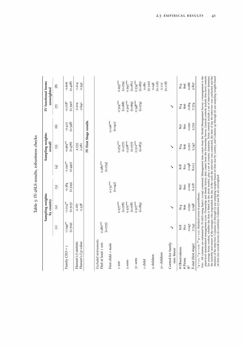
2.3 empirical results 41

Tabl

e5

:IV

-2SL

Sre

sult

s,ro

bust

ness

chec

ks

Sam

plin

gw

eigh

ts:

byco

untr

ySa

mpl

ing

wei

ghts

:ov

eral

lIV

func

tion

alfo

rms

unw

eigh

ted

(1)

(2)

(3)

(4)

(5)

(6)

(7)

(8)

z-m

gmt

z-m

gmt

z-m

gmt

z-m

gmt

z-m

gmt

z-m

gmt

z-m

gmt

z-m

gmt

Fam

ilyC

EO=

1-1

.04

9**

-1.0

14

**-0

.38

4-1

.02

0**

-0.9

62

**-0

.41

5-0

.71

8*

-0.6

06

(0.5

09

)(0

.50

3)

(0.5

29

)(0

.49

0)

(0.4

76

)(0

.54

8)

(0.3

90

)(0

.42

8)

Han

sen’

sJ

stat

isti

c2.1

67

2.5

35

0.2

19

1.2

14

Han

sen’

sJ

p-va

lue

0.3

38

0.2

81

0.6

40

0.5

45

IVFi

rst

Stag

ere

sult

sz-

mgm

tz-

mgm

tz-

mgm

tz-

mgm

tz-

mgm

tz-

mgm

tz-

mgm

tz-

mgm

t

Excl

uded

inst

rum

ents

Had

atle

ast

1so

n0.2

80

***

0.2

80

***

(0.0

75

)(0

.07

4)

Firs

tch

ild=

mal

e0.1

32

***

0.1

26

***

(0.0

42

)(0

.04

1)

1so

n0.2

77

***

0.2

74

***

0.3

04

***

0.2

93

***

(0.0

78

)(0

.07

7)

(0.0

68

)(0

.07

9)

2so

ns0.2

75

***

0.2

78

***

0.3

02

***

0.2

93

***

(0.0

78

)(0

.07

7)

(0.0

69

)(0

.08

1)

3+

sons

0.3

07

***

0.3

12

***

0.3

48

***

0.3

34

***

(0.0

84

)(0

.08

3)

(0.0

74

)(0

.08

5)

1ch

ild0.0

80

(0.1

20

)2

child

ren

0.0

46

(0.1

16

)3+

child

ren

0.1

10

(0.1

18

)C

ontr

olfo

rfa

mily

size

:lin

ear

33

33

3

#O

bser

vati

ons

81

88

14

80

78

18

81

48

07

81

48

14

#Fi

rms

81

08

06

80

08

10

80

68

00

80

68

06

R2

0.0

47

0.0

50

0.0

22

0.0

48

0.0

51

0.0

20

0.0

64

0.0

66

F-st

at(fi

rst

stag

e)7.7

45

5.0

98

6.2

18

8.0

13

5.3

47

5.7

25

7.3

74

5.8

07

*p

<0.1

,**

p<

0.0

5,*

**p

<0.0

1.S

tand

ard

erro

rsin

pare

nthe

ses.

Not

e:A

llco

lum

nsar

ees

tim

ated

byIV

-2SL

Sus

ing

Stat

a’sivreg2

com

man

d.M

anag

emen

tda

taco

mes

from

the

Wor

ldM

anag

emen

tSu

rvey

.z-m

anag

emen

tis

the

plan

t-le

vel

stan

dard

ized

man

agem

ent

scor

e.O

wne

rshi

pan

dfa

mily

hist

ory

data

com

esfr

omth

eO

wne

rshi

pSu

rvey

.Gen

eral

cont

rols

incl

ude

firm

-lev

elco

ntro

lsfo

rav

erag

eho

urs

wor

ked,

whe

ther

the

firm

islis

ted

onth

est

ock

mar

ket,

plus

ase

tof

coun

try

dum

mie

s.N

oise

cont

rols

incl

ude

ase

tof

inte

rvie

wer

dum

mie

s,th

ese

nior

ity

and

tenu

reof

the

man

ager

who

resp

onde

d,th

eda

yof

the

wee

kth

ein

terv

iew

was

cond

ucte

d,th

eti

me

ofda

yth

ein

terv

iew

was

cond

ucte

dan

dth

edu

rati

onof

the

inte

rvie

w.C

olum

ns(1

)th

roug

h(3

)us

esa

mpl

ing

wei

ghts

base

don

firm

size

byco

untr

y,an

dC

olum

ns(4

)th

roug

h(6

)us

esa

mpl

ing

wei

ghts

base

don

firm

size

over

all(

acro

ssal

lcou

ntri

es).

Col

umns

(7)

and

(8)

are

unw

eigh

ted.

2.3 empirical results 42

the 1 to 5 scale of the WMS and the difference between the manager’s percep-

tion and the “true” WMS score become the average information gap variable.

We show in Figure 7 that managers in family firms seem to be systematically

less aware of their own shortcomings than those in non-family firms. Thus, it

seems plausible that family firms are perhaps less well informed about (a) their

own level of quality of management, (b) what “best practice” management is,

(c) whether it is profitable for them to implement new practices, and (d) how

to implement such practices in their firm even if they wanted to do so.

Figure 7: Mechanisms: family firms are less well informed about how well they aremanaged

0 .5 1 1.5Average information gap (family firms - non family firms)

SwedenFrance

United StatesGermany

Great BritainItaly

AustraliaPortugal

NigeriaIndia

ArgentinaVietnam

BrazilChile

KenyaTurkeyMexico

Colombia

Family firmsNon-family firms

Finally, it could also be that incentives, or “influence costs,” are one of the

mechanisms driving lower adoption of management. This mechanism works

from the “bottom up” rather than “top down,” and the idea is that employ-

ees may accept new managerial structures (such as, say, increased monitor-

ing of their work) from a new professional CEO, but would resist it from a

family CEO who might be known to them. On the theoretical side, work by

Meyer, Milgrom, and Roberts [95] suggests this is a plausible scenario, and

there is also empirical evidence of such cases. Atkin et al. [7], in their technol-

ogy adoption experiment with soccer ball factories in Pakistan, show evidence

that worker pushback is indeed a possible reason for lack of technology adop-

tion. If we consider management as technology, as in Bloom, Sadun, and Van

2.4 conclusion 43

Reenen [32], this could be a mechanism driving the lower adoption of manage-

ment practices in family firms.

It is conceivable that family firms may face a different set of costs when

dealing with employees, and if there is a perception that modern management

practices are inherently labour-saving, there might be resistance to adopting

them. The next chapter in this thesis considers this possibility in a theoretical

framework.

2.4 conclusion

We set out to investigate the effect of family control on firm organization and

performance. We define family firms as firms that have a combined owner-

ship and control structure - that is, firms where the same entity (or, family)

both holds the majority of voting shares and the CEO position in the firm.

Adding to previous work in this area, we find that simple family ownership

does not fully explain family firms’ underperformance, but rather it is the

effect of the combination of ownership and control that seems to be driving

this. Given the notorious lack of data for private and family firms, particularly

for emerging economies, we first collect a rich new dataset on the history of

ownership and control successions for a sample of firms in Latin America and

Southern Europe, and match it with a unique dataset on firm organizational

structure and managerial practices. Relying on the body of work that has pro-

vided evidence on the strong relationship between managerial practices and

firm performance along with our new evidence from Brazil, we suggest that

poor management could be a channel driving family firms’ poor performance.

We consider whether the decision to appoint a family CEO had a causal effect

on firm management, and provide a brief discussion on possible mechanisms.

The new dataset we collected allowed us to add to the correlational findings

of Bloom and Van Reenen [29] and Bloom and Van Reenen [33] and suggest a

causal relationship by using an instrumental variables approach. We explored

the gender of the outgoing CEO’s children as exogenous variation to identify

the effect of a family CEO on the quality of management of a firm. We find con-

2.4 conclusion 44

vincing evidence that the gender mix of the children does affect the likelihood

of a succession to a family CEO: in families where there is at least one male

child the likelihood of a family succession of control is 30 percentage points

higher. We also present descriptive evidence that this is, indeed, a stylized fact

and strengthens our claim of the informativeness of the instrument. We argue

that, conditional on number of children, the gender mix of the children is as

good as random and unrelated to the managerial structures implemented in

the firm, thus satisfying the exclusion restriction.

Our OLS and IV-2SLS results suggest that there is a statistically significant

negative effect of family control, and the true effect sits somewhere between

-0.369 (OLS result) and -0.808 (IV result). To put this in context, a one standard

deviation change in management quality is associated with approximately 20%

higher value added per employee in Brazilian family firms. If we take this pro-

portional relationship, our results suggest that keeping the firm under family

control leads to between 7% and 16% lower value added per employee in the

average family firm.29 This result is strikingly within the same range as the

main results from Bennedsen et al. [16] in Denmark.

We believe that better management leads to better firm productivity, and

thus we believe that our results have key implications for policies in emerging

economies, where family firms dominate various industries. To the best of

our knowledge, this is the first piece of work to show causal evidence of this

negative effect of family control on internal organization of the firm, and also the

first such analysis to be done with emerging economies. This is also, however,

only the first step in this research agenda. Future research is needed into the

mechanism behind the choice of family CEOs to implement less managerial

structures than non-family CEOs, and what effect this might have on other

firm outcomes and characteristics, such as on employee satisfaction, wages

and work-life balance.

29Calculated as 0.369 ×20%≈ 7% ; 0.808 ×20%≈ 16%

2.5 appendix 45

2.5 appendix

ownership categories and additional summary statistics

Table 6 describes the definition of ownership and control structures used in

this paper. We differentiate between combined ownership and control, which

we refer to generally as “family firms” (for ease of exposition) and separate

ownership and control “non-family firms.” Table 7 shows the summary statis-

tics of the dataset we use in our analysis.

Table 6: Data categories - The Ownership Survey

Ownership category Ownership & controlNon-family Family

Founder or family ownedFounder owned, founder CEO 3

Founder owned, professional CEO 3

Family owned, family CEO 3

Family owned, professional CEO 3

Privately owned (non-founding family owners)*Single owner, owner CEO 3

Single owner, professional CEO 3

Many owners, owner CEO 3

Many owners, professional CEO 3

Dispersed shareholders** 3

* For the category of Privately owned, at least one entity owns more than 25% of votingshares, and they are not members of the founding family.** For the category of Dispersed shareholders, no one entity owns more than 25% ofvoting shares.

Figure 8 shows the share of employment attributed to family firms in the

WMS dataset. This graph is to quell concerns that, while there are many firms

in the manufacturing sector in these countries, they account for a small share

of employment.

2.5 appendix 46

Table 7: Summary statistics

Family CEO Non-family CEOMean Median SD N Mean Median SD N

Family characteristicsOf previous CEOFirst child = male 0.80 1.0 (0.40) 680 0.65 1.0 (0.48) 133

Had at least one son 0.95 1.0 (0.22) 689 0.81 1.0 (0.40) 135

# children 3.10 3.0 (1.60) 689 2.45 2.0 (1.46) 135

# children | first = boy 3.09 3.0 (1.60) 541 2.75 2.0 (1.53) 87

# boys 1.98 2.0 (1.12) 689 1.50 1.0 (1.12) 135

Of current firm# family members working in firm 2.04 2.0 (6.74) 689

Son 0.09 0.0 (0.28) 689

Brother 0.16 0.0 (0.36) 689

Total %: male family members 0.29 0.0 (0.45) 689

Daughter 0.04 0.0 (0.20) 689

Sister 0.08 0.0 (0.26) 689

Total %: female family members 0.17 0.0 (0.37) 689

Firm characteristicsEmployment 462.80 230.0 (701.70) 689 544.84 250.0 (822.46) 135

Firm age 50.52 47.0 (28.61) 689 46.35 41.0 (30.18) 135

MNE = 1 0.12 0.0 (0.33) 688 0.52 1.0 (0.50) 135

Share in low tech industries 0.47 0.0 (0.50) 689 0.30 0.0 (0.46) 135

% of employees with degrees 11.35 7.8 (12.77) 689 14.44 10.2 (14.41) 135

Management scoresManagement (overall) 2.68 2.7 (0.57) 689 2.90 2.9 (0.57) 135

Management: ops & monitoring 2.86 2.9 (0.72) 689 3.16 3.1 (0.70) 135

Management: targets 2.58 2.6 (0.68) 689 2.84 2.8 (0.68) 135

Management: people 2.55 2.5 (0.52) 689 2.63 2.7 (0.57) 135

Figure 8: Share of employment in founder/family firms, by country (manufacturing)

Middle/Low Income√√√√√√√√

√

√

√

√√√

√√

√

√

SingaporeSwedenAustralia

MozambiqueUnited StatesGreat Britain

FranceJapan

PolandIrelandChina

New ZealandCanadaEthiopia

ChileN. IrelandGermanyVietnamMexicoZambia

PortugalArgentina

GreeceTanzania

ItalyNicaragua

SpainBrazil

GhanaIndia

KenyaColombia

TurkeyMyanmar

Nigeria

0 .2 .4 .6 .8 1Share of employment in founder/family firms, manufacturing (WMS sample)

Note: Firms between 50 and 5000 employees, manufacturing sector. This graph uses the full WMS dataset and represents a random sample of firms within the manufacturing sector of each country. Each bar denotes the proportion of employees in founder/family firms WITHIN the WMSsample only. To create this graph, we took the random sample of firms in the manufacturing sector from each of the countries (ie. the fullWMS sample) and simply calculated the total number of workers as reported by the firms within each country, calculated the total number ofworkers within only family firms in each country, and took the ratio of these two numbers. This is, admittedly, a crude measure of employmentshare given it is only using the WMS sample of firms rather than the universe of firms. Given the data constraints in over half of the countries in the graph, however, and the fact that the WMS sample is a close approximation of a random sample of firms between 50 and 5000 employees in the manufacturing sector of these countries, we believe it is a good estimate of the pattern we are trying to show.

2.5 appendix 47

management across regions and industries One important con-

sideration is to what extent we should be treating this relationship between

family control and management practices as something that is common across

countries. It could be that family ownership and control matters more in coun-

tries where there is less competition, better rule of law, or a different mix of

industries. To consider this, we broke the full WMS sample into the continen-

tal regions and report the results in Table 8. The coefficients across nearly all

regional specifications are not statistically different from each other, with the

exception of Africa. This suggests that across the world, being owned and con-

trolled by a founder or founding family is associated with a similar negative

effect on firm management.

Table 8: Management and family ownership and control across regions, WMS

Anglo-Saxon

Sca’ via &W. Europe

S & CEurope

LatinAmerica

Asia Africa

Family Control = 1 -0.166*** -0.149*** -0.162*** -0.211*** -0.168*** -0.122***(0.024) (0.032) (0.030) (0.021) (0.029) (0.034)

Ln(employment) 0.123*** 0.153*** 0.178*** 0.221*** 0.129*** 0.134***(0.008) (0.012) (0.017) (0.010) (0.010) (0.016)

Observations 4299 2438 1904 3049 2453 867

Noise controls 3 3 3 3 3 3

Industry controls 3 3 3 3 3 3

Firm controls 3 3 3 3 3 3

* p < 0.1, ** p < 0.05, *** p < 0.01. Standard errors in parentheses.Note: All columns estimated by OLS with standard errors clustered by firm and reported in brackets below the estimates.

Sample includes all firms with controls data. Management is the plant-level management score. Controls include a fullset of country dummies, US-SIC dummies and year dummies, as well as firm-level controls including the proportionof employees with college degrees (from the survey), interviewer dummies, the seniority and tenure of the managerwho responded, the day of the week the interview was conducted, the duration of the interview, and an indicator ofthe reliability of the information as coded by the interviewer.

Finally, another interesting feature to consider in terms of firm characteris-

tics is the industrial mix in each group of firms. Figure 9 shows the relation-

ship between management and the share of family firms within each 2-digit

industrial sector. Each observation is an industrial sector and it is colour coded

to indicate high (red) and low (hollow blue) tech industries. High tech indus-

tries are overwhelmingly both better managed and have lower shares of family

firms. This result echoes one of the findings in Bennedsen et al. [16], where they

suggest that the negative effect of family CEOs are worse for firms in higher

tech industries. To take this into account we ensure we add industry fixed ef-

2.5 appendix 48

fects to all our specifications, and this is an avenue of research that could be

explored in the future with more detailed administrative datasets.

Figure 9: Share of family firms and average management scores, by industry

Food

TextileApparel

Lumber

Furniture

Paper

Printing

Leather products

Other manufacturing

Chemicals

Petrol products

Stone, clay and glass

Primary metal

Non-elecrical machineryElectronic equipment

Instruments

Rubber & plasticsFabricated metal

Transportation equipment

2.4

2.6

2.8

33.

2Av

erag

e fo

rmal

man

agem

ent p

ract

ices

0 .1 .2 .3 .4Share of family firms

High tech industry sectorsLow tech industry sectorsmanagement xshare of founder/family firms

Note: Data from the World Management Survey. N=14939.

ownership survey : data structure details Figure 10 shows a di-

agram of a hypothetical firm surveyed both by the Ownership Survey and the

WMS. In this example, the WMS surveyed this hypothetical firm once between

t = 1 and t = 2. The Ownership Survey collected data on: the date of foun-

dation (t = 0) and each date of succession (t = 1); who owned the firm at

each time bracket and the family characteristics of the founder and each fam-

ily owner-CEO after. In terms of the merged data, the family characteristics of

the founder, who owned and managed the firm between t = 0 and t = 1, will

be the instrumental variables for the WMS management measurement after

t = 1.

For example, take two hypothetical Brazilian firms: Firm A is currently a

“family firm” and Firm B is currently a “non-family firm.” Firm A was founded

in 1980 and its founder handed down control of the firm to his son in 2005,

who is still presiding over the company. Firm B was founded in 1990 by a

founder who decided to sell the firm in 2000 to a set of investors (“private in-

dividuals,” by our categorization). These investors chose to hire a professional

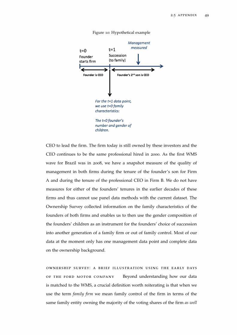
2.5 appendix 49

Figure 10: Hypothetical example

CEO to lead the firm. The firm today is still owned by these investors and the

CEO continues to be the same professional hired in 2000. As the first WMS

wave for Brazil was in 2008, we have a snapshot measure of the quality of

management in both firms during the tenure of the founder’s son for Firm

A and during the tenure of the professional CEO in Firm B. We do not have

measures for either of the founders’ tenures in the earlier decades of these

firms and thus cannot use panel data methods with the current dataset. The

Ownership Survey collected information on the family characteristics of the

founders of both firms and enables us to then use the gender composition of

the founders’ children as an instrument for the founders’ choice of succession

into another generation of a family firm or out of family control. Most of our

data at the moment only has one management data point and complete data

on the ownership background.

ownership survey : a brief illustration using the early days

of the ford motor company Beyond understanding how our data

is matched to the WMS, a crucial definition worth reiterating is that when we

use the term family firm we mean family control of the firm in terms of the

same family entity owning the majority of the voting shares of the firm as well

2.5 appendix 50

as having a family member presiding over the company as CEO: combined own-

ership and control. To illustrate the data we collected and our definitions, it is

useful to consider a well-known example such as the early days of the Ford

Motor Company. Ford was founded in 1903 by Henry Ford, who had one son.

In 1919 Henry Ford passed the position of CEO to his son, Edsel, until Edsel

(unexpectedly) died in 1943. Edsel had four children: three boys and one girl.

Henry Ford briefly took control for the interim two years until 1945 when Ed-

sel’s first son, Henry Ford II, returned to the US and assumed the helm of the

firm. Henry Ford II had three children: two girls and one boy, Edsel Ford II.30

In 1956, Ford went public in the largest IPO (initial public offering) of common

stock shares in history at the time, but the Ford family still retained 40% of the

voting shares.31 Up to this point, the Ford Motor Co. would be considered a

family firm in the Ownership Survey as the Ford family held over 25% of the

voting shares and a family member from the original founding family held the

CEO position in the firm. We would have, thus far, registered three successions

of power within the family.32

A non-family firm, on the other hand, has separate ownership and control.

Continuing with the Ford Motor Co. example, in 1980 Phillip Caldwell be-

came the first non-Ford-family member to take the post of CEO. From 1980

onwards Ford is considered a non-family firm in our analysis. The data point

would be recorded as “family owned, professional CEO,” (ie. the green boxes

in Figure 3) but as discussed earlier, we combine all categories that are not

owned and controlled by families under non-family firm. An example of what

the early Ford history would look like in our survey instrument is shown in

Figure 11. If the Ford family ever chose to divest or dilute their voting shares

such that the family’s voting ownership stake of the firm fell to below 25% of

the shares, they would then continue to be coded as a non-family firm category,

but their ownership sub-category would change to dispersed shareholders.33 Cru-

30Edsel Ford II ran Ford Australia between 1978 and 1980.31According to Ford Motor Co.’s website. It is important to note that when they took the com-

pany public the family separated the type of stock offered into 95% Class A shares (no votingrights) and 5% Class B (voting rights) shares. The Ford family in fact owned less than 2% ofthe company as a whole, but crucially, they own 40% of the Class B voting shares, affordingthem majority control of the company.

32Henry Ford 1903-1919, Edsel Ford 1919-1943, Henry Ford 1943-1945, Henry Ford II 1945-1979.33History of the Ford Motor Co. primarily obtained from the Ford Motor Co.’s website:

https://corporate.ford.com/company/history.html, last accessed on January 15, 2016.

2.5 appendix 51

cially, our identification strategy would not use ownership successions that, for

example, started as “family owned, professional CEO” and switched to “dis-

persed shareholders, professional CEO.” Our identification is coming from

firms that have successions of control, such as a “family owned, family CEO”

firm hiring a professional CEO or, alternatively, selling the firm outright/dilut-

ing their shares to under 25% voting ownership to non-family investors who

then hire a professional CEO.

A concern could be that what we will capture with this strategy is the effect

of the change in ownership rather than the change in control, as in our anal-

ysis we combine firms that have changed only control with those who change

ownership and control. The best scenario would, indeed, be to have a large sam-

ple of firms that switched from having family ownership and control to family

ownership and professional control, but that is a limitation of our dataset (in-

deed, of “reality”) that we do not think is fatal. First, as evidenced in Figure 3,

although the family ownership with professional CEO structure is relatively

more common in OECD countries than in middle- and low-income countries,

it still constitutes a very small share of the overall ownership and control struc-

tures that we study. Among the countries we study it is an even smaller part of

the share of firms in the economy. Thus, the next best alternative is comparing

family owned and controlled firms with non-family owned and professionally

controlled firms.34

34Once we match the Ownership Survey data with the Brazilian industrial census we will hope-fully be able to say more about the effect of changes in ownership without changes in CEO.

2.5 appendix 52

Figu

re1

1:S

urve

yin

stru

men

t,hy

poth

etic

alex

ampl

e:Fo

rdM

otor

Com

pany

2.5 appendix 53

world management survey : 18 management topics measured

The tables below describe the WMS practices measured and what they mean.35

Practices What is the WMS measuringOperations Management and Performance MonitoringIntroducing Lean (modern)Techniques

Measures how well lean (modern) manufacturing man-agement techniques have been introduced

Rationale for introducing Lean(modern) Techniques

Measures the motivation/impetus behind changes to theoperational processes, and whether a change story waswell communicated turning into company culture

Continuous Improvement Measures attitudes towards process documentation andcontinuous improvement

Performance Tracking Measures whether firm performance is measured withthe right methods and frequency

Performance Review Measures whether performance is reviewed with appro-priate frequency and follow-up

Performance Dialogue Measures the quality of review conversations

Consequence Management Measures whether differing levels of firm performance(not personal but plan/process based) lead to differentconsequences

Target SettingTarget Balance Measures whether targets cover a sufficiently broad set of

metrics and whether financial and non-financial targetsare balanced

Target Interconnection Measures whether targets are tied to the organiza-tion’s objectives and how well they cascade down theorganization

Time Horizon of Targets Measures whether the firm has a ’3 horizons’ approachto planning and targets

Target Stretch Measures whether targets based on a solid rationale andare appropriately difficult to achieve

Clarity and Comparability ofTargets

Measures how easily understandable performance mea-sures are and whether performance is openly communi-cated to staff

People ManagementManaging Talent Measures what emphasis is out on overall talent manage-

ment within the organization

Rewarding High Performers Measures whether there is a systematic approach to iden-tifying good and bad performers and rewarding themproportionately

Removing Poor Performers Measures how well the organization is able to deal withunderperformers

Promoting High Performers Measures whether promotion is performance-based andwhether talent is developed within the organization

Retaining Talent Measures whether the organization will go out of its wayto keep its top talent

Creating a Distinctive Em-ployee Value Proposition

Measures the strength of the employee value proposition

35Note: Full survey instruments available at www.worldmanagementsurvey.org.

3FA M I LY F I R M S A N D T H E C O S T S O F M O N I T O R I N G : A

T H E O R E T I C A L P E R S P E C T I V E

“ Mischief occurs when economists begin to treat a model as the model.Then the narrative takes on a life of its own and becomes dislodgedfrom the setting that produced it. It turns into an all-purpose expla-nation that obscures alternative, and potentially more useful, storylines. ”

Dani Rodrik, Economics Rules, p.174, 2017

3.1 introduction

As shown in the previous chapter, firms owned and controlled by families are

the most common ownership type in the world. This chapter will focus on the

CEO appointment decision by family firm owners, and crucially how the ap-

pointed CEO makes the decision regarding managerial structures they adopt

in their firms. This is an important set of decisions to unpack: the decision of

who is appointed the CEO of the firm significantly matters for management

quality as well as productivity. The reasons underpinning the relationship be-

tween CEO choice and management, however, are still unclear. The previous

chapter proposes that one of the reasons for family firms’ underperformance is

the lack of formal managerial structures relative to other firms, and provides

causal evidence that a succession to family CEO leads firms to implement

fewer such structures. In this chapter I will build a theoretical framework to

guide the discussion of the possible mechanisms behind this result, and sug-

gest ways to empirically test this framework in future work.

I propose a practical theoretical framework that suggests family CEOs choose

different levels of managerial structures compared to professional CEOs based

54

3.2 why we should care about family control 55

on costs unique to them that arise as a result of implicit labour contracts

present in family-controlled enterprises. In this model, I consider managerial

structures as a type of monitoring technology that allows the CEO to identify

the level of worker effort. It is only profitable to implement such a technology

if the CEO makes use of the information and takes action against low effort

employees. Family CEOs incur a utility cost of carrying out such actions – such

as possibly dealing with a community backlash, or a “firm reputation” cost –

and as such they cannot credibly commit to discipling workers. This, therefore,

elicits low effort from employees and reduces the return to adopting this ad-

vanced monitoring technology for CEOs who cannot make the commitment to

discipline. Professional CEOs, on the other hand, can credibly commit to take

action on low effort workers (ie. layoffs), and thus elicit high effort from them.

The key aim of this theoretical framework is to characterize one aspect of

the decision process of the family CEO regarding the adoption of good man-

agerial structures (henceforth “monitoring”), and disentangle the reasons why

some CEOs choose to do so and others do not. There is an extensive literature

examining the decision of a firm owner to hire a professional CEO versus ap-

pointing a family member as CEO, as well as more recent work on the hiring

and firing decisions of family and professional CEOs — I discuss both in the

next section. The work in this area has primarily focused on profits, however,

and has not directly considered how organizational choices, such as manage-

ment practices, may be affected. The approach I propose in this chapter is to

focus on this organizational choice, and characterize the different costs and the

mechanism behind the tradeoffs faced by the family firm owners when mak-

ing joint decisions on adoption of management best practices and succession

of firm control.

3.2 why we should care about family control

There are two strands of literature that relate to this chapter: the first is the

literature on the relationship between firm ownership and productivity, and the

second is the literature on firm control and productivity. The literature on the

3.2 why we should care about family control 56

performance of family vs non-family owned firms is relatively mixed, though

evidence for the underperformance of family-run firms is more consistent.

Starting with ownership, the literature on ownership concentration spun

from the seminal work of Berle and Means [21], The Modern Corporation and

Private Property. The authors were concerned with the move towards owner-

ship structures where shares were widely held and firms were controlled by

a class of professional managers. They warned that separation of ownership

and control would create a structure that moved agents away from maximiz-

ing profit in favour of non-value-maximizing management’s desires, such as

on-the-job consumption. A few decades later, their ideas started being formal-

ized in the agency literature.1 The main tension in this set of models is between

the principal (the owner) whose objective is maximization of profits, and the

agent (the manager) who maximizes his own utility and whose effort level is

not perfectly observed by the principal.

The ubiquitous “dispersed shareholder” corporation of the Berle and Means

[21] vision, however, has not materialized. Empirical studies have shown that,

with the exception of the United States and the United Kingdom, the predomi-

nant structure in the world is not dispersed ownership but rather is one where

the major group of controlling shareholders is a family. La Porta, Silanes, and

Shleifer [89] look at the ownership structures of the 20 largest publicly traded

firms in each of 27 richest economies and find that 36% of firms worldwide are

widely held while 30% are family-controlled and 18% are state-controlled.2

One leading explanation for this difference put forward by the authors is

that ownership structure of firms is linked with a country’s shareholder protec-

tion regulation.3 In a related paper, La Porta et al. [90] suggest that the under-

development of financial markets and weak legal systems in many countries

make the separation of ownership and control difficult. Mueller and Philippon

[99] argue for an alternative — though not mutually exclusive — explanation,

where family firms are particularly effective at coping with difficult labour re-

1See, for example, Berhold [20] and Jensen and Meckling [81]2The remaining 15% are other categories. They define a family firm as a firm where the familyholds at least 20% of the shareholdings.

3Thus, family firms prevail in countries with poor minority shareholder protection and, by con-trast, widely dispersed firms are more common in countries with strong minority shareholderprotection.

3.2 why we should care about family control 57

lations, so they arise as a natural response in countries where labour relations

are hostile. As it relates to productivity, it is unclear whether higher ownership

concentration is good for productivity, and it seems to be quite context specific:

ownership concentration and performance has been found to have a positive

correlation (Anderson and Reeb [2], Claessens and Djankov [50], and Sraer and

Thesmar [114], an inverse u-shaped relationship (Morck, Shleifer, and Vishny

[96]) or even no relationship (Demsetz and Villalonga [56]) depending on the

sample of firms used.

In terms of control, there is a larger consensus that family CEOs are asso-

ciated with lower financial outcomes, but perhaps better labour outcomes. A

study by Bennedsen et al. [16] was one of the first to provide rigorous evi-

dence of the effect of family control using the incidence of male primogeniture

among CEOs of firms in Denmark to infer the causal effect of family control

on firm performance. They find a large negative causal impact on firm perfor-

mance following family successions in the top management role. In particular,

they find that the type of industry is important, and that family CEOs under-

performance is worse in innovative and fast-growing industries, where there

is a relatively higher incidence of larger firms and higher skilled employees.

Other studies have also found that who the CEO is matters for firm perfor-

mance (Bandiera et al. [11], Bennedsen, Perez-Gonzales, and Wolfenzon [17,

18], Bertrand and Schoar [23], Bertrand et al. [25], and Perez-Gonzales [105]),

and Chapter 2 of this thesis presents evidence that who the CEO is matters for

the quality of management in the firm.

Although there is a relative consensus that family controlled firms have

poorer financial outcomes, there is some evidence that they have arguably

better labour outcomes. Bassanini et al. [12] show that French family firms pay

lower wages, and attribute this to both a sorting of lower-productivity workers

into family firms and a compensating differential for higher job security. Bach

and Serrano-Velarde [8] find similar results when interacting with an exoge-

nous productivity shock, and suggest the level of frictions within the labour

market widen the difference in job security (ie. layoff incidence) between fam-

ily and non-family firms. Bennedsen, Tsoutsoura, and Wolfenzon [19], however,

3.2 why we should care about family control 58

find that employees at family firms in Denmark tend to exert higher effort – as

measured by employee workplace absenteeism – and find that the firm-specific

component accounts for 72% of the absenteeism gap. Looking at the manage-

rial level, using a time-use survey of over 1,100 CEOs across six countries,

Bandiera, Prat, and Sadun [10] family CEOs tend to work fewer “in-office”

hours. Ellul, Pagano, and Schivardi [59] show for a sample of 41 countries

that family firms tend to provide better job security, but provide less wage

stability. They further use Italian employer-employee data to show that family

firms pay lower wages and have less separations, and that adjustments occur

through the hiring margin (that is, they hire less). Bach and Serrano-Velarde [8]

find identical patterns using French data. Mueller and Philippon [99] suggest

that family firms are “particularly effective” at dealing with labour relations

and thus are more prevalent in settings where labour relations are difficult.

These results suggest there is evidence that family firms, indeed, have implicit

contracts with employees relating to job security, and this should feature in a

model of technology adoption if the technology could be perceived as a threat

to jobs. I return to this in the set up of my model.

In all, there is plenty of empirical evidence that points to the fact that the

choice of CEO matters, and it is thus an important decision to understand. The

model I present in this chapter starts with the owner’s decision of whether to

hire a professional CEO or appoint a family CEO, and I will briefly discuss the

literature surrounding this decision to put the model into context.

3.2.1 The succession decision

A wave of research followed Berle and Means [21] and debated the results as

well as formalized the ideas. Demsetz [55] argued, opposing Berle and Means,

that the ownership structure of a firm is an endogenous result of a maximiz-

ing process, that is, the structure can be seen as the result of firm decisions

aimed at value maximization, even if that means utility maximization by the

owner-manager.4 Later Demsetz and Lehn [57] further developed Demzetz’

4To illustrate this point, Demsetz uses the example of an owner-manager’s consumption interms of hiring workers. Considering this to be part of the owner-manager’s on-the-job con-

3.2 why we should care about family control 59

initial idea and introduce the concept of “amenity potential” as a component

of owner-managers’ utility maximization problem, which refers to private ben-

efits of control accruing to the family member who owns and runs the firm.

These can include political and social influence associated with the family com-

pany’s name or perhaps the pleasure of running the firm or having his child

run it.5

The conceptual frameworks established by these earlier works were then fur-

ther developed to consider the context of family firms, and formalized most

notably by Chami [46], Bhattacharya and Ravikumar [26, 27] and Burkart and

Panunzi [42]. The key question addressed in this set of works considers the

principal-agent problem of the owner-manager who is choosing whether to

separate the ownership and control of his firm, or stay as a concentrated own-

ership family firm.

Chami [46] develops a theoretical model to explain the continued existence

of family firms despite evidence of their lower average levels of productivity.

and concludes that trust among family members gives family firms a com-

petitive edge because it mitigates moral hazard problems while raising the

expected effort of the child (agent).6 Bhattacharya and Ravikumar [26] look at

the family business as a dynamic household model where capital market im-

perfections determine the evolution of the family business, though the focus of

their paper is on when the family decides to sell its business to a private buyer,

rather than who they sell it to.7 Bhattacharya and Ravikumar [27] consider the

evolution of firm management, but analyze the trade-off between hiring an in-

sider with aligned interests (that is, a family member) and hiring an outsider

sumption set, he could maximize utility by hiring a set of workers based on sets of character-istics he valued more than sheer labour productivity, such as religious affiliation.

5They empirically analyze 511 large US firms and find no relationship between dispersion andfirm performance. They also suggest that the predictability of the environment where thefirm operates has an effect on the monitoring and transaction costs associated with hiringprofessional managers to run the firm, and that regulation reduces the cost of monitoring anddisciplines managers - a point later picked up by many in explaining the incidence of family-run firms across countries.For a formal treatment of imperfect information on monitoring costs,see Holmström [75] and Holmström and Tirole [76].

6This trust also allows the principal to avoid reliance on monitoring schemes to elicit effort fromthe agent but also means the agency problem is exacerbated if this altruism is one-sided.

7They characterize the family business as a household operating constant-returns-to-scale pro-duction and see “business skill” as the fixed factor of production that gets passed throughgenerations. Their main result is that family businesses tend to be larger when they cash out,and they also last longer and have lower investment rates in economies with less well devel-oped primary capital markets.

3.2 why we should care about family control 60

with non-aligned interests (a professional CEO) who is more productive than

the insider. The key result is that, although the external manager is unequivo-

cally more productive, the family only chooses to hire the outsider after they

reach a certain critical size, which in turn depends on the level of development

of the capital markets.

Burkart and Panunzi [42], consider the same problem as Bhattacharya and

Ravikumar [26] but in a static, cross-sectional framework. They focus on the

fear of expropriation by the outside manager and build a theoretical model to

weigh the costs and benefits of separating ownership and control in a family

firm. Their static model considers the point of succession, that is, the moment

the founder either chooses to pass the business on to his kin or to separate

ownership and control. Their founder has three choices: (a) disperse ownership

and delegate control by selling the company into this dispersed shareholder

structure and hiring a professional CEO, (b) keeping ownership concentrated

but delegating control by staying as a majority shareholder, hiring an profes-

sional CEO and actively monitoring him, or (c) keeping ownership and control

concentrated by retaining shareholdings in the family and either staying on as

CEO or passing control to a family member who is, presumably, less talented

than an professional CEO. The founder’s goal is to maximize his welfare, a

function of his shares’ value (both retained and value of sales) and “amenity

potential.” The professional CEO’s goal is also to maximize his own welfare,

a function of possible rents and wages. Monitoring by the founder - as in (b) -

and a better legal institutional framework both reduce the possibility of expro-

priation by the outsider.

They find that, in equilibrium, good legal systems negate the need for mon-

itoring and we end up with Berle and Means’ dispersed shareholder-owned

and professionally managed firm. When legal protection is so weak that it hin-

ders the ability of the founder to monitor expropriation, the founder does not

delegate management to an outsider but rather keeps it within the family de-

spite lower levels of talent. In the intermediate range of legal protection, the

founder does hire an outsider to run the firm, but stays as a majority share-

holder and implements a certain level of monitoring. They thus predict an

3.2 why we should care about family control 61

inverse relationship between the quality of legal systems and the concentra-

tion of ownership, which is indeed what the empirical evidence points to. It

also consistent with the empirical evidence on the average lower quality of

top-level management of family firms vis-à-vis non-family firms.

I build on this result from the literature in the first step of the model I

propose. In my model, the first decision taken by the family firm owner is

whether to hire a professional CEO or to appoint a family CEO. As the value

added in my framework is to understand a possible mechanism behind why

CEOs – family and professional – choose to adopt a monitoring technology

or not, I simplify the parameters in the model to reflect the result already

discussed in the literature.

My model draws on the general findings of the literature thus far, and adds

to understanding the black box of the internal workings of family firms and

decisions of family CEOs. Much of the literature has suggested that family

CEOs are inherently different from professional CEOs, most clearly in terms

of education and perceived ability. Although it is reasonable to assume that a

CEO picked from a small pool of family members (with, say, a random draw

from an ability distribution) is likely to be of lower ability than a CEO picked

from a larger pool of individuals self-selected into the profession, this is likely

only one part of the story. Simply ascribing family firms’ lower productivity

to lower CEO ability ignores, for example, firm-specific knowledge that the

family CEO may inherit, as well as other labour dynamics that may be at play

such as the different objectives and costs faced by family CEOs. In my model,

I seek to characterize the structure of the differential costs faced by family

CEOs, and suggest how they relate to the decisions of CEO succession and

management structures.

3.3 model 62

3.3 model

3.3.1 Setup: conceptual overview

The overview of the model is as follows: the game has three players: the owner,

the CEO and the worker. The owner decides who the CEO is. The CEO can

be a professional CEO hired by the owner, or the owner himself taking on the

role of CEO. The worker is hired by the CEO and is not a family member.

The game starts with the family firm owner first choosing whether he will

hire a professional CEO or manage the firm himself (and be a family CEO).

The CEO (family or professional) moves second and chooses to invest in mon-

itoring (ie. good management practices) or not to invest in monitoring (ie. no

management practices), and hires workers to produce output. Workers move

third and choose high or low effort, based on their relative cost of effort to

the cost of being laid off. The worker can be of high or low ability: high abil-

ity workers have low cost of effort and will opportunistically choose to shirk

(exert low effort) depending on the chance of getting caught. Low ability work-

ers have high cost of effort and will opportunistically always choose to shirk,

regardless of the chance of getting caught. For any given industry, there is a

share of workers η who will be of high ability.

Investing in monitoring allows the CEO to see whether workers are exerting

effort or not. The technology has a fixed cost, and it is only worth imple-

menting if the CEO uses the information to discipline (lay off) the low-effort

workers. All CEOs incur a cost of laying off employees, but the family CEO

also has a dynastic commitment to their workforce and faces an additional

cost of doing so. The workers know whether the CEO invested in monitoring,

and know that family CEOs tend to have higher costs of disciplining workers.

They choose effort based on these facts, and only choose high effort when the

monitoring technology is in place (that is, they can be caught shirking) and

there is a chance they would be disciplined.

The key trade-off in this model is between the private benefit of control the

owner gets from being the CEO of the family firm, the cost of firing employees

3.3 model 63

incurred by the different CEOs, and the inducement of worker effort that is

afforded by investing in monitoring. If the added profit from hiring a profes-

sional CEO is substantial enough to outweigh the private benefit of control,

the owner will hire a professional CEO.

Crucially, I do not assume that professional CEOs are of higher ability than

family CEOs, distinguishing this model from others such as Burkart, Panunzi,

and Shleifer [43]. Although there is evidence that firms run by heirs tend to be

less profitable, the point of this model is to explore why else this might be the

case if we assume family CEOs are as capable as professional CEOs. This is a

worthwhile exercise because it is not clear that family firm CEOs in middle in-

come countries are, in fact, less well educated — or less “professional” — than

their non-family counterparts. Indeed there is anecdotal evidence that sons set

to inherit family firms are often groomed to take on positions of power within

the company from an early age and families invest substantial resources on the

child for that reason.8 Thus, in this model I choose to allow CEOs to be of sim-

ilar ability and consider alternative explanations behind the observed lower

levels of profitability under the assumption that they are making rational and

informed choices. In this model, profits are simply a function of worker ef-

fort and are higher when CEOs invest in monitoring because it induces higher

worker effort. I abstract from the possibility that workers in family firms can

have intrinsic motivation at this point, but discuss this as an avenue of fur-

ther research in the conclusion of this thesis. I also abstract from assuming

a productivity shock that encourages firms to fire employees, as in Bach and

Serrano-Velarde [8].

3.3.2 Actions and information

There are four action choices in the game, one action each for the owner and

for the worker and two actions for the CEO.

An action set for an owner is a binary management choiceMg ∈ PRO, FAM,

where Mg = PRO means that the owner is hiring a professional CEO, and

8In a separate project, I am collecting data on education of the CEO and their siblings to findempirical evidence on this question.

3.3 model 64

Mg = FAM means that the owner is choosing to manage the firm himself

and acts as a family CEO.

An action for a CEO is a pair: an investment choice, i, and a disciplining

choice, d. The investment choice is a binary investment choice i ∈ iy, in,

where i = iy denotes investment in the monitoring technology and i = in

denotes no investment. The disciplining choice is a binary choice d ∈ DK,DL,

where d = DK denotes keeping the worker, and d = DL denotes laying off the

worker.

An action for worker is a binary effort choice, e ∈ e, e.

Figure 12 presents the model’s timeline of the order of the actions. The game

only runs once. I consider a firm owner at t = 0, and the owner moves first to

choose a manager, family or professional. At t = 1, the appointed CEO chooses

whether to invest in a monitoring technology or not. At t = 2 the workers

decide whether to exert effort. At t = 3 production is realized and total profits

generated. The CEO then decides whether to keep or lay off workers and final

payoffs are realized.

Figure 12: Timing of decisions

Owner choosesmanager Mg

t=0

CEO choosesinvestment i

t=1

Worker chooseseffort e

t=2

CEO choosesdisciplining action d

t=3

All decisions by the owner and the CEOs are public information. The worker’s

effort choice is observable by the CEO only if the CEO invested in monitoring,

otherwise the worker’s decisions are private. Workers can be of high or low

ability. Individual worker ability is private information, but within each indus-

try the share of workers who are high ability, η, is public information.

3.3 model 65

3.3.3 Payoffs and strategies

3.3.3.1 Workers

The payoff of a worker is a function of effort, wages and the disciplining deci-

sion of the CEO. Let the utility function for the worker be:

uw =

W if e = e and d=DK

W − ce if e = e and d=DK

W − `w if e = e and d=DL

W − ce − `w if e = e and d=DL

(9)

where W is the worker wage, ce is the cost of effort if the worker chooses to

exert effort (e = e), and `w is the fixed utility cost of being laid off if the CEO

chooses d = DL.

3.3.3.2 CEOs

The payoffs for the CEO have the same structure, but individual parameter

values depend on the CEO’s identity. For the sake of clarity I specify the pay-

offs for the family CEO and the professional CEO separately below, but note

how they follow the same structure. Let the cost of laying off workers that is

common to all CEOs be `c and let us call it the “industry cost”. This cost is

exogenously set. Let the cost of investment in the monitoring technology be m.

Let firm profits be only a function of worker effort: π(e).

professional ceo : Professional CEOs are paid a share of profits, λπ(e),

as their compensation. λ is exogenously set. The professional CEO’s cost of

effort in running the firm is embedded in the contract design and the “wage”

he has accepted the contract at. The payoff of a professional CEO is a function

3.3 model 66

of wages λπ(e), cost of adopting managementm, and cost of laying off workers

`c.9

upro =

λπ(e) if d = DK and i = in

λπ(e) − `c if d = DL and i = in

λπ(e) − m if d = DK and i = iy

λπ(e) − `c − m if d = DL and i = iy

(10)

family ceo : The family CEO incurs a cost of effort of running the firm

cMg ∈ [0, 1], but unlike the professional CEO he also accrues a private utility

benefit from controlling his family firm, B ∈ [0, 1]. Let Γ be the net utility cost

of control: Γ = cMg −B ∈ [−1, 1].

The family CEO incurs an additional cost of laying off workers: a firm rep-

utation cost f. The payoffs of a family CEO is a function of the profits of the

firm π(e), the cost of control Γ , the cost of the investment choice m and the

total costs of laying off workers `c + f:

ufam =

π(e) if d = DK and i = in

π(e) − (`c + f) if d = DL and i = in

π(e) − m − Γ if d = DK and i = iy

π(e) − (`c + f) − m − Γ if d = DL and i = iy

(11)

In short, the two types of CEOs face the same payoff structure, but family

CEOs have a set value of λ = 1, and professional CEOs have set values of f = 0

and Γ = 0.

9The cost of adopting the monitoring technology m is incurred by CEO rather the firm as he isthe executive in charge of pushing changes through.

3.4 equilibrium 67

3.3.3.3 Owner

The family firm owner’s payoffs are the same as the family CEO’s if he chooses

to manage the firm himself, Mg = FAM, and simply the share of leftover

profits if he chooses Mg = PRO:

uown =

π(e) if Mg = FAM, d = DK and i = in

π(e) − (`c + f) if Mg = FAM, d = DL and i = in

π(e) − Γ − m if Mg = FAM, d = DK and i = iy

π(e) − (`c + f) − Γ − m if Mg = FAM, d = DL and i = iy

(1− λ)π(e) if Mg = PRO

(12)

3.4 equilibrium

3.4.1 Comments on modelling choices

worker’s effort choice Let workers have a cost of effort ce ∼ U(0, 1).

There is a share of workers, η, for which the cost of effort is below the fixed cost

of getting laid off lw, such that ce 6 `w. These workers will choose to exert

effort if they have a chance of getting laid off, and will choose not to exert effort

if they have no chance of getting laid off. There is a share of workers 1− η for

which the cost of effort is above the cost of getting laid off, such that ce > `w.

These workers will never exert effort, regardless of the chance of getting laid

off. A way to interpret this setup is to think of employees as being of high or

low ability and a share of them who have high ability (η) can choose to work

as it is not too costly, whereas a share 1− η has low ability and always find it

too onerous to work.

3.4 equilibrium 68

Figure 13: Distribution of the cost of worker effort, ce

Low ce

0

`w High ce

1

η

Work when i = iyShirk when i = in

1− η

Always shirk

professional ceo compensation λπ(e) is the executive’s compensa-

tion. I assume the CEO does not have enough capital to purchase the firm

outright and thus has to be employed. I assume λ to be exogenous and rep-

resents the CEO net wages, taking into account the manager’s cost of effort

of running the firm. The λ here could also include any profit appropriation

that may happen because of low legal oversight, as in Burkart, Panunzi, and

Shleifer [43]. I assume this payoff will be larger than their outside option, such

that there is at least one professional CEO who always agrees to manage the

firm if the contract is offered.

ceo costs of control Γ is the net cost of control. It is essentially rep-

resenting the cost of effort that a CEO has to expend to run a firm, net of any

private benefit of control he may accrue from doing so. Intuitively, the variable

setup suggests that if the private benefit of control is relatively low, the family

CEO would compare the cost of effort to the financial cost of hiring a profes-

sional CEO. If the family CEO gains a very high level of private benefit from

control relative to how onerous it is for him to manage the firm, the utility cost

would be “negative”.

Γ = 0 for professional CEO is a simplification, but a reasonable one for the

current purposes of the model. Conceptually, the professional CEO would also

incur cMg, but this cost would be included into the λπ(e) payoff bundle. I am

implicitly assuming that cMg is equal for professional CEOs and family CEOs

— that is, I am in a sense assuming the same level of ability for both CEO

3.4 equilibrium 69

types. This is a departure from the usual assumption in previous models, but

one that can be relaxed at a later time.10

ceo layoff costs All CEOs incur a common cost of laying off workers,

`c ∈ `−c , `+c , where `−c denotes the lowest cost possible across all industries

and `+c denotes the highest. In the game, this cost is exogenously set in each

industry. Conceptually, we can interpret this cost as, say, an industry with

higher rates of unionization than the average having an `c closer to `+c , or a

country with lax labour laws relative to the average country having `c closer to

`−c .11 The industry for each firm and worker is determined before the game.12

Family CEOs incur an additional firm reputation utility cost, f if they have

to discipline workers (regardless of effort). This cost reflects how emotionally

important the firm’s standing in the community is for the family CEO, and is

consistent with the idea that family firms are held to a higher “moral standard”

than faceless corporations: for example, if a family firm CEO lays off workers

they can suffer a backlash from the wider community the firm is located in.

For professional CEOs, it is always the case that f = 0.

For each CEO, there will be a threshold L at which the cost of disciplining

workers is too high to be worth investing in monitoring. Because the cost is

increasing in both `c and f, this implies that the total cost of laying off workers

will always be higher for the family CEO, except in the case where f = 0 for

the family CEO.

3.4.2 Preliminary analysis

Four actions with four binary choices lead the full game to be quite high in

dimensionality. However, there are some actions that we can rule out as out-

comes because they are never optimal for the actors to take. To reduce the

10For example, Burkart, Panunzi, and Shleifer [43] assume professional CEOs have higher abil-ity.

11In a dynamic model, there would be a cost of recruitment for the next period.12Of course, in reality firms can choose their industries and thus it is endogenous, but I am

abstracting from this for the time being.

3.4 equilibrium 70

dimensionality of the game and simplify the problem, I replace these actions

with their sub-game perfect equilibrium outcomes. The actions are as follows:

1. The CEO will never lay off a worker who he observes exerting effort,

since laying off workers is a costly action. Thus, DL is only not chosen

when:

• the CEO chooses not to invest monitoring and thus cannot observe

effort (i = in)

or

• the CEO chooses to invest monitoring (i = iy) and the worker

exerts effort (e = e).

2. The worker will not exert effort unless the cost of effort is lower than the

cost of being laid off. Workers choose low effort (e = e) when:

• the CEO chooses not to invest monitoring and thus cannot observe

effort (i = in),

or

• the worker is of low ability.

Therefore, eighteen out of thirty two outcomes can be replaced by their sub-

game perfect equilibria. For example, in both the branches where the CEO

opts not to invest in monitoring (i = in), no layoffs happen as they cannot

tell which workers shirked. We can replace all the relevant CEO disciplining

choice branches with the outcome of DK. Similarly, when workers know that

they will not be caught shirking because the CEO did not invest in monitoring,

they always choose to shirk as exerting effort is too costly in this context. Thus,

we can replace all the relevant worker choice branches with the outcome of

e = e. Imposing these results yields the game tree in the Appendix, Figure 22,

which is a relatively more straightforward problem to deal with. The full game

tree can be found in Figure 23.

To isolate the key insights of the model, I make further simplifications. The

key choice that I seek to understand with this framework is the investment

choice of each CEO. The first choice of the game determining whether the

3.4 equilibrium 71

owner will be a family CEO or choose to hire a professional CEO is a choice

that has been explored in the literature before, and here is simply a function of

the size of the private benefit of control. As both CEO types face the same set

of choices with slightly different payoff functions, I will focus the backward

induction exercise on determining the subgame equilibria for each CEO type

and discuss the owner’s choice last.

Figure 14: Game tree: CEO’s investment decision

α β

νDDK

e

L[1−η]

νCDKe

δC

H[η]i

n

νB

DK

DL

e

δBL[1−η]

νA

DK

DLe

δADK

eH[η]

i y

ufam = π(e) − Γupro = λπ(e)uw = wg

ufam = π(e) − Γupro = λπ(e)uw = wg

ufam = π(e) −m− (`c + f) − Γ

upro = λ[π(e)] −m− `cuw = wg− c`

ufam = π(e) −m− Γupro = λ[π(e)] −muw = wg

ufam = π(e) −m− Γ

upro = λ[π(e)] −muw = wg

ufam = π(e) −m− (`c + f) − Γ

upro = λ[π(e)] −m− `cuw = wg− `c

ufam = π(e) −m− Γupro = λπ(e) −muw = wg− ce

Mover #2: CEO

Mover #3: Worker

Mover #4: CEO

3.4.3 Backwards induction

Figure 14 shows the game tree outlining the possible decisions of the CEO,

already including the results from the preliminary analysis in place of the full

set of choices wherever possible. The utility functions shown as the payoffs

next to each terminal node specify the utility functions for the family and

professional CEOs and for the worker. Note that it only specifies the owner’s

payoffs as a family CEO, as I will address the owner’s choice last accounting

3.4 equilibrium 72

for the payoffs under a professional CEO as well. β, ν and δ inside the nodes

or dashed lines label the information sets.

fourth mover (last) — ceo : The last actor to make a decision is the

CEO. He chooses whether he will lay off the worker (d = DL) or keep the

worker (d = DK). This is the CEO’s second action choice; the CEO’s first action

choice is the investment choice (i ∈ iy, in).

ceo strategy : The CEO has only one rational choice at the information

sets δB and δC: DK (to keep the worker). The action chosen at δA depends on

the world and firm reputation costs of laying off workers, `c + f. Recall there

is a threshold at which layoff costs become too high — say, L, and for each

industry, there is a share η of workers who will work and a share (1− η) who

will shirk and could be fired.

Thus, the CEOs strategies at δA, δB, δC are:

1. HC = DK,DK,DK if `c + f > L

2. HC = DK,DL,DK if `c + f 6 L

In his disciplining choice, he will choose to lay off a worker under the fol-

lowing conditions:

(a) the worker shirks (e = e)

and

(b) the CEO invested in monitoring (i = iy)

and

(c) the costs of laying off workers is below the threshold: (`c + f) 6 L.

If any of these three conditions is violated, the CEO will keep the worker

(d = DK). I will discuss the layoff choice in context of the investment decision

after describing the investment decision for the second mover.

third mover — worker : Moving backwards, the second-last actor to

make a decision is the worker. Workers naturally prefer to exert low effort and

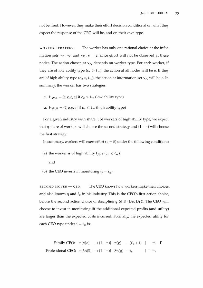
3.4 equilibrium 73

not be fired. However, they make their effort decision conditional on what they

expect the response of the CEO will be, and on their own type.

worker strategy : The worker has only one rational choice at the infor-

mation sets νB, νC and νD: e = e, since effort will not be observed at these

nodes. The action chosen at νA depends on worker type. For each worker, if

they are of low ability type (ce > `w), the action at all nodes will be e. If they

are of high ability type (ce 6 `w), the action at information set νA will be e. In

summary, the worker has two strategies:

1. HW,L = e, e, e, e if ce > `w (low ability type)

2. HW,H = e, e, e, e if ce 6 `w (high ability type)

For a given industry with share η of workers of high ability type, we expect

that η share of workers will choose the second strategy and (1− η) will choose

the first strategy.

In summary, workers will exert effort (e = e) under the following conditions:

(a) the worker is of high ability type (ce 6 `w)

and

(b) the CEO invests in monitoring (i = iy).

second mover — ceo : The CEO knows how workers make their choices,

and also knows η and `c in his industry. This is the CEO’s first action choice,

before the second action choice of disciplining (d ∈ DK,DL). The CEO will

choose to invest in monitoring iff the additional expected profits (and utility)

are larger than the expected costs incurred. Formally, the expected utility for

each CEO type under i = iy is:

Family CEO: η[π(e)] +(1− η)[ π(e) −(`c + f) ] −m− Γ

Professional CEO: η[λπ(e)] +(1− η)[ λπ(e) −`c ] −m

3.4 equilibrium 74

The equivalent expected utility under i = in is:

Family CEO: π(e) −Γ

Professional CEO: λπ(e)

ceo strategy : Let ∆π = π(e) − π(e). At information set β each type

of CEO will choose i = iy and invest in the monitoring technology iff the

following conditions hold:

Family CEO: η∆π > (1− η) (`c + f) +m

Professional CEO: λη∆π > (1− η) (`c) +m

For each representative CEO type, let L generally be the threshold at which

it becomes optimal for any CEO to invest in monitoring. Let the threshold be

Lf for the family CEO and let the threshold be Lp for the professional CEO.

Rearranging the terms in the conditions above yields the following thresholds:

Family CEO: Lf 6η∆π−m

(1− η)

Professional CEO: Lp 6λη∆π−m

(1− η)

Conceptually, these conditions suggest that the professional CEO will only

invest if the cost of layoffs is less than or equal to the added profit they can

expect the firm to make minus the cost of investment, multiplied by the inverse

of the share of low ability workers. Notably, this threshold is relatively lower

for the professional CEO as they only get a share of the profits: the first term

on the numerator of the condition is λη∆π for the professional CEO and η∆π

for the family CEO. Thus, Lf > Lp.

Figure 15 shows the two-dimensional space of `c and f for each CEO type.

The darker colours indicate investment in monitoring and the lighter colours

3.4 equilibrium 75

indicate no investment and are divided along the L thresholds for each type.

Each graph also includes a dotted line with the threshold of the other CEO

type for ease of comparison.

Figure 15: CEO investment decision: parameter space

The CEOs full strategies at β, δA, δB, δC are:

1. HC = in,DK,DK,DK if `c + f > Lf (family) or if `c > Lp (professional)

2. HC = iy,DK,DL,DK if `c + f 6 Lf (family) or if `c 6 Lp (professional)

first mover – owner : Finally, the owner’s choice depends on the util-

ity he would get if he acted as family CEO, versus the utility he would get

from receiving the profits achieved by the professional CEO. Figure 16 shows

the owner’s payoffs at each terminal node if we substitute the game for the

subgame perfect equilibrium at that node.

The owner’s decision depends on whether he would choose investment or

not given a set of parameters, as well as his opportunity cost, which depends

on whether the professional CEO would have invested or not. There are four

possible set of parameters that determine the space for four equilibria, as de-

scribed below.

3.4.4 Four regions of the parameter space with unique equilibria

Ultimately there are four cases to be considered, each of which will have its

unique equilibrium depending on the region of the parameter space. The CEO

3.4 equilibrium 76

Figure 16: Game tree: owner’s decision

α

β2

in

i y

FAM

β1

in

i y

PRO

uown = π(e) − Γ

uown = ηπ(e) + (1− η)π(e) − Γ −m− (1− η)(`c + f)

uown = (1− λ)π(e)

uown = (1− λ)[ηπ(e) + (1− η)π(e)]Mover #1: Owner

Mover #2: CEO

can be a professional or a family type, and each can reach an equilibrium

where they invest in monitoring and one where they do not. I describe each

of the cases and the possible equilibria below. There will be three threshold

values that determine the parameter space based on the utility functions above,

which I define here to simplify notation:

Lp =ηλ∆π−m

1− η

Lf =η∆π−m

1− η

Γ =λπ(e)1− η

where ∆π = π(e) − π(e).

Figure 17 visually depicts the four possible parameter regions for each equi-

libria, and are colour coded such that family CEO is shown in green shades

and professional CEO is shown in blue shades; investment is shown in darker

shades and no investment in lighter shades. The purpose of this first figure is

simply to serve as a visual guide for the four cases described below, and I have

imposed η = 0.5 and λ = 0.3 for this example. I reserve a discussion of how

changing these exogenous parameters might change the sizes of the regions

within the parameter space for the discussion and interpretation section.

3.4 equilibrium 77

Figure 17: Parameters determining the four equilibria space, for η = .5

3.4 equilibrium 78

case 1 : both ceos choose to invest in monitoring

Both CEOs would choose to invest, i = iy, if `c 6 Lp and `c + f 6 Lf. The

owner’s choice is based on the following utilities:

• uown(PRO, iy) = (1− λ)[ηπ(e) + (1− η)π(e)]

• uown(FAM, iy) = ηπ(e) + (1− η)π(e) − Γ −m− (1− η)(`c + f)

The owner will choose Mg = PRO when both CEOs opt for i = iy iff his

utility from doing so is higher than his utility from running the firm himself,13

otherwise, he will choose Mg = FAM:

(1− λ)[ηπ(e) + (1− η)π(e)] > ηπ(e) + (1− η)π(e) − Γ −m− (1− η)(`c + f)

The conditions specifying where each equilibrium lies are as follows:

Mg = PRO, i = iy if: `c + f+Γ

1− η> Γ + Lp

Mg = FAM, i = iy if: `c + f+Γ

1− η6 Γ + Lp

case 2 : both ceos choose not to invest in monitoring

Both CEOs would choose not to invest, i = in, if `c > Lp and `c + f > Lf. The

owner’s choice is based on the following utilities:

• uown(PRO, in) = (1− λ)π(e)

• uown(FAM, in) = π(e) − Γ

The owner will choose the CEO following the same logic, and the conditions

for the key parameters are as follows:

13Rearranging the terms provides an intuitive interpretation: the wage he expects to pay theprofessional CEO is smaller than the costs he will face if he chooses to manage the firmhimself: λ[ηπ(e) + (1− η)π(e)] < Γ +m+ (1− η)(`c + f)

3.4 equilibrium 79

Mg = PRO, i = in if: `c + f+Γ

1− η> Γ + Lp

Mg = FAM, i = in if: `c + f+Γ

1− η6 Γ + Lp

case 3 : only professional ceo chooses to invest

The professional CEO would choose to invest, i = iy, while the family CEO

would not, i = in if: `c 6 Lp and `c + f > Lf. The owner’s choice is then based

on the following utilities:

• uown(PRO, iy) = (1− λ)[ηπ(e) + (1− η)π(e)]

• uown(FAM, in) = π(e) − Γ

The owner will choose the CEO following the same logic, and the conditions

for the key parameters are as follows:

Mg = PRO, i = iy if:Γ

1− η> Γ + Lp − Lf

Mg = FAM, i = in if:Γ

1− η6 Γ + Lp − Lf

case 4 : only family ceo chooses to invest

The family CEO would choose to invest, i = iy, while the professional CEO

would not, i = in if: `c > Lp and `c + f 6 Lf. The owner’s choice is then based

on the following utilities:

• uown(PRO, in) = (1− λ)π(e)

• uown(FAM, iy) = ηπ(e) + (1− η)π(e) − Γ −m− (1− η)(`c + f)

The owner will choose the CEO following the same logic, and the conditions

for the key parameters are as follows:

3.5 discussion and interpretation 80

Mg = PRO, i = in if: `c + f+Γ

1− η> Γ + Lf

Mg = FAM, i = iy if: `c + f+Γ

1− η6 Γ + Lf

3.5 discussion and interpretation

This simple theoretical framework suggests a set of implications that can be

tested in empirical work. I will discuss each key parameter in turn and sug-

gest possible ways to empirically test the implications. In this section I will re-

vert to using the terms “good management practices” and “bad management

practices” instead of “investment in monitoring” and “no investment”.

the cost of layoffs , `c : The industry cost of laying off workers (`c)

is a crucial determinant of whether it is worth it for CEOs to invest in good

management. Conceptually, if management only helps with identifying who

the shirkers are, it is only worth adopting it if the extra information garnered

from it will be used and there can be credible commitment that it will result

in layoffs for the shirkers. One interpretation of `c could be unionization rates

within an industry, or labour laws within a country. For example, we could

expect that CEOs in industries with high unionization rates would be less

likely to adopt good management as they might encounter severe pushback in

any layoff attempts, despite observing who the shirking workers are. Similarly

in countries with stringent labour laws, it could be that the process of laying

off employees for shirking is too costly in terms of paperwork or other barriers.

Analytically, Figure 17 shows that when `c > L both family and professional

CEOs opt for no investment in good management practices. Empirically, there

are at least two implications that could be tested with available data:

Testable implication 1.

A. Industries with higher labour power will have fewer firms with good manage-

ment practices.

3.5 discussion and interpretation 81

B. Countries with tougher labour laws will have fewer firms with good management

practices.

To consider implication 1A, one can collect data on measures of labour

power — such as unionization rates — and correlate these with average quality

of management across industries and countries. This would be the first step to

see if such stylized facts could be observed, and if that is the case then more

careful tests that would account for possible biases could also be carried out.

For example, if may be possible to exploit a policy change, such as if a law

is passed that curbs union activity, or if trade agreements change the market

and power structure of particular industries. There is some evidence of this

currently in the literature: Bloom, Draca, and Van Reenen [31] use China’s

entry into the World Trade Organization and subsequent increased imports

from Chinese firms across a selected group of industries to identify the effect

of increased competition on management quality. They find that management

quality improved within surviving firms. They did not, however, consider the

effect on shares of family and non-family firms given the shock.

Figure 18: A firm-level measure of `c

010

2030

4050

60Pe

rcen

tage

of u

nion

ized

work

ers

(firm

)

1 2 3 4 5People management Score

Family CEOProfessional CEO

Data from the World Management Survey, 2004-2014.

At a firm level, the World Management Survey collects data on the share of

employees who are unionized within a firm. As a simple first approximation,

Figure 18 shows the lowess plot of the relationship between share of union-

3.5 discussion and interpretation 82

ized workers and the firm’s score in people management.14 The graph shows

that the lower the percentage of unionized workers within a firm, the higher

the quality of people management practices in the firm. This is the case for

both family and professional CEO firms, but the relationship is much more

pronounced in professional CEO firms.15

For the testable implication 1B, one can consider the stylized fact by looking

at the relationship between labour laws and management. The World Bank

publishes a rank where they score countries on their “difficulty of employ-

ment” on a scale of 0 to 100, and Figure 19 plots the relationship between

the country average quality of people management and the World Bank index.

There is a negative relationship between the toughness of labour laws and the

quality of people management at the country-level, though of course there are

myriad endogeneity issues that could be considered in future work.

Figure 19: A country-level measure of `c

Argentina

Australia

Brazil

Canada

ChileChina France

Germany

Great Britain

GreeceIndia

Italy

Japan

Mexico

New Zealand

Northern Ireland Poland

Portugal

Republic of Ireland

Sweden

United States

22.

53

3.5

Aver

age

Peop

le M

anag

emen

t Pra

ctic

es

0 20 40 60World Bank Difficulty of Employment Index (0-100)

Management data from the World Management Survey. Difficulty of employment index data from the WorldBank Doing Business report, 2014.

14The people management score measures the quality of monitoring, selection and reward pro-cesses within the firm.

15Another possible way to think about unionization rates would be that in a highly unionizedenvironment there is a higher need for monitoring and “paperwork” in order to lay off aworker, and thus there should be an incentive to invest in monitoring. The concept of `c hereis, however, that it is more expensive generally to lay off workers when there is higher unionpower, and even if there was a high investment in monitoring it may still be expensive to layoff workers despite having documentation — so much so that it is no longer profitable toinvest in a lot of monitoring structure.

3.5 discussion and interpretation 83

the firm reputation cost of layoffs , f : The model assumes by con-

struction that family CEOs also face firm-specific costs of discipling workers.

The concept has been used in previous work, such as in Bach and Serrano-

Velarde [8], where the authors propose that family firms enter into an implicit

contract with workers that allows them to offer lower wages in exchange for

an expectation of longer tenure of employment — regardless of productivity

shocks. In my framework, it could be interpreted that there are reputation costs

associated with breaking this implicit contract with workers. Let “separation”

refer to a worker being laid off from their job.

Testable implication 2.

A. Family CEO firms with high reputation costs will have worse management prac-

tices.

B. Family CEO firms will have lower rates of separation than professional CEO

firms, but better managed family CEO firms will have higher separation rates

relative to worse managed family CEO firms.

One way to measure reputation costs would be to create an indicator for

eponymous firms, assuming that family CEOs of firms that bear the family

name are more likely to care about the reputation of their firm. Another mea-

sure could be to use the size of the municipality (or other small regional mea-

sure) where each firm is, under the assumption that firms in smaller communi-

ties are more likely to employ a large share of the local population and suffer

from a stronger community backlash if workers are laid off. These could then

be used to check the relationship between separation rates and each of the

firm types: family/professional CEO, well/badly managed. Building a dataset

with this information is possible with access to matched employer-employee

administrative datasets. I have secured access to the datasets from Brazil and

Italy, and will test these implications in future work.

the share of high ability workers , η : The industry share of high

ability workers, η, is important for (a) determining the size of the additional

profit that could be made by the firm if the CEO opts for investment in monitor-

3.5 discussion and interpretation 84

ing, and (b) the share of workers who would be fired. The model suggests that

in industries where there is a large share of high ability workers, the return

to investment in monitoring is higher and thus more CEOs will choose good

management. This is the case because, in the model, only workers who are of

high ability would change their behaviour in the face of monitoring — hence,

the higher the share of high ability workers, the higher the share of workers

who would exert higher effort. This would both lead to a larger ultimate effect

on profits and a smaller possible cost of layoffs. Figure 21 shows the parameter

space for η = 0 .2 and η = 0 .8, and it is clear that in the figure where η = 0 .8

the space taken by the darker shades indicating i = iy is higher.

Testable implication 3.

A. Industries with higher shares of high ability workers will have more firms with

good management practices.

Figure 20: An industry-level measure of η

Food

TobaccoTextile

ApparelLumber

Furniture

Paper

Printing

Chemicals

Petrol products

Rubber & plastics

Leather products

Stone, clay and glass

Primary metalFabricated metal

Non-elecrical machineryElectronic equipment

Transportation equipmentInstruments

Other manufacturing

2.2

2.4

2.6

2.8

33.

2Av

erag

e Pe

ople

Man

agem

ent P

ract

ices

5 10 15 20 25 30Share of workers with a university degree

Family CEO firms

FoodTobacco

TextileApparel

Lumber

Furniture

Paper

Printing

Chemicals

Petrol products

Rubber & plastics

Leather products

Stone, clay and glassPrimary metalFabricated metal

Non-elecrical machineryElectronic equipmentTransportation equipment

Instruments

Other manufacturing

2.2

2.4

2.6

2.8

33.

2Av

erag

e Pe

ople

Man

agem

ent P

ract

ices

5 10 15 20 25 30Share of workers with a university degree

Professional CEO firms

Notes: Data from the World Management Survey.

Empirically, Figure 20 shows a stylized fact relating to this testable impli-

cation using data from the WMS. The graph shows a positive relationship

between the average people management score for each 2-digit SIC industry

and the share of workers with a university degree at the industry level — and

the relationship is present both in the sample of family CEO firms as well as

the professional CEO firms.

3.5 discussion and interpretation 85

Figu

re2

1:P

aram

eter

sde

term

inin

gth

efo

ureq

uilib

ria

spac

e,fo

rη=

.2an

dη=

.8

3.6 conclusion 86

3.6 conclusion

This aim of this chapter was to outline a basic framework considering a pos-

sible mechanism behind the decisions made by CEOs regarding management

adoption, and by a family firm owner regarding the CEO appointment. I build

the model such that there are three key parameters that affect the returns of

investing in a management technology in interesting ways: the share of high-

ability workers in an industry η, the industry cost of layoffs `c and the family

firm’s reputation cost f.16

The final key parameter, Γ , only influences the ultimate decision of the firm

owner whether to hire a professional CEO or to appoint a family member. Con-

ceptually, there are utility costs of being CEO as effort must be expended on

the day to day running of the firm. The family CEO can also gain a “private

benefit of control” from running their family’s firm — that can be simply be-

cause they are proud to do so, or perhaps there are monetary or other types of

influence benefits that come from owning a firm within a community.17 If the

owner chooses to run the firm himself, it must be that the benefits are larger

than the costs of running the firm, and that this net benefit is also larger than

the additional profits that would have been earned if a professional CEO had

been hired.

How large the benefit or cost needs to be depends on whether the profes-

sional CEO would have adopted management or not: for example, if the indus-

try has high union rates and the professional CEO would not have adopted the

monitoring technology either, the additional revenue earned by hiring a pro-

fessional CEO is very low. Thus, an owner would only hire a professional CEO

if their personal net costs of running the firm are larger than the salary they

would have to pay to the professional CEO. Symmetrically, in the case where a

family CEO would not adopt monitoring but the professional CEO would, we

would only observe an owner opting for a family CEO if they have a substan-

tially high private benefit of control and low utility costs of running the firm —

16Two more parameters, the cost of investment in managementm and the CEO’s share of profitstaken as payment λ are necessary in the model but behave in a straightforward way, and thusdo not warrant discussion at this point.

17As in Demsetz [55], for example.

3.7 appendix 87

that is, the additional profit that would have been earned by the professional

CEO would have been substantial, so it requires a much higher level of private

benefit to compensate for the lost profit.

Considering the four equilibria, we can expect to find CEOs falling on each

of the four final nodes depending on the parameters discussed above. We may

generally expect that professional CEO firms have higher layoff rates when

compared to family CEO firms, but that “better managed” professional CEO

and family CEO firms have the higher layoff rates relative to poorly managed

professional CEO and family CEO firms. This framework partly explains why

we might see a distribution of management quality as seen in the second figure

of the previous chapter, where both family CEO-run firms and professional

CEO-run firms have good and bad management across the distribution, but

the distribution of non-family firms is shifted to the right of the family firms

distribution. The innovation here is that we do not need to assume that family

CEOs are of lower ability, but rather that they are simply responding to differ-

ential costs of implementing personnel policy because of the unique structure

of contracts — including implicit contracts — that family firms have with their

employees. A more rigorous treatment of the empirical tests is left to future

work.

3.7 appendix

additional game tress The information sets are shown in nodes of

the summary game tree in Figure 22, and are shown inside the nodes when

they are singletons and inside the dashed lines when they are sets. Let α be the

information set when the owner chooses who to manage the firm. Let β1 and

β2 be the information sets at the time the CEOs take their investment action.

Let ν1 to ν8 be the information sets at the time that the worker has to take

their effort action. Let δ1 to δ6 be the information sets at the time the CEO has

to take their disciplining action.

Figure 23 shows the full game tree, with all the nodes but omits the payoffs.

The information sets are depicted by dashed lines and labelled above the set.

3.7 appendix 88

Figure 22: Game tree: summary decision set

α

β2

ν8DK

e

L[1−η]

ν7DKe

δ6

H[η]

in

ν6

DK

DL

e

δ5L[1−η]

ν5

DK

DLe

δ4DK

e

H[η]

i y

FAM

β1

ν4DKe

L[1−η]

ν3DKe

δ3

H[η]

in

ν2

DK

DL

e

δ2L[1−η]

ν1

DK

DLe

δ1DK

e

H[η]

i y

PRO

ufam = π(e) − Γuw = wg

ufam = π(e) − Γuw = wg

ufam = π(e) − Γ −m− (`c + f)uw = wg− c`

ufam = π(e) − Γ −muw = wg

ufam = π(e) − Γ −muw = wg

ufam = π(e) − Γ −m− (`c + f)uw = wg− `c

ufam = π(e) − Γ −muw = wg− ce

upro = λπ(e)ufam = (1− λ)π(e)uw = wg

upro = λπ(e)ufam = (1− λ)π(e)uw = wg

upro = λπ(e) −mufam = (1− λ)π(e)uw = wg

upro = λπ(e) −m− `cufam = (1− λ)π(e)uw = wg− c`

upro = λπ(e) −mufam = (1− λ)π(Y)uw = wg

upro = λπ(e) −m− `cufam = (1− λ)π(e)uw = wg− c`

upro = λπ(e) −mufam = (1− λ)π(e)uw = wg− ce

Mover #1: Owner

Mover #2: CEO

Mover #3: Worker

Mover #4: CEO

3.7 appendix 89

Figure 23: Game tree: full decision set

α

β2

ν8

DK

DLe

DK

DL

e

L[1−η]

ν7

DK

DLe

DK

DL

e

δ6

H[η]

in

ν6

DK

DLe

DK

DL

e

L[1−η]

ν5

DK

DLeδ5

δ4DK

DL

e

H[η]

i y

FAM

β1

ν4

DK

DLe

DK

DL

e

L[1−η]

ν3

DK

DLe

DK

DL

e

δ3

H[η]in

ν2

DK

DLe

DK

DL

e

L[1−η]

ν1

DK

DLeδ2

δ1DK

DL

e

H[η]

i y

PRO

Mover #1: Owner

Mover #2: CEO

Mover #3: Nature

Mover #4: Worker

Mover #5: CEO

4D E V E L O P I N G M A N A G E M E N T: A N E X T E N D E D T O O L T O

M E A S U R E Q U A L I T Y O F M A N A G E M E N T O F S C H O O L S I N

D E V E L O P I N G C O U N T R I E S

with Renata Lemos

“ If the system does not add up to a functional whole, the causal impactof augmenting individual elements is completely unpredictable. ”

Lant Pritchett, RISE Working Paper 15/005, 2015

4.1 introduction

Although there has been much progress in improving school enrolment around

the world, there is still striking heterogeneity in the distribution of student

learning outcomes across countries. This is particularly true for the developing

world, and researchers and policy makers are paying increasing attention to

addressing this “learning crisis”. The traditional economics literature that con-

siders the effect of an individual input on output has provided us with great

insights into the individual effect of inputs such as teacher salaries, school in-

frastructure, school financing, extra teachers, different curriculums, and more

textbooks, among many. However, variation in these inputs has not been able

to explain a substantial share of the variation in student learning (Glewwe

and Muralidharan [67]). Thus, a new research agenda is urging a more holistic

view of education systems in a “systems framework” that includes a series of

interconnected types of relationships between different actors and stakehold-

ers, outlined in Pritchett [106].

This chapter makes a methodological contribution by taking lessons from

private enterprise and applying to the “public sector” (broadly defined). We

develop a feasible tool to measure management practices in schools in develop-

90

4.1 introduction 91

ing countries, based on the well-established World Management Survey tool.1

Here we describe the Development WMS, a survey tool based on the original

WMS but tailored to measuring management practices in the public sector of

developing countries. We discuss each innovation in detail below, but in short:

1. We identified three management processes - implementation, usage, and

monitoring - taken into consideration when measuring the strength of

each management practice covered by the WMS but which could not be

extricated ex-post from a score in the original methodology.

2. We expanded the survey “vertically” by disentangling and mapping these

processes to each question of the 20 management practices, creating 60

items to score.2 In this new survey, however, the responsibility of weight-

ing the importance of each process does not lie with the interviewer,

thereby reducing measurement error and allowing the data user to know

precisely what led the score for a particular practice to be higher or lower.

3. We expanded the survey “horizontally” to allow for greater variation of

scores and allow interviewers to differentiate at a finer level between the

strength of processes in place at these schools and hospitals.

While we have strived to keep the essence of the WMS in terms of the ques-

tions and practices being measured and the spirit of the scoring grid, we also

ensured that the adapted version was applicable in the development setting

by addressing three main challenges to using the original WMS in developing

countries.

First, the distribution of scores in the education sector in the two developing

countries surveyed in the original WMS, India and Brazil, was tight around

the scores for weak management practices. Although the global context of

the WMS project allows for a useful comparison of world-class and poorly

managed organizations across a number of countries, the very thick — almost

1Since 2008, we have worked alongside Nicholas Bloom, Raffaella Sadun and John Van Reenento significantly expand the original WMS data collection project and systematically measuremanagement practices within and across countries and it is using this experience that wedeveloped this tool in a comparable way.

2We did this based on our seven years of training interviewers to conduct the WMS interviews,such that the questions asked related to types of processes are comparable to previous yearsof surveys.

4.1 introduction 92

truncated — left tail for developing countries makes it harder to explore the

variation of managerial practices in the less well managed organizations. For

example, Lemos and Scur [91] points out the thick left tail in both schools

and hospitals in India and Bloom et al. [37] show that there is evidence of

truncation at the lower bound score of 1, with 82% of the schools in the WMS

Indian sample having an overall management score between 1 and 2 that and

no schools have a score above 3 on the original WMS scale. During the data

collection for these countries, we often heard interviewers wishing they could

“give a 0” to those schools and hospitals that had no process whatsoever to

differentiate those from schools and hospitals that had minimal processes, but

not enough of an informal process to warrant a score of 2 in the scoring grid.3

Second, in terms of implementation, the WMS original methodology uses

available sampling frames from established organizations and phone calls to

carry out the interviews. Although this was less of a barrier in the manufactur-

ing survey, it was a massive barrier in the public sector surveys in developing

countries. For instance, sampling frames in India were difficult to acquire and

build, and, when available, they often had names of schools and hospitals but

no phone numbers. Unfortunately a common reason for the lack of phone

number was that schools simply did not have a physical phone line available.

We often ran interviews through managers’ cell phones, and a handful of times

through payphones located near these organizations as cellphones or landlines

were not available. When we were able to reach them, the connection itself was

sometimes problematic and several calls had to be placed to complete the in-

terview.4

Finally, when thinking about policy implications, we did not have much in-

formation in the WMS to pinpoint precisely what part of the process these

organizations were failing at the most. Although useful experiments such as

Bloom et al. [34] and Fryer [63] have substantially helped us learn about the

large effect that improvements in whole sets of management practices can

afford, we do not yet have a systematic picture of what particular types of

3The reason we refrained from stretching the scoring grid to 0 and instead added half pointswas to preserve comparability of the ordinal scale and increase specificity equally across allscore categories.

4The higher the number of calls that have to be made, the lower the probability of completingan interview.

4.1 introduction 93

processes matter the most across different settings in developing countries.5

The 20 management practices covered by the WMS are scored based on a

set of processes which are systematically triangulated by the skilled inter-

viewer and facts are evaluated based on the survey grid to determine higher

or lower scores. However, we argue that it becomes important to understand

the marginal importance of each type of process when considering the type

of policy interventions that are feasible, especially in the context of countries

facing limited budgets and institutional constraints.

We have also developed accompanying field paper forms to facilitate the

interview process as the Development WMS is meant to be run face-to-face by

enumerators who visit the schools and hospitals. These forms were carefully

designed to ensure that the information collected during the interviews would

be sufficient for the post-interview scoring. In the phone interviews, the enu-

merators are able to consult the grid to ensure they have enough information,

but in the face-to-face interviews they are not allowed to take the grid along as

it would undermine the double-blind exercise. The importance of providing a

useful field-friendly data collection tool is often underestimated. The enumer-

ators are often not researchers by training and may fail to record important

information or even record wrong information during survey interviews if not

properly prompted by their field tool.6

With a set of individual project partners, we are in the process of collect-

ing data using this new expanded survey tool in schools in Andhra Pradesh-

India (completed), Mexican schools (ongoing, pilot completed), Colombian

schools (completed), Chinese hospitals (ongoing) and Indian hospitals (pilot

completed).7 This survey tool has often been used as an additional module

5Focusing on charter schools in the US, Dobbie and Fryer [58] run a similar exercise where theycollect a large amount of information on the inner-workings of 35 charter schools to investigatethe practices that matter the most for school effectiveness.

6A website with instructional videos and interactive calibration tools to minimize the fixedcosts of training and implementation will be made freely available to the research communityin mid-2017.

7We have partnered with Karthik Muralidharan and the APSC project for Indian schools, Ar-turo Harker Roa and the Colombian Ministry of Education for Colombian schools, Rafael deHoyos and Ciro Avitabile from the World Bank and the Mexican Ministry of Education forMexican schools, Winnie Yip and the Ministry of Health for Chinese hospitals and RaffaellaSadun for Indian hospitals. We are immensely thankful to Raissa Ebner and Kerenssa Kay fortraining the Mexican school pilot teams, Raissa Ebner for training the Mexican and Colombianschool teams, and Kerenssa Kay for running the Indian hospital pilot. For an initial look at theColombian data, see Bermudez and Harker [22].

4.2 measuring processes in developing countries 94

in larger projects, and sampling frames of these projects were not always nec-

essarily representative random samples and thus are not directly comparable.

While these samples were not formally designed to be representative of all

schools in these countries, collectively they paint a useful picture of selected

public sector organizations in low- and middle-income countries and allow us

to validate our new survey tool.8

4.2 measuring processes in developing countries

The original public sector WMS covers 20 questions across two main areas:

operations management and people management. The original survey sub-

divides operations management into lean operations, monitoring and target

management, as follows:

1. Operations management

a) Lean operations in schools covers practices including whether the

school has meaningful processes that allow pupils to learn over time;

teaching methods that ensure all pupils can master the learning ob-

jectives; whether the school uses assessment to verify learning out-

comes at critical stages and makes data easily available and adapts

pupil strategies accordingly.

b) Monitoring management covers practices of continuous improvement,

performance tracking, review and dialogue, and consequence man-

agement. It measures whether the school has processes towards con-

tinuous improvement and lessons are captured and documented,

whether school performance is regularly tracked with useful met-

rics, reviewed with appropriate frequency, quality, and follow-up,

and communicated to staff.

8The samples are as follows: the Andhra Pradesh data is a random sample of public and privateprimary schools in 5 districts from the APRESt project; the Mexican data is a combinationof samples from primary schools that are part of PEC (Programa Escuelas de Calidad) inDurango, Guanajuato, Estado de Mexico and Tabasca, marginalized primary schools in Puebla,and primary and junior high schools in Tlaxcala and Morelos; the Colombian data is a randomsample from the lowest performing public schools in the country (approximately 4,000 of the22,000 schools in Colombia); the Chinese hospital data is a random sample of hospitals andthe Indian hospital data is from a pilot of 25 hospitals in Andhra Pradesh.

4.2 measuring processes in developing countries 95

c) Target management covers practices in the balance and interconnec-

tion of targets, the time-horizon and difficulty of the targets, as well

as their clarity and comparability. It measures whether the school,

department, and individual targets cover a sufficiently broad set of

metrics; whether these targets are aligned with each other and the

overall goals.

2. People management covers practices in handling good and bad perfor-

mance, measuring whether there is a systematic approach to identifying

good and bad performance, rewarding school teachers proportionately,

dealing with underperformers, and promoting and retaining good per-

formers.

As mentioned before, we preserve the practices and areas covered in the

original WMS and identify three key processes used to systematically mea-

sure these practices, and expand it both “vertically,” by further dividing each

of the 20 practices into the three processes we are looking to measure and

“horizontally,” increasing the granularity of scores by allowing half points.

4.2.1 Identifying processes behind management practices

In the Development WMS, we identify three key processes that are captured

to measure the strength of each management practice within an organization.

Each process consists of:

1. Process implementation: formulating, adopting and putting into effectmanagement practices;

2. Process usage: carrying out and using management practices frequentlyand efficiently;

3. Process monitoring: monitoring the appropriateness and efficient use ofmanagement practices.

More specifically, in the original WMS, each of the overall management, op-

erations and people management indices is made up of a set of the 20 practices,

and each practice is measured through several structured questions. Each one

4.2 measuring processes in developing countries 96

of the 20 management practices contains a large amount of information about

how that specific practice being carried out at the establishment. For example,

when measuring “data-driven planning and student transitions” at a school,

the WMS interviewer evaluates the practice based on three processes: (1) what

type of data is available (test scores, attendance, etc), (2) leaders understand

critical points of transition for students (when to change learning levels), (3)

leaders have a data-driven approach to decisions (principal and teachers use

data to determine transitions). The combined responses to this practice are

scored against a grid which goes from 1 - defined as “School may be aware

of critical transitions for students, but little or no effort is made to match sup-

port services to students; data is often unavailable or difficult to use.” up to

5 - defined as “Student transitions are managed in an integrated and proac-

tive manner, supported by formative assessments tightly linked to learning

expectations; data is widely available and easy to use.”

In the original WMS instrument, the interviewer triangulates the processes

herself and assigns one single score taking all the processes into account. This

task requires a high cognitive ability from the interviewer as well as consistent

monitoring of the interviewing process by supervisors to ensure comparabil-

ity.9 It is not possible, however, to extricate from the final data ex-post how each

process weighed in the interviewer decision. In the Development WMS, each

process is evaluated separately and ex-post averaged out to get the practice’s

score. This is useful in a practical sense because it removes the triangulation

responsibility from the interviewer, which then lowers the cognitive threshold

required in hired interviewers and facilitates the deployment of the survey in

low-capacity contexts.

Furthermore, in an academic and policy research sense we can now disen-

tangle precisely where the process is failing and be much more specific in

targeting of interventionist policies. For example, in one of the pilot school

visits we carried out in Andhra Pradesh, when asked the first question in the

earlier example the principal promptly pulled out examples of report cards

that they used to track student performance (Figure 24). The report cards had

9This is one of the reasons for the high per-interview cost of the WMS. Interviewers are gener-ally masters students from top UK schools and experienced supervisors monitor over 80% ofthe interviews.

4.2 measuring processes in developing countries 97

plenty of detail on student achievement and behaviour over time, and were

signed by the teacher, principal and parent. This would certainly warrant a

score of 3.5 or 4 on the implementation process part of the topic being mea-

sured. When we then asked the subsequent questions of how the data is used

and how it relates to student transitions, we received the unsatisfying answer

that the report cards were simply stacked in the corner of the principal’s office

and if the teachers were curious they could go and find an individual student’s

card whenever they wanted.

Figure 24: Report card from a rural school in Andhra Pradesh

In short, there was no process of compiling the data to be useful more gen-

erally, and there was certainly no process to use the data to help guide the

transition between levels of learning. Crucially, the scores for the usage and

monitoring parts would have been low, in the 1-1.5 range and the overall score

might have been around a 2-2.5, and we would correctly interpret that there is

not a very good formal system of data-driven student transitions, but we would

have missed important information that it is not the data collection part of the

process that is failing, but rather the usage of the data already collected. If we

think in policy terms, a policy that targets giving schools best practices for

report card development would be relatively useless in this context, whereas

4.2 measuring processes in developing countries 98

one that builds a system that they can use the data already collected would be

much more effective.

4.2.2 Expanding the instrument vertically: higher dimensionality

Operationally, we develop the extended grid by mapping each of the three key

processes back to the questions asked for measuring each WMS practice. Pro-

cess implementation is broadly related to question 1, process usage is broadly

related to question 2, and process monitoring is broadly related to question

3 in each management practice. Thus, beyond looking at the average score of

each practice, we can also dig deeper to understand what part of the process

is driving the results. This increases the number of scores from 20 to 60.

With the increased number of variables, we can create a new set of indices to

test whether they are any more informative than the original survey. We con-

struct four sets of indices. For the first set, we follow a similar methodology to

the original WMS and use the information referring to all three processes very

simply. First we take an average of the three sub-questions to build a single

score for each of the 20 original practices, analogous to how a WMS inter-

viewer would assign a single score to each practice. We then take the z-score

of each practice and creating indices for overall management (average of 20

practices), operations management (average of fourteen operations practices),

people management (average of six people management practices). This can be

interpreted in the same way as the original WMS, but with less measurement

error.10

The main innovation in our survey is in the second, third and fourth set

of indices. To build these, we skip the first step of averaging across the three

processes for each practice and re-organize the dataset into three new sets of

20 practices along the lines of each process. We take the z-score of all the sub-

questions and build average indices for overall management, operations man-

agement and people management using the 20 sub-practices for each of the

process types. For example, we can build an implementation management in-

10The original WMS excludes the leadership questions from its overall management score, sowe follow the same convention here.

4.2 measuring processes in developing countries 99

dex by taking the average of the 20 implementation sub-practices, and again do

the same to create a usage management index and a monitoring management

index. Further, we could build implementation operations and implementa-

tion people management indices using only the first sub-questions within each

management practice.

In short, we first produce a set of overall management, operations manage-

ment and people management indices using a similar methodology to the

original WMS (ie. using all the information given for a particular question),

and also produce three “finer” sets of indices, broadly referring to (1) process

implementation of overall, operations and people management, (2) process us-

age of overall, operations and people management, and (3) process monitoring

of overall, operations and people management.

While we broadly follow the original WMS convention for building the com-

parable indices (overall management, operations and people management), we

have conducted a factor analysis of our new school survey tool with the data

from Andhra Pradesh, Mexico and Colombia to validate this. We find that

factor analysis on the 20 management practices as well as the more granular

60 processes yields generally similar results to those found in the manufac-

turing sector in Bloom et al. [35], though considering the factors within each

of the processes is rather telling. We present the results of the factor analysis

in Table 9. The first two factors across all the four sets of variables analyzed

explained all the variation across the variables, so we present only the first two

factors here for each set of variables analyzed. The first two columns use the

management practice scores that are comparable to the original WMS; that is,

each of the 20 management scores is an average of the three respective pro-

cesses in the D-WMS. The following six columns break down the use of the

dataset instead of taking an average of the three processes: columns (3) and

(4) use only the first process for each management practice —implementation,

columns (5) and (6) use only the second process for each management practice

— usage, and columns (7) and (8) use only the third process for each manage-

ment practice — monitoring.

4.2 measuring processes in developing countries 100

Starting with the original WMS practices, the first factor pattern suggests

the largest pattern of relationships in the data, and we see that there is one

principal factor that explains 87% of the variance and loads positively on all

practices, and the loadings are high.11 Similar to the result in manufacturing in

[35], this suggests that there is a “common factor of good management” (Fac-

tor 1). In the context of the D-WMS data, this suggests that schools that are

well managed on one practice are more generally also likely to be well man-

aged across all practices. The second factor pattern suggests the second largest

pattern of relationships that is uncorrelated with the first, and this second fac-

tor that explains about 13% of the variance and loads negatively on nearly

all of the operations management practices, but positively on all the people

management practices. The loadings on the second factor are, however, much

smaller than those seen in the first factor — especially those in operations. In

the manufacturing results, the second factor loaded positively on operations

and negatively on people management. Here we see the opposite loadings but

a similar pattern of specialization. In our context, it seems there is a second

factor of “good people management” suggesting schools specialize in people

management versus operations management.

Moving on to examining the results for each individual process, the first

pattern we note is that across all three processes we find a common factor of

“good management” as the first factor. The second factor, however, is not the

same across processes. In the implementation process questions across the full

survey, we see that the second factor loads negatively across all people man-

agement practices, while it loads positively across the same practices under

the usage and monitoring processes.

In all, it is reassuring to see that the general patterns that have been found in

the literature using the WMS hold with our new instrument as well. However,

it is also reassuring to see that we find some different patterns across different

processes within each management practice. The analysis suggests that we can,

indeed, learn something new in terms of the patterns of management within

schools from the new survey. In the next section we will show how each of the

processes are correlated with the outcome of interest in this context — student

11A general rule of thumb tends to be factor loadings of 0.4 and above are relevant.

4.2 measuring processes in developing countries 101

Tabl

e9

:Fac

tor

anal

ysis

ofm

anag

emen

tpr

acti

ces

and

proc

esse

s(u

nrot

ated

)

Ori

gina

lWM

SIm

plem

enta

tion

only

Usa

geon

lyM

onit

orin

gon

ly

(1)

(2)

(3)

(4)

(5)

(6)

(7)

(8)

Fact

or1

Fact

or2

Fact

or1

Fact

or2

Fact

or1

Fact

or2

Fact

or1

Fact

or2

Ops

1:S

tand

ardi

sati

onof

inst

ruct

iona

lpro

cess

es0

.7257

-0.1

389

0.5

831

0.1

985

0.5

490

-0.1

507

0.5

713

-0.0

255

Ops

2:D

ata

driv

enpl

anni

ngan

dst

uden

ttr

ansi

tion

0.7

064

-0.1

008

0.6

287

0.1

769

0.4

864

0.0

132

0.6

315

-0.0

934

Ops

3:P

erso

naliz

atio

nof

inst

ruct

ion

and

lear

ning

0.7

524

-0.1

228

0.5

909

0.1

253

0.6

221

-0.1

599

0.5

671

-0.1

140

Ops

4:A

dopt

ing

educ

atio

nalb

est

prac

tice

s0.7

535

-0.1

421

0.5

994

0.1

226

0.5

608

-0.1

406

0.6

699

-0.1

680

Ops

5:C

onti

nuou

sIm

prov

emen

t0.7

106

-0.1

761

0.5

959

0.1

915

0.5

717

-0.2

039

0.6

038

-0.1

100

Ops

6:P

erfo

rman

ceTr

acki

ng0.6

791

-0.2

727

0.5

248

0.0

144

0.4

044

-0.3

834

0.6

354

-0.1

892

Ops

7:R

evie

wof

Perf

orm

ance

0.6

956

-0.3

445

0.4

165

0.2

374

0.5

881

-0.1

080

0.6

343

-0.2

265

Ops

8:P

erfo

rman

ceD

ialo

gue

0.7

585

-0.2

517

0.5

737

0.2

257

0.5

998

-0.2

800

0.7

036

-0.1

505

Ops

9:C

onse

quen

ceM

anag

emen

t0.7

165

-0.2

725

0.6

511

0.2

714

0.4

102

-0.3

295

0.6

065

-0.1

642

Ops

10:T

ype

ofTa

rget

s0.7

547

-0.0

392

0.5

964

0.1

142

0.6

412

0.0

441

0.6

596

-0.0

059

Ops

11:I

nter

conn

ecti

onof

Goa

ls0.7

479

-0.0

989

0.5

504

0.2

372

0.5

761

0.2

020

0.5

988

-0.0

543

Ops

12:T

ime

Hor

izon

0.5

292

-0.0

727

0.4

730

0.0

943

0.4

216

-0.1

601

0.3

600

0.0

766

Ops

13:G

oals

are

Stre

tchi

ng0.6

800

0.0

236

0.4

763

0.1

107

0.5

682

-0.0

392

0.4

505

0.1

552

Ops

14:C

lari

tyof

Goa

ls0.7

215

0.1

141

0.5

911

0.0

362

0.4

672

0.2

729

0.6

181

0.0

421

Peop

le1:I

nsti

lling

ata

lent

min

dset

0.6

910

0.5

543

0.6

783

-0.4

340

0.7

096

0.4

230

0.4

986

0.4

205

Peop

le2:I

ncen

tive

san

dA

ppra

isal

s0.7

462

0.2

712

0.7

367

-0.4

433

0.5

863

0.1

609

0.4

146

0.2

262

Peop

le3:M

akin

gro

omfo

rTa

lent

0.7

059

0.2

156

0.6

778

-0.4

421

0.6

488

0.0

233

0.3

597

0.0

895

Peop

le4:D

evel

opin

gTa

lent

0.5

544

0.2

292

0.5

896

-0.3

115

0.5

290

0.0

854

-0.0

934

0.2

893

Peop

le5:D

isti

ncti

veEm

pV

alue

0.6

163

0.3

884

0.5

018

-0.1

004

0.4

966

0.2

886

0.5

143

0.3

385

Peop

le6:R

etai

ning

Tale

nt0.4

507

0.5

486

0.3

737

-0.1

714

0.1

990

0.5

648

0.5

074

0.4

272

Eige

nval

ue9

.513

1.3

882

6.6

605

1.1

278

5.9

000

1.2

148

6.1

177

0.8

507

%to

talv

aria

nce

0.8

712

0.1

271

0.8

639

0.1

463

0.8

600

0.1

771

0.9

532

0.1

326

Cum

ulat

ive

vari

ance

0.8

712

0.9

983

0.8

639

1.0

102

0.8

600

1.0

371

0.9

532

1.0

858

4.2 measuring processes in developing countries 102

and teacher outcomes — but for now we resume the discussion of the other

survey changes.

4.2.3 Expanding the instrument horizontally: greater score variation

The horizontal expansion of the instrument is more straightforward. In the

original WMS, interviewers are allowed to score values of 1, 2, 3, 4 or 5. No

half points are allowed and no “2 or 3” values are accepted. If interviewers are

unsure of whether the practice warrants a 2 or a 3, they discuss it with their

colleagues and their supervisors to make a final decision. This scoring guide-

line worked well in developed countries as there was wide range of scores,

with some schools or hospitals being very well managed and some being very

badly managed, but most schools or hospitals had at least some practice in

place, even if rudimentary. In the India and Brazil waves, however, we found

several schools that had absolutely no practices in place and some that had

very minimal practices in place. To score a 2 in the WMS, there must be a rea-

sonable practice in place that is informal (if it were a formal practice it would

be awarded a 3 or higher). Thus, both schools with no practices and minimal

practices were awarded 1, whereas in the Development WMS the interviewer

would be able to distinguish and score 1 for no practices and 1.5 for minimal

practices.

Crucially, however, we follow the same gradual scoring scheme as the orig-

inal WMS, which allows us to easily re-cast the scores into what they would

have been in the original survey. For example, if an interviewer gave a practice

in a school a score of 1.5, it is because it did not reach a high enough level

to be a 2, and thus in the original WMS it would have been a score of 1. We

implement these adjustments to create original WMS-comparable scores, and

plot both distributions in Figure 25.

The figure shows an example of the distribution of scores using data from

Andhra Pradesh, Colombia and Mexico. The main goal of the new scoring

guide was to allow for a systematic distinction between schools with absolutely

no structures in place — a score of 1 — and schools with very minor structures

4.2 measuring processes in developing countries 103

in place that could not yet be considered informal processes, but were also not

completely nonexistent — a score of 1.5. Allowing for 0.5 extra points in all

scores has the expected effect of shifting the distribution to the right as analysts

are allowed to score higher points, but crucially we now observe a longer tail

between the score of 1 and 2 despite still seeing distributions skewed to the

left.

Figure 25: Difference in distribution of scores between WMS and D-WMS

0.5

11.

5Ke

rnel

Den

sity

1 2 3Average management score

Andhra Pradesh

0.5

11.

5Ke

rnel

Den

sity

1 2 3 4Average management score

Colombia

0.2

.4.6

.8Ke

rnel

Den

sity

1 2 3 4Average management score

Mexico

Note: Data from the Development WMS. Original WMS comparable scores were computed by recoding half points into the smaller full point.

Development WMSOriginal WMS

4.2.4 Interpreting the management index and sub-indices measures

Before we move on to providing an overview of the data collected thus far, it is

important to emphasise a few key points when interpreting the management

index and sub-indices.

The D-WMS (as well as the WMS) does not measure the skills of the man-

ager but rather measures the processes embedded in each managerial practice

in place within the establishment. Thus, the methodology requires that inter-

views be conducted with managers who have been in the establishment long

enough to become acquainted with the practices in place at that establishment.

4.2 measuring processes in developing countries 104

If the interview is conducted with a manager who has recently taken a post in

the establishment in question (that is, less than one year), the manager might

refer to practices that were in place in her previous post rather than the par-

ticular establishment she is currently working in.12 For example, a principal

who has been at a school for only two months might not have gone through

a review process with their teachers and cannot speak directly about the ap-

praisal systems in place in that particular school. Although they possibly bring

in new and different managerial practices into the school, it becomes difficult

to discern whether these practices have truly been implemented in the new

school or whether it is a current “wish list” of the new principal.

Considering that we are measuring the management practices currently in

use, in general the management indices can be interpreted as follows:

• A score between 1 to 2 refers to an establishment with practically no

structured management practices or very weak management practices

implemented;

• A score between 2 to 3 refers to an establishment with some informal

practices implemented, but these practices consist mostly of a reactive

approach to managing the organization;

• A score between 3 to 4 refers to an establishment that a good, formal

management process in place (though not yet often or consistent enough)

and these practices consist mostly a proactive approach to managing the

organization;

• A score between 4 to 5 refers to well-defined strong practices in place

which are often seen as best practices in the sector.

12In fact, this does happen during interviews and those conducting the interviews are instructedto continuously check that the examples provided are from the current establishment ratherthan any previous post.

4.3 does d-wms provide any new meaningful variation for data analysis? 105

4.3 does d-wms provide any new meaningful variation for data

analysis?

4.3.1 Observing within-practices and between-practice variation

As mentioned in the previous section, the expanded D-WMS instrument al-

lows us to improve the quality of data collection in a number of practical ways,

but is this new way of collecting data also helpful in terms of data analysis?

That is, do we observe any within-practice and between-practice variations in the

data which can be further explored?

Within-practice variation indicates whether organizations emphasize one pro-

cess over the other within each management practices such as scoring highly

in process implementation but poorly in process usage or process monitoring.

For example, in order to track their performance, schools may formulate and

put into effect a system of metrics to monitor performance but not use this

system frequently and efficiently. Alternatively, some schools may define per-

haps only one or two indicators to monitor performance but use this indicators

appropriately and frequently. Between-practice variation indicates if the scores

for the three types of processes vary systematically across all management

practices. For example, schools may be able to formulate and put into effect

systems for performance monitoring, target setting as well as people manage-

ment. But while process implementation scores may be high across the board

for some organizations, they might not be able to effectively use or monitor all

systems in place.

We present the correlation matrix for processes within each practice in Fig-

ures 26 and 27. We observe that all correlations are positive and significant at

the 1% level but of varying coefficients, ranging from 0.04 to 0.66: 14.1% of

correlated pairs present a coefficient of equal or lower than 0.25, 65.0% present

a coefficient between 0.25 and 0.50, while 21% present a coefficient of equal or

above 0.50.

4.3 does d-wms provide any new meaningful variation for data analysis? 106

Figure 26: Management process: correlations

implem

entatio

n

usage

mon

itorin

g

implem

entatio

n

usage

mon

itorin

g

implem

entatio

n

usage

mon

itorin

g

implementation 1.00 1.00 1.00usage 0.52 1.00 0.37 1.00 0.44 1.00monitoring 0.42 0.37 1.00 0.45 0.38 1.00 0.42 0.44 1.00implementation 1.00 1.00 1.00usage 0.11 1.00 0.36 1.00 0.26 1.00monitoring 0.04 0.52 1.00 0.52 0.57 1.00 0.45 0.39 1.00implementation 1.00 1.00 1.00usage 0.34 1.00 0.44 1.00 0.39 1.00monitoring 0.39 0.38 1.00 0.42 0.43 1.00 0.37 0.45 1.00implementation 1.00 1.00 1.00usage 0.47 1.00 0.47 1.00 0.56 1.00monitoring 0.43 0.32 1.00 0.48 0.55 1.00 0.48 0.53 1.00implementation 1.00 1.00 1.00usage 0.41 1.00 0.42 1.00 0.44 1.00monitoring 0.30 0.57 1.00 0.42 0.56 1.00 0.52 0.61 1.00implementation 1.00 1.00 1.00usage 0.26 1.00 0.25 1.00 0.28 1.00monitoring 0.12 0.26 1.00 0.44 0.27 1.00 0.32 0.35 1.00implementation 1.00 1.00 1.00usage 0.29 1.00 0.21 1.00 0.30 1.00monitoring 0.32 0.41 1.00 0.26 0.44 1.00 0.34 0.41 1.00implementation 1.00 1.00 1.00usage 0.36 1.00 0.46 1.00 0.48 1.00monitoring 0.33 0.31 1.00 0.43 0.52 1.00 0.57 0.56 1.00implementation 1.00 1.00 1.00usage 0.26 1.00 0.16 1.00 0.32 1.00monitoring 0.18 0.23 1.00 0.47 0.17 1.00 0.33 0.34 1.00implementation 1.00 1.00 1.00usage 0.35 1.00 0.60 1.00 0.54 1.00monitoring 0.48 0.41 1.00 0.54 0.59 1.00 0.26 0.46 1.00

equal or below 0.25equal or above 0.50

Colombia Schools

11. Balance of Targets/Goal Metrics

Andhra Pradesh Schools

Mexico Schools

2. Standardization of Instructional Planning Processes

3. Personalization of Instruction and Learning

4. Data-­‐driven Planning and Student Transitions

5. Adopting Educational Best Practices

6. Continuous Improvement

7. Performance Tracking

8. Performance Review

9. Performance Dialogue

10. Consequence Management

Note: All correlations are significant at the 1% level.

4.3 does d-wms provide any new meaningful variation for data analysis? 107

Figure 27: Management process: correlations

implem

entatio

n

usage

mon

itorin

g

implem

entatio

n

usage

mon

itorin

g

implem

entatio

n

usage

mon

itorin

g

implementation 1.00 1.00 1.00usage 0.40 1.00 0.31 1.00 0.29 1.00monitoring 0.31 0.47 1.00 0.31 0.54 1.00 0.34 0.52 1.00implementation 1.00 1.00 1.00usage 0.08 1.00 0.58 1.00 0.64 1.00monitoring 0.18 0.20 1.00 0.42 0.50 1.00 0.48 0.35 1.00implementation 1.00 1.00 1.00usage 0.15 1.00 0.36 1.00 0.29 1.00monitoring 0.11 0.14 1.00 0.28 0.34 1.00 0.14 0.32 1.00implementation 1.00 1.00 1.00usage 0.30 1.00 0.49 1.00 0.47 1.00monitoring 0.40 0.30 1.00 0.47 0.41 1.00 0.39 0.38 1.00implementation 1.00 n.a. 1.00usage 0.46 1.00 n.a. n.a 0.34 1.00monitoring 0.57 0.66 1.00 n.a. n.a n.a 0.36 0.26 1.00implementation 1.00 1.00 1.00usage 0.27 1.00 0.51 1.00 0.13 1.00monitoring 0.07 0.12 1.00 0.34 0.37 1.00 0.36 0.30 1.00implementation 1.00 1.00 1.00usage 0.57 1.00 0.42 1.00 0.41 1.00monitoring 0.42 0.57 1.00 0.24 0.38 1.00 0.10 0.20 1.00implementation 1.00 1.00 1.00usage 0.10 1.00 0.35 1.00 0.52 1.00monitoring 0.27 0.07 1.00 0.15 0.02 1.00 0.45 0.65 1.00implementation 1.00 1.00 1.00usage 0.44 1.00 0.43 1.00 0.43 1.00monitoring 0.36 0.57 1.00 0.42 0.56 1.00 0.32 0.40 1.00implementation 1.00 1.00 1.00usage 0.55 1.00 0.44 1.00 0.39 1.00monitoring 0.45 0.53 1.00 0.52 0.37 1.00 0.33 0.35 1.00

equal or below 0.25equal or above 0.50

Colombia Mexico

12. Interconnection of Targets/Goals

13. Time Horizon of Targets/Goals

14. Stretch of Targets/Goals

17. Clarity and Comparability of Goals

20. Promoting High Performers

21. Managing Talent

22. Retaining talent

23. Creating a Distinctive Employee Value Proposition

Andhra Pradesh

18. Building a High Performance Culture/ Rewarding High Performers

19. Making Room for Talent/ Removing Poor Performers

Note: All correlations are significant at the 1% level.

4.3 does d-wms provide any new meaningful variation for data analysis? 108

4.3.2 Validation of the new survey

At its core, the relevance of this research project relies on how much of the

variation in the outcomes we are concerned about can be picked up by our

management measure. Bloom et al. [37] show that the original WMS measure

is correlated with student outcomes across a range of countries, so we can ex-

pect that our measure will also likely be correlated with school-based student

outcomes. What we can explore further is whether any one of the process types

explain more of the variation compared to the other processes. To explore this,

we can use the data from Andhra Pradesh as it is the most detailed dataset we

have available.

Table 10 shows the results of a regression between student value added and

each of the management measures. As detailed analysis of the relationship be-

tween student value added and management is provided in the next chapter

of this thesis, we abstract from that discussion and focus instead on the differ-

ences in the significance and magnitude differences across coefficients.13 Each

of the three first columns looks at the individual relationship between each of

the management process indices and student value added, while column (4)

includes all three processes in the same regression and column (5) uses the

original WMS aggregate index.

Reassuringly, we see that the overall management measure that is compara-

ble to the original WMS is correlated with student value added, in line with

previous results in the literature. Considering the new set of results and turn-

ing first to Panel A, we see that each of the processes in general is correlated

with student value added, but naturally we expect a high level of correlation

between them. Including all three in the regression in Column (4), we see that

in terms of overall management it seems it is the usage process that is driv-

ing the relationship. That is, conditional on implementation and monitoring

processes, one standard deviation higher usage of general management prac-

tices is associated with a 0.123 increase in student value added. We expand

on what this coefficient means in the context of Indian schools in the next

13Chapter 5 gives more detail on the specification used here. In short, it includes all standardcontrols and follows the literature on student value added.

4.3 does d-wms provide any new meaningful variation for data analysis? 109

Table 10: Correlation between management processes and student value added

Outcome: student value added(1) (2) (3) (4) (5)

Panel A: Overall management

z-management 0.072**(0.029)

z-implementation 0.048* -0.018

(0.025) (0.046)z-usage 0.080*** 0.123**

(0.029) (0.059)z-monitoring 0.051* -0.031

(0.029) (0.063)

Panel B: Operations management

z-operations 0.047*(0.027)

z-implementation 0.052** 0.077

(0.024) (0.050)z-usage 0.054** 0.062

(0.027) (0.050)z-monitoring 0.029 -0.086

(0.025) (0.055)

Panel C: People management

z-people 0.117***(0.034)

z-implementation 0.017 -0.070*(0.031) (0.039)

z-usage 0.135*** 0.139***(0.036) (0.050)

z-monitoring 0.106*** 0.073*(0.037) (0.043)

# Observations 9278 9278 9278 9278 9278

# Schools 264 264 264 264 264

4.4 conclusion 110

chapter, but for the purposes of this analysis the interesting comparison is to

the overall management measure in Column (5) that suggests a relationship

that seems smaller on average — though the two coefficients are not statisti-

cally different. Looking at the two sub-indices of management, the operations

management overall relationship with student value added is relatively small

and marginally significant and it seems to be driven by implementation and

usage processes. When including all three in the regression, however, we lose

all significance across all coefficients. The relationship in people management

is the strongest, and it looks like this is where most of the variation is being ex-

plained. Unlike operations, it is the usage and monitoring processes that have

the stronger relationship with student value added, and the positive relation-

ship remains when the three variables are included together. Strikingly, the us-

age process barely changes and remains highly significant. A superficial read-

ing of this relationship could be that, given the context of Indian schools where

few people management practices are in place, it is how much schools use and

monitor the management practices in place that correlate with better student

outcomes. In fact, conditional on levels of usage and monitoring, more imple-

mentation could even be counter-productive. Although we should approach

these preliminary results with caution, it is clear that there is a promising road

to be followed.

4.4 conclusion

Over the past decade the research agenda on the economics of management

practices has been moving forward in exciting ways. As development economists,

we see and hear about the missed opportunities in our field visits and in hun-

dreds of interviews when it comes to “good management” practices. As sug-

gested in Pritchett [106], management practices are important facet in under-

standing public service delivery from a systems framework view. This new

measurement tool is only the first step, and we are building a training plat-

form that will allow individual research teams to include the full survey or

individual modules in their own field work. This will be crucial for building a

4.4 conclusion 111

large-scale comparable dataset and start to uncover how schools across the world

are managed, and which levers are more important in which contexts.

We have two main avenues where we plan to take this work. The first is to

conduct a more rigorous analysis of identifying the patterns of management

processes that are correlated with student outcomes, and also expand these

to other important outcomes such as teacher behaviour and value added. We

plan to use new methods such as machine learning to tackle these new ques-

tions. A second avenue of work is considering theoretically what might be

behind this relationship between management and student outcomes. Bloom,

Sadun, and Van Reenen [32] develops a model for the manufacturing sector,

but the education sector is fraught with issues of interdependent relationships

of accountability and deals with different types of workers — such as intrin-

sically motivated teachers and principals. We hope to use the stylized facts

we have learned from this new picture of management across different school

systems in different countries to help guide a starting point for a theoretical

framework.

4.5 appendix 112

4.5 appendix

collecting data using the development wms In order to collect

the data in developing countries, rigorous training on the Development WMS

for schools was provided to 15 interviewers in India, 30 interviewers in Colom-

bia, 70 interviewers in Mexico, and training on the Development WMS for

hospitals was provided to 40 interviewers in China.

The training consists of thorough explanations of the scoring grid in an inter-

active environment, and multiple group scoring sessions of mock interviews to

correct any inconsistent interpretation of responses and to ensure consistency

across interviewers.14 This one-week training session and subsequent routine

data and calibration checks are crucial for data quality, and we have developed

a process to standardize both the training and the supervisory follow up.

The Development WMS uses the same open-ended questions used in the

original WMS methodology, seeking both comparability and to follow best

practices in eliciting truthful responses from respondents. Continuing with

the example on the management practice of “Performance Tracking,” the inter-

viewer starts by asking the open question “What kind of main indicators do

you use to track school performance?”, rather than a closed ended question

such as “Do you use class-room level test scores indicators [yes/no].” The first

question is then usually followed up by further open-ended questions such as

“how frequently are these indicators measured?”, “Who gets to see this data?”

and “If I were to walk through your school what could I tell about how you

are doing against your indicators?” Such open-ended questions avoid leading

responders towards a particular answer and produce higher quality data. As

mentioned above, the interviewer knows the information she is seeking and

will continue to ask follow up questions if necessary.

In order to ensure the interviews are consistent within interviewer groups

and non-biased, all interviews were “double-scored” and “double-blind,” fol-

lowing the WMS methodology but adapting it to face-to-face interviews. Dou-

14During the training week for the school survey in India, we also piloted the DevelopmentWMS in 5 schools (a mix of private and public) to ensure the detailed questions and scoringgrid appropriately captured the information provided during the interview. Travel expenseswere generously covered by J-PAL.

4.5 appendix 113

ble scored means that the first interviewer was accompanied by a second inter-

viewer whose main role was to monitoring the quality of the interview being

conducted by taking notes and separately scoring the responses after the inter-

views had ended. The first and second interviewers would then discuss their

individual scores to correct for any misinterpretation of responses. We mixed

pairs of interviewers as much as possible throughout the survey, conditional

on geographic limitations. Double-blind means that, at one end, interviewers

conducted the face-to-face interview without informing school principals or

hospital managers that their answers would be evaluated against a scoring

grid.15 At the other end, our interviewers did not know in advance anything

about the school or hospital’s performance.

As detailed in Bloom et al. [35], the original WMS is an expensive survey

to run and requires highly skilled interviewers to conduct the interviews and

consistently score establishment practices. The WMS has primarily employed

masters and PhD students from top European and North American universi-

ties to conduct the interviews over the past 10 years of the project. With the

Development WMS instrument the level of skill of the interviewers is relatively

lower considering that the decision of “weighting” the quality of the processes

to decide on a single score for each practice is taken away. To be sure, the inter-

viewers still need to be skilled enough to understand the training session and

the practices being measured, but in general the new tool allows for greater

flexibility in recruitment of interviewers and facilitates local capacity building

by hiring from local institutions.

15None of the forms used by both the first and the second interviewers contained the detailedscoring grid. The interviewers would score the interviews based on their notes after the inter-views had been completed and, therefore, the scoring grid was not shared with the principal.

5O R G A N I Z AT I O N I N E D U C AT I O N S Y S T E M S : E V I D E N C E

F R O M M A N A G E M E N T A N D P E R F O R M A N C E I N I N D I A N

S C H O O L S

5.1 introduction

As we move from the Millennium Development Goals (MDGs) to the Sus-

tainable Development Goals (SDGs), the focus of the education goals shifted

from simple student enrolment in the MDGs to student learning in the SDGs.

Teachers are pivotal to improving learning outcomes, and have long been gar-

nering increasing attention from academic and policy research across fields.

The prolific literature on teacher effectiveness has three key broad findings:

first, teacher effects on student outcomes seem to depreciate quickly in the

short- and mid-term,1 but seem to matter for the long-term outcomes – such

as employment and earnings.2 Second, readily observable teacher characteris-

tics such as formal education explain very little of differences in teacher effec-

tiveness.3 Third, what teachers do in the classroom through student-teacher

interactions – such as extra help for struggling students and varying meth-

ods of teaching – is strongly correlated with student outcomes in developing

countries.4

Still, what explains teacher effectiveness remains an open question. In this

chapter I seek to contribute to the debate by considering how management

practices within a school – particularly across institutional contexts – matter

1See, for example, Jackson, Rockoff, and Staiger [79], Jacob et al. [80], and Rothstein [110]2See, for example, Chetty, Friedman, and Rockoff [48] and Chetty et al. [49]. Reviews in Bruns,Filmer, and Patrinos [39], Glewwe and Muralidharan [67], and Kremer, Brannen, and Glenner-ster [87] and Evans and Popova [60] show that research suggests traditional educational inputshave little impact on test scores but incentivizing teacher effort and supporting specific aspectsof pedagogy do have an impact.

3See, for example, Hanushek and Rivkin [72], Hanushek and Woessmann [73], and Rivkin,Hanushek, and Kain [108]

4See, for example, Araujo et al. [5], Bold et al. [38], and Bruns and Luque [40].

114

5.1 introduction 115

for teacher effectiveness.5 I look at the case of primary school teachers in the

public and private school sub-systems in a large state in India: Andhra Pradesh.

I use new survey data from two innovative projects, the Development World

Management Survey (D-WMS) and the Andhra Pradesh School Choice (APSC)

project. The D-WMS is an extension survey tool developed in Lemos and Scur

[92] to fit the context of surveying schools about the quality of their day-to-

day management practices in low-capacity settings.6 The APSC project of Mu-

ralidharan and Sundararaman [104] collected five years of rich panel data on

schools, students and teachers in Andhra Pradesh. The combination of these

two datasets is uniquely suited to explore the relationship between school man-

agement and teacher effectiveness: the expanded nature of the D-WMS allows

for finer measurement of the management practices used at schools in devel-

oping countries, and the detailed panel data afforded by the APSC allows us

to observe teacher practices, teacher salaries, and teacher transfers as well esti-

mate student and teacher value added through multiple rounds of panel data

collection over 4 years.

I find three sets of results. First, I find that public schools in AP are signif-

icantly worse managed than private schools, though this deficit is primarily

driven by extremely poor people management. Second, for a set of measures

of teacher effort and preparedness that I find to be strongly correlated with

student value added, I show that better school management is a strong predic-

tor of these practices. I also show that management is associated with better

selection and retention of high value-added teachers in private schools. I find

evidence that private schools reward teachers according to outcomes, with

higher value added teachers receiving higher salaries. Third, I show there is a

strong positive relationship between school management practices and student

value added in public schools, but not in private schools. Taken together, these

results suggest that higher use of better teacher practices could be a possible

channel driving the management and student outcomes relationship in pub-

5It is important to note that the survey is not measuring teacher ability but practices; that is,whether teachers do certain things or not. A teacher may well have the ability to do manythings, but may choose not to.

6The D-WMS extends the original school and hospitals surveys, which are both adaptations ofthe original Bloom and Van Reenen [30] management survey. See Bloom et al. [37] for the firstcross-country results from the schools survey.

5.1 introduction 116

lic schools where there are binding institutional constraints in selection and

retention of good teachers. On the other hand, in private schools, where se-

lection and incentives of better teachers seem to be already occurring through

the labour market forces, small changes in lower-end management practices

are second order.

This chapter contributes to three related literatures. First, this paper relates

to the voluminous literature on teacher effectiveness in developing countries.

Many studies consider the relationship between student-teacher interaction and

learning through classroom observation data, and find that there is a set of spe-

cific practices and behaviours that are conducive to better student learning.7

I identify the set of teacher practices that are correlated with higher student

value added and explore whether I find a correlation between better manage-

ment at the school level and increased use of these teacher practices.

Second, in the spirit of looking at a school as a complex organization, this

chapter contributes to the well-established literature on management and pro-

ductivity through the relatively younger niche on management and productiv-

ity in the public sector. Bloom et al. [37] presents stylized facts from the first

project that measured management practices in over 1,800 schools across eight

countries using data from the World Management Survey, finding substantial

variation in school management practices across countries and a strong corre-

lation between management practices and student outcomes within countries

and Lemos and Scur [91] focuses on stylized facts in India. I can push the anal-

ysis further in this paper by taking advantage of the detailed student outcomes

and teacher characteristics data as is available from the APSC dataset. There

are also a series of studies in the US that support the view that “management

matters” for student outcomes, for example, Fryer [64], but as the focus of this

paper is the development context, I refrain from discussing US results in more

detail.8

7For example, Araujo et al. [5], Bold et al. [38], Bruns and Luque [40], and Muralidharan andSundararaman [101]. There are also a number of studies that look at types of teacher con-tracts and effectiveness and find mixed results. For example, Menezes-Filho and Pazello [94],Muralidharan and Sundararaman [102, 103], and Ree et al. [107].

8Briefly, Dobbie and Fryer [58] collected detailed data on a sample of 39 New York charterschools and found that practices such as teacher feedback, data-driven instruction and a cul-ture of high expectations were correlated with significantly better student outcomes. Angrist,Pathak, and Walters [3] survey a sample of 36 Massachussets charter schools and find similar

5.2 the indian primary school institutional context 117

Third, this chapter relates to the emerging literature on education systems.

While countries have made substantial progress in achieving near-universal

primary school registration, there is still a “learning crisis” across much of

the developing world. Glewwe and Muralidharan [67] provide a comprehen-

sive review of the research thus far, and the main takeaway is that there is

substantial heterogeneity across contexts in what works, what does not, and

why. Pritchett [106] suggests that beyond considering the relationship between

individual inputs and student learning, research should move towards an un-

derstanding of how the several moving parts of a complex education system

work together and lead to the different – and sometimes unexpected – effects

of similar interventions across countries.

5.2 the indian primary school institutional context

Andhra Pradesh (AP) is the fifth largest Indian state, with a population equiv-

alent to that of South Korea (50 million). About three quarters of the popula-

tion in Andhra Pradesh live in rural areas. AP is an interesting Indian state

to study because it is similar to pan-Indian averages on measures of human

development and per capita net state domestic product, as well as primary

school enrolment, literacy, infant mortality and teacher absenteeism.9 Public

schools here mean schools that are owned and run by the government, and

private schools are schools owned and run by private individuals or organiza-

tions (for profit and not for profit). In total, it is estimated that approximately

3.2 million children in AP attend public schools and approximately 2.1 million

children attend private schools.10 These private schools are not elite schools

found in much of the developed world, but rather they are mostly low-cost

schools targeted at children of poor families. Since their explosion in popu-

larity across a number of developing countries, they have attracted much aca-

demic and media attention.11 The Annual Status of Education Report (ASER)

results for urban charter schools on practices such as instructional time, classroom techniqueand school philosophy, though they mixed results for non-urban charter schools.

9Das et al. [54] and Lemos and Scur [91].10

2008 data from Vennam, Komanduri, and Duggani [119].11For example, media coverage: “The $1-a-week school” [116].

5.2 the indian primary school institutional context 118

reports an increase of 60% in the share of children attending low-cost private

schools over 7 years — an increase from about 19% in 2006 to nearly 30% in

2013.12

The main feature of these low-cost private schools is that they have sub-

stantially lower per-student expenditure when compared to public schools,

and one of the main reasons is the striking difference in teacher pay. In our

sample, the average teacher monthly salary in public schools is about 12,350

rupees, while the private school teacher salary is about 2,400 rupees.13 This

over five-fold difference is partially due to the nature of the contracts within

each type of school; teachers in public schools are civil servants with relatively

higher teaching qualifications and lifelong contracts, and teachers in low-cost

private schools tend to be “contract teachers” with only annual renewable con-

tracts and lower qualification requirements.14 Incentives for teacher effort (at-

tendance and performance) in public schools tend to be lacking, with reported

teacher absence rates on average over 25% with little to no disciplinary action

for offending teachers.15

The voluminous literature on low-cost private schools in India finds that,

although these schools are targeted at the poor, the students who attend these

schools tend to come from relatively less-poor households and have parents

who tend to have relatively higher levels of education. 16. Cross-sectional re-

sults have found that children in low-cost private schools tend to outperform

the children in public schools, but more rigorous panel analysis accounting for

time-use as well as experimental evidence from a school voucher experiment

suggest that private schools do not have a value added premium per se in

math and local language (Telugu), but that they are able to achieve the same

level of grades with lower instructional time and use the additional time to

achieve higher value added in English.17

12Children between 6 and 14 years of age. ASER data available at http://www.asercentre.org/.Data cited here from the time close to the APSC survey.

13In fact, the average salary of a regular teacher is over four times the income per capita inAndhra Pradesh. Das et al. [54] and Muralidharan and Sundararaman [101]

14Das et al. [54] and Muralidharan and Sundararaman [103]15Kremer et al. [88] and Muralidharan and Sundararaman [101].16Muralidharan and Kremer [100], Muralidharan and Sundararaman [104], The Beautiful Tree: A

Personal Journey into How the World’s Poorest People are Educating Themselves [117], and Vennam,Komanduri, and Duggani [119]

17Panel analysis using Young Lives data in Singh [112], and experimental evidence from Mu-ralidharan and Sundararaman [104].

5.3 data 119

Most public schools are quite small, and the reason is that the government

considers it a priority to provide children with access to primary schooling

within one kilometer from their homes. Public schools in Andhra Pradesh in

our sample have on average 65 students and about 3 teachers. Public schools

are substantially larger with a over 200 students on average and about 14

teachers. Primary schools cover grades one through five, and classes are not

usually separated by subject at the primary school level. In public schools, it is

usually one teacher who teaches all subjects within a grade though that is not

the case in private schools, where teachers teach their own specialty. Finally,

there is a ‘no detention’ policy in place in the state, where grade promotion

is automatic and students advance through school mostly based on age rather

than learning outcomes. I describe the summary statistics for our sample of

schools in the next section.

5.3 data

5.3.1 Management data: the Development WMS (D-WMS)

As the previous chapter in this thesis describes the development of this survey

tool at length, I will omit a discussion here and move on. The D-WMS data

was collected for a random sample of schools in the APSC project sample

within five districts from January to May 2013 through face-to-face interviews

with school principals. Each interview lasted approximately 1.5 hours and was

carried out by two enumerators – a primary interviewer and secondary note-

taker – who immediately after the interview reviewed the notes and scored

the practices according to the scoring manual. The enumerators passed a one-

week intensive training session with the D-WMS team and reported to the

APSC project partners in AP with the data they collected.

Recall that the D-WMS measures the level of formality of different manage-

ment practices within schools and, in general, more formality and procedural

clarity leads to higher scores. A score of 3 suggests there are some formal

processes in place though with some weaknesses, while a score of 1 suggests

5.3 data 120

there are no processes of any kind. A score of 2 suggests some processes exist,

though they are all informal and heavily dependent on who the head teacher

is. That is, if the head teacher was to suddenly leave the school, the incoming

administration would not have anything to start from. The average manage-

ment index spans questions on school operations – such as having key perfor-

mance indicators and keeping track of them – as well as people management

questions. For use in the analysis, the management score is standardized rela-

tive to the AP sample, such that the average is 0 and standard deviation is 1.

This is the conventional use of this measure in the literature, and it facilitates

interpretation. The standard deviation in the full AP sample is 0.30.18

In this chapter I use the conventional measure of management by using

the averaged measures of the 20 management topics, taking the z-score of

each topic, and subsequently building the management, operations and people

indices by taking a simple average of those sets of topics. Finally, I take a z-

score of each index and use this standardized measure in all the analyses in

this chapter.

5.3.2 School, teacher and student data: the APSC dataset

The main student-teacher-school data from the APSC project is explained in

detail in Muralidharan and Sundararaman [104], and spans the 4 years of the

project in AP (2008/09-2011/12). I rely on the panel data characteristic of the

APSC data and proxy student learning by student test scores across years. I

use the subject-specific test scores from tests administered by the APSC project

team for Telugu and Math, and include student characteristics as controls in

our specifications, namely the student test score from the previous year as

well as the student’s gender, caste, religion, whether parents are labourers

and whether parents are literate. This data was collected through the student

questionnaires and tests. A short description of the student test scores data is

replicated here in Appendix 5.6.

18As a comparison, the standard deviation in the cross-country WMS sample including 9 coun-tries is 0.64, and for the pan-Indian sample in the original WMS the standard deviation is0.53.

5.3 data 121

teacher variables : constructing teacher practices

For teacher characteristics and practices variables I use the data from question-

naires that were administered by enumerators to all teachers in the schools.

There were over 20 practices measured by the APSC survey, each of which I

correlated with student value added to identify the most effective ones. There

were six practices in particular that showed a correlation with student value

added in either the public or private sector. I describe each teacher practice

and how it is coded below:

(i) Do you prepare a lesson plan before teaching?

(ii) Do you have a copy of the textbook? Do you have a copy of the work-

book? (having both = 1)

(iii) How often are the children observed for health/hygiene related habits?

(daily=1)

(iv) How much time do you spend in a typical day on each of the following

activities? Teaching activity; preparing for classes; correcting homework;

maintaining order and discipline; administrative/paper work; breaks dur-

ing school; getting children to attend school; mid-day meals; extra classes;

others. The first variable I use from this set of questions is the amount

of time dedicated to teaching divided by the total time reported by the

teacher.

(v) I also define a variable as “time on-task”: the sum of teaching, preparing

for classes, correcting homework and extra classes, and divide this sum

by the total time reported.

(vi) Do you get time to provide remedial teaching to the students? The ques-

tionnaire also includes questions regarding the shape that the remedial

attention takes: taking extra class; paying extra attention in the class it-

self; paying extra attention outside the class; help children by arranging

private tuition; helping children in studies at home; other. If the teacher

gives remedial attention, I calculate the average amount of extra time al-

located to extra attention in class and assign a value of 1 if the teacher

5.3 data 122

dedicates above average time to this task. I also use information on teacher

wages and a set of observable characteristics including age, experience,

gender, rank (head teacher, regular teacher, volunteer teacher), education

and teacher training.

But how do these practices correlate with student value added? To explore

the relationship between the set of teacher practices measured in the APSC

survey and student outcomes, I estimate the following relationship:

StuScoreps,t = α+βTPracticejst+ δ′xXj +γ

′cCst + θStuScoreps,t−1+ εjst

(13)

where StuScoreps is the student test score for student p at school s in year

t and t− 1. TPracticejst is one of six teacher practices for teacher j in school s

in year t measured in the APSC survey. Xj is a vector of teacher characteristic

controls (teacher education, teacher training, potential experience, potential

experience squared and teacher rank), Cst is a vector of school controls in year

t (log of school size, year of survey, average student population characteristics).

Standard errors are clustered at the school level. The data is organized such

that there is one observation per student-teacher-year in the sample.

Table 11 shows the regression results for public and private schools sepa-

rately in a table of coefficients: each cell represents a separate regression.19

Columns (1) and (4) show the raw correlation between each practice and stu-

dent value added for public and private schools respectively. Columns (2) and

(5) show the results including school and teacher controls, and columns (3)

and (6) include district fixed effects. I classify the two first practices as “teacher

preparedness”: making lesson plans before classes and having a copy of the

textbook and workbook. I classify the next four practices as “teacher effort”:

checking students’ hygiene daily, the share of their workday they spend in

teaching only and on teaching activities (teaching, preparing classes, correcting

19For the sake of brevity I have omitted all the non-significant results, but they are availableupon request.

5.3 data 123

Table 11: Teacher practices and student outcomes (key coefficients only)

Public schools Private schools

(1) (2) (3) (4) (5) (6)student

test score(endline)

studenttest score(endline)

studenttest score(endline)

studenttest score(endline)

studenttest score(endline)

studenttest score(endline)

Makes lesson plans -0.051 -0.070 -0.060 0.106** 0.112** 0.079*(0.084) (0.089) (0.096) (0.052) (0.050) (0.044)

Observations 1773 1773 1773 6922 6922 6922

# schools 81 81 81 162 162 162

test score test score test score test score test score test score

Has textbook/workbook 0.145* 0.121 0.159* 0.039 0.008 -0.029

(0.084) (0.087) (0.086) (0.047) (0.048) (0.048)Observations 1773 1773 1773 7012 7012 7012

# schools 81 81 81 162 162 162

test score test score test score test score test score test score

Checks hygiene daily 0.198** 0.218** 0.203** 0.062 0.055 0.027

(0.083) (0.086) (0.088) (0.052) (0.045) (0.045)Observations 1773 1773 1773 6969 6969 6969

# schools 81 81 81 162 162 162

test score test score test score test score test score test score

% time teaching 0.729*** 0.845*** 0.860*** 0.179 0.157 0.107

(0.250) (0.284) (0.283) (0.150) (0.139) (0.120)Observations 1773 1773 1773 7002 7002 7002

# schools 81 81 81 161 161 161

test score test score test score test score test score test score

% time on task 1.334*** 1.612*** 1.589*** 0.398** 0.210 0.165

(0.333) (0.333) (0.343) (0.188) (0.188) (0.169)Observations 1773 1773 1773 7002 7002 7002

# schools 81 81 81 161 161 161

test score test score test score test score test score test score

Remedial: extra attention 0.268 0.296** 0.326** 0.194 0.074 0.034

(0.177) (0.134) (0.147) (0.142) (0.144) (0.142)Observations 1088 1088 1088 4121 4121 4121

# schools 55 55 55 137 137 137

Baseline score 3 3 3 3 3 3

School controls 3 3 3 3

Teacher controls 3 3 3 3

District FE 3 3

Variable mean 0.049 0.049 0.049 0.497 0.497 0.497

Analysis level: Student Student Student Student Student Student

* p < 0.1, ** p < 0.05, *** p < 0.01. Standard errors in parentheses.Notes: Each cell represents a regression of each individual classroom practice and the outcome variable. All regressionscontrol for baseline test scores, so the interpretation here can be of student value added. The table presents only the coefficientof interest. School controls include: log of school size (number of students), year of survey, subject, student characteristics andclass-specific average student characteristics (share female, from scheduled caste, Christian, Muslim, with illiterate parents andwith labourer parents). Teacher controls include teacher education, training, and rank. Standard errors clustered by school.

5.3 data 124

homework and extra classes), and if they dedicate extra attention to remedial

students in class.

An initial look at the results shows that the majority of teacher effort and

preparedness practices are strongly and positively correlated to student value

added in public schools while only one practice seems to have a similar re-

lationship in private schools. Discussing each teacher practice in turn, I start

with whether the teachers make lesson plans: there is no significant relation-

ship between this practice and student value added in public schools, but there

is a significant relationship in private schools. The coefficients in the private

school results that if a student’s teacher reports preparing lessons plans prior

to class they have 0.08 higher test scores. The average test score for a private

school student in our sample is 0.496, so this is an economically substantial

relationship. Next, whether the teacher has a copy of the textbook and of the

workbook is correlated with higher student value added in public schools but

not in private schools. The magnitude of the relationship is striking: 0.187

higher endline test scores if the teacher answers positively to the questions.

Similarly, students whose teachers report providing daily hygiene checks have

about 0.287 higher test scores in public schools. Neither of these practices have

a relationship that is significantly different from zero in private schools. In

terms of share of time spent in teaching activities, I consider time only teach-

ing and time on teaching activities – or, “on-task”. I find a significant correla-

tion in public schools for both variables when I account for school and teacher

characteristics, but only find a significant relationship in private schools in the

raw correlation for time on-task. Finally, teachers reporting to offer remedial

classes does not have a significant relationship with student value added in

either school type, though provision of above-average time to paying extra at-

tention in class to remedial students has a significant relationship with student

outcomes in public schools. The results are strikingly robust to the inclusion

of controls and district fixed effects.

These teacher practices were the only practices out of all measured that

showed a correlation with student value added, but of course they could also

be correlated with each other, and the effectiveness of any one practice could

5.3 data 125

also be different to the effectiveness of a bundle of practices. To consider these

issues I first check the correlation between practices and report the pairwise

correlation in Table 12. The correlation between each pair of practices is not

very high for the majority of the practices, with all but one pair of practices

scoring about 0.20 and below. The one practice with high correlation is, natu-

rally, the share of time spent teaching and on task since the former includes

the latter. The other two sets of practices with relatively higher correlation are

makes lesson plans and has a copy of the textbook/workbook, which is also

intuitive — teachers who have a copy of the textbook/workbook presumably

could find it easier to make lesson plans. having a copy of the textbook/-

workbook is also correlated with checking hygiene daily, which in India is a

common measure of attention and care for the students.

Table 12: Pairwise correlation between teacher practices - APSC data

Makes Has Checks share of share of Remediallesson textbook hygiene time time time: extraplan & workbook daily teaching on-task attention

Lesson plans 1

Textbook/workbook 0.2113 1

Checks hygiene daily 0.023 0.1848 1

% time teaching 0.0968 0.0697 0.1514 1

% time on task 0.0922 0.0762 0.1375 0.7779 1

Remedial attention -0.0256 0.0258 0.041 0.0267 0.0062 1

* p < 0.1, ** p < 0.05, *** p < 0.01. Standard errors in parentheses.Notes: This table includes data for 287 schools.

Although their pairwise correlation is not too high, it could be that practices

matter as a bundle. To consider this, I add all practices in a multiple regression

of the same form as Equation 13, but instead of entering each practice alone I

include all at once. I omit share of time teaching from this regression as it is

included in the % time on-task variable. Table 13 reports the results of a mul-

tiple regression including all the practices that were shown to have a positive

correlation with student value added individually in either public or private

schools. Column (1) starts with the pooled sample of all schools and reports the

raw marginal relationship of each teacher practice with student value added,

including a dummy variable control for private school. Columns (2) and (3)

add school and teacher controls, though none of the coefficients move much.

Columns (4) and (5) show the results for only the sample of public school and

5.3 data 126

only the sample of private schools, including all controls. Comparing with the

results above, the coefficients on makes lesson plans is no longer significant in

the pooled sample nor in the private sector sample, where it was significant be-

fore. The has textbook/workbook is not significant on average, but it remains

significant in the public school sample as it was in the earlier results — though

now the coefficient has doubled. The measure of teaching caring, checks hy-

giene daily, is significant throughout though it seems to be driven by a strong

relationship in private schools. The variable that measures the share of time

teachers spend on-task is marginally significant in the pooled sample but not

in the sub-samples by sector. Finally, remedial attention in class is significant

in the pooled sample and in the public school sample, but not in the private

school sample.

Table 13: Student value added and teacher practices: multiple regression

Pooled: all schools Public Private

(1) (2) (3) (4) (5)student

test score(endline)

studenttest score(endline)

studenttest score(endline)

studenttest score(endline)

studenttest score(endline)

Makes lesson plans 0.043 0.063 0.048 -0.025 0.096

(0.041) (0.043) (0.042) (0.101) (0.058)Has textbook/workbook 0.031 -0.002 -0.010 0.342*** -0.018

(0.038) (0.040) (0.039) (0.093) (0.068)Checks hygiene daily 0.129*** 0.101** 0.105*** 0.105 0.100**

(0.043) (0.040) (0.040) (0.091) (0.043)% time on task 0.237 0.348* 0.352* 0.718 0.303

(0.187) (0.192) (0.191) (0.456) (0.207)Remedial: extra attention 0.316*** 0.196* 0.205* 0.331*** 0.159

(0.105) (0.118) (0.115) (0.112) (0.129)Baseline control 3 3 3 3 3

Private dummy 3 3 3

School controls 3 3 3 3

Teacher controls 3 3 3

Observations 22762 21720 21720 2956 18764

# schools 287 263 263 85 178

R2 0.166 0.177 0.179 0.211 0.168

Dep. variable mean 0.421 0.421 0.421 0.049 0.497

Analysis level: Student Student Student Student Student

* p < 0.1, ** p < 0.05, *** p < 0.01. Standard errors in parentheses.Notes: All regressions control for baseline test scores, so the interpretation here can be of student value added.School controls include: log of school size (number of students), year of survey, subject, student characteristicsand class-specific average student characteristics (share female, from scheduled caste, Christian, Muslim, withilliterate parents and with labourer parents). Teacher controls include teacher education, training, and rank.Standard errors clustered by school.

In all, most of the practices that show a relationship on their own with stu-

dent value added survive inclusion along with the other practices. To avoid

5.3 data 127

multiple hypothesis testing when looking at the relationship between manage-

ment and teacher practices, I build an index of these teacher practices in the

same way as the management index was built: by standardizing each measure,

taking an average of the practices and standardizing the average. To avoid

double-counting, I use only the value of the share of time a teacher spends

“on task” and omit the share of time a teacher spends teaching, as the latter is

already part of the “on task” measure. For the main analysis in Section 5.4 I

use only this teacher practice index.

teacher variables : constructing teacher value added

In this chapter I primarily use the detailed student test scores data at the stu-

dent level, but parts of the analysis will be at the teacher level. For these sec-

tions I will use a measure of teacher value added. Value-added models (VAMs)

of student achievement have increased in popularity in the past decades, and,

with great controversy, have been used by researchers, policy markers and

school boards to assess and rank teacher quality. There has been a prolific dis-

cussion on how to best calculate teacher value added, a literature that started

in the early 1970s with Hanushek [70], and grew substantially since then. Us-

ing such value added estimation methods as measures of “teacher quality” is

highly controversial, particularly if they are used with the aim of ranking teach-

ers solely on this metric and possibly attaching pay-per-performance schemes

to these results.20 Although this important debate is ongoing, the aim of this

paper is not to contribute directly to the discussion of measurement of teacher

value added and its merits as a proxy for teacher quality, but rather to under-

stand how better school management practices are related to current available

measures of teacher value added as a proxy for labour productivity in the

education sector.

20Among many parties to this argument, Hanushek [71] advocates for “deselecting” - or, firing- the most ineffective teachers. Gordon, Kane, and Staiger [68] also support measuring teachereffectiveness using teacher value added measures as a key component, though also includingsubjective evaluations by principals, peers and parents. Rivkin, Hanushek, and Kain [108]suggest that “there is a strong reason to believe that a closer link between rewards and per-formance would improve the stock of teachers.” Naturally concerns such as fairness of themeasure, possible measurement error and “teaching to the test” tactics are raised; as in Bakeret al. [9] and Corcoran [53].

5.3 data 128

Notwithstanding the debate on the usage of teacher value added, the recent

literature on the quality of the measure itself in terms of producing a relatively

unbiased estimator of a teacher’s causal impact on student test scores over the

period of a school year is less contentious. In a thorough test of the six most

common approaches to measuring teacher value added, Guarino, Reckase, and

Wooldridge [69] simulate a dataset of a hypothetical school system and with

knowledge of the true parameters of their data, they test the ability of the fol-

lowing models to assess teacher quality: (a) Dynamic OLS (DOLS); (b) Arellano

and Bond Approach; (c) Pooled OLS on the gain score; (d) Average Residual

(AR) approach; (e) Fixed Effects on the gain score; (f) Empirical Bayes and

related estimators. They carefully describe the assumptions implied in each

method, and how they could be violated in practice. They suggest that if I con-

sider that violations of the assumptions will invariably happen given the “real

world” data generating mechanisms, which estimator performs best becomes

an empirical question. They put this to the test and conclude that the DOLS

method is best among the six studied methods, with AR also performing well

but inferior to DOLS in some settings.21

The DOLS model is expected to control for a student’s ability and previous

inputs through the lagged test score, but teacher effects are assumed to be

constant over time. It is also computationally challenging to estimate and not

as efficient as methods such as the Empirical Bayes methods used by Chetty,

Friedman, and Rockoff [47] and Kane and Staiger [82]. In a more recent paper,

Chetty, Friedman, and Rockoff [47] expand the model by allowing teacher

quality to vary across time. Using data from a large urban school district in the

US, they show that “value-added models that control for a student’s prior-year

test scores provide unbiased forecasts of teachers’ causal impacts on student

achievement." This model was subsequently used in replication exercises by

Rothstein [111] using data from North Carolina and Kane, Staiger, and Bacher-

Hicks [83] using data from Los Angeles.22

21Singh [112] uses the DOLS method in his context using the Young Lives dataset also fromAndhra Pradesh.

22Although Rothstein [111] argues that there are issues with the methodology, Chetty et al.post responses and further analysis to refute the claims. Raj Chetty’s website for this project,http://www.rajchetty.com/chettyfiles/valueadded.htm,hasalltheworkingpapersandresponses.

5.3 data 129

In this chapter, my preferred specifications will use the method by Chetty,

Friedman, and Rockoff [47], but I provide comparison tables with the AR and

DOLS methods as well to reassure the reader the coefficients are not substan-

tially different, though we gain efficiency in using this method.

I rely on the panel data characteristic of the data to employ teacher value

added models in building the key dependent variable. To be clear, I use teacher

value added in the sense that Kane and Staiger [82] suggest: rather than look-

ing at teacher value added with the goal of estimating the underlying educa-

tion production function that requires large, detailed datasets and strong as-

sumptions,23 I will more simply use the measure as one that helps in assessing

the “average difference” a teacher made on the test score results of the stu-

dents in her class throughout the year she was teaching them.24 In particular,

I explore the how school management within public and private schools af-

fect student test scores through their effect on teacher value added in primary

schools in Andhra Pradesh.

For the sake of clarity, I reproduce here the essence of the statistical model

underlying the teacher value added model from Chetty, Friedman, and Rock-

off [47] in Equation 14. It shows how the authors suggest estimating teacher

value added to extract the teacher effect, µjt from a panel of student-level data.

Ai(t) and Ai(t−1) are the standardized end-of-year test score for student i in

years t and t− 1. Controlling for students’ prior year test scores (or, lagged test

scores) captures “most of the sorting of students to teachers that is relevant for

future test achievement.”25 Further, there is some consensus in the literature

that including a student’s prior test scores is the best proxy available for the

cumulative learning and other characteristics (such as parent’s input and indi-

vidual motivation) up to the point where the “new” teacher is matched with

the student.26 I describe the APSC data tests in detail in Appendix 5.6, but in

short the test scores are subject-specific test scores administered by the APSC

project team for English, Telugu, Science and social studies and Hindi. As

only Math and Telugu tests are administered in all the primary school grades

23See Todd and Wolpin [118]24Kane and Staiger [82]25Chetty, Friedman, and Rockoff [47]26For example, Guarino, Reckase, and Wooldridge [69]

5.3 data 130

(1 through 5 in Andhra Pradesh) I primarily use these two subjects but also

include some results using the additional subjects. The vector Xit includes stu-

dent and classroom characteristics as controls, namely gender, caste, religion,

whether parents are labourers and whether parents are literate. Each student

can be matched to a teacher, year, class and subject.

Ai(t) = αAi(t−1) +βXit+ νit

where νit = µjt + θc + εit

(14)

where the residual term νijt is expressed by Chetty, Friedman, and Rockoff

[47] as a composite of teacher value added (µjt), exogenous class shocks (θc)

and idiosyncratic student-level variation (εit).27 The individual “teacher effect”

is not assumed to be fixed over time but rather is allowed to fluctuate stochasti-

cally over time. They do not place restrictions on the stochastic process except

that they must follow a stationary process.28

In short, Chetty, Friedman, and Rockoff [47] predict each teacher’s value

added in a school year based on the mean test scores of students she taught

in other (prior and later) years. However, their innovation is that they allow

teacher quality to vary over years by essentially regressing student scores in

year t on the average scores in other years, “allowing the coefficients to vary

across different lags.” They then estimate the autocovariance of scores across

classrooms taught by each teacher non-parametrically and use that informa-

tion to account for “drift” in teacher quality.

27Chetty, Friedman, and Rockoff [47] note that their approach is similar to Kane and Staiger[82], except that it accounts for drift. In Kane and Staiger [82], the authors use “the studentresiduals ν to form empirical Bayes estimates of each teacher’s value added.” Essentially,this approach uses the noisy estimate of teacher value added multiplied by an estimate of itsreliability, that is, the mean residual multiplied by ratio of (signal)-variance to (signal + noise)-variance. In a simulation exercise, however, Guarino, Reckase, and Wooldridge [69] found thatempirical Bayes estimates were not the most reliable estimators among the six most commonstudied. Another common approach is to treat two of the components of νit, namely theteacher and classroom effects as fixed effects, for example, as in Gordon, Kane, and Staiger[68], Rockoff [109].

28As Chetty, Friedman, and Rockoff [47] explain, it thus requires an assumption that meanteacher quality does not vary across calendar years and that the correlation of teacherquality, class shocks and student shocks across pairs of years depends only on the timeelapsed between the years. Formally: E[µjt|t] = E[εit] = 0, Cov(µjt,µj(t+s)) = σµs ,Cov(εit, εi(t+s)) = σεs ∀t.

5.3 data 131

They construct the estimator in three steps: The first is to run the regres-

sion in Equation 14 to recover the residuals, νijt. They use variation across

students taught by the same teacher, which is a departure from previous tech-

niques that used both within-teacher and between-teacher variation. The sec-

ond step is to estimate mean test score residuals in classrooms in year t based

on mean test score residuals in prior years. If we let the mean residual test

score in the class teacher j teaches in year t be Ajt =1

nΣi∈i:j(i,t)=jνit, and

A−tj = (Aj1, ...,aj(t−1))

′is the vector of mean residual scores prior to year t in

classes taught by teacher j, then a regression of Ajt on A−tj results in a set of

coefficients that are the best linear predictors of Ajt based on prior scores.29

The third step is using the coefficients recovered from the “best linear pre-

dictor” to predict the teachers’ value added for year t, using a leave-year-out

approach.

Their results using US data suggest that a 1 standard deviation improvement

in teacher quality leads to higher test scores of approximately 0.14 SD for

maths and 0.1 SD in English. In their measure, they scale teacher value added

such that “the average teacher has value added µjt = 0 and the effect of a 1

unit increase in teacher value added on end-of-year test scores is 1.”30 It is this

methodology that I use to calculate teacher value added in the context of the

data available for this paper.31

I have opted to use Chetty, Friedman, and Rockoff [47] as the measure of

teacher value added for this chapter, but have also checked the main results

using Chetty, Friedman, and Rockoff [47]’s measure, the DOLS method, and

the average residual (AR) method and include the results in Figure 28 and

Table 14. The figure shows the raw relationship between the different value

added measures and overall management, and it is clear that although there is

a level difference between the DOLS method and the Chetty and AR methods,

the slopes of the linear relationships seem similar. Looking at the coefficients

in Table 14, the DOLS and AR methods have very similar coefficients to the

29I mention the OLS equivalent here for ease of exposition, but the technique used by Chetty,Friedman, and Rockoff [47] is analogous to the OLS regression method and describe it indetail in their paper.

30Chetty, Friedman, and Rockoff [47]31To implement their method I used the accompanying Stata command vam.

5.3 data 132

Chetty VA method, though they are much less efficient and are estimated with

larger standard errors.

Figure 28: Graphical difference between three measures teacher value added

-10

12

3Te

ache

r val

ue a

dded

, sch

ool a

vera

ge

1 1.5 2 2.5 3Overall Management

Chetty et al. VA DOLS Avg ResidualLfit Chetty Lfit DOLS Lfit Avg Residual

All schools

Table 14: Differences between three ways of computing teacher value added

All schools, pooled

Dependent variable: (1) (2) (3) (4) (5) (6) (7) (8) (9)Teacher value added Chetty Chetty Chetty DOLS DOLS DOLS AR AR AR(by method)

z-management 0.026** 0.029 0.025

(0.011) (0.025) (0.023)z-operations 0.022** 0.025 0.021

(0.010) (0.022) (0.021)z-people 0.036** 0.038 0.040

(0.016) (0.038) (0.036)School controls 3 3 3 3 3 3 3 3 3

Student controls 3 3 3 3 3 3 3 3 3

# Observations 1583 1583 1583 1583 1583 1583 1583 1583 1583

# Schools 286 286 286 286 286 286 286 286 286

R2 0.082 0.081 0.078 0.473 0.473 0.473 0.064 0.064 0.064

* p < 0.1, ** p < 0.05, *** p < 0.01. Standard errors in parentheses.

teacher variables : constructing selection and retention

For exploring teacher selection and retention, I use a set of questions collected

during enumerator visits that measure each teacher’s transfer status:

(i) whether they were at the school in the beginning of the year and are still

currently at the school;

5.4 empirical results : management, student value added and teachers 133

(ii) whether they were in the school in the beginning of the year but have

since left;

(iii) whether they were not in the school at the beginning of the year but were

transferred in during the school year.

I use this data along with the teacher value added measures to build a “good

HR outcome” indicator. In short, for each school an HR outcome is considered

good when a high value added teacher is retained in the school (transfer status

i), or transferred into the school (transfer status iii), or when a low value added

teacher is transferred out of the school (transfer status ii).

Using the teacher value added measure also described in the Data section,

I rank teachers within each school in three different ways and construct a

dummy variable to identify: (a) the teachers with value added above and be-

low the school mean and (b) the teachers with value added above and below

the school median. For each ranking I then construct a measure of “good HR

outcome” that takes a value of 1 when:

• a high value added teacher is retained in the school,

• a high value added teacher is transferred into the school,

• a low value added teacher is transferred out of the school.

The variable takes a value of 0 otherwise. For this analysis I use the sample

from years 1 and 2 as in years 3 and 4 only a sample of schools were re-visited.

5.4 empirical results : management, student value added and

teachers

In this chapter, I investigate whether better school management practices can

improve student outcomes via better teacher preparedness, teacher effort, and

high-value-added teacher retention. I go beyond the general correlation of

management and student value added and use our detailed data to make a

first attempt at tackling the black box of the management technology in the

school setting and understand how management practices interacts with the

work of teachers and the composition of teachers within the school.

5.4 empirical results : management, student value added and teachers 134

5.4.1 Key differences between public and private schools

Public and private schools in AP are quite different from each other, so I will

focus on the within-system variation rather than between-system variation. Mu-

ralidharan and Sundararaman [104] notes that the amount of instructional time

used by teachers across school types in this dataset are significantly and sub-

stantially different across different subjects. Private school teachers spend on

average 204 and 161 less minutes per week on Telugu and Math respectively,

with more time on English, Social Studies, Science and Hindi. This has implica-

tions for our analysis, as it suggests I should not be pooling data for public and

private schools to be analysed together, but rather I should conduct separate

analyses for both types of schools. Otherwise I would be incorrectly compar-

ing teacher value added across schools that spend different amounts of time

in each subject. As the dataset only includes hours spent in each subject for

a small sample of schools, I cannot calculate “per unit of teacher hour” mea-

sures to account for this difference. Thus, I will separate the samples of private

and public schools to conduct a within-school-type analysis rather than across-

school-types looking to mitigate this issue.

Table 15 shows the difference in means between public and private schools

for school, teacher and principal variables. Public schools tend to be substan-

tially smaller than private schools in terms of number of students, number

of teachers, and student-teacher ratio. The medium of instruction in public

schools is strictly Telugu, while only 43% of the private schools have Telugu as

the medium of instruction – English is the alternative medium of instruction

for private schools. The class composition across public and private schools

is also mostly significantly different, with public schools having significantly

higher shares of female students, students from scheduled castes, Christian

students, and students whose parents are both labourers. The share of Muslim

students across school types is not significantly different, and the share of stu-

dents where both parents are literate is higher in private schools than public

5.4 empirical results : management, student value added and teachers 135

Table 15: Public and private schools are starkly different on observables

Private Public MeanDifference

SDPrivate

SDPublic

PublicN

PrivateN

School CharacteristicsNumber of students 212.86 64.77 148.09*** 135.61 39.45 107 182

Number of teachers 13.80 3.39 10.41*** 8.09 4.35 107 182

Student-teacher ratio 16.24 21.61 -5.37*** 6.61 7.38 107 181

Medium of instruction: telugu 0.43 1.00 -0.57*** 0.48 0.00 107 182

School InfrastructureAverage school infrastructure index 1.96 0.91 1.05*** 2.96 2.02 107 182

– available water 1.00 0.97 0.03 0.03 0.15 107 182

– functional toilet 0.94 0.75 0.20*** 0.22 0.39 107 182

– functional girls toilet 0.88 0.53 0.35*** 0.31 0.49 107 182

– functional electricity 0.95 0.74 0.21*** 0.21 0.41 107 182

– functional computers 0.62 0.02 0.60*** 0.48 0.13 107 182

– functional library 0.90 1.00 -0.10*** 0.28 0.00 107 182

– functional radio 0.31 0.80 -0.49*** 0.46 0.34 107 182

Student Characteristics% Female students 0.46 0.54 -0.08** 0.20 0.25 103 165

% students from Scheduled Caste 0.17 0.40 -0.23*** 0.21 0.37 103 165

% Muslim students 0.11 0.07 0.04 0.20 0.16 107 182

% Christian students 0.03 0.09 -0.06** 0.08 0.20 107 182

% students with both parents literate 0.68 0.53 0.14*** 0.26 0.35 107 182

% students with both parents as laborers 0.25 0.48 -0.24*** 0.24 0.34 107 182

Average Household Asset Index 3.62 3.20 0.42*** 0.59 0.65 106 167

Endline score (school average) 0.39 0.03 0.36*** 0.43 0.45 107 182

Teacher WagesMonthly wage (000 Rs) 2.47 12.35 -9.89*** 3.18 6.21 255 989

Teacher CharacteristicsMale 0.24 0.44 -0.21*** 0.42 0.50 284 997

Age 27.90 37.70 -9.80*** 8.09 8.43 284 998

Teaching experience 5.49 12.66 -7.17*** 6.23 7.27 283 995

Years of education 14.63 15.81 -1.19*** 2.25 1.93 284 992

–Matriculation 0.06 0.02 0.05*** 0.24 0.13 284 998

–Higher secondary 0.28 0.14 0.14*** 0.44 0.34 284 998

–College or Masters degree 0.65 0.84 -0.19*** 0.47 0.36 284 998

Completed teacher training 0.33 0.93 -0.61*** 0.46 0.24 284 998

Teacher teaches all subjects = 1 0.12 0.79 -0.67*** 0.32 0.37 284 998

Teacher practicesTeacher prepares lesson plan = 1 0.44 0.69 -0.24*** 0.48 0.45 284 996

Teacher has textbook/workbook = 1 0.38 0.37 0.02 0.47 0.47 284 998

Teacher observes hygiene daily = 1 0.51 0.76 -0.25*** 0.49 0.41 284 995

Share of time used on teaching 0.55 0.57 -0.01 0.15 0.14 284 996

Share of time used on teaching activities 0.74 0.70 0.03*** 0.12 0.10 284 996

Remedial action: + attention in class = 1 0.03 0.07 -0.03 0.17 0.24 171 668

Principal characteristicsPrincipal age 40.62 43.46 -2.84*** 7.73 7.23 284 991

Principal gender (male = 1) 0.81 0.69 0.12*** 0.39 0.46 284 998

Principal tenure in school 10.05 5.08 4.97*** 6.79 3.91 284 998

* p < 0.1, ** p < 0.05, *** p < 0.01. Standard errors in parentheses.

5.4 empirical results : management, student value added and teachers 136

schools. In terms of school infrastructure, the average index for public schools

is slightly lower – though significantly so – than for private schools.32

Next I consider differences between teachers. It is clear that teachers in pub-

lic and private schools as quite different from each other on observable char-

acteristics. Public school teachers are paid over five times more in the public

schools, 33 tend to be about 9.5 years older and have about 1.2 years more

education. Teachers in public schools thus have about 8.3 more years of po-

tential experience (measured as age minus years in education) and nearly 7

years more teaching experience (years of reported actual teaching experience

measured by the survey). Public schools teachers are about twice as likely to

be male, and much more likely to teach all subjects rather than specialise.

Looking at the teacher practices measured by the APSC survey that I will

study, we see that public school teachers are more likely to prepare lesson

plans, and check children’s hygiene daily. They also tend to spend a slightly

higher share of their work day teaching, but slightly less on more general teach-

ing activities (including correcting homework, preparing for class and dedicat-

ing time for extra classes). Teachers in public schools are as likely to have a

copy of the textbook/workbook as their private school counterparts, and as

likely to give attention to remedial students in-class.34 Finally, the principals

across the two school types are significantly difference across age, gender and

tenure. Public school principals are about 3 years older, on average, are slightly

less likely to be male and tend to have half as long a tenure in the school as

private school principals (5 vs 10 years).

Focusing next on the new measures of management practices, Table 16

shows the difference in means across each of the 20 management topics mea-

32The school infrastructure index is a sum of four binary-outcome questions on whether theschool has available drinking water, functioning toilets, electricity and a functioning library.

33For ease of exposition I have presented the monthly wage in thousands of Rupees.34Muralidharan and Sundararaman [104] note that the amount of instructional time used by

teachers across school types in this dataset are significantly and substantially different acrossdifferent subjects. Private school teachers spend on average 204 and 161 less minutes perweek on Telugu and Math respectively, with more time on English, Social Studies, Scienceand Hindi. This has implications for our analysis, as it suggests I should not be pooling datafor public and private schools to be analysed together, but rather I should conduct separateanalyses for both types of schools. Otherwise I would be incorrectly comparing teacher valueadded across schools that spend different amounts of time in each subject. As the dataset onlyincludes hours spent in each subject for a small sample of schools, I cannot calculate “per unitof teacher hour” measures to account for this difference. I leave a more detailed descriptionof the variables and distributions across school types in the Appendix.

5.4 empirical results : management, student value added and teachers 137

sured in the D-WMS. It is immediately obvious that private schools are better

managed than public schools across the majority of individual management

practices. In terms of “operations” measures, private schools are better on av-

erage as well as in most of the components of the index. Private schools are

no better at adopting education best practices – the practice that measures

how well schools support the ability of teachers to discover the latest teaching

methods and diffuse them across the school via teacher meetings and collab-

oration. Private schools are not significantly different from public schools in

performance tracking and review of performance, but are mildly worse at per-

formance dialogue. These three practices measure how well key performance

indicators in the school are tracked and reviewed. Finally, although private

schools tend to have a better variety of school targets, the interconnection of

the targets across the organization is as well – or poorly – done as in public

schools. They also have similar time horizons, and tend to be as non-binding in

terms of difficulty. The targets do tend to be slightly clearer in private schools,

however.

Table 16: Public and private schools have different management scores

Private Public MeanDiff

SDPrivate

SDPublic

PrivateN

PublicN

OVERALL MANAGEMENT INDEX 2.15 1.81 0.34*** 0.26 0.25 182 107

Operations average index 2.15 2.04 0.11** 0.28 0.31 182 107

Standardisation of instructional processes 2.20 1.86 0.34*** 0.42 0.33 182 107

Data driven planning and student transition 2.06 1.93 0.13** 0.38 0.34 182 107

Personalization of instruction and learning 2.24 1.98 0.26*** 0.39 0.34 182 107

Adopting educational best practices 2.10 2.21 -0.11 0.42 0.63 182 107

Continuous Improvement 2.15 1.89 0.26*** 0.36 0.44 182 107

Performance Tracking 2.31 2.24 0.07 0.47 0.44 182 107

Review of Performance 2.38 2.45 -0.07 0.47 0.55 182 107

Performance Dialogue 2.12 2.23 -0.11* 0.36 0.38 182 107

Consequence Management 2.23 2.05 0.18** 0.48 0.42 182 107

Type of Targets 2.03 1.87 0.16*** 0.43 0.34 182 107

Interconnection of Goals 2.18 2.11 0.08 0.50 0.53 182 107

Time Horizon 2.22 2.09 0.13 0.47 0.61 182 107

Goals are Stretching 1.91 1.91 0.00 0.35 0.48 182 107

Clarity of Goals 1.99 1.73 0.27*** 0.37 0.39 182 107

People average index 2.13 1.26 0.87*** 0.25 0.18 182 107

Instilling a talent mindset 2.47 1.14 1.33*** 0.42 0.28 182 107

Incentives and Appraisals 2.00 1.51 0.48*** 0.39 0.37 182 107

Making room for Talent 2.31 1.31 1.00*** 0.40 0.27 182 107

Developing Talent 2.08 1.41 0.67*** 0.45 0.35 182 107

Distinctive Employee Value 1.96 1.05 0.91*** 0.36 0.16 182 107

Retaining Talent 1.96 1.13 0.83*** 0.31 0.18 182 107

* p < 0.1, ** p < 0.05, *** p < 0.01. Standard errors in parentheses.

5.4 empirical results : management, student value added and teachers 138

Finally, people management is certainly where the largest private school

advantage lies, with a difference of 0.87 — well over two standard deviations

above the mean. Figure 29 shows the stark difference between the distributions

of public and private schools across an average of the overall operations (lean

operations, monitoring and targets) and people management indices. All in-

dividual practices are significantly and substantially better in private schools,

mostly notably the practice on instilling a talent mindset – measuring whether

the organization values high performers and how well leaders show this, and

the practice on making room for talent – measuring whether poor performers

can be identified and poor performance addressed, are at an advantage by a

full point or more on the management scale. Although some of the difference

can be accounted for by the tighter institutional constraints faced by public

schools, many of the practices measured are not de facto bound by such rules.

For example, there may be institutional constraints in terms of hiring and firing

teachers, but they do not prevent the principal from identifying the high and

low performing teachers using a transparent set of criteria and putting steps in

place to address poor performance and somehow reward good performance.

Even if the rewards are non-financial – such as a “gold star” or certificate of

achievement, it could that in settings where employees have higher levels of

intrinsic motivation such rewards are also effective incentives. This is the first

detailed picture of the internal workings of public and private schools in a

developing country, and it is critical to understand where the improvement

opportunities exist.

5.4.2 What explains student value added?

The best previous analysis showing the relationship between management and

student outcomes across countries is in Bloom et al. [37], though the cross-

sectional nature of the data for India did not allow for a value added inter-

pretation of the results. With the more detailed data available from the APSC

project this can now be done, and I take the analysis a step further by includ-

5.4 empirical results : management, student value added and teachers 139

Figure 29: Distribution of operations and people management in AP

0.5

11.

52

2.5

Kern

el D

ensit

y

1 2 3Average management score

Operations management

0.5

11.

52

2.5

Kern

el D

ensit

y

1 2 3Average management score

People management

Note: Management measure comes from the Development WMS. Data at the school level.N Private = 182; N Public = 107.

Public schools Private schools

ing a battery of controls and discussing the contribution of each set of controls

to explaining the differences in student value added. I estimate the following

relationship:

SScoreps,t = α+βMMs+ δ′Xp +γ

′Cs,t + θbSScoreps,t−1+ ηd+ εps,t (15)

where SScoreps is the student test score for student p at school s at time t

and t− 1, MMs is the z-score of each management index, Xj is a set of teacher

characteristic controls (formal education, teacher-specific training and teacher

rank), Cst is a set of school controls in year t (log of school size, year of survey,

average student population characteristics). Standard errors are clustered at

the school level.

Table 17 shows the detailed OLS results for the relationship between stu-

dent value added and the main measures of management quality, and the

summary relationship is shown in Figure 30. Column (1) shows the raw cor-

relation between management and student value added, and each successive

column adds a set of controls for student characteristics and teacher charac-

teristics. Columns (4) and (5) report the results for the preferred specification

using the sub-indices of management — operations management and people

5.4 empirical results : management, student value added and teachers 140

Table 17: Management is correlated with student value added

All schools, pooled Public Private

(1) (2) (3) (4) (5) (6) (7) (8)endline

test scoreendline

test scoreendline

test scoreendline

test scoreendline

test scoreendline

test scoreendline

test scoreendline

test score

Management scoresz-management 0.053** 0.050* 0.053*

(0.026) (0.027) (0.028)z-operations 0.040 0.008 0.101** -0.055

(0.025) (0.033) (0.045) (0.040)z-people 0.103** 0.094* 0.092 0.127*

(0.041) (0.056) (0.107) (0.066)School characteristicsprivate 0.201*** 0.202*** 0.146* 0.181** 0.024 0.035

(0.053) (0.062) (0.078) (0.077) (0.096) (0.110)Ln (# students) -0.016 -0.019 -0.017 -0.020 -0.020 0.030 -0.015

(0.035) (0.035) (0.035) (0.035) (0.035) (0.058) (0.043)Student characteristicsFemale = 1 0.025 0.024 0.024 0.026 0.025 0.020 0.031

(0.024) (0.024) (0.024) (0.024) (0.024) (0.048) (0.028)Scheduled caste = 1 -0.065* -0.065* -0.064* -0.064* -0.065* -0.093 -0.044

(0.036) (0.035) (0.036) (0.035) (0.036) (0.074) (0.037)Minority religion = 1 -0.041 -0.040 -0.040 -0.039 -0.039 -0.122 -0.019

(0.046) (0.046) (0.046) (0.046) (0.045) (0.093) (0.054)Parents are literate =1 0.087*** 0.087*** 0.088*** 0.086*** 0.085*** 0.065 0.084**

(0.032) (0.032) (0.032) (0.032) (0.032) (0.060) (0.037)Parents are labourers = 1 -0.063** -0.061** -0.063** -0.058** -0.058** 0.011 -0.080**

(0.029) (0.029) (0.029) (0.028) (0.028) (0.053) (0.033)Teacher characteristicsTeacher degree = 1 -0.005 -0.004 -0.003 -0.004 0.040 -0.017

(0.058) (0.058) (0.056) (0.056) (0.086) (0.061)Teacher training = 1 -0.047 -0.047 -0.044 -0.045 0.173 -0.070

(0.054) (0.055) (0.053) (0.053) (0.145) (0.053)Potential experience 0.002 0.002 0.003 0.003 0.004 0.004

(0.007) (0.007) (0.007) (0.007) (0.014) (0.008)Potential exp squared -0.000 -0.000 -0.000 -0.000 -0.000 -0.000

(0.000) (0.000) (0.000) (0.000) (0.000) (0.000)Baseline score 3 3 3 3 3 3 3 3

Observations 9278 9278 9278 9278 9278 9278 2362 6916

# schools 264 264 264 264 264 264 103 161

R2 0.223 0.228 0.230 0.230 0.231 0.231 0.249 0.190

Variable mean 0.42 0.42 0.42 0.42 0.42 0.42 0.05 0.50

P-value of F-test: student ch 0.00 0.00 0.00 0.00 0.00 0.43 0.00

P-value of F-test: teacher ch 0.70 0.69 0.73 0.72 0.70 0.41

Analysis level: Student Student Student Student Student Student Student Student

* p < 0.1, ** p < 0.05, *** p < 0.01. Standard errors in parentheses.

5.4 empirical results : management, student value added and teachers 141

management — and column (6) includes both sub-indices together. Columns

(7) and (8) reproduce the same specification for the public and private school

samples separately.

Figure 30: Management is correlated with student value added-1

-.50

.51

Stud

ent v

alue

add

ed, r

esid

uals

1 1.5 2 2.5 3Overall Management

Public schools

-1-.5

0.5

1St

uden

t val

ue a

dded

, res

idua

ls

1 1.5 2 2.5 3Overall Management

Private schools

Notes: Andhra Pradesh data comes from the APSC project with Karthik Muralidharan. N=289 schools, 182 private and 107 public. Each circlerepresents the sample size in the 0.05 bin of management scores. Student value added calculated as the student-specific residual from a regression of current score on past score and year/subject controls.

Starting with Column (1), the relationship between management and stu-

dent value added is positive and significant, suggesting that one standard de-

viation better management is correlated with 0.053 increase in student value

added (the average student endline test score is 0.42). As controls for student

characteristics and teacher characteristics are added, the coefficient on man-

agement barely moves. A series of student characteristics are correlated with

student value added and have the expected signs: negative correlations with

being from a scheduled caste and having labourer parents, and a positive cor-

relation with having literate parents. Student characteristics are jointly signifi-

cant while teacher characteristics are not, a result that confirms what has been

found elsewhere in the literature.35

Columns (4) and (5) show the relationship between each of the sub-indices

of management and value added, and suggest that the relationship is being

driven by people management. Column (6) includes both sub-indices and con-

35Muralidharan and Sundararaman [104] and Singh [112].

5.4 empirical results : management, student value added and teachers 142

firms that the conditional correlation of management and value added is sig-

nificant for people management but not operations management. Columns (7)

and (8) break the sample into public and private schools only, and an interest-

ing pattern emerges. For public schools, the conditional correlation between

management and value added comes through the operations sub-index, while

the opposite is true for private schools. This is intuitive as the people man-

agement channel is shut down in the public sector as schools have no control

over much of their people management policy, and indeed have extremely low

scores in people management. Private schools, on the other hand, would have

a relative advantage in people management as they are unconstrained in what

they can do. In fact, the private school premium is absorbed almost entirely

by the people management variable in Columns (5) and (6). I return to this

argument in the later sections and show further evidence of this pattern. Be-

fore doing so, I will turn to a discussion of why, conceptually, we might expect

management to matter for student outcomes in schools.

5.4.3 Mechanisms: looking into the black box of management

why would management matter in public and private schools?

There are myriad ways that better management could affect the student learn-

ing environment and therefore student achievement. I will focus this discus-

sion on how better management may affect student achievement by helping

teachers teach more effectively. Although the WMS (and here, the D-WMS) is

the first project to systematically measure the quality of management practices

in schools across countries, the concept that school management practices are

important for student achievement has been explored empirically in the liter-

ature elsewhere as well. For example, Dobbie and Fryer [58] show evidence

from a small sample of New York City schools that sets of practices such as

frequent teacher feedback and data-driven instruction - both practices which

are measured by the WMS/D-WMS - as well as increased instructional time

via high dosage tutoring and a culture of high expectations account for nearly

50% of the variation in student outcome in NYC charter schools. Fryer [64],

5.4 empirical results : management, student value added and teachers 143

in turn, shows experimental evidence of the impact of such practices in low-

performing schools in Texas. As this is still new research territory, much of the

hypotheses on “what works” have come from industry specialists, qualitative

interviews with principals and observational research.36

Notwithstanding the lack of a formal theoretical framework, the existing em-

pirical and qualitative evidence can help in developing a framework to guide

our analysis. The WMS/D-WMS measures two broad areas of managerial prac-

tices: operations management and people management. In the presence of a

well-functioning labour market and the absence of institutional constraints, the

survey suggests that management can improve teacher effectiveness in several

ways, including (1) gathering data on students and sharing with teachers to

inform lesson plans, target students and tailor methods; (2) creating account-

ability between teachers and parents/students despite a lack of formal contract

between them; (3) attracting, hiring, incentivizing and retaining the best teach-

ers in the school and moving the poor performing teachers out of critical roles.

In the context of the operations management index, the first set of topics

measure the extent to which the school gathers data on students and shares

with teachers to inform lesson plans, to target problem students and tailor

teaching methods. These practices are similar to those examined in Dobbie

and Fryer [58] and Fryer [64], and it is intuitive that information about stu-

dents could enhance teacher performance by helping teachers understand

where students’ current achievement stands and how they can best help them

progress during their school year. The second set of topics within operations

— monitoring management — measures the processes in place that allow prin-

cipals to keep track of how students (and teachers) are doing, and in turn

how the school as a whole is moving ahead towards year-end goals of the aca-

demic year. Having processes that organise standard meeting schedules and

effectively-run meetings37 should, on average, improve school performance.

The third set of topics within operations — target management — measures

whether the school sets effective and reasonable targets. Effectively set targets

36For example, the original WMS school-specific questions were developed based on advicefrom a large consultancy company and interviews with school principals in the UK and theUS, and the experiments in Fryer [64] were developed based on evidence of charter schooleffectiveness in Dobbie and Fryer [58].

37Such as having set agendas, no time wasting or delays, finding the root cause of problems.

5.4 empirical results : management, student value added and teachers 144

that are reasonable to achieve yet require hard work can motivate teachers

to exert effort, particularly if the targets are linked to an incentive structure

(financial or non-financial).

In the context of the people management index, the set of topics measure

the quality of the processes that the school has for hiring and keeping the best

teachers as well as re-allocating the poor performing teachers to less critical

roles. Hoffman, Kahn, and Li [74] have shown evidence that if organisations

(in their case, firms) rely on open managerial discretion rather than “hard met-

rics,” hiring outcomes are systematically worse. Studying the healthcare sector,

Ashraf, Bandiera, and Lee [6] show that career incentives affect performance

of newly hired health workers in Zambia, suggesting that the largest portion

of the gap in performance is not to do with selection on observables but rather

91% is due to unobservables. They conclude that their results “highlight the

importance of incentive design at the recruitment stage as a tool to improve

performance in organisations." Although points on recruitment apply less gen-

erally to public schools, considering the hard institutional constraints they face,

they are quite salient for the private school system. In both systems, however,

the existence of formal managerial structures and processes should allow for

greater transparency on what is expected out of the teaching staff, how re-

wards and handed out, and what happens if underperformance is detected.

In all, there are several ways that better organisational structures such as the

management practices described above can affect student achievement. The re-

mainder of this section will shed some light on different aspects of the above

discussion by exploiting the detailed data from APSC in three main ways. First,

I will focus on teacher quality as measured by teacher value added, and con-

sider what personnel policies — such as hiring, firing and retaining teachers

— look like in public and private schools. I explore two aspects of the teacher

labour market and how they relate to value added and management quality in

schools: (i) selection and retention, and (ii) value-added consistent compensa-

tion. Secondly, I will use the teacher practices data to consider the relationship

between management and the types of practices teachers use in the classroom.

5.4 empirical results : management, student value added and teachers 145

5.4.3.1 Teacher selection and retention: evidence from teacher transfers

The APSC survey includes a question on the transfer status of teachers, as de-

scribed in the Data section of this chapter, and I use this data to look at patterns

of teacher selection and retention. I estimate the following relationship:

HROutcomejs = α +βjMMs + δ′j1Xj + δ

′j2sizes + εjst (16)

where HROutcomejst is defined as above, for teacher j in school s. MMs is

the z-score of management, Xj is a set of teacher characteristic controls (educa-

tion, teacher training, potential experience and potential experience squared),

sizes is the log of school size. Standard errors are clustered at the school level.

Table 18: Management and high value added teachers: selection and retention

Public schools Private schools

(1) (2) (3) (4)good HRoutcome

=1 (mean)

good HRoutcome

=1 (median)

good HRoutcome

=1 (mean)

good HRoutcome

=1 (median)

z-management -0.043 -0.043 0.054*** 0.038***(0.029) (0.029) (0.010) (0.007)

School controls 3 3 3 3

Teacher controls 3 3 3 3

# Teachers 125 125 376 376

# Schools 88 88 164 164

Analysis level: Teacher Teacher Teacher Teacher

* p < 0.1, ** p < 0.05, *** p < 0.01. Standard errors in parentheses.Notes: z-management is the standardized measure of management. Teacher value added isestimated using the method in Chetty, Friedman, and Rockoff [47]. School controls includesschool size (log of number of students). Teacher controls are: teacher education, teacher train-ing, potential experience, potential experience squared and and rank. Standard errors clus-tered by school.

Table 18 shows the results of this analysis. As expected considering the tight

institutional constraints, public schools show no significant results in any of

the specifications. I thus focus the discussion on private schools. Column (3)

suggests that one standard deviation better management practices is associ-

ated with a 5.4% higher probability of having a high value added teacher

transferred in or remain in the school for private schools. Column (4) repeats

the exercise but classifies a high value added teacher as a teacher whose value

5.4 empirical results : management, student value added and teachers 146

added is above the median rather than the mean within a school. The coeffi-

cient is somewhat smaller at 3.8%, but qualitatively the result that better man-

aged schools are better able to achieve “good HR outcomes” as I have defined

here is robust to a different specification of good outcome.

5.4.3.2 Teacher performance related compensation: evidence from teacher wages

To explore whether schools compensate teachers according to their quality, I

used the data on teacher wages from the APSC and the constructed teacher

value added measure. I run the following specification to explore the relation-

ship between teacher wages, management and teacher value added:

LnWagesjst = α +βTVAj + δ0MGMTs + δ′1Xjt + δ

′2Sst + ηt + εjst (17)

where LnWagesjst is the log of wages of each teacher j in school s at time

t. Xj is a set of teacher characteristic controls (education, teacher training, po-

tential experience and potential experience squared) and Ss is the set of school

controls (school size and infrastructure). Standard errors are clustered at the

school level.

Figure 31: Teacher value added is correlated with wages in private schools

8.5

99.

510

ln(m

onth

ly w

age)

-.5 -.25 0 .25 .5Teacher value added, calculated

Public schools

7.2

7.4

7.6

7.8

8ln

(mon

thly

wag

e)

-.5 -.25 0 .25 .5Teacher value added, calculated

Private schools

Notes: Andhra Pradesh data comes from the APSC project. N=289 schools, 182 private and 107 public.Bins = 25. Teacher value added calculated using Chetty et al.'s vam Stata command.

5.4 empirical results : management, student value added and teachers 147

Tabl

e1

9:T

each

erva

lue

adde

dan

dw

ages

Publ

icPr

ivat

e

(1)

(2)

(3)

(4)

(5)

(6)

(7)

(8)

(9)

(10

)ln

(wag

es)

ln(w

ages

)ln

(wag

es)

ln(w

ages

)ln

(wag

es)

ln(w

ages

)ln

(wag

es)

ln(w

ages

)ln

(wag

es)

ln(w

ages

)

Teac

her

valu

ead

ded

-0.0

77

-0.2

34

-0.2

42

-0.2

47

-0.2

16

0.2

93

**0

.23

4**

0.2

09

*0

.20

6*

0.2

26

**(0

.35

5)

(0.1

59

)(0

.15

9)

(0.1

59

)(0

.16

0)

(0.1

31

)(0

.10

5)

(0.1

06

)(0

.10

6)

(0.1

05

)z-

man

agem

ent

0.0

07

0.0

42

(0.0

31

)(0

.03

1)

z-op

erat

ions

0.0

11

0.0

41

(0.0

25

)(0

.02

7)

z-pe

ople

-0.0

41

0.0

31

(0.0

80

)(0

.05

6)

Deg

ree

=1

0.0

87

0.0

85

0.0

84

0.0

89

0.3

68

***

0.3

56

***

0.3

55

***

0.3

64

***

(0.0

90

)(0

.09

1)

(0.0

91

)(0

.09

1)

(0.0

38

)(0

.04

0)

(0.0

40

)(0

.03

9)

Teac

her

trai

ning

=10.3

91

***

0.3

90

***

0.3

89

***

0.3

94

***

0.2

45

***

0.2

40

***

0.2

40

***

0.2

43

***

(0.0

86

)(0

.08

6)

(0.0

86

)(0

.08

7)

(0.0

46

)(0

.04

5)

(0.0

45

)(0

.04

5)

Pote

ntia

lexp

erie

nce

0.0

34

**0.0

34

**0

.03

4**

0.0

33

**0

.01

7**

*0.0

17

***

0.0

17

***

0.0

17

***

(0.0

14

)(0

.01

4)

(0.0

14

)(0

.01

4)

(0.0

06)

(0.0

06

)(0

.00

6)

(0.0

06

)O

ther

teac

her

cont

rols

33

33

33

33

Scho

olco

ntro

ls3

33

33

33

3

#Te

ache

rs2

47

24

72

47

24

72

47

78

67

80

78

07

80

78

0

#Sc

hool

s1

03

10

31

03

10

31

03

18

11

80

18

01

80

18

0

R2

0.0

00

22

10

.75

10

.75

10

.75

10

.75

10.0

06

99

0.3

14

0.3

16

0.3

17

0.3

14

Var

iabl

em

ean

9.2

14

9.2

14

9.2

14

9.2

14

9.2

14

7.5

28

7.5

28

7.5

28

7.5

28

7.5

28

Var

iabl

em

ean

(lev

els,

Rs)

12

44

61

24

46

12

44

61

24

46

12

44

62

53

02

53

02

53

02

53

02

53

0

*p

<0.1

,**

p<

0.0

5,*

**p

<0.0

1.S

tand

ard

erro

rsin

pare

nthe

ses.

Not

es:

z-m

anag

emen

tis

the

stan

dard

ized

mea

sure

ofm

anag

emen

t.C

ontr

ols

for

scho

olsi

ze,

year

,su

bjec

t,pr

ivat

est

atus

,an

dst

uden

tco

ntro

ls(f

emal

edu

mm

y,sc

hedu

led

cast

e,re

ligio

n,pa

rent

slit

erac

yan

dla

bour

erst

atus

,hou

seho

ldin

fras

truc

ture

inde

x).N

oise

cont

rols

are

D-W

MS

surv

eyno

ise

cont

rols

such

asan

alys

tdum

mie

san

din

terv

iew

date

.Sta

ndar

der

rors

clus

tere

dby

scho

ol.

5.4 empirical results : management, student value added and teachers 148

Table 19 and Figure 31 show the results. There is no relationship between

teacher quality – as measured by value added – and wages in public schools.

In private schools, the coefficient is positive and significant. Experience and

training are positively and significantly correlated with wages in both public

and private schools, even when we control for other teacher characteristics

(such as gender), school size and district fixed effects. Management, however,

is not significantly correlated with wages conditional on the other covariates.

This is intuitive: if the private school premium can be mostly explained by the

people management measure — which measures the ability of schools to deal

with good and bad teachers — this analysis is evidence of what they actually

do beyond reporting that they do it. That is, the survey measures the extent

to which principals report that they carry out practices such as rewarding

teachers based on performance, and the relationship presented here reassures

us that they do indeed do so. To the extent that this regression is already

considering the dynamic measured by the D-WMS survey, it is intuitive that

it would not explain any more of the variation in wages than what is already

picked up by teacher value added.

5.4.3.3 Teacher practices: evidence from classroom observations

I first explored the aspect of the labour market for teachers, looking at how

management was correlated with selection, retention and rewards of teach-

ers. It is clear that this is a channel primarily present in private schools, and

conspicuously absent from public schools. This is consistent with the fact that

public schools are constrained in the types of people management policies that

they can enact, while private schools are free to carry them out as they see fit.

Beyond possibly affecting the stock of teachers within a particular school, how-

ever, management can also affect student outcomes through the promotion of

better teacher practices given the current stock of teachers in a school. I explore

this next, by using the data on effective teacher practices as described in the

Data section of this chapter.

5.4 empirical results : management, student value added and teachers 149

To explore the relationship between each of the teacher practices I measure

and school management, I run the following specification:

TPracticest = α +βjMMs + δ′j1Xj + δ

′j2Cst + εjst (18)

where TPracticest is the index of teacher practices of six classroom prac-

tices I study for teachers in school s in year t measured in the APSC survey.

MMs is the z-score of each management index, Xj is a set of average teacher

characteristic controls (education, teacher training, potential experience, po-

tential experience squared and teacher rank), Cst is a set of school controls in

year t (school size, year of survey, average student population characteristics).

Standard errors are clustered at the school level.

Table 20 shows the summary table of the relationship between the teacher

practices index and the management indices for public and private schools.

The table only shows the coefficients of each regression. Columns (1) and (4)

show the raw correlation of each management index and the teacher practice

index, while columns (2) and (5) and (3) and (6) add school and teacher con-

trols respectively. The coefficient in Column (1) suggests that one standard

deviation better overall management is associated with 0.355 standard devi-

ation better teacher practices in public schools. The relationship is 0.283 and

0.573 for operations management and people management respectively. Includ-

ing school controls (such as school size) and teacher characteristics does not

change the relationship.

In private schools, the relationship is existent albeit much weaker. There is

a marginally significant relationship suggesting that a one standard deviation

improvement in management is associated with 0.108 standard deviation im-

provement in teacher practices. The relationship is similar for operations and

only slightly higher for people management at 0.096 and 0.141 respectively.

One way to interpret these results is that, once a school has managed to at-

tract and retain the best teachers, micromanaging the types of practices used

is second order. In institutionally constrained public schools, however, the data

suggests that management quality is correlated with teachers using more effec-

5.5 conclusion 150

Table 20: Teacher practices and management (key coefficients only)

Public schools Private schools

(1) (2) (3) (4) (5) (6)teacherpracticeindex

teacherpracticeindex

teacherpracticeindex

teacherpracticeindex

teacherpracticeindex

teacherpracticeindex

z-management 0.355*** 0.343*** 0.343*** 0.139** 0.108* 0.108*(0.081) (0.084) (0.084) (0.061) (0.058) (0.058)

practice practice practice practice practice practice

z-operations 0.283*** 0.272*** 0.272*** 0.127** 0.096* 0.096*(0.067) (0.069) (0.069) (0.057) (0.054) (0.054)

practice practice practice practice practice practice

z-people 0.573*** 0.581*** 0.564*** 0.168* 0.184** 0.141*(0.174) (0.172) (0.166) (0.088) (0.086) (0.083)

School controls 3 3 3 3

Teacher controls 3 3

Observations 472 472 472 797 788 788

# schools 107 107 107 180 178 178

Analysis level: Teacher Teacher Teacher Teacher Teacher Teacher

* p < 0.1, ** p < 0.05, *** p < 0.01. Standard errors in parentheses.Notes: Each cell represents a regression of the teacher practices index and the outcome variable. All regressions control for baseline test scores,so the interpretation here can be of student value added. The table presents only the coefficient of interest. School controls include: log of schoolsize (number of students), year of survey, subject, student characteristics and class-specific average student characteristics (share female, fromscheduled caste, Christian, Muslim, with illiterate parents and with labourer parents). Teacher controls include teacher education, training, andrank. Standard errors clustered by school.

tive practices and this is possibly one of the channels behind the relationship

between management and student value added.

5.5 conclusion

Teachers are one of the most important factors in the education production

function, and how to attract, retain and nurture the best teachers is a crucial

area of research in education policy. In economics, despite the general prefer-

ence of examining problems through the production function framework, there

is a push towards considering multiple factors in an education system rather

than marginal effects of one input on one output. One important component

of education systems is the management structures within a school and how

these affect the functioning of these complex organizations, which is where

this chapter places a contribution.38

In this chapter, I consider how management practices within a school may

affect teacher selection and retention, teacher rewards and teacher practices.

I look at the case of teachers in a large Indian state, using a new matched

dataset including micro-data on student, teacher and school characteristics

38In policy, for example, new theories of reform look at teachers as actors rather than simplyinputs. Bruns and Schneider [41]

5.5 conclusion 151

and finely-measured management practices within schools. I are able to pro-

vide the first detailed look at the inner organizational structures of public and

private schools in a low-capacity setting, and identify the critical points of

improvement opportunities. I also provide the first evidence on the relation-

ship between management and student value added in this setting, and more

importantly, on potential channels that might be driving this relationship.

Recall that the D-WMS measures the level of formality of different manage-

ment practices within schools and, in general, more formality and procedural

clarity leads to higher scores (and presumably also to better outcomes). A

score of 3 suggests there are some formal processes in place though with some

weaknesses, while a score of 1 suggests there are no processes of any kind.

A score of 2 suggests some processes exist, though they are all informal and

heavily dependent on who the head teacher is. That is, if the head teacher was

to suddenly leave the school, the incoming administration would not have any-

thing to start from. The average management index spans questions on school

operations – such as having key performance indicators and keeping track of

them – as well as people management questions.

Consider two types of channels that may influence the aggregate level of

teacher quality in a school: (a) selection and retention of the best teachers and

(b) how much effort and how well prepared the currently-employed teachers

are in the school. While private schools are able to act along both channels

of influence, public schools face binding institutional constraints that effective

shut down the second channel. The first key finding from this study is that

there are stark differences across public and private schools in quality of man-

agement, and indeed the difference is primarily driven by much worse people

management in public schools. The first key finding is that schools in AP gener-

ally have poor quality of management and rely primarily on informal practices

with very few more formal and transparent processes. The second key finding

is that in settings where schools are not able to act on the selection/retention

channel – such as public schools – the first channel of good use of current

teachers becomes much more important. In this context, our results suggest

that even small improvements in management quality have a strong positive

5.5 conclusion 152

relationship with student value added. An example of such changes would

be to simply start using the data collected on student attendance and test per-

formance to inform lesson plans and school targets. The third key finding is

that, in contrast, in settings where schools are able to use the selection/reten-

tion channel – such as private schools, changes in management at this level

supporting the first channel become second order. I find that better managed

private schools are better able to select and retain better teachers, and I also

find evidence of rewards systems being implemented – higher value added

teachers tend to earn higher salaries in private schools.

In all, governments spend a substantial amount of public funds seeking to

improve educational outcomes. In this chapter I study several ways that bet-

ter management practices can influence student outcomes. When compared

to other policy-actionable items, however, investment in improving manage-

rial practices has a major advantage of being of relatively low capital intensity

with potentially high returns – at least in the public sector. Improving man-

agement practices at this level is essentially a re-organization (or, often in this

case, a simple organization in first place) of processes and how things are run

. At higher levels it involves small capital investments such as the purchase of

new computers and IT systems, but still nowhere near the amount required for

overhauling funding for teachers, for example. Although the capacity building

involved in implementing managerial improvements can, of course, be sub-

stantial,39 it needn’t be so for the public sector in developing countries. The

type of intervention that would improve management in this setting is so ba-

sic that a concerted effort from ministries or NGOs could have a meaningful

effect.

This is only the first step in a incipient but fast-growing research agenda.

More thought needs to be given to the theoretical foundations of where we ex-

pect management practices and management processes to have an impact, and

why. Exploring the determinants of management itself, such as size, competi-

tion and leadership characteristics of the principals, but in developing coun-

tries is also a further avenue, especially considering the interesting results from

39High-end consulting companies charge thousands for their expertise, and one academic ex-periment using managerial practices as the treatment reportedly cost around US$250,000 perfirm at the “research cost.”

5.6 appendix 153

this initial exercise. Finally, delving into wages and regional labour market

characteristics would also be an interesting point of study.

5.6 appendix

measurement in apsc data This section explains how the student

achievement (test scores) data from the APSC project was collected. I will omit

quotes for ease of exposition, but this is a collection of excerpts from a series of

papers using this data including Muralidharan and Sundararaman [102–104].

Student test scores data comes from annual in-school assessments admin-

istered by the Azim Premji Foundation. Students were tested on math and

language (English and Telugu) in all grades, and also tested on science and

social studies in grades 3-5. Science and social studies are tested only from

grade 3 onwards because they are introduced in the curriculum only in the

third grade. The tests were unplanned and would not be announced until a

few days prior to the test in the first year, but in the subsequent years schools

knew the schedule of the tests. Tests were designed to include both “mechani-

cal” questions resembling the types of questions one would see in a textbook,

as well as “conceptual” questions testing a similar underlying idea but in dif-

ferent ways to test a deeper understanding of the concept.

Primary school in Andhra Pradesh covers grades 1 through 5. The school

year runs from mid-June to mid-April, and the baseline test in the first year of

the APSC project was conducted in June-July 2005. Five subsequent rounds of

tests were conducted at the end of each academic year, starting March-April

2006 and ending in March-April 2010. Each of these rounds of testing featured

two days of testing, typically two weeks apart. Math and language were tested

on both days, and the first test (called the “lower end line” or LEL) covered

competencies up to that of the previous school year, while the second test

(called the “higher end line” or HEL) covered materials from the current school

year’s syllabus. Doing two rounds of testing at the end of each year allows for

the inclusion of more materials across years of testing, reduces the impact of

5.6 appendix 154

measurement errors specific to the day of the test, and also reduces sample

attrition due to student absence on the day of the test.

In the APSC dataset Year 0 refers to the baseline tests in June-July 2005, Year

1 refers to the tests conducted at the end of the first year of the program in

March-April, 2006, and so on with Year 5 referring to the tests conducted at the

end of the fifth year of the program in March-April, 2010. Muralidharan and

Sundararaman [104] normalized scores in year 0 relative to the distribution

of scores across all schools for the same test (pretreatment), while scores in

subsequent years are normalized with respect to the score distribution in the

control schools for the same test. Student test scores on each round (LEL and

HEL), which are conducted two weeks apart, are first normalized relative to

the score distribution in the control schools on that test, and then averaged

across the 2 rounds to create the normalized test score for each student at each

point in time. Thus, a student can be absent on one testing day and still be

included in the analysis without bias because the included score would have

been normalized relative to the distribution of all control school students on

the same test that the student took. Since cohorts 5-9 (those who enter the

project in grade 1 in years 1 through 5 respectively) did not have a baseline

test, Muralidharan and Sundararaman [104] set the normalized baseline score

to zero for the students in these cohorts.

Tests in Telugu (native language of AP and the medium of instruction in

public schools), math, and English were conducted at the end of two and four

years, while additional tests in social studies (EVS) and Hindi were adminis-

tered at the end of four years. All subjects except Hindi were administered

as written tests, whereas the Hindi tests were administered individually to

students by enumerators. The written tests were administered to the full set of

students who had applied for the voucher in Muralidharan and Sundararaman

[104]’s experiment, and a representative sample of students who had either not

applied or who were in the private schools at the start of the project. The Hindi

tests were more expensive to conduct and were administered to a representa-

tive sample of the students who applied for the voucher. Field enumerators

made extensive efforts to keep track of all students who were in the frame of

5.6 appendix 155

the study at the beginning, but some attrition was unavoidable. The two-year

attrition rate was 10% and 15% in the treatment and control groups of their

experiment respectively, and the four-year attrition rate was 15% and 19% in

the two groups. Most of the attrition is due to students who had migrated

and could not be found, as opposed to students still attending schools but

not present for testing. The initial tests at the end of two years of the project

were conducted in schools, but had high attrition rates (around 40%). This

was followed by an intense effort by enumerators to track down all the stu-

dents who had applied for the voucher and conduct an additional round of

testing in each village outside school hours. This was conducted in November

2010 (around a third of the way into the third year of the program), and so the

test score results corresponding to two years as described in the text are based

on tests conducted around 2.33 years into the program. A similar protocol was

followed for testing after four years. Test scores are normalized relative to the

distribution of the public school students in the control villages from Muralid-

haran and Sundararaman [104]’s experiment. The reason behind this would be

to normalize relative to a group of students that would represent the “business

as usual” distribution of test scores.

Part III

C O N C L U S I O N

6C O N C L U S I O N A N D F U RT H E R AV E N U E S O F R E S E A R C H

The age of big data, access to administrative datasets and measuring the “pre-

viously unmeasurable” opens several new avenues of exciting research. In this

thesis I have explored one such aspect using a set of innovative datasets, partic-

ularly ones that measure the quality of management in establishments across

industries and countries. I have focused on manufacturing firms and schools

— two types of establishments that may be starkly different in a number of

ways, but in the context of organizational economics are also quite similar.

In the first two chapters I have argued that family firms are one of the most

important types of firms in the world, yet receive relatively less attention in

research. That is likely to be due to the difficulty in accessing good quality

data for these firms. With my colleagues, I collected a new dataset that in-

cludes ownership and control information, as well as a measure of manage-

ment quality for a set of countries in Latin American and Southern Europe. In

the first core chapter I show causal evidence of the negative relationship be-

tween a succession of control to a family CEO (instead of a professional CEO)

and quality of management. I suggest that this poorer management could be

one of the channels driving the average financial underperformance of family

firms observed in the literature. This was a first step, and there are a number

of potential extensions to this project. A replication of Bennedsen et al. [16]

using data from the Ownership Survey merged with the Brazilian industrial

survey and employer-employee matched data, for example. We can also char-

acterize further who the CEOs of family firms are in Latin American countries,

and expand this research to other developing regions such as Africa and Asia.

Looking beyond firm performance, new data on work-life balance and other

labour outcomes also allows us to look beyond the financial performance of

firms and into possible alternative objective functions of family CEOs.

157

conclusion and further avenues of research 158

In the second core chapter I develop a theoretical framework to consider one

possible reason behind the poorer management of family firms: larger firm rep-

utation costs that arise as a result of implicit contracts with the workforce. The

model suggests a set of testable implications which could be possible with

further data collection. Exploring these mechanisms further is an exciting av-

enue of research, particularly as more details about the workforce and the

CEOs themselves become available in administrative datasets and other “big

data” alternatives. The model itself can be extended by, for example, making

it dynamic and allowing for employee sorting between periods. Investment

in monitoring could be continuous, such that CEOs can choose a particular

level of management rather than simply “yes” or “no”. This setting could also

allow family firm workers to have different intrinsic motivation, opening the

analysis to consider how different levels of monitoring might interact with this

motivation. For example, perhaps there is a level of monitoring that is accept-

able and promotes effort, but too much may crowd out intrinsic motivation in

family firms.

In the second two chapters I detailed the expansion of the WMS into the

Development WMS, aimed at schools in developing countries. The third core

chapter details the new information that can be learned with the D-WMS tool,

and how it may apply to policy setting. In the fourth core chapter I use it exten-

sively to explore whether management can help explain the private school pre-

mium in Indian schools. I find that private schools are significantly better than

public schools in people management, and seem to effectively use the main

personnel policy tools at their disposal: matching salaries with teacher value

added as well as selecting and retaining high value added teachers in schools.

Public schools, constrained by institutional rigidities, are as good as private

schools in operations management and gain substantially more at the margin

from a focus on teacher classroom activities. This is also an exciting avenue of

research, particularly focusing on labour market dynamics and management.

B I B L I O G R A P H Y

[1] Michelle Alexopoulos and Trevor Tombe. “Management Matters.” In:

Journal of Monetary Economics 59.3 (2012), pp. 269–285.

[2] Ronald Anderson and David Reeb. “Founding-Family Ownership and

Firm Performance: Evidence from the SP 500.” In: The Journal of Finance

58.3 (2003), pp. 1301–1328.

[3] Joshua Angrist, Parag Pathak, and Christopher Walters. “Explaining

Charter School Effectiveness.” In: American Economic Journal: Applied

Economics 5.4 (2013), pp. 1–27.

[4] Joshua Angrist and Jörn-Steffen Pischke. Mostly Harmless Econometrics:

an empiricist’s companion. Princeton University Press, 2009.

[5] M. Caridad Araujo, Pedro Carneiro, Yyannu Cruz-Aguayo, and Nor-

bert Schady. “Teacher Quality and Learning Outcomes in Kindergarten.”

In: The Quarterly Journal of Economics 131.3 (2016), p. 1415.

[6] Nava Ashraf, Oriana Bandiera, and Scott Lee. “Do-gooders and go-

getters: career incentives, selection, and performance in public service

delivery.” 2015.

[7] David Atkin, Azam Chaudhry, Shamyla Chaudry, Amit K. Khandelwal,

and Eric Verhoogen. “Organizational Barriers to Technology Adoption:

Evidence from Soccer-Ball Producers in Pakistan.” Mimeo, Columbia

University. 2014.

[8] Laurent Bach and Nicolas Serrano-Velarde. “CEO identity and labour

contracts: theory and evidence from CEO transitions.” In: Journal of Cor-

porate Finance 33 (2015).

[9] Eva Baker, Paul Barton, Linda Darling-Hammond, Edward Haertel,

Helen Ladd, Robert Linn, Diane Ravitch, Richard Rothstein, Richard

Shavelson, and Lorrie Shepard. Problems with the use of student test scores

159

Bibliography 160

to evaluate teachers. Economic Policy Institute Briefing Paper 278. Eco-

nomic Policy Institute, 2010.

[10] Oriana Bandiera, Andrea Prat, and Raffaella Sadun. “Managing the

family firm: evidence from CEOs at work.” STICERD Discussion Pa-

per. 2014.

[11] Oriana Bandiera, Luigi Guiso, Andrea Prat, and Raffaella Sadun. What

do CEOs do? CEP Discussion Papers dp1145. Centre for Economic Per-

formance, LSE, 2012.

[12] Andrea Bassanini, Thomas Breda, Eve Caroli, and Antoine Reberioux.

“Working in family firms: less paid but more secure?” In: Industrial and

Labor Relations Review 66.2 (2013), pp. 433–466.

[13] Christopher F Baum, Mark E Schaffer, and Steven Stillman. IVREG2:

Stata module for extended instrumental variables/2SLS and GMM estimation.

Statistical Software Components, Boston College Department of Eco-

nomics. 2002.

[14] Christopher Baum, Mark Schaffer, and Stephen Stillman. “Enhanced

Routines for Instrumental Variables/GMM Estimation and Testing.” In:

Stata Journal 7.4 (2007), pp. 465–506.

[15] Jan Bena, Christian Fons-Rosen, and Jan Hanousek. “European Pyra-

mid Ownership Structures.” UPF Mimeo.

[16] M Bennedsen, K.M Nielsen, F Perez-Gonzales, and D Wolfenzon. “In-

side the Family Firm: The Role of Families in Succession Decisions and

Performance.” In: The Quarterly Journal of Economics 122 (2007), pp. 647–

691.

[17] Morten Bennedsen, Francisco Perez-Gonzales, and Daniel Wolfenzon.

Do CEOs matter? NYU Working Paper Series FIN-06-032. New York

University, 2006.

[18] Morten Bennedsen, Francisco Perez-Gonzales, and Daniel Wolfenzon.

Estimating the value of the boss: evidence from CEO hospitalization events.

Working Paper. Columbia Business School, 2011.

Bibliography 161

[19] Morten Bennedsen, Margarita Tsoutsoura, and Daniel Wolfenzon. “Own-

ership structure and employee effort: evidence from family firms.” Mimeo.

2016.

[20] Marvin Berhold. “A Theory of Linear Profit-Sharing Incentives.” In: The

Quarterly Journal of Economics 85.3 (1971), pp. 460–482.

[21] A Berle and G Means. The Modern Corporation and Private Property. Trans-

action Publishers, 1932.

[22] N Bermudez and Arturo Harker. Factors associated with the quality of

school management practices: an empirical analysis for Colombia. Working

Paper Series: Documentos de Trabajo EGOB. Universidad de los Andes,

2016.

[23] Marianne Bertrand and Antoinette Schoar. “Managing with style: the

effect of managers on firm policies.” In: The Quarterly Journal of Eco-

nomics 118 (2003), pp. 1169–1208.

[24] Marianne Bertrand and Antoinette Schoar. “The Role of Family in Fam-

ily Firms.” In: Journal of Economic Perspectives 20.2 (2006), pp. 73–96.

[25] Marianne Bertrand, Simon Johnson, Krislert Samphantharak, and An-

toinette Schoar. “Mixing family with business: A study of Thai business

groups and the families behind them.” In: Journal of Financial Economics

88 (2008), p. 466.

[26] Utpal Bhattacharya and B Ravikumar. From Cronies to Professionals: The

Evolution of Family Firms. MPRA Paper 22939. University Library of Mu-

nich, Germany, 1997.

[27] Utpal Bhattacharya and B Ravikumar. “Capital Markets and the Evolu-

tion of Family Business.” In: The Journal of Business 74.2 (2001), pp. 187–

219.

[28] S E Black and L M Lynch. “How to Compete: the Impact of Workplace

Practices and Information Technology on Productivity.” In: The Review

of Economics and Statistics 83 (2001), pp. 434–445.

Bibliography 162

[29] NIcholas Bloom and John Van Reenen. “Measuring and Explaining

Management Practices Across Firms and Countries.” In: The Quarterly

Journal of Economics 122 (2007), pp. 1351–1408.

[30] NIcholas Bloom and John Van Reenen. “Measuring and Explaining

Management Practices Across Firms and Countries.” In: The Quarterly

Journal of Economics 122 (2007), pp. 1351–1408.

[31] Nicholas Bloom, Mirko Draca, and John Van Reenen. Trade induced tech-

nical change? The impact of chinese imports on innovation, IT and productiv-

ity. Discussion Paper 1000. Centre for Economic Performance, 2011.

[32] Nicholas Bloom, Raffaella Sadun, and John Van Reenen. “Management

as a Technology?” 2015.

[33] Nicholas Bloom and John Van Reenen. “Why do Management Practices

Differ across Firms and Countries?” In: Journal of Economic Perspectives

24 (2010), pp. 203–224.

[34] Nicholas Bloom, Benn Eifert, Aprajit Mahajan, David McKenzie, and

John Roberts. “Does Management Matter? Evidence from India.” In:

The Quarterly Journal of Economics 128 (2013), pp. 1–51.

[35] Nicholas Bloom, Renata Lemos, Raffaella Sadun, Daniela Scur, and

John Van Reenen. “The New Empirical Economics of Management.”

In: Journal of the European Economics Association (2014).

[36] Nicholas Bloom, Renata Lemos, Raffaella Sadun, Daniela Scur, and

John Van Reenen. “The New Empirical Economics of Management.”

In: Journal of the European Economic Association 12.4 (2014).

[37] Nicholas Bloom, Renata Lemos, Raffaella Sadun, and John Van Reenen.

“Does Management Matter in Schools?” In: The Economic Journal 125

(2015), pp. 647–674.

[38] Tessa Bold, Deon Filmer, Gayle Martin, Ezequiel Molina, Christophe

Rockmore, Brian Stacy, Jakob Svensson, and Waly Wane. What Do Teach-

ers Know and Do? Does It Matter? Evidence from Primary Schools in Africa.

Policy Research Working Paper WPS7956. World Bank, 2017.

Bibliography 163

[39] Barbara Bruns, Deon Filmer, and Harry Patrinos. Making Schools Work:

new evidence on accountability reforms. World Bank Group, 2011.

[40] Barbara Bruns and Javier Luque. Great teachers: how to raise student learn-

ing in Latin America and the Caribbean. World Bank Group, 2015.

[41] Barbara Bruns and Ben Schneider. Managing the politics of quality reforms

in education: policy lessons from global experience. Tech. rep. The Education

Commission Background Paper, 2016.

[42] Mike Burkart and Fausto Panunzi. “Agency conflicts, ownership con-

centration, and legal shareholder protection.” In: Journal of Financial In-

termediation 15 (2006), pp. 1–31.

[43] Mike Burkart, Fausto Panunzi, and Andrei Shleifer. “Family firms.” In:

The Journal of Finance 58.5 (2003), pp. 2167–2201.

[44] Hongbin Cai, Hongbin Li, Albert Park, and Li-An Zhou. “Family ties

and organizational design: evidence from chinese private firms.” In:

Review of Economics and Statistics 95.3 (2013), pp. 850–867.

[45] Francesco Caselli and Nicola Gennaioli. “Dynastic Management.” In:

Economic Inquiry 51.1 (2013), pp. 971–996.

[46] Ralph Chami. What is Different About Family Businesses? IMF Working

Papers 01/70. International Monetary Fund, 2001.

[47] Raj Chetty, John Friedman, and Jonah Rockoff. “Measuring the im-

pact of teachers I: evaluating bias in teacher value-added estimates.”

In: American Economic Review 104.9 (2014), pp. 2593–2632.

[48] Raj Chetty, John Friedman, and Jonah Rockoff. “Measuring the impact

of teachers II: Teacher Value-Added and Student Outcomes in Adult-

hood.” In: American Economic Review 104.9 (2014), pp. 2633–2679.

[49] Raj Chetty, John Friedman, Nathaniel Hilger, Emmanuel Saez, Diane

Schanzenbach, and Danny Yagan. “How does your kindergarten class-

room affect your earnings? Evidence from project STAR.” In: The Quar-

terly Journal of Economics 126.4 (2011), pp. 1593–1660.

Bibliography 164

[50] S Claessens and S Djankov. “Ownership Concentration and Corporate

Performance in the Czech Republic.” In: Journal of Comparative Eco-

nomics 27 (1999), pp. 498–513.

[51] Stijn Claessens, Simeon Djankov, and Larry Lang. “The separation of

ownership and control in East Asian corporations.” In: Journal of Finan-

cial Economics 58.1-2 (2000), pp. 81–112.

[52] Stijn Claessens, Simeon Djankov, Joseph Fan, and Larry Lang. “Disen-

tangling the Incentive and Entrenchment Effects of Large Sharehold-

ings.” In: Journal of Finance 57.6 (2002), pp. 2741–2771.

[53] Sean Corcoran. Can Teachers be Evaluated by Their Students’ Test Scores?

Should they Be? The Use of Value-Added Measures of Teacher Effectiveness

in Policy and Practice. Education Policy for Action Series. Annenberg

Institute for School Reform, 2010.

[54] Jishnu Das, Stefan Dercon, James Habyarimana, Pramila Krishnan, Karthik

Muralidharan, and Venkatesh Sundararaman. School inputs, household

substitution, and test scores. NBER Working Paper series 16830. National

Bureau of Economic Research, 2011.

[55] H Demsetz. “The Structure of Ownership and the Theory of the Firm.”

In: Journal of Law and Economics 26 (1983), pp. 375–390.

[56] H Demsetz and B Villalonga. “Ownership Structure and Corporate Per-

formance.” In: Journal of Corporate Finance 7 (2001), pp. 209–233.

[57] Harold Demsetz and Kenneth Lehn. “The Structure of Corporate Own-

ership: Causes and Consequences.” In: Journal of Political Economy 93.6

(1985), pp. 1155–1177.

[58] Will Dobbie and R G Fryer. “Getting beneath the veil of effective schools:

evidence from New York City.” In: American Economic Journal: Applied

Economics 5.4 (2013), pp. 28–60.

[59] Andrew Ellul, Marco Pagano, and Fabiano Schivardi. Employment and

Wage Insurance within Firms: Worldwide Evidence. Tech. rep. 369. CSEF

Working Papers, 2014.

Bibliography 165

[60] David K. Evans and Anna Popova. “What Really Works to Improve

Learning in Developing Countries? An Analysis of Divergent Findings

in Systematic Reviews.” In: The World Bank Research Observer 31.2 (2016),

p. 242.

[61] Mara Faccio and Larry Lang. “The ultimate ownership of Western Euro-

pean corporations.” In: Journal of Financial Economics 65.3 (2002), pp. 365–

395.

[62] Christian Fons-Rosen, Jan Bena, and Peter Ondko. “Zephyr: Ownership

Changes Database.” LSE Mimeo. 2008.

[63] R G Fryer. “Injecting charter school best practices into traditional pub-

lic schools: evidence from field experiments.” In: Quarterly Journal of

Economics 129.3 (2014), pp. 1355–407.

[64] R G Fryer. “Injecting charter school best practices into traditional pub-

lic schools: evidence from field experiments.” In: Quarterly Journal of

Economics 129.3 (2014), pp. 1355–407.

[65] Robert Gibbons and John Roberts. The Handbook of Organizational Eco-

nomics. Princeton University Press, 2013.

[66] Michela Giorcelli. “The Effects of Management and Technology Trans-

fer: Evidence from the Marshall Plan Productivity Program.” Job Mar-

ket Paper, Stanford University mimeo. 2016.

[67] Paul Glewwe and Karthik Muralidharan. Improving School Education

Outcomes in Developing Countries. Working Paper 15/001. RISE, 2015.

[68] Robert Gordon, Thomas Kane, and Douglas Staiger. Identifying Effective

Teachers Using Performance on the Job. The Hamilton Project White Paper

2006-1. Brookings Institution, 2006.

[69] C Guarino, M D Reckase, and J M Wooldridge. “Can value-added mea-

sures of teacher performance be trusted?” In: Education Finance and Pol-

icy (2014).

[70] Eric Hanushek. “Teacher Characteristics and Gains in Student Achieve-

ment: Estimation Using Micro Data.” In: American Economic Review: Pa-

pers and Proceedings 61.2 (1971), pp. 280–88.

Bibliography 166

[71] Eric Hanushek. “Teacher Deselection.” In: ed. by Dan Goldhaber and

Jane Hannaway. Washington, DC: Urban Institute Press, 2009. Chap. 8,

pp. 165–180.

[72] Eric Hanushek and Steven Rivkin. “The Distribution of Teacher Quality

and Implications for Policy.” In: Annual Review of Economics 4 (2012),

pp. 131–157.

[73] Eric Hanushek and Ludger Woessmann. The Economics of International

Differences in Educational Achievement. Tech. rep. Working Paper 15949.

NBER, 2010.

[74] Mitchell Hoffman, Lisa Kahn, and Danielle Li. Discretion in Hiring. Work-

ing Paper series 21709. National Bureau of Economic Research, 2015.

[75] Bengt Holmström. “Moral Hazard and Observability.” In: Bell Journal

of Economics 10.1 (1979), pp. 74–91.

[76] Bengt Holmström and Jean Tirole. “The Theory of the Firm.” In: Hand-

book of Industrial Organization. Ed. by R Schmalensee and R Willig. Hand-

book of Industrial Organization. Elsevier, 1989. Chap. 2, pp. 61–133.

[77] Leonardo Iacovone, William Maloney, and Nick Tsivanidis. “Family

firms and contractual institutions.” Mimeo. 2015.

[78] C Ichniowski, K Shaw, and G Prennushi. “The Effects of Human Re-

source Management Practices on Productivity: A Study of Steel Finish-

ing Lines.” In: The American Economic Review 87 (1997), pp. 291–313.

[79] C. Kirabo Jackson, Johan Rockoff, and Douglas Staiger. “Teacher Effects

and Teacher-Related Policies.” mimeo. 2016.

[80] Brian Jacob, Johan Rockoff, Eric Taylor, Benjamin Lindy, and Rachel

Rosen. Teacher applicant hiring and teacher performance: evidence from DC

public schools. NBER Working Paper series 22054. NBER, 2016.

[81] Michael Jensen and William Meckling. “Theory of the Firm: managerial

behavior, agency costs and ownership structure.” In: Journal of Financial

Economics 3.4 (1976), pp. 305–360.

Bibliography 167

[82] Thomas Kane and Douglas Staiger. Estimating Teacher Impacts on Student

Achievement: An Experimental Evaluation. Working Paper series 14607.

National Bureau of Economic Research, 2008.

[83] Thomas Kane, Douglas Staiger, and Andrew Bacher-Hicks. Validating

Teacher Effect Estimates Using Changes in Teacher Assignments in Los An-

geles. NBER Working Paper series 20657. National Bureau of Economic

Research, 2014.

[84] Tarun Khanna and Krishna Palepu. “Is Group Affiliation Profitable in

Emerging Markets? An Analysis of Diversified Indian Business Groups.”

In: Journal of Finance 55.2 (2000), pp. 867–891.

[85] Frank Kleibergen. “Pivotal statistics for testing structural parameters in

instrumental variables regression.” In: Econometrica 70.5 (2002), pp. 1781–

1803.

[86] Frank Kleibergen and Richard Paap. “Generalized Reduced Rank Test

Using the Singular Value Decomposition.” In: Journal of Econometrics

133.1 (2006), pp. 97–126.

[87] Michael Kremer, Conner Brannen, and Rachel Glennerster. “The Chal-

lenge of Education and Learning in the Developing World.” In: Science

340.6130 (2013), pp. 297–300.

[88] Michael Kremer, Nazmul Chaudhury, Jeffrey Hammer, Karthik Mu-

ralidharan, and Halsey Rogers. “Teacher Absence in India: A Snap-

shot.” In: Journal of the European Economic Association 3.2-3 (2005), pp. 658–

67.

[89] R La Porta, F Lopez de Silanes, and Andrei Shleifer. “Corporate own-

ership around the world.” In: The Journal of Finance 54 (1999), pp. 471–

517.

[90] R La Porta, F Lopez de Silanes, Andrei Shleifer, and R Vishny. “Legal

determinants of external finance.” In: The Journal of Finance 52 (1997),

pp. 1131–1150.

[91] Renata Lemos and Daniela Scur. Could Poor Management be Holding Back

Development? Working Paper. International Growth Centre, 2012.

Bibliography 168

[92] Renata Lemos and Daniela Scur. Developing Management: An Expanded

Evaluation Tool For Developing Countries. Tech. rep. 007. RISE Working

Paper Series, 2016.

[93] David McKenzie and Christopher Woodruff. Business Practices in Small

Firms in Developing Countries. NBER Working Papers 21505. National

Bureau of Economic Research, 2015.

[94] Naercio Menezes-Filho and Elaine Pazello. “Do Teachers’ Wages Mat-

ter for Proficiency? Evidence from a Funding Reform in Brazil.” In:

Economics of Education Review 26.6 (2007), pp. 660–672.

[95] Margaret Meyer, Paul Milgrom, and John Roberts. “Organizational prospects,

influence costs, and ownership changes.” In: Journal of Economics and

Management Strategy 1.1 (1992), pp. 9–35.

[96] R Morck, Andrei Shleifer, and Robert Vishny. “Management ownership

and market valuation: an empirical analysis.” In: Journal of Financial

Economics 20 (1988), pp. 293–315.

[97] R Morck, D Wolfenzon, and B Yeung. “Corporate governance, economic

entrenchment and growth.” In: Journal of Economic Literature 43 (2005),

pp. 655–720.

[98] Randall Morck, David Strangeland, and Bernard Yeung. “Concentrated

Corporate Ownership.” In: ed. by Randall Morck. Chicago: Chicago

University Press, 2000. Chap. Inherited Wealth, Corporate Control and

Economic Growth?

[99] Holger Mueller and Thomas Philippon. “Family firms and labor rela-

tions.” In: American Economic Journal: Macroeconomics 3.2 (2011), pp. 218–

245.

[100] Karthik Muralidharan and Michael Kremer. “School Choice Interna-

tional.” In: ed. by Paul Peterson and Rajashri Chakrabarti. Cambridge,

MA: MIT Press, 2008. Chap. Public and private schools in rural india.

[101] Karthik Muralidharan and Venkatesh Sundararaman. “The impact of

diagnostic feedback to teachers on student learning: experimental evi-

dence from India.” In: The Economic Journal 120 (2010).

Bibliography 169

[102] Karthik Muralidharan and Venkatesh Sundararaman. “Teacher Perfor-

mance Pay: Experimental Evidence from India.” In: Journal of Political

Economy 119.1 (2011), pp. 39–77.

[103] Karthik Muralidharan and Venkatesh Sundararaman. Contract teachers:

experimental evidence from India. Working Paper series 19440. National

Bureau of Economic Research, 2013.

[104] Karthik Muralidharan and Venkatesh Sundararaman. “The aggregate

effects of school choice: evidence from a two-stage experiment in In-

dia.” In: The Quarterly Journal of Economics 130.3 (2015), pp. 1011–1066.

[105] Francisco Perez-Gonzales. “Inherited Control and Firm Performance.”

In: American Economic Review 96.5 (2006).

[106] Lant Pritchett. Creating Education Systems Coherent for Learning Outcomes.

Working Paper 15/005. RISE, 2015.

[107] Joppe de Ree, Karthik Muralidharan, Menno Pradhan, and Halsey Rogers.

Double for Nothing? Experimental Evidence on the Impact of an Uncondi-

tional Teacher Salary Increase on Student Performance in Indonesia. Working

Paper 21806. NBER, 2015.

[108] Steven Rivkin, Eric Hanushek, and John Kain. “Teachers, schools and

academic achievement.” In: Econometrica 73.2 (2005), pp. 417–458.

[109] Jonah Rockoff. “The Impact of Individual Teachers on Student Achieve-

ment: Evidence from Panel Data.” In: American Economic Review: Papers

and Proceedings 94 (2004), pp. 247–252.

[110] Jesse Rothstein. Teacher quality in educational production: tracking, decay

and student achievement. NBER Working Paper series 14442. NBER, 2008.

[111] Jesse Rothstein. Revisiting the Impacts of Teachers. Working Paper series.

UC Berkeley, 2014.

[112] Abhijeet Singh. “Private school effects in urban and rural India: Panel

estimates at primary and secondary school ages.” In: Journal of Develop-

ment Economics 113 (2015), pp. 16–32.

Bibliography 170

[113] David Sraer and David Thesmar. “Performance and behavior of family

firms: evidence from the french stock market.” In: Journal of the European

Economic Association 5.4 (2007), pp. 709–751.

[114] David Sraer and David Thesmar. “Performance and behavior of family

firms: evidence from the french stock market.” In: Journal of the European

Economic Association 5.4 (2007), pp. 709–751.

[115] James Stock and Motohiro Yogo. “Identification and Inference for Econo-

metric Models: Essays in Honor of Thomas J Rothenberg.” In: ed. by

James Stock and Donald Andrews. New York: Cambridge University

Press, 2005. Chap. Testing for Weak Instruments in Linear IV Regres-

sion.

[116] “The $1-a-week school.” In: The Economist (August 1st 2015).

[117] The Beautiful Tree: A Personal Journey into How the World’s Poorest People

are Educating Themselves. New Delhi: Penguin, 2009.

[118] P E Todd and K I Wolpin. “The production of cognitive achievement in

children: home, school and racial test score gaps.” In: Journal of Human

Capital 1.1 (2007), pp. 91–136.

[119] Uma Vennam, Anuradha Komanduri, and Udaya Duggani. Changing

schools in Andhra Pradesh. Working Paper 131. Young Lives, 2014.

[120] World Management Survey team. Management matters - presentation. url:

http://worldmanagementsurvey.org/wp-content/images/2010/10/

presentation_manufacturing_20101025.ppt.