OPTIMIZING MIXING IN THE DILUTION SYSTEM OF A ...
68
OPTIMIZING MIXING IN THE DILUTION SYSTEM OF A PAPER MACHINE A Thesis Presented to The Academic Faculty by Joseph Steele In Partial Fulfillment of the Requirements for the Degree Masters of Paper Science and Engineering in the School of Mechanical Engineering Georgia Institute of Technology May 2010
-
Upload
khangminh22 -
Category
Documents
-
view
0 -
download
0
Transcript of OPTIMIZING MIXING IN THE DILUTION SYSTEM OF A ...

OPTIMIZING MIXING IN THE DILUTION SYSTEM OF A PAPER
MACHINE
A Thesis Presented to
The Academic Faculty
by
Joseph Steele
In Partial Fulfillment of the Requirements for the Degree
Masters of Paper Science and Engineering in the School of Mechanical Engineering
Georgia Institute of Technology May 2010

OPTIMIZING MIXING IN THE DILUTION SYSTEM OF A PAPER
MACHINE
Approved by:
Dr. Cyrus Aidun, Advisor School of Mechanical Engineering Georgia Institute of Technology Dr. Marc Smith School of Mechanical Engineering Georgia Institute of Technology Dr. S. Mostafa Ghiaasiaan School of Mechanical Engineering Georgia Institute of Technology Date Approved: January 15, 2010
iv
TABLE OF CONTENTS
LIST OF TABLES vi
LIST OF FIGURES vii-viii
LIST OF SYMBOLS AND ABBREVIATIONS ix-x
SUMMARY xi-xii
CHAPTER
1 Introduction 1
Research Objectives 3
2 Background 6
Research Gaps 15
3 Methods 17
Fluent Methods 24
Continuity and Momentum 24
k-epsilon turbulent methods 25
Reynold’s Stress Method 26
Discrete Phase Model 26
4 Results and Discussion 30
Flow Rates 30
Mixing 34
Quantitative Analysis 34
Visualizations 36
Pressure 39
5 Closing 43

v
APPENDIX A: Mixing Images 45
REFERENCES 56

vi
LIST OF TABLES
Table 1.1: Dimensions for the actual dilution system 4
Table 3.1: Boundary conditions used in simulations 18
Table 3.2: Inlet pressures (kPa) required for each case. 22
Table 3.3: Turbulent intensity at the injection boundary as a function of r 22
Table 4.1: Outlet flow rates for each case as a function of velocity ratio, r 30
Table 4.2: Second moment of concentration as a function of distance 35
Table 4.3: Static pressure for cases 3 and 4 as a function of velocity ratio and distance 40

vii
LIST OF FIGURES
Figure 1.1: Two dimensional diagram of tee junction for modeling cases 1 and 2 5
Figure 1.2: Cross sectional view of tee junction for modeling cases 1 and 2 5
Figure 1.3: Two dimensional diagram of the tee junction for modeling for case 3 6
Figure 1.4: Two dimensional diagram of the tee junction for modeling for case 4 6
Figure 2.1: Diagram of a tee-mixer as used by Forney and Sroka 9
Figure 2.2: Vortical structures found in a tee-junction as described by Meng and Pan 11
Figure 2.3: Schematics of the CD dilution system used by Voith 14
Figure 3.1: Boundary conditions used to determine the required inlet pressure 19
Figure 3.2: Boundary conditions used for all simulations 21
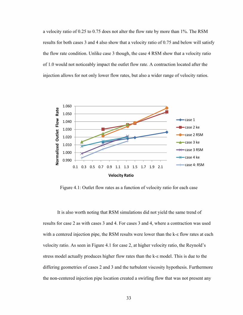
Figure 4.1: Outlet flow rates as a function of velocity ratio for each case 33
Figure 4.2: Second moments of concentration as a function of distance 36
Figure 4.3: Case 1: Particle traces from injection to orifice 37
Figure 4.4: Case 2: Particle traces from injection to orifice 38
Figure 4.5: Case 3: Particle traces from injection to orifice 38
Figure 4.6: Case 4: Particle traces from injection to orifice 39
Figure 4.7: Pressure drop across the injection for cases 3and 4 41
Figure 4.8: Static pressure measured throughout the pipe for r = 0.25 42
Figure A.1: Case 1: Particle traces from injection to orifice; r = 1.33 45
Figure A.2: Case 1: Particle traces near orifice; r = 1.33 45
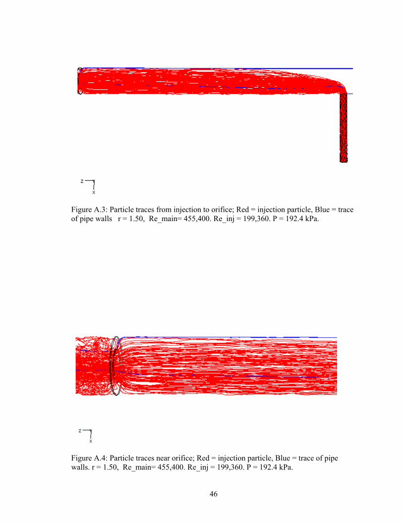
Figure A.3: Case 1: Particle traces from injection to orifice; r = 1.5 46
Figure A.4: Case 1: Particle traces near orifice; r = 1.5 46
Figure A.5: Case 1: Particle traces from injection to orifice; r = 2.25 47
viii
Figure A.6: Case 1: Particle traces near orifice; r = 2.25 47
Figure A.7: Case 2: Particle traces near injection; r = 0.75 48
Figure A.8: Case 2: Particle traces from injection to orifice; r = 1.33 48
Figure A.9: Case 2: Particle traces near injection; r = 1.33 49
Figure A.10: Case 2: Particle traces from injection to orifice; r = 1.50 49
Figure A.11: Case 2: Particle traces near injection; r = 1.50 50
Figure A.12: Case 2: Particle traces from injection to orifice; r = 2.25 50
Figure A.13: Case 2: Particle traces near injection; r = 2.25 51
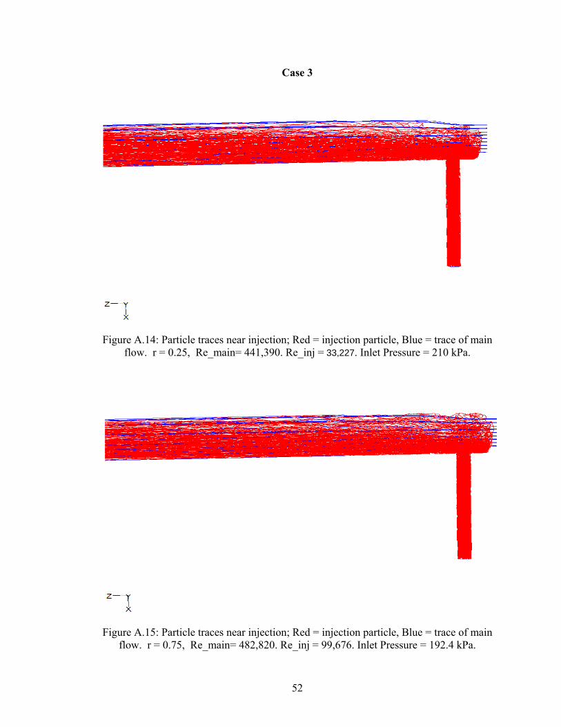
Figure A.14: Case 3: Particle traces near injection; r = 0.25 52
Figure A.15: Case 3: Particle traces near injection; r = 0.75 52
Figure A.16: Case 3: Particle traces from injection to orifice; r = 1.33 53
Figure A.17: Case 3: Particle traces near injection; r = 1.33 53
Figure A.18: Case 4: Particle traces near injection; r = 1.33 54
Figure A.19: Case 4: Particle traces near injection; r = 0.75 54
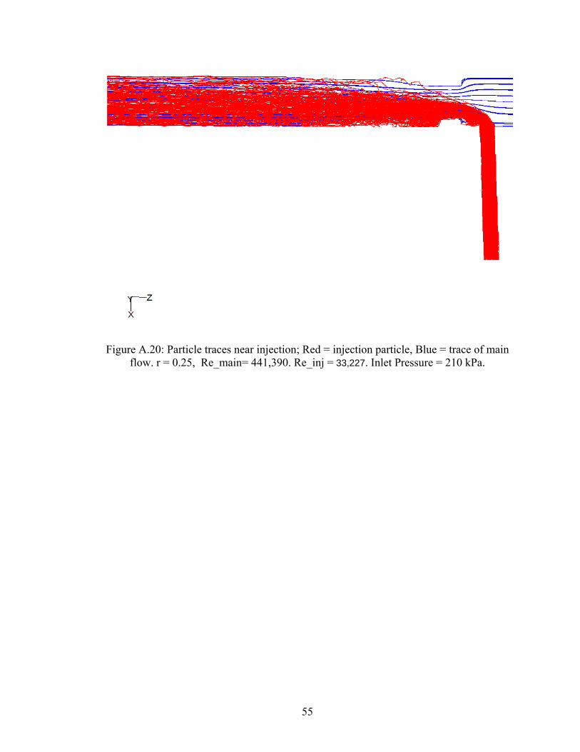
Figure A.20: Case 4: Particle traces near injection; r = 0.25 55

ix
LIST OF SYMBOLS AND ABBREVIATIONS
lm jet momentum length
q volumetric flow rate
density of fluid
ρp density of the injected particles
fluid velocity in a given direction i
dynamic viscosity of the fluid p pressure of the fluid
average pressure of the fluid
g the force of gravity
A area
u’ turbulent velocity fluctuation
k turbulent kinetic energy dissipation rate
FD drag force on an injected particle
Fpr force of the pressure gradient on an injected particle
c concentration of the injected particles
average concentration of the injected particle
mass flow rate of the injected particles
t residence time of the injected particles
volume of the cell containing the injected particles
M second moment of concentration of the injected particles
N number of cells at a selected surface
CD Cross Direction

x
MD Machine Direction k- ε k-epsilon
RSM Reynold’s stress method
DPM Discrete phase model
xi
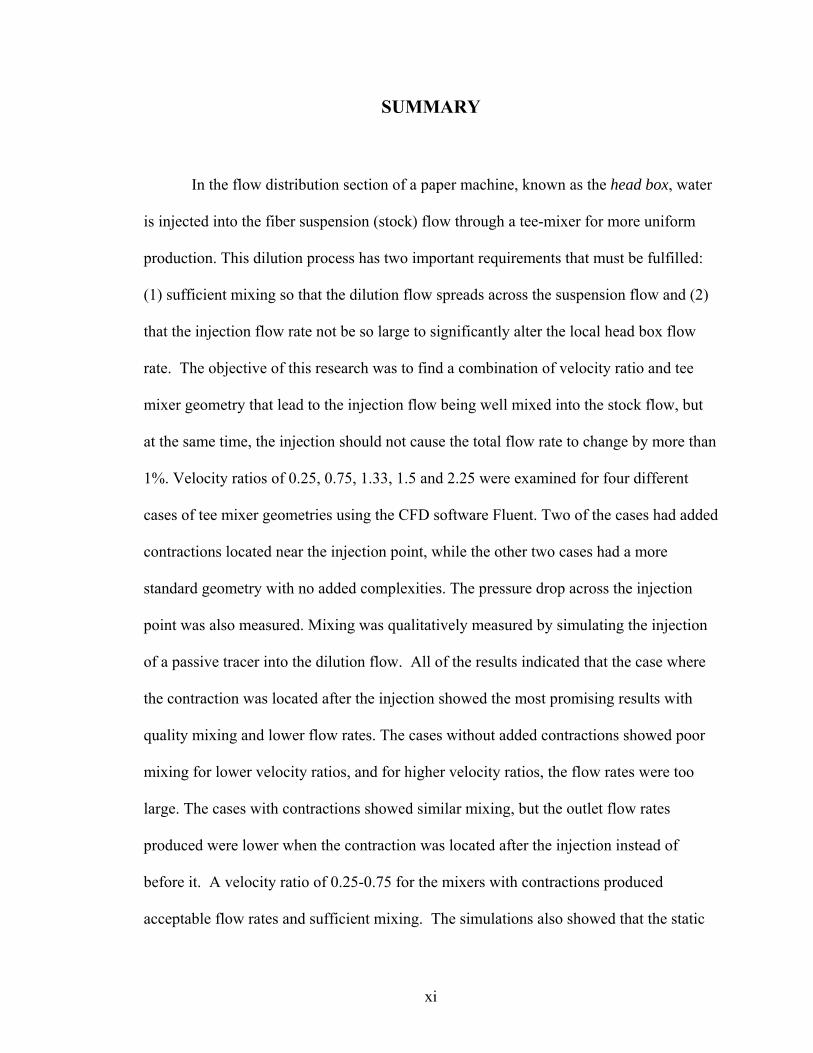
SUMMARY
In the flow distribution section of a paper machine, known as the head box, water
is injected into the fiber suspension (stock) flow through a tee-mixer for more uniform
production. This dilution process has two important requirements that must be fulfilled:
(1) sufficient mixing so that the dilution flow spreads across the suspension flow and (2)
that the injection flow rate not be so large to significantly alter the local head box flow
rate. The objective of this research was to find a combination of velocity ratio and tee
mixer geometry that lead to the injection flow being well mixed into the stock flow, but
at the same time, the injection should not cause the total flow rate to change by more than
1%. Velocity ratios of 0.25, 0.75, 1.33, 1.5 and 2.25 were examined for four different
cases of tee mixer geometries using the CFD software Fluent. Two of the cases had added
contractions located near the injection point, while the other two cases had a more
standard geometry with no added complexities. The pressure drop across the injection
point was also measured. Mixing was qualitatively measured by simulating the injection
of a passive tracer into the dilution flow. All of the results indicated that the case where
the contraction was located after the injection showed the most promising results with
quality mixing and lower flow rates. The cases without added contractions showed poor
mixing for lower velocity ratios, and for higher velocity ratios, the flow rates were too
large. The cases with contractions showed similar mixing, but the outlet flow rates
produced were lower when the contraction was located after the injection instead of
before it. A velocity ratio of 0.25-0.75 for the mixers with contractions produced
acceptable flow rates and sufficient mixing. The simulations also showed that the static

xii
pressure for the contraction cases were nearly identical throughout the majority of the
pipe. For both contraction cases the pressure drop across the injection increased with
increasing injection flow rate. When the contraction was located before the injection, a
pressure drop of 16% was calculated. A pressure drop of 18% to 20% across the
injection resulted when the contraction was located after the injection.

1
CHAPTER 1
INTRODUCTION
Turbulent mixers are widely used today in many different industries from
chemical mixing to paper production. In paper manufacturing, local basis weight
distribution is one of the most important properties that must be controlled since it
describes the uniformity of the paper sheet. Basis weight is defined as the ratio of the
mass of the sheet of paper to its area. Because the paper thickness is difficult to quickly
measure, basis weight is used to implicitly describe it. An increase in basis weight can
therefore imply an increase in the paper thickness. A non-uniform sheet must be avoided
since not only does it waste pulp, but perhaps more importantly, the paper sheet may not
meet a customer’s demands. The basis weight of the final paper product is directly related
to the flow rate of the pulp mixture running through the paper machine. Because of the
importance of a uniform sheet, the basis weight is controlled in two directions: the
machine direction (MD) and the cross direction (CD). The machine direction is parallel
to the direction pulp is processed through the machine, and the cross direction is the
transverse direction and perpendicular to the machine direction. One of the methods for
controlling basis weight is by locally diluting the pulp mixture, also called the stock flow,
with water in either the machine or cross direction. This dilution control occurs in the
head box of a paper machine. In general a paper machine takes in wet pulp, and through
various mechanical processes, creates a final product in the form of dry rolls of paper.
The process is commonly divided into sections known as the wet end and dry end. Pulp
entering the wet end of the machine usually consists of around 99% water. The goal of

2
the wet end is to reduce the water in the pulp and to form the fiber webs into an even wet
sheet. The dry end of the machine then further reduces the water in the wet sheet to under
1% and adds final coatings if desired.
For this study, the wet end is the most relevant part of the machine. The wet end
can be divided into three main sections: the head box, former, and the press. The purpose
of the head box is to uniformly distribute the pulp onto the forming tray where the actual
paper sheet is formed. The goal of the head box is then to mix the fiber water suspension
so that the fibers have a homogenous distribution across the width of the machine. The
head box is comprised of a tapered section that feeds the stock flow through a bank of
several hundred identical tubes. The tapered section and tube bank are used to create
turbulence and to evenly divide the flow. Turbulence is generated to disperse clumps in
the fiber which would cause a non-uniform final product. Furthermore dilution water can
be pumped into each individual tube in order to control the amount of fibers flowing
through that tube. The head box then delivers the stock flow to the wire tray, which
appears like a conveyor belt covered with a mesh cloth, in the forming section. The
former is where the fibers are shaped into a paper sheet and where drainage begins. From
the former, the sheet is then processed into the pressing section before moving to the dry
end.
In the head box of a paper machine, dilution flow is injected into the stock flow
through a tee-mixer for CD basis weight control. The basis weight of the paper sheet is
measured at several points across the width of the sheet at the end of the paper machine.
Some variation in basis weight is expected, but if the basis weight is determined to be too
large or too small at one point on the sheet, then the dilution flow in the head box is

3
adjusted to alleviate this problem. If the basis weight is too high at one point, then the
dilution flow is increased in the corresponding section in tube bank of the head box. The
result of this that since flow rate through the head box is kept constant, the stock flow in
that section of the head box is reduced and the fiber to water ratio in that tube of the head
box is reduced. The total flow rate, stock plus dilution, exiting the head box is kept
constant in order to maintain a uniform product. Because fewer fibers are now flowing to
that particular section, the local basis weight at that point in the sheet will drop to the
desired level. This dilution flow usually consists of excess water collected from the
former drainage trays injected at 5% to 15% of the stock flow rate. The dilution process
has two important requirements that must be fulfilled: (1) sufficient mixing so that the
dilution flow spreads across the stock flow and (2) that the injection flow rate not be so
large to significantly alter the local head box flow rate. The ratio of the injected dilution
flow rate to the main stock flow rate is known as the velocity ratio. An important
consideration is that the impact of the injection on the head box flow depends on flow
resistances present in the system. Different styles of head boxes will produce different
flow resistances upstream and downstream. Therefore it is necessary to test different tee-
mixer geometries that will produce varying flow resistance.
Research Objectives
The objective of this research is to find a combination of velocity ratio and tee
mixer geometry that leads to the injection flow being well mixed into the stock flow, but
at the same time, the injection should not cause the total flow rate to change by more than
1%. Since the main inlet conditions were fixed, altering velocity ratio actually

4
demonstrates the impact of the increased injection flow rate on the system. Furthermore
the geometry of the tee-junction is specifically varied by adjusting the location of the
injection tee and adding contractions in the main pipe. The contractions are added to
increase flow resistance and to study their effect on mixing. Velocity ratios of 0.25, 0.75,
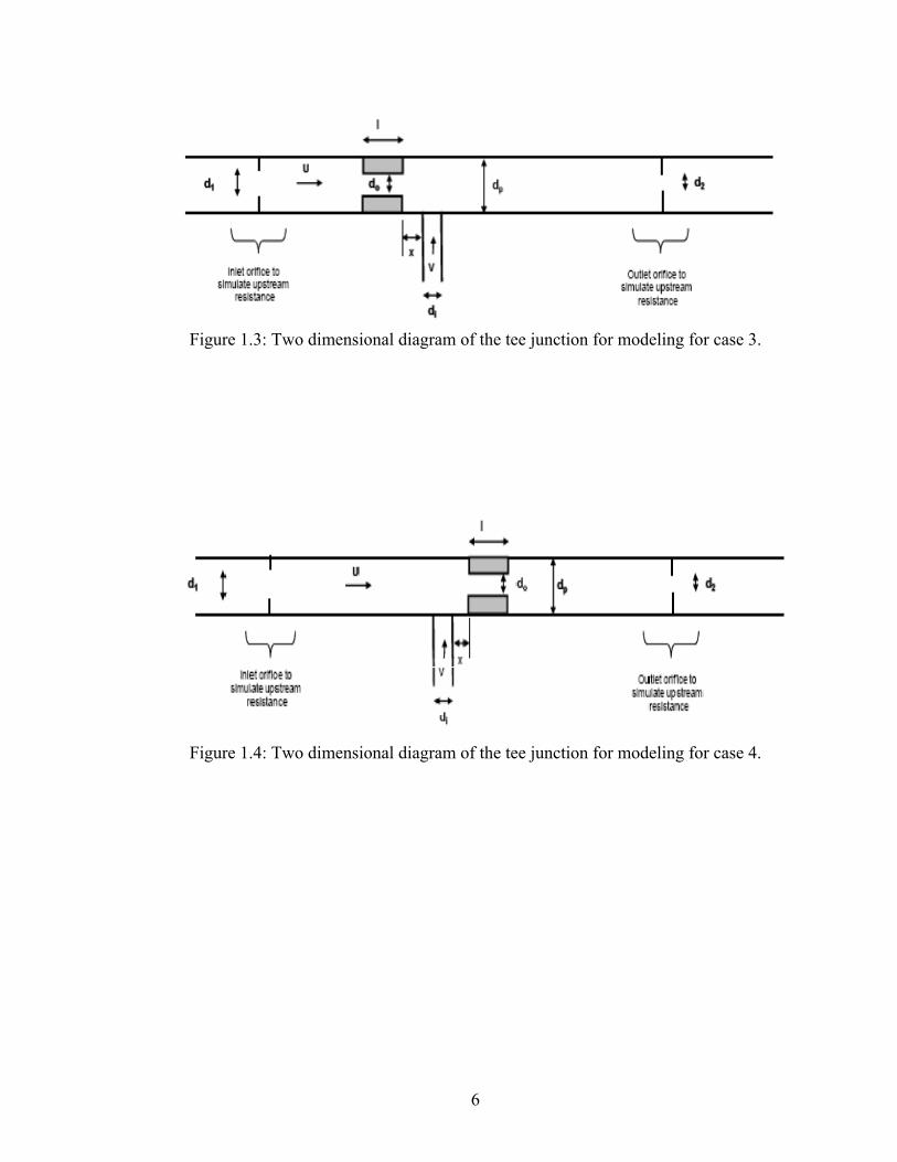
1.33, 1.5 and 2.25 were examined for four different cases of tee mixer geometries as
shown in Figures 1.1-1.4. The dimensions of Table 1.1 and the diagrams shown in
Figures 1.1-1.4 were provided by Dr. Jay Shands of Johnson Foils (personal
communication, August 2008). Cases 3 and 4, shown in Figures 1.3 and 1.4 respectively,
use the same cross section and injection pipe location as case 1 shown in Figure 1.2. The
values for the dimensions shown in Figures 1.1-1.4 are presented in Table 1.1. The
variables d represent the various diameters shown in Figures 1.1-1.4, and l is the length of
the contractions. These contractions are circular and connected to the walls of the pipe. In
Figures 1.1-1.4, u and v are fluid velocities. Mixing is judged by examining the
concentration and trajectories of a simulated tracer injected into the tee junction. Flow
rates are measured at both the inlet and outlet of the tee mixer so that the change in flow
rate can be calculated. Simulations were conducted using both the k-epsilon and
Reynold’s stress models. Pressure drops across the injection point were also measured.
Table 1.1: Dimensions for the actual dilution system
Dimensions Values Unitsdp 60 mmdi 16 mmd1 42 mmd2 35 mmx 18 mmdo 42 mml 25 mm

5
Figure 1.1: Two dimensional diagram of tee junction for modeling cases 1 and 2.
Figure 1.2: Cross sectional view of tee junction for modeling cases 1 and 2.
6
Figure 1.3: Two dimensional diagram of the tee junction for modeling for case 3.
Figure 1.4: Two dimensional diagram of the tee junction for modeling for case 4.

7
CHAPTER 2
BACKGROUND
Turbulent mixers are used in many industries including chemical production,
combustion reactors, and paper production. In 1930, Chilton and Genereuax used smoke
visualization to determine that a right angle was necessary for rapid tee mixing in pipes.
Furthermore they found that with velocity ratios of 2 to 3, the injected flow had
completely dispersed across the diameter of the pipe within 3 pipe diameters. Since then
injecting a secondary fluid at right angle into a turbulent flow has been used as a simple
method for efficient mixing.
One historically used method for quantitatively measuring the quality of the
mixing is by computing the second moment of concentration of a tracer injected into the
flow. The second moment is also known as the standard deviation which is a
measurement of the spread of a set from an average value. In this case, the second
moment of concentration measures the degree to which the concentration of the tracer
changes across the diameter of the pipe. A lower second moment is equivalent to a well-
mixed state since a near-zero second moment shows that the concentration across the
diameter is nearly identical. Forney and Sroka (1989) in examining tee mixers assumed
that the mixing could be divided into two sections. For several pipe diameters near the
injection point, mixing is controlled by the turbulence of the jet. Downstream the injected
flow is assumed to move parallel to the centerline of the pipe with mixing controlled by
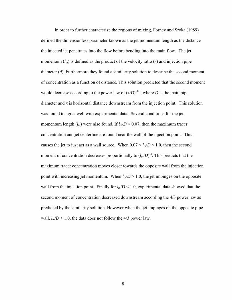
diffusion. An example of the tee-junction used by Forney and Sroka (1989) in their
studies is shown in Figure 2.1.
8
In order to further characterize the regions of mixing, Forney and Sroka (1989)
defined the dimensionless parameter known as the jet momentum length as the distance
the injected jet penetrates into the flow before bending into the main flow. The jet
momentum (lm) is defined as the product of the velocity ratio (r) and injection pipe
diameter (d). Furthermore they found a similarity solution to describe the second moment
of concentration as a function of distance. This solution predicted that the second moment
would decrease according to the power law of (x/D)-4/3, where D is the main pipe
diameter and x is horizontal distance downstream from the injection point. This solution
was found to agree well with experimental data. Several conditions for the jet
momentum length (lm) were also found. If lm/D < 0.07, then the maximum tracer
concentration and jet centerline are found near the wall of the injection point. This
causes the jet to just act as a wall source. When 0.07 < lm/D < 1.0, then the second
moment of concentration decreases proportionally to (lm/D)-2. This predicts that the
maximum tracer concentration moves closer towards the opposite wall from the injection
point with increasing jet momentum. When lm/D > 1.0, the jet impinges on the opposite
wall from the injection point. Finally for lm/D < 1.0, experimental data showed that the
second moment of concentration decreased downstream according the 4/3 power law as
predicted by the similarity solution. However when the jet impinges on the opposite pipe
wall, lm/D > 1.0, the data does not follow the 4/3 power law.
9
Figure 2.1: Diagram of a tee-mixer as used by Forney and Sroka.
Forney and Gray (1990) later investigated jet impingement and fast turbulent
mixers where mixing occurred within the first three pipe diameters. In their study, they
found an equation that describes where the point of jet impingement on the opposite wall
occurs downstream from injection based on the main and injection pipe diameters and
velocity ratio. This equation was found to be accurate to within 3% of experimental data.
Busko and Cozewith (1989) also studied mixing in the first three pipe diameters. With
increasing velocity ratio, it was found that the jet penetrated farther into the cross flow
before bending. Velocity ratios that positioned the jet along the pipe centerline were
found for several diameter ratios. All of these velocity ratios were greater than 2, and at a
high enough velocity ratio, the jet impinged on the opposite wall. This study used a
colored tracer injected into a fluid to perform mixing experiments with the mixing length
defined as the length downstream measured from the injection point where the color of
the tracer disappeared. The minimal mixing length was found over a range of velocity
ratios rather than one distinct value. Furthermore, the mixing length would eventually

10
increase past the minimum length with increasing velocity ratio. Impingement though did
not improve mixing, but rather increased the required mixing length. Therefore Busko
and Cozewith concluded that the optimum range of velocity ratios corresponded to the jet
being centered along the pipe centerline.
The effect of Reynolds (Re) number on mixing length was also studied. For
Re > 10,000, the mixing length was found to be independent of Reynolds number.
Meng and Pan (2001) further studied mixing in the near field of a tee mixer using
non-intrusive laser based experimental techniques in order to provide validation and
insight into existing CFD models used for tee mixers. In the near field, less than 2 pipe
diameters, it was assumed that turbulent dispersion dominates the flow in a tee mixer
while diffusion dominates the flow after 3 pipe diameters. Velocity ratios of 3.06 and
5.04 were studied within the jet mixing regime where 0.07 < lm/D < 1.0. Velocity ratios
that cause jet impingement on the pipe wall were not examined since this creates
undesired stresses on the walls. Also for lm/D < 0.07, the mixing is poor and was
therefore not studied. The flow structure for these two velocity ratios was visualized and
described in terms of five vortical structures that are shown in Figure 2.2: the jet shear
layer with Kelvin-Helmholz vortices, the counter-rotating vortex pair that comes from the
jet once the jet bends into the main flow, the wake structures behind the jet, the horseshoe
vortices upstream of the injection point, and the hanging vortex. The jet shear layer was
found to be present on the upper half of the jet with a roll-up of the shear layer in the
spanwise direction. The visible rolled up vortices are responsible for entraining the main
flow into the jet. Although the counter-rotating vortex pairs (CVP) could not be
visualized, evidence of their existence was found to be present in statistical data of the

11
flow. The data suggests that the CVP is responsible for the injection jet expansion.
Hanging vortices were apparent in all of the visualizations and were shown to be
responsible for both creating the CVP and causing upward motion in the jet downstream.
Figure 2.2: Vortical structures in a tee-junction as described by Meng and Pan (2001). The physical characteristics of the injection jet were also examined by Meng and
Pan (2001). A similarity solution for the jet centerline decay was validated for the
downstream region. The rate at which the jet centerline decays is important since it
describes the mixing in the flow. Finally as the jet travels downstream, it was shown to
expand into the main flow while the centerline concentration decreases. Eventually the jet
will expand to the point where the jet is no longer distinguishable from the main flow
leading to a well-mixed status. Visualizations showed that as the jet is lifted in an

12
upward motion due to the CVP, the jet expands spanwise. In addition to the flow
structure, the concentration probability function across the mixing layer was examined
and revealed that on the upstream side of the jet, mixing is controlled by large-scale
turbulent structures, and on the downstream side, diffusion dominates. This shows that
eddy viscosity CFD models are will be more accurate for predictions downstream than
upstream.
The accuracy of CFD models for tee-mixers has also been researched. Forney and
Monclova (1995) used the k-ε model to analyze tee mixing quality by calculating the
second moment of a simulated inert tracer. Water was injected into a pipe at a right angle
and steady, single phase flow was simulated for injection to main pipe diameter ratio of
0.026 < d/D < 0.36 with velocity ratios from 2 to 10. Several simulations were conducted
and showed that changing the number of sweeps or decreasing the grid size only changed
the predicted second moment of concentration by less than 3%. Initial values of the
turbulent kinetic energy and the dissipation rate also had little effect on the results.
Turbulent kinetic energy was found to be symmetrically distributed across the diameter
of the pipe while concentration was found to be asymmetric with the largest
concentration along the bottom of the pipe opposite the injection point. The simulated
second moment of the tracer downstream from the tee junction was found to agree well
with previously found experimental data showing that the k-ε model is a valid model for
simulating tee-mixers.
The k-ε model was also used and validated for non-cylindrical geometries.
Bertrand (1993) used the k-ε model to simulate tee-mixing in a square duct. A tracer was
injected at a right angle into the main turbulent flow with a Reynolds number of 27,300

13
in the square duct. The geometry of the simulation used a jet-to-duct diameter ratio of 0.2
with a velocity ratio of 1 and 5. These velocity ratios led to the two distinctive conditions
of a non-impinging and impinging jet. A velocity ratio of 5 caused the injection jet to
impinge against the opposite wall. This simulation showed mixing to be poorer for the
impinging condition and predicted a higher concentration of the injection fluid near the
opposite wall. For the non-impinging condition, the highest concentration of the tracer
was found on the symmetry plane of the duct with little mixing on the lateral side.
Sharma and Khokhar (2001) used the CFD program FLUENT to simulate tee
mixers with both the k-ε model and the Reynold’s Stress Model. Mixing was measured
by calculating the temperature field. The temperature of the injection fluid was set at a
higher temperature than the main pipe fluid, and 95% mixing was assumed to have been
achieved when the bulk fluid temperature was within 5% of the main pipe’s fluid’s
initial temperature. Velocity ratios of 17.1, 9.66, and 6.22 required 9, 11, and 13 pipe
diameters, respectively, for 95% mixing. As expected, the simulations showed that the
mixing length is a function of the velocity ratio. Both the RSM and k-ε model predicted
the same pipe length required for 95% mixing but produce differing predictions for the
highly turbulent region in the vicinity of the jet impingement. Experimental temperature
data was shown to agree well with the simulations, especially for regions downstream
near the 95% mixing point.
There has been a variety of dilution injection systems designed for paper machine
head boxes. Voith and Metso are companies that produce two dilution systems that are
currently used in the industry today. Invented by Begemann (1994) and associates, Voith
patented a mixing system for mixing two liquids at the inlet of head box that is shown in
14
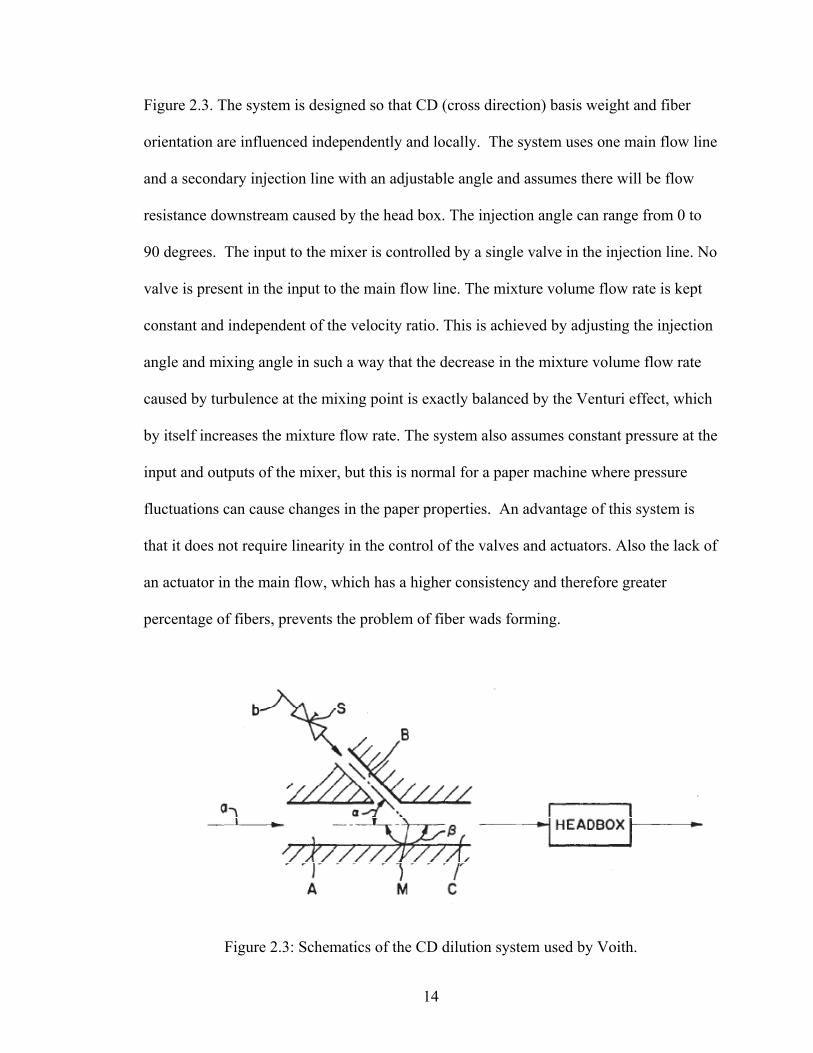
Figure 2.3. The system is designed so that CD (cross direction) basis weight and fiber
orientation are influenced independently and locally. The system uses one main flow line
and a secondary injection line with an adjustable angle and assumes there will be flow
resistance downstream caused by the head box. The injection angle can range from 0 to
90 degrees. The input to the mixer is controlled by a single valve in the injection line. No
valve is present in the input to the main flow line. The mixture volume flow rate is kept
constant and independent of the velocity ratio. This is achieved by adjusting the injection
angle and mixing angle in such a way that the decrease in the mixture volume flow rate
caused by turbulence at the mixing point is exactly balanced by the Venturi effect, which
by itself increases the mixture flow rate. The system also assumes constant pressure at the
input and outputs of the mixer, but this is normal for a paper machine where pressure
fluctuations can cause changes in the paper properties. An advantage of this system is
that it does not require linearity in the control of the valves and actuators. Also the lack of
an actuator in the main flow, which has a higher consistency and therefore greater
percentage of fibers, prevents the problem of fiber wads forming.
Figure 2.3: Schematics of the CD dilution system used by Voith.

15
Metso currently uses a dilution system patented by Jarmo Kirvesmaki (2009) and
company. Older dilution systems have proven to be expensive because of the need for
multiple valves, costly machining, and complex cleaning. This system attempted to solve
these issues. This dilution system delivers all of the dilution flow through a single valve
which is then fed into multiple mixing chambers. The dilution flow and the stock meet in
the mixing chamber before being carried off through other ducts to the rest of the head
box. There are multiple mixing chambers located across the width of the head box so
that dilution flow can be injected at multiple desired locations. The ducts that carry the
dilution flow open into the top part of the mixing chambers, but these ducts do not extend
into the mixing chamber. Mixing takes place in the gap between the inlet ducts and the
outlet. Outside of the mixing point, the mixing chamber is filled with dilution water. The
pressure of the dilution water is higher than that of the stock flow, and the dilution water
flows downward into the mixing chamber.
Research Gaps
Past research on tee mixers has not placed limits on the outlet flow rate, and most
research used velocity ratios of 2 or greater. Many studies used velocity ratios that either
centered the jet in the main flow or caused impingement on the opposite wall. Velocity
ratios below 1 have historically been ignored. Furthermore the research on tee mixers
has primarily focused on simple geometries like smooth pipes with no contractions or
other complex structures. It is usually assumed that the injection pipe is centered along
the main pipe at 90 degree angle. Most studies on tee-mixers have focused on chemical

16
mixers and not paper machine dilution systems. Paper dilution systems would differ
from other studies since the water is not only at a higher temperature, but also contains
solid wood pulp. The paper machine also creates upstream and downstream pressure
resistances which are not commonly simulated. Also comparisons of simulated mixing
using RSM and the k-e model are very limited. The k-ε model has been implemented for
many CFD simulations of tee-mixers, but RSM is rarely used due to high computational
costs.

17
CHAPTER 3
METHODS
The mesh for the T-junction for case 1 was created with Ansys Gambit with a
mesh element size of 3 mm. Cases 2-4 required a more detailed mesh for analysis so an
element size of 2.25 mm was used for these cases. Using the CFD program Fluent, water
flowing through the tee-junction was simulated with a steady, two equation k-epsilon
method. In order to compare the accuracy of turbulence models, the Reynolds stress
method was also used for cases 2, 3, and 4. The density and viscosity of water were
derived at a temperature of 120 F in order to approximate the actual temperature of pulp
in a paper machine. Momentum, turbulent kinetic energy, and turbulent dissipation rate
were all discretized with second order methods. As described in the Fluent manual, an
implicit pressure based solver is used for incompressible flow. The SIMPLE algorithm
described by Chorin (1968) was chosen to describe the relationship between the pressure
and velocity. The SIMPLE algorithm relates velocity and pressure correction to solve for
continuity and the pressure field. The full SIMPLE algorithm can be found in the Fluent
manual (2006) or in a standard CFD textbook. To ensure convergence, residuals in the
conservation equations were required to be below 10-4.
The following boundary conditions were prescribed: total and initial gauge
pressure at the main inlet, velocity at the injection inlet, atmospheric gauge pressure at
the outlet, and no-slip on all the walls. These conditions are summarized in Table 3.1.
The velocity condition at the injection inlet was derived from the velocity ratio, r. r is the
ratio of the injection velocity to the desired outlet velocity that would produce the

18
required flow rate of 13 liters per second (lps). Based on the diameter of the main pipe,
the needed outlet velocity was calculated to be 4.598 m/s. Therefore the injection velocity
was calculated as r × 4.598 m/s. Five different velocity ratios were investigated: 0.25,
0.75, 1.33, 1.5, and 2.25. These ratios were chosen since according to previous research,
they would not cause the jet to impinge on the opposite pipe wall. Cases 3 and 4 used the
same model, boundary conditions, and velocity ratios as cases 1 and 2. The geometry of
the mesh for cases 3 and 4 has been modified though so that a contraction is located in
the main pipe near the injection point
Table 3.1: Boundary conditions used in simulations.
Location ConditionMain Inlet total and initial pressure (gauge)Injection Inlet velocity = r × 4.598 m/sOutlet static pressure =0 kPa (gauge)Walls no slip
In order to simulate realistic conditions in the head box of a paper machine, the
simulations were designed to create an outlet flow rate of 13 liters per second (lps).
Therefore the initial inlet (gauge) pressure was chosen so that in the case of zero
injection, this inlet pressure would lead to the desired 13 lps at the outlet. The boundary
conditions used to determine the necessary inlet pressure are shown in Figure 3.1. In
Figure 3.1, q is a volumetric flow rate, p is the pressure, and u is the fluid velocity. The
pressure at the main inlet was determined by first prescribing a pre-determined velocity
corresponding to the 13 lps at the main inlet and zero flow at the injection inlet. The inlet
velocity was determined from the cross-sectional area of the tee-junction and the desired

19
q1
pgauge= 0
q2=0
q3
inlet outlet
u = 4.598 m/s
outlet flow rate of 13 lps. Simulations were then conducted using the following steps with
reference to Figure 3.1.
Figure 3.1: Boundary conditions used to determine the required inlet pressure
First a constant velocity profile with a magnitude of u was specified at the inlet
using the determined velocity based on 13 lps. Fluent then calculates mass flow rate
based on a velocity profile of a fluid entering a cell adjacent to the inlet from the
following equation,
·
where is the mass flow rate, is the specified fluid velocity vector at the inlet, and Ac
is the area of each cell. The velocity at the injection inlet was set to zero so that q2 = 0 as
shown in Figure 3.1. A pressure outlet condition with a zero static pressure was specified

20
at the tee-mixer outlet. Here the inlet flow rate will equal the outlet flow rate, or q1 = q3.
Using these results, the total and static pressure are measured at each node on the main
inlet and averaged using the following equation where p is the pressure at each cell and
is the average pressure,
1·
Next to perform the desired simulations, a pressure inlet was now specified at the
main inlet as shown in Figure 3.2. Using the average pressures found for the zero
injection case, the total and initial static pressures were prescribed at the inlet. Pressures
are gauge and are relative to the atmospheric conditions. From these pressures, the initial
fluid velocity magnitude at the inlet is then calculated using Bernoulli’s equation as
shown below,
012
2
where p0 is the total pressure, ps is the static pressure, and u is the velocity magnitude.
From this velocity magnitude and known flow direction, the initial velocity components
and mass flow rate and volumetric flow rate are determined. The static pressure at the
inlet is used to initialize the flow and the velocity magnitude, calculated through
Bernoulli’s equation, is an initial approximation for the inlet flow. Because this is a
pressure driven flow, the actual fluid velocity will be lower based on downstream
resistance.
21
pgauge= 0
q2
q1 q3
inlet outlet
(total and static)
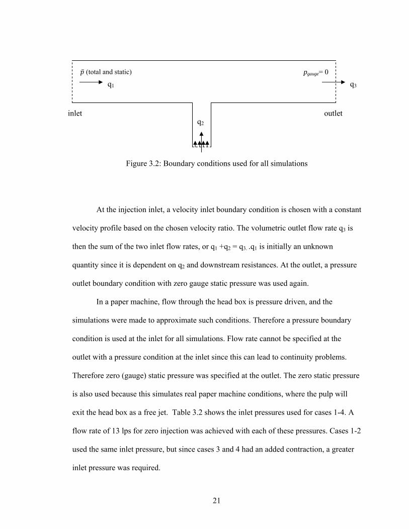
Figure 3.2: Boundary conditions used for all simulations
At the injection inlet, a velocity inlet boundary condition is chosen with a constant
velocity profile based on the chosen velocity ratio. The volumetric outlet flow rate q3 is
then the sum of the two inlet flow rates, or q1 +q2 = q3. .q1 is initially an unknown
quantity since it is dependent on q2 and downstream resistances. At the outlet, a pressure
outlet boundary condition with zero gauge static pressure was used again.
In a paper machine, flow through the head box is pressure driven, and the
simulations were made to approximate such conditions. Therefore a pressure boundary
condition is used at the inlet for all simulations. Flow rate cannot be specified at the
outlet with a pressure condition at the inlet since this can lead to continuity problems.
Therefore zero (gauge) static pressure was specified at the outlet. The zero static pressure
is also used because this simulates real paper machine conditions, where the pulp will
exit the head box as a free jet. Table 3.2 shows the inlet pressures used for cases 1-4. A
flow rate of 13 lps for zero injection was achieved with each of these pressures. Cases 1-2
used the same inlet pressure, but since cases 3 and 4 had an added contraction, a greater
inlet pressure was required.

22
Table 3.2: Inlet pressures (kPa) required for each case.
case Inlet Pres.1 192.42 192.43 210.04 210.0
Turbulent conditions were set at each boundary by specifying the turbulence
intensity and hydraulic diameter. The hydraulic diameter, DH, is the diameter of the
respective pipe depending on the location of the boundary. The turbulence intensity, I, is
determined from the following empirical equation described by the Fluent manual (2006),
0.16 /
where uavg is the mean velocity and u’ is the velocity fluctuations. The turbulence
intensities used at the injection point are shown in Table 3.3. At the main inlet and outlet,
turbulence intensity was specified by assuming the fluid velocity was the required
4.598 m/s with zero injection. This yielded a turbulence intensity of 3.1%.
Table 3.3: Turbulent intensity at the injection boundary as a function of r.
r I (%)
0.25 4.350.75 3.801.33 3.531.5 3.482.25 3.31

23
In order to qualitatively model and visualize the mixing, passive particles were
injected into the main water flow using the discrete phase model. First the domain of the
main flow, water, was solved using the k-ε method. To solve this continuous domain,
water was assumed to flow from both the main and injection inlets. After the main
domain had converged, the passive particles were released from the injection inlet in
order to visualize the flow coming from this section. The injected particles were set to use
a random walk turbulent dispersion model in order to include the effect of turbulent
velocity fluctuations.
When tracking particles in Fluent, the momentum of the fixed, continuous flow
field and the injected particles can be either coupled or uncoupled. For the visualizations,
an uncoupled model was used so that the injected particles did not exchange momentum
or mass with the main flow. In this way, the injected particles did not affect the results of
the solved continuous domain, but instead functioned as a means of post-processing and
provided a visualization of the results. The validity of the choice of an uncoupled solution
is based on the mass and momentum loading of the injected particles when compared to
that of the main flow. Since the mass flow rate of the injected particles will be an order of
magnitude smaller than those flowing from the main inlet, the injected particles will not
noticeably impact the continuous phase.
As well as a visual critique of the mixing, a quantitative evaluation of the mixing
was performed by measuring the concentration of the injected particles. To determine the
concentration, a coupled solution had to be used so that the water and injected particles
interacted. With a coupled solution, the injected particles and main flow now exchange
momentum and mass. This required that the water’s flow field and the injected particles’

24
flow fields be solved simultaneously. Using this solution, the concentration of the
injected particles was measured at multiple points throughout the pipe.
Fluent Methods
Continuity and Momentum
The CFD program Fluent iteratively solves the conservation equations for
continuity and momentum for all flows. Continuity is expressed in the above equation,
and momentum is shown in the following set of equations. As the fluid being modeled is
water, the flow is assumed to be incompressible. Both continuity and the resultant
velocities from the momentum equations are used as criteria for convergence. Residuals
are measured from the conservation equations and once they are below 10-4, the
simulations are assumed to be converged.
x:
: Z:

25
k-epsilon turbulent method In order to model turbulence, two models were used in Fluent. The first was the
standard two equation k-ε method proposed by Launder and Spalding (1972). The
momentum and continuity equations are first time averaged. Then, based on the kinetic
theory of gases, the turbulent viscosity is assumed to be a function of the turbulent kinetic
energy, k, and the viscous dissipation rate, . By assuming k and to be transported
properties and solving the relevant equations for them, the velocity field can be
determined. The standard k-ε model found in textbooks like Turbulent Flows by Pope
(2000) was used for all simulations. This model intrinsically requires an important
assumption, known as the Turbulent Viscosity hypothesis, which states that the
Reynold’s stress tensor is proportional to the mean strain rate. As stated in Turbulent
Flows (2000), the consequence of this assumption is that the accuracy of the model will
vary with the geometry and conditions of the flow. Furthermore since the Reynold’s
stresses are the mechanism through which the turbulent fluctuations impact the mean
flow, a relationship between the mean straining and Reynold’s stresses describes how the
geometry and flow conditions affect the turbulence. For simple shear flows and
geometries like pipe flow, Pope states this assumption has proven to be very reasonable.
However with more complex geometries like a contraction, the assumption that there is a
relationship between the local strain rate and the stress is not valid, and therefore the k-
model will be less accurate. Pope states that experiments have shown that the effects of
sudden geometry changes like contractions propagate much farther downstream than
expected that so that local effects no longer completely determine strain rate. Because of

26
this, the Reynold’s stress model is used for the simulations with contractions since it does
not rely on the turbulent viscosity hypothesis and the concept of eddy diffusivity.
Reynold’s Stress Method (RSM) The general Reynolds stress method equations as described in textbooks like
Turbulent Flows by Pope (2000) was used for the simulations. The Reynolds stress
methods model transport equations for the Reynolds stresses and solves them numerically
with an equation for dissipation and other conservation equations. The Reynolds Stresses
are the physical mechanisms through which the turbulent velocity fluctuations impact the
mean flow. The RSM method requires seven equations to be solved. An important
distinction is that RSM does not rely on the turbulent viscosity hypothesis and local
isotropy. This causes RSM to be more accurate than the k- model, but the RSM is more
computationally expensive since it must solve seven equations. Furthermore, unlike the
k-ε model, the RSM can handle rapid changes in strain rate allowing it to more accurately
model complex situations like swirling flows and contractions.
Discrete Phase Model (DPM)
The discrete phase model is used to simulate the flow of injected particles. The
typical solver used to evaluate fluid flow implements an Eulerian solution where the fluid
phase is treated as a continuous phase by solving the Navier Stokes and continuity
equations. The discrete phase model creates a second phase, consisting of spherical
particles, in a Lagrangian frame of reference dispersed in the continuous main phase. In
the continuous phase, the fluid is assumed to have infinitesimally small particles;

27
however, the discrete phase uses particles of a given diameter and solves for momentum
and continuity on each particle. There are two ways in which these phases can interact:
uncoupled and coupled. In an uncoupled solution, the fluid phase imparts momentum on
each particle, but the injected particles do not enact forces on the continuous fluid and
alter their results. Because of this, the fluid phase is solved first, and then particle
trajectories can be calculated integrating the following force balance on each particle,
In this equation, u is the fluid velocity, is the particle velocity, is the drag force per
unit particle mass, Fpr is the force due to the pressure gradient in the fluid, and is a set
of additional forces dependent on the density gradient and other special circumstances.
The pressure gradient force is described by the following equation,
where is the fluid density and is the density of the particles. A detailed description
on the drag force and other forces, Fx , can be found in the Fluent manual (2006).
This uncoupled solution was used for the mixing visualizations. The particles
were chosen to have a density and viscosity equivalent to that of water with a particle
diameter of 1 micron. The particles were given an initial velocity equivalent to the
injection inlet boundary condition velocity used when solving the continuous phase and

28
were required to reflect off walls. The mass flow rate of the particles was based off this
initial velocity, particle density, and cross sectional area of the injection pipe.
An uncoupled solution is valid when the mass flow rate of the injected particles is
much lower than that of the continuous flow. To ensure the accuracy of the results, the
injection flow rate should be no more than 10% of the main flow. Since the mass flow
rate of the injected particles in these simulations were an order of magnitude smaller than
those flowing from the main inlet, the injected particles did not noticeably impact the
continuous phase. For the simulated geometry and flow conditions, an uncoupled solution
provided an accurate method to model the paths of the injected particles.
In order to establish a quantitative measurement of the mixing in the tee-junction,
a coupled discrete phase model was used in Fluent to measure the concentration of the
injected particles throughout the pipe. The concentration of particles can only be
calculated using a coupled approach. This coupled solution now assumed that the injected
particles would impact the continuous flow field. When the two phases are coupled, the
continuous phase and discrete phase will exchange momentum and mass. This coupling
requires that flow in the two phases be solved simultaneously. Furthermore, the
trajectories of the particles are predicted in Fluent by solving a force balance on each
particle in the Lagrangian frame. The equations of motions of the particles were solved
using a 5th order Runge Kutta method.
The mixing was quantified by using the method described by Forney (1989)
where the second moment of the concentration of a tracer is measured at various
locations in the pipe. This is useful since the second moment describes the spread of the
particle concentration, or more directly the diffusion of the injected particles across the

29
pipe diameter. Therefore as the second moment decreases, the concentration of the
particles across the diameter of the pipe becomes more similar at each measured location.
An even distribution of the particles represents quality mixing.
In the steady state simulations in Fluent, the discrete phase can be viewed as a
stream of particles rather than large number of particles distributed throughout the
domain. Furthermore the total mass of particle entering the domain is equal to the mass of
particles leaving. Therefore the DPM concentration will be calculated based on the
particle residence time in each cell. Fluent uses the following equation to calculate the
mass concentration, c, of particles for steady state flows:
where is the mass flow rate of the particles, t is the residence time in each cell, and Vc
is the volume of each cell. The second moment of concentration, M¸ is calculated based
on the average concentration, , using the following equation with N as the number of
cells and :
∑

30
CHAPTER 4
RESULTS AND DISCUSSION
Flow Rates
The following table and graphs show comparisons of the flow rates for cases 1-4.
All of these results were obtained using the k-ε method for turbulent flows unless noted
otherwise. Results were taken after convergence had been achieved with respect to mass
conservation and momentum. Table 4.1 shows the outlet flow rates obtained from the k-ε
and RSM simulations with all of the values normalized to the desired flow rate of 13 lps.
Cases 1 and 2 were simulated for velocity ratios of 0.75 to 2.25. Because the mixing was
already found to be poor at r = 0.75 for these cases, velocity ratios below 0.75 were not
investigated since previous research had shown the injected particle diffusion across the
pipe to be proportional to velocity ratio. With cases 3 and 4, acceptable mixing was
achieved with a velocity ratio of 0.75. As a result, velocity ratios greater than 1.33 were
not investigated since it was unnecessary. Velocity ratios below 0.25 though were not
simulated since previous research has shown that such small ratios cause the injection jet
to act as a wall source which produces poor particle dispersion.
Table 4.1: Outlet flow rates for each case as a function of velocity ratio, r.
r case 1 case 2 case 2 (RSM) case 3 (ke) case 3 (RSM) case 4 (ke) case 4 (RSM)0.25 NA NA NA 1.014 0.999 1.008 0.9930.75 1.013 1.030 1.021 1.025 1.010 1.015 1.0041.33 1.018 1.036 1.034 1.036 1.021 1.020 1.0151.5 1.019 1.038 1.039 NA NA NA NA2.25 1.026 1.053 1.058 NA NA NA NA

31
An acceptable outlet flow rate is 1.01 since this fulfils the requirement of a
maximum flow rate change of 1% from the zero injection case. As shown in Table 4.1,
all of the flow rates for cases 1 and 2, the non-contraction geometries, were greater than
1.01 with case 2 generating the highest flow rates. The most interesting aspect of Table
4.1 though is the results of the contraction geometries, cases 3 and 4. The lower flow
rates of the contraction cases are expected since they contain sources of resistance which
dissipate the increased energy from the injection flow. The results for both cases k-ε and
RSM simulations show there is potential to find outlet flow rate below 1.01. With the
contraction located either before or after the injection, velocity ratios of 0.25 and 0.75
produced flow rates below 1.01. In fact the k-ε and RSM results for case 4 show flow
rates that are lower than the other cases.
When comparing the results of the two turbulent models for each individual case,
it can be seen in Table 4.1 that the RSM results are only at most 2% smaller than those of
the respective k-ε model. This shows that the two turbulence models produce similar
results. As explained in Turbulent Flows by Pope (2000), the RSM has been shown to
perform with increased accuracy over the standard k-ε model for axisymmetric
contractions like those found in cases 3 and 4. This would then indicate that the lower
flow rates found for the contraction cases using the Reynold’s stress method are more
accurate than those produced with the k-ε model. With a paper machine, a 1% change in
flow rate is significant, so the 2% difference in the turbulent model results is a significant
outcome and warrants the RSM being chosen as the preferred model. However
convergence for the RSM required over 5 times as many iterations as the k-ε model and
an order of magnitude more time.

32
Finally, the lower flow rates for case 4 shown in Table 4.1 indicate that placing
the contraction after the injection leads to the lowest flow rates. This is expected as the
contractions can be viewed as sources of flow resistance in the main pipe. Since the fluid
is pressure driven, contractions that reduce the fluid pressure will lower the fluid flow
rate. A contraction after the injection will directly reduce the added energy caused by the
injection since it acts as a source of viscous dissipation. In the limiting case of very high
downstream resistance, the effects of the injected flow would be mitigated due to the high
resistance, and instead, the outlet flow rate would be controlled by the inlet flow rate due
to the constant pressure condition. When the contraction is located before the injection,
the reduction in energy caused by the contraction will not affect the injection flow. This
leads to higher flow rates for case 3 when compared to case 4.
Figure 4.1 shows the outlet flow rates found for cases 1-4 as a function of velocity
ratio. Figure 4.1 demonstrates that flow rate tends to increase with velocity ratio linearly.
Outlet flow rates are lowest for cases 3 and 4, the contraction cases, and highest for case
2, the geometry where the injection pipe was not centered. Because the non-centered
injection pipe produced the highest flow rates, a centered pipe was used for both of the
contraction cases. It can be concluded that with further investigation, a velocity ratio
producing an acceptable flow rate for case 1 could potentially be found. However
because of the poor mixing found in case 1 as shown in the mixing results, simulations
using the standard tee-junction of case 1 for velocity ratios below 0.75 were not
conducted.
The key lines to examine in Figure 4.1 are those for cases 3 and 4. These are the
only cases whose flow rates are below the 1.01 mark. The k-ε results for case 4 show that
33
a velocity ratio of 0.25 to 0.75 does not alter the flow rate by more than 1%. The RSM
results for both cases 3 and 4 also show that a velocity ratio of 0.75 and below will satisfy
the flow rate condition. Unlike case 3 though, the case 4 RSM show that a velocity ratio
of 1.0 would not noticeably impact the outlet flow rate. A contraction located after the
injection allows for not only lower flow rates, but also a wider range of velocity ratios.
0.990
1.000
1.010
1.020
1.030
1.040
1.050
1.060
0.1 0.3 0.5 0.7 0.9 1.1 1.3 1.5 1.7 1.9 2.1
Normalized
Outlet Flow Rate
Velocity Ratio
case 1
case 2 ke
case 2 RSM
case 3 ke
case 3 RSM
case 4 ke
case 4: RSM
Figure 4.1: Outlet flow rates as a function of velocity ratio for each case
It is also worth noting that RSM simulations did not yield the same trend of
results for case 2 as with cases 3 and 4. For cases 3 and 4, where a contraction was used
with a centered injection pipe, the RSM results were lower than the k-ε flow rates at each
velocity ratio. As seen in Figure 4.1 for case 2, at higher velocity ratio, the Reynold’s
stress model actually produces higher flow rates than the k-ε model. This is due to the
differing geometries of cases 2 and 3 and the turbulent viscosity hypothesis. Furthermore
the non-centered injection pipe location created a swirling flow that was not present any

34
of the other simulations. According to Turbulent Flows by Pope (2000), the Reynold’s
stress model is more suited to handle swirling flows where vorticity production has
increased and local isotropy cannot be assumed. Vorticity was seen to increase with
velocity ratio, and for these higher velocity ratios the Reynold’s stress models predicted
higher flow rates for case 2.
Mixing
Quantitative Analysis
In order to evaluate mixing, the second moment is measured at five different
planes downstream from the injection points for the two contraction cases. The
contraction cases were numerically evaluated since they showed the lowest flow rates.
Mixing is then characterized by the size of the second moment of concentration. Table
4.2 shows the values of the second moment measurements for cases 3 and 4 as a function
of distance and velocity ratio. The distance x is normalized to the pipe diameter D. Since
the concentration is a function of flow rate, the second moment is normalized to the
average concentration for each velocity ratio. A smaller second moment of concentration
indicates that the distribution of the injected particles has become more equalized across
the diameter of the pipe. Moreover, the smaller second moment shows that there is not a
high concentration of particles in one location of the pipe. Therefore a lower second
moment is equivalent to the desired high quality mixing. As shown in Table 4.2, the
second moment decreases as the distance downstream increases. Furthermore it can also
be seen that the second moment decreases with velocity ratio. This shows that the

35
injected particles spread across the diameter of the pipe as they move downstream from
the injection which proves that increased velocity ratios leads to more effective mixing.
Table 4.2: Second moment of concentration as a function of distance
x/D case 3 case 4 case 3 case 4 case 3 case 45.0 1.75 2.12 1.50 1.87 1.54 1.985.8 1.55 2.13 1.41 1.84 1.35 1.816.7 1.49 2.04 1.34 1.87 1.29 1.607.5 1.45 1.90 1.29 1.74 1.27 1.508.3 1.46 1.80 1.33 1.68 1.26 1.58
r = 0.25 r = 0.75 r = 1.33
Figure 4.2 graphically shows the second moment of concentration for cases 3 and
4 as a function of downstream distance. When comparing cases 3 and 4, Figure 4.2
shows that all of case 3’s second moments of concentrations are lower than those of case
4. This shows that placing a contraction before the injection leads to greater particle
dispersion than when the contraction is placed after the injection. When comparing the
actual values between the two cases using Table 4.2, case 4 on average only produces
about 20% higher second moments of concentration. Within each individual case, the
graph further supports the conclusion that increased velocity ratio leads to lower second
moments and therefore more effective mixing.

36
Figure 4.2: Second moments of concentration as a function of distance for cases 3 and 4
Visualizations
Figures 4.3-4.6 show the mixing for cases 1-4 for a velocity ratio of 0.75. Flow is
from the right to the left. The blue lines represent the main flow. The red lines represent
the trajectories of the injected particles. The particles, the red lines, do not interact with
the continuous flow, the blue lines. The blue lines simply show the pathlines of the
continuous flow and are shown only to demonstrate the geometry of the main pipe. As
stated, a stochastic random walk model was used to simulate the effect of the turbulent
velocity fluctuations. The key result to exam in Figures 4.3-4.6 is the distance required
for the red lines, the injected particles, to spread completely across the diameter of the
pipe. When the injected particles, red, reach the opposite wall of the pipe, the top blue
line, the desired mixing has occurred. Figures 4.3-4.6 show the mixing near the injection
point up to the first resistance orifice. The orifice is not actually a part of the dilution
system, but instead it was only added to simulate downstream resistance in the head box.
1.2
1.4
1.6
1.8
2
2.2
5.00 6.00 7.00 8.00
Normalized
Secon
d Mom
ent o
f Co
centratoin
Horizontal Distance from injection (pipe diameters)
case 4: r = 0.25
case 4: r = 0.75
case 4: r = 1.33
case 3: r = 0.25
case 3: r = 0.75
case 3: r = 1.33
37
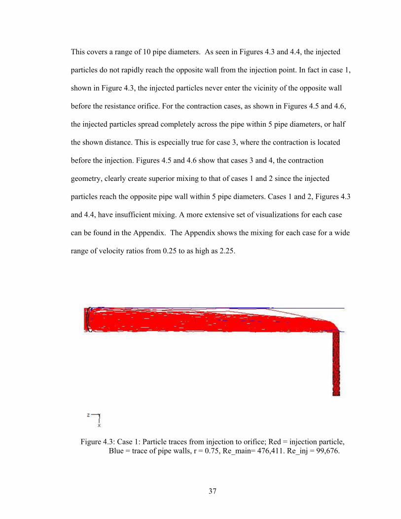
This covers a range of 10 pipe diameters. As seen in Figures 4.3 and 4.4, the injected
particles do not rapidly reach the opposite wall from the injection point. In fact in case 1,
shown in Figure 4.3, the injected particles never enter the vicinity of the opposite wall
before the resistance orifice. For the contraction cases, as shown in Figures 4.5 and 4.6,
the injected particles spread completely across the pipe within 5 pipe diameters, or half
the shown distance. This is especially true for case 3, where the contraction is located
before the injection. Figures 4.5 and 4.6 show that cases 3 and 4, the contraction
geometry, clearly create superior mixing to that of cases 1 and 2 since the injected
particles reach the opposite pipe wall within 5 pipe diameters. Cases 1 and 2, Figures 4.3
and 4.4, have insufficient mixing. A more extensive set of visualizations for each case
can be found in the Appendix. The Appendix shows the mixing for each case for a wide
range of velocity ratios from 0.25 to as high as 2.25.
Figure 4.3: Case 1: Particle traces from injection to orifice; Red = injection particle, Blue = trace of pipe walls, r = 0.75, Re_main= 476,411. Re_inj = 99,676.

38
Figure 4.4: Case 2: Particle traces from injection to orifice; Red = injection particle, Blue = trace of pipe walls , r = 0.75, Re_main= 482,820. Re_inj = 99,676.
Figure 4.5: Case 3: Particle traces from injection to orifice; Red = injection particle, Blue = trace of pipe walls, r = 0.75, Re_main= 482,820. Re_inj = 99,676

39
Figure 4.6: Case 4: Particle traces from injection to orifice; Red = injection particle, Blue = trace of pipe walls, r = 0.75, Re_main= 482,820. Re_inj = 99,676
Pressure
Table 4.3 shows the static pressure (gauge) for cases 3 and 4 as a function of
velocity ratio and horizontal distance from the injection. The distance is shown in terms
of pipe diameters from the injection point, and pressures are normalized in terms of the
inlet pressure of 210 kPa. As can be seen in the Table 4.3, the static pressure for case 3 is
very similar to that of case 4. Table 4.3 also shows that though the pressure increases
with velocity ratio, it does not vary significantly.
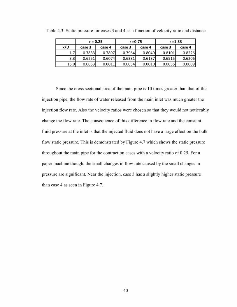
40
Table 4.3: Static pressure for cases 3 and 4 as a function of velocity ratio and distance
x/D case 3 case 4 case 3 case 4 case 3 case 4‐1.7 0.7833 0.7897 0.7964 0.8049 0.8101 0.82263.3 0.6251 0.6074 0.6381 0.6137 0.6515 0.6206
15.0 0.0053 0.0011 0.0054 0.0010 0.0055 0.0009
r = 0.25 r =0.75 r =1.33
Since the cross sectional area of the main pipe is 10 times greater than that of the
injection pipe, the flow rate of water released from the main inlet was much greater the
injection flow rate. Also the velocity ratios were chosen so that they would not noticeably
change the flow rate. The consequence of this difference in flow rate and the constant
fluid pressure at the inlet is that the injected fluid does not have a large effect on the bulk
flow static pressure. This is demonstrated by Figure 4.7 which shows the static pressure
throughout the main pipe for the contraction cases with a velocity ratio of 0.25. For a
paper machine though, the small changes in flow rate caused by the small changes in
pressure are significant. Near the injection, case 3 has a slightly higher static pressure
than case 4 as seen in Figure 4.7.

41
Figure 4.7: Static pressure measured throughout the pipe for r = 0.25
Another important quantity often measured in tee-mixers is pressure drop. Figure
4.8 shows the static pressure drop across the injection point for cases 3 and 4. The
pressure drop is measured as the difference between the pressure at -1.7 and 3.3 pipe
diameters from the injection point. For both cases 3 and 4, the pressure drop increases
with increasing velocity ratio. The pressure drop for case 4 though, as shown in Figure
4.8, increases more rapidly with velocity ratio than case 3, which stays near 16%.
0.0000
0.1000
0.2000
0.3000
0.4000
0.5000
0.6000
0.7000
0.8000
‐2.0 3.0 8.0 13.0
Normalized
Static Pressure
Horizontal Distance from Injection
case 3
case 4

42
Figure 4.8: Pressure drop across the injection for cases 3 and 4.
The trends shown in Figure 4.8 can be explained through the location of the
contractions. Through the conservation of energy, the pressure gradient in the pipe is
balanced by the viscous effects of the pipe and more noticeably here, the contractions.
Although the injected flow increases the energy in the combined flow, this increase in
energy is reduced by the increase in viscous dissipation due to the contractions. This
shows why the cases without contractions have higher flow rates. Since the flows are
pressure driven, it is then expected that the contraction cases which have lower flow rates
would then experience greater pressure losses. This is demonstrated in Figure 4.8 where
pressure drops ranging from 16%-20% are shown. With case 4, the combined fluid flows
through the contraction. This contraction then directly reduces the energy of the
combined flow. With case 3, the contraction is located before the injection, so the
combined flow will not be impacted by the contraction resistance. This explains why the
case 4 pressure drops are greater than those of case 3 and also the reduced influence on
the pressure drop of case 3.
0.15
0.16
0.17
0.18
0.19
0.2
r = 0.25 r = 0.75 r = 1.33
Normalized
Pressure Drop
case 3
case 4

43
CHAPTER 5
CLOSING
The goal of the project was to design a dilution system that will rapidly mix the
dilution water with the main flow while at the same time not altering the outlet flow rate
by more than 1%. All of the results indicate that placing a contraction after the injection,
the geometry of case 4, is the most promising with quality mixing and lower flow rates.
The tee-junctions without contractions showed poor mixing for lower velocity ratios, and
for higher velocity ratios, the flow rates were too large. Furthermore a non-centered
location of the injection pipe yielded the greatest increase in flow rates and did not
noticeably improve the mixing compared to the results of a centered injection pipe. By
measuring the second moment of concentration, it was shown that increasing the velocity
ratio increased the dispersion of the injected particles. When comparing the effect on
mixing of the contraction locations, a contraction before the injection, case 3, was shown
to have about 20% lower second moments than a contraction after the injection, case 4,
within 10 pipe diameters of the injection point. From the second moment data, it can be
inferred that a contraction before the injection results in more rapid mixing than a
contraction after the injection. Visually, both contraction cases showed acceptable
mixing, but the outlet flow rates produced by case 3 were slightly higher than those of
case 4. While case 3’s flow rates were less than 2% higher than those of case 4, it is
desirable to have as small of a flow rate change as possible. An acceptable flow rate
change and rapid mixing for these contraction cases was found at a velocity ratio of 0.25-
0.75 within the first 10 pipe diameters. Overall placing a contraction before the injection
44
led to better mixing, but when the contraction was located after the injection, the flow
rates were lower. The change in flow rate is the most important factor for a paper
machine, and since case 4 provided adequate mixing and the lowest flow rates, a
contraction after the injection proved to be the best geometry.
The k-e method provided sufficient results for all simulations, the RSM predicted
lower flow rates for the contraction cases at the cost of increased computational time.
While the flow rates computed using the Reynold’s stress methods were only at most 2%
smaller than those of the k-ε model, increased accuracy is paramount for a paper machine
where small changes in flow rate will noticeably alter the dimensions of the paper sheet.
Since previous studies have documented by Pope (2000) in his textbook demonstrated
that the Reynold’s stress methods are more accurate than the k-ε model for contractions,
the Reynold’s stress model should be used to simulate dilution systems containing
contractions.
The simulations also showed that the static pressure for case 3 and case 4 was
very similar throughout the majority of the pipe. The pressure drop across the injection
increased with velocity ratio for both contraction cases. When the contraction was located
after the injection, pressure drops were calculated to be between 18% and 20%. Higher
pressure drops were associated with higher velocity ratios. When the contraction was
located before the injection, a pressure drop of around 16% was found. For this geometry
the pressure drop only slightly increased with velocity ratio. A dilution system with a
contraction after the injection point showed effective mixing with injected particles
rapidly dispersed with a low flow rate change for a velocity ratio potentially as high as
1.0.

45
APPENDIX A
MIXING IMAGES
Case 1
Figure A.1: Particle traces from injection to orifice; Red = injection particle, Blue = trace of pipe walls. r = 1.33, Re_main= 460,210. Re_inj = 176,756. P = 192.4 kPa.
Figure A.2: Particle traces near orifice; Red = injection particle, Blue = trace of pipe walls. r = 1.33, Re_main= 460,210. Re_inj = 176,756. P = 192.4 kPa.
46
Figure A.3: Particle traces from injection to orifice; Red = injection particle, Blue = trace of pipe walls r = 1.50, Re_main= 455,400. Re_inj = 199,360. P = 192.4 kPa.
Figure A.4: Particle traces near orifice; Red = injection particle, Blue = trace of pipe walls. r = 1.50, Re_main= 455,400. Re_inj = 199,360. P = 192.4 kPa.

47
Figure A.5: Particle traces from injection to orifice; Red = injection particle, Blue = trace of pipe walls. r = 2.25, Re_main= 434,856. Re_inj = 299,054. P = 192.4 kPa.
Figure A.6: Particle traces near orifice; Red = injection particle, Blue = trace of pipe walls. r = 2.25, Re_main= 434,856. Re_inj = 299,054. P = 192.4 kPa.

48
Case 2
Figure A.7: Particle traces near injection; Red = injection particle, Blue = trace of main flow. r = 0.75, Re_main= 482,820. Re_inj = 99,676. P = 192.4 kPa
Figure A.8: Particle traces from injection to orifice; Red = injection particle, Blue = trace of pipe walls. r = 1.33, Re_main= 465,297. Re_inj = 176,756. P = 192.4 kPa.

49
Figure A.9: Particle traces near injection; Red = injection particle, Blue = trace of main flow. r = 1.33, Re_main= 465,297. Re_inj = 176,756. P = 192.4 kPa.
Figure A.10: Particle traces from injection to orifice; Red = injection particle, Blue = trace of pipe walls. r = 1.50, Re_main= 460,429. Re_inj = 199,360. P = 192.4 kPa.

50
Figure A.11: Particle traces near injection; Red = injection particle, Blue = trace of main flow. r = 1.50, Re_main= 460,429. Re_inj = 199,360. P = 192.4 kPa.
Figure A.12: Particle traces from injection to orifice; Red = injection particle, Blue = trace of pipe walls. r = 2.25, Re_main= 441,390. Re_inj = 299,054. P = 192.4 kPa.

51
Figure A.13: Particle traces near injection; Red = injection particle, Blue = trace of main flow r = 2.25, Re_main= 441,390. Re_inj = 299,054. P = 192.4 kPa.
52
Case 3
Figure A.14: Particle traces near injection; Red = injection particle, Blue = trace of main
flow. r = 0.25, Re_main= 441,390. Re_inj = 33,227. Inlet Pressure = 210 kPa.
Figure A.15: Particle traces near injection; Red = injection particle, Blue = trace of main
flow. r = 0.75, Re_main= 482,820. Re_inj = 99,676. Inlet Pressure = 192.4 kPa.

53
Figure A.16: Particle traces from injection to orifice; Red = injection particle, Blue = trace of pipe walls. r = 1.33, Re_main= 465,297. Re_inj = 176,756. P = 192.4 kPa.
Figure A.17: Particle traces near injection; Red = injection particle, Blue = trace of pipe walls. r = 1.33, Re_main= 465,297. Re_inj = 176,756. Inlet Pressure = 192.4 kPa.

54
Case 4
Figure A.18: Particle traces near injection; Red = injection particle, Blue = trace of main
flow. r = 1.33, Re_main= 465,297. Re_inj = 176,756. P = 210 kPa.
Figure A.19: Particle traces near injection; Red = injection particle, Blue = trace of main
flow. r = 0.75, Re_main= 482,820. Re_inj = 99,676. P = 210 kPa.
55
Figure A.20: Particle traces near injection; Red = injection particle, Blue = trace of main flow. r = 0.25, Re_main= 441,390. Re_inj = 33,227. Inlet Pressure = 210 kPa.
56
REFERENCES
Begemann, Ulrich, and Scherb, Thoroe. “Mixing System for Mixing Two Liquids at Constant Mixture Volume Flow for Supplying Headbox of a Paper Machine.” U.S. Patent 5316383. 31 May 1994.
Bertrand, J., Duquenne, A.M., Etcheto, L., and Guirand, P., “Numerical Simulation of In-Line Mixers,” European Federation of Chemical Engineers, vol. 17, pp. S511-S516, 1993.
Busko, Michael Jr., and Cozewith, Charles. “Design Correlations for Mixing Tees,” Industrial Engineering Chemical Research, vol. 28, pp. 1521-1530, 1989.
Chorin, A.J. “Numerical solutions of navier-stokes equations.” Mathematics of Computation. vol 22: pp.745-762, 1968.
Fluent. Fluent 6.3 UDF Manual. Fluent Inc., Centerra Resource Park, 10 Cavendish Court, Lebanon, NH, January 2006.
Forney, L.J. and Gray, G.E., “Optimum Design of a Tee Mixer for Fast Reactions,” AIChE Journal, vol. 36, no. 11, pp. 1773-1776, November, 1990.
Forney, Larry J. and Louis A. Monclova, “Numerical Simulation of a Pipeline Tee Mixer,” Industrial Engineering Chemical Research, vol. 34, pp. 1488-1493, 1995.
Forney, L.J. and Sroka, L.M. “Fluid Mixing with a Pipeline Tee: Theory and Experiment,” AIChE Journal, vol. 35, no. 3, pp. 406-414, March, 1989.
Kemilainen, I., Kirvesmäki, J., Lappi, J., Turpeinen, H.“Apparatus in Connection with a Headbox of a Paper Machine or Equivalent.” U.S. Patent 7485206. 3 February, 2009.
Khokhar, Zahid, Sharma, Rajendra, and Zughbi, Habib D. “Mixing in Pipelines with Side-Tees,” 6th Saudi Engineering Conference, vol. 2, 171-182, December, 2002.
Launder, B.E., and Spalding D.B. Lectures in Mathematical Models of Turbulence. London, England. Academic Press. 1972.

57
Meng, Hui, and Pan, Gang. “ Experimental Study of Turbulent Mixing in a Tee Mixer Using PIV and PLIF,” AIChE Journal, vol. 47, no. 12, pp. 2653-2665, December, 2001.
Pope, Stephen B. Turbulent Flows. Cornell: Cambridge University Press, 2000.